On Some Geometric Selection and Optimization Problems via Sorted Matrices

ELSEVIER Computational Geometry 11 (1998) 17-28

C o m p u t a t i o n a l G e o m e t r y

Theory and Applications

On some geometric selection and optimization problems via sorted matrices"

Alex Glozman a, Klara Kedem a,b,,, 1, Gregory Shpitalnik a

a Department of Mathematics and Computer Science, Ben-Gurion University of the Negev, Beer-Sheva 84105, Israel b Computer Science Department, Cornell University, Upson Hall, Ithaca, NY 14853, USA

Communicated by M.J. Atallah; submitted 12 November 1996, accepted 6 February 1998

Abstract

In this paper we apply the selection and optimization technique of Frederickson and Johnson to a number of geometric selection and optimization problems, some of which have previously been solved by parametric search, and provide efficient and simple algorithms. Our technique improves the solutions obtained by parametric search by a log n factor. For example, we apply the technique to the two-line center problem, where we want to find two strips that cover a given set S of n points in the plane, so as to minimize the width of the largest of the two strips. © 1998 Elsevier Science B.V. All rights reserved.

Keywords: Computational geometry; Algorithm; Selection; Optimization; Two-line center

1. Introduction

Consider a set 8 of arbitrary elements. Selection in the set 8 determines, for a given rank k, an element that is kth in some total ordering of 8. The complexity of selection in 8 has been shown to be proportional to the cardinality of the set [2]. Frederickson and Johnson [10] considered selection in a set of sorted matrices. An m x n matrix M is a sorted matrix if each row and each column of M is in a nondecreasing

order. Frederickson and Johnson have demonstrated that selection in a set of sorted matrices, that together represent the set 8 , can be done in t ime sublinear in the size of 8 . They have also observed that given certain constraints on the set 8 , one can construct a set of sorted matrices representing 8 . For instance, given two sorted arrays, X = {Xl . . . . . Xm} and Y = {Yl . . . . . Yn}, the Cartesian sum X + Y, defined as {xi + yj I 1 ~< i ~< m, 1 ~< j ~< n }, can be represented succinctly as a sorted matrix M by means of X

A version of this paper appeared in Fourth Workshop on Algorithms and Data Structures, S.G. Akl, E Dehne, J. Sack and N. Santoro (Eds.), Lecture Notes in Computer Science 955, Springer-Verlag, pp. 26-35.

* Corresponding author. E-mail: [email protected]. ! Work by K. Kedem has been supported by a grant from the U.S.-Israeli Binational Science Foundation, and by a grant

from the Israel Science Foundation founded by The Israel Academy of Sciences and Humanities.

0925-7721/98/$19.00 © 1998 Elsevier Science B.V. All rights reserved. PII: S0925-7721 (98)00017-0

18 A. Glozman et al. / Computational Geometry 11 (1998) 17-28

and Y (Mij = xi + yj) [8]. In [7,9,10] a number of selection and optimization problems on trees were considered. For example, in [9] Frederickson and Johnson presented an O(n logn) time algorithm for selecting the kth longest path in a tree with n nodes.

More generally, the Frederickson and Johnson algorithm for selecting the kth smallest item in an m x n sorted matrix M runs in time O(m log(2n/m)) , when m ~< n [10]. When M is sorted by columns only, their algorithm runs in time O(n logm) [10].

The optimization technique via sorted matrices follows the general idea of the parametric search [17], although this technique has a number of advantages over the parametric search technique: it does not require parallelization of the decision algorithm and, usually, it produces more efficient algorithms than the ones obtained by the parametric search technique. Assume we have a decision problem 79(d) that receives as an input a real parameter d and we need to find the minimal value d* of the parameter d such that 79(d) satisfies certain properties, depending monotonically on d. Assume, furthermore, that the set ,S of all potential values that d* can get is presented in an m x n sorted matrix M and there is a decision algorithm A for T'(d), which in time T decides whether the given d is equal to, smaller than, or larger than the desired value d*. Frederickson and Johnson [7,9] show that the overall runtime consumed by the optimization algorithm is O(T log n + m log(2n/m)) when m ~< n. If the matrix M is sorted by columns only then the overall runtime of the optimization algorithm is O (T max {log m, log n } + n log m).

There have been some attempts to apply these techniques to geometric selection and optimization problems (e.g., [3,4,16]). In this paper we show some more such applications. In general our approach is the following. We examine geometric properties of the optimal solution for the particular problem. This leads to the determination of constraints on the set S of potential solutions for the problem. The constraints allow us to partition the set S into subsets, with a total or partial ordering defined on their elements, and to represent the subsets succinctly, as a set of sorted matrices. Next we apply the technique of Frederickson and Johnson, using as subroutines the linear time selection algorithm of [2] and the decision algorithm for the particular optimization problem. Below we present a list of the problems which we solve in this paper.

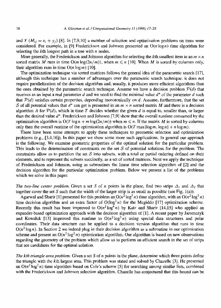
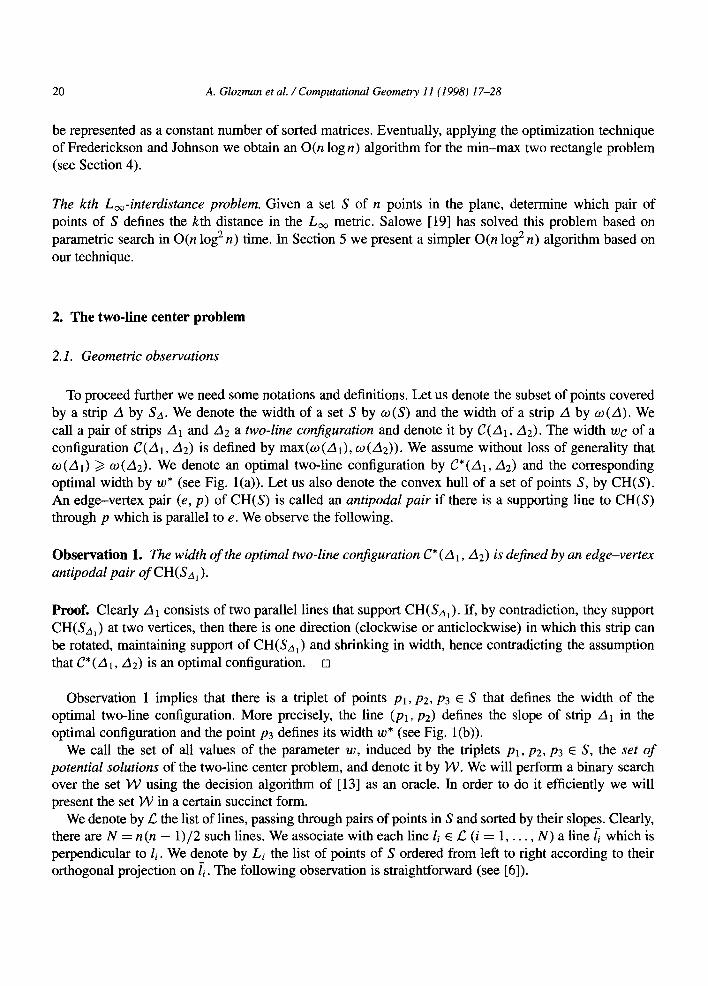
The two-line center problem. Given a set S of n points in the plane, find two strips A1 and A2 that together cover the set S such that the width of the larger strip is as small as possible (see Fig. 1 (a)).

Agarwal and Sharir [1] presented for this problem an O(n 2 log 5 n) time algorithm, with an O(n 2 log 3 n) time decision algorithm and an extra factor of O(log 2 n) for the Megiddo [17] optimization scheme. Recently this result has been improved to O(nZlog4n) by Katz and Sharir [14,15] who applied an expander-based optimization approach with the decision algorithm of [1]. A recent paper by Jaromczyk and Kowaluk [13] improved this runtime to O(nZlogZn) using special data structures and polar coordinates. Their data structure can be applied to a decision version algorithm that runs in time O(n 2 log n). In Section 2 we indeed plug in their decision algorithm as a subroutine in our optimization scheme and present an O(n 2 log 2 n) optimization algorithm. Our algorithm is based on new observations regarding the geometry of the problem which allow us to perform an efficient search in the set of strips that are candidates for the optimal solution.

The kth triangle area problem. Given a set S of n points in the plane, determine which three points define the triangle with the kth largest area. This problem was stated and solved by Chazelle [3]. He presented an O(n 2 log 2 n) time algorithm based on Cole's scheme [5] for searching among similar lists, combined with the Frederickson and Johnson selection algorithm. Chazelle has conjectured that this bound can be

A. Glozman et al./ Computational Geometry 11 (1998) 17-28 19

/%2 •

" . • 2

(a)

O . " - I t I " "

(c)

(b)

f

(d)

Fig. 1. Two-line center problem.

improved to O(n 2 log n). In Section 3 we show that the geometric observations and structures which we use in our solution for the two-line center problem lead to the improved O(n 2 log n) time algorithm for the kth triangle area problem.

The min-max two rectangle problem. Given a set S of n points in the plane, find two axis- parallel rectangles rl and r2 that together cover the set S and minimize the following expression: max(#(rl) , It(r2)), where It is a two-argument nondecreasing in each argument function of the height and width of a rectangle (e.g., area, perimeter or diagonal length).

Hershberger and Suri [11] consider a rectangular measure It(r) which is a two-argument, nondecreas- ing in each argument function of the height and width of a rectangle r. They solve the following clustering problem: given a planar set of points S, a rectangular measure # acting on S and a pair of values #~ and It2, does there exist a bipartition S = S1 U 82 satisfying It(Si) <~ Iti for i = 1,2? They have presented an algorithm which solves this problem in O(n logn) time.

We use a modification of their algorithm as a decision algorithm for the min-max two rectangle problem. Then we show that the set of potential solutions for the min-max two rectangle problem can

20 A. Glozman et al. /Computational Geometry 11 (1998) 17-28

be represented as a constant number of sorted matrices. Eventually, applying the optimization technique of Frederickson and Johnson we obtain an O(n log n) algorithm for the min-max two rectangle problem (see Section 4).

The kth L~-interdistance problem. Given a set S of n points in the plane, determine which pair of points of S defines the kth distance in the L ~ metric. Salowe [19] has solved this problem based on parametric search in O(n log 2 n) time. In Section 5 we present a simpler O(n log 2 n) algorithm based on our technique.

2. The two-line center problem

2.1. Geometric observations

To proceed further we need some notations and definitions. Let us denote the subset of points covered by a strip A by S~. We denote the width of a set S by w(S) and the width of a strip A by w(A). We call a pair of strips A1 and A2 a two-line configuration and denote it by C(A1, A2). The width wc of a configuration C(A1, A2) is defined by max(w(A1), w(A2)). We assume without loss of generality that 0)(AI) ~ O.)(A2). We denote an optimal two-line configuration by C*(A1, A2) and the corresponding optimal width by w* (see Fig. l(a)). Let us also denote the convex hull of a set of points S, by CH(S). An edge-vertex pair (e, p) of CH(S) is called an antipodal pair if there is a supporting line to CH(S) through p which is parallel to e. We observe the following.

Observation 1. The width of the optimal two-line configuration C* (A1, A2) is defined by an edge-vertex antipodal pair of CH(Sza~ ).

Proof. Clearly A 1 consists of two parallel lines that support CH(S~ 1 ). If, by contradiction, they support CH(S~al) at two vertices, then there is one direction (clockwise or anticlockwise) in which this strip can be rotated, maintaining support of CH(Sz~) and shrinking in width, hence contradicting the assumption that C*(A1, A2) is an optimal configuration. []

Observation 1 implies that there is a triplet of points Pl, P2, P3 E S that defines the width of the optimal two-line configuration. More precisely, the line (pl, P2) defines the slope of strip A 1 in the optimal configuration and the point P3 defines its width w* (see Fig. l(b)).

We call the set of all values of the parameter w, induced by the triplets Pl, P2, P3 E S, the set of potential solutions of the two-line center problem, and denote it by 142. We will perform a binary search over the set )/V using the decision algorithm of [13] as an oracle. In order to do it efficiently we will present the set W in a certain succinct form.

We denote by/~ the list of lines, passing through pairs of points in S and sorted by their slopes. Clearly, there are N = n(n - 1)/2 such lines. We associate with each line li E / ~ (i ---- 1 . . . . . N) a line// which is perpendicular to li. We denote by Li the list of points of S ordered from left to right according to their orthogonal projection on/ / . The following observation is straightforward (see [6]).

A. Glozman et al. /Computational Geometry 11 (1998) 17-28 21

Observation 2. Given two consecutive lines li, li+l E £ and the list Li, then the list Li+l can be obtained f rom Li by a single swap of points p', p" ~ S, where p' and p" is the pair o f points which defines the line li.

Fig. l(c) illustrates the line li = 1 determined by p' and pl,. The two points are projected to one point on [. Clearly when we rotate l (with its perpendicular line [) very slightly clockwise, and then anticlockwi- se, the projections of p' and p" swap order on f, while the other points remain in the same order as before.

Observation 3. Given the l&t Li and the pair of points p', p" ~ S which defines the line li. The point p ~ S having the kth distance from line li, among the points of S lying on the right (left) side of line li, can be found in constant time (here i = 1 . . . . . N and k = 1 . . . . . n).

Proof. The list Li c a n be maintained as a sorted array, ordered along the projections of the points on fi from left to right. We know the (consecutive) indices of the points p' and p" in Li, say p' = Pa and p" = Pa+l. The point p ~ S with kth distance from l;, among the points of S to the right of li, is P = Pa+l+k. (Symmetrically, on the left side of li, it is p = Pa-k, see Fig. l(d).) If the resulting index is greater than n (or, symmetrically, less than 1) then there is no such point in S and we assume that the kth distance is +cx~. []

2.2. The representation of ],'V

We build a list ~ of N records. The first record rl E ~ remains empty for the time being. Each record ri E 7~ (i -= 2 . . . . . N) consists of the two indices i', i" in Li-1 of the two elements which have to be swapped in order to produce Li. Clearly, with this structure available, and with the first list L1, we can produce all the lists Li (i = 2 . . . . . N) successively by proceeding from one record of 7~ to the next one, each time performing a single swap of two elements of Li-1.

In the following preprocessing algorithm we build the structure ~ . We use a dynamic auxiliary array, Index, which contains, at the ith step, pointers from the points of S to their location in the list Li. (E.g., if Pk 6 S is the third point in Li then Index[k] = 3.)

The preprocessing algorithm 1. Produce the list £ by sorting all the lines li by their slopes. Store them by means of the pairs of points

of S defining the lines. 2. For the first line l~ 6 £, sort the set of points S according to their projections on ll, store the sorted set

in L1, and the corresponding pointers in Index. 3. For each record ri (i ~--- 2 . . . . . N) do:

(a) Assume that the line li is defined by a pair of points with indices 1 ~< jl , j2 ~< n. Perform i' = Index[jl] and i" = Index[j2].

(b) Swap the elements with indices i', i" in the list Li-1. (c) Perform Index[j1] = i" and Index[j2] = i'.

Lemma 4. The preprocessing algorithm above builds correctly the structure R in O(N log N) time, requires O(N) space.

22 A. Glozman et al. /Computational Geometry 11 (1998) 17-28

Proof. The correctness of the algorithm can be proved by induction on step 3, applying Observation 2 N - 1 times. Step 1 of the algorithm requires O(N log N) time. Step 2 consumes O(n log n) time. Steps 3(a)-(c) require a constant amount of time each. Clearly each record ri (i = 1 . . . . . N ) is of constant size. This completes the proof. []

Corollary 5. The structure T¢ can be t raversed record by record in O ( N ) time, a l lowing access to the

list Li at each step i, i = 1 . . . . . N .

Corollary 6. The list L1 and the structure 7"~ provide a succinct representat ion o f the set 142.

2.3. The algori thm

In this section we present our algorithm which solves the two-line center problem. It uses the following result of Frederickson and Johnson [7,8]: given a matrix M of size m × n with each column sorted in ascending order, and provided a constant time access to each element of M, one can solve the optimization problem over the values of the matrix M in time O(T max{log m, log n} + n log m), where T is the runtime of the decision algorithm.

The structure ~ and L1 succinctly represent a matrix M of size n x N, sorted by its columns, which contains W. In this matrix the ith column, ci, corresponds to one line li G ~ , and contains the sorted array of distances from the points in S to the line li. Notice that instead of maintaining all the lists Li ,

i = 1 . . . . . N, we just keep L l (of length n), and the structure ~ with N records, each containing zero to four integer numbers. It follows from Corollary 5 and Observation 3 that given a column ci ~ M we can access an element of it in a constant time. This representation is therefor sufficient for the application of the optimization algorithm of Frederickson and Johnson [9]. Below we apply their algorithm to our problem, adding some steps for efficiently accessing the elements in M. The algorithm recurses on subarrays which are sub-columns in M. Associated with each subarray s is its smallest element (smallest distance) min(s) which is the element with smallest row index in the subarray, and its largest element max(s) which is the element with largest row index in the subarray.

Initially we subdivide each column of M into four equal size subarrays. We use the decision algorithm [ 13] to decide which of the subarrays should be discarded and which will take part in the continuation of the search. We discard at least half of the subarrays [9], divide each subarray into four and recurse. When there is only one element in each subarray we combine them to one array, sort it and search for the minimum width with the standard binary search and the decision algorithm. The number of discarded subarrays in each column is unknown, but we know that the subarrays that are left in the column for the continuation of the search have consecutive row indices in the column (because M is sorted by columns). We maintain in 7~ also the lowest and the highest indices of the subarrays left in each column ci, i = 1 . . . . . N . Assume that at the end of the preprocessing algorithm we added to each record of the indices 1 and n as the beginning and end of the initial subarrays.

The optimization algorithm 1. Perform the preprocessing algorithm. 2. Perform the following steps until there is one element in each subarray:

(a) Produce the columns ci of the matrix M one column after the other, starting from the first column cl ~ M, and then traversing ~ to achieve each ci in its turn.

A. Glozman et al . / Computational Geometry 11 (1998) 17-28 23

Partition the subarrays in each column Ci into four subarrays of equal size and select the minimum and maximum elements from each subarray, forming two lists: Lmin of the minimum values and Lmax of the maximum values, respectively, of the subarrays.

(b) Select the medians V~, of Lmin and Vmax of Lmax. (c) Run the decision algorithm of [13] on Vmin and Vmax. (d) Produce the columns of the matrix M successively again. This time, by going over the subarrays

of each column ci, discard the subarrays according to the answers of the decision algorithm in the previous step, store in ~ the lowest and highest indices of the part of ci that was not discarded.

3. Find the optimal value w* by performing a binary search. 4. Sort the remaining O(N) values (one from each subarray), and find the optimal value w* by

performing a binary search using the decision algorithm of [13]. Discarding a subarray s is done according to the result of the decision algorithm on Vmi n and Vmax. Assume, without loss of generality, that the decision algorithm found that Vmi n is smaller than the optimal width and Vmax is larger than the optimal width. In this case a subarray s is discarded if min(s) ~> Vmax or if max(s) ~< Vmi n. The other cases are treated similarly.

2.4. Analysis of the algorithm

Step 1 requires O(N log N) time as was shown in Lemma 4. From the analysis in [9,10] it follows that step 2 is repeated O(logn) times and the number of the subarrays in each stage of step 2 is O(N). In step 2(a) we partition every subarray in each column of M into four subarrays of equal size, and form two lists Lmin and Lmax. Corollary 5 implies that step 2(a) can be performed in O(N) time. Indeed, as was shown in Observation 2, we can obtain the column Ci+l from column ci by making a single swap in the list Li and producing the list Li+ 1 . Moreover, the selection of a minimal or maximal element in each subarray can be done in constant time as stated in Observation 3. In step 2(b) we apply the linear time median algorithm of [2] in time O(N). In step 2(c) we run twice the decision algorithm, hence it runs in 2- T time. Step 2(d) requires the same runtime as step 2(a). Thus we see that one iteration of step 2 requires O(T + N) time, and multiplying by the number of iterations we get to a total time of O((T + N) logn) for step 2. Step 3 performs a sort of O(N) elements in O(NlogN) time, and then O(log N) decision algorithms, for a total of O((T + N)log N) time. Thus our algorithm runs in time O((T + N)log N). Plugging in this formula the runtime of the decision algorithm T = O(n 2 logn) [13], and O(n 2) for N, we obtain an O(n 2 log 2 n) algorithm for the two-line center problem. It can be easily seen that the space requirement of the algorithm is O(n2). We conclude with the following theorem.

Theorem 7. The algorithm above solves the two-line center problem in O(n 2 log 2 n) time and O(n 2) space.

3. The kth area triangle problem

The kth area triangle problem is stated as follows: given a set S of n points in the plane, determine which three points define the triangle with the kth largest area.

Consider all triplets of points of the set S. Clearly, each triplet Pl, P2, P3 c S defines a triangle T. We can compute the area of T as the length of the segment [Pl, P2] times half the distance from point P3 tO

24 A. Glozman et al . / Computational Geometry 11 (1998) 17-28

the line through pl, P2. Let us denote by 7" the set of all possible areas of triangles, determined by S. The data structures for this problem are identical to those in the former section. As in the former section we can represent the set 7" succinctly in a matrix M of size n × N, sorted by its columns, which contains all the areas. Each column, ci, corresponds to a line l; 6 E, and thus is defined by some pair of points of S. The base of a triangle for this column is the distance between the points, and the rows within the column ci store the sorted distances from the points of S to the line l;. We use the selection algorithm of Frederickson and Johnson [8], which states the following: given a matrix M of size m x n, with each column sorted in ascending order, and provided a constant time access to each element of M, one can solve the selection problem over the values of M in time O(n log m).

Our algorithm for the kth area triangle problem is almost identical to the algorithm for the two-line center problem. The difference is that instead of calling a decision algorithm as a subroutine it runs a linear time selection algorithm [2]. Thus we have proved the following theorem.

Theorem 8. The kth area triangle problem can be solved in O(n 2 logn) time consuming O(n 2) space.

4. The min-max two rectangle problem

The min-max two rectangle problem is formulated as follows: given a set S of n points in the plane, find two axis-parallel rectangles rl and r2 that together cover the set S and minimize the expression: max(/z(rl),/z(r2)), where/z is a two-argument nondecreasing in each argument, function of the height and the width of a rectangle (for example area, perimeter or diagonal length).

4.1. The decision algorithm for the min-max two rectangle problem

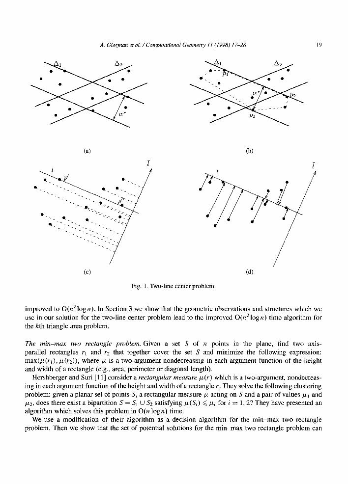
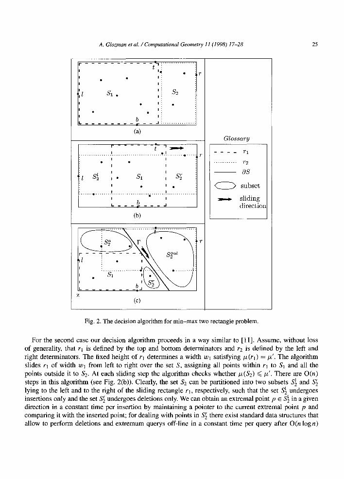
In this subsection we present an algorithm which solves the following decision problem: given a planar set of points S, a rectangular measure/.t acting on S and a value/z', does there exist a bipartition S = $1 U $2 satisfying max(/z(S0,/z(S2)) ~</z'. Hershberger and Suri [11] consider such a rectangular measure/z(r) of the height and the width of a rectangle r and solve the following clustering problem: given a planar set of points S, a rectangular measure Iz acting on S and a pair of values /~1 and/z2, does there exist a bipartition S = $1 U $2 satisfying lz(Si) <<, lzi for i = (1, 2)? They present an algorithm which solves this problem in O(n logn) time. First we review some notations and observations from [11]. The bounding box of the given point set S, denoted by OS, is the smallest axis-parallel rectangle that contains S. The bounding box of S is determined by the topmost, bottommost, leftmost, and rightmost points of S, which we denote by t, b, l and r (see Fig. 2). We call these points determinators of O S. Clearly, the rectangles rl and r2 have to cover together these four points. There are essentially three different ways to partition the determinators between sets $1 and $2: (1) one of the subsets gets three determinators and the other gets one determinator, (2) each subset gets two determinators lying on opposite sides of 0 S, (3) each subset gets two determinators lying on adjacent sides of OS.

According to the first case, assigning three determinators to, say, $1 fixes three of the four sides of rl. Thus we need to find a placement of the fourth side of rl such that/x(rl) <~/z' and/x(r2) ~< ~'. We place the fourth side of rl such that/z(rl) = /z ' . In linear time we can test whether the set of points outside of rl can be covered by a rectangle with measure/z ~</z' (see Fig. 2(a)).

A. Glozman et al. /Computational Geometry 11 (1998) 17-28 2 5

t t ~

I • l :

t i i

l i i $ 2 ;1 $1 . ,i I • l i •

I I :

t t ! b

L i - J " . . . . .

(a)

i r

'il

[ . . . . . . • . . . . . . .

I

I

I

I

I • S 1

I •

I

I

L b

(b)

e l

I

I

I

I

I

I

I

J

t . . . . : , r

. . . . . . . . . . . . . . . . . . . . . . . q • ....... > .

. . . .

Z

(c)

Glossary

r l

i r2 i i

i os subset

sliding direction

Fig. 2. The decision algorithm for min-max two rectangle problem.

For the second case our decision algorithm proceeds in a way similar to [11]. Assume, without loss of generality, that rl is defined by the top and bottom determinators and r2 is defined by the left and right determinators. The fixed height of rl determines a width Wl satisfying/z(rl) =/z ' . The algorithm slides ra of width Wl from left to right over the set S, assigning all points within rl to S] and all the points outside it to $2. At each sliding step the algorithm checks whether/z(S2) ~< #'. There are O(n) steps in this algorithm (see Fig. 2(b)). Clearly, the set $2 can be partitioned into two subsets S~ and S t lying to the left and to the fight of the sliding rectangle rl, respectively, such that the set $12 undergoes insertions only and the set S~ undergoes deletions only. We can obtain an extremal point p 6 S~ in a given direction in a constant time per insertion by maintaining a pointer to the current extremal point p and comparing it with the inserted point; for dealing with points in S~ there exist standard data structures that allow to perform deletions and extremum querys off-line in a constant time per query after O(n logn)

26 A. Glozman et al . / Computational Geometry 11 (1998) 17-28

preprocessing (see [18]). Also, one can easily show that if the order of points of the set S along the x-axis (y-axis) is known then the ordered list of updates to the sets S~ and S~ can be constructed in linear time. It implies that after O(n log n) preprocessing the decision algorithm for the second case runs in O(n) time.

In the third case we assign two adjacent determinators, say l and b, to rl, and t and r to r2. In this case the lower left comer of rl must coincide with the lower left comer of 0S (let us define it by z as in [11]). Similarly, the upper right comer of r2 must coincide with the upper right comer of OS. The decision algorithm for this case is based on the same idea as in the previous case. Namely, it tries all placements of rl of measure/z' and checks whether the set of points outside of rl can be covered by rectangle r2, such that #(r2) ~< #'. As was observed in [11], all the rectangles rl, satisfying/z(rl) = #' , whose lower left comer is z, have their upper right comer on a particular curve F . If/z is the area then F is a hyperbola; i f /z is the perimeter then F is a segment with slope - 1 ; and if # is the diagonal length then F is a quarter-circle of radius # ' centered at z. Fig. 2(c) illustrates the case where # is the perimeter. As seen in the figure, the set $2 can be partitioned into three subsets S~ ut, S~ and S~. The subset S~ ut consists of the points of S lying in 0S to the right of F , outside of rl. The set S~ consists of the points above the sliding rectangle rl and to the left of F , and the set S~ consists of the points to the right of rl and to the left of F . Clearly, S~ ut does not change during the running of the algorithm, since rl cannot cover any point from S~ ut. When sliding the upper right comer of rl along F from its topmost point to its bottommost point, the set S~ undergoes insertions only and the set S~ undergoes deletions only. As above, if the order of the points of S along the x-axis (and y-axis) is known, then the ordered list of updates for sets S~ and S~ can be constructed in linear time. It implies that after O(n log n) preprocessing the algorithm for the third case runs in O(n) time. These observations lead to the following lemma.

Lemma 9. After O(n logn) preprocessing time, the decision algorithm for the min-max two rectangle problem runs in O(n) time.

4.2. The optimization step

We make the following two observations.

Observation 10. The set of all distances measured along the x-axis (y-axis) between the points of S can be represented as a sorted matrix M of size n × n if the order of the points of S along the x-axis (y-axis) is known.

Observation 11. Given two sorted arrays X and Y, the values of the monotone, nondecreasing in each argument, function F(X , Y), can be represented succinctly as a sorted matrix M of size n × n by means of X and Y.

Proofi It is a straightforward extension of the case where the function F(X, Y) is a Cartesian product of two arrays X and Y [8]. []

Let us consider the geometry of the optimal solution for the min-max two rectangle problem and determine the potential values of/z for the optimal solution. Clearly there can be three kinds of solutions according to the three cases of positioning the determinators on the rectangles rl and r2. In the first and the second cases the bigger rectangle has its height (width) fixed and thus its measure/z is defined by

A. Glozman et a l . / Computational Geometry 11 (1998) 17-28 27

the second parameter - width (height). By Observation 10 we can represent all these values as a sorted matrix M of size n x n. In the third case the optimal rectangle with the larger measure/z, say rl, has its width and height defined by two pairs of points lying on its opposite sides, where one point in each pair is a determinator of rl. The distances from each such determinator to the other points of S, measured along the x-axis (respectively y-axis) define an array X (respectively Y) of linear size. Having the arrays X and Y available we can represent all potential values of/z in the third case as a sorted matrix M of size n x n, as stated in Observation 11. These observations lead to the following lemma.

Lemma 12. The set of potential values of lz can be represented as a constant number of sorted matrices of size n x n each.

Taking into account Lemmas 9 and 12 and applying the optimization technique of Frederickson and Johnson [7,9] we obtain the following result.

Theorem 13. The min-max two rectangle problem can be solved in O(n logn) time.

5. The kth L~-interdistance problem

Salowe [19] has solved the following problem: given a set S of n points in the plane, determine which pair of points of S defines the kth distance in metric L~. Following the parametric search paradigm Salowe has presented a decision algorithm, which in O(n log n) time decides whether the given value d is less, equal or greater than the kth interdistance in metric L~. Applying the parametric search technique he was able to obtain an O(n log 2 n) solution to the kth L~-interdistance problem.

We start with the following simple observation.

Observation 14. The kth L~-interdistance is defined by the distance between a pair of points of the set S, measured along the x-axis or the y-axis.

By combining this observation and Observation 10 with the optimization technique of Frederickson and Johnson [7,9] and using the same decision algorithm as in [19] we obtain the following result.

Theorem 15. The kth Loc-interdistance problem can be solved in O(n log 2 n) time.

6. Summary

In this paper we solve efficiently a number of geometric selection and optimization problems by exploring the geometry of the optimal configurations. The discovering of some partial or total ordering on the set of potential solutions allows one to apply the technique of Frederickson and Johnson for the selection or the optimization part of the problem.

Acknowledgements

The authors thank the referees for their relevant and helpful remarks.

28 A. Glozman et al. / Computational Geometry 11 (1998) 17-28

References

[1] E Agarwal, M. Sharir, Planar geometric location problems, Algorithmica 11 (1994) 185-195. [2] M. Blum, R.W. Floyd, V.R. Pratt, R.L. Rivest, R.E. Tarjan, Time bounds for selection, J. Comput. Syst. Sci. 7

(1972) 448-461. [3] B. Chazelle, New techniques for computing order statistics in Euclidean space, in: Proc. 1st ACM Symp. on

Computational Geometry, 1985, pp. 125-134. [4] L.E Chew, K. Kedem, Improvements on geometric pattern matching problems, in: SWAT, Lecture Notes in

Computer Science, Vol. 621, Springer, Berlin, 1992, pp. 318-325. Revised version: Getting around a lower bound for the minimum Hausdorff distance, Computational Geometry: Theory and Applications 10 (1998) 197-202.

[5] R. Cole, Searching and storing similar lists, J. Comput. Syst. Sci. 23 (1981) 166-204. [6] H. Edelsbrunner, Algorithms in Combinatorial Geometry, Springer, Heidelberg, 1987. [7] G.N. Frederickson, Optimal algorithms for tree partitioning, in: Proc. 2nd ACM-SIAM Syrup. on Discrete

Algorithms, 1991, pp. 168-177. [8] G.N. Frederickson, D.B. Johnson, The complexity of selection and ranking in X + Y and matrices with sorted

columns, J. Comput. Syst. Sci. 24 (1982) 197-208. [9] G.N. Frederickson, D.B. Johnson, Finding kth paths and p-centers by generating and searching good data

structures, J. Algorithms 4 (1983) 61-80. [10] G.N. Frederickson, D.B. Johnson, Generalized selection and ranking: sorted matrices, SIAM J. Computing 13

(1984) 14-30. [11] J. Hershberger, S. Suri, Finding tailored partitions, J. Algorithms 12 (1991) 431-463. [ 12] M. Houle, G. Toussaint, Computing the width of a set, in: Proc. 1 st ACM Symp. on Computational Geometry,

1985, pp. 1-7. [13] J.W. Jaromczyk, M. Kowaluk, The two-line center problem from a polar view: A new algorithm and data

structure, in: Proc. 4th Workshop Algorithms Data Structures, Lecture Notes in Computer Science, Vol. 955, 1995, pp. 13-25.

[14] M.J. Katz, Improved algorithms in geometric optimization via expanders, in: Proc. 3rd Israel Symposium on Theory of Computing and Systems, 1995, pp. 78-87.

[15] M.J. Katz, M. Sharir, An expander-based approach to geometric optimization, in: Proc. 9th ACM Symp. on Computational Geometry, 1993, pp. 198-207.

[16] D. Kravets, J. Park, Selection and sorting in totally monotone arrays, in: Proc. 2nd ACM-SIAM Symp. on Discrete Algorithms, 1990, pp. 494-502.

[17] N. Megiddo, Applying parallel computation algorithms in the design of serial algorithms, J. ACM 30 (1983) 852-865.

[18] M. Overmars, J. van Leeuwen, Maintenance of configurations in the plane, J. Comput. Syst. Sci. 23 (1981) 166-204.

[19] J.S. Salowe, L-infinity interdistance selection by parametric search, Inform. Process. Lett. 30 (1989) 9-14.