On Simple Binomial Approximations for Two Variable Functions in Finance Applications

On Simple Binomial Approximations for Two Variable Functions in Finance

Applications

Hemantha Herath * and Pranesh Kumar**

* Assistant Professor, Business Program, University of Northern British Columbia, 3333University Way, Prince George, British Columbia, Canada V2N 4Z9; Tel (250) 960-6459; email:[email protected].

** Associate Professor, Mathematics, University of Northern British Columbia, 3333 UniversityWay, Prince George, British Columbia, Canada V2N 4Z9; Tel (250) 960-6671; email:[email protected].

2

On Simple Binomial Approximations for Two Variable Functions in Finance

Applications

Hemantha S. B. Herath and Pranesh Kumar

University of Northern British Columbia

Abstract

We extend the volatility stabilization transformation technique to two correlated Brownian

motions. This technique allows to construct a computationally simple binomial tree and to obtain

the probabilities for the up- and down- movements. We derive the expressions for correlated

Geometric Brownian Motions by considering two variable functions. We discuss particular

functions of two variables, which are commonly employed in finance. Further, we simulate

results for the numerical accuracy of the approximations using an exchange option.

Keywords: Contingent claims, option pricing, numerical approximations, volatility stabilization

transformation

3

1. Introduction

Nelson and Ramaswamy (1990) used an elegant instantaneous volatility stabilization

transformation to approximate diffusions commonly used in finance such as the Ornstein-

Uhlenbeck (OU or mean reversion) process and the Constant Elasticity of Variance (CEV) to a

computationally simple binomial lattice. Although, binomial approximations for these types of

diffusions may exist, the binomial tree structures may not necessarily recombine. Such binomial

tree structures are computationally complex because the number of nodes in the tree doubles at

each time step. The idea is to obtain a computationally simple binomial tree structure where an

up move followed by a down move causes a displacement which is equal to a displacement

caused by a down move that is followed by an up move. This objective is achieved by

employing a transformation that makes the heteroskedastic process a homoskedastic process. In

other words, employing a transformation that makes the instantaneous volatility of the

transformed process constant.

In this paper, we extend the volatility stabilization transformation technique for two

variable functions. There are numerous situations where two variable functions are commonly

encountered when pricing options. We derive general expressions for correlated Geometric

Brownian Motions. Then we consider some cases, which are commonly employed in finance

applications. The paper is organized as follows: Section 2 includes the transformation technique

applied by Nelson and Ramaswamy (1990) to a single asset that follows a diffusion process. We

extend the transformation technique to two correlated Brownian motions in Section 3. Log

transformed variables are presented in Section 4. Section 5 discuses the numerical accuracy of

4

the approximations using an exchange option. A summary of findings and conclusions are

included in Section 6.

2. Nelson-Ramaswamy Instantaneous Volatility Stabilization Transformation

The basic intuition of the instantaneous volatility stabilization transformation is as follows.

Consider the stochastic differential equation

dWtydttydy ),(),( σµ += (1)

where W is a standard Brownian motion, µ(y,t), σ(y,t) ≥ 0, are the instantaneous drift and

standard deviation of y at time t and the initial value y0 is a constant. The time interval [0, T] is

divided into n equal time steps of size ∆t = T/n . The objective is to find a sequence of binomial

processes that converge in probability to the process (1) on [0, T].

Nelson and Ramaswamy (1990) consider a transform X(y,t) which is twice differentiable

in y and once in t. By Ito's Lemma,

dWy

tyXtydt

t

tyX

y

tyXty

y

tyXtytydX

∂

∂+

∂∂

+∂

∂+

∂∂

=),(

),(),(),(

),(2

1),(),(),(

2

22 σσµ (2)

Now make the term

dWdWtyy

tyX=

∂∂

),(),(σ

in (2) so that the instantaneous volatility of the transformed process x = X(y,t) is constant by

taking

1),(

),( =∂

∂y

tyXtyσ

Then by integrating the above term

5

( )∫ ∫∂

=∂ty

ytyX

,),(

σ

and substituting y by z we get

, ),(

),( ∫=y

tz

dZtyX

σ (3)

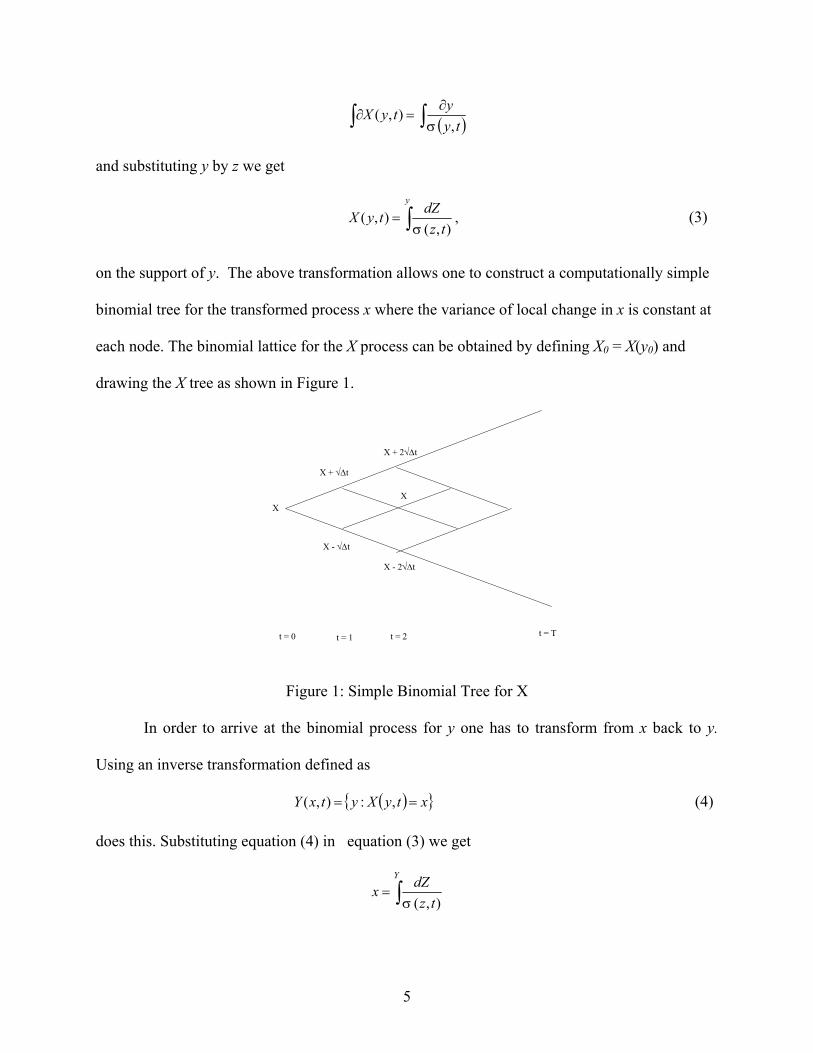
on the support of y. The above transformation allows one to construct a computationally simple

binomial tree for the transformed process x where the variance of local change in x is constant at

each node. The binomial lattice for the X process can be obtained by defining X0 = X(y0) and

drawing the X tree as shown in Figure 1.

Figure 1: Simple Binomial Tree for X

In order to arrive at the binomial process for y one has to transform from x back to y.

Using an inverse transformation defined as

( ){ }xtyXytxY == ,:),( (4)

does this. Substituting equation (4) in equation (3) we get

∫=Y

tz

dZx

),(σ

t = 0 t = 1 t = 2 t = T

X

X + √∆t

X - √∆t

X + 2√∆t

X - 2√∆t

X

6

and taking the partial derivative we obtain ∂y/∂x = σ(y,t) which implies that Y(x,t) is weakly

monotone in x for a fixed value of t. The inverse transform in equation (4) can be used to

construct the lattice for y such that the up- movement Y+(x,t) and a down- movement Y -(x,t) are

given by

( ) ( )tttxYtxY ∆+∆+=+ ,, (5)

( ) ( )tttxYtxY ∆+∆−=− ,, (6)

and the up- movement probability

( )( ) ( ) ( )

( ) ( )txYtxY

txYtxYttxYtp

,,

,,,,−+

−

−−+∆

=µ

(7)

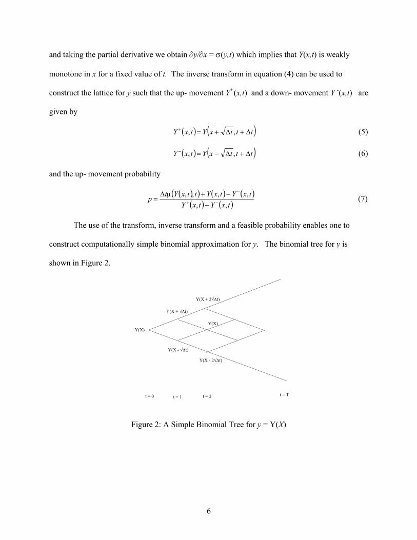
The use of the transform, inverse transform and a feasible probability enables one to

construct computationally simple binomial approximation for y. The binomial tree for y is

shown in Figure 2.

Figure 2: A Simple Binomial Tree for y = Y(X)

t = 0 t = 1 t = 2 t = T

Y(X)

Y(X + √∆t)

Y(X - √∆t)

Y(X + 2√∆t)

Y(X - 2√∆t)

Y(X)

7

3. Transform for Two Variables

We extend the transformation technique for two correlated Brownian motions. Consider a

function of two variables S1, S2 each following a Geometric Brownian Motion where

111111 dWSdtSdS σµ += (8a)

222222 dWSdtSdS σµ += (8b)

with [ ] ρε =21dWdW , the correlation between S1 and S2.

Consider a general functional form as a power function of S1 and S2 given by

F(S1 , S2, t ) = S1a S2

b, where constants a and b are real numbers

Since

ba SaSSF 21

11−=∂∂ , 1

212−=∂∂ ba SbSSF , 0=∂∂ tF

ba SSaaSF 22

121

2 )1( −−=∂∂ 221

22

2 )1( −−=∂∂ ba SSbbSF , 12

1121

2 −−=∂∂∂ ba SabSSSF

from the Ito lemma

( ) ( ) 211

21

12

22

212

122

121

21121

1 )1(2

1)1(

2

1dSdSSabSdSSSbbdSSSaadSSbSdSSaSdF bababababa −−−−−− +−+−++=

8(c)

Substituting for dS1 and dS2 and rearranging terms we obtain

( ) ( )FdWbdWaFdtabbbaabadF 22112122

2121 )1()1(

2

1)( σσσσρσσµµ ++

+−+−++=

8(d)

Notice that F follows a Geometric Brownian Motion with

( ) ( )

+−+−++= 21

22

2121 )1()1(

2

1)(, σσρσσµµµ abbbaabatF ,

8

( )2211 dWbdWa σσ + ≥ 0 where Wi are Wiener processes. Now define

2211 dWbdWadW σσ += , then since ( )1,0N~idW and σi are constant, for i = 1, 2 we have

( )2122

221

2 2a0,N~ σρσσσ abbdW ++ (8e)

The standardized value is

21

22

221

2 2a σρσσσ abb

dWdWz

++= (8f)

Substituting for dW in Equation (8d) we have

( ) ( ) zdWabbFFdtabbbaabadF 2122

221

221

22

2121 2a)1()1(

2

1)( σρσσσσσρσσµµ +++

+−+−++=

(8g)

In order to obtain a computationally simple binomial approximation we need to make the

volatility term constant in Equation (8g). The transform is

σρσσσσ1

22

221

2 2a

ln

),(),(

abb

F

tZ

dZtFH

F

++== ∫ (8h)

The inverse transformation provides ( ) σρσσσ 122

221

2 2a abbHeHF ++= and defining

( )σρσσσ 1

22

221

2

00

2a

ln

abb

FFH

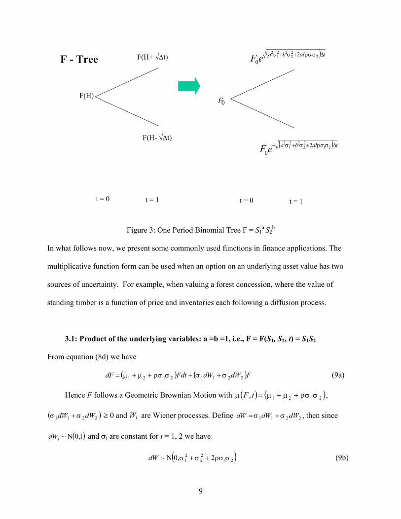
++= , we obtain the H – tree and F tree as previously. From the

F –tree in Figure 3 and equation (7), we can obtain the expressions for up, down movements and

the probability on an up- movement.

9

Figure 3: One Period Binomial Tree F = S1a S2

b

In what follows now, we present some commonly used functions in finance applications. The

multiplicative function form can be used when an option on an underlying asset value has two

sources of uncertainty. For example, when valuing a forest concession, where the value of

standing timber is a function of price and inventories each following a diffusion process.

3.1: Product of the underlying variables: a =b =1, i.e., F = F(S1, S2, t) = S1S2

From equation (8d) we have

( ) ( )FdWdWFdtdF 22112121 σσσρσµµ ++++= (9a)

Hence F follows a Geometric Brownian Motion with ( ) ( )2121, σρσµµµ ++=tF ,

( )2211 dWdW σσ + ≥ 0 and Wi are Wiener processes. Define 2211 dWdWdW σσ += , then since

( )1,0N~idW and σi are constant for i = 1, 2 we have

( )2122

21 20,N~ σρσσσ ++dW (9b)

t = 0 t = 1 t = 0 t = 1

F(H)

F(H+ √∆t)

F(H- √∆t)

F - Tree

0F

( ) tabbaeF ∆++− 2122

221

2 20

σρσσσ

( ) tabbaeF ∆++ 2122

221

2 20

σρσσσ

10


21

22

21 2 σρσσσ ++

=dW

dWz (9c)

Substituting for dW in Equation (9a) we have

( ) ( ) zdWFFdtdF 2122

212121 2 σρσσσσρσµµ +++++= (9d)

To make the volatility term constant in Equation (9d) the transformation is

2122

21 2

ln

),(),(

σρσσσσ ++== ∫

F

tZ

dZtFH

F

(9e)

The inverse transformation provides ( ) 2122

21 2 σρσσσ ++= HeHF and defining

( )21

22

21

00

2

ln

σρσσσ ++=

FFH , we obtain the H – tree and F tree as previously.

Now we consider the ratio functional form, which is typically, encountered among others in

exchange options and real options to abandon a project for its salvage value. For example, an

opportunity to exchange one company's securities for those of another within a stated time period

Margrabe (1978).

3.2: Relative value of the underlying variables a=1, b= -1, i.e., F = F(S1, S2, t) = S1 / S2

From equation (8d) we have

( ) ( )FdWdWFdtdF 2211212221 σσσρσσµµ −+−+−= (10a)

Therefore F follows a Geometric Brownian Motion with ( ) ( )212221, σρσσµµµ −+−=tF ,

and ( )2211 dWdW σσ − ≥0. Define 2211 dWdWdW σσ −= , then since ( )1,0N~idW and σi are

constant for i = 1, 2 we have

( )2122

21 20,N~ σρσσσ −+dW (10b)

11


21

22

21 2 σρσσσ −+

=dW

dWz (10c)


( ) zdWFFdtdF

−++−+−= 21

22

2121

2221 2 σρσσσσρσσµµ (10d)

Making the volatility term constant in Equation (10d) gives us a computationally simple

binomial approximation. The transform is

2122

21 2

ln

),(),(

σρσσσσ −+== ∫

F

tZ

dZtFH

F

(10e)


21 2 σρσσσ −+= HeHF and defining

( )21

22

21

00

2

ln

σρσσσ −+=

FFH , we obtain the H – tree and F tree as in the previous cases.

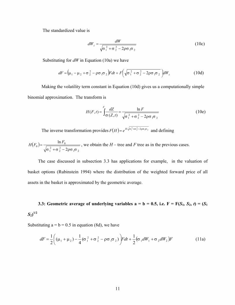
The case discussed in subsection 3.3 has applications for example, in the valuation of

basket options (Rubinstein 1994) where the distribution of the weighted forward price of all

assets in the basket is approximated by the geometric average.

3.3: Geometric average of underlying variables a = b = 0.5, i.e. F = F(S1, S2, t) = (S1

S2)1/2

Substituting a = b = 0.5 in equation (8d), we have

( )FdWdWFdtdF 22112122

2121 2

1)(

4

1)(

2

1σσσρσσσµµ ++

−+−+= (11a)

12

In the above equation F follows a Geometric Brownian Motion with

( )

−+−+= )(

4

1)(

2

1, 21

22

2121 σρσσσµµµ tF , and ( )2211 dWdW σσ + ≥0. Define

)(2

12211 dWdWdW σσ += , then since ( )1,0N~idW and σi are constant for i = 1, 2, we have

++ )2(

4

10,N~ 21

22

21 σρσσσdW (11b)


21

22

21 2

2

σρσσσ ++=

dWdWz (11c)


zdWFFdtdF

+++

−+−+= 21

22

2121

22

2121 2

2

1)(

4

1)(

2

1σρσσσσρσσσµµ

(11d)

Making the volatility term constant in Equation (11d) gives us a computationally simple

binomial approximation. The transform is

2122

21 2

ln2

),(),(


F

tZ

dZtFH

F

(11e)


21 2

2

1σρσσσ ++

=H

eHF and defining

( )21

22

21

00

2

ln2

σρσσσ ++=

FFH , we obtain the H – tree and F tree as in the previous cases.

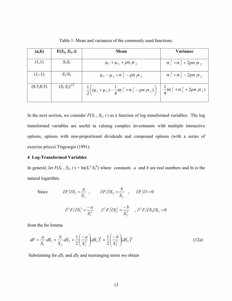
We summarize the parameters, mean and variance of the processes for two state variables in

Table 1.

13

Table 1: Mean and variances of the commonly used functions.

(a,b) F(S1, S2, t) Mean Variance

(1,1) S1S2 2121 σρσµµ ++21

22

21 2 σρσσσ ++

(1,-1) S1/S2 212221 σρσσµµ −+− 21

22

21 2 σρσσσ −+

(0.5,0.5) (S1 S2)1/2

−+−+ )(

4

1)(

2

121

22

2121 σρσσσµµ )2(

4

121

22

21 σρσσσ ++

In the next section, we consider F(S1 , S2, t ) as a function of log transformed variables. The log

transformed variables are useful in valuing complex investments with multiple interactive

options, options with non-proportional dividends and compound options (with a series of

exercise prices) Trigeorgis (1991).

4 Log-Transformed Variables

In general, let F(S1 , S2, t ) = ln(S1a S2

b) where constants a and b are real numbers and ln is the

natural logarithm.

Since 1

1S

aSF =∂∂ ,

2

2S

bSF =∂∂ , 0=∂∂ tF

21

21

2

S

aSF

−=∂∂

22

22

2

S

bSF

−=∂∂ , 021

2 =∂∂∂ SSF

from the Ito lemma

( ) ( )222

2

212

1

2

2

1

1 2

1

2

1dS

S

bdS

S

adS

S

bdS

S

adF

−+

−++= (12a)

Substituting for dS1 and dS2 and rearranging terms we obtain

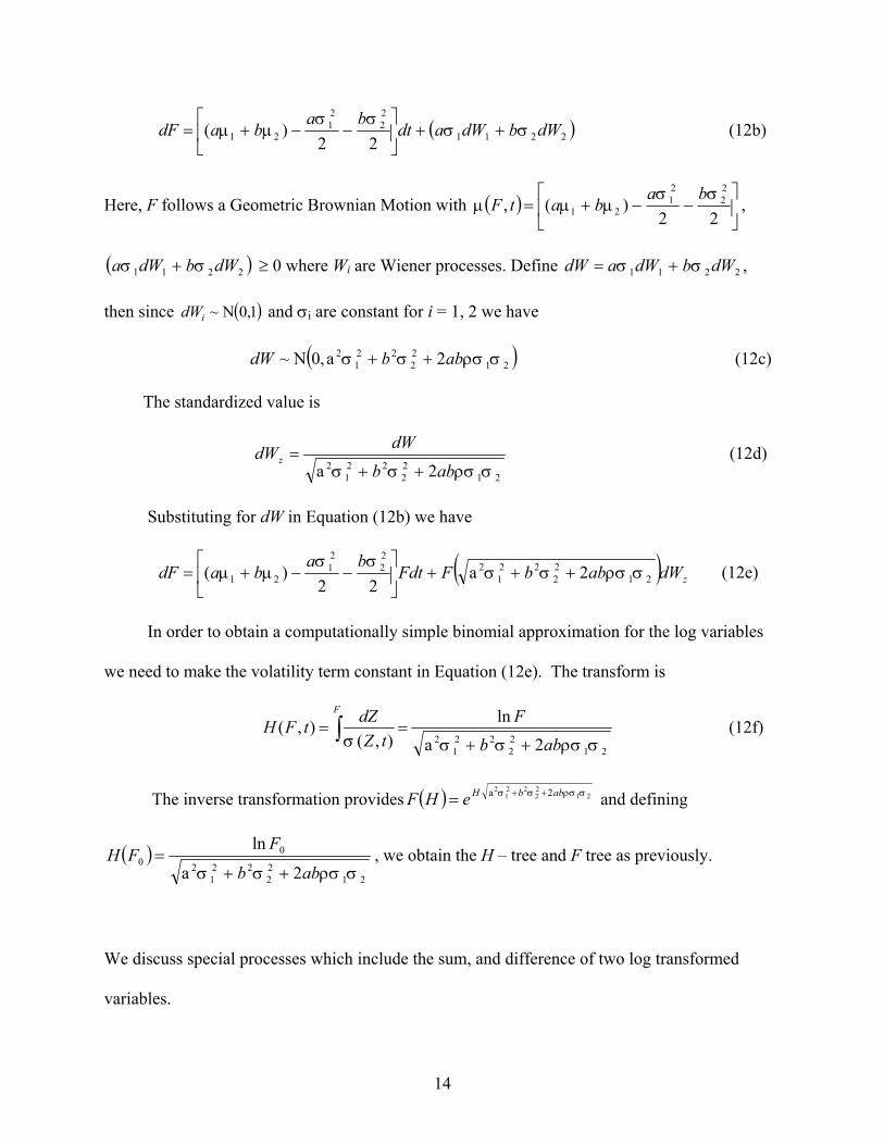
14

( )2211

22

21

21 22)( dWbdWadt

babadF σσ

σσµµ ++

−−+= (12b)

Here, F follows a Geometric Brownian Motion with ( )

−−+=

22)(,

22

21

21

σσµµµ

babatF ,

( )2211 dWbdWa σσ + ≥ 0 where Wi are Wiener processes. Define 2211 dWbdWadW σσ += ,

then since ( )1,0N~idW and σi are constant for i = 1, 2 we have

( )2122

221

2 2a0,N~ σρσσσ abbdW ++ (12c)


21

22

221

2 2a σρσσσ abb

dWdWz

++= (12d)

Substituting for dW in Equation (12b) we have

( ) zdWabbFFdtba

badF 2122

221

222

21

21 2a22

)( σρσσσσσ

µµ +++

−−+= (12e)

In order to obtain a computationally simple binomial approximation for the log variables

we need to make the volatility term constant in Equation (12e). The transform is

2122

221

2 2a

ln

),(),(

σρσσσσ abb

F

tZ

dZtFH

F

++== ∫ (12f)


221

2 2a σρσσσ abbHeHF ++= and defining

( )21

22

221

2

00

2a

ln

σρσσσ abb

FFH

++= , we obtain the H – tree and F tree as previously.

We discuss special processes which include the sum, and difference of two log transformed

variables.

15

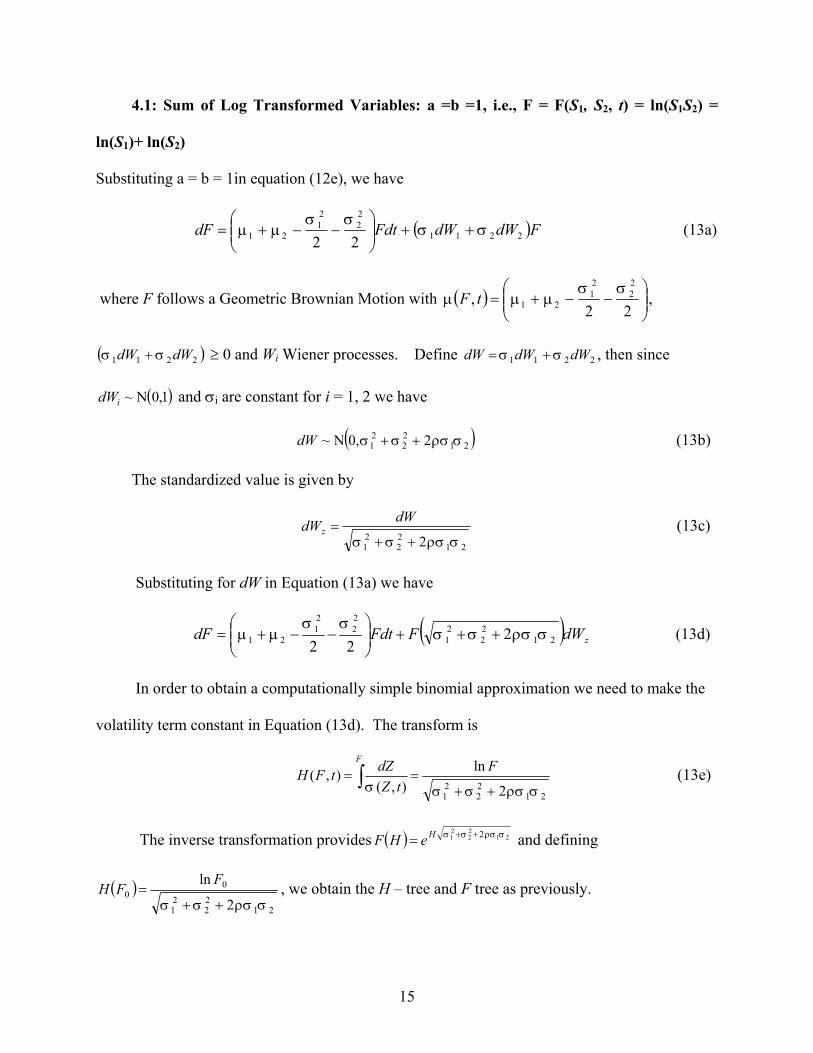
4.1: Sum of Log Transformed Variables: a =b =1, i.e., F = F(S1, S2, t) = ln(S1S2) =

ln(S1)+ ln(S2)

Substituting a = b = 1in equation (12e), we have

( )FdWdWFdtdF 2211

22

21

21 22σσ

σσµµ ++

−−+= (13a)

where F follows a Geometric Brownian Motion with ( )

−−+=

22,

22

21

21

σσµµµ tF ,

( )2211 dWdW σσ + ≥ 0 and Wi Wiener processes. Define 2211 dWdWdW σσ += , then since


( )2122

21 20,N~ σρσσσ ++dW (13b)

The standardized value is given by

21

22

21 2 σρσσσ ++

=dW

dWz (13c)


( ) zdWFFdtdF 2122

21

22

21

21 222

σρσσσσσ

µµ +++

−−+= (13d)


volatility term constant in Equation (13d). The transform is

2122

21 2

ln

),(),(


F

tZ

dZtFH

F

(13e)


21 2 σρσσσ ++= HeHF and defining

( )21

22

21

00

2

ln

σρσσσ ++=


16

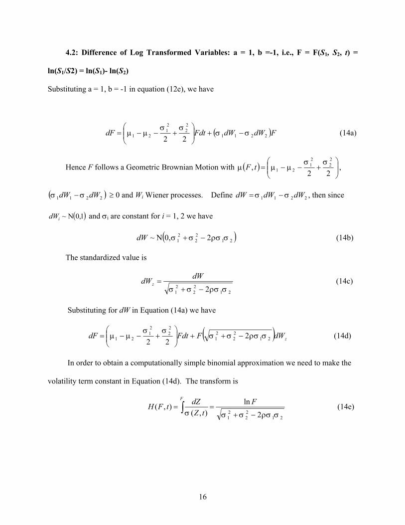
4.2: Difference of Log Transformed Variables: a = 1, b =-1, i.e., F = F(S1, S2, t) =

ln(S1/S2) = ln(S1)- ln(S2)

Substituting a = 1, b = -1 in equation (12e), we have

( )FdWdWFdtdF 2211

22

21

21 22σσ

σσµµ −+

+−−= (14a)

Hence F follows a Geometric Brownian Motion with ( )

+−−=

22,

22

21

21

σσµµµ tF ,

( )2211 dWdW σσ − ≥ 0 and Wi Wiener processes. Define 2211 dWdWdW σσ −= , then since


( )2122

21 20,N~ σρσσσ −+dW (14b)


21

22

21 2 σρσσσ −+

=dW

dWz (14c)


( ) zdWFFdtdF 2122

21

22

21

21 222

σρσσσσσ

µµ −++

+−−= (14d)


volatility term constant in Equation (14d). The transform is

2122

21 2

ln

),(),(

σρσσσσ −+== ∫

F

tZ

dZtFH

F

(14e)

17


21 2 σρσσσ −+= HeHF and defining

( )21

22

21

00

2

ln

σρσσσ −+=


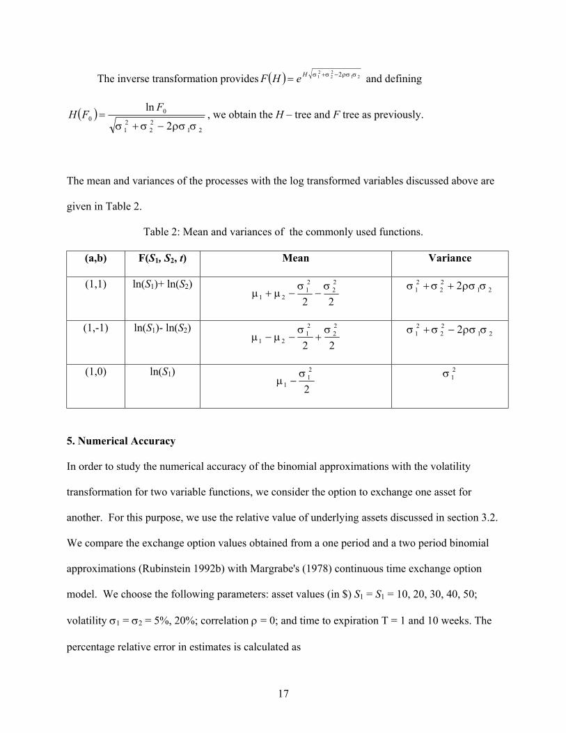
The mean and variances of the processes with the log transformed variables discussed above are

given in Table 2.

Table 2: Mean and variances of the commonly used functions.

(a,b) F(S1, S2, t) Mean Variance

(1,1) ln(S1)+ ln(S2)

22

22

21

21

σσµµ −−+ 21

22

21 2 σρσσσ ++

(1,-1) ln(S1)- ln(S2)

22

22

21

21

σσµµ +−− 21

22

21 2 σρσσσ −+

(1,0) ln(S1)

2

21

1

σµ −

21σ

5. Numerical Accuracy

In order to study the numerical accuracy of the binomial approximations with the volatility

transformation for two variable functions, we consider the option to exchange one asset for

another. For this purpose, we use the relative value of underlying assets discussed in section 3.2.

We compare the exchange option values obtained from a one period and a two period binomial

approximations (Rubinstein 1992b) with Margrabe's (1978) continuous time exchange option

model. We choose the following parameters: asset values (in $) S1 = S1 = 10, 20, 30, 40, 50;

volatility σ1 = σ2 = 5%, 20%; correlation ρ = 0; and time to expiration T = 1 and 10 weeks. The

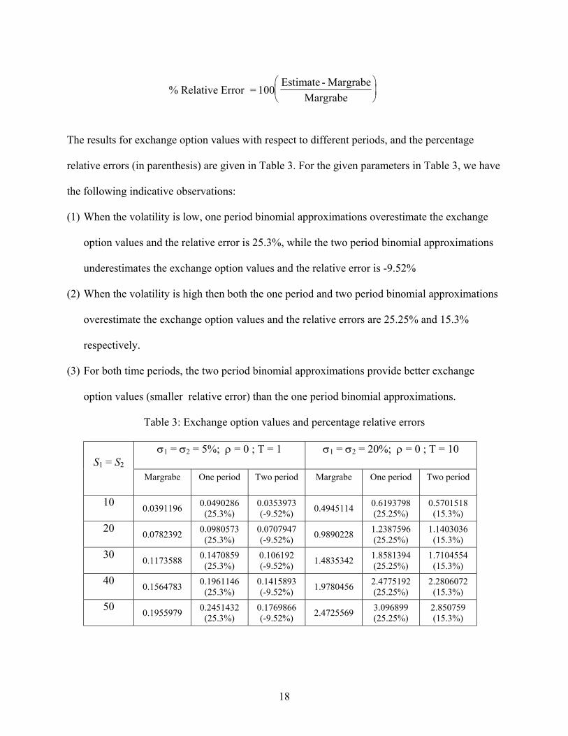
percentage relative error in estimates is calculated as

18

The results for exchange option values with respect to different periods, and the percentage

relative errors (in parenthesis) are given in Table 3. For the given parameters in Table 3, we have

the following indicative observations:

(1) When the volatility is low, one period binomial approximations overestimate the exchange

option values and the relative error is 25.3%, while the two period binomial approximations

underestimates the exchange option values and the relative error is -9.52%

(2) When the volatility is high then both the one period and two period binomial approximations

overestimate the exchange option values and the relative errors are 25.25% and 15.3%

respectively.

(3) For both time periods, the two period binomial approximations provide better exchange

option values (smaller relative error) than the one period binomial approximations.

Table 3: Exchange option values and percentage relative errors

σ1 = σ2 = 5%; ρ = 0 ; T = 1 σ1 = σ2 = 20%; ρ = 0 ; T = 10S1 = S2

Margrabe One period Two period Margrabe One period Two period

100.0391196

0.0490286(25.3%)

0.0353973(-9.52%)

0.49451140.6193798(25.25%)

0.5701518(15.3%)

200.0782392

0.0980573(25.3%)

0.0707947(-9.52%)

0.98902281.2387596(25.25%)

1.1403036(15.3%)

300.1173588

0.1470859(25.3%)

0.106192(-9.52%)

1.48353421.8581394(25.25%)

1.7104554(15.3%)

400.1564783

0.1961146(25.3%)

0.1415893(-9.52%)

1.97804562.4775192(25.25%)

2.2806072(15.3%)

500.1955979

0.2451432(25.3%)

0.1769866(-9.52%)

2.47255693.096899(25.25%)

2.850759(15.3%)

% Relative Error = 100Estimate - Margrabe

Margrabe

19

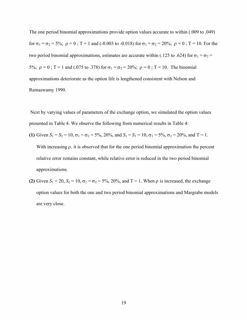
The one period binomial approximations provide option values accurate to within (.009 to .049)

for σ1 = σ2 = 5%; ρ = 0 ; T = 1 and (-0.003 to -0.018) for σ1 = σ2 = 20%; ρ = 0 ; T = 10. For the

two period binomial approximations, estimates are accurate within (.125 to .624) for σ1 = σ2 =

5%; ρ = 0 ; T = 1 and (.075 to .378) for σ1 = σ2 = 20%; ρ = 0 ; T = 10. The binomial

approximations deteriorate as the option life is lengthened consistent with Nelson and

Ramaswamy 1990.

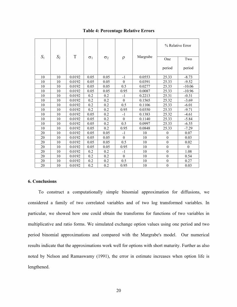
Next by varying values of parameters of the exchange option, we simulated the option values

presented in Table 4. We observe the following from numerical results in Table 4:

(1) Given S1 = S2 = 10, σ1 = σ2 = 5%, 20%, and S1 = S1 = 10, σ1 = 5%, σ2 = 20%, and T = 1.

With increasing ρ, it is observed that for the one period binomial approximation the percent

relative error remains constant, while relative error is reduced in the two period binomial

approximations.

(2) Given S1 = 20, S2 = 10, σ1 = σ2 = 5%, 20%, and T = 1. When ρ is increased, the exchange

option values for both the one and two period binomial approximations and Margrabe models

are very close.

20

Table 4: Percentage Relative Errors

% Relative Error

S1 S2 T σ1 σ2 ρ MargrabeOne

period

Two

period

10 10 0.0192 0.05 0.05 -1 0.0553 25.33 -8.7310 10 0.0192 0.05 0.05 0 0.0391 25.33 -9.5210 10 0.0192 0.05 0.05 0.5 0.0277 25.33 -10.0610 10 0.0192 0.05 0.05 0.95 0.0087 25.33 -10.9610 10 0.0192 0.2 0.2 -1 0.2213 25.31 -0.3110 10 0.0192 0.2 0.2 0 0.1565 25.32 -3.6910 10 0.0192 0.2 0.2 0.5 0.1106 25.33 -6.0110 10 0.0192 0.2 0.2 0.95 0.0350 25.33 -9.7110 10 0.0192 0.05 0.2 -1 0.1383 25.32 -4.6110 10 0.0192 0.05 0.2 0 0.1140 25.33 -5.8410 10 0.0192 0.05 0.2 0.5 0.0997 25.33 -6.5510 10 0.0192 0.05 0.2 0.95 0.0848 25.33 -7.2920 10 0.0192 0.05 0.05 -1 10 0 0.0720 10 0.0192 0.05 0.05 0 10 0 0.0320 10 0.0192 0.05 0.05 0.5 10 0 0.0220 10 0.0192 0.05 0.05 0.95 10 0 020 10 0.0192 0.2 0.2 -1 10 0 1.0820 10 0.0192 0.2 0.2 0 10 0 0.5420 10 0.0192 0.2 0.2 0.5 10 0 0.2720 10 0.0192 0.2 0.2 0.95 10 0 0.03

6. Conclusions

To construct a computationally simple binomial approximation for diffusions, we

considered a family of two correlated variables and of two log transformed variables. In

particular, we showed how one could obtain the transforms for functions of two variables in

multiplicative and ratio forms. We simulated exchange option values using one period and two

period binomial approximations and compared with the Margrabe's model. Our numerical

results indicate that the approximations work well for options with short maturity. Further as also

noted by Nelson and Ramaswamy (1991), the error in estimate increases when option life is

lengthened.

21

Acknowledgement

We would like to thank Gordon Sick, University of Calgary for suggesting the research work by

Nelson and Ramaswamy in the context of multinomial approximation models.

References

Boyle, P. P., 1998. A Lattice Framework for Option Pricing with Two State Variables. Journal

and Quantitative Analysis. 23(1) (March), 1 -12.

Boyle, P. P., J Evnine and S. Gibbs 1989. Numerical Evaluation of Multivariate Contingent

Claims. The Review of Financial Studies. 2(2) 241-250.

Cortazar G., and E. S. Schwartz. 1993. A Compound Option Model of Production and

Intermediate Inventories. Journal of Business 66(4) 17-540.

Johnson H. 1987. Options on the Maximum or the Minimum of Several Assets. Journal of

Financial and Quantitative Analysis. 22(3) (September) 277- 283.

Kamrad B., and Ritchken P. 1991. Multinomial Approximating Model for Options with k-State

Variables. Management Science. 37(12) (December) 1640-1652.

Margrabe W., 1978. The Value of an Option to Exchange One Asset for Another. The Journal of

Finance. 33(1)177-186.

Nelson D. B., and K. Ramaswamy. 1990. Simple Binomial Processes as Diffusion

Approximations in Financial Models. The Review of Financial Studies. 3(3) 393- 430.

Rubinstein M. 1992. One for Another. RISK (July-August) 191-194.

Stulz R. M. 1982. Options on the Minimum or the Maximum of Two Risk Assets: Analysis and

Applications. Journal of Financial Economics. 10 (July) 161-185.

22

Trigeorgis L. 1991. A Log-Transformed Binomial Numerical Analysis Method for Valuing

Complex Multi-Option Investments .Journal of Financial and Quantitative Analysis. 26 (3)

(September) 309-326.

On Simple Binomial Approximations for Two Variable Functions in Finance Applications

Documents