Journal of Machine Learning Research 9 (2008) 1875-1908 Submitted 4/07; Revised 4/08; Published 8/08 On Relevant Dimensions in Kernel Feature Spaces Mikio L. Braun MIKIO@CS. TU- BERLIN. DE Technische Universit¨ at Berlin Franklinstr. 28/29, FR 6-9 10587 Berlin, Germany Joachim M. Buhmann JBUHMANN@INF. ETHZ. CH Institute of Computational Science ETH Zurich, Universit¨ atstrasse 6 CH-8092 Z ¨ urich, Switzerland Klaus-Robert M ¨ uller * KRM@CS. TU- BERLIN. DE Technische Universit¨ at Berlin Franklinstr. 28/29, FR 6-9 10587 Berlin, Germany Editor: Peter Bartlett Abstract We show that the relevant information of a supervised learning problem is contained up to negligi- ble error in a finite number of leading kernel PCA components if the kernel matches the underlying learning problem in the sense that it can asymptotically represent the function to be learned and is sufficiently smooth. Thus, kernels do not only transform data sets such that good generalization can be achieved using only linear discriminant functions, but this transformation is also performed in a manner which makes economical use of feature space dimensions. In the best case, kernels pro- vide efficient implicit representations of the data for supervised learning problems. Practically, we propose an algorithm which enables us to recover the number of leading kernel PCA components relevant for good classification. Our algorithm can therefore be applied (1) to analyze the interplay of data set and kernel in a geometric fashion, (2) to aid in model selection, and (3) to denoise in feature space in order to yield better classification results. Keywords: kernel methods, feature space, dimension reduction, effective dimensionality 1. Introduction Kernel machines implicitly map the data into a high-dimensional feature space in a non-linear fash- ion using a kernel function. This mapping is often referred to as an empirical kernel map (Sch ¨ olkopf et al., 1999; Vapnik, 1998; M¨ uller et al., 2001; Sch ¨ olkopf and Smola, 2002). By virtue of the empir- ical kernel map, the data is ideally transformed in a way such that a linear discriminative function can separate the classes with low generalization error by a canonical hyperplane with large mar- gin. Such large margin hyperplanes provide an appropriate mechanism of capacity control and thus “protect” against the high dimensionality of the feature space. However, this picture is incomplete as it does not explain why the typical variants of capacity control cooperate well with the induced feature map. This paper adds a novel aspect as the key idea *. Also at Fraunhofer FIRST.IDA, Kekul´ estr. 7, 12489 Berlin, Germany. c 2008 Mikio L. Braun, Joachim M. Buhmann and Klaus-Robert M ¨ uller.

Welcome message from author
This document is posted to help you gain knowledge. Please leave a comment to let me know what you think about it! Share it to your friends and learn new things together.
Transcript
Journal of Machine Learning Research 9 (2008) 1875-1908 Submitted 4/07; Revised 4/08; Published 8/08
On Relevant Dimensions in Kernel Feature Spaces
Mikio L. Braun [email protected]
Technische Universitat BerlinFranklinstr. 28/29, FR 6-910587 Berlin, Germany
Joachim M. Buhmann [email protected]
Institute of Computational ScienceETH Zurich, Universitatstrasse 6CH-8092 Zurich, Switzerland
Klaus-Robert Muller∗ [email protected]
Technische Universitat BerlinFranklinstr. 28/29, FR 6-910587 Berlin, Germany
Editor: Peter Bartlett
AbstractWe show that the relevant information of a supervised learning problem is contained up to negligi-ble error in a finite number of leading kernel PCA components if the kernel matches the underlyinglearning problem in the sense that it can asymptotically represent the function to be learned and issufficiently smooth. Thus, kernels do not only transform data sets such that good generalization canbe achieved using only linear discriminant functions, but this transformation is also performed ina manner which makes economical use of feature space dimensions. In the best case, kernels pro-vide efficient implicit representations of the data for supervised learning problems. Practically, wepropose an algorithm which enables us to recover the number of leading kernel PCA componentsrelevant for good classification. Our algorithm can therefore be applied (1) to analyze the interplayof data set and kernel in a geometric fashion, (2) to aid in model selection, and (3) to denoise infeature space in order to yield better classification results.
Keywords: kernel methods, feature space, dimension reduction, effective dimensionality
1. Introduction
Kernel machines implicitly map the data into a high-dimensional feature space in a non-linear fash-ion using a kernel function. This mapping is often referred to as an empirical kernel map (Scholkopfet al., 1999; Vapnik, 1998; Muller et al., 2001; Scholkopf and Smola, 2002). By virtue of the empir-ical kernel map, the data is ideally transformed in a way such that a linear discriminative functioncan separate the classes with low generalization error by a canonical hyperplane with large mar-gin. Such large margin hyperplanes provide an appropriate mechanism of capacity control and thus“protect” against the high dimensionality of the feature space.
However, this picture is incomplete as it does not explain why the typical variants of capacitycontrol cooperate well with the induced feature map. This paper adds a novel aspect as the key idea
∗. Also at Fraunhofer FIRST.IDA, Kekulestr. 7, 12489 Berlin, Germany.
c©2008 Mikio L. Braun, Joachim M. Buhmann and Klaus-Robert Muller.
BRAUN, BUHMANN AND MULLER
to this picture. We show theoretically that if the learning problem matches the kernel well, the rele-vant information of a supervised learning data set is always contained in the subspace spanned by afinite and typically small number of leading kernel PCA components (principal component analysisin the feature space induced by the kernel, see below and Section 2), up to negligible error. This re-sult is based on recent approximation bounds for the eigenvectors of the kernel matrix which showthat if a function can be reconstructed using only a few kernel PCA components asymptotically,then the same already holds in a finite sample setting, even for small sample sizes.
Consequently, the use of a kernel function not only greatly increases the expressive power oflinear methods by non-linearly transforming the data, but it does so ensuring that the high dimen-sionality of the feature space does not become overwhelming: the relevant information for learningstays confined within a comparably low-dimensional subspace. This finding underlines the efficientuse of data that is made by kernel machines if the kernel works well for the learning problem. Asmart choice of kernel permits to make better use of the available data at a favorable “number ofdata points per effective dimension”-ratio, even for infinite-dimensional feature spaces. The kernelinduces an efficient representation of the data in feature space such that even unregularized methodslike linear least squares regression are able to perform well on the reduced feature space.
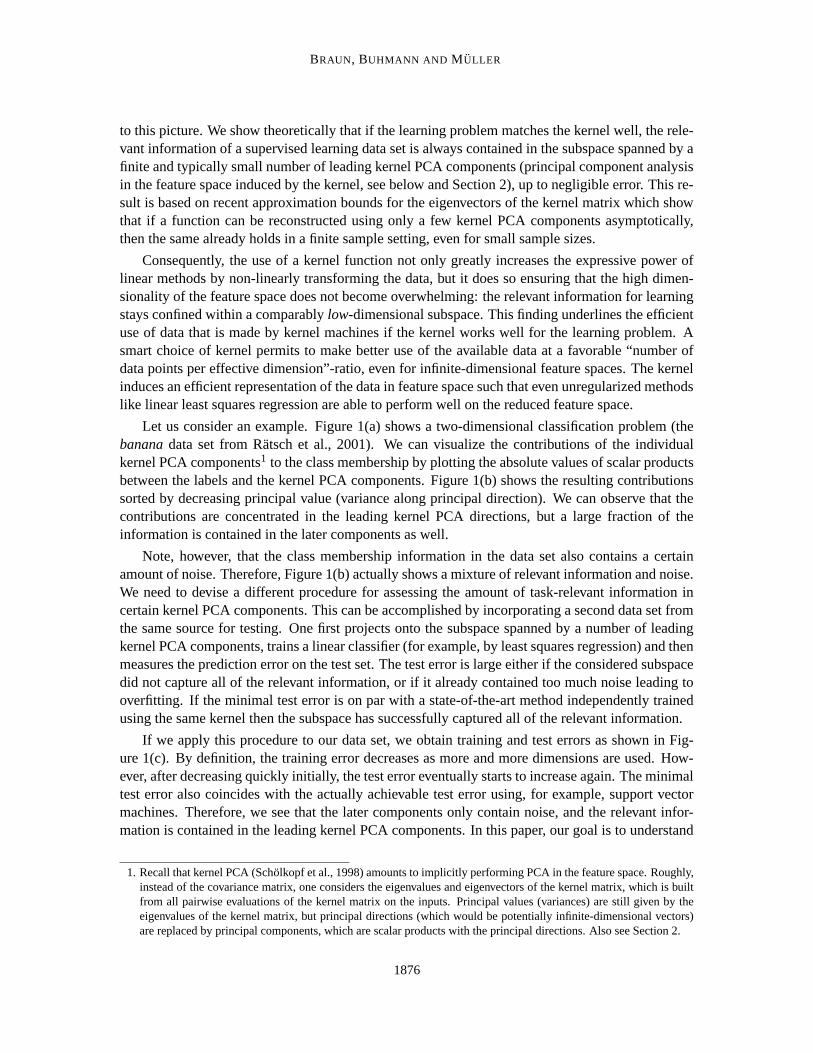
Let us consider an example. Figure 1(a) shows a two-dimensional classification problem (thebanana data set from Ratsch et al., 2001). We can visualize the contributions of the individualkernel PCA components1 to the class membership by plotting the absolute values of scalar productsbetween the labels and the kernel PCA components. Figure 1(b) shows the resulting contributionssorted by decreasing principal value (variance along principal direction). We can observe that thecontributions are concentrated in the leading kernel PCA directions, but a large fraction of theinformation is contained in the later components as well.
Note, however, that the class membership information in the data set also contains a certainamount of noise. Therefore, Figure 1(b) actually shows a mixture of relevant information and noise.We need to devise a different procedure for assessing the amount of task-relevant information incertain kernel PCA components. This can be accomplished by incorporating a second data set fromthe same source for testing. One first projects onto the subspace spanned by a number of leadingkernel PCA components, trains a linear classifier (for example, by least squares regression) and thenmeasures the prediction error on the test set. The test error is large either if the considered subspacedid not capture all of the relevant information, or if it already contained too much noise leading tooverfitting. If the minimal test error is on par with a state-of-the-art method independently trainedusing the same kernel then the subspace has successfully captured all of the relevant information.
If we apply this procedure to our data set, we obtain training and test errors as shown in Fig-ure 1(c). By definition, the training error decreases as more and more dimensions are used. How-ever, after decreasing quickly initially, the test error eventually starts to increase again. The minimaltest error also coincides with the actually achievable test error using, for example, support vectormachines. Therefore, we see that the later components only contain noise, and the relevant infor-mation is contained in the leading kernel PCA components. In this paper, our goal is to understand
1. Recall that kernel PCA (Scholkopf et al., 1998) amounts to implicitly performing PCA in the feature space. Roughly,instead of the covariance matrix, one considers the eigenvalues and eigenvectors of the kernel matrix, which is builtfrom all pairwise evaluations of the kernel matrix on the inputs. Principal values (variances) are still given by theeigenvalues of the kernel matrix, but principal directions (which would be potentially infinite-dimensional vectors)are replaced by principal components, which are scalar products with the principal directions. Also see Section 2.
1876
ON RELEVANT DIMENSIONS IN KERNEL FEATURE SPACES
−3 −2 −1 0 1 2 3−2
−1.5
−1
−0.5
0
0.5
1
1.5
2
2.5
(a) The training data set.
0 50 100 150 200 250 300 350 4000
1
2
3
4
5
6
7
8
9
10
kernel PCA components
abso
lute
con
trib
utio
n to
cla
ss m
embe
rshi
p
(b) Contributions of kernel PCA components.
0 50 100 150 200 250 300 350 4000
10
20
30
40
50
60
number of kernel PCA components
pred
ictio
n er
rors
(%
)
training errortest error
(c) Training and test errors using only leading kernel PCAcomponents.
−3 −2 −1 0 1 2
−2
−1.5
−1
−0.5
0
0.5
1
1.5
2
2.5
3
(d) The solution on the test data set.
Figure 1: A more complex example (resample 1 of the “banana” data set, see Section A). This time,the information is not contained in a single component. Nevertheless, the test error of ahyperplane learned using only the first d components has a clear minimum at d = 34 atoptimal error rate (cf. Table 3), showing that the relevant information is contained in theleading 34 directions.
more thoroughly why and when this effect occurs, and to estimate the dimensionality of a concretedata set given a kernel.
Our claim—that the relevant information about a learning problem is contained in the spacespanned by the leading kernel PCA components—is similar to the idea that the information aboutthe learning problem is contained in the kernel PCA components with the largest contributions.However, our results show that the magnitude of the contribution of a kernel PCA component tothe label information is only partially indicative of the relevance of that component. Instead, weshow that the leading kernel PCA components (sorted by corresponding principal value) contain
1877

BRAUN, BUHMANN AND MULLER
the relevant information. Components which contain only little variance will therefore not containrelevant information. If such a component manages to contribute much to the label information, itwill only reflect noise.
What practical implications follow from these results? We explore several possibilities of usingthese ideas to assess the suitability of a kernel or a family of kernels to a specific data set. Themain idea is that the observed dimensionality of the data set in feature space is characteristic forthe relation between a data set and a kernel. Roughly speaking, the relevant dimensionality of thedata set corresponds to the complexity of the learning problem when viewed through the “lens”of the kernel function. Using the estimated dimensionality, one can project the labels onto thecorresponding subspace and obtain a noise free version of the labels. By comparing the denoisedlabels to the original labels, one can estimate of the amount of noise contained in the labels. Onetherefore obtains a more detailed measure of the fit between the kernel and the data set as comparedto, for example, the cross-validation error alone. This allows us to take a closer look at data sets onwhich the achieved error is quite large. In such cases, we are able to distinguish whether the dataset is highly complex and the amount of data is insufficient, or the amount of intrinsic noise is verylarge. This is practically relevant as one has to deal with both these cases quite differently, either byproviding more data, or by thinking about means to obtain less noisy or ambiguous features.
We summarize the main contributions of this paper: (1) We provide theoretical bounds showingthat the relevant information (defined in Section 2) is actually contained in the leading projectedkernel principal components under appropriate conditions. (2) We propose an algorithm which es-timates the relevant dimensionality and related estimates of the data set and permits to analyze theappropriateness of a kernel for the data set, and thus to perform model selection among different ker-nels. (3) We validate the accuracy of the estimates experimentally by showing that non-regularizedmethods perform on the reduced feature space on par with state-of-the-art kernel methods. We ana-lyze some well-known benchmark data sets in Section 5. Note that we do not claim to obtain betterperformance within our framework when compared to, for example, cross-validation techniques.Rather, we are on par. Our contribution is to foster an understanding about a data set and to gainbetter insights of whether a mediocre classification result is due to intrinsic high dimensionality ofthe data (and consequently insufficient number of examples), or an overwhelming noise level.
2. Preliminaries
Let us start to formalize the ideas introduced so far. As usual, we consider a data set (X1,Y1),. . . ,(Xn,Yn) where the inputs X lie in some space X and the outputs Y to be predicted are in Y ={±1} for classification or Y = R for regression. We often refer to the outputs Yi as the “labels”irrespective of whether we are considering a classification or regression task. We assume that the(Xi,Yi) are drawn i.i.d. from some probability measure PX×Y . In kernel methods, the data is non-linearly mapped into some feature space F via the feature map Φ. Scalar products in F can becomputed by the kernel k in closed form: 〈Φ(x),Φ(x′)〉 = k(x,x′). Summarizing all the pairwisescalar products results in the (normalized) kernel matrix K with entries k(Xi,X j)/n.
In the discussion below, we study the relationship between the label vector Y = (Y1, . . . ,Yn) andthe kernel PCA components which are introduced next. Kernel PCA (Scholkopf et al., 1998) is akernelized version of PCA. Since the dimensionality of the feature space might be too large to deal
1878
ON RELEVANT DIMENSIONS IN KERNEL FEATURE SPACES
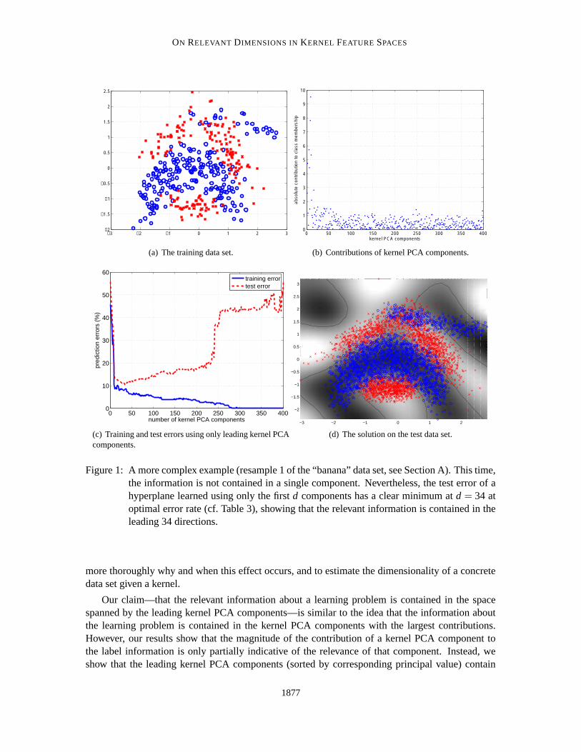
Symbol Meaningn number of training examplesXi ∈ X input examplesYi ∈ Y output labelsk : X ×X → R kernel functionK = (k(Xi,X j))/n (normalized) kernel matrixY = (Y1, . . . ,Yn) label vectorΦ : X → F feature maplm ∈ R≥0 mth kernel PCA value (in descending order),
mth eigenvalue of kernel matrix Kvm ∈ F mth kernel PCA directionfm(x) = 〈Φ(x),vm〉 mth kernel PCA componentum = ( fm(X1), . . . , fm(Xn)) mth kernel PCA component evaluated on X1, . . . ,Xn,
mth eigenvector of kernel matrix Kπd(Y ) = ∑d
i=1 uiuiY projection onto first d kernel PCA componentsG = (E(Y1|X1), . . . ,E(Yn|Xn)) relevant information vectorzi = u>i G contribution of ith eigenvector to relevant informationg(x) = E(Y |X = x) relevant information functionL2(X ,PX ) set of all square integrable functions with respect to PXTk f (s) =
R
X k(s, t) f (t)PX (dt) integral operator associated with kλi ∈ R≥0 ith eigenvalue of Tk
ψi ∈ L2(X ,PX ) ith eigenfunction of Tk
ζi = 〈ψi,g〉 contribution of ith eigenfunction to relevant informationd estimated relevant dimensioncvloo leave-one-out cross-validation errorG estimated relevant information vectorS = ∑d
i=1 uiu>i “hat”-matrixˆerr estimated noise-level
Table 1: Overview of notation used in this paper.
with the vectors directly, the principal directions are represented using the points Xi of the data set:
vm =n
∑i=1
αiΦ(Xi),
where αi = [um]i/lm, [um]i is the ith component of the mth eigenvector of the kernel matrix K, andlm the corresponding eigenvalue.2 Still, vm can usually not be computed explicitly such that oneinstead works with kernel PCA components
fm(x) = 〈Φ(x),vm〉.
We are interested in the relation between fm and a label vector Y . As we have seen in the introduc-tion, it seems that only a finite number of leading kernel PCA components are necessary to representthe relevant information about the learning problem up to a small error.
2. As usual, we assume that lm and um have been sorted such that l1 ≥ . . .≥ ln.
1879
BRAUN, BUHMANN AND MULLER
Therefore, we would like to compare fm with the values Y1, . . . ,Yn at the points X1, . . . ,Xn. Thefollowing easy lemma summarizes the relationship between the sample vector of fm and Y .
Lemma 1 The mth kernel PCA component fm evaluated on the Xis is equal to the mth eigenvector ofthe kernel matrix K: ( fm(X1), . . . , fm(Xn)) = um. Consequently, the sample vectors are orthogonal,and the projection of a vector Y ∈R
n onto the leading d kernel PCA components is given by πd(Y ) =
∑dm=1 umu>mY.
Proof The mth kernel PCA component for a point X j in the training set is
fm(X j) = 〈Φ(X j),vm〉=1lm
n
∑i=1
〈Φ(X j),Φ(Xi)〉[um]i =1lm
n
∑i=1
k(X j,Xi)[um]i.
The sum computes the jth component of Kum, and Kum = lmum, because um is an eigenvector of K.Therefore
fm(X j) =1lm
[lmum] j = [um] j.
Since K is a symmetric matrix, its eigenvectors um are orthonormal, and the projection of Y ontothe space spanned by the first d kernel PCA components is given by ∑d
m=1 umu>mY . �
Since the kernel PCA components are orthogonal, the coefficients of a vector Y ∈ Rn with
respect to the basis u1, . . . ,un is easily computed by forming the scalar products. We call the coeffi-cients
zm = u>mY (1)
of Y w.r.t. the basis formed from the kernel PCA components the kernel PCA coefficients. They arethe central object of our discussion.
The projection of Y to a kernel PCA component can be thought of as the least squares regressionof Y using only the direction along the kernel PCA component in feature space.
Using the kernel PCA coefficients, we can extend the projected labels to new points via
Y (x) =d
∑m=1
zm fm(x),
which amounts to the prediction of least squares regression on the reduced feature space.
3. The Label Vector and Kernel PCA Components
In the introduction, we have discussed an example which suggests that a small number of leadingkernel PCA components might suffice to capture the relevant information about the output variable.It is clear that we cannot expect this behavior for all possible data sets and kernels. It seems plausiblethough, that under certain conditions, the distribution of the data and the kernel fit together well.Then we can expect to observe this behavior with high probability for a random sample from thisdistribution through some form of concentration or convergence property.
1880

ON RELEVANT DIMENSIONS IN KERNEL FEATURE SPACES
−3 −2 −1 0 1 2 3 4 5
−1
−0.8
−0.6
−0.4
−0.2
0
0.2
0.4
0.6
0.8
1
X
Y
d a tare le v a n t in fo rm a tio n Gp (x | Y = 1)p (x | Y = −1)
−4 −3 −2 −1 0 1 2 3 4−0.4
−0.2
0
0.2
0.4
0.6
0.8
1
1.2
X
Y
d a tare le v a n t in fo rm a tio n G
Figure 2: Relevant information vectors visualized for the classification and the regression case.In the (two-class) classification case (left) it encodes the posterior probability (scaledbetween −1 and 1), in the regression case it is the sample vector of the function to belearned.
3.1 Decomposing the Label Vector Information
We start the discussion by defining formally what the relevant information contained in the labelsis. Given a label vector Y , we define the relevant information vector as the vector of the expectedlabels:
G = (E(Y1|X1), . . . ,E(Yn|Xn)).
Intuitively speaking, G is a noise-free version of Y . This vector contains all the relevant informationabout the outputs Y of the learning problem: For regression, G amounts to the values of the truefunction. For the case of two-class classification, the vector G contains all the information about theoptimal decision boundary. Since E(Y |X) = P(Y = 1|X)−P(Y =−1|X), the sign of G contains therelevant information on the true class membership by telling us which class is more probable (seeFigure 2 for examples). Thus, using this denoised label information, the learning problem becomesmuch easier as the denoised labels already contain the Bayes optimal prediction at that point.3
Using G we obtain a very useful additive decomposition of the labels into “signal” and “noise”:
Y = G+N.
In this setting, we are now interested in showing that G is contained in the leading kernel PCA com-ponents, such that projecting G onto the leading kernel PCA components leads to only negligibleerror. In the following, we treat the signal and noise part of Y separately. This is possible becausethe projection πd is a linear operation such that πd(Y ) = πd(G+N) = πd(G)+πd(N).
3. Also note that the capacity control typically employed in kernel methods amounts to some form of regularization, or“implicit denoising” (Smola et al., 1998). Therefore, we do not expect that the results using G are generally betterthan with the original labels. However, as we will see below, unregularized methods perform on par with kernelmethods with capacity control using the estimated relevant information vector G.
1881
BRAUN, BUHMANN AND MULLER
3.2 The Relevant Information Vector
We first treat the relevant information vector G. The location of G with respect to the kernel PCAcomponents is characterized by scalar products with the eigenvectors of the kernel matrix. We startby discussing this relationship in an asymptotic setting and then transfer the results back to the finitesample setting using convergence results for the spectral properties of the kernel matrix
Using the kernel function k, we define the integral operator
Tk f (s) =Z
Xk(s, t) f (t)PX (dt),
where PX is the marginal distribution which generates the inputs Xi. It is well known that the linearoperator
Tk f (s) =1n
n
∑i=1
k(s,Xi) f (Xi)
represented by the kernel matrix approximates Tk as the number of points tend to infinity (see, forexample, von Luxburg, 2004). While this follows easily for a fixed f and s, making the argumenttheoretically exact for operators (this means uniform over all functions) is not trivial.
As a consequence, the eigenvalues and eigenvectors of Tk, which are equal to those of the kernelmatrix, converge to those of Tk (see Koltchinskii and Gine, 2000; Koltchinskii, 1998). In particular,scalar products of sample functions and eigenvectors of K converge to scalar products with eigen-functions of Tk. The asymptotic counterpart of the relevant information vector G is the function
g(x) = E(Y |X = x).
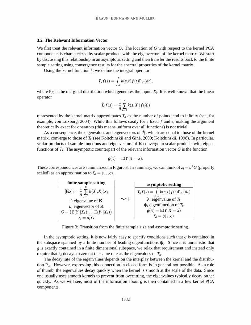
These correspondences are summarized in Figure 3. In summary, we can think of zi = u>i G (properlyscaled) as an approximation to ζi = 〈ψi,g〉.
finite sample setting
[Kx]i =1n
n
∑j=1
k(Xi,X j)x j
li eigenvalue of Kui eigenvector of K
G =(
E(Y1|X1), . . .E(Yn|Xn))
zi = u>i G
asymptotic setting
Tk f (s) =Z
Xk(s, t) f (t)PX (dt)
λi eigenvalue of Tk
ψi eigenfunction of Tk
g(x) = E(Y |X = x)ζi = 〈ψi,g〉
Figure 3: Transition from the finite sample size and asymptotic setting.
In the asymptotic setting, it is now fairly easy to specify conditions such that g is contained inthe subspace spanned by a finite number of leading eigenfunctions ψi. Since it is unrealistic thatg is exactly contained in a finite dimensional subspace, we relax that requirement and instead onlyrequire that ζi decays to zero at the same rate as the eigenvalues of Tk.
The decay rate of the eigenvalues depends on the interplay between the kernel and the distribu-tion PX . However, expressing this connection in closed form is in general not possible. As a ruleof thumb, the eigenvalues decay quickly when the kernel is smooth at the scale of the data. Sinceone usually uses smooth kernels to prevent from overfitting, the eigenvalues typically decay ratherquickly. As we will see, most of the information about g is then contained in a few kernel PCAcomponents.
1882
ON RELEVANT DIMENSIONS IN KERNEL FEATURE SPACES
A natural assumption is that the learning problem can be asymptotically represented by thegiven kernel function k. By this we mean that there exists some function h ∈ L 2(X ,PX ) such thatg = Tkh. Using the spectral decomposition of Tk, this implies
g = Tkh =∞
∑i=1
λi〈ψi,h〉ψi. (2)
Since the sequence of αi = 〈ψi,h〉 is square summable, it follows that
ζi = 〈ψi,g〉= λiαi = O(λi).
Intuitively speaking, (2) translates to asymptotic representability of the learning problem: As n→∞,it becomes possible to represent the optimal labels using the kernel function k.
Furthermore, we assume that k is bounded. This technical requirement is mainly necessary toensure that g is also bounded. The requirement holds for common radial basis function kernels likethe Gaussian kernel, and also if the underlying space X is compact and the kernel is continuous.
Note that the requirement that g lies in the range of Tk is essential. If this is not the case, wecannot expect that the scalar products decay at a given rate. Also note that it is in fact possible tobreak this condition. For example, if k is continuous, every non-continuous function does not lie inthe range of Tk.
The question is now whether the same behavior can be expected for a finite data set. Thisquestion is not trivial, because eigenvector stability is known to be linked to the gap between thecorresponding eigenvalues, which is fairly small for small eigenvalues (see, for example, Zwald andBlanchard, 2006).
The main theoretical result of this paper (Theorem 1 in the Appendix) provides a bound of theform
1n|u>i G| ≤ liC +E
which expresses an essential equivalence between the finite sample setting and the asymptotic set-ting with two modifications: The decay rate O(λi) of the scalar products 〈ψi,g〉 holds for the finitesample up to a (small) additive error E with λi replaced by its finite sample approximation li.
The technical details of this theorem and the proof are deferred to the appendix. Let us discusshow the absolute term occurs in the bound and why it can be expected to be small. An exactscaling bound (without additive term E) can only be derived (at least following the approach takenin this paper) for the case where the kernel function is degenerate, that is, Tk has only finitely manynon-zero eigenvalues. The same finiteness restriction also holds for the expansion of g in terms ofthe eigenfunctions of Tk. The proof thus contains a truncation step of general kernels and generalfunctions g, leading to a scaling bound on the scalar product and an additive term arising from thetruncation. However, as the name suggests, the truncation error E can be made arbitrarily small byconsidering approximations with many non-zero eigenvalues. At the same time, considering suchkernels with more terms in the expansion leads to a larger constant C in the actual scaling part. Thus,both terms have to be balanced by the order of truncation, which permits to control the additive termwell practically.
Note that the problem considered here is significantly different from the problem studying theperformance of kernel PCA itself (see, for example, Blanchard et al., 2007; Shawe-Taylor et al.,2005; Mika, 2002). There, only the projection error using the Xs is studied. Here, we are specificallyinterested in the relationship between the Y s and the Xs.
1883
BRAUN, BUHMANN AND MULLER
In view of our original concern, the bound shows that the relevant information vector G (asintroduced in Section 2) is contained in a number of leading kernel PCA components up to a neg-ligible error. The number of dimensions depends on the asymptotic coefficients αi and the decayrate of the asymptotic eigenvalues of k. Since this rate is related to the smoothness of the kernelfunction, the dimension is small for smooth kernels whose leading eigenfunctions ψi permit goodapproximation of g.
3.3 The Noise
To study the relationship between the noise and the eigenvectors of the kernel matrix, no asymptoticarguments are necessary. The key insight is that the eigenvectors are independent of the noise in thelabels, such that the noise vector N is typically evenly distributed over all coefficients u>i N: Let U bethe matrix whose ith column is equal to ui. The coefficients of N with respect to the eigenbasis of Kare then given by U>N. Note that since U is orthogonal, multiplication by its transpose amounts toa (random) rotation. In particular, this rotation is independent of the noise N as the ui depend on theXs only. Now if the noise has a spherical distribution, for example, N is normally distributed withcovariance matrix σ2
εI, it follows that U>N ∼ N (0,σ2εI). For heteroscedastic noise in a regression
setting, or for classification, this simple analysis is not sufficient. In that case, the individual u>i Nare no longer uncorrelated. However, because of the independence of the Ni, the variance of u>i N isupper bounded by
Var(u>i N) =n
∑j=1
u2i, j Var(N j)≤ max
1≤ j≤nVar(N j)
since ∑nj=1 u2
i, j = ‖ui‖2 = 1. Therefore, the variance of the u>i N is not concentrated in any singlecoefficient as the total variance does not increase by rotating the basis and the individual variancesare bounded by the maximum individual variance before the rotation.
The practical relevance of these observations is that the relevant information and noise part haveradically different properties with respect to the kernel PCA components, allowing us to practicallyestimate the number of relevant dimension for a given kernel and data set. In the next section, wewill propose two different algorithms for this task.
4. Relevant Dimension Estimation and Related Estimates
We have seen that the number of leading kernel PCA components necessary to capture the relevantinformation about the labels of a finite size data set is bounded under the mild assumptions that thelearning problem can be represented asymptotically and the kernel is smooth such that the eigenval-ues of the kernel matrix decay quickly. The actual number of necessary dimensions depends on theinterplay between kernel and learning data set, giving insights into the suitability of the kernel. Forexample, a kernel might fail to provide an efficient representation of the learning problem, leadingto an embedding requiring many kernel PCA components to capture the information on Y . Or, evenworse, a kernel might completely fail to model some part of the learning problem, such that a part ofthe information appears to be just noise. Therefore, in order to make practical use of the presentedinsights, we need to devise a method to estimate the number of relevant kernel PCA components fora given concrete data set and choice of kernel.
In this section we propose methods for estimating the actual dimensionality of a data set, and tworelated estimators. Based on the dimensionality estimate, one can denoise the labels by projecting
1884
ON RELEVANT DIMENSIONS IN KERNEL FEATURE SPACES
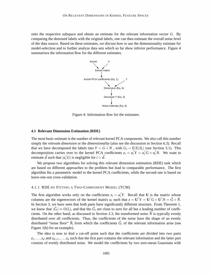
onto the respective subspace and obtain an estimate for the relevant information vector G. Bycomparing the denoised labels with the original labels, one can then estimate the overall noise levelof the data source. Based on these estimates, we discuss how to use the dimensionality estimate formodel-selection and to further analyze data sets which so far show inferior performance. Figure 4summarizes the information flow for the different estimates.
Y
Kernel matrix
XKernel
Noise estimate (Eq. 6)
Dimension (Eq. 4)
Kernel PCA coefficients (Eq. 1)
Denoised Y (Eq. 5)
Figure 4: Information flow for the estimates.
4.1 Relevant Dimension Estimation (RDE)
The most basic estimate is the number of relevant kernel PCA components. We also call this numbersimply the relevant dimension or the dimensionality (also see the discussion in Section 6.3). Recallthat we have decomposed the labels into Y = G + N , with Gi = E(Yi|Xi) (see Section 3.1). Thisdecomposition carries over to the kernel PCA coefficients zi = u>i Y = u>i G + u>i N. We want toestimate d such that |u>i G| is negligible for i > d.
We propose two algorithms for solving this relevant dimension estimation (RDE) task whichare based on different approaches to the problem but lead to comparable performance. The firstalgorithm fits a parametric model to the kernel PCA coefficients, while the second one is based onleave-one-out cross-validation.
4.1.1 RDE BY FITTING A TWO-COMPONENT MODEL (TCM)
The first algorithm works only on the coefficients zi = u>i Y . Recall that U is the matrix whosecolumns are the eigenvectors of the kernel matrix ui such that z = U>Y = U>G + U>N = G + N.In Section 3, we have seen that both parts have significantly different structure. From Theorem 1,we know that |Gi| ≈ O(li), and that the Gi are close to zero for all but a leading number of coeffi-cients. On the other hand, as discussed in Section 3.3, the transformed noise N is typically evenlydistributed over all coefficients. Thus, the coefficients of the noise have the shape of an evenlydistributed “noise floor” Ni from which the coefficients Gi of the relevant information arise (seeFigure 1(b) for an example).
The idea is now to find a cut-off point such that the coefficients are divided into two partsz1, . . . ,zd and zd+1, . . . ,zn such that the first part contains the relevant information and the latter partconsists of evenly distributed noise. We model the coefficients by two zero-mean Gaussians with
1885
BRAUN, BUHMANN AND MULLER
individual variances
zi ∼{
N (0,σ21) 1≤ i≤ d,
N (0,σ22) d < i≤ n.
Of course, in order to be able to extract meaningful information, it should hold that σ1 � σ2.Alternatively, one could assume that zi ∼N (0,σ2
1 +σ22), for 1≤ i≤ d, which nevertheless leads to
the exact same choice of d.For real data, both parts need not be actually Gaussian distributed. However, due to lack of
additional a priori knowledge on the signal or the noise, the Gaussian distribution represents theoptimal choice among all distributions with the same variance according to the maximum entropyprinciple (Jaynes, 1957).
The negative log-likelihood is proportional to
− log`(d)∼ dn
logσ21 +
n−dn
logσ22, with σ2
1 =1d
d
∑i=1
z2i , σ2
2 =1
n−d
n
∑i=d+1
z2i . (3)
The estimated dimension is then given as the maximum likelihood fit
d = argmin1≤d≤n′
(− log`(d)) = argmin1≤d≤n′
(
dn
logσ21 +
n−dn
logσ22
)
. (4)
Due to numerical instabilities of kernel PCA components corresponding to small eigenvalues, thechoice of d should be restricted to 1≤ d ≤ n′ < n: The coefficients zi are computed by taking scalarproducts with eigenvectors ui. For small eigenvalues (small meaning of the order of the availablenumerical precision, for double precision floating point numbers, this is typically around 10−16),individual eigenvectors cannot be computed accurately, although the space spanned by all theseeigenvectors is accurate. Therefore, coefficients zi for large i are not be reliable. To systematicallystabilize the algorithm, one should therefore limit the range of possible effective dimensions. Wehave found the choice of 1 ≤ d ≤ n/2 to work well as this choice ensures that at least half of thecoefficients are interpreted as noise. For very small and very complex data sets, this choice mightprove suboptimal and better thresholds based, for example, on the actual decay of eigenvalues mightbe advisable. However, on all data sets discussed in this paper, the above choice performed verywell.
4.1.2 RDE BY LEAVE-ONE-OUT CROSS-VALIDATION (LOO-CV)
We propose a second algorithm which is based on cross validation, a more general concept thanparametric noise modeling. This algorithm only depends on our theoretical results to the extent thatit searches for subspaces spanned by leading kernel PCA components. We later compare the twomethods to see whether our assumptions were justified.
As stated in Lemma 1, the projection of Y onto the space spanned by the d leading kernel PCAcomponents is given by ∑d
i=1 uiu>i Y , where ui are the eigenvectors of the kernel matrix. The matrixS = ∑d
i=1 uiu>i can be interpreted as a “hat matrix” in the context of regression.4 The idea is now tochoose the dimension which minimizes the leave-one-out cross-validation error. This subspace thencaptures all of the relevant information about Y without overfitting.
4. Recall that for regression methods where the fitted function depends linearly on the labels, the matrix S whichcomputes Y = SY is called the “hat matrix” since it “puts the hat on Y .”
1886
ON RELEVANT DIMENSIONS IN KERNEL FEATURE SPACES
Computationally, note that one can write the squared error leave-one-out cross-validation inclosed form, similar to kernel ridge regression (see Wahba, 1990):
cvloo(d) =1n
n
∑i=1
(
[SY ]i−Yi
1−Sii
)2
.
It is possible to organize the computation in a way such that given the eigendecomposition of K,each value cvloo(d) can be computed in O(n) (instead of O(n2) if one naively implements the aboveformula): Note that Sii is equal to ∑d
j=1(u j)2i , therefore, one can compute Sii iteratively by
S0ii← 0
Sd+1ii ← Sd
ii +(ud+1)2i .
In the same way, since Y = SY = ∑dj=1 u ju>jY , we get that
Y 0← 0
Y d+1← Y d +ud+1u>d+1Y.
The squared error is in principle not the most appropriate loss function for classification problems.But as we will see below, it nevertheless works well also for classification problems.
4.2 Denoising the Labels and Estimating the Noise Level
One direct application of the dimensionality estimate is the projection of Y onto the first d kernelPCA components. By Lemma 1, this projection is
G′ =d
∑i=1
uiu>i Y.
Then, an estimate of the noiseless labels is given by
G =
{
sign G′ classification against ±1 labels
G′ regression. (5)
Note that this amounts to computing the in-sample fit using kernel principal component regression(kPCR).
The estimated dimension can also be used to estimate the noise level present in the data set by
ˆerr =1n
n
∑i=1
L(Yi,Yi), (6)
where L is the loss function.The accuracy of both these estimates depends on a number of factors. Basically, the estimation
error is small if the first d kernel PCA components capture most of G and d is small such thatmost of the noise is removed. Note that our assumption that the kernel suits the data set is crucialfor both these requirements. If g does not lie in the span of the associated integral operator Tk,the coefficients decay only slowly and a huge number of dimensions are necessary to capture mostinformation about G, leading to a huge amount of residual noise.
1887
BRAUN, BUHMANN AND MULLER
10−5
100
105
0
0.1
0.2
0.3
0.4
0.5
0.6
0.7
kernel width
est.
nois
e le
vel (
%)
dimension (%)noise level
(a) Classification (“banana” data set)
10−6
10−4
10−2
100
102
104
106
0
0.05
0.1
0.15
0.2
0.25
0.3
0.35
0.4
0.45
0.5
kernel width
est.
nois
e le
vel (
MS
E)
dimension (%)noise level
(b) Regression (noisy sinc function)
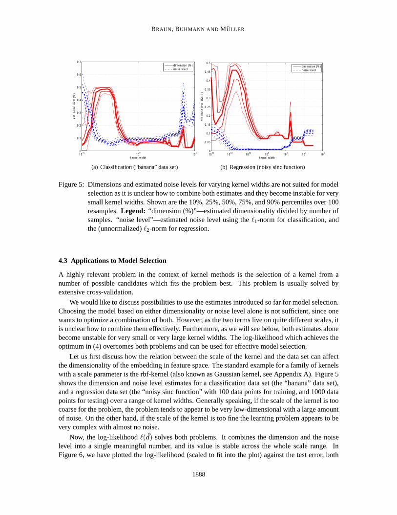
Figure 5: Dimensions and estimated noise levels for varying kernel widths are not suited for modelselection as it is unclear how to combine both estimates and they become instable for verysmall kernel widths. Shown are the 10%, 25%, 50%, 75%, and 90% percentiles over 100resamples. Legend: “dimension (%)”—estimated dimensionality divided by number ofsamples. “noise level”—estimated noise level using the `1-norm for classification, andthe (unnormalized) `2-norm for regression.
4.3 Applications to Model Selection
A highly relevant problem in the context of kernel methods is the selection of a kernel from anumber of possible candidates which fits the problem best. This problem is usually solved byextensive cross-validation.
We would like to discuss possibilities to use the estimates introduced so far for model selection.Choosing the model based on either dimensionality or noise level alone is not sufficient, since onewants to optimize a combination of both. However, as the two terms live on quite different scales, itis unclear how to combine them effectively. Furthermore, as we will see below, both estimates alonebecome unstable for very small or very large kernel widths. The log-likelihood which achieves theoptimum in (4) overcomes both problems and can be used for effective model selection.
Let us first discuss how the relation between the scale of the kernel and the data set can affectthe dimensionality of the embedding in feature space. The standard example for a family of kernelswith a scale parameter is the rbf-kernel (also known as Gaussian kernel, see Appendix A). Figure 5shows the dimension and noise level estimates for a classification data set (the “banana” data set),and a regression data set (the “noisy sinc function” with 100 data points for training, and 1000 datapoints for testing) over a range of kernel widths. Generally speaking, if the scale of the kernel is toocoarse for the problem, the problem tends to appear to be very low-dimensional with a large amountof noise. On the other hand, if the scale of the kernel is too fine the learning problem appears to bevery complex with almost no noise.
Now, the log-likelihood `(d) solves both problems. It combines the dimension and the noiselevel into a single meaningful number, and its value is stable across the whole scale range. InFigure 6, we have plotted the log-likelihood (scaled to fit into the plot) against the test error, both
1888
ON RELEVANT DIMENSIONS IN KERNEL FEATURE SPACES
10−5
100
105
0
0.1
0.2
0.3
0.4
0.5
0.6
0.7
0.8
0.9
kernel width
test
err
or (
%)
log−lik. (scaled)test error
(a) Classification (“banana” data set)
10−6
10−4
10−2
100
102
104
106
0
0.05
0.1
0.15
0.2
0.25
0.3
0.35
0.4
0.45
kernel width
test
err
or (
MS
E)
log−lik. (scaled)test error
(b) Regression (noisy sinc function)
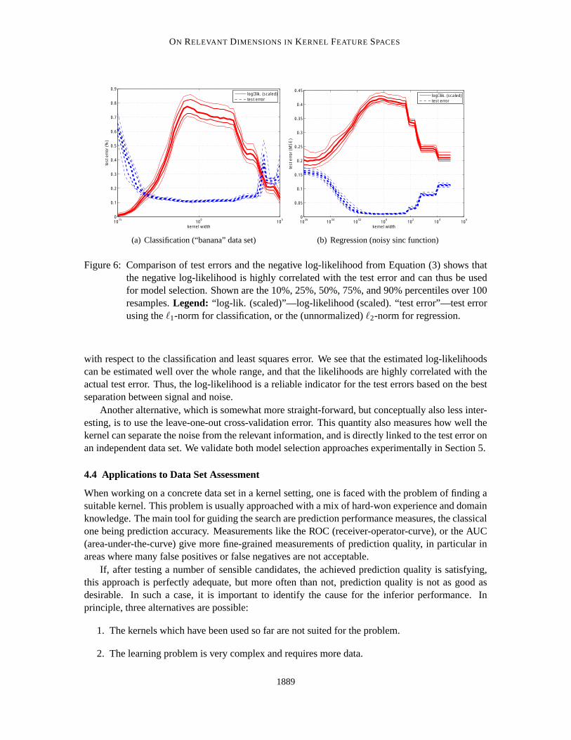
Figure 6: Comparison of test errors and the negative log-likelihood from Equation (3) shows thatthe negative log-likelihood is highly correlated with the test error and can thus be usedfor model selection. Shown are the 10%, 25%, 50%, 75%, and 90% percentiles over 100resamples. Legend: “log-lik. (scaled)”—log-likelihood (scaled). “test error”—test errorusing the `1-norm for classification, or the (unnormalized) `2-norm for regression.
with respect to the classification and least squares error. We see that the estimated log-likelihoodscan be estimated well over the whole range, and that the likelihoods are highly correlated with theactual test error. Thus, the log-likelihood is a reliable indicator for the test errors based on the bestseparation between signal and noise.
Another alternative, which is somewhat more straight-forward, but conceptually also less inter-esting, is to use the leave-one-out cross-validation error. This quantity also measures how well thekernel can separate the noise from the relevant information, and is directly linked to the test error onan independent data set. We validate both model selection approaches experimentally in Section 5.
4.4 Applications to Data Set Assessment
When working on a concrete data set in a kernel setting, one is faced with the problem of finding asuitable kernel. This problem is usually approached with a mix of hard-won experience and domainknowledge. The main tool for guiding the search are prediction performance measures, the classicalone being prediction accuracy. Measurements like the ROC (receiver-operator-curve), or the AUC(area-under-the-curve) give more fine-grained measurements of prediction quality, in particular inareas where many false positives or false negatives are not acceptable.
If, after testing a number of sensible candidates, the achieved prediction quality is satisfying,this approach is perfectly adequate, but more often than not, prediction quality is not as good asdesirable. In such a case, it is important to identify the cause for the inferior performance. Inprinciple, three alternatives are possible:
1. The kernels which have been used so far are not suited for the problem.
2. The learning problem is very complex and requires more data.
1889
BRAUN, BUHMANN AND MULLER
data set RDE method dimension noise-levelcomplex data set TCM 50 16.07%
LOO-CV 25 40.59%noisy data set TCM 9 40.71%
LOO-CV 9 40.71%
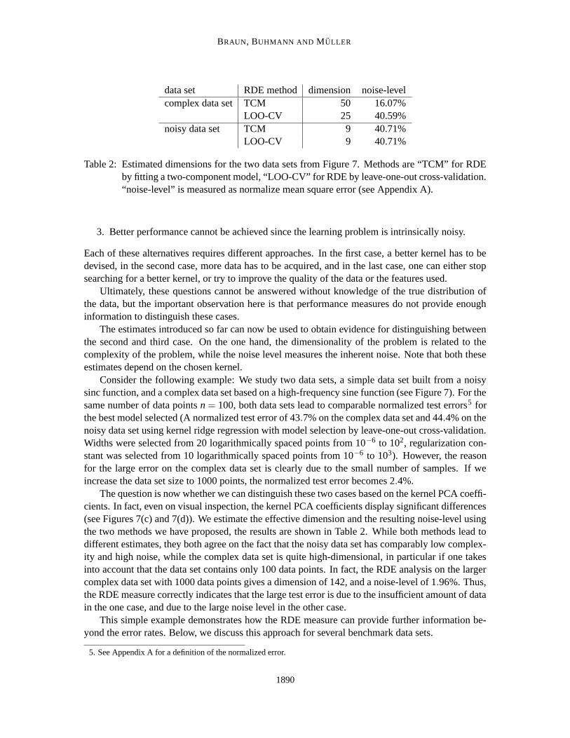
Table 2: Estimated dimensions for the two data sets from Figure 7. Methods are “TCM” for RDEby fitting a two-component model, “LOO-CV” for RDE by leave-one-out cross-validation.“noise-level” is measured as normalize mean square error (see Appendix A).
3. Better performance cannot be achieved since the learning problem is intrinsically noisy.
Each of these alternatives requires different approaches. In the first case, a better kernel has to bedevised, in the second case, more data has to be acquired, and in the last case, one can either stopsearching for a better kernel, or try to improve the quality of the data or the features used.
Ultimately, these questions cannot be answered without knowledge of the true distribution ofthe data, but the important observation here is that performance measures do not provide enoughinformation to distinguish these cases.
The estimates introduced so far can now be used to obtain evidence for distinguishing betweenthe second and third case. On the one hand, the dimensionality of the problem is related to thecomplexity of the problem, while the noise level measures the inherent noise. Note that both theseestimates depend on the chosen kernel.
Consider the following example: We study two data sets, a simple data set built from a noisysinc function, and a complex data set based on a high-frequency sine function (see Figure 7). For thesame number of data points n = 100, both data sets lead to comparable normalized test errors5 forthe best model selected (A normalized test error of 43.7% on the complex data set and 44.4% on thenoisy data set using kernel ridge regression with model selection by leave-one-out cross-validation.Widths were selected from 20 logarithmically spaced points from 10−6 to 102, regularization con-stant was selected from 10 logarithmically spaced points from 10−6 to 103). However, the reasonfor the large error on the complex data set is clearly due to the small number of samples. If weincrease the data set size to 1000 points, the normalized test error becomes 2.4%.
The question is now whether we can distinguish these two cases based on the kernel PCA coeffi-cients. In fact, even on visual inspection, the kernel PCA coefficients display significant differences(see Figures 7(c) and 7(d)). We estimate the effective dimension and the resulting noise-level usingthe two methods we have proposed, the results are shown in Table 2. While both methods lead todifferent estimates, they both agree on the fact that the noisy data set has comparably low complex-ity and high noise, while the complex data set is quite high-dimensional, in particular if one takesinto account that the data set contains only 100 data points. In fact, the RDE analysis on the largercomplex data set with 1000 data points gives a dimension of 142, and a noise-level of 1.96%. Thus,the RDE measure correctly indicates that the large test error is due to the insufficient amount of datain the one case, and due to the large noise level in the other case.
This simple example demonstrates how the RDE measure can provide further information be-yond the error rates. Below, we discuss this approach for several benchmark data sets.
5. See Appendix A for a definition of the normalized error.
1890

ON RELEVANT DIMENSIONS IN KERNEL FEATURE SPACES
−4 −3 −2 −1 0 1 2 3 4−1.5
−1
−0.5
0
0.5
1
1.5Normalized Test Error: 43.73%
test points predicted function training points
(a) A complex data set.
−4 −3 −2 −1 0 1 2 3 4−1.5
−1
−0.5
0
0.5
1
1.5
2Normalized Test Error: 44.37%
test pointspredicted functiontraining points
(b) A noisy data set.
0 10 20 30 40 50 60 70 80 90 1000
0.2
0.4
0.6
0.8
1
1.2
1.4
1.6
1.8
2
kernel PCA components
abso
lute
val
ue o
f sca
lar
prod
uct
kernel width 0.001000
(c) Kernel PCA coefficients for the complex data set.
0 10 20 30 40 50 60 70 80 90 1000
0.5
1
1.5
2
2.5
kernel PCA components
abso
lute
val
ue o
f sca
lar
prod
uct
kernel width 5.000000
(d) Kernel PCA coefficients for the noisy data set.
Figure 7: For both data sets, the X values were sampled uniformly between−π and π. For the com-plex data set, Y = sin(35X)+ ε where ε has mean zero and variance 0.01. For the noisydata set, Y = sinc(X)+ ε′ where ε′ has mean zero and variance 0.09. Errors are reportedas normalized mean squared error (see Appendix A). Below, the kernel PCA coefficients(scalar products with eigenvectors of the kernel matrix) for the optimal kernel selectedbased on the RDE (TCM) estimates are plotted. Coefficients are sorted by decreasingcorresponding eigenvalue.
5. Experiments
We test our methods on several benchmark data sets. As discussed in the introduction, in order tovalidate whether our dimension estimates are accurate, we compare the achieved test error rates onthe reduced feature space to other state-of-the-art algorithms. If the estimate is accurate, the testerrors should be on par with these algorithms. Furthermore, we apply our method to estimate thecomplexity and noise level of the various data sets.
1891
BRAUN, BUHMANN AND MULLER
5.1 Benchmark Data Sets
We performed experiments on the classification data sets from Ratsch et al. (2001). For each of thedata sets, we analyze it using a family of rbf kernels (see Appendix A). The kernel width is selectedautomatically using the achieved log-likelihood as described above. The width of the rbf kernel isselected from 20 logarithmically spaced points between 10−2 and 104 for each data set.
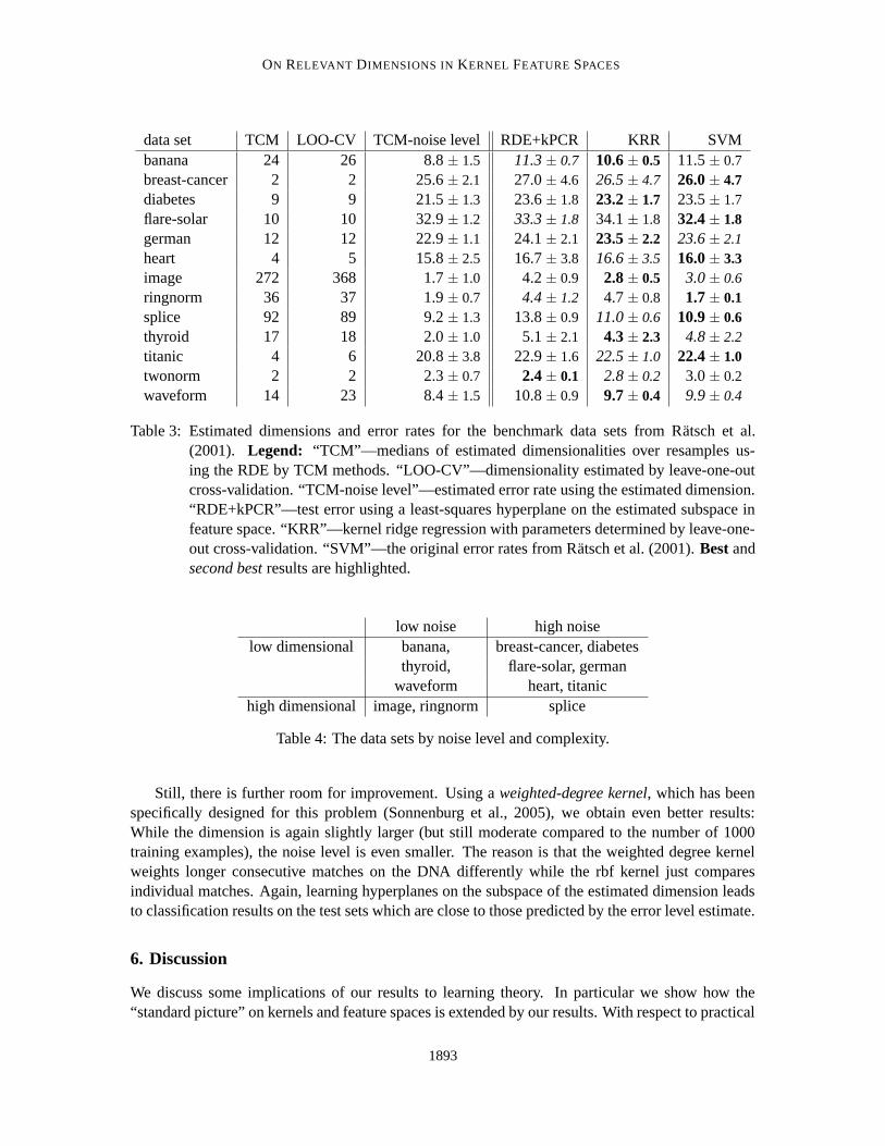
Table 3 shows the resulting dimension estimates using both RDE methods, with the cross-validation based RDE method being slightly biased towards higher dimensions. We see that bothmethods perform on par, which shows that the strong structural prior assumption underlying RDEis justified.
To assess the accuracy of the dimensionality estimate, we compare an unregularized least-squares fit in the reduced feature space (RDE+kPCR) with kernel ridge regression (KRR) and sup-port vector machines (SVM) on the original data set. The resulting test errors are also shown inTable 3. Note that the combination of RDE and kPCR is conceptually very similar to the kernelprojection machine (Vert et al., 2005) which also produces comparable results. However, in that pa-per, no practical method for estimating the dimension (beyond cross-validation) has been proposed.From the resulting test errors, we see that a relatively simple method on the reduced features per-forms on par with the state-of-the-art competitors. We conclude that the identified reduced featurespace really contains all of the relevant information. Also note that the estimated noise levels matchthe actually observed error rates quite well, although there is a slight tendency to under-estimate thetrue error.
As discussed in Section 4.4, while the test errors only suggest a linear ordering of the data setsby increasing difficulty, using the dimension and noise level estimates, a more fine-grained analysisis possible. We can roughly divide the data sets into four classes (see Table 4), depending on whetherthe dimensionality is small or large, and the noise level is low or high. Data sets with small noiselevel show good results, almost irrespective of the dimensionality. The data set image seems to beparticularly noise free, given that one can achieve a small error in spite of the large dimensionality.
The data sets breast-cancer, diabetes, flare-solar, german, and titanic, which all have test errorsof 20% or more, have only moderately large dimensionalities. This means that the complexity ofthe underlying optimal decision boundary is not overly large (at least when viewed through the lensof the rbf-kernel), but a large inherent noise level prevents better results. Since this holds for rbf-kernels over a wide range of kernel widths, these results can be taken as a strong indicator that theBayes error is in fact large.
The splice data set seems to be a good candidate for improvement. The noise level is moderatelyhigh, while the dimensionality with respect to the rbf-kernel seems quite high. We would like touse our dimensionality and noise level estimate as a tool to examine different kernel choices. (SeeSection C for further details).
Closer inspection of the data set reveals that a plain rbf-kernel is a suboptimal choice. The taskof the splice data set consists in predicting whether there is a splice-site in the middle of a string ofDNA (such sites encode the beginning and endings of coding regions on the DNA). In the data set,the four amino-acids A, C, G, T are encoded as numbers 1, 2, 3, and 4. Therefore, an rbf-kernelincorrectly assumes that C and G are more similar than A and T. One alternative which is moresuited to this data set consists in encoding A, C, G, and T as binary four-vectors. The resultingkernel matrix has much smaller dimension, and also a smaller error rate (see Table 5).
1892
ON RELEVANT DIMENSIONS IN KERNEL FEATURE SPACES
data set TCM LOO-CV TCM-noise level RDE+kPCR KRR SVMbanana 24 26 8.8 ± 1.5 11.3 ± 0.7 10.6 ± 0.5 11.5 ± 0.7breast-cancer 2 2 25.6 ± 2.1 27.0 ± 4.6 26.5 ± 4.7 26.0 ± 4.7diabetes 9 9 21.5 ± 1.3 23.6 ± 1.8 23.2 ± 1.7 23.5 ± 1.7flare-solar 10 10 32.9 ± 1.2 33.3 ± 1.8 34.1 ± 1.8 32.4 ± 1.8german 12 12 22.9 ± 1.1 24.1 ± 2.1 23.5 ± 2.2 23.6 ± 2.1heart 4 5 15.8 ± 2.5 16.7 ± 3.8 16.6 ± 3.5 16.0 ± 3.3image 272 368 1.7 ± 1.0 4.2 ± 0.9 2.8 ± 0.5 3.0 ± 0.6ringnorm 36 37 1.9 ± 0.7 4.4 ± 1.2 4.7 ± 0.8 1.7 ± 0.1splice 92 89 9.2 ± 1.3 13.8 ± 0.9 11.0 ± 0.6 10.9 ± 0.6thyroid 17 18 2.0 ± 1.0 5.1 ± 2.1 4.3 ± 2.3 4.8 ± 2.2titanic 4 6 20.8 ± 3.8 22.9 ± 1.6 22.5 ± 1.0 22.4 ± 1.0twonorm 2 2 2.3 ± 0.7 2.4 ± 0.1 2.8 ± 0.2 3.0 ± 0.2waveform 14 23 8.4 ± 1.5 10.8 ± 0.9 9.7 ± 0.4 9.9 ± 0.4
Table 3: Estimated dimensions and error rates for the benchmark data sets from Ratsch et al.(2001). Legend: “TCM”—medians of estimated dimensionalities over resamples us-ing the RDE by TCM methods. “LOO-CV”—dimensionality estimated by leave-one-outcross-validation. “TCM-noise level”—estimated error rate using the estimated dimension.“RDE+kPCR”—test error using a least-squares hyperplane on the estimated subspace infeature space. “KRR”—kernel ridge regression with parameters determined by leave-one-out cross-validation. “SVM”—the original error rates from Ratsch et al. (2001). Best andsecond best results are highlighted.
low noise high noiselow dimensional banana, breast-cancer, diabetes
thyroid, flare-solar, germanwaveform heart, titanic
high dimensional image, ringnorm splice
Table 4: The data sets by noise level and complexity.
Still, there is further room for improvement. Using a weighted-degree kernel, which has beenspecifically designed for this problem (Sonnenburg et al., 2005), we obtain even better results:While the dimension is again slightly larger (but still moderate compared to the number of 1000training examples), the noise level is even smaller. The reason is that the weighted degree kernelweights longer consecutive matches on the DNA differently while the rbf kernel just comparesindividual matches. Again, learning hyperplanes on the subspace of the estimated dimension leadsto classification results on the test sets which are close to those predicted by the error level estimate.
6. Discussion
We discuss some implications of our results to learning theory. In particular we show how the“standard picture” on kernels and feature spaces is extended by our results. With respect to practical
1893
BRAUN, BUHMANN AND MULLER
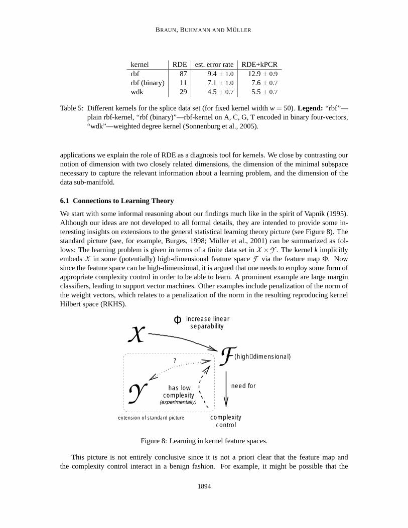
kernel RDE est. error rate RDE+kPCRrbf 87 9.4 ± 1.0 12.9 ± 0.9rbf (binary) 11 7.1 ± 1.0 7.6 ± 0.7wdk 29 4.5 ± 0.7 5.5 ± 0.7
Table 5: Different kernels for the splice data set (for fixed kernel width w = 50). Legend: “rbf”—plain rbf-kernel, “rbf (binary)”—rbf-kernel on A, C, G, T encoded in binary four-vectors,“wdk”—weighted degree kernel (Sonnenburg et al., 2005).
applications we explain the role of RDE as a diagnosis tool for kernels. We close by contrasting ournotion of dimension with two closely related dimensions, the dimension of the minimal subspacenecessary to capture the relevant information about a learning problem, and the dimension of thedata sub-manifold.
6.1 Connections to Learning Theory
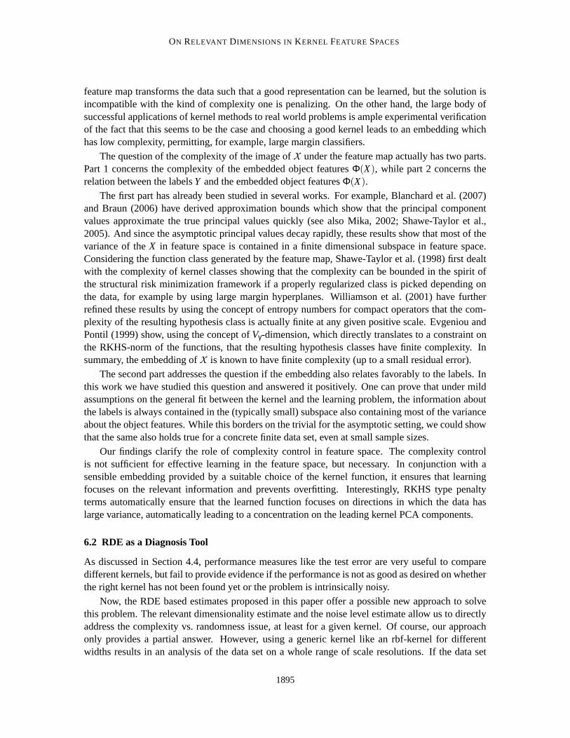
We start with some informal reasoning about our findings much like in the spirit of Vapnik (1995).Although our ideas are not developed to all formal details, they are intended to provide some in-teresting insights on extensions to the general statistical learning theory picture (see Figure 8). Thestandard picture (see, for example, Burges, 1998; Muller et al., 2001) can be summarized as fol-lows: The learning problem is given in terms of a finite data set in X ×Y . The kernel k implicitlyembeds X in some (potentially) high-dimensional feature space F via the feature map Φ. Nowsince the feature space can be high-dimensional, it is argued that one needs to employ some form ofappropriate complexity control in order to be able to learn. A prominent example are large marginclassifiers, leading to support vector machines. Other examples include penalization of the norm ofthe weight vectors, which relates to a penalization of the norm in the resulting reproducing kernelHilbert space (RKHS).
F (high−dimensional)
c omp lex ityhas low
c omp lex ityc ontrol
inc rease linearsep arab ility
Y?
need for
X
ex tension of standard p ic tu re
(experimentally)
Φ
Figure 8: Learning in kernel feature spaces.
This picture is not entirely conclusive since it is not a priori clear that the feature map andthe complexity control interact in a benign fashion. For example, it might be possible that the
1894
ON RELEVANT DIMENSIONS IN KERNEL FEATURE SPACES
feature map transforms the data such that a good representation can be learned, but the solution isincompatible with the kind of complexity one is penalizing. On the other hand, the large body ofsuccessful applications of kernel methods to real world problems is ample experimental verificationof the fact that this seems to be the case and choosing a good kernel leads to an embedding whichhas low complexity, permitting, for example, large margin classifiers.
The question of the complexity of the image of X under the feature map actually has two parts.Part 1 concerns the complexity of the embedded object features Φ(X), while part 2 concerns therelation between the labels Y and the embedded object features Φ(X).
The first part has already been studied in several works. For example, Blanchard et al. (2007)and Braun (2006) have derived approximation bounds which show that the principal componentvalues approximate the true principal values quickly (see also Mika, 2002; Shawe-Taylor et al.,2005). And since the asymptotic principal values decay rapidly, these results show that most of thevariance of the X in feature space is contained in a finite dimensional subspace in feature space.Considering the function class generated by the feature map, Shawe-Taylor et al. (1998) first dealtwith the complexity of kernel classes showing that the complexity can be bounded in the spirit ofthe structural risk minimization framework if a properly regularized class is picked depending onthe data, for example by using large margin hyperplanes. Williamson et al. (2001) have furtherrefined these results by using the concept of entropy numbers for compact operators that the com-plexity of the resulting hypothesis class is actually finite at any given positive scale. Evgeniou andPontil (1999) show, using the concept of Vγ-dimension, which directly translates to a constraint onthe RKHS-norm of the functions, that the resulting hypothesis classes have finite complexity. Insummary, the embedding of X is known to have finite complexity (up to a small residual error).
The second part addresses the question if the embedding also relates favorably to the labels. Inthis work we have studied this question and answered it positively. One can prove that under mildassumptions on the general fit between the kernel and the learning problem, the information aboutthe labels is always contained in the (typically small) subspace also containing most of the varianceabout the object features. While this borders on the trivial for the asymptotic setting, we could showthat the same also holds true for a concrete finite data set, even at small sample sizes.
Our findings clarify the role of complexity control in feature space. The complexity controlis not sufficient for effective learning in the feature space, but necessary. In conjunction with asensible embedding provided by a suitable choice of the kernel function, it ensures that learningfocuses on the relevant information and prevents overfitting. Interestingly, RKHS type penaltyterms automatically ensure that the learned function focuses on directions in which the data haslarge variance, automatically leading to a concentration on the leading kernel PCA components.
6.2 RDE as a Diagnosis Tool
As discussed in Section 4.4, performance measures like the test error are very useful to comparedifferent kernels, but fail to provide evidence if the performance is not as good as desired on whetherthe right kernel has not been found yet or the problem is intrinsically noisy.
Now, the RDE based estimates proposed in this paper offer a possible new approach to solvethis problem. The relevant dimensionality estimate and the noise level estimate allow us to directlyaddress the complexity vs. randomness issue, at least for a given kernel. Of course, our approachonly provides a partial answer. However, using a generic kernel like an rbf-kernel for differentwidths results in an analysis of the data set on a whole range of scale resolutions. If the data set
1895
BRAUN, BUHMANN AND MULLER
appears to be low-dimensional and noisy at every scale, there is a strong indication that the noiselevel is actually quite high.
In the data sets discussed in Section 5, we have considered kernel widths in the range 10−2 to104. The data sets breast-cancer, diabetes, flare-solar, german, heart, and titanic, which all haveprediction errors larger than 15%, turn out to be fairly low-dimensional over the whole range.
On the other hand, the splice data set seemed to be quite complex, but not very noisy. Usingdomain knowledge, we improved the encoding, and finally chose a different kernel, which furtherreduced the complexity and noise (see Section C for further details).
In summary, using the RDE based estimates as a diagnosis tool, it is possible to obtain moredetailed insights into how well a kernel is adapted to the characteristic properties of a data set andits underlying distribution than by using integrative performance measures like test errors only.
6.3 The “True” Dimensionality of the Data
We estimate the number of leading kernel PCA components necessary to capture the relevant infor-mation contained in the learning problem. This “relevant dimensionality estimate” captures only avery special kind of dimensionality notion, and we would like to compare it with two other aspectsof dimensionality.
In our dimensionality estimate, the basis was fixed and given by leading kernel PCA compo-nents. One might wonder how many dimensions are necessary to capture the relevant informationabout the learning problem if one were also allowed to choose the basis. The answer is easy: Inorder to capture G, it suffices to consider the one-dimensional space spanned by G itself, whichmeans that the minimal dimensionality of the learning problem is 1. However, note that G is notknown, and estimating G amounts to solving the learning problem itself. In other words, the choiceof a kernel can be interpreted as implicitly specifying an appropriate basis in feature space which isable to capture G using as few basis vector as possible, and also using a subspace which contains asmuch of the variance of the data as possible.
For most data sets, the different input variables are highly dependent, such that the data doesnot occupy all of the space but only a sub-manifold in the space. The dimension of this sub-manifold is a further notion of dimensionality of a data set. However, note that we consider thedimensionality of the data with respect to the information in the labels, while the sub-manifold viewusually concentrates on the inputs only. Also, we are considering linear subspaces (in an RKHS),which typically require more dimensions to capture the data than a non-linear manifold would. Onthe other hand, since we are only looking at the subspace which is relevant for predicting the labels,the estimated dimension may also be smaller than the dimension of the data manifold in featurespace.
7. Conclusion
Both in theory and on practical data sets, we have demonstrated that the relevant information in asupervised learning scenario is contained in the leading projected kernel PCA components if thekernel matches the learning problem and is sufficiently smooth. This behavior complements thecommon statistical learning theoretical view on kernel based learning adding insight on the intricateinterplay of data and kernel: An appropriately selected kernel (a) leads to an efficient model whichgeneralizes well, since only a comparatively low dimensional representation has to be learned for a
1896
ON RELEVANT DIMENSIONS IN KERNEL FEATURE SPACES
fixed given data size. An appropriately selected kernel (b) permits a dimension reduction step thatdiscards some irrelevant projected kernel PCA directions and thus yields a regularized model.
We propose two algorithms for the relevant dimensionality estimate (RDE) task. These canalso be used to automatically select a suitable kernel model for the data and to extract as addi-tional side information an estimate of the effective dimension and estimated expected error for thelearning problem. Compared to common cross-validation techniques one could argue that all wehave achieved is to find a similar model as usual at a comparable computing time. However, wewould like to emphasize that the side information extracted by our procedure contributes to a betterunderstanding of the learning problem at hand: Is the classification result limited due to intrinsichigh dimensional structure or are we facing noise and nuisance dimensions? Simulations show theusefulness of our RDE algorithms.
An interesting future direction lies in combining these results with generalization bounds whichare also based on the notion of an effective dimension, this time, however, with respect to someregularized hypothesis class (see, for example, Zhang, 2005). Linking the effective dimension of adata set with the “dimension” of a learning algorithm, one could obtain data dependent bounds in anatural way with the potential to be tighter than bounds which are based on the abstract capacity ofa hypothesis class.
Acknowledgments
Parts of this work have been performed while MLB was with the Intelligent Data Analysis Groupat the Fraunhofer Institute FIRST. The authors would like to thank Volker Roth, Tilman Lange,Gilles Blanchard, Stefan Harmeling, Motoaki Kawanabe, Claudia Sannelli, Jan Muller, and NicoleKramer for fruitful discussions. The authors would also like to thank the anonymous referees whosecomments have helped to improve the paper further, and in particular Peter Bartlett for his valuablecomments. This work was supported in part by the BMBF FaSor project, 16SV2234, and by theFP7-ICT Programme of the European Community, under the PASCAL2 Network of Excellence,ICT-216886.
Appendix A. Data Sets and Kernel Functions
In this section, we introduce some data sets and define the Gaussian kernel, since there exists somevariability with respect to its parameterization.
A.1 Gaussian kernel
The Gaussian kernel, or rbf-kernel, used in this paper are parameterized as follows: The Gaussianwith width w is
k(x,y) = exp
(
−‖x− y‖2
2w
)
.
A.2 Classification Data Sets
For classification, we use the data sets from Ratsch et al. (2001). This benchmark data set consistsof 13 classification data sets, which are partly synthetic, and partly derived from real-world data.The data sets are pre-arranged into different resamples of training and test data sets. The number
1897
BRAUN, BUHMANN AND MULLER
of resamples is 100 with the exception of the “image” and “splice” data sets which have only 20resamples (because these data sets are fairly large). For visualization purposes, we often take thefirst resample of the “banana” data set, which is a two-dimensional classification problem (seeFigure 1(a)).
A.3 Regression Data Sets
The “noisy sinc function” data set is defined as follows:
Xi ∼ uniformly from [−π,π],
Yi = sinc(Xi)+ εi,
εi ∼N (0,σ2ε).
There are different alternatives for defining the sinc function, we choose sinc(x) = sin(πx)/πx,sinc(0) = 1.
For regression, we sometimes measure the error using the “normalized mean squared error.” Ifthe original labels are given by Yi, 1≤ i≤ n, and the predicted ones are Yi, then this error is definedas
nmse =∑n
i=1(Yi− Yi)2
∑ni=1(Yi− 1
n ∑nj=1Yj)2
.
Appendix B. Proof of the Main Theorem
In this section, the main theorem of the paper is stated and proven. We start with some definitions,then introduce and discuss the assumptions of the main result. Next we define a few quantities onwhich the bound depends. The bound itself is split into two theorems. First the general bound isderived and then the asymptotic rates of these quantities are studied.
B.1 Preliminaries
Using the probability measure PX which generates the Xs, we can define a scalar product via 〈 f ,g〉=R
X f (x)g(x)PX (dx) which induces the Hilbert space L2(X ,PX ). Unless indicated otherwise, ‖ f‖will denote the norm with respect to this scalar product. Let k(x,y) = ∑∞
`=1 λ`ψ`(x)ψ`(y) be a kernelfunction (such that λ` ≥ 0). The ψ` form an orthogonal family of functions on the Hilbert spaceL2(X ,PX ). Given an n-sample X1, . . . ,Xn from PX , the sample vector of a function g is the vectorg(X) = (g(X1), . . . ,g(Xn)). The kernel matrix given a kernel function k and an n-sample X1, . . . ,Xn
is the n×n matrix K with entries k(Xi,X j)/n.Let g(x) = ∑∞
`=1 α`λ`ψ`(x) with (α`) ∈ `2, the set of all square-summable sequences. Theexpansion of g in terms of λ`ψ` amounts to assuming that g lies in the range of the integral operatorTk defined by Tk f =
R
X k( · ,x) f (x)PX (dx). Then, g = Tkh with h = ∑∞`=1 α`ψ`.
The act of truncating an object with an infinite expansion to its first r coefficients is so ubiquitousin the following that we introduce a generic notation. If k is a kernel function, k is the kernelfunction whose expansion has been reduced to the first r terms. Likewise, K is the kernel matrixinduced by k. For a sequence (α`) ∈ `2, α is the tuple consisting of the first r elements of thesequence. The sample vector matrices Ψ is formed by the sample vector of the first r eigenvectors,that is, Ψi j = ψ j(Xi)/
√n, and Λ is the diagonal matrix formed from the first r eigenvalues, such that
K = ΨΛΨ>. Finally, g is obtained from g by truncating the expansion to the first r eigenfunctions.
1898
ON RELEVANT DIMENSIONS IN KERNEL FEATURE SPACES
The eigen-decompositions of the kernel matrix and the truncated kernel matrix (kernel matrixfor the truncated kernel function) are
K = ULU>, K = ULU>,
where U, U are orthogonal matrices with columns ui, u j, and L, L are diagonal matrices with entriesli, l j, such that the eigenpairs of K are (li,ui), and those of K are (l j, u j). We stick to the generalconvention that eigenvalues are always sorted in decreasing order.
Tail-sums of eigenvalues are denoted by
Λ>r =∞
∑i=r+1
λi, Λ≥r =∞
∑i=r
λi.
We will refer to the following result relating decay rates of the eigenvalues to the tail-sums. Forproofs, see, for example, Braun (2006). It holds that if λr = r−d with d ≥ 1, then Λ>r = O(r1−d). Ifλr = exp(−cr) with c > 0, then Λ>r = O(exp(−cr)). The same rates hold for Λ≥r.
Furthermore, we will often make use of the fact that√
a+b≤√a+√
b if a,b≥ 0.
B.2 Assumptions
The overall goal is to derive a meaningful upper bound on 1√n |u>i g(X)|. In particular, the bound
should scale with the corresponding eigenvalue li. We proceed as follows: First, we derive theactual bound which depends on a number of quantities. In the next step, we estimate the worst caseasymptotic rates of these quantities. The actual bound depends on assumptions which are discussedin the following.
(A1) We assume that the kernel is uniformly bounded, that is,
supx,y∈X×X
|k(x,y)|= K < ∞.
(A2) We assume that n≥ r large enough such that Ψ>Ψ is invertible.
(A3) We assume that λi = O(i−5/2−ε) for some ε > 0.
Assumption (A1) is true for radial basis functions like the Gaussian kernel, but also if the un-derlying space X is compact and the kernel is continuous. From (A1), it follows easily that g isbounded as well since
|g(x)| ≤ K‖h‖.
Furthermore, since the ψi are orthogonal, it follows that ‖h− h‖ ≤ ‖h‖, and therefore
|g(x)− g(x)| ≤ K‖h‖
since g− g = Tk(h− h), and therefore |g(x)− g(x)| ≤ K‖h− h‖ ≤ K‖h‖. These inequalities play animportant role for bounding the truncation error g− g in a finite sample setting.
Since the sample vectors ψ`(X) are asymptotically pairwise orthogonal, Ψ>Ψ converges to I,and for large enough n, assumption (A2) is met. See also Lemma 2 below.
1899
BRAUN, BUHMANN AND MULLER
Assumption (A3) ensures that the term r(∑ri=1 |αi|)Λ≥r occurring in the bound vanishes as r→
∞. Note that since the sequence of αi is square-summable,
r
∑i=1
|αi| ≤√
rr
∑i=1
α2i ≤√
r‖α‖`2 = O(√
r).
Therefore, r ∑ri=1 |αi|= O(r3/2). Also, Λ≥r = O(r−3/2−ε), such that r(∑r
i=1 |αi|)Λ≥r = O(r−ε). Notethat (A3) is quite modest and eigenvalues often decay much faster, even at exponential rates.
B.3 The Main Result
The following five quantities occur in the bound:
• ci = |{1≤ j≤ r | li/2≤ l j ≤ 2li}| is the number of eigenvalues of the truncated kernel matrixwhich are close to the eigenvalues of the normal kernel matrix. This is a measure for theapproximate degeneracy of eigenvalues.
• a = ‖α‖1, is a measure for the size of the first r coefficients which define g.
• E = K− K is the truncation error for the kernel matrix.
• T = ‖g− g‖=√
∑∞j=r+1 α2
jλ2j is the asymptotic truncation error for the function g.
• F = ‖g‖∞ < ∞, an upper bound on g.
We study these quantities in more detail after proving the actual bound, which follows next.
Theorem 1 With the definitions introduced so far, it holds that with probability larger that 1− δ,for all 1≤ i≤ n,
1√n|u>i g(X)|< min
1≤r≤n
[
liciD(r,n)+E(r,n)+T (r,n)]
where the three terms are given by
D(r,n) = 2a‖Ψ+‖, E(r,n) = 2ra‖Ψ+‖‖E‖, T (r,n) = T +√
FT 4
√
1nδ
.
Proof First, we replace g = g+(g− g) and obtain
1√n|u>i g(X)| ≤ 1√
n|u>i g(X)|+ 1√
n‖g(X)− g(X)‖=: (I),
using the Cauchy-Schwarz-inequality and the fact that ‖ui‖= 1 for the second term.Next, we re-express g(X) = ∑r
`=1 λ`α`ψ`(X) as follows. By definition, g(X) lies in the imageof K, therefore, g(X) = ∑r
j=1 u ju>j g(X). Using both these equations, we obtain
1√n|u>i g(X)| ≤
r
∑=1
|α`|r
∑j=1
(u>i u j)
[
1√n
λ`ψ`(X)>u j
]
=: (II)
1900

ON RELEVANT DIMENSIONS IN KERNEL FEATURE SPACES
The term u>i u j measures the angle between the eigenvectors of K and K. Note that K can beconsidered an additive perturbation of K by E = K− K. Such perturbations are studied by the so-called sin-theta-theorems. Specializing Theorem 6.2 of Davis and Kahan (1970) (see Section D) totwo single eigenvectors, we obtain that
|u>i u j| ≤min
( ‖E‖|li− l j|
,1
)
.
The term λ`ψ`(X)>u j/√
n is bounded by l j‖Ψ+‖ (where Ψ+ denotes the pseudo-inverse of Ψ),since
l ju j = Ku j = ΨΛΨ>u j ⇒ l jΨ+u j = ΛΨ>u j.
Taking norms, we obtain ‖ΛΨ>u j‖ ≤ l j‖Ψ+‖, from which the claimed inequality follows for eachindividual coordinate of the vector on the left-hand side.
Combining the bounds for the two terms u>i u j and λ`ψ`(X)>u j/√
n, we obtain
(u>i u j)
[
1√n
λ`ψ`(X)>u j
]
≤ ‖Ψ+‖min
( ‖E‖|li− l j|
,1
)
l j =: ‖Ψ+‖ci j.
For j /∈ J(li) = {1≤ j ≤ r | 12 li ≤ l j ≤ 2li}, it holds that ‖E‖l j/|li− l j| ≤ 2‖E‖, therefore,
r
∑j=1
ci j = ∑j∈J(li)
ci j + ∑j/∈J(li)
ci j ≤ 2|J(li)|li +2r‖E‖.
We have just shown that
(II)≤ ‖Ψ+‖r
∑=1
|α`|(
2|J(li)|li +2r‖E‖)
. (7)
Now concerning the other term in (I), note that by the strong law of large numbers,
1n‖g(X)− g(X)‖2
Rn →‖g− g‖2L2(X ,PX ) =
∞
∑j=r+1
α2jλ
2j =: T 2.
Since g is bounded, ‖g‖∞ = F < ∞, we can bound the variance of g− g:
VarPX ((g− g)2)≤ ‖g− g‖2∞‖g− g‖2 = F2T 2.
We can thus bound the probability of a large deviation using the Chebychev-inequality. Taking thesquare roots, we obtain that with probability larger than 1−δ,
1√n‖g(X)− g(X)‖ ≤ T +
√
FT (nδ)−14 . (8)
Combining bound (7) and (8), we obtain that
1√n|u>i g(X)| ≤ 2li|J(li)|‖α‖1‖Ψ+‖+2r‖E‖‖α‖1‖Ψ+‖+ T +
√
FT (nδ)−14 .
This proves the upper bound on the coefficients.
1901
BRAUN, BUHMANN AND MULLER
B.4 Worst Case Asymptotic Rates of the Error Matrices
The bound depends on a number of error terms, whose worst case asymptotic rates and their depen-dency on r are studied next.
The norm of the pseudo-inverse of Ψ can be related to the matrix C = Ψ>Ψ−I, which measuresthe deviation from orthonormality of the sample vectors of the first r eigenfunctions of Tk. Since theeigenfunctions are asymptotically orthonormal, it is guaranteed that ‖C‖→ 0 as n→ ∞.
Lemma 2 Let C = Ψ>Ψ− I. If ‖C‖< 1, then
‖Ψ+‖ ≤ (1−‖C‖)−1/2 = 1+O(
√
‖C‖).
Proof Recall that ‖Ψ+‖ = 1/σr(Ψ), where σr(Ψ) is the rth singular value of Ψ in descendingorder. The singular values are the square roots of the eigenvalues of Ψ>Ψ, and
1−λr(Ψ>Ψ)≤ max1≤i≤r
|λi(Ψ>Ψ)−1| ≤ ‖Ψ>Ψ− I‖,
and therefore σr(Ψ) = (λr(Ψ>Ψ))1/2 ≥ (1−‖Ψ>Ψ− I‖)1/2, which proves the inequality.For the asymptotic rate, observe that
‖Ψ+‖ ≤√
1
1−‖C‖=
√
‖C‖−1
‖C‖−1−1=
√
1+1
‖C‖−1−1≤ 1+
√
1
‖C‖−1−1.
Now, 1/(x−1) = O(1/x) for x→ ∞, which proves the asymptotic rate.
The two error matrices C and E were discussed in depth by Braun (2006). However, note thatthese asymptotic rates are worst case rates over certain families of kernel functions. This means thatthe results on the asymptotic rates do not describe typical behavior but rather worst case behavior,and their main purpose of these rates is to ensure that the error terms cannot diverge rather thangiving realistic estimates.
The following result is Theorem 4 from Braun (2006).
Lemma 3 For 1≤ r ≤ n, with probability larger than 1−δ,
‖C‖< r
√
r(r +1)Kλrnδ
, ‖E‖< λr +Λ>r +
√
2KΛ>r
nδ.
¿From Lemma 3, it follows that
‖Ψ+‖= 1+O(rλ−1/4r n−1/4),
‖E‖= Λ≥r +O(√
Λ>rn−1/2).
If we plug these rates into the bound from Theorem 1 and suppress all parts which converge tozero, the bound becomes
1√n|u>i g(X)| ≤ 2ciali +2raΛ≥r + T + terms which vanish as n→ ∞.
1902
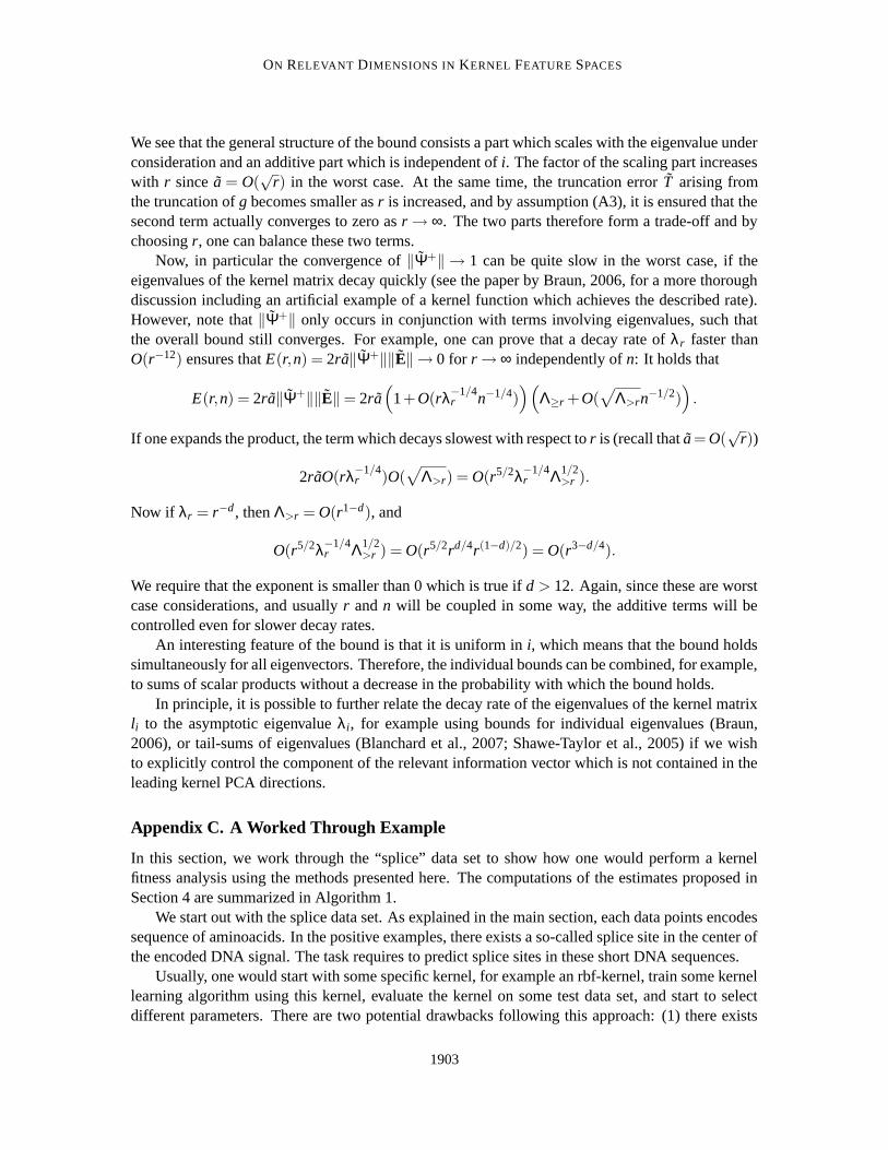
ON RELEVANT DIMENSIONS IN KERNEL FEATURE SPACES
We see that the general structure of the bound consists a part which scales with the eigenvalue underconsideration and an additive part which is independent of i. The factor of the scaling part increaseswith r since a = O(
√r) in the worst case. At the same time, the truncation error T arising from
the truncation of g becomes smaller as r is increased, and by assumption (A3), it is ensured that thesecond term actually converges to zero as r→ ∞. The two parts therefore form a trade-off and bychoosing r, one can balance these two terms.
Now, in particular the convergence of ‖Ψ+‖ → 1 can be quite slow in the worst case, if theeigenvalues of the kernel matrix decay quickly (see the paper by Braun, 2006, for a more thoroughdiscussion including an artificial example of a kernel function which achieves the described rate).However, note that ‖Ψ+‖ only occurs in conjunction with terms involving eigenvalues, such thatthe overall bound still converges. For example, one can prove that a decay rate of λr faster thanO(r−12) ensures that E(r,n) = 2ra‖Ψ+‖‖E‖→ 0 for r→ ∞ independently of n: It holds that
E(r,n) = 2ra‖Ψ+‖‖E‖= 2ra(
1+O(rλ−1/4r n−1/4)
)(
Λ≥r +O(√
Λ>rn−1/2)
)
.
If one expands the product, the term which decays slowest with respect to r is (recall that a = O(√
r))
2raO(rλ−1/4r )O(
√
Λ>r) = O(r5/2λ−1/4r Λ1/2
>r ).
Now if λr = r−d , then Λ>r = O(r1−d), and
O(r5/2λ−1/4r Λ1/2
>r ) = O(r5/2rd/4r(1−d)/2) = O(r3−d/4).
We require that the exponent is smaller than 0 which is true if d > 12. Again, since these are worstcase considerations, and usually r and n will be coupled in some way, the additive terms will becontrolled even for slower decay rates.
An interesting feature of the bound is that it is uniform in i, which means that the bound holdssimultaneously for all eigenvectors. Therefore, the individual bounds can be combined, for example,to sums of scalar products without a decrease in the probability with which the bound holds.
In principle, it is possible to further relate the decay rate of the eigenvalues of the kernel matrixli to the asymptotic eigenvalue λi, for example using bounds for individual eigenvalues (Braun,2006), or tail-sums of eigenvalues (Blanchard et al., 2007; Shawe-Taylor et al., 2005) if we wishto explicitly control the component of the relevant information vector which is not contained in theleading kernel PCA directions.
Appendix C. A Worked Through Example
In this section, we work through the “splice” data set to show how one would perform a kernelfitness analysis using the methods presented here. The computations of the estimates proposed inSection 4 are summarized in Algorithm 1.
We start out with the splice data set. As explained in the main section, each data points encodessequence of aminoacids. In the positive examples, there exists a so-called splice site in the center ofthe encoded DNA signal. The task requires to predict splice sites in these short DNA sequences.
Usually, one would start with some specific kernel, for example an rbf-kernel, train some kernellearning algorithm using this kernel, evaluate the kernel on some test data set, and start to selectdifferent parameters. There are two potential drawbacks following this approach: (1) there exists
1903

BRAUN, BUHMANN AND MULLER
Algorithm 1 Computing the estimates from Section 4Input: Kernel matrix K, label vector Y , loss function LOutput: kernel PCA coefficients z, dimensionality d,
negative log-likelihood ˆ, denoised labels Y ,noise-level ˆerr
1: {Compute kernel PCA coefficients}2: Compute eigendecomposition KU = UD3: z← U>Y4: {Estimate dimensionality d (Eq. 4)}5: c← 0; C←‖z‖2 {here, it is shown in detail how to achieve linear run-time}6: for d = 1 to n/2 do7: c← c+ z2
i8: s1← c/d9: s2← (C− c)/(n−d)
10: ld ← d logs1 +(n−d) logs2
11: end for12: d← argmin1≤d≤n/2 ld13: ˆ← ld .14: {Compute denoised labels (Eq. 5)}15: Extract first d eigenvectors T← U:,1:d
16: Y ← TT>Y17: {Estimate noise-level (Eq. 6)}18: err = 1
n ∑ni=1 L(Y,Y )
no absolute measure of the goodness of a certain kernel choice, only comparisons to other kernels,(2) there exists some dependency on the kernel learning method employed. Using the methodsdeveloped in this paper, it is possible to explore the relationship between the kernel and the data setin an algorithm independent way. Furthermore, in the case of poor performance, it is possible todistinguish between very complex cases (which require more input data), and cases where the dataset appears to be very noisy (either requiring better data quality, or a kernel which can capture moreinformation about the learning problem).
The splice data set consists of 20 resamples. We first try an rbf-kernel with width w = 50(see Section A). We start by computing and plotting the kernel PCA coefficients. The resultingcoefficients are plotted in Figure 9(a). We see that the data set appears to be rather high-dimensional,and the noise level is also quite high. The estimated median estimated dimension is 87.5, but itseems that roughly up to dimension 200, relevant information might be contained.
As explained in the main text, the encoding used by the rbf-kernel is not fit for this example.The four aminoacids A, C, G, and T have just been mapped to the numbers 1–4. We re-encode theobject features by mapping A, C, G, and T to the four vectors (1,0,0,0), (0,1,0,0), and so on. Theresulting kernel PCA coefficients are plotted in Figure 9(b). The encoding has obviously resultedin a large improvement, as the dimension is much smaller now, while the amount of noise has alsobeen reduced.
Finally, we consider using a weighted-degree-kernel (Sonnenburg et al., 2005). The resultingkernel PCA coefficients are plotted in Figure 9(c). While the estimated dimension is larger than
1904
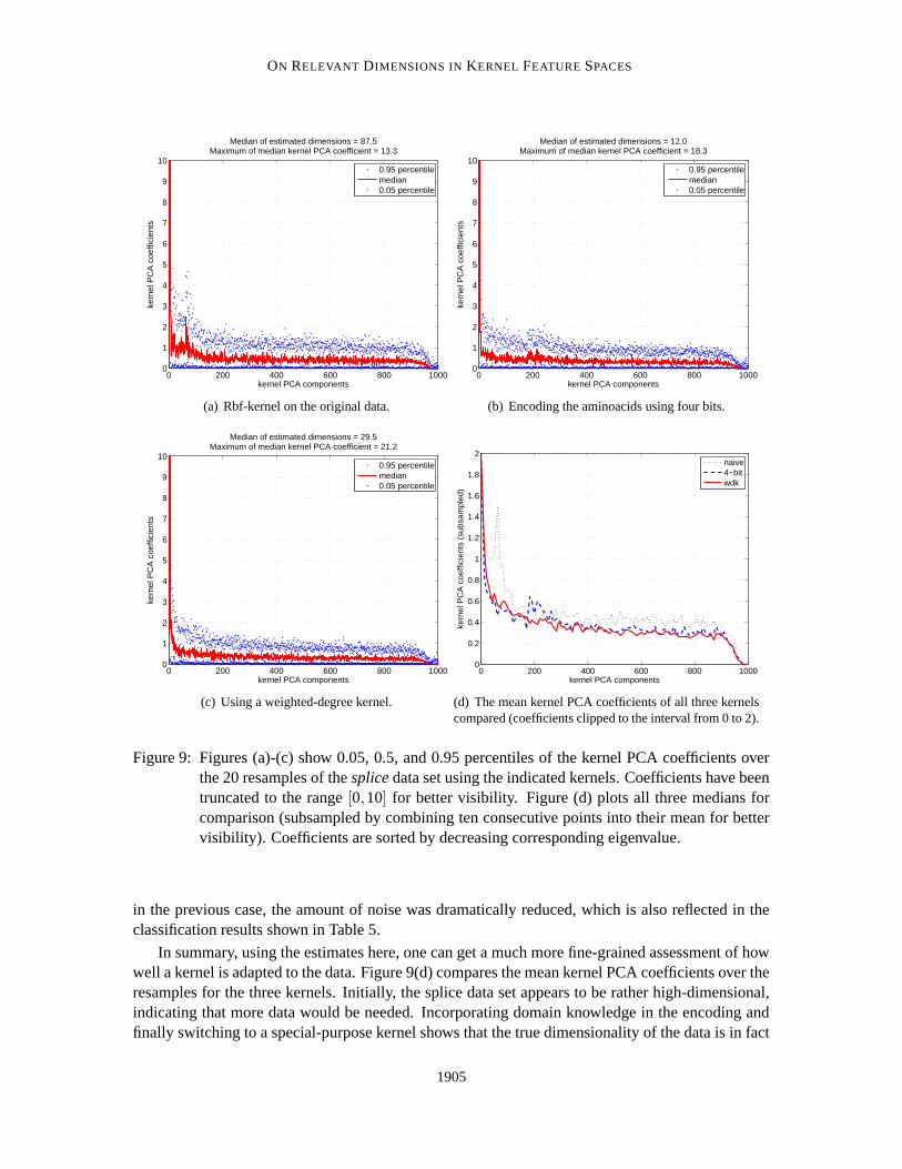
ON RELEVANT DIMENSIONS IN KERNEL FEATURE SPACES
0 200 400 600 800 10000
1
2
3
4
5
6
7
8
9
10
kernel PCA components
kern
el P
CA
coe
ffici
ents
Median of estimated dimensions = 87.5Maximum of median kernel PCA coefficient = 13.3
0.95 percentilemedian0.05 percentile
(a) Rbf-kernel on the original data.
0 200 400 600 800 10000
1
2
3
4
5
6
7
8
9
10
kernel PCA components
kern
el P
CA
coe
ffici
ents
Median of estimated dimensions = 12.0Maximum of median kernel PCA coefficient = 18.3
0.95 percentilemedian0.05 percentile
(b) Encoding the aminoacids using four bits.
0 200 400 600 800 10000
1
2
3
4
5
6
7
8
9
10
kernel PCA components
kern
el P
CA
coe
ffici
ents
Median of estimated dimensions = 29.5Maximum of median kernel PCA coefficient = 21.2
0.95 percentilemedian0.05 percentile
(c) Using a weighted-degree kernel.
0 200 400 600 800 10000
0.2
0.4
0.6
0.8
1
1.2
1.4
1.6
1.8
2
kernel PCA components
kern
el P
CA
coe
ffici
ents
(su
bsam
pled
)
naive4−bitwdk
(d) The mean kernel PCA coefficients of all three kernelscompared (coefficients clipped to the interval from 0 to 2).
Figure 9: Figures (a)-(c) show 0.05, 0.5, and 0.95 percentiles of the kernel PCA coefficients overthe 20 resamples of the splice data set using the indicated kernels. Coefficients have beentruncated to the range [0,10] for better visibility. Figure (d) plots all three medians forcomparison (subsampled by combining ten consecutive points into their mean for bettervisibility). Coefficients are sorted by decreasing corresponding eigenvalue.
in the previous case, the amount of noise was dramatically reduced, which is also reflected in theclassification results shown in Table 5.
In summary, using the estimates here, one can get a much more fine-grained assessment of howwell a kernel is adapted to the data. Figure 9(d) compares the mean kernel PCA coefficients over theresamples for the three kernels. Initially, the splice data set appears to be rather high-dimensional,indicating that more data would be needed. Incorporating domain knowledge in the encoding andfinally switching to a special-purpose kernel shows that the true dimensionality of the data is in fact
1905
BRAUN, BUHMANN AND MULLER
smaller, and that the noise level, which was initially quite high, could also be lowered significantly.Using the weighted-degree-kernel the data quality and the amount of data seem to be suited forpredicting with high accuracy.
Appendix D. A Sin-Theta-Theorem
The following theorem is a special case of Theorem 6.2 in the book by Davis and Kahan (1970).
Theorem 2 Let A be a symmetric n×n-matrix with eigendecomposition A = ULU>. Let U and Lbe partitioned as follows:
U = [U1 U2], L =
[
L1 00 L2
]
,
where U1 is an n× k-matrix, L1 is a k× k-matrix, U2 is an n× n− k-matrix, and L2 is an n− k×n− k-matrix. Furthermore, let E be another symmetric n× n-matrix, and A = A + E. Let l be aneigenvalue of A and x an associated unit-length eigenvector. Then,
‖U>2 x‖ ≤ ‖E‖min
n−k≤i≤n|l− li|
.
The proof of this theorem can also be found in the thesis of Braun (2005), Lemma 4.50, p. 70.
References
Gilles Blanchard, Olivier Bousquet, and Laurent Zwald. Statistical properties of kernel principalcomponent analysis. Machine Learning, 66(2–3):259–294, 2007.
Mikio L. Braun. Accurate error bounds for the eigenvalues of the kernel matrix. Journal of MachineLearning Research, 7:2303–2328, Nov 2006.
Mikio L. Braun. Spectral Properties of the Kernel Matrix and Their Application to Kernel Meth-ods in Machine Learning. PhD thesis, University of Bonn, 2005. Available electronically athttp://hss.ulb.uni-bonn.de/diss online/math nat fak/2005/braun mikio.
Chris J. C. Burges. A tutorial on support vector machines for pattern recognition. Data Mining andKnowledge Discovery, 2(2):121–167, 1998.
Chandler Davis and William M. Kahan. The rotation of eigenvectors by a perturbation, iii. SIAMJournal of Numerical Analysis, 7:1–46, 1970.
Theodoros Evgeniou and Massimiliano Pontil. On the Vγ dimension for regression in reproducingkernel hilbert spaces. In Proceedings of Algorithmic Learning Theory, 1999.
Edwin T. Jaynes. Information theory and statistical mechanics. Physical Review, 160(620–630),1957.
Vladimir Koltchinskii and Evariste Gine. Random matrix approximation of spectra of integraloperators. Bernoulli, 6(1):113–167, 2000.
1906
ON RELEVANT DIMENSIONS IN KERNEL FEATURE SPACES
Vladimir I. Koltchinskii. Asymptotics of spectral projections of some random matrices approximat-ing integral operators. Progress in Probability, 43:191–227, 1998.
Sebastian Mika. Kernel Fisher Discriminants. PhD thesis, Technische Universitat Berlin, December2002.
Klaus-Robert Muller, Sebastian Mika, Gunnar Ratsch, Koji Tsuda, and Bernhard Scholkopf. Anintroduction to kernel-based learning algorithms. IEEE Transaction on Neural Networks, 12(2):181–201, May 2001.
Gunnar Ratsch, Takashi Onoda, and Klaus-Robert Muller. Soft margins for AdaBoost. MachineLearning, 42(3):287–320, March 2001.
Bernhard Scholkopf and Alexander J. Smola. Learning with Kernels. MIT Press, 2002.
Bernhard Scholkopf, Alexander J. Smola, and Klaus-Robert Muller. Nonlinear component analysisas a kernel eigenvalue problem. Neural Computation, 10:1299–1319, 1998.
Bernhard Scholkopf, Sebastian Mika, Christopher J. C. Burges, Philipp Knirsch, Klaus-RobertMuller, Gunnar Ratsch, and Alex J. Smola. Input space vs. feature space in kernel-based methods.IEEE Transactions on Neural Networks, 10(5):1000–1017, 1999.
John Shawe-Taylor, Peter L. Bartlett, Robert C. Williamson, and Martin Anthony. Structural riskminimization over date-dependent hierarchies. IEEE Transactions on Information Theory, 44(5):1926–1940, 1998.
John Shawe-Taylor, Christopher K. I. Williams, Nello Christianini, and Jaz Kandola. On the eigen-spectrum of the Gram matrix and the generalization error of kernel-PCA. IEEE Transactions onInformation Theory, 51(7):2510–2522, July 2005.
Alex J. Smola, Bernhard Scholkopf, and Klaus-Robert Muller. The connection between regulariza-tion operators and support vector kernels. Neural Networks, 11(4):637–649, 1998.
Soren Sonnenburg, Gunnar Ratsch, and Bernhard Scholkopf. Large scale genomic sequence SVMclassifiers. In Proceedings of the 22nd International Machine Learning Conference, pages 848–855. ACM Press, 2005.
Vladimir Vapnik. The Nature of Statistical Learning Theory. Springer, 1995.
Vladimir Vapnik. Statistical Learning Theory. Wiley, 1998.
Regis Vert, Laurent Zwald, Gilles Blanchard, and Pascal Massart. Kernel projection machine: anew tool for pattern recognition. In Advances in Neural Information Processing Systems (NIPS2004), pages 1649–1656. 2005, 2005.
Ulrike von Luxburg. Statistical Learning with Similarity and Dissimilarity Functions. PhD thesis,Technische Universitat Berlin, 2004.
Grace Wahba. Spline Models For Observational Data. Society for Industrial and Applied Mathe-matics, 1990.
1907

BRAUN, BUHMANN AND MULLER
Robert C. Williamson, Alex J. Smola, and Bernhard Scholkopf. Generalization bounds for regular-ization networks and support vector machines via entropy numbers of compact operators. IEEETransaction on Information Theory, 47(6):2516–2532, 2001.
Tong Zhang. Learning bounds for kernel regression using effective data dimensionality. NeuralComputation, 17:2077–2098, 2005.
Laurent Zwald and Gilles Blanchard. On the convergence of eigenspaces in kernel principal compo-nents analysis. In Advances in Neural Information Processing Systems (NIPS 2005), volume 18,2006.
1908
Related Documents


