J. Math. Anal. Appl. 336 (2007) 18–30 www.elsevier.com/locate/jmaa On regularly perturbed fundamental matrices ✩ Vladimir Ejov a , Jerzy A. Filar a,∗ , Flora M. Spieksma b a Centre for Industrial and Applied Mathematics, School of Mathematics and Statistics, University of South Australia, Mawson Lakes Boulevard, Mawson Lakes SA509, Australia b Institute of Mathematics, University of Leiden, Snellius Gebouw, PO Box 9512, 2300RA Leiden, Netherlands Received 20 June 2006 Available online 16 February 2007 Submitted by M. Peligrad Abstract In this note we characterize regular perturbations of finite state Markov chains in terms of continuity properties of its fundamental matrix. A perturbation turns out to be regular if and only if the fundamental matrix can be approximated by the discounted deviation from stationarity for small perturbation parameters. We also give bounds to asses the quality of the approximation. 2007 Elsevier Inc. All rights reserved. Keywords: Markov chain; Fundamental matrix; Regular perturbation; Coupling 1. Introduction In the theory of Markov chains the fundamental matrix (denoted by Z) is a key notion that is often used to establish identities for mean hitting and occupation times (see, for instance, [11] and [1]). In recent years a lot of work has been done on the analysis of perturbed Markov chains, a line of research stemming from Schweitzer’s seminal paper [14]. In these works, the proba- bility transition matrix P is replaced by P ε , where ε is called the perturbation parameter and the asymptotic properties (as ε → 0) of the resulting Markov chain are the subject of investiga- tions. A recent survey of results emerging from these studies—many of which concern the limit of Z ε , the fundamental matrix of the perturbed process as ε → 0—can be found in Avrachenkov ✩ This work is supported by Australian Research Council Grants DP0666632 and LX0560049. * Corresponding author. E-mail address: j.fi[email protected] (J.A. Filar). 0022-247X/$ – see front matter 2007 Elsevier Inc. All rights reserved. doi:10.1016/j.jmaa.2007.01.107

Welcome message from author
This document is posted to help you gain knowledge. Please leave a comment to let me know what you think about it! Share it to your friends and learn new things together.
Transcript
J. Math. Anal. Appl. 336 (2007) 18–30
www.elsevier.com/locate/jmaa
On regularly perturbed fundamental matrices ✩
Vladimir Ejov a, Jerzy A. Filar a,∗, Flora M. Spieksma b
a Centre for Industrial and Applied Mathematics, School of Mathematics and Statistics, University of South Australia,
Mawson Lakes Boulevard, Mawson Lakes SA509, Australiab Institute of Mathematics, University of Leiden, Snellius Gebouw, PO Box 9512, 2300RA Leiden, Netherlands
Received 20 June 2006
Available online 16 February 2007
Submitted by M. Peligrad
Abstract
In this note we characterize regular perturbations of finite state Markov chains in terms of continuity
properties of its fundamental matrix. A perturbation turns out to be regular if and only if the fundamental
matrix can be approximated by the discounted deviation from stationarity for small perturbation parameters.
We also give bounds to asses the quality of the approximation.
2007 Elsevier Inc. All rights reserved.
Keywords: Markov chain; Fundamental matrix; Regular perturbation; Coupling
1. Introduction
In the theory of Markov chains the fundamental matrix (denoted by Z) is a key notion that is
often used to establish identities for mean hitting and occupation times (see, for instance, [11]
and [1]). In recent years a lot of work has been done on the analysis of perturbed Markov chains,
a line of research stemming from Schweitzer’s seminal paper [14]. In these works, the proba-
bility transition matrix P is replaced by Pε , where ε is called the perturbation parameter and
the asymptotic properties (as ε → 0) of the resulting Markov chain are the subject of investiga-
tions. A recent survey of results emerging from these studies—many of which concern the limit
of Zε , the fundamental matrix of the perturbed process as ε → 0—can be found in Avrachenkov
✩ This work is supported by Australian Research Council Grants DP0666632 and LX0560049.* Corresponding author.
E-mail address: [email protected] (J.A. Filar).
0022-247X/$ – see front matter 2007 Elsevier Inc. All rights reserved.
doi:10.1016/j.jmaa.2007.01.107
V. Ejov et al. / J. Math. Anal. Appl. 336 (2007) 18–30 19
et al. [2]. However, it is well known that the fundamental matrix can also be obtained as an “Abel
limit” of powers of deviations of the probability transition matrix and the stationary distribution
matrix of the underlying Markov chain. Here the discount factor α is the parameter of interest
and the limit is as α → 1, from below.
In view of the above it is evident that the asymptotic analysis of Zε as ε → 0, actually con-
stitutes a study of an iterated limit of the matrix U(α, ε) =∑
t�0 αt (Pε − P ∗ε )t , first as α → 1
and then as ε → 0, where P ∗ε is the stationary distribution matrix of the perturbed Markov chain.
This immediately raises the question of whether the latter is consistent with the reverse iterated
limit of U(α, ε). To the best of our knowledge, this question has not been studied up to now.
The fundamental matrix of a perturbed Markov chain is also used in applications of stochastic
analysis to combinatorial optimisation and control theory. For instance, in [4,7] the [1,1]-element
of the fundamental matrix of Markov chains associated with the Hamiltonian cycle problem
embedded in Markov decision processes provides the global minimum precisely for the chains
corresponding to Hamiltonian cycles. These Markov decision processes, in fact, constitute a fam-
ily of perturbed Markov chains. The problem is that they may be periodic and in general they
allow a multichain structure. Thus the question of whether the corresponding fundamental ma-
trices can be adequately approximated by matrices of the form U(α, ε) becomes quite relevant.
Of course, the interchangeability of the limits (with respect to α and ε) is a key requirement in
this context.
Consequently, in this note we derive necessary and sufficient conditions for the above inter-
changeability of limits and, in the process, we characterise certain continuity properties of the
fundamental matrix in terms of the perturbation parameter, for perturbed Markov chains with a
possibly periodic and/or multichain structure.
Consider a time-homogenous Markov chain ξt , t = 0,1, . . . , on a finite state space S with
transition matrix P , which has entries pij = P{ξt+1 = j | ξt = i}. The Cesaro sum limit [18]
P ∗ = limT →∞
1
T
T∑
t=1
P (t−1)
always exists and is also called the stationary matrix. Here P (0) = I and P (t) is the t th iterate
of P . The fundamental matrix
Z =(
I − P + P ∗)−1
exists as well and is given by
Z = limα↑1
∞∑
t=0
αt(
P − P ∗)t
= limT →∞
1
T
T∑
t=1
t∑
n=1
(
P − P ∗)n−1
. (1.1)
The stationary matrix P ∗ is a solution to
P ∗P = P P ∗ = P ∗ (1.2)
and the fundamental matrix Z is a solution to
ZP ∗ = P ∗Z = P ∗,
PZ = ZP = Z + P ∗ − I. (1.3)
Note that the stationary matrix is, generally, not the unique solution to (1.2). In contrast, the
fundamental matrix is the unique solution to (1.3). A less restricted system suffices: suppose that
the matrix A solves
20 V. Ejov et al. / J. Math. Anal. Appl. 336 (2007) 18–30
P ∗X = P ∗, (1.4)
PX = X + P ∗ − I, (1.5)
then A = Z. Indeed, let A and Z be two solutions of (1.4)–(1.5). Then, by (1.5), A − Z =
P(A − Z). Iterating this, we obtain A − Z = P (t)(A − Z), t = 0,1,2, . . . . Hence
A − Z =1
T
T −1∑
t=0
P (t)(A − Z).
Taking the limit T → ∞ yields that A − Z = P ∗(A − Z) = 0 by virtue of (1.4). We will need
this result later on.
Instead of the matrix P we consider a set of perturbed stochastic matrices Pε , ε ∈ (0, ε0], such
that Pε is close to P for ε sufficiently small. In other words, we assume that
limε↓0
Pε = P.
Example 1. Take any multichain Markov chain with transition matrix P . Define Pε =
(1 − ε)P + εI.
Example 2. Take the same multichain Markov chain. Define E by Eij = 1 for all i, j ∈ S. Define
Pε = (1 − ε)P + ε#S
E.
All quantities associated with an ε-perturbation have a subscript ε. For notational conve-
nience, we indicate all operators associated with the original matrix by subscript 0, so that we
write P0 instead of P , and so on.
One might expect that Z0 can be approached by∑∞
t=0 αt (Pε − P ∗ε )t for α close to 1 and
ε sufficiently small. The latter expression may be computationally more tractable in some con-
texts. Preferably, one would also wish to have bounds on the difference between the limit and its
approximation.
In order to investigate this problem, we recall the definition of a regular perturbation. A collec-
tion of ε-perturbations, (0, ε0], is called regular, if limε↓0 P ∗ε = P ∗
0 . Schweitzer [14, Theorem 5]
showed that limε↓0 P ∗ε = P ∗
0 if and only if limε↓0 νε = ν0, where νε is the number of closed
classes in the ε-perturbed Markov chain. Since νε has only integer values, the latter holds if and
only if there exists ε1, 0 < ε1 < ε0, such that νε = ν0 for ε � ε1.
As a consequence, Example 1 is a regular perturbation, whereas Example 2 is not. The latter
is called a singular perturbation.
2. Main results
As before, we define
U(α, ε) =∑
t�0
αt(
Pε − P ∗ε
)t.
By virtue of (1.1), limα↑1 U(α, ε) = Zε . The posed problem now reduces to investigating the
following two questions:
(i) Under what conditions
limα↑1
limε↓0
U(α, ε) = limε↓0
limα↑1
U(α, ε)? (2.1)
(ii) Under what conditions is this limit equal to Z0?
V. Ejov et al. / J. Math. Anal. Appl. 336 (2007) 18–30 21
The following theorem supplies an essentially complete answer to the above questions.
Theorem 2.1. The limit on either side of (2.1) is finite if and only if the ε-perturbation is regular.
In that case we have
limα↑1
limε↓0
U(α, ε) = Z0 = limε↓0
limα↑1
U(α, ε).
While this result is not unexpected1—to the best of our knowledge—it has not been formally
stated and proved, hither to.
The proof uses different techniques and hence it has been divided into two parts. The main
part, Theorem 2.2, is based on the use of generating functions in a not entirely straightforward
manner. The second part, Lemma 2.3, uses a coupling argument for showing the existence of
uniform geometric bounds on the differences∑
j |p(t)ij,ε − p∗
ij,ε|, for ε small and i ∈ S, in case
of aperiodic perturbed Markov chains. This argument is analogous to [13, Theorem 16.2.4], but
more involved since we allow a multichain structure and transient states. The periodic case finally
follows from a data transformation argument due to Schweitzer [15].
Theorem 2.2.
(i) Suppose that either limit
limε↓0
Zε = A
or
limα↑1
limε↓0
U(α, ε) = A
exists for some finite S ×S-matrix A. Then, A = Z0 and the set of ε-perturbations is regular,
that is, limε↓0 P ∗ε = P ∗
0 .
(ii) If the set of ε-perturbations is regular, then limα↑1 limε↓0 U(α, ε) = Z0.
Lemma 2.3. If the set of ε-perturbations is regular, then limε↓0 Zε = limε↓0 limα↑1 U(α, ε) = Z0.
The tools used for proving the lemma imply an approximation result that is discussed next.
It is easy to see that (cf. Schweitzer [14, Theorem 5]) there is an enumeration of the recurrent
classes Rn0 of P0 (respectively Rn
ε of Pε) for 0 < ε � ε1, such that Rn0 ⊂ Rn
ε , n = 1, . . . , ν0.
Denote by Tε = S \⋃
n Rnε the set of transient states.
Choose bn ∈ Rn0 , n = 1, . . . , ν0, and denote B = {b1, . . . , bν0}. We will call bn a reference
state and B a set of reference states (for the chain ξ0,t associated with P0). Note that B is a set of
reference states for all ε-perturbations, with ε � ε1. Let d denote the period of the Markov chain
associated with P0. One can choose ε1 small enough, so that the period of all ε-perturbations,
ε � ε1, is at most equal to d .
Choose 0 < δ < 1, t0 and ε2, 0 < ε2 � ε1, such that for all i ∈ S there exists k ∈ {0, . . . , d −1}
for which∑
b∈B
p(t0−k)ib,ε � δ for ε � ε2. (2.2)
1 It may, indeed, be known to some experts.
22 V. Ejov et al. / J. Math. Anal. Appl. 336 (2007) 18–30
This is possible for δ small enough, that is, for δ < mini∈S, b∈B πib .
Furthermore, let
η =
(
1 −d − 1
t0
)t0
, c = 2 ·1
(1 − ηδ)1−t−10
, β = (1 − ηδ)1/t0 . (2.3)
The approximation result of this note can now be summarized in the statement of the following
theorem.
Theorem 2.4. Let a set of regular ε-perturbations, be given, such that νε = ν0, ε � ε1. Let
0 < δ < 1 and t0 be such that (2.2) holds. Choose constants c and β as in (2.3). Fix time N > 1
and let positive constants γ and ε3 � ε2 be such that
supi
∑
j
∣
∣p(t)ij,ε − p
(t)ij,0
∣
∣ � γ for ε � ε3, t < N.
Then
∑
j
∣
∣Uij (α, ε) − Zij,0
∣
∣ � 2cN ·βN−1
1 − β
(
1 + 1{i∈Tε}δN
t0
)
+ 2Nγ
+ c ·(1 − α)
(1 − β)2
(
1 + 1{i∈Tε}δ
t0(1 − β)2
)
, ε � ε3.
For the sake of brevity, many proofs have been omitted. A reader interested in technical
derivations of the claimed results is referred to an extended version [8] containing the omitted
arguments.
3. Characterizing regularity
In this section we prove the central Theorem 2.2 of this note.
Proof of Theorem 2.2. Assume that the limit limε↓0 Zε = A exists for some finite matrix A. We
adapt an argument from Spieksma [16, p. 72]. Consider the set of matrix limit points of P ∗ε as
ε ↓ 0: these are also stochastic matrices. Take any limit point B and a sequence {εn}n ↓ 0 such
that P ∗εn
→ B , n → ∞.
First note that Pεn P ∗εn
= P ∗εn
Pεn = P ∗εn
, (1.2) implies
P0B = BP0 = B, (3.1)
by taking the limit n → ∞ and using that all matrices are finite matrices. Similarly, (1.4) for εn
implies that
BA = B. (3.2)
By (1.5),
A = limn→∞
Zεn = limn→∞
(
PεnZεn + I − P ∗εn
)
= P0A + I − B.
Hence,
A = I − B + P0A, (3.3)
V. Ejov et al. / J. Math. Anal. Appl. 336 (2007) 18–30 23
whence by subtracting zP0A from both sides, z ∈ C,
(I − zP0)A = I − B + (1 − z)P0A. (3.4)
For z, with |z| < 1, the inverse matrix (I − zP0)−1 exists and equals
(I − zP0)−1 =
∑
t�0
zt P(t)0 .
Multiplying both sides of (3.4) by this inverse matrix yields
A =
[
∑
t�0
zt P(t)0
]
(I − B) + (1 − z)
[
∑
t�0
zt P(t)0
]
P0A
=∑
t�0
zt(
P(t)0 − B
)
+ (1 − z)
[
∑
t�0
zt P(t)0
]
P0A, (3.5)
since P(t)0 B = B , for each t = 0,1, . . . , by virtue of (3.1). Now, putting z = x ∈ R+ and taking
the limit as x ↑ 1 in (3.5) implies
A = limx↑1
∑
t�1
xt(
P(t)0 − B
)
+ P ∗0 A,
because
limx↑1
(1 − x)
[
∑
t�0
xt P(t)0
]
P0A = P ∗0 P0A = P ∗
0 A,
where the first equality above follows from finiteness of the state space and the fact that
limx↑1(1 − x)∑
t�0 xt P(t)0 = P ∗
0 by a now classical result due to Blackwell [5]. Next, for x < 1,
∑
t�0
xt(
P(t)0 − B
)
=∑
t�0
xt(
P(t)0 − P ∗
0
)
+∑
t�0
xt(
P ∗0 − B
)
, (3.6)
because∑
t xt converges. Since limx↑1
∑
t�0 xt (P(t)0 −B) and limx↑1
∑
t�0 xt (P(t)0 − P ∗
0 ) both
exist as finite limits, necessarily the limit limx↑1
∑
t�0 xt (P ∗0 − B) exists. However, P ∗
0 − B is
independent of t , and so this limit can only exist if P ∗0 = B .
Any limit point of the sequence P ∗εn
must henceforth be equal to P ∗0 and so we have
limε↓0 P ∗ε = P ∗
0 .
As a consequence, the limit matrix A is a solution to (3.3) and (3.2) for B = P ∗0 . This is the
determining set of Eqs. (1.4), (1.5) for the fundamental matrix Z0, so that A = Z0.
Next, we assume that
limα↑1
limε↓0
U(α, ε) = A
for some finite matrix A.
Again we consider the set of matrix limit points of the sequence {P ∗ε }ε↓0. Take any limit
point B and a sequence εn such that limn→∞ P ∗εn
= B . As before, BP0 = P0B = B .
By dominated convergence
limn→∞
U(α, εn) = limn→∞
∑
t�0
αt(
Pεn− P ∗
εn
)t
24 V. Ejov et al. / J. Math. Anal. Appl. 336 (2007) 18–30
=∑
t�0
αt (P0 − B)t
=∑
t�0
αt(
P(t)0 − B
)
+ B. (3.7)
One can now follow the argument from (3.6) onwards to obtain that B = P ∗0 = limε↓0 P ∗
ε . Taking
the limit α ↑ 1, yields limα↑1 limn→∞ U(α, εn) = Z0.
In order to prove (ii), we assume that the set of ε-perturbations is regular. Then
limε↓0
U(α, ε) = limε↓0
∑
t�0
αt(
Pε − P ∗ε
)t
=∑
t�0
αt(
P0 − P ∗0
)t,
by dominated convergence, regularity and the fact that |(P0 − P ∗0 )tij | � 2 for i, j ∈ S and t � 0.
Taking the limit α ↑ 1 yields the required result. ✷
4. Analysis of aperiodic perturbations
For completing the proof of Theorem 2.1, we have to show the validity of Lemma 2.3.
This follows largely from results by Dekker and Hordijk [6] on denumerable state Markov de-
cision chains with compact action spaces. One can view the perturbation parameter ε as a control
parameter. Their conditions translated to the finite state space case, reduce to: (i) continuity of the
one-step transition probabilities and the one-step rewards as a function of the control parameter,
and (ii) continuity of the number of closed classes as a function of the stationary, deterministic
policies. A consequence of their theory is, that the fundamental matrix is a continuous matrix
function of the stationary, deterministic policies.
Here we would have the same situation, if we would allow to ‘mix’ the perturbation para-
meters across initial states. However, this is merely a formal matter. The proofs in Dekker and
Hordijk for deriving continuity of the fundamental matrix, apply in the general setting of a com-
pact parameter space, the parameter indexing policies or a perturbation parameter, etc.
However, these proofs do not yield any bounds. We prefer to give an alternative proof using
coupling techniques, that does allow us to obtain the bounds as in Theorem 2.4. For the bounds
we do not use any prior knowledge of the stationary distributions at play.
However, to achieve this we have to reduce the problem to the case of aperiodic ε-
perturbations, that is, that all transition matrices Pε correspond to aperiodic Markov chains, for
ε sufficiently small. Assuming this, one has (cf. [1])
Zε =∑
t�0
(
Pε − P ∗ε
)t=
∑
t�0
(
P (t)ε − P ∗
ε
)
+ P ∗ε . (4.1)
The proof for the general case (allowing periodicity) will follow from a transformation trick.
In order to obtain bounds, we will need a result on uniform exponentially quick convergence
of the marginal distributions to the stationary matrix. To this end we will use a standard coupling
argument (cf. Thorisson [17]), that we will describe first.
Let {Xt ,X′t }t=0,1,... be a bivariate stochastic process on S × S and let τ be a stopping time,
such that P{Xt = X′t , t � τ } = 1, that is, from stage τ on the chains coincide. Then τ is called a
coupling time and we have the following bound:
V. Ejov et al. / J. Math. Anal. Appl. 336 (2007) 18–30 25
∑
j
∣
∣P{Xt = j} − P{
X′t = j
}∣
∣ � 2P{τ > t}. (4.2)
We aim to apply this by constructing a bivariate stochastic process in such a way that
P{Xt = j} = p(t)ij,ε and P{X′
t = j} = p∗ij,ε . Then the distance of marginal and stationary prob-
abilities will be bounded by tail distribution of the coupling time.
Let us now be given a Markov chain with transition matrix P . Let R1, . . . ,Rν be the recurrent
classes of this chain, R =⋃ν
n=1 Rn and T = S \ R is the set of transient states. Choose a set of
reference states B = {b1, . . . , bν}, bn ∈ Rn.
The construction of the bivariate process for recurrent initial states i is given in [13, Theo-
rem 16.2.4]. We will describe the mechanism for our particular situation. Assume that piB � δ
for all i ∈ S (i.e. condition (2.2) for t0 = 1 and period d = 1). Then p∗iB � δ by iteration and
taking limits.
Let i ∈ Rn and let {Xt }t and {X̃t }t be two Markov chains, with independent initial distributions
given by P{X0 = j} = δij and P{X̃0 = j} = p∗bnj , j ∈ S. At each time instant t � 0, given that
Xt = i, Xt+1 = X̃t+1 = bn with probability δ. With probability (1 − δ) choose for each chain
independently the next position from the distribution (P{Xt+1 = k | Xt = ·} − δ1{k=bn})/(1 − δ).
Let τ = min{t � 1 | Xt = X̃t = bn}. Define a third Markov chain {X′t }t by
X′t =
{
X̃t , t � τ,
Xt , t > τ.(4.3)
Since P{Xt = j} = p(t)ij and P{X′
t = j} = p∗bnj = p∗
ij , (4.2) implies
∑
j
∣
∣p(t)ij − p∗
ij
∣
∣ � 2P{τ > t}. (4.4)
The construction for transient initial states is slightly more involved. Let i ∈ T . Let ani denote the
absorption probability in the class Rn:
ani = P
{
⋃
t�1
{Xt ∈ Rn}
∣
∣
∣X0 = i
}
.
Then p∗ij = an
i p∗bnj , j ∈ S,
∑
j∈Rnp∗
ij = ani and
∑νn=1 an
i = 1.
Divide the unit interval (0,1] up into ν left open, right closed intervals Ii(n) of length ani .
Each of these intervals we further partition into denumerably many left open, right closed inter-
vals I (t, j) of length |I (t, j)| = P{Xt = j, Xk /∈ Rn, k < t | X0 = i}, t = 1, . . . , j ∈ Rn.
Additionally, we partition each interval I (t, j), t � 2, into (#T )t−1 left open, right closed
intervals I (t, j, i1, . . . , it−1), with i1, . . . , it−1 ∈ T , of length∣
∣I (t, j, i1, . . . , it−1)∣
∣ = P{X1 = i1, . . . ,Xt−1 = it−1 | X0 = i, Xt = j, Xk /∈ Rn, k < t}
×∣
∣I (t, j)∣
∣.
Finally, we partition each interval I (t, j, i1, . . . , it−1) into left open, right closed intervals
I (t, j, i1, . . . , it−1, j′, i′0, . . . , i
′t−1) of length p∗
bni′0pi′0i
′1pi′1i
′2· · ·pi′
t−1j′ |I (t, j, i1, . . . , it−1)|,
j ′, i′0, . . . , i′t−1 ∈ Rn.
At time 0, we select a random number u from the unit interval (0,1]. The interpretation is
that—if u ∈ Ii(n)—this selects the recurrent class that the two chains to be constructed, will be
absorbed in. Furthermore, if u is also in I (t, j), then this selects the time t and the particular
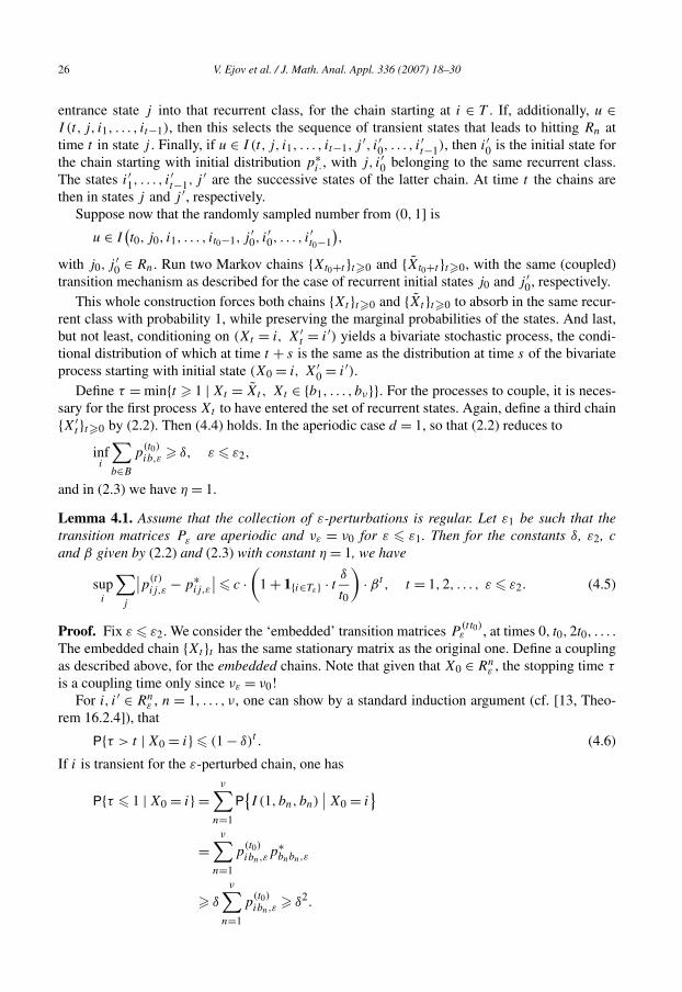
26 V. Ejov et al. / J. Math. Anal. Appl. 336 (2007) 18–30
entrance state j into that recurrent class, for the chain starting at i ∈ T . If, additionally, u ∈
I (t, j, i1, . . . , it−1), then this selects the sequence of transient states that leads to hitting Rn at
time t in state j . Finally, if u ∈ I (t, j, i1, . . . , it−1, j′, i′0, . . . , i
′t−1), then i′0 is the initial state for
the chain starting with initial distribution p∗i·, with j, i′0 belonging to the same recurrent class.
The states i′1, . . . , i′t−1, j
′ are the successive states of the latter chain. At time t the chains are
then in states j and j ′, respectively.
Suppose now that the randomly sampled number from (0,1] is
u ∈ I(
t0, j0, i1, . . . , it0−1, j′0, i
′0, . . . , i
′t0−1
)
,
with j0, j′0 ∈ Rn. Run two Markov chains {Xt0+t }t�0 and {X̃t0+t }t�0, with the same (coupled)
transition mechanism as described for the case of recurrent initial states j0 and j ′0, respectively.
This whole construction forces both chains {Xt }t�0 and {X̃t }t�0 to absorb in the same recur-
rent class with probability 1, while preserving the marginal probabilities of the states. And last,
but not least, conditioning on (Xt = i, X′t = i′) yields a bivariate stochastic process, the condi-
tional distribution of which at time t + s is the same as the distribution at time s of the bivariate
process starting with initial state (X0 = i, X′0 = i′).
Define τ = min{t � 1 | Xt = X̃t , Xt ∈ {b1, . . . , bν}}. For the processes to couple, it is neces-
sary for the first process Xt to have entered the set of recurrent states. Again, define a third chain
{X′t }t�0 by (2.2). Then (4.4) holds. In the aperiodic case d = 1, so that (2.2) reduces to
infi
∑
b∈B
p(t0)ib,ε � δ, ε � ε2,
and in (2.3) we have η = 1.
Lemma 4.1. Assume that the collection of ε-perturbations is regular. Let ε1 be such that the
transition matrices Pε are aperiodic and νε = ν0 for ε � ε1. Then for the constants δ, ε2, c
and β given by (2.2) and (2.3) with constant η = 1, we have
supi
∑
j
∣
∣p(t)ij,ε − p∗
ij,ε
∣
∣ � c ·
(
1 + 1{i∈Tε} · tδ
t0
)
· β t , t = 1,2, . . . , ε � ε2. (4.5)
Proof. Fix ε � ε2. We consider the ‘embedded’ transition matrices P(tt0)ε , at times 0, t0,2t0, . . . .
The embedded chain {Xt }t has the same stationary matrix as the original one. Define a coupling
as described above, for the embedded chains. Note that given that X0 ∈ Rnε , the stopping time τ
is a coupling time only since νε = ν0!
For i, i′ ∈ Rnε , n = 1, . . . , ν, one can show by a standard induction argument (cf. [13, Theo-
rem 16.2.4]), that
P{τ > t | X0 = i} � (1 − δ)t . (4.6)
If i is transient for the ε-perturbed chain, one has
P{τ � 1 | X0 = i} =
ν∑
n=1
P{
I (1, bn, bn)∣
∣ X0 = i}
=
ν∑
n=1
p(t0)ibn,εp
∗bnbn,ε
� δ
ν∑
n=1
p(t0)ibn,ε � δ2.
V. Ejov et al. / J. Math. Anal. Appl. 336 (2007) 18–30 27
By an induction argument and combination with (4.6) (see [8] for details) we obtain
P{τ > t | X0 = i} � (1 + tδ) · (1 − δ)t . (4.7)
This yields the required result. ✷
Finally, a dominated convergence argument and the regularity assumption directly implies the
validity of the next lemma.
Lemma 4.2. Assume that the set of ε-perturbations is regular. Assume that all transition matri-
ces Pε , 0 � ε � ε′ are aperiodic for some ε′ � ε0. Then
limε↓0
Zε = Z0.
5. The aperiodic transformation
This section discusses a data-transformation (cf. Schweitzer [15]), showing that is sufficient
to restrict to the aperiodic case.
Following the construction of Example 1, let λ ∈ (0,1) and put Pε,λ = λI + (1 − λ)Pε . All
previous notation with subscript λ added, denotes the corresponding quantity for the transformed
chains. By inspection one has P ∗ε,λ = P ∗
ε . First, we note that
Uλ(α, ε) =
∞∑
t=0
αt(
Pε,λ − P ∗ε,λ
)t
=
∞∑
t=0
αt P(t)ε,λ −
α
1 − αP ∗
ε,λ.
Rewriting yields the relation
Uλ(α, ε) =1
1 − λαU(α′, ε) −
λα
1 − λαP ∗
ε , (5.1)
where α′ = (1 − λ)α/(1 − λα). Note that α → 1 ⇔ α′ → 1.
In view of (5.1), the fundamental matrices Z̃ε and Zε are related by
Zε,λ =1
1 − λZε −
λ
1 − λP ∗
ε . (5.2)
As a consequence, for all λ ∈ (0,1),
U(α, ε) − Z0 = (1 − λ)(
Uλ(α′, ε) − Z0,λ
)
+ λ(
P ∗ε − P ∗
0
)
+ λ(1 − α′)(
Uλ(α′, ε) − P ∗
ε
)
.
The aperiodic transformation together with Lemma 4.2 yields Lemma 2.3. Theorem 2.1 now
follows immediately from Theorem 2.2 and Lemma 2.3. Theorem 2.4 finally can be derived by
applying standard geometric bounding arguments together with Lemma 2.3.
6. Conclusion and open problems
In this paper we have characterised regular perturbations by means of the existence of finite
limits in both sides of (2.1). For singular perturbations it is not clear whether either limit exists
and if so, under which conditions they are equal.
28 V. Ejov et al. / J. Math. Anal. Appl. 336 (2007) 18–30
Notice, however, that the limit
limα↑1
limε↓0
U(α, ε) = limα↑1
∑
t�0
αt(
P0 − P l0
)t
= Z0 + limα↑1
α
1 − α
(
P ∗0 − P l
0
)
(6.1)
always exists componentwise in the extended reals, provided that the limit P l0 := limε↓0 P ∗
ε ex-
ists. Haviv and Ritov [12] (see also Avrachenkov and Lasserre [3]) studied the case of analytic
perturbations, i.e.
Pε = P0 +
∞∑
k=1
εkGk,
where Gk are S × S matrices. Under the assumption that all perturbed Markov chains are
unichain, they showed that the fundamental matrix Zε admits a Laurent expansion in a neigh-
bourhood of ε = 0. This implies that also limε↓0 Zε exists in the extended reals.
The question is whether limε↓0 Zε = limα↑1 limε↓0 U(α, ε). We will give two examples, one
of a linearly perturbed Markov chain and one of an analytically perturbed one, where this is
not the case. In fact, the examples show that in general there does not seem to be much of a
connection between the values of either limit for singularly perturbed Markov chains. For other
interesting analyses carried out in a somewhat similar spirit, the reader is referred to Hunter [10].
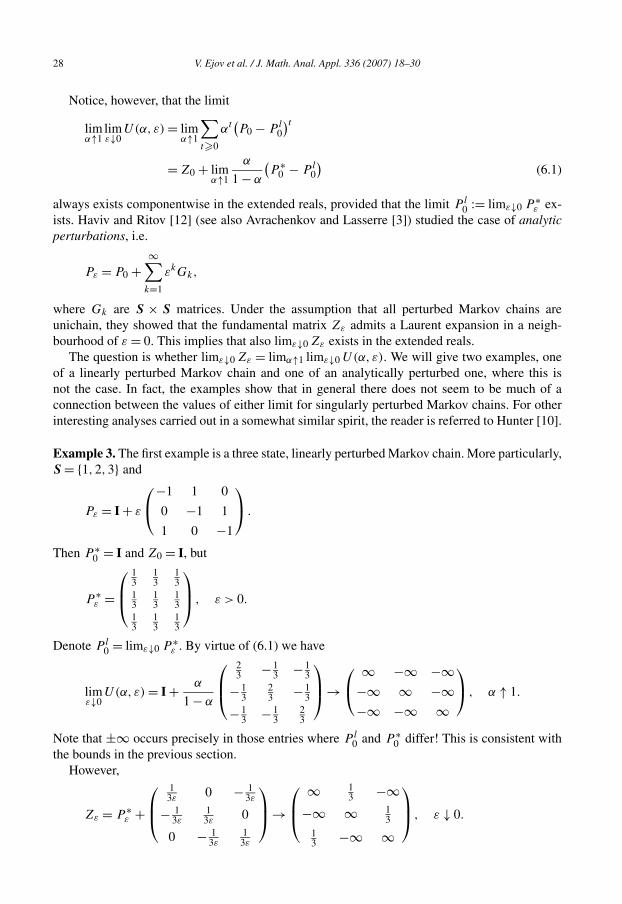
Example 3. The first example is a three state, linearly perturbed Markov chain. More particularly,
S = {1,2,3} and
Pε = I + ε
⎛
⎝
−1 1 0
0 −1 1
1 0 −1
⎞
⎠ .
Then P ∗0 = I and Z0 = I, but
P ∗ε =
⎛
⎜
⎝
13
13
13
13
13
13
13
13
13
⎞
⎟
⎠, ε > 0.
Denote P l0 = limε↓0 P ∗
ε . By virtue of (6.1) we have
limε↓0
U(α, ε) = I +α
1 − α
⎛
⎜
⎝
23 − 1
3 − 13
− 13
23 − 1
3
− 13 − 1
323
⎞
⎟
⎠→
⎛
⎝
∞ −∞ −∞
−∞ ∞ −∞
−∞ −∞ ∞
⎞
⎠ , α ↑ 1.
Note that ±∞ occurs precisely in those entries where P l0 and P ∗
0 differ! This is consistent with
the bounds in the previous section.
However,
Zε = P ∗ε +
⎛
⎜
⎝
13ε
0 − 13ε
− 13ε
13ε
0
0 − 13ε
13ε
⎞
⎟
⎠→
⎛
⎜
⎝
∞ 13 −∞
−∞ ∞ 13
13 −∞ ∞
⎞
⎟
⎠, ε ↓ 0.
V. Ejov et al. / J. Math. Anal. Appl. 336 (2007) 18–30 29
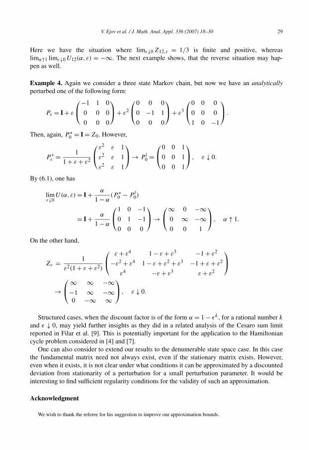
Here we have the situation where limε↓0 Z12,ε = 1/3 is finite and positive, whereas
limα↑1 limε↓0 U12(α, ε) = −∞. The next example shows, that the reverse situation may hap-
pen as well.
Example 4. Again we consider a three state Markov chain, but now we have an analytically
perturbed one of the following form:
Pε = I + ε
⎛
⎝
−1 1 0
0 0 0
0 0 0
⎞
⎠ + ε2
⎛
⎝
0 0 0
0 −1 1
0 0 0
⎞
⎠ + ε3
⎛
⎝
0 0 0
0 0 0
1 0 −1
⎞
⎠ .
Then, again, P ∗0 = I = Z0. However,
P ∗ε =
1
1 + ε + ε2
⎛
⎝
ε2 ε 1
ε2 ε 1
ε2 ε 1
⎞
⎠ → P l0 =
⎛
⎝
0 0 1
0 0 1
0 0 1
⎞
⎠ , ε ↓ 0.
By (6.1), one has
limε↓0
U(α, ε) = I +α
1 − α(P ∗
0 − P l0)
= I +α
1 − α
⎛
⎝
1 0 −1
0 1 −1
0 0 0
⎞
⎠ →
⎛
⎝
∞ 0 −∞
0 ∞ −∞
0 0 1
⎞
⎠ , α ↑ 1.
On the other hand,
Zε =1
ε2(1 + ε + ε2)
⎛
⎝
ε + ε4 1 − ε + ε3 −1 + ε2
−ε2 + ε4 1 − ε + ε2 + ε3 −1 + ε + ε2
ε4 −ε + ε3 ε + ε2
⎞
⎠
→
⎛
⎝
∞ ∞ −∞
−1 ∞ −∞
0 −∞ ∞
⎞
⎠ , ε ↓ 0.
Structured cases, when the discount factor is of the form α = 1 − ǫk , for a rational number k
and ǫ ↓ 0, may yield further insights as they did in a related analysis of the Cesaro sum limit
reported in Filar et al. [9]. This is potentially important for the application to the Hamiltonian
cycle problem considered in [4] and [7].
One can also consider to extend our results to the denumerable state space case. In this case
the fundamental matrix need not always exist, even if the stationary matrix exists. However,
even when it exists, it is not clear under what conditions it can be approximated by a discounted
deviation from stationarity of a perturbation for a small perturbation parameter. It would be
interesting to find sufficient regularity conditions for the validity of such an approximation.
Acknowledgment
We wish to thank the referee for his suggestion to improve our approximation bounds.
30 V. Ejov et al. / J. Math. Anal. Appl. 336 (2007) 18–30
References
[1] D. Aldous, J. Fill, Reversible Markov chains and random walks on graphs, 1999, in preparation. Available at:
http://www.stat.berkeley.edu/users/aldous/RWG/book.html.
[2] K.E. Avrachenkov, J.A. Filar, M. Haviv, Singular perturbations of Markov chains and decision processes, in: E.A.
Feinberg, A. Shwartz (Eds.), Handbook of Markov Decision Processes, Kluwer, Boston, 2001, pp. 113–152.
[3] K.E. Avrachenkov, J.B. Lasserre, The fundamental matrix of singularly perturbed Markov chains, Adv. in Appl.
Probab. 31 (1999) 679–697.
[4] V. Borkar, V. Ejov, J. Filar, Directed graphs, Hamiltonicity and doubly stochastic matrices, Random Structures
Algorithms 25 (4) (2004) 376–395.
[5] D. Blackwell, Discrete dynamic programming, Ann. of Math. Statist. 33 (1962) 719–726.
[6] R. Dekker, A. Hordijk, Recurrence conditions for average and Blackwell optimality in denumerable state Markov
decision chains, Math. Oper. Res. 17 (2) (1992) 271–289.
[7] V. Ejov, J. Filar, M.-T. Nguyen, Hamiltonian cycles and singularly perturbed Markov chains, Math. Oper. Res. 29 (1)
(2004) 114–131.
[8] V. Ejov, J. Filar, F. Spieksma, Continuity properties of regularly perturbed fundamental matrices, Report MI 2006-
09, Leiden University, 2006, http://www.math.leidenuniv.nl/nieuw/en/reports/.
[9] J. Filar, H.A. Krieger, Z. Syed, Cesaro limits of analytically perturbed stochastic matrices, Linear Algebra
Appl. 353 (1) (2002) 227–243.
[10] J.J. Hunter, Mixing times with applications to perturbed Markov chains, Res. Lett. Inf. Math. Sci. 4 (2003) 35–49,
http://www.massey.ac.nz/~wwiims/research/letters/.
[11] J.G. Kemeny, J.L. Snell, Finite Markov Chains, Van Nostrand, New York, 1960.
[12] M. Haviv, Y. Ritov, On series expansions and stochastic matrices, SIAM J. Matrix Anal. Appl. 14 (1993) 670–676.
[13] S.P. Meyn, R.L. Tweedie, Markov Chains and Stochastic Stability, Springer, Berlin, 1993.
[14] P. Schweitzer, Perturbation theorie and finite Markov chains, J. Appl. Probab. 5 (1968) 401–413.
[15] P. Schweitzer, Interative solution to the functional equations of undiscounted Markov renewal programming,
J. Math. Anal. Appl. 34 (1971) 495–501.
[16] F. Spieksma, Geometrically ergodic Markov chains and the optimal control of queues, PhD thesis, 1990, available
on request.
[17] H. Thorisson, Coupling, Stationarity and Regeneration, Springer, Berlin, 1999.
[18] A. Veinott Jr., Markov decision chains, in: G.B. Dantzig, B.C. Eaves (Eds.), Studies in Optimization, in: Stud. in
Math., vol. 10, Mathematical Association of America, 1974, pp. 124–159.
Related Documents


![Asymptotic behavior of singularly perturbed control …€¦ · Asymptotic behavior of singularly perturbed control ... [Lions, Papanicolau, Varadhan 1986]; ... Asymptotic behavior](https://static.cupdf.com/doc/110x72/5b7c19bc7f8b9a9d078b9b98/asymptotic-behavior-of-singularly-perturbed-control-asymptotic-behavior-of-singularly.jpg)


