On rank tests for shift detection in time series

econstor www.econstor.eu

Der Open-Access-Publikationsserver der ZBW – Leibniz-Informationszentrum WirtschaftThe Open Access Publication Server of the ZBW – Leibniz Information Centre for Economics

Nutzungsbedingungen:Die ZBW räumt Ihnen als Nutzerin/Nutzer das unentgeltliche,räumlich unbeschränkte und zeitlich auf die Dauer des Schutzrechtsbeschränkte einfache Recht ein, das ausgewählte Werk im Rahmender unter→ http://www.econstor.eu/dspace/Nutzungsbedingungennachzulesenden vollständigen Nutzungsbedingungen zuvervielfältigen, mit denen die Nutzerin/der Nutzer sich durch dieerste Nutzung einverstanden erklärt.

Terms of use:The ZBW grants you, the user, the non-exclusive right to usethe selected work free of charge, territorially unrestricted andwithin the time limit of the term of the property rights accordingto the terms specified at→ http://www.econstor.eu/dspace/NutzungsbedingungenBy the first use of the selected work the user agrees anddeclares to comply with these terms of use.

zbw Leibniz-Informationszentrum WirtschaftLeibniz Information Centre for Economics

Fried, Roland; Gather, Ursula

Working Paper

On rank tests for shift detection in time series

Technical Report / Universität Dortmund, SFB 475 Komplexitätsreduktion in MultivariatenDatenstrukturen, No. 2006,48

Provided in Cooperation with:Collaborative Research Center 'Reduction of Complexity in MultivariateData Structures' (SFB 475), University of Dortmund

Suggested Citation: Fried, Roland; Gather, Ursula (2006) : On rank tests for shift detectionin time series, Technical Report / Universität Dortmund, SFB 475 Komplexitätsreduktion inMultivariaten Datenstrukturen, No. 2006,48

This Version is available at:http://hdl.handle.net/10419/22692

On rank tests for shift detection in time series

Roland Fried, Ursula Gather

Department of Statistics, University of Dortmund, Germany

Abstract

Robustified rank tests, applying a robust scale estimator, are investi-gated for reliable and fast shift detection in time series. The tests showgood power for sufficiently large shifts, low false detection rates forGaussian noise and high robustness against outliers. Wilcoxon scoresin combination with a robust and efficient scale estimator achieve goodperformance in many situations.

Key words: signal extraction, jumps, outliers, test resistance

1 Introduction

Sudden level shifts in time series, also called edges or jumps, represent im-

portant information on the course of a variable. Reliable automatic rules for

level shift detection with a short time delay are needed for online analysis.

A basic demand is to distinguish level shifts from minor fluctuations and

short sequences of irrelevant outliers. We formalize the task using a simple

additive components model, decomposing the observations (Yt) as

Yt = µt + ut + vt, t ∈ Z, (1)

where (µt) is the time-varying level of the time series, which is assumed

to vary smoothly with only a few sudden shifts, while ut is observational

noise with median zero and possibly time-varying variance σ2t . The impulsive

(spiky) noise vt represents an outlier generating mechanism. It is zero most

of the time, but occasionally takes large absolute values.

Many filtering procedures are available for approximation of µt. Linear fil-

ters such as moving averages are efficient for Gaussian noise, but they are sen-

sitive to outliers. Running medians approximate the level µt in the center of a

1

moving window (yt−k, . . . , yt+k) by the median, µt = med(yt−k, . . . , yt+k), t ∈Z. They offer the advantages of removing outliers and better preserving

jumps (Tukey, 1977, Nieminem, Neuvo and Mitra, 1989).

Sometimes preservation of level shifts for better visualization is not enough

and we want shifts to be detected automatically. There is a growing literature

on robust control charts for change-point detection in time series (Davis and

Adams, 2005). However, these charts typically need strong assumptions for

the in-control process and the existence of a steady state, they react to sev-

eral types of structural changes and they aim at a minimal average delay of

detection, while sometimes the exact delay does not matter if it is too large.

We however consider detection rules which are particularly designed to de-

tect level shifts within a given time span and require only weak assumptions.

Two-sample rank tests as suggested by Bovik, Huang and Munson (1986) and

Lim (2006) are promising candidates for this, also because of their simplic-

ity. The ranks of the data in a moving data window yt+1, . . . , yt+k of width

k are determined within a longer window including h further observations

yt−h+1, . . . , yt left of t. An upward (downward) shift between times t and

t + 1 is detected if the ranks of yt+1, . . . , yt+k or suitable transformations of

them are very large (small).

We investigate rank tests for shift detection in time series with small

delays, modifying them to distinguish outlier sequences of a certain length

from long-term shifts. Section 2 presents rank tests and analytic measures

of their robustness. Section 3 reports a simulation study. Section 4 applies

the methods to time series before some conclusions are drawn.

2 Shift detection

To formulate and compare rules for shift detection we assume an ideal edge

of height δ after a time point t ∈ Z:

µt+j =

{µ, j ≤ 0 ,

µ + δ, j > 0 .(2)

2

For detection of a positive (negative) shift at time t we test H0 : δ = 0

vs. H+1 : δ > 0 (H−

1 : δ < 0). We restrict to a single time point in the

following, considering the n = h+k observations yt−h+1, . . . , yt, yt+1, . . . , yt+k

with median µt, h ≥ k. Guidelines for the choice of h and k are given later.

2.1 Tests based on linear rank statistics

Tests based on linear rank statistics have been suggested for edge detection,

in particular the Wilcoxon and the median test (Bovik, Huang and Munson,

1986). Let yt(1) ≤ . . . ≤ yt(n) be the ordered observations within the window,

and r−h+1, . . . , rk the ranks of yt−h+1, . . . , yt+k in this sequence. A general

linear rank statistic of the most recent k observations can be written as

S+ =

k∑j=1

a(rj) ,

with given scores a(1), . . . , a(n). The complement of S+ is denoted by S− =∑h−1i=0 a(r−i) =

∑ni=1 a(i) − S+. The linear rank statistic

L =(h + k)[h(S− − a)2 + k(S+ − a)2]

h+k∑i=1

(a(i) − a)2

, (3)

with a = n−1∑n

j=1 a(j), is distribution-free and asymptotically χ21-distributed

under H0 in case of a constant variance.

The Wilcoxon test uses a(i) = i, i = 1, . . . , n, i.e. S+ =∑k

i=1 ri. The

normalized Wilcoxon statistic W = S+ − k(k + 1)/2 takes values between

zero and k(3k + 1)/2 if h = k. The Wilcoxon scores lead to estimators and

tests which are almost as effective under Gaussian noise as methods based

on averages, while being more robust to deviations from this assumption

(McKean, 2004).

The median test uses a(i) = 1, i = �n/2� + 1, . . . , n, and a(i) = 0

otherwise. Then S+ corresponds to the number of values in yt+1, . . . , yt+k

larger than the median of the full window and takes values between zero and

k. The median test is regarded as reliable even in case of heavy-tailed noise.

3

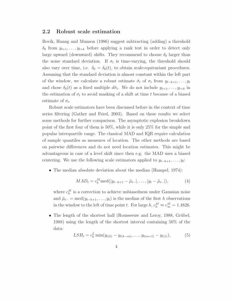
2.2 Robust scale estimation

Bovik, Huang and Munson (1986) suggest subtracting (adding) a threshold

δ0 from yt+1, . . . , yt+k before applying a rank test in order to detect only

large upward (downward) shifts. They recommend to choose δ0 larger than

the noise standard deviation. If σt is time-varying, the threshold should

also vary over time, i.e. δ0 = δ0(t), to obtain scale-equivariant procedures.

Assuming that the standard deviation is almost constant within the left part

of the window, we calculate a robust estimate σt of σt from yt−h+1, . . . , yt

and chose δ0(t) as a fixed multiple dσt. We do not include yt+1, . . . , yt+k in

the estimation of σt to avoid masking of a shift at time t because of a biased

estimate of σt.

Robust scale estimators have been discussed before in the context of time

series filtering (Gather and Fried, 2003). Based on these results we select

some methods for further comparison. The asymptotic explosion breakdown

point of the first four of them is 50%, while it is only 25% for the simple and

popular interquartile range. The classical MAD and IQR require calculation

of sample quantiles as measures of location. The other methods are based

on pairwise differences and do not need location estimates. This might be

advantageous in case of a level shift since then e.g. the MAD uses a biased

centering. We use the following scale estimators applied to yt−h+1, . . . , yt:

• The median absolute deviation about the median (Hampel, 1974):

MADt = cMh med(|yt−h+1 − µt−|, . . . , |yt − µt−|), (4)

where cMh is a correction to achieve unbiasedness under Gaussian noise

and µt− = med(yt−h+1, . . . , yt) is the median of the first h observations

in the window to the left of time point t. For large h, cMh ≈ cM

∞ = 1.4826.

• The length of the shortest half (Rousseeuw and Leroy, 1988, Grubel,

1988) using the length of the shortest interval containing 50% of the

data:

LSHt = cLh min(yt(h) − yt(h−m), . . . , yt(m+1) − yt(1)), (5)

4

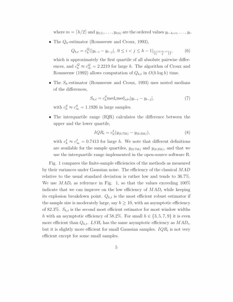
where m = �h/2� and yt(1), . . . , yt(h) are the ordered values yt−h+1, . . . , yt.

• The Qh-estimator (Rousseeuw and Croux, 1993),

Qh,t = cQh (|yt−i − yt−j|, 0 ≤ i < j ≤ h − 1)((�h/2�+1

2 )), (6)

which is approximately the first quartile of all absolute pairwise differ-

ences, and cQh ≈ cQ

∞ = 2.2219 for large h. The algorithm of Croux and

Rousseeuw (1992) allows computation of Qh,t in O(h log h) time.

• The Sh-estimator (Rousseeuw and Croux, 1993) uses nested medians

of the differences,

Sh,t = cShmedimedj �=i|yt−i − yt−j |, (7)

with cSh ≈ cS

∞ = 1.1926 in large samples.

• The interquartile range (IQR) calculates the difference between the

upper and the lower quartile,

IQRt = cIh(y(0.75h) − y(0.25h)), (8)

with cIh ≈ cI

∞ = 0.7413 for large h. We note that different definitions

are available for the sample quartiles, y(0.75h) and y(0.25h), and that we

use the interquartile range implemented in the open-source software R.

Fig. 1 compares the finite-sample efficiencies of the methods as measured

by their variances under Gaussian noise. The efficiency of the classical MAD

relative to the usual standard deviation is rather low and tends to 36.7%.

We use MADt as reference in Fig. 1, so that the values exceeding 100%

indicate that we can improve on the low efficiency of MADt while keeping

its explosion breakdown point. Qh,t is the most efficient robust estimator if

the sample size is moderately large, say h ≥ 10, with an asymptotic efficiency

of 82.3%. Sh,t is the second most efficient estimator for most window widths

h with an asymptotic efficiency of 58.2%. For small h ∈ {3, 5, 7, 9} it is even

more efficient than Qh,t. LSHt has the same asymptotic efficiency as MADt,

but it is slightly more efficient for small Gaussian samples. IQRt is not very

efficient except for some small samples.

5

0 5 10 15 20 25 30

050

100

150

200

250

h

effic

ienc

y [%

]

Figure 1: Efficiencies of the LSH (dashed), Qh (solid), Sh (bold dotted) and

the IQR (dotted) relatively to the MAD for different sample sizes h.

2.3 Test resistances

One reason for median filters being popular is their robustness against a

substantial amount of contamination (outliers). Breakdown points are simple

measures of robustness of an estimator. Given a vector of observations y =

(y1, . . . , yn), the finite sample replacement breakdown point represents the

minimal fraction of data set to arbitrary values that changes the estimate by

any amount. This is a local concept since by definition the breakdown point

depends on the sample. Fortunately, the breakdown point of the median

is the same for all samples, namely �(n + 1)/2�/n, converging to 50% with

increasing n.

Of course, the outcome of the test should not be determined by a few

outliers. Let Um(y) denote a neighborhood of y consisting of all data vectors

z = (z1, . . . , zn) with zi = yi for at most 0 ≤ m ≤ n positions. Let φ

6

be the decision function of the test, φ(z) = 1 and φ(z) = 0 representing

rejection and non-rejection of the null hypothesis, respectively. Ylvisaker

(1977) suggests the global concept of resistance of a test to acceptance and

rejection. Deviating slightly from his definition, these quantities are

εA =1

nmin{m ≥ 0 : sup

y∈Rn

infz∈Um(y)

φ(z) = 0} , and

εR =1

nmin{m ≥ 0 : inf

y∈Rnsup

z∈Um(y)

φ(z) = 1} , respectively.

Ylvisaker considers modifications to occur only at the last positions for sim-

plification. For unstructured data the resulting resistances are usually iden-

tical to those obtained when modifications are allowed at arbitrary positions

as it is done here. The resistances depend on the significance level but not on

the sample since the supremum (infimum) over all possible data y is taken,

i.e. the test breaks down if it does so for any sample. We cannot use a worst

case data set in the definition since for y with φ(y) = 0 we always have

infz∈Um(y) φ(z) = 0. Another, computationally very expensive approach to

overcome the dependence on the sample is expected resistance (Coakley and

Hettmansperger, 1992).

We apply the concept of resistances to search for tests which can detect

a level shift in spite of nearby outliers. For this we analyze two-sample

tests comparing the levels in the left- and the right-hand window. Denote

the corresponding samples by y11, . . . , y1h and y21, . . . , y2k, respectively. It

is easy to see that the test based on the difference of the arithmetic means,

y2 − y1, applied in case of a known scale σ posses resistance to rejection and

to acceptance both equal to 1/n at any significance level α with n = h + k.

This test can easily be mislead since a single outlier can either cause incorrect

detection of a shift or mask a shift so that it is not detected.

The two-sample t-test for the situation of an unknown scale also has got

resistance to acceptance equal to 1/n. Moving one observation is always

sufficient to get a difference of the arithmetic means of zero: a single outlier

can mask a level shift of any size for the t-test. The resistance to rejection is

7

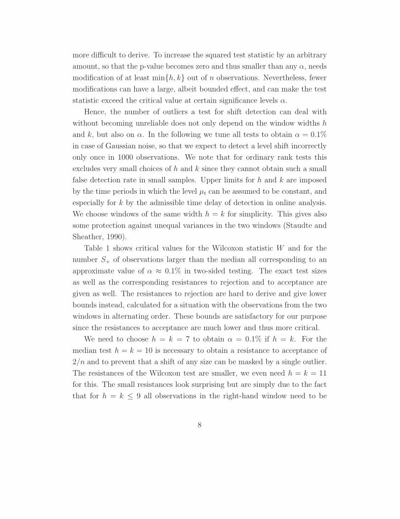
more difficult to derive. To increase the squared test statistic by an arbitrary

amount, so that the p-value becomes zero and thus smaller than any α, needs

modification of at least min{h, k} out of n observations. Nevertheless, fewer

modifications can have a large, albeit bounded effect, and can make the test

statistic exceed the critical value at certain significance levels α.

Hence, the number of outliers a test for shift detection can deal with

without becoming unreliable does not only depend on the window widths h

and k, but also on α. In the following we tune all tests to obtain α = 0.1%

in case of Gaussian noise, so that we expect to detect a level shift incorrectly

only once in 1000 observations. We note that for ordinary rank tests this

excludes very small choices of h and k since they cannot obtain such a small

false detection rate in small samples. Upper limits for h and k are imposed

by the time periods in which the level µt can be assumed to be constant, and

especially for k by the admissible time delay of detection in online analysis.

We choose windows of the same width h = k for simplicity. This gives also

some protection against unequal variances in the two windows (Staudte and

Sheather, 1990).

Table 1 shows critical values for the Wilcoxon statistic W and for the

number S+ of observations larger than the median all corresponding to an

approximate value of α ≈ 0.1% in two-sided testing. The exact test sizes

as well as the corresponding resistances to rejection and to acceptance are

given as well. The resistances to rejection are hard to derive and give lower

bounds instead, calculated for a situation with the observations from the two

windows in alternating order. These bounds are satisfactory for our purpose

since the resistances to acceptance are much lower and thus more critical.

We need to choose h = k = 7 to obtain α = 0.1% if h = k. For the

median test h = k = 10 is necessary to obtain a resistance to acceptance of

2/n and to prevent that a shift of any size can be masked by a single outlier.

The resistances of the Wilcoxon test are smaller, we even need h = k = 11

for this. The small resistances look surprising but are simply due to the fact

that for h = k ≤ 9 all observations in the right-hand window need to be

8

Table 1: Critical values C, test sizes α (in %), lower bounds for the resistances

to rejection (RR) and exact values of the resistances to acceptance (RA) for

the median (top) and the Wilcoxon test (bottom) and different values of

h = k (n = h + k).

k 6 7 8 9 10 11 12 13 14 15

C 6 7 8 9 9 10 11 11 12 13

α .216 .058 .016 .004 .109 .035 .011 .120 .042 .015

n · RR 5 6 7 8 8 9 10 10 11 12

n · RA 1 1 1 1 2 2 2 3 3 3

C 36 48 61 76 91 108 127 148 169 191

α .216 .117 .093 .078 .105 .106 .089 .10 .10 .10

n · RR 5 5 5 6 6 6 6 7 7 7

n · RA 1 1 1 1 1 2 2 2 2 3

either larger or smaller than those in the left one for shift detection. For the

median test we have the formula n · RA = k − C + 1.

2.4 Robustified rank tests

Given the structural weakness of both the Wilcoxon and the median test

observed above we robustify rank tests aiming at higher resistances. We fix

the critical values for W and S+ to be maximal under the restriction that

we always want to detect an upward (downward) shift if, after subtracting

(adding) a threshold, the largest (smallest) �(k + 1)/2� observations are in

the right-hand window. Putting things the other way round, this gives us

a chance to detect an upward (downward) shift even if almost half of the

observations (�(k − 1)/2� out of k) in the right-hand window are extremely

small (large). We thus fix critical values for W and S+ guaranteeing high

resistances without taking the desired false detection rate α into account.

For h = k = 7 e.g., we choose 28 and 4, respectively. Then α is regulated

by subtracting (adding) a suitable multiple δ0(t) = dσt of one of the robust

9

scale estimates presented in Section 2.2 from the observations in the right-

hand window when testing for an upward (downward) shift. We determine

suitable constants d achieving α = 0.1% in simulations. Two one-sided tests

are performed at each time point to detect upward and downward shifts.

The resistance to acceptance of these tests is at least min{�(k+1)/2�/n, ε∗h/n},with ε∗ being the explosion breakdown point of the scale estimator σ: Let

y1 = (y11, . . . , y1h)′ be arbitrary observations in the left-hand window. When

moving less than h · ε� of them, the resulting scale estimate is still bounded,

say smaller than M(y1). Let now the observations in the right-hand win-

dow y2 = (y21, . . . , y2k)′ be such that min(y21, . . . , y2k) > max(y11, . . . , y1h) +

dM(y1). By construction, the modified values, which we obtain from y2 after

subtracting d times the scale estimate for the left-hand window, are all larger

than all values in y1, even when modifying at most h · ε� − 1 observations in

the left-hand window before. If we then move at most �(k − 1)/2� observa-

tions in y2, by construction there are still enough unmodified observations

in y2 to detect a shift.

The resistance to rejection of the robustified tests is at least �(k+1)/2�/n.

Let y1 = (y11, . . . , y1h)′ be arbitrary, with all values different, and all values

of y2 = (y21, . . . , y2k)′ in the median interval of y1 for k even, and in between

the neighbors of the median of y1 for k odd. The tests will not reject the null

for any sample obtained from this one by less than �(k+1)/2� modifications.

3 Monte Carlo experiments

We perform a simulation study to compare small-sample properties of the

different detection rules introduced in Section 2. We use the components

model (1) and analyze the behavior at a single time point t. The suitable

choice of the window widths h and k depends on the application, i.e. on

the situations a filtering procedure needs to handle. For resisting patches of

subsequent outliers we must choose h and k sufficiently large, while upper

limits are imposed by the duration of periods in which the level can be

10

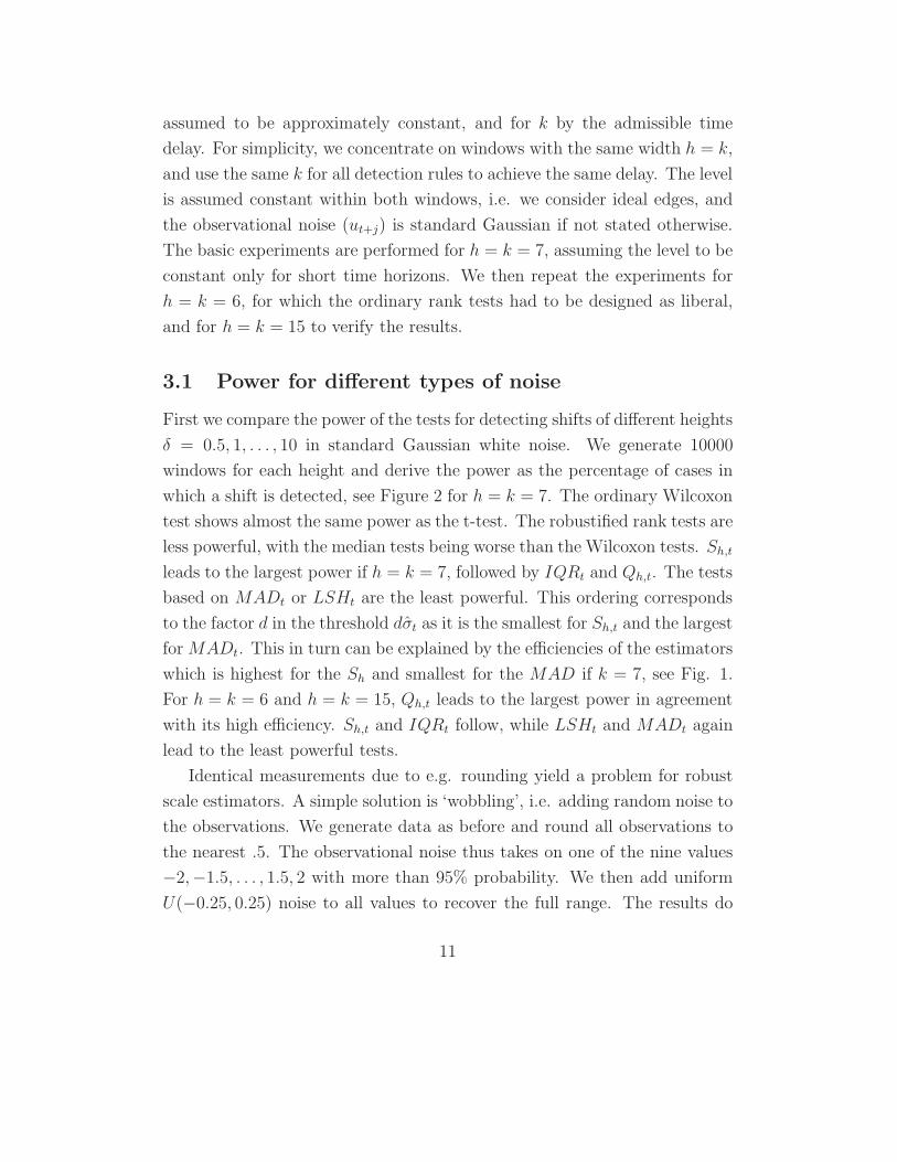
assumed to be approximately constant, and for k by the admissible time

delay. For simplicity, we concentrate on windows with the same width h = k,

and use the same k for all detection rules to achieve the same delay. The level

is assumed constant within both windows, i.e. we consider ideal edges, and

the observational noise (ut+j) is standard Gaussian if not stated otherwise.

The basic experiments are performed for h = k = 7, assuming the level to be

constant only for short time horizons. We then repeat the experiments for

h = k = 6, for which the ordinary rank tests had to be designed as liberal,

and for h = k = 15 to verify the results.

3.1 Power for different types of noise

First we compare the power of the tests for detecting shifts of different heights

δ = 0.5, 1, . . . , 10 in standard Gaussian white noise. We generate 10000

windows for each height and derive the power as the percentage of cases in

which a shift is detected, see Figure 2 for h = k = 7. The ordinary Wilcoxon

test shows almost the same power as the t-test. The robustified rank tests are

less powerful, with the median tests being worse than the Wilcoxon tests. Sh,t

leads to the largest power if h = k = 7, followed by IQRt and Qh,t. The tests

based on MADt or LSHt are the least powerful. This ordering corresponds

to the factor d in the threshold dσt as it is the smallest for Sh,t and the largest

for MADt. This in turn can be explained by the efficiencies of the estimators

which is highest for the Sh and smallest for the MAD if k = 7, see Fig. 1.

For h = k = 6 and h = k = 15, Qh,t leads to the largest power in agreement

with its high efficiency. Sh,t and IQRt follow, while LSHt and MADt again

lead to the least powerful tests.

Identical measurements due to e.g. rounding yield a problem for robust

scale estimators. A simple solution is ‘wobbling’, i.e. adding random noise to

the observations. We generate data as before and round all observations to

the nearest .5. The observational noise thus takes on one of the nine values

−2,−1.5, . . . , 1.5, 2 with more than 95% probability. We then add uniform

U(−0.25, 0.25) noise to all values to recover the full range. The results do

11

not appear sensitive to such changes in the data, i.e., wobbling allows to

maintain the properties of the methods almost completely.

There are also only small changes in the ordering of the methods when

generating the noise from a t-distribution with three degrees of freedom. The

differences between the t-test and the rank tests are somewhat reduced as

compared to the Gaussian situation if h = k = 6 or h = k = 7, while for

h = k = 15 robustified Wilcoxon tests perform almost as well as the t-test,

and the ordinary Wilcoxon test does even better, see Figure 2.

3.2 Single outlier

Next we check the sensitivity of the methods against a single outlier, starting

with the false detection rate. We replace one of the observations by an

additive outlier of size s ∈ {1, 2, . . . , 20} and calculate the error of first kind

from 20000 simulation runs for each s, see Fig. 3 for h = k = 7. The

error rate of the t-test decreases to zero since the limit of the squared test

statistic is 1 as the outlier size tends to infinity. An outlier increases the false

detection rate of the rank tests to up to 0.2%-0.3% while it is in the right-

hand window, with Qh,t and LSHt providing slightly more stable results

than the other methods. When the outlier enters the left-hand window it

still increases the false detection rates of the robustified rank tests, but to

a smaller amount than before. This continuing increase might be due to a

small effect on the robust scale estimates in small samples. The influence of

a single outlier decreases with the window width as could be expected.

We also investigate the effect of an outlier on the power of the procedures

in case of a shift of height 10σ and h = k = 7. We replace either one

observation in the left-hand window by a positive outlier of size 20σ, or

one in the right-hand window by a negative one, see Fig. 3 for the powers

from 10000 simulations runs. The power of the two-sample t-test approaches

zero as the outlier size becomes larger than the height of the shift. For the

12

0 2.5 5 7.5 10

020

4060

8010

0

shift height

pow

er [%

]

0 2.5 50 7.5 10

020

4060

8010

0

shift height

pow

er [%

]

0 1 2 3 4 5

020

4060

8010

0

shift height

pow

er [%

]

0 1 2 3 4 5

020

4060

8010

0

shift height

pow

er [%

]

Figure 2: Power for shifts of different heights in case of Gaussian noise with

h = k = 7 (left) and t3-noise with h = k = 15 (right), Wilcoxon (top) and

median tests (bottom): δ0 = 0 (dash-dot), MAD (dashed), IQR (dotted),

LSH (bold dashed), Qh (bold solid) and Sh (bold dotted); the t-test (solid)

is included for comparison.

13

0 5 10 15 20

020

4060

8010

0

shift height

pow

er [%

]

0 5 10 15 20

020

4060

8010

0

shift height

pow

er [%

]

0 5 10 15 20

0.00

0.05

0.10

0.15

0.20

0.25

0.30

outlier size

fals

e de

tect

ion

rate

[%]

0 5 10 15 20

0.00

0.05

0.10

0.15

0.20

0.25

0.30

outlier size

fals

e de

tect

ion

rate

[%]

Figure 3: Power for a shift of size 10σ in case of an outlier in the left window

(left) and false detection rate in case of an outlier in the right window (right),

Wilcoxon (top) and median tests (bottom), h = k = 7: δ0 = 0 (dash-dot),

MAD (dashed), IQR (dotted), LSH (bold dashed), Qh (bold solid) and Sh

(bold dotted); t-test (solid).

14

ordinary rank tests this happens even earlier. A few outliers can prevent shift

detection when using ordinary rank tests with a short window. These findings

confirm the relevance of the resistances to acceptance given in Subsection 2.3

in practice.

The power of the robustified rank tests remains almost unaffected by an

outlier in the right window, even in case of small samples. An outlier in the

left window, i.e. just before the shift, causes a moderate loss of power. This

effect might again be due to a slight increase of the scale estimate. It stops

increasing as the outlier size becomes larger than 4σ.

The results for h = k = 6 and h = k = 15 are similar to those above.

Choosing longer windows reduces the loss of power of the two-sample t-test

and the ordinary rank tests, but such choices are not always possible and also

lead to results inferior to those of robustified rank tests with robust scales.

3.3 Multiple outliers

Next we investigate the performance in case of multiple outliers. Starting

from a steady state, we insert an increasing number of outliers of the same

size into one window. Fig. 4 shows the detection rates for h = k = 7

obtained from 10000 simulations runs each. The t-test needs at least six

(out of seven) deviating observations to detect a shift. This resistance is not

desirable since a situation with five shifted observations is closer to a shift

with two outliers in a sense than to a steady state with five outliers. Two

outliers of the same size as the shift can mask a shift for the t-test, like one

outlier larger than the shift. For the ordinary rank tests all observations must

be shifted to guarantee detection, see Subsection 3.2. The robustified rank

tests indicate a shift of size 10σ reliably if the outliers are in the right window.

The methods are almost unaffected if less than half of the observations are

deviating (three out of seven), and mostly indicate a shift whenever more

than half of the observations are shifted.

The situation gets more difficult when the outliers are in the left-hand

window, before the shift. All tests rarely detect a shift in case of four outliers

15

then. Only Sh,t allows detection with high power in case of five deviant

observations, a situation which could arise from two outliers occurring just

before a shift. The other scale estimators yield a smooth increase of the

detection rate with increasing number of deviations. Generally, the most

efficient scale estimators result in the largest power if the majority of the

observations is shifted. Only the tests using IQRt perform as poorly as the

t-test, since IQRt increases strongly if two to five out of seven observations

are deviating. The robustified rank tests show higher detection rates in

case of four or five observations shifted by a larger amount 20σ in the left-

hand window, but only Qh,t leads to a good power in case of four shifted

observations, thus allowing the construction of robustified rank tests with

consistent behavior for huge shifts.

We find similar results for h = k = 6. The robustified rank tests detect

a shift if more than three observations in the right-hand window are shifted,

with Qh,t yielding the largest powers according to its high efficiency. A shift

is rarely detected by any method in case of up to three outliers in the left- or

the right-hand window. At most one outlier before a shift is tolerated with

high power since all scale estimators are affected by two outliers within six

observations.

For h = k = 15 we consider a smaller shift of size 6σ, see Fig. 5. The

detection rate of the t-test increases from six to nine shifted observations

(out of fifteen). The robustified rank tests are again rather consistent if

the outliers are in the right window. They resist about five outliers well

and indicate a shift reliably in case of eight outliers, where again the most

efficient estimators yield the most powerful tests. If the outliers are in the

left window only Qh,t leads to a reasonable power in case of eight shifted

observations. In general, tests using the IQRt can be severely mislead by

outliers just before a shift because of its rather low breakdown point.

16

0 1 2 3 4 5 6 7

020

4060

8010

0

number of outliers

dete

ctio

n ra

te [%

]

0 1 2 3 4 5 6 7

020

4060

8010

0

number of outliers

dete

ctio

n ra

te [%

]

0 1 2 3 4 5 6 7

020

4060

8010

0

number of outliers

dete

ctio

n ra

te [%

]

0 1 2 3 4 5 6 7

020

4060

8010

0

number of outliers

dete

ctio

n ra

te [%

]

Figure 4: Percentage of detected shifts in case of an increasing number of ob-

servations shifted by 20σ in the left or by 10σ in the right window, Wilcoxon

(top) or median tests (bottom), h = k = 7: δ0 = 0 (dash-dot), MAD

(dashed), IQR (dotted), LSH (bold dashed), Qh (bold solid), Sh (bold dot-

ted); t-test (solid).

17

0 2 4 6 8 10 12 14

020

4060

8010

0

number of outliers

dete

ctio

n ra

te [%

]

0 2 4 6 8 10 12 14

020

4060

8010

0

number of outliers

dete

ctio

n ra

te [%

]

0 2 4 6 8 10 12 14

020

4060

8010

0

number of outliers

dete

ctio

n ra

te [%

]

0 2 4 6 8 10 12 14

020

4060

8010

0

number of outliers

dete

ctio

n ra

te [%

]

Figure 5: Percentage of detected shifts in case of an increasing number of

observations shifted by 6σ in the left or the right window, Wilcoxon (top)

and median tests (bottom), h = k = 15: δ0 = 0 (dash-dot), MAD (dashed),

IQR (dotted), LSH (bold dashed), Qh (bold solid), Sh (bold dotted); t-test

(solid).

18

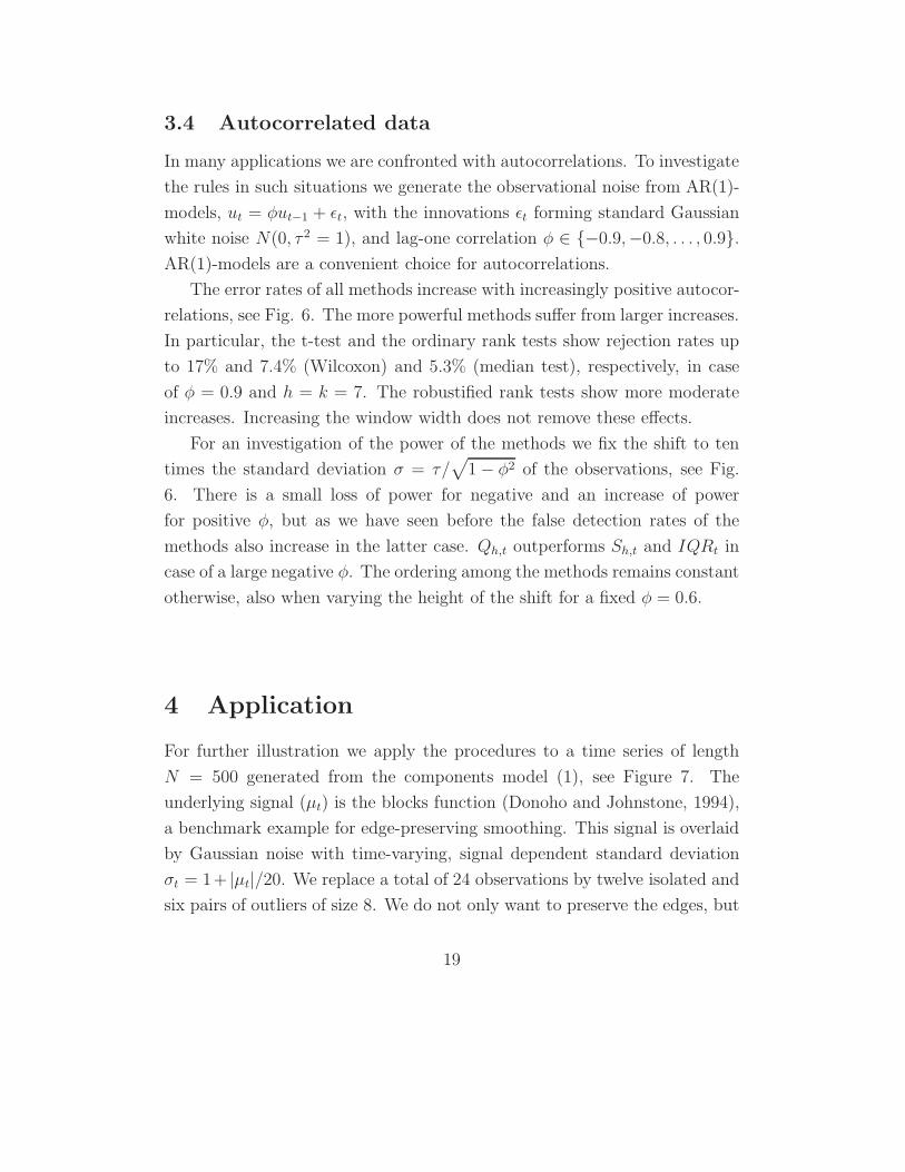
3.4 Autocorrelated data

In many applications we are confronted with autocorrelations. To investigate

the rules in such situations we generate the observational noise from AR(1)-

models, ut = φut−1 + εt, with the innovations εt forming standard Gaussian

white noise N(0, τ 2 = 1), and lag-one correlation φ ∈ {−0.9,−0.8, . . . , 0.9}.AR(1)-models are a convenient choice for autocorrelations.

The error rates of all methods increase with increasingly positive autocor-

relations, see Fig. 6. The more powerful methods suffer from larger increases.

In particular, the t-test and the ordinary rank tests show rejection rates up

to 17% and 7.4% (Wilcoxon) and 5.3% (median test), respectively, in case

of φ = 0.9 and h = k = 7. The robustified rank tests show more moderate

increases. Increasing the window width does not remove these effects.

For an investigation of the power of the methods we fix the shift to ten

times the standard deviation σ = τ/√

1 − φ2 of the observations, see Fig.

6. There is a small loss of power for negative and an increase of power

for positive φ, but as we have seen before the false detection rates of the

methods also increase in the latter case. Qh,t outperforms Sh,t and IQRt in

case of a large negative φ. The ordering among the methods remains constant

otherwise, also when varying the height of the shift for a fixed φ = 0.6.

4 Application

For further illustration we apply the procedures to a time series of length

N = 500 generated from the components model (1), see Figure 7. The

underlying signal (µt) is the blocks function (Donoho and Johnstone, 1994),

a benchmark example for edge-preserving smoothing. This signal is overlaid

by Gaussian noise with time-varying, signal dependent standard deviation

σt = 1+ |µt|/20. We replace a total of 24 observations by twelve isolated and

six pairs of outliers of size 8. We do not only want to preserve the edges, but

19

−.8 −.6 −.4 −.2 .0 .2 .4 .6 .8

02

46

8

lag−one autocorrelation

leve

l [%

]

−.8 −.6 −.4 −.2 .0 .2 .4 .6 .8

02

46

8

lag−one autocorrelation

leve

l [%

]

−.8 −.6 −.4 −.2 0 .2 .4 .6 .8

020

4060

8010

0

lag−one autocorrelationpo

wer

[%]

−.8 −.6 −.4 −.2 0 .2 .4 .6 .8

020

4060

8010

0

lag−one autocorrelation

pow

er [%

]

Figure 6: False detection rate (left) and power for a 10σ-shift (right) in

dependence on φ, Wilcoxon (top) and median tests (bottom), h = k = 7:

δ = 0 (dash-dot), MAD (dashed), IQR (dotted), LSH (bold dashed), Qh

(bold solid), Sh (bold dotted); t-test (solid).

20

detect them with a small time delay and without unnecessary false alarms.

We filter this time series by a running median with window width 15.

The rules for shift detection investigated above are applied to improve the

results, analyzing at each time point t the ranks of yt+1, . . . , yt+7 as compared

to yt−7, . . . , yt−1, i.e. we choose the window widths h = k = 7. Detection of a

shift allows to take some appropriate action. We calculate a simple estimate

of the time point at which the level has shifted as follows: if at time t a shift

is detected without a previous alarm at t − 1, a candidate time point for

the shift is right before the first t + j, j > 0, for which yt+j is closer to the

median µt+ of yt+1, . . . , yt+7 than to the median µt− of yt−7, . . . , yt−1. Instead

of the median of the full window we then take the median of the left-hand

window up to the candidate time t+ j, verifying (and possibly changing) the

candidate time point in each step. From time point t + j on we then use

the median of the current right-hand window until returning to the standard

procedure at time t + j + 4.

As we have seen before false alarms are rarely triggered by any of the

rules. Accordingly, the results of all methods are identical during a steady

state without shift. Fig. 7 depicts several parts of the series in which one or

several shifts occurred along with some filter outputs. The shifts at times 50

and 106 are neither detected by the t-test nor by the ordinary rank tests. In

the first case the reason is masking by the pair of outliers right after the shift.

The filters applying one of these rules therefore do not adapt early enough to

the shift or smear it slightly like the running median without detection rules.

The latter additionally smooths the shifts at times 66 and 75 somewhat.

The robustified median tests, just like the Wilcoxon tests except for Sh,t and

LSHt, do not detect the shift at t = 75 before this time point. Similarly, the

ordinary rank tests detect the shifts at t = 325 and t = 380 rather late.

In general, the robustified Wilcoxon test using Sh,t gives the best results

as could be expected in view of Section 3. We note that a smoother filter

output could be obtained easily using one of these procedures in combination

with exponential smoothing between the identified level shifts.

21

0 100 200 300 400 500

−10

−5

05

1015

20

time

valu

e

90 100 110 120 130 140

−10

−5

05

10

time

valu

e

300 310 320 330 340 350

510

1520

time

valu

e

40 50 60 70 80 90

−5

05

1015

time

valu

e

180 190 200 210 220 230

−5

05

10

time

valu

e

370 380 390 400 410 420

05

1015

20

time

valu

e

Figure 7: Time series (bold dots) generated from the blocks function (bold

dotted) overlaid by time-varying noise and some time periods: running me-

dian (dashed), ordinary rank tests (dash-dot), robustified Wilcoxon test with

Qh (solid) and with Sh (bold solid).

22

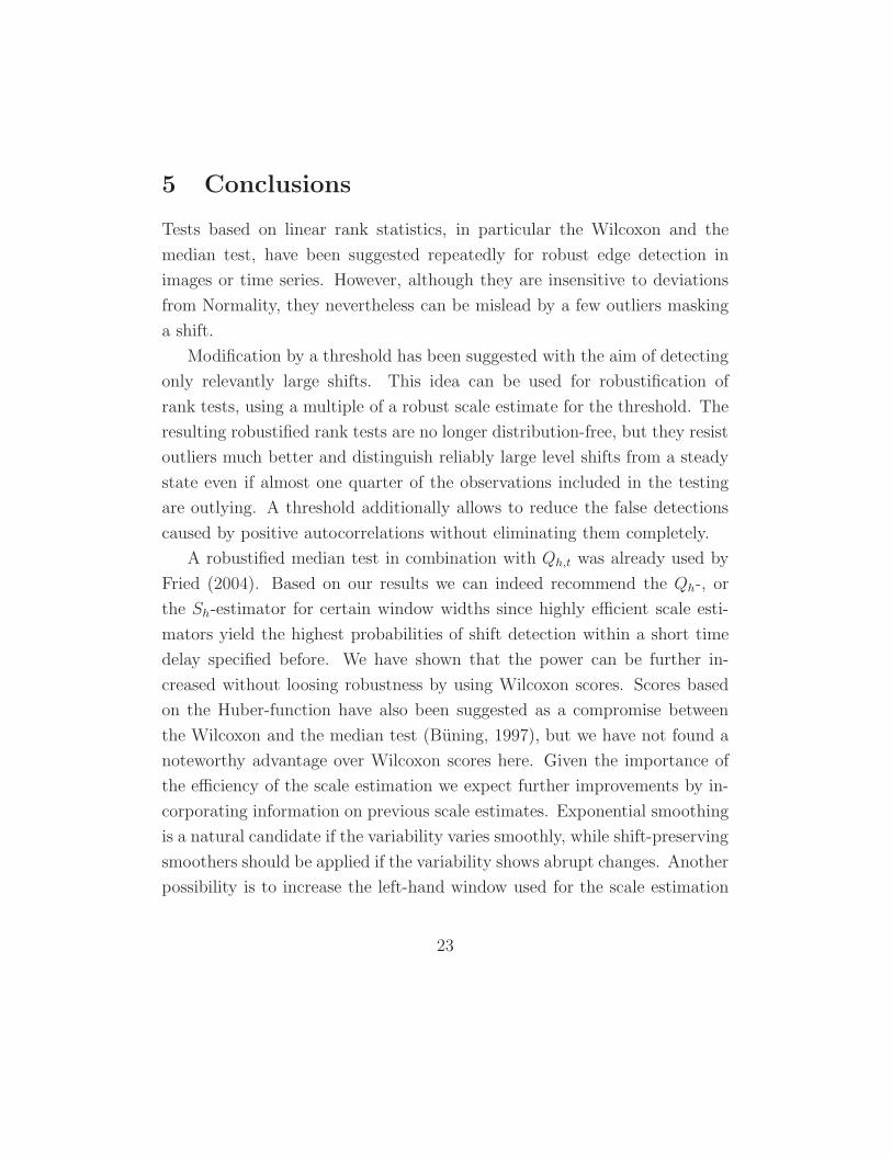
5 Conclusions

Tests based on linear rank statistics, in particular the Wilcoxon and the

median test, have been suggested repeatedly for robust edge detection in

images or time series. However, although they are insensitive to deviations

from Normality, they nevertheless can be mislead by a few outliers masking

a shift.

Modification by a threshold has been suggested with the aim of detecting

only relevantly large shifts. This idea can be used for robustification of

rank tests, using a multiple of a robust scale estimate for the threshold. The

resulting robustified rank tests are no longer distribution-free, but they resist

outliers much better and distinguish reliably large level shifts from a steady

state even if almost one quarter of the observations included in the testing

are outlying. A threshold additionally allows to reduce the false detections

caused by positive autocorrelations without eliminating them completely.

A robustified median test in combination with Qh,t was already used by

Fried (2004). Based on our results we can indeed recommend the Qh-, or

the Sh-estimator for certain window widths since highly efficient scale esti-

mators yield the highest probabilities of shift detection within a short time

delay specified before. We have shown that the power can be further in-

creased without loosing robustness by using Wilcoxon scores. Scores based

on the Huber-function have also been suggested as a compromise between

the Wilcoxon and the median test (Buning, 1997), but we have not found a

noteworthy advantage over Wilcoxon scores here. Given the importance of

the efficiency of the scale estimation we expect further improvements by in-

corporating information on previous scale estimates. Exponential smoothing

is a natural candidate if the variability varies smoothly, while shift-preserving

smoothers should be applied if the variability shows abrupt changes. Another

possibility is to increase the left-hand window used for the scale estimation

23

and the reference level, but then we need to rely on the level being approxi-

mately constant during longer time periods. Experiments not reported here

show that a substantial increase in power is possible in this way with the

ordering of the methods being essentially the same as reported above.

An issue not addressed in detail here is the action to be taken after a

shift is detected. As opposed to the t-test and the ordinary rank tests the

robustified rank tests indicate a level shift during several subsequent time

points as long as the majority of the observations in one window is on a

different level than the observations in the other window. As pointed out in

Section 4, an estimate of the time point of the jump is needed if we want to

use different level estimates before and after the shift. We might also want to

reduce the window width close to the level shift for reducing the bias of the

estimation there. This is especially important when using a longer left-hand

window for comparison since we must only include observations coming from

the same level in it.

Many more rules have been suggested for shift detection. Median com-

parisons also appear promising for locally constant, strongly contaminated

time series. A closer investigation of such methods and a comparison to the

robustified rank tests developed here is a task for further research. Robusti-

fied rank tests offer the advantage that they can easily be modified to detect

abrupt shifts within monotonic trends. Replacing the median by Siegel’s

(1982) repeated median, we can fit a local linear trend to the data (Davies,

Fried and Gather, 2004) and perform the tests on the residuals.

Acknowledgements

This work was prepared while the first author was working at the Department

of Statistics of the University Carlos III of Madrid (Spain). The financial

support of the Deutsche Forschungsgemeinschaft (SFB 475, ”Reduction of

complexity in multivariate data structures”), of the DAAD and the Minsterio

de Educacion (”Acciones integradas”) is gratefully acknowledged.

24

References

Bovik, A.C., Huang, T.S., Munson, D.C. Jr., 1986. Nonparametric tests for edgedetection in noise. Pattern Recognition 19, 209-219.

Buning, H., 1997. Robust analysis of variance. J. Applied Statistics 24, 319-332.

Coakley, C.W., Hettmansperger, T.P., 1992. Breakdown bounds and expected re-sistance. J. Nonparametric Statistics 1, 267-276.

Croux, C., Rousseeuw, P.J., 1992. Time-efficient algorithms for two highly robustestimators of scale. In Dodge, Y., Whittaker, J. (eds.): Computational Statistics,Vol. 1, Heidelberg, Physica-Verlag, pp. 411-428.

Davies, P. L., Fried, R., Gather, U., 2004. Robust signal extraction for on-linemonitoring data. J. Statistical Planning and Inference 122, 65-78.

Donoho, D.L., Johnstone, I.M., 1994. Ideal spatial adaptation by wavelet shrink-age. Biometrika 81, 425-455.

Fried, R., 2004. Robust filtering of time series with trends. J. NonparametricStatistics 16, 313-328.

Gather, U., Fried, R., 2003. Robust estimation of scale for local linear temporaltrends. Tatra Mountains Mathematical Publications 26, 87-101.

Grubel, R., 1988. The length of the shorth. Annals of Statistics 16, 619-628.

Hampel, F.R., 1974. The influence curve and its role in robust estimation. J.American Statistical Association 69, 383-393.

Lim, D.H., 2006. Robust edge detection in noisy images. Computational Statisticsand Data Analysis 50, 803-812.

McKean, J.W., 2004. Robust analysis of linear models. Statistical Science 19,562-570.

Nieminem, A., Neuvo, Y., Mitra, U., 1989. Algorithms for real-time trend detec-tion. Signal Processing 18, 1-15.

Rousseuw, P.J., Croux, C., 1993. Alternatives to the median absolute deviation.J. American Statistical Association 88, 1273-1283.

25

Rousseeuw, P.J., Leroy, A.M., 1988. A robust scale estimator based on the short-est half. Statistica Neerlandica 42, 103-116.

Siegel, A.F., 1982. Robust regression using repeated medians. Biometrika 69, 242-244.

Staudte, R.G., Sheather, S.J., 1990. Robust Estimation and Testing. John Wiley& Sons, New York.

Tukey, J. W., 1977. Exploratory Data Analysis. Addison-Wesley, Reading, Mass.(preliminary edition 1971).

Ylvisaker, D., 1977. Test resistance. J. American Statistical Association 72, 551-556.

26