On Quasiperiodic Perturbations of Ordinary Differential Equations Àngel Jorba i Monte ADVERTIMENT. La consulta d’aquesta tesi queda condicionada a l’acceptació de les següents condicions d'ús: La difusió d’aquesta tesi per mitjà del servei TDX (www.tesisenxarxa.net ) ha estat autoritzada pels titulars dels drets de propietat intel·lectual únicament per a usos privats emmarcats en activitats d’investigació i docència. No s’autoritza la seva reproducció amb finalitats de lucre ni la seva difusió i posada a disposició des d’un lloc aliè al servei TDX. No s’autoritza la presentació del seu contingut en una finestra o marc aliè a TDX (framing). Aquesta reserva de drets afecta tant al resum de presentació de la tesi com als seus continguts. En la utilització o cita de parts de la tesi és obligat indicar el nom de la persona autora. ADVERTENCIA. La consulta de esta tesis queda condicionada a la aceptación de las siguientes condiciones de uso: La difusión de esta tesis por medio del servicio TDR (www.tesisenred.net ) ha sido autorizada por los titulares de los derechos de propiedad intelectual únicamente para usos privados enmarcados en actividades de investigación y docencia. No se autoriza su reproducción con finalidades de lucro ni su difusión y puesta a disposición desde un sitio ajeno al servicio TDR. No se autoriza la presentación de su contenido en una ventana o marco ajeno a TDR (framing). Esta reserva de derechos afecta tanto al resumen de presentación de la tesis como a sus contenidos. En la utilización o cita de partes de la tesis es obligado indicar el nombre de la persona autora. WARNING. On having consulted this thesis you’re accepting the following use conditions: Spreading this thesis by the TDX (www.tesisenxarxa.net ) service has been authorized by the titular of the intellectual property rights only for private uses placed in investigation and teaching activities. Reproduction with lucrative aims is not authorized neither its spreading and availability from a site foreign to the TDX service. Introducing its content in a window or frame foreign to the TDX service is not authorized (framing). This rights affect to the presentation summary of the thesis as well as to its contents. In the using or citation of parts of the thesis it’s obliged to indicate the name of the author.

Welcome message from author
This document is posted to help you gain knowledge. Please leave a comment to let me know what you think about it! Share it to your friends and learn new things together.
Transcript
On Quasiperiodic Perturbations of Ordinary
Differential Equations
Àngel Jorba i Monte
ADVERTIMENT. La consulta d’aquesta tesi queda condicionada a l’acceptació de les següents condicions d'ús: La difusió d’aquesta tesi per mitjà del servei TDX (www.tesisenxarxa.net) ha estat autoritzada pels titulars dels drets de propietat intel·lectual únicament per a usos privats emmarcats en activitats d’investigació i docència. No s’autoritza la seva reproducció amb finalitats de lucre ni la seva difusió i posada a disposició des d’un lloc aliè al servei TDX. No s’autoritza la presentació del seu contingut en una finestra o marc aliè a TDX (framing). Aquesta reserva de drets afecta tant al resum de presentació de la tesi com als seus continguts. En la utilització o cita de parts de la tesi és obligat indicar el nom de la persona autora. ADVERTENCIA. La consulta de esta tesis queda condicionada a la aceptación de las siguientes condiciones de uso: La difusión de esta tesis por medio del servicio TDR (www.tesisenred.net) ha sido autorizada por los titulares de los derechos de propiedad intelectual únicamente para usos privados enmarcados en actividades de investigación y docencia. No se autoriza su reproducción con finalidades de lucro ni su difusión y puesta a disposición desde un sitio ajeno al servicio TDR. No se autoriza la presentación de su contenido en una ventana o marco ajeno a TDR (framing). Esta reserva de derechos afecta tanto al resumen de presentación de la tesis como a sus contenidos. En la utilización o cita de partes de la tesis es obligado indicar el nombre de la persona autora. WARNING. On having consulted this thesis you’re accepting the following use conditions: Spreading this thesis by the TDX (www.tesisenxarxa.net) service has been authorized by the titular of the intellectual property rights only for private uses placed in investigation and teaching activities. Reproduction with lucrative aims is not authorized neither its spreading and availability from a site foreign to the TDX service. Introducing its content in a window or frame foreign to the TDX service is not authorized (framing). This rights affect to the presentation summary of the thesis as well as to its contents. In the using or citation of parts of the thesis it’s obliged to indicate the name of the author.


On Quasiperiodic Perturbations of Ordinary
Differential Equations
Angel Jorba i Monte
Memòria presentada per a aspirar al grau de
Doctor en Ciències Matemàtiques
Departament de Matemàtica Aplicada i Anàlisi
Universitat de Barcelona
Barcelona, Agost del 1991

Quasiperiodic Perturbations of Ordinary
Differential Equations
Angel Jorba i Monte
Memòria presentada per a aspirar al grau de
Doctor en Ciències Matemàtiques
Departament de Matemàtica Aplicada i Anàlisi
Universitat de Barcelona
Barcelona, Agost del 1991 VcilVC/tfc.
W ;
'•Ü 1
o ° : ^ < Û . ; • . • 'í a-c % .• > Ui <i '' .. -- -35 V-* L l ' ' " * ' . ")
% > •
'.'> (y/g
MATEMÀTIQUES


CERTIFICO que la present memoria ha estat realitzada
per en Angel Jorba i Monte, i dirigida per mi, al Depar
tament de Matemàtica Aplicada i Anàlisi de la Univer
sitat de Barcelona.
Barcelona, Agost de 1991,
Dr. Caries Simó i Torres.


a la Monti

U N I V E R S I T A T D E B A R C E L O N A
FACUITAT DE MATEMÀTIQUES
Biblioteca Facultat de Matemàtiques
Adjunt us trameto pel vostre coneixement
i efectes un exemplar de la Tesi Doctoral
d'en Angel JORBA I MONTE, llegida amb data
11 d'octubre de 1991.
Barcelona, 18 d'octubre de 1991
CAP DE SECRETARIA
L <Hs T^vU,,
Conxita MARIN I GUERRERO
.¿tfaotto
S^nK»^


No voldria començar sense fer constar el meu agraïment a totes
aquelles persones que, de una manera o altra, m'han ajudat a dur
a terme aquest treball.
En primer lloc he de citar a la Montse, la meva esposa, per la seva
paciència i suport.
També he d'agrair l'ajut moral i/o científic dels meus companys,
especialment d'en Josep Masdemont (i dels seus coneixements de
UNIX).
Finalment, vull manifestar el meu reconeixement a en Carles Simó
per la direcció d'aquest treball, així com per tot allò que d'ell he
après durant aquests anys.

Contents
1 Quasiperiodic Perturbations of Linear Equations 7 1.1 Introduction 7 1.2 Main Results 8 1.3 Lemmas 10 1.4 Proof of Theorem 1.1 16 1.5 Back to the Floquet Theorem 20
2 Quasiperiodic Perturbations of Elliptic Equilibrium Points 25 2.1 Introduction 25 2.2 A Dynamical Equivalent to Elliptic Equilibrium Points 26
2.2.1 Theorems 28 2.2.2 Previous Lemmas 30 2.2.3 Proof of Theorem 2.1 39 2.2.4 Proof of Theorem 2.2 44
2.3 The Neighbourhood of an Elliptic Equilibrium Point of a Hamiltonian System 44 2.3.1 Sketch of the Proof of Theorem 2.3 47
3 A Semianalytical Study of the Equilateral Libration Points of the Earth-Moon System 51 3.1 Introduction 51
3.1.1 Expansion of the Equations 52 3.2 Idea of the Resolution Method 54 3.3 The Planar Case 54
3.3.1 The Method 56 3.3.2 The Manipulator 59 3.3.3 Results 60
3.4 The Spatial Case 67 3.4.1 The Algebraic Manipulator 67 3.4.2 The Newton Method 72 3.4.3 The Program 76
1
2
3.4.4 Results of the Algebraic Manipulator 78 3.5 Numerical Refinement 85
3.5.1 Final Results 86 3.6 The Behaviour Near the Computed Nearly Quasiperiodic Solution . . 89 3.7 Problems and Extensions 96
A The Modified Parallel Shooting Method 97 A.l Introduction 97
A.l.l The Program 97 A.2 Results 98
A.2.1 Results for a Time Interval of 5 Years 98 A.2.2 Results for a Time Interval of 3000 Days 107
B The Model Equations Near the Equilateral Points in the Earth-Moon System 115 B.l Introduction 115 B.2 Systems of Reference 116 B.3 The Lagrangian 117 B.4 The Hamiltonian and the Related Expansions 119 B.5 Some Useful Expansions 121 B.6 Fourier Analysis: Relevant Frequencies and Related Coefficients . . .123 B.7 Simplified Normalized Equations 135 B.8 Numerical Tests 141
C Proof of Theorem 2.3 147 C.l Previous Lemmas and Theorems 147 C.2 Proof of Theorem 2.3 156
Bibliography 159
Introduction
In this work we study several topics concerning quasiperiodic time-dependent perturbations of ordinary differential equations. This kind of equations appear as models in many applied problems of Celestial Mechanics, and we have used, as an illustration, the study of the behaviour near the equilateral libration points of the real Earth-Moon system. Let us introduce this problem as a motivation. As a first approximation, suppose that the Earth and Moon are revolving in circular orbits around their centre of masses, neglect the effect of the rest of the solar system and neglect the aspherical terms coming from the Earth and Moon (of course, all the effects minor than the above mentioned, as the relativistic corrections, must be neglected). With this, we can write the equations of motion of an infmitessirnal particle (by infmitessirnal we mean that the particle is influenced by the Earth and Moon, but it does not affect them) by means of Newton's law. The study of the motion of that particle is the so-called Restricted Three Body Problem (RTBP). Usually, in order to simplify the equations, the units of lenght, time and mass are chosen so that the angular velocity of rotation, the sum of masses of the bodies and the gravitational constant are all equal to one. With these normalized units, the distance between the bodies is also equal to one. If these equations of motion are written in a rotating frame leaving fixed the Earth and Moon (these main bodies are usually called primaries), it is known that the system has five equilibrium points (see [22] for details). Two of them can be found as the third vertex of equilateral triangles having the Earth and Moon as vertices, and they are usually called equilateral libration points.
It is also known that, when the mass parameter fi (the mass of the small primary in the normalized units) is less than the Routh critical value //# = | ( 1 — J23/27) = 0.03852... (this is true in the Earth-Moon case) these points are linearly stable. Applying the KAM theorem to this case we can obtain that there exist invariant tori around these points. Now, if we restrict the motion of the particle to the plane of motion of the primaries we have that, inside each energy level, these tori split the phase space and this allows to prove (see [20]) that the equilateral points are stable (except for two values, n = Ht and ß = fi3 with low order resonances). In the spatial case, the invariant tori do not split the phase space and, due to the possible Arnold diffusion, these points can be unstable. But Arnold diffusion is a very slow
3
4
phenomenon and we can have small neighbourhoods of "practical stability" (see [10], [19] and [5]), that is, the particle will stay near the equilibrium point for very long time spans.
Unfortunately, the real Earth-Moon system is rather complex. In this case, due to the fact that that the motions of the Earth and the Moon are non circular (even non elliptical!) and the strong influence of the Sun, the libration points do not exist as equilibrium points, and we need to define "instantaneous" libration points as the ones forming an equilateral triangle with the Earth and the Moon at each instant. If we perform some numerical integrations starting at (or near) these points we can see that the solutions go away after a short period of time (see [17] and [13]), showing that these regions are unstable.
Two conclusions can be obtained from this fact. First: if we are interested in keeping a spacecraft there, we will need to use some kind of control. Second: the RTBP is not a good model for this problem, because the behaviour displayed by it is different from the one of the real system.
For these reasons, an improved model has been developped in order to study this problem (see [13] and [12]). This model includes the main perturbations (due to the solar effect and to the noncircular motion of the Moon), assuming that they are quasiperiodic. This is a very good approximation for time spans of some thousands of years. It is not clear if this is true for longer time spans, but this matter will not be considered in this work. This model is in good agreement with the vector field of the solar system directly computed by means of the JPL ephemeris, for the time interval for which the JPL model is available.
The study of this kind of models is the main purpose of this work. First of all, we have focused our attention on linear differential equations with
constant coefficients, affected by a small quasiperiodic perturbation. These equations appear as variational equations along a quasiperiodic solution of a general equation and they also serve as an introduction to nonlinear problems.
The purpose is to reduce those systems to constant coefficients ones by means of a quasiperiodic change of variables, as the classical Floquet theorem does for periodic systems. It is also interesting to have a way to compute this constant matrix, as well as the change of variables. The most interesting case occurs when the unperturbed system is of elliptic type. Other cases, as the hyperbolic one, have already been studied (see [3]). We have added a parameter e in the system, multiplying the perturbation, such that if e is equal to zero we recover the unperturbed system. In this case we have found that, under suitable hypothesis of nonresonance, analyticity and nondegeneracy with respect to e, it is possible to reduce the system to constant coefficients, for a cantorian set of values of e. Moreover, the proof is constructive in an iterative way. This means that it is possible to find approximations to the reduced matrix as well as to the change of variables that performs such reduction. These results are given in Chapter 1.
5
The nonlinear case is now going to be studied. We have then considered an elliptic equilibrium point of an autonomous ordinary differential equation, and we have added a small quasiperiodic perturbation, in such a way that the equilibrium point does not longer exist. As in the linear case, we have put a parameter (e) multiplying the perturbation. There is some "practical" evidence (see [7] and [12]) that there exists a quasiperiodic orbit, having the same basic frequencies that the perturbation, such that, when the Pertubation goes to zero, this orbit goes to the equilibrium point. Our results show that, under suitable hypothesis, this orbit exists for a cantorian set of values of e. We have also found some results related to the stability of this orbit. These results are given in Chapter 2.
A remarkable case occurs when the system is Hamiltonian. Here it is interesting to know what happens to the invariant tori near these points when the perturbation is added. Note that the KAM theorem can not be applied directly due to the fact that the Hamiltonian is degenerated, in the sense that it has some frequencies (the ones of the perturbation) that have fixed values and they do not depend on actions in a diffeomorphic way. In this case, we have found that some tori still exist in the perturbed system. These tori come from the ones of the unperturbed system whose frequencies are nonresonant with those of the perturbation. The perturbed tori add these perturbing frequencies to the ones they already had. This can be described saying that the unperturbed tori are "quasiperiodically dancing" under the "rhythm" of the perturbation. These results can also be found in Chapter 2 and Appendix C.
The final point of this work has been to perform a study of the behaviour near the instantaneous equilateral libration points of the real Earth-Moon system. The purpose of those computations has been to find a way of keeping a spacecraft near these points in an unexpensive way. As it has been mentioned above, in the real system these points are not equilibrium points, and their neighbourhood displays unstability. This leads us to use some control to keep the spacecraft there. It would be useful to have an orbit that were always near these points, because the spacecraft could be placed on it. Thus, only a station keeping would be necessary. The simplest orbit of this kind that we can compute is the one that replaces the equilibrium point. In Chapter 3, this computation has been carried out first for a planar simplified model and then for a spatial model. Then, the solution found for this last model has been improved, by means of numerical methods, in order to have a real orbit of the real system (here, by real system we mean the model of solar system provided by the JPL tapes). This improvement has been performed for a given (fixed) time-span. That is sufficient for practical purposes. Finally, an approximation to the linear stability of this refined orbit has been computed, and a very mild unstability has been found, allowing for an unexpensive station keeping. These results are given in Chapter 3.
As the numerical methods used in Chapter 3 have some difficulties to refine an

6
orbit for very long time intervals, some modifications have been introduced. These modifications can overcome those troubles and give good nominal orbits for very large time intervals. The description of these modified methods can be found inside Appendix A, as well as the results obtained.
Finally, in Appendix B the reader can find the technical details concerning the way of obtaining the models used to study the neighbourhood of the equilateral points. This has been jointly developped with Gerard Gómez, Jaume Llibre, Regina Martínez, Josep Masdemont and Carles Simó.
Chapter 1
Quasiperiodic Perturbations of Linear Equations
1.1 Introduction
In this Chapter we study linear differential equations under quasiperiodic time-dependent perturbations. First of all, let us define rigorously the concept "quasiperiodic".
Definition 1.1 A function f = f(t) is said to be a quasiperiodic function with basic frequencies u>i,... ,u>r if f(t) = F{9\,..., 6r), where F is 2it periodic in all its arguments and 0j = ujjt for j = 1 , . . . , r.
We assume that the quasiperiodic functions appearing in our equations are analytical. For definiteness we give the following
Definition 1.2 A function f = f(t) is said to be analytic quasiperiodic on a strip of width p if it is quasiperiodic and F (see Definition 1.1) is analytical for |Im 9¡\ < p for j = 1 , . . . , r. In this case let us denote by \\f\\p the norm
sup{\F((611...,8T)\/\lm6j\<p,l<j<r}.
Let us consider first the following equation:
x = A(t)x, (1.1)
where A(t) is an n x n matrix that depends on time in a quasiperiodic way with basic frequencies u> = (u>i,... ,u>r)
T- A change of variables x — P(t)y is said to be a Lyapunov-Perron (LP) transformation if P(t) is nonsingular and P(t), -P-1(i) and P(t) are bounded for all í S R. Moreover, if P, P~l and P are quasiperiodic, the change x = P(t)y is called a quasiperiodic LP transformation.
7
8 Quasiperiodic Perturbations of Linear Equations
If x = P(t)y is a LP transformation, then y satisfies the equation
y = B(t)y, (1.2)
where B = P~1(AP — P). Equation (1.1) is said to be reducible if there is a quasiperiodic LP transformation that transforms (1.1) to (1.2), where B is a constant matrix. Obviously if Q is periodic the reducibility in all cases is given by the classical Floquet theory (see, for example, [4] or [2]).
Classical results concerning to almost periodic systems can be found in [9] and [6]. In [3] this problem is studied for different conditions on A and Q and the ideas used here are very close to the ones found in [3]. Another source of inspiration has been the proof of KAM theorem given in [1].
A different approach to this problem can be found in [14]. To introduce it, let us define the spectrum E = E (A) of (1.1) as the collection of À 6 R for which the shifted equation x = (A(t) — XI)x (here, / denotes the identity matrix in Rn) does not have an exponential dichotomy (see [6]). We will say that (1.1) satisfies the "full spectrum" hypothesis if E = { a i , . . . , ctn}, where a,- / a¿ for i ^ j . Then, in [14] is shown that if A is sufficiently smooth, its frequencies satisfy a suitable nonresonance condition and it has "full spectrum" then the system (1.1) is reducible.
In this work we will drop the "full spectrum" hypothesis and we will consider A(t) analytical and close to a nonresonant constant matrix. Our system will be
x = (A + eQ{t))x, (1.3)
being x a ¿-dimensional vector. Let Xj, j = 1 , . . . ,d be the eigenvalues of A and XT = (Ai , . . . , Xd). The greatest difficulties are found when the real parts of all Xj are equal (perhaps zero). We present a theorem which holds in this case asking for some nonresonance conditions for the vector vT = (XT,u>T). These conditions are satisfied by a set of big relative measure in the space of the parameter u. Under some nondegeneracy conditions we will prove that if e0 is small enough, there exists a cantorian subset £ of [0,£o] of positive measure such that, if e G S then (1.3) is reducible. Moreover, our proof is constructive using an iterative scheme with quadratic convergence with respect to e. That is, after n steps the transformed equation looks like (1.3) with An(e), e2" and Qn(t,e) (bounded by some Mn) instead of A, s and Q(t) for e in some cantorian set Sn.
Similar ideas have been used in [8], but only for Hamiltonian systems.
1.2 Main Results
The average of Q(t) is defined as
T-+0O ¿1 J-T
Main Results 9
For the existence of the limit see [9]. We consider first the equation (1.3) after averaging with respect to t and some rearrangement
x = (Ä + eQ(t))x,
where Q(t) = Q(t) - Q, ~Ä~ = A + ¿Q. Next we do the change of variables x = (I + eP)y to get
y = {(I + eP)-l(A + e(ÄP - P + Q)) + e2(7 + eP^QP] y, (1.4)
We would like to have
(/ + eP)-\Ä + e(ÄP -P + Q))=~Â~
and this implies P=~Â~P-PÂ + Q. (1.5)
Suppose now that we have a quasiperiodic solution of (1.5) with the same frequencies which appear in Q. Then, (1.4) becomes
y = [A + e2{I + eP)-lQP}y.
Now we average again and restart the process. Obviously, if we can do this until the nth step, we shall get an equation like
Xn — \™n i £ Uinj-^ni
where | |Qn | | can be very large. We are going to see that, under suitable conditions, this method converges.
Theorem 1.1 Consider the equation x = (A + eQ(t))x, e (E (0,£o) an& % £ Rd, where A is a constant matrix with different eigenvalues Xi,...,X¿ and Q(t) is a quasiperiodic matrix with basic frequencies u>i,... ,u>r. Suppose that
1. Q is analytic on a strip of width po with po > 0.
2. The vector v, where vT = (Ai , . . . , A , y/— lu>i,..., \J— la>r) satisfies the non-resonance conditions
for all m G {ma € Zd, |ma | = 0 or |mx| = 2} x {m2 € Z r, \m2\ ^ 0}, where r+d
cv is a positive number, 7^ = r + d + /?, ß > — 1 and \m\ — ¿ J \™3\, where m? 3=1
denote the components of m in Z r + .
10 Quasiperiodic Perturbations of Linear Equations
3. Let Q be the average of Q with respect to t and let X%e) be an eigenvalue of A = A + eQ for j = 1 , . . . , d. We require
^(A?(e) - A?(£))U| > 26 > 0, V 1 < i < j < d.
Then there exists a cantonan set S C (0, £o) with positive Lebesgue measure such that the system x = (A-rsQ)x is reducible. Ifeo is small enough the relative measure of £ in (0, £o) is close to 1. Furthermore the quasiperiodic change of variables that transforms the system to y = By (B being a constant matrix) has the same basic frequencies than Q.
Remark 1. The nonresonance condition for v is satisfied for most of the values of v. More concretely, if v belongs to a ball of radius R then we have that the condition is satisfied for all u except by a set of relative Lebesgue measure less than 4cv(d + r)ï"2ft' where ( denotes the Riemann zeta function. The third condition is a nondegeneracy condition, not allowing to be locked at resonance. This condition can be replaced by a higher order nondegeneracy condition but it is not so simple to state in the hypothesis. Remark 2. We can suppose that A = diag (Ax , . . . , A^). Let \\Q\\P be the matricial norm associated to the vector norm defined by | | ( / i , . . . , fd)T\\P = m&Xi<k<d \\fk\\P, where \\fk\\P is the norm defined in the Introduction. Introducing a new time r = st where
s = max < -2 , ||Q||Po
( Po
we can suppose pQ > ^- + 1, \\Q\\P0 < 1. These bounds will be used in the proof of the theorem. The scaling can change the constant cv and, therefore the admisible set of e is scaled by the same factor.
1.3 Lemmas
We need some lemmas.
Lemma 1.1 Let N? = #{fc € T / |ib| = ¿ |fc,-| = m}. Then ¡=i
2r / r V - 1
Lemmas 11
Proof: As kr ranges from — r to r we have the recurrence relation
m—1
AT = 2 ^ JV*.! + iV™ ! + 2
and N™ = 2 for all m. This satisfies the relation given on the statement. Suppose that this relation holds for all m and some r. Then
K r + l
m—1
= 2*£Nrk + N? + 2<
2T k=l
tm 2T ( ry-1 , 2 r / r \ r " 1 21 / r
)r+l
rl
( r\r ( r\T r ( ry1 r\
But
r y r / r m + 2 J + 2 l m + 2
r _ 1 / r 1 < ( m + 2 + 2
r y r / r
= | m + - j + (m +
r - l •set; ( ry-3 r+2) '
and, using that § < (1 + §) r the result follows. • Remark. A simpler (and worse if r > 3 and m not too small) bound as N™ < 2rmr~1 can also be obtained by induction. There is numerical evidence that the factor | , which multiplies r on the statement of the Lemma can be replaced by 0.1872183, slightly larger than (2e)_1. The bound of the Lemma is also true for m = 0.
Lemma 1.2 Let
P = E J ) I
feeZr
ke(k,w)V=ït
be an analytic Fourier series satisfying \pk\ < A^k^e-"1^ fork^O with 7 > 0. / /
92 € (0,pi) then, for k ¿ 0, we have \pk\ < A2e-"2W where A2 = Ax ( ( p i^P 2 ) e)7-
Proof: We know |p*| < Al\k\'1e~^1-p2^e-p2^. Using that the maximum of g{x) = x-ye-(pi-P2)x j s r e a ched when x = 7 the proof is completed. •
P1-P2 r r
12 Quasiperiodic Perturbations of Linear Equations
Lemma 1.3 We consider P = AP — PA + Q, where A = diag (Ai , . . . , Xd) and Q is a quasiperiodic matrix with basic frequencies UJ = (a>i,... ,w r)
T and with zero average. Let q^ be the elements of Q:
%• = E <êe(*<")vCîf. JfceZr\{0}
We suppose also \q^\ < Me~pl^ and |A,- — Xj — (k,uj)y/^ï\ > •&; for all i,j G
{l,...,d} and all k € Zr \ {0}. Then there exist a unique solution P of P = AP — PA + Q with the same frequencies that Q and satisfies |p*-| < JVe-P2'fc' with
P2e(0,Pl)andN = M^T^.y.
Proof: We look for
fc€Zr\{0}
and this means that we have to solve the linear system
Pij = (XiiPij + 9«i, <*«j = Xi - Xj, 1 < i,j < d.
It is easy to obtain the coefficients p'-y.
a*-,J (Ä; ,w)V^T-ay
From the hypothesis one has the bound
and using Lemma 1.2 we get
|p* | < Í Í f ? V e-«l*l = iVe-"2lfcl. • 3 c \{pi-p2)e)
Remark. The worst situation is found when A,- — Xj are on the imaginary axis. If they are out of it the given bounds of |p*- | are very high compared with the actual values. Therefore it is enough to restrict to the case when Re (A¿ — Xj) = 0 for all h 3 € {1, • •. ,d], both for the initial matrix A and for all the matrices An found in the iterative process.
Lemma 1.4 Let q(t) = ]T 9*e(*'w>vC"
¡teZr
Lemmas 13
be such that \qk\ < Me'"1^. Then, for r > 2, one has
,/>l ~ / > 2 , fair-1), Proof: Let í be a complex number verifying |Im 0j\ < p2, where 0j = u>jt, 1 < j < r. Then
fceZr fceZr AreZr
Let us define 8 = px — p2. This implies that
and using Lemma 1.1
*eZr
2r ~ / r V - 1 c
As the function x H-> (¡E + | ) r *e 5a: has at most one maximum on [0, oo) the sum is bounded by the maximum plus the integral. Hence
ML < M \P2
+
( r - 1 ) ! [\ 8e
l \ r ör /•<*>
r - l V " 1 it 62 +
G)'-fK-i)n-S(^K)) = M- 7T7Te2
(r - l)!<Sr
Ä , / 2 V ir [ ( r - 1 )
< M Q e 1 +
(r-iy-1
{ .I ¿ + ( r - l ) ! er x
r - l
e5-1 ( r - l ) ! + 1 <
V ^ r i r - l ) .
Remark. In the statement one should replace the last factor of the bound by (l + f ) i f r = l.
Lemma 1.5 Let {Kn}neN ^e a sequence of positive real numbers such that Kn <
an bl/2 KU. Then
Kn<-( ! / *
2"
14 Quasiperiodic Perturbations of Linear Equations
Proof: It is easy to see that
Kn < al+2+22+...+2»-l 7 1 - 1
U(n-if L»=0
i\0 .
To bound the expression in brackets we take logarithms:
/ n - l \ n - 2
2«+2 \ «=0 / i=0 t=0
Then
Hence
^ ln(» + 2) ^ln(» + 2) *n (fi + 2) (£§)"')
J ^ ln(t + 2) ln(j + 2) (j + 3\ 1 ^ fc ¿2 2¿+2 + 2i+i Vi + 2J 2^+3 ¿12*"1
tiln(t + 2) 1 , ,. „.
expc<n(¿ + 2 ) 2 - ^ ( i + 3)2
¿=o
and taking j — 3 one obtains exp c < | because 24 32 24 < Í | j . Finally Kn < / \ 2"
a2" -1 Í (exp c)b) KQ" and the result follows. • Remark : One can improve the bound on exp c but not more than three per thousand.
Lemma 1.6 Consider the expression an = (iz¡±Ü!) forne N U { 0 } . Ifc> 3
c—1
the maximum is obtained for n = 1 and therefore an < 2~. Proof: Let g(x) = In (^Y^)2 1 = c2-*(ln(x + 1) - In or), where a = 2« and
a; > 0. Computing the derivative and equating to zero one should have h(x) = In 2(ln(x + 1) — In a) — -^ = 0 to get a maximum. The function h is monotonically increasing, as l n a < | In 2 one has h(l) < 0, h(2) > 0 for all c > 3. To see that the maximum over the integers is attained at n — 1 we compare the valors for n = 1
and n = 2. One obtains (—)2 and ( y J4 and the first one is larger than the second
if c> H « 2.41 • Inf
Lemmas 15
Lemma 1.7 Let M be a diagonal matrix with different eigenvalues fij, j = 1 , . . . , d, and a = min , - j ; ^ \fi¡ — fij\. Let N be a matrix such that (<£ +l)||iVH < a (here ||. || is the sup norm). Let Vj, j = l , . . . , d be the eigenvalues of M + N, B a suitable matrix such that B~l(M + N)B = D = diag (i/j) with condition number C(B). Then
1. ß = min , j . , w \vi - Vj\ > a - 2||JV||.
2- °(B) Z â-KîlH- In Particular> »/ WNW < Sfe then C(B) < 2-Proof: From Gerschgorin Lemma (see, for example, [21]) it follows \fij — Uj\ < \\N\\ and hence 1 holds. Let N = (n¿¿), B — (6y). The matrix B is made of eigenvectors of M + N. We choose a matrix S such that bjj = 1, j = 1 , . . . ,d. To determine bkj, k — 1 , . . . , á, & T¿ j we have to solve a (<¿ — l)-dimensional linear system where the diagonal entries of the matrix are //& — Vj + «tt , k ^ j and the out of diagonal entries are nkm, k ^ j , m =fi j . The independent term has entries —rikj, k ^ j . Let bsj such that \bsj\ = maxfc^j |6fc¿|. From
nsihj + h ïîsj_ifej_i j + nsj+1bj+ij + \- nsdbdj + (/xs - Vj)baj = -n SJ
one has
1 « ' - IA*. - i -l - ||JV|| - « - 2||JV||-
Therefore B = I + B' with
i 2 ? « < 7rT2pr < 1 -Then C(5) = M I I B - ! < i r | f j j and g follows. •
Lemma 1.8 Let wGR r and \ s , s = 1 , . . . ,d such that
c \\a-\j-y/=ï{k,U>)\>
M*
for all s, j € {!,...,d} and all k 6 Zr \ {0}, where c> 0, 71 > 0. Define a resonant
subset IZp as
^ = { ^ € A / = T R , \<p\<n/3s,je{l,...,d} A 3k'elr\{0}
such that \<p + Xs - Xj - V^ï(k\uj)\ < -rrjr^}.
Let ip(fJ-) = "ffi^ , where m denotes the Lebesgue measure. If 72 = 71 + r + 1 then
liminf t/>(fi) = 0. p.—>0
16 Quasiperiodic Perturbations of Linear Equations
Proof: Take pn = ^%-. For any k' with \k'\ >n and any couple s, j the measure of the resonant interval of <p is bounded by n ^ - . Adding for all the values of k' with \k'\ = n' and all s, j and using the remark following Lemma 1.1, we have
m(7^ n ) < ¿Ire £ , , w . r + 1 < 2crd3(n - I)-*»"). n'>n
( n ' ) T 2 - r + l
Furthermore the resonant intervals associated to n' < n are disjoint with TZßn if n is large enough. Hence, for n large enough, i¡>(fin) < rcPrf1^ — 1)~(T I + 1) which goes to zero if n goes to infinity. •
1.4 Proof of Theorem 1.1
First we are going to do the proof without worrying about resonances, and then we shall take out the values of e for which the proof fails.
We suppose that we have applied the method exposed in Section 1.2 until step n, and we are going to see that we can apply it again to get the n + 1 step. In this way we will obtain bounds for the quasiperiodic part at the nth step and for the transformation at this step, and this allows us to prove the convergence.
Now suppose that we are at nth step. This means that we have
where An is a diagonal matrix with eigenvalues A", . . . , X¿ satisfying
with 7 = 7J, + r + 1 and cn is taken as cn = / „ ^ p . We have Qn = (qnij) with
^ = £^<^ A5Í0
and \qnij\ < Mne~Pn^ where Mn = ||Qn||p„- Moreover, {pn}n is a sequence defined by Pn = Pn-i - £ with po = ^ + 1, and ~pn = pn + ¿ .
We note that the limit value lim^oo pn is equal to 1. Finally we suppose that Qn
has already been averaged: Qn = 0. Now we need to solve Pn = AnPn — PnAn + Qn
and we use Lemma 1.3 to get a unique Pn = (pnij)ij whose elements verify
k e (^)v^ï í Pnij ~ ¿_j Pnij
keZT\{o}
and
C" \(n+l)»

Proof of Theorem 1.1 17
Introducing E = ¿ (^)7 we have that \pknij\ < EMn(n + l)2(T+i)e-"»+il*l where £
does not depend on n. Now we can apply Lemma 1.4 to bound ||-Pn||pn+1:
| | Jn |L+ 1 <dmax | |p m j | | p
Therefore
\\Pn\\Pn+1<dEMn(n + iyW (2(n + l ) 2 ) r e ^ F 1+ , (n+1)2
We can bound the previous expression by
| |P„ | |P n + 1<LM n(n + l ) 2 ^ + 1 > , (1.6)
where
L = dETé | 1 + l
) / 2 * ( r - l ) ,
Of course, if r = 1 we replace J2ir{r — 1) by e. Now, remembering that Mn = ||Q||p„ we get the bound that we were looking for:
l|P»lk+1<Mn+l)2(7+r+1)IW«lk. (1-7)
If we change variables through yn+1 = (/ + e2"Pn)xn we get
î/n+1 = (A» +£ 2 n + 1 ( / + £2nP„)_1Q„Pn)i/n+l.
We suppose now that ||£2"Pn|| < \ (we will see after that it can be achieved by selecting e small enough). Let Q*+1 = (I + £ 2 nP n ) - 1Q nP n . We can bound now the new quasiperiodic part:
l l^n+l l lpn+i — ¡ il o" p II l l ' e n | | p „ + i | | - ' n | | p „ + n 1 ~~ ll£ rn\\pn+i
and using (1.7) we obtain:
At this point we introduce the following matrices: Q*+1 (see Section 1.2) and An+i =
An + e2"+1 Q*n+i (we note that, in general, Ai+i has no diagonal form). We still have
IIÄ+ill,„+1<2I(n + l ) 2^^| |Q n | |L-
18 Quasiperiodic Perturbations of Linear Equations
Now we have the following equation
l/n+i = (An+1 + e2" Qn+i)y»+i-
Let Bn+i be a matrix such that B~+xAn+xBn+i = An+\ is diagonal. We choose the diagonal of Bn+i equal to the identity as in Lemma 1.7. Making xn+i = L?n+1t/n+i one obtains
Zn+i = (An+i + e Qn+i)xn+i,
where Qn+i = ¿C+iQn+i-^n+i- As Q n + 1 = 0 we only need to control the size of ||Qn+i||p„+i- We define the condition number C(B) — | |-B -1 | | ||L?|| for all nonsingular constant matrices B, and we will see later that C(Bn) < 2 Vn.
Now we can bound ||Qn+i||Pn+1:
IIGn+ilk« = KlA+iBn^lU, <4L(n + l)^+V\\Qn\\l.
If we suppose that the same inequality holds for ||Qn||pnJ • • • , \\QI\\PI a n d we use
Lemma 1.5 together with ||Qo||p0 = 1 o n e obtains
ll<3n+l||pn+i < -j-j^ ZJ
4L 2 n+ l
where h = 2(7 + r + 1). At this point we are in situation to prove the convergence. The quasiperiodic
part at the nth step is e2nQn whose norm on the strip |Imz| < pn is bounded by
4L eljpUL
This converges to 0 if the bracket is less than 1, that is, if e < K , where K =
We had left without proof the fact ||e2 L^H^^j < | . Recall (1.6) and then
To have ||£2nL'Tl||pn+1 < \ it is enough to take
- 1 , „ if(n + l)c\2'
e < \ K max < -——— n6Nu{0} I \ 2 )
where c = 2(7 + r + 1) > 2(2r + d). Using Lemma 1.6 it is enough to take e < (K2iy/2)-x = £ l .
Proof of Theorem 1.1 19
To end this part we need to prove that the condition C(Bn) < 2 Vn holds if e is sufficiently small. Let a = min.-^j |A° — A°|. The succesive steps change the minimum distance between eigenvalues (see Lemma 1.7) at most by
2E^NIÜ; + 1 I I , + 1 <¿EW-<¿ T ^ (ei<y
We ask this value to be less than ~. Then |A" - AJ| > f and the condition 2 of Lemma 1.7 to have C(Bn) < 2 is written as
8LK ' - 3 d - l
that holds for all n if it holds for n = 0. Hence it is enough to impose the condition
£ < \\3d-lJ ' V 1 + 2 W
n - i
= £2
to guarantee C(Bn) < 2 for all the transformations. Hence ||£2"Q„||p=i goes to zero if £ < min(£i,£2) = £3- To see that the composition of all the transformations Bn+t(I + £2"Pn) is convergent we first bound the transformation at step n:
\Bn+1(I + £2 P n ) |L + 1 <
§ — 2£ llVn+lllpn+i < [l+e2n||Pn|L+1]<
< 1 + ( d - i ) ^ Q
,x2n+1
8L
2 4L
[-\2"+l
' (n + l)2 ( 7 + 1 )(£/Q2" 4
= ( l + a „ ) ( l + 6„).
It is clear that an and 6n go to zero when n goes to infinity and that the series
00 00
n=0 n = 0
are convergent if e < £3. Then the full procedure works for £ < min(£0,£3) = £4 provided the nonresonant condition
|Af - A? - (k,u,)y/=ï\ > ^
holds for all i, ; G { 1 , . . . , ¿}, for all fc € Zr \ {0} and for all n € N U {0}.
20 Quasiperiodic Perturbations of Linear Equations
To end the proof we are going to take into account the resonances. Let ^{e) be the function that gives the values of A" — A™ at step n:
¥$(e) = A?(C) - A°(e) + e'd?. 2 + £3 ^ > 3 + • • •
At every step the eigenvalues and the diagonalizing matrix, Bn+i, depend algebraically, and therefore analytically, on e. Hence, as
|(A?(e) - A°(£))U >26
one has ^|</>"j(£)| > S if e is small enough, e < s5. On the other side \-j£-\ is bounded by some S for all ¿, j , n in some interval £ € (0,ë) C (0,e4) D (0,£s). Here we use, for simplicity, the remark following Lemma 1.3 and consider all the (p*- as purely imaginary. If we take some fim (see Lemma 1.8), with 71 = 7^, 72 = 7, c = c0 — ^ , such that £p < ë, when e ranges on (0,e) then <£>?• ranges on (—//m, /¿m).
To obtain the cantonan set £0 where the nonresonant conditions holds for n = 0 one should delete an infinity of intervals in the range of e with a measure at most V>(//TO)2/¿m|<¿2. The relative measure of £0 in (0, £•?•) is at least 1 — ^>(/ím)2¿-y. In a similar way we obtain the set £n C £„_i where the nonresonant condition holds up to n. Its relative measure in (0 ,^-) is at least
which goes to 1 if n goes to infinity. The limit set
£•00 == I I ^ n n>0
is the cantorian that we were looking for. •
1.5 Back to the Floquet Theorem
We have seen in the previous sections that it is possible (under suitable hypothesis) to reduce a quasiperiodic linear system to constant coefficients, for a cantorian set of values of e.
Here we want to note that the fact of eliminating "resonant" values of e is due to technical reasons and, sometimes, such reduction can be performed even in the resonant case. For example, let us define
Q(t) = "o, n , * e R2
Back to the Floquet Theorem 21
ans let us consider the equation
x = (A + eQ(t))x. (1.8)
As Q is periodic (of period IT), the Floquet Theorem ensures that this equation can be reduced to constant coefficients by means of a (perhaps complex) 7r-periodic change of variables (see [4] or [2]). On the other hand, Theorem 1.1 can not be applied to this equation: the frequency of the perturbation is 2, the eigenvalues of the constant part A are ±y/— 1, and this means that we are in resonance. Moreover, we can not avoid this resonance using the parameter e.
Let us see this with more detail. Floquet Theorem ensures the existence of a change of variables x = P(t,e)y such that equation (1.8) becomes y = B(e)y, where B(e) does not depend on t. Now, let us try to find B{e) "analytically". If x = P(t,e)y transforms equation (1.8) into y = B(e)y, this means that P{t,e) must satisfy the equation
P(t,e) = AP{t,e) - P(t,e)B(e) + eQ(t)P(t,e). (1.9)
Assuming that P and B depend analytically on e we can write P(t,e) = Po(t) + ePi(t)-\ , B(e) = Bo+eBi-] . Putting these expressions into (1.9) and equating the coefficients of the powers of e we get
P0{t) = AP0(t) - PQ{t)B0,
Pi(t) = AP1(t)-Pï(t)B0 + Q(t)P0(t)-B1P0(t),
Now, let us try to compute B0, Po, B\ and P\. It is natural to choose B0 = A and PQ = I (this means that, when e is equal to zero, the change of variable is the identity and the reduced equation is the original one). Now, to find Pi we need to solve
A(<) = ^ i ( 0 - A ( i M + Ç(0--Bi-Note that there is no way to select the constant matrix B\ in order to get periodic solutions of this equation. This is due to the fact that the linear operator C i—> AC — CA has, in this case, the eigenvalues ±2 \ /^T and 0, and the matrix Q(t) has the frequency 2 (otherwise, we could choose Bx as Q and to find a ^-periodic solution).
This method has failed. But, what is wrong in it?. To see it, we will look at it more carefully. The first point is the calculus of BQ and P0. We can compute their values using the proof of the Floquet Theorem (see [4] or [2]): let us denote by <f>(t, e) the fundamental matrix (<f>(Q,e) = I) of (1.8). It is easy to see that <f>(ff,0) = —/, and this implies that B0 must satisfy the equation
e*Bo = - / .
Let us see some properties of this equation.
22 Quasiperiodic Perturbations of Linear Equations
• One solution is Bo = A.
• Define f(xi,X2,x3,x4) = ewX, where
\ x3 x4 J
Then, rang f(A) = 2.
• If C is a matrix such that t*c = —/, then for all nonsingular matrix S we have
This implies that there exists a 2-parametric family of matrices C\iß such that
• Let D be a matrix near —/. Then, generically, there exists a countable set of matrices {Cn}n¿i such that evCn = D.
Now let us consider again the fundamental matrix <f>(t,e), where e is small. This implies that ^(TT,£) is near —/, and then, there exist a countable set of matrices {C„(e)}n€z such that
c*°-W = <£(*-,£).
Moreover, the matrices Cn(0) are elements of the set of the matrices Cxtfl defined above.
Then, if we want the matrix B(e) of the reduced system to be continuous with respect to e, we have to choose BQ = Cn(0) for some n. We select, as an example, B0 = s/^-il1. Now it is possible to compute Po{t) from the proof of the Floquet Theorem to obtain Po{t) = eAte~Bot, that satisfies
Po(t) = AP0(t) - P0(t)B0.
Making the change of variables x = Po(t)y to equation (1.8) we get
y = (BQ + eR(i))y,
where R(t) = P0(t)~lQ(t)P0(t). For simplicity we rename the vector and matrices
of this equation to ¿ = (A + eQ(t))x.
Now, starting again the process and assuming that P(t,e) = Po(t) + £P\{t) + • •', B(e) = B0 + eBi + • • • we can get
P0(t) = AP0(t) - Po(t)B0,
A W = AP1(t)-P1(t)B0 + Q(t)Po(t)-BlP0(t),
This has been suggested by a numerical computation.
Back to the Floquet Theorem 23
and here we can take B0 = A and P0(t) = / . Using that A = sf^ll the equation to find Px is
Pi(t) = Q(t) - Bu
that can be solved easily by selecting Bx — Q- With this, the first step of the inductive process has been done.
Here, it has been shown how to overcome the resonance problems in the periodic case, showing that it is possible to find the reduced equation by means of a sequence of steps as the one described just above.
Unfortunately, the quasiperiodic case is not so simple. In this case we have to worry about not only of exact resonances but also of quasiresonances2, and this makes the problem (of reducing a quasiperiodic system to constant coefficients for a full set of values of e) really difficult.
2In this case, as we have a lot of different perturbing frequencies, we can have resonances involving many eigenvalues.
24 Quasiperiodic Perturbations of Linear Equations
Chapter 2
Quasiperiodic Perturbations of Elliptic Equilibrium Points
2.1 Introduction
In this Chapter we shall consider autonomous differential equations under quasiperiodic time-dependent perturbations, near an elliptic equilibrium point. The kind of equations we shall deal with is
x = (A + eQ(t,e))x + eg(t,e) + h(x,t,e),
where A is assumed to be elliptic, h is of second order in x and the system is autonomous when e = 0.
This kind of equations appears in many problems. As an example, we can consider the equations of the motion near the Equilateral Libration points of the Earth-Moon system, including (quasiperiodic) perturbations coming from the noncircular motion of the Moon and the effect of the Sun (see [7], [13], [11] and [12]). In those works, some seminumerical methods have been applied to compute a quasiperiodic orbit replacing the equilateral relative equilibrium point (this means that, when the perturbation tends to zero, that quasiperiodic orbit tends to the libration point), but there is a lack of theoretical support to ensure that the methods used are really convergent, and the computed quasiperiodic orbit really exists. Here, the existence of that dynamical equivalent is shown for a cantorian set (of positive measure) of values of e.
Another problem related to this is the study of the stability of that quasiperiodic solution. In order to do this a kind of Floquet theory is available (see [15] and Chapter 1 of this work), that now can be obtained as a result of the more general study presented here.
Finally, it is interesting to consider the Hamiltonian case. Here we show that
25
26 Quasiperiodic Perturbations of Elliptic Equilibrium Points
some (nonresonant) tori still persist when the quasiperiodic time-dependent perturbation is added.
A study of this kind can be found in [16], but for a slightly different problem.
2.2 A Dynamical Equivalent to Elliptic Equilibr ium Points
As we have already said, we are interested in the equation
x = (A + eQ(t,e))x + eg(t,e) + h(x,t,e), (2.1)
where the time-dependence is quasiperiodic with vector of basic frequencies u> = (ci>i,... ,cjr) and analytic on a strip of width pQ > 0 (see Definitions 1.1 and 1.2).
First of all, we are going to try to eliminate the independent term (g(t)) by means of quasiperiodic changes of variables. To do this, we shall need an scheme with quadratic convergence (otherwise the small divisors effect would make the method divergent). This kind of schemes are based in the Newton's method, that is, to linearize the problem in a known approximation of the solution, solve this linear problem and take this solution as a new (better) approximation to the solution we are looking for. These algorithms can overcome the effect of the small divisors and ensure convergence on certain regions. To apply this method to our problem we have to consider the linearized problem (we take as initial guess the zero solution, and we linearize around this point):
x = (A + eQ(t, e))x + eg(t, e).
We are looking for a quasiperiodic solution x{t, e) with basic frequencies the ones of g and Q such that \ime->o 3i(t,e) = 0. At this point we note that we do not need to know x.(t, e) exactly, because an approximation of order e is enough. This is another property of the Newton's method: we do not need to know the Jacobian matrix exactly but some approximation of it, and this approximation can be of the order of the independent term we want to make zero. In our case, this can be done by considering the linear system
x = Ax + eg(t,e). (2.2)
Here we need the nonresonance condition
\(k,L0)V^Ï~\i\>jï-,
where A,- are the eigenvalues of A. Let us call x.(t, e) the solution of (2.2) which is quasiperiodic with respect to t (with basic frequencies the ones of g) and is of order
A Dynamical Equivalent to Elliptic Equilibrium Points 27
e. The existence of that solution will be shown by Lemma 2.5. Now we can perform the change of variables x = x(t,e) + y to equation (2.1) to obtain
y = (A + eQx(t, e))y + e2gi(t, e) + hx(y, t, e), (2.3)
where, if e ¿ 0, Qx(t,e) = Q(t,e) + ±Dxh(x(t,e),t,e), gx(t,e) = jsh(x(t,e),t,e) + \Q(t, e)x_(t, e) and hx(y, t, e) = A(s(i, e) + y,¿, e) - h(x(t, e), i, e) - Dxh(x(t, e), i, e)y. Note that we have found troubles: now we need a solution of
y = (A + eQ1(t,e))y + e2g1(t,e). (2.4)
with an accuracy of order e2, and this does not allow to take the kind of approximation of (2.2). To proceed, we need to perform a new change of variables changing the term sQi by something like e2Q2. This can be done as follows: let us define the average of Q\ as
07(e) = lim ^- fT Q1(t,e)dt. T-KX> ¿1 J-T
For the existence of the limit see [9]. Consider equation (2.4) after averaging with respect to t and some rearrangement
y = (Ä(e) + eQx{t, s))y + e2g1(t,e),
where Qi(t,e) = Qi(t,e) — Q1(e), A(e) = A + sQ^e). Assume now that we are able to find a quasiperiodic solution of
P=ÄP-PA~+Q1,
with the same basic frequencies than Q\. Then, making the change of variables y = (/ + eP)z (I denotes the identity matrix) to equation (2.3) (these changes of variables have already been considered in [3] and [15], and they have been used in Chapter 1 of this work), we get the equation
z = (1(e) + e2Qi(t, e))z + e2g2(t, e) + h2(z, i, e), (2.5)
where Q2(t,e) = (I + ePfaefi-^Pfae), g2(t,e) = (I + £P(M))~\í7i(M) and h2(z,t,e) = (I + eP(t,e))-lhx((I + eP(t,e))z,t,e). Now, using i = Az + e2g2(t) we are able to find an approximate solution of (2.5) with an accuracy of order e2 that allows to proceed with the Newton's method. Note that, due to the fact that the constant matrix A changes at each step of the process, we need to have some control about its eigenvalues, to avoid resonances. This is done by means of the parameter e and, for this reason, we ask for a nondegeneracy condition with respect to that parameter. This allows to ensure that, under suitable hypothesis, this process converges on a cantorian set of values of e, to an equation like
y = Ax>J/ + koo(y,*,e),
28 Quasiperiodic Perturbations of Elliptic Equilibrium Points
where Aoo is a constant matrix and hoo(y,t,£) is of second order in y. As usual, the relative measure of this cantorian is close to 1 provided that e be small enough. That equation has the trivial solution y = 0 and this shows that, in the original system of equations, the origin is replaced by a quasiperiodic orbit whose basic frequencies are the ones of the perturbations, for a cantorian set of values of e.
At this point, it is convenient to remark the following: as the equations we are dealing with are not necessarily Hamiltonian, it is possible that, in some step of the inductive process, the eigenvalues of the matrix A leave the imaginary axis. In this case, we do not need to worry about resonances anymore. As we can not know in advance if this is going to happen, we have considered during all the proof the worst case, that is, the eigenvalues are always on the imaginary axis.
In some cases it is possible that at the first step of the inductive process the eigenvalues leave the imaginary axis (this is the general case, really). Theorem 2.2 ensures that this case can be detected averaging the original system and looking for the new equilibrium point of this autonomous system. The linearized equations around that point and the "Floquet" matrix (A^) of the quasiperiodic orbit differ in 0(e2).
2.2.1 Theorems
From now on, if x G Rn we denote by ||a;|| the sup norm of x. If A is a matrix, ||A|| denotes the corresponding sup norm.
Theorem 2.1 Consider the differential equation
x = (A + eQ(t,e))x + eg(t,e) + h(x, t, e), (2.6)
where Q{t,e), g(t,£) and h(x,t,e) depend on time in a quasiperiodic way, with basic frequencies (wi , . . . ,uv)4 and \e\ < SQ. We assume that A is a constant dx d matrix with d different eigenvalues A,- and det A =¿ 0. Let us suppose that h(x,tte) is analytic with respect to x on the ball BT(0), h(0,t,e) = 0 and Dxh(0,t,e) = 0. Moreover, we assume that
1. Q, g and h are analytic with respect to t on a strip of width p0 > 0, and they depend on e in a bounded way.
2. \\Dxxh(x,t,e)\\ < K, where ||x|| < T, \e\ < So andt belongs to the strip defined in 1.
3. The vector v, where vT = (Ai , . . . , A¿, V ^ î w i , . . . , y/^îuJT) satisfies the non-resonance conditions
A Dynamical Equivalent to Elliptic Equilibrium Points 29
for all m e {ma G 2d, 0 < \mx\ < 2} x {m2 € Z r, |m2| 7¿ O}, where cu is a r+d
positive number, 7„ = r + d+ ß, ß > - 1 and \m\ = ^ \mJ\> where m? denote
the components of m in Tr+d.
4- Let us denote by x_(t, e) the unique analytical quasiperiodic solution of x = Ax + eg(t,e) such that l im^o x(i,e) = 0 (the existence of that solution is shown by Lemma 2.5), and define
A(e) = A + eQ(e) + Dxh(x(t, e), t, e).
Let A°(e), j = 1 , . . . , d be the eigenvalues of A- We require the existence of 6, 6 > 0 such that
| | £ l - e2\ > |A?(ei) - A°(£l) - (Af(e2) - \%e2))\ > 2S\£l - e2\ > 0,
2^1 - £2| > |Ag(ei) - A°(e2)| > 2S\£l - e2\ > 0,
for all i, j , k satisfying I < i < j < d, 1 < k < d and provided that \e-i\ and \s2\ are less than some small value eo-
Then there exists a cantonan set S C (0,£o) with positive Lebesgue measure such that the equation (2.6) can be transformed into
y = 4 » y + Ä0O(y,i,e),
where A^ is a constant matrix and h^y^t^e) is of second order in y. If So is small enough the relative measure of S in (0,£o) is close to 1. Furthermore the quasiperiodic change of variables that performs this transformation is analytic with respect to t and it has the same basic frequencies than Q, g and h.
Remark: During the proof of this Theorem, it will be supposed that p0 > 1 + 7r2/6. This condition can be achieved introducing a new time r = st, where
s = max
This scaling may change the constant c„ and, therefore the set S is scaled by the same factor.
Corollary 2.1 Under the hypothesis of Theorem 2.1, there exists a cantorian set S C (0,£o) with positive Lebesgue measure such that the equation (2.6) has a quasiperiodic solution xc(t) with basic frequencies (u)\,... ,w r), such that
lim ||x,|| = 0. e —> 0 see
30 Quasiperiodic Perturbations of Elliptic Equilibrium Points
Theorem 2.2 Let us consider the equation (2.6) and let us assume that all the hypothesis of Theorem 2.1 hold. Moreover, let us assume that the nonlinear part h(x, t, e) is of class C2 with respect to e and h(x, £, 0) = h(x). Then, if e is sufficiently small, the averaged system
y = (A + eQ)y -reg + h(y,e)
has an equilibrium point x0(e) such that
1. lim||x0(e)|| = 0.
(2.7)
£->0 '
2. The matrix AXo of the linearized system around Xo(e) and the matrix A^ obtained in Theorem 2.1 satisfy \\AXo — Aoo\\ = 0(e2).
Corollary 2.2 Let us define Af°, 1 < i < d, as the eigenvalues of the matrix Axo
defined in Theorem 2.2. Then, under the hypothesis of Theorem 2.2, an equivalent version of the hypothesis 4 in Theorem 2.1 is obtained if A? are replaced by Af°.
2.2.2 Previous Lemmas
In this section the reader will find the lemmas used during the proofs.
Lemma 2.1 Let 8 6 ]0,e r + a-1] and a > 0. Then
2r+l(r + a-l)r+a-1
J2 \k\ae~sW < kelr
ßr+a
Proof: Using that #{fc G Zr / |Jb| = ¿ |fc,-| = m} < 2rmr-1 we obtain »=i
£ \k\ae~m < 2r ¿ mr+a-1e-Äm = (A) kelr m=0
As the unique maximum of g(x) = xr+a 1e Sx is reached when x = r±f- i, we can bound the sum above by this maximum plus the integral:
(A) < 2 r
= 2 r
= 2'
r + a-iy*"-1 , 1 , '
.(r + a-iy+a-1
¿r+a 6 T(r + a)
e r + a - l (r + a - l ^ + a - l
Now, using that the value between brackets is bounded by 2, the result follows.
A Dynamical Equivalent to Elliptic Equilibrium Points 31
Lemma 2.2 Let h : U C Rd -* Rd be a function of class C2 on a ball BT(0), satisfying that h(0) = 0, Dxh(0) = 0 and ||jDir/i(x)|| < K, where x G BT(0). Then \\h(x)\\ < &\\x\\* and WDJWW < K\\x\\.
Proof: This follows from Taylor's formula:
\\h(x)\\ = ||Ä(0) + Dxh(0)x + R2(x)\\ = ||ñ2(*)ll < f N | 2 ,
\\Dxh(x)\\ = \\Dxh(x) - Dxh(0)\\ < \\D„h(t)\\ \\x\\ < K\\x\\t
that works if x 6 BT(0). •
Lemma 2.3 Let M be a diagonal matrix with d diferent nonzero eigenvalues fij, j = 1 , . . . ,d, and a = min{min¿¿.t-£¿ |/x, — /i¿|,min,- \ni\}. Let N be a matrix such that (d+ 1)\\N\\ < a. Let Vj, j = 1 , . . . , d be the eigenvalues of M + N, B a suitable matrix such that B~1(M + N)B — D = diag(i>¿) with condition number C(B). Then
1. ß = min{min,j. lW \v{ - ^ m i n , - |i/,-|} > a - 2\\N\\.
2- C(B) ^ l%7xwl In nrticular, if\\N\\ < ^ then C(B) < 2.
Proof: It is essentially the same that the one of Lemma 1.7.
Lemma 2.4 Let A0 be a dxd matrix such that Spec(j40) = { i> • - • » ^°}> |^° | > 2/¿, |À° — A°J > 2fi, i ^ j , where ß > 0. Then, there exists a > 0 and ß > 1 such that, if A verifies \\A — v4o|| < o, the following conditions hold:
1. Spec(A) = {\x,...,Ád}, and |A,| > p, |A¿ - \j\ > fi, i ^ j .
2. There exists a nonsingular matrix B such that B~x AB = diag(A l 5 . . . , X¿) satisfying \\B\\ < ß and | | ß _ 1 | | < ß.
Proof: Let us define B0 to be a nonsingular dxd matrix satisfying that BQ1 A0B0 = Do = diag(A°,..., A°). Let A be a matrix, and we write A = AQ + (A — A0). Then BQ1AB0 = D0 + N, where N = BQ~1(A - A0)B0. Here we can apply Lemma 2.3 to obtain 2, if \\A — AQ\\ is small enough. Note that Lemma 2.3 states that the condition number of the matrix C that diagonalizes D0 + N is less than 2, provided that \\A — A0\\ is sufficiently small. In this case, the matrix that diagonalizes A can be obtained multiplying B0 by C. Hence, its norm can be bounded by 2||J50||- •
L e m m a 2.5 Let us consider the equation x = Ax + eg(t), where A is a d x d matrix belonging to the ball Ba(A0) C £(Rd,Rd) with a as given by Lemma 2.4,
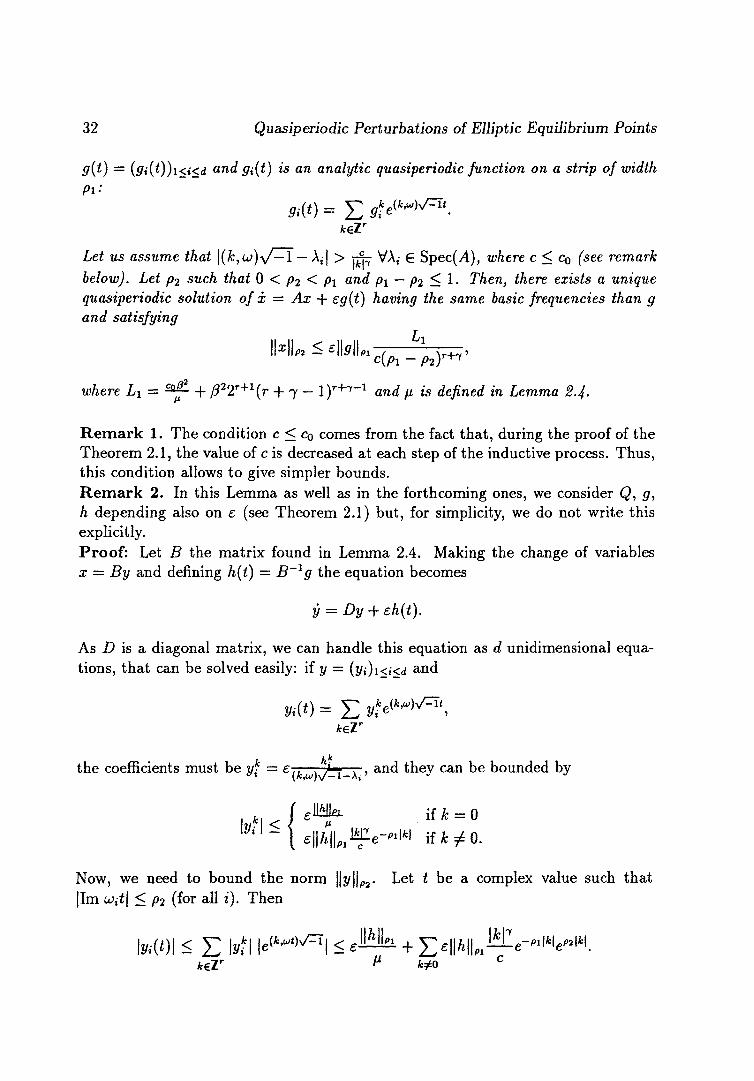
32 Quasiperiodic Perturbations of Elliptic Equilibrium Points
g(t) = (gi(t))i<i<d and gi(t) is an analytic quasiperiodic function on a strip of width
Pi-'
9i(t) = E 3telk*,h/=It. kélr
Let us assume that \(k,w)^/—ï — \¿\ > rfa VÀt- G Spec(A), where c < CQ (see remark below). Let p2 such that 0 < p2 < p\ and pi — pi < 1. Then, there exists a unique quasiperiodic solution of x = Ax + eg(t) having the same basic frequencies than g and satisfying
M^^sM"c{Pl-\2y^
where L1 = *f- + ß22r+1(r + 7 - l ) ^ " 1 and p is defined in Lemma 2.4.
Remark 1. The condition c < CQ comes from the fact that, during the proof of the Theorem 2.1, the value of c is decreased at each step of the inductive process. Thus, this condition allows to give simpler bounds. Remark 2. In this Lemma as well as in the forthcoming ones, we consider Q, g, h depending also on e (see Theorem 2.1) but, for simplicity, we do not write this explicitly. Proof: Let B the matrix found in Lemma 2.4. Making the change of variables x = By and defining h(t) = B~lg the equation becomes
y = Dy + eh(t).
As D is a diagonal matrix, we can handle this equation as d unidimensional equations, that can be solved easily: if y = (y,)i<,<<¿ and
vu) = E y?e(*,wh/CÎ<.
*eZr
the coefficients must be yf = g fA ,>--_. , and they can be bounded by
I * | < / £ ^ iffc = 0
Now, we need to bound the norm | | j / | | P 2 . Let í be a complex value such that IIm Uit\ < p2 (for all i). Then
W)\ < E \vt\ | e ^ ^ | < î * + £e||A||wJíCe-«Wc«M. JteZr ^ fc#o c
A Dynamical Equivalent to Elliptic Equilibrium Points 33
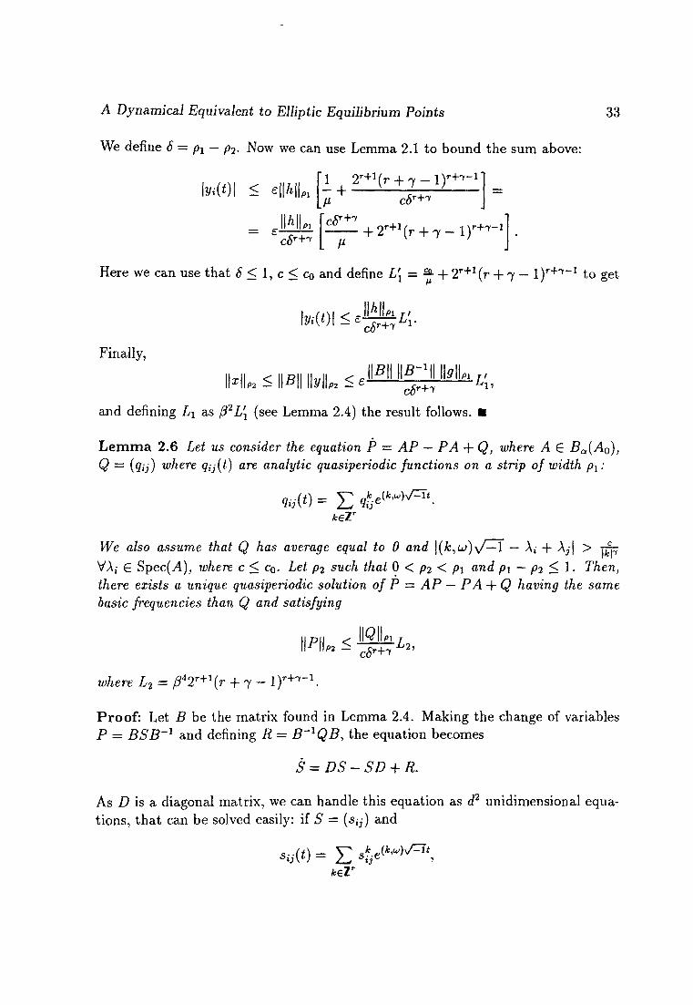
We define 6 = px- p2. Now we can use Lemma 2.1 to bound the sum above:
I 2 r+1(r + 7 - l ) r +T f - 1
fi c8r+i \Vi{t)\ < en-lift
HA PI
c6r+"<
c8r+i
V + 2r+1(r + 7 - l ) r + ^ - 1
Here we can use that S < 1, c < CQ and define L\ = f + 2 r + 1 ( r + 7 - l ) * " ^ - 1 to get
IÄI M*)l < e^E:L[
Finally,
ML < \\B\\ \\y\\P2 < e
c6r+i
B\\\\B-l\ c8T+i
llfflU n
and defining Lx as ß2L'1 (see Lemma 2.4) the result follows. •
Lemma 2.6 Let us consider the equation P = AP — PA + Q, where A £ Ba(A0), Q — (qij) where qij(t) are analytic quasiperiodic functions on a strip of width px:
to® = £ «£·e(fc·w)V=ít.
We also assume that Q has average equal to 0 and |(fc,u>)\/—T — A,- + A | > ^ 7 VA¿ € Spec(yl)J where c < CQ. Let p2 such that 0 < P2 < pi and p\ — p2 < 1. Then, there exists a unique quasiperiodic solution of P = AP — PA + Q having the same basic frequencies than Q and satisfying
\P\L < \\Q\L r
where L2 = ß42T+i(r + 7 - l ) ^ " 1 .
Proof: Let B be the matrix found in Lemma 2.4. Making the change of variables P — BSB'1 and defining R = B~XQB, the equation becomes
S = DS - S D + R.
As i ) is a diagonal matrix, we can handle this equation as d? unidimensional equations, that can be solved easily: if S = (s¡j) and
keZr
34 Quasiperiodic Perturbations of Elliptic Equilibrium Points
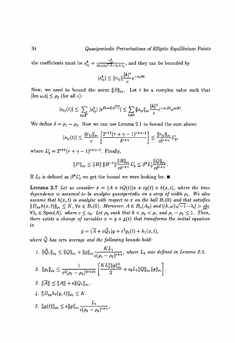
the coefficients must be 4 = ,kw)s/^(_x., A., and they can be bounded by
141 £ Ih;!!1^ - M 1*1
Now, we need to bound the norm \\S\\P2. Let í be a complex value such that |Im u>it\ < p2 (for all i):
MOI < £ 141 l« ( W = î l < EK·|UJaIe-M,fc,c«W. keLT k¿o c
We define & — px — p2. Now we can use Lemma 2.1 to bound the sum above:
k-(*)l < * ^ 2r+1(r + 7 - l ) r + ^ - 1
fr+l <r illiilifl/''
where 2£ = 2 r + 1(r + 7 - l ) ^ " 1 . Finally,
IÄI ,4r , IM PI ^ iU<l |5 | | p -MI™i ' 2 <^ 2 c ¿ r + 7 .
If L2 is defined as ßiL2 we get the bound we were looking for. •
Lemma 2.7 Let us consider x = (A + eQ(t))x + eg(t) + h(x,t), where the time dependence is assumed to be analytic quasiperiodic on a strip of width p\. We also assume that h(x,t) is analytic with respect to x on the ball BT(Q) and that satisfies \\Dxxh{x,t)\\n < K, \/x e Br(Q). Moreover, A 6 Ba(A0) and |(Ar,w)v'=T-Ai| > ^ VA,- € Spec(j4), where c < CQ. Let p2 such that 0 < p2 < P\ and px — p2 < 1. Then, there exists a change of variables x = y + xft) that transforms the initial equation in
y = (I + eQx)y + e2g1{t) + hx{x,t),
where Q has zero average and the following bounds hold:
1- WQiL·i < IIQIL + llírllí>i~7 r~7~> where L\ was defined in Lemma 2.5. c(pi — p2)
r+1
2- Hall» < 1
C2(pi-P2)2r+21
3. m<U\\+e\\Qx\\*-
I \\Dyyh,{y,t)\\P2<K-
5- IliWL < *h\ Ll
KL\\\g\ p\ + c0L1\\Q\\Pl\\g\L
i pi ciPi-PiY+i'
A Dynamical Equivalent to Elliptic Equilibrium Points 35
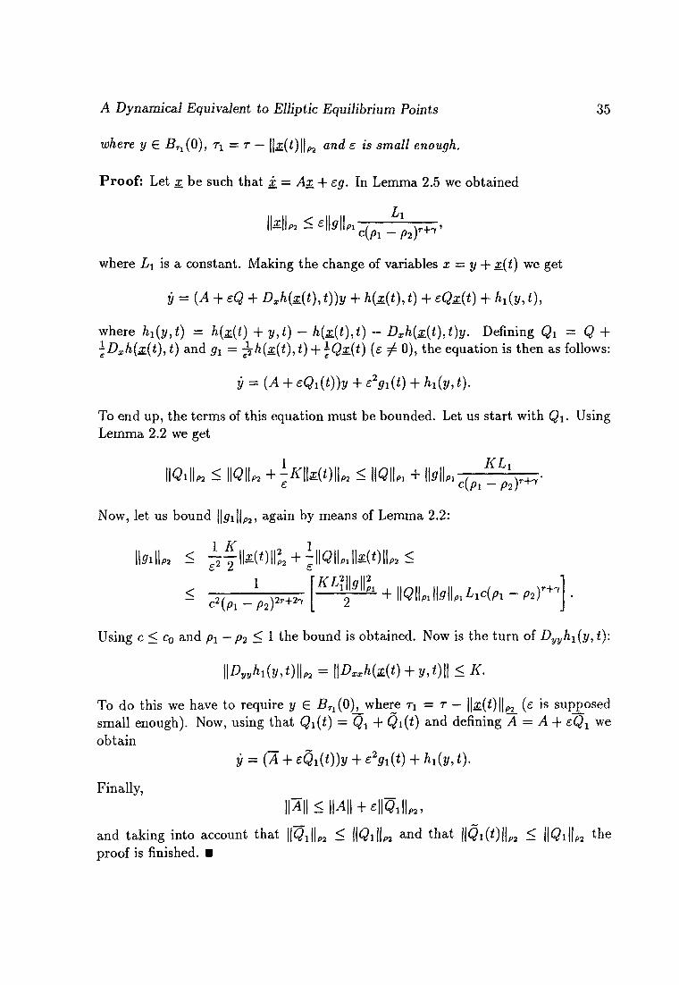
where y £ BTl(Q), TX = r — ||£(<)IL and e is small enough.
Proof: Let x be such that ¿ = Ax, + eg. In Lemma 2.5 we obtained
N L < e\\g\\ PI
where L\ is a constant. Making the change of variables x = y + x(¿) we get
y = {A + eQ + Dxh{x(t), t))y + h(2i{t),t) + eQ£.(t) + hx{y, t),
where hx(y,t) = h(x(t) + y,t) — h(x(t),t) — Dxh(x.(t),t)y. Defining Q\ = Q + ^Dxh(x(t), i) and ^ = ^¡h(x{t),t) + -Qx{i) (e ^ 0), the equation is then as follows:
y = (A + eQ!(t))y + e2gx{t) + hx{y,t).
To end up, the terms of this equation must be bounded. Let us start with Qx. Using Lemma 2.2 we get
IIQill* < IIQIL + -J<U(t)\\P2 < IML + \\g\\P1- KLl
Now, let us bound ||áfi||p2, again by means of Lemma 2.2:
M « + ? M L < ~Mt)\\2P2 + ~\\Q\LUt)\\P2<
l^ + \\QL·hL·LAPi-P2Y+'1 i <
C2(pi-P2)2r+2^
2||„l|2 f^lMI 2
Using c< CQ and px — p2 < 1 the bound is obtained. Now is the turn of Dyyhi(y,t):
\\Dwhi(y,t)\\» = \\Dxxh(x(t) + y,t)\\ < K.
To do this we have to require y € BTl (O^where T\ — T — ||z(i)||p2_ (e is supposed small enough). Now, using that Qx(t) = Qx + Qx(t) and defining A = A + eQx we obtain
y = (A + eQx{t))y + e3Si(*) + h{y, t).
Finally,
lFll<IHI + e||$,||„, and taking into account that ||Qi||P2 < HQilL a n d t n a t IIQiMIL ^ WQiWn t h e
proof is finished. •
36 Quasiperiodic Perturbations of Elliptic Equilibrium Points
Lemma 2.8 Let us consider x = {A + eQ(t))x + e2g(t) + h(x, t), where the time dependence is assumed to be analytic quasiperiodic on a strip of width pi and Q has zero average. We also assume that h(x,t) is analytic with respect to x on the ball BT(0) and that satisfies \\Dxxh(x,t)\\pl < K, Vx € BT(0). Moreover, A G Ba(A0) and |(&,w)\/—T — A,- + Xj\ > ré^ VA,-, A¿ G Spec(A), where c < CQ. Let p2 such that O < P2 < Pi and pi — p2 < 1. Then, there exists a change of variables x = (I + eP(t))y, where I is the identity d x d matrix and P(t) is analytic quasiperiodic on a strip of width pi, that transforms the initial equation in
y = (Ä + e2Qi)y + e2gx{t) + hx(y, t),
where Qx has zero average and the following bounds hold:
L ll&ll« ^ ITIPW I1Q1U' where HpIU < ^hL*and L* was defined in
II l|P2
Lemma 2.6. 1
*. IMU< „p.. 1MU-1 £ l | · r l lP2
3. \\DMyM» < K{\^[p£)9-P2
P\
wh
I l|A|i<||Aii + £ l ^ £ [ | ' p | U i | g iu ,
T ere y € Bn(0), Ti = —-— and e is small enough.
1 -j- £\\r \\P2
Proof: Using Lemma 2.6 we can solve P — AP - PA + Q. The solution that we have found verifies
IIPIL < i L ^ £ i -¿2
Now, by means of the change of variables x = (I+sP)y and introducing the notation Q1 = {I + eP)-xQP,gx = (I + eP)-^ and h^t) = {I + eP)-xh{{I + eP)y,t) we obtain the following equation
y = (A + e2Qx(t))y + e2gx(t) + hx{y,t).
Now we are going to bound the terms of this equation. For this purpose we need the bound of | |P||P2 provided by Lemma 2.6 and displayed above.
A Dynamical Equivalent to Elliptic Equilibrium Points
1 ., ..
37
|£yvMy,<)IU
NU < 1
l-e\\P\ I P l ! Pi
-K\\i + ePt<K (i + e||P|U2
1 - c M « " 2 " 1-cll^lU Of course, we require y € BTl(0), where TJ = r / ( l + e||-f||pa) and £ is small enough. To end up this, we rewrite the equation using Qi(t) = Qx + Q\(t) and A = A + e2Qx
and we obtain
y = (Ä + e2Qx)y + e29l{t) + MîM),
and we only need to bound A:
im<l|A||+62||Q,|l«. • Lemma 2.9 Let {Kn}n be a sequence of positive real numbers satisfying Kn < atfrCKl^, where b > 1. Then
Kn< aK0b2 5\71
a L
Proof: It is easy to see that
K < a1+2+22+-+2n~15n+2(n-1)+22(n-2)+-+2"~1
To obtain the exponent of 6 we use the identity „n+l n - 1
n - 1
ri(«-o2' L«=0
1\0 .
X — X"
1 - x = £*i+1. ¿=0
We compute the derivatives of both sides and put x = 1/2. Then
n - 1
53 2*'(n - i) = 2n+1 - n - 2. ¿=o
To end up, we need to bound the expression between brackets in the bound of Kn
displayed above. For this purpose we take logarithms:
fn-l n-1
^^("-02>£2Mn(n-^)<2"f:*^^ = c2^ \ i = 0 / «=0 «=0 L
In Lemma 1.5 it has been shown that expc < 5/3. Finally
i r / ^ N ^ i 2 " Kn < -a2n(b2)2nb-^+2^ [(f)
a l\oJ
and taking into account that 6 > 1 the result follows
IX0 )
38 Quasiperiodic Perturbations of Elliptic Equilibrium Points
Lemma 2.10 Let {an}„ be a sequence of positive real numbers satisfying an € ]0,1], n^Loan = a G ]0,1]. Let {6n}„ be another sequence of positive real numbers satisfying Y^Lo^n = b < +oo. Consider the new sequence { r n } n defined by Tn+i = ûn^n — bn- Then the sequence { r n } n converges to a limit value r ^ satisfying Too > aT0 — b-
Proof: It is easy to see that
/ n \ n—1 T«+i= (IIa« r ° ~ S
\ t = 0 / «=0 n «il*
U = t + i
- 6 n -
As all the terms appearing in this expression converge, r„ does. Moreover, using that
n «i < !
for all n, the result follows. •
L e m m a 2.11 Let u) € Rr ana A,-, z = 1 , . . . ,d swcn that
c \\i-V^l{k,u)\>
i*r» ' for alii e { 1 , . . . ,d} and a// & G Z r \ { 0 } , where c > 0, 71 > 0. We a*e/ine a resonant subset Ttß as
nß = {ye^R, M</x/3¿e{i,...,d} A 3*' ezr\{0}
such that \tp + A; - V^ï(fc',w)| < 7 T ^ } -
Z/d ip((i) = m\ *', where m denotes the Lebesgue measure. If 72 = 71 + r + 1 f/ien liminf t/>(/¿) = 0.
Proof: Take ¡xn = ^%-. For any fc' with |¿ ' | > n and any z, the measure of the resonant interval of ip is bounded by r¡^- Adding for all the values of k' with \k'\ = n' and all ¿, we have
m ( ^ n ) < c2rd £ r + 1 < 2crd(n - 1) n'>n V /
_ ( -y 2 _ r )
Furthermore the resonant intervals associated to n' < n are disjoint with Tl^ if n is large enough. Hence, for n large enough, ip(fin) < rdn^^n — l ) -^ 1* 1 ) which goes to zero if n goes to infinity. •
A Dynamical Equivalent to Elliptic Equilibrium Points 39
2.2.3 Proof of Theorem 2.1 First we are going to do the proof without worrying about resonances, and then we shall take out the values of s for which the proof fails.
First of all, let us denote by AQ the initial matrix A (see Theorem 2.1) corresponding to the averaged linear part of the differential system. Let / ¿bea real value such that, if Spec(Ao) = {A°,. . . , A^}, then |A?| > 2p, |A? - Aj| > 2/z for all i ¿ j . Then Lemma 2.4 can be applied to obtain values a and ß such that all the matrices contained inside the ball Ba(A0) = {A/ \\A — Ao\\ < a} can be diagonalized. Moreover, the matrix B of the diagonalizing change of variables satisfies ||J3|| < ß, ||£?-11| < ß. During the proof we shall see that, if e is small enough, all the matrices An that appear during the inductive process are inside that ball.
As we assume that the dependence of Q, g and h with respect to e is bounded, every time we compute some norm we mean, without explicit mention, that we look not only for the maximum with respect to t in the suitable strip, but also with respect to e in the allowed range.
To begin the proof, we suppose that we have applied the method exposed before up to step n, and we are going to see that we can apply it again to get the n + 1 step. In this way we shall obtain bounds for the quasiperiodic part at the nih step and for the transformation at this step, and this allows us to prove the convergence.
Now suppose that we are at nth step. This means that the equation we have is
¿n = (An(e) + e2nQn(t, e))xn + e2"gn(t, e) + hn(xn, t, e), (2.8)
where An belongs to Ba(Ao), its eigenvalues A,- verify the nonresonance condition
\(k,U)y/=ï-\i\>-^,
where 7 = 7„ + r + 1 and cn = Co/(n + l ) 2 . Due to the fact that we need to reduce the width of the analyticity strip of the quasiperiodic functions, we define pn = pn_x — 1/n2 and <xn = pn — l/(2(n + l)2), with p0 = 1 + 7T2/6. During the proof we shall see that the analyticity ball (with respect to a;) of hn(x,t) has to be reduced at each step of the inductive process, and we shall found that, by selecting e small enough, the limit radius of this ball is positive. Let us define rn as this radius at step n. Now we can apply Lemma 2.7 to transform equation (2.8) into
yn = (An(e) + e2nQn{t,e))yn+e2n+1gn{t,e) + K{yn,t,e), (2.9)
where the width of the analyticity strip has been reduced to an. Now, assuming that the nonresonance condition
|(tlU)V=I-A( + A j |> 1 ^, ¿Tf- ; %
~>
%B MAT^AilUUS*
40 Quasiperiodic Perturbations of Elliptic Equilibrium Points
holds for all A,-, \j € Spec(An(e)) we can apply Lemma 2.8 to equation (2.9) and to get
xn + i = (An+1(e) + e2" Qn+i(t,e))xn+1 + e2n+1#n+1(f,e) + hn+1(xn+i,t,e). (2.10)
Now, the width of the analyticity strip has been reduced to pn+i. The next step of the proof is to obtain bounds of the terms appearing in equation (2.10) depending on the bounds of the terms of equation (2.8). Using Lemma 2.8, and a condition on II^IL+i ( s e e below) we get
where Mi = 2r+ry+1L2/co. Here we need Lemma 2.7 to bound the expression above, but the bound provided by this Lemma has an "uncontrolled" term, that is, the bound of the second derivative of hn. Let us call this value Kn. Note that it is "modified" at each step by Lemma 2.8. In order to bound it, we shall assume that e is small enough to ensure that £2"||^n|k+i is less than 1/2. This implies that the value of e will be reduced at each step, if necessary, to guarantee that condition. We will see that this condition is achieved from a certain step onwards, without modifying e anymore. Therefore, we assume that Kn < (9/2)nKo (when the convergence will be proved, we shall give a more realistic bound of Kn, that converges to a real number) and Lemma 2.7 states that
HÔnlk < IIQnIL + M2{U + l ) 2 r + 2 ^ 2 Q n ( M L ,
where Mi = 2r+'yLiK0/cQ. Now we bound the norm of gn+i:
Ikn+l||p„+1 <2||<7n I k ,
and from Lemma 2.7
\\gn+i\\Pn+1 < M3(n + l ) 4 r + w [ M 4 (~y \\9n\\2
pn + M s U ^ I U I ^ I k
where M3 = 22r+2y+1 /(%, M4 = KQL\¡2 and M5 = CQL\. For simplicity reasons, let us denote a n = ||Qn||p„ and ßn = ||<7n|k- This means that we have obtained the following bounds:
a n + 1 < M1(n + i r + w ( a n + M 2 Q (n + l ) 2 r + w & )
AH-I < M3(n + l)4^+4(M4(~yß2n + M5anßn
A Dynamical Equivalent to Elliptic Equilibrium Points
To bound ctn and ßn we define r)n = max{an,/?n}. After some rearranging we
where Mß and M? are constants such that
M 3 ( M 4 + ( J ) " W ) <M7.
Defining M8 — max{ikfg, A/7} we obtain a bound for r¡n+i'
r,n+1<M&(^)n(n + ir^6Vl
and, using Lemma 2.9 we obtaii
Vn+l <
tain
M8 M87/o
9\2 /5\6 r+6^+6 l2"+ 1
])'(!) Let us denote M9 = M8r/0(9/2)2(5/3)6r+67+6. We have proved that
Note that this bound allows to ensure that, if e < £\ = M¿"a
The next step is to bound ||-P»||,>n+1. For this purpose we use Lemma 2.8:
\\pn+l —
< H ! Ü Í 2 ( n + 1)^+27+2
2 r + U 2
Co (n + l)2^+2 | |Qn |U<
Co liQn||,„ + M2g)n(n-fir+ w | |^| <
< H ^ * ^9\n (n+1)4r+47+4 [—(f r
Co
Let Mio be a real number such that
( „ + l ) 2 r + 2 ^ + 2 ^ J J 2 »/«•
IT ^ Ml°" M8
42 Quasiperiodic Perturbations of Elliptic Equilibrium Points
This implies that
| |Pn|L+ 1 < Mw Q n (n + 1 ) 4 ^ + 4 M | " ,
and due to the fact that e < E\ = MQ1 we have proved that
lim £2n||P„|L+1 = 0. n—*oo " r T <
This allows to have the condition £r2" ||JP„||P„+1 < 1/2, without reducing the value of £ at each step. Now we are going to bound ||£n(')IUn:
HanWIk < ^ ^ ( n + l ) 2 r + 2 7 + V " l k l L < Mn(n + 1 ) 2 ^ + 2 ( £ M 9 ) 2 " , CO
where M\\ — 2 r+7Li/(coM8). When the changes of coordinates have been bounded, we can estimate the decrease of the radius rn of the ball where hn is analytic with respect to x. It has been shown that
•Tn -n+1 l + e2"| |P„|L+1 l+e 2 n | | Pn |U , + 1 ' n 1 + e^WPnlUi'
Now, we define
„ i h _ fc«WIL (J, _ — A n M n II * "« . n l+e'-HPnlU,' " l + ^ l l^ lUx*
oo
It is easy to prove that J J an converges: n = 0
JV
In Y[an n=0
N N
< E llnö"l < E ^ H ^ I U , < OO ViV e N. n = 0 n = 0
As J2 &n is also convergent, we can apply Lemma 2.10 to get r^ > ar0 — 6, that is positive if s is taken small enough.
Now, let us bound \\An\\:
1~£ ll-ni||p„+i I I P II
- 2 n | | / 0 II i _2" IlJ n\\pn+i < WA.W+eniQnL·+e'^J^ n| |pTi+l
Using the bounds found above we can write that
IK+l | |<IK||+Kn,
A Dynamical Equivalent to Elliptic Equilibrium Points 43
where
«n = 2M10 ( J ) " (n + l)4r+4^+4(£M9)2n + jf(eM9)2n.
As Y2 Kn is convergent we can ensure that, if e is selected small enough, the matrices An are always inside the ball Ba(Ao) defined before.
Consider now the value Kn. We have used above the pesimistic bound Kn < (9/2)nK0- Note that this bound does not allow to guarantee the convergence of the functions hn(xn,t) to an analytic function h^x^^t) with respect to x. Now we can use a more accurate bound of that value to get this: From Lemma 2.8 we know that
K < K ( l + e 2 l / > n | L + 1 ) 2
n + 1 - - l - e 2 " P > n | L + 1 '
and, by means of the inequality 1/(1 — x) < 1 + 2x if 0 < x < 1/2, we get
Kn+i<(l+2e2n\\Pn\\Pn+1)3Kn.
And, using the bounds of ||-P„||Pn+1 that we already know, it is easy to see that the (bound of the) value Kn converges.
To end up the proof we are going to take into account the resonances. Let <¿>"(e), 1 < i < cP + d be the functions that give the values of A" and A£ — A"2 at step n. At every step the eigenvalues depend on £ in an unknown but controlled way. As \<p9(ei) - ^ ( e 3 ) | > 2S\Sl - £2| and |<^(e) - v?(e)| = 0(e2) one has lv?(£i) ~~ V?(£2)| > ^l£i - £2\ h° |£i|, |£2| a r e small enough. On the other side \<Pi{e\) — <¿?"(£2)| is bounded by 8 for all e, j , n if £1; £2 belong to some interval (0,e). Here we suppose, for simplicity, that all the y?" are purely imaginary. If we take some \im (see Lemma 2.11), with 71 = 7*, 72 = 7, c = Co = f, such that ^f- < £, when £ ranges on (0,£) then 9?" ranges on (—fim, (im).
To obtain the cantorian set £0 where the nonresonance condition holds for n = 0 one should delete an infinity of intervals in the range of e with a measure at most il>(nm)2nm±(d2 + d). The relative measure of £Q in (0, f) is at least 1 -í¡)(pim)2l^fA. In a similar way we obtain the set £n C £n-i where the nonresonance condition holds up to n. Its relative measure in (0, Bf-) is at least
1 - m)(ßl±±) ± jjl^ > 1 - ^m)pͱí
which goes to 1 if n goes to infinity. The limit set
C-oo = I I Cn n>0
is the cantorian that we were looking for. •
44 Quasiperiodic Perturbations of Elliptic Equilibrium Points
2.2 A Proof of Theorem 2.2
As det A T¿ 0, the Contraction Lemma (see [21]) ensures that, if e is small enough, there exists a function x0(e) such that
(A + eQ)x0(e) + eg+ ~h(x0(e), e) = 0,
and verifying x0(e) = 0{e). Let us define
AX0 = A + eQ + Dxh(x0(e),e),
and let 2i(t,e) be such that
¿ = Ax + eg(t,e). (2.11)
(The existence of that solution was shown in Lemma 2.5 and we recall that is 0(e)). The terms of order e of the matrix Aoo are provided by Lemma 2.7 at the first step of the inductive process. This modified matrix A is
 = A + eQ + Dxh(x, t, e).
Then, ^ _ \\AX0 - A|| = \\Dxh(x0(e),e) - Dxh(gi(t,e),t,e)\\.
But Dxh{x(t, e), t, e) = (C + eR{t))x(t) + ö(e2) = C& + ö(e2),
where C = |Z)XI./i(0,i,0) is a constant matrix by hypothesis. Moreover, it is also easy to obtain that
Dxh(xo(e), e) = (C + e~R)x0(e) + 0{e2) = Cx0(e) + 0(e2)
We have obtained that
114* - Â\\ = C(xQ(e) -1 ) + 0(e2).
Now, averaging (2.11) we get that Ax.+eg~ = 0, and using Ax0(e)+eg = —(eQx0(e)+ h(x0(£),e)) = 0(e2), we obtain ||x0(e) — 1 | | = 0(e2), that ends the proof. •
2.3 The Neighbourhood of an Elliptic Equilibrium Point of a Hamiltonian System
It is also interesting to consider the Hamiltonian case. Let us suppose that the origin is a fixed point of the vector field for all the values of e less that a certain value.
Neighbourhood of an Elliptic Equilibrium Point of a Hamiltonian System 45
Then, we can take action-angle variables and write the equations as:
dHe
Pi = —O— , Oq\ dHe
P2 = Ô—, dq2
9i = V, dHe
92 = - 5 — , OP2
where q\ are the angles of the perturbation, p\ are the corresponding actions, q2, P2 are the angles and actions of the unperturbed system and <p = (<¿>i,..., <pr) is a constant vector of frequencies. Note that the first equation is not relevant. It has been added to get a Hamiltonian form. The corresponding Hamiltonian is:
He{PuP2,qi,q2) = (v>»Pi) + #o(p2)+e#i(p2,gi,92).
As this Hamiltonian is degenerate, we can not use the KAM theorem directly to conclude the existence of invariant tori near the origin for e small enough. We have considered this case in Theorem 2.3, and we have found that the proof of the classical KAM theorem (see [1]) still works, because the perturbing frequencies are not modified in any step of the inductive process, and we only have to worry about the proper frequencies of the Hamiltonian, that can be controlled provided that the nondegeneracy condition
holds. The result obtained is that there exist invariant tori near the origin for s small enough. The frequencies of these tori are the ones of the unperturbed tori plus the ones of the perturbation. The tori whose frequencies are in resonance with the ones of the perturbation are destroyed.
Finally, in case that the origin is not a fixed point of the perturbed Hamiltonian, we can reduce to this case performing a change of variables transforming the quasiperiodic orbit that replaces the equilibrium point (we recall that this orbit exists for a cantorian set of values of e) in a fixed point.
Theorem 2.3 Let us consider the Hamiltonian
H(pi, P2,qu ?2) = (<P,Pi) + H0(p2) + HI(P2, 91,92),
where q\ are the angles of the perturbation, p\ are the corresponding actions, q2, p2 are the angles and actions of the unperturbed system and ip = (ipi,.. .,tpni) is a constant vector of frequencies satisfying the nonresonance condition
| < * , P > l > T £ p VfceZni\{0}, 7 > n , - l .

46 Quasiperiodic Perturbations of Elliptic Equilibrium Points
Let G1 be a compact domain of Rni, let G2 be a compact domain of FT2 and let G be G1 x G2. Suppose now that this Hamiltonian function H(pi,p2,qi,q2) = H(p,q) is analytic on the domain F = {(p,q) / p = (P11P2) 6 G, |Im q\ < p] and has period 2TT with respect to the variables q. Let us assume that, in the domain F,
det d2H0
d(p2Y 9E 0. (2.12)
Then for any /c > 0 there exists M = M(n,p, G, Ho) > 0 such that if in F we have
| # i | < M , (2.13)
then the motion defined by the Hamiltonian equations
dH .
(2.14) Pi =
Pi =
dqx
ÖH . dH
% ¡ ' ?2
dp2
has the following properties:
1. There exists a decomposition Re F = F\ + F2, where Fi is invariant and F2 is small: mes F2 < «mes F.
2. F\ is composed of invariant n-dimensional analytic tori 1$, defined parametri-cally by the equations
P = P* + U(Q)> q = Q + 9<l>(Q), (2.15)
where / ¿ , g^ are analytic functions of period 2ir in the variables Q, and <j> is a parameter determining the torus I¿. In fact (f> consists of all the frequencies, i.e., the ones of the external excitation and the proper frequencies:
4>= (^l,-.-,<Au,Wl,.--,^n2).
3. The invariant tori I¿ differ little from the tori p = p¿;
\ÎÂQ)\ < *, \9ÁQ)\ < * (2.16)
4- The motion (2.14) on the invariant torus 1$ is quasiperiodic with n frequencies <Pi,...,<pni, wi>..-,wn2 (n = nx +n2):
Q = <j), u = dHp
dp2
(2.17) P<t>

Neighbourhood of an Elliptic Equilibrium Point of a Hamiltonian System 47
2.3.1 Sketch of the Proof of Theorem 2.3
The proof of this Theorem is essentially the same of the KAM Theorem contained in [1], and its technical details can be found inside Appendix C. Here we show the idea of that proof.
Let us define p and q as the vectors pi,p2 and qi,q2 respectively. Now, the Hamiltonian we have is
H£ = (<p,Pl) + H0(p2) + e~H1(p2) + elÍM, q), (2.18)
and let us consider the generating function S(P,q) = J2k¿o Sk(P2)e(·k'q'í"/:~í'. If we
perform the canonical change of variables
as Pi Px oq-i
as P2 — Pi + e—, dq2 Qi z^ 9i, as
Q2 — ft + ewy to (2.18) we obtain
W = {ip, A ) + Ho(P2) + eH~i{P2) + eF + e2R(P2, q),
where F = (tpySqi) + HP2),Sq2) + %{P2,q) and u(p2) = f$(p2). Let <f>(P2) be the vector ip,u(P2). We ask for the condition F = 0:
(HP2),Sq) + H1(P2,q) = 0.
Now, using that Hi(P2,q) = E f c / o ^ í ^ e ^ ^ , the coefficients of the Fourier expansion for the generating function S can be obtained easily:
{<f>{p2hk)
To ensure the convergence of that series, we need the usual nonresonance condition
\(<f>(P2),k)\>^ (2-19)
that allows to proof the convergence in a smaller strip than the one on which Hi is analytic. With this the Hamiltonian takes the form
H* = (<p, Pi) -r H¡(P2) + e2H3(P2) + e2H3(P2, Q).
48 Quasiperiodic Perturbations of Elliptic Equilibrium Points
This new Hamiltonian is very similar to (2.18), but with e2 instead of e. Note that the difference between this proof and the one contained in [1] is the condition (2.19). Due to the fact that the first components of ^(^2) are the ones of <p, that are constant in all the inductive process, we only have to worry about the last ones, u){P?). These components are different at each step of the process, but they can be controlled by the nondegeneracy condition
d e tOH The way to do that is exactly the same one showed in [1]. Note that, to get an rigorous proof of this theorem, we only need to copy the proof contained in [1], but adding the "parameter" <p. The unique difference is that now, the nonresonance condition is stronger, in the sense that we must eliminate a bigger set of (resonant) tori.
In order to bound the measure of the resonant set of frequencies, we give the following lemma.
Lemma 2.12 Let us define the set ft = 0(y>, p, C2,n1; 712,72) of the following way:
0 = {wE Bfi(0) C Rn2 / 3(k, l) € Zni x (Z"2 \ {0}) such
ttfli|<fclV> + </)W>|<_S_},
where 72 > "1 + n2 — 1> ™i > 0, n2 > 0 and Bp(0) denotes the elements whose Euclidean norm is less than p. Then, the Lebesge measure of ft can be bounded by
H(íí) < c2a(n1,n2,f2)pn2~1-
Proof: Let (k,l) be an element of Zni x (Zn2 \ {0}). The corresponding resonant hyperplane is defined as the set of a>'s satisfying
< k,(f > + <l,u> >= 0.
The elements of ft are contained in strips of width
c2
l'll(l*l + |/|)*» around these hyperplanes (here, ||.|| states for the usual Euclidean norm). By intersecting those hyperplanes with the ball Bp(0) we obtain the bound
Neighbourhood of an Elliptic Equilibrium Point of a Hamiltonian System 49
where we have used ||/|| > \l\/n2, Sm is the measure of the m-dimensional unit ball and <r(k) is defined as
Now, let us bound a(k). For this purpose we consider two cases:
1. ib = 0.
Now, using # { / € Zn2 / 1 / | = ¿} < 2n2î'n2-a it is easy to get that
^ ( 0 ) < 2 n 2 C ( 7 2 - n 2 + 2),
where ( states for the Riemann zeta function that is well defined because 72 - n2 + 2 > 2.
2. Jfe^O.
n(L\ _ y 1 < 2nz y — = 2n2 v ^ ~ M)"2 < 1 j " & i/i(i*i+iw» - e ( w + ¿ ) 7 2
Í>W+I ¿72 "
1 r00 ¿T 2"2
< o"2 V : < 2"2 / — = .jfe_, ¿^-"2+2 - y|fc| x-Y2-n2+2 (72 _ n2 + l)|fc|-»-«2+i
Let us bound J^cr(k):
2"2 1
2nl +«2
72 - "2 +
2nl +«2 < 2n2C(72 - n2 + 2) + -rC(72 - «i - n2 + 2).
T2 — no + í
Now, defining
a(ni ,n 2 ,7 2 ) = 2n25„2_i
we obtain the bound we were looking for.
2ni +n2
2n2C(72 - n2 + 2) + —C(72 - nx - n2 + 2) 72 — n2 + 1
50 Quasiperiodic Perturbations of Elliptic Equilibrium Points
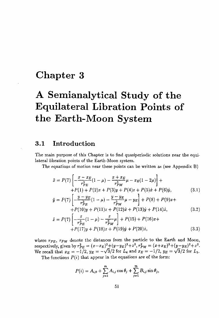
Chapter 3
A Semianalytical Study of the Equilateral Libration Points of the Earth-Moon System
3.1 Introduction
The main purpose of this Chapter is to find quasiperiodic solutions near the equilateral libration points of the Earth-Moon system.
The equations of motion near these points can be written as (see Appendix B)
x = P(7) —3 (1 -n) 5 n - xB{l - 2/i) PE ' PM
+ +P(1) + P(2)x + P(3)y + P(A)z + P(5)x + P(6)y,
y = P(7) y-VE
PE ( 1 - M )
y-yE -p-VE
PM + P(8) + P(9)x+
+P(lO)y + P(ll)z + P(12)¿ + P(13)y + P(14)i,
z = P(7) . rPE
•(l-(*)~ PM J
+ P(15) + P(16)x+
+P(U)y + P(lB)z + P(l9)y + P(20)i,
(3.1)
(3.2)
(3.3)
where rpjs, rpM denote the distances from the particle to the Earth and Moon, respectively, given by r2
PE = {x-xE)2+{y-yE)2+z2,r2PM = (x+xE)2+(y-yE)2+z2.
We recall that xE = - 1 / 2 , yE = - V 5 / 2 for L4 and xE = - 1 / 2 , yE = \ /3/2 for L5. The functions P(i) that appear in the equations are of the form:
m m
P(i) = Ai jo + Y, Aij cos 6j + £ #¿j sin 0jt i=i i=i
51
52 A Semianalytical Study of the Equilateral Points
with 0j = Vjt + (fj, where t denotes the normalized time. Values for all of the coefficients, frequencies and phases can be found in Appendix B.
An expansion of the nonlinear terms of the equations of motion, in power series of the coordinates (x, y, z), can be done easily using Legendre polynomials as it will be described in the next section.
Another possibility is to produce those terms by means of a recurrence based on the one of the Legendre polynomials.
3.1.1 Expansion of the Equations
We consider the potential V = —£ + -JL-. Let é be the angle between the vectors r rpE TPM f ö
(XE, ¡JE, 0) and (x, y, z) and p2 be x2 + y2 + z2. Then
1 1 rpE y/\ -2pcosr/> + p2 ~
where Pn is the Legendre polynomial of degree n:
1 dn ^
= X>"Pn(cosV>), (3.4)
^ ) = ^ T T ^ ( - 2 - i r = E«n ,^ ,n-2fe 2nn! du k=o
Here 11 denotes the integer part of * and
(-If fn\{2n-2k)\ an,k ~ 2"n! \k) (n -2k)\'
Substituting these expressions in (3.4) one obtains
OO L 2 J 1
rPE J > * £ <*n,k COs"-2fe 0 n=0 n=0
OO L"2 J (3.5)
= E E «».*(«* + yyE)n-2k(x2 + y2 + z2f. n=0 k=0
Finally, in order to obtain the expansion for L4 (the Ls case can be done with
identical process) we put XE = - } , VE = —^ an(^ (3-5) becomes
I OO I 3 J
— = E E P\Á* + ^y)n-2k(x2 + y2 + ñk, (3.6) rPE n = 0 jk=0
where (-l)"-*(2n-2fc)!
Pn,k - An-k(n _ 4"-fc(n - fc)!Jb!(n - 2k)V
Introduction 53
To perform the expansion (3.6) by algebraic manipulation it is better to change the order of the sums:
¿ = E(*2 + y2 + ñk E /M* + Vsy)-2fc,
where N denotes the expansion order wanted. With a similar computation it can be found that:
- 1 - = ¿(*2 + y2 + z2f E /M"* + vSy)-2* rpM fc=0 „rffc
and, finally,
F = i ^ + ** r , r P ß rPM l — l
= E(*2 + y2 + ñk E ßn,k [(i - P)(X + v5yr2*+ k=0 n=2fc
+ (-a; + ) n - 2 f c .
(3.7)
Now, using a program which takes advantage of the particularities of the latter expression, the expansions of — , ~ and ~ are obtained. This program has been written to give the final solution up to order nine. This is enough for practical purposes, because the contribution of higher order terms is much less than the threshold used to select the coefficients Ai¿, B{¿. Now let us see a short description of that program as well as of its routines:
Subroutine DERJV Given a polynomial of three variables x, y and 2, this routine returns three polynomials which are its derivatives with respect to a;, y and z. This is used at the end of the computation of (3.7) to obtain the expansion wanted.
Subroutine PRODE This routine performs the product of two polynomials of three variables. It is used to multiply the term (a;2 + y2 + z2)k by the result of the inner summatory of (3.7).
Subroutine XYZK Given a polynomial 5, this routine returns S x (x2+ y2 + z2). It is used to obtain the different powers of (x2 + y2 + z2) starting from 5 = 1.
Subroutine PART2V This routine computes the result of the inner summatory of (3.7), taking advantage of the cancellations that occur in this formula
54 A Semianalytical Study of the Equilateral Points
Subroutine INIT This routine fills a real array with the powers of y/3 (they will be used inside PART2V) and a couple of integer arrays containing information about the way to store polynomials (in fact this is not necessary, but it allows to increase the speed of the program).
Main Program This routine initializes the parameters used by the program (XE, ¡JE and ¡j.) and it uses the formula (3.7) to compute V. Then the final result is obtained (by derivation) and the result is written in the files EXPAN.l (expansion of the first equation), EXPAN.2 (second one) and EXPAN.3 (third one).
3.2 Idea of the Resolution Method
The equations of motion can be written as
x = fx{t,x,y,z,x,y,z), V = h(t,x,y,z,x,y,z), z = f3(t,x,y,z,x,y,z).
Define G = (G^, (72, G3), where Gx = / i — x, G2 = f2 — y, and G3 = / 3 — z. We are looking for quasiperiodic solutions of the form
y = X^exp^fc^v/^ï), z - ]CZfcexp((k'u,)ív'-J")>
where u> = (ui, u2, • •., u>r )* is a known set of basic frequencies, the ones that appear as basic frequencies, in the developments of the functions P(i), and (k,u) denotes the inner product of k = (¿1} ¿2,..., K)* and w. We consider x, y and z truncated up to some order. After substitution, G may be considered as a function of xjt, y\¡ and Zk, which means that looking for quasiperiodic solutions of this problem is more or less equivalent (this depends on the order of approximation taken for the trigonometric expansions of x, y, and z) to look for a zero of the function G : Rm —> Rm, where m denotes the total number of coefficients. To solve this equation we use a Newton method. In order to calculate the Jacobian matrix, the chain rule is used in the following way: g = f f • | ^ , and so on.
3.3 The Planar Case
In order to do a preliminar study, the following simplifications are introduced:
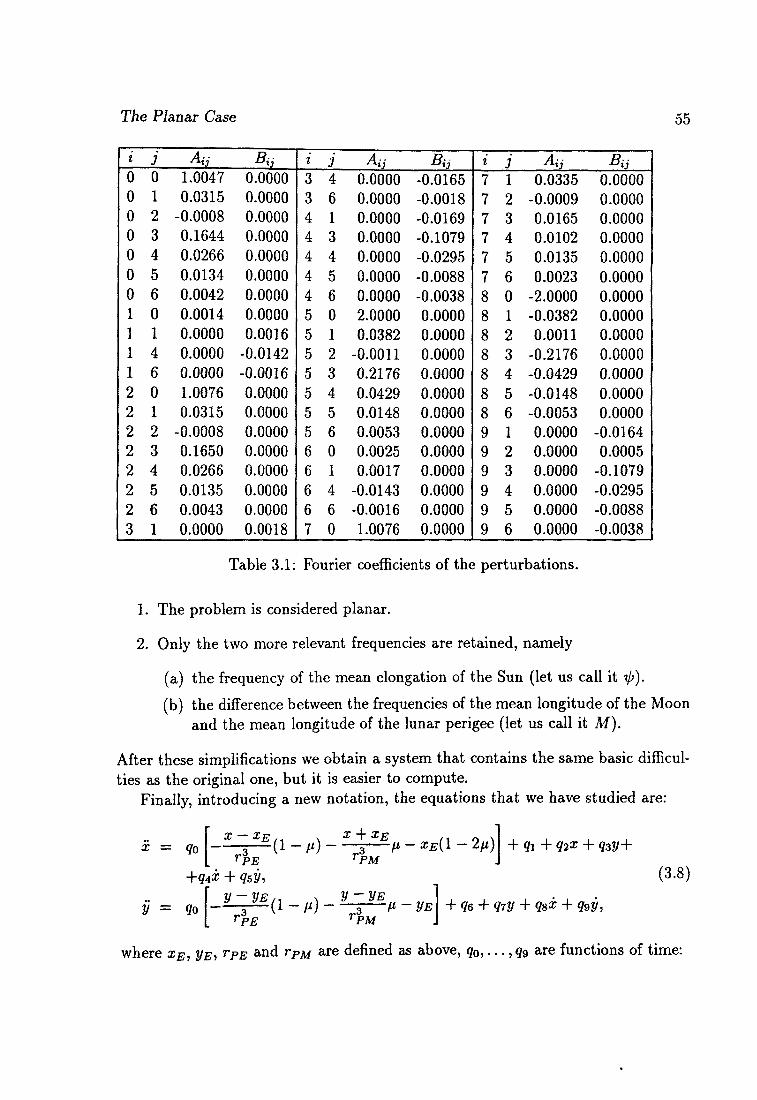
The Planar Case
i j Aij Bii * 3 Aij Bij * i Aij Bij
0 0 1.0047 0.0000 3 4 0.0000 -0.0165 7 1 0.0335 0.0000 0 1 0.0315 0.0000 3 6 0.0000 -0.0018 7 2 -0.0009 0.0000 0 2 -0.0008 0.0000 4 1 0.0000 -0.0169 7 3 0.0165 0.0000 0 3 0.1644 0.0000 4 3 0.0000 -0.1079 7 4 0.0102 0.0000 0 4 0.0266 0.0000 4 4 0.0000 -0.0295 7 5 0.0135 0.0000 0 5 0.0134 0.0000 4 5 0.0000 -0.0088 7 6 0.0023 0.0000 0 6 0.0042 0.0000 4 6 0.0000 -0.0038 8 0 -2.0000 0.0000 1 0 0.0014 0.0000 5 0 2.0000 0.0000 8 1 -0.0382 0.0000 1 1 0.0000 0.0016 5 1 0.0382 0.0000 8 2 0.0011 0.0000 1 4 0.0000 -0.0142 5 2 -0.0011 0.0000 8 3 -0.2176 0.0000 1 6 0.0000 -0.0016 5 3 0.2176 0.0000 8 4 -0.0429 0.0000 2 0 1.0076 0.0000 5 4 0.0429 0.0000 8 5 -0.0148 0.0000 2 1 0.0315 0.0000 5 5 0.0148 0.0000 8 6 -0.0053 0.0000 2 2 -0.0008 0.0000 5 6 0.0053 0.0000 9 1 0.0000 -0.0164 2 3 0.1650 0.0000 6 0 0.0025 0.0000 9 2 0.0000 0.0005 2 4 0.0266 0.0000 6 1 0.0017 0.0000 9 3 0.0000 -0.1079
2 5 0.0135 0.0000 6 4 -0.0143 0.0000 9 4 0.0000 -0.0295
2 6 0.0043 0.0000 6 6 -0.0016 0.0000 9 5 0.0000 -0.0088
3 1 0.0000 0.0018 7 0 1.0076 0.0000 9 6 0.0000 -0.0038
Table 3.1: Fourier coefficients of the perturbations.
1. The problem is considered planar.
2. Only the two more relevant frequencies are retained, namely
(a) the frequency of the mean elongation of the Sun (let us call it i/>)-
(b) the difference between the frequencies of the mean longitude of the Moon and the mean longitude of the lunar perigee (let us call it M).
After these simplifications we obtain a system that contains the same basic difficulties as the original one, but it is easier to compute.
Finally, introducing a new notation, the equations that we have studied are:
x = q0
x - x E r . N X + XE n 0 v rPE
y = qo
+q4x + q5y, y-VE
rpE
rPM
,, x y-VE (1 - A0 - —3—M - VE
rPM
+ 9 1 + Ç2Z + Ç3Î/+
(3.8)
+ ce + qiy + q&x + q9y,
where xE, VE, TPE and rPM are defined as above, q0,..., q9 are functions of time:
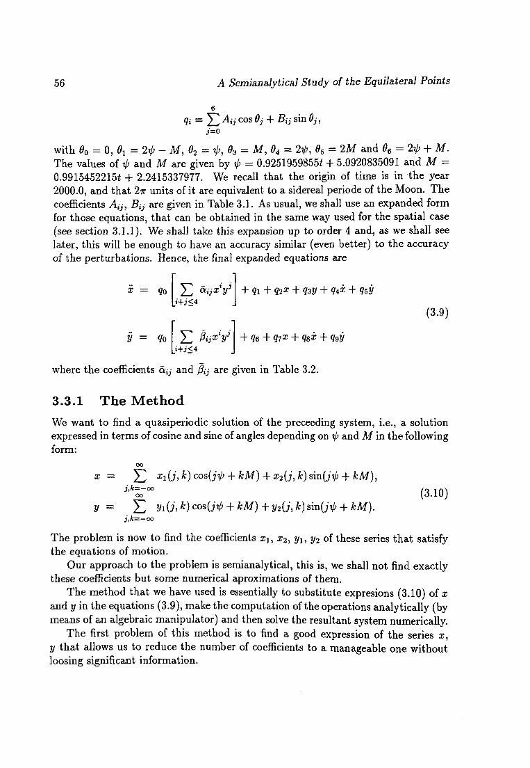
56 A Semianalytical Study of the Equilateral Points
qi = J2 Á¡i c o s ®i + Bii s i n e i > j=o
with 0O = 0, 0x = 2V> - M, ô2 = 4?,B3 = M, 04 = 2V>, «5 = 2M and 06 = 2t/> + M. The values of %j> and M are given by r¡> = 0.9251959855* + 5.0920835091 and M = 0.9915452215t + 2.2415337977. We recall that the origin of time is in the year 2000.0, and that 2ir units of it are equivalent to a sidereal période of the Moon. The coefficients A{j, ¿?t¿ are given in Table 3.1. As usual, we shall use an expanded form for those equations, that can be obtained in the same way used for the spatial case (see section 3.1.1). We shall take this expansion up to order 4 and, as we shall see later, this will be enough to have an accuracy similar (even better) to the accuracy of the perturbations. Hence, the final expanded equations are
X = Ço
y = %
53 ocijxY ¿+i<4
+ q\ + qi* + Ç3V + 94¿ + qsy
(3.9)
i+j<4 + q6 + qjx + q8x + q9y
where the coefficients a,-¿ and /?,_, are given in Table 3.2.
3.3.1 The Method We want to find a quasiperiodic solution of the preceeding system, i.e., a solution expressed in terms of cosine and sine of angles depending on ip and M in the following form:
oo
x = ]C a ;i(Í>¿)cos0^ + fc^) + a;2(Í!¿)sin(iV' + ¿M), itkV°° (3.10)
y = Yl yi(hk)cosü^ + kM) + y2Ü,k)sm{jj} + kM). j,k=-oo
The problem is now to find the coefficients xu x2, y\, y2 of these series that satisfy the equations of motion.
Our approach to the problem is semianalytical, this is, we shall not find exactly these coefficients but some numerical aproximations of them.
The method that we have used is essentially to substitute expresions (3.10) of x and y in the equations (3.9), make the computation of the operations analytically (by means of an algebraic manipulator) and then solve the resultant system numerically.
The first problem of this method is to find a good expression of the series x, y that allows us to reduce the number of coefficients to a manageable one without loosing significant information.
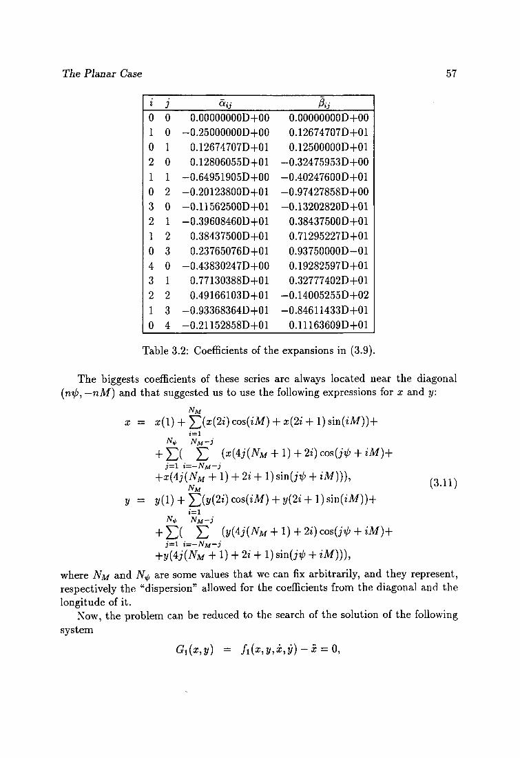
The Planar Case 57
i 3 <*.j ßü 0 0 O.OOOOOOOOD+00 O.OOOOOOOOD+00 1 0 -0.25000000D+00 0.12674707D+01 0 1 0.12674707D+01 0.12500000D+01 2 0 0.12806055D+01 -0.32475953D+00 1 1 -0.64951905D+00 -0.40247600D+01 0 2 -0.20123800D+01 -0.97427858D+00 3 0 -0.11562500D+01 -0.13202820D+01 2 1 -0.39608460D+01 0.38437500D+01 1 2 0.38437500D+01 0.71295227D+01 0 3 0.23765076D+01 0.93750000D-01 4 0 -0.43830247D+00 0.19282597D+01 3 1 0.77130388D+01 0.32777402D+01 2 2 0.49166103D+01 -0.14005255D+02
1 3 -0.93368364D+01 -0.84611433D+01 0 4 -0.21152858D+01 0.11163609D+01
Table 3.2: Coefficients of the expansions in (3.9).
The biggests coefficients of these series are always located near the diagonal (nip, —nM) and that suggested us to use the following expressions for x and y:
NM
x = x(l) + ^(x(2i) cos(iM) + x(2i + I) sm(iM))+
N* NM-3
+ E ( E (x(4J(NM + l) + 2i)cos(jil> + iM)+ J=l Í=-NM-3
+x{4j(NM + 1) + 2i + 1) sin(j'iA + ¿M))), . .
y = y(l) + Ôy(2 i )cos ( tM) + y(2» + l)sin(t'M))+ i'=i
+ E ( E (y(4J(NM + l) + 2i)cos(JT{> + iM)+ j=\ i=-NM-j
+2/(4j(7VM + 1) + 2i + 1) sinOV + ¿M ))),
where NM and N$ are some values that we can fix arbitrarily, and they represent, respectively the "dispersion" allowed for the coefficients from the diagonal and the longitude of it.
Now, the problem can be reduced to the search of the solution of the following system
Gi(x,y) = f1{x,y,x,y)-x = 0,
58 A Semianalytical Study of the Equilateral Points
G2{x,y) = h(x,y,x,y)-y = 0,
where
h(x,y,x,y) = qo
f2(x,y,x,y) = q0
£ <*ijX*yJ
i+j<L + qi + q^x + q3y + q*x + q5y,
+ qe + qix + q»x + q9y.
Because x and y are considered as a function of its coefficients, we can see our problem as the search of the zero of a function:
F : R 2 p
(x(l),... ,x(p),y(l),... ,y(p))
R 2 p
(/i -¿J*- y) (3.12)
where p = (2N^ + \){2NM + 1) and in the computation of / i and f2 we keep the same kind of terms used for x, y.
The numerical method that we have used to solve this equation is a Newton continuation method.
Thus, the general scheme of the method is the following: We consider a m-th approximation of the system (3.12), F^m\ Then, we compute
the Jacobian of the system as usual, using the following expressions
dFJm)
dx(j)
dFJm)
dy{j)
dFl (m)
dx dF(m)
dx
dx(j)
dy
+
+
dFJm)
dx gpjyn)
dx dx(j)
dy
+
+
dFJm)
dx dF(m)
dx
dx(jY
dy dy dy(j) dy dy(j) dy dy(j)'
The relationship between ip, M and t and (4.2) allows finally to write the corresponding expressions for gfgy, ^fgy, gf^y, ^ y , in each case.
Actually, we took a first degree aproximation to the system, and the solution of this system is found in one iteration. The following step consisted in adding the next order terms. By means of a continuation method, using as the initial condition of every iteration the solution obtained in the preceeding one it has been possible to get the solution when quadratic terms were included in the equation. The third degree terms and the quartic ones could be added without needing of continuation, and finally we have obtained a solution of the fourth degree aproximation to the system that is also a good aproximation to the solution of the system. We shall see this further on.
Before finishing this point we must make an important remark. Using the method explained below, the matrix of the system we must solve in every step was of 2p X 2p. Because the final values for iV , and NM are, respectively, 70 and 30 and not all the
The Planar Case 59
coefficients are significant, we need to solve a smaller system containing only the most significant coefficients.
The central point of this is how to choose these coefficients. After each iteration we have two series, x, y, which are approximations to the solutions of the system. If we substitute now these series £, y in F^ we obtain a series F^m\x, y) from which we can choose its biggests coefficients and add them to the ones that take part into the Newton method. In this way the list of elements to keep for x and y is modified on line as required.
It is important to note that all the operations involved in the computation of the function have been made with all the coefficients, and it is only in the resolution of the linear system where we use the selected ones. This is because we can not choose, a priori, which ones are the most significant and, on the other hand, the operations involved in the function (such as product of series) produced many new components. If we had worked only with a small number of coefficients in all the operations we would have lost much information. With this method all the operations are done to lose as few information as possible. Using the results above, we corrected the coefficients dynamically and accurately.
3.3.2 The Manipulator
In order to do all the computations in an easy way we have implemented an algebraic manipulator that can deal with Fourier series of the type explained below. This manipulator has to do four main operations: product and derivatives (of first and second orders) of the series and conversions between series with selected coefficients and series with all the coefficients, in both ways.
These four operations have been increased with two more: the square of a series and the product of a series by an unitary series (only one coefficient different from 0). These last operations were not necessary, but they must be done very often and, in order to optimize the computations, we built them.
The nucleus of the manipulator consists in two routines that allow us to separate the operations explained before from the actual disposition of the terms inside the vectors that we used to store them. These routines are, in fact, the only ones that know this disposition. One of these routines returns, given an index of the vector, the coefficient of i¡) and M and if the component is either a sine or a cosine. The other routine returns the index of the vector of a sin(jtj> + kM) or cos(jt/> + kM).
The other routines of the manipulator simply apply the formulae for each operation and they call these routines to know the information about the computation of the vectors they are working with.
There is another routine of the manipulator which compares all the components of the vector with a threshold value, dropping all of them that are less than this tolerance. This routine is called after each operation of the manipulator and it allows
60 A Semianalytical Study of the Equilateral Points
us to pay attention only to the meaningful components, preventing the program from an uncontrolled growth of the vectors.
3.3.3 Results
In this part the results obtained with these computations are presented. The dominant coefficients of the fourth order solution are given in Table 3.3.
First we check the quality of the linear approximation. We consider the semianalytical solution of the linearized system and we take the value of this solution at t = 0 as an initial condition for numerical integration of the model equations (3.8). This is shown on Figure 3.1. The same process is made for the semianalytical solutions of the equations of 2nd, 3th and 4th order and the results are shown in Figures 3.2, 3.3 and 3.4. These plots show that the solution of the linear and quadratic systems are not good approximations to the numerical solution of the model. For this reason we consider the euclidean norm of the difference between numerical and semianalytical solutions. This allows to see that, in the quartic case, we have a degree of accuracy similar to the accuracy of the perturbations. Plots of the error in this case can be seen in Figure 3.5. Note that the error shows an exponential behaviour due to the existence of an unstable direction.
To compute the local behaviour associated to this orbit we observe that, after 192 days, the solution passes near (in the four-dimensional phase space) the initial conditions and it suggests to compute a pseudo-monodromy matrix, obtain its eigenvalues (shown in Table 3.4) and use the corresponding eigenvectors to get a linear approximation to the invariant manifolds. Figures 3.6 to 3.9 represent, in linear approximation, the behaviour inside each one of these manifolds. These results seem to show the existence of three invariant manifolds associated with this orbit. One of them is slightly unstable and gives this nature to the orbit, another one is stable and the last one looks like a central manifold.
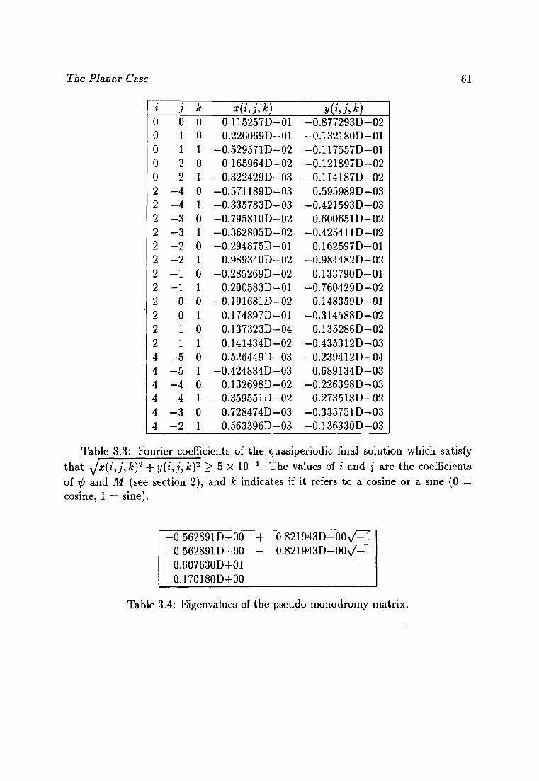
The Planar Case 61
i i ib x(i,j,k) y(*\¿,*0 0 0 0 0.115257D-01 -0.877293D-02 0 1 0 0.226069D-01 -0.132180D-01 0 1 1 -0.529571D-02 -0.117557D-01 0 2 0 0.165964D-02 -0.121897D-02 0 2 1 -0.322429D-03 -0.114187D-02 2 - 4 0 -0.571189D-03 0.595989D-03 2 - 4 1 -0.335783D-03 -0.421593D-03 2 - 3 0 -0.795810D-02 0.600651D-02 2 - 3 1 -0.362805D-02 -0.425411D-02 2 - 2 0 -0.294875D-01 0.162597D-01 2 - 2 1 0.989340D-02 -0.984482D-02 2 - 1 0 -0.285269D-02 0.133790D-01 2 - 1 1 0.200583D-01 -0.760429D-02 2 0 0 -0.191681D-02 0.148359D-01 2 0 1 0.174897D-01 -0.314588D-02 2 1 0 0.137323D-04 0.135286D-02 2 1 1 0.141434D-02 -0.435312D-03 4 - 5 0 0.526449D-03 -0.239412D-04 4 - 5 1 -0.424884D-03 0.689134D-03 4 - 4 0 0.132698D-02 -0.226398D-03 4 - 4 1 -0.359551D-02 0.273513D-02 4 - 3 0 0.728474D-03 -0.335751D-03 4 - 2 1 0.563396D-03 -0.136330D-03
Table 3.3: Fourier coefficients of the quasiperiodic final solution which satisfy that Jx(i,j,k)2 + y(i,j, k)2 > 5 x 10~4. The values of i and j are the coefficients of V' and M (see section 2), and k indicates if it refers to a cosine or a sine (0 = cosine, 1 = sine).
-0.562891D+00 + 0.821943D+0(V-Í -0.562891D+00 - 0.821943D+00V^Î
0.607630D+01 0.170180D+00
Table 3.4: Eigenvalues of the pseudo-monodromy matrix.
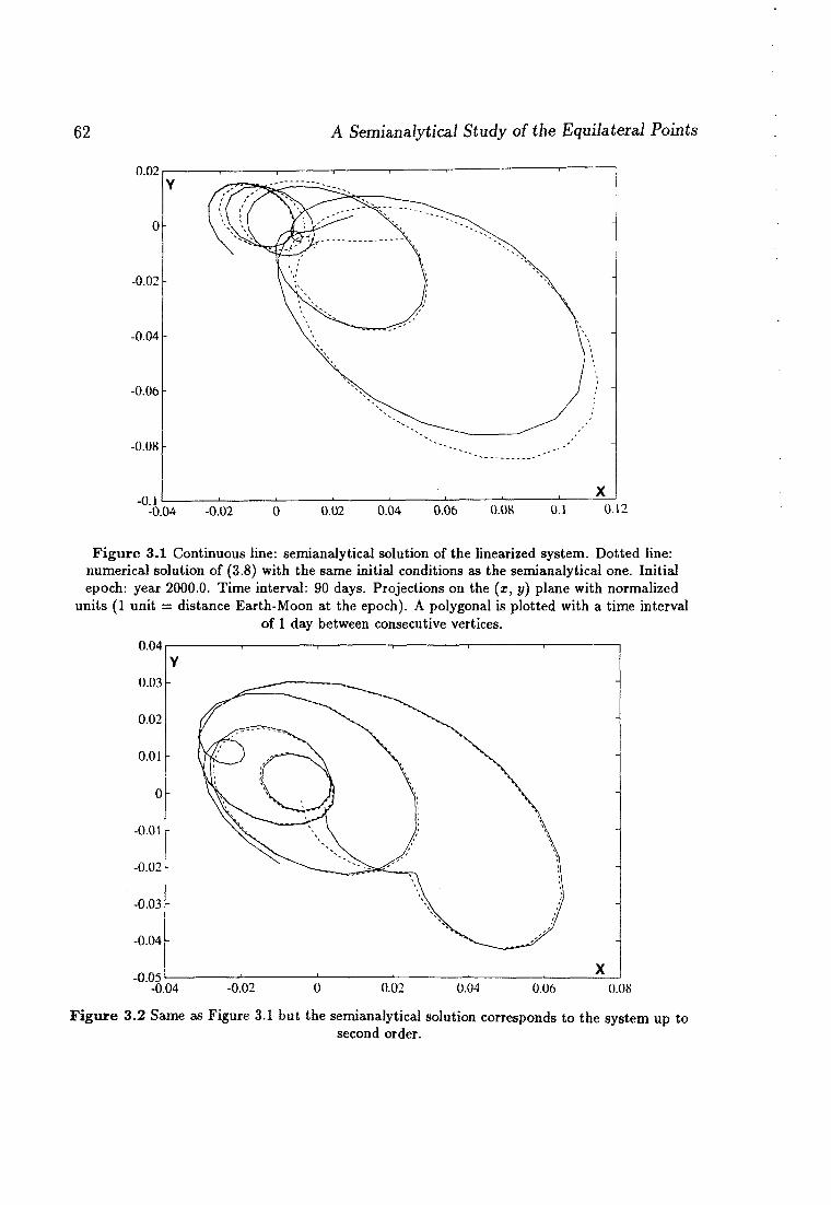
62 A Semianalytical Study of the Equilateral Points
0.02
-0.02
-0.04
-0.06
-0.08
-0.04 0.12
Figure 3.1 Continuous line: semianalytical solution of the linearized system. Dotted line: numerical solution of (3.8) with the same initial conditions as the semianalytical one. Initial epoch: year 2000.0. Time interval: 90 days. Projections on the (x, y) plane with normalized
units (1 unit = distance Earth-Moon at the epoch). A polygonal is plotted with a time interval of 1 day between consecutive vertices.
0.04 r
-0.04
-0.05 -0.04 -0.02 0.04 0.06 0.08
Figure 3.2 Same as Figure 3.1 but the semianalytical solution corresponds to the system up to second order.

The Planar Case 63
0.04
0.02
-0.02 -
-0.04 -
-0.06
-0.08 -
-0.06 -0.04 -0.02 0 0.02 0.04 0.06 0.08 0.1 0.12
Figure 3.3 Same as Figure 3.1 but the semianalytical solution corresponds to the system up to ihird order. Time interval: 192 days.
0.04
0.02
0.02 0.04 Ü.Ü6 0.08 0.12
Figure 3.4 Same as Figure 3.1 but the semianalytical solution corresponds to the system up to fourth order. Time interval: 192 days.
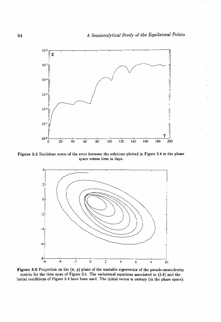
64 A Semianalytical Study of the Equilateral Points
10* 0 20 40 60 80 100 120 140 160 180 200
Figure 3.5 Euclidean norm of the error between the solutions plotted in Figure 3.4 in the phase space versus time in days.
Figure 3.6 Projection on the ( i , y) plane of the unstable eigenvector of the pseudo-monodromy matrix for the time span of Figure 3.4. The variational equations associated to (3.8) and the
initial conditions of Figure 3.4 have been used. The initial vector is unitary (in the phase space).
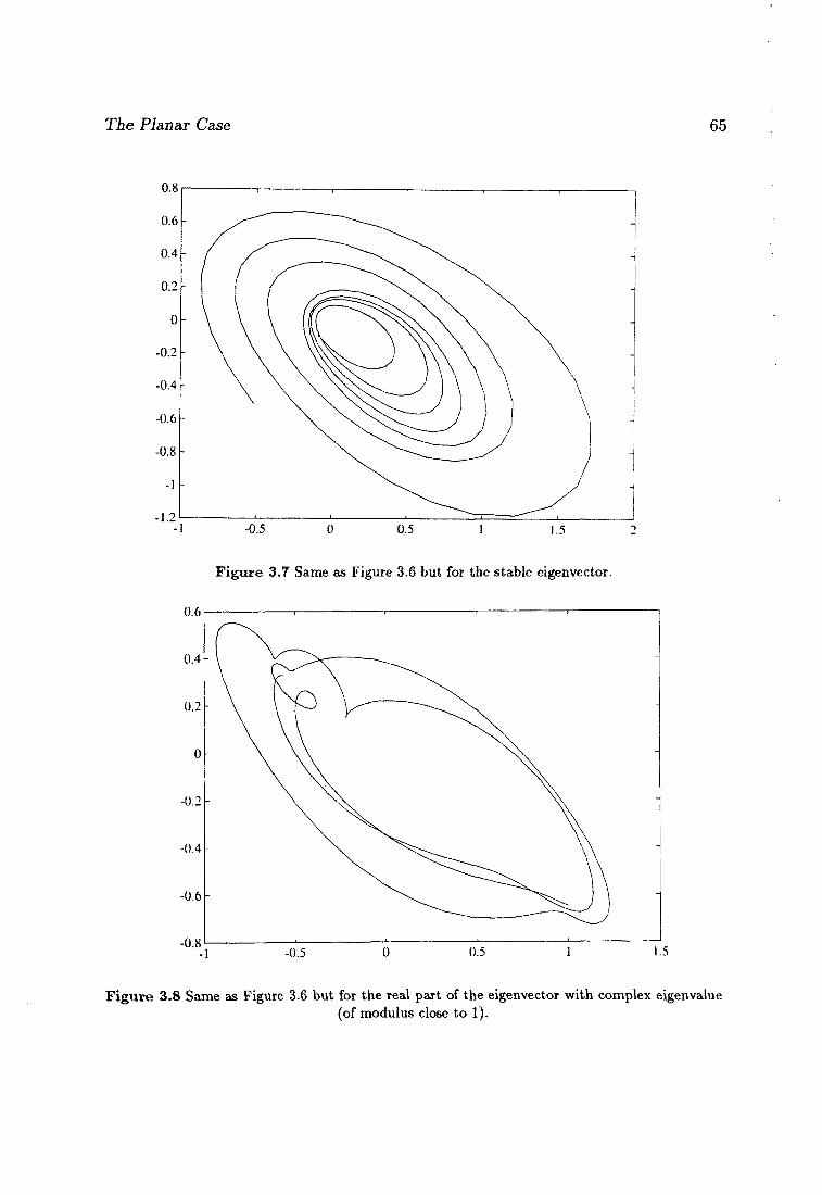
The Planar Case 65
"°'8-l -0.5 0 0.5 1 1.5
F igu re 3.8 Same as Figure 3.6 but for the real part of the eigenvector with complex eigenvalue (of modulus close to 1).
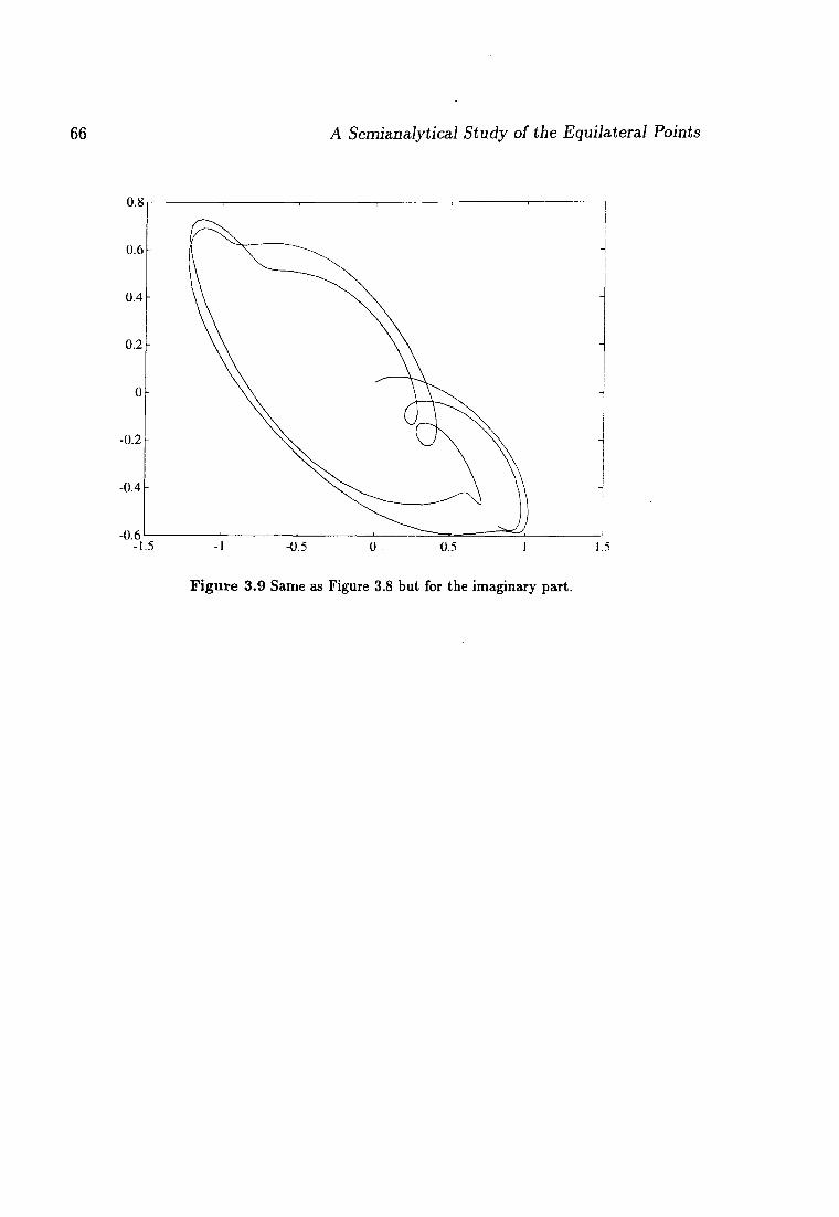
66 A Semianalytical Study of the Equilateral Points
Figure 3.9 Same as Figure 3.8 but for the imaginary part.
The Spatial Case 67
3.4 The Spatial Case
Here, the spatial case is considered, and the model given in section 3.1 is studied. As before, we are interested in a quasiperiodic solution of the equations of motion having the same basic frequencies that the perturbation. The algorithm will be the one described in Section 3.2 and used for the planar case. As the algebraic manipulator used for the planar problem is not enough to deal with this case, a new one has been built. It is going to be described in the next sections, as well as the results obtained with it.
3.4.1 The Algebraic Manipulator
Now we are going to describe the algebraic manipulator specially built (in FORTRAN 77 language) to solve the latter problem. Here, a trigonometric series is stored as a vector of real numbers (each one corresponding to a coefficient), a vector of integers (of the same dimension) and an integer containing this dimension. This integer is only used in some operations to check an "overflow trigonometric series" condition. An auxiliary table, with the coefficients of the linear combinations of the basic frequencies, will also be used by the manipulator.
Storing Fourier Series
We need to store trigonometric series and handle them in a fast way. Moreover, we want the size of the vectors that contain them to be as short as possible. In order to get the latter condition, we have decided to store only the non-zero coefficients, positioned in a contiguous way (as a stack). This means that we must have a way to recognize those coefficients, because their position inside the vector does not allow to identify them.
For this reason we have taken an auxiliar integer table of frequencies which contains, for each column, different integer values. For example, if a column contains the integers (fc l 5 . . . , kr) it means that it refers to the frequency kxu>i + • • • + kru>r, where (a>l5... ,cjr) is the vector of basic frequencies (obviously, the number of rows must be at least the number of frequencies). This table will be used in two different ways:
1. Given a position, to find the corresponding coefficients of the frequencies.
2. Given an integer vector, to search for its position inside the table.
The first use is easy and fast to do, but not the second one. At this point, it would be useful that elements of the table were given in some order, because we could use a binary search. One could think that it would be enough to fill the table at the beginning of the program using the selected order, but this does not work very well,
68 A Semianalytical Study of the Equilateral Points
due to the fact that when we start the program we do not know yet which frequencies will appear in the intermediate computations. We need to add frequencies to the table during the process, and we need to restart the order in a quick way. For this reason we have added to the table an integer vector which refers to the table in an ordered way and, when a new frequency is added (at the end of the table), the program only needs to modify this vector to get the table in order again. The order selected has been lexicographic:
(fc1,...,fcrj<(A:1,...,fcrj^| (kl,...,kl)<(kl...,Pr) iík¡=k¡.
Now, let us see how we can use this. We suppose that the real vector of coefficients is called x and we define an integer vector called nx. The first component of x is always used to store the independent term (the average). The first component of nx is used to store the number of non-zero coefficients of the series (the last meaningful component of vector x). Now, let j be an integer less than or equal to nx( l ) and we consider the coefficient x ( j ) . If nx(j) is even, x ( j ) corresponds to a cosinus, otherwise it corresponds to a sinus. In the column m=nx(j)/2 (integer division) of the table described above we can find the frequencies corresponding to this coefficient.
Now we are going to see how all of these things have been programmed. In what refers to storing frequencies in the table, we restrict ourselves to the ones that have the first integer coefficient (kx using the above notation) greater than or equal to zero. If we have a frequency with ki < 0, we change its sign and, in the case that it corresponds to a sinus, the sign of the coefficient is also changed. If ki = 0 we impose that the latter condition holds for ki. If ¿2 = 0 we impose it to ¿3, and so on.
All of these arrays have been included inside a common called t au l e s :
common / t a u l e s / t auf re ,n tau ,ord tau ,busc
tauf r e has been declared as integer*2 and ntau, ordtau and busc as integer*4. t a u f r e ( r , n ) contains the table of frequencies (n is the maximum number of them and r the number of basic frequencies), ntau is the actual number of frequencies in the table, ordtau(n) is the vector that holds the order of taufre and busc(2 ,m) is an array used to get a quicker binary search. Let us see how it works. Given a frequency (kx,..., fcr), kx > 0 the numbers busc(l ,k x + 1) and busc(2,A;i + 1) refer to the first and last place (of ordtau) where this kx appears, and then the search field is shorter. If there do not exist any frequencies with this k\ the corresponding values of busc are —1.
Finally, we are going to comment on some points about another system of storing Fourier series used in some intermediate computations. As we will see later, in many operations the manipulator uses a real array as a workspace. This vector has twice
The Spatial Case 69
more components that the table of frequencies and it is used to hold series in such a way that it allows to make sums faster. This is due to the fact that the position of a coefficient in this vector plays the same role that the index vector seen before. For example, with the same notation as before, the coefficient x ( j ) is put in the component nx( j ) (this is only true for j > 1, x ( l ) is put in the first component of the working vector). Note that if we have two vectors of this kind, the sum of them can be done by adding, component by component, the two vectors. The dissadvantage of having many vectors like this is the waste of memory that they require, because many of this components may be zero. For this reason we prefer to keep the Fourier series in the packed form seen before. We have only one working vector and we pass it to routines that make use of it.
Basic Subroutines
The following routines have been built with the aim of having an easy-to-use system to handle the tables of frequencies.
Subroutine FREQ The first parameter is an integer*4 variable coming from a Fourier series (for example, using the above notation, some value nx(k)) that contains information relative to a coefficient. Unchanged on exit. The second parameter is an integer*4 array that will contain on exit the frequencies corresponding to n, and the third parameter will contain 0 if it refers to a cosinus or 1 if it refers to a sinus.
Subroutine POSI This routine is inverse of the former one: it returns an integer which contains information about the frequency (following with the example, information to be stored in the vector nx). The first parameter is an integer*4 vector of frequencies and the second one is an integer containing 0 or 1. These parameters are unchanged on exit. The routine returns an integer value n to be stored in an integer vector corresponding to a Fourier series. The routine performs a binary search of f v in the table of frequencies and, assuming that fv is found in the place j , makes n=2*j+i. If fv is not found (i. e., it is not in the table) the routine calls the subroutine ACTUAL.
Subroutine ACTUAL This routine adds a frequency to the table. The first parameter is the vector containing the frequency to be added and the second one ( l loc) is the place (of ordtau) where this frequency must be (this value has been found during the binary search of the routine POSI). The elements which previously were stored in ortau, in places from Hoc up to the end, are shifted one place to the right. Both parameters are unchanged on exit.
Subroutine EMPAQ As we have already seen, in many operations the manipulator uses a real array as a workspace. This routine packs a trigonometric series
70 A Semianalytical Study of the Equilateral Points
contained in the working vector.
Subroutine NORMAL The first parameter is an integer vector (f ) containing a frequency, the second one is an integer saying how many frequencies we have. With this, the routine puts f in normal form (the first component non equal to zero must be positive) and returns i s= - l if it has changed the sign of f, or i s= l otherwise. If all of the components of f are equal to 0 it returns is=0. This routine is called during some operations (for example, a product of series).
Subroutine WFREC This routine returns the numerical value of the frequency corresponding to a place (given by means of a parameter) of the working vector.
Subroutine INITAU This routine initializes the tables used by the manipulator. It must be called at the beginning of the program, before making any other call to a routine of the manipulator. It has no parameters.
Subroutine AVALUA This routine computes the numerical value of a trigonometric series at a given time value t .
Subroutine LLEGEIX Given a channel (already opened), this routine reads a Fourier series through this channel and returns it in packed form.
Subroutine ESCRIU Given a channel (already opened), this routine writes a Fourier series given in packed form.
Making Operat ions
Now we are going to describe the main operations performed by the manipulator, which include sums, multiplications of Fourier series and multiplications of Fourier series by real numbers, differentiation and some special operations that we shall describe later. To keep only the meaningful terms of the series, we have included a threshold that allows to drop terms less (in absolute value) than this threshold, which is in a common named control.
Subroutine SUMA This routine performs the sum of two Fourier series. The method consists in expanding the first series inside the working array and then add the second series putting the results in the same working vector. Finally, the result is packed (this routine calls SUMAF).
Subroutine SUMAF Given a Fourier series in packed form and a Fourier series in expanded form, this routine adds them and puts the result in the same vector that contains the series in expanded form (the vector in expanded form
The Spatial Case 71
is the working vector mentioned in section 3.4.1). This routine has been built to increase the speed of operations of type a — a + b.
Subroutine PROD This routine obtains the product of two series. The way to do this is to fill a working vector with zeros and to call the routine PRODF (see below). This routine returns the result inside the working vector and finally it is packed.
Subroutine PRODF Given two Fourier series in packed form (we can call them a and 6) and a Fourier series in expanded form called w, this routine performs the operation w = w-\-a x b. To do this, each term of the first series is multiplied by each term of the second one. If the absolute value of the resultant coefficient is less than the threshold, it is dropped, otherwise the frequencies of the terms that are multiplying are computed. With this, the result is added to the corresponding position of the working array. As SUMAF, this routine has been built to increase the speed of some operations.
Subroutine PR1C This routine performs the product of a series containing only one term (whose coefficient is equal to one) by a Fourier series in packed form. The result is returned also in packed form. The unitary series is given by a number displaying the frequencies and if it is a sinus or a cosinus (this number is of the same kind as the components of the index vector (nx) seen before). The routine works with the same algorithm as PROD. This operation is needed a lot of times during the calculus of the Jacobian matrix. This routine can be avoided, but it is easy to write and allows to simplify the main algorithm (we do not need to fill a trigonometric array with an unitary series and to call PROD).
Subroutine PR1CF This routine makes the same operation as PR1C, but adding the result to the series contained in the working vector. This allows us to get more speed during some operations.
Subroutine PRESC This routine multiplies a real number by a trigonometric series. This is a very common operation in the main algorithm and we preferred to write it instead of using the routine PROD.
Subroutine DF This routine computes the derivative of a Fourier series as usual: for each term the integer vector k containing the frequency is obtained, and the coefficient is multiplied by (k,uj) (the vector u is stored in a common called f reque) and if it is a cosinus, its sign is changed.
Subroutine MDF2 This routine performs the second derivative of a trigonometric series, and multiplies it by — 1. Note that it is faster to compute this directly
72 A Semianalytical Study of the Equilateral Points
than to call routine DF twice and then to call PRESC. The algorithm is of the same kind that in the latter routine.
Subroutine NORMA This routine returns the norm of a Fourier series. The norm that we have selected is the euclidean norm of the vector containing its coefficients.
3.4.2 The Newton Method
Now, using the manipulator described above, it is possible to write a program that looks for a zero of the function G defined before, by means of a Newton method. For this purpose we need an initial condition close enough to the solution that we are looking for. Due to the fact that the perturbation is too big to take the zero solution as initial condition, we are going to use a Newton continuation method. For this reason we have added a continuation parameter (h) multiplying the non constant terms of the perturbations. Thus, when h is equal to 0 we have an autonomous differential system with an equilibrium point near the origin (the equilibrium point is not the origin itself because the constant terms of the perturbations are not multiplied by h). This point is close enough to the origin to be found by the Newton process starting from the zero solution. Then we increase h and this point becomes a small quasiperiodic orbit (see Chapter 2) that can be found by the Newton method (otherwise the value of h must be reduced to an intermediate value). Now the value of h is increased again and the Newton process is started from the solution found for the last value of the parameter. If no problems appear (that is, bifurcations and/or turning points), this process can continue until h reaches the value 1. We shall come back to this point later.
Some Remarks abou t t h e Jacobian Mat r ix
Due to the big quantity of coefficients appearing in the Fourier series, it is impossible to include all of them in the Newton method. For this reason we have selected some of them. The selected elements are stored in integer vectors (we store the indices corresponding to them as the vector nx seen before) and put in a common called f renew. Because of this, we have two different values of the function G: the ordinary value and the one obtained taking into account only the terms included in the Newton method. Note that we are solving with respect to this last value.
Adding terms to the Newton Process
The criterion to select the coefficients that will take part in the Newton process is based on the size of the amplitudes of the residual acceleration. At the beginning only the terms appearing in the initial condition are selected (if this is constant
The Spatial Case 73
and equal to zero, only the independent terms take part in the process). When the reduced equation (that is, taking into account only the terms of the Newton process) is solved, the program checks the size of the amplitudes of the terms of the residual acceleration that are outside the Newton process. If it finds that some of them are larger than a given threshold, then they must be added to the Newton process, else this step of the continuation method is finished and we can start the next one.
We want to make a remark about adding terms to the Newton process. If we add too many terms to it, we can find out that the neighbourhood of convergence is too small and we are out of it. In order to avoid this, we have a control on the maximum number of terms going in the Newton process, and if this number is reached, the threshold is increased. We have also implemented a similar procedure if the program is going to take a few new terms for the Newton method. Of course, in this case the corresponding threshold is reduced.
High Level Routines
We start writing a routine that evaluates the function G. This is not a problem, using the algebraic manipulator and a series expansion for the terms coming from the RTBP. We also have continuation parameters in the terms of each degree and an integer variable containing the actual degree of the power expansion. These parameters are stored in a common called cont i . This allows to select the degree at which the solution is wanted.
Then, we need a routine that computes the Jacobian matrix of G. This is easy using the chain rule as mentioned in 3.2 and the polynomial expansion of the equations. Note that in this part we also have the continuation parameters for the expansion. Moreover, in order to increase the speed, we realize that some powers and products of series that we need in this part have already been done during the evaluation of G, so, we keep these results in memory.
Once the Jacobian matrix is filled up, we need to solve a linear system with a big matrix (note that this matrix is not sparse at all). This system involves only the terms selected before. For this purpose, we have written a routine adapted to a paged environment. The method used is based on the Gaussian elimination.
Due to the fact that we do not know the stepsize for the continuation parameter, we have implemented an automatic stepsize control. This works in the following way: when the Newton method does not find the zero in a few iterations (this number is supplied by a control input file), it assumes that the continuation parameter has been increased too much. Then the program recovers the solution corresponding to the last value of the parameter (it has been stored previously by the program in a disk file), assigns to the parameter an intermediate value and starts the process again. Of course, if the difference between this intermediate value and the last successful one is less than a fixed threshold (given also by a control file) the program stops
74 A Semianalytical Study of the Equilateral Points
issuing the corresponding error message.
Subrout ine I N I P O T This routine computes the required powers x*yjzk, where (x,y, z) is a vector of Fourier series, and stores the result (in the common /pow/) to be used by the routines that compute the function G and its Jacobian matrix. If n is the actual degree of the expansion we are working with, then the powers are computed and stored (except those of degree one) up to order n — 1. This is due to the fact that the powers of order n are only needed once (during the computation of (?), while the ones of order less than n are used many times (in the computations of G and its Jacobian matrix). The way to obtain the powers of x, y and z is the following: powers of orders less or equal than three are computed "explicitely" (using the algebraic manipulator, we have written directly the expressions for order two and, using these results, the ones of order three). The powers of degree greater or equal than four are obtained as a product of two powers previously computed. This routine calls POSAP, TREUP and SPLIT.
Subrout ine P O S A P This routine stores a Fourier series a = xlyizk in the common /pow/. The parameters are the Fourier series a, ia, na (see section 3.4.1) and i, j , k. The routine puts the Fourier series in the vectors real*8 pot and integer*4 npot. This common also has an integer*4 value containing the first free component of the vectors, in order to add the Fourier series at the end of the series already contained in the vectors. Once the series is added, this value is updated. To recover these series we need to write down where they are. This is done by means of the routine LLP (see below): given the integer vector of exponents i , j and k, this routine returns an integer value 1. Then, in the column 1 of the array integer*4 inpo (2,161) we store the first and the last component of pot and npot in which we can find that Fourier series.
Subrout ine LLP Given the integer vector (i, j , k), the routine returns the column of inpo in which we can find the first and the last components of the arrays pot and npot containing the value xly*zk. More concretely, if n = i + j + k, then the returned value is ( ( ( n + 3 ) n + 2 ) n - 2 4 ) 6 + i ( n + l ) —((¿-l)*')/2+j + l.
Subrout ine T R E U P This routine extracts the Fourier series of xiyizk. In order to know where it is stored, a call to the routine LLP is done.
Subroutine T R E U P P This routine works exactly as TREUP but returning the result multiplied by a given real*8 variable. It is used by the routine MONOMI (see below).
Subrout ine SPLIT Given an integer vector (i, j , k), this routine returns two integer vectors (h,ji ,&i) and (¿2 , j2 , h) such that ix+i2 = i,ji+j2 - j , kx+k2 = k
The Spatial Case 75
and satisfying ii+ji + h = E(n/2) (i?=integer part), where n = i+j + k. This routine is used to know which powers we must multiply to get the power we want. This is used to obtain powers that are not in the common /pow/ (this happens with the powers of maximum order and during the filling of pow).
Subroutine MONOMI Given an integer vector ( i , j , k), a real number p, the Fourier series x, y and z and a working vector w containing a Fourier series, this routine returns w — w + px x%y*zk, where w is the working vector. Before calling this routine a previous call to INIPOT (to compute the required powers of x, y and z) is needed.
Subroutine CORXETl This routine computes the value between brackets ([ ]) in equation (3.1), by means of calls to MONOMI. The value is returned in expanded form inside a working vector.
Subroutine CORXET2 Like CORXETl, but for equation (3.2).
Subroutine CORXET3 Like CORXETl, but for equation (3.3).
Subroutine FUNC Routine that computes the value of function G (see page 54), calling routines CORXETl, C0RXET2, C0RXET3 and using the manipulator to compute the other terms appearing in the equations.
Subroutine DFUNC This routine computes the Jacobian of function G, calling the following routines:
1. DIX: it computes ——. ox
2. DI Y: it computes ——. dy
3. dGi
DIZ: it computes ——. dz
4. dG2 D2X: it computes ——.
5. dG2 D2Y: it computes ——. dy
6. . dG2 D2Z: it computes ——.
7. dG3 D3X: it computes ——.
8. dG3 D3Y: it computes ——.
76 A Semianalytical Study of the Equilateral Points
9. D3Z: it computes ——. oz
Subroutine SISTEMA This routine solves a linear system by means of LU decomposition (see [21]). The operations are done taking into account that FORTRAN stores the matrices as a sequence of columns, and trying to avoid big jumps inside the matrix.
3.4.3 The Program The program uses many data files in order to read the values of the basic frequencies (the values u = (wj , . . . ,w r)'), some phases related to them, control parameters (threshold to drop terms and to stop Newton method, maximum number of iterations and continuation parameters) and coefficients of the polynomial expansions of the equations. The program also reads a file containing the initial condition to start all the process (usually, it is taken equal to zero). During the execution, the program creates a file (called NEWTON .TMP) in which the actual solution is stored. This is due to the fact that if the new step of continuation does not succeed, the program can recover the last succesful solution (for the last continuation parameter, of course) to start again with a smaller parameter. This file is usually small (less than 20K). During the run, the program writes an execution log in a file called QPL4.CON. If the execution is succesful, the result is stored in a file called QPL4.RES.
Subroutine INIEXP This routine reads the coefficients of the power expansion of the vectorfield from the files EXPAN.l, EXPAN.2 and EXPAN.3 for the first, second and third equations, respectively.
Subroutine LLEQ This routine reads one perturbing function P (from the data file QUS.COE), and multiplies the non-constant terms of it by the continuation parameter h.
Subroutine INQUS This routine reads all the perturbing functions stored in the file QUS.COE and multiplies the non-constant terms of them by the continuation parameter. To do this, the routine LLEQ is used.
Subroutine INIQP This routine initializes all the program. It reads the values of the basic frequencies (and phases) of the perturbations (from the file FREQUE.VAL), the control parameters for the Newton method (from the file CONTROL.QP), the coefficients of the power expansion of the vectorfield, the values of the perturbations and the initial condition (from QPL4.DAD). This routine calls INIEXP and INQUS.
Subroutine QAF This routine returns the number of terms of the residual acceleration with amplitude larger (in absolute value) than a given threshold.
The Spatial Case 77
Subroutine AFE This routine adds the terms of the residual acceleration whose amplitude is larger (in absolute value) than a given threshold to the set of variables and to the equations to be solved by Newton's method.
Subroutine CHECK This routine is called before adding terms to the Newton process in order to avoid having out-of-range arrays.
Subroutine CTI From the residual acceleration (the value of G), this routine computes the independent term of the linear system that appears in the Newton method. This step needs a "conversion" from Fourier series to an array, using the vectors of coefficients that take part in the Newton process.
Subroutine NOUP This routine computes the new approximation to the solution of G = 0, using the solution of the linear system. As in CTI, here we need a "conversion" from an array to Fourier series.
Subroutine SCOOBY This routine looks inside the residual acceleration and searches for amplitudes larger (in absolute value) than a threshold rea l*8 t o l , and adds them to the Newton process. The number of terms added must be between the integer*4 values mitn and matn, modifying the value of t o l if necessary. This routine calls the routine AFE.
Subroutine CNFNA This routine controls all the Newton process. It checks the actual step of the process and takes the following decisions:
• If the residual acceleration is not small enough, the new independent term is computed.
• If the value of G is small enough, it looks for "big terms" inside the residual acceleration (calling SCOOBY), adding them if necessary.
• If G is small enough and there are not terms inside the residual acceleration big enough to be added to the process, the continuation parameter is moved.
• If the number of iterations with this value of the continuation parameter is too large, it sets a flag telling the routine NWTA to recover the last succesful solution, and the continuation parameter step is halved.
The routine returns a flag containing what it has done, because the routine NWTA (this is the one that calls CNFNA) needs to know what is happening (see below).
Subroutine NWTA This routine performs the Newton method. It computes G and then calls CNFNA in order to know what to do. Depending on the value of the flag returned by this routine, the action taken can be:
78 A Semianalytical Study of the Equilátera,! Points
• To continue with the process computing the Jacobian matrix (DFUNC), the independent term (CTI), solving the linear system (SISTEMA), obtaining the new approximation (NDUP) and computing again G.
• To overwrite the last succesful solution stored in the disk file NEWTON.TMP with the solution obtained for the actual value of the parameter and to compute G again (the continuation parameter has been increased inside CNFNA).
• To recover the last succesful solution from NEWTON.TMP and to compute G again (the continuation parameter has been moved inside CNFNA).
• To return the control to the main program because the final solution has been found.
Main Program Here we can find all the declarations of the arrays. This program calls INIQP to initialize the execution and then it calls NWTA to perform the Newton method. Finally, it opens the file QPL4.RES and writes in it the final result.
Test of the Program
In order to check all of these routines, we have solved again the planar problem (see section 3.3).
We start by setting the continuation parameter of the perturbation (h) to 1, and we select the degree of the power expansion equal to one. With this, we get a linear problem that the Newton method can solve easily. Then we add the quadratic terms (without need of any kind of continuation), and finally the third and fourth order terms. We have made another tests starting with the power expansion up to order four and moving the continuation parameter h from 0 to 1. All the results obtained with these tests are in good agreement with the ones mentioned in 3.3
3.4.4 Results of the Algebraic Manipulator
We have done several runs of this software package. Initially, we tried to use the same scheme as in [7], that is, to fix the continuation parameter h to 1, and the degree n of the power expansion to 1. With this we got a linear problem that the Newton process solved without troubles. Then we added the second degree terms and by using continuation we could solve this problem, but the number of terms taking part in the Newton process was very large and we had many troubles with the memory and swap needed by the program. Then the third degree terms could not be added directly (this is because they are meaningful in this problem) and we had to use continuation again. During this continuation the number of terms inside the Newton process became so high that we started to have troubles with the capacity
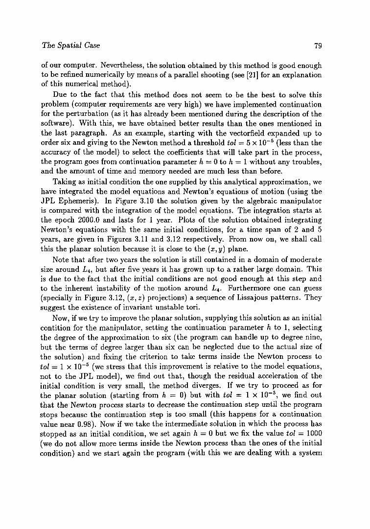
The Spatial Case 79
of our computer. Nevertheless, the solution obtained by this method is good enough to be refined numerically by means of a parallel shooting (see [21] for an explanation of this numerical method).
Due to the fact that this method does not seem to be the best to solve this problem (computer requirements are very high) we have implemented continuation for the perturbation (as it has already been mentioned during the description of the software). With this, we have obtained better results than the ones mentioned in the last paragraph. As an example, starting with the vectorfield expanded up to order six and giving to the Newton method a threshold tol = 5 x 10 - 5 (less than the accuracy of the model) to select the coefficients that will take part in the process, the program goes from continuation parameter h — 0 to h = 1 without any troubles, and the amount of time and memory needed are much less than before.
Taking as initial condition the one supplied by this analytical approximation, we have integrated the model equations and Newton's equations of motion (using the JPL Ephemeris). In Figure 3.10 the solution given by the algebraic manipulator is compared with the integration of the model equations. The integration starts at the epoch 2000.0 and lasts for 1 year. Plots of the solution obtained integrating Newton's equations with the same initial conditions, for a time span of 2 and 5 years, are given in Figures 3.11 and 3.12 respectively. From now on, we shall call this the planar solution because it is close to the (x, y) plane.
Note that after two years the solution is still contained in a domain of moderate size around £4, but after five years it has grown up to a rather large domain. This is due to the fact that the initial conditions are not good enough at this step and to the inherent instability of the motion around L4. Furthermore one can guess (specially in Figure 3.12, (x,z) projections) a sequence of Lissajous patterns. They suggest the existence of invariant unstable tori.
Now, if we try to improve the planar solution, supplying this solution as an initial contition for the manipulator, setting the continuation parameter h to 1, selecting the degree of the approximation to six (the program can handle up to degree nine, but the terms of degree larger than six can be neglected due to the actual size of the solution) and fixing the criterion to take terms inside the Newton process to tol = 1 X 10"5 (we stress that this improvement is relative to the model equations, not to the JPL model), we find out that, though the residual acceleration of the initial condition is very small, the method diverges. If we try to proceed as for the planar solution (starting from h = 0) but with tol — 1 x 10 - 5 , we find out that the Newton process starts to decrease the continuation step until the program stops because the continuation step is too small (this happens for a continuation value near 0.98). Now if we take the intermediate solution in which the process has stopped as an initial condition, we set again h = 0 but we fix the value tol = 1000 (we do not allow more terms inside the Newton process than the ones of the initial condition) and we start again the program (with this we are dealing with a system
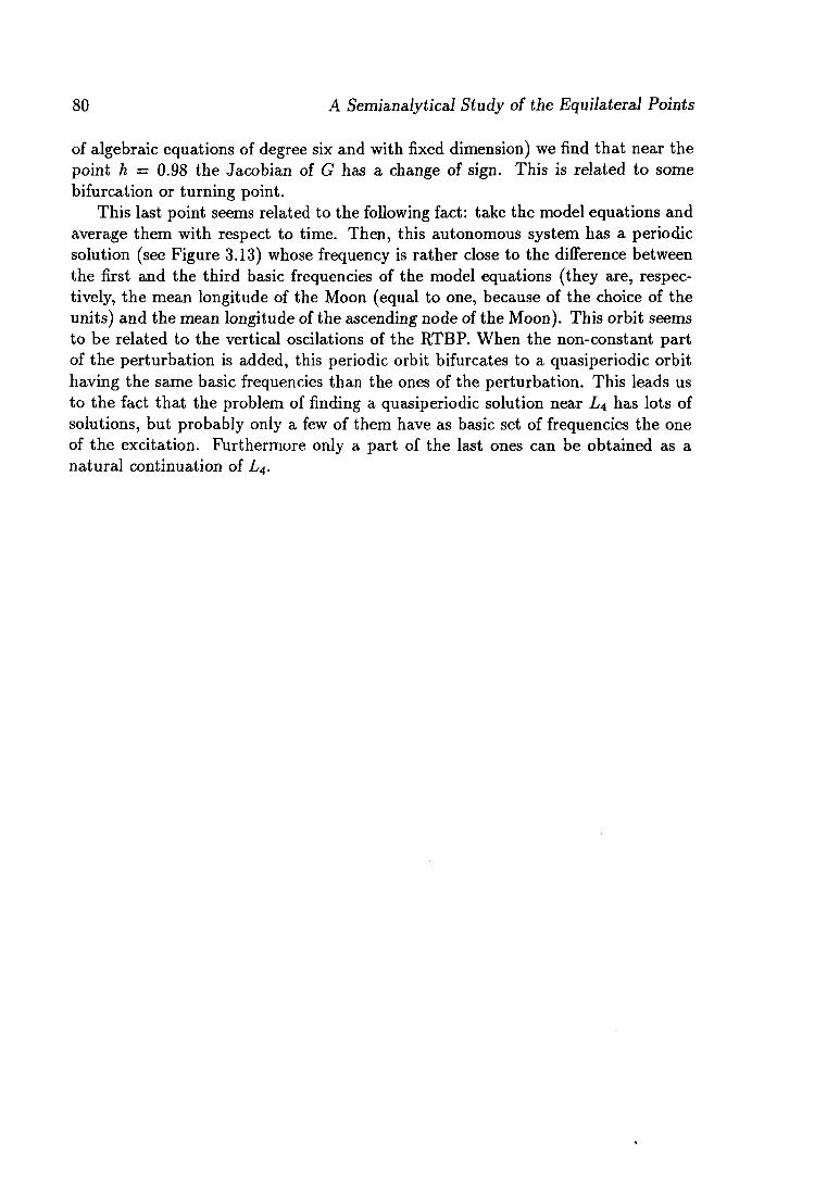
80 A Semianalytical Study of the Equilateral Points
of algebraic equations of degree six and with fixed dimension) we find that near the point h = 0.98 the Jacobian of G has a change of sign. This is related to some bifurcation or turning point.
This last point seems related to the following fact: take the model equations and average them with respect to time. Then, this autonomous system has a periodic solution (see Figure 3.13) whose frequency is rather close to the difference between the first and the third basic frequencies of the model equations (they are, respectively, the mean longitude of the Moon (equal to one, because of the choice of the units) and the mean longitude of the ascending node of the Moon). This orbit seems to be related to the vertical oscilations of the RTBP. When the non-constant part of the perturbation is added, this periodic orbit bifurcates to a quasiperiodic orbit having the same basic frequencies than the ones of the perturbation. This leads us to the fact that the problem of finding a quasiperiodic solution near L4 has lots of solutions, but probably only a few of them have as basic set of frequencies the one of the excitation. Furthermore only a part of the last ones can be obtained as a natural continuation of L4.
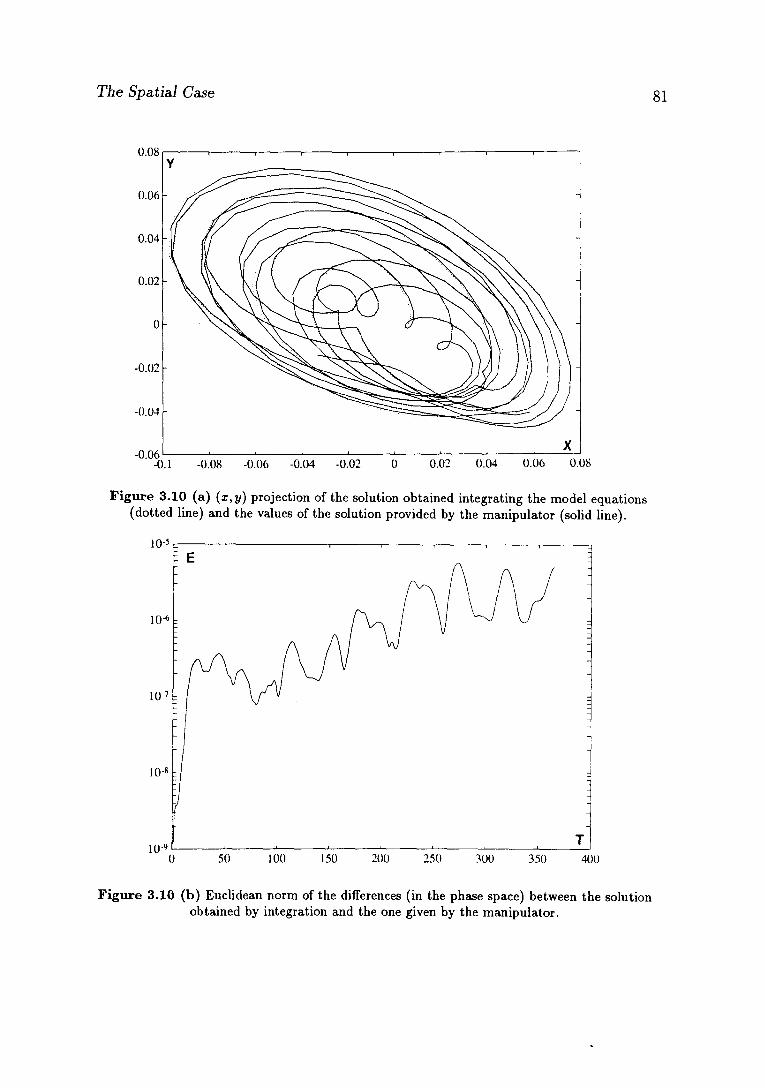
The Spatial Case 81
0.08
-0.08 -0.06 -0.04 -0.02 0.02 0.04 0.06 0.08
Figure 3.10 (a) (x,y) projection of the solution obtained integrating the model equations (dotted line) and the values of the solution provided by the manipulator (solid line).
10-5F
400
Figure 3.10 (b) Euclidean norm of the differences (in the phase space) between the solution obtained by integration and the one given by the manipulator.
82 A Semianalytical Study of the Equilateral Points
-0.15 0.15
0.15
Figure 3.11 Projections of the solution obtained integrating Newton's equations of motion for a time span of 2 years. The initial condition is the one given by the manipulator and it has not
been refined.
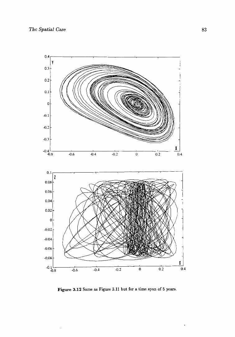
The Spatial Case 83
i "" i — - i 1 1
Y
X
0.3
X X
rp
X X
0.1
0
0.1
0.2
X
0.3
X
0.3
X n A .. i i i i X
-0.8 -0.6 -0.4 -0.2 0.2 0.4
-0.8
Figure 3.12 Same as Figure 3.11 but for a time span of 5 years.
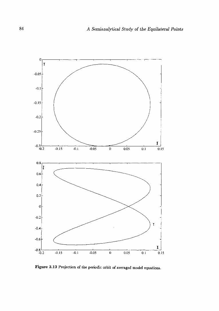
84 A Semianalytical Study of the Equilateral Points
-0.2 -0.15 -0.1 -0.05 0 0.05 0.1 0.15
Figure 3.13 Projection of the periodic orbit of averaged model equations.
Numerical Refinement 85
3.5 Numerical Refinement
In order to obtain a good nominal orbit we have implemented a parallel shooting method (see [21]) to get a solution of the JPL model very similar to the one found with the algebraic manipulator.
Now, let us see some details about this parallel shooting. First of all, we split the time span [a, b] in which we want to find the nominal orbit in several pieces [U, í,+i], i € {0 , . . . , n — 1}, verifying that t0 = a, tn = b and h = í,+i — í¿ = (b— a)/n (different time intervals can be used but we have chosen here all of them equal). Now let ¿ b e a value between 1 and n — 1 and let T¡, be the function defined as follows: if Xi is a point of the phase space, then FÍ(XÍ) = y,+i, where y,+1 is the value of the solution defined by the initial conditions (í¿,x¿) at time <¿+1, under the flow of the JPL model. Now we consider the vector (xo,...,xn), where x, are coordinates in the phase space corresponding to time i,. We can define T = {To, • • • , ^n - i ) in the usual way:
( a r 0 , . . . , a ; « ) i—• ( y i , . . . , y » ) ,
and note that, if the values x, are all from the same solution of the JPL model, then we should have that t/¿ = xt-, 1 < i < n. Then we impose these conditions and this leads us to solve a nonlinear system of 6n equations and 6n + 6 unknowns. To do this, we have used again a Newton method and we have taken as initial guess the values provided by the planar solution obtained using the algebraic manipulator. Due to the fact that we have more unknowns than equations, we have added six more conditions: we have fixed the initial position (the three first components of x0) and the final one (the three first components of xn). With this, the system we deal with has 6n equations and the same number of unknowns. Finally, we note that the linear system that appears at each iteration of the Newton method has a band matrix. For this reason we have written a routine adapted to this kind of matrix. Another way to perform the parallel shooting procedure is the following: instead of adding to the set of 6n equations the above mentioned six conditions (which in some sense can force the solution in a non natural way), replace them trying to minimize, with respect to some norm, the total corrections to be done at each step. The results of this procedure can be found in Appendix A.
Subrout ine SISBAN This routine solves a linear system of equations with a banded matrix, using only the band of the matrix plus three diagonals. The method is based in Gaussian elimination with partial pivoting.
Subrout ine O M P P This routine computes the initial guess for the Newton method, from a Fourier series corresponding to an approximation obtained by means of the algebraic manipulator. This guess is stored in a vector. This routine uses the routines AVALUA and DF of the manipulator.
86 A Semianalytical Study of the Equilateral Points
Subroutine COIN This routine changes coordinates, from the normalized ones to ecliptic ones (JPL), to the vector of initial conditions obtained by OMPP.
Subroutine F U N This routine computes the value of the function we want to make zero. For this purpose it performs a numerical integration of the equations of motion in the solar system using the JPL tapes to obtain the position of the bodies. The routine also integrates the variational equations and fills the Jacobian matrix of the function. The device used in this numerical integration has been the Shampine-Gordon method (see [18]).
Subroutine COOF This routine performs a change of coordinates, from the ecliptic ones to normalized ones, to the vector of final conditions obtained by the Newton method.
Main Program This routine reads the basic frequencies of the perturbations from the file FREQUE.VAL, the initial Fourier series (to obtain the initial condition for the Newton method) from the file QPL4.RES, some control parameters from the file TPL4.CTL (initial time, time step, number of time steps for the Newton process as well as thresholds for the numerical integration and a tolerance to know when the Newton process has finished) and the model of the solar system used from the file MODEL.DAT. With this, the program performs a Newton method (using the routines mentioned above), writing in the console some information about what it is doing. When the solution is found, the program writes the initial condition of the final orbit in the file TPL4.RES.
3.5.1 Final Results
Now, using the program described above, it is possible to find an orbit for the JPL model with a behaviour similar to the one of the planar solution obtained by the manipulator. In Figure 3.14 we show the numerical refinement of the planar orbit obtained in Section 3.4.4 for a time span of five years starting at the year 2000. The time step used in the parallel shooting has been of 1 day. To refine this orbit for longer time spans is very difficult (the parallel shooting does not converge) due to the fact that there exists a resonance (already mentioned in section 3.4.4) implying that this solution is not an exact solution of the system but a minimum of the residual acceleration. Nevertheless, the solution found for five years has a very slow "diffusion" and it goes away of L4 slowly. As an example of this, Figure 3.15 shows its behaviour for more than seven years, and it looks like quasiperiodic.

Numerical Refinement 87
-0.08
0.15
d O"3
1.5
0.5
O
-0.5
-1
-1.5
-2 -0.15
Z ,
S^^B / Kte^/' 1—
-i—
i
i i
t^L¿M?n&
^ ^ V ^ V ^ ^ ^ ^ ^ ^ M ]
j$C
X -0.1 -0.05 0.05 0.1 0.15
Figure 3.14 Numerical refinement of the planar orbit for a time span of 5 years,-
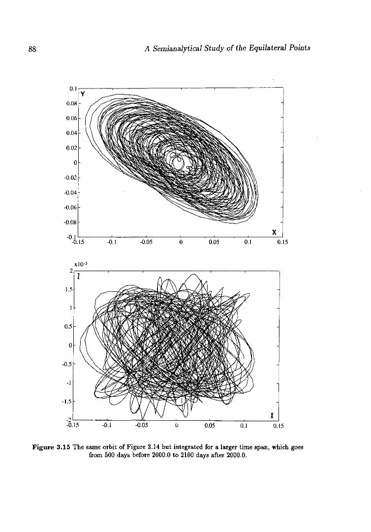
88 A Semianalytical Study of the Equilateral Points
0.15
2
1.5
x l O 3
2
1.5
Z * / \ 2
1.5
1 Y/^^Ê^^^^^^^^^^^^^^^^^^^^f
0.5 - y[l js ^ ^ x \
// \\(vO^^\\^ 0
¡j^JWegfiBC^fYVK^^A j|MfJ YJ \
0.5 - \ \ Iv^^Ë^^ ^^^^^^ fò^^S^ WfkWnjM
-1 ^^^^^j tegj j^z-Pf^L/^ y i
1.5
^^^^^j tegj j^z-Pf^L/^ y i
-, v/y v / ^ ' x
1 C. 1 I .
-0.15 -0.1 -0.05 0.05 0.1 0.15
Figure 3.15 The same orbit of Figure 3.14 but integrated for a larger time span, which goes from 500 days before 2000.0 to 2100 days after 2000.0.

The Behaviour Near the Computed Nearly Quasiperiodic Solution 89
3.6 The Behaviour Near the Computed Nearly Quasiperiodic Solution
To study both the stability properties of the computed solution and the relative motion of particles running in orbits close to that one, we have performed a variational study. Of course, in this case we can not talk about monodromy matrix because we never return to the initial conditions or, even if this happens, the subsequent motion will be different. But we can look for points returning close to the initial conditions on the phase space. Figure 3.16 gives the distance to the initial conditions in adi-mensional units as a function of time. One can see a typical quasiperiodic pattern and after, roughly, 1625 days, we are not too far from the initial point. Now we can consider the variational matrix after that time interval as if it were a monodromy matrix.
On the other hand, during the integration of the variational equations (using the JPL model, of course), we can record the spectral radius of the instantaneous variational matrix. That value has been plotted as a function of time in Figure 3.17, during the full period 2000.0 to 2005.0. Letting aside some local (in time) irregularities on the first 600 days, the pattern is quite neat. These irregularities can be due to the strong constraints on the parallel shooting method which forces the initial and final positions to coincide with the one given by the semianalytical approximation. From the end of the second year on, there are large oscillations with half a year period with superimposed smaller oscillations with period roughly equal to one half of the lunar sinodic period. This can be better seen in Figure 3.18, where we have plotted the quotient In p(t)/t. Here t is the time elapsed since the initial epoch 2000.0 and p(t) is the spectral radius (i.e. the maximum of the moduli of the eigenvalues) of the variational matrix at the current time. To skip the initial irregular behaviour this has been plotted starting at the year 2002.0 and the abscisae in the figure denote days since 2002.0. The limit of In p{t)/t should give the maximal Lyapunov exponent. This seems to be close to 3.65 x 10 - 3 if the time unit is one day. This implies an average increasing of the distance to the computed orbit at a rate of exp(365 x 3.65 x 10 -3) « 3.79 per year. This is an extremely mild instability and offers no problems concerning station keeping.
We return to the approximate monodromy matrix after 1625 days. Let A¿, i = 1 , . . . , 6 the eigenvalues of this matrix. The numerical values are
Ai = -30.664197, A3 = -0.079456 + 0.996838Í, A5 = -0.511657, A2 = -1.954433, A4 = -0.079456 - 0.996838Í, A6 = -0.032611.
They appear almost exactly in reciprocal pairs (AjA7_, = 1) as it happens for autonomous Hamiltonians. Note that the chosen epoch (2000.0 + 1625 days) is particularly good. For that epoch In p(t)/t equals 2.11 x 10"3. But we recall that the limit
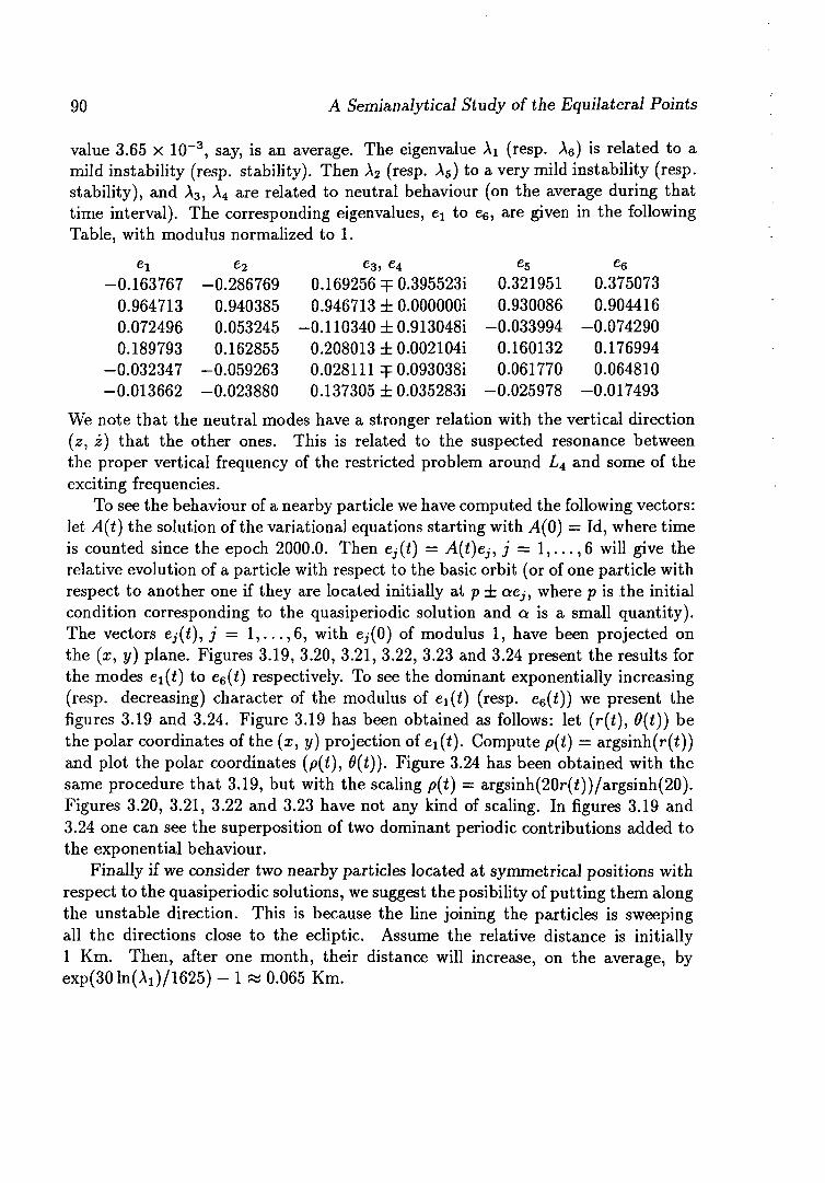
90 A Semianalytical Study of the Equilateral Points
value 3.65 x 10"3, say, is an average. The eigenvalue Ax (resp. A6) is related to a mild instability (resp. stability). Then A2 (resp. A5) to a very mild instability (resp. stability), and A3, A4 are related to neutral behaviour (on the average during that time interval). The corresponding eigenvalues, t^ to e6, are given in the following Table, with modulus normalized to 1.
e i e2 e3, e4 e5 e6 0.163767 -0.286769 0.169256 T0.395523Í 0.321951 0.375073 0.964713 0.940385 0.946713 ± O.OOOOOOi 0.930086 0.904416 0.072496 0.053245 -0.110340 ±0.913048i -0.033994 -0.074290 0.189793 0.162855 0.208013 ± 0.002104Í 0.160132 0.176994 0.032347 -0.059263 0.028111 q= 0.093038Í 0.061770 0.064810 0.013662 -0.023880 0.137305 ± 0.035283Í -0.025978 -0.017493
We note that the neutral modes have a stronger relation with the vertical direction (z, i ) that the other ones. This is related to the suspected resonance between the proper vertical frequency of the restricted problem around L4 and some of the exciting frequencies.
To see the behaviour of a nearby particle we have computed the following vectors: let A(t) the solution of the variational equations starting with A(0) = Id, where time is counted since the epoch 2000.0. Then ej(t) = A(t)ej, j = 1 , . . . ,6 will give the relative evolution of a particle with respect to the basic orbit (or of one particle with respect to another one if they are located initially at p ± ae¿, where p is the initial condition corresponding to the quasiperiodic solution and a is a small quantity). The vectors e3-(i), j = 1,.. . ,6, with ej(0) of modulus 1, have been projected on the (x, y) plane. Figures 3.19, 3.20, 3.21, 3.22, 3.23 and 3.24 present the results for the modes e\{t) to e6(t) respectively. To see the dominant exponentially increasing (resp. decreasing) character of the modulus of ti(t) (resp. e6(t)) we present the figures 3.19 and 3.24. Figure 3.19 has been obtained as follows: let (r(t), 0(t)) be the polar coordinates of the (z, y) projection of ei(t). Compute p(t) = argsinh(r(i)) and plot the polar coordinates (p(t), 6(t)). Figure 3.24 has been obtained with the same procedure that 3.19, but with the scaling p(t) = argsinh(20r(<))/argsinh(20). Figures 3.20, 3.21, 3.22 and 3.23 have not any kind of scaling. In figures 3.19 and 3.24 one can see the superposition of two dominant periodic contributions added to the exponential behaviour.
Finally if we consider two nearby particles located at symmetrical positions with respect to the quasiperiodic solutions, we suggest the posibility of putting them along the unstable direction. This is because the line joining the particles is sweeping all the directions close to the ecliptic. Assume the relative distance is initially 1 Km. Then, after one month, their distance will increase, on the average, by exp(301n(Ai)/1625) - 1 « 0.065 Km.
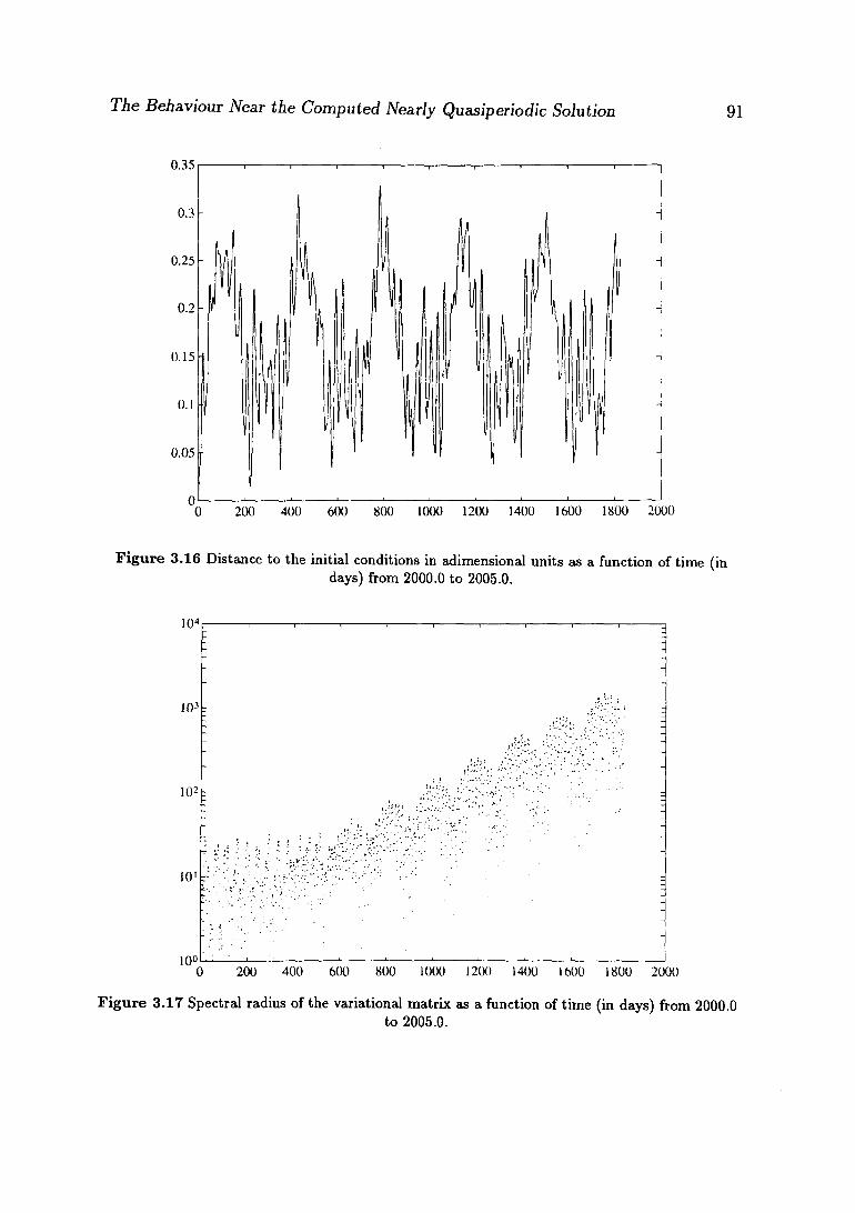
The Behaviour Near the Computed Nearly Quasiperiodic Solution 91
0.35
0.25
0.15
0.05
0 200 400 600 800 1000 1200 1400 1600 1800 2000
Figure 3.16 Distance to the initial conditions in adimensional units as a function of time (in days) from 2000.0 to 2005.0.
104p
0 200 400 600 800 1000 1200 1400 1600 1800 2000
Figure 3.17 Spectral radius of the variational matrix as a function of time (in days) from 2000.0 to 2005.0.
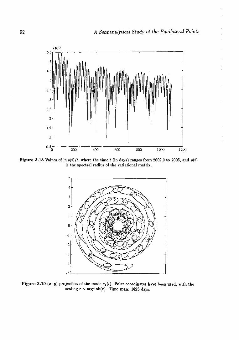
92 A Semianalytical Study of the Equilateral Points
1200
Figure 3.18 Values of Inp(t)/t, where the time t (in days) ranges from 2002.0 to 2005, and p(t) is the spectral radius of the variational matrix.
Figure 3.19 (x, y) projection of the mode e^t). Polar coordinates have been used, with the scaling r ~ argsinh(r). Time span: 1625 days.
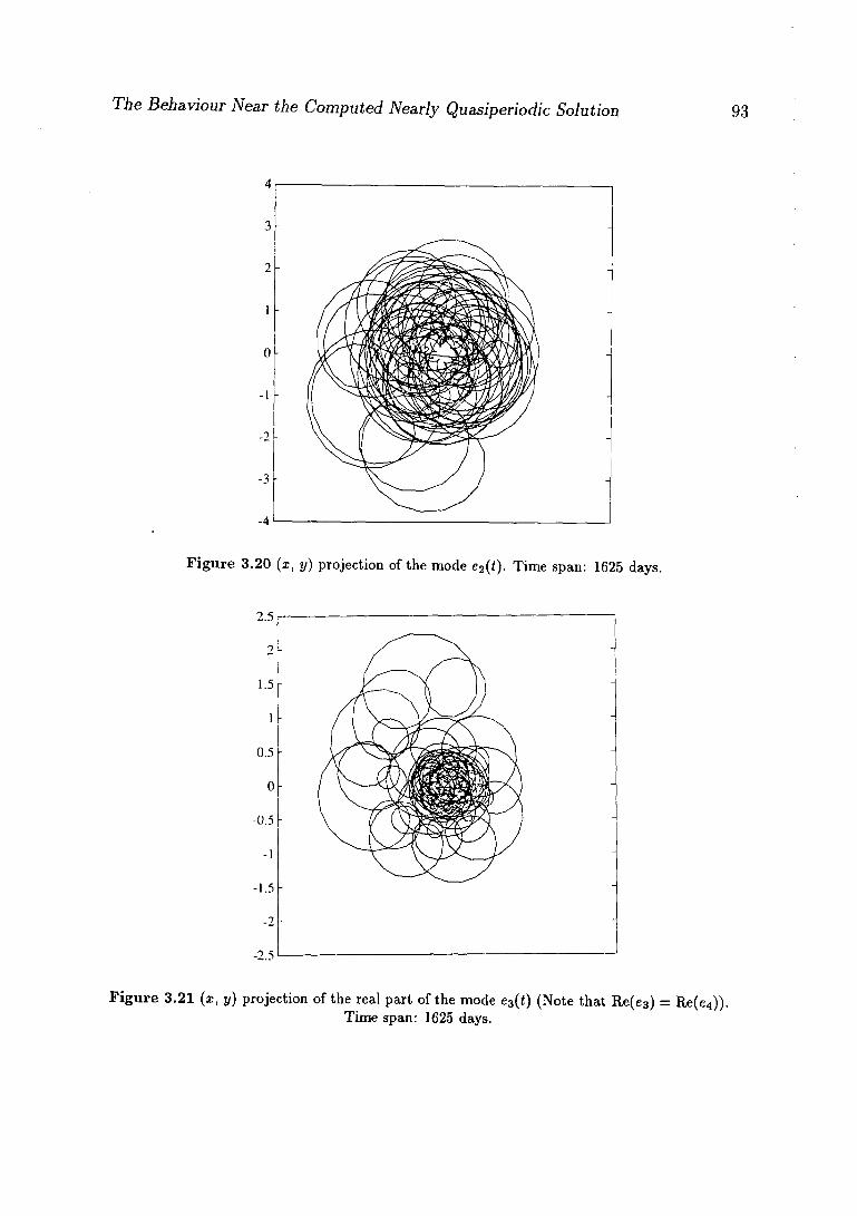
The Behaviour Near the Computed Nearly Quasiperiodic Solution 93
Figure 3.20 ( i , y) projection of the mode e2(t). Time span: 1625 days.
Figure 3.21 (x, y) projection of the real part of the mode e3(f) (Note that Re(e3) = Re(e4)). Time span: 1625 days.
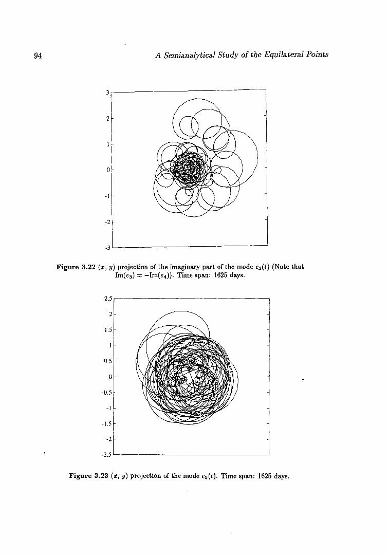
94 A Semianalytical Study of the Equilateral Points
3p
2 -
1 -
0 -
-1 -
-3
Figure 3.22 (x, y) projection of the imaginary part of the mode ez(i) (Note that Im(e3) = —Im(e4)). Time span: 1625 days.
2.51-
2 -
1.5 -
1 -
0.5 -
0 -
-0.5 -
-1 -
-1.5 -
-2 -
-2.5 -
Figure 3.23 (x, y) projection of the mode e5(<). Time span: 1625 days.
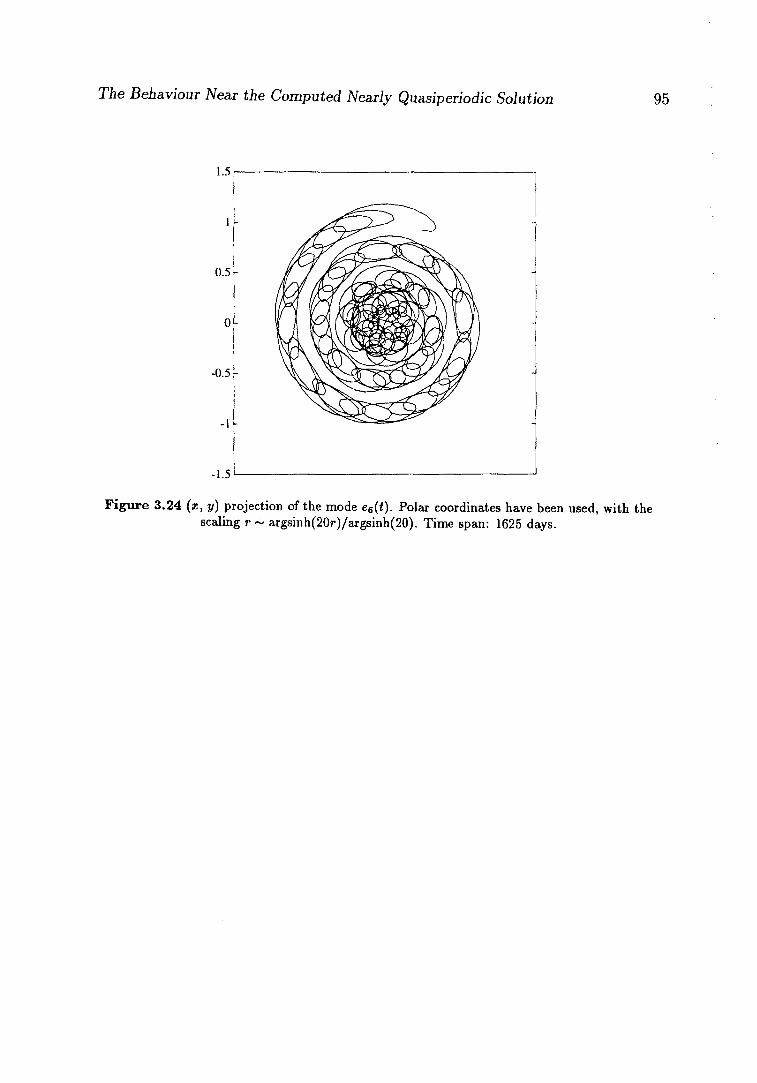
The Behaviour Near the Computed Nearly Quasiperiodic Solution
-0.5
-1.5
Figure 3.24 (x, y) projection of the mode e6(t). Polar coordinates have been use scaling r ~ argsinh(20r)/argsinh(20). Time span: 1625 days.

96 A Semianalytical Study of the Equilateral Points
3.7 Problems and Extensions Looking for the behaviour of the orbits near the geometrical triangular points of the Earth-Moon system we are faced with several problems. If we consider first the RTBP the phase space is filled up by periodic orbits, two-dimensional and three-dimensional tori as well as stochastic zones. The last ones are extremely small near the equilibrium point but the size increases when the distance to the equilibrium point does. To this simplified model we add relatively very important perturbations, mainly due to the effect of the Sun and to the non circular motion of the Moon and the Earth. Those perturbations can be assumed to be quasiperiodic for moderate time intervals. This produces strong resonances in some domains of the phase space and therefore large deviations from the (relatively) clear situation found for the RTBP. For small perturbations we have just to add a kind of quasiperiodic swinging to the previous structure. But the actual size of the perturbations is big enough to produce bifurcations loosing uniqueness. Therefore this is a source of problems for the analytical approximate solutions and for the subsequent numerical refinement as stated in 3.4.4 and 3.5.
The global problem, that is, the study with great detail of the real behaviour in a full neighbourhood of the former equilibrium point is worthy. It is useful for the design of future missions. From the abstract point of view there is a lack of supporting theory. From the analytical and numerical points of view this is a formidable task. We think that the methodology to be used to deal with this problem would be useful in many other contexts.
Appendix A
The Modified Parallel Shooting Method
A.l Introduction
As it has been mentioned before (see Section 3.5), the parallel shooting method needs some extra conditions, because the matching ones are not enough to provide a system with the same number of equations and variables. To overcome this difficulty is usual to add some boundary conditions to the initial and final points of the orbit, but sometimes these conditions can force the solution in a non natural way. In order to avoid this we shall not add extra conditions, and we shall apply Newton's method directly. This leads to a linear system with more unknowns than equations, having (in the general case) an hyperplane of solutions. Then, we select one of these solutions to proceed. Now, the criterion to select this solution has to be fixed. It is natural to look for the solution nearest (with respect to some norm) to the initial condition of the Newton's method, and this leads us to choose the point of the hyperplane nearest to the origin. We have used the euclidean distance to select that point, but it is possible to use other distances.
A. 1.1 The Program
This is essentially the same program that the one described in Section 3.5, but with some modifications inside its routines. The biggest one is inside routine SISBAN, because it is the one that looks for the solution of minimum norm. There are several ways of computing that solution, but due to the fact that the linear system we deal with has a band matrix and the dimension is very large, we have look at that point as the orthogonal projection of the origin on the hyperplane of solutions (as the distance is the euclidean one, the scalar product is the euclidean one). With
97
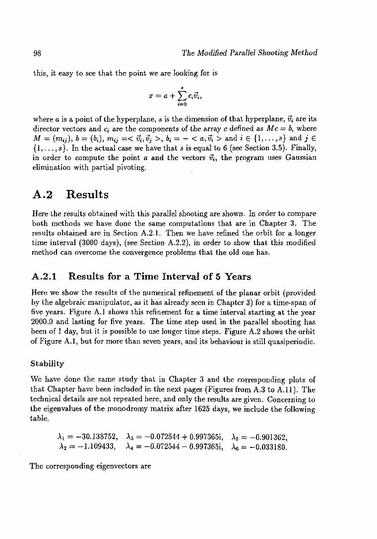
98 The Modified Parallel Shooting Method
this, it easy to see that the point we are looking for is
s
x = a + ^2 c,u,-, »=o
where a is a point of the hyperplane, s is the dimension of that hyperplane, u,- are its director vectors and c,- are the components of the array c defined as Mc = b, where M = (m,j), b = (bi), mtj = < u,-,Vj >, &,- = - < a,Vi > and i € {1 , . . . , s} and j G { 1 , . . . , s}. In the actual case we have that s is equal to 6 (see Section 3.5). Finally, in order to compute the point a and the vectors u,-, the program uses Gaussian elimination with partial pivoting.
A. 2 Results
Here the results obtained with this parallel shooting are shown. In order to compare both methods we have done the same computations that are in Chapter 3. The results obtained are in Section A.2.1. Then we have refined the orbit for a longer time interval (3000 days), (see Section A.2.2), in order to show that this modified method can overcome the convergence problems that the old one has.
A.2.1 Results for a Time Interval of 5 Years
Here we show the results of the numerical refinement of the planar orbit (provided by the algebraic manipulator, as it has already seen in Chapter 3) for a time-span of five years. Figure A.l shows this refinement for a time interval starting at the year 2000.0 and lasting for five years. The time step used in the parallel shooting has been of 1 day, but it is possible to use longer time steps. Figure A.2 shows the orbit of Figure A.l, but for more than seven years, and its behaviour is still quasiperiodic.
Stabil i ty
We have done the same study that in Chapter 3 and the corresponding plots of that Chapter have been included in the next pages (Figures from A.3 to A.11). The technical details are not repeated here, and only the results are given. Concerning to the eigenvalues of the monodromy matrix after 1625 days, we include the following table.
Xi = -30.138752, A3 = -0.072544 + 0.997365Í, A5 = -0.901362, A2 = -1.109433, A4 = -0.072544 - 0.997365Í, A6 = -0.033180.
The corresponding eigenvectors are
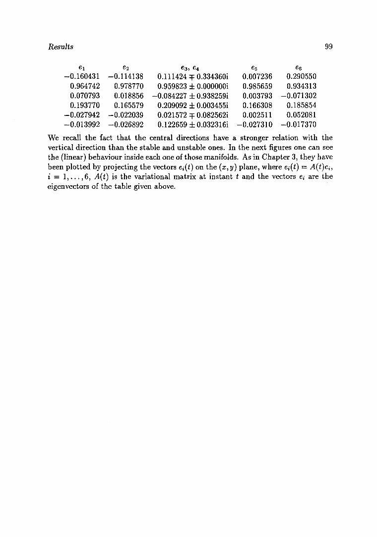
Results 99
ei e2 e3, e4 e5 e6
0.160431 -0.114138 0.111424 qp0.334360i 0.007236 0.290550 0.964742 0.978770 0.959823 ± O.OOOOOOi 0.985659 0.934313 0.070793 0.018856 -0.084227 ± 0.938259Í 0.003793 -0.071302 0.193770 0.165579 0.209092 ± 0.003455Í 0.166308 0.185854 0.027942 -0.022039 0.021572 T 0.082562Í 0.002511 0.052081 0.013992 -0.026892 0.122659 ± 0.032316Í -0.027310 -0.017370
We recall the fact that the central directions have a stronger relation with the vertical direction than the stable and unstable ones. In the next figures one can see the (linear) behaviour inside each one of those manifolds. As in Chapter 3, they have been plotted by projecting the vectors e¿(í) on the (x, y) plane, where e,-(i) = v4(i)e,, i = 1 , . . . ,6, A(t) is the variational matrix at instant t and the vectors e¿ are the eigenvectors of the table given above.
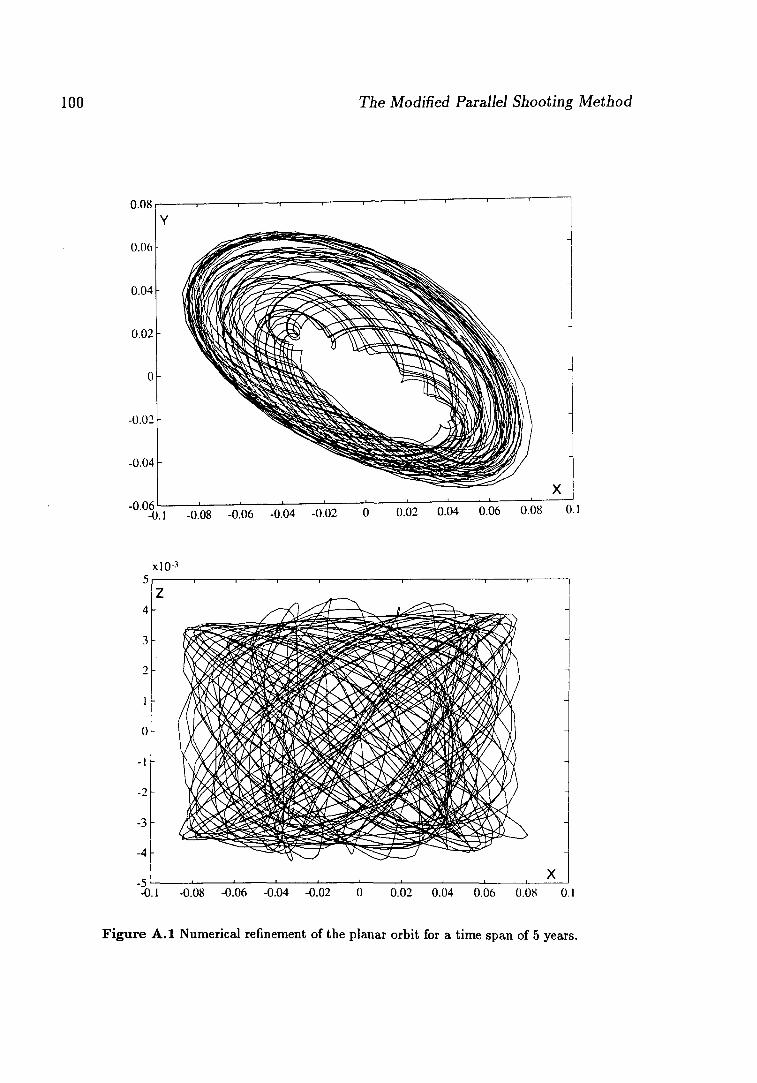
100 The Modified Parallel Shooting Method
0.08
0.06
0.04
0.02
-0.02
-0.04 -
- i r-
-0.06 0.1 -0.08 -0.06 -0.04 -0.02 0 0.02 0.04 0.06 0.08 0.1
xlO-3
0.08 -0.06 -0.04 -0.02 0 0.02 0.04 0.06 0.08 0.1
Figure A. l Numerical refinement of the planar orbit for a time span of 5 years.
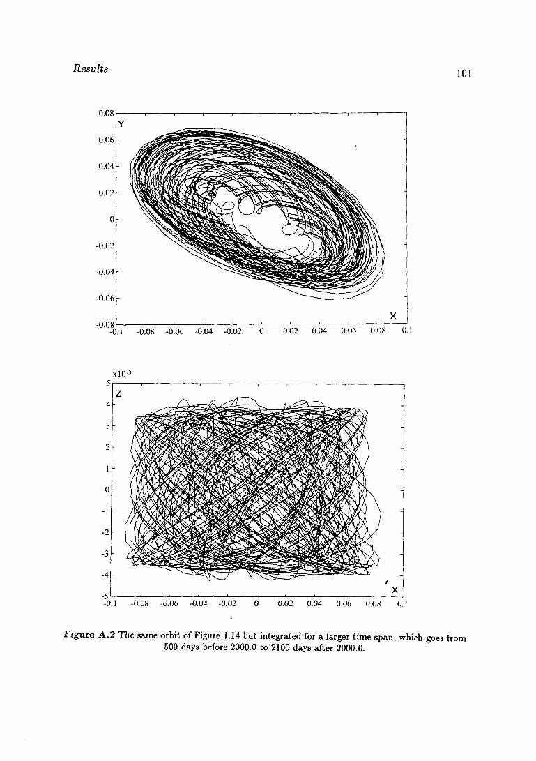
Results 101
-~Û.l -0.08 -0.06 -0.04 -0.02 0 0.02 0.04 0.06 0.08 0.1
xlO-3
Figure A .2 The same orbit of Figure 1.14 but integrated for a larger time span, which goes from 500 days before 2000.0 to 2100 days after 2000.0.
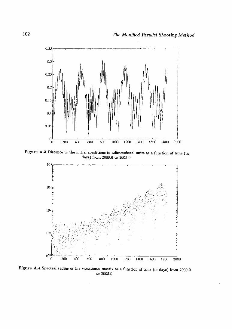
102 The Modified Parallel Shooting Method
0.35
0.25
0.15 •
0.05
0 200 400 600 800 1000 1200 1400 1600 1800 2000
Figure A.3 Distance to the initial conditions in adimensional units as a function of time (in days) from 2000.0 to 2005.0.
0 200 400 600 800 1000 1200 1400 1600 1800 2000
Figure A.4 Spectral radius of the variational matrix as a function of time (in days) from 2000.0 to 2005.0.
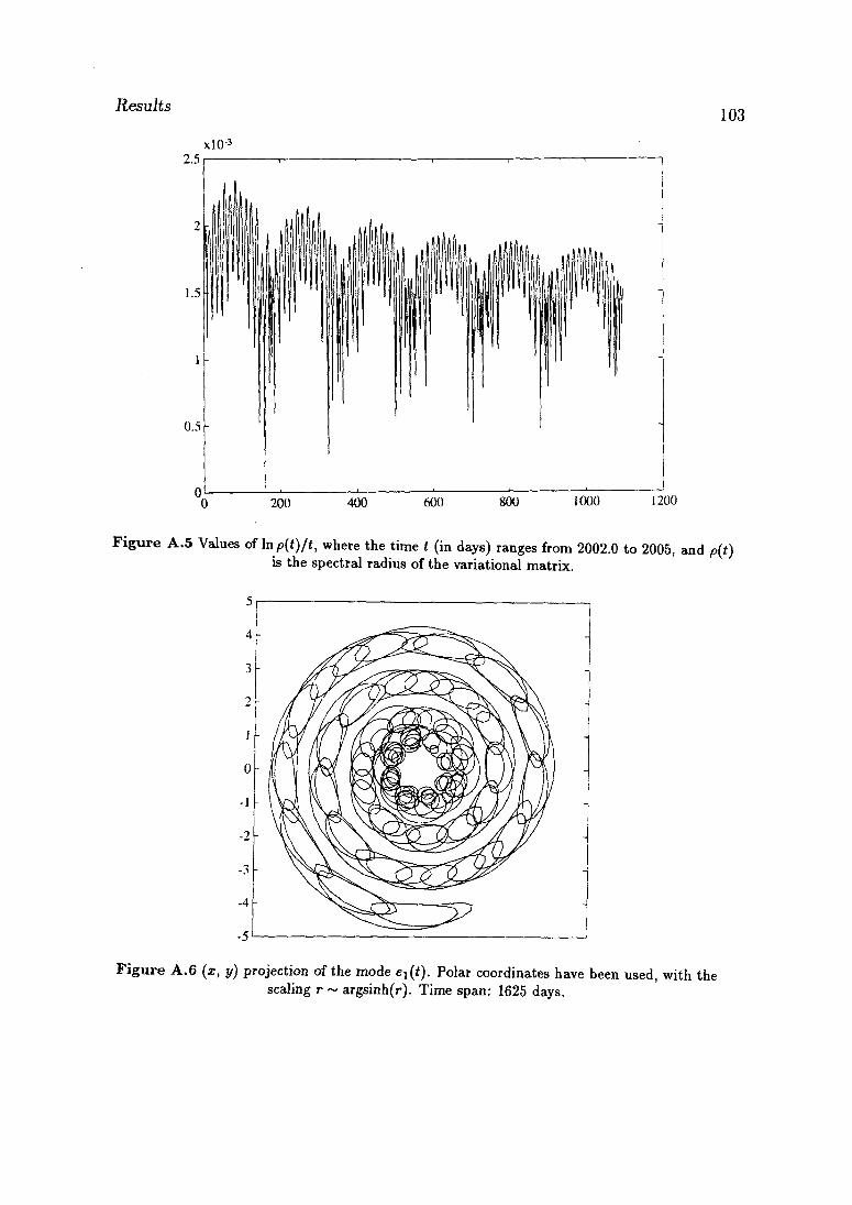
Results
xlO-3 2.51
°0 200 400 600 800 1000 1200
F igure A.5 Values of In p(t)/t, where the time t (in days) ranges from 2002.0 to 2005, and p{t) is the spectral radius of the variational matrix.
5
4
3
2
1
0
-1
_2
-3
-4
-5
F i g u r e A.6 (x, y) projection of the mode e^t). Polar coordinates have been used, with the scaling r ~ argsinh(r). Time span: 1625 days.
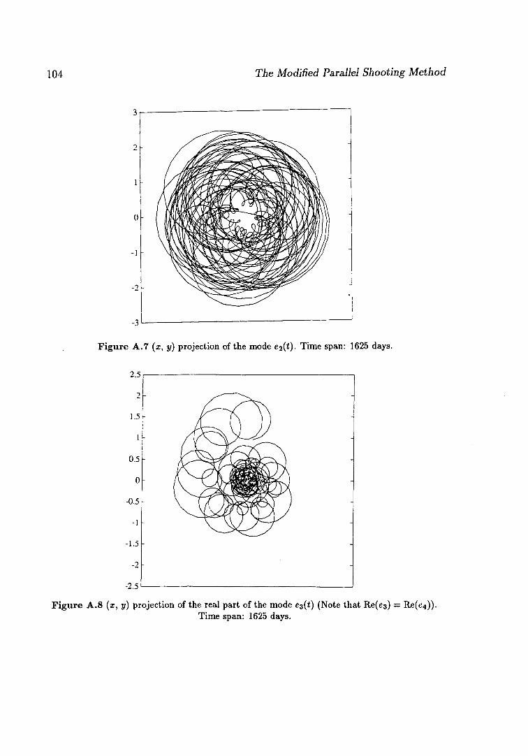
The Modified Parallel Shooting Method
.31 _ —
Figure A.7 (x, y) projection of the mode e^t). Time span: 1625 days.
2.5 r-
2 -
1.5 -
1 -
0.5 -
0 -
-0.5-
-1 -
-1.5 -
_2 -
- 2 . 5 -
ure A.8 (x, y) projection of the real part of the mode ez(t) (Note that Re(e3) = Re(e4)). Time span: 1625 days.
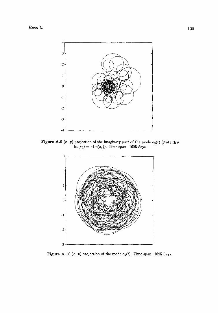
Results 105
Figure A.9 (x, y) projection of the imaginary part of the mode e3(i) (Note that Im(e3) = -Im(e4)). Time span: 1625 days.
Figure A.10 (x, y) projection of the mode e5(t). Time span: 1625 days.
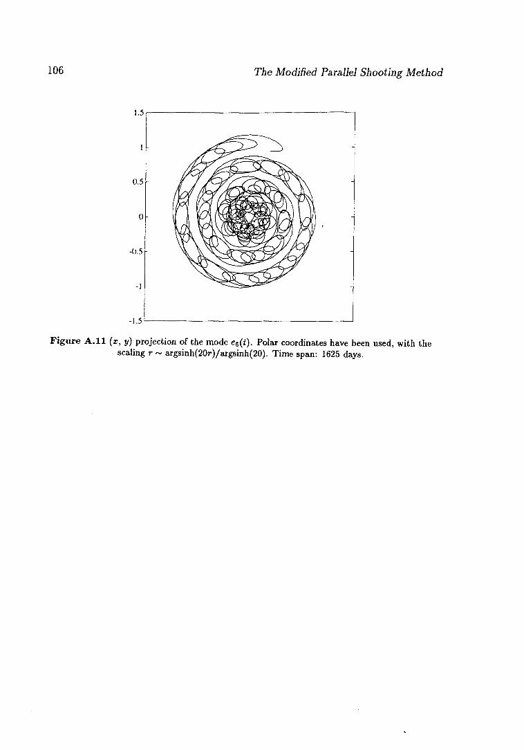
106 Tiie Modified Parallel Shooting Method
Figure A . l l (x, y) projection of the mode e6(i). Polar coordinates have been used, with the scaling r ~ argsinh(20r)/argsinh(20). Time span: 1625 days.
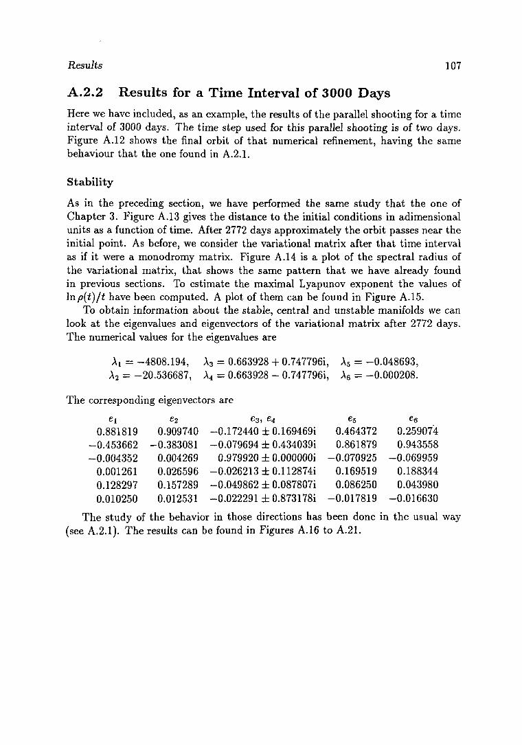
Results 107
A.2.2 Results for a Time Interval of 3000 Days
Here we have included, as an example, the results of the parallel shooting for a time interval of 3000 days. The time step used for this parallel shooting is of two days. Figure A. 12 shows the final orbit of that numerical refinement, having the same behaviour that the one found in A.2.1.
Stability
As in the preceding section, we have performed the same study that the one of Chapter 3. Figure A. 13 gives the distance to the initial conditions in adimensional units as a function of time. After 2772 days approximately the orbit passes near the initial point. As before, we consider the variational matrix after that time interval as if it were a monodromy matrix. Figure A.14 is a plot of the spectral radius of the variational matrix, that shows the same pattern that we have already found in previous sections. To estimate the maximal Lyapunov exponent the values of In p(t)/t have been computed. A plot of them can be found in Figure A.15.
To obtain information about the stable, central and unstable manifolds we can look at the eigenvalues and eigenvectors of the variational matrix after 2772 days. The numerical values for the eigenvalues are
Ax = -4808.194, A3 = 0.663928 + 0.747796Í, A5 = -0.048693, A2 = -20.536687, A4 = 0.663928 - 0.747796Í, A6 = -0.000208.
The corresponding eigenvectors are
ei e2 e3, e4 e5 e6 0.881819 0.909740 -0.172440 ±0.169469i 0.464372 0.259074
-0.453662 -0.383081 -0.079694 ± 0.434039Í 0.861879 0.943558 -0.004352 0.004269 0.979920 ± O.OOOOOOi -0.070925 -0.069959
0.001261 0.026596 -0.026213 ±0.112874i 0.169519 0.188344 0.128297 0.157289 -0.049862 ± 0.087807Í 0.086250 0.043980 0.010250 0.012531 -0.022291 ± 0.873178i -0.017819 -0.016630
The study of the behavior in those directions has been done in the usual way (see A.2.1). The results can be found in Figures A.16 to A.21.
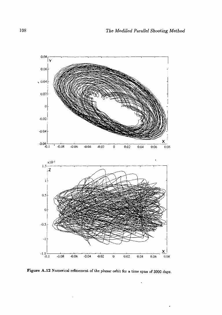
108 The Modified Parallel Shooting Method
0.08
s 0.04
Ö.1 ' -0.08 -0.06 -0.04 -0.02 0 0.02 0.04 0.06 0.08
xl0-:
-0.5
-0.08 -0.06 -0.04 -0.02 0.02 0.04 0.06 0.08
Figure A.12 Numerical refinement of the planar orbit for a time span of 3000 days.
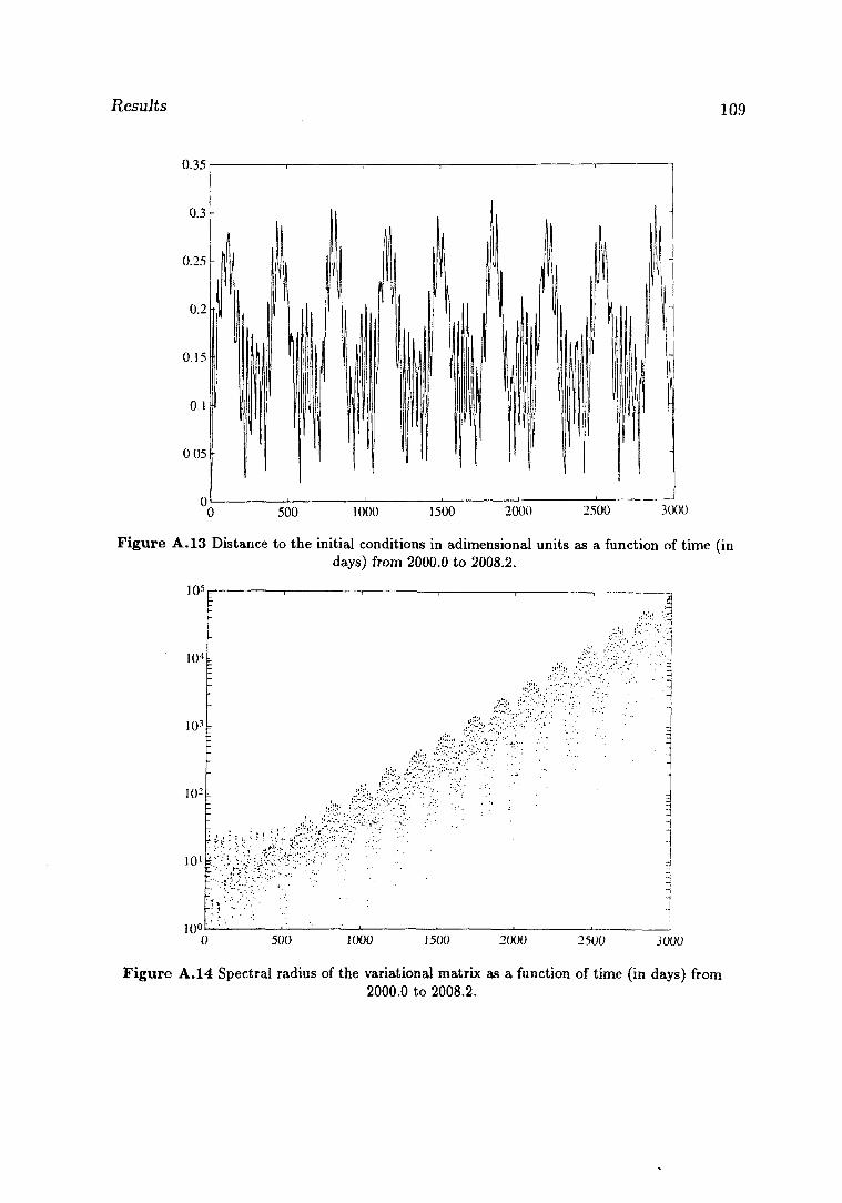
Results 109
0.35
0.25-
0.15
0.05
3000
Figure A.13 Distance to the initial conditions in adimensional units as a function of time (in days) from 2000.0 to 2008.2.
105
10"
10-
101
W°l
0
. >£*•,>:;•:;•••,•.;,
500 1000 1500 2000 2500 3000
Figure A.14 Spectral radius of the variational matrix as a function of time (in days) from 2000.0 to 2008.2.
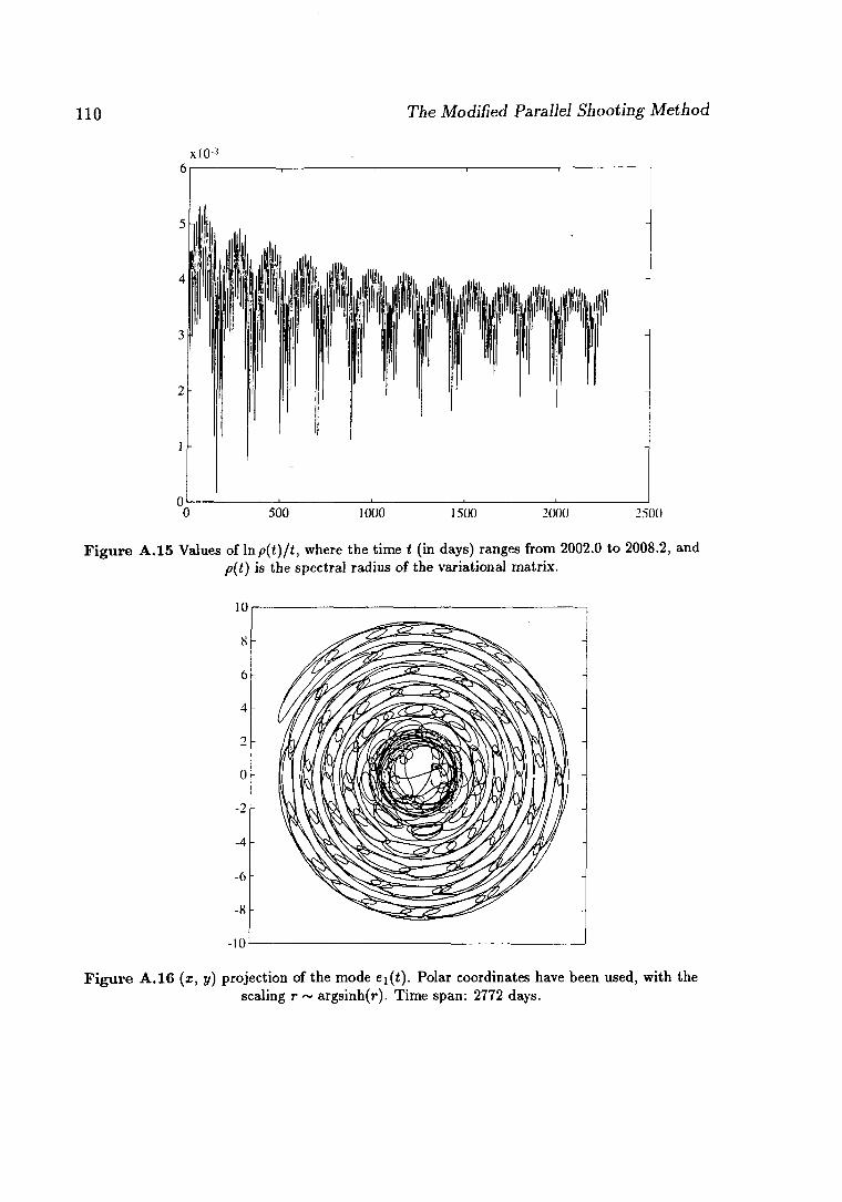
110 The Modified Parallel Shooting Method
Xl0-3
2500
Figure A.15 Values of In p(t)/t, where the time t (in days) ranges from 2002.0 to 2008.2, and p(t) is the spectral radius of the variational matrix.
Figure A.16 (x, y) projection of the mode ej(i). Polar coordinates have been used, with the scaling r ~ argsinh(r). Time span: 2772 days.
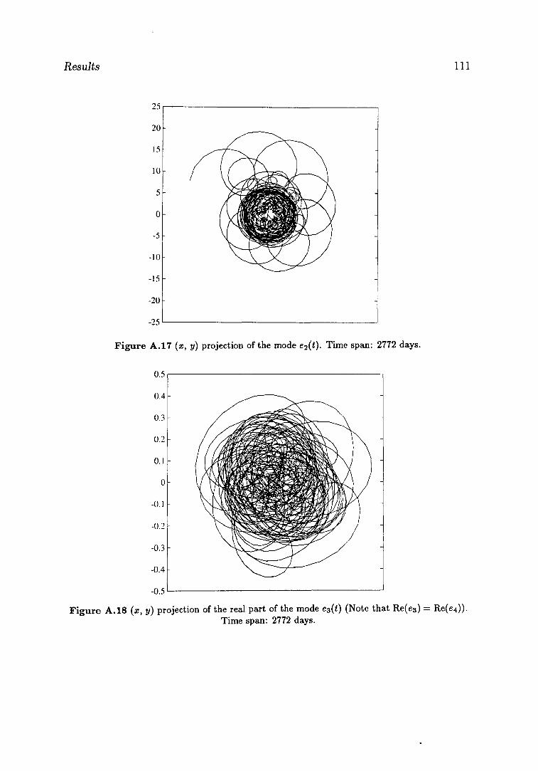
Results 111
Figure A.17 (x, y) projection of the mode e2(<)- Time span: 2772 days.
Figure A.18 (x, y) projection of the real part of the mode e3(t) (Note that Re(e3) = Re(e4)). Time span: 2772 days.
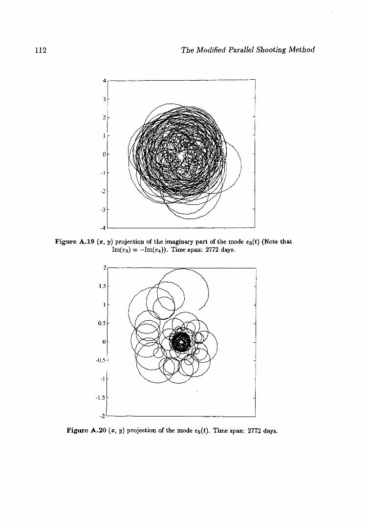
112 The Modified Parallel Shooting Method
Figure A.19 (x, y) projection of the imaginary part of the mode 63(f) (Note that Im(e3) = —Im(e4)). Time span: 2772 days.
Figure A.20 (x, y) projection of the mode e5(t). Time span: 2772 days.
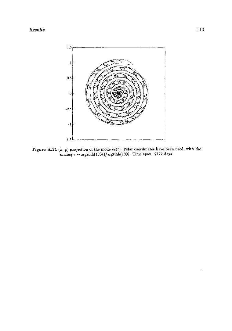
Results 113
-1.5
Figure A.21 (x, y) projection of the mode e6(i). Polar coordinates have been used, with the scaling r ~ argsinh(100r)/argsinh(100). Time span: 2772 days.

114 The Modified Parallel Shooting Method
Related Documents


