On positive semidefinite modification schemes for incomplete Cholesky factorization

On positive semidefinite modification schemes for incomplete

Cholesky factorization

Jennifer Scott1 and Miroslav Tuma2

ABSTRACT

Incomplete Cholesky factorizations have long been important as preconditioners for use in solving large-

scale symmetric positive-definite linear systems. In this paper, we present a brief historical overview of

the work that has been done over the last fifty years, highlighting key discoveries and rediscoveries. We

focus in particular on the relationship between two important positive semidefinite modification schemes,

namely that of Jennings and Malik and that of Tismenetsky. We present a novel view of their relationship

and implement them in combination with a limited memory approach. We explore their effectiveness

using extensive numerical experiments involving a large set of test problems arising from a wide range

of practical applications. The experiments are used to isolate the effects of semidefinite modifications to

enable their usefulness in the development of robust algebraic incomplete factorization preconditioners

to be assessed. We show that we are able to compute sparse incomplete factors that provide robust,

general-purpose preconditioners.

Keywords: sparse matrices, sparse linear systems, positive-definite symmetric systems, iterative solvers,

preconditioning, incomplete Cholesky factorization.

AMS(MOS) subject classifications: 65F05, 65F50

1 Computational Science and Engineering Department, Rutherford Appleton Laboratory, Harwell Oxford,

Oxfordshire, OX11 0QX, UK.

Correspondence to: [email protected]

Supported by EPSRC grant EP/I013067/1.

2 Institute of Computer Science, Academy of Sciences of the Czech Republic.

Partially supported by the Grant Agency of the Czech Republic Project No. P201/13-06684 S. Travel

support from the Academy of Sciences of the Czech Republic is also acknowledged.

April 18, 2013

1 Introduction

Iterative methods are widely used for the solution of large sparse symmetric linear systems of equations

Ax = b. To increase their robustness, the system matrix A generally needs to be transformed by

preconditioning. For positive-definite systems, an important class of preconditioners is represented by

incomplete Cholesky (IC) factorizations, that is, factorizations of the form LLT in which some of the fill

entries (entries that were zero in A) that would occur in a complete factorization are ignored. Over the last

fifty years, many different algorithms for computing incomplete factorizations have been proposed and they

have been used to solve problems from a wide range of application areas. In Section 2, we provide a brief

historical overview and highlight important developments and significant contributions in the field. Some

crucial ideas that relate to modifications and dropping are explained in greater detail in Section 3. Here

we consider two important semidefinite modification schemes that were introduced to avoid factorization

breakdown (that is, zero or negative pivots): that of Jennings and Malik [61, 62] from the mid 1970s and

that of Tismenetsky [109] from the early 1990s. Variations of the Jennings-Malik scheme were adopted

by engineering communities and it is recommended in, for example, [92] and used in experiments in [11]

to solve hard problems, including the analysis of structures and shape optimization. The Tismenetsky

approach has also been used to provide a robust preconditioner for some real-world problems, see, for

example, [4, 9, 77, 78]. However, in his authoritative survey paper [10], Benzi remarks that Tismenetsky’s

idea “has unfortunately attracted surprisingly little attention”. Benzi also highlights a serious drawback

of the scheme which is that its memory requirements can be prohibitively large (in some cases, more than

70 per cent of the storage required for a complete Cholesky factorization is needed, see also [12]). We seek

to gain a better understanding of the Jennings-Malik and Tismenetsky semidefinite modifications schemes

and to explore the relationship between them. Our main contribution in Section 3 is new theoretical

results that compare the 2-norms of the modifications to A that each approach makes. Then, in Section 4,

we propose a memory-efficient variant of the Tismenetsky approach, optionally combined with the use of

drop tolerances and the Jennings-Malik modifications to reduce factorization breakdowns. In Section 5, we

report on extensive numerical experiments in which we aim to isolate the effects of the modifications so as

to assess their usefulness in the development of robust algebraic incomplete factorization preconditioners.

Finally, we draw some conclusions in Section 6.

2 Historical overview

The rapid development of computational tools in the second half of the 20th century significantly pushed

forward progress in solving systems of linear algebraic equations. Both software and hardware tools

helped to solve still larger and more challenging problems from a wide range of engineering and scientific

applications. This further motivated research into the development of improved algorithms and better

understanding of their theoretical properties and practical limitations. In particular, within a very short

period, important seminal papers were published by Hestenes and Stiefel [51] and Lanczos [74], on which

most contemporary iterative solvers are based. The work of Householder and others in the 1950’s and

early 1960’s on factorization approaches to matrix computations substantially changed the field (see [53]).

Around the same time (and not long after Turing coined the term preconditioning in [111]), another set of

important contributions led to the rapid development of sparse direct methods [93] and preconditioning

of iterative methods by incomplete factorizations.

In this paper, we consider preconditioning techniques based on incomplete factorizations that belong

to the group of algebraically constructed techniques. To better understand contemporary forms of these

methods and the challenges they face, it is instructive to summarize key milestones in their development.

Here we follow basic algorithms without mentioning additional enhancements, such as block strategies,

algorithms developed for parallel processing or for use within domain factorization or a multilevel

framework. We also omit the pivoting techniques based on computing some auxiliary criteria for the

factorization (like minimum discard strategy), mentioning them only when needed for modifying dropping

1

strategies. We concentrate on incomplete factorizations of symmetric positive-definite systems. Since some

of the related ideas have been developed in the more general framework of incomplete LU factorizations

for preconditioning non symmetric systems, we will refer to them as appropriate.

2.1 Early days motivated by partial differential equations

The development of incomplete factorizations closely accompanies progress in the derivation of new

computational schemes, especially for partial differential equations (PDEs) that still often motivate simple

theoretical ideas as well as attempts to achieve fast and robust implementations, even when the incomplete

factorizations are computed completely algebraically. Whilst there is a general acceptance that the solution

of some discretized PDEs requires the use of physics-based or functional space-based preconditioners, the

need for reliable incomplete factorizations is widespread. They can be used not only as stand-alone

procedures but they are also useful in solving augmented systems, smoothing intergrid transformations

and solving coarse grid systems.

The earliest incomplete factorizations were described independently by several researchers. In the

late 1950s, in a series of papers [20, 21] (see also [22]), Buleev proposed a novel way to solve systems of

linear equations arising from two- and three-dimensional elliptic equations that had been discretized by

the method of finite differences using five- and seven-point stencils, respectively. Buleev’s approach was to

extend the sweep method for solving the difference equations from the one-dimensional case. To do this

efficiently, he modified the system matrix so that it could be expressed in the form of a scaled product

of two triangular matrices. In contemporary terminology, these two matrices represent an incomplete

factorization.

A slightly different and more algebraic approach to deriving an incomplete factorization can be found

in the work of Oliphant [89] in the early 1960s. Starting from a PDE model of steady-state diffusion, he

obtained the incomplete factorization of a matrix A corresponding to the five-point stencil discretization

by neglecting the fill-in during the factorization that occurs in sub-diagonal positions. An independent

algebraic derivation of the methods of Buleev and Oliphant and their interpretation as instances of

incomplete factorizations was given by Varga [115]. Varga also discussed the convergence properties of the

splitting using the concept of regular splitting, and mentioned a generalization to the nine-point stencil.

Solving pentadiagonal systems from two-dimensional discretizations of PDEs motivated the development

of another incomplete factorization that forms a crucial part of the sophisticated iterative method called

the strongly implicit (SIP) method [107]. This connects a stationary iterative method with a specific

incomplete factorization; a nice explanation is given in [8]. In specialized applications, the SIP method

remains popular (see also its symmetric version [2]).

Subsequent developments included experiments with incomplete factorizations with additional

functionality that later led to heavily parametrized procedures and included even more general stencils

arising from finite differences. They were often individually modified to solve specific types of equations

and boundary conditions. The fact that around that time the iterative methods for solving linear systems

were dominantly based on stationary schemes probably led to the detailed algorithms that sometimes

changed at individual steps of the iterative procedure [101]. An overview of the early and often very

specialized procedures and the motivations behind them may be found in [58, 59].

As a consequence of the simple stencils used by finite-difference discretizations, early incomplete

factorizations were based on prescribed sparsity patterns composed of a small number of sub-diagonals and

thus were precursors of the class of structure-based incomplete factorizations. The simplest and earliest

procedures proposed the same sparsity pattern for the preconditioner L as that of the system matrix

A. For symmetric positive-definite systems, this type of incomplete Cholesky factorization is denoted by

IC(0). Later, more general preconditioners included additional sub-diagonals in the sparsity pattern of

L [37] (the efficiency of such modifications is discussed in, for example, [38]). Early classifications were

based on counting the number of additional sub-diagonals of non zeros that were not present in A [83]

(see also [84]). Progress in deriving more general preconditioners was supported by an increased number

of papers describing the incomplete factorizations using modern matrix terminology [8]. There was also

2

an increased interest in factorizations of more general matrices arising in the numerical solution of PDEs,

for example M -matrices and H-matrices [39].

2.2 Modifications to enhance convergence

This progress brought about the question of convergence of sometimes rather complicated iterative schemes.

Dupont, Kendall and Rachford [33] (see also [32]) made an important contribution in this direction

and gave some of the earliest theoretical convergence rate results. Still considering specific underlying

PDE models with specific boundary conditions and their finite-difference discretizations, the authors

proposed a diagonal perturbation of the incomplete factorization and showed that this implies a decrease

in the conditioning of the preconditioned system. Subsequent research led to the further development of

modified incomplete Cholesky (MIC) factorizations involving explicitly modifying the diagonal entries of

the preconditioner using the discarded entries [44, 45, 46, 47, 48] (see also [49] and [99]). For specific PDEs,

this diagonal compensation typically leads to substantially improved convergence of the preconditioned

iterative method. Thus the motivation to develop modified factorizations was connected to the fact that

the convergence for model problems can be roughly estimated in terms of the decrease in the condition

number of the preconditioned system matrix. Here the requirement that the modified matrix is a diagonally

dominant M -matrix plays a crucial role. Diagonal modification has become an important component

of incomplete factorizations for more general problems although, as we discuss later, there are other

motivations behind such modifications.

The next step in this direction was the development of relaxed incomplete Cholesky (RIC) factorizations

[6] (see also [23] and their algebraic generalizations [112, 113]). It is interesting to note that the question

of the need to perturb or modify the diagonal entries of the preconditioner was later considered and solved

in a number of practical cases within the elegant framework of the support theory [13] but the work on

these combinatorial preconditioners is outside the scope of this overview. Observe that modified incomplete

factorizations can be considered as constraint factorizations obtained by a sum condition (or perturbed sum

condition). That is, instead of throwing away the disallowed fill-ins in the factorization algorithm, the sum

of these entries is added to the diagonal of the same column. This diagonal compensation reduction may

be motivated by the physics of the underlying continuous problem. It can be generalized to a constraint

that involves the result of multiplication of the incomplete factor with another vector see, for instance, [5]

(also [57] and [104]). A nice example of the compensation strategy for the ILUT factorization of Saad [98]

(which we mention below) that takes into account the stability of the factors is given in [80].

2.3 Introduction of preconditioning for Krylov subspace methods

The real revolution in the practical use of algebraic preconditioning based on incomplete factorizations

came with the important 1977 paper of Meijerink and van der Vorst [82]. They recognized the potential of

incomplete factorizations as preconditioners for the conjugate gradient method. This paper also implied

an understanding of the crucial role of the separate computation of the incomplete factorization as well as

recognizing the possibility of prescribing the sparsity structure of the preconditioner by allowing additional

sub-diagonals. In this case, extending the sparsity structure in the construction of the preconditioner was

theoretically sound since the authors proved that the factorization is breakdown-free (that is, the diagonal

remains positive) for M -matrices; this property was later also proved for H-matrices [81, 116]. The paper

of Meijerink and van der Vorst also represents a turning point in the use of iterative methods. Although it

is difficult to make a general statement about how fast Krylov subspace-based iterative methods converge,

in general they converge much faster than classical iteration schemes and convergence takes place for a

much wider class of matrices [114]. Consequently, much of the later development since the late 1970s has

centered on Krylov subspace methods.

Shortly after the work of Meijerink and van der Vorst, Kershaw [69] showed that the incomplete

Cholesky factorization of a general symmetric positive-definite matrix from a laser fusion code can suffer

seriously from breakdowns. To complete the factorization in such cases, Kershaw locally replaced zero or

3

negative diagonal entries by a small positive number. This helped popularise incomplete factorizations,

although local modifications with no relation to the overall matrix can lead to large growth in the entries

and the subsequent Schur complements and hence to unstable preconditioners. A discussion of the possible

effects of local modifications for more general factorizations (and that can occur even in the symmetric

positive-definite case) can be found in [25]. Another notable feature of [69] was that dropping of small

off-diagonal entries was still restricted to prespecified parts of the matrix structure. Moreover, it was a

straightforward strategy to implement.

Manteuffel [81] proposed an alternative simple diagonal modification strategy to avoid breakdowns. He

introduced the notion of a shifted factorization, factorizing the diagonal shifted matrix A + αI for some

positive α (provided α is large enough, the incomplete factorization always exists). Diagonal shifts were

used in some implementations even before Manteuffel (see [86, 87]) and, although currently the only way

to find a suitable shift is by trial-and-error, provided an α can be found that is not too large, the approach

is surprisingly effective and remains well used (but see an interesting observation in [85] that a posteriori

post-processing may make the preconditioner less sensitive to the actual choice of the shift value). Note

that in some application papers, in particular structural engineering, shifting is sometimes replaced by

scaling the off-diagonal entries (see, for example, [63, 64, 70, 75]).

2.4 The use of drop tolerances

Another significant breakthrough in the field of incomplete factorizations was the adoption of strategies

to drop entries in the factor by magnitude, according to a threshold or drop tolerance parameter τ , rather

than dropping entries because they lie outside a chosen sparsity pattern. This type of dropping was

introduced back in the early 1970s by Tuff and Jennings [110], long before any systematic attack on the

problem of breakdowns, that is, before modified incomplete factorizations, shifted factorizations or other

techniques were introduced. Absolute dropping can be used (all entries of magnitude less τ are dropped),

or relative dropping (entries smaller than τ multiplied by some quantity chosen to reflect matrix scaling

or possible growth in the factor entries). The original strategy in [110] was to drop entries that were small

in magnitude compared to the diagonal entries of the system. The resulting factorization was used to

precondition a stationary method. However, the experiments of Tuff and Jennings did not face breakdown

problems since they dealt with M -matrices.

A few years later, Jennings and Malik [61, 62], (see also [96]) introduced a modification strategy

to prevent factorization breakdown for symmetric positive-definite matrices arising from structural

engineering. They were motivated only by the need to compute a preconditioner without breakdown

and not by any consideration of the conditioning of the preconditioned system. Their work, which we

discuss in greater detail in Section 3, was extended by Ajiz and Jennings [1], who discussed dropping

(rejection) strategies as well as implementation details. In fact, once the dropping strategies became

sufficiently general, implementations that addressed memory and efficiency issues became very important.

With dropping by magnitude, a possible solution for the memory limitations was the choice of a static

chunk of memory for the computed preconditioner. Fast implementations using left-looking updates were

later developed that exploited research aimed at efficient sparse direct solvers [35, 36]. New algorithmic

and implementation schemes that were able to accept arbitrary fill-in entries were proposed in [7] (see also

[86, 87], and the detailed experimental results in [90] where data structures from the direct solver MA28

[30] from the HSL software library [54] were used).

2.5 The use of prescribed memory

When dropping by magnitude, the question of how to get better preconditioners and to increase their

robustness appears straightforward: intuitively, the dropping of small entries is more likely to produce a

better quality preconditioner than the dropping of larger entries [100]. That is, a smaller drop tolerance τ

may produce a better quality incomplete factorization, measured by the iteration count of a preconditioned

Krylov subspace method. This approach may also work when dropping is determined by the sparsity

4

pattern. In his paper [48], Gustafson used the terminology that a preconditioner is more accurate if its

structure is a superset of another preconditioner sparsity structure; as an example of a similar conclusion

in a specific application, see [91]. But this feature, which may be called the dropping inclusion property,

although often valid when solving simple problems, can be very far from reality for tougher problems. Also,

improvements in robustness through extending the preconditioner structure by adding simple patterns or

by reducing the drop tolerance have their limitations and, importantly, for algebraic preconditioning, do

not address the problem of memory consumption. A strategy that appeared in the historical development

and that solves this problem is simply to prescribe the maximum number of entries in each column of the

incomplete factor, retaining only the largest entries. In this case, the dropping inclusion property is often

satisfied, that is, by increasing the maximum number of entries, a higher quality preconditioner is obtained.

This strategy appears to have been proposed first in 1983 by Axelsson and Munksgaard [7]. It enabled

them to significantly simplify their right-looking implementation just because it allowed simple bounds on

the amount of memory needed for the factorization. They also mentioned dynamic changes in the value of

the drop tolerance parameter, a problem that was introduced and studied by Munksgaard [87]. He tried

to get the “fill-in curve” close to that of the exact factorization by changing the drop tolerance parameter.

Axelsson and Munksgaard also proposed exploiting memory saved in some factorization steps in the case

where some columns retained fewer than the maximum number of allowed entries. Dropping based on

a prescribed upper bound for the largest number of entries in a column of the factor combined with an

efficient strategy to keep track of left-looking updates was implemented in a successful and influential

incomplete factorization code by Jones and Plassman [65, 66]. They retained the nj largest entries in the

strictly lower triangular part of the j−th column of the factor, where nj is the number of entries in the

j−th column of the strictly lower triangular part of A. The code has predictable memory demands and

uses the strategy of applying a global diagonal shift from [81] to increase its robustness.

The combination of dropping by magnitude with bounding the number of entries in a column was

first proposed in [40] but a very popular concept that has predictable storage requirements is the dual

threshold ILUT (p, τ) factorization of Saad [98]. This paper has achieved significant attention not only

from the numerical linear algebra community but from much further afield. A drop tolerance τ is used to

discard all entries in the computed factors that are smaller than τl, where τl is the product of τ times the

l2-norm of the l−th row of A. Additionally, only the p largest entries in each column of L and row of U

are retained. The beauty of this approach is that it not only combines the use of a drop tolerance with

the strategy of prescribed maximum column and row counts, it also offers a new row-wise implementation

(in the non symmetric case) that has become widely used. However, it ignores symmetry in A and, if A

is symmetric, the sparsity patterns of L and UT are normally be different.

One of the best implementations of incomplete Cholesky factorization covering a number of the features

we have outlined is the ICFS code of Lin and More [76]. They aim to exploit the best features of the

Jones and Plassmann factorization and the ILUT (p, τ) factorization of Saad, adding an efficient loop for

changing the Manteuffel diagonal shift α and l2-norm based scaling. Their approach retains the nj + p

largest entries in the lower triangular part of the j−th column of L and uses only memory as the criterion

for dropping entries (thus having both the advantage and disadvantage of not requiring a drop tolerance).

Reported results for large-scale trust region subproblems indicate that allowing additional memory can

substantially improve performance on difficult problems. A lot of the contemporary application papers

in fact profit from the basic building blocks of incomplete factorizations sketched here, see, for instance,

[24, 73, 97].

2.6 The level-based approach

Despite all the achievements and progress discussed so far, the problem of robustness for harder problems

remains a challenging issue. In fact, simply prescribing the number of factor entries, using a drop tolerance

and/or a memory-based criteria, may result in a loss of the structural information stored in the matrix.

This led to a line of development that partially mimics the way in which the pattern of A is developed

during the complete factorization; such a strategy is called a level-based approach and was introduced by

5

Watts for general problems in 1981 [121]. During a symbolic factorization phase, each potential fill entry is

assigned a level and an entry is only permitted in the factor if its level is at most `. The notation IC(`) for

the incomplete Cholesky factorization (or, for general systems, ILU(`)) employing the concept of levels of

fill is commonplace. Nevertheless, relying solely on the sparsity pattern may bring another disadvantage.

While entries of the error matrix A − LLT are zero inside the prescribed sparsity pattern, outside they

can be very large, and the pattern of IC(`) (even for large `) may not guarantee that L is a useful

preconditioner, see [31]. Note that the error can be particularly large for matrices in which the entries

do not decay significantly with distance from the diagonal. Furthermore, it was soon understood that

although IC(1) can be a significant improvement over IC(0) (that is, an appropriate iterative method

preconditioned using IC(1) generally requires fewer iterations to achieve the requested accuracy than

IC(0)), the fill-in resulting from increasing ` can be prohibitive in terms of both storage requirements

and the time to compute and then apply the preconditioner. Further and importantly, until relatively

recently it was not clear how the structure of the incomplete factors could be computed efficiently for

larger `. A significant advancement to remove this second drawback came with the 2002 paper of Hysom

and Pothen [56] (see also [55]). They describe the relationship between level-based factorizations and

lengths of fill paths and propose a fast method of efficiently computing the sparsity pattern of IC(`) (and

ILU(`)) factorizations, opening the way to the further development of structure-based preconditioners.

The effectiveness of level-based preconditioners in the context of a Newton-Krylov method was shown in

[14, 94] while that of block level-based preconditioners is illustrated in [50]. However, the problem that

level-based methods can lead to relatively dense (and hence expensive) factorizations remains.

2.7 The development of complex dropping strategies

Imposing additional aims on the incomplete factorization can lead to the use of complex dropping

rules. For example, incomplete factorizations that aim to take advantage of high-performance computer

architectures and to use supernodes may motivate the use of new dropping strategies, as in [79] (see

also [41, 42] for an extensive set of numerical experiments). Supernodal construction may also influence

level-based preconditioners [50]. Similarly, additional features of the computational environment can feed

further characteristics of the computational model into the incomplete factorizations via optimized local

approximations, as in [3, 43] and the references therein. However, although the fact that the size of the

overall numerical perturbation caused by dropping entries from the factorization is very important was

mentioned back in the late 1980s by Duff and Meurant [31], dropping strategies typically do not take into

account the overall numerical perturbation caused by updates to the sequence of the incomplete Schur

complements.

While we believe that dropping rules should be as transparent as possible, we also hold that the

future challenge in the development of such strategies lies in coupling them with numerical properties

of the factorization. A step in this direction is the approach of Bollhofer and Saad [15, 16, 17]. Here

the dropping is relative to the estimated norms of the rows and columns of the factors of the inverse

matrix. It has been shown both theoretically and experimentally that this approach yields very reliable

preconditioners. Extended dropping of this kind that mutually balances sparse direct and inverse factors

has been introduced recently by Bru, Marın, Mas, and Tuma [18] (see also their comparison of incomplete

factorization schemes [19]).

Useful bounds on the condition number of the preconditioned system, as required to estimate the

convergence rate of iterative methods, may be derived in the case of special restricted dropping strategies,

such as in the analysis of orthogonal dropping given in [88]. A similar challenge is determining a threshold

such that computed entries that are smaller than it can be safely neglected since they would not play

any role anyway because of the errors committed in computing the factorization, in particular, because of

conditioning of intermediate quantities. Such analysis was introduced for inverse incomplete factorizations

in [72], partially based on the analysis from [71]. The analysis given in [72] leads naturally to theoretically

motivated adaptive dropping and an open problem is to propose such a strategy for incomplete Cholesky

factorizations.

6

2.8 Final remarks

Our historical excursion into incomplete factorizations has been devoted to the main lines of development.

It was also intended to show the complex relation of the ideas with their implementations. Progress was

made as well as limited by the development of suitable data structures and efficient implementations.

New ideas sometimes appeared once computational support was available. There have been attempts to

combine the advantages offered by different classes of incomplete factorizations. Combinations of threshold-

based methods and memory-based methods can be considered as somewhat natural, and they led, as we

have mentioned above, to the very successful ILUT implementation. There have also been attempts to

combine threshold-based methods and level-based methods. D’Azevedo, Forsyth, Tang [27] started to solve

the problem by combining the approach by levels with dropping by values. Another combination of these

two approaches targeted to reduce the sometimes prohibitive memory demand of level-based methods was

recently given in [102]. This latter approach exploited the idea that small entries should contribute to the

sparsity pattern of the preconditioner less than larger entries.

3 Positive semidefinite modification schemes

As discussed in Section 2, apart from dropping schemes, additional modifications to the incomplete

factorization approach were introduced over time. The motivations for these modifications were not

always the same; here we are primarily concerned with them from the point of view of preconditioner

robustness and performance predictability. We examine two important modification schemes designed to

avoid breakdown: that of Jennings and Malik [61, 62] and that of Tismenetsky [109]. Our objective is

to gain a better insight into them and then, using extensive numerical experiments in which we aim to

isolate the effects of the modifications (Section 5), to assess their usefulness in the development of robust

algebraic incomplete factorization preconditioners.

3.1 The Jennings-Malik scheme

The scheme proposed by Jennings and Malik [61, 62] can be interpreted as modifying the factorization

dynamically by adding to A simple symmetric positive semidefinite matrices, each having just four nonzero

entries. Although our software will use a left-looking implementation, for simplicity of explanation, we

consider here an equivalent right-looking approach: at each stage, we compute a column of the factorization

and then modify the subsequent Schur complement. For j = 1, we consider the matrix A and, for 1 < j < n,

we obtain the j−th Schur complement by applying the previous j − 1 updates and possible additional

modifications. Throughout our discussions, we denote the Schur complement of order n − j + 1 that is

computed on the j−th step by A and let Aj be the first column of A (corresponding to column j of A). The

j−th column of the incomplete factor L is obtained from Aj by dropping some of its entries (for example,

using a drop tolerance or the sparsity pattern). The Jennings-Malik diagonal compensation scheme

modifies the corresponding diagonal entries every time an off-diagonal entry is discarded. Specifically,

if the nonzero entry aij of Aj is to be discarded, the Jennings-Malik scheme adds to A a modification (or

cancellation) matrix of the form

Eij = eieTi γ|aij |+ eje

Tj γ−1|aij | − eieTj aij − ejeTi aij , (3.1)

where γ =√aii/ajj . Here the indices i, j are global indices (that is, they relate to the original matrix A).

Eij has nonzero entries γ|aij | and γ−1|aij | in the ith and jth diagonal positions, respectively, and entry

−aij in the (i, j) and (j, i) positions. The scalar γ may be chosen to keep the same percentage change to

the diagonal entries aii and ajj that are being modified (see [1]). Alternatively, γ may be set to 1 (see

[52]) and this is what we employ in our numerical experiments (but see also the weighted strategy in [34]).

A so-called relaxed version of the form

E′ij = ωeieTi γ|aij |+ ωeje

Tj γ−1|aij | − eieTj aij − ejeTi aij , (3.2)

7

with 0 ≤ ω ≤ 1, was proposed by Hladik, Reed and Swoboda [52].

It is easy to see that the modification matrix Eij (and E′ij)is symmetric positive semidefinite. The

sequence of these dynamic changes leads to a breakdown-free factorization that can be expressed in the

form

A = LLT + E,

where L is the computed incomplete factor and E is a sum of positive semidefinite matrices with non-

positive off-diagonal entries and is thus positive semidefinite.

3.2 Tismenetsky scheme

The second modification scheme we wish to consider is that of Tismenetsky [109]. A matrix-based

formulation with significant improvements and theoretical foundations was later supplied by Kaporin [67].

The Tismenetsky scheme is based on a matrix decomposition of the form

A = LLT + LRT +RLT + E, (3.3)

where L is a lower triangular matrix with positive diagonal entries that is used for preconditioning, R is

a strictly lower triangular matrix with small entries that is used to stabilize the factorization process, and

E has the structure

E = RRT . (3.4)

As before, we refer to a right-looking implementation. Consider the j−th step as above and the first

column of the computed Schur complement Aj . It can be decomposed into a sum of two vectors each of

length n− j + 1

lj + rj ,

such that |lj |T |rj | = 0 (with the first entry in lj nonzero), where lj (respectively, rj) contains the entries that

are retained (respectively, not retained) in the incomplete factorization. At step j+ 1 of the factorization,

the Schur complement of order n − j is updated by subtracting the outer product of the pivot row and

column. That is, by subtracting

(lj + rj)(lj + rj)T .

The Tismenetsky incomplete factorization does not compute the full update as it does not subtract

Ej = rjrTj . (3.5)

Thus, the positive semidefinite modification Ej is implicitly added to A.

The obvious choice for rj (which was proposed in the original paper [109]) is the smallest off-diagonal

entries in the column (those that are smaller in magnitude than a chosen drop tolerance). Then in the

right-looking formulation, at each stage implicitly adding Ej is combined with the standard steps of

the Cholesky factorization, with entries dropped from the incomplete factor after the updates have been

applied to the Schur complement. The approach is naturally breakdown-free because the only modification

of the Schur complement that is used in the later steps of the factorization is the addition of the positive

semidefinite matrices Ej .

The fill in L can be controlled by choosing the drop tolerance to limit the size of |lj |. However,

it is important to note that this does not limit the memory required to compute L. A right-looking

implementation of a sparse factorization is generally very demanding from the point of view of memory as

it is necessary to store all the fill-in for column j until the modification is applied in the step j, as follows

from (3.5). Hence, a left-looking implementation (or, as in [67], an upward-looking implementation) might

be thought preferable. But to compute column Aj in a left-looking implementation and to apply the

modification (3.5) correctly, all the vectors lk and rk for k = 1, . . . , j − 1 have to be available. Therefore,

the dropped entries have to be stored throughout the left-looking factorization and the rk may only be

discarded once the factorization is finished (and similarly for an upward-looking implementation). These

8

vectors thus represent intermediate memory. Note the need for intermediate memory is caused not just by

the fill in the factorization: it is required because of the structure of the positive semidefinite modification

that forces the use of the rk. Sparsity allows some of the rk to be discarded before the factorization is

complete but essentially the total memory is as for a complete factorization, without the other tools that

direct methods offer. This memory problem was discussed by Kaporin [67], who proposed using two drop

tolerances τ1 > τ2. Only entries of magnitude at least τ1 are kept in L and entries smaller than τ2 are

dropped from R; the larger τ2 is, the closer the method becomes to that of Jennings and Malik. The error

matrix E then has the structure

E = RRT + F + FT ,

where F is a strictly lower triangular matrix that is not computed while R is used in the computation of

L but is then discarded.

When drop tolerances are used, the factorization is no longer guaranteed to be breakdown-free. To

avoid breakdown, diagonal compensation (as in the Jennings-Malik scheme) for the entries that are dropped

from R may be used. Kaporin coined the term second order incomplete Cholesky factorization to denote

this combined strategy (but note an earlier proposal of virtually the same strategy by Suarjana and Law

[108]).

Finally, consider again the left-looking implementation of the Jennings-Malik scheme where the column

Aj that is computed at stage j is based on the columns computed at the previous j − 1 stages. Standard

implementations perform the updates using the previous columns of L (without the dropped entries). But

the dropped entries may also be used in the computation and, if we do this, the only difference between

the Jennings-Malik and Tismenetsky schemes lies in the way in which the factorization is modified to

safeguard against breakdown.

3.3 Related research

A discussion of the Tismenetsky approach and a modification with results for finite-element modeling of

linear elasticity problems is given in [68]. In [122], Yamazaki et al use the Kaporin approach combined with

the global diagonal shift strategy of Manteuffel [81]. In contrast to Kaporin [67], who uses the upward-

looking factorization motivated by Saad [98], Yamazaki et al employ a left-looking implementation based

on the pointer strategy from Eisenstat et al [35, 36]; moreover, they do not compensate the diagonal entries

fully as in the Jennings-Malik strategy. There is an independent derivation of the Tismenetsky approach

for incomplete Cholesky factorizations in [120], which emphasizes the relation with the special case of

incomplete QR factorization (see also [117]). In fact, this variant of the incomplete QR factorization of

A in which there is no dropping in Q is equivalent to the Tismenetsky approach applied to ATA. For

completeness, note that a related incomplete QR factorization was introduced earlier by Jennings and

Ajiz [60]. From a theoretical point of view, the authors of [118, 119] show some additional structural

properties of this type of incomplete Cholesky factorization.

The Tismenetsky approach has been used to provide a robust preconditioner for some real-world

problems, see, for example, the comparison for tasks in linear elasticity in [4], emphasizing reduced

parametrization in the upward-looking implementation of Kaporin [67], diffusion equations in [77, 78] and

Stokes problem in [9]. We note, however, that there are no reported comparisons with other approaches

that take into account not only iteration counts but also the size of the preconditioner.

3.4 Some theoretical results

The importance of the size of the modifications to the matrix was emphasized by Duff and Meurant in [31].

In particular, the modifications should not be large in terms of the norm of the matrix. In this section, we

therefore consider the Jennings-Malik and Tismenetsky modifications from this point of view. We have

the following simple lemma for the size of the Jennings-Malik modification.

9

Lemma 3.1. The squared 2-norm of the modification in the Jennings-Malik approach based on the fill-in

entry aij and the update formula (3.1) is equal to

γ|aij |+ γ−1|aij |.

Proof: The modification (3.1) can be written as the outer product matrix

Eij = vvT ,

where v ∈ Rn has entries

vk =

γ1/2√a, if k = i

γ−1/2√a, if k = j

0, otherwise

where a = |aij |. The result follows from the fact that the 2-norm of vvT is equal to vT v. �

Turning to the Tismenetsky approach, let us denote the vector of nonzero entries in lj by lj with

|lj | = lsize and, similarly, denote the vector of nonzero entries in rj by rj with |rj | = rsize. Further,

assume that the entries in both these vectors are in descending order of their magnitudes and that the

magnitude of each entry in lj is at least as large as the magnitude of the largest entry in rj . We have the

following result.

Lemma 3.2. The squared 2-norm of the j−th modification in the Tismenetsky approach is equal to

(r1,j , ..., rrsize,j)(r1,j , ..., rrsize,j)T . (3.6)

It is natural to ask how these modifications are related. Setting the parameter γ = 1 in (3.1), the

two previous simple lemmas imply the following result, which surprisingly prefers the Jennings-Malik

modification if we consider just the norms of the modifications.

Theorem 3.1. Assume Aj has been computed and all but the lsize entries of largest magnitude are dropped

from column j of L. Then the 2-norm of the Jennings-Malik modification (3.1) that compensates for all

the dropped entries is not larger than the 2-norm of the Tismenetsky modification (3.5) corresponding to

the positive semidefinite update related to the remaining |Aj | − lsize ≡ rsize entries.

Proof: From Lemma 3.2, the squared 2-norm of the Tismenetsky modification is

rsize∑k=1

r2k,j .

Each of the modifications in the Jennings-Malik approach is of the form −rk,j rl,j for some 1 ≤ k, l ≤rsize, k 6= l. The sum of the squared 2-norms of these modifications is equal to the overall 2-norm of the

modifications and is, by Lemma 3.1 (with γ = 1), equal to

2 ∗∑

(k,l)∈Zj ,k<l

rk,j rl,j ,

where Zj denotes the set of pairs (i, j) of off-diagonal positions in Aj corresponding to dropped entries.

Sincersize∑k=1

r2k,j − 2 ∗∑

(k,l)∈Zj ,k<l

rk,j rl,j ≥ 0,

the result follows. �

When using the Jennings-Malik scheme, the number of modifications that must be performed at stage

j is equal to |Zj | ≤ (|Aj | − lsize)(|Aj | − lsize − 1)/2. Such a potentially large number of modifications

may result in the preconditioner being far from the original matrix (and hence of poor quality). Further,

10

the Tismenetsky modification in (3.5) does not take advantage of the entries in the matrix that do not

need to be modified (so that more modifications than are necessary may be performed). Incorporating

the Jennings-Malik approach on top of the Tismenetsky update may appear an obvious idea because it

can make the Tismenetsky update sparser. However, consider a simple 2 × 2 case where we add a rank-

one modification of the form (3.1) to a symmetric positive semidefinite submatrix that may represent the

update (3.6). We have the following negative result.

Lemma 3.3. Consider a 2× 2 positive semidefinite matrix A =

(a c

c b

)and its modification in the form

of the outer product E = vvT for vT = (√k,−√k), k > 0. When this update is applied, both eigenvalues

of A increase.

Proof: The eigenvalues of A are given by

λA1,2 = (a+ b±√D)/2,

where D = (a− b)2 + 4c2, and those of A+ E are

λA+E1,2 = (a+ b+ 2k ±

√D + 4k(k − 2c))/2.

It is easy to see that the minimum of λA+E1,2 with respect to k > 0 is obtained for k = c. For this minimum,

λA+E1,2 = (a+ b+ 2k)±

√D − 4k2, from which the result follows. �

Thus using the Tismenetsky approach and then the Jennings-Malik modification to nullify some off-

diagonal entries does not appear helpful. However, the two schemes can be combined differently. Indeed,

the new unified explanation of the Tismenetsky and Jennings-Malik modifications indicates two ideas that

we will report on in Section 5: (1) the norm of the matrix modification during the Tismenetsky update

can be decreased by including some entries of RRT and (2) the remaining off-diagonal entries of RRT

can be compensated for using the Jennings-Malik scheme. As we will see, the strategy that is the best

theoretically may not be the best when solving practical problems using limited memory.

3.5 A limited memory approach

For an algebraic preconditioner to be really practical it needs to have predictable and reasonable memory

demands. All previous implementations of the Tismenetsky-Kaporin approach known to us drop entries

based on their magnitude alone but this does not provide practical predictable memory demands. As in the

ICFS code of Lin and More [76], the memory predictability in our IC implementation depends on specifying

a parameter lsize that limits the maximum number of nonzero off-diagonal fill entries in each column of L.

In addition, we retain at most rsize entries in each column of R. At each step j of the factorization, the

candidate entries for inclusion in the j−th column of L are sorted and the largest nj + lsize off-diagonal

entries plus the diagonalare retained; the next rsize largest entries form the j−th column of R and all

other entries are discarded. Following Kaporin, the use drop tolerances can be included. In this case,

entries in L are retained only if they are at least τ1 in magnitude while those in R must be at least τ2.

3.6 Dynamic choice of factor size

An important consideration for any practical strategy for computing incomplete factorizations is limiting

the number of parameters that must be set by the user while still getting an acceptably robust

preconditioner. As we shall see in Section 5, we have observed in our numerical experiments that the

intermediate memory can, to some extent, replace the memory used for the preconditioner. In other

words, our experiments show that if the sum lsize + rsize = tsize is kept constant (and lsize is not too

small in relation to rsize), the performance of the preconditioner is maintained. Therefore, we could require

a single input parameter tsize and choose lsize and rsize internally. Consider stage j of the factorization

and the Tismenetsky update restricted to the submatrix determined by the first tsize components of the

11

column Aj (with the entries ak,j , j ≤ k ≤ n− j − 1, in Aj in descending order of their magnitudes). The

modification restricted to this submatrix is

(alsize+1,j , ..., atsize,j)T (alsize+1,j , ..., atsize,j),

where lsize is to be determined. Consequently, we have to find a splitting of tsize into lsize and rsize

such that the off-diagonal block

(alsize+1,j , ..., atsize,j)T (aj+1,j , ..., alsize,j)

is not small with respect to the “error” block

(alsize+1,j , ..., atsize,j)T (alsize+1,j , ..., atsize,j),

measured in a suitable norm. A possible strategy is to choose lsize such that

1/(lsize− j)lsize∑

k=j+1

|akj | ≥ β/(tsize− lsize)tsize∑

k=lsize+1

|akj |

for some modest choice of β ≥ 1 (that is, we compare the average magnitude of the first lsize− j entries

in the column with β times the average magnitude of the remaining entries). If there is no such lsize

(which occurs if there is insufficient “block diagonal dominance” in the column), lsize is set to tsize; if

there is reasonable diagonal dominance in L, lsize should be smaller than tsize. Such a strategy provides

a dynamic splitting of tsize since it is determined separately for each column of L. Using the following

result, lsize can be found by a simple search through Aj .

Lemma 3.4. The function f(j) defined as

1/(lsize− j)lsize∑

k=j+1

|akj | − β/(tsize− lsize)tsize∑

k=lsize+1

|akj |

is nondecreasing for j = 1, ..., n.

The proof follows from the fact that the nonzero entries in Aj are ordered in descending order of their

magnitudes. �

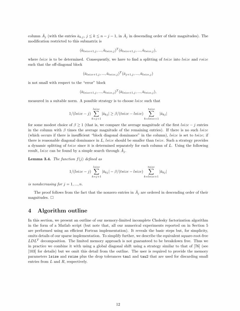
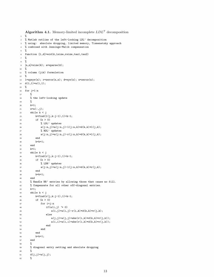
4 Algorithm outline

In this section, we present an outline of our memory-limited incomplete Cholesky factorization algorithm

in the form of a Matlab script (but note that, all our numerical experiments reported on in Section 5

are performed using an efficient Fortran implementation). It reveals the basic steps but, for simplicity,

omits details of our sparse implementation. To simplify further, we describe the equivalent square-root-free

LDLT decomposition. The limited memory approach is not guaranteed to be breakdown free. Thus we

in practice we combine it with using a global diagonal shift using a strategy similar to that of [76] (see

[103] for details) but we omit this detail from the outline. The user is required to provide the memory

parameters lsize and rsize plus the drop tolerances tau1 and tau2 that are used for discarding small

entries from L and R, respectively.

12

Algorithm 4.1. Memory-limited incomplete LDLT decomposition%1

% Matlab outline of the left-looking LDL’ decomposition2

% using: absolute dropping, limited memory, Tismenetsky approach3

% combined with Jennings-Malik compensation4

%5

function [l,d]=eid(A,lsize,rsize,tau1,tau2)6

%7

%8

[n,n]=size(A); a=sparse(A);9

%10

% column (jik) formulation11

%12

l=speye(n); r=zeros(n,n); d=eye(n); w=zeros(n);13

d(1,1)=a(1,1);14

%15

for j=1:n16

%17

% the left-looking update18

%19

k=1;20

w=a(:,j);21

while k < j22

k=find(l(j,k:j-1),1)+k-1;23

if (k > 0)24

% LDL’ updates25

a(j:n,j)=a(j:n,j)-l(j:n,k)*d(k,k)*l(j,k);26

% RDL’ updates27

a(j:n,j)=a(j:n,j)-r(j:n,k)*d(k,k)*l(j,k);28

end29

k=k+1;30

end31

k=1;32

while k < j33

k=find(r(j,k:j-1),1)+k-1;34

if (k > 0)35

% LDR’ updates36

a(j:n,j)=a(j:n,j)-l(j:n,k)*d(k,k)*r(j,k);37

end38

k=k+1;39

end40

% Handle RR’ entries by allowing those that cause no fill.41

% Compensate for all other off-diagonal entries.42

k=1;43

while k < j44

k=find(r(j,k:j-1),1)+k-1;45

if (k > 0)46

for i=j:n47

if(a(i,j) ~= 0)48

a(i,j)=a(i,j)-r(i,k)*d(k,k)*r(j,k);49

else50

a(j,j)=a(j,j)+abs(r(i,k)*d(k,k)*r(j,k));51

a(i,i)=a(i,i)+abs(r(i,k)*d(k,k)*r(j,k));52

end53

end54

end55

k=k+1;56

end57

%58

% diagonal entry setting and absolute dropping59

%60

d(j,j)=a(j,j);61

%62

13

% keep at most lsize largest off-diagonals in L(:,j)63

%64

if (j < n)65

v=a(j+1:n,j);66

[y,iy] = sort(abs(v),1,’descend’);67

end68

for i=j+1:n69

y(i-j)=v(iy(i-j));70

l(i,j)=0.0;71

end72

lmost=min(lsize,n-j);73

for i=1:lmost74

if (abs(y(i))/d(j,j) > tau1)75

l(j+iy(i),j)=y(i);76

end77

end78

%79

% keep at most rsize off-diagonals in R(:,j)80

%81

count=0; i=1;82

while (count < rsize & i <= n-j)83

if (abs(y(i))/d(j,j) > tau2)84

r(j+iy(i),j)=y(i);85

y(i)=0;86

count=count+1;87

end88

i=i+1;89

end90

%91

% Jennings-Malik compensation for all entries not in L or R92

%93

i=1;94

while (i < n-j)95

k=j+iy(i)96

if (abs(y(i)-w(k)) ~= 0 & w(k) == 0)97

a(k,k)=a(k,k)+abs(y(i));98

a(j,j)=a(j,j)+abs(y(i));99

end100

i=i+1;101

end102

%103

% scale the j-th column of L and of R104

%105

for i=j+1:n106

l(i,j)=l(i,j)/d(j,j);107

r(i,j)=r(i,j)/d(j,j);108

end109

l(j,j)=1;110

end111

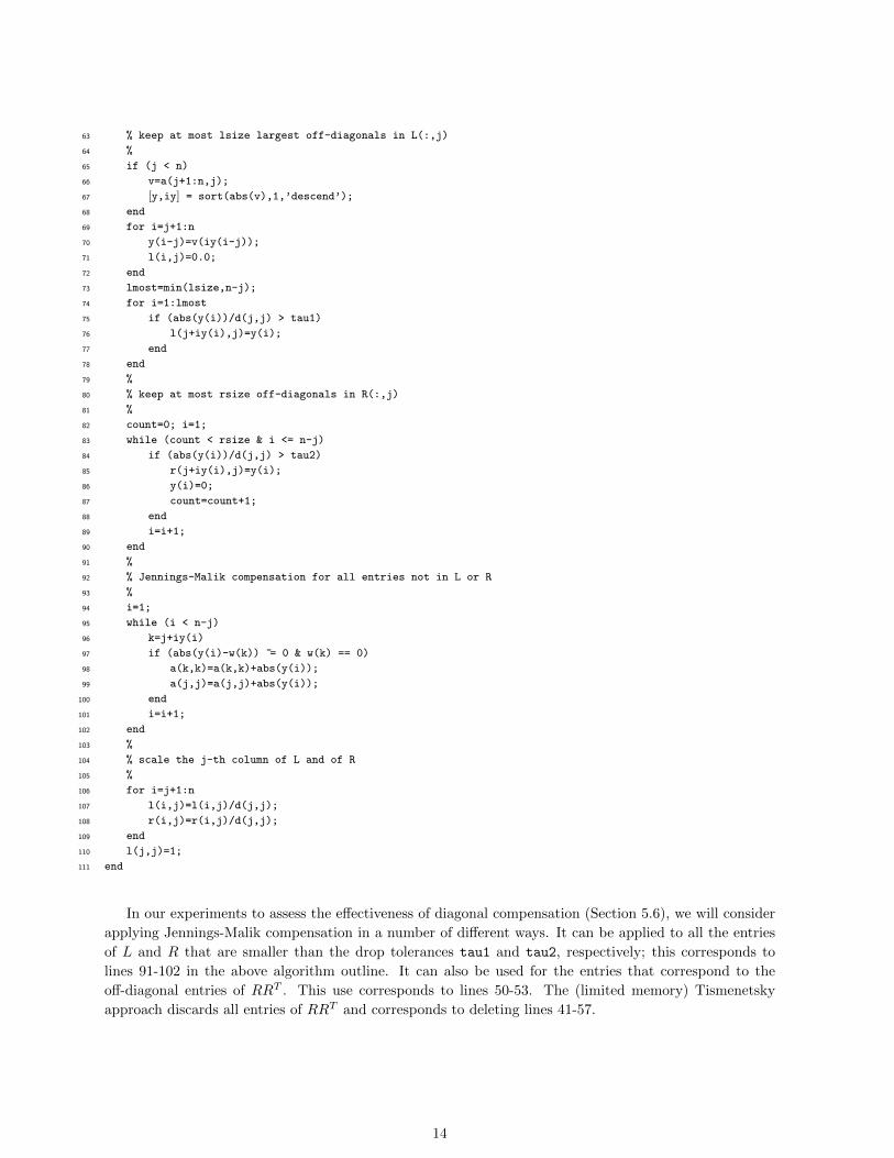
In our experiments to assess the effectiveness of diagonal compensation (Section 5.6), we will consider

applying Jennings-Malik compensation in a number of different ways. It can be applied to all the entries

of L and R that are smaller than the drop tolerances tau1 and tau2, respectively; this corresponds to

lines 91-102 in the above algorithm outline. It can also be used for the entries that correspond to the

off-diagonal entries of RRT . This use corresponds to lines 50-53. The (limited memory) Tismenetsky

approach discards all entries of RRT and corresponds to deleting lines 41-57.

14

5 Numerical experiments

5.1 Test environment

All the numerical results reported on in this paper are performed (in serial) on our test machine that has

two Intel Xeon E5620 processors with 24 GB of memory. Our software is written in Fortran and the ifort

Fortran compiler (version 12.0.0) with option -O3 is used. The implementation of the conjugate gradient

algorithm offered by the HSL routine MI22 is employed, with starting vector x0 = 0, the right-hand side

vector b computed so that the exact solution is x = 1, and stopping criteria

‖Ax− b‖2 ≤ 10−10‖b‖2, (5.1)

where x is the computed solution. In addition, for each test we impose a limit of 2000 iterations. In

all the tests, we order and scale the matrix A prior to computing the incomplete factorization. Based

on numerical experiments (see [103], we use a profile reduction ordering based on a variant of the Sloan

algorithm [95, 105, 106]. We also use l2 scaling, in which the entries in column j of A are normalised by

the 2-norm of column j; this scaling is chosen as it is used by Lin and More [76] in their ICFS incomplete

factorization code and it is inexpensive and simple to apply. Note that it is important to ensure the

matrix A is prescaled before the factorization process commences; other scalings are available and yield

comparable results but, if no scaling is used, the effectiveness of the incomplete factorization algorithms

used in this paper can significantly effected (see [103] for some results).

We define the iteration count for an incomplete factorization preconditioner for a given problem to be

the number of iterations required by the iterative method using the preconditioner to achieve the requested

accuracy and we define the preconditioner size to be the number of entries nz(L) in the incomplete factor

L.

While we are well aware that the number of entries in the preconditioner may increase but its

effectiveness decrease, in many practical situations, the mutual relation between the iteration count

and preconditioner size provides an important insight into the usefulness of an incomplete factorization

preconditioner if we assume that the following two important conditions are fulfilled:

1. the preconditioner is sufficiently robust with respect to changes to the parameters of the

decomposition, such as the limit on the number of entries in a column of L and of R;

2. the time required to compute the preconditioner grows slowly with the problem dimension n.

We define the efficiency of the preconditioner P to be

iter × nz(L), (5.2)

where iter is the iteration count for P = (LLT )−1 (see [102]). Assuming the IC preconditioners Pq =

(LqLTq )−1 (q = 1, . . . , r) each satisfy the above conditions, we say that, for solving a given problem, Pi is

themost efficient of the r preconditioners if

iteri × nz(Li) ≤ minq 6=i

(iterq × nz(Lq)). (5.3)

We use this measure of efficiency in our numerical experiments.

A weakness of this measure is that it does not taken into account the number of entries in R. We

anticipate that, with the number of entries in each column of L fixed, increasing the permitted number of

entries in each column of R will lead to a more efficient preconditioner. However, this improvement will

be at the cost of additional work in the construction of the preconditioner. Thus we record the time to

compute the preconditioner together with the time for convergence of the iterative method: the sum of

these will be referred to as the total time and will also be used to assess the quality of the preconditioner.

Note that in this study, a simple matrix-vector product routine is used with the lower triangular part of

15

A held in compressed sparse column format: we have not attempted to perform either the matrix-vector

products or the application of the preconditioner in parallel and all times are serial times.

Our test problems are real positive-definite matrices of order at least 1000 taken from the University

of Florida Sparse Matrix Collection [26]. Many papers on preconditioning techniques and iterative solvers

select a small set of test problems that are somehow felt to be representative of the applications of interest.

However, our interest is more general and we want to test the different ideas and approaches on as wide a

range of problems as we can. Thus we took all such problems and then discarded any that were diagonal

matrices and, where there was more than one problem with the same sparsity pattern, we chose only one

representative problem. This resulted in a test set of 153 problems of order up to 1.5 million. Following

initial experiments, 8 problems were removed from this set as we were unable to achieve convergence to

the required accuracy within our limit of 2000 iterations without allowing a large amount of fill. To assess

performance on our test set, we use performance profiles [29].

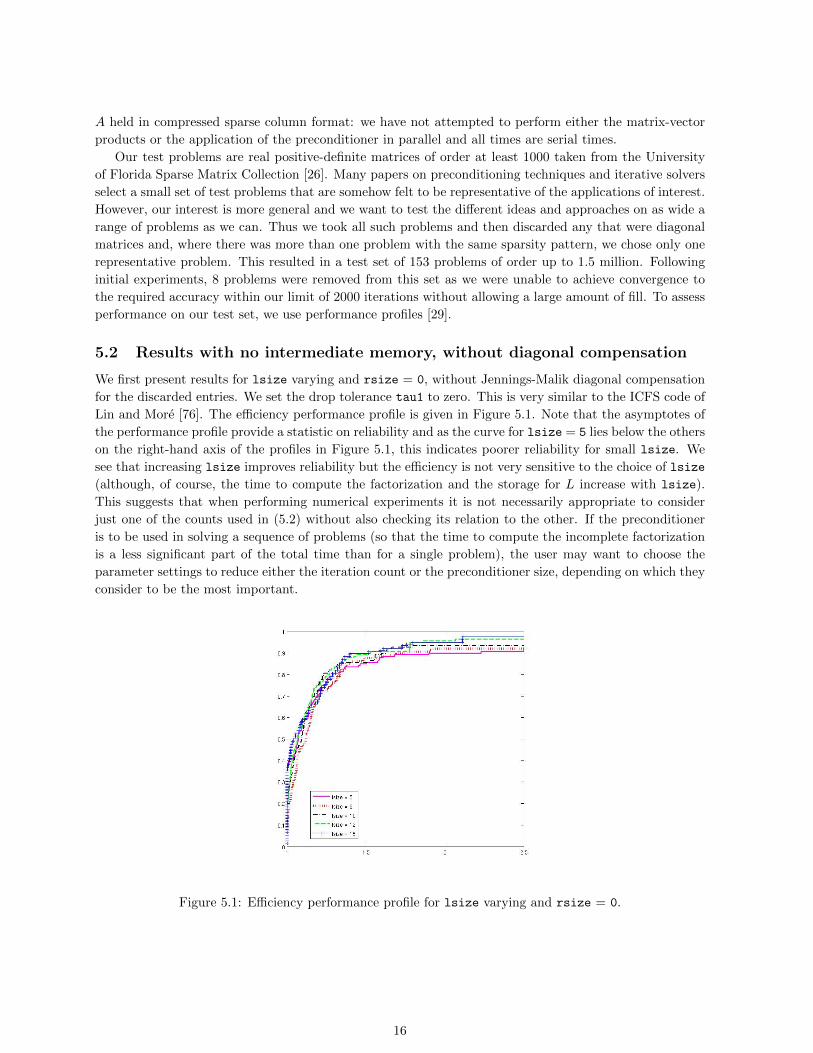
5.2 Results with no intermediate memory, without diagonal compensation

We first present results for lsize varying and rsize = 0, without Jennings-Malik diagonal compensation

for the discarded entries. We set the drop tolerance tau1 to zero. This is very similar to the ICFS code of

Lin and More [76]. The efficiency performance profile is given in Figure 5.1. Note that the asymptotes of

the performance profile provide a statistic on reliability and as the curve for lsize = 5 lies below the others

on the right-hand axis of the profiles in Figure 5.1, this indicates poorer reliability for small lsize. We

see that increasing lsize improves reliability but the efficiency is not very sensitive to the choice of lsize

(although, of course, the time to compute the factorization and the storage for L increase with lsize).

This suggests that when performing numerical experiments it is not necessarily appropriate to consider

just one of the counts used in (5.2) without also checking its relation to the other. If the preconditioner

is to be used in solving a sequence of problems (so that the time to compute the incomplete factorization

is a less significant part of the total time than for a single problem), the user may want to choose the

parameter settings to reduce either the iteration count or the preconditioner size, depending on which they

consider to be the most important.

Figure 5.1: Efficiency performance profile for lsize varying and rsize = 0.

16

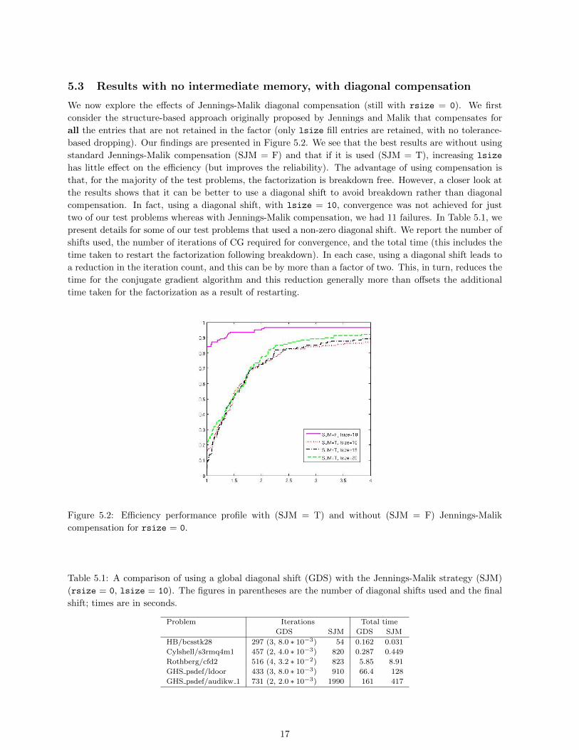
5.3 Results with no intermediate memory, with diagonal compensation

We now explore the effects of Jennings-Malik diagonal compensation (still with rsize = 0). We first

consider the structure-based approach originally proposed by Jennings and Malik that compensates for

all the entries that are not retained in the factor (only lsize fill entries are retained, with no tolerance-

based dropping). Our findings are presented in Figure 5.2. We see that the best results are without using

standard Jennings-Malik compensation (SJM = F) and that if it is used (SJM = T), increasing lsize

has little effect on the efficiency (but improves the reliability). The advantage of using compensation is

that, for the majority of the test problems, the factorization is breakdown free. However, a closer look at

the results shows that it can be better to use a diagonal shift to avoid breakdown rather than diagonal

compensation. In fact, using a diagonal shift, with lsize = 10, convergence was not achieved for just

two of our test problems whereas with Jennings-Malik compensation, we had 11 failures. In Table 5.1, we

present details for some of our test problems that used a non-zero diagonal shift. We report the number of

shifts used, the number of iterations of CG required for convergence, and the total time (this includes the

time taken to restart the factorization following breakdown). In each case, using a diagonal shift leads to

a reduction in the iteration count, and this can be by more than a factor of two. This, in turn, reduces the

time for the conjugate gradient algorithm and this reduction generally more than offsets the additional

time taken for the factorization as a result of restarting.

Figure 5.2: Efficiency performance profile with (SJM = T) and without (SJM = F) Jennings-Malik

compensation for rsize = 0.

Table 5.1: A comparison of using a global diagonal shift (GDS) with the Jennings-Malik strategy (SJM)

(rsize = 0, lsize = 10). The figures in parentheses are the number of diagonal shifts used and the final

shift; times are in seconds.

Problem Iterations Total time

GDS SJM GDS SJM

HB/bcsstk28 297 (3, 8.0 ∗ 10−3) 54 0.162 0.031

Cylshell/s3rmq4m1 457 (2, 4.0 ∗ 10−3) 820 0.287 0.449

Rothberg/cfd2 516 (4, 3.2 ∗ 10−2) 823 5.85 8.91

GHS psdef/ldoor 433 (3, 8.0 ∗ 10−3) 910 66.4 128

GHS psdef/audikw 1 731 (2, 2.0 ∗ 10−3) 1990 161 417

17

We now consider a dropping-based Jennings-Malik strategy in which off-diagonal entries that are less

than a chosen tolerance tau1 in absolute value are dropped from L and added to the corresponding

diagonal entries. The largest (in absolute value) entries in each column j (up to lsize + nj entries) are

retained in the computed factor. Figure 5.3 presents an efficiency performance profile for a range of values

of tau1. We include tau1 = 0 (no dropping and no compensation). Although not given here, the total

time performance profile is very similar. For these experiments, we use lsize = 10. We see that, as

tau1 increases, the efficiency steadily deteriorates and the robustness of the preconditioner decreases. In

Figure 5.4, we compare dropping small entries without compensation (denoted by JM = F) with using

Jennings-Malik compensation (JM = T). It is clear that, in terms of efficiency, it is better not to use the

Jennings-Malik compensation. However, an advantage of the later is that, taken over the complete test

set, it reduces the number of breakdowns and subsequent restarts. Furthermore, the computed incomplete

factor is generally sparser when compensation is used, potentially reducing its application time.

Figure 5.3: Efficiency performance profile for the Jennings-Malik strategy based on a drop tolerance for

rsize = 0 and a range values of the drop tolerance tau1.

5.4 Results for rsize varying, without diagonal compensation

We have seen that increasing lsize with rsize = 0 does little to improve the preconditioner quality

(in terms of efficiency). We now consider fixing the incomplete factor size (lsize = 5) and varying the

amount of intermediate memory (controlled by rsize). We run with no intermediate memory, rsize =

2, 5, and 10, and with unlimited intermediate memory (all entries in R are retained, which we denote by

rsize = -1). Note that the latter is the original Tismenetsky approach with the memory limit lsize

used to determine L. Figure 5.5 presents the efficiency performance profile (on the right) and total time

performance profile (on the left). Since lsize is the same for all runs, the fill in L is essentially the same in

each case and thus comparing the efficiency here is equivalent to comparing the iteration counts. For many

of our test problems, using unlimited intermediate memory gives the most efficient preconditioner but there

were a number of our largest problems that we were not able to factorize in this case because of insufficient

memory, that is, a memory allocation error was returned before the factorization was complete; this is

reflected by poor reliability and makes the original Tismenetsky approach impractical for large problems.

However, in terms of time as well as memory, this is the most expensive option. Unlimited memory

was used in the original Tismenetsky proposal and most of the complaints regarding the high memory

consumption of this algorithm are caused either by this option or by the difficulty in selecting the drop

18

Figure 5.4: Efficiency performance profile with (JM = T) and without (JM = F) the Jennings-Malik

strategy based on a drop tolerance. Here rsize = 0.

Figure 5.5: Efficiency (left) and total time (right) performance profiles for rsize varying.

19

tolerances introduced by Kaporin [67] (recall Section 3.2). We see that, as rsize is increased from 0 to

10, the efficiency and robustness of the preconditioner steadily increases, without significantly increasing

the total time. Since a larger value of rsize reduces the number of iterations required, if more than one

problem is to be solved with the same preconditioner, it may be worthwhile to increase rsize in this case

(but the precise choice of rsize is not important).

5.5 Results for lsize+rsize constant, without diagonal compensation

We present the efficiency performance profile for tsize = lsize+rsize = 10 in Figure 5.6. We see that

Figure 5.6: Efficiency performance profile for different pairs (lsize, rsize) with lsize+rsize = 10.

increasing rsize at the expense of lsize can improve efficiency. This is because the computed L is sparser

for smaller lsize while the use of R helps maintains the quality of the preconditioner.

It is of interest to compare Figure 5.6 with Figure 5.1 (in the latter, lsize varies but rsize = 0); this

clearly highlights the effects of using R. In terms of time, increasing rsize while decreasing lsize keeps

the time for computing the incomplete factorization essentially the same, while the cost of each application

of the preconditioner reduces but, as the number of iterations increases, we found in our tests that the

total time (in our serial implementation) for tsize constant was not very sensitive to the split between

lsize and rsize.

5.6 Results for rsize > 0, with diagonal compensation

We now consider Jennings-Malik compensation used with rsize > 0. In our discussion, we refer to lines

within the algorithm outline given in Section 4. We present results for three strategies for dealing with the

entries of RRT , denoted by jm = 0, 1 and 2. When computing column j, we gather updates to column j

of L and column j of R from the previous j − 1 columns of L, before gathering updates to column j of L

from the previous j−1 columns of R (LLT +RLT +LRT ). We then consider gathering updates to column

j of R from the previous j − 1 columns of R (RRT ). With jm = 0, we allow entries of RRT that cause no

further fill in LLT +RLT +LRT and discard all other entries of RRT (in this case, lines 50-52 are deleted).

With jm = 1, we use Jennings-Malik compensation for these discarded entries (this is as in the algorithm

outline). Finally, with jm = 2, we discard all entries of RRT ; this is the limited memory) Tismenetsky

approach (lines 41-57 are deleted). An efficiency performance profile is presented in Figure 5.7 for lsize

= rsize = 5 and 10. Here we do not apply Jennings-Malik compensation to the entries that are discarded

20

from column j of R before it is stored and used in computing the remaining columns of L and R (only the

rsize largest entries are retained in each column of R); this corresponds to deleting lines 91-102. We see

that, considering the whole test set, there is generally little to choose between the three approaches. We

also note the very high level of reliability when allowing only a modest number of entries in L (for lsize

= 10, the only problem that was not solved with jm = 0 and jm = 2 was Oberwolfach/boneS10).

We also want to determine whether Jennings-Malik compensation for the entries that are discarded

from R is beneficial. In Figure 5.8, we compare running with and without compensation (that is, with and

without lines 91-102). We can clearly see that in terms of efficiency, time and reliability, compensating for

the dropped entries is not, in general, beneficial.

Figure 5.7: Efficiency performance profile for lsize = rsize = 5 and 10 with jm = 0, 1, 2.

Figure 5.8: Efficiency (left) and total time (right) performance profiles with (T) and without (F) Jennings-

Malik compensation for the discarded entries (lsize = rsize = 10).

In Table 5.2, we present some more detailed results with and without Jennings-Malik compensation

for the discarded entries. These problems were chosen as, without compensation, diagonal shifts are

21

required to prevent breakdown. With compensation, there is no guarantee that a shift will not be required

(examples are Cylshell/s3rmt3m3 and DNVS/shipsec8) but fewer problems require a shift (in our test set,

with and without compensation the number of problems that require a shift is 16 and 59, respectively).

From our tests, we see that, using diagonal shifts generally results in a higher quality preconditioner than

using Jennings-Malik compensation and, even allowing for the extra time needed when the factorization is

restarted, the former generally leads to a smaller total time. Note that for example Janna/Serena, using

a diagonal shift leads to a higher quality preconditioner but, as four shifts are used, the factorization time

dominates and leads to the total time being greater than for Jennings-Malik compensation. In this case,

the initial non-zero shift α1 = 0.001 leads to a breakdown-free factorization and, as we want to use as

small a shift as possible, we decrease the shift (see [103] for full details). However, if we do not try to

minimise the shift, the total time reduces to 38.9 seconds. Clearly, how sensitive the results are to the

choice of α is problem-dependent.

Table 5.2: A comparison of using (T) and not using (F) Jennings-Malik compensation for the discarded

entries (jm = 2, lsize = rsize = 10). The figures in parentheses are the number of diagonal shifts used

and the final shift; times are in seconds.

Problem Iterations Total time

T F T F

FIDAP/ex15 503 (0, 0.0) 322 (3, 1.60 ∗ 10−2) 0.184 0.135

Cylshell/s3rmt3m3 1005 (3, 2.50 ∗ 10−4) 615 (2, 2.00 ∗ 10−3) 0.495 0.299

Janna/Fault 639 300 (0, 0.0) 122 (3, 2.50 ∗ 10−4) 31.6 18.5

ND/nd24k 407 (0, 0.0) 173 (3, 2.50 ∗ 10−4) 14.2 8.59

DNVS/shipsec8 956 (4, 9.76 ∗ 10−7) 648 (3, 2.50 ∗ 10−4) 17.2 10.3

GHS psdef/audikw 1 1447 (0, 0.0) 517 (2, 2.00 ∗ 10−3) 335 106

Janna/Serena 165 (0, 0.0) 122 (4, 9.76 ∗ 10−7) 44.9 69.6

5.7 The use of L+R

So far, we have used R in the computation of L but once the incomplete factorization has finished, we

have discarded R and used L as the preconditioner. We now consider using L+R as the preconditioner.

In Figure 5.9, we present performance profiles for L+R and L, with jm = 0 and 2. Here lsize = rsize

= 10, tau1 = 0.001, tau2 = 0.0. We see that, in terms of efficiency, using L is better than using L+R.

This is because the number of entries in L is much less than in L+R. However, L+R is a higher quality

preconditioner, requiring fewer iterations for convergence (with jm = 0 giving the best results). In terms

of total time, there is little to choose between using L+R and L.

It is interesting to see whether we can drop entries from the computed L + R to obtain a sparser

preconditioner while retaining the same quality. We present results in Figure 5.10 for no dropping and

dropping of all entries of L+R that are smaller in absolute value than a prescribed dropping parameter.

It is clear that dropping small entries can improve efficiency but, as the dropping parameter increases,

the quality (in terms of the iteration count) and reliability of the preconditioner deteriorates. Finally, in

Figure 5.11, we compare using L + R with dropping with using L, with lsize=rsize=10 and L with

lsize=20, rsize=0. Note that the dropping parameter is equal to tau1 (= 0.001), so that the entries

in both L+R and L are at least tau1 in absolute value.

22

Figure 5.9: Efficiency (top left), iteration (top right) and total time (bottom left) performance profiles for

L+R and L with jm = 0 and 2.

23

Figure 5.10: Efficiency (left) and iteration (right) performance profiles for L+R with a range of values of

the dropping parameter.

Figure 5.11: Efficiency and iteration performance profiles for L + R, L with lsize=rsize=10 (denoted

by L,R) and L with lsize=20, rsize=0 (denoted by L).

24

6 Conclusions

In this paper, we have focused on the use of positive semidefinite modification schemes for computing

incomplete Cholesky factorization preconditioners. To put our work into context, we have included an

historical overview of the development of IC factorizations, dating back more than fifty years. We have

studied in particular the methods proposed originally by Jennings and Malik and by Tismenetsky and

we have presented new theoretical results that aim to achieve a better understanding of the relationship

between them. To make the robust but memory-expensive approach of Tismenetsky into a practical

algorithm for large-scale problems, we have incorporated the use of limited memory.

A major contribution of this paper is the inclusion of extensive numerical experiments. We are

persuaded that using a large test set drawn from a range of practical applications allows us to make general

and authoritative conclusions. The experiments emphasize the concept of the efficiency of a preconditioner

(defined by (5.2)) as a measure that can be employed to help capture preconditioner usefulness, although

we recognise that it can also be necessary to consider other statistics (such as the time and the number of

iterations).

Without the use of intermediate memory (rsize = 0), our results have shown that increasing the

amount of fill allowed within a column of L (that is, increasing lsize) does not generally improve

the efficiency of the preconditioner. The real improvment comes through following Tismenetsky and

introducing intermediate memory. In our version, we prescribe the maximum number of entries in each

column of both L and R; we also optionally allow small entries to be dropped to help further sparsify the

preconditioner without significant loss of efficiency. Our results show that this leads to a highly robust

yet sparse IC preconditioner. An interesting finding is that increasing rsize at the expense of lsize can

result in a sparser preconditioner without lose of efficiency.

We have found that the fact that the Tismenetsky approach can be made breakdown-free through

the use of diagonal compensation appears to be of less importance. We obtained the same conclusion

for a number of variations of the Jennings-Malik strategy. Provided we can catch zero or negative pivots

and then restart the factorization process using a global diagonal shift, we can handle breakdowns. In our

tests, this well-established approach was found to be the more efficient overall, that is, it produced a higher

quality preconditioner than using a Jennings-Malik scheme to modify diagonal entries. However, we must

emphasize that this conclusion relies on having appropriately prescaled the matrix; if not, a large number

of restarts can be required (adding to the computation time) and the diagonal shift needed to guarantee

a breakdown-free factorization can be so large as to make the resulting IC preconditioner ineffective.

Of course, the Jennings-Malik strategy can suffer from the same type of drawback, namely, although the

factorization is breakdown-free, the resulting preconditioner may not be efficient (see [28]). Indeed, if many

fill entries are dropped from the factorization, large diagonal modifications may be performed, reducing

the accuracy of the preconditioner.

Finally, we note that we have developed a library-quality code HSL MI28 based on the findings of this

paper (see [103] for details). This is a general-purpose IC factorization code. The user specifies the

maximum column counts for L and R (and thus the amount of memory to be used for the factorization)

but, importantly for non-experts, it is not necessary to perform a lot of tuning since, although the default

settings of the control parameters will clearly not always be the best choices for a given class of problems,

they have been chosen to give good results for a wide range of problems. Of course, a more experienced

user may choose to perform experiments and then to reset the controls. This “black-box” approach is in

contrast to the Tismenetsky-Kaporin-related work reported, for example, by Yamazaki et al [122], where

by restricting attention to a specific class of problems, it is possible to determine an interval of useful drop

tolerances that limit the size of the computed factor.

25

References

[1] M. A. Ajiz and A. Jennings. A robust incomplete Choleski-conjugate gradient algorithm.

International J. of Numerical Methods in Engineering, 20(5):949–966, 1984.

[2] B.-B. Amnon and P. E. Saylor. A symmetric factorization procedure for the solution of elliptic

boundary value problems. SIAM J. on Numerical Analysis, 10:190–206, 1973.

[3] P. Arbenz, S. Margenov, and Y. Vutov. Parallel MIC(0) preconditioning of 3D elliptic problems

discretized by Rannacher-Turek finite elements. Computers and Mathematics with Applications,

55(10):2197–2211, 2008.

[4] O. Axelsson, I. Kaporin, I. Konshin, A. Kucherov, M. Neytcheva, B. Polman, and A. Yeremin.

Comparison of algebraic solution methods on a set of benchmark problems in linear elasticity. Final

Report of the STW project NNS.4683, Department of Mathematics, University of Nijmegen, 2000.

[5] O. Axelsson and L. Y. Kolotilina. Diagonally compensated reduction and related preconditioning

methods. Numerical Linear Algebra with Applications, 1(2):155–177, 1994.

[6] O. Axelsson and G. Lindskog. On the eigenvalue distribution of a class of preconditioning methods.

Numerische Mathematik, 48(5):479–498, 1986.

[7] O. Axelsson and N. Munksgaard. Analysis of incomplete factorizations with fixed storage allocation.

In Preconditioning Methods: Analysis and Applications, volume 1 of Topics in Computational

Mathematics, pages 219–241. Gordon & Breach, New York, 1983.

[8] R. Beauwens and L. Quenon. Existence criteria for partial matrix factorizations in iterative methods.

SIAM J. on Numerical Analysis, 13(4):615–643, 1976.

[9] L. Beirao da Veiga, V. Gyrya, K. Lipnikov, and G. Manzini. Mimetic finite difference method for

the Stokes problem on polygonal meshes. J. of Computational Physics, 228(19):7215–7232, 2009.

[10] M. Benzi. Preconditioning techniques for large linear systems: a survey. J. of Computational Physics,

182(2):418–477, 2002.

[11] M. Benzi, R. Kouhia, and M. Tuma. An assessment of some preconditioning techniques in shell

problems. Communications in Numerical Methods in Engineering, 14:897–906, 1998.

[12] M. Benzi and M. Tuma. A robust incomplete factorization preconditioner for positive definite

matrices. Numerical Linear Algebra with Applications, 10(5-6):385–400, 2003.

[13] M. Bern, J. R. Gilbert, B. Hendrickson, N. T. Nguyen, and S. Toledo. Support-graph preconditioners.

SIAM J. on Matrix Analysis and Applications, 27(4):930–951, 2006.

[14] M. Blanco and D.W. Zingg. A Newton-Krylov algorithm with a loosely coupled turbulence model

for aerodynamic flows. AIAA Journal, 45:980–987, 2007.

[15] M. Bollhofer. A robust ILU with pivoting based on monitoring the growth of the inverse factors.

Linear Algebra and its Applications, 338:201–218, 2001.

[16] M. Bollhofer. A robust and efficient ILU that incorporates the growth of the inverse triangular

factors. SIAM J. on Scientific Computing, 25(1):86–103, 2003.

[17] M. Bollhofer and Y. Saad. On the relations between ILUs and factored approximate inverses. SIAM

J. on Matrix Analysis and Applications, 24(1):219–237, 2002.

[18] R. Bru, J. Marın, J. Mas, and M. Tuma. Balanced incomplete factorization. SIAM J. on Scientific

Computing, 30(5):2302–2318, 2008.

26

[19] R. Bru, J. Marın, J. Mas, and M. Tuma. Improved balanced incomplete factorization. SIAM J. on

Matrix Analysis and Applications, 31(5):2431–2452, 2010.

[20] N. I. Buleev. A numerical method for solving two-dimensional diffusion equations (in Russian).

Atomnaja Energija, 6:338–340, 1959.

[21] N. I. Buleev. A numerical method for solving two-dimensional and three-dimensional diffusion

equations (in Russian). Matematiceskij Sbornik, 51:227–238, 1960.

[22] N. I. Buleev. A new variant of the method of incomplete factorization for the solution of two-

dimensional difference equations of diffusion (in Russian). Chisl. Metody Mekh. Sploshn. Sredy,

9(1):5–19, 1978.

[23] T. F. Chan. Fourier analysis of relaxed incomplete factorization preconditioners. SIAM J. on

Scientific and Statistical Computing, 12(3):668–680, 1991.

[24] D. C. Charmpis. Incomplete factorization preconditioners for the iterative solution of stochastic

finite element equations. Computers & Structures, 88(3-4):178–188, February 2010.

[25] E. Chow and Y. Saad. Experimental study of ILU preconditioners for indefinite matrices. J. of

Computational and Applied Mathematics, 86(2):387–414, 1997.

[26] T. A. Davis and Y. Hu. The University of Florida sparse matrix collection. ACM Transactions on

Mathematical Software, 38(1), 2011.

[27] E. F. D’Azevedo, P. A. Forsyth, and Wei-Pai Tang. Two variants of minimum discarded fill ordering.

In Iterative Methods in Linear Algebra (Brussels, 1991), pages 603–612. North-Holland, Amsterdam,

1992.

[28] J. K. Dickinson and P. A. Forsyth. Preconditioned conjugate gradient methods for three-dimensional

linear elasticity. International J. of Numerical Methods in Engineering, 37(13):2211–2234, 1994.

[29] E. D. Dolan and J. J. More. Benchmarking optimization software with performance profiles.

Mathematical Programming, 91(2):201–213, 2002.

[30] I. S. Duff. MA28–a set of Fortran subroutines for sparse unsymmetric linear equations. Harwell

Report, UK AERE-R.8730, Harwell Laboratories, 1980.

[31] I. S. Duff and G. A. Meurant. The effect of ordering on preconditioned conjugate gradients. BIT

Numerical Mathematics, 29:635–657, 1989.

[32] T. Dupont. A factorization procedure for the solution of elliptic difference equations. SIAM J. on

Numerical Analysis, 5:735–782, 1968.

[33] T. Dupont, R. P. Kendall, and H. H. Jr. Rachford. An approximate factorization procedure for the

solving self-adjoint elliptic difference equations. SIAM J. on Numerical Analysis, 5:559–573, 1968.

[34] V. Eijkhout. The ‘weighted modification’ incomplete factorisation method, 1999. Lapack Working

Note No. 145, UT-CS-99-436, http://www.netlib.org/lapack/lawns/.

[35] S. C. Eisenstat, M. C. Gursky, M. H. Schultz, and A. H. Sherman. The Yale Sparse Matrix Package

(YSMP) – II : The non-symmetric codes. Technical Report No. 114, Department of Computer

Science, Yale University, 1977.

[36] S. C. Eisenstat, M. C. Gursky, M. H. Schultz, and A. H. Sherman. The Yale Sparse Matrix Package

(YSMP) – I : The symmetric codes. International J. of Numerical Methods in Engineering, 18:1145–

1151, 1982.

27

[37] D. J. Evans. The use of pre-conditioning in iterative methods for solving linear equations with

symmetric positive definite matrices. J. of the Institute of Mathematics and its Applications, 4:295–

314, 1968.

[38] D. J. Evans. On preconditioned iterative methods for partial differential equations. In Preconditioning

Methods: Analysis and Applications, volume 1 of Topics in Computational Mathematics, pages 1–46.

Gordon & Breach, New York, 1983.

[39] M. Fiedler and V. Ptak. On matrices with non-positive off-diagonal elements and positive principal

minors. Czechoslovak Mathematical Journal, 12 (87):382–400, 1962.

[40] R. W. Freund and N. M. Nachtigal. An implementation of the look-ahead Lanczos algorithm for

non-Hermitian matrices, part II. Technical Report TR 90-46, RIACS, NASA Ames Research Center,

1990.

[41] T. George, A. Gupta, and V. Sarin. A recommendation system for preconditioned iterative solvers.

In ICDM 2008. Eighth IEEE International Conference on Data Mining, pages 803–808, 2008.

[42] T. George, A. Gupta, and V. Sarin. An empirical analysis of the performance of preconditioners for

SPD systems. ACM Transactions on Mathematical Software, 38(4):24:1–24:30, August 2012.

[43] I. Georgiev, J. Kraus, S. Margenov, and J. Schicho. Locally optimized MIC(0) preconditioning of

Rannacher-Turek FEM systems. Applied Numerical Mathematics, 59(10):2402–2415, 2009.

[44] I. Gustafsson. A class of first order factorization methods. BIT Numerical Mathematics, 18(2):142–

156, 1978.

[45] I. Gustafsson. On modified incomplete Cholesky factorization methods for the solution of problems

with mixed boundary conditions and problems with discontinuous material coefficients. International

J. of Numerical Methods in Engineering, 14(8):1127–1140, 1979.

[46] I. Gustafsson. On modified incomplete factorization. In Colloquium: Numerical Solution of Partial

Differential Equations (Delft, Nijmegen, Amsterdam, 1980), volume 44 of MC Syllabus, pages 41–58.

Math. Centrum, Amsterdam, 1980.

[47] I. Gustafsson. On modified incomplete factorization methods. In Numerical integration of differential

equations and large linear systems (Bielefeld, 1980), volume 968 of Lecture Notes in Math., pages

334–351. Springer, Berlin, 1982.

[48] I. Gustafsson. Modified incomplete Cholesky (MIC) methods. In Preconditioning methods: analysis

and applications, volume 1 of Topics in Computational Mathematics, pages 265–293. Gordon &

Breach, New York, 1983.

[49] W. Hackbusch. Iterative solution of large sparse systems of equations, volume 95 of Applied

Mathematical Sciences. Springer-Verlag, New York, 1994. Translated and revised from the 1991

German original.

[50] P. Henon, P. Ramet, and J. Roman. On finding approximate supernodes for an efficient block-ILU(k)

factorization. Parallel Computing, 34(6-8):345–362, 2008.

[51] M. R. Hestenes and E. Stiefel. Methods of conjugate gradients for solving linear systems. J. of

Research of the National Bureau of Standards, 49:409–435, 1952.

[52] I. Hladık, M. B. Reed, and G. Swoboda. Robust preconditioners for linear elasticity FEM analyses.

International J. of Numerical Methods in Engineering, 40:2109–2127, 1997.

[53] A. S. Householder. Principles of Numerical Analysis. McGraw Hill, New York, 1953.

28

[54] HSL. A collection of Fortran codes for large-scale scientific computation, 2013. http://www.hsl.

rl.ac.uk.

[55] D. Hysom and A. Pothen. A scalable parallel algorithm for incomplete factor preconditioning. SIAM

J. on Scientific Computing, 22:2194–2215, 2001.

[56] D. Hysom and A. Pothen. Level-based incomplete LU factorization: Graph model and algorithms.

Technical Report UCRL-JC-150789, Lawrence Livermore National Labs, November 2002.

[57] V. P. Il′in and K. Y. Laevskii. Generalized compensation principle in incomplete factorization

methods. Russian J. Numer. Anal. Math. Modelling, 12(5):399–420, 1997.

[58] Y. M. Il′in. Difference Methods for Solving Elliptic Equations (in Russian). Novosibirskij

Gosudarstvennyj Universitet, Novosibirsk, 1970.

[59] Y. M. Il′in. Iterative Incomplete Factorization Methods. World Scientific, Singapore, 1992.

[60] A. Jennings and M. A. Ajiz. Incomplete methods for solving ATAx = b. SIAM J. on Scientific and

Statistical Computing, 5(4):978–987, 1984.

[61] A. Jennings and G. M. Malik. Partial elimination. J. of the Institute of Mathematics and its

Applications, 20(3):307–316, 1977.

[62] A. Jennings and G. M. Malik. The solution of sparse linear equations by the conjugate gradient

method. International J. of Numerical Methods in Engineering, 12(1):141–158, 1978.

[63] Z. Y. Jiang, W. P. Hu, P. F. Thomson, and Y. C. Lam. Solution of the equations of rigid-plastic FE

analysis by shifted incomplete Cholesky factorisation and the conjugate gradient method in metal

forming processes. J. of Materials Processing Technology, 102:70 – 77, 2000.

[64] Z. Y. Jiang, W. P. Hu, P. F. Thomson, and Y. C. Lam. Analysis of slab edging by a 3-D rigid

viscoplastic FEM with the combination of shifted incomplete Cholesky decomposition and the

conjugate gradient method. Finite Elements in Analysis and Design, 37(2):145 – 158, 2001.

[65] M. T. Jones and P. E. Plassmann. Algorithm 740: Fortran subroutines to compute improved

incomplete Cholesky factorizations. ACM Transactions on Mathematical Software, 21(1):18–19,

1995.

[66] M. T. Jones and P. E. Plassmann. An improved incomplete Cholesky factorization. ACM

Transactions on Mathematical Software, 21(1):5–17, 1995.

[67] I. E. Kaporin. High quality preconditioning of a general symmetric positive definite matrix based

on its UTU + UTR+RTU decomposition. Numerical Linear Algebra with Applications, 5:483–509,

1998.

[68] I. E. Kaporin. Using the modified 2nd order incomplete Cholesky decomposition as the conjugate

gradient preconditioning. Numerical Linear Algebra with Applications, 9(6-7):401–408, 2002.

Preconditioned robust iterative solution methods, PRISM ’01 (Nijmegen).

[69] D. S. Kershaw. The incomplete Cholesky-conjugate gradient method for the iterative solution of

systems of linear equations. J. of Computational Physics, 26:43–65, 1978.

[70] S. A. Kilic, F. Saied, and A. Sameh. Efficient iterative solvers for structural dynamics problems.

Computers & Structures, 82(28):2363 – 2375, 2004.

[71] J. Kopal, M. Rozloznık, A. Smoktunowicz, and M. Tuma. Rounding error analysis of

orthogonalization with a non-standard inner product. BIT Numerical Mathematics, 52:1035–1058,

2012.

29

[72] J. Kopal, M. Rozloznık, and M. Tuma. Gram-Schmidt based preconditioners and their properties.

In Proceedings of Pareng’13: The Third International Conference on Parallel, Distributed, Grid and

Cloud Computing for Engineering. Elsevier, to appear.

[73] F. Kuss and F. Lebon. Stress based finite element methods for solving contact problems:

Comparisons between various solution methods. Advances in Engineering Software, 40(8):697–706,

August 2009.

[74] C. Lanczos. Solutions of linear equations by minimized iterations. J. of Research of the National

Bureau of Standards, 49:33–53, 1952.

[75] S. Lew, C. H. Wolters, T. Dierkes, C. Roer, and R. S. MacLeod. Accuracy and run-time comparison

for different potential approaches and iterative solvers in finite element method based EEG source

analysis. Applied Numerical Mathematics, 59(8):1970–1988, August 2009.

[76] C.-J. Lin and J. J. More. Incomplete Cholesky factorizations with limited memory. SIAM J. on

Scientific Computing, 21(1):24–45, 1999.

[77] K. Lipnikov, M. Shashkov, D. Svyatskiy, and Yu. Vassilevski. Monotone finite volume schemes

for diffusion equations on unstructured triangular and shape-regular polygonal meshes. J. of

Computational Physics, 227(1):492–512, 2007.

[78] K. Lipnikov, D. Svyatskiy, and Y. Vassilevski. Interpolation-free monotone finite volume method for

diffusion equations on polygonal meshes. J. of Computational Physics, 228(3):703–716, 2009.

[79] Y. Luo. Direct and incomplete Cholesky factorizations with static supernodes. Technical Report

AMSC 661 Term Project Report, University of Maryland, 2010.

[80] S. MacLachlan, D. Osei-Kuffuor, and Y. Saad. Modification and compensation strategies for

threshold-based incomplete factorizations. SIAM J. on Scientific Computing, 34(1):A48–A75, 2012.

[81] T. A. Manteuffel. An incomplete factorization technique for positive definite linear systems.

Mathematics of Computation, 34:473–497, 1980.

[82] J. A. Meijerink and H. A. van der Vorst. An iterative solution method for linear systems of which the

coefficient matrix is a symmetric M -matrix. Mathematics of Computation, 31(137):148–162, 1977.

[83] J. A. Meijerink and H. A. van der Vorst. Guidelines for the usage of incomplete decompositions in

solving sets of linear equations as they occur in practical problems. J. of Computational Physics,

44(1):134–155, 1981.

[84] G. Meurant. Computer Solution of Large Linear Systems. Elsevier, Amsterdam – Lausanne – New

York – Oxford – Shannon – Singapore – Tokyo, 1999.

[85] Y. Miki and T. Washizawa. A2ILU: Auto-accelerated ILU preconditioner for sparse linear systems.

Preprint, arXiv:1301.5412 [cs.NA], 2012.

[86] N. Munksgaard. New factorization codes for sparse, symmetric and positive definite matrices. BIT

Numerical Mathematics, 19(1):43–52, 1979.

[87] N. Munksgaard. Solving sparse symmetric sets of linear equations by preconditioned conjugate

gradients. ACM Transactions on Mathematical Software, 6(2):206–219, 1980.

[88] A. Napov. Conditioning analysis of incomplete Cholesky factorizations with orthogonal dropping.

Technical Report LBNL-5353E, Computational Research Division, Lawrence Berkeley National

Laboratory, 2012.

30

[89] T. A. Oliphant. An extrapolation procedure for solving linear systems. Quarterly of Applied

Mathematics, 20:257–265, 1962/1963.

[90] O. Østerby and Z. Zlatev. Direct methods for sparse matrices, volume 157 of Lecture Notes in

Computer Science. Springer-Verlag, Berlin, 1983.

[91] H. M. Panayirci. Efficient solution for galerkin-based polynomial chaos expansion systems. Advances

in Engineering Software, 41(12):1277–1286, December 2010.

[92] M. Papadrakakis and M. C. Dracopoulos. Improving the efficiency of incomplete Choleski

preconditionings. Communications in Applied Numerical Methods, 7(8):603–612, 1991.

[93] S. Parter. The use of linear graphs in Gaussian elimination. SIAM Review, 3:119–130, 364–369,

1961.

[94] A. Pueyo and D.W. Zingg. Efficient Newton-Krylov solver for aerodynamic computations. AIAA

Journal, 36:1991–1997, 1998.

[95] J. K. Reid and J. A. Scott. Ordering symmetric sparse matrices for small profile and wavefront.

International J. of Numerical Methods in Engineering, 45:1737–1755, 1999.

[96] Y. Robert. Regular incomplete factorizations of real positive definite matrices. Linear Algebra and

its Applications, 48:105–117, 1982.

[97] A. Rodrıguez-Ferran and M. L. Sandoval. Numerical performance of incomplete factorizations for

3d transient convection-diffusion problems. Advances in Engineering Software, 38(6):439–450, June

2007.

[98] Y. Saad. ILUT: a dual threshold incomplete LU factorization. Numerical Linear Algebra with

Applications, 1(4):387–402, 1994.

[99] Y. Saad. Iterative Methods for Sparse Linear Systems. Society for Industrial and Applied

Mathematics, Philadelphia, PA, second edition, 2003.

[100] Y. Saad and H. A. van der Vorst. Iterative solution of linear systems in the 20th century. J. Comput.

Appl. Math., 123(1-2):1–33, 2000.

[101] V. I. Sabinin. An algorithm of the incomplete factorization method. Chisl. Metody Mekh. Sploshn.

Sredy, 16(2):103–117, 1985.

[102] J. A. Scott and M. Tuma. The importance of structure in incomplete factorization preconditioners.

BIT Numerical Mathematics, 51:385–404, 2011.

[103] J. A. Scott and M. Tuma. HSL MI28: an efficient and robust limited memory incomplete Cholesky

factorization code. Technical Report RAL-P-2013-004, 2013.

[104] M. Sedlacek. Sparse Approximate Inverses for Preconditioning, Smoothing and Regularization. PhD

thesis, Technical University of Munich, 2012.

[105] S. W. Sloan. An algorithm for profile and wavefront reduction of sparse matrices. International J.

of Numerical Methods in Engineering, 23:239–251, 1986.

[106] S. W. Sloan. A Fortran program for profile and wavefront reduction. International J. of Numerical

Methods in Engineering, 28:2651–2679, 1989.

[107] H. L. Stone. Iterative solution of implicit approximations of multidimensional partial differential

equations. SIAM J. on Numerical Analysis, 5:530–558, 1968.

31

[108] M. Suarjana and K. H. Law. A robust incomplete factorization based on value and space constraints.

International J. of Numerical Methods in Engineering, 38:1703–1719, 1995.

[109] M. Tismenetsky. A new preconditioning technique for solving large sparse linear systems. Linear

Algebra and its Applications, 154–156:331–353, 1991.

[110] A. D. Tuff and A. Jennings. An iterative method for large systems of linear structural equations.

International J. of Numerical Methods in Engineering, 7:175–183, 1973.

[111] A. M. Turing. Rounding-off errors in matrix processes. The Quarterly Journal of Mechanics and

Applied Mathematics, 1:287–308, 1948.

[112] H. A. van der Vorst. High performance preconditioning. SIAM J. on Scientific and Statistical

Computing, 10(6):1174–1185, 1989.

[113] H. A. van der Vorst. The convergence behaviour of preconditioned CG and CG-S in the presence

of rounding errors. In Preconditioned conjugate gradient methods (Nijmegen, 1989), volume 1457 of

Lecture Notes in Math., pages 126–136. Springer, Berlin, 1990.

[114] H. A. van der Vorst. Efficient and reliable iterative methods for linear systems. J. of Computational

and Applied Mathematics, 149(1):251–265, 2002.

[115] R. S. Varga. Factorizations and normalized iterative methods. In Boundary problems in differential

equations, pages 121–142, Madison, WI, 1960. University of Wisconsin Press.

[116] R. S. Varga, E. B. Saff, and V. Mehrmann. Incomplete factorizations of matrices and connections

with h-matrices. SIAM J. on Numerical Analysis, 17:787–793, 1980.

[117] X. Wang. Incomplete Factorization Preconditioning for Linear Least Squares Problems. PhD thesis,

Department of Computer Science, University of Illinois Urbana-Champaign, 1993.

[118] X. Wang, R. Bramley, and K. A. Gallivan. A necessary and sufficient symbolic condition for the

existence of incomplete Cholesky factorization. Technical Report TR440, Department of Computer

Science, Indiana University, Bloomington, 1995.

[119] X. Wang, K. A. Gallivan, and R. Bramley. Incomplete Cholesky factorization with sparsity pattern

modification. Technical report, Department of Computer Science, Indiana University, Bloomington,

1993.

[120] X. Wang, K. A. Gallivan, and R. Bramley. CIMGS: an incomplete orthogonal factorization

preconditioner. SIAM J. on Scientific Computing, 18(2):516–536, 1997.

[121] J. W. Watts-III. A conjugate gradient truncated direct method for the iterative solution of the

reservoir simulation pressure equation. Society of Petroleum Engineer J., 21:345–353, 1981.

[122] I. Yamazaki, Z. Bai, W. Chen, and R. Scalettar. A high-quality preconditioning technique for multi-

length-scale symmetric positive definite linear systems. Numerical Mathematics: Theory, Methods

and Applications, 2(4):469–484, 2009.

32