On polyharmonic univalent mappings

ON POLYHARMONIC UNIVALENT MAPPINGS

J. CHEN, A. RASILA, AND X. WANG ∗

Abstract. In this paper, we introduce a class of complex-valued polyharmonicmappings, denoted by HSp(λ), and its subclass HS0

p(λ), where λ ∈ [0, 1] is aconstant. These classes are natural generalizations of a class of mappings studiedby Goodman in 1950’s. We generalize the main results of Avci and Z lotkiewiczfrom 1990’s to the classes HSp(λ) and HS0

p(λ), showing that the mappings inHSp(λ) are univalent and sense preserving. We also prove that the mappingsin HS0

p(λ) are starlike with respect to the origin, and characterize the extremalpoints of the above classes.

1. Introduction

A complex-valued mapping F = u + iv, defined in a domain D ⊂ C, is calledpolyharmonic (or p-harmonic) if F is 2p (p ≥ 1) times continuously differentiable,and it satisfies the polyharmonic equation ∆pF = ∆(∆p−1F ) = 0, where ∆1 := ∆is the standard complex Laplacian operator

∆ = 4∂2

∂z∂z:=

∂2

∂x2+

∂2

∂y2.

It is well known (see [7, 17]) that for a simply connected domain D, a mapping Fis polyharmonic if and only if F has the following representation:

F (z) =

p∑k=1

|z|2(k−1)Gk(z),

where Gk are complex-valued harmonic mappings in D for k ∈ {1, · · · , p}. Further-more, the mappings Gk can be expressed as the form

Gk = hk + gk

for k ∈ {1, · · · , p}, where all hk and gk are analytic in D (see [9, 11]).Obviously, for p = 1 (resp. p = 2), F is a harmonic (resp. biharmonic) mapping.

The biharmonic model arises from numerous problems in science and engineering(cf. [14, 15, 16]). However, investigation of biharmonic mappings in the context ofthe geometric function theory has been started only recently (see [1, 2, 3, 5, 6, 8]).The reader is referred to [7, 17] for discussion on polyharmonic mappings, and [9, 11]for the properties of harmonic mappings.

File: p-harmonic.tex, printed: 11-2-2013, 1.11

2010 Mathematics Subject Classification. Primary 30C65, 30C45; Secondary 30C20.Key words and phrases. polyharmonic mapping, starlikeness, convexity, extremal point

∗ Corresponding author.

1

arX

iv:1

302.

2018

v1 [

mat

h.C

V]

8 F

eb 2

013

In [4], Avci and Z lotkiewicz introduced the class HS of univalent harmonic map-pings F with the series expansion:

(1.1) F (z) = h(z) + g(z) = z +∞∑n=2

anzn +

∞∑n=1

bnzn

such that∞∑n=2

n(|an|+ |bn|) ≤ 1− |b1| (0 ≤ |b1| < 1),

and the subclass HC of HS, where

∞∑n=2

n2(|an|+ |bn|) ≤ 1− |b1| (0 ≤ |b1| < 1).

The corresponding subclasses of HS and HC with b1 = 0 are denoted by HS0 andHC0, respectively. These two classes constitute a harmonic counterpart of classesintroduced by Goodman [13]. They are useful in studying questions of so-calledδ-neighborhoods (Ruscheweyh [19], see also [17]) and in constructing explicit k-quasiconformal extensions (Fait et al. [12]). In this paper, we define polyharmonicanalogues HSp(λ) and HS0

p(λ), where λ ∈ [0, 1], to the above classes of mappings.Our aim is to generalize the main results of [4] to the mappings of the classes HSp(λ)and HS0

p(λ).This paper is organized as follows. In Section 3, we discuss the starlikeness and

convexity of polyharmonic mappings in HS0p(λ). Our main result, Theorem 1, is a

generalization of [4, Theorem 4]. In Section 4, we find the extremal points of theclass HS0

p(λ). The main result of this section is Theorem 2, which is a generalizationof [4, Theorem 6]. Finally, we consider convolutions and existence of neighborhoods.The main results in this section are Theorems 3 and 4 which are generalizations of[4, Theorems 7 (i) and 8], respectively.

2. Preliminaries

For r > 0, write Dr = {z : |z| < r}, and let D := D1, i.e., the unit disk. We useHp to denote the set of all polyharmonic mappings F in D with a series expansionof the following form:

(2.1) F (z) =

p∑k=1

|z|2(k−1)(hk(z) + gk(z)

)=

p∑k=1

|z|2(k−1)∞∑n=1

(an,kzn + bn,kzn)

with a1,1 = 1 and |b1,1| < 1. Let H0p denote the subclass of Hp for b1,1 = 0 and

a1,k = b1,k = 0 for k ∈ {2, · · · , p}.

2

In [17], J. Qiao and X. Wang introduced the class HSp of polyharmonic mappingsF with the form (2.1) satisfying the conditions(2.2)

p∑k=1

∞∑n=2

(2(k − 1) + n)(|an,k|+ |bn,k|) ≤ 1− |b1,1| −p∑

k=2

(2k − 1)(|a1,k|+ |b1,k|),

0 ≤ |b1,1|+p∑

k=2

(|a1,k|+ |b1,k|) < 1,

and the subclass HCp of HSp, where(2.3)

p∑k=1

∞∑n=2

(2(k − 1) + n2)(|an,k|+ |bn,k|) ≤ 1− |b1,1| −p∑

k=2

(2k − 1)(|a1,k|+ |b1,k|),

0 ≤ |b1,1|+p∑

k=2

(|a1,k|+ |b1,k|) < 1.

The classess of all mappings F in H0p which are of the form (2.1), and subject to

the conditions (2.2), (2.3), are denoted by HS0p , HC

0p , respectively.

Now we introduce a new class of polyharmonic mappings, denoted by HSp(λ), asfollows: A mapping F ∈ Hp with the form (2.1) is said to be in HSp(λ) if(2.4)

p∑k=1

∞∑n=2

(2(k − 1) + n(λn+ 1− λ)

)(|an,k|+ |bn,k|) ≤ 2−

p∑k=1

(2k − 1)(|a1,k|+ |b1,k|),

1 ≤p∑

k=1

(2k − 1)(|a1,k|+ |b1,k|) < 2,

where λ ∈ [0, 1]. We denote by HS0p(λ) the class consisting of all mappings F in

H0p , with the form (2.1), and subject to the condition (2.4). Obviously, if λ = 0

or λ = 1, then the class HSp(λ) reduces to HSp or HCp, respectively. Similarly, ifp− 1 = λ = 0 or p = λ = 1, then HSp(λ) reduces to HS or HC.

If

F (z) =

p∑k=1

|z|2(k−1)∞∑n=1

(an,kz

n + bn,kzn)

and

G(z) =

p∑k=1

|z|2(k−1)∞∑n=1

(An,kz

n +Bn,kzn),

then the convolution F ∗G of F and G is defined to be the mapping

(F ∗G)(z) =

p∑k=1

|z|2(k−1)∞∑n=1

(an,kAn,kz

n + bn,kBn,kzn),

3

while the integral convolution is defined by

(F �G)(z) =

p∑k=1

|z|2(k−1)∞∑n=1

(an,kAn,k

nzn +

bn,kBn,k

nzn).

See [10] for similar operators defined on the class of analytic functions.Following the notation of J. Qiao and X. Wang [17], we denote the δ-neighborhood

of F the set by

Nδ(F (z)) =

{G(z) :

p∑k=1

∞∑n=2

(2(k − 1) + n

)(|an,k − An,k|+ |bn,k −Bn,k|)

+

p∑k=2

(2k − 1)(|a1,k − A1,k|+ |b1,k −B1,k|) + |b1,1 −B1,1| ≤ δ

},

whereG(z) =∑p

k=1 |z|2(k−1)∑∞

n=1

(An,kz

n +Bn,kzn)

andA1,1 = 1 (see also Ruscheweyh[19]).

3. Starlikeness and convexity

We say that a univalent polyharmonic mapping F with F (0) = 0 is starlike withrespect to the origin if the curve F (reiθ) is starlike with respect to the origin foreach 0 < r < 1.

Proposition 1. ([18]) If F is univalent, F (0) = 0 and ddθ

(argF (reiθ)

)> 0 for

z = reiθ 6= 0, then F is starlike with respect to the origin.

A univalent polyharmonic mapping F with F (0) = 0 and ddθF (reiθ) 6= 0 whenever

0 < r < 1, is said to be convex if the curve F (reiθ) is convex for each 0 < r < 1.

Proposition 2. ([18]) If F is univalent, F (0) = 0 and ∂∂θ

[arg(∂∂θF (reiθ)

)]> 0 for

z = reiθ 6= 0, then F is convex.

LetX be a topological vector space over the field of complex numbers, and letD bea set of X. A point x ∈ D is called an extremal point of D if it has no representationof the form x = ty + (1 − t)z (0 < t < 1) as a proper convex combination of twodistinct points y and z in D.

Now we are ready to prove results concerning the geometric properties of mappingsin HS0

p(λ).

Theorem A. [17, Theorems 3.1, 3.2 and 3.3] Suppose that F ∈ HSp. Then F isunivalent and sense preserving in D. In particular, each member of HS0

p (or HC0p)

maps D onto a domain starlike w.r.t. the origin, and a convex domain, respectively.

Theorem 1. Each mapping in HS0p(λ) maps the disk Dr, where r ≤ max{1

2, λ},

onto a convex domain.

4

-1.0 - 0.5 0.5 1.0 1.5

-1.0

- 0.5

0.5

1.0

- 0.5 0.5 1.0 1.5

-1.5

-1.0

- 0.5

0.5

1.0

1.5

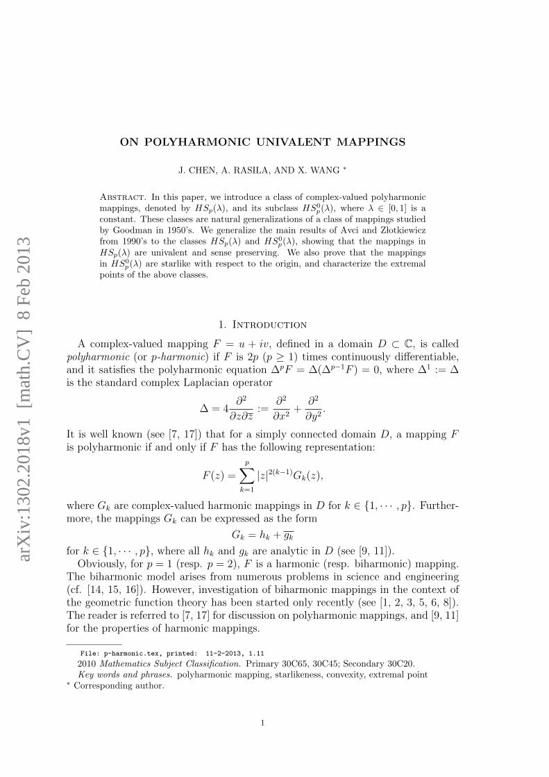
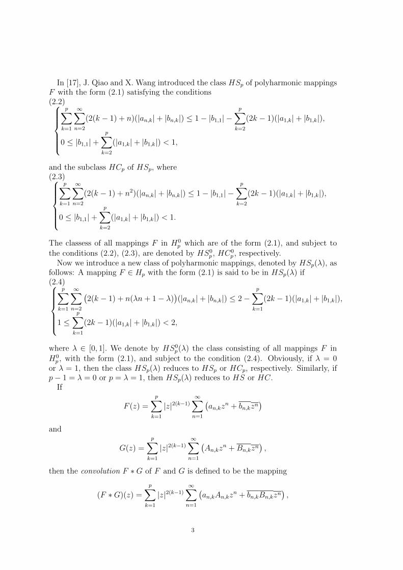
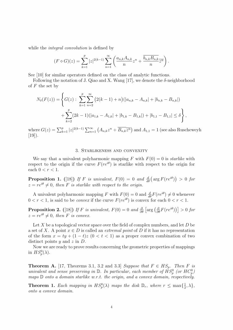
Figure 1. The images of D under the mappings F1(z) = z+ 110z2+ 1

5z2

(left) and F2(z) = z + 1101z2 + 49

101z2 (right).

Proof. Let F ∈ HS0p(λ), and let r ∈ (0, 1) be fixed. Then r−1F (rz) ∈ HS0

p(λ) by(2.4), and we have

p∑k=1

∞∑n=2

(2(k − 1) + n2

)(|an,k|+ |bn,k|)r2k+n−3

≤p∑

k=1

∞∑n=2

(2(k − 1) + n(λn+ 1− λ)

)(|an,k|+ |bn,k|) ≤ 1

provided that (2(k − 1) + n2

)r2k+n−3 ≤ 2(k − 1) + n(λn+ 1− λ)

for k ∈ {1, · · · , p}, n ≥ 2 and 0 ≤ λ ≤ 1, which is true if r ≤ max{12, λ}. Then the

result follows from Theorem A. �

Follows immediately from Theorem A, we get the following.

Corollary 1. Let F ∈ HSp(λ). Then F is a univalent, sense preserving polyhar-monic mapping. In particular, if F ∈ HS0

p(λ), then F maps D onto a domainstarlike w.r.t. the origin.

Example 1. Let F1(z) = z + 110z2 + 1

5z2. Then F1 ∈ HS0

1(23) is a univalent, sense

preserving polyharmonic mapping. In particular, F1 maps D onto a domain starlikew.r.t. the origin, and it maps the disk Dr, where r ≤ 2

3, onto a convex domain. See

Figure 1.

This example shows that the class HS0p(λ) of polyharmonic mappings is more

general than the class HS0 which is studied in [4] even in the case of harmonicmappings (i.e. p=1).

5

Example 2. Let F2(z) = z + 1101z2 + 49

101z2. Then F2 ∈ HS0

1( 1100

) is a univalent,sense preserving polyharmonic mapping. In particular, F2 maps D onto a domainstarlike w.r.t. the origin, and it maps the disk Dr, where r ≤ 1

2, onto a convex

domain. See Figure 1.

4. Extremal points

First, we determine the distortion bounds for mappings in HSp(λ).

Lemma 1. Suppose that F ∈ HSp(λ). Then the following statements hold:(1) For 0 ≤ λ ≤ 1

2,

(1− |b1,1|)|z| −1− |b1,1|2(1 + λ)

|z|2 ≤ |F (z)| ≤ (1 + |b1,1|)|z|+1− |b1,1|2(1 + λ)

|z|2.

Equalities are obtained by the mappings

F (z) = z + |b1,1|eiµz +1− |b1,1|2(1 + λ)

eiνz2,

for properly chosen real µ and ν;(2) For 1

2< λ ≤ 1,

|F (z) ≤ (1 + |b1,1|)|z|+1− |b1,1| − 3(|a1,2|+ |b1,2|)

2(1 + λ)|z|2 + (|a1,2|+ |b1,2|)|z|3

and

|F (z)| ≥ (1− |b1,1|)|z| −1− |b1,1| − 3(|a1,2|+ |b1,2|)

2(1 + λ)|z|2 − (|a1,2|+ |b1,2|)|z|3.

Equalities are obtained by the mappings

F (z) = z + |b1,1|eiηz +1− |b1,1| − 3(|a1,2|+ |b1,2|)

2(1 + λ)eiϕz2 + (|a1,2|+ |b1,2|)eiψz|z|2,

for properly chosen real η, ϕ and ψ.

Proof. Let F ∈ HSp(λ), where λ ∈ [0, 1]. By (2.1), we have

|F (z)| ≤ (1 + |b1,1|)|z|+

(p∑

k=1

∞∑n=2

(|an,k|+ |bn,k|) +

p∑k=2

(|a1,k|+ |b1,k|)

)|z|2.

For 0 ≤ λ ≤ 12, we have

(4.1) 2(1 + λ) ≤ 2k − 1,

where k ∈ {2, · · · , p}, and

(4.2) 2(1 + λ) ≤ 2(k − 1) + n(λn+ 1− λ),

6

where k ∈ {1, · · · , p} and n ≥ 2. Then (4.1), (4.2) and (2.4) givep∑

k=1

∞∑n=2

(|an,k|+ |bn,k|) +

p∑k=2

(|a1,k|+ |b1,k|)

≤ 1

2(1 + λ)

(1− |b1,1| −

p∑k=1

∞∑n=2

(2(k − 1) + n(λn+ 1− λ)− 2(1 + λ)

)(|an,k|+ |bn,k|)

−p∑

k=2

((2k − 1)− 2(1 + λ)

)(|a1,k|+ |b1,k|)

),

so

(1− |b1,1|)|z| −1− |b1,1|2(1 + λ)

|z|2 ≤ |F (z)| ≤ (1 + |b1,1|)|z|+1− |b1,1|2(1 + λ)

|z|2.

By (2.1), we obtain

|F (z)| ≤ (1 + |b1,1|)|z|+

(p∑

k=1

∞∑n=2

(|an,k|+ |bn,k|) +

p∑k=3

(|a1,k|+ |b1,k|)

)|z|2

+ (|a1,2|+ |b1,2|)|z|3.For 1

2< λ ≤ 1, we have

(4.3) 2(1 + λ) ≤ 2k − 1,

where k ∈ {3, · · · , p}, and

(4.4) 2(1 + λ) ≤ 2(k − 1) + n(λn+ 1− λ),

where k ∈ {1, · · · , p}, n ≥ 2. Then (4.3), (4.4) and (2.4) implyp∑

k=1

∞∑n=2

(|an,k|+ |bn,k|) +

p∑k=3

(|a1,k|+ |b1,k|)

≤ 1

2(1 + λ)

(1− |b1,1| −

p∑k=1

∞∑n=2

(2(k − 1) + n(λn+ 1− λ)− 2(1 + λ)

)(|an,k|+ |bn,k|)

−p∑

k=3

(2k − 1− 2(1 + λ)

)(|a1,k|+ |b1,k|)− 3(|a1,2|+ |b1,2|)

).

Then

|F (z)| ≥ (1− |b1,1|)|z| −1− |b1,1| − 3(|a1,2|+ |b1,2|)

2(1 + λ)|z|2 − (|a1,2|+ |b1,2|)|z|3

and

|F (z)| ≤ (1 + |b1,1|)|z|+1− |b1,1| − 3(|a1,2|+ |b1,2|)

2(1 + λ)|z|2 + (|a1,2|+ |b1,2|)|z|3.

The proof of this lemma is complete. �

7

Remark 1. Suppose that F ∈ HSp(λ) is of the form

F (z) =

p∑k=1

|z|2(k−1)Gk(z) =

p∑k=1

|z|2(k−1)∞∑n=1

(an,kz

n + bn,kzn).

Then for each k ∈ {1, · · · , p},

|Gk(z)| ≤ (|a1,k|+ |b1,k|)|z|+1− |b1,1|2(1 + λ)

|z|2.

Lemma 2. The family HSp(λ) is closed under convex combinations.

Proof. Suppose Fi ∈ HSp(λ) and ti ∈ [0, 1] with∑∞

i=1 ti = 1. Let

Fi(z) =

p∑k=1

|z|2(k−1)∞∑n=1

(a(i)n,kz

n + b(i)n,kz

n).

By Lemma 1, there exists a constant M such that |Fi(z)| ≤ M for all i = 1, · · · , p.It follows that

∑∞i=1 tiFi(z) is absolutely and uniformly convergent, and by Remark

1, the mapping∑∞

i=1 tiFi(z) is polyharmonic. Since∑∞

i=1 tiFi(z) is absolutely anduniformly convergent, we have

∞∑i=1

tiFi(z) =∞∑i=1

ti

p∑k=1

|z|2(k−1)(∞∑n=1

a(i)n,kz

n +∞∑n=1

b(i)n,kz

n

)

=

p∑k=1

|z|2(k−1)(∞∑n=1

∞∑i=1

tia(i)n,kz

n +∞∑n=1

∞∑i=1

tib(i)n,kz

n

).

By (2.4), we get

(4.5)

p∑k=1

∞∑n=1

(2(k − 1) + n(λn+ 1− λ)

)(∣∣∣∣∣∞∑i=1

tia(i)n,k

∣∣∣∣∣+

∣∣∣∣∣∞∑i=1

tib(i)n,k

∣∣∣∣∣)

≤∞∑i=1

ti

(p∑

k=1

∞∑n=1

(2(k − 1) + n(λn+ 1− λ)

)(|a(i)n,k|+ |b

(i)n,k|)

)≤ 2.

It follows from

1 ≤p∑

k=1

(2k − 1)

(∣∣∣∣∣∞∑i=1

tia(i)1,k

∣∣∣∣∣+

∣∣∣∣∣∞∑i=1

tib(i)1,k

∣∣∣∣∣)< 2

and (4.5) that∑∞

i=1 tiFi ∈ HSp(λ). �

From Lemma 1, we see that the class HSp(λ) is uniformly bounded, and hencenormal. Lemma 2 implies that HS0

p(λ) is also compact and convex. Then there

exists a non-empty set of extremal points in HS0p(λ).

8

Theorem 2. The extremal points of HS0p(λ) are the mappings of the following form:

Fk(z) = z + |z|2(k−1)an,kzn or F ∗k (z) = z + |z|2(k−1)bm,kzm,where

|an,k| =1

2(k − 1) + n(λn+ 1− λ), for n ≥ 2, k ∈ {1, · · · , p},

and

|bm,k| =1

2(k − 1) +m(λm+ 1− λ), for m ≥ 2, k ∈ {1, · · · , p}.

Proof. Assume that F is an extremal point of HS0p(λ), of the form (2.1). Suppose

that the coefficients of F satisfy the following:p∑

k=1

∞∑n=2

(2(k − 1) + n(λn+ 1− λ)

)(|an,k|+ |bn,k|) < 1.

If all coefficients an,k (n ≥ 2) and bn,k (n ≥ 2) are equal to 0, we let

F1(z) = z +1

2(1 + λ)z2 and F2(z) = z − 1

2(1 + λ)z2.

Then F1 and F2 are in HS0p(λ) and F = 1

2(F1+F2). This is a contradiction, showing

that there is a coefficient, say an0,k0 or bn0,k0 , of F which is nonzero. Without lossof generality, we may further assume that an0,k0 6= 0.

For γ > 0 small enough, choosing x ∈ C with |x| = 1 properly and replacingan0,k0 by an0,k0 − γx and an0,k0 + γx, respectively, we obtain two mappings F3 andF4 such that both F3 and F4 are in HS0

p(λ). Obviously, F = 12(F3 +F4). Hence the

coefficients of F must satisfy the following equality:p∑

k=1

∞∑n=2

(2(k − 1) + n(λn+ 1− λ)

)(|an,k|+ |bn,k|) = 1.

Suppose that there exists at least two coefficients, say, aq1,k1 and bq2,k2 or aq1,k1and aq2,k2 or bq1,k1 and bq2,k2 , which are not equal to 0, where q1, q2 ≥ 2. Withoutloss of generality, we assume the first case. Choosing γ > 0 small enough and x ∈ C,y ∈ C with |x| = |y| = 1 properly, leaving all coefficients of F but aq1,k1 and bq2,k2unchanged and replacing aq1,k1 , bq2,k2 by

aq1,k1 +γx

2(k1 − 1) + q1(λq1 + 1− λ)and bq2,k2 −

γy

2(k2 − 1) + q2(λq2 + 1− λ),

or

aq1,k1 −γx

2(k1 − 1) + q1(λq1 + 1− λ)and bq2,k2 +

γy

2(k2 − 1) + q2(λq2 + 1− λ),

respectively, we obtain two mappings F5 and F6 such that F5 and F6 are in HS0p(λ).

Obviously, F = 12(F5 + F6). This shows that any extremal point F ∈ HS0

p(λ) must

have the form Fk(z) = z + |z|2(k−1)an,kzn or F ∗k (z) = z + |z|2(k−1)bm,kzm, where

|an,k| =1

2(k − 1) + n(λn+ 1− λ), for n ≥ 2, k ∈ {1, · · · , p},

9

and

|bm,k| =1

2(k − 1) +m(λm+ 1− λ), for m ≥ 2, k ∈ {1, · · · , p}.

Now we are ready to prove that for any F ∈ HS0p(λ) with the above form must

be an extremal point of HS0p(λ). It suffices to prove the case of Fk, since the proof

for the case of F ∗k is similar.Suppose there exist two mappings F7 and F8 ∈ HS0

p(λ) such that Fk = tF7 + (1−t)F8 (0 < t < 1). For q = 7, 8, let

Fq(z) =

p∑k=1

|z|2(k−1)∞∑n=1

(a(q)n,kz

n + b(q)n,kz

n).

Then

(4.6) |ta(7)n,k + (1− t)a(8)n,k| = |an,k| =1

2(k − 1) + n(λn+ 1− λ).

Since all coefficients of Fq (q = 7, 8) satisfy, for n ≥ 2 and k ∈ {1, · · · , p},

|a(q)n,k| ≤1

2(k − 1) + n(λn+ 1− λ), |b(q)n,k| ≤

1

2(k − 1) + n(λn+ 1− λ),

(4.6) implies a(7)n,k = a

(8)n,k, and all other coefficients of F7 and F8 are equal to 0. Thus

Fk = F7 = F8, which shows that Fk is an extremal point of HS0p(λ). �

5. Convolutions and neighborhoods

Let C0H denote the class of harmonic univalent, convex mappings F of the form

(1.1) with b1 = 0. It is known [9] that the below sharp inequalities hold:

2|an| ≤ n+ 1, 2|bn| ≤ n− 1.

It follows from [9, Theorems 5.14] that if H and G are in C0H , then H ∗ G (or

H �G) is sometime not convex, but it may be univalent or even convex if one of themappings H and F satisfies some additional conditions. In this section, we considerconvolutions of harmonic mappings F ∈ HS0

1(λ) and H ∈ C0H .

Theorem 3. Suppose that H(z) = z+∑∞

n=2(Anzn+Bnzn) ∈ C0

H and F ∈ HS01(λ).

Then for 12≤ λ ≤ 1, the convolution F ∗H is univalent and starlike, and the integral

convolution F �H is convex.

Proof. If F (z) = z +∑∞

n=2(anzn + bnzn) ∈ HS0

1(λ), then for F ∗H, we obtain

∞∑n=2

n(|anAn|+ |bnBn|) ≤∞∑n=2

n

(n+ 1

2|an|+

n− 1

2|bn|)

≤∞∑n=2

n(λn+ 1− λ)(|an|+ |bn|) ≤ 1.

10

-1.0 - 0.5 0.5 1.0

-1.0

- 0.5

0.5

1.0

-1.0 - 0.5 0.5 1.0

-1.0

- 0.5

0.5

1.0

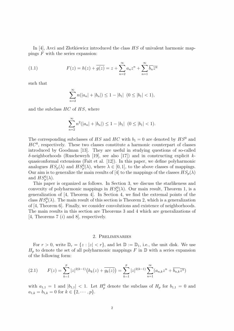
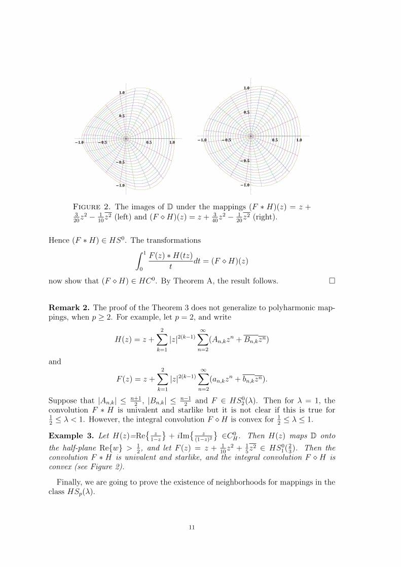
Figure 2. The images of D under the mappings (F ∗ H)(z) = z +320z2 − 1

10z2 (left) and (F �H)(z) = z + 3

40z2 − 1

20z2 (right).

Hence (F ∗H) ∈ HS0. The transformations∫ 1

0

F (z) ∗H(tz)

tdt = (F �H)(z)

now show that (F �H) ∈ HC0. By Theorem A, the result follows. �

Remark 2. The proof of the Theorem 3 does not generalize to polyharmonic map-pings, when p ≥ 2. For example, let p = 2, and write

H(z) = z +2∑

k=1

|z|2(k−1)∞∑n=2

(An,kzn +Bn,kzn)

and

F (z) = z +2∑

k=1

|z|2(k−1)∞∑n=2

(an,kzn + bn,kzn).

Suppose that |An,k| ≤ n+12

, |Bn,k| ≤ n−12

and F ∈ HS02(λ). Then for λ = 1, the

convolution F ∗ H is univalent and starlike but it is not clear if this is true for12≤ λ < 1. However, the integral convolution F �H is convex for 1

2≤ λ ≤ 1.

Example 3. Let H(z)=Re{

z1−z

}+ iIm

{z

(1−z)2}∈C0

H . Then H(z) maps D onto

the half-plane Re{w} > 12, and let F (z) = z + 1

10z2 + 1

5z2 ∈ HS0

1(23). Then the

convolution F ∗ H is univalent and starlike, and the integral convolution F � H isconvex (see Figure 2).

Finally, we are going to prove the existence of neighborhoods for mappings in theclass HSp(λ).

11

Theorem 4. Assume that λ ∈ (0, 1] and F ∈ HSp(λ). If

δ ≤ λ

p+ λ

(2−

p∑k=1

(2k − 1)(|a1,k|+ |b1,k|)

),

then Nδ(F ) ⊂ HSp.

Proof. Let H(z) =∑p

k=1 |z|2(k−1)∑∞

n=1(An,kzn +Bn,kz

n) ∈ Nδ(F ). Thenp∑

k=1

∞∑n=2

(2(k − 1) + n

)(|An,k|+ |Bn,k|) +

p∑k=2

(2k − 1)(|A1,k|+ |B1,k|) + |B1,1|

≤p∑

k=1

∞∑n=2

(2(k − 1) + n

)(|An,k − an,k|+ |Bn,k − bn,k|)

+

p∑k=2

(2k − 1)(|A1,k − a1,k|+ |B1,k − b1,k|) + |B1,1 − b1,1|

+

p∑k=1

∞∑n=2

(2(k − 1) + n

)(|an,k|+ |bn,k|) +

p∑k=2

(2k − 1)(|a1,k|+ |b1,k|) + |b1,1|

≤δ +

p∑k=1

∞∑n=2

(2(k − 1) + n

)(|an,k|+ |bn,k|) +

p∑k=2

(2k − 1)(|a1,k|+ |b1,k|) + |b1,1|

≤δ +p

p+ λ

p∑k=1

∞∑n=2

(2(k − 1) + n(λn+ 1− λ)

)(|an,k|+ |bn,k|)

+

p∑k=2

(2k − 1)(|a1,k|+ |b1,k|) + |b1,1|

≤δ +p− λp+ λ

+λ

p+ λ

p∑k=1

(2k − 1)(|a1,k|+ |b1,k|) < 1.

Hence, H ∈ HSp. �

References

1. Z. Abdulhadi and Y. Abu Muhanna, Landau’s theorem for biharmonic

mappings. J. Math. Anal. Appl. 338 (2008), 705–709.

2. Z. Abdulhadi, Y. Abu Muhanna and S. Khuri, On univalent solutions of

the biharmonic equation. J. Inequal. Appl. 5 (2005), 469–478.

3. Z. Abdulhadi, Y. Abu Muhanna and S. Khuri, On some properties of

solutions of the biharmonic equation. Appl. Math. Comput. 117 (2006), 346–

351.

4. Y. Avci and E. Z lotkiewicz, On harmonic univalent mappings. Ann. Univ.

Mariae Curie-Sk lodowska (Sect A) 44 (1990), 1–7.

12

5. Sh. Chen, S. Ponnusamy and X. Wang, Landau’s theorem for certain bi-

harmonic mappings, Appl. Math. Comput. 208 (2009), 427–433.

6. Sh. Chen, S. Ponnusamy and X. Wang, Compositions of harmonic map-

pings and biharmonic mappings. Bull. Belg. Math. Soc. Simon Stevin. 17

(2010), 693–704.

7. Sh. Chen, S. Ponnusamy and X. Wang, Bloch constant and Landau’s theo-

rem for planar p-harmonic mappings. J. Math. Anal. Appl. 373 (2011), 102–110.

8. J. Chen and X. Wang, On certain classes of biharmonic mappings defined by

convolution. Abstract and Applied Analysis. 2012, Article ID 379130, 10 pages.

doi:10.1155/2012/379130

9. J. G. Clunie and T. Sheil-Small, Harmonic univalent functions. Ann. Acad.

Sci. Fenn. Ser. A. I. 9 (1984), 3–25.

10. P. Duren, Univalent functions. Spring-Verlag, New York 1983.

11. P. Duren, Harmonic mappings in the plane. Cambridge University Press,

Cambridge 2004.

12. M. Fait, J. Krzyz and J. Zygmunt, Explicit quasiconformal extensions for

some classes of univalent functions. Comment. Math. Helv. 51 (1976), 279–285.

13. A. W. Goodman, Univalent functions and nonanalytic curves, Proc. Amer.

Math. Soc. 8 (1957), 588–601.

14. J. Happel and H. Brenner, Low Reynolds Number Hydrodynamics with Spe-

cial Applications to Particulate Media. Prentice-Hall, Englewood Cliffs, NJ,

USA, 1965.

15. S. A. Khuri, Biorthogonal series solution of Stokes flow problems in sectorial

regions. SIAM J. Appl. Math. 56 (1996), 19–39.

16. W. E. Langlois, Slow Viscous Flow. Macmillan, New York, NY, USA, 1964.

17. J. Qiao and X. Wang, On p-harmonic univalent mappings (in Chinese). Acta

Math. Sci. 32A (2012), 588–600.

18. C. Pommerenke, Univalent functions. Vandenhoeck and Ruprecht, Gotting-

en, 1975.

19. S. Ruscheweyh, Neighborhoods of univalent functions. Proc. Amer. Math.

Soc. 18 (1981), 521–528.

13

J. Chen, Department of Mathematics, Hunan Normal University, Changsha, Hu-nan 410081, People’s Republic of China.

E-mail address: [email protected]

A. Rasila, Department of Mathematics, Hunan Normal University, Changsha,Hunan 410081, People’s Republic of China, and Department of Mathematics andSystems Analysis, Aalto University, P. O. Box 11100, FI-00076 Aalto, Finland.

E-mail address: [email protected]

X. Wang, Department of Mathematics, Hunan Normal University, Changsha, Hu-nan 410081, People’s Republic of China.

E-mail address: [email protected]

14