On Peres' Statement ``Opposite Momenta Lead to Opposite Directions,'' Decaying Systems and Optical Imaging

arX

iv:q

uant

-ph/

0401

095v

1 1

7 Ja

n 20

04

On Peres’ statement “opposite momenta lead to opposite

directions”, decaying systems and optical imaging

W. Struyve, W. De Baere, J. De Neve and S. De Weirdt

Laboratory for Theoretical PhysicsUnit for Subatomic and Radiation PhysicsProeftuinstraat 86, B–9000 Ghent, Belgium

E–mail: [email protected], [email protected]

Abstract

We re-examine Peres’ statement “opposite momenta lead to opposite

directions”. It will be shown that Peres’ statement is only valid in the large

distance or large time limit. In the short distance or short time limit an

additional deviation from perfect alignment occurs due to the uncertainty

of the location of the source. This error contribution plays a major role in

Popper’s orginal experimental proposal. Peres’ statement applies rather

to the phenomenon of optical imaging, which was regarded by him as a

verification of his statement. This is because this experiment can in a

certain sense be seen as occurring in the large distance limit. We will also

reconsider both experiments from the viewpoint of Bohmian mechanics.

In Bohmian mechanics particles with exactly opposite momenta will move

in opposite directions. In addition it will prove particularly usefull to use

Bohmian mechanics because the Bohmian trajectories coincide with the

conceptual trajectories drawn by Pittman et al. In this way Bohmian

mechanics provides a theoretical basis for these conceptual trajectories.

1 Introduction

Already in 1934 Popper [1–3] proposed an experiment which aimed to test thegeneral validity of quantum mechanics. Popper assumes a source S from whichpairs of particles are emitted in opposite directions. Two observers, say Aliceand Bob, are located at opposite sides of the source, both equiped with an arrayof detectors. If Alice puts a screen with a slit in her way of the particles, she willobserve a diffraction pattern behind the screen. According to Popper, quantummechanics will also predict a diffraction pattern on the other side of the source,where Bob is located, when coincidence counts are considered. This is becauseevery measurement by Alice is in fact a virtual position measurement of thecorrelated particle on Bob’s side, leading to an increased momentum uncertaintyfor Bob’s particle as well. This is the same diffraction pattern that would beobserved when a physical slit was placed on Bob’s side. Popper, who declared

1

himself a metaphysical realist, found this idea of “virtual scattering” absurdand predicted no increased momentum uncertainty for Bob’s measurement dueto Alice’s position measurement. He therefore saw his proposed experiment asa possible test against quantum mechanics and in favour of his realist vision inwhich particles have at each time well defined positions and momenta; particlesfor which the Heisenberg uncertainty, for example, is only a lower, statisticallimit of scatter.

Unfortunately, to describe the setup of the experiment, Popper occasionallyinvoked classical language, which veiled some severe problems which could ob-struct a practical realization of his experiment (for an extensive discussion seePeres [4]). Popper writes: “We have a source S (positronium, say) from whichpairs of particles that have interacted are emitted in opposite directions. Weconsider pairs of particles that move in opposite directions . . . ”. It is the valid-ity of this statement, which appears to be a very delicate issue, that we shalldeal with in the present paper.

Of course, when we consider a decaying system at rest in classical mechanics,the fragments will have opposite momenta

p1 + p2 = 0 (1)

and if we take the place of decay of the system as the centre of our coordinatesystem the positions of the two fragments will satisfy m1r1 +m2r2 = 0, so thefragments will be found in opposite, isotropically distributed directions. If thefragments have equal masses then they will be found at opposite places, relativeto the centre of the coordinate system.

But these properties don’t hold in quantum mechanics. Suppose that asystem has a two–particle wavefunction ψ which has a sharp distribution atp1+p2 = 0, i.e. both |〈p1j+p2j〉| and ∆(p1j+p2j) are small for every componentj of the momentum vectors p1+p2. Then according to the uncertainty relations

∆(p1j + p2j)∆(m1r1j +m2r2j) ≥~

2(m1 +m2), (2)

the distribution of m1r1j +m2r2j will be broad for every component j. In thecase of equal masses, the inequalities in Eq. (2) imply that opposite momentaare incompatible with opposite positions. In particular, at the moment of decay,the inequalities imply that opposite momenta of the particles are incompatiblewith the latter being both located at the origin of our coordinate system. Itwas even shown by Collett and Loudon [5] that this initial uncertainty on thelocation of the source implies that Popper’s experiment is inconclusive.

Although the original proposal of Popper’s experiment can hence not beperformed practically, due to the fact that opposite momenta are incompatiblewith opposite positions, the intention of Popper’s proposal can be maintainedif we have a two–particle system which displays some form of entanglement inthe position coordinates.1 One is then in principle able to test experimentally

1The position entanglement should not be exact, otherwise, as shown by Short [6], both ofthe observers would observe an infinite momentum spread.

2

wether one of the particles will experience an increased momentum spread dueto a position measurement (within a slit width) of the correlated particle, i.e.we would be able to test a possible “virtual scattering”. Such an experimenthas actually been carried out by Kim and Shih [7], who used the phenomenonof optical imaging, which was reported by Pittman et al. [8]. In the process ofoptical imaging, position entangled photons are created by placing a lens in theway of one of the momentum entangled photons created by parametric downconversion.

Recently Peres gave an analysis to which extent opposite momenta leadto opposite directions [9]. He argues that the inequalities in Eq. (2) do notexclude a priori the possibility that opposite momenta of particles lead to op-posite directions (instead of positions) where the particles will be found whena measurement is performed. On the contrary, the operator equivalent of (1)would even lead to an observable alignment of the detection points of the twoparticles. However in section 2 we show that Peres’ analysis can only be ap-plied in what we will call the “large time” or “large distance” regime. This isthe regime where the two particles have travelled a “large” distance from thesource. In this limit the Heisenberg uncertainty will be of minor importance forthe angular correlation. This result agrees with the scattering into cones theo-rem, which applies in the limit of infinite time. In the “short” distance regimethe uncertainty on the location of the source, due to the Heisenberg uncertainty,leads to an additional error contribution to the angular alignment. We will alsomake clear what is exactly meant by the “large” or “short” distance regime.

An example which shows the importance of the additional error, even in thelong time regime, is the orginial experiment of Popper (section 3). The situationis different for the phenomenon of optical imaging, which was considered byPeres as a justification for his analysis. Because the experiment can in a certainsense be seen as occuring in the long distance limit, Peres’ analysis can beapplied to this experiment.

In section 4, we will provide a simplified description of a decaying system us-ing the Bohmian picture [10, 11]. It will prove usefull to use Bohmian mechanicsbecause Bohmian mechanics inherits some of the language of classical mechanics.This is because Bohmian mechanics describes the motion of particles, allowingone to consider possible trajectories of the particles. This is contrary to “stan-dard quantum mechanics” where we can only speak of probabilities where aparticle will be detected when a position measurement is performed. Before theposition measurement is performed, particles can’t, according to standard quan-tum mechanics, be seen as localized pointlike objects. As such, there is no basisin the standard quantum formalism to use trajectories of particles between twomeasurements. The classical language present in Bohmian mechanics can thenbe compared with the classical language used by Popper in his experimentalproposal, in order to examine the possible interplay between opposite momentaand opposite positions.

We will also give an alternative explanation of the phenomenon of opticalimaging (or at least of its massive particle equivalent) with the use of Bohmianmechanics (section 5). Although the experiment could be equally well described

3

by quantum optics, there is an additional advantage by using Bohmian mechan-ics. The paper of Pittman et al. contains drawings of conceptual trajectoriesof the photons. These trajectories are not the real paths followed by the pho-tons, as explained above, but merely serve as a tool to visualize the experiment.In section 4, we show that the Bohmian trajectories (calculated in the massiveparticle equivalent of the experiment of Pittman et al.), coincide with these con-ceptual trajectories in Pittman’s paper. As such, Bohmian mechanics providesa theoretical basis for these trajectories.

We want to stress that by using Bohmian mechanics we don’t intend tocontest the validity of standard quantum mechanics. Besides, as is well knownBohmian mechanics and standard quantum mechanics are completely equivalentat the empirical level. Now, wether one believes or not in the existence ofparticles as localized objects between two measurements, Bohmian mechanicsprovides a possible way of dealing with particle trajectories, consistent withquantum mechanics at the level of detections. Even if one is dissatisfied withthe picture of moving particles, one can interpret the Bohmian trajectories asthe flowlines of the probability, because the speeds of the Bohmian particles aredefined as proportional to the quantum mechanical probability current.

Finally we want to remark that, unfortunately Kim and Shih failed in theiroriginal intention to perform Popper’s gedankenexperiment. It was shown byShort [6], that due to imperfect momentum entanglement of the parametricdown converted photons (caused by a restricted diameter of the source), theimage was not perfect, which blurred the predicted results.

2 Opposite momenta and opposite directions

To discuss the possible angular alignment of momentum entangled particles,Peres considers a nonrelativistic wavefunction describing massive particles. Ac-cording to Peres, the reason for angular correlation of momentum entangledphotons (as in the experiment of Pittman et al.) is the same as in the consid-ered massive case.

The momentum correlated particles can be assumed to result from a decayingsystem at rest. The decaying system can then be described by the wavefunction

ψ(r1, r2, t) =

∫

F (p1,p2)ei(p1·r1+p2·r2−Et)/~dp1dp2 (3)

where the momentum distribution F is peaked around p1 +p2 = 0 and aroundthe rest energy E0 of the decaying system. According to Peres the oppositemomenta of the particles lead to opposite directions where the particles willbe found when a measurement is performed. His argument goes as follows.The main contribution in the integral in Eq. (3) comes from values p1 and p2

for which p1 + p2 ≃ 0. Because of the rapid oscillations of the phase in theintegrand in Eq. (3), the integral will be appreciably different from zero only ifthe phase is stationary with respect to the six integration variables p1 and p2

4

in the vicinity of p1 + p2 = 0, i.e.

∂S

∂pi+ ri −

∂E

∂pit = 0, i = 1, 2 (4)

where S is the phase of F (p1,p2) measured in units ~, i.e.

F (p1,p2) = |F (p1,p2)|eiS(p1,p2)/~ (5)

and the equations (4) have to be evaluated for p1 + p2 = 0. The equations (4)then determine the conditions on ri in order to have a non–zero ψ (and |ψ|2).

Peres then introduces spherical coordinates to describe pi and ri, and variesthe phase with respect to the six spherical variables pi, φi, θi (the sphericalcoordinates of pi). Peres further assumes that the phase of F obeys

∂S/∂pi = 0 (6)

in the vicinity of p1 + p2 = 0. This would restrict the place of decay near theorigin of the coordinate system, because of Eq. (4). By varying with respect tothe momentum angles, Peres obtains that the phase is stationary if pi and ri

have the same direction. Because F is peaked at p1 + p2 = 0, this results in

θ′1 + θ′2 = π

|φ′1 − φ′2| = π (7)

where ri, φ′i, θ

′i are the spherical coordinates of ri. These equations show that

the two particles can only be detected at opposite directions relative to thecentre of our coordinate system. This is because the integral in Eq. (3) (andhence |ψ|2) would only be appreciably different from zero if ri obey Eq. (7).

Peres mentions two error contributions to the angular alignment. The firstis a transversal deviation of the order

√

ht/m due to the spreading of the wave-function, which was recognized as the standard quantum limit [12]. The secondis an angular spread of the order ∆(p1j + p2j)/pi. One of the aims of the presentpaper is now to show that there is another error contribition which arises fromthe uncertainty on the source and which is particularly important in the “short”distance or “short” time regime.

First we note that there is, apart from the conditions on θ′i and φ′i, also acondition on the variables ri, which is not mentioned by Peres. This conditionis obtained by varying the phase of the integrand with respect to pi, having inmind the previous result that pi and ri have the same direction. If we definevi = dE/dpi, then the additional condition reads

ri = vit (8)

where the vi have to be evaluated for p1 + p2 = 0. Because ψ obeys the non-

relativistic Schrodinger equation, E equalsp21

2m1+

p22

2m2, with mi the masses of

the particles. In this way Eq. (8) becomes

r1 =p1

m1t, r2 =

p2

m2t. (9)

5

Using p1 + p2 = 0 one obtains

r1m1 = r2m2. (10)

Note that we haven’t yet used the fact that F is peaked around a certain energyE0, as is required in the case of a decaying system at rest. As Peres remarks inhis paper, a restriction of the energy to E0 further restricts the momenta of theparticles to satisfy p2

1 = p22 = 2E0m1m2/(m1 +m2).

Combining (7) and (10) one obtains that the joint detection probability hasa maximum for the classically expected relation m1r1 +m2r2 = 0. Hence Peres’statement “opposite momenta lead to opposite directions” may be replaced bya stronger statement, i.e. the opposite momenta lead to a maximum detectionprobability for m1r1 +m2r2 = 0. However we still have to consider the possiblesources of deviation from this classical relation. Classically one can, in theory,make both quantities ∆(p1j + p2j) and ∆(m1r1j +m2r2j) as small as wanted.Quantum mechanically one can at best prepare the system, such that initiallythe equality in

∆(p1j + p2j)∆(m1r1j +m2r2j) ≥~

2(m1 +m2) (11)

is reached. Remark that this equation implies that in case of opposite momenta,the particles can’t depart from a confined, fixed source.

Because the operator p1j + p2j commutes with the free Hamiltonian, thevariance of the momentum operator p1j + p2j is stationary. The variance ofr1j + r2j however, will in general increase with time due to the spreading ofthe wavefunction. This can be seen if we write down the expression for the freeevolution of the operator m1r1 +m2r2 in the Heisenberg picture

m1r1(t) +m2r2(t) = m1r1(0) + p1(0)t+m2r2(0) + p2(0)t (12)

The variance of this operator for an arbitrary component j is

∆(

m1r1j(t) +m2r2j(t))2

= ∆(

m1r1j(0) +m2r2j(0))2

+ ∆(

p1j(0) + p2j(0))2t2

+⟨{

(

m1r1j(0) +m2r2j(0))

,(

p1j(0) + p2j(0))

}⟩

t

−2⟨

m1r1j(0) +m2r2j(0)⟩⟨

p1j(0) + p2j(0)⟩

t (13)

where the brackets {, } denote the anticommutator. If we assume a distributionF which is real and symmetric, i.e. F (p1,p2) = F (−p1,−p2) then the last twoterms in Eq. (13) are each zero. So the variance of m1r1j(t)+m2r2j(t) increaseswith time

∆(

m1r1j(t) +m2r2j(t))2

= ∆(

m1r1j(0) +m2r2j(0))2

+ ∆(

p1j(0) + p2j(0))2t2.

(14)This leads to an increasing deviation from the relation m1r1 +m2r2 = 0.

There is thus always an interplay between opposite momenta and oppositedirections which is expressed in Eq. (11) and Eq. (14). We argue that one

6

should study Eq. (14), where the variances at t = 0 in the right hand side of theexpression are limited by the Heisenberg uncertainty in Eq. (11), to determineto which extent we can speak of possible angular alignment.

Let us now see how Peres’ error contributions come about and in whichregime they are important. Assume for convenience that m1 = m2 = m. Thetransversal deviation L(t) can be taken of the order ∆

(

r1j(t) + r2j(t))

. There

are two contributions to this transversal deviation. The first is ∆(

r1j(0) +

r2j(0))

= L(0) and is important for small times. The second contribution

is ∆(

p1j + p2j

)

t/m which becomes important for larger times. The angulardeviation θ may be derived from tan(θ) = L(t)/R(t), where R(t) = pt/m is thedistance that both particles have travelled. For small times one has tan(θ) ≃∆

(

r1j(0) + r2j(0))

m/pt and for large times one has tan(θ) ≃ ∆(

p1j + p2j

)

/p.Hence for large times we obtain the error mentioned by Peres. From the relations(11) and (14) one can also easily derive the standard quantum limit

∆(

r1j(t) + r2j(t))2

≥ 2∆(

r1j(0) + r2j(0))

∆(

p1j(0) + p2j(0))

t/m

≥ 2~t/m. (15)

However, this uncertainty is misleading because for small times it neglects thecontribution arising from the uncertainty on the source ∆

(

m1r1j(0)+m2r2j(0))

.

Especially in the considered case this contribution will be large because ∆(

p1j(0)+

p2j(0))

is small.In summary we see that Peres gave error contributions which only apply in

the large time regime. These error contributions are in perfect agreement withthe “scattering into cones” theorem which states that for every cone C in R

m

with apex in the origin

limt→∞

∫

C

dmx|ψ(x, t)|2 =

∫

C

dmp|φ(p)|2 (16)

with φ(p) the momentum wave function [13]. This means that the probabilitythat in the infinite future the particles will be found in the cone C is equalto the probability that their momenta lie in the same cone. In the smalltime regime the uncertainty on the source gives the major contribution. Wecould say that the transition between the small time regime and the large timeregime occurs at time T when both contributions to L(t) are equally large, i.e.L(0) = ∆

(

p1j(0) + p2j(0))

T/m. Because we can at best reach the Heisenberguncertainty, a lower bound for the time is given by T = L(0)2kc/c with kc thewavevector corresponding to the compton wavelength of the particles. In thenext section we will plug some numbers into this relation to show that we arenot making a trivial point in stressing this additional error contribution. Let itfor the moment be sufficient to provide an example which illustrates the impor-tance of this uncertainty on the source. We can use a Gaussian distribution torepresent the momentum correlation

F (p1,p2) ∼ e−(p1+p2)2

σ . (17)

7

The smaller the value of σ, the better the momentum correlation between thetwo fragments. In the limit σ → 0 this distribution approaches the Dirac deltadistribution. Remark that this distribution is not peaked around a certain en-ergy E0 as should be required for a decaying system at rest. In the Appendix itis explained why we can leave this restriction on the energy aside without chang-ing the main result. It will follow that a reasonable energy width, peaked aroundE0, will imply only a minor broadening of the wavefunction. The wavefunctionat t = 0 is

ψ(r1, r2, 0) ∼ δ(r1 − r2)e−r2

1σ/4~2

. (18)

Thus clearly ψ represents a decaying system because initially r1 = r2. Butfor small values of σ (when F is peaked around p1 + p2 = 0) the probabilityof finding the particles at t = 0 at some configuration is totally smeared out,although the probability has a maximum at the origin of the coordinate system.Note that although the relation ∂S/∂pi = 0 is satisfied, this condition doesn’trestrict the place of decay near the origin of the coordinate system, as wasassumed by Peres. So in the short time regime, it may be hard to speak ofpossible opposite movements of particles relative to the origin because we cannotexactly say (at least without measurement) where the decay of the system tookplace. As time increases the deviation from the detection probability peak atm1r1 +m2r2 = 0 will even increase with time as was shown above. However,because the distance from the particles to the source increases, the uncertaintyof the source will become less important for the angular deviation. In the longdistance regime the angular deviation will then be dominated by the momentumuncertainty.

In section 4 we will show that we can retain the classical picture of a decayingsystem in the previous example, in both the short time regime and the longtime regime, when it is described by Bohmian mechanics. Namely in the case ofthe considered wavefunction, the Bohmian particles will depart near eachotherand will move along opposite directions. However, the place of departure willvary from pair to pair over an extended region. The more this initial regionis confined, the less perfect the momentum entanglement will be, and the lessperfect the opposite movements of the Bohmian particles will be.

3 Opposite momenta and opposite directions in

the case of the experiments of Popper and

Pittman et al.

The importance of the error contribution arising from the uncertainty of thesource becomes clear if we consider the example of Popper’s experimental pro-posal. It can easily be seen that Popper’s experiment cannot occur in the largetime regime. If the particles would travel long distances (and hence obtaingood angular correlation), the virtual slit (which is of the order of the transver-sal deviation) would be too large to have virtual diffraction of the particles on

8

Bob’s side. Hence Popper’s original experimental proposal should be consid-ered in the short time regime. However, in this regime the uncertainty on thesource becomes the most important contribution to the angular deviation andas follows from the analysis of Collett and Loudon, this uncertainty makes adetectable virtual diffraction impossible. This also implies that in discussingPopper’s experiment one should be carefull with statements such as “. . . the al-lowed deviation from perfect alignment is of the order of ∆|p1 + p2|/|p1 − p2|,which is much too small to be of any consequence in the present discussion.”and “. . . nearly perfect alignment can be taken for granted, . . . ” [4].

In the case of optical imaging, performed by Pittman et al., Peres’ analy-sis can be applied. Let us first briefly review this experiment. The experimentuses momentum correlated photons resulting from spontaneous parametric downconversion (SPDC). In this process a pump photon incident on a nonlinear betabarium borate (BBO) crystal leads to the creation of a signal and idler photon.The place of creation within the BBO crystal is unknown. Due to momentumconservation the sum of the momenta of these photons has to equal the mo-mentum of the pump photon. This results in the momentum entanglement ofthe two photons, because the momenta of the idler and signal photon can becombined in an infinite number of ways to equal the momentum of the pumpphoton. In the same way the energies of the created photons add up to theenergy of the pump photon. In the experiment the signal and idler photons aresent in two different directions where coincidence records may be performed bytwo photon counting detectors. A convex lens, with focal length f , is placedin the signal beam in order to turn the momentum correlation of the createdphotons into spatial correlation (see Fig. 1). In front of the detector for thesignal beam an aperture is placed at a distance S from the lens. By placing thedetector for the idler beam at a distance S′ from the lens, prescribed by theGaussian thin lens equation, i.e.

1

S+

1

S′=

1

f(19)

and scanning in the transverse plane of the idler beam, an image of this aper-ture is observed in the coincidence counts. This image obeys the classical lensequations in the following sense. If a classical pointlike light source would beplaced in the plane of the aperture, where the signal photon was detected, itwould have an image where the idler photon was detected. This is the spatialcorrelation of the photons.

The experiment can be seen to occur in the long distance regime because ofthe lens. In some sense the lens can be seen as projecting the angular correlationat infinity, to finite distances (at distances 2f from the lens). The better themomentum correlation, the better the angular correlation is at infinity or thebetter the optical imaging is.

It is interesting to use the data of this experiment to give an example wherethe border can be situated between the long distance and the short distanceregime for a stongly momentum correlated system. A lower bound for the timeis T = L(0)2kc/c, hence if there would be no lens in the Pittman experiment,

9

lensBBO

f f

S=2f S’=2f

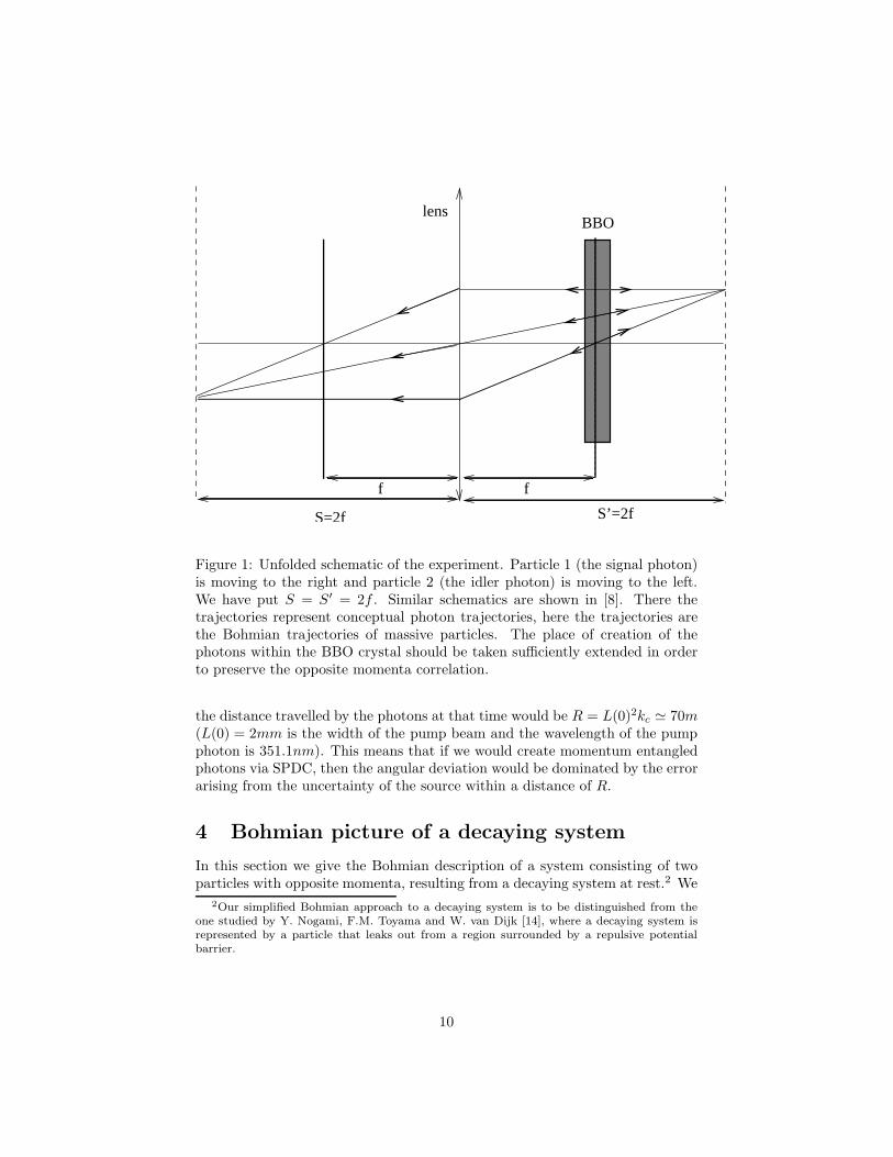
Figure 1: Unfolded schematic of the experiment. Particle 1 (the signal photon)is moving to the right and particle 2 (the idler photon) is moving to the left.We have put S = S′ = 2f . Similar schematics are shown in [8]. There thetrajectories represent conceptual photon trajectories, here the trajectories arethe Bohmian trajectories of massive particles. The place of creation of thephotons within the BBO crystal should be taken sufficiently extended in orderto preserve the opposite momenta correlation.

the distance travelled by the photons at that time would be R = L(0)2kc ≃ 70m(L(0) = 2mm is the width of the pump beam and the wavelength of the pumpphoton is 351.1nm). This means that if we would create momentum entangledphotons via SPDC, then the angular deviation would be dominated by the errorarising from the uncertainty of the source within a distance of R.

4 Bohmian picture of a decaying system

In this section we give the Bohmian description of a system consisting of twoparticles with opposite momenta, resulting from a decaying system at rest.2 We

2Our simplified Bohmian approach to a decaying system is to be distinguished from theone studied by Y. Nogami, F.M. Toyama and W. van Dijk [14], where a decaying system isrepresented by a particle that leaks out from a region surrounded by a repulsive potentialbarrier.

10

use the wavefunction in Eq. (3) with momentum distribution

F (p1,p2) = Nδ(p1 + p2)e−αp2

1/~ (20)

where N is a normalisation factor. The parameter α sets the scale of the initialseparation of the two particles, as will be seen soon. A small α will correspondto the considered physical situation, i.e. a decaying system. The parameteris introduced in order to avoid singularities arising from the delta distributionwhen calculating the Bohmian trajectories later on. Again we have left asidethe restriction on the total energy, as required in the case of a decaying system(see Appendix). Remark that the exponential factor in Eq. (20) doesn’t restrictthe value of the total energy for a small α. The wavefunction corresponding tothe distribution F is

ψ(r1, r2, t) = N

(

π~

α+ it/2µ

)3/2

e−(r1−r2)2/4~(α+ it2µ

) (21)

with µ the reduced mass of the fragments: 1µ = 1

m1+ 1

m2. At t = 0 the

probability distribution is

|ψ(r1, r2, 0)|2 = N2

(

π~

α

)3

e−(r1−r2)2/2~α. (22)

It follows that a small value for α corresponds to the considered physical situ-ation of a decaying system. However, the place of decay is unknown. This is aconsequence of the Heisenberg uncertainty, as explained in the section 2.

The Bohmian trajectories Rj(t) of the particles are found by solving thedifferential equations

dRj

dt=

1

mj

Reψ∗(r1, r2, t)pjψ(r1, r2, t)

|ψ(r1, r2, t)|2

∣

∣

∣

∣

∣

ri=Ri

. (23)

Because (p1 + p2)ψ = 0 the trajectories of the particles satisfy

d

dt(m1R1 +m2R2) = 0. (24)

This shows that the particles have opposite speeds and thus move in oppositedirections. Integration of the differential equations (23) leads to

R1(t) = C1 + C2

√

t2/4µ2 + α2

R2(t) = C1 − C2

√

t2/4µ2 + α2 (25)

where C1 and C2 are arbitrary constant vectors. It follows that the particlesalso move along straight lines. If we consider an ensemble of identically preparedsystems, the probability density of the Bohmian particles equals the quantummechanical distribution |ψ|2 [10, 11]. This is also called the quantum equilib-rium hypothesis [15] and ensures the empirical equivalence between Bohmian

11

mechanics and standard quantum mechanics. This equality determines the dis-tribution of the vectors Ci in the ensemble. Because the probability distributionat t = 0 is sharply peaked at r1 = r2 (for small values of α), the particles departnear each other. As follows from Eq. (25) their further propagation proceedsalong straight lines, in the direction of their connecting line. Thus oppositemomenta lead to opposite directions of movement for Bohmian particles. Buttheir place of departure is located within an extended area, in order to preservemomentum correlation.

By using Bohmian mechanics, we are thus able to retain part of the clas-sical picture of a decaying system at rest. Remark the similarity in languagewith the one used by Popper to describe his experiment. The difference is thatPopper assumed the particles to depart from a confined region (which is how-ever incompatible with opposite momenta in quantum mechanics). Note thatthe opposite movements of Bohmian particles can not be verified experimen-tally. This is because a measurement of the place of departure of the Bohmianparticles would cause a change of the wavefunction (this is the collapse of thewavefunction in standard quantum mechanics), which in turn implies differentparticle trajectories.

5 The experiment of Pittman et al. revisited by

Bohmian mechanics

Although the experiment of Pittman et al. can be correctly explained withquantum optics, we will provide a Bohmian account of the experiment, when itis “translated” into its massive particle equivalent. One of the reasons to useBohmian mechanics is that it justifies the conceptual photon trajectories drawnby Pittman et al. [8]. I.e. the photon trajectories coincide with the trajecto-ries of Bohmian particles in the massive particle equivalent of the experiment.This (Bohmian) quantum mechanical approach is contrary to the explanationin terms of “usual” geometrical optics used by Pittman et al. In quantum opticsthese paths are usually regarded as a visualisation of the different contributionsto the detection probabilities.

Because there is at present no satisfactory Bohmian particle interpretationfor photons, see discussion elsewhere [16–19], we will follow Peres’ departureand consider the nonrelativistic massive particle wavefunction in Eq. (3) in-stead of quantum optics, to study the experiment by Pittman et al. The SPDCsource then corresponds to a decaying system at rest, resulting in two energyand momentum correlated fragments. We will assume the total momentum ofthe fragments to be zero, instead of some fixed value corresponding to the initialmomentum of the total system (which would represent the momentum of thepump photon). This assumption corresponds to the “unfolded” schematic intro-duced by Pittman et al. [8] (see Fig. 1). In this way we can use the momentumdistribution F defined in previous section

F (p1,p2) = Nδ(p1 + p2)e−αp2

1/~. (26)

12

In previous section we described the free evolution after the decay of the system.The unknown place of decay in the massive particle case corresponds to theunknown place of creation within the BBO crystal in the photon case (whichis also related to the width of the pump beam). To complete the Bohmiandescription of the massive particle equivalent of optical imaging, we just haveto describe the system’s interaction with the lens. In classical optics we canuse ray optics to describe the action of the lens on an impinging light beam[20]. The rays are such that the Gaussian thin lens equations are satisfied. Twogeneric examples, which we will need later on, are the following. The effect ofthe lens on a plane wave is to turn it into a converging wave, with focus inthe focal plane, such that the corresponding rays obey the lens equations. Thecharacteristics of the converging wave are then determined by the momentum ofthe incoming plane wave and the focal length. A second example is a sphericalwave, representing a point source. If we assume that the light source is locatedin a plane at a distance S from the lens, then the spherical wave will turn intoa converging wave with focus in the plane at a distance S′ from the lens so that1/S + 1/S′ = 1/f and the source, the image and the centre of the lens will bealigned. In massive particle quantum physics the equivalent of optical lensesare electrostatic or magnetic lenses. These electromagnetic lenses are generallyused to collimate or focus beams of charged particles. This field of research isusually called optics of charged–particle beams or the theory of charged–particlebeams through electromagnetic systems. Most of the literature deals with theclassical description of the particles and only recently the quantum mechanicalapproach has been studied, see for example Hawkes and Kasper [21], and Khanand Jagannathan [22] and references therein. Here we will not bother aboutthe detailed analysis of particles passing through such electromagnetic lenses,and use directly, in the spirit of de Broglie, the analogy with classical optics.For example we can describe the action of an electromagnetic lens as turning aquantum mechanical plane wave into a Gaussian wave (we can take this as theanalogue of the converging wave in classical optics, because a Gaussian wave iscontracting before expanding), determined by the momentum of the incomingwave and the focal length. This analogy is very appealing because the raysin classical optics can be “identified” with the Bohmian trajectories. This isbecause in the one–particle case, the curves determined by the normals of thewavefronts of the quantum mechanical wavefunction are just the possible orbitsof a particle described by Bohmian mechanics [23]. If we apply this to ourdecaying system, then every plane wave of the particle impinging on the lens,say particle two, in the integral in Eq. (3) is turned into a particular Gaussianwave. The resulting wave is then

ψ′(r1, r2, t) =

∫

F (p1,p2)ei(p1·r1−p2

1t/2m1)/~G(r2,p2, f)dp1dp2 (27)

where G represents the Gaussian wave. This wave is guiding the particles afterparticle two passed the lens. To avoid unnecessary mathematical complicationswhen calculating the Bohmian trajectories implied by the wave Eq. (27), weassume that the place of decay of the system is somewhere in the middle between

13

the lens and the detector on the right (where the idler photon arrives in theexperiment of Pittman et. al.). This corresponds to a BBO crystal placed inthe middle instead of it placed near the lens, as in the experiment. Whenparticle two arrives in the vicinity of the lens, particle one arrives in the vicinityof the detector placed on the right. We can describe the effect of the detectoron the wavefunction as the first stage of a von Neumann measurement process(see for example Bohm and Hiley [24]). In this process the wavefunction getsentangled with a pointer which is represented by a wavefunction φ with a smallwidth. In this way the wavefunction in Eq. (3) turns into

ψ′′(r1, r2,y, t) =

∫

F (p1,p2)δ(a − r1)φ(y, t,a)ei(

p1·(a−r2)−Et)

/~dp1dp2da

(28)where we have written the factorization into position eigenfunctions δ(a − r1)of particle one explicitly. It is supposed that the interaction of the detectingapparatus with the decaying system lasted long enough in order to assure thatthe wavepackets φ(y,a) are non overlapping for each a. During this process,the pointer particle has entered one of the packets φ(y,a), determined by itsinitial position. While the packets are non overlapping, only the consideredwavepacket is determining the subsequent trajectory of the pointer particle.The other wavepackets can then be dismissed for the further description of thesystem. In conventional quantum mechanics this process would be treated asa collapse of the wavefunction, which is the second stage of the von Neumannmeasurement process. As a result, the effective wave guiding particle two, isalso reduced to the following superposition of plane waves

ψ2(r2, t) = N

∫

ei~

(

p·(a−r2)−p2t/2m2

)

−αp2/~dp

= N

(

π~

α+ it/2m2

)3/2

e−(a−r2)2/4~(α+ it

2m2). (29)

The phase of this wave is

S(r2, t) =t(a − r2)

2

8m2α2 + t2/m2−

3~

2tan−1(t/2m2α). (30)

So the wavefronts of the guiding wave of particle two are spheres with centrein a. Because the detectors are placed in planes at distances S and S′ fromthe lens, with S and S′ obeying the Gaussian lens equation (19), this wave willresult, after propagation through the lens, in a converging wave with focus inthe plane at a distance S from the lens and where the focus is determined by theGaussian thin lens equations. Hereby we used again the analogy with classicalGaussian optics. If for example S = S′ and if the centre of the lens is takenas the origin of our coordinate system, then the focus will be at −a (see Fig.1). As a consequence of the quantum equilibrium hypothesis, particle two willbe detected in the focus of the wave. Because we used a Gaussian to describethe converging wave, the Bohmian trajectories will not be straight lines, but

14

will be curved (for images see Holland [23]). The curvature will depend on thewidth in the focus of the Gaussian. In the limit of a zero width, however, thetrajectories will approach straight lines, directed from the lens towards the focusof the wave. When the coincidence detections are considered, it will appear asif particle two departs from the place of detection of particle one.

This completes the Bohmian analysis of the phenomenon of optical imaging.Before the fragments reach the lens, they move along straight lines from theplace of decay. Note that this place of decay is not fixed, in order to guaranteethe momentum correlation p1 + p2 = 0. When one of the particles reaches thelens, its direction of movement will change in accordance with the classical thinlense approximations. We assumed hereby the place of decay to be centeredbetween the right detector and the lens. It can be expected, although it is notproven, that a random place of decay (for example near the lens) will lead tothe same results in the Bohmian description of the experiment.

6 Conclusions

In conclusion we showed that Peres’ analysis concerning the question to whatextent opposite momenta lead to opposite directions, is only valid in the longdistance regime. In the short time regime there is an additional source of an-gular deviation. On the other hand the statement “opposite momenta lead toopposite directions” is true in the Bohmian language. I.e. Bohmian particlestravel in opposite directions when the wavefunction has eigenvalue zero for thetotal momentum operator (however from an unknown place of departure). Wealso showed that Bohmian trajectories can be used to gain insight into thephenomenon of ghost imaging as reported by Pittman et al. In fact Bohmianmechanics can be used to describe similar quantum optical experiments as well,such as Popper’s experiment in the version of Kim and Shih [7] and the ex-periment reported by Strekalov et al. [25]. In particular, Bohmian mechanicsjustifies the use of the conceptual pictures of photon trajectories present in thesepapers. Note that the experiment of Kim and Shih is very illustrative for theneed for perfect momentum correlation of the photons, or equivalently that theremust be very little restriction on the place of creation of the photons to createa perfect image. This is because Kim and Shih failed in their original intentionto perform Popper’s gedankenexperiment, due to the restricted diameter of thepump beam used in the experiment. The imperfect momentum correlation thenled to an imperfect optical image [6]. This is immediately obvious when weconsider our Bohmian picture of optical imaging, because if the momentum cor-relation is imperfect, the Bohmian particles will not move in opposite directionsbefore the system reaches the lens.

15

Appendix

Conservation of energy requires that the energy of the total system equals theenergy of the decaying system E0. If this decaying system is initially at rest,E0 will be the rest energy of the system. Suppose now that we take a delta–distribution for this energy restriction i.e.

F (p1,p2) = f(p1,p2)δ(E − E0) (31)

where f determines the momentum correlation (this is for example the distri-bution in Eq. (17) or Eq. (20)). If we take a distribution f which is real andsymmetric, i.e. f(p1,p2) = f(−p1,−p2) then the probability currents of thetwo particles are both zero for all times, i.e.

ji =Im(ψ∗∇ri

ψ)

mi= 0, i = 1, 2. (32)

This implies that the particles show no evolution. In Bohmian mechanics thisrepresents particles that stand still, because the Bohmian speeds are defined asdRi/dt = ji/|ψ|

2. As a result the considered distribution in Eq. (31) doesn’tcorrespond to a decaying system. We can resolve this problem by allowing afinite energy width centered around E0. However, it will follow that, if thewavefunction displays strong momentum correlation in the sense that p1 +p2 =0, the restriction to a small energy width only involves a minor broadening ofthe wavefunction, which implies that we can leave the restriction on the totalenergy aside for our qualitative analysis.

For the momentum distribution f we will take the distribution in Eq. (20),

i.e. f(p1,p2) ∼ δ(p1 + p2)e−αp2

1/~. The restriction on the total energy is ac-complished by integrating over values for (p1,p2) for wich E− ≤ E ≤ E+, for acertain minimum energy value E− and a certain maximimum energy value E+.We therefore define the following function

disc(E±)(p1,p2) =

{

1 ifp21

2m1+

p22

2m2≤ E±

0 otherwise

The momentum distribution then becomes

F (p1,p2) = f(p1,p2)[

disc(E+) − disc(E−)]

. (33)

The resulting wavefunction of the system is then

ψ(r1, r2, t) =

∫

f(p1,p2)[

disc(E+) − disc(E−)]

ei(p1·r1+p2·r2−Et)/~dp1dp2

∼

∫

eip·(r1−r2)/~−(it/2µ+α)p2/~[

disc’(E+) − disc’(E−)]

dp (34)

where

disc’(E±)(p) =

{

1 if p2/2µ ≤ E±

0 otherwise

16

If we write Eq. (34) as a Fourier transform then we can apply the convolutiontheorem

ψ(r1, r2, t) ∼ F+{(r1−r2)/~}

(

e−(it/2µ+α)p2/~)

⊗F+({r1−r2)/~}

(

disc’(E+) − disc’(E−))

∼ h(x, t) ⊗ g(x) (35)

where we have defined

h(x, t) = F+{(r1−r2)/~}

(

e−(it/2µ+α)p2/~)

,

g(x) = F+{(r1−r2)/~}

(

disc’(E+) − disc’(E−))

,

x = |r1 − r2|. (36)

We present now two methods to show that the restriction on the energy canbe relinquished, without changing the qualitative analysis. The first methodproceeds as follows. The first function in the convolution in Eq. (35) is just thewavefunction in Eq. (21),

h(x, t) ∼

(

π~

α+ it/2µ

)3/2

e−(r1−r2)2/4~(α+ it

2µ). (37)

If we define a± = 2π√

E±2µ/~ then the second function in the convolution inEq. (35) in two–dimensional physical space becomes

g(x) ∼[

a+J1(a+x) − a−J1(a−x)]

/x (38)

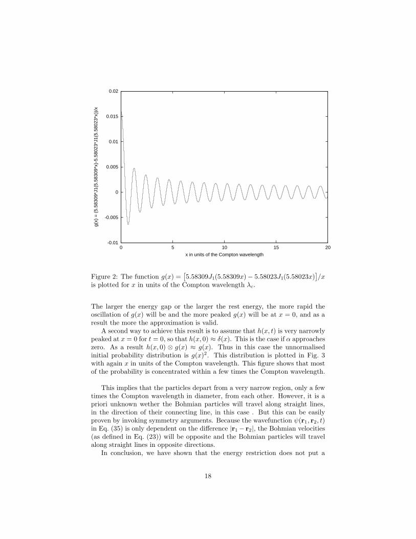
where J1 is the first order spherical Bessel function. To evaluate g(x) we willsubstitute some reasonable values for E+ and E− in Eq. (38). In addition wewill assume that the fragments have equal masses so that we can put 2µ = m,with m the mass of one fragment. For E+ we will take one percent of the restmass of the total system in order to avoid the relativistic regime, E+ = 0.02mc2.We will take an energy gap of 0.001E+, so that E− = 0.999E+. In this waya+ ≈ 5.58309/λc and a− ≈ 5.58023/λc, where λc is the Compton wavelengthof the fragments. In Fig. 2 the function g(x) =

[

a+J1(a+x) − a−J1(a−x)]

/x isplotted for x in units of the Compton wavelength λc.

The figure shows that g(x) is a rapidly oscillating function with a peak atx = 0. We now give the distribution of h(x, t) at t = 0 a width of the orderof twenty times the Compton wavelength, which can be done by adjusting α.Recall that the function h was in fact the wavefunction of the system if wedidn’t restrict the energy. So the width of h is in fact the measure of theinitial nearness of the fragments, which is then of the order of twenty times theCompton wavelength. Then due to the rapid oscillation, the main contributionin the convolution will arise only from the peak in g(x) at x = 0. This peak willresult in only a small broadening of h(x, 0) so that h(x, 0) ⊗ g(x) ≈ h(x, 0).

Because the width of h(x, t) only increases with time, this approximationwill become more precise with time. In conclusion we can put the unnormalisedwavefunction equal to

ψ(r1, r2, t) ≈

(

π~

α+ it/2µ

)3/2

e−(r1−r2)2/4~(α+ it

2µ). (39)

17

-0.01

-0.005

0

0.005

0.01

0.015

0.02

0 5 10 15 20

g(x)

= (

5.58

309*

J1(5

.583

09*x

)-5.

5802

3*J1

(5.5

8023

*x))

/x

x in units of the Compton wavelength

Figure 2: The function g(x) =[

5.58309J1(5.58309x)− 5.58023J1(5.58023x)]

/xis plotted for x in units of the Compton wavelength λc.

The larger the energy gap or the larger the rest energy, the more rapid theoscillation of g(x) will be and the more peaked g(x) will be at x = 0, and as aresult the more the approximation is valid.

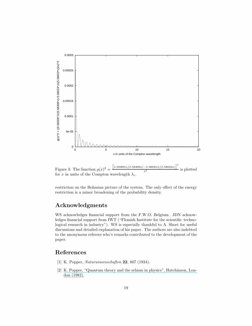
A second way to achieve this result is to assume that h(x, t) is very narrowlypeaked at x = 0 for t = 0, so that h(x, 0) ≈ δ(x). This is the case if α approacheszero. As a result h(x, 0) ⊗ g(x) ≈ g(x). Thus in this case the unnormalisedinitial probability distribution is g(x)2. This distribution is plotted in Fig. 3with again x in units of the Compton wavelength. This figure shows that mostof the probability is concentrated within a few times the Compton wavelength.

This implies that the particles depart from a very narrow region, only a fewtimes the Compton wavelength in diameter, from each other. However, it is apriori unknown wether the Bohmian particles will travel along straight lines,in the direction of their connecting line, in this case . But this can be easilyproven by invoking symmetry arguments. Because the wavefunction ψ(r1, r2, t)in Eq. (35) is only dependent on the difference |r1 − r2|, the Bohmian velocities(as defined in Eq. (23)) will be opposite and the Bohmian particles will travelalong straight lines in opposite directions.

In conclusion, we have shown that the energy restriction does not put a

18

0

5e-05

0.0001

0.00015

0.0002

0.00025

0.0003

0 5 10 15 20

g(x)

^2 =

((5

.583

09*J

1(5.

5830

9*x)

-5.5

8023

*J1(

5.58

023*

x))/

x)^2

x in units of the Compton wavelength

Figure 3: The function g(x)2 =

[

5.58309J1(5.58309x)−5.58023J1(5.58023x)]2

x2 is plottedfor x in units of the Compton wavelength λc.

restriction on the Bohmian picture of the system. The only effect of the energyrestriction is a minor broadening of the probability density.

Acknowledgments

WS acknowledges financial support from the F.W.O. Belgium. JDN acknow-ledges financial support from IWT (“Flemish Institute for the scientific–techno-logical research in industry”). WS is especially thankful to A. Short for usefuldiscussions and detailed explanation of his paper. The authors are also indebtedto the anonymous referees who’s remarks contributed to the development of thepaper.

References

[1] K. Popper, Naturwissenschaften 22, 807 (1934).

[2] K. Popper, “Quantum theory and the schism in physics”, Hutchinson, Lon-don (1982).

19

[3] K. Popper in “Open Questions in Quantum Physics”, ed. G. Tarozzi andA. van der Merwe, D. Reidel Publishing Company, Dordrecht, 3 (1985).

[4] A. Peres, Studies in History and Philosophy of Modern Physics 33, 23(2002) and quant-ph/9910078.

[5] M.J. Collett and R. Loudon, Nature 328, 675 (1987).

[6] A.J. Short, Found. Phys. Lett. 14, 275 (2001) and quant-ph/0005063.

[7] Y.H. Kim, Y. Shih, Found. Phys. 29, 1849 (1999) and quant-ph/9905039.

[8] T.B. Pittman, Y.H. Shih, D.V. Strekalov and A.V. Sergienko, Phys. Rev.

A 52, 3429 (1995).

[9] A. Peres, Am. J. Phys. 68, 991 (2000) and quant-ph/9910123.

[10] D. Bohm, Phys. Rev. 85, 166 (1952).

[11] D. Bohm, Phys. Rev. 85, 180 (1952).

[12] C.M. Caves, Phys. Rev. Lett. 54, 2465 (1985).

[13] R.G. Newton, “Scattering Theory of Waves and Particles”, Springer Verlag,New York (1966).

[14] Y. Nogami, F.M. Toyama, W. van Dijk, Phys. Lett. A 270, 279 (2000) andquant-ph/0005109.

[15] D. Durr, S. Goldstein and N. Zanghı, Jour. Stat. Phys. 67, 843 (1992).

[16] P.R. Holland, Phys. Rep. 224, 95 (1993).

[17] D. Bohm and B.J. Hiley, “The Undivided Universe”, Routledge, New York,(1993).

[18] P.N. Kaloyerou, Phys. Rep. 244, 288 (1994).

[19] W. Struyve, W. De Baere, J. De Neve and S. De Weirdt, quant-ph/0311098,to appear in Phys. Lett. A.

[20] M. Born and E. Wolf, “Principles of Optics”, Pergamon Press, Oxford,(1980).

[21] P.W. Hawkes and E. Kasper, “Principles of Electron Optics”, Academic,London, Vols. I, II and III (1996).

[22] S.A. Khan and R. Jagannathan, Phys. Rev. E 51, 2510 (1995).

[23] P.R. Holland, “The Quantum Theory of Motion”, Cambridge UniversityPress, Cambridge (1993).

[24] D. Bohm and B.J. Hiley, Found. Phys. 14, 255 (1984).

[25] D.V. Strekalov, A.V. Sergienko, D.N. Klyshko and Y.H. Shih, Phys. Rev.

Lett. 74, 3600 (1995).

20