On optimizing production nofed in supply chain systems

On optimizing production nodes in supply chainsystems

D. Giglio, R. Minciardi, S. Sacone, S. Siri

Department of Communications, Computers and Systems ScienceUniversity of Genova, Via Opera Pia, 13, 16145, Genova, [email protected], [email protected],

[email protected], [email protected]

1 Introduction

Analysis, planning and control of distributive logistic systems represent nowadays amajor research field, which has aroused great interest of companies as well. Actually,because of the ever increasing competition, companies mustalways be efficient andproductive, with ambitious objectives such as maximizing service levels, complyingwith required due-dates, minimizing inventory levels at each stage of the network,minimizing transportation and infrastructure costs. For this reason, the integration ofproduction, distribution and inventory management results to be a crucial aspect to beconsidered. In this context, different groups of researchers have devoted their atten-tion to the design, analysis, optimization and management of distributed productionsystems, in order to define optimal decisions or coordination schemes for the diffe-rent decision makers acting in such networks. All these aspects are summarized inthe common expressionsupply chain management, which emphasizes the view ofthe company as a part of a chain composed of different stages, such as suppliers,manufacturers, assemblers, warehouses, customers ([1], [2], [3]).

From a modelling point of view, a supply chain can be represented in differentways, corresponding to centralized or decentralized structures, to analytical or simu-lation models, and so on. For the single node of a distributedproduction system, animportant distinction is between continuous-time models and discrete-event models:in the former case, models are referred to as fluid models, in which all the quantitiesare represented by means of continuous variables; in the latter case, the whole systemdynamics is driven by the occurring of asynchronous events which usually changethe values of system state variables. Many continuous-timemodels have been develo-ped for representing production systems. Among them, an important research streamconsists in the determination of analytical solutions for production systems that haveto meet a random demand ([4], [5], [6]). Other works are relative to multi-inventorysystems in which demand is supposed to be unknown but generally bounded andthe proposed control schemes are aimed at defining appropriate inventory levels inorder to meet such demand ([7], [8]). On the other hand, discrete-event models are

2 D. Giglio, R. Minciardi, S. Sacone, S. Siri

generally suited for representing real case studies with a high level of detail or forcomparing different scenarios characterized by the presence of stochastic aspects, forwhich an analytical evaluation is too difficult. In [9] a discrete-event simulation mo-del is used for an integrated product supply chain system, where different decisionmakers act and real-time information is provided. In [10] a simulation-based optimi-zation framework involving simultaneous perturbation stochastic approximation isdeveloped for supply chain systems.

The objective of the present work is the definition of a model for a single node ofa supply chain and the statement and solution of a relative optimization problem. Theultimate objective of our research work consists in studying the behaviour of a supplychain system, by defining some coordination mechanisms among the different nodesof the network; as a consequence, each node needs to be analytically represented ata quite aggregate level of detail. Moreover, in our model, wewant to focus on theinteractions among the different nodes; this means that for each production node theprocess of raw material arrivals and finite product departures must be represented indetail. For all these reasons, the model that we have defined integrates some aspectsof continuous-time models with other aspects of discrete-event approaches. On onehand, fluid models generally allow to determine closed-loopsolutions (that is, so-lutions expressed as functions of the current system state)for planning/control pro-blems, while they normally do not represent in detail the interactions with externalentities (such as arrivals and departures of parts). On the other hand, discrete-eventmodels can describe a supply chain system with a high level ofdetail, managing sto-chastic aspects as well, but they do not allow the definition of analytical solutions.Since our objective is that of defining an analytical approach for a single productionnode interacting with other nodes in a supply chain, the resulting model we proposeis ahybrid modelcombining a continuous dynamics (corresponding to the produc-tion process) with discrete-event processes (representing the arrivals of raw materialsand departures of finite products).

In this work, we propose an optimization procedure based on this hybrid model,acting at a tactical/operational decision level and being relevant to the minimizationof order costs, inventory costs and costs due to deviations from the external demand;decisions concern the process of raw material arrivals, theprocess of finite productdeliveries and the production effort. The resulting optimization problem is hard tobe solved and, then,it is decomposed into two subproblems. The former subproblemrefers to the determination of the optimal production effort and the optimal productdeparture process, whereas the latter subproblem corresponds to the determination ofthe optimal replenishment policy. The overall optimization problem and its decom-position have already been presented in [11], [12], [13], [14], where only the firstsubproblem has been fully described and dealt with. One of the main novelties of thepresent work is a detailed analysis of the second subproblem(which has been definedin [15]) and, thus, the definition of a solution procedure forthe overall optimizationproblem.

As a further innovative aspect, in this work some basic multi-site structures areconsidered, which exploit the solution procedure determined for the single nodes of asupply chain. Generally speaking, if a supply chain is represented as a decentralized

On optimizing production nodes in supply chain systems 3

structure, several decision agents are considered, each one provided with its owninformation set, giving rise to either a cooperative or a competitive environment. Inthe case of cooperation among different agents, the main aspect to consider is the wayin which the coordination of the various decisional entities may be achieved. On thecontrary, in the case of competition, the decisional agentsare provided not only withdifferent information sets, but also with individual performance objectives. In thiswork, two simple schemes are presented: a competitive environment of two parallelproducers which compete for serving a customer and a cooperative framework oftwo producers belonging to subsequent stages in the supply chain.

The paper is organized as follows. In Section 2 the proposed model and opti-mization problem for a production node in a supply chain system is defined. Thedecomposition of the optimization problem into two subproblems is also discussedin the same section. Sections 3 and 4 are devoted to the statement and solution ofthe first and second subproblem, respectively. Some simple multi-site structures arediscussed in Section 5, where the described optimization procedure is adopted andexploited by different decision agents in the network.

2 The optimization problem for a single node in a supply chain

A single node of a supply chain is here modeled as a productioncenter, where rawparts arriving from suppliers (or from previous nodes in thechain) are manufacturedand immediately transformed into final products, without considering any assemblyoperation. More specifically, each part entering the singlenode is supposed to beprocessed by a single operation and, then, it is transformedinto one product. A sche-matization of this model is represented in Fig. 1, where the two inventories refer toraw materials and final products, respectively; the corresponding inventory levels attime t are indicated with variablesξ(t) andx(t).

ξ(t) x(t)Raw materials Finite products

Fig. 1. Schematization of the production node

As previously specified in the Introduction, the proposed model is a hybrid mo-del, which combines a continuous-time dynamics, related tothe production process,together with a discrete-event dynamics, associated with arrivals of raw materialsand departures of finite products. The production process isrepresented by a produc-tion effort k(t), which models the portion of the overall work-capacityK assigned tothe production at timet. On the other hand, arrivals of raw materials and departu-res of finite products are modelled as discrete-event processes, in which the events(arrivals and departures) are not equally spaced in time. Inparticular, in the arrival


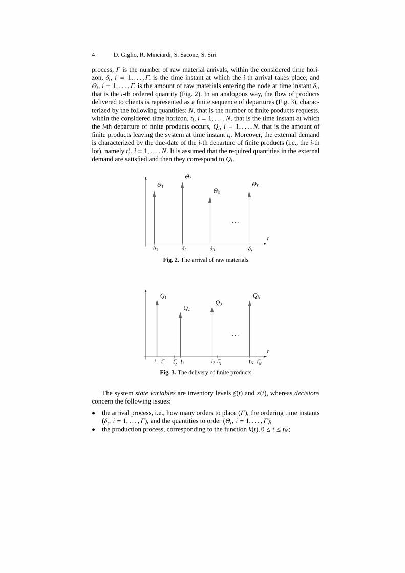
process,Γ is the number of raw material arrivals, within the considered time hori-zon, δi , i = 1, . . . , Γ, is the time instant at which thei-th arrival takes place, andΘi , i = 1, . . . , Γ, is the amount of raw materials entering the node at time instant δi ,that is thei-th ordered quantity (Fig. 2). In an analogous way, the flow ofproductsdelivered to clients is represented as a finite sequence of departures (Fig. 3), charac-terized by the following quantities:N, that is the number of finite products requests,within the considered time horizon,ti , i = 1, . . . ,N, that is the time instant at whichthe i-th departure of finite products occurs,Qi , i = 1, . . . ,N, that is the amount offinite products leaving the system at time instantti . Moreover, the external demandis characterized by the due-date of thei-th departure of finite products (i.e., thei-thlot), namelyt∗i , i = 1, . . . ,N. It is assumed that the required quantities in the externaldemand are satisfied and then they correspond toQi .

Θ1

Θ2

Θ3

ΘΓ

. . .

δ1 δ2 δ3 δΓ

t

Fig. 2. The arrival of raw materials

Q1

Q2

Q3

QN

. . .

t1 t2 t3 tNt∗1 t∗2 t∗3 t∗N

t

Fig. 3. The delivery of finite products

The systemstate variablesare inventory levelsξ(t) andx(t), whereasdecisionsconcern the following issues:

• the arrival process, i.e., how many orders to place (Γ), the ordering time instants(δi , i = 1, . . . , Γ), and the quantities to order (Θi , i = 1, . . . , Γ);

• the production process, corresponding to the functionk(t),0 ≤ t ≤ tN;


• the departure process, i.e., the delivering time instants for each lot of finite pro-ducts (ti , i = 1, . . . ,N).

Taking into account the asynchronous time instants which characterize the arrivaland the departure processes, the state equations of the proposed single node modelcan be written, for the raw material inventory and for the finite product inventory,respectively, as

ξ(δi+1) = ξ(δi) −∫ δi+1

δi

k(t) dt + Θi+1 i = 0, . . . , Γ − 1 (1)

x(ti+1) = x(ti) +∫ ti+1

ti

k(t) dt − Qi+1 i = 0, . . . ,N − 1 (2)

whereδ0 = 0, t0 = 0, andξ(0) andx(0) are given initial inventory levels.The proposed optimization takes into account the order costCO due to the ac-

quisition of raw materials from suppliers, the costCI relevant to the inventory occu-pancy, and the costCT relevant to the deviations from the due-dates, stated respecti-vely as in the following

CO =

Γ∑

i=1

(

cf + cvΘi

)

(3)

CI = Hξ

∫ δΓ

0ξ(t) dt + Hx

∫ tN

0x(t) dt (4)

CT = α

N∑

i=1

(ti − t∗i )2 (5)

wherecf andcv are the fixed and variable unitary order costs, respectively, Hξ andHx are the unitary inventory costs for raw materials and finite products, respecti-vely, whileα is a suitable parameter, weighing the deviation of the delivering timesfrom the corresponding due-dates. As regards the expression of cost termCT , notethat early and late deliveries are equally penalized. Everydeviation from the corre-sponding due-date yields a decrease of the node service level, which results to bea crucial performance indicator in a supply chain system. This is the reason why aquadratic form of the cost has been chosen, aiming at strongly penalizing deviationsfrom due-dates.

The overall optimization problem can then be stated as follows.

Problem 1. Given the initial conditionsδ0 = 0, t0 = 0, ξ(0) ≥ 0, andx(0) ≥ 0, find

minΓ, δi ,Θi , i=1,...,Γ

ti , i=1,...,Nk(t), 0≤t≤tN

C1 = CO + CI + CT

subject to (1), (2), and0 ≤ k(t) ≤ K 0 ≤ t ≤ tN (6)


δi+1 > δi i = 0, . . . , Γ − 1 (7)

ti+1 > ti i = 0, . . . ,N − 1 (8)

ξ(t) ≥ 0 0< t ≤ δΓ (9)

x(t) ≥ 0 0< t ≤ tN (10)

Θi > 0 i = 1, . . . , Γ (11)

�

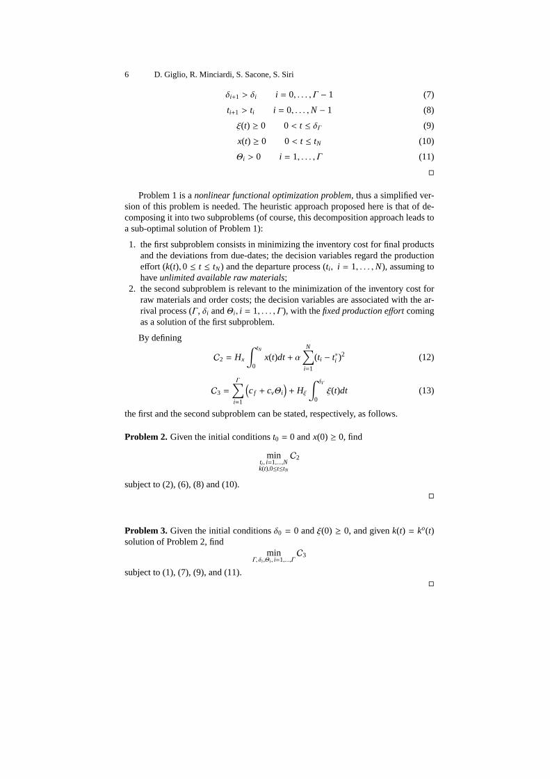
Problem 1 is anonlinear functional optimization problem, thus a simplified ver-sion of this problem is needed. The heuristic approach proposed here is that of de-composing it into two subproblems (of course, this decomposition approach leads toa sub-optimal solution of Problem 1):

1. the first subproblem consists in minimizing the inventorycost for final productsand the deviations from due-dates; the decision variables regard the productioneffort (k(t),0 ≤ t ≤ tN) and the departure process (ti , i = 1, . . . ,N), assuming tohaveunlimited available raw materials;

2. the second subproblem is relevant to the minimization of the inventory cost forraw materials and order costs; the decision variables are associated with the ar-rival process (Γ, δi andΘi , i = 1, . . . , Γ), with thefixed production effort comingas a solution of the first subproblem.

By defining

C2 = Hx

∫ tN

0x(t)dt+ α

N∑

i=1

(ti − t∗i )2 (12)

C3 =

Γ∑

i=1

(

cf + cvΘi

)

+ Hξ

∫ δΓ

0ξ(t)dt (13)

the first and the second subproblem can be stated, respectively, as follows.

Problem 2. Given the initial conditionst0 = 0 andx(0) ≥ 0, find

minti , i=1,...,Nk(t),0≤t≤tN

C2

subject to (2), (6), (8) and (10).�

Problem 3. Given the initial conditionsδ0 = 0 andξ(0) ≥ 0, and givenk(t) = ko(t)solution of Problem 2, find

minΓ, δi ,Θi , i=1,...,Γ

C3

subject to (1), (7), (9), and (11).�


Note that Problem 2 still is a functional optimization problem, while Problem 3is a parametric optimization problem. In the following, these two problems will bestudied, in order to find some properties of their optimal solutions and, thus, to definesolution procedures for the two problems. Problem 2 will be analysed in Section 3,whereas Problem 3 will be studied in Section 4.

3 Solution of Problem 2

In this section, Problem 2 is analysed and some fundamental results about the op-timal solution of the problem will be reported. The proofs ofthe theorems are onlysketched in the present section, whereas their complete version can be found in [14].

As previously pointed out, Problem 2 is afunctional optimization problem, as afunctionk(t) has to be determined over the considered optimization interval. A firstsimple result can be provided, in order to convert Problem 2 into a more tractable (pa-rametric) optimization problem. Note that, in the following, k◦(t) refer to the optimalpattern of the decision variablek(t).

Proposition 1. In the optimal solution of Problem 2, the function k(t) is such thatin each time interval between two subsequent delivery instants, e.g.,(ti , ti+1], thefollowing conditions hold

k◦(t) ≡ 0, ti < t < ti + τi , i = 0, . . . ,N − 1 (14)

k◦(t) ≡ K, ti + τi < t ≤ ti+1, i = 0, . . . ,N − 1 (15)

for someτi such that0 ≤ τi ≤ ti+1 − ti . Note that the value k◦(ti + τi) is irre-levant, and thus it is not necessary to precise it in the statement of the proposi-tion; it is possible to set either k◦(ti + τi) = 0 or k◦(ti + τi) = K, indifferently.

�

Proof. Suppose,ab absurdo, that an optimal solution of Problem 2 exists that doesnot satisfy conditions (14), (15). This implies that a time intervalτi such that 0≤τi ≤ ti+1 − ti exists, where one or both of the following conditions hold:

a) there is an interval (ti + τi , ti+1) of nonzero length in which the value ofk(t) is notconstantly its maximum value, that is,

k(t) . K, ti + τi < t ≤ ti+1

with τi < ti+1 − tib) there are some intervals (at least one) of nonzero length,preceding time instant

ti + τi , in which the value ofk(t) is not identically zero, that is,

k(t) . 0, ti < t < ti

with ti ≤ ti < ti ≤ ti + τi .


Then, in case condition a) occurs, it is immediate to understand that a new solutioncan be obtained by ”reducing” the length of the interval (ti + τi , ti+1), and imposingthat in such interval the production effort is at its maximum value, i.e.,

k(t) ≡ K, ti + τ′i < t ≤ ti+1

beingτ′i > τi , and∫ ti+1

ti+τik(t) dt =

∫ ti+1

ti+τ′ik(t) dt.

Evidently, this new solution is characterized by the same value of costCT , but ithas a lower value of costCI , then the original solution cannot be optimal.

Similar considerations apply in connection with conditionb), or even with refe-rence to the combination of the two conditions. �

The result provided by Proposition 1 allows to convert the functional optimiza-tion problem into a parametric one, by restricting the search for optimal solutions ofProblem 2 to those characterized by functionsk(t) satisfying conditions (14), (15).Thus, it is possible to define

• τi , i = 0, . . . ,N − 1, that represents the (nonnegative)idle timebetweenti andti+1;

• Ti , i = 0, . . . ,N−1, that is the (nonnegative)production timebetweenti andti+1.

Thanks to Proposition 1, Problem 2 can also be stated as amultistage optimalcontrol problem. First of all, the following assumptions will be made concerning theparameters characterizing Problem 1:

• the initial inventory level is all consumed to satisfy the first order, that is

x(0) < Q1 (16)

This assumption is not restrictive since, if this conditionis not verified, in theoptimal solution of Problem 2 no production is realized (Ti = 0) for a certainnumber of orders starting from the first one; then, the beginning of the sequenceof orders can be simply shifted onward till meeting condition (16);

• the two terms of cost functionC2 are ”well balanced”, that is the inventory costhas not a prevailing effect with respect to the deviation cost from due-dates; thiscorresponds to suppose that

HxK < α (17)

If such a condition were not fulfilled, then the optimizationproblem would be ofpoor interest.

Taking into account Proposition 1 and on the basis of the above considerations,cost functionC2 can now be written as

C4 = Hx

N−1∑

i=0

x(ti)(τi + Ti) +KT2

i

2

+ α

N−1∑

i=0

(

τi + Ti + ti − t∗i+1

)2(18)


Furthermore, the state equation (2) and the time instantsti , i = 1, . . . ,N can beexpressed, respectively, as

x(ti) = x(ti−1) + KTi−1 − Qi i = 1, . . . ,N (19)

ti = ti−1 + τi−1 + Ti−1 i = 1, . . . ,N (20)

On these bases, Problem 2 can be re-stated as follows.

Problem 4. Given the initial conditionst0 = 0 andx(0) ≥ 0, find

minτi ,Ti , i=0,...,N−1

C4

whereC4 is given by (18), subject to (19), (20) and

Ti ≥ 0 i = 0, . . . ,N − 1 (21)

τi ≥ 0 i = 0, . . . ,N − 1 (22)

x(ti) ≥ 0 i = 1, . . . ,N (23)

�

It is apparent that Problem 4 is structured intoN stages, beingx(ti) and ti thestate variables at stagei, τi−1 andTi−1 the control variables acting at the same stage.Obviously, Problem 4 can be also viewed as amathematical programming problemwith non linear objective and non linear constraints. It canbe solved by mathematicalprogramming solvers, yielding the optimal control law in anopen-loop form for aspecific value of the initial conditions. In this work, instead, we are interested inadopting optimal control strategies defined as functions ofthe system state, that is,solutions typically denoted as closed–loop ones. Then, we will find the solution ofProblem 4 as a set of optimalfeedback control strategies. In order to do that, it isfirst of all necessary to discuss some significant propertiesof the optimal solutionof Problem 4. Note that in the following propositions the valuesT◦i and τ◦i , i =0, . . . ,N − 1, refer to the optimal values of the decision variablesTi and τi , i =0, . . . ,N − 1, respectively.

Proposition 2. In the optimal solution of Problem 4, the decision variable Ti is al-ways positive, that is

T◦i > 0 i = 0, . . . ,N − 1 (24)

�

Proof. The value of the inventory level just after the generic delivery time instanttiis given by

x(ti) = x(ti−1) + KTi−1 − Qi ≥ 0, i = 1, . . . ,N (25)


Note that, in an optimal solution of Problem 4, the inequality x(ti−1) < Qi musthold. In fact, if x(ti−1) were greater or equal toQi , this would imply that thewholequantity of products required at the delivery timeti has been manufactured duringthe time intervals precedingti−1 (remember also that condition (16) prevents the ini-tial inventory contents from being still partially available after the first delivery timeinstant). But, due to the structure of the cost function (including the inventory cost),this is never convenient since it makes the cost function value increase without provi-ding any advantage. Then, some part of the required quantityQi has to be producedjust during time interval (ti−1, ti), that is,x(ti−1) < Qi , as above claimed. Thus, bytaking into account (25), conditionT◦i−1 > 0, i = 1, . . . ,N, is proved.

�

Proposition 3. In the optimal solution of Problem 4, ifτi > 0 for some i∈ {1, . . . ,N−1}, that is, if the i-th time interval(ti , ti+1) includes a nonzero idle time, then theinventory level x(ti) (that is, just after the delivery at time instant ti) is zero.

�

Proof. Suppose,ab absurdo, x(ti) = x̄ > 0 andτi > 0, in an optimal solution.Products corresponding to this inventory levelx(ti) have been realised in time interval(ti−1, ti) or in previous time intervals, and they cannot be part of theinitial inventorythat is all consumed, by assumption, to satisfy the first order. These products are notnecessary for order deliveries realised inti or before and certainly they are not allnecessary for order deliveries afterti , owing to conditionτi > 0. This implies that asolution withτi > 0 andx(ti) = ¯̄x such that 0≤ ¯̄x < x̄ is feasible and guarantees thesame deliveries in the same time instants (thus yielding thesame value of costCT),but with a lower value of the inventory costCI . This proves that any solution withτi > 0 andx(ti) > 0 cannot be optimal.

�

t1 t2 t3 t4 t5

Q1

Q2

Q3

Q4

Q5

t

x(t)

σ1 = 0

σ2 = 1

σ3 = 4

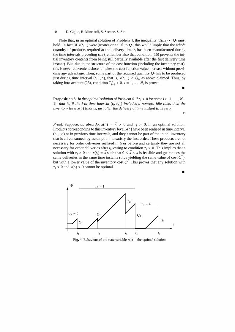
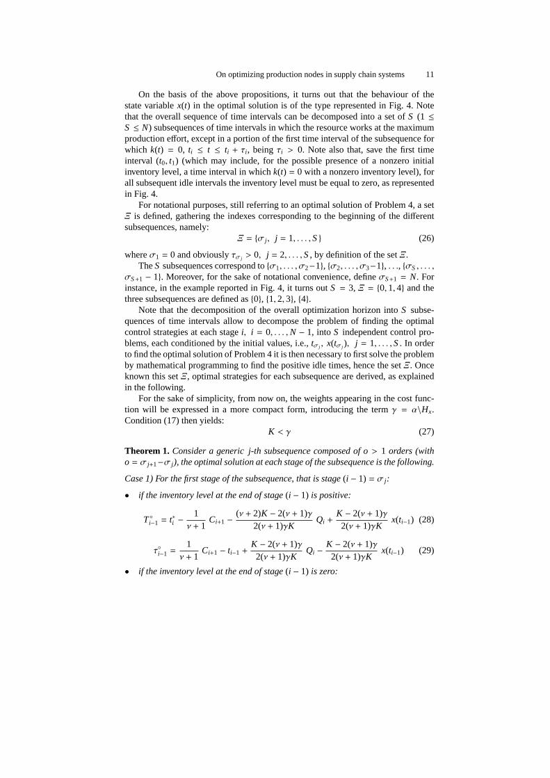
Fig. 4. Behaviour of the state variablex(t) in the optimal solution


On the basis of the above propositions, it turns out that the behaviour of thestate variablex(t) in the optimal solution is of the type represented in Fig. 4.Notethat the overall sequence of time intervals can be decomposed into a set ofS (1 ≤S ≤ N) subsequences of time intervals in which the resource worksat the maximumproduction effort, except in a portion of the first time interval of the subsequence forwhich k(t) = 0, ti ≤ t ≤ ti + τi , beingτi > 0. Note also that, save the first timeinterval (t0, t1) (which may include, for the possible presence of a nonzero initialinventory level, a time interval in whichk(t) = 0 with a nonzero inventory level), forall subsequent idle intervals the inventory level must be equal to zero, as representedin Fig. 4.

For notational purposes, still referring to an optimal solution of Problem 4, a setΞ is defined, gathering the indexes corresponding to the beginning of the differentsubsequences, namely:

Ξ = {σ j , j = 1, . . . ,S} (26)

whereσ1 = 0 and obviouslyτσ j > 0, j = 2, . . . ,S, by definition of the setΞ.TheS subsequences correspond to{σ1, . . . , σ2−1}, {σ2, . . . , σ3−1}, . . ., {σS, . . . ,

σS+1 − 1}. Moreover, for the sake of notational convenience, defineσS+1 = N. Forinstance, in the example reported in Fig. 4, it turns outS = 3, Ξ = {0,1,4} and thethree subsequences are defined as{0}, {1,2,3}, {4}.

Note that the decomposition of the overall optimization horizon into S subse-quences of time intervals allow to decompose the problem of finding the optimalcontrol strategies at each stagei, i = 0, . . . ,N − 1, into S independent control pro-blems, each conditioned by the initial values, i.e.,tσ j , x(tσ j ), j = 1, . . . ,S. In orderto find the optimal solution of Problem 4 it is then necessary to first solve the problemby mathematical programming to find the positive idle times,hence the setΞ. Onceknown this setΞ, optimal strategies for each subsequence are derived, as explainedin the following.

For the sake of simplicity, from now on, the weights appearing in the cost func-tion will be expressed in a more compact form, introducing the termγ = α\Hx.Condition (17) then yields:

K < γ (27)

Theorem 1. Consider a generic j-th subsequence composed of o> 1 orders (witho = σ j+1−σ j), the optimal solution at each stage of the subsequence is the following.

Case 1) For the first stage of the subsequence, that is stage(i − 1) = σ j :

• if the inventory level at the end of stage(i − 1) is positive:

T◦i−1 = t∗i −1ν + 1

Ci+1 −(ν + 2)K − 2(ν + 1)γ

2(ν + 1)γKQi +

K − 2(ν + 1)γ2(ν + 1)γK

x(ti−1) (28)

τ◦i−1 =1ν + 1

Ci+1 − ti−1 +K − 2(ν + 1)γ2(ν + 1)γK

Qi −K − 2(ν + 1)γ2(ν + 1)γK

x(ti−1) (29)

• if the inventory level at the end of stage(i − 1) is zero:


T◦i−1 =Qi − x(ti−1)

K(30)

τ◦i−1 =1ν + 1

t∗i +1ν + 1

Ci+1 − ti−1 −Qi

K−

K − 2(ν + 1)γ2(ν + 1)γK

x(ti−1) (31)

whereν is the total number of stages in the subsequence whose inventory level goesto zero, and the generic constant Ci+1 is calculated iteratively depending on data ofthe whole subsequence, following these steps:

• for i = σ j+1:

Ci = t∗i −Qi

K(32)

• from i = σ j+1 − 1 backward to i= σ j + 3:- if the inventory level at the end of the stage i is positive:

Ci = Ci+1 −νi + 1

KQi +

Qi

2γ(33)

- if the inventory level at the end of the stage i is zero:

Ci = Ci+1 + t∗i −νi + 1

KQi (34)

whereνi is the number of stages whose inventory is equal to zero, fromthe stagei (included) to the last stage of the subsequence.

Case 2) For the intermediate stage of the subsequence, that is stage(i − 1) = σ j +

1, . . . , σ j+1 − 2, when o> 2:

• if the inventory level at the end of stage(i − 1) is positive:

T◦i−1 = t∗i − ti−1 −Qi

2γτ◦i−1 = 0 (35)

• if the inventory level at the end of stage(i − 1) is zero:

T◦i−1 =Qi − x(ti−1)

Kτ◦i−1 = 0 (36)

Case 3) For the last stage of the subsequence, that is stage(i − 1) = σ j+1 − 1:

T◦i−1 =Qi − x(ti−1)

Kτ◦i−1 = 0 (37)

�

Sketch of the proof.The results stated in the Theorem have been found applyingdynamic programming techniques, starting from the last interval (stage) of a subse-quence and proceeding backwards up to the first interval (stage). First of all, the laststage of a subsequence, that is stage (n−1), is considered and the relative problem is


stated, as a function of the initial conditionstn−1, x(tn−1), and of the decision variablesτn−1 andTn−1. In this case, the optimal values of the decision variables are found, asstated in the Theorem, and the optimal cost-to-go at stage (n− 1) is obtained.

Then, the intermediate stage is considered, but different cases must be analysed.Actually, the intermediate stage can be stage (n − 2), or (n − 3), or previous stages;thus, each of these stages has been considered, starting from stage (n − 2). In thiscase, the problem is stated adding the cost-to-go at stage (n− 1), already computed,and the optimal solutions are found considering first-orderKuhn-Tucker conditions;two cases arise, depending on whether the inventory level atthe end of stage (n− 2),i.e. x(tn−1), is positive or null. Therefore, two optimal solutions arefound and twocosts-to-go are determined, corresponding to the two cases. When considering theintermediate stage (n − 3), two different problems must be stated according to thebehaviour of the optimal solution at stage (n− 2) (eitherx(tn−1) > 0 or x(tn−1) = 0),which correspond to two different costs-to-go. For each of the two problems statedfor stage (n−3) two different solutions are found, corresponding to whetherx(tn−2) ispositive or null (this means that four different cases are developed for stage (n− 3)).Generalising this approach to a generic intermediate stageof a subsequence, theresult stated in the Theorem is proved.

The optimal values of the decision variables for the first stage of a subsequenceare computed following the same reasoning line already described for the interme-diate stage, since the first stage of the subsequence can be either stage (n − 2), or(n− 3) or previous stages, depending on the length of the subsequence. As a matterof fact, the problems to be solved at each stage are the same for the intermediate andthe first stage, while the solutions are different because they correspond to differentcases of Kuhn-Tucker conditions.

�

Theorem 2. Consider a generic j-th subsequence, composed of o= 1 orders (witho = σ j+1 − σ j), the optimal solution at stage(i − 1) = σ j is:

T◦i−1 =Qi − x(ti−1)

K(38)

τ◦i−1 = t∗i − ti−1 −Qi − x(ti−1)

K−

x(ti−1)2γ

(39)

�

Sketch of the proof.The previous statement is proved considering the last stageofthe subsequence, i.e. stage (n − 1), which is both the first and the last stage (sincethe considered subsequence is composed of 1 order). First-order Kuhn-Tucker con-ditions are developed and the optimal values of the decisionvariables are found.

�

4 Solution of Problem 3

Once Problem 4 has been solved, in particular finding the feedback control law, Pro-blem 3 still needs to be studied. As previously described andas it is clear in the


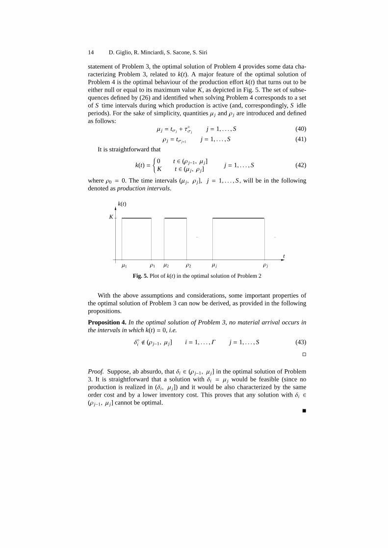
statement of Problem 3, the optimal solution of Problem 4 provides some data cha-racterizing Problem 3, related tok(t). A major feature of the optimal solution ofProblem 4 is the optimal behaviour of the production effort k(t) that turns out to beeither null or equal to its maximum valueK, as depicted in Fig. 5. The set of subse-quences defined by (26) and identified when solving Problem 4 corresponds to a setof S time intervals during which production is active (and, correspondingly,S idleperiods). For the sake of simplicity, quantitiesµ j andρ j are introduced and definedas follows:

µ j = tσ j + τ◦σ j

j = 1, . . . ,S (40)

ρ j = tσ j+1 j = 1, . . . ,S (41)

It is straightforward that

k(t) =

{

0 t ∈ (ρ j−1, µ j ]K t ∈ (µ j , ρ j ]

j = 1, . . . ,S (42)

whereρ0 = 0. The time intervals (µ j , ρ j ], j = 1, . . . ,S, will be in the followingdenoted asproduction intervals.

......

t

k(t)

K

ρ1 ρ2 ρ jµ1 µ2 µ j

Fig. 5. Plot ofk(t) in the optimal solution of Problem 2

With the above assumptions and considerations, some important properties ofthe optimal solution of Problem 3 can now be derived, as provided in the followingpropositions.

Proposition 4. In the optimal solution of Problem 3, no material arrival occurs inthe intervals in which k(t) = 0, i.e.

δ◦i < (ρ j−1, µ j ] i = 1, . . . , Γ j = 1, . . . ,S (43)

�

Proof. Suppose, ab absurdo, thatδi ∈ (ρ j−1, µ j ] in the optimal solution of Problem3. It is straightforward that a solution withδi = µ j would be feasible (since noproduction is realized in (δi , µ j ]) and it would be also characterized by the sameorder cost and by a lower inventory cost. This proves that anysolution withδi ∈(ρ j−1, µ j ] cannot be optimal.

�


The above proposition states that it is never convenient to have material arrivalsin the time intervals in which production is not active. Thisfact is actually quiteintuitive since it can be easily argued that placing orders in such time intervals wouldonly yield an increased inventory cost. This is actually thesame reasoning line thatleads to prove the following result.

Proposition 5. In the optimal solution of Problem 3, the raw materials arrived attime δi−1 are all consumed in the production process before the following arrivaloccurs atδi . This means that

ξ◦(δ−i ) = 0 i = 1, . . . , Γ (44)

ξ◦(δ+i ) = Θi i = 1, . . . , Γ (45)

�

Proof. Suppose, ab absurdo, that in the optimal solution of Problem3, the inventorylevel in the time instantδi is positive. It is easy to verify that a solution in whichthe i-th order is placed in the time instantδ̄i > δi (with Θ̄i = Θi) and such that theinventory level inδ̄i is equal to zero would be feasible and would guarantee a lowerinventory cost (with the same order cost). This proves that any solution in which ageneric order is placed when the inventory level is still positive cannot be optimal.

�

Proposition 4 implies that the inventory levelξ(t) keeps constant during the timeintervals (ρ j−1, µ j ], j = 1, . . . ,S, thus yielding

ξ(µ j) = ξ(ρ j−1) j = 1 . . . ,S (46)

Moreover, thanks to Proposition 5, it is possible to state that in the time instantin which thei-th material arrival occurs, the inventory level changes instantaneouslyfrom 0 to the ordered quantityΘi . A possible behaviour ofξ(t) is then depicted inFig. 6.

In the following, some results will be provided concerning ageneric productioninterval j, for which a costC j is considered, made of the fixed order cost and theinventory cost. Actually, the variable order cost (which has been considered in thedefinition of Problem 3) can be neglected when searching for some properties of theoptimal solution of Problem 3. This is motivated by the fact that the variable ordercost (obtained as the sum of the ordered quantitiesΘi , i = 1, . . . , Γ, times a costtermcv) does not depend on the problem decision variables. This fact is due to thefollowing consideration. The decision variablesΘi , i = 1, . . . , Γ, can be derived ifthe order time instantsδi , i = 1, . . . , Γ, are known. The quantityΘi to order at eachtime instantδi must assure that the inventory levelξ(t) never becomes negative andthat it becomes equal to 0 exactly inδi+1, as stated in Proposition 5. Thus, supposingto have a null initial inventory level, it must be


t

ξ(t)

. . .

µ1 = δ1 δ2 ρ1 µ2 ρ2 µ3 = δ3

Θ1

Θ2

Θ3

Fig. 6. A possible pattern ofξ(t)

S∑

j=1

K(ρ j − µ j) =Γ∑

i=1

Θi (47)

The variable order costΓ∑

i=1

cvΘi (48)

can be written as

cv

Γ∑

i=1

Θi = cvKS∑

j=1

(ρ j − µ j) (49)

thus, it depends only on problem data. For this reason, this cost term will be fromnow on neglected.

Consider a genericj-th production interval, with an initial inventoryξ(µ j) and afinal inventoryξ(ρ j), as depicted in Fig. 7. From now on, we define asn j the numberof orders to be placed in thej-th interval andδ j,i , i = 1, . . . ,n j , the time instant inwhich thei-th order is placed in thej-th production interval. Of course, it must be

S∑

j=1

n j = Γ (50)

Analogously, the corresponding ordered quantities will bereferred to asΘ j,i , i =1, . . . ,n j . With these considerations, in a production intervalj, there aren j+1 reorderperiods, whose length is denoted as∆ j,i , i = 1, . . . ,n j + 1. In the following propo-sition, a property relevant to the values of these quantities in the optimal solution isreported.

Proposition 6. In the optimal solution of Problem 3, if nj orders (nj > 1) areplaced within the j-th production interval, then the time intervals between twosubsequent order deliveries inside the interval (except the first and the last one)have the same length. The reorder periods are obtained as a function of the ini-tial and final inventory level,ξ(µ j) and ξ(ρ j), and of the number of orders nj .

�


t

ξ(t)

. . .

. . .. . .

µ j ρ jδ j,1 δ j,2 δ j,n j

∆ j,1 ∆ j,2 ∆ j,n j+1

Θ j,1Θ j,n j

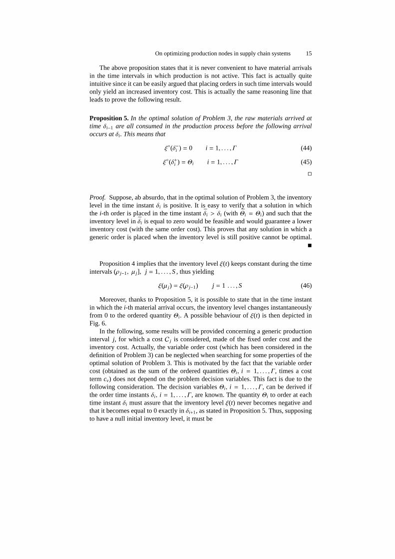
Fig. 7. ξ(t) in a generic production intervalj

Proof. The generic costC j associated with the intervalj can be written as

C j = n jcf + Hξ

12∆ j,1ξ(µ j) +

n j∑

i=2

12

K∆2j,i +

12

K∆2j,n j+1 + ∆ j,n j+1ξ(ρ j)

(51)

where, thanks to Proposition 5,∆ j,1 is given by

∆ j,1 =1Kξ(µ j) (52)

Moreover, variables∆ j,i are related by the following expression

n j+1∑

i=1

∆ j,i = ρ j − µ j (53)

which, considering (52), becomes

1Kξ(µ j) +

1K

n j+1∑

i=2

∆ j,i = ρ j − µ j (54)

that can be written as

h j =1Kξ(µ j) +

1K

n j+1∑

i=2

∆ j,i − ρ j + µ j = 0 (55)

The problem concerning intervalj can be stated as follows, being∆ j,i , i =2, . . . ,n j+1 the decision variables, whileξ(ρ j), ξ(µ j) andn j are considered as knowndata

min∆ j,i , i=2,...,n j+1

C j

whereC j is given by (51), subject to


h j = 0 (56)

∆ j,i > 0 j = 2, . . . ,n j + 1 (57)

with h j defined as in (55).This problem is a quadratic programming problem, characterized by a quadratic

objective function,n j decision variables and one linear equality constraint. Consi-dering Kuhn-Tucker conditions for this problem, one Lagrangian multiplier, i.e.λ,must be considered, leading to the following equations:

∂C j

∆ j,i+ λ∂h j

∆ j,i= 0 i = 2, . . . ,n j + 1 (58)

which becomeK∆ j,i + λ = 0 i = 2, . . . ,n j (59)

K∆ j,n j+1 + ξ(ρ j) + λ = 0 (60)

These equations, together with the relation (54), let us obtain∆ j,i , i = 2, . . . ,n j+1as

∆ j,i = ∆ j =1

Kn j

[

K(ρ j − µ j) + ξ(ρ j) − ξ(µ j)]

i = 2, . . . ,n j (61)

∆ j,n j+1 = ∆ j −1Kξ(ρ j) (62)

�

t

ξ(t)

. . .. . .

µ j ρ jδ j,1 δ j,2 δ j,3

∆ j,1 ∆ j,2 ∆ j,3 ∆ j,41K ξ(ρ j)

Θ j Θ j Θ j

Fig. 8. The optimal behaviour ofξ(t) for the casenj = 3

The result proposed in Proposition 6 implies that, in a givenproduction intervalj, the reorder periods are equal, except the first and the last one. In the following,such intermediate reorder periods will be referred to as∆ j , j = 1, . . . ,S (withoutusing∆ j,i). Moreover, the ordered quantities are the same (an exampleis provided in


Fig. 8 for the case ofn j = 3). Therefore, also the ordered quantities can be simplyindexed byj (instead of using the pairj, i), and will be in the following referred toasΘ j such that:

Θ j =1n j

[

K(ρ j − µ j) + ξ(ρ j) − ξ(µ j)]

(63)

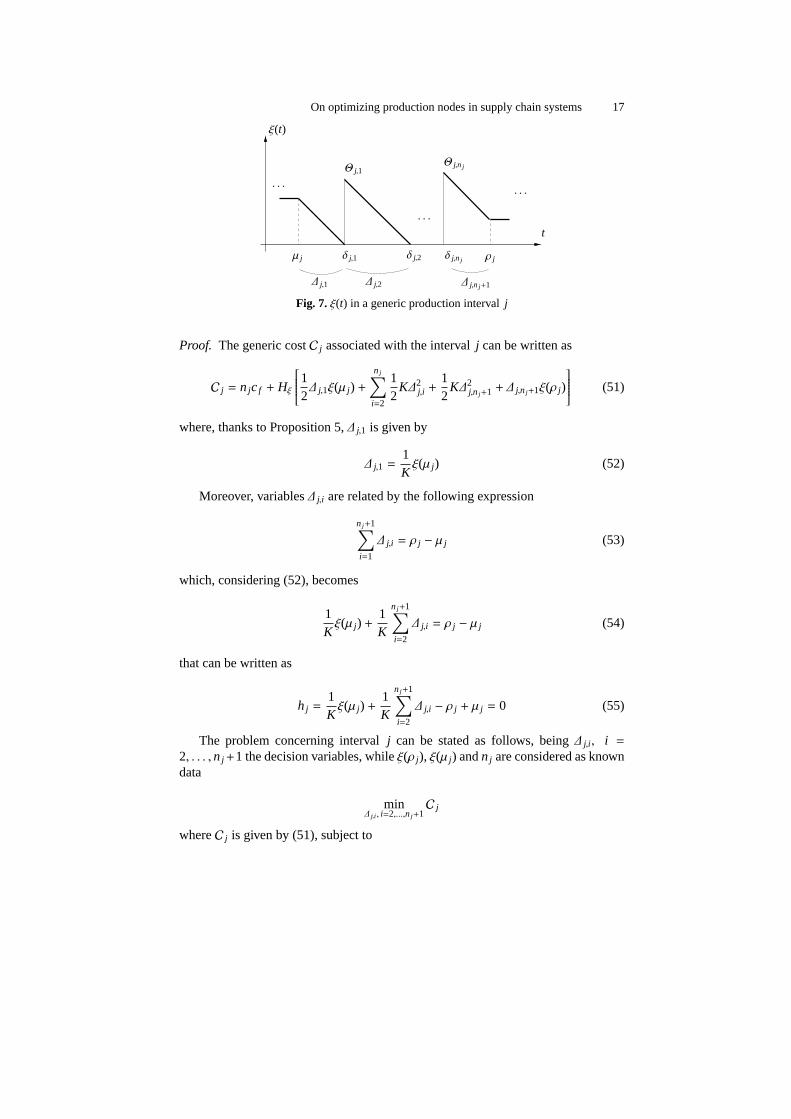
The statement of Proposition 6 does not consider the case in whichn j = 1, that iswhen only one order is placed in thej–th production interval. In this case, the reorderperiods can be simply derived by remembering the result of Proposition 5 (implyingthat the inventory level goes to zero before reordering again). As also depicted inFig. 9, the following relations hold:

∆ j,1 =ξ(µ j)

K(64)

∆ j,2 = ρ j − µ j −ξ(µ j)

K(65)

Θ j = K(ρ j − µ j) + ξ(ρ j) − ξ(µ j) (66)

t

ξ(t)

. . .

. . .. . .

µ j ρ jδ j,1

∆ j,1 ∆ j,2

Θ j

Fig. 9. The optimal behaviour ofξ(t) for the casenj = 1

The propositions previously reported define some significant properties of theoptimal solution of Problem 3. Such properties help in rewriting Problem 3 in asimplified way. For doing this, it is necessary to introduce abinary variable indicatingwhether in a given production interval any orders are placedor not; to this end, wedefineω j ∈ {0,1} as follows:

ω j =

{

0 if n j = 01 if n j > 0

j = 1, . . . ,S (67)

Before rewriting Problem 3, it is still necessary to expressthe inventory cost.Note that such a cost is the area defined byξ(t) multiplied by the unitary costHξ.Such an area is computed by exploiting the geometric properties ofξ(t) coming fromthe previous propositions. Two different expressions of the inventory cost in thej–th


production interval can be written, depending on whether any orders are placed ina production interval or not. In the former case (corresponding toω j = 1), the areadefined byξ(t) in the production intervalj is:

A1j =

12K

[

ξ(µ j)]2+

12

Kn j∆2j −

12K

[

ξ(ρ j)]2

(68)

On the contrary, ifω j = 0, the area defined byξ(t) in the production intervalj is:

A0j =

12

(ρ j − µ j)[

ξ(µ j) + ξ(ρ j)]

(69)

Moreover, for completing the expression of the inventory cost, it is still necessaryto add the term corresponding to a positive inventory level during idle intervals. Thisis the last term included in the cost function of the following problem which is thenew version of Problem 3.

Problem 5. Given the initial conditionsρ0 = 0 andξ(0) = 0, find

minω j ,n j , ∆ j , ξ(ρ j ), ξ(µ j )

j=1,...,S

cf

S∑

j=1

n j+HξS∑

j=1

[

ω j · A1j + (1− ω j) · A

0j

]

+HξS−1∑

j=1

[

ξ(ρ j)(µ j+1 − ρ j)]

whereA1j is given by (68),A0

j is given by (69), subject to

ξ(µ j) = ξ(ρ j−1) j = 1, . . . ,S (70)

ξ(ρ j) = ξ(µ j) + Kn j∆ j − K(ρ j − µ j) j = 1, . . . ,S (71)

ξ(ρ j) ≥ 0 j = 1, . . . ,S (72)

ξ(µ j) ≥ 0 j = 1, . . . ,S (73)

∆ j ≤ ρ j − µ j j = 1, . . . ,S (74)

∆ j ≥ 0 j = 1, . . . ,S (75)

Mω j − n j ≥ 0 j = 1, . . . ,S (76)

ω j − n j ≤ 0 j = 1, . . . ,S (77)

ω j ∈ {0,1} j = 1, . . . ,S (78)

whereM is a positive and sufficiently large number.

�

In constraints (71), the values of the inventory level at theend of each productioninterval are defined. Note that such constraints hold both for the case in which ordersare placed within the production interval and for the opposite case (in which, ofcourse,n j = 0).


Problem 5 is anonlinear mixed-integer mathematical programming problem,which can be solved by nonlinear solvers included in mathematical programmingsoftware tools. The solution of Problem 5 provides decisions about how many ordersmust be forwarded to suppliers, the time instants corresponding to order deliveriesand the ordered quantities. Actually, the provided solution is typically a local opti-mum.

Note that Problem 5, which is here considered as a subproblemwithin the op-timization procedure defined for a node of a supply chain, is actually a general re-plenishment problem that significantly extends the classical Wagner-Within model.More specifically, in the model proposed here, demand is a time-varying determini-stic quantity (as in Wagner-Within model), but the time instants in which orders areplaced are asynchronous (and no time discretization has been realized). Moreover,in the present case, the inventory serves a production process characterized by a pie-cewise constant production effort (which can be also null in specified time intervals).

5 The multi-site case

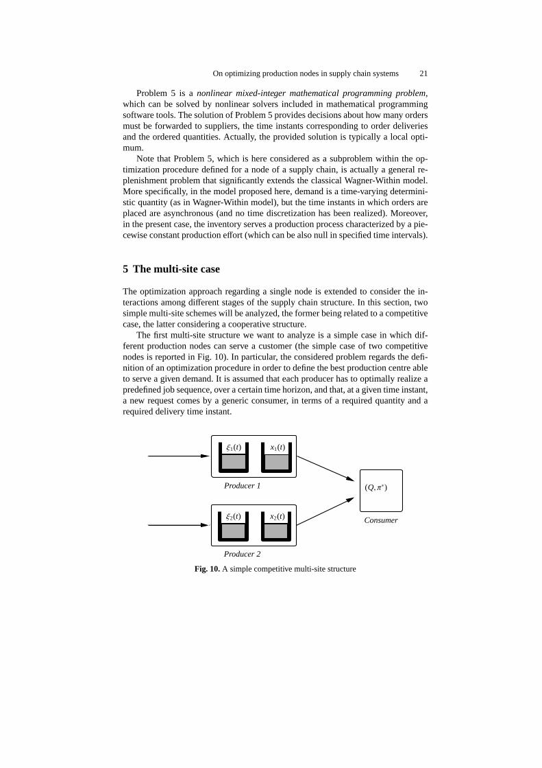
The optimization approach regarding a single node is extended to consider the in-teractions among different stages of the supply chain structure. In this section,twosimple multi-site schemes will be analyzed, the former being related to a competitivecase, the latter considering a cooperative structure.

The first multi-site structure we want to analyze is a simple case in which dif-ferent production nodes can serve a customer (the simple case of two competitivenodes is reported in Fig. 10). In particular, the consideredproblem regards the defi-nition of an optimization procedure in order to define the best production centre ableto serve a given demand. It is assumed that each producer has to optimally realize apredefined job sequence, over a certain time horizon, and that, at a given time instant,a new request comes by a generic consumer, in terms of a required quantity and arequired delivery time instant.

ξ1(t) x1(t)

ξ2(t) x2(t)

(Q, π∗)Producer 1

Producer 2

Consumer

Fig. 10. A simple competitive multi-site structure


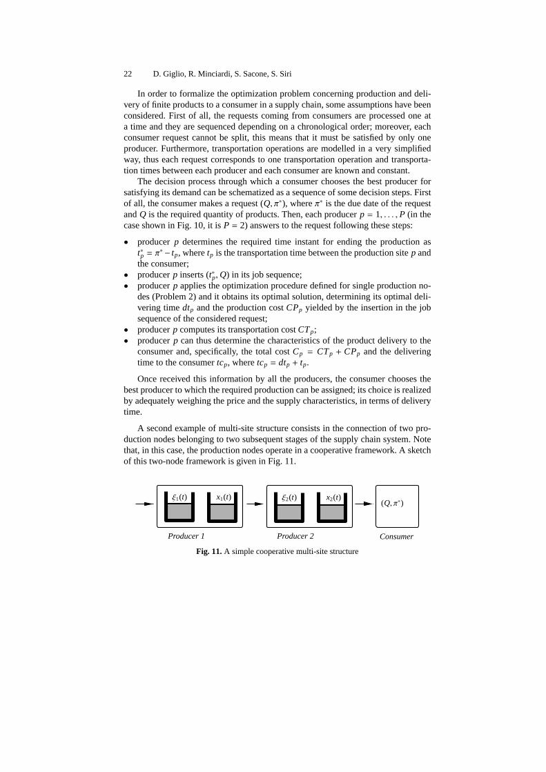
In order to formalize the optimization problem concerning production and deli-very of finite products to a consumer in a supply chain, some assumptions have beenconsidered. First of all, the requests coming from consumers are processed one ata time and they are sequenced depending on a chronological order; moreover, eachconsumer request cannot be split, this means that it must be satisfied by only oneproducer. Furthermore, transportation operations are modelled in a very simplifiedway, thus each request corresponds to one transportation operation and transporta-tion times between each producer and each consumer are knownand constant.

The decision process through which a consumer chooses the best producer forsatisfying its demand can be schematized as a sequence of some decision steps. Firstof all, the consumer makes a request (Q, π∗), whereπ∗ is the due date of the requestandQ is the required quantity of products. Then, each producerp = 1, . . . ,P (in thecase shown in Fig. 10, it isP = 2) answers to the request following these steps:

• producerp determines the required time instant for ending the production ast∗p = π

∗− tp, wheretp is the transportation time between the production sitep andthe consumer;

• producerp inserts (t∗p,Q) in its job sequence;• producerp applies the optimization procedure defined for single production no-

des (Problem 2) and it obtains its optimal solution, determining its optimal deli-vering timedtp and the production costCPp yielded by the insertion in the jobsequence of the considered request;

• producerp computes its transportation costCTp;• producerp can thus determine the characteristics of the product delivery to the

consumer and, specifically, the total costCp = CTp + CPp and the deliveringtime to the consumertcp, wheretcp = dtp + tp.

Once received this information by all the producers, the consumer chooses thebest producer to which the required production can be assigned; its choice is realizedby adequately weighing the price and the supply characteristics, in terms of deliverytime.

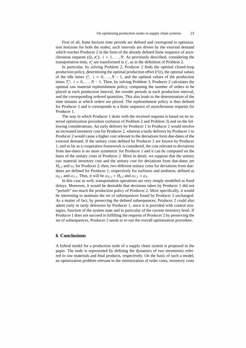
A second example of multi-site structure consists in the connection of two pro-duction nodes belonging to two subsequent stages of the supply chain system. Notethat, in this case, the production nodes operate in a cooperative framework. A sketchof this two-node framework is given in Fig. 11.

ξ1(t) x1(t) ξ2(t) x2(t) (Q, π∗)

Producer 1 Producer 2 Consumer

Fig. 11. A simple cooperative multi-site structure


First of all, finite horizon time periods are defined and correspond to optimiza-tion horizons for both the nodes; such intervals are driven by the external demandwhich reaches Producer 2 in the form of the already defined finite sequence of asyn-chronous requests (Qi , π

∗i ), i = 1, . . . ,N. As previously described, considering the

transportation time,π∗i are transformed int∗i , as in the definition of Problem 2.In particular, by solving Problem 2, Producer 2 finds the optimal closed-loop

production policy, determining the optimal production effort ko(t), the optimal valuesof the idle timesτoi , i = 0, . . . ,N − 1, and the optimal values of the productiontimesTo

i , i = 0, . . . ,N − 1. Then, by solving Problem 3, Producer 2 calculates theoptimal raw material replenishment policy, computing the number of orders to beplaced at each production interval, the reorder periods at each production interval,and the corresponding ordered quantities. This also leads to the determination of thetime instants at which orders are placed. The replenishmentpolicy is thus definedfor Producer 2 and it corresponds to a finite sequence of asynchronous requests forProducer 1.

The way in which Producer 1 deals with the received requests is based on its in-ternal optimization procedure (solution of Problem 2 and Problem 3) and on the fol-lowing considerations. An early delivery by Producer 1 to Producer 2 would involvean increased inventory cost for Producer 2, whereas a tardy delivery by Producer 1 toProducer 2 would cause a higher cost relevant to the deviations form due-dates of theexternal demand. If the unitary costs defined by Producer 2 are known by Producer1, and as far as a cooperative framework is considered, the cost relevant to deviationsfrom due-dates is no more symmetric for Producer 1 and it can be computed on thebasis of the unitary costs of Producer 2. More in detail, we suppose that the unitaryraw material inventory cost and the unitary cost for deviations from due-dates areHξ,2 andα2 for Producer 2; then, two different unitary costs for deviations from due-dates are defined for Producer 1, respectively for earlinessand tardiness, defined asαE,1 andαT,1. Thus, it will beαE,1 = Hξ,2 andαT,1 = α2.

In this case as well, transportation operations are very simply modelled as fixeddelays. Moreover, it would be desirable that decisions taken by Producer 1 did not”perturb” too much the production policy of Producer 2. Morespecifically, it wouldbe interesting to maintain the set of subsequences found by Producer 2 unchanged.As a matter of fact, by preserving the defined subsequences, Producer 2 could alsoadmit early or tardy deliveries by Producer 1, since it is provided with control stra-tegies, function of the system state and in particular of thecurrent inventory level. IfProducer 1 does not succeed in fulfilling the requests of Producer 2 by preserving theset of subsequences, Producer 2 needs to re-run the overall optimization procedure.

6 Conclusions

A hybrid model for a production node of a supply chain system is proposed in thepaper. The node is represented by defining the dynamics of twoinventories refer-red to raw materials and final products, respectively. On thebasis of such a model,an optimization problem relevant to the minimization of order costs, inventory costs


and costs due to deviations from the external demand has beenstated. The decisionvariables refer to the process of raw material arrivals, theprocess of finite product de-liveries and the production effort. The resulting optimization problem is a nonlinearfunctional optimization problem. A solution procedure based on the decompositionof the problem into two subproblems is proposed. The former subproblem refersto the determination of the optimal production effort and the optimal product de-parture process, whereas the latter subproblem corresponds to the determination ofthe optimal replenishment policy. Finally, the exploitation of the proposed solutionprocedure in two very simple multi-site structures is described.

Present and future research is devoted to the definition of more complex decen-tralized decisional structures in which production nodes equipped with the describedoptimization algorithm interact both in cooperative and incompetitive frameworks.

References

1. Chopra S and Meindl P (2001) Supply chain management: strategy, planning, and ope-ration. Prentice-Hall

2. Min H, Zhou G (2002) Supply chain modeling: past, present and future. Computers andIndustrial Engineering 43:231–249

3. Tan KC (2001) A framework of supply chain management literature.European Journalof Purchasing and Supply Management 7:39–48

4. Gershwin SB (1994) Manufacturing Systems Engineering. Prentice-Hall5. Tan B, Gershwin SB (2004) Production and Subcontracting Strategiesfor Manufacturers

with Limited Capacity and Volatile Demand. Annals of Operations Research 125: 205-232

6. Hu JQ, Vakili P, Huang L (2004) Capacity and Production Managmentin a Single Pro-duct Manufacturing System. Annals of Operations Research 125: 191–204

7. Blanchini F, Miani S, Ukovich W (2000) Control of production-distribution systems withunknown inputs and system failures. IEEE Transactions on Automatic Control 45: 1072–1081

8. Bauso D, Blanchini F, Pesenti R (2006) Robust control strategies for multiinventory sy-stems with average flowconstraints. Automatica 42: 1255–1266

9. Xu J, Hancock KL, (2004) Enterprise-Wide Freight Simulation in an Integrated Logisticsand Transportation System. IEEE Transactions on Intelligent transportation Systems 5:342–346

10. Schwartz JD, Wang W, Rivera DE, (2006) Simulation-based optimization of process con-trol policies for inventory management in supply chains. Automatica 42: 1311–1320

11. Giglio G, Minciardi R, Sacone S, Siri S (2005) A hybrid model for optimal control ofsingle nodes in supply chains. Proceedings of 16th IFAC World Congress

12. Giglio G, Minciardi R, Sacone S, Siri S (2006) Supply chain management and optimiza-tion. Proceedings of LT’06, International Workshop on Logistics and Transportation

13. Siri S (2006) Modelling, optimization and control of logistic systems. PhD Thesis, Uni-versity of Genova, Italy

14. Giglio G, Minciardi R, Sacone S, Siri S (2007) Optimal control of single nodes in supplychains by a hybrid model. DIST Technical Report - June 2007

15. Giglio G, Minciardi R, Sacone S, Siri S (2007) Optimal replenishmentpolicies in pro-duction nodes of supply chain models. Proceedings of the European Control Conference

On optimizing production nofed in supply chain systems

Documents