On occurrence of spectral edges for periodic operators inside the Brillouin zone

arX

iv:m

ath-

ph/0

7020

35v2

14

Feb

2007

On occurrence of spectral edges for periodic

operators inside the Brillouin zone

J. M. Harrison1, P. Kuchment1, A. Sobolev2 and B. Winn1

1 Mathematics Department, Texas A&M University, College Station, Texas

77843-3368, USA2 School of Mathematical Sciences, University of Birmingham, Edgbaston,

Birmingham, B15 2TT, UK

Abstract. The article discusses the following frequently arising question on the

spectral structure of periodic operators of mathematical physics (e.g., Schrodinger,

Maxwell, waveguide operators, etc.). Is it true that one can obtain the correct spectrum

by using the values of the quasimomentum running over the boundary of the (reduced)

Brillouin zone only, rather than the whole zone? Or, do the edges of the spectrum occur

necessarily at the set of “corner” high symmetry points? This is known to be true in

1D, while no apparent reasons exist for this to be happening in higher dimensions. In

many practical cases, though, this appears to be correct, which sometimes leads to the

claims that this is always true. There seems to be no definite answer in the literature,

and one encounters different opinions about this problem in the community.

In this paper, starting with simple discrete graph operators, we construct a variety

of convincing multiply-periodic examples showing that the spectral edges might occur

deeply inside the Brillouin zone. On the other hand, it is also shown that in a “generic”

case, the situation of spectral edges appearing at high symmetry points is stable under

small perturbations. This explains to some degree why in many (maybe even most)

practical cases the statement still holds.

AMS classification scheme numbers: 35P99, 47F05, 58J50, 81Q10

Spectral edges of periodic operators 2

1. Introduction

The article discusses the following frequently arising question on the spectral structure

of periodic operators of mathematical physics, which in particular is prominent due to

the recent surge in studying photonic crystals [19]-[21], [36]-[38]. Let us have a periodic

elliptic self-adjoint operator L(x,D) (e.g., Schrodinger, Maxwell), where we use the

standard notation D = 1i∇. The operator is considered in the whole space Rn, or

in a periodic domain (on a periodic periodic manifold), e.g. in a periodic waveguide.

The standard Floquet-Bloch theory (e.g., [1, 35, 53]) shows that the spectrum of L

in the infinite periodic medium can be obtained as follows: one fixes a value k of

the quasimomentum in the first Brillouin zone B, finds the (discrete) spectrum of the

corresponding Bloch Hamiltonian L(k) = L(x,D+ k) acting on periodic functions, and

then takes the union over all quasimomenta in the Brillouin zone. The question we

address in this work is whether the correct spectrum can be obtained as the union over

the boundary of the Brillouin zone only‡This is well known to be true in 1D (e.g., [13, 53]). In particular, the edges of

the spectrum occur at the spectra of the periodic and anti-periodic problems on the

single period. If this claim is correct in higher dimensions, the computational task

is significantly simplified, due to reduced dimension. This is important, for instance,

in optimization procedures, when one needs to run the spectral computation at each

iteration [9, 10]. An experimental observation is that in most practical cases this

is correct. One frequently encounters the belief that this is always true (albeit no

justification is ever provided). On the other hand, unlike in 1D, there is no analytic

reason for this property to hold. Moreover, many researchers are aware that numerics

sometimes produces counterexamples. Surprisingly, such examples are hard to come

by and are usually not very convincing for an analyst (e.g., the error in computing

the spectrum using only the boundary of the Brillouin zone is usually very small).

The experience is that one needs to make the medium inside the fundamental domain

(Wiegner-Seitz cell) truly asymmetric to achieve such examples.

The first goal of this text is to provide simple definite examples to disprove the claim

that the edges of the spectral bands can be found by using the boundary of the (reduced)

Brillouin zone only. This is done by first analyzing some discrete graph systems. Section

2 describes such combinatorial graph counterexamples. Section 3 deduces from this some

quantum graph (see [39]) examples. Then in Section 4, we bootstrap this to examples of

waveguide systems or Laplace-Beltrami operators on thin tubular branching manifolds.

Possibilities for obtaining counterexamples of the Schrodinger and Maxwell cases are

discussed in Section 5.

‡ If additional symmetries are present in the system, one considers the reduced (with respect to these

symmetries) Brillouin zone. Another version of this question is whether the edges of the spectrum are

attained on the set of high symmetry points of the Brillouin zone only. The importance of such points

has been known since at least the paper [4]. When one needs to find the density of states, the full

Brillouin zone is always required.

Spectral edges of periodic operators 3

It is surprising, however, that the claim that we show to be incorrect in general, is

still correct (or almost correct) so often. Thus, in many practical cases, computations

along the boundary of the (reduced) Brillouin zone (and as a matter of fact, often at high

symmetry corner points only) provide the correct spectrum. We suggest an explanation

of this effect in the final Section 6. There we attempt to explain how it can happen that

one often sees the spectral edges occurring at the high symmetry points only. It is shown

that “generically” this occurrence is stable under small perturbations. In other words,

there are open sets of “good” and “bad” periodic operators, the boundary between

which consists of non-generic operators. This probably explains the frequent occurrence

of the effect in practice.

Finally, the last sections provide additional remarks and acknowledgments.

2. Combinatorial graph examples

We start by considering difference operators acting on a periodic graph. These will

serve to illustrate the general ideas in a situation which is not difficult to analyze.

Furthermore, building upon them, we will provide examples of more complex periodic

spectral problems with the desired spectral feature.

2.1. The main graph operators

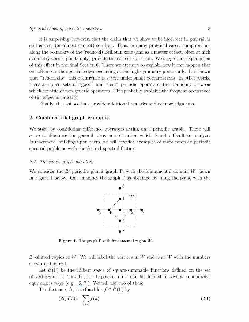
We consider the Z2-periodic planar graph Γ, with the fundamental domain W shown

in Figure 1 below. One imagines the graph Γ as obtained by tiling the plane with the

4 5 2

3

1 W

9

8

7

6

Figure 1. The graph Γ with fundamental region W .

Z2-shifted copies of W . We will label the vertices in W and near W with the numbers

shown in Figure 1.

Let ℓ2(Γ) be the Hilbert space of square-summable functions defined on the set

of vertices of Γ. The discrete Laplacian on Γ can be defined in several (not always

equivalent) ways (e.g., [6, 7]). We will use two of these.

The first one, ∆, is defined for f ∈ ℓ2(Γ) by

(∆f)(v) :=∑

u∼v

f(u), (2.1)

Spectral edges of periodic operators 4

where the notation u ∼ v means that vertex u is adjacent (connected by an edge) to

vertex v. For instance,

(∆f)(5) = f(1) + f(2) + f(4).

The Laplacian defined in (2.1) differs from another discrete Laplacian often used in

the literature by the term dvf(v), where dv is the degree (valence) of the vertex v:∑u∼v f(u) − dvf(v).

We will also employ another version, L, of the Laplacian, which is defined as

(Lf)(v) :=1√dv

∑

u∼v

1√du

f(u). (2.2)

One could call it the Laplace-Beltrami operator. The need for this operator in our study

will become clear when we move to the quantum graph case.

One notices that both ∆ and L are bounded operators in ℓ2(Γ).

In the case of a regular graph (i.e. the one with constant degrees dv = d of vertices),

the spectra of ∆ and L can be easily related. However, our graph Γ is not regular, and

thus these spectra need to be studied independently.

The following statement is well known (e.g., [6]) and immediate:

Lemma 2.1. The operators ∆ and L commute with any automorphism T ∈ Aut(Γ) of

the graph Γ. In particular, they commute with Z2-shifts on Γ.

For p = (p1, p2) ∈ Z2, we denote by T (p) the shift operator by p on Γ. E.g., T (1, 0)

shifts the vertex 4 to the vertex 7 and T (0, 1) shifts 3 to 6.

Due to the periodicity of the operators, one can use the standard Floquet-Bloch

theory [1, 13, 35, 53] to study their spectra. In the particular case of graphs, this theory

is also described, for instance, in [16], [34]-[40], [49].

Let k = (k1, k2) be a quasimomentum in the Brillouin zone B = [−π, π]2. Consider

the space ℓ2k of all functions f satisfying the following Floquet (Bloch, cyclic) condition:

f(T (p)v) = eip·kf(v) (2.3)

for all p ∈ Z2. Here p ·k = p1k1 +p2k2. Such a function f is clearly uniquely determined

by the vector (f1, f2, ..., f5)t of its values at the five vertices in W , and thus ℓ2k is five-

dimensional and naturally isomorphic to ℓ2(W ).

Definition 2.2. We will denote by Ξ the boundary ∂B of the Brillouin zone B =

[−π, π]2 and by X the set of points k = (k1, k2) ∈ B such that k1 and k2 are integer

multiples of π.

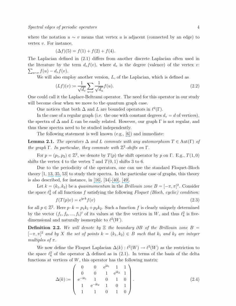
We now define the Floquet Laplacian ∆(k) : ℓ2(W ) → ℓ2(W ) as the restriction to

the space ℓ2k of the operator ∆ defined as in (2.1). In terms of the basis of the delta

functions at vertices of W , this operator has the following matrix:

∆(k) :=

0 0 eik1 1 1

0 0 1 eik2 1

e−ik1 1 0 1 0

1 e−ik2 1 0 1

1 1 0 1 0

. (2.4)

Spectral edges of periodic operators 5

In a similar way, one can define L(k) and observe that

L(k) = S−1∆(k)S−1, (2.5)

where S is the matrix

S :=

√3 0 0 0 0

0√

3 0 0 0

0 0√

3 0 0

0 0 0 2 0

0 0 0 0√

3

. (2.6)

We now state the standard conclusion of the Floquet theory about the relation

between the spectra of ∆ and ∆(k), or L and L(k) (e.g., [13, 16, 34, 35, 40, 49, 53]). For

each fixed k, the matrix ∆(k) (correspondingly, L(k)) is self-adjoint, and thus admits a

spectrum of 5 eigenvalues λj(k)5j=1 (correspondingly, µj(k)5

j=1), which we number

in non-decreasing order. It is well known that then each of the functions λj(k) is

continuous. The multiple-valued function k 7→ λj(k) is called the dispersion relation.

Its graph is the dispersion curve, also called the Bloch variety. Each of the individual

functions k 7→ λj(k) is called the jth branch of the dispersion relation.

Proposition 2.3. [13, 35, 34, 40, 53] The spectrum of ∆ (correspondingly, L) is the

union over k ∈ B of the spectra of ∆(k) (correspondingly, L(k)):

σ(∆) =⋃

k∈B

σ(∆(k)) =⋃

k∈B

5⋃

j=1

λj(k),

σ(L) =⋃

k∈B

σ(L(k)) =⋃

k∈B

5⋃

j=1

µj(k).

(2.7)

The segments Ij =⋃

k∈B

λj(k) (and their analogs for the operator L) are called bands of

the spectrum of ∆ (correspondingly, of L).

Notice that our graph Γ does not have any point symmetries, and thus the reduced

Brillouin zone is equal to the full one. So, the question we would like to address is

whether one can replace the union over k ∈ B in (2.7) by the union along the boundary

Ξ = ∂B of the Brillouin zone B only. A more restricted question is whether the band

edges are attained at points of X only. As we will show in the next sub-section, both

of these properties do not hold, and calculations along the boundary lead to significant

errors in spectra of ∆ and L.

2.2. Spectral edges - counterexamples

In this sub-section we show that computations along Ξ = ∂B (and thus over X

as well) do not necessarily lead to the correct spectra of ∆ and L, and the errors

can be significant. We are interested in whether the segments Ij =⋃

k∈B λj(k) and

I ′j =⋃

k∈∂B λj(k) coincide. We will show that for our examples, even the unions

Spectral edges of periodic operators 6

σ(∆) =5⋃

j=1

Ij and5⋃

j=1

I ′j are different (the situation is analogous for L). This means

that using only the boundary of the Brillouin zone, one does not recover the spectral

edges (and thus the spectrum) correctly.

2.2.1. Operator ∆ One can easily find the spectrum of the Floquet Laplacian ∆(k)

(which is a simple 5 × 5 matrix), using for instance Matlab. Computing it for a grid

in the Brillouin zone (we have used the uniform 64 × 64 grid in B), one can obtain the

whole spectrum of ∆. This leads to the following numerical values of the five bands:

[−2.73,−1.90], [−1.63,−1.00], [−0.73, 0.73], [0, 1.46], and [2.00, 3.23]. One notices that

there are spectral gaps present between all consecutive bands, except the 3rd and 4th

ones, which overlap.

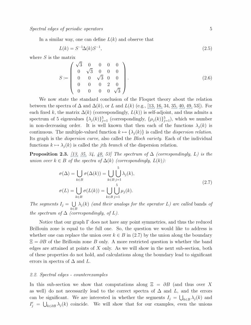
Since it is sufficient for our purpose to provide a single counterexample, we will

focus on the second band [−1.63,−1.00] only.

A gray scale plot of the second branch (corresponding to the second band of the

spectrum) is given in Figure 2 §. This numerical evidence shows that the band edges

λ −1.001

−1.630

Figure 2. A gray scale image of the second branch of the spectrum of ∆(k). Extrema

points are highlighted.

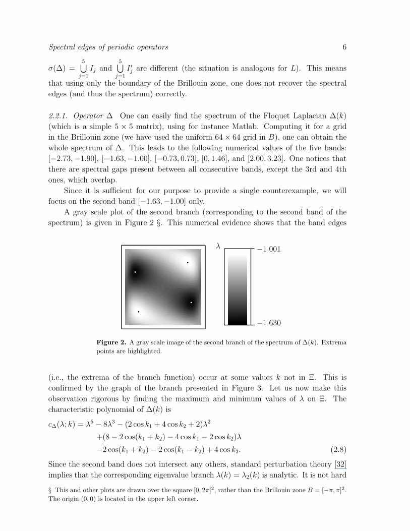
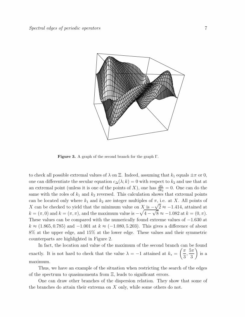
(i.e., the extrema of the branch function) occur at some values k not in Ξ. This is

confirmed by the graph of the branch presented in Figure 3. Let us now make this

observation rigorous by finding the maximum and minimum values of λ on Ξ. The

characteristic polynomial of ∆(k) is

c∆(λ; k) = λ5 − 8λ3 − (2 cos k1 + 4 cos k2 + 2)λ2

+(8 − 2 cos(k1 + k2) − 4 cos k1 − 2 cos k2)λ

−2 cos(k1 + k2) − 2 cos(k1 − k2) + 4 cos k2. (2.8)

Since the second band does not intersect any others, standard perturbation theory [32]

implies that the corresponding eigenvalue branch λ(k) = λ2(k) is analytic. It is not hard

§ This and other plots are drawn over the square [0, 2π]2, rather than the Brillouin zone B = [−π, π]2.

The origin (0, 0) is located in the upper left corner.

Spectral edges of periodic operators 7

Figure 3. A graph of the second branch for the graph Γ.

to check all possible extremal values of λ on Ξ. Indeed, assuming that k1 equals ±π or 0,

one can differentiate the secular equation c∆(λ; k) = 0 with respect to k2 and use that at

an extremal point (unless it is one of the points of X), one has ∂λ∂k2

= 0. One can do the

same with the roles of k1 and k2 reversed. This calculation shows that extremal points

can be located only where k1 and k2 are integer multiples of π, i.e. at X. All points of

X can be checked to yield that the minimum value on X is −√

2 ≈ −1.414, attained at

k = (π, 0) and k = (π, π), and the maximum value is −√

4 −√

8 ≈ −1.082 at k = (0, π).

These values can be compared with the numerically found extreme values of −1.630 at

k ≈ (1.865, 0.785) and −1.001 at k ≈ (−1.080, 5.203). This gives a difference of about

8% at the upper edge, and 15% at the lower edge. These values and their symmetric

counterparts are highlighted in Figure 2.

In fact, the location and value of the maximum of the second branch can be found

exactly. It is not hard to check that the value λ = −1 attained at k∗ =

(π

3,5π

3

)is a

maximum.

Thus, we have an example of the situation when restricting the search of the edges

of the spectrum to quasimomenta from Ξ, leads to significant errors.

One can draw other branches of the dispersion relation. They show that some of

the branches do attain their extrema on X only, while some others do not.

Spectral edges of periodic operators 8

2.2.2. Operator L The operator L can be analyzed similarly. We briefly summarize

the findings. The characteristic polynomial for L(k) is

cL(λ; k) = λ5 − 7

9λ3 −

(1

18+

1

9cos k2 +

1

18cos k1

)λ2

+

(13

162− 7

162cos k1 −

1

54cos k2 −

1

54cos(k1 + k2)

)λ

+1

81cos k2 −

1

162cos(k1 − k2) −

1

162cos(k1 + k2). (2.9)

We observe that (2.9) is quite similar to (2.8), modulo changes in some constants. The

structure of the branches of solutions to cL(λ; k) = 0 are also qualitatively similar

to the ones for the spectrum of ∆. The spectrum of L on Γ consists of five bands:

[−0.830,−0.606], [−0.518,−0.297], [−0.219, 0.219], [0, 0.485], [0.611, 1.000], with the

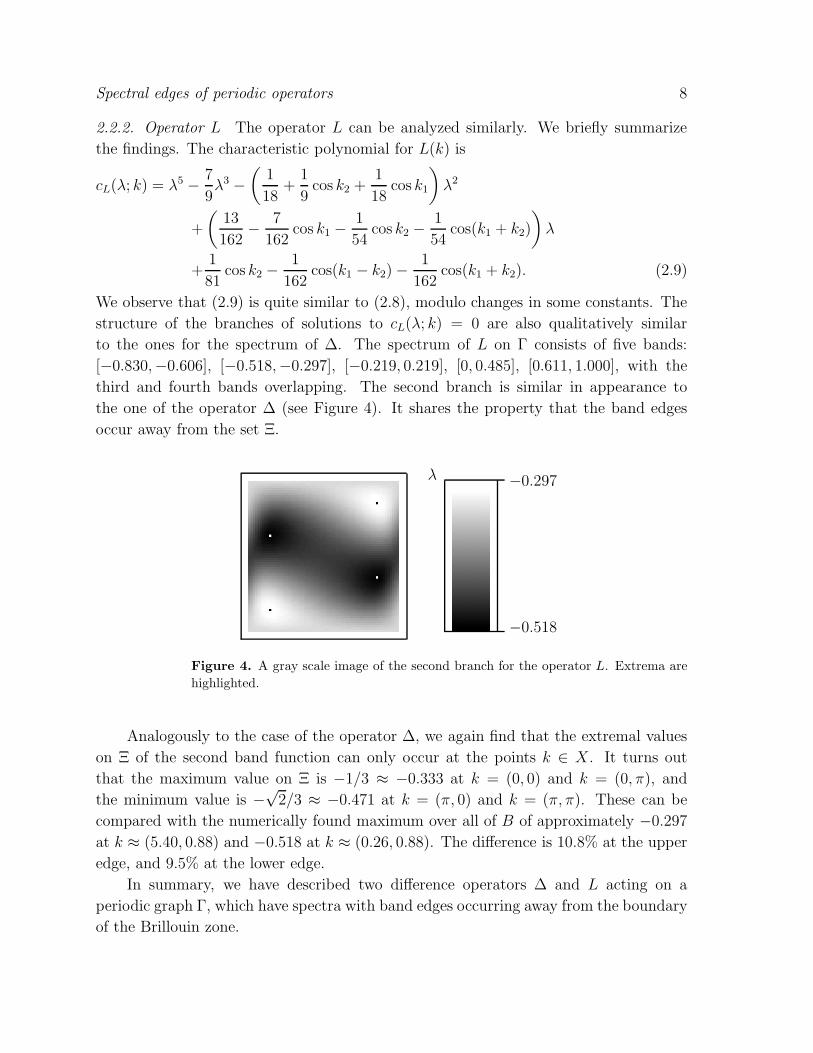
third and fourth bands overlapping. The second branch is similar in appearance to

the one of the operator ∆ (see Figure 4). It shares the property that the band edges

occur away from the set Ξ.

λ −0.297

−0.518

Figure 4. A gray scale image of the second branch for the operator L. Extrema are

highlighted.

Analogously to the case of the operator ∆, we again find that the extremal values

on Ξ of the second band function can only occur at the points k ∈ X. It turns out

that the maximum value on Ξ is −1/3 ≈ −0.333 at k = (0, 0) and k = (0, π), and

the minimum value is −√

2/3 ≈ −0.471 at k = (π, 0) and k = (π, π). These can be

compared with the numerically found maximum over all of B of approximately −0.297

at k ≈ (5.40, 0.88) and −0.518 at k ≈ (0.26, 0.88). The difference is 10.8% at the upper

edge, and 9.5% at the lower edge.

In summary, we have described two difference operators ∆ and L acting on a

periodic graph Γ, which have spectra with band edges occurring away from the boundary

of the Brillouin zone.

Spectral edges of periodic operators 9

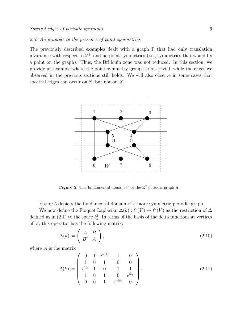
2.3. An example in the presence of point symmetries

The previously described examples dealt with a graph Γ that had only translation

invariance with respect to Z2, and no point symmetries (i.e., symmetries that would fix

a point on the graph). Thus, the Brillouin zone was not reduced. In this section, we

provide an example where the point symmetry group is non-trivial, while the effect we

observed in the previous sections still holds. We will also observe in some cases that

spectral edges can occur on Ξ, but not on X.

45

2

W

1 3

6 7 8

910

Figure 5. The fundamental domain V of the Z2-periodic graph Λ.

Figure 5 depicts the fundamental domain of a more symmetric periodic graph.

We now define the Floquet Laplacian ∆(k) : ℓ2(V ) → ℓ2(V ) as the restriction of ∆

defined as in (2.1) to the space ℓ2k. In terms of the basis of the delta functions at vertices

of V , this operator has the following matrix:

∆(k) :=

(A B

B† A

), (2.10)

where A is the matrix

A(k) :=

0 1 e−ik1 1 0

1 0 1 0 0

eik1 1 0 1 1

1 0 1 0 eik1

0 0 1 e−ik1 0

, (2.11)

Spectral edges of periodic operators 10

and B is

B(k) :=

1 0 0 0 0

0 0 0 0 0

0 0 eik2 0 0

0 0 0 eik2 0

0 0 0 0 1

. (2.12)

The matrix B describes the interaction between the two symmetric halves of the

fundamental domain V .

In a similar way, one can define L(k) and observe that

L(k) =

(T−1 0

0 T−1

)∆(k)

(T−1 0

0 T−1

), (2.13)

where T is the matrix

T :=

2 0 0 0 0

0√

2 0 0 0

0 0√

5 0 0

0 0 0 2 0

0 0 0 0√

3

. (2.14)

The fundamental domain has 10 vertices, and so there are 10 bands to the

spectrum. The lowest 5 bands are approximately [−3.840,−2.265], [−2.943,−1.834]

[−1.865,−1.113], [−1.536,−0.333] and [−0.803, 0.377]. The spectrum is symmetric

about λ = 0, and the remaining five bands are reflections of the previously mentioned

bands about this point.

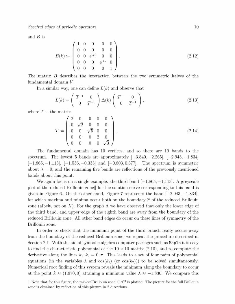
We again focus on a single example: the third band [−1.865,−1.113]. A greyscale

plot of the reduced Brillouin zone‖ for the solution curve corresponding to this band is

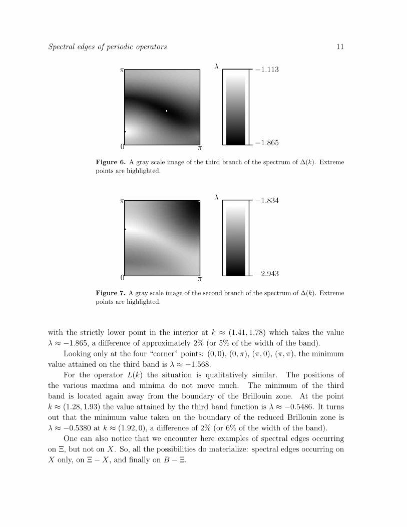
given in Figure 6. On the other hand, Figure 7 represents the band [−2.943,−1.834],

for which maxima and minima occur both on the boundary Ξ of the reduced Brillouin

zone (albeit, not on X). For the graph Λ we have observed that only the lower edge of

the third band, and upper edge of the eighth band are away from the boundary of the

reduced Brillouin zone. All other band edges do occur on these lines of symmetry of the

Brillouin zone.

In order to check that the minimum point of the third branch really occurs away

from the boundary of the reduced Brillouin zone, we repeat the procedure described in

Section 2.1. With the aid of symbolic algebra computer packages such as Maple it is easy

to find the characteristic polynomial of the 10 × 10 matrix (2.10), and to compute the

derivative along the lines k1, k2 = 0, π. This leads to a set of four pairs of polynomial

equations (in the variables λ and cos(k1) (or cos(k2))) to be solved simultaneously.

Numerical root finding of this system reveals the minimum along the boundary to occur

at the point k ≈ (1.970, 0) attaining a minimum value λ ≈ −1.830. We compare this

‖ Note that for this figure, the reduced Brillouin zone [0, π]2 is plotted. The picture for the full Brillouin

zone is obtained by reflection of this picture in 2 directions.

Spectral edges of periodic operators 11

λ −1.113

−1.8650

π

π

Figure 6. A gray scale image of the third branch of the spectrum of ∆(k). Extreme

points are highlighted.

λ −1.834

−2.9430

π

π

Figure 7. A gray scale image of the second branch of the spectrum of ∆(k). Extreme

points are highlighted.

with the strictly lower point in the interior at k ≈ (1.41, 1.78) which takes the value

λ ≈ −1.865, a difference of approximately 2% (or 5% of the width of the band).

Looking only at the four “corner” points: (0, 0), (0, π), (π, 0), (π, π), the minimum

value attained on the third band is λ ≈ −1.568.

For the operator L(k) the situation is qualitatively similar. The positions of

the various maxima and minima do not move much. The minimum of the third

band is located again away from the boundary of the Brillouin zone. At the point

k ≈ (1.28, 1.93) the value attained by the third band function is λ ≈ −0.5486. It turns

out that the minimum value taken on the boundary of the reduced Brillouin zone is

λ ≈ −0.5380 at k ≈ (1.92, 0), a difference of 2% (or 6% of the width of the band).

One can also notice that we encounter here examples of spectral edges occurring

on Ξ, but not on X. So, all the possibilities do materialize: spectral edges occurring on

X only, on Ξ −X, and finally on B − Ξ.

Spectral edges of periodic operators 12

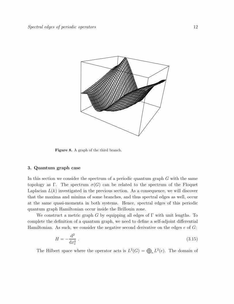
Figure 8. A graph of the third branch.

3. Quantum graph case

In this section we consider the spectrum of a periodic quantum graph G with the same

topology as Γ. The spectrum σ(G) can be related to the spectrum of the Floquet

Laplacian L(k) investigated in the previous section. As a consequence, we will discover

that the maxima and minima of some branches, and thus spectral edges as well, occur

at the same quasi-momenta in both systems. Hence, spectral edges of this periodic

quantum graph Hamiltonian occur inside the Brillouin zone.

We construct a metric graph G by equipping all edges of Γ with unit lengths. To

complete the definition of a quantum graph, we need to define a self-adjoint differential

Hamiltonian. As such, we consider the negative second derivative on the edges e of G:

H = − d2

dx2e

. (3.15)

The Hilbert space where the operator acts is L2(G) =⊕

e L2(e). The domain of

Spectral edges of periodic operators 13

the operator consists of all functions f such that

f ∈ H2(e) for each edge e,∑

e

‖f‖2H2(e) <∞,

f is continuous at each vertex∑

e∼v

f ′e(v) = 0 (Kirchhoff, or Neumann, conditions).

(3.16)

Here, f ′e(v) denotes the outgoing derivative of f at v along the edge e.

It is well known (e.g., [16, 40, 43, 49]) and easy to check that Floquet theory applies

to the quantum graph case. In particular, the spectrum σ(H) coincides with the union

over the Brillouin zone B of the spectra of Floquet Hamiltonians H(k). Here H(k) is

the operator defined similarly to H on H2loc functions with the same Kirchhoff vertex

conditions as in (3.16), and with the additional cyclic (Bloch, Floquet) condition (2.3):

f(T (px)) = eik·pf(x) (3.17)

for any p ∈ Z2, x ∈ G. We will call such functions Bloch (generalized) eigenfunctions.

Thus, describing the spectrum of an either combinatorial, or quantum periodic graph

operator, we can work with such generalized eigenfunctions only.

So, let ψ be a Bloch eigenfunction of H on G with a quasimomentum k and

eigenvalue ω2,

Hψ = ω2ψ . (3.18)

Let us define a function ϕ on the combinatorial counterpart Γ of G as the restriction

of ψ to the vertices of G. Clearly, ϕ is a Bloch function with the same quasimomentum

k (e.g., [40]). Due to (3.18), on each edge e = (u, v) the function ψ can be written in

terms of its values ϕ(v), ϕ(u) at the endpoints:

ψe(xe) = ϕ(v) cosωxe +

(ϕ(u) − cosω ϕ(v)

sinω

)sinωxe (3.19)

Here ψe and xe denote the restriction of ψ to the edge e and the coordinate along

e respectively. Then one has

ψ′e(v) =

ϕ(u) − cosω ϕ(v)

tanω. (3.20)

Vertex conditions (3.16) imply that at each vertex v the equation

1

dv

∑

u∼v

ϕ(u) = cosω ϕ(v) (3.21)

holds. Thus, ϕ is a Bloch eigenfunction of the difference operator 1dv

∑u∼v ϕ(u) on Γ

with eigenvalue cosω. Notice that the spectrum of this operator coincides with the

spectrum of its symmetrized version L investigated in the previous section. Thus, we

have constructed a quantum graph example of a periodic operator with a spectral edge

attained inside the Brillouin zone.

Spectral edges of periodic operators 14

The reader might notice that the correspondence between the spectra of L and H

works smoothly only outside zeros of sinω, i.e. not on the Dirichlet spectrum of the

edges. This is a well known phenomenon, see for instance [40]. However, it is easy

to observe that this does not influence our case and thus we have an example when a

spectral edge of a periodic quantum graph occurs inside the Brillouin zone.

4. Neumann waveguides and periodic tubular manifolds

In this section, we will show existence of periodic elliptic second order operators on

manifolds with a free co-compact action of Z2, some of whose spectral edges are attained

inside the Brillouin zone. The simplest example is of the Laplace operator with Neumann

boundary conditions in a periodic planar waveguide.

In order to construct the guide, let us assume our graph G (see Figure 1) to be

embedded into the plane in such a way that:

1. Each edge is a smooth simple curve of length 1.

2. Edges intersect only at the vertices.

3. Edges intersect transversally (i.e., there are no tangent edges).

4. The embedded graph is Z2-periodic.

Such an embedding is clearly possible.

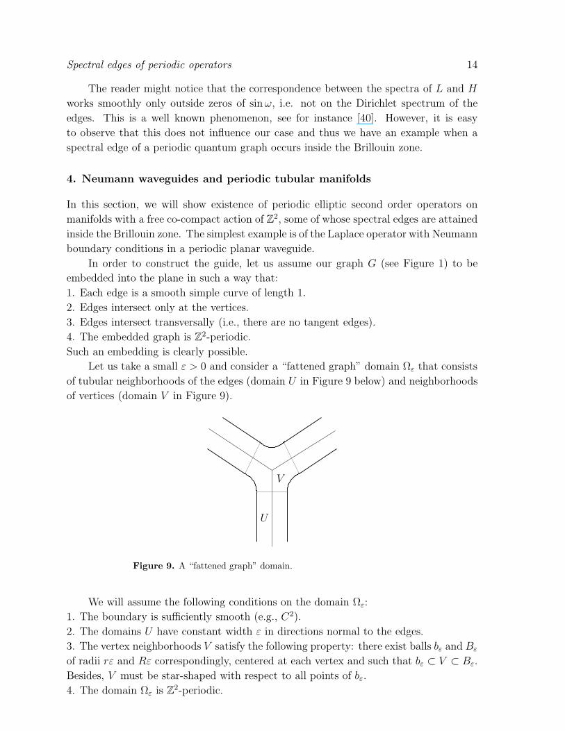
Let us take a small ε > 0 and consider a “fattened graph” domain Ωε that consists

of tubular neighborhoods of the edges (domain U in Figure 9 below) and neighborhoods

of vertices (domain V in Figure 9).

U

V

Figure 9. A “fattened graph” domain.

We will assume the following conditions on the domain Ωε:

1. The boundary is sufficiently smooth (e.g., C2).

2. The domains U have constant width ε in directions normal to the edges.

3. The vertex neighborhoods V satisfy the following property: there exist balls bε and Bε

of radii rε and Rε correspondingly, centered at each vertex and such that bε ⊂ V ⊂ Bε.

Besides, V must be star-shaped with respect to all points of bε.

4. The domain Ωε is Z2-periodic.

Spectral edges of periodic operators 15

It is easy to see that one can construct an ε-dependent family of domains satisfying all

these properties.

Consider now the (positive) Laplace operator −∆N,ε in Ωε with Neumann boundary

conditions on ∂Ωε.

It is proven in [44, 45], [54]-[57] that for any value of the quasimomentum k and any

finite interval I of the spectral axis, the part in I of the spectrum of the Floquet operator

−∆N,ε(k) converges to the corresponding part of the spectrum of the quantum graph

Hamiltonian (3.15)-(3.16) on G. Moreover, this convergence is uniform with respect to

k. This, in particular, implies immediately the following

Theorem 4.1. For sufficiently small values of ε, there is an isolated band of the

spectrum of the waveguide operator −∆N,ε, whose end points are attained strictly inside

the first Brillouin zone.

Proof. Indeed, this property holds for the quantum graph Hamiltonian H on G, and

thus the convergence result shows that it survives in Ωε for small values of ε.

This construction does not necessarily require the graph to be planar. For instance,

one would not be able to have a planar embedding with required properties for the more

symmetric graph Λ considered in Section 2.3. However, one can embed Λ into R3 in

such a way that it is Z2-periodic, with all other properties as required before. Then a

3D waveguide domain Ωε can be constructed around Λ in a similar manner to the one

above, such that the statement of Theorem 4.1 still holds.

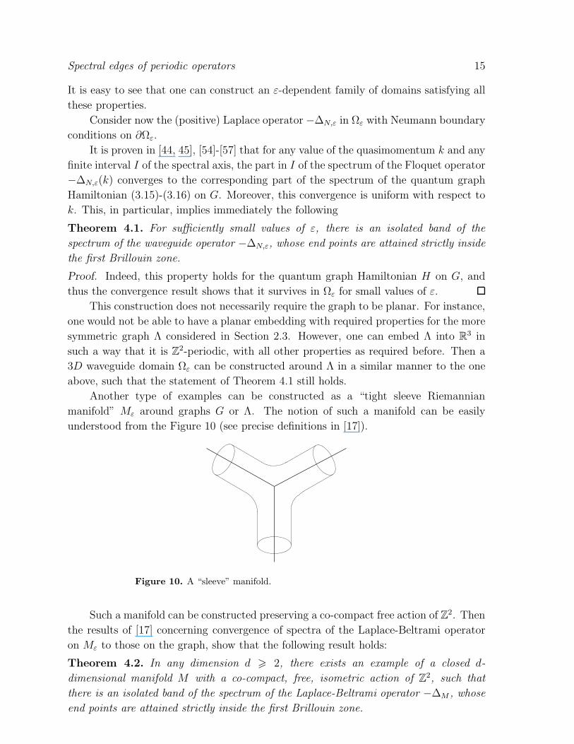
Another type of examples can be constructed as a “tight sleeve Riemannian

manifold” Mε around graphs G or Λ. The notion of such a manifold can be easily

understood from the Figure 10 (see precise definitions in [17]).

Figure 10. A “sleeve” manifold.

Such a manifold can be constructed preserving a co-compact free action of Z2. Then

the results of [17] concerning convergence of spectra of the Laplace-Beltrami operator

on Mε to those on the graph, show that the following result holds:

Theorem 4.2. In any dimension d > 2, there exists an example of a closed d-

dimensional manifold M with a co-compact, free, isometric action of Z2, such that

there is an isolated band of the spectrum of the Laplace-Beltrami operator −∆M , whose

end points are attained strictly inside the first Brillouin zone.

Spectral edges of periodic operators 16

The proof coincides with the one of the previous theorem.

5. Schrodinger and Maxwell operators

The previous discussion does not leave any doubt that examples can be found for

essentially any type of periodic equations of mathematical physics. However, it is

desirable to have such explicitly described examples for the cases of periodic Schrodinger

and Maxwell equations, interest in which stems from the solid state and photonic crystal

theories (e.g., [1], [19]-[21], [30, 31], [35]-[37], [53]).

Although we do not currently have rigorous arguments to show the existence of

such examples, we can expect that they may be obtained as follows. Consider a planar

embedding of the graph G, as the one considered in the previous section, with the

additional requirement that at each vertex the tangent lines to the converging edges

form equal angles. This can obviously be achieved. Consider then a “fattened graph”

domain Ωε described before and the Schrodinger operator S := −∆ + V (x) in R2 with

the Z2-periodic potential V (x) that is equal to zero in Ωε and equal to a large constant

C outside.

Conjecture 5.1. Under appropriate asymptotics ε → 0, C → ∞, the spectrum of

the operator S will display an isolated spectral band with its edges attained inside the

Brillouin zone.

What is lacking here, in spite of significant attention paid to such asymptotics

(e.g., [11, 12, 15, 17, 18, 22, 23, 25, 36, 37, 38, 41, 42, 44, 45, 46, 47, 52], [54]-[59],

[63]), is a spectral convergence result analogous to the one for the Neumann Laplace

operator. Moreover, it is known that such convergence (even after appropriate spectral

re-scaling), does not hold, due to the appearance of low energy (below the energy of the

first transversal eigenfunction) bound states attached to vertices [12, 18, 38]. However,

for creating an example that we are looking for, the full spectral convergence is not

truly needed. What is required, is some kind of convergence above the energy of the

first transversal eigenfunction, which must hold (see some results in this direction in

[46, 47]). When the angles formed by the edges are equal, we expect vertex conditions

of Kirchhoff type to arise.

Concerning the periodic Maxwell operators ∇×ε−1(x)∇×, where ε(x) is the electric

permeability, we expect that the simplest to come by will be an example of a 2D periodic

medium (i.e., a medium which is periodic in two directions and homogeneous in the

third one). As it is well known [29, 30, 31, 37], in this case the Maxwell operator splits

(according to two polarizations) into the direct sum of two scalar operators −∇·ε−1(x)∇and −ε−1(x)∆. We expect that similar high-contrast narrow media as described above

should provide necessary examples (see also considerations of such high contrast limits

in [3], [19]-[21],[24, 28, 37, 41, 42, 60]).

Spectral edges of periodic operators 17

6. Why do spectral edges often appear at the symmetric points of the

Brillouin zone?

In this section, we will show why, in spite of the examples of this paper, the spectral

edges are often attained at the highest symmetry points, and hence at the boundary of

the reduced Brillouin zone. Namely, let H0 be a periodic self-adjoint elliptic Hamiltonian

with real coefficients (i.e., the corresponding non-stationary Schrodinger equation has

time-reversal symmetry). Suppose that the spectral edges of H0 are attained at

symmetry points of the Brillouin zone B = [−π, π]n only (see the details below). Then

we will show that for a “generic” H0, this feature of the spectrum cannot be destroyed by

small perturbations (with the same symmetry) of the operator. This robustness might

be the reason why one very rarely observes spectral edges appearing inside the reduced

Brillouin zone.

Let us now introduce some notions. We will assume, for simplicity of presentation,

that the Hamiltonian is the Schrodinger operator in Rn:

H0 = −∆ + V (x), (6.22)

where V (x) is a real-valued bounded potential such that V (x + p) = V (x) for all

integer vectors p ∈ Zn. For any quasimomentum k ∈ B, we will denote by H(k)

the Bloch Hamiltonian defined on Zn-periodic functions (i.e., on functions on the torus

Tn = Rn/Zn) as

H(k) =

(1

i∇ + k

)2

+ V (x).

It depends polynomially, and thus analytically, on k. We denote by λj(k), j = 1, 2, . . . ,

the eigenvalues of H(k) counted with their multiplicity in non-decreasing order. The

band functions λj( · ) are continuous functions of k ∈ B. Since the potential V is

real-valued, the eigenvalues are also even in k, i.e. λj(−k) = λj(k). This follows from

the fact that complex conjugate to an eigenfunction is an eigenfunction (presence of a

magnetic potential would destroy this symmetry). This symmetry will be crucial for

what follows.

The ranges

∆j = λj(k)| k ∈ Bare closed finite intervals of the spectral axis (spectral bands), whose union is the

spectrum σ(H0). Global maxima and minima of the band functions λj( · ) are the

endpoints (edges) of spectral bands. It is also known (e.g., [32, 35, 53]) that λj ’s are

analytic in k away from the eigenvalue crossing points. In case of the crossing, we point

out the following elementary, but useful result:

Lemma 6.1. Let us fix an open interval ∆ = (a, b) ⊂ R. Suppose that for a neighborhood

U ⊂ B the band functions λs, j 6 s 6 j +m, satisfy

λs(k) ∈ ∆, k ∈ U,

Spectral edges of periodic operators 18

and that the remaining band functions take values in U that lie outside a neighborhood

of the closed interval ∆. Then the functions

j+m∏

s=j

λs(k) and

j+m∑

s=j

λs(k) (6.23)

are analytic with respect to k ∈ U .

Proof. Let us assume that m = 1 (the case of arbitrary m works out exactly same way),

i.e. we have two eigenvalue branches λ−(k) := λj(k) and λ+(k) := λj+1(k). Consider a

positively oriented circle Γ ⊂ C centered at (a + b)/2 with radius (b − a)/2 + ε with a

small ε > 0. The two-dimensional projection

P (k) =1

2πi

∫

Γ

(λ−H(k))−1 dλ, (6.24)

depends analytically on k ∈ U . Let M(k) be the range of P (k). It forms an analytic

two-dimensional vector-bundle [35, 62]. Let e1, e2 be a basis in M(k0) with some

k0 ∈ U . For k close to k0 we can define a basis of M(k) analytically depending on k as

follows:

fj(k) := P (k)ej. (6.25)

In this basis, the operator function

P (k)H(k)P (k)|M(k) = H(k)P (k)|M(k)

can be written as an analytic 2×2 matrix-function A(k) with eigenvalue branches λ−(k)

and λ+(k). Therefore, the functions

detA(k), tr A(k)

are analytic in k in a neighborhood of k0.

The only fixed points k ∈ B for the symmetries k → −k + p, p ∈ 2πZn, are the

ones from the set

X = k = (k1, · · · , kn) ∈ B | kj ∈ 0, π, j = 1, · · · , n. (6.26)

In view of the symmetry λj(k) = λj(−k) we also have λj(k0 + k) = λj(k0 − k) for

any k0 ∈ X. We have already shown in this text that the global extrema of the band

functions can occur outside the set X. The experimental observation, however, is that

for most periodic operators of practical importance and for practical values of their

parameters (e.g., potentials, electric permittivity, etc.), the band endpoints do occur

on X. One can easily observe this by looking at dispersion curve calculations in solid

state physics or photonic crystals literature (e.g., [51, ?]). Our main question now

is: Why do the spectral edges occur so often on X?

Our considerations will be local on the spectrum. Thus, let us fix a finite interval

Λ = (a, b) of the spectral axis. Note that the number of spectral bands ∆j overlapping

with Λ is finite. We first introduce the following notion:

Spectral edges of periodic operators 19

Definition 6.2. We call a periodic Hamiltonian H simple on a finite interval Λ, if

the global extrema of the band functions λj(k) which occur inside Λ, are attained at the

points of the set X only.

The simplicity property defined above will be discussed for “generic” periodic

operators:

Definition 6.3. We call a periodic Hamiltonian H generic on a finite interval Λ, if

for every band edge λ0 occuring inside Λ, the band functions λj assume the value λ0 at

finitely many points of the Brillouin zone B, and in a neighborhood U of each such point

k0 one of the following two conditions is satisfied:

(i) There is a unique band function λ( · ) for k ∈ U such that λ(k0) = λ0; moreover,

k0 is a non-degenerate extremum of λ(k).

(ii) For k ∈ U there are only two band functions λ+( · ), λ−(· ) such that λ−(k0) =

λ+(k0) = λ0. Moreover, λ−(k) < λ+(k) for all k ∈ U − k0, and k0 is a non-

degenerate maximum of the product D(k) = (λ+(k) − λ0)(λ−(k) − λ0).

Above by a non-degenerate extremum we understand an extremum with a non-degenerate

Hessian.

Recall that in view of Lemma 6.1, the determinant of A(k) is analytic on U .

Definition 6.3 means that the band functions of a generic Hamiltonian behave near

band edges as eigenvalues of a “generic” 2× 2 self-adjoint analytic matrix function. We

refer to cases (1) and (2) in the above definition as the single edge case and the case of

two touching bands respectively. Note also that in Definition 6.3 the band edge λ0 is

not assumed to be (albeit could be) an endpoint of the spectrum.

The following conjecture is believed to hold (see a variety of similar genericity

conjectures in, e.g., [2, 8, 37, 48]).

Conjecture 6.4. Generic periodic Hamiltonians form a set of second Baire category in

a suitable class of periodic operators.

The closest to the proof of this conjecture is the result of [33], where it was shown

that generically a band edge, which is an endpoint of the spectrum, is attained by a

single band function.

Our aim is to show that a generic simple Hamiltonian H0 remains generic and

simple under small perturbations. More precisely, we introduce the family of operators

Hg = H0 + gV (x), H0 = −∆ + V0,

where V0 and V are bounded real-valued Zn-periodic functions, and g ∈ R is a parameter.

We denote by λj(k, g) the band functions of Hg. If g = 0, we drop g and write simply

λj(k). Since Hg is analytic in g, the band functions λj(k, g) are analytic in (k, g) away

from the crossing points, and the quantities defined in (6.23) are analytic in (k, g) under

the conditions of Lemma 6.1.

We can now formulate a result that gives a partial answer to the question posed in

this Section.

Spectral edges of periodic operators 20

Theorem 6.5. Let Λ ⊂ R be a finite closed interval, and let the operator H0 (see (6.22))

be simple and generic in a neighborhood of Λ. Then, for sufficiently small values of g,

the operator Hg is also simple and generic in a neighborhood of Λ.

Proof. Let Λ′ be a finite closed interval containing Λ in its interior and such that

operator H0 is simple and generic in an open neighborhood Λ′′ of Λ′. The continuity

of λj(k, g) in g guarantees that for small g, the spectral band edges of the perturbed

operator occurring on Λ′, are either perturbations of the band edges of H0 that are

inside Λ′′, or are produced by opening a gap between two touching spectral bands of

H0.

Let λ0 ∈ Λ′′ be a single band edge of H0, or the point where two bands touch.

Assume without loss of generality that λ0 = 0. Since the unperturbed operator H0

is simple, again, by continuity of λj(k, g) in g, for sufficiently small values of g, the

perturbed eigenvalues cannot reach their global maxima outside a neighborhood of the

set X. Thus, it suffices to consider the neighborhood of each point k0 ∈ X individually.

We assume without loss of generality that k0 = 0.

Further proof requires different arguments for the two cases featuring in Definition

6.3.

6.1. The single edge case

Let λ(k) be the unique band function of the operator H0, which attains at k0 = 0 its

non-degenerate extremum, which for definiteness will be assumed to be a maximum.

Recall that λ( · ) is analytic in k and λ(k) = λ(−k), so that

λ(k) = λ2(k) + λe(k),

where λ2 is a negative definite quadratic form and λe is an analytic function such that

λe(k) = O(|k|4). For sufficiently small g and k, the eigenvalue λ(k, g) will remain

separated from the rest of the spectrum of Hg(k). Thus, to complete the proof, we

need to show that λ( · , g) attains its maximal value at k = 0 and this maximum is

non-degenerate. Due to analyticity,

λ(k, g) = λ2(k) + λe(k) + gλ(k, g),

where λ(k, g) is a real-valued real-analytic function of (k, g), and λ(k, g) = λ(−k, g).The latter property implies that

∇kλ(k, g) = O(|k|),uniformly in g. Making an appropriate linear change of variables, we can always assume

that λ2(k) = −|k|2/2. Then, taking the gradient with respect to k, we obtain

∇kλ(k, g) = −k + ∇kλe(k) + g∇kλ(k, g).

Consequently

|∇kλe(k) + g∇kλ(k, g)| 6 C(|k|3 + g|k|),

Spectral edges of periodic operators 21

with some positive constant C, and hence, for |g| < (4C)−1, |k| < (2√C)−1, k 6= 0, we

get,

|∇kλ(k, g)| > |k|2

6= 0.

This proves that the only stationary point of λ( · , g) is k = 0. Moreover, since λ2( · ) is

negative definite, the function λ( · , g) has a non-degenerate Hessian if g is sufficiently

small. Thus the band function λ(k, g) attains its extremum on X and satisfies the

requirements of Definition 6.3(1).

6.2. The case of two touching bands

Assume, as above, that λ0 = 0, k0 = 0, and that λ−(k) and λ+(k) are the band functions

as given in Definition 6.3. Denote by λ±(k, g) the perturbed band functions. According

to Lemma 6.1, the functions

d(k, g) = λ−(k, g)λ+(k, g), t(k, g) =1

2(λ−(k, g) + λ+(k, g))

are analytic in a neighborhood of (k, g) = (0, 0). Remembering the central symmetry of

the eigenvalues and the genericity assumption for H0, we can write

d(k, g) = d2(k) + de(k) + gd(k, g),

t(k, g) = t2(k) + te(k) + gt(k, g).(6.27)

Here all functions are analytic near (k, g) = (0, 0) and even in k. The functions t2and d2 are quadratic forms, the terms de, te are O(|k|4), and, by virtue of genericity,

d2 is negative definite. Thus, as in the first part of the proof, we may assume that

d2(k) = −|k|2/2. Note also, that d(0, g) = 0, since the eigenvalues λ±(0, g) are of order

O(g), and hence d(0, g) = O(g2). Introduce the quantity

m = t2 − d =1

2(λ+ − λ−)2

> 0.

Using (6.27) we get

m(k, g) = g2m0(g) − d2(k) +me(k, g), me(k, g) = O(|k|2)(k2 + g),

where the functions m0(g) = t(0, g)2 − ∂gd(0, g) and me(k, g) are analytic in k, g, and

me is even in k. Since m(0, g) = g2m0(g), we also have m0(g) > 0.

Let us list some simple estimates that these functions and their gradients with

respect to k satisfy in a neighborhood of (0, 0). Below we denote by C,C1 some positive

constants whose precise value is not important:

|t(k, g)| 6 C(k2 + g), |m(k, g)| 6 C(|k|2 + g2),

|∇kt(k, g)|, |∇km(k, g)| 6 C|k|,(6.28)

|∇km(k, g)| >1

2|k|,

m(k, g) > g2m0(g) +1

4|k|2.

(6.29)

Spectral edges of periodic operators 22

The eigenvalues λ±(k, g) solve the characteristic equation

λ2 − 2t(k, g)λ+ d(k, g) = 0,

and thus

λ±(k, g) = t(k, g) ±√m(k, g). (6.30)

By (6.29) the eigenvalues λ±(k, g) can coincide only at k = 0, so that they are analytic in

k for k 6= 0. Let us prove that λ±( · , g) have no stationary points if k 6= 0. Differentiate:

∇kλ±(k, g) = ∇kt(k, g) ±∇km(k, g)

2√m(k, g)

.

Now the estimates (6.28) and (6.29) imply:

|∇kλ±| >

∣∣∣∣∇km

2√m

∣∣∣∣− |∇kt| >c|k|√

|k|2 + g2− C|k| > C1|k|

for small g and k 6= 0. This proves that λ±( · , g) attain their extrema only at k = 0.

It remains to show that the eigenvalues satisfy the requirements either of Part (1)

or Part (2) of Definition 6.3. If m0(g) > 0, then by (6.29) and (6.30), the eigenvalues

λ+(k, g) and λ−(k, g) are decoupled for all k and g, and their extrema are clearly non-

degenerate. If m0(g) = 0, then by (6.30) λ+(0, g) = λ−(0, g), and then by (6.27) the

determinant d(k, g) has a non-degenerate Hessian for small k, g.

The proof of the 6.5 is complete.

7. Final remarks

• Suppose that for a particular periodic operator the spectral edges do occur at the

point of X = k| kj = ±π or 0 only. This means then that one can find the correct

spectral edges (and thus the spectrum as a set), computing only spectra of problems

that are periodic or anti-periodic with respect to each variable (say, periodic with

respect to x1 and x3 and anti-periodic with respect to x2). This resembles then the

1D situation [13, 53], when the edges of the spectrum are attained at the spectra

of the periodic and anti-periodic problems.

• In the last Section we have restricted ourselves to the case of Schrodinger operators

with electric potentials only. However, the proof in fact does not use the structure

of the operator and could be extended to arbitrary analytically fibered operator in

the sense of [26], as long as the central symmetry k 7→ −k holds.

We also assumed parametric perturbation (i.e., perturbation by gV with a small

scalar parameter g). However, without any change in the proof, one can consider

V as a functional parameter and prove the same statements for small values of this

parameter.

• Observations of stability under small perturbations of critical points of a function

in “general position” in presence of symmetries, analogous to the ones in the last

section, have been made before in different circumstances, e.g. in [27].

Spectral edges of periodic operators 23

Acknowledgements

The authors thank G. Berkolaiko, K. Busch, D. Dobson, B. Helffer, A. Tip,

M. Weinstein, and Ya Yan Lu for discussing the topic of this paper.

The research of the second author was partly sponsored by the NSF through the

Grant DMS-0406022. The work of the first and fourth authors was partly sponsored by

the NSF Grant DMS-0604859. The authors thank the NSF for this support.

Part of the work by the second and third authors was completed during the Isaac

Newton Institute program on Spectral Theory in July 2006. The authors thank the INI

for the support.

References

[1] N.W. Ashcroft and N.D. Mermin, Solid State Physics, Holt, Rinehart and Winston, New York-

London, 1976.

[2] J.E. Avron and B. Simon, Analytic properties of band functions, Ann. Physics 110(1978), 85-101.

[3] W. Axmann, P. Kuchment, and L. Kunyansky, Asymptotic methods for thin high contrast 2D

PBG materials, Journal of Lightwave Technology, 17(1999), no.11, 1996- 2007.

[4] L. P. Bouckaert, R. Smoluchowski and E. Wigner, Theory of Brillouin zones and symmetry

properties of wave functions in crystals, Phys. Rev. 50 (1936), 58–67.

[5] K. Busch, G. von Freyman, S. Linden, S. F. Mingaleev, L. Tkeshelashvili, M. Wegener, Periodic

nanostructures for photonics, preprint 2006.

[6] F. Chung, Spectral Graph Theory, Amer. Math. Soc., Providence R.I., 1997.

[7] Y. Colin de Verdiere, Spectres De Graphes, Societe Mathematique De France, 1998

[8] Y. Colin de Verdiere, Sur les singularites de Van Hove generiques. Memoires de la Societe

Mathematique de France Ser. 2, 46 (1991), p. 99–109.

[9] S. J. Cox and D. C. Dobson, Maximizing band gaps in two-dimensional photonic crystals, SIAM

J. Appl. Math. 59(1999), no.6, 2108 - 2120.

[10] S. J. Cox and D. C. Dobson, Band structure optimization of two-dimensional photonic crystals in

H-polarization, J. Comp. Phys., 158 (2000), 214-224.

[11] G. Dell’Antonio and L. Tenuta, Quantum graphs as holonomic constraints, preprint

arXiv:math-ph/0603044.

[12] P. Duclos, P. Exner, Curvature-induced bound states in quantum waveguides in two and three

dimensions, Rev. Math. Phys. 7 (1995), 73-102

[13] M. S. P. Eastham, The Spectral Theory of Periodic Differential Equations, Scottish Acad. Press

Ltd., Edinburgh-London, 1973.

[14] W. D. Evans and D. J. Harris, Fractals, trees and the Neumann Laplacian, Math. Ann. 296(1993),

493-527.

[15] W. D. Evans and Y. Saito, Neumann Laplacians on domains and operators on associated trees,

Quart. J. Math. Oxford 51(2000), 313-342.

[16] P. Exner, R. Gawlista, Band spectra of rectangular graph superlattices, Phys. Rev. B53 (1996),

7275-7286

[17] P. Exner and O. Post, Convergence of spectra of graph-like thin manifolds, J. Geom. Phys. 54

(2005), 77-115.

[18] P. Exner and P. Seba, Electrons in semiconductor microstructures: a challenge to operator

theorists, in Schrodinger Operators, Standard and Nonstandard (Dubna 1988)., World Scientific,

Singapore 1989; pp. 79-100.

[19] A. Figotin and P. Kuchment, Band-gap structure of the spectrum of periodic and acoustic media.

I. Scalar model, SIAM J. Applied Math. 56(1996), no.1, 68-88.

Spectral edges of periodic operators 24

[20] A. Figotin and P. Kuchment, Band-gap structure of the spectrum of periodic and acoustic media.

II. 2D Photonic crystals, SIAM J. Applied Math. 56(1996), 1561-1620.

[21] A. Figotin and P. Kuchment, Spectral properties of classical waves in high contrast periodic media,

SIAM J. Appl. Math. 58(1998), no.2, 683-702.

[22] M. Freidlin, Markov Processes and Differential Equations: Asymptotic Problems, Lectures in

Mathematics ETH Zurich, Birkhauser Verlag, Basel 1996.

[23] M. Freidlin and A. Wentzell, Diffusion processes on graphs and the averaging principle, Annals of

Probability, 21(1993), no.4, 2215-2245.

[24] L. Friedlander, On the density of states of periodic media in the large coupling limit, Comm. PDE

27 (2002), No. 1-2, 355–380.

[25] R. Froese and I. Herbst, Realizing holonomic constraints in classical and quantum mechanics,

Comm. Math. Phys. 220 (2001), 489-535.

[26] C. Gerard and F. Nier, The Mourre theory for analytically fibered operators, J. Funct. Anal. 152

(1998), no. 1, 202–219.

[27] B. Helffer and J. Sjostrand, Analyse semi-classique pour l’equation de Harper (avec application a

l’equation de Schrodinger avec champ magnetique), Mm. Soc. Math. France (N.S.) No. 34 (1988),

113 pp.; Analyse semi-classique pour l’equation de Harper. II. Comportement semi-classique pres

d’un rationnel, Mm. Soc. Math. France (N.S.) No. 40 (1990), 139 pp; Semiclassical analysis for

Harper’s equation. III. Cantor structure of the spectrum. Mm. Soc. Math. France (N.S.) No. 39

(1989), 1–124.

[28] R. Hempel and K. Lienau, Spectral properties of periodic media in the large coupling limit, Comm.

PDE. 25(2000), no.7-8, 1445-1470.

[29] J. D. Jackson, Classical Electrodynamics, John Wiley & Sons, NY, 1962.

[30] J. D. Joannopoulos, R. D. Meade, and J. N. Winn, Photonic Crystals, Molding the Flow of Light,

Princeton Univ. Press, Princeton, N.J. 1995.

[31] S. G. Johnson and J. D. Joannopoulos, Photonic Crystals, The road from Theory to Practice,

Kluwer Acad. Publ., Boston 2002.

[32] T. Kato, Perturbation Theory for Linear Operators, Springer Verlag, Berlin e.a., 1980.

[33] F. Klopp and J. Ralston, Endpoints Of The Spectrum Of Periodic Operators Are Generically

Simple, Methods Appl. Anal. 7 (2000), no. 3, 459–463.

[34] P. Kuchment, To the Floquet theory of periodic difference equations, in : Geometrical and

Algebraical Aspects in Several Complex Variables, Cetraro (Italy), June 1989, 203-209, EditEl,

1991.

[35] P. Kuchment, Floquet Theory for Partial Differential Equations, Birkhauser Verlag, Basel, 1993.

[36] P. Kuchment, On some spectral problems of mathematical physics, in: Partial Differential

Equations and Inverse Problems, C. Conca, R. Manasevich, G. Uhlmann, and M. S. Vogelius

(Editors), Contemp. Math. 362, 2004

[37] P. Kuchment, The Mathematics of Photonics Crystals, Ch. 7 in Mathematical Modeling in Optical

Science, Bao, G., Cowsar, L. and Masters, W.(Editors), 207–272, Philadelphia: SIAM, 2001.

[38] P. Kuchment, Graph models of wave propagation in thin structures, Waves in Random Media

12(2002), no. 4, R1-R24.

[39] P. Kuchment, Quantum graphs I. Some basic structures, Waves in Random media, 14 (2004),

S107–S128.

[40] P. Kuchment, Quantum graphs II. Some spectral properties of quantum and combinatorial graphs,

J. Phys. A 38 (2005), 4887-4900.

[41] P. Kuchment and L. Kunyansky, Spectral Properties of High Contrast Band-Gap Materials and

Operators on Graphs, Experimental Mathematics, 8(1999), no.1, 1-28.

[42] P. Kuchment and L. Kunyansky, Differential operators on graphs and photonic crystals, Adv.

Comput. Math. 16(2002), 263-290.

[43] P. Kuchment and B. Vainberg, On the structure of eigenfunctions corresponding to embedded

eigenvalues of locally perturbed periodic graph operators

Spectral edges of periodic operators 25

686.

[44] P. Kuchment and H. Zeng, Convergence of spectra of mesoscopic systems collapsing onto a graph,

J. Math. Anal. Appl. 258(2001), 671-700.

[45] P. Kuchment and H. Zeng, Asymptotics of spectra of Neumann Laplacians in thin domains, in

Advances in Differential Equations and Mathematical Physics, Yu. Karpeshina, G. Stolz, R.

Weikard, and Y. Zeng (Editors), Contemporary Mathematics v.387, AMS 2003, 199-213.

[46] S. Molchanov and B. Vainberg, Transition from a network of thin fibers to the quantum graph:

an explicitly solvable model, Contemporary Mathematics, v. 415, AMS (2006), pp 227-240.

[47] S. Molchanov and B. Vainberg, Scattering solutions in a network of thin fibers: small diameter

asymptotics, preprint arXiv:math-ph/0609021.

[48] S. P. Novikov, Two-dimensional Schrodinger operators in periodic fields, in: Itogi Nauki i Techniki,

Contemporary Problems of Math., v.23, VINITI, Moscow 1983,3-32. (In Russian). English

translation in Journal of Mathematical Sciences, 28 (1985), No.1 1–20.

[49] V. L. Oleinik, B. S. Pavlov, and N. V. Sibirev, Analysis of the dispersion equation for the

Schrodinger operator on periodic metric graphs, Waves in Random Media 14(2004), 157-183.

[50] K. Pankrashkin, Spectra of Schrodinger operators on equilateral quantum graphs, Lett. Math.

Phys. 77 (2006) 139–154.

[51] Photonic and Acoustic Band-Gap Bibliography,

http://phys.lsu.edu/~jdowling/pbgbib.html

[52] O. Post, Spectral convergence of non-compact quasi-one-dimensional spaces, Ann. Henri Poincare

7 (2006), no. 5, 933–973.

[53] M. Reed, B. Simon, Methods of Modern Mathematical Physics, Vol. IV: Analysis of Operators,

Academic Press, London, 1978.

[54] J. Rubinstein and M. Schatzman, Spectral and variational problems on multiconnected strips, C.

R. Acad. Sci. Paris Ser. I Math. 325(1997), no.4, 377-382.

[55] J. Rubinstein and M. Schatzman, Asymptotics for thin superconducting rings, J. Math. Pures

Appl. (9) 77 (1998), no. 8, 801–820.

[56] J. Rubinstein and M. Schatzman, On multiply connected mesoscopic superconducting structures,

Semin. Theor. Spectr. Geom., no. 15, Univ. Grenoble I, Saint-Martin-d’Heres, 1998, 207-220.

[57] J. Rubinstein and M. Schatzman, Variational problems on multiply connected thin strips. I. Basic

estimates and convergence of the Laplacian spectrum. Arch. Ration. Mech. Anal. 160 (2001),

no. 4, 271–308.

[58] Y. Saito, The limiting equation of the Neumann Laplacians on shrinking domains, Electronic J.

Diff. Equations 2000 (2000), no. 31,1–25.

[59] Y. Saito, Convergence of the Neumann Laplacians on shrinking domains, Analysis 21(2001),171–

204.

[60] J. Selden, Periodic Operators in High-Contrast Media and the Integrated Density of States

Function, Comm. PDE 30 (2005), No. 7, 1021–1037.

[61] M. Skriganov, Geometric and Arithmetic Methods in the Spectral Theory of Multidimensional

Periodic Operators, Amer. Math. Soc. 1987.

[62] M. Zaidenberg, S. Krein, P. Kuchment, and A. Pankov, Banach bundles and linear operators,

Russian Math. Surveys 30 (1975), 115–175.

[63] H. Zeng, Convergence of spectra of mesoscopic systems collapsing onto a graph, PhD Thesis,

Wichita State University, Wichita, KS 2001.