Biometrics & Biostatistics International Journal On Modeling of Lifetime Data Using Akash, Shanker, Lindley and Exponential Distributions Submit Manuscript | http://medcraveonline.com Introduction In reliability analysis the time to the occurrence of event of interest is known as lifetime or survival time or failure time. The event may be failure of a piece of equipment, death of a person, development (or remission) of symptoms of disease, health code violation (or compliance). The modeling and statistical analysis of lifetime data are crucial for statisticians, research workers and policy makers in almost all applied sciences including engineering, medical science/biological science, insurance and finance, amongst others. In statistics literature a number of lifetime distributions for modeling lifetime data-sets have been proposed. In this paper, the main objective is to have a critical and comparative study on one parameter lifetime distributions namely, Akash, Shanker, Lindley and exponential and their applications for modeling lifetime dats-sets from engineering, medical sciences, and other fields of knowledge. Akash, Shanker, Lindley and Exponential Distributions Akash distribution introduced by Shanker [2] for modeling lifetime data from engineering and medical science is a two- component mixture of an exponential ( ) θ distribution and a gamma ( ) 3, θ distribution with their mixing proportions 2 2 2 θ θ + and 2 2 2 θ + respectively. Shanker [2] has discussed its various mathematical and statistical properties including its shape, moment generating function, moments, skewness, kurtosis, hazard rate function, mean residual life function, stochastic orderings, mean deviations, distribution of order statistics, Bonferroni and Lorenz curves, Renyi entropy measure, stress- strength reliability , amongst others. Shanker et al. [3] has detailed study about modeling of various lifetime data from different fields using Akash, Lindley and exponential distributions and concluded that Akash distribution gives better fit in most of the lifetime data. Shanker [5] has also obtained a Poisson mixture of Akash distribution named, “Poisson-Akash (PAD)” for modeling count data. Shanker distribution introduced by Shanker [2] for modeling lifetime data from engineering and medical science is a two- component mixture of an exponential ( ) θ distribution and a gamma ( ) 2, θ distribution with their mixing proportions 2 2 1 θ θ + and 2 1 1 θ + respectively. Shanker [3] has discussed its various mathematical and statistical properties including its shape, moment generating function, moments, skewness, kurtosis, hazard rate function, mean residual life function, stochastic orderings, mean deviations, distribution of order statistics, Bonferroni and Lorenz curves, Renyi entropy measure, stress-strength reliability , amongst others. Shanker [6] has also obtained a Poisson mixture of Shanker distribution named, “Poisson-Shanker (PSD)” for modeling count data. Lindley [7] distribution is a two-component mixture of an exponential ( ) θ distribution and a gamma ( ) 2, θ distribution with their mixing proportions 1 θ θ + and 1 1 θ + respectively. A detailed study about its various mathematical properties, estimation of parameter and application showing the superiority of Lindley distribution over exponential distribution for the waiting times before service of the bank customers has been done by Ghitany et al. [8]. A number of researchers have studied in detail the Volume 3 Issue 6 - 2016 1 Department of Statistics, Eritrea Institute of Technology, Eritrea 2 Department of Economics, College of Business and Economics, Eritrea *Corresponding author: Rama Shanker, Department of Statistics, Eritrea Institute of Technology, Asmara, Eritrea; Email: Received: May 03, 2016 | Published: June 24, 2016 Research Article Biom Biostat Int J 2016, 3(6): 00084 Abstract The statistical analysis and modeling of lifetime data are crucial for statisticians and research workers in almost all applied sciences including engineering, biomedical science, insurance, and finance, amongst others. The two important and popular one parameter distributions for modeling lifetime data are exponential and Lindley distributions. Shanker et al. [1] observed that there are many lifetime data where these distributions are not suitable from theoretical and applied point of view. Recently Shanker [2,3] has introduced two one parameter Lifetime distribution namely “Akash distribution” and “Shanker distribution” for modeling lifetime data. In the present paper the relationships and comparative studies of Akash, Shanker, Lindley and exponential distributions, their distributional properties and estimation of parameter have been discussed. The applications, goodness of fit and theoretical justifications of these distributions for modeling life time data through various examples from engineering, medical science and other fields have been discussed and explained. Keywords: Akash distribution; Shanker distribution; Lindley distribution; Exponential distribution; Statistical properties; Estimation of parameter; Goodness of fit

Welcome message from author
This document is posted to help you gain knowledge. Please leave a comment to let me know what you think about it! Share it to your friends and learn new things together.
Transcript

Biometrics & Biostatistics International Journal
On Modeling of Lifetime Data Using Akash, Shanker, Lindley and Exponential Distributions
Submit Manuscript | http://medcraveonline.com
IntroductionIn reliability analysis the time to the occurrence of event of
interest is known as lifetime or survival time or failure time. The event may be failure of a piece of equipment, death of a person, development (or remission) of symptoms of disease, health code violation (or compliance). The modeling and statistical analysis of lifetime data are crucial for statisticians, research workers and policy makers in almost all applied sciences including engineering, medical science/biological science, insurance and finance, amongst others.
In statistics literature a number of lifetime distributions for modeling lifetime data-sets have been proposed. In this paper, the main objective is to have a critical and comparative study on one parameter lifetime distributions namely, Akash, Shanker, Lindley and exponential and their applications for modeling lifetime dats-sets from engineering, medical sciences, and other fields of knowledge.
Akash, Shanker, Lindley and Exponential DistributionsAkash distribution introduced by Shanker [2] for modeling
lifetime data from engineering and medical science is a two-component mixture of an exponential ( )θ distribution and a gamma ( )3,θ distribution with their mixing proportions
2
2 2
θ
θ +
and 2
2
2θ + respectively. Shanker [2] has discussed its various
mathematical and statistical properties including its shape, moment generating function, moments, skewness, kurtosis, hazard rate function, mean residual life function, stochastic orderings, mean deviations, distribution of order statistics,
Bonferroni and Lorenz curves, Renyi entropy measure, stress-strength reliability , amongst others. Shanker et al. [3] has detailed study about modeling of various lifetime data from different fields using Akash, Lindley and exponential distributions and concluded that Akash distribution gives better fit in most of the lifetime data. Shanker [5] has also obtained a Poisson mixture of Akash distribution named, “Poisson-Akash (PAD)” for modeling count data.
Shanker distribution introduced by Shanker [2] for modeling lifetime data from engineering and medical science is a two- component mixture of an exponential ( )θ distribution and a gamma ( )2,θ distribution with their mixing proportions
2
2 1
θ
θ +
and 2
1
1θ + respectively. Shanker [3] has discussed its various
mathematical and statistical properties including its shape, moment generating function, moments, skewness, kurtosis, hazard rate function, mean residual life function, stochastic orderings, mean deviations, distribution of order statistics, Bonferroni and Lorenz curves, Renyi entropy measure, stress-strength reliability , amongst others. Shanker [6] has also obtained a Poisson mixture of Shanker distribution named, “Poisson-Shanker (PSD)” for modeling count data.
Lindley [7] distribution is a two-component mixture of an exponential ( )θ distribution and a gamma ( )2,θ distribution with their mixing proportions 1
θθ+
and 1
1θ+ respectively. A detailed study about its various mathematical properties, estimation of parameter and application showing the superiority of Lindley distribution over exponential distribution for the waiting times before service of the bank customers has been done by Ghitany et al. [8]. A number of researchers have studied in detail the
Volume 3 Issue 6 - 2016
1Department of Statistics, Eritrea Institute of Technology, Eritrea 2Department of Economics, College of Business and Economics, Eritrea
*Corresponding author: Rama Shanker, Department of Statistics, Eritrea Institute of Technology, Asmara, Eritrea; Email:
Received: May 03, 2016 | Published: June 24, 2016
Research Article
Biom Biostat Int J 2016, 3(6): 00084
Abstract
The statistical analysis and modeling of lifetime data are crucial for statisticians and research workers in almost all applied sciences including engineering, biomedical science, insurance, and finance, amongst others. The two important and popular one parameter distributions for modeling lifetime data are exponential and Lindley distributions. Shanker et al. [1] observed that there are many lifetime data where these distributions are not suitable from theoretical and applied point of view. Recently Shanker [2,3] has introduced two one parameter Lifetime distribution namely “Akash distribution” and “Shanker distribution” for modeling lifetime data.
In the present paper the relationships and comparative studies of Akash, Shanker, Lindley and exponential distributions, their distributional properties and estimation of parameter have been discussed. The applications, goodness of fit and theoretical justifications of these distributions for modeling life time data through various examples from engineering, medical science and other fields have been discussed and explained.
Keywords: Akash distribution; Shanker distribution; Lindley distribution; Exponential distribution; Statistical properties; Estimation of parameter; Goodness of fit
On Modeling of Lifetime Data Using Akash, Shanker, Lindley and Exponential Distributions
2/12Copyright:
©2016 Shanker et al.
Citation: Shanker R, Fesshaye H (2016) On Modeling of Lifetime Data Using Akash, Shanker, Lindley and Exponential Distributions. Biom Biostat Int J 3(6): 00084. DOI: 10.15406/bbij.2016.03.00084
generalized, extended, mixtures and modified forms of Lindley distribution including Sankaran [9], Zakerzadeh & Dolati [10], Nadarajah et al. [11], Bakouch et al. [12], Shanker & Mishra [13,14], Shanker & Amanuel [15], Shanker et al. [16,17], Ghitany et al. [18], are some among others.
In statistical literature, exponential distribution was the first widely used lifetime model in areas ranging from studies on the lifetimes of manufactured to research involving survival or remission times in chronic diseases. The main reason for its wide usefulness and applicability as lifetime model is partly because of the availability of simple statistical methods for it and partly because it appeared to be suitable for representing the lifetimes of many things such as various types of manufactured items.
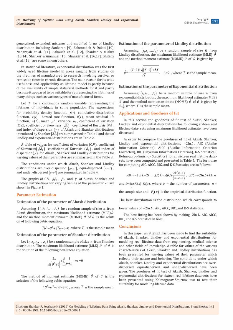
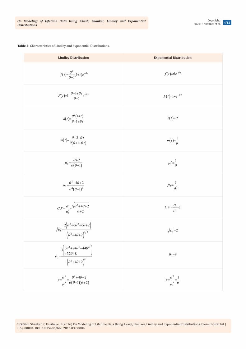
Let T be a continuous random variable representing the lifetimes of individuals in some population The expressions for probability density function, ( )f t , cumulative distribution function, ( )F t , hazard rate function, ( )h t , mean residual life function, ( )m t , mean 1µ ′ , variance 2µ , coefficient of variation (C.V.), coefficient of Skewness ( )1β , coefficient of Kurtosis ( )2β , and index of dispersion ( )γ of Akash and Shanker distributions introduced by Shanker [2,3] are summarized in Table 1 and that of Lindley and exponential distributions are in Table 2.
A table of values for coefficient of variation (C.V.), coefficient of Skewness ( )1β , coefficient of Kurtosis ( )2β , and index of dispersion ( )γ for Akash , Shanker and Lindley distributions for varying values of their parameter are summarized in the Table 3.
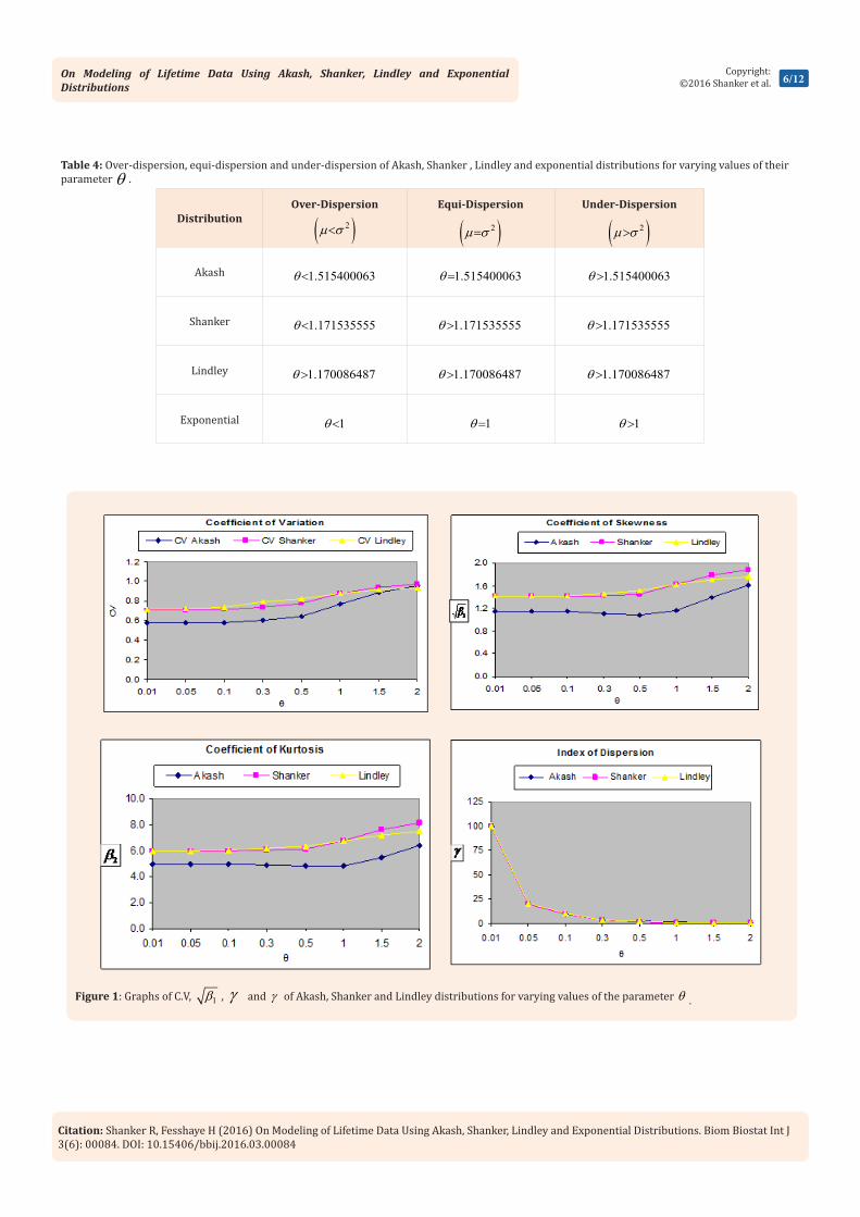
The conditions under which Akash, Shanker and Lindley distributions are over-dispersed ( )2µ σ< , equi-dispersed ( )2µ σ= , and under-dispersed
( )2µ σ> are summarized in Table 4.
The graphs of C.V, 1β , 2β and γ of Akash, Shanker and Lindley distributions for varying values of the parameter θ are shown in Figure 1.
Parameter Estimation
Estimation of the parameter of Akash distribution
Assuming ( )1 2 3, , , ... , nt t t t be a random sample of size n from Akash distribution, the maximum likelihood estimate (MLE) θ̂ and the method moment estimate (MOME) θ of θ is the soluti on of following cubic equation.
3 2 2 6 0t tθ θ θ− + − = , where t is the sample mean
Estimation of the parameter of Shanker distribution
Let ( )1 2 3, , , ... , nt t t t be a random sample of size n from Shanker distribution. The maximum likelihood estimate (MLE) θ̂ of θ is the solution of the following non-linear equation.
( )21
2 1 01
n
ii
n n ttθθ θ =
+ − =∑++
The method of moment estimate (MOME) θ of θ is the solution of the following cubic equation
3 2 2 0t tθ θ θ− + − = , where t is the sample mean.
Estimation of the parameter of Lindley distribution
Assuming ( )1 2, ,...., nt t t be a random sample of size n from Lindley distribution, the maximum likelihood estimate (MLE) θ̂ and the method moment estimate (MOME) θ of θ is given by
( ) ( )21 1 8ˆ ; 02
t t tt
tθ
− − + − += >
, where t is the sample mean.
Estimation of the parameter of Exponential distribution
Assuming ( )1 2, ,...., nt t t be a random sample of size n from exponential distribution, the maximum likelihood estimate (MLE) θ and the method moment estimate (MOME) θ of θ is given by
1ˆt
θ= , where t is the sample mean.
Applications and Goodness of FitIn this section the goodness of fit test of Akash, Shanker,
Lindley and exponential distributions for following sixteen real lifetime data- sets using maximum likelihood estimate have been discussed.
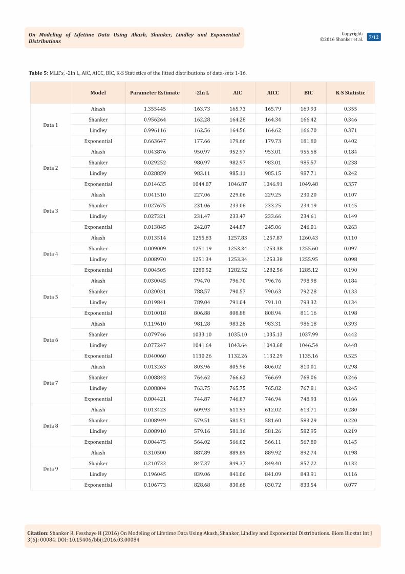
In order to compare the goodness of fit of Akash, Shanker, Lindley and exponential distributions, 2ln L− , AIC (Akaike Information Criterion), AICC (Akaike Information Criterion Corrected), BIC (Bayesian Information Criterion), K-S Statistics ( Kolmogorov-Smirnov Statistics) for all sixteen real lifetime data- sets have been computed and presented in Table 5. The formulae for computing AIC, AICC, BIC, and K-S Statistics are as follows:
2ln 2AIC L k=− + , ( )( )2 1
1k k
AICC AICn k
+= +
− −, 2ln lnBIC L k n=− +
and ( ) ( )Sup 0nx
D F x F x= − , where k = the number of parameters, n =
the sample size and ( )nF x is the empirical distribution function.
The best distribution is the distribution which corresponds to
lower values of 2ln L− , AIC, AICC, BIC, and K-S statistics.
The best fitting has been shown by making -2ln L, AIC, AICC, BIC, and K-S Statistics in bold.
ConclusionsIn this paper an attempt has been made to find the suitability
of Akash, Shanker, Lindley and exponential distributions for modeling real lifetime data from engineering, medical science and other fields of knowledge. A table for values of the various characteristics of Akash, Shanker, and Lindley distributions has been presented for varying values of their parameter which reflects their nature and behavior. The conditions under which Akash, shanker, Lindley and exponential distributions are over-dispersed, equi-dispersed, and under-dispersed have been given. The goodness of fit test of Akash, Shanker, Lindley and exponential distributions for sixteen real lifetime data-sets have been presented using Kolmogorov-Smirnov test to test their suitability for modeling lifetime data.
On Modeling of Lifetime Data Using Akash, Shanker, Lindley and Exponential Distributions
3/12Copyright:
©2016 Shanker et al.
Citation: Shanker R, Fesshaye H (2016) On Modeling of Lifetime Data Using Akash, Shanker, Lindley and Exponential Distributions. Biom Biostat Int J 3(6): 00084. DOI: 10.15406/bbij.2016.03.00084
Table 1: Characteristics of Akash and Shanker Distributions.
Akash Distribution Shanker Distribution
( ) ( )32
21
2tf t t e θθ
θ−= +
+( ) ( )
2
2 1tf t t e θθ θ
θ−= +
+
( ) ( )2
21 1
2tt t
F t e θθ θ
θ− +
= − + +
( )2
1 11
ttF t e θθ
θ−
= − + +
( )( )
( ) ( )3 2
2
1
2 2
th t
t t
θ
θ θ θ
+=
+ + +( ) ( )
( )2
2 1
th t
t
θ θ
θ θ
+=
+ +
( )( )
( ) ( )2 2 2
2
4 6
2 2
t tm t
t t
θ θ θ
θ θ θ θ
+ + +=
+ + +
( ) ( )2
2
2
1
tm tt
θ θ
θ θ θ
+ +=
+ +
( )2
1 2
6
2
θµθ θ
+′=+ ( )
2
1 2
2
1
θµθ θ
+′=+
( )4 2
2 22 2
16 12
2
θ θµθ θ
+ +=
+ ( )4 2
2 22 2
4 2
1
θ θµθ θ
+ +=
+
4 2
21
16 12.6
C V σ θ θ
µ θ
+ += =
′ +
4 2
21
4 2.2
C V σ θ θ
µ θ
+ += =
′ +
( )( )
6 4 2
1 3/24 2
2 30 36 24
16 12
θ θ θβ
θ θ
+ + +=
+ +
( )( )
6 4 2
1 3/24 2
2 6 6 2
4 2
θ θ θβ
θ θ
+ + +=
+ +
( )
8 6 4
2
2 24 2
3 128 4083
576 240
16 12
θ θ θ
θβ
θ θ
+ + + + =
+ +
( )( )
8 6 4 2
2 24 2
3 3 24 44 32 8
4 2
θ θ θ θβ
θ θ
+ + + +=
+ +
( )( )2 4 2
2 21
16 12
2 6
σ θ θγµ θ θ θ
+ += =
′ + + ( )( )2 4 2
2 21
4 2
1 2
σ θ θγµ θ θ θ
+ += =
′ + +
On Modeling of Lifetime Data Using Akash, Shanker, Lindley and Exponential Distributions
4/12Copyright:
©2016 Shanker et al.
Citation: Shanker R, Fesshaye H (2016) On Modeling of Lifetime Data Using Akash, Shanker, Lindley and Exponential Distributions. Biom Biostat Int J 3(6): 00084. DOI: 10.15406/bbij.2016.03.00084
Table 2: Characteristics of Lindley and Exponential Distributions.
Lindley Distribution Exponential Distribution
( ) tf t e θθ −=
( ) 111
ttF t e θθ θθ
−+ += −
+ ( ) 1 tF t e θ−= −
( ) ( )2 11
th t
tθθ θ
+=
+ +( )h t θ=
( ) ( )21
tm tt
θ θθ θ θ
+ +=
+ + ( ) 1m tθ
=
( )121
θµθ θ
+′=+ 1
1µθ
′=
( )
2
2 22
4 2
1
θ θµθ θ
+ +=
+2 2
1µθ
=
2
1
4 2.2
C V σ θ θµ θ
+ += =
′ + 1. 1C V σ
µ= =
′
( )( )
3 2
1 3 22
2 6 6 2
4 2
θ θ θβ
θ θ
+ + +=
+ +1 2β =
( )
4 3 2
2 22
3 24 44332 8
4 2
θ θ θθ
βθ θ
+ + + + =
+ +
2 9β =
( )( )2 2
1
4 21 2
σ θ θγθ θ θµ
+ += =
+ +′
2
1
1σγθµ
= =′
( ) ( )2
11
tf t t e θθθ
−= ++

On Modeling of Lifetime Data Using Akash, Shanker, Lindley and Exponential Distributions
5/12Copyright:
©2016 Shanker et al.
Citation: Shanker R, Fesshaye H (2016) On Modeling of Lifetime Data Using Akash, Shanker, Lindley and Exponential Distributions. Biom Biostat Int J 3(6): 00084. DOI: 10.15406/bbij.2016.03.00084
Table 3: Values of 1 'µ , 1β , CV, 1β , 2β and θ of Akash, Shanker and Lindley distributions for varying values of the parameter θ .
Values of θ for Akash Distribution
0.01 0.05 0.1 0.3 0.5 1 1.5 2
1 'µ 299.990 59.950 29.900 9.713 5.556 2.333 1.294 0.833
2µ 30001.000 1200.996 300.985 34.208 12.691 3.222 1.306 0.639
CV 0.577 0.578 0.580 0.602 0.641 0.769 0.883 0.959
1β 1.155 1.153 1.149 1.115 1.084 1.165 1.388 1.614
2β 5.000 4.997 4.987 4.897 4.785 4.834 5.473 6.391
γ 100.007 20.033 10.066 3.522 2.284 1.381 1.009 0.767
Values of θ for Shanker Distribution
0.01 0.05 0.1 0.3 0.5 1 1.5 2
1 'µ 199.990 39.950 19.901 6.391 3.600 1.500 0.872 0.600
2µ 20000.000 799.998 199.990 22.146 7.840 1.750 0.676 0.340
CV 0.707 0.708 0.711 0.736 0.778 0.882 0.943 0.972
1β 1.414 1.414 1.414 1.421 1.452 1.620 1.779 1.876
2β 6.000 6.000 6.000 6.020 6.121 6.796 7.593 8.159
γ 100.005 20.025 10.049 3.465 2.178 1.167 0.775 0.567
Values of θ for Lindley Distribution
0.01 0.05 0.1 0.3 0.5 1 1.5 2
1 'µ 199.010 39.048 19.091 5.897 3.333 1.500 0.933 0.667
2µ 19999.020 799.093 199.174 21.631 7.556 1.750 0.729 0.389
CV 0.711 0.724 0.739 0.789 0.825 0.882 0.915 0.935
1β 1.414 1.417 1.422 1.464 1.512 1.620 1.699 1.756
2β 6.000 6.007 6.025 6.162 6.343 6.796 7.173 7.469
γ 100.493 20.465 10.433 3.668 2.267 1.167 0.781 0.583
On Modeling of Lifetime Data Using Akash, Shanker, Lindley and Exponential Distributions
6/12Copyright:
©2016 Shanker et al.
Citation: Shanker R, Fesshaye H (2016) On Modeling of Lifetime Data Using Akash, Shanker, Lindley and Exponential Distributions. Biom Biostat Int J 3(6): 00084. DOI: 10.15406/bbij.2016.03.00084
Table 4: Over-dispersion, equi-dispersion and under-dispersion of Akash, Shanker , Lindley and exponential distributions for varying values of their parameter θ .
DistributionOver-Dispersion Equi-Dispersion
( )2µ σ=
Under-Dispersion
( )2µ σ>
Akash 1.515400063θ< 1.515400063θ= 1.515400063θ>
Shanker 1.171535555θ< 1.171535555θ> 1.171535555θ>
Lindley 1.170086487θ> 1.170086487θ> 1.170086487θ>
Exponential 1θ< 1θ= 1θ>
( )2µ σ<
Figure 1: Graphs of C.V, 1β , γ and γ of Akash, Shanker and Lindley distributions for varying values of the parameter θ .
On Modeling of Lifetime Data Using Akash, Shanker, Lindley and Exponential Distributions
7/12Copyright:
©2016 Shanker et al.
Citation: Shanker R, Fesshaye H (2016) On Modeling of Lifetime Data Using Akash, Shanker, Lindley and Exponential Distributions. Biom Biostat Int J 3(6): 00084. DOI: 10.15406/bbij.2016.03.00084
Table 5: MLE’s, -2ln L, AIC, AICC, BIC, K-S Statistics of the fitted distributions of data-sets 1-16.
Model Parameter Estimate -2ln L AIC AICC BIC K-S Statistic
Data 1
Akash 1.355445 163.73 165.73 165.79 169.93 0.355
Shanker 0.956264 162.28 164.28 164.34 166.42 0.346
Lindley 0.996116 162.56 164.56 164.62 166.70 0.371
Exponential 0.663647 177.66 179.66 179.73 181.80 0.402
Data 2
Akash 0.043876 950.97 952.97 953.01 955.58 0.184
Shanker 0.029252 980.97 982.97 983.01 985.57 0.238
Lindley 0.028859 983.11 985.11 985.15 987.71 0.242
Exponential 0.014635 1044.87 1046.87 1046.91 1049.48 0.357
Data 3
Akash 0.041510 227.06 229.06 229.25 230.20 0.107
Shanker 0.027675 231.06 233.06 233.25 234.19 0.145
Lindley 0.027321 231.47 233.47 233.66 234.61 0.149
Exponential 0.013845 242.87 244.87 245.06 246.01 0.263
Data 4
Akash 0.013514 1255.83 1257.83 1257.87 1260.43 0.110
Shanker 0.009009 1251.19 1253.34 1253.38 1255.60 0.097
Lindley 0.008970 1251.34 1253.34 1253.38 1255.95 0.098
Exponential 0.004505 1280.52 1282.52 1282.56 1285.12 0.190
Data 5
Akash 0.030045 794.70 796.70 796.76 798.98 0.184
Shanker 0.020031 788.57 790.57 790.63 792.28 0.133
Lindley 0.019841 789.04 791.04 791.10 793.32 0.134
Exponential 0.010018 806.88 808.88 808.94 811.16 0.198
Data 6
Akash 0.119610 981.28 983.28 983.31 986.18 0.393
Shanker 0.079746 1033.10 1035.10 1035.13 1037.99 0.442
Lindley 0.077247 1041.64 1043.64 1043.68 1046.54 0.448
Exponential 0.040060 1130.26 1132.26 1132.29 1135.16 0.525
Data 7
Akash 0.013263 803.96 805.96 806.02 810.01 0.298
Shanker 0.008843 764.62 766.62 766.69 768.06 0.246
Lindley 0.008804 763.75 765.75 765.82 767.81 0.245
Exponential 0.004421 744.87 746.87 746.94 748.93 0.166
Data 8
Akash 0.013423 609.93 611.93 612.02 613.71 0.280
Shanker 0.008949 579.51 581.51 581.60 583.29 0.220
Lindley 0.008910 579.16 581.16 581.26 582.95 0.219
Exponential 0.004475 564.02 566.02 566.11 567.80 0.145
Data 9
Akash 0.310500 887.89 889.89 889.92 892.74 0.198
Shanker 0.210732 847.37 849.37 849.40 852.22 0.132
Lindley 0.196045 839.06 841.06 841.09 843.91 0.116
Exponential 0.106773 828.68 830.68 830.72 833.54 0.077

On Modeling of Lifetime Data Using Akash, Shanker, Lindley and Exponential Distributions
8/12Copyright:
©2016 Shanker et al.
Citation: Shanker R, Fesshaye H (2016) On Modeling of Lifetime Data Using Akash, Shanker, Lindley and Exponential Distributions. Biom Biostat Int J 3(6): 00084. DOI: 10.15406/bbij.2016.03.00084
Data 10
Akash 0.050293 354.88 356.88 357.02 358.28 0.421
Shanker 0.033569 325.74 327.74 327.88 329.14 0.351
Lindley 0.033021 323.27 325.27 325.42 326.67 0.345
Exponential 0.016779 305.26 307.26 307.40 308.66 0.213
Data 11
Akash 1.165719 115.15 117.15 117.28 118.68 0.156
Shanker 0.853374 112.91 114.91 115.03 116.44 0.131
Lindley 0.823821 112.61 114.61 114.73 116.13 0.133
Exponential 0.532081 110.91 112.91 113.03 114.43 0.089
Data 12
Akash 0.295277 641.93 643.93 643.95 646.51 0.100
Shanker 0.198317 635.26 637.26 637.30 639.86 0.042
Lindley 0.186571 638.07 640.07 640.12 642.68 0.058
Exponential 0.101245 658.04 660.04 660.08 662.65 0.163
Data 13
Akash 0.024734 194.30 196.30 196.61 197.01 0.456
Shanker 0.016492 181.58 183.58 183.89 184.29 0.388
Lindley 0.016360 181.34 183.34 183.65 184.05 0.386
Exponential 0.008246 173.94 175.94 176.25 176.65 0.277
Data 14
Akash 1.156923 59.52 61.52 61.74 62.51 0.320
Shanker 0.803867 59.78 61.78 61.22 62.77 0.325
Lindley 0.816118 60.50 62.50 62.72 63.49 0.341
Exponential 0.526316 65.67 67.67 67.90 68.67 0.389
Data 15
Akash 0.097062 240.68 242.68 242.82 244.11 0.266
Shanker 0.064712 252.35 254.35 254.49 255.78 0.326
Lindley 0.062988 253.99 255.99 256.13 257.42 0.333
Exponential 0.032455 274.53 276.53 276.67 277.96 0.426
Data 16
Akash 0.964726 224.28 226.28 226.34 228.51 0.348
Shanker 0.658029 233.01 235.01 235.06 237.24 0.355
Lindley 0.659000 238.38 240.38 240.44 242.61 0.390
Exponential 0.407941 261.74 263.74 263.80 265.97 0.434
Data Set 1: The data set represents the strength of 1.5cm glass fibers measured at the National Physical Laboratory, England. Unfortunately, the units of measurements are not given in the paper, and they are taken from Smith & Naylor [19].
0.55 0.93 1.25 1.36 1.49 1.52 1.58 1.61 1.64 1.68 1.73 1.81 2.00
0.74 1.04 1.27 1.39 1.49 1.53 1.59 1.61 1.66 1.68 1.76 1.82 2.01
0.77 1.11 1.28 1.42 1.50 1.54 1.60 1.62 1.66 1.69 1.76 1.84 2.24
0.81 1.13 1.29 1.48 1.50 1.55 1.61 1.62 1.66 1.70 1.77 1.84 0.84
1.24 1.30 1.48 1.51 1.55 1.61 1.63 1.67 1.70 1.78 1.89
On Modeling of Lifetime Data Using Akash, Shanker, Lindley and Exponential Distributions
9/12Copyright:
©2016 Shanker et al.
Citation: Shanker R, Fesshaye H (2016) On Modeling of Lifetime Data Using Akash, Shanker, Lindley and Exponential Distributions. Biom Biostat Int J 3(6): 00084. DOI: 10.15406/bbij.2016.03.00084
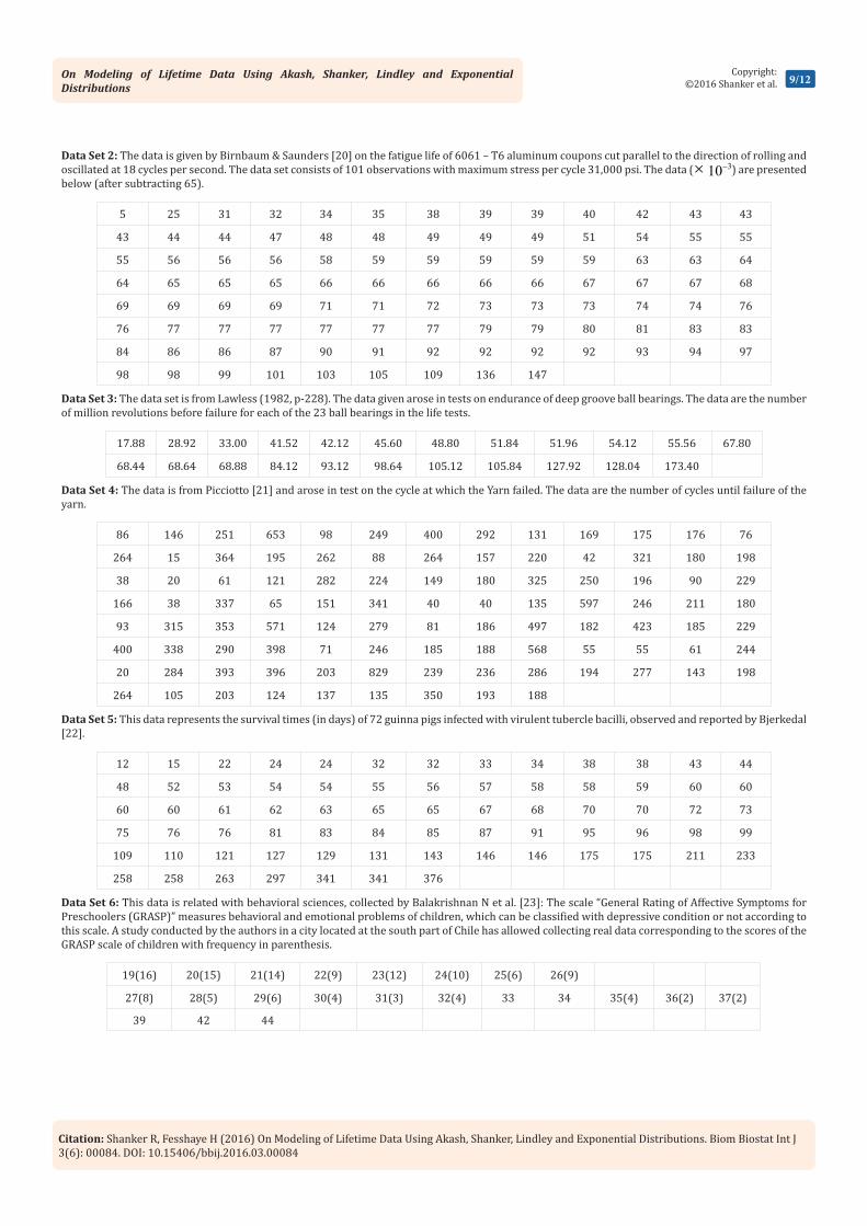
Data Set 2: The data is given by Birnbaum & Saunders [20] on the fatigue life of 6061 – T6 aluminum coupons cut parallel to the direction of rolling and oscillated at 18 cycles per second. The data set consists of 101 observations with maximum stress per cycle 31,000 psi. The data (× 310− ) are presented below (after subtracting 65).
5 25 31 32 34 35 38 39 39 40 42 43 43
43 44 44 47 48 48 49 49 49 51 54 55 55
55 56 56 56 58 59 59 59 59 59 63 63 64
64 65 65 65 66 66 66 66 66 67 67 67 68
69 69 69 69 71 71 72 73 73 73 74 74 76
76 77 77 77 77 77 77 79 79 80 81 83 83
84 86 86 87 90 91 92 92 92 92 93 94 97
98 98 99 101 103 105 109 136 147
Data Set 3: The data set is from Lawless (1982, p-228). The data given arose in tests on endurance of deep groove ball bearings. The data are the number of million revolutions before failure for each of the 23 ball bearings in the life tests.
17.88 28.92 33.00 41.52 42.12 45.60 48.80 51.84 51.96 54.12 55.56 67.80
68.44 68.64 68.88 84.12 93.12 98.64 105.12 105.84 127.92 128.04 173.40
Data Set 4: The data is from Picciotto [21] and arose in test on the cycle at which the Yarn failed. The data are the number of cycles until failure of the yarn.
86 146 251 653 98 249 400 292 131 169 175 176 76
264 15 364 195 262 88 264 157 220 42 321 180 198
38 20 61 121 282 224 149 180 325 250 196 90 229
166 38 337 65 151 341 40 40 135 597 246 211 180
93 315 353 571 124 279 81 186 497 182 423 185 229
400 338 290 398 71 246 185 188 568 55 55 61 244
20 284 393 396 203 829 239 236 286 194 277 143 198
264 105 203 124 137 135 350 193 188
Data Set 5: This data represents the survival times (in days) of 72 guinna pigs infected with virulent tubercle bacilli, observed and reported by Bjerkedal [22].
12 15 22 24 24 32 32 33 34 38 38 43 44
48 52 53 54 54 55 56 57 58 58 59 60 60
60 60 61 62 63 65 65 67 68 70 70 72 73
75 76 76 81 83 84 85 87 91 95 96 98 99
109 110 121 127 129 131 143 146 146 175 175 211 233
258 258 263 297 341 341 376
Data Set 6: This data is related with behavioral sciences, collected by Balakrishnan N et al. [23]: The scale “General Rating of Affective Symptoms for Preschoolers (GRASP)” measures behavioral and emotional problems of children, which can be classified with depressive condition or not according to this scale. A study conducted by the authors in a city located at the south part of Chile has allowed collecting real data corresponding to the scores of the GRASP scale of children with frequency in parenthesis.
19(16) 20(15) 21(14) 22(9) 23(12) 24(10) 25(6) 26(9)
27(8) 28(5) 29(6) 30(4) 31(3) 32(4) 33 34 35(4) 36(2) 37(2)
39 42 44
On Modeling of Lifetime Data Using Akash, Shanker, Lindley and Exponential Distributions
10/12Copyright:
©2016 Shanker et al.
Citation: Shanker R, Fesshaye H (2016) On Modeling of Lifetime Data Using Akash, Shanker, Lindley and Exponential Distributions. Biom Biostat Int J 3(6): 00084. DOI: 10.15406/bbij.2016.03.00084
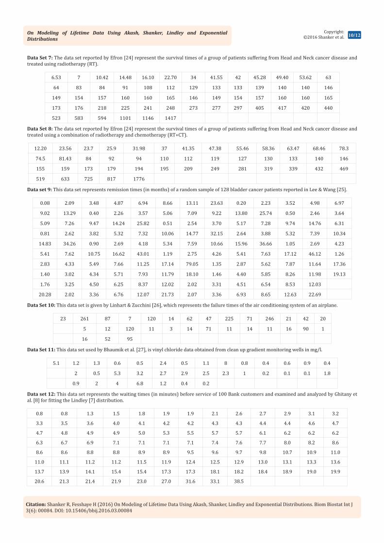
Data Set 7: The data set reported by Efron [24] represent the survival times of a group of patients suffering from Head and Neck cancer disease and treated using radiotherapy (RT).
6.53 7 10.42 14.48 16.10 22.70 34 41.55 42 45.28 49.40 53.62 63
64 83 84 91 108 112 129 133 133 139 140 140 146
149 154 157 160 160 165 146 149 154 157 160 160 165
173 176 218 225 241 248 273 277 297 405 417 420 440
523 583 594 1101 1146 1417
Data Set 8: The data set reported by Efron [24] represent the survival times of a group of patients suffering from Head and Neck cancer disease and treated using a combination of radiotherapy and chemotherapy (RT+CT).
12.20 23.56 23.7 25.9 31.98 37 41.35 47.38 55.46 58.36 63.47 68.46 78.3
74.5 81.43 84 92 94 110 112 119 127 130 133 140 146
155 159 173 179 194 195 209 249 281 319 339 432 469
519 633 725 817 1776
Data set 9: This data set represents remission times (in months) of a random sample of 128 bladder cancer patients reported in Lee & Wang [25].
0.08 2.09 3.48 4.87 6.94 8.66 13.11 23.63 0.20 2.23 3.52 4.98 6.97
9.02 13.29 0.40 2.26 3.57 5.06 7.09 9.22 13.80 25.74 0.50 2.46 3.64
5.09 7.26 9.47 14.24 25.82 0.51 2.54 3.70 5.17 7.28 9.74 14.76 6.31
0.81 2.62 3.82 5.32 7.32 10.06 14.77 32.15 2.64 3.88 5.32 7.39 10.34
14.83 34.26 0.90 2.69 4.18 5.34 7.59 10.66 15.96 36.66 1.05 2.69 4.23
5.41 7.62 10.75 16.62 43.01 1.19 2.75 4.26 5.41 7.63 17.12 46.12 1.26
2.83 4.33 5.49 7.66 11.25 17.14 79.05 1.35 2.87 5.62 7.87 11.64 17.36
1.40 3.02 4.34 5.71 7.93 11.79 18.10 1.46 4.40 5.85 8.26 11.98 19.13
1.76 3.25 4.50 6.25 8.37 12.02 2.02 3.31 4.51 6.54 8.53 12.03
20.28 2.02 3.36 6.76 12.07 21.73 2.07 3.36 6.93 8.65 12.63 22.69
Data Set 10: This data set is given by Linhart & Zucchini [26], which represents the failure times of the air conditioning system of an airplane.
23 261 87 7 120 14 62 47 225 71 246 21 42 20
5 12 120 11 3 14 71 11 14 11 16 90 1
16 52 95
Data Set 11: This data set used by Bhaumik et al. [27], is vinyl chloride data obtained from clean up gradient monitoring wells in mg/l.
5.1 1.2 1.3 0.6 0.5 2.4 0.5 1.1 8 0.8 0.4 0.6 0.9 0.4
2 0.5 5.3 3.2 2.7 2.9 2.5 2.3 1 0.2 0.1 0.1 1.8
0.9 2 4 6.8 1.2 0.4 0.2
Data set 12: This data set represents the waiting times (in minutes) before service of 100 Bank customers and examined and analyzed by Ghitany et al. [8] for fitting the Lindley [7] distribution.
0.8 0.8 1.3 1.5 1.8 1.9 1.9 2.1 2.6 2.7 2.9 3.1 3.2
3.3 3.5 3.6 4.0 4.1 4.2 4.2 4.3 4.3 4.4 4.4 4.6 4.7
4.7 4.8 4.9 4.9 5.0 5.3 5.5 5.7 5.7 6.1 6.2 6.2 6.2
6.3 6.7 6.9 7.1 7.1 7.1 7.1 7.4 7.6 7.7 8.0 8.2 8.6
8.6 8.6 8.8 8.8 8.9 8.9 9.5 9.6 9.7 9.8 10.7 10.9 11.0
11.0 11.1 11.2 11.2 11.5 11.9 12.4 12.5 12.9 13.0 13.1 13.3 13.6
13.7 13.9 14.1 15.4 15.4 17.3 17.3 18.1 18.2 18.4 18.9 19.0 19.9
20.6 21.3 21.4 21.9 23.0 27.0 31.6 33.1 38.5

On Modeling of Lifetime Data Using Akash, Shanker, Lindley and Exponential Distributions
11/12Copyright:
©2016 Shanker et al.
Citation: Shanker R, Fesshaye H (2016) On Modeling of Lifetime Data Using Akash, Shanker, Lindley and Exponential Distributions. Biom Biostat Int J 3(6): 00084. DOI: 10.15406/bbij.2016.03.00084
Data Set 13: This data is for the times between successive failures of air conditioning equipment in a Boeing 720 airplane, Proschan [28].
74 57 48 29 502 12 70 21 29 386 59 27 153 26
326
Data set 14: This data set represents the lifetime’s data relating to relief times (in minutes) of 20 patients receiving an analgesic and reported by Gross & Clark [29].
1.1 1.4 1.3 1.7 1.9 1.8 1.6 2.2 1.7 2.7 4.1 1.8 1.5 1.2
1.4 3 1.7 2.3 1.6 2
Data Set 15: This data set is the strength data of glass of the aircraft window reported by Fuller et al. [30].
18.83 20.8 21.657 23.03 23.23 24.05 24.321 25.5 25.52 25.8 26.69 26.77 26.78
27.05 27.67 29.9 31.11 33.2 33.73 33.76 33.89 34.76 35.75 35.91 36.98 37.08
37.09 39.58 44.045 45.29 45.381
Data Set 16: The following data represent the tensile strength, measured in GPa, of 69 carbon fibers tested under tension at gauge lengths of 20mm Bader & Priest [31,32].
1.312 1.314 1.479 1.552 1.700 1.803 1.861 1.865 1.944 1.958 1.966 1.997 2.006
2.021 2.027 2.055 2.063 2.098 2.140 2.179 2.224 2.240 2.253 2.270 2.272 2.274
2.301 2.301 2.359 2.382 2.382 2.426 2.434 2.435 2.478 2.490 2.511 2.514 2.535
2.554 2.566 2.570 2.586 2.629 2.633 2.642 2.648 2.684 2.697 2.726 2.770 2.773
2.800 2.809 2.818 2.821 2.848 2.880 2.954 3.012 3.067 3.084 3.090 3.096 3.128
3.233 3.433 3.585 3.858
AcknowledgementNone.
Conflict of Interest
None.
References1. Shanker R, Hagos F, Sujatha S (2015 a) On modeling of Lifetimes
data using exponential and Lindley distributions. Biometrics & Biostatistics International Journal 2(5): 1-9.
2. Shanker R (2015 a) Akash distribution and Its Applications. International Journal of Probability and Statistics 4(3): 65-75.
3. Shanker R (2015 b) Shanker distribution and Its Applications. International Journal of Statistics and Applications 5(6): 338-348.
4. Shanker R, Hagos F, Sujatha S (2015 b) On modeling of Lifetimes data using one parameter Akash, Lindley and exponential distributions. Biometrics & Biostatistics International Journal 3(2): 1-10.
5. Shanker R (2016 a) The discrete Poisson-Akash distribution. Communicated.
6. Shanker R (2016 b) The discrete Poisson-Shanker distribution. Communicated.
7. Lindley DV (1958) Fiducial distributions and Bayes’ Theorem. Journal of the Royal Statistical Society 20(1): 102-107.
8. Ghitany ME, Atieh B, Nadarajah S (2008) Lindley distribution and its Applications. Mathematics Computing and Simulation 78: 493-506.
9. Sankaran M (1970) The discrete Poisson-Lindley distribution. Biometrics 26(1): 145-149.
10. Zakerzadeh H, Dolati A (2009) Generalized Lindley distribution. Journal of Mathematical extension 3(2): 13-25.
11. Nadarajah S, Bakouch HS, Tahmasbi R (2011) A generalized Lindley distribution. The Indian Journal of Statistics 73(2): 331-359.
12. Bakouch SH, Al-Zahrani BM, Al-Shomrani AA, Marchi VAA, Louzada F (2012) An extended Lindley distribution. Journal of Korean Statistical Society 41(1): 75-85.
13. Shanker R, Mishra A (2013 a) A quasi Lindley distribution. African journal of Mathematics and Computer Science Research 6 (4): 64 -71.
14. Shanker R, Mishra A (2013 b) A two-parameter Lindley distribution. Statistics in transition new series 14(1): 45-56.
15. Shanker R, Amanuel AG (2013) A new quasi Lindley distribution. International Journal of Statistics and systems 9(1): 87-94.
16. Shanker R, Sharma S, Shanker R (2013) A two-parameter Lindley distribution for modeling waiting and survival times data. Applied Mathematics 4: 363-368.
17. Shanker R, Hagos F, Sharma S (2015 c) On Two Parameter Lindley distribution and Its Applications to model lifetime data. Biometrics & Biostatistics International Journal 3(1): 1-8.
18. Ghitany M, Al-Mutairi D, Balakrishnan N, Al-Enezi I (2013) Power Lindley distribution and associated inference. Computational Statistics and Data Analysis 64: 20-33.

On Modeling of Lifetime Data Using Akash, Shanker, Lindley and Exponential Distributions
12/12Copyright:
©2016 Shanker et al.
Citation: Shanker R, Fesshaye H (2016) On Modeling of Lifetime Data Using Akash, Shanker, Lindley and Exponential Distributions. Biom Biostat Int J 3(6): 00084. DOI: 10.15406/bbij.2016.03.00084
19. Smith RL, Naylor JC (1987) A comparison of Maximum likelihood and Bayesian estimators for the three parameter Weibull distribution. Applied Statistics 36(3): 358-369.
20. Birnbaum ZW, Saunders SC (1969) Estimation for a family of life distributions with applications to fatigue. Journal of Applied Probability 6(2): 328-347.
21. Picciotto R (1970) Tensile fatigue characteristics of a sized polyester/viscose yarn and their effect on weaving performance, Master thesis, North Carolina State, University of Raleigh, USA.
22. Bjerkedal T (1960) Acquisition of resistance in guinea pigs infected with different doses of virulent tubercle bacilli. Am J Hyg 72(1): 130-148.
23. Balakrishnan N, Victor L, Antonio S (2010) A mixture model based on Birnhaum-Saunders Distributions, A study conducted by Authors regarding the Scores of the GRASP (General Rating of Affective Symptoms for Preschoolers), in a city located at South Part of the Chile.
24. Efron B (1988) Logistic regression, survival analysis and the Kaplan-Meier curve. Journal of the American Statistical Association 83(402): 414-425.
25. Lee ET, Wang JW (2003) Statistical methods for survival data analysis, 3rd edition, John Wiley and Sons, New York, USA.
26. Linhart H, Zucchini W (1986) Model Selection. John Wiley, New York, USA.
27. Bhaumik DK, Kapur K, Gibbons RD (2009) Testing Parameters of a Gamma Distribution for Small Samples. Technometrics 51(3): 326-334.
28. Proschan F (1963) Theoretical explanation of observed decreasing failure rate. Technometrics 5(3): 375-383.
29. Gross AJ, Clark VA (1975) Survival Distributions: Reliability Applications in the Biometrical Sciences, John Wiley, New York, USA.
30. Fuller EJ, Frieman S, Quinn J, Quinn G, Carter W (1994) Fracture mechanics approach to the design of glass aircraft windows: A case study. SPIE Proc 2286, 419-430.
31. Lawless JF (1982) Statistical models and methods for lifetime data, John Wiley and Sons, New York, USA.
32. Bader MG, Priest AM (1982) Statistical aspects of fiber and bundle strength in hybrid composites. In: Hayashi T, et al. (Eds.), Progress in Science in Engineering Composites. ICCM-IV, Tokyo, pp. 1129-1136.
Related Documents


![Index [link.springer.com]978-0-387-85536-3/1.pdfIndex A Accelerated testing and statistical lifetime modeling lifetime tests ... polymer electrolyte membrane (PEM), 236 postmortem](https://static.cupdf.com/doc/110x72/5e3304b240fda46b7d421821/index-link-978-0-387-85536-31pdf-index-a-accelerated-testing-and-statistical.jpg)