ON IMPLEMENTING TIME-FREQUENCY REPRESENTATIONS ON HARDWARE/SOFTWARE COMPUTATIONAL STRUCTURES FOR SAR APPLICATIONS By Ana Beatriz Ramirez Silva A thesis submitted in partial fulfillment of the requirements for the degree of MASTER OF SCIENCE in ELECTRICAL ENGINEERING UNIVERSITY OF PUERTO RICO MAYAG ¨ UEZ CAMPUS June, 2006 Approved by: Hamed Parsiani, Ph.D Date Member, Graduate Committee Rogelio Palomera, Ph.D Date Member, Graduate Committee Domingo Rodriguez, Ph.D Date President, Graduate Committee Edgardo Lorenzo, Ph.D Date Representative of Graduate Studies Isidoro Couvertier, Ph.D Date Chairperson of the Department

Welcome message from author
This document is posted to help you gain knowledge. Please leave a comment to let me know what you think about it! Share it to your friends and learn new things together.
Transcript
ON IMPLEMENTING TIME-FREQUENCY REPRESENTATIONSON HARDWARE/SOFTWARE COMPUTATIONAL STRUCTURES
FOR SAR APPLICATIONS
By
Ana Beatriz Ramirez Silva
A thesis submitted in partial fulfillment of the requirements for the degree of
MASTER OF SCIENCE
in
ELECTRICAL ENGINEERING
UNIVERSITY OF PUERTO RICOMAYAGUEZ CAMPUS
June, 2006
Approved by:
Hamed Parsiani, Ph.D DateMember, Graduate Committee
Rogelio Palomera, Ph.D DateMember, Graduate Committee
Domingo Rodriguez, Ph.D DatePresident, Graduate Committee
Edgardo Lorenzo, Ph.D DateRepresentative of Graduate Studies
Isidoro Couvertier, Ph.D DateChairperson of the Department

Abstract of Dissertation Presented to the Graduate Schoolof the University of Puerto Rico in Partial Fulfillment of the
Requirements for the Degree of Master of Science
ON IMPLEMENTING TIME-FREQUENCY REPRESENTATIONSON HARDWARE/SOFTWARE COMPUTATIONAL STRUCTURES
FOR SAR APPLICATIONS
By
Ana Beatriz Ramirez Silva
June 2006
Chair: PhD. Domingo RodriguezMajor Department: Electrical and Computer Engineering
Synthetic Aperture Radar (SAR) applications require that imaging systems
be able to gather and process appropriate environmental information to aid in the
process of effective decision making. This is the one major reason for the imple-
mentation of new modeling and simulation techniques for the prototyping of such
systems. For the design of radar systems, advanced electronic devices have been
developed to make more efficient implementations of image processing algorithms,
and we can use hardware-in-the-loop technique as a methodology for real systems
simulation.
This work presents developments of theoretical frameworks for the modeling
of SAR raw data through the efficient computation of the point surface response
function and multidimensional cyclic convolution operations used in SAR imaging
processing and experimental hardware/software implementations of imaging algo-
rithms using recent technology in floating point digital signal processors.
ii
Resumen de Disertacion Presentado a Escuela Graduadade la Universidad de Puerto Rico como requisito parcial de los
Requerimientos para el grado de Maestrıa en Ciencias
IMPLEMENTACION DE REPRESENTACIONESTIEMPO-FRECUENCIA SOBRE ESTRUCTURAS
COMPUTACIONALES HARDWARE/SOFTWARE PARAAPLICACIONES SAR
Por
Ana Beatriz Ramirez Silva
Junio 2006
Consejero: PhD. Domingo RodriguezDepartamento: Ingenierıa Electrica y de Computadoras
En aplicaciones de Radares de Abertura Sintetica se requiere que los sistemas
usados en la formacion de las imagenes tomen la informacion proveniente del medio
y la procesen de forma adecuada para permitir una correcta toma de decisiones en
base a la informacion procesada. Esta es una de las razones principales para la
implementacion de modelos y tecnicas de simulacion para el prototipado de esos
sistemas. Para el diseno de sistemas de radares se han desarrollado dispositivos
electronicos mas avanzados que han permitido desarrollar implementaciones mas
eficientes de algoritmos de procesamiento de imagenes y en este trabajo se hace uso
de la tecnica de “Hardware-in-the-Loop”como una metodologıa para la simulacion
de sistemas reales. Este trabajo presenta marcos teoricos para el modelamiento de
los datos crudos de SAR a traves del computo de la funcion de la respuesta al impulso
del systema y las operaciones de la convolucion cıclica usadas en el procesamiento
de imagenes SAR ası como implementaciones experimentales hardware/software de
los algoritmos de formacion de imagenes.
iii

Copyright c© 2006
by
Ana Beatriz Ramirez Silva

To my Family...

ACKNOWLEDGMENTS
I want to give my gratitude to my advisor Dr. Domingo Rodriguez because
of his guidance and support to my master work. I am very fortunate of having a
great advisor and a friend. Also, I would like to thank to my graduate committee
formed by Dr. Hamed Parsiani, Dr. Rogelio Palomera and Dr. Edgardo Lorenzo
for their contributions and corrections to my work and I would like to thank to
the Automated Information Processing (AIP) group for being collaborators of my
project.
I have special gratitude to Ivan J. Rivera and to my friends because of their
support which encouraged me during these two years.
This work was supported by National Science Foundation (NSF) under CISE CNS
grant No. 0424546.
vi

TABLE OF CONTENTSpage
ABSTRACT ENGLISH . . . . . . . . . . . . . . . . . . . . . . . . . . . . . . ii
ABSTRACT SPANISH . . . . . . . . . . . . . . . . . . . . . . . . . . . . . . iii
ACKNOWLEDGMENTS . . . . . . . . . . . . . . . . . . . . . . . . . . . . . vi
LIST OF TABLES . . . . . . . . . . . . . . . . . . . . . . . . . . . . . . . . . ix
LIST OF FIGURES . . . . . . . . . . . . . . . . . . . . . . . . . . . . . . . . x
LIST OF ABBREVIATIONS . . . . . . . . . . . . . . . . . . . . . . . . . . . xiv
LIST OF SYMBOLS . . . . . . . . . . . . . . . . . . . . . . . . . . . . . . . . xvi
1 INTRODUCTION . . . . . . . . . . . . . . . . . . . . . . . . . . . . . . 1
1.1 Previous Work . . . . . . . . . . . . . . . . . . . . . . . . . . . . . 21.1.1 Agencies and Companies Working in SAR . . . . . . . . . . 5
1.2 Justification . . . . . . . . . . . . . . . . . . . . . . . . . . . . . . 71.2.1 Environmental Monitoring . . . . . . . . . . . . . . . . . . 71.2.2 Target Detection . . . . . . . . . . . . . . . . . . . . . . . . 71.2.3 High Power Line Monitoring . . . . . . . . . . . . . . . . . 8
1.3 Thesis Objectives . . . . . . . . . . . . . . . . . . . . . . . . . . . 91.4 Research Methodology . . . . . . . . . . . . . . . . . . . . . . . . 101.5 Original Contributions . . . . . . . . . . . . . . . . . . . . . . . . 11
2 DIGITAL SIGNAL PROCESSING: CONCEPTS . . . . . . . . . . . . . 12
2.1 Concepts. . . . . . . . . . . . . . . . . . . . . . . . . . . . . . . . 122.1.1 Basic Definitions . . . . . . . . . . . . . . . . . . . . . . . . 122.1.2 Digital Signal Tools: Operators . . . . . . . . . . . . . . . . 142.1.3 Description and Representation of Some Signals . . . . . . 182.1.4 Other Signal Processing Fundamentals . . . . . . . . . . . 20
2.2 Algorithms for Time-frequency Representations . . . . . . . . . . 22
3 SAR SIGNAL PROCESSING FUNDAMENTALS . . . . . . . . . . . . . 28
3.1 SAR Concepts . . . . . . . . . . . . . . . . . . . . . . . . . . . . . 283.1.1 Range Resolution . . . . . . . . . . . . . . . . . . . . . . . 293.1.2 Azimuth Resolution . . . . . . . . . . . . . . . . . . . . . . 30
3.2 SAR System Description . . . . . . . . . . . . . . . . . . . . . . . 33
vii

3.2.1 Fundamentals of Active Imaging . . . . . . . . . . . . . . . 333.2.2 One Dimensional SAR Model for Image Formation . . . . . 373.2.3 Two Dimensional SAR Model . . . . . . . . . . . . . . . . 383.2.4 Raw Data Storage . . . . . . . . . . . . . . . . . . . . . . . 42
3.3 Adaptive Imaging System . . . . . . . . . . . . . . . . . . . . . . 433.3.1 Newton Adaptive Filter Description . . . . . . . . . . . . . 44
4 HARDWARE/SOFTWARE COMPUTATIONAL STRUCTURES . . . . 47
4.1 Hardware and Software Characteristics . . . . . . . . . . . . . . . 474.2 Hardware/Software Co-Design Description . . . . . . . . . . . . . 49
4.2.1 Hardware-In-The-Loop Modeling and Simulation . . . . . . 504.3 Hardware-in-the-Loop System Result . . . . . . . . . . . . . . . . 52
4.3.1 DSP Processor Option . . . . . . . . . . . . . . . . . . . . 524.3.2 Considerations for Hardware-in-the-Loop Process . . . . . . 56
5 HARDWARE/SOFTWARE IMPLEMENTATION RESULTS . . . . . . 57
5.1 Hardware Results . . . . . . . . . . . . . . . . . . . . . . . . . . . 575.1.1 Ambiguity Function Computation Results Using DSP Proces-
sors . . . . . . . . . . . . . . . . . . . . . . . . . . . . . . 575.1.2 Fast Fourier Transforms Using DSP Processors: One and
Two Dimensions . . . . . . . . . . . . . . . . . . . . . . . 595.1.3 Some Results of the Two Dimensional Cyclic Convolution . 63
5.2 Software Results . . . . . . . . . . . . . . . . . . . . . . . . . . . . 645.2.1 Synthesis Image Formation Using One Dimensional Method 645.2.2 Computational SAR Signal Processing Environment . . . . 67
6 CONCLUSIONS AND FUTURE WORKS . . . . . . . . . . . . . . . . . 77
6.1 Conclusions . . . . . . . . . . . . . . . . . . . . . . . . . . . . . . 776.2 Future Works . . . . . . . . . . . . . . . . . . . . . . . . . . . . . 78
APPENDICES . . . . . . . . . . . . . . . . . . . . . . . . . . . . . . . . . . . 84
A RADARSAT CEOS FORMAT . . . . . . . . . . . . . . . . . . . . . . . 85
B EXTRACTING RAW DATA AND GENERATING IMAGES . . . . . . 89
C SAR IMAGE FORMATION USER’S GUIDE - HARDWARE/SOFTWAREIMPLEMENTATION . . . . . . . . . . . . . . . . . . . . . . . . . . . 94
viii

LIST OF TABLESTable page
5–1 Benchmark Computational Operation for the Ambiguity Function . . 58
5–2 Benchmark Computational Operation for the One Dimensional FFT . 60
5–3 Benchmark Computational Operation for the Two Dimensional FFTin Core . . . . . . . . . . . . . . . . . . . . . . . . . . . . . . . . . . 61
5–4 Benchmark Computational Operation for the Two Dimensional FFTout Core . . . . . . . . . . . . . . . . . . . . . . . . . . . . . . . . . 61
5–5 Benchmark Computational Operation for the Two Dimensional CyclicConvolution in a DSP . . . . . . . . . . . . . . . . . . . . . . . . . . 64
ix

LIST OF FIGURESFigure page
1–1 Power Line Monitoring. . . . . . . . . . . . . . . . . . . . . . . . . . . 9
2–1 Impulse Response of a Two-Dimensional System. . . . . . . . . . . . 20
2–2 Cyclic Convolution by Indirect Method. . . . . . . . . . . . . . . . . . 21
2–3 Matrix Transposition Representation. . . . . . . . . . . . . . . . . . . 21
2–4 Ambiguity Function Using Filter Method. . . . . . . . . . . . . . . . 25
2–5 Ambiguity Function Using Transform Method. . . . . . . . . . . . . . 26
2–6 Ambiguity Function Example. . . . . . . . . . . . . . . . . . . . . . . 27
2–7 Ambiguity Function Example. . . . . . . . . . . . . . . . . . . . . . . 27
3–1 RADARSAT Modes of SAR Operation. . . . . . . . . . . . . . . . . . 29
3–2 SAR Geometry. . . . . . . . . . . . . . . . . . . . . . . . . . . . . . . 29
3–3 Range Resolution. . . . . . . . . . . . . . . . . . . . . . . . . . . . . . 30
3–4 Doppler Variation Computation. . . . . . . . . . . . . . . . . . . . . . 31
3–5 Azimuth Geometry. . . . . . . . . . . . . . . . . . . . . . . . . . . . . 32
3–6 Azimuth Geometry. . . . . . . . . . . . . . . . . . . . . . . . . . . . . 32
3–7 Mapping From the Object Space to the Image Space. . . . . . . . . . 35
3–8 Functional Block Diagram for Image Formation Using one Dimen-sional Signal Processing. . . . . . . . . . . . . . . . . . . . . . . . . 38
3–9 Example of the Transmit and Receive Signal Cycles of a Radar. . . . 39
3–10 Diagram for SAR Raw Data Generation. . . . . . . . . . . . . . . . . 40
3–11 Target Location With Respect to a Flight Platform. . . . . . . . . . . 41
3–12 Image Formation Diagram Block. . . . . . . . . . . . . . . . . . . . . 42
3–13 Adaptive Imaging Sensor Model. . . . . . . . . . . . . . . . . . . . . . 45
3–14 Adaptive Imaging Using Newton Adaptive Filter. . . . . . . . . . . . 45
x

4–1 Hardware/Software System Development Structure. . . . . . . . . . . 48
4–2 Characteristics of the TMS320C6713 DSK Board. . . . . . . . . . . . 51
4–3 Hardware/Software Development System. . . . . . . . . . . . . . . . . 52
4–4 Main Menu for SAR Image Processing. . . . . . . . . . . . . . . . . . 53
4–5 DSP Processor Interface Menu. . . . . . . . . . . . . . . . . . . . . . 53
4–6 Example of a 2D FFT Using Hardware-in-the-Loop Simulation. . . . 54
4–7 Example of the Two Dimensional Cyclic Convolution Using Hardware-in-the-Loop Simulation. . . . . . . . . . . . . . . . . . . . . . . . . 55
4–8 Example of a Imaging Impulse Response Function Generated UsingHardware-in-the-Loop Simulation. . . . . . . . . . . . . . . . . . . . 55
5–1 Results of Performance Ambiguity Function Computation. a.Withoutaccelerating the data transfer. b. With an accelerator for the datatransfer. . . . . . . . . . . . . . . . . . . . . . . . . . . . . . . . . 58
5–2 Example of a Signal Transmitted by a SAR Radar. . . . . . . . . . . 59
5–3 Example of a Signal Received by a SAR Radar. . . . . . . . . . . . . 59
5–4 Ambiguity Function of Previous Signals. . . . . . . . . . . . . . . . . 60
5–5 2D FFT Standard Process. . . . . . . . . . . . . . . . . . . . . . . . . 61
5–6 2D FFT Standard Process Using Register Banks. . . . . . . . . . . . 62
5–7 Results of 2D FFT Standard Process Using Register Banks. . . . . . 63
5–8 Difference in Percentage Between Using Register Banks and UsingOne Register. . . . . . . . . . . . . . . . . . . . . . . . . . . . . . . 63
5–9 Synthesis Image Formation Using One Dimensional Method. . . . . . 64
5–10 Raw Data Representation. . . . . . . . . . . . . . . . . . . . . . . . . 65
5–11 Image Range Compressed. . . . . . . . . . . . . . . . . . . . . . . . . 66
5–12 Final Image Formation Stage. . . . . . . . . . . . . . . . . . . . . . . 66
5–13 Read Level 0 Data process. . . . . . . . . . . . . . . . . . . . . . . . . 67
5–14 Read Level Zero Data - Specifying Parameters Process. . . . . . . . . 68
5–15 Read Level Zero Data - Raw Data Image. . . . . . . . . . . . . . . . . 68
5–16 Read Level Zero Data - Save Data For Post-Processing. . . . . . . . . 69
xi

5–17 Generate level Zero Data. . . . . . . . . . . . . . . . . . . . . . . . . 69
5–18 Generate level Zero Data - Open a Reflectivity Function. . . . . . . . 70
5–19 Generate level Zero Data - Generates an Ambiguity Function. . . . . 70
5–20 Generate level Zero Data - Generates a Delta Function. . . . . . . . . 71
5–21 Generate level Zero Data - Generates a Gaussian Function. . . . . . . 71
5–22 Generate Level Zero Data - Synthetic Raw Data Image. . . . . . . . . 72
5–23 Synthesize Level 1 Data. . . . . . . . . . . . . . . . . . . . . . . . . . 72
5–24 Synthesize Level 1 Data - Synthesized Image With a Gaussian Filter. 73
5–25 Synthesize Level 1 Data - Synthesized Image With an Adequate GaussianFilter. . . . . . . . . . . . . . . . . . . . . . . . . . . . . . . . . . . 73
5–26 Synthesize Level 1 Data - Mean Square Error (MSE) Computation. . 74
5–27 Image Processing - Importing an Image. . . . . . . . . . . . . . . . . 75
5–28 Image Processing - Two dimensional Fourier Transform. . . . . . . . . 75
5–29 Image Processing - Two Dimensional Cyclic Convolution. . . . . . . . 76
A–1 SAR Data File (CEOS Format). . . . . . . . . . . . . . . . . . . . . . 87
C–1 Software Environment. . . . . . . . . . . . . . . . . . . . . . . . . . . 94
C–2 Read Level 0 Data. . . . . . . . . . . . . . . . . . . . . . . . . . . . . 95
C–3 Computed Image. . . . . . . . . . . . . . . . . . . . . . . . . . . . . . 96
C–4 Example of a Reflectivity Function in the Generation of Level 0 Data. 97
C–5 Delta Function Example. . . . . . . . . . . . . . . . . . . . . . . . . . 98
C–6 Gaussian Function Example. . . . . . . . . . . . . . . . . . . . . . . . 99
C–7 Ambiguity Function Example. . . . . . . . . . . . . . . . . . . . . . . 100
C–8 Raw Data Example. . . . . . . . . . . . . . . . . . . . . . . . . . . . . 101
C–9 Import Raw Data Example. . . . . . . . . . . . . . . . . . . . . . . . 101
C–10Filter Computation. . . . . . . . . . . . . . . . . . . . . . . . . . . . . 102
C–11Image Formation Example. . . . . . . . . . . . . . . . . . . . . . . . . 102
C–12Image Formation Example. . . . . . . . . . . . . . . . . . . . . . . . . 103
xii

C–13Import Images Example. . . . . . . . . . . . . . . . . . . . . . . . . . 103
C–142-D FFT Example. . . . . . . . . . . . . . . . . . . . . . . . . . . . . 104
C–152-D Cyclic Convolution Example. . . . . . . . . . . . . . . . . . . . . 105
C–16DSP Processor Menu. . . . . . . . . . . . . . . . . . . . . . . . . . . . 105
C–17Two Dimensional FFT of an Image Using a DSP Board. . . . . . . . 106
C–182D Cyclic Convolution Using a DSP Board. . . . . . . . . . . . . . . 107
C–19Imaging Impulse Response Using a DSP Board. . . . . . . . . . . . . 107
xiii
LIST OF ABBREVIATIONS
[1D] One Dimension.
[2D] Two Dimensions.
[AF ] Ambiguity Function.
[AIP ] Automated Information Processing.
[ASIC] Application-Specific Integrated Circuit.
[BPS] Bits Per Second.
[CEOS] Committee of Earth Observation Surface.
[CPU ] Central Proccesing Unit.
[CSA] Canadian Space Agency.
[CT ] Chirp Transform.
[DFT ] Discrete Fourier Transform.
[DSP ] Digital Signal Processing.
[DSTFT ] Discrete Short Time Fourier Transform.
[FIR] Finite Impulse Response.
[FFT ] Fast Fourier Transform.
[FLOPS] Floating Point Operations Per Second.
[FPGA] Field-Programmable Gate Array.
[IDFT ] Inverse Discrete Fourier Transform.
[IDL] Interactive Data Language.
[JPL] Jet Propulsion Laboratories.
[MSE] Mean Square Error.
[MIPS] Millions of Instructions Per Second.
[PC] Personal Computer.
xiv

[RISC] Reduced Instruction Set Computer.
[RTDX] Real Time Data Exchange.
[SAR] Synthetic Aperture Radar.
[STFT ] Short Time Fourier Transform.
[TI] Texas Instruments.
[USB] Universal Serial Bus.
[WD] Wigner Distribution.
[WT ] Wavelet Transform.
xv

LIST OF SYMBOLS
A Ambiguity Function Operator.AT Transpose of a Matrix.Az Azimuth Coordinate.ZN Finite Set of Natural Numbers.C Set of the Complex Numbers.
�N : Hadarmard Product Operator.SN Cyclic Shift Operator.RN Cyclic Reflection Operator.⊗N Cyclic Convolution Operator.c©N Cyclic Correlation Operator.〈, 〉 Inner Product Operator.
〈m〉N Module Arithmetic Operation.FN Discrete Fourier Transform.F −1
N Inverse Discrete Fourier Transform.⊗N0×N1 Two Dimensional Cyclic Convolution Operator.c©N0×N1 Two Dimensional Cyclic Correlation Operator.F{N0,N1} Two Dimensional DFT Operator.
R Set of the Real Numbers.Z Set of the Natural Numbers.
ST v DSTFT Operator.∗ Conjugated Operator.xT SAR Signal Transmitted Example.xR SAR Signal Received Example.Rg Range Coordinate.c Light velocity.τ Time Delay.Rs Slant Range.λ Wavelength of the SAR Pulse.fc Carrier Frequency of a the SAR Pulse.L Length of the Antenna.ψ Incidence Angle with the Vertical Axis.ϕ Squint Angle.Oh Raw Data Image Generation Operation.γ Reflectivity Function.g Raw Data Function.h Impulse Response Function.τp Length Duration of a Pulse.τr Time Duration While Radar Receives Echoes.
xvi

φ Frequency Shift.γ Estimated Reflectivity Function.St SAR Pulse Transmitted.Sr SAR Pulse Received.
L2 (R × R) Hilbert Space of Two Dimensional Continuous Energy Signals.Sλx,λy Two Dimensional Shift Operator.δ Delta Dirac Function.
xvii

CHAPTER 1
INTRODUCTION
Synthetic Aperture Radar (SAR) is an active imaging sensor system based on
a very long antenna synthesized by moving a small antenna along the platform
flight path [Franceschetti]. This technology has been used in different applications
such as reconnaissance, surveillance, and targeting in military uses. It is used for
monitoring crop characteristics, deforestation, ice flows, and oil spills in environment
monitoring, due to the improvement in the resolution of the ground images compared
with the resolution of the images obtained with conventional radars. SAR systems
have the ability to operate in all weather conditions as cloudy, rainy, and smoked
due to the active nature of SAR sensors they can operate equally well in all lighting
conditions.
Studies about radar are based on understanding the behavior of the electromag-
netic waves and the possibility to implement signal processing methods on electronic
devices to analyze those behaviors, sometimes in real time. There are two charac-
teristics that are examined in an electromagnetic wave in order to obtain relevant
information for any radar application: time and frequency. An important aspect in
Digital Signal Processing is to understand how the behavior of a signal is described
in time and in frequency simultaneously. This means studying how its frequency
content changes with time.
Some time-frequency representations have been formulated to define algorithms
that can be implemented on hardware computational structures, which are based on
1

2
implementations of Fast Fourier Transforms(FFTs), convolutions, correlations, and
Hadamard products. Some useful tools for joint time-frequency analysis in signal
processing are Short Time Fourier Transform (STFT), Ambiguity Function(AF),
Wigner Distribution(WD), Wavelet Transform (WT), and Chirp Transform(CT).
The AF is studied in this work and it is used to model the impulse response of a
SAR system.
This work is divided in six chapters. The first chapter presents an introduc-
tion of the work, the previous works related with SAR and original contributions
accomplished for the project. The second chapter contains an explanation of the
mathematical concepts of the two dimensional Fast Fourier Transform, the ma-
trix transpose, hadamard product, shift operation, convolution operation, corre-
lation operation, and reflection operation using signal algebra, which is useful to
understand the implementation of the algorithms. The third chapter presents the
theoretical background about Synthetic Aperture Radar, the processes for synthesis
image formation and raw data generation and the models used to perform them.
The fourth chapter contains a description of the tools and environments used for
the implementation of the algorithms and an explanation of the hardware/software
co-design of the implementation of the algorithms for SAR applications. The fifth
chapter contains the results obtained with the implementation of the algorithms and
the last chapter presents conclusions and future research of this work.
1.1 Previous Work
This work is interested in hardware and software implementation of Digital
Signal Processing operators for real time Synthetic Aperture Radar applications.
3
Literature and some publications concerning to the objectives of this work are des-
cribed below.
A method proposed by Huang Jian-Xi [Jian-Xi] et all consider the implementa-
tion of a real time signal processor for high resolution SAR imaging using DSP chips.
Their work presents a methodology to apply range and azimuth compression to the
raw data to get SAR images and also they present results of the implementation of
that method using the DSP LH9124.
R. Tolimeri and L. Auslander [Tolimieri] have made many studies about time-
frequency algorithms, principally on the Ambiguity Function and the Wigner Distri-
bution. A fast algorithm for computing decimated finite cross-ambiguity functions
was designed. This method was compared with the direct method to compute the
cross-ambiguity function. In their work, arithmetic operations count was used as a
measure of algorithmic efficiency in evaluating performance of the proposed method
for the ambiguity function computation.
Tianhe Chi [Chi] and others developed a work called Agent Communication
Based SAR Image Parallel Processing. Their work is focused to study the SAR
image processing using parallel computation technology and a parallel computer
cluster with a large virtual shared memory technology. The architecture proposed
in their work is an agent based on network communication to get high efficiency of
the system.
G. Franceschetti and R. Lanari [Franceschetti] present a book with an overview
of features, capabilities and limitations of SAR systems. Also they present SAR
systems modes of operation, algorithms for SAR signal processing and SAR appli-
cations such as interferometry. They implement numerical codes that transform the
received raw data or level zero data into level one images of the surface explored.
They discuss techniques to obtain the image such us scan technique and spotlight

4
mode. Finally it presents a SAR data processing code example on real and simulated
data to obtain SAR images starting of the raw data using IDL.
A book titled Synthetic Aperture Radar, systems and signal processing wri-
tten by John C. Curlander and Robert N. McDonough [Curlander] is an important
support tool to understand the basis of SAR imaging since there is explained the
antenna properties of the system and a source and receiver noise description, also
there is an analysis of the SAR flight system. The authors propose some algorithms
for SAR imaging and radiometric and geometric calibrations of SAR data.
Laurens Bierens and Ed Deprettere [Bierens] present a schematic design metho-
dology for multirate convolution systems, where the principal advantage is that it
allows direct mapping of an algebraic specification of signal processing algorithms
into efficient prototyping architectures based on parallel programming of multiples
DSP. Their work presents the mathematical formulation of multirate convolution
and FFT, and then applies that theory to radar imaging application. Their work
explains the design of a hardware architecture using parallel processing. This pro-
totype proposes a hardware architecture with the implementation on a single chip
of the convolution processor.
Other work have been developed in applications of Synthetic Aperture Radar
for monitoring of high power lines [park], in which have studied this technology for
detection and identification of power lines or power towers to avoid accidents of the
low-flying aircrafts or helicopters. His work is called Milimeter-wave polarimetric
radar sensor for detection of power lines in strong clutter background, which uses the
polarimetric characteristics of power lines as detection scheme using SAR images.
In Marconi Radar Systems [Tulodziecki], some hardware tools have been de-
veloped and in the article titled the application of parallel DSP architectures to
radar signal processing the author indicates the implementation of parallel signal
processing architectures based on Texas Instruments TMS320C40 devices. In their
5
work an example from practical experience is presented and it considers some hard-
ware characteristics such as processing bandwidth, CPU architecture, communica-
tions bandwidth, and multi-processor topology for the implementation.
1.1.1 Agencies and Companies Working in SAR
In applications related with radar image processing different types of technolo-
gies for computing are used, such as Digital Signal Processors (DSP’s), embedded
computers, and Field-Programmable Gate Arrays (FPGA’s). The companies men-
tioned below are interested in the hardware and software implementation of algo-
rithms for SAR applications.
Canadian Space Agency (CSA) This is the agency that operates the
program for RADARSAT-1 and RADARSAT-2 satellites. It is in charge of provide
SAR images to near to 22 ground stations for remote sensing of the earth surface in
civilian applications. Those programs began in november of 1995 with the launching
of the RADARSAT-1 satellite. Some operational improvements have been done to
the satellite in last years and is hoped that it continues working until 2007. Now
in collaboration with the Canadian Centre for Remote Sensing and other partners
have initiated the second program RADARSAT-2 that is expected to be launched
in August 2006 in order to start operations in 2007.
DLR (German Aerospace Research Center) This organization uses highly
sophisticated imaging radar in different satellite and airborne missions to get images
from the earth. The sensors operate at different frequency bands and this organiza-
tion is oriented towards the use of these images from different bands for SAR interfer-
ometry and SAR polarimetry applications. The SAR processor was developed at the
German Remote Sensing Data Center funded by DLR just like all the developments
and operations to get the images from the earth.

6
SANDIA National Laboratories This group researches in system design for
SAR data collection and analysis in a completely automated process. For example,
Sandia has developed image formation algorithms with some variations including
phase error correction and linear Doppler processing where the data is processed on
ground-based computers.
NASA’s Jet Propulsion Laboratories Currently, this research group is
working with SAR processors using ASIC or FPGA technology to get images from
the surface in satellite missions. This group is interested in developing highly trans-
portable SAR processors in order to exploit the real time processing of the radar
data and, thus, reducing ground processing.
Array Systems Computing Inc. It is a company that has developed ad-
vanced SAR processing systems. These systems includes a set of software tools
running on DSP units or in a personal computer. The tools are coded in Matlab
and C and are oriented to SAR image processing and motion compensation.
Alaska SAR Facility It is a research group with experience in satellite remote
sensing. The data from the satellite is downloaded to a receiving ground station and
recorded for future processing. The SAR products available are images in low and
full resolution, raw data in complex format (Amplitude and Phase information) and
geocoded data. Currently, this group develops some tools to export CEOS data
to common imagery formats, tools for display metadata obtained from SAR data,
software tools for SAR interferometry and programs for view images.
Vexcel It is a company with special interest in designing ground systems and
image product processors for data reception, processing, and image exploitation.
These ground systems are working on PC’s with Linux operating system and can
use multiple PC’s for higher processing performance. Ground station operations
attend from download raw data to produce images in different levels incorporating
radiometric and geometric corrections to get better images.

7
1.2 Justification
Currently, better and complex software and hardware tools have appeared to
assist in the implementation of algorithms for synthetic aperture radar systems due
to the demand of new applications requiring real time image processing. Some of
the applications using synthetic aperture radar technology are environmental moni-
toring, target detection in military applications and high power line monitoring.
1.2.1 Environmental Monitoring
Environmental Monitoring includes soil moisture, geology, hydrology, oil spilling,
agriculture, and sea ice monitoring with the purpose of detecting and preventing en-
vironment hazards and natural disasters. In addition, it is used in characterization
of urban areas for the estimation of the population growth, analysis of the land
use maps and monitoring to avoid disasters in urban areas [Henderson]. Techniques
used on environmental monitoring are based on the characterization of the areas due
to the dielectric, physicalchemical, and geometric nature that makes that the elec-
tromagnetic backscattering changes according to the area [Franceschetti01]. SAR
images are used to detect changes in the environment with methodologies such as in-
terferometry allowing to prevent landslides, floods, fires, and other natural hazards.
1.2.2 Target Detection
Target detection applications are particulary guided to surveillance problems in
areas with sparse population centers and over large seas areas. The main difficulty
occur when the target is very small and the area to be monitored is too large. Syn-
thetic aperture radar imaging systems achieve high resolution comparatively with
other radar systems. The location of a static target is based on the echo pulses

8
information by using a chirp signal as transmitted pulse. In addition, some tech-
niques are using to detect moving targets such as the Doppler-frequency estimation
technique.
1.2.3 High Power Line Monitoring
In the monitoring of high power lines SAR technology is useful to detect and
seek for the lines in order to avoid accidents caused by collision particulary of the he-
licopters (used for rescue operations or reparation of damage in power lines). Those
helicopters are equipped with platforms that transports an expert person in work
on energized lines (see Figure 1-1 taken from Haverfield Corporation) and in that
way get access to the portion of the power line that requires the maintenance. In
some cases, the crashes against the lines are due to the pilot of the helicopters have
bad visibility conditions due to the light and/or weather conditions and/or changes
in the visual perspective [Park]. SAR polarimetry is the base of the algorithms
used to improve the detection of high power lines and power towers. Polarimetric
characteristics depends on the target structure and it turns in its signature which is
used in the target detection, [Sarabandi] in synthetic aperture radar images.
In those applications, it has been necessary to make use of new and sophisticated
tools to get better performance of the systems. However, the system performance
changes from hardware unit to hardware unit and it is desirable to identify on which
computing hardware unit it performs best.
This work is concerning with implementing algorithms on a hardware and soft-
ware structure that will be used for Synthetic Aperture Radar (SAR) imaging where
the processing algorithms that forms the basis of SAR operations demands high com-
putational cost. Those algorithms are used in other applications that are object of
studies at the Automated Information Processing (AIP) laboratory. Currently, it

9
Figure 1–1: Power Line Monitoring.
is desirable to implement the algorithms using new methods and new technology
taking into account issues in the algorithm implementation to increase the system
performance and reduce problems such as memory constrains and time delays occu-
rred due to processing speed.
1.3 Thesis Objectives
1. To develop theoretical formulations that will contribute to the development of
algorithms for time-frequency representations using mathematical tools such as
operator theory, group theory, and linear system theory.
2. To implement time-frequency algorithms in a development environment such as
Matlab.
3. To implement algorithms for synthetic aperture radar (SAR) applications on a
hardware/software computational structure.
4. To conduct performance analysis on implemented algorithms.
10
1.4 Research Methodology
The strategies followed to reach the proposed objectives were:
1. Research literature methods for the elaboration of the theoretical documentation.
The search of literature is directed to subjects related to signal processing of syn-
thetic aperture radar using techniques of time-frequency operators and its imple-
mentation on hardware structures, giving attention to Digital Signal Processors.
On this stage of literature search is implicit the study and handling of the new
hardware and software DSP tools.
2. Study of the different time-frequency representations for analysis of discrete-time,
periodic signals. Make a review of the representations useful in Synthetic Aperture
Radar.
3. Develop theoretical formulations of the necessary algorithms to generate time-
frequency representations. Obtain the radar equation that represents the basic
mathematical model of a SAR system. Special attention will be given to develop
the theoretical formulation of the cross-ambiguity function so that can be presented
mathematically in form of operators.
4. Evaluate the functionality of the cross-ambiguity function algorithm proposed in a
development environment as Matlab and develop the algorithm using C language.
5. Implementation of the algorithms on Digital Signal Processors and define the archi-
tecture design requirements. Establish the performance characteristics to evaluate
results.
6. Conduct performance tests of the time-frequency computation using simulated
SAR data.
7. Write results and conclusions of the research work.

11
1.5 Original Contributions
This work developed the implementation of Synthetic Aperture Radar concepts
on processors with RISC architecture, among them as DSP320C6713, which is the
latest DSP unit from Texas Instruments, Inc. It helps to set the capability of these
units to perform SAR algorithms based on double precision (64- bits) in order to
evaluate execution time, number of floating point operations and memory capacity
of the unit. In addition, this work examines a model for SAR systems based on the
Ambiguity Function for onboard real time applications [Rodriguez]. The large scale
implementation of the ambiguity function in a hardware structure is an important
ontribution of this work.
A two dimensional model based on the ambiguity function used for raw data
generation and synthesis image formation algorithms was implemented on a hard-
ware/software structure. These algorithms are composed of a set of operators such
as the two dimensional fast Fourier transform, the Hadamard product, the matrix
transposition, and the complex conjugated operator [Tolimieri]. This work presents
the implementation of these operators and results of the computational time spent
in the computation of some of these operators.
In SAR applications, there are too large quantity of data stored in the main
memory. This work uses the out-of-core type of processing of that data in a hard-
ware/software computational structure [Isenburg]. All the algorithms implemented
on this work are stored on a CD as a library resource together with the user guide
to handle the DSP320C6713 to provide a tool for students in the DSP laboratories.
Finally, a conceptual model is presented joint to a basis for its implementation
on a hardware/software structure. This model refers to the estimation of an adap-
tive filter for the SAR image formation process.
CHAPTER 2
DIGITAL SIGNAL PROCESSING: CONCEPTS
This chapter is concerning with the fundamental definitions and operations used
for the processing of synthetic aperture radar signals. Descriptions of relevant op-
erators for the formulation of time-frequency tools such as the Short Time Fourier
Transform and the Ambiguity Function are also presented.
2.1 Concepts.
2.1.1 Basic Definitions
Some basic concepts used for the development of this work [Rodriguez02] are
described below:
Algorithm: It is a well defined procedure to solve a problem in a finite number of
steps. A first step in the analysis and design of algorithms is the identification of
mathematical tools that may allow the formulation of the algorithms.
Physical Signal: It is defined as the entity which carries the information in a
transmission or reception process.
Mathematical Signal: It is defined as a numeric signal or numeric function.
Information: It is defined as anything which can be sent from one point to another
in the physical world.
12
13
Set: A collection of “things ”that are viewed as a simple entity.
Signal Space: The set A is a signal space or simply a space if each element of A
is a signal or a function.
Cartesian Product: A cartesian product is a new set A×B, where every element
of A×B is an ordered pair (p, q) where p is an element of A and q is an element of
B.
A× B = {(p, q) | p ∈ A, q ∈ B}The cartesian products perform an important role in the formulation of a linear
algebra since they are used to describe linear operators.
Relation: ρ is a relation between two sets A and B if it is a subset of the cartesian
group A×B
ρ : A→ B
ak → bn
Thus, (ak, bl) ∈ ρ means, the relation ρ such that it goes from the set A to the set
B. The first set of a relation, in this case A, is termed the domain of the relation
and the second set, in this case B, is called the co-domain of the relation.
Function: A function f over a two-dimensional cartesian product, say
C = A× B, is a relation where the first entry of each element of the relation
appears once and only once.
Space of Finite Complex Signals: Let l (ZN) be the set of all complex signals
of length N defined as follows:
x : ZN → C
n → x [n]
14
The set l (ZN) is called the space of complex signals of length N. That is,
l (ZN) = {x : x [n] ∈ C, n ∈ ZN}. An arbitrary signal x ∈ l (ZN) can be described
using the following notation:
x = {x [o] , x [1] , x [2] , ..., x [N − 1]}
Computational Signal Processing: It deals with the algebraic and system theo-
retical treatment of signals in order to extract information. This treatment of the
signals is performed through the use of algorithms.
Energy of a Signal: the total energy associated with the signal x is given by:
Ex = 〈x, x〉 =∑n∈Z
x [n] x∗ [n] =∑n∈Z
|x[n]|2
Since the total energy associated with the signal x is finite (<∞), the signal x is
called a finite energy signal.
Euclidean Norm: The Euclidean norm is described as follows:
‖x‖ =√Ex = 〈x, x〉(1/2)
2.1.2 Digital Signal Tools: Operators
Here the operators used in the formulation of time-frequency representation
tools and other operators used in imaging processes are described:
Hadamard Product over l (ZN): This operation is defined as follows:
�N : l (ZN) × l (ZN) → l (ZN)
(x, v) → �N (x, v) = s
where, s [n] = (�N (x, v)) [n] = x [n] .v [n] , n ∈ ZN
Normally, can be used x�N v instead of �N (x, v) .

15
Shift Operator over l (ZN): The cyclic shift operator SN over the space l (ZN)
with respect to the standard basis ∆N is defined as follows:
∆N ={δ{k} : δ{k} [n] = 1;n = k; δ{k} [n] = 0, n = k
}.n, k ∈ ZN
SN : l (ZN) × l (ZN) → l (ZN)
δ{k} → SN
{δ{k}
}= δ{〈k+1〉N}.
Cyclic Reflection Operator over l (ZN): The cyclic reflection operator over
the space l (ZN) is defined as follows:
RN : l (ZN) → l (ZN)
x → RN
{δ{k}
}where, (RN {x}) [n] = x(−) [n] = x [〈−n〉N ] .
Cyclic Convolution Operator over l (ZN): this operation is defined as follows:
⊗N : l (ZN) × l (ZN) → l (ZN)
(x, h) → y = ⊗N (x, h)
where, y [n] = (⊗N (x, h)) [n]
y [n] =∑
k∈ZN
x [k] h [〈n− k〉N ]
Here, the 〈p〉N denotes the module arithmetic operation, that is, 〈p〉N � remainder
(P/N) .
Cyclic Correlation Operator over l (ZN): The cyclic correlation operation is
defined as follows:
c©N : l (ZN) × l (ZN) → l (ZN)
(x, g) → y = c©N (x, g)

16
where, y [n] = ( c©N (x, g)) [n]
y [n] =∑
m∈ZN
x [m] h [〈n+m〉N ] ;n ∈ ZN
Inner Product Operator over l (ZN): The inner product of two vectors, say
xm, xn ∈ l (ZN) is defined as follows:
〈, 〉 : l (ZN) × l (ZN) → C
(xm, xn) → 〈xm, xn〉where,
〈xm, xn〉 =∑
k∈ZN
xm [k] x∗n [k] .
Discrete Fourier Transform Operator over l (ZN): The DFT operator
acting over the space l (ZN) is given by the following expression:
FN : l (ZN) → l (ZN)
x → X = FN {x}where,
X [k] = (FN {x}) [k] =∑
n∈ZN
x [n] e−j2πkn/N .
Inverse Discrete Fourier Transform Operator over l (ZN): The IDFT
operator acting over the space l (ZN) is given by the following expression:
F −1N : l (ZN) → l (ZN)
X → x = F −1N {X}
where,
x [n] =(F −1
N {X}) [n] =1
N
∑k∈ZN
X [k] ej2πkn/N .
Two Dimensional Cyclic Convolution Operator over l2 (ZN0 × ZN1): The
cyclic convolution in two dimensions is defined as:
17
⊗N0×N1 : l2 (ZN0 × ZN1) × l2 (ZN0 × ZN1) → l2 (ZN0 × ZN1)
(x, h) → y = x⊗N0×N1 h
Where,
y [n0, n1] =∑
k1∈ZN1
∑k0∈ZN0
x [k0, k1]h [〈n0 − k0〉N0 , 〈n1 − k1〉N1]
or
y [n0, n1] =∑
k1∈ZN1
∑k0∈ZN0
h [k0, k1] x [〈n0 − k0〉N0 , 〈n1 − k1〉N1]
Two Dimensional Cyclic Correlation Operator over l2 (ZN0 × ZN1): The
cyclic correlation in two dimensions is defined as:
c©N0×N1 : l2 (ZN0 × ZN1) × l2 (ZN0 × ZN1) → l2 (ZN0 × ZN1)
(x, g) → y = x c©N0×N1g
Where,
y [n0, n1] =∑
k1∈ZN1
∑k0∈ZN0
x [k0, k1] g [〈n0 + k0〉N0 , 〈n1 + k1〉N1]
Two Dimensional Discrete Fourier Transform Operator over
l2 (ZN0 × ZN1): The DFT operator in two dimensions is given by the following
expression:
F{N0,N1} : l2 (ZN0 × ZN1) → l2 (ZN0 × ZN1)
x → X = F{N0,N1} {x}where, X [k0, k1] =
(F{N0,N1} {x}
)[k0, k1]
X [k0, k1] =∑
n0∈ZN0
∑n1∈ZN1
x [n0, n1] e−j2π[k0n0/N0+k1n1/N1].

18
2.1.3 Description and Representation of Some Signals
This subsection presents a brief description of the common signals used in SAR
applications.
Real Signal: It is a signal whose co-domain is the set of real numbers
x : R → R
t → x(t)
Complex Signal: It is a signal whose co-domain is the set of complex numbers
x : R → C
t → x(t)
Analog Signal: It is a signal whose domain is the set of real numbers
x : R → C
t → x(t)
Discrete Signal: It is a signal whose domain is the set of integer numbers
x : Z → C
n → x[n]
Discrete signals can be obtained sampling continuous signals in intervals of time.
Digital Signal: It is a signal whose co-domain is a finite set
Multidimensional Signal: It is a mathematical signal which more than one
independent variable.
Unit Impulse Sequence: An impulse sequence is defined as follows
δ [n] =
⎧⎪⎨⎪⎩
1 if n = 0
0 if n = 0
19
Two Dimensional Unit Impulse Sequence: An unit impulse sequence in two
dimensions can be expressed as the product of two one-dimensional impulses
δ [n0, n1] = δ [n0] δ [n1]
where, δ [ni] =
⎧⎪⎨⎪⎩
1 if ni = 0
0 if ni = 0
fori = 0, 1
Rectangle Function: A rectangle function can be described as follows
rect[n/N
]
where, rect [n/N ] =
⎧⎪⎨⎪⎩
1 if −N/2 < n < N/2
0 otherwise
Two Dimensional Rectangle Function: A two dimensional rectangle function
can be expressed as the product of two one-dimensional rectangle functions
rect [n0/N ] rect [n1/N ]
where, rect [ni/N ] =
⎧⎪⎨⎪⎩
1 if −N/2 < n < N/2
0 otherwise
where, i = 0 or i = 1
Two Dimensional Exponential Function: Exponential functions are used in
SAR processing
x [n0, n1] = x [n0] x [n1] = ejπk0n20ejπk1n2
1
where, k0 and k1 are constants and n0 ∈ ZN0 and n1 ∈ ZN1
Complex Chirp Signal: It is a signal in which the frequency changes with time.
SAR applications involves the transmission of chirp pulses.
x [n] = A0W−(k0n+l0n2)N

20
where WN = e−j2π/N ; n, is the number of samples; k0 is the carrier frequency; l0 is
the chirp frequency and A0 the amplitude.
2.1.4 Other Signal Processing Fundamentals
On this section, some signal processing fundamentals used in SAR are reviewed.
Impulse Response of a Two-Dimensional System: Is the output obtained
from a linear and shift invariant system (LSI) when the input to the system is a
two dimensional unit impulse sequence δ (n0, n1). A representation of the system is
in Figure 2-1.
The impulse response of the system x is described by:
h [n0, n1] = x [n0, n1] ∗ δ [n0, n1] =∞∑
l0=−∞
∞∑l1=−∞
x [l0, l1] δ [n0 − l0, n1 − l1]
Figure 2–1: Impulse Response of a Two-Dimensional System.
Zero Padding: The zero padding is an operation that pads a signal x with a
quantity of zeros as necessary to increase the size of the signal up to a desired size.
One of the requirements of cyclic convolution is that both signals must be of the
same length and zero padding operation is used to be accomplished this
requirement. Zero padding can be defined as:
xp [n0, n1] =
⎧⎪⎨⎪⎩
x if (0 ≤ n0 ≤ N0 − 1) and (0 ≤ n1 ≤ N1 − 1)
0 if (N0 ≤ n0 ≤ N0 + p0 − 1) and (N1 ≤ n1 ≤ N1 + p1 − 1)
where, n0 ∈ ZN0+p0, n1 ∈ ZN1+p1, and xp is the padded signal.

21
One Dimensional Cyclic Convolution Using Indirect Method: Cyclic
convolution in time domain implies point by point multiplication in frequency
domain according to the cyclic convolution theorem (Figure 2-2):
y = F {x⊗ h} = F {x} � F {h}This method is used on this work for SAR image formation and synthetic raw data
generation processes in the two dimensional case.
Figure 2–2: Cyclic Convolution by Indirect Method.
Matrix Transpose: The matrix transposition operation consists in exchange
rows by columns and it is expressed as follows:
Let the matrix A = (aij), the matrix transpose of A is AT = (aji)
where, i ∈ ZN0 and j ∈ ZN1
Figure 2–3: Matrix Transposition Representation.
Two Dimensional DFT Using One Dimensional DFT: The two
dimensional discrete Fourier transform can be computed using one dimensional
discrete Fourier transform over the rows and one dimensional Fourier transform
over the columns.
22
Let x ∈ 2(ZN0 × ZN1).
Its Fourier transform is given by FN0×N1{x} = x, where (x)[k0, k1] is given by the
following expression:
(x)[k0, k1] =∑
n1∈ZN1
(∑
n0∈ZN0
x[n0, n1]Wk0,n0
N0)W k1,n1
N1
.
Let xn0 [n1] = x[n0, n1];n1 ∈ ZN1 , n0 ∈ ZN0.
Then,∑
n1∈ZN1
xn0 [n1]Wk1n1N1
= xn0 [k1];n0 ∈ ZN0
.
Hence,
(x)[k0, k1] =∑
n0∈ZN0
xn0 [k1]Wk0n0N0
=∑
n0∈ZN0
xk1 [n0]Wk0n0N0
= xk1[k0] = xk0 [k1]
2.2 Algorithms for Time-frequency Representations
In digital signal processing it is necessary to evaluate the properties of the sig-
nals in time domain and in frequency domain, since the majority of signals change
its frequency content over time. Time-frequency representations is a joint interpre-
tation efficient since it provides more information than a time or frequency domain
representations alone, but it is disadvantageous due to the computational comple-
xity. Time-frequency distribution can be seen as a mapping of one dimensional
signals into a new two dimensional domain (time and frequency).

23
Discrete Short Time Fourier Transform: The Discrete Short Time Fourier
Transform is a well known time-frequency tool used in signal processing analysis
that describes the behavior of the spectrum of a signal over finite time intervals. It
consists in apply to a signal x, one window v of short time duration. The DSTFT
operation is given by:
ST v : l2 (ZN) × l2 (ZN) → l (ZN × ZN)
(x, v) → xv = ST {x}where,
xv [m, k] =∑
n∈ZN
x [n] v [〈n−m〉N ]W knN ;
m, k ∈ ZN with WN = e−j2π/N .
The STFT can be represented using two different methods:
1. Filter Method:
Let x, v ∈ 2(ZN) the STFT is given by the following expression:
xv [m, k] =∑
n∈ZN
x [n] v [〈n−m〉N ]W knN ;
m, k ∈ ZN with WN = e−j2π/N .
Let xk [n] = x[n]W knN , with WN = e−j2π/Nand (n, k) ∈ ZN and let v[n] a window
with n ∈ ZN .
Then, xv [m, k] = xk[n] ∗ v[n]
xv [m, k] =∑
n∈ZN
x [n] v [〈n−m〉N ]W knN ;
m, k ∈ ZN with WN = e−j2π/N
2. Transform method:
Let x, v ∈ 2(ZN) the STFT is given by the following expression:
24
xv [m, k] =∑
n∈ZN
x [n] v [〈n−m〉N ]W knN ;
m, k ∈ ZN with WN = e−j2π/N .
Let, vn [m] = v [〈n−m〉N ] and xn [m] = x [m] vn [m]
y [n, k] =∑
m∈ZN
xn [m]W kmN
yn [k] =∑
m∈ZN
xn [m]W kmN
Ambiguity Function: The ambiguity function has been studied in
time-frequency analysis of many applications. This formulation is important due
to its interpretation as a cross-correlation in time and frequency and for that
reason, it is useful to determine important parameters (time delay and frequency
shift between two signals) in radar applications. The AF operator is given by :
A : l2 (ZN) × l2 (ZN) → l (ZN × ZN)
(x, y) → A (x, y)
where,
A(x,y) [m, k] =∑
n∈ZN
x [n] y∗ [〈n +m〉N ] e−j2πkn/N ;m, k ∈ ZN
The ambiguity function can be represented using two different methods:
1. Filter Method
Let xT , xR ∈ 2(ZN) be the discrete ambiguity function of xT and xR is given by
the following expression:
AxT ,xR[m, k] =
∑n∈ZN
xT [n] x∗R [〈n+m〉N ] e−j2πkn/N

25
for k,m ∈ 2(ZN).
Let Mk = ψk ∈ Ψ = ψk : ψk [n] = e−j2πkn/N ; k, n ∈ Zn.
The set Ψ is called the set of character basis vectors on simply characters. The
action of Mk on the signal xT is defined as follows:
Mk : 2(ZN) → 2(ZN) such that
(Mk {xT}) [n] = xT [n]ψk [n] , n ∈ ZN
Let, x∗R{〈−m〉N} = S 〈−m〉N
N {x∗R}.
Then,
(x∗
R{〈−m〉N})
[n] =(
S 〈−m〉NN {x∗R}
)[n] = x∗R [〈n+m〉N ] allowing 〈−m〉N =
〈N −m〉N = l < N
Thus, (x∗R {〈−m〉N}) [n] = (x∗R {l}) [n]
Gathering expressions results in the following formulation:
AxT ,xR[m, k] =
∑n∈ZN
(M ∗k {xT}) [n]
(S l
N {x∗R})[n] =
∑n∈ZN
(M ∗k {xT}) [n]
(S l
N {xR})∗
[n]
finally, AxT ,xR[m, k] =
⟨(M ∗
k {xT}) [n](S l
N {xR})⟩
Figure 2-4 depicts the methodology for computing the ambiguity function using
the filter method.
Figure 2–4: Ambiguity Function Using Filter Method.

26
2. Transform Method
Let xT , xR ∈ 2(ZN) be the discrete ambiguity function of xT and xR is given by
the following expression:
AxT ,xR[m, k] =
∑n∈ZN
xT [n] x∗R [〈n +m〉N ]W kn
for k,m ∈ 2(ZN).
Let S 〈−m〉N {x∗R} = x∗R{−m}. Also, allow xm = xT �N x∗R{−m}. Thus, an evaluation
of xm al n ∈ ZN results in xm [n] = xT [n] x∗R{−m} [n] , n ∈ ZN .
Then,
AxT ,xR[m, k] =
∑n∈ZN
xm [n]W knN =
((xm)∧
)[k] = Xm [m]
where, Xm [k] = FN {xm}Figure 2-5 depicts the methodology for computing the ambiguity function using
the transform method.
Figure 2–5: Ambiguity Function Using Transform Method.
The ambiguity function is used in radar systems to estimate the frequency
doppler and the time delay of the received chirp pulse signals.
For example, if the transmitted signal xt(t) is given by:
xt(t) = cos(
at2
2+ 2πbt
)and the received echo signal xr(t) is given by:
xr(t) = cos(
a(t−τ)2
2+ 2π(b+ fd)(t− τ)
)

27
For a = 2.5 × 10⁵, b = 1 × 10⁴, fd = 0, and τ = 2mS the ambiguity function is
shown in Figure 2-6.
Figure 2–6: Ambiguity Function Example.
In other example, if the transmitted pulse is given by the following charac-
teristics: a = 2.5 × 10⁵ and b = 1 × 10⁴ In addition, the received pulse has a time
delay given by τ = 2mS and a doppler frequency given by fd = 5 × 10³, then the
ambiguity function computation is shown in Figure 2-7.
Figure 2–7: Ambiguity Function Example.

CHAPTER 3
SAR SIGNAL PROCESSING
FUNDAMENTALS
This chapter provides an introduction and description of the fundamentals of
operation of the synthetic aperture radars. Those concepts were the basis for the de-
velopment of the implementation algorithms on hardware/software structures. Also,
this chapter presents the fundamentals of active imaging and the models used for
raw data generation and synthesis image formation. The final section describes an
adaptive imaging system that was studied during this work.
3.1 SAR Concepts
Synthetic Aperture Radar Systems are based in a active sensor that emits elec-
tromagnetic pulses in the microwave frequency band (3 × 10¹¹Hz − 3 × 10⁸ Hz) to
the earth’s surface and receives echoes from the illuminated target [Cumming]. The
concept of the synthetic aperture is related to move a small antenna along to the
flight path synthesizing a long antenna in order to achieve accuracy in the images if
the signals are processed adequately.
A SAR system can operate in different modes (Figure 3-1) such as stripmap
SAR, scan SAR, spotlight SAR, and Inverse SAR (see [Franceschetti], [Francechetti04],
[Franceschestti02], [Pantaleoni], and [Bamler] for other SAR operations modes).
This work is focused on stripmap SAR systems where the antenna on the plat-
form is pointing to one constant direction while the system is moving (see Figure
28

29
Figure 3–1: RADARSAT Modes of SAR Operation.
3-1 taken from the Canadian Spatial Agency ).
The image is obtained by processing the transmitted finite pulses and received echoes
from the surface. The image formation process is based on understanding the geome-
try configuration which is depicted in the Figure 3-2. Here, x represents the direction
of flight, h is the nadir distance of the vehicle to the ground, R is the slant distance,
and τp is the pulse width.
Figure 3–2: SAR Geometry.
3.1.1 Range Resolution
There are two orthogonal dimensions called Range and Azimuth. The main
difference between a Real Aperture Radar system and a Synthetic Aperture Radar
system is the spatial resolution in azimuth coordinate. The range resolution is the

30
same for both systems and it is determined by the transmitted pulse width (Figure
3-3).
Figure 3–3: Range Resolution.
Thus, the resolution in range is giving by:
∆Rg = cτp
2cosθi
where, c is the light velocity, τp is the pulse time duration and θi is the incidence
angle. It means that two point targets separated by less than ∆Rg will be seen as
only one point target (Figure 3-3). To obtain high resolution in range ( small ∆Rg
values ), it requires a short pulse duration but it implies an increment in the band-
width of the pulse due to the proportion ∆f = 1/τp. For example, for RADARSAT
systems the pulse duration time is around 43 µs giving a resolution range of 6.5 Km
approximately.
3.1.2 Azimuth Resolution
The second dimension is called azimuth and it is parallel to the flight path,
then, this dimension is obtained due to the movement of the sensor along a trajec-
tory. The resolution in azimuth [Nava] for a synthetic array is given by:
31
∆A = Rλ/2L
where, R is the slant range or distance from the target to sensor in line sight
direction, λ is the wavelength associated to the carrier frequency fc (λ = 1/fc) and
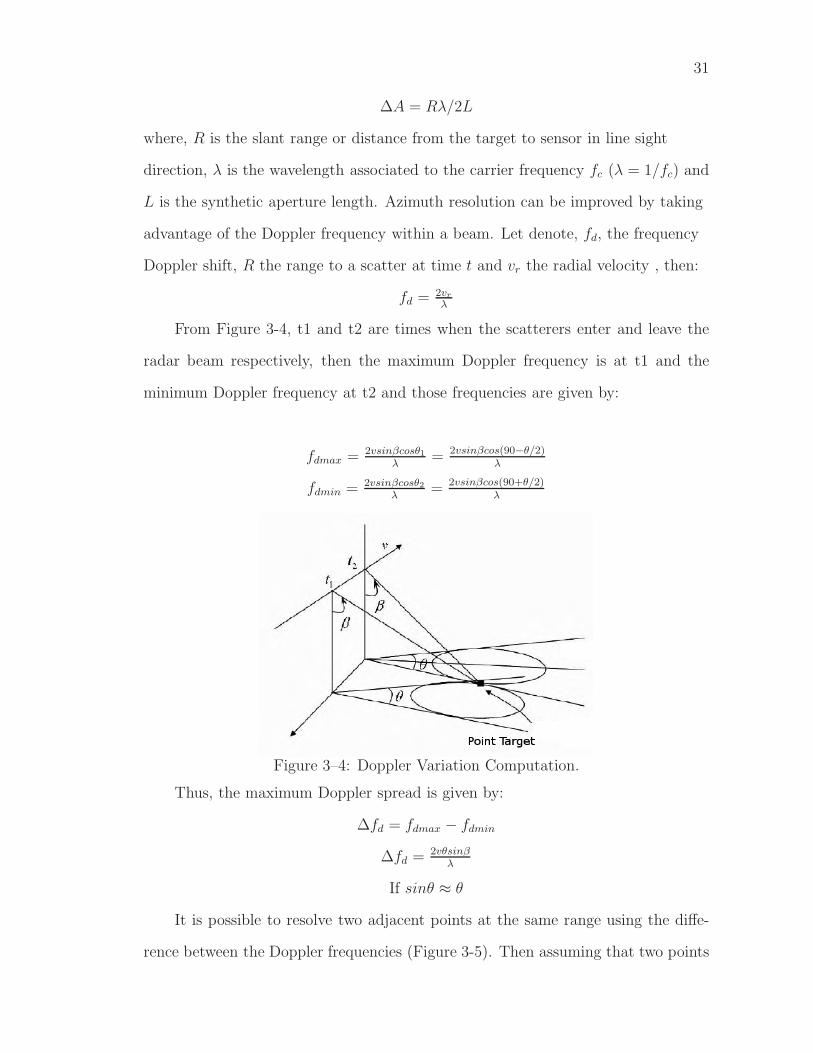
L is the synthetic aperture length. Azimuth resolution can be improved by taking
advantage of the Doppler frequency within a beam. Let denote, fd, the frequency
Doppler shift, R the range to a scatter at time t and vr the radial velocity , then:
fd = 2vr
λ
From Figure 3-4, t1 and t2 are times when the scatterers enter and leave the
radar beam respectively, then the maximum Doppler frequency is at t1 and the
minimum Doppler frequency at t2 and those frequencies are given by:
fdmax = 2vsinβcosθ1
λ= 2vsinβcos(90−θ/2)
λ
fdmin = 2vsinβcosθ2
λ= 2vsinβcos(90+θ/2)
λ
Figure 3–4: Doppler Variation Computation.
Thus, the maximum Doppler spread is given by:
∆fd = fdmax − fdmin
∆fd = 2vθsinβλ
If sinθ ≈ θ
It is possible to resolve two adjacent points at the same range using the diffe-
rence between the Doppler frequencies (Figure 3-5). Then assuming that two points

32
are within the kth range and using the ∆fd minimum then:
∆fdmin = 2v∆θsinβk
λ
Figure 3–5: Azimuth Geometry.
Figure 3–6: Azimuth Geometry.
where ∆θ is the angular displacement between the points and βk is the elevation
angle corresponding to the kth range. The synthetic aperture length L is equal to
vTobs where Tobs is the interval of observation and Tobs = 1∆fdmin
.
Then substituting L in previous equation and solving for ∆θ, we obtain the following
equation:
∆θ = λ2Lsinβk
Finally the azimuth resolution within the kth range is given by:
∆A = Rk∆θ = Rkλ
2Lsinβk
33
3.2 SAR System Description
This section describes important aspects of a SAR system model such as the im-
pulse response function, the raw data generation, and the image formation processes.
3.2.1 Fundamentals of Active Imaging
In this section fundamentals of active imaging is presented as it pertains to
SAR applications. A synthetic aperture radar is described in this work as a two di-
mensional linear shift invariant system with a prescribed impulse response function
which represent the inherent attributes of the system [Rodriguez]. It is customary to
use the ambiguity function of a transmitted and a received signal as the prescribed
impulse response of the system. This concept of active imaging modeled as a linear
shift invariant system is a simplification of a more general concept which is here
described in two stages, a raw data image generation stage of SAR presented here
in a generalized manner, using an operator theoretic approach.
In the stage one, the Hilbert space of two-dimensional continuous finite energy sig-
nals are viewed as points in this space. The second stage is to allows the introduction
of operators which act on these points in the Hilbert space. A formal description of
this operation action is presented as follows:
Oh : L2 (R × R) → L2 (R × R)
γ → Oh {γ} = g
where,
g (mx, my) =
∫λx∈R
∫λy∈R
γ (λx, λy) h (mx, my, λx, λy) dλxdλy
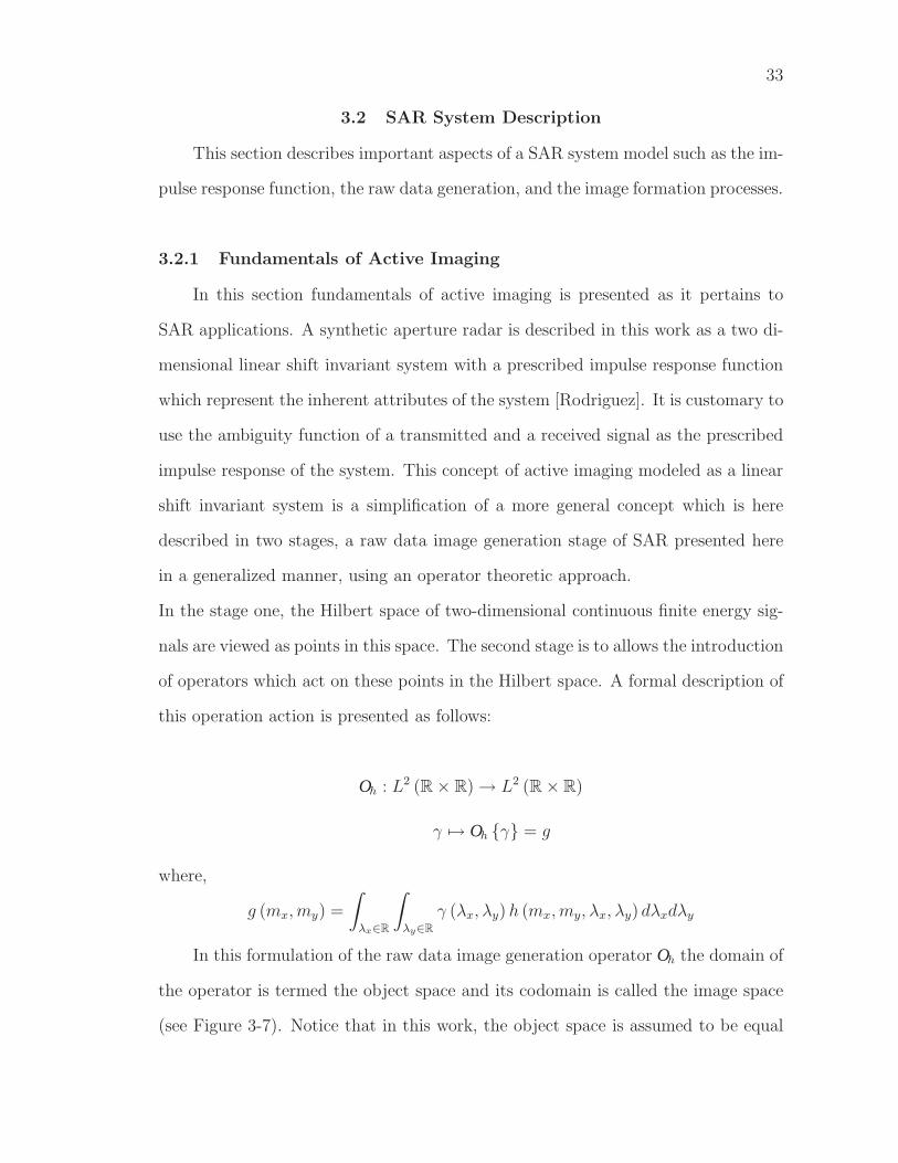
In this formulation of the raw data image generation operator Oh the domain of
the operator is termed the object space and its codomain is called the image space
(see Figure 3-7). Notice that in this work, the object space is assumed to be equal

34
to the image space, namely, L2 (R × R).
To arrive to the initial simplification of modeling the SAR system as a linear
shift invariant system, the properties of linearity and shift invariance must be added
to the formulation above. First, the shift invariance condition is introduced. An
operator Oh, acting over a Hilbert space L2 (R × R), is said to be shift invariant if
it commutes with the shift operator S . This shift operator acting over L2 (R × R)
may be described as follows:
(Sλx,λy {δ}) (mx, my) = δλx,λy (mx, my) = δ (mx − λx, my − λy)
for δ, δλx,λy ∈ L2 (R × R) being delta dirac unit impulse functions.
Thus, if the system is shift invariant:
OhS = SOh
Also,
OhSλx,λy = Sλx,λyOh
The operator Oh acting over a point target is given by:
(Oh {δ}) (mx, my) = g (mx, my) =
∫λx∈R
∫λy∈R
γ (λx, λy)h (mx, my, λx, λy) dλxdλy
In this case, we have γ = δ, then:
g (mx, my) =
∫λx∈R
∫λy∈R
δ (λx, λy)h (mx, my, λx, λy) dλxdλy
g (mx, my) = h (mx, my)
The shift operator acting over a point target is given by:
δ{λx,λy} = Sλx,λy {δ}

35
Now, let τx and τy time delay in x and time delay in y axis respectively. Then,
Oh
{δ{τx,τy}
}(mx, my) = g (mx, my)∫
λx∈R
∫λy∈R
γ (λx, λy) h (mx, my, λx, λy) dλxdλy
∫λx∈R
∫λy∈R
δ{τx,τy} (λx, λy)h (mx, my, λx, λy) dλxdλy
∫λx∈R
∫λy∈R
δ (λx − τx, λy − τy)h (mx, my, λx, λy) dλxdλy
Therefore,
g (mx, my) = Oh
{δ{τx,τy}
}= h (mx, my, τx, τy)
The Figure 3-7 represents a mapping of a point target in the object space or
domain to the image space or co-domain using the operator Oh.
Figure 3–7: Mapping From the Object Space to the Image Space.
Now, assuming shift invariance:
(Oh
{δ{τx,τy}
})= Oh {S τx,τy {δ}} = S τx,τy {Oh {δ}}
Knowing that,
Oh {δ} = h

36
and
(Oh {δ}) (mx, my) = h (mx, my)
then,
S τx,τy {Oh {δ}} = S τx,τy {h} = h{τx,τy}
(S τx,τy {Oh {δ}}) (mx, my) = (S τx,τy {h}) (mx, my) = h{τx,τy} (mx, my) = h (mx − τx, my − τy)
Therefore shift invariance implies that
h (mx, my, τx, τy) = h (mx − τx, my − τy)
Next, the active imaging will be modeled using linearity and shift invariance
properties.
A surface image can be written as:
γ (mx, my) =
∫λx∈R
∫λy∈R
γ (λx, λy) δ (mx − λx, my − λy) dλxdλy
for γ ∈ L2 (R × R)
then, the surface representation can be expressed using operator thus:
γ (mx, my) =
∫λx∈R
∫λy∈R
γ (λx, λy) (S τx,τy {δ}) (mx, my) dλxdλy
Assuming linearity:
(Oh {γ}) (mx, my) = g (mx, my) =
∫λx∈R
∫λy∈R
γ (λx, λy)(Sλx,λy {Oh {δ}}
)(mx, my) dλxdλy
=
∫λx∈R
∫λy∈R
γ (λx, λy)(h{λx,λy} (mx, my)
)(mx, my) dλxdλy
g (mx, my) =
∫λx∈R
∫λy∈R
γ (λx, λy) (h (mx − λx, my − λy)) dλxdλy
It corresponds to the active imaging model in continuous time.

37
Now, assuming ideal sampling when using the Nyquist theorem:
g [n0, n1] =∑k0∈Z
∑k1∈Z
γ [k0, k1]h [n0 − k0, n1 − k1]
where, (n0, n1) ∈ Z × Z
Assuming causal FIR filtering, with h ∈ l2 (ZM0 × ZM1), and allowing commutativ-
ity,
g [n0, n1] =∑k0∈Z
∑k1∈Z
h [k0, k1] γ [n0 − k0, n1 − k1]
where, (n0, n1) ∈ Z × Z
This is a computational expression.
Now assuming causal finite input for the model, then:
g [n0, n1] =∑
k0∈ZM0
∑k1∈ZM1
h [k0, k1] γ [n0 − k0, n1 − k1]
where, (n0, n1) ∈ ZN0 × ZN1
This expression is fully computational even though there may not exist efficient
implementations.
A way to search for efficient implementations of computational models is to
study these models under a mathematical setting which may be reach in algebraic
structures. In particular, abelian and cyclic properties of sets are very important,
in order to find efficient methods for computational implementations.
3.2.2 One Dimensional SAR Model for Image Formation
Studies about synthetic aperture radar systems have used different metho-
dologies to make image formation algorithms that allow to get images from the
ground with an acceptable resolution.

38
Figure 3–8: Functional Block Diagram for Image Formation Using one DimensionalSignal Processing.
Those are algorithms concerning to implement range and azimuth compression
techniques joint to radiometric and geometric correction such as range cell migration
correction or chirp scaling processes [Cumming]. The methodologies are based on
the treatment of the imaging problem as a one dimensional problem. A diagram is
depicted in Figure 3-8.
3.2.3 Two Dimensional SAR Model
Unlike the one-dimensional case, the two dimensional SAR signal processing
becomes a 2D convolution, with the SAR system impulse response modeled as a
function in two dimensions. This subsection describes a SAR model using the fun-
damentals of active imaging and 2D processing algorithms.
1. Transmitted Pulse
The radar system sends pulses of length τp given by s (t) = ej αt2
2 . Those pulses
are modulated in frequency by the following function c (t) = ej2πfct, called the
carrier signal associated with the SAR transmission system, where fc is the carrier
frequency. Then, the transmission signal has the following form:

39
St (t) = S (t) c (t) rect[
tτp
]The parameters (τp, fc and α) given by the transmitted pulse are important in
the imaging process and in the quality of the recovered image. Figure 3-9 is an
example of the transmission of pulses of the system.
Figure 3–9: Example of the Transmit and Receive Signal Cycles of a Radar.
2. Point Target Impulse Response
The radar sends pulses St equally spaced to illuminate a point target area. In the
intervals of time τr the radar is not sending pulses (see Figure 3-9), then, it is
receiving the scattered signals Sr from the surface. The transmitted and received
signals (St and Sr) are stored in form of signal data (telemetry). The following
step is to sent telemetric data to the ground station (in satellite systems) for level
0 processing (convert telemetric data into raw data). Finally the raw data is used
to obtain an image of the illuminated area.
The received signal of a point target illuminated has the form of the transmitted
signal but delayed in time by a quantity τ = 2Rc
, where R is the distance of the
target to the radar in the line sight. In addition it is shifted in frequency by an
amount φ giving the relative speed between the sensor and the surface that is called
SAR Doppler frequency. The received signal or reflectivity model is giving by:
Sr (t; τ, φ) = aϕej α(t−τ)2
2 ej2π(fc−φ)(t−τ)rect[
t−ττp
]
40
In last equation aϕ is the amplitude of the echo signal. The model uses the ambi-
guity function between the received and transmitted signals as point impulse res-
ponse or point spread function of a SAR system. The ambiguity function is giving
by:
A{St,Sr}[τ, φ] =∑
n∈ZN
St[n]S∗r [〈n+ τ〉N ] e−j 2πφn
N
where, St is the transmitted signal, Sr is the received signal, τ is the time delay, φ
is the frequency shift and N is the length of the transmitted signal.
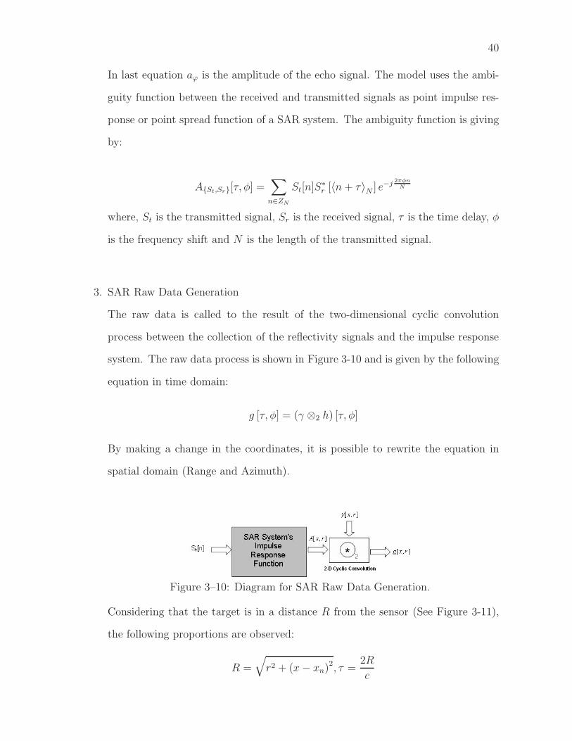
3. SAR Raw Data Generation
The raw data is called to the result of the two-dimensional cyclic convolution
process between the collection of the reflectivity signals and the impulse response
system. The raw data process is shown in Figure 3-10 and is given by the following
equation in time domain:
g [τ, φ] = (γ ⊗2 h) [τ, φ]
By making a change in the coordinates, it is possible to rewrite the equation in
spatial domain (Range and Azimuth).
Figure 3–10: Diagram for SAR Raw Data Generation.
Considering that the target is in a distance R from the sensor (See Figure 3-11),
the following proportions are observed:
R =
√r2 + (x− xn)2, τ =
2R
c
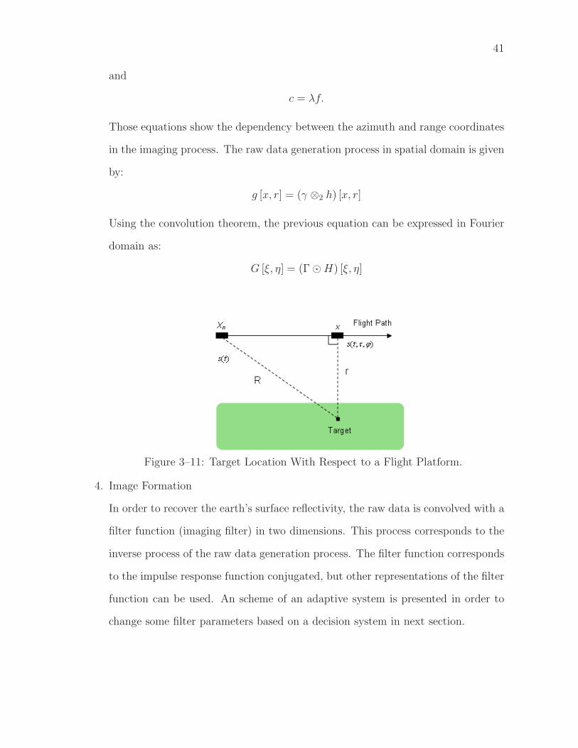
41
and
c = λf.
Those equations show the dependency between the azimuth and range coordinates
in the imaging process. The raw data generation process in spatial domain is given
by:
g [x, r] = (γ ⊗2 h) [x, r]
Using the convolution theorem, the previous equation can be expressed in Fourier
domain as:
G [ξ, η] = (Γ �H) [ξ, η]
Figure 3–11: Target Location With Respect to a Flight Platform.
4. Image Formation
In order to recover the earth’s surface reflectivity, the raw data is convolved with a
filter function (imaging filter) in two dimensions. This process corresponds to the
inverse process of the raw data generation process. The filter function corresponds
to the impulse response function conjugated, but other representations of the filter
function can be used. An scheme of an adaptive system is presented in order to
change some filter parameters based on a decision system in next section.

42
The image formation process consists in obtain the reflectivity function γ (Γ in the
Fourier domain), and it is given by:
Γ [ξ, η] = (G�H∗) [ξ, η]
Then, applying the inverse Fourier transform process:
γ [x, r] = F −1N {(G�H∗) [ξ, η]}
The imaging problem can be resolved by using the convolution theorem due to the
possibility of implement the discrete Fourier transform using the fast algorithm
called the Fast Fourier Transform.
Figure 3–12: Image Formation Diagram Block.
Figure 3-12 shows the image formation process using two-dimensional opera-
tions.
3.2.4 Raw Data Storage
To convert the one-dimensional data received from the radar to the two di-
mensional format of the raw data, each echo signal received is located in a row of

43
the matrix arrangement. The number of rows depends on the sensor motion in the
azimuth coordinate, it means that each row corresponds to a different azimuth po-
sition giving by the movement of the radar.
Next, the echo signal is sampled and it is stored in memory joint to the other impor-
tant image information in a complex format in such way that each row contains one
real data follows by one imaginary data. For example, for RADARSAT products, a
pulse replica of the transmitted is stored each eigth lines. In addition, line descrip-
tors and one file descriptor, which contains relevant information about the sensor
and the platform, are stored with the data (CEOS format for RADARSAT level
zero products), and it is neglected during the extraction data process (see appendix
A).
3.3 Adaptive Imaging System
An adaptive system for image formation appears next. This system is based on
the use of images previously acquired of a radar system and then is computed the
synthetic raw data as it was explained in previous section. The adaptive system uses
the knowledge about images to change the parameters used in the filter generation
find the best approach for the impulse system response. Once the wished system
impulse response has been obtained by means of the use of a decision system, it
is used as image formation system for the raw data given by a radar in a physical
environment.
The Figure 3-13 depicts a diagram of the adaptive system for the image forma-
tion. The training image formation filter is observed in yellow color with the system
impulse response function given by a variation of the filter parameters according
to a decision system. In blue color is the process of obtaining synthetic raw data
from images previously computed, which is obtained by computing the ambiguity
44
function to model the active sensor imaging system. For that process it is required
to know signal representation theory explained in previous chapter. Finally in red
color is presented the active imaging sensor system that corresponds to the radar
located in the physical environment that generates the real raw data which is the
input to the image formation system once has been adapted by the decision system.
The ρ (mx, my) function corresponds to the stored image, h(mx, my) is the imaging
sensor system model, g(mx, my) is the synthetic raw data computed using the image
and the imaging sensor system model. The function called Γ(mx, my) corresponds
to the output of the image formation system and it is used as input to the decision
system just like the computed image in order to establish a judgment to adapt the
system impulse response function and get images close to the original images. The
function g (mx, my) corresponds to the SAR raw data acquired by the active imaging
sensor system in the physical environment.
So much the imaging sensor system modes as the image formation system corre-
spond to a two dimensional cyclic convolution operation. The decision system is
given by using the error computation between the image computed and the original
image. One example of a decision system using the Newton adaptive filter is pre-
sented here but other possibilities can be analyzed. The decision system consists in
use the mean square error of the magnitude of the images (computed and original)
and it is used in the Newton adaptive filter as shows the Figure 3-14.
3.3.1 Newton Adaptive Filter Description
The goal of this function is trying to minimize the Mean Square Error (MSE)
between the original image and the synthesized image, based on the best estimate
the delay parameter of the ambiguity function in order to get better images in the
image formation process. The Newton adaptive filter methods implemented since it
is an iterative method where the parameter ( τ - delay ) will be modified to find the
filter that minimizes the MSE.
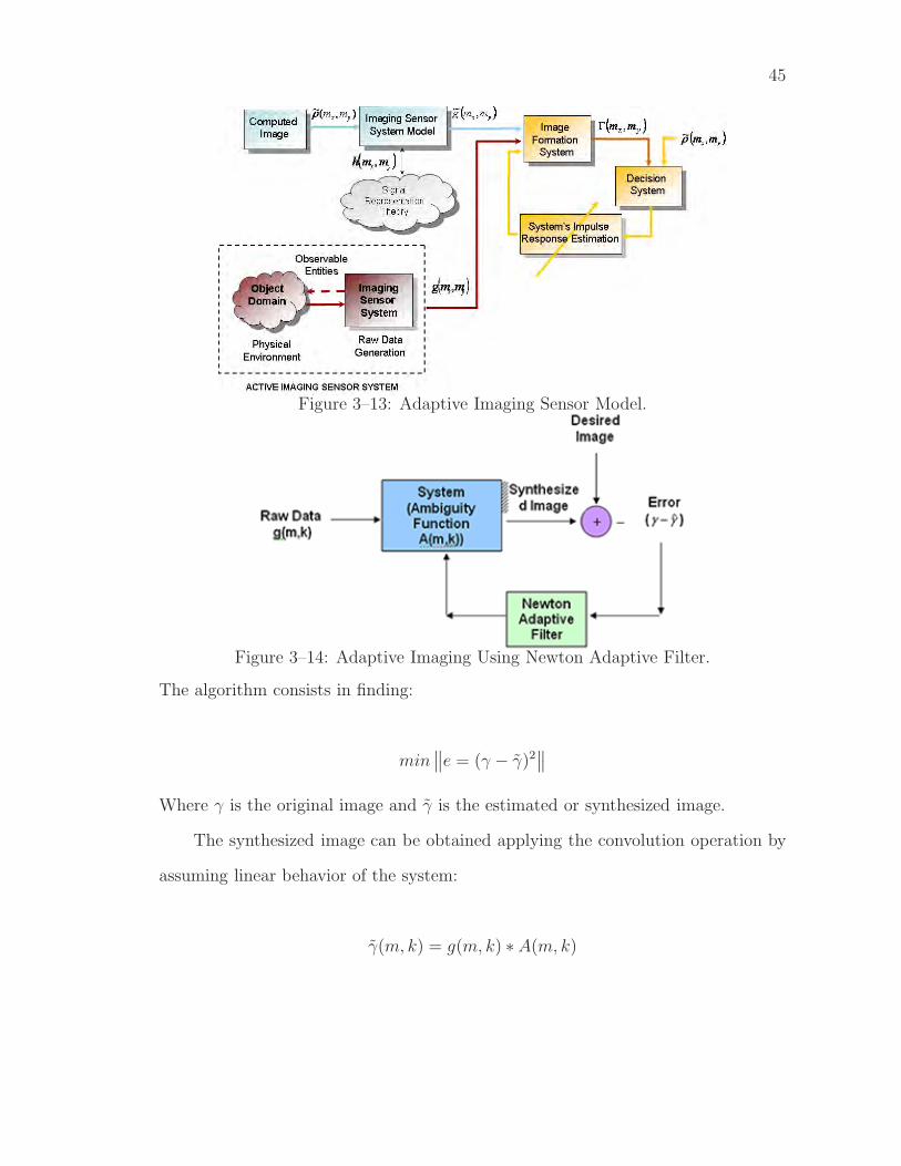
45
Figure 3–13: Adaptive Imaging Sensor Model.
Figure 3–14: Adaptive Imaging Using Newton Adaptive Filter.
The algorithm consists in finding:
min∥∥e = (γ − γ)2
∥∥Where γ is the original image and γ is the estimated or synthesized image.
The synthesized image can be obtained applying the convolution operation by
assuming linear behavior of the system:
γ(m, k) = g(m, k) ∗ A(m, k)

46
The Newton algorithm can be written as follows:
pn+1 = pn −H−1(pn)g(pn)
H−1(pn) =∂e
dpn.∂e
dpn
′
g(pn) =∂e
dpn.e(pn)
In this case, pn is the parameter τn that corresponds to the time delay in the iteration
n.
The error given in the iteration n is:
e(pn) = e(τn) = γ − γ(τn) = γ − g ∗ A(τn)
∂e
dτn=∂(γ − γ)
dτn
The Newton adaptive filter was implemented using previous equations in order to
find the parameter τ in a limited number of iterations.

CHAPTER 4
HARDWARE/SOFTWARE COMPUTATIONAL
STRUCTURES
This chapter is concerned with the design of a computational structure model
for Synthetic Aperture Radar applications that includes data processing in hardware
and software tools. A software structure implies that the algorithm is implemented
in a system with an own operating system, such as a PC or an embedded system. For
this work, a PC with windows operating system is used for the implementation of the
software component. In other respect, the hardware implementation is considered
over one or more systems without an own operating system, that corresponds to
floating point digital signal processors (TMS320C6713).
In this thesis, a computational structure is called to a combination of hardware
and software components required for the application. The joint use of hardware
and software tools entails to study a new methodology for modeling and simulation
of active sensor imaging systems using a hardware-in-the-loop technique based on
TI6713 Digital Signal Processor (DSP) units. The Figure 4-1 depicts a diagram of
the hardware/software structures used on this work.
4.1 Hardware and Software Characteristics
In order to process images of active sensors systems, high precision and com-
putational efficiency are required. Regularly these two characteristics are opposed
since high precision of the data implies greater time of processing which decreases
the efficiency and on the other hand a high computational efficiency implies to de-
crease precision (data representation with less bits) to define the data in a system.
47
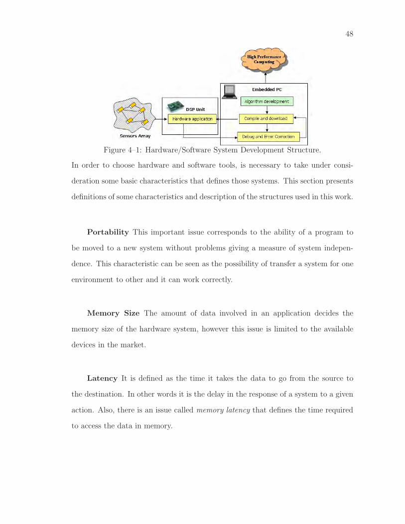
48
Figure 4–1: Hardware/Software System Development Structure.
In order to choose hardware and software tools, is necessary to take under consi-
deration some basic characteristics that defines those systems. This section presents
definitions of some characteristics and description of the structures used in this work.
Portability This important issue corresponds to the ability of a program to
be moved to a new system without problems giving a measure of system indepen-
dence. This characteristic can be seen as the possibility of transfer a system for one
environment to other and it can work correctly.
Memory Size The amount of data involved in an application decides the
memory size of the hardware system, however this issue is limited to the available
devices in the market.
Latency It is defined as the time it takes the data to go from the source to
the destination. In other words it is the delay in the response of a system to a given
action. Also, there is an issue called memory latency that defines the time required
to access the data in memory.
49
Bandwidth This issue is a measure of the capacity of a communication channel
which gives the quantity of data that can be sent from one point to other in an
interval of time. It can be set, for example, in bits per second (bps) or in hertz (Hz)
units.
Throughput It gives a measure the speed of a system to process data. It
is usually defined as the number of operations that systems perform per second
for example FLOPS: Floating Point Operations Per Second or MIPS: Millions of
Instructions Per Second.
Numerical Accuracy The capacity of a system to represent the data with
high precision gives the numerical accuracy in an application. For example, a single
precision number is defined with 32 bits and a double precision number is defined
with 64 bits. Currently there are systems with quadrature precision where the num-
ber is represented with 128 bits.
4.2 Hardware/Software Co-Design Description
Hardware/software co-design is a technique used to develop digital signal pro-
cessing applications since it mixes advantages of having a system dedicated hardware
for the execution of specific processes joint to a software system that may control
the hardware. These are usually connected by a local bus for communication. Along
this work constrains in the communication between hardware and software devices
are considered.
There are some ways to evaluate characteristics in hardware-software designs such
as performance of the system or accuracy of the output data. The description of
a hardware-in-the-loop technique that is used to model and simulate the co-design
hardware/software of a complex system and evaluate the performance characteristics
50
is presented next.
4.2.1 Hardware-In-The-Loop Modeling and Simulation
The hardware-in-the-loop system used in this work is an aggregate of the follo-
wing units: A mathematical model for SAR imaging and a PC workstation with a
link to the Digital Signal Processor (DSP) unit.
The mathematical model for SAR image processing is based on the ambiguity
function computation as point spread function or impulse response function of a
SAR system. See the description of the used mathematical model in chapter three.
The PC workstation has a communication with the DSP units through the
MATLAB numeric computation and scientific visualization software package. For
this work, a PC station is used to control the hardware-in-the-loop process, to pro-
vide the data to the DSP, and to test results obtained in the simulation operation.
An embedded computer system interacting with digital signal processors may be
used to replace the PC in order to make a stand alone system that is commonly
used in airborne radar applications.
The DSP component is used to execute the algorithms generated from a mathe-
matical model of a SAR active sensor imaging system. This unit has an architecture
that is designed to support digital signal processing functions in order to achieve
high performance. Other advantage of these units is to allow the data representa-
tion in double precision format to increase accuracy (floating point DSP’s) since it is
one of the main characteristics in radar applications. The floating point DSP used
on this work was the TMS320C6713. The Figure 4-2 shows the most important

51
characteristics of the TMS320C6713 DSK.
Figure 4–2: Characteristics of the TMS320C6713 DSK Board.
The following three issues constitutes the design for an overall modeling and
simulation system:
1. The PC controls the hardware-in-the-loop simulation denoting when it starts and
ends. Any process starts when the DSP board is connected by software in order
to establish communication or open the USB port for the data flow between both
units. The data transmission uses RTDX (Real Time Data Exchange) tool which
allows to exchange data between the PC and the board without stop the target
application. The key is to have a high data transfer of such a way that the simu-
lation in almost real time can be maintained. For that reason, an emulator can be
used to provide dramatically faster high-speed Real-Time Data Exchange.
2. The PC contains the digital data stored in memory and sends it via USB port
(using RTDX) to the DSP board using MATLAB interface. The algorithm is exe-
cuted on the DSP board and results are returned upon PC and stored for further
analysis or processing.
3. A graphical interface is necessary to make a hardware-in-the-loop simulation process
friendly to the user. Functions such as to connect the board, to select the data
to be transferred and to store computed data in each process can be controlled
by the user. In addition, results of each DSP computation can be retrieved and

52
manipulated a user in future processing since it can be stored in PC workstation
disk memory.
Figure 4-3 shows a picture of the hardware-in-the-loop system running on a
portable computer.
Figure 4–3: Hardware/Software Development System.
4.3 Hardware-in-the-Loop System Result
The complete version of the system for SAR image processing is composed of
several parts as can be seen in the Figure 4-4. The first four options: Read Level
Zero Data, Generate Level Zero Data, Synthesize Level 1 Data and Image Processing,
corresponds to processes executed in software. The DSP Processor option opens the
menu to initiate the hardware-in-the-loop process. The Figure 4-4 shows the main
menu in the graphical interface for SAR image processing.
4.3.1 DSP Processor Option
This tool allows to execute the hardware-in-the-loop simulation process on a
DSP unit (see Figure 4-5).
The process starts activating the board in “ConnectBoard”option so that it
opens the communication channel between the DSP and the PC. The system is con-
figured to display a report of the processes performed. Then, one of the following
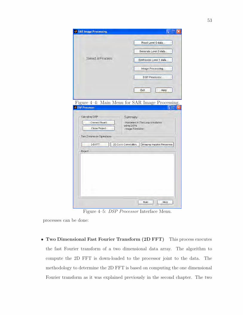
53
Figure 4–4: Main Menu for SAR Image Processing.
Figure 4–5: DSP Processor Interface Menu.
processes can be done:
• Two Dimensional Fast Fourier Transform (2D FFT) This process executes
the fast Fourier transform of a two dimensional data array. The algorithm to
compute the 2D FFT is down-loaded to the processor joint to the data. The
methodology to determine the 2D FFT is based on computing the one dimensional
Fourier transform as it was explained previously in the second chapter. The two
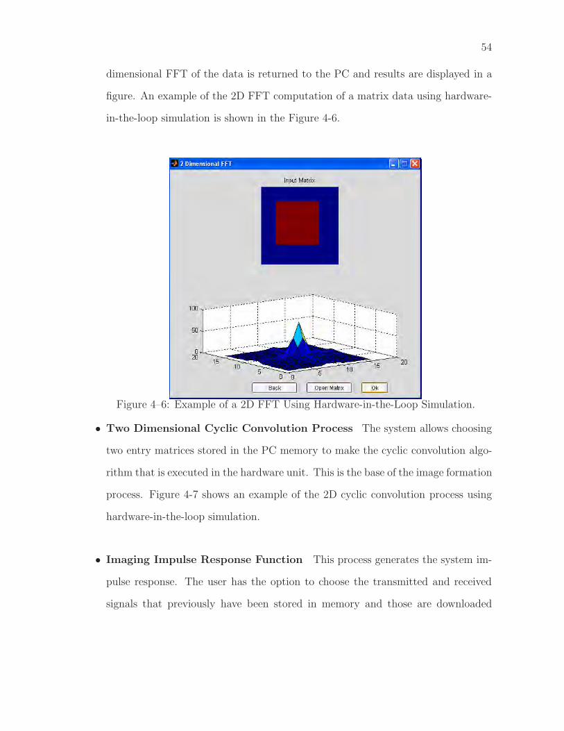
54
dimensional FFT of the data is returned to the PC and results are displayed in a
figure. An example of the 2D FFT computation of a matrix data using hardware-
in-the-loop simulation is shown in the Figure 4-6.
Figure 4–6: Example of a 2D FFT Using Hardware-in-the-Loop Simulation.
• Two Dimensional Cyclic Convolution Process The system allows choosing
two entry matrices stored in the PC memory to make the cyclic convolution algo-
rithm that is executed in the hardware unit. This is the base of the image formation
process. Figure 4-7 shows an example of the 2D cyclic convolution process using
hardware-in-the-loop simulation.
• Imaging Impulse Response Function This process generates the system im-
pulse response. The user has the option to choose the transmitted and received
signals that previously have been stored in memory and those are downloaded

55
Figure 4–7: Example of the Two Dimensional Cyclic Convolution Using Hardware-in-the-Loop Simulation.
to the hardware unit for processing and generation of the system impulse res-
ponse. Figure 4-8 shows an example of an imaging impulse response function
using hardware-in-the-loop simulation.
4.3.2 Considerations for Hardware-in-the-Loop Process
This section presents some considerations for hardware-in-the-loop simulation.
It is reiterated that Matlab environment was used to develop all signal processing
algorithms joint to code composer studio IDE.
1. The input data to any process on the hardware unit had to be computed previously
and stored in the PC memory.
2. The input data that is used in all processes must have a length of 2n (< 16384)
since this algorithm is based on the 1 dimension fast Fourier transform (FFT)
algorithm.
3. If the input data is a matrix, the columns and rows of the matrix must be of lengths
of 2n (< 16384) as same as the previous item.

56
Figure 4–8: Example of a Imaging Impulse Response Function Generated UsingHardware-in-the-Loop Simulation.
4. If a hardware-in-the-loop process is finalized you must close the project which dis-
connects the PC to the DSP and clean the report file.

CHAPTER 5
HARDWARE/SOFTWARE
IMPLEMENTATION RESULTS
This chapter presents results obtained in the implementation on hardware and
software computational structures for SAR applications. Those results are related
to the execution of the algorithms for the raw data generation and image formation
processes using hardware structures, software structures or a combination of both.
5.1 Hardware Results
In this section, some useful results to evaluate the operation of the floating point
digital signal processor (TMS320C6713 DSP) like a fundamental hardware unit for
the execution of the basic algorithms used in SAR applications of image processing
are presented.
5.1.1 Ambiguity Function Computation Results Using DSP Processors
The ambiguity function was used as a radar system impulse response (SAR),
therefore, the evaluation of its computation in a hardware unit was made. Some
conditions such as maximum length of the transmitted and received signal for the
ambiguity function computation and the processing times on the DSP unit were re-
vised. Also the transfer data times involved in the ambiguity function computation
for different lengths in the signals transmitted and received were evaluated.
57
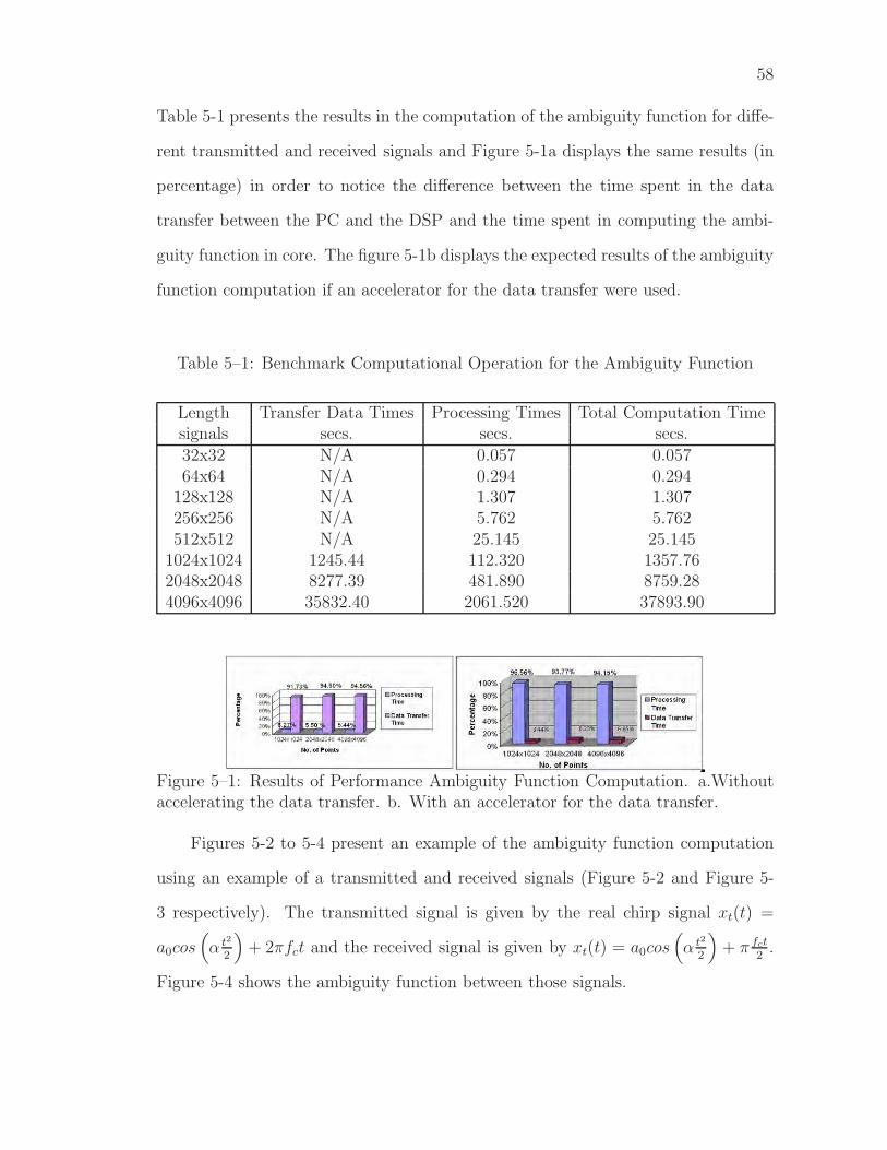
58
Table 5-1 presents the results in the computation of the ambiguity function for diffe-
rent transmitted and received signals and Figure 5-1a displays the same results (in
percentage) in order to notice the difference between the time spent in the data
transfer between the PC and the DSP and the time spent in computing the ambi-
guity function in core. The figure 5-1b displays the expected results of the ambiguity
function computation if an accelerator for the data transfer were used.
Table 5–1: Benchmark Computational Operation for the Ambiguity Function
Length Transfer Data Times Processing Times Total Computation Timesignals secs. secs. secs.32x32 N/A 0.057 0.05764x64 N/A 0.294 0.294
128x128 N/A 1.307 1.307256x256 N/A 5.762 5.762512x512 N/A 25.145 25.145
1024x1024 1245.44 112.320 1357.762048x2048 8277.39 481.890 8759.284096x4096 35832.40 2061.520 37893.90
Figure 5–1: Results of Performance Ambiguity Function Computation. a.Withoutaccelerating the data transfer. b. With an accelerator for the data transfer.
Figures 5-2 to 5-4 present an example of the ambiguity function computation
using an example of a transmitted and received signals (Figure 5-2 and Figure 5-
3 respectively). The transmitted signal is given by the real chirp signal xt(t) =
a0cos(α t2
2
)+ 2πfct and the received signal is given by xt(t) = a0cos
(α t2
2
)+ π fct
2.
Figure 5-4 shows the ambiguity function between those signals.

59
Figure 5–2: Example of a Signal Transmitted by a SAR Radar.
Figure 5–3: Example of a Signal Received by a SAR Radar.
5.1.2 Fast Fourier Transforms Using DSP Processors: One and TwoDimensions
The Fourier transform is one of the most important tools in digital signal pro-
cessing. In this work, it was used to make fast computations of the two dimensional
cyclic convolution. We presented some results of the one and two dimensional fast
Fourier transform using floating point DSP’s. Table 5-2 shows the one dimensional

60
Figure 5–4: Ambiguity Function of Previous Signals.
FFT computation results (time computation and floating point operations), the Fig-
ure 5-5 shows the 2D FFT standard process implemented and Table 5-3 shows two
dimensional FFT computation results.
Table 5–2: Benchmark Computational Operation for the One Dimensional FFT
Length 1D FFT Floating Pointsignals msecs. Operations
16 0.0166 33732 0.03639 827264 0.08034 18261128 0.178 40487256 0.395 89881512 0.8999 2045281024 1.969 4475562048 25 56827284096 55.01 125040968192 117.406 2668328816384 252.403 57364419
In the Table 5-3 are results of the two-dimensional FFT computation in core,
it means, using the DSP memory. Also, the two dimensional FFT can be computed
using external memory of the DSP (out of core). In the last case, a PC is used

61
Figure 5–5: 2D FFT Standard Process.Table 5–3: Benchmark Computational Operation for the Two Dimensional FFT inCore
Length 2D FFT Floating Pointsignals secs. Operations16x16 0.00989 224872432x32 0.04857 1104075364x64 0.21338 48495674
128x128 0.94998 215906104256x256 4.20757 956266644512x512 18.08019 4109134539
as external memory in order to store data for the two dimensional FFT compu-
tation and using the RTDX tool for the data transmission. Table 5-4 shows some
results of the 2D FFT computation using out of core processing and the RTDX tool.
Table 5–4: Benchmark Computational Operation for the Two Dimensional FFT outCore
Length 2D FFTsignals secs.16x16 6632x32 14564x64 290
128x128 600256x256 1510512x512 2186
Two Dimensional FFT computation Using Register Banks
Another approach to perform the two dimensional FFT is using register banks as it
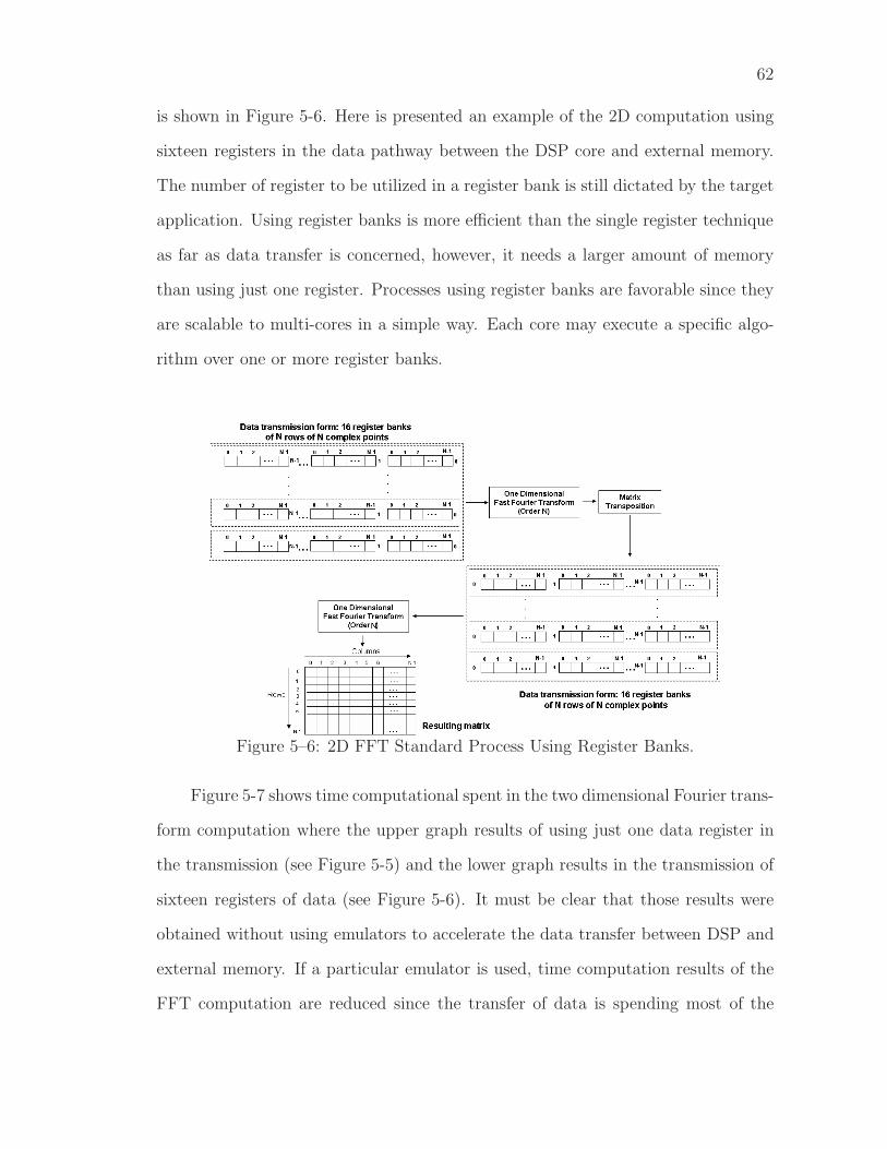
62
is shown in Figure 5-6. Here is presented an example of the 2D computation using
sixteen registers in the data pathway between the DSP core and external memory.
The number of register to be utilized in a register bank is still dictated by the target
application. Using register banks is more efficient than the single register technique
as far as data transfer is concerned, however, it needs a larger amount of memory
than using just one register. Processes using register banks are favorable since they
are scalable to multi-cores in a simple way. Each core may execute a specific algo-
rithm over one or more register banks.
Figure 5–6: 2D FFT Standard Process Using Register Banks.
Figure 5-7 shows time computational spent in the two dimensional Fourier trans-
form computation where the upper graph results of using just one data register in
the transmission (see Figure 5-5) and the lower graph results in the transmission of
sixteen registers of data (see Figure 5-6). It must be clear that those results were
obtained without using emulators to accelerate the data transfer between DSP and
external memory. If a particular emulator is used, time computation results of the
FFT computation are reduced since the transfer of data is spending most of the

63
computation time in the process.
Figure 5–7: Results of 2D FFT Standard Process Using Register Banks.
Figure 5-8 represents the difference in percentage between using register banks
and just one register. Results show that is advantageous to use register banks since
that methodology spends less computational time for the computation of the two
dimensional FFT of an image.
Figure 5–8: Difference in Percentage Between Using Register Banks and Using OneRegister.
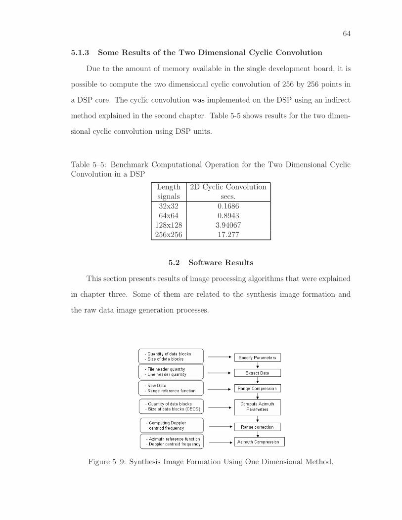
64
5.1.3 Some Results of the Two Dimensional Cyclic Convolution
Due to the amount of memory available in the single development board, it is
possible to compute the two dimensional cyclic convolution of 256 by 256 points in
a DSP core. The cyclic convolution was implemented on the DSP using an indirect
method explained in the second chapter. Table 5-5 shows results for the two dimen-
sional cyclic convolution using DSP units.
Table 5–5: Benchmark Computational Operation for the Two Dimensional CyclicConvolution in a DSP
Length 2D Cyclic Convolutionsignals secs.32x32 0.168664x64 0.8943
128x128 3.94067256x256 17.277
5.2 Software Results
This section presents results of image processing algorithms that were explained
in chapter three. Some of them are related to the synthesis image formation and
the raw data image generation processes.
Figure 5–9: Synthesis Image Formation Using One Dimensional Method.

65
5.2.1 Synthesis Image Formation Using One Dimensional Method
Following the steps depicted in Figure 5-9 is possible to get images from Vancouver-
Canada provided by the international agency RADARSAT. Now, the process to com-
pute images starting from the level zero data (CEOS format) which it was taken
from RADARSAT is described.
Image Formation of a Data Block: Example.
The image formation process requires to specify some image parameters and here is
presented one example of the parameters used for image formation:
1. Number of image’s blocks: 1 block
2. Number of azimuth lines: 1536 lines
3. Number of range cells: 2048 cells
4. First range cell: 700
5. First azimuth line: 1500
The program “specify parameters.m”is used to define the data to be extracted,
using the parameters listed above.
The next program “extract data”is used to read the data from the CD eliminating
the header files and pulse replicas. It calls the program “read CEOS raw.m”and
generates the raw data stored in a .mat file called ‘CDdata1’. Figure 5-10 depicts
the raw data image related to the specified parameters.
The program “image form.m”makes the range and azimuth compression al-
gorithms. The program uses two input data files: the raw data file stored in the
“CDdata1.mat”file and the Doppler centroid frequency file stored in the “fdc.mat”file
by using the program “compute azim spectra.m”. This program generates an image

66
Figure 5–10: Raw Data Representation.
in range and azimuth compressed. Figures 5-11 and 5-12 shows the image range com-
pressed and the image range and azimuth compressed respectively.
Figure 5–11: Image Range Compressed.
5.2.2 Computational SAR Signal Processing Environment
A computational tool was designed and developed to work with the algorithms
in order to help the user with a graphical interface. This environment was developed
using Matlab and C language.

67
Figure 5–12: Final Image Formation Stage.
This tool allows to perform the following processes: to read level zero data, to gene-
rate level zero data, to synthesize level one data and to process images.
Figure 5–13: Read Level 0 Data process.
Read Level 0 Data
This process allows to read a portion of raw data from an image and shows the raw
data in form of image by taking the magnitude of each pixel. The file description of
the raw data is explained in the appendix A. The process requires the specification

68
of parameters to define the portion of the raw data image to be read. Figures 5-13 to
5-16 depict an example of the process for read level zero data. First image represents
the graphical user interface. To specify the input data parameters is possible in the
import data option as it is shown in Figure 5-14. The raw data selected is displayed
as it shows the Figure 5-15. Finally, the raw data image can be stored with the
option “save”as it is shown in Figure 5-16.
Figure 5–14: Read Level Zero Data - Specifying Parameters Process.
Generate Level 0 Data
This process alludes to the synthetic generation of raw data images from an of given
reflectance image (see Figure 5-17). Using the models explained in chapter three,
the synthetic raw data is generated using a reflectance image (see Figure 5-18) and
the system impulse response function. On this computational environment, three
different filters that can be used as system impulse response: the delta function, the
gaussian function and the ambiguity function. The Figures 5-19 to 5-21 show filter
examples that can be computed using this computational environment.
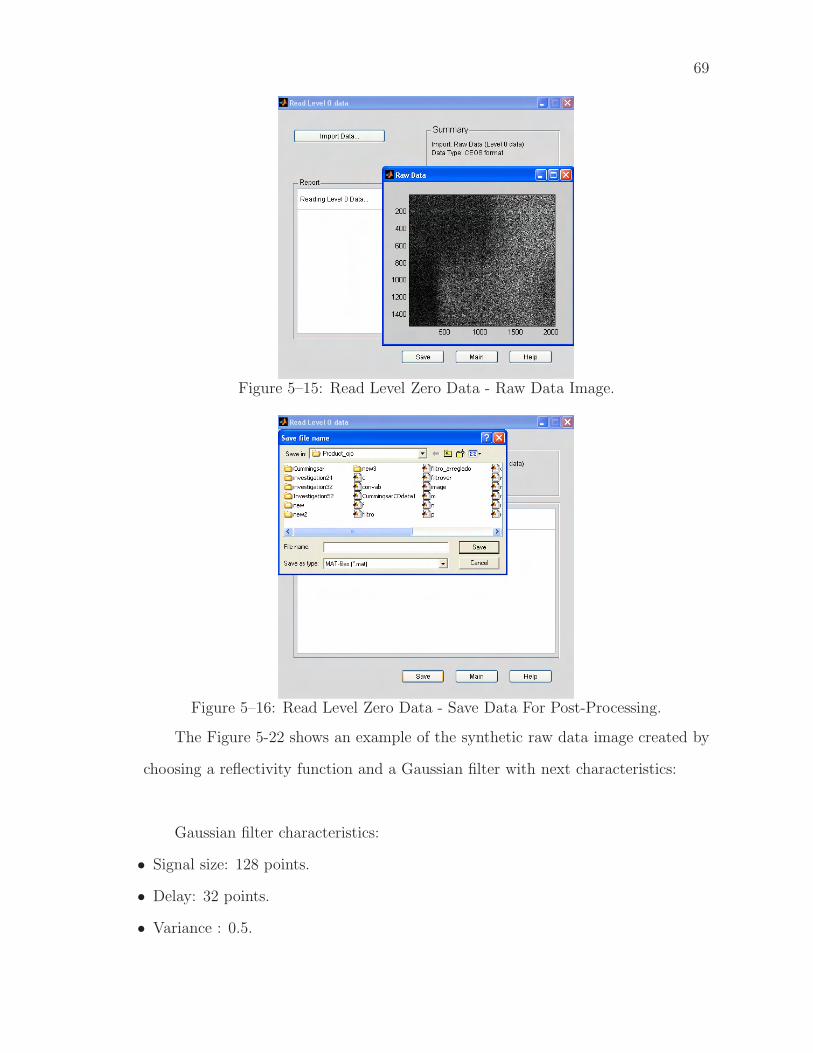
69
Figure 5–15: Read Level Zero Data - Raw Data Image.
Figure 5–16: Read Level Zero Data - Save Data For Post-Processing.
The Figure 5-22 shows an example of the synthetic raw data image created by
choosing a reflectivity function and a Gaussian filter with next characteristics:
Gaussian filter characteristics:
• Signal size: 128 points.
• Delay: 32 points.
• Variance : 0.5.

70
Figure 5–17: Generate level Zero Data.
Figure 5–18: Generate level Zero Data - Open a Reflectivity Function.
Synthesize Level 1 Data
In this stage, the inverse process of raw data generation is performed (see Figure
5-23). It uses the two dimensional cyclic convolution to synthesize images using as
system input entries the raw data and a given filter. The desired raw data must
be stored in memory and the filters can be generated similarly as it was explained
in ‘Generation Level 0 Data’step. Figure 5-24 shows an example of the synthesized
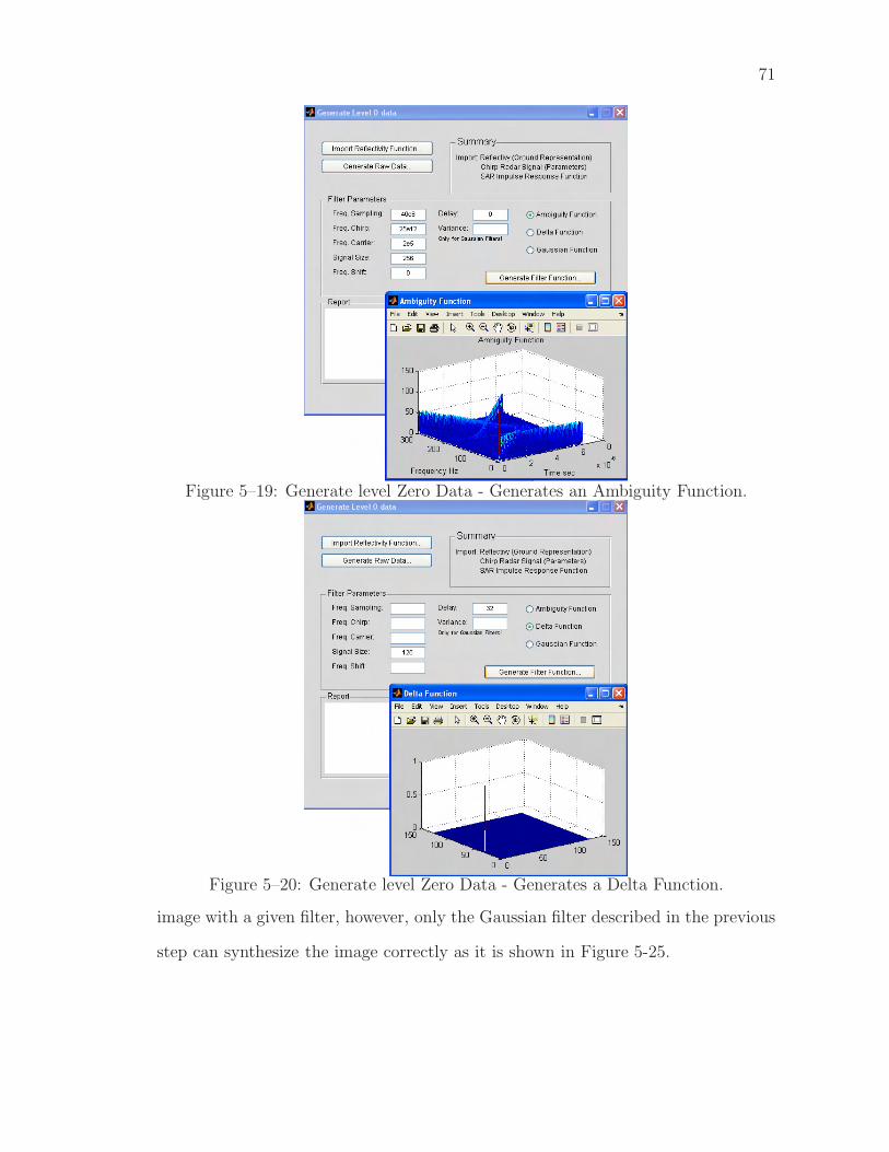
71
Figure 5–19: Generate level Zero Data - Generates an Ambiguity Function.
Figure 5–20: Generate level Zero Data - Generates a Delta Function.
image with a given filter, however, only the Gaussian filter described in the previous
step can synthesize the image correctly as it is shown in Figure 5-25.

72
Figure 5–21: Generate level Zero Data - Generates a Gaussian Function.
Figure 5–22: Generate Level Zero Data - Synthetic Raw Data Image.
Other important characteristic of the computational environment is the possi-
bility of computing the mean square error between the magnitude of a synthesized
image and the magnitude of the original reflectivity function. It can be done by
choosing MSE computation option and one example is depicted in Figure 5-26.

73
Figure 5–23: Synthesize Level 1 Data.
Figure 5–24: Synthesize Level 1 Data - Synthesized Image With a Gaussian Filter.
The generation of level zero data , the synthesis of level one data, and the MSE com-
putation processes are the fundamentals of the adaptive model for image formation,
explained in chapter three.
Image Processing
This tool allows to compute two processes used in image processing: the two dimen-
sional Fourier transform and the two dimensional cyclic convolution. Figure 5-27
shows an example of importing an image from memory and Figure 5-28 shows the
corresponding two dimensional FFT of the image. In a process were one image is

74
Figure 5–25: Synthesize Level 1 Data - Synthesized Image With an AdequateGaussian Filter.
Figure 5–26: Synthesize Level 1 Data - Mean Square Error (MSE) Computation.
involved, the option Image 1 or Image 2 should be selected in the menu. Figure 5-29
shows an example of the two dimensional cyclic convolution between two images.
In this case, the Image 1 and Image 2 option must be selected from the menu for a
correct functioning.
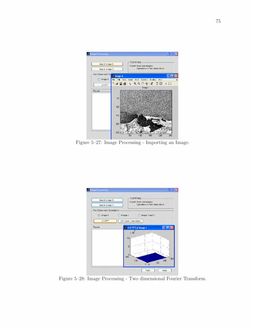
75
Figure 5–27: Image Processing - Importing an Image.
Figure 5–28: Image Processing - Two dimensional Fourier Transform.
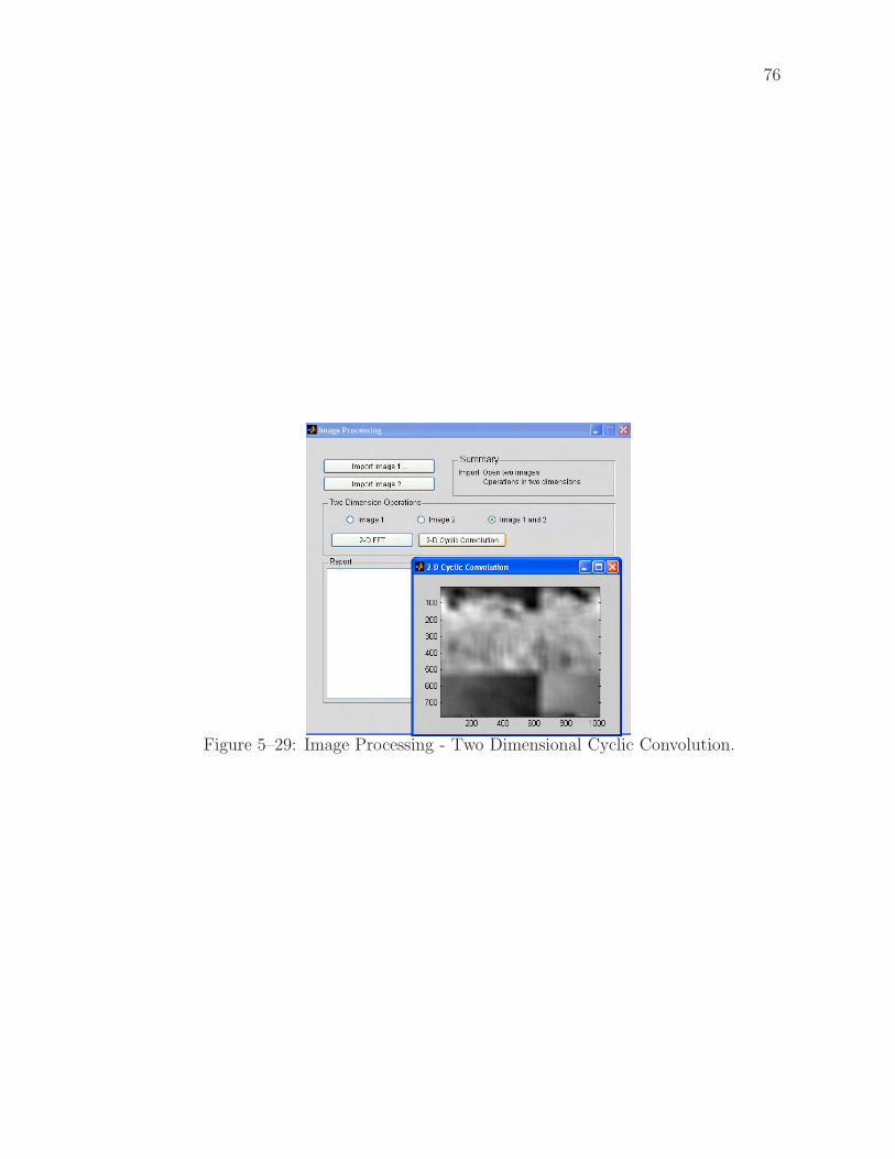
76
Figure 5–29: Image Processing - Two Dimensional Cyclic Convolution.
CHAPTER 6
CONCLUSIONS AND FUTURE WORKS
6.1 Conclusions
This thesis has presented a theoretical formulation for the development of algo-
rithms for time-frequency representations to be used in Synthetic Aperture Radar.
These algorithms were implemented on a Hardware/software computational struc-
ture.
Some of the conclusions of the modeling and implementation of the algorithms
on DSP’s units are:
• A large scale algorithm for the ambiguity function computation using the trans-
form method has been implemented on the TMS320C6713 DSP and a personal
computer.
• Having a hardware dedicated to processing an algorithm allows having an portable
system. Also, it allows increasing in size of the system by adding more dedicated
devices without changing the basic structure of the system. Results in the exe-
cution of algorithms using data matrices show that current devices (DSP) data
processors are very efficient and can be used in applications that require data pro-
cessing in near to real time.
• On this work, some hardware and software characteristics such as memory size,
throughput, bandwidth of a communication channel and numerical accuracy were
77

78
evaluated with the implementation of the SAR algorithms. Some results show that
is necessary to increase the quantity of memory due to the capabilities in current
digital signal processing devices. Increasing external memory implies to decrease
the system performance due to the time spent in the access to external memory.
For this thesis, results of processing times and quantity of memory required were
obtained using register banks for data transfer between memory and the central
processing unit.
• The system model for generation of raw data and image formation were based on
the two dimensional cyclic convolution. This thesis developed the implementa-
tion of the two dimensional cyclic convolution by using the fast Fourier transform
(FFT). This operation was made in core and out of core by means of external
memory and real time data exchange.
• A method for image formation using raw data was presented based on an one di-
mensional model given by I. Cumming. The algorithm implementation was based
on some tools from Cumming’s book.
• A method for image formation by using an adaptive filter was presented. This
method refers to change just one parameter in the ambiguity function (τ) compu-
tation in order to find a better imaging filter for image formation.
6.2 Future Works
Future works in SAR image processing applications need to study the following
issues.

79
• The hardware implementation of the algorithms on parallel or multiple Digital
Signal Processors.
• The hardware implementation of the algorithms on FPGA’s and DSP’s structures.
• The hardware implementation of the model presented using embedded systems
instead of a PC.
• Evaluation of an adaptive filter changing more than one parameter in the ambi-
guity function computation.
• Study of a methodology for computing errors between an image generated by a two
dimensional convolution and an image computed by the one dimensional convo-
lution. That is, the study in errors in the magnitude and phase between the images.

REFERENCE LIST
[Bamler] Bamler, R. and Eineder, M. ‘ScanSAR Processing Using Standard
High Precision SAR Algorithms’. IEEE Transactions on Geoscience
and Remote Sensing. Vol. 34. Pags. 212-218. January 1996.
[Bierens] Bierens, L and Deprettere, E. ‘Engineering Multirate Convolutions
for Radar Imaging’. IEEE International Conference on Acoustics,
Speech, and Signal Processing. Vol. 6. 1996.
[CEOS89] CEOS(Committee on Earth Observations Satellites). ‘SAR Data
Products Format Standard’. Report written by CEOS SAR Data
Standards Subgroup. Febreruary, 1989.
[CEOS89] CEOS(Committee on Earth Observations Satellites). ‘RADARSAT-1
Standard Beam SAR Images’. June, 1999.
[Chi] Chi, T.; Zhang, X.; Wu, H. and Fang, J. ‘Agent Communication
Based SAR Image Parallel Processing’. Procecedings of hte Fourth
International Conference on Parallel and Distributed Computing, Ap-
plications and Technologies. Pags. 532-534. August 2003.
[Cumming] Cumming, I. and Wong, F. H. ‘Digital Processing of Synthetic Aper-
ture Radar Data: Algorithms and Implementation’. Book. January
2005.
[Curlander] Curlander, J.C. and McDonough, R.N. ‘Synthetic Aperture Radar :
Systems and Signal Processing’. John Wiley and sons. Inc. 1991.
[Franceschetti] Franceschetti, G. and Lanari, R. ‘Synthetic Aperture Radar Pro-
cessing’. Book, 1999.
80
81
[Franceschetti01] Franceschetti,G and others. ‘An Electromagnetic Model for SAR
Raw Signal Simulation of Urban Areas’. IEEE/ISPRS Joint Work-
shop in Remote Sensing and Data Fusion over Urban Areas. pags.10-
14. Nov. 2001.
[Franceschetti02] Franceschetti,G and others. ‘A 2-D Fourier Domain Approach for
Spotligth SAR Raw Signal Simulation of Extended Scenes’. IEEE In-
ternational Geoscience and Remote Sensing Symposium. Vol.2. Pags
853-855. June 2002.
[Franceschetti02-b] Franceschetti,G and others. ‘SAR Raw Signal Simulation of Oil
Slicks in Ocean Environments’. IEEE Transactions on Geoscience
and Remote Sensing. Vol. 40. September 2002.
[Franceschetti04] Franceschetti,G and others. ‘Efficient Hybrid Stripmap/spotlight
SAR Raw Signal Simulation’. IEEE International Proceedings In
Geoscience and Remote Sensing Symposium. Vol.5. Pags 3329-3332.
2004.
[Henderson] Henderson, F.M. and Zong-Guo, X. ‘SAR Applications in Human
Settlement Detection, Population Estimation and Urban Land Use
Pattern Analysis: a Status Report. IEEE Transactions on Geoscience
and Remote Sensing. Vol. 35. Pags. 79-85. January 1997.
[Isenburg] Isenburg, M.; Gumhold, S. and Snoeyink, J. ‘Processing Sequences:
A new Paradigm for Out-of-Core Processing on Large Meshes’. Uni-
versity of North Carolina at Chapel Hill. 2003.
[Jian-Xi] Jian-Xi, H.; Jing-hong, W. and Shun-ji, H. ‘The hardware implemen-
tation of real-time SAR signal processor’. IEEE International Radar
Conference. 2000.
[Nava] Nava, H. ‘Modeling and Simulation of Point Spread Functions for
Advanced SAR Systems’. 2004.
82
[Pantaleoni] Pantaleoni-Vidal, A. and Fernando, M. ‘Quality Evaluation for Ef-
ficient ScanSAR Data Processing Algorithms’. IEEE International
Geoscience and Remote Sensing Symposium. Vol. 6. Pags. 4022-4024.
July 2003.
[Park] Park,M. ‘Millimeter-Wave Polarimetric Radar Sensor for Detection of
Power Lines in Strong Clutter Background’. Ph.D. Thesis. University
of Michigan. 2004.
[Quartulli] Quartulli, M. and Datcu, M. ‘Information Fusion for Scene Under-
standing from Interferometric SAR Data in Urban Environments’.
IEEE Transactions on Geoscience and Remote Sensing. Vol. 41.
Pags.1976-1985. September 2003.
[RADARSAT00] ‘RADARSAT Data Products Specifications’. Report written by
Radarsat International and revised by RSI. Canada, May-2000.
[Rodriguez] Rodriguez, D and Nava, H. R. ‘High Performance Artificial SAR Raw
Data Generation Algorithms For Remote-Sensed Imaging Applica-
tions’. IEEE International Geoscience and Remote Sensing Sympo-
sium. Vol. 5. Pags. 2747-2749. 2002.
[Rodriguez02] Rodriguez, D. ‘Computational Signal Processing and Sensor Array
Signal Algebra’. September 2002.
[Sarabandi] Sarabandi,K. and park,M. ‘Milimeter-Wave Radar Phenomenology of
Power Lines and a Plarimetric Detection Algorithm’. IEEE Transac-
tions on Antennas and Propagation. Vol.47. December, 1999.
[Soumekh] Soumekh, M. ‘Synthetic Aperture Radar Signal Processing with Mat-
lab Algorithms’. Book, 1999.
[Tolimieri] Auslander, L. and Tolimieri, R. ‘Computing Decimated Finite Cross-
Ambiguity Functions’. IEEE Transaction On Acoustics Speech and
Signal Processing.Vol. 36. NO. 3. March 1988.

83
[Tulodziecki] Tulodziecki, J. ‘The Application of Parallel DSP architectures to
Radar Signal Processing’. IEE. Marconi Radar Systems. 1995.

APPENDICES

APPENDIX A
RADARSAT CEOS FORMAT
This appendix presents the format used to store the data by the RADARSAT
sensor system. The level zero data is distributed to the ground station in CEOS
(Committee on Earth Observing Systems) format. This committee is formed by
representatives of different international Earth observation or remote sensing enti-
ties and the main objective is to standardize different existing data formats for easy
understanding.
A raw product contains unprocessed radar data in complex in-phase and quadra-
ture signal format. This format consists in a metadata file joint to the data file. The
metadata file has important and relevant information about the radar system. It
consists in the following records: The Volume Directory File, the SAR Leader File,
the SAR Data File, the SAR Trailer File, and the Null Volume Directory File.
The volume directory file provides information about the data containers, such
as the name of the tapes and information of the agency that generates the tape. Also
it has information about the file such as name and length and information about
characteristics of the image such as identification of the scenes and coordinates for
localization.
85
86
The SAR leader file contains information related with the geography, satellite
coordinates and date and time of the data acquisition.
The SAR trailer file contains information about the software to compute the
raw data.
The null volume directory file gives information about the type of data, the
volume identification and the number of volumes used.
The SAR data file is composed by two registers: The One file descriptor record
and the SAR data records.
One File Descriptor Record.
It describes the format of the SAR data in the file, giving the number and length of
the SAR data records. Also it has the detailed information of the method to pack
the SAR data samples in each record and the size of the prefix data.
Signal Data Record.
The SAR signal data record is a record containing the following information:
the first 193 bytes corresponds to the header, the next 50 bytes corresponds to auxi-
liary information and the remaining corresponds to the data per se.
The Figure A-1 shows an example of the CEOS format for a SAR data file.
The extraction of the desired SAR data to get images consists in eliminate the
header files from the SAR data file. Next is the procedure for extract the desired
SAR data.
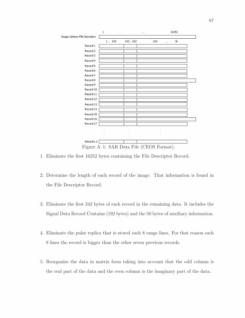
87
Figure A–1: SAR Data File (CEOS Format).
1. Eliminate the first 16252 bytes containing the File Descriptor Record.
2. Determine the length of each record of the image. That information is found in
the File Descriptor Record.
3. Eliminate the first 242 bytes of each record in the remaining data. It includes the
Signal Data Record Contains (192 bytes) and the 50 bytes of auxiliary information.
4. Eliminate the pulse replica that is stored each 8 range lines. For that reason each
8 lines the record is bigger than the other seven previous records.
5. Reorganize the data in matrix form taking into account that the odd column is
the real part of the data and the even column is the imaginary part of the data.

88
6. Integrate the real and imaginary part to get the complex data ready to be processed.
Each row with a complex number represents a range line.
Further information can be found in [CEOS89], [CEOS99], and [RADARSAT00].

APPENDIX B
EXTRACTING RAW DATA AND
GENERATING IMAGES
The following document contains the methodology to extract raw data and to
generate images. This document comes including with the book written by Ian
Cumming and Frank Wong: ’Digital Processing of Synthetic Aperture Data’.
There are two main programs and one function that are used to extract data.
First run “specify parameters.m”to define the parameters for the current experi-
ment, then run “extract data.m”to extract the data. The only parameters you need
to change are in the first program. If desired, the call to “extract data.m”can be
placed at the end of “specify parameters.m”. Finally you can use the program
“image form.m”to use the raw data extracted for computing the image.
specify parameters.m
Only one file is needed, “dat 01.001”. This file can be copied to your hard
disk, for convenience. The path to this file, whether it be located, must be specified
by the variable “input path”. The size of the data file is 364 MB. Data extracted
is written to files in a directory specified by the variable, “output path”. Another
variable, “output prefix”, is provided in case you want to store more than one set
of data in the same directory. To define the limits of the data to be extracted, set
the variables, first rg cell, Nrg cells, first rg line, Nrg lines, and Nrg lines blk
to the desired values for this experiment. The term ’range cell’ refers to samples
89

90
in the range or ’fast time’ direction. The term ’range line’ refers to samples in the
azimuth or ’slow time’ direction. The first range cell, first rg cell, and the number
of range cells, Nrg cells, can be set to any value within the boundaries of the data
array (1 to 9288). The first range line, first rg line, should be set to a multiple
of 8 plus 1, and the number of lines per block, Nrg lines blk, should be set to a
multiple of 8. Also, the total number of lines to be extracted, Nrg lines, should be
set to a multiple of the number of lines per block. If these rules are not obeyed, the
“extract data.m”program will quantize the values accordingly.
The variable, Nrg lines blk, allows you to control the extracted file size, so that the
data can be extracted into a number of smaller files, rather than one big file. This is
helpful in limiting the memory size needed by the extraction and analysis programs.
The extracted data can be stored in two ways - in MAT files or general binary
files. The binary files can be used with any program, such as programs written in
C. But if you are using MATLAB for all your processing, it is more efficient to use
MAT files for the extracted data. In the latter case, set UseMATfiles to 1 (true). If
you want to use binary files, set UseMATfiles to 0 (false).
After these parameters are specified, they are stored in the file, “CD run params”
in the current directory, for use by the subsequent data extraction and processing
programs.
extract data.m
This program is run after “specify parameters.m”. It calls the function
“read CEOS raw.m”to read the data from the CD, extract the desired data, de-
code the data (in the case of MAT files), and write the data into easy-to-access disk
files. Because the data on CD has a pulse replica stored every 8 range lines, it is
convenient to read the CD 8 lines at a time. To simplify the read procedure, the

91
first range line and number of range lines per block are restricted to be multiples of
8.
Next, a set of parameters are specified that pertain to the specific RADARSAT
beam used and certain fixed parameters of the CD. These include radar parameters
such as the PRF and sampling rate, and are defined in the in-line comments in the
program. Do not change these values for this data set. These parameters are added
to the parameters already stored in “CD run params.mat”. These parameters are
added in this program in order to keep the program “specify parameters.m”as sim-
ple as possible.
Note that while the number of replica samples stored is 1440 complex samples, 1349
samples is the effective length of the transmitted replica. Its center frequency is zero
and its FM rate is 0.72135e12Hz/s, rather than the lower value given in the book.
The transmitted chirp is generated digitally and is a linear FM function, so it is
more accurate to generate the chirp within your processing programs rather than
use the 4-bit replica stored.
read CEOS raw.m
This is the function that reads the bits, bytes, and words from the book CD
and stores them in a form more easily read by your application programs. There are
two ways of storing the extracted data, as set by the parameter “UseMATfiles”in
“specify parameters.m”. If this variable is true, the raw SAR data is stored in a
MATLAB MAT file. No other data is stored. This is the easiest and quickest way
of extracting and using the SAR data if you are going to use MATLAB for all the
subsequent processing. In the block diagram on the preceding page, the operations
shown in red solid lines pertain to this option.
92
If the “UseMATfiles”parameter is false, the data is stored in binary disk files,
that can be read by any program. In addition to the SAR data and auxiliary data,
the file header, the line headers, and the pulse replicas are also stored. For most
processing, you will not need this extra data, especially as none of the variable pa-
rameters like the PRF and range gate delay change in this data set.
compute azim spectra.m
This is an example of an application program you might write. It illustrates how
the SAR data is read and used, including adjusting the signal data for the automatic
gain control (AGC) attenuation values. It first loads the “CD run params.mat”file,
which was created when the data was extracted. It then calls the functions
“load AGC block.m”and “load DATA block.m”for each block of data to be processed,
and proceeds with the application.
This application divides the range swath into Nspect sub-swaths. It then finds the
azimuth or Doppler power spectrum of each swath, and fits a curve of Doppler cen-
troid vs. range to the estimates. Fitting the Doppler centroid curve is most useful if
the whole range swath is specified. In this case, the azimuth blocks should be small,
up to 1024 range lines. If a larger azimuth block is desired and memory is critical,
multiple blocks can be used.
load AGC block.m, extract AGC.m
If MAT files are used, “load AGC block”simply reads the MAT file,
“AGC attenuation values.mat”that has the AGC attenuation values. The program
then picks out the values pertaining to the range lines currently being processed.
These values are the attenuation values used by the radar receiver for each
range line. The AGC system is needed so that the received analog signal stays
93
within a suitable range for the 4-bit A/D converter. These values should be used in
your application program to reverse the effects of the AGC gain changes. If binary
disk files are used, “load AGC block”calls the function “extract AGC.m”to read
the auxiliary file associated with the block of data currently being processed. The
AGC attenuation values are extracted from the bit stream, converted to a byte then
to a decimal value in units of dB.
load DATA block.m
If MAT files are used, “load DATA block”simply reads the MAT file CD-
datai.mat that was saved by “read CEOS raw.m”. If binary files are used, the
data is read from the SAR raw data file, and converted to single (v7) or double (v6)
precision floating point data. The data is then decoded and converted to complex
numbers (this step is already done in the case of MAT files). Finally, the data is
compensated for the receiver AGC attenuation setting, which can change for every
range line.
SAR Processing
After “load AGC block.m”and “load DATA block.m”are completed, the data
are now ready for SAR processing. The raw data in the file “CDdata1.mat”and the
frequencies Doppler computed previously are used in the image computation. The
program “image form.m”is used for the SAR processing.

APPENDIX C
SAR IMAGE FORMATION USER’S GUIDE -
HARDWARE/SOFTWARE
IMPLEMENTATION
This appendix presents the user’s guide of a graphical user interface designed
and implemented for SAR applications.
The SAR Image Processing Tool is an interface developed in Matlab and C
languages for treatment of algorithms of SAR applications. This tool allows under-
standing the models used for raw data generation and image formation processes.
The main menu has five processes:
1. Read Level 0 Data
2. Generate Level 0 Data
3. Synthesize level 1 Data
4. Image Processing
5. DSP Processor
Figure C–1: Software Environment.
94

95
The first four options are concerning with the computation of raw data and
generation of images using one and two dimensional models. Those processes are
completely computed in software using Matlab. The last option is concerning with
three basic processes in image processing and those are implemented on a DSP
board. (See Figure C-1)
1. Read Level 0 Data This option opens a new window with the option “import data”.
If you make click on this option, it will open a new window with white spaces to
enter the data. In the spaces you should enter the information of the portion
of the raw data image to be read. The Figure C-2 shows an example of the
“Read Level 0Data”window and an example of the window to enter the raw data
parameters.
Figure C–2: Read Level 0 Data.
The input parameters of a raw data image are:
Data Source: In this space you must indicate the raw data image name with the
extension (.dat, .raw, etc). You have to be sure that the file is in the current file.
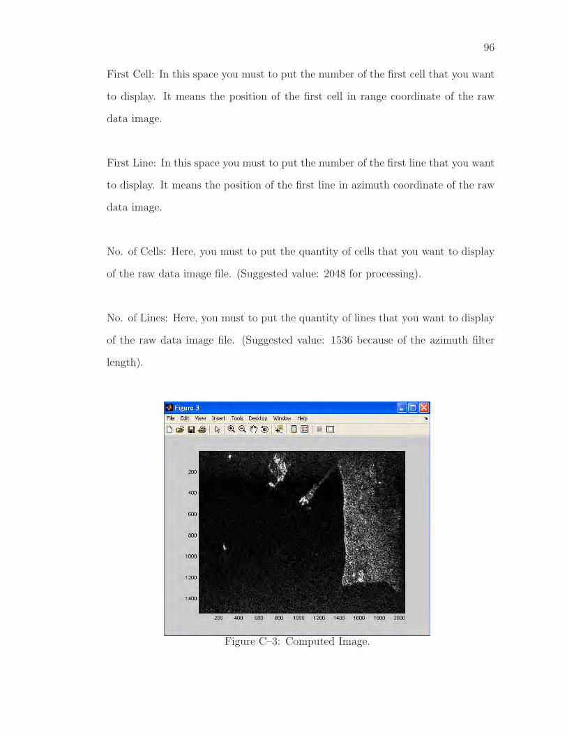
96
First Cell: In this space you must to put the number of the first cell that you want
to display. It means the position of the first cell in range coordinate of the raw
data image.
First Line: In this space you must to put the number of the first line that you want
to display. It means the position of the first line in azimuth coordinate of the raw
data image.
No. of Cells: Here, you must to put the quantity of cells that you want to display
of the raw data image file. (Suggested value: 2048 for processing).
No. of Lines: Here, you must to put the quantity of lines that you want to display
of the raw data image file. (Suggested value: 1536 because of the azimuth filter
length).
Figure C–3: Computed Image.
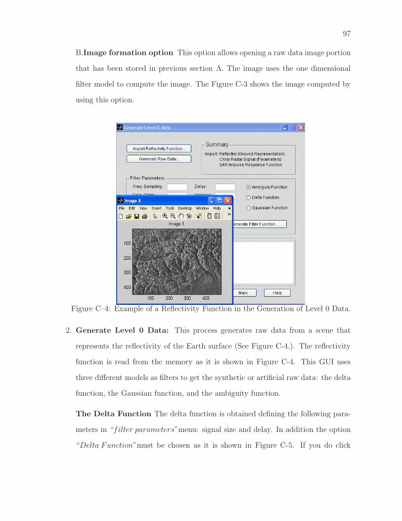
97
B.Image formation option This option allows opening a raw data image portion
that has been stored in previous section A. The image uses the one dimensional
filter model to compute the image. The Figure C-3 shows the image computed by
using this option.
Figure C–4: Example of a Reflectivity Function in the Generation of Level 0 Data.
2. Generate Level 0 Data: This process generates raw data from a scene that
represents the reflectivity of the Earth surface (See Figure C-4.). The reflectivity
function is read from the memory as it is shown in Figure C-4. This GUI uses
three different models as filters to get the synthetic or artificial raw data: the delta
function, the Gaussian function, and the ambiguity function.
The Delta Function The delta function is obtained defining the following para-
meters in “filter parameters”menu: signal size and delay. In addition the option
“Delta Function”must be chosen as it is shown in Figure C-5. If you do click

98
Figure C–5: Delta Function Example.
in “Generate F ilter Function”, the filter is computed. The Figure C-5 shows an
example of a delta function with the following parameters:
Signal size: 256
Delay: 12
The Gaussian Function The Gaussian filter is obtained by defining the follo-
wing parameters in “filter parameters”menu: Signal size, delay, and variance.
The option ’Gaussian Function’ must be chosen as it is shown in Figure C-6. If
you do click in “Generate F ilter Function”, the filter is computed. The Figure
C-6 shows an example of a Gaussian function with the following parameters:
Signal size: 128
Delay: 12
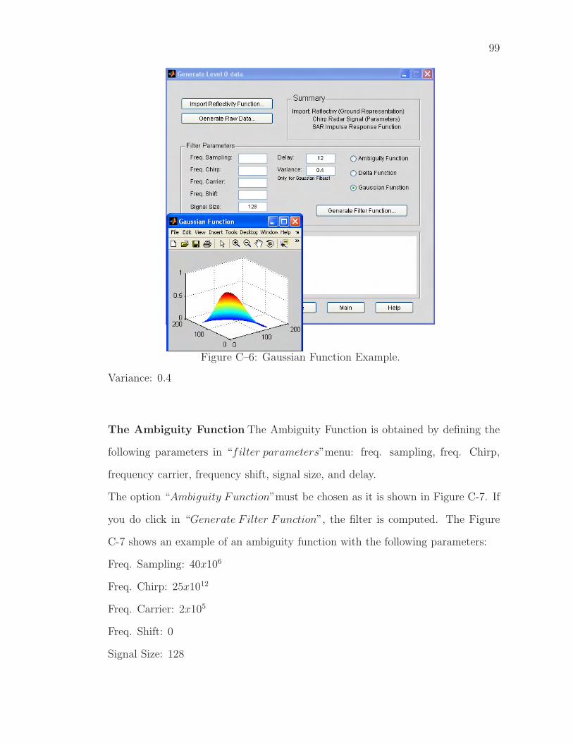
99
Figure C–6: Gaussian Function Example.
Variance: 0.4
The Ambiguity Function The Ambiguity Function is obtained by defining the
following parameters in “filter parameters”menu: freq. sampling, freq. Chirp,
frequency carrier, frequency shift, signal size, and delay.
The option “Ambiguity Function”must be chosen as it is shown in Figure C-7. If
you do click in “Generate F ilter Function”, the filter is computed. The Figure
C-7 shows an example of an ambiguity function with the following parameters:
Freq. Sampling: 40x106
Freq. Chirp: 25x1012
Freq. Carrier: 2x10⁵
Freq. Shift: 0
Signal Size: 128
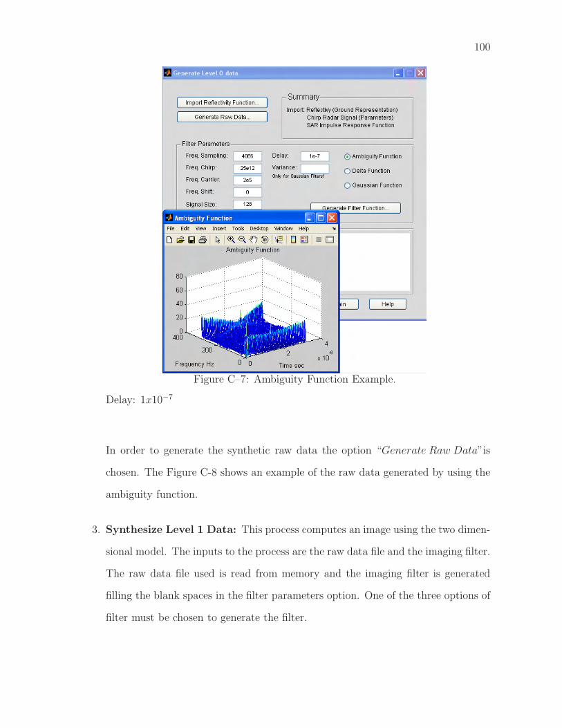
100
Figure C–7: Ambiguity Function Example.
Delay: 1x10⁻⁷
In order to generate the synthetic raw data the option “Generate Raw Data”is
chosen. The Figure C-8 shows an example of the raw data generated by using the
ambiguity function.
3. Synthesize Level 1 Data: This process computes an image using the two dimen-
sional model. The inputs to the process are the raw data file and the imaging filter.
The raw data file used is read from memory and the imaging filter is generated
filling the blank spaces in the filter parameters option. One of the three options of
filter must be chosen to generate the filter.

101
Figure C–8: Raw Data Example.
Figure C–9: Import Raw Data Example.
A. Import Raw Data: Stored raw data will be used as input in the image for-
mation process. The raw data is stored in a .mat file in the option:
“Generate Level 0Data”. The Figure C-9 shows an example of import a raw data
file.
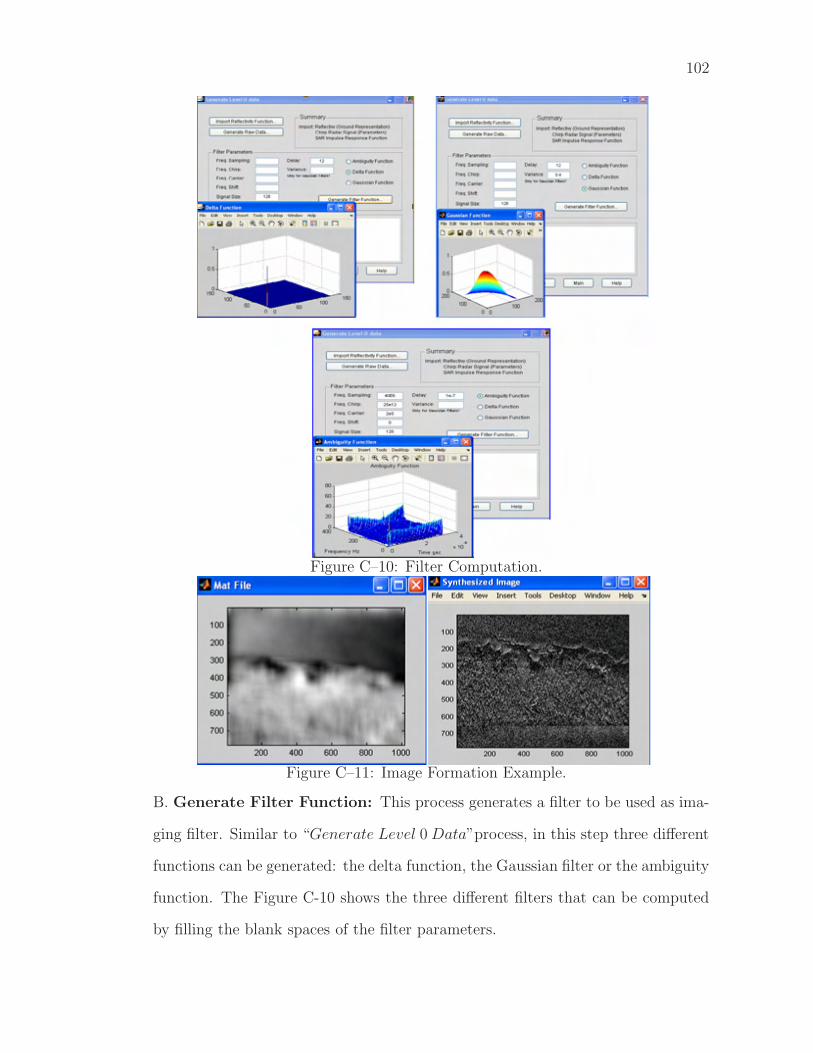
102
Figure C–10: Filter Computation.
Figure C–11: Image Formation Example.
B. Generate Filter Function: This process generates a filter to be used as ima-
ging filter. Similar to “Generate Level 0Data”process, in this step three different
functions can be generated: the delta function, the Gaussian filter or the ambiguity
function. The Figure C-10 shows the three different filters that can be computed
by filling the blank spaces of the filter parameters.

103
Figure C–12: Image Formation Example.
C. Image Formation: This action uses the raw data file selected and the imaging
filter generated in order to compute an estimated image. Accuracy in the computed
image depends on the imaging filter used. If a correct imaging filter is used, the
image results in a good approximation of the original image. In the other way, if
the suitable filter is not chosen, the image will be different from the original image.
The Figure C-11 shows an example of the computed image by using a non-suitable
imaging filter and the Figure C-12 shows the computed image by using a suitable
imaging filter.
Figure C–13: Import Images Example.
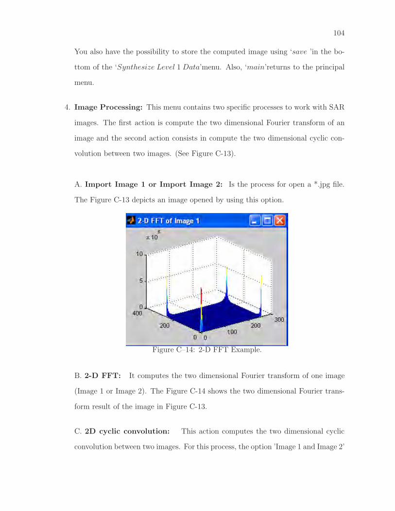
104
You also have the possibility to store the computed image using ‘save ’in the bo-
ttom of the ‘Synthesize Level 1 Data’menu. Also, ‘main’returns to the principal
menu.
4. Image Processing: This menu contains two specific processes to work with SAR
images. The first action is compute the two dimensional Fourier transform of an
image and the second action consists in compute the two dimensional cyclic con-
volution between two images. (See Figure C-13).
A. Import Image 1 or Import Image 2: Is the process for open a *.jpg file.
The Figure C-13 depicts an image opened by using this option.
Figure C–14: 2-D FFT Example.
B. 2-D FFT: It computes the two dimensional Fourier transform of one image
(Image 1 or Image 2). The Figure C-14 shows the two dimensional Fourier trans-
form result of the image in Figure C-13.
C. 2D cyclic convolution: This action computes the two dimensional cyclic
convolution between two images. For this process, the option ’Image 1 and Image 2’

105
Figure C–15: 2-D Cyclic Convolution Example.
should be chosen. The Figure C-15 shows a 2D cyclic convolution process between
two images.
Figure C–16: DSP Processor Menu.
5. DSP Processor: This window contains the actions to be computed on a DSP
board. The Figure C-16 shows the main menu for this option. In this case, you
must have a DSP board unit.
A. Connect Board: It connects the PC to the DSP board and set up the
communication between them.

106
Figure C–17: Two Dimensional FFT of an Image Using a DSP Board.
B. 2D FFT : With this option you can compute the two dimensional FFT on the
DSP board by using the RTDX CCS tool. The matrix sent to the board is chosen
with the option ‘Open Matrix’that is at the bottom of the menu. The Figure C-17
shows an example of the computation of the 2D FFT of an image.
C. 2D cyclic convolution: This option generates the two dimensional cyclic
convolution between two images opened with the button ‘Open Matrix’at the bo-
ttom of the menu. The Figure C-18 shows an example of this process.
D. Imaging Impulse Response: This process computes the ambiguity function
used as impulse response function. In this case, you must choose two signals that
will be transferred to the DSP board in order to compute the ambiguity function on
the DSP. The Figure C-19 computes the ambiguity function between two signals.
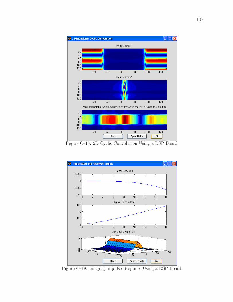
107
Figure C–18: 2D Cyclic Convolution Using a DSP Board.
Figure C–19: Imaging Impulse Response Using a DSP Board.

ON IMPLEMENTING TIME-FREQUENCY REPRESENTATIONS
ON HARDWARE/SOFTWARE COMPUTATIONAL STRUCTURES
FOR SAR APPLICATIONS
Ana Beatriz Ramirez Silva
(787) 464-7447
Department of Electrical and Computer Engineering
Chair: PhD. Domingo Rodriguez
Degree: Master of Science
Graduation Date: June 2006
Related Documents