On implementing a primal-dual interior-point method for conic quadratic optimization

On implementing a primal-dual interior-pointmethod for conic quadratic optimization

E. D. Andersen∗, C. Roos†, and T. Terlaky‡

December 18, 2000

Abstract

Conic quadratic optimization is the problem of minimizing a linearfunction subject to the intersection of an affine set and the productof quadratic cones. The problem is a convex optimization problemand has numerous applications in engineering, economics, and otherareas of science. Indeed, linear and convex quadratic optimization isa special case.

Conic quadratic optimization problems can in theory be solved ef-ficiently using interior-point methods. In particular it has been shownby Nesterov and Todd that primal-dual interior-point methods devel-oped for linear optimization can be generalized to the conic quadraticcase while maintaining their efficiency. Therefore, based on the workof Nesterov and Todd, we discuss an implementation of a primal-dualinterior-point method for solution of large-scale sparse conic quadraticoptimization problems. The main features of the implementation areit is based on a homogeneous and self-dual model, handles the rotatedquadratic cone directly, employs a Mehrotra type predictor-corrector

∗Helsinki School of Economics and Business Administration, Department of Economicsand Management Science, Runeberginkatu 14-16, Box 1210, FIN-00101 Helsinki, Finland,Email: [email protected]. Part of this research was done while the author had aTMR fellowship at TU Delft. This author has been supported by the Finnish Academyof Science†TU Delft, Mekelweg 4, 2628 CD Delft, The Netherlands, Email: [email protected].‡McMaster University, Department of Computing and Software, Hamilton, Ontario,

Canada. L8S 4L7. Email: [email protected]. Part of this research was done whilethe author was employed at TU Delft.

1

extension, and sparse linear algebra to improve the computational ef-ficiency.

Computational results are also presented which documents thatthe implementation is capable of solving very large problems robustlyand efficiently.

1 Introduction

Conic quadratic optimization is the problem of minimizing a linear objectivefunction subject to the intersection of an affine set and the direct product ofquadratic cones of the formx : x2

1 ≥n∑j=2

x2j , x1 ≥ 0

. (1)

The quadratic cone is also known as the second-order, the Lorentz, or theice-cream cone.

Many optimization problems can be expressed in this form. Some ex-amples are linear, convex quadratic, and convex quadratically constrainedoptimization. Other examples are the problem of minimizing a sum of normsand robust linear programming. Various applications of conic quadratic op-timization are presented in [11, 17].

Over the last 15 years there has been extensive research into interior-point methods for linear optimization. One result of this research is thedevelopment of a primal-dual interior-point algorithm [16, 20] which is highlyefficient both in theory and in practice [8, 18]. Therefore, several authors havestudied how to generalize this algorithm to other problems. An importantwork in this direction is the paper of Nesterov and Todd [22] which showsthat the primal-dual algorithm maintains its theoretical efficiency when thenonnegativity constraints are replaced by a convex cone as long as the coneis homogeneous and self-dual or in the terminology of Nesterov and Todd aself-scaled cone. It has subsequently been pointed out by Guler [15] that theonly interesting cones having this property are direct products of R+, thequadratic cone, and the cone of positive semi-definite matrices.

In the present work we will mainly focus on conic quadratic optimizationand an algorithm for this class of problems.

Several authors have already studied algorithms for conic quadratic opti-mization. In particular Tsuchiya [27] and Monteiro and Tsuchiya [21] have

2

studied the complexity of different variants of the primal-dual algorithm.Schmieta and Alizadeh [3] have shown that many of the polynomial algo-rithms developed for semi-definite optimization immediately can be trans-lated to polynomial algorithms for conic quadratic optimization.

Andersen [9] and Alizadeh and Schmieta [2] discuss implementation ofalgorithms for conic quadratic optimization. Although they present goodcomputational results then the implemented algorithms have an unknowncomplexity and cannot deal with primal or dual infeasible problems.

Sturm [26] reports that his code SeDuMi can perform conic quadraticand semi-definite optimization. Although the implementation is based on thework of Nesterov and Todd as described in [25] then only limited informationis provided about how the code deals with the conic quadratic case.

The purpose of this paper is to present an implementation of a primal-dual interior-point algorithm for conic quadratic optimization which employsthe best known algorithm (theoretically), which can handle large sparse prob-lems, is robust, and handles primal or dual infeasible problems in a theoret-ically satisfactory way.

The outline of the paper is as follows. First we review the necessary du-ality theory for conic optimization and introduce the so-called homogeneousand self-dual model. Next we develop an algorithm based on the work ofNesterov and Todd for the solution of the homogeneous model. After pre-senting the algorithm we discuss efficient solution of the Newton equationsystem which has to be solved in every iteration of the algorithm. Indeedwe show that the big Newton equation system can be reduced to solvinga much smaller system of linear equations having a positive definite coeffi-cient matrix. Finally, we discuss our implementation and present numericalresults.

2 Conic optimization

2.1 Duality

In general a conic optimization problem can be expressed in the form

(P ) minimize cTxsubject to Ax = b,

x ∈ K(2)

3

where K is assumed to be a pointed closed convex cone. Moreover, weassume that A ∈ Rm×n and all other quantities have conforming dimensions.For convenience and without loss of generality we will assume A is of fullrow rank. A primal solution x to (P ) is said to be feasible if it satisfies allthe constraints of (P ). Problem (P ) is feasible if it has at least one feasiblesolution. Otherwise the problem is infeasible. (P ) is said to be strictlyfeasible if (P ) has feasible solution such that x ∈ int(K), where int(K)denote the interior of K.

LetK∗ := {s : sTx ≥ 0, ∀x ∈ K} (3)

be the dual cone, then the dual problem corresponding to (P ) is given by

(D) maximize bTysubject to ATy + s = c,

s ∈ K∗.(4)

A dual solution (y, s) is said to be feasible if it satisfies all the constraintsof the dual problem. The dual problem (D) is feasible if it has at least onefeasible solution. Moreover, (D) is strictly feasible if a dual solution (y, s)exists such that s ∈ int(K∗).

The following duality theorem is well-known:

Theorem 2.1 Weak duality: Let x be a feasible solution to (P ) and (y, s)be a feasible solution to (D), then

cTx− bTy = xT s ≥ 0.

Strong duality: If (P ) is strictly feasible and its optimal objective valueis bounded or (D) is strictly feasible and its optimal objective value isbounded, then (x, y, s) is an optimal solution if and only if

cTx− bTy = xT s = 0

and x is primal feasible and (y, s) is dual feasible.

Primal infeasibility: If

∃(y, s) : s ∈ K∗, ATy + s = 0, bTy∗ > 0, (5)

then (P ) is infeasible.

4

Dual infeasibility: If

∃x : x ∈ K, Ax = 0, cTx < 0, (6)

then (D) is infeasible.

Proof: For a proof see for example [11]. 2

The difference cTx− bTy stands for the duality gap whereas xT s is calledthe complementarity gap. If x ∈ K and s ∈ K∗, then x and s are said to becomplementary if the corresponding complementarity gap is zero.

For a detailed discussion of duality theory in the conic case we refer thereader to [11].

2.2 A homogeneous model

The primal-dual algorithm for linear optimization suggested in [16, 20] andgeneralized by Nesterov and Todd [22] does not handle primal or dual in-feasible problems very well. Indeed one assumption for the derivation ofthe algorithm is that both the primal and dual problem has strictly feasiblesolutions.

However, if a homogeneous model is employed then the problem aboutdetecting infeasibility vanish. This model was first used by Goldman andTucker [13] in their work for linear optimization. The idea of the homo-geneous model is to embed the optimization problem into a slightly largerproblem which always has a solution. Furthermore, an appropriate solutionto the embedded problem either provides a certificate of infeasibility or a(scaled) optimal solution to the original problem. Therefore, instead of solv-ing the original problem using an interior-point method, then the embeddedproblem is solved. Moreover, it has been shown that a primal-dual interior-point algorithm based on the homogeneous model works well in practice forthe linear case, see [6, 28].

The Goldman-Tucker homogeneous model can be generalized as follows

Ax− bτ = 0,ATy + s− cτ = 0,

−cTx+ bTy − κ = 0,(x; τ) ∈ K, (s;κ) ∈ K∗

(7)

5

to the case of conic optimization. Here we use the notation that

K := K ×R+ and K∗ := K∗ ×R+.

The homogeneous model (7) has been used either implicitly or explicitlyin previous works. Some references are [12, 23, 25].

Subsequently we say a solution to (7) is complementary if the comple-mentary gap

xT s+ τκ

is identical to zero.

Lemma 2.1 Let (x∗, τ ∗, y∗, s∗, κ∗) be any feasible solution to (7), then

i)

(x∗)T s∗ + τ ∗κ∗ = 0.

ii) If τ ∗ > 0, then (x∗, y∗, s∗)/τ ∗ is a primal-dual optimal solution to (P ).

iii) If κ∗ > 0, then at least one of the strict inequalities

bTy∗ > 0 (8)

andcTx∗ < 0 (9)

holds. If the first inequality holds, then (P ) is infeasible. If the secondinequality holds, then (D) is infeasible.

Proof: Statements i) and ii) are easy to verify. In the case κ∗ > 0 one has

−cTx∗ + bTy∗ = κ∗ > 0

which shows that at least one of the strict inequalities (8) and (9) holds. Nowsuppose (8) holds then we have that

bTy∗ > 0,ATy∗ + s∗ = 0,s∗ ∈ K∗

(10)

6

implying the primal problem is infeasible. Indeed, y∗ is a Farkas type certifi-cate of primal infeasibility. Finally, suppose that (9) holds, then

cTx∗ < 0,Ax∗ = 0,

x∗ ∈ K(11)

and x∗ is a certificate the dual infeasibility. 2

This implies that any solution to the homogeneous model with

τ ∗ + κ∗ > 0 (12)

is either a scaled optimal solution or a certificate of infeasibility. Therefore,an algorithm that solves (7) and computes such a solution is a proper solutionalgorithm for solving the conic optimization problems (P ) and (D). If no suchsolution exists, then a tiny perturbation to the problem data exists such thatthe perturbed problem has a solution satisfying (12) [11]. Hence, the problemis ill-posed. In the case of linear optimization this is never the case. Indeedin this case a so-called strictly complementary solution satisfying (12) andx∗+s∗ > 0 always exist. However, for example for a primal and dual feasibleconic quadratic problem having non-zero duality gap, then (12) cannot besatisfied. See [11] for a concrete example.

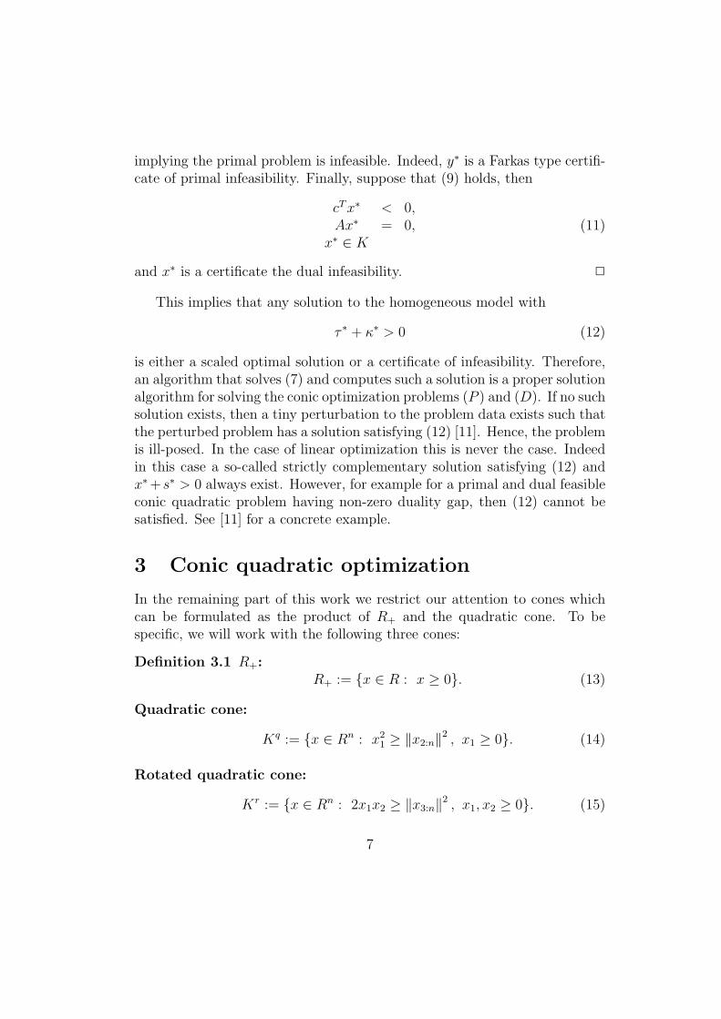
3 Conic quadratic optimization

In the remaining part of this work we restrict our attention to cones whichcan be formulated as the product of R+ and the quadratic cone. To bespecific, we will work with the following three cones:

Definition 3.1 R+:R+ := {x ∈ R : x ≥ 0}. (13)

Quadratic cone:

Kq := {x ∈ Rn : x21 ≥ ‖x2:n‖2 , x1 ≥ 0}. (14)

Rotated quadratic cone:

Kr := {x ∈ Rn : 2x1x2 ≥ ‖x3:n‖2 , x1, x2 ≥ 0}. (15)

7

These three cones are homogeneous and self-dual, see Definition A.1. With-out loss of generality it can be assumed that

K = K1 × . . .×Kk.

i.e. the cone K is the direct product of several individual cones each one ofthe type (13), (14), or (15) respectively. Furthermore, let x be partitionedaccording to the cones i.e.

x =

x1

x2

...xk

and xi ∈ Ki ⊆ Rni .

Associated with each cone are two matrices

Qi, T i ∈ Rni×ni

which are defined in Definition 3.2.

Definition 3.2 i.) If Ki is R+, then

T i := 1 and Qi = 1. (16)

ii.) If Ki is the quadratic cone, then

T i := Ini and Qi := diag(1,−1, . . . ,−1). (17)

iii.) If Ki is the rotated quadratic cone, then

T i :=

1√2

1√2

0 · · · 01√2− 1√

20 · · · 0

0 0 1 · · · 0...

......

. . ....

0 0 0 · · · 1

(18)

and

Qi :=

0 1 0 · · · 01 0 0 · · · 00 0 −1 · · · 0...

......

. . ....

0 0 0 · · · −1

. (19)

8

It is an easy exercise to verify that each Qi and T i are orthogonal. Hence

QiQi = I and T iT i = I.

The definition of the Q matrices allows an alternative way of stating thequadratic cone because assume Ki is the quadratic cone then

Ki = {xi ∈ Rni : (xi)TQixi ≥ 0, xi1 ≥ 0}

and if Ki is a rotated quadratic cone, then

Ki = {xi ∈ Rni : (xi)TQixi ≥ 0, xi1, xi2 ≥ 0}.

If the ith cone is a rotated quadratic cone, then

xi ∈ Kq ⇔ T ixi ∈ Kr.

which demonstrates that the rotated quadratic cone is identical to the qua-dratic cone under a linear transformation. This implies it is possible byintroducing some additional variables and linear constraints to pose the ro-tated quadratic cone as a quadratic cone. However, for efficiency reason wewill not do that but rather deal with the rotated cone directly. Nevertheless,from a theoretical point of view all the results for the rotated quadratic conefollow from the results for the quadratic cone.

For algorithmic purposes the complementarity conditions between theprimal and dual solution are needed. Using the notation that if v is a vector,then capital V denotes a related “arrow head” matrix i.e.

V := mat (v) =

[v1 vT2:n

v2:n v1I

]and v2:n :=

v2...vn

.The complementarity conditions can now be stated compactly as in Lemma3.1.

Lemma 3.1 Let x, s ∈ K then x and s are complementary, i.e. xT s = 0, ifand only if

X iSiei = SiX iei = 0, i = 1, . . . , k, (20)

where X i := mat (T ixi), Si := mat (T isi). ei ∈ Rni is the first unit vector ofappropriate dimension.

9

Proof: See the Appendix. 2

Subsequently let X and S be two block diagonal matrices with X i and Si

along the diagonal i.e.

X := diag(X1, . . . , Xk) and S := diag(S1, . . . , Sk).

Given v ∈ int(K), then it is easy to verify the following useful formula

mat (v)−1 = V −1 =1

v21 − ‖v2:n‖2

v1 −vT2:n

−v2:n

(v1 − ‖v2:n‖2

v1

)I +

v2:nvT2:n

v1

.3.1 The central path

The guiding principle in primal-dual interior-point algorithms is to followthe so-called central path towards an optimal solution. The central path isa smooth curve connecting an initial point and a complementary solution.Formally, let an (initial) point (x(0), τ (0), y(0), s(0), κ(0)) be given such that

(x(0); τ (0)), (s(0);κ(0)) ∈ int(K)

then the set of nonlinear equations

Ax− bτ = γ(Ax(0) − bτ (0)),ATy + s− cτ = γ(ATy(0) + s(0) − cτ (0)),

−cTx+ bTy − κ = γ(−cTx(0) + bTy(0) − κ(0)),XSe = γµ(0)e,τκ = γµ(0),

(21)

defines the central path parameterized by γ ∈ [0, 1]. Here µ(0) is given by theexpression

µ(0) :=(x(0))T s(0) + τ (0)κ(0)

k + 1.

and e by the expression

e :=

e1

...ek

.The first three blocks of equations in (21) are feasibility equations whereasthe last two blocks of equations are the relaxed complementarity conditions.

10

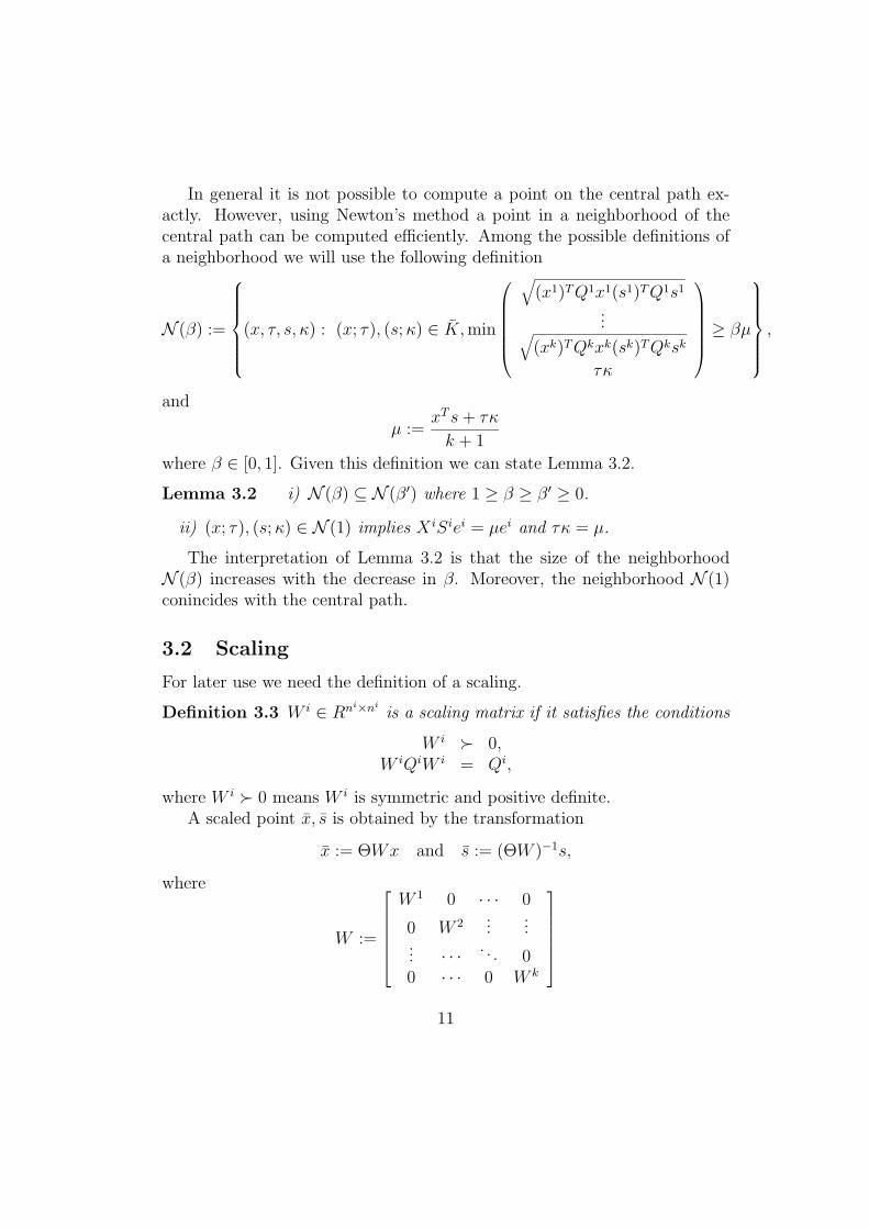
In general it is not possible to compute a point on the central path ex-actly. However, using Newton’s method a point in a neighborhood of thecentral path can be computed efficiently. Among the possible definitions ofa neighborhood we will use the following definition

N (β) :=

(x, τ, s, κ) : (x; τ), (s;κ) ∈ K,min

√(x1)TQ1x1(s1)TQ1s1

...√(xk)TQkxk(sk)TQksk

τκ

≥ βµ

,

and

µ :=xT s+ τκ

k + 1

where β ∈ [0, 1]. Given this definition we can state Lemma 3.2.

Lemma 3.2 i) N (β) ⊆ N (β′) where 1 ≥ β ≥ β′ ≥ 0.

ii) (x; τ), (s;κ) ∈ N (1) implies X iSiei = µei and τκ = µ.

The interpretation of Lemma 3.2 is that the size of the neighborhoodN (β) increases with the decrease in β. Moreover, the neighborhood N (1)conincides with the central path.

3.2 Scaling

For later use we need the definition of a scaling.

Definition 3.3 W i ∈ Rni×ni is a scaling matrix if it satisfies the conditions

W i � 0,W iQiW i = Qi,

where W i � 0 means W i is symmetric and positive definite.A scaled point x, s is obtained by the transformation

x := ΘWx and s := (ΘW )−1s,

where

W :=

W 1 0 · · · 0

0 W 2 ......

... · · · . . . 00 · · · 0 W k

11

andΘ = diag(θ11n1 ; . . . ; θk1nk).

1ni is the vector of all ones having the length ni and θ ∈ Rk.Hence, W is a block diagonal matrix having the W is along the diagonal

and Θ is a diagonal matrix.In Lemma 3.3 it is shown that scaling does not change anything. For

example if the original point is in the interior of the cone K then the scaledpoint is in the interior too. Similarly, if the original point belongs to a certainneighborhood, then the scaled point belong to the same neighborhood.

Lemma 3.3 i) (xi)T si = (xi)T si.

ii) θ2i (x

i)TQixi = (xi)TQixi.

iii) θ−2i (si)TQisi = (si)TQisi.

iv) x ∈ K ⇔ x ∈ K and x ∈ int(K)⇔ x ∈ int(K).

v) Given a β ∈ (0, 1) then

(x, τ, s, κ) ∈ N (β)⇒ (x, τ, s, κ) ∈ N (β).

Proof: See the Appendix. 2

4 The search direction

As mentioned previously the main algorithmic idea in a primal-dual interior-point algorithm is to trace the central path loosely. However, the central pathis defined by the nonlinear equations (21) which cannot easily be solved, butan approximate solution can be computed using Newton’s method. Indeedif one iteration of Newton’s method is applied to (21) for a fixed γ, then asearch direction (dx, dτ , dy, ds, dκ) is obtained. This search direction is givenas the solution to the linear equation system:

Adx − bdτ = (γ − 1)(Ax(0) − bτ (0)),ATdy + ds − cdτ = (γ − 1)(ATy(0) + s(0) − cτ (0)),

−cTdx + bTdy − dκ = (γ − 1)(−cTx(0) + bTy(0) − κ),X(0)Tds + S(0)Tdx = −X(0)S(0)e+ γµ(0)e,

τ (0)dκ + κ(0)dτ = −τ (0)κ(0) + γµ(0).

(22)

12

where

T :=

T 1 0 · · · 0

0 T 2 ......

... · · · . . . 00 · · · 0 T k

.This direction is a slight generalization of the direction suggested in [1] tothe homogeneous model. A new point is obtained by moving in the direction(dx, dτ , dy, ds, dκ) as follows

x(1)

τ (1)

y(1)

s(1)

κ(1)

=

x(0)

τ (0)

y(0)

s(0)

κ(0)

+ α

dxdτdydsdκ

(23)

for some step size α ∈ [0, 1]. This is a promising idea because if the searchdirection is well-defined, then the new point will be closer to being feasibleto the homogeneous model and complementary as shown in Lemma 4.1.

Lemma 4.1 Given (22) and (23) then

Ax(1) − bτ (1) = (1− α(1− γ))(Ax(0) − bτ (0)),ATy(1) + s(1) − cτ (1) = (1− α(1− γ))(ATy(0) + s(0) − cτ (0)),

−cTx(1) + bTy(1) − κ(1) = (1− α(1− γ))(−cTx(0) + bTy(0) − κ(0)),dTx d

Ts + dτdκ = 0,

(x(1))T s(1) + τ (1)κ(1) = (1− α(1− γ))((x(0))T s(0) + τ (0)κ(0)).

(24)

Proof: The first three equalities are trivial to prove, so we will only provethe last two equalities. First observe that

A(ηx(0) + dx)− b(ητ (0) + dτ ) = 0,AT (ηy(0) + dy) + (ηs(0) + ds)− c(ητ (0) + dτ ) = 0,−c(ηx(0) + dx) + bT (ηy(0) + dy)− (ηκ(0) + dκ) = 0,

whereη := 1− γ. (25)

This implies

0 = (ηx(0) + dx)T (ηs(0) + ds) + (ητ (0) + dτ )(ηκ

(0) + dκ)= η2((x(0))T s(0) + τ (0)κ(0))

+η((x(0))Tds + (s(0))Tdx + τ (0)dκ + κ(0)dτ )+dTx ds + dτdκ.

(26)

13

Moreover,

(x(0))Tds + (s(0))Tdx + τ (0)dκ + κ(0)dτ = eT (X(0)Tds + S(0)Tdx) + τ (0)dκ + κ(0)dτ= eT (−X(0)S(0)e+ γµ(0)e)− τ (0)κ(0) + γµ(0)

= (γ − 1)µ(0)k.

These two facts combined gives

dTx ds + dτdκ = 0

and(x(1))T s(1) + τ (1)κ(1) = (1− α(1− γ))((x(0))T s(0) + τ (0)κ(0)).

2

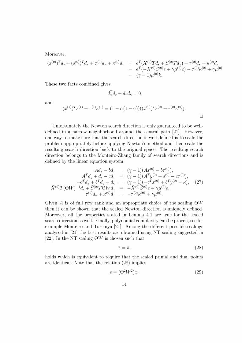
Unfortunately the Newton search direction is only guaranteed to be well-defined in a narrow neighborhood around the central path [21]. However,one way to make sure that the search-direction is well-defined is to scale theproblem appropriately before applying Newton’s method and then scale theresulting search direction back to the original space. The resulting searchdirection belongs to the Monteiro-Zhang family of search directions and isdefined by the linear equation system

Adx − bdτ = (γ − 1)(Ax(0) − bτ (0)),ATdy + ds − cdτ = (γ − 1)(ATy(0) + s(0) − cτ (0)),

−cTdx + bTdy − dκ = (γ − 1)(−cTx(0) + bTy(0) − κ),X(0)T (ΘW )−1ds + S(0)TΘWdx = −X(0)S(0)e+ γµ(0)e,

τ (0)dκ + κ(0)dτ = −τ (0)κ(0) + γµ(0).

(27)

Given A is of full row rank and an appropriate choice of the scaling ΘWthen it can be shown that the scaled Newton direction is uniquely defined.Moreover, all the properties stated in Lemma 4.1 are true for the scaledsearch direction as well. Finally, polynomial complexity can be proven, see forexample Monteiro and Tuschiya [21]. Among the different possible scalingsanalysed in [21] the best results are obtained using NT scaling suggested in[22]. In the NT scaling ΘW is chosen such that

x = s, (28)

holds which is equivalent to require that the scaled primal and dual pointsare identical. Note that the relation (28) implies

s = (Θ2W 2)x. (29)

14

In the case of NT scaling both Θ and W can be computed cheaply for eachof our cones as demonstrated in Lemma 4.2.

Lemma 4.2 Assume that xi, si ∈ int(Ki) then

θ2i =

√√√√ (si)TQisi

(xi)TQixi. (30)

Moreover, if Ki is

i) the positive half-line R+, then:

W i =1

θi((X i)−1Si)

12 .

ii) a quadratic cone, then:

W i =

wi1 (wi2:ni)T

wi2:ni I +wi

2:ni(wi

2:ni)T

1+wi1

= −Qi +

(ei1+wi)(ei1+wi)T

1+(ei1)Twi

(31)

where

wi =θ−1i si + θiQ

ixi

√2

√(xi)T si +

√(xi)TQixi(si)TQisi

. (32)

Furthermore,(W i)2 = −Qi + 2wi(wi)T . (33)

iii) a rotated quadratic cone, then:

W i = −Qi +(T iei1 + wi)(T iei1 + wi)T

1 + (ei1)TT iwi(34)

where wi is given by (32). Furthermore,

(W i)2 = −Qi + 2wi(wi)T . (35)

Proof: In case of the quadratic cone the Lemma is derived in [27], but weprefer to include a proof here for completeness. See the Appendix details. 2

15

Lemma 4.3 Let be W i be given as in Lemma 4.2 then

(θiWi)−2 = θ−2

i Qi(W i)2Qi.

Proof: Using Definition 3.3 we have that W iQiW i = Qi and QiQi = Iwhich implies (W i)−1 = QiW iQi and (W i)−2 = Qi(W i)2Qi. 2

One observation which can be made from Lemma 4.2 and Lemma 4.3 isthat the scaling matrix W can be stored by using an n dimensional vectorbecause only the vector wi has to be stored for each cone. Furthermore,any multiplication with W or W 2 or their inverses can be carried out inO(n) complexity. This is an important fact that should be exploited in animplementation.

4.1 Choice of the step size

After the search direction has been computed then a step size has to bechosen. It can be shown given the primal-dual algorithm is initiated with asolution sufficiently close to the central path and γ is sufficiently close to 1,then the unit step size (α = 1) is always a suitable choice which also makessure that the iterates stay in a close neighborhood of the central path.

However, in practice an aggressive choice of γ give rise to vastly improvedperformance. This makes it necessary to use a step size smaller than one,because otherwise the updated solution may move too far from the centralpath and even be infeasible with respect to the cone constraint.

In general the step size α should be chosen such that

(x(1), τ (1), s(1), κ(1)) ∈ N (β) (36)

where β ∈ (0, 1) is a fixed constant. Next we will discuss how to computethe step size to satisfy this requirement.

First define

vx1i := (xi)TQixi, vx2

i := 2dTxiQixi, and vx3

i := dTxiQidxi

and define vs1i , vs2i , and vs3i in a similar way. Next define

fxi (α) := (xi + αdxi)TQi(xi + αdxi) = vx1

i + αvx2i + α2vx3

i , (37)

andf si (α) := (si + αdsi)

TQi(si + αdsi) = vs1i + αvs2i + α2vs3i . (38)

16

Note given the v vectors have been computed, then fxi (·) and f si (·) can beevaluated in O(k) complexity. Now define αmax such that it is maximal andsatisfies

(ei)T (x(0) + αdx) ≥ 0, ∀i, α[0, αmax],(ei)T (s(0) + αds) ≥ 0, ∀i, α[0, αmax],

(ei)TQi(x(0) + αdx) ≥ 0, ∀i, α[0, αmax],(ei)TQi(s(0) + αds) ≥ 0, ∀i, α[0, αmax],

τ + αdτ ≥ 0, ∀α[0, αmax],κ+ αdκ ≥ 0, ∀α[0, αmax],fx(α) ≥ 0, ∀α[0, αmax],fs(α) ≥ 0, ∀α[0, αmax].

The purpose of the first four inequalities is to make sure that the appropriateelements of x and s stay positive. The choice of αmax implies that for anyα ∈ (0, αmax) we have

(x(1); τ (1)), (s(1);κ(1)) ∈ int(K).

Next a decreasing sequence of αl’s for l = 1, 2, . . . in the interval (0, αmax) ischosen and the largest element in the sequence which satisfies√

fx(αl)fs(αl) ≥ β(1− αl(1− γ))µ(0),

(τ (0) + αldτ )(κ(0) + αldκ) ≥ β(1− αl(1− γ))µ(0),

(39)

is chosen as the step size. Enforcing the condition (39) is equivalent to enforcethe condition (36).

4.2 Adapting Mehrotra’s predictor-corrector method

Several important issues have not been addressed so far. In particular noth-ing has been stated about the choice of γ. In theoretical work on primal-dualinterior-point algorithms γ is usually chosen as a constant close to one but inpractice this leads to slow convergence. Therefore, in the linear case Mehro-tra [19] suggested a heuristic which chooses γ dynamically depending on howmuch progress that can be made in the pure Newton (affine scaling) direc-tion. Furthermore, Mehrotra suggests using a second-order correction of thesearch direction which increases the efficiency of the algorithm significantlyin practice [18].

17

In this section we discuss how these two ideas proposed by Mehrotra canbe adapted to the primal-dual method based on the Monteiro-Zhang familyof search directions.

Mehrotra’s predictor-corrector method utilizes the observation that

mat (Tx) + mat (Tdx) = mat (T (x+ dx))

which implies

(X +Dx)(S +Ds)e = mat (T (x+ dx)) mat (T (s+ ds)) e= XSe+ SDxe+XDse+DxDse,

whereDx := mat (Tdx) and Ds := mat (Tds) .

When Newton’s method is applied to the perturbed complementarity condi-tions

XS = γµ(0)e

then the quadratic termDxDse (40)

is neglected and the search direction is obtained by solving the resultingsystem of linear equations. Instead of neglecting the quadratic term, thenMehrotra suggests estimate it using the pure Newton direction. Indeed,Mehrotra suggests to compute the primal-dual affine scaling direction

(dnx, dnτ , d

ny , d

ns , d

nκ)

first which is the unique solution of (27) for γ = 0. Next this direction isused to estimate the quadratic term as follows

DxDse ≈ DnxD

ns e and dτdκ ≈ dnτ d

nκ.

In the framework of the Monteiro-Zhang family of search directions this im-plies that the linearized complementarity conditions in (27) are replaced by

X(0)T (ΘW−1ds + S(0)TΘWdx = −X(0)S(0)e+ γµ(0)e− DnxD

ns e,

τ (0)dκ + κ(0)dτ = −τ (0)κ(0) + γµ(0) − dnτ dnκ

where

Dnx := mat (TΘWdnx) and Dn

s := mat(T (ΘW )−1dns

).

18

Note that even though the corrector term is included in the right-hand sidethen it can be proved that the final search direction satisfies all the propertiesstated in Lemma 4.1.

Mehrotra suggests another use of the pure Newton direction because hesuggests to use it for a dynamic choice of γ based on how much progressthat can be made in the affine scaling direction. Now let αmax

n be the max-imum step size to the boundary which can be taken along the pure Newtondirection. According to Lemma 4.1 this implies that the residuals and thecomplementarity gap are reduced by a factor of

1− αmaxn .

Then it seems reasonable to choose γ small if αmaxn is large. The heuristic

γ = min(δ, (1− αmaxn )2)(1− αmax

n )

achieve this, where δ ∈ [0, 1] is a fixed constant.

4.3 Adapting Gondzio’s centrality correctors

In Mehrotra’s predict-corrector method the search direction is only correctedonce. An obvious idea is to repeat the corrections several times to obtaina high-order search directions. However, most of the computational exper-iments with this idea has not been successful. More recently Gondzio [14]has suggested another modification to the primal-dual algorithm for linearoptimization which employs so-called centrality correctors. The main ideaunderlying this approach is to compute corrections to the search direction insuch a way that the step size increases and hence faster convergence of thealgorithm is achieved.

The idea of centrality correctors can successfully be adapted to the casewhen the earlier presented homogeneous primal-dual algorithm is appliedto a linear optimization problem[6]. Therefore, in the present section wewill discuss how to adapt the centrality corrector idea to the case when theoptimization problem contains quadratic cones.

As mentioned previously then the iterates generated by our algorithmshould stay in a close neighborhood of the central path or, ideally,

(x(1), τ (1), s(1), κ(1)) ∈ N (1).

19

This implies that we are targeting√(xi(1))TQixi(1)(si(1))TQisi(1) = τ (1)κ(1) = µ(1).

However, this is in general a too ambitious target to reach and many itera-tions of Newton’s method may be required to compute a good approximationof such a point. However, it might be possible to reach the less ambitioustarget

µl ≤

√(x

(1)1 )TQ1x

(1)1 (s

(1)1 )TQ1s

(1)1

...√(x

(1)k )TQkx

(1)k (s

(1)k )TQks

(1)k

τ (1)κ(1)

≤ µu (41)

where µl and µu are suitably chosen constants. We will use the perhapsnatural choice

µl = λγµ(0) and µu = λ−1γµ(0)

for some λ ∈ (0, 1).Now assume a γ and a search direction (dx, dτ , dy, ds, dκ) have been com-

puted as discussed in the previous sections and if for example√fxi (α)f si (α) < µl (42)

for a reasonably chosen α, then we would like to compute a modification ofthe search direction such that the left-hand side of (42) is increased whenthe corrected search direction is employed.

This aim can be achieved as follows. First define

f i =

µlei − (X(0) + αDx)(S

(0) + αDs)ei, fxi (α)f si (α) ≤ (µl)2,

µuei − (X(0) + αDx)(S(0) + αDs)e

i, fxi (α)f si (α) ≥ (µu)2,0ei, otherwise

(43)

and

fτκ =

µl − (τ (0) + αdτ )(κ

(0) + αdκ), (τ (0) + αdτ )(κ(0) + αdκ) ≤ µl,

µu − (τ (0) + αdτ )(κ(0) + αdκ), (τ (0) + αdτ )(κ

(0) + αdκ) ≥ µu,0, otherwise.

(44)

20

Moreover, let

f :=

f 1

...fk

and

µc := γµ(0) − eTf + fτκk + 1

, (45)

then we will define a corrected search direction by

Adx − bdτ = (γ − 1)(Ax(0) − bτ (0)),ATdy + ds − cdτ = (γ − 1)(ATy(0) + s(0) − cτ (0)),

−cTdx + bTdy − dκ = (γ − 1)(−cTx(0) + bTy(0) − κ),X(0)T (ΘW )−1ds + S(0)TΘWdx = −X(0)S(0)e+ µce− Dn

xDns + f,

τ (0)dκ + κ(0)dτ = −τ (0)κ(0) + µc − dnτ dnκ + fτκ.

(46)

Note compared to the original search direction then only the right-hand sideof the linearized complementarity conditions have been modified. Next let ηbe given by (25) then due to

A(ηx(0) + dx)− b(ητ (0) + dτ ) = 0,AT (ηy(0) + dy) + (ηs(0) + ds)− c(ητ (0) + dτ ) = 0,

−cT (ηx(0) + dx) + bT (ηy(0) + dy)− (ηκ(0) + dκ) = 0,

holds the orthogonality of the search direction holds as well i.e. (26) holds.Furthermore, we have that

(x(0))Tds + (s(0))Tdx + τ (0)dκ + κ(0)dτ= eT (X(0)T (ΘW )−1ds + S(0)TΘWdx) + τ (0)dκ + κ(0)dτ= eT (−X(0)S(0)e+ µce− Dn

xDns + f − τ (0)κ(0) + µc − dnτ dnκ + fτκ)

= −(x(0))T s(0) − τ (0)κ(0) + µc(1 + eT e)− eT DnxD

ns e− dnτ dnκ + eTf + fτκ

= (γ − 1)((x(0))T s(0) + τ (0)κ(0))

because of the facteT Dn

xDns e+ dnτ d

nκ = 0

and the definition of t and tτκ. The combination of these facts leads to theconclusion

dTx ds + dτdκ = 0.

21

Hence, the search direction defined by (46) satisfies all the properties ofLemma 4.1.

After the corrected search direction defined by (46) has been computedthen the maximal step size αmax is recomputed. However, there is nothingwhich guarantees that the new maximal step size is larger than the step sizecorresponding to original search direction. If this is not the case, then thecorrected search direction is discarded and the original direction is employed.

Clearly, this process of computing corrected directions can be repeatedseveral times, where the advantage of computing several corrections is thatthe number of iterations (hopefully) is further decreased. However, the com-putation of the corrections is not free so there is a trade-off between thetime it takes to compute an additional corrected search direction and theexpected reduction in the number of iterations. Therefore, the maximumnumber of corrections computed is determined using a strategy similar tothat of Gondzio [14]. Moreover, an additional correction is only computed ifthe previous correction increases the step size by more than 20%.

5 Computing the search direction

The computationally most expensive part of a primal-dual algorithm is thecomputation of the search direction because this involves the solution of apotentially very large system of linear equations. Indeed, in each iteration ofthe primal-dual algorithm, a system of linear equations of the form

Adx − bdτ = r1,ATdy + ds − cdτ = r2,

−cTdx + bTdy − dκ = r3,X(0)T (ΘW )−1ds + S(0)TΘWdx = r4,

τ (0)dκ + κ(0)dτ = r5

(47)

must be solved for several different right-hand sides r. An important factis that for most large-scale problems appearing in practice, then the ma-trix A is sparse. This sparsity can and should be exploited to improve thecomputational efficiency.

Before proceeding with the details of the computation of the search direc-tion then recall that any matrix-vector product involving the matrices X(0),S(0), T , W , Θ, W 2, and Θ2, or their inverses, can be carried out in O(n)

22

complexity. Hence, these operations are computationally cheap operationsand will not be considered further.

The system (47) can immediately be reduced by eliminating ds and dκfrom the system using

ds = ΘWT (X(0))−1(r4 − S(0)TΘWdx),dκ = (τ (0))−1(r5 − κ0dτ ).

(48)

Next let (g1, g2) and (h1, h2) be defined as the solutions to[−(ΘW )2 AT

A 0

] [g1

g2

]=

[cb

](49)

and [−(ΘW )2 AT

A 0

] [h1

h2

]=

[r2 −ΘWT (X(0))−1r4

r1

]. (50)

Given A is of full rank, then these two systems have a unique solution.Moreover, we have that

dτ =r3 − cTh1 + bTh2

(τ (0))−1κ(0) + cTg1 − bTg2

and [dxdy

]=

[g1

g2

]+

[h1

h2

]dτ .

After dτ and dx have been computed, then ds and dκ can be computed usingrelation (48). Therefore, given (49) and (50) can be solved efficiently, thenthe search direction can be computed efficiently as well. Now the solution to(49) and (50) is given by

g2 = (A(ΘW )−2AT )−1(b+ A(ΘW )2c),g1 = −(ΘW )−2(c− ATg2),

and

h2 = (A(ΘW )−2AT )−1(r1 + A(ΘW )2(r2 − (ΘWTX(0))−1r4)),h1 = −(ΘW )−2(r2 −ΘW (X(0))−1r4 − ATh2),

respectively. Hence, we have reduced the computation of the search directionto computing

(A(ΘW )−2AT )−1

23

or equivalently to solve a linear equation system of the form

Mh = f

whereM := A(ΘW )−2AT .

Recall W is a block diagonal matrix having the W is along the diagonal.Moreover, Θ is a positive definite diagonal matrix. This implies (ΘW )2 isa positive definite block diagonal matrix and hence M is symmetric andpositive definite. Therefore, M has a Cholesky factorization i.e.

M = LLT

where L is a lower triangular matrix. It is well-known that if the matrix M issparse, then the Cholesky factorization can usually be computed efficiently inpractice. This leads to the important questions whether M can be computedefficiently and whether M is likely to be sparse.

First observe that

M = A(ΘW )−2AT =k∑i=1

θ−2i Ai(W i)−2(Ai)T ,

where Ai is the columns of A corresponding to the variables in xi. In thecase the ith cone is R+ then W i is a scalar and Ai is a column vector. Thisimplies the term

Ai(W i)−2(Ai)T

can easily be computed and is sparse if Ai is sparse. In the case the ith coneis a quadratic or a rotated quadratic cone then

Ai(W i)−2(Ai)T = AiQi(−Qi + 2wi(wi)T )Qi(Ai)T

= −AiQi(Ai)T + 2(AiQiwi)(AiQiwi)T ,(51)

which is a sum of two terms. The term

(AiQiwi)(AiQiwi)T

is sparse if the vectorAiQiwi (52)

is sparse and Ai contains no dense columns. Note if ni is large, then itcannot be expected that (52) is sparse, because the sparsity pattern of (52)

24

is identical to the union of the sparsity patterns of all the columns in Ai.The term

AiQi(Ai)T (53)

also tends to be sparse. Indeed in the case the ith cone is a quadratic conethen the sparsity pattern of (53) is identical to the sparsity pattern of Ai(Ai)T

which is likely to be sparse given Ai contains no dense columns. In the caseof the rotated quadratic cone we have that

AiQi(Ai)T = Ai:1(Ai:2)T + Ai:2(Ai:1)T − Ai:(3:ni)(Ai:(3:ni))

T .

This term is likely to be sparse except if the union of the sparsity patternsin Ai:1 and Ai:2 are dense or Ai contain dense columns. (Ai:j denotes the jthcolumn of Ai and Ai:(j:k) denotes the columns j to k of Ai.)

In summary if all the vectors wi are of low dimmension and the columnsof Ai are sparse, then M can be expected to be sparse which implies that theNewton equation system can be solved very efficiently using the Choleskyfactorization.

In the computational results reported in Section 8 we use this approach.Details about how the Cholesky decomposition is computed can be seen in[5, 6].

5.1 Exploiting structure in the constraint matrix

In practice most optimization problems have some structure in the constraintmatrix which can be exploited to speed up the computations. In our imple-mentation we exploit the following two types of constraint structures:

Upper bound constraints: If a variable xj has both a lower and an upperbound, then an additional constraint of the form

xj + xk = u

must be introduced where xk is a slack variable and therefore occurs inonly one constraint.

Singleton constraints: For reasons that becomes clear in Section 7.1, con-straints of the form

xj = b

25

frequently arises where xj only occurs in one constraint. Moreover,we will assume that xj does not belong to a linear cone because suchvariable can simply be substituted out of the problem.

Exploiting the upper bound constraints is trivial and similar to the purelinear optimization case as discussed in for example [7]. Therefore, we willnot discuss this case further and the subsequent discussion is limited to thesingleton constraints case only.

After a suitable reordering of the variables and the constraints, we mayassume A has the form

A =

[0 A12

I 0

]where

[ I 0 ]

corresponds to the set of singleton constraints. This observation can beexploited when solving the systems (49) and (50). Subsequently we willdemonstrate how to do this for the system (49).

First assume that the vector g and the right-hand side of the system hasbeen partitioned similar to A and according to the partition of

H :=

[−H11 −H12

−H21 −H22

]= −(ΘW )−2.

This implies the system (49) may be written as−H11 −H12 0 I−H21 −H22 AT12 0T

0 A12 0 0I 0 0 0

g1

1

g12

g21

g22

=

c1

c2

b1

b2

.

This large system can be reduced to the two small systems[−H22 AT12

A12 0

] [g2

1

g12

]=

[c2

b1

]+

[H21b2

0

](54)

and [−H11 IT

I 0

] [g1

1

g22

]=

([c1

b2

]−[−H12 0

0 0

] [g2

1

g12

])(55)

26

that has to be solved in the order as stated. First observe that the secondsystem (55) is trivial to solve whereas system (54) is easily solved if theinverses or appropriate factorizations of the matrices

H22

andA21H

−122 A

T21 (56)

are known. Next observe that A21 is of full row rank because A is of fullrow rank. Finally, due to H is positive definite, then H22 is positive definitewhich implies that matrix (56) is positive definite.

Since matrix H22 is identical to H, except some rows and columns havebeen removed, then H22 is also a block diagonal matrix where each blockoriginate from a block in H. Subsequently we will show that the inverse ofeach block in H22 can be computed efficiently.

In the discussion we will assume that H22 consists of one block only. Itshould be obvious how to extend the discussion to the case of multiple blocks.Any block in H can be written in the form

−Q+ 2wwT ,

where we have dropped the cone subscript i for convenience. Here Q is eitherof the form (17) or (19) and w is a vector. Next we will partition the blockto obtain

−[Q11 Q21

Q12 Q22

]+ 2

[w1

w2

] [w1

w2

]T.

After dropping the appropriate rows and columns we assume we are left withthe H22 block

−Q11 + 2w1wT1

which we have to compute an inverse of. First assume Q11 is nonsingularthen by the Sherman-Morrison-Woodbury formula1 we have that

(−Q11 + 2w1wT1 )−1 = −Q−1

11 − 2Q−1

11 w1wT1 Q−111

1− 2wT1 Q−111 w1

which is the required explicit representation for the inverse of the block.

1If the matrices B and matrix B + vvT are nonsingular, then 1 + vTB−1v is nonzeroand (B + vvT )−1 = B−1 − B−1vvTB−1

1+vTB−1v.

27

In most cases Q11 is a nonsingular matrix, because it is only singular ifthe block corresponds to a rotated quadratic cone and either x1 or x2 but notboth variables are fixed. This implies that in the case Q11 is singular then itcan be assumed that Q11 has the form

Q11 =

[0 00 I

].

Now let

w1 =

[w1

w2

]where w1 is a scalar and it can be verified that w1 > 0. It is now easy toverify that

−Q11 + 2w1wT1 = FF T

where

F :=

[ √2w1 0√2w2 I

]and F−1 =

[1√2w1

0

− w2

w1I

].

Hence,

(−Q11 + 2w1wT1 )−1 = (FF T )−1

=

1+2‖w2‖22w2

1− wT2

w1

− w2

w1I

=

1+2‖w2‖22w2

10

0 I

− 1w1

[ 0w2

]eT1 + e1

[0w2

]T ,which is the explicit representation of the inverse of the H22 block we werelooking for. In summary instead of computing a factorization ofA(ΘW )−2AT ,then it is sufficient to compute a factorization of the potentially much smallermatrix (56) plus additional cheap linear algebra.

6 Starting and stopping

6.1 Starting point

In our implementation we use the simple starting point:

xi(0) = si(0) = T iei1.

28

Moreover, let y(0) = 0 and τ (0) = κ(0) = 1. This choice of starting pointimplies that

(x(0), τ (0), s(0), κ(0)) ∈ N (1).

In the special case of linear optimization, the algorithm presented here isequivalent to the algorithm studied in Andersen and Andersen [6]. However,they employ a different starting point, than the one suggested above, whichimproves the practical efficiency for the linear case. Therefore, it might bepossible to develop another starting point which works better for most prob-lems occurring in practice. However, this is a topic left for future research.

6.2 Stopping criteria

An important issue is when to terminate the interior-point algorithm. Ob-viously the algorithm cannot be terminated before a feasible solution to thehomogeneous model has been obtained. Therefore, to measure the infeasi-bility the following measures

ρ(k)P :=

‖Ax(k)−bτ (k)‖max(1,‖Ax(0)−bτ (0)‖)

,

ρ(k)D :=

‖AT y(k)+s(k)−cτ (k)‖max(1,‖AT y(0)+s(0)−cτ (0)‖)

,

ρ(k)G := |−cT x(k)+bT y(k)−κ(k)|

max(1,|−cT x(0)+bT y(0)−κ(0)|)

are employed which essentially measure the relative reduction in the primal,dual, and gap infeasibility respectively. Also define

ρ(k)A :=

|cTx(k) − bTy(k)|τ (k) + |bTy(k)|

=|cTx(k)/τ (k) − bTy(k)/τ (k)|

1 + |bTy(k)/τ (k)|(57)

which measures the number of significant digits in the objective value. Thekth iterate is considered nearly feasible and optimal if

ρ(k)P ≤ ρP , ρ

(k)D ≤ ρD, and ρkA ≤ ρA,

where ρP , ρD, ρA ∈ (0, 1] are (small) user specified constants. In this case thesolution

(x∗, y∗, s∗) = (x(k), y(k), s(k))/τ (k)

is reported to be the optimal solution to (P ).

29

The algorithm is also terminated if

ρ(k)P ≤ ρP , ρ

(k)D ≤ ρD, ρ

(k)G ≤ ρG, and τ (k) ≤ ρI max(1, κ(k)),

where ρI ∈ (0, 1) is a small user specified constant. In this case a feasi-ble solution to the homogeneous model with a small τ has been computed.Therefore, it is concluded that the problem is primal or dual infeasible. IfbTy(k) > 0, then the primal problem is concluded to be infeasible and ifcTx(k) < 0, then the dual problem is concluded to be infeasible. Moreover,the algorithm is terminated if

µ(k) ≤ ρµµ(0) and τ (k) ≤ ρI min(1, κ(k))

and the problem is reported to be ill-posed. ρA, ρG, ρµ, ρI ∈ (0, 1] are all userspecified constants.

7 Implementation

The algorithm for solving conic quadratic optimization problems have nowbeen presented in details and we will therefore turn the attention to a fewimplementational issues.

7.1 Input format

In practice an optimization problem is usually specified by using an MPS fileor a modeling language such as AIIMS, AMPL, GAMS, or MPL. However,none of these formats allow the user to specify that a part of x belongs toa quadratic cone (or a semi-definite cone). Indeed they can only handleconstraints of the type2

g(x) ≤ 0.

However, the two quadratic cones the proposed algorithm can handle is givenby

{x ∈ Rn : x21 ≥ ‖x2:n‖2 , x1 ≥ 0}

and{x ∈ Rn : 2x1x2 ≥ ‖x3:n‖2 , x1, x2 ≥ 0}

2Of course these formats can also handle equalities, but that does not help.

30

which are quadratic constraints of the form

g(x) =1

2xTQx+ aTx+ b ≤ 0. (58)

plus some additional bounds on the variables. Hence, it is possible to spec-ify any conic quadratic optimization problem using quadratic inequalities.Therefore, any input format which allows description of linear and quadraticconstraints can be used as an input format. Such an input format will ofcourse also allow the specification of nonconvex quadratic problems andtherefore it is necessary to require that Q has a particular form. In ourimplementation we require that Q has the form

q11 0 · · · 00 q22 · · · 0...

.... . .

...0 0 · · · qnn

(59)

or

q11 0 . . . · · · · · · · · · 00 q22 . . . · · · · · · · · · 0...

.... . . · · · · · · · · · 0

......

... 0 qij · · · 0...

...... qji 0 · · · 0

......

......

.... . .

...0 0 0 0 0 · · · qnn

. (60)

First note that by introducing some additional variables and linear con-straints then it can be assumed that no two Q matrices has a nonzero inthe same positions. Moreover, by introducing some additional linear con-straints and by rescaling the variables then it can be assumed that all theelements in the matrices Q belong to the set {−1, 0, 1}.

We will therefore assume this is the case. After this transformation itis checked whether any of the quadratic inequalities falls into one of thefollowing cases.

Case 1: Q has the form (59). Moreover, assume all the diagonal elements in Qare positive, a = 0, and b ≤ 0. In this case the constraint (58) can bewritten as

u =√−2b,

xTQx ≤ u2, u ≥ 0,

31

where u is an additional variable.

Case 2: Q has the form (59) and all the diagonal elements are positive. In thiscase the constraint (58) can be written as

u+ aTx+ b = 0,xTQx ≤ 2uv, u, v ≥ 0,

v = 1,

where u and v are two additional variables.

Case 3: Q has the form (60) and all the diagonal elements are positive exceptthe jth element i.e., qjj < 0. Moreover, the assumptions xj ≥ 0, a = 0,and b ≥ 0 should be satisfied. In this case the constraint (58) can bewritten as

u =√

2b(xTQix− qjjx2

j) + u2 ≤ −qjjx2j ,

where u is an additional variable. If b = 0, then it is not necessary tointroduce u.

Case 4: Q has the form (60) and all the diagonal elements are positive andqij < 0. Moreover,the assumptions xi, xj ≥ 0, a = 0, and b ≥ 0 shouldbe satisfied. In this case the constraint (58) can be written as

u =√

2b,xTQx− 2qijxjxi + u2 ≤ −2qijxixj,

where u is an additional variable.

Observe that it is computationally cheap to check whether one of the fourcases occurs for a particular quadratic inequality.

In all four cases a modified quadratic inequality is obtained possibly af-ter the inclusion of some linear variables and constraints. Moreover, thesequadratic inequalities can be represented by quadratic cones implying a conicquadratic optimization problem in the required form is obtained. (This mayinvolve the introduction of some additional linear constraints to make theappropriate variables in the cone free i.e. instead of letting xi be a memberof a cone, then a constraint having the form xi = xj is introduced and we letxj be a member of the cone.)

32

Hence, in our implementation we assume that the user specifies the conicquadratic optimization problem using linear constraints and quadratic in-equalities. Moreover, it is implemented such that the system checks whetherthe quadratic inequalities can be converted to conic quadratic form and thisconversion is automatic if the quadratic inequalities satisfy the weak require-ments discussed above.

7.2 Presolving the problem

Before the problem is optimized it is preprocessed to remove obvious redun-dancies using most of the techniques presented in [4]. For example fixedvariables are removed, obviously redundant constraints are removed, lineardependencies in A are removed. Finally, some of the linear free variables aresubstituted out of the problem.

8 Computational results

A complete algorithm for solution of conic quadratic optimization problemshas now been specified and we will now turn our attention to evaluating thepractical efficiency of the presented algorithm.

The algorithm has been implemented in the programming language C andis linked to the MOSEK optimizer3. During the computational testing allthe algorithmic parameters are held constant at the values shown in Table 1.In the computational results reported, then the method of multiple correc-tors is not employed because it gave only rise to insignificant saving in thecomputation time.

The computational test is performed on a 333MHZ PII based PC having256MB of RAM. The operating system used is Windows NT 4.

In Table 2 the test problems are shown along with the size of the problemsbefore and after the presolve procedure has been applied to the problems.The test problem comes from different sources. The problems belonging tothe nb*, nql*, qssp*, and *socp families are all DIMACS Challenge prob-lems [24]. The dttd* family of problems are multi load truss topology designproblems, see [11, p. 117]. The traffic* problems arises from a model de-veloped by C. Roos to study a traffic phenomena. The remaining problemshave been obtained by the authors from various sources. The problems in

3See http://www.mosek.com

33

Constant Value Sectionβ 10−8 3.1δ 0.5 4.2ρP 10−8 6.2ρD 10−8 6.2ρA 10−8 6.2ρG 10−8 6.2ρI 10−10 6.2ρµ 10−10 6.2

Table 1: Algorithmic parameters.

the nql* and qssp* families have previously been solved in [10] and are dualproblems of minimum sum of norms problems.

It is evident from Table 2 that the presolve procedure in some cases iseffective at reducing the problem size. In particular the nql* and traffic*

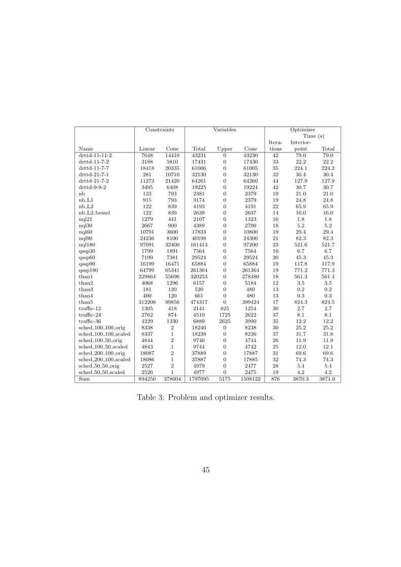
models are reduced significantly by the presolve procedure.The purpose of the subsequent Table 3 is to show various optimizer related

statistics i.e. the size of the problems actually solved and performance relatedstatistics. Recall that in some cases additional constraints and variables areadded to the problems to state them in the required conic quadratic form.The first two columns of Table 3 show the number of constraints and thenumber of cones in each problem. Next the total number of variables, thenumber variables which has both a finite lower and upper bound, and thenumber of variables which is member of a cone are shown. Finally, thenumber interior-point iterations performed to optimize the problems, thetime spend in the interior-point optimizer, and the total solution time areshown.

The main conclusion that can be drawn from Table 3 is even though someof the problems are large, then the total number of interior-point iterationsrequired to solve each problem are small. An important observation is thatthe number of iterations tend to grow slowly with the problem size. This canfor instance be observed for the nql* and qssp* problems.

Finally, in Table 4 we show feasibility and optimality related measures.The columns primal and dual feasibility report the numerator in ρ

(∗)P and

ρ(∗)D respectively. The first “primal objective” and “Sig fig.” columns show

the value cTx∗ the number figures that are identical in the optimal primal

34

and dual objective values as reported by the interior-point optimizer. In allcases those numbers demonstrate that the required accuracy is achieved andabout 8 figures in the reported primal and dual objective values are identi-cal. The final two columns of Table 4 shows the optimal primal objectivevalue reported to the user specified model and the corresponding number ofsignificant figures. Recall, that the optimization problems are specified usingquadratic inequalities but is solved on conic form. Hence, the solution to theconic model has to be converted to a primal and dual solution to the modelbased on the quadratic inequalities.

In general it can be seen that the primal objective value reported by theinterior-point optimizer and the one corresponding to the converted primalsolution is almost identical. However, the number of significant figures is notso high. This indicates the dual solution looses some of the accuracy whenit is converted.

9 Conclusion

The present work discusses a primal-dual interior-point method designed tosolve large-scale sparse conic quadratic optimization problems. The maintheoretical features of the algorithm is that it employs the Nesterov-Toddsearch direction and the homogeneous model. Moreover, the algorithm hasbeen extended with a Mehrotra predicter-corrector scheme, treats the rotatedquadratic cone without introducing additional variables and constraints andemploys structure and sparsity exploiting linear algebra.

The presented computational results indicates that the suggested algo-rithm is capable of computing accurate solutions to very large sparse conicquadratic optimization problems in a fairly low amount of time.

Although the proposed algorithm works well then, some work is left for thefuture. Particularly it might be possible to invent a heuristic for computing agood starting point which might improve the efficiency of the algorithm. Alsoit should be possible to specify the problem directly in conic form instead ofusing the implicit form based on quadratic inequalities. This would make iteasy to report an accurate optimal dual solution.

Acknowledgement: We would like to thank K. D. Andersen and A.Nemirovskii for helping us during the collection of the test problems.

35

A Appendix

Definition A.1 Let K be a pointed and closed convex cone, then K is self-dual if

K = K∗

and homogeneous if for any x, s ∈ int(K) we have

∃B ∈ Rn×n : B(K) = K, Bx = s.

Self-dual and homogeneous cones have been studied extensively in the liter-ature and is called self-scaled by Nesterov and Todd.

Proof of Lemma 3.1:

We first prove X iSi = 0 implies (xi)T si = 0. Observe that

eTXSe =n∑i=1

(ei)TX iSiei

=k∑i=1

(T ixi)TT isi

= xT s.

(61)

This implies that any solution satisfying (20) is also a complementary solu-tion. Next we prove if (xi)T si = 0, then X iSiei = 0. In explicit form thecomplementarity conditions can be stated as

(xi)T si = 0,(T ixi)1(T isi)2:n + (T isi)1(T ixi)2:n = 0.

Note that T ixi, T isi ∈ Kq. This implies if either (T ixi)1 = 0 or (T isi)1 = 0then (20) is true as claimed. Therefore, assume this is not the case. Since xand s are complementary then

0 = xT s

=k∑i=1

(T ixi)TT isi

≥k∑i=1

(T ixi)1(T isi)1 − ‖(T ixi)2:n‖ ‖(T isi)2:n‖

≥k∑i=1

√(xi)TQixi(si)TQisi

≥ 0

36

The first inequality follows from the Cauchy-Schwartz inequality and thesecond inequality follows from T ixi, T isi ∈ Kq. This implies that both(xi)TQixi = 0 and (si)TQisi = 0 are the case. Moreover, we conclude that

(T ixi)1(T isi)1 =∥∥∥(T ixi)2:n

∥∥∥ ∥∥∥(T isi)2:n

∥∥∥ .However, this can only be the case if

∃α : (T ixi)2:n = α(T isi)2:n

for some α ∈ R. Therefore, given the assumptions we have

0 = (xi)T si

= (T ixi)1(T isi)1 + α ‖(T isi)2:ni‖2

and

α = −(T ixi)1

(T isi)1

implying the complementarity conditions (20) are satisfied.

Proof of Lemma 3.3:

i), ii), and iii) follows immediately from the definition of a scaling. iv) isproved next. In the case Ki is R+ then the statement is obviously true. Inthe case Ki is the quadratic cone then due to W iQiW i = I we have that

w21 − ‖w2:n‖2 = 1,

where w denotes the first row of W i because. This implies

x1i = (ei)T xi

= (ei)TΘW ixi

= θi(w1xi1 + wT2:nx

i2:n)

≥ θi(w1xi1 − ‖w2:ni‖ ‖xi2:n‖)

= θi(√

1 + ‖w2:ni‖2xi1)≥ θix

i1

≥ 0

and(xi)TQixi = θi(x

i)TQixi ≥ 0.

37

Hence, xi ∈ Ki implies xi ∈ Ki for the quadratic cone. Similarly, it easyto verify xi ∈ int(Ki) implies xi ∈ int(Ki). Now assume Ki is a rotatedquadratic cone and xi, si ∈ Ki. Let xi := T ixi and si := T isi then xi, si ∈ Kq.Therefore, a scaling θiW

i exist such that

si = T isi = (θiWi)2T ixi = (θiW

i)2xi,

where

θ2i =

√(T isi)T QiT isi

(T ixi)T QiT ixi

= θ2i .

This impliessi = θ2

i Ti(W i)2T ixi

which shows W i = T iW iT i. We know that θiWiT ixi ∈ Kq and hence

θiTiW iT ixi = θiW

ixi ∈ Kr. vi) Follows from v) and the fact√xTQxsTQs =√

xTQxsTQs.

Proof of Lemma 4.2:

(30) follows immediately from Lemma 3.3. It is trivial to compute W i in thecase Ki is R+. Next assume Ki is a quadratic cone. First define

w1 := wi1 and w2 := wi2:ni

then

W iW i =

[w1 wT2w2 I +

w2wT21+w1

] [w1 wT2w2 I +

w2wT21+w1

]T

=

‖w‖2(1 + w1 + ‖w2‖2

1+w1

)wT2(

1 + w1 + ‖w2‖21+w1

)w2 w2w

T2 +

(I +

w2wT21+w1

)2

= −Qi + 2wi(wi)T ,

(62)

because(wi1)2 −

∥∥∥wi2:ni

∥∥∥2= 1

follows from the definition of Qi and the fact W iQiW i = Qi. When (62) iscombined with (29) one has

si = θ2i (−Qi + 2wi(wi)T )xi

38

and(xi)T si = θ2

i (−(xi)TQixi + 2((wi)Txi)2).

Therefore,

2θ2i ((w

i)Txi)2 = (xi)T si + θ2i (x

i)TQixi

= (xi)T si +√

(xi)TQixi(si)TQisi

and then

wi =θ−1i si + θiQ

ixi

√2

√(xi)T si +

√(xi)TQixi(si)TQisi

.

Clearly,

(xi)T si +√

(xi)TQixi(si)TQisi > 0

when xi, si ∈ int(K)i. Now assume Ki is the rotated quadratic cone. Letxi := T ixi and si := T isi then xi, si ∈ int(Kq). Moreover, define

Qi := T iQiT i

andW i := T iW iT i.

Since T iT i = I and W iQiW i = Qi then W iQiW i = Qi. Further by definitionwe have that si = θ2

i (Wi)2xi which implies

si = T isi

= θ2i T

i(W i)2xi

= θ2i (T

iW iT i)2T ixi

= θ2i (W

i)2xi

(63)

because

θ2i =

√(T isi)T QiT isi

(T ixi)T QiT ixi

= θ2i .

Now xi, si ∈ int(Kq) which implies we can use relation (31) to compute thescaling W i in (63). Therefore,

wi =θ−1i si+θiQ

ixi

√2

√(xi)T si+

√(xi)T Qixi(T isi)T QiT isi

=θ−1i T isi+θiT

iQixi

√2

√(xi)T si+

√(xi)TQixi(si)TQisi

= T iwi

39

andW i = −Qi +

(ei1+wi)(ei1+wi)T

1+wi

= T i(−Qi +

(T iei1+wi)(T iei1+wi)T

1+(ei1)TT iwi

)T i

= T iW iT i

from which (34) follows.

References

[1] I. Adler and F. Alizadeh. Primal-dual interior point algorithms for con-vex quadratically constrained and semidefinite optimization problems.Technical Report RRR-111-95, RUTCOR, Rutgers Center for Opera-tions Research, P.O. Box 5062, New Brunswick, New Jersey, 1995.

[2] F. Alizadeh and S. H. Schmieta. Optimization with semidefinite,quadratic and linear constraints. Technical Report RRR 23-97, RUT-COR, Rutgers Center for Operations Research, P.O. Box 5062, NewBrunswick, New Jersey, November 1997.

[3] S. H. Schmieta F. Alizadeh. Associative algebras, symmetric cones andpolynomial time interior point algorithms. Technical Report RRR 17-98, RUTCOR, Rutgers Center for Operations Research, P.O. Box 5062,New Brunswick, New Jersey, June 1998.

[4] E. D. Andersen and K. D. Andersen. Presolving in linear programming.Math. Programming, 71(2):221–245, 1995.

[5] E. D. Andersen and K. D. Andersen. A parallel interior-point based lin-ear programming solver for shared-memory multiprocessor computers:A case study based on the XPRESS LP solver. Technical Report COREDP 9808, CORE, UCL, Belgium, 1997.

[6] E. D. Andersen and K. D. Andersen. The MOSEK interior point opti-mizer for linear programming: an implementation of the homogeneousalgorithm. In H. Frenk, K. Roos, T. Terlaky, and S. Zhang, editors,High performance optimization, pages 197–232, 2000.

40

[7] E. D. Andersen, J. Gondzio, Cs. Meszaros, and X. Xu. Implementationof interior point methods for large scale linear programming. In T. Ter-laky, editor, Interior-point methods of mathematical programming, pages189–252. Kluwer Academic Publishers, 1996.

[8] K. D. Andersen. Minimizing a Sum of Norms (Large Scale solutions ofsymmetric positive definite linear systems). PhD thesis, Odense Univer-sity, 1995.

[9] K. D. Andersen. QCOPT a large scale interior-point code for solvingquadratically constrained quadratic problems on self-scaled cone form.1997.

[10] K. D. Andersen, E. Christiansen, and M. L. Overton. Computing limitloads by minimizing a sum of norms. SIAM Journal on Scientific Com-puting, 19(2), March 1998.

[11] A. Ben-Tal and A Nemirovski. Convex optimization in engineering:Modeling, analysis, algorithms. 1999.

[12] E. de Klerk, C. Roos, and T. Terlaky. Initialization in semidefiniteprogramming via a self–dual, skew–symmetric embedding. OR Letters,20:213–221, 1997.

[13] A. J. Goldman and A. W. Tucker. Theory of linear programming. InH. W. Kuhn and A. W. Tucker, editors, Linear Inequalities and relatedSystems, pages 53–97, Princeton, New Jersey, 1956. Princeton Univer-sity Press.

[14] J. Gondzio. Multiple centrality corrections in a primal-dual methodfor linear programming. Computational Optimization and Applications,6:137–156, 1996.

[15] O. Guler. Barrier functions in interior-point methods. Math. Oper. Res.,21:860–885, 1996.

[16] M. Kojima, S. Mizuno, and A. Yoshise. A primal-dual interior pointalgorithm for linear programming. In N. Megiddo, editor, Progressin Mathematical Programming: Interior-Point Algorithms and RelatedMethods, pages 29–47. Springer Verlag, Berlin, 1989.

41

[17] M. S. Lobo, L. Vanderberghe, S. Boyd, and H. Lebret. Applications ofsecond-order cone programming. Linear Algebra Appl., pages 193–228,November 1998.

[18] I. J. Lustig, R. E. Marsten, and D. F. Shanno. Interior point methodsfor linear programming: Computational state of the art. ORSA J. onComput., 6(1):1–15, 1994.

[19] S. Mehrotra. On the implementation of a primal-dual interior pointmethod. SIAM J. on Optim., 2(4):575–601, 1992.

[20] R. D. C. Monteiro and I. Adler. Interior path following primal-dualalgorithms. Part I: Linear programming. Math. Programming, 44:27–41,1989.

[21] R. D. C. Monteiro and T. Tsuchiya. Polynomial convergence of primal-dual algorithms for the second-order cone program based on the MZ-family of directions. Math. Programming, 88(1):61–83, 2000.

[22] Y. Nesterov and M. J. Todd. Self-scaled barriers and interior-point meth-ods for convex programming. Math. Oper. Res., 22(1):1–42, February1997.

[23] Yu. Nesterov, M. J. Todd, and Y. Ye. Infeasible-start primal-dual meth-ods and infeasibility detectors for nonlinear programming problems.Math. Programming, 84(2):227–267, February 1999.

[24] G. Pataki and S. Schmieta. The DIMACS library of semidefinte-quadratic-linearprograms. Technical report, Computational Optimiza-tion Research Center, Columbia University, November 1999.

[25] J. F. Sturm. Primal-dual interior point approach to semidefinite pro-gramming. PhD thesis, Tinbergen Institute, Erasmus University Rot-terdam, 1997.

[26] J. F. Sturm. SeDuMi 1.02, a MATLAB toolbox for optimizing oversymmetric cones. Optimization Methods and Software, 11–12:625–653,1999.

[27] T. Tsuchiya. A polynomial primal-dual path-following algorithm forsecond-order cone programming. Technical report, The Institute of Sta-tistical Mathematics, Tokyo, Japan, October 1997.

42

[28] X. Xu, P. -F. Hung, and Y. Ye. A simplified homogeneous and self-dual linear programming algorithm and its implementation. Annals ofOperations Research, 62:151–171, 1996.

43

Before presolve After presolveName Constraints Variables Nz(A) Constraints Variables Nz(a)drttd-11-11-2 14853 36026 70017 14853 36026 70017drttd-11-7-2 6093 14526 27757 6093 14526 27757drttd-11-7-7 21323 43576 89887 21323 43576 89887drttd-21-7-1 10992 32131 58661 10991 32130 47950drttd-21-7-2 21983 53551 106612 21983 53551 106612drttd-9-9-2 6699 16021 30350 6699 16021 30350nb 916 2383 191519 916 2381 191293nb L1 1708 3176 192312 915 2381 190500nb L2 962 4195 402285 961 4192 402050nb L2 bessel 962 2641 208817 961 2638 208582nql21 1820 1765 8287 1720 1666 8287nql30 3680 3601 16969 3567 3489 16969nql60 14560 14401 68139 14391 14233 68139nql90 32640 32401 153509 32336 32098 153509nql180 130080 129601 614819 129491 129013 614819qssp30 3691 5674 34959 3690 5673 34950qssp60 14581 22144 141909 14580 22143 141900qssp90 32671 49414 320859 32670 49413 320850qssp180 130141 196024 1289709 130140 196023 1289700than1 285560 264557 944944 285560 264557 944944than2 5364 4861 16884 5364 4861 16884than3 301 520 1524 301 520 1524than4 520 541 1884 520 541 1884than5 412064 374461 1320564 412064 374461 1320564traffic-12 2277 1342 4383 887 876 4380traffic-24 4593 2722 8955 1888 1865 8955traffic-36 6909 4102 13527 2899 2864 13527sched 100 100 orig 8340 18240 104902 8340 18240 104902sched 100 100 scaled 8338 18238 114899 8338 18238 114899sched 100 50 orig 4846 9746 55291 4846 9746 55291sched 100 50 scaled 4844 9744 60288 4844 9744 60288sched 200 100 orig 18089 37889 260503 18089 37889 260503sched 200 100 scaled 18087 37887 280500 18087 37887 280500sched 50 50 orig 2529 4979 25488 2529 4979 25488sched 50 50 scaled 2527 4977 27985 2527 4977 27985Sum 1235543 1458057 7269897 1225363 1453418 7256639

Table 2: The test problems.

44

Constraints Variables OptimizerTime (s)

Itera- Interior-Name Linear Cone Total Upper Cone tions point Totaldrttd-11-11-2 7648 14410 43231 0 43230 42 79.0 79.0drttd-11-7-2 3188 5810 17431 0 17430 33 22.2 22.2drttd-11-7-7 18418 20335 61006 0 61005 35 224.1 224.2drttd-21-7-1 281 10710 32130 0 32130 32 30.4 30.4drttd-21-7-2 11273 21420 64261 0 64260 44 127.9 127.9drttd-9-9-2 3495 6408 19225 0 19224 42 30.7 30.7nb 123 793 2381 0 2379 19 21.0 21.0nb L1 915 793 3174 0 2379 19 24.8 24.8nb L2 122 839 4193 0 4191 22 65.9 65.9nb L2 bessel 122 839 2639 0 2637 14 16.0 16.0nql21 1279 441 2107 0 1323 16 1.8 1.8nql30 2667 900 4389 0 2700 18 5.2 5.2nql60 10791 3600 17833 0 10800 19 29.4 29.4nql90 24236 8100 40198 0 24300 21 82.3 82.3nql180 97091 32400 161413 0 97200 23 521.6 521.7qssp30 1799 1891 7564 0 7564 16 6.7 6.7qssp60 7199 7381 29524 0 29524 20 45.3 45.3qssp90 16199 16471 65884 0 65884 19 117.8 117.9qssp180 64799 65341 261364 0 261364 19 771.2 771.3than1 229864 55696 320253 0 278480 18 561.3 561.4than2 4068 1296 6157 0 5184 12 3.5 3.5than3 181 120 520 0 480 13 0.2 0.2than4 400 120 661 0 480 13 0.3 0.3than5 312208 99856 474317 0 399424 17 824.3 824.5traffic-12 1305 418 2141 825 1254 30 2.7 2.7traffic-24 2762 874 4510 1725 2622 37 8.1 8.1traffic-36 4229 1330 6889 2625 3990 35 12.2 12.2sched 100 100 orig 8338 2 18240 0 8238 30 25.2 25.2sched 100 100 scaled 8337 1 18238 0 8236 37 31.7 31.8sched 100 50 orig 4844 2 9746 0 4744 26 11.9 11.9sched 100 50 scaled 4843 1 9744 0 4742 25 12.0 12.1sched 200 100 orig 18087 2 37889 0 17887 31 69.6 69.6sched 200 100 scaled 18086 1 37887 0 17885 32 74.3 74.3sched 50 50 orig 2527 2 4979 0 2477 28 5.4 5.4sched 50 50 scaled 2526 1 4977 0 2475 19 4.2 4.2Sum 894250 378604 1797095 5175 1508122 876 3870.3 3871.0

Table 3: Problem and optimizer results.

45

Optimizer FinalFeasibility Primal Sig. Primal Sig.

Name primal dual objective fig. objective fig.drttd-11-11-2 1.2e-008 1.7e-010 7.61821404e+003 9 7.61821404e+003 5drttd-11-7-2 1.2e-007 2.5e-009 1.14361939e+003 9 1.14361939e+003 5drttd-11-7-7 4.3e-008 1.1e-009 8.57614313e+003 9 8.57614313e+003 5drttd-21-7-1 1.6e-008 1.6e-010 1.40452440e+004 9 1.40452440e+004 5drttd-21-7-2 3.8e-008 4.3e-010 7.59987339e+003 9 7.59987339e+003 5drttd-9-9-2 7.3e-009 1.5e-010 5.78124166e+003 9 5.78124166e+003 5nb 4.8e-006 1.7e-007 -5.07030944e-002 10 -5.07030944e-002 9nb L1 2.7e-007 2.4e-008 -1.30122697e+001 9 -1.30122697e+001 8nb L2 2.8e-006 1.7e-007 -1.62897176e+000 8 -1.62897176e+000 8nb L2 bessel 6.4e-008 1.0e-008 -1.02569500e-001 8 -1.02569500e-001 8nql21 1.9e-013 1.5e-007 -9.55221085e-001 9 -9.55221085e-001 6nql30 2.9e-011 1.9e-007 -9.46026849e-001 9 -9.46026849e-001 6nql60 2.3e-010 3.8e-007 -9.35048150e-001 9 -9.35048150e-001 5nql90 8.4e-011 4.8e-007 -9.31375780e-001 9 -9.31375780e-001 5nql180 2.8e-009 1.4e-006 -9.27698253e-001 9 -9.27698253e-001 4qssp30 3.5e-014 2.2e-008 -6.49667527e+000 9 -6.49667527e+000 8qssp60 1.6e-013 2.4e-007 -6.56269681e+000 10 -6.56269681e+000 6qssp90 3.3e-013 9.9e-008 -6.59439558e+000 11 -6.59439558e+000 7qssp180 6.5e-011 8.4e-007 -6.63951191e+000 14 -6.63951191e+000 5than1 1.6e-010 2.2e-006 -5.59410181e+000 13 -5.59410181e+000 6than2 5.1e-010 2.5e-007 -5.30444254e-001 11 -5.30444254e-001 7than3 4.8e-010 1.4e-011 7.76311624e-001 10 7.76311624e-001 10than4 1.7e-010 5.0e-009 -7.76311611e-001 10 -7.76311611e-001 8than5 7.6e-009 2.8e-006 -4.63823105e-001 14 -4.63823105e-001 5traffic-12 1.0e-006 1.2e-007 8.63441371e+002 9 8.63441371e+002 5traffic-24 6.0e-007 5.4e-008 2.68377252e+003 9 2.68377252e+003 4traffic-36 4.6e-007 3.5e-008 5.39022850e+003 9 5.39022850e+003 4sched 100 100 orig 1.1e+000 1.4e-008 7.17367643e+005 9 7.17367643e+005 9sched 100 100 scaled 4.7e-002 2.7e-008 2.73314579e+001 9 2.73314579e+001 7sched 100 50 orig 1.0e-001 3.2e-007 1.81889861e+005 9 1.81889861e+005 8sched 100 50 scaled 3.0e-002 1.4e-007 6.71662899e+001 9 6.71662899e+001 7sched 200 100 orig 2.4e-001 3.1e-007 1.41359802e+005 9 1.41359802e+005 7sched 200 100 scaled 9.7e-002 2.3e-007 5.18124709e+001 10 5.18124709e+001 8sched 50 50 orig 3.5e-004 1.8e-009 2.66729911e+004 9 2.66729911e+004 8sched 50 50 scaled 2.0e-002 1.6e-007 7.85203845e+000 10 7.85203845e+000 10

Table 4: Feasibility measures and objective values.

46