ON EXPONENTIAL ASYMPTOTIC STABILITY IN LINEAR VISCOELASTICITY

ON EXPONENTIAL ASYMPTOTIC STABILITY IN LINEARVISCOELASTICITY

JOHN A. D. APPLEBY, MAURO FABRIZIO, BARBARA LAZZARI,AND DAVID W. REYNOLDS

Abstract. This paper establishes results concerning the exponential decay ofstrong solutions of a linear hyperbolic integrodifferential equation in Hilbert

space, which is an abstract version of the equation of motion for dynamic linear

viscoelastic solids. Rather than the more commonly used assumptions thatthe relaxation function be non-negative, decreasing and convex, dissipation is

modelled by requiring that the dynamic viscosity be a positive function. This

restriction has a firm thermodynamic basis. Frequency domain methods areemployed.

1. Introduction

This paper establishes results concerning the exponential decay of strong solu-tions of a linear hyperbolic integrodifferential equation in Hilbert space, which isan abstract version of the equation of motion for dynamic linear viscoelastic solids.Rather than the more commonly used assumptions that the relaxation function isnon-negative, decreasing and convex, dissipation is modelled by requiring that thedynamic viscosity be a positive function. This restriction has a firm thermodynamicbasis. Since it is formulated in terms of the Laplace transform, it is natural to usefrequency domain methods.

Fabrizio and Lazzari [9] establish exponential asymptotic stability, under moresevere assumption than the aforementioned monotonicity assumptions. Similarrestrictions are supposed in Desch and Miller [8] and Liu and Zheng [14]. The re-laxation function is, for example, forbidden from being flat on subintervals. Recentworks by Medjden and Tatar [21] and Pata [25] have weakened the condition thatthe relaxation function be convex. In this work, we prove a new result on expo-nential decay, that requires that the relaxation function decays exponentially, butnot that it be even decreasing, let alone convex. This result is contrasted with anasymptotic stability result that allows the kernel to decay less rapidly.

The sharpness of our hypotheses that the relaxation function decay exponentiallyis confirmed by establishing it as a necessary and sufficient condition for exponentialstability, granted that the usual monotonicity assumptions hold.

Date: 19th September, 2005.1991 Mathematics Subject Classification. 45K05, 74D05.Key words and phrases. Volterra integro-differential equation, linear viscoelasticity, exponen-

tial stability, Laplace transforms.J. A. and D. R. are grateful for the support provided by the Enterprise-Ireland International

Collaboration Scheme, grant IC/2000/081. This research was also performed under the auspices of

GNFN (INDAM) and partially supported by the Italian MIUR (Cofin 2002) through the researchproject “Mathematical models for material science” and by the University of Bologna – Funds for

selected topics.

1

2 J. A. D. APPLEBY, M. FABRIZIO, B. LAZZARI, AND D. W. REYNOLDS

2. Discussion and Main Results

Let H be a real Hilbert space with inner product (·, ·) and associated norm ‖·‖H,and A : D(A) → H a self-adjoint, positive definite, closed, linear operator whosedomain D(A) is a dense subset of H. The resolvent operator R(µ;A) = (A−µI)−1

is assumed to be compact, if it exists. We investigate the linear integro-differentialequation

u′′(t) +Au(t) +∫ t

−∞k(t− s)Au(s) ds = 0, t > 0, (2.1)

supplemented by the initial conditions

u(t) = φ(t) for all t ≤ 0, u′(0) = u1. (2.2)

Here Aφ : (−∞, 0] → H is bounded and continuous, u1 is in H, and the kernelk : [0,∞) → R is a C1 function with k and k′ both in L1(0,∞). A strong solutionof this problem is a function

u ∈ C(R, D(A)) ∩ C2([0,∞),H), (2.3)

which satisfies (2.1) for all t > 0, and (2.2). Solutions of this initial-value problemsatisfy the Volterra integro-differential equation

u′′(t) +Au(t) +∫ t

0

k(t− s)Au(s) ds = f(t), t > 0, (2.4)

where the forcing function is defined in terms of the initial history by

f(t) = −∫ 0

−∞k(t− s)Aφ(s) ds, t ≥ 0; (2.5)

and the initial conditions

u(0) = u0 := φ(0), u′(0) = u1, (2.6)

hold. There is no difficulty in directly adding a forcing function to (2.1), to accountfor body forces.

Details of how the abstract equation (2.4) relates to problems in linear viscoelas-ticity can be found, for example, in Dafermos [4, 5], Fabrizio and Morro [10] andRenardy, Nohel and Hrusa [15]. The function G : [0,∞) → R given by

G(t) = 1 +∫ t

0

k(s) ds, (2.7)

plays the role of the relaxation function (with the instantaneous elastic modulusincorporated into A). Linear viscoelastic materials which are both synchronous andinhomogeneous are allowed in this formulation. We assume that

G∞ = 1 +∫ ∞

0

k(s) ds > 0, (2.8)

which says that the viscoelastic material is solid rather than fluid. These assump-tions hold throughout.

In addition we will impose conditions on the kernel that would ensure that alinear viscoelastic material dissipates energy. One such set of conditions is

1η

Im k(iη) > 0 for all η 6= 0, (2.9a)

k(0) < 0, (2.9b)

EXPONENTIAL DECAY IN LINEAR VISCOELASTICITY 3

where the Laplace transform of k has been denoted by

k(λ) :=∫ ∞

0

k(t)e−λt dt, Reλ ≥ 0.

If k obeys and (2.9a) and t 7→ tk(t) is in L1(0,∞), then k(0) ≤ 0. Thus (2.9) is onlyslightly more restrictive than (2.9a). η 7→ Im k(iη) corresponds to the loss modulusin linear viscoelasticity, and η 7→ Im k(iη)/η the dynamic viscosity. Alternativelythe monotonicity conditions

k(t) < 0 and k′(t) ≥ 0 for all t ≥ 0, (2.10)

can be employed. These imply (2.9), but there are kernels k which obey (2.9), butnot (2.10). Indeed the oscillatory kernel given by

k(t) = −(1−G∞)d

dt(e−αt cosωt), t ≥ 0.

satisfies (2.8) and (2.9) if 0 < G∞ < 1 and α > 0. Indeed

1η

Im k(iη) =(1−G∞)α(α2 + ω2 + η2)

[α2 + (η + ω)2][α2 + (η − ω)2]> 0, η 6= 0. (2.11)

In this paper we prefer to assume (2.9), because it is intimately connected withdissipativity and thermodynamic restrictions imposed by the second law of ther-modynamics. Indeed a necessary and sufficient condition for the Second Law ofThermodynamics to hold for a linear viscoelastic material in our context is thatthe dynamic viscosity be non-negative. For a systematic exposition of this and rel-evant literature we refer to Fabrizio and Morro [10]. Note that (2.1) and (2.4) onlyhave the weak damping engendered by the the memory term; there is no dampingterm which depends on the current value of u′.

The nature of (2.9a) suggests the use of frequency domain methods. See Pruss [26]for a comprehensive study of, among other topics, the use of frequency domainmethods to study the asymptotic behaviour of solutions of both parabolic andhyperbolic infinite-dimensional integrodifferential equations. Positivity conditionssuch as (2.9a) are particularly exploited in, for example, MacCamy [16, 17, 18, 20]and Staffans [27].

Theorem 4.2 in Miller and Wheeler [22] yields the following L2–stability resultfor solutions of (2.4) and (2.6).

Theorem 1. Suppose that k obeys (2.9), and∫ ∞

0

t|k(t)| dt <∞,

∫ ∞

0

t|k′(t)| dt <∞. (2.12)

Then the strong solution u of (2.1) and (2.2) satisfies∫ ∞

0

{‖u(t)‖2H + ‖u′(t)‖2

H} dt <∞, (2.13)

‖u(t)‖H → 0 as t→∞. (2.14)

Dafermos [6] formulates the dynamic problem of linear viscoelasticity as an ab-stract differential equation and studies asymptotic stability using semigroups anddynamical systems theory. Within this theory Fabrizio and Lazzari [9] subsequentlyuse a result of Dakto [7] to obtain a result on exponential asymptotic stability: in


the case of a scalar kernel, their conditions reduce to (2.10), and the existence ofδ > 0 such that

k′(t) + δk(t) ≥ 0, t ≥ 0. (2.15)The semigroup approach has been used in many papers, including Liu and Zheng [14].Recently Medjden and Tatar [21] and Pata [25] have proved exponential stabilityresults under restrictions on k′ that are less severe than (2.15).

Other approaches have been used to investigate the exponential decay of solu-tions of (2.4), assuming conditions like (2.10). Our paper is closely related to thetopic of exponential stabilisation in linear viscoelasticity, and in particular to De-sch and Miller [8], which extends the concept of essential growth rate to resolventoperators for integrodifferential equations. They argue that (2.4) can be regardedas a perturbation of

u′′(t) +Au(t) + k(0)Au′(t) = f(t),

which is like a damped wave equation (cf. [19, 27]).Our first result on exponential stability generalises a theorem in MacCamy [16]

for a second order scalar functional differential equation, to our class of linear hy-perbolic integrodifferential equations in Hilbert space: The only condition requiredon k and k′ is exponential integrability.

Theorem 2. Suppose that k obeys (2.9), and there is a constant α > 0 such that∫ ∞

0

|k(t)|eαt dt <∞,

∫ ∞

0

|k′(t)|eαt dt <∞. (2.16)

Then there is a γ > 0, depending on just on k, such that the strong solution of(2.1) and (2.2) obeys ∫ ∞

0

{‖u(t)‖2H + ‖u′(t)‖2

H}e2γt dt <∞.

Furthermore, there is a constant M > 0 such that

‖u(t)‖H ≤Me−γt, t ≥ 0. (2.17)

Next we give a result which suggests that the exponential integrability condi-tion (2.16) is an essential hypothesis. We give necessary and sufficient conditionsfor solutions of a Volterra integral equation to decay exponentially. The result ismotivated by the work of Murakami [23, 24] on the asymptotic stability of finite-dimensional linear Volterra integro-differential equations. It is shown there that,once a sign condition is imposed on the kernel, a necessary and sufficient condi-tion for exponential stability is the exponential integrability of the kernel. Applebyand Reynolds [1] gives necessary and sufficient conditions for exponential stability,without restrictions on the kernel’s sign.

Due to the dependence of f on the kernel k in the definition (2.5), we do notconsider (2.4). Instead we examine a problem which provides the fundamentalsolution or resolvent associated with (2.4). We impose the initial conditions

u(t) = 0 for all t < 0, u(0) = u0, u′(0) = u1, (2.18)

with u0 and u1 in D(A), instead of (2.2), and obtain the homogeneous Volterraequation

u′′(t) +Au(t) +∫ t

0

k(t− s)Au(s) ds = 0, t > 0. (2.19)


We allow the solution u, which has domain R, to be discontinuous at t = 0, andreplace the definition (2.3) of strong solution by the requirement that the restrictionof u to [0,∞) be in C([0,∞), D(A)) ∩ C2([0,∞),H).

Theorem 3. Let u be the strong solution of (2.19) and (2.18). Suppose that kobeys (2.10).

(i) Suppose that there is α > 0 such that (2.16) holds. Then there exists a γ > 0such that ∫ ∞

0

{‖u(t)‖2H + ‖Au(t)‖2

H + ‖u′(t)‖2H}e2γt dt <∞. (2.20)

Moreover there is a constant M > 0 such that

‖u(t)‖H ≤Me−γt, ‖u′(t)‖H ≤Me−γt, for all t ≥ 0. (2.21)

(ii) Suppose that for some u1 6= 0, there is γ > 0 such that (2.20) holds. Thenthere exists α > 0 for which (2.16) holds, and there exists K > 0 such that

|k(t)| ≤ Ke−αt for all t ≥ 0.

Part (ii) of this theorem shows that it is a strong restriction on k for themonotonicity conditions (2.10) and the exponential integrability conditions (2.16)to hold. Incidentally part (ii) shows that once (2.10) is granted, the hypotheses ofTheorem 3.3 in [8] are essentially optimal.

It would be better if the conclusions of Theorem 3 could be established with ksatisfying (2.9) rather than (2.10).

A natural question to ask is at what rate do solutions of (2.19) decay to zero if thetrivial solution is asymptotically stable but (2.16) does not hold. In Theorem 4.1of Fabrizio and Polidoro [11] it is shown that if k decays polynomially at a rategreater than one and the solution u decays polynomially, then u decays no fasterthan k.

3. Mathematical Preliminaries

In this paper (2.4) is transformed to the frequency domain by taking Laplacetransforms. Therefore we consider the complexification of H, which is denoted byHC. Each element v of HC can be expressed as

v = v1 + iv2, (3.1)

where v1 and v2 are in the real Hilbert space H. The inner product (·, ·) on Hinduces a sesquilinear form (·, ·)HC on HC defined by

(v, w)HC = (v1, w1) + (v2, w2) + i{(v2, w1)− (v1, w2)

}.

HC is a complex Hilbert space with respect to this sesquilinear form. Clearly theinduced norm on HC, is given by ‖v‖2

HC= ‖v1‖2

H + ‖v2‖2H. The closed operator A

can be extended to an operator AC : D(AC) → HC defined by{v ∈ D(AC) if and only if v1 ∈ D(A) and v2 ∈ D(A),ACv = Av1 + iAv2,

using the notation of (3.1). AC inherits properties from A in the obvious manner.The Banach space of bounded linear operators on H by L(H).


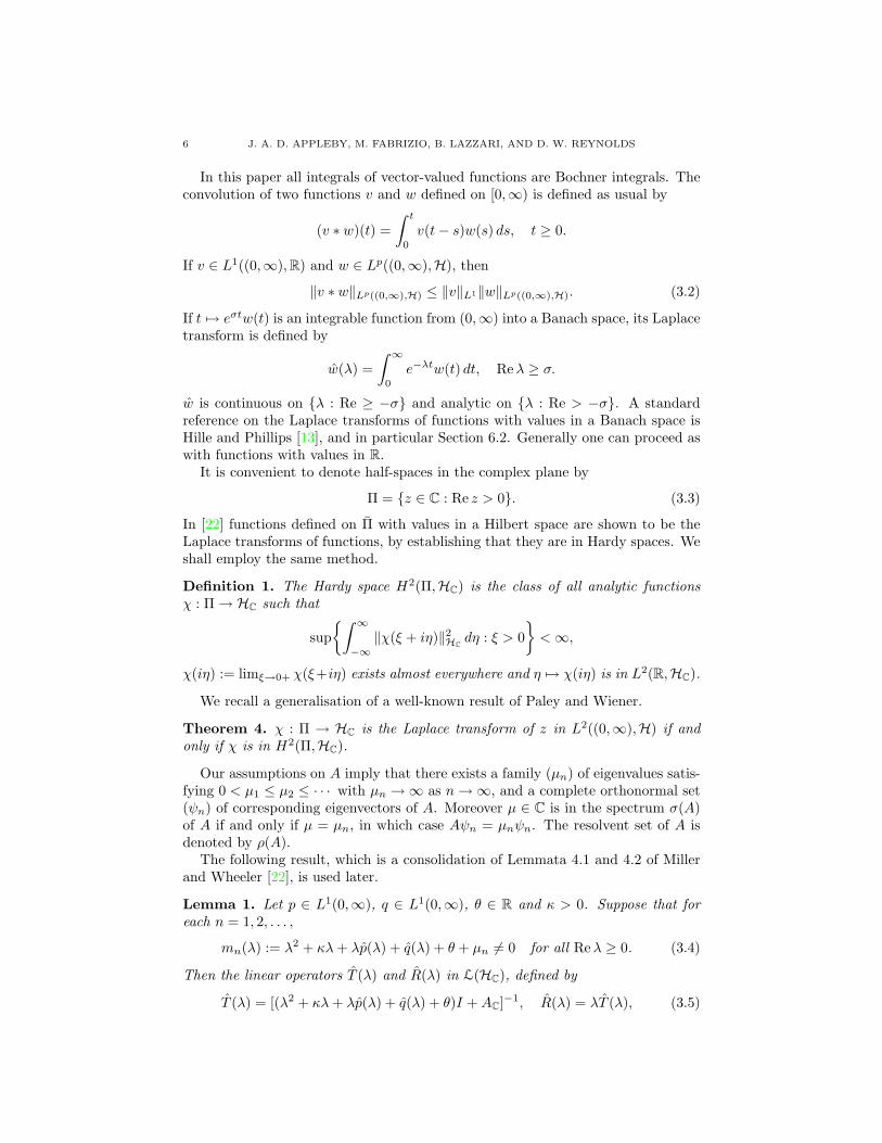
In this paper all integrals of vector-valued functions are Bochner integrals. Theconvolution of two functions v and w defined on [0,∞) is defined as usual by

(v ∗ w)(t) =∫ t

0

v(t− s)w(s) ds, t ≥ 0.

If v ∈ L1((0,∞),R) and w ∈ Lp((0,∞),H), then

‖v ∗ w‖Lp((0,∞),H) ≤ ‖v‖L1‖w‖Lp((0,∞),H). (3.2)

If t 7→ eσtw(t) is an integrable function from (0,∞) into a Banach space, its Laplacetransform is defined by

w(λ) =∫ ∞

0

e−λtw(t) dt, Reλ ≥ σ.

w is continuous on {λ : Re ≥ −σ} and analytic on {λ : Re > −σ}. A standardreference on the Laplace transforms of functions with values in a Banach space isHille and Phillips [13], and in particular Section 6.2. Generally one can proceed aswith functions with values in R.

It is convenient to denote half-spaces in the complex plane by

Π = {z ∈ C : Re z > 0}. (3.3)

In [22] functions defined on Π with values in a Hilbert space are shown to be theLaplace transforms of functions, by establishing that they are in Hardy spaces. Weshall employ the same method.

Definition 1. The Hardy space H2(Π,HC) is the class of all analytic functionsχ : Π → HC such that

sup{∫ ∞

−∞‖χ(ξ + iη)‖2

HCdη : ξ > 0

}<∞,

χ(iη) := limξ→0+ χ(ξ+iη) exists almost everywhere and η 7→ χ(iη) is in L2(R,HC).

We recall a generalisation of a well-known result of Paley and Wiener.

Theorem 4. χ : Π → HC is the Laplace transform of z in L2((0,∞),H) if andonly if χ is in H2(Π,HC).

Our assumptions on A imply that there exists a family (µn) of eigenvalues satis-fying 0 < µ1 ≤ µ2 ≤ · · · with µn →∞ as n→∞, and a complete orthonormal set(ψn) of corresponding eigenvectors of A. Moreover µ ∈ C is in the spectrum σ(A)of A if and only if µ = µn, in which case Aψn = µnψn. The resolvent set of A isdenoted by ρ(A).

The following result, which is a consolidation of Lemmata 4.1 and 4.2 of Millerand Wheeler [22], is used later.

Lemma 1. Let p ∈ L1(0,∞), q ∈ L1(0,∞), θ ∈ R and κ > 0. Suppose that foreach n = 1, 2, . . . ,

mn(λ) := λ2 + κλ+ λp(λ) + q(λ) + θ + µn 6= 0 for all Reλ ≥ 0. (3.4)

Then the linear operators T (λ) and R(λ) in L(HC), defined by

T (λ) = [(λ2 + κλ+ λp(λ) + q(λ) + θ)I +AC]−1, R(λ) = λT (λ), (3.5)


exist for all Reλ ≥ 0, and

sup{∫ ∞

−∞‖T (ξ + iη)‖2

L(HC) dη : ξ ≥ 0}<∞,

sup{∫ ∞

−∞‖R(ξ + iη)v‖2

HCdη : ξ ≥ 0

}<∞ for all v ∈ HC.

The notation in (3.5) should not confuse. Though for each fixed v in HC, λ 7→T (λ)v and λ 7→ R(λ)v are not defined as Laplace transforms, due to Theorem 4they are indeed so.

4. The Resolvent of the Kernel

Consider the resolvent r : [0,∞) → R of k, defined to be the solution of

r(t) + (k ∗ r)(t) = −k(t), t ≥ 0. (4.1)

Let kβ(t) := eβtk(t) and rβ(t) := eβtr(t). We use the notation r′β(t) := (rβ)′(t).Of course kβ(λ) = k(λ − β) etc. It immediately follows from (4.1) that rβ is theresolvent of kβ . It is important to note that r(0) = −k(0) > 0 if (2.9b) is true.(4.2) and (4.3) in the next result are proved in Proposition 5.1 of [17] in the casethat the values k(t) are symmetric bounded linear operators on H. The relevanceof (4.2) and (4.3) to linear viscoelasticity is evident from [9, 10].

Proposition 1. Suppose that k satisfies (2.9). Then

1η

Im k(ξ + iη) > 0, ξ ≥ 0 and η 6= 0, (4.2)

1 + Re k(ξ) > 0, ξ ≥ 0. (4.3)

Furthermore r ∈ C1[0,∞), r ∈ L1(0,∞) ∩ L2(0,∞) and r′ ∈ L1(0,∞). Also

1η

Im r(λ) < 0, ξ ≥ 0 and η 6= 0, (4.4)

1 + Re r(ξ) > 0, ξ ≥ 0. (4.5)

Moreover if (2.16) also holds, then there is 0 < β ≤ α such that rβ and r′β are inL1(0,∞).

Proof. It is well-known that the resolvent r is continuous. Moreover Paley andWiener showed that r is in L1(0,∞) if and only if 1 + k(λ) 6= 0 for all Reλ ≥ 0.(cf., e.g., Thm. 2.4.1 of [12]). Since λ 7→ 1 + k(λ) is analytic, its imaginary partis a harmonic function whose minimum on a closed bounded region occurs on itsboundary. By considering a region of the form

{λ ∈ C : Reλ ≥ 0, Imλ ≥ 0, |λ| ≤ ρ}

with ρ > 0 large, we conclude from the Riemann-Lebesgue lemma and (2.9a) thatIm k(λ) ≥ 0 for all Reλ ≥ 0 and Imλ ≥ 0. But since k is not constant, the OpenMapping Theorem says that Im k(λ) > 0 for all Reλ ≥ 0 and Imλ > 0. Since

k(λ) = k(λ),


(4.2) has been established. The Hilbert integral representation for the Laplacetransform yields

Re k(ξ) = − 2π

∫ ∞

0

ω

ξ2 + ω2Im k(iω) dω, ξ > 0.

Since ξ 7→ (ξ2 + ω2)−1 is strictly decreasing on (0,∞), ξ 7→ Re k(ξ) is strictlyincreasing on (0,∞). (4.3) is therefore true, because k(0) > −1 and k(ξ) → 0 asξ → ∞. (4.2) and (4.3) together imply that 1 + k(λ) 6= 0 for every Reλ ≥ 0,and hence that r ∈ L1(0,∞). The assertions concerning r′ follow easily fromr′ = k(0)r − k′ ∗ r − k′.

To see that r is in L2(0,∞), observe that r(t) → 0 as t → ∞ because r and r′

are in L1(0,∞). Therefore there is a T > 0 such that r(t)2 ≤ |r(t)| for all t ≥ T .Now assume in addition that (2.16) holds. To show that rβ is in L1(0,∞), we

prove that there is a constant β in (0, α] such that 1+ kβ(λ) = 1+ k(λ−β) 6= 0 forall Reλ ≥ 0. It is only necessary to further prove that 1 + k(λ) 6= 0 for all −β ≤Reλ ≤ 0. The Riemann-Lebesgue lemma implies that there is a constant M1 > 0such that 1 + k(ξ + iη) 6= 0 for all −α ≤ ξ ≤ 0 and |η| ≥ M1. Since k(0) > −1,there are constants 0 < β1 ≤ α and 0 < M2 < M1 such that Re k(ξ + iη) > −1 forall −β1 ≤ ξ ≤ 0 and |η| ≤ M2. Finally there is a constant β2 in (0, α] such thatIm k(ξ + iη) > 0 for all −β2 ≤ ξ ≤ 0 and M2 ≤ |η| ≤ M1. The result now followswith β = min{β1, β2}.

It is simple to derive from

r(λ) = − k(λ)

1 + k(λ), Reλ ≥ 0,

that

Re(1 + r(λ)) =1 + Re k(λ)

|1 + k(λ)|2, Im r(λ) = − Im k(λ)

|1 + k(λ)|2.

Then (4.4) is a consequence of this and (4.2), and (4.5) follows from it and (4.3). �

5. Proof of Theorem 1

We begin by recording the properties of the forcing function in (2.5). The as-sumption that the initial history is such that Aφ is bounded can be relaxed if weconstruct a suitable influence function from k and k′, as was done in Lemma 2.1 ofDafermos [5], and require φ to lie in a weighted space. Coleman and Noll [2, 3] in-troduced influence functions as part of a theory of functionals with fading memory.

Proposition 2. The function f defined in (2.5) is in C1([0,∞),H). If (2.12) alsoholds, f and f ′ are both in L1((0,∞),H).

Proof. To show that f is continuous, we note that

‖f(t+ τ)− f(t)‖H ≤∫ 0

−∞|k(t+ τ − s)− k(t− s)|‖Aφ(s)‖H ds

≤ sups≤0

‖Aφ(s)‖H∫ 0

−∞|k(t+ τ − s)− k(t− s)| ds

= sups≤0

‖Aφ(s)‖H∫ ∞

t

|k(τ + σ)− k(σ)| ds→ 0


as τ → 0, since k is in L1(0,∞).As a preliminary to proving that f is continuously differentiable, note that∫ t2

t1

∥∥∥∥∫ 0

−∞k′(t− s)Aφ(s) ds

∥∥∥∥Hdt ≤ sup

s≤0‖Aφ(s)‖H

∫ t2

t1

∫ 0

−∞|k′(t− s)| ds dt

≤ sups≤0

‖Aφ(s)‖H∫ t2

t1

∫ ∞

t

|k′(σ)| dσ dt <∞,

since k′ is in L1(0,∞). Hence the Tonelli-Fubini theorem can be applied to yield∫ t2

t1

∫ 0

−∞k′(t− s)Aφ(s) ds dt =

∫ 0

−∞{k(t2 − s)− k(t1 − s)}Aφ(s) ds

= f(t1)− f(t2).

This and the fact that∥∥∥∥∫ 0

−∞{k′(t+ τ − s)− k′(t− s)}Aφ(s) ds

∥∥∥∥H

≤ sups≤0

‖Aφ(s)‖H∫ ∞

t

|k′(τ + σ)− k′(σ)| ds→ 0 as τ → 0,

shows that f is in C1([0,∞),H), and

f ′(t) = −∫ 0

−∞k′(t− s)Aφ(s) ds, t ≥ 0.

The integrability of f follows from (2.12), because then∥∥∥∥∫ ∞

0

∫ 0

−∞k(t− s)Aφ(s) ds dt

∥∥∥∥H≤ sup

s≤0‖Aφ(s)‖H

∫ ∞

0

∫ 0

−∞|k(t− s)| ds dt

≤ sups≤0

‖Aφ(s)‖H∫ ∞

0

σ|k(σ)| dσ <∞.

Similarly f ′ is in L1(0,∞). �

The stability of solutions is studied in this paper, not their existence or unique-ness. But we remark that Theorem 3.1 of [22] ensures that (2.4) and (2.6) has aunique strong solution on [0,∞), if u1 is in an intermediate space between D(A)and H. Also at the end of §3 in [22] an argument is given that shows that, for astrong solution of (2.4) and (2.6), u, u′ and Au all have Laplace transforms providedf and f ′ do. There are also results in [22] about (2.4) being well-posed.

Theorem 1 is a consequence of Theorem 4.2 of [22]. Sketching its proof enablessubsequent results to be proved more succinctly.

Firstly (2.4) is transformed using MacCamy’s trick to a problem in which thepresent value of Au occurs but not its history, as is done in [22]. By taking theconvolution of (2.4) with r, we obtain

(r ∗ u′′)(t)− (k ∗Au)(t) = (r ∗ f)(t).

Substitution of the resulting expression for k ∗ Au into (2.4) and integration byparts yields

u′′(t) + r(0)u′(t) + (r′ ∗ u′)(t) +Au(t) = g(t) + r(t)u1, t ≥ 0, (5.1)


where g(t) = f(t)+(r∗f)(t). By Propositions 1 and 2, g and g′ are in L1(0,∞),H)).It follows from (5.1) that the Laplace transform of u satisfies

[λ2 + r(0)λ+ λr′(λ)]u(λ) +ACu(λ)

= λu0 + [1 + r(λ)]u1 + [r′(λ) + r(0)]u0 + g(λ), Reλ ≥ σ,

for some σ ≥ 0 in R. Lemma 1 tells us that linear operators T (λ) and R(λ) inL(HC) can be defined for all Reλ ≥ 0 by

T (λ) = [λ2(1 + r(λ))I +AC]−1, R(λ) = λT (λ), (5.2)

u(λ) then has the representation

u(λ) = T (λ)[(1 + r(λ))u1 + r′(λ)u0 + r(0)u0 + g(λ)] + R(λ)u0. (5.3)

In order to conclude from Lemma 1 and Theorem 4 that u is in L2((0,∞),H),and that (5.3) holds for all Reλ ≥ 0, we must show that (3.4) holds.

Lemma 2. Suppose that k obeys (2.9) holds. For each n ∈ N,

mn(λ) := λ2(1 + r(λ)) + µn 6= 0, Reλ ≥ 0. (5.4)

Proof. In this casemn(λ) given in (3.4) has the form (5.4). If the notation λ = ξ+iηis used,

Remn(λ) = (ξ2 − η2)(1 + Re r(λ))− 2ξη Im r(λ) + µn,

Immn(λ) = 2ξη(1 + Re r(λ)) + (ξ2 − η2) Im r(λ).

If Immn(λ) = 0, a short computation and (4.4) yield

2ξRemn(λ) = − Im r(λ)η

(ξ2 + η2)2 + 2ξµn > 0,

if ξ > 0 and η 6= 0. By (4.5),

Remn(ξ) = ξ2 Re(1 + r(ξ)) + µn > 0, (5.5)

for all ξ ≥ 0. It remains to show that mn(iη) 6= 0 for η 6= 0. But we observe that

Immn(iη) = −η2 Im r(iη) 6= 0, η 6= 0. (5.6)

�

Remark 1. Lemma 2 shows that

−λ2(1 + r(λ) = − λ2

1 + k(λ)∈ ρ(AC),

for all Reλ ≥ 0.

To show the corresponding bound on u′, we note that (5.3) and the definition ofT in (3.5) imply that

u′(λ) = λu(λ)− u(0)

= T (λ)[λr(λ)u1 + λg(λ)] + T (λ)[(λ2 + r(0)λ+ λr′(λ))u0] + R(λ)u1 − u0

= T (λ)[r′(λ)u1 + g′(λ)] + T (λ)[r(0)u1 + g(0)−ACu0] + R(λ)u1.

Using the properties of T and R, it can be demonstrated that u′ is in H2(Π,HC),and hence u′ is in L2((0,∞),H).


If it can be shown that u is uniformly continuous, it will follow from the factthat u is in L2((0,∞),H) that (2.14) is true. But the uniform continuity of u is aconsequence of

‖u(t2)− u(t1)‖H ≤∣∣∣∣∫ t2

t1

‖u′(t)‖H dt∣∣∣∣ ≤ |t2 − t1|1/2

(∫ ∞

0

‖u′(t)‖2H dt

)1/2

.

This finishes our sketch of the proof of Theorem 1.

6. Proof of Theorem 2

Firstly we note that (2.16) forces f and f ′ to decay exponentially.

Proposition 3. If (2.16) holds, then∫ ∞

0

‖f(t)‖Heαt dt <∞,

∫ ∞

0

‖f ′(t)‖Heαt dt <∞. (6.1)

Proof. Due to (2.16),∫ ∞

0

eαt‖f(t)‖H dt =∫ ∞

0

eαt

∥∥∥∥∫ 0

−∞k(t− s)Aφ(s) ds

∥∥∥∥Hdt

≤ sups≤0

‖Aφ(s)‖H∫ ∞

0

|k(τ)|∫ τ

0

eαt dt dτ

=1α

sups≤0

‖Aφ(s)‖H∫ ∞

0

|k(τ)|(eατ − 1) dτ <∞.

Similarly∫ ∞

0

eαt‖f ′(t)‖H dt ≤1α

sups≤0

‖Aφ(s)‖H∫ ∞

0

|k′(τ)|(eατ − 1) dτ <∞.

�

We now state a lemma which corresponds to Lemma 2: it is essentially Theorem 6of [16].

Lemma 3. Suppose that (2.9) and (2.16) hold. Let β > 0 be as in Proposition 1,and mn(λ) as in (5.4). Then there exists 0 < β1 ≤ β with 2β1 < r(0), such thatmn(λ) 6= 0 for all Reλ ≥ −β1.

Proof. By Proposition 1, mn(λ) can be defined for all Reλ ≥ −β. Because of (5.4),it only remains to show mn(λ) 6= 0 for all −β1 ≤ Reλ ≤ 0 for some β1 in (0, β).Because

mn(λ) = λ2 + r(0)λ+ λr′(λ) + µn, λ 6= 0,it is easily seen that

limη→∞

1η

Immn(λ) = 2ξ + r(0), (6.2)

where λ = ξ + iη. Let β2 be a number in (0, β] such that r(0) > 2β2. Then (6.2)implies that there is a constant M1 > 0 such that Immn(λ) 6= 0 for all −β2 ≤ ξ ≤ 0and |η| ≥ M1. By (5.5), there are constants 0 < β3 ≤ β and M2 > 0 such thatRemn(ξ+ iη) > 0 for all −β3 ≤ ξ ≤ 0 and |η| ≤M2. Also we can deduce from (5.6)that there is a constant β4 in (0, β] such that Immn(ξ+ iη) > 0 for all −β4 ≤ ξ ≤ 0and M2 ≤ |η| ≤M1. The result now follows with β1 = min{β2, β3, β4}. �


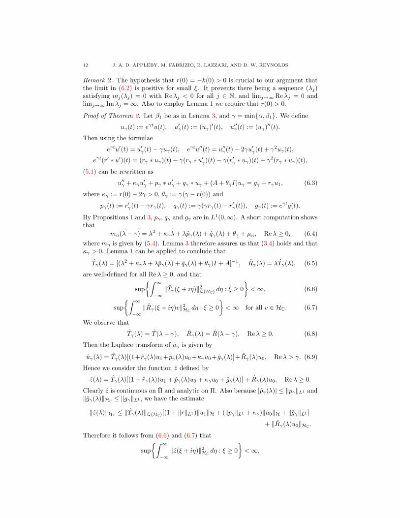
Remark 2. The hypothesis that r(0) = −k(0) > 0 is crucial to our argument thatthe limit in (6.2) is positive for small ξ. It prevents there being a sequence (λj)satisfying mj(λj) = 0 with Reλj < 0 for all j ∈ N, and limj→∞Reλj = 0 andlimj→∞ Imλj = ∞. Also to employ Lemma 1 we require that r(0) > 0.

Proof of Theorem 2. Let β1 be as in Lemma 3, and γ = min{α, β1}. We define

uγ(t) := eγtu(t), u′γ(t) := (uγ)′(t), u′′γ(t) := (uγ)′′(t).

Then using the formulae

eγtu′(t) = u′γ(t)− γuγ(t), eγtu′′(t) = u′′γ(t)− 2γu′γ(t) + γ2uγ(t),

eγt(r′ ∗ u′)(t) = (rγ ∗ uγ)(t)− γ(rγ ∗ u′γ)(t)− γ(r′γ ∗ uγ)(t) + γ2(rγ ∗ uγ)(t),

(5.1) can be rewritten as

u′′γ + κγu′γ + pγ ∗ u′γ + qγ ∗ uγ + (A+ θγI)uγ = gγ + rγu1, (6.3)

where κγ := r(0)− 2γ > 0, θγ := γ(γ − r(0)) and

pγ(t) := r′γ(t)− γrγ(t), qγ(t) := γ(γrγ(t)− r′γ(t)), gγ(t) := eγtg(t).

By Propositions 1 and 3, pγ , qγ and gγ are in L1(0,∞). A short computation showsthat

mn(λ− γ) = λ2 + κγλ+ λpγ(λ) + qγ(λ) + θγ + µn, Reλ ≥ 0, (6.4)where mn is given by (5.4). Lemma 3 therefore assures us that (3.4) holds and thatκγ > 0. Lemma 1 can be applied to conclude that

Tγ(λ) = [(λ2 + κγλ+ λpγ(λ) + qγ(λ) + θγ)I +A]−1, Rγ(λ) = λTγ(λ), (6.5)

are well-defined for all Reλ ≥ 0, and that

sup{∫ ∞

−∞‖Tγ(ξ + iη)‖2

L(HC) dη : ξ ≥ 0}<∞, (6.6)

sup{∫ ∞

−∞‖Rγ(ξ + iη)v‖2

HCdη : ξ ≥ 0

}<∞ for all v ∈ HC. (6.7)

We observe that

Tγ(λ) = T (λ− γ), Rγ(λ) = R(λ− γ), Reλ ≥ 0. (6.8)

Then the Laplace transform of uγ is given by

uγ(λ) = Tγ(λ)[(1+ rγ(λ)u1+ pγ(λ)u0+κγu0+ gγ(λ)]+Rγ(λ)u0, Reλ > γ. (6.9)

Hence we consider the function z defined by

z(λ) = Tγ(λ)[(1 + rγ(λ))u1 + pγ(λ)u0 + κγu0 + gγ(λ)] + Rγ(λ)u0, Reλ ≥ 0.

Clearly z is continuous on Π and analytic on Π. Also because |pγ(λ)| ≤ ‖pγ‖L1 and‖gγ(λ)‖HC ≤ ‖gγ‖L1 , we have the estimate

‖z(λ)‖HC ≤ ‖Tγ(λ)‖L(HC)[(1 + ‖r‖L1)‖u1‖H + (‖pγ‖L1 + κγ)‖u0‖H + ‖gγ‖L1 ]

+ ‖Rγ(λ)u0‖HC .

Therefore it follows from (6.6) and (6.7) that

sup{∫ ∞

−∞‖z(ξ + iη)‖2

HCdη : ξ ≥ 0

}<∞,


and hence that λ 7→ z(λ) is in the Hardy space H2(Π,HC). Therefore Theorem 4says that there is z ∈ L2((0,∞),H) whose Lapace transform is z(λ) for all λ ≥ 0.By the uniqueness of the Laplace transform, z(t) = uγ(t) for almost every t > 0,and therefore ∫ ∞

0

‖u(t)‖2He

2γt dt =∫ ∞

0

‖uγ(t)‖2H dt <∞.

To show the corresponding bound on u′, we note that (6.9) and the definition ofTγ in (6.8) imply that

u′γ(λ) = λuγ(λ)− uγ(0)

= Tγ(λ)[r′γ(λ)u1 + g′γ(λ)] + Tγ(λ)[r(0)u1 + gγ(0)−ACu0] + Rγ(λ)u1.

Therefore we consider the function y : Π → HC defined by

y(λ) = Tγ(λ)[r′γ(λ)u1 + g′γ(λ)] + Tγ(λ)[r(0)u1 + gγ(0)−ACu0] + Rγ(λ)u1.

Using the properties of Tγ and Rγ , it can be demonstrated that y is in H2(Π,HC).Hence there is a function y in L2((0,∞),H) whose Laplace transform is y. Weobserve that u′γ = y, and ∫ ∞

0

‖u′(t)‖2He

2γt dt <∞.

The assertion that uγ(t) → 0 in H as t→∞ follows, because

‖uγ(t2)− uγ(t1)‖H ≤∣∣∣∣∫ t2

t1

‖u′γ(t)‖H dt∣∣∣∣ ≤ |t2 − t1|1/2

(∫ ∞

0

‖u′γ(t)‖2H dt

)1/2

.

shows that uγ is uniformly continuous. Thus (2.17) is true. �

7. Proofs of Theorem 3

7.1. Proof of (i). We continue to assume (2.9), since this is weaker than (2.10).The proof involves the same kind of arguments used before. It is elementary toshow that ACTγ = TγAC on D(AC), and hence that ACRγ = RγAC on D(AC).Therefore (6.9) leads to

ACuγ(λ) = Tγ(λ)[(1+ r(λ))ACu1+ pγ(λ)ACu0+κγACu0]+Rγ(λ)ACu0, Reλ > γ.

Using an argument similar to those used previously, we can deduce that∫ ∞

0

‖Au(t)‖2He

2γt dt <∞.

It follows from (3.2) and (6.3) that u′′γ is in L2((0,∞),H). Because this implies thatu′γ is uniformly continuous, the pointwise estimate on ‖u′(t)‖H in (2.21) follows.

7.2. Proof of (ii). The proof uses a result that appears in the proof of Theorem2 of Murakami [23]. It would be more satisfactory if there were a version of thislemma involving assumptions on Re h(iη) or Im h(iη), rather than a condition onthe sign of h.


Lemma 4. Let h : (0,∞) → R be an integrable function with a single sign almosteverywhere. Suppose that there is an analytic function a : U → C, defined on aneighbourhood U of 0 in C, such that h(λ) = a(λ) for all λ ∈ U with Reλ ≥ 0.Then there is a α > 0 such that∫ ∞

0

|h(s)|eαs ds <∞.

Indeed α can be any positive number less than the radius of the convergence of thepower series of a about 0.

Since (2.20) holds for some γ > 0, the Laplace transforms of u, u′, and Au are(weakly) holomorphic in {λ : Reλ > −γ}. It can be deduced from (3.2) and (2.19)that u′′γ is in L2((0,∞),H), and that the Laplace transform of u′′ is also (weakly)holomorphic in {λ : Reλ > −γ}. By taking the Laplace transform of each term in(2.4), we see that

λ2u(λ)− λu0 − u1 + [1 + k(λ)]ACu(λ) = 0, Reλ ≥ 0. (7.1)

Since A is positive definite, (ACu(0), u(0))HC = 0 if and only if u(0) = 0. Becauseu(0) = 0 implies that u1 = 0, this possibility is excluded by hypotheses. Thereforeλ 7→ (ACu(λ), u(0)))HC is analytic and non-zero on a neighbourhood U of 0, and

k(λ) = − (λ2u(λ)− λu0 − u1 +ACu(λ), u(0))HC

(ACu(λ), u(0))HC

, Reλ ≥ 0.

It is a consequence of Lemma 4 that∫ ∞

0

|k(s)|eα1s ds <∞,

for any 0 < α1 < γ. Since if k′ is integrable and k′(s) ≥ 0 for s ≥ 0, then Lemma 4can be applied to k′(λ) = λk(λ)− k(0) to yield∫ ∞

0

|k′(s)|eαs ds <∞,

0 < α < α1. It follows from

k(t)eαt =∫ t

0

{k′(s) + αk(s)}eαs ds− k(0),

that k(t)eαt tends to a limit as t→∞ and this limit must be 0.

References

1. J. A. D. Appleby and D. W. Reynolds, On necessary and sufficient conditions for exponen-

tial stability in linear Volterra integro–differential equations, J. Integral Equations Appl. 16

(2004), no. 3, 221–240.2. B. D. Coleman. and W. Noll, An approximation theorem for functionals, with applications in

continuum mechanics, Arch. Rational Mech. Anal. 6 (1960), 355–370 (1960).

3. B. D. Coleman and W. Noll, Foundations of linear viscoelasticity, Rev. Modern Phys. 33(1961), 239–249.

4. C. M. Dafermos, An abstract Volterra equation with applications to linear viscoelasticity, J.Differential Equations 7 (1970), 554–569.

5. , Asymptotic stability in viscoelasticity, Arch. Rational Mech. Anal. 37 (1970), 297–

308.6. , Contraction semigroups and trend to equilibrium in continuum mechanics, Lecture

Notes in Mathematics, no. 503, pp. 295–306, Springer-Verlag, 1975.


7. R. Dakto, Extending a thorem of A. M. Liapunov to Hilbert space, J. Math. Appl. Anal. 32

(1970), 610–616.8. W. Desch and R. K. Miller, Exponential stabilization of Volterra integrodifferential equations

in Hilbert space, J. Differential Equations 70 (1987), 366–389.

9. M. Fabrizio and B. Lazzari, On the existence and the asymptotic stability of solutions for

linearly viscoelastic solids, Arch Rational Mech. Anal. 116 (1991), 139–152.10. M. Fabrizio and A. Morro, Mathematical problems in linear viscoelasticity, SIAM Studies in

Applied Mathematics, SIAM, 1992.11. M. Fabrizio and S. Polidoro, Asymptotic decay for some differential systems with fading

memory, Appl. Anal. 81 (2002), no. 6, 1245–1264.

12. G. Gripenberg, S. O. Londen, and O. Staffens, Volterra integral and functional equations,

Encyclopaedia of Mathematics and its Applications, Cambridge University Press, 1990.13. E. Hille and R. S. Phillips, Functional analysis and semigroups, Amer. Math. Soc. Coll. Publ.,

American Mathematical Society, 1957.14. Z. Liu, , and S. Zheng, On the exponential stability of linear viscoelasticity and thermoelas-

ticity, Quart. Appl. Math. 54 (1996), 21–31.15. J. Nohel M. Renardy and W. Hrusa, Mathematical problems in linear viscoelasticity, Pitman

Monographs Surveys in Pure and Applied Mathematics, Longman, 1987.16. R. C. MacCamy, Exponential stability for a class of functional differential equations, Arch.

Rational Mech. Anal. 40 (1970/1), 120–138.17. , Nonlinear Volterra equations on a Hilbert space, J. Differential Equations. 16 (1974),

373–393.18. , Stability theorems for a class of functional differential equations, SIAM J. Appl.

Math. 30 (1976), no. 3, 557–576.19. , A model for one-dimensional, nonlinear viscoelasticity, Quart. Appl. Math. 35

(1977), no. 1, 21–33.20. R. C. MacCamy and J. S. W. Wong, Exponential stability for a nonlinear functional differ-

ential equation, J. Math. Anal. Appl. 39 (1972), 699–705.21. M. Medjden and N. Tatar, Asymptotic behaviour for a viscoelastic problem with not neces-

sarily decreasing kernel, Appl. Math. Comput. 167 (2005), no. 2, 1221–1235.22. R. K. Miller and R. L. Wheeler, Well-Posedness and stability of linear Volterra integrodiffer-

ential equations in abstract spaces, Funkcialaj Ekvacioj 21 (1978), 279–305.23. Satoru Murakami, Exponential asymptotic stability of scalar linear Volterra equations, Diff.

and Integral Equations 4 (1991), no. 3, 519–525.24. , Exponential asymptotic stability for fundamental solution of linear functional differ-

ential equations, Proceedings of the International Symposium Functional Differential Equa-

tions (T. Yoshizawa and J. Kato, eds.), World Scientific, 1992, pp. 259–263.25. V. Pata, Exponential stability in linear viscoelasticity, Quart. Appl. Math. In press ( ), .26. Jan Pruss, Evolutionary integral equations and applications, Birkhauser, Boston MA, 1993.27. O. J. Staffans, On a nonlinear hyperbolic Volterra integral equation, SIAM J. Math. Anal. 11

(1980), 793–812.

School of Mathematical Sciences, Dublin City University, Dublin 9, Ireland

E-mail address: [email protected]

Dipartimento di Matematica, Piazza di Porta S. Donato, 5, 40127 Bologna, Italy

E-mail address: [email protected]

Dipartimento di Matematica, Piazza di Porta S. Donato, 5, 40127 Bologna, ItalyE-mail address: [email protected]

School of Mathematical Sciences, Dublin City University, Dublin 9, IrelandE-mail address: [email protected]

ON EXPONENTIAL ASYMPTOTIC STABILITY IN LINEAR VISCOELASTICITY

Documents