Retrospective eses and Dissertations Iowa State University Capstones, eses and Dissertations 2002 On-board three-dimensional constrained entry flight trajectory generation Zuojun Shen Iowa State University Follow this and additional works at: hps://lib.dr.iastate.edu/rtd Part of the Aerospace Engineering Commons is Dissertation is brought to you for free and open access by the Iowa State University Capstones, eses and Dissertations at Iowa State University Digital Repository. It has been accepted for inclusion in Retrospective eses and Dissertations by an authorized administrator of Iowa State University Digital Repository. For more information, please contact [email protected]. Recommended Citation Shen, Zuojun, "On-board three-dimensional constrained entry flight trajectory generation " (2002). Retrospective eses and Dissertations. 1029. hps://lib.dr.iastate.edu/rtd/1029

Welcome message from author
This document is posted to help you gain knowledge. Please leave a comment to let me know what you think about it! Share it to your friends and learn new things together.
Transcript
Retrospective Theses and Dissertations Iowa State University Capstones, Theses andDissertations
2002
On-board three-dimensional constrained entryflight trajectory generationZuojun ShenIowa State University
Follow this and additional works at: https://lib.dr.iastate.edu/rtd
Part of the Aerospace Engineering Commons
This Dissertation is brought to you for free and open access by the Iowa State University Capstones, Theses and Dissertations at Iowa State UniversityDigital Repository. It has been accepted for inclusion in Retrospective Theses and Dissertations by an authorized administrator of Iowa State UniversityDigital Repository. For more information, please contact [email protected].
Recommended CitationShen, Zuojun, "On-board three-dimensional constrained entry flight trajectory generation " (2002). Retrospective Theses andDissertations. 1029.https://lib.dr.iastate.edu/rtd/1029
INFORMATION TO USERS
This manuscript has been reproduced from the microfilm master. UMI films
the text directly from the original or copy submitted. Thus, some thesis and
dissertation copies are in typewriter face, while others may be from any type of
computer printer.
The quality of this reproduction is dependent upon the quality of the
copy submitted. Broken or indistinct print, colored or poor quality illustrations
and photographs, print bleedthrough, substandard margins, and improper
alignment can adversely affect reproduction.
In the unlikely event that the author did not send UMI a complete manuscript
and there are missing pages, these will be noted. Also, if unauthorized
copyright material had to be removed, a note will indicate the deletion.
Oversize materials (e.g., maps, drawings, charts) are reproduced by
sectioning the original, beginning at the upper left-hand corner and continuing
from left to right in equal sections with small overlaps.
ProQuest Information and Learning 300 North Zeeb Road, Ann Arbor, Ml 48106-1346 USA
800-521-0600

On-board three-dimensional constrained entry flight trajectory generation
by
Zuojun Shen
A dissertation submitted to the graduate faculty
in partial fulfillment of the requirements for the degree of
DOCTOR OF PHILOSOPHY
Major: Aerospace Engineering
Program of Study Committee: Ping Lu. Major Professor
Bion L. Pierson Jerald M. Vogel
Murti V. Salapaka Robvn R. Lutz
Steven M. LaValle
Iowa State University
Ames. Iowa
2002
Copyright © Zuojun Shen, 2002. All rights reserved.

UMI Number: 3061864
UMI UMI Microform 3061864
Copyright 2002 by ProQuest Information and Learning Company. All rights reserved. This microform edition is protected against
unauthorized copying under Title 17, United States Code.
ProQuest Information and Learning Company 300 North Zeeb Road
P.O. Box 1346 Ann Arbor, Ml 48106-1346
i i
Graduate College Iowa State University
This is to certify that the doctoral dissertation of
Zuojun Shen
has met the dissertation requirements of Iowa State University
For the&laj rogram
Signature was redacted for privacy.
Signature was redacted for privacy.
i i i
TABLE OF CONTENTS
LIST OF TABLES vii
LIST OF FIGURES viii
NOMENCLATURE xii
ACKNOWLEDGEMENT xvi
ABSTRACT xviii
CHAPTER 1. INTRODUCTION 1
1.1 Background 1
1.2 Related Work 4
1.3 Overview S
CHAPTER 2. PROBLEM FORMULATION 11
2.1 Objective and Assumptions 11
2.2 Entry Vehicle Dynamics 12
2.3 Trajectory Constraints 13
2.4 Entry and TA EM Conditions 16
CHAPTER 3. ON BOARD 3DOF CONSTRAINED ENTRY TRA
JECTORY GENERATION METHOD 19
3.1 Longitudinal Reference Profiles 20
3.1.1 Quasi-Equilibrium Glide Condition 22
3.1.2 Enforcement of the Inequality Trajectory Constraints 24
i v
3.1.3 Initial Descent 27
3.1.4 Terminal Backward Trajectory 29
3.1.5 Completion of the Longitudinal Reference Profiles 34
3.2 Completion of the 3D0F Trajectory 37
3.2.1 Approximate Receding-Horizon Control Method 39
3.2.2 Longitudinal Reference Profiles Tracking 43
3.2.3 Single Bank-Reversal Strategy 45
3.2.4 Terminal Ground-Track Control 54
3.2.5 Terminal Metric-Based Open-Loop Trajectory Search 59
CHAPTER 4. ALGORITHM IMPLEMENTATION 65
4.1 Input and Output 67
4.1.1 Input 67
4.1.2 Output 71
4.2 Major Blocks 72
4.2.1 Dravv_StateConstraints( ) 72
4.2.2 Initial _Descend( ) 72
4.2.3 T mlReverseIntegration( ) 73
4.2.4 Quasi_EG() 74
4.2.5 RefTrajTrackingO 75
4.2.6 TmlGrndTrackingO 77
4.3 Key Global Variables 79
CHAPTER 5. APPLICATIONS 81
5.1 Vehicle Models 82
5.1.1 X-33 82
5.1.2 X-38 84
5.2 Entry Trajectory Design for X-33 and X-38 86

V
5.2.1 Entry Missions 86
5.2.2 Entry Trajectories Generated 88
5.3 Adaptability Demonstration 102
5.3.1 Enforcement of Stringent Heat Rate Constraint 102
5.3.2 Trajectory Generation from Non-orbital Entry Conditions .... 104
5.4 High Fidelity Simulation Results 108
5.5 Performance Assessment 118
CHAPTER 6. CONCLUSIONS AND FUTURE WORK 122
6.1 Conclusions 122
6.2 Future work 124
APPENDIX A. EXPRESSIONS OF H AND 5 MATRICES 127
APPENDIX B. X-33 VEHICLE AND ENTRY MISSION DATA . . . 1 3 0
APPENDIX C. X-38 VEHICLE AND ENTRY MISSION DATA . . . 135
APPENDIX D. 3DOF ENTRY TRAJECTORY DESIGN PARAME
TERS 138
BIBLIOGRAPHY 140

LIST OF TABLES
Table 5.1 X-33 entry missions 87
Table 5.2 X-38 entry missions 88
Table 5.3 Terminal precision of 3D0F entry trajectories for X-33 and X-38 119
Table 5.4 Algorithm performance statistics 121
Table B.l X-33 vehicle/mission parameters 130
Table B.2 Case AGC13: 3DOF entry from ISS orbit (51.6 deg) 131
Table B.3 Case AGC14: 3DOF "early" entry from ISS orbit (51.6 deg) . . 131
Table B.4 Case AGCl5: 3DOF "late" entry from ISS orbit (51.6 deg) . . . 132
Table B.5 Case AGC16: 3DOF entry from ISS orbit (51.6 deg) 132
Table B.6 Case AGCl7: 3DOF "early" entry from ISS orbit (51.6 deg) . . 133
Table B.7 Case AGC18: 3DOF "late" entry from ISS orbit (51.6 deg) . . . 133
Table B.8 Case AGCl9: 3DOF entry from LEO orbit (28.5 deg) 134
Table B.9 Case AGC20: 3DOF "early" entry from LEO orbit (28.5 deg) . . 134
Table B.10 Case AGC21: 3DOF "late" entry from LEO orbit (28.5 deg) . . 135
Table C.I X-38 vehicle/mission parameters 136
Table C.2 X-38 entry test case 1 137
Table C.3 X-38 entry test case 2 137
Table C.4 X-38 entry test case 3 138
Table C.5 X-38 entry test case 4 139

vii
Table D.l X-33 entry trajectory design parameters 140
Table D.2 X-38 entry trajectory design parameters 141

vin
LIST OF FIGURES
Figure 1.1 Rapidly-exploring random tree method 6
Figure 2.1 Entry corridor 14
Figure 2.2 Allowed region for a variation along the nominal a profile .... 17
Figure 2.3 TA EM interface requirements IS
Figure 3.1 Altitude versus velocity reference profile 21
Figure 3.2 Bank angle versus velocity reference profile 21
Figure 3.3 Heading error along the entry trajectory 23
Figure 3.4 Bounded cr{V) profile (zoomed in the region where the QEGC
applies) 26
Figure 3.5 Bounded v-r profile (zoomed in the region where the QEGC applies) 26
Figure 3.6 Initial descent with constant bank angle 27
Figure 3.7 Ground track of terminal backward trajectory 30
Figure 3.8 Backward tracking of the geometry reference curve 32
Figure 3.9 Backward trajectory tracking of several reference curves with d-
ifferent 7 values at TAEM 33
Figure 3.10 Backward trajectory tracking of a "bad1* reference curve 34
Figure 3.11 Longitudinal reference state profiles 36
Figure 3.12 Longitudinal reference control profiles 36
Figure 3.13 Spherical geometry of entry flight 38
Figure 3.14 Concept of the single bank-reversal strategy 46

ix
Figure 3.15 Generalized range-togo for determining the single bank-reversal
point 4S
Figure 3.16 Single bank-reversal point prediction 49
Figure 3.17 Bank-reversal happens very close to the TAEM 51
Figure 3.18 a profile: bank-reversal happens very close to the TAEM .... 52
Figure 3.19 Bad result due to bank-reversal close to the TAEM 52
Figure 3.20 No bank-reversal is allowed 53
Figure 3.21 5th order polynomial curve used as the reference ground track . 55
Figure 3.22 Ground path tracking iteration 60
Figure 3.23 Different terminal altitude reached by ground path tracking ... 60
Figure 3.24 No bank-reversal and TAEM interface missed 61
Figure 3.25 No bank-reversal and TAEM r and V missed 61
Figure 3.26 All terminal open-loop trajectories terminate at the TAEM spe
cific energy 63
Figure 3.27 Different open-loop trajectory ground paths 63
Figure 3.28 Terminal open-loop control histories 64
Figure 4.1 Flowchart of the overall algorithm 66
Figure 4.2 Flowchart of the algorithm for completing the 3DOF trajectory . 76
Figure 4.3 Initialization of the U'TAEM for terminal ground tracking .... 77
Figure 4.4 Flowchart of the algorithm for terminal ground tracking 78
Figure 5.1 X-33 83
Figure 5.2 3-view of the X-33 Reusable Launch Vehicle (RLV) 83
Figure 5.3 X-38 85
Figure 5.4 3-vievv of the X-38 Crew Return Vehicle(CRV) 85
Figure 5.5 Ground track of the X-33 AGC13 entry test case 91
Figure 5.6 Entry trajectory of the X-33 AGC13 entry test case 91

X
Figure 5.7 Flight path angle vs. velocity profile of the X-33 AGC13 entry
test case 92
Figure 5.8 Bank angle vs. velocity profile of the X-33 AGCl3 entry test case 92
Figure 5.9 Angle of attack vs. velocity profile of the X-33 AGC13 entry test
case 93
Figure 5.10 Control history of the X-33 AGCl3 entry test case 93
Figure 5.11 Ground tracks of AGC13-21 entry trajectories 94
Figure 5.12 Enlarged view of the terminal ground tracks 94
Figure 5.13 Ground tracks of the X-33 entry trajectories drawn with the
world map 95
Figure 5.14 Entry trajectories of AGCl3-21 entry test cases 96
Figure 5.15 Flight path angle vs. velocity profiles of AGC13-21 entry test cases 96
Figure 5.16 Angle of attack vs. velocity profiles of AGCl3-21 entry test cases 97
Figure 5.17 Control histories of AGCl3-21 entry test cases 97
Figure 5.18 Ground tracks of the X-38 entry test cases 98
Figure 5.19 Ground tracks of the X-38 entry trajectories drawn with the
world map 99
Figure 5.20 Entry trajectories of the X-38 entry test cases 100
Figure 5.21 Flight path angle vs. velocity profiles of the X-38 entry test cases 100
Figure 5.22 Angle of attack vs. velocity profiles of the X-38 entry test cases . 101
Figure 5.23 Control histories of the X-38 entry test cases 101
Figure 5.24 Ground track of the AGCl9 entry with stringent heat rate con
straint 103
Figure 5.25 Entry trajectory of the AGC19 entry with stringent heat rate
constraint 103
Figure 5.26 Ground tracks for AGC13 and trajectories from disturbed states 105
Figure 5.27 Enlarged view of the terminal ground track 106

xi
Figure 5.28 Entry trajectories for AGCl3 and trajectories from disturbed s-
tates 106
Figure 5.29 Flight path angle vs. velocity profiles 107
Figure 5.30 Angle of attack vs. velocity profiles 107
Figure 5.31 Control histories 108
Figure 5.32 Actual TAEM conditions from the MAVERIC simulation .... 110
Figure 5.33 Ground tracks recorded from the MAVERIC simulation for the
X-33 AGC cases 112
Figure 5.34 Enlarged view of the terminal ground tracks 112
Figure 5.35 Altitude time history recorded from the MAVERIC simulation
for the X-33 AGC cases 113
Figure 5.36 Velocity time history recorded from the MAVERIC simulation
for the X-33 AGC cases 113
Figure 5.37 Flight path angle time history recorded from the MAVERIC sim
ulation for the X-33 AGC cases 114
Figure 5.38 Heading error time history recorded from the MAVERIC simu
lation for the X-33 AGC cases 114
Figure 5.39 Control histories recorded from the MAVERIC simulation for the
X-33 AGC cases 115
Figure 5.40 Ground tracks for AGC cases 19-21 with Q m a x = 60 BTU/ f t 2 • secll6
Figure 5 .41 Ent ry t ra jec to r ies fo r AGC cases 19-21 wi th Qmax = 60 BTU / f t 2 -
sec 116
Figure 5.42 Control histories for AGC cases 19-21 with Q m a x = 60 BTU / f t 2 - sec \ \~

xii
NOMENCLATURE
Nomenclature
a angle of attack, degree
cr bank angle, rad
p atmospheric density, f cg /m 3
7 flight path angle, rad
v velocity azimuth angle, measure from north clockwise in rad
o latitude, rad
0 longitude, rad
T nondimensional time, real time normalized by YJRQ/go
<yf nondimensional natural frequency for ground path tracking control
u.Vfl nondimensional natural frequency for terminal backward V — r ref
erence curve tracking control
Kv parameter of the control law for tracking velocity profile
damping ratio for ground path tracking control law
ÇVR damping ratio for terminal backward V — r reference curve tracking
control law

xiii
fi Earth self-rotation rate normalized by YJR Q/ G A . 0.0586
e nondimensional specific energy
go Earth gravitational acceleration. 9.81 m/s tc 2
h nondimensional step size for RH control method.
n=mai maximum allowable load acceleration. gQ
q dynamic pressure. N/m 2
qmax maximum allowable dynamic pressure
r radius distance from Earth's center to the vehicle, normalized by R0
RTAE.\I nondimensional TAEM altiude
s down range distance, normalized by RQ
t time, second
CL lift coefficient
Co drag coefficient
D nondimensional drag acceleration. g a
L nondimensional lift acceleration. g Q
M Mach number
Q Heat rate. BTU/( f t 2 sec)
Qmax maximum allowable Q
Ro Radius of Earth, 6,378,145 m

xiv
RTAEU $TOSO from TAEM to H AC
STOGO downrange distance, normalized by R0
SG generalized range-to-go distance, normalized by R0
S'T threshold range-to-go for doing terminal ground path tracking
V* Earth-relative velocity, normalized by \JR0g0
I'TAEM nondimensional TAEM velocity-
Acronyms
3 DO F T h ree-Degree-of-Freedom
CRY" Crew Return Vehicle
EGC Equilibrium Glide Condition
GNC Guidance. Navigation, and Control
HAC Heading Alignment Circle
ISS International Space Station
LEO Lower Earth Orbit
LTV Linear Time-Varying
MAVERIC Marshall Aerospace Vehicle Representation in C
QEGC Quasi-Equilibrium Glide Condition
RH Receding-Horizon
RLV Reusable Launch Vehicle

X V
RRT Rapidly-Exploring Random Tree
TAEM Terminal Area Energy Management

xvi
ACKNOWLEDGEMENT
I am fortunate to have had Dr. Ping Lu as my research advisor. My deepest gratitude
goes to him. Ping has been a tremendous source of encouragement, understanding, and
inspiring discussions for me over the years. As my major professor, he set for me an
awesome example of integrity, creativity, and diligence. As my friend, he is always ready
for help with enthusiasm, patience, and generousness.
Some key ideas developed in this dissertation stemmed from numerous discussions
with Ping. By his suggestion, the use of the quasi-equilibrium glide condition and the
Receding-Horizon reference tracking method turned out to be two of those corner stones
of this research. His insight in the nature of aerospace engineering research piloted me
to achieve the best in my academic pursuit.
My appreciation also goes to Dr. Steven Lavalle who is now a faculty of University
of Illinois at Urbana-Champaign. Without many eye-open discussions with him and the
research effort on solving the entry trajectory generation problem using Robotics motion
strategy concepts conducted under his support the summer of 2000. I would have never
turned to the current research direction.
Lots of thanks to Dr. Bion Pierson. Dr. Jerald Vogel. and Dr. Murti Salapaka
for their valuable suggestions for the research. Great appreciation also goes to Dr.
Robvn Lutz for her understanding and support for my pursuit of concurrent degrees on
Aerospace Engineering and Computer Science.
I would also like to thank Bruce Tsai for his helpful hints on using Latex writing this
dissertation.

xvii
The outstanding academic environment of Iowa State University, the remarkable
working conditions provided by both the Aerospace Engineering and the Computer
Science departments make me feel here a paradise for research.
I am indebted to my wife Ying and my son Fangjia for the irreplaceable warmness
they brought and the patience they showed numerous times when I worked on computer
till midnight.
This research was partially supported by NASA grant NAGS 1637 and the Boeing
Dissertation Fellowship.

X V I I I
ABSTRACT
This dissertation presents a method for on-board generation of three-degree-of-freedom
(3D0F) constrained entry trajectory. Given any feasible entry conditions and terminal
area energy management (TAEM) interface conditions, this method generates rapidly a
3D0F trajectory featuring a single bank-reversal that satisfies all the entry corridor con
straints and meets the TAEM requirements with high precision. First, the longitudinal
reference profiles for altitude, velocity, flight path angle, and the corresponding controls
with respect to range-to-go. are designed using the quasi-equilibrium glide condition
(QEGC). Terminal backward trajectory integration and initial descent approaches are
used to make the longitudinal references intrinsically flvable. Then the 3D0F entry
trajectory is completed by tracking the longitudinal references with the approximate
receding-horizon control method, while the bank-reversal point is searched such that
the TAEM heading and distance to the Heading Alignment Circle (HAC) requirements
are satisfied within specified precision. For extreme entry cases that marginally allow
a single bank-reversal or no bank-reversals, a terminal reference ground path tracking
method and a terminal open-loop trajectory search method are developed respectively
to complement the on-board 3D0F trajectory generation method. The overall compu
tational load needed by this method for any entry trajectory design amounts to less
than integrating the 3 DO F trajectory five times on average. Simulations with the X-33
and X-38 vehicle models and a broad range of entry conditions and TAEM interface
requirements demonstrate the desired performance of this method. The on-board entry
guidance scheme is then completed and tested by integrating this trajectory generation

xix
method with a state of art reference trajectory regulation algorithm on a high fidelity
simulation software developed at NASA Marshall Space Flight Center. Instead of pre
loading a reference trajectory, this method generates a 3DOF entry trajectory from the
current state in 1 to 2 seconds on the simulator. Then this freshly generated trajectory
is used as the reference for the guidance system. The results demonstrate the great
potential of this innovative entry guidance method.

1
CHAPTER 1. INTRODUCTION
1.1 Background
Entry guidance system is an indispensable component of any entry vehicle. It pro
vides steering commands to the entry vehicle so that the vehicle can safely return to the
landing site from the orbit. Entry guidance design thus forms one of the major areas of
space flight technology. The flight trajectory from the orbit to the ground base typically
consists of two parts. The first part, the entry flight, goes from the orbital entry inter
face at an altitude of about 120 km to the Terminal Area Energy Management (TAEM)
interface, which is usually at an altitude between 20 and 30 km. The second part starts
from the TAEM interface and completes the final approach and landing. Entry trajec
tory usually refers to the first part of the trajectory, for which we defined the scope of
this research.
Entry reference trajectory is an essential component of entry guidance planning.
Typically, entry guidance design consists of two parts: generating a reference entry
trajectory for a specific mission, and designing a feedback control law for tracking the
reference trajectory and eventually leading the vehicle to the target point. Although
entry guidance technology has made large stride from the early days of Gemini. Apollo [I]
to the Space Shuttle [10], the X-33 [24], and most recently the X-38 [8. 14], this basic
framework for entry guidance design has almost remained unchanged.
However, designing a reference trajectory is a challenging task, due to the highly
nonlinear nature of the vehicle dynamics, the stringent constraints on the entry path

2
and the final conditions, and the very limited maneuvering capability of entry vehicles.
These factors make the design of a reference trajectory a very difficult and labor-intensive
task in entry guidance design. Traditionally, the reference trajectory is generated off
line and pre-loaded before the launch. In flight, the control commands for tracking the
reference trajectory are issued by the on board guidance system based on the current
state information and the control laws for tracking the reference [ 1 ]. The potential
problem with it lies in the flexibility of the guidance scheme. Once the reference entry
trajectory is generated off-line and pre-loaded for specific entry interface conditions and
target conditions, feedback control methods are used to force the actual trajectory to
track this reference, no matter how far the actual state has been disturbed away from the
nominal trajectory or how big the environmental uncertainties are. Another problem
is that the vehicle can only try to land at the predetermined sites with the current
approach. Should the need to perform an emergency landing at an unplanned site arise,
such as in an abort, the current entry guidance system cannot meet the requirements.
It is the dream of most entry guidance designers that they can generate a three-
degree-of-freedom (3D0F) trajectory instantaneously based on the current state and the
presently selected landing site, which may not be the same as the original one. Ideally, if
the 3DOF trajectory can be generated very fast, for example, within one guidance cycle,
then the corresponding control profiles may even be flown open-loop. After a certain
time period, a new trajectory is generated again based on the current state, and then the
open-loop process continues. Therefore, the feedback control for tracking the reference
is no longer needed. In this sense, the on-board 3D0F trajectory generation will at least
obviate the need for off-line designing and pre-loading the nominal trajectory, and even
the need for the corresponding reference trajectory tracking. This capability not only
gives great flexibility to the entry vehicle and reduces dramatically the labor and costs
needed for pre-mission planning, but also greatly enhances the possibility for the vehicle
to survive in an abort scenario.

3
Obviously, the bottleneck for further advancing today's entry guidance design tech
nology lies in the reference trajectory generation, since tracking a 3D0F reference tra
jectory is no longer a daunting challenge thanks to the remarkable progress made on
trajectory regulation methods in recent years [19. 20). Possibly due to the difficulty of
generating aboard a 3DOF reference trajectory and tracking such a full state reference,
the reference trajectory for the Space Shuttle is actually a reference profile of certain
parameters [31]. such as the reference drag-acceleration profile with respect to velocity
or energy [10]. Feedback control is used for tracking the reference drag profile while the
heading control is achieved through bank angle reversals according to a bank-reversal
schedule. This simple algorithm works very well for the Space Shuttle. But as different
entry vehicle configurations, various ranges of lift-to-drag ratios, and different mission
requirements are examined after the Shuttle, the shuttle guidance method was found
not to be always best suited in some cases which involve large cross-range with low
L/D ratio or more stringent requirements at the TAEM interface. Many approaches
for enhancing the adaptability of the Shuttle guidance method have been developed in
last decade [17. 22. 12. 25. 30]. Many of them did make remarkable contributions to
the tracking part of entry guidance technology. But the fundamental issue, on-board
generation of the reference trajectory, even in a reduced-order form, basically remains
unsolved, and many fewer research reports can be found on this aspect.
Optimization algorithm is commonly used for generating 3DOF trajectory or Shuttle
type drag profiles [11. 27]. But because the entry flight trajectory is highly constrained
and the maneuverability and control authority of space vehicle are usually very limited,
there is not much room left for optimization beyond a feasible trajectory. In this sense,
the optimization method serves merely as a systematic means for generating a feasible
trajectory. The problem with optimization method is that it inevitably requires inten
sive computation and great expertise with the optimization algorithm. Reference [11]
presented a trajectory optimization method as an extension of the Shuttle guidance

4
principles, by which a velocity dependent drag-profile was generated in hundreds of sec
onds on a workstation. But we notice that certain path constraints were not enforced.
For highly constrained entry scenarios, this method may find a drastic increase in the
CPU time. For example, it took 10 CPU hours of an alpha work station to generate
a sub-orbital entry trajectory for X-33. for which the control history is represented by
20 parameters, let alone generating a trajectory with continuous control history [24].
It is not surprising that designing one feasible 3DOF entry trajectory can easily cost
an experienced engineer few weeks. Due to this problem, it is probably not feasible
to generate a 3 DO F entry trajectory on-board by conventional optimization algorithms
in the foreseeable future, given the intensive computational requirements and issues on
reliable convergence.
1.2 Related Work
The challenging task of developing methods for on-board generation of reference tra
jectories has attracted many researchers. Some of them resorted to a class of approaches
known as predictor-corrector methods, in which the guidance command profiles are ad
justed on-board in each guidance cycle based on numerical solution of the equations of
motion to meet the target conditions. Such a method is employed in Ref. [28] where
bank angle profile for the entry vehicle is found on-line. Two predictor-corrector meth
ods are studied in Ref. [7] for aeroassisted flight maneuvers. More recently, a simple
predictor-corrector method is used for entry guidance of the Kistler vehicle [6]. While
the concept of this class of methods is very appealing, the computational need for on-line
iterations involving repeated numerical integrations has forces the number of adjustable
parameters that define the guidance command profile to be two or at most three. With
this limited degree of freedom, only two or three target conditions at most can be ex
pected to be met. Generally no mechanism is left for enforcing path constraints, which

5
is a critically important part of entry guidance.
Another class of approaches depend on efficient application of optimization algo
rithms and on-board updating of the nominal reference profiles. The key for utilizing
optimization algorithms lies in reducing the number of parameters to be designed. To
this end. the Space Shuttle type reference profile, i.e.. drag acceleration versus velocity
o r e n e r g y g u i d a n c e p r o f i l e , i s c o m m o n l y u s e d t o r e p l a c e t h e v e h i c l e d y n a m i c s f o r t h e
o p t i m i z a t i o n . R e f e r e n c e [ 2 4 ] s h o w s t h a t t h e d r a g v e r s u s e n e r g y r e f e r e n c e p r o f i l e f o r t h e
X-33 vehicle can be solved in tens of seconds using parameter optimization algorithm for
optimizing the amounts of heat accumulated on the nose the vehicle. During the entry
flight, the drag reference is updated on-line as needed. The cross-range motion is con
trolled by choosing the sign of the bank angle according to a predetermined bank-reversal
schedule.
Reference [29] proposed an adaptive on-board guidance scheme as an extension to
the traditional shuttle guidance method. In this approach, prior to de-orbit, a nom
inal trajectory planning is done autonomously by Quasi-Newton-Method optimization
method and then reference updates are done during the entry as needed to compensate
for atmospheric and aerodynamic disturbances. The involved optimization process was
targeted on maximizing the vehicle's ranging capability.
Reference [S] introduces a recent work for X-34 subsonic drop test conducted below
an altitude of 40.000 ft. Even though the test scenario is quite different from that
of a typical entry problem, the proposed on-board guidance method illustrates some
interesting concepts such as "adaptive center-of-capacitv reference", which guarantees
the intrinsic flyabilitv of the trajectory designed. The on-board trajectory is generated
by solving a two-point boundary value problem formulated based on the known initial
state and the desired terminal state. Geometric approach incorporating the dynamic
information is used in the design. This work still follows the trend of the predictor-
corrector approach and resorts to optimization method, but with remarkable departure
6
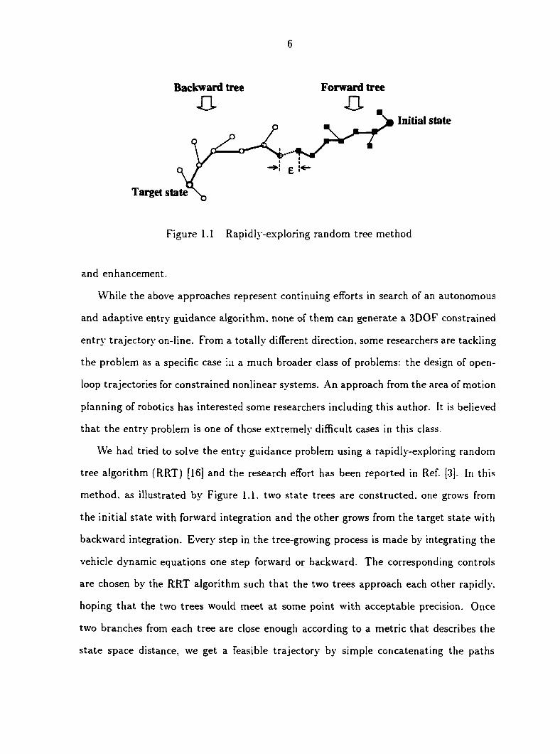
Backward tree Forward tree
-a 43-Initial state
Target state
Figure 1.1 Rapidly-exploring random tree method
and enhancement.
While the above approaches represent continuing efforts in search of an autonomous
and adaptive entry guidance algorithm, none of them can generate a 3DOF constrained
entry trajectory on-line. From a totally different direction, some researchers are tackling
the problem as a specific case in a much broader class of problems: the design of open-
loop trajectories for constrained nonlinear systems. An approach from the area of motion
planning of robotics has interested some researchers including this author. It is believed
that the entry problem is one of those extremely difficult cases in this class.
We had tried to solve the entry guidance problem using a rapidly-exploring random
tree algorithm (RRT) [16] and the research effort has been reported in Ref. [3]. In this
method, as illustrated by Figure 1.1. two state trees are constructed, one grows from
the initial state with forward integration and the other grows from the target state with
backward integration. Every step in the tree-growing process is made by integrating the
vehicle dynamic equations one step forward or backward. The corresponding controls
are chosen by the RRT algorithm such that the two trees approach each other rapidly,
hoping that the two trees would meet at some point with acceptable precision. Once
two branches from each tree are close enough according to a metric that describes the
state space distance, we get a feasible trajectory by simple concatenating the paths

t
together as indicated by the thick line in the figure. The gap £ poses no problem
since it can be easily overcome by the reference tracking algorithm of the entry guidance
system. The most impressive feature of this approach is its graceful handling of whatever
constraints or obstacles in the state/control space, since the controls are picked by the
RRT algorithm from the allowable control space corresponding to the control constraints
such as maximum bank rate and acceleration constraint, and the branches that grow out
of the boundary of the allowable state space are simply discarded. Reference [5] shows
great success in handling a path finding problem for a helicopter moving on a plane by
this approach. The randomized path planning algorithm is capable of finding dozens of
feasible trajectories in seconds for the helicopter moving on a plane full of obstacles that
are otherwise hard to be described in terms of. for example, state constraints by any
optimization method.
Although this approach seems promising in solving problems as difficult as the he
licopter path planning problem, it also presents an undesired property, the stochastic
feature. For on-board use. the randomized process may fail to produce a trajectory
within a specified time period. On the other hand, as the problem size increases, the
difficulty level increases drastically. The bottleneck of this approach lies in the metric
design for those very complicated dynamics. For example, imagining two states in the
entry trajectory problem, one state differs from the other only in the flight path angle
and the velocity. It is very hard to tell which state is closer to the target point unless we
know how to control the vehicle to reach the target point from each state. This problem
is almost equivalent to the whole trajectory design problem. The effort we made on
designing a good metric led us to think about ways for doing direct state transition
between any two mutually reachable (by integration forward or backward) states so that
we can know the distance between and the possible control profiles connecting them.
The first idea of this dissertation research was sparkled by the ground-track design
method introduced in Ref. [24] when we were exploring the method for designing a RRT

s
metric. Reference [24] shows by tracking a ground-track using bank angle control. 3
state variables, i.e.. latitude, longitude, and heading angle can be precisely led to meet
their required values simultaneously. We further concluded that the altitude could also
be adjusted by modifying the geometrical shape of the ground-track. Then we could
use the bank angle alone to control these 4 variables by tracking the ground path. The
remaining variables could be controlled by manipulating the angle of attack. Although
little trace of this concept is left in the final method, which shall be presented in the
rest of this dissertation, it did form the starting point of this research.
1.3 Overview
This dissertation presents an innovative approach for fast generation of 3DOF con
strained entry trajectory. First, the longitudinal reference profiles for altitude, velocity,
and flight path angle with respect to range-to-go are generated. To make these profiles
flvable. they are designed by 3 pieces:
1. The initial descent that starts from the entry interface and ends at the point when
the vehicle smoothly transits onto an equilibrium glide path:
2. The terminal backward trajectory integration that starts from the TA EM interface
and ends at an intermediate state, called the pre-TA EM point:
3. The quasi-equilibrium glide profile that connects the preceding two pieces.
The first 2 pieces are implemented by integrating the full 3 DO F vehicle dynamic
equations and recording the corresponding state and control histories. This guarantees
the flyabilitv of the trajectory. The quasi-equilibrium glide piece is based on a novel
concept of quasi-equilibrium glide condition (QEGC) and used to adjust the whole lon
gitudinal profiles such that all the reference profiles are continuous at both conjunction
9
points, i.e.. the QEGC transition point and the pre-TAEM point. The entry path con
straints are strictly enforced in designing the central piece, the quasi-equilibrium glide
profile.
Next, the 3D0F reference trajectory is completed by tracking the longitudinal ref
erence profiles using an approximate Receding-Horizon(RH) control method. The bank
angle is reversed at a proper point according to a single bank-reversal strategy such
that the TAEM heading and distance to the H AC requirements are precisely met with
in specified precision. Finally, for some extreme entry cases with large cross-range for
which either no bank reversal exists, or the bank reversal would occur too close to the
TAEM interface, we developed a terminal reference ground path tracking technique. By
systematically designing the geometry shape of the terminal reference ground path, the
altitude reached at TAEM can be adjusted.
One additional merit of this on-board trajectory design method is that the designer
can set the TAEM interface flight path angle and bank angle, which are usually not
specified in entry mission specifications with preferred values. This gives great flexibility
to the design for the final approach and landing phase trajectory.
For any entry cases, usually two. at most three iterations for a single parameter
to be search sequentially, are needed by this method: the iteration for searching the
longitudinal reference profiles and the iteration for searching the single bank-reversal
point. Both iterations are strictly monotonie with respect to their respective parameters.
This feature makes both processes converge very fast, usually in the order of single digit
number of iterations. For a broad range of entry cases of the X-33 and X-3S vehicles with
down range between 3500 to 5000 nm. each 3DOF reference trajectory can be generated
in 2.5 seconds on a 500MHz a DEC Alpha workstation, or 3.3 seconds on a 800MHz PC
on average, for achieving the terminal precision of ±10 m/s for velocity, 5 degree for
heading error, and ±100 meters for altitude.
10
Adaptability of this method is also demonstrated. Given any state along a nominal
entry trajectory, we deliberately add perturbations to it. then a new 3DOF trajectory-
can be generated from that perturbed state with ease. The perturbations can be so
large that it is unlikely that any trajectory regulation method can bring it back to the
original reference trajectory. This capability demonstrates the potential of this method
for handling sub-orbital entry and abort scenarios.
The algorithm has been tested on a high fidelity simulation software developed at
NASA Marshall Space Flight Center, called the Marshall Aerospace Vehicle Represen
tation in C (MAVERIC). At the entry interface, the on-board trajectory generator is
called with the current state information and the specified H AC and TAEM interface
requirements, a 3DOF reference trajectory is generated rapidly. In the short time peri
od. usually 1 to 2 seconds, for calculating the reference trajectory, we just let the vehicle
fly open-loop. Then a state-of-art trajectory regulation algorithm [21]. is activated to
track the 3DOF reference trajectory just generated. This procedure survived all entry-
test cases for the X-33 vehicle model, and all guidance mission were accomplished with
remarkable terminal precision.
11
CHAPTER 2. PROBLEM FORMULATION
2.1 Objective and Assumptions
The entry reference trajectory generation problem is defined as follows: given the
terminal conditions at the entry interface, and the state conditions at the terminal area
energy management (TA EM) interface, find the required bank angle history cr(Z) and
angle of attack profile a(t) so that:
1. The entry vehicle reaches the TAEM interface with specified conditions on altitude,
velocity, velocity azimuth angle, and range to the Heading Alignment Circle(HAC):
2. The trajectory observes all the path constraints imposed by the load/acceleration,
dynamic pressure, heat rate constraints, and the equilibrium glide condition:
3. The a profile is consistent with the entry vehicle trim capability, and both a and
q do not exceed the flight control system authority in terms of the maximum
magnitudes, rates and accelerations of a and a.
The basic assumptions establishing the scope of applicability of this research are:
1. The entry vehicle is a lifting vehicle with L j D ̂ 0:
2. The TAEM conditions are specified in terms of altitude, velocity. range-to-HAC.
and velocity heading pointing to the H AC:
3. A nominal a versus Mach profile is available, and limited variations about this
nominal profile are allowable.

12
4. All the path constraints can be expressed as constraints in the altitude and velocity
space with the given o profile;
2.2 Entry Vehicle Dynamics
The entry flight is subject to the vehicle dynamics described by the following three-
dimensional point mass dimensionless equations over a spherical rotation Earth:
r = V'sin-/ (2.1)
6 = ' C0s''sin1, (2.2, r cos o
V* cos -y cos v o = ! (2.3)
r
V = — D — + f?2r coso(sin 7 cos o — cos sin ocos v) (2.4)
: L cos a + ^V*2 ^ ^+ 20V cos osin c
+ fi2r cos o(cos 7 cos o — sin 7 cos c sin o)] (2.5)
1 V = V
4 cos 7 sin t'tan 0 — 201 "(tan 7 cos c cos o — sin o) cos 7 r
J. Q2 • • + sin csin ocoso COS-)
(2.6)
where there are six state variables, r. 6. o. V. 7 . and e. The r is the radial dis
tance from the center of the earth to the vehicle, normalized by the radius of the earth.
RQ = 637Skm. The longitude and latitude are 6 and à measured in radian, respectively.
The Earth-relative velocity is V. normalized by y/gofio. where gQ is the gravitational
acceleration. 7 is the flight path angle measured in radian, c is the velocity azimuth
angle in radian, measured from the north in a clockwise direction. Derivatives of these
variables are taken with respect to dimensionless time r. which is obtained from nor
malizing the real time by r = t/YJRQ/ÇQ. fi is the normalized Earth self-rotation rate.
D and L represent the non-dimensional drag and lift accelerations, in terms g0, and can
be calculated from

13
L = r2l-pV2S r e JCL (2.7)
D = -^^p\ 'SrefCo (2.8)
where S r ef is the reference area of the entry vehicle, m the mass, and p the atmospheric
density. The lift and drag coefficients CL and Co are modelled as table functions of angle
of attack o and Mach number M. respectively. Given the altitude r. velocity V. and
the angle of attack a. M is calculated and then the corresponding C'L and CO values are
found by looking up the table functions with the M and the a value. The atmospheric
density can be modelled as an exponential function of the altitude p = pae~kf~T~R°\ with
k > 0 and pQ > 0 being constants, or a look-up table function of altitude for better
precision.
There are two controls for the entry dynamics, the bank angle a and the angle of
attack a. But a is the primary control since the o profile should be consistent with
the entry vehicle trim capability and only a limited variation about the nominal o is
allowed. This issue will be further discussed in section 2.3.
The effect of Earth self-rotation is involved in the V. and c dynamics and should
not be discarded as usually done in entry reference trajectory tracking law design. In
fact, the Earth self-rotation term in the velocity dynamic, for example, is the dominant
term in the initial phase of orbital entry, where the atmospheric effect is negligible. This
can result an increase of the velocity and energy in the initial phase of orbital entry.
2.3 Trajectory Constraints
Entry trajectory is subject to a number of constraints imposed by the allowable heat
rate, dynamic pressure, load acceleration, and the equilibrium glide condition. These
constraints can be translated into velocity-altitude coordinate and form the so-called

14
entry corridor as illustrated by Figure 2.1. Implicitly, entry trajectory is also subject
to the limited authority of flight control system. For example, the control constraints
imposed by the maximum magnitude, rate, and acceleration of a have great effect in
shaping the trajectory, especially where bank-reversal happens.
1 . 0 2 Entry interface
Entry trajectory
1.015
i.
1.01
Load constraint
1.005
TAEM
0.1 0.2 0.3 0.4 0.6 0.7 0.8 0.9 1 0.5
V
Figure 2.1 Entry corridor
Heat rate constraint
Q < Qmax (2.9)
specifies that the heat accumulated on the vehicle per unit surface area and per unit
time, should not exceed a maximum value Qmax- Reference^ 1] gives a more detailed

15
analysis of heat constraints. The heat rate can be calculated from
Q = ky/pV3 '1 5 (2.10)
where k is a constant. Since p is a function of r. Eq. ( 2.10) uniquely defines a boundary
curve in the r — V space as shown in Figure 2.1.
Depending on vehicle structure specification, load constraint can be either specified
in terms of body normal load
\Lcosa + Dsino| < nZ m a i (2.11)
or in terms of total load
y/L* + D2 < (2.12)
where n.mM is the maximum load in terms of gQ that the vehicle can sustain. The angle
of attack o is involved explicitly in Eq. ( 2.11) and implicitly in the terms of L and D.
Since o is a table function of Mach number, which again is a function of r and V. the
above load inequalities can also be solved as a boundary curve in the r — V space as
shown in Figure 2.1.
Dynamic pressure constraint
<7 < Qmax (2.13)
is also an inequality that can be translated into the r — V space, since q = \pV2 and p
a function of r.
All the constraints above should be enforced strictly. Otherwise, the vehicle may
sustain either structural or thermal damages. In this sense, they are "hard" constraints.
Another constraint comes from the so-called equilibrium glide condition (EGC)
"1
r ( r ) -J — L cos OEQ < 0 (2.14)

16
which is obtained by omitting the Earth self-rotation term and setting i = 0 and = 0
in Eq. (2.5) This condition is intended for reducing the altitude phugoid oscillation along
the entry trajectory. The term <7EQ is a constant bank angle. For a major part of the
entry trajectory, where the Earth self-rotation effect is less important and the flight part
angle -• remains small, the EGC approximately represents the actual -, dynamics. But
in the terminal part of the entry trajectory, where the -, is no longer small and changes
rapidly, the EGC is less accurate. Similarly, the EGC can be projected into the r — V
space and forms the upper boundary of the entry corridor as illustrated in Figure 2.1. By
limiting the entry trajectory below this boundary, the undesirable phugoid oscillation in
the altitude are eliminated. For some entry cases, the specified TAEM point may even
be above the upper boundary formed by the EGC. In this sense, the EGC is intended
for achieving good quality of the entry trajectory and thus a "soft" constraint.
Both a and o are subject to maximum magnitude, rate, and acceleration constraints.
Besides, the a profile should be consistent with the entry vehicle trim capability. This is
enforced in this research by allowing a band of region for o variation along the nominal
a versus ,\f profile. The width of the band is chosen to be ±5 degrees, as shown by
Figure 2.2. a variation is only allowed inside this band region.
2.4 Entry and TAEM Conditions
The initial state of the entry trajectory is available from the entry interface condition-
s, which contains all 6 state variables and the 2 control variables a and o. The terminal
state is determined by the TAEM interface requirements illustrated by Figure 2.3.
Let the terminal state variables of the entry trajectory be denoted by the subscript
f. The TAEM conditions require that the terminal velocity azimuth heading is pointing
to the tangency of the HAC and the range to HAC equals to the specified value RTAEM-
Thus the allowable terminal ground coordinates form a circle centering the HAC with
17
50
45
40
35
O) •§ 30
25
20
15
10
+5 deg
-5 deg
Upper bound
Norminai a profile
Lower bound
10 15 20 Mach number M
25 30
Figure 2.2 Allowed region for a variation along the nominal o profile
radius RTAEM as shown in Figure 2.3. Therefore the allowable terminal spherical coor
dinate (ôj.Of) and cy are related by the geometric condition shown in Figure 2.3.
The terminal velocity V} and altitude ry should equal the specified TAEM velocity
and altitude
r/ = rT A E\! (2.15)
V/ = V'TAE.M (2.16)
The terminal flight path angle is usually unspecified by the TAEM conditions. As
will be shown later, we leave •)/ asa design parameter whose value is determined by the
designer.
The terminal angle of attack otj at the TAEM point is obtained from the nominal
profile a{M). The terminal bank angle aj is also unspecified. But a smaller oj value is
usually preferred by the final approach and landing phase. Thus, we also let the crj be a

IS
design parameter up to the designer's choice, or else it can be fixed at a small value.
North A
Latitude <|>
TAEM point (0f ,<j>r) Entry trajectory ground-track
Longitude 0
Figure 2.3 TAEM interface requirements
19
CHAPTER 3. ON-BOARD 3DOF CONSTRAINED ENTRY
TRAJECTORY GENERATION METHOD
The major challenge of entry trajectory generation lies in designing a 3D0F tra
jectory that meets all the state and control constraints. The commonly used methods
for designing 3D0F constrained entry trajectory include the infinite-dimensional search
methods such as optimal control or finite-dimensional search methods such as param
eter optimization. However, because of the highly nonlinear nature of the entry vehi
cle dynamics, those methods inevitably require many iterations and great expertise in
adjusting parameters of the optimization processes. Usually one iteration means inte
grating the whole trajectory at least once. Thus, the corresponding computation time
is unaffordable for on-board use. let alone the convergence reliability issue.
By utilizing some interesting features of space vehicle dynamics, a conceptually differ
ent design method is found to be much more efficient in reducing the search dimensions
and guaranteeing fast convergence of the iterations and hence the rapidness of the trajec
tory generation. By this method, we decompose the search process into two sequential
parts. First, the longitudinal reference profiles for the altitude, velocity, and flight path
angle with respect to range-to-go to HAC are designed. The magnitude of the reference
bank angle a profile is parameterized with a single parameter which is to be itér
ât ively determined. Then the obtained longitudinal reference profiles are tracked with
linear time-varying control laws for <r and a. A single bank-reversal strategy is developed
and the range-to-go point where the unique bank-reversal happens is searched. Both

20
searches are monotonie with respect to their corresponding parameters: thus, very few
iterations are needed for convergence. Finally, a full 3DOF trajectory featuring a single
bank-reversal and satisfying all the constraints is obtained. Special cares are also given
to those extreme entry cases where bank reversal does not exist.
In this chapter, section 3.1 introduces how the longitudinal reference profiles are
designed: section 3.2 presents how a 3DOF trajectory is completed based on tracking
the longitudinal reference profiles.
3.1 Longitudinal Reference Profiles
The longitudinal reference profiles include velocity, altitude, flight path angle, and
bank angle versus range-to-go reference profiles: l ' (5,O J O). r(S t o go) *>(•?,o g o). and a(S t o g û).
The angle of attack profile a(Stogo) is available from the nominal o profile o(.U) because
of the dependence of V* and r on Stogo- The reference profiles represented in the altitude-
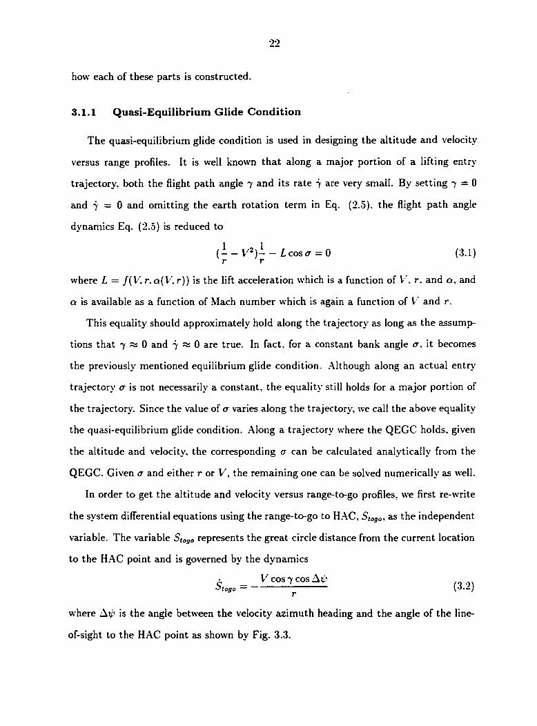
velocity space are illustrated in Fig. 3.1. The corresponding reference control profile
&{Stogo) with respect to V is shown in Fig. 3.2.
Illustrated by Fig. 3.1. the initial part of the reference profile starts from the entry
interface and ends at a transition point inside the flight corridor, which is marked by
the dashed line of QEGC transition. This initial part is obtained by 3DOF trajectory
integration from the entry interface with the nominal o and a constant a. The terminal
part, which starts from some point inside the entry corridor, marked by the dashed
line of pre-TAEM transition, and ends at the TAEM point is obtained by integrat
ing the trajectory backward starting from the TAEM point. The central part, named
Quasi-Equilibrium Glide (QEG) profile, connects the above two parts. It is obtained by
utilizing the so-called quasi-equilibrium glide condition (QEGC), which is adjusted so
that the whole reference profile is continuous at both transition points.
Starting from introducing the QEGC. the following subsections describe why and
21
1.02 Entry Interface
1.015 QEGC transition
QEGC
preTAEM transition 1.01
1.005 Terminal backward trajectory
0.9 0.1 0.3 0.4 0.5 0.6 0.7 0.8 1 V
Figure 3.1 Altitude versus velocity reference profile
QEGC transition
QEGC a upper bound from load constraint QEGC o upper bound
from heat constraint
preTAEM transition
QEGC a profile
terminal backward trajectory
initial
0.3 0.1 0.4 0.5 0.9 0.6 0.7 0.8 1 V
Figure 3.2 Bank angle versus velocity reference profile
22
how each of these parts is constructed.
3.1.1 Quasi-Equilibrium Glide Condition
The quasi-equilibrium glide condition is used in designing the altitude and velocity
versus range profiles. It is well known that along a major portion of a lifting entry
trajectory, both the flight path angle 7 and its rate 7 are very small. By setting 7 — 0
and 7 = 0 and omitting the earth rotation term in Eq. (2.5), the flight path angle
dynamics Eq. (2.5) is reduced to
(1- V2)- - Lcosa = 0 (3.1) r r
where L = /( V, r. a( V, r)) is the lift acceleration which is a function of V. r. and a, and
û is available as a function of Mach number which is again a function of V and r.
This equality should approximately hold along the trajectory as long as the assump
tions that 7 % 0 and 7 % 0 are true. In fact, for a constant bank angle <r. it becomes
the previously mentioned equilibrium glide condition. Although along an actual entry
trajectory a is not necessarily a constant, the equality still holds for a major portion of
the trajectory. Since the value of a varies along the trajectory, we call the above equality
the quasi-equilibrium glide condition. Along a trajectory where the QEGC holds, given
the altitude and velocity, the corresponding a can be calculated analytically from the
QEGC. Given a and either r or V, the remaining one can be solved numerically as well.
In order to get the altitude and velocity versus range-to-go profiles, we first re-write
the system differential equations using the range-to-go to HAC, S togo, as the independent
variable. The variable S t0go represents the great circle distance from the current location
to the HAC point and is governed by the dynamics
6 V cos 7 cos Atf /0 Stogo — ~ W"-/
where Av> is the angle between the velocity azimuth heading and the angle of the line-
of-sight to the HAC point as shown by Fig. 3.3.

23
Entry trajectory \ j HAÇ„̂ ta^
.2 ;
AV l̂̂ 'x_v
Entry interface —" Vehicle
Figure 3.3 Heading error along the entry trajectory
By dividing V equation with S t 0go, we get the velocity differential equation with S t 0go
as the independent variable
dV r :{—D — —y-) (3.3) dStogo cos 7 cos Ay V r2
where the earth rotation terms has been omitted. Note that the independent variable
Stogo is decreasing. Since Aip % 0 in most part of the trajectory except for the portion
near the end, we let A0 = 0. Now, we can apply the QEGC. Since 7 % 0 along the
QEGC, Eq. (3.3) can be simplified to be
dV = D77 (3.4) dStogo V
Replacing D with L(CD/CL) and substituting L from the QEGC, we get
^ . , 1 -VGM. (3.5) dStogo r V' cos a
Note that the dominant factor in the above equation is cos <7 since r as 1 and the term
CD/CL is usually not a sensitive function of velocity. If we schedule A as a function of
V, Eq. (3.5) can be integrated to the given final value of St090, i.e., the St0g0 value at the
pre-TAEM transition point that shall be introduced later. By adjusting the <r( V) profile,
the final value of V is changed. It is easy to see that if a is small, the right-hand-side
value is small and therefore V* decreases slowly, and vice versa. We can use only one

24
parameter to represent the er(V) profile for the region between the pre-TAEM and the
QEGC transitions, such as the piecewise linear schedule of <r as shown in Fig. 3.2. In
conclusion, the variation of the terminal velocity from the integration of Eq. (3.5) is
monotonie with respect to the value of crmi(j.
3.1.2 Enforcement of the Inequality Trajectory Constraints
The inequality entry trajectory constraints Eqs. (2.9)-(2.14) are enforced by appro
priately bounding the cr(V') profile along the QEGC. Note that when integrating Eq.
(3.5) with the <r(V) profile, the r value is obtained by solving the QEGC with the current
A and V. Given V, the corresponding r should be bounded within the entry corridor.
Denote the entry corridor lower boundary with rmin(V), and the upper boundary with
rmax(V ). Then apply the QEGC along the entry corridor lower boundary to get
o-max(V') = A QEGC [rmin(V'), V] (3.6)
where the function <TQEGci r- V) calculates the cr value for the given V and r using the
QEGC. and can be easily derived from Eq. (3.1). Similarly, the a lower bound crmin(V)
value can be obtained from
tfm.n(V') = (TQEGC [RMAX(V), V] (3.7)
= <7 EQ (3.8)
since the entry corridor upper boundary is formed by the EGC Eq. (3.1), which is in fact
a QEGC with a constant value &EQ. Thus the <r( V) profile should be bounded between
the (TEQ and <RMAX(V) in order for r to be bounded by the entry corridor. Figure 3.4 shows
the obtained <JMAX{V) and (TEQ in the V-C space corresponding to the entry corridor,
zoomed in the region where the QEGC applies.
The (Tmid, and hence a part of the <r(V) profile, may be found to be outside the
QEGC a boundaries. If this is the case, the portion of the <t{V) profile that lies outside

25
the allowed region is replaced with the corresponding boundaries. Figure 3.4 illustrates
this approach. Correspondingly, Fig. 3.5 shows that the r — V reference profile goes
along the entry corridor lower boundary for the region where <r( V) = <rmor(V).
This way, by restricting the magnitude of the cr(V'), the corresponding r and V* values
will be inside the entry flight corridor. And no inequality trajectory constraints will be
violated along the QEGC profile.
At this point, two problems remain unsolved. First, the entry interface usually lies
well above the flight corridor, hence a portion of the trajectory from the entry interface
can not be approximated by the QEGC path. Second, usually the QEGC can not be
extended to the TAEM point for the following reasons:
1. There is no guarantee that the specified TAEM condition lies inside the entry
corridor:
2. The assumptions for QEGC will not be true in the lower velocity and altitude
region since both 7 and 7 may not be small. In fact, if the QEGC is extended to
the TAEM point, the corresponding reference altitude profile will usually result
a very large flight path angle 7. This can be observed by taking a look at the
flight corridor upper boundary, which corresponds to a fixed bank angle quasi-
equilibrium glide profile. The slope in the altitude-velocity coordinate increases
drastically as the velocity approaches the TAEM velocity. However, the altitude-
velocity slope dr/dV is approximately linear to sin 7. Hence the reference flight
path angle 7 will become unrealistically large if the quasi-equilibrium glide profile
is used for the low velocity range;
To solve these problems, two techniques, initial descent and terminal backward tra
jectory integration, are developed for designing parts of the reference profiles where the
QEGC can not be applied.
26
QEGC a upper bound
60 OEGCo upper bound
50
preTAEM transition 40 ?
5. o OEGCo
30
QEGC transition
QEGC a lower bound from EGC constraint EO
0.9 0.6 0.7 0.8 0.3 0.4 0.5 V
Figure 3.4 Bounded a{V) profile (zoomed in the region where the QEGC applies)
.02
1.015
QEGC transition
QEGC profile
1.01 -preTAEM transition
1.005 0.3 0.4 0.6 0.7 0.8 0.9 0.5
V
Figure 3.5 Bounded v-r profile (zoomed in the region where the QEGC applies)

27
3.1.3 Initial Descent
The entry point usually lies above the entry corridor. Thus from the entry interface,
the vehicle needs to descend to enter the entry corridor and transit smoothly onto a
QEGC profile. By examining the trajectory characteristics of descent from the entry
interface with a constant bank angle, as show by Fig. 3.6, a simple method is designed
for constructing the longitudinal reference profiles before the QEGC can be applied.
1.02
1 I • T 1 1 1 1—
1.019 Entry interlace. 1
1.018 - -
Trajectory with constant o
1.017 - -
1.016 - -
h.
1.015 • -
1.014 11 1
y»-Tangent line of the 1.013 / / 7
' local EGC profile
QEGC transition point 1.012 '
1.011
' --" l -— I ' , i i 0.6 0.7 0.8 0.9 1 1.1 1.2
Figure 3.6 Initial descent with constant bank angle
The nominal a and a constant bank angle <tq is chosen for the descent integration.
Demonstrated by Fig. 3.3, the sign of <r0 is set such that the vehicle turns toward to
HAC point, which means
SIGN{*0) = -SIGN(A^eh) (3.9)
where AipEH = V'o — *EH• The terms 0O and ^EH are the velocity azimuth angle and
the azimuth angle of the line-of-sight to the HAC point, both measured at the entry

28
point. The value of <tq is first set to be zero. But in some cases small cr0 value will
result in the trajectory bouncing a few times before it can enter the entry corridor, a
phenomenon known as phugoid motion. If this happens, the <TQ is increased bv a fixed
increment and the numerical integration is repeated from the entry interface. Once it
enters the entry corridor, the transition point for a smooth transition onto an QEGC
profile is searched along the integration. The criteria for a smooth QEGC transition is
described by
is calculated for the current state. (dr/dV )çEGC is calculated from the QEGC at the
current V and r. It can be obtained either by differentiating the QEGC once with
respect to V, or using finite difference method along a constant a QEGC profile. A
reasonable discontinuity bound S can also be calculated from Eq.(3.11). It shows that
at given V and r. dV/dr is linear to 1/sin(7). Thus the discontinuity at the transition
point means a jump of 7 value. Given a tolerance of 7 discontinuity, we can calculate
the corresponding S value. The condition (3.10) assures that at the transition point the
r — V curve is reasonably smooth. With the selected cr0, Eqs. (2.1-2.6) are integrated
with the given a profile. The obtained r(Stogo), V'(5,ogo). and 7(S togo) profiles are stored,
together with the control profiles a(S t o g o) and a{S t o g o)-
Since the <TQ used for the initial descent is usually different from the corresponding
er value of the QEGC profile at the transition point, there will exist a discontinuity in
the control profile cr(5togo) at the transition point. To eliminate the discontinuity, once
the descent trajectory enters the entry corridor, the bank angle used in the integration
3 DOF (3.10)
where 5 > 0 is a small value bounding the discontinuity, and
(3.11)
29
is set to be
{<70 i f <r0 > crçEGc(r. V) (3.12)
<7QEGc{r, V) i f (To < <7(5£Gc(r, V)
By this formula, the bank angle for the initial descent is continuously set to be the a value
obtained from the QEGC corresponding to the current r and V. Thus whenever the
transition point is found, the a profile is continuous at that transition point. Figure 3.2
shows the effect of this method. It shows that the a increases smoothly From cr0 to cr2
which is the QEGC a at the transition point.
3.1.4 Terminal Backward Trajectory
The goal of terminal backward trajectory integration is to obtain a longitudinal
profile for the terminal phase where the QEGC is not valid and also to provide lateral
ground track information for later use. Inspired by the RRT dual-tree method introduced
in Chapter 1, we start the integration from the TA EM state backward to a state in the
entry corridor where the QEGC can be well satisfied. In order to get the control a for
the backward integration, we use an analytic curve that represents the desired altitude
versus velocity profile to facilitate the integration. The actual state and control histories
are recorded from the integration process. Since the TA EM interface conditions only
specify the velocity, altitude and RTAEM, and the TA EM geographic coordinates 6 and
<p are not defined, we need to assign values to those unknown state variables 9, p and rb
in order to get the initial state for backward integration.
Illustrated by Fig. 3.7, the TAEM point is chosen to be on the line-of-sight from
the HAC to the entry point. The TAEM heading is pointing toward the HAC point.
Thus both the TAEM coordinate and heading angle at TAEM can be calculated. This
choice is just for simplicity and turns out to be uncritical for the design and will be
further discussed later in section 3.2.3. Second, the sign of <r is determined by the single
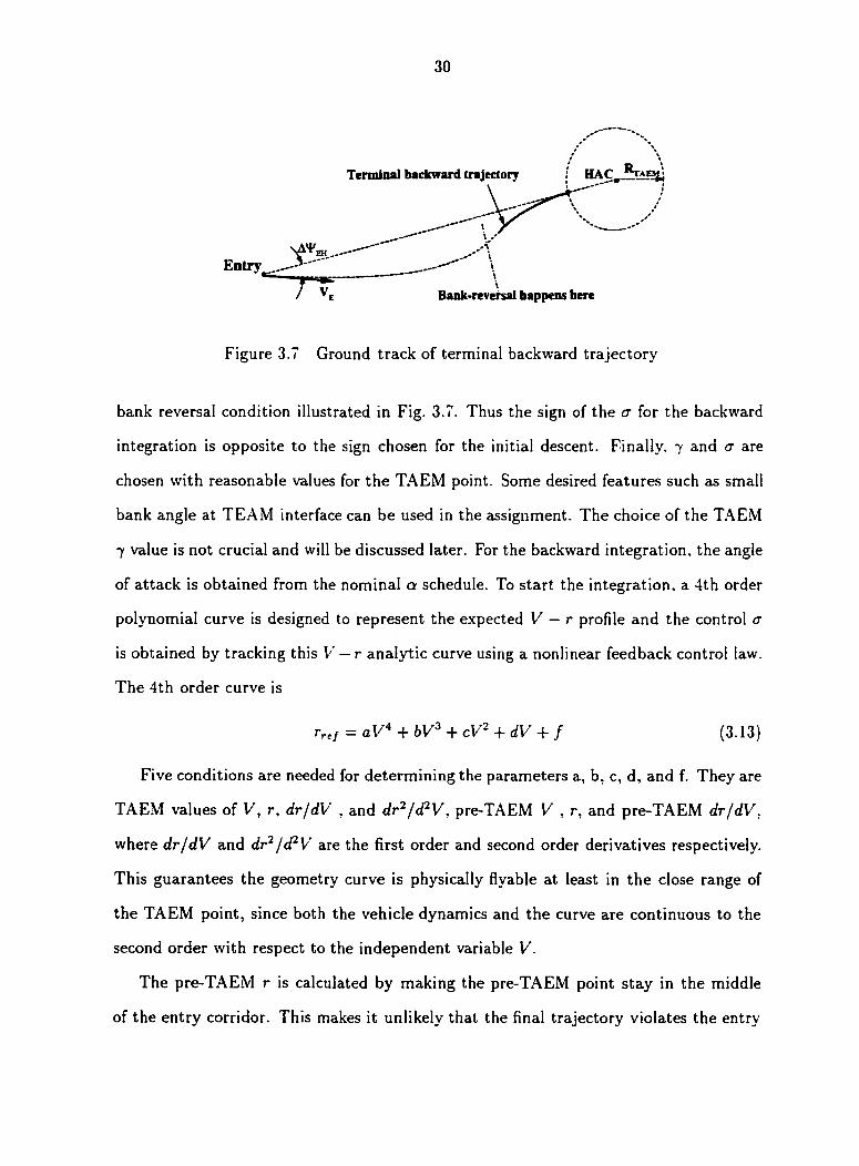
30
R_ \ Terminal backward trajectory HAC "tap^
Entry,,.,
Bank-reversal happens here
Figure 3.7 Ground track of terminal backward trajectory
bank reversal condition illustrated in Fig. 3.7. Thus the sign of the a for the backward
integration is opposite to the sign chosen for the initial descent. Finally. 7 and a are
chosen with reasonable values for the TAEM point. Some desired features such as small
bank angle at TEAM interface can be used in the assignment. The choice of the TAEM
7 value is not crucial and will be discussed later. For the backward integration, the angle
of attack is obtained from the nominal a schedule. To start the integration, a 4th order
polynomial curve is designed to represent the expected V — r profile and the control a
is obtained by tracking this V — r analytic curve using a nonlinear feedback control law.
The 4th order curve is
r r e J = aV4 + bV3 + cV2 + dV + f (3.13)
Five conditions are needed for determining the parameters a, b, c, d, and f. They are
TAEM values of V, r, dr/dV , and dr2/dPV, pre-TAEM V , r , and pre-TAEM dr/dV,
where dr/dV and dr2/d?V are the first order and second order derivatives respectively.
This guarantees the geometry curve is physically flyable at least in the close range of
the TAEM point, since both the vehicle dynamics and the curve are continuous to the
second order with respect to the independent variable V.
The pre-TAEM r is calculated by making the pre-TAEM point stay in the middle
of the entry corridor. This makes it unlikely that the final trajectory violates the entry

31
corridor constraints in the terminal phase. In fact, we leave the choice of the r position
in the corridor up to the designer's choice as a design parameter. The derivative dr/dV
at pre-TAEM is assigned a value equal to the corresponding local slope of the QEGC
profile with a constant a which passes through the pre-TAEM V and r point. As will be
shown later, the slope discontinuity at the pre-TAEM transition point introduced by the
difference between the actual QEGC profile and the QEGC glide profile with a constant
<7 is almost negligible and can easily be overcome by the tracking control law.
A nonlinear feedback tracking control law for tracking the V-r curve can be designed.
Define the difference between the actual altitude r and the reference altitude rre/ as
Sr = r - r ref (3.14)
Differentiate it with respect to velocity V to get
— D — (sin-y/r?) - (4a V'3 + 3bV2 + 2cV + d) (3.15)
and
Sr" = G r cos <7 + H r (3.16)
where
(3.17)
sin 7 D\ r 2r^ sin 7 — + —: :—
V V2 r3V'3 + _Lcos72(l + S-^X){V2 - 1) - 12aV2 - 6bV - 2c
rV 2 r2 yA r'
(3.18)
Design a nonlinear feedback linearization control law
cos <7 = HR — '2UV RÇV Rdr' — JyRdr
Crr (3.19)

32
1.008
preTAEM 1.0075
1.007
1.0065
>- 1.006
1.0055
Flight corridor
Geometry reference curve
— Actual backward trajectory
1.005
1.0045 TAEM
1.004 L-0.1 0.25 0.35 0.15 0.2 0.3
V
Figure 3.8 Backward tracking of the geometry reference curve
where u:VR and £VR are two positive constants, the dimensionless natural frequency and
the damping ratio. The close-loop dynamics can be obtained by substituting Eq. (3.19)
into Eq. (3.16):
Sr" + 2UJV R£,V RSr' + J \RRSr = 0 (3.20)
It can be seen from Eq. (3.20) that for any a'VR > 0 and ÇVR > 0. Sr goes to zero
asymptotically, or r —• aV4 + bV3 + cV2 + dV + f. Note that the damping ratio ÇVR
is usually set to be 0.7, and the choice of the natural frequency UJVR depends on the
maneuverability of the vehicle. Proper choices of U>VR will maintain a balance between
tracking accuracy and control saturation. Figure 3.8 shows how the reference curve is
built and tracked. Figure 3.9 demonstrates the robustness of this backward trajectory
tracking method. With different 7 values at TAEM, the slopes of the reference curves at

33
TAEM are different. As shown in the figure, the choice of the TAEM flight path angle
spans a broad range from -6 deg to -12 deg, and all the reference curves can be closely
tracked. This feature gives the flexibility to the designer that he/she can choose the
TAEM 7 value which is preferred by the design of the final approach and landing phase
trajectory.
1.008
1.0075
1.007
1.0065
k 1.006
1.0055
1.005
night corridor
— - •Geometry reference curve
Actaul backward trajectory
TAEM 1.0045
1.004
0.15 0.25 0.3 0.2 V
Figure 3.9 Backward trajectory tracking of several reference curves with different 7 values at TAEM
In some extreme entry cases, the vehicle dynamics, the a rate and acceleration con
straints, and the ubad" choice of the TAEM 7 may make it difficult to track the whole
reference curve very closely. But this does not affect the effectiveness of the method,
since the only purpose for doing the terminal backward trajectory integration is to get
a flyable reference trajectory that connects the TAEM point to some point in the entry
corridor beyond which the QEGC can be closely satisfied. In this sense, the reference V-
r curve tracking only serves as a practical means for providing the control input for the

34
backward integration and bridging the TAEM with the QEGC profiles. This underlying
feature makes the backward tracking very robust in terms of reaching such a pre-TAEM
point and allows a wide acceptable range for TAEM state initialization. Figure 3.10
further demonstrates the robustness of this methodology. It shows with a "bad™ choice
of the flight path angle for TAEM and the pre-TAEM condition, the reference curve can
not be closely tracked. But as long as the actual backward integration ends up at some
point in the entry corridor where the QEGC can be well satisfied, our goal is achieved.
Since the backward integration uses full dynamics, the obtained reference trajectory is
flyable, no matter what the actual backward trajectory looks like.
1.008
Nominal preTAEM
1.0075
1.007
1.0065
1.006
1.0055
Flight corridor
_ _ Geometry reference curve
— Actual backward trajectory
1.005
1.0045 TAEM
1.004 L-0.1 0.35 0.15 0.2 0.3 0.25
V
Figure 3.10 Backward trajectory tracking of a "bad" reference curve
3.1.5 Completion of the Longitudinal Reference Profiles
Once the transition points from the initial descent and the terminal backward path
are determined, a quasi-equilibrium glide profile is designed to connect the actual pre-

35
TAEM point and the QEGC transition point. Denote the pre-TAEM and the initial
descent transition points by the subscripts 'preTM' and 'Dsnd\ respectively. The a
value at the pre-TAEM point and the QEGC transition point are solved by Eq. (3.1).
and denoted by the corresponding subscript. Let ama be a value to be determined at
the midway point of VpreT\i and Voandi a piecewise linear continuous cr(V) profile can be
obtained using aprcT\t, <?m,d and (TDsnd- Thus for any selected amid. <?{V) is determined
for all V Ç [VprtTM-, Vbjnd]- At any V and the corresponding <r(V). the value of r is found
from the QEGC. With the nominal a prof i le and the vehic le aerodynamic model . CD /CL
is evaluated. Thus Eq. (3 .5) can be numerical ly integrated from S t 0goD s n d to S t o g o P r e T X r
The obtained velocity VpreTM' is compared against VpreTM and the difference is used
to update the ami(f for the next iteration. Since VpRET\i> changes monotonically with
respect to <7m,d, the iteration converges very fast by a simple secant algorithm
(VLTX, - VpreTM) (3.21) PreTM ~ VPreTM
The QEGC 7 (Stogo) profile is obtained by numerical differentiation along the QEGC
profile and recorded with respect to the corresponding St0go- For any given V and r',
, r* — r'—1
7 ' = tan' 1 (3.22) db
where dS is the range-to-go step size for the integration. Once the amid is found, the
reference profiles for the QEGC phase is determined. The whole reference profiles,
V(Stogo), r(Stogo), 7{Stogo), and a(Stogo), from the entry to the TAEM, are obtained by
concatenating the profiles of the initial descent, the QEGC profile, and the terminal
backward trajectory. Figure 3.11 demonstrates the longitudinal state reference profiles.
Figure 3.12 shows the corresponding control histories.
The o(St0g0) profile is trivially available by calculating the a value using the provided
nominal a(M) profile. Given any V and r, the Mach number is calculated and then the
scheduled a value is found. Figure 3.11 shows that the state variables V and r are
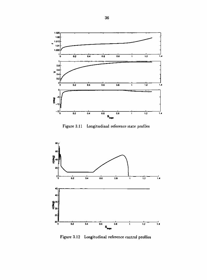
36
1.025
1.02
1.015
1.01
1.005
1.4 0.4 0.6 0.8
1
0.8
0.6 >
0.4
0.4 0.6 0.8 1.4
0
5 î
-10
-15 1.4 0.2 0.4 0.6 0.8
S. loge
Figure 3.11 Longitudinal reference state profiles
80
0> 40
0.4 0.6 0.8 1.4
45 ri
40
r d 30
25
2qL 1 1 i 1 1 1 1 0 02 0.4 0.6 0.8 1 12 1.4
s*
Figure 3.12 Longitudinal reference control profiles

37
continuous for the whole range. Shown in Fig. 3.12, the o-(Stogo) profile is continuous
at the QEGC transition point due to the use of Eq. (3.12). It also shows that a curve
smoothly transits the a value from 0, which happens to be the constant <r0 used for the
initial descent in this case, to a larger a value corresponding to the QEGC transition
point.
Also illustrated is the bounding of the <7(St0ff0) profile by the entry corridor upper
boundary, which is determined by the OEQ value. From the definition of the correspond
ing QEGC profile, we know that the corresponding part of the r versus V reference
profile goes along the entry corridor upper boundary. Usually, a(S togo) is not continuous
at the pre-TAEM junction point as shown in Fig. 3.2 and Fig. 3.12. Other discontinu
ities of the reference profiles mainly involve the 7 profile. The discontinuities may exist
at the QEGC transition point, the Vmid point and the pre-TAEM junction point. Since
these discontinuities can be easily overcome by the tracking law when completing the
3DOF trajectory that will be introduced in the next section, no special treatments are
devised for totally getting rid of them here. Nevertheless, some methods are possible to
this end. such as using tighter error bound for determining the QEGC transition point
or rounding the angle at the point of the <r{V) linear schedule, etc.
3.2 Completion of the 3DOF Trajectory
The obtained longitudinal reference profiles actually describe only part of an entry
trajectory in the longitudinal plane containing the entry point and the HAC point as
illustrated by Fig. 3.13. The missing part at this point is the lateral part of the trajectory.
In the actual entry flight, the vehicle, represented by the point C (vehicle) in Fig. 3.13,
will surely deviate from the great-circle plane with a spherical distance <j>'. The velocity
heading may also bias away from the line-of-sight by an angle A#. Mathematically,
neither A# nor <p' keeps constantly at zero. What these longitudinal profiles provide are
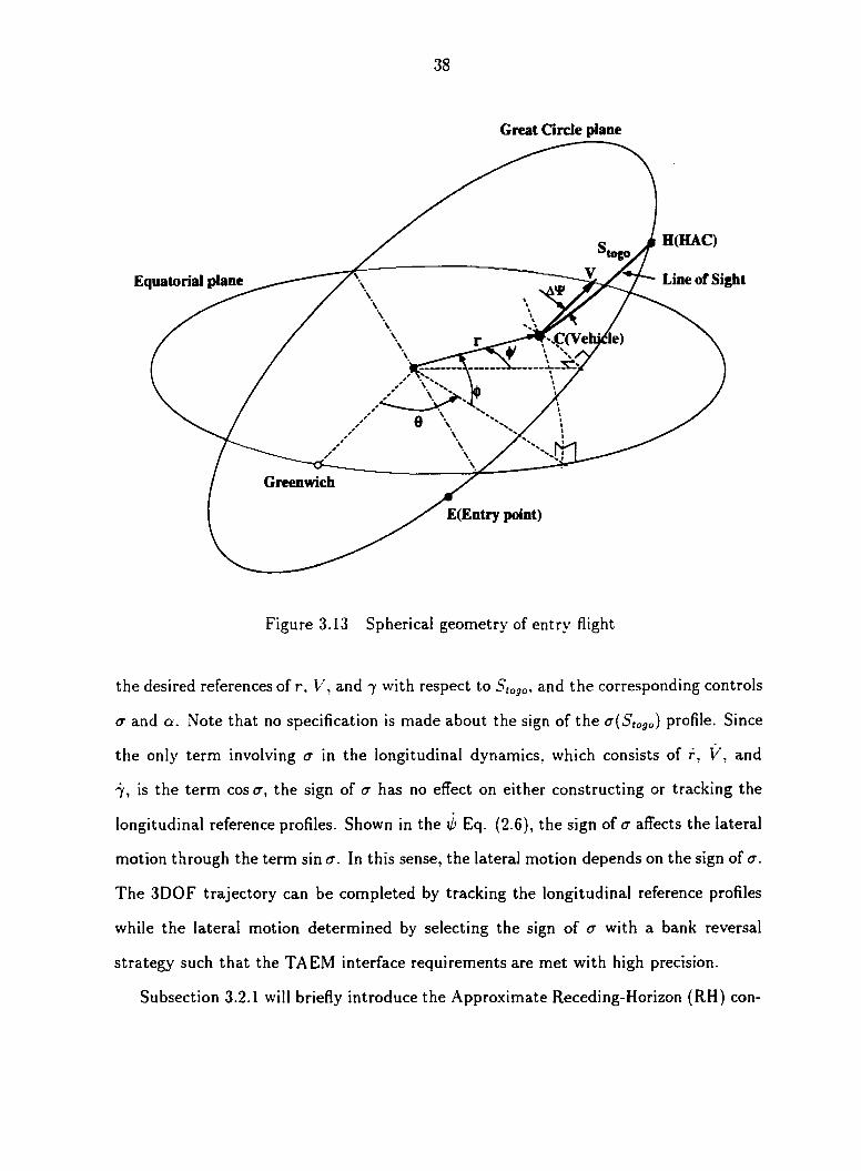
38
Great Circle plane
H(HAC) logo
Line of Sight Equatorial plane
Greenwich
E(Entry point)
Figure 3.13 Spherical geometry of entry flight
the desired references of r, V, and 7 with respect to S(ogo, and the corresponding controls
<7 and a. Note that no specification is made about the sign of the a(S togo) profile. Since
the only term involving a in the longitudinal dynamics, which consists of r, V, and
7, is the term cos <7, the sign of <7 has no effect on either constructing or tracking the
longitudinal reference profiles. Shown in the i/> Eq. (2.6), the sign of a affects the lateral
motion through the term sin <r. In this sense, the lateral motion depends on the sign of a.
The 3DOF trajectory can be completed by tracking the longitudinal reference profiles
while the lateral motion determined by selecting the sign of <7 with a bank reversal
strategy such that the TAEM interface requirements are met with high precision.
Subsection 3.2.1 will briefly introduce the Approximate Receding-Horizon (RH) con

39
trol method used for designing the tracking control law; subsection 3.2.2 will present the
application of RH method in tracking the longitudinal reference profiles: subsection 3.2.3
will present a bank-reversal strategy that generates a single bank reversal for most entry
cases; subsection 3.2.4 and subsection 3.2.5 will describe the methods used to address
those marginal entry cases where either the bank reversal must take place very close to
the TAEM interface or no bank reversal exists at all.
3.2.1 Approximate Receding-Horizon Control Method
Consider a linear, time-varying (LTV) system
x = A(t)x + B(t)u (3.23)
y = C(t)x (3.24)
where x G R 7 1 . u € A™, y G R p with p < n. The matrices A(-) : R -* /?"*". B(-) :
R —> Rnxm. and C(-) : R —> Rpxn are continuous. The system (3.23) is assumed to be
uniformly completely controllable, and C(t) is full rank for all t. A feedback control law
u = K(t)x is sought to regulate y so y(t) —> 0 from arbitrary initial conditions, and the
closed-loop system is stable.
An approximate receding-horizon control approach is introduced in Ref. [19] for state-
regulation. i.e.. when y = x. This approach can be readily extended to above problem.
The corresponding receding-horizon control problem at any t > to is defined to be an
optimal control problem in which the performance index
r f + T
/
'+'
[ y T ( T ) Q y i T ) + Ut{T)RU(T) ] (1T
ft+T
= [X T {T)C t(T )QC{T)X{T) + U T {T)RU(T) ] (1T (3.25)
is minimized for some Q > 0, R > 0, and T > 0. subject to system dynamics (3.23),
initial condition x(t) which is the current state, and the terminal constraint
y( t + T) = C{t + T)x{t + T) = 0 (3.26)

40
When the optimal control u*(-) for the above problem is found in [£, t + T]. the current
applied control u{t) is taken to be u'(t), and the rest of u'(-) is discarded. For the next
t, the above process is repeated to obtain the control at the next t. When y = x, the
closed-loop asymptotic stability is ensured under this strategy [15]. when y ^ x. the
choice of y must be such that y = 0 necessitates bounded x from the state equations
(3.23) to guarantee closed-loop stability.
In Ref. [19] an analytical approximation to the above computationally intensive
receding-horizon problem is proposed. For completeness we briefly describe here how it
can be adopted to the trajectory tracking problem. Consider the above receding-horizon
problem in the interval [(, t + T]. Divide this interval into N equal subintervals of length
h = T/N for some integer N > njm. With the current state x(t) known, a first-order
predict ion of x( t - f h) as a funct ion of u{t) is g iven by a Taylor ser ies expansion a t t
x( t + h) as x( t ) + /i[.4(/)x(<) + B(t)u( t )}
= ( / + hA)x + hBu (3.27)
Denote At = A(t + kh) . Bk = B(t + kh) . Ck = C{t + kh) . Xk = x(t + kh) and
ujt = u(t + kh) . k = 1, . . . . N. Then another f i rs t -order Taylor ser ies expansion a t t + h.
together with Eq. (3.27), gives
x( t + 2h) % x\ -f- / j[AjX i + B\Ui]
% ( / + hAi)(I + hA)x + /z( / + hA\ )Bu + h B\U\
Continuing this process, we have
it-1
x k % AfcX + ̂ 2Gk.iUi , k = 1 , . . .N (3.28) i=0

41
where
A* = ( / + hAk-i)^k-i, vvith A0 = /
Gk,i = ( / + hAk-i)Gk-i , i , i — 0, \ , . . . . k 2. (3.29)
G k,k- i = hBk-1
The subscript 0 in above expressions denotes the values at t . Let L 0 = z r (<)C r (<)QC(<)- r (0+
uT(t)Ru(t) and Lk = x^ClQCkXk + ulRuk, k = l....,Ar. The integral in Eq. (3.25) is
approximated by the standard trapezoidal formula for integrals:
J ~ h(Q.5Lo L\ -{• . . . + Z/jV—i + 0.5L.V ) (3.30)
Define an (myV)-dimensional vector u = co/{u(<), Hi,.... u.v-i}- If the j^-'s in Eq. (3.30)
are replaced by the prediction (3.28). the performance index is thus approximated by a
quadrat ic funct ion of v:
J = ]jVTH{t. . \ \h)v + xTS{t , N,h)v + q(x. t . N.h.u\) (3.31)
where H € f lm N x m N is positive definite for any t > <o, integer A* and h > 0. 5 6 /2nxm V
and q is quadratic in x and u.v- These terms are obtained directly by rearranging the
expression of J in Eq. (3.30) once jjt's are replaced by Eq. (3.28). The Appendix
gives the expressions of H and 5 for N = 2. 3 and 4. The constraint (3.26) can be
approximated by setting C^xx = 0 with x,\ from Eq. (3.28). which can be rewritten in
a compact form
MT ( t , N,h)v = -CNAjVx (3.32)
where
M t = Cv[GA,O ... G n , n . i ] 6 R p x m N (3.33)
The minimization of J in Eq. (3.31) with respect to v subject to constraint (3.32)
constitutes a quadratic programming (QP) problem. It can be shown that for sufficiently

42
small h (equivalently, sufficiently large N for a fixed T). MT has full rank.[19] given the
uniform controllability of the system. Then the above QP problem has a unique solution
v = - { [/ /" ' - H~ lM (MTH~ lM)~ l MTH~ l
xST + [//"'A/ (MT/f-'A/)"1] C.vA;V} x (3.34)
Define an m x miX matrix
AnJV = {Anxm-O, ....0} (3.35)
A closed-form, linear, time-varying feedback control law for u(t) . denoted by û(t: A*. h )
hereafter to signify its dependence on time and the values of A* and h, is then obtained
from the first m equations in (3.34)
u{t;N.h) = Im i \v = I\ ' ( t , i \ ' ,h)x{t) (3.36)
It has been established that when C = Inxn the closed-loop stability can always be
achieved with a control law properly constructed this way.[19] For other cases the closed-
loop stability will depend on the selection of y, i.e., whether or not y —> 0 leads to x —> 0.
For a given physical system, it is often not difficult to make such a selection.
The conventional gain-scheduled controllers for LTV systems require significant time
and effort to design. The entire process must be repeated if system model changes
which happens when a different reference trajectory is used to obtain the linearized
dynamics of a nonlinear system. Moreover, simple scheduling of controller gains does
not theoretically guarantee closed-loop stability of the LTV system even if the closed-
loop system is stable at the design points with frozen time. The recently emerged
linear parameter varying (LPV) methods overcome this stability problem, but the time-
consuming re-design process must still be carried out if the system model changes.
The above approach produces a controller that does not need explicit gain-scheduling.
The closed-loop stability is theoretically ensured. The controller development is a one
time effort. When the system model changes, we simply replace the A(-) and B(-) in

43
the controller code with the new matrices. In the entry guidance problem, the LTV*
system is the linearized dynamics about the reference trajectory. For different reference
trajectories, the corresponding A and B matrices can be easily obtained analytically
or numerically, and no re-design of the controller is required. The only parameters
that may need to be adjusted for the best performance are Q. R. and h (once the
value of <V is decided). But Q and R bear the same meaning of the weightings as in
the well-understood linear quadratic regulator design, therefore can be quickly selected.
The parameter h is inversely proportional to the controller gain, and can be tuned
accordingly.
3.2.2 Longitudinal Reference Profiles Tracking
Since the longitudinal reference profiles are with respect to the range-to-go. we re
write the system differential equations with Stogo as the independent variable in order
to derive the tracking control law. Figure 3.13 shows the spherical geometry defining
the range-to-go Stogo. Geometrically. Stogo represents the great circle distance CH from
the current spherical coordinate^.#) of the vehicle to the targeted HAC point . S t o go
decreases from the initial range-to-go EH, which is the great circle distance from the
entry point E to the HAC point H. to RTAEM- the specified distance from TAEM to
HAC. It is easy to show that
• V* cos 7 cos At' btogo = (3.37)
or
. , V cos 7 cos At/' , dbt o go = dr (3.38)
Since for the most part of the flight, A0 is small, will set A^ = 0 for simplicity.
Then divide the vehicle dynamic equations by St0go to get the longitudinal dynamic
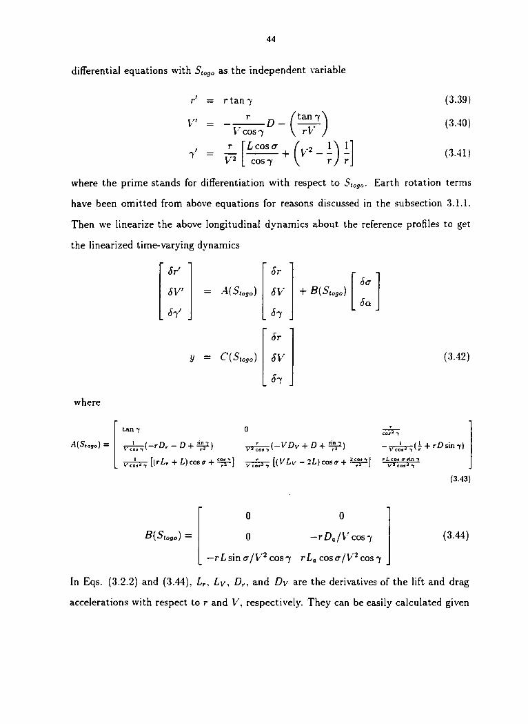
44
differential equations with S(ogo as the independent variable
r ' = r tan 7
V = - r
V* cos 7 D -
tan 7
rV
7 yi L c o s " [ A--» M 1
cos7 X ry r
(3.39)
(3-40)
(3.41)
where the prime stands for differentiation with respect to S t o g a . Earth rotation terms
have been omitted from above equations for reasons discussed in the subsection 3.1.1.
Then we linearize the above longitudinal dynamics about the reference profiles to get
the linearized time-varying dynamics
where
A(Stogo ) —
Sr '
SV'
W
= A(S,ogo)
y — C ( S t o g o )
Sr
SV
h
Sr
SV
S~i
+ B ( S t o g o )
Sa
Sa
(3.42)
tan 1 0
^ ( - r D r - D + ̂ ) -^—(-VDv + D+'•*?•)
VT^ [l^r + L) cos«x + [(VLv - 2L) cos<r +
- v ^ ( ; + rDsim) TL cow <r fin 7
V3 cosa "Y (3.43)
0 0
B { S t ogo) = 0 — r Da/V c os 7 (3.44)
—rLs'm cr/V 2 cos7 r£„ coscr/V'2 cos7
In Eqs. (3.2.2) and (3.44), Lr, Lv, Dr, and Dy are the derivatives of the lift and drag
accelerations with respect to r and V, respectively. They can be easily calculated given
45
the vehicle's aerodynamic model. The system output matrix C { S t 0 g o ) is set to be
By this output choice, we just explicitly track the state variables r and V*. The ~ i ( S t 0 g o )
profile is in fact automatically tracked because along the longitudinal reference profiles.
7 i s c o m p l e t e l y d e t e r m i n e d b y t h e r a n d V p r o f i l e s s i n c e d V / d r = — D / ( V s i n 7 ) —
l/( W2). Such a choice of the matrix C guarantees the closed-loop asymptotic stability
by the criteria stated in subsection 3.2.1, meanwhile it reduces the computational load
in calculating the feedback gains due to the smaller C matrix size.
To complete the 3D0F trajectory, a single bank-reversal strategy has been developed.
By this bank-reversal strategy, the control command acom and ocom for the current state
is given as
where S t o g o is the range-to-go to the HAC from the current state, a r e j and ar,/ are the
reference controls corresponding to the current 5(0ff0. and 5a and 5a are the commands
provided by the RH control feedback. B AN K SIG N(S togo) is the bank-reversal strategy
function providing the sign of crcom for the current state which is discussed in the next
subsection. After the command acom and acom are calculated, they are checked for
satisfaction of the rate and acceleration constraints. Then the actual 3D0F trajectory
is integrated one step forward. This process is repeated till the end of the integration.
1 0 0 C ( S t o g o ) (3.45)
0 1 0
c o m (3.47)
(3.46)
3.2.3 Single Bank-Reversal Strategy
A bank-reversal means that the sign of the bank angle is changed to the opposite of
its current value, but the magnitude of the bank angle remains unchanged. An entry
46
Bank-reversal happens here
Entry
W HAC ^taemI
backward trajectory
Expected entry trajectory
Figure 3.14 Concept of the single bank-reversal strategy
trajectory with a single bank-reversal, illustrated by Fig. 3.14. can be found by solving for
the correct bank-reversal point while tracking the longitudinal reference profiles. Based
on the illustration of Fig. 3.14, obviously, if no bank-reversal is done, the trajectory will
turn upward and miss the targeted HAC point. On the other hand, if the bank reversal
take place too early, say. very close to the entry point, the trajectory will go downward
and also miss the HAC in the opposition. Given the tracking of the same longitudinal
references, the obvious kinematic relation suggests the existence of a point where if the
bank-reversal happens, the TAEM conditions on the heading angle and the distance to
the HAC are precisely met. Heuristically, once the longitudinal reference profiles are
determined, and hence the magnitude history of a needed for tracking the reference also
determined by the RH control method, there should exist such a single bank-reversal
point, except for some very marginal cases where even the vehicle always turns toward
the same direction, it would still be difficult to reach the specified TAEM conditions.
Another design feature demonstrated by Fig. 3.14 is the great feasibility of the ter
minal backward trajectory. As described in subsection 3.1.4, the backward trajectory
starts out from the TAEM along the line-of-sight direction to the entry point, then it
gradually biases away from the original line-of-sight from HAC to Entry. However, the
geometry shape of the resulting ground track is almost independent of what specific

47
value the heading angle has at the TAEM interface starting point of the backward inte
gration. especially for a relatively short range. As a comparison, imagine steering a car
in whatever direction, the geometry shape of the ground path the car makes is always
the same as long as one turns the steering wheel the same angle. Since all the informa
tion we need from the terminal backward trajectory is the longitudinal reference profiles
with respect to the range-to-go to HAC, the obtained reference can be used regardless
of at what direction the actual trajectory is approaching the TAEM point. Figure 3.14
shows that the actual trajectory may end up somewhere above the backward one. but
the longitudinal profiles from the backward trajectory can still be used as the references
for completing the 3D0F trajectory and the shape of the actual ground track is almost
the same as that of the backward trajectory.
Because of the nearly monotonie dependence of the final heading angle on the distance
to HAC where the bank-reversal takes place, we can use simple iteration scheme, such
as a secant method, to find the correct reversal point. In order to do so. we need a
metric for measuring how close the current trajectory is to the correct one that precisely
meets the TAEM heading and distance to HAC conditions. A generalized range-to-go.
denoted by Sg in Fig. 3.15, has been designed as a metric to this end.
The line-of-sight from a trail bank-reversal point to the HAC is used for measuring
the generalized range-to-go and judging the trajectory for whether the bank-reversal
took place too early or too late. If it is too early, the trajectory will cross the line-of-
sight from the bank-reversal point to the HAC somewhere before the TAEM circle is
reached as shown in case 2. Then the distance from the crossing point to the HAC is
calculated as the generalized range-to-go Sg and we define Sg < 0. If it is too late, the
trajectory will not cross the line-of-sight before the TAEM circle is reached as shown
in case 1. Then we can geometrically extend the trajectory along the terminal heading
direction with a straight line. The crossing point with the extended line of the line-of-
48
Projected crossing point
Bank-reversal point
HAC Crossing point fAEM
Entry Case 1
Bank-reversal point
Entry Case 2
Figure 3.15 Generalized range-to-go for determining the single bank-reversal point
sight from the bank-reversal point is then determined and the generalized range-to-go
SG is calculated to be positive as shown in the figure. Only if the generalized range-to-go
to HAC is zero, the trajectory exactly meets the TAEM interface heading and distance
to HAC condi t ions . Based on the obta ined S G , the bank-reversa l point , measured as SQ
in Fig. 3.15, is adjusted for the next iteration. The underlying monotonie feature makes
the iteration converges very fast by a simple secant algorithm
5 I (3.48) 9 ^9

49
Rotated backward trajectory
HAC
Vehicle C
Incoming trajectory
Figure 3.16 Single bank-reversal point prediction
where i stands for the ;th iteration, and Sg for the newly obtained generalized range-to-
go-
To start the iteration process, a bank-reversal predictor, which gives the prediction of
the bank-reversal point based on the ground track information of the terminal backward
trajectory, is used for the first iteration. Figure 3.16 illustrates the prediction scheme.
As discussed previously in this subsection, the terminal ground path of the actual 3 DO F
trajectory should be very similar to the backward ground path in terms of their geometry
shape, regardless of the ground track orientation. Thus the backward ground path can
be rotated to represent the expected trajectory, as shown by the thick black curve in
Fig. 3.16.
In Fig. 3.16, R stands for the end point of the backward trajectory, C for the vehicle's
current position, and AWVH for the heading difference between the current velocity
azimuth and the line-of-sight direction to the HAC. The ground track of the terminal
backward trajectory is recorded as a numerical function AVgr(Siogo), where A^st
stands for the heading error along the terminal backward trajectory. Especially, the

50
heading error at the end point of the backward trajectory is denoted by A^bto-
Assume that the bank-reversal from bank to the left to bank to the right happens
at point C so that the TAEM heading and distance to the HAC conditions are precisely
met. Then we can approximate the ground track of the actual trajectory as shown in
the figure, in which the ground track of the terminal backward trajectory is rotated to
such a place that when a straight line CR is used to connect the incoming trajectory and
the rotated backward trajectory, the line CR is tangent to both the incoming trajectory
and rotated backward trajectory at the junction points C and R respectively.
Clearly, the difference between this approximation and the actual trajectory lies in
the straight line part, because the vehicle will actually turns downward instead of going
along the straight line CR due to the usually nonzero magnitude of the control a. Thus
the actual heading difference at the bank-reversal point will be larger than the angle
A#i #. In other words, A#r# provides a rough lower bound for the heading difference
at the bank-reversal point. In fact the rate and acceleration constraints on a have an
effect of "delaying" the bank-reversal at the C point and thus offsetting the prediction
inaccuracy introduced by the straight line CR to some extent.
By spherical trigonometry, the threshold heading error A#i # can be expressed as
where. SQ stands for the current range-to-go to the HAC. Based on the above ob
servations, the bank-reversal point for the first iteration is predicted by comparing the
current heading error A$ with AWVH- As soon as A# > A^v//, the bank-reversal
takes place and the trajectory is integrated forward till it reaches the TAEM circle or
crosses the line-of-sight from the bank-reversal point to the HAC. The resulting gener
alized range-to-go SG is used to adjust the bank-reversal point for the second iteration
by 5q = Sq + SG. After the first two iterations are done, the iterations using the secant
A<Pv// = < sin-1 [sin(SgTo)sin(A^BTo)/sin(So)]
A$bt{SO) i f SO < SBTO
51
algorithm on So begin, until the TAEM heading and distance to the HAC conditions are
satisfied with a prescribed precision level.
Backward trajectory
HAC 'TAEM Incoming trajectory
Figure 3.17 Bank-reversal happens very close to the TAEM
For some entry cases where large cross-range is involved, the bank-reversal may take
place too close to the HAC. In such a case there would not be enough time left to
correct the trajectory dispersions introduced by the bank-reversal before the vehicle
reaches the specified TAEM range-to-HAC. Figure 3.17 illustrates such a scenario that
the condition (3.49) for doing bank-reversal has not become true even after the range-
to-HAC has decreased to a value smaller than St, which is the pre-selected minimum
range-to-HAC value representing the last point where the bank-reversal is allowed to
happen according to the single bank-reversal strategy. A rough criteria based on the
current velocity and the maximum bank rate can be used to determine a reasonable
value for ST- For example, given 5 deg/sec as the maximum A rate, it takes at least
20 seconds to reverse from cr = —50 deg to cr = 50 deg. Assume the current velocity
2000 m/sec and the TAEM velocity 1000 m/sec, then the vehicle travels at least 30 km
during the bank-reversal period. In this period, the trajectory will surely deviate away
from the reference profiles. Accounting for additional range for recovering back to the
reference profiles, 150 km could be a good choice for the Sr by experience.

52
80
60
Reference profile 40
20
Bank-reversal
Actual control history
-60
0.6 0.2 0.5 0.7 0.8 0.1 0.3 0.4 0.9
V
Figure 3.18 a profile: bank-reversal happens very close to the TAEM
1.008
Right corridor upper boundary
1.0075
1.007
1.0065 - Actual trajectory
1.006
1.0055
1.005
1.0045 Reference profile TAEM
1.004
1.0035
0.1 0.15 0.3 V
Figure 3.19 Bad result due to bank-reversal close to the TAEM

53
Backward trajectory
HAC
Incoming trajectory
Figure 3.20 No bank-reversal is allowed
Figure 3.18 shows that the bank-reversal takes place right before the TAEM interface.
Figure 3.19 shows the corresponding trajectory. It shows that the r and V* reference
prof i les can not be closely t racked in the bank-reversa l per iod and therefore the VJAEXI
and VTAEM can not be reached precisely. Thus for this kind of extreme scenarios the
single bank-reversal strategy does not work well . even though the TAEM heading and
distance requirements could still be satisfied. To address this potential problem, another
approach, a terminal ground path tracking method has been developed and will be
introduced in subsection 3.2.4.
Even more extreme case where no bank-reversal exist are also considered. Such a
case is illustrated in Fig. 3.20: the vehicle never turns to point toward the HAC before
the TAEM circle is reached or even bypassed. This means no feasible trajectories that
meet all the TAEM conditions can be found by tracking the corresponding longitudi
nal references. This extreme scenario does not necessarily mean there absolutely exist
no feasible trajectories for this entry case, since different longitudinal reference profiles
might allow a feasible 3DOF trajectory. However, given that fact that the entry corri
dor is highly constrained and usually no much variabilities among feasible longitudinal
references, it is very likely that no feasible trajectory exists for the scenario shown in
54
Fig. 3.20. Nevertheless, the on-board trajectory design scheme should still provide a
solution that gives a best possible trajectory, even though not all the TAEM conditions
can be met precisely. Subsection 3.2.5 will introduce an open-loop control approach
based on a user-defined metric for handling this scenario.
3.2.4 Terminal Ground-Track Control
The basic idea is using two nonlinear feedback controllers, one for tracking the original
V (S'togo) reference profile with a as the control, and one for tracking a reference ground
track with a as the control. The reference ground track, as illustrated in Fig. 3.21. is
designed in such a way that the TAEM heading and range to HAC conditions can be
exactly satisfied by tracking this path. And more important, following such a ground
track will make the altitude reach exactly the specified TAEM altitude.
It is easy to see that tracking a more curved ground track such as the path a in
Fig. 3.21 requires larger bank angle and hence results more rapid descent than tracking
path b. and vice versa. Therefore, by changing the overall curvature of the ground track,
we can control the altitude decrease while tracking the reference ground track. Again,
this feature is heuristicallv monotonie, which means fast convergence with simple search
ing logic like secant method. Another intuition observed is that the overall curvature of
the curve is determined by the terminal heading azimuth represented by the arrows in
Fig. 3.21.
A 5th order polynomial curve
à = aÔ'° + bd4 + c03 + dd2 + f6 (3.50)
is used to represent the reference ground track. The above expression is for the new
spherical coordinates 0 and 4> which are transformed and rotated from the original frame
so that the vehicle's current position is at the origin and the HAC point is on the
abscissa axis. The relevant spherical coordinate frame transformation and rotation can

55
p '
S* order reference ground tracks
Incoming trajectory ... r \ 1 4, 1
Vehicle C \ HAC ! e
Figure 3.21 5th order polynomial curve used as the reference ground track
be easily solved by using spherical geometry. Five conditions are needed to determine
the coefficients a. b, c, d and f. First, the reference ground track should be continuous
at the junction point C to the incoming trajectory in both the slope do/dO and the 2nd
order derivative <Po/d92. The later actually means the continuity of the bank angle.
Thus we get two known conditions
dd_
do ^ (3.51)
cos<p0
and
dd2 1 dii' = "
+ tanl"°sin0° (3.52) COS2 OQ 0 cos2 xba cos <p0 do
where the subscript 0 stands for the values measured or evaluated at the point C, dt^/dcp
is computed by dividing the 0 equation with the o equation. Then, the TAEM conditions
are used as the remaining boundary conditions of the ground track. Let subscript /
stand for the TAEM conditions. As discussed earlier, the overall geometry curvature of
the reference ground path is controlled by rbf. Thus we let it be the design parameter
to be iterated. Given 1/7, the (9j, <j>f) is uniquely determined by the TAEM interface
heading and distance requirements. Therefore the third condition available for solving

56
the polynomial coefficients is
d6_
do tan"'' (3.53)
y COS 0f
The fourth condition comes from the second order derivative at the TAEM point.
1 dxb dP_
d?o + (3.54)
cos2 4>j j cos2 ti'/ cos Of do
In order to evaluate dib/do. we need to know aj and L j. we can simply set <7/ = 0
and let Lj be evaluated with the specified TAEM r and V value. Then a very good
feature can be resulted by this setting. That is. when the reference ground path is
precisely tracked, the terminal a necessarily goes to zero, which is a desirable feature
for the TAEM interface. This setting may be relaxed with a relatively larger oy value
to allow the use of larger bank angle for meeting the TAEM interface for some extreme
cases. The fifth condition for determining the five coefficients is the coordinate value Oj
and O/ with respect to the origin C.
G = Of when 6 = Of (3.55)
Finally, by these five known conditions, we can uniquely determine the 5th order
polynomial reference ground track by Eq. (3.50). Once the reference ground path is
available, a nonlinear feedback control law for a is designed for tracking it. Meanwhile,
another nonlinear feedback control law for a is designed for tracking the original V*(5(ogo)
reference profile.
a Controller Design
In the new spherical frame, the difference between the actual ground track and the
polynomial reference path at given 0 is defined as
5<j> = 4> — éref (3.56)
= j>-(a9 5 + bÔ 4+ c0 3 + d9 2 + fë) (3.57)

57
where the bar stands for values in the new spherical coordinate. Differentiate it once
wi th r e spec t t o 0 ,
S# = ^Z-(5a0 4 + 4b0 3 + 3c0 2 + 2d0 + f) (3.58) du
= - (oad 4 + 4M3 + 3c0 2 + 2d9 + f) (3.59) tan 0
After differentiating it again with respect to 0. the control a explicitly shows up in
the form
Sij>' = A a sin a + B c (3.60)
where
* - <3-6» V 2 sin ip cos2 7
B a = _ s m o c o s ° _ S ' n O C O S ° _ (OQad 3 + V2b0 2 + 6c0 + 2d) (3.62) tan' ip sin xp
Then,we can design a feedback linearization control law
— B a — 2^duj \ 'FSÔ ioeto\ sin <7 = (3.0.5)
where lv.vf > 0 and > 0 are the natural frequency and damping ratio. Substituting
the control law Eq. (3.63) into Eq. (3.60). we have
So + 2^DUJXFSO + LJ% f SÔ = 0 (3.64)
Clearly, So —• 0 asymptotically. Note that the damping ratio ÇD is usually set to be
0.7, and the choice of the natural frequency ujjvf depends on the maneuverability of the
vehicle. Proper choices of U>SF will maintain a balance between tracking accuracy and
control saturation.
o Controller Design
58
Given the current range-to-go S t o go, denote the reference velocity by V r e f = V(S t 0go)
and define the difference between the actual V and the reference Vrej as
SV = V - V r e / (3.65)
Differentiating it once with respect to time, we get
SV = V-^-S t o g o (3.66) U^togo
sin 7 dVref V cos 7 cos All' = -D - — (3.6/)
r' abtogo r
where dV r e f /dS t o go is numerically evaluated from the V{S t o go) reference profile. We
desire to have closed-loop dynamics
SV = -KVSV (3.68)
where the parameter nv > 0 such that SV —> 0 exponentially. Substitute Eq. (3.68)
into Eq. (3.67), we get the desired drag
p 2E2- ,3.69) r 2 dS t o g o
Since at given r and V. D is an unique function of the angle of attack, we can easily find
the desired a from Eq. (3.69) numerically.
Terminal Ground Track Iteration
Once the terminal reference ground track is designed based on a trial TAEM heading
azimuth 1/7, we obtain the values of the a and o from the control laws (3.63) and
(3.69) for tracking the current reference ground track and the V(St030) reference profile
simultaneously. The equations of motion are integrated using these values of <7 and a.
The terminal altitude error from the trajectory integration is used as the convergence
criteria for updating 0/ by the secant algorithm
i ) l t ~ V' f" 1
" A r ' > < 3 ' 7 0 >

59
where ARJ = RJ — VTAEM is the altitude error between the terminal altitude reached
and the specified TAEM altitude. Because of the underlying monotonie feature, this
iteration converges very fast.
Figures 3.22 and 3.23 demonstrate the iteration process. First, a reference ground
track, the path 1, is designed and tracked. Notice that the actual ground track overlaps
the reference curve. The terminal altitude ends up too high as shown in Fig. 3.23.
Then we make the reference ground track more curved for the next iteration. That is
the ground track 2 shown in Fig. 3.22. But this reference path turns out to be too
curved that tracking it makes the terminal altitude drop below the TAEM altitude.
Thus a reference ground track, the path 3 as shown in the figure, with a medium overall
curvature is designed. Then the TAEM altitude is reached with high precision.
3.2.5 Terminal Metric-Based Open-Loop Trajectory Search
Figure 3.24 shows an entry case that even with no bank-reversal the vehicle fails
to turn toward the HAC to meet the TAEM interface conditions. It shows when the
range-to-go reduces to the required value. 30nm for this case, the heading errdr is about
27 degrees.
Without bank-reversal, the longitudinal reference profiles can usually be precisely
tracked. But in this case, due to the increasing heading error A# as the vehicle ap
proaches the HAC, the longitudinal reference can not be closely tracked. Eventually,
the TEAM r and V requirements are also missed by about 2500 m (meters) and 80 m/sec
respectively, as shown by Fig. 3.25.
In treating this kind of very extreme entry cases, priority can be assigned to the
most desired requirements, upon which a metric can be built for choosing the best fit
trajectory. Then a simple brute force search can be done with respect to the terminal a
control history. Given the short range of the terminal phase, this search process takes
little time. For example, for balancing the TAEM altitude and velocity requirement, the

60
0.5 i T • - r -i 1 1 1 1 1 1 r-
° HAC
0.495
2
// , 0.49 -
// / Î |0.485 - {(/
0.48 - vl / 0.475 -
\m J reference ground tracks
\ |1 / actual ground tracks
0.47 If • l 1 1 1 1 1 1 -4.864 4.866 4.868 4.87 4.872 4.874 4.876 4.878 4.88 4.882 4.884
ttMta<rad)
Figure 3.22 Ground path tracking iteration
Starting point of ground path tracking 1.008
1.0075
1.007
Reference profile 1.0065
1.006
1.0055
1.005 actual trajectories by tracking different reference ground tracks
TAE| 1.0045
1.004
1.0035
0.1 0.3 0.15 V
Figure 3.23 Different terminal altitude reached by ground path tracking
61
0.53
0.52
0.51
f •8 0.49
!-
0.47
0.46
0.45
Figure 3.24 No bank-reversal and TAEM interface missed
Actual trajectory
o HAC
' Terminal backward trajectory
4.84 4.85 4.86 4.87 4.88
Longltude(rad) 4.89
Reference profile
TAEM
Actual trajectory
0.05 0.1 0.15 0.2 0.25
Figure 3.25 No bank-reversal and TAEM r and V missed

62
specific energy
e = V 2 /2 - 1/r (3.71)
is used as the criteria for terminating the trajectory integration. Whenever the TAEM
specific energy GTAEM is reached, the trajectory terminates. Similarly, a lateral metric
based on the wish list of the trajectory designer can also be built. Weightings can be put
on terms like the terminal heading error or the terminal distance to HAC. For example,
a lateral metric can be designed as
With these metrics, the integration search process can start with simple logic . The
reference control profile a(S togo) is again used as the baseline. For the z'th open-loop
trajectory search process, the control acom is obtained by
where Sa is a constant value for a increment. Then the trajectory that gives the best
(the smallest here) lateral metric value is chosen to be the final output trajectory.
As an example, the following figures show an open loop search process with the
setting: Sa = 5 deg and i = —2,-1.0.1.2. The trajectories are marked with numbers
from 1 to 5 corresponding to the values of i from -2 to 2. Figure 3.27 shows that the
terminal control a profiles keep the same shape of the reference control profile, except
the magnitude of a. Figure 3.26 presents how the open-loop trajectories are terminated
according the TAEM specific energy. Figure 3.27 shows that by the lateral metric, the
trajectory 4 gives the best result. The corresponding control history shown in Fig. 3.28
is obtained by decreasing the original reference a profile for 5 deg.
h = A<I>/ + 0.5 (S 'TOGOF — RTAEM) (3.72)
&com = &ref + iSa where / = - - - — 2. —1.0,1.2.-- (3.73)

63
1.006
1.0055
TAEM
1.004 -
1.005 -
1.0045 -
Figure 3.26 All terminal open-loop trajectories terminate at the TAEM specific energy
0.54
0.53
0.52
0.51
0.5 ¥ ! 0.49
0.48
0.47
0.46
-
Open-loop trajectories
~ T
- o
-
HAC
Termine! backward tra| BCtocy
i \ \ i 4.84 4.85 4.86 4.87
Longitude(red) 4.88 4.89
Figure 3.27 Different open-loop trajectory ground paths
64
•S deg
mi
«f 40
0.3 0.4 0.5 0.1 0.6 0.2 0.7 0.8 0.9 1
V
Figure 3.28 Terminal open-loop control histories
65
CHAPTER 4. ALGORITHM IMPLEMENTATION
This chapter describes the implementation of the algorithms for on-board genera
tion of 3D0F constrained entry trajectory. The algorithm is implemented in C with a
moderate code size of about 5,000 lines.
A flowchart description of the overall algorithm is shown in Fig. 4.1. First, the
input parameters, which are categorized into 3 struct variables in C representing the
vehicle, the mission, and the design parameters, respectively, are read in by the IN
TERFACE function. Then, the entry corridor boundary information is calculated by
the function DrawStateConstraints() and stored for later use. After that, the initial
descent and the terminal backward trajectory integration are executed by the functions
Initial-Descend() and TmlReverseIntegration(), respectively. They provide the initial
and the terminal piece of the longitudinal reference profiles, the QEGC transition point,
and the preTAEM conditions for the QEGC profile. These two points serve as the start
ing and ending points of the QEGC (see Figs. 3.1 and 3.2). Repetition of the descent
trajectory integration with an incremented bank angle may be necessary depending on
whether a transition point for QEGC is found before the trajectory starts to climb due to
the phugoid oscillation as discussed in section 3.1.3. Typically one or two repetitions suf
fice for obtaining the initial descent piece. Once the longitudinal references are available,
the function RefTrajTracking() is called for tracking them and completing the 3DOF
trajectory. The single bank-reversal point is also searched in this function. Depending
on the terminal heading and distance conditions, two branches, TmlGrndTracking()
and TmlOpenLSigmaTrackingi), for doing the terminal reference ground path track-

66
Read in Vehicle J)esign,and Mission parameters
INTERFACED")
If bank-reversal very close to the TAEM
If no bank-reversal allowed
Store and output the 3DOF trajectory
Initial free descent trajectory integration
Initial_Desccnd()
Iteration on terminal reference ground path tracking TmlGrndTracldngO
Terminal backward Trajectory integration
TmlReverselntegrationO
Store the longitudinal reference profile
Design the QEG profile by iterating on the
Quasi_EG()
Calculate and store the entry corridor information data Draw_StiteConstiiints()
Metric-based terminal open-loop integration
TmlOpenL_SigmaTt*ddngO
Complete the 3DOF trajectory by tracking the reference & iterating on the
bank-reversal point RefTrajTracltingO
Figure 4.1 Flowchart of the overall algorithm

67
ing and the terminal open-loop control profile search, respectively, may be called for
handling those extreme cases. Finally, the state and control histories of the obtained
3D0F entry trajectory are outputted in the form of a multi-dimensional array.
In this chapter, section 4.1 presents the input/output interface and the relevant
formats: section 4.2 analyzes some design features of those major blocks listed in the
flowchart Fig. 4.1: section 4.3 introduces some key global variables.
4.1 Input and Output
The input/output interface is implemented through the function I NT ERF AC E{).
4.1.1 Input
Since the design of entry trajectory involves a number of parameters specifying the
entry trajectory problem, we categorize those parameters into 3 sets describing the
vehicle, the mission, and the trajectory design, respectively. The first set of parameters
defines the vehicle profile and are encapsulated into a data struct VehicleParam in C
as shown below.
Some of the above parameters are of specific units, which are listed in the comments.
The struct members Mass. S~ref represent the mass and reference area, qjiiax. Qmax,
and N M Load.max represent the maximal dynamic pressure, maximal heat rate, and
maximal load, respectively. The variable sigma-EQglideUpBound represents the term
<T£q in Eq. (2.14) that determines the entry corridor upper boundary. The following
5 terms define the constraints on the control a and a respectively. Specially, the term
M ax sigma specifies the maximal magnitude of the bank angle. Instead of using 90 deg.
a smaller value such as 80 deg, or even 70 deg, is preferred in the design. With this choice,
it leaves larger control margin for the guidance system to track the reference trajectory
generated on-board in the presence of model inaccuracy and trajectory disturbances.
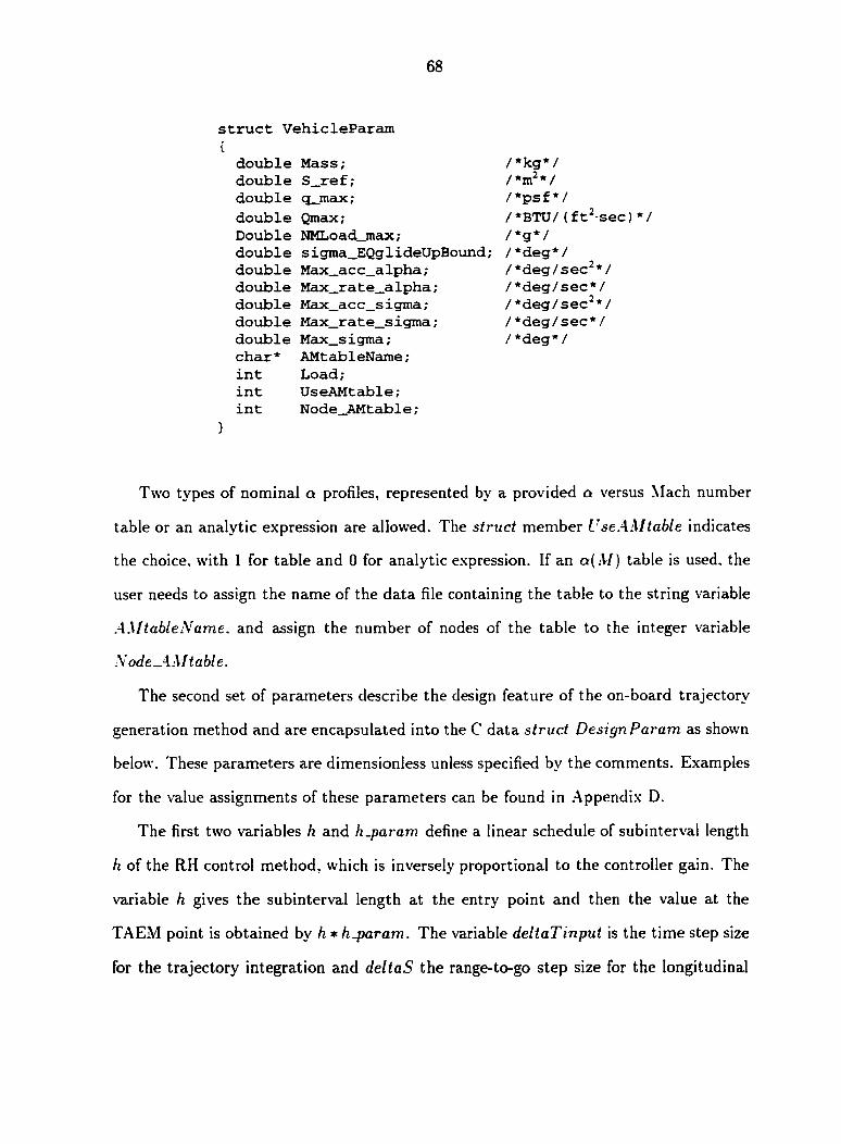
68
struct VehicleParam {
double Mass ; double S_ref; double q_max;
double Qmax; Double NMLoad_max; double sigma_EQglideUpBound; double Max_acc_alpha; double Max_rate_alpha; double Max_acc_sigma; double Max_rate_sigma; double Max_sigma; char* AMtableName; int Load; int UseAMtable;
/*kg*/ /*m2*/ /*psf*/
/ *BTU/ (ft2-sec) */ / *g* / /*deg*/ /*deg/sec2*/ /*deg/sec*/ /*deg/sec2*/ /*deg/sec*/ /*deg*/
int Node_AMtable;
>
Two types of nominal q profiles, represented by a provided a versus Mach number
table or an analytic expression are allowed. The struct member UseAMtable indicates
the choice, with 1 for table and 0 for analytic expression. If an ct(M) table is used, the
user needs to assign the name of the data file containing the table to the string variable
AMtableName. and assign the number of nodes of the table to the integer variable
Node-.AM table.
The second set of parameters describe the design feature of the on-board trajectory
generation method and are encapsulated into the C data struct Design Param as shown
below. These parameters are dimensionless unless specified by the comments. Examples
for the value assignments of these parameters can be found in Appendix D.
The first two variables h and h.param define a linear schedule of subinterval length
h of the RH control method, which is inversely proportional to the controller gain. The
variable h gives the subinterval length at the entry point and then the value at the
TAEM point is obtained by h * hjparam. The variable deltaTinput is the time step size
for the trajectory integration and deltaS the range-to-go step size for the longitudinal

69
reference profiles. For improving the trajectory precision, a variable time step size is
used by setting the parameter deltaTjrate.
struct DesignParam {
double h; double h_param; double deltaT_rate ; double deltaTinput ; double deltas; double PreTAEM_V; double PreTAEM_r_Ratio2Upbound; double TmlRelaxFactor; double Dis2HAC_forGrndTracking; double Max_sigma_forGrndTracking, /*deg*/ double TAEM_HeadingErrBnd; /*deg*/ double TAEM_A1tErrBnd; double epsilon_TmlGrnd ; double omiga_TmlGrnd ; double epsilonV_TmlGrnd ; double epsilon_TmlVRrev ; double omiga_TmlVRrev ; double TAEM gamma; /*deg*/ double TAEM_sigma;
}
When approaching the TAEM or the bank-reversal point, the usual time step-size can
be decreased by deltaT .rate times. The variable PreT AE M _l" sets the nominal pre-
TAEM velocity while the corresponding r is set by PreT AE M _r .Ratio'lU pbound, which
gives the ratio between the distances from the preTAEM (V. r) point to corridor upper
boundary and to the lower boundary. The variable Dis'lHAC-f orGrndTracking repre
sents the threshold range-to-go Sj illustrated in Fig. 3.17 forjudging the need for termi
nal reference ground path tracking. If there is a need, then the actual ground-tracking
takes place from some point before the threshold range-to-go is reached by multiplying
this variable with a relax factor TmlRelaxFactor. This approach may prevent the con
trol saturation in the ground-tracking phase due to the larger curvature of the ground
track. Similar as previously mentioned, the variable Max sigma.f orGrndTracking is
used to assign the maximal magnitude of the bank angle for the terminal ground tracking

70
phase. This gives larger control margin for on board tracking of the reference trajectory.
The variable T AE M-Heading Err Bnd is used to assign the TAEM heading error
bound for applying the single bank-reversal strategy (see section 3.2.3). When the TAEM
heading error is small than this value, the iteration stops and trajectory outputted.
Similarly, the term T AE M-Alt Err Bnd is used as the TAEM altitude error bound for
applying the terminal reference ground tracking. When the TAEM altitude error is
smaller than this value, the iteration stops and the trajectory outputted.
The variables omiga-TmlGrnd and epsilon-TmlGrnd are the natural frequency
and damping ratio of the nonlinear controller Eq. (3.63) for the terminal ground
path tracking. The variables omigaJTmlVRrev and epsilonJTmlVRrev are the natural
frequency uIvr and damping ratio of the nonlinear controller Eq. (3.19) for the
terminal backward trajectory integration. The variable epsilonV.TmlGrnd represents
the parameter k\- of the nonlinear controller Eq. (3.69) for tracking the reference V(STOGO)
profile while tracking the reference ground track.
The third set of parameters describes the mission profile including the HAC and
TAEM interface conditions and the entry interface conditions. The entry interface condi
tions can be conditions at any point where redesign of the reference trajectory is desired,
as will be demonstrated in the next chapter. The mission parameters are encapsulated
into the following C data struct variable MissionParam.
Referring to Fig. 2.3. the HAC latitude and longitude are denoted by the terms
PhiHAC and ThetaHAC, the TAEM distance RTAEM to HAC is represented by the
variable TAEM2HAC. and the TAEM altitude and velocity are denoted by the terms
TAEMjr and TAEM-V, respectively.
All the values of the 6 state variables and 2 controls at the entry interface point are
represented by the remaining MissionParam members with self-explanatory names. All
above mission parameters are dimensionless, except those with comments indicating their
units. Appendix B lists the values of these parameters for the vehicles X-33 and X-38.

71
struct MissionParam
double PhiHAC ; double ThetaHAC ; double TAEM_r ; double TAEM_V ; double TAEM2HAC; double Entry_sigma ; double Entry_alpha ; double Entry_altitude ; double Entry_longitude ; double Entry_latitude ; double Entry_velocity ; double Entry_gamma ; double Entry_heading ;
/*deg*/ /*deg*/
/•deg*/ /•deg*/
4.1.2 Output
The output consists of an array containing the reference trajectory state and control
histories and an integer indicating whether the terminal ground-tracking has been used
in the design. The number of nodes of the trajectory is also outputted by the integer
variable Statejiod.es. The array StateJCraj stores the reference trajectory with the
format
where e stands for the specific energy defined by Eq. (3.71).
The ground-tracking indicator is represented by the flag variable GroundTrack, with
value 1 for having done a ground-tracking and value 0 for the opposite. This flag serves
as an alert to the guidance system. Because the terminal ground-tacking method is
used to handle those very extreme entry cases, the corresponding bank angle usually
experiences saturation in tracking the reference ground path. This results the obtained
trajectory hard to be tracked in the terminal phase due to control saturation and special
control adjustment for the reference trajectory tracking may be needed when seeing this
flag on.
[e, Stogo- r. 6. o. V, 7, u\ a, a]

72
4.2 Major Blocks
This section describes the basic structures and logics for each of the major blocks
illustrated in the flowchart Fig. 4.1. Some local variables that are hard-coded with
specific values are also introduced in the relevant subsections.
4.2.1 Draw_StateConstraints()
Given the mission profile, the entry corridor for the applicable range of veloci
ty [0.95Vt.4£iV/, 1.01 VE\ is calculated. This velocity range is divided into a total of
M ax Num. subintervals. Bases on the entry trajectory constraints, i.e.. Eq. (2.10). Eq.
(2.11). Eq. (2.13). and Eq. (2.14), the altitude boundaries corresponding to the current
velocity are calculated and stored in the arrays EqGlide_r[], DynPressure_r[], Heat_r[],
and NMLoad_r[]. respectively, where the array EqGlide_rQ represents the corridor upper
boundary and the largest one among the remaining three represents the entry corridor
lower boundary (see Fig. 2.1) and is stored in another array R_DHN[].
4.2.2 Initial _Descend()
The variable sigma.fix stands for the bank angle cr0 for the initial descent (see
section 3.1.3. It is initialized with 0 for the descent integration. If the trajectory bounces
up before entering the entry corridor, then the trajectory integration restarts from the
original entry point with a bank angle that is 14 degrees larger then the previous one.
This process is repeated until the QEGC transition point is found.
The sigma.fix increment is implemented in the outer loop of the Initial J)escent{).
With the current trial sigma.fix value the inner while loop does the trajectory inte
gration till the QEGC transition is found or a bouncing up before entering the entry
corridor is found, which indicates the need of incrementing the sigma.fix for the next
try.
73
In the inner while loop, as the integration goes on, the derivative dV/dr is constantly
computed and compared against the local (at the same V) slope value dV/dr of the corri
dor upper boundary, which is computed by the function DvDr.CoridupBndry(). If the
derivative dV/dr becomes larger than the slope of the corridor upper boundary, and this
happens after the trajectory has entered the corridor, the QEGC transition point is found
and the descent integration stops. The descent trajectory history is recorded in the glob
al arrays: Ref.vJD\\, Re/_r _/£)[], Re f .gamma J D\\, Re fS'2HAC\\. Re f sigma JD[].
and Re f .alpha J D\\. The array index for the QEGC transition point is recorded in
another global integer variable iJZQentry.
As discussed in section 3.1.3. the relative velocity usually increases slightly imme
diately after the entry begins due to the Earth self-rotation effects. This will result in
irregular variation of dV/dr and make it hard to design simple logic for the compari
son with the slope of the corridor upper boundary. To avoid this dilemma, we let the
comparison starts only after the dimensionless altitude is less then 1.015. which is cor
responding to about 96 km in altitude. This setting can save some computational load
as well.
Once the trajectory enters the corridor, as indicated by the flag in.corridor. the
QEGC transition prediction function Sigma J^rans Predictor is constantly called to
compute the QEGC a value corresponding to the current I* and r. And the obtain
value sigmaJead is used to replace the sigma.fix if sigmaJead > sigma.fix so that
Eq. (3.12) is enforced.
4.2.3 TmlReverseIntegration()
The function TmlReverseIntegration() does the terminal backward trajectory in
tegration. The sign of the integration time step for the integration is changed by
deltaT = —fabs(deltaT), and the starting state is initialized with the TAEM state.
Since we want to avoid the situation that the bank angle remains small in the terminal

74
phase which means the vehicle's full maneuverability might not have been used for
reaching the TAEM interface conditions and hence fail to produce a trajectory for some
extreme entry cases, we slightly modified the terminal backward trajectory generation
method which is introduced in section 3.1.4. In the implementation, we let the backward
trajectory integration starts out with open-loop control first. From the TAEM a value
assigned in the DesignParam, let the <r increase at half of the maximum rate. At each
integration step, we design a 3rd order V — r reference curve based on the current r,
V, drjdV, and, and the pre-TAEM r, V, and dr/dV. Then the 2nd order derivative
dr2/dV2 of this reference curve at the current r and V point is calculated and returned
by the function TempTest(). The returned value is compared against the derivative
dr2/dV2 evaluated from the current state by the function Dr'IDv.finder. If a match is
found, the current 3rd order reference curve is in fact equivalent to a 4th order curve
whose 2nd order derivative is a straight line. Then the flag TmlRYcurvedone is set and
the corresponding geometry curve parameters that described the reference V — r profile
are fixed for the following use. Then the control turns to the nonlinear feedback control
law. i.e.. Eq. (3.19), for tracking the geometry curve.
Once the nominal pre TAEM V is reached in the backward integration, the actual
preTAEM state is stored in the global array variable PreTAE.\[J?tate. For later use
by the single bank-reversal point predictor, the preTAEM range-to-go SBTO and the
heading error 'I'sro- as illustrated in Fig. 3.16. are also stored in the global variables
PreT AE M2H AC and PreT AE M Heading Err.
4.2.4 Quasi_EG()
At the beginning od this function, the total number of steps for the integration of
Eq. (3.5), represented by the variable NumJief EQTraj is calculated based on the
range-to-go integration step size deltaS and the range between the preTAEM point and
the QEGC transition point. The <7miy, represented by Midsigma, is first set to be 20

75
deg. Then the integration is done for NumJlefEQTraj steps and the final velocity is
recorded in V.end. By comparing V.end with the preTAEM velocity PreTAEM_V",
the Midsigma is updated with a 10 deg interval. Once the 10 deg interval in which
the M id.sigma lies is found, the secant search method is used to find the M id sigma
accurately.
The linear schedule for a is calculated by the function sigma.V .LinSchedule(). Two
parameters, the current V and the Midsigma. are used for solving the scheduled bank
angle. Hard-coded in the sigma.V .LinSchedule function, the M id.sigma is chosen to
be located at the point where the distance to the preTAEM V accounts for 3/4 of the
whole range of V. The enforcement of the entry corridor constraints by bounding the
a(V) profile as illustrated by Fig. 3.2 is also enforced in this function.
4.2.5 RefTrajTrackingO
The function RefTrajTrackingO serves as the major block for completing the 3D-
OF trajectory. Figure 4.2 illustrates the structure of this function. The trajectory
integration starts from the entry interface by tracking the longitudinal reference profiles
outputted from Quasi JLG{). The sign of bank angle indicated by the global variable
EntryBankingSign is calculated at the beginning of this function using the method
described in section 3.1.3. Then the trajectory is integrated forward till the TAEM
distance is reached or the range to HAC begins to increase due to large heading error.
Based on the terminal state reached by the integration, it is determined whether a nor
mal single bank-angle can be allowed. If yes, the iteration using single bank-reversal
strategy is done in this function. Otherwise, depending on the terminal conditions, ei
ther the function TmlGrndTracking() is called for doing reference ground path tracking
(see section 3.2.3 and Fig. 3.17), or the function TmlOpenLJ>igmaTracking() is called
for terminal open-loop control profile search (see Fig. 3.17). The starting state for both
branches is the same and stored in the global array variable TmlGrndEntrystate.

76
Calculate the Initial sign for O
no
Trajectory moving^ away or TAEM circle
N^reachedl/^ JBfiL
yes
no TAEM condition _ satisfied? _
yes
Store and output the 3DOF trajectory
A regular single bank-reversal
^ exists?/-
—-̂ 1 yes
Do terminal ground tracking or open-loop search
Calculated the terminal generalized S ,̂,, hac
Initialize the starting state and update the bank-reversal point
Integrate the 3DOF trajectory with bank-reversal happens at
the point predicted
Integration the 3DOF trajectory forward
Figure 4.2 Flowchart of the algorithm for completing the 3D0F trajectory

In the second box of the flowchart, the function Bankreversal Predictor() is contin
uously called to check the condition for doing bank-reversal. If the condition (3.49) for
bank-reversal becomes true, the predictor set the flag dorev on. And then the sign of
Entry Banking Sign is changed to the opposite of the current sign.
4.2.6 TmlGrndTracking()
The terminal ground path tracking is implemented by the function TmlGrndTracking().
as illustrated by the flowchart in Fig. 4.4. First, a brute force search for bounding the
range of the TAEM heading angle 0/, illustrated in Fig. 2.3, is executed. The range
interval is set to be 5.7 deg. or one tenth of a radian.
Figure 4.3 Initialization of the iPtaem for terminal ground tracking
The initialization of V"/, denoted by psiTAEMO in the code, is done by the statement
where k is a constant, H AC .LOS and Statejnew[b\ stand for the line-of-sight azimuth
and velocity azimuth of the starting point, respectively. By above equation, the initial
ipj is set so that it forms a spherical triangle as shown in Fig. 4.3, in which AW0 < 0 by
North
Reference ground path
Ground tracking starting point
psiTAEMO = HACJjOS — k(Statejiew[ 5] — H AC .LOS)

78
initialize the TAEM heading CtAEM and calculate the reference ground path
5
Integrate the 3DOF trajectory by tracking the ground path
Restore the starting slate, update the ground path
Integrate the 3DOF trajectory by tracking the ground path
Restore the starting slate, update the ground path
as the interv bounding Otaem
been found?
VFW- 5.7 deg or Vr Vr 5.7 deg
Update OrAEM by secant method, update the ground path
Integrate the 3DOF trajectory by tracking the ground path
Is the termina altitude error ^acceptable?,
yes
no
c Store and output the 3DOF trajectory )
Figure 4.4 Flowchart of the algorithm for terminal ground tracking

79
definition and AW0 = &A#/• Then the brute force search is conducted by decreasing
the V/ for 5.7 deg each time till the bounding range is found. After that, the secant
method is used to find the accurate 0/. If A$o > 0. the brute force search is conducted
by increasing the xbf for 5.7 deg each time. Experiments show that assigning a value in
the range of 1-2 for k works very well for all test cases.
4.3 Key Global Variables
Some global variables are used to facilitate the implementation. All the input param
eters including the design, vehicle, and mission parameters as described in section 4.1
are stored as global variables. A number of other key global variables that are used
solely for algorithm implementation purpose are listed as follows with explanations for
their purpose and use.
1. RK-f actor: the index of the current internal step of the 4th order Runge-Kutta
integration method. One purpose is for saving computational load. The RH control
gains, which involves intensive matrix calculation, is only calculated at the first
step of each Runge-Ixutta cycle, and then the same gain is used for the following
3 steps. Another purpose of RK-Jactor is for enforcing the rate and acceleration
constraints on a and a inside the Runge-Kutta cycle.
2. NumJtefTraj: the total number of nodes of the longitudinal reference profiles.
3. Num.-.\ctualTraj: the total number of nodes of the actual 3DOF trajectory.
4. Former-alpha, Former .alpha-rate: the previous a value and rate, used for en
forcing the rate and acceleration constraints on a.
5. Former^sigma, Formerjsigmajrate: the previous a value and rate, used for en
forcing the rate and acceleration constraints on <r.

80
6. iJZQentry: the array index indicating the QEGC transition point of longitudinal
reference profile.
7. iSmlRVrevTraj: the number of nodes of the terminal backward trajectory.
8. jJTmlGrnd Entry: the array index indicating the number of nodes of the actual
3DOF trajectory before the terminal ground-tracking starts.
9. TmlGrndEntry^State: the starting state for the terminal ground tracking.
10. TmlGrndEntryJrormersigma.TmlGrndEntry^sigmarate: the a value and rate
at the starting point of the terminal ground tracking or the terminal open-loop
control search.
11. TmlGrndEntryJ^ormeralpha.TmlGrndEntryjalpharate: the a value and rate
at the starting point of the terminal ground tracking or the terminal open-loop
control search.
81
CHAPTER 5. APPLICATIONS
Two vehicle models, X-3S and X-33, are used for illustrating our 3D0F constrained
entry trajectory generation method. Four entry cases of the X-38 vehicle and 9 entry
cases of the X-33 vehicle are examined, respectively. Those tested entry cases represented
a broad range of mission profiles. Especially, the 9 X-33 entry cases are grouped into 3
sets. Each set has a normal entry case, an early entry case, and a late entry case. Those
early and late cases involve large left or right crossranges that were intentionally set to
make the tasks of entry guidance design for them very difficult.
This chapter presents the results of generating reference trajectories for all the test
cases mentioned above. Section 5.1 describes the X-38 and X-33 vehicle models and
the corresponding vehicle parameters. Section 5.2 presents the trajectories generated
using our method. Section 5.3 demonstrates the method's robustness and adaptability
by handling some abnormal sub-orbital entry cases artificially composed by perturbing
some states along a nominal entry trajectory. Section 5.4 demonstrates the simulation
results of integrating this algorithm with other state-of-art entry guidance components on
a NASA-based high fidelity X-33 flight simulator. Section 5.5 presents the performance
analysis of this method.
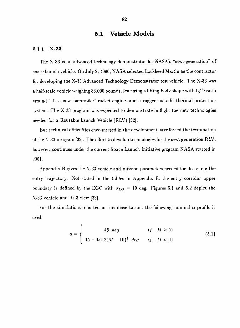
82
5.1 Vehicle Models
5.1.1 X-33
The X-33 is an advanced technology demonstrator for NASA's "next-generation" of
space launch vehicle. On July 2, 1996, NASA selected Lockheed Martin as the contractor
for developing the X-33 Advanced Technology Demonstrator test vehicle. The X-33 was
a half-scale vehicle weighing 83.000 pounds, featuring a lifting-body shape with L/D ratio
around 1.1. a new "aerospike"1 rocket engine, and a rugged metallic thermal protection
system. The X-33 program was expected to demonstrate in flight the new technologies
needed for a Reusable Launch Vehicle (RLV) [32].
But technical difficulties encountered in the development later forced the termination
of the X-33 program [32]. The effort to develop technologies for the next generation RLV.
however, continues under the current Space Launch Initiative program NASA started in
Appendix B gives the X-33 vehicle and mission parameters needed for designing the
entry trajectory. Not stated in the tables in Appendix B. the entry corridor upper
boundary is defined by the EGC with <7£g = 10 deg. Figures 5.1 and 5.2 depict the
X-33 vehicle and its 3-view [33].
For the simulations reported in this dissertation, the following nominal a profile is
used:
2001.
45 deg if M > 10 (5.1) a =
45 - 0.612(A/ - 10)2 deg -y A/ < 10
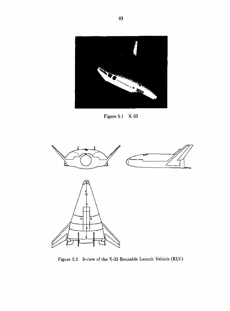
83
Figure 5.1 X-33
Figure 5.2 3-view of the X-33 Reusable Launch Vehicle (RLV)
84
5.1.2 X-38
The X-38 is a NASA's technology demonstrator for the Crew Return Vehicle(CRV)
that will serve as both an ambulance for medical emergencies and as an evacuation
vehicle. The first concept study of X-38 kicked off in early 1995. The first X-38 prototype
vehicle, known as Vehicle 131, made its maiden flight at Dry den in March of 1998 [2].
The most recent flight test, in which the X-38 prototype vehicle was launched from the
wing of a NB-52B aircraft, was conducted in December 13, 2001.
The X-38 design uses a lifting body concept originally developed by the U.S. Air
Force's X-24A project in the mid-1960s. Following the jettison of a de-orbit engine
module, the X-38 will glide from orbit unpowered like the Space Shuttle and then use a
steerable parafoil parachute, a technology recently developed by the Army, for its final
descent to landing [2]. The CRY* spacecraft has a moderate L/D ratio of 0.9. and is 30
feet long, 14.5 feet wide and weighs around 20.000 pounds.
Appendix C gives the X-38 vehicle and mission parameters needed for designing the
entry trajectory. Not stated in the tables in Appendix C. the entry corridor upper
boundary is defined by the EGC with <7eg — 10deg. Figure 5.3 and 5.4 depict the X-38
vehicle and its 3-view [33].
For the simulations reported in this dissertation, the following nominal a profile is
used:
40 deg if M > 10 a = (5.2)
40 - 0.2668(M - 10)2 deg if M < 10

85
Figure 5.4 3-view of the X-38 Crew Return Vehicle(CRV)

86
5.2 Entry Trajectory Design for X-33 and X-38
5.2.1 Entry Missions
The entry mission description is given in terms of the entry interface state, the H AC
coordinate, the TAEM velocity and altitude, and the trajectory inequality constraints.
X-33 Entry Missions
For X-33, 9 test cases dubbed AGC13-AGC21, are provided. Details of these AGC
cases can be found in Appendix B. The following list and table 5.1 give a brief description
of the AGC entry missions. Notice that those "early"" and "late" cases are supposed
to represent the extreme entry scenarios with large right and left cross ranges. The
term "crossrange" measures the entry interface heading status. Usually, the larger the
magnitude of the crossrange is. the more difficult the entry will be. Further explanation
of crossrange can be found in Ref. [13]. For clarity of demonstration, we kept the entry
interface conditions as provided, but used the AGC13 HAC and TAEM conditions,
and 75 BTU/ft2 • sec as the heat rate constraint for all the AGC cases. A complete
description of the guidance design for X-33 can be found in Ref. [4].
• The cases AGC13-AGC1S are for entries from the International Space Station (ISS)
orbit with an inclination angle of 51.6 deg. Cases AGC 13 and AGC16 represent
the normal entry scenarios and cases AGC 14, 15. 17, and 18 provide the "early"
and "late" entry scenarios for cases AGC 13 and AGC16. respectively.
• The cases AGC19-AGC21 are for entries from the Lower Earth Orbit (LEO) with
an inclination angle of 28.5 deg. AGC19 is for the normal scenario and AGC20
and AGC21 for the "early" and "late" entry scenarios.
• The entry interface altitude ranges from 120.13 km to 124.85 km and the velocity
ranges from 7440.12 m/sec to 7625.99 m/sec.
87
• The TAEM interface altitude is 30.43 km and the velocity is 908.15 m/sec.
• The landing site for all the AGC entry cases is the Kennedy Space Center.
• The entry trajectory is constrained by: Qmax = 75 BTU/(ft2 • sec). qmax =
300.0 psf, Loadmax = 2.5 g, and ceq = 10 deg.
• The vehicle's maneuverability is constrained by: |â|mox = 5.0 deg I sec. |a|mox =
2.0 deg I sec2, \à\max = 5.0 deg I sec, and |cr|mar = 3.5 deg/sec2.
The following table gives the range-to-go and crossrange information of the AGC
cases. Negative value of the crossrange means a left crossrange. and vice versa. Clearly,
cases AGC 13, 16, and 19 have smaller crossranges which mean good heading alignment
to the landing site at the entry interface.
Table 5.1 X-33 entry missions
Case No. Range-to-HAC (nm) Crossrange (nm) Landing site AGC 13 3520 32 KSC AGC14 3539 437 KSC AGC 15 3558 -458 KSC AGC 16 4406 80 KSC AGC 17 4414 477 KSC AGC IS 4426 -420 KSC AGC 19 3974 144 KSC AGC20 3986 406 KSC AGC21 4117 205 KSC
X-38 Entry Missions
We tested 4 entry cases for X-38. The following list and table 5.2 give a brief
description of the entry cases of X-38. More details of the description can be found in
Appendix C. These entry cases are different from each other in that the entry interfaces
and the HAC coordinates are widely distributed corresponding to entries from the orbit
targeting at different landing sites. All 4 test cases of X-38 have the same entry altitude
and velocity and the same TAEM altitude and velocity.
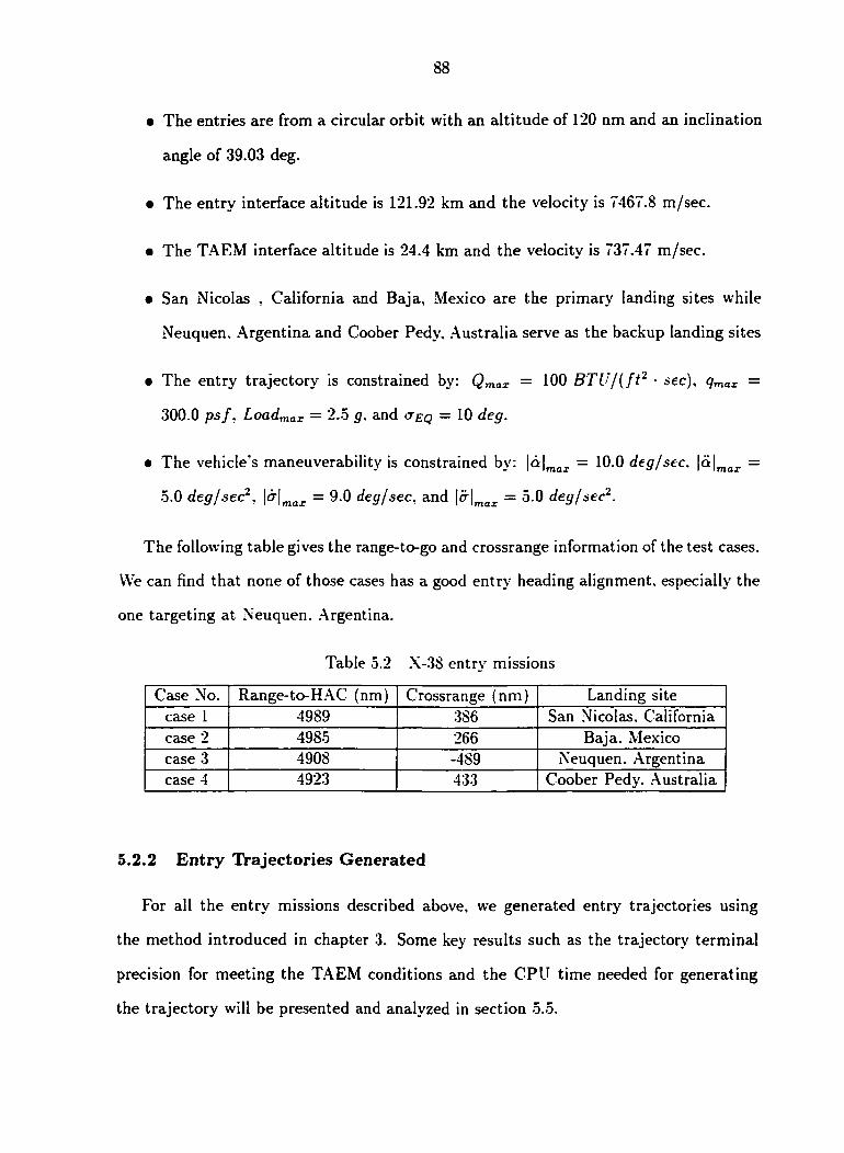
88
• The entries are from a circular orbit with an altitude of 120 nm and an inclination
angle of 39.03 deg.
e The entry interface altitude is 121.92 km and the velocity is 7467.8 m/sec.
• The TAEM interface altitude is 24.4 km and the velocity is 737.47 m/sec.
• San Nicolas , California and Baja, Mexico are the primary landing sites while
Neuquen, Argentina and Coober Pedy, Australia serve as the backup landing sites
e The entry trajectory is constrained by: Qmax = 100 B T U / { f t 2 • sec), çmax =
300.0 psF, Loadmax = 2.5 g. and <TEQ = 10 deg.
e The vehicle's maneuverability is constrained by: |ô|mai = 10.0 deg/sec. |c*|max =
5.0 deg I sec2, |ô"|max = 9.0 deg/sec, and |<x|max = 5.0 deg/sec2.
The following table gives the range-to-go and crossrange information of the test cases.
We can find that none of those cases has a good entry heading alignment, especially the
one targeting at Neuquen. Argentina.
Table 5.2 X-38 entry missions
Case No. Range-to-HAC (nm) Crossrange (nm) Landing site case 1 4989 386 San Nicolas, California case 2 4985 266 Baja. Mexico case 3 4908 -489 Neuquen. Argentina case 4 4923 433 Coober Pedy. Australia
5.2.2 Entry Trajectories Generated
For all the entry missions described above, we generated entry trajectories using
the method introduced in chapter 3. Some key results such as the trajectory terminal
precision for meeting the TAEM conditions and the CPU time needed for generating
the trajectory will be presented and analyzed in section 5.5.
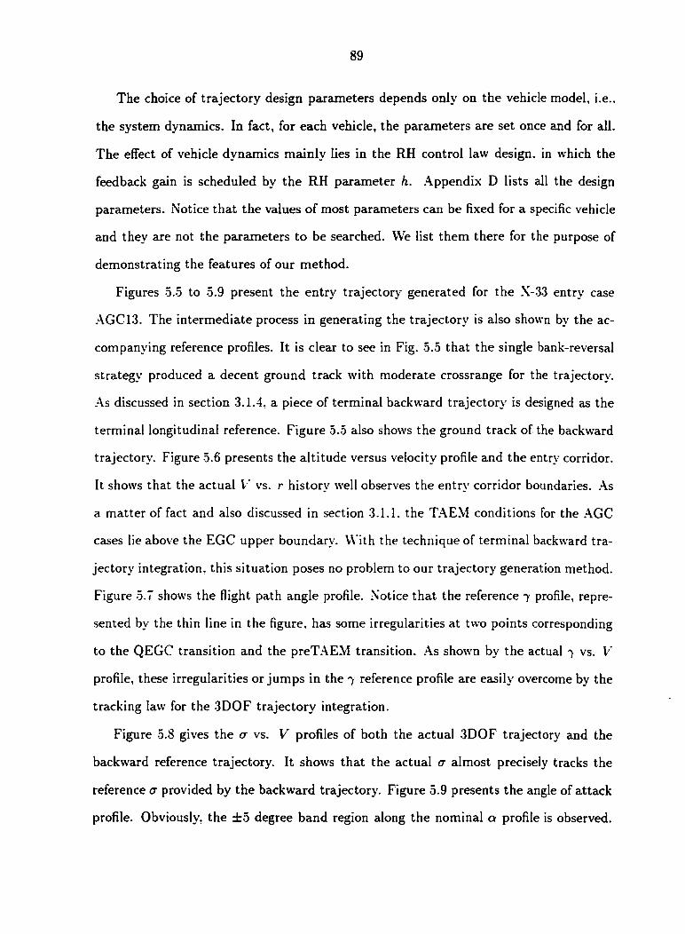
89
The choice of trajectory design parameters depends only on the vehicle model, i.e.,
the system dynamics. In fact, for each vehicle, the parameters are set once and for all.
The effect of vehicle dynamics mainly lies in the RH control law design, in which the
feedback gain is scheduled by the RH parameter h. Appendix D lists all the design
parameters. Notice that the values of most parameters can be fixed for a specific vehicle
and they are not the parameters to be searched. We list them there for the purpose of
demonstrating the features of our method.
Figures 5.5 to 5.9 present the entry trajectory generated for the X-33 entry case
AGC13. The intermediate process in generating the trajectory is also shown by the ac
companying reference profiles. It is clear to see in Fig. 5.5 that the single bank-reversal
strategy produced a decent ground track with moderate crossrange for the trajectory.
As discussed in section 3.1.4, a piece of terminal backward trajectory is designed as the
terminal longitudinal reference. Figure 5.5 also shows the ground track of the backward
trajectory. Figure 5.6 presents the altitude versus velocity profile and the entry corridor.
It shows that the actual V vs. r history well observes the entry corridor boundaries. As
a matter of fact and also discussed in section 3.1.1. the TAEM conditions for the AGC
cases lie above the EGC upper boundary. With the technique of terminal backward tra
jectory integration, this situation poses no problem to our trajectory generation method.
Figure 5.7 shows the flight path angle profile. Notice that the reference 7 profile, repre
sented by the thin line in the figure, has some irregularities at two points corresponding
to the QEGC transition and the preTAEM transition. As shown by the actual 7 vs. V
profile, these irregularities or jumps in the 7 reference profile are easily overcome by the
tracking law for the 3DOF trajectory integration.
Figure 5.8 gives the a vs. V profiles of both the actual 3D0F trajectory and the
backward reference trajectory. It shows that the actual a almost precisely tracks the
reference a provided by the backward trajectory. Figure 5.9 presents the angle of attack
profile. Obviously, the ±5 degree band region along the nominal a profile is observed.

90
Not surprisingly, the angle of attack profile closely follows the nominal one, especially,
in the low velocity range which corresponds to the terminal phase of the entry flight.
Figure 5.10 shows the time history of the controls <r and a. It clearly shows that a single
bank reversal takes place at the time about 600 seconds after the entry. Also observed
is the moderate a magnitude when approaching the TAEM. which is a desirable feature
of entry trajectory design.
Figures 5.11 to 5.17 show the trajectories generated for all the 9 cases for the X-
33. Wherever distinguishable in the figures, the trajectories are marked xvith their
AGC case number. Figure 5.11 shows the ground tracks for every AGC test case.
Fig. 5.13 illustrates the positions of these entry trajectories in a world map. Shown
by Fig. 5.12 with the enlarged view of the terminal ground tracks, the TAEM heading
requirement is almost perfectly satisfied with a heading error of 1.238 deg on average for
all 9 cases. Figure 5.14 shows the altitude versus velocity profiles in the entry corridor
frame. Observe that some trajectories go along the corridor's EGC upper boundary.
Those trajectories correspond to those low energy entry cases, such as AGC 17 and
AGC18, in which the energy must be dissipated slowly in order to travel a relatively
'longer distance to reach the TAEM interface. Figures 5.15 and 5.16 show the flight path
angle and angle of attack profiles, respectively. Figure 5.17 presents the control histories.
As shown by the a histories, in 7 of the 9 AGC entry cases, the vehicle banks first to
the left and then to the right by the single bank-reversal strategy, while the remaining
two cases require a first right and then left banking sequence. Shown by the a histories
in Fig. 5.17, the nominal a profile is closely followed by all cases.
Similarly, Figures 5.18 to 5.23 show the 3DOF reference trajectories generated for the
four test cases of the X-38 vehicle. As previously mentioned, the design parameters are
reset for the X-38 vehicle. Comparing the two tables of design parameters in Appendix
D, we can find that the difference exists only in few parameters.

91
Terminal backward reference trajectory
I I
5 -
-10
-15 TAEM
-20 250 275 280 240 245 255 260 265 270
longitude(deg)
Figure 5.5 Ground track of the X-33 AGC 13 entry test case
140
Entry
120
100
EGC constraint
Heat rate constraint
Normal load constraint
Dynamic pressure constraint TAEM
6000 7000 20
5000 2000 1000 3000 4000 8000 velocity(m/sec)
Figure 5.6 Entry trajectory of the X-33 AGC 13 entry test case

92
longitudinal Reference y profitai
-2
î i I
-7
1000 2000 3000 5000 6000 8000 7000
Figure 5.7 Flight path angle vs. velocity profile of the X-33 AGC 13 entry test case
40
Terminal backward trajectory o profile
I -20
-40
-60
-SO 1000 2000 3000 4000
vekicity(m/sc) 5000 6000 7000 8000
Figure 5.8 Bank angle vs. velocity profile of the X-33 AGC13 entry test case
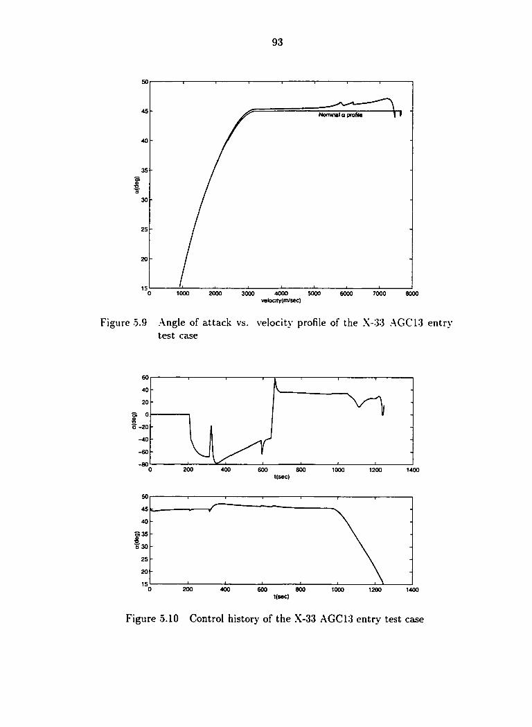
93
45 Nommai a profile
25
20
1000 2000 5000 3000 6000 7000 8000
ure 5.9 Angle of attack vs. velocity profile of the X-33 AGC13 entry test case
60
40
20
0 "e -20
-40
-60
-80 0 200 400 600 800 1000 1200 1400 t(sec)
40
"a 30
200 400 800 600 1000 1200 1400 t(sec)
Figure 5.10 Control history of the X-33 AGC13 entry test case
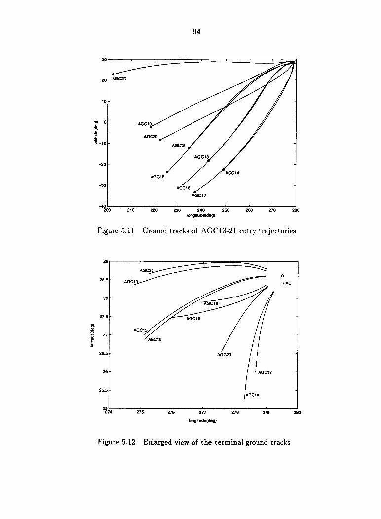
94
AGC21 20
AGC19
AGC20
S -10 AGC15
AGC13
-20
AGC14 AGC18
-30 AGC16
AGC17
-40 200 210 220 230 240 250 260 270 280
longitude(deg)
Figure 5.11 Ground tracks of AGC 13-21 entry trajectories
29
AGC21
28.5 AGC1 HAC
iC18
27.5 AGC15
AGC13,
AGC16
26.5 AGC20
AGC17
25.5 IAGC14
25 274 275 276 277 278 279 280
tongitude(deg)
Figure 5.12 Enlarged view of the terminal ground tracks
95
NewYork Los Angeles
g Kennedy Space Center
AGC21
Hawaii
AGC19
AGC20 AGC 15.
AGC 13,
AGC 18 AGC14
AGC16
AGC17
180°W 150°W 60°W 120°W 90°W 30°W
Figure 5.13 Ground tracks of the X-33 entry trajectories drawn with the world map

96
140
120
100
I 1 I
60
40
TAEM
8000 3000 5000 7000 1000 2000 6000
Figure 5.14 Entry trajectories of AGC13-21 entry test cases
"3 -3
-6
-7
-8 8000 1000 3000 5000 7000 2000 6000
Figure 5.15 Flight path angle vs. velocity profiles of AGC13-21 entry test cases
97
Nominal a profile
40
I o
30
20 -
8000 3000 7000 1000 2000 5000 6000
Figure 5.16 Angle of attack vs. velocity profiles of AGC13-21 entry test cases
100
-50
-too 500 1500 1000
t(sec) 100
I c
-50
500 1500 1000 t(sec)
40 -
20
500 1500 1000
Figure 5.17 Control histories of AGC13-21 entry test cases

98
case 2
case 3
a
-10
case 4
-20
-30
-40 50 250 100 150
longitude(deg) 200 300
Figure 5.18 Ground tracks of the X-38 entry test cases
50 N
San Nicolas t
4—
case 1 Beijing
case 2 v6aja
Hawaii case 3
Coober Pedy
/Sydney-
rçëuquen
60°E 180°W 120°W 60°W 120°E
Figure 5.19 CI round tracks of the X-38 entry trajectories drawn with the world map

100
140
Entry
120
100
Heat rate constrant
Dynamic pressure constraint
TAEM
3000 1000 2000 6000 7000 8000 5000
Figure 5.20 Entry trajectories of the X-38 entry test cases
1 l l l i I : » I
-91 1 i 1 i £ I I 0 1000 2000 3000 4000 5000 6000 7000 6000
vetodty(mZsec)
Figure 5.21 Flight path angle vs. velocity profiles of the X-38 entry test cases

101
I
0 1000 2000 3000 4000 5000 6000 7000 8000 vek)ctty(m/sec)
Figure 5.22 Angle of attack vs. velocity profiles of the X-38 entry test cases
44
40 Nominal a profite
36
34
30
a.
Figure 5.23 Control histories of the X-38 entry test cases

102
5.3 Adaptability Demonstration
The adaptability of this method is illustrated in 2 aspects. First, we demonstrate
the enforcement of a more stringent heat rate constraint. This feature has not been
demonstrated by any test cases of either the X-33 or the X-38. Next, we examine the
method by using it to generate trajectories from some randomly picked and disturbed
states along a nominal trajectory.
5.3.1 Enforcement of Stringent Heat Rate Constraint
A common feature of all the test cases of either X-38 or X-33 is that the trajectory
is more or less close to the entry corridor upper boundary. They are of typical low
energy entry scenarios. This actually makes the test cases more challenging since low
energy entry trajectory is typically more difficult to design due to vehicle's weak control
authority at higher altitude. For purpose of demonstrating the capability of our method
for designing entry trajectories in which the lower boundary of the entry corridor has to
be enforced, we intensionally decrease the heat rate limit from 75 BTU/{ft2 • sec) to 60
BTU/[ft2 • sec) to narrow the entry corridor. Then we re-design the trajectory for the
case AGC 19 (We can also do so for cases AGC20 and AGC 21. But for cases AGC 13 -
AGC18, this more stringent heat rate constraint will inevitably be violated even if we
used zero bank angle for the initial descent, which means no feasible trajectory exist at
all). Figures 5.24 and 5.25 show the key aspects of the obtained trajectory. As expected,
Fig. 5.25 shows that a significant part of the trajectory goes along the lower boundary
formed by the stringent heat rate constraint. But this does not affect the effectiveness of
our method at all. As a matter of fact, tracking the lower boundary as the longitudinal
reference profile is easier than doing so with the EGC upper boundary because of the
stronger trajectory control authority at lower altitude where the atmospheric density is
higher.
103
30
5 10
Entry
-5 280 250 260 270 210 220 230 240
longrtude(deg)
Figure 5.24 Ground track of the AGC 19 entry with stringent heat rate constraint
140
Entry
120
100
I «
TAEM
1000 5000 8000 2000 3000 6000 7000
Figure 5.25 Entry trajectory of the AGC19 entry with stringent heat rate constraint

104
5.3.2 Trajectory Generation from Non-orbital Entry Conditions
The initial conditions from which a reference entry trajectory is to be generated are
not necessarily those at the orbital entry interface for applying our method. The poten
tial of extending our method to handling sub-orbital entry or abort cases is illustrated
by the following testing.
Along the trajectory just generated for case AGC13. we arbitrarily pick a state
and add perturbations to it. The perturbation could be so large that it is unlikely for
any trajectory tracking method to get the vehicle back to track the original reference
trajectory. Two tests were conducted, each representing a different possible sub-orbital
entry or abort scenario. In the first test, we picked a state with an altitude of 79.25
km from the AGC13 trajectory. Then we increased the altitude by 2 km and perturbed
its latitude for 120 nm to the north while all other state variables remained unchanged.
In the second test, we selected a state with a velocity of about 4000 m/sec. Then we
perturbed its longitude to the east for 30 nm while all other state variables remained
unchanged. New trajectories were easily generated by applying the method based on
the perturbed states, as shown by the trajectories 1 and 2 in the Figs. 5.26- 5.31.
The single bank-reversal strategy was still used in generating trajectory 1 in the first
test, even though the perturbed state was already in the entry corridor. However in the
second test, the remaining range-to-go to HAC was so short that it was difficult to use
the single bank-reversal strategy. For this test, the terminal ground tracking method was
automatically activated by the algorithm in the design. Figure 5.27 shows the enlarged
view of the terminal phase. The thick dotted line represents the final shape of the
reference ground path. It shows that the reference ground path is closely tracked, thus
the TA EM heading and distance requirements are precisely satisfied by trajectory 2.
Figure 5.31 shows the control histories for the 2 trajectories plus the AGC13 trajectory
obtained before. As a price for applying the terminal reference ground path tracking
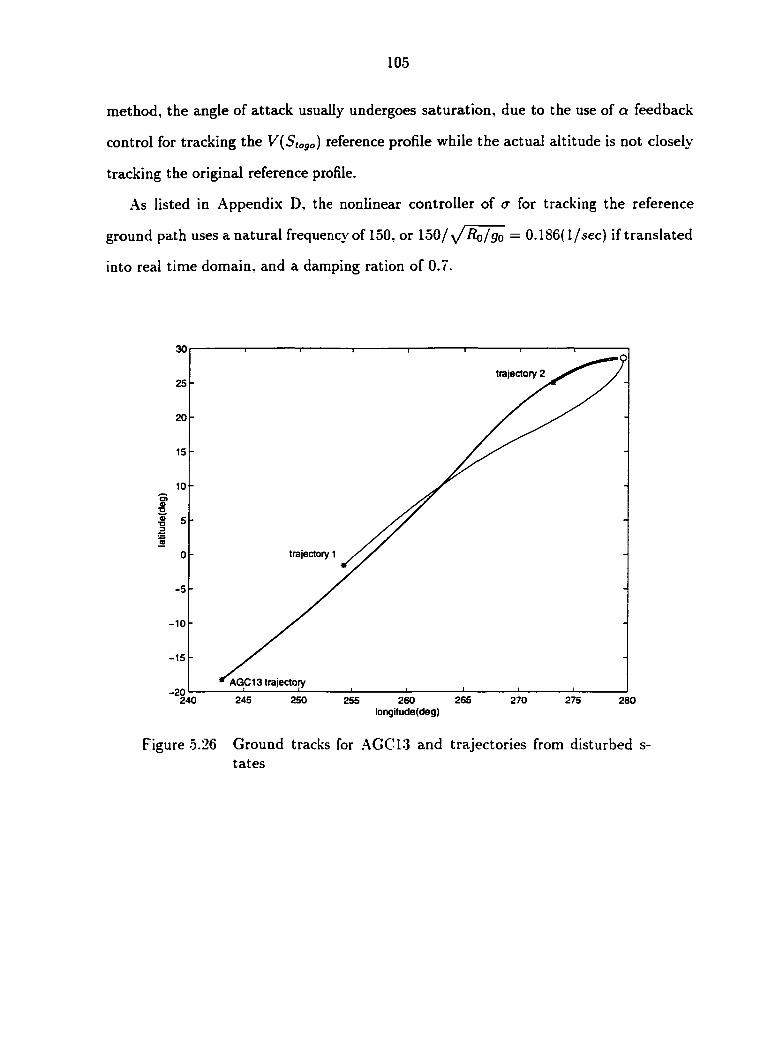
105
method, the angle of attack usually undergoes saturation, due to the use of a feedback
control for tracking the V(StoJO) reference profile while the actual altitude is not closely-
tracking the original reference profile.
As listed in Appendix D, the nonlinear controller of a for tracking the reference
ground path uses a natural frequency of 150, or 150/ yjRo/go — 0.1S6(l/sec) if translated
into real time domain, and a damping ration of 0.7.
30
trajectory 2
20
1 a
trajectory 1
-5
-10
-15
AGC13 trajectory -20
250 265 240 245 270 275 255 260 280 longitude(deg)
Figure 5.26 Ground tracks for AGC13 and trajectories from disturbed s-tates
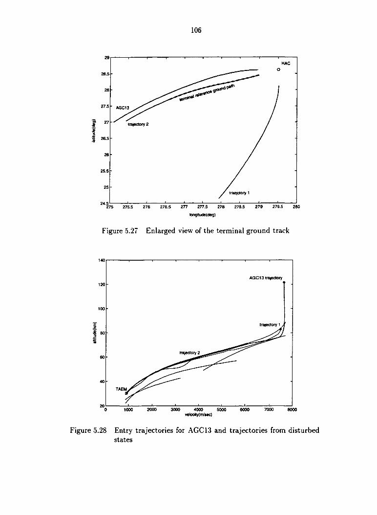
106
HAC
AGC13
27
26.5
26
25.5
traejctory 1
24.5 279 279.5 276.5 277 277.5 278 280 275 275.5 276
tongrtucte(deg)
Figure 5.27 Enlarged view of the terminal ground track
140
AGC13 trajectory
120
100
trajectory 1
40
TAEM
1000 5000 2000 3000 7000 4000 6000 8000 velocity(nVsec)
Figure 5.28 Entry trajectories for AGC13 and trajectories from disturbed states

107
I I
-6
-7 AGC13 trajectory 1 trajectory 2
2000 6000 7000 8000 1000 3000 5000
Figure 5.29 Flight path angle vs. velocity profiles
50
45 Normmal a profile
3
trajectory 2 — AGC13 trajectory
trajectory 1
2000 6000 1000 3000 5000 7000 8000
Figure 5.30 Angle of attack vs. velocity profiles
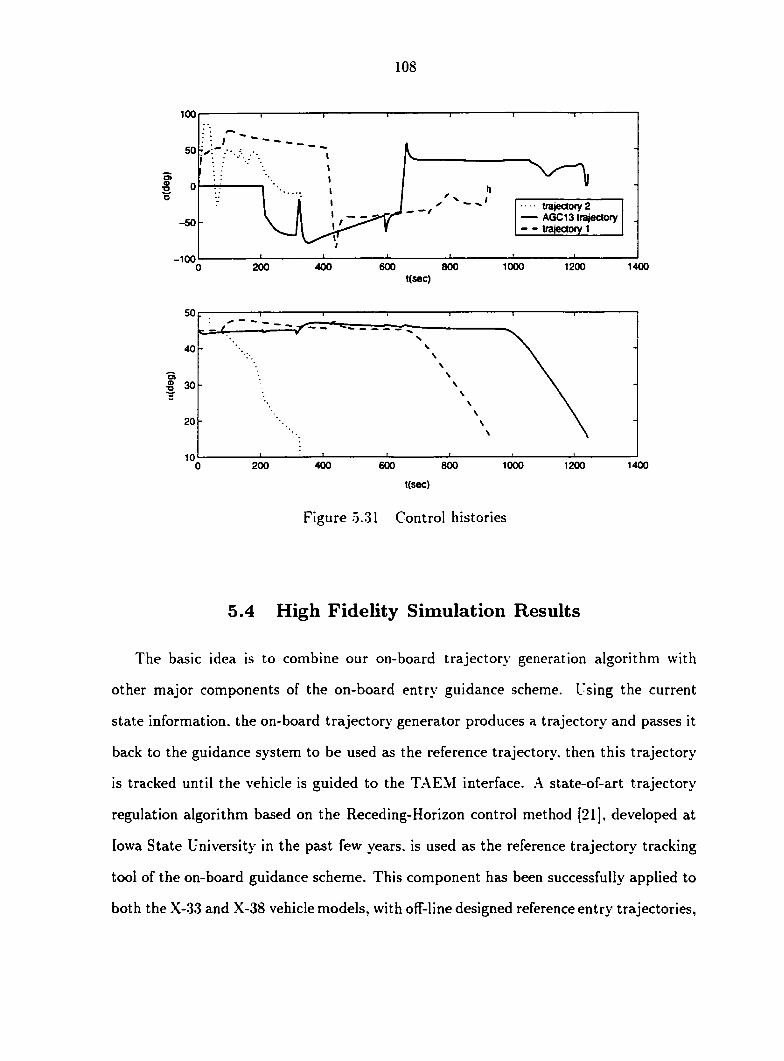
108
100
50
— trajectory 2 AGC13 trajectory
- - trajectory 1 -50
-100 1000 1200 1400 400 600 800 200
t(sec)
40
a a "O
20
1400 400 600 800 1000 1200 200 0 t(sec)
Figure 5.31 Control histories
5.4 High Fidelity Simulation Results
The basic idea is to combine our on-board trajectory generation algorithm with
other major components of the on-board entry guidance scheme. Using the current
state information, the on-board trajectory generator produces a trajectory and passes it
back to the guidance system to be used as the reference trajectory, then this trajectory
is tracked until the vehicle is guided to the TA EM interface. A state-of-art trajectory
regulation algorithm based on the Receding-Horizon control method [21], developed at
Iowa State University in the past few years, is used as the reference trajectory tracking
tool of the on-board guidance scheme. This component has been successfully applied to
both the X-33 and X-38 vehicle models, with off-line designed reference entry trajectories,

109
in other research projects [17, 18, 21].
The simulation is performed on a high fidelity flight simulator of the X-33 vehicle,
developed at the NASA Marshall Space Flight Center and called Marshall Aerospace
Vehicle Representation in C (MAVERIC). MAVERIC simulates the complete flight his
tory, from lift-off to entry, of the X-33 vehicle. Any significant factors affecting the
flight, such as the vehicle model, propulsion system model, and the atmospheric envi
ronment including the effect of winds, are realistically represented in the MAVERIC.
Upon de-orbiting, the current state information and the TA EM interface specification
are passed to our on-board trajectory generator, meanwhile the vehicle flies open-loop
with constant a and a. On average, this open-loop phase lasts 1-2 seconds in our testing.
As soon as the trajectory is generated and passed back to the tracking component, the
process of entry guidance by trajectory regulation begins from the current state. The
entry guidance command is updated every guidance cycle which is one second in the
simulation shown below, until the vehicle reaches the TA EM interface velocity.
In order to meet the input convention of MAVERIC. the TA EM velocity, altitude,
and distance to HAC are set to be 2979.5ft/sec, 100,000ft and 30 nautical miles, respec
tively. The errors in meeting the TA EM conditions are depicted in Fig. 5.32 with the
attached numbers indicating the corresponding AGC cases. It shows that high precision
is achieved for meeting the TA EM requirements. The average heading error is only 3
deg which almost means a perfect TA EM heading. The average terminal range-to-HAC
error is about 0.18 nm, or 330 m. This error is more likely resulted from the discrete
recording of the trajectory history.
The simulation of entry flight terminates based on whether the prescribed TAEM
velocity has been reached. For some reasons, 2979.5ft/sec is used for cases AGC 13-15,
and 3007.5ft/sec for cases AGC16-21. Note that even though the actual trajectories
of AGC16-21 terminate at V = 3007.5ft/sec, the reference trajectories for them were
generated with the same TAEM conditions for AGC13-15. Roughly measured from the
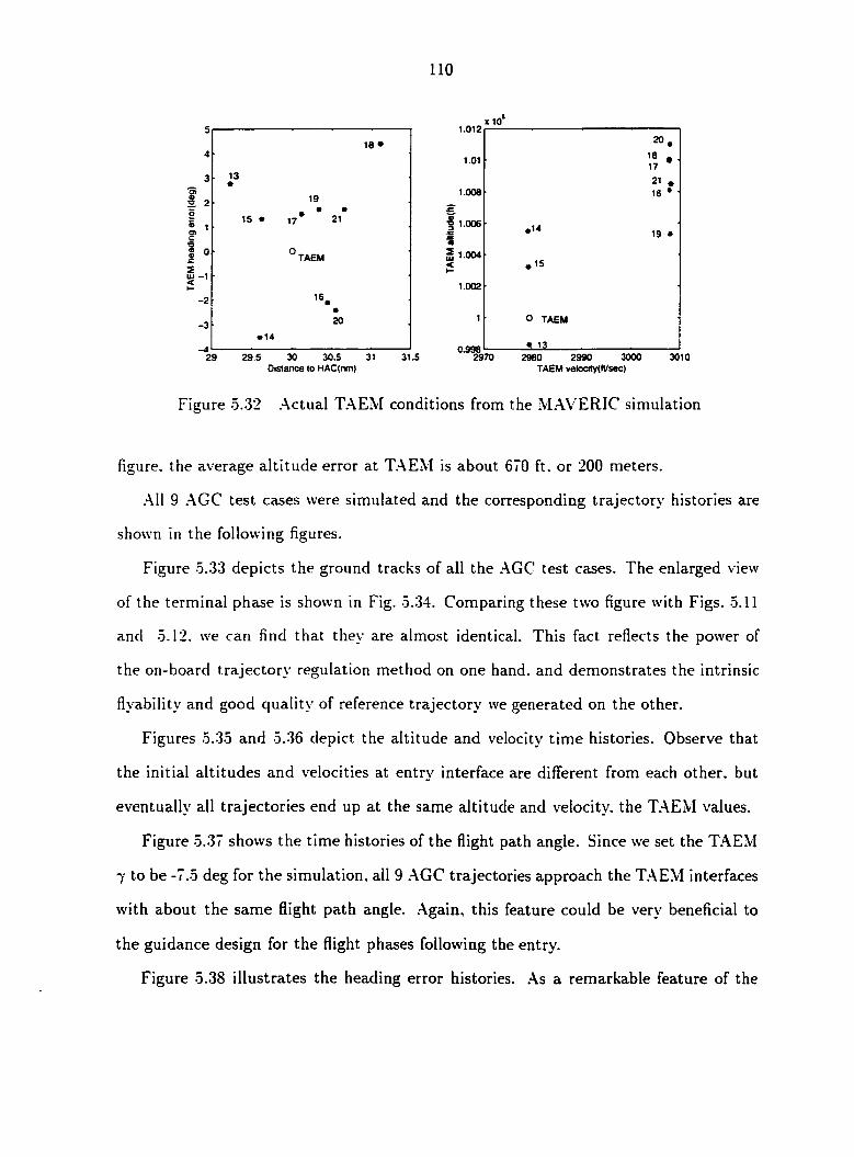
110
18 •
13 •
19 * *
15 • 17 21
° TAEM
16 • • 20
• 14
1.012
1.01
x 10
1.008
| 1.006
I | 1.004
1.002
1
29 29.5 30 30.5 31 31.1 Distance to HAC(nm)
0.998
2°.
21 .
16 *
.14 19 •
.15
O TAEM
. 13 2970 2980 2990 3000 3010
TAEM vekxaty(ltZsec)
Figure 5.32 Actual TAEM conditions from the MAVERIC simulation
figure, the average altitude error at TAEM is about 670 ft. or 200 meters.
All 9 AGC test cases were simulated and the corresponding trajectory histories are
shown in the following figures.
Figure 5.33 depicts the ground tracks of all the AGC test cases. The enlarged view
of the terminal phase is shown in Fig. 5.34. Comparing these two figure with Figs. 5.11
and 5.12. we can find that they are almost identical. This fact reflects the power of
the on-board trajectory regulation method on one hand, and demonstrates the intrinsic
flyability and good quality of reference trajectory we generated on the other.
Figures 5.35 and 5.36 depict the altitude and velocity time histories. Observe that
the initial altitudes and velocities at entry interface are different from each other, but
eventually all trajectories end up at the same altitude and velocity, the TAEM values.
Figure 5.37 shows the time histories of the flight path angle. Since we set the TAEM
7 to be -7.5 deg for the simulation, all 9 AGC trajectories approach the TAEM interfaces
with about the same flight path angle. Again, this feature could be very beneficial to
the guidance design for the flight phases following the entry.
Figure 5.38 illustrates the heading error histories. As a remarkable feature of the

Ill
single bank-reversal strategy, we can observe from the figure that there is exactly one
hump on each heading error history. Interestingly, the maximum magnitude of the
heading error for all cases are around 15 degree. This proves that the single bank-
reversal strategy works well in terms of not making the trajectory biased too much away
from the original line-of-sight from entry to HAC.
In traditional entry guidance design, the bank-reversal is typically done according
to a pre-scheduled heading error vs. Mach number plan. At certain Mach number, if
the heading error exceeds the planned value, the bank-reversal takes place. This type
of scheduled reversal usually results in the maximum magnitude of heading error larger
than the planned boundary value due to the kinematical delay of the bank-reversal. It
not unusual to observe heading error bigger than 10 deg along the trajectory produced by
the conventional bank-reversal schedule. In this sense, our single bank-reversal strategy
provides very acceptable results.
Figure 5.39 shows the control histories commanded by the on-board entry guidance
system for tracking the reference trajectories. Comparing this figure with the control
history of the reference entry trajectory, great similarity can be found between them
without surprise. We also observe that the desirable feature of small a magnitude when
approaching TAEM is preserved by the simulation, even in the presence of environmental
disturbance and model uncertainties automatically introduced by the MAVERIC.
Finally, we tested the on-board guidance system by setting Qmax = 60 BTU/f t 2 • s e c
for the AGC19-21 cases. With this maximum allowable heat rate, the entry corridor
is extremely narrowed. Figures 5.40 to 5.42 show the trajectories generated for cases
AGC19-21. Compare Fig. 5.41 with Fig. 5.25, we can conclude that the method we
designed for enforcing the entry corridor constraints is very successful. There is only
a slight violation of the 60 BTU/ft2 • sec heat rate constraint in case 19, where the
maximal heat rate is about 62 BTU/ft2 • sec for a short period as shown by Fig. 5.41.
Figure 5.40 shows the ground tracks and Fig. 5.42 demonstrates the control histories.
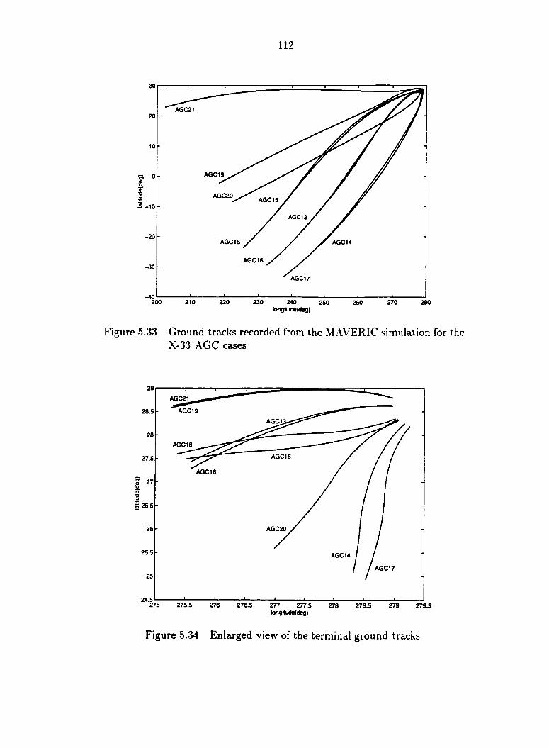
112
AGC21
AGC19
AGC20 AGC15
-10
AGC13
-20 AGC18 AGC14
AGC16 -30 -
AGC17
230 200 210 220 240 270 260 280 250 longitude(deg)
Figure 5.33 Ground tracks recorded from the MAVERIC simulation for the X-33 AGC cases
29
AGC21
AGC19 28.5
AGC1
AGC18
AGC15 27.5
AGC16
S 27
I AGC20 26
25.5 AGC14
AGC17
24.5 275.5 275 276 276.5 277 277.5 279 278 278.5 279.5
longitude(deg)
Figure 5.34 Enlarged view of the terminal ground tracks

113
1
î
1500 500 1000 t(sec)
Figure 5.35 Altitude time history recorded from the MAVERIC simulation for the X-33 AGC cases
500 1500 1000 t(sec)
Figure 5.36 Velocity time history recorded from the MAVERIC simulation for the X-33 AGC cases

114
f
I
-s
-7
—S 1500 500 1000
t(sec)
Figure 5.37 Flight path angle time history recorded from the MAVERIC simulation for the X-33 AGC cases
20
I s
1 I
-5
-10
-15
-20 1500 500 1000
t(sec)
Figure 5.38 Heading error time history recorded from the MAVERIC simulation for the X-33 AGC cases

115
100
20
-50
-100 1500 1000 500
((sec)
100
-50
-100 1500 500 1000
t(sec)
_ 40
I 3 30
1500 500 1000
t(sec)
Figure 5.39 Control histories recorded from the MAVERIC simulation for the X-33 AGC cases
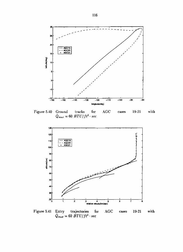
116
25
AGC19 - - AGC20 - AGC21
-80 -100 -90 -150 -140 -130 -110 -120
kmgitude(deg)
Figure 5.40 Ground tracks for AGC cases 19-21 with Qmax = 60 BTU/ft2 - sec
130
120
AGC19 - - AGC20 - AGC21
110
100
90
40
30
relative velotity(knVsec)
Figure 5.41 Entry trajectories for AGC cases 19-21 with Qmax = 60 BTU/ft2 • sec

117
100
AGC19 - - AGC20 - AGC21
I O
-50
-100 200 400 1400 600 800 1000 1200
time (sec)
55
45
40
I 3
30
200 400 800 1000 1400 600 1200
time (sec)
Figure 5.42 Control histories for AGC cases 19-21 with Qmax = 60 BTU/ft2 • sec

118
5.5 Performance Assessment
In this section, the performance of the on-board trajectory generation method is
evaluated in 3 aspects: the precision of meeting the TAEM conditions, the number
of integration iterations, and the CPU time needed for computing the entry reference
trajectory. The code is executed on a Gateway Pentium3 800MHz machine and a DEC
Alpha 500/500 work station for timing, respectively.
Nine AGC cases for X-33 and four cases for X-38 were examined for the performance
assessment. The dimensionless time step size dt for the 3DOF trajectory integration is
set to be 0.002. or 1.612 sec in real time. Another factor that affects the code efficiency is
the range step size ds for the longitudinal reference profiles. It was set to be 5.8173e-004,
or 2 nm in real distance. With these settings, we achieved a rough balance between the
numbers of integration steps for completing the 3DOF trajectory and for obtaining the
longitudinal profiles. For test cases of both the X-33 and X-38. which are all of normal
orbital entries, this integration time step size produces about . .000 data points for the
output reference trajectories.
Table 5.3 gives the TAEM precision of the reference trajectories we generated for all
test cases presented in section 5.2. The symbol A stands for the error that is obtained
by subtracting the designated TAEM value from the actual terminal value of the 3DOF
trajectory. The heading error A# is obtained by subtracting the line-of-sight azimuth
value from the terminal velocity azimuth. The range errors AStogo are all negative due to
the discrete recording of the trajectory, which terminates when the range-to-go to HAC
is less than the TAEM radius. As listed in the table, the average TAEM altitude and
velocity errors are about 47.6 meters and 5 m/sec respectively. Notice that the average
TAEM heading error and altitude error are calculated for |A#| and |Ar|, respectively.
Our experience shows that the velocity and altitude error can be further reduced by
using more elaborate h schedule for the RH control method. The performance in terms

119
of terminal precision shown in the table is comparable with that presented in Ref. [18].
in which off-line designed reference trajectories were used.
Table 5.3 Terminal precision of 3DOF entry trajectories for X-33 and X-38
Atf(deg) AiS'togo (ill) Ar (m) AV" (m/sec) X-38 easel 1.26 -45.62 -23.4 -2.7 X-38 case2 3.77 -73.29 -42.47 -7.9 X-38 case3 -3.88 -93.75 -2.19 -9.3 X-38 case4 4.99 -9.62 18.26 -6.63
X-33 AGC13 1.87 -107.03 88.16 -2.7 X-33 AGC 14 -2.23 -59.73 57.22 -5.63 X-33 AGC15 2.24 -17.23 68.15 -0.77 X-33 AGC16 1.96 -71.93 90.58 -3.17 X-33 AGC17 2.09 -97.67 30.47 -10.14 X-33 AGC18 1.0 -117.82 59.98 -2.31 X-33 AGC 19 -0.96 -76.3 78.8 -1.7 X-33 AGC20 1.87 -141.62 41.22 -8.67 X-33 AGC21 2.96 -88.73 67.56 -6.66
average 2.39 -76.5 47.6 -5.24
Table 5.4 gives the algorithm performance statistics in terms of CPU time and num
ber of iterations. The term iter 1 stands for the number of iterations on crmid for solving
the QEGC profile. We name this process iteration 1. The term iter'2 stands for the
number of iterations searching the single bank-reversal point in completing the 3D0F
trajectory. We call this process iteration 2. As stated previously in the method de
scription. both searching processes are monotonie and fast convergence guaranteed in a
small number of iterations. Due to the use of the single-bank-reversal point predictor,
the value of iter2 is even smaller as shown in the table. The term iterZ represents the
number of repetitions of the initial descent integration.
We can now heuristically estimate the number of iterations needed by the algorithm
in terms of the 3D0F integration from entry to TAEM. The iteration 1 involves inte
grating a single differential equation, i.e, Eq. (3.5), from the QEGC transition point,
to the preTAEM point with range-to-go as the independent variable. Thus the average

120
computational load for iteration 1 should be less than integrating a 3DOF trajectory
for 6 times on average. Given the fact that the QEGC integration is only conducted
for the central part of the trajectory , we can optimistically estimate that average com
putational load is roughly equal to integrating a whole 3DOF trajectory for 3 times.
Iteration 2 involves integrating the 3DOF dynamic equations from some point, which is
not necessarily the entry point except for the first iteration, to the terminal point, which
is not necessarily the TAEM interface except for the last iteration. Thus, the value of
iter2 actually accounts for times of integrating part of the 3 DO F trajectory. By exam
ining all the test cases, we estimate that the equivalent number of iterations in terms
of integrating a whole 3DOF trajectory from entry to TAEM is about half the value of
iter'l. The times of repetition of the initial descent integration is almost negligible as
indicated by the value of iter'i. This gives us a rough estimate that the normal entry
trajectory generation demands a computational load equivalent to about 5 iterations of
integrating a 3DOF trajectory from entry interface to the TAEM.
The CPU time is also listed as a performance index. On average, a trajectory can
be generated in 3.23 sec on a 800MHz PC or 2.48 sec on a DEC Alpha 500/500 station.
Note that the number of nodes of the trajectory could be cut by half or even more for
most cases by increasing the integration time step size.

121
Table 5.4 Algorithm performance statistics
nodes iterl iter2 iter3 PC CPU(sec) Unix CPU(sec) X-38 easel 1200 9 4 0 3.796 2.545 X-38 case2 1134 8 6 0 3.901 3.19 X-38 case3 1291 5 4 0 2.645 1.949 X-38 case4 1208 9 4 0 3.375 2.483
X-33 AGC 13 909 4 5 0 3.73 3.03 X-33 AGC 14 922 4 3 0 2.234 1.733 X-33 AGC 15 870 4 2 0 2.25 1.733 X-33 AGC16 1072 5 7 0 4.922 3.948 X-33 AGC17 1070 5 3 0 2.906 2.249 X-33 AGC 18 1045 7 2 0 3.531 2.683 X-33 AGC 19 763 6 6 1 3.344 2.666 X-33 AGC20 1007 6 3 1 2.922 2.266 X-33 AGC21 1032 6 4 2 2.656 2.033
average 1040 6 4 0.3 3.23 2.48

CHAPTER 6. CONCLUSIONS AND FUTURE WORK
On-board reference trajectory design has been a great challenge of entry guidance
development since the early days of the manned space flight era. Almost all available
entry guidance schemes today depend on tracking a reference profile or trajectory. But
the difficulty in designing even a two dimensional reference profile, such as the drag
versus energy reference profile based on the Space Shuttle entry guidance technology,
has made it necessary for pre-loading an off-line designed reference profile/trajectory. It
has been a long desired goal of entry guidance designers that a 3D0F entry trajectory
satisfying all constraints and terminal requirements can be generated aboard based on
the current information. Due to the difficulties associated with the problem, to the
best of our knowledge no comparable research has been reported on tackling the 3DOF
constrained trajectory generation problem before this dissertation.
The major contribution of this dissertation is the development of an efficient method
for generating 3D0F constrained entry trajectories. Our method is not only a useful ref
erence trajectory generator for on-board use, but also a powerful tool for entry guidance
planning analysis on the ground.
6.1 Conclusions
The primary objective of this research is to develop a method for on-board generation
of 3D0F constrained entry trajectories. Several key techniques have been developed to
form the major components of our method illustrated by this dissertation. They are: the
123
novel use of the quasi-equilibrium glide condition that enables the enforcement of the
trajectory constraints and the design of the intermediate longitudinal reference profiles,
the single bank-reversal strategy' that enables the completion of the 3DOF trajectory,
and the terminal backward trajectory integration that makes it possible for precisely
meeting the TAEM interface conditions. To handle those extreme entry cases that
merely allow one bank-reversal, a terminal reference ground path tracking technique has
been developed to complement our method. Also, those entry cases that no feasible
entry trajectory may exist has also been considered by providing a trajectory that best
meets the TAEM conditions.
Our method illustrated is conceptually different from other known trajectory gener
ation methods. The involved parameter searching processes are strictly monotonie and
fast convergence guaranteed in few partial trajectory integration iterations.
Two space vehicles with different L/D ratios, the X-33 reusable launch vehicle and
the X-38 crew return vehicle, were examined using this entry trajectory generation
method for a broad range of entry cases. Simulation results show that algorithm works
efficiently for all entry scenarios. The design parameters are only vehicle dependent.
Once the parameters are tuned for a specific vehicle, the algorithm can handle various
entry scenarios, including those very extreme cases. On a Pentium3 PC or a DEC Alpha
station, the average CPU time for generating a 3DOF constrained entry trajectory under
all test scenarios is about 2-3 seconds. The obtained entry trajectories observe all the
trajectory and control constraints and precisely meet the TAEM interface conditions.
We have also demonstrated the great adaptability of this trajectory generation method.
Along an entry trajectory just generated by this method, we arbitrarily picked some s-
tates and added perturbation on it. The perturbation could be so large that it is highly
impossible to get it back to the original trajectory by any trajectory regulation method.
Then from this intensionally perturbed state, a new trajectory, that may be quite dif
ferent from the original one, can be generated even fast due to the shorter range. This
124
shows the promising capability of this method for guidance design for sub-orbital entry
or ascent abort scenarios.
The C code of this algorithm has been successfully integrated into a high fidelity flight
simulator for the X-33 vehicle, the MAVERIC. Instead of loading a pre-designed reference
trajectory for the entry guidance scheme, upon de-orbit, the current entry interface state
information and the TAEM conditions were passed to the on-board trajectory generator.
Within 1-2 seconds, a 3D0F constrained trajectory was generated and passed back to
the guidance system to be used as the conventional reference trajectory. Then the
vehicle was guided to the TAEM interface by tracking this trajectory and reached the
TAEM interface with high precision as expected. Even in the presence of vehicle model
inaccuracy and environmental disturbance automatically presented by the high fidelity
flight simulator, this on-board guidance strategy succeeded in all test cases.
6.2 Future work
The sequential feature of the method and the modularized structure of the algorithm
gives large room for further extending the scope and adaptability of this method, as well
as improving the robustness and efficiency.
1) The first improvement can be done on the terminal backward trajectory. Based
on the reasoning that the flight corridor is so narrow that we do not have much choice in
determining the shape of the r — V reference profile, we set the preTAEM altitude as a
user-provide parameter at the given preTAEM velocity. This resulted that the terminal
control history and hence the state history were the same for all missions, as shown by
the X-33 and X-38 test cases. Even though the terminal phase is very short compared to
the whole entry flight range, the location of the preTAEM altitude does matter in some
extreme entry cases. Thus an automatic detection of the feasible preTAEM state is in
order. Tentatively, we tried to introduce another iteration for searching the preTAEM

125
altitude based on the QEGC as well.
2) The feedback control method for tracking the terminal backward reference V — r
curve needs to be more robust. In other words, we want a clean and robust method
(not necessarily a control method ) to transfer the TAEM state to some state (to be
determined as the preTAEM state) in the entry corridor beyond which the QEGC can be
closely satisfied. The path of the state transferring is unimportant, as far as the method
can bring the state from TAEM to the preTAEM state. This problem statement sounds
straightforward and simple, but it could actually involve much work in the nonlinear
system control domain.
3) The initial descent and terminal backward integration phases may need to be
coordinated in order to achieve better results. The current method always chooses the
smallest <r0 value by which the initial descent enters the corridor and transits onto a
QEGC profile. But it is possible that a smaller a0 may make it inevitable that no longi
tudinal reference profile can be found. This is specially important for sub-orbital entry
in which there is usually not much room for adjusting the <rmij so that the longitudinal
reference profile is continuous at the preTAEM state. If this is the case, we may need
to check if it works with a larger (TQ value.
4) The most time-consuming part of this algorithm is computing the feedback gains
by the RH method, which involves intensive matrix calculation. But the same goal can be
achieved theoretically by using two independent nonlinear feedback controllers, one using
q for tracking the V{Stogo) profile, and the other using a for tracking the r(St0go) profile.
In fact, in the early stage of developing our method, we used this concept and found
out that control saturation was almost inevitable when going through the transition
points and doing bank-reversals (according to a bank-reversal schedule instead of the
single bank-reversal strategy presented in this dissertation). It seems that combining
the RH method and the nonlinear feedback control method in some way may save a lot
of computational load.

126
5) We have assumed that the TAEM conditions are always given as described in Fig
ure 2.3. But this is not necessarily the case in reality. Sometimes, special considerations
such as avoiding flying over a densely populated area are made in designing the TAEM
conditions. This will restrict the applicability of the single bank-reversal strategy. For
solving this kind of problems, Ref. [24] introduces the ground tracking method, but with
no guarantee for meeting the TAEM altitude and velocity conditions simultaneously due
to the very limited control authority by angle of attack. It seems there may exist a way
combining the single bank-reversal strategy with the ground tracking method such that
we can achieve a prescribed terminal heading requirement while precisely tracking the
longitudinal reference profiles.
127
APPENDIX A. EXPRESSIONS OF H AND S MATRICES
The following expressions are from Ref. [21].
In the Eq. (3.31) the sizes and expressions of H and S depend on the value of V
(the term q in Eq. (3.31) does not affect the solution (3.34). For an integer A" let
and
H =
HQo
Hl0
HQI
Hn
... /fo(.V-l)
... H i(<v-i)
//(,v_i)i ... H(,\-1)(.v—i)
(A.l)
5 = [S0 Si ... S,v-i] (.4.2)
Let Ck = C(t + kh). k = 1,.... Ar.
For .V = 2:
Hoo — hR + '2hG\QCj ÇCiGi.o
+ hGjpCj QC2G2,0
Hn = 2 hR + hGllCjQC2G2.i
Hoi = Hw = hGl0CjQC2G2A
50 = 2h&JCfQCiGi,o + hA%CjQC2G2,0
51 = hAlCjQC2G2,i
(A.3)
For N = 3:

128
Hoo = hR + 2hOrl0CjQCxGl.0
+ 2hGj qCJ QCiGz# + hGz QCj QCsGs#
Hu = 2hR + 2hGllCjQC2G2A
H22 = 2hR + hGl2CjQC3G3,2
Hox = Hx0 = 2hGl0C?QC2G2,l
+ hGl0Cj QCzGz,i
H02 = H20 = hGl0CjQC3G3,2
Hl2 = H2i = hG3 lC3 QCzGz.2
SQ = 2hAjCjQCxGx,0 + 2hAlCjQC2G2.o
+ hA^CjQC3Gz$
5, = 2h^CjQC2G2A + hA^Cj QC3G3a
For N = 4:
H00 — hR + 2hGj0C[QCiGi,o
+ 2hGloCjQC2G2,o + 2hGl0CjQC3G3,o
+ hGl0CjQC4GAfi
Hn = 2hR + 2hGllCjQC2G2,i
+ 2AG^Cf QC3G3.1 + AGLCf
H22 = 2 hR + 2/iGj2Cj QC3G3.2
+
H33 = 2hR + hGl3CjQC4G4,3
Hoi = H io = 2 hGl0GlQC2G2.i
+ ZACLCfQCsGa., +
H02 = = 2AGT,C?0C3G3.2
+
Hq3 = Hzo = hGl0Cj QC4G43
H12 = ^21 = 2AGLCfQC3G3.2
+ &GLCTQC4G4.2
H13 = //si =
H23 = H32 = hGj2Cj QC\ G4 ,3
So = 2h±JCfQCiGi,0 + 2h^CjQC2G2,0
+ 2AAlCfQC3G3.o + AAlCfOCAo
Si = 2h^CjQC2G2,l + 2hAlCjQC3G3,i
+ hùJACjQC4G4,1
S2 = 2AA^CfQC3G3.2 + AA4(?rQC4G4.2
S3 = hAjCjQC4G4,3
For other values of N, it is not difficult to follow the patterns exhibited in above
expressions and obtain the corresponding H and S matrices.

130
APPENDIX B. X-33 VEHICLE AND ENTRY MISSION
DATA
Table B.l X-33 vehicle/mission parameters
vehicle parameter value unit mass 37362.9 kg Sre/ 149.388 m2
7m ax 300.0 psf Qmax 75 B T L ' / i f t 2 • s e c )
L/OOTDYNQJ. 2.5 g Hmax 5.0 deg/sec
iaim» 2.0 degjsec2
85.0 deg
Hmax 5.0 deg/sec
l^lmax 3.5 deg/sec2
Table B.2 Case AGC13: 3DOF entry from ISS orbit (51.6 deg)
mission parameter value unit/equivalent to PhiHAC 28.6112 deg
ThetaHAC 279.504 deg TAEM-r 1.0048 30.427 km TAEM-V 0.1148 908.15 m/sec
TAEM2HAC 0.0087 30 nm Entry .sigma 0 deg Entry jilpha 45 deg
Entry .altitude 1.0191 121.92 km Entry Jongitude 4.241 242.993 deg Entry Jatitude -0.3186 -18.255 deg Entry .velocity 0.9636 7622 m/sec Entry .gamma -0.0251 -1.4379 deg Entry .heading 0.669 38.329 deg
131
Table B.3 Case AGC14: 3D0F "early" entry from ISS orbit (51.6 deg)
mission parameter value unit/equivalent to
PhiHAC 28.6112 deg ThetaHAC 279.504 deg
TAEM-r 1.0048 30.427 km TAEM-V 0.1148 908.15 m/sec
TAEM2HAC 0.0087 30 nm Entry .sigma 0 deg
Entry .alpha 45 deg Entry .altitude 1.0192 122.558 km
Entry .longitude 4.3457 248.993 deg Entry Jatitude -0.3929 -22.5101 deg Entry .velocity 0.9635 7621.3 m/sec Entry .gamma -0.0251 -1.43803 deg Entry-heading 0.6956 39.8557 deg
Table B.4 Case AGC15: 3DOF "late" entry from ISS orbit (51.6 deg)
mission parameter value unit/equi valent to PhiHAC 28.6112 deg
ThetaHAC 279.504 deg TAEM-r 1.0048 30.427 km TAEM-V 0.1148 908.15 m/sec
TAEM2HAC 0.0087 30 nm Entry .sigma 0 deg Entry .alpha 45 deg
Entry .altitude 1.0189 120.374 km Entry Jongitude 4.1014 234.993 deg Entry Jatitude -0.2135 -12.2299 deg Entry .velocity 0.9637 7622.79 m/sec Entry .gamma -0.0251 -1.43775 deg Entry-heading 0.6425 36.8122 deg

132
Table B.5 Case AGC16: 3D0F entry from ISS orbit (51.6 deg)
mission parameter value unit/equi valent to PhiHAC 28.67 deg
ThetaHAC 279.494 deg TAEM-r 1.0046 29.4315 km TAEM-V 0.1159 916.8628 m/sec
TAEM2HAC 0.0087 30 nm Entry-sigma 0 deg Entry .alpha 45 deg
Entry .altitude 1.0191 121.858 km Entry Jongitude 4.0579 232.502 deg Entry Jatitude -0.5151 -29.516 deg Entry .velocity 0.9641 7625.99 m/sec Entry .gamma -0.0218 -1.2492 deg Entry-heading 0.7583 43.447 deg
Table B.6 Case AGC17: 3DOF "'early" entry from ISS orbit (51.6 deg)
mission parameter value unit/equivalent to PhiHAC 28.67 deg
ThetaHAC 279.494 deg TAEM_r 1.0046 29.4315 km TAEM-V 0.1159 916.8628 m/sec
TAEM2HAC 0.0087 30 nm Entry .sigma 0 deg Entry .alpha 45 deg
Entry .altitude 1.0193 123.104 km Entry Jongitude 4.1452 237.502 deg Entry Jatitude -0.5805 -33.2629 deg Entry .velocity 0.964 7625.15 m/sec Entry .gamma -0.0218 -1.24943 deg Entry Jieading 0.8039 46.0617 deg

133
Table B.7 Case AGC18: 3D0F "late" entry from ISS orbit (51.6 deg)
mission parameter value unit/equivalent to
PhiHAC 28.67 deg ThetaHAC 279.494 deg
TAEM-r 1.0046 29.4315 km TAEM-V 0.1159 916.8628 m/sec
TAEM2HAC 0.0087 30 nm Entry .sigma 0 deg
Entry_alpha 45 deg Entry .altitude 1.0188 120.132 km
Entry Jongitude 3.9357 225.502 deg Entry Jatitude -0.4145 -23.7507 deg Entry .velocity 0.9642 7627.18 m/sec Entry .gamma -0.0218 -1.24901 deg Entry .heading 0.7053 40.4095 deg
Table B.8 Case AGC19: 3DOF entry from LEO orbit (28.5 deg)
mission parameter value unit/equivalent to PhiHAC 28.67 deg
ThetaHAC 279.494 deg TAEM-r 1.0046 29.4315 km TAEM-V 0.1159 916.8628 m/sec
TAEM2HAC 0.0087 30 nm Entry .sigma 0 deg Entry .alpha 45 deg
Entry .altitude 1.0191 121.649 km Entry Jongitude 3.8096 218.2761 deg Entry Jatitude -0.0402 -2.30465 deg Entry .velocity 0.9409 7442.37 m/sec Entry .gamma -0.0179 -1.02749 deg Entry-heading 1.0446 59.8538 deg

134
Table B.9 Case AGC20: 3D0F "early" entry from LEO orbit (28.5 deg)
mission parameter value unit/equi valent to PhiHAC 28.67 deg
ThetaHAC 279.494 deg TAEM-r 1.0046 29.4315 km TAEM.V 0.1159 916.8628 m/sec
TAEM2HAC 0.0087 30 nm Entry .sigma 0 deg Entry .alpha 45 deg
Entry_altitude 1.0191 122.079 km Entry Jongitude 3.8794 222.2760 deg Entry Jatitude -0.1474 -8.44634 deg Entry .velocity 0.9408 7442.07 m/sec Entry_gamma -0.0179 -1.02753 deg Entry-heading 1.0651 61.0263 deg
Table B.10 Case AGC21: 3DOF "late" entry from LEO orbit (28.5 deg)
mission parameter value unit/equivalent to PhiHAC 28.67 deg
ThetaHAC 279.494 deg TAEM-r 1.0046 29.4315 km TAEM.V 0.1159 916.8628 m/sec
TAEM2HAC 0.0087 30 nm Entry .sigma 0 deg Entry .alpha 45 deg
Entry .altitude 1.0196 124.848 km Entry Jongitude 3.5304 202.276 deg Entry Jatitude 0.3985 22.83 deg Entry .velocity 0.9406 7440.12 m/sec Entry-gamma -0.0179 -1.0278 deg Entry .heading 1.2471 71.4535 deg
135
APPENDIX C. X-38 VEHICLE AND ENTRY MISSION
DATA
Table C.l X-38 vehicle/mission parameters
vehicle parameter value unit mass 11566.5 kg S r e f 21.672 m2
Çmax 300.0 psf
Qmax 100 B T U / ( f t 2 • s e c )
L/Oddmax 2.5 g
Mmax 10.0 deg/sec
Kax 5.0 deg/sec2
\&\max 85.0 deg
\ & Lax 9.0 deg/sec
l*L«x 5.0 deg/sec2
Table 0.2 X-38 entry test case 1
design parameter value unit/equivalent to PhiHAC 33.2333 deg
ThetaHAC 240.55 deg TAEM-r 1.0038 24.4 km TAEM.V 0.0932 737.47 m/sec
TAEM2HAC 0.0087 30 nm Entry _sigma 0 deg Entry .alpha 40 deg
Entry .altitude 1.0191 121.92 km Entry-longitude 2.453 140.575 deg Entry-latitude 0.4706 26.965 deg Entry .velocity 0.9441 7467.8 m/sec Entry-gamma -0.0179 -1.02589 deg Entry .heading 1.0289 58.949 deg

136
Table C.3 X-38 entry test case 2
design parameter value unit/equivalent to PhiHAC 27.5 deg
ThetaHAC 246.25 deg TAEM-r 1.0038 24.4 km TAEM.V 0.0932 737.47 m/sec
TAEM2HAC 0.0087 30 nm Entry .sigma 0 deg Entry .alpha 40 deg
Entry .altitude 1.0191 121.92 km Entry Jongitude 2.5777 147.69 deg Entry Jatitude 0.5318 30.47 deg Entry .velocity 0.9441 7468 m/sec Entry .gamma -0.0178 -1.02179 deg Entry-heading 1.0964 62.819 deg
Table C.4 X-38 entry test case 3
design parameter value unit/equivalent to PhiHAC -38.95 deg
ThetaHAC 291.843 deg TAEM-r 1.0038 24.4 km TAEM.V 0.0932 737.47 m/sec
TAEM2HAC 0.0087 30 nm Entry_sigma 0 deg Entry .alpha 40 deg
Entry .altitude i .0191 121.92 km Entry Jongitude 3.9938 228.83 deg Entry Jatitude 0.3126 17.91 deg Entry .velocity 0.9441 7467.8 m/sec Entry .gamma -0.0168 -0.96 deg Entry .heading 2.222 127.313 deg

137
Table C.5 X-38 entry test case 4
design parameter value unit/equivalent to PhiHAC -28.2425 deg
ThetaHAC 134.98 deg
TAEM-r 1.0038 24.4 km TAEM.V 0.0932 737.47 m/sec
TAEM2HAC 0.0087 30 nm Entry .sigma 0 deg Entry-alpha 40 deg
Entry .altitude 1.0191 121.92 km Entry Jongitude 0.781 44.75 deg Entry Jatitude -0.3042 -17.43 deg Entry .velocity 0.9440 7467.1 m/sec Entry-gamma -0.0182 -1.04 deg Entry Jieading 2.226 127.547 deg
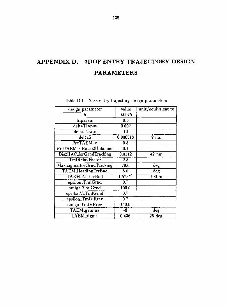
138
APPENDIX D. 3DOF ENTRY TRAJECTORY DESIGN
PARAMETERS
Table D.l X-33 entry trajectory design parameters
design parameter value unit/equivalent to h 0.0075
h-param 0.5 deltaTinput 0.002 deltaT _rate 10
deltaS 0.000518 2 nm PreTAEM.V 0.3
PreTA EM _r _Ratio2 Upbound 0.1 Dis2HAC JorGrndTracking 0.0112 42 nm
TmlRelaxFactor 2.3 Max^igma JorGrndTracking 70.0 deg
TAEM_HeadingErrBnd 5.0 deg TAEM_AltErrBnd 1.57e-5 100 m epsilon-TmlGrnd 0.7 omiga.TmlGrnd 100.0
epsilon V_TmlGrnd 0.7 epsilon.T ml VRrev 0.7 omiga_TmlVRrev 150.0
TAEM_gamma -8 deg TAEM-sigma 0.436 25 deg

139
Table D.2 X-38 entry trajectory design parameters
design parameter value unit/equivalent to h 0.0015
h_param 1 deltaTinput 0.002 deltaT_rate 10
deltaS 0.000518 2 nm PreTAEM.V 0.3
PreTAEM_r_Ratio2Upbound 0.1 Dis2H AC JorGrndTracking 0.0112 42 nm
TmlRelaxFactor 2.3 Max .sigma JorGrndTracking 70.0 deg
TAEM_HeadingErrBnd 5.0 deg TAEM-AltErrBnd 1.57e-5 100 m epsilon.T mlGrnd 0.7 omiga.TmlGrnd 50.0
epsilon V_T mlGrnd 0.27 epsilon.TmlVRrev 0.7 omiga.T mlVRrev 50.0
TA EM .gamma -8 deg TAEM_sigma 0.436 25 deg
140
BIBLIOGRAPHY
[1] Anon, "Guidance and Navigation for Entry Vehicles," NASA SP-8015. November
1968.
[2] Baer-Riedhart, J., "X-38 Project Summary,
http://www.dfrc.nasa.gov/Projects/X38/.
[3] Cheng, P., Shen, Z., and LaValle, S. M., "RRT-Based Trajectory Design for Au
tonomous Automobiles and Spacecraft," Archives of Control Sciences, Vol. 11
(XLVII), No, 3-4, 2001, pp. 51-78.
[4] Coughlin, D., Dukeman, G., Hanson. J., Mulqueen, J., and McCarter, J., "Ascent.
Transition, Entry, and Abort Guidance Design for the X-33 Vehicle," AI A A paper-
98-4409, Proceedings of the AI A A Guidance, Navigation, and Control Conference,
August 10-12, 1998, Boston, MA.
[5] Frazzoli, E., Dahleh, M. A., and Feron, E., "Real-Time Motion Planning for Agile
Autonomous Vehicles," Journal of Guidance, Control, and Dynamics, Vol. 25, No.
1, January-February 2002, pp. 116-129.
[6] Fuhry, D. P., "Adaptive Atomspheirc Reentry Guidance for the Kistle K-l Prbital
Vehicle," Proceedings of Guidance, Navigation, and Control Conference, Denver,
CO, August 14-17, 2000.

141
[7] Gamble. J. D., Cerimele, C. J., Moore, T. E., and Higgins. J.. "Atmospheric Guid
ance Concepts for an Aeroassisted Experiment," The Journal of the Astronautical
Sciences, Vol.36, No. 1-2, 1988, pp. 45-71.
[8] Girerd, A., and Barton. G., "Next Generation Entry Guidance - Onboard Trajec
tory Generation for Un powered Drop Tests," Proceedings of the AI A A Guidance.
Navigation, and Control Conference, Denver, CO, August 14-17, 2000.
[9] Hanson. J., "Advanced Guidance and Control Project for Reusable Launch Vehi
cles." Proceedings of Guidance, Navigation, and Control Conference. Denver. CO.
August 14-17, 2000.
[10] Harpold, J. C.. and Graves. C. A., "Shuttle Entry Guidance." The Journal of the
Astronautical Sciences. Vol. XXXVII. No. 3, 1979, pp. 239-268.
[11] Jansch, C., and Markl, A.. "Trajectoty Optimization and Guidance for a HERMES-
Tvpe Reentry Vehicle," AIAA-91-2659-CP, Aerican Institute of Aeronauticss and
Astronautics, 1991.
[12] Jouhaud, F., "Fuzzy Logic control - Allpication to the Guidance of a Re-Entrv space
Capule," IAF, International Astronautical Congress, 48th, Turin, Italy, October 6-
10, 1997.
[13] Kindler, J. T., " Optimal Reentry Trajectories for the Experimental Vehicle X-38
V201," Master's Thesis, University of Stuttgart, Germany, September 1999.
[14] Kindler, J. T., Schoettle, U. M., and Well, K. H., "Entry Interface Window of
Landing Site Coober Pedy for the Experiemental Vehicle X-38 V201," AIAA-2000-
4117, American Institute of Aeronauticss and Astronautics, 2000.
142
[15] Kwon, W. H., and Pearson, A. E., "A Modified Quadratic Cost Problem and Feed
back Stabilization of a Linear System," IEEE Trans, on Automatic Control. Vol.
22, 1977, pp. 838-842.
[16] Lavalle, S. M., "Rapidly-Exploring Random Trees: A new Tool for Path planning."
Technique Report No. 98-11, Dept. of Computer Science. Iowa State University.
October 1998.
[17] Lu, P., "Regulation about Time-Varying Trajectories: Precision Entry Guidance
Illustrated," Journal of Guidance. Control, and Dynamics, Vol. 22. No. 6. 1999. pp.
784-790.
[18] Lu, P., "Entry Guidance Algorithm Performance Assessment." Final Report pre
pared for Lockheed Martin Space Systems Company, February 15. 2001.
[19] Lu, P., "Close-Form control Laws for Linear Time-Varying Systems." IEEE Trans,
on Automatic Control, Vol. 45, No. 3, March 2000, pp. 537-542.
[20] Lu, P., "Nonlinear Trajectory Tracking Guidance with Application to a Launch
Vehicle," Journal of Guidance, Control, and Dynamics, Vol. 19. No. 1, January-
February, 1996, pp. 784-790.
[21] Lu, P., and Shen, Z., "Entry Guidance by Trajectory Regulation," Proceedings
of the AIAA Guidance, Navigation, and Control Conference, Denver, CO, August
14-17, 2000.
[22] Lu, P., Hanson, J. M., Dukeman, G. A., and Bhargava, S., "An Alternative En
try Guidance Scheme for the X-33," Proceedings of Atmospheric Flight Mechanics
Conference, Boston, MA, August 10-12, 1998.
[23] Lu, P., "Entry Guidance for the Reusable Launch Vehicle," Final Report, January
5, 1997 - July 6, 1999.

143
[24] Lu, P., and Hanson. J. M., "Entry Guidance for the X-33 Vehicle." Journal of
Spacecraft and Rockets, Vol. 35, No. 3, May - June 1998. pp. 342-349.
[25] Mease, K. D., Chen, D. T., Tandon, S., Young, D. H., and Kim. S., "A Three-
Dimentional Predictive Entry Guidance Approach," Proceedings of the .47.4.4 Guid
ance. Navigation, and Control Conference, Denver, CO, August 14-17. 2000.
[26] Mease, K. D., and Kremer, J. P., "Shuttle Entry Guidance Revisted Using Nonlinear
Geometri Methods." Journal of Guidance, Control, and Dynamics, Vol. 17. No. 6,
November-December 1994, pp. 1350-1356.
[27] Mease. K. 0., Teufel, P.. Schoenenberger, H., Chen. D. T., and Bharadwaj. S., "Re-
Entry Trajectory Planning for a Reusable Launch Vehicle," Paper 99-4160, AIAA
A FM-Conference, Portland, August 1999.
[28] Powell, R. W., "Six-degree-of-freedom Guidance and Control-Entry Analysis of the
HL-20," Journal of Spacecraft and Rockets. Vol. 30, No. 5, September-October,
1993, pp. 537-542
[29] Roenneke, A. J.,"Adaptive On-board Guidance for Entry Vehicles," Proceedings
of the AIAA Guidance, Navigation, and Control Conference, Montreal, Canada,
August 6-9, 2001.
[30] Roenneke, A. J., and Cornell, P. J., "Trajectory Control for a Low-Lift Re-Entry
Vehicle," Journal of Guidance, Control, and Dynamics, Vol. 16, No. 5, 1993, pp.
927-933.
[31] Roenneke, A. J., and Markl, A., "Re-Entry Control to a 0rag-vs-Energy Profile
Vehicle," Journal of Guidance, Control, and Dynamics, Vol. 17, No. 5, September-
October 1994, pp. 784-790.

144
[32] uKev X-33 Events in 2001," http://www.hq.nasa.gov/office/pao/History/x-
33/2001.htm.
[33] "NASA Dryden Flight Research Center Photo Gallery,"
http://www.dfrc.nasa.gov/galIery/photo/.
Related Documents