Advances in Differential Equations Volume 9, Numbers 5-6, May/June 2004, Pages 563–586 ON AN EVOLUTION SYSTEM DESCRIBING SELF-GRAVITATING FERMI–DIRAC PARTICLES Piotr Biler Instytut Matematyczny, Uniwersytet Wroc lawski pl. Grunwaldzki 2/4, 50–384 Wroc law, Poland Philippe Laurenc ¸ot Math´ ematiques pour l’Industrie et Physique, CNRS UMR 5640 Universit´ e Paul Sabatier – Toulouse 3, 118 route de Narbonne F–31062 Toulouse cedex 4, France Tadeusz Nadzieja Instytut Matematyki, Uniwersytet Zielonog´ orski ul. Szafrana 4a, 65–516 Zielona G´ ora, Poland (Submitted by: Herbert Amann) Abstract. The global-in-time existence of solutions for a system de- scribing the interaction of gravitationally attracting particles that obey the Fermi–Dirac statistics is proved. Stationary solutions of that system are also studied. 1. Introduction and derivation of the system Our aim in this paper is to study a nonlinear, nonlocal, parabolic system with nonlinear diffusion describing the evolution of a cloud of self-gravitating particles that obey the Fermi–Dirac statistics. This model has been intro- duced in [14] on the basis of considerations of kinetic equations, and has been studied in [13, 10]. Unlike the models of interacting particles where the particles are subject to linear Brownian diffusion (see, e.g., [7, 4, 5, 6, 23, 24]), the assumption that the density 0 ≤ f = f (x, v, t) of particles at the point (x, t) ∈ Ω × R + ,Ω ⊂ R d , moving at the velocity v ∈ R d is bounded by, say η 0 > 0, leads to mathematically completely different models. They involve nonlinear diffusion resembling that for fast-diffusing gases (at large densities). The plan of this paper is following: after discussing the derivation of the system of partial differential equations in Section 1 and properties of Accepted for publication: January 2004. AMS Subject Classifications: 35Q, 35K60, 35B40, 82C21. 563

Welcome message from author
This document is posted to help you gain knowledge. Please leave a comment to let me know what you think about it! Share it to your friends and learn new things together.
Transcript
Advances in Differential Equations Volume 9, Numbers 5-6, May/June 2004, Pages 563–586
ON AN EVOLUTION SYSTEM DESCRIBINGSELF-GRAVITATING FERMI–DIRAC PARTICLES
Piotr BilerInstytut Matematyczny, Uniwersytet Wroclawskipl. Grunwaldzki 2/4, 50–384 Wroclaw, Poland
Philippe LaurencotMathematiques pour l’Industrie et Physique, CNRS UMR 5640Universite Paul Sabatier – Toulouse 3, 118 route de Narbonne
F–31062 Toulouse cedex 4, France
Tadeusz NadziejaInstytut Matematyki, Uniwersytet Zielonogorskiul. Szafrana 4a, 65–516 Zielona Gora, Poland
(Submitted by: Herbert Amann)
Abstract. The global-in-time existence of solutions for a system de-scribing the interaction of gravitationally attracting particles that obeythe Fermi–Dirac statistics is proved. Stationary solutions of that systemare also studied.
1. Introduction and derivation of the system
Our aim in this paper is to study a nonlinear, nonlocal, parabolic systemwith nonlinear diffusion describing the evolution of a cloud of self-gravitatingparticles that obey the Fermi–Dirac statistics. This model has been intro-duced in [14] on the basis of considerations of kinetic equations, and hasbeen studied in [13, 10].
Unlike the models of interacting particles where the particles are subjectto linear Brownian diffusion (see, e.g., [7, 4, 5, 6, 23, 24]), the assumptionthat the density 0 ≤ f = f(x, v, t) of particles at the point (x, t) ∈ Ω ×R+, Ω ⊂ Rd, moving at the velocity v ∈ Rd is bounded by, say η0 > 0,leads to mathematically completely different models. They involve nonlineardiffusion resembling that for fast-diffusing gases (at large densities).
The plan of this paper is following: after discussing the derivation ofthe system of partial differential equations in Section 1 and properties of
Accepted for publication: January 2004.AMS Subject Classifications: 35Q, 35K60, 35B40, 82C21.
563
564 Piotr Biler, Philippe Laurencot, and Tadeusz Nadzieja
auxiliary functions in Section 2, we will study the evolution problem inSection 3, and describe steady states in Section 4. The main outcome of ourstudy is that for the systems of Fermi–Dirac self-gravitating particles, thegravitational collapse does not occur in dimensions d ≤ 3, which contrastsmarkedly with the linear Brownian diffusion case [7, 9].
The main steps in the derivation of the model (1.7)–(1.8) below are asfollows:– Suppose that the local entropy of the system is given by
S =1∫
Rd f dv
∫Rd
( f
η0log
f
η0+
(1 − f
η0
)log
(1 − f
η0
))dv
with some fixed η0 > 0.– The evolution of the density f , described generally by a kinetic equationft +v ·∇xf−∇φ ·∇vf = −∇vJ , subject to mass density and the energy den-sity constraints, is governed by the maximum entropy production principle(MEPP), discussed in detail in [14]. This principle determines the dissipa-tion flux −∇vJ , and then the equation (1.7) up to the diffusion coefficientafter the following procedure:– averaging f over the velocities v, and the passage to the limit of largefriction (or large times), thus obtaining “hydrodynamic” equations in the(x, t) space.
Such a procedure leads to the following form of the distribution function,
f(x, v, t) = η01
1 + λeβ|v|2/2,
which is called the Fermi–Dirac distribution, with the fugacity λ = λ(x, t)and the inverse temperature β = 1/ϑ. Note that 0 ≤ f(x, v, t) ≤ η0, and forlarge |v|, f resembles a Maxwell–Boltzmann distribution. Thus, the spatio-temporal density is
n(x, t) =∫
Rd
f(x, v, t) dv,
and the pressure is
p(x, t) =1d
∫Rd
|v|2f(x, v, t) dv.
In other words, we have (r = |v|)
n(x, t) =∫ ∞
0
η0
1 + λeβr2/2σdr
d−1 dr (1.1)
= η02d/2−1σdβ−d/2
∫ ∞
0
yd/2−1 dy
1 + λey= η02d/2−1σdϑ
d/2Id/2−1(λ),
on an evolution system 565
where σd is the area of the unit sphere in Rd, and Iα denotes the Fermiintegral of order α > −1,
Iα(λ) =∫ ∞
0
yα dy
1 + λey, (1.2)
defined for all λ > 0. Similarly we get
p(x, t) =1d
∫ ∞
0η0
r2
1 + λeβr2/2σdr
d−1 dr (1.3)
= η02d/2ωdβ−d/2−1
∫ ∞
0
yd/2 dy
1 + λey= η02d/2ωdϑ
d/2+1Id/2(λ),
where ωd = σd/d is the volume of the unit ball in Rd.Remark. The bound 0 ≤ f ≤ η0 at the starting point of the derivation ofequations may lead to arbitrarily large values of the density n in the positionspace. This bound has nothing to do with the Pauli exclusion principle inthe (x, t) space, which would bound a priori the density n, as is, e.g., in [23].
The total mass of the system is M =∫Ω n(x, t) dx. The no-flux condition
(1.9) below will guarantee the conservation of mass during the evolution.The particles generate the gravitational potential ϕ that satisfies the Pois-
son equation∆ϕ = σdGn,
where G is the gravitation constant.The total energy of the system is thus
E =12
∫Ω
∫Rd
f(x, v, t)|v|2 dv dx +12
∫Ω
n(x, t)ϕ(x, t) dx,
or
E =d
2
∫Ω
p(x, t) dx +12
∫Ω
n(x, t)ϕ(x, t) dx.
The MEPP implies the following form of the mean field equation for n andp:
nt = ∇ · (D (∇p + n∇ϕ)) ,
where the diffusion coefficient D may depend on n, p, ϑ, x, t, . . . . A naturalchoice arising from the analysis in [14] is
D = −Id/2−1(λ)λI ′d/2−1(λ)
. (1.4)
Note that the diffusion coefficient in [14, Section 5.2] is ϑD/ξ with a posi-tive parameter ξ, and ξ → ∞ corresponds to the high friction limit in theevolution equation above. Similarly, we can get rid of constants σd and G
566 Piotr Biler, Philippe Laurencot, and Tadeusz Nadzieja
in the Poisson equation. Thus, the relations between the density n in (1.1)and the pressure p in (1.3) are now given implicitly by
n =µ
2ϑd/2Id/2−1(λ), (1.5)
p =µ
dϑd/2+1Id/2(λ), (1.6)
with µ = η02d/2Gσ2d, and the Fermi integrals defined above in (1.2). After
the normalization (1.5)–(1.6) (different from that in [14]) of the density,pressure, and the equation for the potential, we will consider the system
nt = ∇ · (D (∇p + n∇ϕ)) , (1.7)∆ϕ = n, (1.8)
with the natural no-flux boundary condition
(∇p + n∇ϕ) · ν = 0 (1.9)
(ν is the unit exterior normal vector to ∂Ω), the Dirichlet boundary condition
ϕ|∂Ω = 0, (1.10)
and an initial conditionn(x, 0) = n0(x). (1.11)
Note that another condition for ϕ, the “free” (physically acceptable) condi-tion
ϕ = Ed ∗ n (1.12)with Ed being the fundamental solution of the Laplacian in Rd, can beconsidered. In the case of radially symmetric solutions (1.10) is equivalentto (1.12) by adding a constant to the potential ϕ; cf. also the discussionof this issue in [7, 8, 3]. We will study in this paper mainly the Dirichletcondition for ϕ, but some comments on the problem with the free conditionwill be given.
The model we consider is a simplified version of (5.18) in [14], where thefull system takes into account the conservation of the energy, the angular andlinear momenta for the cloud of particles in rotational and linear motion. Ouranalysis thus concerns the isothermal model, where the temperature ϑ is putconstant as it was in [7]. The analysis in the case of time-dependent but spacehomogeneous temperature ϑ = ϑ(t) is more complicated; cf. [12, 21, 16, 9]for the linear diffusion case. However, if ϑ = const we cannot take intoaccount the relation E = const valid in the microcanonical ensemble, butnot verified in the canonical ensemble.
Note that other models can take into account also spatial nonhomo-geneities of the temperature; cf. [24] for the particles in an exterior potential,

on an evolution system 567
and [6] for self-interacting particles. Those systems are much more difficultto analyze rigorously, even for the linear (i.e., Brownian) diffusion studiedin the references above.
Notation. In the sequel | . |p will denote the Lp(Ω) norms, ‖ . ‖Hk will beused for the Sobolev space Hk(Ω) norm, and ‖ . ‖Cε – for the Holder space Cε
norm. The letter C will denote inessential constants which may vary fromline to line.
2. Properties of Fermi integrals and auxiliary functions
Concerning the properties of the Fermi integrals let us notice that I0(λ) =log(1 + 1/λ), because
d
dλI0(λ) = − 1
λ(1 + λ). (2.1)
For α > −1 and |1/λ| < 1 the function Iα has the asymptotic expansion inthe powers of 1/λ
Iα(λ) =1λ
∫ ∞
0yαe−y
(1 +
1λ
e−y)−1
dy =1λ
∫ ∞
0yαe−y
( ∞∑k=0
(−1)k( 1
λ
)ke−ky
)dy
= Γ(α + 1)∞∑
k=0
(−1)k
(k + 1)α+1
( 1λ
)k+1. (2.2)
For α > −1 we have
d
dλIα(λ) = −
∫ ∞
0
yαey dy
(1 + λey)2=
∫ ∞
0
yα
λ
d
dy
( 11 + λey
)dy = −α
λIα−1(λ),
(2.3)the second line being valid for α > 0 only. Moreover, the formula
d2
dλ2Iα(λ) = 2
∫ ∞
0
yαe2y dy
(1 + λey)3(2.4)
for the second derivative holds. Therefore, Iα is a decreasing convex functionof λ.
It is important that the Fermi integrals (1.2) have the asymptotics
Iα(λ) ∼ 1α + 1
(− log λ)α+1 as λ 0, (2.5)
and
Iα(λ) ∼ Γ(α + 1)λ
as λ ∞. (2.6)
568 Piotr Biler, Philippe Laurencot, and Tadeusz Nadzieja
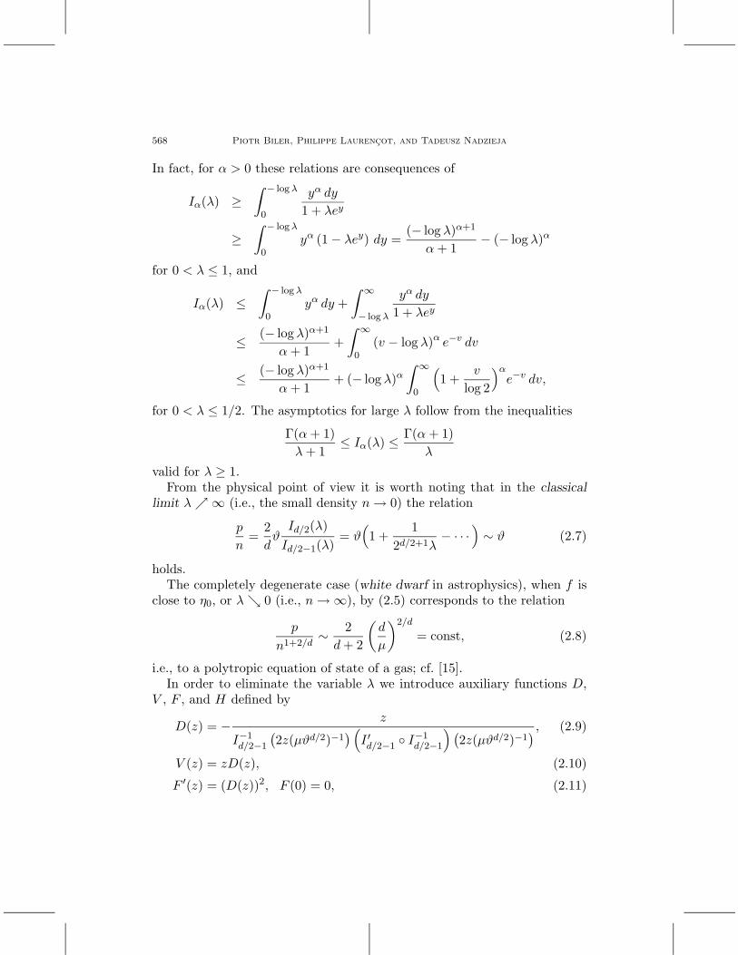
In fact, for α > 0 these relations are consequences of
Iα(λ) ≥∫ − log λ
0
yα dy
1 + λey
≥∫ − log λ
0yα (1 − λey) dy =
(− log λ)α+1
α + 1− (− log λ)α
for 0 < λ ≤ 1, and
Iα(λ) ≤∫ − log λ
0yα dy +
∫ ∞
− log λ
yα dy
1 + λey
≤ (− log λ)α+1
α + 1+
∫ ∞
0(v − log λ)α e−v dv
≤ (− log λ)α+1
α + 1+ (− log λ)α
∫ ∞
0
(1 +
v
log 2
)αe−v dv,
for 0 < λ ≤ 1/2. The asymptotics for large λ follow from the inequalities
Γ(α + 1)λ + 1
≤ Iα(λ) ≤ Γ(α + 1)λ
valid for λ ≥ 1.From the physical point of view it is worth noting that in the classical
limit λ ∞ (i.e., the small density n → 0) the relation
p
n=
2dϑ
Id/2(λ)Id/2−1(λ)
= ϑ(1 +
12d/2+1λ
− · · ·)∼ ϑ (2.7)
holds.The completely degenerate case (white dwarf in astrophysics), when f is
close to η0, or λ 0 (i.e., n → ∞), by (2.5) corresponds to the relation
p
n1+2/d∼ 2
d + 2
(d
µ
)2/d
= const, (2.8)
i.e., to a polytropic equation of state of a gas; cf. [15].In order to eliminate the variable λ we introduce auxiliary functions D,
V , F , and H defined by
D(z) = − z
I−1d/2−1
(2z(µϑd/2)−1
) (I ′d/2−1 I−1
d/2−1
) (2z(µϑd/2)−1
) , (2.9)
V (z) = zD(z), (2.10)
F ′(z) = (D(z))2, F (0) = 0, (2.11)
on an evolution system 569
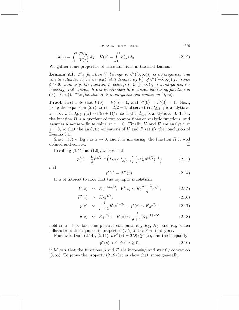
h(z) =∫ z
1
F ′(y)V (y)
dy, H(z) =∫ z
1h(y) dy. (2.12)
We gather some properties of these functions in the next lemma.
Lemma 2.1. The function V belongs to C2([0,∞)), is nonnegative, andcan be extended to an element (still denoted by V ) of C2([−δ,∞)) for someδ > 0. Similarly, the function F belongs to C3([0,∞)), is nonnegative, in-creasing, and convex. It can be extended to a convex increasing function inC3([−δ,∞)). The function H is nonnegative and convex on [0,∞).
Proof. First note that V (0) = F (0) = 0, and V ′(0) = F ′(0) = 1. Next,using the expansion (2.2) for α = d/2− 1, observe that Id/2−1 is analytic atz = ∞, with Id/2−1(z) ∼ Γ(α + 1)/z, so that I−1
d/2−1 is analytic at 0. Then,the function D is a quotient of two compositions of analytic functions, andassumes a nonzero finite value at z = 0. Finally, V and F are analytic atz = 0, so that the analytic extensions of V and F satisfy the conclusion ofLemma 2.1.
Since h(z) ∼ log z as z → 0, and h is increasing, the function H is welldefined and convex.
Recalling (1.5) and (1.6), we see that
p(z) =µ
dϑd/2+1
(Id/2 I−1
d/2−1
) (2z(µϑd/2)−1
)(2.13)
andp′(z) = ϑD(z). (2.14)
It is of interest to note that the asymptotic relations
V (z) ∼ K1z1+2/d, V ′(z) ∼ K1
d + 2d
z2/d, (2.15)
F ′(z) ∼ K2z4/d, (2.16)
p(z) ∼ d
d + 2K3z
1+2/d, p′(z) ∼ K3z2/d, (2.17)
h(z) ∼ K4z2/d, H(z) ∼ d
d + 2K4z
1+2/d (2.18)
hold as z → ∞ for some positive constants K1, K2, K3, and K4, whichfollows from the asymptotic properties (2.5) of the Fermi integrals.
Moreover, from (2.14), (2.11), ϑF ′′(z) = 2D(z)p′′(z), and the inequality
p′′(z) > 0 for z ≥ 0, (2.19)
it follows that the functions p and F are increasing and strictly convex on[0,∞). To prove the property (2.19) let us show that, more generally,

570 Piotr Biler, Philippe Laurencot, and Tadeusz Nadzieja
Lemma 2.2. For α > β, Iα I−1β is an increasing convex function, while
for α < β this is an increasing concave function.
The desired property (2.19) for p as a function of z will follow immediatelyfor α = d/2 and β = d/2 − 1.Proof. Setting g = Iα I−1
β we have g′ = I ′α I−1β /(I ′β I−1
β ) > 0. Next weconsider G = g′ Iβ = I ′α/I ′β and
G′(z) =(I ′′α(z)I ′β(z) − I ′α(z)I ′′β(z)
) (I ′β(z)
)−2 = −2J(z)(I ′β(z)
)−2.
Here we have
J(λ) =∫ ∞
0
∫ ∞
0
(yαe2y
(1 + λey)3vβev
(1 + λev)2− yαey
(1 + λey)2vβe2v
(1 + λev)3
)dv dy
=∫ ∞
0
∫ ∞
0
yαvβey+v
(1 + λey)3(1 + λev)3(ey − ev) dv dy
because the derivatives of the Fermi integrals are calculated from the formu-lae (2.3) and (2.4). After symmetrization the quantity J becomes
J(λ) =12
∫ ∞
0
∫ ∞
0
ey+vyαvα
(1 + λey)3(1 + λev)3(vβ−α − yβ−α
)(ey − ev) dv dy.
Now it is clear that for α > β we get J(λ) > 0; i.e., sign(α − β)g′′ > 0.
3. The evolution problem
From now on we suppose that d ≤ 3, the temperature is a fixed positiveconstant ϑ > 0, and the diffusion coefficient in (1.7) is given by (1.4).
Since we have∇p = p′(n)∇n = ϑD(n)∇n, (3.1)
by (2.14), the initial–boundary-value problem (1.7)–(1.8) reads
nt = ∇ ·(ϑ F ′(n) ∇n + V (n) ∇ϕ
)in Ω × (0,∞) , (3.2)
∆ϕ = n in Ω × (0,∞) , (3.3)(ϑF ′(n) ∇n + V (n) ∇ϕ
)· ν = ϕ = 0 on ∂Ω × (0,∞) , (3.4)n(0) = n0 in Ω . (3.5)
Theorem 3.1. If d ≤ 3 and n0 ∈ L2(Ω), then there exists a global-in-time solution (n, ϕ) ∈ C
([0, T ];w − L2(Ω)
)×L∞ (
0, T ; H2(Ω))
of the system(3.2)–(3.5) such that p(n) ∈ L2(0, T ; H1(Ω)), F (n) ∈ L2(0, T ; W 1,6/5(Ω)),and∫
Ω(n(x, t) − n0(x)) χ dx +
∫Ω∇χ · (ϑ ∇F (n) + V (n)∇ϕ) dx = 0,
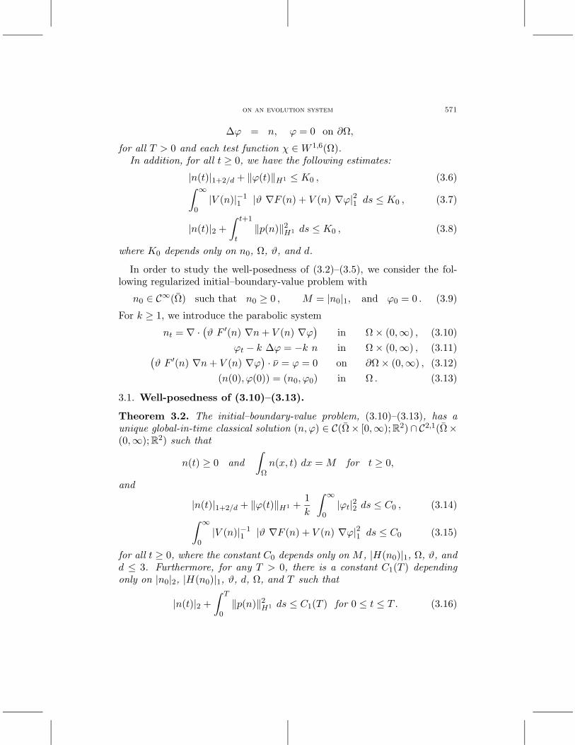
on an evolution system 571
∆ϕ = n, ϕ = 0 on ∂Ω,
for all T > 0 and each test function χ ∈ W 1,6(Ω).In addition, for all t ≥ 0, we have the following estimates:
|n(t)|1+2/d + ‖ϕ(t)‖H1 ≤ K0 , (3.6)∫ ∞
0|V (n)|−1
1 |ϑ ∇F (n) + V (n) ∇ϕ|21 ds ≤ K0 , (3.7)
|n(t)|2 +∫ t+1
t‖p(n)‖2
H1 ds ≤ K0 , (3.8)
where K0 depends only on n0, Ω, ϑ, and d.
In order to study the well-posedness of (3.2)–(3.5), we consider the fol-lowing regularized initial–boundary-value problem with
n0 ∈ C∞(Ω) such that n0 ≥ 0 , M = |n0|1, and ϕ0 = 0 . (3.9)
For k ≥ 1, we introduce the parabolic system
nt = ∇ ·(ϑ F ′(n) ∇n + V (n) ∇ϕ
)in Ω × (0,∞) , (3.10)
ϕt − k ∆ϕ = −k n in Ω × (0,∞) , (3.11)(ϑ F ′(n) ∇n + V (n) ∇ϕ
)· ν = ϕ = 0 on ∂Ω × (0,∞) , (3.12)
(n(0), ϕ(0)) = (n0, ϕ0) in Ω . (3.13)
3.1. Well-posedness of (3.10)–(3.13).
Theorem 3.2. The initial–boundary-value problem, (3.10)–(3.13), has aunique global-in-time classical solution (n, ϕ) ∈ C(Ω× [0,∞); R2)∩ C2,1(Ω×(0,∞); R2) such that
n(t) ≥ 0 and∫
Ωn(x, t) dx = M for t ≥ 0,
and
|n(t)|1+2/d + ‖ϕ(t)‖H1 +1k
∫ ∞
0|ϕt|22 ds ≤ C0 , (3.14)∫ ∞
0|V (n)|−1
1 |ϑ ∇F (n) + V (n) ∇ϕ|21 ds ≤ C0 (3.15)
for all t ≥ 0, where the constant C0 depends only on M , |H(n0)|1, Ω, ϑ, andd ≤ 3. Furthermore, for any T > 0, there is a constant C1(T ) dependingonly on |n0|2, |H(n0)|1, ϑ, d, Ω, and T such that
|n(t)|2 +∫ T
0‖p(n)‖2
H1 ds ≤ C1(T ) for 0 ≤ t ≤ T . (3.16)
572 Piotr Biler, Philippe Laurencot, and Tadeusz Nadzieja
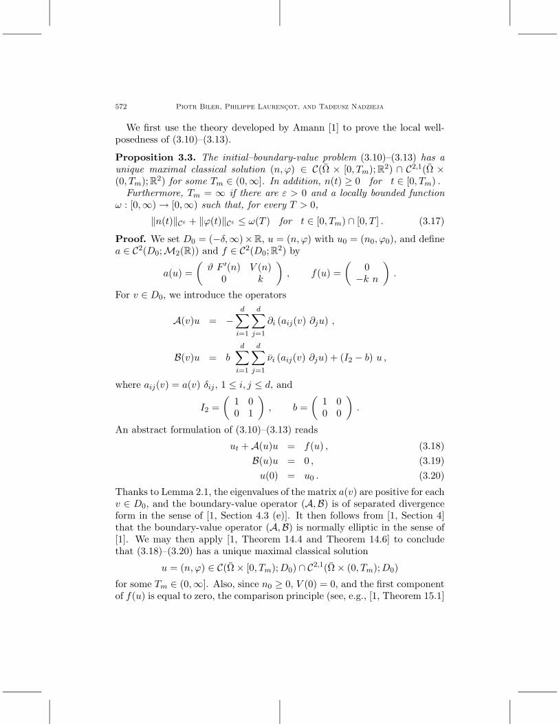
We first use the theory developed by Amann [1] to prove the local well-posedness of (3.10)–(3.13).
Proposition 3.3. The initial–boundary-value problem (3.10)–(3.13) has aunique maximal classical solution (n, ϕ) ∈ C(Ω × [0, Tm); R2) ∩ C2,1(Ω ×(0, Tm); R2) for some Tm ∈ (0,∞]. In addition, n(t) ≥ 0 for t ∈ [0, Tm) .
Furthermore, Tm = ∞ if there are ε > 0 and a locally bounded functionω : [0,∞) → [0,∞) such that, for every T > 0,
‖n(t)‖Cε + ‖ϕ(t)‖Cε ≤ ω(T ) for t ∈ [0, Tm) ∩ [0, T ] . (3.17)
Proof. We set D0 = (−δ,∞)×R, u = (n, ϕ) with u0 = (n0, ϕ0), and definea ∈ C2(D0;M2(R)) and f ∈ C2(D0; R2) by
a(u) =(
ϑ F ′(n) V (n)0 k
), f(u) =
(0
−k n
).
For v ∈ D0, we introduce the operators
A(v)u = −d∑
i=1
d∑j=1
∂i (aij(v) ∂ju) ,
B(v)u = b
d∑i=1
d∑j=1
νi (aij(v) ∂ju) + (I2 − b) u ,
where aij(v) = a(v) δij , 1 ≤ i, j ≤ d, and
I2 =(
1 00 1
), b =
(1 00 0
).
An abstract formulation of (3.10)–(3.13) reads
ut + A(u)u = f(u) , (3.18)B(u)u = 0 , (3.19)
u(0) = u0 . (3.20)
Thanks to Lemma 2.1, the eigenvalues of the matrix a(v) are positive for eachv ∈ D0, and the boundary-value operator (A,B) is of separated divergenceform in the sense of [1, Section 4.3 (e)]. It then follows from [1, Section 4]that the boundary-value operator (A,B) is normally elliptic in the sense of[1]. We may then apply [1, Theorem 14.4 and Theorem 14.6] to concludethat (3.18)–(3.20) has a unique maximal classical solution
u = (n, ϕ) ∈ C(Ω × [0, Tm); D0) ∩ C2,1(Ω × (0, Tm); D0)
for some Tm ∈ (0,∞]. Also, since n0 ≥ 0, V (0) = 0, and the first componentof f(u) is equal to zero, the comparison principle (see, e.g., [1, Theorem 15.1]
on an evolution system 573
or [17, Corollary I.2.1]) implies that n(t) ≥ 0 for t ∈ [0, Tm). Furthermore,since f does not depend on ∇u and n ≥ 0, Theorem 15.3 in [1] ensures thatTm = ∞ if there are ε > 0 and a locally bounded function ω : [0,∞) → [0,∞)such that (3.17) holds true for every T > 0.
We now proceed to show that (3.17) is satisfied. We define the functionalW by
W =∫
Ω
(ϑ H(n) + n ϕ +
12|∇ϕ|2
)dx
which will play the role of a Lyapunov functional for the regularized problem.
Lemma 3.4. We have
|n(t)|1 = M for t ∈ [0, Tm) , (3.21)
and there is a constant C1 depending only on M , ϑ, and |H(n0)|1 such that
|n(t)|1+2/d + ‖ϕ(t)‖H1 +1k
∫ t
0
∫Ω|ϕt|2 dx ds ≤ C1 , (3.22)∫ t
0|V (n)|−1
1 |ϑ ∇F (n) + V (n) ∇ϕ|21 ds ≤ C1 , (3.23)
for t ∈ [0, Tm). In addition, t −→ W(t) is a nonincreasing function on[0, Tm).
Proof. It first readily follows from (3.10) and (3.12) by integration overΩ × (0, t) that ∫
Ωn(x, t) dx =
∫Ω
n0(x) dx
for t ∈ [0, Tm), whence (3.21) since n is nonnegative.We next consider δ ∈ (0, 1) and put
hδ(z) = h(max z, δ) , Hδ(z) =∫ z
1hδ(y) dy
for z ≥ 0. Using the monotonicity of h, we realize that
supz≥0
|Hδ(z) − H(z)| ≤ δ h(δ) − H(δ)−→δ→0
0 , (3.24)
since h(δ) ∼ log δ as δ → 0 and H(0) = 0.We infer from (3.10), (3.11), and (3.12) that∫Ω(ϑhδ(n) + ϕ)nt dx = −
∫Ω
(ϑ∇hδ(n) + ∇ϕ) · (ϑ∇F (n) + V (n)∇ϕ) dx
= −ϑ
∫n≥δ
∇h(n) · (ϑ ∇F (n) + V (n) ∇ϕ) dx

574 Piotr Biler, Philippe Laurencot, and Tadeusz Nadzieja
−∫n≥δ
∇ϕ · (ϑ ∇F (n) + V (n) ∇ϕ) dx
−∫n<δ
∇ϕ · (ϑ ∇F (n) + V (n) ∇ϕ) dx
= −∫n≥δ
V (n) |∇ (ϑ h(n) + ϕ)|2 dx
−∫n<δ
∇ϕ · (ϑ ∇F (n) + V (n) ∇ϕ) dx ,
where we have used the identity
ϑ F ′(n) ∇n + V (n) ∇ϕ = V (n) ∇ (ϑ h(n) + ϕ)
to obtain the last equality. Since∫Ω
hδ(n) nt dx =d
dt
∫Ω
Hδ(n) dx ,
and ∫Ω
ϕ nt dx =d
dt
∫Ω
n ϕ dx −∫
Ωn ϕt dx
=d
dt
∫Ω
(n ϕ +
12|∇ϕ|2
)dx +
1k
∫Ω|ϕt|2 dx
by (3.11), we end up withdWδ
dt+
1k|ϕt|22 +
∫n≥δ
V (n) |∇ (ϑ h(n) + ϕ)|2 dx
= −∫n<δ
∇ϕ · (ϑ ∇F (n) + V (n) ∇ϕ) dx ,
whereWδ =
∫Ω
(ϑ Hδ(n) + nϕ +
12|∇ϕ|2
)dx .
Next it follows from the Holder inequality that∫n≥δ
|ϑ ∇F (n) + V (n) ∇ϕ| dx
≤ |V (n)|1/21
( ∫n≥δ
|ϑ ∇F (n) + V (n) ∇ϕ|2V (n)
)1/2,
whence ( ∫n≥δ
|ϑ ∇F (n) + V (n) ∇ϕ| dx)2
|V (n)|−11
on an evolution system 575
≤∫n≥δ
V (n) |∇ (ϑ h(n) + ϕ)|2 dx .
Consequently,
dWδ
dt+
1k|ϕt|22 +
( ∫n≥δ
|ϑ ∇F (n) + V (n) ∇ϕ| dx)2
|V (n)|−11
≤ −∫n<δ
∇ϕ · (ϑ ∇F (n) + V (n) ∇ϕ) dx .
Consider now t1 ∈ [0, Tm) and t2 ∈ (t1, Tm). Integrating the above inequalityover (t1, t2) yields
Wδ(t2) +1k
∫ t2
t1
|ϕt|22 ds
+∫ t2
t1
( ∫n≥δ
|ϑ ∇F (n) + V (n) ∇ϕ| dx)2
|V (n)|−11 ds
≤ Wδ(t1) −∫ t2
t1
∫n<δ
∇ϕ · (ϑ ∇F (n) + V (n) ∇ϕ) dx ds . (3.25)
On the one hand, it readily follows from (3.24) that
limδ→0
Wδ(ti) = W(ti) for i = 1, 2 .
On the other hand, since V (0) = 0, 1n≥δ → 1n>0, and 1n<δ → 1n=0as δ → 0, the regularity of (n, ϕ) and the Lebesgue dominated convergencetheorem ensure that
limδ→0
∫ t2
t1
∫n<δ
∇ϕ · (ϑ ∇F (n) + V (n) ∇ϕ) dx ds
=∫ t2
t1
∫n=0
∇ϕ · (ϑ ∇F (n) + V (n) ∇ϕ) dx ds = 0 ,
and
limδ→0
∫ t2
t1
( ∫n≥δ
|ϑ ∇F (n) + V (n) ∇ϕ| dx)2
|V (n)|−11 ds
=∫ t2
t1
( ∫n>0
|ϑ ∇F (n) + V (n) ∇ϕ| dx)2
|V (n)|−11 ds
=∫ t2
t1
( ∫Ω|ϑ ∇F (n) + V (n) ∇ϕ| dx
)2|V (n)|−1
1 ds .

576 Piotr Biler, Philippe Laurencot, and Tadeusz Nadzieja
We may then let δ → 0 in (3.25) and conclude that
W(t2) +1k
∫ t2
t1
|ϕt|22ds +∫ t2
t1
|ϑ∇F (n) + V (n)∇ϕ|21 |V (n)|−11 ds ≤ W(t1).
(3.26)The monotonicity of W and the bounds (3.22) and (3.23) are then straight-forward consequences of (3.26) by the Poincare inequality and Lemma 3.5below. Lemma 3.5. There are positive constants CW and DW depending on d ≤ 3,Ω, ϑ, and M such that
W ≥ CW(|n|1+2/d1+2/d + |∇ϕ|22) − DW . (3.27)
Proof. Let ε ∈ (0, 1). It follows from the continuous imbedding of H1(Ω)in L6(Ω) and the Holder inequality that∣∣∣ ∫
Ωn ϕ dx
∣∣∣ ≤ |n|6/5 |ϕ|6 ≤ C |n|(10−d)/121 |n|(d+2)/12
1+2/d |∇ϕ|2 .
We next infer from (3.21) and the Young inequality that∣∣∣ ∫Ω
n ϕ dx∣∣∣ ≤ 1
4|∇ϕ|22 + C |n|(d+2)/6
1+2/d ≤ 14|∇ϕ|22 + ε |n|1+2/d
1+2/d + C(ε) .
Now, by (2.12) and (2.18), there is a constant C > 0 such that h′(z) ≥C z2/d−1 for z ≥ 0, from which we deduce that
H(z) ≥ CH z1+2/d − C ′H , z ≥ 0 , (3.28)
for some CH > 0 and C ′H > 0. It then follows from (3.28) and the previous
inequality with ε = ϑCH/2 that
W ≥ ϑ CH |n|1+2/d1+2/d − C − 1
4|∇ϕ|22 − ϑ
CH
2|n|1+2/d
1+2/d − C +12|∇ϕ|22 ,
whence (3.27). Thanks to (3.22), we may improve the regularity of ∇ϕ.
Lemma 3.6. Let q ∈ (1,∞) and T > 0. There is a constant C(q, T )depending only on q and T such that∫ t
0|∇ϕ(s)|q15/4 ds ≤ C(q, T ) for t ∈ [0, Tm) ∩ [0, T ] .
Proof. For τ ∈ [0, kTm) and x ∈ Ω, we put ϕ(x, τ) = ϕ(x, τ/k) andn(x, τ) = n(x, τ/k). Owing to (3.11) and (3.12), ϕ is a solution to
(ϕ)τ − ∆ϕ = −n in Ω × (0, kTm) ,
on an evolution system 577
with the homogeneous Dirichlet boundary conditions and ϕ(0) = 0. Wethen infer from [18, Corollaire 1.1] that there is a constant C(q) dependingonly on q such that
| (ϕ)τ |Lq(0,kt;L1+2/d(Ω)) + |∆ϕ|Lq(0,kt;L1+2/d(Ω)) ≤ C(q) |n|Lq(0,kt;L1+2/d(Ω))
for each t ∈ (0, Tm). In terms of ϕ and n, the above estimate reads
1k|ϕt|Lq(0,t;L1+2/d(Ω)) + |∆ϕ|Lq(0,t;L1+2/d(Ω)) ≤ C(q) |n|Lq(0,t;L1+2/d(Ω)) .
Now, if t ∈ [0, Tm) ∩ [0, T ], it follows from (3.22) and the above inequalitythat ∫ t
0‖ϕ(s)‖q
W 2,1+2/d ds ≤ C(q, T ) .
Then we use the continuity of the imbedding of W 2,1+2/d(Ω) in W 1,15/4(Ω)to complete the proof of Lemma 3.6.
Owing to Lemma 3.6, an L2 estimate is available for n.
Lemma 3.7. Let T > 0. There is a constant C2(T ) depending only on |n0|2,|H(n0)|1, ϑ, and T such that
|n(t)|2 +∫ t
0‖p(n(s))‖2
H1 ds ≤ C2(T ) (3.29)
for t ∈ [0, Tm) ∩ [0, T ].
Proof. Let t ∈ [0, Tm)∩ [0, T ]. We multiply (3.10) by 2n and integrate overΩ to obtain
d
dt|n|22 + 2ϑ
∫Ω
F ′(n) |∇n|2 dx = −2∫
ΩV (n) ∇n · ∇ϕ dx .
Since V (n) = n (F ′(n))1/2, we have
2∣∣∣ ∫
ΩV (n) ∇n · ∇ϕ dx
∣∣∣ ≤ ϑ
∫Ω
F ′(n) |∇n|2 dx +1ϑ
∫Ω
n2 |∇ϕ|2 dx
by the Young inequality, whence
d
dt|n|22 + ϑ
∫Ω
F ′(n) |∇n|2 dx ≤ 1ϑ
∫Ω
n2 |∇ϕ|2 dx . (3.30)
It follows from the Holder inequality that∫Ω
n2 |∇ϕ|2 dx ≤ |n|230/7 |∇ϕ|215/4 ≤∣∣∣n1+2/d
∣∣∣2d/(d+2)
30d/7(d+2)|∇ϕ|215/4 .
578 Piotr Biler, Philippe Laurencot, and Tadeusz Nadzieja
Since p(z) ∼ C z as z → 0, we infer from (2.17) that there is a positiveconstant Cp such that p(z) ≥ Cp z1+2/d for all z ≥ 0. Consequently,∫
Ωn2 |∇ϕ|2 dx ≤ C |p(n)|2d/(d+2)
30d/7(d+2) |∇ϕ|215/4 ≤ C ‖p(n)‖2d/(d+2)H1 |∇ϕ|215/4 ,
where the last inequality follows from the continuous imbedding of H1(Ω)in L30d/7(d+2)(Ω). We next use the Young inequality to conclude that∫
Ωn2 |∇ϕ|2 dx ≤ ε ‖p(n)‖2
H1 + C(ε) |∇ϕ|d+215/4 (3.31)
for each ε ∈ (0, 1).Since p′(n) = ϑ (F ′(n))1/2, it follows from (3.30), (3.31) (with ε =
1/(2ϑ2)), and the Poincare inequality that
d
dt|n|22 +
12ϑ2
∫Ω|∇p(n)|2 dx ≤ C
(|p(n)|2L1 + |∇ϕ|d+2
15/4
).
Now, p(n) ≤ C (1 + n1+2/d) by (2.17) and (3.22) yields
d
dt|n|22 +
12ϑ2
|∇p(n)|22 ≤ C(1 + |∇ϕ|d+2
15/4
). (3.32)
Now, (3.29) readily follows from (3.32) after integration with respect totime, thanks to (3.22), Lemma 3.6 (with q = d + 2), and the Poincareinequality. Remark. Observe that, up to now, the estimates obtained on n and ϕ donot depend on k ≥ 1.
We are now in a position to complete the proof of Theorem 3.2.Proof of Theorem 3.2. We consider only d = 3, the cases d = 1 and d = 2being handled in a similar way. Let T > 0 and t ∈ [0, Tm)∩ [0, T ]. We claimthat there is a positive constant C4(T ) depending only on n0 and T suchthat
|V (n)|L14/5(Ω×(0,t)) + |∇V (n)|L2(Ω×(0,t)) ≤ C4(T ) . (3.33)
Indeed, we infer from (2.15), (2.17), and Lemma 2.1 that V (z) ≤ C (1+z5/3)and V ′(z) ≤ Cp′(z) for z ≥ 0. Consequently, it follows from (3.29) that
sups∈[0,t]
|V (n(s))|6/5 +∫ t
0‖V (n(s))‖2
H1 ds ≤ C(T ).
We next use the continuity of the imbedding of H1(Ω) in L6(Ω) and aninterpolation argument to deduce (3.33).

on an evolution system 579
We now employ a bootstrap argument to show that (3.17) holds true. Itfollows from (3.29), (2.17), and the continuity of the imbedding of H1(Ω) inL6(Ω) that
|n|L10/3(0,t;L10(Ω)) ≤ |p(n)|3/5L2(0,t;L6(Ω))
≤ C(T ) ,
which, together with (3.29), leads to∫ t
0|n(s)|14/3
14/3 ds ≤∫ t
0|n(s)|10/3
10 |n(s)|4/32 ds ≤ C(T ) .
Therefore,|n|L14/3(Ω×(0,t)) ≤ C(T ) ,
and we infer from (3.11) and [17, Theorem IV.9.1 and Lemma II.3.3] that
|∇ϕ|L70(Ω×(0,t)) + |∆ϕ|L14/3(Ω×(0,t)) ≤ C(k, T ) .
This estimate and (3.33) ensure that
|∇V (n) · ∇ϕ|L35/18(Ω×(0,t)) + |V (n) ∆ϕ|L2(Ω×(0,t)) ≤ C(k, T ) .
Sincent − ϑ∆F (n) = ∇V (n) · ∇ϕ + V (n) ∆ϕ ,
we use once more [17, Theorem IV.9.1] to obtain that
‖n‖W 2,1
38/15(Ω×(0,t))
≤ C(k, T ) ,
which, in turn, implies that
‖n‖Cε([0,t]) ≤ C(k, T )
for ε ∈ (0, 1/38) by [17, Lemma II.3.3]. A similar estimate is then availablefor ϕ, from which we conclude that (3.17) holds true and complete the proofof Theorem 3.2.
3.2. Proof of Theorem 3.1. We consider n0 ∈ L2(Ω) such n0 ≥ 0 al-most everywhere in Ω and put M = |n0|1. Let (n0,k)k≥1 be a sequence ofnonnegative functions in C∞(Ω) such that
|n0,k|1 = M and limk→∞
|n0,k − n0|2 = 0 . (3.34)
For k ≥ 1, we denote by (nk, ϕk) the unique classical solution to (3.10)–(3.13) with initial datum (n0,k, 0) given by Theorem 3.2. Fix T > 0. Owingto (3.14), (3.16), and (3.34), there is a constant C5(T ) such that
|nk(t)|2 + ‖ϕk(t)‖H1 +1k
∫ T
0|(ϕk)t|22 ds

580 Piotr Biler, Philippe Laurencot, and Tadeusz Nadzieja
+∫ T
0‖p(nk(s))‖2
H1 ds ≤ C5(T ) (3.35)
for t ∈ [0, T ]. Observe that (3.35), (2.17), (2.15), (2.16), and Lemma 2.1imply that
|∇F (nk)|6/5 ≤ C |n2/3k ∇p(nk)|6/5 ≤ C |∇p(nk)|2 ,
|V (nk) ∇ϕ|3/2 ≤ C |p(nk) ∇ϕk|3/2 ≤ C |p(nk)|6 ,
whence, thanks to the continuity of the imbedding of H1(Ω) in L6(Ω),∫ T
0
(|∇F (nk)|26/5 + |V (nk) ∇ϕk|23/2
)ds ≤ C(T ) . (3.36)
We then deduce from (3.10) and (3.36) that
|(nk)t|L2(0,T ;W 1,6/5(Ω)′) ≤ C(T ) . (3.37)
Consequently, owing to (3.37) and Lemma 2.1, the sequence (nk) is boundedin L2(0, T ; H1(Ω)) and in H1(0, T ; W 1,6/5(Ω)′).
Owing to the compactness of the imbedding of H1(Ω) in L2(Ω) and tothe continuity of the imbedding of L2(Ω) in W 1,6/5(Ω)′, we infer from [20,Corollary 4] that (nk) is relatively compact in L2(Ω × (0, T )). Therefore,there are n ∈ L2(Ω× (0, T )) and a subsequence of (nk) (not relabeled) suchthat
nk −→ n in L2(Ω×(0, T ))∩C([0, T ];W 1,6/5(Ω)′) and a.e. in Ω×(0, T ) .(3.38)
Let ϕ ∈ L∞(0, T ; H2(Ω)) be the solution to
∆ϕ = n in Ω × (0, T ) , ϕ = 0 on ∂Ω × (0, T ) . (3.39)
It follows from (3.11) and (3.39) that ϕk − ϕ is a solution of the Poissonequation
−∆(ϕk − ϕ) = n − nk − 1k
(ϕk)t
with the homogeneous Dirichlet boundary conditions, and the right-handside of the above equation converges to zero in L2(Ω × (0, T )) as k → ∞ by(3.35) and (3.38). Therefore,
ϕk −→ ϕ in L2(0, T ; H2(Ω)) . (3.40)
Combining (3.35) with the convergence results (3.38) and (3.40) finally allowus to conclude that (∇F (nk)) and (V (nk) ∇ϕk) converge weakly to ∇F (n)and V (n) ∇ϕ in L6/5(Ω×(0, T )) and L3/2(Ω×(0, T )), respectively. It is nowstraightforward to pass to the limit as k → ∞ in (3.10)–(3.13) and concludethat (n, ϕ) is a weak solution to (3.2)–(3.4) in the sense of Theorem 3.1.
on an evolution system 581
We may also pass to the limit in (3.14) and (3.15) and use classical lower-semicontinuity arguments to deduce that (3.6) and (3.7) hold true.
Next, since inf p′ > 0 by (2.17) and Lemma 2.1, it follows from (3.21),(3.32), and the Poincare inequality that
d
dt|nk|22 + γ
(|nk|22 + ‖p(nk)‖2
H1
)≤ C
(1 + |∇ϕk|d+2
15/4
)for some positive constant γ. After integration with respect to time, weobtain
|nk(t)|22 ≤ |n0,k|22 e−γt + C
∫ t
0
(1 + |∇ϕk|d+2
15/4
)eγ(s−t) ds (3.41)
for t ≥ 0, and∫ t+1
t‖p(nk(s))‖2
H1 ds ≤∫ t
t−1
∫ τ+2
τ‖p(nk(s))‖2
H1 ds dτ
≤ C(1 +
∫ t
t−1|nk(τ)|22 dτ +
∫ t+2
t−1|∇ϕk(s)|d+2
15/4 ds)
(3.42)
for t ≥ 1. Now, |∇ϕk|15/4 is bounded in Lq(0, t) for any q ∈ (1,∞) byLemma 3.6, and we infer from (3.40) and the continuous imbedding of H2(Ω)in W 1,15/4(Ω) that (|∇ϕk − ∇ϕ|15/4) converges to zero in L2(0, t). Conse-quently, (|∇ϕk − ∇ϕ|15/4) converges to zero in Ld+2(0, t). We then maypass to the limit as k → ∞ in (3.41) and (3.42) with the help of (3.38) andweak-convergence arguments for the left-hand sides and conclude that
|n(t)|22 ≤ |n0|22 e−γt + C
∫ t
0
(1 + |∇ϕ|d+2
15/4
)eγ(s−t) ds
for t ≥ 0 and∫ t+1
t‖p(n)‖2
H1 ds ≤ C(1 +
∫ t
t−1|n(s)|22 ds +
∫ t+2
t−1|∇ϕ(s)|d+2
15/4 ds)
for t ≥ 1. Since ϕ is a solution to the Poisson equation (1.8), we have
|∇ϕ(s)|15/4 ≤ C ‖ϕ(s)‖W 2,1+2/d ≤ C |n(s)|1+2/d ≤ C
by (3.6). Inserting this estimate in the previous two inequalities yields firstthe boundedness of |n|2 with respect to time, and then (3.8). Corollary 3.8. Let n0 ∈ L2(Ω) be a nonnegative function, and denoteby (n, ϕ) the corresponding solution of (3.2)–(3.5) given by Theorem 3.1.The trajectory (n(t), ϕ(t)) , t ≥ 0 is weakly relatively compact in the spaceL2(Ω)×H2(Ω), and the accumulation points are steady states, that is, solve(4.1), (4.2), and (1.10).
582 Piotr Biler, Philippe Laurencot, and Tadeusz Nadzieja
Proof. The entropy dissipation formula (3.7) (which is a weaker form of(4.7)), together with the a priori estimates in Theorem 3.1 suffice to provethe relative compactness, and then to identify the possible accumulationpoints as steady states.
4. The steady-state problem with fixed mass
The stationary solutions (N, Φ) of the problem (1.7)–(1.12) (or (1.7)–(1.10)) with arbitrary diffusion coefficient D and a constant ϑ, are charac-terized by the identity ∇ (ϑ log Λ − Φ) = 0. Here, the relation between Λand N is as was for λ and n in (1.5). This can be obtained formally fromthe equation (1.7) by taking the product with ϑ log Λ − Φ and integratingby parts, using of course the boundary conditions (1.9). Indeed, by (3.1)we get in such a way the identity
∫Ω ND |∇(ϑ log Λ − Φ)|2 dx = 0, and thus
log Λ = Φ/ϑ − c where c is an appropriate integration constant.Taking into account the relations (2.13), (1.5), and the Poisson equation
(1.8), we arrive at the relation
∆Φ =µ
2ϑd/2Id/2−1(e
Φ/ϑ−c), (4.1)
for the stationary potential Φ and the density N given by
N =µ
2ϑd/2Id/2−1(e
Φ/ϑ−c).
The constant c is so that the mass constraint∫Ω
∆Φ dx =∫
∂Ω
∂Φ∂ν
dσ = M (4.2)
is satisfied. The equation (4.1) will be called the Poisson–Fermi–Dirac equa-tion. It can be simplified a bit by introducing the new potential Ψ = −Φ/ϑ,leading to
∆Ψ +µ
2ϑd/2−1Id/2−1
(e−Ψ−c
)= 0 (4.3)
with the constant c satisfying the mass constraint∫∂Ω
∂Ψ∂ν
dσ = −M
ϑ. (4.4)
4.1. Solutions satisfying the Dirichlet condition (1.10). The problem(4.3)–(4.4) has the form
∆U + f(U + c) = 0,
∫∂Ω
∂U
∂ν= −K (4.5)
on an evolution system 583
with a given constant K and the homogeneous Dirichlet condition (1.10).An analysis of the problem (4.5) can be found in [25, (2.2)–(2.3)] (see also[2]), where the following results have been proved using variational methods.
Assume that(i) f is a continuous, nondecreasing function on R which is increasing
whenever f > 0, and lims→∞ f(s) = ∞,(ii) lims→∞ f(s)/sp∗ = 0, where p∗ = d/(d − 2) if d ≥ 3 or p∗ < ∞ is
arbitrary if d = 2.Then the problem (4.5) with (1.10) has at least one solution for every
0 < K < ∞.Moreover, if d ≥ 3 and(iii) lims→∞ f(s)/sp∗ = κ > 0,
then the problem (4.5), (1.10) is solvable for each 0 < K < K, with someK < ∞.Remark. In fact one has κ = 1 in [25], but a simple scaling leads to theformulation (4.5).
In our case the nonlinearity in (4.5) is
f(s) =µ
2ϑd/2−1Id/2−1
(e−s
)∼ |s|d/2 |s|d/(d−2) if d ≤ 3 .
Thus, we obtain the following existence result:
Proposition 4.1. For d = 1, 2, 3, given M > 0 there exists at least onesolution Φ of the Poisson–Fermi–Dirac equation (4.1) satisfying the Dirichletcondition (1.10) and (4.2).
For d = 4 such a solution exists for all sufficiently small M > 0.
The question of the existence of multiple solutions of the equation (4.1),and their stability as solutions of the evolution problem (1.7)–(1.11), is ratherdelicate. There are some numerical results in the case of radially symmetricsolutions in the ball of R3 in [10] and [11].Remark. For the existence of solutions of (4.3), (4.4) with Ψ satisfyingeither the free condition (1.12) or the Dirichlet condition (1.10) for smallM > 0 and each d ≥ 3, we refer the reader to [22]. These results are provedin the spirit of fixed-point theorems based on the compactness propertiesof the operator N → Ψ. Also, it is shown in [22] (by an application ofthe Pohozaev identity) that for d ≥ 5, the equation (4.3) with the boundarycondition (1.10) in a star-shaped domain has no solution for sufficiently largeM 1.
4.2. Solutions satisfying the free condition (1.12). An approach forthe existence of solutions satisfying the free condition is possible using the

584 Piotr Biler, Philippe Laurencot, and Tadeusz Nadzieja
(neg)entropy functional W defined by
W =∫
Ω
(ϑH(n) +
12nϕ
)dx. (4.6)
Note that for ϕ satisfying the Poisson equation (3.3) with the homogeneousDirichlet condition, the functional W coincides with the entropy W consid-ered in the preceding section. The entropy W satisfies, for all sufficientlyregular solutions of the evolution problem constructed in Theorem 3.1, therelation
dW
dt= −
∫Ω
nD |∇ (ϑh(n) + ϕ)|2 dx ≤ 0 . (4.7)
Moreover, W is bounded from below by a result similar to Lemma 3.5.
Lemma 4.2. If d = 1, 2, 3, then the entropy W controls from above theL1+2/d(Ω) norm of n. More precisely, for each 0 < c1 < d1+2/d
d+2 µ−2/d thereexists a constant c2 = c2(c1, Ω, M) such that
W ≥ c1|n|1+2/d1+2/d − c2.
If d = 4 such an estimate is valid only for small mass M = |n|1 since
W ≥(c3 − C(Ω)M1/2
)|n|3/2
3/2 − c4,
holds for some c3 > 0, c4 > 0, and C(Ω) > 0.
The proof follows from the idea used in Lemma 3.5, but now one has touse the Poisson equation (1.7) to estimate ϕ in terms of n. Remark. This result on the integrability n ∈ L1+2/d(Ω) under the finitenessassumption on W was first obtained by R. Robert in [19] for the radiallysymmetric functions n, ϕ, and λ defined in the unit ball of R3 by a clever,simple argument on the level of kinetic equations.
Minimizers of the entropy W are steady states. Thus we have
Proposition 4.3. For d ≤ 3 and given M > 0 there is a solution of thePoisson–Fermi–Dirac equation (4.1) satisfying the free condition (1.12) and(4.2). For d = 4 such a solution exists for all sufficiently small M > 0.
Proof. By Lemma 4.2, we can take a minimizing sequence nk ∈ L1+2/d(Ω)for W such that
W (nk) → infW (n) : 0 ≤ n ∈ L1+2/d(Ω),∫
Ωn dx = M > −∞.
on an evolution system 585
Again by Lemma 4.2, a subsequence, still denoted by nk, weakly convergesto an element n∞ ∈ L1+2/d(Ω). Now we arrive at∫
Ω(nkϕk − n∞ϕ∞) dx =
∫Ω
nk(ϕk − ϕ∞) dx +∫
Ω(nk − n∞)ϕ∞ dx → 0
since the sequence of the associated potentials (ϕk) converges in L1+d/2(Ω),thanks to the compactness of the imbedding of W 2,1+2/d(Ω) into L1+d/2(Ω)for d ≤ 4. The functional
∫Ω H(n) dx is convex by Lemma 2.1 and thus
weakly lower semicontinuous. Therefore
lim infk→∞
∫Ω
H(nk) dx ≥∫
ΩH(n∞) dx
holds and the minimum of W is attained at n∞. Acknowledgments. The preparation of this paper was partially sup-ported by the KBN grants 2/P03A/011/19, 2/P03A/002/24, the POLO-NIUM project EGIDE–KBN 2003–05643SE, and by the EU network HYKEunder the contract HPRN-CT-2002-00282. We acknowledge the hospital-ity of the Juliusz Schauder Center for Nonlinear Studies (Torun), where webegan some calculations related to this subject in November 2002. We aregrateful to Pierre-Henri Chavanis and Carole Rosier for interesting and en-lightening conversations. We thank Robert Stanczy and Gershon Wolanskyfor pertinent remarks.
References
[1] H. Amann, Nonhomogeneous linear and quasilinear elliptic and parabolic boundaryvalue problems, 9–126 in “Function Spaces, Differential Operators and NonlinearAnalysis,” H. Triebel, H.J. Schmeisser, eds., Teubner-Texte Math., 133, Teubner,Stuttgart, 1993.
[2] H. Berestycki and H. Brezis, On a free boundary problem arising in plasma physics,Nonlinear Anal., 4 (1980), 415–436.
[3] P. Biler, J. Dolbeault, M.J. Esteban, P.A. Markowich, and T. Nadzieja, Steady statesfor Streater’s energy-transport models of self-gravitating particles, 37–56 in “Transportin Transition Regimes,” N. Ben Abdallah et al., eds., IMA Volumes in Mathematicsand Its Applications, 135, Springer, New York, 2003.
[4] P. Biler, W. Hebisch, and T. Nadzieja, The Debye system: existence and long timebehaviour of solutions, Nonlinear Anal., 23 (1994), 1189–1209.
[5] P. Biler, D. Hilhorst, and T. Nadzieja, Existence and nonexistence of solutions fora model of gravitational interaction of particles, II, Colloq. Math., 67 (1994), 297–308.
[6] P. Biler, A. Krzywicki, and T. Nadzieja, Self-interaction of Brownian particles coupledwith thermodynamic processes, Rep. Math. Phys., 42 (1998), 359–372.
[7] P. Biler and T. Nadzieja, Existence and nonexistence of solutions for a model ofgravitational interaction of particles, I, Colloq. Math., 66 (1994), 319–334.
586 Piotr Biler, Philippe Laurencot, and Tadeusz Nadzieja
[8] P. Biler and T. Nadzieja, Structure of steady states for Streater’s energy-transportmodels of gravitating particles, Topol. Methods Nonlinear Anal., 19 (2002), 283–301.
[9] P. Biler and T. Nadzieja, Global and exploding solutions in a model of self-gravitatingsystems, Rep. Math. Phys., 52 (2003), 205–225.
[10] P.-H. Chavanis, Phase transitions in self-gravitating systems: self-gravitating fermionsand hard sphere models, Phys. Rev. E, 65 (2002), 056123.
[11] P.-H. Chavanis, M. Ribot, C. Rosier, and C. Sire, Collapses, explosions and hysteresisin self-gravitating systems: a thermodynamical approach, in preparation.
[12] P.-H. Chavanis, C. Rosier, and C. Sire, Thermodynamics of self-gravitating systems,Phys. Rev. E, 66 (2002), 036105.
[13] P.-H. Chavanis and J. Sommeria, Degenerate equilibrium states of collisionless stellarsystems, Mon. Not. R. Astron. Soc., 296 (1998), 569–578.
[14] P.-H. Chavanis, J. Sommeria, and R. Robert, Statistical mechanics of two-dimensionalvortices and collisionless stellar systems, Astrophys. J., 471 (1996), 385–399.
[15] P.-H. Chavanis and C. Sire, Anomalous diffusion and collapse of self-gravitatingLangevin particles in D dimensions, Phys. Rev. E 69 (2004), to appear.
[16] C.J. van Duijn, I.A. Guerra, and M.A. Peletier, Global existence conditions for anon-local problem arising in statistical mechanics, 1–21, to appear.
[17] O.A. Ladyzenskaja, V.A. Solonnikov, and N.N. Ural’ceva, “Linear and QuasilinearEquations of Parabolic Type,” Transl. Math. Monogr., 23, Amer. Math. Soc., Provi-dence, RI, 1968.
[18] D. Lamberton, Equations d’evolution lineaires associees a des semi-groupes de con-traction dans les espaces Lp, J. Funct. Anal., 72 (1987), 252–262.
[19] R. Robert, On the gravitational collapse of stellar systems, Classical Quantum Grav-ity, 15 (1998), 3827–3840.
[20] J. Simon, Compact sets in the space Lp(0, T ; B), Ann. Mat. Pura Appl., 146 (1987),65–96.
[21] C. Sire and P.-H. Chavanis, Thermodynamics and collapse of self-gravitating Brownianparticles in D dimensions, Phys. Rev. E, 66 (2002), 046133.
[22] R. Stanczy, Steady states for a system describing Fermi–Dirac particles, preprint.[23] R.F. Streater, A model of dense fluids, in “Quantum Probability” (Gdansk, 1997),
381–393, Banach Center Publications, 43, Polish Acad. Sci, Warsaw, 1998.[24] R.F. Streater, The Soret and Dufour effects in statistical dynamics, Proc. R. Soc.
London A, 456 (2000), 205–211.[25] G. Wolansky, Critical behaviour of semi-linear elliptic equations with sub-critical ex-
ponents, Nonlinear Anal., 26 (1996), 971–995.
Related Documents

![Gravitating compact Q-ball and Q-shell solutions in the CPN … · 2019. 1. 17. · arXiv:1812.08363v2 [hep-th] 16 Jan 2019 Gravitating compact Q-ball and Q-shell solutions in the](https://static.cupdf.com/doc/110x72/60becbb11237cf6a56585364/gravitating-compact-q-ball-and-q-shell-solutions-in-the-cpn-2019-1-17-arxiv181208363v2.jpg)


