On a Family of Circulant Matrices for Quasi-Cyclic Low-Density Generator Matrix Codes

1

On a Family of Circulant Matrices for

Quasi-Cyclic Low-Density Generator Matrix

CodesMarco Baldi,Member, IEEE,Federico Bambozzi, and Franco Chiaraluce,Member, IEEE

Abstract

We present a new class of sparse and easily invertible circulant matricesthat can have a sparse inverse though

not being permutation matrices. Their study is useful in the design of quasi-cyclic low-density generator matrix

codes, that are able to join the inner structure of quasi-cyclic codes with sparse generator matrices, so limiting

the number of elementary operations needed for encoding. Circulant matrices of the proposed class permit to hit

both targets without resorting to identity or permutation matrices that may penalize the code minimum distance

and often cause significant error floors.

Index Terms

Low-density generator matrix (LDGM) codes, low-density parity-check(LDPC) codes, quasi-cyclic (QC)

codes, sparse circulant matrices.

I. I NTRODUCTION

Low-Density Parity-Check (LDPC) codes are extremely efficient in regard to decoding algorithms, based on

the message passing principle, that exploit the sparse nature of their parity-check matrices to achieve excellent

performance with low complexity [1], [2].

On the other hand, the generator matrixG of an LDPC code is usually dense and, when it is used for

encoding, this gives a complexity that is quadratic in the block length. To reduce the encoding complexity,

several solutions have been proposed in the past. Among them, some techniques aim at exploiting the sparse

nature of the parity-check matrixH also in the encoding stage. This can be easily achieved whenH admits

a sparse representation in lower triangular form. When this does not occur, anApproximate Lower Triangular

(ALT) version ofH could be obtained by performing only row and column permutations [3]. Alternatively, the

ALT form of the parity-check matrix can be ensured by a properdesign [4].

Copyright (c) 2011 IEEE. Personal use of this material is permitted. However, permission to use this material for any other purposes

must be obtained from the IEEE by sending a request to [email protected].

The material in this paper was presented in part at the International Symposium on Information Theory and its Applications,Auckland,

New Zealand, December 2008, and at the IEEE Information TheoryWorkshop, Taormina, Italy, October 2009.

M. Baldi and F. Chiaraluce are with Dipartimento di Ingegneria Biomedica, Elettronica e Telecomunicazioni, Università Politecnica delle

Marche, Ancona, Italy (e-mail: {m.baldi; f.chiaraluce}@univpm.it). F. Bambozzi is with Dipartimento di Matematica Pura e Applicata,

Università degli Studi di Padova, Padova, Italy (e-mail: [email protected]).

2

A different technique for low complexity encoding of LDPC codes is represented by iterative encoding [5].

According to such an approach, the parity bits corresponding to each information vector are considered as

erasures, and recovered by means of the message passing decoder for channels with erasures. In order for

iterative encoding to be successful, the nodes associated to the parity bits must not contain a stopping set; so

the structure of the parity-check matrix must be constrained. For this reason, the design of iterative encodable

codes with good performance could represent a challenge [6].

One of the most effective approaches for reducing the encoding complexity is given by Low-Density Generator

Matrix (LDGM) codes [7]. For such codes,G is also sparse and this permits to reduce significantly the amount

of processing required at the encoder.

In [8], LDGM codes with a very sparse generator matrix were considered, and their performance estimated.

It was verified that an LDGM code with Tanner graph containingdegree-1 variable nodes exhibits high error

floors. In the same paper and in [9], it was demonstrated that these floors can be substantially reduced by

serially concatenating two (or more) of these codes, at the cost of an increased complexity. In the concatenated

scheme, the component codes could be selected in such a way toallow the usage of the same decoder structure

for both of them [10], but serial concatenation still has consequences on complexity and latency.

LDGM codes are a wide family of codes, including, for example, concatenated single parity-check codes

[11]. They also provide the core for Repeat Accumulate (RA) codes, that can be seen as the serial concatenation

of an outer LDGM code and an inner accumulator [12]. RA codes represent an alternative solution to the usage

of two serially concatenated LDGM codes for reducing the error floor. Variants of RA codes, as Irregular RA

(IRA) codes [13] and Accumulate-RA (ARA) codes [14], can improve performance of RA codes, and it has

been proved they can also be capacity-achieving codes [15].

Recently, an increasing interest has been devoted to Quasi-Cyclic Low-Density Parity-Check (QC-LDPC)

codes, whose parity-check and generator matrices are formed by circulant blocks. Such structure of the matrices

allows the usage of very simple encoding circuits, based on shift registers, that exploit the quasi-cyclic nature

of the codes [16]. A widespread family of QC-LDPC matrices are formed by circulant permutation blocks [17].

Codes having this form have also been included in the amendment for mobility of the IEEE 802.16 standard

[18]. Several encoding schemes are suggested in the standard; due to the almost lower triangular form of the

matrices, the solution in [3] has a nearly-linear complexity. The number of operations required can be further

reduced by suitable processing [19].

So, even for QC-LDPC codes, a common approach to exploit sparse matrices for encoding is to find parity-

check matrices having an almost lower triangular form [18],[20]. In fact, the quasi-cyclic property facilitates

the hardware implementation of the encoder, but complexity(in terms of number of elementary operations) still

depends on the density of the matrix used for encoding. However, to find almost lower triangular parity-check

matrices is not possible in several cases. Moreover, when the parity-check matrix of a QC-LDPC code is formed

by circulant blocks that are not permutation matrices, the corresponding generator matrix is usually dense. This

occurs when the row (column) weight of each non-null circulant block in the parity-check matrix is greater

than one, and can be found, for example, in the QC-LDPC codes proposed for near-Earth missions by the

Consultative Committee for Space Data Systems (CCSDS) [16], [21]. Another interesting family of QC-LDPC

codes having circulant blocks with row (column) weight greater than one are those based on Difference Families

3

and their variants [22], [23]. The structure of the parity-check matrix of these codes is as follows:

H = [H0|H1|...|HNb−1], (1)

i.e., it consists of a row ofNb sparse circulant blocks, each with sizen = N/Nb, whereN is the code length.

Provided that at least one of theHi blocks is of full rank, the code rate is(Nb − 1)/Nb. Despite their very

simple structure, codes having this form can be able to achieve good performance, especially for moderate/high

code rates.

For codes having a parity-check matrix in the form (1), a low-density generator matrix can be found if one

of the Hi blocks is replaced with ann × n identity matrix or cyclic permutation matrix. This way, however,

the minimum distance of the code is penalized, and becomes less than or equal to the lowest row (column)

weight of the non-identityHi blocks, increased by1.

In this paper, we define a new class of sparse circulant matrices, that we callψ-unitary (the reason for such

notation will be explained afterwards). These matrices aresimple to design, easily invertible and can have

a sparse inverse, though not being circulant permutation matrices. Furthermore, they can be free of length-4

cycles; so, we propose to use them for constructing the parity-check matrix in the form (1). By replacing one

of the Hi blocks with aψ-unitary matrix, the density of the code generator matrix can be rendered very low

while maintaining a good minimum distance.

The features of the new class of matrices are derived by extending the theory of orthogonal circulant matrices

([24], [25]), that are a special case of circulant matrices but that cannot be used for the design of QC-LDPC

codes. This is explained in Section II, which is devoted to remind basic definitions and properties. Theψ-

unitary circulant matrices are introduced in Section III, where conditions for the absence of length-4 cycles are

explicitly stated. Section IV presents some families of matrices that are free of length-4 cycles, while Section

V discusses the inversion issues. The inversion method we propose has complexity that depends mainly on the

matrix weight and is basically independent of the matrix size; moreover, availability of explicit expressions for

the inverse matrix permits us to estimate its density. In Section VI, examples of usage ofψ-unitary circulant

matrices in LDGM codes are given. Finally, Section VII concludes the paper.

II. C IRCULANT MATRICES: NOTATION AND PROPERTIES

The general structure of ann× n circulant matrixA defined over the Galois field of orderp, GF (p), is as

follows:

A =

a0 a1 a2 · · · an−1

an−1 a0 a1 · · · an−2

......

..... .

...

a1 a2 a3 · · · a0

, (2)

whereai ∈ GF (p), i = 0 . . . n− 1. Thus,A is described by one of its rows (typically the first one), the others

being obtained as cyclically shifted versions of such row. In the following, we will denote byW [A] the number

of non-zero symbols in each row (or column) ofA.

A simple isomorphism exists between the ringMn of n × n circulant matrices overGF (p) and the ring

Rn = GF (p)[x]/(xn − 1) of the polynomials overGF (p) modulo (xn − 1). Let us consider the following

4

n× n circulant permutation matrix:

T =

0 1 0 · · · 0

0 0 1 · · · 0...

......

. .....

0 0 0 · · · 1

1 0 0 · · · 0

. (3)

It it easy to verify that the circulant matrix (2) can be written as:

A =

n−1∑

i=0

aiTi, (4)

whereT0 = Tn = I. This relationship is the basis to establish the isomorphism, defined by the following map:

φ :

n−1∑

i=0

aiTi →

n−1∑

i=0

aixi = a(x), (5)

that transforms matrices into polynomials modulo(xn−1). The minimal polynomial ofT is Tn−I. According

to this isomorphism, we can work, when more convenient, withpolynomials instead of matrices. So, from now

on, a matrixA will be equivalently denoted by the polynomiala(x); W [a] is the weight ofa(x) (number of

its non-zero coefficients) and it coincides withW [A]. According to (5), the polynomiala(x) is specified by

its coefficients(a0, a1, ..., an−1).

A length-4 cycle in matrixA is a closed rectangular path linking non-zero elements. Explicitly, this means that

a length-4 cycle exists when two rows have a pair of non-zero symbols at the same positions (i.e., belonging to

the same columns). Obviously, each matrix can have manifoldloops of this kind, depending on the distribution

of the non-zero symbols. It is easy to verify that length-4 cycles in matrixA do not appear if and only if

the distances between any pair of non-zero symbols in each row of the matrix are different from each other

(explicitly, we say that the matrix has no repeated distances). So, ifδi,k represents the distance (modn) between

the i-th andk-th non-zero elements, it must beδi,k = δj,l if and only if i = j andk = l.

Orthogonal circulant matrices are a special case of circulant matrices, for whichA ·AT = I. So, the inverse

of an orthogonal matrix coincides with its transpose. The following theorem holds:

Theorem II.1 An orthogonal circulant matrixA overGF (p), with W [A] > 1, has always length-4 cycles.

Proof: Let us suppose that matrix (2) is orthogonal; then, the innerproduct between itsi-th andj-th rows

must be 0, fori 6= j. Without loss of generality, let us consideri = 0; the following condition must be satisfied:

a0an−j + a1an−j+1 + ...+ avam + ...+ an−1an−j−1 = 0,

where all subscripts are modn. If a column ofA has at least two non-zero elements (which means it is not a

permutation matrix, the latter being a particular case, notof interest for the present analysis), sayav andam,

with m = (v− j) modn, thenavam 6= 0. Condition above implies there exists at least another termaway 6= 0,

with aw belonging to the same row ofav, anday to the same row ofam, andy = (w− j) modn. Therefore,

av, am, aw anday define a length-4 cycle, sincev −m = w − y = j mod n.

Because of Theorem II.1, orthogonal circulant matrices with weight greater than 1 are not suitable for the

design of QC-LDPC codes. However, starting from the theory developed in previous literature (see [24] and

5

[25]) for the study and characterization of orthogonal circulant matrices, it is possible to define a new class of

matrices that, instead, can be free of length-4 cycles. This is done in the following section.

III. ψ-UNITARY CIRCULANT MATRICES

A. Definition and properties

Let us considern = ps, with s an integer, and the ringRs = GF (p)[y]/(ys−1). Let us define the following

map from the ringRn to the ringRs:

ψpss :n−1∑

i=0

aixi →

s−1∑

k=0

ukyk, (6)

where

uk =

p−1∑

t=0

ak+st, ∀k ∈ {0, 1, . . . , s− 1} . (7)

The map transforms elements ofRn into elements ofRs, according to the specified rule.

Example 1

Let us considerψ42 : R4 → R2 overGF (2). The elements ofR4 are:

(0, 0, 0, 0), (0, 0, 0, 1), (0, 0, 1, 0), (0, 0, 1, 1),

(0, 1, 0, 0), (0, 1, 0, 1), (0, 1, 1, 0), (0, 1, 1, 1),

(1, 0, 0, 0), (1, 0, 0, 1), (1, 0, 1, 0), (1, 0, 1, 1),

(1, 1, 0, 0), (1, 1, 0, 1), (1, 1, 1, 0), (1, 1, 1, 1).

So:

ψ42((0, 0, 0, 0)) = ψ4

2((0, 1, 0, 1)) = ψ42((1, 0, 1, 0)) =

= ψ42((1, 1, 1, 1)) = (0, 0),

ψ42((1, 0, 0, 0)) = ψ4

2((0, 0, 1, 0)) = ψ42((1, 1, 0, 1)) =

= ψ42((0, 1, 1, 1)) = (1, 0),

ψ42((0, 1, 0, 0)) = ψ4

2((0, 0, 0, 1)) = ψ42((1, 1, 1, 0)) =

= ψ42((1, 0, 1, 1)) = (0, 1),

ψ42((1, 1, 0, 0)) = ψ4

2((0, 1, 1, 0)) = ψ42((1, 0, 0, 1)) =

= ψ42((0, 0, 1, 1)) = (1, 1).

The same elements can also be written in polynomial form:

ψ42(0) = ψ4

2(x+ x3) = ψ42(1 + x2) = ψ4

2(1 + x+ x2 + x3) = 0,

ψ42(1) = ψ4

2(x2) = ψ4

2(1 + x+ x3) = ψ42(x+ x2 + x3) = 1,

ψ42(x) = ψ4

2(x3) = ψ4

2(1 + x+ x2) = ψ42(1 + x2 + x3) = x,

ψ42(1 + x) = ψ4

2(x+ x2) = ψ42(1 + x3) = ψ4

2(x2 + x3) = 1 + x.

�

It is known [24] thatψpss is an homomorphism, with kernelKer(ψpss ) = Ipss , whereIpss = 〈xs − 1〉 ∈ Rn

denotes the ideal generated by(xs − 1). Ipss is completely described by the following formula:

a(x) =n−1∑

i=0

aixi ∈ Ipss ⇔

p−1∑

t=0

ak+ts = 0, (8)

6

for all k ∈ {0, 1, . . . , s− 1}.

Generalizing (6), we can considern = pqs and the mapψpqsprs : Rpqs → Rprs, with 0 ≤ r ≤ q and

Ker(ψpqsprs) = Ip

qsprs =

⟨

xprs − 1

⟩

(if r = q, ψpqspqs is the identity map). From a computational point of view, the

mapψpqsprs corresponds to iterating (q− r) times the elementary mapping fromRpts to Rpt−1s, with q ≥ t > r.

Noting byψ(c(x)) the result of the single mapping, applied to the polynomialc(x), we should write:

ψpqsprs(a(x)) = ψp

r+1sprs (ψp

r+2s

pr+1s(...ψp

qs

pq−1s(a(x))...)).

Let us denote by1prs the identity element ofRprs. The following definition holds:

Definition: A circulant matrix inMpqs is a ψ-unitary circulant matrix if its polynomiala(x) ∈ Rpqs, for

somer ≤ q, satisfies the condition:

ψpqsprs(a(x)) = 1prs. (9)

ψ-unitary matrices, so defined, form a subset of the matrices in Mpqs, that in the following will be denoted

by Ψpqsprs. It is evident that, if a matrixA ∈ Ψp

qsprs for a givenr, then it satisfies the conditionψp

qs

pts(a(x)) = 1pts

for any 0 ≤ t < r.

Example 2

Let us considerp = 2, r = 0, q = 1 ands = 4 (hence,n = 2s = 8). The following polynomials with weight 3 satisfy the

conditionψ84 = 14 = (1, 0, 0, 0); so, they defineψ-unitary circulant matrices of size8×8: (a0, a1, a2, a3, a4, a5, a6, a7) =

(1, 1, 0, 0, 0, 1, 0, 0), (1, 0, 0, 1, 0, 0, 0, 1), (0, 1, 0, 0, 1, 1, 0, 0), (0, 0, 0, 1, 1, 0, 0, 1), (1, 0, 1, 0, 0, 0, 1, 0), (0, 0, 1, 0, 1, 0, 1, 0).

�

For the sake of simplicity, and because this work aims at designing binary codes, from now on we will set

p = 2. Moreover, as we are mainly interested in considering sparse matrices, it is often convenient to denote

a(x) by the positionsbj of its W [a] non-zero elements (1 ≤ j ≤W [a]), that isa(x) = (b1; b2; ...; bW [a])n.

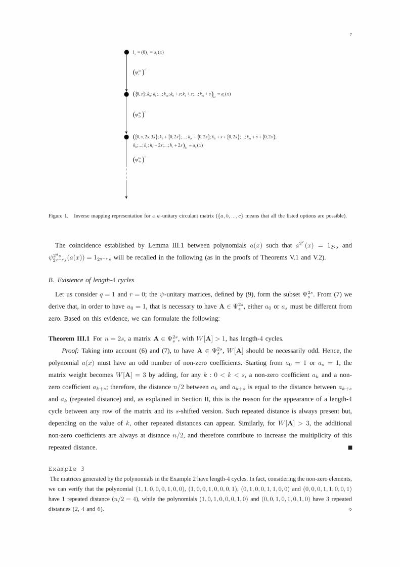
For the subsequent analysis, it will be essential to consider the inverse mappingψ−1. This is schematically

shown in Fig. 1, where the case of aψ-unitary circulant matrix is considered. Basically, the inverse mapping

(ψ2qs2q−1s

(a(x)))−1 adds toa(x) an element of the idealI2qs

2q−1s. In the following, this will be indicated as

{a(x) + I2qs

2q−1s}. Moreover, because of (8), for anyw(x) ∈ I2

qs2q−1s

, it is easy to verify that[w(x)]2 = 0, and

vice versa. So, if we define the mapη : Rn → Rn as η[a(x)] = [a(x)]2, it follows that w(x) ∈ I2qs

2q−1s⇔

w(x) ∈ Ker(η). By iterating the reasoning, and denotingr consecutive applications ofη asηr, it follows that:

Ker(ψ2qs2q−rs) = Ker(ηr). (10)

This property can be used to demonstrate the equivalence between (9) and a condition on the powers ofa(x).

For simplifying the notation, in the following we will set:[a(x)]z = az(x). So, in particular,a−z(x) = [a−1(x)]z

will denote thez-power of the polynomiala−1(x), that corresponds to the inverse matrixA−1. The following

lemma holds:

Lemma III.1 For n = 2qs anda(x) ∈ Rn, a2r

(x) = 12qs ⇔ ψ2qs2q−rs(a(x)) = 12q−rs, with 0 < r ≤ q.

Proof: If ψ2qs2q−rs(a(x)) = 12q−rs, a(x) must be in the forma(x) = b(x)+w(x), whereb(x) is a monomial

mapped into12q−rs by ψ2qs2q−rs and w(x) ∈ I2

qs2q−rs. It follows from its definition thatb(x) = (j2q−rs)n,

j ∈ {0, 1, . . . , 2r − 1}, so b2r

(x) = (0)n = 1n. Due to (10),w2r (x) = 0, so a2r

(x) = b2r

(x) + w2r (x) = 1n.

The reverse implication follows by the same argument.

7

( )1

8

4

s

s

-

y

{ } { } { } { } { }(

)

0 0

0 0 24

0, ,2 ,3 ; 0,2 ;...; 0, 2 ; 0, 2 ;...; 0, 2 ;

;...; ; 2 ;...; 2 ( )

m m

r r s

s s s k s k s k s s k s s

h h h s h s a x

+ + + + + +

+ + =

( )1

4

2

s

s

-

y

{ }( )0 1 0 1 120, ; ; ;...; ; ; ;...; ( )

m ms

s k k k k s k s k s a x+ + + =

( )1

2s

s

-

y

01 (0) ( )s s

a x= =

Figure 1. Inverse mapping representation for aψ-unitary circulant matrix ({a, b, ..., c} means that all the listed options are possible).

The coincidence established by Lemma III.1 between polynomials a(x) such thata2r

(x) = 12qs and

ψ2qs2q−rs(a(x)) = 12q−rs will be recalled in the following (as in the proofs of Theorems V.1 and V.2).

B. Existence of length-4 cycles

Let us considerq = 1 andr = 0; theψ-unitary matrices, defined by (9), form the subsetΨ2ss . From (7) we

derive that, in order to haveu0 = 1, that is necessary to haveA ∈ Ψ2ss , eithera0 or as must be different from

zero. Based on this evidence, we can formulate the following:

Theorem III.1 For n = 2s, a matrixA ∈ Ψ2ss , with W [A] > 1, has length-4 cycles.

Proof: Taking into account (6) and (7), to haveA ∈ Ψ2ss , W [A] should be necessarily odd. Hence, the

polynomial a(x) must have an odd number of non-zero coefficients. Starting from a0 = 1 or as = 1, the

matrix weight becomesW [A] = 3 by adding, for anyk : 0 < k < s, a non-zero coefficientak and a non-

zero coefficientak+s; therefore, the distancen/2 betweenak andak+s is equal to the distance betweenak+s

andak (repeated distance) and, as explained in Section II, this isthe reason for the appearance of a length-4

cycle between any row of the matrix and itss-shifted version. Such repeated distance is always presentbut,

depending on the value ofk, other repeated distances can appear. Similarly, forW [A] > 3, the additional

non-zero coefficients are always at distancen/2, and therefore contribute to increase the multiplicity of this

repeated distance.

Example 3

The matrices generated by the polynomials in the Example 2 have length-4 cycles. In fact, considering the non-zero elements,

we can verify that the polynomial(1, 1, 0, 0, 0, 1, 0, 0), (1, 0, 0, 1, 0, 0, 0, 1), (0, 1, 0, 0, 1, 1, 0, 0) and (0, 0, 0, 1, 1, 0, 0, 1)

have1 repeated distance (n/2 = 4), while the polynomials(1, 0, 1, 0, 0, 0, 1, 0) and (0, 0, 1, 0, 1, 0, 1, 0) have3 repeated

distances (2, 4 and6). �

8

In order to find matrices free of length-4 cycles, the following theorem is useful:

Theorem III.2 Forn = 2qs, with q > 1, a matrixA ∈ Ψ2qss can be free of length-4 cycles forW [A] ≤ 2q−1;

on the other hand, matrixA has length-4 cycles forW [A] > 2q − 1.

Proof: Let us consider at first the caseq = 2, that isn = 4s. By applyingψ4s2s to the polynomiala(x) we

obtain a polynomiala′(x) that defines a matrixA′. Obviously, we haveW [A] ≥W [A′]. So, whenW [A] = 3,

it must beW [A′] ≤ 3 and odd. In the caseW [A′] = 1, matrixA certainly has length-4 cycles. This is because

Theorem III.1 can be applied.

In the caseW [A′] = 3, instead, it must bea′(x) = (0; k; k+s)2s or a′(x) = (s; k; k+s)2s. By considering the

first case (demonstration is similar for the second one), we havea(x) = ({0, 2s}; k+{0, 2s}; k+s+{0, 2s})4s;

by examining the structure of these polynomials, it is easy to verify that, except for some values ofk, in relation

with the value ofs, the corresponding matrices do not exhibit repeated distances, and therefore they are free

of length-4 cycles.

WhenW [A] > 3, matrix A has always length-4 cycles. For example, whenW [A] = 5, three cases are

possible:

i) W [A′] = 5; thena(x) = ({0, s, 2s, 3s}; k0 + {0, 2s}; k1 + {0, 2s}; k0 + s+ {0, 2s}; k1 + s+ {0, 2s})4s,

and it is easy to verify that, regardless the values ofk0 andk1, these polynomials always exhibit repeated

distances.

ii) W [A′] = 3; thena(x) = ({0, s, 2s, 3s}; k0 + {0, 2s}; k0 + s+ {0, 2s};h0;h0 + 2s)4s, and the repeated

distance2s = n/2 appears, which is due to the symbols 1 at positionsh0 andh0 + 2s.

iii) W [A′] = 1; then a(x) = ({0, s, 2s, 3s};h0;h1;h0 + 2s;h1 + 2s)4s, and there are multiple repeated

distances equal ton/2.

The analysis can be immediately extended to the case ofW [A] > 5, where the same conclusions hold.

Now let us consider the general case withq > 2. Based on the demonstration above, it is clear that a necessary

condition for havingA free of length-4 cycles is thatW [A] = W [A′], whereA′ is the matrix relative to the

polynomiala′(x) = ψ2qs2q−1s

(a(x)). In fact, in all cases whereW [A] > W [A′], the additional elements ina(x)

must necessarily be at distancen/2, thus generating a repeated distance. In order to complete the proof, we can

proceed by induction from small matrices to larger ones, through the application of the inverse mapping. Let

us suppose thata′(x) defines a matrixA′, with n′ = 2q−1s, free of length-4 cycles. According to the induction

hypothesis, its weight isW [A′] ≤ 2(q − 1) − 1. Let us consider this relationship with the equality sign (i.e.,

we assume the maximum weight). It is not difficult, by applying the inverse mapping(ψ2qs2q−1s

(a(x)))−1, to

obtain a polynomiala(x) defining a matrixA with the same weight ofA′ and also free of length-4 cycles.

For example, the rightmost (or leftmost) part ofa(x) can be coincident witha′(x) (but this is not, obviously,

the only solution).

If we now consider another polynomial,a′′(x), defining a matrixA′′ with n′′ = 2q−1s but weightW [A′′] =

2q− 1, according to the induction hypothesis, surely it has repeated distances (and, therefore, length-4 cycles).

Actually, it is not difficult to design a matrixA′′ that contains only one repeated distance. To this purpose,

it suffices to start froma′(x) and to add two elements at distancen′′/2 = n/4. When applying the inverse

mapping(ψ2qs2q−1s

(a′′(x)))−1, these two elements translate into elements ina(x) that are at distancen/4 in their

9

turn. This demonstrates that a matrixA can exist, withn = 2qs andW [A] = 2q − 1, that is free of length-4

cycles. An explicit rule for its construction will be given in Theorem IV.1.

If, always starting froma′(x), the number of added elements is four instead of two, the weight of A′′

becomesW [A′′] = 2q + 1. Because of the definition ofψ-unitary matrix, these further elements must be

placed in positions that necessarily introduce (at least) another repeated distance. By applying the inverse

homomorphism, two (or more) repeated distances ina′(x) will translate into one (or more) repeated distance

in a(x), and matrixA will certainly contain length-4 cycles. The same reasoning obviously applies for larger

weights, so that we can conclude that a matrixA, with n = 2qs andW [A] > 2q − 1, has always length-4

cycles.

IV. D ESIGN OFψ-UNITARY CIRCULANT MATRICES FREE OF LENGTH-4 CYCLES

Theorem III.2 states thatψ-unitary binary circulant matrices can exist, that are freeof length-4 cycles and

have an arbitrary odd weight (through a proper choice ofq). However, it does not provide an explicit structure

for these matrices. The latter can be found on the basis of other theorems, that will be given next.

We now introduce the sets of polynomials we will use to designparity-check matrices of QC-LDGM codes.

To make more explicit the notation, we will often put, in the following, q = m + 2 and assumen = 2m+2s.

The sets of interest can be described by polynomials having the structure (11), wherem ≥ 0, 0 < k0 < s, 0 <

k1 < 2s, ..., 0 < km < 2ms, ki 6= kj , ∀i 6= j andci, di are integer coefficients:0 ≤ ci, di < 2m+1−i:

a(x) =(c−1s; k0 + c02s; k1 + c14s; . . . ; km + cm2m+1s;

k0 + s+ d02s; k1 + 2s+ d14s; . . . ;

km + 2ms+ dm2m+1s)2m+2s. (11)

The set of matrices (11) will be denoted byΞ2m+2ss ; clearlyΞ2m+2s

s ⊂ Ψ2m+2ss . A matrix in Ξ2m+2s

s can be

free of length-4 cycles under a suitable choice of theki’s (we note this is coherent with Theorem III.2). The

following theorem holds:

Theorem IV.1 Let us considern = 2m+2s. The matrix:

a(x) = (0; k0; k1; ...; km; k0 + s; k1 + 2s; ...; km + 2ms)n, (12)

with 0 < k0 < k1 < ... < km, ki+1 > 2ki ands > 2km, is free of length-4 cycles.

Proof: We note thata(x) ∈ Ξ2m+2ss . Proof is immediate by calculating all possible distances between

symbols 1 ina(x). Because of the geometric progression, when fixing the attention on thei-th position, the

distancesδi,j , with j < i, are all different one each other and always greater than thedistancesδi−1,k, with

k < i− 1. Moreover, because of the assumption on the value ofn, independently ofm, it is alwaysδi,j < δj,i

for i > j. As an example, the distance between the first and the last position is 3 · 2ms− km > 2ms+ km, the

latter being the distance between the last and the first position; similarly for the other distances. This ensures

that repeated distances cannot exist ina(x).

10

Since the weight ofa(x) in (12) isW [a] = 2m + 3, Theorem IV.1 gives an explicit rule to design matrices

free of length-4 cycles with such a weight.

Example 4

Let us setm = 1, s = 7 andn = 2m+2s = 56 and choosek0 = 1 andk1 = 3. The following matrix:

a(x) = (0; 1; 3; 8; 17)56

is free of length-4 cycles. �

Obviously, we cannot say that (12) is the only structure ableto ensure the absence of length-4 cycles. Even

more,a(x) could have the structure (12) but without satisfying the relationships between theki’s ands specified

by the theorem, while remaining free of length-4 cycles.

Example 5

Let us consider the matrix:

a(x) = (0; 1; 3, 7; 12; 25; 51)176,

that has the structure (12) withm = 2, k0 = 1, k1 = 3, k2 = 7, ands = 11 < 2k2. It is possible to verify, through explicit

calculation, that this matrix is free of length-4 cycles. �

It is important to note that the interest on the structure (11) is justified by its simplicity and the possibility

of fast matrix inversion through the procedure described inthe next section.

In Section V we also derive bounds on the weight of the inverseof a ψ-unitary matrix, and we show that its

actual weight can be very low with respect to the matrix size.Moreover, the bounds we derive on the weight

of the inverse do not depend on the matrix size; so, such matrices are able to provide encoding complexity

that is linear in the code length. These are the reasons whyψ-unitary matrices are of interest for the design of

QC-LDPC codes in the form of LDGM codes.

V. ψ-UNITARY MATRIX INVERSION

A standard algorithm for inverting ann × n circulant matrix exploits the fact that any matrix of this type

can be made diagonal through the so-called Fourier matrix. This permits for a very fast inversion. The main

limitation of this approach is that, when operating in a ringZm, inversion is possible if and only ifm andn

are coprime. In addition, it is also necessary to find an extension of the ring, in such a way as to guarantee the

presence ofn roots in the unit circle, as required by the implementation of the fast Fourier transform. These

limitations can be overcome by exploiting the isomorphism between matrices and polynomials [26].

A. Explicit evaluation of the inverse matrix

For a matrixA with n = 2s (i.e.,q = 1) satisfying the conditionψ2ss = 1s, Lemma III.1 impliesa2(x) = 12s,

and thereforea−1(x) = a(x), which means thatA coincides with its inverse. This result permits to prove the

following:

Theorem V.1 If n = 4s (i.e., q = 2) andA0 ∈ Ψ4ss then,∀a(x) ∈ {a0(x) + I4s2s}, the following relationship

holds:a(x) + a−1(x) = w(x), wherew(x) ∈ I4s2s is independent of the choice ofa(x).

Proof: As ψ4ss = 1s, from Lemma III.1 we have:a40(x) = 14s. This impliesa20(x) · a

20(x) = 14s and

thena20(x) = a−20 (x). By applying the mapψ4s

2s to both sides of the equality, because of the homomorphism

11

properties, one finds[ψ4s2s(a0(x))]

2 = [ψ4s2s(a

−10 (x))]2. To verify this equality,a0(x) anda−1

0 (x) must differ by

an element belonging to the idealI4s2s , i.e., it must be:

a0(x) + {a−10 (x) + w0(x)} = 0,

for somew0(x) ∈ I4s2s . Similarly, by considering another elementa1(x) ∈ {a0(x)+ I4s2s} 6= a0(x) we shall find

a w1(x) ∈ I4s2s such that:

a1(x) + {a−11 (x) + w1(x)} = 0.

So:

a0(x) + a−10 (x) + w0(x) = a1(x) + a−1

1 (x) + w1(x).

To demonstrate thatw0(x) = w1(x) = w(x) (that is, uniqueness ofw(x)) it is sufficient to prove that:

a0(x) + a−10 (x) = a1(x) + a−1

1 (x).

For this purpose, we observe thata1(x) ∈ {a0(x) + I4s2s} can be always written as follows:

a1(x) = a0(x) + w2(x).

Then, the above equality is verified if and only if:

a−11 (x) = a0(x) + w0(x) + w2(x).

But this relationship is certainly true. In fact, by using it, we have, as necessary:

a1(x)a−11 (x) = [a0(x) + w2(x)] [a0(x) + w0(x) + w2(x)]

= a20(x) + a0(x)w0(x)

= a0(x)a−10 (x) = 14s

having exploited the fact thatw22(x) = 0 andw0(x)w2(x) = 0 (this is because, by definition, the non-zero

elementsw(x) ∈ I4s2s are of typeb(x)(x2s+1), whereb(x) is a polynomial with the maximum order< 2s).

For the matrices satisfying the hypotheses of Theorem V.1, the inverse matrix can be found by addingw(x)

to a(x); w(x) can be calculated by inverting one matrix of the set{a0(x) + I4s2s}, and using it for all matrices

of the set.

Theorem V.1 can be extended as follows:

Theorem V.2 If n = 2m+2s andA0 ∈ Ψ2m+2ss then,∀a(x) ∈ {a0(x) + I2

m+2s2m+1s

}, the following relationship

holds:

a−1(x) = (a2m

(x) + w(x))

m−1∏

i=0

a2i

(x), (13)

wherew(x) ∈ I2m+2s

2m+1sis independent of the choice ofa(x).

Proof: Proceeding like in the demonstration of Theorem V.1, we can see that, by Lemma III.1, ifψ2m+2ss (a0(x)) =

1s then

a2m+2

0 (x) = 12m+2s → a2m+1

0 (x) = a−2m+1

0 (x).

12

From this:

[a2m

0 (x)]2 = [a−2m

0 (x)]2

and then:[

ψ2m+2s2m+1s(a

2m

0 (x))]2

=[

ψ2m+2s2m+1s(a

−2m

0 (x))]2

.

This equality is satisfied by assuming:

a−2m

0 (x) = a2m

0 (x) + w(x),

for w(x) ∈ I2m+2s

2m+1s. The same holds for any othera(x) ∈ {a0(x)+I

2m+2s2m+1s

}, and the polynomialw(x) is unique

(demonstration as in Theorem V.1). Replacinga0(x) by a(x), to obtaina−1(x), we need to multiply both sides

of the above relationship by:

a2m−1(x) =

m−1∏

i=0

a2i

(x),

from which (13) is derived.

B. Fast inversion

Eq. (13) provides a direct method for the computation of the inverse of aψ-unitary circulant matrix, that

can be much faster than more conventional methods. The key point of the procedure is the calculation of the

polynomialw(x). Multiplying both sides of (13) bya(x), we see thatw(x) can be obtained, in general, as the

solution of the following equation:

a2m

(x)w(x) = 1 + a2m+1

(x). (14)

However, for the matrices in the ensembleΞ2m+2ss , that has been defined in Section IV, Eq. (14) can be directly

solved.

More precisely, it can be verified that, for these matrices,

a2m

(x) =2m(c−1s; k0 + c02s; k1; (15)

k0 + s+ d02s; k1 + 2s((1 + δm,0)))2m+2s, (16)

whereδi,j is the Kronecker delta function, and

a2m+1

(x) = 2m+1(c−1s; k0 + c02s; k0 + s+ d02s)2m+2s. (17)

By replacing (16) and (17) in (14), the expression ofw(x) can be explicitly found and then, through (13),

the polynomial of the inverse,a−1(x), can also be obtained.

On the basis of the previous expressions, it could seem thatc−1 = 0, 1, 2, 3, c0 = 0, 1 and d0 = 0, 1, in

all their possible16 combinations, define as many different situations. Actually, it is possible to verify, even

through explicit calculation, that the structure ofw(x) depends only on the value ofc−1.

In detail, for evenc−1 (that is,c−1 = 0, 2), we have:

w(x)e = 2m(2k0; 3k0; 3k0 + s; 2k0 + 2s; 3k0 + 2s; 3k0 + 3s)n (18)

13

while, for oddc−1 (that is,c−1 = 1, 3), we have:

w(x)o = 2m(k0; 3k0; s; k0 + s; 2k0 + s; 3k0 + s; k0 + 2s;

3k0 + 2s; 3s; k0 + 3s; 2k0 + 3s; 3k0 + 3s)n. (19)

It is interesting to note thatw(x) is independent ofk1. It can be easily proved thatW [a2m

+ w] ≤ 11; this

result will be useful in the following (see Appendix A, in particular).

According to (18) and (19), we see that, for computingw(x), we can always refer to the casem = 0, as the

effect ofm > 0 simply results in multiplying the polynomial so obtained by2m. The values ofc−1, c0 and

d0 determine the structure ofa(x) and, eventually, that ofa−1(x). Form = 0, however, it is possible to verify

that the following combinations: (c−1, c0, d0) = (0, 0, 0), (1, 1, 0), (2, 1, 1) and (3, 0, 1) are equivalent, in the

sense they define polynomials that differ by a cyclic shift ofs = n/4 positions, or a multiple of it. Precisely,

these polynomials are:(0; k0; s+ k0)4s, (s; s+ k0; 2s+ k0)4s, (2s; 2s+ k0; 3s+ k0)4s and(k0; 3s; 3s+ k0)4s

respectively. Similarly, (0, 0, 1), (1, 0, 0), (2, 1, 0) and (3, 1, 1) are also equivalent, and the same holds for

combinations (0, 1, 0), (1, 1, 1), (2, 0, 1), (3, 0, 0) and for combinations (0, 1, 1), (1, 0, 1), (2, 0, 0), (3, 1, 0). For

any equivalent set, only one matrix must be considered. In fact, if two polynomials differ by a right shift ofs

positions, their inverses differ by a left shift ofs positions as well.

When required, in the following we will focus on the choicec−1 = 0, that is the first matrix of each equivalent

set.

C. Comparison with Euclid’s algorithm

The inverse of a matrix satisfying the assumptions of Theorem V.2 can be easily found by using (13).

This reflects in a computation algorithm that, in many cases,can be significantly faster than more conventional

approaches for matrix inversion. In this subsection, in particular, we give some examples of comparison between

the proposed approach and the more classic Euclid’s algorithm.

A distinctive feature of the proposed approach, against Euclid’s algorithm, is that it exhibits a much weaker

dependence on the matrix size. In fact, the complexity of ourapproach is mainly influenced by the matrix

weight. This can make the proposed procedure highly effective in the case of large and sparse matrices, like

those of interest for LDPC code design.

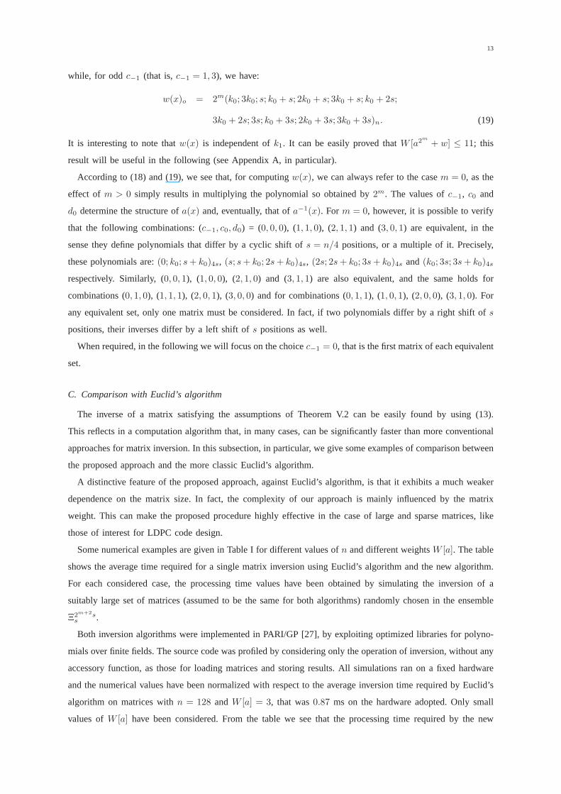
Some numerical examples are given in Table I for different values ofn and different weightsW [a]. The table

shows the average time required for a single matrix inversion using Euclid’s algorithm and the new algorithm.

For each considered case, the processing time values have been obtained by simulating the inversion of a

suitably large set of matrices (assumed to be the same for both algorithms) randomly chosen in the ensemble

Ξ2m+2ss .

Both inversion algorithms were implemented in PARI/GP [27], by exploiting optimized libraries for polyno-

mials over finite fields. The source code was profiled by considering only the operation of inversion, without any

accessory function, as those for loading matrices and storing results. All simulations ran on a fixed hardware

and the numerical values have been normalized with respect to the average inversion time required by Euclid’s

algorithm on matrices withn = 128 andW [a] = 3, that was0.87 ms on the hardware adopted. Only small

values ofW [a] have been considered. From the table we see that the processing time required by the new

14

Table I

NORMALIZED AVERAGE TIME FOR MATRIX INVERSION USING EUCLID ’ S ALGORITHM AND THE NEW ALGORITHM

n 128 256 512 1024 2048 4096 8192

W [a] = 3

Euclid’s alg. 1.00 1.96 4.19 9.13 22.88 60.59 174.39

New alg. 0.22 0.22 0.23 0.24 0.23 0.23 0.23

W [a] = 5

Euclid’s alg. 3.17 9.99 32.07 108.89 552.78 2145.35 9511.17

New alg. 0.52 0.55 0.58 0.59 0.57 0.61 0.60

W [a] = 7

Euclid’s alg. 4.33 13.98 50.11 196.99 941.40 4083.91 16769.77

New alg. 2.29 2.96 3.79 4.47 4.86 5.33 5.45

W [a] = 9

Euclid’s alg. 4.91 16.25 60.21 232.80 1069.89 4802.12 20076.41

New alg. 4.64 9.53 21.86 34.40 44.08 86.63 94.11

algorithm is smaller than that required by Euclid’s algorithm for the considered weights, that are of interest for

the design of LDPC codes.

D. Weight of the inverse matrix

Another important consequence of the availability of explicit expressions forw(x), and then fora−1(x), is

the possibility to estimate the weight of the inverse matrix. To this purpose, the following theorems hold:

Theorem V.3 For n = 4s, the matrices inΞ4ss with W [a] = 3, free of length-4 cycles, have5 ≤W [a−1] ≤ 9.

Proof: Let us consider the first combination of each equivalent set,that hasc−1 = 0. Because of Theorem

V.1, by using (16) and (18) withm = 0, we obtain:

a−1(x) = (0; k0 + c02s; 2k0; k0 + s+ d02s; 3k0;

3k0 + s; 2k0 + 2s; 3k0 + 2s; 3k0 + 3s)4s.

Depending on the values ofk0 ands, at most four positions can be coincident two by two; therefore, the weight

of a−1(x) is between 5 and 9 (the latter when no positions are coincident).

For W [a] > 3 the weight of the inverse is destined to increase and the evaluation of a range of variability

for W [a−1] becomes more difficult as well. In Section VI, however, wherethe proposed theory will be applied

for the design of LDGM codes, we will limit to considerW [a] ≤ 5 (i.e.,m = 0 andm = 1), as this weight is

large enough to ensure the achievement of good performance.

Similarly to Theorem V.3, that holds form = 0, an upper bound forW [a−1] in the case ofm = 1 can be

found through explicit calculation. More precisely, starting from (13) and using the properties of the matrices

15

in Ξ8ss it is easy to find:

a−1(x) = (a2(x) + w(x))a(x) =

(0; 2k0; 4k0; 6k0; 2k1; 2s+ 2k0; 4s+ 2k1; 2s+ 6k0; 4s+ 4k0;

4s+ 6k0; 6s+ 6k0; k0; 3k0; 5k0; 7k0; 2k1 + k0; 2s+ 3k0;

4s+ 2k1 + k0; 2s+ 7k0; 4s+ 5k0; 4s+ 7k0; 6s+ 7k0; k1;

2k0 + k1; 4k0 + k1; 3k1; 4s+ 3k1; 4s+ 4k0 + k1; s+ k0;

s+ 3k0; s+ 5k0; s+ 7k0; s+ 2k1 + k0; 3s+ 3k0;

5s+ 2k1 + k0; 3s+ 7k0; 5s+ 5k0; 5s+ 7k0; 7s+ 7k0;

2s+ k1; 2s+ 4k0 + k1; 2s+ 3k1; 4s+ 2k0 + k1;

6s+ 3k1; 6s+ 4k0 + k1)8s, (20)

that providesW [a−1] ≤ 45. Obviously, this upper bound has a sense only fors sufficiently large (s ≥ 6);

otherwise, the upper bound would be greater thann.

Depending on the values ofk0 andk1, the upper bound can be lower. This occurs when some terms, in(20),

become equal and, therefore, annul each other. As an example, for k1 = 3k0 the maximum weight is21.

Moreover, depending on the value ofs, the actual weight of the inverse can be smaller.

Example 6

Let us consider the matrix of the Example 4. By applying (18), we findw(x) = (4; 6; 20; 32; 34; 48)56. Then, using (13),

the inverse matrix is obtained as:

a−1(x) = (a2(x) + w(x))a(x)

= ((0; 2; 6; 16; 34)56 + (4; 6; 20; 32; 34; 48)56) ·

·(0; 1; 3; 8; 17)56

= (0; 2; 4; 16; 20; 32; 48)56 · (0; 1; 3; 8; 17)56

= (1; 2; 4; 7; 8; 9; 10; 12; 16; 20; 23; 24; 28; 32; 35; 37;

40; 48; 51)56.

ThusW [a−1] = 19, which is smaller than the upper bound. �

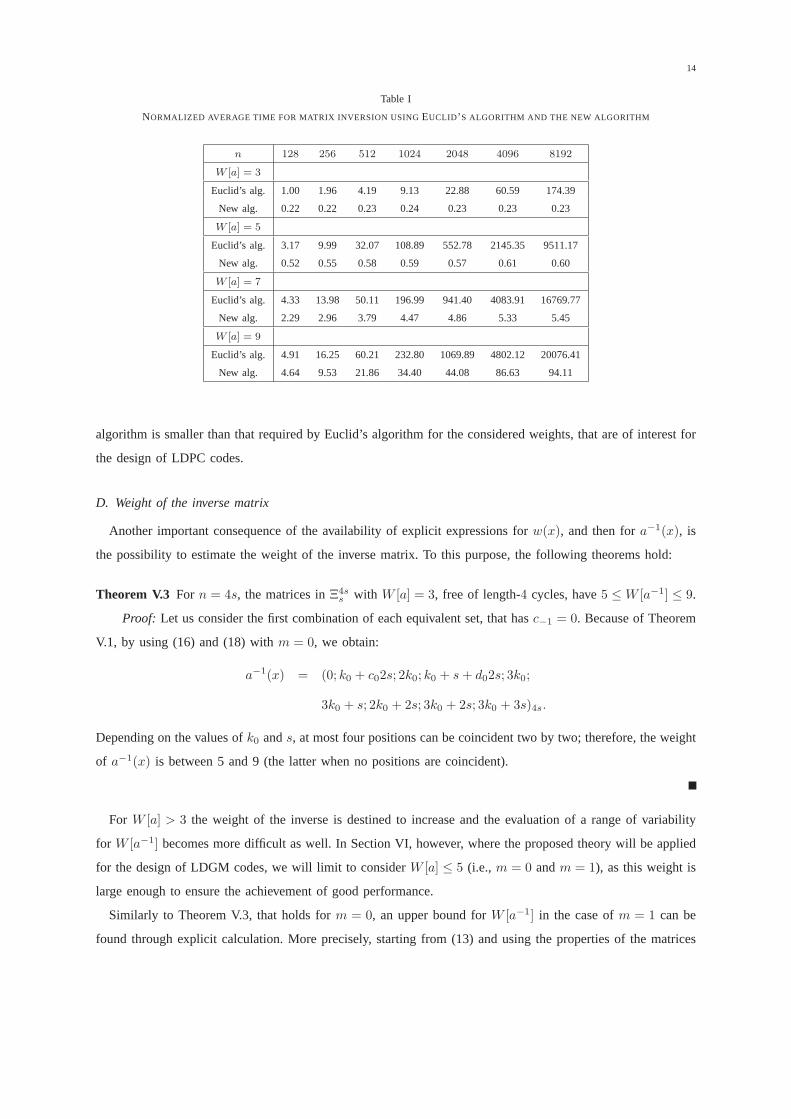
Another interesting issue concerns the distribution of theinverse matrix weight. Form = 1, some examples

are shown in Table II, where we have reported the (per cent) incidence of each weight, estimated through a

Montecarlo simulation of100, 000 matrices of each size. We see that, fors > 16, the weight spectrum has

a maximum at the upper bound. The convergence to the upper bound, confirmed by the trend of the average

value⟨

W [a−1]⟩

, becomes more and more evident for increasings, since further elisions in the expression

above become less and less probable. Explicitly, this meansthat, for very largen, the upper bound gives the

actual weight for an increasing fraction of the inverse matrices.

In Appendix A, a bound on the weight of the inverse is derived for the casem > 1.

16

Table II

WEIGHT DISTRIBUTION OF THE INVERSE MATRICES IN THE CASE OFm = 1, FOR DIFFERENT VALUES OFs

W [a−1] s = 16 s = 64 s = 256 s = 1024

5 0.04 0 0 0

7 0.08 0.01 0 0

9 0.08 0.01 0 0

11 0.04 0.01 0 0

13 0.67 0.03 0 0

15 0.93 0.07 0.01 0

17 0.93 0.06 0 0

19 1.04 0.07 0.01 0

21 3.22 0.91 0.23 0.05

23 4.51 1.14 0.29 0.07

25 7.10 1.15 0.27 0.06

27 4.10 0.84 0.17 0.05

29 2.89 0.63 0.16 0.05

31 0.46 0.03 0 0

33 2.29 0.12 0.01 0

35 16.77 4.03 1.00 0.23

37 11.60 4.97 1.33 0.34

39 10.02 3.17 0.81 0.20

41 20.62 10.80 3.05 0.77

43 8.99 6.63 1.93 0.48

45 3.62 65.32 90.73 97.70⟨

W [a−1]⟩

34.95 42.40 44.35 44.84

VI. ψ-UNITARY MATRICES IN LDGM CODES

A. Code features

The LDGM codes considered in [8] are systematic codes with generator matrixG = [I|P], whereP is a

K× (N −K) sparse matrix andI is theK×K identity matrix. The parity-check matrix of these codes canbe

expressed asH = [PT |I], where the identity matrix has size(N −K)× (N −K) and superscriptT denotes

transposition. So, matrixH is also sparse, and this permits the application of standardalgorithms for decoding

of LDPC codes.

The weakness of these codes is the existence, in the Tanner graph, ofN −K coded (parity) bit nodes with

degree1. This implies that the messages propagated from the order-1 coded bits to their corresponding check

bits are always the same and are not affected by the decoding algorithm. As a consequence, these codes exhibit

high error floors, which require resorting to serial concatenation of two LDGM codes [9].

It is reasonable to think that the performance of LDGM codes,both in single and concatenated configuration,

can be improved by replacing the identity matrix inH, that is responsible for the order-1 coded bits, with

some other sparse matrix having weight larger than1. So, contrary to [8], our starting point is the parity-check

matrix.

Let us consider (1). By assuming that at least one of theHi blocks (i = 0 . . . Nb − 1), e.g., the last block,

17

is of full rank, the generator matrixG can be obtained as:

G =

I

(

H−1Nb−1 ·H0

)T

(

H−1Nb−1 ·H1

)T

...(

H−1Nb−1 ·HNb−2

)T

; (21)

so, it is formed by aK ×K identity matrix (remind thatK is the information length) followed by a column

of Kb = Nb − 1 circulant blocks with sizen = N/Nb. MatricesG andH are related through the expression

H ·GT = 0.

We observe that the LDGM codes in [8] and [9] can be interpreted as a special case of the codes with (1) and

(21), whereHNb−1 = I. The choice of the identity matrix gives the lowest possibledensity of the generator

matrix, but at the expense of the code minimum distance. As mentioned, this reflects on high error floors. We

will denote such codes asidentity (or I-based) QC-LDGM codes in the following.

The alternative choice we propose consists in using, asHNb−1, aψ-unitary block with suitable weight (greater

than 1). We have seen in Section V thatψ-unitary matrices, properly designed, can have sparse inverses, so

producing LDGM codes in the specified sense. They ensure easyencoding and good decoding features without

penalizing the distance properties. We will denote such codes asψ-unitary QC-LDGM codes in the following,

and we will compare their performance and complexity with those of I-based codes both in analytical and

numerical terms.

In order to avoid the existence of length-4 cycles in the Tanner graph associated to eachψ-unitary QC-LDGM

code, we adoptψ-unitary matrices in the form (12) asHNb−1. They are designed by randomly choosing the

k0 . . . km parameters, with the constraints0 < k0 < k1 < ... < km ands > 2km (see Theorem IV.1). Though

the further constraintki+1 > 2ki has not always been imposed, matrices free of length-4 cycles have been

found for all the considered choices of code parameters. Theselection ofψ-unitary matrices has been done

by aiming at reducing the weight of the inverse matrix with respect to the bounds found in Section V-D, as

much as possible. The circulant blocksHi, i ∈ {0, 1, . . . , Nb − 2}, have been designed on a random basis, by

avoiding the introduction of length-4 cycles with theψ-unitary block and between each couple of them.

All codes we consider can be treated as LDPC codes, and decoded through standard belief propagation

algorithms. We adopt the log-likelihood ratios sum-product algorithm (LLR-SPA) [28].

In order to compare performance ofψ-unitary QC-LDGM codes with that ofI-based QC-LDGM codes,

we first refer to transmission over the Binary Symmetric Channel (BSC). Then, we will give some examples

of performance over the Additive White Gaussian Noise (AWGN) channel, where we will also assess the

concatenated scheme proposed forI-based codes [8], [9].

B. Minimum distance and multiplicity

In order to estimate the minimum distance and its multiplicity for I-based andψ-unitary codes, we can refer

to previous literature. For parity-check matrices in the form (1), it is proved in [29] that,∀i, j : 0 ≤ i < j < Nb,

there exists a codeword of weightW [HiHj ] ≤W [Hi]+W [Hj ]; so, the code minimum distance can be upper

bounded as follows:

dmin ≤ min0≤i<j<Nb

{W [Hi] +W [Hj ]} = dmin. (22)

18

Based on these arguments, we can also obtain a (loose) lower bound on the number of weight-dmin codewords

as follows:

Pdmin=

∣

∣

{

i, j :W [Hi] +W [Hj ] = dmin; 0 ≤ i < j < Nb}∣

∣ . (23)

Each of thePdminlow weight codewords involves a different pair of circulantblocks(i, j); so, it cannot coincide

with a cyclically shifted version of another of such codewords. We denote each of them as alow weight pattern

in the following. The numberPdminof low weight patterns can be easily estimated starting fromthe two smallest

block weights and their block multiplicity:

W1 = min0≤i<Nb

W [Hi];

W2 = min0≤i<Nb

{W [Hi] :W [Hi] > W1} ;

N1 = |{Hi :W [Hi] =W1}| ;

N2 = |{Hi :W [Hi] =W2}| .

(24)

Based on (24),Pdmincan be estimated as follows:

Pdmin=

N2, if N1 = 1;(

N1

2

)

, if N1 > 1.(25)

Due to the quasi-cyclic nature of the codes, each of thePdminlow weight patterns can give rise, at most, ton

cyclically shifted versions of itself that are still valid codewords. So, an estimate of the weight-dmin codewords

multiplicity can be expressed as:

Admin≈ n · Pdmin

. (26)

For the codes considered in Section VI-D, we have found that (22) holds with the equality sign and we have

verified (25) by analyzing undetected errors (or decoder errors) that occur due to transitions of the received

codeword to near codewords during Montecarlo simulations.In almost all cases, we have found a number

of different low weight patterns exactly coincident with that predicted by (25). The only exception was the

(8192, 7168) ψ-unitary code, for which only21 different low weight patterns (out of28 predicted by (25))

were found.

C. Complexity assessment

In order to compareI-based withψ-unitary QC-LDGM codes under the complexity viewpoint, we need to

estimate both their encoding and decoding requirements.

An exact complexity evaluation should be referred to a specific implementation, and depends on a variety of

factors as the degree of parallelization, the routing strategies and the memory occupation. All these aspects are

influenced by the hardware architecture adopted and the design choices. On the contrary, we need a complexity

measure independent of the final implementation, but significant enough for a fair comparison between different

codes.

For this reason, we express complexity in terms of the numberof elementary operations needed for encoding

and decoding. Such number is strictly related to the densityof symbol 1 in the generator and parity-check

matrices, and allows to compare complexity of different codes without referring to any specific hardware or

software implementation.

19

As a measure of encoding complexity, we consider the number of elementary operations needed to calculate

each redundancy bit. So, encoding complexity can be expressed as the average column weight in the lastN−K

columns of the generator matrix in systematic form:

Cenc =

∑N−1i=K W [gi]

N −K, (27)

whereW [gi] denotes the Hamming weight of thei-th column ofG.

We consider generator matrices in the form (21); so, the column weight in their lastN − K columns is

constant and coincident with the sum of the Hamming weights of a row (or column) ofH−1Nb−1 ·H0,H

−1Nb−1 ·

H1, . . . ,H−1Nb−1 ·HNb−2.

For anI-based QC-LDGM code,HNb−1 is an identity block, and the Hamming weights of the blocks inthe

non-identity part ofG coincide with those of the firstNb − 1 blocks ofH. If they all have row (or column)

weightX, it results inCenc = (Nb − 1)X. For aψ-unitary QC-LDGM code, instead, the weight of the last

N −K columns ofG is greater. However, it remains significantly smaller than that of a generic code, whose

generator matrix is dense. In the latter case, (27) gives an encoding complexity approximately equal toK/2,

and this number can be extremely large for rather long codes.

As for decoding complexity, we consider that belief propagation decoding algorithms work on the Tanner

graph, exchanging messages along its edges. Thus, as a measure of decoding complexity, we can use the

number of messages exchanged by belief propagation per decoded bit per iteration, that coincides with the

average Hamming weight of the parity-check matrix columns.In formula:

Cdec =

∑N−1i=0 W [hi]

N, (28)

whereW [hi] denotes the Hamming weight of thei-th column ofH. In the parity-check matrix of a regular

I-based QC-LDGM code, the first(Nb − 1) blocks have column weightX, while the last block has column

weight 1. So, for these codes,Cdec = [(Nb − 1)X + 1]/Nb.

D. Code examples

In this section, we consider some examples of codes having parity-check matrices in the form (1) and compare

the performance achieved byI-based (CI) andψ-unitary (Cψ) QC-LDGM codes.

The parameters of the considered codes are summarized in Table III. Matrix HNb−1 is specified by the

positions of the non-zero coefficients in its representative polynomial. The table also provides the weights of

the other blocks ofH. As expected,I-based codes exhibit the lowest encoding complexity, but this is paid

in terms of error correction performance, as will be shown inthe following. This can also be argued by

the minimum distance values, reported in Table III, together with the corresponding multiplicity. ForI-based

codes,dmin simply coincides with the lowest column weight in the leftmost part of the parity-check matrix (K

columns), augmented by1. Forψ-unitary codes, instead, the minimum distance can be higher, and this reflects

into lower error floors. The minimum distance of the codes andtheir minimum weight codewords multiplicity

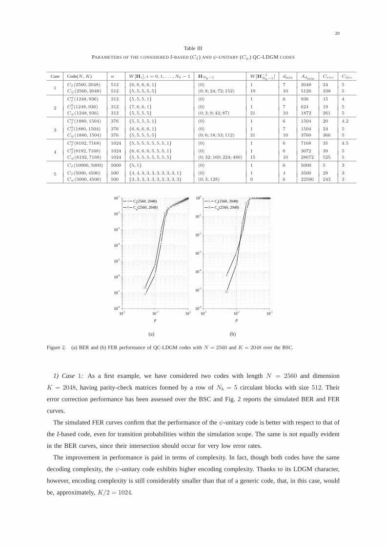
have been estimated as explained in Section VI-B.

20

Table III

PARAMETERS OF THE CONSIDEREDI-BASED (CI ) AND ψ-UNITARY (Cψ ) QC-LDGM CODES

Case Code(N , K) n W [Hi], i = 0, 1, . . . , Nb − 1 HNb−1 W [H−1

Nb−1] dmin Admin

Cenc Cdec

CI(2560, 2048) 512 {6, 6, 6, 6, 1} (0) 1 7 2048 24 51

Cψ(2560, 2048) 512 {5, 5, 5, 5, 5} (0; 8; 24; 72; 152) 19 10 5120 338 5

CaI (1248, 936) 312 {5, 5, 5, 1} (0) 1 6 936 15 4

CbI (1248, 936) 312 {7, 6, 6, 1} (0) 1 7 624 19 52Cψ(1248, 936) 312 {5, 5, 5, 5} (0; 3; 9; 42; 87) 21 10 1872 261 5

CaI (1880, 1504) 376 {5, 5, 5, 5, 1} (0) 1 6 1504 20 4.2

CbI (1880, 1504) 376 {6, 6, 6, 6, 1} (0) 1 7 1504 24 53Cψ(1880, 1504) 376 {5, 5, 5, 5, 5} (0; 6; 18; 53; 112) 21 10 3760 366 5

CaI (8192, 7168) 1024 {5, 5, 5, 5, 5, 5, 5, 1} (0) 1 6 7168 35 4.5

CbI (8192, 7168) 1024 {6, 6, 6, 6, 5, 5, 5, 1} (0) 1 6 3072 39 54Cψ(8192, 7168) 1024 {5, 5, 5, 5, 5, 5, 5, 5} (0; 32; 160; 224; 480) 15 10 28672 525 5

CI(10000, 5000) 5000 {5, 1} (0) 1 6 5000 5 3

CI(5000, 4500) 500 {4, 4, 3, 3, 3, 3, 3, 3, 3, 1} (0) 1 4 3500 29 35Cψ(5000, 4500) 500 {3, 3, 3, 3, 3, 3, 3, 3, 3, 3} (0; 3; 128) 9 6 22500 243 3

10-3 10-2 10-110-8

10-7

10-6

10-5

10-4

10-3

10-2

10-1

p

CI(2560, 2048)

Cψ(2560, 2048)

(a)

10-3 10-2 10-110-6

10-5

10-4

10-3

10-2

10-1

100

p

CI(2560, 2048)

Cψ(2560, 2048)

(b)

Figure 2. (a) BER and (b) FER performance of QC-LDGM codes withN = 2560 andK = 2048 over the BSC.

1) Case1: As a first example, we have considered two codes with lengthN = 2560 and dimension

K = 2048, having parity-check matrices formed by a row ofNb = 5 circulant blocks with size512. Their

error correction performance has been assessed over the BSCand Fig. 2 reports the simulated BER and FER

curves.

The simulated FER curves confirm that the performance of theψ-unitary code is better with respect to that of

the I-based code, even for transition probabilities within the simulation scope. The same is not equally evident

in the BER curves, since their intersection should occur forvery low error rates.

The improvement in performance is paid in terms of complexity. In fact, though both codes have the same

decoding complexity, theψ-unitary code exhibits higher encoding complexity. Thanksto its LDGM character,

however, encoding complexity is still considerably smaller than that of a generic code, that, in this case, would

be, approximately,K/2 = 1024.

21

10-3 10-2 10-110-8

10-7

10-6

10-5

10-4

10-3

10-2

10-1

p

CI

a(1248, 936)

CI

b(1248, 936)

Cψ(1248, 936)

(a)

10-3 10-2 10-110-6

10-5

10-4

10-3

10-2

10-1

100

p

CI

a(1248, 936)

CI

b(1248, 936)

Cψ(1248, 936)

(b)

Figure 3. (a) BER and (b) FER performance of QC-LDGM codes withN = 1248 andK = 936 over the BSC.

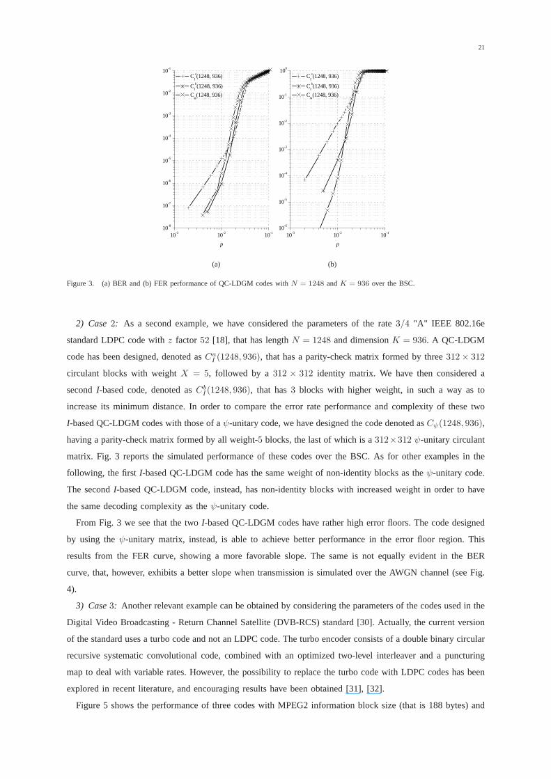
2) Case2: As a second example, we have considered the parameters of therate 3/4 "A" IEEE 802.16e

standard LDPC code withz factor 52 [18], that has lengthN = 1248 and dimensionK = 936. A QC-LDGM

code has been designed, denoted asCaI (1248, 936), that has a parity-check matrix formed by three312× 312

circulant blocks with weightX = 5, followed by a312 × 312 identity matrix. We have then considered a

secondI-based code, denoted asCbI (1248, 936), that has3 blocks with higher weight, in such a way as to

increase its minimum distance. In order to compare the errorrate performance and complexity of these two

I-based QC-LDGM codes with those of aψ-unitary code, we have designed the code denoted asCψ(1248, 936),

having a parity-check matrix formed by all weight-5 blocks, the last of which is a312×312 ψ-unitary circulant

matrix. Fig. 3 reports the simulated performance of these codes over the BSC. As for other examples in the

following, the firstI-based QC-LDGM code has the same weight of non-identity blocks as theψ-unitary code.

The secondI-based QC-LDGM code, instead, has non-identity blocks withincreased weight in order to have

the same decoding complexity as theψ-unitary code.

From Fig. 3 we see that the twoI-based QC-LDGM codes have rather high error floors. The code designed

by using theψ-unitary matrix, instead, is able to achieve better performance in the error floor region. This

results from the FER curve, showing a more favorable slope. The same is not equally evident in the BER

curve, that, however, exhibits a better slope when transmission is simulated over the AWGN channel (see Fig.

4).

3) Case3: Another relevant example can be obtained by considering theparameters of the codes used in the

Digital Video Broadcasting - Return Channel Satellite (DVB-RCS) standard [30]. Actually, the current version

of the standard uses a turbo code and not an LDPC code. The turbo encoder consists of a double binary circular

recursive systematic convolutional code, combined with anoptimized two-level interleaver and a puncturing

map to deal with variable rates. However, the possibility toreplace the turbo code with LDPC codes has been

explored in recent literature, and encouraging results have been obtained [31], [32].

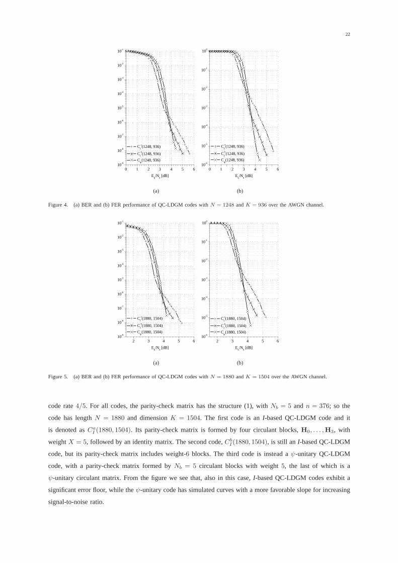
Figure 5 shows the performance of three codes with MPEG2 information block size (that is 188 bytes) and

22

0 1 2 3 4 5 610-9

10-8

10-7

10-6

10-5

10-4

10-3

10-2

10-1

Eb/N

0 [dB]

CI

a(1248, 936)

CI

b(1248, 936)

Cψ(1248, 936)

(a)

0 1 2 3 4 5 610-6

10-5

10-4

10-3

10-2

10-1

100

Eb/N

0 [dB]

CI

a(1248, 936)

CI

b(1248, 936)

Cψ(1248, 936)

(b)

Figure 4. (a) BER and (b) FER performance of QC-LDGM codes withN = 1248 andK = 936 over the AWGN channel.

2 3 4 5 610-9

10-8

10-7

10-6

10-5

10-4

10-3

10-2

10-1

Eb/N

0 [dB]

CI

a(1880, 1504)

CI

b(1880, 1504)

Cψ(1880, 1504)

(a)

2 3 4 5 610-6

10-5

10-4

10-3

10-2

10-1

100

Eb/N

0 [dB]

CI

a(1880, 1504)

CI

b(1880, 1504)

Cψ(1880, 1504)

(b)

Figure 5. (a) BER and (b) FER performance of QC-LDGM codes withN = 1880 andK = 1504 over the AWGN channel.

code rate4/5. For all codes, the parity-check matrix has the structure (1), with Nb = 5 andn = 376; so the

code has lengthN = 1880 and dimensionK = 1504. The first code is anI-based QC-LDGM code and it

is denoted asCaI (1880, 1504). Its parity-check matrix is formed by four circulant blocks, H0, . . . ,H3, with

weightX = 5, followed by an identity matrix. The second code,CbI (1880, 1504), is still an I-based QC-LDGM

code, but its parity-check matrix includes weight-6 blocks. The third code is instead aψ-unitary QC-LDGM

code, with a parity-check matrix formed byNb = 5 circulant blocks with weight5, the last of which is a

ψ-unitary circulant matrix. From the figure we see that, also in this case,I-based QC-LDGM codes exhibit a

significant error floor, while theψ-unitary code has simulated curves with a more favorable slope for increasing

signal-to-noise ratio.

23

2 3 4 510-9

10-8

10-7

10-6

10-5

10-4

10-3

10-2

10-1

CI

a(8192, 7168)

CI

b(8192, 7168)

Cψ(8192, 7168)

Eb/N

0 [dB]

(a)

2 3 4 510-6

10-5

10-4

10-3

10-2

10-1

100

Eb/N

0 [dB]

CI

a(8192, 7168)

CI

b(8192, 7168)

Cψ(8192, 7168)

(b)

Figure 6. (a) BER and (b) FER performance of QC-LDGM codes withN = 8192 andK = 7168 over the AWGN channel.

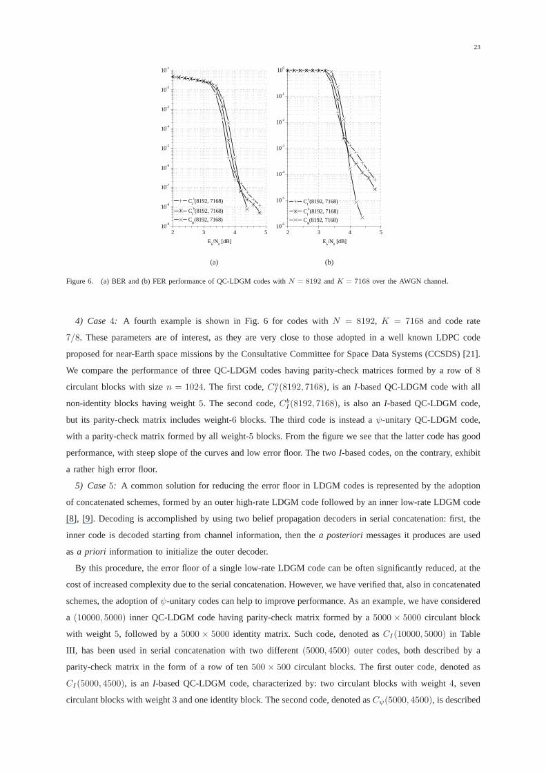
4) Case4: A fourth example is shown in Fig. 6 for codes withN = 8192, K = 7168 and code rate

7/8. These parameters are of interest, as they are very close to those adopted in a well known LDPC code

proposed for near-Earth space missions by the ConsultativeCommittee for Space Data Systems (CCSDS) [21].

We compare the performance of three QC-LDGM codes having parity-check matrices formed by a row of8

circulant blocks with sizen = 1024. The first code,CaI (8192, 7168), is an I-based QC-LDGM code with all

non-identity blocks having weight5. The second code,CbI (8192, 7168), is also anI-based QC-LDGM code,

but its parity-check matrix includes weight-6 blocks. The third code is instead aψ-unitary QC-LDGM code,

with a parity-check matrix formed by all weight-5 blocks. From the figure we see that the latter code has good

performance, with steep slope of the curves and low error floor. The twoI-based codes, on the contrary, exhibit

a rather high error floor.

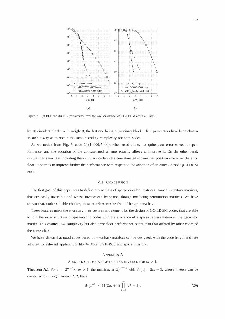
5) Case5: A common solution for reducing the error floor in LDGM codes isrepresented by the adoption

of concatenated schemes, formed by an outer high-rate LDGM code followed by an inner low-rate LDGM code

[8], [9]. Decoding is accomplished by using two belief propagation decoders in serial concatenation: first, the

inner code is decoded starting from channel information, then thea posteriori messages it produces are used

asa priori information to initialize the outer decoder.

By this procedure, the error floor of a single low-rate LDGM code can be often significantly reduced, at the

cost of increased complexity due to the serial concatenation. However, we have verified that, also in concatenated

schemes, the adoption ofψ-unitary codes can help to improve performance. As an example, we have considered

a (10000, 5000) inner QC-LDGM code having parity-check matrix formed by a5000 × 5000 circulant block

with weight 5, followed by a5000 × 5000 identity matrix. Such code, denoted asCI(10000, 5000) in Table

III, has been used in serial concatenation with two different (5000, 4500) outer codes, both described by a

parity-check matrix in the form of a row of ten500 × 500 circulant blocks. The first outer code, denoted as

CI(5000, 4500), is an I-based QC-LDGM code, characterized by: two circulant blocks with weight4, seven

circulant blocks with weight3 and one identity block. The second code, denoted asCψ(5000, 4500), is described

24

0 1 2 3 4 5 6 710-9

10-8

10-7

10-6

10-5

10-4

10-3

10-2

10-1

Eb/N

0 [dB]

CI(10000, 5000)

with CI(5000, 4500) outer

with Cψ(5000, 4500) outer

(a)

0 1 2 3 4 5 6 710-6

10-5

10-4

10-3

10-2

10-1

100

Eb/N

0 [dB]

CI(10000, 5000)

with CI(5000, 4500) outer

with Cψ(5000, 4500) outer

(b)

Figure 7. (a) BER and (b) FER performance over the AWGN channel of QC-LDGM codes of Case5.

by 10 circulant blocks with weight3, the last one being aψ-unitary block. Their parameters have been chosen

in such a way as to obtain the same decoding complexity for both codes.

As we notice from Fig. 7, codeCI(10000, 5000), when used alone, has quite poor error correction per-

formance, and the adoption of the concatenated scheme actually allows to improve it. On the other hand,

simulations show that including theψ-unitary code in the concatenated scheme has positive effects on the error

floor: it permits to improve further the performance with respect to the adoption of an outerI-based QC-LDGM

code.

VII. C ONCLUSION

The first goal of this paper was to define a new class of sparse circulant matrices, namedψ-unitary matrices,

that are easily invertible and whose inverse can be sparse, though not being permutation matrices. We have

shown that, under suitable choices, these matrices can be free of length-4 cycles.

These features make theψ-unitary matrices a smart element for the design of QC-LDGM codes, that are able

to join the inner structure of quasi-cyclic codes with the existence of a sparse representation of the generator

matrix. This ensures low complexity but also error floor performance better than that offered by other codes of

the same class.

We have shown that good codes based onψ-unitary matrices can be designed, with the code length and rate

adopted for relevant applications like WiMax, DVB-RCS and space missions.

APPENDIX A

A BOUND ON THE WEIGHT OF THE INVERSE FORm > 1.

Theorem A.1 For n = 2m+2s, m > 1, the matrices inΞ2m+2ss with W [a] = 2m + 3, whose inverse can be

computed by using Theorem V.2, have

W [a−1] ≤ 11(2m+ 3)

m∏

k=2

(2k + 3). (29)

25

Proof: Let us consider (13). Based on the expressions in Section V-B, we know that:

W [a2m

+ w] ≤ 11.

On the other hand, it is easy to find:

W [a2i

] =

2m+ 3 for i = 0,

2m+ 5− 2i for i > 0.(30)

Therefore:

W [a−1] ≤ W [a2m

+ w]m−1∏

i=0

W [a2i

]

≤ 11(2m+ 3)

m−1∏

i=1

(2m+ 5− 2i)

and, through simple algebra, (29) is finally obtained.

It should be noticed that the upper bound (29) can be loose: depending on the matrix structure, the actual

weight of the inverse can be much smaller.

Example 7

Let us consider the matrix of the Example 5, that is characterized bym = 2. Its inverse, computed through (13), results in:

a−1(x) = (a4(x) + w(x))a2(x)a(x)

= (0; 1; 2; 8; 12; 14; 15; 16; 17; 19; 20; 24; 28; 32; 36;

39; 40; 43; 44; 48; 56; 60; 63; 68; 72; 80; 84; 87; 92;

96; 103; 105; 107; 108; 120; 127; 131; 132; 144; 151;

156; 168; 175)176

and, therefore,W [a−1] = 43. On the other hand, the upper bound in this case givesW [a−1] < 539, that exceeds the value

of n. It should be observed, however, that the polynomiala(x) (as well asa−1(x)) can be scaled in such a way as to

maintain the weight with a larger size. For example, we can define:

a′(x) = 8 ∗ a(x) = 8 ∗ (0; 1; 3; 7; 12; 25; 51)176 =

= (0; 8; 24; 56; 96; 200; 408)1408

such thata′(x) has the same features ofa(x) but a lower density. Moreover, its inverse has the same weight ofa−1(x). �

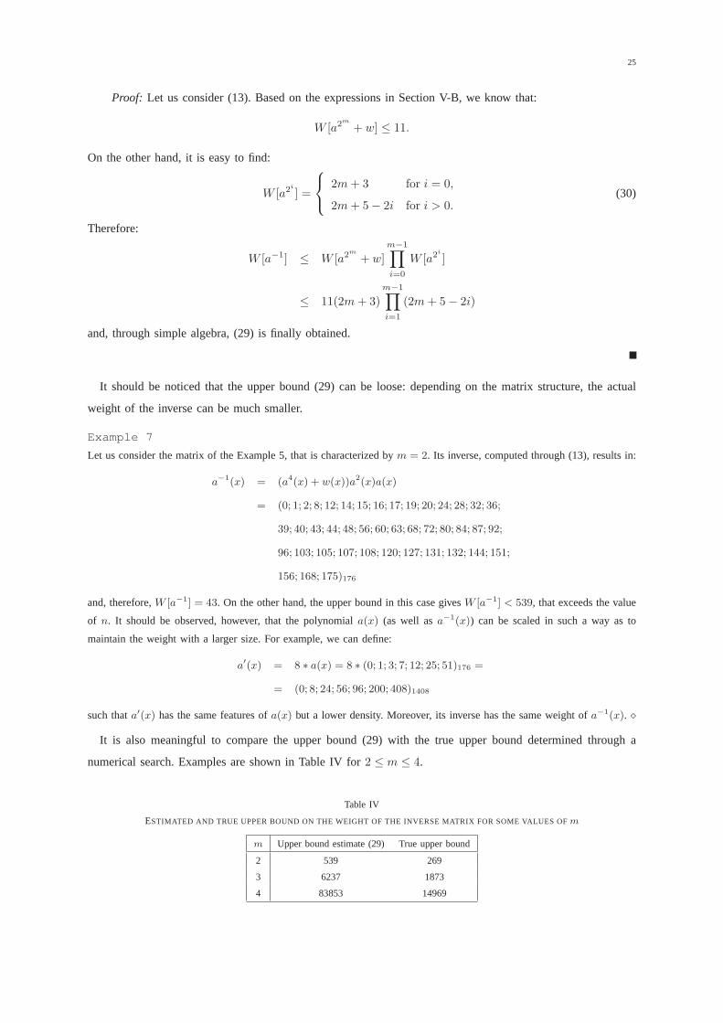
It is also meaningful to compare the upper bound (29) with thetrue upper bound determined through a

numerical search. Examples are shown in Table IV for2 ≤ m ≤ 4.

Table IV

ESTIMATED AND TRUE UPPER BOUND ON THE WEIGHT OF THE INVERSE MATRIX FOR SOME VALUES OFm

m Upper bound estimate (29) True upper bound

2 539 269

3 6237 1873

4 83853 14969

26

As already observed form = 1, the upper bound becomes smaller if specific relationships between theki’s

are established. As an example, form = 2, k1 = 3k0 andk2 = 4k0 we findW [a−1] ≤ 75.

ACKNOWLEDGMENT

The authors are grateful to the anonymous reviewers for their comments, which helped to improve several

aspects of this paper. In particular, they wish to thank one reviewer for having suggested the procedure for

obtaining the minimum distance and multiplicity of the considered codes. They are also very grateful to Prof.

Igal Sason for fruitful discussion on the estimate of the codes performance.

REFERENCES

[1] T. Richardson and R. Urbanke, “The capacity of low-density parity-check codes under message-passing decoding,”IEEE Trans.

Inform. Theory, vol. 47, no. 2, pp. 599–618, Feb. 2001.

[2] G. Wiechman and I. Sason, “Parity-check density versus performance of binary linear block codes: New bounds and applications,”

IEEE Trans. Inform. Theory, vol. 53, no. 2, pp. 550–579, Feb. 2007.

[3] T. Richardson and R. Urbanke, “Efficient encoding of low-density parity-check codes,”IEEE Trans. Inform. Theory, vol. 47, no. 2,

pp. 638–656, Feb. 2001.

[4] S. Freundlich, D. Burshtein, and S. Litsyn, “Approximately lower triangular ensembles of LDPC codes with linear encoding

complexity,” IEEE Trans. Inform. Theory, vol. 53, no. 4, pp. 1484–1494, Apr. 2007.

[5] D. Haley, A. Grant, and J. Buetefuer, “Iterative encoding of low-density parity-check codes,” inProc. IEEE Global Telecommunications

Conference (GLOBECOM ’02), vol. 2, Taipei, Taiwan, Nov. 2002, pp. 1289–1293.

[6] D. Haley and A. Grant, “Improved reversible LDPC codes,” in Proc. IEEE International Symposium on Information Theory (ISIT

2005), Adelaide, Australia, Sep. 2005, pp. 1367–1371.

[7] J. F. Cheng and R. J. McEliece, “Some high-rate near capacity codecs for the Gaussian channel,” inProc. 34th Allerton Conference

on Communications, Control and Computing, Allerton, IL, Oct. 1996.

[8] J. Garcia-Frias and W. Zhong, “Approaching Shannon performance by iterative decoding of linear codes with low-density generator

matrix,” IEEE Commun. Lett., vol. 7, no. 6, pp. 266–268, Jun. 2003.

[9] M. González-López, F. J. Vázquez-Araújo, L. Castedo, and J. Garcia-Frias, “Serially-concatenated low-density generator matrix

(SCLDGM) codes for transmission over AWGN and Rayleigh fadingchannels,”IEEE Trans. Wireless Commun., vol. 6, no. 8, pp.

2753–2758, Aug. 2007.

[10] J.-S. Kim and H.-Y. Song, “Concatenated LDGM codes withsingle decoder,”IEEE Commun. Lett., vol. 10, no. 4, pp. 287–289, Apr.

2006.

[11] T. R. Oenning and J. Moon, “A low-density generator matrix interpretation of parallel concatenated single bit parity codes,”IEEE

Trans. Magn., vol. 37, no. 2, pp. 737–741, Mar. 2001.

[12] C.-H. Hsu and A. Anastasopoulos, “Asymptotic weight distributions of irregular repeat-accumulate codes,” inProc. IEEE Global

Telecommunications Conference (GLOBECOM ’05), Saint Louis, MO, Nov. 2005, pp. 1147–1151.

[13] H. Jin, A. Khandekar, and R. McEliece, “Irregular repeat-accumulate codes,” inProc. Second International Symposium on Turbo

Codes, Brest, France, Sep. 2000, pp. 1–8.

[14] A. Abbasfar, D. Divsalar, and K. Yao, “Accumulate repeataccumulate codes,” inProc. IEEE Global Telecommunications Conference

(GLOBECOM ’04), Dallas, TX, Nov. 2004, pp. 509–513.

[15] H. D. Pfister and I. Sason, “Accumulate-repeat-accumulate codes: Capacity-achieving ensembles of systematic codes for the erasure

channel with bounded complexity,”IEEE Trans. Inform. Theory, vol. 53, no. 2, pp. 2088–2115, Jun. 2007.

[16] Z. Li, L. Chen, L. Zeng, S. Lin, and W. Fong, “Efficient encoding of quasi-cyclic low-density parity-check codes,”IEEE Trans.

Commun., vol. 54, no. 1, pp. 71–81, Jan. 2006.

[17] M. P. C. Fossorier, “Quasi-cyclic low-density parity-check codes from circulant permutation matrices,”IEEE Trans. Inform. Theory,

vol. 50, no. 8, pp. 1788–1793, Aug. 2004.

[18] 802.16e 2005,IEEE Standard for Local and Metropolitan Area Networks - Part 16: Air Interface for Fixed and Mobile Broadband

Wireless Access Systems - Amendment for Physical and MediumAccess Control Layers for Combined Fixed and Mobile Operation

in Licensed Bands, IEEE Std., Dec. 2005.

27

[19] C. Yoon, E. Choi, M. Cheong, and S.-K. Lee, “Arbitrary bit generation and correction technique for encoding QC-LDPCcodes with

dual-diagonal parity structure,” inProc. IEEE WCNC 2007, Hong Kong, Mar. 2007, pp. 663–667.

[20] S. Myung, K. Yang, and J. Kim, “Quasi-cyclic LDPC codes for fast encoding,”IEEE Trans. Inform. Theory, vol. 51, no. 8, pp.

2894–2901, Aug. 2005.

[21] CCSDS, “Low Density Parity Check Codes for Use in Near-Earth and Deep Space Applications,” Consultative Committee for Space

Data Systems (CCSDS), Washington, DC, USA, Tech. Rep. OrangeBook, Sep. 2007.

[22] S. J. Johnson and S. R. Weller, “A family of irregular LDPCcodes with low encoding complexity,”IEEE Commun. Lett., vol. 7,

no. 2, pp. 79–81, Feb. 2003.

[23] T. Xia and B. Xia, “Quasi-cyclic codes from extended difference families,” inProc. IEEE Wireless Commun. and Networking Conf.,

vol. 2, New Orleans, LA, Mar. 2005, pp. 1036–1040.

[24] F. MacWilliams, “Orthogonal circulant matrices over finite fields, and how to find them,”J. Comb. Theory Series A, vol. 10, pp.

1–17, 1971.

[25] Z. Zhang, “Construction of the orthogonal groups ofn × n circulant matrices over finite fields,” Ph.D. dissertation, Concordia

University, Montreal, Quebec, Canada, Jan. 1997.

[26] D. Bini, G. M. Del Corso, G. Manzini, and L. Margara, “Inversion of circulant matrices overZm,” Math. Comp., vol. 70, pp.

1169–1182, 2001.

[27] (2009) PARI/GP. [Online]. Available: http://pari.math.u-bordeaux.fr/

[28] J. Hagenauer, E. Offer, and L. Papke, “Iterative decoding of binary block and convolutional codes,”IEEE Trans. Inform. Theory,

vol. 42, no. 2, pp. 429–445, Mar. 1996.

[29] N. Kamiya, “High-rate quasi-cyclic low-density parity-check codes derived from finite affine planes,”IEEE Trans. Inform. Theory,

vol. 53, no. 4, pp. 1444–1459, Apr. 2007.

[30] Digital Video Broadcasting (DVB); Interaction channel forsatellite distribution systems, ETSI EN Std. 301 790 (v1.4.1), Sep. 2005.

[31] T. Lestable, E. Zimmerman, M.-H. Hamon, and S. Stiglmayr, “Block-LDPC codes vs duo-binary turbo-codes for european next

generation wireless systems,” inProc. IEEE VTC-2006 Fall, Montreal, Canada, Sep. 2006, pp. 1–5.

[32] M. Baldi, G. Cancellieri, and F. Chiaraluce, “Finite-precision analysis of demappers and decoders for LDPC-coded M-QAM-systems,”

IEEE Trans. Broadcast., vol. 55, no. 2, pp. 239–250, Jun. 2009.