UNIVERSITA’ DI PADOVA DIPARTIMENTO DI INGEGNERIA DELL’INFORMAZIONE DOTTORATO DI RICERCA IN INGEGNERIA INFORMATICA ED ELETTRONICA INDUSTRIALI - XV CICLO OMNIDIRECTIONAL VISION FOR MOBILE ROBOTS Coordinatore: Prof.ssa Concettina Guerra Tutore: Prof. Enrico Pagello Emanuele Menegatti Padova - 31 Dicembre 2002

Welcome message from author
This document is posted to help you gain knowledge. Please leave a comment to let me know what you think about it! Share it to your friends and learn new things together.
Transcript

UNIVERSITA’ DI PADOVA
DIPARTIMENTO DI INGEGNERIA
DELL’INFORMAZIONE
DOTTORATO DI RICERCA IN INGEGNERIA INFORMATICAED ELETTRONICA INDUSTRIALI - XV CICLO
OMNIDIRECTIONAL VISION FORMOBILE ROBOTS
Coordinatore: Prof.ssa Concettina Guerra
Tutore: Prof. Enrico Pagello
Emanuele Menegatti
Padova - 31 Dicembre 2002


Abstract
This dissertation describes the work done by the author in the period of
his Ph.D. in the field of omnidirectional vision.
After a general presentation on omnidirectional vision, the dissertation
focuses on omnidirectional vision for mobile robotics. Each chapter of the dis-
sertation covers a different topic in omnidirectional vision for mobile robotics.
The three main chapters describe the evolution of an omnidirectional vision
system to be mounted on a mobile robot. First, a new simple algorithm
used to produce low-cost omnidirectional mirrors with custom profiles is pre-
sented. Second, a new method of hierarchical localisation is described. Hi-
erarchical localisation is defined as the determination of the robot’s position
with different accuracies depending on the environment structure. Third,
the implementation of the Spatial Semantic Hierarchy is described in detail.
The Spatial Semantic Hierarchy of B. Kuipers has been previously imple-
mented only on simulated robots or on robots with sonar in very simple
environments. The described implementation deals with a real robot, in a
real-world environment, equipped with an omnidirectional vision sensor only.
The last chapter describes an extension of omnidirectional vision from
single robot domain to multi-robot domain. The aim is to build an Omni-
directional Distributed Vision System. In a Distributed Vision System, the
different sensors are networked. The interaction and the communication be-
tween the sensors enables intelligent behaviours not achievable with a single
sensor. This last section should be considered as an overview of the current
work of the author, in which preliminary results and preliminary experiments
are reported.

ii

Abstract
Questa tesi descrive il lavoro svolto dall’autore nel campo della visione
omnidirezionale durante il suo adottarti.
La tesi, dopo una presentazione generale sulla visione omnidirezionale,
si concentra sulla visione omnidirezionale per robot mobili. Ogni capitolo
affronta un diverso argomento di visione omnidirezionale per robotica mo-
bile. I tre capitoli principali descrivono l’evoluzione di un sistema di visione
omnidirezionale per un robot mobile. Dapprima presentato un nuovo algo-
ritmo per la produzione di specchi omnidirezionali a basso costo con profilo
variabile. Poi si passa alla descrizione di un nuovo metodo di localizzazione
gerarchica per il robot: l’idea quella di determinare la posizione del robot
con un’accuratezza che dipende dalla struttura dell’ambiente che circonda
il robot. In fine viene descritta in dettaglio l’implementazione della Spatial
Semantic Hierarchy di B. Kuipers su un robot reale. La Spatial Semantic
Hierarchy era stata testata precedentemente solo su robot simulati o robot
dotati di sonar che operano in ambienti molto semplici. L’implementazione
descritta stata realizzata su un robot reale, che opera in un ambiente reale
ed dotato solo di un sensore di visione omnidirezionale.
L’ultimo capitolo riporta il lavoro svolto per applicare la visione omni-
direzionale a sistemi multi-robot. L’obiettivo quello di realizzare un Om-
nidirectional Distributed Vision System in cui i vari sensori omnidirezionali
siano collegati in rete tra loro e in cui l’interazione tra i singoli sensori genera
dei comportamenti intelligenti che non possono essere ottenuti con un singolo
sensore. L’ultimo capitolo dovrebbe essere considerato come una panoramica
del lavoro attuale dell’autore, in cui vengono riportati risultati ed esperimenti
preliminari.

ii

Al Mio Amore,
“. . . viaggiare io e te
con la stessa valigia in due
dividendo tutto sempre”
(Tiromancino)
Alla Mia Mamma e al Mio Papa,
“. . . dammi ancora la mano, anche se quello stringerla
e solo un pretesto per sentire la fiducia totale che nes-
suno mi ha dato o mi ha mai chiesto. . . (F. Guccini)
iii

iv

Acknowledgement
To compress in one page all the people I met in three years of Ph.D. is
not easy. There are so many people I wish to thank for their support and
their help. First of all I wish to mention my wife Maria Grazia that forwent
three years of beach holidays for following me around the world. My parents
always present and ready to support me. I wish to remember my mother
always worried about my health especially when I was on the other side of
the world. My friends, they were close even if I was on the other side of the
world: Samuele, Matteo, Marco, Carlo, Nico, Daniel, Justin.
I wish to thank all the scientists I met, for the marvellous things they
taught me: my supervisor Enrico Pagello, Bob Fisher, Mark Right and John
Hallam of the University of Edinburgh (U.K.), Hiroshi Ishiguro and Takayuki
Nakamura of the University of Wakayama (Japan), Wolfram Burgard of the
University of Freibur (Germany), Ben Krose of the University of Amsterdam
(The Nederlands), Ryad Benosman of the University of Paris 6 (France).
A special thank goes to Hiroshi Ishiguro for the invitation in his labo-
ratory at Wakayama University (Japan), for the wonderful atmosphere he
created there for me and for the support he kindly provided me.
Last but not least, I wish to mention my colleagues of the box dottorandi
at the University of Padua. Thank to them, lunch was a relief from work
and coffee was an extra pleasure: Barbara, Chiara, Marco, Enrico, Andrea,
Gianluigi, Stefano, Francesco.
This research has been supported by: the PRASSI project of ENEA (the
v

Italian National Agency for New Technologies, Energy and Environment),
Padova Richerche s.c.p.a. (Padova - ITALY), Tecnogamma s.p.a. (Traviso
- ITALY), the Scottish Award Agency (U.K.), the University of Wakayama
(Japan), Progetto sui Sistemi Multi-Robot of The University of Padua, the
Ph.D. School of the University of Padua.
vi

Contents
1 Introduction 11.1 The Sense of Vision . . . . . . . . . . . . . . . . . . . . . . . . 11.2 Omnidirectional Vision . . . . . . . . . . . . . . . . . . . . . . 31.3 Omnidirectional Vision for Mobile Robotics . . . . . . . . . . 41.4 The dissertation overview . . . . . . . . . . . . . . . . . . . . 5
2 Omnidirectional Imaging 92.1 Omnidirectional Vision in Animals . . . . . . . . . . . . . . . 92.2 Omnidirectional Vision in Arts . . . . . . . . . . . . . . . . . 11
2.2.1 The extension of the perception . . . . . . . . . . . . . 122.2.2 Capturing the horizon . . . . . . . . . . . . . . . . . . 16
2.3 Omnidirectional Vision in Science . . . . . . . . . . . . . . . . 192.3.1 Compound-eye cameras . . . . . . . . . . . . . . . . . 212.3.2 Panoramic cameras . . . . . . . . . . . . . . . . . . . . 222.3.3 Omnidirectional cameras . . . . . . . . . . . . . . . . . 222.3.4 Special lens cameras . . . . . . . . . . . . . . . . . . . 232.3.5 Convex mirror cameras . . . . . . . . . . . . . . . . . . 242.3.6 Folded catadioptric cameras . . . . . . . . . . . . . . . 26
2.4 Conclusions . . . . . . . . . . . . . . . . . . . . . . . . . . . . 27
3 Omnidirectional Mirror Design 293.1 Classical Mirror Shapes . . . . . . . . . . . . . . . . . . . . . . 303.2 The design of the mirror . . . . . . . . . . . . . . . . . . . . . 35
3.2.1 The algorithm . . . . . . . . . . . . . . . . . . . . . . . 373.2.2 The making of the mirror . . . . . . . . . . . . . . . . 38
3.3 The task commits the design . . . . . . . . . . . . . . . . . . . 393.3.1 Requirements for the soccer robots . . . . . . . . . . . 403.3.2 Requirements for the mapping robot . . . . . . . . . . 42
3.4 The final design . . . . . . . . . . . . . . . . . . . . . . . . . . 433.4.1 The common structure . . . . . . . . . . . . . . . . . . 443.4.2 The mirrors’ parameters . . . . . . . . . . . . . . . . . 47
vii

3.5 Conclusions . . . . . . . . . . . . . . . . . . . . . . . . . . . . 49
4 Omnidirectional Vision for Robot Localisation 514.1 Robot Localisation . . . . . . . . . . . . . . . . . . . . . . . . 524.2 Image-based Localisation . . . . . . . . . . . . . . . . . . . . . 53
4.2.1 Image signature . . . . . . . . . . . . . . . . . . . . . . 564.2.2 Similarity computation . . . . . . . . . . . . . . . . . . 60
4.3 Hierarchical Memory-based Localisation . . . . . . . . . . . . 634.4 Monte-Carlo Localisation . . . . . . . . . . . . . . . . . . . . . 694.5 Conclusions . . . . . . . . . . . . . . . . . . . . . . . . . . . . 71
5 Omnidirectional Vision for Mapping 755.1 Mobile Robot Navigation . . . . . . . . . . . . . . . . . . . . . 755.2 The Spatial Semantic Hierarchy . . . . . . . . . . . . . . . . . 785.3 Omnidirectional vision and map building . . . . . . . . . . . . 80
5.3.1 The assumptions . . . . . . . . . . . . . . . . . . . . . 835.4 The Simulations . . . . . . . . . . . . . . . . . . . . . . . . . . 84
5.4.1 The feature selection . . . . . . . . . . . . . . . . . . . 875.4.2 Qualitative Analysis . . . . . . . . . . . . . . . . . . . 88
5.5 The Vision System . . . . . . . . . . . . . . . . . . . . . . . . 965.5.1 The algorithm . . . . . . . . . . . . . . . . . . . . . . . 97
5.6 The Simulated Experiment . . . . . . . . . . . . . . . . . . . . 1055.7 The Real Experiment . . . . . . . . . . . . . . . . . . . . . . . 1085.8 Conclusions . . . . . . . . . . . . . . . . . . . . . . . . . . . . 120
6 Distributed Omnidirectional Vision 1236.1 Distributed Vision in Robotics . . . . . . . . . . . . . . . . . . 1236.2 Mobile Robot DVS . . . . . . . . . . . . . . . . . . . . . . . . 126
6.2.1 VAs on the same robot . . . . . . . . . . . . . . . . . . 1266.2.2 VAs on different robots . . . . . . . . . . . . . . . . . . 128
6.3 Learning DVS . . . . . . . . . . . . . . . . . . . . . . . . . . . 1336.3.1 The task to be learnt . . . . . . . . . . . . . . . . . . . 1356.3.2 Vision System . . . . . . . . . . . . . . . . . . . . . . . 1376.3.3 Training the Neural Networks . . . . . . . . . . . . . . 143
6.4 Conclusions . . . . . . . . . . . . . . . . . . . . . . . . . . . . 144
Appendices 158
viii

List of Figures
1.1 The field of view of preys and predators . . . . . . . . . . . . 2
2.1 The close-up view of the eye of a fossil trilobite . . . . . . . . 10
2.2 A sketch of the compound eye of a diurnal insect . . . . . . . 10
2.3 A sketch of the compound eye of a nocturnal insect. . . . . . . 11
2.4 A sketch of the compound eye of a crustacean. . . . . . . . . . 12
2.5 “The Wedding of Giovanni Arnolfini” of Jan van Eyck. . . . . 13
2.6 The zoom on the witch mirror . . . . . . . . . . . . . . . . . . 13
2.7 “The praetor and his wife” of Quentin Metsys. . . . . . . . . . 13
2.8 The zoom on the witch mirror . . . . . . . . . . . . . . . . . . 13
2.9 A litograph of Escher: Hand with Reflecting Sphere 1935. . . . 14
2.10 An example of anamorphosis . . . . . . . . . . . . . . . . . . . 15
2.11 A second example of anamorphosis . . . . . . . . . . . . . . . 15
2.12 The panorama . . . . . . . . . . . . . . . . . . . . . . . . . . . 17
2.13 The panorama of Edinburgh . . . . . . . . . . . . . . . . . . . 18
2.14 An ancian panoramic camera. . . . . . . . . . . . . . . . . . . 18
2.15 A panoramic picture . . . . . . . . . . . . . . . . . . . . . . . 19
2.16 The DodecaTM 1000 Camera . . . . . . . . . . . . . . . . . . 20
2.17 The S.O.S. sensor . . . . . . . . . . . . . . . . . . . . . . . . . 20
2.18 The RingCam realised in the Microsoft Laboratories. . . . . . 20
2.19 The dome at CMU . . . . . . . . . . . . . . . . . . . . . . . . 20
2.20 The panning camera and the range technique . . . . . . . . . 22
ix

2.21 omnidirectional image . . . . . . . . . . . . . . . . . . . . . . 23
2.22 A camera mounting a PAL lens. . . . . . . . . . . . . . . . . . 24
2.23 A cameras mounting convex mirrors of Accowle Co. Ltd. . . . 24
2.24 An example of folded catadioptric camera. . . . . . . . . . . . 24
2.25 A sketch of a basic optics of PAL . . . . . . . . . . . . . . . . 25
2.26 A sketch of a basic optics of a convex mirror camera. . . . . . 25
2.27 A sketch of a basic optics of a folded catadioptric camera. . . 26
3.1 The omnidirectional vision system. . . . . . . . . . . . . . . . 30
3.2 The different mirror profiles . . . . . . . . . . . . . . . . . . . 32
3.3 Hyperboloidal projection and examples of transformed images 33
3.4 (Left) Image formation sketch (Right) The geometrical con-
struction of the custom mirror . . . . . . . . . . . . . . . . . . 35
3.5 (Left) The virtual model of a custom profile mirror. (Right)
A virtual omnidirectional image of the virtual reconstruction
of the RoboCup field of play. . . . . . . . . . . . . . . . . . . 39
3.6 (Left) The actual mirror produced for the goalkeeper. (Right)
An omnidirectional image acquired with the omnidirectional
sensor of the goalkeeper. . . . . . . . . . . . . . . . . . . . . . 40
3.7 (Left) The radial dimension of the mirror if we want the om-
nidirectional view to occupy the widest portion of the image.
(Right) A sketch of the multi-part mirror profile. . . . . . . . 44
3.8 Mirror profiles . . . . . . . . . . . . . . . . . . . . . . . . . . . 48
3.9 Comparation of three mirrors . . . . . . . . . . . . . . . . . . 49
4.1 Image based localisation. . . . . . . . . . . . . . . . . . . . . . 53
4.2 An omnidirectional image taken at a reference location. . . . . 55
4.3 The panoramic cylinder created by the omnidirectional image
of Fig. 4.2. . . . . . . . . . . . . . . . . . . . . . . . . . . . . . 55
4.4 The power spectrum of the Fourier transform of the image . . 59
x

4.5 The plot of the similarity function values . . . . . . . . . . . . 61
4.6 The values of the similarity functions . . . . . . . . . . . . . . 62
4.7 The relation between brightness pattern and spatial frequency 65
4.8 An example of hierarchical localisation . . . . . . . . . . . . . 66
4.9 Several examples of hierarchical localisation . . . . . . . . . . 68
4.10 Two examples of Monte-Carlo localisation . . . . . . . . . . . 72
5.1 The robot with its omnidirectional vision sensor. . . . . . . . . 78
5.2 The conic projection . . . . . . . . . . . . . . . . . . . . . . . 81
5.3 The “exploring around the block” problem. . . . . . . . . . . . 81
5.4 The virtual environment . . . . . . . . . . . . . . . . . . . . . 84
5.5 The Mirror Profile. . . . . . . . . . . . . . . . . . . . . . . . . 85
5.6 Perspective and omnidirectional views in the virtual environment 86
5.7 A perspective sequence and the corresponding omnidirectional
view . . . . . . . . . . . . . . . . . . . . . . . . . . . . . . . . 89
5.8 The simulation of an edge exiting from occlusion. . . . . . . . 91
5.9 The simulation of an edge going to be occluded. . . . . . . . . 91
5.10 The simulation of the robot passing through a door . . . . . . 92
5.11 The simulation of the crossing point of the imaginary lines
connecting opposites edges. . . . . . . . . . . . . . . . . . . . 92
5.12 The bird’s eye view of the crossing point of the imaginary lines
connecting opposites edges. . . . . . . . . . . . . . . . . . . . 93
5.13 The simulation of a sequence acquired by the omnidirectional
camera of the robot while it turns on the spot . . . . . . . . . 94
5.14 The simulation showing that not all radial lines are vertical
edges. . . . . . . . . . . . . . . . . . . . . . . . . . . . . . . . 95
5.15 The unprocessed image as view from the robot’s camera. . . . 98
5.16 The image after the Canny edge detection. . . . . . . . . . . . 98
5.17 The edge image after the Hough transform. . . . . . . . . . . . 98
5.18 The final result showing the edge matching. . . . . . . . . . . 98
xi

5.19 The two possible processes for a Canny colour edge detection. 100
5.20 The Hough transform . . . . . . . . . . . . . . . . . . . . . . . 101
5.21 A close up of a processed image showing the averaging windows.103
5.22 The disposition of the averaging windows in the 360◦ . . . . . . 103
5.23 The path of the robot through the virtual environment. . . . . 106
5.24 The simulation of an ephemeral edge . . . . . . . . . . . . . . 106
5.25 The simulation of a false edge . . . . . . . . . . . . . . . . . . 107
5.26 Tracking the vertical edges in a simulated sequence. Translation109
5.27 Tracking the vertical edges in a simulated sequence. Rotation 110
5.28 The experimental set-up . . . . . . . . . . . . . . . . . . . . . 111
5.29 The centre of a real image . . . . . . . . . . . . . . . . . . . . 112
5.30 An example of the image process stages for a real image. . . . 113
5.31 An example of false edge . . . . . . . . . . . . . . . . . . . . . 114
5.32 The averaging windows used for the real robot . . . . . . . . . 115
5.33 An example of strong reflection on the body of the robot . . . 117
5.34 Tracking the vertical edges in a real sequence. Translation . . 118
5.35 Tracking the vertical edges in a real sequence. Rotation . . . . 119
6.1 Our team of heterogeneous robots . . . . . . . . . . . . . . . . 126
6.2 A close view of the vision system of Nelson. On the left,
the perspective camera. In the middle, pointed up-ward the
omnidirectional camera . . . . . . . . . . . . . . . . . . . . . . 127
6.3 A close view of two of our robots. Note the different vision
systems . . . . . . . . . . . . . . . . . . . . . . . . . . . . . . 129
6.4 A picture of the whole system showing two Vision Agents and
the robot used in the experiments. . . . . . . . . . . . . . . . 134
6.5 The knowledge propagation process . . . . . . . . . . . . . . . 136
6.6 A picture of the hardware resource of the Vision Agent . . . . 137
6.7 The simplified scheme of a Vision Agents . . . . . . . . . . . . 138
6.8 A snapshot of the image processing software . . . . . . . . . . 140
xii

6.9 The structure of the used neural network. . . . . . . . . . . . 140
6.10 A plot of the sigmoid function. . . . . . . . . . . . . . . . . . . 141
6.11 The positions of the robot in the image for the training data. . 144
6.12 A plot of the learning error on the speed output. . . . . . . . . 145
6.13 A plot of the learning error on the jog output. . . . . . . . . . 145
xiii

xiv

List of Tables
3.1 The capabilities required to the vision system of the soccer
robots . . . . . . . . . . . . . . . . . . . . . . . . . . . . . . . 41
3.2 The constraints on the vision system of the soccer robots . . . 41
3.3 The constraints on the vision system of the soccer robots . . . 42
3.4 The constraints on the vision system of the soccer robots . . . 42
3.5 The requirements on the vision system of the mapping robot . 43
3.6 The constraints on the vision system of the mapping robot . . 43
3.7 The areas at different resolution of the three omnidirectional
vision sensors . . . . . . . . . . . . . . . . . . . . . . . . . . . 47
4.1 Memory saving introduced by the Fourier signature . . . . . . 60
xv

xvi

Chapter 1
Introduction
The sense of vision is one of the most effective way of collecting information on
the surrounding environment. This is true both for animals and for machines.
Since the beginning of research on mobile robotics the scientists tried to
give the robots the sense of vision. Many times the progress of science and
technology was inspired by the observation of the Nature. We will introduce
the omnidirectional vision and its advantages by looking at the world of
nature. From these observations, it will be evident the need to design different
vision systems for robots performing different tasks.
1.1 The Sense of Vision
The knowledge of the surroundings in Nature is essential to survive. For
instance, the ability to effectively track the motion of a pray or the ability
to spot a predator while it is far away are essential skills in the struggle for
survival. The natural distinction of animals into preys and predators brought
to the development of two different kind of vision systems.
The vision systems of preys is “designed” with the largest possible vision
field in order to survey the widest area around them. This brought to very
large eyes positioned on the opposing sides of the snout. This arrangement
1

2 Omnidirectional Vision for Mobile Robots
Figure 1.1: The field of view of preys (left) and predators (right).
assures the maximum coverage of the environment, because the field of views
of the two eyes have a very little overlap or do not overlap at all. With this
arrangement preys can achieve up to 360◦ of field of view.
The vision system of predators is designed with the highest acuity in
order to accurately locate their preys. This brought to eyes positioned on
the forward part of the snout with a big overlap of the vision fields of the two
eyes in order to perform stereoscopic vision enabling the accurate estimation
of the pose of objects of interest. The resolution achievable by animals is
impressive, e.g. an eagle can spot an hare from two kilometres away.
The two tracks followed by the evolution are evidences of the trade off we
face when building an artificial vision system: should we privilege the high
resolution or should we privilege the wide field of view? The two approaches
can be combined only to some extent. In fact, increasing the resolution of
the vision sensor and extending the vision field of the sensor, both increase
the amount of information gathered from the sensor. This information then
should be processed. If the amount of information is too high this processing
is too burdensome and there is no advantage. This is true for the vision
organs of the animals and for the artificial vision systems we can build.

Chapter 1. Introduction 3
In this dissertation, we will present our efforts for building an artificial
vision system with a very large field of view. We will focus on the design
of sensors that can grab images with 360◦ of horizontal field of view and on
the techniques developed by the author for extracting from omnidirectional
images the information needed by a mobile robot.
1.2 Omnidirectional Vision
The term Omnidirectional Vision refers to vision sensor with a very large
field of view, i.e. sensor with a horizontal field of view of 360◦ and a variable
vertical field of view usually between 60◦ and 150◦ .
Usually animals achieve a 360◦ field of view with two eyes. The field of
view of every eye is limited to 140–220◦ , but some animal presents eyes with
a 360◦ of horizontal field of view. These eyes can be considered as omnidirec-
tional sensors. When the mankind started to reproduce the world into paint-
ings, it tried to give the sense of “reality” by generating very large sight of the
represented environment. Lately, machine vision researchers discovered that
the imaging techniques developed as a form of art or “divertissment” could
be used also in scientific domains and new generations of omnidirectional
sensors sprouted out.
Omnidirectional vision is a new technique and probably is not mature
yet for commercial and market application, but its use is growing very fast.
More and more laboratory around the world are developing new sensors and
new applications of omnidirectional vision.1 Today, omnidirectional vi-
sion is used in tasks as: wide area surveillance [32], video-conferencing [25],
remote reality [11], non-destructive inspections [30] [5], 3D environment re-
1As an example of the rate of growth, consider the web page “The Page of Omnidi-rectional Vision” (www.cis.upenn.edu/ kostas/omni.html). This page links to Universitiesand Companies working in the field of omnidirectional vision. When the author startedhis work on omnidirectional vision in 2000, this page had only 10 links to Universities and5 or 6 links to companies. Now the links present in the page are more than doubled.

4 Omnidirectional Vision for Mobile Robots
construction [15], etc. Probably, the domain where omnidirectional vision
found the largest application is the mobile robotics domain. This disserta-
tion will illustrate the work of the author in several fields of applications of
omnidirectional vision to mobile robotics.
1.3 Omnidirectional Vision for Mobile Robotics
Usually the cameras used in machine vision tasks are off-the-shelf cameras.
These cameras are designed for television purpose or for grabbing still pic-
tures. In order to apply them to Computer Vision or Robot Vision tasks,
the researchers developed several workarounds to overcome the limitations of
these systems. On the contrary, we believe that, as nature designed different
kind of eyes for different tasks, we should employ (or design, as well) different
imaging sensors for the different tasks assigned to the machines. This is not
always possible due to external constraints (like costs and technological limi-
tations), but omnidirectional cameras, and in particular catadioptric camera,
greatly extended the flexibility of the imaging systems.
Omnidirectional vision is a relatively new technique for mobile robotics.
Its range of applications and the new possibilities offered are not fully under-
stood. In fact, despite the fact that the first works that used omnidirectional
vision sensors mounted on mobile robots date back to the early 90’s, there are
no public available software libraries dedicated to omnidirectional vision.2
Omnidirectional vision sensors are valuable sensors in the field of mobile
robotics, because they offer in one shot a global view of the area surrounding
the robot. For instance, the knowledge of the positions of the objects at
360◦ around the robot is essential in tasks like map matching or image-based
navigation. The field of view at 360◦ greatly reduces the perceptual aliasing
2At the time of writing, at the Intelligent Autonomous System Laboratory (IAS-Lab)of the University of Padua we are working on the first release of V2 our omnidirectionalvision software suite

Chapter 1. Introduction 5
(i.e. the possibility that two distinct places offer the same sensory reading).
In addition, in highly dynamic environment, the continuous view of the area
surrounding the robot enable simple tracking techniques to follow the objects
of interest.
Moreover, the impact of omnidirectional vision is not fully understood
also by people working with omnidirectional vision sensor. The use of an
omnidirectional vision sensor should influence the entire robot. Omnidi-
rectional vision sensors should be considered as a totally different sensors
with respect to a standard perspective cameras. The completeness of their
360◦ field of view should influence the complete robot: the whole body, the
driving system and the software controlling the robot. There should be a
complete synergy between the omnidirectional sensor and the body of the
robot . The body should not impair the omnidirectional vision sensor. For
instance, the body should have a rotational symmetry and be shaped in order
not to occlude the sensor preventing the observation of some areas around
the robot. This recommendation is not followed by many researchers. For
instance, in the RoboCup competitions almost every team is using omnidi-
rectional vision sensors, but only few of them have robots with a circular
symmetry and behaviours that fully exploit the omnidirectional sensor.
1.4 The dissertation overview
This dissertation is intended as a description of the work done by the author
in the field of omnidirectional vision during his Ph.D.
Chapter 2 presents a general overview of the different techniques used
to grab omnidirectional images. The chapter starts with an overview on
omnidirectional vision in animals, then gives a brief panoramic of omnidi-
rectional vision in arts, concluding with the different techniques used at the
moment in the scientific laboratories around the world to capture omnidirec-

6 Omnidirectional Vision for Mobile Robots
tional images. The aim of the chapter is to identify the roots of the modern
omnidirectional vision used in mobile robotics.
Chapter 3 proposes the idea that the omnidirectional vision sensor mounted
on a mobile robot should be customised on the robot’s task and on the robot’s
body. In the chapter, we also detailed the technique used to design and pro-
duce low-cost omnidirectional mirrors with custom profile. Some examples
of realised mirrors are proposed.
Chapter 4 discusses the main scientific result: a method for the hierarchi-
cal localisation of a mobile robot within the image-based localisation frame.
We realised this work when we were visiting researcher at The Intelligent
Robotics Laboratory of Prof. H. Ishiguro at Wakayama University (Japan).
The second part of the chapter discusses the integration of a Monte-Carlo
localisation method with our method of image-based localisation in order to
solve the main problem that affects image-based localisation, i.e. the percep-
tual aliasing. Experimental results are presented.
Chapter 5 presents another main scientific result: the implementation
of the Spatial Semantic Hierarchy of Prof. B. Kuipers on a real robot
fitted only with an omnidirectional vision sensor. The chapter describes why
the omnidirectional vision sensor is a good sensor to implement the Spatial
Semantic Hierarchy. This work started when we were a Master Student in
Artificial Intelligence at the University of Edinburgh (U.K.) during the first
year of our Ph.D and then continued in Padua.
Chapter 6 presents some new topics we are working on. This chapter
should be considered as a kind of “work-in-progress” section even if the ideas
and the first experiments presented have been published in some conferences.
In the first part of the chapter, we present the concept of Distributed Vision
System and Vision Agents. Then we explore how these concepts can be
exploited with omnidirectional vision. In the end we present the first stage
of an Omnidirectional Distributed Vision system composed of uncalibrated

Chapter 1. Introduction 7
omnidirectional cameras that can learn to control a mobile robot.

8 Omnidirectional Vision for Mobile Robots

Chapter 2
Omnidirectional Imaging
In this chapter, we will give an overview of the omnidirectional vision sensors.
We will start introducing some examples of omnidirectional vision in animals
showing that different eyes evolved for different tasks. Then, we will discuss
how the mankind approached the idea of omnidirectional vision within arts
in order expand the perceptive experience of the observer. We will discuss
some of the philosophical implication of this. In the end of the chapter we will
present a brief survey of the modern technique to capture omnidirectional
images and how these are used in science to build more effective artificial
vision systems.
2.1 Omnidirectional Vision in Animals
Several times, the progress of science has been inspired by the observation of
the Nature, so we will start this overview on omnidirectional vision sensors
by analysing some examples of omnidirectional eyes in animals.
One of the first examples of omnidirectional vision sensor appeared on
Earth about 50 Million of years ago. Fig. 2.1 shows a picture of the fossil
eye of a trilobite. This was a compound eye similar to the one of the modern
insects.
9

10 Omnidirectional Vision for Mobile Robots
Figure 2.1: The close-up view of the eye of a fossil trilobite. One of the firstexamples of omnidirectional vision system.
Figure 2.2: A sketch of the compound eye of a diurnal insect. Every facetshas a photoreceptor associated.
Almost, all animal eyes that can be considered omnidirectional vision
sensor are compound eye. The compound eye is composed of a set of optical
elements apt to collect the light rays coming from different directions. These
optical elements are densely packed to form the eye and are called facets.
For the purpose of this panorama on omnidirectional eye, we can broadly
divide the animal compound eyes in three main categories. This division
depends on the technique used to focus the light on the retina.
The first set is composed of eyes where at every facet is associated a
photoreceptive cell, as sketched in Fig. 2.2. This kind of eye is frequent in
diurnal insects.
The second group is composed of eyes with a single retina. The refraction

Chapter 2. Omnidirectional Imaging 11
Figure 2.3: A sketch of the compound eye of a nocturnal insect. Note thatrays of light entering at different facets are focused in the same point on theretina with a refraction.
index of every facet is graduated in order to progressively bend the path of
the incoming light rays. The bending causes parallel rays coming from the
same source to focus at the same point in the retina, Fig. 2.3. Such kind of
eye is apt to work in conditions of very low lightening. This compound eye
is found in nocturnal insects.
The third group is composed of eyes similar to the one of the night insects,
but this group uses reflections instead of refractions in order to focus the
light on the retina. At every facet is associated a lenticular element with a
reflective lateral surface. Once the parallel rays of light coming from the same
object enter the different facet, they are reflected at the lateral surface of the
lenticular elements and focused on the retina. Fig. 2.4 shows a sketch of this
kind of compound eye. This last type of eye can be found in crustaceans.
2.2 Omnidirectional Vision in Arts
At the beginning of the XV century, after the brilliant intuition of Giotto in
the middle of the XIV century, Filippo Brunelleschi unrevealed the geomet-
rical rules underlying the human visual perception and created the perspec-

12 Omnidirectional Vision for Mobile Robots
Figure 2.4: A sketch of the compound eye of a crustacean. Note that rays oflight entering at different facets are focused in the same point on the retinawith a reflection.
tive. The perspective enabled the artist to give a more realistic representa-
tion of reality by following some simple geometrical rules. At the same time,
the artists discovered that they could play with these geometrical rules to
alter the perception of reality. One of the first examples is the representation
in paintings of hemispherical mirror called witch mirror1 .
2.2.1 The extension of the perception
In the painting “The Wedding of Giovanni Arnolfini” of Jan van Eyck (Fig. 2.5)
the witch mirror represents a scenical artifice to extend the perception of the
spectator. The artist was bind to the classical representation of the bridal
couple in the nuptial room. Introducing the witch mirror, he can expand
our sensorial horizont behind the usual border and can represent the whole
room, himself while observing the bridal couple from the door of a second
room.
The same functionality of enlarging our sensorial experience perceiving a
larger portion of the world and then having a better understanding of the
1The name of these mirrors come from the “strange” reality that is reflected by thesemirrors, like if it was altered by a witch or some evil spirit.

Chapter 2. Omnidirectional Imaging 13
Figure 2.5: “The Wedding of Gio-vanni Arnolfini” of Jan van Eyck.
Figure 2.6: The zoom on thewitch mirror on the wall behindthe bridal couple showing the restof the room and the painter.
Figure 2.7: “The praetor and hiswife” of Quentin Metsys.
Figure 2.8: The zoom on the witchmirror on the table of the mon-eylender reflecting the window, theperson waiting beside the windowand the view out of the window.

14 Omnidirectional Vision for Mobile Robots
reality is performed by the witch mirror in the “The moneylender and his
wife” of Quentin Metsys (Fig. 2.7). Here, the scene illustrates the moneylen-
der and his wife while they are counting some coins and looking at an object.
The main scene does not tell the whole story, it is only the convex mirror
that reveal the drama that is going on. Close to the window reflected in the
mirror, there is a person waiting for the decision of the moneylender. This
person is pawning his goods and he is waiting with impatience the decision
of the moneylender.
Figure 2.9: A litograph of Escher: Hand with Reflecting Sphere 1935.
The philosophycal meaning of extension of the reality and of the knowl-
edge is reached in the famous printing of Escher Hand with Reflecting Sphere
(1935) (Fig. 2.9). Here the painter is observing the spectator through the
reflection on the sphere. The observer has a complete view of the world of
the painter and he completely identify himself with the painter and with his

Chapter 2. Omnidirectional Imaging 15
mind.
Figure 2.10: An example of anamorphosis. The correct perception of the staris perceived only after the reflection on the reflecting cilindrical surface.
Figure 2.11: An second example of anamorphosis. The correct perceptionof the painted scene is perceived only after the reflection on the cilindricalsurface.
Another example of how reflecting surface can enlarge and puzzle our sen-
sorial experience is the case of anamorphosis. A simple example of anamor-
phosis is depicted in Fig. 2.10. In anamorphosis the object is not represented
following the geometrical rule of perspective, but it is geometrically distorted
at a grade where it is not recognisable. The geometrical distortion can be

16 Omnidirectional Vision for Mobile Robots
removed only with a reflecting surface with an appropriate shape and po-
sition. The image reflected by the mirror surface appear now to follow the
perspective rules. A more complex example is represented in Fig. 2.11. As
Benosman and Kang brilianntly say in their book “Panoramic Vision” [6]:
“...The catoptric anamorphosis is fascinating not only because it
reveals what is hidden, but it also offers two contraddictory ways
of perceiving reality. In fact, the eye perceives the distorted and its
corrected version on the mirror, and simultaneously understands
both the illusion and the mechanism of the illusion. ...”
The distortion of the perspective, the witch mirrors, the anamorphosis,
all toghether contributed to create the understanding that what we perceive
through our eyes is just one of the possible representation of reality. If we
can change the way we perceive the reality we can expand our knowledge or
extract more information from the appearance of reality as we will show in
the next chapters.
2.2.2 Capturing the horizon
In the first part of this section, we saw how artists played with the geometrical
rules underlaying perception, in order to extend the sensorial horizont of the
observer. In the second part, we will briefly report the efforts made by the
artists to capture a complete view at 360◦ of a scene, in order to reproduce
the apparence of the environemnt: the panoramic art.
The world panorama was introduced at the end of the XVIII Century
and is the result of the union of the two greek words pan (παν = “all”) and
horama (oραµα=”sight”). For a person of the beginning of the XIX century,
the meaning of the word “panorama” was very different from the current
meaning. The initial meaning of this word refered to the invenction of the
Scottish Robert Barker patented in 1767. The panorama was a format of

Chapter 2. Omnidirectional Imaging 17
Figure 2.12: The panorama. A) Entrance, B) dark access corridor, C) spec-tator stage, D) field of view of the spectators, E) vellum: a reversed umbrellathat limited the field of view of the spectators, G) painting, F) slope coveredof grass.
painting at 360◦ that sourrounded the spectator. A scketch of the typical
structure of a panorama is depicted in Fig. 2.12. The spectator was within a
“rotunda” surrounded by the painting. The aim was to impress the spectator
with a realistic representation of a natural or urban landscape. Everything
was designed to convey this reality impression on spectators. The specta-
tors entered the rotunda through a dark tunnel that brought them directly
to the center of the panorama, a sort of mysterious trip. Once entered in
the panorama the impression was really to be in the center of the depicted
scenary. The lighting where shielded by the vellum (a kind of reversed um-
brella that limited the field of view of the spectators), the slope between the
stage and the painting was covered with grass (in order to convey the idea
of a natural landscape). We could say it was one of the first attempt to
realise an immersive virtual reality. Most of the paintings realised for the
panorams have been lost. Few of them survided. In Fig. 2.13 is represented
the cityscape of Edinburgh in Scottland as painted by Robert Barker in 1787.
18 Omnidirectional Vision for Mobile Robots
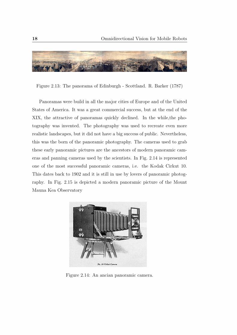
Figure 2.13: The panorama of Edinburgh - Scottland. R. Barker (1787)
Panoramas were build in all the major cities of Europe and of the United
States of America. It was a great commercial success, but at the end of the
XIX, the attractive of panoramas quickly declined. In the while,the pho-
tography was invented. The photography was used to recreate even more
realistic landscapes, but it did not have a big success of public. Nevertheless,
this was the born of the panoramic photography. The cameras used to grab
these early panoramic pictures are the ancestors of modern panoramic cam-
eras and panning cameras used by the scientists. In Fig. 2.14 is represented
one of the most successful panoramic cameras, i.e. the Kodak Cirkut 10.
This dates back to 1902 and it is still in use by lovers of panoramic photog-
raphy. In Fig. 2.15 is depicted a modern panoramic picture of the Mount
Mauna Kea Observatory
Figure 2.14: An ancian panoramic camera.

Chapter 2. Omnidirectional Imaging 19
Figure 2.15: A panoramic picture at the Mauna Kea observatory.
2.3 Omnidirectional Vision in Science
The bending of the laws of perspective and the panoramic art inpired the
machine vision community to explore new way of capturing pictures of the
environment.
The modern omnidirectional sensors used in computer vision and robot
vision can be devided in three big groups. This distinction arises from the
different imaging technique2 . The three goups are:
• the compound-eye cameras;
• the panoramic cameras;
• the omnidirectional cameras;
At this point, a brief note on terminology is needed. There is a mix-up
in terminology in the scientific community. The adjectives panoramic and
omnidirectional are used as synonims, with a sligtly more technical flavour
for omnidirectional. In this dissertation we will use the term “panoramic”
for imaging device able to generate a perspective image at 360◦ of the sur-
rounding with a limited vertical field of view (tipically a panning perspective
camera). The term “omnidirectional will be used for sensors that produces
non-perspective images with a 360◦ horizontal fild of view and with a vertical
field of view that can be bounded or not.
2For a more detailed survey on the different types of omnidirectional sensor, see thesurvey paper of Y. Yagi [88].
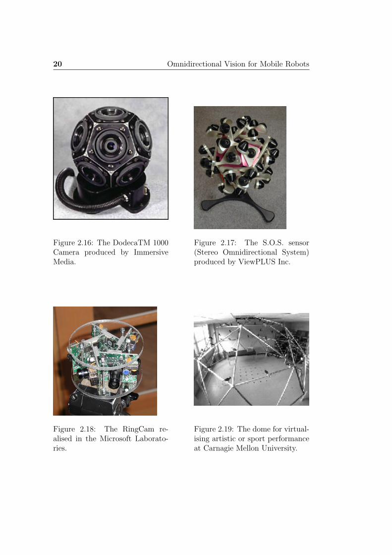
20 Omnidirectional Vision for Mobile Robots
Figure 2.16: The DodecaTM 1000Camera produced by ImmersiveMedia.
Figure 2.17: The S.O.S. sensor(Stereo Omnidirectional System)produced by ViewPLUS Inc.
Figure 2.18: The RingCam re-alised in the Microsoft Laborato-ries.
Figure 2.19: The dome for virtual-ising artistic or sport performanceat Carnagie Mellon University.

Chapter 2. Omnidirectional Imaging 21
2.3.1 Compound-eye cameras
We will not discuss in detail the compound-eye cameras. We will only men-
tion it for sake of completeness in this overview. Compound-eye cameras
uses multiple camera to grab pictures in different directions and then stich
them one to the other in order to produce a global view of the environment.
The advantages of these cameras are the high resolution these sensors can
achieve and the possibility to grab the pictures in different direction at the
same time. The disadvantage is the complexity of the system and the need
of a accurate calibration process.
The DodecaTM 1000 Camera is composed of 11 cameras able to grab
almost spherical image. DodecaTM 1000 Camera is produced by Immersive
Media. The S.O.S. sensor (Stereo Omnidirectional System) has almost the
same spherical field of view of the DodecaTM 1000 Camera, but it can per-
form stareo vision in this sphere of view. This is possible because the system
is composed by 20 triplets of CMOS cameras looking at different directions.
The S.O.S. sensor was realised by ViewPLUS Inc. Despite these two pro-
totypes, the most commonly used compound-eye cameras are composed of
few cameras looking at the horizon in different directions that shot at the
same time, like the RingCam depicted in Fig 2.18 realised in the Microsoft
Laboratories in U.K. The pictures from the different cameras are merged to
produce a panoramic image, called also panoramic cylinder [40].
Out of curiosity, we present a fourth type of sensor that usually it is not
considered an omnidirectional sensor, but it can be considered a peculiar
kind of compound-eye camera. This sensor is not looking around, like the
other sensor presented, it is looking inside, Fig. 2.19. It does not generate a
unique omnidirectional image. It performs N-stereo vision and it is used to
digitalize motion performances as dance or sportive events [42].

22 Omnidirectional Vision for Mobile Robots
2.3.2 Panoramic cameras
As we said in the previous note, in this dissertation we use the term panoramic
camera for sensors able to produce perspective panoramic views using a sin-
gle camera. Usually this is achieved by panning a camera around the vertical
axis passing through the focal point of the camera, see Fig. 2.20. This ap-
proach requires very fine calibration and synchronisation of the movements
of the camera and provides high definition panoramic images. If the camera
does not rotate about its vertical axis, but around a vertical axis at a certain
distance from its focal point, it is possible to obtain rough range panoramic
images by matching the views of an object from different positions [13] [40].
This technique is very slow and it is not suited for dynamic environment. In
dynamic environment, we need cameras able to capture a global view in one
shot in order to have at any time in the field of view all the moving objects.
These cameras are omnidirectional cameras.
Figure 2.20: The panning camera (left) and the range technique(right).(Courtesy of Prof. Y. Yagi at Osaka University)
2.3.3 Omnidirectional cameras
Even if omnidirectional camera have been realised with different techniques,
the basic idea is always the same, i.e to gather the light coming from the

Chapter 2. Omnidirectional Imaging 23
objects in the surrounding of the sensor and convey it into the sensor by
changing the path of the rays of light. Cameras that use only the refractive
effect of lens to bend the light are called dioptric cameras (from dioptrics
the science of refracting elements). Cameras that use the combined effects
of reflection from a mirror and of refraction from a lens are called catadiop-
tric cameras (from catoptrics, i.e. the science of reflecting surfaces and
dioptrics).
Figure 2.21: An Omnidirectional image.
The omnidirectional camera mostly used by the machine vision commu-
nity can be groupped in three cathegories: cameras that uses special lens,
camera that uses a convex mirror and a set of lens, and cameras that uses
two mirrors and a set of lens.
2.3.4 Special lens cameras
Cameras with the use of fish-eye lens can acquire almost a hemispherical
view. The drawback is that the resolution of the images is good at the centre
but very low at the periphery. This is not good for robot navigation, where
the objects to locate lie on the floor and they appear at the horizon or below.

24 Omnidirectional Vision for Mobile Robots
Figure 2.22: A cameramounting a PAL lens.
Figure 2.23: A cam-eras mounting convexmirrors of Accowle Co.Ltd.
Figure 2.24: An exam-ple of folded catadiop-tric camera.
In other words, the resolution is very good looking at the ceiling but poor
at the horizon. Greguss proposed an optical lens called Panoramic Annular
Lens (PAL) composed of three reflective and two refractive planes [31]. See
Figure 2.25. This does not need alignment and can be easily miniaturised.
2.3.5 Convex mirror cameras
Convex mirror cameras are the most widely used in robotics to obtain omni-
directional images. The sensor is composed by a perspective camera pointed
upward to the vertex of a convex mirror. The optical axis of the camera and
the geometrical axis of the mirror are aligned. This system is usually fixed on
top of a mobile robot like in Figure 5.1. Different shapes of the mirror have
been used. The most common are conical mirrors, hemispherical mirrors,
hyperboloidal mirrors and paraboloidal mirrors; see Figure 3.2. Every shape
presents different properties that one has to take in account when choosing
the mirror for a particular task. In Chapter 3, we will compare three possible

Chapter 2. Omnidirectional Imaging 25
Figure 2.25: A sketch of a basic optics of PAL. (Courtesy of Prof. Y. Yagiat Osaka University)
different profiles for the mirrors.
Camera
α
Figure 2.26: A sketch of a basic optics of a convex mirror camera.
To produce these mirrors out of glass would be very expensive and for
some particular shape would not be possible. Fortunately, they can be real-
ized from a cylinder of stainless steel shaped with a numeric control lathe.
The surface of these mirror is smooth enough and reflective enough for the

26 Omnidirectional Vision for Mobile Robots
purposes of omnidirectional vision.
The catadioptric omnidirectional cameras with a single convex mirror will
be the sensor we will discuss in the rest of the dissertation, but before moving
on in the next chapter, where we will explain how to build a convex mirror
with a custom profile, let us discuss the third type of omnidirectional camera.
2.3.6 Folded catadioptric cameras
Camera
Figure 2.27: A sketch of a basic optics of a folded catadioptric camera.
Usually catadioptric cameras tend to have big dimensions compared to
conventional cameras, because a minimal distance is required between the
camera and the convex mirror. To overcome this limitation, folded catadiop-
tric cameras were developped [74]. They use the optical folding method to
fold the optical path between the curved mirror and the lens system. Folding
with a curved mirror creates a 180◦ fold and can reduce undesidered optical
effects. An example is like the Omnirama of Versacorp in Fig. 2.24.

Chapter 2. Omnidirectional Imaging 27
2.4 Conclusions
In this chapter, we saw the different ways used by animals, artists and
scientists to capture omnidirectional images. The lesson we learned from
panoramic are is that reality depends on the way we observe it. The lesson
we learned from the vision of animals is that “the way we observe” depends
on what we are looking for. Again animals tell us that our perspective sight
is just one of the possible way of vision.
In summary, when we design an artificial vision system for a robot we
should take into account the task of the robot. From this analysis we could
conclude that maybe the robot does not need a high resolution image, but
a wide image with different resolutions in different regions of the image.
Therefore, we should design an omnidirectional vision sensor customised on
these requirements.
In the next chapter, we will see a technique to build omnidirectional vision
sensor tailored on the task of the mobile robot.

28 Omnidirectional Vision for Mobile Robots

Chapter 3
Omnidirectional Mirror Design
In the previous chapter, we gave an overview on the variety of panoramic
and omnidirectional sensors. As we said, the catadioptric sensors are the
most successful omnidirectional vision sensor. Their popularity is due to:
the low cost (compared to PAL1 sensors); the high-speed in collecting the
data (compared to the panoramic cameras) and the flexibility.
The flexibility of the catadioptric systems derives from the possibility to
easily change the transfer function of the sensor. The transfer function of the
sensor describes how points in the three dimensional world are mapped into
points in the two dimensional image. In a catadioptric system, the shape of
the mirror determines the transfer function of the sensor.
In this chapter, we will show how a desired mapping between world points
and image points can be obtained with a customised profile of the omnidi-
rectional mirror. The design of a custom mirror profile enables to overcome
the limitations of classical omnidirectional sensors and to expand their range
of applications. In other words, the design of omnidirectional sensors with a
custom profile is a key issue in simplifing or developping new applications.
In the second part of the chapter, we will present the actual design of three
1PAL = Panoramic Annular Lens.
29

30 Omnidirectional Vision for Mobile Robots
Camera
Mirror
Figure 3.1: The omnidirectional vision system. The camera is the verticalblack stick and it is pointed upward to the omnidirectional mirror. Note thecustom profile of the mirror.
mirrors tailored for different applications.
3.1 Classical Mirror Shapes
Before describing in detail how is possible to create a custom profile for an
omnidirectional mirror, we will give a brief overview on the most used types
of omnidirectional mirror. These shapes has been so widely used in mobile
robotics that they can be called classical mirror shapes. In Fig. 3.2, some of
the most used mirror shapes are presented. As we said, every one of these
mirror shapes realises a different mapping between the world points and the
image points. These mappings determine the resolution and the field of view
(FOV) of the different sensors. Let us discuss briefly the properties of each
shape:
• (a) conical mirrors have good resolution in the peripheral, but they
produce a singularity at the cone tip.

Chapter 3. Omnidirectional Mirror Design 31
• (b) hemispherical mirrors they have good resolution in the centre
area but poor resolution at the peripheral region. These mirrors present
the widest view angle among convex mirrors.
• (c) hyperboloidal mirrors have good resolution both in the centre
and in periphery. The view angle is almost as wide as that of the hemi-
spherical mirror, but the most important advantage is the presence of
an “effective view point” located at the focus of the hyperbole . The
presence of a single viewpont enables the reconstruction of distortion
free images. As it is depicted in Figure 3.3, from the image of a hyper-
boloidal mirror it is possible to reconstruct a panoramic cylinder or a
perspective images at the desired angles.
• (d) paraboloidal mirrors have the same resolution as hyperboloidal
mirrors even if with smaller angle of view. They present a single view-
point when used with a orthographic projection camera.
These typologies can be mixed to exploit the benefits of the different
classes. For instance, Bonarini used a mirror composed by a sphere inter-
secting a reverse cone in order to avoid the excessive distortion introduced by
the cone tip and have the good resolution of the hemispherical mirror in the
centre of the image [9]. Another example is the mirror of Sorrenti, he pro-
posed a multi-part mirror for the specific task of the Robocup competitions
(www.robocup.org). In this mirror, each part is devoted to the observation
of a different area of the play ground [52].
The two major drawbacks of the systems that acquire a single omnidirec-
tional image in a snapshot are the low resolution and the typical distortion
of the omnidirectional images. The low resolution combined with the geo-
metrical distortion produces images hardly intelligible by a human. This can
be a problem for applications like video–conferencing or tasks that require
to display images to a human operator. If the application requires to display

32 Omnidirectional Vision for Mobile Robots
Figure 3.2: The different mirror profiles. (Courtesy of Prof. H. Ishiguro atOsaka University)
a final image to a human operator, it is possible to reconstruct perspec-
tive images from omnidirectional images [78]. This type of reconstruction
is limited by the resolution of the sensor, but mainly by the geometry of
the omnidirectional vision sensor. In fact, only sensors with a unique ef-
fective viewpoint enable an exact geometrical reconstruction of perspective
images (for a detailed theory on omnidirectional catadioptric systems with a
single–viewpoint, please refer to the work of Nayar [3]).
The single viewpoint constraint can be relaxed if we are not interested
in an exact reconstruction of the perspective image (the work of Derrien
and Konolige reports how is possible to approximate the single viewpoint
condition even in catadioptric system without this geometrical property [26]).

Chapter 3. Omnidirectional Mirror Design 33
Hyperboloidal MirrorFocal Point
Perspective viewOmni-directional Image
Camera Centre
Hyperboloidal Projection
Panoramic Cylinder
Figure 3.3: Hyperboloidal projection and examples of transformed images.(Courtesy of Prof. Y. Yagi at Osaka University)
On the other hand, the human readability is not always essential. In lots
of applications the final step of the image processing is not the presentation
of an image to a human operator, but is to extract features to be used in
successive processes. A typical example is a vision system for navigating a
mobile robot . Here the distortion is not a problem, because we can design
the algorithm to take in account the geometrical distortion. Neither is the
low resolution, because we are more interested in the positions of the objects

34 Omnidirectional Vision for Mobile Robots
rather than in the details on their surfaces. An extreme example of this is
the work of Franz [27].
Abandoning the single viewpoint constraint permits a greater flexibility
in the design of the omnidirectional vision sensor because we are no longer
limited by geometrical constraints. In particular, it is possible to consider
the geometry of the mirror as a variable in the design of the vision system.
In the past, most of the catadioptric omnidirectional vision systems used
convex mirrors with simple geometrical revolution surfaces: hemi-spheres,
cones, hyperboles and parabolas. All these shapes have nice geometrical
properties that have been diffusely studied [4] [37], but they strongly limit
the flexibility of the sensor. Lately, researchers started to use more complex
surfaces in order to realise custom mapping functions between the world
points and the point on the imaging sensor. The mirror can be shaped in
order to have a mapping function that simplifies the image processing [33]
[28]. An example is the work of Lima that used an omnidirectional mirror
designed to give a bird’s eye view of the RoboCup field of play [53] [33]. This
choice preserves the field geometry in the image, permitting a straightforward
exploitation of the natural landmarks of the soccer field, goals and fields lines,
for a reliable self-localisation. Another example is the work of Bonarini, that
introduced the idea of multi-part mirrors to obtain different image resolutions
in specific areas around the robot [10]. The work of Marchese and Sorrenti
combines the two ideas proposing a mirror composed by three parts [52]. The
works of these authors have been the starting points to develop our work also
presented in [59] and in [58].
In this chapter, we present our approach to the design of a mirror with a
custom profile and three examples of mirrors designed for different applica-
tions. Our approach showed to be successful also in the map building task
(as documented in [70]) and not only in the RoboCup community (where
our work [59] was selected as a candidate for the Best Paper Award of the

Chapter 3. Omnidirectional Mirror Design 35
RoboCup Symposium of 2001 in Seattle – USA). Our design technique raised
interest in other research groups, like the GMD Robocup Team of the Fraun-
hofer Institut of Bonn that committed us the design and production of the
omnidirectional mirror for their goalkeeper, the CS Friburgh Robocup Team
of the University of Freiburg that is testing one of our three parts mirrors
and the University of Catania that wanted us to design a new omnidirec-
tional sensor for one of their new robot.
CCD
Pinhole
P
r1
D D D
d d
r
CCD
mirror profile
r
2 1
2
3
1 2min
f
P1
1P
Figure 3.4: (Left) Image formation sketch (Right) The geometrical construc-tion of the custom mirror
3.2 The design of the mirror
In this section we delineate an algorithm for the design of a custom mirror
profile. The algorithm is a modification of the one presented in [52]. To
understand the algorithm, we have to understand first the image formation
mechanism.
In Fig. 3.4, we sketch the image formation mechanism in a catadioptric
omnidirectional vision sensor. Consider the point P laying on the floor. Using
the pin-hole camera model and the optical laws, for every point at distance

36 Omnidirectional Vision for Mobile Robots
dOP from the sensor, it is possible to calculate the coordinates (x, y) of the
corresponding image point P’ on the CCD.
Vice versa, knowing the coordinate (x, y) of a point in the image plane,
we can calculate the distance dOP of the corresponding point in the world2
. Because of the finite size of the sensitive element of the CCD, we do not
have access to the actual coordinates (x, y) of the image point, but to the
discrete corresponding pair (xd, yd) (i.e. the location of the corresponding
pixel of the CCD). So, if we calculate the distance dOP from (xd, yd), this will
be discrete. The discrete distance deviates from the actual distance with an
error that depends on the geometry of the mirror. In the next section, we
will see how the amount of error we decide to tolerate impinges on the profile
of the mirror.
The main point in the design of a custom profile is the identification of the
function that maps the desired points of the world into the desired points
of the CCD. This is a function f : R3 → R2 that transform world point
(X’,Y’,Z’) into image points (x,y).
Actually, what we want is a simpler function. We want a function that
maps points laying on the plane Y=0 (the ground) around the sensor from
a distance DMIN up to a distance DMAX . Therefore, exploiting the rota-
tional symmetry of the system, the problem can be reduced to find a one-
dimensional function f ∗ where dMAX is the maximum distance on the CCD:
f ∗ : [DMIN , DMAX ] → [0, dMAX ] (3.1)
The exact solution of this problem can be found with a quite complex differ-
ential equation. In [33] a solution to this equation is reported for the simple
case d = f ∗(D) = KD, i.e. the distance, from the centre of the CCD, of
the image of a world point is proportional to the distance of the world point
from the sensor’s axis. In [52] is reported an approximated solution. In [59]
2For a detailed theory of catadioptric image formation, refer to the homonym paper ofNayar [3]
Chapter 3. Omnidirectional Mirror Design 37
we presented this algorithm applied to the design of a mirror to be used in
the RoboCup domain, but this technique can be applied to design mirrors
for any application.
3.2.1 The algorithm
The solution we use is similar to the one presented in [52], consisting in a local
linear approximation of the mirror’s profile with its tangent. This solution
is completely general and permits to choose a arbitrary set of world points
and map them in an arbitrary set of CCD points. Let us see in the detail
the algorithm:
1. transform the interval [DMIN , DMAX ] in a discrete set of points in the
world [D0, D1, D2..., DN ] that will be mapped by f ∗ in the discrete set
of points on the CCD [0, d1, d2, ..., dN ] (remember these two sets can be
arbitrarily chosen);
2. the tip of the mirror is in P0 = (0, Y0) and the tangent to the mirror
is tan(arctan(DMIN/y0)/2). With this choice the point at distance
D = DMIN is mapped into d=0. Let us call r2 the line passing by P0
whose derivative is tan(arctan(DMIN/y0)/2);
3. r1 is the line passing by the pin hole (0, f) and the point (−d1, h) on the
CCD, where h is the height of the CCD on the ground. The intersection
between r1 and r2 determines the point P1. The line r3 will be created
as the line passing by the point P1 and the point (D1, 0). Now the line
r3 and r1 constitute the path the light has to follows if we want to map
the world point (D1, 0) into CCD point (−d1, h). Therefore the tangent
to the profile of the mirror in the point P1 must be perpendicular to
the bisector formed by r3 and r1. And so on, until all the points in the
set [D0, D1, D2..., DN ] are mapped in the set [0, d1, d2..., dN ];

38 Omnidirectional Vision for Mobile Robots
4. The mirror profile is obtained by the envelope of all the previously
calculated tangents at the points Pi, i=0, 1, 2, ..., N;
Another variable in the design of the mirror is its radial dimension. If
we want that the omnidirectional view will be maximised in the camera
image, we have to choose the radial dimension of the mirror depending on
the camera–mirror distance. Consider Fig. 3.7(left), α is the angular aperture
of the camera. If the border of the mirror is tangent to the solid angle α, the
omnidirectional image will be exactly circumscribed by the camera image
frame. The closer we position the mirror to the camera, the smaller the
radial dimensions of the mirror will be. If we want that the system can grab
focused images, the minimum distance between the mirror and the camera
(Dmin) is limited by the closest subject distance of the camera3 [37]. On the
other hand, if we can tolerate a certain amount of defocus on the images, we
can place the mirror closer and make it smaller and lighter.
3.2.2 The making of the mirror
In order to test the mirror profile obtained with this algorithm, before ma-
chining the actual mirror, we can test its performances in a simulated envi-
ronment. The set of points describing the mirror profile can be used to create
a virtual model of the mirror in a virtual world created with a ray-tracing
program. In our work we chose the open-source program POV-Ray4 . In
Fig. 3.5(a) the virtual model of a mirror is depicted and in Fig. 3.5(b) is pre-
sented a simulated omnidirectional image obtained with the virtual mirror
in a virtual reconstruction of the RoboCup field of play. Using the synthetic
images generated with PovRay the final design of the mirror profile is as-
sessed. If this is satisfactory, the set of points describing the mirror profile
3In fact, the virtual image of reflected objects forms behind the mirror surface, asdetailed by Ishiguro in [37]. Also the focal depth (∆min) is important if we want to havethe whole image in focus and not just a slide of the mirror’s reflection.
4Information and downloads at www.povray.org

Chapter 3. Omnidirectional Mirror Design 39
Figure 3.5: (Left) The virtual model of a custom profile mirror. (Right) Avirtual omnidirectional image of the virtual reconstruction of the RoboCupfield of play.
is passed to a numerically controlled lathe, that machines a cylinder of an
aluminium alloy to obtain the final mirror. To decrease the weight of the
final mirror it is possible to unload the mirror by scooping a concave hollow
in the back side of the mirror. In Fig. 3.6(a) you can see the actual mirror
produced and in Fig. 3.6(b) you can see an omnidirectional image captured
in the RoboCup field of play.
3.3 The task commits the design
As we tried to stress in the previous sections, the mirror’s profile should be
designed according to the task performed by the robot. As an example, we
will consider the design of mirrors for similar tasks and for very different
tasks. In this paper, we report the differences in the design of the mirrors for
two of our soccer player robots and for a robot whose task is to explore an
unknown environment and to build a map of it using the Spatial Semantic
Hierarchy [70] [46].
The task of the goalkeeper is to prevent the ball from rolling into its own
goal, by stopping the ball with its own body and kicking the ball away with

40 Omnidirectional Vision for Mobile Robots
Figure 3.6: (Left) The actual mirror produced for the goalkeeper. (Right)An omnidirectional image acquired with the omnidirectional sensor of thegoalkeeper.
its pneumatic kicker.
The task of the attacker is to kick the ball in the opponent goal and to
catch the ball when this is still or to win the ball when this is carried by an
opponent.
The task of the mapping robot is to locate the objects in the environment,
to track the vertical edges of the objects and to follow the baseline of the
objects.
The tasks of the two soccer robots are quite similar, but nevertheless we
will see how a mirror tailored for each robot can improve the performances
of the robots. On the other hand, we will see that the mirror designed for
the mapping robot will have a totally different profile. Let us consider first
the requirements for the soccer robots and then for the mapping robot.
3.3.1 Requirements for the soccer robots
Similarities: The described tasks implies that the vision systems of the two
robot should have the following capabilities:
All these requirements corresponds to the following requirements on
the vision sensor:

Chapter 3. Omnidirectional Mirror Design 41
Num. CapabilitiesA to spot the ball in the field of play, even when it is far awayB to precisely locate the ball when it is near the robot’s bodyC to identify the team’s markers carried by the other robots
Table 3.1: The capabilities required to the vision system of the soccer robots
Num. Constraints
Ato have a large field of view with a good resolution for lookingat the field of play
B to present a high resolution area around the robot
Cto have a very wide field of view that extends from the groundup to above the horizontal, the resolution is not important
Table 3.2: The constraints on the vision system of the soccer robots
These constraints require to have three different zones of the sensor with
very different optical properties. So, we decided to design a multi-part mirror
composed of three parts: a inner part and two circular rings, that we called
respectively: the measurement mirror that observes the wider area of the
field of play with a good resolution; the proximity mirror that observes the
area around the robot’s body with a high resolution; the marker mirror
with a large field of view, but with very low resolution.
Differences: There are small differences in the tasks performed by the two
robots. For instance,
So, we obtain two additional requirements for the vision sensor of the
attacker:
Also the mechanical construction of the two robots influences the design
of the tailored mirrors. The bodies of the two robots have different sizes and
heights, so the regions of low, good and high resolution around the robots
should have different dimensions.

42 Omnidirectional Vision for Mobile Robots
Num. Requirements
D
the goalkeeper should observe precisely its own goal in orderto be able to shield it effectively and to locate it-self withrespect to it. The attacker robot should be able to see bothgoals from any points of the field of play, in order to alwaysknow where are its own goal and the opponent goal
Ethe attacker moves much more in the field of play and so itshould be lighter than the goalie
Table 3.3: The constraints on the vision system of the soccer robots
Num. Constraints
Dto have a wider vertical field of view (to view both goals fromanywhere)
E be more compact (in order to be lighter)
Table 3.4: The constraints on the vision system of the soccer robots
3.3.2 Requirements for the mapping robot
As will be diffusely explained in Chapter refchpt:omniMapping detailed in
[70], in order to build a topological map of an unknown environment using
the Spatial Semantic Hierarchy proposed by Kuipers, the robot should be
able to spot the distinct places along its path and to navigate using the pre-
defined control laws between two distinct places. As detailed in [71], the
robot uses the vertical edges to detect meaningful topological situations and
to pose new distinct places and uses the baseline of the objects to navigate
between two distinct places. Therefore the vision system should be able to:
All these requirements corresponds to the following constraints on the
vision sensor:
A ) to have a vertical field of view spanning from the ground close to the
robot to some degrees over the horizon (every vertical in the environ-

Chapter 3. Omnidirectional Mirror Design 43
Num. Requirements
Ato robustly detect the vertical edges present in the environ-ment
B to precisely locate the baseline of the objects close to the robot
Table 3.5: The requirements on the vision system of the mapping robot
Num. Constraints
Ato have a vertical field of view spanning from the ground closeto the robot to some degrees over the horizon (every verticalin the environment will be in the field of view)
B to present a high resolution area around the robot
Table 3.6: The constraints on the vision system of the mapping robot
ment will be in the field of view);
B ) to present a high resolution area around the robot;
These requirements are satisfied with a mirror composed by two parts
with different profiles. The inner part of the mirror occupies most of the
image and generates a highly distorted image in order to stretch the vertical
edges (longer lines are recognised more robustly) and distorts non-vertical
lines into curves that cannot be confused with radial lines. The outer part
of the mirror presents high resolution and low distortion to easily detect,
using a Hough transform, the position and directions of the base lines of the
objects.
3.4 The final design
The relative radial dimensions of the different parts of the mirror depends
both on the proportion of the image we want to dedicate to the rays reflected
by each part and by the resolution we want in each area.

44 Omnidirectional Vision for Mobile Robots
Dmin
Camera
Mirrors
α
Possible∆f
CCD
Pinhole
Mirror
M2
M1M3
Figure 3.7: (Left) The radial dimension of the mirror if we want the omnidi-rectional view to occupy the widest portion of the image. (Right) A sketchof the multi-part mirror profile.
In the general structure of the three mirrors, we can identify two similar
regions: the inner part and the outer part. We will discuss first the inner
part and the outer part common to all mirrors and then the annular ring
introduced only for the soccer robots. These three parts are called respec-
tively: measurement mirror, proximity mirror and marker mirror.
In Section 3.4.2, we will detail the differences between the mirrors explain-
ing the differences in the geometrical dimensions of the mirrors and in the
different curvatures of their parts.
3.4.1 The common structure
Let us consider first the inner part of the mirror, called the measurement
mirror. This part has the wider field of view. For the tip of the measurement
mirror we have two possibility: a mirror with a continuous curvature, like
the Bonarini’s and Sorrenti’s mirrors, or a mirror with a discontinuity in the

Chapter 3. Omnidirectional Mirror Design 45
vertex, like conical mirrors. The latter has been our choice. In fact, in a
multi-part mirror is possible to eliminate the disadvantages presented by a
conic mirror, exploiting other sections of the mirror. The first disadvantage
is the low resolution close to the sensor. This is overcome by the outer
part of the mirror: the proximity mirror, that permits to have a very good
resolution near the body of the robot. The second disadvantage (in the case
of soccer robots), the limited field of view, is eliminated by the middle circular
ring of the mirror, i.e the marker mirror, that permits a long range field of
view. Therefore, considering the whole structure of the mirror we have no
drawbacks to the advantages introduced by a mirror with a discontinuity in
the vertex and thus this will be our choice.
The measurement mirror
We chose to design a mirror that maps world points on the CCD with a
constant relative error α, i.e. a relative error that does not depend on the
distance from the sensor. So, the position of an object close to the sensor will
be determined with good precision while an object far away from the robot
will have a sensible absolute error. This choice is sensible both for the soccer
robots and for the mapping robot. The constant relative error is obtained
dividing the space between the minimum and the maximum visible distance
in a set of intervals of increasing size, each one mapped in one pixel.
The resulting profile is the first part of the mirror profile sketched in
Fig. 3.7 and it maps the world points into the area I1 of the CCD.
The proximity mirror
The measurement mirror produces low resolution images close to the sensor.
To clearly see objects close to the body of the robot we designed the proximity
mirror. The proximity mirror is the outer part of the multi-part mirror, so
it has the most convenient position to observe objects close to the body of
46 Omnidirectional Vision for Mobile Robots
the robot. This part is designed with a low curvature and a quite large
portion of the image is dedicated to the light it gathers. Thus, objects close
to the robot have quite big apparent dimensions. To enhance this effect we
made this latter part concave, so points closer to the robot are mapped in
outer points of the image, Fig. 3.7 (right). Fig. 3.7 (right) presents a sketch
showing how the different areas of the world are mapped on the image. Note
that there is an overlapping region that is seen by both the measurement
mirror and the proximity mirror. This is not a problem, on the contrary, it
can be used to perform more precise measures.
As we said before, these two parts are enough for the mirror dedicated to
the mapping task, while for the soccer robots we need an additional portion
with very low resolution and very wide field of view called marker mirror.
The marker mirror
In the RoboCup competitions every robot has to wear a coloured marker that
identifies the team the robot belongs to. The marker must be positioned at a
maximum height of 60cm. Therefore, we need a part of the mirror pointing
to objects over the field of play. This implies to see objects out of the game
arena. The vision of object out of the field of play causes troubles to the vision
systems of the robots that are designed for the highly structured RoboCup
environment. In order to reduce the bad influence caused by seeing many
unknown objects, we dedicated just a small portion of the image to the vision
of the markers. The light reflected by the marker mirror will be mapped in
a low resolution annular ring: area I2 in Fig. 3.7 (right). In this area we do
not care about precision of the measurements, we want only to be able to
detect the markers and to associate them to the robots localised with the
measurement mirror.
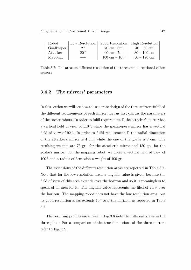
Chapter 3. Omnidirectional Mirror Design 47
Robot Low Resolution Good Resolution High ResolutionGoalkeeper 2 ◦ 70 cm– 6m 40 – 80 cmAttacker 20 ◦ 60 cm– 7m 30 – 100 cmMapping −− 100 cm – 10 ◦ 30 – 120 cm
Table 3.7: The areas at different resolution of the three omnidirectional visionsensors
3.4.2 The mirrors’ parameters
In this section we will see how the separate design of the three mirrors fulfilled
the different requirements of each mirror. Let us first discuss the parameters
of the soccer robots. In order to fulfil requirement D the attacker’s mirror has
a vertical field of view of 110 ◦, while the goalkeeper’s mirror has a vertical
field of view of 92 ◦. In order to fulfil requirement D the radial dimension
of the attacker’s mirror is 4 cm, while the one of the goalie is 7 cm. The
resulting weights are 75 gr. for the attacker’s mirror and 150 gr. for the
goalie’s mirror. For the mapping robot, we chose a vertical field of view of
100 ◦ and a radius of 5cm with a weight of 100 gr.
The extensions of the different resolution areas are reported in Table 3.7.
Note that for the low resolution areas a angular value is given, because the
field of view of this area extends over the horizon and so it is meaningless to
speak of an area for it. The angular value represents the filed of view over
the horizon. The mapping robot does not have the low resolution area, but
its good resolution areas extends 10 ◦ over the horizon, as reported in Table
3.7
The resulting profiles are shown in Fig.3.8 note the different scales in the
three plots. For a comparison of the true dimensions of the three mirrors
refer to Fig. 3.9

48 Omnidirectional Vision for Mobile Robots270
−6
−4
−2
02
46
−3
−2
−1 0 1 2 3 4 5 6 7
(1)
−3
−2
−1
01
23
−1 0 1 2 3 4
(2)(3)
(1)(2)
(3)
Figu
re3.8:
(Left)
The
profi
leof
the
mirror
ofth
eattacker
robot.
(Cen
ter)T
he
profi
leof
the
mirror
ofth
egoalkeep
errob
ot.(R
ight)
the
profi
leof
the
mirror
ofth
em
appin
grob
ot.

Chapter 3. Omnidirectional Mirror Design 49
Figure 3.9: A comparation of the attacker’s, the goalie’s and the mapping’smirror profiles. Note that not only the sizes of the three mirrors, but alsothe slopes of the different segments are different.
3.5 Conclusions
In the first part of this chapter we detailed the design and production steps
to realise a mirror with a custom profile for an omnidirectional sensor. We
detailed all the phases of the process: the design, the simulations and the
actual machining of the mirror. In the second part of the chapter we focused
on showing how the task assigned to the robot commits the design of the
omnidirectional mirror. We highlighted how different tasks produces different
requirements for the vision sensor. We gave an example of this, detailing
the design choices for three different mirrors. We showed the three mirrors
produced for the mapping robot, the attacker robot and the goalkeeper robot,
discussing the similarities and the differences.
This chapter is the result of several works presented in [59] [64] [62] [66]
[70].

50 Omnidirectional Vision for Mobile Robots

Chapter 4
Omnidirectional Vision for
Robot Localisation
In the previous chapter, we understood in detail how the omnidirectional
vision system works and how is possible to build a custom sensor. In this
chapter, we will apply this sensor to the robot localisation problem. We
will present two original results in the localisation problem: the hierarchical
localisation and a solution to the perceptual aliasing. The hierarchical local-
isation is the possibility to have different accuracies in the robot localisation
depending on the environment structure. The problem of the perceptual
aliasing is the problem to be able to discriminate between two different loca-
tion that have the same appearance. The two solution have been proposed
within the image-based localisation approach. This work sprouted from a
collaboration with prof. H. Ishiguro of the University of Osaka (Japan), so
the approach we used in the image-based localisation is the one proposed by
Ishiguro in [39].
51

52 Omnidirectional Vision for Mobile Robots
4.1 Robot Localisation
A mobile robot, that moves from place to place in a large scale environment,
needs to know its position in the environment to successfully plan its path
and its movements. The general approach to this problem is to provide the
robot with a detailed description of the environment (usually a geometrical
map) and use some kind of sensors mounted on the robot to locate it in its
world representation. Unfortunately, the sensors used by the robots are noisy
and they are easily mislead by the complexity of the environment. Neverthe-
less, several works successfully addressed this solution using high precision
sensors like laser range scanners combined with very robust uncertainty man-
agement systems [84] [16]. Another solution, very popular in real-life robot
applications, is the engineering of the environment. Artificial landmarks,
as stripes or reflecting dots, are added to the environment. The robot can
use these objects, easy to spot and to locate, to calculate its position. An
example of successful application is the work of Hu [35].
Unfortunately, this two approaches are not always feasible. First of all
because there are situations in which an exact map of the environment either
is not available, like old buildings or unexplored environment, or is not useful,
like in dynamics environments in which the configuration of the objects in the
space frequently changes. So, the robot needs to built its own representations
of the world. This internal representation of the world can be something
different from a metrical map, for instance a topological map. Topological
maps are representations of the environment that capture the topology of
the environment and that have been successfully used for tasks like robot
navigation or map building [22] [50] [81].

Chapter 4. Omnidirectional Vision for Robot Localisation 53
Figure 4.1: Image based localisation. The map of a test environment. Thered circles represent the reference locations.
4.2 Image-based Localisation
If we shift our attention from robots to humans, it is proved that, in addition
to the capability of reasoning about the environment topology and geometry,
humans show the capability of recalling memorised scenes that help them-
selves to navigate. This implies that humans have a sort of visual memory
that can help them to locate themselves in a large environment. There are
experimental evidences that also very simple animals like bees and ants use
the visual memory to move in very large environments [23].
In order to mimic this approach the robotics researchers proposed a new
approach to the robot navigation, i.e. the image-based navigation [1] [41]
[29] [45] [39]. In the image based navigation approach, the robotic agent is
provided with a set of views of the environment taken at several locations in
the environment. These locations are called reference locations because
the robot will refer to them to locate itself in the environment. The corre-
sponding images are called reference images. In Fig. 4.1 is sketched the

54 Omnidirectional Vision for Mobile Robots
map of the test environment we will use in the reminder of the chapter. The
red circles represent the reference locations, i.e. the locations where the ref-
erence images were grabbed . When the robot moves in the environment, it
can compare the current view with the reference images stored in the visual
memory. When the robot finds which one of the reference images is more
similar to the current view, it can infer its position in the environment. In
fact, it is closer to the corresponding reference location more than to any
other reference location. This give a topological localisation of the robot.
If the reference positions are organised in a metrical map, an approximate
geometrical localisation can be derived.
With this technique, the problem of finding the position of the robot in
the environment is reduced to the problem of finding the best match for the
current image among the reference images. The problem now is how to store
and to compare the reference images, that for a wide environment can be a
large number. As we will see in Section 4.2.1, different methods have been
proposed.
As we said, this work started from a collaboration with prof. H. Ishiguro.
Therefore, we adopted the image-based approach proposed by Ishiguro in
[39]. This method is different from the ones of the other authors because
it uses peculiar properties of the omnidirectional images. Let us see how
this method works. The robot is equipped with an omnidirectional camera
and takes a set of omnidirectional images at the reference location, then it
compares the current omnidirectional image with the reference images. In
order to store and match efficiently a large number of images, we transform
each omnidirectional view into a compact representation by expanding it
into Fourier series. The agent memorises each view by storing the Fourier
coefficients of the low frequency components. This drastically reduces the
amount of memory required to store a view at a reference location. With this
approach also the matching of the current view against the visual memory is

Chapter 4. Omnidirectional Vision for Robot Localisation 55
computationally inexpensive. Details on how to calculate the image signature
from the original image are given in Section 4.2.1. In Section 4.2.2, we will
describe the process of matching the current view against the visual memory.
This process is based on the calculation of the degree of similarity between
two omnidirectional images using the signature associated to them.
Figure 4.2: An omnidirectional image taken at a reference location.
Figure 4.3: The panoramic cylinder created by the omnidirectional image ofFig. 4.2.
Through the rest of the chapter, we will show why this method should
be preferred with respect to other methods proposed and we will illustrate
several benefits this method carries with it. In particular, we will focus on
the possibility of calculating a hierarchical localisation for the robot and
how the similarity between the images can be used as weights of the samples
in a Monte Carlo localisation process.

56 Omnidirectional Vision for Mobile Robots
In Section 4.3, we will show experimental evidence of the hierarchical
localisation in a complex real-world environment in which many objects are
present and we will give some hints on how it will be possible to create a
hierarchical description of the environment.
In this first section, we introduced the problem of image-based localisation
and navigation, we outlined the solution adopted in this work, we highlighted
the advantages of our method with respect of the approaches of other authors.
In the next section, we will explain the technique we used to reduce the
dimensionality of the input data and how the signature associated to each
image is calculated.
4.2.1 Image signature
As we pointed out in the introduction, the first problem to tackle when
building an image-based localisation system is to find a manageable way of
storing and compare the reference image. The aim is to have a data set that
fully describes the environment and permits to reliably associate the current
view with the reference view taken at a nearby location, all this while keeping
the dataset small enough to be easily stored and fast processed.
The first step, in order to lower the number of required reference image, is
to use an omnidirectional camera [37]. An omnidirectional camera can store
in a single image a 360◦ view of the environment from a certain location, see
Fig. 4.2. Conversely, if the robot is fitted just with a standard perspective
camera, the view of the environment from a certain location changes with
the direction of gaze. In order to be able to recognise this point regardless
of the instantaneous heading, the robot needs to take several pictures in the
different directions. The amount of memory required to store and retrieve
such a big number of images can rapidly grow to an unmanageable size. A
solution can be to constraint the movements of the robot in order to have
the camera pointing always at the same location [21], but this strongly limits

Chapter 4. Omnidirectional Vision for Robot Localisation 57
the motion of the robot. Another solution can be to extract from the images
some features that reduce the amount of required memory while retaining a
unambiguous description of the image. A good example of this is reported in
[87], where 936 images where store in less than 4MB. Nonetheless, to collect
such a big number of images is tedious and time consuming. Moreover, high
resolution images are not needed for tasks like navigation and localisation.
Let us come to the second step, the comparison of the current image
with the reference images. The simplest approach might appear some sort of
direct comparison of two images pixel by pixel, but this is not robust at all
and will force us to store the whole image using a lot of memory storage.
Ishiguro proposed to use the Fourier transform of the omnidirectional im-
age and to use a subset of its Fourier coefficients as signature for the image
[39]. He did not apply the 2-D Fourier transform to the original omnidirec-
tional image, Fig. 4.2, but he calculated the 1-D Fourier transform of every
line of the corresponding panoramic cylinder. The panoramic cylinder
is a new image obtained unwarping the original omnidirectional image, as
depicted in Fig. 4.3 .
The use of the panoramic cylinder brings great simplifications in the so-
lution of the matching problem. First of all, the panoramic cylinder is a
periodic function along the x-axis and this simplify the calculation of the
Fourier transform and second it is the natural representation for implement-
ing a rotational invariance. As we said, the robot must be able to match
the current view with the corresponding reference image regardless of the
current heading. So, we need to introduce a sort of rotational invariance
in the calculation of the similarity between two images. Using the Fourier
coefficients as signature for the images, this come for free. Let us explain
how this works.
If the robot grabs two omnidirectional images at the same location but
with different headings, these two images are actually the same omnidirec-

58 Omnidirectional Vision for Mobile Robots
tional image rotated about its centre. The amount of rotation correspond
exactly at the number of degrees the robot rotated. This means the two
panoramic cylinders created by unwarping the omnidirectional image are
actually the same image just shifted along the x-axis. Let see how this con-
sideration affects the Fourier transform of the two images. If f(x) is one
row of the the first panoramic cylinder, f(x − a) is the corresponding row
of the shifted panoramic cylinder and we applying the Shift Theorem, we
can write:
F{f(x− a)} = e−j2πasF{f(x)} (4.1)
where F{f(x)} is the Fourier transform of f(x). In other words, the
Fourier transform of a shifted signal is equal to the Fourier transform of
the original signal, multiplied by the unit magnitude complex coefficient
e−j2πas. This properties states for every row of the panoramic cylinder. This
means that the amplitude of the Fourier transform of the shifted image is
not changed and there is only a phase change, proportional to the amount
of shift a.
Coming back to our panoramic images, we can then associate the mag-
nitude of the Fourier transform to the appearance of the environment from
a particular place and the phase of the Fourier transform to the heading of
the robot. In such a way, when the robot is turning on the spot and the
apparency of the environment is not changing, the magnitude of the Fourier
transform does not change. What is changing is the phase of the Fourier
transform and the amount of change is proportional to the change in the
heading.
Associating the apparency of the environment, and then the position
of the robot, to the magnitude of the Fourier transform and the heading
of the robot to the phase of the Fourier transform, we obtained both the
desired rotational invariance and a way to calculate the difference between

Chapter 4. Omnidirectional Vision for Robot Localisation 59
Figure 4.4: The power spectrum of the Fourier transform of the image inFig. 4.3. Note that only the first 30 components are shown and compo-nents after the 15th have very small values and so can be neglected in thecalculation of the similarity function.
the current heading and the heading associated to the reference image. On
the rotational invariance using the Fourier transform, see also [77].
Other authors used different approaches for reducing the memory require-
ment of the omnidirectional images. The most used technique is to extract a
set of eigenimages from the set of reference images and to project the images
into eigenspaces. The drawback of such systems is that they need to prepro-
cess the panorama images they created from the omnidirectional image in
order to obtain the rotational invariance like in [1], in [41] and in [29] or to
constrain the heading of the sensor like in [45].
The reduction on the memory requirement with our method is large, Ta-
ble 4.1. Figure 4.2 shows a 640× 480 pixels omnidirectional image at 24 bit
per pixel. Figure 4.3 is shown the 512×80 pixels panorama cylinder at 24 bit

60 Omnidirectional Vision for Mobile Robots
Image Memory Required (in bit) Memory Requiredomnidirectional 640× 480× 24 7.3 Mbitpanoramic cylinder 512× 80× 24 980 KbitFourier signature 80× 15× 2× 8 19 Kbit
Table 4.1: The different memory requirements illustrating the impressivememory saving introduced by the Fourier signature.
per pixel, created from the omnidirectional image. Figure 4.4 shows a plot of
its magnitude coefficients of the Fourier series. As the figure shows, dominant
powers exist in the frequencies before the 15th. As a result, we can repre-
sent the omnidirectional image just with the values of the first 15th Fourier
components. In summary, the signature associated to each omnidirectional
image is a three dimensional array composed of 80 rows (corresponding to
the rows of the panoramic image), 15 columns (corresponding to the first 15
Fourier components) and two values for each element (corresponding to the
module and the phase of the Fourier component).
In the next section, we will describe how these 15 values are used to assess
the degree of similarity between the images.
4.2.2 Similarity computation
To compute the similarity between two omnidirectional images we define a
similarity function that takes as arguments the two sets of m values rep-
resenting the magnitude of the first m Fourier components associated with
two omnidirectional images. First of all, we transform the two omnidirec-
tional images in the two corresponding panoramic cylinders. Suppose each
panorama image is composed by l row. We transform every row into Fourier
series and we take only the first m frequency components, the first m compo-
nents with non neglectable magnitude. We define the similarity Sim(Oi, Oj)
between two omnidirectional images Oi and Oj as

Chapter 4. Omnidirectional Vision for Robot Localisation 61
Figure 4.5: The plot of the similarity function values versus the distancebetween the reference image and the current image. The different lines inthe plot represent different pairs of reference image - current image.
Sim(Oi, Oj) =l−1∑y=0
m−1∑k=0
|Fiy(k)− Fjy(k)| (4.2)
where Fiy(k) and Fjy(k) are the Fourier coefficients of the k-th frequency
of y-th row of Oi and Oj, respectively. In other words, as a measure of
similarity between two omnidirectional images, we are using the L1 norm
between the Fourier coefficient of the corresponding panoramic cylinders.
The plot in Fig. 4.5 depicts how the value of the similarity function
changes depending on the distance between the current image and the ref-
erence image. The different lines in the plot represent five different pairs of
reference image-current image taken in an cluttered office environment. The
similarity linearly decreases with the distance within a short range and it
is related, somehow, even for a long distance. In fact, as you can see from
the plot in Fig. 4.5, the value of the similarity function steadily grows when
the distance between the two images increases, but after a certain distance it
will saturate. This happens because when the two images are taken at points
far apart one from the other there is no correlation at all between the two

62 Omnidirectional Vision for Mobile Robots
02
46
8
02
46
810
12140
1
2
3
4
5
6
7
Figure 4.6: The values of the similarity functions calculated at every referencepoint for the current image. The empty circles on the xy plane represent thereference images. The full circle represents the actual position of the currentimage. The hight of the surface at every reference location is proportionalto the degree of similarity of the reference image with the current image.
images1 . The absolute value of the similarity function is unimportant, it
depends on the environment layout, what is important is the relative values
obtained for the current image against all the reference images. The refer-
ence image that matches best the current image is the one with the lowest
value for the similarity function. So this give us a topological localisation for
the robot. In other words we do not know where the robot is, but we know
that it is closer to the location of the matched reference image than to any
other reference location.
However, most of the time a precise geometrical localisation is not neces-
sary for tasks like navigation. For the robot is enough to have a topological
localisation and in most situations the robot can effectively navigate with a
broad topological localisation. In fact, the localisation accuracy the robot
needs to navigate depends on the environment and on the current action the
robot is performing. If the robot is crossing a wide open space, it does not
need to know where it is down to the centimetre, but if it has to enter a
1This is exploited in the practical implementation of the algorithm to speed up compu-tation: when the partial sum of Eq. 4.2 exceeds a predetermined threshold the computationof the similarity function is stopped and a no-matching value is returned.

Chapter 4. Omnidirectional Vision for Robot Localisation 63
door the accuracy must be high. This is similar to the behaviour we expe-
rience walking in a street of an unknown town using a map. When we are
following the high-street we do not need to know our exact position on the
map, but when we have to take a detour or to enter a building we need to
shrink down the uncertainty about our position, maybe looking for additional
environmental clues. We called this process hierarchical localisation.
In this section we proposed a quantitative measure of the amount of simi-
larity between two omnidirectional images. In the next section we will intro-
duce the concept of the hierarchical memory-based localisation and how this
can be easily calculated from the signature associated to the omnidirectional
images.
4.3 Hierarchical Memory-based Localisation
As we hinted in the previous section, when navigating in large environments
the robot needs to know its position with different accuracies depending if
it is travelling in a clear area or if its manoeuvring in a cluttered area. This
can be achieved with hierarchical localisation.
Also other authors spotted the need for different localisation accuracy de-
pending on the kind of motion required to the robot. The work in [29] is an
example of a vision-based navigation system that uses different localisation
accuracies for different tasks. This system uses two different vision-based
navigation strategy: a topological navigation and a visual-path following nav-
igation. The system switches between these two alternatives depending on
the situation. The drawback of this solution is that visual path following
requires handmade design and an accurate control systems. We solved the
requirement of a different localisation accuracy within the frame of topologi-
cal image-based navigation using the same technique described in Section 4.2,
actually simplifying this technique.

64 Omnidirectional Vision for Mobile Robots
To explain how this work, we need to give some insight on the meaning
of the Fourier coefficients we can calculate from the panoramic cylinders.
When we calculate the Fourier transform of a brightness signal, like one
row of the panoramic cylinder, we are actually decomposing this signal in its
component on a set of basis functions:
{sin(2πωx), cos(2πωx), ω ∈ R}
This basis functions are related to the spatial brightness variation. The
first basis function, the one with zero frequency, is the constant brightness
signal and the coefficient associated to it is giving the level of brightness.
Basis functions with higher frequencies are related to brightness patterns
with higher spatial frequencies. The relation between the Fourier components
and the brightness pattern present in the image can be easily understood
with the example of Fig. 4.7, kindly provided by Marco Foracchia. The test
image presents a continuum of brightness patterns at different frequencies
Fig. 4.7 (a). In Fig. 4.7 (b) is represented the Fourier transform of the test
image. Now, we apply a pass-band filter to the Fourier transform and we keep
only the middle frequencies, i.e. those components that are with in the filter,
Fig. 4.7 (c). In the last stage, we calculate the Fourier antitrasformation of
the filtered components and we will obtain Fig. 4.7 (d). As you can see, this is
just the test image with the spatial frequency of the brightness signal filtered
if out of the the pass band filter.
When we are calculating the similarity function for two images we are
summing up all the contribution from the different frequency components,
the low frequency values give the biggest contribution to the final value of
the similarity function.
When looking for the similarity between two images we can see that the
average brightness of the images changes very slowly when increasing the
distance between the two images. While the distribution and the presence of

Chapter 4. Omnidirectional Vision for Robot Localisation 65
(a) (b)
(c) (d)
Figure 4.7: The relation between brightness pattern and spatial frequency.(a) The test image presenting a continuum of brightness patterns at differentfrequencies. (b) the Fourier transform of the test image. (c) A pass-bandfilter applied to the Fourier transform. (d) The Fourier antitrasformation of(c)

66 Omnidirectional Vision for Mobile Robots
Figure 4.8: An example of hierarchical localisation. The number of Fouriercomponents used to calculate the similarity function is increasing from theleft to the right. The empty circles represent the reference images. The fullcircle represents the actual position of the current image and the gray arearepresent the calculated possible locations of the robot.
brightness patterns (that represent the objects in the environment) changes
much faster. Therefore, we can expect that the low frequency components
of the Fourier transform of the two images are similar in a larger interval of
distances than the higher frequency components. This means that if in the
calculation of the similarity function we stop the calculation of the sum in
Eq. 4.2 to the first N Fourier components (with N < 15) our current image
will match not only the closest reference image, but also a larger number of
reference images distributed in the surroundings of the current position.

Chapter 4. Omnidirectional Vision for Robot Localisation 67
As a result, we can have an hierarchical localisation just by choosing the
number of Fourier components to compare with the similarity function. In
other words, within the technique used in this work, the hierarchical localisa-
tion comes for free from the calculation of the similarity function and actually
save some computational power as well. In fact, if the robot needs only a
broad localisation it does not need to calculate the inner sum in Eq. 4.2 for
every value of k, it can just stop at the very first values. The result is to
match the current view not only with the closest view but also with other
reference views close to it. When a more precise localisation is needed, like
in situation in which the robot has to manoeuvre in a cluttered environment,
the sum can be extended to higher values of N in order to have a more strict
matching against only one reference images. So Eq. 4.2 becomes Eq. 4.3
Sim(Oi, Oj) =l−1∑y=0
N∑k=0
|Fiy(k)− Fjy(k)| where N < 15 (4.3)
In Fig. 4.8 is depicted a graphical representation of the hierarchical local-
isation achieved with our system. The empty circles represent the reference
images. The full circle represents the actual position of the current image.
The possible position of the robot, as calculated by the system, is represented
by the gray area. From the left to the right the number of Fourier components
used to calculate the similarity function is increasing, consequently the gray
area showing the possible localisation of the robot is shrinking. In this test
the reference image were taken on a 25 cm grid in a office environment clut-
tered with many pieces of furniture, as you can see from pictures in Fig. 4.2
and Fig. 4.3.
In Fig. 4.9, we present the hierarchical localisation obtained at different
locations in the same environment. In the figure is sketched also a rough map
of the test environment. In which the objects present in the environment are
sketched as boxes of different colour. Lighter boxes represent lower objects

68 Omnidirectional Vision for Mobile Robots
Figure 4.9: Several examples of hierarchical localisation at different placesin the environment. The layout of the room in which experiments wereperformed is shown and the boxes represent the objects in the environment.Lighter boxes represent lower objects, darker boxes represent taller objects.

Chapter 4. Omnidirectional Vision for Robot Localisation 69
(like desks or chairs), darker boxes represent taller objects (like filers or
shelves ). At the moment of writing, we are investigating the relation between
the shape of the localisation areas and the disposition of the objects in the
environment.
In summary, our method provide a direct way of calculating the hier-
archical localisation for the robot by comparing the frequency spectrum of
the current image with the frequency spectrum of the set of reference images.
Broad localisation is provided at minimal computational cost, just comparing
very few frequency components. When higher accuracy in the localisation is
needed, the system will use a little extra computational power.
4.4 Monte-Carlo Localisation
As we stated in the introduction, the image-based navigation is mislead in
situation in which the appearance of the environment is the same in two
different points. For this reason, we used a Markov particle filter to represent
the belief about the robot position and how this belief can be updated every-
time the robot grabs a new image.
The approach we used is inspired by the one proposed by Burgard in
[87]. Every time the robot moves, it grabs a new image. The grabbed image
is compared with the reference images in the memory of the robot and a
similarity value is calculated for every reference image. These similarity
values are used to assign a weight to the sample used in the Monte-Carlo
localisation process.
There are two main differences with respect to Burgard’s work. The first
is that we used an omnidirectional vision sensor, so that at every position
in the environment is associated one and only one image (with a drastic
reduction of the number of required images). The second is that we do not
associate any visibility region to the reference images in the memory database.

70 Omnidirectional Vision for Mobile Robots
The pose of the robot lt is estimated with Monte-Carlo localisation, a
variant of the Markov localisation [2, 87, 19]. The Monte-Carlo localisation
algorithm is composed of the following steps:
Algorithm 4.1 Monte-Carlo Localisation algorithm
1: {s′t} = Predict({st−1}, odometry(at−1))
2: {w′t} = Weight({st−1}, similarity-grid)
3: {s′t, w′′t } = Normalise({st−1, w
′t})
4: {st} = Re-sample({st−1, w′′t })
5: lt = Estimate({st})
Let us discuss in detail the single steps.
1. the step Predict predicts the position of the new sample s′t from the
current sample st−1 using the odometry information.
2. the step Weight assigns to each sample s′t obtained in step 1 a weight.
The weight is proportional to the degree of similarity of the current
image with the reference images in the neighbours of the sample. Every
weight is calculated as the weighted mean of the similarity values Sj
associated to the closest reference images gj (i.e. gi ∈ C). The closer
is a sample to a reference image and the higher is the contribution of
the corresponding similarity value to the final value of the weight, as
can be inferred from Eq. 4.4
w′it =
∑gi∈C
Sj(D − ||s′it − gj||) (4.4)
where D is the distance threshold.
3. the step Normalise simply normalises the samples before the re-sampling;
4. the step Re-sample eliminates the sample with lower weights (i.e. the
sample with a low similarity to the current image) in order to focus

Chapter 4. Omnidirectional Vision for Robot Localisation 71
the elaboration on the samples with higher similarity. The re-sampling
algorithm is the one proposed in [19];
5. the step Estimate returns as estimation of the robot position the av-
erage position of all the samples present at the moment;
In Fig. 4.10 are presented two examples of Monte-Carlo localisation based
on the similarity between the current image and the reference images. The
estimated position of the robot is calculated as the average position of the
samples and is marked with a black square. The upper series presents the
position tracking problem. In the position tracking task the robot knows
its initial position (left) and the belief distribution is update with the new
observation at every step the robot takes (middle and right). The lower
series presents global localisation problem. The initial position is unknown
to the robot (the samples are uniformly distributed in the environment) (left)
and the robot has to infer its position in the environment. During the motion
of the robot the belief distribution is updated and converges to the actual
position of the robot (middle and right).
4.5 Conclusions
In this chapter, we presented two steps we took toward a robust vision-
based localisation system that can operate in every type of environment. We
presented our approach to the problem of lowering the computational and
memory requirements posed by the image-based localisation. This solution
uses the Fourier transforms of the omnidirectional images grabbed by the
robot. We discussed the advantages of this solution with respect to the
solutions devised by other authors. We focused on the possibility offered by
this representation to implement a hierarchical localisation of the robot.
To overcome the limitation of the vision-based localisation systems, i.e. the

72 Omnidirectional Vision for Mobile Robots
Figure 4.10: Two examples of Monte-Carlo localisation are presented. Theseare some snapshot of our system while tracking the robot position, in theupper sequence, and while performing a global localisation, in the lower se-quence.
lack of robustness in case of perceptual aliasing, we introduced a Monte-
Carlo localisation technique. We showed that this system is able to
track the position of the robot while moving and it is able to estimate the
position of the robot without any prior knowledge on the real position. This
work has been described in [57] and [68]. At the moment of writing, we
are testing robustness of our system to occlusion, kidnapping and odometric
noise. The final step of this project will be to test this system in large outdoor
environment and in indoor environment with high perceptual aliasing like a
long corridor with several identical doors and junctions. The feeling is that
because the current system does not make any assumption on the structure of
the environment, it should work on outdoor images without any modification.
The natural extension of the hierarchical localisation is a hierarchi-
cal description of the environment in which the density of the reference
images in the space is no longer constant but depends on the structure of

Chapter 4. Omnidirectional Vision for Robot Localisation 73
the environment. In fact, consider an empty space where the reference im-
ages are very similar, we can represent this space just with a single reference
image representative of all close reference image.

74 Omnidirectional Vision for Mobile Robots

Chapter 5
Omnidirectional Vision for
Mapping
In the previous chapter, we saw how the robot can calculate its position with
respect to a set of reference images. The image-based localisation is feasible in
environments with a limited extensions. In very large environments, we need
a more compact representation of the world. In this chapter we will see how
this compact representation could be a topological map of the environment.
We will explain how a robot fitted with an omnidirectional vision sensor
can extract the topology of the environment using the theory of the Spatial
Semantic Hierarchy (SSH) proposed by Kuipers. This work demonstrated
that an omnidirectional vision sensor has properties that enables to simplify
the implementation of the SSH (Spatial Semantic Hierarchy).
5.1 Mobile Robot Navigation
Often, a mobile robot does not need a map to perform a simple displacement,
especially if the environment is very simple or highly engineered. But, if the
robot’s task requires an understanding of the world, the robot has to answer
the three questions posed by Levitt and Lawton [51]: “Where am I?”, “How
75

76 Omnidirectional Vision for Mobile Robots
do I get to other places from here?”, “Where are other places relative to
me?”.
In other words, it needs a map of its world. There is a wide range of
different maps a robot can use. Different kinds of maps answer the three
basic questions using different properties of the environment. We have to
keep in mind that the distance which separates two objects is only one of the
properties of the space in which the two objects are embedded. The choice
of which property to exploit and therefore which kind of map to use depends
on the task the robot will be required to perform.
Two examples that are poles apart are metric and qualitative maps. In
metric maps the space is represented in a single global coordinate system.
The relation between different places is a metrical relation composed of mea-
sure of distances and angles. In qualitative maps, the environment is repre-
sented as a set of places connected by paths. There is no metric or geometric
information, such as distances, angles, etc. but only the notion of proximity
and order [43].
What if there is no map? Can the robot be induced to build its own
map? This idea opens another stream of research: the map building task.
In this case, the robot has to travel through an unknown and unexplored
environment and to construct a map of it. Again, depending on the task these
maps can be very different [7] [27]. One of the most effective representations
of an environment is the so called topological map. This is a qualitative map
which extracts from the environment the topological relationships between
the different places and paths. The advantages of such a representation are its
compactness, because it represents only interesting places and not the whole
space, and its intrinsic solution to the problem of movement uncertainty.
This is because when a robot goes to places, its position is known with a
certain error and this error accumulates while it moves. Because topological
maps do not rely on a global coordinate system, the error in position is reset

Chapter 5. Omnidirectional Vision for Mapping 77
whenever the robot reaches one of the distinct places identified within the
space. One of the key issues in the generation of topological maps is the
abstraction of a discrete set of distinct places from the continuous sensorial
experience. Topological maps can be upgraded to metric maps by adding
metric information to the places and to the relationship between paths and
places. Therefore, a map can be seen as a hierarchal structure built layer by
layer. Benjamin Kuipers created a formalisation of this intuition: the Spatial
Semantic Hierarchy (SSH).
The purpose of this chapter is to show the effectiveness of omnidirectional
vision as sole sensor for a robot building a topological map of a man-made
environment1 , using the Spatial Semantic Hierarchy. So far, the SSH was
only implemented on either simulated robots or real robots with very simple
sensors, as sonars. No attempt to use a vision sensor has been made.
In Section 5.2, the basic concepts of the Spatial Semantic Hierarchy are
introduced. In Section 5.4, we present the simulations run in a virtual en-
vironment to generate simulated omnidirectional image sequence. We per-
formed a qualitative analysis of the simulated images. From this analysis, we
identified transitions in the image sequence and features in the images them-
self, strictly related to the SSH representation. In Section 5.5.1 We present
the algorithms designed to extract the desired information from the image
sequences. Finally, in Section 5.6, we present the results of simulated exper-
iments and in Section 5.7 we present the results of experiments performed
with the real robot of Fig. 5.1, in a test environment. The robot depicted in
the picture is the goal keeper of the Artisti Veneti Team2 .
1like an office or a building2Artisti Veneti Team is the team of The University of Padua at Robocup Championship,
the robot football competition.

78 Omnidirectional Vision for Mobile Robots
Camera
Mirror
Figure 5.1: The robot with its omnidirectional vision sensor.
5.2 The Spatial Semantic Hierarchy
The SSH (Spatial Semantic Hierarchy) is a model of the way humans organise
their knowledge of a large environment that extends beyond their sensorial
horizon, i.e. an environment with section not directly perceptible. In other
words, the SSH is a model of the knowledge of large-scale spaces of humans,
intended to serve as a “method for robot exploration and map building” [46].
This model was proposed by Benjamin Kuipers [49] [47] [48] [79]. The SSH
is made up of several layers: the sensory level, the control level, the causal
level, the topological and the metrical level. Each layer can be implemented
independently, even if they strongly interact. Let us see in details what each
layer is about:
The Sensory Level
The sensory level is the interface with the agent’s sensory system. It extracts
the useful environmental clues from the continuous flux of information it
receives from the robots’ sensors.

Chapter 5. Omnidirectional Vision for Mapping 79
The Control Level
The control level describes the world in terms of continuous actions called
control laws. A control law is a function which relates the sensory input with
the motor output. Each control law has conditions for its appropriateness
and termination. A selected control law is retained until a transition of
state is detected. These transitions can be detected with a function called
a distinctiveness measure. The distinctiveness function must be identified
depending on the sensor used and the features which are to be extracted
from the environment.
The Causal Level
The causal level abstracts a discrete model of the environment from the con-
tinuous world. This discrete model is composed of views3 , actions4 and the
causal relations between them. At this stage causal maps and planning are
possible using these three basics elements. For this purpose, it is convenient
to classify actions into two categories: travels and turns. “A turn is an ac-
tion that leaves the agent at the same place. A travel takes the agent from
one place to another” [79].
The Topological Level
The topological level represents the environments as places, paths and re-
gions, with details of how they are connected or contained one in the other.
To use Kuipers words:
The topological model of the environment is constructed by the
non monotonic process of abduction, positing the minimal set
3A view is defined as the sensor’s reading at a place where a transition of state isdetected.
4An action is defined as the application of a sequence of control laws.
80 Omnidirectional Vision for Mobile Robots
of places and paths needed to explain the regularities observed
among views and actions at the causal level.
The Metrical Level
The metrical level augments the topological representation of the environ-
ment by including metric properties such as distance, direction, shape, etc.
At this stage, it is possible to build a global geometric map of the envi-
ronment in a single frame of reference. This may be useful, but is seldom
essential.
5.3 Omnidirectional vision and map building
omnidirectional vision produces images with a wide angle of view but with
low resolution. This is not a problem, because most of the task which require
an understanding of what is happening in the surroundings do not need high
resolution images. It is better to gather the biggest amount of information
from the highest number of directions than to have a detailed analysis of a
small area.
In the case of a map building robot, the advantages of omnidirectional
vision are clear. For this task a vision sensor with high acuity is useless, it
is not necessary to capture the details of objects and surfaces, but only to
estimate their positions and dimensions. An omnidirectional image captures
at once all the objects visible from the robot location. This image has a strict
connection with the views introduced in the causal level of the SSH, i.e. with
the sensor reading at a distinct place. With an omnidirectional sensor, the
robot does not need several shots to understand the surroundings. It does
not need to turn and take a look around. It does not need to be fitted with
moving parts (camera or mirrors) to increment its field of view. These are
just implementational considerations, there are deeper aspects supporting

Chapter 5. Omnidirectional Vision for Mapping 81
the use of an omnidirectional sensor in the process of building a map with
the SSH.
Figure 5.2: The conic projection. (Courtesy of Prof. Y. Yagi at OsakaUniversity)
To understand these considerations we have to take a look at how a
omnidirectional sensor maps the scene into the image plane. Consider Figure
5.2. In this figure a conical mirror is represented, but the properties which
are illustrated apply to any kind of omnidirectional sensor.
P1 P2
P3
P5
P4
Figure 5.3: The “exploring around the block” problem. The problem ofrecognising the same place under different state labels.

82 Omnidirectional Vision for Mobile Robots
The vertical edges in the scene are mapped in the image plane as radial
lines originating from the point corresponding to the tip of the mirror. There-
fore, to extract the vertical edges from the images, the image is searched for
radial lines. The azimuth of a radial line in the image corresponds to the
azimuth of the vertical edge in the scene, as viewed from the optical axis of
the camera. The vertical lines in the environment provide an optimal clue
to divide the environment into topologically different places and they can be
used to generate a distinctiveness measure needed to distinguish transition of
state in the robot ontology. Another advantage of the omnidirectional vision
is its rotational invariance. If the robot rotates of a certain angle about the
optical axis of the camera, the relative position of the objects in the image
does not change. The image is only rotated and the objects appear to have
experienced an azimuthal shift equal to the angle of rotation. This permits a
straightforward solution to the problem of exploring around the block, i.e. of
recognising the same place under different state labels. See Figure 5.3. Using
the SSH terminology, it is easy to spot whether the current view is the same
as has been experienced before and therefore to consider this view not as a
different place but as the same place reached from a different direction.
Another problem which is easily solved by omnidirectional vision is to
discriminate the type of movement the robot is performing at a given time.
Using optical flow techniques, Svoboda showed that with an omnidirectional
vision system it is very easy to discriminate between a small rotational move-
ment and a small translational movement [82]. This task is very difficult for a
vision system fitted with a perspective camera. Moreover, using active vision
on an omnidirectional vision system it is possible to estimate precisely the
motion of a robot. See again [82] for a literature review.
The main disadvantage of omnidirectional vision with respect to perspec-
tive vision is the already mentioned poor resolution. This is because with an
omnidirectional sensor light is gathered from a much wider area than with

Chapter 5. Omnidirectional Vision for Mapping 83
a perspective camera. Therefore, if the sensitive surface of the CCDs is the
same, more points have to be mapped into the same pixel. The shape and
size of the mirror influences the resolution of the sensor. Within certain lim-
its, it is possible to design mirrors that maximise the image resolution in the
most interesting regions of the scene.
Other disadvantages of the omnidirectional images are the high distortion
introduced into the image and the poor human readability. A mirror with
a single focal point, like a hyperboloidal mirror, overcomes these difficulties.
In fact the geometry of such a mirror permits transformation of portions of
interest of the omnidirectional image into a perspective image. See Figure
3.3.
5.3.1 The assumptions
In the image analysis, we make use of some assumptions. It is worth to make
them explicit here.
• The robot is moving in a indoor environment. This is a man-madeenvironment like an office or a building;
• The lighting in the environment does not change during the motion ofthe robot;
• The objects present in the scene are static: they do not change theirpositions;
• The floor is almost flat and horizontal;
• The walls and the object present in the scene have vertical edges andsurfaces;
• The axis of the camera and the mirror are vertical;
• The robot can only turn on the spot or move on a straight line. Itcannot make more complex movements;

84 Omnidirectional Vision for Mobile Robots
The last assumption is strong but permits to greatly simplify the image
sequence interpretation. Several constraints on the edge movements are based
on this last assumption.
5.4 The Simulations
As reported in the previous chapter, omnidirectional images are not easy
to understand. They present a point of view (and a field of view) we are
not used to. So we used a simulator to generate omnidirectional images of
a virtual environment. The aim of this simulator was to gain an intuitive
understanding of the dynamic of the sensor (i.e. how the image changes
when the robot moves), and of the proprieties of omnidirectional images.
The qualitative analysis of the images permitted us to extract clues about
the distinctiveness measure and features we should use in the process of
building the map of the environment.
To generate simulation of omnidirectional images we used a ray-tracing
program called POV-Ray5 .
Figure 5.4: The virtual environment generated for the simulations of thevision system. The robot is the red square with the white sphere on top ofit.
5POV-Ray is a free software for creating three-dimensional graphics. It is downloadableat the web site www.povray.org.

Chapter 5. Omnidirectional Vision for Mapping 85
18 cm
8 cm 3.5
cm
Figure 5.5: The Mirror Profile.
Using POV-Ray we created a virtual environment in which to carry out
the simulations. A simulated robot moves in this environment taking snap-
shots with its omnidirectional viewer. The environment is designed to present
to the robot typical views of an indoor space. The environment is a basic
model of a man-made environment like an office. See Figure 5.4. Typi-
cal views are corners, doors, corridors and convex objects (like cabinets or
boxes). The robot is represented as a red square with a white sphere on
top of it. The robot moves through the maze along a predefined path. We
generated a sequence of simulated images captured by the omnidirectional
sensor while the robot moves in the maze.
To simulate the omnidirectional sensor we built a model of the omnidi-
rectional sensor mounted on the real robot. The mirror of the real sensor is
a multipart-mirror composed of a cone intersecting a sphere. It has a hybrid
shape with respect the ones reviewed in Subsection 2.3.5. The dimension
of the cone, the radius of the sphere and the position of the point of inter-
section are calculated such that the cone and the sphere are tangential at
the intersection point. If they were not tangential, a discontinuity would be
present in the image. Figure 5.5 depicts a sketch of the mirror profile with
its dimensions.
We reproduced a model of this mirror in POV-Ray. The multi-part mirror

86 Omnidirectional Vision for Mobile Robots
is defined as the intersection of two primitives: a sphere and a cone. The
surfaces of the two primitives are defined as totally reflective, so they behave
like mirrors on which the image of the surrounding world reflects. This
reflection is the image captured by a perspective camera placed under the
mirror and pointing upward to the mirror.
In Figure 5.6.a we show a perspective view of the simulated environment
and in Figure 5.6.b how the same scene is seen by the omnidirectional viewer.
Note that the body of the robot does not appear in the simulated images.
We simulated only the viewer not the whole body. In the next paragraph,
we will explain which kind of feature we extracted from the omnidirectional
images to understand the surrounding environment.
(a) (b)
Figure 5.6: (a) The perspective view of the virtual environment. The robotis the red square with the white sphere on top of it. (b) How the same sceneis seen from the simulated omnidirectional viewer. Note that the body of therobot does not appear in the image.
Chapter 5. Omnidirectional Vision for Mapping 87
5.4.1 The feature selection
To extract from the images the information about where are the objects in
the environment and where the robot is going, we need to select a feature,
or a set of features, to search for. These features must be present in the
environment or in the pictures of the environment and must be reliably, and
possibly easily, detectable. First, we have to decide if we want to search
for features naturally present in the scene or if we want to exploit the use
of artificial landmarks. The task for which this robot is designed: map
building, presumes the existence of an unknown and unexplored environment.
Therefore, we have to discard the use of artificial landmarks. Several author
selected features that strictly speaking are not present in the environment
but only in the pictures of the environment, like brightness pattern or other
features only loosely related to the objects in the world. Usually, these
features are extracted from the pictures with the use of heavy mathematical
tools [44] [86] [27]. We decided not to follow this approach, but to select
features that humans can easily understand and that are strictly binded
to the objects in the real world. The features we selected are the vertical
edges present in the world. The vertical edges are diffusely present in the
environment the robot is designed for: an indoor man-made environment like
an office or a building. Examples of vertical edges are doors, the sides of a
cabinet, the legs of a chair, etc. As we said, vertical edges are mapped by the
omnidirectional mirror as radial lines. Therefore, we search the images for
radial lines. When the robot moves, the edges appear to move in the image.
Analysing this movement it is possible to extract information both on the
topology of the environment and on the robot’s movements.

88 Omnidirectional Vision for Mobile Robots
5.4.2 Qualitative Analysis
We decided to move the robot in the maze with two basic movements: trans-
lations and rotation on the spot. This was done to mimic the distinction
made by the SSH between the two type of actions: travel and turns. If we
force the robot to move only in straight lines and to turn on the spot to
change the heading direction, it is possible to identify two separate sets of
constraints on the apparent movements of the edges. The apparent motion
of the edges depends on the movements of the robot and on the topology of
the environment.
The topological events for translations
In Figure 5.7 is presented a simulation of the translation of the robot. For
a better understanding of the scene two frame sequences are presented: the
perspective view of the environment in which the robot is moving and the
corresponding sequence acquired by the omnidirectional camera of the robot.
The situation depicted in the sequence is a typical situation faced by the
robot: it exits a corridor and it aims for an object. In this sequence several
thing happen. Focus your attention on the following:
• The robot approaches some objects and it moves away from others;
• Objects in the heading directions appear to expand;
• Objects in the escaping directions appear to contract;
• The vertical edges of the scene appear as radial lines that move changingtheir azimuth;
• There is an optical flow of radial lines with respect to the headingdirection;
It is possible to identify some topological events in the frame sequence.
These events happen at a single point in the space, therefore they can be used
to identify distinct points in the space. This is the key idea that permits us

Chapter 5. Omnidirectional Vision for Mapping 89
(1)
(2)
(3)
(4)
(1)
(2)
(3)
(4)
Fig
ure
5.7:
(Top
)Per
spec
tive
vie
wof
the
robot
mov
ing
alon
ga
corr
idor
.T
he
robot
isth
ere
dsq
uar
ew
ith
the
whit
esp
her
eon
top
ofit.
(Bot
tom
)T
he
corr
espon
din
gse
quen
ceac
quir
edby
the
omnid
irec
tion
alca
mer
aof
the
robot

90 Omnidirectional Vision for Mobile Robots
to extract from the continuous world a set of distinct places as required by
the Spatial Semantic Hierarchy.
• A new edge exits from occlusion, Figure 5.8;
• An edge disappear because occluded by another object, Figure 5.9;
• The two vertical edges are 180◦ apart in the vision sensor, Figure 5.10;
• The robots sees two pairs of vertical edges 180◦ apart, Figure 5.11. Thisidentify a single point in the space. This point is the crossing point ofthe imaginary lines connecting opposites edges, as shown in the bird’seye view in Figure 5.12;
The movements of the edges in the frame sequence are subject to the
following constraints. These constraints will be used by the algorithm that
track the edges in the frame sequence.
• New edges exit from occlusion at a smaller6 angle than the occluding
edge;
• When an edge is occluded by another, the one that survives is the one
with the smaller azimuth in the previous frame;
• The edges closer to the robot have a bigger azimuthal speed;
• Given a certain speed of the robot there is a maximum displacement
an edge can experience from a frame to the next;
• The colours on the side of the edges change only slightly from a frame
to the next one;
New edges exit from occlusion at a smaller angle than the occluding edge,
referring to the absolute value of the angles. It is possible to look at it as if
one edge splits in two when a new edge exits from occlusion, Figure 5.8.
6We define an angle as “smaller” than another, when it is closer to the robot’s headingdirection

Chapter 5. Omnidirectional Vision for Mapping 91
(1) (2) (3)
Figure 5.8: The simulation of an edge exiting from occlusion. Note that inthe first frame a part of the two cyan boxes is occluded by the corridor walls.In the second frame all the edges of the cyan box are visible. In the thirdthe cyan boxes are clearly visible.
(1) (2) (3)
Figure 5.9: The simulation of an edge going to be occluded. In the firstframe, the edge between the yellow corridor boxes and the red walls areclearly visible. In the second frame, they are just visible. In the third frame,they disappeared.

92 Omnidirectional Vision for Mobile Robots
(1) (2) (3)
Figure 5.10: The simulation of the robot passing through a door. In the firstframe, the edges of the yellow corridor boxes are not yet at 180◦ . In thesecond frame, they are at 180◦ . In the third, they are not longer at 180◦ .
(1) (2) (3)
Figure 5.11: The simulation of the crossing point of the imaginary linesconnecting opposites edges. In the first and third frame, the edges of theblue box and the corridor are not exactly 180◦ apart. In the second theyare.
When an edge is occluded by another, the one that survives is the one with
the smaller azimuth in the previous frame (always referring to the absolute
value of the azimuth). It is possible to look at it as two edges merge when
one edge disappear because occluded by the other, Figure 5.9.
The two vertical parts of a door frame are 180◦ apart in the vision sensor
when the robot is passing through a door, Figure 5.10;
The robots sees two pairs of vertical edges 180◦ apart, Figure 5.11. This
identify a single point in the space. This point is the crossing point of the
imaginary lines connecting opposites edges, as shown in the bird’s eye view
in Figure 5.12.

Chapter 5. Omnidirectional Vision for Mapping 93
Figure 5.12: The bird’s eye view of the crossing point of the imaginary linesconnecting opposites edges.
The topological events for rotations
Refer to Figure 5.13, in this sequence the robot is turning on the spot in front
of the blue box where it stopped in the sequence of Figure 5.7. As before we
draw from these pictures the considerations and the constraints that apply
to the movement of the vertical edges in the image. Focus your attention on
the following events:
• The robot turns on the spot;
• The distance of the robot from the objects does not change;
• Objects do not change their shape;
• The vertical edges of the scene appear as radial lines that move onlyby changing their azimuth;
• The number of visible edges is constant: no edges appear or disappear;
The last consideration comes from the fact that there is no relative dis-
placement between the robot and the objects. Therefore, the occlusions do
not change. In other words, the image does not change, it appears only
rotated around its centre.

94 Omnidirectional Vision for Mobile Robots
(1) (2)
(3) (4)
Figure 5.13: The simulation of a sequence acquired by the omnidirectionalcamera of the robot while it turns on the spot

Chapter 5. Omnidirectional Vision for Mapping 95
(1) (2) (3)
Figure 5.14: The simulation showing that not all radial lines are verticaledges. Notice how the baseline of the right yellow corridor box appears tobe radial only in the first frame and in the others frame it is not.
The only topological consideration we can draw from the rotation se-
quence is that nothing changes and all the views the robot experiences are
related to the same physical place. Therefore, in the implementation of the
SSH all the views that differ only for a rotation around the centre of the
image must be correlated to the same place.
We can extract the following constraints for the edges:
• All the edges experience the same azimuthal shift;
• The colours on the sides of the edges change only slightly from a frameto the next one;
All the vertical edges in the scene are mapped into radial lines in the
image, but the converse is not always true. It is not true that all the radial
lines in the image correspond to vertical edges in the scene. There could be
some radial lines in the image that are actually radial to the vision sensor.
For an example see Figure 5.14. There, the right baseline of the corridor
happens to be radial in the first frame. In fact, if the robot is moving on
a straight line, an accidentally radial line will appear as radial only for few
frames, unless the line lies in the direction of the motion. If the robot is
turning on the spot, the accidentally radial line will not disappear until the
robot moves away from that spot. This suggests that it is not enough to

96 Omnidirectional Vision for Mobile Robots
match the edges in two consecutive frames, but that we need a check over a
longer period of time: a memory, as to say. For instance, we could require
a minimum life time before confirming a candidate radial line as a vertical
edge.
5.5 The Vision System
The vision system has to perform two tasks necessary for the navigation of
the robot: to detect and locate the objects in the surroundings of the robot
and to give information about the movements of the robot it-self. Because
the robot does not have direct access to information on its position or on
its movements, the autonomous behaviours that will control the robot must
come from the mix of these two sources of information.
The vision software is thought to work in real time while the robot moves
from point to point. Its work can be ideally divided into two parts: to extract
the selected features from the single frame and to use the information in the
frames sequence to understand the environment. From a single frame the
robot extracts the vertical edges and from the frame sequence it understands
how the edges moves in the image. From the apparent motion of the edges we
can draw conclusions about the topology of the surroundings. For instance,
if an object occludes a second one, it must be closer to the robot than the
second one. The robot takes a snapshot at a certain location, Figure 5.15.
While it moves to the next location, it processes the image. First, it performs
an edge detection to extract the edges from the picture, generating a black
and white image, Figure 5.16. Second, the black and white image, containing
only the detected edges, is processed with a Hough transform to identify the
radial lines, see Figure 5.17 where the detected radial lines are marked with
a black dot. Lastly, the most delicate task is performed: the edge matching.
The robot has to recognise an edge from frame to frame. Therefore every

Chapter 5. Omnidirectional Vision for Mapping 97
edge has to be matched with its corresponding edge in the previous frame.
The matching process exploit the colours in the image. The average of the
colours in small areas around the detected edge is used as a signature of
the edge. By comparing these signatures in consecutive frames we solve the
correspondence problem. Figure 5.18 shows the output image of our program
after the edge matching. The coloured dots are used to label the edges, every
edge is associated to a unique colour. The black star-like dots beside each
edge are the regions where we calculate the average of the colours to calculate
the edge signature.
The approach used has been inspired by the paper of Yagi [89] Neverthe-
less, the novel matching algorithm is designed by the author.
5.5.1 The algorithm
In this paragraph, we present the algorithm that tracks the edges throughout
the image sequence. This can be divided into three main parts: an edge
detector, the Hough transform and the matching algorithm. The program
we developed in this project is not real time as in the design specification.
This is because in the project we focused more in the problem-understanding
and in the accuracy of the results than in the optimisation of the software.
For this reason in the design and choice of the software the speed was not an
issue.
The edge detector
The edge detector used is the Canny edge detector [18]. This edge detector
is computationally intensive, but it works well and compared with other edge
detectors, like the Sobel’s one, it produces thinner lines. The Canny edge
detector does not produce a shift of the edge position with respect to their
position in the original image. There is a problem: the Canny edge detector

98 Omnidirectional Vision for Mobile Robots
Figure 5.15: The unprocessed im-age as view from the robot’s cam-era.
Figure 5.16: The image after theCanny edge detection.
Figure 5.17: The edge image afterthe Hough transform.
Figure 5.18: The final result show-ing the edge matching.

Chapter 5. Omnidirectional Vision for Mapping 99
works with monochromatic images and we have RGB colour images7 . To
overcome this problem two approaches are possible. We can transform the
colour image into a grey level one and use this as input for the Canny edge
detector. Otherwise, we split the colour image in three images, one for each
colour channel and we apply the Canny edge detector separately to each
channel image. In the end, we combine the three resulting images by applying
the logical OR operator. In other words, each pixel reported as an edge pixel
at least in one of the three edge detections is an edge pixel of the final
image. The two possibilities are displayed in Figure 5.19. The latter process
is computationally intensive but it is very accurate. Simulations showed that
working with the grey level image obtained from the colour image can result
in a loss of information. As you can see in Figure 5.19 working with the grey
scale image we lost the two vertical edges on the left of the image.
The Hough transform
Once we have extracted the edges in the image, we have to select only the
edges corresponding to the vertical edges in the scene. Therefore, we need
a process to identify the radial edge in the picture. The Hough transform is
such a process [34]. For this task a new parametrisation of the image was
found by the author which greatly simplifies the complexity of the transform.
The new parameters are the angular coordinate and the radial coordinate of
the pixels in a polar coordinate system with the origin in the centre of the
image. In such a polar coordinate system, a radial line is described as a
sequence of pixels with the same angular coordinate and varying radial co-
ordinate. See Figure 5.20 a). To find out where the radial lines are in the
image we apply the following algorithm: for each edge pixel we calculate its
angular coordinate, we round it down to the unit of degree and we incre-
7An RGB colour image is a colour image where each pixel is represented as a triplet ofvalues: one value for the amount of red in the pixel, one for the amount of green and onefor the amount of blue

100 Omnidirectional Vision for Mobile Robots
ChannelRed
EdgeDetection
EdgeDetection
EdgeDetection
EdgeDetection
OR
Channel ChannelGreen Blue
Figure 5.19: The two possible processes for a Canny colour edge detection.
ment a counter corresponding to this number. When all the edge pixels are
processed, we look at the histogram of the counters values. The counters
that show a value over a certain threshold correspond to the position of the
radial edges in the image. See Figure 5.20 a). The threshold corresponds to
the minimal length (in pixels) of the radial lines that we consider as vertical

Chapter 5. Omnidirectional Vision for Mapping 101
edges. The choice of the threshold to set for the minimal length of a vertical
edge must be well assessed. A threshold set too low can detect as composing
a radial line also pixels that have the same angular coordinate but not belong
to the same line or lines that occur to be radial just for a small bit. On the
other hand, a threshold set too high does not identify some vertical edges,
especially when they just appeared in the field of view and they are like small
segments in the periphery of the image.
deg.180 deg.
-180 deg.
(a)
Angle
Cou
nter
val
ues
(b)
Figure 5.20: A the Hough transform.(a) The black squares are enlarged pixel. Notice they all have the sameangular coordinate. (b) The histogram for the Hough transform.
The matching algorithm
Once we have identified the vertical edges in the pictures, we have to track
them along the frame sequence, i.e. we have to be able to recognise an edge
in different frames. To identify an edge, we use the colours on the left and
the right side of the detected edge. To extract colour information, robust to
the noise of the picture, we calculate the colour as the average colour over a
window positioned across the edge. In Figure 5.21 is presented a close up of a
processed image showing the averaging windows. Each window is composed
of two sub-windows. These are the star-like dots on the sides of each edge.

102 Omnidirectional Vision for Mobile Robots
The colour of a pixel in the image is represented by a RGB triplet. The
average colour calculated over the pixels of each sub-windows is represented
by a RGB triplet, as well. Each component of the triplet is the average of
the values of the corresponding colour channel over the pixels of the sub-
windows. The windows are placed on a circumference that intersect all the
significant edges, Figure 5.22. The windows are designed to follow the edge
as it moves around in the circle. To understand how this is done, think of the
two sub-windows connected by a rod. The rod is kept always tangential to
the ideal circle shown in red in Figure 5.22. The length of the rod is enough
to keep the sub-windows at a certain distance from the edge, this permits us
to avoid eventual border effects caused by the edge, but short enough not to
overlap with another edge detected nearby. The shape of the sub-windows
has been chosen to be approximately circular for two reasons. First, because
in this way the minimum distance between the edge and the sub-windows
is approximately constant and second because while the sub-windows moves
around with the edge, it spans always over the same pixels. The former
assures us that the sub-windows never goes too close to the edge. The latter
that we calculate the average colours around the edge always on the same
pixels.
At this stage, the program is able to assign to each edge its colour signa-
ture. To track the edges along the whole frame, the program tries to match
the edges in the current frame against the edges on the previous frame and so
on for the whole length of the sequence. The matching is done with the colour
signature, but this could be not enough to correctly identify an edge in the
previous frame. In fact, there could be other edges in the image that have
similar colours signatures. Using the two sets of constraints drawn in the
previous subsection for the edge motion, it is possible to avoid mismatches
by shrinking the area where to look for the corresponding edge. In the case of
linear motion, the first constraint is that the absolute value of the azimuthal
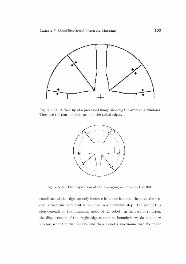
Chapter 5. Omnidirectional Vision for Mapping 103
Figure 5.21: A close up of a processed image showing the averaging windows.They are the star-like dots around the radial edges.
Figure 5.22: The disposition of the averaging windows in the 360◦ .
coordinate of the edge can only increase from one frame to the next, the sec-
ond is that this increment is bounded to a maximum step. The size of this
step depends on the maximum speed of the robot. In the case of rotation,
the displacement of the single edge cannot be bounded: we do not know
a priori what the turn will be and there is not a maximum turn the robot

104 Omnidirectional Vision for Mobile Robots
can take8 . There is only a loose bound given by the maximum rotational
velocity, but this is not such a constraint. Therefore, an edge can match any-
one of the edges in the image with a similar signature. The only constraint
we can use is that every edge has to experience the same azimuthal shift.
Therefore, we implemented a backtracking algorithm that finds a matching
for every edge checking that all edges experienced the same azimuthal shift.
The backtracking is necessary to search completely the space of all possible
edge matching.
There is a problem: we have these two different sets of constraints for the
two different type of motion and the robot does not have access to any infor-
mation to decide which set should be used. To overcome this, the matching
algorithm tries to match the edges assuming the robot performed a rotation.
If this does not results in a good matching, it assume a translation and applies
the appropriate rules. A good matching is defined as a matching where
more than half of the edges present in the image are correctly identified. If
neither of the two set of rules is able to match more than half of the edges,
the match that correctly labelled more edges is returned.
We defined a good match as requiring the match of more than half of the
edges present in the image, because we cannot require that every edge in
the current frame is matched with an edge of the previous frame. In fact, if
a new edge exited from occlusion in this frame it cannot be matched with
anything. On the other hand, it is very unlikely that a wrong matching could
identify more than half of the edges.
In all the tests performed by the matching algorithm we introduced a
certain amount of tolerance. We have tolerance on the colour signature, on
the azimuthal shift and on the azimuthal increase. Let us consider them in
detail. The tolerance on the colour signature states that two colour signatures
8Remember the robot does not have any direct access to informations about its move-ments
Chapter 5. Omnidirectional Vision for Mapping 105
are considered the same if the values of each colour component differs by less
than a certain threshold. The tolerance on the azimuth shift states that two
azimuthal shifts are equal if the shift angle differ less than a certain threshold.
The tolerance on the azimuthal increase allows an edge to pass this check
even if its actual azimuthal coordinate is slightly smaller than in the previous
frame. The tolerances reported have been tuned during the experiments on
simulated and real sequences in order to have a matching algorithm flexible
enough to cope with the noise but not so loose to produce mismatches.
After the matching process is completed, the program writes in a log file
the information about the edges in the current frame: the unique label of
the edge, its azimuthal position and the values of its left and right averaging
windows. This file is useful for debugging purpose and can be used off-line
for the reconstruction of the topology of the environment. So far, only the
first two of the types of topological transition we saw in Subsection 5.4 are
detected on the fly. In fact, the software is able to detect the topological
event if the number of edges changes from one frame to the next.
To test the software we wrote, we performed first an experiment with a
simulated sequence of frames and then we implemented the system on the
actual robot.
5.6 The Simulated Experiment
To perform the simulated experiments, we generated a sequence of images
captured by the camera under the mirror while the robot moves in the maze.
This sequence of images were used as input for the vision system. Unfortu-
nately, in POV-Ray it is possible to create only off-line simulations. It is only
possible to generate a sequence of images, it is not possible to introduce an
interaction between the vision system software and the rendering program.
In other words, it is not possible to create an interaction between the robot

106 Omnidirectional Vision for Mobile Robots
= Translation
= Rotation on the spot
Figure 5.23: The path of the robot through the virtual environment.
(1) (2) (3)
Figure 5.24: The simulation of an ephemeral edge. Notice that the edge onthe left marked with the red dot is not present in the second frame.
and the virtual environment. So the robot followed the pre-planned path of
Fig. 5.23.
Two problems sensitive to the choice of the threshold are the ephemeral
edges and the false edges. These cannot be eliminated just tuning the thresh-
old but their effects can be lowered.
We called ephemeral edges, those edges whose presence in the frame
sequence is not detected for some frames and after a few frames is detected
again. An example is the left edge in Figure 5.24. This happens because the
value of the edge counters are under the threshold just for few frames. The

Chapter 5. Omnidirectional Vision for Mapping 107
(1) (2) (3)
Figure 5.25: The simulation of a false edge. Notice that in the second framethe right baseline of the corridor is detected as a radial line. This does nothappen neither in the previous frame or in the next.
reason can be either that the pixels of the edge spread in the neighbourhood
in such a way that none of their counter is over the threshold or that there is
a variation on the number of the edge pixels introduced by the Canny edge
detector. So far, the program is not able to handle correctly the ephemeral
edges. It does not realise that the new edge that appeared is actually the
same that disappeared a few frames before. This is because the matching
process uses only two frames: the current one and the previous one. This
problem suggests the need of implementing a memory that spans over more
frames causing a persistence of the edges for a certain number of frames after
they disappeared. In this way, when an ephemeral edge reappears, it can be
matched with this persistent image of the edge.
The false edges are the accidentally radial lines in the image. In other
words, these are lines that are radial in the omnidirectional image, but that
does not correspond to vertical edges in the environment as we discuss at the
end of Section 5.4. In Figure 5.25 is presented the same sequence of Figure
5.14. The right base line of the corridor is detected just for one frame as a
new vertical edge. This suggests the need of a confidence measure on the
confirmation of an edge. An edge should be confirmed only if it is present in
a minimum number of frames.

108 Omnidirectional Vision for Mobile Robots
Despite these problems, the vision system software showed to be able to
correctly track the edges all along the path followed by the robot in these
simulations. See sequence in Figure 5.26 and Figure 5.27
The problems of the ephemeral edge and of the false edges could probably
be solved off-line from the software that exploits the information on the edge
to build the topological map. In other words, the memory of the system
could be implemented at a higher level than the sensory level. Probably, it
would be easy for this program to analyse the log file of the vision system
and spot the presence of an ephemeral or false edge, easier than for the vision
system to spot them on the fly.
5.7 The Real Experiment
As we said in the introduction, the environment chosen for carrying out the
experiments was the robot football playground at the Intelligent Autonomous
Systems Laboratory at the University of Padova. The room has white walls
and a floor covering of green carpet. In this room we built a simple corri-
dor with a turn. In the corridor were two boxes to reproduce a door-like
view. See Picture 5.28. All the vertical surfaces were painted with uniform
colours, except the two boxes. This was done to avoid textures that could
fool the edge detector. During the experiments, also the boxes where covered
with a uniform colour fabric, because of the noise they introduced. Like for
the virtual environment, the colours chosen for the surfaces are vivid and
they stand out one against the other to facilitate the recognition of the edge
signatures.
When we described the omnidirectional vision system we said that the
optical axis of the camera and the geometrical axis of the mirror are aligned.
On the real robot this calibration is not an issue. It can be done roughly
by hand and then we can find in the image where the tip of the mirror is

Chapter 5. Omnidirectional Vision for Mapping 109
270
(1)
(2)
(3)
(4)
(1)
(2)
(3)
(4)
Fig
ure
5.26
:(T
op)
The
cam
era
vie
wof
asi
mula
ted
imag
ese
quen
cefo
ra
tran
slat
ion
ofth
ero
bot
.(B
otto
m)
The
trac
kin
gof
the
edge
sin
this
sequen
ce.

110 Omnidirectional Vision for Mobile Robots
(1)(2)
(3)(4)
(1)(2)
(3)(4)
Figu
re5.27:
(Top
)T
he
camera
view
ofa
simulated
image
sequen
cefor
arotation
ofth
erob
ot.(B
ottom)
The
trackin
gof
the
edges
inth
isseq
uen
ce.

Chapter 5. Omnidirectional Vision for Mapping 111
Figure 5.28: The experimental set-up. This is the corridor where the exper-iments were conducted. The two box represent a door. On the right, behindthe wood box there is the turn of the corridor.
mapped. We need this information, because this is the point from where
all the radial edges sprout and where we have to centre the polar reference
system. The performance of the Hough transform depends on the accuracy of
this estimation. In Figure 5.29 is represented how we found the real centre of
the image. We prolonged the radial edges present in the picture, the crossing
point of all the edges is the image centre. This estimations is simple and
accurate enough for our purposes.
The results
All the thresholds set in the previous chapter had to be reset when working
with the real images. The images are much noisier now. In Figure 5.30 an

112 Omnidirectional Vision for Mobile Robots
Figure 5.29: The centre of a real image. In red the prolongations of thevertical edges to find out where is mapped the vertex of the mirror.
example of the image process stages for a real image. The noise in the picture
propagates down to all stages of the image process. The edge detection
result is noisy, Figure 5.30 a). Several noise edgelets are detected, some
edges are broken and noise spots are present. This makes it more difficult to
reliably detect the radial lines and the radial lines only. In fact, in the Hough
transform the pixels of the noise sums over the edge pixels and sometimes
the noisy pixels can trigger a false detection of a radial line. An example
is shown in Figure 5.31. The arrow shows a marker of a detected edge
but the edge does not exists in the picture. It is just the effect of several
noisy pixels accidentally having the same angular coordinate. This cannot be
avoided setting the threshold higher, because we would have to set it so high
to loose significant edges. These false edges do not last for more than two
frames and then they could be easily filtered out by the software in charge
of reconstructing the topology of the environment, if this is fitted with a

Chapter 5. Omnidirectional Vision for Mapping 113
(a) The unprocessed image as viewfrom the robot’s camera.
(b) The image after the Cannyedge detection.
(c) The edge image after theHough transform.
(d) The final result showing theedge matching.
Figure 5.30: An example of the image process stages for a real image.

114 Omnidirectional Vision for Mobile Robots
Figure 5.31: An example of false edge produced by the noise in the image.The arrow points the wrong marker.
temporal memory.
The problem of the ephemeral edges exists also in the real image se-
quences. The noise of the images worsens the problem compared to the
simulated images. It happens more often, that an edge disappear and then
reappear after some frame. Again this could be solved by introducing a
temporal memory of the edges.
The undermining problem in the real image is the noise introduced by the
CCD sensor of the camera. This noise affects mostly the colour of the pixels.
The noise is so high that even if the robot is steady in the same position, the
edge signatures of the same edge in two consecutive frame are different. This
problem has been solved with two changes in the vision system software: the
tolerance within two colours are considered the same has been increased and
the windows over which the mean colour is calculated have been doubled.
See Figure 5.32. Doubling the size of the averaging window, we use more
pixels to calculate the mean colour and then the edge signature values are

Chapter 5. Omnidirectional Vision for Mapping 115
Figure 5.32: The averaging windows used in the real experiments. Noticethat the averaging windows are doubled.
more stable.
When the robot moves, the colours around the edges change slightly be-
cause of different shadows and different reflections on the surfaces of the
objects. To cope with this change we had to relax further the colour toler-
ance. Remember that the colour of every pixels of the image and the edge
signature are represented as a RGB triplet. The new criterion we used is:
two edge signatures are considered the same when at least two elements of
their triplets are equal within a certain interval. This is enough to cope with
the noise present when the robot moves in straight lines, but does not work
when the robot turns.
Analysing the images taken from the robot when it rotates, we discovered
that the robot failed to recognise the edges because the colours on the sides
of the edges in different images are actually different. Consider that the view
of the scene does not change and even the shadows and the reflections on
the objects’ surfaces are the same, this should not happen, and the image

116 Omnidirectional Vision for Mobile Robots
should be exactly the same, only rotated by the angle the robot rotated.
If the explanation of this change of the colours is not in the scene, it must
be in the vision system. The software of the vision system cannot be held
responsible for that: it works fine in the simulation. The only candidate is
the hardware of the vision system. Remember the camera sees the world
through the Perspex cylinder that support the mirror. The explanation of
the change of colours can be found in the changes of the light reflection
on the Perspex cylinder. These reflections change because the robot’s body
does not have a cylindrical symmetry. As you can see in Figure 5.1 not only
the body is rectangular but also the cover on the top of the mirror has a
rectangular shape. The purpose of this cover is to avoid that the camera is
blinded by the lights on the ceiling, but it also shadows the Perspex cylinder
preventing most of the reflection on it. Because the cover is rectangular, it
shields better some region of the Perspex cylinder than others. When the
robot rotates it sees the same points in the world through regions of the
cylinders with different shadowing from the cover and so different reflections
occur at the cylinder surface. The final effect is that the colours appear to
change. This effect is made even worst by the reflections occurring on the
top cover of the robot body. See Figure 5.33 for an example in which these
reflections are particularly strong. Notice the bright spot that seems to move
on the left part of the robots body.
The explanation provided for the failure of the tracking algorithm in the
rotations is consistent with the fact that this effect does not occur when the
robot moves along a straight line. In fact, in this case the change in the
reflection is not sharp.
The solution to the problem of reliably detect the colour of the edges
could be solved changing the colour space. In fact, the RGB space is not
perceptually uniform. As such, the proximity of colours in RGB colour space
does not indicate colour similarity. It would probably be a good idea to

Chapter 5. Omnidirectional Vision for Mapping 117
(1) (2)
(3) (4)
Figure 5.33: A close up of a sequence showing an example of strong reflectionon the body of the robot. Notice the bright spot on the left of the robot’sbody that appears to move from one frame to the next.

118 Omnidirectional Vision for Mobile Robots270
(1)(2)
(3)(4)
(1)(2)
(3)(4)
Figu
re5.34:
(Top
)T
he
camera
view
ofa
realim
ageseq
uen
cefor
atran
slationof
the
robot.
(Bottom
)T
he
trackin
gof
the
edges
inth
isseq
uen
ce.

Chapter 5. Omnidirectional Vision for Mapping 119
(1)
(2)
(3)
(4)
(1)
(2)
(3)
(4)
Fig
ure
5.35
:(T
op)
The
cam
era
vie
wof
asi
mula
ted
imag
ese
quen
cefo
ra
rota
tion
ofth
ero
bot
.(B
otto
m)
The
trac
kin
gof
the
edge
sin
this
sequen
ce.

120 Omnidirectional Vision for Mobile Robots
transfer the image to the HSI colour space. In this space, colour pixels are
defined as triplets representing hue (H), saturation (S) and intensity (I). This
colour space has the advantage of being approximately perceptually uniform.
Therefore, colour similarity implies proximity in this colour space [80]
5.8 Conclusions
This work implemented the Spatial Semantic Hierarchy on a real robot. We
realised the sensory level with an omni-directional vision system. This is the
first step toward the construction of an agent able to draw a topological map
of the environment it travels through. Experiments were performed both in
simulation and with a real robot.
In this work, we showed that an omni-directional vision system is a good
sensor for the SSH. We pointed out which of the features present in a omni-
directional image can be used to detect the transitions of state needed by the
control level of the SSH. We showed the existence of a strict link between
the views of the SSH and the image taken by an omnidirectional sensor. We
built a vision system able to extract these features from the images. We
showed that the software runs properly in a virtual environment and finally,
we tested the same software on a real robot discovering that what worked in
the simulations does not work in the real world. This confirms what Ronald
Arkin said, which might seem self-evident but is often forgotten:
To conduct robotics research, robots are needed
—Ronald Arkin ’Behaviour-Based Robotics’ MIT Press
At the time of writing, we are working to solve this implementational
problem. The work presented in this chapter was presented in [70] [71].
At the same time we are working also to extend to multi-robot systems
our approach to the mapping problem. The basic idea is every robot build

Chapter 5. Omnidirectional Vision for Mapping 121
the local map of the portion of environment it visited. When two robots meet
they share their portions of the map, fusing them in a global map. This idea
was presented in [65], preliminary experiments were presented in [67].

122 Omnidirectional Vision for Mobile Robots

Chapter 6
Distributed Omnidirectional
Vision
In the previous chapter, we showed the synergy that can be implemented
between an omnidirectional vision sensor and the theory of the Spatial Se-
mantic Hierarchy (SSH) proposed by Kuipers. In this chapter we will present
our current works on the distributed omnidirectional vision. In the first part
of the chapter we will explain the concept of distributed vision system and
we will illustrate some of the research lines we are following. In the second
part of the chapter we will present an experiment where a distributed vi-
sion system is autonomously learning how to control a mobile robot. The
works presented in this chapter are in progress and the experiments we are
performing are giving new hints and new insights on the investigated topics.
6.1 Distributed Vision in Robotics
Our work has been inspired by the work of Ishiguro [36]. He proposed an
infrastructure called Perceptual Information Infrastructure (PII). In his pa-
per, he proposed an implementation of the PII composed by static Vision
Agents, i.e. fixed cameras with a certain amount of computational power.
123

124 Omnidirectional Vision for Mobile Robots
This realisation of the Perceptual Information Infrastructure was called Dis-
tributed Vision System (DVS). The DVS presented in [36] has 16 cameras,
strategically placed in the environment, that navigate two mobile robots.
The robots are not autonomous, in the sense that they need the DVS to nav-
igate, but they has a certain amount of deliberative power, in the sense that
they can decide which Vision Agent provides them the more reliable informa-
tion on the surroundings. The assumption that every Vision Agents is static
simplifies the problem and allows to use very simple vision algorithms. In
fact, to detect the moving objects (the robots) Ishiguro used the background
subtraction algorithm. This implies that the whole system is not scalable to
include Mobile Vision Agents, as we will see in the following.
A parallel but independent work is the one of Matsuyama [54]. Mat-
suyama explicitly introduced mobile robots in the theoretical frame of its
Cooperative Vision System. In the experiments presented in [54], he used
active cameras mounted on a special tripod. The active cameras were pan-
tilt-zoom cameras modified in order to have a fix view point. This allowed,
again, the use of a simple vision algorithm, not very different from the case
of static cameras.
As far as we know, no attempt has been tried to realise a DVS with truly
mobile robots running robot vision algorithms.
Mobile robots are more and more fitted with vision systems. The popu-
larity of such sensors arises from their capability of gathering a huge amount
of information from the environment surrounding the robot.
In multi-robot systems there are two possibilities to acquire visual infor-
mation, i.e. a centralised vision system or a distributed vision system.
The first approach consists in controlling a robot team with a unique
camera that monitors the whole environment where the robots move. This
has been applied in well structured and relatively small environments [14],
but it is unfeasible for large environments. If this is the case, we are compelled

Chapter 6. Distributed Omnidirectional Vision 125
to move toward the second approach, a distributed vision system. Nowadays,
the relatively low cost of the required hardware allows to equip every robot
with a vision sensor mounting a camera on each robot of the team.
In the second approach, each robot can gather a detailed information
on its surrounding and the system is more versatile. In fact, fix camera
positioned in a priori location in the environment limits the flexibility and
robustness of the system, even if we dispose of several fixed cameras. As an
example think of an industrial site watched with a video monitoring system
composed only of cameras with fixed locations (even pan-tilt-zoom cameras).
If an alarm or a meaningful event happens outside the field of view of any
camera, the system cannot “see” this event. This is because the system has a
predetermined field of view. If we have also some cameras mounted on mobile
robots, the system can send a robot to inspect the new location of interest.
With such a solution the system is more flexible and we realise what we call
a dynamic field of view.
Introducing mobile robots fitted with cameras distributes the sensors in
the environment, but this is not enough: we aim to the creation of a Dis-
tributed Vision System. A set of cameras scattered in the environment (fixed
or mounted on mobile robots) needs to communicate over a network in order
to became a unique Distributed System. If not, they are just a set of different
vision sensors of pertinence of the single vision system.
In the following we will prefer the term Vision Agent instead of “vision
system”. The term Vision Agent emphasises that the vision system is not
just one of the several sensors of a single robot, but that it interacts with the
other vision systems to create an intelligent distributed system.
The final goal
The aim of this work is to introduce a real Mobile Vision Agent in the DVS
architecture, i.e. to apply the ideas and the concepts of Distributed Vision

126 Omnidirectional Vision for Mobile Robots
Figure 6.1: Our team of heterogeneous robots
to a mobile robot equipped with a camera.
The domain in which we are testing our ideas is the RoboCup compe-
tition. We are on the way to create a Distributed Vision System within a
team of heterogeneous robots fitted with heterogeneous vision sensors. We
want to create a dynamic model of the environment, which can be used by
mobile robots or humans to monitor the environment or to navigate through
it. The model of the environment is built fusing the data collected by every
Vision Agent. The redundancy of observers (and observations) is a key issue
for system robustness.
6.2 Mobile Robot DVS
6.2.1 VAs on the same robot
The first implemental step is to realise a Cooperative behaviour between
two heterogeneous vision agents embodied in the same robot. Exploiting the
knowledge acquired in our previous research [56] [71], we want to create a
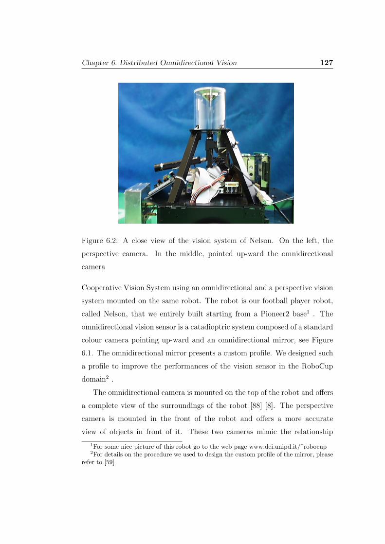
Chapter 6. Distributed Omnidirectional Vision 127
Figure 6.2: A close view of the vision system of Nelson. On the left, the
perspective camera. In the middle, pointed up-ward the omnidirectional
camera
Cooperative Vision System using an omnidirectional and a perspective vision
system mounted on the same robot. The robot is our football player robot,
called Nelson, that we entirely built starting from a Pioneer2 base1 . The
omnidirectional vision sensor is a catadioptric system composed of a standard
colour camera pointing up-ward and an omnidirectional mirror, see Figure
6.1. The omnidirectional mirror presents a custom profile. We designed such
a profile to improve the performances of the vision sensor in the RoboCup
domain2 .
The omnidirectional camera is mounted on the top of the robot and offers
a complete view of the surroundings of the robot [88] [8]. The perspective
camera is mounted in the front of the robot and offers a more accurate
view of objects in front of it. These two cameras mimic the relationship
1For some nice picture of this robot go to the web page www.dei.unipd.it/˜robocup2For details on the procedure we used to design the custom profile of the mirror, please
refer to [59]

128 Omnidirectional Vision for Mobile Robots
between the peripheral vision and the foveal vision in humans. The peripheral
vision gives a general, and less accurate, information on what is going on
around the observer. The foveal vision determines the focus of attention
and provides more accurate information on a narrow field of view. So, the
omnidirectional vision is used to monitors the surroundings of the robot to
detect the occurrence of particular events. Once one of these events occurs,
the Omnidirectional Vision Agent (OVA) send a message to the Perspective
Vision Agent (PVA). If the PVA is not already focused on a task, it will move
the robot in order to put the event in the field of view of the perspective
camera. This approach was suggested by our previous researches presented
in [20].
Experiments on such a system are running and they will provide more
insight on the cooperation of the two heterogeneous vision agents.
6.2.2 VAs on different robots
Another stream of research is the creation of a Cooperative Distributed Vi-
sion System for our team of football player robots3 , depicted in Figure 6.1.
Our aim is to implement the idea of the Cooperative Object Tracking
Protocol proposed by Matsuyama [54]. In the work of Matsuyama the central
notion is the concept of agency.
An agency, in the definition of Matsuyama, is the group of the VAs that
see the objects to be tracked and keeps an history of the tracking. This group
is neither fixed nor static. In fact, a VA exits the agency, if it is not able to
see the tracked object anymore and a new VA can joint the agency as soon as
the tracked object comes in its field of view. To reflect the dynamics of the
agency we need a dynamic data structure with a dynamic role assignment
[55].
3For a detailed description of the robots employed in these experiments, please refer to[75] [76].

Chapter 6. Distributed Omnidirectional Vision 129
Figure 6.3: A close view of two of our robots. Note the different vision
systems
Let us sketch how the agency works, using an example draw from our
application field: the RoboCup domain. Suppose to have a team of robots
in the field of play. Each robot is fitted with a Vision Agent. None of the
Vision Agents is seeing the ball. In such a situation no agency exists. As
soon as a Vision Agent see the ball, it creates the agency sending a broadcast
message to inform the other Vision Agents the agency has been created and
it is the master of the agency. After this message a second message follows,
telling the other Vision Agents the estimated position of the ball. All the
other Vision Agents manoeuvre the robots in order to see the ball. Once
a Vision Agent has the ball in its field of view, it asks permission to joint
the agency and send to the master its estimation of the ball position. If this
information is compatible with the information of the master, i.e. if the new
Vision Agent has seen the correct ball, it is allowed to joint the agency.
The described algorithm has been realised by Matsuyama with his fixed
vied point cameras. His system was composed of four pan tilt zoom cameras
mounted on a special active support in order to present a fixed view point.

130 Omnidirectional Vision for Mobile Robots
The system was able to track a radio controlled toy car in a small indoor
environment. As mentioned before, in such a system there is not a truly
mobile agent. Moreover, the vision algorithm used is typical of static Vision
Agents. In fact, it is a smart adaptation of the background subtraction
technique.
Our novel approach is to implement the Cooperative Object Tracking
Protocol within a team of mobile robots equipped with Vision Agents. This
requires a totally new vision approach. In fact, the point of view of the Vision
Agent changes all the time. The changes in the image are due not only to the
changes in the world (as in the Matsuyama testbed), but also to the change
of position of the Vision Agent. Therefore, we need a vision algorithm able
to identify the different objects of interest and not only to reveal the objects
that are moving. Moreover, we have to introduce a measure of uncertainty
in the estimation of the position of these objects, because the location of
the Vision Agents is not known exactly anymore and there are errors in the
determination of the relative distance between the objects the Vision Agents.
To explain these issues, let us come back to our RoboCup example. Above
we said that if a new Vision Agent sees the ball, it sends a message to the
master that checks if it has seen the correct ball. In a RoboCup match there
is just one ball, but sometimes what a robot identifies as a ball is not the
correct one. This can result either because the robot sees objects resembling
the ball, and erroneously interprets them as a ball (like spectators hands or
reflex of the ball on walls), or because it is not properly localised and so it
reports the ball to be in a fallacious position.
To cope with the uncertainty in the objects position, every Vision Agent
transmits to the master the calculated ball position with the confidence of this
estimation. The master dispatches to the other robot a position calculated as
an average of the different position estimations, weighted by the confidences
reported by every Vision Agent (if there is more than one Vision Agents in

Chapter 6. Distributed Omnidirectional Vision 131
the agency).
Especially in the described dynamic system, the master role is crucial in
the correct functioning of the agency. The master role cannot be statically
assigned. The ball is continuously moving during the game. The first robot
that sees the ball will not have the best observational position for long. So,
the master role must pass from robot to robot. The processes of swapping
the master role is critical. If the master role is passed to a robot that sees
an incorrect ball the whole agency will fail in the ball tracking task.
The simplest solution could be to pass the master role to the robot with
the highest confidence on the ball position. This means to shift the problem
to identify a reliable confidence function. This makes sense, because the
confidence function will be used for two services that are two sides of the
same coin. In fact, if a robot is correctly localised and correctly calculates
the relative distance of the ball, it will have strong weight in the calculation
of the ball position. Given this, it can reliably take the role of master.
The confidence function
The confidence function ψabs associated to the reliability of the estimation of
the absolute ball position is a combination of several factors. It has to account
for the different aspects that contributes to a correct estimation of the ball
position. In fact, the position of the ball in the field of play is calculated
by a vectorial sum of the relative distance of the ball from the robot and
the absolute position of the robot in the pitch. So, the confidence of the
estimation of the absolute position of the ball is the sum of the confidences
function associated to the self-localisation, ψsl, and of the confidence function
associated to the estimation of the relative position of the ball with respect
to the robot, ψrel.
ψabs = ψsl + ψrel (6.1)

132 Omnidirectional Vision for Mobile Robots
The self-localisation process uses the vision system to locate landmarks in
the field of play. The process is run only by time to time and if the landmarks
are visible. Between two of these process the position is calculated with the
odometers. This means that the localisation information degrades with time.
The confidence function associated with the self-localisation is the result of
the following contribution:
• type of vision system (perspective, omnidirectional, etc.);
• a priori estimated absolute error made from the vision system in thecalculation of the landmarks position;
• time passed after the last self-localisation process;
The relative position of the ball with respect to the robot is calculated
as in [59]. The confidence function in this process presents the following
contribution:
• type of vision system;
• distance from the ball;
At the moment the exact definition of the confidence function is under
testing. The experiments will tell us how much every contribution should
weight in the final function.
In the next section, we will present some experiments we realised on
Distributed Vision Systems that can learn to control a mobile robot.

Chapter 6. Distributed Omnidirectional Vision 133
6.3 Learning DVS
Nowadays the applications of networks of sensors are more and more com-
mon. There is an increasing need for intelligent sensors able to dialogue
one to the other in order to exchange information and to perform intelli-
gent tasks. For instance, networks of cameras are something we are used in
every-day-life, but in most cases these are just a set of dummy sensors (e.g.
multi-camera video surveillance systems in banks or airports). They collect
a huge amount of videotape data that human operators need to interpret. In
the scientific community, there is a strong will to integrate these sensors into
an intelligent system. Several researchers are working on autonomous system
of surveillance [24] [73] or on intelligent environments [12] [83], like intelligent
rooms. In the robotics community as well, the interest of the researchers is
shifting form a single agent working in a cell-space to multiple agents working
in the real world. For these kind of applications a single camera is not enough
and multiple cameras are needed to observe the scene. Again, the aim is to
provide an intelligent infrastructure able to support robots’ activities [38]
[36].
In this chapter, we present a network of uncalibrated omnidirectional vi-
sion sensors able to autonomously learn to control a mobile robot in a large
scale environment. The cameras in the network can communicate among
them and with the mobile robot. To stress that the camera network is more
than a simple bunch of sensors scattered in the environment, we called it a
Distributed Vision System (DVS). The term DVS (Distributed Vision
System) emphasises that the camera network acts as a whole, as a single
“super-sensor”, able to navigate the robot. The DVS is composed of several
Vision Agent (VA). A VA (Vision Agent) is a vision sensor able to acquire
images, to process them and to communicate with other VAs over a network.
In the taxonomy of Weiss, a Vision Agent can be defined as a Smart Agent,

134 Omnidirectional Vision for Mobile Robots
OmnidirectionalVision Agents
MobileRobot
Figure 6.4: A picture of the whole system showing two Vision Agents andthe robot used in the experiments.
because it is autonomous, it is able to learn from experience and it can coop-
erate with other agents to achieve a global goal [85]. In our implementation,
everyone of these agents is embodied in a different sensor and is situated at a
different position. Form a hardware point of view, the DVS presented in this
chapter looks like a set of uncalibrated omnidirectional cameras distributed
in the environment, see Fig. 6.4. The omnidirectional cameras are catadiop-
tric omnidirectional cameras composed of a standard perspective camera and
a convex mirror [37]. The camera is pointed upward to the mirror that is
reflecting the light gathered by the surroundings of the sensor, see Fig. 6.6.
Every camera is connected to a PC that provides computational power for
image processing and network communication.
Ishiguro showed how a Distributed Vision System can navigate a robot
in a toy-scale real-world environment [36]. In that work the learning phase
required the intervention of a human operator guiding the robot in the free
space in the toy town reproduction. In this chapter, we propose a totally
autonomous Distributed Vision System able to learn how to control a mobile

Chapter 6. Distributed Omnidirectional Vision 135
robot by autonomously generating a set of examples and by propagating the
knowledge through the network.
In Section 2, we will discuss in further detail the task of the DVS. In
Section 3, we will explain the structure of an Omnidirectional Vision Agents.
In Section 4, the learning procedure is discussed and experimental results are
presented. Finally, future work are hinted and conclusions are drawn.
6.3.1 The task to be learnt
As we said in the introduction the task of the DVS is to learn to drive a mobile
robot. This knowledge is first acquired by a single VA and then is propagated
to other VAs in the network. The distributed learning is composed of four
steps:
1. a Vision Agent learns the mapping between its image space and the
robot’s motor space;
2. the Vision Agent transmits the learnt mapping to a second Vision
Agent;
3. the second Vision Agent checks if the received mapping is valid, if not
starts a re-learning phase guided by the first Vision Agent;
4. the knowledge is propagated from the second Vision Agent to the third
Vision Agent, and so on;
The bridge to propagate the knowledge among the Vision Agents is the
robot. The first Vision Agents controls a robot by sending to the robots a
set of random motion commands, see Fig. 6.5. Looking at the motion of the
robot, the system learns the mapping between the position of the robot in
the image space and the robot’s motor space, see Fig. 6.8. As we said, the
acquired knowledge is then propagated to the other Vision Agents on the

136 Omnidirectional Vision for Mobile Robots
Commands
Observes
Knowledge
Figure 6.5: The knowledge propagation process: the VA on the right sendcommands to the robot, the VA on the left observing the robot evaluates theknowledge received by the first VA.
network, Fig. 6.5. Because the vision sensors are not previously calibrated,
the propagated knowledge cannot be immediately used and a certain amount
of re-learning can be needed. In fact, if the vision sensors are not previously
calibrated, the mapping between the image space and the motor space might
be different: the cameras could be located at different heights or at different
distances from the mirrors, the poles supporting the cameras could be not ex-
actly vertical, etc. In addition, the Vision Agents could mount heterogeneous
vision sensors and so the mapping function have to be relearned. Examples
of heterogeneous vision sensors can be omnidirectional vision sensors with
mirrors with different profiles customised for different tasks [59].
Omnidirectional Vision Agent
Every sensor in the network is composed of hardware and software resources.
We discussed the hardware resources in which the VA is embodied in the
introduction. In Fig. 6.6, the hardware resources of the VA are depicted. In

Chapter 6. Distributed Omnidirectional Vision 137
Mirror
Camera
Tripod
Figure 6.6: A picture of the hardware resource of the Vision Agent. On thetop the omnidirectional mirror (here a hyperbolic mirror), under the mirrorthe camera and the tripod supporting the system.
this section we will discuss the software resources called Vision Agent.
The Omnidirectional Vision Agents used in this work are composed of
the following modules:
• a vision system
• a neural network called navigator
• a neural network called supervisor
• a communication network module
In the next section we will discuss in detail the single modules of the
Vision Agent.
6.3.2 Vision System
The vision system is the sensorial module of the Vision Agent. The Vision
Agent gathers information on the world using the vision system.

138 Omnidirectional Vision for Mobile Robots
Communication Module
SupervisorNNNN
Navigator
SystemVision
Vision Agent
OUT
IN
Figure 6.7: The simplified scheme of a Vision Agents. The drawing highlightsthe main blocks composing the VA.
The task of the vision system is to calculate the position and the heading
of the robot in the image. To easily detect the position and the heading of
the robot, two coloured balls are fixed on the top of the robot and the vision
system looks for these two coloured blobs. The midpoint between the centres
of gravity of the two balls gives the position of the robot and the line passing
by the centres of gravity of the two balls gives the heading of the robot. In
order to avoid to search the whole image for the coloured blobs, the vision
system uses a background subtraction algorithm to detect the broad region
of image in which is located the robot.
The background subtraction algorithm can be used because we are as-
suming the Vision Agent is static (i.e. its view of the environment does not
change) and the robot is the only moving object in the filed of view of the
camera. The current image with the robot moving in the environment is
subtracted from a reference image in which the robot is not in the field of
view of the Vision Agents. The difference image is thresholded. The centre
of gravity and the vertical and horizontal standard deviations of the “differ-
ent” pixels are calculated. A region of interest (ROI) is created in a region

Chapter 6. Distributed Omnidirectional Vision 139
centred in the calculated COG (centre of gravity) and spanning an area wide
as six times the horizontal standard deviation and height as six times the
vertical standard deviation. This choice for the width and height of the ROI
assures that all pixels belonging to the robot are included in the ROI (region
of interest). The current image is searched only within this ROI for the blue
and red pixels of the two balls.
The selected ROI is searched twice for the blue pixels and twice for the
red pixels, in order to increase the robustness of the calculation of the blobs’
COGs. In the first scan of the ROI, narrow colour thresholds are used, i.e.
only pixels strictly blue or strictly red are found. The COGs and standard
deviations of the found pixels are calculated and the pixels farther than
twice the standard deviations from the COGs are discarded as false matches.
Two ROIs are created around the calculated COGs and these two ROIs
are searched again with broad colour thresholds for blue and red pixels. In
the end the two COGs of this new blue and red blobs are calculated. This
algorithm proved to be very robust against the image noise and the COGs
of the blobs are steadily detected.
Once the COGs of the blue and red blobs are calculated, we can calculate
the position of the robot as the midpoint between the COGs of the blobs.
The heading of the robot is calculated as the angle between the line going
from the blue blob to the red blob and the image’s frame of reference.
The final output of the vision system is the heading and the position
of the robot calculated both in the polar coordinates centred in the image
centre and the Cartesian coordinates in the usual frame of reference for the
images.
Neural Networks
The output of the vision system is passed to the two neural networks. In
the learning stage the two neural nets are trained using the robot positions

140 Omnidirectional Vision for Mobile Robots
Figure 6.8: A snapshot of the image processing software that detects theposition and heading of the robot in the image.
X_S
X_S
X_S
X_F
Y_F
1
N
N−1
2
Speed
Jog
Figure 6.9: The structure of the used neural network.

Chapter 6. Distributed Omnidirectional Vision 141
Figure 6.10: A plot of the sigmoid function.
and the robot speeds of the autonomously generated training examples. In
the running stage, the task of the navigator network is to calculate the in-
stantaneous translational and rotational speeds necessary to reach the target
position. The task of the supervisor network is to check if the commands
sent to the robot have been successfully executed.
In this first implementation of our system we used a very simple structure
for the neural networks. These are three layer networks with an input layer,
an hidden layer and an output layer, see Fig. 6.9. The units of the networks
are sigmoid units and the networks are trained with the back-propagation
algorithm [72]. The sigmoid function is plotted in Fig. 6.10 and it is defined
as:
σ(x) =1
1 + e−x(6.2)
Navigator Network
As depicted in Fig. 6.9, the network has five input units, four hidden units
and two output units. The input units take the three parameters of the
initial position and heading of the robot and the two parameters of the final
position of the robot, respectively named:

142 Omnidirectional Vision for Mobile Robots
input→ {(xS, yS, hS), (xF , yF )}output→ {(Speed, Jog)}
(6.3)
Note that in the first part of this work we are not considering the final
heading of the robot, i.e. the robot has only to reach the final position, but
the final heading is not important.
The outputs of the network are the values of linear speed and angular
speed to be set on the motors of the robot, respectively.
These values are the instant speeds necessary to move the robot from the
starting position to the final position. These values are sent at every cycle
of the Vision Agent to the Agent on the robot through the network module.
Supervisor Network
The supervisor network takes as input the starting position of the robot and
the speeds set on the motors and predicts the final position of the robot. The
topology of the Supervisor Network is the same of the Navigator Network,
but inputs and outputs are respectively:
input→ {(xS, yS, hS), (Speed, Jog)}output→ {(xP , yP )}
(6.4)
If the actual final position of the robot, as reported from the vision system,
is not compatible with the predicted position an exception is raised. This
exception means that the learnt control of the robot is no longer valid and
a re-learning is needed. As we said, in our experiment this mean that the
knowledge received from another Vision Agents cannot be used and a certain
amount of re-learning is needed..

Chapter 6. Distributed Omnidirectional Vision 143
Communication Network Module
The network subsystem used here is a part of the ADE library, a software
suite written in C++ and used by our RoboCup4 team: Artisti Veneti5 .
ADE provides basic C++ classes implementing thread scheduling, message
passing and seamless network communication [17].
The protocol used for data transmission is the connectionless User Data-
gram Protocol (UDP) over IP. This protocol allows fast network responses
even in case of a temporary failure (as it is often the case in noisy wireless
networks). Packet loss for our application is not an issue since packets are
self-contained and repeatedly sent.
The messages sent via the ADE network (ANet), from a programmers’
point of view, are objects descending from a common virtual base class;
this allows the library to find out at runtime, via the C++ RTTI facilities,
the actual object class and its size. This information is then sent, together
with the real object data, to the receiver network port, where the object is
reconstructed in memory and cast to the correct type.
In this application, we send two types of messages: the motor commands
to the robot and the messages between the Vision Agents.
6.3.3 Training the Neural Networks
The first problem in training a neural net is to have a rich set of unbiased
training examples. In the learning phase, the Vision Agent generates a set
of random commands for the motors of the robot. The Vision Agent stores
in a file the initial pose of the robot, its final pose and the command that
moved the robot from the starting position to the finish position. These data
are used to train the two networks. In the first experiments we performed
4RoboCup: the Robotics Soccer Championship, URL www.robocup.org5Artisti Veneti is the RoboCup team of the University of Padua for the Middle-Size
League [76]

144 Omnidirectional Vision for Mobile Robots
Figure 6.11: The positions of the robot in the image for the training data.
the motion of the robot was constrained in a portion of the field of view of
the Omnidirectional VA. Fig. 6.11 shows the position of the robot for each
training example. As you can see, the robot moved in the left field of view
of the camera, approximately. Every motion had random speed and jog in
order to present to the network a set of examples of velocity and jog values
not biased by the choices of the user. The linear speed was randomly chosen
between -400 mm/s and 400 mm/s. The angular speed was randomly chosen
between -1 rad/s and 1 rad/s. We collected sets of about 200-300 examples
and we used about 160-260 examples as training examples and the rest as
validation examples. The training errors for a set of examples is reported in
Fig. 6.12 and in Fig. 6.13. The two figures respectively refer to the error in
the linear speed determination (called speed) and in the angular speed (called
jog).
6.4 Conclusions
In the first part of the chapter, we introduced the concept of Vision Agent
and Distributed Vision System and we presented some of the experiments we
are carrying on these topics. These works on Omnidirectional Distributed

Chapter 6. Distributed Omnidirectional Vision 145
Figure 6.12: A plot of the learning error on the speed output.
Figure 6.13: A plot of the learning error on the jog output.

146 Omnidirectional Vision for Mobile Robots
Vision have been presented in [63] [62] [61] [60].
In the second part of the chapter, we presented a new idea in the creation
of an intelligent network of sensor. We proposed a Distributed Vision System
that is able to navigate a mobile robot in a large space. The DVS is composed
of several Vision Agents that are able to autonomously learn how to control
the robot. This knowledge is acquired locally and is distributed through the
network from a Vision Agent to the rest of the Vision Agents using as a
bridge the mobile robot for this knowledge propagation. This work has been
presented in [69].

Bibliography
[1] H. Aihara, N. Iwasa, N. Yokoya, and H. Takemura. Memory-based self-
localisation using omnidirectional images. In A. K. Jain, S. Venkatesh,
and B. C. Lovell, editors, Proc. of the 14th International Conference on
Pattern Recognition, volume vol. I, pages 1799–1803, 1998.
[2] S. Arulampalam, S. Maskell, N. Gordon, and T. Clapp. A tutorial
on particle filters for on-line non-linear/non-gaussian bayesian tracking.
IEEE Transactions on Signal Processing, 50(2):174–188, Feb. 2002.
[3] S. Baker and S. Nayar. A theory of single-viewpoint catadioptric image
formation. International Journal of Computer Vision, vol. 35(no. 2):pp.
1–2, 1999.
[4] S. Baker and S. K. Nayar. A theory of catadioptric image formation. In
Proceeding of the 6th Intern. Conf. on Computer Vision, January 1998.
[5] A. Basu and D. Southwell. Omni-directional sensor for pipe inspection.
In Proc. of IEEE Int. Conf. Systems, Man and Cybernetics, volume 4,
pages pp. 3107–3112, 1995.
[6] R. Benosman and S. B. Kang, editors. Panoramic Vision. Springer,
2001.
147

148 Omnidirectional Vision for Mobile Robots
[7] G. Bianco and A. Zelinsky. Biologically-inspired visual landmark learn-
ing and navigation for mobile robots. Proceedings of the 1999 IEEE/RSJ
Int. Conf. on Intelligent Robots and Systems, 1999.
[8] A. Bonarini. The body, the mind or the eye, first? In M. Veloso,
E. Pagello, and H. Kitano, editors, RoboCup99: Robot Soccer World
Cup III, volume 1856 pp. 210-221 of LNCS. Springer, 2000.
[9] A. Bonarini, P. Aliverti, and M. Lucioni. An omnidirectional vision sen-
sor for fast tracking for mobile robot. Proceedings of the IEEE IMTC99,
1999.
[10] A. Bonarini, P. Aliverti, and M. Lucioni. An omnidirectional vision
sensor for fast tracking for mobile robot. IEEE Transaction of Instru-
mentation and Measurements, 49(3):pp. 509–512, 2000.
[11] T. Boult, C. Qian, W. Yin, A. Erkin, P. Lewis, C. Power, and R. Micheal.
Applications of omnidirectional imaging: Multi-body tracking and re-
mote reality. In IEEE Workshop on Applications of Computer Vision,
Dec 1998.
[12] R. A. Brooks. The intelligent room project. In Proceedings of the Second
International Cognitive Technology Conference (CT’97), Aizu, Japan,
August 1997.
[13] G. Browitt. Virtual reality telepresence using a mobile robot. Master’s
thesis, University of Edinburgh, Department of Artificial Intelligence,
1997.
[14] J. Bruce, T. Balch, and M. M. Veloso. Fast and inexpensive color im-
age segmentation for interactive robots. In Proceedings of the 2000
IEEE/RSJ Int. Conf. on Intelligent Robots and Systems (IROS ’00),
volume 3, pages 2061 – 2066, October 2000.

BIBLIOGRAPHY 149
[15] R. Bunschoten and B. Krse. 3-d scene reconstruction from cylindrical
panoramic images. Robotics and Autonomous Systems (special issue),
2002. (to appear).
[16] W. Burgard, D. Fox, M. Moors, R. Simmons, and S. Thrun. Collabora-
tive multi-robot exploration. In Proceedings of the IEEE International
Conference on Robotics and Automation (ICRA). IEEE, 2000.
[17] L. Burrelli, S. Carpin, F. Garelli, E. Menegatti, and E. Pagello. Ade: a
software suite for multi-threading and networking. Technical report, In-
telligent Autonomous Systems Laboratory, Department of Information
Engineering, University of Padova, ITALY, 2002.
[18] J. Canny. A computational approach to edge detection. In Transactions
on Pattern Analysis and Machine Intelligence, volume 8, pages 679–697.
IEEE, 1986.
[19] J. Carpenter, P. Clifford, and P. Fearnhead. An improved particle filter
for non-linear problems. In IEEE Proc. Radar, Sonar and Navigation,
volume vol. 146, 1999.
[20] S. Carpin, C. Ferrari, E. Pagello, and P. Patuelli. Bridging deliberation
and reactivity in cooperative multi-robot systems through map focus. In
M.Hannebauer, J. Wendler, and E. Pagello, editors, Balancing Reactivity
and Social Deliberation in Multi-Agent Systems,, LNCS. Springer, 2001.
[21] R. Cassinis, D. Duina, S. Inelli, and A. Rizzi. Unsupervised matching
of visual landmarks for robotic homing unsing fourier-mellin transform.
Robotics and Autonomous Systems, 40(2-3), August 2002.
[22] H. Choset and K. Nagatani. Topological simultaneous localisation and
mapping (slam): Toward exact localization without explicit localization.

150 Omnidirectional Vision for Mobile Robots
IEEE Transaction on Robotics and Automation, 17(2):125–137, April
2001.
[23] T. Collett, E. Dillmann, A. Giger, and R. Wehner. Visual landmarks
and route following in desert ants. Journal of Comparative Physiology
A, 170:pp. 435–442, 1992.
[24] R. Collins, A. Lipton, and T. Kanade. A system for video surveillance
and monitoring. Technical report, Robotics Institute at Carnagie Mellon
University, 2000.
[25] R. Cutler, Y. Rui, A. Gupta, J. C. I. Tashev, L. wei He, A. Colburn,
Z. Zhang, Z. Liu, and S. Silverberg. Distributed meetings: A meeting
capture and broadcasting system. In ACM Multimedia, 2002.
[26] S. Derrien and K. Konolige. Approximating a single effective viewpoint
in panoramic imaging devices. In Proceedings IEEE Workshop on Om-
niDirectional Vision, pages pp. 85–96., June 2000.
[27] M. O. Franz, B. Scholkopf, H. A. Mallot, and H. H. Bulthoff. Learning
view graph for robot navigation. Autonomous Robots, 5:pp. 111–125,
1998.
[28] J. Gaspar, C. Decco, J. Okamoto, and J. Santos-Victor. Constant reso-
lution omnidirectional cameras. In To Appear in Omnivis’02 Workshop
on Omnidirectional Vision, June 2002.
[29] J. Gaspar, N. Winters, and J. Santos-Victor. Vision-based naviga-
tion and environmental representations with an omnidirectional cam-
era. IEEE Transaction on Robotics and Automation, Vol 16(number 6),
December 2000.
[30] P. Greguss. The tube peeper: A new concept in endoscopy. In Optics
and Laser Technologies, pages pp. 41–45, 1985.

BIBLIOGRAPHY 151
[31] P. Greguss. Pal-optic based instruments for for space research and
robotics. Laser and Optoelektronik, 28:43–49, 1996.
[32] D. Gutchess, A. K. Jain, and Sei-Wang. Automatic surveillance using
omnidirectional and active cameras. In Asian Conference on Computer
Vision (ACCV), January 2000.
[33] A. Hicks and R. Bajcsy. Reflective surfaces as computational sensors.
In Proc. of the Second Workshop on Perception for Mobile Agents, Fort
Collins, pages pp. 82–86, 1999.
[34] P. Hough. Method for recognizing complex patterns. Technical report,
US Patent 3069654, 1962.
[35] Hu and Gu. Landmark-based localisation of industrial mobile robots.
International Journal of Industrial Robot, Vol. 27(No. 6):pp. 458 – 467,
November 2000.
[36] H. Ishiguro. Distributed vision system: A perceptual information in-
frastructure for robot navigation. In Proceedings of the Int. Joint Conf.
on Artificial Intelligence (IJCAI97), pages 36–43, 1997.
[37] H. Ishiguro. Development of low-cost compact omnidirectional vision
sensors. In R. Benosman and S. Kang, editors, Panoramic Vision, chap-
ter 3, pages pp. 23–38. Springer, 2001.
[38] H. Ishiguro and M. Trivedi. Integrating a perceptual information in-
frastructure with robotic avatars: A framework for tele-existence. In
Proceedings of the IEEE/RSJ International Conference on Intelligent
Robots and Systems (IROS-99), October 1999.
[39] H. Ishiguro and S. Tsuji. Image-based memory of environment. In
Proceedings of the IEEE/RSJ International Conference on Intelligent
Robots and Systems (IROS-96), pages pp. 634–639, 1996.

152 Omnidirectional Vision for Mobile Robots
[40] H. Ishiguro, M. Yamamoto, and S. Tsuji. Omni-directional stereo.
IEEE Transaction on Pattern Analysis and Machine Intelligence, VOL.
14(NO. 2):pp. 257–262, February 1992.
[41] M. Jogan and A. Leonardis. Robust localization using panoramic view-
based recognition. In Proc. of the 15th Int.Conference on Pattern Recog-
nition (ICPR00), volume 4, pages pages 136–139. IEEE Computer So-
ciety, September 2000.
[42] T. Kanade, P. Rander, S. Vedula, and H. Saito. Virtualized reality:
Digitizing a 3d time-varying event as is and in real time. In Y. Ohta and
e. Hideyuki Tamura, editors, Mixed Reality, Merging Real and Virtual
Worlds, pages pp. 41–57. Springer-Verlag, 1999.
[43] D. Kortenkamp, P. Bonasso, and R. Murphy, editors. Artificial Intelli-
gence and Mobile Robotics. AAAI Press/ MIT Press, 1998.
[44] B. Krose, N. Vlassis, R. Bunschoten, and Y. Motomura. Feature se-
lection for appareance-based robot localization. Proceedings 2000 RWC
Symposium, 2000.
[45] B. Krose, N. Vlassis, R. Bunschoten, and Y. Motomura. A probabilis-
tic model for appareance-based robot localization. Image and Vision
Computing, vol. 19(6):pp. 381–391, April 2001.
[46] B. Kuipers. The spatial semantic hierarchy. Artificial Intelligence,
119:191–233, February 2000.
[47] B. J. Kuipers and Y.-T. Byun. A robot exploration and mapping strat-
egy based on a semantic hierarchy of spatial representations. Journal of
Robotics and Autonomous Systems, 8:47–63, 1991.

BIBLIOGRAPHY 153
[48] B. J. Kuipers and Y.-T. Byun. A robot exploration and mapping strat-
egy based on a semantic hierarchy of spatial representations. Journal of
Robotics and Autonomous Systems, 8:47–63, 1991.
[49] B. J. Kuipers and T. Levitt. Navigation and mapping in large scale
space. AI Magazine, 9(2):25–43, 1988. Reprinted in Advances in Spa-
tial Reasoning, Volume 2, Su-shing Chen (Ed.), Norwood NJ: Ablex
Publishing, 1990, pages 207–251.
[50] W. Y. Lee, Ph.D. Spatial Semantic Hierarchy for a Physical Mobile
Robot. PhD thesis, The University of Texas at Austin, 1, 1996.
[51] T. S. Levitt and D. T. Lawton. Qualitative navigation for mobile robots.
Artificial Intelligence Journal, 44(3):305–361, 1990.
[52] F. Marchese and D. G. Sorrenti. Omni-directional vision with a multi-
part mirror. In P. Stone, T. Balch, and G. Kraetzschmar, editors,
RoboCup 2000: Robot Soccer World Cup IV, LNCS. Springer, 2001.
[53] C. F. Marques and P. U. Lima. Vision-based self-localization for soccer
robots. In Proceedings of the 2000 IEEE/RSJ Int. Conf. on Intelligent
robots and systems, 2000.
[54] T. Matsuyama. Cooperative distributed vision: Dynamic integration
of visual perception, action, and communication. In W. Burgard,
T. Christaller, and A. B. Cremers, editors, Proc. of the Annual Ger-
man Conf. on Advances in Artificial Intelligence (KI-99), volume 1701
of LNAI, pages 75–88, Berlin, Sept. 1999. Springer.
[55] T. Matsuyama, S. Hiura, T.Wada, K.Murase, and A.Yoshioka. Dy-
namic memory: Architecture for real time integration of visual per-
ception, camera action, and network communication. In W. Burgard,

154 Omnidirectional Vision for Mobile Robots
T. Christaller, and A. B. Cremers, editors, Proc. of Computer Vision
and Pattern Recognition Conference, pages pp. 728–735, June 2000.
[56] E. Menegatti. The caboto project. Master’s thesis, MSc in Artificial
Intelligence - Informatics Graduate School - University of Edinburgh,
September 2000.
[57] E. Menegatti, T. Maeda, and H. Ishiguro. Image-based memory for robot
navigation using properties of the omnidirectional images. submitted to
an International Journal, 2002.
[58] E. Menegatti, F. Nori, and E. Pagello. Design of omnidirectional mirrors
for mobile robotics based on robot’s task. In Submitted to an Interna-
tional Journal, 2002.
[59] E. Menegatti, F. Nori, E. Pagello, C. Pellizzari, and D. Spagnoli. Design-
ing an omnidirectional vision system for a goalkeeper robot. In A. Birk,
S. Coradeschi, and S. Tadokoro, editors, RoboCup-2001: Robot Soccer
World Cup V., pages pp. 78–87. Springer, 2002.
[60] E. Menegatti and E. Pagello. Cooperation of heterogeneous vision agents
for mobile robots. Workshop of the Gruppo di Lavoro Robotica of Italian
Association for Artificial Intelligence (AI*IA) Milan, December 2001.
(on the web only URL: http://aiia.elet.polimi.it/Workshop.html).
[61] E. Menegatti and E. Pagello. Cooperative distributed vision for mobile
robots. Workshop on Artificial Intelligence, Vision and Pattern Recogni-
tion 7th Conference of the Italian Association for Artificial Intelligence
(AI*IA) September, pages pp. 75–82, September 2001. Printed on AIIA
Notizie, Anno 15, No. 1, 2002, pp. 11- 14.
[62] E. Menegatti and E. Pagello. Designing omnidirectional vision systems
and inserting them in a distributed vision system for mobile robots. In

BIBLIOGRAPHY 155
S. Taraglio and V. Nanni, editors, Enabling Technologies for the PRASSI
Autonomous Robot, pages pp. 98–108. ENEA, 2001.
[63] E. Menegatti and E. Pagello. Cooperation between omnidirectional vi-
sion agents and perspective vision agents for mobile robots. In Pro-
ceedings of the 7th International Conference on Intelligent Autonomous
Systems (IAS-7), pages pp. 231–235, Los Angeles, USA, March 2002.
[64] E. Menegatti and E. Pagello. Howto design omnidirectional mirrors for
different robotic applications. In submitted to an international magazine,
2002.
[65] E. Menegatti and E. Pagello. Omnidirectional distributed vision for
multi-robot mapping. In Proceedings of the 6th International Symposium
on Distributed Autonomous Robotic Systems (DARS02), pages pp.279–
288, Fukuoka, Japan, June 2002.
[66] E. Menegatti and E. Pagello. Omnidirectional mirror design based on
the vision task. In Proceeding of 1a Conferenza Nazionale su ”Sistemi
Autonomi Intelligenti e Robotica Avanzata, Frascati - Roma, Ottobre
2002. (to be printed).
[67] E. Menegatti and E. Pagello. Toward a topological mapping with a
multi-robot team. In Proc. of the Workshop on Cooperative Robotics,
A. Saffiotti Organizer IEEE/RSJ International Conference on Intelli-
gent Robots and Systems (IROS02-WS7), pages pp.V/1–V/7, Lausanne,
October 2002.
[68] E. Menegatti, E. Pagello, and H. Ishiguro. Hierarchical image-based lo-
calisation for mobile robots
with monte-carlo localisation. In submitted to an International Confer-
ence, 2002.

156 Omnidirectional Vision for Mobile Robots
[69] E. Menegatti, E. Pagello, T. Minato, T. Nakamura, and H. Ishiguro.
Toward knowledge propagation in an omnidirectional
distributed vision system. In submitted to an International Conference,
2002.
[70] E. Menegatti, E. Pagello, and M. Wright. Using omnidirectional vision
sensor within the spatial semantic hierarchy. In IEEE International
Conference on Robotics and Automation (ICRA2002), pages pp. 908–
914, Washinton, USA, May 2002.
[71] E. Menegatti, M. Wright, and E. Pagello. A new omnidirectional vision
sensor for the spatial semantic hierarchy. In IEEE/ASME Int. Conf. on
Advanced Intelligent Mechatronics (AIM ’01), pages 93–98, July 2001.
[72] T. Mitchell. Machine Learning. McGraw-Hill, 1997.
[73] A. Nakazawa, H. Kato, S. Hiura, and S. Inokuchi. Tracking multiple
people using distributed vision systems. In Proceedings of the IEEE In-
ternational Conference on Robotics and Automation (ICRA2002), pages
pp. 2974–2981, May 2002.
[74] S. Nayar and V. Peri. Folded catadioptric cameras. In R. Benosman
and S. B. Kang, editors, Panoramic Vision, pages pp.103–119. Springer,
2001.
[75] E. Pagello, M. Bert, M. Barbon, E. Menegatti, C. Moroni, C. Pelliz-
zari, D. Spagnoli, and S. Zaffalon. Artisti veneti: an heterogeneous
robot team for the 2001 middle-size league. In A. Birk, S. Coradeschi,
and S. Tadokoro, editors, RoboCup-2001: Robot Soccer World Cup V.,
volume 2377 of L. N. on A. I, pages pp. 599–602. Springer, 2001.
[76] E. Pagello, M. Bert, M. Barbon, E. Menegatti, C. Moroni, C. Pellizzari,
D. Spagnoli, and S. Zaffalon. Artisti veneti 2002: evolving an heteroge-

BIBLIOGRAPHY 157
neous robot team for the middle-size league. In G. A. Kaminka, P. U.
Lima, and R. Rojas, editors, RoboCup-2002: Robot Soccer World Cup
VI., L. N. on A. I. Springer, 2002.
[77] T. Pajdla and V. Hlavac. Zero phase representation of panoramic images
for image based localization. In F. Solina and A. Leonardis, editors, 8-th
International Conference on Computer Analysis of Images and Patterns,
number 1689 in Lecture Notes in Computer Scinence, pages 550–557,
Trzaska 25, Ljubljana, Slovenia, September 1999. Springer Verlag.
[78] V. N. Peri and S. K. Nayar. Generation of perspective and panoramic
video from omnidirectional video. In Proc. of DARPA Image Under-
standing Workshop, May 1997.
[79] K. Pierce and B. Kuipers. Map learning with uninterpreted sensors and
effectors. Artificial Intelligence, 92:169–227, 1997.
[80] J. R. Smith. Integrated spatial and feature image sys-
tems: Retrieval, analysis and compression. Techni-
cal report, Columbia University, 1997. Available at the
URL:disney.ctr.columbia.edu/jrsthesis/thesissmall.html.
[81] T. Sogo, H. Ishiguro, and T. Ishida. Acquisition and propagation of spa-
tial constraints based on qualitative information. IEEE Trans. Pattern
Analysis and Machine Intelligence, Vol.23:pp.268–278, 2001.
[82] T. Svoboda, T. Pajdla, and V. Hlavac. Motion estimation using cen-
tral panoramic cameras. IEEE Conf. on Intelligent Vehicles, Stuttgart,
Germany, October 1998.
[83] H. Takeda, N. Kobayashi, Y. Matsubara, and T. Nishida. A knowledge-
level approach for building human-machine cooperative environment.
In A. Drogoul, M. Tambe, and T. Fukuda, editors, Collective Robotics,

158 Omnidirectional Vision for Mobile Robots
volume 1456 of Lecture Notes in Artificial Intelligence, pages pages 147–
161. Springer, 1998.
[84] S. Thrun, M. Beetz, M. Bennewitz, W. Burgard, A. Cremers, F. D. Fox,
D. Haehnel, C. Rosenberg, N. Roy, J. Schulte, and D. Schulz. Probabilis-
tic algorithms and the interactive museum tour-guide robot minerva. In
International Journal of Robotics Research, volume Vol. 19, pages pp.
972–999, November 2000.
[85] G. Weiss. Multiagent Systems. MIT Press, 1999.
[86] N. Winters and J. Santos-Victor. Mobile robot navigation using omni-
directional vision. 3rd Irish Machine Vision and Image Processing Conf.
IMVIP99, Dublin, Ireland, September 1999.
[87] J. Wolf, W. Burgard, and H. Burkhardt. Robust vision-based localiza-
tion for mobile robots using an image retrieval system based on invariant
features. In Proc. of the IEEE International Conference on Robotics &
Automation (ICRA), 2002.
[88] Y. Yagi. Omni directional sensing and its applications. IEICE TRANS.
INF. & SYST., VOL. E82-D(NO. 3):pp. 568–579, MARCH 1999.
[89] Y. Yagi, Y. Nishizawa, and M. Yachida. Map-based navigation for a
mobile robot with omnidirectional image sensor copis. IEEE Transac-
tion on Robotics and automation, VOL. 11(NO. 5):pp. 634–648, October
1995.
Related Documents