OLD DOMINION UNIVERSITY Department of Biological Sciences Old Dominion University, Norfolk, Virginia 23529 BIOLOGICAL CONDITION OF MONEY PONT BENTHIC COMMUNITIES, SOUTHERN BRANCH OF THE ELIZABETH RIVER (2010, 2013, 2016) Prepared by Principal Investigator: Dr. Daniel M. Dauer Submitted to: Josef Rieger Director of Watershed Restoration The Elizabeth River Project 475 Water Street, Suite 103 Portsmouth, Virginia 23704 December 2017

Welcome message from author
This document is posted to help you gain knowledge. Please leave a comment to let me know what you think about it! Share it to your friends and learn new things together.
Transcript
OLD DOMINION UNIVERSITY Department of Biological Sciences Old Dominion University, Norfolk, Virginia 23529
BIOLOGICAL CONDITION OF MONEY PONT BENTHIC COMMUNITIES,
SOUTHERN BRANCH OF THE ELIZABETH RIVER (2010, 2013, 2016) Prepared by Principal Investigator: Dr. Daniel M. Dauer Submitted to: Josef Rieger Director of Watershed Restoration The Elizabeth River Project 475 Water Street, Suite 103 Portsmouth, Virginia 23704 December 2017
Table of Contents EXECUTIVE SUMMARY .................................................................................................................... 1 INTRODUCTION ............................................................................................................................... 2 RATIONALE ...................................................................................................................................... 3
Characterizing Benthic Community Condition .................................................................... 3 Estuarine Contaminant Perspective .................................................................................... 4 The Chesapeake Bay Index of Biotic Integrity ..................................................................... 5
METHODS ........................................................................................................................................ 7
Probability-Based Sampling ................................................................................................ 7 Fixed Point Stations ……………………………………………………………………………………………………… 7 Probability-Based Estimation of Degradation .................................................................... 8 Laboratory Analysis ............................................................................................................. 8 Benthic Index of Biotic Integrity .......................................................................................... 9
B-IBI and Benthic Community Status Designations ............................................................ 9 Further Information concerning the B-IBI .......................................................................... 9
Statistical Analyses ……………………………………………………………………………………………………… 10 RESULTS AND SUMMARY ............................................................................................................. 11
Benthic Community Condition using Probability-Based Sampling ................................... 11 Environmental Parameters ............................................................................................... 11 Benthic Community Condition .......................................................................................... 11 Benthic Community Dominants ....................................................................................... 14 REFERENCES .................................................................................................................................. 16 FIGURES ......................................................................................................................................... 27 TABLES ........................................................................................................................................... 62 APPENDIX A – Taxon List ............................................................................................................... 68 APPENDIX B – Raw Data ............................................................................................................... 71 APPENDIX C – Glossary of Terms ............................................................................................... 127 APPENDIX D – Community Data (2010, 2013, 2016) ................................................................. 128
EXECUTIVE SUMMARY
This report summarizes the ecological condition of the subtidal macrobenthic communities off Money Point in the Southern Branch of the Elizabeth River based upon quantitative sampling in summer 2016. The designated Money Point study area was part of a sediment contaminant remediation effort. The primary objectives were to: (1) characterize the biological health of the benthos of Money Point comparing pre-remediation condition (2010) to post-remediation condition in 2013 and again in 2016, and (2) assess the effectiveness of the sediment contamination remediation efforts with respect to the ecological condition of the Money Point benthos.
Prior to sediment contaminant remediation, Dauer (2011) characterized the benthic community condition off Money Point as consistent with previous characterizations of the Elizabeth River watershed: (1) benthic community species diversity and biomass were below reference condition levels; (2) abundance often above reference condition levels and considered excessive; and (3) community composition was unbalanced with levels of pollution indicative species above, and levels of pollution sensitive species below, reference conditions.
Compared to previous characterizations of the benthos of the Elizabeth River, the Money Point benthos as sampled in 2010 had (1) the lowest average B-IBI value, 2.0, a level characterized as severely degraded; (2) relatively high abundance levels, exceeding 6,000 individuals per m2; (3) the lowest Shannon Diversity Index value; and (4) the lowest biomass level. The low level of biomass was probably indicative of poor ecological value of the benthos as a food source for higher trophic levels, i.e. fish, crabs, birds, etc.
In 2013 after sediment contaminant remediation (Dauer 2014), the benthic community showed (1) a significant increase in the value of the B-IBI from 1.8 to 2.1; (2) a highly significant reduction in abundance levels from 6,012 to 2,640 individuals per m2; (3) a highly significant increase in the Shannon Diversity Index value from 1.62 to 2.33; and (4) a highly significant increase in the level of biomass from 0.35 to 0.85 AFDW g C per m2 (142% increase). The increase in the species diversity (H’) was due to both an increase in species richness (the species per sample increased significantly from 9.48 to 11.96) and lower dominance by two pollution indicative polychaete species (Mediomastus ambiseta and Streblospio benedicti) from a combined level of 4,956 individuals per m2 in 2010 to 1,244 individuals per m2 in 2013. Those levels of these two species represented, respectively, 82.4% of the individuals in 2010 and only 47.1% of the individuals in 2013.
Benthic data collected in 2016 (this report) showed that at Money Point the B-IBI, abundance,
biomass and species richness all decreased and were significantly lower than levels at Blows
Creek. The declines in the BIBI, abundance, biomass and species richness at Money Point were
most likely due to factors such as poor larval recruitment, low post-larval survivorship,
increased mortality associated with predation, etc. This conclusion is based on the observed
Money Point Benthos 2010, 2013, 2016
1
patterns of benthic community condition at two long-term benthic monitoring stations – one
located downstream of Money Point (SBE2) and the other upstream of Money Point (SBE5).
These two fixed point stations of the Chesapeake Bay Benthic Monitoring Program have been
sampled yearly since 1989. The long-term patterns of the BIBI and its metrics at the fixed
stations (SBE2 and SBE5) indicate that over time at larger spatial scales (e.g. for the entire
Southern Branch) patterns of recruitment and survivorship may have overwhelmed the signal
of the initial remediation improvement of benthic community condition at Money Point shown
in the 2013 data.
In contrast there were positive aspects of changes in benthic community composition at
Money Point after remediation in the 2013 data that continued in the 2016 data. Specifically
(1) the continued decline of the two pollution indicative polychaete species, Mediomastus
ambiseta and Streblospio benedicti, at Money Point; (2) the larger body size of species at
Money Point; (3) continued lowered level of pollution indicative abundance; and the (4) slightly
higher level of pollution sensitive abundance. All these metrics collectively indicate that the
very positive improvement in benthic community composition quantified after remediation in
the 2013 sampling has continued in 2016.
Continued periodic sampling at Money Point and Blows Creek will provide further assessment
of the apparent beneficial effects of the remediation on the benthic community condition.
INTRODUCTION
The Money Point region in the Southern Branch of the Elizabeth River was previously characterized by high levels of PAHs in the sediments. As part of a sediment contaminant remediation project the subtidal macrobenthic communities of a designated portion off Money Point in the Southern Branch of the Elizabeth River (Figs. 1-3) was quantitatively characterized based upon samples collected in the summer of 2010 (Dauer 2011). In addition, a reference stratum across the channel near Blows Creek (Fig. 4) was also sampled in the summer of 2010 prior to any remediation efforts (Webb 2014). This study represents a post-remediation assessment of the biological condition of the benthos of Money Point by comparing macrobenthic community condition from samples from Money Point and the Blows Creek strata collected in 2010, 2013 and 2016. This comparison emphasizes the values of the Benthic Index of Biotic Integrity (B-IBI) developed for the Chesapeake Bay (Ranasinghe et al. 1994; Weisberg et al. 1997; Alden et al. 2002) and probability-based sampling to calculate confidence intervals around estimates of condition of the benthic communities and allowed estimates of the areal extent of degradation of the benthic communities. In addition, the important metrics of abundance, biomass, species diversity and species richness were also compared between strata (Money Point and Blows Creek) and among years (2010, 2013, 2016).
Money Point Benthos 2010, 2013, 2016
2
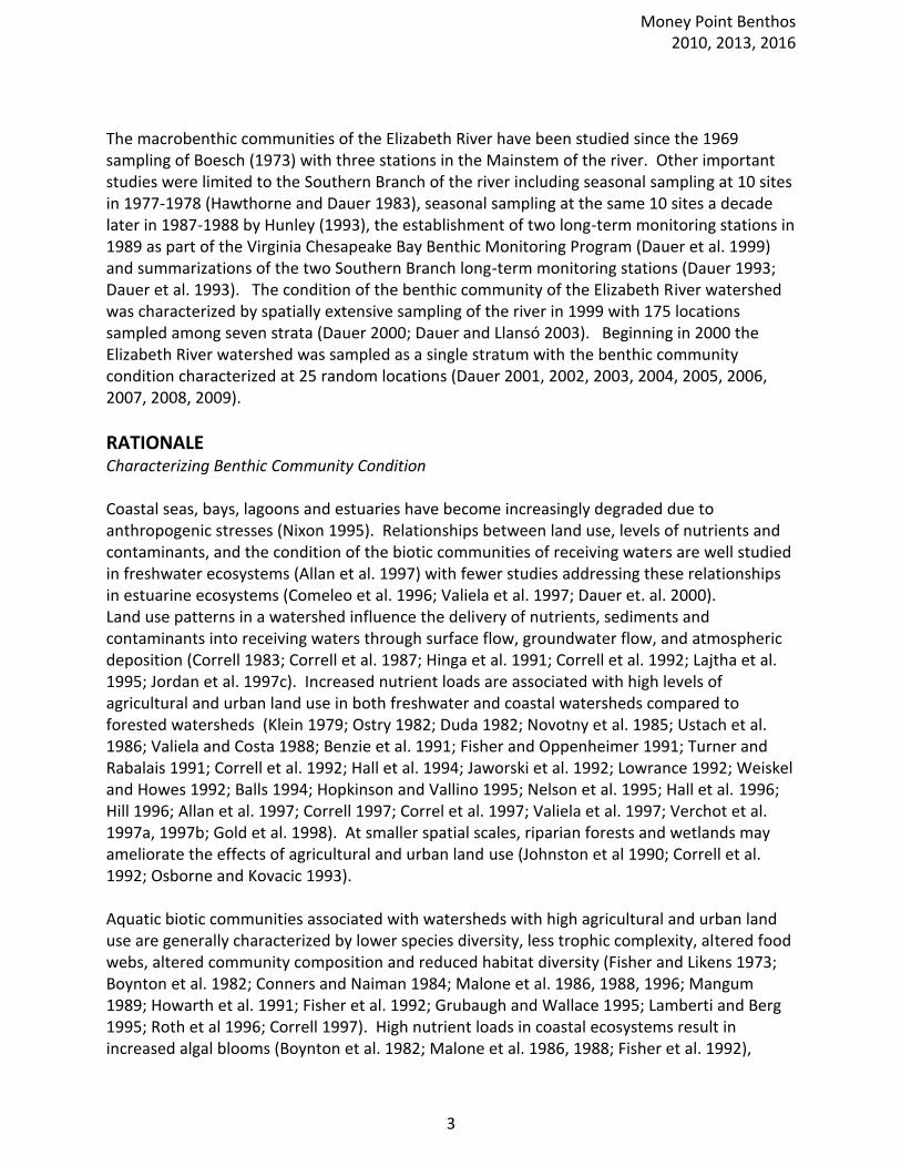
The macrobenthic communities of the Elizabeth River have been studied since the 1969 sampling of Boesch (1973) with three stations in the Mainstem of the river. Other important studies were limited to the Southern Branch of the river including seasonal sampling at 10 sites in 1977-1978 (Hawthorne and Dauer 1983), seasonal sampling at the same 10 sites a decade later in 1987-1988 by Hunley (1993), the establishment of two long-term monitoring stations in 1989 as part of the Virginia Chesapeake Bay Benthic Monitoring Program (Dauer et al. 1999) and summarizations of the two Southern Branch long-term monitoring stations (Dauer 1993; Dauer et al. 1993). The condition of the benthic community of the Elizabeth River watershed was characterized by spatially extensive sampling of the river in 1999 with 175 locations sampled among seven strata (Dauer 2000; Dauer and Llansó 2003). Beginning in 2000 the Elizabeth River watershed was sampled as a single stratum with the benthic community condition characterized at 25 random locations (Dauer 2001, 2002, 2003, 2004, 2005, 2006, 2007, 2008, 2009).
RATIONALE Characterizing Benthic Community Condition Coastal seas, bays, lagoons and estuaries have become increasingly degraded due to anthropogenic stresses (Nixon 1995). Relationships between land use, levels of nutrients and contaminants, and the condition of the biotic communities of receiving waters are well studied in freshwater ecosystems (Allan et al. 1997) with fewer studies addressing these relationships in estuarine ecosystems (Comeleo et al. 1996; Valiela et al. 1997; Dauer et. al. 2000). Land use patterns in a watershed influence the delivery of nutrients, sediments and contaminants into receiving waters through surface flow, groundwater flow, and atmospheric deposition (Correll 1983; Correll et al. 1987; Hinga et al. 1991; Correll et al. 1992; Lajtha et al. 1995; Jordan et al. 1997c). Increased nutrient loads are associated with high levels of agricultural and urban land use in both freshwater and coastal watersheds compared to forested watersheds (Klein 1979; Ostry 1982; Duda 1982; Novotny et al. 1985; Ustach et al. 1986; Valiela and Costa 1988; Benzie et al. 1991; Fisher and Oppenheimer 1991; Turner and Rabalais 1991; Correll et al. 1992; Hall et al. 1994; Jaworski et al. 1992; Lowrance 1992; Weiskel and Howes 1992; Balls 1994; Hopkinson and Vallino 1995; Nelson et al. 1995; Hall et al. 1996; Hill 1996; Allan et al. 1997; Correll 1997; Correl et al. 1997; Valiela et al. 1997; Verchot et al. 1997a, 1997b; Gold et al. 1998). At smaller spatial scales, riparian forests and wetlands may ameliorate the effects of agricultural and urban land use (Johnston et al 1990; Correll et al. 1992; Osborne and Kovacic 1993). Aquatic biotic communities associated with watersheds with high agricultural and urban land use are generally characterized by lower species diversity, less trophic complexity, altered food webs, altered community composition and reduced habitat diversity (Fisher and Likens 1973; Boynton et al. 1982; Conners and Naiman 1984; Malone et al. 1986, 1988, 1996; Mangum 1989; Howarth et al. 1991; Fisher et al. 1992; Grubaugh and Wallace 1995; Lamberti and Berg 1995; Roth et al 1996; Correll 1997). High nutrient loads in coastal ecosystems result in increased algal blooms (Boynton et al. 1982; Malone et al. 1986, 1988; Fisher et al. 1992),
Money Point Benthos 2010, 2013, 2016
3
increased low dissolved oxygen events (Taft et al. 1980; Officer et al. 1984; Malone et al. 1996), alterations in the food web (Malone 1992) and declines in valued fisheries species (Kemp et al. 1983; USEPA 1983). Sediment and contaminant loads are also increased in watersheds dominated by agricultural and urban development mainly due to storm-water runoff (Wilber and Hunter 1979; Hoffman et al. 1983; Medeiros et al. 1983; Schmidt and Spencer 1986; Beasley and Granillo 1988; Howarth et al. 1991; Vernberg et al. 1992; Lenat and Crawford 1994; Corbett et al. 1997). Benthic invertebrates are used extensively as indicators of estuarine environmental status and trends because numerous studies have demonstrated that benthos respond predictably to many kinds of natural and anthropogenic stress (Pearson and Rosenberg 1978; Tapp et al. 1993; Wilson and Jeffrey 1994; Dauer et al. 2000). Many characteristics of benthic assemblages make them useful indicators (Bilyard 1987; Dauer 1993), the most important of which are related to their exposure to stress and the diversity of their responses to stress. Exposure to hypoxia is typically greatest in near-bottom waters and anthropogenic contaminants often accumulate in sediments where benthos live. Benthic organisms generally have limited mobility and cannot avoid these adverse conditions. This immobility is advantageous in environmental assessments because, unlike most pelagic fauna, benthic assemblages reflect local environmental conditions (Gray 1979). The structure of benthic assemblages responds to many kinds of stress because these assemblages typically include organisms with a wide range of physiological tolerances, life history strategies, feeding modes, and trophic interactions (Pearson and Rosenberg 1978; Rhoads et al. 1978; Boesch and Rosenberg 1981; Dauer 1993). Benthic community condition in the Chesapeake Bay watershed has been related in a quantitative manner to water quality, sediment quality, nutrient loads, and land use patterns (Dauer et al. 2000). Estuarine Contaminant Perspective
Historically our nations’ estuarine and coastal waters have been repositories of potentially toxic contaminants through municipal sewage, agricultural runoff, industrial effluents, and various other routes. The accumulation of these contaminants varies between different components of coastal ecosystems and their ecological effects are depended upon the different chemical/biological states of each contaminant.
The ultimate fate of all organisms, particles and compounds is to reside at some time in the benthos.
Most contaminant entities become attached to very small suspended particles in the water (e.g. clay sized particles). As these particles sink to the bottom they carry the toxicants with them. The natural interaction of currents, waves and tides results in the accumulation in fine-grained sedimentary deposits. Typically, the concentrations of toxicants are much higher in sediments than in the overlying water. High winds, shallow water depth, strong currents, or changes in ambient chemistry, result in the release, resuspension or dispersion of accumulated
Money Point Benthos 2010, 2013, 2016
4
contaminants are released. Sediments are both sinks and sources of contaminants and; therefore, can pose serious threats to the health of resident marine life. The Chesapeake Bay Index of Biotic Integrity The Benthic Index of Biotic Integrity (B-IBI) was developed for macrobenthic communities of the Chesapeake Bay (Weisberg et al. 1997). The index defines expected conditions based upon the distribution of metrics from reference samples. Reference samples were collected from locations relatively free of anthropogenic stress. In calculating the index, categorical values are assigned for various descriptive metrics by comparison with thresholds of the distribution of metrics from reference samples. The result is a multi-metric index of biotic condition, frequently referred to as an index of biotic integrity (IBI). The analytical approach is similar to the one Karr et al. (1986) used to develop comparable indices for freshwater fish communities. Selection of benthic community metrics and metric scoring thresholds were habitat-dependent but by using categorical scoring comparisons between habitat types are possible. A six-step procedure was used to develop the index: acquire and standardize data sets from a number of monitoring programs; temporally and spatially stratify data sets to identify seasons and habitat types; identify reference sites; select benthic community metrics; select metric thresholds for scoring; and validate the index with an independent data set (Weisberg et al. 1997). The B-IBI developed for Chesapeake Bay is based upon subtidal, unvegetated, infaunal macrobenthic communities. Hard-bottom communities, e.g., oyster beds, were not sampled as part of the monitoring program because the sampling gears could not obtain adequate samples to characterize the associated infaunal communities. Infaunal communities associated with submerged aquatic vegetation (SAV) were not avoided, but were rarely sampled due to the limited spatial extent of SAV in Chesapeake Bay. Only macrobenthic data sets based on processing with a sieve of 0.5-mm mesh aperture and identified to the lowest possible taxonomic level were used. A data set of over 2,000 samples collected from 1984 through 1994 was used to develop, calibrate and validate the index (see Table 1 in Weisberg et al. 1997). Because of inherent sampling limitations in some of the data sets, only data from the period of July 15 through September 30 were used to develop the index. A multivariate cluster analysis of the biological data was performed to define habitat types. Salinity and sediment type were the two important factors defining habitat types and seven habitats were identified - tidal freshwater, oligohaline, low mesohaline, high mesohaline sand, high mesohaline mud, polyhaline sand, and polyhaline mud habitats (see Table 5 in Weisberg et al. 1997). Metrics to include in the index were selected from a candidate list proposed by benthic experts of the Chesapeake Bay. Selected metrics had to (1) differ significantly between reference and all other sites in the data set and (2) differ in an ecologically meaningful manner. Reference sites were selected as those sites which met all three of the following criteria: no sediment contaminant exceeded Long et al.’s (1995) effects range-median (ER-M) concentration, total organic content of the sediment was less than 2%, and bottom dissolved oxygen concentration
Money Point Benthos 2010, 2013, 2016
5
was consistently high. A total of 11 metrics representing measures of species diversity, community abundance and biomass, species composition, depth distribution within the sediment, and trophic composition were used to create the index (see Table 2 in Weisberg et al. 1997). The habitat-specific metrics are scored and combined into a single value of the B-IBI. Thresholds for the selected metrics were based on the distribution of values for the metric at the reference sites. The IBI approach involves scoring each metric as 5, 3, or 1, depending on whether its value at a site approximates, deviates slightly, or deviates greatly from conditions at reference sites (Karr et al. 1986). Threshold values are established as approximately the 5th and 50th (median) percentile values for reference sites in each habitat. For each metric, values below the 5th percentile are scored as 1; values between the 5th and 50th percentiles are scored as 3, and values above the 50th percentile are scored as 5. Metric scores are combined into an index by computing the mean score across all metrics for which thresholds were developed. Assemblages with an average score less than three are considered stressed, as they have metric values that on average are less than values at the poorest reference sites. Two of the metrics, abundance and biomass, respond bimodally; that is, the response can be greater than at reference sites with moderate degrees of stress and less than at reference sites with higher degrees of stress (Pearson and Rosenberg 1978; Dauer and Conner 1980; Ferraro et al. 1991). For these metrics, the scoring is modified so that both exceptionally high (those exceeding the 95th percentile at reference sites) and low (<5th percentile) responses are scored as a 1. Values between the 5th and 25th percentiles or between the 75th and 95th percentiles are scored as 3, and values between the 25th and 75th percentiles of the values at reference sites are scored as 5. The index was validated by examining its response at a new set of reference sites and a new set of sites with known environmental stress. Data used for validation were collected between 1992 and 1994 and were independent of data used to calibrate the index. The B-IBI classified 93% of the validation sites correctly (Weisberg et al. 1997). Values for the B-IBI range from 1.0 to 5.0. Benthic community condition was classified into four levels based on the B-IBI. Values ≥ 2 were classified as severely degraded; values from 2.1 to 2.6 were classified as degraded; values greater than 2.6 but less than 3.0 were classified as marginal; and values of 3.0 or more were classified as meeting the goal. Values in the marginal category do not meet the Restoration Goals, but they differ from the goals within the range of measurement error typically recorded between replicate samples. These categories are used in annual characterizations of the condition of the benthos in the Chesapeake Bay (Dauer et al. 2006a,b,c).
Money Point Benthos 2010, 2013, 2016
6
METHODS
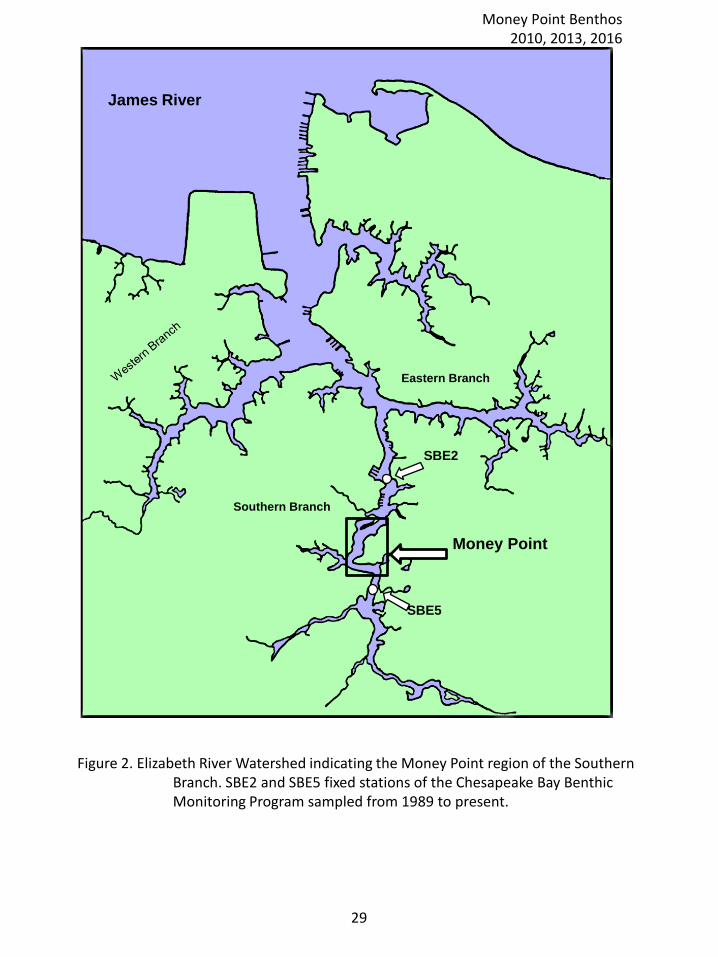
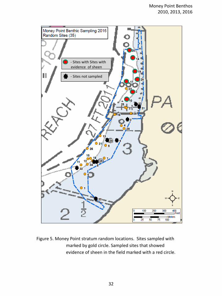
A glossary of selected terms used in this report is found in Appendix C. Probability-based Sampling A wide variety of sampling designs have been used in marine and estuarine environmental monitoring programs (e.g., see case studies reviewed recently in Kramer, 1994; Kennish, 1998; Livingston, 2001). Allocation of samples in space and time varies depending on the environmental problems and issues addressed (Kingsford and Battershill, 1998) and the type of variables measured (e.g., water chemistry, phytoplankton, zooplankton, benthos, nekton). In the Chesapeake Bay, the benthic monitoring program consists of both fixed-point stations and probability-based samples. The fixed-point stations are used primarily for the determination of long-term trends (e.g., Dauer and Alden, 1995; Dauer, 1997; Dauer et al. 2006a,b,c) and the probability-based samples for the determination of the areal extent of degraded benthic community condition (Llansó et al. 2003; Dauer and Llansó 2003). The probability-based sampling design consists of equal replication of random samples among strata and is, therefore, a stratified simple random design (Kingsford, 1998). Sampling design and methodologies for probability-based sampling are based upon procedures developed by EPA's Environmental Monitoring and Assessment Program (EMAP, Weisberg et al. 1993) and allow unbiased comparisons of conditions between strata (Dauer and Llansó 2003). Within each stratum (Money Point and Blows Creek) 25 random locations were sampled using a 0.04 m2 Young grab. The 2010 sampling locations are in Table 1 of Dauer (2011), for the 2013 sampling in Table 1 of Appendix B of Dauer (2014). The 2016 sampling locations are shown in Figures 5 and 6 and the coordinates are in Table 1 of Appendix B. The minimum acceptable depth of penetration of the grab was 7 cm. At each station one grab sample was taken for macrobenthic community analysis and an additional grab sample for sediment particle size analysis and the determination of total volatile solids. A 50 g subsample of the surface sediment was taken for sediment analyses. Salinity, temperature and dissolved oxygen were measured at the bottom and water depth was recorded. Fixed point stations To better understand the spatial and temporal patterns in benthic community condition measures at the two probability-based strata (Money Point and Blows Creek), data from two fixed stations of the Chesapeake Bay Benthic Monitoring Program (Dauer et al. 2017) were included. Station SBE2 is downstream of the Money Point beyond the Jordon Bridge and SBE5 is located upstream between the Gilmerton Bridge and the High Rise Bridge (Figure 2). Both stations have been sampled every summer since 1989. For the fixed point stations three replicate box core samples were collected for benthic community analysis. Each replicate had a surface area of 0.0184 m2, a minimum depth of penetration to 25 cm within the sediment, was sieved on a 0.5 mm screen, relaxed in dilute
Money Point Benthos 2010, 2013, 2016
7
isopropyl alcohol and preserved with a buffered formalin-rose bengal solution. At each station on each collection date a 50g subsample of the surface sediment was taken for sediment analysis. Probability-Based Estimation of Degradation
Areal estimates of degradation of benthic community condition within a stratum can be made because all locations in each stratum are randomly selected. The estimate of the proportion of a stratum failing the Benthic Restoration Goals developed for Chesapeake Bay (Ranasinghe et al. 1994; updated in Weisberg et al. 1997) is the proportion of the 25 samples with B-IBI values of less than 3.0. The process produces a binomial distribution: the percentage of the stratum attaining goals versus the percentage not attaining the goals. With a binomial distribution the 95% confidence interval for these percentages can be calculated as:
95% Confidence Interval = p ± 1.96 (SQRT(pq/N)) where p = percentage attaining goal, q = percentage not attaining goal and N = number of samples. This interval reflects the precision of measuring the level of degradation and indicates that with a 95% certainty the true level of degradation is within this interval. Differences between levels of degradation using a binomial distribution can be tested using the procedure of Schenker and Gentleman (2001). 50 random points were selected using the GIS system of Versar, Inc. Decimal degree reference coordinates were used with a precision of 0.000001 degrees (approximately 1 meter) which is a smaller distance than the accuracy of positioning; therefore, no area of a stratum is excluded from sampling and every point within a stratum has a chance of being sampled. In the field the first 25 acceptable sites are sampled. Sites may be rejected because of inaccessibility by boat, inadequate water depth or inability of the grab to obtain an adequate sample (e.g., on hard bottoms). Laboratory Analysis Each replicate was sieved on a 0.5 mm screen, relaxed in dilute isopropyl alcohol and preserved with a buffered formalin-rose bengal solution. In the laboratory each replicate was sorted and all the individuals identified to the lowest possible taxon and enumerated. Biomass was estimated for each taxon as ash-free dry weight (AFDW) by drying to constant weight at 60 oC and ashing at 550 oC for four hours. Biomass was expressed as the difference between the dry and ashed weight. Particle-size analysis was conducted using the techniques of Folk (1974). Each sediment sample is first separated into a sand fraction (> 63 µm) and a silt-clay fraction (< 63 µm). The sand fraction was dry sieved and the silt-clay fraction quantified by pipette analysis. For random stations, only the percent sand and percent silt-clay fraction were estimated. Total volatile solids of the sediment was estimated by the loss upon ignition method as described
Money Point Benthos 2010, 2013, 2016
8
above and presented as percentage of the weight of the sediment. Benthic Index of Biotic Integrity
B-IBI and Benthic Community Status Designations The B-IBI is a multiple-metric index developed to identify the degree to which a benthic community meets the Chesapeake Bay Program's Benthic Community Restoration Goals (Ranasinghe et al. 1994; Weisberg et al. 1997; Alden et al. 2002). The B-IBI provides a means for comparing relative condition of benthic invertebrate communities across habitat types. It also provides a validated mechanism for integrating several benthic community attributes indicative of community health into a single number that measures overall benthic community condition. The B-IBI is scaled from 1 to 5, and sites with values of 3 or more are considered to meet the Restoration Goals. The index is calculated by scoring each of several attributes as either 5, 3, or 1 depending on whether the value of the attribute at a site approximates, deviates slightly from, or deviates strongly from the values found at reference sites in similar habitats, and then averaging these scores across attributes. The criteria for assigning these scores are numeric and dependent on habitat type. Application of the index is limited to a summer index period from July 15th through September 30th.
Benthic community condition was classified into four levels based on the B-IBI. Values ≥ 2
were classified as severely degraded; values from 2.1 to 2.6 were classified as degraded; values greater than 2.6 but less than 3.0 were classified as marginal; and values of 3.0 or more were classified as meeting the goal. Values in the marginal category do not meet the Restoration Goals, but they differ from the goals within the range of measurement error typically recorded between replicate samples. These categories are used in annual characterizations of the condition of the benthos in the Chesapeake Bay (e.g. Dauer et al. 2002a, b; Llansó et al 2004).
Further Information concerning the B-IBI The analytical approach used to develop the B-IBI was similar to the one Karr et al. (1986) used to develop comparable indices for freshwater fish communities. Selection of benthic community metrics and metric scoring thresholds were habitat-dependent but by using categorical scoring comparisons between habitat types were possible. A six-step procedure was used to develop the index: (1) acquiring and standardizing data sets from a number of monitoring programs, (2) temporally and spatially stratifying data sets to identify seasons and habitat types, (3) identifying reference conditions, (4) selecting benthic community metrics, (5) selecting metric thresholds for scoring, and (6) validating the index with an independent data set (Weisberg et al. 1997). The B-IBI developed for Chesapeake Bay is based upon subtidal, unvegetated, infaunal macrobenthic communities. Hard-bottom communities, e.g., oyster beds, were not sampled because the sampling gears could not obtain adequate samples to characterize the associated infaunal communities. Infaunal communities associated with
Money Point Benthos 2010, 2013, 2016
9
submerged aquatic vegetation (SAV) were not avoided, but were rarely sampled due to the limited spatial extent of SAV in Chesapeake Bay. Only macrobenthic data sets based on processing with a sieve of 0.5 mm mesh aperture and identified to the lowest possible taxonomic level were used. A data set of over 2,000 samples collected from 1984 through 1994 was used to develop, calibrate and validate the index (see Table 1 in Weisberg et al. 1997). Because of inherent temporal sampling limitations in some of the data sets, only data from the period of July 15 through September 30 were used to develop the index. A multivariate cluster analysis of the biological data was performed to define habitat types. Salinity and sediment type were the two important factors defining habitat types and seven habitats were identified - tidal freshwater, oligohaline, low mesohaline, high mesohaline sand, high mesohaline mud, polyhaline sand and polyhaline mud habitats (see Table 5 in Weisberg et al. 1997). Reference conditions were determined by selecting samples which met all three of the following criteria: no sediment contaminant exceeded Long et al.'s (1995) effects range-median (ER-M) concentration, total organic content of the sediment was less than 2%, and bottom dissolved oxygen concentration was consistently high. A total of 11 metrics representing measures of species diversity, community abundance and biomass, species composition, depth distribution within the sediment, and trophic composition were used to create the index. The habitat-specific metrics were scored and combined into a single value of the B-IBI. Thresholds for the selected metrics were based on the distribution of values for the metric at the reference sites. Data used for validation were collected between 1992 and 1994 and were independent of data used to develop the index. The B-IBI classified 93% of the validation sites correctly (Weisberg et al. 1997). Llansó et al. 2016 using new data collected after Weisberg et al. 1997, in order to assess whether the B-IBI and the thresholds for its metric should be re-calibrated. They concluded that modifications to the original thresholds of Weisberg et al. (1997) and Alden et al. (2002) based upon new data did not result in better overall classification efficiencies. The single change in the B-IBI metrics was changing the classification of the polychaete Mediomastus ambiseta from pollution sensitive to unclassified. This species has been referred to as opportunistic and pollution indicative based both on ecological surveys (Grassle and Grassle, 1974; Boesch, 1977; Billheimer et al., 1997) and experimental results (Shaffner, 1990). Given the evidence from the literature and their extensive data analyses, Llansó et al. 2016, concluded that M. ambiseta could not be classified as either pollution sensitive or pollution indicative for the purposes of the B-IBI calculation. This change did result in lower B-IBI values for both Money Point and Blows Creek as reported in Dauer (2011, 2014). Statistical Analyses Two-way ANOVAs were performed on the BIBI, abundance, biomass, species diversity, species richness, body size (weight per individual), percentage of pollution indicative species
Money Point Benthos 2010, 2013, 2016
10
abundance and percentage of pollution tolerant species abundance with stratum (Money Point versus Blows Creek) and year (2010, 2013, 2016) as the main effects. A significant interaction term between the main effects would indicate that significant changes occurred between the strata and the years. This results in a BACI (Before- After Control-Impact) design where a significant space-time interaction term is indicative of a possible remediation effect (Green 1979; Stewart-Oaten et al. 1992). All tests with a significant interaction term were further tested separately by the main effects. A One Way ANOVA and the post hoc Scheffe was used to test for the main effect of years and a t-test for the main effect of stratum within each year.
RESULTS AND SUMMARY
Benthic Community Condition using Probability-Based Sampling
Environmental Parameters
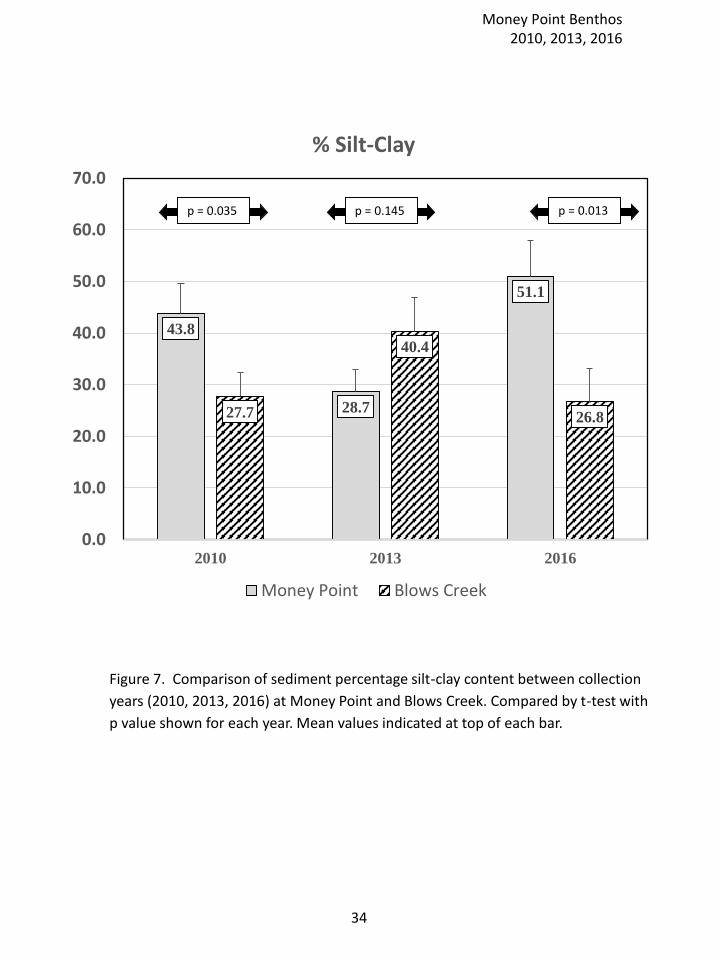
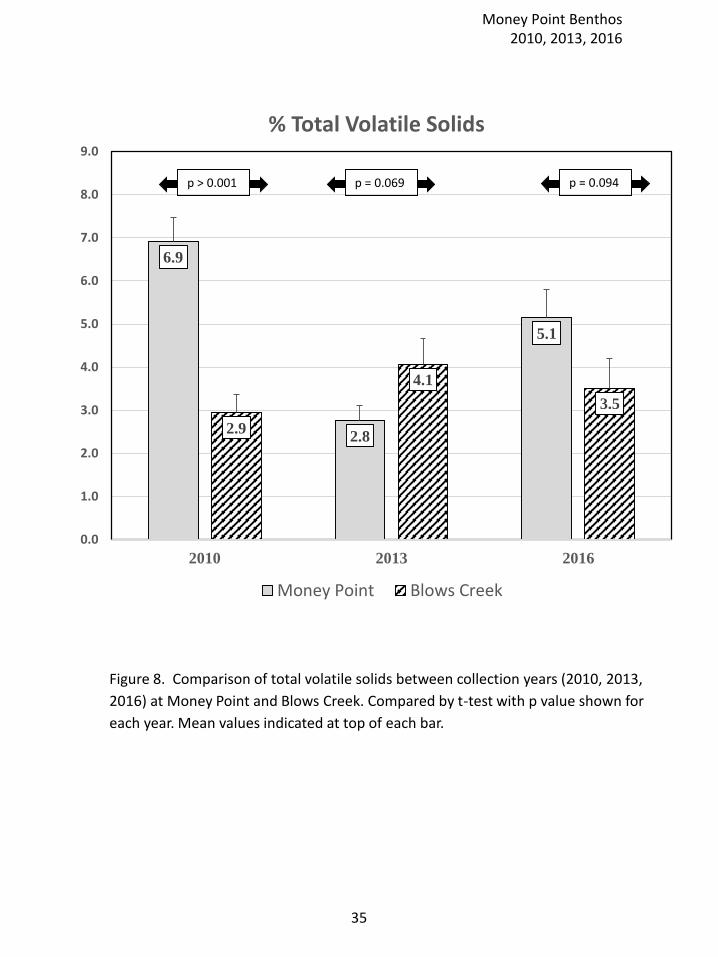
Physical-chemical parameters are summarized in Tables 2-5 of Appendix B. Salinity was in the polyhaline range (18-32) for all samples except for the Blows Creek samples collected on 9/23/2016 when salinities in the low mesohaline to oligohaline range were recorded. Rainfall was higher than average that year. Between the September 9 and September 23 samples at Blows Creek, 5.8 inches of rain fell with the average total rainfall for September is 4.8 inches (measured at Norfolk International Airport and data from the Weather Underground website). Sediments were a mixture of sands and muds. For both the mean percentage of silt-clay and total volatile solids the pattern at Money Point was high values of both in 2010, a decrease in both in 2013 and then an increase again in 2016 (Figures 7 and 8). The high total volatile solids (mean of 6.9%) at Money Point in 2010 reflects the levels of PAHs in the sediment at that time. In 2013 after remediation total volatile solids greatly decreased and the sediments were less muddy (greater amount of sand probably due to the cap of clean sand). However, in 2016 the sediments at Money Point were muddier, having the highest mean percent silt-clay but with total volatile solids lower than in 2010 and only marginally different from Blows Creek in 2016 (p = 0.094). Clearly the remediation affected the sediments at Money Point and resulted in sandier sediment; however, in 2016 sedimentation of fine particles changed the sediments at Money Point back to finer sediments than Blows Creek (Figure 7).
Benthic Community Condition The benthic community parameters (the B-IBI value, abundance, biomass, Shannon diversity index and species richness) were compared between the strata (Money Point, Blows Creek) and times (summer samples from 2010, 2013, 2016). The two-way ANOVAs with stratum and year as the main effects resulted in significant stratum-year interaction terms for the BIBI (0.008), biomass (0.0007), Shannon diversity (<0.0001), and species richness (0.005) but not for abundance (0.319). The BIBI and the metrics with significant interactions terms indicate significant changes occurred between the strata and years that could be indicative of a significant remediation effect. Therefore, separate statistical tests were necessary between the
Money Point Benthos 2010, 2013, 2016
11
strata and among the years as indicated in Table 1 - t-tests for the stratum comparisons and one-way ANOVAs for the year comparisons. BIBI The value of the BIBI was significantly lower at Money Point in 2010 compared to Blows Creek,
increased in 2013 and then decreased in 2016 and was again significantly lower than Blows
Creek (Figures 9). However, the BIBI values at Money Point did not change significantly over
the years (Figure 10). BIBI values showed a convex, non-linear trend at SBE2 and a declining
trend at SBE5 over the previous 10-year period (Figures 25, 26). BIBI values at both SBE2 and
SBE5 showed more variability and often higher values in the years between the sampling at
Money Point (2010, 2013, 2016). Compared to SBE2 and SBE5, Money Point BIBI values were
higher in all three years except for the 2010 BIBI value at SBE2. BIBI values at both SBE2 and
SBE5 were higher that the sampling years of 2010, 2013 and 2016 with the single exception of
SBE5 in 2015.
Abundance
The abundance at both Money Point and Blows Creek were high in 2010, declined at both
strata in 2013 with the Money Point value significantly lower than at Blows Creek, and again
declined at both strata in 2016 with the Money Point value again significantly lower than at
Blows Creek (Figure 11). At Money Point the abundance values were significantly different in
each year and declined in each sampling year (Figure 12). Abundance values at both SBE2 and
SBE5 showed declining patterns over the past decade (Figures 12, 27, 28) with a single
exception at SBE5 in 2011 (Figure 28).
Biomass Biomass at Money Point was significantly lower than that at Blows Creek in 2010, significantly
increased in 2013, but decreased in 2016 and was again significantly lower than levels at Blows
Creek (Figure 13). There was a pattern of declining biomass at Blows Creek over the years but
the differences were not significant (Figure 14). In general, there was a pattern of decreasing
biomass at both SBE2 and SBE5 over the past decade (Figures 29, 30) and during the collections
years (2010, 2013, 2016) biomass values at both SBE2 and SBE5 were similar to, or lower than,
both the Money Point and Blows Creek strata except for the Money Point values in 2010
(Figures 29, 30). The 2010, 2013 and 2016 biomass values at SBE5 were the lowest recorded at
that station for the past decade.
Money Point Benthos 2010, 2013, 2016
12
Species Diversity (H’)
Species diversity (H’) in 2010 was not significantly different between the strata (Figure 15),
increased significantly at Money Point in 2013 and was also significantly higher at Money Point
than at Blows Creek (Figure 15), and H’ increased to the highest levels at both strata in 2016
(Figure 15, 16). The pattern for species diversity values at SBE2 showed an increasing trend
similar to the increasing pattern at the two strata (Figure 31). In contrast, the species diversity
values at SBE5 showed no pattern (Figure 32). In 2016, species diversity values at the two
strata were higher than either fixed station (Figures 31, 32).
Species Richness
Species richness (number of species per sample) showed a very different pattern than species
diversity (H’) (Figures 17, 18). Species richness was significantly lower at Money Point in 2010
(Figure 17), significantly increased at Money Point in 2013 to a level not different from Blows
Creek, and declined in 2016 with a value significantly lower than Blows Creek (Figure 18).
Species richness at both fixed stations did not show a strong pattern and values at these two
stations cannot be directly compared because different gear types were used – a Young grab
(0.04 m2) at MP and BC and a box-corer (0.0184 m2) at SBE2 and SBE5 (Figures 33, 34).
Pollution Sensitive Species, Pollution Indicative Species, and Body Size
Benthic communities unaffected by anthropogenic or natural stress are expected to have (1)
higher species diversity, (2) higher community biomass and (3) are dominated in composition
by longer-lived, larger-bodied and often deeper-dwelling (within the sediment) species
(Rhoads and Boyer, 1982; Warwick, 1986, Dauer 1993). Such species are often referred to as
equilibrium, K-selected (McCall 1977, Gray 1979, Dauer 1993) or pollution sensitive species
(Weisberg et al. 1997). In contrast, stressed benthic communities are characterized by (1) lower
species diversity, (2) often lower community biomass and (3) are dominated in composition by
short-lived, small-bodied and often surface-dwelling species (Boesch, 1977; Pearson and
Rosenberg, 1978, Dauer 1993). Such species are often referred to as eurytopic opportunistic, r-
selected or pollution tolerant species (Boesch, 1977; Pearson and Rosenberg, 1978, Dauer
1993).
Prior to the sediment remediation the average body size of benthic species was only marginally
different between the strata in 2010 and after remediation the average body size increased
significantly at Money Point in 2013 (Figure 20) and was significantly greater that at Blows
Creek (Figure 19). Finally, in 2016 the average body size at Money Point remained high and was
marginally greater than at Blows Creek in 2016 (Figure 19).
Money Point Benthos 2010, 2013, 2016
13
The percentage of pollution sensitive abundance was lowest at Money Point in 2010 but not
significantly different from that at Blows Creek in 2010 (Figure 21). After remediation the
pollution sensitive abundance increased steadily at both Money Point and Blows Creek in 2013
and again in 2016 (Figures 21 and 22). By 2016 the pollution sensitive species abundance was
significantly higher at Money Point compared to the pre-remediation value in 2010 (Figure 22)
although lower than the value at Blows Creek in 2016 (Figure 21).
The percentage of pollution indicative abundance was highest at Money Point in 2010 and was
significantly higher than at Blows Creek (Figure 23). The value of pollution indicative taxa
abundance significantly declined after remediation in 2013 and remained unchanged in 2016
(Figure 24).
In 2016 at Money Point the (1) continued large body size (Figure 20), (2) continued lowered
level of pollution indicative abundance (Figure 24) and (3) slightly higher level of pollution
sensitive abundance (Figure 22) all indicate that the very positive improvement in benthic
community composition quantified after remediation in the 2013 sampling continued in 2016.
Although the percentage of pollution sensitive abundance in 2016 was significantly lower at
Money Point (Figure 21) and the percentage of pollution indicative abundance was significantly
higher (Figure 23), the average body size was higher at Money Point – all positive indicators of
persistent remediation improvements.
Benthic Community Condition Summary The patterns above for the BIBI, abundance, biomass, species diversity and species richness are summarized in Table 2. The patterns above for the body size, pollution indicative species abundance and pollution sensitive abundance are summarized in Table 3.
Benthic Community Dominant Species The dominant taxa of the random sites are summarized in Tables 4 and 5. Consistent with
previous studies the Money Point stratum was dominated by annelid species including the
polychaete species Mediomastus ambiseta, Hermundura sp. A, Paraprionospio pinnata,
Streblospio benedicti, Leitoscoloplos spp., and Glycinde solitaire.
The only major change was that the two pollution indicative polychaete species (Mediomastus
ambiseta and Streblospio benedicti) at Money Point decreased from a combined level of 4,956
individuals per m2 in 2010 to 1,244 individuals per m2 in 2013 and then to 457 individuals per
Money Point Benthos 2010, 2013, 2016
14
m2 in 2016; representing, 82.4% of the individuals in 2010, 47.1% of the individuals in 2013,
and 33.5% of the individuals in 2016.
Mediomastus ambiseta has often been characterized as a stress tolerant or opportunistic
species characteristic of disturbed habitats (Grassle and Grassle 1974; Schaffner 1990; Dauer et
al. 1993; Dauer 1993). Streblospio benedicti has also been characterized as a stress tolerant or
euryhaline opportunist characteristic of disturbed habitats (Boesch 1977; Holland et al. 1987;
Dauer et al. 1993; Dauer 1993) with tolerance to both hypoxic bottom water conditions (Ritter
and Montagna 1999; Llansó, 1991, 1992) and sediment PAHs (Chandler et al. 1997).
The decline in abundance of these two pollution indicative species indicates that there are no
lasting and returning sediment contaminant effects at Money Point. More importantly
abundance values at both SBE2 and SBE5 showed declining patterns over the past decade
(Figures 12, 19, 20) indicating larger scale watershed factors were influencing abundance
patterns at the level of the entire Southern Branch, for example, poor larval recruitment, low
post-larval survivorship, increased mortality associated with predation, etc.
The most consistent and common species was the polychaete Hermundura sp. A (reported as Parandalia tricuspis in Dauer 2011) recorded as the third most common species in 2010 (514
individuals per m2), second most common species in 2013 (381 individuals per m2), and again
second most common species in 2016 (351 individuals per m2). Hermundura sp. A is most similar to a species described in the Gulf of Mexico (H. americana (Hartman 1947)) and was first reported in Chesapeake Bay in 2009 from a single sample in the Southern Branch of the Elizabeth River. This species is now collected throughout the tidal James River but nowhere else in Chesapeake Bay. Nothing is known of its biology.
Benthic Community Level of Degraded Area The 2010 level of degraded benthic bottom of Money Point was 96% ± 4.0% - the highest level of degradation recorded by any previous studies in the Elizabeth River watershed. Previous quantitative areal estimates of benthic degradation in the watershed have varied from 52 ± 19.6% in 2001 to 84 ± 12.7% in 2005. In the summer of 2013 the level of degraded benthic bottom off Money Point declined to 76% ± 16.3%. However, in the summer of 2016 level of degraded benthic bottom off Money Point increased again to 92% ± 10.6%.
Recommendation
The benthic community condition at Money Point clearly improved after sediment remediation as shown in the results from the 2013 field sampling (Dauer 2014). The present results indicate that (1) natural sedimentation increased the silt-clay content and percent total volatile solids content; (2) although the BIBI remains unchanged over time at Money Point, species diversity remains relatively high and is tracking the levels at Blows Creek; (3) the continued decrease in
Money Point Benthos 2010, 2013, 2016
15
abundance of the two dominant pollution indicative polychaete species clearly indicates that there are not any persistent sediment contaminant effects; (4) the larger body size of species at Money Point, continued lowered level of pollution indicative abundance, and slightly higher level of pollution sensitive abundance indicate that the very positive improvement in benthic community composition quantified after remediation in the 2013 sampling continued in 2016. Continued periodic sampling at Money Point and Blows Creek will provide further assessment of the apparent beneficial effects of the remediation on the benthic community condition.
REFERENCES ALDEN, R.W. III, D.M. DAUER, J.A. RANASINGHE, L.C. SCOTT, AND R.J. LLANSÓ. 2002. Statistical verification of the Chesapeake Bay Benthic Index of Biotic Integrity. Environmetrics 13: 473- 498. ALLAN, J. D., D. L. ERICKSON, AND J. FAY. 1997. The influence of catchment land use on stream integrity across multiple spatial scales. Freshwater Biology 37:149–161. BALLS, P. W. 1994. Nutrient inputs to estuaries from nine Scottish east coast rivers: Influence of estuarine processes on inputs to the North Sea. Estuarine Coastal and Shelf Science 39: 329 –352. BEASLEY, R. S. AND A. B. GRANILLO. 1988. Sediment and water yields from managed forests on flat coastal plain sites. Water Resources Bulletin 24:361–366. BENZIE, J. A. H., K. B. PUGH, AND M. B. DAVIDSON. 1991. The rivers of North East Scotland (UK): Physicochemical characteristics. Hydrobiologia 218:93–106. BILLHEIMER, D., D.T. CARDOSO, E. FREEMAN, P. GUTTORP, H. KO, AND M. SILKEY. 1997. Natural variability of benthic species composition in the Delaware Bay. Environmental and Ecological Statistics 4:95-115. BILYARD, G. R. 1987. The value of benthic infauna in marine pollution monitoring studies. Marine Pollution Bulletin 18:581-585. BOESCH, D.F. 1977. A new look at the zonation of benthos along the estuarine gradient. Pp. 245-266, In B.C. Coull (ed.), Ecology of Marine Benthos, University South Carolina Press, Columbia, SC. BOESCH, D. F. AND R. ROSENBERG. 1981. Response to stress in marine benthic communities, p. 179-200. In G. W. Barret and R. Rosenberg (eds.), Stress Effects on Natural Ecosystems. John Wiley & Sons, New York.
Money Point Benthos 2010, 2013, 2016
16
BOYNTON, W. R., W. M. KEMP, AND C. W. KEEFE. 1982. A comparative analysis of nutrients and other factors influencing estuarine phytoplankton production, p. 69–90. In V. S. Kennedy (ed.), Estuarine Comparisons. Academic Press, New York. CHANDLER, G.T., M. R. SHIPP, AND T.L. DONELAN. 1997. Bioaccumulation, growth and larval settlement effects of sediment-associated polynuclear aromatic hydrocarbons on the estuarine polychaete, Streblospio benedicti (Webster). Journal of Experimental Marine Biology and Ecology 213: 95-110. COMELEO, R. L., J. F. PAUL, P. V. AUGUST, J. COPELAND, C. BAKER, S. S. HALE, AND R. W. LATIMER. 1996. Relationships between watershed stressors and sediment contamination in Chesapeake Bay estuaries. Landscape Ecology 11:307–319. CONNERS, M. E. AND R. J. NAIMAN. 1984. Particulate allochthonous inputs: Relationships with stream size in an undisturbed watershed. Canadian Journal of Fisheries and Aquatic Sciences 41:1473–1488. CORBETT, C. W., M. WAHL, D. E. PORTER, D. EDWARDS, AND C. MOISE. 1997. Nonpoint source runoff modeling: A comparison of a forested watershed and an urban watershed on the South Carolina coast. Journal of Experimental Marine Biology and Ecology 213:133–149. CORRELL, D. L. 1983. N and P in soils and runoff of three coastal plain land uses, p. 207–224. In R. Lowrance, R. Todd, L. Asmussen, and R. Leonard (eds.), Nutrient Cycling in Agricultural Ecosystems. University of Georgia Press, Athens, Georgia. CORREL, D. L. 1997. Buffer zones and water quality protection: General principles, p. 7–20. In N. E. Haycock, T. P. Burt, K. W. T. Goulding, and G. Pinay (eds.), Buffer Zones: Their Processes and Potential in Water Protection. Quest Environmental, Hertfordshire, United Kingdom. CORRELL, D. L., T. E. JORDAN, AND D. E. WELLER. 1992. Nutrient flux in a landscape: Effects of coastal land use and terrestrial community mosaic on nutrient transport to coastal waters. Estuaries 15:431–442. CORRELL, D. L., T. E. JORDAN, AND D. E. WELLER. 1997. Livestock and pasture land effects on the water quality of Chesapeake Bay watershed streams, p. 107–116. In K. Steele (ed.), Animal Waste and the Land-Water Interface. Lewis Publishers, New York. CORRELL, D. L., J. J. MIKLAS, A. H. HINES, AND J. J. SCHAFER. 1987. Chemical and biological trends associated with acidic atmospheric deposition in the Rhode River watershed and estuary (Maryland, USA). Water Air and Soil Pollution 35:63–86. DAUER, D. M. 1993. Biological criteria, environmental health and estuarine macrobenthic community structure. Marine Pollution Bulletin 26:249–257.
Money Point Benthos 2010, 2013, 2016
17
DAUER, D.M. 1997. Dynamics of an estuarine ecosystem: Long-term trends in the macrobenthic communities of the Chesapeake Bay, USA (1985-1993). Oceanologica Acta 20: 291-298. DAUER, D. M. 2000. Benthic Biological Monitoring Program of the Elizabeth River Watershed (1999). Final Report to the Virginia Department of Environmental Quality, Chesapeake Bay Program, 73 pp. DAUER, D. M. 2001. Benthic Biological Monitoring Program of the Elizabeth River Watershed (2000). Final Report to the Virginia Department of Environmental Quality, Chesapeake Bay Program, 35 pp. Plus Appendix. DAUER, D. M. 2002. Benthic Biological Monitoring Program of the Elizabeth River Watershed (2001) with a study of Paradise Creek. Final Report to the Virginia Department of Environmental Quality, Chesapeake Bay Program, 45 pp. DAUER, D. M. 2003. Benthic Biological Monitoring Program of the Elizabeth River Watershed (2002). Final Report to the Virginia Department of Environmental Quality, Chesapeake Bay Program, 56 pp. DAUER, D. M. 2004. Benthic Biological Monitoring Program of the Elizabeth River Watershed (2003). Final Report to the Virginia Department of Environmental Quality, Chesapeake Bay Program, 88 pp. DAUER, D. M. 2005. Benthic Biological Monitoring Program of the Elizabeth River Watershed (2004). Final Report to the Virginia Department of Environmental Quality, Chesapeake Bay Program, 178 pp. DAUER, D. M. 2006. Benthic Biological Monitoring Program of the Elizabeth River Watershed (2005). Final Report to the Virginia Department of Environmental Quality, Chesapeake Bay Program, 171 pp. DAUER, D. M. 2007. Benthic Biological Monitoring Program of the Elizabeth River Watershed (2006). Final Report to the Virginia Department of Environmental Quality, Chesapeake Bay Program, 40 pp. DAUER, D. M. 2008. Benthic Biological Monitoring Program of the Elizabeth River Watershed (2007). Final Report to the Virginia Department of Environmental Quality, Chesapeake Bay Program, 112 pp. DAUER, D. M. 2009. Benthic Biological Monitoring Program of the Elizabeth River Watershed (2008). Final Report to the Virginia Department of Environmental Quality, Chesapeake Bay Program, 119 pp.
Money Point Benthos 2010, 2013, 2016
18
DAUER, D.M. 2011. Biological condition of Money Pont benthic communities, Southern Branch of the Elizabeth River (2010). Final report to The Elizabeth River Project. 77 pp. DAUER, D.M. 2014. Biological condition of Money Pont benthic communities, Southern Branch of the Elizabeth River (2010 and 2013). Final report to The Elizabeth River Project. 101 pp. DAUER, D.M. AND R.W. ALDEN III. 1995. Long-term trends in the macrobenthos and water quality of the lower Chesapeake Bay (1985-1991). Marine Pollution Bulletin 30: 840-850. DAUER, D.M. AND W.G. CONNER. 1980. Effects of moderate sewage input on benthic polychaete populations. Estuarine and Coastal Marine Science 10: 335-346. DAUER, D.M., T.A. EGERTON, J.R. DONAT, M.F. LANE, S.C. DOUGHTEN, C. JOHNSON, AND M. Arora. 2017. Current status and long-term trends in water quality and living resources in the Virginia Tributaries and Chesapeake Bay Mainstem from 1985 through 2015. Final report to the Virginia Department of Environmental Quality. 67 pp. DAUER, D.M., R.M. EWING, G.H. TOURTELLOTTE, W.T. HARLAN, J.W. SOURBEER, AND H. R. BARKER JR. 1982a. Predation pressure, resource limitation and the structure of benthic infaunal communities. Internationale Revue der gesamten Hydrobiologie (International Review of Hydrobiology) 67: 477-489. DAUER, D.M. AND R. J. LLANSÓ. 2003. Spatial scales and probability based sampling in determining levels of benthic community degradation in the Chesapeake Bay. Environmental Monitoring and Assessment 81: 175-186. DAUER, D.M., H.G. MARSHALL, J.R. DONAT, M. F. LANE, S. DOUGHTEN, P.L. MORTON AND F.J. HOFFMAN. 2006a. Status and trends in water quality and living resources in the Virginia Chesapeake Bay: James River (1985-2004). Final report to the Virginia Department of Environmental Quality. 73 pp. DAUER, D.M., H.G. MARSHALL, J.R. DONAT, M. F. LANE, S. DOUGHTEN, P.L. MORTON AND F.J. HOFFMAN. 2006b. Status and trends in water quality and living resources in the Virginia Chesapeake Bay: York River (1985-2004). Final report to the Virginia Department of Environmental Quality. 63 pp. DAUER, D.M., H.G. MARSHALL, J.R. DONAT, M. F. LANE, S. DOUGHTEN, P.L. MORTON AND F.J. HOFFMAN. 2006c. Status and trends in water quality and living resources in the Virginia Chesapeake Bay: Rappahannock River (1985-2004). Final report to the Virginia Department of Environmental Quality. 66 pp. DAUER, D.M., J. A. RANASINGHE, AND S. B. WEISBERG. 2000. Relationships between benthic community condition, water quality, sediment quality, nutrient loads, and land use patterns in Chesapeake Bay. Estuaries 23: 80-96.
Money Point Benthos 2010, 2013, 2016
19
DAUER, D.M., W.W. ROBINSON, C.P. SEYMOUR, AND A.T. LEGGETT, JR. 1979. The environmental impact of nonpoint pollution on benthic invertebrates in the Lynnhaven River System. Virginia Water Resources Research Center Bulletin 117, 112 pp. DAUER, D.M., M.W. LUCHENBACK, AND A.J. RODI, JR. 1993. Abundance biomass comparisons (ABC method): Effects of an estuary gradient, effects of an estuarine gradient, anoxic/hypoxic events and contaminated sediments. Marine Biology 116: 507-518. DAUER, D.M., G.H. TOURTELLOTTE, AND R.M. EWING. 1982b. Oyster shells and artificial worm tubes: the role of refuges in structuring benthic infaunal communities. Internationale Revue der gesamten Hydrobiologie (International Review of Hydrobiology) 67: 661-677. DUDA, A. M. 1982. Municipal point source and agricultural nonpoint source contributions to coastal eutrophication. Water Resources Bulletin 18:397–407. EWING, R.M. AND D.M. DAUER 1982. Macrobenthic communities of the lower Chesapeake Bay. I. Old Plantation Flats, Old Plantation Creek, Kings Creek and Cherrystone Inlet. Internationale Revue der gesamten Hydrobiologie (International Review of Hydrobiology) 67: 777-791. FISHER, S. G. AND G. E. LIKENS. 1973. Energy flow in Bear Brook, New Hampshire: An integrative approach to stream ecosystem metabolism. Ecological Monographs 43:421–439. FISHER, D. C. AND M. OPPENHEIMER 1991. Atmospheric deposition and the Chesapeake Bay estuary. Ambio 20:102–108. FISHER, D. C., E. R. PEELE, J. W. AMMERMAN, AND L. W. HARDING, JR. 1992. Nutrient limitation of phytoplankton in Chesapeake Bay. Marine Ecology Progress Series 82:51–64. FOLK, R.L. 1974. Petrology of sedimentary rocks. Hemphills, Austin, 170 pp. GOLD, A. A., P. A. JACINTHE, P. M. GROFFMAN, W. R. WRIGHT, AND P. H. PUFFER. 1998. Patchiness in groundwater nitrate removal in a riparian forest. Landscape Ecology 27:146–155. GRASSLE, J. F. AND GRASSLE, J. P. 1974. Opportunistic life histories and genetic systems in marine benthic polychaetes. Journal of Marine Research 32:253-284.
GRAY, J. S. 1979. Pollution-induced changes in populations. Transactions of the Royal Philosophical Society of London (B) 286:545-561. GREEN, R. H. 1979. Sampling design and statistical methods for environmental biologists. John Wiley and Sons, New York.
Money Point Benthos 2010, 2013, 2016
20
GRUBAUGH, J. W. AND J. B. WALLACE. 1995. Functional structure and production of the benthic community in a Piedmont river: 1956–1957 and 1991–1992. Limnology and Oceanography 40: 490–501. HALL, JR., L. W., S. A. FISCHER, W. D. KILLEN, JR., M. C. SCOTT, M. C. ZIEGENFUSS, AND R. D. ANDERSON. 1994. Status assessment in acid-sensitive and non-acid-sensitive Maryland coastal plain streams using an integrated biological, chemical, physical, and land-use approach. Journal of Aquatic Ecosystem Health 3:145–167. HALL, JR., L. W., M. C. SCOTT, W. D. KILLEN, AND R. D. ANDERSON. 1996. The effects of land-use characteristics and acid sensitivity on the ecological status of Maryland coastal plain streams. Environmental Toxicology and Chemistry 15:384–394. HAWTHORNE, S.D. AND D.M. DAUER. 1983. Macrobenthic communities of the lower Chesapeake Bay. III. Southern Branch of the Elizabeth River. Internationale Revue der gesamten Hydrobiologie (International Review of Hydrobiology) 68: 193-205. HILL, A. 1996. Nitrate removal in stream riparian zones. Journal of Environmental Quality 25:743–755. HINGA, K. R., A. A. KELLER, AND C. A. OVIATT. 1991. Atmospheric deposition and nitrogen inputs to coastal waters. Ambio 20: 256–260. HOFFMAN, E. J., G. L. MILLS, J. S. LATIMER, AND J. G. QUINN. 1983. Annual inputs of petroleum hydrocarbons to the coastal environment via urban runoff. Canadian Journal of Fisheries and Aquatic Sciences 40:41–53. HOLLAND, A. F., A. T. SHAUGHNESSY, AND M. H. HEIGEL. (1987). Long-term variation in mesohaline Chesapeake Bay macrobenthos: spatial and temporal patterns. Estuaries 10: 227-245. HOPKINSON, JR., C. S. AND J. J. VALLINO. 1995. The relationships among man’s activities in watersheds and estuaries: A model of runoff effects on patterns of estuarine community metabolism. Estuaries 18:598–621. HOWARTH, R. W., J. R. FRUCI, AND D. SHERMAN. 1991. Inputs of sediment and carbon to an estuarine ecosystem: Influence of land use. Ecological Applications 1:27–39. HUNLEY, W.S. 1993. Evaluation of long term changes in the macrobenthic community of the Southern Branch of the Elizabeth River, Virginia. Master’s Thesis. Old Dominion University. 120 pp. JAWORSKI, N. A., P. M. GROFFMAN, A. A. KELLER, AND J. C. PRAGER. 1992. A watershed nitrogen and phosphorus balance: The Upper Potomac River Basin. Estuaries 15:83–95.
Money Point Benthos 2010, 2013, 2016
21
JOHNSTON, C. A., N. E. DETENBECK, AND G. J. NIEMI. 1990. The cumulative effect of wetlands on stream water quality and quantity: A landscape approach. Biogeochemistry 10:105–142. JORDAN, T. E., D. L. CORRELL, AND D. E. WELLER. 1997. Relating nutrient discharges from watersheds to land use and stream-flow variability. Water Resources Research 33:2579–2590. KARR, J. R., K. D. FAUSCH, P. L. ANGERMEIER, P. R. YANT, AND I. J. SCHLOSSER. 1986. Assessing Biological Integrity in Running Waters: A Method and Its Rationale. Special Publication 5. Illinois Natural History Survey, Champaign, Illinois. KEMP, W. M., R. R. TWILLEY, J. C. STEVENSON, W. R. BOYNTON, AND J. C. MEANS. 1983. The decline of submerged vascular plants in Upper Chesapeake Bay: Summary of results concerning possible causes. Marine Technology Society Journal 17: 78–89. KENNISH, M.J. 1998, Pollution impacts on marine biotic communities, CRC Press, Boca Raton, 310 pp. KINGSFORD, M.J. 1998, ‘Analytical aspects of sampling design’, in Kingsford, M. and Battershill, C. (eds), Studying temperate marine environments. A handbook for ecologists, CRC Press, Boca Raton, p. 49–83.
KINGSFORD, M.J. AND BATTERSHILL, C. N. 1998, ‘Procedures for establishing a study’, in Kingsford, M. and Battershill, C. (eds), Studying temperate marine environments. A handbook for ecologists, CRC Press, Boca Raton, p. 29–48. KRAMER, K.J.M. 1994, Biomonitoring of coastal waters and estuaries, CRC Press, Boca Raton, 327 pp. LAJTHA, K., B. SEELY, AND I. VALIELA. 1995. Retention and leaching of atmospherically-derived nitrogen in the aggrading coastal watershed of Waquiot Bay, MA. Biogeochemistry 28:33–54. LAMBERTI, G. A. AND M. B. BERG. 1995. Invertebrates and other benthic features as indicators of environmental change in Juday Creek, Indiana. Natural Areas Journal 15:249–258. LENAT, D. R. AND J. K. CRAWFORD. 1994. Effects of land use on water quality and aquatic biota of three North Carolina Piedmont streams. Hydrobiologia 294:185–199. LIVINGSTON, R.J. 2001. Eutrophication processes in coastal systems, CRC Press, Boca Raton, 327 pp. LLANSÓ, R.J. 1991. Tolerance of low dissolved oxygen and hydrogen sulfide by the polychaete Streblospio benedicti (Webster). Journal of Experimental Marine Biology and Ecology 153: 165-178.
Money Point Benthos 2010, 2013, 2016
22
LLANSÓ, R.J. 1992. Effects of hypoxia on estuarine benthos: the Lower Rappahannock River (Chesapeake Bay), a case study. Estuarine, Coastal and Shelf Science 35: 491-515. LLANSÓ, R.J., D.M. DAUER AND M.F. LANE. 2016. Chesapeake Bay B-IBI Recalibration. Final report to the Virginia Department of Environmental Quality. 31 pp LLANSÓ, R.J., D.M. DAUER, J.H. VØLSTAD, AND L.S. SCOTT. 2003. Application of the Benthic Index of Biotic Integrity to environmental monitoring in Chesapeake Bay. Environmental Monitoring and Assessment 81: 163-174. LLANSÓ, R.J., F.S. KELLEY AND L.S. SCOTT. 2004. Long-term benthic monitoring and assessment component. Level I Comprehensive Report. July 1984 – December 2003. Final report to the Maryland Department of Natural Resources. LONG, E. R., D. D. MCDONALD, S. L. SMITH, AND F. D. CALDER. 1995. Incidence of adverse biological effects within ranges of chemical concentrations in marine and estuarine sediments. Environmental Management 19:81–97. LOWRANCE, R. 1992. Groundwater nitrate and denitrification in a coastal plain riparian forest. Journal of Environmental Quality 21:401–405. MALONE, T. C. 1992. Effects of water column processes on dissolved oxygen, nutrients, phytoplankton and zooplankton, p. 61–112. In D. E. Smith, M. Leffler, and G. Mackiernan (eds.), Oxygen Dynamics in the Chesapeake Bay. A Synthesis of Recent Research. Maryland Sea Grant College, College Park, Maryland. MALONE, T. C., D. J. CONLEY, T. R. FISHER, P. M. GILBERT, AND L. W. HARDING. 1996. Scales of nutrient-limited phytoplankton productivity in Chesapeake Bay. Estuaries 19:371–385. MALONE, T. C., L. H. CROCKER, S. E. PIKE, AND B. A. WENDLER. 1988. Influences of river flow on the dynamics of phytoplankton production in a partially stratified estuary. Marine Ecology Progress Series 48:235–249. MALONE, T. C., W. M. KEMP, H. W. DUCKLOW, W. R. BOYNTON, J. H. TUTTLE, AND R. B. JONAS. 1986. Lateral variation in the production and fate of phytoplankton in a partially stratified estuary. Marine Ecology Progress Series 32:149–160. MANGUN, W. R. 1989. A comparison of five Northern Virginia (USA) watersheds in contrasting land use patterns. Journal of Environmental Systems 18:133–151. MCCALL, P. L. (1977). Community patterns and adaptive strategies of the infaunal benthos of Long Island Sound. Journal of Marine Research. 35: 221-266.
Money Point Benthos 2010, 2013, 2016
23
MEDEIROS, C., R. LEBLANC, AND R. A. COLER. 1983. An in situ assessment of the acute toxicity of urban runoff to benthic macroinvertebrates. Environmental Toxicology and Chemistry 2: 119–126. NELSON, W. M., A. A. GOLD, AND P. M. GROFFMAN. 1995. Spatial and temporal variation in groundwater nitrate removal in a riparian forest. Journal of Environmental Quality 24:691–699. NIXON, S. W. 1995. Coastal marine eutrophication: A definition, social causes, and future consequences. Ophelia 41:199–219. NOVOTNY, V., H. M. SUNG, R. BANNERMAN, AND K. BAUM. 1985. Estimating nonpoint pollution from small urban watersheds. Journal of the Water Pollution Control Federation 57:339–348. OFFICER, C. B., R. B. BIGGS, J. L. TAFT, L. E. CRONIN, M. A. TYLER, AND W. R. BOYNTON. 1984. Chesapeake Bay anoxia: Origin, development, and significance. Science 223:22–27. OSBORNE, L. L. AND D. A. KOVACIC. 1993. Riparian vegetated buffer strips in water-quality restoration and stream management. Freshwater Biology 29:243–25. OSTRY, R. C. 1982. Relationship of water quality and pollutant loads to land uses in adjoining watersheds. Water Resources Bulletin 18:99–104. OVIATT, C., P. DOERING, B. NOWICKI, L. REED, J. COLE, AND J. FRITHSEN. 1995. An ecosystem level experiment on nutrient limitation in temperate coastal marine environments. Marine Ecology Progress Series 116:171–179. PEARSON, T. H. AND R. ROSENBERG. 1978. Macrobenthic succession in relation to organic enrichment and pollution of the marine environment. Oceanography and Marine Biology: An Annual Review 16:229–311. RANASINGHE, J. A., S. B. WEISBERG, D. M. DAUER, L. C. SCHAFFNER, R. J. DIAZ, AND J. B. FRITHSEN. 1994. Chesapeake Bay Benthic Community Restoration Goals. Report for the U.S. Environmental Protection Agency, Chesapeake Bay Office and the Maryland Department of Natural Resources. Versar, Inc., Columbia, Maryland. RHOADS, D. C. AND BOYER, L. E (1982). The effects of marine benthos on physical properties of sediments: a successional perspective. In Animal-sediment relations, (P. L. McCall and M. J. S. Tevesz, eds), pp. 3-52, Plenum Press, New York. RHOADS, D. C., P. L. MCCALL, AND J. Y. YINGST. 1978. Disturbance and production on the estuarine sea floor. American Scientist 66:577-586.
Money Point Benthos 2010, 2013, 2016
24
RITTER, M.C. AND P.A. MONTAGNA. 1999. Seasonal hypoxia and models of benthic response in a Texas bay. Estuaries 22:7-20. ROTH, N. E., J. D. ALLAN, AND D. L. ERICKSON. 1996. Landscape influences on stream biotic integrity assessed at multiple spatial scales. Landscape Ecology 11:141–156. SCHAFFNER L.C. 1990. Small-scale organism distributions and patterns of species diversity: evidence for positive interactions in an estuarine benthic community. Marine Ecology Progress Series 61:107-117. SCHENKER, N. AND J.F. GENTLEMAN. 2001. On judging the significance of differences by examining the overlap between confidence intervals. The American Statistician 55: 182-186 SCHMIDT, S. D. AND D. R. SPENCER. 1986. The magnitude of improper waste discharges in an urban stormwater system. Journal of the Water Pollution Control Federation 58:744–748. STEWART-OATEN, A., J. R. BENCE, AND C. W. OSENBERG. 1992. Assessing effects of unreplicated perturbations: no simple solutions. Ecology 73:1396–1404. TAFT, J. L., W. R. TAYLOR, E. O. HARTWIG, AND R. LOFTUS. 1980. Seasonal oxygen depletion in Chesapeake Bay. Estuaries 3: 242–247. TAPP, J. F., N. SHILLABEER, AND C. M. ASHMAN. 1993. Continued observation of the benthic fauna of the industrialized Tees estuary, 1979-1990. Journal of Experimental Marine Biology and Ecology 172:67-80. TOURTELLOTTE, G.H. AND D.M. DAUER. 1983. Macrobenthic communities of the lower Chesapeake Bay. II. Lynnhaven Roads, Lynnhaven River, Broad Bay, and Linkhorn Bay. Internationale Revue der gesamten Hydrobiologie (International Review of Hydrobiology) 68: 59-72. TURNER, R. E. AND N. N. RABALAIS 1991. Changes in Mississippi water quality this century. Bioscience 41:140–147. UNITED STATES ENVIRONMENTAL PROTECTION AGENCY. 1983. Chesapeake Bay: A Framework for Action. Philadelphia, Pennsylvania. VALIELA, I., G. COLLINS, J. KREMER, K. LAJTHA, M. GEIST, B. SEELY, J. BRAWLEY, AND C. H. SHAM. 1997. Nitrogen loading from coastal watersheds to receiving estuaries: New method and application. Ecological Applications 7:358–380. VALIELA, I. AND J. COSTA. 1988. Eutrophication of Buttermilk Bay, a Cape Cod coastal embayment: Concentrations of nutrients and watershed nutrient budgets. Environmental Management 12:539–551.
Money Point Benthos 2010, 2013, 2016
25
VERCHOT, L. V., E. C. FRANKLIN, AND J. W. GILLIAM. 1997a. Nitrogen cycling in Piedmont vegetated filter zones: I. Surface soil processes. Journal of Environmental Quality 26:327–336. VERCHOT, L. V., E. C. FRANKLIN, AND J. W. GILLIAM. 1997b. Nitrogen cycling in Piedmont vegetated filter zones: II. Subsurface nitrate removal. Journal of Environmental 26:337–347. VERNBERG, F. J., W. B. VERNBERG, E. BLOOD, A. FORTNER, M. FULTON, H. MCKELLAR, AND W. MICHENER, G. SCOTT, T. SIEWICKI, AND K. EL FIGI. 1992. Impact of urbanization on high salinity estuaries in the southeastern United States. Netherlands Journal of Sea Research 30:239–248. WARWICK, R. M. 1986. A new method for detecting pollution effects on marine macrobenthic communities. Marine. Biology 92: 557-562. WEBB, A.M. 2014. Determination of the ecological condition of benthic communities affected by polycyclic aromatic hydrocarbons in the Elizabeth River, Chesapeake Bay, USA. Master’s Thesis, Old Dominion University.81 pp. WEISBERG, S.B., J.A. RANASINGHE, D.M. DAUER, L.C. SCHAFFNER, R.J. DIAZ AND J.B. FRITHSEN. 1997. An estuarine benthic index of biotic integrity (B-IBI) for Chesapeake Bay. Estuaries 20: 149-158. WEISKEL, P. K. AND B. L. HOWES. 1992. Differential transport of sewage-derived nitrogen and phosphorus through a coastal watershed. Environmental Science and Technology 26:352–360. WILBER, W. G. AND J. V. HUNTER. 1979. Aquatic transport of heavy metals in the urban environment. Water Resources Bulletin 13:721–734.USEPA 1983 WILSON, J. G. AND D. W. JEFFREY. 1994. Benthic biological pollution indices in estuaries, p. 311-327. In J. M. Kramer (ed.), Biomonitoring of Coastal Waters and Estuaries. CRC Press, Boca Raton, Florida.
Money Point Benthos 2010, 2013, 2016
26
Figures 1- 26
Money Point Benthos 2010, 2013, 2016
27
Rappahannock
York
AtlanticOcean
76o77o
James
37o
38o
Pocomoke
38o76
o
77o
0 10 20 km
Chesapeake Bay
Elizabeth River
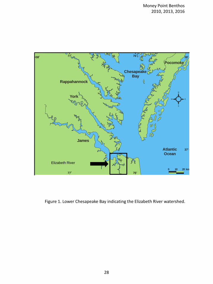
Figure 1. Lower Chesapeake Bay indicating the Elizabeth River watershed.
Money Point Benthos 2010, 2013, 2016
28
Money Point
Eastern Branch
Southern Branch
James River
SBE5
SBE2
Figure 2. Elizabeth River Watershed indicating the Money Point region of the Southern Branch. SBE2 and SBE5 fixed stations of the Chesapeake Bay Benthic Monitoring Program sampled from 1989 to present.
Money Point Benthos 2010, 2013, 2016
29
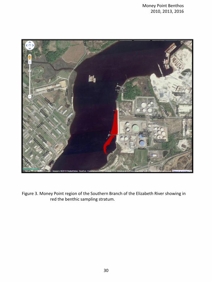
Figure 3. Money Point region of the Southern Branch of the Elizabeth River showing in red the benthic sampling stratum.
Money Point Benthos 2010, 2013, 2016
30
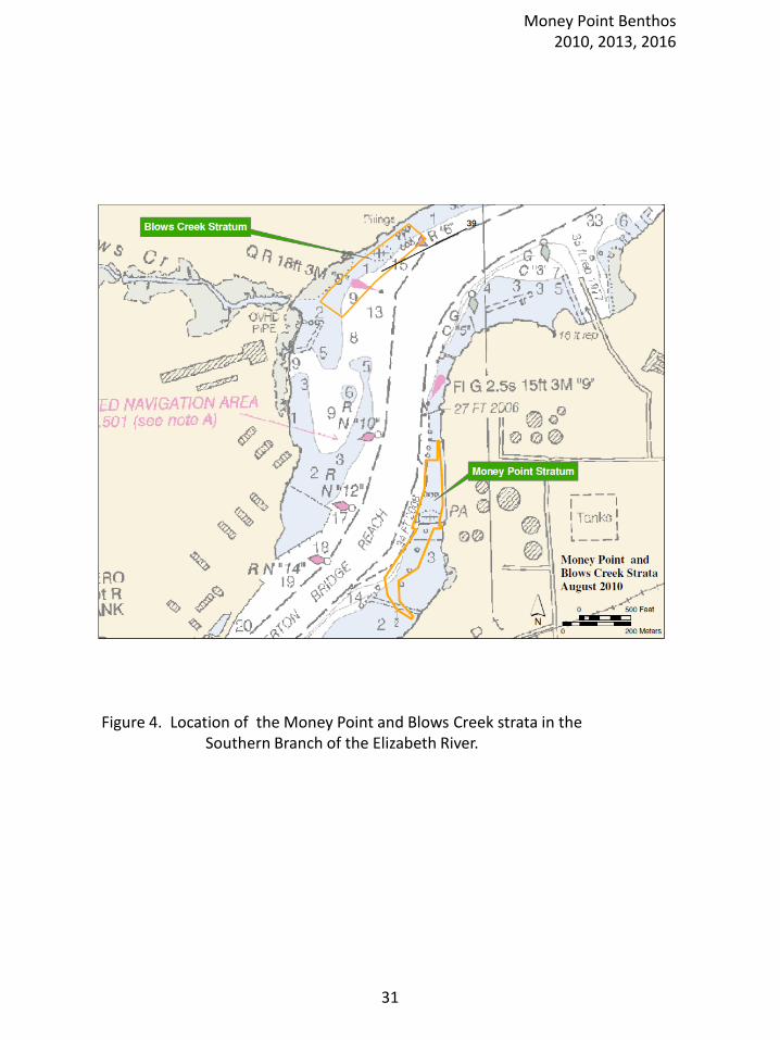
Figure 4. Location of the Money Point and Blows Creek strata in the Southern Branch of the Elizabeth River.
Money Point Benthos 2010, 2013, 2016
31
- Sites with Sites with evidence of sheen
- Sites not sampled
Figure 5. Money Point stratum random locations. Sites sampled with
marked by gold circle. Sampled sites that showed
evidence of sheen in the field marked with a red circle.
Money Point Benthos 2010, 2013, 2016
32
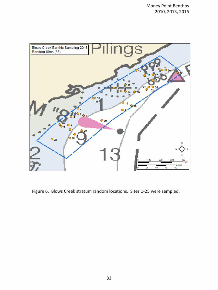
Figure 6. Blows Creek stratum random locations. Sites 1-25 were sampled.
Money Point Benthos 2010, 2013, 2016
33
43.8
28.7
51.1
27.7
40.4
26.8
0.0
10.0
20.0
30.0
40.0
50.0
60.0
70.0
2010 2013 2016
% Silt-Clay
Money Point Blows Creek
Figure 7. Comparison of sediment percentage silt-clay content between collection
years (2010, 2013, 2016) at Money Point and Blows Creek. Compared by t-test with
p value shown for each year. Mean values indicated at top of each bar.
p = 0.035 p = 0.145 p = 0.013
Money Point Benthos 2010, 2013, 2016
34
6.9
2.8
5.1
2.9
4.1
3.5
0.0
1.0
2.0
3.0
4.0
5.0
6.0
7.0
8.0
9.0
2010 2013 2016
% Total Volatile Solids
Money Point Blows Creek
Figure 8. Comparison of total volatile solids between collection years (2010, 2013,
2016) at Money Point and Blows Creek. Compared by t-test with p value shown for
each year. Mean values indicated at top of each bar.
p > 0.001 p = 0.069 p = 0.094
Money Point Benthos 2010, 2013, 2016
35
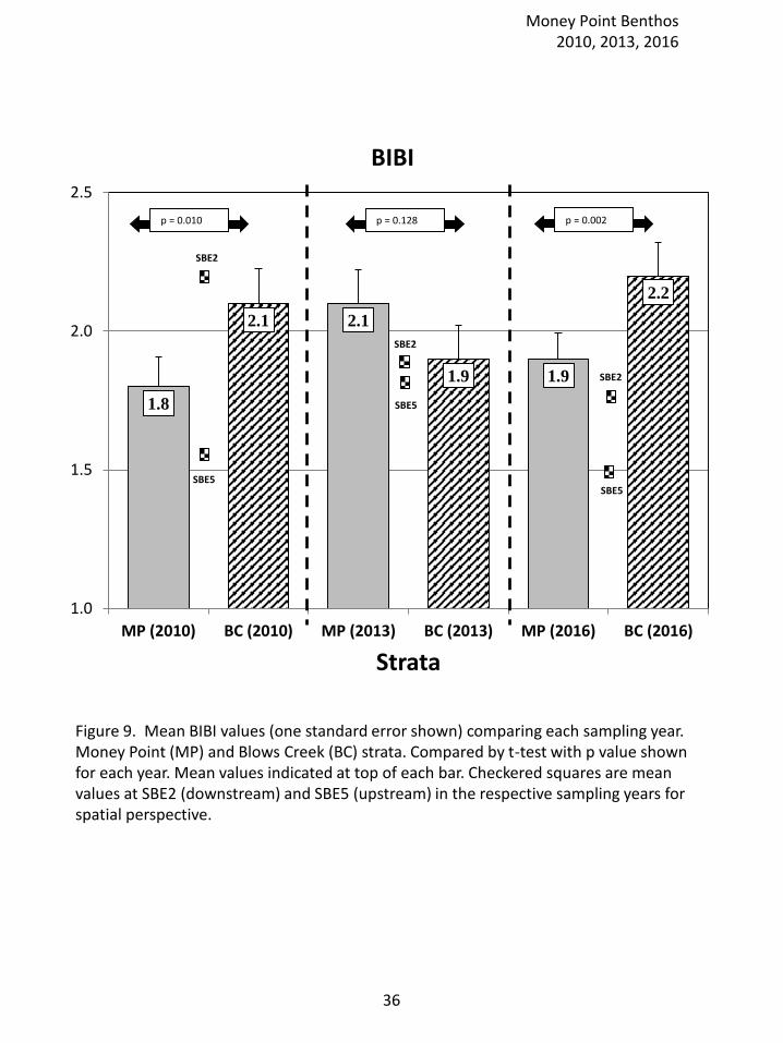
Figure 9. Mean BIBI values (one standard error shown) comparing each sampling year. Money Point (MP) and Blows Creek (BC) strata. Compared by t-test with p value shown for each year. Mean values indicated at top of each bar. Checkered squares are mean values at SBE2 (downstream) and SBE5 (upstream) in the respective sampling years for spatial perspective.
1.8
2.1 2.1
1.9 1.9
2.2
1.0
1.5
2.0
2.5
MP (2010) BC (2010) MP (2013) BC (2013) MP (2016) BC (2016)
Strata
BIBI
p = 0.010 p = 0.128 p = 0.002
SBE2
SBE5
SBE2
SBE5
SBE2
SBE5
Money Point Benthos 2010, 2013, 2016
36
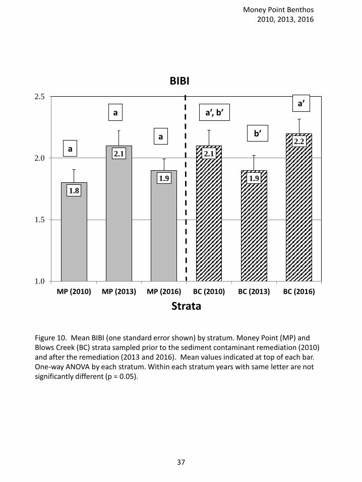
Figure 10. Mean BIBI (one standard error shown) by stratum. Money Point (MP) and Blows Creek (BC) strata sampled prior to the sediment contaminant remediation (2010) and after the remediation (2013 and 2016). Mean values indicated at top of each bar. One-way ANOVA by each stratum. Within each stratum years with same letter are not significantly different (p = 0.05).
1.8
2.1
1.9
2.1
1.9
2.2
1.0
1.5
2.0
2.5
MP (2010) MP (2013) MP (2016) BC (2010) BC (2013) BC (2016)
Strata
BIBI
a
a
a a’, b’a’
b’
Money Point Benthos 2010, 2013, 2016
37
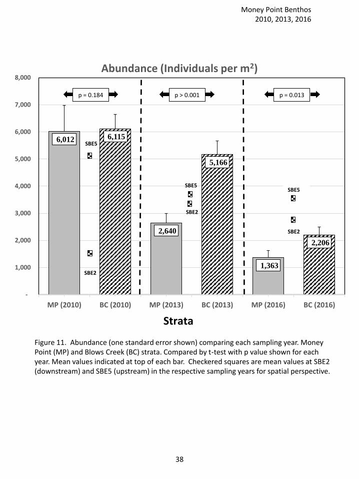
6,012 6,115
2,640
5,166
1,363
2,206
-
1,000
2,000
3,000
4,000
5,000
6,000
7,000
8,000
MP (2010) BC (2010) MP (2013) BC (2013) MP (2016) BC (2016)
Abundance (Individuals per m2)
Strata
Figure 11. Abundance (one standard error shown) comparing each sampling year. Money Point (MP) and Blows Creek (BC) strata. Compared by t-test with p value shown for each year. Mean values indicated at top of each bar. Checkered squares are mean values at SBE2 (downstream) and SBE5 (upstream) in the respective sampling years for spatial perspective.
p = 0.184 p > 0.001 p = 0.013
SBE2
SBE5
SBE2
SBE5
SBE2
SBE5
Money Point Benthos 2010, 2013, 2016
38
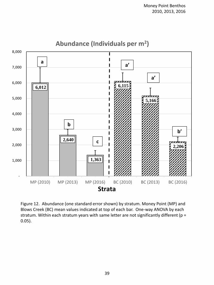
6,012
2,640
1,363
6,115
5,166
2,206
-
1,000
2,000
3,000
4,000
5,000
6,000
7,000
8,000
MP (2010) MP (2013) MP (2016) BC (2010) BC (2013) BC (2016)
Abundance (Individuals per m2)
Strata
Figure 12. Abundance (one standard error shown) by stratum. Money Point (MP) and Blows Creek (BC) mean values indicated at top of each bar. One-way ANOVA by each stratum. Within each stratum years with same letter are not significantly different (p = 0.05).
a
b
c
a’
a’
b’
Money Point Benthos 2010, 2013, 2016
39
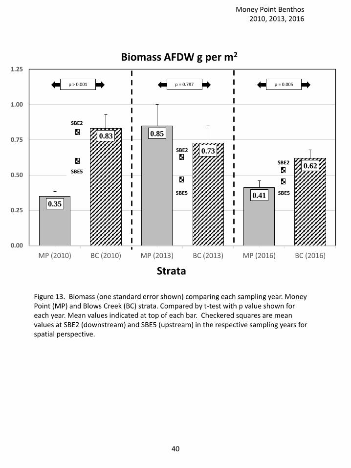
0.35
0.83 0.85
0.73
0.41
0.62
0.00
0.25
0.50
0.75
1.00
1.25
MP (2010) BC (2010) MP (2013) BC (2013) MP (2016) BC (2016)
Strata
Figure 13. Biomass (one standard error shown) comparing each sampling year. Money Point (MP) and Blows Creek (BC) strata. Compared by t-test with p value shown for each year. Mean values indicated at top of each bar. Checkered squares are mean values at SBE2 (downstream) and SBE5 (upstream) in the respective sampling years for spatial perspective.
p > 0.001 p = 0.787 p = 0.005
SBE2
SBE5
SBE2
SBE5
SBE2
SBE5
Biomass AFDW g per m2
Money Point Benthos 2010, 2013, 2016
40
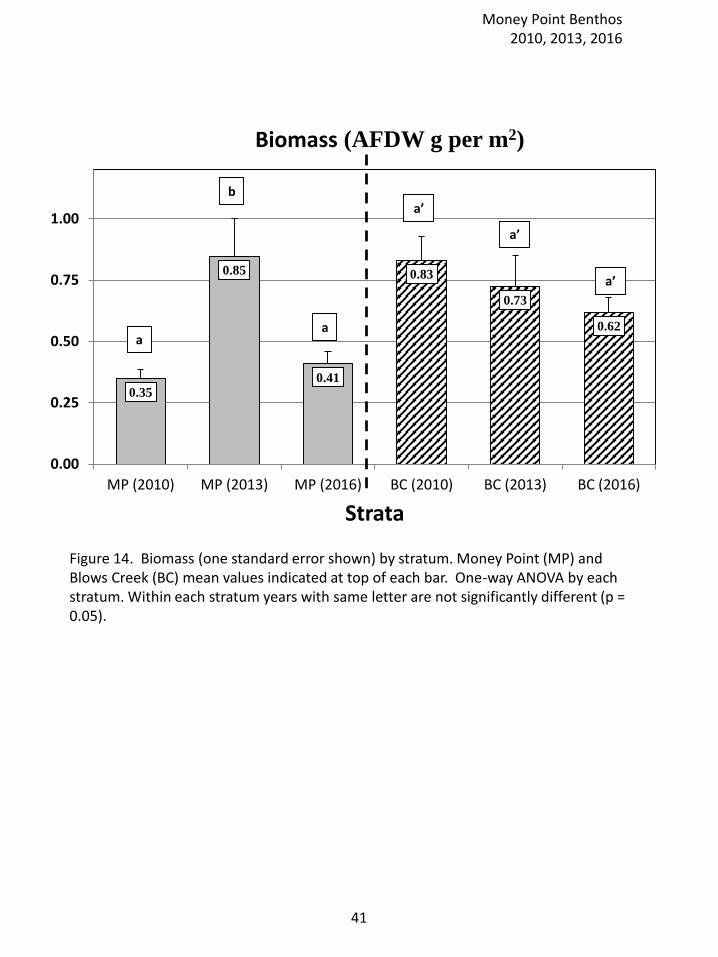
Figure 14. Biomass (one standard error shown) by stratum. Money Point (MP) and Blows Creek (BC) mean values indicated at top of each bar. One-way ANOVA by each stratum. Within each stratum years with same letter are not significantly different (p = 0.05).
0.35
0.85
0.41
0.83
0.73
0.62
0.00
0.25
0.50
0.75
1.00
MP (2010) MP (2013) MP (2016) BC (2010) BC (2013) BC (2016)
Strata
Biomass (AFDW g per m2)
a’
a’
a’
aa
b
Money Point Benthos 2010, 2013, 2016
41
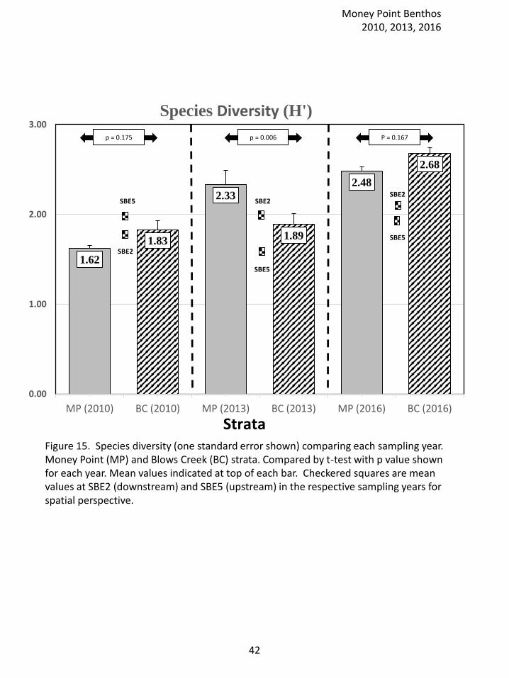
Figure 15. Species diversity (one standard error shown) comparing each sampling year. Money Point (MP) and Blows Creek (BC) strata. Compared by t-test with p value shown for each year. Mean values indicated at top of each bar. Checkered squares are mean values at SBE2 (downstream) and SBE5 (upstream) in the respective sampling years for spatial perspective.
1.62
1.83
2.33
1.89
2.48
2.68
0.00
1.00
2.00
3.00
MP (2010) BC (2010) MP (2013) BC (2013) MP (2016) BC (2016)
Species Diversity (H')
Strata
p = 0.175 p = 0.006 P = 0.167
SBE5
SBE2
SBE5
SBE2SBE2
SBE5
Money Point Benthos 2010, 2013, 2016
42
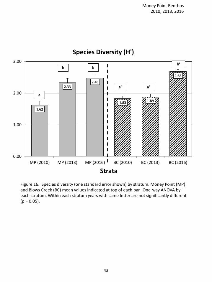
Figure 16. Species diversity (one standard error shown) by stratum. Money Point (MP) and Blows Creek (BC) mean values indicated at top of each bar. One-way ANOVA by each stratum. Within each stratum years with same letter are not significantly different (p = 0.05).
1.62
2.33
2.48
1.831.89
2.68
0.00
1.00
2.00
3.00
MP (2010) MP (2013) MP (2016) BC (2010) BC (2013) BC (2016)
Strata
Species Diversity (H')
a’ a’
b’
a
b b
Money Point Benthos 2010, 2013, 2016
43

9.48
13.52
11.96 12.00
10.48
12.84
0.00
5.00
10.00
15.00
MP (2010) BC (2010) MP (2013) BC (2013) MP (2016) BC (2016)
Strata
Species Richness (species per sample)
Figure 17. Species richness (one standard error shown) comparing each sampling year. Money Point (MP) and Blows Creek (BC) strata. Compared by t-test with p value shown for each year. Mean values indicated at top of each bar. Comparisons with values at MP (Money Point) and BC (Blows Creek) in the respective sampling years cannot be made because sampling gears of different sizes were used - Young grab at MP and BS and box-corer at SBE2 and SBE5.
p > 0.001 p = 0.960 p = 0.031
Money Point Benthos 2010, 2013, 2016
44
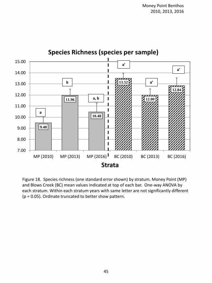
9.48
11.96
10.48
13.52
12.00
12.84
7.00
8.00
9.00
10.00
11.00
12.00
13.00
14.00
15.00
MP (2010) MP (2013) MP (2016) BC (2010) BC (2013) BC (2016)
Strata
Species Richness (species per sample)
Figure 18. Species richness (one standard error shown) by stratum. Money Point (MP) and Blows Creek (BC) mean values indicated at top of each bar. One-way ANOVA by each stratum. Within each stratum years with same letter are not significantly different (p = 0.05). Ordinate truncated to better show pattern.
a’
a’
a’
a
a, b
b
Money Point Benthos 2010, 2013, 2016
45
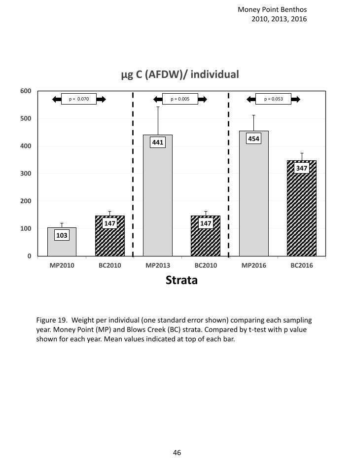
103
147
441
147
454
347
0
100
200
300
400
500
600
MP2010 BC2010 MP2013 BC2010 MP2016 BC2016
Strata
µg C (AFDW)/ individual
Figure 19. Weight per individual (one standard error shown) comparing each sampling year. Money Point (MP) and Blows Creek (BC) strata. Compared by t-test with p value shown for each year. Mean values indicated at top of each bar.
p = 0.070 p = 0.005 p = 0.053
Money Point Benthos 2010, 2013, 2016
46
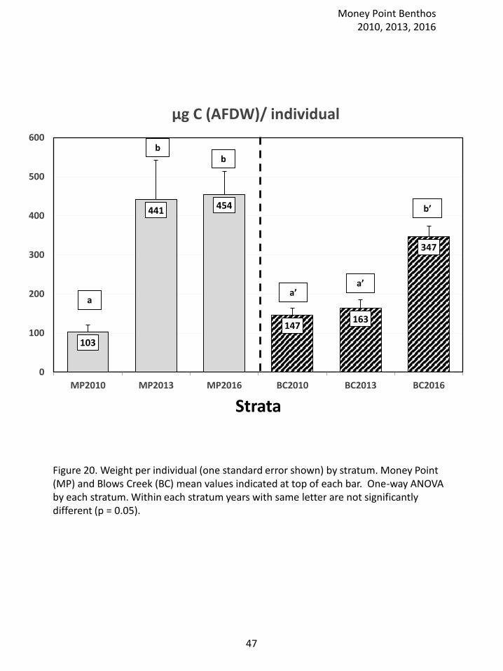
Figure 20. Weight per individual (one standard error shown) by stratum. Money Point (MP) and Blows Creek (BC) mean values indicated at top of each bar. One-way ANOVA by each stratum. Within each stratum years with same letter are not significantly different (p = 0.05).
103
441 454
147163
347
0
100
200
300
400
500
600
MP2010 MP2013 MP2016 BC2010 BC2013 BC2016
Strata
µg C (AFDW)/ individual
a’a’
b’
a
bb
Money Point Benthos 2010, 2013, 2016
47
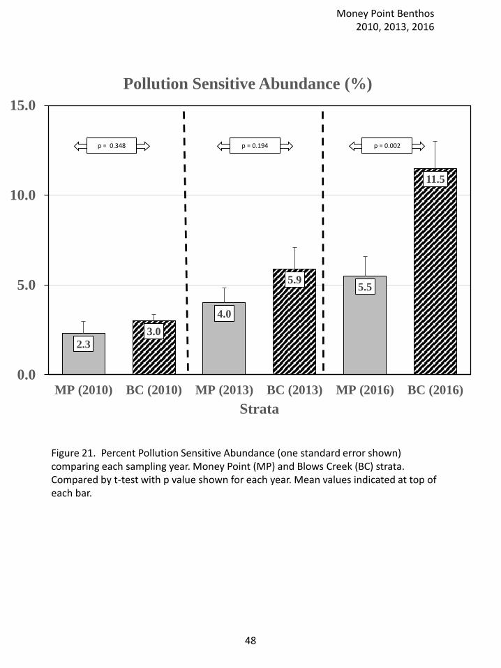
Figure 21. Percent Pollution Sensitive Abundance (one standard error shown) comparing each sampling year. Money Point (MP) and Blows Creek (BC) strata. Compared by t-test with p value shown for each year. Mean values indicated at top of each bar.
2.3
3.0
4.0
5.95.5
11.5
0.0
5.0
10.0
15.0
MP (2010) BC (2010) MP (2013) BC (2013) MP (2016) BC (2016)
Strata
Pollution Sensitive Abundance (%)
p = 0.348 p = 0.194 p = 0.002
Money Point Benthos 2010, 2013, 2016
48
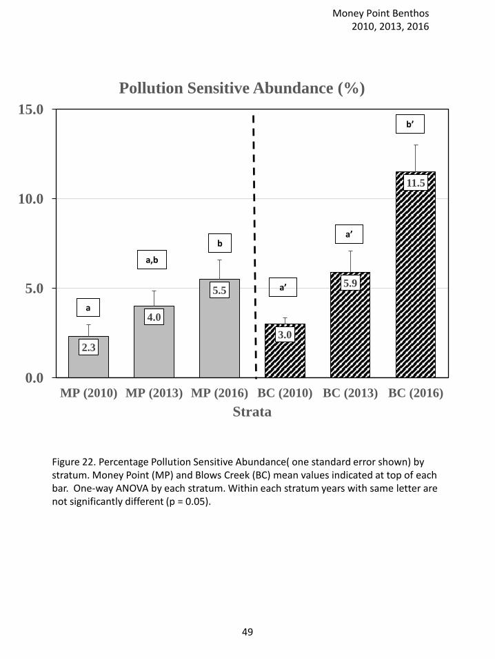
Figure 22. Percentage Pollution Sensitive Abundance( one standard error shown) by stratum. Money Point (MP) and Blows Creek (BC) mean values indicated at top of each bar. One-way ANOVA by each stratum. Within each stratum years with same letter are not significantly different (p = 0.05).
2.3
4.0
5.5
3.0
5.9
11.5
0.0
5.0
10.0
15.0
MP (2010) MP (2013) MP (2016) BC (2010) BC (2013) BC (2016)
Strata
Pollution Sensitive Abundance (%)
a’
a’
b’
a
a,b
b
Money Point Benthos 2010, 2013, 2016
49
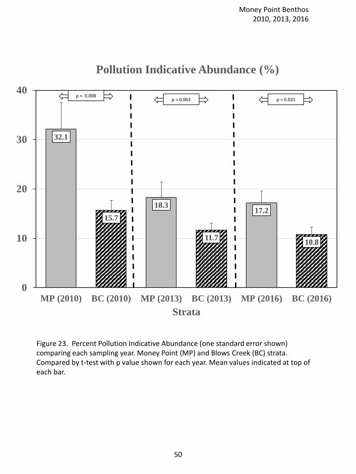
Figure 23. Percent Pollution Indicative Abundance (one standard error shown) comparing each sampling year. Money Point (MP) and Blows Creek (BC) strata. Compared by t-test with p value shown for each year. Mean values indicated at top of each bar.
32.1
15.7
18.3
11.7
17.2
10.8
0
10
20
30
40
MP (2010) BC (2010) MP (2013) BC (2013) MP (2016) BC (2016)
Strata
Pollution Indicative Abundance (%)
p = 0.008p = 0.063 p = 0.031
Money Point Benthos 2010, 2013, 2016
50
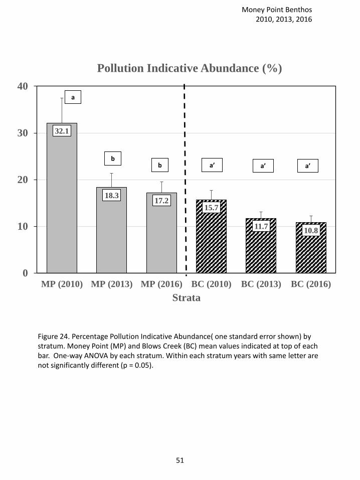
Figure 24. Percentage Pollution Indicative Abundance( one standard error shown) by stratum. Money Point (MP) and Blows Creek (BC) mean values indicated at top of each bar. One-way ANOVA by each stratum. Within each stratum years with same letter are not significantly different (p = 0.05).
32.1
18.317.2
15.7
11.710.8
0
10
20
30
40
MP (2010) MP (2013) MP (2016) BC (2010) BC (2013) BC (2016)
Strata
Pollution Indicative Abundance (%)
a’ a’ a’
a
bb
Money Point Benthos 2010, 2013, 2016
51
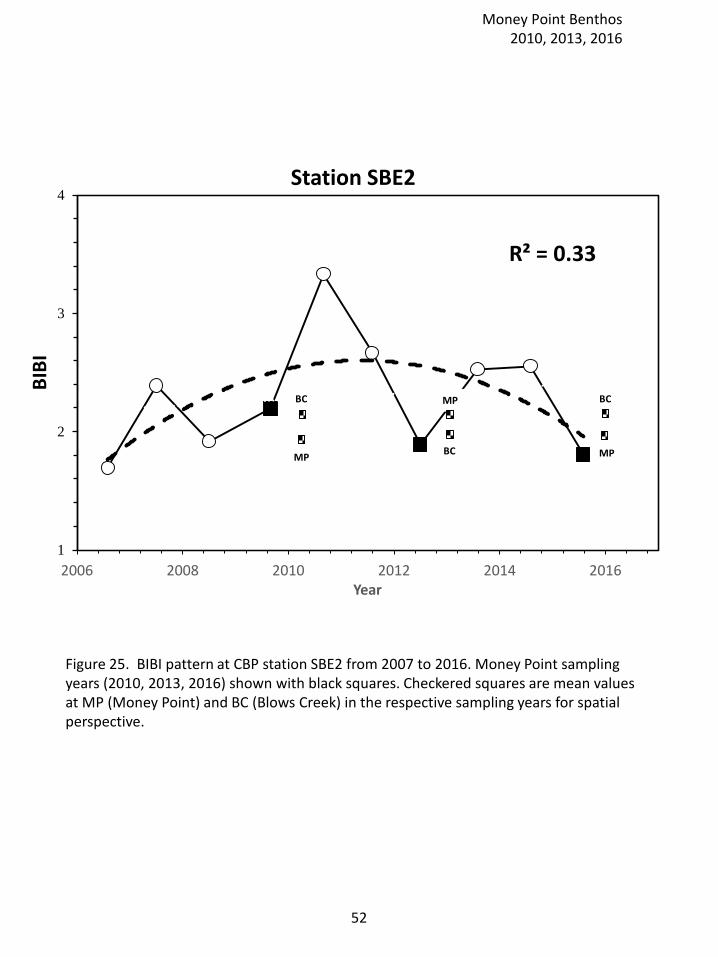
R² = 0.33
1
2
3
4
2006 2008 2010 2012 2014 2016
BIB
I
Year
Station SBE2
BC
MPBC
MP BC
MP
Figure 25. BIBI pattern at CBP station SBE2 from 2007 to 2016. Money Point sampling years (2010, 2013, 2016) shown with black squares. Checkered squares are mean values at MP (Money Point) and BC (Blows Creek) in the respective sampling years for spatial perspective.
Money Point Benthos 2010, 2013, 2016
52
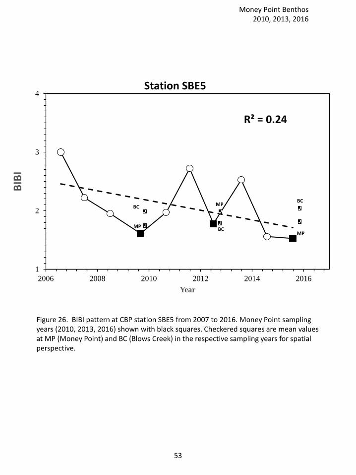
R² = 0.24
1
2
3
4
2006 2008 2010 2012 2014 2016
BIB
I
Year
Station SBE5
BC
MPBC
MPBC
MP
Figure 26. BIBI pattern at CBP station SBE5 from 2007 to 2016. Money Point sampling years (2010, 2013, 2016) shown with black squares. Checkered squares are mean values at MP (Money Point) and BC (Blows Creek) in the respective sampling years for spatial perspective.
Money Point Benthos 2010, 2013, 2016
53
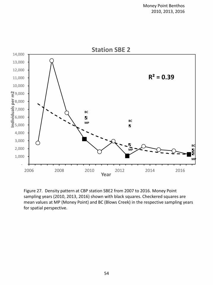
R² = 0.39
-
1,000
2,000
3,000
4,000
5,000
6,000
7,000
8,000
9,000
10,000
11,000
12,000
13,000
14,000
2006 2008 2010 2012 2014 2016
Ind
ivid
ual
s p
er m
2
Year
Station SBE 2
BC
MPBC
MPBC
MP
Figure 27. Density pattern at CBP station SBE2 from 2007 to 2016. Money Point sampling years (2010, 2013, 2016) shown with black squares. Checkered squares are mean values at MP (Money Point) and BC (Blows Creek) in the respective sampling years for spatial perspective.
Money Point Benthos 2010, 2013, 2016
54
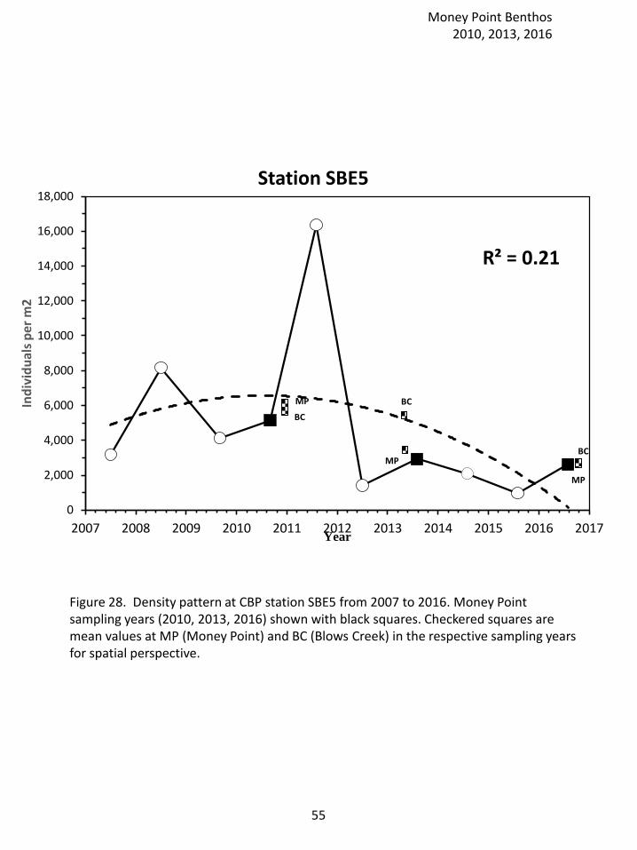
R² = 0.21
0
2,000
4,000
6,000
8,000
10,000
12,000
14,000
16,000
18,000
2007 2008 2009 2010 2011 2012 2013 2014 2015 2016 2017
Ind
ivid
ual
s p
er m
2
Year
Station SBE5
BC
MP BC
MPBC
MP
Figure 28. Density pattern at CBP station SBE5 from 2007 to 2016. Money Point sampling years (2010, 2013, 2016) shown with black squares. Checkered squares are mean values at MP (Money Point) and BC (Blows Creek) in the respective sampling years for spatial perspective.
Money Point Benthos 2010, 2013, 2016
55
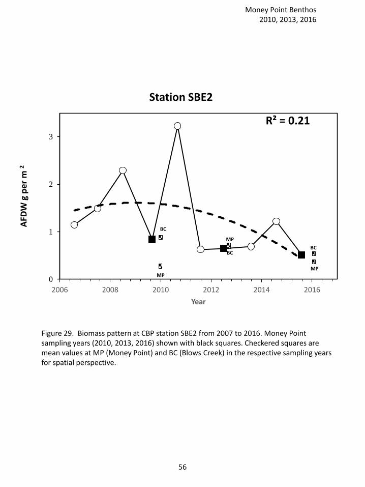
R² = 0.21
0
1
2
3
2006 2008 2010 2012 2014 2016
AFD
W g
pe
r m
2
Year
Station SBE2
BC
MP
BC
MP
BC
MP
Figure 29. Biomass pattern at CBP station SBE2 from 2007 to 2016. Money Point sampling years (2010, 2013, 2016) shown with black squares. Checkered squares are mean values at MP (Money Point) and BC (Blows Creek) in the respective sampling years for spatial perspective.
Money Point Benthos 2010, 2013, 2016
56
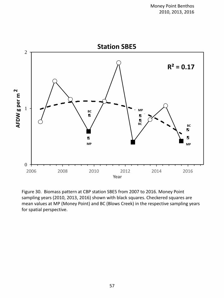
R² = 0.17
0
1
2
2006 2008 2010 2012 2014 2016
AFD
W g
pe
r m
2
Year
Station SBE5
BC
MP
BC
MP
BC
MP
Figure 30. Biomass pattern at CBP station SBE5 from 2007 to 2016. Money Point sampling years (2010, 2013, 2016) shown with black squares. Checkered squares are mean values at MP (Money Point) and BC (Blows Creek) in the respective sampling years for spatial perspective.
Money Point Benthos 2010, 2013, 2016
57
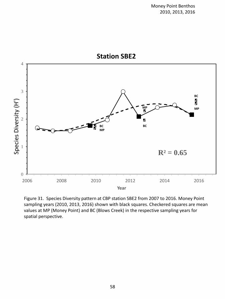
R² = 0.65
0
1
2
3
4
2006 2008 2010 2012 2014 2016
Spec
ies
Div
ersi
ty (
H')
Year
Station SBE2
BCMP
BC
MP
BC
MP
Figure 31. Species Diversity pattern at CBP station SBE2 from 2007 to 2016. Money Point sampling years (2010, 2013, 2016) shown with black squares. Checkered squares are mean values at MP (Money Point) and BC (Blows Creek) in the respective sampling years for spatial perspective.
Money Point Benthos 2010, 2013, 2016
58
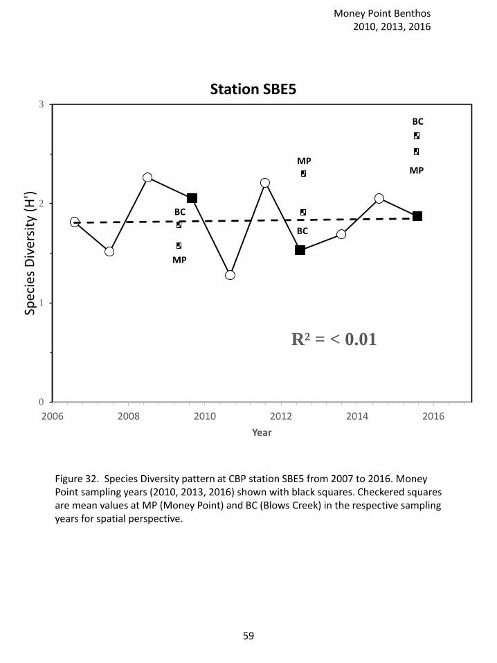
Figure 32. Species Diversity pattern at CBP station SBE5 from 2007 to 2016. Money Point sampling years (2010, 2013, 2016) shown with black squares. Checkered squares are mean values at MP (Money Point) and BC (Blows Creek) in the respective sampling years for spatial perspective.
R² = < 0.01
0
1
2
3
2006 2008 2010 2012 2014 2016
Spec
ies
Div
ersi
ty (
H')
Year
Station SBE5
BC
MP
BC
MP
BC
MP
Money Point Benthos 2010, 2013, 2016
59
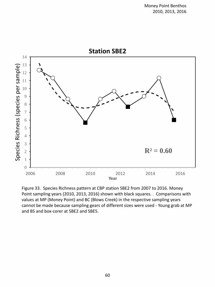
R² = 0.20
R² = 0.60
0
1
2
3
4
5
6
7
8
9
10
11
12
13
14
2006 2008 2010 2012 2014 2016
Spec
ies
Ric
hn
ess
(sp
ecie
s p
er s
amp
le)
Year
Station SBE2
Figure 33. Species Richness pattern at CBP station SBE2 from 2007 to 2016. Money Point sampling years (2010, 2013, 2016) shown with black squares. . Comparisons with values at MP (Money Point) and BC (Blows Creek) in the respective sampling years cannot be made because sampling gears of different sizes were used - Young grab at MP and BS and box-corer at SBE2 and SBE5.
Money Point Benthos 2010, 2013, 2016
60
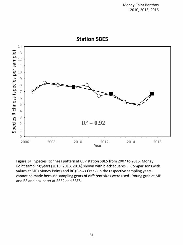
R² = 0.92
0
1
2
3
4
5
6
7
8
9
10
11
12
13
14
2006 2008 2010 2012 2014 2016
Spec
ies
Ric
hn
ess
(sp
ecie
s p
er s
amp
le)
Year
Station SBE5
Figure 34. Species Richness pattern at CBP station SBE5 from 2007 to 2016. Money Point sampling years (2010, 2013, 2016) shown with black squares. . Comparisons with values at MP (Money Point) and BC (Blows Creek) in the respective sampling years cannot be made because sampling gears of different sizes were used - Young grab at MP and BS and box-corer at SBE2 and SBE5.
Money Point Benthos 2010, 2013, 2016
61

Tables 1-4
Money Point Benthos 2010, 2013, 2016
62
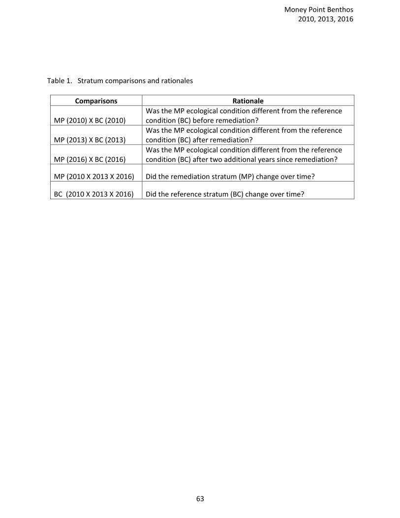
Table 1. Stratum comparisons and rationales
Comparisons Rationale
MP (2010) X BC (2010) Was the MP ecological condition different from the reference condition (BC) before remediation?
MP (2013) X BC (2013) Was the MP ecological condition different from the reference condition (BC) after remediation?
MP (2016) X BC (2016) Was the MP ecological condition different from the reference condition (BC) after two additional years since remediation?
MP (2010 X 2013 X 2016) Did the remediation stratum (MP) change over time?
BC (2010 X 2013 X 2016) Did the reference stratum (BC) change over time?
Money Point Benthos 2010, 2013, 2016
63
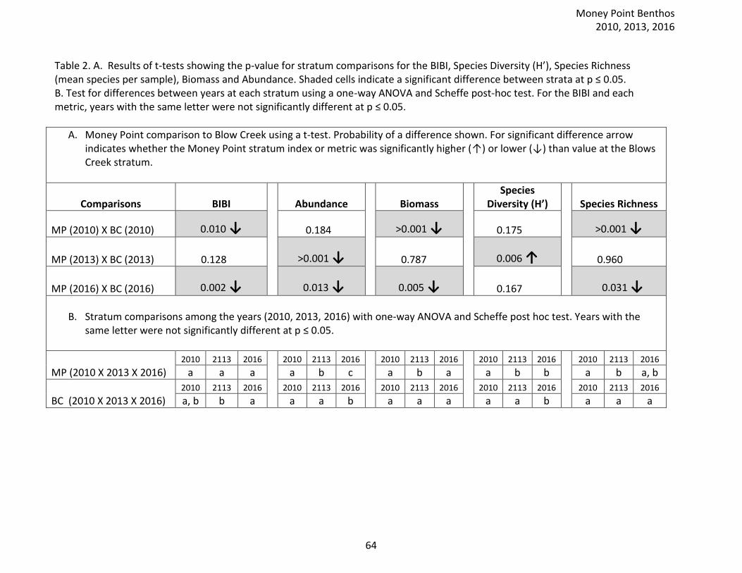
Table 2. A. Results of t-tests showing the p-value for stratum comparisons for the BIBI, Species Diversity (H’), Species Richness (mean species per sample), Biomass and Abundance. Shaded cells indicate a significant difference between strata at p ≤ 0.05. B. Test for differences between years at each stratum using a one-way ANOVA and Scheffe post-hoc test. For the BIBI and each metric, years with the same letter were not significantly different at p ≤ 0.05.
A. Money Point comparison to Blow Creek using a t-test. Probability of a difference shown. For significant difference arrow indicates whether the Money Point stratum index or metric was significantly higher (↑) or lower (↓) than value at the Blows Creek stratum.
Comparisons BIBI
Abundance
Biomass Species
Diversity (H’)
Species Richness
MP (2010) X BC (2010) 0.010 ↓
0.184
>0.001 ↓
0.175
>0.001 ↓
MP (2013) X BC (2013) 0.128
>0.001 ↓
0.787
0.006 ↑
0.960
MP (2016) X BC (2016) 0.002 ↓
0.013 ↓
0.005 ↓
0.167
0.031 ↓
B. Stratum comparisons among the years (2010, 2013, 2016) with one-way ANOVA and Scheffe post hoc test. Years with the
same letter were not significantly different at p ≤ 0.05.
MP (2010 X 2013 X 2016) 2010 2113 2016 2010 2113 2016 2010 2113 2016 2010 2113 2016 2010 2113 2016
a a a a b c a b a a b b a b a, b
BC (2010 X 2013 X 2016) 2010 2113 2016 2010 2113 2016 2010 2113 2016 2010 2113 2016 2010 2113 2016
a, b b a a a b a a a a a b a a a
Money Point Benthos 2010, 2013, 2016
64
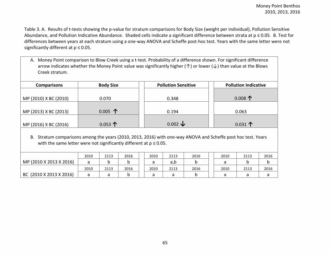
Table 3. A. Results of t-tests showing the p-value for stratum comparisons for Body Size (weight per individual), Pollution Sensitive Abundance, and Pollution Indicative Abundance. Shaded cells indicate a significant difference between strata at p ≤ 0.05. B. Test for differences between years at each stratum using a one-way ANOVA and Scheffe post-hoc test. Years with the same letter were not significantly different at p ≤ 0.05.
A. Money Point comparison to Blow Creek using a t-test. Probability of a difference shown. For significant difference arrow indicates whether the Money Point value was significantly higher (↑) or lower (↓) than value at the Blows Creek stratum.
Comparisons Body Size Pollution Sensitive Pollution Indicative
MP (2010) X BC (2010) 0.070
0.348
0.008 ↑
MP (2013) X BC (2013) 0.005 ↑
0.194
0.063
MP (2016) X BC (2016) 0.053 ↑
0.002 ↓
0.031 ↑
B. Stratum comparisons among the years (2010, 2013, 2016) with one-way ANOVA and Scheffe post hoc test. Years
with the same letter were not significantly different at p ≤ 0.05.
MP (2010 X 2013 X 2016) 2010 2113 2016 2010 2113 2016 2010 2113 2016 2016
a b b a a,b b a b b a, b
BC (2010 X 2013 X 2016) 2010 2113 2016 2010 2113 2016 2010 2113 2016 2016
a a b a a b a a a a
Money Point Benthos 2010, 2013, 2016
65
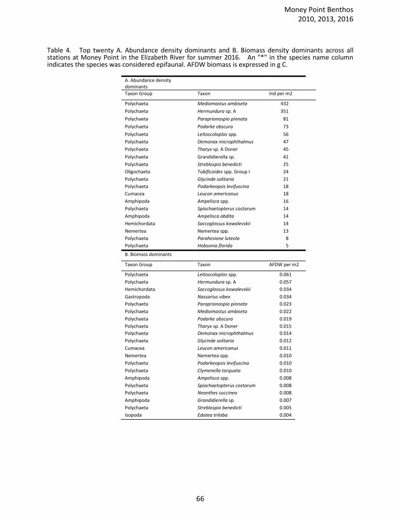
Table 4. Top twenty A. Abundance density dominants and B. Biomass density dominants across all stations at Money Point in the Elizabeth River for summer 2016. An "*" in the species name column indicates the species was considered epifaunal. AFDW biomass is expressed in g C.
A. Abundance density dominants
Taxon Group Taxon Ind per m2
Polychaeta Mediomastus ambiseta 432
Polychaeta Hermundura sp. A 351
Polychaeta Paraprionospio pinnata 81
Polychaeta Podarke obscura 73
Polychaeta Leitoscoloplos spp. 56
Polychaeta Demonax microphthalmus 47
Polychaeta Tharyx sp. A Doner 45
Polychaeta Grandidierella sp. 41
Polychaeta Streblospio benedicti 25
Oligochaeta Tubificoides spp. Group I 24
Polychaeta Glycinde solitaria 21
Polychaeta Podarkeopsis levifuscina 18
Cumacea Leucon americanus 18
Amphipoda Ampelisca spp. 16
Polychaeta Spiochaetopterus costarum 14
Amphipoda Ampelisca abdita 14
Hemichordata Saccoglossus kowalevskii 14
Nemertea Nemertea spp. 13
Polychaeta Parahesione luteola 8
Polychaeta Hobsonia florida 5
B. Biomass dominants
Taxon Group Taxon AFDW per m2
Polychaeta Leitoscoloplos spp. 0.061
Polychaeta Hermundura sp. A 0.057
Hemichordata Saccoglossus kowalevskii 0.034
Gastropoda Nassarius vibex 0.034
Polychaeta Paraprionospio pinnata 0.023
Polychaeta Mediomastus ambiseta 0.022
Polychaeta Podarke obscura 0.019
Polychaeta Tharyx sp. A Doner 0.015
Polychaeta Demonax microphthalmus 0.014
Polychaeta Glycinde solitaria 0.012
Cumacea Leucon americanus 0.011
Nemertea Nemertea spp. 0.010
Polychaeta Podarkeopsis levifuscina 0.010
Polychaeta Clymenella torquata 0.010
Amphipoda Ampelisca spp. 0.008
Polychaeta Spiochaetopterus costarum 0.008
Polychaeta Neanthes succinea 0.008
Amphipoda Grandidierella sp. 0.007
Polychaeta Streblospio benedicti 0.005
Isopoda Edotea triloba 0.004
Money Point Benthos 2010, 2013, 2016
66
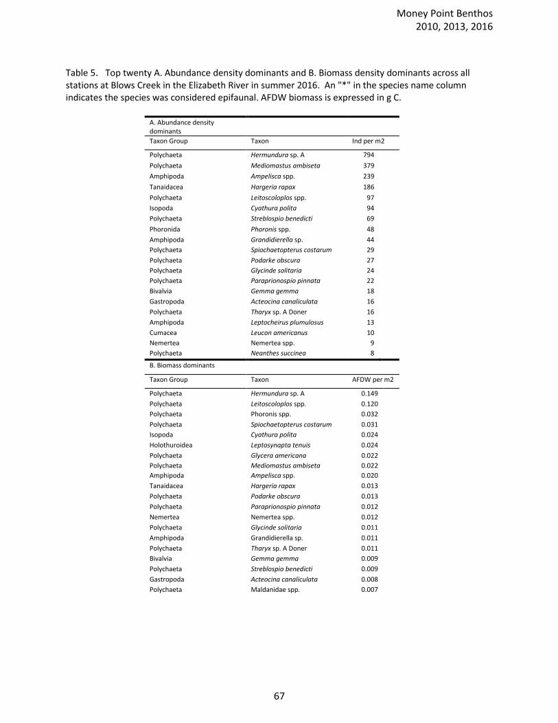
Table 5. Top twenty A. Abundance density dominants and B. Biomass density dominants across all stations at Blows Creek in the Elizabeth River in summer 2016. An "*" in the species name column indicates the species was considered epifaunal. AFDW biomass is expressed in g C.
A. Abundance density dominants
Taxon Group Taxon Ind per m2
Polychaeta Hermundura sp. A 794
Polychaeta Mediomastus ambiseta 379
Amphipoda Ampelisca spp. 239
Tanaidacea Hargeria rapax 186
Polychaeta Leitoscoloplos spp. 97
Isopoda Cyathura polita 94
Polychaeta Streblospio benedicti 69
Phoronida Phoronis spp. 48
Amphipoda Grandidierella sp. 44
Polychaeta Spiochaetopterus costarum 29
Polychaeta Podarke obscura 27
Polychaeta Glycinde solitaria 24
Polychaeta Paraprionospio pinnata 22
Bivalvia Gemma gemma 18
Gastropoda Acteocina canaliculata 16
Polychaeta Tharyx sp. A Doner 16
Amphipoda Leptocheirus plumulosus 13
Cumacea Leucon americanus 10
Nemertea Nemertea spp. 9
Polychaeta Neanthes succinea 8
B. Biomass dominants
Taxon Group Taxon AFDW per m2
Polychaeta Hermundura sp. A 0.149
Polychaeta Leitoscoloplos spp. 0.120
Polychaeta Phoronis spp. 0.032
Polychaeta Spiochaetopterus costarum 0.031
Isopoda Cyathura polita 0.024
Holothuroidea Leptosynapta tenuis 0.024
Polychaeta Glycera americana 0.022
Polychaeta Mediomastus ambiseta 0.022
Amphipoda Ampelisca spp. 0.020
Tanaidacea Hargeria rapax 0.013
Polychaeta Podarke obscura 0.013
Polychaeta Paraprionospio pinnata 0.012
Nemertea Nemertea spp. 0.012
Polychaeta Glycinde solitaria 0.011
Amphipoda Grandidierella sp. 0.011
Polychaeta Tharyx sp. A Doner 0.011
Bivalvia Gemma gemma 0.009
Polychaeta Streblospio benedicti 0.009
Gastropoda Acteocina canaliculata 0.008
Polychaeta Maldanidae spp. 0.007
Money Point Benthos 2010, 2013, 2016
67
Appendix A. Taxa collected at Money Point Project Monitoring Stations Random 2016
Money Point Benthos 2010, 2013, 2016
68
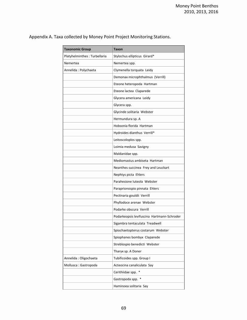
Appendix A. Taxa collected by Money Point Project Monitoring Stations.
Taxonomic Group Taxon
Platyhelminthes : Turbellaria Stylochus ellipticus Girard*
Nemertea Nemertea spp.
Annelida : Polychaeta Clymenella torquata Leidy
Demonax microphthalmus (Verrill)
Eteone heteropoda Hartman
Eteone lactea Claparede
Glycera americana Leidy
Glycera spp.
Glycinde solitaria Webster
Hermundura sp. A
Hobsonia florida Hartman
Hydroides dianthus Verrill*
Leitoscoloplos spp.
Loimia medusa Savigny
Maldanidae spp.
Mediomastus ambiseta Hartman
Neanthes succinea Frey and Leuckart
Nephtys picta Ehlers
Parahesione luteola Webster
Paraprionospio pinnata Ehlers
Pectinaria gouldii Verrill
Phyllodoce arenae Webster
Podarke obscura Verrill
Podarkeopsis levifuscina Hartmann-Schroder
Sigambra tentaculata Treadwell
Spiochaetopterus costarum Webster
Spiophanes bombyx Claparede
Streblospio benedicti Webster
Tharyx sp. A Doner
Annelida : Oligochaeta Tubificoides spp. Group I
Mollusca : Gastropoda Acteocina canaliculata Say
Cerithiidae spp. *
Gastropoda spp. *
Haminoea solitaria Say
Money Point Benthos 2010, 2013, 2016
69
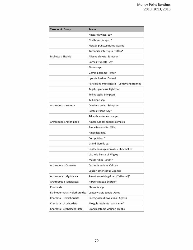
Taxonomic Group Taxon
Nassarius vibex Say
Nudibranchia spp. *
Rictaxis punctostriatus Adams
Turbonilla interrupta Totten*
Mollusca : Bivalvia Aligena elevata Stimpson
Barnea truncata Say
Bivalvia spp.
Gemma gemma Totten
Lyonsia hyalina Conrad
Parvilucina multilineata Tuomey and Holmes
Tagelus plebeius Lightfoot
Tellina agilis Stimpson
Tellinidae spp.
Arthropoda : Isopoda Cyathura polita Stimpson
Edotea triloba Say*
Ptilanthura tenuis Harger
Arthropoda : Amphipoda Ameroculodes species complex
Ampelisca abdita Mills
Ampelisca spp.
Corophiidae *
Grandidierella sp.
Leptocheirus plumulosus Shoemaker
Listriella barnardi Wigley
Melita nitida Smith*
Arthropoda : Cumacea Cyclaspis varians Calman
Leucon americanus Zimmer
Arthropoda : Mysidacea Americamysis bigelowi (Tattersall)*
Arthropoda : Tanaidacea Hargeria rapax (Harger)
Phoronida Phoronis spp.
Echinodermata : Holothuroidea Leptosynapta tenuis Ayres
Chordata : Hemichordata Saccoglossus kowalevskii Agassiz
Chordata : Urochordata Molgula lutulenta Van Name*
Chordata : Cephalochordata Branchiostoma virginae Hubbs
Money Point Benthos 2010, 2013, 2016
70
Appendix B. Data by Site Coordinates, Physical, Sedimentary and Species Abundances and Biomass collected at Money
Point Project Monitoring Stations - 2016
Money Point Benthos 2010, 2013, 2016
71
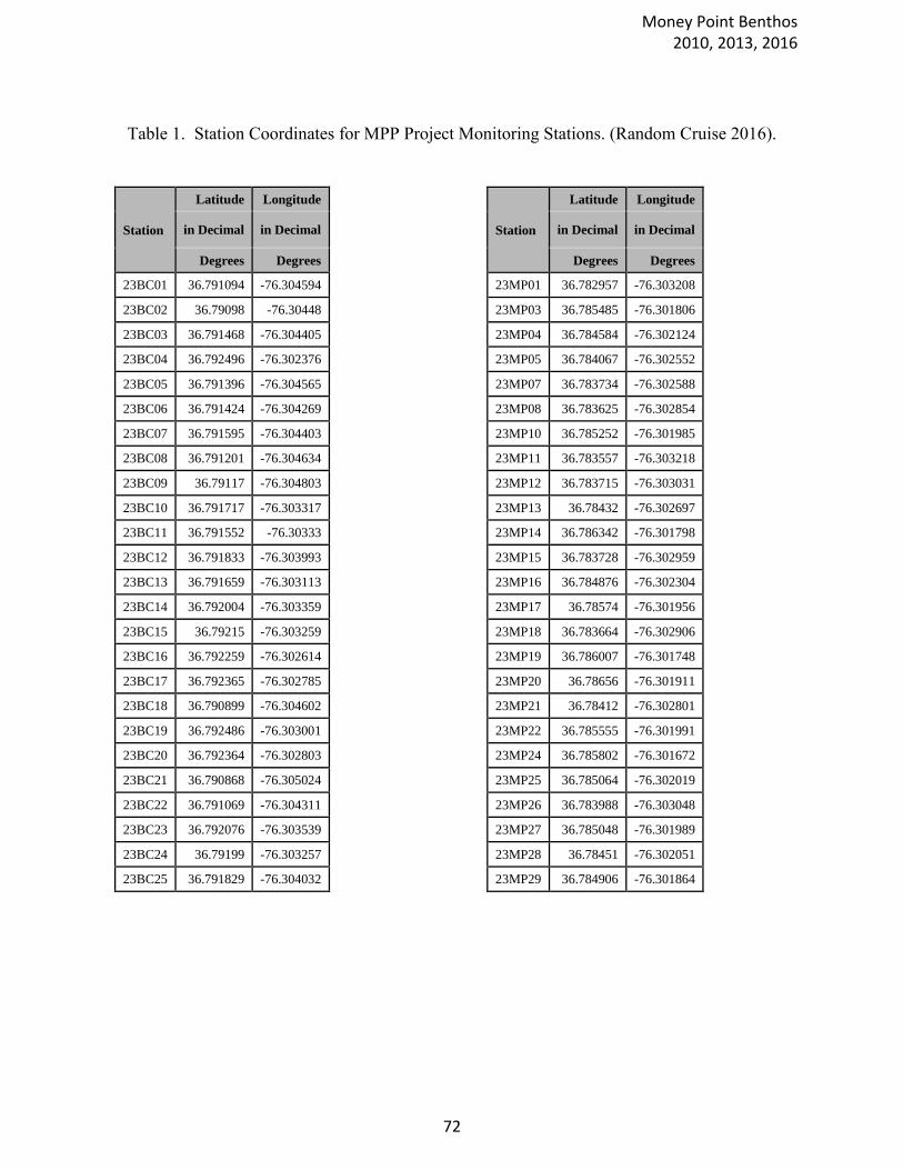
Table 1. Station Coordinates for MPP Project Monitoring Stations. (Random Cruise 2016).
Station
Latitude Longitude
in Decimal in Decimal
Degrees Degrees
23BC01 36.791094 -76.304594
23BC02 36.79098 -76.30448
23BC03 36.791468 -76.304405
23BC04 36.792496 -76.302376
23BC05 36.791396 -76.304565
23BC06 36.791424 -76.304269
23BC07 36.791595 -76.304403
23BC08 36.791201 -76.304634
23BC09 36.79117 -76.304803
23BC10 36.791717 -76.303317
23BC11 36.791552 -76.30333
23BC12 36.791833 -76.303993
23BC13 36.791659 -76.303113
23BC14 36.792004 -76.303359
23BC15 36.79215 -76.303259
23BC16 36.792259 -76.302614
23BC17 36.792365 -76.302785
23BC18 36.790899 -76.304602
23BC19 36.792486 -76.303001
23BC20 36.792364 -76.302803
23BC21 36.790868 -76.305024
23BC22 36.791069 -76.304311
23BC23 36.792076 -76.303539
23BC24 36.79199 -76.303257
23BC25 36.791829 -76.304032
Station
Latitude Longitude
in Decimal in Decimal
Degrees Degrees
23MP01 36.782957 -76.303208
23MP03 36.785485 -76.301806
23MP04 36.784584 -76.302124
23MP05 36.784067 -76.302552
23MP07 36.783734 -76.302588
23MP08 36.783625 -76.302854
23MP10 36.785252 -76.301985
23MP11 36.783557 -76.303218
23MP12 36.783715 -76.303031
23MP13 36.78432 -76.302697
23MP14 36.786342 -76.301798
23MP15 36.783728 -76.302959
23MP16 36.784876 -76.302304
23MP17 36.78574 -76.301956
23MP18 36.783664 -76.302906
23MP19 36.786007 -76.301748
23MP20 36.78656 -76.301911
23MP21 36.78412 -76.302801
23MP22 36.785555 -76.301991
23MP24 36.785802 -76.301672
23MP25 36.785064 -76.302019
23MP26 36.783988 -76.303048
23MP27 36.785048 -76.301989
23MP28 36.78451 -76.302051
23MP29 36.784906 -76.301864
Money Point Benthos 2010, 2013, 2016
72
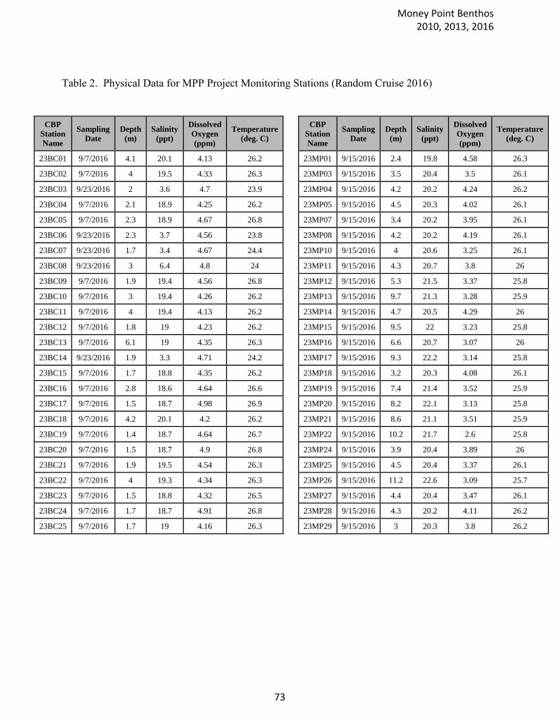
Table 2. Physical Data for MPP Project Monitoring Stations (Random Cruise 2016)
CBP
Station
Name
Sampling
Date
Depth
(m)
Salinity
(ppt)
Dissolved
Oxygen
(ppm)
Temperature
(deg. C)
CBP
Station
Name
Sampling
Date
Depth
(m)
Salinity
(ppt)
Dissolved
Oxygen
(ppm)
Temperature
(deg. C)
23BC01 9/7/2016 4.1 20.1 4.13 26.2 23MP01 9/15/2016 2.4 19.8 4.58 26.3
23BC02 9/7/2016 4 19.5 4.33 26.3 23MP03 9/15/2016 3.5 20.4 3.5 26.1
23BC03 9/23/2016 2 3.6 4.7 23.9 23MP04 9/15/2016 4.2 20.2 4.24 26.2
23BC04 9/7/2016 2.1 18.9 4.25 26.2 23MP05 9/15/2016 4.5 20.3 4.02 26.1
23BC05 9/7/2016 2.3 18.9 4.67 26.8 23MP07 9/15/2016 3.4 20.2 3.95 26.1
23BC06 9/23/2016 2.3 3.7 4.56 23.8 23MP08 9/15/2016 4.2 20.2 4.19 26.1
23BC07 9/23/2016 1.7 3.4 4.67 24.4 23MP10 9/15/2016 4 20.6 3.25 26.1
23BC08 9/23/2016 3 6.4 4.8 24 23MP11 9/15/2016 4.3 20.7 3.8 26
23BC09 9/7/2016 1.9 19.4 4.56 26.8 23MP12 9/15/2016 5.3 21.5 3.37 25.8
23BC10 9/7/2016 3 19.4 4.26 26.2 23MP13 9/15/2016 9.7 21.3 3.28 25.9
23BC11 9/7/2016 4 19.4 4.13 26.2 23MP14 9/15/2016 4.7 20.5 4.29 26
23BC12 9/7/2016 1.8 19 4.23 26.2 23MP15 9/15/2016 9.5 22 3.23 25.8
23BC13 9/7/2016 6.1 19 4.35 26.3 23MP16 9/15/2016 6.6 20.7 3.07 26
23BC14 9/23/2016 1.9 3.3 4.71 24.2 23MP17 9/15/2016 9.3 22.2 3.14 25.8
23BC15 9/7/2016 1.7 18.8 4.35 26.2 23MP18 9/15/2016 3.2 20.3 4.08 26.1
23BC16 9/7/2016 2.8 18.6 4.64 26.6 23MP19 9/15/2016 7.4 21.4 3.52 25.9
23BC17 9/7/2016 1.5 18.7 4.98 26.9 23MP20 9/15/2016 8.2 22.1 3.13 25.8
23BC18 9/7/2016 4.2 20.1 4.2 26.2 23MP21 9/15/2016 8.6 21.1 3.51 25.9
23BC19 9/7/2016 1.4 18.7 4.64 26.7 23MP22 9/15/2016 10.2 21.7 2.6 25.8
23BC20 9/7/2016 1.5 18.7 4.9 26.8 23MP24 9/15/2016 3.9 20.4 3.89 26
23BC21 9/7/2016 1.9 19.5 4.54 26.3 23MP25 9/15/2016 4.5 20.4 3.37 26.1
23BC22 9/7/2016 4 19.3 4.34 26.3 23MP26 9/15/2016 11.2 22.6 3.09 25.7
23BC23 9/7/2016 1.5 18.8 4.32 26.5 23MP27 9/15/2016 4.4 20.4 3.47 26.1
23BC24 9/7/2016 1.7 18.7 4.91 26.8 23MP28 9/15/2016 4.3 20.2 4.11 26.2
23BC25 9/7/2016 1.7 19 4.16 26.3 23MP29 9/15/2016 3 20.3 3.8 26.2
Money Point Benthos 2010, 2013, 2016
73
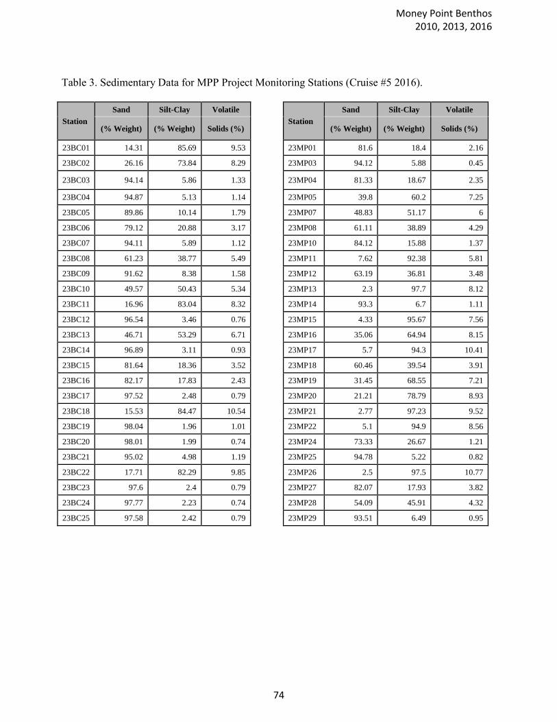
Table 3. Sedimentary Data for MPP Project Monitoring Stations (Cruise #5 2016).
Station
Sand Silt-Clay Volatile
Station
Sand Silt-Clay Volatile
(% Weight) (% Weight) Solids (%)
(% Weight) (% Weight) Solids (%)
23BC01 14.31 85.69 9.53 23MP01 81.6 18.4 2.16
23BC02 26.16 73.84 8.29 23MP03 94.12 5.88 0.45
23BC03 94.14 5.86 1.33
23MP04 81.33 18.67 2.35
23BC04 94.87 5.13 1.14 23MP05 39.8 60.2 7.25
23BC05 89.86 10.14 1.79 23MP07 48.83 51.17 6
23BC06 79.12 20.88 3.17 23MP08 61.11 38.89 4.29
23BC07 94.11 5.89 1.12 23MP10 84.12 15.88 1.37
23BC08 61.23 38.77 5.49 23MP11 7.62 92.38 5.81
23BC09 91.62 8.38 1.58 23MP12 63.19 36.81 3.48
23BC10 49.57 50.43 5.34 23MP13 2.3 97.7 8.12
23BC11 16.96 83.04 8.32 23MP14 93.3 6.7 1.11
23BC12 96.54 3.46 0.76 23MP15 4.33 95.67 7.56
23BC13 46.71 53.29 6.71 23MP16 35.06 64.94 8.15
23BC14 96.89 3.11 0.93 23MP17 5.7 94.3 10.41
23BC15 81.64 18.36 3.52 23MP18 60.46 39.54 3.91
23BC16 82.17 17.83 2.43 23MP19 31.45 68.55 7.21
23BC17 97.52 2.48 0.79 23MP20 21.21 78.79 8.93
23BC18 15.53 84.47 10.54 23MP21 2.77 97.23 9.52
23BC19 98.04 1.96 1.01 23MP22 5.1 94.9 8.56
23BC20 98.01 1.99 0.74 23MP24 73.33 26.67 1.21
23BC21 95.02 4.98 1.19 23MP25 94.78 5.22 0.82
23BC22 17.71 82.29 9.85 23MP26 2.5 97.5 10.77
23BC23 97.6 2.4 0.79 23MP27 82.07 17.93 3.82
23BC24 97.77 2.23 0.74 23MP28 54.09 45.91 4.32
23BC25 97.58 2.42 0.79 23MP29 93.51 6.49 0.95
Money Point Benthos 2010, 2013, 2016
74
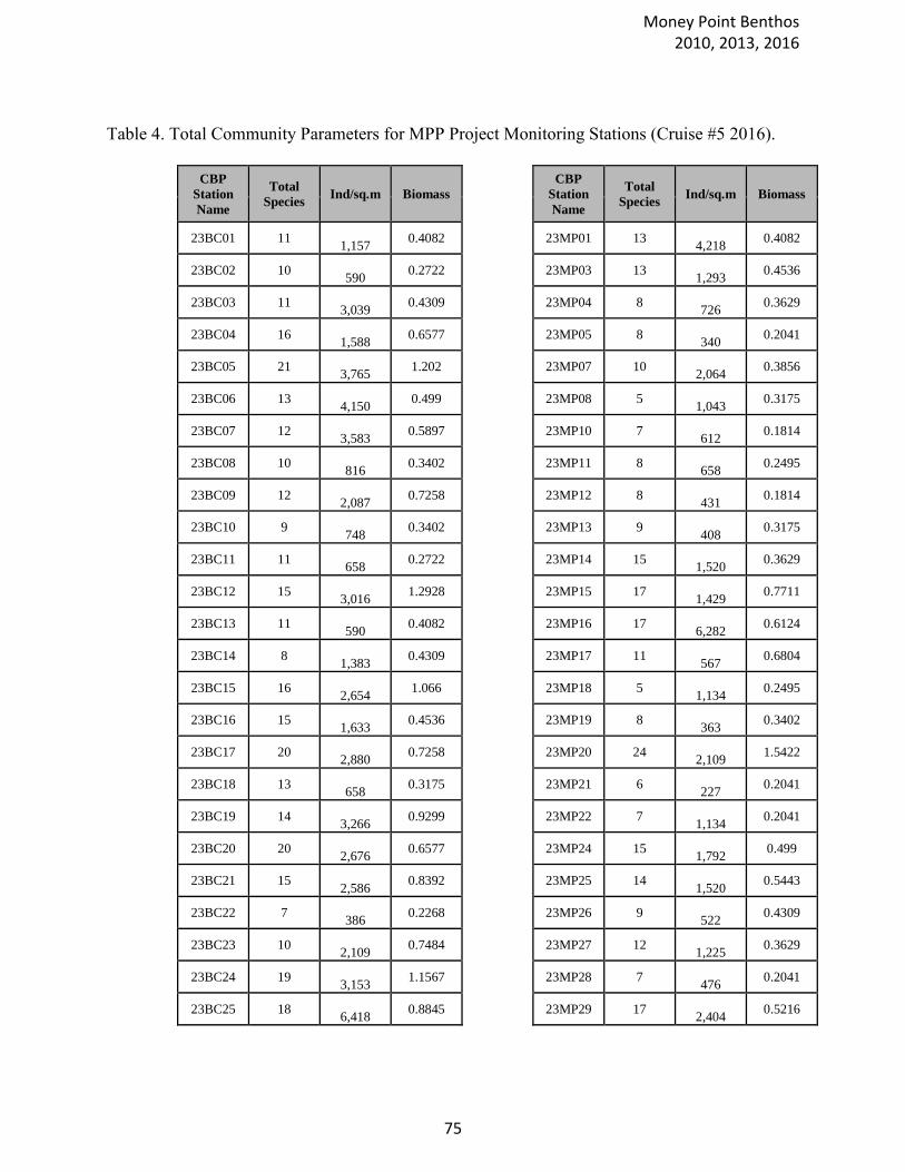
Table 4. Total Community Parameters for MPP Project Monitoring Stations (Cruise #5 2016).
CBP
Station
Name
Total
Species Ind/sq.m Biomass
CBP
Station
Name
Total
Species Ind/sq.m Biomass
23BC01 11
1,157 0.4082
23MP01 13
4,218 0.4082
23BC02 10
590 0.2722
23MP03 13
1,293 0.4536
23BC03 11
3,039 0.4309
23MP04 8
726 0.3629
23BC04 16
1,588 0.6577
23MP05 8
340 0.2041
23BC05 21
3,765 1.202
23MP07 10
2,064 0.3856
23BC06 13
4,150 0.499
23MP08 5
1,043 0.3175
23BC07 12
3,583 0.5897
23MP10 7
612 0.1814
23BC08 10
816 0.3402
23MP11 8
658 0.2495
23BC09 12
2,087 0.7258
23MP12 8
431 0.1814
23BC10 9
748 0.3402
23MP13 9
408 0.3175
23BC11 11
658 0.2722
23MP14 15
1,520 0.3629
23BC12 15
3,016 1.2928
23MP15 17
1,429 0.7711
23BC13 11
590 0.4082
23MP16 17
6,282 0.6124
23BC14 8
1,383 0.4309
23MP17 11
567 0.6804
23BC15 16
2,654 1.066
23MP18 5
1,134 0.2495
23BC16 15
1,633 0.4536
23MP19 8
363 0.3402
23BC17 20
2,880 0.7258
23MP20 24
2,109 1.5422
23BC18 13
658 0.3175
23MP21 6
227 0.2041
23BC19 14
3,266 0.9299
23MP22 7
1,134 0.2041
23BC20 20
2,676 0.6577
23MP24 15
1,792 0.499
23BC21 15
2,586 0.8392
23MP25 14
1,520 0.5443
23BC22 7
386 0.2268
23MP26 9
522 0.4309
23BC23 10
2,109 0.7484
23MP27 12
1,225 0.3629
23BC24 19
3,153 1.1567
23MP28 7
476 0.2041
23BC25 18
6,418 0.8845
23MP29 17
2,404 0.5216
Money Point Benthos 2010, 2013, 2016
75
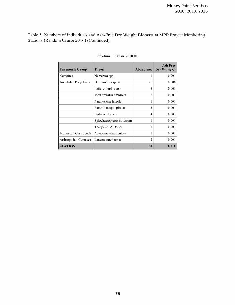
Table 5. Numbers of individuals and Ash-Free Dry Weight Biomass at MPP Project Monitoring
Stations (Random Cruise 2016) (Continued).
Stratum=. Station=23BC01
Taxonomic Group Taxon Abundance
Ash Free
Dry Wt. (g C)
Nemertea Nemertea spp. 1 0.001
Annelida : Polychaeta Hermundura sp. A 26 0.006
Leitoscoloplos spp. 5 0.003
Mediomastus ambiseta 6 0.001
Parahesione luteola 1 0.001
Paraprionospio pinnata 3 0.001
Podarke obscura 4 0.001
Spiochaetopterus costarum 1 0.001
Tharyx sp. A Doner 1 0.001
Mollusca : Gastropoda Acteocina canaliculata 1 0.001
Arthropoda : Cumacea Leucon americanus 2 0.001
STATION 51 0.018
Money Point Benthos 2010, 2013, 2016
76
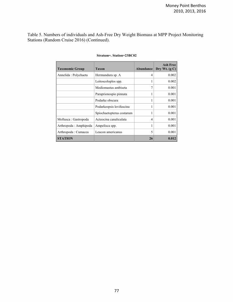
Table 5. Numbers of individuals and Ash-Free Dry Weight Biomass at MPP Project Monitoring
Stations (Random Cruise 2016) (Continued).
Stratum=. Station=23BC02
Taxonomic Group Taxon Abundance
Ash Free
Dry Wt. (g C)
Annelida : Polychaeta Hermundura sp. A 4 0.002
Leitoscoloplos spp. 1 0.002
Mediomastus ambiseta 7 0.001
Paraprionospio pinnata 1 0.001
Podarke obscura 1 0.001
Podarkeopsis levifuscina 1 0.001
Spiochaetopterus costarum 1 0.001
Mollusca : Gastropoda Acteocina canaliculata 4 0.001
Arthropoda : Amphipoda Ampelisca spp. 1 0.001
Arthropoda : Cumacea Leucon americanus 5 0.001
STATION 26 0.012
Money Point Benthos 2010, 2013, 2016
77

Table 5. Numbers of individuals and Ash-Free Dry Weight Biomass at MPP Project Monitoring
Stations (Random Cruise 2016) (Continued).
Stratum=. Station=23BC03
Taxonomic Group Taxon Abundance
Ash Free
Dry Wt. (g C)
Annelida : Polychaeta Eteone heteropoda 1 0.001
Hermundura sp. A 44 0.007
Leitoscoloplos spp. 4 0.003
Mediomastus ambiseta 19 0.001
Podarkeopsis levifuscina 1 0.001
Spiochaetopterus costarum 1 0.001
Tharyx sp. A Doner 1 0.001
Arthropoda : Isopoda Cyathura polita 1 0.001
Arthropoda : Amphipoda Ampelisca spp. 27 0.001
Arthropoda : Tanaidacea Hargeria rapax 34 0.001
Phoronida Phoronis spp. 1 0.001
STATION 134 0.019
Money Point Benthos 2010, 2013, 2016
78
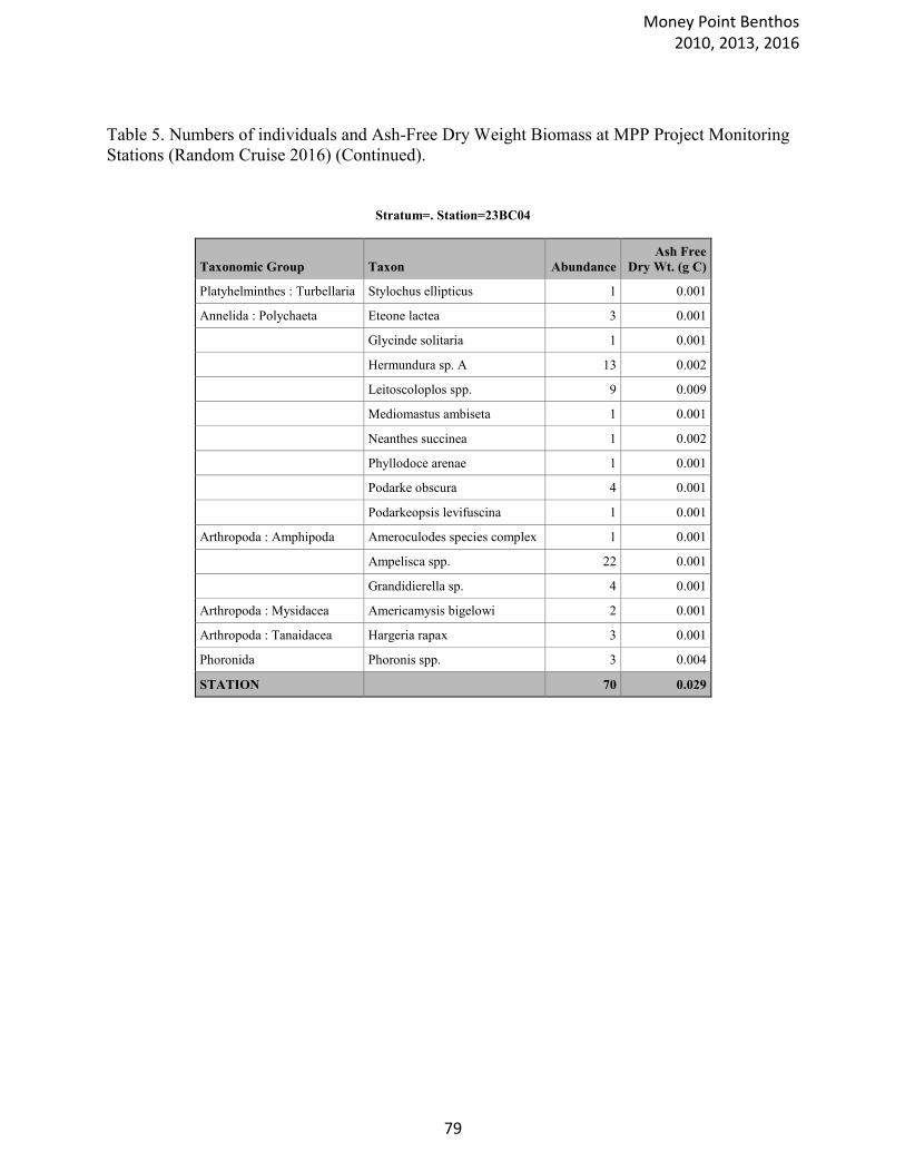
Table 5. Numbers of individuals and Ash-Free Dry Weight Biomass at MPP Project Monitoring
Stations (Random Cruise 2016) (Continued).
Stratum=. Station=23BC04
Taxonomic Group Taxon Abundance
Ash Free
Dry Wt. (g C)
Platyhelminthes : Turbellaria Stylochus ellipticus 1 0.001
Annelida : Polychaeta Eteone lactea 3 0.001
Glycinde solitaria 1 0.001
Hermundura sp. A 13 0.002
Leitoscoloplos spp. 9 0.009
Mediomastus ambiseta 1 0.001
Neanthes succinea 1 0.002
Phyllodoce arenae 1 0.001
Podarke obscura 4 0.001
Podarkeopsis levifuscina 1 0.001
Arthropoda : Amphipoda Ameroculodes species complex 1 0.001
Ampelisca spp. 22 0.001
Grandidierella sp. 4 0.001
Arthropoda : Mysidacea Americamysis bigelowi 2 0.001
Arthropoda : Tanaidacea Hargeria rapax 3 0.001
Phoronida Phoronis spp. 3 0.004
STATION 70 0.029
Money Point Benthos 2010, 2013, 2016
79
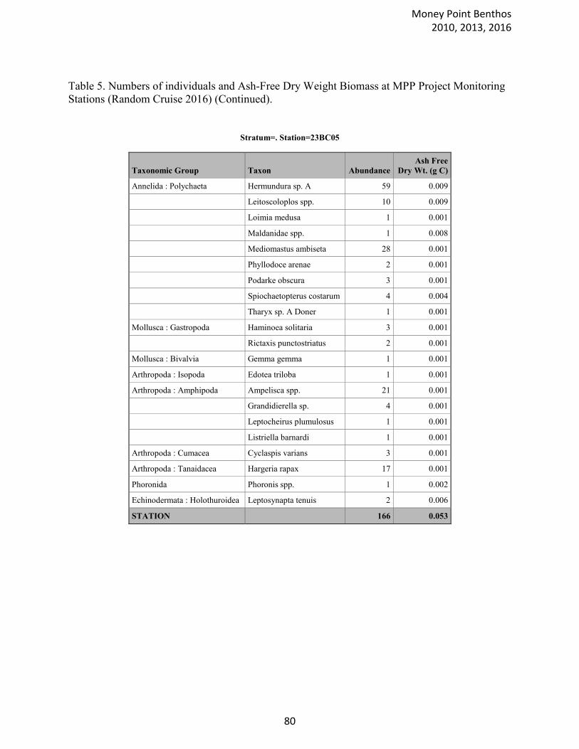
Table 5. Numbers of individuals and Ash-Free Dry Weight Biomass at MPP Project Monitoring
Stations (Random Cruise 2016) (Continued).
Stratum=. Station=23BC05
Taxonomic Group Taxon Abundance
Ash Free
Dry Wt. (g C)
Annelida : Polychaeta Hermundura sp. A 59 0.009
Leitoscoloplos spp. 10 0.009
Loimia medusa 1 0.001
Maldanidae spp. 1 0.008
Mediomastus ambiseta 28 0.001
Phyllodoce arenae 2 0.001
Podarke obscura 3 0.001
Spiochaetopterus costarum 4 0.004
Tharyx sp. A Doner 1 0.001
Mollusca : Gastropoda Haminoea solitaria 3 0.001
Rictaxis punctostriatus 2 0.001
Mollusca : Bivalvia Gemma gemma 1 0.001
Arthropoda : Isopoda Edotea triloba 1 0.001
Arthropoda : Amphipoda Ampelisca spp. 21 0.001
Grandidierella sp. 4 0.001
Leptocheirus plumulosus 1 0.001
Listriella barnardi 1 0.001
Arthropoda : Cumacea Cyclaspis varians 3 0.001
Arthropoda : Tanaidacea Hargeria rapax 17 0.001
Phoronida Phoronis spp. 1 0.002
Echinodermata : Holothuroidea Leptosynapta tenuis 2 0.006
STATION 166 0.053
Money Point Benthos 2010, 2013, 2016
80
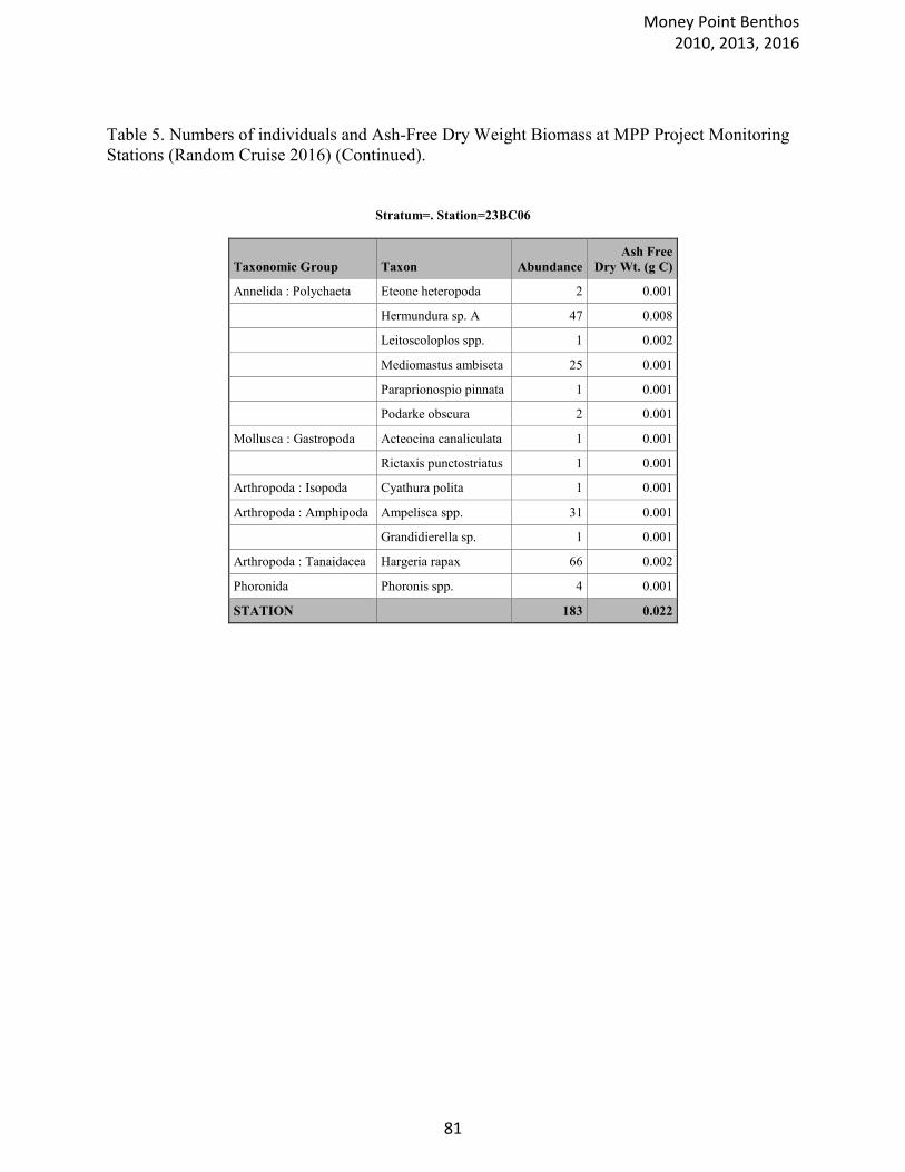
Table 5. Numbers of individuals and Ash-Free Dry Weight Biomass at MPP Project Monitoring
Stations (Random Cruise 2016) (Continued).
Stratum=. Station=23BC06
Taxonomic Group Taxon Abundance
Ash Free
Dry Wt. (g C)
Annelida : Polychaeta Eteone heteropoda 2 0.001
Hermundura sp. A 47 0.008
Leitoscoloplos spp. 1 0.002
Mediomastus ambiseta 25 0.001
Paraprionospio pinnata 1 0.001
Podarke obscura 2 0.001
Mollusca : Gastropoda Acteocina canaliculata 1 0.001
Rictaxis punctostriatus 1 0.001
Arthropoda : Isopoda Cyathura polita 1 0.001
Arthropoda : Amphipoda Ampelisca spp. 31 0.001
Grandidierella sp. 1 0.001
Arthropoda : Tanaidacea Hargeria rapax 66 0.002
Phoronida Phoronis spp. 4 0.001
STATION 183 0.022
Money Point Benthos 2010, 2013, 2016
81
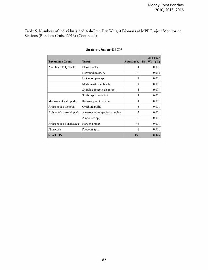
Table 5. Numbers of individuals and Ash-Free Dry Weight Biomass at MPP Project Monitoring
Stations (Random Cruise 2016) (Continued).
Stratum=. Station=23BC07
Taxonomic Group Taxon Abundance
Ash Free
Dry Wt. (g C)
Annelida : Polychaeta Eteone lactea 1 0.001
Hermundura sp. A 74 0.015
Leitoscoloplos spp. 4 0.001
Mediomastus ambiseta 14 0.001
Spiochaetopterus costarum 1 0.001
Streblospio benedicti 1 0.001
Mollusca : Gastropoda Rictaxis punctostriatus 1 0.001
Arthropoda : Isopoda Cyathura polita 5 0.001
Arthropoda : Amphipoda Ameroculodes species complex 2 0.001
Ampelisca spp. 10 0.001
Arthropoda : Tanaidacea Hargeria rapax 43 0.001
Phoronida Phoronis spp. 2 0.001
STATION 158 0.026
Money Point Benthos 2010, 2013, 2016
82

Table 5. Numbers of individuals and Ash-Free Dry Weight Biomass at MPP Project Monitoring
Stations (Random Cruise 2016) (Continued).
Stratum=. Station=23BC08
Taxonomic Group Taxon Abundance
Ash Free
Dry Wt. (g C)
Annelida : Polychaeta Hermundura sp. A 13 0.003
Hobsonia florida 1 0.001
Leitoscoloplos spp. 1 0.002
Mediomastus ambiseta 9 0.001
Paraprionospio pinnata 2 0.001
Spiochaetopterus costarum 3 0.003
Tharyx sp. A Doner 1 0.001
Mollusca : Gastropoda Acteocina canaliculata 1 0.001
Haminoea solitaria 1 0.001
Arthropoda : Amphipoda Ampelisca spp. 4 0.001
STATION 36 0.015
Money Point Benthos 2010, 2013, 2016
83
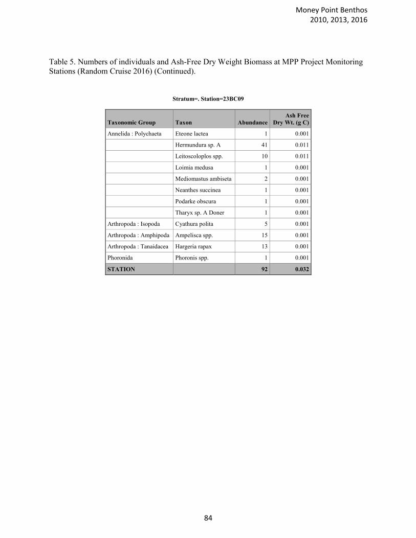
Table 5. Numbers of individuals and Ash-Free Dry Weight Biomass at MPP Project Monitoring
Stations (Random Cruise 2016) (Continued).
Stratum=. Station=23BC09
Taxonomic Group Taxon Abundance
Ash Free
Dry Wt. (g C)
Annelida : Polychaeta Eteone lactea 1 0.001
Hermundura sp. A 41 0.011
Leitoscoloplos spp. 10 0.011
Loimia medusa 1 0.001
Mediomastus ambiseta 2 0.001
Neanthes succinea 1 0.001
Podarke obscura 1 0.001
Tharyx sp. A Doner 1 0.001
Arthropoda : Isopoda Cyathura polita 5 0.001
Arthropoda : Amphipoda Ampelisca spp. 15 0.001
Arthropoda : Tanaidacea Hargeria rapax 13 0.001
Phoronida Phoronis spp. 1 0.001
STATION 92 0.032
Money Point Benthos 2010, 2013, 2016
84
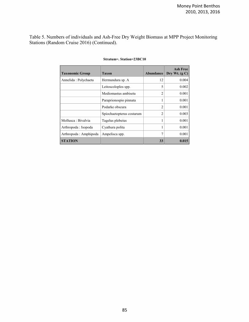
Table 5. Numbers of individuals and Ash-Free Dry Weight Biomass at MPP Project Monitoring
Stations (Random Cruise 2016) (Continued).
Stratum=. Station=23BC10
Taxonomic Group Taxon Abundance
Ash Free
Dry Wt. (g C)
Annelida : Polychaeta Hermundura sp. A 12 0.004
Leitoscoloplos spp. 5 0.002
Mediomastus ambiseta 2 0.001
Paraprionospio pinnata 1 0.001
Podarke obscura 2 0.001
Spiochaetopterus costarum 2 0.003
Mollusca : Bivalvia Tagelus plebeius 1 0.001
Arthropoda : Isopoda Cyathura polita 1 0.001
Arthropoda : Amphipoda Ampelisca spp. 7 0.001
STATION 33 0.015
Money Point Benthos 2010, 2013, 2016
85
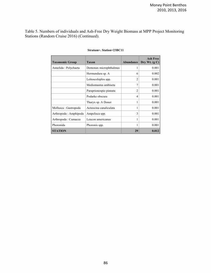
Table 5. Numbers of individuals and Ash-Free Dry Weight Biomass at MPP Project Monitoring
Stations (Random Cruise 2016) (Continued).
Stratum=. Station=23BC11
Taxonomic Group Taxon Abundance
Ash Free
Dry Wt. (g C)
Annelida : Polychaeta Demonax microphthalmus 1 0.001
Hermundura sp. A 6 0.002
Leitoscoloplos spp. 2 0.001
Mediomastus ambiseta 7 0.001
Paraprionospio pinnata 2 0.001
Podarke obscura 4 0.001
Tharyx sp. A Doner 1 0.001
Mollusca : Gastropoda Acteocina canaliculata 1 0.001
Arthropoda : Amphipoda Ampelisca spp. 3 0.001
Arthropoda : Cumacea Leucon americanus 1 0.001
Phoronida Phoronis spp. 1 0.001
STATION 29 0.012
Money Point Benthos 2010, 2013, 2016
86
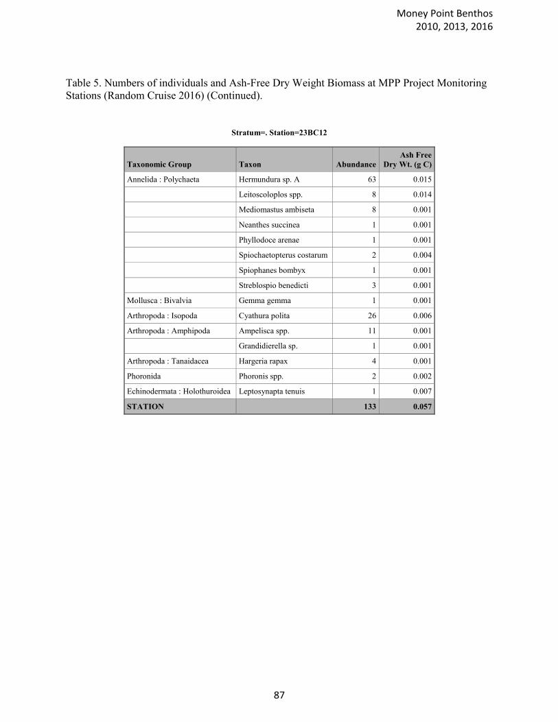
Table 5. Numbers of individuals and Ash-Free Dry Weight Biomass at MPP Project Monitoring
Stations (Random Cruise 2016) (Continued).
Stratum=. Station=23BC12
Taxonomic Group Taxon Abundance
Ash Free
Dry Wt. (g C)
Annelida : Polychaeta Hermundura sp. A 63 0.015
Leitoscoloplos spp. 8 0.014
Mediomastus ambiseta 8 0.001
Neanthes succinea 1 0.001
Phyllodoce arenae 1 0.001
Spiochaetopterus costarum 2 0.004
Spiophanes bombyx 1 0.001
Streblospio benedicti 3 0.001
Mollusca : Bivalvia Gemma gemma 1 0.001
Arthropoda : Isopoda Cyathura polita 26 0.006
Arthropoda : Amphipoda Ampelisca spp. 11 0.001
Grandidierella sp. 1 0.001
Arthropoda : Tanaidacea Hargeria rapax 4 0.001
Phoronida Phoronis spp. 2 0.002
Echinodermata : Holothuroidea Leptosynapta tenuis 1 0.007
STATION 133 0.057
Money Point Benthos 2010, 2013, 2016
87

Table 5. Numbers of individuals and Ash-Free Dry Weight Biomass at MPP Project Monitoring
Stations (Random Cruise 2016) (Continued).
Stratum=. Station=23BC13
Taxonomic Group Taxon Abundance
Ash Free
Dry Wt. (g C)
Nemertea Nemertea spp. 2 0.002
Annelida : Polychaeta Glycinde solitaria 1 0.001
Hermundura sp. A 4 0.002
Leitoscoloplos spp. 2 0.002
Paraprionospio pinnata 4 0.002
Podarke obscura 1 0.001
Podarkeopsis levifuscina 1 0.001
Spiochaetopterus costarum 5 0.003
Tharyx sp. A Doner 2 0.001
Mollusca : Gastropoda Acteocina canaliculata 1 0.001
Phoronida Phoronis spp. 3 0.002
STATION 26 0.018
Money Point Benthos 2010, 2013, 2016
88

Table 5. Numbers of individuals and Ash-Free Dry Weight Biomass at MPP Project Monitoring
Stations (Random Cruise 2016) (Continued).
Stratum=. Station=23BC14
Taxonomic Group Taxon Abundance
Ash Free
Dry Wt. (g C)
Annelida : Polychaeta Eteone heteropoda 1 0.001
Hermundura sp. A 35 0.006
Leitoscoloplos spp. 1 0.001
Mediomastus ambiseta 3 0.001
Spiochaetopterus costarum 3 0.004
Arthropoda : Amphipoda Ampelisca spp. 4 0.001
Grandidierella sp. 7 0.001
Phoronida Phoronis spp. 7 0.004
STATION 61 0.019
Money Point Benthos 2010, 2013, 2016
89
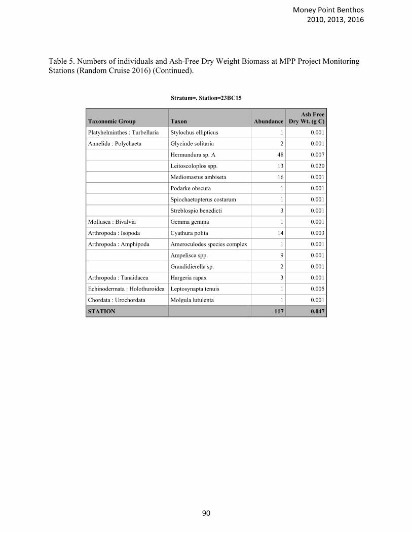
Table 5. Numbers of individuals and Ash-Free Dry Weight Biomass at MPP Project Monitoring
Stations (Random Cruise 2016) (Continued).
Stratum=. Station=23BC15
Taxonomic Group Taxon Abundance
Ash Free
Dry Wt. (g C)
Platyhelminthes : Turbellaria Stylochus ellipticus 1 0.001
Annelida : Polychaeta Glycinde solitaria 2 0.001
Hermundura sp. A 48 0.007
Leitoscoloplos spp. 13 0.020
Mediomastus ambiseta 16 0.001
Podarke obscura 1 0.001
Spiochaetopterus costarum 1 0.001
Streblospio benedicti 3 0.001
Mollusca : Bivalvia Gemma gemma 1 0.001
Arthropoda : Isopoda Cyathura polita 14 0.003
Arthropoda : Amphipoda Ameroculodes species complex 1 0.001
Ampelisca spp. 9 0.001
Grandidierella sp. 2 0.001
Arthropoda : Tanaidacea Hargeria rapax 3 0.001
Echinodermata : Holothuroidea Leptosynapta tenuis 1 0.005
Chordata : Urochordata Molgula lutulenta 1 0.001
STATION 117 0.047
Money Point Benthos 2010, 2013, 2016
90
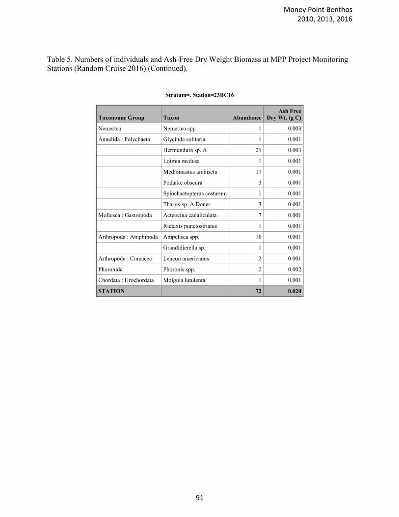
Table 5. Numbers of individuals and Ash-Free Dry Weight Biomass at MPP Project Monitoring
Stations (Random Cruise 2016) (Continued).
Stratum=. Station=23BC16
Taxonomic Group Taxon Abundance
Ash Free
Dry Wt. (g C)
Nemertea Nemertea spp. 1 0.003
Annelida : Polychaeta Glycinde solitaria 1 0.001
Hermundura sp. A 21 0.003
Loimia medusa 1 0.001
Mediomastus ambiseta 17 0.001
Podarke obscura 3 0.001
Spiochaetopterus costarum 1 0.001
Tharyx sp. A Doner 3 0.001
Mollusca : Gastropoda Acteocina canaliculata 7 0.001
Rictaxis punctostriatus 1 0.001
Arthropoda : Amphipoda Ampelisca spp. 10 0.001
Grandidierella sp. 1 0.001
Arthropoda : Cumacea Leucon americanus 2 0.001
Phoronida Phoronis spp. 2 0.002
Chordata : Urochordata Molgula lutulenta 1 0.001
STATION 72 0.020
Money Point Benthos 2010, 2013, 2016
91
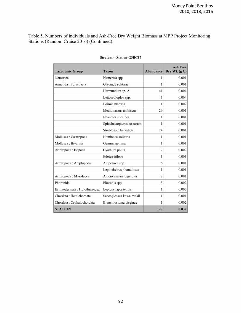
Table 5. Numbers of individuals and Ash-Free Dry Weight Biomass at MPP Project Monitoring
Stations (Random Cruise 2016) (Continued).
Stratum=. Station=23BC17
Taxonomic Group Taxon Abundance
Ash Free
Dry Wt. (g C)
Nemertea Nemertea spp. 1 0.001
Annelida : Polychaeta Glycinde solitaria 1 0.001
Hermundura sp. A 41 0.004
Leitoscoloplos spp. 3 0.004
Loimia medusa 1 0.002
Mediomastus ambiseta 29 0.001
Neanthes succinea 1 0.001
Spiochaetopterus costarum 1 0.001
Streblospio benedicti 24 0.001
Mollusca : Gastropoda Haminoea solitaria 1 0.001
Mollusca : Bivalvia Gemma gemma 1 0.001
Arthropoda : Isopoda Cyathura polita 7 0.002
Edotea triloba 1 0.001
Arthropoda : Amphipoda Ampelisca spp. 6 0.001
Leptocheirus plumulosus 1 0.001
Arthropoda : Mysidacea Americamysis bigelowi 2 0.001
Phoronida Phoronis spp. 3 0.002
Echinodermata : Holothuroidea Leptosynapta tenuis 1 0.003
Chordata : Hemichordata Saccoglossus kowalevskii 1 0.001
Chordata : Cephalochordata Branchiostoma virginae 1 0.002
STATION 127 0.032
Money Point Benthos 2010, 2013, 2016
92
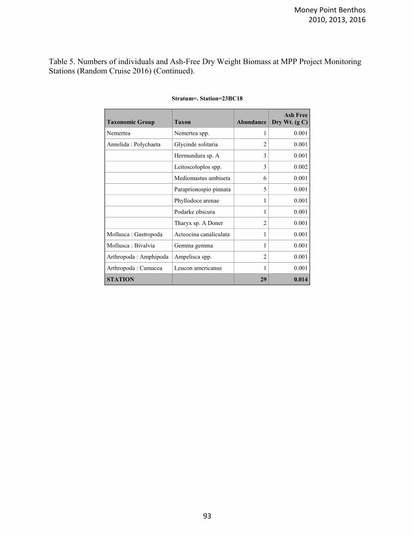
Table 5. Numbers of individuals and Ash-Free Dry Weight Biomass at MPP Project Monitoring
Stations (Random Cruise 2016) (Continued).
Stratum=. Station=23BC18
Taxonomic Group Taxon Abundance
Ash Free
Dry Wt. (g C)
Nemertea Nemertea spp. 1 0.001
Annelida : Polychaeta Glycinde solitaria 2 0.001
Hermundura sp. A 3 0.001
Leitoscoloplos spp. 3 0.002
Mediomastus ambiseta 6 0.001
Paraprionospio pinnata 5 0.001
Phyllodoce arenae 1 0.001
Podarke obscura 1 0.001
Tharyx sp. A Doner 2 0.001
Mollusca : Gastropoda Acteocina canaliculata 1 0.001
Mollusca : Bivalvia Gemma gemma 1 0.001
Arthropoda : Amphipoda Ampelisca spp. 2 0.001
Arthropoda : Cumacea Leucon americanus 1 0.001
STATION 29 0.014
Money Point Benthos 2010, 2013, 2016
93
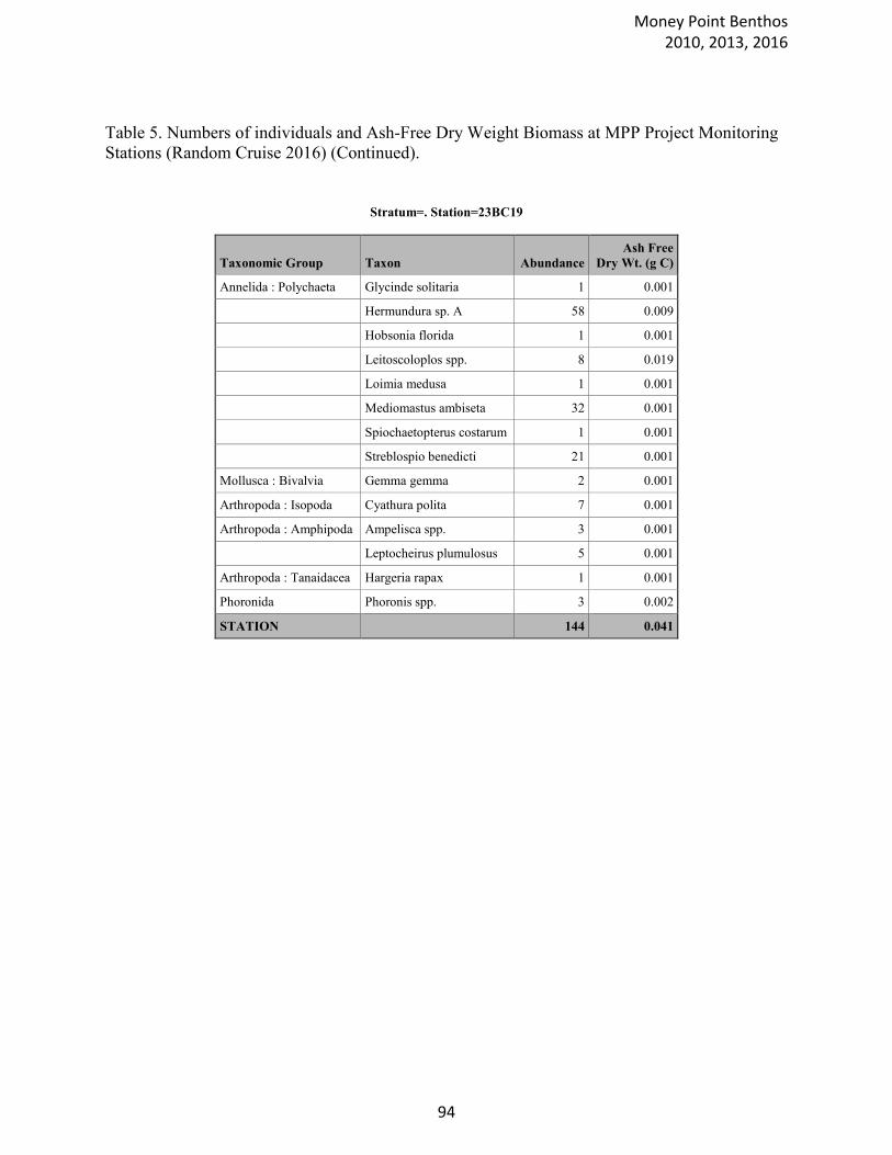
Table 5. Numbers of individuals and Ash-Free Dry Weight Biomass at MPP Project Monitoring
Stations (Random Cruise 2016) (Continued).
Stratum=. Station=23BC19
Taxonomic Group Taxon Abundance
Ash Free
Dry Wt. (g C)
Annelida : Polychaeta Glycinde solitaria 1 0.001
Hermundura sp. A 58 0.009
Hobsonia florida 1 0.001
Leitoscoloplos spp. 8 0.019
Loimia medusa 1 0.001
Mediomastus ambiseta 32 0.001
Spiochaetopterus costarum 1 0.001
Streblospio benedicti 21 0.001
Mollusca : Bivalvia Gemma gemma 2 0.001
Arthropoda : Isopoda Cyathura polita 7 0.001
Arthropoda : Amphipoda Ampelisca spp. 3 0.001
Leptocheirus plumulosus 5 0.001
Arthropoda : Tanaidacea Hargeria rapax 1 0.001
Phoronida Phoronis spp. 3 0.002
STATION 144 0.041
Money Point Benthos 2010, 2013, 2016
94
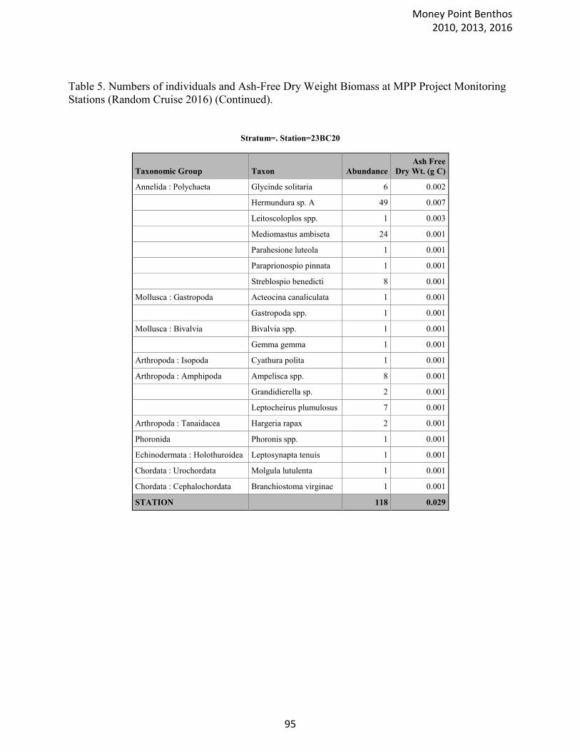
Table 5. Numbers of individuals and Ash-Free Dry Weight Biomass at MPP Project Monitoring
Stations (Random Cruise 2016) (Continued).
Stratum=. Station=23BC20
Taxonomic Group Taxon Abundance
Ash Free
Dry Wt. (g C)
Annelida : Polychaeta Glycinde solitaria 6 0.002
Hermundura sp. A 49 0.007
Leitoscoloplos spp. 1 0.003
Mediomastus ambiseta 24 0.001
Parahesione luteola 1 0.001
Paraprionospio pinnata 1 0.001
Streblospio benedicti 8 0.001
Mollusca : Gastropoda Acteocina canaliculata 1 0.001
Gastropoda spp. 1 0.001
Mollusca : Bivalvia Bivalvia spp. 1 0.001
Gemma gemma 1 0.001
Arthropoda : Isopoda Cyathura polita 1 0.001
Arthropoda : Amphipoda Ampelisca spp. 8 0.001
Grandidierella sp. 2 0.001
Leptocheirus plumulosus 7 0.001
Arthropoda : Tanaidacea Hargeria rapax 2 0.001
Phoronida Phoronis spp. 1 0.001
Echinodermata : Holothuroidea Leptosynapta tenuis 1 0.001
Chordata : Urochordata Molgula lutulenta 1 0.001
Chordata : Cephalochordata Branchiostoma virginae 1 0.001
STATION 118 0.029
Money Point Benthos 2010, 2013, 2016
95
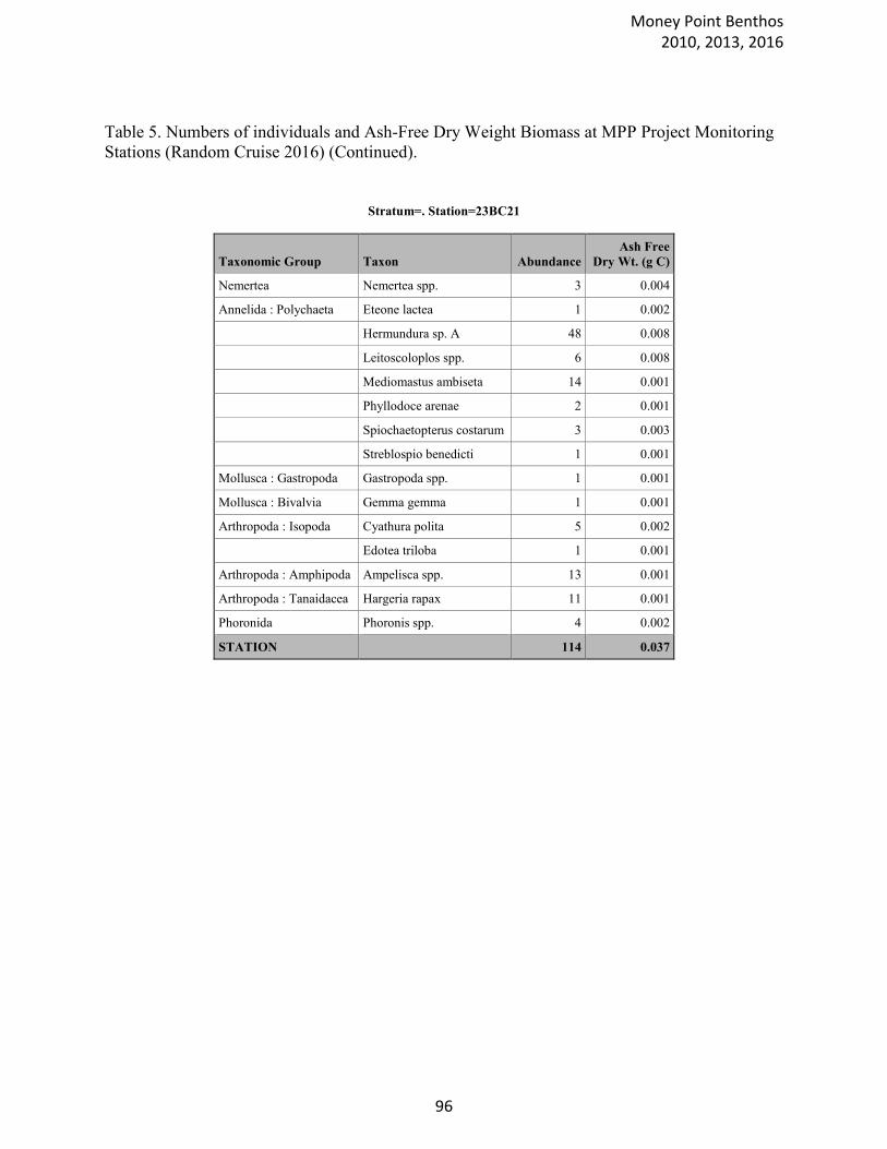
Table 5. Numbers of individuals and Ash-Free Dry Weight Biomass at MPP Project Monitoring
Stations (Random Cruise 2016) (Continued).
Stratum=. Station=23BC21
Taxonomic Group Taxon Abundance
Ash Free
Dry Wt. (g C)
Nemertea Nemertea spp. 3 0.004
Annelida : Polychaeta Eteone lactea 1 0.002
Hermundura sp. A 48 0.008
Leitoscoloplos spp. 6 0.008
Mediomastus ambiseta 14 0.001
Phyllodoce arenae 2 0.001
Spiochaetopterus costarum 3 0.003
Streblospio benedicti 1 0.001
Mollusca : Gastropoda Gastropoda spp. 1 0.001
Mollusca : Bivalvia Gemma gemma 1 0.001
Arthropoda : Isopoda Cyathura polita 5 0.002
Edotea triloba 1 0.001
Arthropoda : Amphipoda Ampelisca spp. 13 0.001
Arthropoda : Tanaidacea Hargeria rapax 11 0.001
Phoronida Phoronis spp. 4 0.002
STATION 114 0.037
Money Point Benthos 2010, 2013, 2016
96
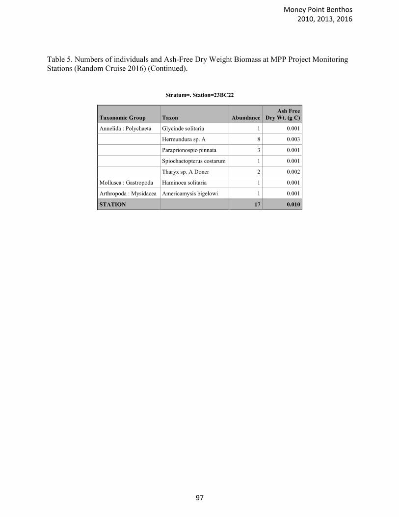
Table 5. Numbers of individuals and Ash-Free Dry Weight Biomass at MPP Project Monitoring
Stations (Random Cruise 2016) (Continued).
Stratum=. Station=23BC22
Taxonomic Group Taxon Abundance
Ash Free
Dry Wt. (g C)
Annelida : Polychaeta Glycinde solitaria 1 0.001
Hermundura sp. A 8 0.003
Paraprionospio pinnata 3 0.001
Spiochaetopterus costarum 1 0.001
Tharyx sp. A Doner 2 0.002
Mollusca : Gastropoda Haminoea solitaria 1 0.001
Arthropoda : Mysidacea Americamysis bigelowi 1 0.001
STATION 17 0.010
Money Point Benthos 2010, 2013, 2016
97

Table 5. Numbers of individuals and Ash-Free Dry Weight Biomass at MPP Project Monitoring
Stations (Random Cruise 2016) (Continued).
Stratum=. Station=23BC23
Taxonomic Group Taxon Abundance
Ash Free
Dry Wt. (g C)
Annelida : Polychaeta Hermundura sp. A 37 0.014
Leitoscoloplos spp. 5 0.009
Mediomastus ambiseta 10 0.001
Streblospio benedicti 1 0.001
Arthropoda : Isopoda Cyathura polita 11 0.002
Arthropoda : Amphipoda Ampelisca spp. 18 0.001
Grandidierella sp. 4 0.001
Arthropoda : Mysidacea Americamysis bigelowi 2 0.001
Phoronida Phoronis spp. 4 0.002
Chordata : Cephalochordata Branchiostoma virginae 1 0.001
STATION 93 0.033
Money Point Benthos 2010, 2013, 2016
98
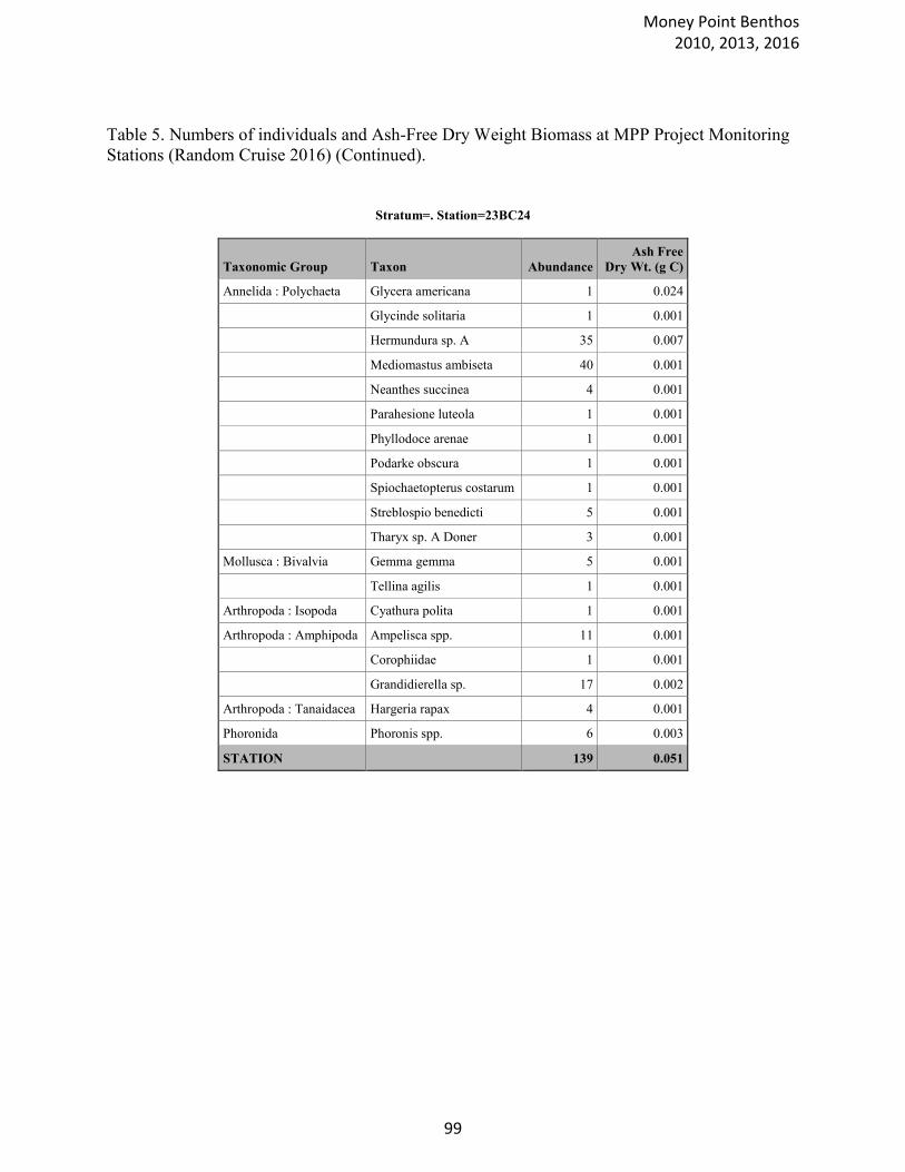
Table 5. Numbers of individuals and Ash-Free Dry Weight Biomass at MPP Project Monitoring
Stations (Random Cruise 2016) (Continued).
Stratum=. Station=23BC24
Taxonomic Group Taxon Abundance
Ash Free
Dry Wt. (g C)
Annelida : Polychaeta Glycera americana 1 0.024
Glycinde solitaria 1 0.001
Hermundura sp. A 35 0.007
Mediomastus ambiseta 40 0.001
Neanthes succinea 4 0.001
Parahesione luteola 1 0.001
Phyllodoce arenae 1 0.001
Podarke obscura 1 0.001
Spiochaetopterus costarum 1 0.001
Streblospio benedicti 5 0.001
Tharyx sp. A Doner 3 0.001
Mollusca : Bivalvia Gemma gemma 5 0.001
Tellina agilis 1 0.001
Arthropoda : Isopoda Cyathura polita 1 0.001
Arthropoda : Amphipoda Ampelisca spp. 11 0.001
Corophiidae 1 0.001
Grandidierella sp. 17 0.002
Arthropoda : Tanaidacea Hargeria rapax 4 0.001
Phoronida Phoronis spp. 6 0.003
STATION 139 0.051
Money Point Benthos 2010, 2013, 2016
99
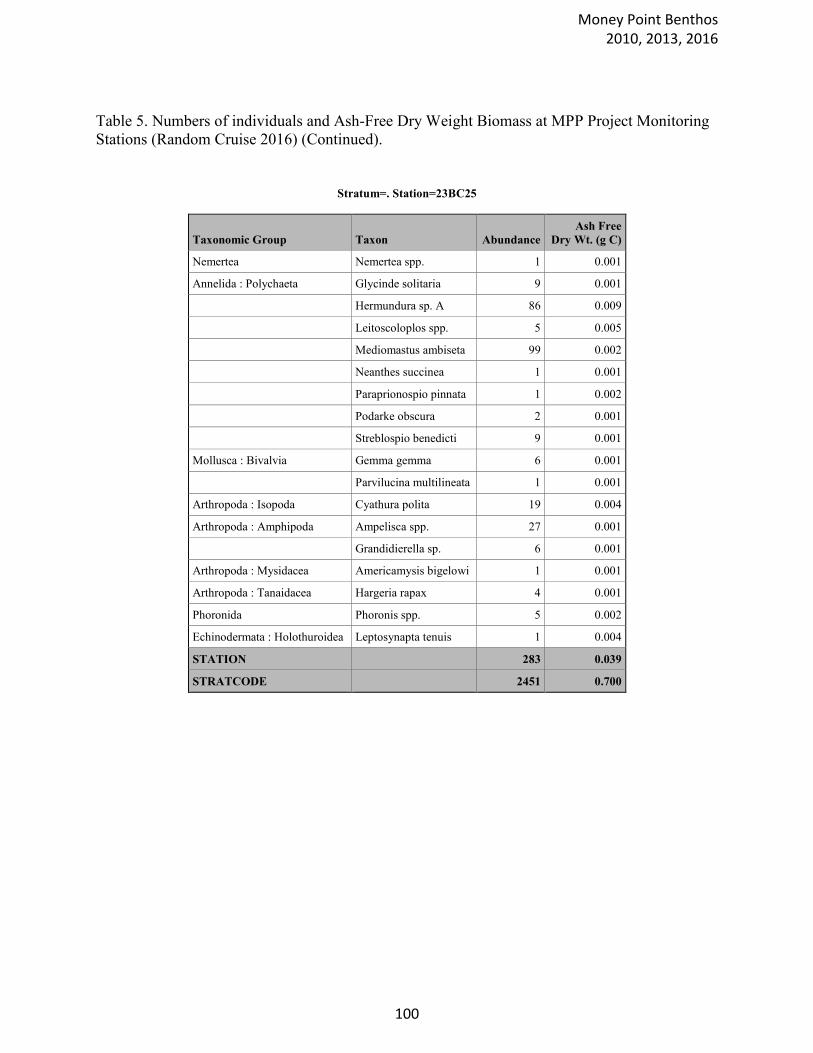
Table 5. Numbers of individuals and Ash-Free Dry Weight Biomass at MPP Project Monitoring
Stations (Random Cruise 2016) (Continued).
Stratum=. Station=23BC25
Taxonomic Group Taxon Abundance
Ash Free
Dry Wt. (g C)
Nemertea Nemertea spp. 1 0.001
Annelida : Polychaeta Glycinde solitaria 9 0.001
Hermundura sp. A 86 0.009
Leitoscoloplos spp. 5 0.005
Mediomastus ambiseta 99 0.002
Neanthes succinea 1 0.001
Paraprionospio pinnata 1 0.002
Podarke obscura 2 0.001
Streblospio benedicti 9 0.001
Mollusca : Bivalvia Gemma gemma 6 0.001
Parvilucina multilineata 1 0.001
Arthropoda : Isopoda Cyathura polita 19 0.004
Arthropoda : Amphipoda Ampelisca spp. 27 0.001
Grandidierella sp. 6 0.001
Arthropoda : Mysidacea Americamysis bigelowi 1 0.001
Arthropoda : Tanaidacea Hargeria rapax 4 0.001
Phoronida Phoronis spp. 5 0.002
Echinodermata : Holothuroidea Leptosynapta tenuis 1 0.004
STATION 283 0.039
STRATCODE 2451 0.700
Money Point Benthos 2010, 2013, 2016
100
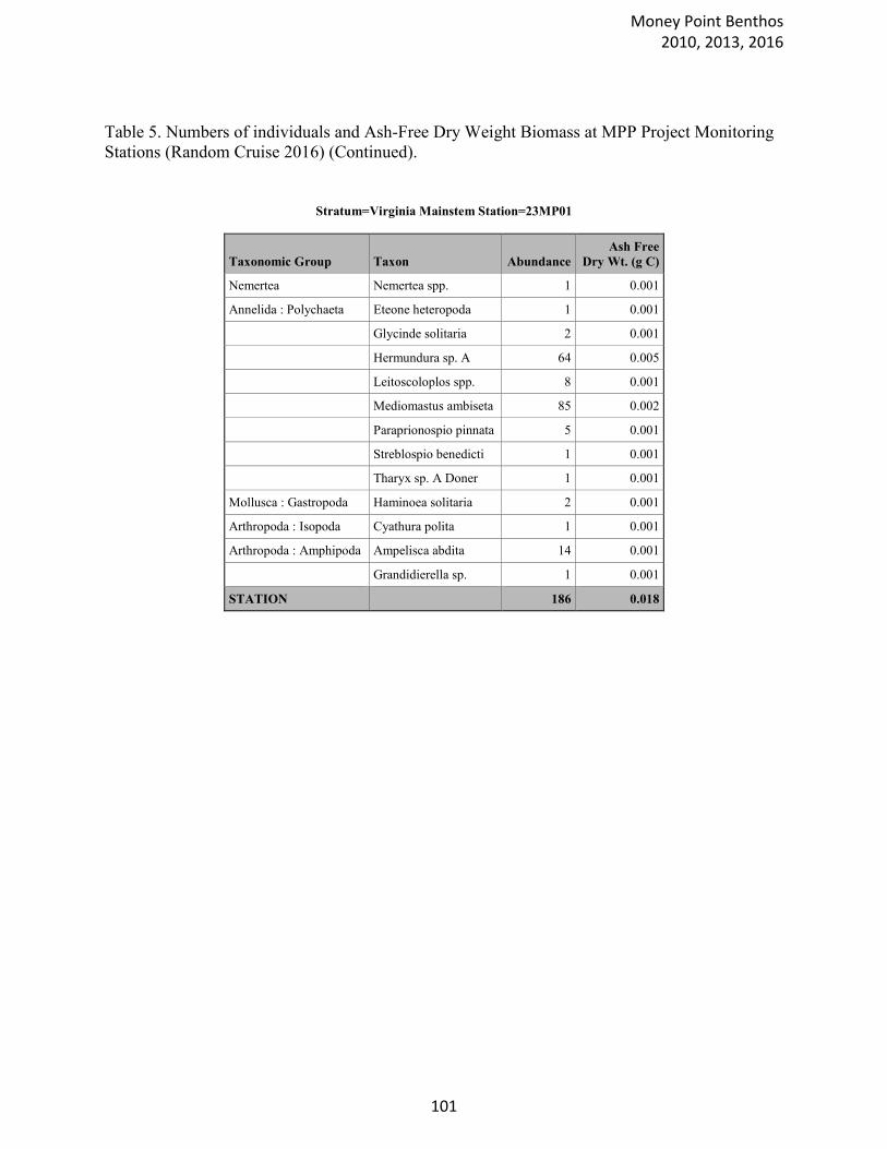
Table 5. Numbers of individuals and Ash-Free Dry Weight Biomass at MPP Project Monitoring
Stations (Random Cruise 2016) (Continued).
Stratum=Virginia Mainstem Station=23MP01
Taxonomic Group Taxon Abundance
Ash Free
Dry Wt. (g C)
Nemertea Nemertea spp. 1 0.001
Annelida : Polychaeta Eteone heteropoda 1 0.001
Glycinde solitaria 2 0.001
Hermundura sp. A 64 0.005
Leitoscoloplos spp. 8 0.001
Mediomastus ambiseta 85 0.002
Paraprionospio pinnata 5 0.001
Streblospio benedicti 1 0.001
Tharyx sp. A Doner 1 0.001
Mollusca : Gastropoda Haminoea solitaria 2 0.001
Arthropoda : Isopoda Cyathura polita 1 0.001
Arthropoda : Amphipoda Ampelisca abdita 14 0.001
Grandidierella sp. 1 0.001
STATION 186 0.018
Money Point Benthos 2010, 2013, 2016
101
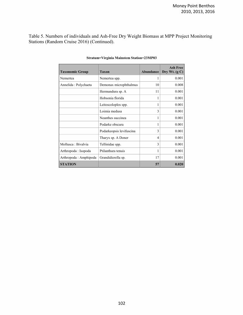
Table 5. Numbers of individuals and Ash-Free Dry Weight Biomass at MPP Project Monitoring
Stations (Random Cruise 2016) (Continued).
Stratum=Virginia Mainstem Station=23MP03
Taxonomic Group Taxon Abundance
Ash Free
Dry Wt. (g C)
Nemertea Nemertea spp. 1 0.001
Annelida : Polychaeta Demonax microphthalmus 10 0.008
Hermundura sp. A 11 0.001
Hobsonia florida 1 0.001
Leitoscoloplos spp. 1 0.001
Loimia medusa 3 0.001
Neanthes succinea 1 0.001
Podarke obscura 1 0.001
Podarkeopsis levifuscina 3 0.001
Tharyx sp. A Doner 4 0.001
Mollusca : Bivalvia Tellinidae spp. 3 0.001
Arthropoda : Isopoda Ptilanthura tenuis 1 0.001
Arthropoda : Amphipoda Grandidierella sp. 17 0.001
STATION 57 0.020
Money Point Benthos 2010, 2013, 2016
102

Table 5. Numbers of individuals and Ash-Free Dry Weight Biomass at MPP Project Monitoring
Stations (Random Cruise 2016) (Continued).
Stratum=Virginia Mainstem Station=23MP04
Taxonomic Group Taxon Abundance
Ash Free
Dry Wt. (g C)
Nemertea Nemertea spp. 1 0.001
Annelida : Polychaeta Glycinde solitaria 3 0.001
Hermundura sp. A 12 0.002
Leitoscoloplos spp. 5 0.007
Mediomastus ambiseta 3 0.001
Paraprionospio pinnata 6 0.002
Arthropoda : Amphipoda Ampelisca spp. 1 0.001
Arthropoda : Cumacea Leucon americanus 1 0.001
STATION 32 0.016
Money Point Benthos 2010, 2013, 2016
103
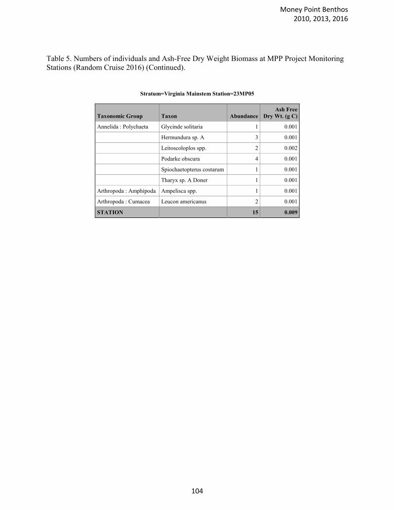
Table 5. Numbers of individuals and Ash-Free Dry Weight Biomass at MPP Project Monitoring
Stations (Random Cruise 2016) (Continued).
Stratum=Virginia Mainstem Station=23MP05
Taxonomic Group Taxon Abundance
Ash Free
Dry Wt. (g C)
Annelida : Polychaeta Glycinde solitaria 1 0.001
Hermundura sp. A 3 0.001
Leitoscoloplos spp. 2 0.002
Podarke obscura 4 0.001
Spiochaetopterus costarum 1 0.001
Tharyx sp. A Doner 1 0.001
Arthropoda : Amphipoda Ampelisca spp. 1 0.001
Arthropoda : Cumacea Leucon americanus 2 0.001
STATION 15 0.009
Money Point Benthos 2010, 2013, 2016
104
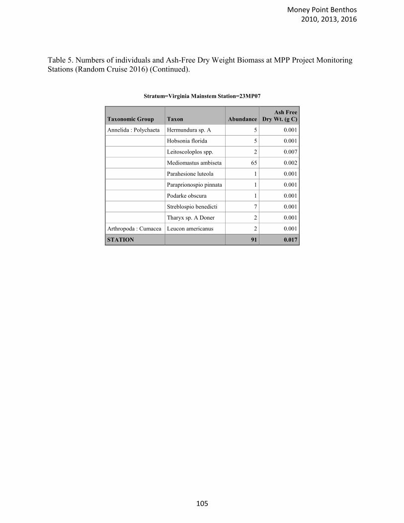
Table 5. Numbers of individuals and Ash-Free Dry Weight Biomass at MPP Project Monitoring
Stations (Random Cruise 2016) (Continued).
Stratum=Virginia Mainstem Station=23MP07
Taxonomic Group Taxon Abundance
Ash Free
Dry Wt. (g C)
Annelida : Polychaeta Hermundura sp. A 5 0.001
Hobsonia florida 5 0.001
Leitoscoloplos spp. 2 0.007
Mediomastus ambiseta 65 0.002
Parahesione luteola 1 0.001
Paraprionospio pinnata 1 0.001
Podarke obscura 1 0.001
Streblospio benedicti 7 0.001
Tharyx sp. A Doner 2 0.001
Arthropoda : Cumacea Leucon americanus 2 0.001
STATION 91 0.017
Money Point Benthos 2010, 2013, 2016
105
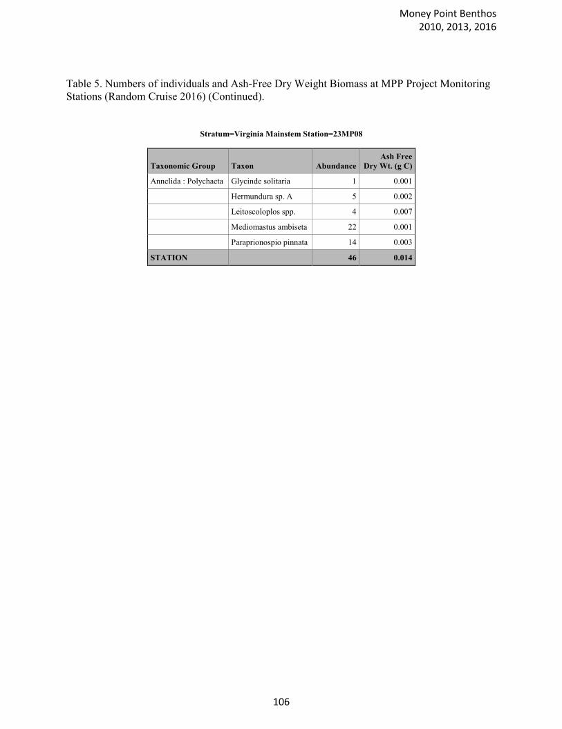
Table 5. Numbers of individuals and Ash-Free Dry Weight Biomass at MPP Project Monitoring
Stations (Random Cruise 2016) (Continued).
Stratum=Virginia Mainstem Station=23MP08
Taxonomic Group Taxon Abundance
Ash Free
Dry Wt. (g C)
Annelida : Polychaeta Glycinde solitaria 1 0.001
Hermundura sp. A 5 0.002
Leitoscoloplos spp. 4 0.007
Mediomastus ambiseta 22 0.001
Paraprionospio pinnata 14 0.003
STATION 46 0.014
Money Point Benthos 2010, 2013, 2016
106

Table 5. Numbers of individuals and Ash-Free Dry Weight Biomass at MPP Project Monitoring
Stations (Random Cruise 2016) (Continued).
Stratum=Virginia Mainstem Station=23MP10
Taxonomic Group Taxon Abundance
Ash Free
Dry Wt. (g C)
Hermundura sp. A 18 0.001
Leitoscoloplos spp. 2 0.002
Paraprionospio pinnata 2 0.001
Pectinaria gouldii 1 0.001
Phyllodoce arenae 1 0.001
Podarke obscura 1 0.001
Tharyx sp. A Doner 2 0.001
STATION 27 0.008
Money Point Benthos 2010, 2013, 2016
107
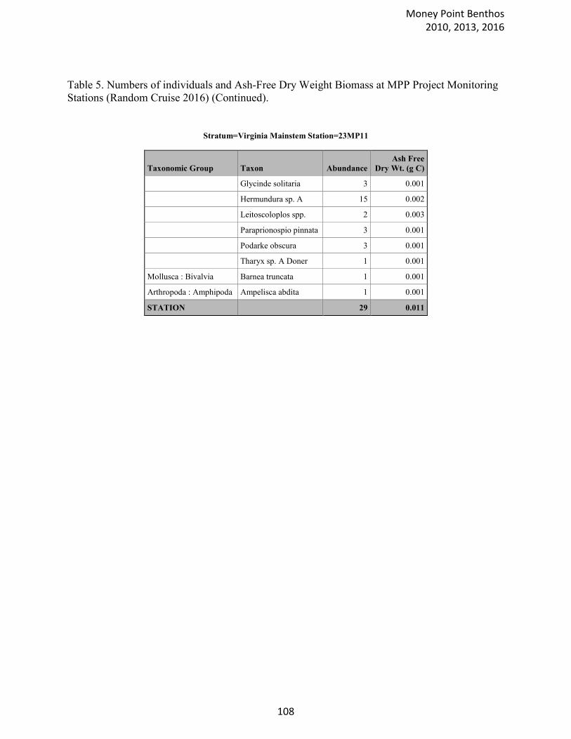
Table 5. Numbers of individuals and Ash-Free Dry Weight Biomass at MPP Project Monitoring
Stations (Random Cruise 2016) (Continued).
Stratum=Virginia Mainstem Station=23MP11
Taxonomic Group Taxon Abundance
Ash Free
Dry Wt. (g C)
Glycinde solitaria 3 0.001
Hermundura sp. A 15 0.002
Leitoscoloplos spp. 2 0.003
Paraprionospio pinnata 3 0.001
Podarke obscura 3 0.001
Tharyx sp. A Doner 1 0.001
Mollusca : Bivalvia Barnea truncata 1 0.001
Arthropoda : Amphipoda Ampelisca abdita 1 0.001
STATION 29 0.011
Money Point Benthos 2010, 2013, 2016
108
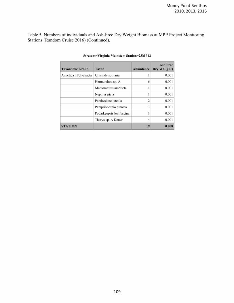
Table 5. Numbers of individuals and Ash-Free Dry Weight Biomass at MPP Project Monitoring
Stations (Random Cruise 2016) (Continued).
Stratum=Virginia Mainstem Station=23MP12
Taxonomic Group Taxon Abundance
Ash Free
Dry Wt. (g C)
Annelida : Polychaeta Glycinde solitaria 1 0.001
Hermundura sp. A 6 0.001
Mediomastus ambiseta 1 0.001
Nephtys picta 1 0.001
Parahesione luteola 2 0.001
Paraprionospio pinnata 3 0.001
Podarkeopsis levifuscina 1 0.001
Tharyx sp. A Doner 4 0.001
STATION 19 0.008
Money Point Benthos 2010, 2013, 2016
109
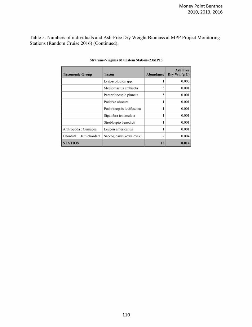
Table 5. Numbers of individuals and Ash-Free Dry Weight Biomass at MPP Project Monitoring
Stations (Random Cruise 2016) (Continued).
Stratum=Virginia Mainstem Station=23MP13
Taxonomic Group Taxon Abundance
Ash Free
Dry Wt. (g C)
Leitoscoloplos spp. 1 0.003
Mediomastus ambiseta 5 0.001
Paraprionospio pinnata 5 0.001
Podarke obscura 1 0.001
Podarkeopsis levifuscina 1 0.001
Sigambra tentaculata 1 0.001
Streblospio benedicti 1 0.001
Arthropoda : Cumacea Leucon americanus 1 0.001
Chordata : Hemichordata Saccoglossus kowalevskii 2 0.004
STATION 18 0.014
Money Point Benthos 2010, 2013, 2016
110
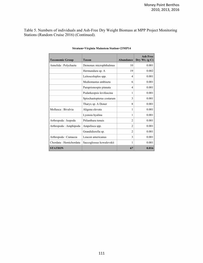
Table 5. Numbers of individuals and Ash-Free Dry Weight Biomass at MPP Project Monitoring
Stations (Random Cruise 2016) (Continued).
Stratum=Virginia Mainstem Station=23MP14
Taxonomic Group Taxon Abundance
Ash Free
Dry Wt. (g C)
Annelida : Polychaeta Demonax microphthalmus 10 0.001
Hermundura sp. A 19 0.002
Leitoscoloplos spp. 4 0.001
Mediomastus ambiseta 6 0.001
Paraprionospio pinnata 4 0.001
Podarkeopsis levifuscina 1 0.001
Spiochaetopterus costarum 3 0.001
Tharyx sp. A Doner 8 0.001
Mollusca : Bivalvia Aligena elevata 1 0.001
Lyonsia hyalina 1 0.001
Arthropoda : Isopoda Ptilanthura tenuis 2 0.001
Arthropoda : Amphipoda Ampelisca spp. 2 0.001
Grandidierella sp. 2 0.001
Arthropoda : Cumacea Leucon americanus 3 0.001
Chordata : Hemichordata Saccoglossus kowalevskii 1 0.001
STATION 67 0.016
Money Point Benthos 2010, 2013, 2016
111
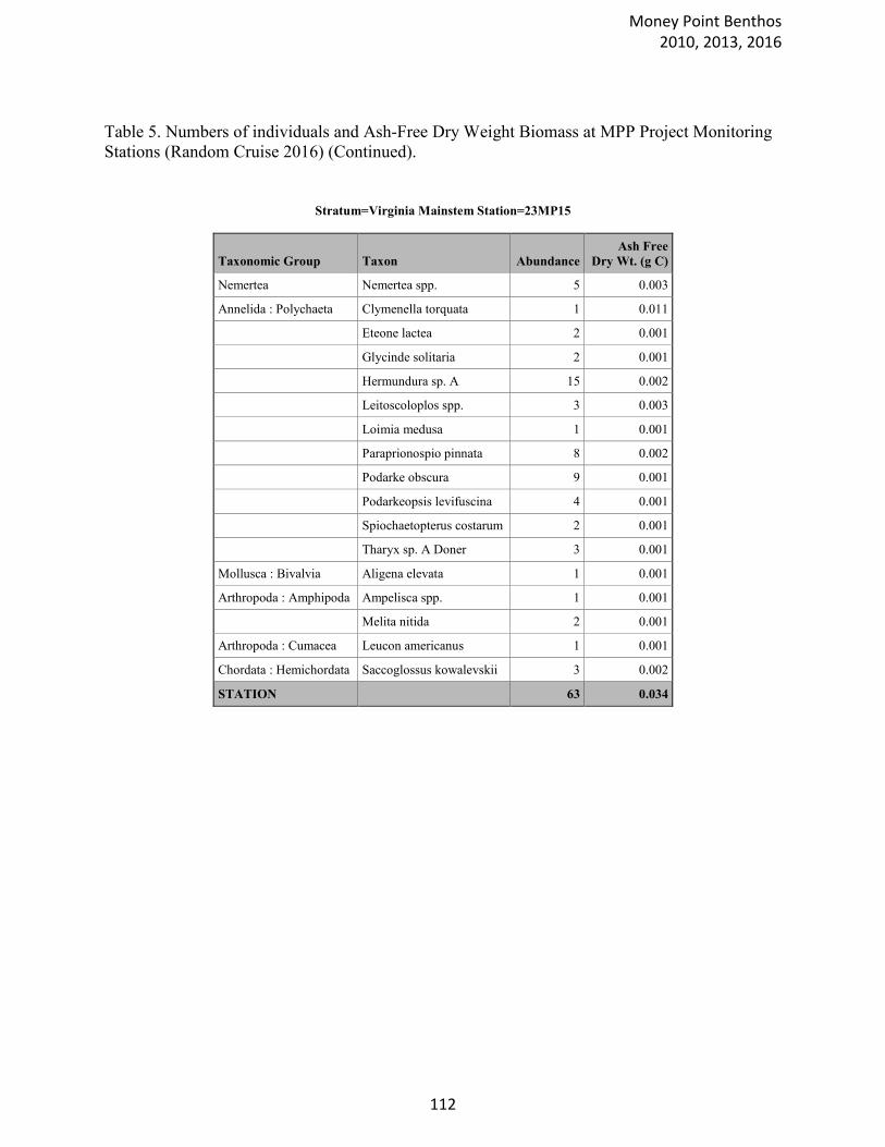
Table 5. Numbers of individuals and Ash-Free Dry Weight Biomass at MPP Project Monitoring
Stations (Random Cruise 2016) (Continued).
Stratum=Virginia Mainstem Station=23MP15
Taxonomic Group Taxon Abundance
Ash Free
Dry Wt. (g C)
Nemertea Nemertea spp. 5 0.003
Annelida : Polychaeta Clymenella torquata 1 0.011
Eteone lactea 2 0.001
Glycinde solitaria 2 0.001
Hermundura sp. A 15 0.002
Leitoscoloplos spp. 3 0.003
Loimia medusa 1 0.001
Paraprionospio pinnata 8 0.002
Podarke obscura 9 0.001
Podarkeopsis levifuscina 4 0.001
Spiochaetopterus costarum 2 0.001
Tharyx sp. A Doner 3 0.001
Mollusca : Bivalvia Aligena elevata 1 0.001
Arthropoda : Amphipoda Ampelisca spp. 1 0.001
Melita nitida 2 0.001
Arthropoda : Cumacea Leucon americanus 1 0.001
Chordata : Hemichordata Saccoglossus kowalevskii 3 0.002
STATION 63 0.034
Money Point Benthos 2010, 2013, 2016
112

Table 5. Numbers of individuals and Ash-Free Dry Weight Biomass at MPP Project Monitoring
Stations (Random Cruise 2016) (Continued).
Stratum=Virginia Mainstem Station=23MP16
Taxonomic Group Taxon Abundance
Ash Free
Dry Wt. (g C)
Nemertea Nemertea spp. 1 0.001
Annelida : Polychaeta Demonax microphthalmus 1 0.001
Glycinde solitaria 2 0.001
Hermundura sp. A 19 0.005
Leitoscoloplos spp. 4 0.003
Mediomastus ambiseta 193 0.004
Paraprionospio pinnata 3 0.001
Podarke obscura 15 0.002
Podarkeopsis levifuscina 3 0.001
Streblospio benedicti 14 0.001
Tharyx sp. A Doner 4 0.001
Annelida : Oligochaeta Tubificoides spp. Group I 9 0.001
Mollusca : Bivalvia Barnea truncata 1 0.001
Arthropoda : Isopoda Edotea triloba 1 0.001
Arthropoda : Amphipoda Ampelisca spp. 2 0.001
Grandidierella sp. 2 0.001
Arthropoda : Cumacea Leucon americanus 3 0.001
STATION 277 0.027
Money Point Benthos 2010, 2013, 2016
113
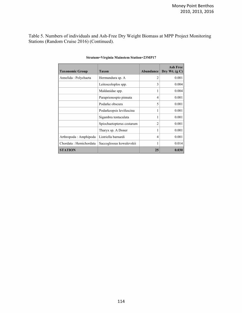
Table 5. Numbers of individuals and Ash-Free Dry Weight Biomass at MPP Project Monitoring
Stations (Random Cruise 2016) (Continued).
Stratum=Virginia Mainstem Station=23MP17
Taxonomic Group Taxon Abundance
Ash Free
Dry Wt. (g C)
Annelida : Polychaeta Hermundura sp. A 2 0.001
Leitoscoloplos spp. 3 0.004
Maldanidae spp. 1 0.004
Paraprionospio pinnata 4 0.001
Podarke obscura 5 0.001
Podarkeopsis levifuscina 1 0.001
Sigambra tentaculata 1 0.001
Spiochaetopterus costarum 2 0.001
Tharyx sp. A Doner 1 0.001
Arthropoda : Amphipoda Listriella barnardi 4 0.001
Chordata : Hemichordata Saccoglossus kowalevskii 1 0.014
STATION 25 0.030
Money Point Benthos 2010, 2013, 2016
114
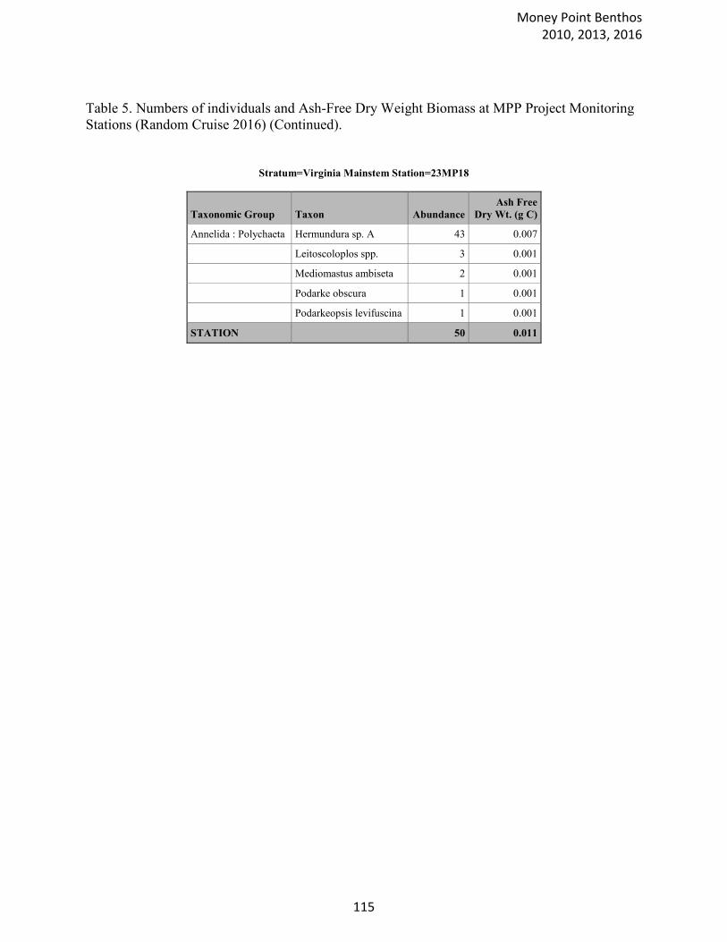
Table 5. Numbers of individuals and Ash-Free Dry Weight Biomass at MPP Project Monitoring
Stations (Random Cruise 2016) (Continued).
Stratum=Virginia Mainstem Station=23MP18
Taxonomic Group Taxon Abundance
Ash Free
Dry Wt. (g C)
Annelida : Polychaeta Hermundura sp. A 43 0.007
Leitoscoloplos spp. 3 0.001
Mediomastus ambiseta 2 0.001
Podarke obscura 1 0.001
Podarkeopsis levifuscina 1 0.001
STATION 50 0.011
Money Point Benthos 2010, 2013, 2016
115
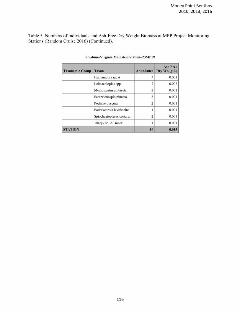
Table 5. Numbers of individuals and Ash-Free Dry Weight Biomass at MPP Project Monitoring
Stations (Random Cruise 2016) (Continued).
Stratum=Virginia Mainstem Station=23MP19
Taxonomic Group Taxon Abundance
Ash Free
Dry Wt. (g C)
Hermundura sp. A 3 0.001
Leitoscoloplos spp. 2 0.008
Mediomastus ambiseta 2 0.001
Paraprionospio pinnata 3 0.001
Podarke obscura 2 0.001
Podarkeopsis levifuscina 1 0.001
Spiochaetopterus costarum 2 0.001
Tharyx sp. A Doner 1 0.001
STATION 16 0.015
Money Point Benthos 2010, 2013, 2016
116
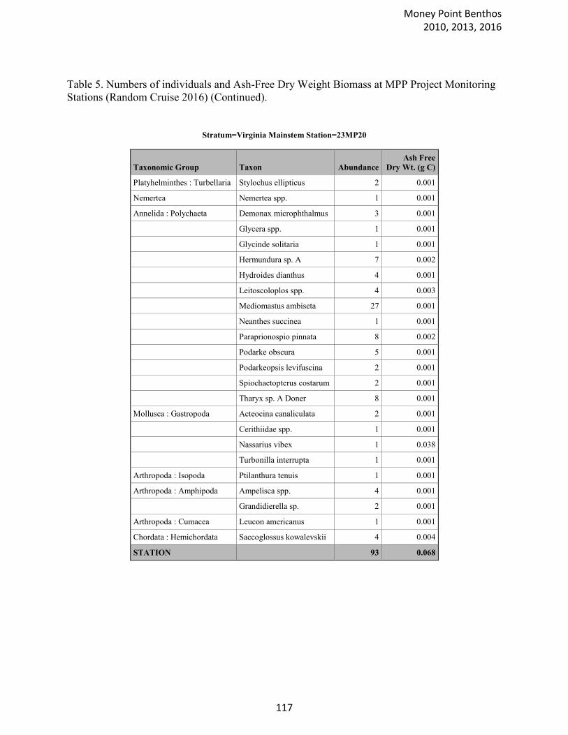
Table 5. Numbers of individuals and Ash-Free Dry Weight Biomass at MPP Project Monitoring
Stations (Random Cruise 2016) (Continued).
Stratum=Virginia Mainstem Station=23MP20
Taxonomic Group Taxon Abundance
Ash Free
Dry Wt. (g C)
Platyhelminthes : Turbellaria Stylochus ellipticus 2 0.001
Nemertea Nemertea spp. 1 0.001
Annelida : Polychaeta Demonax microphthalmus 3 0.001
Glycera spp. 1 0.001
Glycinde solitaria 1 0.001
Hermundura sp. A 7 0.002
Hydroides dianthus 4 0.001
Leitoscoloplos spp. 4 0.003
Mediomastus ambiseta 27 0.001
Neanthes succinea 1 0.001
Paraprionospio pinnata 8 0.002
Podarke obscura 5 0.001
Podarkeopsis levifuscina 2 0.001
Spiochaetopterus costarum 2 0.001
Tharyx sp. A Doner 8 0.001
Mollusca : Gastropoda Acteocina canaliculata 2 0.001
Cerithiidae spp. 1 0.001
Nassarius vibex 1 0.038
Turbonilla interrupta 1 0.001
Arthropoda : Isopoda Ptilanthura tenuis 1 0.001
Arthropoda : Amphipoda Ampelisca spp. 4 0.001
Grandidierella sp. 2 0.001
Arthropoda : Cumacea Leucon americanus 1 0.001
Chordata : Hemichordata Saccoglossus kowalevskii 4 0.004
STATION 93 0.068
Money Point Benthos 2010, 2013, 2016
117
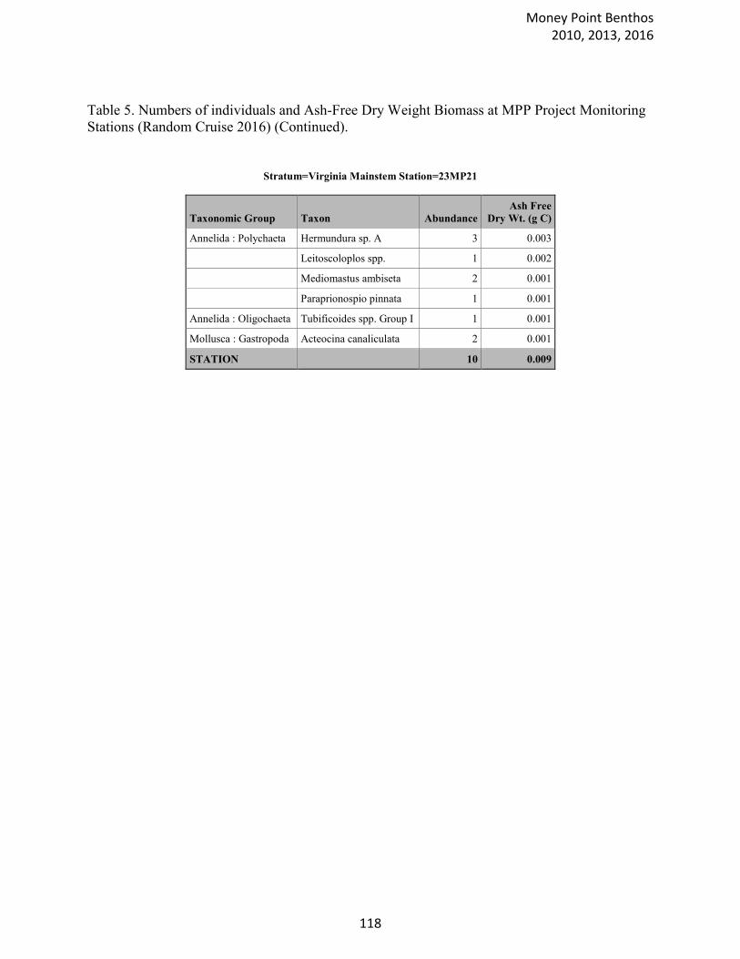
Table 5. Numbers of individuals and Ash-Free Dry Weight Biomass at MPP Project Monitoring
Stations (Random Cruise 2016) (Continued).
Stratum=Virginia Mainstem Station=23MP21
Taxonomic Group Taxon Abundance
Ash Free
Dry Wt. (g C)
Annelida : Polychaeta Hermundura sp. A 3 0.003
Leitoscoloplos spp. 1 0.002
Mediomastus ambiseta 2 0.001
Paraprionospio pinnata 1 0.001
Annelida : Oligochaeta Tubificoides spp. Group I 1 0.001
Mollusca : Gastropoda Acteocina canaliculata 2 0.001
STATION 10 0.009
Money Point Benthos 2010, 2013, 2016
118

Table 5. Numbers of individuals and Ash-Free Dry Weight Biomass at MPP Project Monitoring
Stations (Random Cruise 2016) (Continued).
Stratum=Virginia Mainstem Station=23MP22
Taxonomic Group Taxon Abundance
Ash Free
Dry Wt. (g C)
Nemertea Nemertea spp. 1 0.001
Annelida : Polychaeta Glycinde solitaria 1 0.001
Leitoscoloplos spp. 2 0.003
Mediomastus ambiseta 28 0.001
Streblospio benedicti 2 0.001
Annelida : Oligochaeta Tubificoides spp. Group I 15 0.001
Chordata : Hemichordata Saccoglossus kowalevskii 1 0.001
STATION 50 0.009
Money Point Benthos 2010, 2013, 2016
119
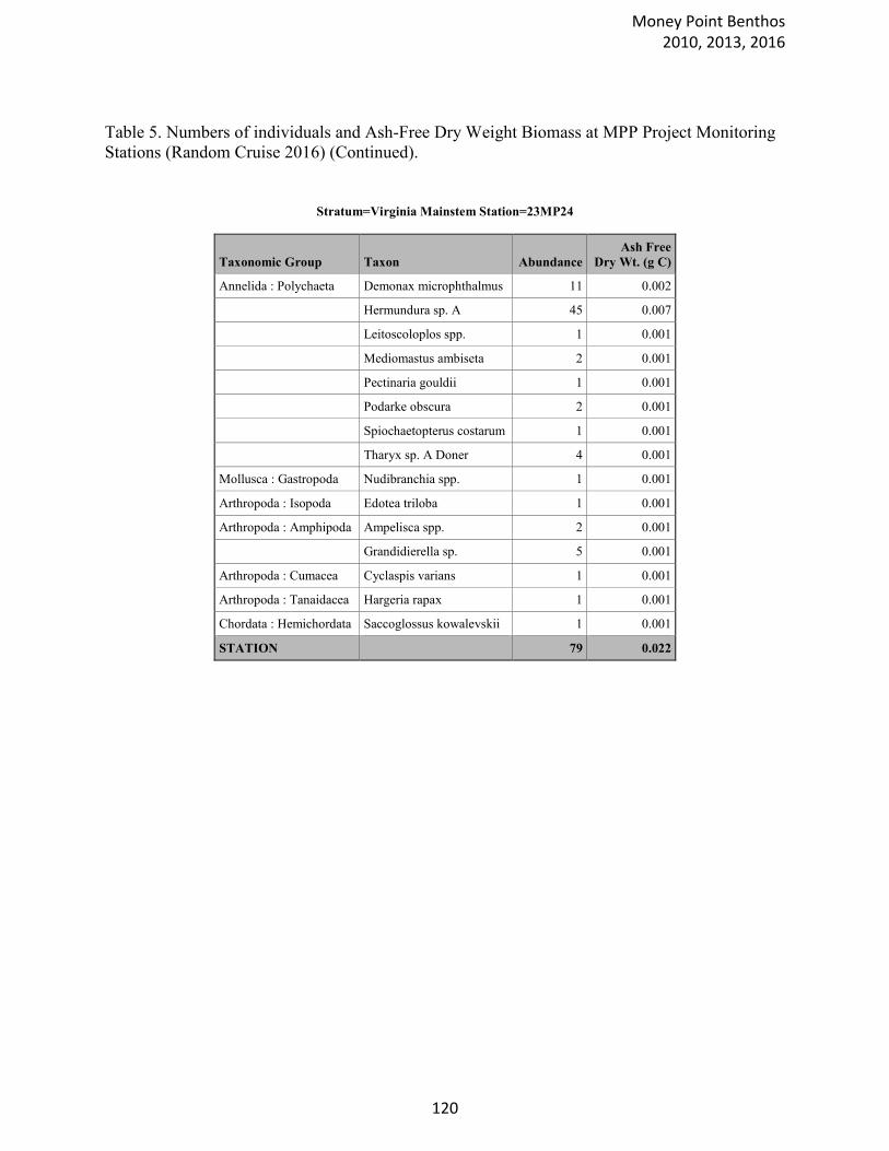
Table 5. Numbers of individuals and Ash-Free Dry Weight Biomass at MPP Project Monitoring
Stations (Random Cruise 2016) (Continued).
Stratum=Virginia Mainstem Station=23MP24
Taxonomic Group Taxon Abundance
Ash Free
Dry Wt. (g C)
Annelida : Polychaeta Demonax microphthalmus 11 0.002
Hermundura sp. A 45 0.007
Leitoscoloplos spp. 1 0.001
Mediomastus ambiseta 2 0.001
Pectinaria gouldii 1 0.001
Podarke obscura 2 0.001
Spiochaetopterus costarum 1 0.001
Tharyx sp. A Doner 4 0.001
Mollusca : Gastropoda Nudibranchia spp. 1 0.001
Arthropoda : Isopoda Edotea triloba 1 0.001
Arthropoda : Amphipoda Ampelisca spp. 2 0.001
Grandidierella sp. 5 0.001
Arthropoda : Cumacea Cyclaspis varians 1 0.001
Arthropoda : Tanaidacea Hargeria rapax 1 0.001
Chordata : Hemichordata Saccoglossus kowalevskii 1 0.001
STATION 79 0.022
Money Point Benthos 2010, 2013, 2016
120
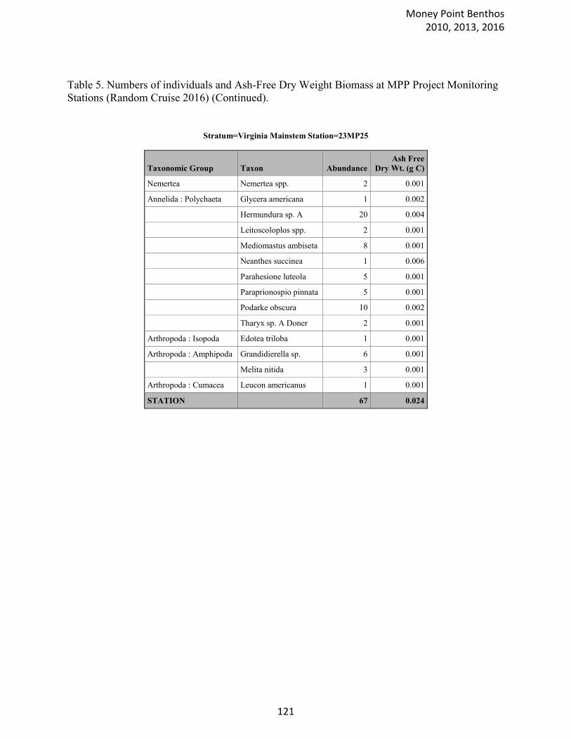
Table 5. Numbers of individuals and Ash-Free Dry Weight Biomass at MPP Project Monitoring
Stations (Random Cruise 2016) (Continued).
Stratum=Virginia Mainstem Station=23MP25
Taxonomic Group Taxon Abundance
Ash Free
Dry Wt. (g C)
Nemertea Nemertea spp. 2 0.001
Annelida : Polychaeta Glycera americana 1 0.002
Hermundura sp. A 20 0.004
Leitoscoloplos spp. 2 0.001
Mediomastus ambiseta 8 0.001
Neanthes succinea 1 0.006
Parahesione luteola 5 0.001
Paraprionospio pinnata 5 0.001
Podarke obscura 10 0.002
Tharyx sp. A Doner 2 0.001
Arthropoda : Isopoda Edotea triloba 1 0.001
Arthropoda : Amphipoda Grandidierella sp. 6 0.001
Melita nitida 3 0.001
Arthropoda : Cumacea Leucon americanus 1 0.001
STATION 67 0.024
Money Point Benthos 2010, 2013, 2016
121

Table 5. Numbers of individuals and Ash-Free Dry Weight Biomass at MPP Project Monitoring
Stations (Random Cruise 2016) (Continued).
Stratum=Virginia Mainstem Station=23MP26
Taxonomic Group Taxon Abundance
Ash Free
Dry Wt. (g C)
Annelida : Polychaeta Hermundura sp. A 1 0.001
Mediomastus ambiseta 5 0.001
Paraprionospio pinnata 7 0.001
Podarke obscura 2 0.001
Streblospio benedicti 3 0.001
Annelida : Oligochaeta Tubificoides spp. Group I 1 0.001
Arthropoda : Amphipoda Listriella barnardi 1 0.001
Arthropoda : Cumacea Leucon americanus 1 0.001
Chordata : Hemichordata Saccoglossus kowalevskii 2 0.011
STATION 23 0.019
Money Point Benthos 2010, 2013, 2016
122
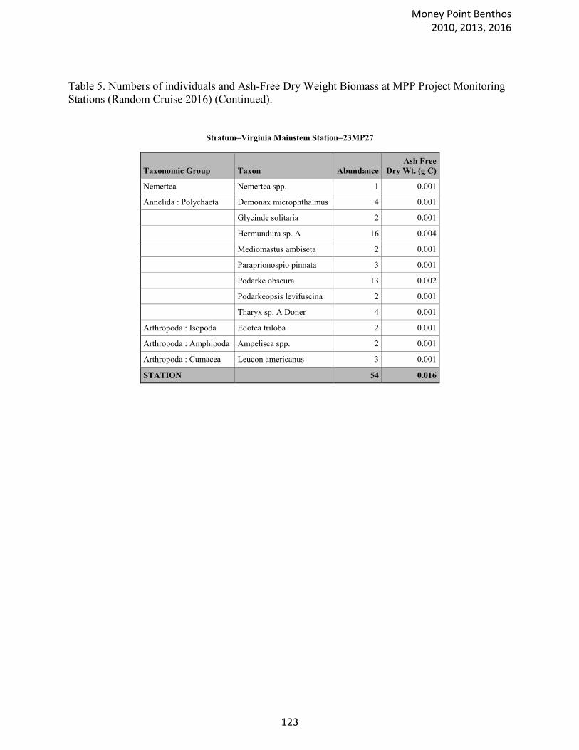
Table 5. Numbers of individuals and Ash-Free Dry Weight Biomass at MPP Project Monitoring
Stations (Random Cruise 2016) (Continued).
Stratum=Virginia Mainstem Station=23MP27
Taxonomic Group Taxon Abundance
Ash Free
Dry Wt. (g C)
Nemertea Nemertea spp. 1 0.001
Annelida : Polychaeta Demonax microphthalmus 4 0.001
Glycinde solitaria 2 0.001
Hermundura sp. A 16 0.004
Mediomastus ambiseta 2 0.001
Paraprionospio pinnata 3 0.001
Podarke obscura 13 0.002
Podarkeopsis levifuscina 2 0.001
Tharyx sp. A Doner 4 0.001
Arthropoda : Isopoda Edotea triloba 2 0.001
Arthropoda : Amphipoda Ampelisca spp. 2 0.001
Arthropoda : Cumacea Leucon americanus 3 0.001
STATION 54 0.016
Money Point Benthos 2010, 2013, 2016
123
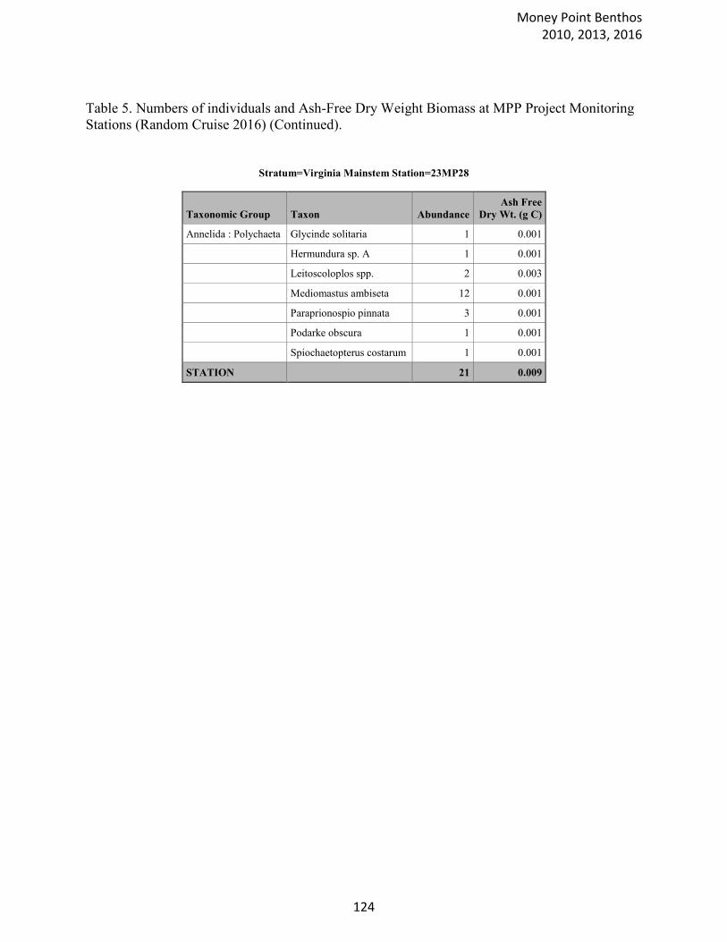
Table 5. Numbers of individuals and Ash-Free Dry Weight Biomass at MPP Project Monitoring
Stations (Random Cruise 2016) (Continued).
Stratum=Virginia Mainstem Station=23MP28
Taxonomic Group Taxon Abundance
Ash Free
Dry Wt. (g C)
Annelida : Polychaeta Glycinde solitaria 1 0.001
Hermundura sp. A 1 0.001
Leitoscoloplos spp. 2 0.003
Mediomastus ambiseta 12 0.001
Paraprionospio pinnata 3 0.001
Podarke obscura 1 0.001
Spiochaetopterus costarum 1 0.001
STATION 21 0.009
Money Point Benthos 2010, 2013, 2016
124
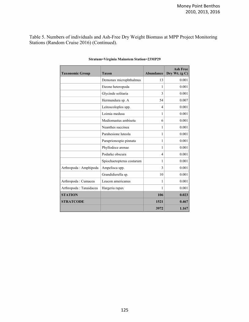
Table 5. Numbers of individuals and Ash-Free Dry Weight Biomass at MPP Project Monitoring
Stations (Random Cruise 2016) (Continued).
Stratum=Virginia Mainstem Station=23MP29
Taxonomic Group Taxon Abundance
Ash Free
Dry Wt. (g C)
Demonax microphthalmus 13 0.001
Eteone heteropoda 1 0.001
Glycinde solitaria 3 0.001
Hermundura sp. A 54 0.007
Leitoscoloplos spp. 4 0.001
Loimia medusa 1 0.001
Mediomastus ambiseta 6 0.001
Neanthes succinea 1 0.001
Parahesione luteola 1 0.001
Paraprionospio pinnata 1 0.001
Phyllodoce arenae 1 0.001
Podarke obscura 4 0.001
Spiochaetopterus costarum 1 0.001
Arthropoda : Amphipoda Ampelisca spp. 3 0.001
Grandidierella sp. 10 0.001
Arthropoda : Cumacea Leucon americanus 1 0.001
Arthropoda : Tanaidacea Hargeria rapax 1 0.001
STATION 106 0.023
STRATCODE 1521 0.467
3972 1.167
Money Point Benthos 2010, 2013, 2016
125
Appendix C. Glossary of terms
Money Point Benthos 2010, 2013, 2016
126
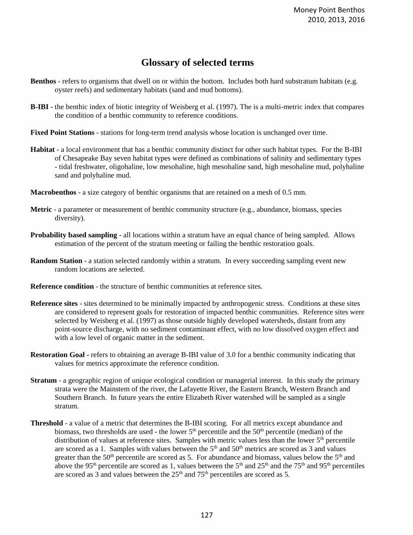
Glossary of selected terms
Benthos - refers to organisms that dwell on or within the bottom. Includes both hard substratum habitats (e.g.
oyster reefs) and sedimentary habitats (sand and mud bottoms).
B-IBI - the benthic index of biotic integrity of Weisberg et al. (1997). The is a multi-metric index that compares
the condition of a benthic community to reference conditions.
Fixed Point Stations - stations for long-term trend analysis whose location is unchanged over time.
Habitat - a local environment that has a benthic community distinct for other such habitat types. For the B-IBI
of Chesapeake Bay seven habitat types were defined as combinations of salinity and sedimentary types
- tidal freshwater, oligohaline, low mesohaline, high mesohaline sand, high mesohaline mud, polyhaline
sand and polyhaline mud.
Macrobenthos - a size category of benthic organisms that are retained on a mesh of 0.5 mm.
Metric - a parameter or measurement of benthic community structure (e.g., abundance, biomass, species
diversity).
Probability based sampling - all locations within a stratum have an equal chance of being sampled. Allows
estimation of the percent of the stratum meeting or failing the benthic restoration goals.
Random Station - a station selected randomly within a stratum. In every succeeding sampling event new
random locations are selected.
Reference condition - the structure of benthic communities at reference sites.
Reference sites - sites determined to be minimally impacted by anthropogenic stress. Conditions at these sites
are considered to represent goals for restoration of impacted benthic communities. Reference sites were
selected by Weisberg et al. (1997) as those outside highly developed watersheds, distant from any
point-source discharge, with no sediment contaminant effect, with no low dissolved oxygen effect and
with a low level of organic matter in the sediment.
Restoration Goal - refers to obtaining an average B-IBI value of 3.0 for a benthic community indicating that
values for metrics approximate the reference condition.
Stratum - a geographic region of unique ecological condition or managerial interest. In this study the primary
strata were the Mainstem of the river, the Lafayette River, the Eastern Branch, Western Branch and
Southern Branch. In future years the entire Elizabeth River watershed will be sampled as a single
stratum.
Threshold - a value of a metric that determines the B-IBI scoring. For all metrics except abundance and
biomass, two thresholds are used - the lower 5th percentile and the 50th percentile (median) of the
distribution of values at reference sites. Samples with metric values less than the lower 5th percentile
are scored as a 1. Samples with values between the 5th and 50th metrics are scored as 3 and values
greater than the 50th percentile are scored as 5. For abundance and biomass, values below the 5th and
above the 95th percentile are scored as 1, values between the 5th and 25th and the 75th and 95th percentiles
are scored as 3 and values between the 25th and 75th percentiles are scored as 5.
Money Point Benthos 2010, 2013, 2016
127
Appendix D. Data by Site – BIBI, Abundance, Biomass, Shannon Index, Species Richness, Total
Volatile Organics, Salinity, Water Depth
Money Point Benthos 2010, 2013, 2016
128
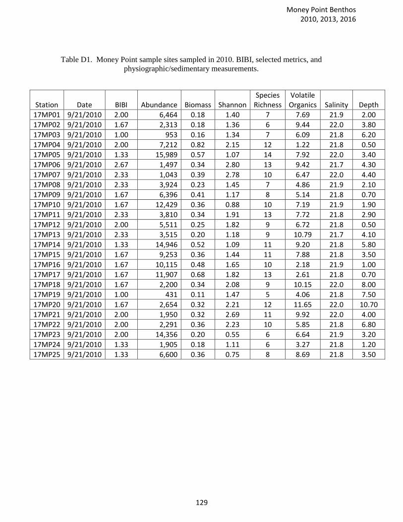
Table D1. Money Point sample sites sampled in 2010. BIBI, selected metrics, and
physiographic/sedimentary measurements.
Station Date BIBI Abundance Biomass Shannon Species
Richness Volatile Organics Salinity Depth
17MP01 9/21/2010 2.00 6,464 0.18 1.40 7 7.69 21.9 2.00
17MP02 9/21/2010 1.67 2,313 0.18 1.36 6 9.44 22.0 3.80
17MP03 9/21/2010 1.00 953 0.16 1.34 7 6.09 21.8 6.20
17MP04 9/21/2010 2.00 7,212 0.82 2.15 12 1.22 21.8 0.50
17MP05 9/21/2010 1.33 15,989 0.57 1.07 14 7.92 22.0 3.40
17MP06 9/21/2010 2.67 1,497 0.34 2.80 13 9.42 21.7 4.30
17MP07 9/21/2010 2.33 1,043 0.39 2.78 10 6.47 22.0 4.40
17MP08 9/21/2010 2.33 3,924 0.23 1.45 7 4.86 21.9 2.10
17MP09 9/21/2010 1.67 6,396 0.41 1.17 8 5.14 21.8 0.70
17MP10 9/21/2010 1.67 12,429 0.36 0.88 10 7.19 21.9 1.90
17MP11 9/21/2010 2.33 3,810 0.34 1.91 13 7.72 21.8 2.90
17MP12 9/21/2010 2.00 5,511 0.25 1.82 9 6.72 21.8 0.50
17MP13 9/21/2010 2.33 3,515 0.20 1.18 9 10.79 21.7 4.10
17MP14 9/21/2010 1.33 14,946 0.52 1.09 11 9.20 21.8 5.80
17MP15 9/21/2010 1.67 9,253 0.36 1.44 11 7.88 21.8 3.50
17MP16 9/21/2010 1.67 10,115 0.48 1.65 10 2.18 21.9 1.00
17MP17 9/21/2010 1.67 11,907 0.68 1.82 13 2.61 21.8 0.70
17MP18 9/21/2010 1.67 2,200 0.34 2.08 9 10.15 22.0 8.00
17MP19 9/21/2010 1.00 431 0.11 1.47 5 4.06 21.8 7.50
17MP20 9/21/2010 1.67 2,654 0.32 2.21 12 11.65 22.0 10.70
17MP21 9/21/2010 2.00 1,950 0.32 2.69 11 9.92 22.0 4.00
17MP22 9/21/2010 2.00 2,291 0.36 2.23 10 5.85 21.8 6.80
17MP23 9/21/2010 2.00 14,356 0.20 0.55 6 6.64 21.9 3.20
17MP24 9/21/2010 1.33 1,905 0.18 1.11 6 3.27 21.8 1.20
17MP25 9/21/2010 1.33 6,600 0.36 0.75 8 8.69 21.8 3.50
Money Point Benthos 2010, 2013, 2016
129
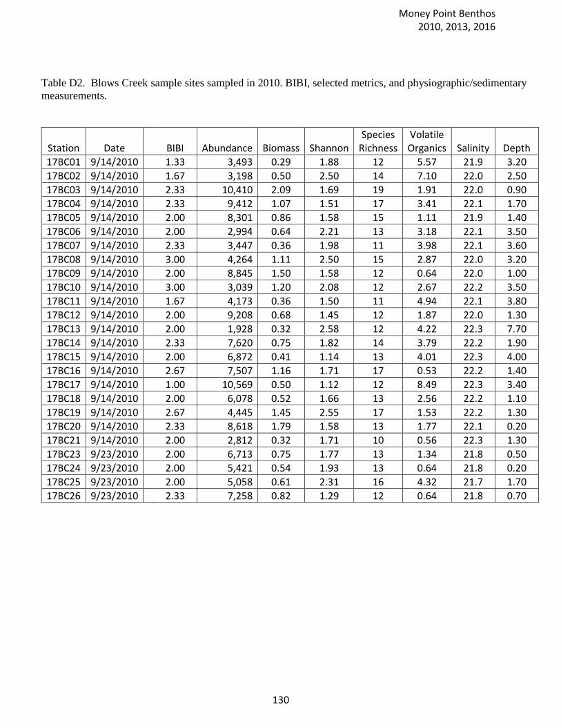
Table D2. Blows Creek sample sites sampled in 2010. BIBI, selected metrics, and physiographic/sedimentary
measurements.
Station Date
BIBI Abundance Biomass Shannon Species
Richness Volatile Organics Salinity Depth
17BC01 9/14/2010 1.33 3,493 0.29 1.88 12 5.57 21.9 3.20
17BC02 9/14/2010 1.67 3,198 0.50 2.50 14 7.10 22.0 2.50
17BC03 9/14/2010 2.33 10,410 2.09 1.69 19 1.91 22.0 0.90
17BC04 9/14/2010 2.33 9,412 1.07 1.51 17 3.41 22.1 1.70
17BC05 9/14/2010 2.00 8,301 0.86 1.58 15 1.11 21.9 1.40
17BC06 9/14/2010 2.00 2,994 0.64 2.21 13 3.18 22.1 3.50
17BC07 9/14/2010 2.33 3,447 0.36 1.98 11 3.98 22.1 3.60
17BC08 9/14/2010 3.00 4,264 1.11 2.50 15 2.87 22.0 3.20
17BC09 9/14/2010 2.00 8,845 1.50 1.58 12 0.64 22.0 1.00
17BC10 9/14/2010 3.00 3,039 1.20 2.08 12 2.67 22.2 3.50
17BC11 9/14/2010 1.67 4,173 0.36 1.50 11 4.94 22.1 3.80
17BC12 9/14/2010 2.00 9,208 0.68 1.45 12 1.87 22.0 1.30
17BC13 9/14/2010 2.00 1,928 0.32 2.58 12 4.22 22.3 7.70
17BC14 9/14/2010 2.33 7,620 0.75 1.82 14 3.79 22.2 1.90
17BC15 9/14/2010 2.00 6,872 0.41 1.14 13 4.01 22.3 4.00
17BC16 9/14/2010 2.67 7,507 1.16 1.71 17 0.53 22.2 1.40
17BC17 9/14/2010 1.00 10,569 0.50 1.12 12 8.49 22.3 3.40
17BC18 9/14/2010 2.00 6,078 0.52 1.66 13 2.56 22.2 1.10
17BC19 9/14/2010 2.67 4,445 1.45 2.55 17 1.53 22.2 1.30
17BC20 9/14/2010 2.33 8,618 1.79 1.58 13 1.77 22.1 0.20
17BC21 9/14/2010 2.00 2,812 0.32 1.71 10 0.56 22.3 1.30
17BC23 9/23/2010 2.00 6,713 0.75 1.77 13 1.34 21.8 0.50
17BC24 9/23/2010 2.00 5,421 0.54 1.93 13 0.64 21.8 0.20
17BC25 9/23/2010 2.00 5,058 0.61 2.31 16 4.32 21.7 1.70
17BC26 9/23/2010 2.33 7,258 0.82 1.29 12 0.64 21.8 0.70
Money Point Benthos 2010, 2013, 2016
130
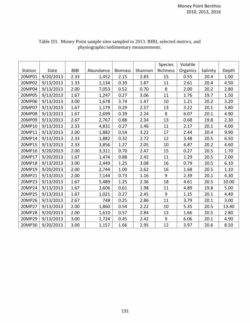
Table D3. Money Point sample sites sampled in 2013. BIBI, selected metrics, and
physiographic/sedimentary measurements.
Station Date BIBI Abundance Biomass Shannon Species
Richness Volatile Organics Salinity Depth
20MP01 9/20/2013 2.33 1,452 2.15 2.83 15 0.55 20.4 1.00
20MP02 9/13/2013 1.33 1,134 0.39 1.87 11 2.61 20.4 4.50
20MP04 9/13/2013 2.00 7,053 0.52 0.70 8 2.00 20.2 2.80
20MP05 9/13/2013 1.67 1,247 0.27 3.06 11 1.76 19.7 1.50
20MP06 9/13/2013 3.00 1,678 3.74 1.47 10 1.21 20.2 3.20
20MP07 9/13/2013 1.67 1,179 0.29 2.57 13 3.22 20.1 3.80
20MP08 9/13/2013 1.67 2,699 0.39 2.24 8 6.07 20.1 4.90
20MP09 9/13/2013 2.67 2,767 0.88 2.34 13 0.68 19.8 2.30
20MP10 9/13/2013 2.33 4,831 0.27 1.46 11 2.17 20.1 4.00
20MP11 9/13/2013 2.00 1,882 0.54 3.22 17 2.44 20.4 9.90
20MP14 9/13/2013 2.33 1,882 0.32 2.72 12 3.48 20.5 6.50
20MP15 9/13/2013 2.33 3,856 1.27 2.05 10 4.87 20.2 4.60
20MP16 9/20/2013 2.00 3,311 0.70 2.47 15 0.27 20.5 1.70
20MP17 9/20/2013 1.67 1,474 0.88 2.42 11 1.29 20.5 2.00
20MP18 9/13/2013 3.00 2,449 1.25 3.08 16 0.79 20.5 6.10
20MP19 9/20/2013 2.00 2,744 1.00 2.62 16 1.68 20.5 1.10
20MP21 9/13/2013 2.00 7,144 0.73 1.16 9 2.39 20.1 4.30
20MP23 9/13/2013 1.67 5,489 1.25 2.36 18 4.61 20.5 10.00
20MP24 9/13/2013 1.67 3,606 0.61 1.98 11 4.89 19.8 5.00
20MP25 9/13/2013 1.67 1,021 0.27 2.45 9 1.15 20.1 4.40
20MP26 9/13/2013 2.67 748 0.25 2.86 11 3.79 20.1 3.00
20MP27 9/13/2013 2.00 1,860 0.54 2.22 10 5.35 20.5 13.40
20MP28 9/20/2013 2.00 1,610 0.57 2.84 13 1.66 20.5 2.80
20MP29 9/13/2013 3.00 1,724 0.45 2.42 9 6.06 20.1 4.90
20MP30 9/20/2013 3.00 1,157 1.66 2.95 12 3.97 20.6 8.50
Money Point Benthos 2010, 2013, 2016
131
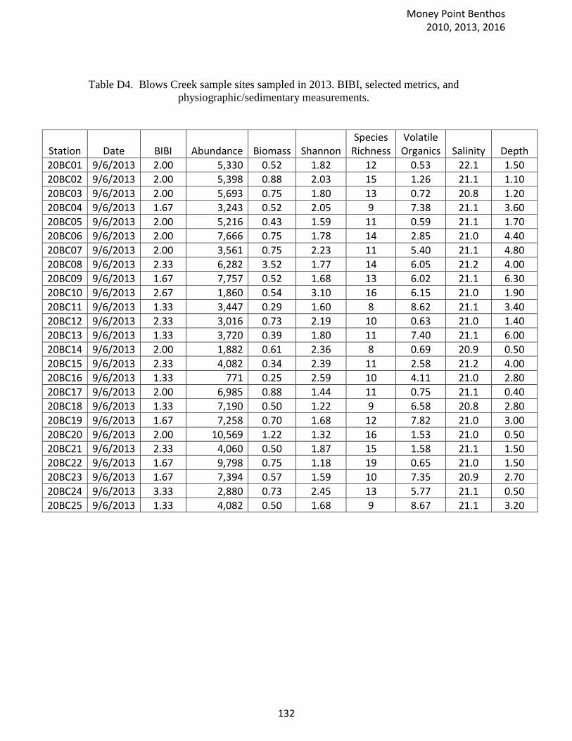
Table D4. Blows Creek sample sites sampled in 2013. BIBI, selected metrics, and
physiographic/sedimentary measurements.
Station Date BIBI Abundance Biomass Shannon Species
Richness Volatile Organics Salinity Depth
20BC01 9/6/2013 2.00 5,330 0.52 1.82 12 0.53 22.1 1.50
20BC02 9/6/2013 2.00 5,398 0.88 2.03 15 1.26 21.1 1.10
20BC03 9/6/2013 2.00 5,693 0.75 1.80 13 0.72 20.8 1.20
20BC04 9/6/2013 1.67 3,243 0.52 2.05 9 7.38 21.1 3.60
20BC05 9/6/2013 2.00 5,216 0.43 1.59 11 0.59 21.1 1.70
20BC06 9/6/2013 2.00 7,666 0.75 1.78 14 2.85 21.0 4.40
20BC07 9/6/2013 2.00 3,561 0.75 2.23 11 5.40 21.1 4.80
20BC08 9/6/2013 2.33 6,282 3.52 1.77 14 6.05 21.2 4.00
20BC09 9/6/2013 1.67 7,757 0.52 1.68 13 6.02 21.1 6.30
20BC10 9/6/2013 2.67 1,860 0.54 3.10 16 6.15 21.0 1.90
20BC11 9/6/2013 1.33 3,447 0.29 1.60 8 8.62 21.1 3.40
20BC12 9/6/2013 2.33 3,016 0.73 2.19 10 0.63 21.0 1.40
20BC13 9/6/2013 1.33 3,720 0.39 1.80 11 7.40 21.1 6.00
20BC14 9/6/2013 2.00 1,882 0.61 2.36 8 0.69 20.9 0.50
20BC15 9/6/2013 2.33 4,082 0.34 2.39 11 2.58 21.2 4.00
20BC16 9/6/2013 1.33 771 0.25 2.59 10 4.11 21.0 2.80
20BC17 9/6/2013 2.00 6,985 0.88 1.44 11 0.75 21.1 0.40
20BC18 9/6/2013 1.33 7,190 0.50 1.22 9 6.58 20.8 2.80
20BC19 9/6/2013 1.67 7,258 0.70 1.68 12 7.82 21.0 3.00
20BC20 9/6/2013 2.00 10,569 1.22 1.32 16 1.53 21.0 0.50
20BC21 9/6/2013 2.33 4,060 0.50 1.87 15 1.58 21.1 1.50
20BC22 9/6/2013 1.67 9,798 0.75 1.18 19 0.65 21.0 1.50
20BC23 9/6/2013 1.67 7,394 0.57 1.59 10 7.35 20.9 2.70
20BC24 9/6/2013 3.33 2,880 0.73 2.45 13 5.77 21.1 0.50
20BC25 9/6/2013 1.33 4,082 0.50 1.68 9 8.67 21.1 3.20
Money Point Benthos 2010, 2013, 2016
132
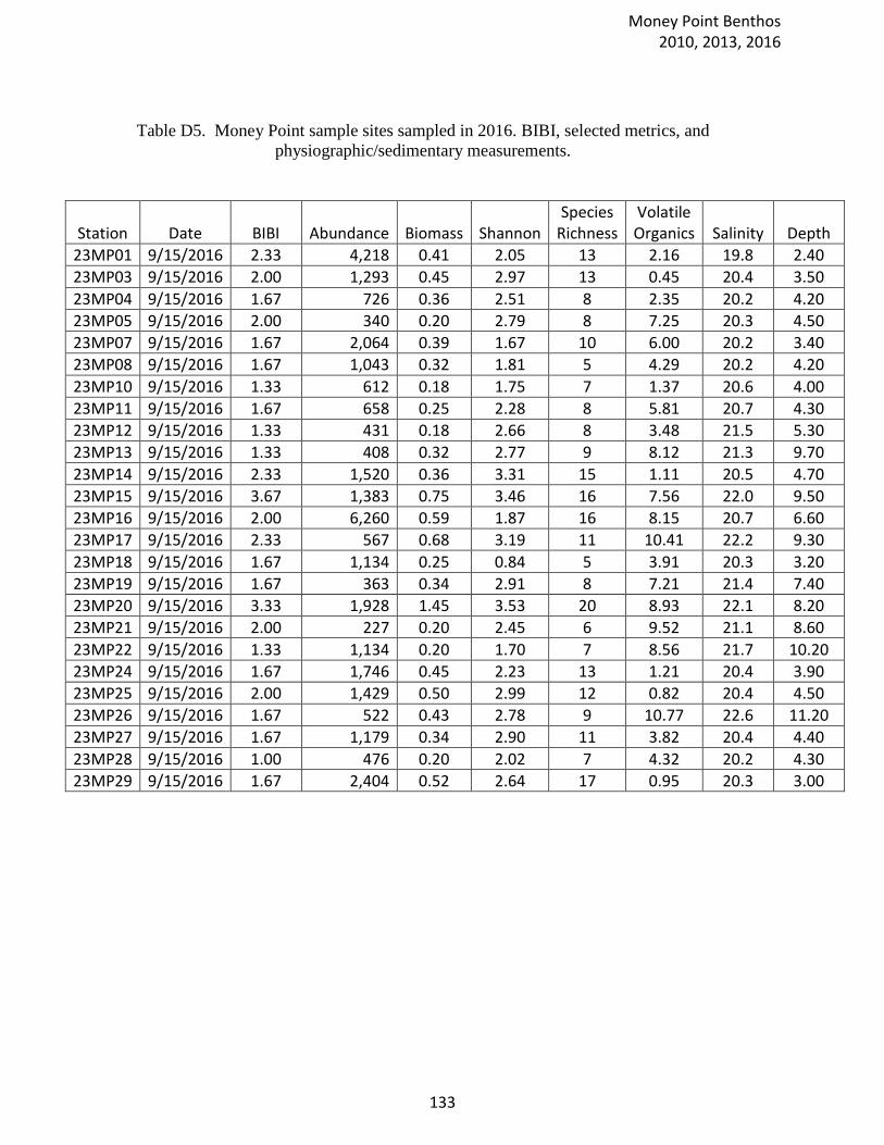
Table D5. Money Point sample sites sampled in 2016. BIBI, selected metrics, and
physiographic/sedimentary measurements.
Station Date BIBI Abundance Biomass Shannon Species
Richness Volatile Organics Salinity Depth
23MP01 9/15/2016 2.33 4,218 0.41 2.05 13 2.16 19.8 2.40
23MP03 9/15/2016 2.00 1,293 0.45 2.97 13 0.45 20.4 3.50
23MP04 9/15/2016 1.67 726 0.36 2.51 8 2.35 20.2 4.20
23MP05 9/15/2016 2.00 340 0.20 2.79 8 7.25 20.3 4.50
23MP07 9/15/2016 1.67 2,064 0.39 1.67 10 6.00 20.2 3.40
23MP08 9/15/2016 1.67 1,043 0.32 1.81 5 4.29 20.2 4.20
23MP10 9/15/2016 1.33 612 0.18 1.75 7 1.37 20.6 4.00
23MP11 9/15/2016 1.67 658 0.25 2.28 8 5.81 20.7 4.30
23MP12 9/15/2016 1.33 431 0.18 2.66 8 3.48 21.5 5.30
23MP13 9/15/2016 1.33 408 0.32 2.77 9 8.12 21.3 9.70
23MP14 9/15/2016 2.33 1,520 0.36 3.31 15 1.11 20.5 4.70
23MP15 9/15/2016 3.67 1,383 0.75 3.46 16 7.56 22.0 9.50
23MP16 9/15/2016 2.00 6,260 0.59 1.87 16 8.15 20.7 6.60
23MP17 9/15/2016 2.33 567 0.68 3.19 11 10.41 22.2 9.30
23MP18 9/15/2016 1.67 1,134 0.25 0.84 5 3.91 20.3 3.20
23MP19 9/15/2016 1.67 363 0.34 2.91 8 7.21 21.4 7.40
23MP20 9/15/2016 3.33 1,928 1.45 3.53 20 8.93 22.1 8.20
23MP21 9/15/2016 2.00 227 0.20 2.45 6 9.52 21.1 8.60
23MP22 9/15/2016 1.33 1,134 0.20 1.70 7 8.56 21.7 10.20
23MP24 9/15/2016 1.67 1,746 0.45 2.23 13 1.21 20.4 3.90
23MP25 9/15/2016 2.00 1,429 0.50 2.99 12 0.82 20.4 4.50
23MP26 9/15/2016 1.67 522 0.43 2.78 9 10.77 22.6 11.20
23MP27 9/15/2016 1.67 1,179 0.34 2.90 11 3.82 20.4 4.40
23MP28 9/15/2016 1.00 476 0.20 2.02 7 4.32 20.2 4.30
23MP29 9/15/2016 1.67 2,404 0.52 2.64 17 0.95 20.3 3.00
Money Point Benthos 2010, 2013, 2016
133
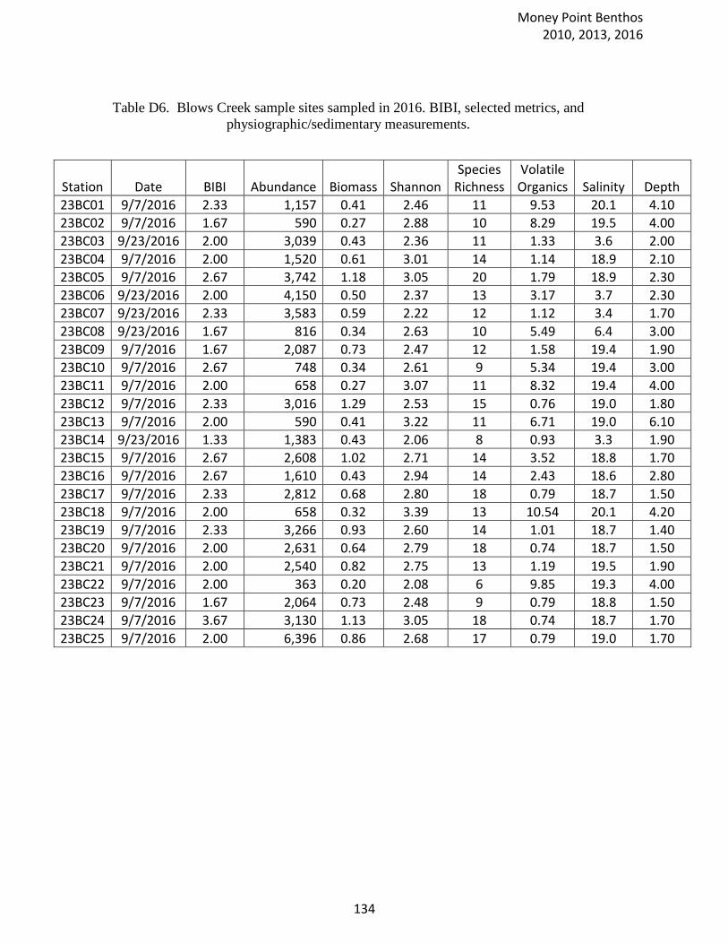
Table D6. Blows Creek sample sites sampled in 2016. BIBI, selected metrics, and
physiographic/sedimentary measurements.
Station Date BIBI Abundance Biomass Shannon Species
Richness Volatile Organics Salinity Depth
23BC01 9/7/2016 2.33 1,157 0.41 2.46 11 9.53 20.1 4.10
23BC02 9/7/2016 1.67 590 0.27 2.88 10 8.29 19.5 4.00
23BC03 9/23/2016 2.00 3,039 0.43 2.36 11 1.33 3.6 2.00
23BC04 9/7/2016 2.00 1,520 0.61 3.01 14 1.14 18.9 2.10
23BC05 9/7/2016 2.67 3,742 1.18 3.05 20 1.79 18.9 2.30
23BC06 9/23/2016 2.00 4,150 0.50 2.37 13 3.17 3.7 2.30
23BC07 9/23/2016 2.33 3,583 0.59 2.22 12 1.12 3.4 1.70
23BC08 9/23/2016 1.67 816 0.34 2.63 10 5.49 6.4 3.00
23BC09 9/7/2016 1.67 2,087 0.73 2.47 12 1.58 19.4 1.90
23BC10 9/7/2016 2.67 748 0.34 2.61 9 5.34 19.4 3.00
23BC11 9/7/2016 2.00 658 0.27 3.07 11 8.32 19.4 4.00
23BC12 9/7/2016 2.33 3,016 1.29 2.53 15 0.76 19.0 1.80
23BC13 9/7/2016 2.00 590 0.41 3.22 11 6.71 19.0 6.10
23BC14 9/23/2016 1.33 1,383 0.43 2.06 8 0.93 3.3 1.90
23BC15 9/7/2016 2.67 2,608 1.02 2.71 14 3.52 18.8 1.70
23BC16 9/7/2016 2.67 1,610 0.43 2.94 14 2.43 18.6 2.80
23BC17 9/7/2016 2.33 2,812 0.68 2.80 18 0.79 18.7 1.50
23BC18 9/7/2016 2.00 658 0.32 3.39 13 10.54 20.1 4.20
23BC19 9/7/2016 2.33 3,266 0.93 2.60 14 1.01 18.7 1.40
23BC20 9/7/2016 2.00 2,631 0.64 2.79 18 0.74 18.7 1.50
23BC21 9/7/2016 2.00 2,540 0.82 2.75 13 1.19 19.5 1.90
23BC22 9/7/2016 2.00 363 0.20 2.08 6 9.85 19.3 4.00
23BC23 9/7/2016 1.67 2,064 0.73 2.48 9 0.79 18.8 1.50
23BC24 9/7/2016 3.67 3,130 1.13 3.05 18 0.74 18.7 1.70
23BC25 9/7/2016 2.00 6,396 0.86 2.68 17 0.79 19.0 1.70
Money Point Benthos 2010, 2013, 2016
134
Related Documents


