HAL Id: tel-01812211 https://tel.archives-ouvertes.fr/tel-01812211 Submitted on 11 Jun 2018 HAL is a multi-disciplinary open access archive for the deposit and dissemination of sci- entific research documents, whether they are pub- lished or not. The documents may come from teaching and research institutions in France or abroad, or from public or private research centers. L’archive ouverte pluridisciplinaire HAL, est destinée au dépôt et à la diffusion de documents scientifiques de niveau recherche, publiés ou non, émanant des établissements d’enseignement et de recherche français ou étrangers, des laboratoires publics ou privés. Oil-spill monitoring in Indonesia Budhi Gunadharma Gautama To cite this version: Budhi Gunadharma Gautama. Oil-spill monitoring in Indonesia. Signal and Image Processing. Ecole nationale supérieure Mines-Télécom Atlantique, 2017. English. NNT: 2017IMTA0036. tel- 01812211

Welcome message from author
This document is posted to help you gain knowledge. Please leave a comment to let me know what you think about it! Share it to your friends and learn new things together.
Transcript

HAL Id: tel-01812211https://tel.archives-ouvertes.fr/tel-01812211
Submitted on 11 Jun 2018
HAL is a multi-disciplinary open accessarchive for the deposit and dissemination of sci-entific research documents, whether they are pub-lished or not. The documents may come fromteaching and research institutions in France orabroad, or from public or private research centers.
L’archive ouverte pluridisciplinaire HAL, estdestinée au dépôt et à la diffusion de documentsscientifiques de niveau recherche, publiés ou non,émanant des établissements d’enseignement et derecherche français ou étrangers, des laboratoirespublics ou privés.
Oil-spill monitoring in IndonesiaBudhi Gunadharma Gautama
To cite this version:Budhi Gunadharma Gautama. Oil-spill monitoring in Indonesia. Signal and Image Processing.Ecole nationale supérieure Mines-Télécom Atlantique, 2017. English. NNT : 2017IMTA0036. tel-01812211

THÈSE / IMT Atlantique
sous le sceau de l’Université Bretagne Loire
pour obtenir le grade de
DOCTEUR D'IMT Atlantique
Spécialité : Signal, Image, Vision
École Doctorale Mathématiques et STIC
Présentée par
Budhi Gunadharma Gautama Préparée dans le département Signal & communications
Laboratoire Labsticc
Oil-Spill Monitoring in Indonesia
Thèse soutenue le 01 décembre 2017
devant le jury composé de :
René Garello Professeur (HDR), IMT Atlantique / président Thomas Corpetti Directeur de recherche (HDR), LETG-Rennes / rapporteur
Serge Andrefouet Directeur de recherche (HDR), INDESO Center JI. Baru Perancak / rapporteur
Nicolas Longepe Chercheur, CLS – Plouzané / examinateur
Emina Mamaca Chercheur, Ifremer – Plouzané examinatrice
Ronan Fablet Professeur (HDR), IMT Atlantique / directeur de thèse


N d’ordre : 2017telb0422
Sous le sceau de l’Université Européenne de Bretagne
IMT Atlantique Bretagne-Pays de la Loire
En accréditation conjointe avec l’École Doctorale – SICMA
Thèse de Doctorat
Mention : STIC – Sciences et Technologies de l’Information et des Communications
Oil Spill Observation in Indonesia
présentée par
Budhi Gunadharma GAUTAMA
Unité de recherche : IMT Atlantique – Signal et Communication
Laboratoire : Lab-STICC, Pôle CID, Équipe TOMS
Entreprise partenaire : CLS FRANCE
Directeurs de thèse : Ronan FABLET
Encadrant de thèse : Grégoire MERCIER et Nicolas LONGÉPÉ
Soutenue le 01 Decembre 2017 devant le jury composé de:
M Thomas CORPETTI RapporteurM. Serge ANDRÉFOUËT RapporteurM. René GARELLO - Professeure, IMT Atlantique ExaminateurMme. Emina MAMACA Examinateur

Contents
Acknowledgments xi
Acronyms xiii
Abstract xv
Résumé xvii
Résumé étendu xix
1 Introduction 1
1.1 Context of the thesis . . . . . . . . . . . . . . . . . . . . . . . . . . . . . . . . . . 2
1.2 A brief review of INDESO Project . . . . . . . . . . . . . . . . . . . . . . . . . . 4
1.3 Thesis motivation and outline . . . . . . . . . . . . . . . . . . . . . . . . . . . . . 6
2 Oil Spill Monitoring in Indonesia 9
2.1 Description of Indonesian waters . . . . . . . . . . . . . . . . . . . . . . . . . . . 10
2.1.1 General aspects of ocean circulation in Indonesia . . . . . . . . . . . . . . 10
2.1.2 Main issue of Indonesia Marine and Fisheries . . . . . . . . . . . . . . . . 11
2.2 Oil spill monitoring as conceived by the INDESO system . . . . . . . . . . . . . . 18
2.2.1 Operational . . . . . . . . . . . . . . . . . . . . . . . . . . . . . . . . . . . 18
2.2.2 INDESO sites for the oil spill monitoring . . . . . . . . . . . . . . . . . . 19
2.2.3 System design . . . . . . . . . . . . . . . . . . . . . . . . . . . . . . . . . . 21
2.3 Detection of oil spill using EO-based imagery . . . . . . . . . . . . . . . . . . . . 24
2.3.1 Spaceborne/airborne remote sensing . . . . . . . . . . . . . . . . . . . . . 24
2.3.2 Detection of oil spill based on SAR imagery . . . . . . . . . . . . . . . . . 27
2.4 Oil spill transport model . . . . . . . . . . . . . . . . . . . . . . . . . . . . . . . . 31
2.4.1 Introduction . . . . . . . . . . . . . . . . . . . . . . . . . . . . . . . . . . 31
i

Contents
2.4.2 Lagrangian 2D Trajectory Model . . . . . . . . . . . . . . . . . . . . . . . 32
2.4.3 Mobidrift . . . . . . . . . . . . . . . . . . . . . . . . . . . . . . . . . . . . 33
2.4.4 Application of Mobidrift in Indonesia’s Oil Spill Trajectory . . . . . . . . 34
2.5 Conclusion . . . . . . . . . . . . . . . . . . . . . . . . . . . . . . . . . . . . . . . 37
3 Oil spill parameter retrieval 39
3.1 Introduction . . . . . . . . . . . . . . . . . . . . . . . . . . . . . . . . . . . . . . . 40
3.2 Proposed approach . . . . . . . . . . . . . . . . . . . . . . . . . . . . . . . . . . . 42
3.3 Montara SAR based oil detection . . . . . . . . . . . . . . . . . . . . . . . . . . 44
3.4 Similarity between SAR oil spill detection and model . . . . . . . . . . . . . . . . 47
3.5 Estimation of oil leakage parameters assimilation of SAR images . . . . . . . . . 49
3.6 Application to Montara case study . . . . . . . . . . . . . . . . . . . . . . . . . . 52
3.7 Conclusion . . . . . . . . . . . . . . . . . . . . . . . . . . . . . . . . . . . . . . . 59
4 Oil spill risk assessment in Indonesian Fisheries Management Area 61
4.1 Introduction . . . . . . . . . . . . . . . . . . . . . . . . . . . . . . . . . . . . . . . 62
4.2 Data and Study area . . . . . . . . . . . . . . . . . . . . . . . . . . . . . . . . . . 65
4.2.1 Study Area . . . . . . . . . . . . . . . . . . . . . . . . . . . . . . . . . . . 65
4.2.2 Data Collection . . . . . . . . . . . . . . . . . . . . . . . . . . . . . . . . . 66
4.2.3 Marine Protected Area Data . . . . . . . . . . . . . . . . . . . . . . . . . 71
4.2.4 Marine fisheries data . . . . . . . . . . . . . . . . . . . . . . . . . . . . . . 74
4.2.5 Socio-economic data for fishing activities, tourism services and salt ponds 75
4.3 Proposed methodology . . . . . . . . . . . . . . . . . . . . . . . . . . . . . . . . . 77
4.3.1 Oil spill risk indices . . . . . . . . . . . . . . . . . . . . . . . . . . . . . . 77
4.3.2 Environmental and socio-economical vulnerability indices . . . . . . . . . 80
4.3.3 Global FMA-level risk index . . . . . . . . . . . . . . . . . . . . . . . . . 83
4.3.4 MPA-level vulnerability analysis . . . . . . . . . . . . . . . . . . . . . . . 84
4.4 Results and Discussion . . . . . . . . . . . . . . . . . . . . . . . . . . . . . . . . . 87
4.5 MPA-level risk assessment . . . . . . . . . . . . . . . . . . . . . . . . . . . . . . . 89
4.6 Conclusion and Discussion . . . . . . . . . . . . . . . . . . . . . . . . . . . . . . . 101
5 Conclusions and Perspectives 105
5.1 Conclusion . . . . . . . . . . . . . . . . . . . . . . . . . . . . . . . . . . . . . . . 106
ii

Contents
5.2 Perspectives . . . . . . . . . . . . . . . . . . . . . . . . . . . . . . . . . . . . . . . 108
Bibliography 122
iii

iv

List of Figures
1.1 Operational Oceanography Schema, Courtesy : INDESO project . . . . . . . . . 4
2.1 Perancak satellite receiving station visibililty circle, Courtesy : INDESO project . 19
2.2 Primary priority (purple) and secondary priority (green) priority areas for oil spill
monitoring . . . . . . . . . . . . . . . . . . . . . . . . . . . . . . . . . . . . . . . 20
2.3 Oil Spill monitoring general architecture showing external systems (INDESO Core
system with a red star), external interfaces (data providers with a pink star) and
applications users (yellow star) . . . . . . . . . . . . . . . . . . . . . . . . . . . . 21
2.4 Oil spill observation in INDESO system with SAR detection in North of Java on
25 July 2016 (black box), the wind vector (black arrow), the vessel ID and position
showed in triangle with yellow number and the contour of oil spill detected in red 23
2.5 Image AQUA on Montara wellhead location (red dot) on 21 August 2009, no oil
slick detected, the purple line is the border of Indonesia territory . . . . . . . . . 25
2.6 Image TERRA on Montara wellhead location on 03 September 2009, oil slick
polygon detected in red line, the purple line is the border of Indonesia territory . 25
2.7 Synthetic aperture radar imaging system basic principle . . . . . . . . . . . . . . 28
2.8 INDESO oil spill report . . . . . . . . . . . . . . . . . . . . . . . . . . . . . . . . 30
2.9 Bathymetry (meter) of the INDESO configuration. (ETOPOV2g/GEBCO1 + in-
house adjustments in straits of major interest) . . . . . . . . . . . . . . . . . . . 35
2.10 Sea surface current velocity (m/s) on 01 January 2015 data from the INDESO
system . . . . . . . . . . . . . . . . . . . . . . . . . . . . . . . . . . . . . . . . . 35
2.11 Wind velocity data (m/s) and its direction (black arrow) on 01 January 2015 data
from the INDESO system . . . . . . . . . . . . . . . . . . . . . . . . . . . . . . . 36
v

List of Figures
3.1 Position of the Montara oil platform on the map of bathymetry, the red sign is
Montara wellhead position and the black box is our boundary box for oil trajectory
simulation. . . . . . . . . . . . . . . . . . . . . . . . . . . . . . . . . . . . . . . . 41
3.2 Flowchart of the proposed approach for the assimilation of oil leakage parameters
from satellite-based SAR observations . . . . . . . . . . . . . . . . . . . . . . . . 43
3.3 SAR Observation on September 02, 2009 by ENVISAT, red contour outlines the
main patches of weathered oil on the sea surface, the red dot is Montara wellhead
position and the purple outlines the border of Indonesia (above the line) and
Australia water territory (below the line). . . . . . . . . . . . . . . . . . . . . . . 48
3.4 Level-set [1] representation of closed contours in a two-dimensional plane : when
the contours t=0 (yellow,-) with the value φ < 0 moving forward on t=1 (blue,-)
with the value φ > 0 . . . . . . . . . . . . . . . . . . . . . . . . . . . . . . . . . . 50
3.5 Spatial density of a set of particles simulated from Lagrangian transport model
(3.2). The simulated particle set is depicted as a set of blue dots. We also display
the contour of the kernel-based estimate of the spatial density of the simulated
particle set. . . . . . . . . . . . . . . . . . . . . . . . . . . . . . . . . . . . . . . . 51
3.6 Minimum RMSE of level set value of images SAR on September 02, 2009 with
simulations of one-day oil leakage from August 21, 2009 to August 02, 2009 (a) and
oil leakage started on 21 August,2009 with different duration (b) from Montara
wellhead platform. . . . . . . . . . . . . . . . . . . . . . . . . . . . . . . . . . . . 53
3.7 Optimum value of wind drift factor Cw from simulations of one-day oil leakage
from Montara wellhead platform from August 21, 2009 to September 02, 2009. . 54
3.8 Optimum value of current drift factor Cc from simulations of one-day oil leakage
from Montara wellhead platform from August 21, 2009 to September 02, 2009 . . 54
3.9 Level-set-based distances between the SAR observation of the oil spill on Septem-
ber, 02 2009, and Lagrangian-based drift simulations of twelve-day oil leakage,
started on August 21, 2009, within Powell’s optimization scheme for wind and cur-
rent drift coefficients. Red dot show the minimum RMSE value founded (3.513)
with the value of CC = 1.285 and Cw = 0.0493. . . . . . . . . . . . . . . . . . . . 55
vi
List of Figures
3.10 Level-set-based representation of the SAR-derived detection of the oil spill on
September 02, 2009, and Lagrangian-based drift simulations for a one-day oil
leakage on August 21, 2009, with optimal wind and current drift coefficients,
Cw = 49.3% and CC = 122.1% (a) and Lagrangian-based drift simulations for
a twelve-days oil leakage started on August 21, 2009 with optimal wind and
current drift coefficients, Cw = 49.3% and CC = 128.5% (b). The SAR detection
and simulation contours are shows in blue and red line respectively and red dot
is the position of Montara oil platform . . . . . . . . . . . . . . . . . . . . . . . . 56
3.11 Optimal level-set-based distances between the SAR observation of the oil spill on
September 02, 2009, and Lagrangian-based drift simulations of oil leakage with
respect to leakage starting date (x-axis) and duration (y-xis). The optimal level-
set-based distances are issued from Powell’s optimization of wind and current
drift coefficients. . . . . . . . . . . . . . . . . . . . . . . . . . . . . . . . . . . . . 57
4.1 Map of the study area with Indonesian Fisheries Management areas in blue, In-
donesian land territory (in white) and its neighboring country (in brown), Marine
Protected Area (in red) and ship density map estimated from AIS data to be used
as potential source of unintentional and intentional oil spills (in green triangle) . 65
4.2 Ship density on Indonesia marine waters based on the AIS data . . . . . . . . . . 69
4.3 SAR-based Detection of oil spills in the framework of INDESO system in Indo-
nesia sea water territory (FMA are depicted in green) from 27 July 2014 until 16
January 2017), the boxes refer to the scene of the SAR images (271 scenes). We
report the contours of oil spill detections in black. . . . . . . . . . . . . . . . . . 70
4.4 Detection of oil spill on the Java Sea using SAR observation (using RADARSAT2
on INDESO system on 25 July 2016 11 :07 :27 (UTC), there are 14 detected oil
spill contours (in red) and 40 neighboring ships (in blue) with their ID reference
number (in yellow) . . . . . . . . . . . . . . . . . . . . . . . . . . . . . . . . . . . 71
4.5 Mapping of 7 zones of MPA in FMA 712 (red) along with potential oil spill sources
(green triangles) associated with high-traffic points in the area determined from
AIS-derived traffic density maps. . . . . . . . . . . . . . . . . . . . . . . . . . . . 85
vii

List of Figures
4.6 Mapping of 14 zones of MPA in FMA 711 (red) along with potential oil spill
sources (green triangles) associated with high-traffic points in the area determined
from AIS-derived traffic density maps. . . . . . . . . . . . . . . . . . . . . . . . . 86
4.7 Oil spill drift simulations from one source point located at 0 36’ 0” S and 107 5’
60” E (green triangle) in FMA 711 with 3-day and 6-day durations (resp. black
and gray dots) for metocean conditions in the Northwest monsoon from December
to February. . . . . . . . . . . . . . . . . . . . . . . . . . . . . . . . . . . . . . . . 90
4.8 Oil spill drift simulations from one source point located at 0 36’ 0” S and 107 5’
60” E (green triangle) in FMA 711 with 3-day and 6-day durations (resp. black
and gray dots) for metocean conditions in the Transition 1 monsoon from March
to May. . . . . . . . . . . . . . . . . . . . . . . . . . . . . . . . . . . . . . . . . . 91
4.9 Oil spill drift simulations from one source point located at 0 36’ 0” S and 107 5’
60” E (green triangle) in FMA 711 with 3-day and 6-day durations (resp. black
and gray dots) for metocean conditions in the SouthEast monsoon from June to
August. . . . . . . . . . . . . . . . . . . . . . . . . . . . . . . . . . . . . . . . . . 92
4.10 Oil spill drift simulations from one source point located at 0 36’ 0” S and 107
5’ 60” E (green triangle) in FMA 711 with 3-day and 6-day durations (resp.
black and gray dots) for metocean conditions in the Transition 2 monsoon from
September to November. . . . . . . . . . . . . . . . . . . . . . . . . . . . . . . . . 93
4.11 Oil spill drift simulations from one source point located at 5 30’ 0” S and 106
54’ 0” E (green triangle) in FMA 712 with 3-day and 6-day durations (resp. black
and gray dots) for metocean conditions from January to December. . . . . . . . . 94
viii

List of Tables
2.1 Targeted areas for oil spill monitoring . . . . . . . . . . . . . . . . . . . . . . . . 20
2.2 List of satellite-borne SAR sensors . . . . . . . . . . . . . . . . . . . . . . . . . . 27
4.1 Oil spills caused by ships in Indonesia FMA between 1975 and 2010 . . . . . . . 67
4.2 Number of potential oil spill source considered in each FMA . . . . . . . . . . . . 68
4.3 Coverage area of SAR images within each FMA and associated percentage with
respect to the total surface area of each FMA . . . . . . . . . . . . . . . . . . . . 70
4.4 Considered MPA-based ecological data for each FMA : number of species for
coral reef fish, sea turtles, mangrove and seabirds, total seagrass area, number of
dugong populations, total MPA area. . . . . . . . . . . . . . . . . . . . . . . . . . 72
4.5 Fish production and associated economic value in each FMA . . . . . . . . . . . 75
4.6 Considered socio-economic characteristics of fisheries activities, maritime tourism
activities and traditional salt ponds in each FMA. . . . . . . . . . . . . . . . . . 76
4.7 Oil spill risk indices derived from different data sources for the 11 FMA. We let
the reader refer to the main text for the definition of the different indices PR_s k 80
4.8 Vulnerability indices computed for each FMA from MPA-level ecological features.
We let the reader refer to the main text for the definition of the different indices
PR_end k. . . . . . . . . . . . . . . . . . . . . . . . . . . . . . . . . . . . . . . . 81
4.9 Categorization of the Global Risk Index (GRI) (Eq.4.6). . . . . . . . . . . . . . . 84
4.10 Synthesis of FMA-level risk and vulnerability indices . . . . . . . . . . . . . . . . 87
4.11 Global Risk Index (GRI) for each FMA . . . . . . . . . . . . . . . . . . . . . . . 88
4.12 Number of particles entering each MPA in FMA 711 and 712 for oil spill drift
simulations with January-to-December metocean conditions. AIS-derived Vessel
density maps were used to generate oil spill source points. . . . . . . . . . . . . . 95
4.13 MPA-level vulnerability indices in FMA 711 issued from oil spill drift simulations
for a 3-day drift duration and January-to-December metocean conditions. . . . . 96
ix

List of Tables
4.14 MPA-level vulnerability indices in FMA 711 issued from oil spill drift simulations
for a 6-day drift duration and January-to-December metocean conditions. . . . . 97
4.15 MPA-level vulnerability indices in FMA 712 issued from oil spill drift simulations
for a 3-day drift duration and January-to-December metocean conditions. . . . . 98
4.16 MPA-level vulnerability indices in FMA 712 issued from oil spill drift simulations
for a 6-day drift duration and January-to-December metocean conditions. . . . . 99
4.17 Mean MPA-level vulnerability indices in FMA 711 for January-to-December me-
tocean conditions . . . . . . . . . . . . . . . . . . . . . . . . . . . . . . . . . . . . 100
4.18 MPA-level vulnerability indices in FMA 712 under different monsoon conditions. 100
x

AcknowledgementsDuring more than three years of my stay in France to study in Telecom Bretagne/IMT Atlantique
for my PhD study, I have had the opportunity to learn a great amount of knowledge and gain
meaningful and valuable work and life experience. For me this experience would be the best
chapter in my life. All of these would not have been possible without the contribution of several
persons with whom I have interacted during this period.
In this opportunity I would like to express my grateful to:
• Foremost, I would like to express my sincere gratitude to my advisor Prof. Ronan Fablet,
Nicolas Longépé and Prof. Gregoire Mercier for the continuous support of my Ph.D
study and research, for his patience, motivation, enthusiasm, and immense knowledge.
His guidance helped me in all the time of research and writing of this thesis. I could not
have imagined having a better advisor and mentor for my Ph.D study.
• Besides my advisor, I would like to thank INDESO National Capacity Building Committee:
Pak Aryo, Pak Berny, Bu Yenung, Pak Aulia, Pak Widodo, Pak Vincent from IPB, Ibu
Ita from UNDIP for their encouragement, insightful comments, and motivation.
• INDESO CLS team in Brest and Toulouse: especially Florence, Beatrice and Philippe.
• KKP team: Head of Marine Research Center and Head of Agency for Marine & Fisheries
Research & Human Resources with all the staffs in Jakarta and Perancak.
• Government of French and Campus France for the best security social system.
• I thank my fellow labmates in Signal et Communication Departement Telecom Bretagne.
• My family that supporting me, especially my wife for giving two beautiful babies to me at
the first place and my mother for supporting me spiritually throughout my life.
• Last but not least to all Indonesian student and my friend in Brest, for all the fun we have
had in the last three years.
xi

xii
AcronymsAIS Automatic Identification System
ASEAN Association of Southeast Asian Nations
CIS Central Information System
CLS Collecte Localisation Satellites
INDESO Infrastructure Development of Space Oceanography
ECMWF European Centre for Medium Range Weather Forecasting
EM Electromagnetic
EO Earth Observation
FMA Fishing Management Area
GRI Global Risk Index
GUI Graphical User Interface
IUU Illegal, Unreported and Unregulated
IR Infra Red
ITF Indonesia Through Flow
ITOPF International Tanker Owners Pollution Federation
JICA Japan International Cooperation Agency
MPA Marine Protected Area
MMAF Ministry of Marine and Fisheries
NCEP National Center for Environmental Prediction
xiii

NRT Near Real Time
OG Oil and Gas
pH potential of Hydrogen
SAR Synthetic Aperture Radar
SLA Sea Level Anomaly
SRS Satellite Receiving Station
SSH Sea Surface Height
SST Sea Surface Temperature
TIR Thermal Infra Red
UV Ultra Violet
ZEE Zone Economic Exclusive
xiv

AbstractIndonesia as the biggest archipelago has a major threat coming from oil spill. Due to the
increasing concerns of environment protection for sustainable development, the government of
Indonesia in cooperation with government of France developed an ocean observation system with
one of its pilot applications is oil spills monitoring. This system is integrated in the operational
oceanography systems within the project of Infrastructure Development of Space Oceanography
(INDESO). The context of this thesis is in the frame of INDESO project particularly in the
monitoring of oil spill in the Indonesian seas. Within the context above, this thesis propose new
methodologies and analyses. This thesis involved two main contributions. The first contribution
addressed the retrieval of oil spill drift parameters from a joint analysis of SAR observations of
an oil spill and of outputs of a Lagrangian oil spill transport model. The proposed framework
exploited a Lagrangian oil spill transport model such that the simulated oil spill drift could match
a SAR-based observation of an oil spill. To confirm the origin of the oil spill detected on a given
date through a SAR observation, we performed simulations with various leakage starting dates,
leakage durations, and different values of wind and current weighing coefficients. We applied the
proposed methodology on the most famous oil spill accident in Indonesia, the Montara case. The
second contribution was the global assessment of oil spill risk in Indonesia. We focused on the 11
Indonesia Fisheries Management Area to support the sustainability development of marine and
fisheries. The focus was given to Fisheries Management Areas as a means to provide synoptic
analysis over the entire Indonesian maritime territory. In this analysis we proposed methodology
that considered the oil spill from different source and their impacts not only to the environment,
but also from social and economic perspectives. For the assessment of vulnerability of Marine
Protected Areas to oil spill pollution, we also exploited the oil spill trajectory model. The result
of this study can be used in the mitigation planning to reduce the negative impacts of oil spill.
Keywords: oil spill, Indonesia, Synthetic Aperture Radar, trajectory model, oceanography
operational.
xv

xvi

RésuméL’Indonésie, l’une de plus grands archipels, a été menacé avec la pollution provenant de la
marée noire. Le gouvernement d’Indonésie en coopération avec le gouvernement Français a
développé un système d’observation de l’océan par satellite afin de supporter de développe-
ment durable. Ce système est intégré dans les systèmes d’océanographie opérationnelle dans le
cadre du projet de développement des infrastructures de l’océanographie spatiale (INDESO).
Le contexte de cette thèse est dans le cadre du projet INDESO notamment dans applications
d’INDESO pour suivre des déversements de pétrole dans les mers d’Indonésie. Dans ce con-
texte, cette thèse propose de nouvelles méthodologies et analyses. Cette thèse comportait deux
contributions principales. La première contribution est sur la récupération des paramètres de
dérive des déversements d’hydrocarbures à partir d’une analyse conjointe des observations SAR
(Synthetic Aperture Radar) et des résultats d’un modèle de transport de déversement de pét-
role. Pour confirmer l’origine du déversement de pétrole détecté à une date donnée par une
observation de SAR, nous avons effectuaient des simulations avec différentes dates de début
de fuite, duré de fuite et différentes valeurs de pondération deux facteurs dominants i.e. vent
et courant. Nous avons appliqué la méthodologie proposée sur le plus grand accident en In-
donésie, l’accident de Montara. La deuxième contribution est l’évaluation globale du risque de
déversement d’hydrocarbures en Indonésie. Nous sommes concentrés sur la zone de gestion des
pêches de l’Indonésie. Dans cette analyse, nous avons proposé une méthodologie qui considère
le déversement de pétrole, qui a des sources différentes et leurs impacts à l’environnement, mais
aussi sur les perspectives sociales et économiques. Pour l’évaluation de la vulnérabilité des zones
marines protégées, nous avons également exploité le modèle de 2D lagrangien. Le résultat de
cette étude peut être utilisé dans la planification d’une action pour réduire les impacts négatifs
du déversement d’hydrocarbures.
Mots clés: déversement d’hydrocarbures, Indonésie, Synthétique Aperture Radar, modèle de
trajectoire, océanographie opérationnelle.
xvii

xviii

Résumé étendu
Note : Les thèses accomplies dans un établissement français mais écrits dans une autre langue
doivent fournir un résumé français.
Introduction
L’Indonésie est un pays maritime avec plus que 17000 îles. Marine et la pêche sont la principal
collaborateur à la croissance d’économique. D’autre part, l’Indonésie a une menace majeure
venant de la fuite de pétrole. Dans les eaux océaniques et côtières, il y a deux sources de fuite de
pétrole, sorties intentionnelles et involontaires. L’exemple de sorties intentionnelles est la fuite
de pétrole venant de décharges opérationnelles en expédiant. Il y a quelques possibilités que la
décharge est légale mais dans la plupart des cas ils sont illégaux. Le risque est plus grand depuis
il y a trois voies de navigation maritime majeures en Indonésie qui connectent l’océan Indien,
l’Océan Pacifique et le Sud-est la Mer de la Chine. Cette trois voies ont la haute densité de trafic.
Le trafic maritime dense est devient potentiellement la source de fuite de pétrole intentionnelle.
Sur côté non intentionnel, l’accident de déversement d’hydrocarbures survenu à la plate-forme
de Montara est l’un des exemples les plus graves de déversement involontaire.
En raison des croissantes de préoccupations de la protection de l’environnement pour le déve-
loppement durable, le gouvernement indonésien a développé un système d’observation océanique
avec sept applications pilotes : lutte contre la pêche illégale, surveillance des stocks de poissons,
surveillance des récifs coralliens, surveillance des déversements d’hydrocarbures, l’aquaculture de
crevettes et d’algues, gestion intégrée des zones côtières et monitorage de mangrove. Ce système
est intégré dans les systèmes d’océanographie opérationnelle dans le cadre du projet de dévelop-
pement des infrastructures de l’océanographie spatiale (INDESO). Le contexte de cette thèse
est dans le cadre du projet INDESO notamment dans l’application de suivi des déversements de
pétrole dans les mers Indonésiennes.
xix

Résumé étendu
Le système d’Indeso devrait aider le gouvernement indonésien à réduire et à préparer la
planification de l’atténuation de l’impact des déversements de pétrole. Malgré le système de
détection SAR que mis en place dans le système INDESO, il y a un besoin d’informations
complémentaires sur la planification de l’atténuation. Pour prévenir l’impact des déversements de
pétrole dans l’environnement, il est essentiel de surveiller l’océan continuellement et d’utiliser des
systèmes de prévision pour prévoir sa dérive. L’information ordinaire basée sur l’océanographie
opérationnelle à partir des observations et des modèles doit être combinée avec le modèle de
trajectoire du déversement d’hydrocarbures afin d’obtenir la position d’évolution du déversement
d’hydrocarbures. Dans ce travail, le transport pétrolier à la surface de la mer est modélisé par un
modèle 2D lagrangien nommé Mobidrift. Dans ce contexte, nous avons utilisé le cas de Montara
comme cas d’étude pour implémenter un schéma d’assimilation de la détection basée sur SAR
dans le modèle de dérive. Pour assimiler l’image SAR, nous proposons une méthodologie basée
sur une approche Level Set. Nous comparons le contour du déversement d’hydrocarbures de la
détection SAR avec le contour des particules simulées par le modèle de trajectoire. Avec cette
comparaison, l’objectif est de déterminer ou de confirmer la source des pollutions. L’objectif
est également de mieux comprendre les phénomènes de dérive, et au moins de régler certains
facteurs tels que la pondération du vent et des effets du courant dans l’advection totale, le temps
et la durée de la fuite.
En outre, pour soutenir le développement durable de la marine et de la pêche, nous de-
vons évaluer le risque lié au déversement d’hydrocarbures. L’Indonésie a un territoire de l’eau
unique puisque c’est un grand archipel pays. Le gouvernement de l’Indonésie a divisé ses zones
économiques exclusives (ZEE) en 11 zones de gestion des pêches (FMA/Fishing Management
Area). Chaque FMA a des caractéristiques différentes. Nous analysons le risque de déversement
d’hydrocarbures dans 11 FMA en Indonésie à partir de différentes sources potentielles de pol-
lution. Dans ce travail, nous synthétisons tous les rapports de différentes institutions liés pour
trouver les données caractérisées de facteurs importants avec ses variables qui déterminent les
amplitudes de risque. Cinq variables sont sélectionnées pour la probabilité d’occurrence de dé-
versements de pétrole, tels que le nombre d’accidents de navires, de plates-formes pétrolières
offshore et de raffineries de pétrole, la densité du trafic maritime, les ports transportant du
pétrole et les polygones de pétrole détectés par SAR dans les systèmes d’INDESO. En facteur
écologique, nous choisissons deux variables liées qui sont le nombre d’espèces importantes et la
xx

superficie de Marine Protegée Région(Marine Protected Area/MPA). Cinq variables liées à l’im-
pact des marées noires sur le facteur socioéconomique sont retenues (nombre de production de
capture marines et leur valeur économique, nombre de centres de production de sel, nombre de
bateaux de pêche operationel et nombre de services de tourisme). Nous calculons l’indice général
de vulnérabilité à partir de ces trois facteurs. Ensuite, nous classons le risque de déversement
d’hydrocarbures dans chaque zone en quatre catégories (minimale, faible, moyenne et élevée).
Pour les zones classées à haut risque, nous simulons le déversement de pétrole à partir de dif-
férents points sources pour différentes saisons et durées afin d’analyser en détail le risque. Avec
cette analyse au moins peut être une contribution sur l’élaboration de la politique nationale sur
la planification de l’atténuation des déversements d’hydrocarbures.
Première contribution : Récupération de paramètre de fuite de
pétrole
L’accident de déversement de pétrole de Montara en 2009 a souligné les besoins urgents de
surveillance opérationnelle des déversements de pétrole dans la mer Indonésiennes. L’exploitant,
PTTEP Australasia (Ashmore Cartier) Proprietary Limited (PTTEP AA), a initialement estimé
la fuite d’huile à 400 barils (soit environ 64 tonnes) de pétrole brut perdu par jour. La libération
incontrôlée a débuté le 21 août 2009 et le pétrole a continué à être libéré jusqu’au 3 novembre
2009, date à laquelle le puits a été maîtrisé. La plate-forme de tête de puits de Montara est
située dans les territoires australiennes à la latitude 1240′20.5′′N and longitude 12432′22.2′′E.
Suite à l’accident de Montara, le Ministère des Affaires Maritimes et de la Pêche d’Indonésie
a initié le développement de systèmes de surveillance des océans, en combinaison avec l’océa-
nographie opérationnelle, notamment dans le cadre du projet INDESO. Dans ce contexte, la
présente étude porte sur l’assimilation des observations déversements d’hydrocarbures par SAR
(Synthetic Aperture Radar) satellite dans un modèle de trajectoire pétrolière. Il repose sur des
simulations lagrangiennes du transport de particules à la surface de la mer. La comparaison à
base de Level Set méthode. En utilisant le déversement d’hydrocarbures de Montara, nous dé-
montrons la pertinence du modèle proposé et du schéma numérique associé pour l’optimisation
des paramètres de fuite de pétrol. Les paramètres sont la date de début de la fuite, sa durée et
ses coefficients de dérives du courant et vents.
xxi

Résumé étendu
Notre approche implique trois composants principaux :
• Un modèle Lagrangien de transport 2D
Modèle simule l’advection de particules à la surface de la mer dans des conditions de vent
et de courant données. Le modèle de transport considéré, à savoir le modèle Mobidrift
développé par Collecte Localisation Satellite (CLS). Dans le modèle de Mobidrift, les
fluides sont modélisés par un ensemble de particules déterministes. Pour une source définie
par une plate-forme pétrolière fixe, nous fournissons au modèle Mobidrift l’emplacement
de la source, l’heure de début de la libération des particules et la durée de la fuite. Pour
chaque particule libérée de la position initiale, nous appliquons le modèle de transport
2D considéré pour dériver sa trajectoire jusqu’à la date finale de la simulation. Dans nos
simulations, nous considérons généralement environ 500 particules libérées sur une base
quotidienne. Formellement, le modèle de Mobidrift repose sur l’advection bidimensionnelle
des particules par un déplacement de surface donné par une somme pondérée du courant
de marée et des vitesses du courant induites par le vent.
• La détection des déversements d’hydrocarbures à partir d’observations SAR par satellite
Dans cette étude, la première image SAR couvrant l’événement Montara est utilisée. Il
a été observé le 02 septembre 2009 à 10h 07 UTC par la mission européenne ENVISAT.
La résolution spatiale est de 75 × 75 mètres avec une largeur d’andain de 400 km. Depuis
l’éruption de la plate-forme de Montara au 21 août 2009, cette image a été prise 12 jours
après l’accident. Comme l’a observé le capteur SAR, la nappe de pétrole est toujours
connectée à la plate-forme de la tête de puits, avec une longueur estimée à 160 km.
• La définition d’une mesure de similarité entre les ensembles de particules simulés et la
détection de déversements d’hydrocarbures à partir d’observations SAR par satellite.
Un élément clé de notre approche est la définition d’une mesure de la qualité de l’adéqua-
tion entre le déversement de pétrole détecté et la simulation des trajectoires des modèles de
transport. Cela revient à définir une mesure de similarité entre un ensemble de particules
et un contour dans un plan bidimensionnel. Nous exploitons les représentations implicites
de niveaux définis par Osher et Sethian.
xxii

Application au cas de Montara
Pour étudier la sensibilité des simulations du modèle de transport en fonction des paramètres
de fuite de pétrol, nous effectuons d’abord une assimilation avec une fuite tous les jours allant
du 21 août au 02 septembre. Cette première simulation utilise différentes dates de fuite avec
une durée d’un jour. Le résultat montre que les cinq premiers jours de fuite donnent la valeur
minimale de RMSE. Pour chaque date, nous résolvons la minimisation de la valeur du level-set
pour estimer les facteurs de dérive du vent et du courant (Cw et Cc). Nous rapportons dans
la série des paramètres optimaux Cw et Cc liés aux simulations. Pour la source de fuite le 21
août 2009 avec une durée d’une journée, le RMSE minimum a été atteint pour les facteurs de
dérive optimaux Cw = 0,0493 et Cc = 1,221 Les valeurs du facteur de dérive du courant optimal
vont de 1,2 à 1,3. Les facteurs de dérive du vent optimaux récupérés vont d’environ 0,037 à
0,049. Dans l’ensemble, ces expériences initiales soulignent la plus grande contribution des fuites
de pétrol, qui sont survenues depuis les cinq premiers jours, au déversement d’hydrocarbures
détecté lors de l’observation SAR le 2 septembre 2009.
Ensuite, nous essayons de simuler la fuite avec une durée différente. Cette simulation montre
que le RMSE diminue à mesure que la durée augmente. Le RMSE minimum a été atteint pour
la source de fuite le 21 août 2009 avec une durée de 12 jours. La majeure partie de la surface du
déversement de pétrole détecté est en fait expliquée par les fuites survenues sur les 5 premiers
jours pour sa durée maximale (12 jours pour la source de fuite 21 août 2009, 11 jours pour la
source de fuite 22 août 2009, 10 jours pour le 23 août 2009, etc.)
Les séries de distances basées sur les level sets montrent une nette tendance à la hausse,
qui souligne l’impact des premières fuites d’huile le 21 août. Ces résultats confortent clairement
l’existence d’une fuite continue d’huile pendant au moins 5 jours à partir du 21 août. 2009 avec
le minimum RMSE atteint pour fuite de pétrol le 21 août 2009 avec une durée de 12 jours. Les
facteurs de dérive optimaux estimés, respectivement Cw = 0,0493 et Cc = 1,285, sont réalistes
et en accord avec les expériences rapportées ci-dessus et les travaux antérieurs.
La comparaison entre les simulations de modèles de transport et la détection de déverse-
ments d’hydrocarbures dérivés de SAR le 2 septembre 2009 met en évidence l’amélioration de
l’appariement associé aux cinq premiers jours avec une durée allant jusqu’à l’hypothèse de fuite
du 02 septembre par rapport à l’hypothèse de fuite journalière avec les nominale facteurs de
dérive du vent et du courant optimisés.
xxiii

Résumé étendu
Deuxième Contribution : Évaluation du risque de déversement
d’hydrocarbures en Indonésie FMA
Les ressources marines et côtières sont d’une importance ressources pour l’Indonésie. La pêche de
capture est l’une des ressources alimentaires les plus importantes. La production de 2005 à 2014
a augmenté en moyenne de 3,58% par an. De 4 408 499 tonnes en 2005, la production de poisson
a atteint 6 037 654 tonnes, avec une valeur commerciale de plus de 7,5 milliards de dollars en
2014. La production de poissons comprend des espèces pélagiques grandes et petites et des stocks
démersaux ainsi que des crustacés, des mollusques et les algues. Pour améliorer la gestion des
ressources marines et halieutiques, le Ministère de la marine et de la pêche de l’Indonésie a divisé
les territoire marines en 11 zones de gestion des pêches. L’Indonésie implique également une très
grande biodiversité d’espèces avec une variété d’espèces importantes telles que les poissons de
récifs coralliens, les cétacés, les tortues de mer, les mangroves, les algues, les dugongs et les
oiseaux de mer. Dans certaines régions spécifiques, le gouvernement de l’Indonésie a créé en
2013 des aires marines protégées pour une superficie totale de 17 144 702 ha. Plusieurs études
ont analysé les pollutions par déversement d’hydrocarbures en termes de dommages écologiques
et de vulnérabilité pour la gestion des zones côtières et des zones côtières. Quelques études
ont ciblé à la fois la vulnérabilité environnementale et socio-économique à la pollution par les
hydrocarbures. On peut citer la combinaison de facteurs environnementaux et socioéconomiques
dans l’île de Noirmoutier (France), la détermination des niveaux de risque de déversement dans
les côtières de la Thaïlande ou l’évaluation des niveaux de risque de déversement dans la mer
de Bohai (Chine). Cette dernière analyse différentes sources de déversement d’hydrocarbures, à
savoir les pollutions de navires et de plateformes de pétrol.
Dans ce contexte, l’objectif de cette étude est de fournir des informations pratiques pour
améliorer les politiques de prévention et de gestion des déversements d’hydrocarbures pour le
gouvernement Indonésien, en mettant l’accent sur les zones de gestion des pêches. La méthodo-
logie proposée comporte deux étapes principales :
• l’évaluation des niveaux global de risque de déversement d’hydrocarbures à l’échelle des
zones de gestion des pêches,
xxiv

• pour les zones de haut risque, une analyse plus poussée à des échelles spatiales plus fines
à l’aide de simulations de dérive d’hydrocarbures.
Pour ces deux niveaux, la vulnérabilité d’une zone est évaluée à la fois en termes d’impacts
écologiques et économiques. L’impact écologique est évalué par rapport à un indice de biodi-
versité et à la surface des MPA, tandis que les impacts économiques prennent en compte la
valeur économique des ressources exploitées ainsi que le niveau d’emploi direct et indirect des
activités de pêche et des services maritimes . Notre étude met clairement en évidence de fortes
divergences dans la vulnérabilité aux déversements d’hydrocarbures dans les zones de gestion des
pêches considérées. Ces connaissances sont d’un intérêt majeur pour mettre en œuvre des plans
de surveillance et de prévention spatialisés appropriés. Notre zone d’étude comprend les eaux
marines Indonésiennes. Décret Ministériel numéro 18 de 2014, ils étaient divisés en 11 Zones de
Gestion des Fisheiries, à savoir : (1) FMA 571 pour le détroit de Malacca et la mer d’Andaman,
(2) FMA 572 pour l’Océan Indien de Sumatera Ouest et de 3) FMA 573 pour l’océan Indien du
sud de Java, sud de Nusa Tenggara, mer de Savu et mer de Timor Est, (4) FMA 711 pour le
détroit de Karimata, la mer de Natuna et la mer de Chine Sud (5) FMA 713 pour le détroit de
Makassar, Bone Bay, la mer de Flores et la mer de Bali, 7 FMA 714 pour la baie de Tolo et la
mer de Banda, 8 FMA 715 pour la baie Tomini, la mer de Maluku, la mer de Seram et la baie
Berau. 9) FMA 716 pour la mer de Sulawesi et au nord de l’île Halmahera, (10) FMA 717 pour
la baie de Cendrawasih et l’océan Pacifique et (11) FMA 718 pour la baie d’Aru, la mer Arafuru
et la mer de Timor Est. Chaque FMA comprend des zones marines protégées.
Les facteurs suivants considérés comme des possibles proxy pour les occurrences de déverse-
ment d’hydrocarbures :
• le nombre d’accidents de navires ;
• le nombre de navires ;
• l’emplacement de toutes les plateformes pétrolières dans la mer d’Indonésie ;
• l’emplacement des raffineries de pétrole en Indonésie ;
• la liste des ports ayant des activités de distribution de pétrole ;
• la zone totale de détection des déversements d’hydrocarbures dérivés des SAR.
xxv

Résumé étendu
Dans le but d’évaluer l’impact des pollutions par déversement de pétrole en termes d’impact en-
vironnemental, social et économique, nous avons collecté les informations suivantes pour chaque
FMA et MPA :
• le nombre d’espèces pour les groupes d’espèces importants (c’est-à-dire les poissons des
récifs coralliens, les cétacés, les tortues de mer, les mangroves, les algues, les dugongs et
les oiseaux marins) ;
• le nombre d’MPA et la zone associée ;
• les productions totales de poisson et les valeurs économiques associées ;
• le nombre de services de tourisme ;
• le nombre de centres d’étangs de sel ;
• le nombre de navires de pêche en operationel ;
Nous calculons d’abord les indices de risque de déversement d’hydrocarbures pour différentes
sources de déversement . Nous définissons ensuite les indices de vulnérabilité par rapport à
impacts écologiques et socio-économiques. Ces indices sont utilisés pour définir global indices
de risque (GRI) au niveau de FMA. Apres, nous explorons une analyse de vulnérabilité à des
échelles spatiales plus fines sur l’MPA.
L’identification des indices de risque utilise le pourcentage de risque moyen. Le pourcentage
de risque moyen est le pourcentage de risque de la variable critique divisé par le nombre de
variables critiques considérées à l’échelle nationale. Dans le calcul du pourcentage de risque
de la variable critique, nous avons envisagé d’utiliser le facteur de pondération pour certaines
variables. Par exemple, pour calculer le pourcentage de risque lié aux accidents de navires, nous
avons utilisé trois facteurs de pondération pour trois classes différentes de ITOPF. Pour certaines
autres variables pour lesquelles nous n’avons pas eu suffisamment d’informations détaillées, nous
avons considéré ne pas utiliser le facteur de pondération.
En plus de l’analyse d’évaluation des risques au niveau FMA ci-dessus, nous avons effectué
une analyse au niveau de l’MPA. Ces échelles spatiales plus fines préconisent également d’en-
visager des échelles temporelles plus fines, car les conditions météorologiques (métocéaniques)
peuvent grandement affecter la dynamique d’un déversement d’hydrocarbures et son impact
régional sur l’environnement côtier et extracôtier et les activités humaines associées. Pour les
xxvi

différentes sources de déversement de pétrole identifiées ci-dessus, nous visons à évaluer leur im-
pact potentiel sur les MPA et comment cet impact peut évoluer en relation avec les variabilités
des conditions métocéaniques.
Le schéma proposé a exploité Mobidrift développé par CLS France pour simuler la dérive
d’un déversement d’hydrocarbures conditionnellement à des conditions métocéaniques données.
Nous avons considéré le paramètre suivant : un facteur de dérive du vent Cw = 0,03, un facteur
de dérive du courant de surface de la mer Cc = 1,0 et 500 particules. Nous avons effectué des
simulations de dérive pour une durée comprise entre 3 et 6 jours de janvier à décembre avec
un pas de temps de 6 heures. En tant que source de déversement de pétrole, nous pourrions
considérer les différentes sources. Ici, nous avons utilisé la carte de densité du navire comme
source de déversement d’hydrocarbures. Nous avons utilisé les conditions météorologiques pour
l’année 2015 comme conditions de référence. Pour une simulation donnée, nous avons évalué le
nombre de particules entrant dans une MPA.
Concernant les indices de vulnérabilité liés à l’environnement, notre résultat montre que 4
zones, soit FMA 573, 711, 717 et 718, ont été classées comme zones à haute vulnérabilité. FMA
712, 715 et 716 impliquaient un niveau moyen, FMA 713 et 714 seulement un niveau bas, et
FMA 571 et 572 un niveau minimal. D’autre part, concernant impacts socio-économiques, les
FMA 711, 712 et 713 (mer de Natuna, mer de Java et détroit de Makassar) représentent un
niveau de risque élevé. La FMA 717 représentait un niveau de risque minimal et les 7 FMA
restantes un niveau à faible risque.
Les valeurs GRI pour toutes les FMA indiquent clairement les zones FMA 711 et 712 en
tant que zones à haut risque. L’FMA 711 est la plus vulnérable car elle présente un risque
élevé pour les différentes sources de déversement d’hydrocarbures et présente également une
grande vulnérabilité en termes d’impacts environnementaux et socio-économiques. En revanche,
la FMA 712 décrit un niveau de vulnérabilité élevé en termes de facteurs socio-économiques mais
seulement un niveau de vulnérabilité moyen en termes d’impact environnemental. Deux zones,
FMA 573 et 713, sont classées comme zones à risque moyen. FMA 573 implique un impact à
haut risque en ce qui concerne les facteurs environnementaux mais un niveau à faible risque
en termes d’exposition aux déversements d’hydrocarbures et d’impacts socio-économiques. La
FMA 713 décrit un niveau de risque / vulnérabilité élevé en termes d’impacts socio-économiques
et d’exposition aux déversements d’hydrocarbures, mais un niveau de risque moyen concernant
xxvii

Résumé étendu
les facteurs environnementaux. Dans l’ensemble, les autres FMA semblent relativement sûres en
ce qui concerne la pollution par les hydrocarbures, avec un niveau de risque faible pour les FMA
571 et 715 et un niveau de risque minimal pour les FMA 572, 714, 716, 717 et 718.
A la base de l’analyse FMA ci-dessus, nous avons effectué une analyse de vulnérabilité à des
échelles spatiales et temporelles plus fines dans les deux FMA à haut risque, à savoir FMA 711
et 712. Pour FMA 711, nous avons effectué des simulations Mobidrift avec 107 points de source
que nous avons obtenus à partir de la carte de densité. Nous présentons des simulations avec
deux durées (3 et 6 jours) pour différentes conditions métocéaniques de janvier à décembre. La
variabilité saisonnière de ces conditions metocéan affecte clairement la dérive du déversement
de pétrole et ses impacts sur les MPA proches. Nous présentons également des exemples de
simulation pour FMA 712, qui impliquent 357 points source de déversement d’hydrocarbures.
Nous avons exécuté la simulation avec des durées de 3 jours et de 6 jours pour les conditions
météorologiques de janvier à décembre.
La simulation montre que MPA 711.7 est la plus vulnérable tout au long de l’année. Cette
AMP est plus vulnérable lors de la mousson NordOuest et Transition 2. Par conséquent, la
surveillance devrait être renforcée dans cette région pendant cette période. MPA 711.6 et MPA
711.9 sont d’autres MPA vulnérables dans la zone FMA 711. Le MPA 711.6 a été menacé sur
la mousson du NordOuest et le MPA 711.9 sur la mousson du SudEst. Dans un zone de l’FMA
712, l’MPA 712.1 était l’MPA la plus menacée par le déversement d’hydrocarbures. Cette MPA
est plus vulnérable sur la mousson de SouthEast, Transation 1 et Transation 2. MPA 712.1 a
besoin de plus de surveillance sur la mousson de la Transation 2 car à cette période les deux
déversements de pétrole provenant de la simulation de 3 et 6 jours ont été menacés dans cette
zone. Les autres MPA qui ont besoin d’attention sont MPA 712.3 et 712.6. Le MPA 712.3 a été
menacé sur la mousson NordOuest et le MPA 712.6 sur la mousson Transition 2 et SouthEast.
Dans FMA 712, le niveau de risque est le plus élevé. La mer de Java joue un rôle important
en termes d’activités maritimes et de production halieutique, tandis que le trafic maritime est
dense et que de nombreuses activités qui sont liées à la production et à la distribution de pétrole
et de gaz. Les îles Seribu (MPA 712.1) au nord de Jakarta sont les MPA les plus menacées.
Cette MPA est menacée presque toute l’année de janvier à décembre avec le niveau de risque le
plus élevé pendant la mousson du SudEst de juin à août. Située au nord de Semarang (capitale
xxviii

de la province centrale de Java) avec un trafic maritime dense, Karimunjawa (MPA 712.6) est
la deuxième MPA la plus menacée de la FMA 712 mais avec un niveau de risque faible.
Dans l’FMA 711, l’MPA les plus vulnérables sont les îles Batam (MPA 711.7 et 711.6) et
Îles Tambelan et Karimata (MPA 711.9 et 711.11). Les îles Batam sont vulnérables en raison de
leur emplacement près des ports de Singapour qui ont une densité de trafic maritime très élevée.
L’amélioration de la surveillance devrait être effectuée sur ces îles. La surveillance et l’atténuation
devraient être axées sur la période de mousson du NordOuest de décembre à février et sur la
période de transition de mars à mai. Les autres MPA de la FMA 711 qui requièrent une attention
particulière sont les MPA des îles Tambelan et Karimata situées dans le détroit de Karimata. Les
îles Tambelan et Karimata sont proches des grandes voies maritimes. Pour cette MPA, l’accent
devrait être mis sur la période de juin-août (mousson SudEst), avec une menace principale liée
à des dérives relativement plus longues (durée de 6 jours).
Conclusion and Discussion
La surveillance des déversements d’hydrocarbures dans les mers indonésiennes est l’un des prin-
cipaux objectifs du projet INDESO. Dans ce cadre, cette thèse visait à proposer de nouvelles
méthodologies et analyses. Cette thèse comportait deux contributions principales. La première
contribution portait sur la récupération des paramètres de dérive des déversements d’hydrocar-
bures à partir d’une analyse conjointe des observations SAR d’un déversement d’hydrocarbures
et des résultats d’un modèle de transport de déversement de pétrole lagrangien. Nous avons
appliqué la méthodologie proposée sur le plus grand accident de déversement d’hydrocarbures
en Indonésie, à savoir Montara. La deuxième contribution a été l’évaluation globale du risque de
déversement d’hydrocarbures en Indonésie. Nous nous sommes concentrés sur la zone de gestion
des pêches de l’Indonésie pour soutenir le développement durable de la marine et des pêches.
Dans cette analyse, nous avons proposé une méthodologie qui a pris en compte le déversement
de pétrole provenant de différentes sources et leurs impacts non seulement sur l’environnement,
mais aussi sur les perspectives sociales et économiques. Pour l’évaluation de la vulnérabilité des
zones marines protégées à la pollution par les hydrocarbures, nous avons également exploité le
modèle de la trajectoire des déversements d’hydrocarbures.
L’étude sur l’assimilation des images SAR dans les modèles de trajectoires de déversements
d’hydrocarbures ouvre de nouvelles voies de recherche pour la surveillance opérationnelle des
xxix
Résumé étendu
déversements d’hydrocarbures par satellite. Les travaux futurs étudieront plus avant l’assimila-
tion des paramètres de fuite d’huile à partir d’observations multi-date ainsi que d’autres confi-
gurations de fuites d’huile, telles que les rejets illégaux d’huile provenant des navires et des
suintements d’huile naturelle. Les deux nouvelles applications seraient d’un intérêt majeur dans
le cadre du projet INDESO. L’analyse du risque de déversement d’hydrocarbures a montré que
plusieurs zones sont classées comme zones hautement vulnérables. Dans ces zones à haut risque,
les données océanographiques telles que la bathymétrie et les informations sur les courants, les
vents et les marées devraient être mieux préparées et préparées à l’avance en vue d’être pleine-
ment opérationnelles en cas de désastres pétroliers le plus souvent inattendus. On peut envisager
de développer et de paramétrer des modèles de dérive des déversements d’hydrocarbures spéci-
fiques aux zones pour les zones à haut risque. En ce qui concerne la mise en œuvre des outils de
surveillance des déversements d’hydrocarbures proposés, une question critique si la disponibilité
des données à l’appui. Dans notre étude, nous avons calculé les indices de risque de déversement
d’hydrocarbures à partir de simulations de dérive de pétrole en utilisant uniquement les posi-
tions des navires comme sources. Les informations sur les positions des plates-formes pétrolières
amélioreraient encore l’analyse du risque de déversement d’hydrocarbures et la cartographie
de ce risque à l’échelle nationale et régionale. La simulation de déversement d’hydrocarbures
sera meilleure compte tenu du processus d’évaporation et d’émulsification. Dans le futur, la si-
mulation utilisant le réglage 3D permettra d’identifier plus clairement l’impact du déversement
d’hydrocarbures sur l’environnement marin. L’expertise en modélisation des trajectoires d’objets
et en analyse d’images satellitaires pour les applications marines reste assez limitée en Indonésie.
Cette thèse peut être utilisée pour soutenir le fonctionnement d’Indeso en particulier pour la
surveillance des déversements d’hydrocarbures en territoire maritime indonésien. Notre travail
peut être utilisé dans l’application de la loi, la réponse et la planification de l’atténuation. À
l’avenir, on peut s’attendre à ce que la pollution marine attire de plus en plus l’attention des
parties prenantes, car les activités maritimes et de pêche ont tendance à être les plus impor-
tantes sources de croissance d’économie. La pollution marine ne se limite pas à la pollution par
les hydrocarbures. Les océans du monde font maintenant face à des montagnes de débris. Le
territoire maritime de l’Indonésie est l’un des plus touchés. L’Indonésie est également soupçon-
née d’être l’un des plus grands pollueurs marins du monde. À cet égard, INDESO est un outil
essentiel pour soutenir le gouvernement de l’Indonésie dans la lutte contre ce problème. Avec les
xxx

données d’observation complètes acquises au sein d’INDESO ainsi que les outils de modélisation
et d’analyse mis en œuvre sont manifestement d’un grand intérêt pour résoudre ce problème.
Par exemple, on pourrait combiner la détection aux débris marins aux modèles de trajectoires
de dérive pour prévoir impact de la pollution par les débris marins sur le écosystèmes côtiers
indonésiens. La détection des débris marins est un véritable défi car les débris sont relative-
ment petits et se retrouvent principalement dans le sous-sol. De nouvelles solutions et un plan
opérationnel doivent ensuite être développés en réponse aux besoins opérationnels.
xxxi

xxxii

1
Chapit
re
Introduction
1.1 Context of the thesis . . . . . . . . . . . . . . . . . . . . . . . . . . . . . . . . . . 2
1.2 A brief review of INDESO Project . . . . . . . . . . . . . . . . . . . . . . . . . . 4
1.3 Thesis motivation and outline . . . . . . . . . . . . . . . . . . . . . . . . . . . . . 6
1

Chapitre 1. Introduction
1.1 Context of the thesis
Indonesia is one of the biggest archipelago country with more than 17000 islands. It is more than
4 000 km wide from West to East with various resources from its ocean. This marine ecosystem
has a major threat coming from oil spill. In the ocean and coastal waters, there are two sources
of oil spill, it may result from intentional or unintentional releases. The example of intentional
releases is oil spill coming from operative discharges by shipping. There are some possibilities
that the discharge are legal but in most cases they are illegal. Indonesia has three major sea
lanes that connect Indian Ocean, Pacific Ocean and South East China Sea with high density of
sea traffic. The high sea traffic potentially becomes the source of intentional oil spill.
On the unintentional side, oil spill accident such as the one occurring at the Montara platform
is one of the most serious example of unintentional spill. Montara oil leakage was happened on
21 August 2009 for the duration 73 days with estimated 400 barrels of crude oils lost per day.
The Montara case became complicate since the location of the oil rig is not in the Indonesian
waters so there was a dispute related to the claim whether the oil spill impacted Indonesia water
territory. We will further discuss the Montara oil spill in the Chapter 3
Beside oil rig platform accidents, other common pollution incidents occur during terminal
operations when oil is being loaded or discharged. Some cases happened in North and South of
Java. Due to the increasing concerns of environment protection for sustainable development, the
Government of Indonesia in cooperation with Government of France developed an ocean obser-
vation system with seven pilot applications, i.e. combating illegal fishing, monitoring fish stock,
monitoring coral reef, oil spills monitoring, shrimp and seaweed farming, and integrated coastal
zone management and mangrove. This system is integrated in the operational oceanography
systems within the project of Infrastructure Development of Space Oceanography (INDESO).
The context of this thesis is in the frame of INDESO project particularly in the monitoring
of oil spill in the Indonesian seas. In this thesis, we will first provide a brief overview of INDESO
project, including the observation of oil spill using Synthetic Aperture Radar (SAR) images. In
operational oceanography system, earth observation satellite data and in situ observation are
eventually processed with model in order to get the information needed. In the INDESO oil spill
application, space-borne SAR images are used to cover large ocean areas to look for possible
oil pollution. Its main advantage compared to space-borne optical sensors is its capability to
2

1.1. Context of the thesis
monitor the ocean day and night, even in cloudy condition. However, in SAR observation, the
wind is essential as it influence sea surface roughness and and may prevent to detect an eventual
oil spill.
Apart from the detection and monitoring system, the trajectory drift model is essential in
the operational system for oil spill forecast. Wind and surface current data from the operational
oceanography system are used as inputs of the model. We assimilate the detection of SAR and the
trajectory model using a new proposed methodology. As the test case, we applied this method on
the Montara event. We optimized the model using variation of starting date of leakage, duration
of leakage and value of coefficient wind and current. The result of assimilation of SAR detection
and the trajectory model is important in the preparation and mitigation during oil spill crisis
to reduce the oil spill impact to the ecosystem.
Meanwhile, the analysis of oil spill risk by taking into account the environment and socioe-
conomic factors on the Indonesia’s Fisheries Management Areas (FMA) and Marine Protected
Areas (MPA) is important as well. The characteristics of the Indonesian archipelago country
may render this analysis quite complex.
The main objective, motivation and outline of this thesis are introduced in 1.3.
3

Chapitre 1. Introduction
1.2 A brief review of INDESO Project
The Ministry of Marine and Fisheries (MMAF) in Indonesia is the government organization
which is responsible for the management of marine and fisheries resources policies based on
the sustainable development as stated in the Law No.32/2014. Indonesia has various natural
resources which one of them is fisheries. Fisheries are a key activity in rural areas and can
generate local economic growth. Meanwhile, Indonesia is highly vulnerable to human activities
processes leading to the degradation of marine ecosystems like voluntary and accidental oil
pollutions. The negative extensive impact of oil spill may affect not only the environment but
also the human life from social and economic aspects. Oil pollutions easily destroy mangrove
ecosystems, coral reef development and fish stock and also threat the society and economy since
fisheries contribute extensively to the total of food agriculture.
Figure 1.1 – Operational Oceanography Schema, Courtesy : INDESO project
The increase of oil spill events makes growing concerns on the protection of marine and
fisheries. Some examples of oil spill accidents like the Prestige wreck and Deepwater Horizon at
international level and Montara case at national level imposed the need to creating operational
monitoring and forecasting center for oil spill. Oil spill monitoring system is one of the applica-
tion of operational oceanography system that was developed in the INDESO project. Figure 1.1
shows the general system of operational oceanography. In this system, the satellite observation
4

1.2. A brief review of INDESO Project
and the data from in situ observation are combined with the model of trajectory of oil spill.
The combination of operational oceanography systems and oil-spill models has been demons-
trated as a very encouraging measure to minimize oil-spill impacts [2]. Using this combination,
comprehensive information can be provided to predict and mitigate the oil spill.
5

Chapitre 1. Introduction
1.3 Thesis motivation and outline
Despite the operational SAR-based detection system set up in INDESO system, there is a need
for more supporting information on the mitigation planning. To prevent the impact of oil spills in
the environment, there is a crucial need to continuously monitor the ocean and to use forecasting
systems to predict its drift. The routinely information based on operational oceanography from
observations and models have to be combined with trajectory model of oil spill in order to get
the evolution position of oil spill. In this work, the oil transport on the sea surface is modeled
by a Lagrangian 2D model named Mobidrift.
In this context, we used the case of Montara as a study case to implement an assimilation
scheme of SAR-based detection within the drift model. To assimilate the SAR image, we propose
a methodology based on a Level Set approach. We compare the contour of oil spill from the SAR
detection with the contour of particles simulated by the trajectory model. With this comparison,
the objective is to determine or confirm the source of pollutions. The aim is also to further
understand the drift phenomena, and at least tune some factors such as the weighting of wind
and current effects within the total advection, the time and duration of leakage.
Furthermore, to support the sustainability development of marine and fisheries we need to
assess the risk linked to oil spill. Indonesia has unique water territory since it is an archipelago’s
country. The Government of Indonesia divided its Economic Exclusive Zones (EEZ) into 11 Fi-
sheries Management Area (FMA). Each FMA has different characteristics. We analyze the risk
of oil spill in 11 FMA in Indonesia from different potential sources of pollution. In this work, we
synthesize all related reports of different institutions to find the characterized data of important
factors with its variables that determine the risk magnitudes. Five variables are selected related
to the occurrence probability of oil spills, such as the numbers of ship accidents, oil offshore plat-
form and oil refineries facilities, maritime traffic density, ports with oil transportation activities,
and oil spill polygon detected by SAR in INDESO systems. In ecological factor, we choose two
variables related (i.e number of important species and area of MPA). Five variables related to
impact of oil spills in social economic factor are selected (i.e number of marine capture fisheries
production and their economic value, number of salt production center area, number of fishing
boat operated and number of water tourism service). We calculate the general vulnerability
index from those three factors. Then, we categorize the risk of oil spill on each zone in four
6

1.3. Thesis motivation and outline
categories (minimal, low, medium, and high). For the zones categorized in high risk, we simulate
the oil spill from different source points for different seasons and durations in order to analyze
in details the risk. With this analysis at least can be one of contribution on the national policy
development on the oil spill mitigation planning.
With respect to the content of our research and for the sake of clarity, this thesis is or-
ganized in five chapters : Introduction, Oil Spill Monitoring in Indonesia, Oil Spill Parameter
Retrieval, Oil Spill Risk Assessment of Indonesia’s Fisheries Management Area and Conclu-
sions/Perspectives.
Out of this first Introduction Chapter, Chapter 2 provides a brief overview of oil spill
monitoring in the Indonesian waters. We will start by a review of the state-of-the-art concerning
oil spill observation by satellite remote sensing, with a focus on SAR imagery. The current
situation of oil spill observation system in Indonesia will be discussed further including the
detail system of INDESO. We will also exposed the review of state-of-the-art of sea surface
transport models and the exploration of Lagrangian 2D model that is used in our trajectory
model. We will explore the CLS model so called Mobidrift and its application on Indonesian oil
spill case.
Chapter 3 will present our first work on the oil spill parameter retrieval. Chapter 3 proposes
a method based on Level Set to assimilate the SAR images and the simulation of 2D Lagrangian
model. By optimizing the factor of wind and current coefficient, start and duration of leakage,
we will attempt to backtrack the SAR-observed oil spill up to its origin.
Chapter 4 is the second contribution from this work. In the Chapter 4, we will expose the
risk analysis of oil spill in Indonesia. We will synthesize various reports from different institutions
and calculate the risk of oil spill from environmental, social and economic perspectives. Using
the oil spill trajectory model, we analyzed the oil spill risk of marine protected area in the most
vulnerable fishing management area.
Chapter 5 will conclude this PhD thesis and will provide some perspectives for future work.
7

8

2
Chapit
re
Oil Spill Monitoring in Indonesia
2.1 Description of Indonesian waters . . . . . . . . . . . . . . . . . . . . . . . . . . . 10
2.1.1 General aspects of ocean circulation in Indonesia . . . . . . . . . . . . . . 10
2.1.2 Main issue of Indonesia Marine and Fisheries . . . . . . . . . . . . . . . . 11
2.2 Oil spill monitoring as conceived by the INDESO system . . . . . . . . . . . . . . 18
2.2.1 Operational . . . . . . . . . . . . . . . . . . . . . . . . . . . . . . . . . . . 18
2.2.2 INDESO sites for the oil spill monitoring . . . . . . . . . . . . . . . . . . 19
2.2.3 System design . . . . . . . . . . . . . . . . . . . . . . . . . . . . . . . . . . 21
2.3 Detection of oil spill using EO-based imagery . . . . . . . . . . . . . . . . . . . . 24
2.3.1 Spaceborne/airborne remote sensing . . . . . . . . . . . . . . . . . . . . . 24
2.3.2 Detection of oil spill based on SAR imagery . . . . . . . . . . . . . . . . . 27
2.4 Oil spill transport model . . . . . . . . . . . . . . . . . . . . . . . . . . . . . . . . 31
2.4.1 Introduction . . . . . . . . . . . . . . . . . . . . . . . . . . . . . . . . . . 31
2.4.2 Lagrangian 2D Trajectory Model . . . . . . . . . . . . . . . . . . . . . . . 32
2.4.3 Mobidrift . . . . . . . . . . . . . . . . . . . . . . . . . . . . . . . . . . . . 33
2.4.4 Application of Mobidrift in Indonesia’s Oil Spill Trajectory . . . . . . . . 34
2.5 Conclusion . . . . . . . . . . . . . . . . . . . . . . . . . . . . . . . . . . . . . . . 37
9

Chapitre 2. Oil Spill Monitoring in Indonesia
2.1 Description of Indonesian waters
Indonesia is located in Southeast Asia between 6 N and 11 S in latitude and 95 and 141
in longitude. It is located between two oceans and two continents, Pacific Oceans in the east
and Indian Ocean in the West and South, Asia continent in the North and Australia in the
South. Indonesia sea territorial is combined between shallow and deep water. The bathymetry
of Malaca Strait, Natuna Sea and South China Sea, Java Sea and Kalimantan Strait are not
exceed 200 meters. Meanwhile to the East, Irian Jaya/Papua, the Aru islands, the islands group
of Nusa Tenggara, Sulawesi, Maluku and Halmahera are surrounded by deep seas. Many places
in this area can reach until 5,000 meters depth.
2.1.1 General aspects of ocean circulation in Indonesia
Wind and ocean current are important factors to determine the direction of trajectory particles
of oil spill. Ocean current of the Indonesian archipelago is characterized by strong seasonal
variations in the upper oceanic circulation. The circulation is influenced by monsoonal winds.
Meanwhile in the wind distribution, the variation of seasonal solar heating over the continents
of Asia and Australian drives the monsoons. This phenomena changes wind direction twice
a year [3]. Indonesia has tropical climate with two typical monsoons i.e southeast monsoon
that prevails from June to August and northwest monsoon from December to February with
its first transition period from September to November, and second transition from March to
May [4]. Southeast monsoons tend to produce upwelling. This upwelling cools the waters and
increases the content of Chlorophyl-A, which is nutrients for fishes. The Southern coast of Java
is very productive in this season. Meanwhile, the inverse conditions happen during the northwest
monsoons.
Besides upwellings that are detected in some areas such as West Sumatra, Makassar Strait,
South Java, South Bali, in the Banda and Arafuru Seas, and in the Sunda Strait, there is another
important coast and ocean process in the Indonesian waters that influences the fisheries, the
so-called Indonesian Through Flow (ITF). Many researches [5], [6], [7], [8] and [9] worked on
these upwelling and ITF phenomena. The ITF flows from the Pacific Ocean to the Indian Ocean
through Indonesian waters because of the global weather patterns. This phenomenon influences
not only the climate system but also marine productivity and pelagic fish migration. Other
10

2.1. Description of Indonesian waters
phenomenon influencing marine productivity is the Sea Surface Temperature (SST) anomalies
due to El Niño [10]. El Niño produces abnormal upwelling developments in some specific areas.
2.1.2 Main issue of Indonesia Marine and Fisheries
Oceans play important role for Indonesia economic development. Indonesia sea water is one
of the primary route to connect the world for trade and commerce. It plays important role
in social economic development since most of population live in coastal areas. The effects of
development such as urbanization, pollution, oil spills, accidents, etc push the negative impacts
to the community.
In the marine and fisheries, fluctuations in fish stocks and the preservation of natural habitats
and resources are urgent problems. The Illegal Unreported and Unregulated (IUU) fishing is one
of most serious problems. Oil pollution is also a serious threat, affecting mangrove ecosystems,
coral reef development and even fish stock. The government of Indonesia in particular Ministry
of Marine and Fisheries (MMAF) needs to develop efficient policy to tackle these issues affecting
both the society and the economy. To manage these problems, ocean forecasting systems and
operational services are needed to produce information to monitor, and eventually mitigate
them.
Oil spill is one of the main sources of marine pollution in Indonesia. Some regions are very
fragile to oil spill, i.e. Malacca Strait and Riau Islands water. For the first area, this is due to its
high density of tanker traffic. Local media reported several incidents on the coasts of Batam and
Bintan islands. These incidents impacted the local tourism and fisheries. Until now, in Batam
and Bintan islands, the causes of several pollution incidents are still unknown. One of the largest
accidents in Malacca Strait happened in 1997. A collision between tanker Evoikos and Orapin
Global spilled more than 20.000 tonnes of oil to Indonesian and Malaysian waters. Riau Islands
water has many activities linked to Oil and Gas (O&G) exploitation and refinery. Besides oil
spill, waste from oil refinery, offshore exploration and shipping activities are the other sources
of pollution in Indonesia seas. Shipping activities contribute to pollution from its ballast water,
domestic waste and oil waste from tank cleaning.
Related to the water pollution, Indonesia has some regulations. Ministry of Environment
Decree on No. 51 Year 2004 regulates the marine water quality standard and President Regu-
lation No. 109 Year 2006 is more specified on Oil Spill on Sea National Contingency Plan. On
11

Chapitre 2. Oil Spill Monitoring in Indonesia
the Ministry of Environment Decree on No. 51 Year 2004, there are several specified parameters
for marine water quality standard. It depends on the type of the uses i.e port, marine tourism,
and marine biota. The President Regulation No. 109 Year 2006 states that when oil spill hap-
pens in the sea, the owner of the ship/operator and the highest leader in the O&G company oil
exploitation have the responsibility to compensate the State for the recovery of oil, conduct the
environmental assessment, take care of the community losses and all environmental damages.
Besides the two aforementioned regulations, Indonesia has ratified and adopted some inter-
national standards, instruments, conventions and protocols into laws and regulation. Some laws
and regulations related to the oil spill are the Presidential Decree No.19/1978 on Ratification
of International Convention on the Establishment of an International Fund for Oil Pollution
Damage and the Presidential Decree No.46/1986 on Ratification of International Convention for
the Prevention of Pollution from Ships.
Beside the preparation of law and regulations, Indonesia has carried out a set of exercises
on combating oil spill at sea. These exercises have been mostly conducted with international
cooperation. Japan and 5 ASEAN (Association of Southeast Asian Nations) countries (Brunei,
Malaysia, Indonesia, Singapore and Philippines) have actively cooperated to enhance the oil spill
response and preparedness with Indonesia.
In this thesis, we will focus on the issue of ocean pollution particularly pollution from oil
spills. We will analysis the oil spills related to marine and fisheries in the frame of INDESO
project systems. Later in the Chapter 3, SAR-detected oil spill will be assimilated with an oil
transport model. A new methodology will be proposed and applied on case of the large oil spill
accident. Then, in Chapter 4 we will conduct the assessment of oil spill risk in the Indonesia sea
water territory related to the marine and fisheries resources.
2.1.2.1 Indonesia as archipelago, marine and fisheries are key activities
MMAF has responsible for the marine and fisheries development in Indonesia. Definition of
marine and fisheries is described on Indonesia Law No. 45 year 2009 and No.32 year 2014.
Based on Law No.32 year 2014, marine is all activities that related to the ocean from the
seabed, water column until its surface including the coastal and small islands. Definition of
fisheries is all activities that related to the management and utilization of fisheries resources and
its environment, starting from pre-production, production, processing, until marketing that all
12

2.1. Description of Indonesian waters
combined in the one comprehensive business system.Fish in this definition is all the organisms
that parts or all of its life cycle were happened in the aquatic environment. With this definition
sea weed and coral are also categorized as fish.
Fishery contributes to 25% of total of food agriculture. Within the archipelago, fisheries play
an important role in employment and national food security, since fishery products are generally
consumed by poor households and other social communities. Based on data from MMAF, marine
capture fisheries production in the 2005-2014 period ranges from 4,408,499 tonnes in 2005 to
6,037,654 tonnes in 2014. The catch production in 2014 was :
• 489,920 tonnes in Malacca Strait and Andaman Sea (8.11%),
• 602,148 tonnes in Indian Ocean of Western Sumatera and Sunda Strait (9.97%),
• 459,749 tonnes in Indian Ocean of Southern Java, Southern Nusa Tenggara, Sawu Sea,
and Western Timor Sea (7.61%),
• 665.754 tonnes in Karimata Strait, Natuna Sea and South China sea (11.03%),
• 1,081,178 tonnes in Java Sea (17.91%),
• 750,377 tonnes in Makassar Strait, Bone Bay, Flores Sea and Bali Sea (12.43%),
• 604.515 tonnes in Tolo Bay and Banda Sea (10.01%),
• 482.035 tonnes in Tomini Bay, Maluku Sea, Halmahera Sea, Seram Sea and Berau Bay
(7.98%),
• 327.364 tonnes in Sulawesi Sea and Northern of Halmahera Island (5.42%),
• 161.496 tonnes in Cendrawasih Bay and Pacific Ocean (2.67%), and
• 413.118 tonnes in Aru Bay, Arafuru Sea and Eastern of Timor Sea (6.84%).
Based on data from MMAF Indonesia in 2014, almost all of the demersal fishes were caught
in Java Sea (20.19%) and Karimata Strait, Natuna Sea and South China sea (14.26%) while
the highest production of crustacean was found in Java Sea (25.51%). The highest production
of big pelagic fish was in Tomini Bay, Maluku Sea, Halmahera Sea, Seram Sea and Berau Bay
(13.51%), followed by Java Sea (12.46%), and then Sulawesi Sea and Northern of Halmahera
13

Chapitre 2. Oil Spill Monitoring in Indonesia
Island (12.34%). While, the small pelagic fishes mostly caught in Java Sea (19.48%), in Makassar
Strait, Bone Bay, Flores Sea and Bali Sea (13.91%), and Tolo Bay and Banda Sea (12.14%). We
will discuss further this production related to the oil spill risk analysis on Chapter 4.
2.1.2.2 Marine and fisheries biodiversity
Indonesia is located on the center of region with world’s highest marine biodiversity known as
the “Coral Triangle” [11]. With this opportunity, the MMAF faces a challenging task. It has to
develop the policy that ensuring marine resources are used in a sustainable manner. Meanwhile,
the values of the marine and fishery sectors should increase with the main objective to improve
the life quality of all Indonesian people.
Based on the marine and fisheries biodiversities, Indonesia divided into twelve ecoregions,
namely ; Papua, Banda Sea, Lesser Sundas, Sulawesi Sea, Halmahera, Palawan/North Borneo,
Western Sumatra, Tomini Bay, Java Sea, Arafura Sea, Southern Java, and Malacca Strait [12].
The main characteristics of these ecoregions are described below :
1. Papua was ranked as the first ecoregion for marine & biodiversity conservation. Papua has
the top coral reef biodiversity, in addition to its particular animals such as endemic fishes,
whales, turtles or dugongs. Papua holds many unique genetic species compared to other
regions in Indonesia.
2. Banda Sea is the 2nd ranked area for marine & biodiversity conservation. It has high
diversities for coral reef species as well. In addition, the location of Banda Sea plays a
significant role on the life cycles of sea turtle and blue whales. The latter are still categorized
as highly endangered cetaceans.
3. Lesser Sunda plays an important role on migration for large marine mammals like ceta-
ceans. It has an important commercial role on big pelagic fishes. Upwelling in this region
provides nutrition to the big pelagic fish.
4. Sulawesi Sea/Makassar Strait has an important role in larval dispersal and habitats for
the cetaceans. Sulawesi Sea has very high diversity of species.
5. Halmahera is a region connecting Sulawesi and Papua. Because of its location, Halmahera
is the habitat for a unique biodiversity since the fauna in this region is mixed between
Asian and Australian continents.
14

2.1. Description of Indonesian waters
6. North Borneo region is located between Indonesia, Malaysia and Philippines. It has man-
grove forests and seagrass which is the habitat for the dolphins, seabirds and sea turtles.
7. Western Sumatra is the habitat for the six sea turtles species that are found in Indonesia.
Even the biodiversity data deficient for this region, Western Sumatra were noted having
wide range of reef.
8. Tomini Bay in Northeast Sulawesi region particularly in Togean Islands National Marine
Park has high biodiversity and endemic taxon.
9. Java Sea has lesser marine species compared to other regions of Indonesia. This region is
relatively disturbed with anthropogenic activities. However, this region is a very important
habitat for Green and Hawksbill turtles. Mangroves found in this ecoregion are the habitats
of seabirds when they migrate to the eastern of Sumatera.
10. Arafura Sea has low degree in reef biodiversity. However, this region holds the largest
mangrove in the world, which is in the south of Papua. This mangrove is an important
habitat of threatened seabirds, dugongs and sea turtles. Whale sharks, coastal cetaceans
and sawfish are found in this ecoregion.
11. Southern Java has less biodiversity compared to the Lesser Sunda and Western Sumatera.
With the impact of rough sea condition, there are few coral reefs. Fishing activities are
limited. Nonetheless, this region is the nest habitat for sea turtles, and mangroves remain
an important habitat for seabirds.
12. Malacca Strait is considered as the lowest priority for marine conservation. Its shallow
water characteristic is an important habitat for many seabirds. The coral reef in this
region has been highly impacted by human activities such as shipping traffic. Many oil
spill accidents and pollutions from ship occurred in this region.
Some marine and coastal environments in Indonesia are in very critical conditions for their
sustainable uses and conservations. The protection of this environment is maintained for securing
livelihoods, fisheries and food resources, and biodiversity conservation. Marine, coastal, and
estuarine protected areas range from small, locally managed and enforced fishery reserves (also
known as no-take ecological reserves) to larger national marine parks that are zoned for multiple
use. Several types of coastal and marine conservation management exist in Indonesia :
15
Chapitre 2. Oil Spill Monitoring in Indonesia
1. Marine National Park, managed by the Ministry of Forestry
2. National Coastal Park managed by the Ministry of Forestry
3. Local Marine Conservation Area managed by the Ministry of Marine and Fisheries
4. Fish Sanctuary managed under co-management of International Donor
5. Marine Protected area managed under community based approach of International Donors
6. "Sasi, awig-awig, panglima laut" managed by communities based of local people
MMAF as a responsible institution in marine together with People’s Representative Council
have developed some acts and regulations to protect the environment. One of the example is
Act no. 7/2007 on Management of Coastal Zone And Small Island. Furthermore, there is the
Presidential Decree No.32/1990 that regulates the Conservation Area Management in Indonesia.
Marine Protected Area (MPA) is one of key tools on the national marine and fisheries
planning. Development of MPAs is important to support sustainable development on MMAF’s
national objective. On the development of MPAs, MMAF has been also actively supported by
the provincial and regional governments.
In the analysis of oil spill risk later in the Chapter 4, we used this biodiversity data to
calculate the cost of oil spill related to its environmental impact. We will analyze the most
vulnerable MPAs in the zone of Fisheries Management Area (FMA).
2.1.2.3 The management of marine and fisheries resources is highly complex, be-
coming a major issue for the country
A comprehensive data collection and information system on key aspects of population, develop-
ment and resource linkages that have implications for environmental quality must be developed
to support planning, implementation and management, and evaluation of, as well as research
on, population and sustainable development programs. For this reason, Indonesia government
uses Fisheries Management Area (FMA) to support the management of marine and fisheries.
The Ministerial Regulations No. PER.18/MEN/14 mentions that the Indonesian marine waters
are divided into 11 FMAs, namely : (1) Malacca Strait and Andaman Sea, (2) Indian Ocean of
Western Sumatera and Sunda Strait, (3) Indian Ocean of Southern Java, Southern Nusa Teng-
gara, Sawu Sea, and Western Timor Sea, (4) Karimata Strait, Natuna Sea and South China Sea,
16

2.1. Description of Indonesian waters
(5) Java Sea, (6) Makassar Strait, Bone Bay, Flores Sea and Bali Sea, (7) Tolo Bay and Banda
Sea, (8) Tomini Bay, Maluku Sea, Halmahera Sea, Seram Sea and Berau Bay, (9) Sulawesi Sea
and Northern of Halmahera Island, (10) Cendrawasih Bay and Pacific Ocean and (11) Aru Bay,
Arafuru Sea and Eastern Timor Sea.
Indonesia has a tropical climate, resulting in multi-species catches. There are various demer-
sal and pelagic fish i.e snappers, tunas like skipjack, yellowfin and bigeye, shrimp, squid, etc.
Production of marine capture fisheries in 2014 was 6,037,654 tonnes. The catch production was :
1) 489,920 tonnes in Malacca Strait and Andaman Sea (8.11%), (2) 602,148 tonnes in Indian
Ocean of Western Sumatera and Sunda Strait (9.97%), (3) 459,749 tonnes in Indian Ocean of
Southern Java, Southern Nusa Tenggara, Sawu Sea, and Western Timor Sea (7.61%), (4) 665.754
tonnes in Karimata Strait, Natuna Sea and South China sea (11.03%), (5) 1,081,178 tonnes in
Java Sea (17.91%), (6) 750,377 tonnes in Makassar Strait, Bone Bay, Flores Sea and Bali Sea
(12.43%), (7) 604.515 tonnes in Tolo Bay and Banda Sea (10.01%), (8) 482.035 tonnes in To-
mini Bay, Maluku Sea, Halmahera Sea, Seram Sea and Berau Bay (7.98%), (9) 327.364 tonnes
in Sulawesi Sea and Northern of Halmahera Island (5.42%), (10) 161.496 tonnes in Cendrawasih
Bay and Pacific Ocean (2.67%), and (11) 413.118 tonnes in Aru Bay, Arafuru Sea and Eastern
of Timor Sea (6.84%)
Indonesia fishermen use various fishing gears, being either traditional with sail boats or
modern with mechanized gears like trawls, purse seines and longlines. The number of traditional
fisherman with non-motorized vessel is still high. On the other side, the number of modern
fishing gears tends to grow. In 2014, there are 165 066 non motorized vessels and 238 010 with
outboard motor and 222 557 inboard motor.
We will take in our consideration the number of fish production and the number of fishing
vessels in each FMA as factors for potential economic and social losses due to an eventual oil
spill.
17

Chapitre 2. Oil Spill Monitoring in Indonesia
2.2 Oil spill monitoring as conceived by the INDESO system
INDESO system and oil spill monitoring application shall support Indonesian authorities (MMAF,
Ministry of Transportation, and Ministry of Environment) in the field of monitoring marine oil
spills. As the application was conceived by the project, it is related to the detection of marine
oil spills caused by ships and platforms.
The oil leakage can be accidental (vessel crash or platform blow out) or voluntary (vessel
bilge water discharge or production water from a platform).
In INDESO, oil spill monitoring application benefits from satellite radar imagery that can be
used for effectively detect oil pollutions at sea. Unlike optical sensors, satellite radar imagery is
not weather dependent, has night/day observation capacity and has a high resolution capacity.
The satellite radar imagery also offers a wide area monitoring which is suitable for the detection
of oil films at the sea surface. In INDESO, the global amount of satellite radar images should be
shared by the 2 applications which use Radar imagery as input, Oil Spill monitoring and IUU
Fishing.
2.2.1 Operational
Since the greatest amount of oil pollution comes from voluntary discharge from vessels, the
standard operational scheme shall be a routine monitoring that will offer the necessary mean for
continuous and global monitoring. The continuous routine monitoring shall enable to quantify
and monitor the level of pollution activities in the targeted areas of interest. When necessary,
a reactive monitoring (less than 3 days) for emergency cases such as vessels accidents or oil
rigs blow out shall be put in place. Thanks to the satellite receiving station in Perancak, the
application shall provide pollution alerts within 2 hours after satellite acquisition to allow an
effective use of the data for follow up activities. Delivery timeliness and quality control of the
data and reports bring the guarantee of the best service.
Before the operational phase of the application starts, the monitoring strategy had to be
defined addressing the following questions : how to optimize acquisitions plans for both routine
and reactive oil spill monitoring ? Where, when and how often shall images be taken ? Based on
the key inputs of the application : - the areas of interest and their priority have been defined -
the amount of unit scenes dedicated to oil spill monitoring has been validated
18
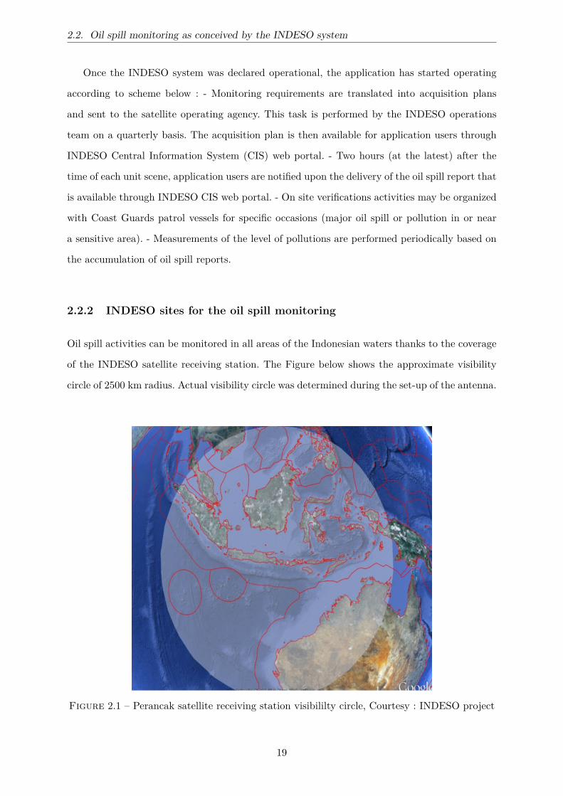
2.2. Oil spill monitoring as conceived by the INDESO system
Once the INDESO system was declared operational, the application has started operating
according to scheme below : - Monitoring requirements are translated into acquisition plans
and sent to the satellite operating agency. This task is performed by the INDESO operations
team on a quarterly basis. The acquisition plan is then available for application users through
INDESO Central Information System (CIS) web portal. - Two hours (at the latest) after the
time of each unit scene, application users are notified upon the delivery of the oil spill report that
is available through INDESO CIS web portal. - On site verifications activities may be organized
with Coast Guards patrol vessels for specific occasions (major oil spill or pollution in or near
a sensitive area). - Measurements of the level of pollutions are performed periodically based on
the accumulation of oil spill reports.
2.2.2 INDESO sites for the oil spill monitoring
Oil spill activities can be monitored in all areas of the Indonesian waters thanks to the coverage
of the INDESO satellite receiving station. The Figure below shows the approximate visibility
circle of 2500 km radius. Actual visibility circle was determined during the set-up of the antenna.
Figure 2.1 – Perancak satellite receiving station visibililty circle, Courtesy : INDESO project
19

Chapitre 2. Oil Spill Monitoring in Indonesia
Oil Spill monitoring application focus on targeted areas which are heavy density maritime
traffic areas and O&G concession areas. On the next figure, primary priority areas are depicted
in pink and secondary priority areas are shown in green. Three initial areas of interest were
originally defined : Makassar Strait, Malacca Strait and Timor Sea. Some precisions of the areas
have been updated during the phase of the project, as follow :
• Primary priority areas : Eastern part of Malacca Strait, Makassar Strait, and Timor Sea
• Secondary priority areas : Western part of Malacca Strait, Natuna Sea, Java Sea
Figure 2.2 – Primary priority (purple) and secondary priority (green) priority areas for oil spillmonitoring
Area Priority Approx. SurfaceEastern Malacca Strait Primary area 100km x 500kmMakassar Strait Primary area 960km x 390kmTimor Sea Primary area 360km x 470kmWestern Malacca Strait Secondary area 100km x 500kmNatuna Sea Secondary area 750km x 400kmJava Sea Secondary area 300km x 300km
Table 2.1 – Targeted areas for oil spill monitoring
The definition of the areas of interest is a key input for the design of the rationale for the
volume of imagery allocated for this application.
20

2.2. Oil spill monitoring as conceived by the INDESO system
2.2.3 System design
The next figure depicts the INDESO sub-systems and the interfaces implemented for the Oil
Spill monitoring application : - From the INDESO Core system : the sub-systems of the INDESO
Core that are considered are those that interact with the applications users. In this context, the
web portal of the CIS (Central Information System) is the only part of the core system that
the applications users can see although the Satellite Receiving Station (SRS) and other parts
of the CIS are operated by the Perancak team to produce the oil spill reports. - External Data
provision : Radar data are provided by satellite operating agency through Radarsat-2 satel-
lite. Meteorological forecast are provided by the National Center for Environmental Prediction
(NCEP) - Applications users will interact with the CIS system and more precisely they will use
the Maestro web portal to access to the online acquisition planning and to the oil spill report.
Figure 2.3 – Oil Spill monitoring general architecture showing external systems (INDESO Coresystem with a red star), external interfaces (data providers with a pink star) and applicationsusers (yellow star)
In INDESO system, we can find comprehensive information related to the oil spill. These
informations are included metocean data that will be used as input on trajectory modelling to
predict the movement of oil spill.
21

Chapitre 2. Oil Spill Monitoring in Indonesia
1. Oil spill detection : Oil spill detection reports are based on satellite radar imagery
and additional processing. If a potential oil spill is detected, the system will provided the
following information of geo-referenced polygon of the oil spill with detail in area, length
and width of the polygon.
2. Data radar image level 0 and level 1 : The Radar level 0 is radar raw data product.
This raw data is data from sensor on remote sensing satellite, and any auxiliary data that
required to produce remote sensing products. All of this data have not been transformed
into a remote sensing product. The Radar level 1 is radar product. It is the image generated
from the satellite signal.
3. Optical remote sensing data : This product is a radiometrically and geometrically
corrected high-precision digital imagery product.
4. Vessel detection : Using the satellite radar image and continue with additional processing
produce the information of all vessel detected, their position, size, speed and heading.
All this information are present in the report. This information is important related to
detection the source of the oil spill.
5. Wind radar : The wind radar product is coming from processing of the roughness of SAR
images.
6. Physical models outputs : This model outputs includes daily mean fields of atmospheric
fluxes, physical parameters (temperature, salinity, currents, sea level. . . ), hourly surface
variables (SST, Sea Surface Height-SSH, currents), and also hourly values of all fields at
selected mooring sites.
7. In situ observations : are real-time and historical, in-situ temperature and salinity
profiles, surface velocities, and sea level.
8. Meteorological data : consists of a 2 weeks hindcast and a 10-day meteorological forecast
for the INDESO area with an ORCA grid at 1/12 and temporal resolution of 3 hours.
9. Validation files : There are 4 datasets of validation :
(a) Daily Ocean volume transports,
22

2.2. Oil spill monitoring as conceived by the INDESO system
(b) Daily Model Sea Surface Temperature (SST) error ratio and error mean time series
per region,
(c) Enriched in situ temperature and salinity profiles with physical ocean model,
(d) Enriched UV drifters files with physical ocean model.
In this thesis we will use some informations from INDESO systems to support our analysis in
particular oil spill observation from SAR image and data related to the oil spill model trajectory.
Figure 2.4 below showed example of information of oil spill SAR detection, vessel position, wind
data, and bathymetry data.
Figure 2.4 – Oil spill observation in INDESO system with SAR detection in North of Java on25 July 2016 (black box), the wind vector (black arrow), the vessel ID and position showed intriangle with yellow number and the contour of oil spill detected in red
23

Chapitre 2. Oil Spill Monitoring in Indonesia
2.3 Detection of oil spill using EO-based imagery
Detection of oil spill in ocean can be conducted with airborne and satellite measurements.
Airborne detection carried out with simple still or video photography [13]. Nowadays, small
remote-controlled aircraft can be equipped with visible and infrared cameras [14]. Satellite de-
tection provides more advantages because it can produce regularly images in remote locations. In
this section, we will review the-state-of-the-art of oil spill detection, based on Earth Observation
(EO) data and in particular SAR-based detection.
2.3.1 Spaceborne/airborne remote sensing
There are mainly two types of remote sensing sensors, optical and infrared sensors and micro-
waves sensors. Meanwhile, there are two methods of sensors, active sensors and passive sensors.
EO-based system with passive optical sensors is using the sun’s energy reflected to the
sensors. These sensors can only be used when the energy from the sun is available, meaning at
daytime. It is possible to detect the energy from the Thermal Infra Red (TIR) at day/night time
when the amount of this energy is sufficient to be detected. Active sensors like laser fluorosensor
and SAR have their own energy emitting source. They produce their own radiation with large
amount of energy and emit directly toward their targets. The targeted object will reflect this
radiation back to the sensors. The active sensors have advantages in their capabilities to work
days and nights, independently on the sun condition. They can also detect the object that
not sufficiently radiated by the sun, for example in case of cloud coverage. Below is the list of
advantages and disadvantages of both type of sensors for oil spill monitoring.
1. Optical remote sensing
Optical remote sensing can be used to get a timely and initial map for the oil spill but it
has limitation because it is weather dependent. In optical remote sensing, measurement can be
conducted by visible, InfraRed (IR), and UltraViolet (UV). In the case of the Montara event,
when the uncontrolled release of hydrocarbon happened on 21 August 2009, AQUA, a multi-
national NASA scientific research satellite launched in 2002, showed no oil slick nearby the
wellhead (Figure 2.5). This is due to the important cloudiness. Figure 2.6 showed the detection
using TERRA (NASA satellite launched in 1999). In this optical image, oil slick was detected
more than 200 km long and its contour is showed in red line.
24

2.3. Detection of oil spill using EO-based imagery
Figure 2.5 – Image AQUA on Montara wellhead location (red dot) on 21 August 2009, no oilslick detected, the purple line is the border of Indonesia territory
Figure 2.6 – Image TERRA on Montara wellhead location on 03 September 2009, oil slickpolygon detected in red line, the purple line is the border of Indonesia territory
Oil has higher surface reflectance than water in the visible region of electromagnetic spectrum
thus oil will show up silvery and reflects light [15].
Detection with IR is relatively inexpensive. It uses scanner with infra red detectors in appli-
cation. In infra red images, thick oil slick appears hot, intermediate thick oil is cool, and thin
oil not detected [16] [17].
25

Chapitre 2. Oil Spill Monitoring in Indonesia
Oil can be detected with Ultra Violet because oil has stronger reflectivity than water in
the UV region. This measurement is relatively inexpensive and can detect thin layers of oil
slicks [18] [17].
2. Laser fluorosensors
Laser fluorosensors has capability to differentiate oil and non-oil substances backgrounds (e.g.,
seaweeds, kelp), detect oil in certain ice and snow situations and detect oil in the water column
but it is relatively expensive with potential interferences from cloud and fog [19], [20]. Currently,
it is essentially available in airborne system.
3. Microwaves sensors
Microwaves sensors has the advantage in its adaptable to different weather and all-day detection.
It is commonly used and generally preferable than optical sensors [21].
A microwave radiometer is categorized as passive device which records the natural microwave
emission from the earth. Passive microwave radiometers detect the presence of an oil film on
water by measuring the reflection of the surface as excited by the radiation from space. Some
researchers have focused on using passive microwave to image oil slicks as a remote sensing
tool [22], [23], and [24]. Radiometers is used in aircraft oil spill monitoring. Passive microwave
radiometers detect the oil-water emissivity difference, with its signals indicating oil thickness.
Even if it is all weather oil sensors, its relatively expensive in operation [25], [26].
There are two types of radar, Synthetic Aperture Radar (SAR) and Side-Looking Airborne
Radar (SLAR). They can be used in large area monitoring because they have wide area cove-
rages. They are more reliable in operation since they are applicable at night and in all weather
condition. The basic concept of radar oil spill monitoring is using capillary waves on the ocean
that reflect radar energy and produce a bright image, known as the sea clutter. Surface oil par-
tially reduces the roughness of capillary waves and gives a darker image. With this concept, it
has limitation by wind speeds. In low sea state situation, it does not produce any sea clutters,
hence the differentiation between oil and water is difficult.
Currently many different SAR systems exist, giving scientists and end-users a choice of
configurations, bands and polarizations. Several different polarizations exist based on vertical
(V) and horizontal (H) electromagnetic wave propagation. Typically transmission and reception
can be in the same polarization, i.e. VV or HH. Emitting and receiving in different polarizations
26

2.3. Detection of oil spill using EO-based imagery
results in the possibility to get 4 different channels : HH, VV, HV and VH. The use of these 4
polarizations is the so-called Polarimetry SAR. Most radar satellites have a variety of coverages,
a variety of resolutions and polarizations. Table 2.2 lists some of the current and future SAR
satellites.
Table 2.2 – List of satellite-borne SAR sensors
Satellite Launch Date Owner/Operator BandRADARSAT-2 2007 Canadian Space Agency C (quad)TerraSAR-X 2007 German Aerospace Centre X (quad)Tandem -X 2010 German Aerospace Centre X (quad)Cosmo Skymed-1/2 2007, 2010 Italian Space Agency X (dual)Risat1 2012 India Space Agency C (quad)Kompsat-5 2013 Korean Space Agency X (dual)Sentinel-1 2014 European Space Agency C (dual)RADARSAT-Constellation (3-satellites) 2018 Canadian Space Agency C (dual)
2.3.2 Detection of oil spill based on SAR imagery
Detection of oil spill is not merely when the accident of oil spill happened but in the operational
level the detection of oil spill is to monitor the oil spill that coming from the intentional release
from the ship. In this thesis we use the detection of SAR in the case of oil accident in Chapter 3.
In Chapter 4 our assessment of oil spill risk include the oil spill coming from intentional release
as capture in the Indeso oil spill detection systems and the position of ship based on the AIS
data. This subsection discuss the detection of oil spill in Indeso based on SAR imagery and it’s
relation to the position of ship.
2.3.2.1 SAR sensors
In SAR imaging, microwave pulses are transmitted by an antenna to the earth surface. The
energy that scattered back is then measured. It calculates the time delay of the scattered and
backscattered signals. Working with different frequency bands, SAR can be used in many ap-
plications. L-band in the frequency 1 GHz - 2 GHz can be applied in agriculture, forestry, soil
moisture, C-Band ( 4 GHz - 8 GHz) in ocean, agriculture and X-band (8 GHz - 12 GHz) agri-
culture, ocean, high resolution radar. Experimental work on oil spills has shown that X-band
radar yields better data than L- or C-band radar ( [27], [28], [29]).
27

Chapitre 2. Oil Spill Monitoring in Indonesia
Figure 2.7 – Synthetic aperture radar imaging system basic principle
Due to the capability to penetrating cloud, SAR can acquire images in all weather. This is
important factor that consider in operational on the tropical regions like Indonesia which are
frequently covered by cloud throughout the year. Other advantage of an active remote sensing
device, it is also capable to operate at night.
2.3.2.2 SAR processing
The detection of oil slick is limited by wind speeds. When there is not enough wind, capillary
waves are not created, radar backscattering becomes weak, and the contrast becomes insufficient.
Some phenomena like fresh water slicks, wind slicks, wave shadows behind land or structures,
seaweed beds that calm the water just above them, glacial flour and biogenic oils can interfere. It
could produce false alarms or look-alikes. Much work has taken place on means to differentiate
oil slicks and false targets as well as methods to automate the analysis process [30]. To solve this
problem, some researches have been developed in the method of edge detection [31], [32], texture
analysis [33], [34], shape analysis [35], [36], fuzzy logics [37], [38], [39], and neural networks [40],
[41], [42], [43], [44], [45].
In INDESO systems, the oil spill detection process is conducted with a semi-automated
process. It means that the system requires supervision from the Radar Analyst and utilize the
SARTool Oil module of SARTool application in the process. SARTool is designed by a CLS team
of radar experts. SARTool has proven high level performance. It has been used to detect sharp
features of interest in the radar scene and capable to produce user-friendly reports for end users.
On the detection of oil spill, there are 4 process. The description of each step is as follows :
• Detection of all suspicious slicks
28

2.3. Detection of oil spill using EO-based imagery
Using SARTool software, radar analyst analyzes SAR level-1 products. In this process, the full
resolution capacity and the best dynamic range of pixel is used. Radar analyst visually identified
all the suspicious slicks directly on the SAR image with its native geometry and projection. If
the inspection result is that no suspicious slick is detected, then the analysis is completed. In
this case no Oil Spill Detection Report is generated.
• Determination of look-alikes
On the process of SAR images analyzing, the operators in charge play an important role. They
have to analyze SAR images using a set of ancillary information about the situation at sea. Using
the supplementary information (in particular Wind product), the Radar Analysts then attempt
to discriminate all detected suspicious slicks. Some of the suspicious slicks can be categorized as
look-alikes. This look-alikes are typically caused by low wind situations, wave-current interac-
tions that dampen the short gravity waves, rain cells, cold upwelling areas and algae blooms or
suspended matters. When the cause of the look-alikes is unknown, the detected feature will be
kept and labeled as "look-alike" in the Oil spill detection report.
• Define of possible oil spills
Using the SARTool Graphical User Interface (GUI), the Radar Analyst create annotation of
possible oil spills. The SARTool GUI is very easy to used to navigate within the SAR image. It
can be used by the Radar Analyst to create Oil Spill Detection Reports as necessary. In each
Report, we can find an overview of a specific pollution that composed of one or many slicks.
• Production of Oil spill detection report
Oil spill detection report produced by the radar analyst is then indexed in INDESO Maestro
module. The report will be available on the CIS Web Interface in Oil Spill Monitoring session.
Example of INDESO oil spill report is showed in Figure 2.8.
29

Chapitre 2. Oil Spill Monitoring in Indonesia
Figure 2.8 – INDESO oil spill report
30
2.4. Oil spill transport model
2.4 Oil spill transport model
2.4.1 Introduction
The development of mathematical models to predict and forecast the fate and transport of oil
spill in marine environment has become an interesting research topic over the last decades. It
is related to the needs to mitigate the effects of oil spill to the environment. It is a challenging
topic since extremely complex phenomena may affect the fate and transport oil spill. It concerns
not only physical but also chemical processes.
Since the early sixties, a number of oil spill models have been developed. There are three
types of model. First models are essentially transport models with limited fate analysis. Second
models are oil spill model with two dimensional hydrodynamics and fate analysis. And the third
models are comprehensive oil spill model that consists of fate and transport in 3-dimensions.
Comprehensive oil spill models generally include the processes of evaporation, emulsification,
dissolution, dispersion, spreading, biodegradation, photolysis, sedimentation, advection, and oil-
shoreline interactions. In the weathering processes, the most important processes is evaporation
and emulsification [46].
Evaporation is the most important weathering process because most parts of the oil spills
evaporate within the initial stage of spill. This process is influenced by the composition of oil,
air and sea temperature, wind speed, solar radiation and slick thickness. Relative reference on
the formulation of evaporation process can be found on the research by [47], [48], [49], [50], [51],
[52], [53]. On the emulsification process, spilled oil is broken into small droplets and enters the
water column due to wave or turbulence. Light oil is usually not emulsified which is not the case
for crude oil. The emulsification significantly changes the physic and chemical properties of oil
(i.e., density and viscosity). Some researches of this process can be found on [47], [49], [50], [54],
[52], [55], and [53].
Many integrated models have been developed for the oil spill transport and fate based on
trajectory method. Some of them focus on the surface movement of spilled oil [56], [57], [58],
[59]. Some commercial versions have been developed, inter alia COZOIL [60], OILMAP [61] or
WOSM [62].
In general, the requirements of oil spill model are :
• Rapid response
31

Chapitre 2. Oil Spill Monitoring in Indonesia
• Accuracy of predictions for forecasting
• Capability to adjust predictions considering data observation
• User friendly
If rapid response is required, the model cannot have complex computational procedures. In
rapid response, the model provides short-term forecast when meteorological data are available
and reliable. Rapidity and accuracy prediction is important to minimize environmental damage
caused by oil spill. To assure the accuracy, the model has to have capability to adjust predictions
considering the input data. And the user-friendliness is yet another consideration to support the
rapid response.
Related to the INDESO project, our focus is on the operational level. In this case, the rapid
response and accuracy are the most important factors considered. The oil spill model has to
have the capability to use the meteorological and oceanography data from INDESO system as
an input data.
Ideally, a model is calibrated during actual oil spill. This concept requires the assimilation
of observed data (location of spill, winds and currents) into the model. We can then compare
with the feedback from the field to ensure the accuracy of the forecast. Linkage between the oil
spill model and satellite data or field observation should be established and used to tune and
calibrate the model. In our thesis, we will calibrate the model using the SAR-detected oil spill
and test our model in the case of Montara.
2.4.2 Lagrangian 2D Trajectory Model
In pollutant fate and transport models, the fundamental principle is the rate of change mass
concentration of pollutant within a given control volume. It is equal to the sum of the net advec-
tive flux of pollutant into the control volume, the net diffusive flux of pollutant into the control
volume and the net rate of production of pollution within the control volume. In mathematically,
that principle stated as advection-diffusion equation :
∂C
∂t= −Va · C + · (DC) + S (2.1)
where :
C = mass concentration of the pollutant
32

2.4. Oil spill transport model
Va = advective velocity of the surrounding medium
D = the diffusivity coefficient
S = external fluxes
The advective velocity depends on the currents and wind velocity, and the sea state. The
diffusive velocity depends on the sea turbulence characteristics. Usually, the latter is simulated
as a Brownian motion of particles by means of a random walk procedure [58].
2.4.3 Mobidrift
Mobidrift is the numerical model implemented by CLS that simulates the trajectory of various
objects in the sea. The objects can be icebergs, oil spill slick, Search and Rescue object and
containers. In the calculation of trajectory of the object, Mobidrift uses a forward approach.
The simulation in this model is based on a 2D Lagrangian advection scheme as we mentioned
in the subsection 2.4.2. Wind and/or current velocities are used as input for the advective
component.
As input data, we used outputs of the INDESO CIS system. In the next paragraph, we
will further discuss the wind and current data of INDESO system used in simulation. Within
Mobidrift, there are three different manner to model the presence of oil spill particles, the so-
called "slick", "outline" and "trajectory" modes. In the "Slick" mode, the oil spill is modeled as
location point or list of location points. In the "Outline" mode, the geographical coordinates of
the oil spill contour are given. The "trajectory" mode can be used when trajectory positions of
ship from AIS data are available. Mobidrift has many output formats. Standard format is XML.
In addition, Mobidrift can produce many graphics of simulated oil spills.
As input of Mobidrift, the zonal and meridian components of 10-m wind come from meteo-
rological data products provided by the INDESO CIS. Those datasets are delivered in Network
Common Data Form (NetCDF) format. The meteorological data products is provided by the
ECMWF (European Centre for Medium Range Weather Forecasting) meteorological analysis
and forecast over the INDESO area on a 1/8 horizontal grid and a 3-hour temporal resolution
up to 6 days and 6-hour temporal resolution after (10 days). The results of post-processed of
this fields are able to be read on the ocean model with an ORCA grid at 1/12 [63].
33

Chapitre 2. Oil Spill Monitoring in Indonesia
Our Mobidrift input of ocean current data is provided by INDESO physical model outputs.
INDESO produce daily mean fields of atmospheric fluxes, physical parameters (temperature,
salinity, currents, sea level. . . ), hourly surface variables (SST, SSH, currents), as well as hourly
values of all fields at selected mooring sites and validation metrics. The regional ocean physical
model provides physical fields for the past two weeks (forced by a global 2-weeks analysis) and
ocean forecasts (forced by a global 10-day forecast) for the next 10 days. INDESO physical ocean
model has a horizontal resolution of 1/12 and 50 vertical layers. The resolutions are increased
near the surface. Meanwhile on the horizontal grids are provided on a regular 1/12.
In our Mobidrift simulation, we used the bathymetry data based on ETOPO2V2g (2-minute
grid) and GEBCO (1-minute grid). This bathymetry has been locally modified by a hand editing
mainly on the straits with a threshold value of 7m.
2.4.4 Application of Mobidrift in Indonesia’s Oil Spill Trajectory
In this thesis, we use the CLS Mobidrift to simulate the drift of oil slick in two applications,
both of them is to support mitigation planning and development of marine and fisheries. First
application is on the case of Montara oil spill. In this application, Mobidrift is used to simulate
the drift of oil spilled from the Montara oil platform. There are three data that we used as
an input to Mobidrift from INDESO system output i.e bathymetry, wind velocity and current
velocity. An illustration of these data is showed in Figure 2.9, 2.11 and 2.10. Then we will
compare this simulation with the detection of SAR. We will discuss in more details application
of Mobidrift in Montara oil spill in Chapter 3. The second application is on the assessment of
oil spill risk in the Indonesian FMA.
34

2.4. Oil spill transport model
Figure 2.9 – Bathymetry (meter) of the INDESO configuration. (ETOPOV2g/GEBCO1 +in-house adjustments in straits of major interest)
Figure 2.10 – Sea surface current velocity (m/s) on 01 January 2015 data from the INDESOsystem
35

Chapitre 2. Oil Spill Monitoring in Indonesia
Figure 2.11 – Wind velocity data (m/s) and its direction (black arrow) on 01 January 2015data from the INDESO system
36
2.5. Conclusion
2.5 Conclusion
This chapter has discussed the current oil spill monitoring system in Indonesia. We began with
the description of Indonesia waters that give brief illustration of general aspects of ocean circu-
lation and main issues of Indonesia marine and fisheries related with oil spill. Then we explain
the oil spill monitoring as conceived by the INDESO system. In this subsection, we showed the
system design of INDESO. Further, we discussed the detection of oil spill using SAR imagery as
used in INDESO systems. The state-of-the-art of SAR detection was presented. And finally, the
oil spill transport model was discussed. First we reviewed the state-of-the-art of oil transport
model and we discussed the Lagrangian 2D model trajectory model. In this research, we use the
Lagrangian-based CLS Mobidrift model to simulate the oil slick transport in the ocean. Using
the output data from INDESO CIS as the input for Mobidrift, we will analyze the Montara
study case and will calculate the risk and cost of oil spill in Indonesia. These applications are
presented in the following two Chapters.
37

38

3
Chapit
re
Oil spill parameter retrieval
3.1 Introduction . . . . . . . . . . . . . . . . . . . . . . . . . . . . . . . . . . . . . . . 40
3.2 Proposed approach . . . . . . . . . . . . . . . . . . . . . . . . . . . . . . . . . . . 42
3.3 Montara SAR based oil detection . . . . . . . . . . . . . . . . . . . . . . . . . . 44
3.4 Similarity between SAR oil spill detection and model . . . . . . . . . . . . . . . . 47
3.5 Estimation of oil leakage parameters assimilation of SAR images . . . . . . . . . 49
3.6 Application to Montara case study . . . . . . . . . . . . . . . . . . . . . . . . . . 52
3.7 Conclusion . . . . . . . . . . . . . . . . . . . . . . . . . . . . . . . . . . . . . . . 59
39
Chapitre 3. Oil spill parameter retrieval
3.1 Introduction
Oil spill is one of the most serious threat for all marine and coastal environments. Oil spill
can cause high economical and ecological damages in marine and coastal ecosystems. Indonesia,
as an archipelago country, is particularly vulnerable to oil spill since national waters, which
account more than 70% of its territory, involve a very active maritime traffic and a large num-
ber of onshore and offshore oil platforms. The accidental or intentional releases of petroleum
products are the two sources of oil pollution into the marine environment. Even though the
pollution from voluntary rejection of waste oil and residual fuel are of high importance, for ins-
tance the equivalent of 50 Erika or 15 Prestige per year in the Mediterranean Sea [64], major
oil spill accidental disasters such as Deepwater Horizon or Torrey Canyon oil spills still have
devastating long-term consequences for society, economically, environmentally, and socially [65].
Montara oil spill in 2009 stressed the urgent needs for the operational monitoring of oil spill in
Indonesian waters. The operator, PTTEP Australasia (Ashmore Cartier) Proprietary Limited
(PTTEP AA), initially estimated the oil leakage to 400 barrels (or approximately 64 tonnes)
of crude oil lost per day [66]. The uncontrolled release started on 21 August 2009 and crude oil
continued to be released until 3 November 2009 when the well brought under control. Montara
wellhead platform is located in Australian waters at coordinate latitude 1240′20.5′′N and lon-
gitude 12432′22.2′′E. The depth of water was approximately 250 ft (76 m) as show in Figure
3.1. It is very close to Indonesian waters, only 310km from Timor island. This south-most island
Indonesia archipelago has an important ecological and economical value. There are 3,355,352.82
hectare of marine protected areas in Sawu seas. Its coral ecosystems with 532 coral reef species
and 11 species endemic with total area 633.39km2 [67] is a peculiar example. Following Mon-
tara oil spill, the Indonesian Ministry of Marine and Fisheries Affairs initiated the development
of ocean monitoring systems, in combination with operational oceanography, especially within
the framework of Infrastructure Development Space Oceanography (INDESO) project. In this
context, the present study addresses the assimilation of satellite-based Synthetic Aperture Ra-
dar (SAR) observations of oil spills into an oil trajectory model. It relies on Lagrangian-based
simulations of the transport of particles at sea surface and on the comparison of transport si-
mulations and detected oil spills from implicit level-set-based representations. Using Montara
oil spill as a case study, we demonstrate the relevance of the proposed model and associated
40

3.1. Introduction
Figure 3.1 – Position of the Montara oil platform on the map of bathymetry, the red sign isMontara wellhead position and the black box is our boundary box for oil trajectory simulation.
numerical scheme for the optimization of oil leakage parameters (namely the starting date of the
leakage, its duration, the mean wind-related and current-related drift coefficients). This work
is organized as follows, in Section 3.2 describes the proposed approach. We report numerical
experiments in Section 3.3. Section 3.4 further discusses the key features of the proposed model.
41

Chapitre 3. Oil spill parameter retrieval
3.2 Proposed approach
We report in Figure 3.2 the synoptic sketch of the proposed approach for the assimilation of oil
leakage parameters from satellite-based SAR observations. Our approach involves three main
components :
• A Lagrangian-based 2D transport model, which simulates the advection of particles at sea
surface under given wind and current conditions. This component is detailed in Section
3.3 ;
• The detection of oil spills from satellite-based SAR observations in Section 3.4 ;
• The definition of a similarity measure between simulated particle sets and oil spill detection
from satellite-based SAR observations as detailed in Section 3.5.
These three components are combined within an assimilation model and applied in Montara
case detailed in Section 3.6 along with the associated numerical resolution.
42

3.2. Proposed approach
Initial source : time (T0),position (P0), duration (∆t0),
Wind drift factor (Cw) andCurrent drift factor (Cc),
Transport modelinitialization
Wind dataECMWF
(Vw) Currentdata Mer-cator (Vc)
Simulation of par-ticle trajectories =
Pt+∆t= P0 + (Vc.Cc +
Vw.Cw).(T + ∆t)
Level-setrepresentation
of the simulatedparticle spread
Islevel-setdistanceminimi-
zed ?
Level-setrepresentationof SAR-derivedoilspill contourOs = (x, y, Ts)
update modelparameters
T, ∆t, Cw, Cc
stop
no
yes
Figure 3.2 – Flowchart of the proposed approach for the assimilation of oil leakage parametersfrom satellite-based SAR observations
43

Chapitre 3. Oil spill parameter retrieval
3.3 Montara SAR based oil detection
The analysis of oil spill dynamics is an active research topics [68]. The considered models
range from 2D surface trajectory to 3D+t space-time dynamics and fate analysis. In gene-
ral, an oil spill model combines a description of the oil spill, which may include the space-
time extension of the oil spill as well as geochemical characteristics, and the undergoing wea-
ther conditions, typically wind and current conditions. In general, commonly used operatio-
nal oil spill models include GNOME (General NOAA Operational Modeling Environment,
http://response.restoration.noaa.gov/), MOTHY (French operational oil spill drift fore-
cast system, http://www.meteorologie.eu.org/mothy/), OSCAR (Oil Spill Contingency and
Response, http://www.sintef.no), ADIOS2 (Automated Data Inquiry for Oil Spills, http:
//response.restoration.noaa.gov), OILMAP (Oil Spill Model and Response System, http:
//www.aims.gov.au/pages/research/oil-map/oil-map01.html) and OSIS (Oil Spill Identi-
fication System, http://www.osis.biz/ss2.asp) [69]. In the Deepwater Horizon, as one of the
biggest oil platform leakage accident, the efforts of observation to detecting the existence of oil
on the ocean surface and modeling of the oil spill trajectory are well documented [70]. One of the
study that was conducted for this accident is an assimilation of modeling and satellite-observed
surface oil locations where models were seeded with oil location inferred from satellite images
with virtual particles and then these particles were advected with the surface velocity fields as
forecast by numerical ocean circulation models [71]. The simulated surface oil trajectories were
compared to the satellite observations in subsequent forecast cycles for veracity testing [72]. We
consider some study application on case of the oil spill accident i.e two oil platforms in the Bohai
Sea, China [73] and The Shell North Sea Gannet Alpha platform [74].
Here, our focus is on the assimilation of oil leakage parameters and we consider a computationally-
tractable surface transport model. The oil spill leakage is characterized by the location of the
source of the leakage, the type and quantity of oil. The considered transport model, namely
Mobidrift model [75] developed by Collecte Localisation Satellite (CLS), simulates Lagrangian
trajectories of particles at sea surface for given wind and current conditions. In Mobidrift mo-
del, fluids are modeled by a set of deterministic particles. For a source defined by a fixed oil
platform, we provide to Mobidrift model the location of the source, the starting time for the
release of particles and the duration of the leakage. For each particle released from the initial
44

3.3. Montara SAR based oil detection
position, we apply the considered 2D transport model to derive its trajectory up to the final
date of the simulation. In our simulations, we typically consider about 500 particles released
on a daily basis. Formally, Mobidrift model relies on the two-dimensional advection of particles
by a surface displacement given by a weighted sum of tidal current and wind-induced current
velocities
uadvp = Cc · Vc + Cw · Vw (3.1)
where uadvp is the advection velocity, Vc the sea surface current and Vw the sea surface wind speed
at a height of 10m. Coefficients Cc and Cw are the current and wind drift factors. In our study,
as sea surface wind and current data, we use PSY4V2 MERCATOR system (1/12 horizontal
resolution) with daily forecast production [76], and 10-meter wind field provided by the analysis
of the European Centre for Medium-Range Weather Forecasts (ECMWF) at a 0.140 spatial
and 6-hour temporal resolution [77].
The transport model is complemented with a diffusion component. Neglecting viscous effects,
the total velocity of a transported particle can be decomposed as
dx
dt= uadv
p (x, t) + udifp (x, t) (3.2)
where udifp (x, t) is the diffusive component, which amounts to an isotropic Gaussian velocity,
parameterized by standard deviation σ.
The simulation of the displacement of a particle between time t and time t + δt resorts to
the integration of Eq. (3.2) :
xp(t + δt) = xp(t) +t+δt∫
t
uadvp (xp, t) dt +
t+δt∫
t
udifp (xp, t) dt. (3.3)
It should be stressed that, through the stochastic diffusive component, the numerical integra-
tion results in a randomized simulation of trajectories. As a result, from multiple numerical
integration, this transport model results in the simulation of the spread of an oil spill.
Wind drift factor Cw in eq. (3.1) typically ranges from 0.01 to 0.06 [78–80]. In many appli-
cations of oil movement forecast, wind drift factor Cw is set to 0.03 [59], [81]. Regarding sea
surface current, drift factor Cc typically ranges from 1.0 to 1.5 [79]. In this study, factors Cw
45

Chapitre 3. Oil spill parameter retrieval
and Cc are among the oil leakage parameters estimated to assimilate the satellite-based SAR
observations and the simulated oil particles from trajectory models.
46

3.4. Similarity between SAR oil spill detection and model
3.4 Similarity between SAR oil spill detection and model
Remote sensing can provide substantial support to routine surveillance in open-ocean and coastal
areas and has the advantage of being able to observe oil spill events in remote and often inac-
cessible areas. The high resolution radar technology (the so called Synthetic Aperture Radar -
hereafter SAR) on board satellites is widely used for operational oil spill surveillance [82], [83].
The information that is present in these data can be useful for extracting important indica-
tions for risk assessment, emergency management, and damage inventory [84].
Thanks to its very wide area coverage and its capability to work day/night independently of
the cloud coverage, space-borne SAR technology provide cost-efficient means. Flying at about
800km altitude, SAR sensors emit electromagnetic (EM) waves with frequency ranging from 1
to 10GHz. At these EM wavelengths, the sea surface back-scatters the EM waves back to the
sensor, depending on the sea state and radar acquisition geometry following Bragg theory. An
oil spill dampens the sea surface roughness, and basically induces a decrease of this EM back-
scattering compared to the surrounding clean water. Hence, the oil spill appears darker on the
SAR image (see red contour in Figure 3.3). It is well established that reliable slick detection’s are
performed for wind speeds in the approximate range of 2.5 to 12.5m/s. In the case of low winds
situation (below 2.5m/s), the clean sea-surface and the slick show similar radar backscattering
and cannot be distinguished automatically. The operators in charge of analyzing SAR images
shall make the best use of any available contextual information such as ancillary data (Sea
Surface Temperature, wind field, chlorophyll-A concentration, etc.) in order to assess in the
most efficient manner the situation at sea such as captured by the SAR sensor. Some method
was developed using µ as a logical scalar descriptor to map oil slicks under low to moderate
wind conditions [85].
The oil properties at the sea surface are affected by weathering processes (evaporation,
emulsification, photo-oxidation). The weathering of hydrocarbons is complex as it combines
the diversity of petroleum products, which have very variable physical-chemical characteristics,
with the variety of environmental conditions (wind and waves, sea temperature, etc.) As the
SAR sensor is mostly sensitive to sea surface roughness, slick with low viscosity or into the sea
subsurface may not be detected.
47

Chapitre 3. Oil spill parameter retrieval
Figure 3.3 – SAR Observation on September 02, 2009 by ENVISAT, red contour outlines themain patches of weathered oil on the sea surface, the red dot is Montara wellhead position andthe purple outlines the border of Indonesia (above the line) and Australia water territory (belowthe line).
In this study, the first SAR image covering the Montara event is used. It was observed on
September 02, 2009 at 10 :07 UTC by the European ENVISAT mission (see Figure 3.3). The
spatial resolution is 75 × 75 meters with swath width of 400km. Since the blowout from the
Montara wellhead platform first occurred on the 21st of August 2009, this image was taken 12
days after the accident. As seen by the SAR sensor, the oil slick is still connected to the wellhead
platform, with estimated 160km long.
It is worth noting that the resolution of SAR observation does not induce a dramatic evolution
of the detection quality [86], nevertheless, spatial resolution of auxiliary data has a significant
impact on the drift simulation and oil slick deformation. So that, the quality of auxiliary data
impacts the quality of oil leakage parameters estimation.
48

3.5. Estimation of oil leakage parameters assimilation of SAR images
3.5 Estimation of oil leakage parameters assimilation of SAR
images
A key component of our approach is the definition of a measure of the goodness of the match bet-
ween the detected oil spill and the simulation of transport model trajectories. This amounts to
defining a similarity measure between a set of particles and a contour within a two-dimensional
plane. We exploit implicit level-set representations of contours as introduced by Osher and Se-
thian [1]. As illustrated in Fig.3.4, the level-set representation comes to define a two-dimensional
contour Γ as the zero-level-set of a function φ, that is to say the set of points of the plane at
which the value of function φ is zero :
Γ = p ∈ Ω such that φ(p) = 0 (3.4)
where Ω is the considered spatial region. As illustrated in Fig. 3.4, the level-set function φ is
positive inside contour Γ and negative outside. Given function φ, the extraction of contour Γ
simply comes to extract the contour of a thresholded version of function φ at zero. Conversely,
one can build the level-set representation of any contour in the plane as the solution of partial
differential equation [1] using efficient numerical algorithms. A key interest of this level-set
representation is its ability to represent non-connected objects.
Level-set functions also provide a simple mean, without any topological constraint, to eva-
luate the similarity between any two contours Γ1 and Γ2 from a distance between their level-set
representations [1] :
d (Γ1, Γ2) =∫
Ω‖φ1(p) − φ2(p)‖2dp. (3.5)
This level-set representation directly applies to the contour of the satellite-based SAR detection
of the oil spill. We also derive a level-set representation of the spread of the particle sets simulated
by the considered Lagrangian transport model. Given a set of particles, we first derive the
associated spatial density distribution DS using a kernel-based estimation [87]. We then extract
the contour ΓS of the level-set of density distribution DS , which accounts for a predefined
percentage of particles. Let us denote by λ this percentage and LLS(ν) the level-set of DS with
respect to level ν
LLS(ν) = p ∈ Ω such that DS(p) > ν. (3.6)
49

Chapitre 3. Oil spill parameter retrieval
Contour ΓS(λ) is then extracted as the contour of level-set LLS(ν∗) such that |LLS(ν∗)|/|Ω| = λ.
We typically set λ to 0.85, such that the contour extracted to represent a particle set accounts for
85% of the simulated particles according to transport model defined by Eq. (3.3). As illustration,
we show on Fig. (3.5) the contours of the kernel-based estimate created with different values for
spatial density of simulated particles from Lagrangian transport model.
Using the standard Euclidean distance between level-set functions, we define a distance
between transport model simulations, characterized by density function DS and associated refe-
rence contour ΓS(λ), and the detected oil spill ΓSAR from the distance between their respective
level-set functions φS(λ) and φSAR :
d (ΓS(λ), ΓSAR) =∫
Ω‖φS(λ)(p) − φSAR(p)‖2dp. (3.7)
Figure 3.4 – Level-set [1] representation of closed contours in a two-dimensional plane : whenthe contours t=0 (yellow,-) with the value φ < 0 moving forward on t=1 (blue,-) with the valueφ > 0
Let us denote by θ the parameters to be estimated, namely leakage date dL and duration
∆L, and the mean surface current and wind drifts, respectively Cc and Cw. Let us denote by
50

3.5. Estimation of oil leakage parameters assimilation of SAR images
ΓSAR the contour of the detected oil spill from the SAR observation. We state the estimation
of leakage parameters θ as the maximization of the similarity between the detected oil spill
and the simulated particle set from the Lagrangian transport model of eq. (3.3) with respect to
parameters θ. Numerically, it comes to solve for the following minimization :
θ = arg minθ
d (ΓS(λ|θ), ΓSAR) , (3.8)
where contour ΓS(λ|θ) refers to the simulation of the Lagrangian transport model of eq. (3.3)
from the known leakage source with respect to parameter θ.
The numerical resolution of this minimization exploits Powell’s method [88] as we cannot
derive the first-order derivatives of the considered function with respect to parameter θ. Powell’s
method iterates until convergence one-dimensional searches along conjugate directions, initiali-
zed as the basis vectors of the considered n-dimensional parameter space. Our implementation
uses the scipy optimization package under Python environment.
Figure 3.5 – Spatial density of a set of particles simulated from Lagrangian transport model(3.2). The simulated particle set is depicted as a set of blue dots. We also display the contourof the kernel-based estimate of the spatial density of the simulated particle set.
51

Chapitre 3. Oil spill parameter retrieval
3.6 Application to Montara case study
As a mean to investigate the sensitivity of transport model simulations with respect to oil leakage
parameters, we first report assimilation results for one-day oil leakage ranging from August 21
to September 02. This first simulation uses different dates of source of leakage with one day
duration.
The result is given in Fig. 3.6-above, showing that the first five days of leakage give the
minimum value of RMSE. For each date, we solve for minimization Eq. (3.8) to estimate wind
and current drift factors Cw and CC . We report in Fig. 3.7 and 3.8 the series of the optimal
parameters Cw and CC related to the simulations on the Fig. 3.6-above. For the source of leakage
August 21, 2009 with one-day duration, the minimum RMSE was reached for the optimal drift
factors Cw = 0.0493 and CC = 1.221 The values of optimal current drift factor range from
1.2 to 1.3 (boundary given to the Powell’s method being [0.1, 2]). The retrieved optimal wind
drift factors range from about 0.037 to 0.049 (boundary for the optimization scheme being
[0.01, 0.06]). Overall, these initial experiments point the greater contribution of the oil leakage,
which occurred from the first five days, to the oil spill detected from the SAR observation on
September 02, 2009.
Then we try to simulate the leakage with different duration. The result for simulation from a
leakage start on August 21,2009 with different duration is given in Fig. 3.6-below. This simulation
shows that the RMS error decreases as the duration increases. The minimum RMS error was
reached for the source of leakage August 21, 2009 with duration 12 days. Most of the surface
of the detected oil spill is actually explained by the leakage occurring on the first 5 days was
happened for its duration maximum (12 days for source of leakage 21 August, 2009, 11 days for
source of leakage 22 August, 2009, 10 days for 23 August, 2009, etc.) We will see the proof of
this hypothesis later in Fig. 3.11.
52

3.6. Application to Montara case study
Figure 3.6 – Minimum RMSE of level set value of images SAR on September 02, 2009 withsimulations of one-day oil leakage from August 21, 2009 to August 02, 2009 (a) and oil leakagestarted on 21 August,2009 with different duration (b) from Montara wellhead platform.
53

Chapitre 3. Oil spill parameter retrieval
Figure 3.7 – Optimum value of wind drift factor Cw from simulations of one-day oil leakagefrom Montara wellhead platform from August 21, 2009 to September 02, 2009.
Figure 3.8 – Optimum value of current drift factor Cc from simulations of one-day oil leakagefrom Montara wellhead platform from August 21, 2009 to September 02, 2009
As an illustration of Powell’s optimization procedure, we illustrate in Fig. 3.9 the minimized
cost function landscape and the points at which the cost function is actually evaluated for
54
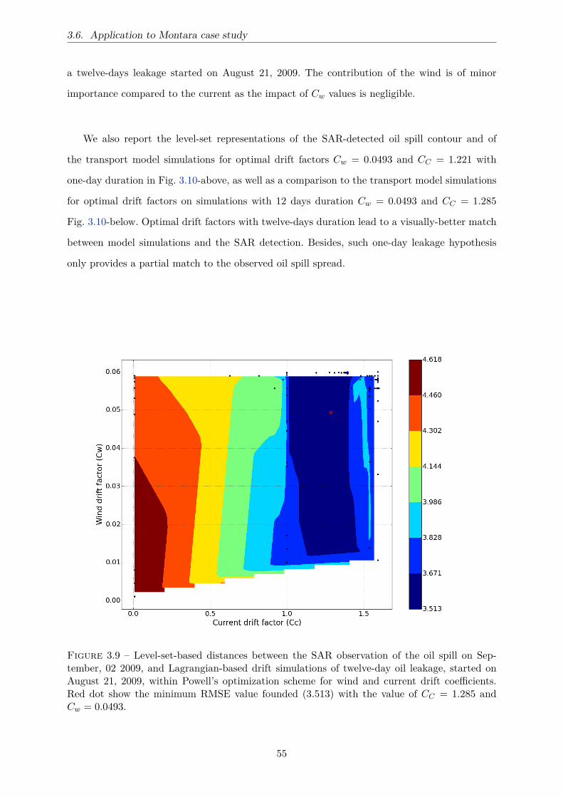
3.6. Application to Montara case study
a twelve-days leakage started on August 21, 2009. The contribution of the wind is of minor
importance compared to the current as the impact of Cw values is negligible.
We also report the level-set representations of the SAR-detected oil spill contour and of
the transport model simulations for optimal drift factors Cw = 0.0493 and CC = 1.221 with
one-day duration in Fig. 3.10-above, as well as a comparison to the transport model simulations
for optimal drift factors on simulations with 12 days duration Cw = 0.0493 and CC = 1.285
Fig. 3.10-below. Optimal drift factors with twelve-days duration lead to a visually-better match
between model simulations and the SAR detection. Besides, such one-day leakage hypothesis
only provides a partial match to the observed oil spill spread.
Figure 3.9 – Level-set-based distances between the SAR observation of the oil spill on Sep-tember, 02 2009, and Lagrangian-based drift simulations of twelve-day oil leakage, started onAugust 21, 2009, within Powell’s optimization scheme for wind and current drift coefficients.Red dot show the minimum RMSE value founded (3.513) with the value of CC = 1.285 andCw = 0.0493.
55

Chapitre 3. Oil spill parameter retrieval
Figure 3.10 – Level-set-based representation of the SAR-derived detection of the oil spill onSeptember 02, 2009, and Lagrangian-based drift simulations for a one-day oil leakage on August21, 2009, with optimal wind and current drift coefficients, Cw = 49.3% and CC = 122.1% (a)and Lagrangian-based drift simulations for a twelve-days oil leakage started on August 21, 2009with optimal wind and current drift coefficients, Cw = 49.3% and CC = 128.5% (b). The SARdetection and simulation contours are shows in blue and red line respectively and red dot is theposition of Montara oil platform
We then carry out to the joint assimilation of both the oil leakage starting date, its duration
and drift factors Cw and CC . For each starting date and duration configuration, we proceed to
56

3.6. Application to Montara case study
Figure 3.11 – Optimal level-set-based distances between the SAR observation of the oil spillon September 02, 2009, and Lagrangian-based drift simulations of oil leakage with respect toleakage starting date (x-axis) and duration (y-xis). The optimal level-set-based distances areissued from Powell’s optimization of wind and current drift coefficients.
minimization of Eq. (3.8). We report in Fig. 3.11 the resulting optimal level-set-based distances
between the detected oil spill and transport model simulations as a function of the starting date
of the oil leakage and of its duration. The series of the level-set-based distance depict a clear
increasing trend, which stresses the impact of the initial oil leakage on August 21. These results
clearly support the existence of a continuous oil leakage for at least 5 days starting on August 21,
2009 with the minimum RMSE reached for oil leakage from oil leakage on August 21,2009 with
duration 12 days. Estimated optimal drift factors, respectively Cw = 0.0493 and CC = 1.285,
are realistic and in agreement with the experiments reported above and previous work [78–80].
In Figure 3.11, the comparison between transport model simulations and the SAR-derived oil
spill detection on September 02, 2009 points out the improved match associated to the five
first-day with duration until the September 02 leakage hypothesis compared with the one-day
leakage hypothesis with nominal and optimized wind and current drift factors. It is worth noting
57

Chapitre 3. Oil spill parameter retrieval
that the Mobidrift simulations does not account for concentration effect of the particles in the
diffusion process so that it yields a similar level-set shape with the duration of leakage. That
explains the flatness of the level-set distances of Fig. 3.11 with duration leakage between 2 and
12 days.
58

3.7. Conclusion
3.7 Conclusion
We developed a novel framework for the assimilation of oil leakage parameters, including lea-
kage starting data and duration along with wind and current drift factors, from a SAR-derived
detection of an oil spill. This framework states the assimilation as the minimization of a level-set
representations of the SAR-derived oil spill detection and of 2D transport model simulations.
We illustrated its relevance on Montara oil spill case study. We showed that the observed oil
spill on September 02, 2009 was mainly due to the oil leakage from August 21 until September
02 with majority of slick is coming from five first days of leakage (August 21-25, 2009). The
estimated wind and current drift factors were in agreement with values previously reported in
the literature. They were however significantly different from nominal parameters and shown to
affect the match between the observed oil spill and transport model simulations.
This study opens new research avenues for the satellite-based operational monitoring of oil
spills. Future work will further investigate the assimilation of oil leakage parameters from multi-
date observations as well as other oil leakage configurations, such as illegal oil discharges from
vessels or natural oil seeps.
59

60

4
Chapit
re
Oil spill risk assessment in Indonesian
Fisheries Management Area
4.1 Introduction . . . . . . . . . . . . . . . . . . . . . . . . . . . . . . . . . . . . . . . 62
4.2 Data and Study area . . . . . . . . . . . . . . . . . . . . . . . . . . . . . . . . . . 65
4.2.1 Study Area . . . . . . . . . . . . . . . . . . . . . . . . . . . . . . . . . . . 65
4.2.2 Data Collection . . . . . . . . . . . . . . . . . . . . . . . . . . . . . . . . . 66
4.2.3 Marine Protected Area Data . . . . . . . . . . . . . . . . . . . . . . . . . 71
4.2.4 Marine fisheries data . . . . . . . . . . . . . . . . . . . . . . . . . . . . . . 74
4.2.5 Socio-economic data for fishing activities, tourism services and salt ponds 75
4.3 Proposed methodology . . . . . . . . . . . . . . . . . . . . . . . . . . . . . . . . . 77
4.3.1 Oil spill risk indices . . . . . . . . . . . . . . . . . . . . . . . . . . . . . . 77
4.3.2 Environmental and socio-economical vulnerability indices . . . . . . . . . 80
4.3.3 Global FMA-level risk index . . . . . . . . . . . . . . . . . . . . . . . . . 83
4.3.4 MPA-level vulnerability analysis . . . . . . . . . . . . . . . . . . . . . . . 84
4.4 Results and Discussion . . . . . . . . . . . . . . . . . . . . . . . . . . . . . . . . . 87
4.5 MPA-level risk assessment . . . . . . . . . . . . . . . . . . . . . . . . . . . . . . . 89
4.6 Conclusion and Discussion . . . . . . . . . . . . . . . . . . . . . . . . . . . . . . . 101
61

Chapitre 4. Oil spill risk assessment in Indonesian Fisheries Management Area
4.1 Introduction
Oil spill is one of the most destructive marine pollution with high impact on marine environ-
ments. Its negative impacts are not limited to wildlife, fisheries and coastal habitats but also
affect human activities. Oil spill source coming from natural events and mostly from anthro-
pogenic activities. Even though the number of marine accidents and the volume of oil released
accidentally have declined, major oil spill accidental disasters such as Deepwater Horizon [89]
Torrey Canyon oil spills [90] still have devastating long-term consequences. In addition, the still-
growing activity of maritime transportation increases the risk of illegal oil discharges as well
as accident-related pollutions. For instance, oil tankers are often among the ships suspected of
illegal discharges. Routine tanker operations can lead to the release of oily ballast water and
tank washing residues. Other oil-related waste produced by all types of ships such as fuel oil
sludge, engine room wastes and foul bilge water, may also be released in the sea.
Indonesia is one of the largest maritime country in the world. It covers a 5.8 million km2
water territory that consists of 2.7 million km2 of exclusive economic zone and a 3.1 million km2
territorial sea [91]. As three international sea lanes go across Indonesia waters, they involve a
dense maritime traffic. From [92], the main sources of marine pollution in Indonesia are wastes
from oil refineries, offshore exploration and shipping. The increase of maritime transportation,
oil refineries and offshore exploration increases the threat of oil spill in Indonesian seas, the
Montara oil spill in 2009 being a striking example [93]. In several regions oil spill is still a
recurrence problem with unidentified source.
Marine and coastal resources are of key importance for Indonesia. Marine capture fisheries
is one of the most important food resources which production from 2005 to 2014 increased
on average of 3.58% per year. From 4 408 499 tonnes in 2005, fish production increased to
6 037 654 tonnes, with a commercial value of more than 7.5 billion dollars in 2014 [94]. The
fish production consists of large and small pelagic species and demersal fish stocks as well
as crustaceans, molluscs, and seaweeds. To enhance the management of marine and fisheries
resources, the Ministry of Marine and Fisheries Indonesia divided marine waters into 11 Fisheries
Management Areas (FMA). Indonesia also involves a very high biodiversity of species with a
variety of important species such as coral reef fish, cetaceans, sea turtles, mangroves, sea grass,
62

4.1. Introduction
dugongs, and seabirds. In some specific regions, the Government of Indonesia created in 2013
Marine Protected Areas (MPA) for a total surface area of 17 144 702 ha [95].
One of important biodiversities in the coastal zone is coral reef . A literature has mentioned
the destructive influence of oil spill on coral reef. The oil will agitate the colony viability, damage
the reproductive systems, lower growth rates and so on [96]. coral reef fish is the habitat for the
coral reef fish. There is a positive relation between the live coral cover and the number of coral
fish species as mentioned in the research conducted in the lagoon of Mataiva Atool, Tuamotu
Archipelago [97]. Oil spill that destruct the coral reef will certainly impacted the coral reef fish.
As reported from Directorate General Aquaculture MMAF, coral reef fish is one of contributor
to Indonesia export product with value in 2014 more than US$ 20 million. In our work, we
consider the coral reef fish as one of component that will be used on the risk assessment of oil
spill that will be discussed later. Due to the increasing awareness of oil spill threat, the Indonesian
government in cooperation with France has been developing ocean observation systems, oil spill
monitoring being one of the targeted applications. This system is integrated with the spatial
oceanography systems in the framework of INDESO project (Infrastructure of Development
Space Oceanography). Using Synthetic Aperture Radar (SAR) sensors on-board satellites, one
can monitor and detect oil spill at sea surface. The combination of such oil spill detection to
Lagrangian drift models provides means to predict the drift of detected oil spills and their
potential impact [93]. Many government institutions, such as the Ministry of Transport, the
Ministry of Environment and Forestry, the Ministry of Marine and Fisheries, the Ministry of
Energy and Mineral Resources, the National Disaster Management Authority, the Maritime
Security Coordinating Agency, etc., have developed specific policies regarding intentional and
unintentional oil spills. To implement such policies, especially monitoring and surveillance efforts,
the assessment of a risk level that vulnerable areas may be impacted by oil spill sources is of high
interest. For instance, in the North of Java and in Batam Island, recurrent oil spill occurrences
are reported. Information onto their impacts on the coastal and marine ecosystems would be of
key interest to implement adequate mitigation plans.
Recent studies have addressed similar issues in other regions. Several studies have analyzed
oil spill pollutions in terms of ecological damage and of vulnerability for coastal area and coastal
zone management [98], [99]. Fewer studies have targeted both environmental and socio-economic
vulnerability to oil spill pollution. We may cite the combination of environmental and socioe-
63

Chapitre 4. Oil spill risk assessment in Indonesian Fisheries Management Area
conomic factor in Noirmoutier Island (France) [100], the determination of oil spill risk levels in
coastal waters of Thailand [101], or the assessment of oil spill risk levels in the Chinese Bohai
Sea [102]. The later analyzes different oil spill sources, namely ship and platform pollutions.
In this context, the objective of this study is to provide practical information for improving oil
spill prevention and management policies for the Indonesia government, with a focus on Fisheries
Management Areas. The proposed methodology involves two main steps : i) the assessment of
global oil spill risk levels at the scale of fisheries management areas, ii) for high-risk areas, a
further analysis at finer space-time scales using oil spill drift simulations. For these two levels,
the vulnerability of a given area is evaluated both in terms of ecological and economical impacts.
The ecological impact is evaluated with respect to a biodiversity index and the surface of MPA
(Marine Protected Areas), whereas the economical impacts takes into account the economic value
of exploited resources as well as the direct and indirect employment level of fisheries activities
and maritime services. Our study clearly highlights strong discrepancies in the vulnerability to
oil spill threat over the considered fisheries management areas. Such knowledge is of key interest
to implement appropriate spatialized monitoring and prevention plans.
This Chapter is organized as follows. In Section II, we describe the characteristics of our study
area. Section III presents the proposed methodology for the assessment of the vulnerability to
oil spill pollution. We report the application of this methodology to the considered case study
are in Section IV. Section V further discusses the key features of the proposed study.
64

4.2. Data and Study area
4.2 Data and Study area
4.2.1 Study Area
Figure 4.1 – Map of the study area with Indonesian Fisheries Management areas in blue,Indonesian land territory (in white) and its neighboring country (in brown), Marine ProtectedArea (in red) and ship density map estimated from AIS data to be used as potential source ofunintentional and intentional oil spills (in green triangle)
Our study area comprise the Indonesian marine waters. From Ministerial Decree Number
18 on 2014, they were divided into 11 Fisheiries Management Areas (FMA), namely : (1) FMA
571 for Malacca Strait and Andaman Sea, (2) FMA 572 for Indian Ocean of Western Sumatera
and Sunda Strait, (3) FMA 573 for Indian Ocean of Southern Java, Southern Nusa Tenggara,
Savu Sea, and Western Timor Sea, (4) FMA 711 for Karimata Strait, Natuna Sea and South
China Sea, (5) FMA 712 for Java Sea, (6) FMA 713 for Makassar Strait, Bone Bay, Flores Sea
and Bali Sea, (7) FMA 714 for Tolo Bay and Banda Sea, (8) FMA 715 for Tomini Bay, Maluku
Sea, Halmahera Sea, Seram Sea and Berau Bay, (9) FMA 716 for Sulawesi Sea and Northern of
Halmahera Island, (10) FMA 717 for Cendrawasih Bay and Pacific Ocean and (11) FMA 718 for
Aru Bay, Arafuru Sea and Eastern Timor Sea. Each FMA comprises Marine Protected Areas
(MPA). The 11 FMA and the associated MPA are shown in Figure.4.1.
65

Chapitre 4. Oil spill risk assessment in Indonesian Fisheries Management Area
4.2.2 Data Collection
Oil spills can cause damage to fishing and aquaculture resources by physical contamination,
toxic effects. They may also alter business activities. We collected and synthesized documents and
reports from various institutions in Indonesia to assessment the vulnerability to oil spill pollution
of the 11 FMA. The following factors regarded as possible proxies for oil spill occurrences were
considered :
• the number of ship accidents (Section 4.3.1.1) ;
• the number of ships (Section 4.3.1.3) ;
• the location of all oil platforms in Indonesian waters (Section 4.3.1.2) ;
• the location of oil refinery facilities in Indonesia (Section 4.3.1.2) ;
• the list of Indonesian ports with oil distribution activities (Section 4.3.1.2) ;
• the total area of SAR-derived oil spill detection (Section 4.3.1.4).
With a view to evaluating the impact of oil spill pollutions in terms of environmental, social
and economical impact, we collected the following information for each FMA and MPA :
• the number of species for important species groups (i.e. coral reef fish, cetaceans, sea
turtles, mangroves, sea grass, dugongs, and sea birds) ;
• the number of MPA and the associated area ;
• total fish productions and associated economic values ;
• the number of water tourism services ;
• the number of salt pond centers ;
• the number of operating fishing vessels ;
4.2.2.1 Ship accident data
According to the International Tanker Owners Pollution Federation, there are three tiers of
spills : tier 1 : x 6 7 where x = amount of oil leak in tonnes categorized as small spills ; tier 2 :
7 6 x 6 700 categorized as medium spills ; and tier 3 : x > 700 categorized as large spills. We
66

4.2. Data and Study area
collected from the Indonesian Ministry of Environment, the Japan International Cooperation
Agency (JICA) in Indonesia in cooperation with the Indonesian Ministry of Transport, ship
accident statistics from 1975 until 2010 [92], [103] and [104]. Table 4.1 shows oil spill occurrences
caused by ships in each FMA and their category. Natuna Sea (FMA 711) involved the greatest
number of ship accidents which caused oil spills. Malacca Strait (FMA 571) was the region
with the second greatest number of such accidents. Using the criteria from ITOPF, we assigned
weights to each tiers of the ship-accident-related oil spill as follows : (wi), w1 = (7÷700) = 0.01,
w2 = ((7 + 700) ÷ (2 × 700) = 0.51, and w3 = 1.
Table 4.1 – Oil spills caused by ships in Indonesia FMA between 1975 and 2010
Year Location FMA Ship type
Categoryof accident
based on volumeof oil spilled
1975 Malaka Strait 571 Oil tanker 31975 Malaka Strait 571 Oil tanker 11979 Lhokseumawe/North Sumatera 571 Oil tanker 31979 North Bali 713 Oil tanker 21992 Malaka Strait 571 Oil tanker 31993 Malaka Strait 571 Oil tanker 11994 Cilacap/South Java 573 Oil tanker 11996 Natuna 711 Oil tanker 11996 Riau Islands 711 Oil tanker 11996 Belawan 711 Oil tanker 11997 Malaka Strait 571 Oil tanker 31999 Batam 711 Oil tanker 12000 Cilacap/South Java 573 Oil tanker 32000 Riau/Batam Island 711 Oil tanker 32001 North Java 712 Oil tanker 32002 Riau/Bengkalis 711 Bulk carrier 12004 Riau 711 Oil tanker 22004 South Java/Cilacap 573 Oil tanker 32004 Malacca Strait 571 Cargo ship 12004 Riau/Pekanbaru 711 Oil tanker 12004 Riau/BatuAmpar 711 Cargo ship 12008 Semarang 712 Oil tanker 22010 Surabaya 712 Oil tanker 22010 Cilacap 573 Oil tanker 1
4.2.2.2 Oil platforms, oil refineries and oil distribution port
We synthesized the 2014 annual report of the Special Task Force for Upstream Oil and Gas Bu-
siness Activities Indonesia [105] for the number of oil platforms, oil refineries and oil distribution
ports. In each offshore and onshore block operated by oil and gas contractor we assumed there
is one oil platform. We categorized the number of oil platforms, oil refineries and oil distribution
ports in the zone of FMA as showed in the Table 4.2. That table shows that the greatest numbers
of oil platforms were observed in Makassar Strait (FMA 713) followed by Natuna Sea (FMA
711). Meanwhile oil refineries and oil distribution ports were mostly observed in Java (Java Sea
67

Chapitre 4. Oil spill risk assessment in Indonesian Fisheries Management Area
in the North (FMA 712) and Indian Ocean in the South (FMA 573)) to support oil needs of
Java Island, the island with the highest population in Indonesia.
Table 4.2 – Number of potential oil spill source considered in each FMA
FMANumber of
oil platformsNumber of
oil refineriesNumber of
oil distribution ports
Number ofpoint of potential source of
unintentional spillsfrom AIS detection
Area ofoil spill polygon detected
from SAR observation in km2
571 9 3 0 348 358.92572 2 0 0 57 45.39573 1 2 3 217 112.37711 16 4 2 107 1230.91712 30 8 7 357 273.46713 35 2 3 275 517.37714 5 0 2 108 1.89715 22 1 0 108 0716 10 0 0 28 27.17717 5 0 0 13 0718 8 0 0 36 0
4.2.2.3 Maritime traffic density from AIS data
As a proxy of maritime traffic density, we extracted data from satellite-based Automatic Iden-
tification System (AIS) over a month on Indonesia marine waters. From this AIS dataset, we
computed ship density maps as shown in Figure 4.2. We proceeded as follows. We computed the
number of AIS messages received on average daily using a resolution cell of 0,01 x 0,01. On
the main sea line, the minimum density equals 10. We extracted the geographical region where
this density is higher than 10. This region will be used as possible source of oil spill from ships.
We used it as input data for the computation of oil spill risk levels both at the FMA and MPA
scales. We synthesized in Table 4.2 the total number of ship-derived oil spill source points.
68

4.2. Data and Study area
Figure 4.2 – Ship density on Indonesia marine waters based on the AIS data
4.2.2.4 Oil spill detection from SAR observation
We used oil spill detections extracted from SAR imagery within the framework of INDESO
system from July 2014 until January 2017. There are 271 scenes collected on that period as seen
in Figure 4.3. Overall 734 oil spill regions were detected corresponding to a total surface area
of 2567.47 km2. We report one example of SAR-based oil spill detection from a RADARSAT2
images on 25 July 2016 11 :07 :27 (UTC) in the Java Sea in Figure 4.4. We calculate the total
surface area of the detected oil spills for each FMA zone as shown in Table 4.2.
To evaluate a risk level from SAR-derived oil spill detections, we used weighting factors. The
weighing factor is the surface area of the detected oil spill divided by the coverage of the SAR
image in the FMA. We report the area covered by SAR observations and the corresponding
percentage w.r.t. the associated FMA area in Table 4.3.
In operational of Indeso system, everyday the chief of operation decided which area and the
resolution of image SAR will be taken from the satellite. In the sake of efficient and effective,
everyday normally only one scene SAR taken. This image will be processed and analyzed for
many applications including for the detection of oil spill. In this relation there will be no overlap
in one region in two scene different because one scene is for one day. If there are two scene was
taken for the same area that will be for two different time.
69

Chapitre 4. Oil spill risk assessment in Indonesian Fisheries Management Area
Figure 4.3 – SAR-based Detection of oil spills in the framework of INDESO system in Indonesiasea water territory (FMA are depicted in green) from 27 July 2014 until 16 January 2017), theboxes refer to the scene of the SAR images (271 scenes). We report the contours of oil spilldetections in black.
Table 4.3 – Coverage area of SAR images within each FMA and associated percentage withrespect to the total surface area of each FMA
ZoneArea of
SAR detection coverage(km2)
Area of FMA(km2)
Coverage of SAR(%)
571 147 129.53 151 679.93 0.97572 441 010.56 980 023.47 0.45573 631 994.95 987 492.11 0.64711 592 274.22 696 793.20 0.85712 314 904.82 431 376.47 0.73713 318 255.47 497 274.17 0.64714 308 624.27 685 831.71 0.45715 157 873.15 526 243.83 0.30716 182 857.67 554 114.15 0.33717 4092.69 409 269 0.01718 7402.54 370 127 0.02
Table 4.3 showed that in FMA 711 and 712 the SAR coverage from 27 July 2014 until 16
January 2017 amounts to more than 70% and 81% of the total surface area of the FMA. FMA
571 has the highest coverage area of almost 100%. Meanwhile FMA 717 and 718 involves a low
coverage only around 1% and 2%. This related to the low ship traffic in that zone. From our
analysis of ship traffic density, the highest densities were found FMA 571, FMA 711 and FMA
70

4.2. Data and Study area
Figure 4.4 – Detection of oil spill on the Java Sea using SAR observation (using RADARSAT2on INDESO system on 25 July 2016 11 :07 :27 (UTC), there are 14 detected oil spill contours(in red) and 40 neighboring ships (in blue) with their ID reference number (in yellow)
712 and the lowest ones in FMA 717 and 718. As shown in Table 4.2, the largest total surface
area of oil spill was found in FMA 712 with 1230.91 km2.
4.2.3 Marine Protected Area Data
To ensure the sustainability of fisheries production, the Government of Indonesia established
Marine Protected Areas. The management of Marine Protected Areas (MPA) in Indonesia in-
volves two types of MPA. A the first category of MPA was established and managed by the
Central Government i.e Marine National Park, Marine Eco-tourism Park, Marine Nature Re-
creation Park, Marine Wildlife Sanctuary, and Marine Natural Preservation. A second one was
established by Provincial or District Government and managed by Ministry of Marine and Fi-
sheries i.e District Marine Conservation Area. We synthesized the area of MPA in each FMA
from the report of Marine Protected Areas Governance [95]. The largest MPA was in FMA 715
with a total surface area of 2 533 986.96 ha and the smallest was reported in FMA 571 with a
total area of 12 001.29 hectares.
Each MPA may involve specific and important species. Indonesia comprise 11 marine ecore-
gions of the world (MEOW) as defined by Spalding [12] i.e. Malacca Strait, Western Sumatra,
71

Chapitre 4. Oil spill risk assessment in Indonesian Fisheries Management Area
Southern Java, Lesser Sunda, Sunda Shelf/Java Sea, Sulawesi Sea/Makassar Strait, Banda Sea,
North East Sulawesi/Tomini Bay, Halmahera, Papua and Arafuru Sea. Each ecoregion involves
a specific habitat type. We used the Report of the Directorate of Conservation for Area and
Fish Species, Ministry of Marine Affairs and Fisheries on 2012 [106]. Based on this report, we
focused on important species, namely coral reef fish, cetaceans, sea turtles, mangrove, sea grass,
dugongs, and seabirds. The associated MPA-related data in each FMA were synthesized in Table
4.4
Table 4.4 – Considered MPA-based ecological data for each FMA : number of species for coralreef fish, sea turtles, mangrove and seabirds, total seagrass area, number of dugong populations,total MPA area.
FMAcoral reef fish
speciescetaceans
spotsseaturtles
speciesmangrove
speciesseagrass area
(hectares)dugongs
populationsseabirdsspecies
area of MPA(hectares)
571 952 0 3 35 162,4 0 63 12 001.29572 915 1 6 0 2 132,4 1 19 865 807.45573 3238 1 5 47 2 059,8 100 321 4 200 451.99711 1509 0 6 31 38 949,87 100 374 2 055 649.77712 1509 0 6 31 1 661,61 100 374 409 758.38713 1785 3 0 0 33 466,05 0 0 1 169 268.68714 1760 1 5 0 19 484,48 50 173 2 127 657.52715 1561 2 4 20 5 664,26 50 301 2 533 986.96716 1711 1 2 23 1 633,82 100 318 1 387 006.39717 1728 1 4 35 621 909,56 100 96 1 832 768.64718 1368 1 5 53 856 300 200 202 550 344.93
coral reef fish coral reef can be regarded as tropical forests of marine ecosystems [107]. coral
reef are very fragile ecosystems. It is very sensitive to the alteration of environment. coral reef is a
habitat for coral reef fish so that the destruction of coral reef will impacted the coral reef fish. In
Indonesia there are five ecoregions whose estimated species richness of coral reef fish exceeds 1700
species i.e Sulawesi Sea/Makassar Strait, Banda Sea, Lesser Sundas, Papua, and Halmahera. It
is estimated that 1785 species to live in the Sulawesi Sea and Makassar Strait ecoregion. All
of these five sites are considered as habitats with an extremely high reef fish diversity. FMA
573 comprises two ecoregions (Southern Java and Lesser Sundas) with the greatest number of
species (3238 species).
Cetaceans 9 FMA, contained within 6 ecoregions, stand out for their special importance for
cetacean populations. Coastal cetaceans living on the nearshore waters are found on the southern
coast of Papua and eastern coast of Kalimantan. In eastern Kalimantan (FMA 713) there are
two spots for coastal cetaceans, one spot in the FMA 715 (Kaimana) and one spot in the FMA
72

4.2. Data and Study area
718 (Arafuru Sea). Great whales and oceanic dolphins are found in the North of Bali (FMA
713), Lesser Sundas (FMA 573), Banda Sea (FMA 714), Halmahera Sea (FMA 715) and several
existing MPAs, such as Bunaken National Park in North Sulawesi (FMA 716) and the Raja
Ampat MPA in Papua (FMA 715) are particularly rich in marine mammal diversity because of
its deep-sea near-shore environment. We faced a lack of data in Western Sumatra (FMA 712).
In this area no cetacean observation data were reported even tough the presence of cetaceans in
this area was acknowledged.
Sea turtles Being a habitat for six of the world’s sea turtle species (Leatherback, Hawksbill,
Green, Olive Ridley, Flatback, Loggerhead), Indonesian seas play a significant role in sustaining
these species. Turtles may be found in different areas, several regions comprising sea turtle
reproduction sites. All six sea turtle species can be found in both Western Sumatra (FMA 572)
and Sunda Shelf/Java Sea (FMA 711 and FMA 712) ecoregions. Five sea turtles were found in
Lesser Sunda (FMA 573) and Arafuru Sea (FMA 718).
Mangrove The mangrove forest grows in tidal areas such as coastal areas, lagoons and estua-
ries. This forest is always or regularly inundated by seawater and affected by tides. For mangrove
ecosystems, the Arafura Sea (FMA 718) ranks first in terms of mangrove species richness with
53 species. The second region is Bali and Lombok in Lesser Sunda (FMA 573) with 47 species,
followed by Papua and the Malacca Strait, each with 35 species.
Seagrass Seagrass is unique flora in the sea. It is the grass that has the roots and leaves and
live submerge in the sea. Seagrass needs sunlight to live so that in general seagrass develops
extensive seagrass beds on the seafloor in regions that can be reached by sufficient sunlight.
Seagrass have been receiving great attention because of their importance : for stabilizing coastal
sediments, providing food and shelter for diverse organisms, as well as nursery grounds for
fish and invertebrates. As such, seagrass is of key importance both for small-scale fisheries. In
Indonesia, the large seagrass beds are found in the Arafura Sea, Papua, the Sunda Shelf and
Java Sea. The surface area in Arafura Sea (FMA 718) is 856 300 hectares [108]. Papua (FMA
717) follows with 621 909,56 hectares and Sunda Shelf (FMA 711) involves 38 949,87 hectares.
Dugongs The distribution and estimated population size of Dugongs in Indonesia closely re-
late to seagrass extent. The Arafura Sea involves the greatest number of dugong populations.
73
Chapitre 4. Oil spill risk assessment in Indonesian Fisheries Management Area
In Arafura Sea (FMA 718) it was estimated that there are more than 200 populations of Du-
gongs, and in FMA 717,FMA 716, FMA 711, FMA 712 and FMA 573 there are more than 100
populations in each of area.
Seabirds Sunda Shelf and Java Sea ecoregion is acknowledged as a important ecoregion for the
conservation of mangrove ecosystem. Mangrove is a habitat for seabirds especially migratory and
colonial seabirds and waterbirds. This ecoregion is the richest in seabird species (374 species). It
is a habitat for a large number of endemic and threatened species. FMA 573 is the second one
with 321 species, with 206 species in Lesser Sundas and 115 species in Southern Java. Sulawesi
Sea and Makassar Strait ecoregion ranks third in terms of seabird richness (318 species), followed
by Arafura Sea (202 species). The Arafura Sea (FMA 718) contains a regionally-important area
(Wasur National Park and Rawa Biru). This is an area where seabirds rest during their migratory
routes.
4.2.4 Marine fisheries data
Fishing and aquaculture are important industries which may be affected by oil spills in various
ways. In this work, we considered two aspects of marine and capture fisheries production :
the total production biomass for the different fish stocks and the associated economic value.
Regarding the first aspect, commercially exploited fish and plants may be killed as a result of
oil smothering and toxicity. Regarding the economic value, catches and cultivated stocks may
become physically contaminated or may acquire an oil-derived taste referred to as ‘tainting’1
Public confidence in seafood products can quickly degrade if suspected of contamination or
actually contaminated, resulting in a economical losses.
Some animals, especially bivalve molluscs, are highly vulnerable to taint. Such animals may
ingest suspended oiled particles in the water column. Other animals, such as high-fat fish, typi-
cally show higher accumulation level of oil-induced molecules in their tissues [109]. The impact
of oil however differs among species. As pointed out by the ITOPF, salmon, trout, and molluscs
are immediately affected by an exposure to oil, whereas crabs may not be. By constrast, 60 days
after an oil contamination, the remaining contamination has almost disappeared for salmon and
1Taint is commonly defined as an odor or flavor that is foreign to a food product. The degree of taint which
may result and consumer tolerance levels for taint are different for different seafood products, communities and
markets.
74

4.2. Data and Study area
trout, but remains important for mussels. These elements suggest considering different species
categories to assess the impact of oil spill on fisheries activities.
To analyze the impact of oil spill in each FMA, we synthesized fisheries production data
from the report of MMAF 2014 [94]. Fisheries production data are categorized w.r.t. large
pelagic species, small pelagic species, demersal species, crustaceans, moluscs, and other fish
(seaweed,etc). We report our synthesis in Table 4.5.
For the calculation of oil spill risk levels for marine capture fisheries, we define a weighing
factor for each category of fisheries production data. For the molluscs and seaweed, we considered
a weighting factor of 1 since they are the most fragile species. Crustaceans are associated with
a weighing factor of 0.3 and the other categories a weighing factor of 0.5, as they have greater
capabilities to reduce the taint 60 days after the exposure to oil.
Table 4.5 – Fish production and associated economic value in each FMA
FMAMarine Capture Fisheries Production (tonnes) Economic
Value (US $)Big Pelagic Small Pelagic Demersal Crustacean Molluscs
other fish(other aquatic animals,
seaweeds)
Totalproduction
571 48 054.87 165 298.70 170 542.49 56 794.78 68 307.09 10 289.39 519 287.33 618 970 680.62572 167 979.70 195 436.04 192 374.80 49 063.18 12 731.18 10 580.41 628 165.30 798 158 542.33573 171 716.73 139 910.28 69 612.83 7189.67 7387.63 7527.40 403 344.56 502 048 320.11711 129 097.55 163 837.50 255 187.41 74 172.84 45 396.04 15 777.47 683 468.81 887 424 463.25712 211 635.05 355 803.17 361 306.71 92 165.08 59 747.78 21 823.72 1 102 481.52 1 369 786 495.97713 172 481.12 254 066.85 189 332.59 45 197.38 14 093.06 14 759.71 689 930.71 869 398 013.25714 179 955.19 221 737.71 164 994.94 3323.87 11 686.31 10 626.09 592 324.11 697 969 715.30715 229 470.90 146 485.70 82 855.38 3721.29 4552.28 5565.13 472 650.68 580 848 485.04716 209 596.67 73 790.80 30 958.92 6611.61 8171.29 1888.47 331 017.76 420 002 357.71717 61 644.08 44 018.77 48 854.25 3179.35 6089.16 2777.89 166 563.50 203 308 612.21718 117 020.14 66 302.13 223 512.67 19 870.95 10 517.17 11 379.30 448 602.36 580 153 106.53
4.2.5 Socio-economic data for fishing activities, tourism services and salt
ponds
With a view to evaluating the socio-economic impact of oil spill, we consider data on fishing
activities, tourism services as well as other coastal activities, namely salt ponds. Oil spill may
have strong impacts on fishing gears. Fishing and cultivation gear may get oiled, leading to the
risk of catches or stock becoming contaminated or fishing being halted until gear is cleaned or
replaced. An other negative impact of oil spill is the interruption of subsistence, recreational
and commercial fishing activity and the disruption of salt production cycles, which can have
important economic consequences. Based on the report of MMAF on 2014, there are more than
8000 fishing vessels that operated in Indonesia marine water [94] in 2014. In 2015, 548 water
tourism services were reported over Indonesia [110].
75

Chapitre 4. Oil spill risk assessment in Indonesian Fisheries Management Area
Traditional salt ponds is an important economic activity of Indonesia with a total production
of 2 077 370.83 tonnes in 2015. The direct employment involves more than 21 000 persons [110].
MMAF reported a total surface area of traditional salt ponds of 25 766.13 hectares. This sector
is vulnerable to oil spills since the intake of salt ponds uses fresh sea water directly from the
ocean. Traditional salt ponds spread over 43 districts and cities in Indonesia. We categorized
the location of these ponds into 11 FMA and we calculated the total surface area, production
level and workers number of traditional salt ponds in each area.
Table 4.6 – Considered socio-economic characteristics of fisheries activities, maritime tourismactivities and traditional salt ponds in each FMA.
FMANumber offishing boat
Number ofwater tourism service
Traditional Salt ProductionArea
(hectares)Production (tonnes) Labor
571 197 18 123,45 9135.84 1080572 748 5 0 0 0573 977 22 706,89 26 033.10 2040711 1917 0 0 0 0712 236 13 21 867.66 2 485 939.53 11020713 693 168 2980.93 264 712.07 6840714 213 73 0 0 0715 528 124 87,2 709,83 70716 478 98 0 0 0717 575 27 0 0 0718 1500 0 0 0 0
76

4.3. Proposed methodology
4.3 Proposed methodology
We detail in this section the proposed methodology for the evaluation of oil spill-related risk
indices in Indonesia. We follow the general framework introduced in [101]. For each type of
data, the risk indices are computed as percentages and typically account for weighing factors,
which weigh the relative contribution or impact of associated categories (e.g., oil spill categories
for ship accident data, species categories for ecological data,...). We detail below the proposed
indices for each type of data.
We first introduce oil spill risk indices with respect to different oil spill sources and the
associated collected data (Section 4.3.1). We then define vulnerability indices with respect to
ecological and socio-economical impacts (Section 4.3.2). These indices are used to define global
FMA-level risk indices (Section 4.3.3). In a second, we explore a vulnerability analysis at finer
space-time scales on MPA (Section 4.3.4).
The identification of oil spill risk indices are using the average percentage risk. The average
percentage risk is the percentage risk of critical variable divided by number of critical variables
considered at the national scale. In the calculation of percentage risk of critical variable, for
some variables we considered using the weighting factor. For example on the calculation of ship
accident related percentage risk that will be discussed later in the subsection 4.3.1, we used the
three weighting factor for three class different. For some other variables that we have not had
enough detail information, we considered not using the weighting factor.
4.3.1 Oil spill risk indices
4.3.1.1 Ship-accident-related risk indices
From Table 4.2 and using the criteria from ITOPF, we assigned weights to each tier of the oil
spill ship accidents as follows : (wi), w1 = (7 ÷ 700) = 0.01, w2 = ((7 + 700) ÷ (2 × 700) = 0.51,
and w3 = 1. We calculated risk indices associated with oil spills due to ship accidents in each of
FMA as follows :
PRshipaccident =
[n∑
i=1
wi ×fi
FIi
]×
100∑ni=1 wi
(4.1)
77

Chapitre 4. Oil spill risk assessment in Indonesian Fisheries Management Area
where fi is cumulative frequencies of oil spill from ship accident observed during the period at
tier i for the FMA interest and FIi is highest frequencies of oil spill from ship accident at tier i
observed at one of the 11 FMA.
For instance, the cumulative frequencies of oil spill from ship accident in FMA 573 are 2,0,2
for category 1,2,3 whereas the FIi at each tier is 7 accidents (in FMA 711), 2 accidents (in
FMA 712) and 4 accidents (in FMA 571). The PR_shipaccident for FMA 573 was estimated as
follows :
PRshipaccident−F MA573 =[(w1 ×
f1
FI1) + (w2 ×
f2
FI2) + (w3 ×
f3
FI3)]
×100
(w1 + w2 + w3)
=[(0.01 ×
27
) + (0.51 ×02
) + (1 ×24
)]
×100
0.1 + 0.51 + 1= 66.07
We estimated the PRshipaccident for all FMA using this method and the results are shown in
Table 4.7 in column PR_s1.
4.3.1.2 Oil-activity-related risk indices
We calculated risk indices for oil spills from oil platforms through the number of oil platforms
observed in a FMA zone of interest normalized by the maximum number of oil platforms en-
countered in one of the 11 FMA. We did not assign any weighing factor because we did not
know the capacity of production and related activities that might cause oil spills with varying
amounts. For instance, 30 oil platforms were observed in the zone FMA 712, whereas the highest
number of oil platforms was found in the zone FMA 713 with 35 oil platforms. The resulting
risk index (PRoilplatform) in zone FMA 712 is thus equal to :
PRoilplatform−F MA712 =3035
× 100 = 85.71 (4.2)
We calculated risk indices from oil refinery and oil distribution port data with the same
method for each zone of FMA. The result of PRoilplatform, PRoilrefineries, PRoildistributionport
for all FMA are shown in Table 4.7 in column PR_s2, PR_s3, PR_s4 respectively.
78

4.3. Proposed methodology
4.3.1.3 Maritime-traffic-related risk indices
From maritime traffic density data reported in Table 4.2, we defined oil spill risk indices from the
ship density observed on each FMA normalized by the highest ship density among the 11 FMA.
In this calculation, we did not assign any weighing factor because we had no complementary
information on the vessel types and nor on their oil capacity. For instance, a ship density of 348
points was observed in FMA 571, whereas the highest ship density was found in FMA 712 with
a density of 357. The resulting risk index (PRshipdensity) in FMA 571 is thus equal to :
PRshipdensity−F MA571 =348357
× 100 = 97.48 (4.3)
Proceeding similarly for all FMA, we report in Table 4.7 in column PR_s5 the oil risk indices
issued from maritime traffic data.
4.3.1.4 SAR-derived risk indices
From the collected SAR-derived oil spill data reported in Table 4.2, we define SAR-derived oil
spill risk indices. We used as weighing factors, the total surface area of the SAR-derived oil
spill detection in each FMA divided by the total surface area of the FMA (Table 4.3). Hence,
associated risk indices are defined as follows for each FMA :
PRdetectionSAR =[
di
DI
]× 100
di =[
AreaPolygonOiliAreaSARi
]× AreaFMAi
(4.4)
where di is the total area of the SAR-derived oil spill detection and DI is highest value among
the 11 FMA.
For instance, the total oil spill area detected in SAR observations on FMA 573 is 112.37 km2
for a global SAR coverage of 631 994.95 km2 and a total surface area of 987 492.11 km2 of FMA
573. The value of di in FMA 573 is :
d573 =[
112.37631 994.95
]× 987 492.11 = 175.58
79

Chapitre 4. Oil spill risk assessment in Indonesian Fisheries Management Area
We calculated the value of di for each zone of FMA and the maximum of di (DI) was found
in FMA 711 with value 1448.13, so that the PR_detectionSAR for FMA 573 was estimated as
follows :
PRdetectionSAR−F MA573 =[
175.581448.13
]× 100 = 12.12
We estimated the PRdetectionSAR the other FMA similarly. Results are shown in column
PRs6 in Table 4.7 .
Table 4.7 – Oil spill risk indices derived from different data sources for the 11 FMA. We letthe reader refer to the main text for the definition of the different indices PR_s k
FMA PR_s1 PR_s2 PR_s3 PR_s4 PR_s5 PR_s6571 66.07 25.71 37.50 0 97.48 25.55572 0 5.71 0 0 15.97 6.96573 33.08 2.86 25 42.86 60.78 12.12711 50.33 45.71 50 28.57 29.97 100712 33.55 85.71 100 100 100 25.87713 16.78 100 25 42.86 77.03 55.82714 0 14.29 0 28.57 30.25 0.29715 0 62.86 12.50 0 31.03 0716 0 28.57 0 0 8.05 5.69717 0 14.29 0 0 3.74 0718 0 22.86 0 0 10.34 0
4.3.2 Environmental and socio-economical vulnerability indices
4.3.2.1 MPA-derived vulnerability indices
From the MPA data collected above, we derive environmental vulnerability indices with respect
to oil spill pollution at the FMA level. For each MPA-related ecological feature described in
Table 4.4, we derive a vulnerability index from the ecological feature observed for a given FMA
divided by the greatest value among the 11 FMAs. In this calculation, we did not assign any
feature-specific weighing factors. We give the same relative significance to all the considered
ecological features. For instance, regarding the vulnerability index for coral reef fish, 952 species
of coral reef fish were observed in FMA 571, whereas the highest number of species of coral reef
80

4.3. Proposed methodology
fish was found in FMA 573 with 3238 species. The resulting vulnerability index for coral reef
fish (PRcoralfish) in FMA 571 is thus equal to :
PRcoralfish−F MA571 =9523238
× 100 = 29.40
We proceeded similarly for all the ecological features to derive vulnerability indices PRcoralfish,
PRcetaceans, PRseaturtles, PRmangorove, PRseagrass, PRdugongs, PRseabirds, and PRMP A as shown
in Table 4.8 from column PR_env1 to column PR_env8 respectively.
Table 4.8 – Vulnerability indices computed for each FMA from MPA-level ecological features.We let the reader refer to the main text for the definition of the different indices PR_end k.
FMA PR_env1 PR_env2 PR_env3 PR_env4571 29.40 0.00 50.00 66.04572 28.26 33.33 100.00 0.00573 100.00 33.33 83.33 88.68711 46.60 0.00 100.00 58.49712 46.60 0.00 100.00 58.49713 55.13 100.00 0.00 0.00714 54.35 33.33 83.33 0.00715 48.21 66.67 66.67 37.74716 52.84 33.33 33.33 43.40717 53.37 33.33 66.67 66.04718 42.25 33.33 83.33 100.00
FMA PR_env5 PR_env6 PR_env7 PR_env8571 0.02 0.00 16.84 0.29572 0.25 0.50 5.08 20.61573 0.24 50.00 85.83 100.00711 4.55 50.00 100.00 48.94712 0.19 50.00 100.00 9.76713 3.91 0.00 0.00 27.84714 2.28 25.00 46.26 50.65715 0.66 25.00 80.48 60.33716 0.19 50.00 85.03 33.02717 72.63 50.00 25.67 43.63718 100.00 100.00 54.01 13.10
4.3.2.2 Fisheries-related vulnerability indices
Proceeding similarly to the MPA-derived indices, we define fisheries-related vulnerability indices
from the fisheries production data reported in Table 4.5 as follows :
PRfishproduction =
[n∑
i=1
wi ×fi
FIi
]×
100∑ni=1 wi
(4.5)
81

Chapitre 4. Oil spill risk assessment in Indonesian Fisheries Management Area
where fi refer to fish production for different fish species observed during the period at tier i for
the FMA interest and FIi is the highest production level at tier i among the 11 FMA.
For instance, fish production in FMA 573 is respectively of 171 716.73 tonnes, 139 910.28
tonnes, 69 612.83 tonnes, 7189.67 tonnes, 7387.64 tonnes, 7527.41 tonnes, for large pelagic spe-
cies, small pelagic species, demersal species, crustaceans, moluscs, and other fish (seaweed,etc)
whereas the greatest production FIi is respectively of 229 470.90 tonnes for large pelagic species
(in FMA 715), 355 803.17 tonnes, 361 306.71 tonnes, 92 165.08 tonnes, 21 823.72 tonnes for small
pelagic, demersal, crustaceans, and others fish species (in FMA 712) and 68 307.09 tonnes for
molluscs (in FMA 571). Thus vulnerability index PR_fishproduction for FMA 573 was estimated
as follows :
PRfishproduction−F MA573 =[(w1 ×
f1
FI1) + (w2 ×
f2
FI2) + (w3 ×
f3
FI3)
+(w4 ×f4
FI4) + (w5 ×
f5
FI5) + (w6 ×
f6
FI6)]
×100
(w1 + w2 + w3 + w4 + w5 + w6)
=[(0.5 ×
171 716.73229 470.90
) + (0.5 ×139 910.28355 803.17
)
+(0.5 ×69 612.83361 306.71
) + (0.3 ×7189.67
92 165.08)
+(1.0 ×7387.64
68 307.09) + (1.0 ×
7527.4121 823.72
)]
×100
(0.5 + 0.5 + 0.5 + 0.3 + 1.0 + 1.0)
= 30.09
We proceeded similarly for the 11 FMA and synthesized our results in column PR_soc1 of
Table 4.6.
We derived similarly vulnerability indices based on the economic value of each fisheries. For
instance, in FMA 571 the economic value of marine capture fisheries is US $618 970 680.62,
whereas the highest economic value was found in FMA 712 with US $1 369 786 495.97. The
resulting vulnerability index (PReconomic−value) in FMA 571 is thus equal to :
PReconomic−value−F MA571 =618 970 680.62
1 369 786 495.97× 100 = 45.19
82

4.3. Proposed methodology
We proceeded similarly for the 11 FMA and synthesized our results in column PR_soc2 of
Table 4.6.
4.3.2.3 Human-activity-related indices
Based on the data collected on coastal and marine human activities (Table 4.6), we derived
associated vulnerability indices. For instance, for salt pond production, we computed indices
based on the total production covered by traditional salt ponds in one FMA normalized by the
maximum production among the 11 FMA. Considering FMA 571 as example, traditional salt
ponds production was 9135.84 tonnes, whereas the largest production was found in FMA 712
with 2 485 939.53 tonnes. The resulting salt-pond-related vulnerability index (PRsalt−ponds) in
FMA 571 is thus equal to :
PRsalt−ponds−F MA571 =9135.84
2 485 939.53× 100 = 0.37
We computed similar vulnerability indices for the other socio-economic features synthetsized
in Table 4.6, referring respectively to fishing vessels, maritime tourism activities and salt pond
production. The resulting indices PRfishing−boat, PRtourism, PRsalt−ponds are shown in Table
4.6 in column PR_soc3, PR_soc4 and PR_soc5.
4.3.3 Global FMA-level risk index
Based on the different oil spill-related risk and vulnerability indices introduced in the previous
sections, we define a global index (GRI) summarizing the overall vulnerability of a given FMA
w.r.t. oil spill pollution. In summary, we defined six oil spill risk indices(PR_s1 to PR_s6)
and eight environmental vulnerability indices (PR_env1 to PR_env8) and five socio-economical
vulnerability indices (PR_soc1 to PR_soc5). The proposed GRI is the following :
GRI =∑N
i=1 PRsource
Nsource×
∑N
i=1P Renv
Nenv+
∑N
i=1P Rsoc
Nsoc
2
(4.6)
To make easier the analysis of this global index, we introduce a four-level categorization of the
GRI as detailed in Table 4.3.2. The same categorization may be applied to the other risk and
vulnerability indices.
83
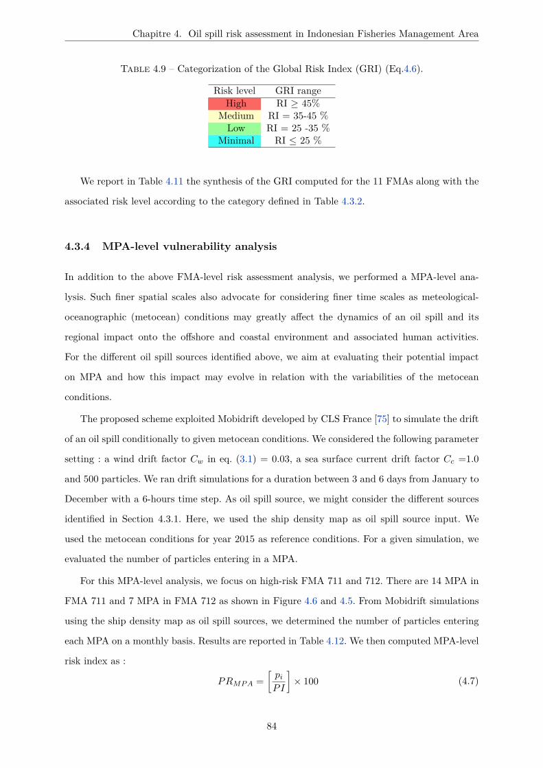
Chapitre 4. Oil spill risk assessment in Indonesian Fisheries Management Area
Table 4.9 – Categorization of the Global Risk Index (GRI) (Eq.4.6).
Risk level GRI rangeHigh RI ≥ 45%
Medium RI = 35-45 %Low RI = 25 -35 %
Minimal RI ≤ 25 %
We report in Table 4.11 the synthesis of the GRI computed for the 11 FMAs along with the
associated risk level according to the category defined in Table 4.3.2.
4.3.4 MPA-level vulnerability analysis
In addition to the above FMA-level risk assessment analysis, we performed a MPA-level ana-
lysis. Such finer spatial scales also advocate for considering finer time scales as meteological-
oceanographic (metocean) conditions may greatly affect the dynamics of an oil spill and its
regional impact onto the offshore and coastal environment and associated human activities.
For the different oil spill sources identified above, we aim at evaluating their potential impact
on MPA and how this impact may evolve in relation with the variabilities of the metocean
conditions.
The proposed scheme exploited Mobidrift developed by CLS France [75] to simulate the drift
of an oil spill conditionally to given metocean conditions. We considered the following parameter
setting : a wind drift factor Cw in eq. (3.1) = 0.03, a sea surface current drift factor Cc =1.0
and 500 particles. We ran drift simulations for a duration between 3 and 6 days from January to
December with a 6-hours time step. As oil spill source, we might consider the different sources
identified in Section 4.3.1. Here, we used the ship density map as oil spill source input. We
used the metocean conditions for year 2015 as reference conditions. For a given simulation, we
evaluated the number of particles entering in a MPA.
For this MPA-level analysis, we focus on high-risk FMA 711 and 712. There are 14 MPA in
FMA 711 and 7 MPA in FMA 712 as shown in Figure 4.6 and 4.5. From Mobidrift simulations
using the ship density map as oil spill sources, we determined the number of particles entering
each MPA on a monthly basis. Results are reported in Table 4.12. We then computed MPA-level
risk index as :
PRMP A =[
pi
PI
]× 100 (4.7)
84

4.3. Proposed methodology
where pi is the number of particles that entered MPA i from the considered Mobidrift simulations
and PI is the greatest number of particles that entered one of the MPA in the considered FMA.
For a given FMA, for instance FMA 712, we refer to MPA 712.k as the kth MPA in FMA 712.
For instance, for Karimun Jawa MPA (MPA 712.6) located in FMA 712, 48 (resp. 248)
particles entered the FMA for Mobidrift simulations run for January metocean conditions with
a 3-day (resp. 6-day) duration, where MPA 712.1 (Seribu Islands) evolved the greatest numbers
of particles (resp. 3761 and 5139 particles for 3-day and 6-day simulation duration). Hence, the
risk indices for MPA 712.6 are given by
PRoil−particles−MP A7126 =48
3761× 100 = 1.28 (for duration = 3 days)
PRoil−particles−MP A7126 =2485139
× 100 = 0.90 (for duration = 6 days)
We proceeded similarly for all MPA in FMA 711 and 712. The results are reported in Table
4.13, 4.14, 4.15 and 4.16 .
Figure 4.5 – Mapping of 7 zones of MPA in FMA 712 (red) along with potential oil spillsources (green triangles) associated with high-traffic points in the area determined from AIS-derived traffic density maps.
85

Chapitre 4. Oil spill risk assessment in Indonesian Fisheries Management Area
Figure 4.6 – Mapping of 14 zones of MPA in FMA 711 (red) along with potential oil spillsources (green triangles) associated with high-traffic points in the area determined from AIS-derived traffic density maps.
86

4.4. Results and Discussion
4.4 Results and Discussion
Table 4.10 showed that FMA 712, 713 and 711 involve the highest oil-spill-risk level. In Natuna
Sea, Java Sea and Makassar Strait, the density of the maritime traffic, of oil platform as well as
of oil transportation activities is very high. FMA 571 has medium risk level that related mostly
to the maritime traffic number in the Malacca Strait. By contrast, FMA 573 depicts a low risk
level in the Indian Ocean on the South of Indonesia. Other FMA were categorized as minimum
risk level.
Regarding environment-related vulnerability indices, 4 zones, namely FMA 573,711,717 and
718, were categorized as high-vulnerability areas. FMA 712, 715 and 716 involved a medium
level, FMA 713 and 714 only a low level, and FMA 571 and 572 a minimal level.
Regarding socio-economic impacts, FMA 711,712 and 713 (Natuna Sea, Java Sea and Ma-
kassar Strait) depict a high-risk level. FMA 717 depicted a minimal-risk level and the remaining
7 FMA a low-risk level.
Table 4.10 – Synthesis of FMA-level risk and vulnerability indices
FMA Risk Index Cost Environment Cost Socioeconomic571 42.05 18.07 25.04572 4.77 20.89 29.20573 29.45 60.16 26.37711 50.76 45.40 46.08712 74.19 40.56 63.15713 52.91 20.76 52.71714 12.23 32.80 29.53715 17.60 42.86 34.83716 7.02 36.79 27.16717 2.99 45.70 14.76718 5.49 58.45 31.48
For a synoptic analysis, we report GRI values for all FMA in Table 4.11. It clearly points
out FMA 711 and 712 as high-risk areas. FMA 711 is the most vulnerable one because it has
high-risk for different oil spill sources and also depict a high vulnerability both in terms of
environmental and socioeconomic impacts. By contrast, FMA 712 depicts a high vulnerability
level in terms of socioeconomic factors but only a medium vulnerability level in terms of envi-
ronmental impact. Two zones, FMA 573 and 713, are categorized as medium-risk areas. FMA
573 involves a high-risk impact w.r.t. environment factors but a low-risk level in terms of oil
spill exposure and socioeconomic impacts. FMA 713 depicts a high risk/vulnerability level in
87
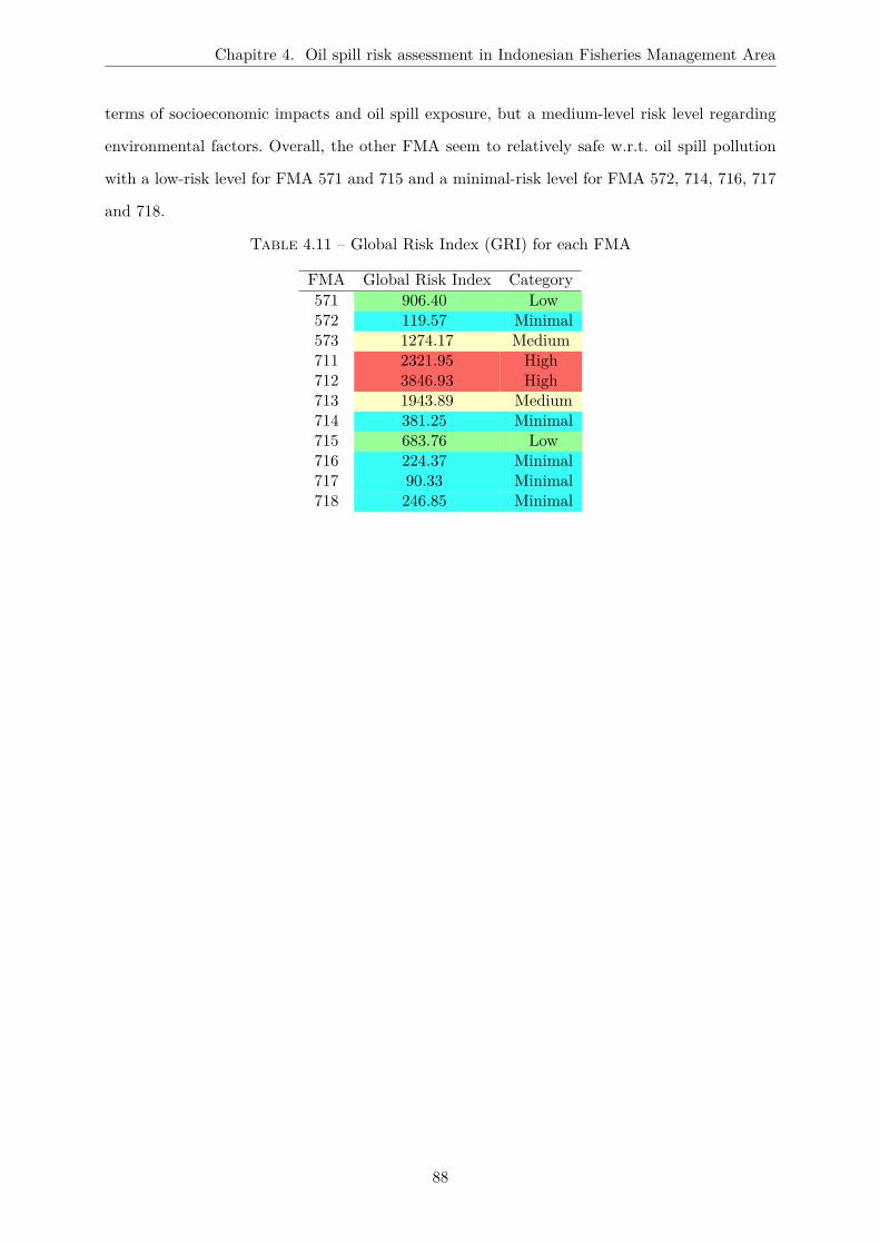
Chapitre 4. Oil spill risk assessment in Indonesian Fisheries Management Area
terms of socioeconomic impacts and oil spill exposure, but a medium-level risk level regarding
environmental factors. Overall, the other FMA seem to relatively safe w.r.t. oil spill pollution
with a low-risk level for FMA 571 and 715 and a minimal-risk level for FMA 572, 714, 716, 717
and 718.
Table 4.11 – Global Risk Index (GRI) for each FMA
FMA Global Risk Index Category571 906.40 Low572 119.57 Minimal573 1274.17 Medium711 2321.95 High712 3846.93 High713 1943.89 Medium714 381.25 Minimal715 683.76 Low716 224.37 Minimal717 90.33 Minimal718 246.85 Minimal
88

4.5. MPA-level risk assessment
4.5 MPA-level risk assessment
Based on the above FMA-level analysis, we performed a vulnerability analysis at finer space and
time scales within the two high-risk FMA, namely FMA 711 and 712. We applied the scheme
detailed in Section 4.3.7. For FMA 711, we ran Mobidrift simulations with 107 source points
from the vessel density map. One simulation example is illustrated in Figure 4.7 for condition
on North West monsoon, 4.9 for condition on SouthEast monsoon, 4.8 and 4.10 for condition on
Transition 1 and Transition 2 monsoon. In these simulations the position of the oil spill source
is point 0 36’ 0” S and 107 5’ 60” E. We depict simulations with two durations (3 and 6
days) for different metocean conditions from January to December. The seasonal variability of
these metocean conditions clearly affect the drift of the oil spill and its impacts on nearby MPA.
During the SouthEast monsoon period (June - August), oil spill mostly drifts to the SouthEast
and threats MPA 711.9. During the North West monsoon period, the oil spill drifts towards
MPA 711.11 and 711.12.
We also report simulation examples for FMA 712, which involve 357 oil spill source points,
in Figure 4.11. In these simulations, the oil spill source is located 5 30’ 0” S and 106 54’
0” E. We ran the simulation with 3-day and 6-day durations for metocean conditions from
January to December. From these simulations, the SouthEast monsoon period (June-August)
and September-November period (Transition 1), a 3-day drift impacted MPA 712.1. During the
North West monsoon, on December, the drift impacted MPA 711.1 for 6-day simulations. By
contrast, on January and February the drift was directed towards MPA 711.3. From March to
May (Transition 2) the simulations showed that MPA 711.3 is still under threat on March but
no more on April and May, where the drift is directed towards MPA 711.1.
We synthesized the outputs of these simulations through the number of particles entering
each MPA in Table 4.12. MPA-level vulnerability indices (4.7) are given in Table 4.13, 4.14,
4.15 and 4.16 respectively for FMA 711 and 712, 3-day and 6-day simulations. We computed
the mean vulnerability indices for each MPA in Table 4.17 for FMA 711 and in Table 4.18.
89

Chapitre 4. Oil spill risk assessment in Indonesian Fisheries Management Area
Figure 4.7 – Oil spill drift simulations from one source point located at 0 36’ 0” S and 107 5’60” E (green triangle) in FMA 711 with 3-day and 6-day durations (resp. black and gray dots)for metocean conditions in the Northwest monsoon from December to February.
90

4.5. MPA-level risk assessment
Figure 4.8 – Oil spill drift simulations from one source point located at 0 36’ 0” S and 107 5’60” E (green triangle) in FMA 711 with 3-day and 6-day durations (resp. black and gray dots)for metocean conditions in the Transition 1 monsoon from March to May.
91

Chapitre 4. Oil spill risk assessment in Indonesian Fisheries Management Area
Figure 4.9 – Oil spill drift simulations from one source point located at 0 36’ 0” S and 107 5’60” E (green triangle) in FMA 711 with 3-day and 6-day durations (resp. black and gray dots)for metocean conditions in the SouthEast monsoon from June to August.
92

4.5. MPA-level risk assessment
Figure 4.10 – Oil spill drift simulations from one source point located at 0 36’ 0” S and 107 5’60” E (green triangle) in FMA 711 with 3-day and 6-day durations (resp. black and gray dots)for metocean conditions in the Transition 2 monsoon from September to November.
93

Chapitre 4. Oil spill risk assessment in Indonesian Fisheries Management Area
January February March
Avril May June
July August September
October November December
Figure 4.11 – Oil spill drift simulations from one source point located at 5 30’ 0” S and 106
54’ 0” E (green triangle) in FMA 712 with 3-day and 6-day durations (resp. black and gray dots)for metocean conditions from January to December.
94

4.5
.M
PA
-level
riskassessm
ent
Table 4.12 – Number of particles entering each MPA in FMA 711 and 712 for oil spill drift simulations with January-to-December metoceanconditions. AIS-derived Vessel density maps were used to generate oil spill source points.
MPA
Number of simulated oil spill particles entering a MPA
January February March April May June July August September October November December
d=3 d=6 d=3 d=6 d=3 d=6 d=3 d=6 d=3 d=6 d=3 d=6 d=3 d=6 d=3 d=6 d=3 d=6 d=3 d=6 d=3 d=6 d=3 d=6
711.1 0 0 0 0 0 0 0 0 0 0 0 0 0 0 0 0 0 0 0 0 0 0 0 0
711.2 0 0 0 0 0 0 0 0 0 0 0 0 0 0 0 0 0 0 0 0 0 0 0 0
711.3 0 0 0 0 0 0 0 0 0 0 0 0 0 0 0 0 0 0 0 0 0 0 0 0
711.4 0 0 0 0 0 0 0 0 0 0 0 0 0 0 0 0 0 0 0 0 0 0 0 0
711.5 0 0 0 0 0 0 0 5 0 277 0 0 0 0 0 0 0 0 0 0 0 0 0 0
711.6 268 170 69 634 27 595 84 407 3 0 0 0 0 0 0 0 0 0 0 0 7 385 294 460
711.7 541 640 486 475 489 535 481 464 458 449 362 336 330 300 235 313 366 215 496 360 385 505 460 460
711.8 21 252 13 514 3 11 1 0 0 0 0 0 0 0 0 0 0 0 0 0 0 10 0 0
711.9 0 0 0 0 0 0 0 0 0 28 0 0 0 2200 0 8 0 0 0 0 0 0 0 0
711.10 0 0 0 0 0 0 0 0 0 28 0 0 0 69 0 51 0 28 0 0 0 0 0 0
711.11 0 2 0 10 0 59 0 1 29 1545 0 0 3 845 0 340 2 428 3 502 0 3 0 0
711.12 3 0 0 149 1 217 43 6 43 6 0 2 0 2 1 230 0 0 0 35 0 0 0 362
711.13 0 0 0 69 0 157 2 0 0 0 0 20 0 0 0 2 0 5 0 53 0 20 0 23
711.14 0 0 0 0 0 4 0 0 0 0 0 0 0 0 0 0 0 0 0 2 0 16 0 0
712.1 1110 10 1946 64 3692 317 2530 1661 1995 5139 3645 1587 2813 1014 3283 808 3423 938 3761 1407 2212 2177 1257 2379
712.2 0 0 7 0 2 1 3 0 2 2 3 1 8 7 5 2 3 2 2 0 11 5 2 5
712.3 989 1998 374 1414 707 2272 805 251 89 18 274 1224 152 40 147 241 138 21 190 926 721 431 597 558
712.4 0 0 0 0 0 0 0 18 0 46 0 9 0 1 0 0 0 0 0 2 0 0 0 0
712.5 0 0 0 0 0 0 0 0 0 0 0 0 0 0 0 0 0 0 0 0 0 0 0 0
712.6 48 248 34 1289 13 1283 0 569 190 2578 14 1602 38 1665 41 1506 34 2481 47 866 1 251 92 800
712.7 0 137 37 23 0 96 232 3 317 0 71 0 69 0 162 0 81 0 9 0 147 0 58 48
95

Chapitre
4.O
ilspill
riskassessm
entin
IndonesianF
isheriesM
anagement
Area
Table 4.13 – MPA-level vulnerability indices in FMA 711 issued from oil spill drift simulations for a 3-day drift duration andJanuary-to-December metocean conditions.
MPA ID January February March April May June July August September October November December
711.1 0 0 0 0 0 0 0 0 0 0 0 0
711.2 0 0 0 0 0 0 0 0 0 0 0 0
711.3 0 0 0 0 0 0 0 0 0 0 0 0
711.4 0 0 0 0 0 0 0 0 0 0 0 0
711.5 0 0 0 0 0 0 0 0 0 0 0 0
711.6 49.54 12.75 4.99 15.53 0.55 0 0 0 0 0 1.29 54.34
711.7 100 89.83 90.39 88.91 84.66 66.91 61.00 43.44 67.65 91.68 71.16 85.03
711.8 3.88 2.40 0.55 0.18 0 0 0 0 0 0 0 0
711.9 0 0 0 0 0 0 0 0 0 0 0 0
711.10 0 0 0 0 0 0 0 0 0 0 0 0
711.11 0 0 0 0 5.36 0 0.55 0 0.37 0.55 0 0
711.12 0.55 0 0.18 7.95 7.95 0 0 0.18 0 0 0 0
711.13 0 0 0 0.37 0 0 0 0 0 0 0 0
711.14 0 0 0 0 0 0 0 0 0 0 0 0
96

4.5
.M
PA
-level
riskassessm
ent
Table 4.14 – MPA-level vulnerability indices in FMA 711 issued from oil spill drift simulations for a 6-day drift duration andJanuary-to-December metocean conditions.
MPA ID January February March April May June July August September October November December
711.1 0 0 0 0 0 0 0 0 0 0 0 0
711.2 0 0 0 0 0 0 0 0 0 0 0 0
711.3 0 0 0 0 0 0 0 0 0 0 0 0
711.4 0 0 0 0 0 0 0 0 0 0 0 0
711.5 0 0 0 0.23 12.59 0 0 0 0 0 0 0
711.6 7.73 28.82 27.05 18.50 0 0 0 0 0 0 17.50 20.91
711.7 29.09 21.59 24.32 21.09 20.41 15.27 13.64 14.23 9.77 16.36 22.95 20.91
711.8 11.45 23.36 0.50 0 0 0 0 0 0 0 0.45 0
711.9 0 0 0 0 1.27 0 100 0.36 0 0 0 0
711.10 0 0 0 0 1.27 0 3.14 2.32 1.27 0 0 0
711.11 0.09 0.45 2.68 0.05 70.23 0 38.41 15.45 19.45 22.82 0.14 0
711.12 0 6.77 9.86 0.27 0.27 0.09 0.09 10.45 0 1.59 0 16.45
711.13 0 3.14 7.14 0 0 0.91 0 0.09 0.23 2.41 0.91 1.05
711.14 0 0 0.18 0 0 0 0 0 0 0.09 0.73 0
97

Chapitre
4.O
ilspill
riskassessm
entin
IndonesianF
isheriesM
anagement
Area
Table 4.15 – MPA-level vulnerability indices in FMA 712 issued from oil spill drift simulations for a 3-day drift duration andJanuary-to-December metocean conditions.
MPA ID January February March April May June July August September October November December
712.1 29.51 51.74 98.17 67.27 53.04 96.92 74.79 87.29 91.01 100 58.81 33.42
712.2 0 0.19 0.05 0.08 0.05 0.08 0.21 0.13 0.08 0.05 0.29 0.05
712.3 26.30 9.94 18.80 21.40 2.37 7.29 4.04 3.91 3.67 5.05 19.17 15.87
712.4 0 0 0 0 0 0 0 0 0 0 0 0
712.5 0 0 0 0 0 0 0 0 0 0 0 0
712.6 1.28 0.90 0.35 0 5.05 0.37 1.01 1.09 0.90 1.25 0.03 2.45
712.7 0 0.98 0 6.17 8.43 1.89 1.83 4.31 2.15 0.24 3.91 1.54
98

4.5
.M
PA
-level
riskassessm
ent
Table 4.16 – MPA-level vulnerability indices in FMA 712 issued from oil spill drift simulations for a 6-day drift duration andJanuary-to-December metocean conditions.
MPA ID January February March April May June July August September October November December
712.1 0.19 1.25 6.17 32.32 100 30.88 19.73 15.72 18.25 27.38 42.36 46.29
712.2 0 0 0.02 0 0.04 0.02 0.14 0.04 0.04 0 0.10 0.10
712.3 38.88 27.52 44.21 4.88 0.35 23.82 0.78 4.69 0.41 18.02 8.39 10.86
712.4 0 0 0 0.35 0.90 0.18 0.02 0 0 0.04 0 0
712.5 0 0 0 0 0 0 0 0 0 0 0 0
712.6 4.83 25.08 24.97 11.07 50.17 31.17 32.40 29.31 48.28 16.85 4.88 15.57
712.7 2.67 0.45 1.87 0.06 0 0 0 0 0 0 0 0.93
99

Chapitre 4. Oil spill risk assessment in Indonesian Fisheries Management Area
Table 4.17 – Mean MPA-level vulnerability indices in FMA 711 for January-to-December me-tocean conditions
MPA IDSouthEast Transition 1 NorthWest Transition 2
3days 6days 3days 6days 3days 6days 3days 6days711.1 0 0 0 0 0 0 0 0711.2 0 0 0 0 0 0 0 0711.3 0 0 0 0 0 0 0 0711.4 0 0 0 0 0 0 0 0711.5 0 0 0 0 0 0 0 4.27711.6 0 0 0.43 5.83 38.88 19.15 7.02 15.18711.7 57.12 14.38 76.83 16.36 91.62 23.86 87.99 21.94711.8 0 0 0 0.15 2.09 11.61 0.25 0.17711.9 0 33.45 0 0 0 0 0 0.42711.10 0 1.82 0 0.42 0 0 0 0.42711.11 0.18 17.95 0.31 14.14 0 0.18 1.79 24.32711.12 0.06 3.55 0 0.53 0.18 7.74 5.36 3.47711.13 0 0.33 0 1.18 0 1.39 0.12 2.38711.14 0 0 0 0.27 0 0 0 0.06
Table 4.18 – MPA-level vulnerability indices in FMA 712 under different monsoon conditions.
MPA IDSouthEast Transition 1 NorthWest Transition 2
3days 6days 3days 6days 3days 6days 3days 6days712.1 86.33 22.11 83.28 29.33 38.23 15.91 72.83 46.16712.2 0.14 0.06 0.14 0.05 0.08 0.03 0.06 0.02712.3 5.08 9.76 9.30 8.94 17.37 25.75 14.19 16.48712.4 0 0.06 0 0.01 0 0 0 0.42712.5 0 0 0 0 0 0 0 0712.6 0.82 30.96 0.73 23.34 1.54 15.16 1.80 28.73712.7 2.68 0 2.10 0 0.84 1.35 4.87 0.64
Table 4.17 showed that MPA 711.7 is the most vulnerable all year long. This MPA is more
vulnerable during the NorthWest and Transition 2 monsoon. Hence, the surveillance should be
enhanced in this region during that period. Other vulnerable MPA in FMA 711 are MPA 711.6
and MPA 711.9. MPA 711.6 was threatened on the NorthWest monsoon and MPA 711.9 on the
SouthEast monsoon.
Regarding, FMA 712, as showed on Table 4.18, MPA 712.1 was the most threatened MPA by
the oil spill. This MPA is more vulnerable on the SouthEast, Transation 1 and Transation 2 mon-
soon. MPA 712.1 needs more surveillance on the Transation 2 monsoon because on this period
both oil spill coming from 3 and 6 days simulation were threatened this area. The others MPA
that needs attention are FMA 712.3 and 712.6. FMA 712.3 was threatened on the NorthWest
monsoon and FMA 712.6 on the Transition 2 and SouthEast monsoon.
100

4.6. Conclusion and Discussion
4.6 Conclusion and Discussion
In this work, we developed a novel method for the assessment of the vulnerability of marine and
coastal Indonesian ecosystems to oil spill pollution. The proposed approach combined a variety
of potential oil spill sources documented from maritime traffic density data, oil-related activities
and satellite-derived oil spill detection. The calculation of oil spill risk on each FMA based on the
value of average percentage rate of each critical variable considered. Regarding the limitation of
data and information, the calculation of average percentage rate is sometimes different between
each variable. For example on the variable risk coming from ship accident we used the weighting
factor as described from ITOPF because we had the information related to the volume of oil
spilled for each accident. In other example, we analyzed the risk from the variable maritime
density not using the weighting factor because no information related to the type of vessel and
volume of oil that being transported. It would be better for the further analysis if we can be
provided by more information but at least this analysis can be identified which area that more
vulnerable from the oil spill.
We evaluated the impact of oil spill pollution both in terms of ecological and socioeconomic
impacts. Our analysis was spatially structured with respect to 11 Fisheries Management Areas
implemented by Indonesia. Same with the methodology used in the calculation of risk, the
calculation of oil spill impact on each FMA based on the value of average percentage rate
of each critical variable considered in the ecological and socioeconomic. As a final result, we
proposed a global risk index (GRI) combining all information sources at the MFA level.
The result of our analysis clearly pointed out FMA 711 and 712 as the areas the most
vulnerable to oil spill. Medium-risk levels were reported from FMA 573 and FMA 713 and the
remaining ones involved a low-risk or minimal-risk level. Its worth to note that the data used
for the calculation of oil spill impact on the environment the data used in the analysis is coming
from ecoregion data which is quite different with Fishing Management Area. In ecoregion FMA
573 divided into 2 ecoregions different namely South Java and Lesser Sunda. This explained why
the FMA 573 is categorized as medium-risk. In FMA 573, even the oil spill risk is low but the
oil spill impact is high considering the marine biodiversities in FMA 573 that combining from
two ecoregions.
101

Chapitre 4. Oil spill risk assessment in Indonesian Fisheries Management Area
In FMA 712, the risk level is the highest. Java Sea has an important role in terms of maritime
activities and fisheries production, meanwhile it has dense ship traffic and a lot of activities
linked to oil and gas production and distribution. Seribu Islands (MPA 712.1) in the North of
Jakarta is the most threatened MPA. This MPA is threatened almost all year long from January
to December with the highest risk level during the SouthEast monsoon from June to August.
Situated in the North of Semarang (Capital of Central Java Province) with a dense ship traffic,
Karimunjawa (MPA 712.6) is the second most threatened MPA in FMA 712 but involved a
low-risk level.
In FMA 711, the most vulnerable MPA are Batam Islands (MPA 711.7 and 711.6) and
Tambelan and Karimata Islands (MPA 711.9 and 711.11). Batam Islands are vulnerable due to
its location near Singapore ports that have very high ship traffic density. The enhancement of
the surveillance should be conducted on these islands. The surveillance and mitigation should
be focused on North West monsoon period from December to February and on the transition
period from March to May. Other MPA in FMA 711 that require particular attention is the
MPA in Tambelan and Karimata Islands located in the Karimata Strait. The Tambelan and
Karimata Islands are close to major sea lanes. For this MPA, the focus should be given to the
June-August period (Monsoon SouthEast), with a main threat related to relatively longer drifts
(6-day duration).
The result of our study should be analyzed with respect to reported oil spill occurences.
Regarding for instance the Seribu Island and Batam Islands. In Seribu Islands, several oil spills
were reported on December 2003, April, May and October 2004, June 2007 and February, March
and August 2011. In FMA 711 particularly in Batam Islands, the last oil spills were found on
January and February 2017. These reported oil spill events and impacts support the significance
of our study, which also identified these zones as being among the most vulnerable ones to oil
spill pollution.
We believe this study to be relevant to decision makers, government officials and local com-
munities in avoiding or limiting the oil spill risk in vulnerable zones. The related regulations
on marine shipping and vessel navigation on the vulnerable zone could be improved based on
the risk levels established through the proposed approach. The determination of vulnerability
indices conditionally to metocean conditions also open the possibility for surveillance and miti-
gation plans adapted to the seasonal and inter-annual variabilities of the metocean conditions.
102

4.6. Conclusion and Discussion
Using SAR-based surveillance in conjunction with surveillance vessel operating in predefined
areas of interest, especially high-risk ones, could improve law enforcement. Our study of the
MPA-level vulnerability further stresses the importance of using high-quality metocean data,
including bathymetry and tidal information, with a view to predicting realistic oil spill drifts as
well as for risk assessment issues as explored in our study as in mitigation for oil spill disasters.
Overall, the proposed methodology could be implemented within INDESO system, including
routine updates from newly documented oil spill events as well as updated knowledge on the
presence of oil-related acitvies (e.g., refinery, platform,....).
103

104

5
Chapit
re
Conclusions and Perspectives
5.1 Conclusion . . . . . . . . . . . . . . . . . . . . . . . . . . . . . . . . . . . . . . . 106
5.2 Perspectives . . . . . . . . . . . . . . . . . . . . . . . . . . . . . . . . . . . . . . . 108
105

Chapitre 5. Conclusions and Perspectives
5.1 Conclusion
Oil spill monitoring in the Indonesian seas is one of the main objective of the INDESO project.
In this framework, this thesis aimed to propose new methodologies and analyses. This thesis
involved two main contributions. The first contribution addressed the retrieval of oil spill drift
parameters from a joint analysis of SAR observations of an oil spill and of outputs of a Lagrangian
oil spill transport model. We applied the proposed methodology on the most famous oil spill
accident in Indonesia, the Montara case. The second contribution was the global assessment of
oil spill risk in Indonesia.We focused on the 11 Indonesia Fisheries Management Area to support
the sustainability development of marine and fisheries. In this analysis we proposed methodology
that considered the oil spill from different source and their impacts not only to the environment,
but also from social and economic perspectives. For the assessment of vulnerability of Marine
Protected Areas to oil spill pollution, we also exploited the oil spill trajectory model.
In the first part of this thesis, we aimed to estimate oil spill drift parameters. The proposed
framework exploited a Lagrangian oil spill transport model such that the simulated oil spill
drift could match a SAR-based observation of an oil spill. In the considered 2D Lagrangian
model there were two dominant factors, i.e. wind and surface current. To confirm the origin
of the oil spill detected on a given date through a SAR observation, we performed simulations
with various leakage starting dates, leakage durations, and different values of wind and current
weighing coefficients. We developed a novel framework for the assimilation of these oil leakage
parametersfrom a SAR-derived detection of an oil spill. This framework states this assimilation
as the minimization of a level-set representations of the SAR-derived oil spill detection and
of 2D transport model simulations. We illustrated its relevance on the Montara oil spill case
study. We showed that the observed oil spill on 02 September 2009 was mainly due to the oil
leakage from August 21 until September 02 with majority of slick is coming from five first days
of leakage (August 21-25, 2009). The estimated wind and current drift factors were in agreement
with values previously reported in the literature. They were however significantly different from
nominal parameters and shown to affect the match between the observed oil spill and transport
model simulations.
The second part of this thesis addressed the assessment of the vulnerability of Indonesian sea
areas to oil spill pollution. The focus was given to Fisheries Management Areas as a means to
106

5.1. Conclusion
provide synoptic analysis over the entire Indonesian maritime territory. Using different informa-
tion from many institutional reports, we collected and analyzed the potential source of oil spill
in each FMA. Each FMA has specific characteristics in terms environmental and socioeconomic
features. We assessed the oil spill risk in each FMA based on all these factors. In total, we have
computed a Global Risk Index (GRI) at the FMA level that combined all information sources.
The resulting distribution of the GRI over the 11 FMA showed that FMA in the North of Java
and Natuna Sea are the most vulnerable ones to oil spill. Furthermore, we exploited oil spill drift
simulations into these two FMA to further assess the vulnerability at a finer spatial scale, focu-
sing on Marine Protected Areas, and a finer time scale, namely up to a monthly scale, with a view
to assessing the impact of the variabilities of the meteorological and oceanographic conditions.
Among 14 MPA in the zone of FMA Natuna Sea the most vulnerable MPA are in Batam Islands,
Bintan Islands and Tambelan & Karimata Islands. The surveillance and mitigation should be
focused on North West monsoon on December until February and on the transition period from
March until May. Meanwhile, in the FMA on the North of Java the most vulnerable MPA is in
Seribu Islands. This MPA is threatened almost all the year long from January until December
with a peak during the South East monsoon from June until August.These results are consistent
with recurrent oil spill events reported in the Seribu Island and Batam Islands. The result of
this study can be used in the mitigation planning to reduce the negative impacts of oil spill. It
might be useful for decision makers, government officials and local communities in avoiding or
limiting the oil spill risk in vulnerable zones. The related regulations on marine shipping and
vessel navigation in the highly-vulnerable zone should be improved. At the operational level, we
might suggest the joint use of the SAR-based surveillance in conjunction with vessels operating
at set.This coordination could reinforce the law enforcement.
In summary, we have proposed several methods for the monitoring of oil spills and their
impacts into Indonesian marine ecosystems and activities, which benefit from both satellite
observation technologies and operational oceanography tools, both aspects being at the core of
INDESO project.
107

Chapitre 5. Conclusions and Perspectives
5.2 Perspectives
The study on the assimilation of SAR images in oil spill trajectory models opens new research
avenues for the satellite-based operational monitoring of oil spills. Future work will further
investigate the assimilation of oil leakage parameters from multi-date observations as well as
other oil leakage configurations, such as illegal oil discharges from natural oil seeps or vessels.
The two novel applications would be of key interest in the framework of INDESO project.
The analysis of oil spill risk showed that several areas are categorized as highly vulnerable
areas. In such high-risk zones, the oceanographic data such as bathymetry and current, wind
and tidal information should be acquired and prepared better in advance with a view to being
fully-operational in case of most often unexpected oil spill disasters. One may consider the
development and parameterization of zone-specific oil spill drift models for high-risk zones.
Regarding the implementation of the proposed oil spill monitoring tools, a critical issue if the
availability of supporting data. In our study, we calculated oil spill risk indices from oil spill drift
simulations using only ship positions as sources. Information on the positions of oil platforms
would further improve the analysis of the oil spill risk and the mapping of this risk at the national
and regional scale. The simulation of oil spill will be better considering the evaporation and
emulsification process. In the future simulation using 3D setting will be more clearly identified
the impact of oil spill to the marine environment.
The expertise in object trajectory model and satellite image analysis for marine applications
remains fairly limited in Indonesia. This thesis can be used in supporting the operational of
Indeso especially for the oil spill monitoring in Indonesia sea territory. Our work can be used in
law enforcement, response and mitigation planning. In the future, sea pollution can be expected
to catch more and more the attention of stakeholders as maritime and fisheries activities tend
to be one of the most important source of growth of the economy. Marine pollution does not
restrict to oil spill pollution. The world’s oceans are now facing mountains of debris. Indonesia
sea territory is among the most affected ones. Indonesia is also stirringly suspected to be one of
the biggest marine polluter in the world. In this respect, INDESO is a critical tool to support the
the government of Indonesia in combating this issue. With the comprehensive observation data
acquired within INDESO along with the modeling and analysis tools implemented are clearly
of great interest to address this issue. For instance, one might combine the detection to marine
108

5.2. Perspectives
debris to drift trajectory models to forecast the impact of marine debris pollution onto the
coastal Indonesian ecosystems. The detection of the marine debris is a real challenge as debris
are is relatively small and mainly found in the subsurface. New solutions and operational plan
have then to be developed in response to the operational needs.
109

110

Bibliography[1] J. A. Sethian, Level set methods and fast marching methods. Cambridge University Press,
1999. [Online]. Available : http://hrcak.srce.hr/file/69388?origin=publicationDetail
[2] A. Jordi, M. Ferrer, G. Vizoso, A. Orfila, G. Basterretxea, B. Casas, A. Álvarez, D. Roig,
B. Garau, M. Martínez et al., “Scientific management of mediterranean coastal zone : A
hybrid ocean forecasting system for oil spill and search and rescue operations,” Marine
Pollution Bulletin, vol. 53, no. 5, pp. 361–368, 2006.
[3] P. J. Webster, A. M. Moore, J. P. Loschnigg, and R. R. Leben, “Coupled ocean-atmosphere
dynamics in the indian ocean during 1997-98,” Nature, vol. 401, no. 6751, pp. 356–360,
1999.
[4] A. Gordon, “Oceanography of the Indonesian Seas,” Oceanography, vol. 18, no. 4, pp.
13–13, 2005.
[5] Y. Masumoto and T. Yamagata, “Seasonal variations of the indonesian throughflow in
a general ocean circulation model,” Journal of Geophysical Research : Oceans, vol. 101,
no. C5, pp. 12 287–12 293, 1996.
[6] R. D. Susanto, A. L. Gordon, and Q. Zheng, “Upwelling along the coasts of java and
sumatra and its relation to enso,” Geophysical Research Letters, vol. 28, no. 8, pp. 1599–
1602, 2001.
[7] J. T. Potemra and N. Schneider, “Interannual variations of the indonesian throughflow,”
Journal of Geophysical Research : Oceans, vol. 112, no. C5, 2007.
[8] R. D. Susanto, A. L. Gordon, and J. Sprintall, “Observations and proxies of the surface
layer throughflow in lombok strait,” Journal of Geophysical Research : Oceans, vol. 112,
no. C3, 2007.
111

Bibliography
[9] J. Sprintall, S. E. Wijffels, R. Molcard, and I. Jaya, “Direct estimates of the indonesian
throughflow entering the indian ocean : 2004–2006,” Journal of Geophysical Research :
Oceans, vol. 114, no. C7, 2009.
[10] C. Caviedes, El Niño in history : storming through the ages. University Press of Florida,
2001.
[11] J. S. Gray, “Marine biodiversity : patterns, threats and conservation needs,” Biodiversity
& Conservation, vol. 6, no. 1, pp. 153–175, 1997.
[12] M. D. Spalding, H. E. Fox, G. R. Allen, N. Davidson, Z. A. Ferdaña, M. Finlayson, B. S.
Halpern, M. A. Jorge, A. Lombana, S. A. Lourie, K. D. Martin, E. McManus, J. Molnar,
C. A. Recchia, and J. Robertson, “Marine ecoregions of the world : A bioregionalization
of coastal and shelf areas,” BioScience, vol. 57, no. 7, p. 573, 2007. [Online]. Available :
+http://dx.doi.org/10.1641/B570707
[13] C. H. Hidrovo and D. P. Hart, “Emission reabsorption laser induced fluorescence (erlif)
film thickness measurement,” Measurement Science and Technology, vol. 12, no. 4, p. 467,
2001.
[14] E. Donnay, “Use of unmanned aerial vehicle (uav) for the detection and surveillance of
marine oil spills in the belgian part of the north sea,” in Proceedings of the 32 AMOP
technical seminar on environmental contamination and response, vol. 2, 2009.
[15] F. Carnesecchi, V. Byfield, P. Cipollini, G. Corsini, and M. Diani, “An optical model for
the interpretation of remotely sensed multispectral images of oil spill,” in Proc. SPIE, vol.
7105, 2008, p. 710504.
[16] R. Belore, “A device for measuring oil slick thickness,” Spill Technology Newsletter, vol. 7,
no. 2, pp. 44–47, 1982.
[17] M. F. Fingas and C. E. Brown, “Review of oil spill remote sensing,” Spill Science &
Technology Bulletin, vol. 4, no. 4, pp. 199–208, 1997.
[18] K. Grüner, R. Reuter, and H. Smid, “A new sensor system for airborne measurements
of maritime pollution and of hydrographic parameters,” GeoJournal, vol. 24, no. 1, pp.
103–117, 1991.
112

Bibliography
[19] A. Samberg, “The state-of-the-art of airborne laser systems for oil mapping,” Canadian
Journal of Remote Sensing, vol. 33, no. 3, pp. 143–149, 2007.
[20] M. N. Jha, J. Levy, and Y. Gao, “Advances in remote sensing for oil spill disaster manage-
ment : state-of-the-art sensors technology for oil spill surveillance,” Sensors, vol. 8, no. 1,
pp. 236–255, 2008.
[21] C. Brekke and A. H. S. Solberg, “Oil spill detection by satellite remote sensing,” Remote
Sensing of Environment, vol. 95, no. 1, pp. 1–13, 2005.
[22] O. Calla, N. Ahmadian, and S. Hasan, “Estimation of emissivity and scattering coefficient
of low saline water contaminated by diesel in cj band (5.3 ghz) and ku band (13.4 ghz),”
84.37.+ q ; 84.40. xb ; 92.05. Hj, 2011.
[23] O. Calla, H. K. Dadhich, and S. Singhal, “Oil spill detection using ssm/i satellite data
over bombay high location in arabian sea,” IJRSP Vol.42(1) February 2013, 2013.
[24] L. Yujiri, M. Shoucri, and P. Moffa, “Passive millimeter wave imaging,” IEEE microwave
magazine, vol. 4, no. 3, pp. 39–50, 2003.
[25] C. Giri, J. Long, and L. Tieszen, “Mapping and monitoring louisiana’s mangroves in the
aftermath of the 2010 gulf of mexico oil spill,” Journal of Coastal Research, vol. 27, no. 6,
pp. 1059–1064, 2011.
[26] R. Goodman, “Remote sensing resolution and oil slick inhomogeneities,” in Proceedings of
the second thematic conference on remote sensing for marine and coastal environments :
needs, solutions and applications. ERIM, Ann Arbor, p I-1-17, 1994.
[27] C.-S. Yang, Y.-S. Kim, K. Ouchi, and J.-H. Na, “Comparison with l-, c-, and x-band real
sar images and simulation sar images of spilled oil on sea surface,” in Geoscience and
Remote Sensing Symposium, 2009 IEEE International, IGARSS 2009, vol. 4. IEEE,
2009, pp. IV–673.
[28] D.-j. Kim, W. M. Moon, and Y.-S. Kim, “Application of terrasar-x data for emergent oil-
spill monitoring,” IEEE Transactions on Geoscience and Remote Sensing, vol. 48, no. 2,
pp. 852–863, 2010.
113

Bibliography
[29] B. Minchew, C. E. Jones, and B. Holt, “Polarimetric analysis of backscatter from the
deepwater horizon oil spill using l-band synthetic aperture radar,” IEEE Transactions on
Geoscience and Remote Sensing, vol. 50, no. 10, pp. 3812–3830, 2012.
[30] R. Solberg and N. Theophilopoulos, “Envisys–a solution for automatic oil spill detection
in the mediterranean,” Environmental Research Institute of Michigan, Ann Arbor, MI
(United States), Tech. Rep., 1997.
[31] Y. Zhang, H. Lin, Q. Liu, J. Hu, X. Li, and K. Yeung, “Oil-spill monitoring in the coastal
waters of hong kong and vicinity,” Marine Geodesy, vol. 35, no. 1, pp. 93–106, 2012.
[32] Z. Yongzhi, L. Hujun, W. Xiao, and W. Dan, “Edge extraction of marine oil spill in sar
images,” in Challenges in Environmental Science and Computer Engineering (CESCE),
2010 International Conference on, vol. 1. IEEE, 2010, pp. 439–442.
[33] F. Zhang, Y. Shao, W. Tian, and S. Wang, “Oil spill identification based on textural
information of sar image,” in Geoscience and Remote Sensing Symposium, 2008. IGARSS
2008. IEEE International, vol. 4. IEEE, 2008, pp. IV–1308.
[34] M. Tello, R. Bonastre, C. Lopez-Martinez, J. J. Mallorqui, A. Danisi, G. Di Martino,
A. Iodice, G. Ruello, and D. Riccio, “Characterization of local regularity in sar imagery
by means of multiscale techniques : application to oil spill detection,” in Geoscience and
Remote Sensing Symposium, 2007. IGARSS 2007. IEEE International. IEEE, 2007, pp.
5228–5231.
[35] D. Chaudhuri, A. Samal, A. Agrawal, A. Mishra, V. Gohri, R. Agarwal et al., “A statistical
approach for automatic detection of ocean disturbance features from sar images,” IEEE
Journal of Selected Topics in Applied Earth Observations and Remote Sensing, vol. 5,
no. 4, pp. 1231–1242, 2012.
[36] A. Mishra, D. Chaudhuri, C. Bhattacharya, and Y. Rao, “Ocean disturbance feature de-
tection from sar images—an adaptive statistical approach,” in Synthetic Aperture Radar
(APSAR), 2011 3rd International Asia-Pacific Conference on. IEEE, 2011, pp. 1–4.
[37] O. Garcia-Pineda, I. MacDonald, and B. Zimmer, “Synthetic aperture radar image proces-
sing using the supervised textural-neural network classification algorithm,” in Geoscience
114

Bibliography
and Remote Sensing Symposium, 2008. IGARSS 2008. IEEE International, vol. 4. IEEE,
2008, pp. IV–1265.
[38] D. I. Morales, M. Moctezuma, and F. Parmiggiani, “Detection of oil slicks in sar images
using hierarchical mrf,” in Geoscience and Remote Sensing Symposium, 2008. IGARSS
2008. IEEE International, vol. 3. IEEE, 2008, pp. III–1390.
[39] M. Robson, J. Secker, and P. Vachon, “Evaluation of ecognition for assisted target detection
and recognition in sar imagery,” in Geoscience and Remote Sensing Symposium, 2006.
IGARSS 2006. IEEE International Conference on. IEEE, 2006, pp. 145–148.
[40] C. Ozkan, C. Ozturk, F. Sunar, and D. Karaboga, “The artificial bee colony algorithm in
training artificial neural network for oil spill detection,” Neural Network World, vol. 21,
no. 6, p. 473, 2011.
[41] S. Singha, T. J. Bellerby, and O. Trieschmann, “Detection and classification of oil spill
and look-alike spots from sar imagery using an artificial neural network,” in Geoscience
and Remote Sensing Symposium (IGARSS), 2012 IEEE International. IEEE, 2012, pp.
5630–5633.
[42] ——, “Satellite oil spill detection using artificial neural networks,” IEEE Journal of Selec-
ted Topics in Applied Earth Observations and Remote Sensing, vol. 6, no. 6, pp. 2355–2363,
2013.
[43] K. Topouzelis, V. Karathanassi, P. Pavlakis, and D. Rokos, “Detection and discrimination
between oil spills and look-alike phenomena through neural networks,” ISPRS Journal of
Photogrammetry and Remote Sensing, vol. 62, no. 4, pp. 264–270, 2007.
[44] K. N. Topouzelis, “Oil spill detection by SAR images : Dark formation detection, feature
extraction and classification algorithms,” Sensors, vol. 8, no. 10, pp. 6642–6659, 2008.
[45] K. Topouzelis, V. Karathanassi, P. Pavlakis, and D. Rokos, “Potentiality of feed-forward
neural networks for classifying dark formations to oil spills and look-alikes,” Geocarto
International, vol. 24, no. 3, pp. 179–191, 2009.
[46] M. Fingas, Oil spill science and technology. Gulf professional publishing, 2016.
115

Bibliography
[47] A. Berry, T. Dabrowski, and K. Lyons, “The oil spill model oiltrans and its application to
the celtic sea,” Marine Pollution Bulletin, vol. 64, no. 11, pp. 2489 – 2501, 2012. [Online].
Available : http://www.sciencedirect.com/science/article/pii/S0025326X12003578
[48] A. Galeev and S. Ponikorov, “Numerical analysis of the process of heated oil evaporation
from the emergency spill surface,” Journal of Engineering Physics and Thermophysics,
vol. 84, no. 6, pp. 1398–1407, 2011.
[49] D. Mackay and C. D. McAuliffe, “Fate of hydrocarbons discharged at sea,” Oil and Che-
mical Pollution, vol. 5, no. 1, pp. 1–20, 1989.
[50] M. Nazir, F. Khan, P. Amyotte, and R. Sadiq, “Multimedia fate of oil spills in a ma-
rine environment—an integrated modelling approach,” process safety and environmental
protection, vol. 86, no. 2, pp. 141–148, 2008.
[51] W. Stiver and D. Mackay, “Evaporation rate of spills of hydrocarbons and petroleum
mixtures,” Environmental science & technology, vol. 18, no. 11, pp. 834–840, 1984.
[52] S. Wang, Y. Shen, and Y. Zheng, “Two-dimensional numerical simulation for transport
and fate of oil spills in seas,” Ocean Engineering, vol. 32, no. 13, pp. 1556–1571, 2005.
[53] Z. Zhong and F. You, “Oil spill response planning with consideration of physicochemical
evolution of the oil slick : A multiobjective optimization approach,” Computers & Chemical
Engineering, vol. 35, no. 8, pp. 1614–1630, 2011.
[54] D. Rasmussen, “Oil spill modeling—a tool for cleanup operations,” in International Oil
Spill Conference, vol. 1985, no. 1. American Petroleum Institute, 1985, pp. 243–249.
[55] H. Xie, P. D. Yapa, and K. Nakata, “Modeling emulsification after an oil spill in the sea,”
Journal of Marine Systems, vol. 68, no. 3, pp. 489–506, 2007.
[56] X. Chao, N. J. Shankar, and H. F. Cheong, “Two-and three-dimensional oil spill model
for coastal waters,” Ocean engineering, vol. 28, no. 12, pp. 1557–1573, 2001.
[57] J. C. Huang, “A review of the state-of-the-art of oil spill fate/behavior models,” in Inter-
national Oil Spill Conference, vol. 1983, no. 1. American Petroleum Institute, 1983, pp.
313–322.
116

Bibliography
[58] S. A. Lonin, “Lagrangian model for oil spill diffusion at sea,” Spill Science & Technology
Bulletin, vol. 5, no. 5, pp. 331–336, 1999.
[59] M. L. Spaulding, “A state-of-the-art review of oil spill trajectory and fate modeling,” Oil
and Chemical Pollution, vol. 4, no. 1, pp. 39–55, 1988.
[60] M. Reed, E. Gundlach, and T. Kana, “A coastal zone oil spill model : development and
sensitivity studies,” Oil and Chemical Pollution, vol. 5, no. 6, pp. 411–449, 1989.
[61] E. Howlett, K. Jayko, and M. Spaulding, “Interfacing real-time information with oilmap,”
Tech. Rep., 1993.
[62] K. Korotenko, R. Mamedov, and C. Mooers, “Prediction of the dispersal of oil transport in
the caspian sea resulting from a continuous release,” Spill Science & Technology Bulletin,
vol. 6, no. 5, pp. 323–339, 2000.
[63] CLS, “Product User Manual – Meteorological data,” INDESO Project, Tech. Rep., 2015.
[64] M. Girin, “Operational pollution at sea,” Safer Seas Symposium Brest, 2007.
[65] A. Jernelöv, “The threats from oil spills : now, then, and in the future,” AMBIO, vol. 39,
no. 6, pp. 353–366, 2010, doi :10.1007/s13280-010-0085-5.
[66] PTTEP-Australasia, “Montara Well Release Monitoring Study Oil Fate and Effects As-
sessment :Spill Trajectory Analysis,” PTTEP-Australasia, Tech. Rep. October, 2010.
[67] MMAF-Indonesia, “Zone and Management Plan Sawu Seas, KEPMEN No.6/KEPMEN-
KP/2014,” 2014.
[68] M. Reed, Ø. Johansen, P. J. Brandvik, P. Daling, A. Lewis, R. Fiocco, D. MacKay, and
R. Prentki, “Oil spill modeling towards the close of the 20th century : Overview of the
state of the art,” Spill Science and Technology Bulletin, vol. 5, no. 1, pp. 3–16, 1999, doi
= 10.1016/S1353-2561(98)00029-2.
[69] Y. Cheng, X. Li, Q. Xu, O. Garcia-Pineda, O. B. Andersen, and W. G. Pichel, “SAR
observation and model tracking of an oil spill event in coastal waters,” Marine Pollution
Bulletin, vol. 62, no. 2, pp. 350–363, 2011.
117

Bibliography
[70] Y. Liu, A. MacFadyen, Z.-G. Ji, and R. Weisberg, “Monitoring and Modeling the Deep-
water Horizon Oil Spill : A Record-Breaking Enterprise,” Washington DC American Geo-
physical Union Geophysical Monograph Series, vol. 195, 2011.
[71] Y. Liu, R. Weisberg, C. Hu, and L. Zheng, “Tracking the Deepwater Horizon Oil
Spill : A Modeling Perspective,” Eos Trans. AGU, vol. 92, no. 6, pp. 45–46, 2011, doi :
10.1029/2011EO060001.
[72] Y. Liu, R. H. Weisberg, C. Hu, and L. Zheng, “Trajectory Forecast as a Rapid Response
to the Deepwater Horizon Oil Spill,” Geophys. Monogr. Ser., vol. 195, pp. 153–165, 2011,
doi :10.1029/2011GM001121.
[73] Q. Xu, X. Li, Y. Wei, Z. Tang, Y. Cheng, and W. G. Pichel, “Satellite observations and
modeling of oil spill trajectories in the Bohai Sea,” Marine Pollution Bulletin, vol. 71, no.
1-2, pp. 107–116, 2013, http ://dx.doi.org/10.1016/j.marpolbul.2013.03.028.
[74] Y. Cheng, B. Liu, X. Li, F. Nunziata, Q. Xu, X. Ding, M. Migliaccio, and W. G. Pichel,
“Monitoring of oil spill trajectories with COSMO-skymed X-band SAR images and model
simulation,” IEEE Journal of Selected Topics in Applied Earth Observations and Remote
Sensing, vol. 7, no. 7, pp. 2895–2901, 2014, doi= 10.1109/JSTARS.2014.234157.
[75] CLS France, “Manuel d’Utilisation de MOBIDIRIFT,” CLS France, Tech. Rep., 2012.
[76] J. Lellouche, O. Le Galloudec, M. Drévillon, C. Régnier, E. Greiner, G. Garric, N. Ferry,
C. Desportes, C. Testut, C. Bricaud et al., “Evaluation of global monitoring and forecasting
systems at mercator océan,” Ocean Sci, vol. 9, no. 1, pp. 57–81, 2013.
[77] L. Parent, N. Ferry, B. Barnier, M. Drevillon, and E. Greiner, “Global Ocean Reanalysis
Simulations at Mercator Océan GLORYS1 : the Argo years 2002-2008,” in EGU General
Assembly Conference Abstracts, ser. EGU General Assembly Conference Abstracts, D. N.
Arabelos and C. C. Tscherning, Eds., vol. 11, Apr. 2009, p. 10679.
[78] W. J. Lehr and D. Simecek-Beatty, “The relation of langmuir circulation processes to
the standard oil spill spreading, dispersion, and transport algorithms,” Spill Science &
Technology Bulletin, vol. 6, no. 3, pp. 247–253, 2000.
118

Bibliography
[79] A. J. Abascal, S. Castanedo, F. J. Mendez, R. Medina, and I. J. Losada, “Calibration of
a lagrangian transport model using drifting buoys deployed during the prestige oil spill,”
Journal of Coastal Research, pp. 80–90, 2009.
[80] P. Lange and H. Hühnerfuss, “Drift response of monomolecular slicks to wave and wind
action,” Journal of Physical Oceanography, vol. 8, no. 1, pp. 142–150, 1978.
[81] M. F. Fingas, “The evaporation of oil spills : development and implementation of new
prediction methodology,” in International Oil Spill Conference, vol. 1999, no. 1. American
Petroleum Institute, 1999, pp. 281–287.
[82] N. Longepe, A. Mouche, M. Goacolou, N. Granier, L. Carrere, J. Lebras, P. Lozach, and
S. Besnard, “Polluter identification with spaceborne radar imagery, AIS and forward
drift modeling,” Marine Pollution Bulletin, vol. 101, no. 2, pp. 826 – 833, 2015.
[83] European Maritime Safety Agency, Pollution Preparedness and Response Activities of The
European Maritime Safety Agency. European Maritime Safety Agency, 2013, no. 107.
[84] C. E. Jones, B. Minchew, B. Holt, and S. Hensley, “Studies of the Deepwater Horizon Oil
Spill With the UAVSAR Radar,” Monitoring and Modeling the Deepwater Horizon Oil
Spill : A Record Breaking Enterprise, no. June, pp. 33–50, 2013.
[85] B. Zhang, W. Perrie, X. Li, and W. G. Pichel, “Mapping sea surface oil slicks using
radarsat-2 quad-polarization sar image,” Geophysical Research Letters, vol. 38, no. 10,
pp. n/a–n/a, 2011, l10602. [Online]. Available : http://dx.doi.org/10.1029/2011GL047013
[86] F. Girard-Ardhuin, G. Mercier, F. Collard, and R. Garello, “Operational oil slick charac-
terization by SAR imagery and synergistic data,” IEEE Trans. on Oceanic Engineering,
vol. 30, no. 3, Jul. 2005.
[87] L. Chang, Z. S. Tang, S. H. Chang, and Y. L. Chang, “A region-based GLRT detection
of oil spills in SAR images,” Pattern Recognition Letters, vol. 29, no. 14, pp. 1915–1923,
2008.
[88] Powell MJD, “An efficient method for finding the minimum function of several variables
without calculating derivatives,” Computer Journal, vol. 7, no. 2, pp. 155–162, 1964.
119

Bibliography
[89] I. Leifer, W. J. Lehr, D. Simecek-Beatty, E. Bradley, R. Clark, P. Dennison, Y. Hu, S. Ma-
theson, C. E. Jones, B. Holt et al., “State of the art satellite and airborne marine oil spill
remote sensing : Application to the bp deepwater horizon oil spill,” Remote Sensing of
Environment, vol. 124, pp. 185–209, 2012.
[90] P. Burrows, C. Rowley, and D. Owen, “Torrey canyon : A case study in accidental
pollution*,” Scottish Journal of Political Economy, vol. 21, no. 3, pp. 237–258, 1974.
[Online]. Available : http://dx.doi.org/10.1111/j.1467-9485.1974.tb00195.x
[91] Indonesia’s National Maritime Council, “Policy Evaluation for Implementation of Interna-
tional Ocean Laws (UNCLOS 1982) In Indonesia,” Indonesia’s National Maritime Council,
Jakarta, Tech. Rep., 2008.
[92] Ministry of Environment Indonesia, “Country report on pollution in the BOBLME - In-
donesia,” Ministry of Environment Indonesia, Tech. Rep., 2011.
[93] B. G. Gautama and R. Fablet, “Assimilative 2-D Lagrangian Transport Model for the
Estimation of Oil Leakage Parameters From SAR Images : Application to the Montara
Oil Spill,” IEEE Journal of Selected Topics in Applied Earth Observations and Remote
Sensing, vol. 9, no. 11, pp. 4962–4969, 2016.
[94] Ministry of Marine and Fisheries Indonesia, “Statistic of Marine Capture Fisheries in Indo-
nesia Fishing Management Area, 2005-2014,” Ministry of Marine and Fisheries Indonesia,
Jakarta, Tech. Rep., 2015.
[95] I. Yulianto, Y. Herdiana, M. H. Halim, P. Ningtias, A. Hermansyah, and S. Campbell,
“Spatial Analysis to Achieve 20 Million Hectares of Marine Protected Areas For Indonesia
by 2020,” Marine Protected Areas Governance (MPAG), Jakarta, Tech. Rep., 2013.
[Online]. Available : http://www.wcs.or.id
[96] Y. Loya and B. Rinkevich, “Effects of oil pollution on coral reef communities,”
Marine Ecology Progress Series, vol. 3, no. 2, pp. 167–180, 1980. [Online]. Available :
http://www.jstor.org/stable/24813665
[97] J. D. Bell and R. Galzin, “Influence of live coral cover on coral-reef fish communities,”
Marine Ecology Progress Series, vol. 15, no. 3, pp. 265–274, 1984. [Online]. Available :
http://www.jstor.org/stable/24815943
120

Bibliography
[98] E. R. Gundlach and M. O. Hayes, “Vulnerability of coastal environments to oil spill im-
pacts,” Marine technology society Journal, vol. 12, no. 4, pp. 18–27, 1978.
[99] M. G. Barron, “Ecological impacts of the deepwater horizon oil spill : implications for
immunotoxicity,” Toxicologic pathology, vol. 40, no. 2, pp. 315–320, 2012.
[100] P. Fattal, M. Maanan, I. Tillier, N. Rollo, M. Robin, and P. Pottier, “Coastal Vulnerabi-
lity to Oil Spill Pollution : the Case of Noirmoutier Island (France),” Journal of Coastal
Research, vol. 26, no. 5, pp. 879–887, 2010.
[101] N. Singkran, “Classifying risk zones by the impacts of oil spills in the coastal waters
of Thailand,” Marine Pollution Bulletin, vol. 70, no. 1-2, pp. 34–43, 2013. [Online].
Available : http://dx.doi.org/10.1016/j.marpolbul.2013.02.004
[102] X. Liu, R. Meng, Q. Xing, M. Lou, H. Chao, and L. Bing, “Assessing oil spill risk in
the Chinese Bohai Sea : A case study for both ship and platform related oil spills,”
Ocean and Coastal Management, vol. 108, pp. 140–146, 2015. [Online]. Available :
http://dx.doi.org/10.1016/j.ocecoaman.2014.08.016
[103] Statistics Indonesia, Statistics of Marine and Coastal Resources. Jakarta : BPS Indonesia,
2011.
[104] JICA, “The study for the maritime traffic safety system development plan in the Republic
of Indonesia,” Ministry of Transportation Indonesia, Tech. Rep., 2002.
[105] Special Task Force for Upstream Oil and Gas Business Activities Indonesia, “Annual Re-
port 2014,” SKK MIGAS, Jakarta, Tech. Rep. 9, 2014.
[106] T. Huffard, C.L., Erdman, M.V., Gunawan, “Geographic priorities for marine biodiver-
sity conservation in Indonesia,” Directorate of Concervation for Area and Fish Species,
Directorate General of Marine, Coasts, and Small Islands Ministry of Marine Affairs and
Fisheries, Jakarta, Tech. Rep., 2012.
[107] J. H. Connell, “Diversity in tropical rain forests and coral reefs,” Science, vol. 199, no.
4335, pp. 1302–1310, 1978.
[108] L. McKenzie, R. Coles, and P. Erftemeijer, “Seagrass ecosystems of papua,” The Ecology
of Papua, Part Two. AJ Marshall and BM Beehler. Singapore, Periplus Editions, 2007.
121

Bibliography
[109] The International Tanker Owners Pollution Federation Limited, “Effects of Oil on
Fisheries and Aquaculture,” Tech. Rep. 3, 2004. [Online]. Available : http://www.imo.
org/en/OurWork/Environment/PollutionResponse/OilPollutionResources/Documents/
Platformforinforamtionsharing/Seafoodsafety/TechnicalInformationPaper.pdf
[110] Ministry of Marine And Fisheries Indonesia, “Marine and Fisheries in Figures 2015,”
Ministry of Marine And Fisheries Indonesia, Tech. Rep., 2015.
122


Résumé
L'observation de la nappe du pétrole à la mer d'Indonésie
L'Indonésie, l’une de plus grands archipels, a été menacé avec la
pollution provenant de la marée noire. Le gouvernement d’Indonésie
en coopération avec le gouvernement Français a développé un
système d'observation de l'océan par satellite afin de supporter de
développement durable. Ce système est intégré dans les systèmes
d'océanographie opérationnelle dans le cadre du projet de
développement des infrastructures de l'océanographie spatiale
(INDESO). Le contexte de cette thèse est dans le cadre du projet
INDESO notamment dans applications d’INDESO pour suivre des
déversements de pétrole dans les mers d’Indonésie. Dans ce contexte,
cette thèse propose de nouvelles méthodologies et analyses. Cette
thèse comportait deux contributions principales. La première
contribution est sur la récupération des paramètres de dérive des
déversements d'hydrocarbures à partir d'une analyse conjointe des
observations SAR (Synthetic Aperture Radar) et des résultats d'un
modèle de transport de déversement de pétrole. Dans cette première
partie, nous estimons les paramètres de dérive de pétrole. On a
exploité un modèle de transport de déversement de pétrole lagrangien,
de sorte que la dérive simulée de déversement d'hydrocarbures
modèles puisse correspondre à l'observation de satellite. Pour
confirmer l'origine du déversement de pétrole détecté à une date
donnée par une observation de SAR, nous avons effectuaient des
simulations avec différentes dates de début de fuite, duré de fuite et
différentes valeurs de pondération deux facteurs dominants i.e. vent et
courant. Nous avons développé une nouvelle méthode pour
l'assimilation de ces paramètres de fuite de pétrole à comparer avec
d'une détection dérivée d'un déversement d'hydrocarbures. Nous
avons appliqué la méthodologie proposée sur le plus grand accident en
Indonésie, l'accident de Montara. La deuxième contribution est
l'évaluation globale du risque de déversement d'hydrocarbures en
Indonésie. Nous sommes concentrés sur la zone de gestion des
pêches de l'Indonésie. Dans cette analyse, nous avons proposé une
méthodologie qui considère le déversement de pétrole, qui a des
sources différentes et leurs impacts à l'environnement, mais aussi sur
les perspectives sociales et économiques. Pour l'évaluation de la
vulnérabilité des zones marines protégées, nous avons également
exploité le modèle de 2D lagrangien. L'accent mis sur les zones de
gestion des pêches (FMA) afin de fournir une analyse synoptique sur
l'ensemble du territoire maritime d’Indonésie. Chaque FMA présente
les caractéristiques spécifiques des paramètres environnementaux et
socio-économiques. Nous avons évalué le risque de déversement
d'hydrocarbures dans chaque zone de gestion sur la base de tous ces
facteurs. Le résultat de cette étude peut être utilisé dans la planification
d'une action pour réduire les impacts négatifs du déversement
d'hydrocarbures.
Mots-clés : Déversement d’hydrocarbures, Indonésie, Synthétique
Aperture Radar, Modèle de trajectoire, Océanographie opérationnelle
Abstract
Oil spill observation in Indonesia
Indonesia as the biggest archipelago has a major threat coming from
oil spill. Due to the increasing concerns of environment protection for
sustainable development, the government of Indonesia in cooperation
with government of France developed an ocean observation system
with one of its pilot applications is oil spills monitoring. This system is
integrated in the operational oceanography systems within the project
of Infrastructure Development of Space Oceanography (INDESO). The
context of this thesis is in the frame of INDESO project particularly in
the monitoring of oil spill in the Indonesian seas. Within the context
above, this thesis propose new methodologies and analyses. This
thesis involved two main contributions. The first contribution addressed
the retrieval of oil spill drift parameters from a joint analysis of SAR
observations of an oil spill and of outputs of a Lagrangian oil spill
transport model. In this first part, we estimate oil spill drift parameters.
The proposed framework exploited a Lagrangian oil spill transport
model such that the simulated oil spill drift could match a SAR-based
observation of an oil spill. In the considered 2D Lagrangian model there
were two dominant factors, i.e. wind and surface current. To confirm
the origin of the oil spill detected on a given date through a SAR
observation, we performed simulations with various leakage starting
dates, leakage durations, and different values of wind and current
weighing coefficients. We developed a novel framework for the
assimilation of these oil leakage parameters from a SAR-derived
detection of an oil spill. We applied the proposed methodology on the
most famous oil spill accident in Indonesia, the Montara case. The
second contribution was the global assessment of oil spill risk in
Indonesia. We focused on the 11 Indonesia Fisheries Management
Area to support the sustainability development of marine and fisheries.
In this analysis we proposed methodology that considered the oil spill
from different source and their impacts not only to the environment, but
also from social and economic perspectives. For the assessment of
vulnerability of Marine Protected Areas to oil spill pollution, we also
exploited the oil spill trajectory model. The focus was given to Fisheries
Management Areas as a means to provide synoptic analysis over the
entire Indonesian maritime territory. Using different information from
many institutional reports, we collected and analyzed the potential
source of oil spill in each FMA. Each FMA has specific characteristics
in terms environmental and socioeconomic features. We assessed the
oil spill risk in each FMA based on all these factors. The result of this
study can be used in the mitigation planning to reduce the negative
impacts of oil spill.
Keywords: Oil spill, Indonesia, Synthetic Aperture Radar, Trajectory
model, Oceanography operational
Related Documents