Oil Field “Mittelplate” – Assessment of EOR / IOR Possibilities in respect of Economical and Technical Boundary Conditions Diploma Thesis 0 10 20 30 40 50 60 70 80 100 80 60 40 20 0 Recovery Factor [% OOIP] Water Fraction [%] Start of polymer-injection Polymer flooding simulation Water flooding simulation Field data Dominik RACHER Submitted to the Department of Mineral Resources and Petroleum Engineering University of Leoben, Austria December 2006

Welcome message from author
This document is posted to help you gain knowledge. Please leave a comment to let me know what you think about it! Share it to your friends and learn new things together.
Transcript

Oil Field “Mittelplate” – Assessment of EOR /
IOR Possibilities in respect of Economical and
Technical Boundary Conditions Diploma Thesis
0 10 20 30 40 50 60 70 80100
80
60
40
20
0
Recovery Factor [% OOIP]
Wat
er F
ract
ion
[%] Start of
polymer-injection
Polymer flooding simulation
Waterflooding
simulation
Field data
Dominik RACHER Submitted to the
Department of Mineral Resources and Petroleum Engineering
University of Leoben, Austria
December 2006

I declare in lieu of oath that I did this work by myself using only literature cited
at the end of this volume.
_____________ Dominik Racher
Leoben, December 2006
ii

Acknowledgements
I would like to thank O.Univ.Prof. Dipl.-Ing. Dr.mont Dr.h.c. Zoltán E.
Heinemann for his help and guidance during the course of this work and the
effort, commitment and enthusiasm he showed towards his students in the many
years he was lecturing at the University of Leoben.
Furthermore, I would like to thank Dr. Curt-Albert Schwietzer, Dipl.-Ing
Christian Jespersen, Dipl.-Ing. Thomas Kainer and all other members of the
reservoir development oil department of the RWE Dea, for continuously
supporting my work with enthusiasm and always having answers when I needed
them.
Most of all, I want to thank my parents, my brother and my sister for their
continuous encouragement throughout my years at the university.
iii

KurzfassungDas Erdölfeld Mittelplate ist die sowohl bedeutendste als auch größte Erdöllagerstätte
Deutschlands und befindet sich seit über 20 Jahren in Produktion. Aufgrund ihres Alters ist in
den letzten Jahren das Interesse an einer Implementierung von „Enhanced“ und „Improved
Oil Recovery“ (EOR und IOR) Methoden stetig gestiegen.
Das Ziel dieser Arbeit ist eine Evaluierung des EOR und IOR Potenzials unter der
Berücksichtung von sowohl wirtschaftlichen als auch technischen Rahmenbedingungen,
basierend auf den technischen Daten der Lagerstätte. Zu den Eckpunkten für diese
Beurteilung zählen, auf anerkannte Literatur basierende, technische Selektionsverfahren und
Studien technischer Schlüsselparameter wie dem minimalen Mischungsdruck.
Aufbauend auf den Resultaten der Selektionsverfahren wurde ein kommerzielles Programm
benutzt, um mögliche EOR Methoden analytisch zu bewerten. Hierbei war das Ziel nicht nur
die Anwendbarkeit, sondern auch die Potenziale möglicher Techniken beurteilen zu können.
Ein zusätzlicher Schwerpunkt der Arbeit war die ökonomische Bewertung eines
Musterbeispiels für ein Chemisches EOR Verfahren, welches die größte technische
Erfolgschance bietet. Hierbei wurde wiederum kommerzielle Software eingesetzt um den
Firmenstandards des Feldbetreibers gerecht zu werden.
Basierend auf allen technischen und ökonomischen Bewertungen wurden Empfehlungen für
eine Weiterführung des Projektes ausgesprochen, welche „Tracer“ Studien, Laboranalysen
und Numerische Simulation für bestimmte Bereiche des Mittelplate Öl Feldes beinhalten.
iv

AbstractThe Mittelplate field is the largest German oil reservoir and has been in production for more
than 20 years. Due to its maturity there has been a rising interest from its operator to apply
Enhanced and Improved Oil Recovery (EOR and IOR) techniques to the field.
The general objective of this thesis is the evaluation of EOR and IOR potential, considering
technical boundary conditions implied through rock and fluid properties of the reservoir
additionally to economical considerations. Corner points for this evaluation are technical
screening studies, adapted from well known literature resources as Taber et al. or done
through the application of commercially available software. To complement the screenings,
different technical studies of key parameters, such as the minimum miscibility pressure, have
been undertaken to improve the viability of the evaluation.
With the results from the screening processes a commercial software package was used to
analyze possible EOR methods analytically, to judge not only the applicability but as well the
performance potential of the different techniques.
Supplementary emphasis has been put into an economical analysis, based on a sample case,
for a possible chemical project, which yielded the most promising technical results. Again
commercial software was used to satisfy corporate standards.
Based on all economical and technical assessments, suggestions will be given on a
continuative project plan including tracer studies, laboratory analysis and numerical
simulations for a chemical injection project within certain areas of the Mittelplate oil field.
v
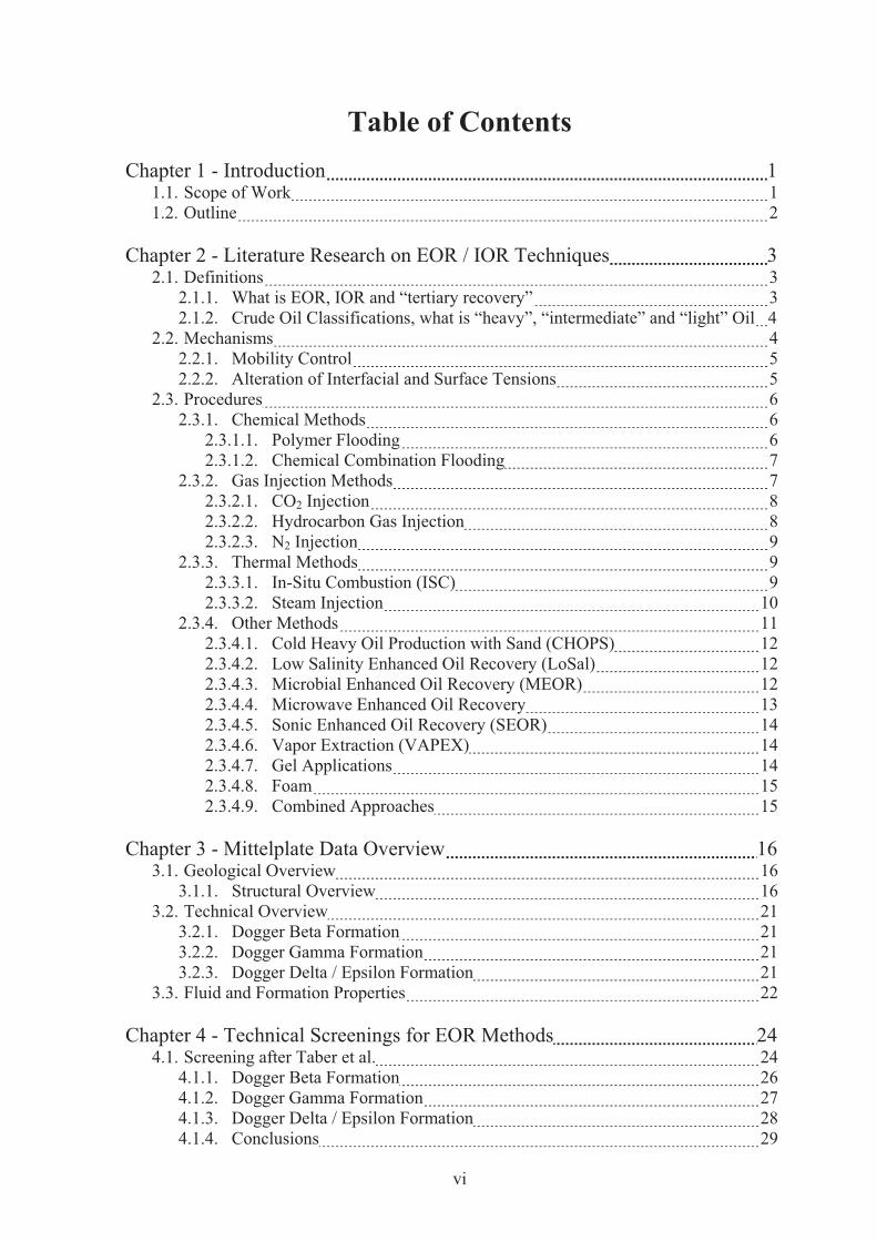
Table of Contents Chapter 1 - Introduction 1
1.1. Scope of Work 11.2. Outline 2
Chapter 2 - Literature Research on EOR / IOR Techniques 32.1. Definitions 3
2.1.1. What is EOR, IOR and “tertiary recovery” 32.1.2. Crude Oil Classifications, what is “heavy”, “intermediate” and “light” Oil 4
2.2. Mechanisms 42.2.1. Mobility Control 52.2.2. Alteration of Interfacial and Surface Tensions 5
2.3. Procedures 62.3.1. Chemical Methods 6
2.3.1.1. Polymer Flooding 62.3.1.2. Chemical Combination Flooding 7
2.3.2. Gas Injection Methods 72.3.2.1. CO2 Injection 82.3.2.2. Hydrocarbon Gas Injection 82.3.2.3. N2 Injection 9
2.3.3. Thermal Methods 92.3.3.1. In-Situ Combustion (ISC) 92.3.3.2. Steam Injection 10
2.3.4. Other Methods 112.3.4.1. Cold Heavy Oil Production with Sand (CHOPS) 122.3.4.2. Low Salinity Enhanced Oil Recovery (LoSal) 122.3.4.3. Microbial Enhanced Oil Recovery (MEOR) 122.3.4.4. Microwave Enhanced Oil Recovery 132.3.4.5. Sonic Enhanced Oil Recovery (SEOR) 142.3.4.6. Vapor Extraction (VAPEX) 142.3.4.7. Gel Applications 142.3.4.8. Foam 152.3.4.9. Combined Approaches 15
Chapter 3 - Mittelplate Data Overview 163.1. Geological Overview 16
3.1.1. Structural Overview 163.2. Technical Overview 21
3.2.1. Dogger Beta Formation 213.2.2. Dogger Gamma Formation 213.2.3. Dogger Delta / Epsilon Formation 21
3.3. Fluid and Formation Properties 22
Chapter 4 - Technical Screenings for EOR Methods 244.1. Screening after Taber et al. 24
4.1.1. Dogger Beta Formation 264.1.2. Dogger Gamma Formation 274.1.3. Dogger Delta / Epsilon Formation 284.1.4. Conclusions 29
vi
4.1.4.1. Dogger Beta Formation 294.1.4.2. Dogger Gamma Formation 304.1.4.3. Dogger Delta / Epsilon Formation 31
4.2. Screening after Al-Bahar et al. 314.2.1. Dogger Beta Formation 334.2.2. Dogger Gamma Formation 344.2.3. Dogger Delta / Epsilon Formation 354.2.4. Conclusions 36
4.2.4.1. Dogger Beta Formation 364.2.4.2. Dogger Gamma Formation 374.2.4.3. Dogger Delta / Epsilon Formation 37
4.3. Screening with Commercial Software 384.3.1. Dogger Beta Formation 394.3.2. Dogger Gamma Formation 394.3.3. Dogger Delta / Epsilon Formation 404.3.4. Conclusions 40
4.3.4.1. Dogger Beta Formation 404.3.4.2. Dogger Gamma Formation 404.3.4.3. Dogger Delta / Epsilon Formation 41
4.4. Screening for unconventional EOR Methods 414.5. Evaluation of Key Parameters 41
4.5.1. Reservoir Depth 414.5.2. Minimum Miscibility Pressure (MMP) 424.5.3. Polymer Suitability 44
4.6. Summary of the technical Screenings 45
Chapter 5 - Analytical Performance Evaluation 465.1. Program Description 465.2. Evaluation of Calculation Options and Boundary Conditions 47
5.2.1. Dogger Beta Formation 475.2.2. Dogger Gamma Formation 495.2.3. Dogger Delta / Epsilon Formation 50
5.3. Prediction for the 2D Cross Sectional Cases 525.3.1. Dogger Beta Formation 525.3.2. Dogger Gamma Formation 555.3.3. Dogger Delta / Epsilon Formation 57
5.4. Prediction for the 3D Cases (5 Spot Pattern) 605.4.1. Dogger Beta Formation 605.4.2. Dogger Gamma Formation 635.4.3. Dogger Delta / Epsilon Formation 65
5.5. Summary of the Analytical Performance Evaluation 68
Chapter 6 - Evaluation of the Promising Methods 696.1. Polymer Injection 69
6.1.1. Surface Equipment 696.1.2. Geological Survey 706.1.3. Technical Analysis 716.1.4. Economical Evaluation 73
6.2. Chemical Combination Flooding 746.3. In-Situ Combustion 746.4. Results of the Detailed Evaluations 76
vii

Chapter 7 - Conclusion and Suggestions 77
Chapter 8 - Nomenclature 78
Chapter 9 - Bibliography 81
Appendix A - Mittelplate Well Overview 85
Appendix B - Mittelplate Formation Volume Factors and Oil Viscosities 86B.1. Dogger Beta Formation 86B.2. Dogger Gamma Formation 88B.3. Dogger Delta Formation 89B.4. Dogger Epsilon Formation 90
Appendix C - Minimum Miscibility Pressure 91C.1. Calculation with Commercial Software 91
C.1.1. Dogger Beta Formation 91C.1.1.1. Carbon Dioxide Injection 91C.1.1.2. Hydrocarbon Gas Injection 92C.1.1.3. Nitrogen Injection 92
C.1.2. Dogger Gamma Formation 93C.1.2.1. Carbon Dioxide Injection 93C.1.2.2. Hydrocarbon Gas Injection 93C.1.2.3. Nitrogen Injection 94
C.1.3. Dogger Delta / Epsilon Formation 94C.1.3.1. Carbon Dioxide Injection 94C.1.3.2. Hydrocarbon Gas Injection 95C.1.3.3. Nitrogen Injection 95
C.2. Calculation of Input Data for MMP Evaluation 96C.2.1. Dogger Beta Formation 96C.2.2. Dogger Gamma Formation 97C.2.3. Dogger Delta / Epsilon Formation 98
Appendix D - Performance Prediction Evaluation 99D.1.Input Data Overview an Origin 99
D.1.1. Dogger Beta Formation 99D.1.2. Dogger Gamma Formation 103D.1.3. Dogger Delta / Epsilon Formation 108
D.2.Evaluation of Calculation Options and Boundary Conditions 113D.2.1. Dogger Beta Formation 113D.2.2. Dogger Gamma Formation 116D.2.3. Dogger Delta / Epsilon Formation 119
Appendix E - Data Correlations for the Dogger Beta Sample Case 122
Appendix F - Data Input for the Wellhead Pressure Calculations 125
viii

List of Figures Figure 2.1.: Phases of Recovery 4Figure 2.2.: Phase Diagram of Water 11
Figure 3.1.: Structural map of the Dogger beta formation 17Figure 3.2.: Structural map of the Dogger gamma formation 18Figure 3.3.: Structural map of the Dogger delta formation 19Figure 3.4.: Structural map of the Dogger epsilon formation 20
Figure 4.1.: Application interval of different polymers in regard to Mittelplate reservoir conditions 44
Figure 5.1.: 2D – Dykstra Parsons – constant rate case for the Dogger beta formation 48Figure 5.2.: 3D – Dykstra Parsons – constant rate case for the Dogger beta formation 48Figure 5.3.: 2D – Dykstra Parsons – constant rate case for the Dogger gamma formation 49Figure 5.4.: 3D – Dykstra Parsons – constant rate case for the Dogger gamma formation 50Figure 5.5.: 2D – Dykstra Parsons – constant rate case for the Dogger delta / epsilon
formation 51Figure 5.6.: 3D – Dykstra Parsons – constant rate case for the Dogger delta / epsilon
formation 51Figure 5.7.: Comparison of the recovery factor for the 2D Dogger beta case 52Figure 5.8.: Comparison of the oil production rate for the 2D Dogger beta case 53Figure 5.9.: Comparison of the water cut for the 2D Dogger beta case 53Figure 5.10.: Injected pore volume for the 2D Dogger beta case 54Figure 5.11.: Comparison of the recovery factor for the 2D Dogger gamma case 55Figure 5.12.: Comparison of the oil production rate for the 2D Dogger gamma case 55Figure 5.13.: Comparison of the water cut for the 2D Dogger gamma case 56Figure 5.14.: Injected pore volume for the 2D Dogger gamma case 56Figure 5.15.: Comparison of the recovery factor for the 2D Dogger delta / epsilon case 57Figure 5.16.: Comparison of the oil production rate for the 2D Dogger delta / epsilon
case 58Figure 5.17.: Comparison of the water cut for the 2D Dogger delta / epsilon case 58Figure 5.18.: Injected pore volume for the 2D Dogger delta / epsilon case 59Figure 5.19: Comparison of the recovery factor for the 3D Dogger beta case 60Figure 5.20.: Comparison of the oil production rate for the 3D Dogger beta case 61Figure 5.21.: Comparison of the water cut for the 3D Dogger beta case 61Figure 5.22.: Injected pore volume for the 3D Dogger beta case 62Figure 5.23.: Comparison of the recovery factor for the 3D Dogger gamma case 63Figure 5.24.: Comparison of the oil production rate for the 3D Dogger gamma case 63Figure 5.25.: Comparison of the water cut for the 3D Dogger gamma case 64Figure 5.26.: Injected pore volume for the 3D Dogger gamma case 64Figure 5.27.: Comparison of the recovery factor for the 3D Dogger delta / epsilon case 65Figure 5.28.: Comparison of the oil production rate for the 3D Dogger delta / epsilon
case 66Figure 5.29.: Comparison of the water cut for the 3D Dogger delta / epsilon case 66Figure 5.30.: Injected pore volume for the 3D Dogger delta / epsilon case 67
Figure 6.1.: Structural map of the Dogger beta formation 70Figure 6.2.: Results of the evaluated sample case 72Figure 6.3.: Computation results of the wellhead pressure for in-situ combustion 75
ix

Figure B.1.: FVF against pressure of Dogger beta crude oil 86Figure B.2.: Viscosity against pressure of Dogger beta crude oil 87Figure B.3.: FVF against pressure of Dogger gamma crude oil 88Figure B.4.: Viscosity against pressure of Dogger gamma crude oil 88Figure B.5.: FVF against pressure of Dogger delta crude oil 89Figure B.6.: Viscosity against pressure of Dogger delta crude oil 89Figure B.7.: FVF against pressure of Dogger epsilon crude oil 90Figure B.8.: Viscosity against pressure of Dogger epsilon crude oil 90
Figure C.1.: MMP for CO2 injection in the Dogger beta formation 91Figure C.2.: MMP for hydrocarbon gas injection in the Dogger beta formation 92Figure C.3.: MMP for nitrogen injection in the Dogger beta formation 92Figure C.4.: MMP for CO2 injection in the Dogger gamma formation 93Figure C.5.: MMP for hydrocarbon gas injection in the Dogger gamma formation 93Figure C.6.: MMP for nitrogen injection in the Dogger gamma formation 94Figure C.7.: MMP for CO2 injection in the Dogger delta / epsilon formation 94Figure C.8.: MMP for hydrocarbon gas injection in the Dogger delta / epsilon formation 95Figure C.9.: MMP for nitrogen injection in the Dogger delta / epsilon formation 95
Figure D.1.: Comparison of the calculation options for the Dogger beta formation, 2D – Dykstra Parsons – constant rate 113
Figure D.2.: Comparison of the calculation options for the Dogger beta formation, 2D – Vertical Equilibrium – constant rate 113
Figure D.3.: Comparison of the calculation options for the Dogger beta formation, 2D – Dykstra Parsons – constant pressure loss 114
Figure D.4.: Comparison of the calculation options for the Dogger beta formation, 3D – Dykstra Parsons – constant rate 114
Figure D.5.: Comparison of the calculation options for the Dogger beta formation, 3D – Vertical Equilibrium – constant rate 115
Figure D.6.: Comparison of the calculation options for the Dogger beta formation, 3D – Dykstra Parsons – constant pressure loss 115
Figure D.7.: Comparison of the calculation options for the Dogger gamma formation, 2D – Dykstra Parsons – constant rate 116
Figure D.8.: Comparison of the calculation options for the Dogger gamma formation, 2D – Vertical Equilibrium – constant rate 116
Figure D.9.: Comparison of the calculation options for the Dogger gamma formation, 2D – Dykstra Parsons – constant pressure loss 117
Figure D.10.: Comparison of the calculation options for the Dogger gamma formation, 3D – Dykstra Parsons – constant rate 117
Figure D.11.: Comparison of the calculation options for the Dogger gamma formation, 3D – Vertical Equilibrium – constant rate 118
Figure D.12.: Comparison of the calculation options for the Dogger gamma formation, 3D – Dykstra Parsons – constant pressure loss 118
Figure D.13.: Comparison of the calculation options for the Dogger delta / epsilon formation, 2D – Dykstra Parsons – constant rate 119
Figure D.14.: Comparison of the calculation options for the Dogger gamma formation, 2D – Vertical Equilibrium – constant rate 119
Figure D.15.: Comparison of the calculation options for the Dogger delta / epsilon formation, 2D – Dykstra Parsons – constant pressure loss 120
Figure D.16.: Comparison of the calculation options for the Dogger delta / epsilon formation, 3D – Dykstra Parsons – constant rate 120
x
Figure D.17.: Comparison of the calculation options for the Dogger delta / epsilon formation, 3D – Vertical Equilibrium – constant rate 121
Figure D.18.: Comparison of the calculation options for the Dogger delta / epsilon formation, 3D – Dykstra Parsons – constant pressure loss 121
Figure F.1.: Data input overview 125Figure F.2.: PVT data input 126Figure F.3.: IPR model selection (1) 126Figure F.4.: IPR model selection (2) 127Figure F.5.: Equipment input overview 127Figure F.6.: Deviation survey 128Figure F.7.: Downhole equipment 128Figure F.8.: Geothermal gradient 129Figure F.9.: Average heat capacities 129
xi
List of Tables
Table 3.1.: Overview of Mittelplate Fluid and Rock Data 22Table 3.2.: Various other important initial reservoir properties 23
Table 4.1.: Sample layout for screening after Taber et al. 25Table 4.2.: Screening after Taber et al. for the Dogger beta formation 26Table 4.3.: Screening after Taber et al. for the Dogger gamma formation 27Table 4.4.: Screening after Taber et al. for the Dogger delta / epsilon formation 28Table 4.5.: Sample layout for screening after Al-Bahar et al. 32Table 4.6.: Screening after Al-Bahar et al. for the Dogger beta formation 33Table 4.7.: Screening after Al-Bahar et al. for the Dogger gamma formation 34Table 4.8.: Screening after Al-Bahar et al. for the Dogger delta / epsilon formation 35Table 4.9.: Reference intervals used by the commercial software 38Table 4.10.: Input values and results for the software screening of the Dogger beta
formation 39Table 4.11.: Input values and results for the software screening of the Dogger gamma
formation 39Table 4.12.: Input values and results for the software screening of the Dogger delta / epsilon
formation 40Table 4.13.: Current reservoir conditions of the Mittelplate horizons 42Table 4.14.: Summary of the results from the software application 42Table 4.15.: Summary of the applied correlations 43
Table 6.1.: Polymer data for the Dogger beta sample case 71Table 6.2.: Example line drive data for the Dogger beta sample case 71Table 6.3.: Results of the evaluated sample case 72Table 6.4.: Results of the economical evaluation 73Table 6.5.: Comparison of operational costs 73Table 6.6.: Comparison of payout period and ROR 74
Table A.1.: Tabular overview of the Mittelplate wells 85
Table C.1.: Calculation of input data for MMP evaluation for the Dogger beta formation 96Table C.2.: Calculation of input data for MMP evaluation for the Dogger gamma
formation 97Table C.3.: Calculation of input data for MMP evaluation for the Dogger delta / epsilon
formation 98
Table D.1.: General reservoir data of the Mittelplate Dogger beta formation 99Table D.2.: Data of the Dogger beta sands 100Table D.3.: Data of the hydrocarbon gas in the Dogger beta formation 100Table D.4.: Relative permeability data of oil and gas in the Dogger beta formation 101Table D.5.: Data of the reservoir brine in the Dogger beta formation 101Table D.6.: Relative permeability data of oil and water in the Dogger beta formation 101Table D.7.: Polymer data for application in the Dogger beta formation 102Table D.8.: Surfactant data for application in the Dogger beta formation 102Table D.9.: Miscible nitrogen injection data for application in the Dogger beta
formation 102Table D.10.: Miscible CO2 injection data for application in the Dogger beta formation 103
xii
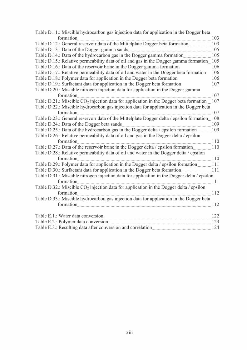
Table D.11.: Miscible hydrocarbon gas injection data for application in the Dogger beta formation 103
Table D.12.: General reservoir data of the Mittelplate Dogger beta formation 103Table D.13.: Data of the Dogger gamma sands 105Table D.14.: Data of the hydrocarbon gas in the Dogger gamma formation 105Table D.15.: Relative permeability data of oil and gas in the Dogger gamma formation 105Table D.16.: Data of the reservoir brine in the Dogger gamma formation 106 Table D.17.: Relative permeability data of oil and water in the Dogger beta formation 106 Table D.18.: Polymer data for application in the Dogger beta formation 106 Table D.19.: Surfactant data for application in the Dogger beta formation 107 Table D.20.: Miscible nitrogen injection data for application in the Dogger gamma
formation 107Table D.21.: Miscible CO2 injection data for application in the Dogger beta formation 107Table D.22.: Miscible hydrocarbon gas injection data for application in the Dogger beta
formation 107Table D.23.: General reservoir data of the Mittelplate Dogger delta / epsilon formation 108Table D.24.: Data of the Dogger beta sands 109Table D.25.: Data of the hydrocarbon gas in the Dogger delta / epsilon formation 109Table D.26.: Relative permeability data of oil and gas in the Dogger delta / epsilon
formation 110Table D.27.: Data of the reservoir brine in the Dogger delta / epsilon formation 110Table D.28.: Relative permeability data of oil and water in the Dogger delta / epsilon
formation 110Table D.29.: Polymer data for application in the Dogger delta / epsilon formation 111Table D.30.: Surfactant data for application in the Dogger beta formation 111Table D.31.: Miscible nitrogen injection data for application in the Dogger delta / epsilon
formation 111Table D.32.: Miscible CO2 injection data for application in the Dogger delta / epsilon
formation 112Table D.33.: Miscible hydrocarbon gas injection data for application in the Dogger beta
formation 112
Table E.1.: Water data conversion 122Table E.2.: Polymer data conversion 123Table E.3.: Resulting data after conversion and correlation 124
xiii

Introduction 1
Chapter 1
Introduction
1.1 Scope of Work Interest in Enhanced and Improved Oil Recovery (in the course of this work abbreviated with
“EOR” and “IOR”) has been on a steady rise during the last couple of years. Due to the
tremendous rise of the oil price, upstream companies in the whole world started to re-evaluate
their assets in the hope for an increased oil production, to satisfy the demands of the open
market. Germany’s largest oil field, the “Mittelplate” field, has been as well a target of
increased consideration from its operator. To clarify the possible applications of tertiary
recovery methods, large literature surveys have been conducted to gasp the full range of
possibilities for the different geological formations of the field. In the course of these
researches, numerous meetings with young external scientists, laboratory and simulation
personal as well as experienced members of the reservoir engineering departments took place,
to question and discuss with them opinions, possible strategies and new developments. After
the technical screenings, where raw data extracted from the simulation models and data sheets
of the formations have been compared to key parameters of the different methods,
supplementary calculations, as for the minimum miscibility pressures of CO2 or N2 miscible
displacements, have been made and compared. Analytical pre simulations have been
conducted afterwards to get a first feeling of the impact of the promising EOR methods and
give base data for a detailed technical and economical evaluation of these techniques. The
results of these studies have been used to suggest further tests and analysis for the continuing
development of the project “EOR – Mittelplate”.
The general objective of the thesis was the evaluation and screening for possible EOR / IOR
mechanisms to apply on the “Mittelplate” oil filed. While an extensive literature research was
conducted to scan for scientific developments and proven industrial screening criteria, the
suggested methods have been examined and interpreted with analytical simulation tools and
under geological, economical and technical aspects. Suggestions for further measurements
and injection targets are made on the basis of these analyses.

Introduction 2
1.2 Outline
Chapter 2 describes the results of the literature surveys. Traditional, specialized and
unconventional EOR methods are presented and briefly discussed.
Chapter 3 gives an introduction about the general data of the Mittelplate oil field. Short
overviews over the structural properties, the reservoir development up until today and the
fluid and formation properties of all oil bearing horizons are presented.
Chapter 4 is a summary of the technical screening studies conducted during this thesis. Two
different literature methods additionally to a software application have been used to evaluate
the Mittelplate oil filed and their results are discussed.
Chapter 5 is comprised of analytical prediction evaluations. Commercial software capable of
analytical simulation has been used to set up models for all Mittelplate horizons and judge
possible additional recovery factors of different EOR methods.
Chapter 6 shows studies conducted for a detailed evaluation of the three promising EOR
methods for the Mittelplate oil field. Geological, economical and technical studies are
presented.
Chapter 7 gives a summary of this thesis work is presented and the main conclusions are
drawn.
Chapter 8 gives an overview over abbreviations, conversion factors and the general
nomenclature used in this work.
Finally, Chapter 9 displays the list of the cited reference literature

Literature Research on EOR / IOR Techniques 3
Chapter 2
Literature Research on EOR / IOR Techniques
The literature research for this diploma thesis has been very extensive. Since the EOR / IOR
market received a huge boost due to the increasing oil prices, many new projects are being
reported in addition to many new scientific approaches. The following chapter tries to capture
the multitude of techniques, definitions and mechanism and put them into a framework,
giving a better overview on the current developments and provide a solid basis for the
practical part of screening and evaluating.
2.1. Definitions2.1.1. What is EOR / IOR and “tertiary recovery” The definitions on what EOR exactly is, are various and very open to interpretation
throughout the literature. This can be explained by the evolution of the term throughout its use
during the last fifty years. After Green et al.1, traditionally primary recovery can be regarded
as production resulting from the natural displacement energy existing in the reservoir, where
no measures to stabilize the pressure are necessary nor taken. Secondary recovery covers the
use of water floods, pressure maintenance and hydrocarbon gas (re-) injection. Tertiary
recovery introduces additional energy into the reservoir over chemical, thermal or physical
means to further enhance oil recovery economically. Usually these mechanisms follow each
other in a chronological sense. As mentioned by Green et al. and Taber et al.2, traditional
tertiary recovery made not always economical or technical sense to be applied last, as for
example with extremely heavy oil reservoirs, and was thus applied already as secondary or
even primary recovery method. Thus the term “Enhanced Oil Recovery” (EOR) got more
accepted within the technical community for the application of advanced recovery
mechanisms. Generally it can be said that EOR describes all processes formally named as
tertiary or advanced secondary process, while in the more recent past the term “Improved Oil
Recovery” has been introduced to describe an even broader spectrum, going from traditional
secondary recovery to improved reservoir management or even infill drilling. As these

Literature Research on EOR / IOR Techniques 4
methods are beyond the scope of this work, only traditional (mostly tertiary) EOR techniques
will be taken into consideration.
1950 1960 1970 1980
Prod
uctio
n ra
te [t
/a]
Primary production
10 %
Secondaryproduction
35 %
Tertiary production
45 % oil rec.
oil
water
Figure 2.1.: Phases of Recovery3
2.1.2. Crude Oil Classifications, what is “heavy”,
“intermediate” and “light” Oil The following definitions from the American Petroleum Institute (API) can be found, among
others, in the literature4,5. For the course of this work this shall be the defining values:
Light crude oil is defined as having an API gravity higher than 31.1 °API
Intermediate crude oil is defined as having an API gravity between 22.3 °API and 31.1 °API
Heavy crude oil is defined as having an API gravity below 22.3 °API.
2.2. MechanismsAll EOR techniques aim to overcome specific limitations in the reservoir to improve the oil
recovery. Those can be either a very bad mobility ratio between the displacing and the
displaced fluid due to high oil viscosity, a very heterogeneous reservoir (both in vertical and
horizontal direction) or high interfacial tensions between the displacing phase and the oil
phase. This chapter deals very briefly with the main mechanisms to improve or overcome the
limitations named above.

Literature Research on EOR / IOR Techniques 5
2.2.1. Mobility Control The mobility1 of a fluid is based on the well known Darcy Equation. For calculation purposes
the concept of the mobility ratio,
dDM �� /� …………………………………………………………………………..………(1)
is a very useful tool to evaluate the impact on the displacement process. It affects both areal
and vertical sweep efficiencies, which decrease as M increases, as well as displacement
efficiency. The displacement front becomes unstable once M > 1 which will lead to viscous
fingering of the front. This situation is usually referred to as an “unfavorable mobility ratio”
while M < 1 is “favorable”. Because of these aspects, control of the mobility ratio can be very
beneficial for the displacement process, and can be achieved over different approaches like
increasing the viscosity of water through the use of chemicals, or decreasing the viscosity of
oil through thermal measures.
2.2.2. Alteration of Interfacial and Surface Tensions Interfacial Tensions (IFT) between fluid – fluid or fluid – rock (so called surface tensions, ST)
systems are key parameters for most EOR methods. IFT influence the capillary forces in the
reservoir, which are key parameters (along with viscous forces) for the capillary number and
thus have a major impact on the residual oil saturation or the entrapment of oil during a
displacement process like water flooding.
The reduction of the IFT, or the enlargement of the dependent capillary number, between oil
and water can considerably reduce the residual oil saturation and thus increase oil recovery.
This mechanism is applied by chemical methods that use alkalis or surfactants (�OW � 0.01
dyne / cm) or by gas displacement methods which reduce the IFT to zero to achieve
miscibility between the oil and the displacing gas phase (CO2, LPG, N2).
Another option is to alter the surface tensions between the reservoir fluids and the reservoir
rock from an oil wet to a water wet system to mobilize the trapped residual oil through the
application of chemical additives.
These techniques and their influences on the IFT’s of the fluid – fluid – rock systems are of a
very complex nature and influence each other severely. These influences have been
extensively discussed in the literature1,6,7. Recent advancements on the experimental side
made IFT measurements between two fluids more practicable, and are helping a lot in the
evaluation of these techniques8,9.

Literature Research on EOR / IOR Techniques 6
2.3. Procedures2.3.1. Chemical Methods Chemical methods are based on the addition of chemicals into the injection water. They either
enhance the viscosity of the drive water (and thus optimize the mobility ratio) or reduce the
IFT. Multiple combinations of different chemicals are used to achieve these targets, which can
be separated into the groups of alkalis, polymers and surfactants.
2.3.1.1. Polymer Flooding10
The addition of polymers into the injection water to enhance its viscosity and thus mobility is
the prime target of this EOR method. Through the enhanced mobility ratio the volumetric
sweep efficiency will be improved and oil from previously untouched parts of the reservoir
will be produced. Although it must be mentioned that polymer flooding does not reduce the
residual oil saturation, but accelerates the time necessary to reach the economic limit of a
project (see analysis later in this work). The recovery mechanism is solely based on mobility
control. Common practical application of this method is the injection of a slug (50 – 100 % of
the pore volume) with a few hundred milligrams polymers, such as for example
polyacrylamides or polysaccharides (biopolymers), per liter of injection water. The polymer
concentration is slowly decreased over time to prohibit viscous fingering of the drive water.
Special care has to be taken with the degradation of polymers due to heat, reservoir brine
salinity, chemical adsorption, stability over time, clay content or bio degradation. Injectivity
of the solution can be a major problem due to its high viscosity and possible damage of the
polymers through shear in the perforations. Generally a pressure drop in the reservoir can be
assumed after the beginning of a polymer injection project due to the higher viscosity of the
injection water. Values as the Residual Resistance Factor (RRF) and the Resistance Factor
(RF) are as well key parameters of polymer floods which need to be checked by laboratory
measurements.
Polymer Flooding is a proved EOR method since decades and thus plentiful literature exists
that describes all major technical aspects, economics, and future outlooks11. Y. Du12 and L.
Guan recently published a paper about experiences gained from the last 40 years of polymer
flooding, which offers a nice overview about this topic. B. K. Maitin offers an overview of all
polymer floods conducted by RWE Dea13. The most prominent and successful international
showcase for polymer injection is the Daqing oilfield in the Peoples Republic of China.

Literature Research on EOR / IOR Techniques 7
2.3.1.2. Chemical Combination Flooding1
Other chemicals aiding the recovery process are surface active agents (surfactants) and
alkaline agents. They do not have an impact on the mobility ratio within the reservoir but
improve recovery through the reduction of IFT. The main differences between these two
chemicals are that alkaline agents have very high pH values (they react with the organic acids
of the crude oil to form surfactants, while regular surfactants are injected with the displacing
water) and the improved economics of alkalis due to their lower cost. The most common form
of surfactants is made up of a hydrophilic and a lipophilic part, which connect themselves to
the aqueous and oleic phases and thus reduce the IFT between oil and water. As well a
reduction of the surface tensions between the reservoir fluids and the reservoir rock can be
achieved, changing the wettability to a more favorable condition and reduce the residual oil
saturation even further.
The injection procedure6 consists of a preflush, which may include sacrificial chemicals and
sweet water to compensate for possible salinity problems and adsorption, followed by the
alkali slug, the actual surfactant slug, where co surfactants such as alcohols might be added to
improve the efficiency even further, a polymer mobility buffer, a taper to reduce viscous
fingering by the drive water and finally the injection water to drive the front through the
reservoir.
Multiple setups of chemical combination floods are possible, examples might be alkaline –
polymer floods, surfactant – polymer floods (also called micellar or low tension floods) or
alkaline – surfactant – polymer floods (ASP Floods), as required by the reservoir or intended
by the responsible engineers.
The necessary precautions which must be taken for chemical combination floods are very
similar to those for polymer floods like injectivity, degradation and proper mixing of the
chemicals.
2.3.2. Gas Injection Methods1
Gas injection methods for EOR purposes are all, so called, “miscible” processes. These
techniques use special injection gases to reduce IFT with crude oils, under specific conditions,
to zero and thus achieve miscibility. Generally two types of miscibility can be distinguished,
one being “First Contact Miscibility (FCM)” and the other “Multiple Contact Miscibility
(MCM)”. With FCM a single phase is established at the first contact between the displacing
gas and the crude oil, while with MCM miscible conditions are generated by in situ
composition upgrading of either the displaced or displacing phase. The reservoir pressure, at

Literature Research on EOR / IOR Techniques 8
which miscibility is achieved, is referred to as the “Minimum Miscibility Pressure (MMP)”.
This pressure is largely dependent on the composition of the crude oil and the injection gas
and the reservoir temperature. As experimental determination of the MMP is an
unstandardized laboratory process, which is difficult and expensive to undertake (slim tube
tests), a wide range of correlations exists to describe it approximately. Much care has to be
taken with these calculations as they usually have only a very narrow range of applicability.
2.3.2.1. CO2 Injection CO2 injection is the most productive gas injection EOR method applied world wide.
Especially in the USA multiple large field projects are conducted due to the large availability
of cheap CO2. The recovery mechanisms of CO2 are manifold. It has a very low IFT with
crude oil (depending on oil composition), which even vanishes at most reservoir pressures and
temperatures and subsequently forms MCM. Other recovery mechanisms include the swelling
of crude oil due to CO2 going in solution, which can increase the volume by 30 %, and the
reduction of crude oil viscosity. The most important parameter is the MMP, for which a large
number of correlations exist in the literature14,15. Special caution must be taken when the
injected CO2 contains impurities, such as methane, as these can have a considerable influence
on the required pressure. The main problems of CO2 injection are the possible asphaltene
precipitation, corrosion problems during injection and production and gas reconditioning.
Injection strategies for CO2 floods usually consist of the CO2 injection (15% hydrocarbon
pore volume or more16) followed by the chase water. Very often WAG strategies are applied
to reduce viscous fingering and improve mobility of the injection process.
2.3.2.2. Hydrocarbon Gas Injection2,15
Three different methods of HC injections are practiced in the field17. Liquefied Petroleum Gas
(LPG) uses the concept of FCM and is usually injected with dry gas and / or water in a WAG
mode. Enriched or Condensing Gas Drive is natural gas enriched with higher components
(such as ethane to hexane) which are transferred during the displacement process to the crude
oil. The slug is as well followed by dry gas and / or water. High pressure or Vaporizing Gas
Drive consists of dry gas (mostly methane) which is injected at a very high pressure to strip
(or vaporize) the crude oil of its light and intermediate components. Both the High Pressure
and the Enriched Gas Drives are MCM processes.

Literature Research on EOR / IOR Techniques 9
The recovery mechanisms are different for the three methods and range from the miscibility
concept over oil swelling to viscosity optimization. The most critical parameters are the
MMP, process economics due to injected hydrocarbon prices and mobility problems.
2.3.2.3. N2 Injection The biggest benefit of nitrogen injection is the price. Because of the low cost it is possible to
inject large volumes for displacement, or even fill portions of the reservoir with it for pressure
support. It recovers additional oil by vaporizing the lighter crude oil components (similar to
the High Pressure Gas Drive) and can achieve miscibility. However, the needed MMP
pressure is the highest within the traditional gas injection methods and thus very hard to
achieve with heavier oils or shallower reservoirs.
2.3.3. Thermal Methods1
Thermal methods have been developed to produce heavy to extra heavy crude oils (bitumen)
and usually apply the principle of mobility control. Introduction of thermal energy via
combustion or steam injection into the reservoir decreases the viscosity of the oil and thus
makes it more mobile and produceable. World wide four different thermal methods developed
into economically feasible processes, namely Forward In Situ Combustion (ISC), Steam
Cycling (also called Huff and Puff), Steam Flooding and Steam Assisted Gravity Drainage
(SAGD) which will be discussed in the following chapter.
2.3.3.1. In-Situ Combustion (ISC) In-Situ Combustion (also called Fire Flooding or Air Injection) can be divided between the
forward and the reverse combustion (similar to Huff and Puff steam injection) processes,
where only the forward combustion will be discussed in detail. The simplified principle is to
inject oxygen or air (due to cost reasons) into the reservoir and ignite it. The reactions
between the oxygen and the crude oil in place (usually around 10% of the OOIP will be
burned, heavy hydrocarbons are preferred) form a very high temperature front which is
propagated, depending on the injection rates, throughout the reservoir. The temperature
ranges from 150 °C to 300 °C for High Pressure Air Injections (HPAI), which is
predominantly used in light oil reservoirs, and 450 °C to 600 °C in heavy oil reservoirs. These
high values are necessary to animate the, for the effective recovery important, “bond scission”
reactions where oxygen breaks the hydrocarbon molecules and forms water and CO2. Other
recovery mechanisms include mobility control, due to increased crude oil temperature

Literature Research on EOR / IOR Techniques 10
(reduced viscosity), oil swelling and near miscible displacement due to CO2 in situ generation
and pressure support due to the injected air. A variation of the classic dry forward combustion
is the “combination of forward combustion and water flooding” (COFCAW) which has
similar effects as the WAG technique.
Key parameters of the process include the process temperature for efficiency control, air
injection rate to keep the combustion alive and control the advancement, air injection
pressures and produced flue gas. A variety of laboratory measurements like flue gas analysis
(CO and O2 determination) exist which help to judge the effectiveness of this EOR method.
Currently several field applications are underway, as the very mature Suplacu de Barcau
project in Romania18 or several projects in the red river formation in North and South Dakota,
USA19.
2.3.3.2. Steam Injection Steam injection is the most productive EOR method world wide with a production of more
then 600,000 bbl oil per day (2004)20. There are three major techniques covering steam
injection, which include Steam Cycling, Steam Flooding and SAGD.
The recovery mechanisms of these methods are the mobilization of the crude oil through the
introduction of heat, steam distillation of the crude oil and pressure support. In general steam
injection is only applied to heavy or extra heavy oil reservoirs which are shallow. The reason
for this can be found in the phase diagram of water, since steam only exists physically at
pressures of up to 221 bar with a temperature exceeding 374 °C21 as shown in Figure 2.2.
Steam Cycling (also called Steam Stimulation, Huff and Puff or Steam Soak) is a technique
applied to a single well. For a few weeks steam is injected into the well, which is then shut in
to let the steam soak into the formation, followed by a production phase. With every
conducted cycle the amount of oil recovered will be decreasing, until the economic limit is
reach. Once that is the case, these producers are usually converted to full time injectors for a
following steam field flood project. It has also been reported that producing wells of a steam
flood project applied the huff and puff technique as well to maximize crude oil recovery.
SAGD is a special technique developed for the tar sands in Canada. It is based on the
application of two horizontal wells, which are separated vertically by a few meters. The
structural higher well injects steam into the reservoir, which heats the crude oil and displaces
it via gravity drainage to the lower production well. The design of this technique is very
similar to the VAPEX method.

Literature Research on EOR / IOR Techniques 11
Key parameters for steam injection projects are thermal conductivities of the well and the
reservoir formation (to maximize heat transfer to the crude oil), reservoir temperature and
pressure to ensure the existence of steam in situ and design appropriated injection conditions,
the energy balance between crude oil required for steam generation in opposition to the
amount produced additionally, water supplies, ecological parameters such as flue gas
generation while steam production and possible environmental impact on the surface when
operating in very shallow reservoirs.
Steam injection techniques have been applied since decades in the Californian Kern County
heavy oil fields, but the most impressive and successful project until today is the Duri22 Steam
Flood in Indonesia with a production of over 200.000 bbl oil per day.
Figure 2.2.: Phase Diagram of Water23
2.3.4. Other Methods Additionally to the traditional EOR methods named above, different specialized methods have
been developed, such as VAPEX or CHOPS, for heavy oil recovery. Besides those
specializations, major research initiatives from companies, universities or governments
developed completely new EOR concepts such as MEOR or the application of microwave
technology for enhanced oil recovery. A short overview over recent developments is
presented in the following chapter.

Literature Research on EOR / IOR Techniques 12
2.3.4.1. Cold Heavy Oil Production with Sand (CHOPS) CHOPS is a primary production technique developed for the extra heavy tar sands in Canada.
Through the use of progressive cavity pumps the reservoir is produced from the beginning
with big sand cuts of up to 50% in volume. Over the course of a year, the sand cuts slowly
reduce to approximately 1 - 5% and stay at this levels for the ensuing years. Due to the large
amount of sand production in the beginning, so called worm holes may form within the
formation. They enhance the effective permeability and the well radius of the borehole and
thus have a positive impact on production. Another possibility, depending on the reservoir
pressure and the gas in solution, is the appearance of foamy oil. Foamy oil describes a special
consistency of the crude oil, which occurs when gas is coming out of solution but stays
trapped within the fluid phase due to the extreme viscosities. Due to this condition, the crude
oil is improved in his flowing capability which benefits production of the reservoir.
Another positive effect of chops is the generation of flow paths for a possibly following steam
injection project, as described in SPE paper 5877320.
2.3.4.2. Low Salinity Enhanced Oil Recovery (LoSal)24,25
In a recent SPE paper, McGuire et al. suggested the use of LoSal EOR in oil fields with high
salinity reservoir brines, like for Alaska’s North Slope. Instead of the produced reservoir brine
sweet water with very low salinities (below 5000 ppm) are injected into the reservoir. The
recovery mechanisms for this technique seem to be very similar to alkaline floods. Due to the
very low salinity of the injection water and thus very high alkalinity or pH value, the injection
water reduces the IFT between oil and water, increases the water wettability of the reservoir
and generates surfactants due to saponifying of acid components in the crude oil. Experiments
on Berea core samples show a considerable increase of recovery. Another possible
mechanism is the detachment of mixed-wet clay particles from the pore walls.
However, the presence of a large sweet water supply with fitting parameters is imperative for
this EOR method. Additionally it is unsure if conducted laboratory research can be scaled up
to reservoir conditions, thus future work on this newly considered EOR method will be very
important.
2.3.4.3. Microbial Enhanced Oil Recovery (MEOR) In the last decade a lot of scientific work in regard to MEOR has been conducted worldwide,
trying to advance this technique from the laboratory to successful field application. Bryant26
and Lockhart published a study describing the reservoir engineering aspects of MEOR,
Literature Research on EOR / IOR Techniques 13
incorporating an analysis of possible methods and reactions and suggesting formulas for
analytical evaluation and process calculations.
MEOR is a technique developed in the 1970’s to 1980’s, seeking to recover additional oil by
the application of microbes. There are several different ways to achieve this, and several
possible recovery mechanisms which might be employed. The basic idea is to have the
microbes generating chemicals or gases, such as surfactants or CO2, in situ and thus achieve a
cost optimization and easier designs due to the lack of surface equipment. An alternative
option is the plugging of thieve zones due to biomass generation.
Key parameters for the application of microbes are the microbial reactor type, the carbon
source, microbe provenance and reservoir conditions such as temperature, salinity and
pressure.
The main issue with MEOR is the lack of descriptive field tests, which have not only been
technical successful, but as well economical viable projects. The US Department of Energy
recently conducted a study27 to increase efficiency of MEOR projects, but more research has
to be conducted until this method can be regarded as adequately described and commercially
promising.
2.3.4.4. Microwave Enhanced Oil Recovery A very new EOR approach, getting a reasonable amount of attention lately, is the possibility
of applying microwave radiation in a reservoir. The mechanisms of this technique are not
completely understood yet, but seem to be composed out of heating and cracking
mechanisms, depending on the existence of a catalyzer within the formation. There already
exist sample laboratory experiments, where crude oil was cracked and possible reactions,
implied through plasma discharges, have been described28. The technique itself has a wide
range of application, from thermal cracking mechanisms in oil refineries, cuttings upgrading
in drilling engineering, heating oil for better pumping properties in pipeline engineering to
possible in situ application for EOR in reservoir engineering. Due to these reasons, American
research institutes, as the US Department of Energy in its “Cold Cracking Report”29, have
been picking up this topic. New start-up business companies formed to develop this technique
even further, while bigger E&P companies are evaluating possible applications30. However,
more fundamental research needs to be conducted to achieve commercial viability.
Literature Research on EOR / IOR Techniques 14
2.3.4.5. Sonic Enhanced Oil Recovery (SEOR) SEOR, as microwave EOR, is another exotic idea being picked up again due to the large EOR
potential deriving from the high crude oil prices. The basic mechanism is a mobilization of
residual oil in the pore throats (so called ganglia) through the application of seismic waves.
An U.S. Department of Energy project was conducted to formulate a theoretical background
for SEOR and conduct field testing31. Application possibilities have been outlined to be
reservoirs with shallow depth, water flooded with a water saturation of 90% percent or higher
and low crude oil viscosity. Emphasize must be taken to select optimal resonant frequencies
to maximize the mobilization effect. Furthermore there have been reports of experiments
conducted in the former U.S.S.R., but the literature was, if reported, in Russian and very hard
to find and thus not further tracked.
2.3.4.6. Vapor Extraction (VAPEX)32
VAPEX is an EOR method very similar to SAGD. It originates, as well, from the Canadian
oil sand production and got developed as an alternative to SAGD. Main reason for the
development is the increasing lack of fresh water supplies for steam projects, but large enough
natural gas resources exist in the region allowing a different approach.
The concept behind VAPEX involves, as with SAGD, the drilling of two horizontal wells in
close vertical distance. However, instead of injecting steam into the structural higher borehole
to mobilize the heavy oil, hydrocarbon gas is used. After injection it diffuses into the crude
oil, enhancing its viscosity and thus mobilizing it. The upgraded crude oil is then displaced by
gravity drainage towards the structural lower well and produced.
One main design consideration of VAPEX is the fact that molecular diffusion works much
slower then thermal, which is its main disadvantage compared to SAGD. However, it is
possible to equalize this problem by drilling longer horizontal wells to maximize reservoir
contact and enhance VAPEX production rates.
2.3.4.7. Gel Applications1
Reservoir heterogeneities are a major reason for low recovery factors. Special attention has to
be given to high permeability layers, so called “thief zones”, which take most of the injected
fluid. These zones can put every EOR / IOR technique in danger and reduce severely the
volumetric sweep efficiencies. One solution technique to fight these zones is the injection of
cross-linking polymer solutions, which form in situ gels of considerable strength and thus
reduce the effective permeability and divert the injection stream towards the lesser flooded
Literature Research on EOR / IOR Techniques 15
areas. An important parameter for the application of this method is the vertical permeability
between the different layers in the reservoir, since they can considerably reduce the efficiency
of the gel placement.
Different procedures, depending on the used polymer system, exist for gel placements. One
option is to inject the chemicals (polymers and cross linking agents) as separated slugs into
the reservoir. Another method is the mixing of the chemicals during the injection, effectively
starting the gel formation in the reservoir, while for the last option (often used with
biopolymers) the solution is already mixed in a surface tank. During this option the gel
formation starts already in the tank, but the solution remains pumpable, until reaching the
reservoir formation. Time management is of importance with this technique, similar as with
cement placement.
2.3.4.8. Foam1
Foam offers a wide range of applications within IOR and EOR. It consists of a large volume
of gas in a much smaller volume of liquid, generated usually through the use of a foaming
agent (surfactant). It can be used for:
� Blocking or restricting flow of unwanted fluids such as water or gas during coning
problems
� Profile modifications (plugging of thief zones, similar to gels, for a better propagation
of injection fluids)
� Mobility control of an injected gas phase (similar benefits as WAG techniques)
Usually only a very small volume (a few percent) of the foaming agent is needed to achieve
the desired effect. However, care must be taken with its application due to the large pressure
losses over the occupied volume.
2.3.4.9. Combined Approaches Another direction to maximize oil recovery even further has been the idea of combining
traditional EOR techniques. Castanier and Kovscek33 presented the idea of using a
combination of solvents and in-situ combustion to increase heavy oil recovery in Canada and
Venezuela in a cyclic injection process. Another publicized method is the combination of
VAPEX and SAGD in a steam-propane trial for the well known Duri field in Indonesia34,
where pilot tests have been pretty successful.
Combined approaches of different EOR methods offer a wide range of possibilities and
applications and their boundaries have yet to be determined.
Mittelplate Data Overview 16
Chapter 3
Mittelplate Data Overview
The following chapter will give a short overview over the known data of the Mittelplate oil
field. Structural maps for geological information, a short overview of the already drilled wells
and a summary of the formation fluid and formation rock data will be given.
3.1. Geological Overview The Mittelplate oil field is situated about 100 km northwest of the city of Hamburg in the
estuary mouth of the river Elbe. This location is a big challenge for the field development due
to two reasons. First the Elbe serves as an important international shipping route to one of
Europe’s biggest commercial harbors located in Hamburg and secondly the area operated in
belongs to the Wadden Sea National Park. These circumstances call for special care in
environmental protection and make the placement of additional drilling rigs or pipelines for
EOR projects extremely difficult.
Geologically the Mittelplate field is situated in the Westholstein Jurassic trough along the
Büsum salt dome. The five oil bearing horizons range from the Lowest Cretaceous Wealden
formation to the Jurassic Dogger formation where the beta, gamma, delta and epsilon horizons
are being produced. Each of the horizons is composed out of different productive sands. The
depth ranges from 1900 meter below sea level (Wealden) to about 3000 meter (Dogger beta),
where the Dogger beta formation is, with an area of more than 60 km², by far the largest
horizon.
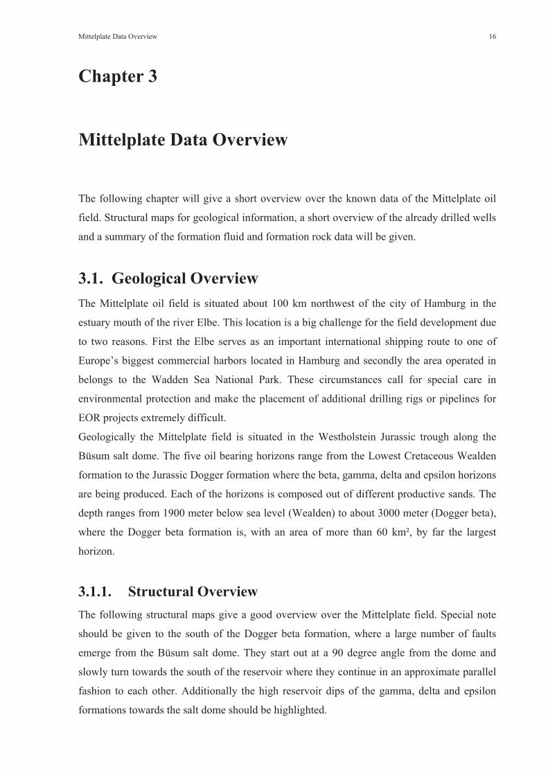
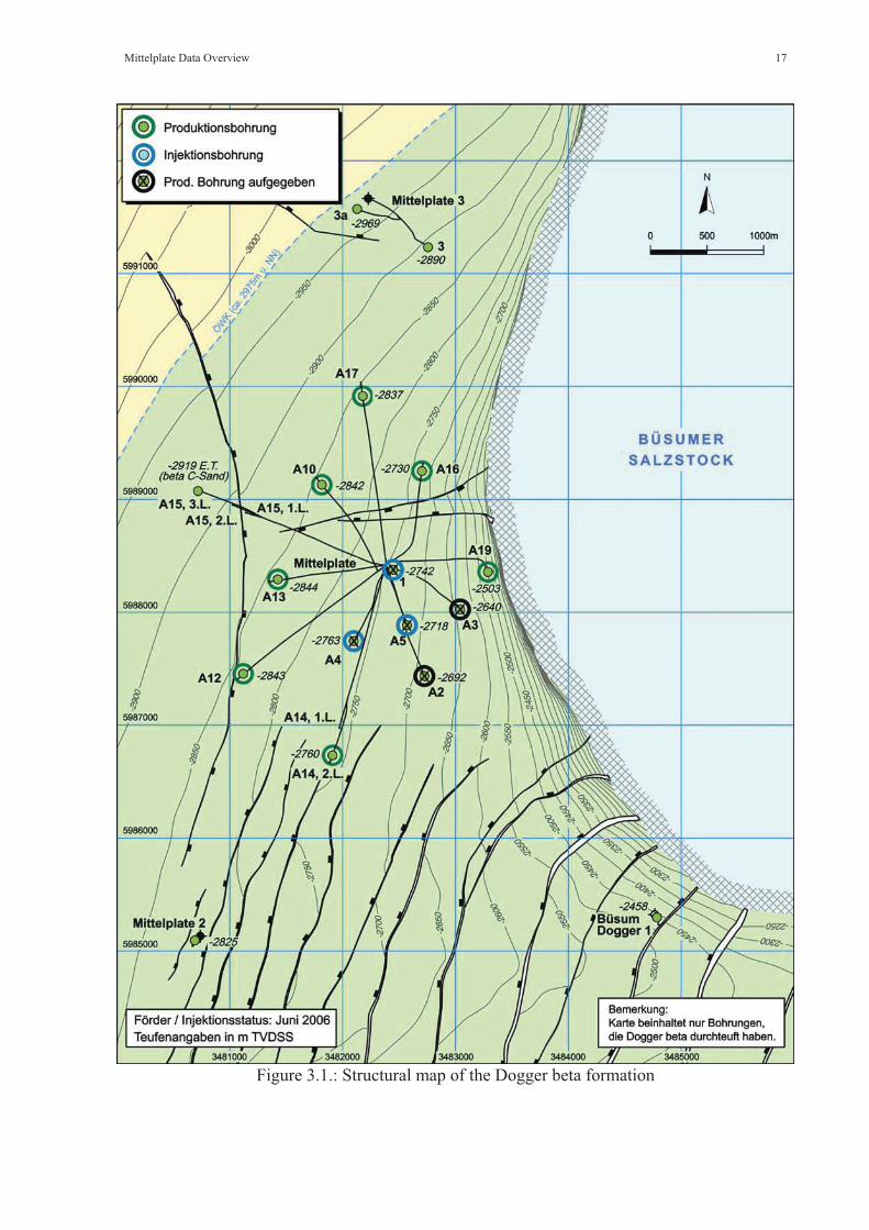
3.1.1. Structural Overview The following structural maps give a good overview over the Mittelplate field. Special note
should be given to the south of the Dogger beta formation, where a large number of faults
emerge from the Büsum salt dome. They start out at a 90 degree angle from the dome and
slowly turn towards the south of the reservoir where they continue in an approximate parallel
fashion to each other. Additionally the high reservoir dips of the gamma, delta and epsilon
formations towards the salt dome should be highlighted.
Mittelplate Data Overview 17
Figure 3.1.: Structural map of the Dogger beta formation
Mittelplate Data Overview 18
Figure 3.2.: Structural map of the Dogger gamma formation

Mittelplate Data Overview 19
Figure 3.3.: Structural map of the Dogger delta formation

Mittelplate Data Overview 20
Figure 3.4.: Structural map of the Dogger epsilon formation

Mittelplate Data Overview 21
3.2. Technical Overview 3.2.1. Dogger Beta FormationThe initial development plan for the largest Mittelplate horizon, the Dogger beta formation,
started with a 5 spot scheme in the central area around the Mittelplate 1 exploration well.
Currently, as can be seen in the structural maps above, the wells 1, A4 and A5 serve as water
injection wells for pressure support, while the wells A3 and A4 have been liquidated due to
economic reasons. The general field development plan follows the intention to drill producers
in a circular pattern around the initial 5 spot scheme, as can be seen by the producers A10 to
A19. All producers are equipped with electric submersible pumps to enhance productivity.
3.2.2. Dogger Gamma FormationThe Dogger gamma formation is the smallest Mittelplate horizon and thus offers only very
limited development possibilities. Currently only one well is producing from this formation,
the well A8b, while pressure supply is provided by an active water aquifer. The production
wells A9a and A3a have been liquidated. The main potential for development lies within the
southern region of the horizon, which is separated from the north by a large fault. The
production well is, analogues to the beta wells, equipped with an electric submersible pump.
3.2.3. Dogger Delta / Epsilon FormationDue to the hydrodynamic contact between these two formations, they will be regarded as one
horizon in the course of this study. They share the water oil contacts (WOC), initial reservoir
pressures and their wells show pressure responses induced from water injectors of both
horizons. A complete list of producers and injectors can be found in appendix A in tabular
form. One of the most interesting aspects about these formations is that the production wells
are mostly extended reach wells drilled from the onshore location Dieksand, while the
injection wells are based out of the Mittelplate offshore platform. The horizontal well AH-1
serves as the main water injector and injects directly into the active aquifer to support the
pressure and dispose produced formation water. The flow paths within the horizons are not
yet fully understood, but are research targets of a tracer study, which is planned for the
coming year. Possible flow paths will be discussed later in this study.
Analogue to the production wells in the other horizons, all Dieksand production wells have
electrical submersible pumps installed.

Mittelplate Data Overview 22
3.3. Fluid and Formation Properties
Table 3.1.: Overview of Mittelplate Fluid and Rock Data
Table 3.1 shows an overview of averaged reservoir rock and fluid parameters for each of the
Mittelplate horizons. The parameters chosen for this table represent all necessary data needed

Mittelplate Data Overview 23
for the application of quick screening tools for EOR methods. Several of those tools have
been applied to the Mittelplate field and will be described in detail in the next chapter.
The data has been compiled from different sources within the operating company, consisting
mainly of the Eclipse models of the different formations, the data handbook for the
Mittelplate field, several PVT Reports of the crude oils and analyses (such as formation water
tests) from the E&P Laboratory.
The data represent here shows mean, low and high values for several parameters and is dated
with September 2006. Obviously several parameters, such as the average reservoir pressure
or saturations, are expected to change over time.
Table 3.2 gives and overview of other initial reservoir properties such as pressure or OWC.
Diagrams for the formation volume factors and the viscosity of the crude oils are presented in
appendix B.
Table 3.2.: Various other important initial reservoir properties

Technical Screenings for EOR Methods 24
Chapter 4
Technical Screenings for EOR Methods
The first step in the assessment of possible EOR methods for the Mittelplate oil field was the
employment of technical screening studies. After an elaborate literature research and a survey
of commercial software for this application, the guidelines of Taber et al.2 and Al-Bahar35 et
al. have been chosen additionally to a software package, which features an applicability
screening and the possibility of analytical simulation. Unconventional EOR methods are
screened after various other literature sources. Additionally studies of critical parameters have
been carried through to improve the viability of the assessment.
In general a color coding principle has been applied to all screening studies, marking data in
the required reference interval green and data outside the interval red. Borderline cases have
been marked yellow, N.C. stands for not critical. It must be said that all given applicability
ranges for EOR methods are derived from published field cases, physical or chemical
limitations and must be generally perceived as suggestion but not definite borders. The results
of said screening methods are thus not of an absolute nature but can show trends and
problematic parameters, thus, before excluding any specific EOR method, further research has
to conducted on reservoir or fluid data, which are marked with a red tag.
Usually screening procedures are applied only to a certain area or pattern within a reservoir
(as for example a 5 spot pattern) but the presented studies tried to cover the whole reservoir
due to the small areal extensions of the Mittelplate gamma, delta and epsilon horizons.
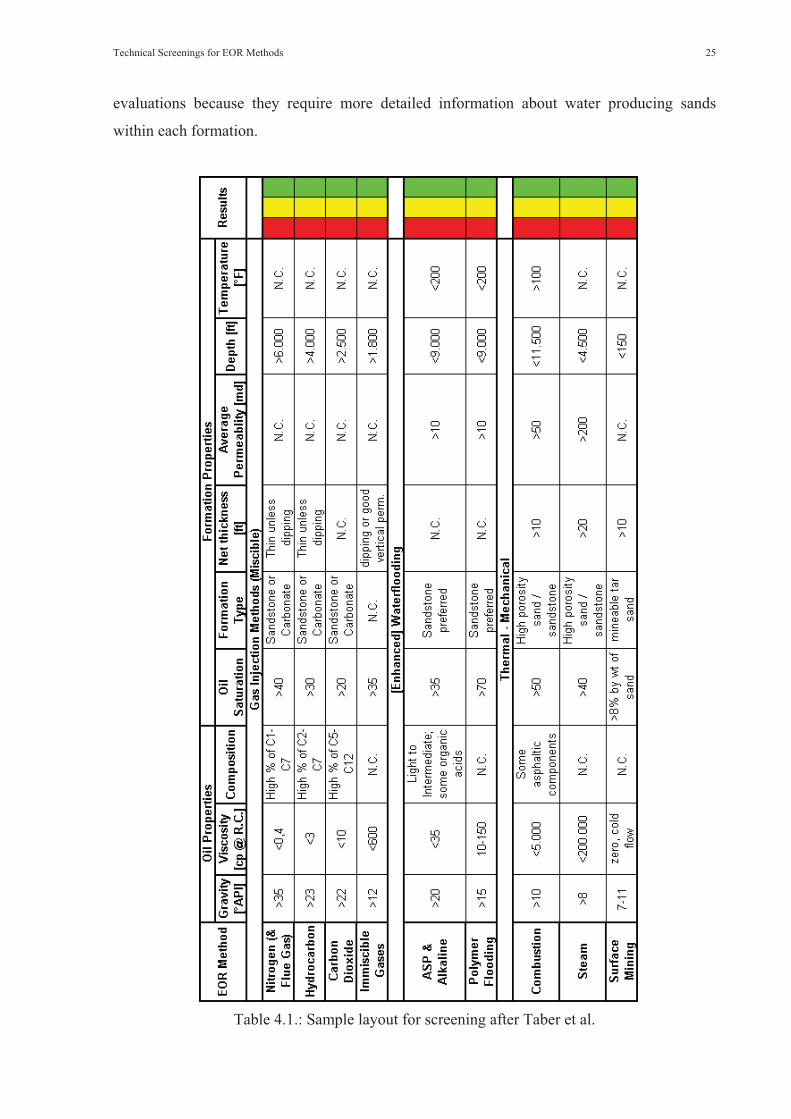
4.1. Screening after Taber et al.2
Taber et al. described screening criteria for gas injection methods (nitrogen, CO2 and
hydrocarbon gas in miscible mode and a generalized immiscible gas injection method),
enhanced water treatments (polymer flooding and chemical combination floods) and thermal
– mechanical methods (in-situ combustion, steam flooding and surface mining) using a wide
range of reservoir rock and fluid properties. Table 4.1 shows a sample layout for the screening
after Taber et al. while the following sub chapters will give detailed studies for each of the
Mittelplate horizon. Gel treatments have been neglected for the general applicability
Technical Screenings for EOR Methods 25
evaluations because they require more detailed information about water producing sands
within each formation.
Table 4.1.: Sample layout for screening after Taber et al.

Technical Screenings for EOR Methods 26
4.1.1. Dogger Beta Formation
Table 4.2.: Screening after Taber et al. for the Dogger beta formation
Technical Screenings for EOR Methods 27
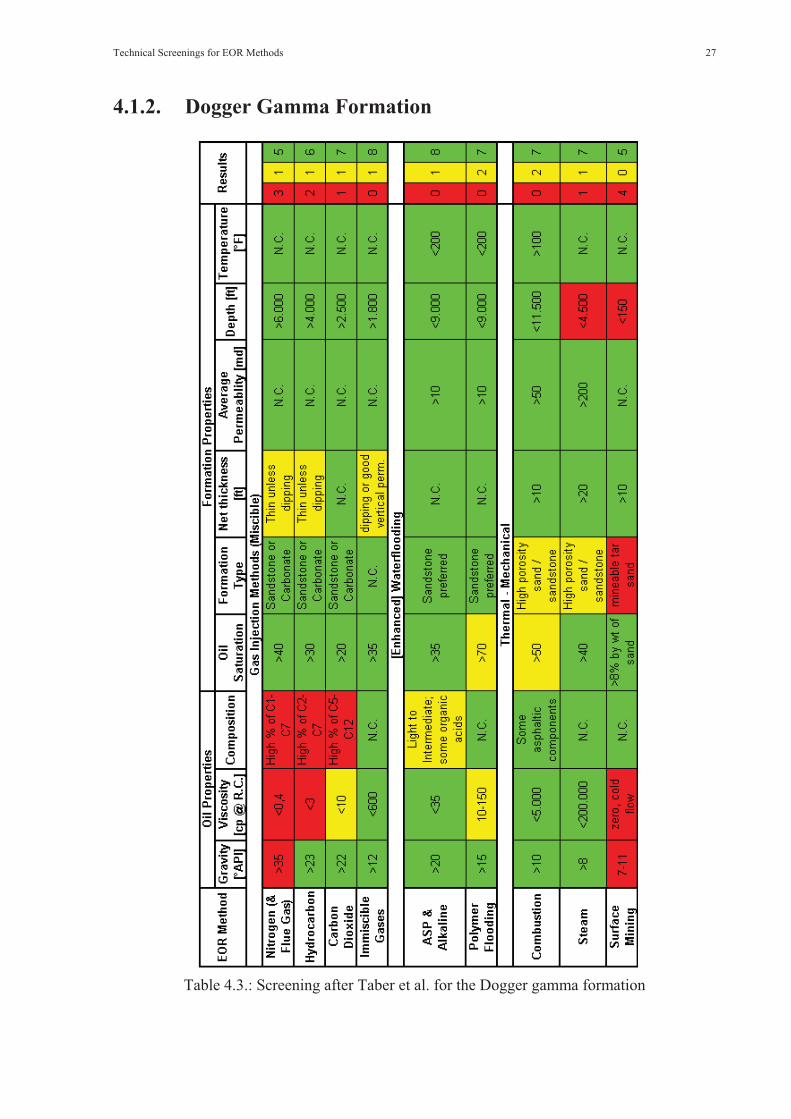
4.1.2. Dogger Gamma Formation
Table 4.3.: Screening after Taber et al. for the Dogger gamma formation
Technical Screenings for EOR Methods 28
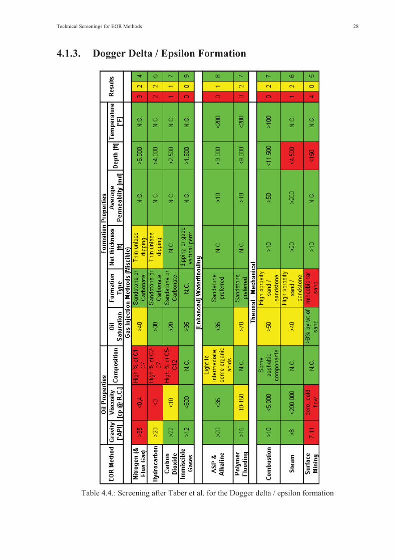
4.1.3. Dogger Delta / Epsilon Formation
Table 4.4.: Screening after Taber et al. for the Dogger delta / epsilon formation

Technical Screenings for EOR Methods 29
4.1.4. Conclusions4.1.4.1. Dogger Beta Formation For the Dogger beta formation, Taber et al. yields immiscible gas displacements, enhanced
water flooding and in-situ combustion as viable EOR mechanisms, all other methods have at
least one parameter that fails the required range.
The only secondary recovery technique considered is immiscible gas displacement, while
regular water injection is neglected in the screening process. As described in chapter 3, water
injection has been chosen over gas injection already several years ago, due to the following
reasons:
� Water injection is far more economical for the Mittelplate field, as produced water can
be disposed again into the formation and thus saving water treatment costs.
� The GOR experienced from Mittelplate horizons is very low (around 10 sm³ gas / sm³
oil) and thus transportation of displacement gas to the offshore platform would to be
required, which is not economically viable.
� All Mittelplate horizons are operated above the bubble point pressure and thus do not
have a gas cap.
� If other gases apart from hydrocarbon gas would have been taken into consideration,
additional technical problems as corrosion and precipitations (if applying CO2) spoke
as well against an application of an immiscible gas displacement.
Due to this reasons and water injection already in place, a further discussion about the
secondary recovery mechanism can be regarded as redundant. As well water alternating gas
(WAG) methods are, due to gas shortage reasons, not a viable technique for the Mittelplate oil
field.
For tertiary recovery mechanisms Taber et al.’s results show that there are two crucial
parameters, namely crude oil quality (API gravity, viscosity and molecular composition) and
reservoir depth. All miscible gas displacements fail due to bad oil composition (all having
three parameters outside the required interval), which implies that the required minimum
miscibility pressure (MMP) cannot be reached. A more detailed study on this topic will
follow later in this work. Steam injection techniques and surface mining methods fail (having
one or more bad parameters) mainly due to the reservoir depth of more then 2500 meters.
Steam can not exist physically at reservoir conditions found within the Dogger beta horizon
and surface mining is not viable at such depths.
Technical Screenings for EOR Methods 30
Due to these reasons the only viable EOR mechanisms, according to reservoir data and
applying Taber et al.’s screening guidelines, for the Dogger beta horizon are enhanced water
flooding techniques (polymer flooding and chemical combination flooding) and in-situ
combustion. Special note has to be taken about the oil saturations within the horizon, as they
differ throughout the field. The central region around the initial 5 spot scheme has already
very high water saturations while the outer regions still have the initial oil saturations.
4.1.4.2. Dogger Gamma FormationGenerally speaking the results for the Dogger gamma formation are similar to the Dogger beta
formation. According to Taber et al.’s screening procedure, again immiscible gas
displacement, enhanced water flooding techniques and in-situ combustion remain the viable
EOR methods.
The main difference to the Dogger beta formation in regard to secondary recovery is that the
Dogger gamma formation does not have water injectors, but an active water aquifer which
supplies the needed pressure for the production well, which is currently the only one in place.
Due to these facts, there is no need to install additional pressure supply through the
application of water or gas injectors, which would as well face the same limitations as for the
Dogger beta formation.
From a screening for tertiary recovery methods perspective, the crude oil from the gamma
formation is quite similar to the beta oil. The main difference lies within the better oil quality
of the gamma crude oil, when looking at the API gravity and viscosity categories. CO2
injection has only one parameter failing the required reference interval and thus might be
eligible for further consideration if the MMP can be achieved without taking the risk of
fracturing the formation. However, side effects as corrosion and asphaltene precipitation must
be taken into consideration. Analogues to the Dogger beta formation, crude oil quality and
reservoir depth are the limiting factors.
Nevertheless, the viable EOR methods resulting from the screening process are analogues to
the Dogger beta results. Enhanced water flooding techniques and in-situ combustion remain
the techniques of choice, while the oil saturation is still a parameter which needs to be taken
care of.

Technical Screenings for EOR Methods 31
4.1.4.3. Dogger Delta / Epsilon Formation The results of the screening process for the Dogger delta / epsilon formation are analogues to
the results of the other horizons, as the crude oil quality can be placed between Dogger beta
quality (worst quality Mittelplate oil) and Dogger gamma quality (best quality Mittelplate
oil).
As a secondary recovery mechanism water injection is already in place within this horizon, as
can be seen from the technical description in chapter 3. Additionally the delta / epsilon
formation is pressure supported by a very strong water aquifer, which makes a further
discussion of a secondary gas injection redundant. It would, as well, face the same limitations
named for the Dogger beta formation.
For the application of tertiary recovery mechanisms, the results for the Dogger delta / epsilon
formation are more similar to the results of the beta formation than the gamma formation,
which can be seen by the results for miscible gas displacement. Again crude oil quality and
reservoir depth rule most EOR mechanisms out.
According to these reasons, the only possible EOR methods left are the application of
enhanced water flooding or in-situ combustion, considering a screening point of view.
4.2. Screening after Al-Bahar et al.35
The screening guidelines of Al-Bahar et al. are based upon the suggestions of Taber et al., but
take more data from published field cases into consideration and offer a more detailed
analysis. Essentially Al-Bahar et al. used a wider range of reservoir rock and fluid data to
describe the possible applicability of EOR methods, while differentiating those into more sub
groups. He considered different chemical combination floods separately (there are separate
data sets for alkali – polymer, surfactant – polymer and alkali – surfactant – polymer floods)
and added water injection as a second secondary recovery method.
Table 4.5 shows a sample layout of Al-Bahar et al.’s analysis and the subsequent Tables 4.6
till 4.8 show the detailed studies for the Mittelplate formations.
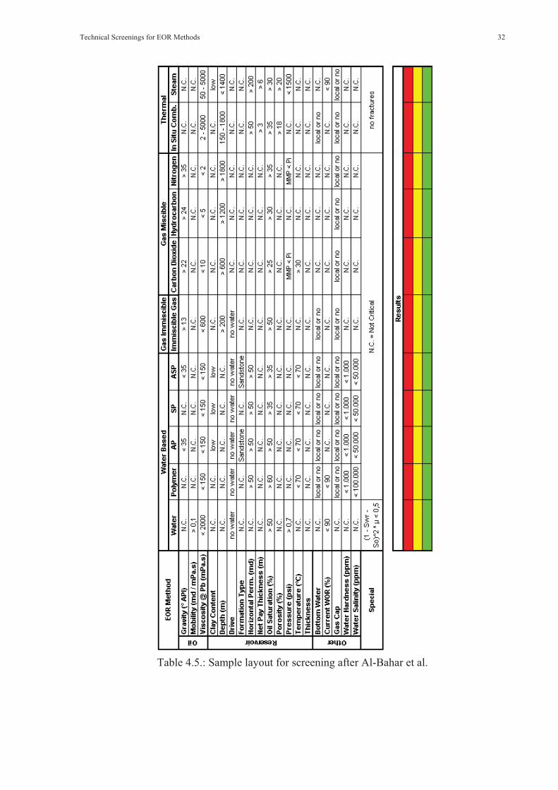
Technical Screenings for EOR Methods 32
Table 4.5.: Sample layout for screening after Al-Bahar et al.
Technical Screenings for EOR Methods 33
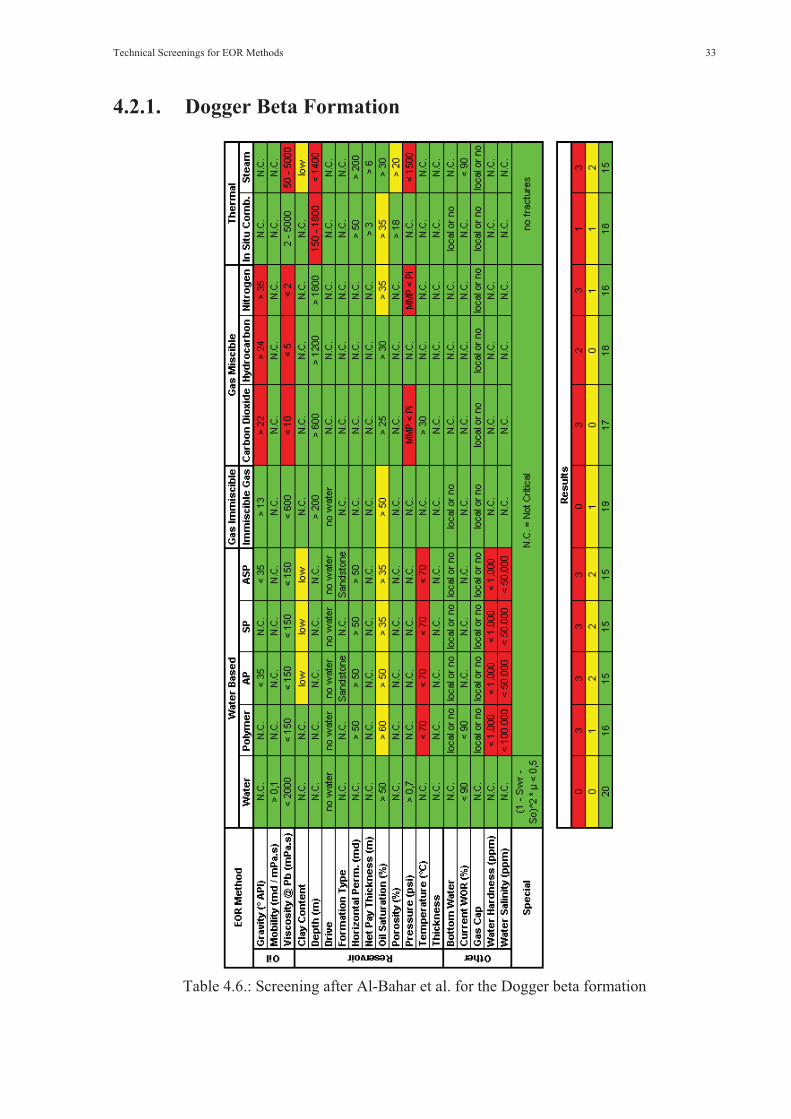
4.2.1. Dogger Beta Formation
Table 4.6.: Screening after Al-Bahar et al. for the Dogger beta formation

Technical Screenings for EOR Methods 34
4.2.2. Dogger Gamma Formation
Table 4.7.: Screening after Al-Bahar et al. for the Dogger gamma formation

Technical Screenings for EOR Methods 35
4.2.3. Dogger Delta / Epsilon Formation
Table 4.8.: Screening after Al-Bahar et al. for the Dogger delta / epsilon formation
Technical Screenings for EOR Methods 36
4.2.4. Conclusions4.2.4.1. Dogger Beta FormationFor the Dogger beta formation Al-Bahar et al. yields only secondary recovery methods as
possible EOR techniques, namely water injection and immiscible gas displacement. All other
methods have between one and three parameters outside the required reference interval and
are thus marked red.
Al-Bahar gives both secondary recovery techniques excellent results. As explained earlier, a
water injection program is already in place for the Dogger beta formation.
More interesting is the study for possible tertiary recovery mechanisms. Analogues to Taber
et al., miscible gas displacement fails due to crude oil quality, which will be studied in more
detail in a later chapter. However, an interesting point is that Al-Bahar et al. included directly
the prerequisite of the MMP being lower than the initial pressure pi. It can be however not
explained, why this condition is missing for the application of a miscible hydrocarbon gas
displacement, as miscibility is as well a requirement for this technique. Both thermal EOR
methods fail because of the high reservoir depth, which is definite bad parameter for steam
injection due to the physical properties of water. For in-situ combustion however, this
requirement is likely to be derived from possible wellhead injection pressures, which needs to
be evaluated separately to make a definite statement. The main differences between Taber et
al. and Al-Bahar et al. are getting visible during the comparison of the results for water based
EOR methods (chemical and chemical combination floods). Al-Bahar et al.’s screening
guidelines include properties such as reservoir temperature, water hardness and water salinity,
which are the main limitations for chemical additives, such as polyacrylamides. The
parameter range applied even suggests that polyacrylamide limitations have been used to set
the boundary conditions. There are of course alternative and more expensive additives, such
as for example biopolymers or synthetic polymers, which can be applied at higher
temperatures or salinities than the boundaries given by Al-Bahar et al. In conclusion there are
five critical parameters for the Dogger beta formation when screening after Al-Bahar et al.,
reservoir depth, reservoir temperature, pressure (reservoir and MMP) crude oil quality and
water salinity.
Due to the reasoning supplied, the screening study after Al-Bahar et al. suggests a more
detailed evaluation of water based or enhanced water floods such as polymer floods or
chemical combination floods and in-situ combustion. As noted already above, caution must be
taken in regard to saturation values.

Technical Screenings for EOR Methods 37
4.2.4.2. Dogger Gamma FormationFor the Dogger gamma formation Al-Bahar et al. yields no EOR method with a spotless
result. All techniques have between one and three parameters outside the reference interval,
which is a rather disappointing result. If we consider all methods with only one parameter
failing, Al-Bahar et al. gives water injection, immiscible gas displacement, miscible CO2 and
hydrocarbon gas injection and in-situ combustion as viable methods.
For the purpose of secondary recovery, both available techniques fail the condition of having
no active waterdrive. This however, is a very arguable limitation as an active water drive
certainly must be taken into consideration when applying water injection or immiscible gas
displacement for pressure support, but hardly rules it out. However, taking the small amount
of producers of the Dogger gamma formation into consideration additionally to the active
water aquifer, there is no further need to implant additional pressure support.
Considering tertiary recovery mechanisms, Al-Bahar et al. gives CO2 injection, hydrocarbon
gas injection and in-situ combustion as the best alternatives. The limiting factor for these
methods are on the one side crude oil quality and the MMP necessary for the miscible
displacements and on the other side reservoir depth for steam injection. A more detailed
analysis for the MMP has to be made to either rule out or further study miscible
displacements. For water based methods the same remarks as for the Dogger beta formation
are valid. The limitations suggested by Al-Bahar et al. are only true for polyacrylamides,
while better and more expensive chemical additives have a wider application range. Thus
further research has to be conducted.
As a conclusion of the analysis made above, closer evaluation of chemical methods (salinity
and reservoir temperature), miscible gas methods (MMP evaluation) and in-situ combustion
(reservoir depth) have to be conducted.
4.2.4.3. Dogger Delta / Epsilon FormationThe results for the Dogger delta / epsilon formation are very similar to those of the gamma
formation. No method passes all criteria, while water injection, immiscible gas displacement,
miscible hydrocarbon gas displacement and in-situ combustion got one failed requirement.
Al-Bahar et al. yields for secondary recovery techniques the same results as for the Dogger
gamma formation, while analogues to the reasons supplied in chapter 4.2.3.3. and the in place
water injection program additionally to the active aquifer make a further discussion obsolete.

Technical Screenings for EOR Methods 38
The results for tertiary recovery methods are similar to those of the Dogger gamma formation,
with the exception of miscible CO2 displacement, which fails two requirements. Besides this
fact, the same conclusions as for the Dogger gamma horizon can be drawn.
Due to this thoughts, further evaluation of water based methods (salinity and reservoir
temperature), miscible hydrocarbon gas injection (MMP evaluation) and in-situ combustion
(reservoir depth) is suggested.
4.3. Screening with Commercial SoftwareAdditionally to the two literature screening guides, a commercial software package was used
to analyze possible EOR methods for the Mittelplate oil field. The tool itself worked basically
analogues to the screening guides. Twelve key parameters are defined by the program, which
need to be entered by the user. Afterwards the program checks if the entered values are within
a certain reference interval, which has been defined by “experts from the EOR industry”
according to the program description. If the entered value is outside the reference interval, it
returns a violation for this parameter (analogues to a red marked value for the literature
guides), if not, the entered value gets weighted towards the average of the reference interval
with the help of a triangular distribution. Additionally it must be noted that the software
screens only for the head categories, but not explicit EOR methods. The program has been
used to analyze the data of all Mittelplate horizons. Table 4.9 shows the reference intervals
given by the program, while the Tables 4.10 to 4.12 show detailed studies of the Dogger beta,
gamma and delta / epsilon formations.
Table 4.9.: Reference intervals used by the commercial software
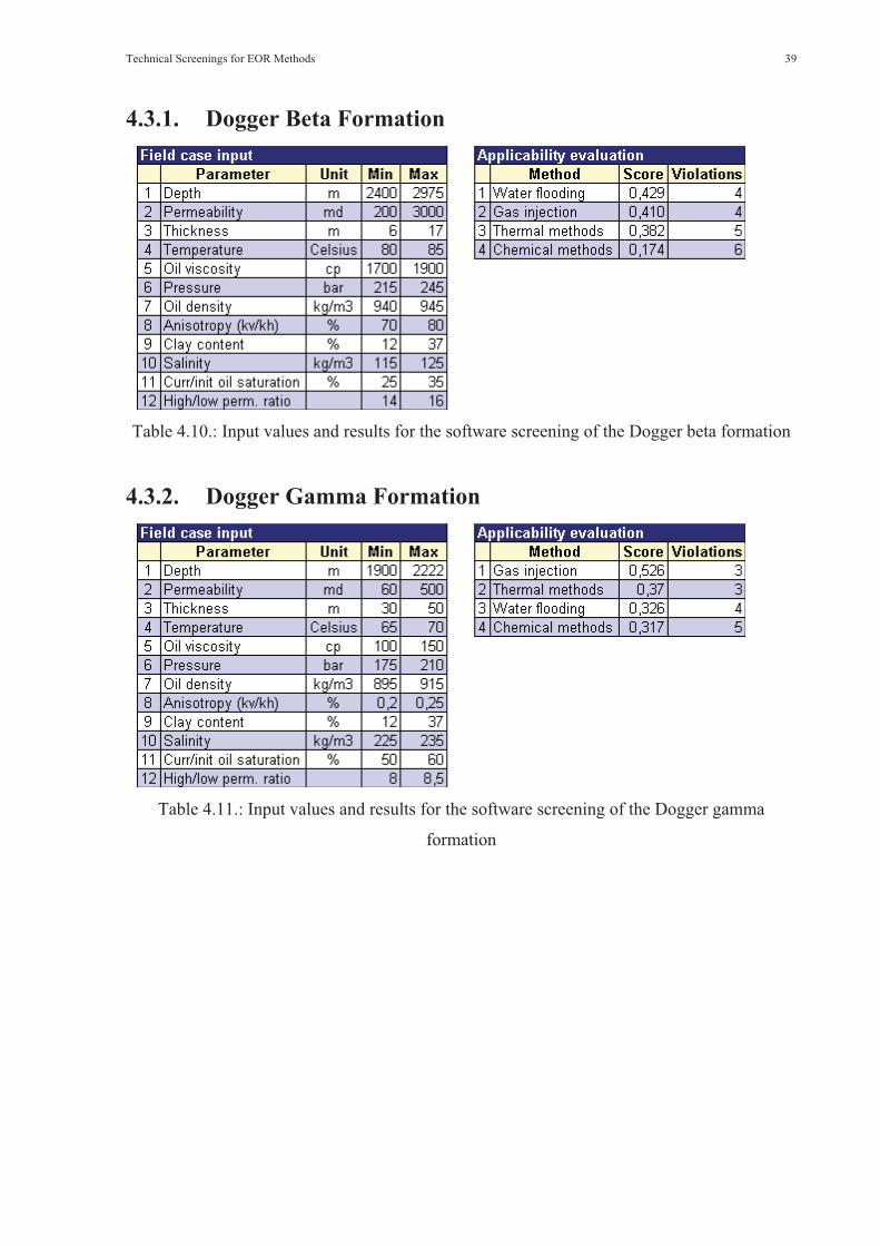
Technical Screenings for EOR Methods 39
4.3.1. Dogger Beta Formation
Table 4.10.: Input values and results for the software screening of the Dogger beta formation
4.3.2. Dogger Gamma Formation
Table 4.11.: Input values and results for the software screening of the Dogger gamma
formation

Technical Screenings for EOR Methods 40
4.3.3. Dogger Delta / Epsilon Formation
Table 4.12.: Input values and results for the software screening of the Dogger delta / epsilon
formation
4.3.4. Conclusions4.3.4.1. Dogger Beta FormationFor the Dogger beta formation the software applicability screening returns very bad results.
None of the listed EOR methods passes the application with positive results, having at least
four violations of the reference data set (similar to red marked values for the literature
screening). Water flooding achieves the best results with a weighted score of 0.429 points.
The meaning of these results is the same for secondary and tertiary recovery methods. No
method considered by the software is applicable for the Mittelplate oil field, including regular
water injection. Of course these results are highly unsatisfying and can be considered highly
unrealistic. The major reason for this outcome lies in the given reference intervals, which
have been very poorly chosen by the software programmers.
4.3.4.2. Dogger Gamma FormationThe results of the software screening for the Dogger gamma formation are similar to those of
the Dogger beta formation. All methods suffer from multiple violations and a bad scoring,
suggesting no other recovery then primary. Gas injection and thermal methods receive even
better marks then regular water injection, making the results highly doubtable from a reservoir
engineering point of view.
The conclusion is identical to the one for the Dogger beta formation as there are no IOR or
EOR possibilities for the Mittelplate Dogger gamma formation due to the same reasons.

Technical Screenings for EOR Methods 41
4.3.4.3. Dogger Delta / Epsilon FormationGoing along with the results of the other two formations, the software applicability screening
tool fails to return positive results for the Dogger delta / epsilon horizon. The best possibilities
given by the program are thermal methods, which fail only two parameters and get a scoring
of 0.476, while water flooding and gas injection methods receive even three violations.
The conclusion of these results is identical to the other two formations, as the program yields
no possibility of secondary or tertiary recovery. The reasoning for that is as well identical.
4.4. Screening for unconventional EOR MethodsAdditionally to the literature and software screenings for traditional EOR methods, other,
more unconventional options have been considered as well. The literature review already
gives an overview over these methods under chapter 2.3.4. However, it must be recognized
that all of these methods are either very specialized approaches for extreme conditions (such
as VAPEX or CHOPS for heavy oils) or are still in research or under evaluation to prove their
economical or technical viability (MEOR, LoSal EOR, Microwave or Sonic EOR). As the
conditions in the Mittelplate oil field are already rather difficult for implementation of EOR or
IOR methods, these techniques have been neglected for closer studies to reduce the economic
risk to a manageable minimum.
4.5. Evaluation of Key ParametersTo increase the viability of the technical screenings after Taber et al. and Al-Bahar et al.
several follow up studies on critical parameters have been conducted. Parameters chosen for
this evaluation have been reservoir depth in comparison to the phase diagram of water to
check the suitability of steam injection, MMP versus initial reservoir pressure of all horizons
to confirm or rule out a possible miscible gas injection and reservoir brine salinity in
combination with reservoir temperature to study the applicability of different polymers.
4.5.1. Reservoir depthFigure 2.2 shows the phase diagram of water, giving the particularly interesting vapor region,
ice region and the liquid region as well as the triple point and the critical point. The
comparison with Table 4.13, which shows the current reservoir conditions of all three
Mittelplate horizons, makes it clear that no water vapor phase can exist at these conditions,

Technical Screenings for EOR Methods 42
thus rendering a possible steam injection project useless. The fluid would be either liquid or
supercritical in the reservoir.
Table 4.13.: Current reservoir conditions of the Mittelplate horizons
4.5.2. Minimum Miscibility Pressure (MMP)For the study of the MMP, only the pressure necessary for CO2 injection has been evaluated.
It is proven throughout the technical literature that the MMP for nitrogen injection is usually
far larger then the pressures required by the other two miscible injection methods. The MMP
for hydrocarbon gas injection however can be quite similar to the one required by CO2
injection. To confirm this thesis, commercial software has been used to calculate all three
minimum miscibility pressures for all Mittelplate horizons. The results of this evaluation can
be seen in appendix C, where all input and output values of the software are documented. A
short summary is shown in Table 4.14.
Additionally to the software evaluation, four correlations for the MMP of CO2 have been
applied to confirm or rule out the application of miscible EOR methods. Table 4.15 gives
summary on these correlations.
Table 4.14.: Summary of the results from the software application

Technical Screenings for EOR Methods 43
Table 4.15.: Summary of the applied correlations
The input data for all correlations and the software have been generated from internal operator
PVT reports of the Mittelplate crude oil. The necessary calculations and correlations can be
found as well in appendix C.
The four correlations applied have been publicized by Yuan et al.14, Yellig and Metcalfe15,
Glaso36 and Cronquist37. The correlation of Yuan et al. uses three parameters, mol% of the C2-
C6 fraction, mole weight of the C7+ fraction and reservoir temperature, but fails to yield stable
results for high gravity oils, which has been confirmed by its authors. The correlation of
Yellig and Metcalfe is a lot simpler and requires only the reservoir temperature to calculate
the MMP. Since this correlation does not use any crude oil data, its results are not very
trustworthy. Glaso’s correlation requires the same parameters as Yuan et al., but delivers
much more reasonable results for high gravity oils. Cronquist’s correlation applied the mol%
of C1, the molecular weight of the C5+ fraction and the reservoir temperature. His correlation
seems to yield good results as well. Due to the factors named above, only the results of the
correlations from Glaso and Cronquist have been taken, additionally to the software results,
into consideration for the decision process.
The results from both studies are identical. None of the Mittelplate crude oils offer the
required quality to reach the minimum miscibility pressure before the initial pressure for any
miscible EOR method. Thus the application of these methods can be ruled out, as damage to
the Mittelplate formations must be assumed.
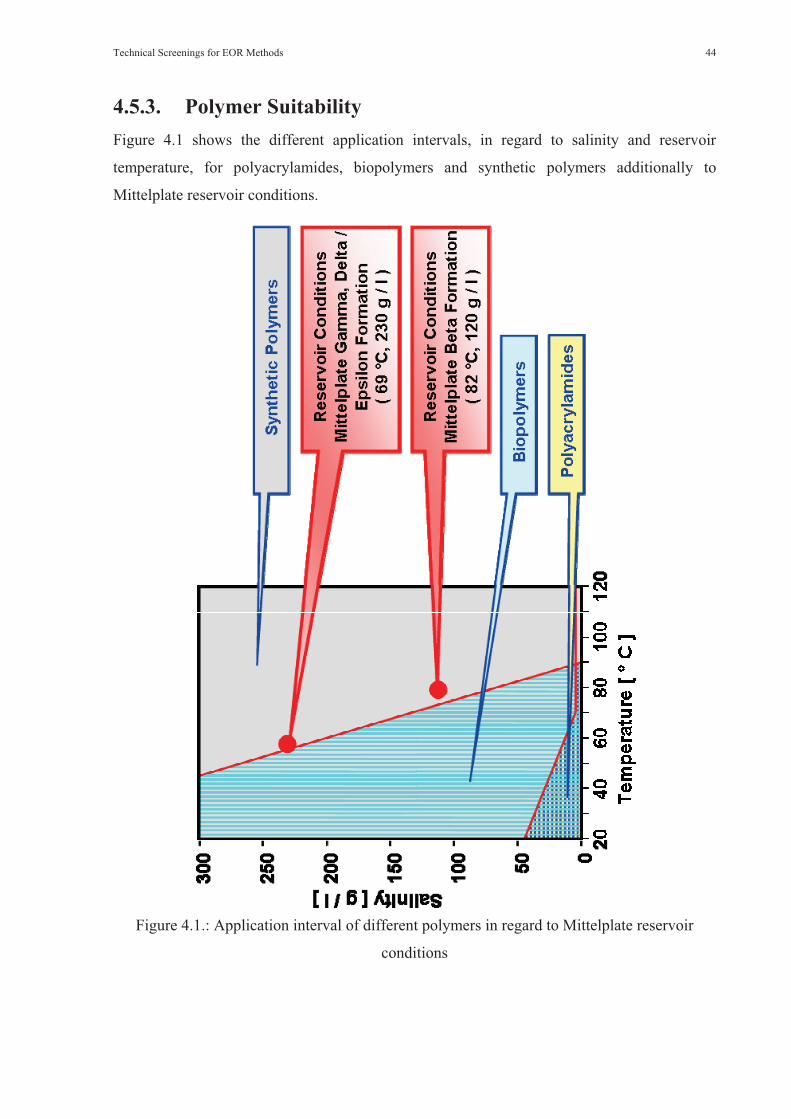
Technical Screenings for EOR Methods 44
4.5.3. Polymer SuitabilityFigure 4.1 shows the different application intervals, in regard to salinity and reservoir
temperature, for polyacrylamides, biopolymers and synthetic polymers additionally to
Mittelplate reservoir conditions.
Figure 4.1.: Application interval of different polymers in regard to Mittelplate reservoir
conditions
Technical Screenings for EOR Methods 45
As can be seen by this figure, the application of polyacrylamides can be certainly ruled out
because of the prevailing reservoir conditions in the Mittelplate field. However, synthetic
polymers can be applied without any big restrictions, even biopolymers such as Xanthan are
in the border area of applicability, providing positive laboratory testing. Earlier laboratory
analysis of the Mittelplate operator company suggested that biopolymers might be stable
enough to consider their application.
Due to theses reasons, the application of polymer or chemical combination floodings can be
taken into consideration, but further laboratory research must be conducted.
4.6. Summary of the technical ScreeningsThe technical screening studies give a good overview over the possibilities for the Mittelplate
oil field, in respect to the reservoir conditions. It has been proven that steam injection
strategies are no viable alternative, because steam cannot exist at the prevailing conditions.
Furthermore the required pressures to achieve miscibility during the application of CO2,
hydrocarbon gas or nitrogen injection are far higher then the initial reservoir pressures for all
Mittelplate horizons, thus there would be an extremely high risk of fracturing the formation
and destroy it. This risk cannot be taken. Unconventional EOR methods are either too
specialized to be considered for the Mittelplate oil field (such as cold heavy oil production
with sand or vapor extraction) or are still not mature enough, and thus economical proven, to
be applied (such as microbial EOR, the application of microwaves for EOR purposes, low
salinity EOR or sonic EOR).
Because of these reasons, only polymer flooding, chemical combination floodings and in-situ
combustion should be considered as possible tertiary recovery methods.
Analytical Performance Evaluation 46
Chapter 5
Analytical Performance Evaluation
The commercial software, which was used to perform the technical screenings, offers as well
the option of analytically simulating multiple EOR methods. Since a performance evaluation
for a test pattern is crucial to determine an EOR methods economical and technical viability,
it was decided to incorporate such a study into this work. Of course this “pre simulation” can
only serve as a guideline and its results must not be taken literally. However, it does show
trends and gives a first approximation on the results to be expected from numerical simulation
and laboratory analysis, which are far more resource intensive studies and would be beyond
the scope of this work. The following chapter will give a short description of the software
used, to show its possibilities, limitations and the reservoir engineering principles it is based
on. Furthermore, models for each Mittelplate formation have been set up and computed. To
obtain the best possible results, different steps have been undertaken. Firstly the data has been
assembled from a multitude of sources to provide a good base for the calculations. A very
detailed description of the data for all horizons can be found in appendix D. Secondly an
evaluation of the possible calculation options and boundary conditions has been undertaken to
judge which parameters fit the formation best. After the optimal settings have been evaluated,
two different models for each formation have been set up, which will be used for further
studies, depending on the test area geometry.
5.1. Program DescriptionThe performance prediction module of the commercial software allows the user quantitative
prediction of the performance of different EOR methods. It covers the possibility to compute
water injection, immiscible gas injection, miscible gas injection (CO2, hydrocarbon gas and
nitrogen) and chemical EOR methods (surfactants, polymer and surfactant – polymer).
However, it is not possible to analyze thermal EOR methods due to the extremely complicated
physical and chemical processes which happen during their application.
The program offers the possibility to simulate the displacements either in a two dimensional
cross section geometry or in an approximate three dimensional geometry (5 spot pattern). It

Analytical Performance Evaluation 47
applies the proven analytical solutions of Dykstra – Parsons (DP) and gravity dominated
Vertical Equilibrium (VE) approximations, accounting either for a constant rate (CR) or a
constant pressure loss (CP) boundary condition. These conditions can be freely selected by
the user to fit the reservoir in the best possible way.
5.2. Evaluation of Calculation Options and Boundary
ConditionsThe main design parameters for all models have been the geometry, analytical solution
method and boundary conditions. The studies incorporate an analysis of the recovery factor of
all possible EOR methods against time, to verify the most descriptive solution in accordance
with reservoir engineering comprehension. The results will be used to set up the base cases
for further evaluation of the EOR methods.
5.2.1. Dogger Beta FormationFrom a reservoir engineering point of view, a constant rate boundary, due to the unknown
aquifer behavior, applying the Dykstra – Parsons solution method would be the best
description of the Dogger beta horizon. An overview of the generated graphs to determine the
best options can be found in appendix D.
The analytical simulation of the different Dogger beta models proved the description
suggested by reservoir engineering comprehension. For both geometries the Vertical
Equilibrium solutions had very unrealistic responses towards the use of a pure polymer
injection, featuring for the 2D case a linear rise of the recovery factor accompanied by a
sudden break of production. For the 3D case the recovery factor increased more smoothly, but
still couldn’t yield a realistic decline before breaking as well in an incomprehensive fashion.
For both geometries surfactant injection yielded an unrealistic low recovery factor (about 17%
- 18%) in comparison to pure water injection (recovery factor of about 68%). In the Dykstra –
Parsons combined with constant pressure loss cases, polymer injection showed a slower rise
in the recovery factor than water, which stands in contradiction with the technical principles
of a polymer injection. As well surfactant injection showed an unrealistic response compared
to a combined surfactant – polymer flood in the 2D case, while it responded in the anticipated
fashion for the 3D case. Furthermore the 3D case required an unrealistic amount of time to
reach ultimate recovery (2500 years in comparison to 50 years of all other models). Due to
these reasons, the 2D, Dykstra – Parsons, constant rate model has been chosen to be the most

Analytical Performance Evaluation 48
descriptive solution for both geometries. Figures 5.1 and 5.2 show the computed graphs for
these cases.
Figure 5.1.: 2D – Dykstra Parsons – constant rate case for the Dogger beta formation
Figure 5.2.: 3D – Dykstra Parsons – constant rate case for the Dogger beta formation

Analytical Performance Evaluation 49
5.2.2. Dogger Gamma FormationThe Dogger gamma formation is very different to the beta formation. The reservoir is know a
lot better due to its smaller areal extension, thus it is known that the aquifer is supplying
actively pressure. Due to the reservoir pressure being above the bubble point pressure and the
supporting water aquifer, Dykstra – Parsons solution using the constant pressure loss
boundary condition seems to be the best description of the horizon. All graphs generated to
evaluate the different options can be found in appendix D.
However, the analytical simulation proved this thesis wrong. The Vertical Equilibrium theory
was ruled out for both geometric cases due to its application needs. The Dogger gamma
formation sands don’t have the high vertical permeabilites, low oil viscosities or low layer
thicknesses required by this theory. Furthermore the results of water injection have been
better then those for polymer injection, while surfactant injection outperformed the combined
polymer – surfactant treatment in both geometric cases for the constant pressure loss
boundary. This behavior is strongly contradicted by the technical implication of its use and
thus the results for Dykstra – Parsons applying a constant pressure loss boundary have been
ruled out. The long times needed to reach ultimate recovery in all three graphs featuring a 3D
case can be explained by the low production rates. The Figures 5.3 and 5.4 show the graphs
for the chosen options (2D, Dykstra – Parsons, constant rate boundary) resulting from this
study.
Figure 5.3.: 2D – Dykstra Parsons – constant rate case for the Dogger gamma formation
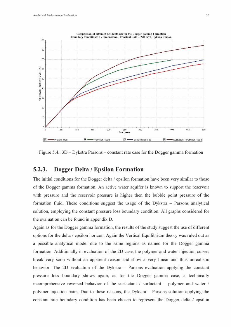
Analytical Performance Evaluation 50
Figure 5.4.: 3D – Dykstra Parsons – constant rate case for the Dogger gamma formation
5.2.3. Dogger Delta / Epsilon FormationThe initial conditions for the Dogger delta / epsilon formation have been very similar to those
of the Dogger gamma formation. An active water aquifer is known to support the reservoir
with pressure and the reservoir pressure is higher then the bubble point pressure of the
formation fluid. These conditions suggest the usage of the Dykstra – Parsons analytical
solution, employing the constant pressure loss boundary condition. All graphs considered for
the evaluation can be found in appendix D.
Again as for the Dogger gamma formation, the results of the study suggest the use of different
options for the delta / epsilon horizon. Again the Vertical Equilibrium theory was ruled out as
a possible analytical model due to the same regions as named for the Dogger gamma
formation. Additionally in evaluation of the 2D case, the polymer and water injection curves
break very soon without an apparent reason and show a very linear and thus unrealistic
behavior. The 2D evaluation of the Dykstra – Parsons evaluation applying the constant
pressure loss boundary shows again, as for the Dogger gamma case, a technically
incomprehensive reversed behavior of the surfactant / surfactant – polymer and water /
polymer injection pairs. Due to these reasons, the Dykstra – Parsons solution applying the
constant rate boundary condition has been chosen to represent the Dogger delta / epsilon
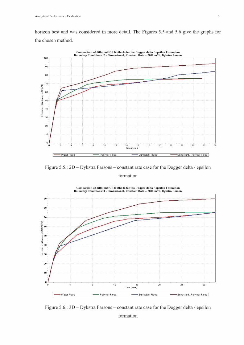
Analytical Performance Evaluation 51
horizon best and was considered in more detail. The Figures 5.5 and 5.6 give the graphs for
the chosen method.
Figure 5.5.: 2D – Dykstra Parsons – constant rate case for the Dogger delta / epsilon
formation
Figure 5.6.: 3D – Dykstra Parsons – constant rate case for the Dogger delta / epsilon
formation

Analytical Performance Evaluation 52
5.3. Predictions for the 2D Cross Sectional CasesBased on the studies to find the optimal settings for the reservoir models, more detailed 2D
analyses for these cases have been set up. All chose models used the 2D, Dykstra – Parsons
and constant rate boundary condition settings. Graphical computations for the recovery factor,
oil production rate, the water fraction of the produced fluid and pore injection volume have
been made and are given in the following sub sections.
5.3.1. Dogger Beta Formation
Figure 5.7.: Comparison of the recovery factor for the 2D Dogger beta case
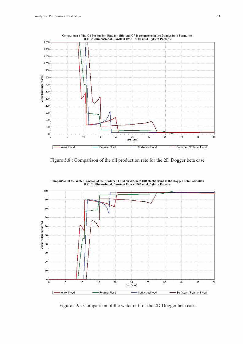
Analytical Performance Evaluation 53
Figure 5.8.: Comparison of the oil production rate for the 2D Dogger beta case
Figure 5.9.: Comparison of the water cut for the 2D Dogger beta case

Analytical Performance Evaluation 54
Figure 5.10.: Injected pore volume for the 2D Dogger beta case
Figure 5.7 shows a comparison of the recovery factor for the different calculated EOR
methods. As can be seen in this graph, polymer injection speeds up the recovery of the crude
oil by a significant amount of time in comparison to regular water injection. The additional
amounts range between 3% and 8% of the OOIP at certain time points and could be even
more if economic limits are considered. The reason for this effect can be found in the
improved volumetric sweep efficiency, induced by the polymer enhanced water viscosity. The
application of a surfactant or surfactant – polymer injection might even have a bigger benefit
(the base case shows an increase in recovery of 8% - 20% over water injection), but must be
taken with caution because of program limitations. The software is an analytical simulator and
cannot capture the different physical or chemical processes caused by the application of
surfactants. The Figures 5.8 and 5.9 show comparisons of the oil production rate and the
water cut respectively. The results can be reasoned analogues to the recovery factor. A very
steep increase in water cut accompanied by short plateaus can be observed after 8 to 12 years
of production resulting from the water breakthrough in the different sands and the Dykstra –
Parsons solution method. For all methods except polymer flooding, the oil production rate and
water cut experience unrealistic spikes, which seem to be the result of problems in the
analytical calculation. Figure 5.10 shows the injected pore volume over time, which follows a

Analytical Performance Evaluation 55
linear increase. This can be reasoned by the volumetric characteristic of the simulation in
combination with the constant rate boundary. After about 23 years a pore volume has been
injected.
5.3.2. Dogger Gamma Formation
Figure 5.11.: Comparison of the recovery factor for the 2D Dogger gamma case
Figure 5.12.: Comparison of the oil production rate for the 2D Dogger gamma case

Analytical Performance Evaluation 56
Figure 5.13.: Comparison of the water cut for the 2D Dogger gamma case
Figure 5.14.: Injected pore volume for the 2D Dogger gamma case

Analytical Performance Evaluation 57
The results and reasoning of the 2D prediction case for the Dogger gamma formation are quite
similar to those of the Dogger beta formation. After an initial production period of about 13
years where the recovery factor for all methods rises linearly, the benefits of the different
methods can be seen. Polymer injection reaches a recovery increase over water injection of
about 2% to 10% of OOIP, depending on the observation moment. Again economic limits
could even increase these amounts. Surfactant and surfactant – polymer injection achieve
even an increase of 10% to 25% of oil production. The same limitations considered for the
Dogger beta formation apply as well to the Dogger gamma formation. Figures 5.12 and 5.13
show comparisons of the oil production rate and the water cut for each EOR method. Again
rather steep increases in water cut can be observed, although they are a bit slower then for the
Dogger beta formation. The accompanying plateaus hold themselves additionally for a longer
time, which can be explain by the more heterogeneous sands of the Dogger gamma formation
that cause a bigger difference in the breakthrough times. The decrease in oil production rate
starts after 12 to 16 years of production. Again unrealistic spikes for water and surfactant
injection can be observed, but they seem as well smoother then for the Dogger beta formation.
Figure 5.14 shows the injected pore volume for the Dogger gamma formation, which features
as in the Dogger beta formation a linear increase. After 35 years a 100% pore volume is
injected.
5.3.3. Dogger Delta / Epsilon Formation
Figure 5.15.: Comparison of the recovery factor for the 2D Dogger delta / epsilon case
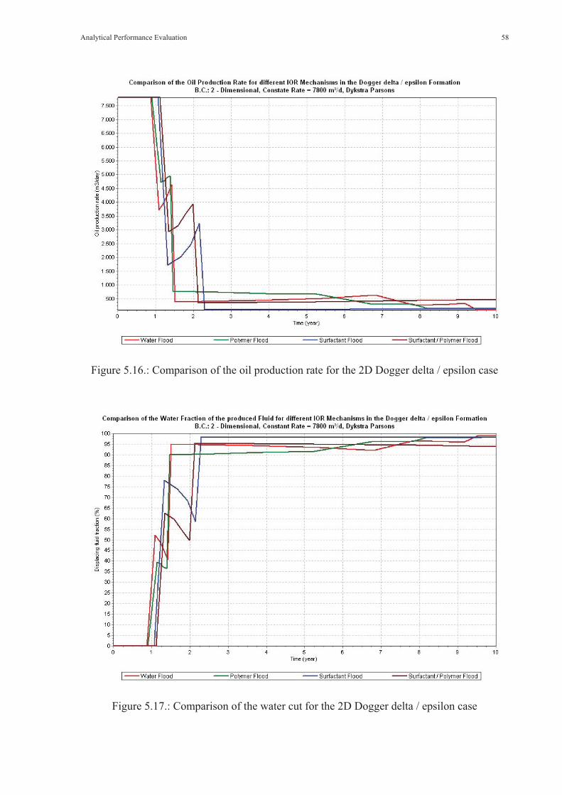
Analytical Performance Evaluation 58
Figure 5.16.: Comparison of the oil production rate for the 2D Dogger delta / epsilon case
Figure 5.17.: Comparison of the water cut for the 2D Dogger delta / epsilon case
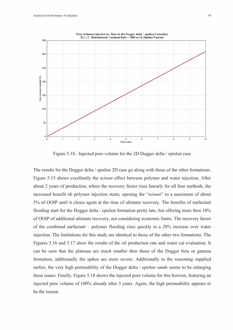
Analytical Performance Evaluation 59
Figure 5.18.: Injected pore volume for the 2D Dogger delta / epsilon case
The results for the Dogger delta / epsilon 2D case go along with those of the other formations.
Figure 5.15 shows excellently the scissor effect between polymer and water injection. After
about 2 years of production, where the recovery factor rises linearly for all four methods, the
increased benefit ob polymer injection starts, opening the “scissor” to a maximum of about
5% of OOIP until it closes again at the time of ultimate recovery. The benefits of surfactant
flooding start for the Dogger delta / epsilon formation pretty late, but offering more then 10%
of OOIP of additional ultimate recovery, not considering economic limits. The recovery factor
of the combined surfactant – polymer flooding rises quickly to a 20% increase over water
injection. The limitations for this study are identical to those of the other two formations. The
Figures 5.16 and 5.17 show the results of the oil production rate and water cut evaluation. It
can be seen that the plateaus are much smaller then those of the Dogger beta or gamma
formation, additionally the spikes are more severe. Additionally to the reasoning supplied
earlier, the very high permeability of the Dogger delta / epsilon sands seems to be enlarging
these issues. Finally, Figure 5.18 shows the injected pore volume for this horizon, featuring an
injected pore volume of 100% already after 3 years. Again, the high permeability appears to
be the reason.

Analytical Performance Evaluation 60
5.4. Predictions for the 3D Cases (5 Spot Pattern)Additionally to the detailed 2D case, 3D analyses have been set up to have the possibility of
evaluation economical studies on both possible geometric settings. All chose models used the
3D, Dykstra – Parsons and constant rate boundary condition settings. Graphical computations
for the recovery factor, oil production rate, the water fraction of the produced fluid and pore
injection volume have been made and are given in the following sub sections.
5.4.1. Dogger Beta Formation
Figure 5.19: Comparison of the recovery factor for the 3D Dogger beta case

Analytical Performance Evaluation 61
Figure 5.20.: Comparison of the oil production rate for the 3D Dogger beta case
Figure 5.21.: Comparison of the water cut for the 3D Dogger beta case

Analytical Performance Evaluation 62
Figure 5.22.: Injected pore volume for the 3D Dogger beta case
In Figure 5.19 the results of the recovery factor comparison for the different mechanisms can
be seen. They are analogues to those of the 2D comparison, featuring an increase of
production for polymer injection of over 10% of OOIP in comparison to water injection. As
well the beneficial impact of surfactants and the combined treatment are obvious on the first
sight, with a maximum of 20% of OOIP of additional production after 50 years. The
limitations named for the 2D prediction case count as well for the 3D case. The Figures 5.20
and 5.21 show the oil production rate and the water cut of the produced fluid. They are a lot
more stable then in the 2D case, showing more or less smooth increases or decreases
respectively and no plateaus. Water production starts after 5 – 8 years and rises sharply at
first. These results can be explained by a reduced effect of the different layer breakthrough
times due to the 3D geometry. Figure 5.22 features the injected pore volume over time,
reaching 100% pore volume after about 28 years of injection.

Analytical Performance Evaluation 63
5.4.2. Dogger Gamma Formation
Figure 5.23.: Comparison of the recovery factor for the 3D Dogger gamma case
Figure 5.24.: Comparison of the oil production rate for the 3D Dogger gamma case

Analytical Performance Evaluation 64
Figure 5.25.: Comparison of the water cut for the 3D Dogger gamma case
Figure 5.26.: Injected pore volume for the 3D Dogger gamma case
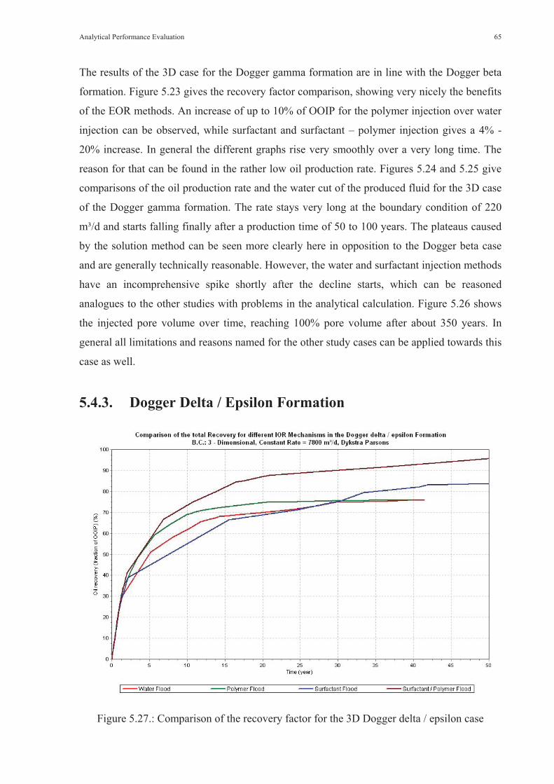
Analytical Performance Evaluation 65
The results of the 3D case for the Dogger gamma formation are in line with the Dogger beta
formation. Figure 5.23 gives the recovery factor comparison, showing very nicely the benefits
of the EOR methods. An increase of up to 10% of OOIP for the polymer injection over water
injection can be observed, while surfactant and surfactant – polymer injection gives a 4% -
20% increase. In general the different graphs rise very smoothly over a very long time. The
reason for that can be found in the rather low oil production rate. Figures 5.24 and 5.25 give
comparisons of the oil production rate and the water cut of the produced fluid for the 3D case
of the Dogger gamma formation. The rate stays very long at the boundary condition of 220
m³/d and starts falling finally after a production time of 50 to 100 years. The plateaus caused
by the solution method can be seen more clearly here in opposition to the Dogger beta case
and are generally technically reasonable. However, the water and surfactant injection methods
have an incomprehensive spike shortly after the decline starts, which can be reasoned
analogues to the other studies with problems in the analytical calculation. Figure 5.26 shows
the injected pore volume over time, reaching 100% pore volume after about 350 years. In
general all limitations and reasons named for the other study cases can be applied towards this
case as well.
5.4.3. Dogger Delta / Epsilon Formation
Figure 5.27.: Comparison of the recovery factor for the 3D Dogger delta / epsilon case
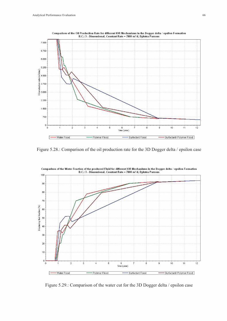
Analytical Performance Evaluation 66
Figure 5.28.: Comparison of the oil production rate for the 3D Dogger delta / epsilon case
Figure 5.29.: Comparison of the water cut for the 3D Dogger delta / epsilon case

Analytical Performance Evaluation 67
Figure 5.30.: Injected pore volume for the 3D Dogger delta / epsilon case
Figure 5.27 shows a comparison of the recovery factors for all applied methods. Analogues to
the 2D case, the scissor effect of the polymer injection towards water injection can be nicely
observed. The linear increase in recovery of all methods last only for a very short amount of
time (1 year) until the positive effects of the EOR methods kick in. The scissor effect peaks at
an extra recovery for the polymer injection of about 8% of OOIP, while surfactant and
surfactant – polymer injection achieve an increase of 8% - 20% of OOIP in recovery, not
taking economic limits into consideration. However, the benefits of the surfactant injection
can only be seen at a very mature state of the test reservoir. Analogues to all other formations,
the results of the two surfactant cases must be taken with caution due to the inability of the
software to describe the complicated physical and chemical processes connected to them. The
Figures 5.28 and 5.29 show the oil production rate and the water cut of the produced fluid for
the 3D Dogger delta / epsilon case. As for the 3D Dogger beta case, production plateaus due
to the Dykstra – Parsons solution cannot be seen, but all methods except polymer injection
show spikes in the production and water cut, shortly after the decline of the reservoir kicks in.
Again the very high permeability of the Dogger delta / epsilon sands might be a main reason
for the stronger severity of the spikes in opposition to the other formations. Lastly, Figure

Analytical Performance Evaluation 68
5.30 shows the injected pore volume over time, where already after 5 years of injected 100%
pore volume is reached.
5.5. Summary of the Analytical Performance EvaluationWith the help of commercial software capable of analytical simulation, a multitude of models
for the Mittelplate Dogger formations have been setup. The decision process for the optimal
software settings yielded models using the Dykstra – Parsons solution method and a constant
rate boundary condition as the best possibility for all horizons. Thus 2D and 3D models have
been set up for each formation to have base cases available for both geometric conditions.
Theses studies resulted in detailed performance evaluations of water injection, polymer
injection, surfactant injection and polymer – surfactant injection for each formation. Generally
the results have been positive throughout the board, confirming a reasonable EOR potential.
However, the software has serious limitations which must be considered in the further
application of its results. Firstly it is a strictly analytical simulator and thus cannot model the
complicated physical and chemical processes of surfactant application. Thus the results of the
two EOR methods using this chemical additive must be considered with caution. Secondly the
software applied a volumetric condition (injection rate = production rate) which leads to an
inaccurate description of formations with a strong water aquifer, since those cannot be
properly accounted for. Furthermore it is only possible to simulate an EOR application from
the time point t = 0, which will hardly happen in reality. Nevertheless the resulting models
gave a good impression of the EOR possibilities within the Mittelplate oil field, without
applying resource intensive numerical simulations or laboratory experiments. Although, those
evaluations have to be the next step in a possible EOR project. The 2D base case of the
Dogger beta formation was used for economical studies following in the next chapter.
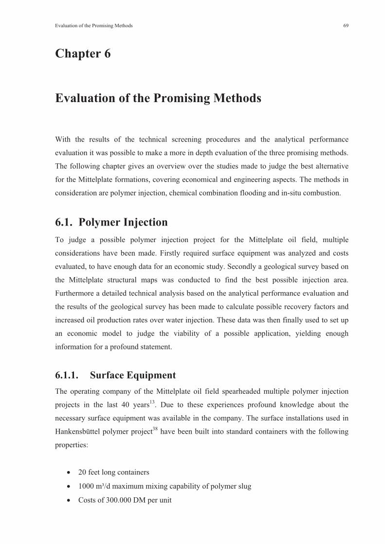
Evaluation of the Promising Methods 69
Chapter 6
Evaluation of the Promising Methods
With the results of the technical screening procedures and the analytical performance
evaluation it was possible to make a more in depth evaluation of the three promising methods.
The following chapter gives an overview over the studies made to judge the best alternative
for the Mittelplate formations, covering economical and engineering aspects. The methods in
consideration are polymer injection, chemical combination flooding and in-situ combustion.
6.1. Polymer InjectionTo judge a possible polymer injection project for the Mittelplate oil field, multiple
considerations have been made. Firstly required surface equipment was analyzed and costs
evaluated, to have enough data for an economic study. Secondly a geological survey based on
the Mittelplate structural maps was conducted to find the best possible injection area.
Furthermore a detailed technical analysis based on the analytical performance evaluation and
the results of the geological survey has been made to calculate possible recovery factors and
increased oil production rates over water injection. These data was then finally used to set up
an economic model to judge the viability of a possible application, yielding enough
information for a profound statement.
6.1.1. Surface EquipmentThe operating company of the Mittelplate oil field spearheaded multiple polymer injection
projects in the last 40 years13. Due to these experiences profound knowledge about the
necessary surface equipment was available in the company. The surface installations used in
Hankensbüttel polymer project38 have been built into standard containers with the following
properties:
� 20 feet long containers
� 1000 m³/d maximum mixing capability of polymer slug
� Costs of 300.000 DM per unit
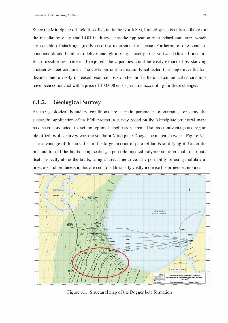
Evaluation of the Promising Methods 70
Since the Mittelplate oil field lies offshore in the North Sea, limited space is only available for
the installation of special EOR facilities. Thus the application of standard containers which
are capable of stacking, greatly ease the requirement of space. Furthermore, one standard
container should be able to deliver enough mixing capacity to serve two dedicated injectors
for a possible test pattern. If required, the capacities could be easily expanded by stacking
another 20 feet container. The costs per unit are naturally subjected to change over the last
decades due to vastly increased resource costs of steel and inflation. Economical calculations
have been conducted with a price of 300.000 euros per unit, accounting for these changes.
6.1.2. Geological SurveyAs the geological boundary conditions are a main parameter to guarantee or deny the
successful application of an EOR project, a survey based on the Mittelplate structural maps
has been conducted to set an optimal application area. The most advantageous region
identified by this survey was the southern Mittelplate Dogger beta area shown in Figure 6.1.
The advantage of this area lies in the large amount of parallel faults stratifying it. Under the
precondition of the faults being sealing, a possible injected polymer solution could distribute
itself perfectly along the faults, using a direct line drive. The possibility of using multilateral
injectors and producers in this area could additionally vastly increase the project economics.
Figure 6.1.: Structural map of the Dogger beta formation
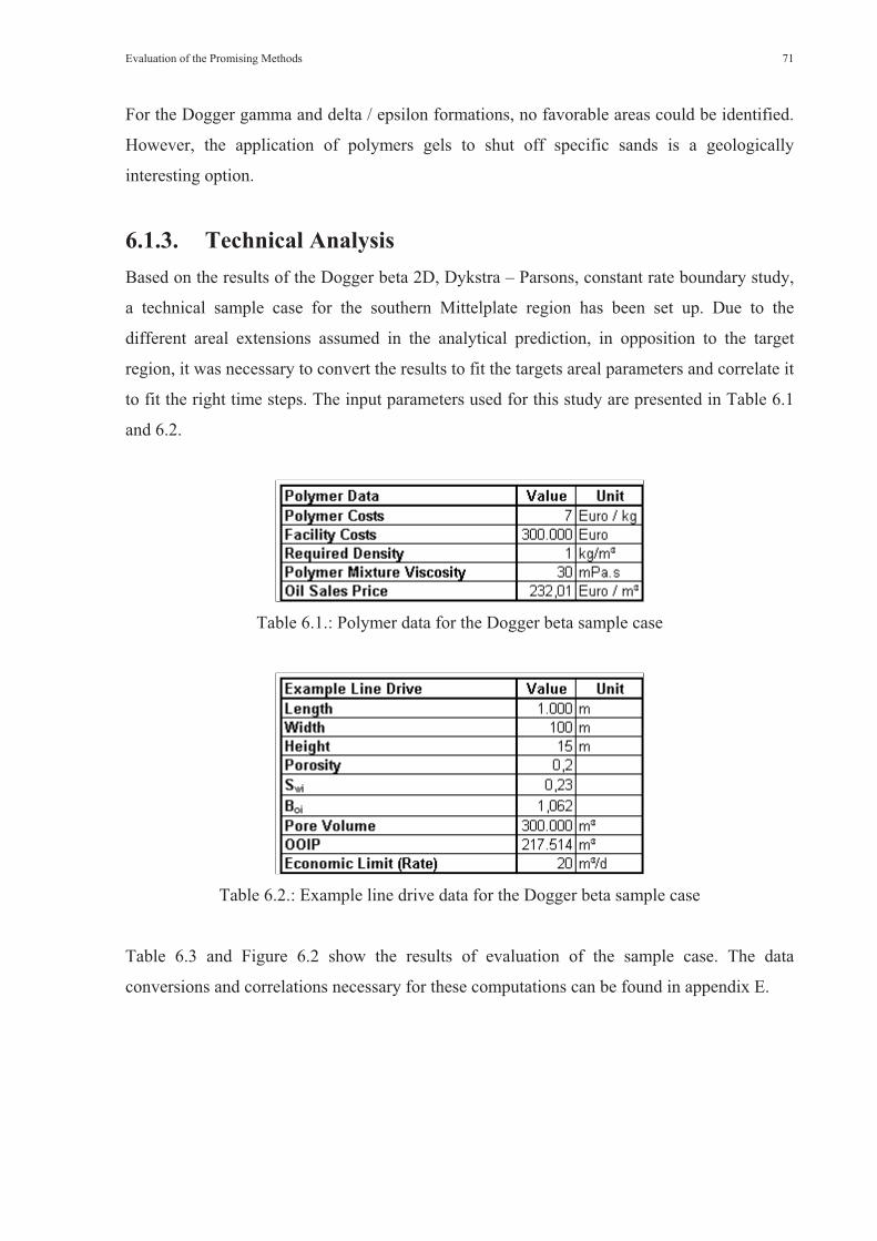
Evaluation of the Promising Methods 71
For the Dogger gamma and delta / epsilon formations, no favorable areas could be identified.
However, the application of polymers gels to shut off specific sands is a geologically
interesting option.
6.1.3. Technical AnalysisBased on the results of the Dogger beta 2D, Dykstra – Parsons, constant rate boundary study,
a technical sample case for the southern Mittelplate region has been set up. Due to the
different areal extensions assumed in the analytical prediction, in opposition to the target
region, it was necessary to convert the results to fit the targets areal parameters and correlate it
to fit the right time steps. The input parameters used for this study are presented in Table 6.1
and 6.2.
Table 6.1.: Polymer data for the Dogger beta sample case
Table 6.2.: Example line drive data for the Dogger beta sample case
Table 6.3 and Figure 6.2 show the results of evaluation of the sample case. The data
conversions and correlations necessary for these computations can be found in appendix E.
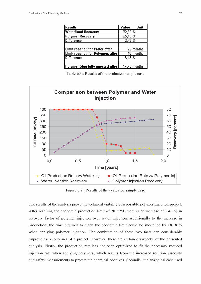
Evaluation of the Promising Methods 72
Table 6.3.: Results of the evaluated sample case
Comparison between Polymer and Water Injection
050
100150200250300350400
0,0 0,5 1,0 1,5 2,0
Time [years]
Oil
Rat
e [m
³/day
]
01020304050607080
Rec
over
y [p
erce
nt]
Oil Production Rate /w Water Inj. Oil Production Rate /w Polymer Inj.Water Injection Recovery Polymer Injection Recovery
Figure 6.2.: Results of the evaluated sample case
The results of the analysis prove the technical viability of a possible polymer injection project.
After reaching the economic production limit of 20 m³/d, there is an increase of 2.43 % in
recovery factor of polymer injection over water injection. Additionally to the increase in
production, the time required to reach the economic limit could be shortened by 18.18 %
when applying polymer injection. The combination of these two facts can considerably
improve the economics of a project. However, there are certain drawbacks of the presented
analysis. Firstly, the production rate has not been optimized to fit the necessary reduced
injection rate when applying polymers, which results from the increased solution viscosity
and safety measurements to protect the chemical additives. Secondly, the analytical case used
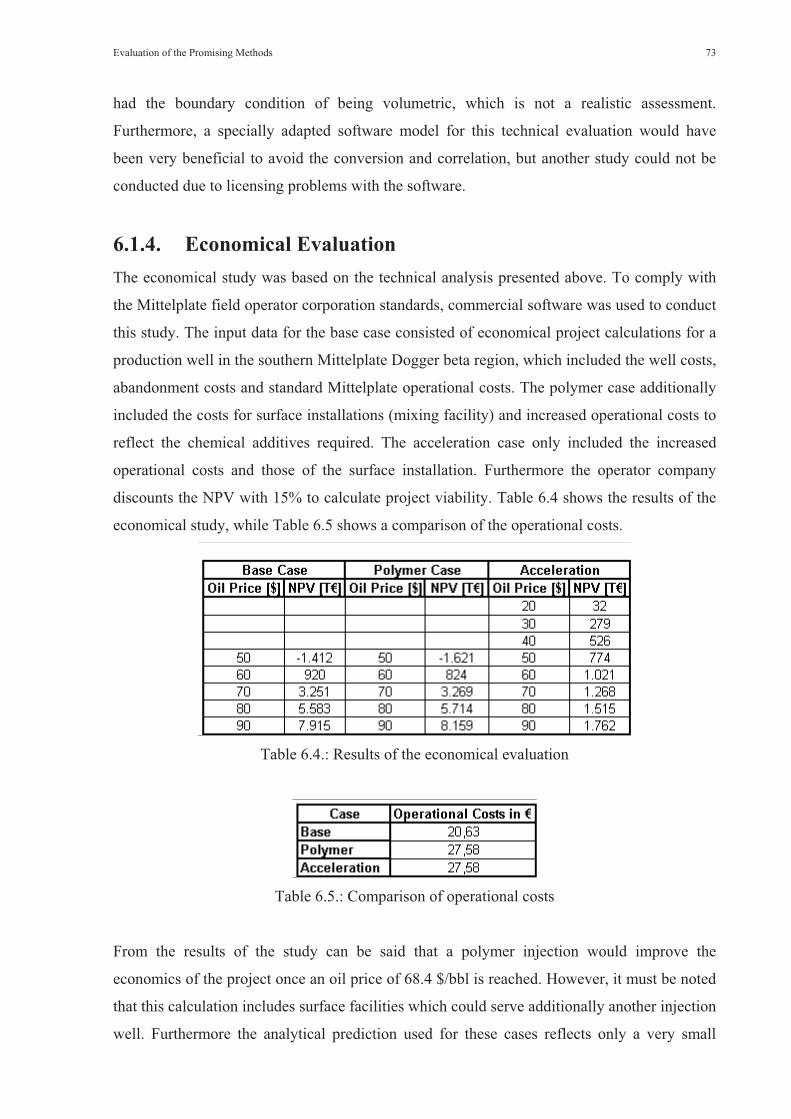
Evaluation of the Promising Methods 73
had the boundary condition of being volumetric, which is not a realistic assessment.
Furthermore, a specially adapted software model for this technical evaluation would have
been very beneficial to avoid the conversion and correlation, but another study could not be
conducted due to licensing problems with the software.
6.1.4. Economical EvaluationThe economical study was based on the technical analysis presented above. To comply with
the Mittelplate field operator corporation standards, commercial software was used to conduct
this study. The input data for the base case consisted of economical project calculations for a
production well in the southern Mittelplate Dogger beta region, which included the well costs,
abandonment costs and standard Mittelplate operational costs. The polymer case additionally
included the costs for surface installations (mixing facility) and increased operational costs to
reflect the chemical additives required. The acceleration case only included the increased
operational costs and those of the surface installation. Furthermore the operator company
discounts the NPV with 15% to calculate project viability. Table 6.4 shows the results of the
economical study, while Table 6.5 shows a comparison of the operational costs.
Table 6.4.: Results of the economical evaluation
Table 6.5.: Comparison of operational costs
From the results of the study can be said that a polymer injection would improve the
economics of the project once an oil price of 68.4 $/bbl is reached. However, it must be noted
that this calculation includes surface facilities which could serve additionally another injection
well. Furthermore the analytical prediction used for these cases reflects only a very small

Evaluation of the Promising Methods 74
area, which would be smaller then the possible drainage area of the production well, as can be
seen in the technical analysis. Due to these reasons there is a lot of potential to reduce the
required oil price to make the polymer project viable. The third case studied, an acceleration
case, assumed the production well to be already in place. Thus the required oil price to make
the polymer injection economical viable drops to 18.7 $/bbl. Table 6.6 gives an analysis of the
payout period and the rate of return for the base and the polymer case, considering different
oil prices.
Table 6.6.: Comparison of payout period and ROR
6.2. Chemical Combination FloodingThe second possible EOR method after the technical screenings and backed up by analytical
prediction is chemical combination flooding. The most interesting possibility of the variety of
available techniques poses certainly the combination of alkalis and surfactants with polymers.
As it is a very similar method to polymer injection, the studies and arguments covering
surface facilities and geological considerations for polymer injection are viable for this
technique as well.
A technical and economic analysis for such an EOR project however, was beyond the scope
of this work. As already pointed out in chapter 5, the very complex chemical and physical
processes induced by the alkalis and surfactants in the reservoir cannot be properly described
by analytical simulation. Thus descriptive technical evaluations require either detailed
numerical simulation or a series of core tests in the laboratory to measure the response of the
reservoir and estimate necessary slug sizes. However, such studies about the Mittelplate oil
field have not been available at the time of this work.
6.3. In-Situ CombustionBased on the technical screening guidelines, the third possible EOR method is in-situ
combustion. However, the processes applied by this technique are still hardly known. Due to

Evaluation of the Promising Methods 75
this fact, there is only very limited literature available giving empirical calculation options to
describe the possible performance. Those calculations available, such as Nelson and McNeil39
and Brigham et al.40, require extensive laboratory work with combustion tube experiments.
Having these reasons in mind, the primary consideration in the detailed evaluation of this
technique has been the calculation of possible well head pressures and the associated injection
rates. The first step has been the computation of the phase behavior of pure oxygen with a
chemical process simulation software. This data was required to calculate the pressure losses
in the annulus during the oxygen injection. Usually only air is compressed and injected into
the reservoir to keep the combustion process alive, but due to the large well spacing used in
offshore field development, larger amounts of oxygen are required. Due to this reason it was
decided to conduct the calculations with pure oxygen. The next step has been the actual
calculation of the well head pressure using commercial software. Figure 6.3 shows the results
of this study.
Figure 6.3.: Computation results of the wellhead pressure for in-situ combustion

Evaluation of the Promising Methods 76
The data input for Figure 6.3 can be found in appendix F. According to this figure, it would
be possible to inject 50000 sm³ of oxygen per hour, at a wellhead pressure of 530 bar and a
reservoir pressure of 300 bar. It is questionable however, if this injection rate would be
sufficient to supply enough oxygen for the combustion, considering for example the large
well spacing of the central 5 spot pattern of the Mittelplate oil field. As mentioned already
above, combustion tube experiments would be necessary for an accurate evaluation.
Additionally the in-situ combustion damages due to corrosion and the high temperatures the
subsurface well equipment, resulting in considerably rising well workover costs.
Due to these facts, a technical and economical successful in-situ combustion project is at best
questionable for the Mittelplate oil field.
6.4. Results of the Detailed EvaluationsIn the detailed evaluations of the three promising methods, it became obvious that chemical
treatments are the way to go for the Mittelplate oil field. The technical and economical
evaluation of polymer flooding proved that a successful application in the southern region of
the Dogger beta formation is possible and should be further tracked. Laboratory
measurements, numerical simulation and a tracer project are however required to confirm the
studies of this work. As well chemical combination treatments seem to be promising, but no
definite statement in respect to its performance can be made without appropriated core
flooding analyses in the laboratory. In-situ combustion on the other side was confirmed to be
theoretically viable in regard to the reservoir parameters, but this could not be confirmed in a
practical evaluation. Eventually combustion tube experiments could back up the theoretical
recommendation, but the studies shown in this chapter reduce this possibility to a minimum.
Additionally a much closer well spacing would be favorable for its application, to have more
possibilities of supervising the hardly known process.
Conclusion and Suggestions 77
Chapter 7
Conclusion and Suggestions
The target of this work was the identification of EOR methods applicable to the Mittelplate
oil field. The first step in this direction was an extensive literature survey to summarize
traditional EOR methods and new developments on the one hand and find up to date technical
screening guidelines on the other hand. After this research multiple technical screenings have
been conducted to check upon traditional EOR techniques, resulting in the identification of
polymer flooding, chemical combination flooding and in-situ combustion as possible
methods. Miscible floodings and steam injection failed the screenings due to unfavorable
reservoir parameters, while new or specialized techniques like MEOR or CHOPS have not
been considered for further evaluation. Afterwards analytical simulation was applied and
confirmed a good response of the reservoir towards the chemical treatments. During the
following detailed analyses of the three potential EOR methods, in-situ combustion could be
ruled out as possible EOR method, since practical considerations of the well head pressure
and the well spacing would considerably complicate its application. Polymer flooding on the
other side showed excellent results in practical considerations. A technical and economical
successful application, in dependency of the oil price, was proven for the southern region of
the Dogger beta formation. For the Dogger gamma and delta / epsilon formations however, no
geologically favorable region could be identified. Chemical combination flooding seems to
have potential as well, but more detailed laboratory analysis on the impact of surfactants on
the reservoir needs to be conducted.
To confirm the results of this work, it is suggested to perform additional laboratory analysis in
respect to polymer and chemical combination flooding (such as retention tests, core flooding
tests and injection tests) and numerical simulation of a possible polymer project in the
southern Dogger beta region. If the results of possible follow up studies deliver the same
conclusions as this work, the implementation of a test project should be considered.
Furthermore tracer studies of all Mittelplate horizons are suggested to evaluate the possibility
of larger field applications. For the Dogger delta / epsilon formation, the application of
polymers shut off high permeability layers should be evaluated. Furthermore it is suggested to
follow studies of new EOR methods, such as microwave application, and support those.

Nomenclature 78
Chapter 8
Nomenclature
Abbreviations
EOR - Enhanced Oil Recovery
IOR - Improved Oil Recovery
API - American Petroleum Institute
IFT - Interfacial Tension
ST - Surface Tension
LPG - Liquefied Petroleum Gas
RF - Resistance Factor
RRF - Residual Resistance Factor
ASP - Alkali / Surfactant / Polymer
FCM - First Contact Miscibility
MCM - Multiple Contact Miscibility
MMP - Minimum Miscibility Pressure
WAG - Water Alternating Gas
HC - Hydrocarbon
ISC - In-Situ Combustion
SAGD - Steam Assisted Gravity Drainage
OOIP - Original Oil in Place
HPAI - High Pressure Air Injection
COFCAW - Combination of Forward Combustion and Water Flooding
VAPEX - Vapor Extraction
CHOPS - Cold Heavy Oil Production with Sand
MEOR - Microbial Enhanced Oil Recovery
LoSal - Low Salinity Enhanced Oil Recovery
SEOR - Sonic Enhanced Oil Recovery
WOC - Water Oil Contact
PVT - Pressure / Volume / Temperature
E&P - Exploration and Production

Nomenclature 79
N.C. - Not Critical
GOR - Gas Oil Ratio
DP - Dykstra – Parsons
VE - Vertical Equilibrium
CR - Constant Rate
CP - Constant Pressure Loss
2D - Two Dimensional
3D - Three Dimensional
DM - Deutsche Mark (Old German Currency)
bbl - Barrel
Symbols
M - Mobility Ratio [-]
t - Time [years]
$ - Dollar
€ - Euro
P - Pressure [bar]
Swi - Initial Water Saturation [-]
BBoi - Initial Oil Formation Volume Factor [m³/sm³]
Greek Symbols
� - Mobility [1/cP]
� - Interfacial Tension [dyne/cm]
Subscripts
D - Displacing Fluid
d - Displaced Fluid
O - Oil
W - Water
I - Initial
r - Reservoir

Nomenclature 80
Conversion Factors
°API = 5.1315.141�
avitySpecificGr
m = ft · 0.3480
kg/m³ = lb/ft³ · 1.601846e+1
mPa·s = cP
bar = psia · 6.894757e-2
°C = 8.1
)32( ��F
Bibliography 81
Chapter 9
Bibliography
1 Green, D. W. and Willhite G.P.: Enhanced Oil Recovery, SPE Textbook Series Vol. 6, Society of Petroleum Engineers, Richardson, TX, USA (1998).
2 Taber, J.J et al.: “EOR Screening Criteria Revisited,” paper SPE 35385 presented at the 1996 SPE/DOE Tenth Symposium on Improved Oil Recovery, Tulsa, USA, April 21-24, 1996.
3 Zettlitzer, M.: “Polymer Flooding,” RWE Dea, 30 November 2004, internal company presentation
4 “API gravity”, Wikipedia, The Free Encyclopedia, Wikimedia Foundation, Inc. 14 September 2006 http://en.wikipedia.org/w/index.php?title=API_gravity&oldid=73015226 .
5 “Heavy Oil”, Oilfield Glossery, Schlumber, 14 September 2006, http://www.glossary.oilfield.slb.com/Display.cfm?Term=heavy%20oil
6 Rao, D.N. and Ayirala, S.C.: “The multiple roles of interfacial tension in fluid phase equilibria and fluid – solid interactions,” J. Adhesion Sci. Technol., Vol.20, No. 2-3 (2006) 125.
7 Weinhardt, B.E.: Fundamentals of Enhanced Oil Recovery, University of Leoben, Leoben, Austria (2004).
8 Ayirala, S.C. and Rao, D.N.: “Comparative Evaluation of a new MMP Determination Technique,” paper SPE 99606 presented at the 2006 SPE/DOE Symposium on Improved Oil Recovery, Tulsa, OK, USA, April 22-26, 2006.
9 Yang, D. and Gu, Y.: “Interfacial Interactions of Crude Oil-Brine-CO2 Systems under Reservoir Conditions,” paper SPE 90198 presented at the SPE Annual Technical Conference and Exhibition, Houston, USA, September 26-29, 2004.
10 Polymer Flooding Handbook, RWE Dea E&P Laboratory Wietze, internal project handbook (1980).
11 Thomas S.: “Chemical EOR – The past, does it have a future ?,” SPE Distinguished Lecturer Series, Hannover, Germany, August 2005.
12 Du, Y. and Guan, L.: “Field-Scale Polymer Flooding: Lessons Learnt and Experiences Gained During Past 40 Years,” paper SPE 91787 presented at the 2004 SPE International Petroleum Conference in Mexico, Puebla, Mexico, November 8-9, 2004.

Bibliography 82
13 Maitin, B.K.: “Performance Analysis of Several Polyacrylamide Floods in North German Oil Fields,” paper SPE 24118 presented at the SPE/DOE Eight Symposium on Enhanced Oil Recovery, Tulsa, OK, USA, April 22-24, 1992.
14 Yuan, H. et al.: “Improved MMP Correlations for CO2 Floods Using Analytical Gas Flooding Theory,” paper SPE 89359 presented at the SPE/DOE Fourteenth Symposium on Improved Oil Recovery, Tulsa, OK, USA, April 17-21, 2004.
15 Yellig, W.F. and Metcalfe, R.S.: “Determination and Prediction of CO2 Minimum Miscibility Pressure,” Journal of Petroleum Technology (Jan. 1980) 160.
16 Satter, A. and Thakur, G.C.: Integrated Petroleum Reservoir Management: A Team Approach, PennWell, Houston, TX, USA, (1994) 193
17 Stalkup, F.E.: Miscible Displacement, Monograph Series, Society of Petroleum Engineers, Dallas, New York, USA (1983)
18 Panait-Patica, A. et al.: “Suplacu de Barcau Field – A Case History of a Successful In-Situ Combustion Exploitation,” paper SPE 100346 presented at the SPE Europec / EAGE Annual Conference and Exhibition, Vienna, Austria, 12-15 June, 2006
19 Moore, R.G. et al.: “A Guide to High Pressure Air Injection (HPAI) Based Oil Recovery,” paper SPE 75207 presented at the SPE/DOE Improved Oil Recovery Symposium, Tulsa, OK, USA, 13-17 April, 2002
20 Moritis, G.: “EOR Survey 2004,” Oil & Gas Journal, 12 April (2004) 45
21 Ehlig-Economides, C.A. et al.: “Global Experiences and Practice for Cold Production of Moderate and Heavy Oil,” paper SPE 58773 presented at the 2000 SPE International Symposium on Formation Damage Control, Lafayette, Louisiana, USA, 23-24 February, 2000
22 Nath, D.K.: “Fiber Optics Used to Support Reservoir Temperature Surveillance in Duri Steamflood,” paper SPE 93240 presented at the 2005 Asia Pacific Oil & Gas Conference and Exhibition, Jakarta, Indonesia, 5-7 April, 2005
23 “Phase Diagram for Water”, MSN Encarta, Microsoft, 30 October 2006, http://encarta.msn.com/media_461541579/Phase_Diagram_for_Water.html
24 McGuire, P.L. et al.: “Low Salinity Oil Recovery: An Exciting New EOR Opportunity for Alaska’s North Slope,” paper SPE 93903 presented at the 2005 SPE Western Regional Meeting, Irvine, CA, USA, 30 March – 1 April, 2005
25 Zhang, Y. and Morrow, N.R.: “Comparison of Secondary and Tertiary Recovery With Change in Injection Brine Composition for Crude Oil / Sandstone Combinations,” paper SPE 99757 presented at the 2006 SPE/DOE Symposium on Improved Oil Recovery, Tulsa, OK, USA, 22-26 April, 2006
26 Bryant, S.L. and Lockhart, T.P.: “Reservoir Engineering Analysis of Microbial Enhanced Oil Recovery,” paper SPE 63229 presented at the 2000 SPE Annual Technical Conference and Exhibition, Dallas, TX, USA, 1-4 October, 2000

Bibliography 83
27 “Bio-Engineering High Performance Microbial Strains for MEOR by Direct-Protein-Evolution Technology” U.S. Department of Energy, 27 September, 2006 http://www.netl.doe.gov/technologies/oil-gas/Petroleum/projects/EP/ImprovedRec/15525CalTech.htm
28 Gramich, J. and Klein, P.: “Plasmagestütztes Cracken in der Mikrowelle” Stiftung Jugend forscht e.V., 29 Mai 2006 http://jugendforscht.fiz-karlsruhe.de/cgi-bin/ih?ID=13063.1.0.1&ACTION=filter&+PARAM=smshowpdf+/data1/ih3000/files/jufobund\attachment\vg21l1a.pdf
29 “Cold Cracking Report” U.S. Department of Energy, NETL, July 2006, http://www.fossil.energy.gov/epact/cold_cracking_report.pdf
30 Jespersen, C.: “Microwave Cracking,” RWE Dea, 20 September 2006, internal company presentation
31 “Calibration and Testing of Sonic Stimulation Technologies” U.S. Department of Energy, 1 March 2005 http://www.netl.doe.gov/technologies/oil-gas/Petroleum/projects/EP/ImprovedRec/15165.htm
32 Singhai, A.K. et al.: “Screening of Reservoirs For Exploitation by Application of Steam Assisted Gravity Drainage / Vapex Processes,” paper SPE 37144 presented at the 1996 International Conference on Horizontal Well Technology, Calgary, Alberta, Canada, 18-20 November, 1996
33 Castanier, M. and Kovscek, A.R.: “Heavy oil upgrading in-situ via solvent injection and combustion: A “new” method,” paper I005 presented at the 67th EAGE Conference and Exhibition, Madrid, Spain, 13-16 June, 2005
34 Mamora, D.D. et al.: “Experiment and Simulation Studies of Steam-Propane Injection for the Hamaca and Duri fields,” paper SPE 84201 presented at the SPE Annual Technical Conference, Denver, Colorado, USA, 5-8 October, 2003
35 Al-Bahar, M.A. et al.: “Evaluation of IOR Potential within Kuwait,” paper SPE 88716 presented at the 11th Abu Dhabi International Petroleum Exhibition and Conference, Abu Dhabi, U.A.E., 10-13 October 2004
36 Glaso, O.: “Generalized Minimum Miscibility Pressure Correlation,” SPEJ (December 1985) 927
37 Cronquist, C.: “Carbon Dioxide Dynamic Miscibility with Light Reservoir Oils,” Proc.,Fourth Annual U.S. DOE Symposium, Tulsa, USA (1977)
38 Maitin, B.K. and Volz, H.: “Performance of Deutsche Texaco AG’s Oerrel and Hankensbuettel Polymer Floods,” paper SPE 9794 presented at the 13th Annual Offshore Technology Conference, Houston, Texas, USA, 4-7 May 1981
39 Nelson, T.W. and McNeil, J.S.: “How to engineer an in situ combustion project,” The Oil and Gas Journal, 5 June (1961) 58

Bibliography 84
40 Brigham, W.E. et al.: “Recovery Correlations for In-Situ Combustion Field Projects and Application to Combustion Pilots,” Journal of Petroleum Technology, December (1980) 2133
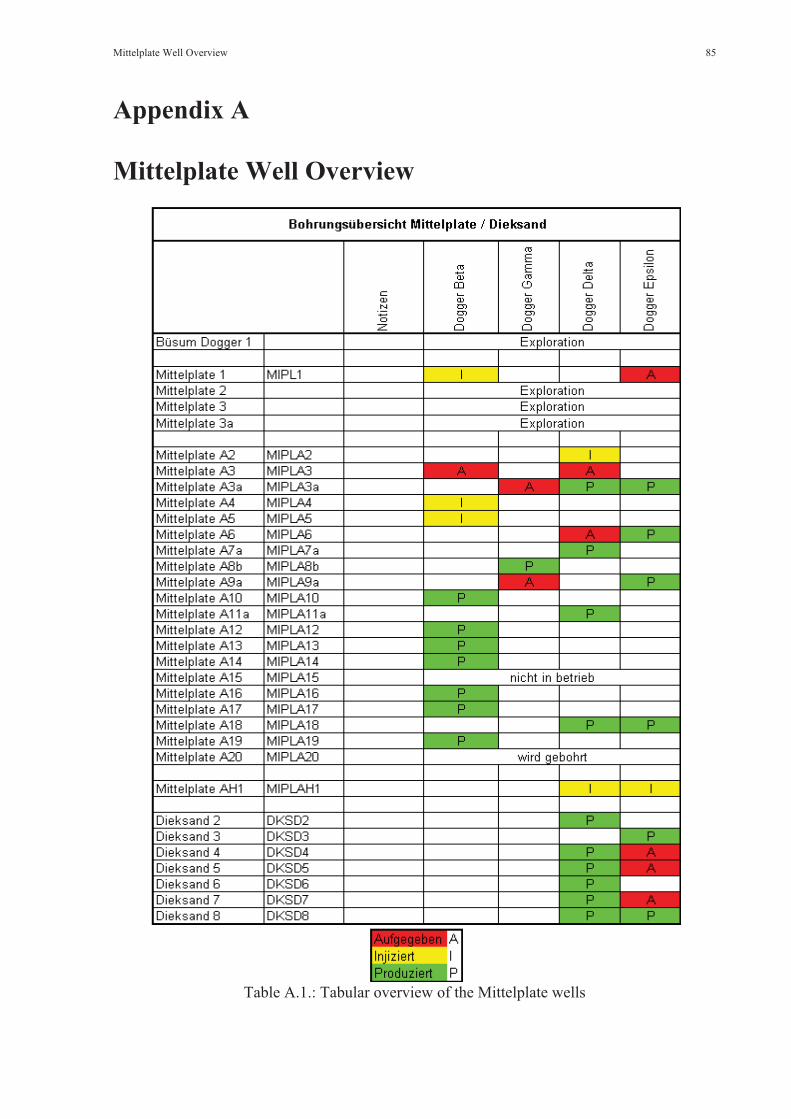
Mittelplate Well Overview 85
Appendix A
Mittelplate Well Overview
Table A.1.: Tabular overview of the Mittelplate wells

Mittelplate Formation Volume Factors and Crude Oil Viscosities 86
Appendix B
Mittelplate Formation Volume Factors and Oil
Viscosities
B.1. Dogger beta formation
Figure B.1.: FVF against pressure of Dogger beta crude oil
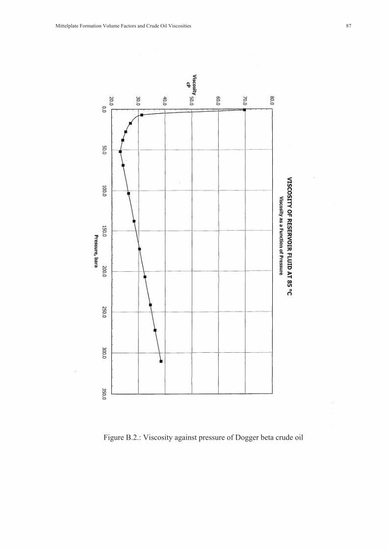
Mittelplate Formation Volume Factors and Crude Oil Viscosities 87
Figure B.2.: Viscosity against pressure of Dogger beta crude oil
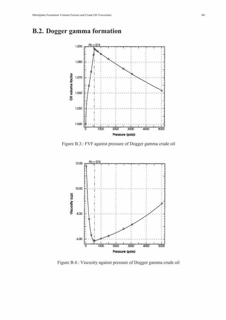
Mittelplate Formation Volume Factors and Crude Oil Viscosities 88
B.2. Dogger gamma formation
Figure B.3.: FVF against pressure of Dogger gamma crude oil
Figure B.4.: Viscosity against pressure of Dogger gamma crude oil

Mittelplate Formation Volume Factors and Crude Oil Viscosities 89
B.3. Dogger delta formation
Figure B.5.: FVF against pressure of Dogger delta crude oil
Figure B.6.: Viscosity against pressure of Dogger delta crude oil

Mittelplate Formation Volume Factors and Crude Oil Viscosities 90
B.4. Dogger epsilon formation
Figure B.7.: FVF against pressure of Dogger epsilon crude oil
Figure B.8.: Viscosity against pressure of Dogger epsilon crude oil

Minimum Miscibility Pressure 91
Appendix C
Minimum Miscibility Pressure
C.1. Calculations with Commercial Software C.1.1 Dogger Beta FormationC.1.1.1. Carbon Dioxide Injection
Figure C.1.: MMP for CO2 injection in the Dogger beta formation
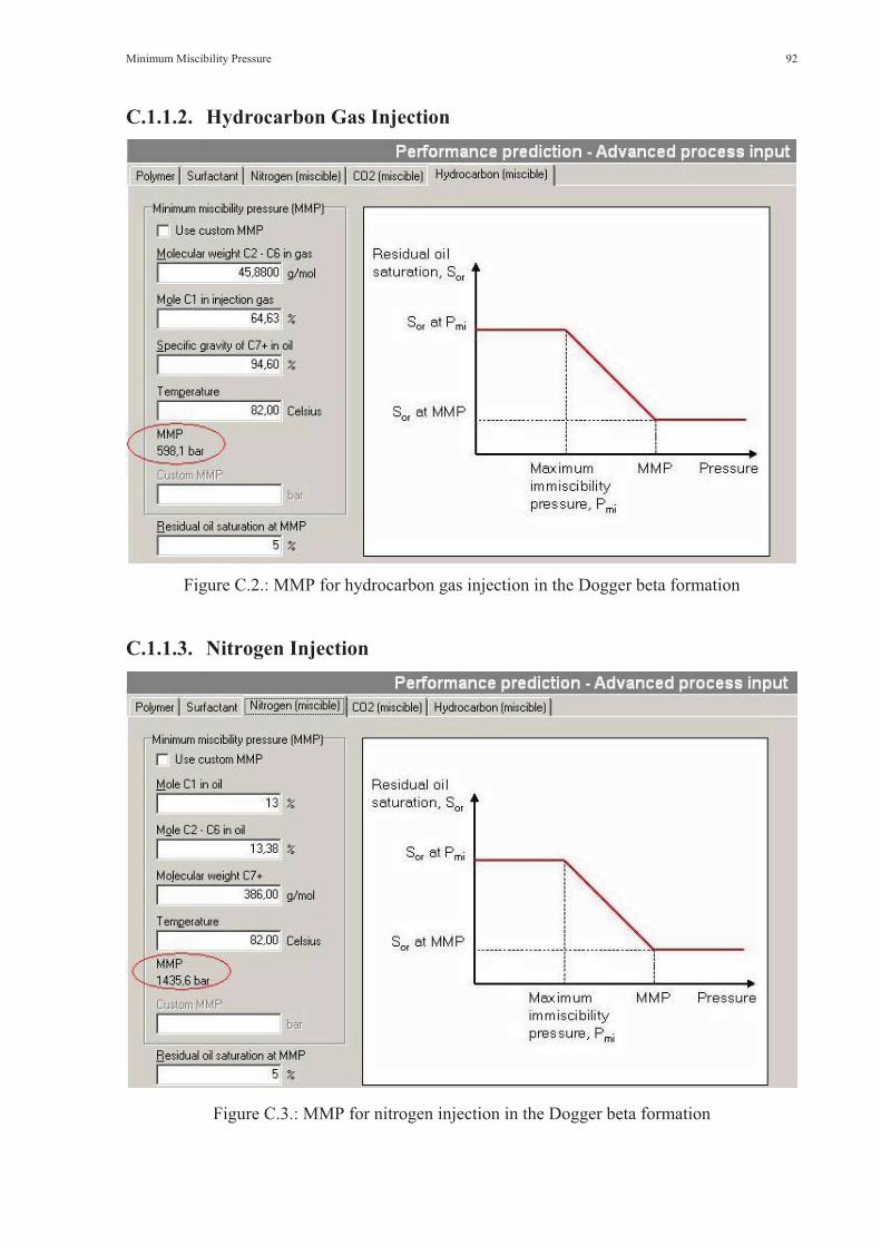
Minimum Miscibility Pressure 92
C.1.1.2. Hydrocarbon Gas Injection
Figure C.2.: MMP for hydrocarbon gas injection in the Dogger beta formation
C.1.1.3. Nitrogen Injection
Figure C.3.: MMP for nitrogen injection in the Dogger beta formation

Minimum Miscibility Pressure 93
C.1.2 Dogger Gamma FormationC.1.2.1. Carbon Dioxide Injection
Figure C.4.: MMP for CO2 injection in the Dogger gamma formation
C.1.2.2. Hydrocarbon Gas Injection
Figure C.5.: MMP for hydrocarbon gas injection in the Dogger gamma formation

Minimum Miscibility Pressure 94
C.1.2.3. Nitrogen Injection
Figure C.6.: MMP for nitrogen injection in the Dogger gamma formation
C.1.3 Dogger Delta / Epsilon FormationC.1.3.1. Carbon Dioxide Injection
Figure C.7.: MMP for CO2 injection in the Dogger delta / epsilon formation

Minimum Miscibility Pressure 95
C.1.3.2. Hydrocarbon Gas Injection
Figure C.8.: MMP for hydrocarbon gas injection in the Dogger delta / epsilon formation
C.1.3.3. Nitrogen Injection
Figure C.9.: MMP for nitrogen injection in the Dogger delta / epsilon formation

Minimum Miscibility Pressure 96
C.2. Calculation of Input Data for MMP EvaluationC.2.1 Dogger Beta Formation
Table C.1.: Calculation of input data for MMP evaluation for the Dogger beta formation

Minimum Miscibility Pressure 97
C.2.2 Dogger Gamma Formation
Table C.2.: Calculation of input data for MMP evaluation for the Dogger gamma formation
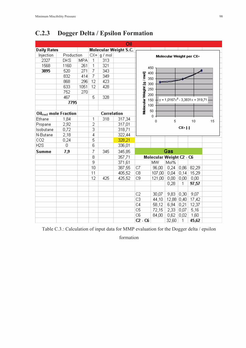
Minimum Miscibility Pressure 98
C.2.3 Dogger Delta / Epsilon Formation
Table C.3.: Calculation of input data for MMP evaluation for the Dogger delta / epsilon
formation
Performance Prediction Evaluation 99
Appendix D
Performance Prediction Evaluation
D.1. Input Data Overview and Origin D.1.1 Dogger Beta Formation
Reservoir Injection to production well distance [m] 1500,000 Pressure drop from injection to production well [bar] 200,0Production well bottomhole pressure [bar] 100,0Injection and production rate [m3/day] 1300,00 Injection and production well radius [m] 0,500Reservoir width [m] 2500,000 Oil viscosity [cp] 28,00Oil density [kg/m3] 890Dip [deg] -7,0
Table D.1.: General reservoir data of the Mittelplate Dogger beta formation
� Injection to production well distance
1500 m - Approximated distance between wells (producers and injectors) in the
Mittelplate beta central area. Information was taken from the Mittelplate structural map of
the Dogger beta formation.
� Pressure drop from injection to production well
200 bar - Approximated Value. Pwf is about 100 bar (much lower is not possible due to
the Pb being around 50 bar. The pressure at the electric submersible pumps must be above
the Pb to guarantee their operation), the wellhead pressure of the injectors is 150 bar, the
hydrostatic pressure in the annulus 280 bar, while the pressure losses in the injectors are
unknown. Thus the Pwf of the injectors is assumed to be around the initial reservoir
pressure Pi of 305 bar, resulting in about 200 bar pressure drop.
� Production well bottom hole pressure
100 bar - Averaged Value from the daily report of the Mittelplate beta production wells.
Report date: 15.08.2006
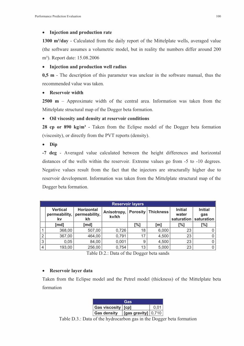
Performance Prediction Evaluation 100
� Injection and production rate
1300 m³/day - Calculated from the daily report of the Mittelplate wells, averaged value
(the software assumes a volumetric model, but in reality the numbers differ around 200
m³). Report date: 15.08.2006
� Injection and production well radius
0,5 m - The description of this parameter was unclear in the software manual, thus the
recommended value was taken.
� Reservoir width
2500 m – Approximate width of the central area. Information was taken from the
Mittelplate structural map of the Dogger beta formation.
� Oil viscosity and density at reservoir conditions
28 cp or 890 kg/m³ - Taken from the Eclipse model of the Dogger beta formation
(viscosity), or directly from the PVT reports (density).
� Dip
-7 deg - Averaged value calculated between the height differences and horizontal
distances of the wells within the reservoir. Extreme values go from -5 to -10 degrees.
Negative values result from the fact that the injectors are structurally higher due to
reservoir development. Information was taken from the Mittelplate structural map of the
Dogger beta formation.
Reservoir layers Vertical
permeability, kv
Horizontalpermeability,
khAnisotropy,
kv/kh Porosity Thickness Initial
water saturation
Initialgas
saturation [md] [md] [%] [m] [%] [%]
1 368,00 507,00 0,726 18 6,000 23 02 367,00 464,00 0,791 17 4,500 23 03 0,05 84,00 0,001 9 4,500 23 04 193,00 256,00 0,754 13 5,000 23 0
Table D.2.: Data of the Dogger beta sands
� Reservoir layer data
Taken from the Eclipse model and the Petrel model (thickness) of the Mittelplate beta
formation
GasGas viscosity [cp] 0,01Gas density [gas gravity] 0,710
Table D.3.: Data of the hydrocarbon gas in the Dogger beta formation
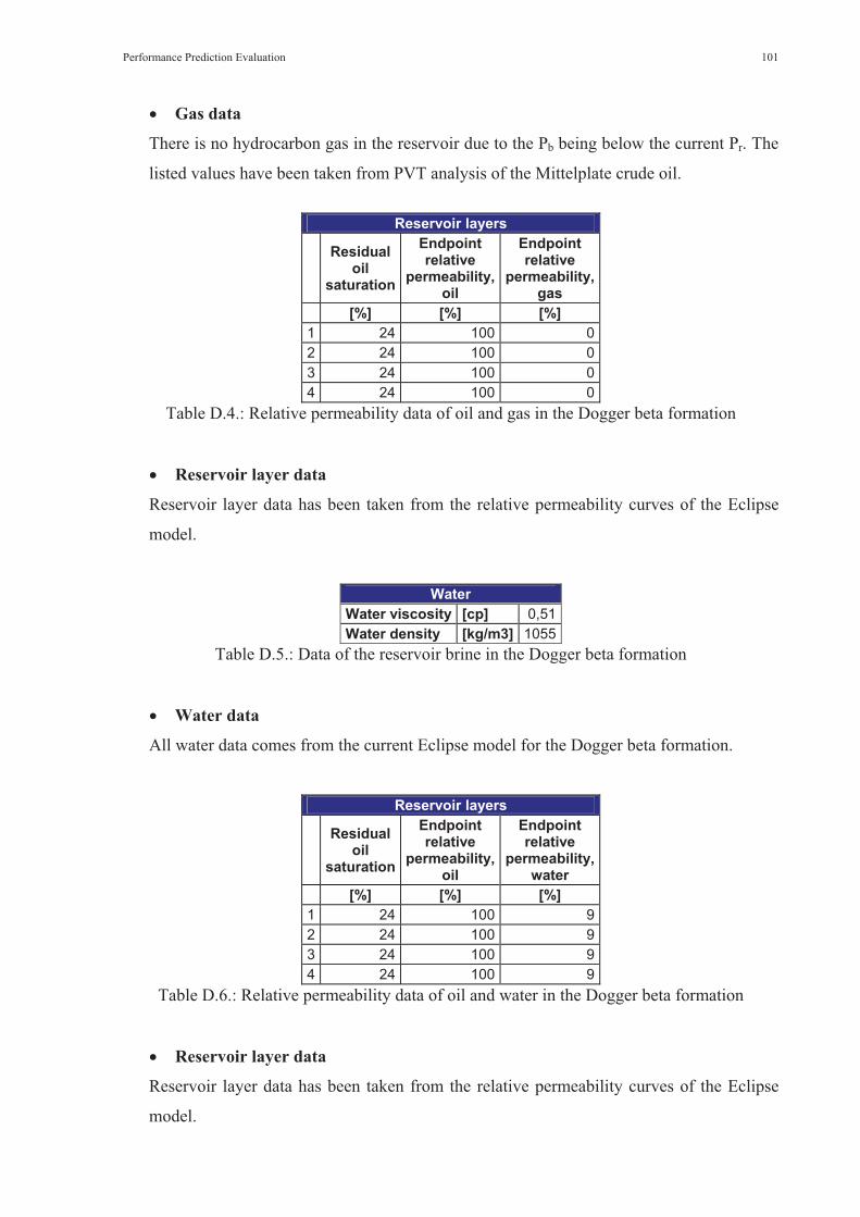
Performance Prediction Evaluation 101
� Gas data
There is no hydrocarbon gas in the reservoir due to the Pb being below the current Pr. The
listed values have been taken from PVT analysis of the Mittelplate crude oil.
Reservoir layers
Residual oil
saturation
Endpointrelative
permeability, oil
Endpointrelative
permeability, gas
[%] [%] [%] 1 24 100 02 24 100 03 24 100 04 24 100 0
Table D.4.: Relative permeability data of oil and gas in the Dogger beta formation
� Reservoir layer data
Reservoir layer data has been taken from the relative permeability curves of the Eclipse
model.
Water Water viscosity [cp] 0,51Water density [kg/m3] 1055
Table D.5.: Data of the reservoir brine in the Dogger beta formation
� Water data
All water data comes from the current Eclipse model for the Dogger beta formation.
Reservoir layers
Residual oil
saturation
Endpointrelative
permeability, oil
Endpointrelative
permeability, water
[%] [%] [%] 1 24 100 92 24 100 93 24 100 94 24 100 9
Table D.6.: Relative permeability data of oil and water in the Dogger beta formation
� Reservoir layer data
Reservoir layer data has been taken from the relative permeability curves of the Eclipse
model.
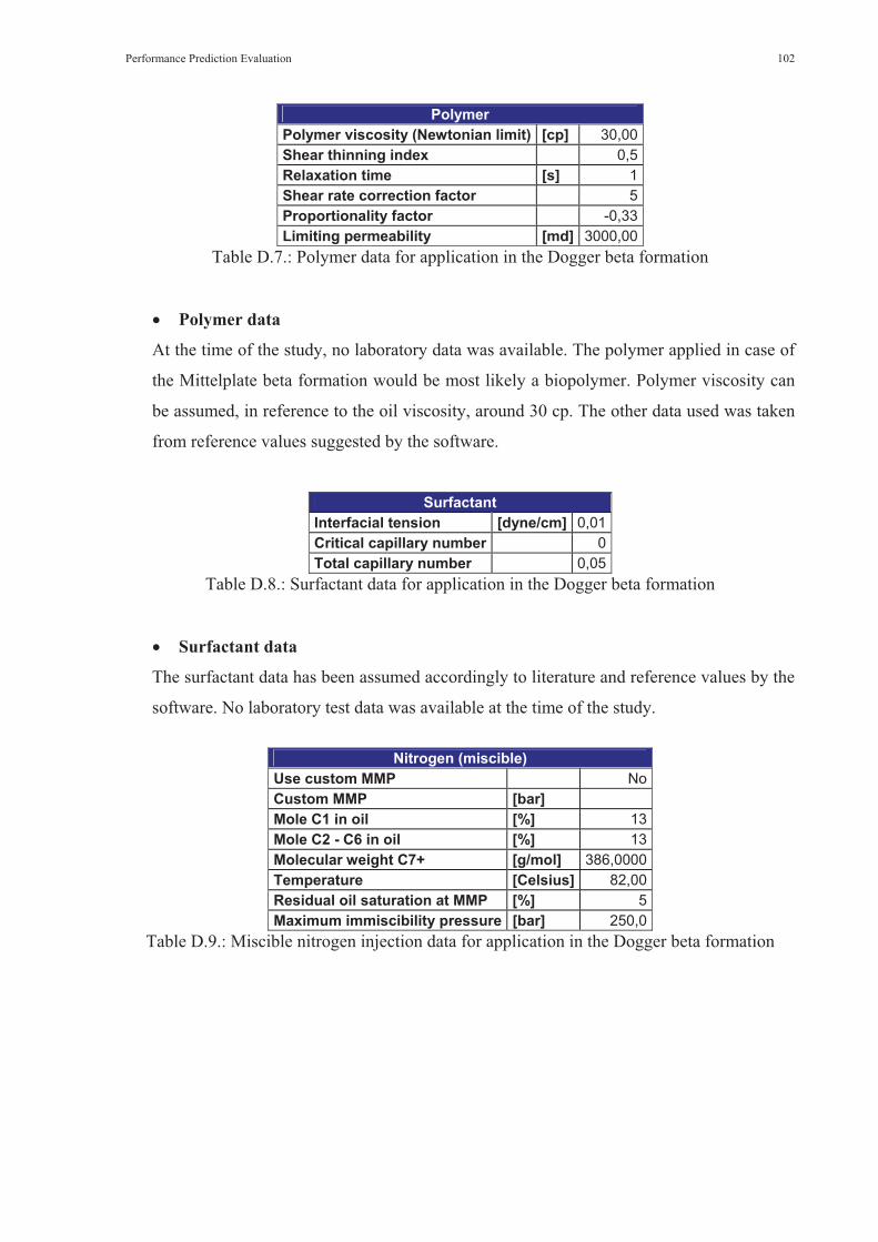
Performance Prediction Evaluation 102
Polymer Polymer viscosity (Newtonian limit) [cp] 30,00Shear thinning index 0,5Relaxation time [s] 1Shear rate correction factor 5Proportionality factor -0,33Limiting permeability [md] 3000,00
Table D.7.: Polymer data for application in the Dogger beta formation
� Polymer data
At the time of the study, no laboratory data was available. The polymer applied in case of
the Mittelplate beta formation would be most likely a biopolymer. Polymer viscosity can
be assumed, in reference to the oil viscosity, around 30 cp. The other data used was taken
from reference values suggested by the software.
SurfactantInterfacial tension [dyne/cm] 0,01Critical capillary number 0Total capillary number 0,05
Table D.8.: Surfactant data for application in the Dogger beta formation
� Surfactant data
The surfactant data has been assumed accordingly to literature and reference values by the
software. No laboratory test data was available at the time of the study.
Nitrogen (miscible) Use custom MMP NoCustom MMP [bar] Mole C1 in oil [%] 13Mole C2 - C6 in oil [%] 13Molecular weight C7+ [g/mol] 386,0000 Temperature [Celsius] 82,00Residual oil saturation at MMP [%] 5Maximum immiscibility pressure [bar] 250,0
Table D.9.: Miscible nitrogen injection data for application in the Dogger beta formation

Performance Prediction Evaluation 103
CO2 (miscible) Use custom MMP NoCustom MMP [bar] Molecular weight C5+ [g/mol] 354,2000 Oil volatile mole fraction [%] 14Oil intermediate mole fraction [%] 8Temperature [Celsius] 82,00Residual oil saturation at MMP [%] 5Maximum immiscibility pressure [bar] 250,0
Table D.10.: Miscible CO2 injection data for application in the Dogger beta formation
Hydrocarbon (miscible) Use custom MMP NoCustom MMP [bar] Molecular weight C2 - C6 in gas [g/mol] 45,8800 Mole C1 in injection gas [%] 65Specific gravity of C7+ in oil [%] 95Temperature [Celsius] 82,00Residual oil saturation at MMP [%] 5Maximum immiscibility pressure [bar] 250,0
Table D.11.: Miscible hydrocarbon gas injection data for application in the Dogger beta
formation
� Nitrogen (miscible), CO2 (miscible) and hydrocarbon gas (miscible) injection data
The compositional data of the Mittelplate beta crude oil and gas has been calculated or
taken from the PVT reports of the production wells. Residual oil saturation at MMP and
MIP can only be estimated with the help of literature and correlations, since they need
closer laboratory evaluation to be accurately measured.
D.1.2 Dogger Gamma FormationReservoir
Injection to production well distance [m] 1500,000 Pressure drop from injection to production well [bar] 150,0Production well bottomhole pressure [bar] 80,0Injection and production rate [m3/day] 220,00Injection and production well radius [m] 0,500Reservoir width [m] 300,000 Oil viscosity [cp] 7,00Oil density [kg/m3] 854Dip [deg] 45,0
Table D.12.: General reservoir data of the Mittelplate Dogger beta formation

Performance Prediction Evaluation 104
� Injection to production well distance
1500 m – Assumed valued for the Dogger gamma formation, due to no injectors being
currently present in addition to the only producer. Information was taken from the
Mittelplate structural map of the Dogger gamma formation.
� Pressure drop from injection to production well
150 bar - Approximated Value. Pwf is about 80 bar (much lower is not possible due to the
Pb being around 50 bar. The pressure at the electric submersible pump must be above the
Pb to guarantee its operation). As there is currently no injection well in the Dogger gamma
formation, the value was assumed analogues to the data of the other Mittelplate horizons
in addition to an initial pressure Pi of 233 bar
� Production well bottom hole pressure
80 bar - Value from the daily report of the Mittelplate MPA8b production well. Report
date: 15.08.2006
� Injection and production rate
220 m³/day – Value from the daily report of the Mittelplate MPA8b production well.
Report date: 15.08.2006
� Injection and production well radius
0,5 m - The description of this parameter was unclear in the software manual, thus the
recommended value was taken.
� Reservoir width
300 m – Average width of the Dogger gamma formation. Information was taken from the
Mittelplate structural map of the Dogger gamma formation.
� Oil viscosity and density at reservoir conditions
7 cp or 854 kg/m³ - Taken from the Eclipse model of the Dogger gamma formation
(viscosity), or directly from the PVT reports (density).
� Dip
29 deg - Averaged value calculated between the height differences and horizontal
distances within the reservoir. Extreme values go from 15 to 45 degrees. Information was
taken from the Mittelplate structural map of the Dogger gamma formation.
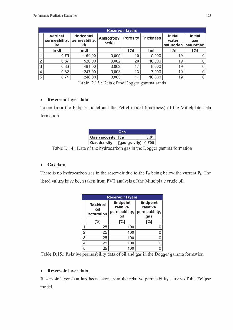
Performance Prediction Evaluation 105
Reservoir layers Vertical
permeability, kv
Horizontalpermeability,
khAnisotropy,
kv/kh Porosity Thickness Initial
water saturation
Initialgas
saturation [md] [md] [%] [m] [%] [%]
1 0,75 164,00 0,005 10 5,000 19 02 0,87 520,00 0,002 20 10,000 19 03 0,86 481,00 0,002 17 8,000 19 04 0,82 247,00 0,003 13 7,000 19 05 0,74 240,00 0,003 14 10,000 19 0
Table D.13.: Data of the Dogger gamma sands
� Reservoir layer data
Taken from the Eclipse model and the Petrel model (thickness) of the Mittelplate beta
formation
GasGas viscosity [cp] 0,01Gas density [gas gravity] 0,705
Table D.14.: Data of the hydrocarbon gas in the Dogger gamma formation
� Gas data
There is no hydrocarbon gas in the reservoir due to the Pb being below the current Pr. The
listed values have been taken from PVT analysis of the Mittelplate crude oil.
Reservoir layers
Residual oil
saturation
Endpointrelative
permeability, oil
Endpointrelative
permeability, gas
[%] [%] [%] 1 25 100 02 25 100 03 25 100 04 25 100 05 25 100 0
Table D.15.: Relative permeability data of oil and gas in the Dogger gamma formation
� Reservoir layer data
Reservoir layer data has been taken from the relative permeability curves of the Eclipse
model.
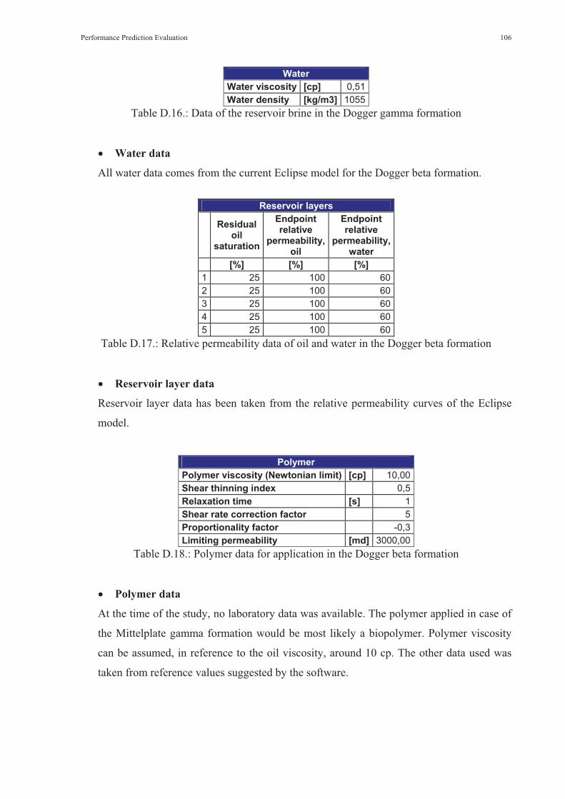
Performance Prediction Evaluation 106
Water Water viscosity [cp] 0,51Water density [kg/m3] 1055
Table D.16.: Data of the reservoir brine in the Dogger gamma formation
� Water data
All water data comes from the current Eclipse model for the Dogger beta formation.
Reservoir layers
Residual oil
saturation
Endpointrelative
permeability, oil
Endpointrelative
permeability, water
[%] [%] [%] 1 25 100 602 25 100 603 25 100 604 25 100 605 25 100 60
Table D.17.: Relative permeability data of oil and water in the Dogger beta formation
� Reservoir layer data
Reservoir layer data has been taken from the relative permeability curves of the Eclipse
model.
Polymer Polymer viscosity (Newtonian limit) [cp] 10,00Shear thinning index 0,5Relaxation time [s] 1Shear rate correction factor 5Proportionality factor -0,3Limiting permeability [md] 3000,00
Table D.18.: Polymer data for application in the Dogger beta formation
� Polymer data
At the time of the study, no laboratory data was available. The polymer applied in case of
the Mittelplate gamma formation would be most likely a biopolymer. Polymer viscosity
can be assumed, in reference to the oil viscosity, around 10 cp. The other data used was
taken from reference values suggested by the software.

Performance Prediction Evaluation 107
SurfactantInterfacial tension [dyne/cm] 0,01Critical capillary number 0Total capillary number 0,05
Table D.19.: Surfactant data for application in the Dogger beta formation
� Surfactant data
The surfactant data has been assumed accordingly to literature and reference values by the
software. No laboratory test data was available at the time of the study.
Nitrogen (miscible) Use custom MMP NoCustom MMP [bar] Mole C1 in oil [%] 10Mole C2 - C6 in oil [%] 11Molecular weight C7+ [g/mol] 323,0000 Temperature [Celsius] 69,00Residual oil saturation at MMP [%] 5Maximum immiscibility pressure [bar] 200,0
Table D.20.: Miscible nitrogen injection data for application in the Dogger gamma formation
CO2 (miscible) Use custom MMP NoCustom MMP [bar] Molecular weight C5+ [g/mol] 309,0000 Oil volatile mole fraction [%] 11Oil intermediate mole fraction [%] 6Temperature [Celsius] 69,00Residual oil saturation at MMP [%] 5Maximum immiscibility pressure [bar] 200,0
Table D.21.: Miscible CO2 injection data for application in the Dogger beta formation
Hydrocarbon (miscible) Use custom MMP NoCustom MMP [bar] Molecular weight C2 - C6 in gas [g/mol] 47,0700 Mole C1 in injection gas [%] 62Specific gravity of C7+ in oil [%] 90Temperature [Celsius] 69,00Residual oil saturation at MMP [%] 5Maximum immiscibility pressure [bar] 200,0
Table D.22.: Miscible hydrocarbon gas injection data for application in the Dogger beta
formation

Performance Prediction Evaluation 108
� Nitrogen (miscible), CO2 (miscible) and hydrocarbon gas (miscible) injection data
The compositional data of the Mittelplate gamma crude oil and gas has been calculated or
taken from the PVT report of the production well. Residual oil saturation at MMP and
MIP can only be estimated with the help of literature and correlations, since they need
closer laboratory evaluation to be accurately measured.
D.1.3 Dogger Delta / Epsilon FormationReservoir
Injection to production well distance [m] 750,000 Pressure drop from injection to production well [bar] 50,0Production well bottomhole pressure [bar] 100,0Injection and production rate [m3/day] 7800,00 Injection and production well radius [m] 0,500Reservoir width [m] 1000,000 Oil viscosity [cp] 11,50Oil density [kg/m3] 866Dip [deg] 14,5
Table D.23.: General reservoir data of the Mittelplate Dogger delta / epsilon formation
� Injection to production well distance
750 m - Approximated distance between wells (producers and injectors) in the Mittelplate
delta / epsilon central area. Information was taken from the Mittelplate structural map of
the Dogger delta / epsilon formation.
� Pressure drop from injection to production well
50 bar - Approximated Value. Pwf is about 100 bar (much lower is not possible due to the
Pb being around 50 bar. The pressure at the electric submersible pumps must be above the
Pb to guarantee their operation), the wellhead pressure of the injectors is 150 bar, the
hydrostatic pressure in the annulus 200 bar, while the pressure losses in the injectors are
unknown. Thus the Pwf of the injectors is assumed to be around the initial reservoir
pressure Pi of 233 bar, resulting in about 50 bar pressure drop.
� Production well bottom hole pressure
100 bar - Averaged Value from the daily report of the Mittelplate and Dieksand delta /
epsilon production wells. Report date: 15.08.2006
� Injection and production rate
7800 m³/day - Calculated from the daily report of the Mittelplate and Dieksand
production wells, averaged value (the software assumes a volumetric model, but in reality
the numbers differ a lot due to the strong aquifer). Report date: 15.08.2006

Performance Prediction Evaluation 109
� Injection and production well radius
0,5 m - The description of this parameter was unclear in the software manual, thus the
recommended value was taken.
� Reservoir width
1000 m – Approximate width of the central area. Information was taken from the
Mittelplate structural map of the Dogger delta / epsilon formation.
� Oil viscosity and density at reservoir conditions
11,5 cp or 866 kg/m³ - Taken from the Eclipse model of the Dogger delta / epsilon
formation (viscosity), or directly from the PVT reports (density).
� Dip
14,5 deg - Averaged value calculated between the height differences and horizontal
distances of the wells within the reservoir. Extreme values go from -10 to 40 degrees.
Information was taken from the Mittelplate structural map of the Dogger delta / epsilon
formation.
Reservoir layers Vertical
permeability, kv
Horizontalpermeability,
khAnisotropy,
kv/kh Porosity Thickness Initial
water saturation
Initialgas
saturation [md] [md] [%] [m] [%] [%]
1 813,00 6000,00 0,136 18 25,000 18 02 1611,00 5744,00 0,28 15 15,000 18 03 227,00 647,00 0,351 10 15,000 18 04 425,00 2384,00 0,178 17 12,500 18 05 211,00 1950,00 0,108 16 7,500 18 06 95,00 511,00 0,186 10 5,000 18 0
Table D.24.: Data of the Dogger beta sands
� Reservoir layer data
Taken from the Eclipse model and the Petrel model (thickness) of the Mittelplate delta /
epsilon formation
GasGas viscosity [cp] 0,01Gas density [gas gravity] 0,710
Table D.25.: Data of the hydrocarbon gas in the Dogger delta / epsilon formation
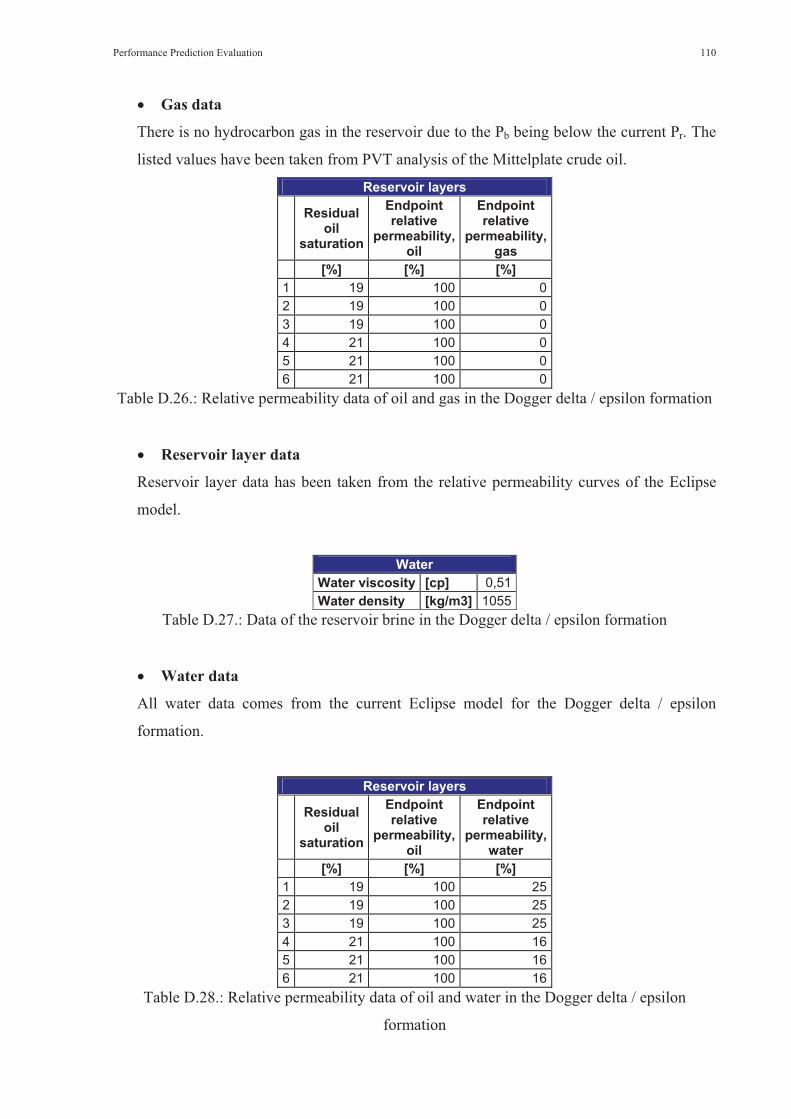
Performance Prediction Evaluation 110
� Gas data
There is no hydrocarbon gas in the reservoir due to the Pb being below the current Pr. The
listed values have been taken from PVT analysis of the Mittelplate crude oil.
Reservoir layers
Residual oil
saturation
Endpointrelative
permeability, oil
Endpointrelative
permeability, gas
[%] [%] [%] 1 19 100 02 19 100 03 19 100 04 21 100 05 21 100 06 21 100 0
Table D.26.: Relative permeability data of oil and gas in the Dogger delta / epsilon formation
� Reservoir layer data
Reservoir layer data has been taken from the relative permeability curves of the Eclipse
model.
Water Water viscosity [cp] 0,51Water density [kg/m3] 1055
Table D.27.: Data of the reservoir brine in the Dogger delta / epsilon formation
� Water data
All water data comes from the current Eclipse model for the Dogger delta / epsilon
formation.
Reservoir layers
Residual oil
saturation
Endpointrelative
permeability, oil
Endpointrelative
permeability, water
[%] [%] [%] 1 19 100 252 19 100 253 19 100 254 21 100 165 21 100 166 21 100 16
Table D.28.: Relative permeability data of oil and water in the Dogger delta / epsilon
formation

Performance Prediction Evaluation 111
� Reservoir layer data
Reservoir layer data has been taken from the relative permeability curves of the Eclipse
model.
Polymer Polymer viscosity (Newtonian limit) [cp] 15,00Shear thinning index 0,5Relaxation time [s] 1Shear rate correction factor 5Proportionality factor -0,3Limiting permeability [md] 10000,00
Table D.29.: Polymer data for application in the Dogger delta / epsilon formation
� Polymer data
At the time of the study, no laboratory data was available. The polymer applied in case of
the Mittelplate delta / epsilon formation would be most likely a biopolymer. Polymer
viscosity can be assumed, in reference to the oil viscosity, around 15 cp. The other data
used was taken from reference values suggested by the software.
SurfactantInterfacial tension [dyne/cm] 0,01Critical capillary number 0Total capillary number 0,05
Table D.30.: Surfactant data for application in the Dogger beta formation
� Surfactant data
The surfactant data has been assumed accordingly to literature and reference values by the
software. No laboratory test data was available at the time of the study.
Nitrogen (miscible) Use custom MMP NoCustom MMP [bar] Mole C1 in oil [%] 11Mole C2 - C6 in oil [%] 13Molecular weight C7+ [g/mol] 345,0000 Temperature [Celsius] 69,00Residual oil saturation at MMP [%] 5Maximum immiscibility pressure [bar] 200,0
Table D.31.: Miscible nitrogen injection data for application in the Dogger delta / epsilon
formation
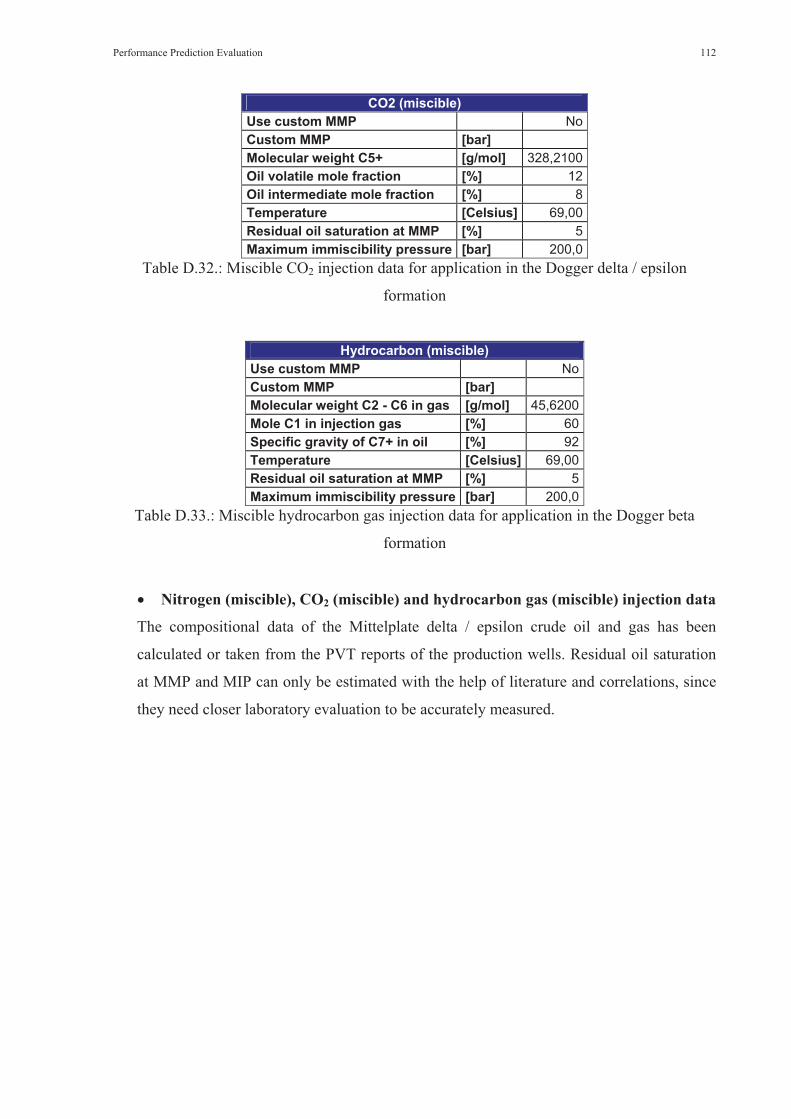
Performance Prediction Evaluation 112
CO2 (miscible) Use custom MMP NoCustom MMP [bar] Molecular weight C5+ [g/mol] 328,2100 Oil volatile mole fraction [%] 12Oil intermediate mole fraction [%] 8Temperature [Celsius] 69,00Residual oil saturation at MMP [%] 5Maximum immiscibility pressure [bar] 200,0
Table D.32.: Miscible CO2 injection data for application in the Dogger delta / epsilon
formation
Hydrocarbon (miscible) Use custom MMP NoCustom MMP [bar] Molecular weight C2 - C6 in gas [g/mol] 45,6200 Mole C1 in injection gas [%] 60Specific gravity of C7+ in oil [%] 92Temperature [Celsius] 69,00Residual oil saturation at MMP [%] 5Maximum immiscibility pressure [bar] 200,0
Table D.33.: Miscible hydrocarbon gas injection data for application in the Dogger beta
formation
� Nitrogen (miscible), CO2 (miscible) and hydrocarbon gas (miscible) injection data
The compositional data of the Mittelplate delta / epsilon crude oil and gas has been
calculated or taken from the PVT reports of the production wells. Residual oil saturation
at MMP and MIP can only be estimated with the help of literature and correlations, since
they need closer laboratory evaluation to be accurately measured.
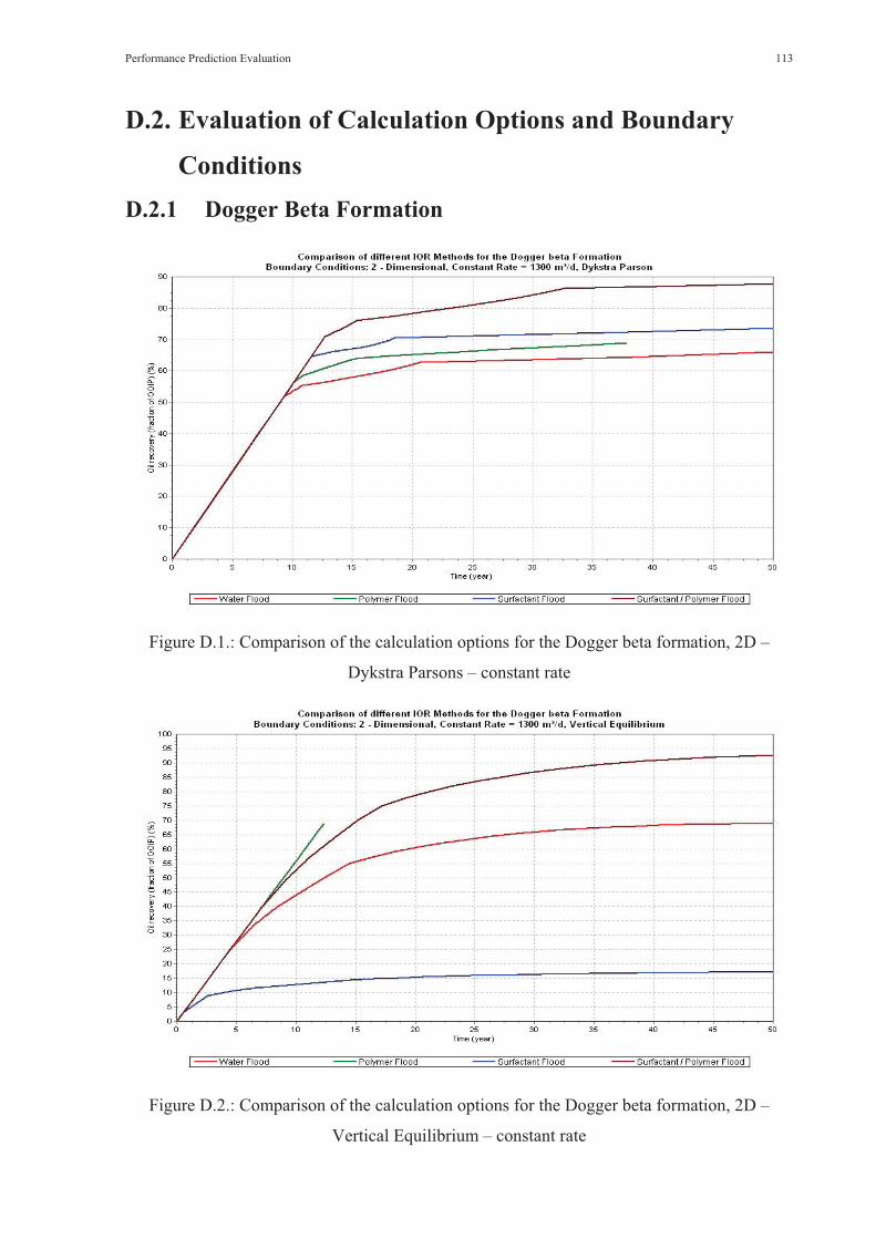
Performance Prediction Evaluation 113
D.2. Evaluation of Calculation Options and Boundary
ConditionsD.2.1 Dogger Beta Formation
Figure D.1.: Comparison of the calculation options for the Dogger beta formation, 2D –
Dykstra Parsons – constant rate
Figure D.2.: Comparison of the calculation options for the Dogger beta formation, 2D –
Vertical Equilibrium – constant rate
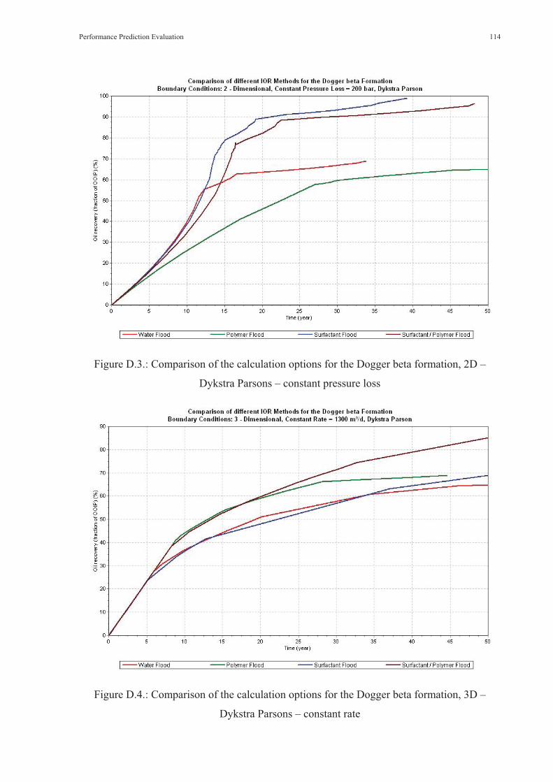
Performance Prediction Evaluation 114
Figure D.3.: Comparison of the calculation options for the Dogger beta formation, 2D –
Dykstra Parsons – constant pressure loss
Figure D.4.: Comparison of the calculation options for the Dogger beta formation, 3D –
Dykstra Parsons – constant rate

Performance Prediction Evaluation 115
Figure D.5.: Comparison of the calculation options for the Dogger beta formation, 3D –
Vertical Equilibrium – constant rate
Figure D.6.: Comparison of the calculation options for the Dogger beta formation, 3D –
Dykstra Parsons – constant pressure loss
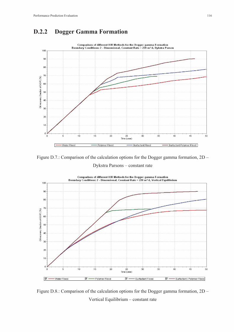
Performance Prediction Evaluation 116
D.2.2 Dogger Gamma Formation
Figure D.7.: Comparison of the calculation options for the Dogger gamma formation, 2D –
Dykstra Parsons – constant rate
Figure D.8.: Comparison of the calculation options for the Dogger gamma formation, 2D –
Vertical Equilibrium – constant rate

Performance Prediction Evaluation 117
Figure D.9.: Comparison of the calculation options for the Dogger gamma formation, 2D –
Dykstra Parsons – constant pressure loss
Figure D.10.: Comparison of the calculation options for the Dogger gamma formation, 3D –
Dykstra Parsons – constant rate

Performance Prediction Evaluation 118
Figure D.11.: Comparison of the calculation options for the Dogger gamma formation, 3D –
Vertical Equilibrium – constant rate
Figure D.12.: Comparison of the calculation options for the Dogger gamma formation, 3D –
Dykstra Parsons – constant pressure loss
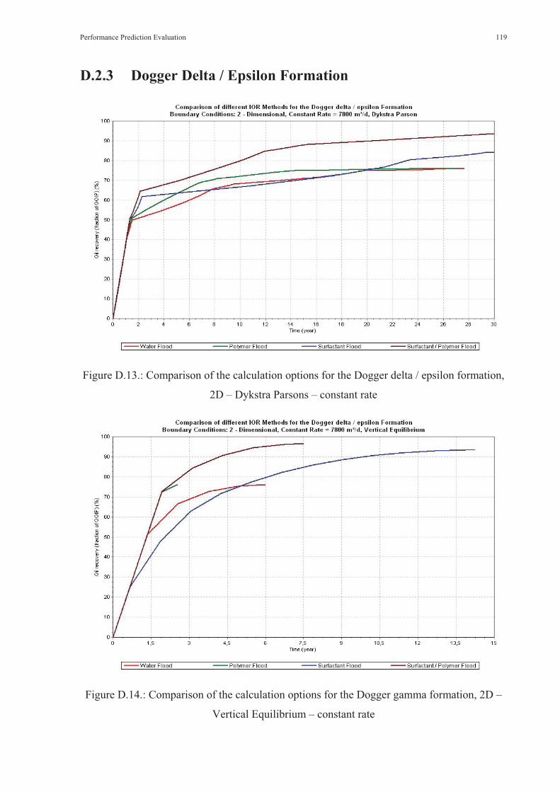
Performance Prediction Evaluation 119
D.2.3 Dogger Delta / Epsilon Formation
Figure D.13.: Comparison of the calculation options for the Dogger delta / epsilon formation,
2D – Dykstra Parsons – constant rate
Figure D.14.: Comparison of the calculation options for the Dogger gamma formation, 2D –
Vertical Equilibrium – constant rate
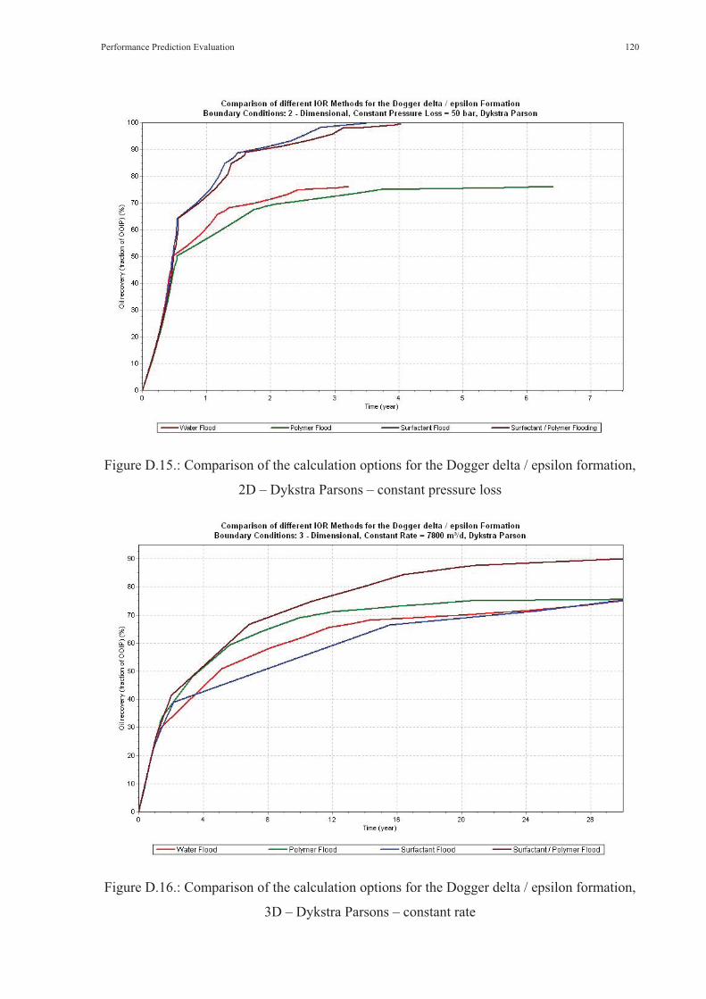
Performance Prediction Evaluation 120
Figure D.15.: Comparison of the calculation options for the Dogger delta / epsilon formation,
2D – Dykstra Parsons – constant pressure loss
Figure D.16.: Comparison of the calculation options for the Dogger delta / epsilon formation,
3D – Dykstra Parsons – constant rate
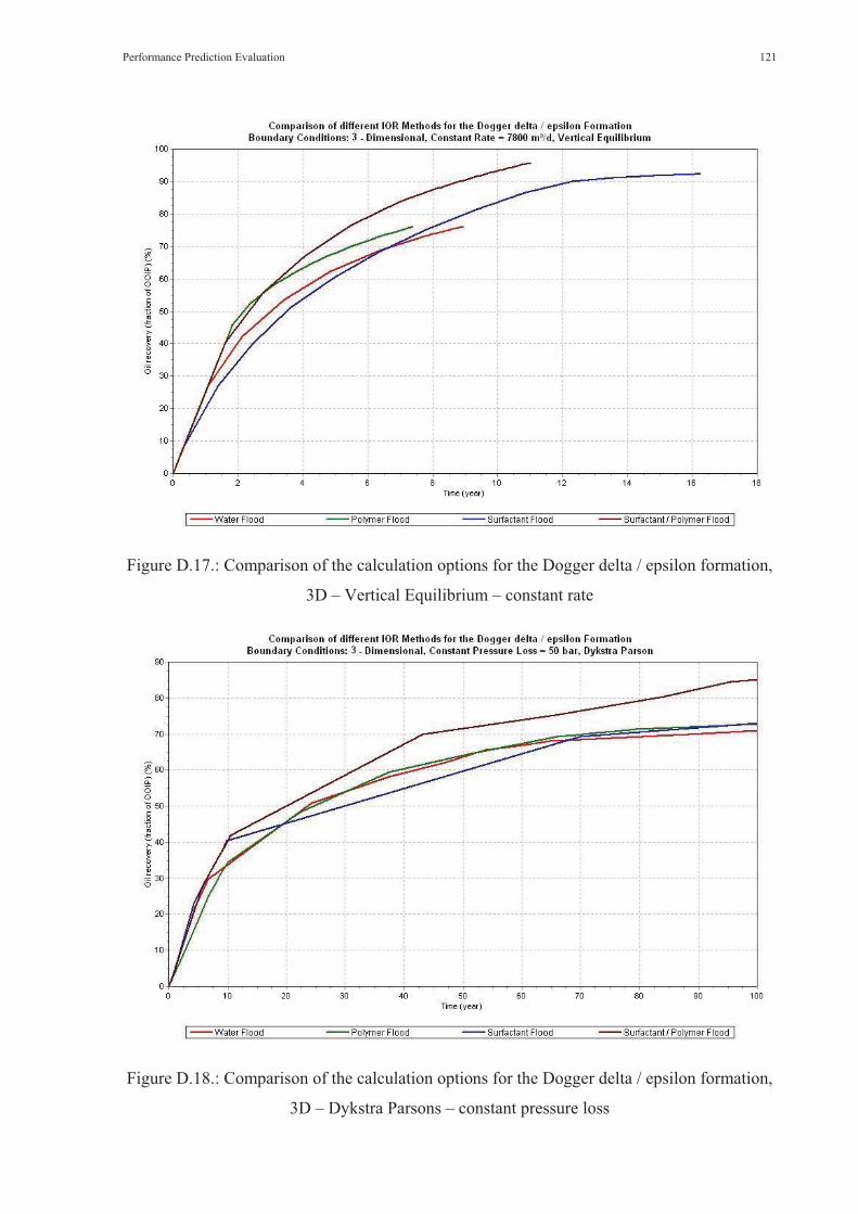
Performance Prediction Evaluation 121
Figure D.17.: Comparison of the calculation options for the Dogger delta / epsilon formation,
3D – Vertical Equilibrium – constant rate
Figure D.18.: Comparison of the calculation options for the Dogger delta / epsilon formation,
3D – Dykstra Parsons – constant pressure loss

Data Correlations for the Dogger Beta Sample Case 122
Appendix E
Data Correlations for the Dogger Beta Sample Case
Table E.1.: Water data conversion
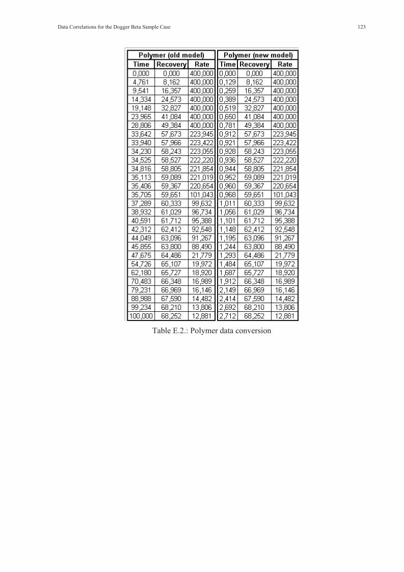
Data Correlations for the Dogger Beta Sample Case 123
Table E.2.: Polymer data conversion

Data Correlations for the Dogger Beta Sample Case 124
Table E.3.: Resulting data after conversion and correlation

Data Input for the Wellhead Pressure Calculations 125
Appendix F
Data Input for the Wellhead Pressure Calculations
Figure F.1.: Data input overview

Data Input for the Wellhead Pressure Calculations 126
Figure F.2.: PVT data input
Figure F.3.: IPR model selection (1)

Data Input for the Wellhead Pressure Calculations 127
Figure F.4.: IPR model selection (2)
Figure F.5.: Equipment input overview
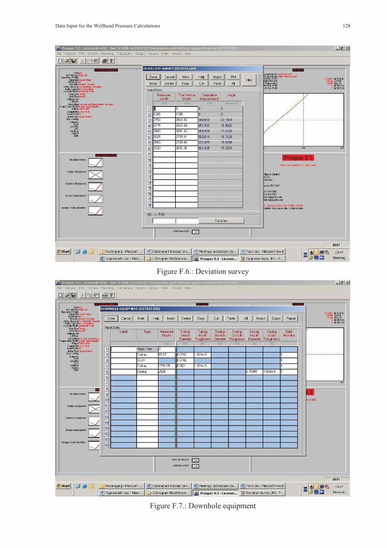
Data Input for the Wellhead Pressure Calculations 128
Figure F.6.: Deviation survey
Figure F.7.: Downhole equipment

Data Input for the Wellhead Pressure Calculations 129
Figure F.8.: Geothermal gradient
Figure F.9.: Average heat capacities
Related Documents


![EOR - Enhanced Oil Recovery 01[1]](https://static.cupdf.com/doc/110x72/577d2f9e1a28ab4e1eb22aa6/eor-enhanced-oil-recovery-011.jpg)