ofp 010 physics - The Open University of Tanzania-Library

THE OPEN UNIVERSITY OF TANZANIA

Institute of Continuing Education

FOUNDATION PROGRAMME

OFP 010

PHYSICS

2

Published by:

The Open University of Tanzania Kawawa Road,

P. O. Box 23409,

Dar es Salaam. TANZANIA

www.out.ac.tz

First Edition: 2013 Second Edition 2018

Copyright © 2018

All Rights Reserved

ISBN 978 9987 00 250 4

http://www.out.ac.tz/

3

Table of Contents

GENERAL INTRODUCTION ........................................................................................... 7

SECTION ONE: RECTILINEAR MOTION .................................................................... 8

Lecture 1: Some Fundamental Concepts of Measurements ........................................... 8 1.1 Introduction ............................................................................................................ 8 1.2 Units of Measurements ........................................................................................... 8

1.3 Units of Base Quantities and their Definitions ......................................................... 9 1.4 Units of Supplementary Quantities ........................................................................ 10

1.5 Derived Units and their Definitions ....................................................................... 10 1.6 Dimensions, Units and Significant Figures ............................................................ 11

1.7 Idealization, Approximation and Precision ............................................................ 11 1.8 Errors, Accuracy and Precision ............................................................................. 12

Lecture 2: Motion in One-dimension ............................................................................ 15 2.1 Introduction .......................................................................................................... 15

2.2 Position ................................................................................................................. 15 2.3 Instantaneous Velocity and Speed ......................................................................... 16

2.4 Acceleration .......................................................................................................... 17 2.5 Equations of Motion under Constant Acceleration ................................................. 17

2.6 Kinematic Equations and Free Fall ........................................................................ 22 2.7 Free-fall Acceleration............................................................................................ 22

Lecture 3: Vectors .......................................................................................................... 25 3.1 Introduction .......................................................................................................... 25

3.2 Addition of Vectors ............................................................................................... 25 3.3 Properties of Vector Addition................................................................................ 25

3.4 Vectors and their Components............................................................................... 26 3.5 Unit Vectors .......................................................................................................... 27

3.6 Adding Vectors by Components ............................................................................ 27 3.7 Multiplying Vectors .............................................................................................. 28

3.8 Vector Product ...................................................................................................... 28

Lecture 4: Newton’s Laws of Motion ............................................................................ 35 4.1 Introduction .......................................................................................................... 35 4.2 Newton’s First Law ............................................................................................... 35

4.3 Newton’s Second Law .......................................................................................... 36 4.4 Some Particular Forces.......................................................................................... 37

Lecture 5: Action and Reaction Forces ....................................................................... 44 5.1 Introduction .......................................................................................................... 44

5.2 Newton’s Third Law ............................................................................................. 44 5.3 Friction ................................................................................................................. 44

5.4 Properties of Friction ............................................................................................ 46

4

SECTION TWO: MECHANICS ...................................................................................... 62

Lecture 6: Work, Energy and Power ............................................................................ 62 6.1 Introduction .......................................................................................................... 62 6.2 Work ..................................................................................................................... 62

6.3 Power.................................................................................................................... 64 6.4 Energy .................................................................................................................. 65

6.5 Work-Energy Theorem ......................................................................................... 72 6.6 Conservation of Mechanical Energy ...................................................................... 75

Lecture 7: Uniform Circular Motion .......................................................................... 88 7.1 Introduction .......................................................................................................... 88

7.2 False Sensation of an Outward Force .................................................................... 88 7.3 The Universe and the Gravitational Force ............................................................. 91

7.4 Kepler’s Laws ....................................................................................................... 94 7.5 Planetary and Satellite Motion............................................................................... 96

7.6 Weightlessness .................................................................................................... 100

Lecture 8: Fluid Dynamics .......................................................................................... 103 8.1 Introduction ........................................................................................................ 103 8.2 Fluids at Rest ...................................................................................................... 104

8.3 Hydraulic Lever .................................................................................................. 104 8.4 Equilibrium of Floating Objects .......................................................................... 105

SECTION THREE: ELECTROSTATICS AND ELECTRIC CIRCUITS .................. 107

Lecture 9 Electrostatics ........................................................................................... 107 9.1 Introduction ........................................................................................................ 107

9.2 Electric Charge and Coulomb’s Law ................................................................... 108 9.3 Electric Point Charge .......................................................................................... 108

9.4 Coulomb’s Law of Force ..................................................................................... 108 9.6 Principle of Superposition ................................................................................... 110

Lecture 10 Electric Field ............................................................................................ 113 10.1 Introduction ........................................................................................................ 113

10.2 Concept of Electric Field ..................................................................................... 113 10.3 Electric Field due to a Point Charge .................................................................... 114

10.4 Electric Lines of Force ........................................................................................ 114 10.5 Electric Potential Energy and Electric Potential ................................................... 115

Lecture 11 Capacitance ............................................................................................ 119 11.1 Introduction ........................................................................................................ 119

11.2 The Capacitance of a Capacitor ........................................................................... 121 11.3 The Dielectric of a Capacitor............................................................................... 123

11.4 Applications ........................................................................................................ 127 11.5 Capacitors in Parallel and in Series Configurations ............................................. 127

11.6 Energy Storage in an Electric Field ..................................................................... 136 11.7 Charging and Discharging a Capacitor ................................................................ 138

Lecture 12 Rc Electric Circuits .................................................................................. 143 12.1 Introduction ........................................................................................................ 143

12.2 Kirchhoff’s Laws ................................................................................................ 143 12.3 Current Loop Method .......................................................................................... 144

5

SECTION FOUR: ELECTROMAGNETISM ............................................................... 149

Lecture 13: The Magnetic Field .................................................................................... 149 13.1 Introduction ........................................................................................................ 149 13.2 Magnetic Field Lines .......................................................................................... 150

13.3 Magnetic Force on a Moving Electric Charge...................................................... 150 13.4 Work Done in a Magnetic Field .......................................................................... 151

13.5 Magnetic Force on a Conductor Carrying a Current ............................................ 153 13.6 Faraday’s Law of Electromagnetic Induction ...................................................... 154

13.7 Lenz's Law .......................................................................................................... 155

Lecture 14: Inductance and RI Electric Circuits ....................................................... 157 14.1 Introduction ........................................................................................................ 157 14.2 Self-inductance ................................................................................................... 157

14.3 Mutual Inductance .............................................................................................. 159 14.4 Combination of Self-inductances......................................................................... 160

14.5 LR Circuits ......................................................................................................... 161 14.6 Energy Storage in a Magnetic Field ..................................................................... 163

14.7 The Alternating Current ...................................................................................... 164

SECTION FIVE: OSCILLATIONS .............................................................................. 169

Lecture 15: Oscillations and Waves............................................................................ 169 15.1 Introduction ........................................................................................................ 169 15.2 Definition of an Oscillating System ..................................................................... 170

15.3 Variables of an Oscillation .................................................................................. 170 15.4 The Basic Simple Harmonic Equation ................................................................. 171

15.5 Features and Characteristics of SHM................................................................... 173 15.6 Energy of a Simple Harmonic Oscillator ............................................................. 174

15.7 Applications of Simple Harmonic Motion ........................................................... 175

Lecture 16: Damped Simple Harmonic Oscillations .................................................. 180 16.1 Introduction ........................................................................................................ 180 16.2 Damping Forces .................................................................................................. 180

16.3 Effect of Damping............................................................................................... 181 16.4 Forced Oscillations and Resonance ..................................................................... 182

Lecture 17: Wave Motion ....................................................................................... 188 17.1 Introduction ........................................................................................................ 188

17.2 Waves versus Oscillations ................................................................................... 189 17.3 Mechanical Waves .............................................................................................. 189

17.4 Wave Characteristics ........................................................................................... 190 17.5 Variables of Wave Motion .................................................................................. 192

17.6 Mathematical Description of Waves .................................................................... 193 17.7 Wave Equation.................................................................................................... 194

17.8 Interference of Waves ......................................................................................... 195 17.9 Standing Waves .................................................................................................. 197

6

SECTION SIX: ELECTRONICS................................................................................... 200

Lecture 18: Electronics ................................................................................................... 200 18.1 Introduction ........................................................................................................ 200 18.2 Diode Valve/Vacuum Tube ................................................................................. 202

18.3 Diode Rectification ............................................................................................. 204 18.4 Semiconductor electronics .................................................................................. 205

18.5 Intrinsic Semiconductors: Electrons and Holes .................................................... 206 18.6 Extrinsic Semiconductors .................................................................................... 207

7

GENERAL INTRODUCTION

Physics, as opposed to natural philosophy (with which it was grouped until the 19th century),

relies upon scientific methods in order to describe the natural world. To understand the

fundamental principles of the universe, physics utilizes many workings from the other natural

sciences. Because of this overlap, phenomena studied in physics (conservation of energy for

example) are common to all material systems. The specific ways in which they apply to

energy (hence, physics) are often referred to as the "laws of physics." Because each of the

other natural sciences i.e. biology, chemistry, geology, material science, medicine,

engineering, and others, work with systems which adhere to the laws of physics, physics is

often referred to as the "fundamental science."

Course Description

The course is designed to provide general physics knowledge. The course introduces to

students the behaviour of physical bodies when subjected to forces or displacements, and the

subsequent effect of the bodies on their environment. It also describes the forces exerted by a

static (i.e. unchanging) electric field upon charged (electrostatics), as well as wave motions. It

therefore equips the learners with the general understanding of theoretical aspects as well as

basic practical skills of physics.

Course Objectives

On completion of this course, students are expected to able to do the following:

1. Define various physics concepts such as Mechanics, Electrostatics, Electromagnetism,

Self inductance, Oscillations and waves

2. State and apply various laws in physics i.e. Newton’s law of motion, Kepler’s Law

and its application in planetary motion, Pascal’s Principle, Coulombs law.

3. Compute various quantities of energy e.g. the energy stored in capacitors, Compute

power in alternating current circuits, energy stored in magnetic field, energy of simple

harmonic motion.

4. Manipulate vectors, RC electric circuits and RL Electric Circuits

5. Explain the Interferences of waves

6. Describe vacuum tube, semiconductor diode and various logic gates.

Pre-requisite To be able to do this course, students must have studied Physics at the ordinary level of

secondary education.

Mode of Assessment Continuous Assessment: 30%

Final Examination: 70%

8

SECTION ONE:

RECTILINEAR MOTION

Lecture 1: Some Fundamental Concepts of Measurements

1.1 Introduction Measurement is at the heart of physics. The ability to make measurements of physical

quantities is necessary for an understanding of the physical world we live in. A famous

physicist once said that when you can measure what you are speaking about, and express it in

numbers, you know something about it; but when you cannot express it in numbers, your

knowledge is of a meagre and unsatisfactory kind.

A physicist would ask questions such as: What is the time interval between two events; what

is the length between two points, A and B; what is the temperature of boiling water; etc. The

quantities which one measures are involved in the laws of physics and hence they are called

physical quantities. Among these quantities are: Mass, Length, Time, Temperature, Pressure,

Electrical resistance, etc.

In order to describe a physical quantity a unit is defined, which is a measure of the quantity

that is defined to be exactly 1.0. After a unit is defined, a standard is defined. The standard is

a reference to which all other examples of the quantity are compared.

The standard ensures that scientists around the world may agree on the measurements they

take. Some physical quantities such as speed are expressed in terms of other quantities, so

that we have base quantities and their standards and derived quantities.

Lecture Objectives

At the end of this lecture, you should be able to do the following:

Define the SI units of measurement.

Describe the base quantities.

Describe the derived units.

Define error, accuracy and precision.

1.2 Units of Measurements

SI units are currently divided into three classes:

(i) Base units

(ii) Derived units

(iii) Supplementary units

9

The three classes together form the “coherent system of SI units”.

1. SI Base units: There are seven base quantities of measurements. These are mass,

length, time, temperature, electric current, luminous intensity and amount of

substance.

2. SI Supplementary units: These are two – the radian and steradian.

3. SI Derived units: These are many including volume, speed, velocity, acceleration,

density, current density, etc.

The definitions of the SI units for the seven base quantities, two supplementary quantities and

some of the derived units are given below.

1.3 Units of Base Quantities and their Definitions

The international system of units devised seven base quantities as part of the metric system

and these quantities are defined as under:

1. Mass: The fundamental unit of mass is the Kilogram (kg). The definition of the

kilogram is based on the International Prototype Kilogram, a 90% platinum and 10%

iridium alloy cylinder of equal height and diameter.

2. Length: The fundamental unit of length is the Metre (m). The metre is defined as the

distance between two known points on an International Prototype metre kept at in

France. There are two modern definitions of the metre:

(a) The length equal to 1,650,763.73 wavelengths in vacuum of radiation emitted

by the krypton 86 nuclide.

(b) The length of the path travelled by light in vacuum during a time interval of 1/

299,792,458 of a second. This definition also fixes the speed of light in

vacuum at exactly 299,792,458 m.s–1.

You will note that these are very precise definitions.

3. Time: The fundamental unit of time is the Second (s). The current definition of a

second is the duration of 9,192,631,770 periods of the radiation corresponding to the

transition between the two hyperfine levels of the ground state of the 133Cs atom.

4. Thermodynamic Temperature: The fundamental unit of thermodynamic temperature,

pegged on the triple point of water, is the Kelvin (K). The triple point of water is

assigned a value of 273.16 K on this scale, and the Kelvin is thus defined as the

fraction 1/273.16 of the thermodynamic temperature of the triple point of water.

5. Electric Current: The fundamental unit of electric current is the Ampere (A). The

current definition of ampere is that constant current which, if maintained in two

straight parallel conductors of infinite length, of negligible circular

cross-sectional area and placed one metre apart in vacuum, would produce between

these conductors a force equal to 2 × 10–7 Nm–1.

6. Luminous Intensity: The fundamental unit of luminous intensity is the Candela (cd).

This is defined as the luminous intensity, in a given direction, of a source that emits

10

monochromatic radiation of frequency 540 × 1012 Hz and that has a radiant intensity

in that direction of (1/683) watt per steradian.

7. Amount of Substance: The fundamental unit of the amount of substance is the Mole

(mol). This is defined as the amount of substance of a system which contains as many

elementary entities as there are atoms in 1.2 × 10-2 kilogram of carbon - 12. Entity

may refer to atoms, molecules, ions, electrons, or other particles.

1.4 Units of Supplementary Quantities

The two units of supplementary quantities are as discussed below:

1. Plane Angle: Plane angles are measured in Radians (rad.). The radian is a plane angle

between two radii of a circle which cut off on the circumference an arc equal in length

to the radius.

2. Solid Angle: Solid angles are measured in Steradians (sr.). This is the solid angle

which, having its vertex at the centre of a sphere, cuts off an area of the surface of the

sphere equal to that of a square with sides of length equal to the radius of the sphere.

1.5 Derived Units and their Definitions

Derived units are obtained from the fundamental and/or supplementary units. There are many

units under this category. The important ones are defined below.

1. Force: The SI unit of force is the Newton (N). This is that force which, when acting

on a mass of one kilogram, gives it an acceleration of one metre per second per

second.

2. Work, Energy and Quantity of Heat: In the SI system, these quantities are all

measured in Joules (J). The joule is defined as the work done by a force of one newton

when its point of application is moved through a distance of one metre in the direction

of the force (or the energy needed to do this amount of work).

3. Power: The SI unit of power is the Watt (W). This is the ability to perform work (or

to generate or dissipate energy) at a rate of one joule per second.

4. Electric Charge: The SI unit of electric charge is the Coulomb (C). This is the

quantity of electricity transported in one second by a current of one ampere.

5. Electric Potential: This SI unit of electric potential is the Volt (V). This is the

difference of potential between two points of a conductor which carries a constant

current of one ampere, when the power dissipated between these two points is one

watt.

6. Electric Capacitance: The SI unit of electric capacitance is the Farad (F). The

capacitance of a given capacitor is one farad if when charged with a quantity of

electricity equal to one coulomb, the difference of potential attained between its plates

is one volt.

7. Electric Resistance: The SI unit of electric resistance is the OHM (). This is the

resistance between two points of a conductor when a constant difference of potential

11

of one volt applied between these two points produces a current of one ampere in the

conductor.

8. Magnetic Flux: The SI unit of magnetic flux is the Weber (Wb). This is that flux

which, when linking a circuit of one turn, and being reduced to zero at a uniform rate

in one second, produces in the circuit an electromotive force of one volt.

9. Electric Inductance: The SI unit of electric inductance is the Henry (H). This is the

inductance of a closed circuit in which an electromotive force of one volt is produced

when the electric current in the circuit varies uniformly at the rate of one ampere per

second.

10. Luminous Flux: The SI unit of luminous flux is the Lumen (lm). This is the flux

emitted in a solid angle of one steradian by a point source having a uniform intensity

of one candela.

11. Illumination: The SI unit of illumination is the Lux (lx). This is an illumination of

one lumen per square metre.

1.6 Dimensions, Units and Significant Figures

The dimension of a quantity is the physical property that it describes. So that all terms in an

equation must have the same dimensions, for example, mass cannot be compared with length,

and an equation such as mass = length is meaningless.

A measurement of a physical quantity must have with it dimensions, units and precision.

Hence a measurement result such as 4.2 m implies that the dimension of the physical quantity

is length, measured in metres, to one significant figure, which is the precision with which the

measurement was made.

Activity 1.1

1. What is the difference between dimensions and units?

2 A butcher gives a result of a measurement of a cut of meat as 4.4869 kg.

Give comments on the measurement.

1.7 Idealization, Approximation and Precision

One of the most difficult things that the student of physics must accept is the fact that no

answer is the correct answer. We are limited by the precision of our experiments, the

sophistication of the mathematics we use to model the systems we are studying, and by the

very complexity of those systems.

A common way to evaluate the quantitative behaviour of a system which is too complicated to

treat precisely is to compute the "order of magnitude" of one (or more) of its variables. The

order of magnitude of a quantity is given by the power of 10 which characterizes the scale of

the quantity. For example, current estimates place the age of the universe at from 5 to 15 billion

years. The order of magnitude of the age of the universe is then 1010 years which is 10 billion

12

years. Many times, we will be very happy if our computational results are of the same order of

magnitude as our experimental results!

At this point in time, a reminder about order of magnitude prefixes may be in order:

k = kilo (103); M = mega (106); G = giga (109); T = tera (1012)

c = centi (10–2); m = milli (10–3); μ = micro (10–6); n = nano (10–9); p = pico (10–12)

1.8 Errors, Accuracy and Precision

If a given physical quantity is measured (repeatedly under identical conditions) by a given

measuring instrument, the results obtained are not always identical. This leaves a degree of

uncertainty as to which of the results obtained is the most representative of the true value of

the quantity being measured. The true value of a physical quantity is itself an ideal and is

never known. This is because an ideally accurate instrument is needed to measure it (all

available instruments will leave a degree of uncertainty no matter how small this may be). For

all practical purposes, the expected value (the conventional value) is adopted to represent the

true value. The expected value is an approximation to the true value such that the difference

between them has no practical significance. Three terms are used alternatively to express

uncertainty in a measurement: error, accuracy and precision.

Errors

Errors in measurement are discrepancies between measured values and corresponding

expected values. They are expressed in two forms: absolute errors and relative errors.

The absolute error of a measurement Ea is the magnitude of a deviation between the measured

value and the expected value of the quantity measured.

Ea = Xm – Xe

where, Xm is the measured value and Xe = Expected value.

The relative error of a measurement Er, normally expressed in percentage, is a ratio of the

absolute error to the expected value.

Er = 100(Xm – Xe)/(Xe)

Errors are further categorised under three major classes: gross errors, systematic errors and

random errors.

1. Gross Errors: These are errors associated with human blunder in making the

measurement, such as incorrect reading of the instrument, incorrect recording of the

observed value and incorrect use of the instrument.

2. Systematic Errors: These are errors associated with inherent problems of the

instrument, environmental effects and observational problems.

3. Random Errors: These are those errors remaining after substantially reducing or

accounting for the gross and systematic errors. They result from the accumulation of a

large number of small effects.

13

Accuracy

Accuracy refers to the closeness between a measured value (Xm) and the expected value (Xe).

The narrower the gap between Xm and Xe, the higher the accuracy (and the lower the error).

Precision

Precision is an indicator of the consistency or reproducibility of the results of a measurement.

That is, if a given physical quantity is measured repeatedly under given conditions by a given

measuring instrument, the variability of the results obtained is an indicator of the precision of

the instrument. A precise instrument indicates readings clustered together about their mean.

This mean of readings may or may not be close to the expected value. Therefore, a precise

instrument is not necessarily accurate and vice-versa.

A chosen measuring instrument must be sufficiently accurate and precise to serve the

intended duty.

Exercise 1. The period of a simple pendulum, defined as the time for one complete oscillation, is

measured in time units and is given by:

2l

Tg

where l is the length of the pendulum and g is the acceleration due to gravity. Show

that this equation is dimensionally consistent, i.e. show that the right hand side of this

equation gives units of time.

2 Astronomical distances are so large compared to terrestrial ones that much larger units

of length are used for easy comprehension of the relative distances of astronomical

objects. An astronomical unit (AU) is equal to the average distance from the Earth to

the Sun, about 1.50 × 108 km. A parsec (pc) is the distance at which 1 AU would

subtend an angle of exactly 1 second of arc. A light-year (ly) is the distance that light,

travelling through a vacuum with a speed of 3.0 × 108 m/s, would cover in 1.0 year.

(a) Express the distance from the Earth to the Sun in parsecs and in light-years.

(b) Express the speed of light in terms of astronomical units per minute.

3. During a total eclipse, your view of the Sun is almost exactly replaced by your view

of the Moon. Assuming that the distance from you to the Sun is about 400 times the

distance from you to the Moon, (a) find the ratio of the Sun’s diameter to the Moon’s

diameter. (b) What is the ratio of their volumes?

4. A person on diet might lose 2.3 kg per week. Express the mass loss rate in milligrams

per second.

14

Summary

Measurement is the determination of the size or magnitude of something by comparing it with

some standard quantity of equal nature, known as measurement unit. Scales are used to

measure. In physics we have certain scales for certain quantities. In this lecture we have

learned that there are three classes of measurements units, which together form the SI system

of units, i.e. the base units, derived units and supplementary units. We have also discussed

approximation, accuracy and precision as important concepts in measurement.

References

Halliday, D., Resnick, R. and Krane, K.S. (1992). Physics Volume II, Fourth Edition. John

Wiley and Sons.

Gottys, W., Keller, F.J. and Skove, M.J. (1989). Physics Classical and Modern. McGraw

Hill.

A.K. Jha, (2009). A Textbook of Applied Physics, I.K. International Pub.

E.F. Redish, (2003). Teaching Introductory Physics with the Physics Suite. John Wiley &

Sons.

Daniel Kleppner and Robert J. Kolenkow (2007). An Introduction To Mechanics. Tata

Mcgraw-Hill Education.

Rogers Muncaster, A-Level Physics, 4th Edition, Oxford Press.

15

Lecture 2: Motion in One-dimension

2.1 Introduction

The motion of objects in one-dimension can be described using words, diagrams, numbers,

graphs, and equations. We shall discuss the language of kinematics and equations of

kinematics; where Kinematics is defined as the science of describing the motion of objects

using words, diagrams, numbers, graphs, and equations.

Lecture Objectives


i. Describe motion of objects in one dimension.

ii. Define scalars and vectors.

iii. Write equations of motion under constant acceleration.

iv. Use the kinematic equations to determine information about an object's motion.

2.2 Position

This is a location of an object in space relative to a reference point, often called the origin of

an axis such as the x-axis.

Scalars and Vectors

Description of motion of objects using words, involves words such as distance, displacement,

speed, velocity and acceleration. These (words) mathematical quantities can be divided into

two categories. The quantity is either a vector or a scalar, distinguished from one another by

their distinct definitions:

(i) Scalars are quantities which are fully described by a magnitude alone.

(ii) Vectors are quantities which are fully described by both a magnitude and a direction.

Distance and Displacement

Distance and displacement are two quantities which may seem to mean the same thing, yet

they have distinctly different meanings and definitions.

(i) Distance is a scalar quantity which refers to "how much ground an object has

covered" during its motion.

(ii) Displacement is a vector quantity which refers to a change of position from x1 to

another final position x2.

12 xxx where the symbol Δ represents a change in a quantity.

16

To test your understanding of this distinction, consider the motion of a physics teacher who

walks 4 metres east, 2 metres south, 4 metres west, and finally 2 metres north. Even though

the physics teacher has walked a total distance of 12 metres, her displacement is 0 metres.

During the course of her motion, she has "covered 12 m of ground"

(distance = 12 m). Yet, when she is finished walking, she is back to her starting point – i.e.

there is no displacement for her motion. Displacement, being a vector quantity, must give

attention to direction. The 4 m east is cancelled by the 4 m West; and the 2 m south is

cancelled by the 2 m North.

Speed and Velocity

Just as distance and displacement have distinctly different meanings (despite their

similarities), so do speed and velocity.

1. Speed is a scalar quantity which refers to "how fast an object is moving." A fast-

moving object has a high speed while a slow-moving object has a low speed. An

object with no movement at all has a zero speed.

2. Velocity is a vector quantity which refers to "the rate at which an object changes its

position." Imagine a person moving rapidly – one step forward and one step back –

always returning to the original starting position. While this might result in a frenzy of

activity, it would also result in a zero velocity. Since velocity is defined as the rate at

which the position changes, this motion results in zero velocity.

3. Average Speed: The average speed s is the total distance travelled in a given time

interval

Total distance

ts

4. Average Velocity: This is a displacement x that occurs over a time interval t

2 1

2 1

vx xx

t t t

… (1.2)

2.3 Instantaneous Velocity and Speed

The instantaneous velocity is the average velocity when the time interval is limitingly small

0lim t

x dxv

t dt

… (1.3)

Alternatively the instantaneous velocity is the rate at which a particle’s position x is changing

with time t at a given instant.

(i) Instantaneous Speed: It is the speed at any given instant in time. You might think of

the instantaneous speed as the speed which the speedometer reads at any given instant

in time and the average speed as the average of all the speedometer readings during

the course of the trip.

(ii) Constant Speed: Moving objects don't always travel with erratic and changing speeds.

Occasionally, an object will move at a steady rate with a constant speed. That is, the

object will cover the same distance every regular interval of time.

17

2.4 Acceleration

The final kinematic quantity to be discussed is acceleration.

(i) Acceleration is a vector quantity which is defined as "the rate at which an object

changes its velocity." An object is accelerating if it is changing its velocity.

(ii) The instantaneous acceleration or simply acceleration is the rate of change of

velocity over a limitingly small interval of time, i.e. the derivative of velocity

dv

adt

… (1.4)

The average acceleration is the rate of change of velocity over a given interval of time

2 1

2 1

v vva

t t t

… (1.5)

The human body reacts to accelerations (it is a kind of an accelerometer) but does not

react to velocities (it is not a speedometer).

(iii) Direction of the Acceleration Vector: The direction of the acceleration vector

depends on two factors:

o whether the object is speeding up or slowing down

o whether the object is moving in the positive (+) or negative (–) direction

The general Rule of Thumb is: If an object is slowing down, then its acceleration is

in the opposite direction of its motion.

(iv) Constant Acceleration

In many common types of motion the acceleration is either constant or approximately

so.

The acceleration is constant when an accelerating object changes its velocity by the

same amount each second.

2.5 Equations of Motion under Constant Acceleration

When the acceleration is constant, there is no distinction between average and instantaneous

acceleration.

From the definition of acceleration, Equation (1.5)

dv

adt

dv = adt

Integrating we have v adt = at + C

Where C is a constant of integration obtained from the initial conditions that at t = 0,

v = v0.

18

v = v0 + at … (1.6)

From the definition of velocity, Equation (1.3)

dxv

dt dx = vdt

Integrating we have x vdt

But from Equation (1.6) we have

0x v at dt = 20

1

2v t at C

where C is a constant of integration.

From the initial conditions that x = x0, t = 0, we have C = x0,

20 0

1

2x – x =v t + at … (1.7)

Equations 1.6 and 1.7 are the basic equations for motion in one dimension under constant

acceleration. They can be combined in three ways to yield three additional equations.

Eliminating t in Equation (1.7), we have

v v v vx x v a

a a

210 0

0 0 2

v v a x x2 2

0 02 … (1.8)

Eliminating the acceleration a in Equation (1.7), we have

v vx x v t t

t

1 200 0 2

x x v v t1

0 02 … (1.9)

Eliminating v0 in Equation (1.9), we have

x x v at t at1 2

0 2

x x vt at 20

1

2 … (1.10)

so that the equations for motion in one dimension under constant acceleration are

Equations.1.6, 1.7, 1.8, 1.9 and 1.10.

19

Problem-solving Strategy

We now use the kinematic equations to determine unknown information about an object's

motion. The process involves the use of a problem-solving strategy. The strategy includes the

following steps:

1. Construct an informative diagram of the physical situation.

2. Identify and list the given information in variable form.

3. Identify and list the unknown information in variable form.

4. Identify and list the equation which will be used to determine the unknown

information from the known variables.

5. Substitute known values into the equation and use appropriate algebraic steps to solve

for the unknown.

6. Check your answer to ensure that it is reasonable and mathematically correct.

The use of this problem-solving strategy is modelled in the example below.

Example:

Huruma approaches a traffic light in her car which is moving with a velocity of +30.0 m/s.

The light turns yellow, she applies the brakes and skids to a stop. If her acceleration is –8.00

m/s2, determine the displacement of the car during the skidding process.

Solution:

Given: v0 = +30.0 m/s, v = 0 m/s, a = –8.00 m/s2, to Find d.

Use the following kinematic equation which allows you to determine the unknown quantity.

v v a x x2 2

0 02 where d = x – x0.

Upon substitution we have

(0 m/s)2 = (30.0 m/s)2 + 2×(–8.00 m/s2) ×d

d = 56.3 m

Kinematics Problems and Solutions

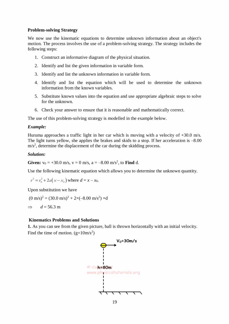
1. As you can see from the given picture, ball is thrown horizontally with an initial velocity.

Find the time of motion. (g=10m/s2)

20

Ball does projectile motion in other words it does free fall in vertical and linear motion in

horizontal. Time of motion for horizontal and vertical is same. Thus in vertical;

H = 1/2g.t2

80 = 1/2.10.t2

T = 4s

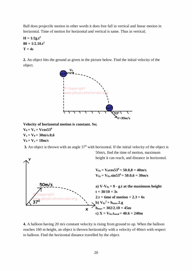
2. An object hits the ground as given in the picture below. Find the initial velocity of the

object.

Velocity of horizontal motion is constant. So;

V0 = Vx = Vcos530

Vx = V0 = 30m/s.0,6

V0 = Vx = 18m/s

3. An object is thrown with an angle 370 with horizontal. If the initial velocity of the object is

50m/s, find the time of motion, maximum

height it can reach, and distance in horizontal.

V0x = V0cos530 = 50.0,8 = 40m/s

V0y = V0y.sin530 = 50.0,6 = 30m/s

a) V-V0y = 0 - g.t at the maximum height

t = 30/10 = 3s

2.t = time of motion = 2.3 = 6s

b) V0y2 = hmax.2.g

hmax = 302/2.10 = 45m

c) X = V0x.ttotal = 40.6 = 240m

4. A balloon having 20 m/s constant velocity is rising from ground to up. When the balloon

reaches 160 m height, an object is thrown horizontally with a velocity of 40m/s with respect

to balloon. Find the horizontal distance travelled by the object.

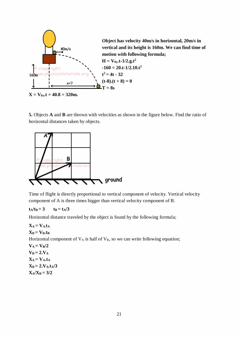
21

Object has velocity 40m/s in horizontal, 20m/s in

vertical and its height is 160m. We can find time of

motion with following formula;

H = V0y.t-1/2.g.t2

-160 = 20.t-1/2.10.t2

t2 = 4t - 32

(t-8).(t + 8) = 0

T = 8s

X = V0x.t = 40.8 = 320m.

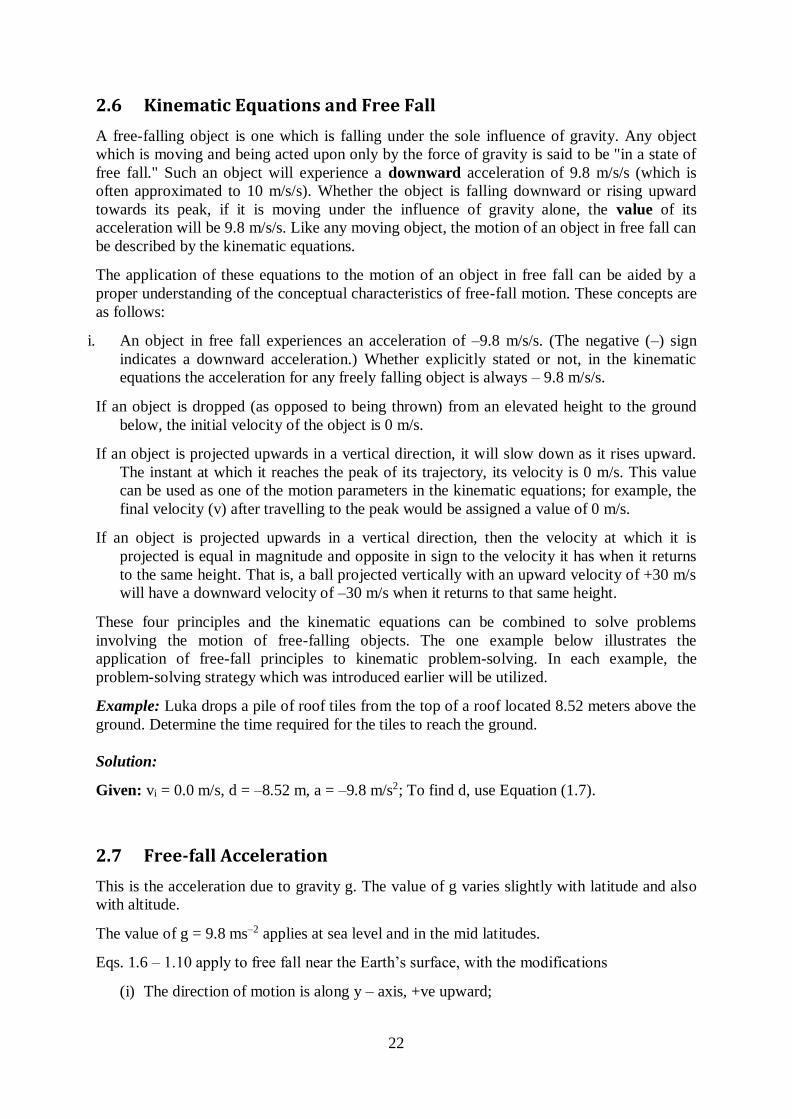
5. Objects A and B are thrown with velocities as shown in the figure below. Find the ratio of

horizontal distances taken by objects.

Time of flight is directly proportional to vertical component of velocity. Vertical velocity

component of A is three times bigger than vertical velocity component of B.

tA/tB = 3 tB = tA/3

Horizontal distance traveled by the object is found by the following formula;

XA = VA.tA

XB = VB.tB

Horizontal component of VA is half of VB, so we can write following equation;

VA = VB/2

VB = 2.VA

XA = VA.tA

XB = 2.VA.tA/3

XA/XB = 3/2

22

2.6 Kinematic Equations and Free Fall

A free-falling object is one which is falling under the sole influence of gravity. Any object

which is moving and being acted upon only by the force of gravity is said to be "in a state of

free fall." Such an object will experience a downward acceleration of 9.8 m/s/s (which is

often approximated to 10 m/s/s). Whether the object is falling downward or rising upward

towards its peak, if it is moving under the influence of gravity alone, the value of its

acceleration will be 9.8 m/s/s. Like any moving object, the motion of an object in free fall can

be described by the kinematic equations.

The application of these equations to the motion of an object in free fall can be aided by a

proper understanding of the conceptual characteristics of free-fall motion. These concepts are

as follows:

i. An object in free fall experiences an acceleration of –9.8 m/s/s. (The negative (–) sign

indicates a downward acceleration.) Whether explicitly stated or not, in the kinematic

equations the acceleration for any freely falling object is always – 9.8 m/s/s.

If an object is dropped (as opposed to being thrown) from an elevated height to the ground

below, the initial velocity of the object is 0 m/s.

If an object is projected upwards in a vertical direction, it will slow down as it rises upward.

The instant at which it reaches the peak of its trajectory, its velocity is 0 m/s. This value

can be used as one of the motion parameters in the kinematic equations; for example, the

final velocity (v) after travelling to the peak would be assigned a value of 0 m/s.

If an object is projected upwards in a vertical direction, then the velocity at which it is

projected is equal in magnitude and opposite in sign to the velocity it has when it returns

to the same height. That is, a ball projected vertically with an upward velocity of +30 m/s

will have a downward velocity of –30 m/s when it returns to that same height.

These four principles and the kinematic equations can be combined to solve problems

involving the motion of free-falling objects. The one example below illustrates the

application of free-fall principles to kinematic problem-solving. In each example, the

problem-solving strategy which was introduced earlier will be utilized.

Example: Luka drops a pile of roof tiles from the top of a roof located 8.52 meters above the

ground. Determine the time required for the tiles to reach the ground.

Solution:

Given: vi = 0.0 m/s, d = –8.52 m, a = –9.8 m/s2; To find d, use Equation (1.7).

2.7 Free-fall Acceleration

This is the acceleration due to gravity g. The value of g varies slightly with latitude and also

with altitude.

The value of g = 9.8 ms–2 applies at sea level and in the mid latitudes.

Eqs. 1.6 – 1.10 apply to free fall near the Earth’s surface, with the modifications

(i) The direction of motion is along y – axis, +ve upward;

23

(ii) The acceleration a is replaced by –g.

So that the free-fall equations of motion become:

v = v0 – gt … (1.11)

y – y = v t – gt 20 0

1

2 … (1.12)

v v g y y2 2

0 02 …. (1.13)

y y v v t0 0

1

2 .… (1.14)

y y vt gt 20

1

2 .… (1.15)

When solving problems under constant acceleration, choose the appropriate equation among

the five equations or alternatively use the pair of basic equations and solve them

simultaneously.

Exercise 1. A car travelling at a constant speed of 30 m/s passes a police car at rest. The

policeman starts to move at the moment the speeder passes his car and accelerates at a

constant rate of 3.0 m/ s 2 until he pulls even with the speeding car. Find:

(a) The time required for the policeman to catch the speeder.

(b) The distance travelled during the chase.

2. A stone is thrown vertically upward from the edge of a building 19.6 m high with

initial velocity 14.7 m/s. The stone just misses the building on the way down. Find:

(a) The time of flight and

(b) The velocity of the stone just before it hits the ground.

3. A rocket moves upward, starting from rest with an acceleration of 29.4 m/s 2 for 4 s.

At this time, it runs out of fuel and continues to move upward. How high does it go?

Summary

Kinematics is the science of describing the motion of objects using words, diagrams,

numbers, graphs, and equations. In this lecture, we have described position and motion of

objects and various kinematic quantities. We have solved equations of motion under constant

acceleration and free-fall acceleration.

24

References

Halliday, D., Resnick, R. and Krane, K.S. (1992). Physics Volume II, Fourth Edition,

John Wiley and Sons.

Gottys, W., Keller, F.J. and Skove, M.J. (1989). Physics Classical and Modern,

McGraw Hill.

Jha, A.K. (2009). A Textbook of Applied Physics, I.K. International Pub.

Redish, E.F. (2003). Teaching Introductory Physics with the Physics Suite, John

Wiley & Sons.




25

Lecture 3: Vectors

3.1 Introduction

We have already introduced vectors in the discussion of one dimensional motion. A vector

quantity is a quantity which is fully described by both magnitude and direction; it is

represented by a vector symbol: A and a scalar quantity is a quantity which is fully

described by its magnitude.

Lecture Objectives


i. Add vectors by different methods.

ii. Describe properties of vector addition

iii. Multiply vectors by different methods

3.2 Addition of Vectors

As is in ordinary arithmetic, only vectors of the same kind can be added.

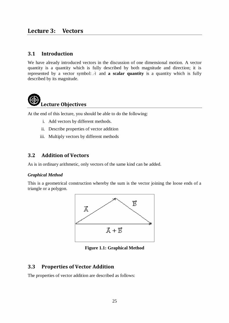
Graphical Method

This is a geometrical construction whereby the sum is the vector joining the loose ends of a

triangle or a polygon.

Figure 1.1: Graphical Method

3.3 Properties of Vector Addition

The properties of vector addition are described as follows:

26

1. Commutative law:

A B B A

In other words, the order of addition of vectors does not matter.

2. Associative Law:

A B C A B C

If there are more than two vectors, it does not matter how they are grouped as they are

added.

4. Subtraction:

A A 0

0 is the null vector. A null vector is a vector with zero magnitude and no direction.

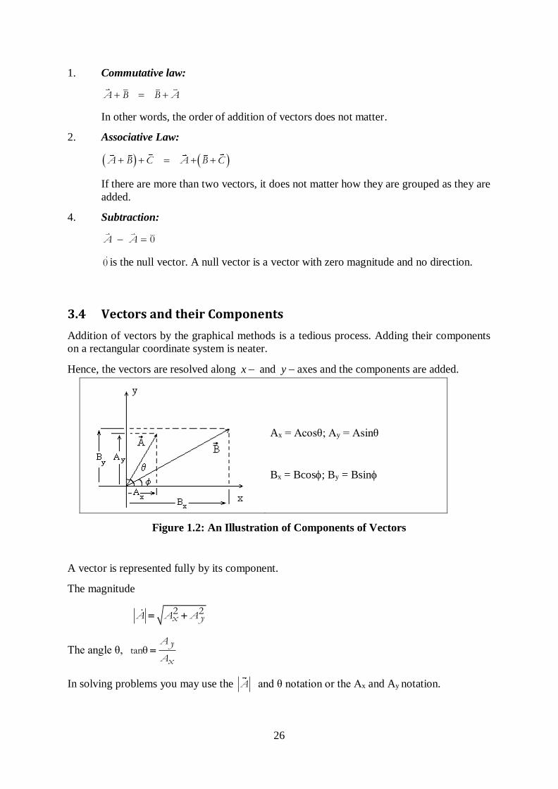
3.4 Vectors and their Components

Addition of vectors by the graphical methods is a tedious process. Adding their components

on a rectangular coordinate system is neater.

Hence, the vectors are resolved along x and y axes and the components are added.

Ax = Acosθ; Ay = Asinθ

Bx = Bcos; By = Bsin

Figure 1.2: An Illustration of Components of Vectors

A vector is represented fully by its component.

The magnitude

2 2A A Ax y

The angle θ, tanA y

Ax

In solving problems you may use the A and θ notation or the Ax and Ay notation.

27

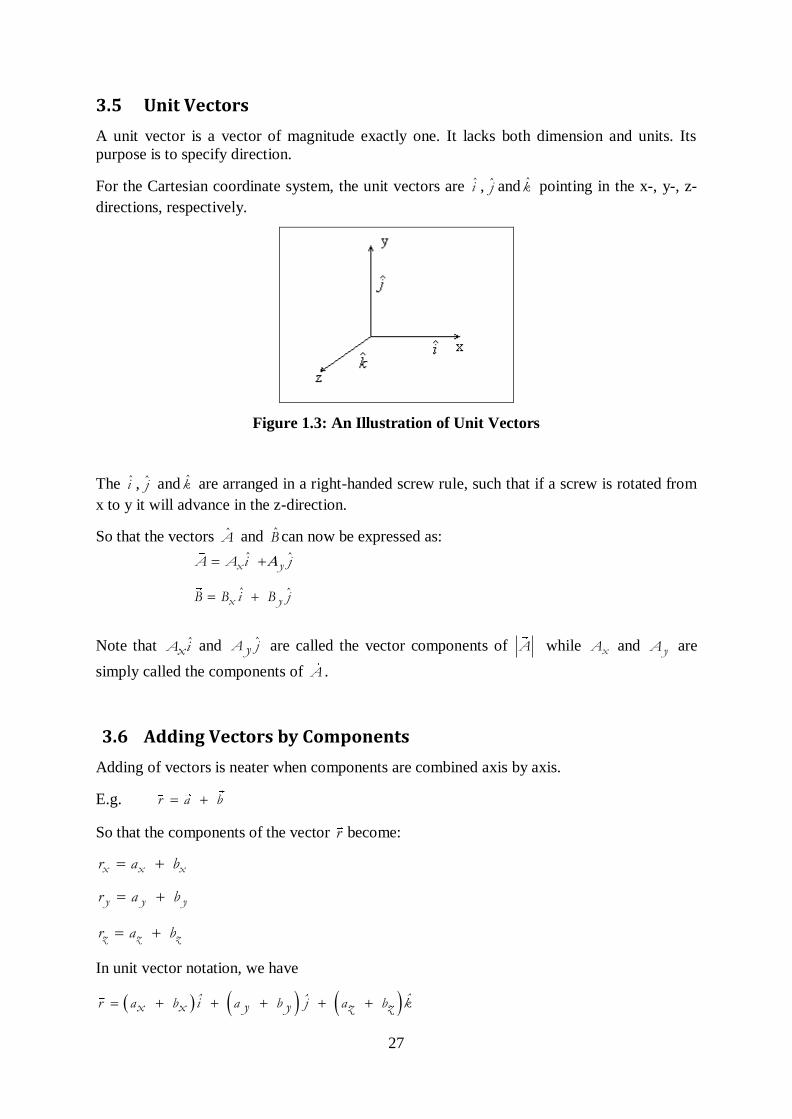
3.5 Unit Vectors

A unit vector is a vector of magnitude exactly one. It lacks both dimension and units. Its

purpose is to specify direction.

For the Cartesian coordinate system, the unit vectors are i , j and k pointing in the x-, y-, z-

directions, respectively.

Figure 1.3: An Illustration of Unit Vectors

The i , j and k are arranged in a right-handed screw rule, such that if a screw is rotated from

x to y it will advance in the z-direction.

So that the vectors A and B can now be expressed as:

ˆ ˆx yA A i j

ˆ ˆx yB B i B j

Note that Â ix and Â jy are called the vector components of A while xA and yA are

simply called the components of A .

3.6 Adding Vectors by Components

Adding of vectors is neater when components are combined axis by axis.

E.g. r a b

So that the components of the vector r become:

x x xr a b

y y yr a b

z z zr a b

In unit vector notation, we have

ˆˆ ˆr a b i a b j a b kx x y y z z

28

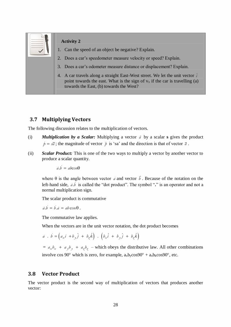
Activity 2

1. Can the speed of an object be negative? Explain.

2. Does a car’s speedometer measure velocity or speed? Explain.

3. Does a car’s odometer measure distance or displacement? Explain.

4. A car travels along a straight East-West street. We let the unit vector i

point towards the east. What is the sign of vx if the car is travelling (a)

towards the East, (b) towards the West?

3.7 Multiplying Vectors

The following discussion relates to the multiplication of vectors.

(i) Multiplication by a Scalar: Multiplying a vector a by a scalar s gives the product

p sa ; the magnitude of vector p is ‘sa’ and the direction is that of vector a .

(ii) Scalar Product: This is one of the two ways to multiply a vector by another vector to

produce a scalar quantity.

. cosa b ab

where θ is the angle between vector a and vector b . Because of the notation on the

left-hand side, .a b is called the “dot product”. The symbol “.” is an operator and not a

normal multiplication sign.

The scalar product is commutative

. . cosa b b a ab .

The commutative law applies.

When the vectors are in the unit vector notation, the dot product becomes

ˆ ˆˆˆ ˆ. .x y z x y za b a i b j b k b i b j b k

= x x y y z za b a b a b – which obeys the distributive law. All other combinations

involve cos 90 which is zero, for example, axbycos90 + axbkcos90, etc.

3.8 Vector Product

The vector product is the second way of multiplication of vectors that produces another

vector:

29

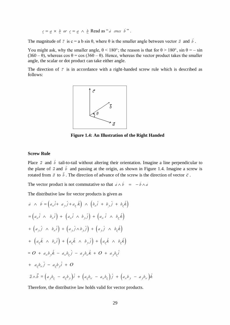
c a b or c a b Read as “ a cross b ” .

The magnitude of c is c = a b sin θ, where θ is the smaller angle between vector a and b .

You might ask, why the smaller angle, θ < 180; the reason is that for θ > 180, sin θ = – sin

(360 – θ), whereas cos θ = cos (360 – θ). Hence, whereas the vector product takes the smaller

angle, the scalar or dot product can take either angle.

The direction of c is in accordance with a right-handed screw rule which is described as

follows:

Figure 1.4: An Illustration of the Right Handed

Screw Rule

Place a and b tail-to-tail without altering their orientation. Imagine a line perpendicular to

the plane of a and b and passing at the origin, as shown in Figure 1.4. Imagine a screw is

rotated from a to b . The direction of advance of the screw is the direction of vector c

.

The vector product is not commutative so that a b b a

The distributive law for vector products is given as

ˆ ˆˆ ˆˆ ˆx y z x y za b a i a j a k b i b j b k

ˆˆ ˆ ˆ ˆˆx x x y x za i b i a i b j a i b k

ˆˆˆ ˆ ˆ ˆy x y y y za j b i a j b j a j b k

ˆ ˆ ˆ ˆˆ ˆz x z y z za k b i a k b j a k b k

= ˆ ˆ ˆˆx y x z y x y za b k a b j a b k a b i

ˆˆz x z ya b j a b i

a b = ˆˆ ˆy z z y z x x z x y y xa b a b i a b a b j a b a b k

Therefore, the distributive law holds valid for vector products.

30

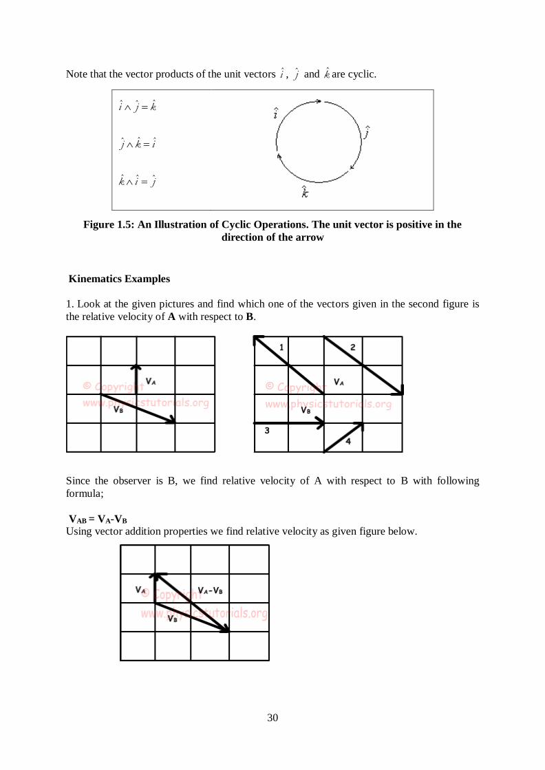
Note that the vector products of the unit vectors i , j and k are cyclic.

ˆˆ î j k

ˆ ˆj k i

ˆ ˆ ˆk i j

Figure 1.5: An Illustration of Cyclic Operations. The unit vector is positive in the

direction of the arrow

Kinematics Examples

1. Look at the given pictures and find which one of the vectors given in the second figure is

the relative velocity of A with respect to B.

Since the observer is B, we find relative velocity of A with respect to B with following

formula;

VAB = VA-VB Using vector addition properties we find relative velocity as given figure below.

31

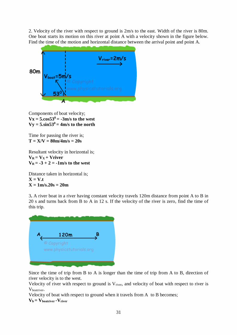
2. Velocity of the river with respect to ground is 2m/s to the east. Width of the river is 80m.

One boat starts its motion on this river at point A with a velocity shown in the figure below.

Find the time of the motion and horizontal distance between the arrival point and point A.

Components of boat velocity;

Vx = 5.cos530 = -3m/s to the west

Vy = 5.sin530 = 4m/s to the north

Time for passing the river is;

T = X/V = 80m/4m/s = 20s

Resultant velocity in horizontal is;

VR = VX + Vriver

VR = -3 + 2 = -1m/s to the west

Distance taken in horizontal is;

X = V.t

X = 1m/s.20s = 20m

3. A river boat in a river having constant velocity travels 120m distance from point A to B in

20 s and turns back from B to A in 12 s. If the velocity of the river is zero, find the time of

this trip.

Since the time of trip from B to A is longer than the time of trip from A to B, direction of

river velocity is to the west.

Velocity of river with respect to ground is Vriver, and velocity of boat with respect to river is

Vboatriver.

Velocity of boat with respect to ground when it travels from A to B becomes;

Vb = Vboatriver -Vriver

32

and when it travels from B to A;

Vb = Vboatriver + Vriver

We can find velocities using following formula;

1. Vboatriver-Vriver = 120/20 = 6m/s

and

2. Vboatriver + Vriver = 120/12 = 10m/s

Solving equations 1. and 2. we find the velocities of river and boat.

Vboatriver=8m/s and Vriver = 2m/s

If the velocity of river is zero, boat travels 240m distance in;

240 = 8m/s.t

t = 30s

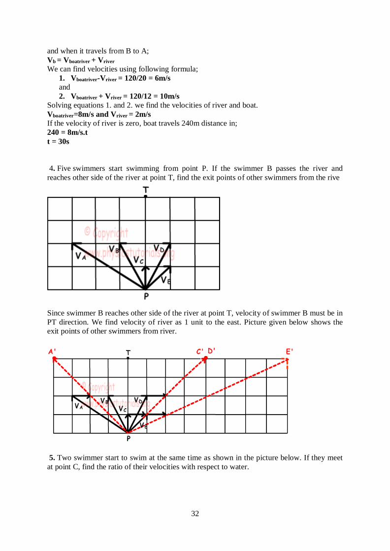
4. Five swimmers start swimming from point P. If the swimmer B passes the river and

reaches other side of the river at point T, find the exit points of other swimmers from the rive

Since swimmer B reaches other side of the river at point T, velocity of swimmer B must be in

PT direction. We find velocity of river as 1 unit to the east. Picture given below shows the

exit points of other swimmers from river.

5. Two swimmer start to swim at the same time as shown in the picture below. If they meet

at point C, find the ratio of their velocities with respect to water.

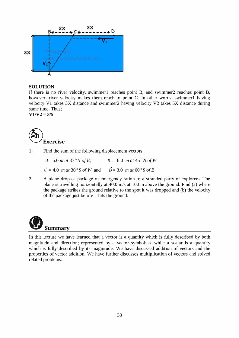
33

SOLUTION

If there is no river velocity, swimmer1 reaches point B, and swimmer2 reaches point B,

however, river velocity makes them reach to point C. In other words, swimmer1 having

velocity V1 takes 3X distance and swimmer2 having velocity V2 takes 5X distance during

same time. Thus;

V1/V2 = 3/5

Exercise 1. Find the sum of the following displacement vectors:

A= 5.0 m at 37 o N of E, B = 6.0 m at 45 o N of W

C = 4.0 m at 30 o S of W, and D = 3.0 m at 60 o S of E

2. A plane drops a package of emergency ration to a stranded party of explorers. The

plane is travelling horizontally at 40.0 m/s at 100 m above the ground. Find (a) where

the package strikes the ground relative to the spot it was dropped and (b) the velocity

of the package just before it hits the ground.

Summary

In this lecture we have learned that a vector is a quantity which is fully described by both

magnitude and direction; represented by a vector symbol: A while a scalar is a quantity

which is fully described by its magnitude. We have discussed addition of vectors and the

properties of vector addition. We have further discusses multiplication of vectors and solved

related problems.

34

References




McGraw Hill.


Redish, E.F. (2003). Teaching Introductory Physics with the Physics Suite, John

Wiley & Sons.




35

Lecture 4: Newton’s Laws of Motion

4.1 Introduction

A force is a ‘pull’ or ‘push’ upon an object resulting from the object’s interaction with

another object. Forces only exist as a result of an interaction.

All forces (interactions) between objects can be placed into two broad categories:

(i) Contact forces

(ii) Forces resulting from action at a distance.

Contact forces include frictional, tensional, normal, air resistance, applied and spring forces.

Forces resulting from action at a distance include gravitational and electromagnetic forces.

Lecture Objectives


i. State the Newton’s Laws of Motion.

ii. Describe everyday experiences related to Newton’s Laws of Motion.

iii. Perform calculations related to Newton’s Laws of Motion.

4.2 Newton’s First Law

Consider a body on which no net force acts. If the body is at rest it will remain at rest. If the

body is moving with constant velocity, it will continue to do so.

Statement

An object at rest tends to stay at rest and an object in motion tends to stay in motion with the

same speed and in the same direction unless acted upon by an unbalanced external force.

Newton’s 1st law is also called the Law of Inertia. Inertia is the tendency of an object to resist

change in its state of motion.

Everyday Experience of Newton’s First Law

The idea expressed by Newton's law of inertia should not be surprising to us. We experience

this phenomenon of inertia nearly everyday when travelling in a motor vehicle.

For example, imagine that you are a passenger in a car stopped at a traffic light. The light

turns green and the driver steps on the accelerator. The car begins to accelerate forward, yet

relative to the seat which you are on, your body begins to lean backwards. Your body being at

http://www.glenbrook.k12.il.us/gbssci/phys/Class/newtlaws/u2l1d.html#balanced

36

rest tends to stay at rest. This is one aspect of the law of inertia – “objects at rest tend to stay

at rest." As the wheels of the car spin to generate a forward force upon the car to cause a

forward acceleration, your body tends to stay in place. It certainly might seem to you as

though your body were experiencing a backwards force causing it to accelerate backwards;

yet you would have a difficult time identifying such a backwards force on your body. There

isn't one. The feeling of being thrown backwards is merely the tendency of your body to resist

the acceleration and to remain in its state of rest. The car is accelerating out from under your

body, leaving you with the false feeling of being thrown backwards.

Now imagine that you're driving along at constant speed and then suddenly approach a stop

sign. The driver steps on the brakes. The wheels of the car lock and begin to skid across the

pavement. This causes a backwards force upon the forward moving car and subsequently a

backwards acceleration on the car. However, your body being in motion tends to continue in

motion while the car is slowing to a stop. It certainly might seem to you as though your body

were experiencing a forward force causing it to accelerate forwards; yet you would once more

have a difficult time identifying such a forward force on your body.

The feeling of being thrown forward is merely the tendency of your body to resist the

deceleration and to remain in its state of forward motion. The unbalanced force acting upon

the car causes it to slow down while your body continues in its forward motion.

4.3 Newton’s Second Law

Newton's first law of motion predicts the behaviour of objects for which all existing forces

are balanced. An object will only accelerate if there is a net or an unbalanced force acting

upon it. The presence of an unbalanced force will accelerate an object – changing either its

speed, direction, or both. Newton's second law of motion can be formally stated as follows:

The acceleration of an object as produced by a net force is directly proportional to the

magnitude of the net force, in the same direction as the net force, and inversely proportional

to the mass of the object.

The vector sum or the net force of all forces that act on a body is given by

F ma …(1.16)

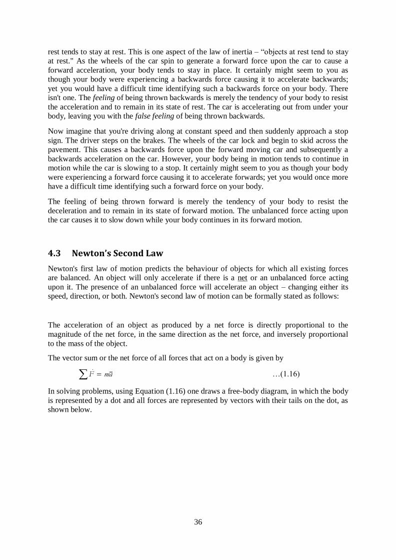
In solving problems, using Equation (1.16) one draws a free-body diagram, in which the body

is represented by a dot and all forces are represented by vectors with their tails on the dot, as

shown below.

http://www.glenbrook.k12.il.us/gbssci/phys/Class/newtlaws/u2l1a.html

http://www.glenbrook.k12.il.us/gbssci/phys/Class/newtlaws/u2l2d.html

http://www.glenbrook.k12.il.us/gbssci/phys/Class/newtlaws/u2l1d.html#balanced

37

Figure 1.6: An Illustration of Free Body Diagrams for (a) A Book at Rest on a Table; (b)

An Object Falling Freely, Air Resistance Neglected; (c) A Book on a Table being Pushed

or Pulled to the Right; and (d) A Car Decelerating to a Halt.

Equation (1.16) is equivalent to three scalar equations:

x xF ma ; y yF ma ; z zF ma …( 1.17)

4.4 Some Particular Forces

Some of the forces which we experience in our day-to-day lives and are familiar with are as

discussed below:

Weight

W mg , W is directed downward.

Many students of physics confuse weight with mass. The mass of an object refers to the

amount of matter that is contained by the object; whereas the weight of an object is the force

of gravity acting upon that object. The mass of an object will be the same no matter where in

the universe that objects are located. Weight is dependent upon the value of g. On the Earth’s

surface g is 9.8 m/s2. On the Moon's surface, g is 1.7 m/s2. Go to another planet, and there

will be another value of g. Hence, the weight of an object (measured in Newtons) will vary

according to where in the universe the object is.

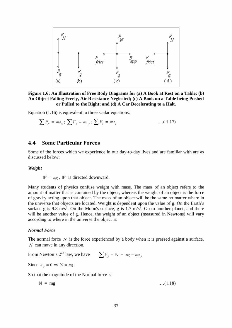
Normal Force

The normal force is the force experienced by a body when it is pressed against a surface.

can move in any direction.

From Newton’s 2nd law, we have y yF N mg ma

Since 0ya N mg .

So that the magnitude of the Normal force is

N = mg …(1.18)

38

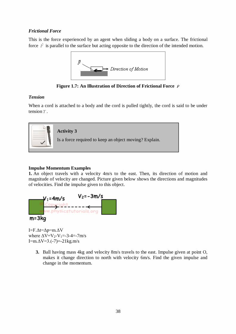
Frictional Force

This is the force experienced by an agent when sliding a body on a surface. The frictional

force F is parallel to the surface but acting opposite to the direction of the intended motion.

Figure 1.7: An Illustration of Direction of Frictional Force F

Tension

When a cord is attached to a body and the cord is pulled tightly, the cord is said to be under

tensionT .

Activity 3

Is a force required to keep an object moving? Explain.

Impulse Momentum Examples

1. An object travels with a velocity 4m/s to the east. Then, its direction of motion and

magnitude of velocity are changed. Picture given below shows the directions and magnitudes

of velocities. Find the impulse given to this object.

I=F.Δt=Δp=m.ΔV

where ΔV=V2-V1=-3-4=-7m/s

I=m.ΔV=3.(-7)=-21kg.m/s

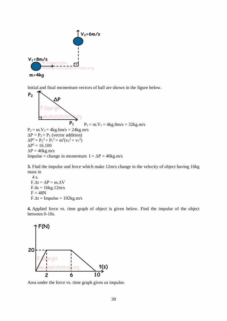
3. Ball having mass 4kg and velocity 8m/s travels to the east. Impulse given at point O,

makes it change direction to north with velocity 6m/s. Find the given impulse and

change in the momentum.

39

Initial and final momentum vectors of ball are shown in the figure below.

P1 = m.V1 = 4kg.8m/s = 32kg.m/s

P2 = m.V2 = 4kg.6m/s = 24kg.m/s

ΔP = P2 + P1 (vector addition)

ΔP2 = P22 + P1

2 = m2(v22 + v1

2)

ΔP2 = 16.100

ΔP = 40kg.m/s

Impulse = change in momentum I = ΔP = 40kg.m/s

3. Find the impulse and force which make 12m/s change in the velocity of object having 16kg

mass in

4 s.

F.Δt = ΔP = m.ΔV

F.4s = 16kg.12m/s

F = 48N

F.Δt = Impulse = 192kg.m/s

4. Applied force vs. time graph of object is given below. Find the impulse of the object

between 0-10s.

Area under the force vs. time graph gives us impulse.

40

F.Δt = 20.2/2+20.(6-2)+20.(10-6)/2

F.Δt = 140kg.m/s

5. A ball having mass 500g hits wall with a10m/s velocity. Wall applies 4000 N force to the

ball and it turns back with 8m/s velocity. Find the time of ball-wall contact.

F.Δt = ΔP = m.ΔV = m.(V2-V1)

-4000.Δt = 0,5kg.(8-10)

Δt = 0,00025s

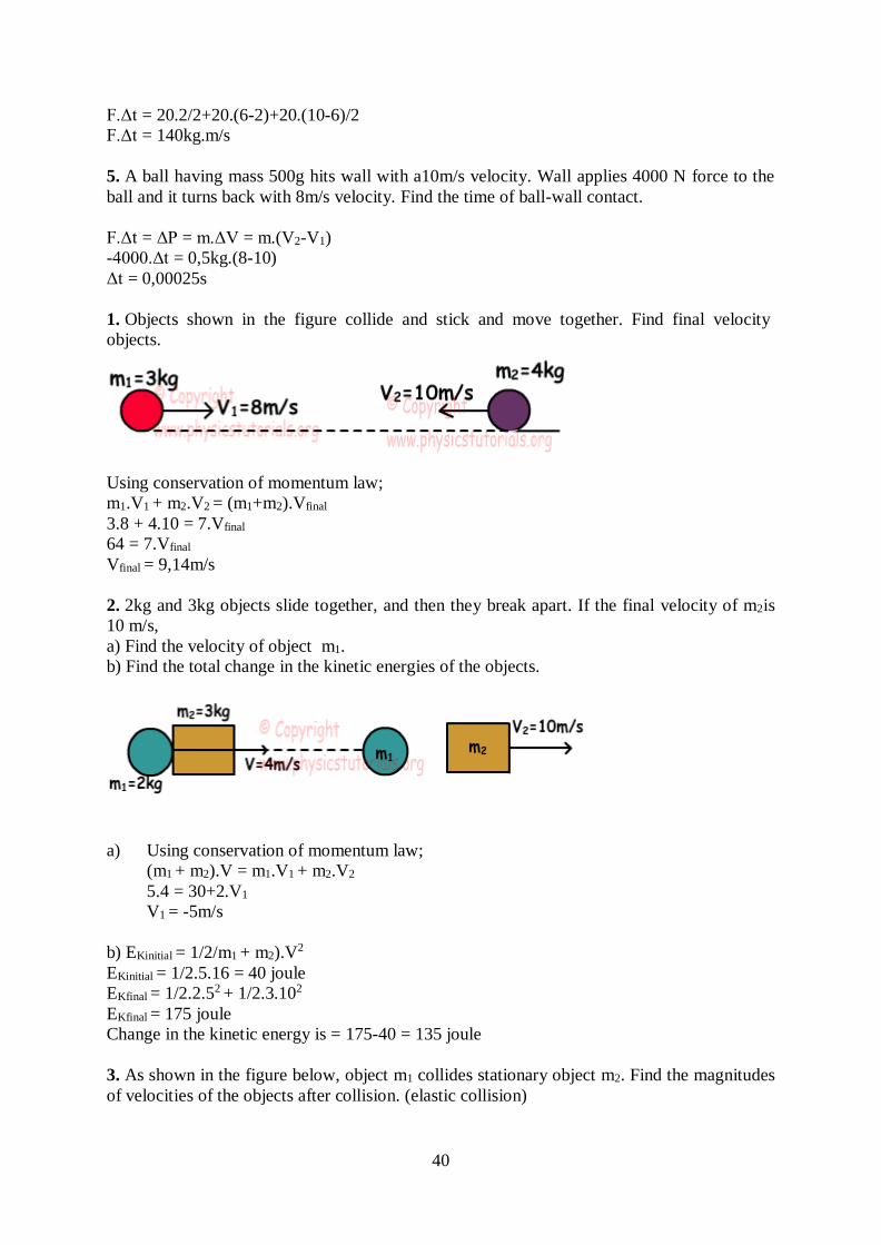
1. Objects shown in the figure collide and stick and move together. Find final velocity

objects.

Using conservation of momentum law;

m1.V1 + m2.V2 = (m1+m2).Vfinal

3.8 + 4.10 = 7.Vfinal

64 = 7.Vfinal

Vfinal = 9,14m/s

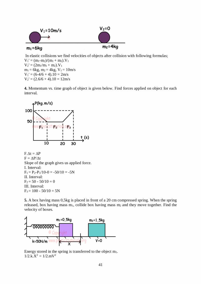
2. 2kg and 3kg objects slide together, and then they break apart. If the final velocity of m2is

10 m/s,

a) Find the velocity of object m1.

b) Find the total change in the kinetic energies of the objects.

a) Using conservation of momentum law;

(m1 + m2).V = m1.V1 + m2.V2

5.4 = 30+2.V1

V1 = -5m/s

b) EKinitial = 1/2/m1 + m2).V2

EKinitial = 1/2.5.16 = 40 joule

EKfinal = 1/2.2.52 + 1/2.3.102

EKfinal = 175 joule

Change in the kinetic energy is = 175-40 = 135 joule

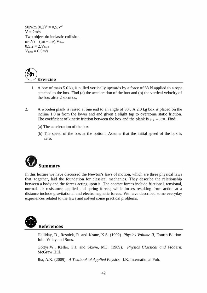
3. As shown in the figure below, object m1 collides stationary object m2. Find the magnitudes

of velocities of the objects after collision. (elastic collision)

41

In elastic collisions we find velocities of objects after collision with following formulas;

V1' = (m1-m2)/(m1 + m2).V1

V2' = (2m1/m1 + m2).V1

m1 = 6kg, m2 = 4kg, V1 = 10m/s

V1' = (6-4/6 + 4).10 = 2m/s

V2' = (2.6/6 + 4).10 = 12m/s

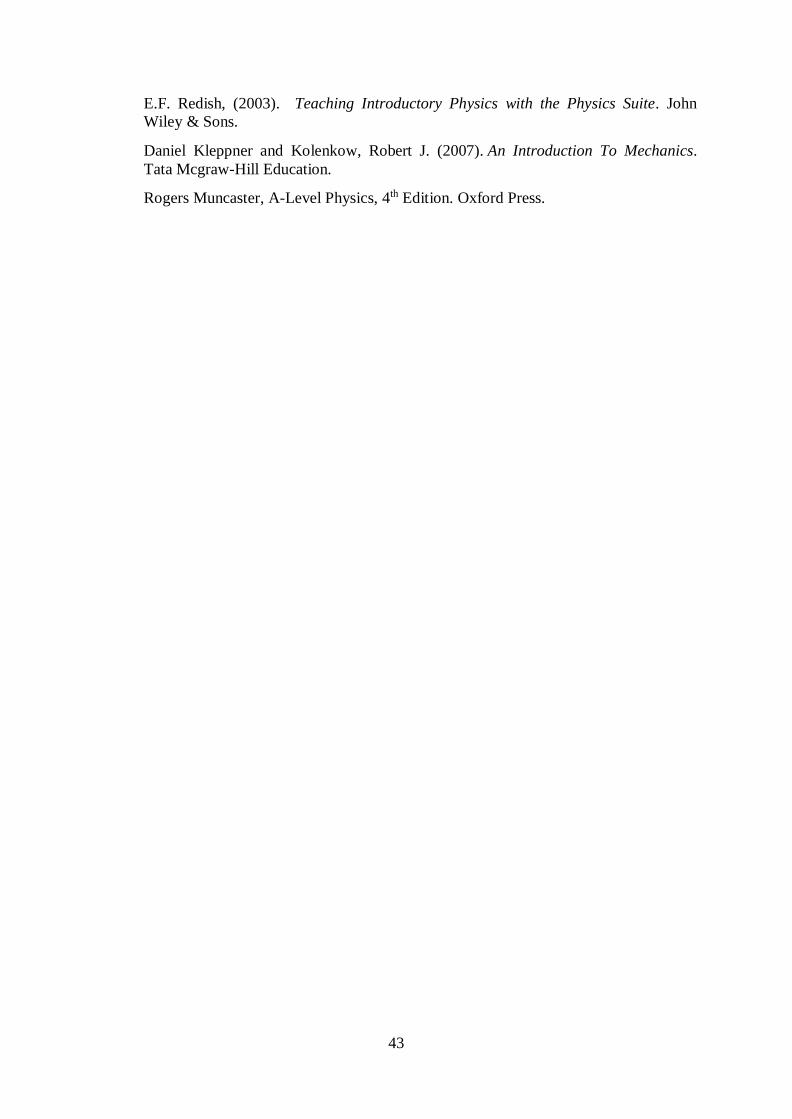
4. Momentum vs. time graph of object is given below. Find forces applied on object for each

interval.

F.Δt = ΔP

F = ΔP/Δt

Slope of the graph gives us applied force.

I. Interval:

F1 = P2-P1/10-0 = -50/10 = -5N

II. Interval:

F2 = 50 - 50/10 = 0

III. Interval:

F3 = 100 - 50/10 = 5N

5. A box having mass 0,5kg is placed in front of a 20 cm compressed spring. When the spring

released, box having mass m1, collide box having mass m2 and they move together. Find the

velocity of boxes.

Energy stored in the spring is transferred to the object m1.

1/2.k.X2 = 1/2.mV2

42

50N/m.(0,2)2 = 0,5.V2

V = 2m/s

Two object do inelastic collision.

m1.V1 = (m1 + m2).Vfinal

0,5.2 = 2.Vfinal

Vfinal = 0,5m/s

Exercise 1. A box of mass 5.0 kg is pulled vertically upwards by a force of 68 N applied to a rope

attached to the box. Find (a) the acceleration of the box and (b) the vertical velocity of

the box after 2 seconds.

2. A wooden plank is raised at one end to an angle of 30o. A 2.0 kg box is placed on the

incline 1.0 m from the lower end and given a slight tap to overcome static friction.

The coefficient of kinetic friction between the box and the plank is 0.20k . Find:

(a) The acceleration of the box

(b) The speed of the box at the bottom. Assume that the initial speed of the box is

zero.

Summary

In this lecture we have discussed the Newton's laws of motion, which are three physical laws

that, together, laid the foundation for classical mechanics. They describe the relationship

between a body and the forces acting upon it. The contact forces include frictional, tensional,

normal, air resistance, applied and spring forces; while forces resulting from action at a

distance include gravitational and electromagnetic forces. We have described some everyday

experiences related to the laws and solved some practical problems.

References

Halliday, D., Resnick, R. and Krane, K.S. (1992). Physics Volume II, Fourth Edition.


Gottys,W., Keller, F.J. and Skove, M.J. (1989). Physics Classical and Modern.

McGraw Hill.

Jha, A.K. (2009). A Textbook of Applied Physics. I.K. International Pub.

43

E.F. Redish, (2003). Teaching Introductory Physics with the Physics Suite. John

Wiley & Sons.

Daniel Kleppner and Kolenkow, Robert J. (2007). An Introduction To Mechanics.

Tata Mcgraw-Hill Education.

Rogers Muncaster, A-Level Physics, 4th Edition. Oxford Press.

44

Lecture 5: Action and Reaction Forces

5.1 Introduction

Forces come in pairs. If you lean against a brick wall, the wall pushes back on you.

Lecture Objectives


i. Apply the Newton’s Third Law of Motion.

ii. Define friction.

iii. State the friction law.

iv. Describe the properties of friction.

5.2 Newton’s Third Law

Statement: To every action there is an equal but opposite reaction.

If a body A exerts a force BAF

on body B, it experiences a force ABF

exerted by body B on A.

BA ABF F …(1.19)

Note that the two forces do not cancel because one acts on A and the other on B.

The forces BAF

and ABF

are also called an action–reaction pair.

In applying Newton’s laws to solve problems one should be able to translate a sketch of a

situation into a free-body diagram, with appropriate axes.

5.3 Friction

There are two types of frictional forces, static frictional force sf and kinetic frictional force

kf .

sf operates against the applied force up to break away point beyond which motion starts and

kf takes over.

Definition: The friction law states that the sliding friction force is proportional to the

perpendicular reaction of the bearing surface and opposite to the body's movement direction.

The coefficient of friction, μ, depends solely upon the properties of the materials rubbing. The

45

rest friction force appears whenever there is a force acting upon the resting body, and it is of

equal magnitude and opposite direction. When the maximum rest friction force is exceeded,

sliding begins.

Explanation

This means that whenever you apply a small force to a body resting on a rough plane, the rest

friction force will be annihilating the former (according to the Third Newton's Law). For

example, if you are trying to push forward a box that is too heavy, the rest friction will be

holding it at the initial position motionless. But as long as you increase your force so that it

will exceed the maximum rest friction, the box will start moving away from the spot. The

maximum rest friction force is usually a bit bigger in magnitude than the sliding friction

force. This is why it is always a little harder to make a resting box move than to keep it

moving.

Applications:

A car's engine makes its wheels move and each part of the wheel that touches the ground

moves in the opposite direction. This causes the friction force from the road surface to appear

and act to the direction of the car's movement. Thus it appears that the acting force in the car

movement is the friction between the wheels and the ground.

Question

The sliding coefficient of friction between the car wheels and the road is μ =.5. What is the

largest acceleration that the car may achieve moving straight on a horizontal road? Presume

that the engine power [and mass are equally distributed to all four tires].

Solution: As it has already been explained, the acting force F that moves the car is the

friction between the wheels and the road. Let a be the acceleration, so according to the

Second Newton's Law, F = m*a where m is the mass of the car. It can be seen that the

acceleration will reach its maximum when the force F will do the same, and it will happen

when the wheels will start sliding. In this case the friction force will be F= μ*N, where N is

the perpendicular reaction force of the road; as the car does not move vertically, it equals the

car's weight, m*g (g is the free fall acceleration, it is almost 10 m/s/s).

So we get F = μ*m*g and F = m*a, that means μ*m*g = m*a and a = μ*g.

In our case the maximum acceleration possible will be (.5)*10 = 5 m/s/s.

[If power is delivered to one tire bearing one quarter the weight of the car, then maximum

acceleration will be:

F = μ*(0.25)*m*g and F = m*a, that means μ*(0.25)*m*g = m*a and a = μ*g/4

So the maximum acceleration would be (.5)*(10)/4 = 1.25 m/s/s)

This explains the advantage of a well balanced 4-wheel drive vehicle.]

We see that the acceleration depends on the coefficient of friction [and weight and power

distribution], no matter how strong the engine is. [The coefficient of friction of rubber on wet

ice may be as low as .05.] That is why a car can hardly [accelerate] on slippery ice.

46

5.4 Properties of Friction

When a body is pressed against a surface (dry and unlubricated) and a force F attempts to

move it along the surface, it results into a friction. The resulting frictional force has three

properties.

1. If the body does not move, then the static frictional force sf and the component of F

that is parallel to the surface are equal in magnitude and sf is directly opposite to that

component of F .

2. The magnitude sf has a maximum value

, max,s sf N … (1.20)

where µs is the coefficient of static friction and N the magnitude of the normal force.

When the component of F that is parallel to the surface exceeds , max,sf the body

begins to slide.

4. When the body begins to slide the magnitude of the frictional force rapidly decreases

to a value kf given by

k kf N … (1.21)

where µk is the coefficient of kinetic friction.

Note that Equations 1.20 and 1.21 are scalar; ,s kf are parallel to the surface whereas is

perpendicular to the surface.

The coefficients s and k are dimensionless.

Friction Force with Examples

Friction Force:

Friction force results from the interactions of surfaces. Irregularities in the structure of the

matters causes friction force. These irregularities can be detected in micro dimensions. You

may not see any irregularity on the surface of the material however, it does exist. Friction

force is always opposite to the direction of motion and tends to decrease net force. All

materials have their own friction constant in other words friction force depends on the type of

materials. Another factor affecting friction force is the normal force. When you apply a force

to an object, then friction force becomes active and resists with the force of having opposite

direction to your net force.

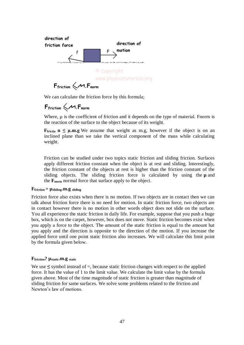
47

We can calculate the friction force by this formula;

Where, µ is the coefficient of friction and it depends on the type of material. Fnorm is

the reaction of the surface to the object because of its weight.

Ffrictio n ≤ µ.m.g We assume that weight as m.g, however if the object is on an

inclined plane than we take the vertical component of the mass while calculating

weight.

Friction can be studied under two topics static friction and sliding friction. Surfaces

apply different friction constant when the object is at rest and sliding. Interestingly,

the friction constant of the objects at rest is higher than the friction constant of the

sliding objects. The sliding friction force is calculated by using the µ and

the Fnorm normal force that surface apply to the object.

Ffriction = µsliding.m.g sliding

Friction force also exists when there is no motion. If two objects are in contact then we can

talk about friction force there is no need for motion. In static friction force, two objects are

in contact however there is no motion in other words object does not slide on the surface.

You all experience the static friction in daily life. For example, suppose that you push a huge

box, which is on the carpet, however, box does not move. Static friction becomes exist when

you apply a force to the object. The amount of the static friction is equal to the amount hat

you apply and the direction is opposite to the direction of the motion. If you increase the

applied force until one point static friction also increases. We will calculate this limit point

by the formula given below.

Ffriction? µstatic.m.g static

We use ≤ symbol instead of =, because static friction changes with respect to the applied

force. It has the value of 1 to the limit value. We calculate the limit value by the formula

given above. Most of the time magnitude of static friction is greater than magnitude of

sliding friction for same surfaces. We solve some problems related to the friction and

Newton’s law of motions.

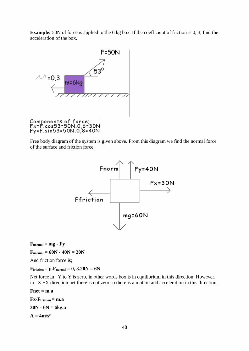
48

Example: 50N of force is applied to the 6 kg box. If the coefficient of friction is 0, 3, find the

acceleration of the box.

Free body diagram of the system is given above. From this diagram we find the normal force

of the surface and friction force.

Fnormal = mg - Fy

Fnormal = 60N - 40N = 20N

And friction force is;

Ffriction = µ.Fnormal = 0, 3.20N = 6N

Net force in –Y to Y is zero, in other words box is in equilibrium in this direction. However,

in –X +X direction net force is not zero so there is a motion and acceleration in this direction.

Fnet = m.a

Fx-Ffriction = m.a

30N - 6N = 6kg.a

A = 4m/s²

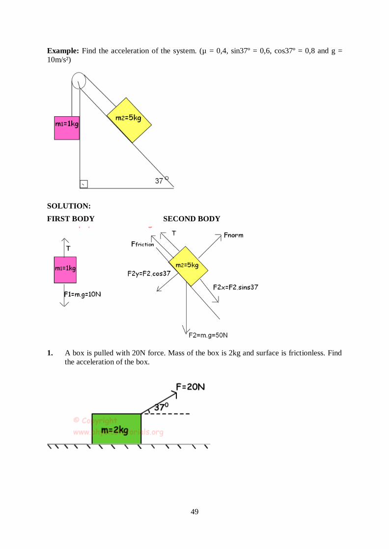
49

Example: Find the acceleration of the system. (µ = 0,4, sin37º = 0,6, cos37º = 0,8 and g =

10m/s²)

SOLUTION:

FIRST BODY SECOND BODY

1. A box is pulled with 20N force. Mass of the box is 2kg and surface is frictionless. Find

the acceleration of the box.

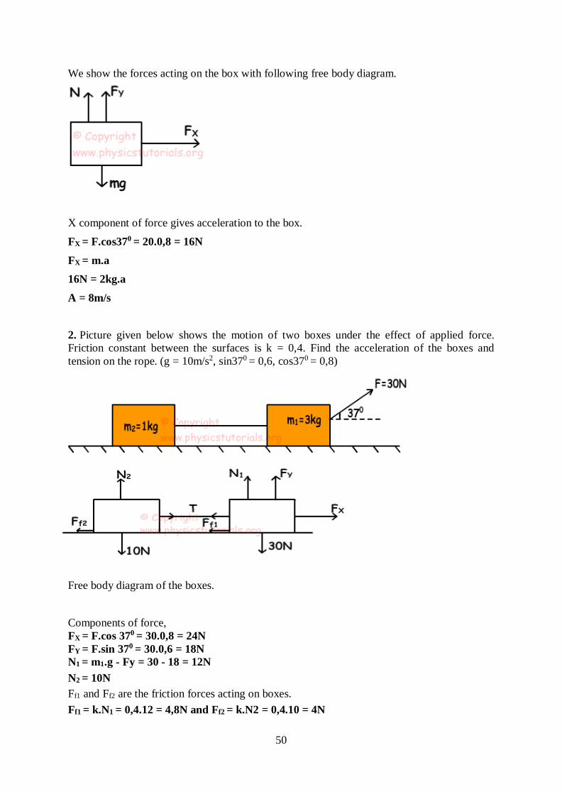
50

We show the forces acting on the box with following free body diagram.

X component of force gives acceleration to the box.

FX = F.cos370 = 20.0,8 = 16N

FX = m.a

16N = 2kg.a

A = 8m/s

2. Picture given below shows the motion of two boxes under the effect of applied force.

Friction constant between the surfaces is k = 0,4. Find the acceleration of the boxes and

tension on the rope. (g = 10m/s2, sin370 = 0,6, cos370 = 0,8)

Free body diagram of the boxes.

Components of force,

FX = F.cos 370 = 30.0,8 = 24N

FY = F.sin 370 = 30.0,6 = 18N

N1 = m1.g - Fy = 30 - 18 = 12N

N2 = 10N

Ff1 and Ff2 are the friction forces acting on boxes.

Ff1 = k.N1 = 0,4.12 = 4,8N and Ff2 = k.N2 = 0,4.10 = 4N

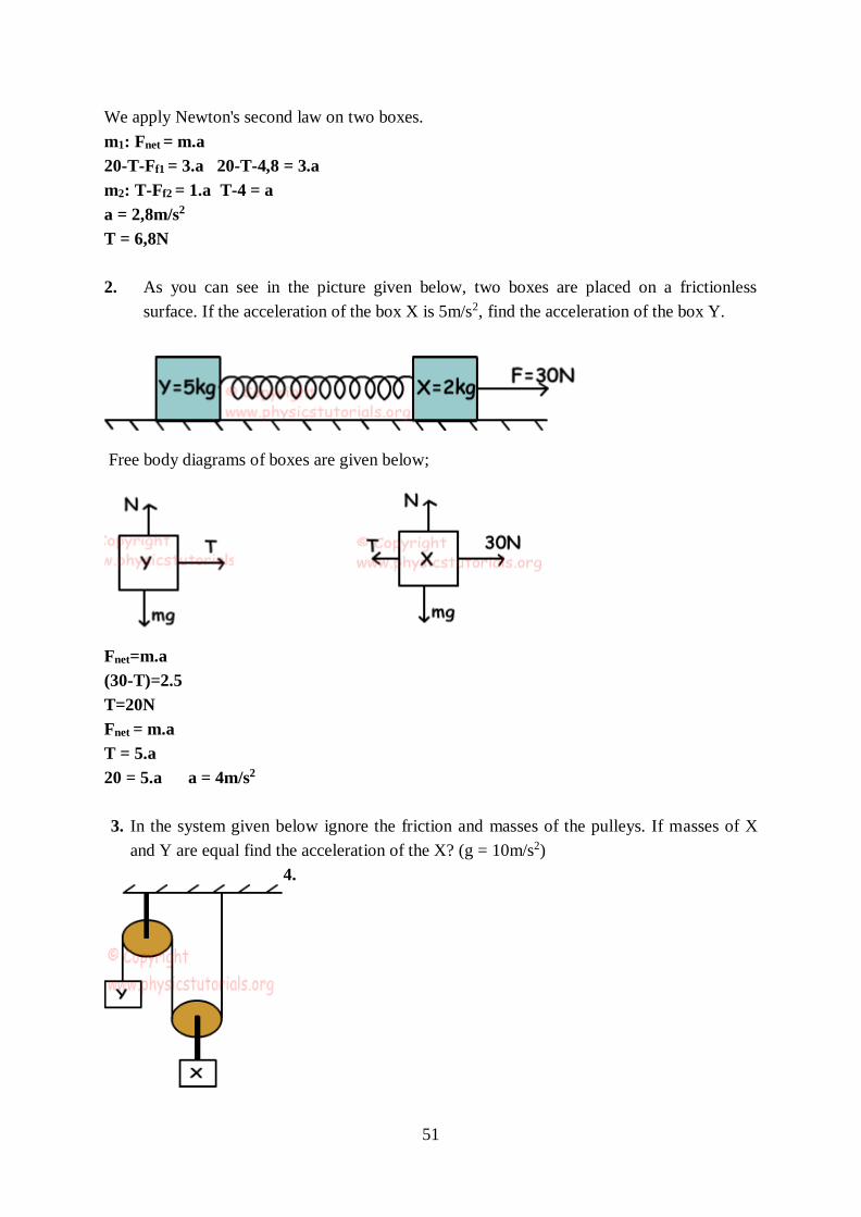
51

We apply Newton's second law on two boxes.

m1: Fnet = m.a

20-T-Ff1 = 3.a 20-T-4,8 = 3.a

m2: T-Ff2 = 1.a T-4 = a

a = 2,8m/s2

T = 6,8N

2. As you can see in the picture given below, two boxes are placed on a frictionless

surface. If the acceleration of the box X is 5m/s2, find the acceleration of the box Y.

Free body diagrams of boxes are given below;

Fnet=m.a

(30-T)=2.5

T=20N

Fnet = m.a

T = 5.a

20 = 5.a a = 4m/s2

3. In the system given below ignore the friction and masses of the pulleys. If masses of X

and Y are equal find the acceleration of the X? (g = 10m/s2)

4.

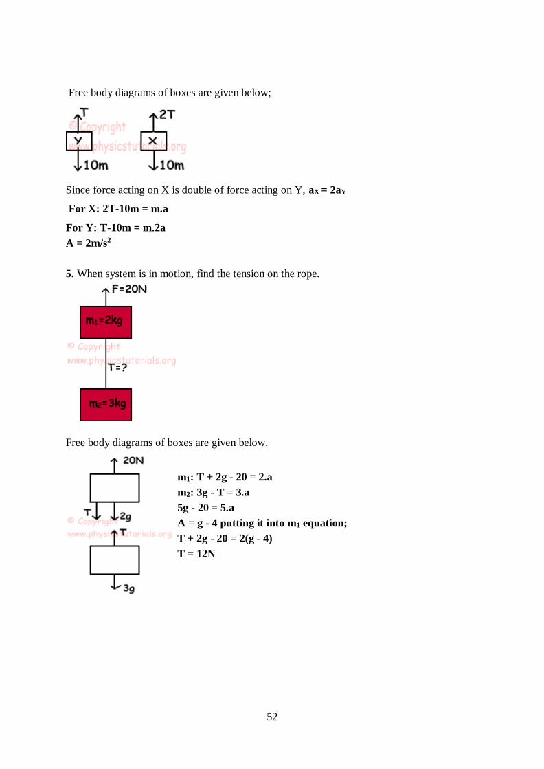
52


Since force acting on X is double of force acting on Y, aX = 2aY

For X: 2T-10m = m.a

For Y: T-10m = m.2a

A = 2m/s2

5. When system is in motion, find the tension on the rope.

Free body diagrams of boxes are given below.

m1: T + 2g - 20 = 2.a

m2: 3g - T = 3.a

5g - 20 = 5.a

A = g - 4 putting it into m1 equation;

T + 2g - 20 = 2(g - 4)

T = 12N

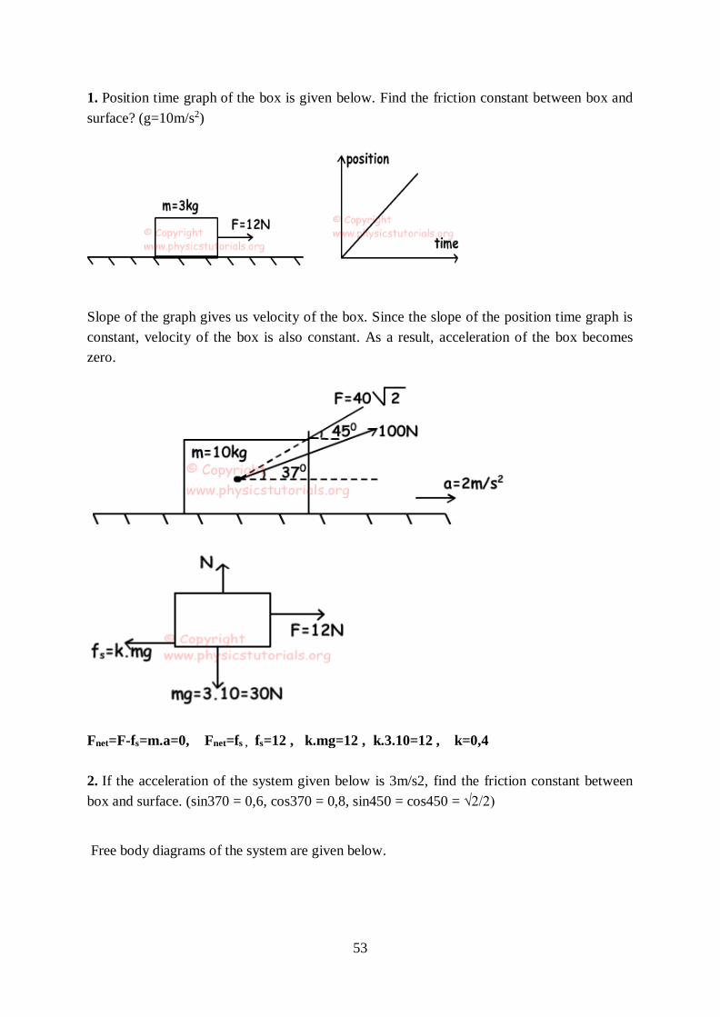
53

1. Position time graph of the box is given below. Find the friction constant between box and

surface? (g=10m/s2)

Slope of the graph gives us velocity of the box. Since the slope of the position time graph is

constant, velocity of the box is also constant. As a result, acceleration of the box becomes

zero.

Fnet=F-fs=m.a=0, Fnet=fs , fs=12 , k.mg=12 , k.3.10=12 , k=0,4

2. If the acceleration of the system given below is 3m/s2, find the friction constant between

box and surface. (sin370 = 0,6, cos370 = 0,8, sin450 = cos450 = √2/2)

Free body diagrams of the system are given below.

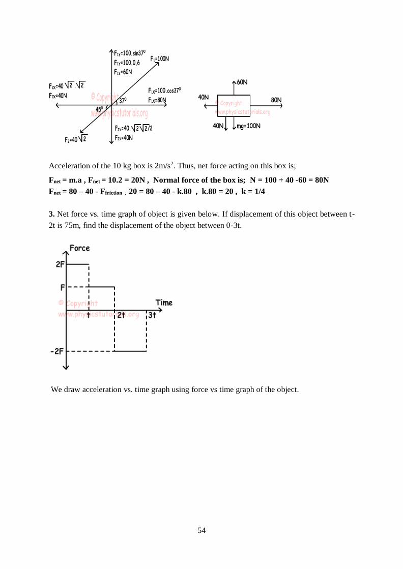
54

Acceleration of the 10 kg box is 2m/s2. Thus, net force acting on this box is;

Fnet = m.a , Fnet = 10.2 = 20N , Normal force of the box is; N = 100 + 40 -60 = 80N

Fnet = 80 – 40 - Ffriction , 20 = 80 – 40 - k.80 , k.80 = 20 , k = 1/4

3. Net force vs. time graph of object is given below. If displacement of this object between t-

2t is 75m, find the displacement of the object between 0-3t.

We draw acceleration vs. time graph using force vs time graph of the object.

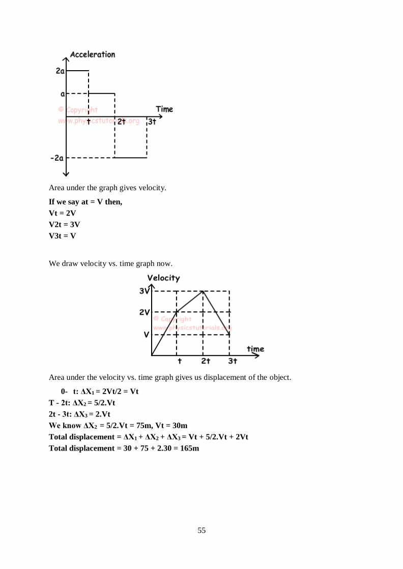
55

Area under the graph gives velocity.

If we say at = V then,

Vt = 2V

V2t = 3V

V3t = V

We draw velocity vs. time graph now.

Area under the velocity vs. time graph gives us displacement of the object.

0- t: ΔX1 = 2Vt/2 = Vt

T - 2t: ΔX2 = 5/2.Vt

2t - 3t: ΔX3 = 2.Vt

We know ΔX2 = 5/2.Vt = 75m, Vt = 30m

Total displacement = ΔX1 + ΔX2 + ΔX3 = Vt + 5/2.Vt + 2Vt

Total displacement = 30 + 75 + 2.30 = 165m

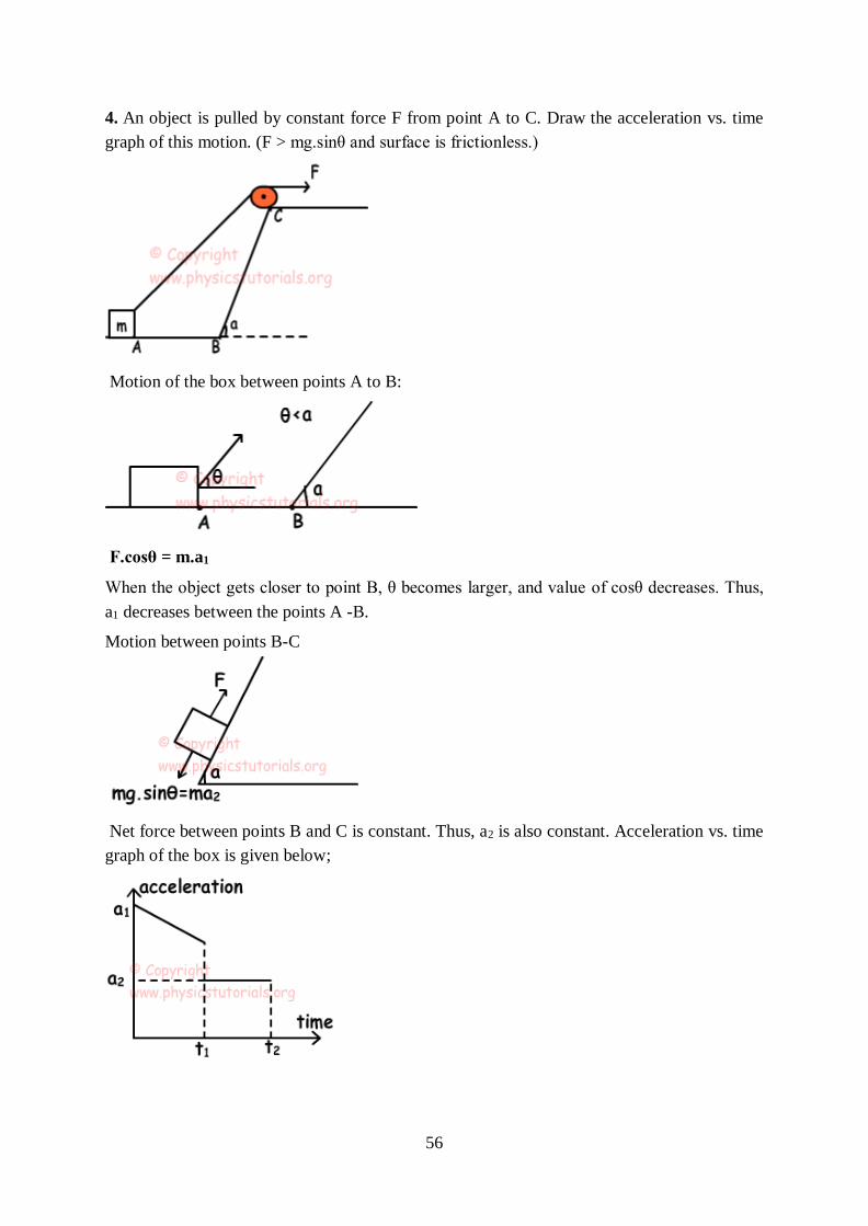
56

4. An object is pulled by constant force F from point A to C. Draw the acceleration vs. time

graph of this motion. (F > mg.sinθ and surface is frictionless.)

Motion of the box between points A to B:

F.cosθ = m.a1

When the object gets closer to point B, θ becomes larger, and value of cosθ decreases. Thus,

a1 decreases between the points A -B.

Motion between points B-C

Net force between points B and C is constant. Thus, a2 is also constant. Acceleration vs. time

graph of the box is given below;

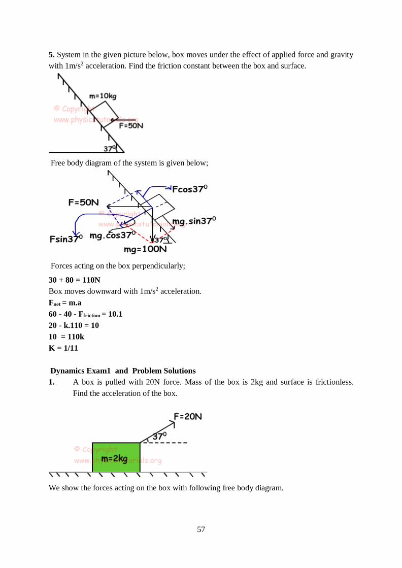
57

5. System in the given picture below, box moves under the effect of applied force and gravity

with 1m/s2 acceleration. Find the friction constant between the box and surface.

Free body diagram of the system is given below;

Forces acting on the box perpendicularly;

30 + 80 = 110N

Box moves downward with 1m/s2 acceleration.

Fnet = m.a

60 - 40 - Ffriction = 10.1

20 - k.110 = 10

10 = 110k

K = 1/11

Dynamics Exam1 and Problem Solutions

1. A box is pulled with 20N force. Mass of the box is 2kg and surface is frictionless.

Find the acceleration of the box.

We show the forces acting on the box with following free body diagram.

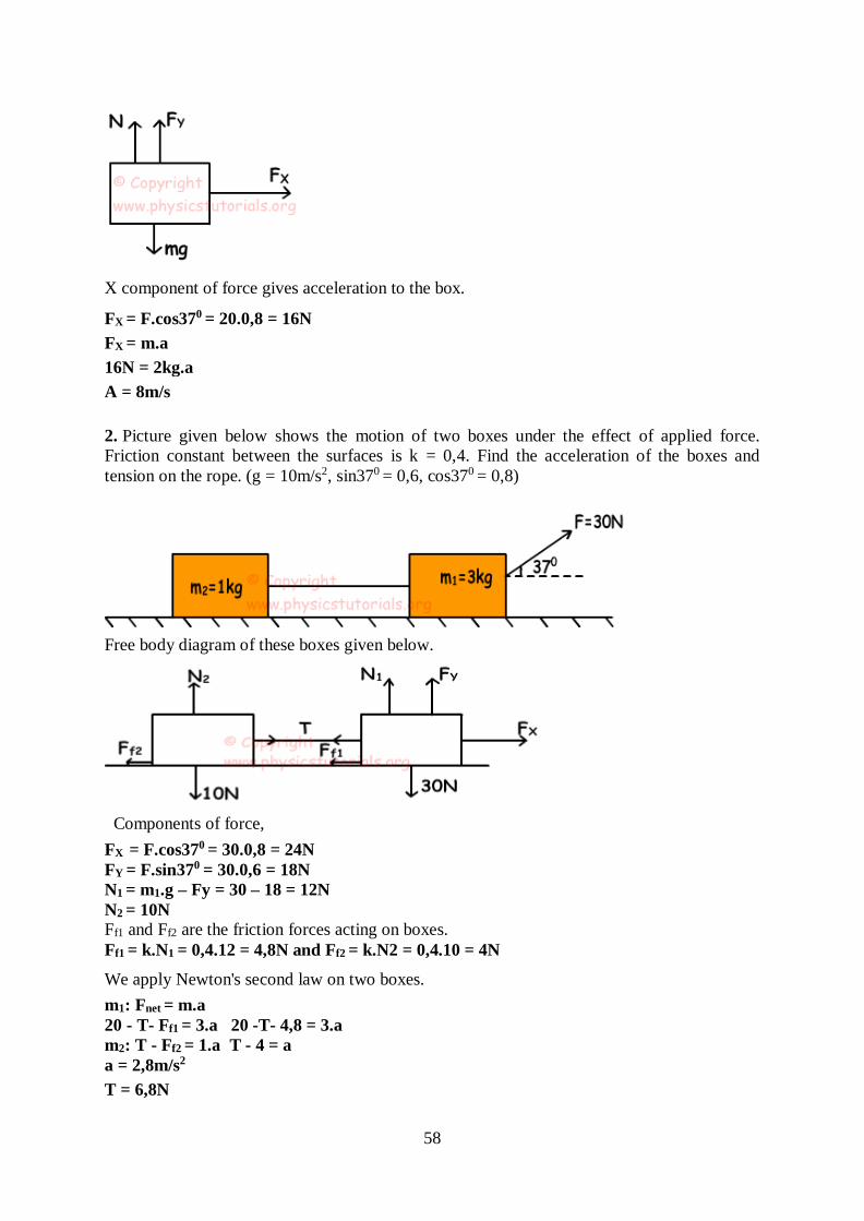
58

X component of force gives acceleration to the box.

FX = F.cos370 = 20.0,8 = 16N

FX = m.a

16N = 2kg.a

A = 8m/s

2. Picture given below shows the motion of two boxes under the effect of applied force.

Friction constant between the surfaces is k = 0,4. Find the acceleration of the boxes and

tension on the rope. (g = 10m/s2, sin370 = 0,6, cos370 = 0,8)

Free body diagram of these boxes given below.

Components of force,

FX = F.cos370 = 30.0,8 = 24N

FY = F.sin370 = 30.0,6 = 18N

N1 = m1.g – Fy = 30 – 18 = 12N

N2 = 10N Ff1 and Ff2 are the friction forces acting on boxes.

Ff1 = k.N1 = 0,4.12 = 4,8N and Ff2 = k.N2 = 0,4.10 = 4N

We apply Newton's second law on two boxes.

m1: Fnet = m.a

20 - T- Ff1 = 3.a 20 -T- 4,8 = 3.a

m2: T - Ff2 = 1.a T - 4 = a

a = 2,8m/s2

T = 6,8N

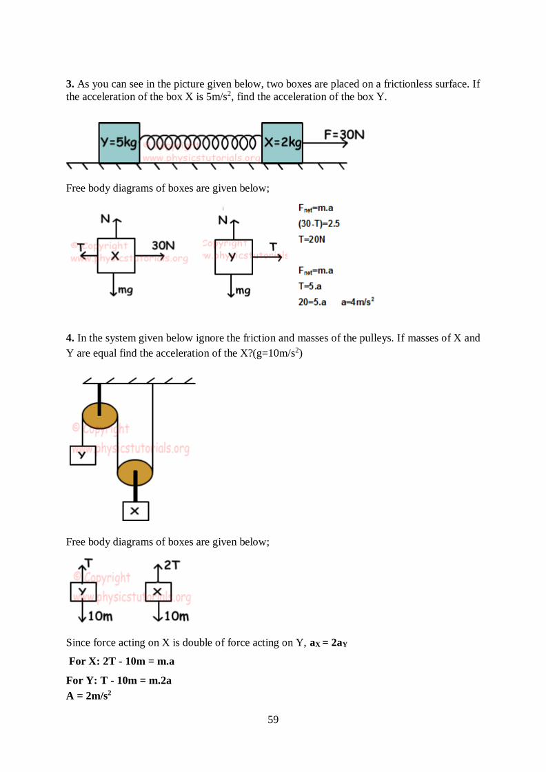
59

3. As you can see in the picture given below, two boxes are placed on a frictionless surface. If

the acceleration of the box X is 5m/s2, find the acceleration of the box Y.


4. In the system given below ignore the friction and masses of the pulleys. If masses of X and

Y are equal find the acceleration of the X?(g=10m/s2)


Since force acting on X is double of force acting on Y, aX = 2aY

For X: 2T - 10m = m.a

For Y: T - 10m = m.2a

A = 2m/s2

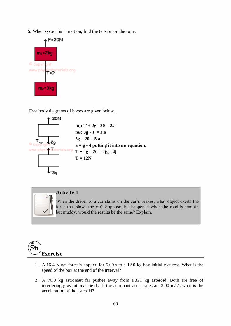
60

5. When system is in motion, find the tension on the rope.

Free body diagrams of boxes are given below.

m1: T + 2g - 20 = 2.a

m2: 3g - T = 3.a

5g – 20 = 5.a

a = g - 4 putting it into m1 equation;

T + 2g – 20 = 2(g - 4)

T = 12N

Activity 1

When the driver of a car slams on the car’s brakes, what object exerts the

force that slows the car? Suppose this happened when the road is smooth

but muddy, would the results be the same? Explain.

Exercise

1. A 16.4-N net force is applied for 6.00 s to a 12.0-kg box initially at rest. What is the

speed of the box at the end of the interval?

2. A 70.0 kg astronaut far pushes away from a 321 kg asteroid. Both are free of

interfering gravitational fields. If the astronaut accelerates at -3.00 m/s/s what is the

acceleration of the asteroid?

61

3. A sled is pulled by a rope at constant velocity across a horizontal surface. If a force of

80.0 N is being applied to the sled rope at an angle of 25.1 º to the ground, what is the

magnitude (in N) of the force of friction?

4. A student of mass 50 kg tests Newton's laws by standing on a bathroom scale in an

elevator. Assume that the scale reads in newtons. Find the scale reading when the

elevator is (a) accelerating upward at 0.5 m/s 2, (b) going up at a constant speed of

3.0 m/s and (c) going up but decelerating at 1.0 m/s2.

Summary

In this lecture, we have learned the application of the third Newton’s law of motion, which

states that ‘to every action there is an equal but opposite reaction.’ Friction refers to any force

resisting the relative motion of solid surfaces, fluid layers, and material elements sliding

against each other. There are two types of friction forces, frictional force and kinetic force.

We have learned about the friction law and its applications and the properties of friction.

References

Gottys,W., Keller, F.J. and Skove, M.J, Physics Classical and Modern, 1989. McGraw

Hill.

A.K. Jha, A Textbook of Applied Physics, 2009. I.K. International Pub.


62

SECTION TWO:

MECHANICS

Lecture 6: Work, Energy and Power

6.1 Introduction In this lecture, we shall discuss work, energy and power and how they relate. We shall further

discuss kinetic energy, potential energy, and mechanical energy as the sum of the two.

Further, we will discuss the principle of conservation of mechanical energy and situations in

which mechanical energy is conserved.

Lecture Objectives


i. Describe the basic terminologies and concepts.

ii. Describe the work-energy relationship, and perform calculations.

iii. Describe the kinetic energy and potential energy of an object.

iv. Use equations related to work and power, to calculate the kinetic, potential and

total mechanical energy of objects.

v. Explain the Work-Energy Theorem.

vi. Describe mechanical energy conservation.

6.2 Work

Suppose that, a force is applied an object and object moves in the direction of applied force,

then we say work has been done. Let me explain in other words. There must be a force

applied to an object and object must move in the direction of the applied force. If the motion

is not in the direction of force or force is applied to an object but there is no motion then we

cannot talk about work. Now we formulize what we said above.

Since force is a vector quantity both having magnitude and direction work is also a vector

quantity and has same direction with applied force. We will symbolize force as F, and

distance as d in formulas and exercises. If there is an angle between force and direction of

motion, then we state our formula as given below;

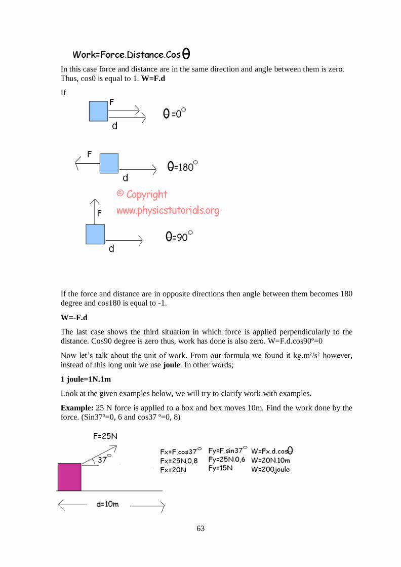
63

In this case force and distance are in the same direction and angle between them is zero.

Thus, cos0 is equal to 1. W=F.d

If

If the force and distance are in opposite directions then angle between them becomes 180

degree and cos180 is equal to -1.

W=-F.d

The last case shows the third situation in which force is applied perpendicularly to the

distance. Cos90 degree is zero thus, work has done is also zero. W=F.d.cos90º=0

Now let’s talk about the unit of work. From our formula we found it kg.m²/s² however,

instead of this long unit we use joule. In other words;

1 joule=1N.1m

Look at the given examples below, we will try to clarify work with examples.

Example: 25 N force is applied to a box and box moves 10m. Find the work done by the

force. (Sin37º=0, 6 and cos37 º=0, 8)

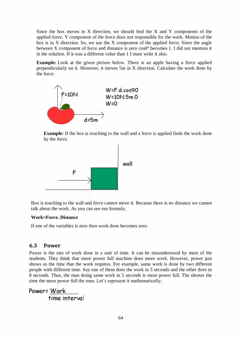
64

Since the box moves in X direction, we should find the X and Y components of the

applied force. Y component of the force does not responsible for the work. Motion of the

box is in X direction. So, we use the X component of the applied force. Since the angle

between X component of force and distance is zero cos0º becomes 1. I did not mention it

in the solution. If it was a different value than 1 I must write it also.

Example: Look at the given picture below. There is an apple having a force applied

perpendicularly on it. However, it moves 5m in X direction. Calculate the work done by

the force.

Example: If the box is touching to the wall and a force is applied finds the work done

by the force.

Box is touching to the wall and force cannot move it. Because there is no distance we cannot

talk about the work. As you can see our formula;

Work=Force. Distance

If one of the variables is zero then work done becomes zero.

6.3 Power Power is the rate of work done in a unit of time. It can be misunderstood by most of the

students. They think that more power full machine does more work. However, power just

shows us the time that the work requires. For example, same work is done by two different

people with different time. Say one of them does the work in 5 seconds and the other does in

8 seconds. Thus, the man doing same work in 5 seconds is more power full. The shorter the

time the more power full the man. Let’s represent it mathematically;

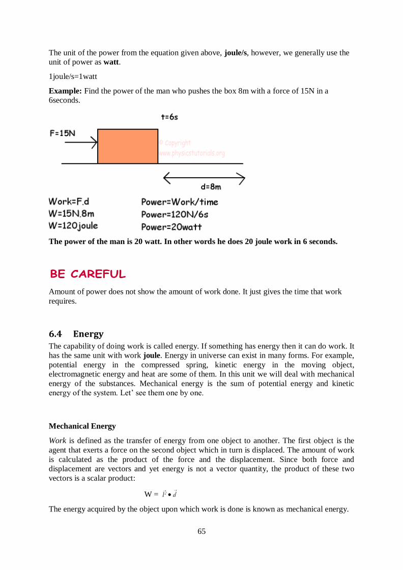
65

The unit of the power from the equation given above, joule/s, however, we generally use the

unit of power as watt.

1joule/s=1watt

Example: Find the power of the man who pushes the box 8m with a force of 15N in a

6seconds.

The power of the man is 20 watt. In other words he does 20 joule work in 6 seconds.

Amount of power does not show the amount of work done. It just gives the time that work

requires.

6.4 Energy The capability of doing work is called energy. If something has energy then it can do work. It

has the same unit with work joule. Energy in universe can exist in many forms. For example,

potential energy in the compressed spring, kinetic energy in the moving object,

electromagnetic energy and heat are some of them. In this unit we will deal with mechanical

energy of the substances. Mechanical energy is the sum of potential energy and kinetic

energy of the system. Let’ see them one by one.

Mechanical Energy

Work is defined as the transfer of energy from one object to another. The first object is the

agent that exerts a force on the second object which in turn is displaced. The amount of work

is calculated as the product of the force and the displacement. Since both force and

displacement are vectors and yet energy is not a vector quantity, the product of these two

vectors is a scalar product:

W = F d

The energy acquired by the object upon which work is done is known as mechanical energy.

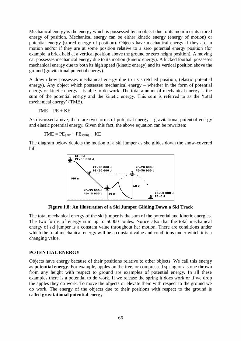
66

Mechanical energy is the energy which is possessed by an object due to its motion or its stored

energy of position. Mechanical energy can be either kinetic energy (energy of motion) or

potential energy (stored energy of position). Objects have mechanical energy if they are in

motion and/or if they are at some position relative to a zero potential energy position (for

example, a brick held at a vertical position above the ground or zero height position). A moving

car possesses mechanical energy due to its motion (kinetic energy). A kicked football possesses

mechanical energy due to both its high speed (kinetic energy) and its vertical position above the

ground (gravitational potential energy).

A drawn bow possesses mechanical energy due to its stretched position, (elastic potential

energy). Any object which possesses mechanical energy – whether in the form of potential

energy or kinetic energy – is able to do work. The total amount of mechanical energy is the

sum of the potential energy and the kinetic energy. This sum is referred to as the ‘total

mechanical energy’ (TME).

TME = PE + KE

As discussed above, there are two forms of potential energy – gravitational potential energy

and elastic potential energy. Given this fact, the above equation can be rewritten:

TME = PEgrav + PEspring + KE

The diagram below depicts the motion of a ski jumper as she glides down the snow-covered

hill.

Figure 1.8: An Illustration of a Ski Jumper Gliding Down a Ski Track

The total mechanical energy of the ski jumper is the sum of the potential and kinetic energies.

The two forms of energy sum up to 50000 Joules. Notice also that the total mechanical

energy of ski jumper is a constant value throughout her motion. There are conditions under

which the total mechanical energy will be a constant value and conditions under which it is a

changing value.

POTENTIAL ENERGY

Objects have energy because of their positions relative to other objects. We call this energy

as potential energy. For example, apples on the tree, or compressed spring or a stone thrown

from any height with respect to ground are examples of potential energy. In all these

examples there is a potential to do work. If we release the spring it does work or if we drop

the apples they do work. To move the objects or elevate them with respect to the ground we

do work. The energy of the objects due to their positions with respect to the ground is

called gravitational potential energy.

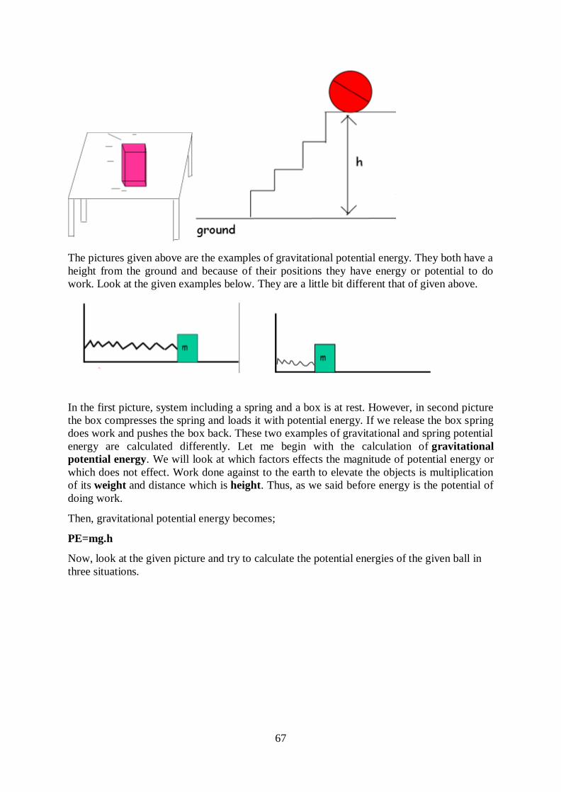
67

The pictures given above are the examples of gravitational potential energy. They both have a

height from the ground and because of their positions they have energy or potential to do

work. Look at the given examples below. They are a little bit different that of given above.

In the first picture, system including a spring and a box is at rest. However, in second picture

the box compresses the spring and loads it with potential energy. If we release the box spring

does work and pushes the box back. These two examples of gravitational and spring potential

energy are calculated differently. Let me begin with the calculation of gravitational

potential energy. We will look at which factors effects the magnitude of potential energy or

which does not effect. Work done against to the earth to elevate the objects is multiplication

of its weight and distance which is height. Thus, as we said before energy is the potential of

doing work.

Then, gravitational potential energy becomes;

PE=mg.h

Now, look at the given picture and try to calculate the potential energies of the given ball in

three situations.

68

We see that gravitational potential energy depends on the weight and height of the object.

Now let’s solve some more examples related to this topic before passing to the kinetic energy.

Example: In the pictures given below, if the potential energy of the ball in the first picture is

P find the potential energy of the ball in second situation in terms of P.

Situation 1 : P=m.g.h=mgh

Situation 2: P’=m.g.2h=2mgh=2P

POTENTIAL ENERGY OF THE SPRING

By compressing the spring or stretching it you load a potential energy to it. Well, if I apply

same force to different springs having different thicknesses, are they loaded with the same

energy? I hear that you all say no! You are absolutely right. Of course the thinner spring is

more compressed than the thicker one where the quantity of compression shows the loaded

potential energy. What I want to say is that, potential energy of the spring depends on the

type of spring and the amount of compression. The mathematical representation of this

definition is given below.

Ep=1/2.k.x²

Where k is the spring constant and x is the amount of compression.

69

Now, we look at the origin of this formula. This is a picture of a spring at rest. There is no

compression or stretching. Thus, we can not talk about the potential energy of the spring.

However, in the pictures given below springs are not at rest position. Let’s examine the

behavior of the springs in two situations.

In the first picture, we apply a force, Fapplied, and spring reacts this force with Fspring = -kx.

The amount of compression is X. In the second picture we stretch the spring by the amount of

X. We apply force of F and spring gives reaction to this force with Fspring = -kx where x is

the stretching amount and k is the spring constant. The given graph below is force versus

distance graph of springs. We find the energy equation of spring by using this graph.

As I said before area under the force vs distance graph gives us the work and energy is the

capability of doing work. So, area under this graph must give us the potential energy of the

spring.

Area = 1/2.F.x = 1/2.kx.x = 1/2kx²

Ep = 1/2kx²

Example: 50N of force is applied to a spring having 150N/m spring constant. Find the

amount of compression of the spring.

70

Fspring = -kx = Fapplied

50N = -150.x

X = -3m “-“shows the direction of compression.

KINETIC ENERGY

Objects have energy because of their motion; this energy is called kinetic energy. Kinetic

energy of the objects having mass m and velocity v can be calculated with the formula given

below;

Ek = 1/2mv²

As you see from the formula, kinetic energy of the objects is only affected by the mass and

velocity of the objects. The unit of the Ek is again from the formula kg.m²/s² or in general

use joule.

Example: Find the kinetic energy of the ball having mass 0,5 kg and velocity 10m/s.

Ek = 1/2mv²

Ek = 1/2.0, 5. (10) ²

Ek = 25joule

As in the case of Kinematics we can use graphs to show the relations of the concepts here.

Look at the given graph of Force vs. Distance.Area under the force vs. distance graph gives

us work.

Work = Force. Distance = Area = F.X (distance)

We can find energy of the objects from their Force vs. Distance graph.

71

Example: Look at the given picture below. If the final velocity of the box is 4m/s find the

work done by friction.

At the top;

Etotal = mgh + 1/2mv²

Etotal = 5kg.10m/s².4m + 1/2.5kg. (2m/s) ² = 210joule

At the bottom;

Etotal = 1/2mv² = 1/2.5kg.(4m/s) ²

Etotal = 40 joule

The difference between the initial and final energy is used by the friction.

Work done by the friction = Efinal – Einitial = 210joule - 40joule = 170joule

72

6.5 Work-Energy Theorem

The Work-Energy Theorem can be explained under the following heads:

Internal and External Forces

There are a variety of ways to categorize all the types of forces. All the types of forces can be

categorized as contact forces or as action-at-a-distance forces.

Forces can also be categorized in terms of whether or not their presence is capable of

changing an object's total mechanical energy. The two categories of forces are called internal

and external forces.

External forces include applied forces, normal forces, tensional forces, friction forces, and air

resistance forces. Internal forces include gravitational forces, magnetic forces, electrical

forces, and elastic forces. The significance of categorizing a force as internal or external is

related to the ability of that type of force to change an object's total mechanical energy when

it does work upon an object. When work is done upon an object by an external force, the total

mechanical energy (KE + PE) of that object is changed. If the work is "positive work", then

the object will gain energy. If the work is "negative work", then the object will lose energy.

The gain or loss in energy can be in the form of potential energy, kinetic energy, or both.

Under such circumstances, the work which is done will be equal to the change in mechanical

energy of the object.

When work is done upon an object by an internal force (for example, gravitational and spring

forces), the total mechanical energy (KE + PE) of that object remains constant. In such cases,

the object's energy changes form. For example, as an object is "forced" from a high elevation

to a lower elevation by gravity, some of the potential energy of that object is transformed into

kinetic energy. Yet, the sum of the kinetic and potential energies remains constant. This is

referred to as energy conservation. When the only forces doing work are internal forces,

energy changes forms - from kinetic to potential (or vice versa); yet the total amount of

mechanical energy is conserved.

Analysis of Situations involving External Forces

Whenever work is done upon an object by an external force, there will be a change in the

total mechanical energy of the object. If only internal forces are doing work (no work done by

external forces), there is no change in total mechanical energy; the total mechanical energy is

conserved. In this section, we will further explore the quantitative relationship between work

and energy. The quantitative relationship between work and mechanical energy is expressed

by the following equation:

TMEi + Wext = TMEf

Where TMEi is the initial amount of total mechanical energy, Wext is the work done by

external forces and TMEf is the final total mechanical energy. Since the mechanical energy

can be either potential energy or kinetic energy, the above equation can be rewritten as

KEi + PEi + Wext = KEf + PEf

The work done by external forces can be a positive or a negative work term.

The above equation is known as the Work-Energy Theorem.

73

The work-energy theorem is the basis for the rest of this section. It forms the basis of the

conceptual aspect of a powerful approach to solving mathematical problems.

Consider a weightlifter who applies an upwards force F (say 100 N) to a weight to displace

it upwards at given distance d (say 0.25 meters) at a constant speed. According to the work-

energy theorem, the initial energy plus the work done by the external force equals the final

energy. If the weight begins with 150 Joules of energy (this is just a made-up value), and the

weightlifter does 25 Joules of work, TMEi

. cosextW F d Fd = 100 × 0.25 cos0 = 25.0 J

then the weight will finish with 125 Joules of mechanical energy.

The final energy (125 J) is equal to the initial energy (100 J) plus the work done by external

forces (25 J).

Now consider a car which is skidding from a high speed to a lower speed. The force of

friction between the tyres and the road exerts a leftward force (say 8000 N) on the rightward

moving car over a given distance (say 30 m). According to the work-energy theorem, the

initial energy plus the work done by the external force equals the final energy. If the car

begins with say 320 000 Joules of energy and the friction force does

– 240 000 Joules of work

cos180 8000 30 ( 1)frictionW Fd = – 240000 J

then the car will finish with 80 000 Joules of mechanical energy. The final energy

(80,000 J) is equal to the initial energy (3,20,000 J) plus the work done by external forces (–

2,40,000 J).

In each of these examples, an external force does work upon an object over a given distance

to change the total mechanical energy of the object. If the external force does positive work,

then the object gains energy; the amount of energy gained is equal to the work done on the

object. If the external force does negative work, then the object loses energy; the amount of

energy lost is equal to the work done on the object. In general, the total energy of the object

in the initial state (prior to the work being done) plus the work done equals the total energy in

the final state.

The work-energy theorem can be combined with the expressions for potential and kinetic

energy to solve complex problems. Like all complex problems, they can be made simple if

first analyzed from a conceptual viewpoint and broken down into parts.

74

1. A 1000 kg car travelling with a speed of 25 m/s skids to a stop. The car

experiences an 8000 N force of friction. Determine the stopping distance of

the car.

2. At the end of a roller-coaster ride, the 6000 kg train of cars (includes

passengers) is slowed from a speed of 20 m/s to a speed of 5 m/s over a

distance of 20 meters. Determine the braking force required to slow the train

of cars by this amount.

3. A shopping cart full of groceries placed at the top of a 2 m hill begins to roll

until it hits a stump at the bottom of the hill. Upon impact, a 0.25 kg can of

peaches flies horizontally out of the shopping cart and hits a parked car with

an average force of 500 N. How deep a dent is made in the car (i.e. over what

distance does the 500 N force act upon the can of peaches before bringing it

to a stop)?

All three of the above problems have one thing in common: there is a force which does work

over a distance in order to remove mechanical energy from an object. The force acts opposite

the object's motion (angle between force and displacement is 180) and thus does "negative

work;" negative work means that the object loses energy. In each situation, the work is related

to the kinetic energy change. And since the distance (d) over which the force does work is

related to the work and since the velocity squared (v2) of the object is related to the kinetic

energy, there must also be a direct relation between the stopping distance and the velocity

squared. Observe the derivation below:

i ext fTME W TME

0i extKE W

21cos180 0

2mv Fd

21

2mv Fd

v2 d

The above equation depicts stopping distance as being dependent upon the square of the

velocity. This means that a twofold increase in velocity would result in a fourfold (two

squared) increase in stopping distance. A threefold increase in velocity would result in a nine-

75

fold (three squared) increase in stopping distance. And a fourfold increase in velocity would

result in a 16-fold (four squared) increase in stopping distance. As shown, an equation is a not

merely an algebraic recipe for solving problems; equations are also cognitive guides to

thinking about how two quantities are related to each other. In this case for a force bringing

an object to a stop over a given distance, the stopping distance of the object is related to the

square of the velocity of the object.

The examples mentioned above involve the application of the work-energy theorem to

situations involving external forces doing work. An entirely different outcome results in

situations in which there is no work done by external forces.

6.6 Conservation of Mechanical Energy

Whenever work is done upon an object by an external force, there will be a change in the

total mechanical energy of the object. If only internal forces are doing work (no work done by

external forces), there is no change in total mechanical energy; the total mechanical energy is

said to be "conserved." In this section, we will further explore the quantitative relationship

between work and mechanical energy in situations in which there are no external forces doing

work.

The quantitative relationship between work and the two forms of mechanical energy is

expressed by the work–energy theorem:

KEi + PEi + Wext = KEf + PEf

The equation illustrates that the total mechanical energy (KE + PE) of the object is changed

as a result of work done by external forces. There are a host of other situations in which the

only forces doing work are internal forces. In such situations, the total mechanical energy of

the object is not changed. In such instances, it is sometimes said that the mechanical energy is

"conserved." The previous equation can be simplified to the following form:

KEi + PEi = KEf + PEf

In these situations, the sum of the kinetic and potential energy is the same everywhere. As

kinetic energy is decreased (due to the object slowing down), the potential energy is increased

(due to the stretch/compression of a spring or an increase in height above the Earth). As

kinetic energy is increased (due to the object speeding up), the potential energy is decreased

(due to the return of a spring to its rest position or a decrease in height above the Earth).

Energy is transformed from kinetic energy to potential energy (or vice versa) – yet the total

amount present is conserved.

The tendency of an object to conserve its mechanical energy is observed whenever external

forces are not doing work. If the influence of friction and air resistance can be ignored (or

assumed to be negligible) and all other external forces are absent or merely not doing work,

then the object is often said to conserve its energy. Consider a pendulum bob swinging to and

fro on the end of a string. There are only two forces acting upon the pendulum bob. Gravity

(an internal force) acts downward and the tensional force (an external force) pulls upwards

towards the pivot point. The external force does not do work since at all times it is directed at

right angle to the motion.

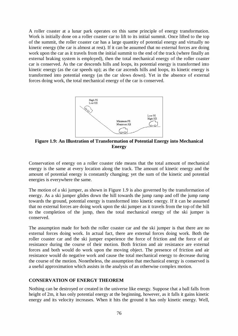
76

A roller coaster at a lunar park operates on this same principle of energy transformation.

Work is initially done on a roller coaster car to lift to its initial summit. Once lifted to the top

of the summit, the roller coaster car has a large quantity of potential energy and virtually no

kinetic energy (the car is almost at rest). If it can be assumed that no external forces are doing

work upon the car as it travels from the initial summit to the end of the track (where finally an

external braking system is employed), then the total mechanical energy of the roller coaster

car is conserved. As the car descends hills and loops, its potential energy is transformed into

kinetic energy (as the car speeds up); as the car ascends hills and loops, its kinetic energy is

transformed into potential energy (as the car slows down). Yet in the absence of external

forces doing work, the total mechanical energy of the car is conserved.

Figure 1.9: An Illustration of Transformation of Potential Energy into Mechanical

Energy

Conservation of energy on a roller coaster ride means that the total amount of mechanical

energy is the same at every location along the track. The amount of kinetic energy and the

amount of potential energy is constantly changing; yet the sum of the kinetic and potential

energies is everywhere the same.

The motion of a ski jumper, as shown in Figure 1.9 is also governed by the transformation of

energy. As a ski jumper glides down the hill towards the jump ramp and off the jump ramp

towards the ground, potential energy is transformed into kinetic energy. If it can be assumed

that no external forces are doing work upon the ski jumper as it travels from the top of the hill

to the completion of the jump, then the total mechanical energy of the ski jumper is

conserved.

The assumption made for both the roller coaster car and the ski jumper is that there are no

external forces doing work. In actual fact, there are external forces doing work. Both the

roller coaster car and the ski jumper experience the force of friction and the force of air

resistance during the course of their motion. Both friction and air resistance are external

forces and both would do work upon the moving object. The presence of friction and air

resistance would do negative work and cause the total mechanical energy to decrease during

the course of the motion. Nonetheless, the assumption that mechanical energy is conserved is

a useful approximation which assists in the analysis of an otherwise complex motion.

CONSERVATION OF ENERGY THEOREM

Nothing can be destroyed or created in the universe like energy. Suppose that a ball falls from

height of 2m, it has only potential energy at the beginning, however, as it falls it gains kinetic

energy and its velocity increases. When it hits the ground it has only kinetic energy. Well,

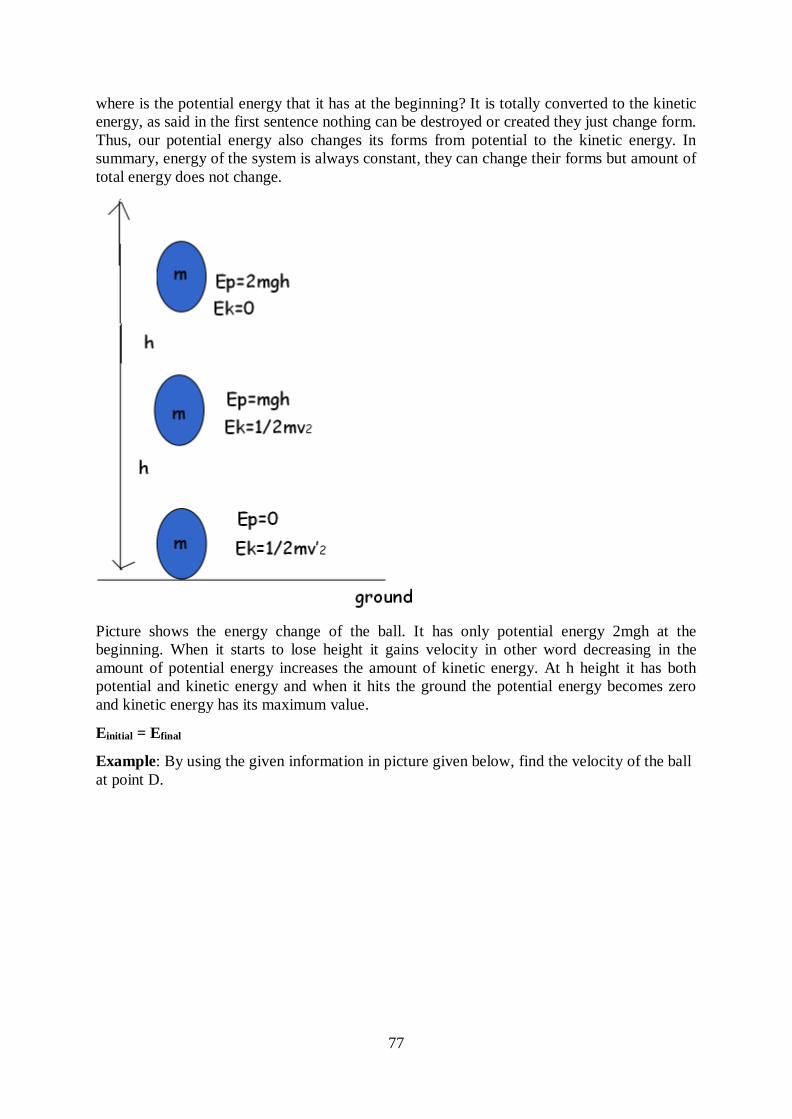
77

where is the potential energy that it has at the beginning? It is totally converted to the kinetic

energy, as said in the first sentence nothing can be destroyed or created they just change form.

Thus, our potential energy also changes its forms from potential to the kinetic energy. In

summary, energy of the system is always constant, they can change their forms but amount of

total energy does not change.

Picture shows the energy change of the ball. It has only potential energy 2mgh at the

beginning. When it starts to lose height it gains velocity in other word decreasing in the

amount of potential energy increases the amount of kinetic energy. At h height it has both

potential and kinetic energy and when it hits the ground the potential energy becomes zero

and kinetic energy has its maximum value.

Einitial = Efinal

Example: By using the given information in picture given below, find the velocity of the ball

at point D.

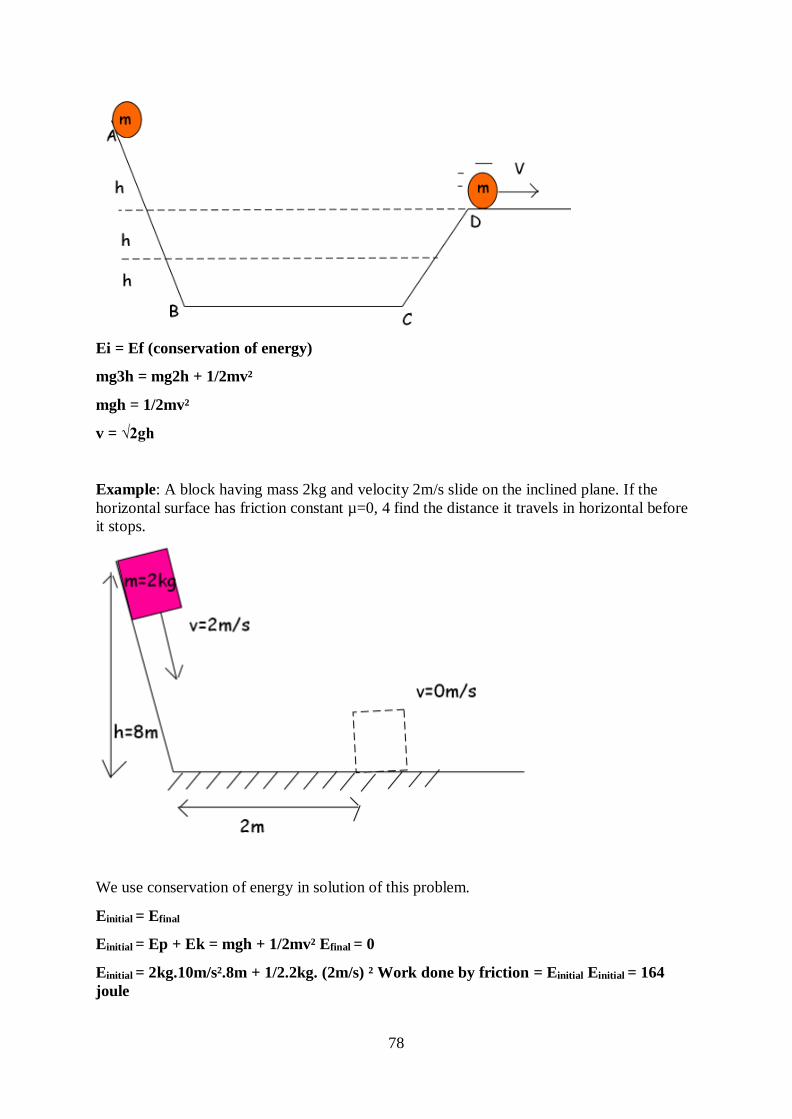
78

Ei = Ef (conservation of energy)

mg3h = mg2h + 1/2mv²

mgh = 1/2mv²

v = √2gh

Example: A block having mass 2kg and velocity 2m/s slide on the inclined plane. If the

horizontal surface has friction constant µ=0, 4 find the distance it travels in horizontal before

it stops.

We use conservation of energy in solution of this problem.

Einitial = Efinal

Einitial = Ep + Ek = mgh + 1/2mv² Efinal = 0

Einitial = 2kg.10m/s².8m + 1/2.2kg. (2m/s) ² Work done by friction = Einitial Einitial = 164

joule

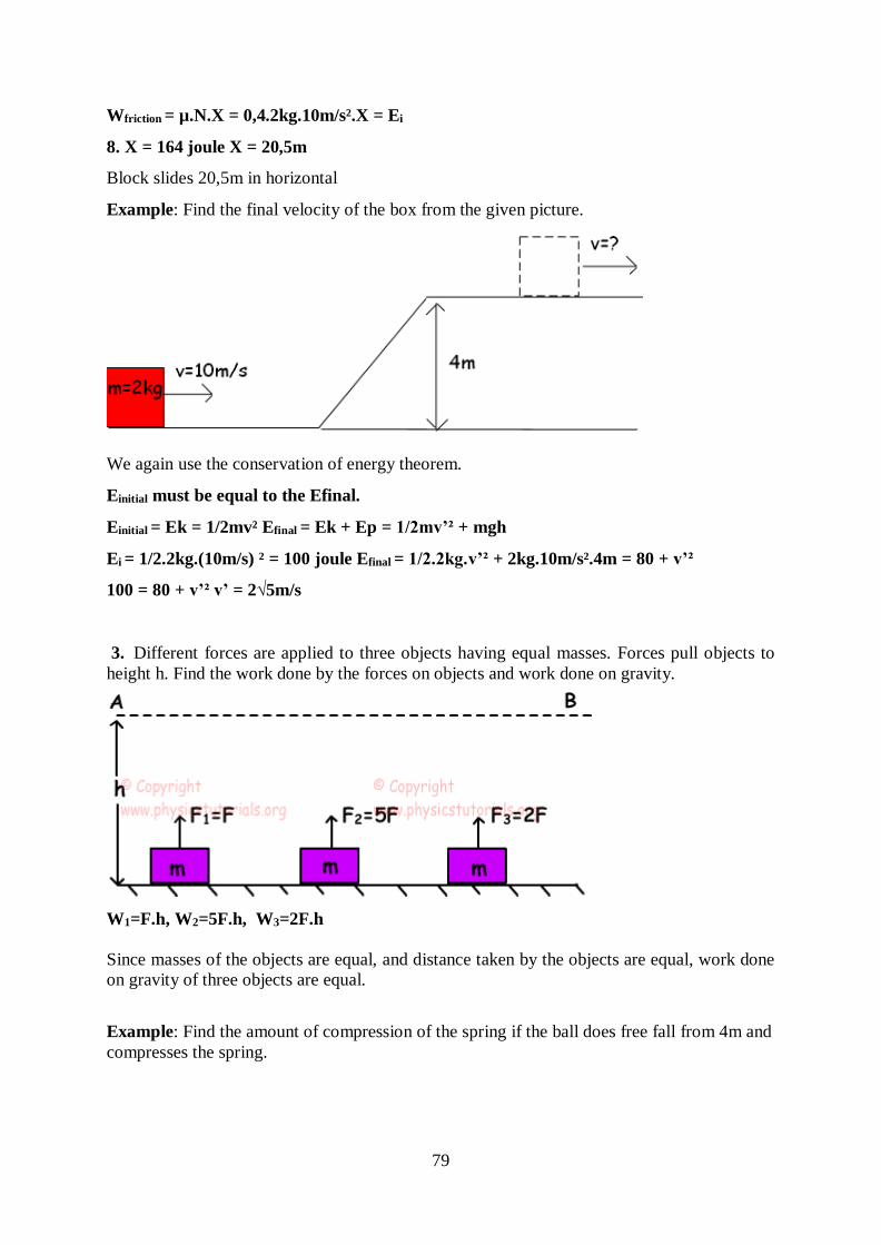
79

Wfriction = µ.N.X = 0,4.2kg.10m/s².X = Ei

8. X = 164 joule X = 20,5m

Block slides 20,5m in horizontal

Example: Find the final velocity of the box from the given picture.

We again use the conservation of energy theorem.

Einitial must be equal to the Efinal.

Einitial = Ek = 1/2mv² Efinal = Ek + Ep = 1/2mv’² + mgh

Ei = 1/2.2kg.(10m/s) ² = 100 joule Efinal = 1/2.2kg.v’² + 2kg.10m/s².4m = 80 + v’²

100 = 80 + v’² v’ = 2√5m/s

3. Different forces are applied to three objects having equal masses. Forces pull objects to

height h. Find the work done by the forces on objects and work done on gravity.

W1=F.h, W2=5F.h, W3=2F.h

Since masses of the objects are equal, and distance taken by the objects are equal, work done

on gravity of three objects are equal.

Example: Find the amount of compression of the spring if the ball does free fall from 4m and

compresses the spring.

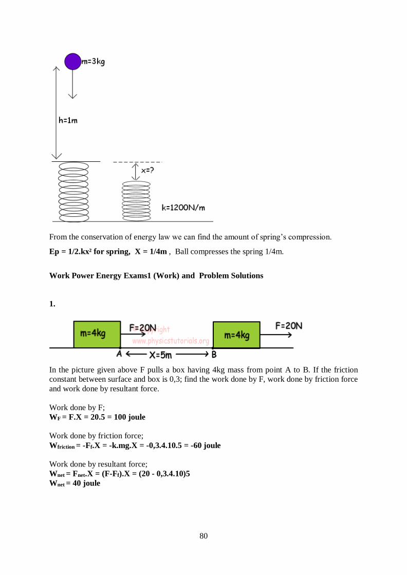
80

From the conservation of energy law we can find the amount of spring’s compression.

Ep = 1/2.kx² for spring, X = 1/4m , Ball compresses the spring 1/4m.

Work Power Energy Exams1 (Work) and Problem Solutions

1.

In the picture given above F pulls a box having 4kg mass from point A to B. If the friction

constant between surface and box is 0,3; find the work done by F, work done by friction force

and work done by resultant force.

Work done by F;

WF = F.X = 20.5 = 100 joule

Work done by friction force;

Wfriction = -Ff.X = -k.mg.X = -0,3.4.10.5 = -60 joule

Work done by resultant force;

Wnet = Fnet.X = (F-Ff).X = (20 - 0,3.4.10)5

Wnet = 40 joule

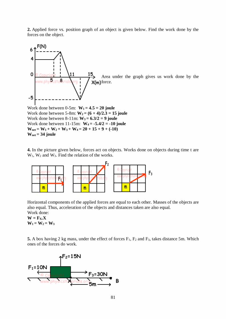
81

2. Applied force vs. position graph of an object is given below. Find the work done by the

forces on the object.

Area under the graph gives us work done by the

force.

Work done between 0-5m: W1 = 4.5 = 20 joule

Work done between 5-8m: W2 = (6 + 4)/2.3 = 15 joule

Work done between 8-11m: W3 = 6.3/2 = 9 joule

Work done between 11-15m: W4 = -5.4/2 = -10 joule

Wnet = W1 + W2 + W3 + W4 = 20 + 15 + 9 + (-10)

Wnet = 34 joule

4. In the picture given below, forces act on objects. Works done on objects during time t are

W1, W2 and W3. Find the relation of the works.

Horizontal components of the applied forces are equal to each other. Masses of the objects are

also equal. Thus, acceleration of the objects and distances taken are also equal.

Work done:

W = FX.X

W1 = W2 = W3

5. A box having 2 kg mass, under the effect of forces F1, F2 and F3, takes distance 5m. Which

ones of the forces do work.

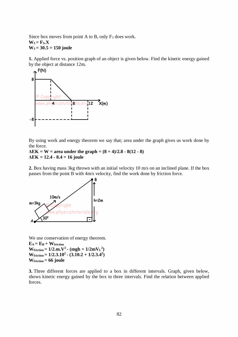
82

Since box moves from point A to B, only F3 does work.

W3 = F3.X

W3 = 30.5 = 150 joule

1. Applied force vs. position graph of an object is given below. Find the kinetic energy gained

by the object at distance 12m.

By using work and energy theorem we say that; area under the graph gives us work done by

the force.

ΔEK = W = area under the graph = (8 + 4)/2.8 - 8(12 - 8)

ΔEK = 12.4 - 8.4 = 16 joule

2. Box having mass 3kg thrown with an initial velocity 10 m/s on an inclined plane. If the box

passes from the point B with 4m/s velocity, find the work done by friction force.

We use conservation of energy theorem.

EA = EB + Wfriction

Wfriction = 1/2.m.V2 - (mgh + 1/2mVL2)

Wfriction = 1/2.3.102 - (3.10.2 + 1/2.3.42)

Wfriction = 66 joule

3. Three different forces are applied to a box in different intervals. Graph, given below,

shows kinetic energy gained by the box in three intervals. Find the relation between applied

forces.

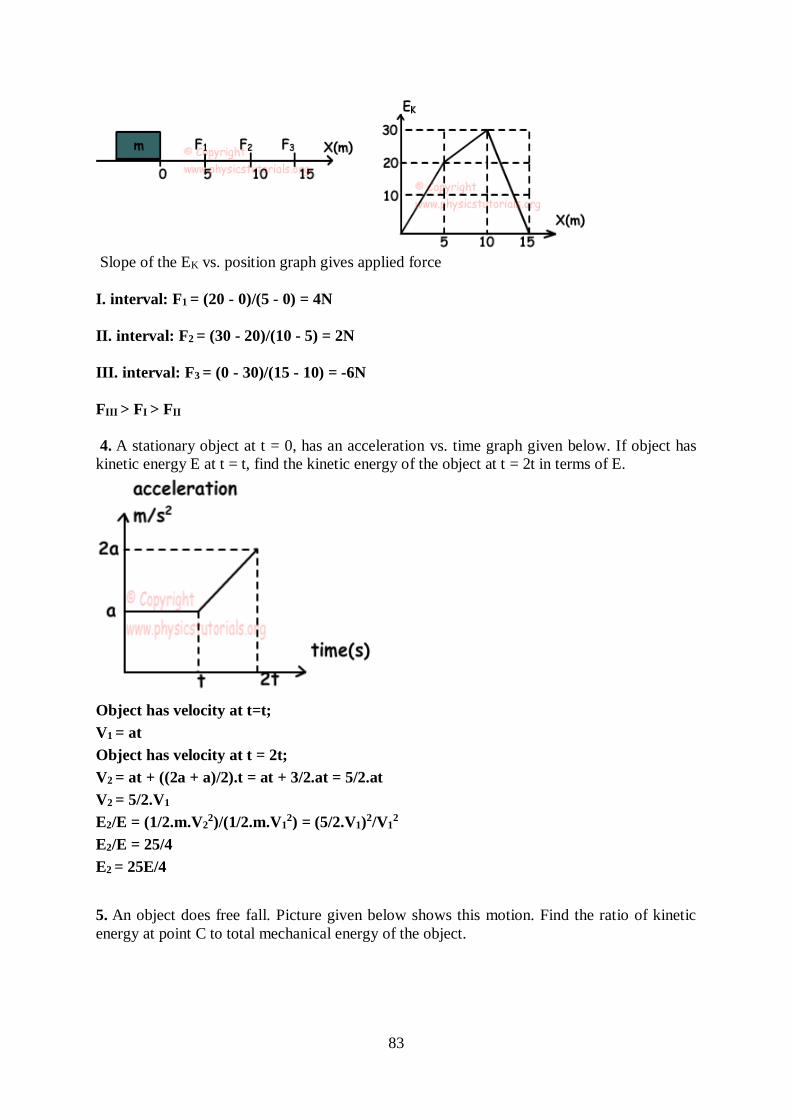
83

Slope of the EK vs. position graph gives applied force

I. interval: F1 = (20 - 0)/(5 - 0) = 4N

II. interval: F2 = (30 - 20)/(10 - 5) = 2N

III. interval: F3 = (0 - 30)/(15 - 10) = -6N

FIII > FI > FII

4. A stationary object at t = 0, has an acceleration vs. time graph given below. If object has

kinetic energy E at t = t, find the kinetic energy of the object at t = 2t in terms of E.

Object has velocity at t=t;

V1 = at

Object has velocity at t = 2t;

V2 = at + ((2a + a)/2).t = at + 3/2.at = 5/2.at

V2 = 5/2.V1

E2/E = (1/2.m.V22)/(1/2.m.V1

2) = (5/2.V1)2/V1

2

E2/E = 25/4

E2 = 25E/4

5. An object does free fall. Picture given below shows this motion. Find the ratio of kinetic

energy at point C to total mechanical energy of the object.

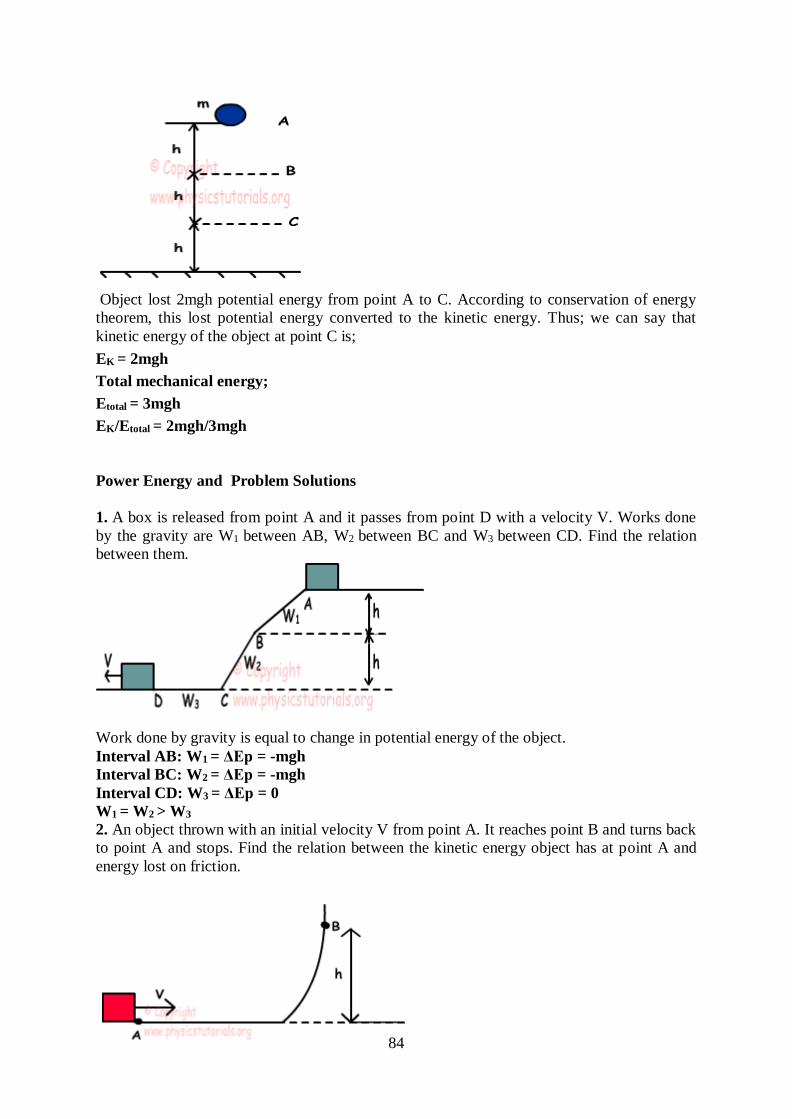
84

Object lost 2mgh potential energy from point A to C. According to conservation of energy

theorem, this lost potential energy converted to the kinetic energy. Thus; we can say that

kinetic energy of the object at point C is;

EK = 2mgh

Total mechanical energy;

Etotal = 3mgh

EK/Etotal = 2mgh/3mgh

Power Energy and Problem Solutions

1. A box is released from point A and it passes from point D with a velocity V. Works done

by the gravity are W1 between AB, W2 between BC and W3 between CD. Find the relation

between them.

Work done by gravity is equal to change in potential energy of the object.

Interval AB: W1 = ΔEp = -mgh

Interval BC: W2 = ΔEp = -mgh

Interval CD: W3 = ΔEp = 0

W1 = W2 > W3

2. An object thrown with an initial velocity V from point A. It reaches point B and turns back

to point A and stops. Find the relation between the kinetic energy object has at point A and

energy lost on friction.

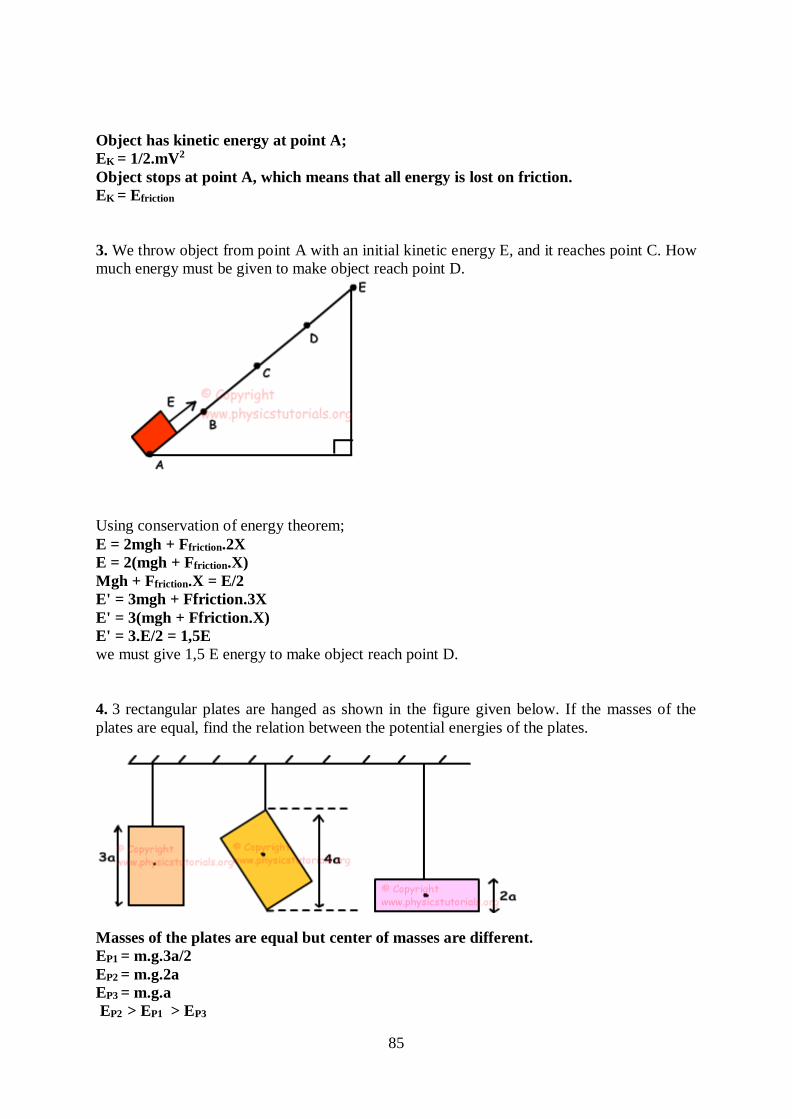
85

Object has kinetic energy at point A;

EK = 1/2.mV2

Object stops at point A, which means that all energy is lost on friction.

EK = Efriction

3. We throw object from point A with an initial kinetic energy E, and it reaches point C. How

much energy must be given to make object reach point D.

Using conservation of energy theorem;

E = 2mgh + Ffriction.2X

E = 2(mgh + Ffriction.X)

Mgh + Ffriction.X = E/2

E' = 3mgh + Ffriction.3X

E' = 3(mgh + Ffriction.X)

E' = 3.E/2 = 1,5E

we must give 1,5 E energy to make object reach point D.

4. 3 rectangular plates are hanged as shown in the figure given below. If the masses of the

plates are equal, find the relation between the potential energies of the plates.

Masses of the plates are equal but center of masses are different.

EP1 = m.g.3a/2

EP2 = m.g.2a

EP3 = m.g.a

EP2 > EP1 > EP3

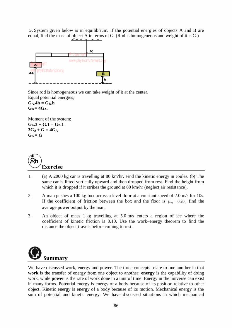
86

5. System given below is in equilibrium. If the potential energies of objects A and B are

equal, find the mass of object A in terms of G. (Rod is homogeneous and weight of it is G.)

Since rod is homogeneous we can take weight of it at the center.

Equal potential energies;

GA.4h = GB.h

GB = 4GA.

Moment of the system;

GA.3 + G.1 = GB.1

3GA + G = 4GA

GA = G

Exercise 1. (a) A 2000 kg car is travelling at 80 km/hr. Find the kinetic energy in Joules. (b) The

same car is lifted vertically upward and then dropped from rest. Find the height from

which it is dropped if it strikes the ground at 80 km/hr (neglect air resistance).

2. A man pushes a 100 kg box across a level floor at a constant speed of 2.0 m/s for 10s.

If the coefficient of friction between the box and the floor is 0.20k , find the

average power output by the man.

3. An object of mass 1 kg travelling at 5.0 m/s enters a region of ice where the

coefficient of kinetic friction is 0.10. Use the work–energy theorem to find the

distance the object travels before coming to rest.

Summary

We have discussed work, energy and power. The three concepts relate to one another in that

work is the transfer of energy from one object to another; energy is the capability of doing

work, while power is the rate of work done in a unit of time. Energy in the universe can exist

in many forms. Potential energy is energy of a body because of its position relative to other

object. Kinetic energy is energy of a body because of its motion. Mechanical energy is the

sum of potential and kinetic energy. We have discussed situations in which mechanical

87

energy is conserved. We have also learned that energy cannot be destroyed or created, but

just changed from one form to another. This is the law of conservation of energy.

References

Daniel Kleppner and Robert J. Kolenkow (2007). An Introduction to Mechanics.. Tata


Gottys, W., Keller, F.J. and Skove, M.J. (1989). Physics Classical and Modern,.

McGraw Hill.

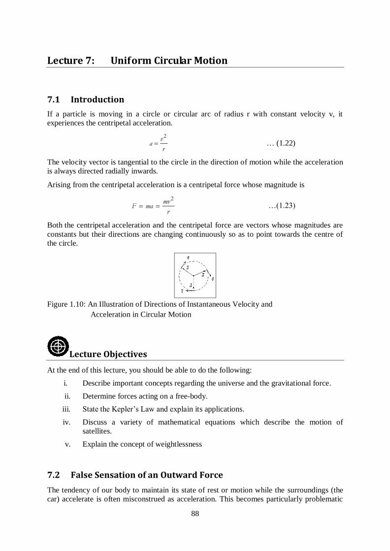
88

Lecture 7: Uniform Circular Motion

7.1 Introduction

If a particle is moving in a circle or circular arc of radius r with constant velocity v, it

experiences the centripetal acceleration.

2v

ar

… (1.22)

The velocity vector is tangential to the circle in the direction of motion while the acceleration

is always directed radially inwards.

Arising from the centripetal acceleration is a centripetal force whose magnitude is

2mv

F mar

…(1.23)

Both the centripetal acceleration and the centripetal force are vectors whose magnitudes are

constants but their directions are changing continuously so as to point towards the centre of

the circle.

Figure 1.10: An Illustration of Directions of Instantaneous Velocity and

Acceleration in Circular Motion

Lecture Objectives


i. Describe important concepts regarding the universe and the gravitational force.

ii. Determine forces acting on a free-body.

iii. State the Kepler’s Law and explain its applications.

iv. Discuss a variety of mathematical equations which describe the motion of

satellites.

v. Explain the concept of weightlessness

7.2 False Sensation of an Outward Force

The tendency of our body to maintain its state of rest or motion while the surroundings (the

car) accelerate is often misconstrued as acceleration. This becomes particularly problematic

89

when we consider the inertia experience of a passenger in a moving car and making the right-

hand turn.

Suppose as you continue driving and suddenly you have to make a sharp turn to the right at

constant speed. During the turn, the car travels in a circular-type path and sweeps out one-

quarter of a circle. The unbalanced force acting upon the turned wheels of the car cause an

unbalanced force upon the car and a subsequent acceleration. The unbalanced force and the

acceleration are both directed towards the centre of the circle about which the car is turning.

This is the centripetal force and acceleration. Your body, however, is in motion and tends to

stay in motion. It is the inertia of your body – the tendency to resist acceleration – which

causes it to continue in its forward motion. While the car is accelerating inward, you continue

in a straight line. If you are sitting on the passenger side of the car, then eventually the outside

door of the car will hit you as the car turns inward. This phenomenon might cause you to

think that you were being accelerated outwards away from the centre of the circle. In reality,

you are continuing in your straight-line inertial path tangent to the circle while the car is

accelerating out from under you.

The sensation of an outward force and an outward acceleration is a false sensation. There is

no physical object capable of pushing you outwards. You are merely experiencing the

tendency of your body to continue in its path tangent to the circular path along which the car

is turning.

Activity 6

1. A 900 kg car moving at 10 m/s takes a turn around a circle with radius R = 25.0

m. Determine the acceleration and the net force acting upon the car.

2. A 95 kg athlete makes a quarter circle turn in 2.1 seconds. If the radius of the

circle R = 12 m, determine the speed, acceleration and the net force acting upon

the athlete.

Example: A 900 kg car makes a 180 turn with a speed of 10.0 m/s. The radius of the circle

through which the car is turning is 25.0 m. Determine the force of friction and the coefficient

of friction acting upon the car.

Solution:

Known Information:

m = 900 kg, v = 10.0 m/s and R = 25.0 m

The mass of the object can be used to determine the force of gravity acting in the downward

direction.

gravF mg

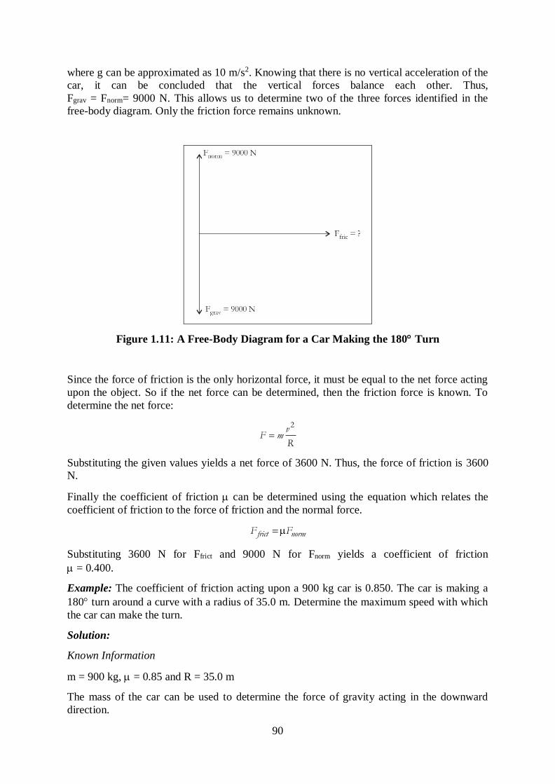
90

where g can be approximated as 10 m/s2. Knowing that there is no vertical acceleration of the

car, it can be concluded that the vertical forces balance each other. Thus,

Fgrav = Fnorm= 9000 N. This allows us to determine two of the three forces identified in the

free-body diagram. Only the friction force remains unknown.

Figure 1.11: A Free-Body Diagram for a Car Making the 180 Turn

Since the force of friction is the only horizontal force, it must be equal to the net force acting

upon the object. So if the net force can be determined, then the friction force is known. To

determine the net force:

2v

F mR

Substituting the given values yields a net force of 3600 N. Thus, the force of friction is 3600

N.

Finally the coefficient of friction can be determined using the equation which relates the

coefficient of friction to the force of friction and the normal force.

frict normF F

Substituting 3600 N for Ffrict and 9000 N for Fnorm yields a coefficient of friction

= 0.400.

Example: The coefficient of friction acting upon a 900 kg car is 0.850. The car is making a

180 turn around a curve with a radius of 35.0 m. Determine the maximum speed with which

the car can make the turn.

Solution:

Known Information

m = 900 kg, = 0.85 and R = 35.0 m

The mass of the car can be used to determine the force of gravity acting in the downward

direction.

91

Fgrav = m g

where g can be approximated as 10 m/s/s. Knowing that there is no vertical acceleration of

the car, it can be concluded that the vertical forces balance each other.

Thus,

Fgrav = Fnorm= 9000 N.

Since the coefficient of friction is given, the force of friction can be determined.

frict normF F

This allows us to determine all three forces identified in the free-body diagram. The net force

acting upon any object is the vector sum of all individual forces acting upon that object. Thus

if all individual force values are known (as is the case here), the net force can be calculated.

The vertical forces add to 0 N. Since the force of friction is the only horizontal force, it must

be equal to the net force acting upon the object. Thus,

Fnet = 7650 N

Once the net force is determined, the acceleration can be quickly calculated using the

equation:

Fnet = ma

Substituting the given values yields an acceleration of 7.65 m/s2. Finally, the speed at which

the car could travel around the turn can be calculated using the equation for centripetal

acceleration:

2v

aR

Substituting the known values for a and R into this equation and solving algebraically yields

a maximum speed of 16.4 m/s.

7.3 The Universe and the Gravitational Force

The following section discusses important concepts regarding the universe and the

gravitational force.

Structure of the Universe

Starting at home on planet Earth our immediate neighbours are the planets Mars and Venus.

Next nearest neighbours are planets Jupiter and Mercury. There are four other planets which

revolve around the Sun. This is our Solar system at the centre of which is the Sun.

Beyond the solar system, we have a collection of stars, 100s of millions which together form

the Milky Way Galaxy.

The Milky Way galaxy is disc-shaped and our Sun is 26,000 light years from its centre.

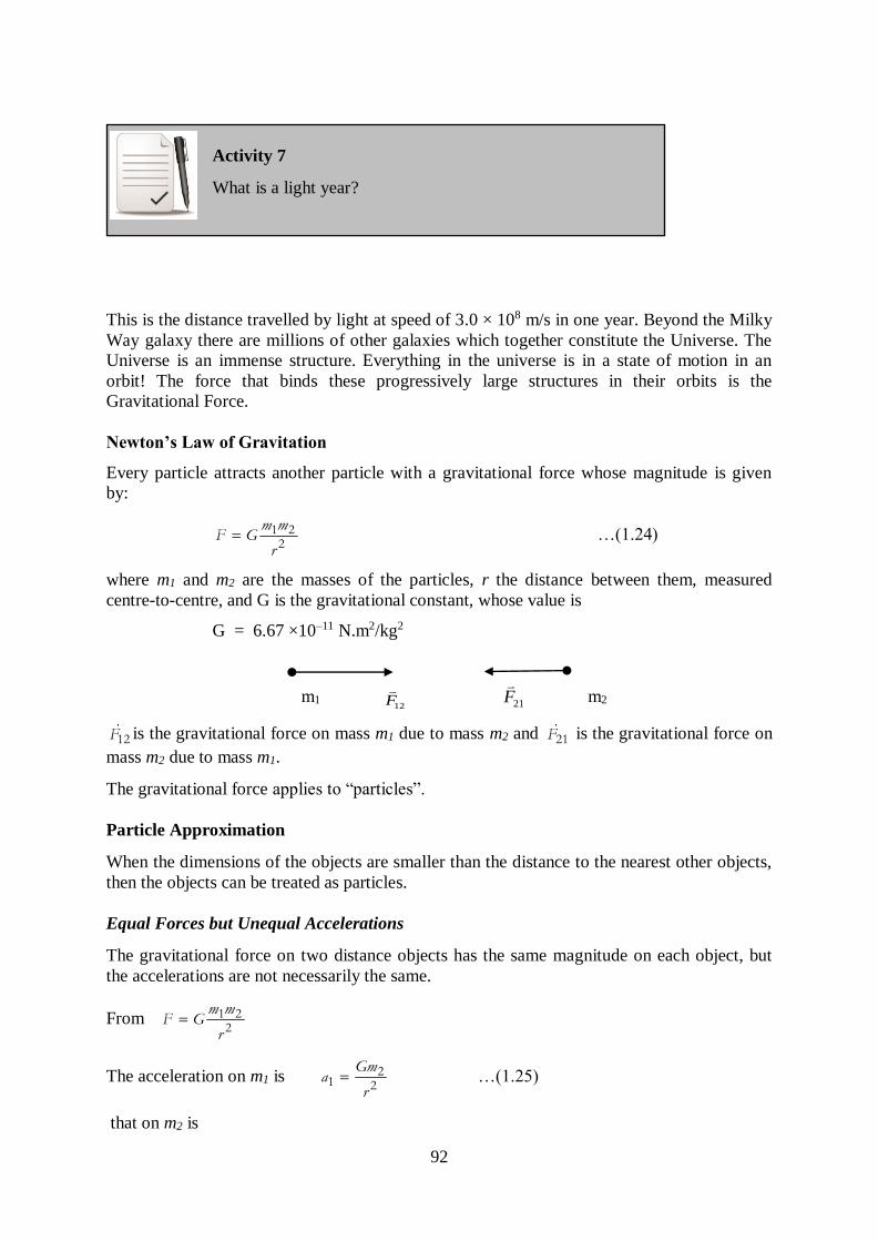
92

Activity 7

What is a light year?

This is the distance travelled by light at speed of 3.0 × 108 m/s in one year. Beyond the Milky

Way galaxy there are millions of other galaxies which together constitute the Universe. The

Universe is an immense structure. Everything in the universe is in a state of motion in an

orbit! The force that binds these progressively large structures in their orbits is the

Gravitational Force.

Newton’s Law of Gravitation

Every particle attracts another particle with a gravitational force whose magnitude is given

by:

1 22

m mF G

r …(1.24)

where m1 and m2 are the masses of the particles, r the distance between them, measured

centre-to-centre, and G is the gravitational constant, whose value is

G = 6.67 ×10–11 N.m2/kg2

m1 12F

21F

m2

12F is the gravitational force on mass m1 due to mass m2 and 21F is the gravitational force on

mass m2 due to mass m1.

The gravitational force applies to “particles”.

Particle Approximation

When the dimensions of the objects are smaller than the distance to the nearest other objects,

then the objects can be treated as particles.

Equal Forces but Unequal Accelerations

The gravitational force on two distance objects has the same magnitude on each object, but

the accelerations are not necessarily the same.

From 1 22

m mF G

r

The acceleration on m1 is 21 2

Gma

r …(1.25)

that on m2 is

93

12 2

Gma

r …(1.26)

Gravitation and the Principle of Superposition

Given a group of particles, the gravitational force exerted on any one of the particles is the

vector sum of the individual gravitational forces on the particle.

For n interacting particles, the net force on particle 1:

1 12 13 1............... nF F F F

where 12F is the gravitational force on particle 1 due to particle 2, etc.

or simply:

1 1

2

n

i

i

F F …(1.27)

Example: Determine the force of gravitational attraction between the Earth (m = 5.98 × 1024

kg) and a 70 kg student if

(a) the student is standing at sea level, a distance of 6.37 × 106 m from the Earth’s centre

and

(b) the student is in an airplane at 40,000 feet above Earth’s surface. This would place the

student a distance of 6.38 × 106 m from Earth’s centre.

Solution:

(a) The solution of the problem involves substituting known values of G = 6.67 × 10–11

Nm2/kg2, m1 = 5.98 × 1024 kg, m2 = 70 kg and r = 6.37 × 106 m into the universal

gravitation equation and solving for Fgrav. The solution is as follows:

11 24

6 2

6.67 10 5.98 10 70688.1

6.37 10 6.37 10gravF N

(b) The solution of the problem involves substituting known values of G = 6.67 × 10–11

Nm2/kg2, m1 = 5.98 × 1024 kg, m2 = 70 kg) and r = 6.38 × 106 m into the universal

gravitation equation and solving for Fgrav. The solution is as follows:

11 24

2 2

6.67 10 5.98 10 70685.9

6.38 10 6.38 10gravF N

Two general conceptual comments can be made about the results of the two worked solutions

above. First, observe that the force of gravity acting upon the student is less on an airplane at

40,000 feet than at sea level. This illustrates the inverse relationship between separation

distance and the force of gravity (or in this case, the weight of the student). The student

weighs less at the higher altitude. However, a mere change of 40,000 feet further from the

centre of the Earth is virtually negligible. This altitude change altered the student's weight by

3N, which is less than 1% of the original weight. A distance of 40,000 feet (from the Earth’s

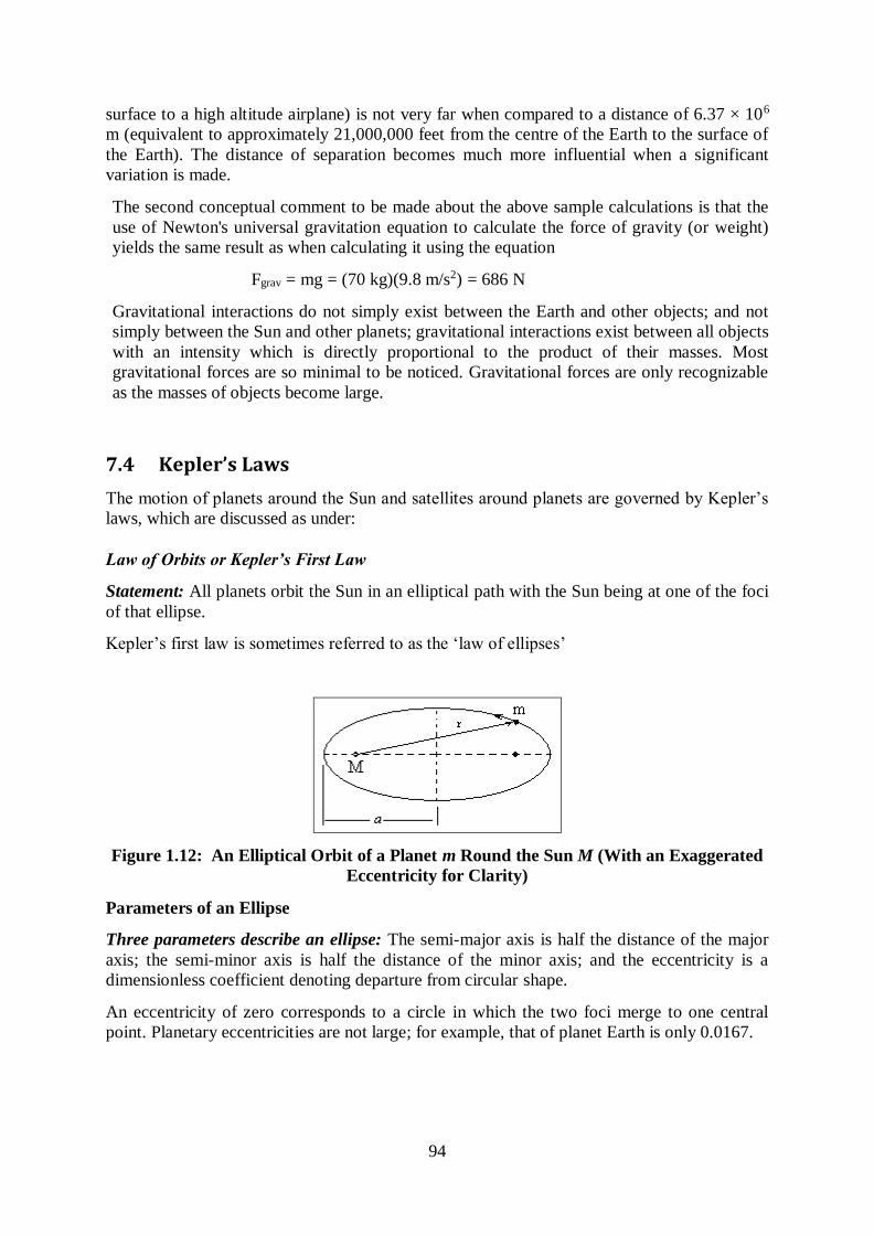
94

surface to a high altitude airplane) is not very far when compared to a distance of 6.37 × 106

m (equivalent to approximately 21,000,000 feet from the centre of the Earth to the surface of

the Earth). The distance of separation becomes much more influential when a significant

variation is made.

The second conceptual comment to be made about the above sample calculations is that the

use of Newton's universal gravitation equation to calculate the force of gravity (or weight)

yields the same result as when calculating it using the equation

Fgrav = mg = (70 kg)(9.8 m/s2) = 686 N

Gravitational interactions do not simply exist between the Earth and other objects; and not

simply between the Sun and other planets; gravitational interactions exist between all objects

with an intensity which is directly proportional to the product of their masses. Most

gravitational forces are so minimal to be noticed. Gravitational forces are only recognizable

as the masses of objects become large.

7.4 Kepler’s Laws

The motion of planets around the Sun and satellites around planets are governed by Kepler’s

laws, which are discussed as under:

Law of Orbits or Kepler’s First Law

Statement: All planets orbit the Sun in an elliptical path with the Sun being at one of the foci

of that ellipse.

Kepler’s first law is sometimes referred to as the ‘law of ellipses’

Figure 1.12: An Elliptical Orbit of a Planet m Round the Sun M (With an Exaggerated

Eccentricity for Clarity)

Parameters of an Ellipse

Three parameters describe an ellipse: The semi-major axis is half the distance of the major

axis; the semi-minor axis is half the distance of the minor axis; and the eccentricity is a

dimensionless coefficient denoting departure from circular shape.

An eccentricity of zero corresponds to a circle in which the two foci merge to one central

point. Planetary eccentricities are not large; for example, that of planet Earth is only 0.0167.

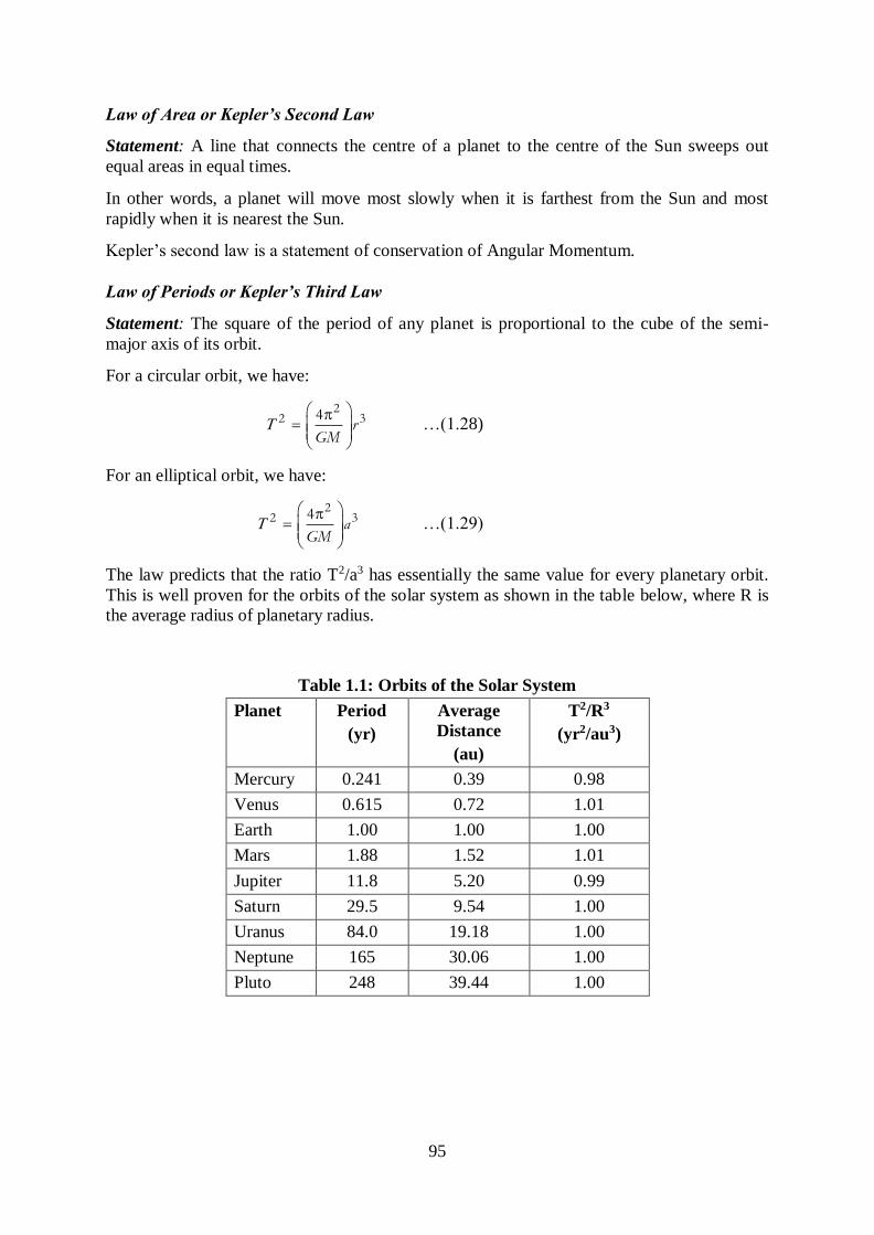
95

Law of Area or Kepler’s Second Law

Statement: A line that connects the centre of a planet to the centre of the Sun sweeps out

equal areas in equal times.

In other words, a planet will move most slowly when it is farthest from the Sun and most

rapidly when it is nearest the Sun.

Kepler’s second law is a statement of conservation of Angular Momentum.

Law of Periods or Kepler’s Third Law

Statement: The square of the period of any planet is proportional to the cube of the semi-

major axis of its orbit.

For a circular orbit, we have:

22 34

rGM

…(1.28)

For an elliptical orbit, we have:

22 34

aGM

…(1.29)

The law predicts that the ratio T2/a3 has essentially the same value for every planetary orbit.

This is well proven for the orbits of the solar system as shown in the table below, where R is

the average radius of planetary radius.

Table 1.1: Orbits of the Solar System

Planet Period

(yr)

Average

Distance

(au)

T2/R3

(yr2/au3)

Mercury 0.241 0.39 0.98

Venus 0.615 0.72 1.01

Earth 1.00 1.00 1.00

Mars 1.88 1.52 1.01

Jupiter 11.8 5.20 0.99

Saturn 29.5 9.54 1.00

Uranus 84.0 19.18 1.00

Neptune 165 30.06 1.00

Pluto 248 39.44 1.00

96

Take Note

The average distance is given in astronomical units where 1 au is equal to the distance

from the Earth to the Sun which is 1.4957 × 1011 m. The orbital period is given in units

of Earth-years where 1 Earth-year is the time required for the Earth to orbit the Sun,

3.156 × 107 seconds.

The equivalence of the ratio T2/a3 among planets has consequently leaded to Kepler’s third

law being sometimes referred to as the Law of Harmonies.

7.5 Planetary and Satellite Motion

The motion of objects is governed by Newton's laws. The same simple laws which govern the

motion of objects on Earth also extend to the heavens to govern the motion of planets, moons,

and other satellites. In this section, we will be concerned with the variety of mathematical

equations which describe the motion of satellites.

Consider a satellite with mass Msat orbiting a central body with a mass, m = MCentral. The

central body could be a planet, the Sun or some other large mass capable of causing sufficient

acceleration on a less massive nearby object. If the satellite moves in a circular motion, then

the net centripetal force acting upon this orbiting satellite is given by the relationship

2

satnet

M vF

R

This net centripetal force is the result of the gravitational force which attracts the satellite

towards the central body and can be represented as:

2

sat centralgrav

GM MF

R

Since Fgrav = Fnet, the above expressions for centripetal force and gravitational force are

equal. Thus,

2

2sat sat centralM v GM M

R R

2 centralGMv

R

The velocity of a satellite moving about a central body in circular motion is given by:

centralGMv

R

where G = 6.67 × 10–11 N m2/kg2, Mcentral = the mass of the central body about which the

satellite orbits, and R = the radius of orbit for the satellite.

http://www.physicsclassroom.com/Class/circles/U6l1e.html

http://www.physicsclassroom.com/Class/circles/U6l3c.html

97

Similar reasoning can be used to determine an equation for the acceleration of our satellite

that is expressed in terms of masses and radius of orbit. The acceleration of a satellite is equal

to the acceleration of gravity of the satellite at whatever location which is given by:

2centralGM

gR

Thus, the acceleration of a satellite in a circular motion about some central body is given by

the following equation:

2centralGM

aR

…(1.30)

where G = 6.67 × 10–11 Nm2/kg2, Mcentral = the mass of the central body about which the

satellite orbits, and R = the average radius of orbit for the satellite. The final equation which

is useful in describing the motion of satellites is Newton's form of Kepler's third law.

Consider a planet with mass Mplanet orbiting in nearly circular motion around the Sun of mass

MSun. The net centripetal force acting upon this orbiting planet is given by the relationship

2planet

net

M vF

R

This net centripetal force is the result of the gravitational force which attracts the planet

towards the Sun and can be represented as:

2

planet sungrav

GM MF

R …(1.31)

Since Fgrav = Fnet, the above expressions for centripetal force and gravitational force are equal.

Thus,

2

2

planet planet sunM v GM M

R R …(1.32)

Since the velocity of an object in nearly circular orbit can be approximated as

2 R

vT

…(1.33)

2 22

2

4 Rv

T

Substitution of the expression for v2 into the equation (1.32) above yields,

2

2 2

4planet planet sunM R GM M

T R

By cross-multiplication, the equation can be transformed into

22

3

4planet

planet sun

MT

GM MR

98

Which upon simplification yields

2 2

3

4

sun

T

GMR …(134)

The right side of the above equation will be the same value for every planet regardless of the

planet's mass. Subsequently, it is reasonable that the T2/R3 ratio would be the same value for

all planets if the force which holds the planets in their orbits is the force of gravity. Newton's

universal law of gravitation provided a theoretical explanation for Kepler's Law of

Harmonies.

Hence, the period of a satellite (T) and the mean distance from the central body (R) are

related by the following equation:

2 2

3

4

central

T

GMR .... (vi)

where T = the period of the satellite, R = the average radius of orbit for the satellite (distance

from centre of central planet), and G = 6.67 × 10–11 Nm2/kg2.

There is an important concept evident in all three of these equations – the period [Equation

(13.5)], speed [Equation (1.33)] and the acceleration [Equation (130)] of an orbiting satellite

are not dependent upon the mass of the satellite.

centralGMv

R

2centralGM

aR

2 2

3

4

central

T

GMR

To illustrate the usefulness of the above equations, consider the following worked examples.

Example: A satellite wishes to orbit the Earth at a height of 100 km (approximately 60 miles)

above the surface of the Earth. Determine the speed, acceleration and orbital period of the

satellite. (Given: Mearth = 5.98 × 1024 kg, Rearth = 6.37 × 106 m)

Solution:

Given data:

R = rearth + height = 6.47 × 106 m, Mearth = 5.98 × 1024 kg and G = 6.67 × 10-11 N m2/kg2

Note that the radius of a satellite's orbit can be found from the knowledge of the Earth’s

radius and the height of the satellite above the Earth.

As shown in the diagram at the right, the radius of orbit for a satellite is equal to the sum of

the Earth’s radius and the height above the Earth. These two quantities can be added to yield

the orbital radius. In this problem, the 100 km must first be converted to 1,00,000 m before

being added to the radius of the Earth. The equations needed to determine the unknown are

those which are listed above. We will begin by determining the orbital speed of the satellite

using the following equation:

/Centralv GM R

which upon substitution yields

99

v = 6.16 × 107 m/s

The acceleration can be found from either one of the following equations (1.30) or from

2 /a v R

Either equation can be used to calculate the acceleration and yields

a = 9.53 m/s2

Observe that this acceleration is slightly less than the 9.8 m/s2 value expected on Earth’s

surface. The increased distance from the centre of the Earth lowers the value of g.

Finally, the period can be calculated using Equation (1.35) and yields:

T = 5177 s = 1.44 hrs

Example: The period of the Moon is approximately 27.2 days (2.35 × 106 s). Determine the

radius of the Moon's orbit and the orbital speed of the Moon. (Given: Mearth = 5.98 × 1024 kg,

Rearth = 6.37 × 106 m)

Solution:

Given data

T = 2.35 × 106 s, Mearth = 5.98 × 1024 kg and G = 6.67 × 10-11 N m2/kg2

The radius of orbit can be calculated Equation (1.33):

R3 = 5.58 × 1025 m3

By taking the cube root of 5.58 × 1025 m3, the radius can be determined to be:

R = 3.82 × 108 m

The orbital speed of the satellite can be computed from Equation (1.33) which upon

substitution yields

v = 1.02 × 103 m/s

Example: A geosynchronous satellite is a satellite which remains above the same point on the

Earth. A geosynchronous satellite orbits the Earth with an orbital period of 24 hours, thus

matching the period of the Earth’s rotational motion. If a satellite has to orbit the Earth at the

equator in 24 hours (86400 s), then how high above the Earth’s surface must it be located?

(Given: Mearth = 5.98 × 1024 kg, Rearth = 6.37 × 106 m).

Solution

Given data

T = 86400 s, Mearth = 5.98 × 024 kg, Rearth = 6.37 × 106 m and G = 6.67 ×10–11 N m2/kg2.

The radius of orbit can be found using Eq.(vi) which upon substitution yields:

R3 = [((86400 s)2 × (6.67 × 0–11 N m2/kg2) × (5.98×024 kg) ) / (4× (3.1415)2)]

R3 = 7.54 ×1022 m3.

By taking the cube root of 7.54 ×1022 m3, the radius becomes R = 4.23 × 107 m.

100

The radius of orbit indicates the distance which the satellite is from the centre of the Earth.

Now that the radius of orbit has been found, the height above the Earth can be calculated.

Since the Earth’s surface is 6.37 × 106 m from its centre (that's the radius of the Earth), the

satellite must be a height of

4.23 ×107 m – 6.37 × 106 m = 3.59 × 107 m

above the surface of the Earth. So the height of the satellite is 3.59 × 107 m.

7.6 Weightlessness

Weightlessness is simply a sensation experienced by an individual when there are no external

objects touching one's body and exerting a push or pull upon it. Weightless sensations exist

when all contact forces are removed. These sensations are common to any situation in which

you are momentarily (or perpetually) in a state of free fall. When in free fall, the only force

acting upon your body is the force of gravity – a non-contact force.

Weightlessness is only a sensation; it is not a reality corresponding to an individual who has

lost weight.

Earth-orbiting astronauts are weightless because there is no external contact force pushing or

pulling upon their body. Gravity is the only force acting upon their body. Being an action-at-

a-distance force, it cannot be felt and, therefore, would not provide any sensation of their

weight.

It is the force of gravity which supplies the centripetal force requirement to allow the inward

acceleration which is characteristic of circular motion. The force of gravity is the only force

acting upon their body. The astronauts are in free-fall. The astronauts and all their

surroundings, i.e. the space shuttle with its contents are falling towards the Earth without

colliding into it. Their tangential velocity allows them to remain in orbital motion while the

force of gravity pulls them inward.

Activity 8

David stands on a bathroom scale and reads the scale while in an elevator

ascending and descending a tall building. David weighs 1000 N, but notices

that the scale readings depend on what the elevator is doing. Use a free-

body diagram and Newton's second law of motion to solve the following

problems.

(a) What is the scale reading when David accelerates upwards at 0.50

m/s2?

(b) What is the scale reading when David is travelling upward at a

constant velocity of at 2 m/s?

(c) As David approaches the top of the building, the elevator slows

down at a rate of 0.50 m/s2. What does the scale read?

101

Exercise 1. A bicycle wheel of radius r = 1.5m starts from rest and rolls 100m without slipping in

30s. Calculate:

(a) The number of revolutions the wheel makes

(b) The number of radians through which it turns

(c) The average angular velocity.

2. The escape velocity of any object is the speed it must achieve to escape the

gravitational pull of the Earth. Calculate the escape velocity for an object of mass m.

3. What is the relationship between the radius of orbit of a satellite mass m and its

period?

4. What is the gravitational field (in N/kg) 2.74 Earth radii above the Earth's surface?

5. What is the gravitational field (in N/kg) 4027 km above a planet with a mass of 7.04 x

1022 kg and a radius of 1.84 x 106 m?

6. An astronaut standing on the surface of the moon launches a projectile straight up

from the surface. What should the initial speed (in m/s) of the projectile be so that it

will reach a height of 1.99 x 106m above the moon's surface? (The moon's mass is

7.35 x 1022 kg and its radius is 1.74 x 106 m.)

7. What is the escape velocity (in m/s) from a planet with a radius of 1.81 x 106 m and a

mass of 7.23 x 1022 kg?

8. How much work (in kJ) is done lifting a 267 kg payload from the Earth's surface to a

height of 17.3 m above the Earth's surface? (The mass of the Earth is 5.98 x 1024 kg

and the Earth's radius is 6.38 x 106 m.)

9. How much work (in MJ) is done to raise a 370 kg payload from Earth's surface to a

height of 4.18 x 106 m above the Earth's surface? (The mass of the Earth is 5.98 x

1024 kg and the Earth's radius is 6.38 x 106 m.)

10. A brick dropped from a roof hits the ground 3.92 seconds later. How high (in m) was

the roof?

11. A ball was thrown straight up at 25.5 m/s then caught at the same place it was

released. How many seconds was it in the air?

12. How high above its release point did the ball in the previous question go?

13. A stone is thrown straight up. To reach a height of 3.18 m above its release point,

what must its initial speed be in m/s?

14. A stone is thrown straight up at 7.05 m/s. What is the stone's acceleration in m/s/s at

the top of its rise?

15. The moon has an orbital period of 27.3 days and a mean distance of 3.80 x 105 km

from the center of the Earth. Find the distance (km) an artificial satellite is from the

center of Earth if its period is91.5 minutes.

102

16. A planet has two moons. the first is 4 times as far from the center of the planet as the

second and has a mass that is 3 times the mass of the second. What is the ratio of the

gravitational force on the first planet to the gravitational force on the second?

17. Two spherical balls are placed so their centers are 3.70 m apart. The force between

them is 2.46 x 10-8 N. If the mass of the smaller ball is 74.0 kg, what is the mass of the

other ball?

18. How far (in km) from the center of the Earth would a person with a weight of 762 N

on Earth have to be to have a weight of 52.2 N?

19. A 36.0 kg child is sitting on a merry-go-round with a radius of 4.00 m. The time it

takes the merry-go-round to make one revolution is 3.04 s. Find the centripetal

acceleration of the child.

Summary

In this lecture we have discussed motion of a particle in a circular motion, including the

concepts centripetal acceleration and centripetal force. We have discussed the sensation of an

outward force and an outward acceleration as false sensations; and some important concepts

regarding the universe and the gravitational force. We have also learned that the same simple

laws which govern the motion of objects on Earth also extend to the heavens to govern the

motion of planets, moons, and other satellites.

References




McGraw Hill.


Redish, E.F. (2003). Teaching Introductory Physics with the Physics Suite. John

Wiley & Sons.



Rogers Muncaster, A-Level Physics, 4th Edition. Oxford Press.

103

Lecture 8: Fluid Dynamics

8.1 Introduction

A fluid is a substance that can flow. A fluid conforms to the boundaries of any container in

which it is put. In other words, a fluid cannot support a shearing stress.

Whereas in the discussion of the mechanics of solids physical quantities of use are mass and

force, in the discussion of the mechanics of fluids the physical quantities of use are density

and pressure.

Lecture Objectives


i. Define fluid and discuss its mechanics.

ii. Determine forces acting on a floating object.

iii. Describe the Pascal’s principle and its application.

Density

By definition, the density of a substance is given by

m

V … (1.36)

where m is the mass and V the volume. Density is a scalar quantity. Whereas the density of

gases varies considerably with pressure the density of liquids does not. Hence gases are said

to be compressible whereas liquids are not.

Pressure

By definition the pressure exerted by the fluid is given by:

F

A …(1.37)

where F is the force exerted over an area A.

Pressure is a scalar quantity even though the force is a vector quantity. Pressure has no

directional properties.

The SI unit of pressure is the Pascal (Pa)

1 Pa = 1 N/m2

The Pascal is a small unit, such that

1 atm = 1.01 × 105 Pa

104

Tyre pressure gauges are calibrated in kilo Pascals.

8.2 Fluids at Rest

For a mountaineer the pressure decreases with altitude while for a diver, the pressure

increases with depth. The pressure encountered by the mountaineer and the diver is called

Hydrostatic pressure.

For a diver, at a depth h, the pressure experienced is given by:

P = Po + gh …(1.38)

Where Po is the surface pressure (atmospheric), is the density of water, g acceleration due

to gravity and h the distance below surface.

The term gh is called the Gauge pressure.

The pressure at a given depth depends on that depth and not on any horizontal dimension.

For a mountaineer, the pressure at a height h is given by

P = Po – gh …(1.39)

The Gauge pressure is in this case is negative.

Pascal’s Principle

‘A change in the pressure applied to an enclosed fluid is transmitted undiminished to every

portion of the fluid and to the walls of the containing vessel.’ The everyday practice of

squeezing one end of toothpaste is a demonstration of Pascal’s principle.

8.3 Hydraulic Lever

Consider the device shown in Figure 1.13, in which piston A is the input and B is the output.

Figure 1.13: The Hydraulic Lever

Piston A has cross-sectional area Ai and B has cross-sectional area Ao. The device is filled

with an incompressible fluid.

When a force Fi is applied on piston A, an upward force Fo is exerted on piston B. In order to

keep the system in equilibrium a load must exert a downward force Fo on B.

The force Fi and the load Fo produce a change of pressure

105

i o

i o

F F

A A

oo i

i

AF F

A …(1.40)

Under the conditions that Ao > Ai, then Fo > Fi.

Hence a small force Fi lifts a heavier load Fo.

Relative Distances

If the input piston is moved downward a distance di then the output piston is moved upwards

a distance do such that the same volume of the incompressible fluid is displaced at both

pistons.

Volume displaced in A = di Ai

Volume displaced in B = do Ao

io i

o

Ad d

A …(1.41)

If Ao > Ai then do < di. In other words, the smaller piston moves through a longer distance in

comparison with the distance covered by the larger piston.

Work Done

From Equation 1.40 and 1.41 we can write the output work as:

i o io o i i i

i o

F A AW F d d F d

A A …(1.36)

which shows that the work W on A by the applied force is equal to the work done by the

output piston in lifting the load placed on it.

8.4 Equilibrium of Floating Objects

Two forces act on a floating object. The weight acts downwards and the buoyant force acts

upwards. The two forces need not necessarily act at the same point. The weight acts at the

centre of mass whereas the buoyant force acts at the control of buoyancy, a fictitious point in

the water.

Hence, torques must play a role in the equilibrium of floating objects.

If the floating object is tilted by a small angle from its equilibrium position, the location of

the centre of buoyancy changes. For the floating object to be in stable equilibrium, the centre

of buoyancy must shift in such a way that the buoyant force and the weight provide a

restoring torque so that the object returns to its original upright position.

If the torque acts in the opposite direction the floating objects will tilt farther and eventually

tip over.

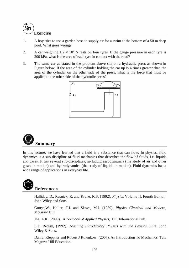
106

Exercise 1. A boy tries to use a garden hose to supply air for a swim at the bottom of a 50 m deep

pool. What goes wrong?

2. A car weighing 1.2 × 104 N rests on four tyres. If the gauge pressure in each tyre is

200 kPa, what is the area of each tyre in contact with the road?

3. The same car as stated in the problem above sits on a hydraulic press as shown in

Figure below. If the area of the cylinder holding the car up is 4 times greater than the

area of the cylinder on the other side of the press, what is the force that must be

applied to the other side of the hydraulic press?

Summary

In this lecture, we have learned that a fluid is a substance that can flow. In physics, fluid

dynamics is a sub-discipline of fluid mechanics that describes the flow of fluids, i.e. liquids

and gases. It has several sub-disciplines, including aerodynamics (the study of air and other

gases in motion) and hydrodynamics (the study of liquids in motion). Fluid dynamics has a

wide range of applications in everyday life.

References



Gottys,W., Keller, F.J. and Skove, M.J. (1989). Physics Classical and Modern,

McGraw Hill.


E.F. Redish, (1992). Teaching Introductory Physics with the Physics Suite. John

Wiley & Sons.

Daniel Kleppner and Robert J Kolenkow, (2007). An Introduction To Mechanics. Tata


107

SECTION THREE:

ELECTROSTATICS AND ELECTRIC CIRCUITS

Lecture 9: Electrostatics

9.1 Introduction

Every object in our visible and tangible world contains an enormous amount of electric

charge. However, this fact is hidden because the object contains equal amounts of positive

and negative charges. With such an equality of charge the object is said to be electrically

neutral. If the two charges are not in balance, then there is a net charge that can interact with

other objects. We say an object is charged when such an object has charge imbalance.

Charged objects interact by exerting forces on one another. Like charges repel each other and

unlike charges attract each other.

The attraction and repulsion between charged bodies has many industrial applications including

electrostatic paint-spraying, non-impact inkjet printing and photocopying. In this lecture, we

shall study the basic law of force of electrostatic charges, the electrostatic field created by

electric charges and the basic application of electrostatic field in the capacitor.

Lecture Objectives

At the end of this lecture, you should be able to:

i. Define an electric point charge

State and apply Coulomb’s law

Define the electric field and compute the electric field due to point charges

Define the electric potential energy and compute the electric potential energy due to point

charges

Define capacitance and compute the capacitance due to a parallel plate capacitor

Compute equivalent capacitance due to series and parallel combinations

Compute energy stored in a capacitor

Manipulate RC electric circuits

Compute power in alternating current circuits

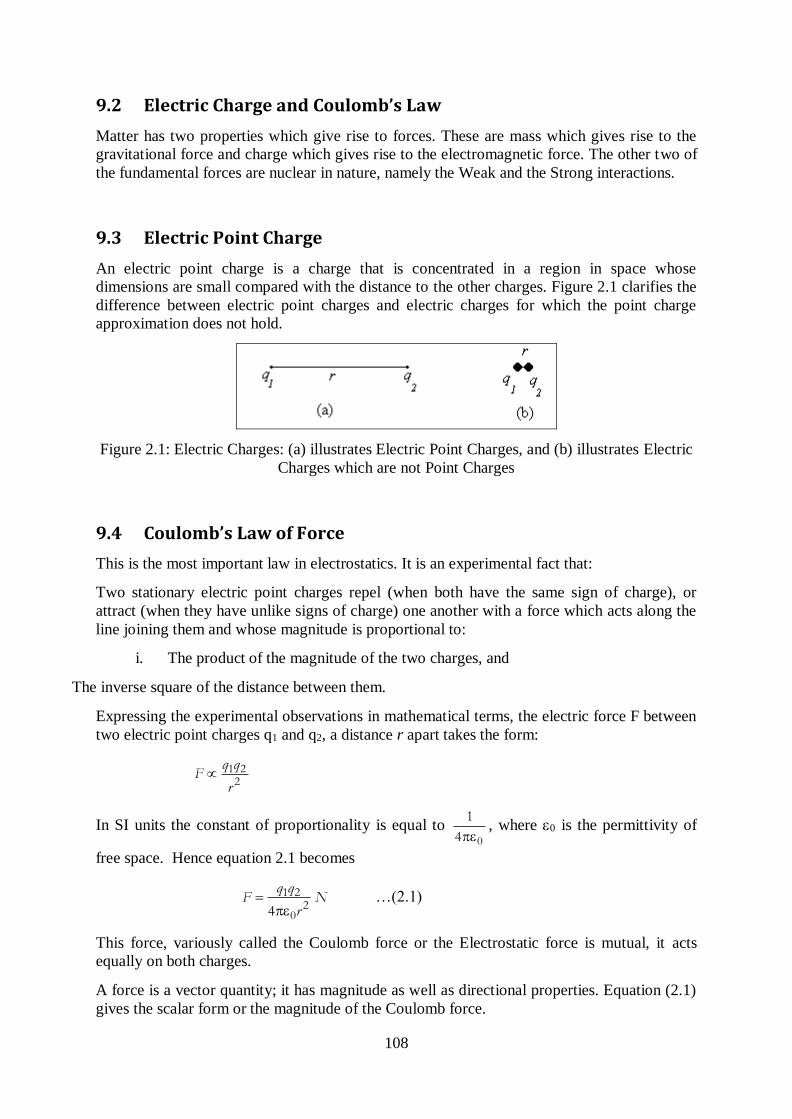
108

9.2 Electric Charge and Coulomb’s Law

Matter has two properties which give rise to forces. These are mass which gives rise to the

gravitational force and charge which gives rise to the electromagnetic force. The other two of

the fundamental forces are nuclear in nature, namely the Weak and the Strong interactions.

9.3 Electric Point Charge

An electric point charge is a charge that is concentrated in a region in space whose

dimensions are small compared with the distance to the other charges. Figure 2.1 clarifies the

difference between electric point charges and electric charges for which the point charge

approximation does not hold.

Figure 2.1: Electric Charges: (a) illustrates Electric Point Charges, and (b) illustrates Electric

Charges which are not Point Charges

9.4 Coulomb’s Law of Force

This is the most important law in electrostatics. It is an experimental fact that:

Two stationary electric point charges repel (when both have the same sign of charge), or

attract (when they have unlike signs of charge) one another with a force which acts along the

line joining them and whose magnitude is proportional to:

i. The product of the magnitude of the two charges, and

The inverse square of the distance between them.

Expressing the experimental observations in mathematical terms, the electric force F between

two electric point charges q1 and q2, a distance r apart takes the form:

1 22

q qF

r

In SI units the constant of proportionality is equal to 0

1

4, where 0 is the permittivity of

free space. Hence equation 2.1 becomes

1 22

04

q qF N

r …(2.1)

This force, variously called the Coulomb force or the Electrostatic force is mutual, it acts

equally on both charges.

A force is a vector quantity; it has magnitude as well as directional properties. Equation (2.1)

gives the scalar form or the magnitude of the Coulomb force.

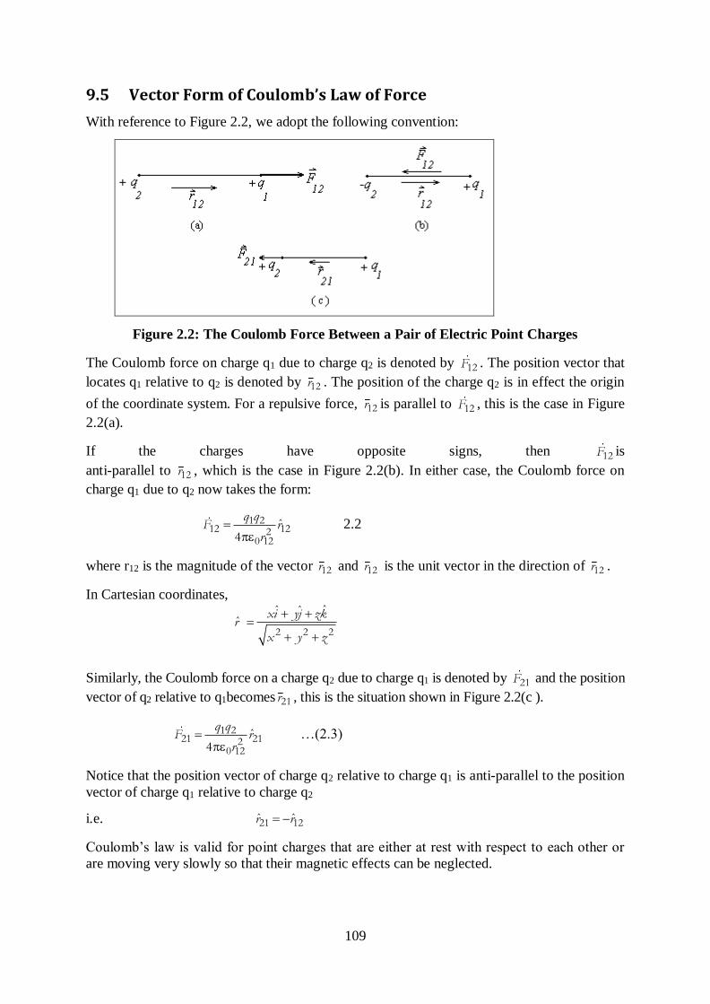
109

9.5 Vector Form of Coulomb’s Law of Force

With reference to Figure 2.2, we adopt the following convention:

Figure 2.2: The Coulomb Force Between a Pair of Electric Point Charges

The Coulomb force on charge q1 due to charge q2 is denoted by 12F . The position vector that

locates q1 relative to q2 is denoted by 12r . The position of the charge q2 is in effect the origin

of the coordinate system. For a repulsive force, 12r is parallel to 12F , this is the case in Figure

2.2(a).

If the charges have opposite signs, then 12F is

anti-parallel to 12r , which is the case in Figure 2.2(b). In either case, the Coulomb force on

charge q1 due to q2 now takes the form:

1 212 122

0 12

ˆ4

q qF r

r 2.2

where r12 is the magnitude of the vector 12r and 12r is the unit vector in the direction of 12r .

In Cartesian coordinates,

2 2 2

ˆˆ ˆˆ

xi yj zkr

x y z

Similarly, the Coulomb force on a charge q2 due to charge q1 is denoted by 21F and the position

vector of q2 relative to q1becomes 21r , this is the situation shown in Figure 2.2(c ).

1 221 212

0 12

ˆ4

q qF r

r …(2.3)

Notice that the position vector of charge q2 relative to charge q1 is anti-parallel to the position

vector of charge q1 relative to charge q2

i.e. 21 12ˆ ˆr r

Coulomb’s law is valid for point charges that are either at rest with respect to each other or

are moving very slowly so that their magnetic effects can be neglected.

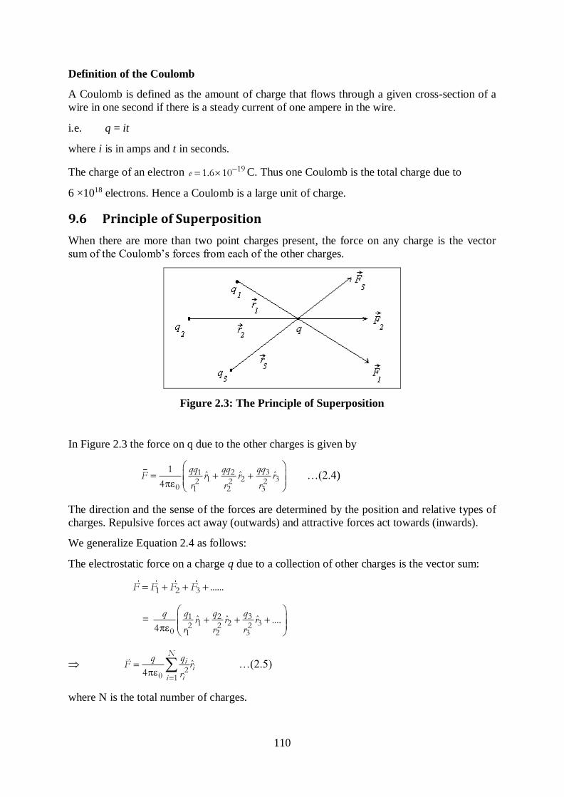
110

Definition of the Coulomb

A Coulomb is defined as the amount of charge that flows through a given cross-section of a

wire in one second if there is a steady current of one ampere in the wire.

i.e. q = it

where i is in amps and t in seconds.

The charge of an electron 191.6 10e C. Thus one Coulomb is the total charge due to

6 ×1018 electrons. Hence a Coulomb is a large unit of charge.

9.6 Principle of Superposition

When there are more than two point charges present, the force on any charge is the vector

sum of the Coulomb’s forces from each of the other charges.

Figure 2.3: The Principle of Superposition

In Figure 2.3 the force on q due to the other charges is given by

31 21 2 32 2 2

0 1 2 3

1ˆ ˆ ˆ

4

qqqq qqF r r r

r r r

…(2.4)

The direction and the sense of the forces are determined by the position and relative types of

charges. Repulsive forces act away (outwards) and attractive forces act towards (inwards).

We generalize Equation 2.4 as follows:

The electrostatic force on a charge q due to a collection of other charges is the vector sum:

1 2 3 ......F F F F

=

31 21 2 32 2 2

0 1 2 3

ˆ ˆ ˆ ....4

qq q qr r r

r r r

2

0 1

ˆ4

Nii

ii

qqF r

r …(2.5)

where N is the total number of charges.

111

Significance of the Coulomb’s Law of Force

The Coulomb law describes

i. The electrical forces that bind the electrons of an atom to its nucleus,

The forces that bind atoms together to form molecules, and

The forces that bind atoms and molecules together to form solids or liquids.

In short, all forces that one encounters in materials, whether binding or contact, are electrical

in nature and therefore they are Coulomb-derived forces.

Exercise 1. Determine the electrical force of attraction between two balloons with separate

charges of +3.5 × 10-8 C and -2.9 × 10-8 C when separated a distance of 0.65 m.

2. Determine the electrical force of attraction between two balloons with opposite

charges but the same quantity of charge of 6.0 × 10–7 C when separated at a distance

of 0.50 m.

3. At what distance of separation must two 1.00-microCoulomb charges be positioned in

order for the repulsive force between them to be equivalent to the weight of a 1.00 kg

mass?

4. Two charged objects have a repulsive force of 0.080 N. If the charge of both of the

objects is doubled, then what is the new force?

5. Two charged objects have a repulsive force of 0.080 N. If the distance separating the

objects is tripled, then what is the new force?

6. Two charged objects have a repulsive force of 0.080 N. If the charge of one of the

objects is doubled, and the distance separating the objects is doubled, then what is the

new force?

7. Three charges are placed along the x-axis. Charge A is a +18 nC charge placed at the

origin. Charge B is a -27 nC charge placed at x = 60 cm location. Where along the

axis must positively-charged P = 10 nC be placed in order to be at equilibrium?

Summary

Electrostatics is a branch of physics that deals with electric charges at rest. Electric charge is

the physical property of matter that causes it to experience a force when placed in an

electromagnetic field.

112

There are two types of electric charges; positive charge and negative charge. With an equality

of positive and negative charges, the object is said to be electrically neutral.

Electrostatic phenomena arise from the forces that electric charges exert on each other. Such

forces are described by Coulomb's law. This is a law in physics for quantifying the amount of

force with which stationary electrically charged particles repel or attract each other. The

Coulomb’s Law of Force states that; the magnitude of the Electrostatics force of interaction

between two charges is directly proportional to the product of the magnitudes of charges and

inversely proportional to the square of the distances between them.

Coulomb’s law is valid for point charges that are either at rest with respect to each other or

are moving very slowly so that their magnetic effects can be neglected. A Coulomb is defined

as the amount of charge that flows through a given cross-section of a wire in one second if

there is a steady current of one ampere in the wire.

References

Halliday, D., Resnick, R. and Krane, K.S. (1992). Physics Volume II, Fourth Edition,.



McGraw Hill.


E.F. Redish (2003). Teaching Introductory Physics with the Physics Suite,. John

Wiley & Sons.

Hilary D. Brewster (2009). Electrostatics. Oxford Book Company.

113

Lecture 10: Electric Field

10.1 Introduction

According to Coulomb’s law, a force exists between point charges that cause them either to

be attracted or repelled. The Coulomb force is an action-at-a-distance kind of force and not a

contact force. Therefore, the space surrounding a point charge, say q, is affected by the point

charge. This effect which would result in a force being exerted on another distant charge q0 is

called an electric field and the electric point charge q is said to be the source of the electric

field.

In general, a field is a physical quantity that is a function of space coordinates, i.e. the field

varies with position. There exists a function to represent the physical quantity that takes a

specific value at each point in space. There are scalar fields as well as vector fields. The

electric field is a vector field whereas the gravitational field is a scalar field.

Lecture Objectives


i. Describe the concept of electric field.

State and apply Coulomb’s law

Define the electric field and compute the electric field due to point charges

Define the electric potential energy and compute the electric potential energy due to point

charges

10.2 Concept of Electric Field

Consider a positive test charge q0 being brought towards a positive point charge q. The test

charge experiences a repulsive force which at any point a distance r from the charge q is

given by Coulomb’s law:

02

0

ˆ4

qqF r

r

The force F decreases at large r but it gets stronger as r is decreased.

Definition of the Electric Field

The Electric Field Strength (or simply the Electric Field) at a point is defined as the Electrical

Force (or the Coulomb Force) per unit positive electric charge.

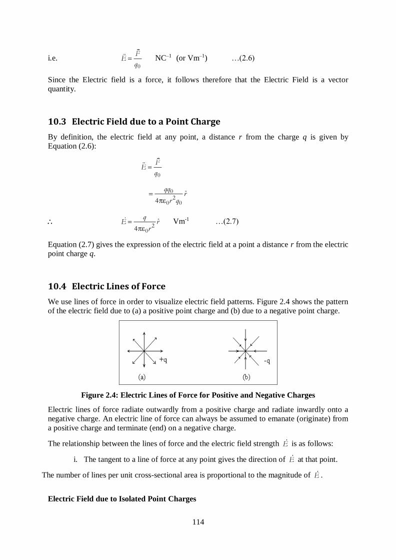
114

i.e. 0

FE

q NC–1 (or Vm–1) …(2.6)

Since the Electric field is a force, it follows therefore that the Electric Field is a vector

quantity.

10.3 Electric Field due to a Point Charge

By definition, the electric field at any point, a distance r from the charge q is given by

Equation (2.6):

0

FE

q

02

0 0

ˆ4

qqr

r q

20

ˆ4

qE r

r Vm-1 …(2.7)

Equation (2.7) gives the expression of the electric field at a point a distance r from the electric

point charge q.

10.4 Electric Lines of Force

We use lines of force in order to visualize electric field patterns. Figure 2.4 shows the pattern

of the electric field due to (a) a positive point charge and (b) due to a negative point charge.

Figure 2.4: Electric Lines of Force for Positive and Negative Charges

Electric lines of force radiate outwardly from a positive charge and radiate inwardly onto a

negative charge. An electric line of force can always be assumed to emanate (originate) from

a positive charge and terminate (end) on a negative charge.

The relationship between the lines of force and the electric field strength E is as follows:

i. The tangent to a line of force at any point gives the direction of E at that point.

The number of lines per unit cross-sectional area is proportional to the magnitude of E .

Electric Field due to Isolated Point Charges

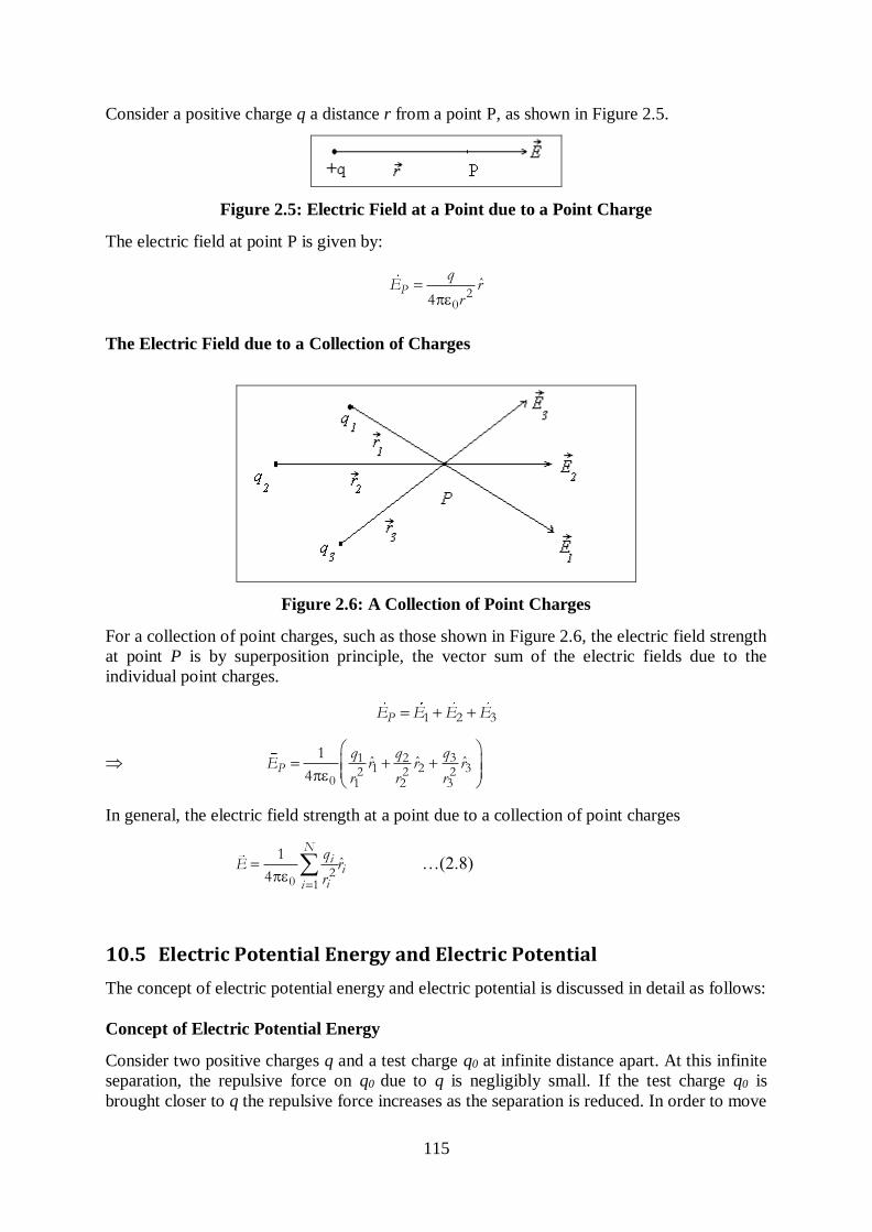
115

Consider a positive charge q a distance r from a point P, as shown in Figure 2.5.

Figure 2.5: Electric Field at a Point due to a Point Charge

The electric field at point P is given by:

20

ˆ4

Pq

E rr

The Electric Field due to a Collection of Charges

Figure 2.6: A Collection of Point Charges

For a collection of point charges, such as those shown in Figure 2.6, the electric field strength

at point P is by superposition principle, the vector sum of the electric fields due to the

individual point charges.

1 2 3PE E E E

31 21 2 32 2 2

0 1 2 3

1ˆ ˆ ˆ

4P

qq qE r r r

r r r

In general, the electric field strength at a point due to a collection of point charges

2

0 1

1ˆ

4

Nii

ii

qE r

r …(2.8)

10.5 Electric Potential Energy and Electric Potential

The concept of electric potential energy and electric potential is discussed in detail as follows:

Concept of Electric Potential Energy

Consider two positive charges q and a test charge q0 at infinite distance apart. At this infinite

separation, the repulsive force on q0 due to q is negligibly small. If the test charge q0 is

brought closer to q the repulsive force increases as the separation is reduced. In order to move

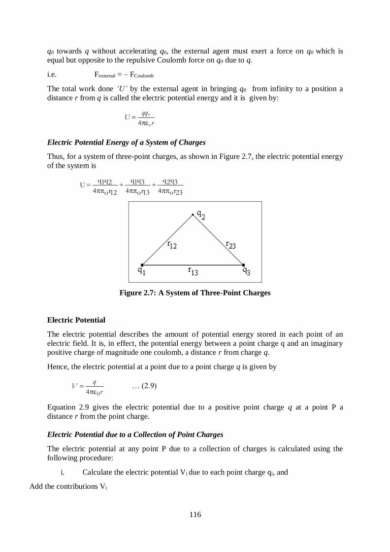
116

q0 towards q without accelerating q0, the external agent must exert a force on q0 which is

equal but opposite to the repulsive Coulomb force on q0 due to q.

i.e. Fexternal = – FCoulomb

The total work done ‘U’ by the external agent in bringing q0 from infinity to a position a

distance r from q is called the electric potential energy and it is given by:

4

qqU

r

Electric Potential Energy of a System of Charges

Thus, for a system of three-point charges, as shown in Figure 2.7, the electric potential energy

of the system is

q q q qq q 1 3 2 31 2U= + +

4 r 4 r 4 ro o o12 13 23

Figure 2.7: A System of Three-Point Charges

Electric Potential

The electric potential describes the amount of potential energy stored in each point of an

electric field. It is, in effect, the potential energy between a point charge q and an imaginary

positive charge of magnitude one coulomb, a distance r from charge q.

Hence, the electric potential at a point due to a point charge q is given by

04

qV

r

… (2.9)

Equation 2.9 gives the electric potential due to a positive point charge q at a point P a

distance r from the point charge.

Electric Potential due to a Collection of Point Charges

The electric potential at any point P due to a collection of charges is calculated using the

following procedure:

i. Calculate the electric potential Vi due to each point charge qi, and

Add the contributions Vi

117

i.e. 01 1

1

4

ii

ii i

qV V

r

…(2.10)

Note that Equation (2.10) is scalar; it is simply an algebraic sum and not a vector sum.

Electric Potential Difference

The electric potential difference between two points B and A is the work done against the

electric field in taking unit positive charge from A to B .

i.e. VAB = VB - VA

.

B

AB

A

V E dx …(2.11)

Exercise 1. Several electric field line patterns are shown in figure below. Which of these patterns

are incorrect? Explain what is wrong with all incorrect diagrams.

2. The following unit is certainly not the standard unit for expressing the quantity of

electric field strength: kg • m / s2 /C. However, it could be an acceptable unit for E.

Use dimensional analysis to identify whether the above set of units is an acceptable

unit for electric field strength.

3. A ball of mass m = 2 g is suspended by a string of length l = 20 cm as in figure shown

below in a constant electric field of E = 1000 N/C. If the string makes an angle of =

15 o with respect to the vertical, what is the net charge on the ball?

1. A constant electric field E = 2000 V/m exists in space. A 10 C charge of mass 20 g,

initially at rest at x = – 1 m, is released. What is its speed at x = 5 m?

118

Summary

Electric field is a region around a charged particle or object within which a force would be

exerted on other charged particles or objects. The electric point charge (q) is said to be the

source of the electric field. Since the Electric field is a force, it follows therefore that the

Electric Field is a vector quantity. The electric potential describes the amount of potential

energy stored in each point of an electric field.

References




McGraw Hill.

A.K. Jha (2009). A Textbook of Applied Physics, I.K. International Pub.

E.F. Redish (2003). Teaching Introductory Physics with the Physics Suite, John

Wiley & Sons.


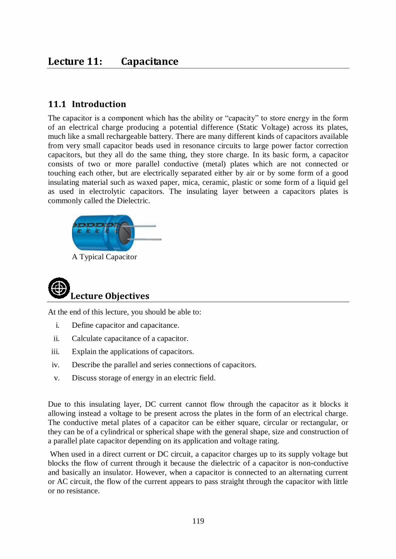
119

Lecture 11: Capacitance

11.1 Introduction

The capacitor is a component which has the ability or “capacity” to store energy in the form

of an electrical charge producing a potential difference (Static Voltage) across its plates,

much like a small rechargeable battery. There are many different kinds of capacitors available

from very small capacitor beads used in resonance circuits to large power factor correction

capacitors, but they all do the same thing, they store charge. In its basic form, a capacitor

consists of two or more parallel conductive (metal) plates which are not connected or

touching each other, but are electrically separated either by air or by some form of a good

insulating material such as waxed paper, mica, ceramic, plastic or some form of a liquid gel

as used in electrolytic capacitors. The insulating layer between a capacitors plates is

commonly called the Dielectric.

A Typical Capacitor

Lecture Objectives


i. Define capacitor and capacitance.

ii. Calculate capacitance of a capacitor.

iii. Explain the applications of capacitors.

iv. Describe the parallel and series connections of capacitors.

v. Discuss storage of energy in an electric field.

Due to this insulating layer, DC current cannot flow through the capacitor as it blocks it

allowing instead a voltage to be present across the plates in the form of an electrical charge.

The conductive metal plates of a capacitor can be either square, circular or rectangular, or

they can be of a cylindrical or spherical shape with the general shape, size and construction of

a parallel plate capacitor depending on its application and voltage rating.

When used in a direct current or DC circuit, a capacitor charges up to its supply voltage but

blocks the flow of current through it because the dielectric of a capacitor is non-conductive

and basically an insulator. However, when a capacitor is connected to an alternating current

or AC circuit, the flow of the current appears to pass straight through the capacitor with little

or no resistance.

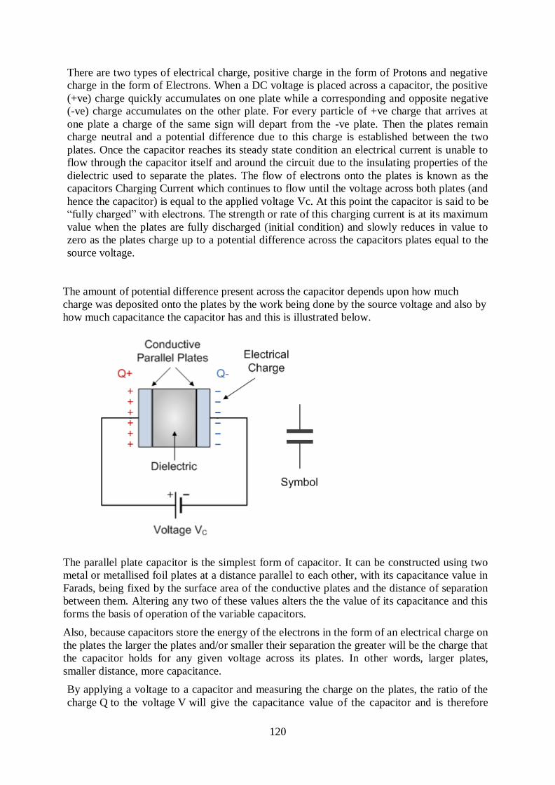
120

There are two types of electrical charge, positive charge in the form of Protons and negative

charge in the form of Electrons. When a DC voltage is placed across a capacitor, the positive

(+ve) charge quickly accumulates on one plate while a corresponding and opposite negative

(-ve) charge accumulates on the other plate. For every particle of +ve charge that arrives at

one plate a charge of the same sign will depart from the -ve plate. Then the plates remain

charge neutral and a potential difference due to this charge is established between the two

plates. Once the capacitor reaches its steady state condition an electrical current is unable to

flow through the capacitor itself and around the circuit due to the insulating properties of the

dielectric used to separate the plates. The flow of electrons onto the plates is known as the

capacitors Charging Current which continues to flow until the voltage across both plates (and

hence the capacitor) is equal to the applied voltage Vc. At this point the capacitor is said to be

“fully charged” with electrons. The strength or rate of this charging current is at its maximum

value when the plates are fully discharged (initial condition) and slowly reduces in value to

zero as the plates charge up to a potential difference across the capacitors plates equal to the

source voltage.

The amount of potential difference present across the capacitor depends upon how much

charge was deposited onto the plates by the work being done by the source voltage and also by

how much capacitance the capacitor has and this is illustrated below.

The parallel plate capacitor is the simplest form of capacitor. It can be constructed using two

metal or metallised foil plates at a distance parallel to each other, with its capacitance value in

Farads, being fixed by the surface area of the conductive plates and the distance of separation

between them. Altering any two of these values alters the the value of its capacitance and this

forms the basis of operation of the variable capacitors.

Also, because capacitors store the energy of the electrons in the form of an electrical charge on

the plates the larger the plates and/or smaller their separation the greater will be the charge that

the capacitor holds for any given voltage across its plates. In other words, larger plates,

smaller distance, more capacitance.

By applying a voltage to a capacitor and measuring the charge on the plates, the ratio of the

charge Q to the voltage V will give the capacitance value of the capacitor and is therefore

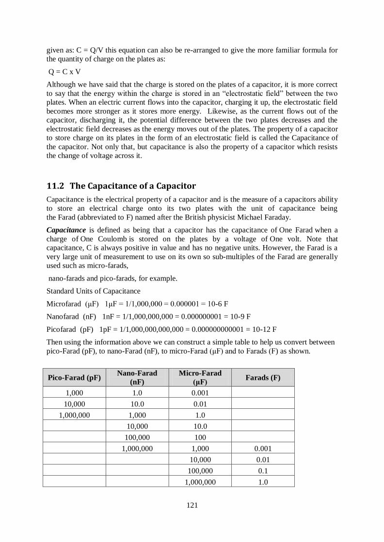
121

given as: C = Q/V this equation can also be re-arranged to give the more familiar formula for

the quantity of charge on the plates as:

Q = C x V

Although we have said that the charge is stored on the plates of a capacitor, it is more correct

to say that the energy within the charge is stored in an “electrostatic field” between the two

plates. When an electric current flows into the capacitor, charging it up, the electrostatic field

becomes more stronger as it stores more energy. Likewise, as the current flows out of the

capacitor, discharging it, the potential difference between the two plates decreases and the

electrostatic field decreases as the energy moves out of the plates. The property of a capacitor

to store charge on its plates in the form of an electrostatic field is called the Capacitance of

the capacitor. Not only that, but capacitance is also the property of a capacitor which resists

the change of voltage across it.

11.2 The Capacitance of a Capacitor

Capacitance is the electrical property of a capacitor and is the measure of a capacitors ability

to store an electrical charge onto its two plates with the unit of capacitance being

the Farad (abbreviated to F) named after the British physicist Michael Faraday.

Capacitance is defined as being that a capacitor has the capacitance of One Farad when a

charge of One Coulomb is stored on the plates by a voltage of One volt. Note that

capacitance, C is always positive in value and has no negative units. However, the Farad is a

very large unit of measurement to use on its own so sub-multiples of the Farad are generally

used such as micro-farads,

nano-farads and pico-farads, for example.

Standard Units of Capacitance

Microfarad (μF) 1μF = 1/1,000,000 = 0.000001 = 10-6 F

Nanofarad (nF) 1nF = 1/1,000,000,000 = 0.000000001 = 10-9 F

Picofarad (pF) 1pF = 1/1,000,000,000,000 = 0.000000000001 = 10-12 F

Then using the information above we can construct a simple table to help us convert between

pico-Farad (pF), to nano-Farad (nF), to micro-Farad (μF) and to Farads (F) as shown.

Pico-Farad (pF) Nano-Farad

(nF)

Micro-Farad

(μF) Farads (F)

1,000 1.0 0.001

10,000 10.0 0.01

1,000,000 1,000 1.0

10,000 10.0

100,000 100

1,000,000 1,000 0.001

10,000 0.01

100,000 0.1

1,000,000 1.0

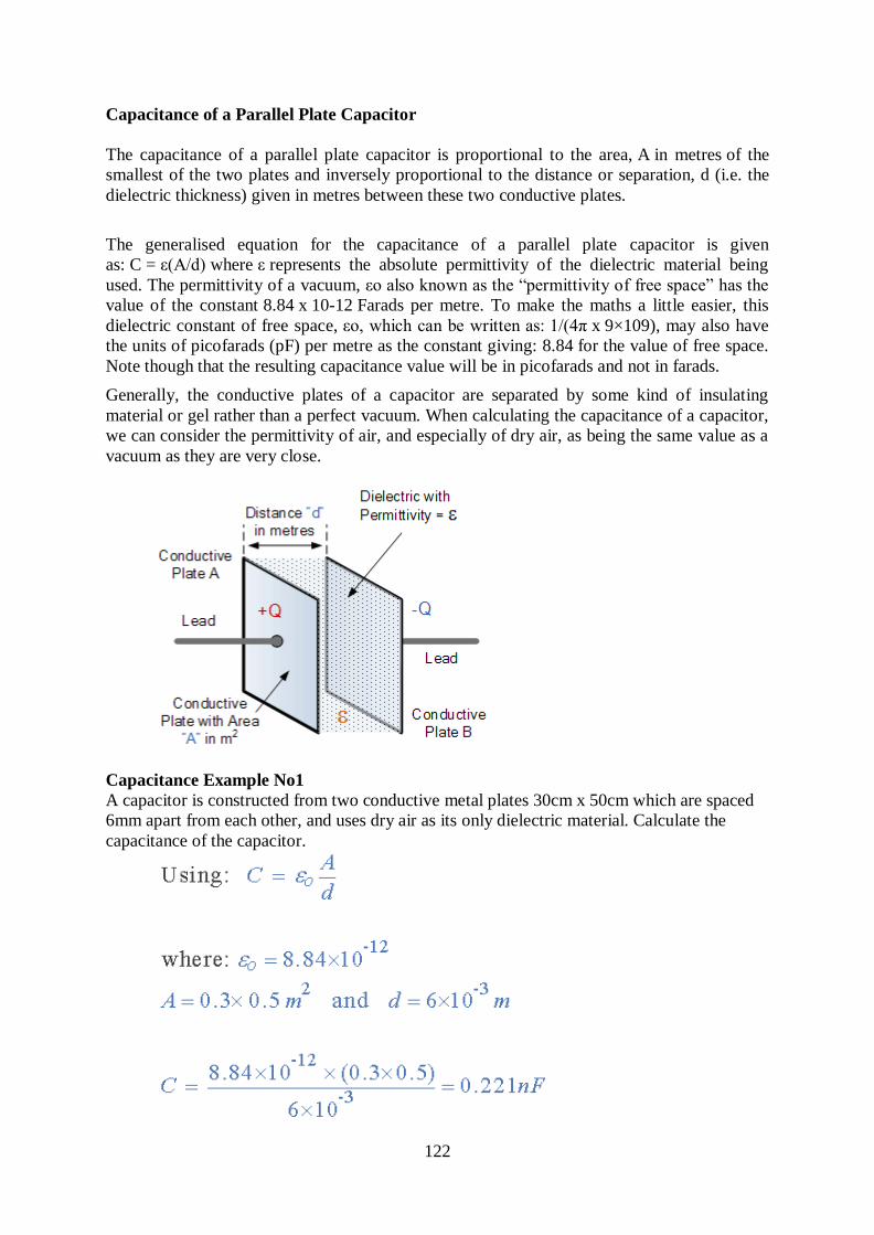
122

Capacitance of a Parallel Plate Capacitor

The capacitance of a parallel plate capacitor is proportional to the area, A in metres of the

smallest of the two plates and inversely proportional to the distance or separation, d (i.e. the

dielectric thickness) given in metres between these two conductive plates.

The generalised equation for the capacitance of a parallel plate capacitor is given

as: C = ε(A/d) where ε represents the absolute permittivity of the dielectric material being

used. The permittivity of a vacuum, εo also known as the “permittivity of free space” has the

value of the constant 8.84 x 10-12 Farads per metre. To make the maths a little easier, this

dielectric constant of free space, εo, which can be written as: 1/(4π x 9×109), may also have

the units of picofarads (pF) per metre as the constant giving: 8.84 for the value of free space.

Note though that the resulting capacitance value will be in picofarads and not in farads.

Generally, the conductive plates of a capacitor are separated by some kind of insulating

material or gel rather than a perfect vacuum. When calculating the capacitance of a capacitor,

we can consider the permittivity of air, and especially of dry air, as being the same value as a

vacuum as they are very close.

Capacitance Example No1

A capacitor is constructed from two conductive metal plates 30cm x 50cm which are spaced

6mm apart from each other, and uses dry air as its only dielectric material. Calculate the

capacitance of the capacitor.

123

Then the value of the capacitor consisting of two plates separated by air is calculated as

221pF or 0.221nF

11.3 The Dielectric of a Capacitor

As well as the overall size of the conductive plates and their distance or spacing apart from

each other, another factor which affects the overall capacitance of the device is the type of

dielectric material being used. In other words the “Permittivity” (ε) of the dielectric. The

conductive plates of a capacitor are generally made of a metal foil or a metal film allowing

for the flow of electrons and charge, but the dielectric material used is always an insulator.

The various insulating materials used as the dielectric in a capacitor differ in their ability to

block or pass an electrical charge. This dielectric material can be made from a number of

insulating materials or combinations of these materials with the most common types used

being: air, paper, polyester, polypropylene, Mylar, ceramic, glass, oil, or a variety of other

materials.

The factor by which the dielectric material, or insulator, increases the capacitance of the

capacitor compared to air is known as the Dielectric Constant, k and a dielectric material with

a high dielectric constant is a better insulator than a dielectric material with a lower dielectric

constant. Dielectric constant is a dimensionless quantity since it is relative to free space.

The actual permittivity or “complex permittivity” of the dielectric material between the plates

is then the product of the permittivity of free space (εo) and the relative permittivity (εr) of

the material being used as the dielectric and is given as:

Complex Permittivity

In other words, if we take the permittivity of free space, εo as our base level and make it

equal to one, when the vacuum of free space is replaced by some other type of insulating

material, their permittivity of its dielectric is referenced to the base dielectric of free space

giving a multiplication factor known as “relative permittivity”, εr. So the value of the

complex permittivity, ε will always be equal to the relative permittivity times one.

Typical units of dielectric permittivity, ε or dielectric constant for common materials are:

pure vacuum = 1.0000, air = 1.0006, paper = 2.5 to 3.5, glass = 3 to 10, mica = 5 to 7, wood =

3 to 8 and metal oxide powders = 6 to 20 etc. This then gives us a final equation for the

capacitance of a capacitor as:

One method used to increase the overall capacitance of a capacitor while keeping its size

small is to “interleave” more plates together within a single capacitor body. Instead of just

one set of parallel plates, a capacitor can have many individual plates connected together

thereby increasing the surface area, A of the plates.

For a standard parallel plate capacitor as shown above, the capacitor has two plates,

labelled A and B. Therefore as the number of capacitor plates is two, we can say that n = 2,

where “n” represents the number of plates.

Then our equation above for a single parallel plate capacitor should really be:

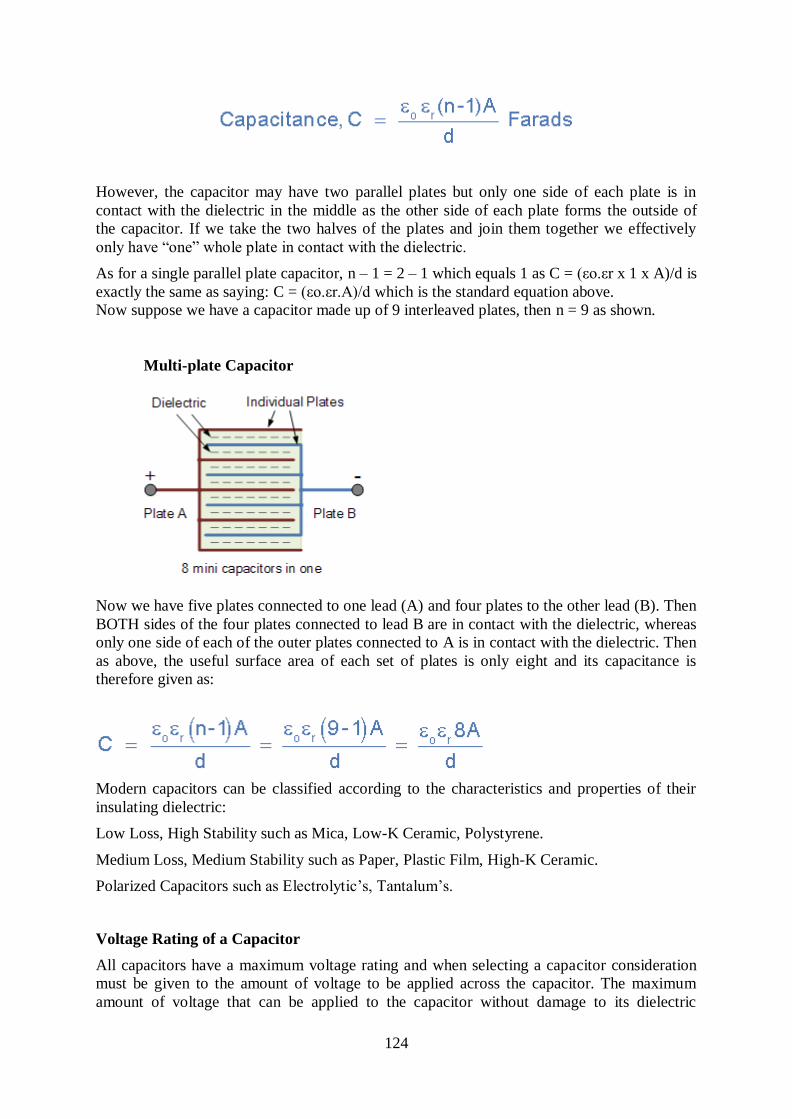
124

However, the capacitor may have two parallel plates but only one side of each plate is in

contact with the dielectric in the middle as the other side of each plate forms the outside of

the capacitor. If we take the two halves of the plates and join them together we effectively

only have “one” whole plate in contact with the dielectric.

As for a single parallel plate capacitor, n – 1 = 2 – 1 which equals 1 as C = (εo.εr x 1 x A)/d is

exactly the same as saying: C = (εo.εr.A)/d which is the standard equation above.

Now suppose we have a capacitor made up of 9 interleaved plates, then n = 9 as shown.

Multi-plate Capacitor

Now we have five plates connected to one lead (A) and four plates to the other lead (B). Then

BOTH sides of the four plates connected to lead B are in contact with the dielectric, whereas

only one side of each of the outer plates connected to A is in contact with the dielectric. Then

as above, the useful surface area of each set of plates is only eight and its capacitance is

therefore given as:

Modern capacitors can be classified according to the characteristics and properties of their

insulating dielectric:

Low Loss, High Stability such as Mica, Low-K Ceramic, Polystyrene.

Medium Loss, Medium Stability such as Paper, Plastic Film, High-K Ceramic.

Polarized Capacitors such as Electrolytic’s, Tantalum’s.

Voltage Rating of a Capacitor

All capacitors have a maximum voltage rating and when selecting a capacitor consideration

must be given to the amount of voltage to be applied across the capacitor. The maximum

amount of voltage that can be applied to the capacitor without damage to its dielectric

125

material is generally given in the data sheets as: WV, (working voltage) or as WV DC, (DC

working voltage). If the voltage applied across the capacitor becomes too great, the dielectric

will break down (known as electrical breakdown) and arcing will occur between the capacitor

plates resulting in a short-circuit. The working voltage of the capacitor depends on the type of

dielectric material being used and its thickness.

The DC working voltage of a capacitor is just that, the maximum DC voltage and NOT the

maximum AC voltage as a capacitor with a DC voltage rating of 100 volts DC cannot be

safely subjected to an alternating voltage of 100 volts. Since an alternating voltage has an

r.m.s. value of 100 volts but a peak value of over 141 volts! Then a capacitor which is

required to operate at 100 volts AC should have a working voltage of at least 200 volts. In

practice, a capacitor should be selected so that its working voltage either DC or AC should be

at least 50 percent greater than the highest effective voltage to be applied to it.

Another factor which affects the operation of a capacitor is Dielectric Leakage. Dielectric

leakage occurs in a capacitor as the result of an unwanted leakage current which flows

through the dielectric material. Generally, it is assumed that the resistance of the dielectric is

extremely high and a good insulator blocking the flow of DC current through the capacitor

(as in a perfect capacitor) from one plate to the other. However, if the dielectric material

becomes damaged due excessive voltage or over temperature, the leakage current through the

dielectric will become extremely high resulting in a rapid loss of charge on the plates and an

overheating of the capacitor eventually resulting in premature failure of the capacitor. Then

never use a capacitor in a circuit with higher voltages than the capacitor is rated for otherwise

it may become hot and explode.

Concept of Capacitance

When a finite isolated conductor is given a charge, it acquires an electric potential. A positive

charge raises the potential of the conductor whereas a negative charge lowers it.

Definition of Capacitance

The capacitance of a conductor is defined as the amount of charge that must be placed on the

conductor to raise its electric potential by one volt.

i.e. Q

CV

(Farads) or (F) …(2.12)

The larger the capacitance of a conductor, the larger the amount of charge required to raise

the potential by one volt. If charge is continually added to a conductor, the potential may be

raised to such a level that a corona discharge may result.

Capacitance due to a Parallel Plate Capacitor

Technologically, this is the most important arrangement of charged conducting plates.

We consider a parallel-plate capacitor formed of two parallel conducting plates of area A

separated by a distance d, as shown in Figure 2.8.

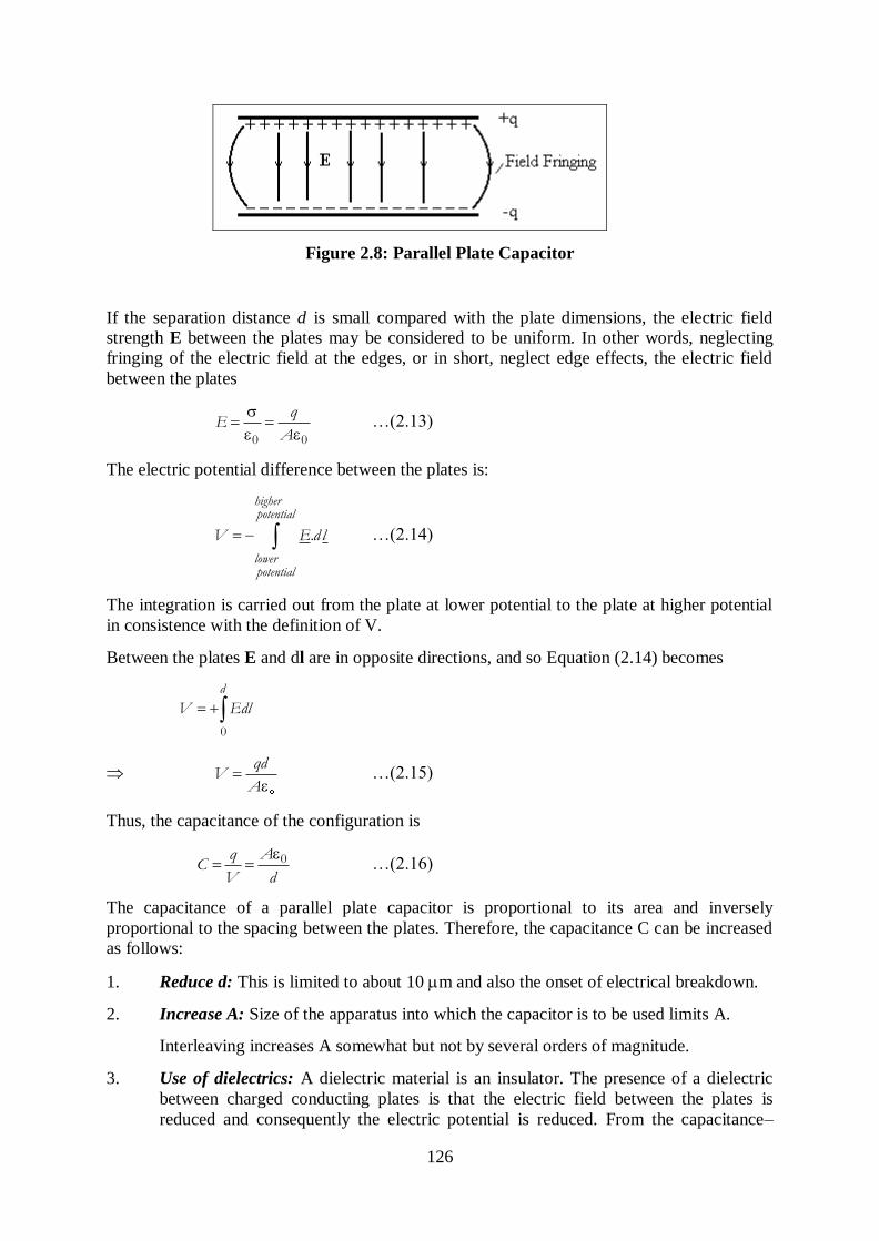
126

Figure 2.8: Parallel Plate Capacitor

If the separation distance d is small compared with the plate dimensions, the electric field

strength E between the plates may be considered to be uniform. In other words, neglecting

fringing of the electric field at the edges, or in short, neglect edge effects, the electric field

between the plates

0 0

qE

A

…(2.13)

The electric potential difference between the plates is:

.

higherpotential

lowerpotential

V E d l …(2.14)

The integration is carried out from the plate at lower potential to the plate at higher potential

in consistence with the definition of V.

Between the plates E and dl are in opposite directions, and so Equation (2.14) becomes

0

d

V Edl

qdV

A …(2.15)

Thus, the capacitance of the configuration is

0AqC

V d

…(2.16)

The capacitance of a parallel plate capacitor is proportional to its area and inversely

proportional to the spacing between the plates. Therefore, the capacitance C can be increased

as follows:

1. Reduce d: This is limited to about 10 m and also the onset of electrical breakdown.

2. Increase A: Size of the apparatus into which the capacitor is to be used limits A.

Interleaving increases A somewhat but not by several orders of magnitude.

3. Use of dielectrics: A dielectric material is an insulator. The presence of a dielectric

between charged conducting plates is that the electric field between the plates is

reduced and consequently the electric potential is reduced. From the capacitance–

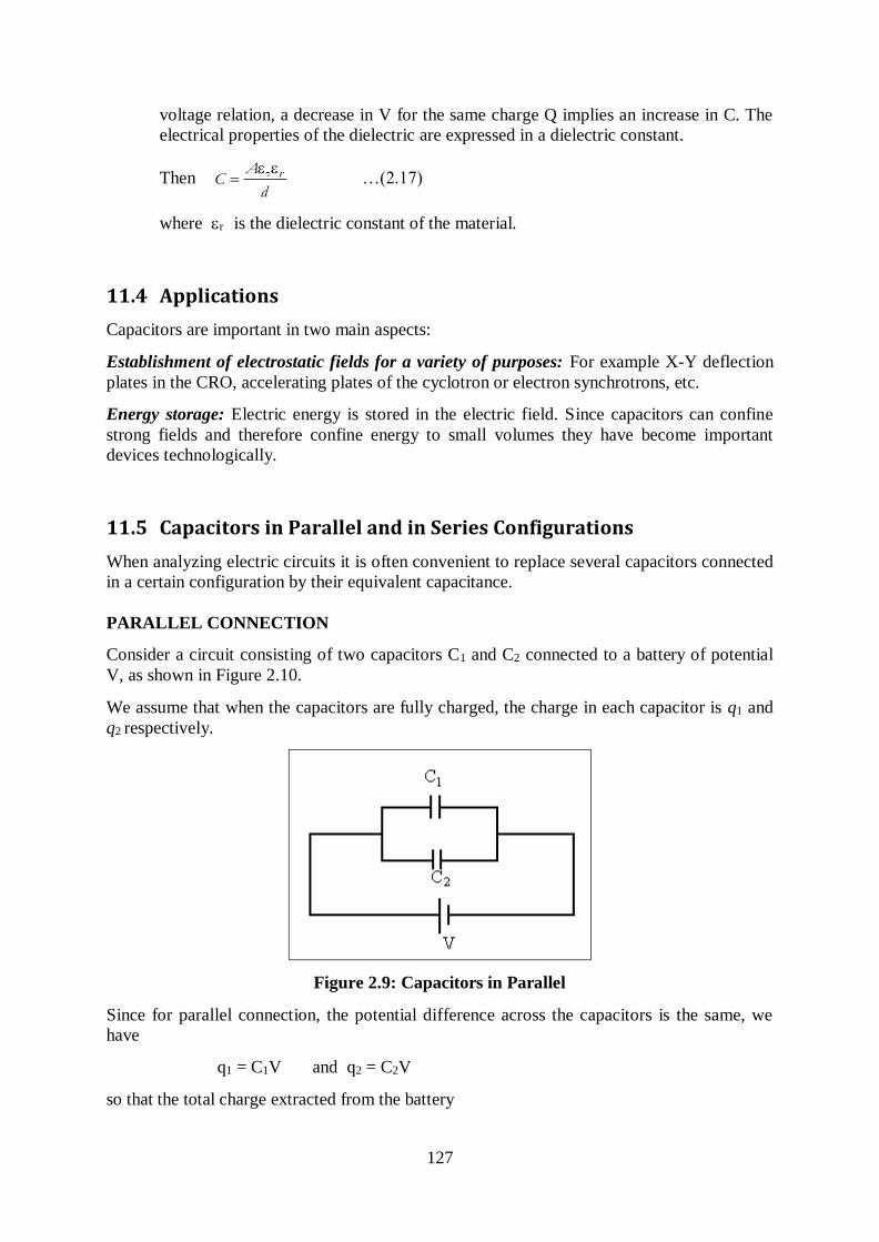
127

voltage relation, a decrease in V for the same charge Q implies an increase in C. The

electrical properties of the dielectric are expressed in a dielectric constant.

Then

rAC

d …(2.17)

where r is the dielectric constant of the material.

11.4 Applications

Capacitors are important in two main aspects:

Establishment of electrostatic fields for a variety of purposes: For example X-Y deflection

plates in the CRO, accelerating plates of the cyclotron or electron synchrotrons, etc.

Energy storage: Electric energy is stored in the electric field. Since capacitors can confine

strong fields and therefore confine energy to small volumes they have become important

devices technologically.

11.5 Capacitors in Parallel and in Series Configurations

When analyzing electric circuits it is often convenient to replace several capacitors connected

in a certain configuration by their equivalent capacitance.

PARALLEL CONNECTION

Consider a circuit consisting of two capacitors C1 and C2 connected to a battery of potential

V, as shown in Figure 2.10.

We assume that when the capacitors are fully charged, the charge in each capacitor is q1 and

q2 respectively.

Figure 2.9: Capacitors in Parallel

Since for parallel connection, the potential difference across the capacitors is the same, we

have

q1 = C1V and q2 = C2V

so that the total charge extracted from the battery

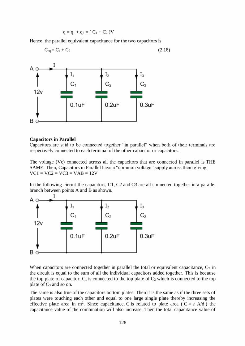
128

q = q1 + q2 = ( C1 + C2 )V

Hence, the parallel equivalent capacitance for the two capacitors is

Ceq = C1 + C2 (2.18)

Capacitors in Parallel

Capacitors are said to be connected together “in parallel” when both of their terminals are

respectively connected to each terminal of the other capacitor or capacitors.

The voltage (Vc) connected across all the capacitors that are connected in parallel is THE

SAME. Then, Capacitors in Parallel have a “common voltage” supply across them giving:

VC1 = VC2 = VC3 = VAB = 12V

In the following circuit the capacitors, C1, C2 and C3 are all connected together in a parallel

branch between points A and B as shown.

When capacitors are connected together in parallel the total or equivalent capacitance, CT in

the circuit is equal to the sum of all the individual capacitors added together. This is because

the top plate of capacitor, C1 is connected to the top plate of C2 which is connected to the top

plate of C3 and so on.

The same is also true of the capacitors bottom plates. Then it is the same as if the three sets of

plates were touching each other and equal to one large single plate thereby increasing the

effective plate area in m2. Since capacitance, C is related to plate area ( C = ε A/d ) the

capacitance value of the combination will also increase. Then the total capacitance value of

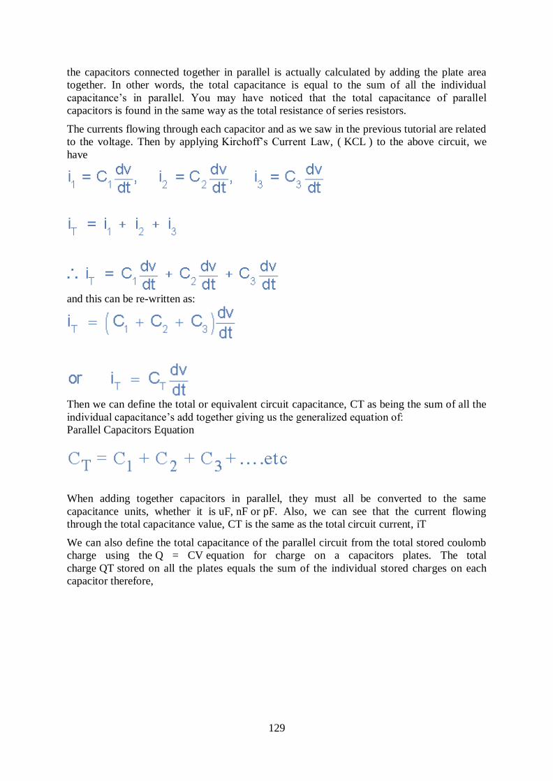
129

the capacitors connected together in parallel is actually calculated by adding the plate area

together. In other words, the total capacitance is equal to the sum of all the individual

capacitance’s in parallel. You may have noticed that the total capacitance of parallel

capacitors is found in the same way as the total resistance of series resistors.

The currents flowing through each capacitor and as we saw in the previous tutorial are related

to the voltage. Then by applying Kirchoff’s Current Law, ( KCL ) to the above circuit, we

have

and this can be re-written as:

Then we can define the total or equivalent circuit capacitance, CT as being the sum of all the

individual capacitance’s add together giving us the generalized equation of:

Parallel Capacitors Equation

When adding together capacitors in parallel, they must all be converted to the same

capacitance units, whether it is uF, nF or pF. Also, we can see that the current flowing

through the total capacitance value, CT is the same as the total circuit current, iT

We can also define the total capacitance of the parallel circuit from the total stored coulomb

charge using the Q = CV equation for charge on a capacitors plates. The total

charge QT stored on all the plates equals the sum of the individual stored charges on each

capacitor therefore,

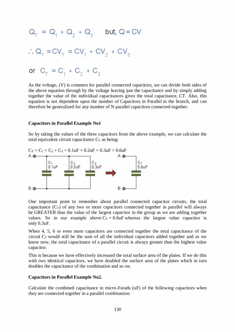
130

As the voltage, (V) is common for parallel connected capacitors, we can divide both sides of

the above equation through by the voltage leaving just the capacitance and by simply adding

together the value of the individual capacitances gives the total capacitance, CT. Also, this

equation is not dependent upon the number of Capacitors in Parallel in the branch, and can

therefore be generalized for any number of N parallel capacitors connected together.

Capacitors in Parallel Example No1

So by taking the values of the three capacitors from the above example, we can calculate the

total equivalent circuit capacitance CT as being:

CT = C1 + C2 + C3 = 0.1uF + 0.2uF + 0.3uF = 0.6uF

One important point to remember about parallel connected capacitor circuits, the total

capacitance (CT) of any two or more capacitors connected together in parallel will always

be GREATER than the value of the largest capacitor in the group as we are adding together

values. So in our example above CT = 0.6uF whereas the largest value capacitor is

only 0.3uF.

When 4, 5, 6 or even more capacitors are connected together the total capacitance of the

circuit CT would still be the sum of all the individual capacitors added together and as we

know now, the total capacitance of a parallel circuit is always greater than the highest value

capacitor.

This is because we have effectively increased the total surface area of the plates. If we do this

with two identical capacitors, we have doubled the surface area of the plates which in turn

doubles the capacitance of the combination and so on.

Capacitors in Parallel Example No2.

Calculate the combined capacitance in micro-Farads (uF) of the following capacitors when

they are connected together in a parallel combination:

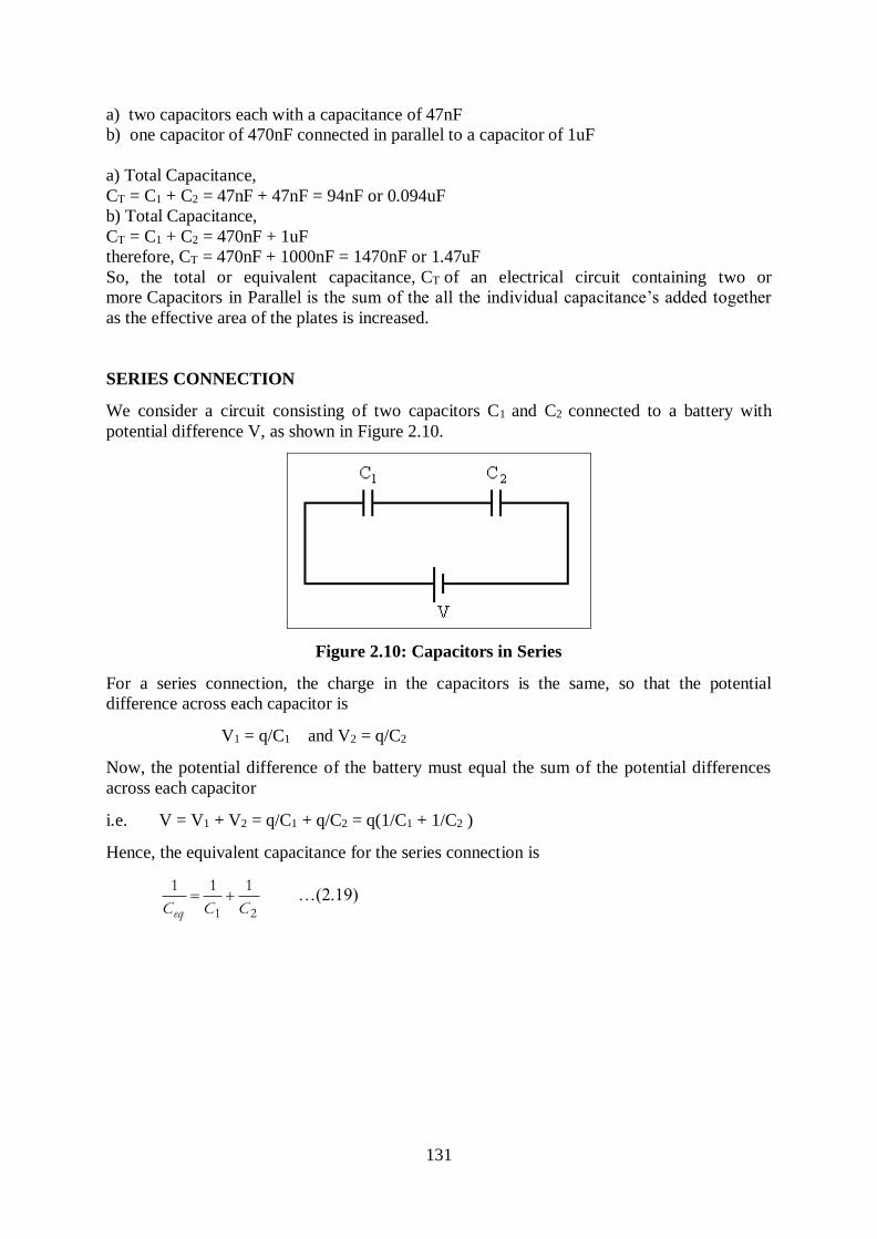
131

a) two capacitors each with a capacitance of 47nF

b) one capacitor of 470nF connected in parallel to a capacitor of 1uF

a) Total Capacitance,

CT = C1 + C2 = 47nF + 47nF = 94nF or 0.094uF

b) Total Capacitance,

CT = C1 + C2 = 470nF + 1uF

therefore, CT = 470nF + 1000nF = 1470nF or 1.47uF

So, the total or equivalent capacitance, CT of an electrical circuit containing two or

more Capacitors in Parallel is the sum of the all the individual capacitance’s added together

as the effective area of the plates is increased.

SERIES CONNECTION

We consider a circuit consisting of two capacitors C1 and C2 connected to a battery with

potential difference V, as shown in Figure 2.10.

Figure 2.10: Capacitors in Series

For a series connection, the charge in the capacitors is the same, so that the potential

difference across each capacitor is

V1 = q/C1 and V2 = q/C2

Now, the potential difference of the battery must equal the sum of the potential differences

across each capacitor

i.e. V = V1 + V2 = q/C1 + q/C2 = q(1/C1 + 1/C2 )

Hence, the equivalent capacitance for the series connection is

1 2

1 1 1

eqC C C …(2.19)

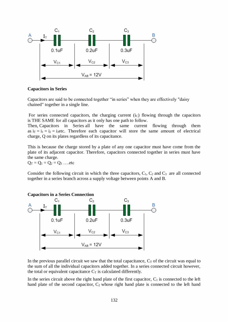
132

Capacitors in Series

Capacitors are said to be connected together “in series” when they are effectively "daisy

chained" together in a single line.

For series connected capacitors, the charging current (iC) flowing through the capacitors

is THE SAME for all capacitors as it only has one path to follow.

Then, Capacitors in Series all have the same current flowing through them

as iT = i1 = i2 = i3etc. Therefore each capacitor will store the same amount of electrical

charge, Q on its plates regardless of its capacitance.

This is because the charge stored by a plate of any one capacitor must have come from the

plate of its adjacent capacitor. Therefore, capacitors connected together in series must have

the same charge.

QT = Q1 = Q2 = Q3 ….etc

Consider the following circuit in which the three capacitors, C1, C2 and C3 are all connected

together in a series branch across a supply voltage between points A and B.

Capacitors in a Series Connection

In the previous parallel circuit we saw that the total capacitance, CT of the circuit was equal to

the sum of all the individual capacitors added together. In a series connected circuit however,

the total or equivalent capacitance CT is calculated differently.

In the series circuit above the right hand plate of the first capacitor, C1 is connected to the left

hand plate of the second capacitor, C2 whose right hand plate is connected to the left hand

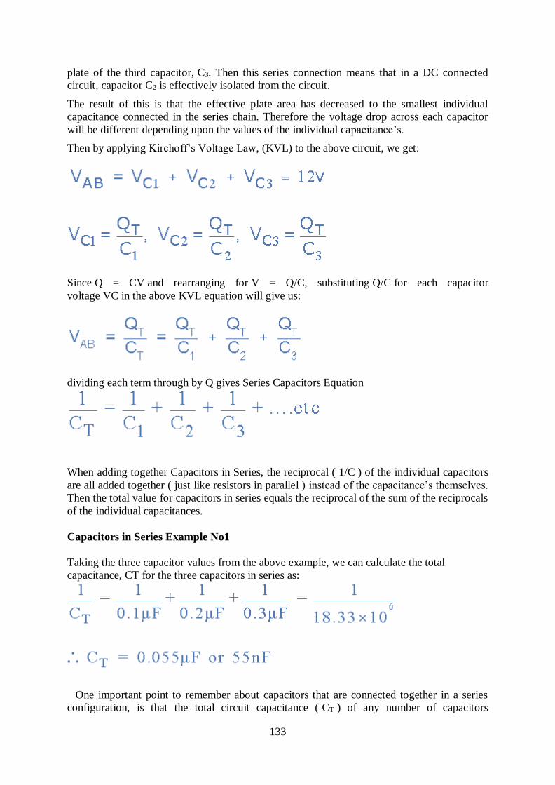
133

plate of the third capacitor, C3. Then this series connection means that in a DC connected

circuit, capacitor C2 is effectively isolated from the circuit.

The result of this is that the effective plate area has decreased to the smallest individual

capacitance connected in the series chain. Therefore the voltage drop across each capacitor

will be different depending upon the values of the individual capacitance’s.

Then by applying Kirchoff’s Voltage Law, (KVL) to the above circuit, we get:

Since Q = CV and rearranging for V = Q/C, substituting Q/C for each capacitor

voltage VC in the above KVL equation will give us:

dividing each term through by Q gives Series Capacitors Equation

When adding together Capacitors in Series, the reciprocal ( 1/C ) of the individual capacitors

are all added together ( just like resistors in parallel ) instead of the capacitance’s themselves.

Then the total value for capacitors in series equals the reciprocal of the sum of the reciprocals

of the individual capacitances.

Capacitors in Series Example No1

Taking the three capacitor values from the above example, we can calculate the total

capacitance, CT for the three capacitors in series as:

One important point to remember about capacitors that are connected together in a series

configuration, is that the total circuit capacitance ( CT ) of any number of capacitors

134

connected together in series will always be LESS than the value of the smallest capacitor in

the series and in our example above CT = 0.055uF with the value of the smallest capacitor in

the series chain is only 0.1uF.

This reciprocal method of calculation can be used for calculating any number of individual

capacitors connected together in a single series network. If however, there are only two

capacitors in series, then a much simpler and quicker formula can be used and is given as:

If the two series connected capacitors are equal and of the same value, that is: C1 = C2, we

can simplify the above equation further as follows to find the total capacitance of the series

combination.

Then we can see that if and only if the two series connected capacitors are the same and

equal, then the total capacitance, CT will be exactly equal to one half of the capacitance value,

that is: C/2.

With series connected resistors, the sum of all the voltage drops across the series circuit will

be equal to the applied voltage VS ( Kirchoff’s Voltage Law ) and this is also true about

capacitors in series.

With series connected capacitors, the capacitive reactance of the capacitor acts as an

impedance due to the frequency of the supply. This capacitive reactance produces a voltage

drop across each capacitor, therefore the series connected capacitors act as a capacitive

voltage divider network.

The result is that the voltage divider formula applied to resistors can also be used to find the

individual voltages for two capacitors in series. Then:

Where: CX is the capacitance of the capacitor in question, VS is the supply voltage across the

series chain and VCX is the voltage drop across the target capacitor.

Capacitors in Series Example No2

Find the overall capacitance and the individual rms voltage drops across the following sets of

two capacitors in series when connected to a 12V a.c. supply.

a) two capacitors each with a capacitance of 47nF

b) one capacitor of 470nF connected in series to a capacitor of 1uF

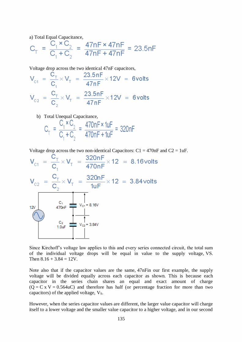
135

a) Total Equal Capacitance,

Voltage drop across the two identical 47nF capacitors,

b) Total Unequal Capacitance,

Voltage drop across the two non-identical Capacitors: C1 = 470nF and C2 = 1uF.

Since Kirchoff’s voltage law applies to this and every series connected circuit, the total sum

of the individual voltage drops will be equal in value to the supply voltage, VS.

Then 8.16 + 3.84 = 12V.

Note also that if the capacitor values are the same, 47nFin our first example, the supply

voltage will be divided equally across each capacitor as shown. This is because each

capacitor in the series chain shares an equal and exact amount of charge

(Q = C x V = 0.564uC) and therefore has half (or percentage fraction for more than two

capacitors) of the applied voltage, VS.

However, when the series capacitor values are different, the larger value capacitor will charge

itself to a lower voltage and the smaller value capacitor to a higher voltage, and in our second

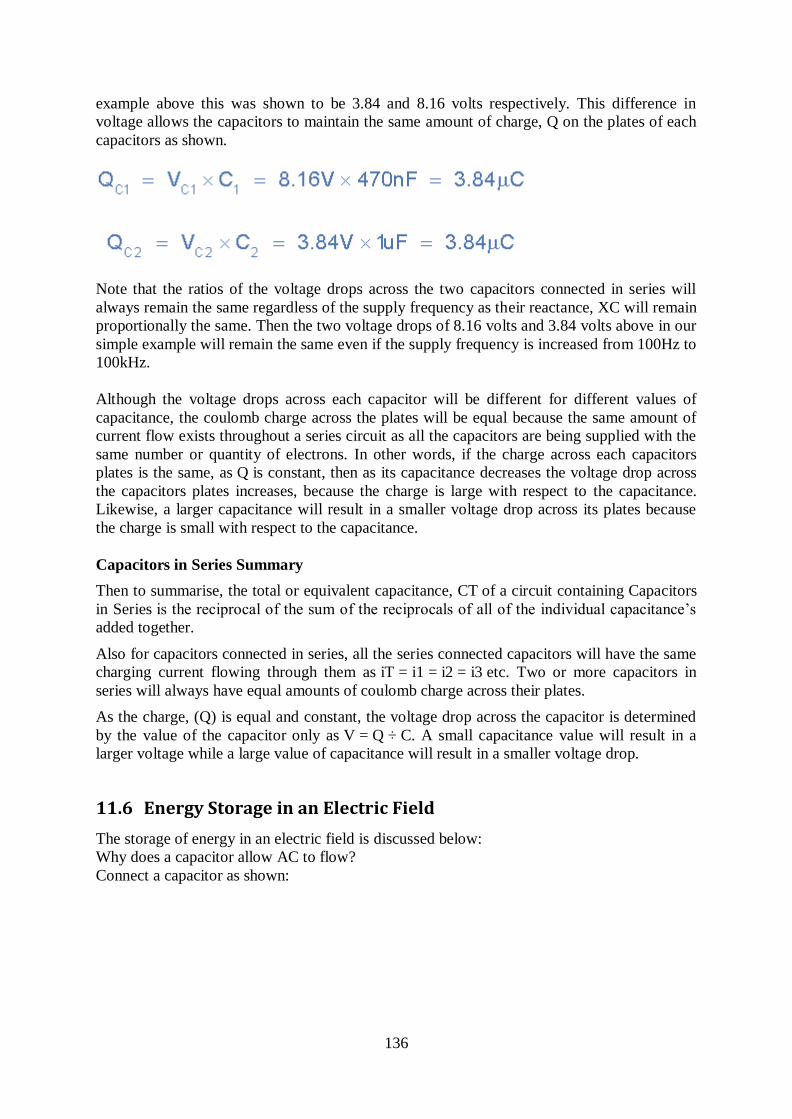
136

example above this was shown to be 3.84 and 8.16 volts respectively. This difference in

voltage allows the capacitors to maintain the same amount of charge, Q on the plates of each

capacitors as shown.

Note that the ratios of the voltage drops across the two capacitors connected in series will

always remain the same regardless of the supply frequency as their reactance, XC will remain

proportionally the same. Then the two voltage drops of 8.16 volts and 3.84 volts above in our

simple example will remain the same even if the supply frequency is increased from 100Hz to

100kHz.

Although the voltage drops across each capacitor will be different for different values of

capacitance, the coulomb charge across the plates will be equal because the same amount of

current flow exists throughout a series circuit as all the capacitors are being supplied with the

same number or quantity of electrons. In other words, if the charge across each capacitors

plates is the same, as Q is constant, then as its capacitance decreases the voltage drop across

the capacitors plates increases, because the charge is large with respect to the capacitance.

Likewise, a larger capacitance will result in a smaller voltage drop across its plates because

the charge is small with respect to the capacitance.

Capacitors in Series Summary

Then to summarise, the total or equivalent capacitance, CT of a circuit containing Capacitors

in Series is the reciprocal of the sum of the reciprocals of all of the individual capacitance’s

added together.

Also for capacitors connected in series, all the series connected capacitors will have the same

charging current flowing through them as iT = i1 = i2 = i3 etc. Two or more capacitors in

series will always have equal amounts of coulomb charge across their plates.

As the charge, (Q) is equal and constant, the voltage drop across the capacitor is determined

by the value of the capacitor only as V = Q ÷ C. A small capacitance value will result in a

larger voltage while a large value of capacitance will result in a smaller voltage drop.

11.6 Energy Storage in an Electric Field

The storage of energy in an electric field is discussed below:

Why does a capacitor allow AC to flow?

Connect a capacitor as shown:

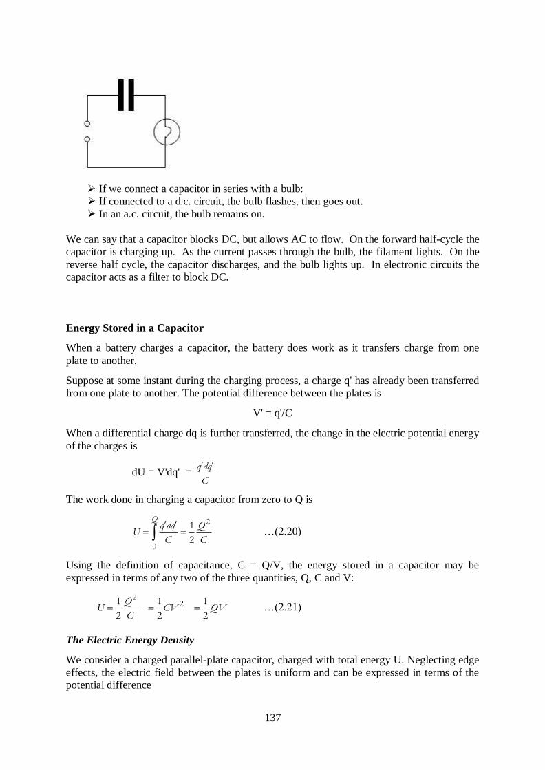
137

If we connect a capacitor in series with a bulb:

If connected to a d.c. circuit, the bulb flashes, then goes out.

In an a.c. circuit, the bulb remains on.

We can say that a capacitor blocks DC, but allows AC to flow. On the forward half-cycle the

capacitor is charging up. As the current passes through the bulb, the filament lights. On the

reverse half cycle, the capacitor discharges, and the bulb lights up. In electronic circuits the

capacitor acts as a filter to block DC.

Energy Stored in a Capacitor

When a battery charges a capacitor, the battery does work as it transfers charge from one

plate to another.

Suppose at some instant during the charging process, a charge q' has already been transferred

from one plate to another. The potential difference between the plates is

V' = q'/C

When a differential charge dq is further transferred, the change in the electric potential energy

of the charges is

dU = V'dq' = q dq

C

The work done in charging a capacitor from zero to Q is

2

0

1

2

Qq dq Q

UC C

…(2.20)

Using the definition of capacitance, C = Q/V, the energy stored in a capacitor may be

expressed in terms of any two of the three quantities, Q, C and V:

2

21 1 1

2 2 2

QU CV QV

C …(2.21)

The Electric Energy Density

We consider a charged parallel-plate capacitor, charged with total energy U. Neglecting edge

effects, the electric field between the plates is uniform and can be expressed in terms of the

potential difference

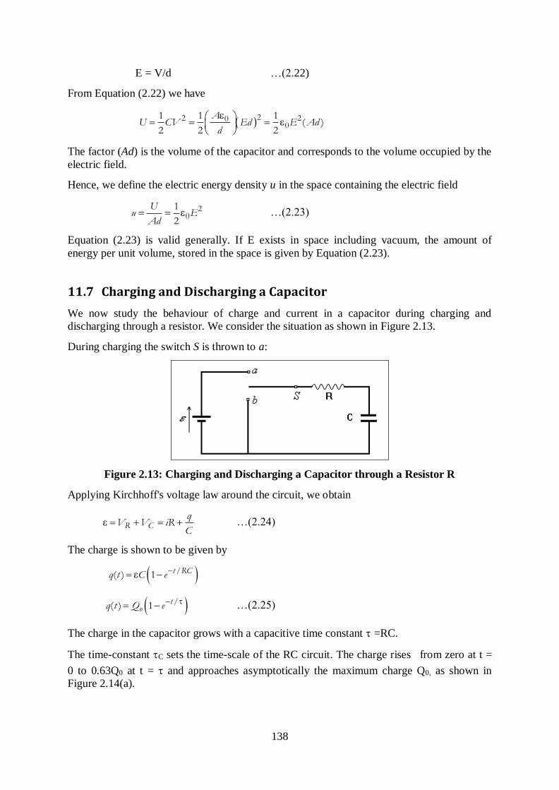
138

E = V/d …(2.22)

From Equation (2.22) we have

22 20

01 1 1

( )2 2 2

AU CV Ed E Ad

d

The factor (Ad) is the volume of the capacitor and corresponds to the volume occupied by the

electric field.

Hence, we define the electric energy density u in the space containing the electric field

20

1

2

Uu E

Ad …(2.23)

Equation (2.23) is valid generally. If E exists in space including vacuum, the amount of

energy per unit volume, stored in the space is given by Equation (2.23).

11.7 Charging and Discharging a Capacitor

We now study the behaviour of charge and current in a capacitor during charging and

discharging through a resistor. We consider the situation as shown in Figure 2.13.

During charging the switch S is thrown to a:

Figure 2.13: Charging and Discharging a Capacitor through a Resistor R

Applying Kirchhoff's voltage law around the circuit, we obtain

R Cq

V V iRC

…(2.24)

The charge is shown to be given by

/( ) 1 t RCq t C e

/( ) 1 toq t Q e …(2.25)

The charge in the capacitor grows with a capacitive time constant =RC.

The time-constant C sets the time-scale of the RC circuit. The charge rises from zero at t =

0 to 0.63Q0 at t = and approaches asymptotically the maximum charge Q0, as shown in

Figure 2.14(a).

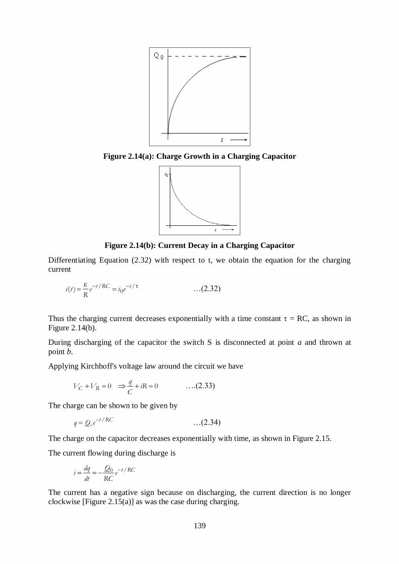
139

Figure 2.14(a): Charge Growth in a Charging Capacitor

Figure 2.14(b): Current Decay in a Charging Capacitor

Differentiating Equation (2.32) with respect to t, we obtain the equation for the charging

current

/ /0( ) t RC ti t e i e

R

…(2.32)

Thus the charging current decreases exponentially with a time constant = RC, as shown in

Figure 2.14(b).

During discharging of the capacitor the switch S is disconnected at point a and thrown at

point b.

Applying Kirchhoff's voltage law around the circuit we have

0 0C Rq

V V iRC

….(2.33)

The charge can be shown to be given by

/t RCq Q e …(2.34)

The charge on the capacitor decreases exponentially with time, as shown in Figure 2.15.

The current flowing during discharge is

/0 t RCQdqi edt RC

The current has a negative sign because on discharging, the current direction is no longer

clockwise [Figure 2.15(a)] as was the case during charging.

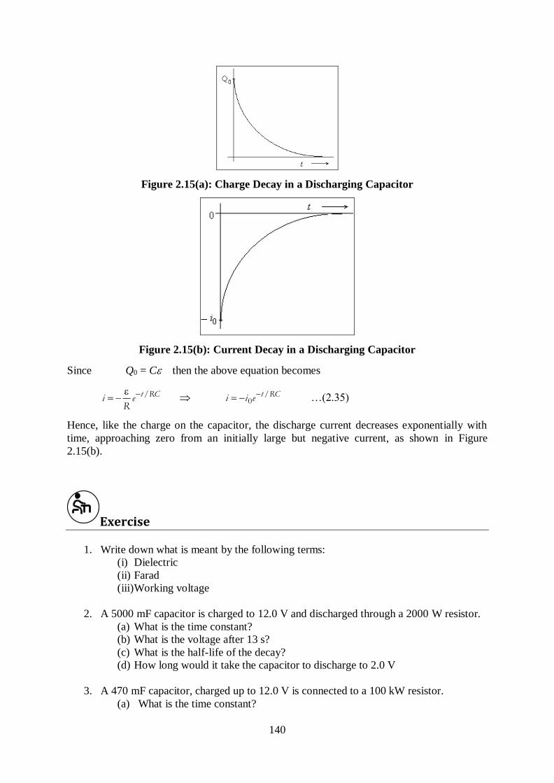
140

Figure 2.15(a): Charge Decay in a Discharging Capacitor

Figure 2.15(b): Current Decay in a Discharging Capacitor

Since Q0 = C then the above equation becomes

/t RCi eR

/0

t RCi i e …(2.35)

Hence, like the charge on the capacitor, the discharge current decreases exponentially with

time, approaching zero from an initially large but negative current, as shown in Figure

2.15(b).

Exercise

1. Write down what is meant by the following terms:

(i) Dielectric

(ii) Farad

(iii)Working voltage

2. A 5000 mF capacitor is charged to 12.0 V and discharged through a 2000 W resistor.

(a) What is the time constant?

(b) What is the voltage after 13 s?

(c) What is the half-life of the decay?

(d) How long would it take the capacitor to discharge to 2.0 V

3. A 470 mF capacitor, charged up to 12.0 V is connected to a 100 kW resistor.

(a) What is the time constant?

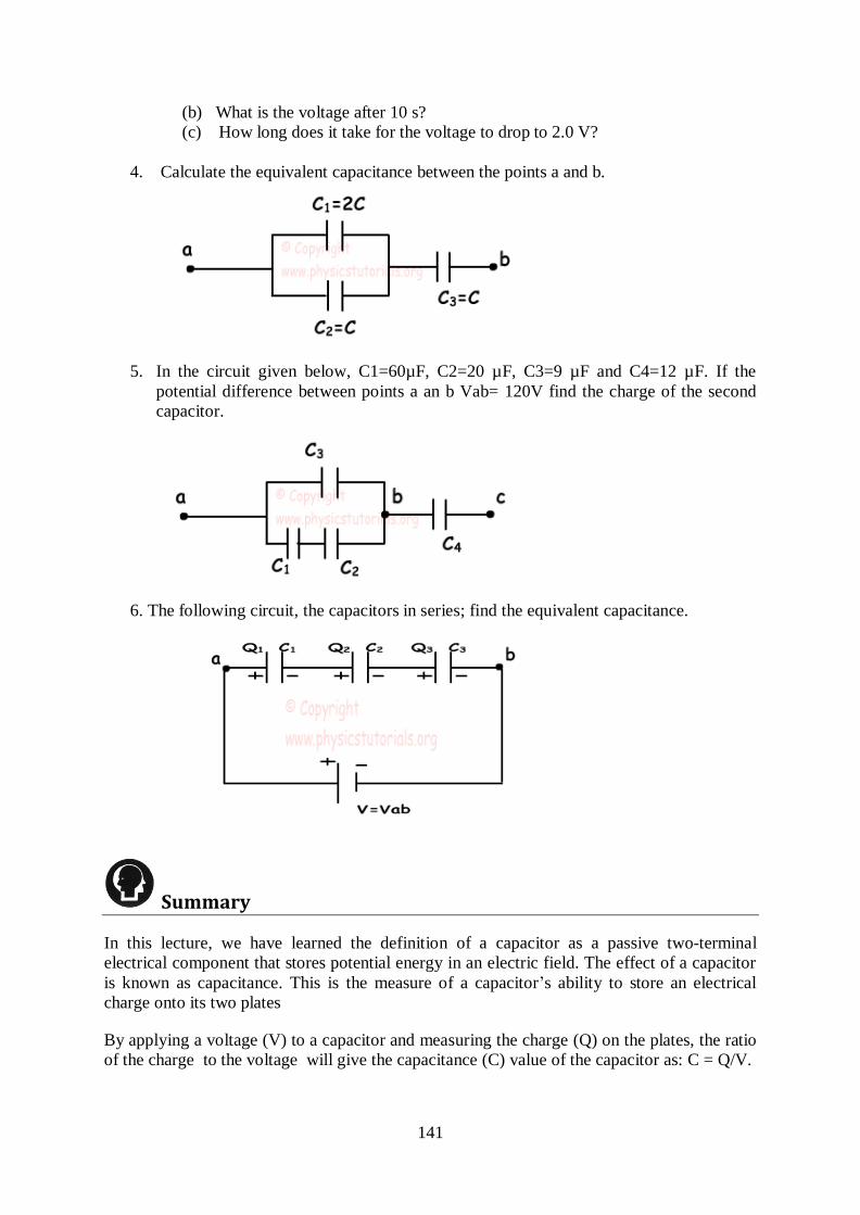
141

(b) What is the voltage after 10 s?

(c) How long does it take for the voltage to drop to 2.0 V?

4. Calculate the equivalent capacitance between the points a and b.

5. In the circuit given below, C1=60µF, C2=20 µF, C3=9 µF and C4=12 µF. If the

potential difference between points a an b Vab= 120V find the charge of the second

capacitor.

6. The following circuit, the capacitors in series; find the equivalent capacitance.

Summary

In this lecture, we have learned the definition of a capacitor as a passive two-terminal

electrical component that stores potential energy in an electric field. The effect of a capacitor

is known as capacitance. This is the measure of a capacitor’s ability to store an electrical

charge onto its two plates

By applying a voltage (V) to a capacitor and measuring the charge (Q) on the plates, the ratio

of the charge to the voltage will give the capacitance (C) value of the capacitor as: C = Q/V.

142

Capacitors are important in two main aspects: Establishment of electrostatic fields for a

variety of purposes and Energy storage. Capacitors can be connected in parallel or series

configurations.

References




McGraw Hill.


143

Lecture 12: Rc Electric Circuits

12.1 Introduction

We now study electric circuits containing only capacitors and resistors as circuit elements.

However, we shall first review the basic laws in analysis of electric circuits. These laws are

referred to as Kirchhoff's laws.

Lecture Objectives


i. State and discuss the Kirchhoff’s Laws.

ii. Apply the Kirchhoff's laws to calculate circuit questions.

iii. Discuss the Current Loop Method.

12.2 Kirchhoff’s Laws

Kirchhoff’s Laws are discussed as under:

Kirchhoff’s Current Law

The algebraic sum of currents at any junction (also called a node or Branch point) in a circuit

is zero, i.e.

currents entering a junction = currents leaving the junction

This is basically a statement of conservation of charge.

Kirchhoff's Voltage Law (KVL)

The algebraic sum of potential differences across any closed loop is zero, i.e.

potential drops = emfs

In theory, a straight forward application of Kirchhoff's laws may be used to solve any circuit;

but in practice the method in this form is suitable only for simple circuits for which the

number of unknowns does not exceed three. Then one has to solve at most three simultaneous

equations.

For example, in Figure 2.12, E = 10V, R1 = 5k, R2 = 2k and R3 = 10k ohms to find I1, I2 and

I3.

Applying Kirchhoff's voltage law around loop a we have:

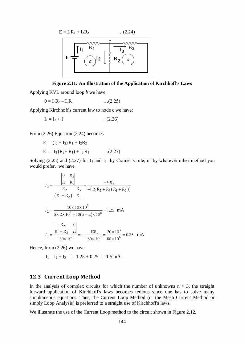
144

E = I1R1 + I2R2 …(2.24)

Figure 2.11: An Illustration of the Application of Kirchhoff's Laws

Applying KVL around loop b we have,

0 = I3R3 – I2R2 …(2.25)

Applying Kirchhoff's current law to node c we have:

I1 = I2 + I …(2.26)

From (2.26) Equation (2.24) becomes

E = (I2 + I3) R1 + I2R2

E = I2 (R2+ R1) + I3 R1 …(2.27)

Solving (2.25) and (2.27) for I2 and I3 by Cramer’s rule, or by whatever other method you

would prefer, we have

3

1 32

2 3 1 2 3 1 2

1 2 1

0 R

E R ERI

R R R R R R R

R R R

3

2 6 6

10 10 101.25

5 2 10 10 5 2 10I mA

23

1 2 23 6 6 6

0

20 100.25

80 10 80 10 80 10

R

R R E ERI mA

Hence, from (2.26) we have

I1 = I2 + I3 = 1.25 + 0.25 = 1.5 mA.

12.3 Current Loop Method

In the analysis of complex circuits for which the number of unknowns n > 3, the straight

forward application of Kirchhoff's laws becomes tedious since one has to solve many

simultaneous equations. Thus, the Current Loop Method (or the Mesh Current Method or

simply Loop Analysis) is preferred to a straight use of Kirchhoff's laws.

We illustrate the use of the Current Loop method to the circuit shown in Figure 2.12.

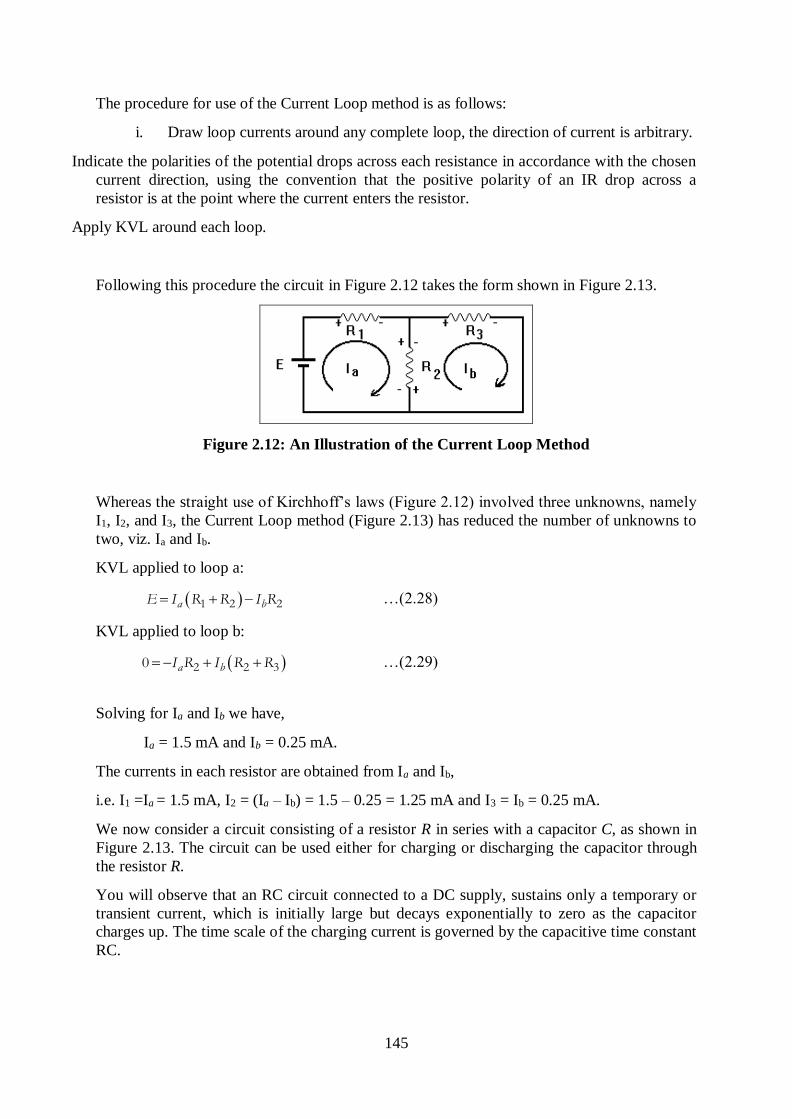
145

The procedure for use of the Current Loop method is as follows:

i. Draw loop currents around any complete loop, the direction of current is arbitrary.

Indicate the polarities of the potential drops across each resistance in accordance with the chosen

current direction, using the convention that the positive polarity of an IR drop across a

resistor is at the point where the current enters the resistor.

Apply KVL around each loop.

Following this procedure the circuit in Figure 2.12 takes the form shown in Figure 2.13.

Figure 2.12: An Illustration of the Current Loop Method

Whereas the straight use of Kirchhoff’s laws (Figure 2.12) involved three unknowns, namely

I1, I2, and I3, the Current Loop method (Figure 2.13) has reduced the number of unknowns to

two, viz. Ia and Ib.

KVL applied to loop a:

1 2 2a bE I R R I R …(2.28)

KVL applied to loop b:

2 2 30 a bI R I R R …(2.29)

Solving for Ia and Ib we have,

Ia = 1.5 mA and Ib = 0.25 mA.

The currents in each resistor are obtained from Ia and Ib,

i.e. I1 =Ia = 1.5 mA, I2 = (Ia – Ib) = 1.5 – 0.25 = 1.25 mA and I3 = Ib = 0.25 mA.

We now consider a circuit consisting of a resistor R in series with a capacitor C, as shown in

Figure 2.13. The circuit can be used either for charging or discharging the capacitor through

the resistor R.

You will observe that an RC circuit connected to a DC supply, sustains only a temporary or

transient current, which is initially large but decays exponentially to zero as the capacitor

charges up. The time scale of the charging current is governed by the capacitive time constant

RC.

146

Activity

Inflate a balloon and tie the end. Sprinkle a small amount of salt and pepper

on a sheet of paper or on your desk top. Rub the balloon with the cloth.

Bring the balloon within about an inch or two of the salt and pepper.

Observe for a minute or two. You will notice that the same grains of salt and

pepper are attracted to the balloon, repelled, and then attracted again over

and over. Explain what is happening and why?

Summary

All forces that one encounters in materials, whether binding or contact, are electrical

in nature and therefore they are Coulomb derived forces.

The electric potential describes the amount of potential energy stored in each point of

an electric field.

The electric potential difference between two points B and A is the work done against

the electric field in taking unit positive charge from A to B .

The capacitance of a conductor is defined as the amount of charge that must be placed

on the conductor to raise its electric potential by one volt.

Kirchhoff’s Current Law: The algebraic sum of currents at any junction in a circuit is

zero.

Kirchhoff's Voltage Law: The algebraic sum of potential differences across any closed

loop is zero.

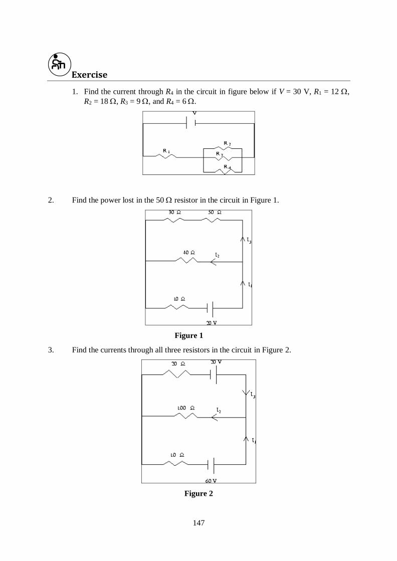
147

Exercise 1. Find the current through R4 in the circuit in figure below if V = 30 V, R1 = 12 ,

R2 = 18 , R3 = 9 , and R4 = 6 .

2. Find the power lost in the 50 resistor in the circuit in Figure 1.

Figure 1

3. Find the currents through all three resistors in the circuit in Figure 2.

Figure 2

148

References




McGraw Hill.


E.F. Redish (2003). Teaching Introductory Physics with the Physics Suite, John Wiley

& Sons.


149

SECTION FOUR: ELECTROMAGNETISM

Lecture 13: The Magnetic Field

13.1 Introduction

Iron fillings sprinkled loosely onto a sheet of paper, under which there is a bar magnet, will

form themselves into a regular pattern.

A similar pattern is obtained when the bar magnet is replaced by a loop of wire carrying a

direct current, provided that the plane of the loop is at right angle to the axis of the magnet.

The space around a permanent magnet or a current-carrying conductor is described to be the

location of a magnetic field. The magnitude and the direction of the magnetic field are

indicated by the vector B.

There is not general agreement on the naming of field vectors in magnetism. B may be called

the magnetic induction or magnetic flux density, while another field vector denoted by H is

called the magnetic field intensity.

Generally, B is regarded to be more fundamental than H and hence B is called the magnetic

field. In this course, the vector field B shall be called the magnetic field.

Unlike the electric field E whose origin is the electric charge, the magnetic field does not

originate from magnetic charges which are also called magnetic monopoles, (these do not

exist) instead B originates from moving electric charges.

A moving electric point charge or an electric current sets up a magnetic field, which in turn

can exert a magnetic force on other moving electric point charges or currents.

Lecture Objectives


i. Define the magnetic field

ii. Describe magnetic field lines

State the magnetic force on a moving electric point charge

Compute the magnetic force on a current-carrying conductor

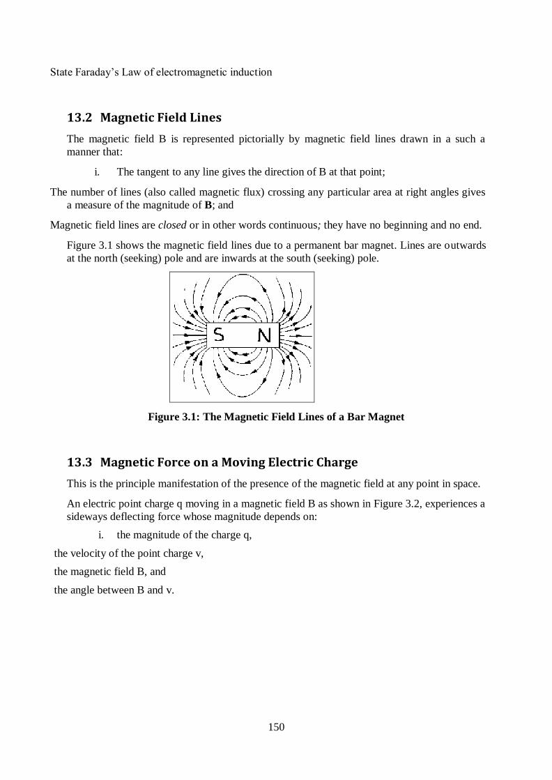
150

State Faraday’s Law of electromagnetic induction

13.2 Magnetic Field Lines

The magnetic field B is represented pictorially by magnetic field lines drawn in a such a

manner that:

i. The tangent to any line gives the direction of B at that point;

The number of lines (also called magnetic flux) crossing any particular area at right angles gives

a measure of the magnitude of B; and

Magnetic field lines are closed or in other words continuous; they have no beginning and no end.

Figure 3.1 shows the magnetic field lines due to a permanent bar magnet. Lines are outwards

at the north (seeking) pole and are inwards at the south (seeking) pole.

Figure 3.1: The Magnetic Field Lines of a Bar Magnet

13.3 Magnetic Force on a Moving Electric Charge

This is the principle manifestation of the presence of the magnetic field at any point in space.

An electric point charge q moving in a magnetic field B as shown in Figure 3.2, experiences a

sideways deflecting force whose magnitude depends on:

i. the magnitude of the charge q,

the velocity of the point charge v,

the magnetic field B, and

the angle between B and v.

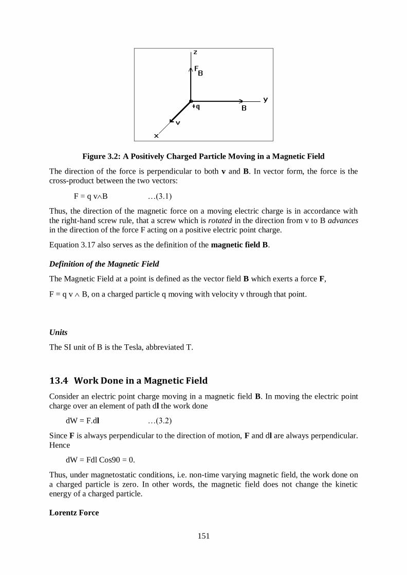
151

Figure 3.2: A Positively Charged Particle Moving in a Magnetic Field

The direction of the force is perpendicular to both v and B. In vector form, the force is the

cross-product between the two vectors:

F = q vB …(3.1)

Thus, the direction of the magnetic force on a moving electric charge is in accordance with

the right-hand screw rule, that a screw which is rotated in the direction from v to B advances

in the direction of the force F acting on a positive electric point charge.

Equation 3.17 also serves as the definition of the magnetic field B.

Definition of the Magnetic Field

The Magnetic Field at a point is defined as the vector field B which exerts a force F,

F = q v B, on a charged particle q moving with velocity v through that point.

Units

The SI unit of B is the Tesla, abbreviated T.

13.4 Work Done in a Magnetic Field

Consider an electric point charge moving in a magnetic field B. In moving the electric point

charge over an element of path dl the work done

dW = F.dl …(3.2)

Since F is always perpendicular to the direction of motion, F and dl are always perpendicular.

Hence

dW = Fdl Cos90 = 0.

Thus, under magnetostatic conditions, i.e. non-time varying magnetic field, the work done on

a charged particle is zero. In other words, the magnetic field does not change the kinetic

energy of a charged particle.

Lorentz Force

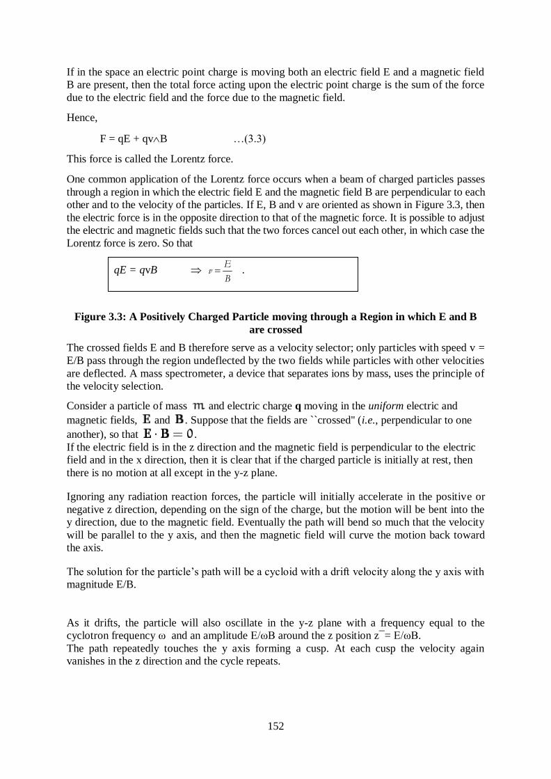
152

If in the space an electric point charge is moving both an electric field E and a magnetic field

B are present, then the total force acting upon the electric point charge is the sum of the force

due to the electric field and the force due to the magnetic field.

Hence,

F = qE + qvB …(3.3)

This force is called the Lorentz force.

One common application of the Lorentz force occurs when a beam of charged particles passes

through a region in which the electric field E and the magnetic field B are perpendicular to each

other and to the velocity of the particles. If E, B and v are oriented as shown in Figure 3.3, then

the electric force is in the opposite direction to that of the magnetic force. It is possible to adjust

the electric and magnetic fields such that the two forces cancel out each other, in which case the

Lorentz force is zero. So that

qE = qvB E

vB

.

Figure 3.3: A Positively Charged Particle moving through a Region in which E and B

are crossed

The crossed fields E and B therefore serve as a velocity selector; only particles with speed v =

E/B pass through the region undeflected by the two fields while particles with other velocities

are deflected. A mass spectrometer, a device that separates ions by mass, uses the principle of

the velocity selection.

Consider a particle of mass and electric charge q moving in the uniform electric and

magnetic fields, and . Suppose that the fields are ``crossed'' (i.e., perpendicular to one

another), so that .

If the electric field is in the z direction and the magnetic field is perpendicular to the electric

field and in the x direction, then it is clear that if the charged particle is initially at rest, then

there is no motion at all except in the y-z plane.

Ignoring any radiation reaction forces, the particle will initially accelerate in the positive or

negative z direction, depending on the sign of the charge, but the motion will be bent into the

y direction, due to the magnetic field. Eventually the path will bend so much that the velocity

will be parallel to the y axis, and then the magnetic field will curve the motion back toward

the axis.

The solution for the particle’s path will be a cycloid with a drift velocity along the y axis with

magnitude E/B.

As it drifts, the particle will also oscillate in the y-z plane with a frequency equal to the

cyclotron frequency ω and an amplitude E/ωB around the z position z¯= E/ωB.

The path repeatedly touches the y axis forming a cusp. At each cusp the velocity again

vanishes in the z direction and the cycle repeats.

153

Charged Particle Motion in Electric and Magnetic Fields

The force acting on the particle is given by the familiar Lorentz law:

(194)

where is the particle's instantaneous velocity. Hence, from Newton's second law, the

particle's equation of motion can be written

(195)

It turns out that we can eliminate the electric field from the above equation by transforming to

a different inertial frame. Thus, writing

(196)

Equation (195) reduces to

13.5 Magnetic Force on a Conductor Carrying a Current

As a consequence of the magnetic force on moving electric charged particles, a straight wire

of length l carrying a current I placed in a magnetic field B, experiences a sideways force

F = I lB …(3.4)

where l is the displacement vector whose direction is the same as that of the current I.

When the conducting wire is non-linear, i.e. not straight, or the magnetic field is not uniform,

we divide the wire into small segments each of length, say dl such that over the length of each

segment, the conditions of linearity of the conductor and uniformity of the magnetic field are

fulfilled, then the magnetic force on a differential element of the conductor of length dl

becomes

dF = I dlB …(3.5)

The total force on a segment of length L is then obtained by a suitable integration over the

length L.

Technological Applications

The magnetic force on a moving charge, current carrying conductor is the basis for mass

spectrometry, electric motors, speakers, etc.

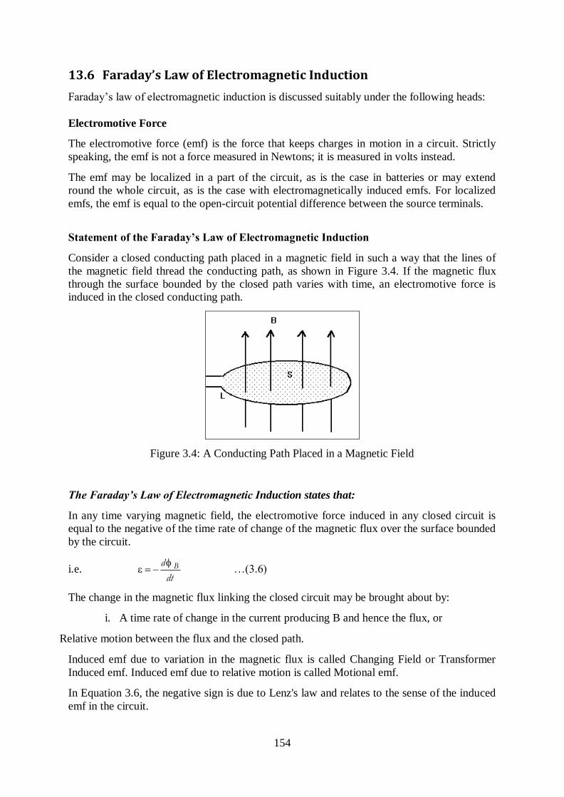
http://farside.ph.utexas.edu/teaching/336k/Newtonhtml/node30.html#e5.23

154

13.6 Faraday’s Law of Electromagnetic Induction

Faraday’s law of electromagnetic induction is discussed suitably under the following heads:

Electromotive Force

The electromotive force (emf) is the force that keeps charges in motion in a circuit. Strictly

speaking, the emf is not a force measured in Newtons; it is measured in volts instead.

The emf may be localized in a part of the circuit, as is the case in batteries or may extend

round the whole circuit, as is the case with electromagnetically induced emfs. For localized

emfs, the emf is equal to the open-circuit potential difference between the source terminals.

Statement of the Faraday’s Law of Electromagnetic Induction

Consider a closed conducting path placed in a magnetic field in such a way that the lines of

the magnetic field thread the conducting path, as shown in Figure 3.4. If the magnetic flux

through the surface bounded by the closed path varies with time, an electromotive force is

induced in the closed conducting path.

Figure 3.4: A Conducting Path Placed in a Magnetic Field

The Faraday’s Law of Electromagnetic Induction states that:

In any time varying magnetic field, the electromotive force induced in any closed circuit is

equal to the negative of the time rate of change of the magnetic flux over the surface bounded

by the circuit.

i.e.

Bd

dt …(3.6)

The change in the magnetic flux linking the closed circuit may be brought about by:

i. A time rate of change in the current producing B and hence the flux, or

Relative motion between the flux and the closed path.

Induced emf due to variation in the magnetic flux is called Changing Field or Transformer

Induced emf. Induced emf due to relative motion is called Motional emf.

In Equation 3.6, the negative sign is due to Lenz's law and relates to the sense of the induced

emf in the circuit.

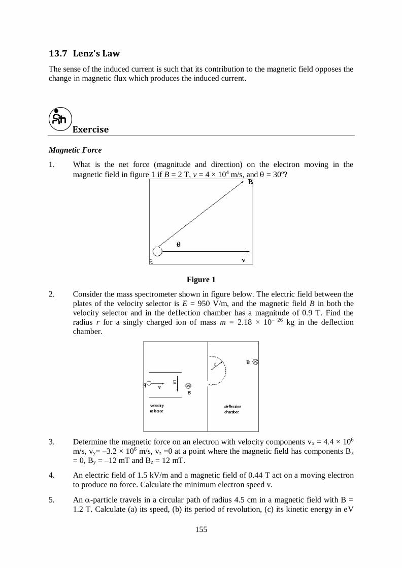
155

13.7 Lenz's Law

The sense of the induced current is such that its contribution to the magnetic field opposes the

change in magnetic flux which produces the induced current.

Exercise

Magnetic Force

1. What is the net force (magnitude and direction) on the electron moving in the

magnetic field in figure 1 if B = 2 T, v = 4 × 104 m/s, and = 30o?

Figure 1

2. Consider the mass spectrometer shown in figure below. The electric field between the

plates of the velocity selector is E = 950 V/m, and the magnetic field B in both the

velocity selector and in the deflection chamber has a magnitude of 0.9 T. Find the

radius r for a singly charged ion of mass m = 2.18 × 10– 26 kg in the deflection

chamber.

3. Determine the magnetic force on an electron with velocity components vx = 4.4 × 106

m/s, vy= –3.2 × 106 m/s, vz =0 at a point where the magnetic field has components Bx

= 0, By = –12 mT and Bz = 12 mT.

4. An electric field of 1.5 kV/m and a magnetic field of 0.44 T act on a moving electron

to produce no force. Calculate the minimum electron speed v.

5. An -particle travels in a circular path of radius 4.5 cm in a magnetic field with B =

1.2 T. Calculate (a) its speed, (b) its period of revolution, (c) its kinetic energy in eV

156

and (d) the potential difference through which it would have to be accelerated to

achieve this energy.

Faraday’s Law

6. A small loop of area A is inside, and has its axis in the same direction as a long

solenoid of n turns per unit length and current i. If i = io sin wt, find the emf in the

loop, given that the magnetic field inside a solenoid is given by B = 0ni.

7. A uniform magnetic field B is perpendicular to the plane of a circular wire loop of

radius r. The magnitude of the field varies with time according 0

tB B e , where Bo

and τ are constants. Find the emf in the loop as a function of time.

8. The magnetic flux through a loop of resistance R increases according to the relation

2( ) 6.0 7.0B t t t ,

where ΦB is in milliwebers and t is in seconds. What is the magnitude of the emf

induced in the loop when t = 2.0 s?

Summary

In this lecture, we have learned that a magnetic field is a vector field that describes the

magnetic influence of electrical currents and magnetized materials. A moving electric point

charge or an electric current sets up a magnetic field, which in turn can exert a magnetic force

on other moving electric point charges or currents. The direction of the magnetic force on a

moving electric charge is in accordance with the right-hand screw rule. Under magnetostatic

conditions, i.e. non-time varying magnetic field, the work done on a charged particle is zero.

In other words, the magnetic field does not change the kinetic energy of a charged particle.

The electromotive force (emf) is the force that keeps charges in motion in a circuit. Strictly

speaking, the emf is not a force measured in Newtons; it is measured in volts instead. We

have also discussed the Faraday’s Law of Electromagnetic Inductionand its applications.

References




McGraw Hill.


E.F. Redish (2003). Teaching Introductory Physics with the Physics Suite, John Wiley

& Sons.

Kiwanga, C.A. (1994). OPH 105: Electromagnetism II, OUT

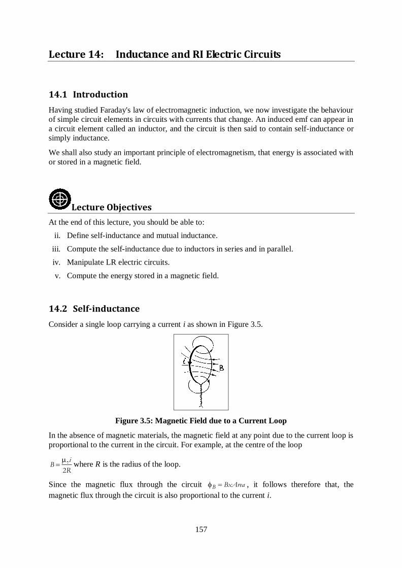
157

Lecture 14: Inductance and RI Electric Circuits

14.1 Introduction

Having studied Faraday's law of electromagnetic induction, we now investigate the behaviour

of simple circuit elements in circuits with currents that change. An induced emf can appear in

a circuit element called an inductor, and the circuit is then said to contain self-inductance or

simply inductance.

We shall also study an important principle of electromagnetism, that energy is associated with

or stored in a magnetic field.

Lecture Objectives At the end of this lecture, you should be able to:

ii. Define self-inductance and mutual inductance.

iii. Compute the self-inductance due to inductors in series and in parallel.

iv. Manipulate LR electric circuits.

v. Compute the energy stored in a magnetic field.

14.2 Self-inductance

Consider a single loop carrying a current i as shown in Figure 3.5.

Figure 3.5: Magnetic Field due to a Current Loop

In the absence of magnetic materials, the magnetic field at any point due to the current loop is

proportional to the current in the circuit. For example, at the centre of the loop

2

iB

Rwhere R is the radius of the loop.

Since the magnetic flux through the circuit B BxArea , it follows therefore that, the

magnetic flux through the circuit is also proportional to the current i.

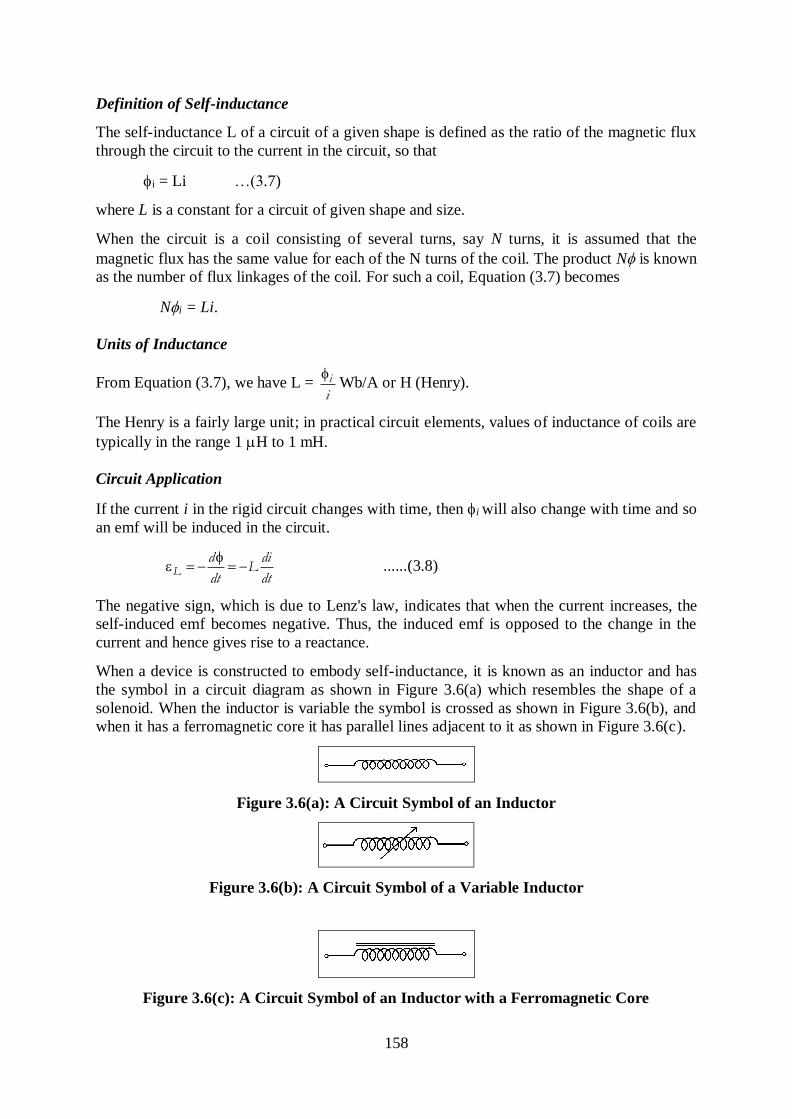
158

Definition of Self-inductance

The self-inductance L of a circuit of a given shape is defined as the ratio of the magnetic flux

through the circuit to the current in the circuit, so that

i = Li …(3.7)

where L is a constant for a circuit of given shape and size.

When the circuit is a coil consisting of several turns, say N turns, it is assumed that the

magnetic flux has the same value for each of the N turns of the coil. The product N is known

as the number of flux linkages of the coil. For such a coil, Equation (3.7) becomes

Ni = Li.

Units of Inductance

From Equation (3.7), we have L = i

iWb/A or H (Henry).

The Henry is a fairly large unit; in practical circuit elements, values of inductance of coils are

typically in the range 1 H to 1 mH.

Circuit Application

If the current i in the rigid circuit changes with time, then i will also change with time and so

an emf will be induced in the circuit.

Ld di

Ldt dt

......(3.8)

The negative sign, which is due to Lenz's law, indicates that when the current increases, the

self-induced emf becomes negative. Thus, the induced emf is opposed to the change in the

current and hence gives rise to a reactance.

When a device is constructed to embody self-inductance, it is known as an inductor and has

the symbol in a circuit diagram as shown in Figure 3.6(a) which resembles the shape of a

solenoid. When the inductor is variable the symbol is crossed as shown in Figure 3.6(b), and

when it has a ferromagnetic core it has parallel lines adjacent to it as shown in Figure 3.6(c).

Figure 3.6(a): A Circuit Symbol of an Inductor

Figure 3.6(b): A Circuit Symbol of a Variable Inductor

Figure 3.6(c): A Circuit Symbol of an Inductor with a Ferromagnetic Core

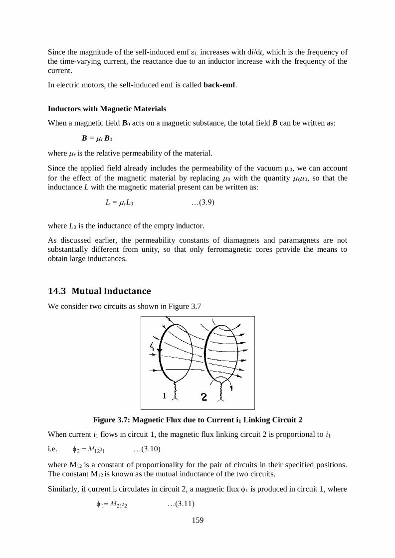
159

Since the magnitude of the self-induced emf L increases with di/dt, which is the frequency of

the time-varying current, the reactance due to an inductor increase with the frequency of the

current.

In electric motors, the self-induced emf is called back-emf.

Inductors with Magnetic Materials

When a magnetic field B0 acts on a magnetic substance, the total field B can be written as:

B = r B0

where r is the relative permeability of the material.

Since the applied field already includes the permeability of the vacuum 0, we can account

for the effect of the magnetic material by replacing 0 with the quantity r0, so that the

inductance L with the magnetic material present can be written as:

L = rL0 …(3.9)

where L0 is the inductance of the empty inductor.

As discussed earlier, the permeability constants of diamagnets and paramagnets are not

substantially different from unity, so that only ferromagnetic cores provide the means to

obtain large inductances.

14.3 Mutual Inductance

We consider two circuits as shown in Figure 3.7

Figure 3.7: Magnetic Flux due to Current i1 Linking Circuit 2

When current i1 flows in circuit 1, the magnetic flux linking circuit 2 is proportional to i1

i.e. 2 12 1M i …(3.10)

where M12 is a constant of proportionality for the pair of circuits in their specified positions.

The constant M12 is known as the mutual inductance of the two circuits.

Similarly, if current i2 circulates in circuit 2, a magnetic flux 1 is produced in circuit 1, where

1 21 2M i …(3.11)

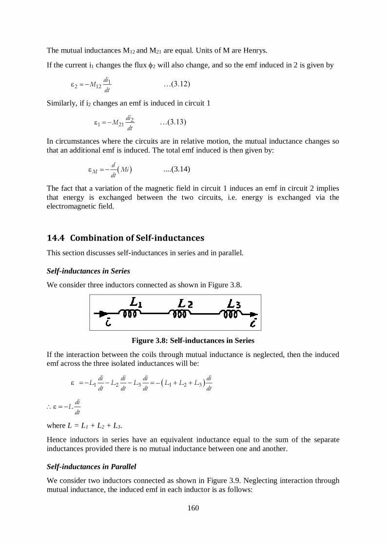
160

The mutual inductances M12 and M21 are equal. Units of M are Henrys.

If the current i1 changes the flux 2 will also change, and so the emf induced in 2 is given by

12 12

diM

dt …(3.12)

Similarly, if i2 changes an emf is induced in circuit 1

21 21

diM

dt …(3.13)

In circumstances where the circuits are in relative motion, the mutual inductance changes so

that an additional emf is induced. The total emf induced is then given by:

MdMi

dt ....(3.14)

The fact that a variation of the magnetic field in circuit 1 induces an emf in circuit 2 implies

that energy is exchanged between the two circuits, i.e. energy is exchanged via the

electromagnetic field.

14.4 Combination of Self-inductances

This section discusses self-inductances in series and in parallel.

Self-inductances in Series

We consider three inductors connected as shown in Figure 3.8.

Figure 3.8: Self-inductances in Series

If the interaction between the coils through mutual inductance is neglected, then the induced

emf across the three isolated inductances will be:

1 2 3 1 2 3–di di di di

L L L L L Ldt dt dt dt

di

Ldt

where L = L1 + L2 + L3.

Hence inductors in series have an equivalent inductance equal to the sum of the separate

inductances provided there is no mutual inductance between one and another.

Self-inductances in Parallel

We consider two inductors connected as shown in Figure 3.9. Neglecting interaction through

mutual inductance, the induced emf in each inductor is as follows:

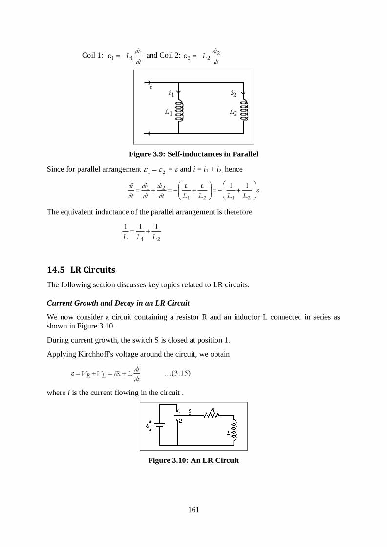
161

Coil 1: 11 1

diLdt

and Coil 2: 22 2

diL

dt

Figure 3.9: Self-inductances in Parallel

Since for parallel arrangement 1 2 = and i = i1 + i2, hence

1 2

1 2 1 2

1 1di didi

dt dt dt L L L L

The equivalent inductance of the parallel arrangement is therefore

1 2

1 1 1

L L L

14.5 LR Circuits

The following section discusses key topics related to LR circuits:

Current Growth and Decay in an LR Circuit

We now consider a circuit containing a resistor R and an inductor L connected in series as

shown in Figure 3.10.

During current growth, the switch S is closed at position 1.

Applying Kirchhoff's voltage around the circuit, we obtain

R Ldi

V V iR Ldt

…(3.15)

where i is the current flowing in the circuit .

Figure 3.10: An LR Circuit

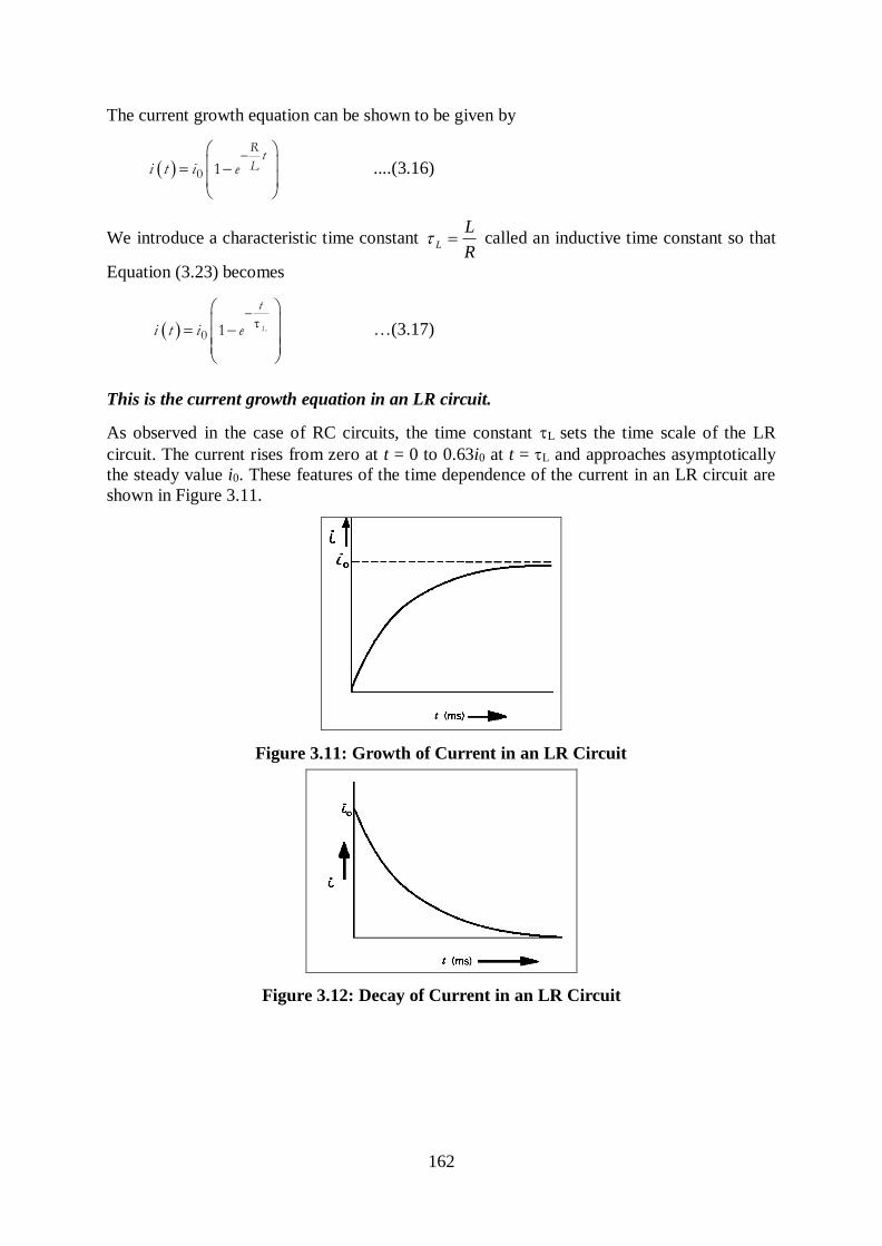
162

The current growth equation can be shown to be given by

0 1

Rt

Li t i e ....(3.16)

We introduce a characteristic time constant R

LL called an inductive time constant so that

Equation (3.23) becomes

0 1L

t

i t i e …(3.17)

This is the current growth equation in an LR circuit.

As observed in the case of RC circuits, the time constant L sets the time scale of the LR

circuit. The current rises from zero at t = 0 to 0.63i0 at t = L and approaches asymptotically

the steady value i0. These features of the time dependence of the current in an LR circuit are

shown in Figure 3.11.

Figure 3.11: Growth of Current in an LR Circuit

Figure 3.12: Decay of Current in an LR Circuit

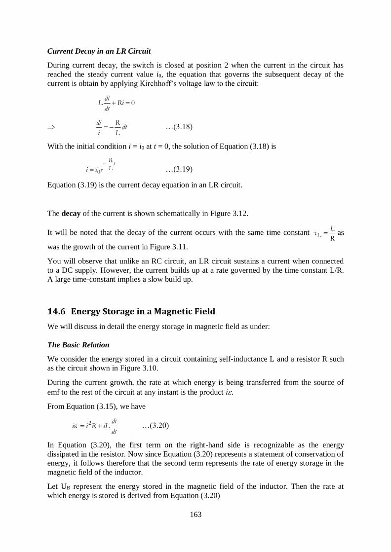
163

Current Decay in an LR Circuit

During current decay, the switch is closed at position 2 when the current in the circuit has

reached the steady current value i0, the equation that governs the subsequent decay of the

current is obtain by applying Kirchhoff’s voltage law to the circuit:

0di

L Ridt

di R

dti L

…(3.18)

With the initial condition i = i0 at t = 0, the solution of Equation (3.18) is

0

Rt

Li i e …(3.19)

Equation (3.19) is the current decay equation in an LR circuit.

The decay of the current is shown schematically in Figure 3.12.

It will be noted that the decay of the current occurs with the same time constant LL

Ras

was the growth of the current in Figure 3.11.

You will observe that unlike an RC circuit, an LR circuit sustains a current when connected

to a DC supply. However, the current builds up at a rate governed by the time constant L/R.

A large time-constant implies a slow build up.

14.6 Energy Storage in a Magnetic Field

We will discuss in detail the energy storage in magnetic field as under:

The Basic Relation

We consider the energy stored in a circuit containing self-inductance L and a resistor R such

as the circuit shown in Figure 3.10.

During the current growth, the rate at which energy is being transferred from the source of

emf to the rest of the circuit at any instant is the product i.

From Equation (3.15), we have

2 dii i R iL

dt …(3.20)

In Equation (3.20), the first term on the right-hand side is recognizable as the energy

dissipated in the resistor. Now since Equation (3.20) represents a statement of conservation of

energy, it follows therefore that the second term represents the rate of energy storage in the

magnetic field of the inductor.

Let UB represent the energy stored in the magnetic field of the inductor. Then the rate at

which energy is stored is derived from Equation (3.20)

164

BdU di

iLdt dt

or dUB = i Ldi

The total energy stored in the magnetic field as the current grows from zero to a final value i

becomes

0 0

BU i

BdU Lidi

21

2BU Li …(3.21)

This is the energy that dissipates in the resistor R when the switch in Figure (3.10) is thrown

from position 1 to 2 after a current i has been established.

Equation (3.21) is to be compared with Equation (2.21) for the energy stored in a charged

capacitor

21

2E

qU

C

14.7 The Alternating Current

By Faraday’s law of electromagnetic induction, the emf induced in a coil of N turns, area A,

rotating with an angular frequency in a uniform magnetic field B is given by:

sinNAB t

or 0 sin t …(3.22)

where 0 NAB

Since the emf develops a voltage across the circuit, Equation (3.22) may be written as

0v V sin t …(3.23)

Equation (3.23) describes a sinusoidal voltage. The constant V0 is called the peak value of the

voltage and also the amplitude of the sinusoidal waveform.

A sinusoidal waveform is completely described by its frequency, amplitude, and the phase

angle.

Definitions

Frequency: If T is the period, the time interval required for one cycle, then the frequency

11f sT

or Hertz (Hz).

Amplitude v0 or i0: The maximum magnitude of the voltage or current.

165

Phase : The angle between the unit normal to the plane of the coil n

and the magnetic field

B at t = 0; (i.e. the phase angle sets the starting point of the rotating coil).

Phase Difference: Two sinusoidal waveforms of the same frequency are said to be out of

phase when they have different starting points. The phase difference cannot exceed 90 or /2

radians.

Average Value: A sinusoidal voltage with period T has an average value

ave

0

1v v( )

T

t dtT

…(3.24)

Root Mean Square (RMS) Value: A sinusoidal voltage with period T has an r.m.s

(or effective) value

2

rms

0

1v v( )

T

t dtT

…(3.25)

From Equation 3.23 we have

2 2rms 0

0 0

1 1 1v v( ) V 1 cos2

2

T T

t dt t dtT T

rms 0v V / 2 …(3.26)

Because the integral of the cosine function over a complete cycle is zero.

Similarly, the rms value of a sinusoidal current

rms 0I / 2i …(3.27)

It should be noted that AC meters measure rms values.

Power: The electrical power is the product of impressed voltage and the resulting current

P(t) = v(t) ×i(t).

This is instantaneous and therefore fluctuates with time. The average power is

rms rmsP v i

Energy: Power is the time rate of energy transfer

i.e. dW

Pdt

So the energy transferred during the time interval t1 to t2 is

2

1

t

t

W Pdt

166

1. The power rating of an element used in AC circuits refers to the

element's average power rating. What is the maximum instantaneous

power to a 60 W light bulb?

2. The average current in the power line to your house is zero. Despite

this fact, electric power is delivered to your house. Explain.

Example: A resistance R = 25 is connected to a sinusoidal source of voltage v = 150sint.

Determine:

(a) the current i

(b) the rms current

(c) the instantaneous power, and

(d) the average power.

Solution:

(a) i = 6sin t

(b) irms = 6/ 2 = 4.24 A.

(c) instantaneous power p = 6sin t × 150sin t = 900sin t watts.

(d) the average power pave = irms × vrms = 4.24 × 106.07 = 449.7 watts.

Summary

1. Electromagnetism is the branch of physics concerned with the forces that occur

between electrically charged particles.

2. Magnetic field is defined by the force it exerts on a moving charged particle. The

Magnetic Field at a point is defined as the vector field B which exerts a force F, F

= q vB, on a charged particle q moving with velocity v through that point.

3. magnetic field is represented pictorially by magnetic field lines.

4. The SI unit of magnetic field is the Tesla (T).

5. The electromotive force (emf) is the force that keeps charges in motion in a circuit.

6. Faraday Law of Electromagnetic Induction: In any time varying magnetic field, the

electromotive force induced in any closed circuit is equal to the negative of the time rate

of change of the magnetic flux over the surface bounded by the circuit.

167

7. Lenz's Law: The sense of the induced current is such that its contribution to the

magnetic field opposes the change in magnetic flux which produces the induced

current.

Exercise

Inductance

1. Two inductors L1 and L2 are connected in series and are separated by a large distance.

(a) Show that the equivalent inductance is given by .21 LLLeq

(b) Why must their separation be large for this relationship to hold?

(c) What is the generalization of (a) for N inductors in series?

2. Two inductors L1 and L2 are connected in parallel and separated by a large distance.

(a) Show that the equivalent inductance is given by:

1 2

1 1 1

eqL L L

(b) Why must their separation be large for this relation to be valid?

RL Circuits

3. The current in an RL circuit builds up to 1/3 of its steady state value in 5 .0 s.

Calculate the inductive time constant.

4. The current in an RL circuit drops from 1.0 A to 10 mA in 1 s following removal of

the battery from the circuit. If L = 10 H, find the resistance R in the circuit.

Energy Storage

5. The magnetic energy stored in a certain inductor is 25 mJ when the current is 60.0

mA.

(a) Calculate the inductance.

(b) What current is required for the magnetic energy to be four times as much?

6. A coil with inductance L= 2.0 H and a resistance R = 10 Ω is suddenly connected to a

resistance-less battery with ε = 100 V.

(a) What is the equilibrium current?

(b) How much energy is stored in the magnetic field when this current exists in the

circuit?

168

7. A coil is connected in series with a resistance R = 10.k. When a 50 V battery is

applied to the circuit the current reaches a value of 2.00 mA after 5 mS.

(a) Find the inductance of the coil.

(b) How much energy is stored in the coil when the current is 2 mA?

References

Halliday, D., Resnick, R. and Krane, K.S. Physics Volume II, Fourth Edition, 1992.


Gottys,W., Keller, F.J. and Skove, M.J, Physics Classical and Modern, 1989.

McGraw Hill.


E.F. Redish, Teaching Introductory Physics with the Physics Suite, 2003. John Wiley

& Sons.

Kiwanga, C.A. OPH 105: Electromagnetism II, OUT 1994.

169

SECTION FIVE:

OSCILLATIONS

Lecture 15: Oscillations and Waves

15.1 Introduction

In Section one, we studied the most common types of motion, namely One-dimensional and

Rotational motions. We have developed the concepts of work, energy and momentum for

these types of motion. In this lecture, we are going to study oscillations. Unlike the other

types of motion we have studied so far, oscillations generally do not have constant

acceleration, are many times chaotic, and require far more advanced mathematics to handle.

As such, we are going to concentrate on the most basic kinds of oscillations which are

naturally easier to examine.

Practically everyday one encounters many kinds of oscillatory motion. Common examples

include children playing on a swing, vibration of a guitar string, low and high tides at the sea-

shore, etc. Examples on a microscopic scale include the vibration of air molecules that

transmit sound waves and the oscillation of atoms in a quartz crystal of an electronic watch.

The examples mentioned so far are mechanical oscillations. Examples of electrical

oscillations range from simple oscillator circuits comprising a capacitor and an inductor to

complex circuits to be found in transmitters and receivers of electromagnetic waves.

One common feature of all these systems is the mathematical formulations used to describe

their oscillations. In all cases, the oscillating quantity can be described in terms of sine or

cosine functions.

In this lecture we shall study simple harmonic motion which is the most fundamental

vibration of a single particle or a one-dimensional system. Many problems involving

mechanical vibrations at small amplitudes reduce to that of the simple harmonic oscillator or

to a combination of such oscillators.

Lecture Objectives At the end of this lecture, you should be able to:

i. Define an oscillation system.

ii. Describe the variables of an oscillation.

iii. Derive the simple harmonic equation.

iv. Describe the characteristics of simple harmonic motion.

170

v. Compute the energy of a simple harmonic motion.

vi. Apply the physics of oscillation to the simple and compound pendulums.

15.2 Definition of an Oscillating System

An oscillating system is a system in which a particle or set of particles moves back and forth,

always returning to its initial position after a certain period of time. It can be a ball bouncing

on a floor, or a pendulum swinging back and forth, or a spring compressing and stretching.

This kind of motion is called periodic motion and it is encountered in all branches of physics.

We can also define an oscillating system a little more precisely, in terms of the forces acting

on a particle in the system. In every oscillating system there is an equilibrium point at which

no net force acts on the particle. A pendulum, for example, has its equilibrium position when

it is hanging vertical, and the gravitational force is counteracted by the tension. If displaced

from this point, however, the pendulum will experience a gravitational force that causes it to

return to the equilibrium position. No matter which way the pendulum is displaced from

equilibrium, it will experience a force returning it to the equilibrium point. If we denote our

equilibrium point as x = 0, we can generalize this principle for any oscillating system: In an

oscillating system, the force always acts in a direction opposite to the displacement of the

particle from the equilibrium point.

This force, called a restoring force, can be constant or it can vary with time or position.

15.3 Variables of an Oscillation

In an oscillating system, the traditional variables – displacement x, velocity v, time t, and

acceleration a – still apply to the motion, but we introduce two new variables that describe

the periodic nature of the motion, namely the amplitude A, the period T, and the frequency f

or .

Amplitude

A simple oscillator generally goes back and forth between two extreme points; the points of

maximum displacement from the equilibrium point. This point of maximum displacement

denoted by either xm or A is defined as the amplitude of the oscillation.

Period and Frequency

In simple oscillations, a particle completes a round trip in a certain period of time. This time,

T, which denotes the time it takes for an oscillating particle to return to its initial position, is

called the period of oscillation.

We also define another variable related to time called the frequency. Frequency, denoted by ν

or f, is defined as the number of cycles per unit time and is related to period by the equation

ν = 1/T

The period is measured in seconds, while frequency is measured in Hertz (or Hz), where 1 Hz

= 1cycle/second. The variable angular frequency denoted by ω defines the number of radians

171

per second in an oscillating system. This concept of angular frequency may seem to be

confusing because most oscillations don't engage in circular motion and thereby sweep out

radians like in rotational motion. However, oscillating systems do complete cycles, and if we

think of each cycle as containing 2π radians, then we can define angular frequency.

The three variables dealing with the cycle of an oscillation are related by the equation

22

T

Equipped with these variables, we now look at the special case of the simple harmonic

oscillator.

15.4 The Basic Simple Harmonic Equation

Simple Harmonic Motion (SHM) results when a particle which is displaced at a small

distance x from its equilibrium position experiences a restoring force which is proportional to

x.

The restoring force

F = – kx …(4.1)

where k is a constant of proportionality and is generally called the force constant or stiffness

and has the dimensions of force per unit length. The negative sign shows that F acts against

the direction of increasing displacement.

By Newton’s second law, we have the equation of motion of the simple harmonic oscillator

2

2

d xm kxdt

2

20

d x kx

mdt …(4.2)

The dimensions of k/m are

2

2MLT

TM L

And so we let 2 /k m , where is the angular frequency with which the particle oscillates.

Take Note

The frequency of an oscillation is determined by the elastic and inertial properties of the

system.

172

In terms of , Equation (4.2) becomes

2

22

0d x

xdt

…(4.3)

Equation (4.3) is called the equation of motion of a simple harmonic oscillator.

Let us interpret this equation. The second derivative of a function of x plus the function itself

(times a constant) is equal to zero. Thus the second derivative of our function must have the

same form as the function itself. What readily comes to mind is the sine and cosine function.

Let us come up with a trial solution to our differential equation, and see if it works.

As a tentative solution, we write:

x = Acos (ωt) …(4.4)

where A is a constant. Differentiating this equation, we see that

sindx

A tdt

and differentiating again we have

2

22

cosd x

A tdt

Plugging this into Eq.4.3, we have

2 2cos cos 0A t A t

Equation 4.3 is indeed satisfied. Thus the equation governing simple harmonic oscillation is:

x = Acos (ωt) …(4.5)

Equation 4.5 is rather too simple in the sense that it lacks a phase constant which sets how the

simple harmonic motion is initiated. Hence, we add the phase constant to make the equation

complete.

x = Acos (ωt+) …(4.6)

where the constant A is the amplitude.

Activity

1. Give some examples of motions that are approximately simple

harmonic. Why are motions that are exactly simple harmonic rare?

2. What would happen to the motion of an oscillating system if the sign

of the force term -kx were changed?

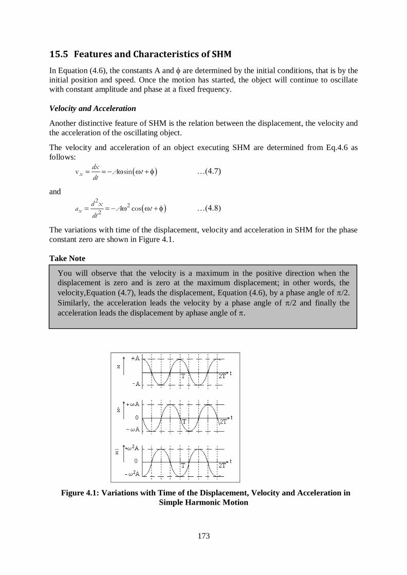
173

15.5 Features and Characteristics of SHM

In Equation (4.6), the constants A and are determined by the initial conditions, that is by the

initial position and speed. Once the motion has started, the object will continue to oscillate

with constant amplitude and phase at a fixed frequency.

Velocity and Acceleration

Another distinctive feature of SHM is the relation between the displacement, the velocity and

the acceleration of the oscillating object.

The velocity and acceleration of an object executing SHM are determined from Eq.4.6 as

follows:

v sinxdx

A tdt

…(4.7)

and

2

22

cosxd x

a A tdt

…(4.8)

The variations with time of the displacement, velocity and acceleration in SHM for the phase

constant zero are shown in Figure 4.1.

Take Note

You will observe that the velocity is a maximum in the positive direction when the

displacement is zero and is zero at the maximum displacement; in other words, the

velocity,Equation (4.7), leads the displacement, Equation (4.6), by a phase angle of /2.

Similarly, the acceleration leads the velocity by a phase angle of /2 and finally the

acceleration leads the displacement by aphase angle of .

Figure 4.1: Variations with Time of the Displacement, Velocity and Acceleration in

Simple Harmonic Motion

174

Activity 2

What changes could you make in a harmonic oscillator that would double

the maximum speed of the oscillating object?

15.6 Energy of a Simple Harmonic Oscillator

The simple harmonic oscillator is a conservative system. The kinetic energy of the system at

any given time is given by:

221 1

sin2 2

K mv m t

2 21sin

2K kA t

Since the velocity of the oscillator does change, going from zero to a maximum value, there

must be an expression for the potential energy of the system, such that the total energy of the

system is constant.

The kinetic energy has a maximum value when the potential energy is zero and sin(ωt+) =

1, so that

2max

1

2K kA

Since the potential energy is zero at this point, this value must give the total energy of the

system. Thus, at any time, we can state that:

E = U + K

2 2 21 1sin

2 2kA U A k t

Solving for U we have

2 211 sin

2U kA t

Recall that sin2a + cos2a = 1, so that we have

2 21cos

2U kA t

21

2U kx

The potential energy U is largest when the displacement is at its maximum value x = A and

zero at the equilibrium position, while the kinetic energy is maximum at the equilibrium

position and zero when the displacement is at its maximum value.

175

Example: An object executes SHM with an amplitude of 0.17 m and a period of 0.84 s.

(a) Determine (i) the frequencyand (ii) the angular frequency;

(b) Write expressions for the time dependence of (i) coordinate, (ii) the velocity

component, and (iii) the acceleration component.

Solution:

(a) (i) the frequency v = 1/T = 1/0.84 s = 1.2 Hz.

(ii) the angular frequency = 2?T = 2/(0.84 s)= 7.5 rad/s

(b) Since the problem is silent regarding the phase constant, we set = 0. So that

(i) x = 0.17cos7.5t

(ii) vx = -1.3sin7.5t and

(iii) ax =- 2Acos (t + ) = – 9.5 cos 7.5t

Example: A particle oscillates simple harmonically with amplitude 4 cm and a frequency of 5

Hz. At time t = 0, the particle is at its equilibrium position. Write down the equation

describing the position of the particle as a function of time.

Solution:

The equation of motion is Equation (4.6), where the amplitude A = 4 cm; the angular

frequency = 2 = 2 × 5 = 10 rad/s; the phase constant: at t = 0, x = 0 => 0 = 4cos

=/2. So that the equation of motion becomes x = 4cos(10t /2).

15.7 Applications of Simple Harmonic Motion

We shall now analyse a few systems that oscillate simple harmonically.

Simple Pendulum

A simple pendulum is an idealized system consisting of a massless inextensible string, fixed

rigidly at one end having a point mass at the other, as shown in Figure 4.2.

We consider a point mass m attached to a string of length L. Let at some instant the angle

subtended by the string with the vertical be . The forces acting on the particle are the weight

mg and the tension on the cord T. The motion will be along an arc of a circle of radius L.

We choose axes tangent to the circle and along the radius, i.e. radially.

Resolving the forces radially, we have T = mgcos

Resolving tangentially, we have the unbalanced tangential component of the weight, mgsin ,

directed towards the equilibrium position, a direction opposite to that of increasing .

176

Figure 4.2: A Simple Pendulum

Therefore, the tangential component constitutes the restoring force F.

sinF mg

Take Note

You will notice that the restoring force is not proportional to , the angular

displacement, and hence the oscillation is not necessarily simple harmonic.

The displacement along the arc is L and for small angles this is nearly straight-line motion.

Hence, assuming

sin and x = L

We obtain

F mg mg mgx

L

mg

Lx

sin

The force is now proportional to the displacement and is oppositely directed. Such a force

fulfils the criterion for simple harmonic motion.

By Newton’s second law we obtain the equation of motion of the simple harmonic oscillator

0xx

ma mgL

0xg

a xL

…(4.9)

For which the angular frequency of the system /g L ;

the frequency

1

2

gv

L

and so the period 2L

Tg

177

Take Note

When the amplitude of the oscillation is not small, the assumption sin ceases to be

valid and so the force becomes no longer proportional to the displacement and hence,

the motion of the oscillator is no longer simple harmonic.

Activity 3

Could we ever construct a true simple pendulum? Explain your answer.

Predict by qualitative arguments whether a pendulum oscillating with a

large amplitude will have a period longer or shorter than the period for

oscillations with small amplitude.

Example: An astronaut on the surface of the Moon sets up a simple pendulum of length 860

mm and measures its period for small oscillations to be 4.6 s. Determine the acceleration due

to gravity at the location of the astronaut.

Solution:

Since for the simple pendulum, the period

2

2

42 1.6

L LT g

g T m/s

Compound Pendulum (or The Physical Pendulum)

A compound pendulum is a rigid body, of any shape, pivoted to rotate about a fixed

horizontal axis, such as shown in Figure 4.3. This is, in fact, a generalization of the simple

pendulum in which a ‘weightless’ chord holds a single particle.

Figure 4.3: The Compound Pendulum

178

The period of a compound pendulum is given by:

2I

TmgL

…(4.10)

Exercise

Simple Harmonic Oscillations

1. A mass m = 0.5 kg is hung on a vertical massless spring. The new equilibrium

position of the spring is found to be 3 cm below the equilibrium position of the spring

without the mass. What is the spring constant, k?

2. Consider a simple harmonic oscillation with m = 0.5 kg, k = 10 N/m and amplitude A

= 3 cm. ( a) What is the total energy of the oscillator? (b) What is its maximum speed?

(c) What is the speed when x = 2 cm? (d) What are the kinetic and potential energies

when x = 2 cm?

3. If the oscillator in the above problem is released from rest at x = A when the clock is

set to t = 0 seconds, (a) determine the position and velocity of the oscillator at t = 2 s.

(b) At what time does the oscillator get to x = – 1 cm?

4. A simple pendulum is used in a physics laboratory experiment to obtain an

experimental value for the gravitational acceleration, g. A student measures the length

of the pendulum to be 0.510 meters, displaces it 10 o from the equilibrium position,

and releases it. Using a stopwatch, the student determines that the period of the

pendulum is 1.44 s. Determine the experimental value of the gravitational

acceleration.

5. Find the mechanical energy of a block-spring system having a spring constant of 1.3

N/cm and an amplitude of 2.4 cm.

6. An oscillating block-spring system has a mechanical energy of 1.00J, an amplitude of

10.0 cm, and a maximum speed of 1.20 m/s. Find (a) the spring constant, (b) the mass,

and (c) the frequency of oscillation.

7. What is the length of a simple pendulum whose period is 1.00 s at a point where g =

9.8 m/s2?

8. If a simple pendulum with length 1.50 m makes 72.0 oscillations in 180 s, what is the

acceleration of gravity at its location?

9. The amplitude of a lightly damped oscillator decreases by 3.0% during each cycle.

What fraction of the energy of the oscillator is lost in each full oscillation?

179

Summary

i. An oscillating system is a system in which a particle or set of particles moves back

and forth, always returning to its initial position after a certain period of time.

ii. The frequency of an oscillation is determined by the elastic and inertial properties of

the system

iii. Simple Harmonic Motion (SHM) results when a particle which is displaced at a small

distance x from its equilibrium position experiences a restoring force which is

proportional to x.

iv. Once the motion has started, the object will continue to oscillate with constant

amplitude and phase at a fixed frequency.

v. Applications of SHM include simple pendulum.

References

Halliday, D., Resnick, R. and Krane, K.S. Physics Volume II, Fourth Edition, 1992.


Gottys,W., Keller, F.J. and Skove, M.J, Physics Classical and Modern, 1989.

McGraw Hill.


E.F. Redish, Teaching Introductory Physics with the Physics Suite, 2003. John Wiley

& Sons.

Kiwanga, C.A. OPH 104: Vibrations and Waves, OUT 2000.

180

Lecture 16: Damped Simple Harmonic Oscillations

16.1 Introduction

In the previous sections, we considered the case of ideal free simple harmonic oscillations

which, once started would continue indefinitely, with a constant amplitude and a constant

frequency. The total energy of an ideal free simple harmonic oscillator remains constant. Free

simple harmonic oscillations of this kind are never realized in practice. A free oscillation of a

real physical system gradually decreases with time and eventually the system comes to rest.

The total energy of a real physical system decreases with time due to losses arising from:

i. frictional forces in the medium through which the oscillator moves, and

radiation; the oscillator imparts periodic motion to the particles of the medium in which

it oscillates, thus producing waves. It is this effect that is responsible for the

propagation of sound and electromagnetic waves.

The effect of radiation and frictional forces on a free oscillator is that the amplitude of

oscillations gradually decreases with time. The reduction in amplitude, and hence energy, of

the oscillator is called damping and the oscillations are said to be damped. In this lecture, we

will study the effect of damping on harmonic oscillations.

Lecture Objectives


i. Describe damping forces.

ii. Explain the effect of damping on a simple harmonic oscillator.

iii. Describe forced oscillations and resonance.

16.2 Damping Forces

The damping of a real system is a complex phenomenon involving several kinds of damping

forces such as viscous damping, Coulomb friction (ordinary friction) and structural damping

(internal friction). Because it is very difficult to predict the magnitude of the various damping

forces, the damping of a system is usually approximated by an equivalent viscous damping.

For small velocities, the viscous damping force is proportional to the velocity of the

oscillator,

F = –pv …(4.11)

where p is called the viscous damping coefficient. This linear viscous damping force model

shall be adopted throughout.

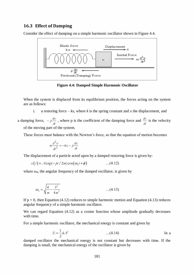
181

16.3 Effect of Damping

Consider the effect of damping on a simple harmonic oscillator shown in Figure 4.4.

Figure 4.4: Damped Simple Harmonic Oscillator

When the system is displaced from its equilibrium position, the forces acting on the system

are as follows:

i. a restoring force – kx, where k is the spring constant and x the displacement, and

a damping force, dxpdt

, where p is the coefficient of the damping force and dx

dtis the velocity

of the moving part of the system.

These forces must balance with the Newton’s force, so that the equation of motion becomes

2

2

d x dxm kx p

dtdt

The displacement of a particle acted upon by a damped restoring force is given by:

exp( /2 )cos dx t A pt m t …(4.12)

where ωd, the angular frequency of the damped oscillator, is given by

2

24d

k b

m m …(4.13)

If p = 0, then Equation (4.12) reduces to simple harmonic motion and Equation (4.13) reduces

angular frequency of a simple harmonic oscillator.

We can regard Equation (4.12) as a cosine function whose amplitude gradually decreases

with time.

For a simple harmonic oscillator, the mechanical energy is constant and given by

21

2E kA …(4.14) In a

damped oscillator the mechanical energy is not constant but decreases with time. If the

damping is small, the mechanical energy of the oscillator is given by

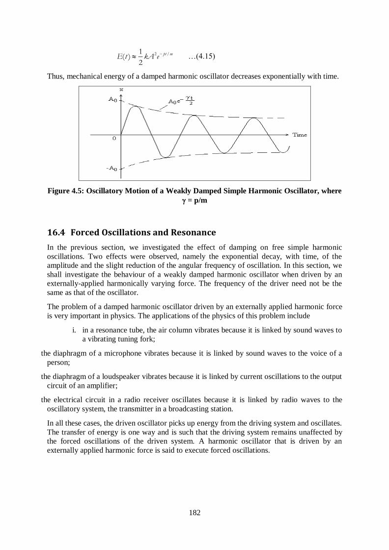
182

2 /1( )

2

pt mE t kA e …(4.15)

Thus, mechanical energy of a damped harmonic oscillator decreases exponentially with time.

Figure 4.5: Oscillatory Motion of a Weakly Damped Simple Harmonic Oscillator, where

= p/m

16.4 Forced Oscillations and Resonance

In the previous section, we investigated the effect of damping on free simple harmonic

oscillations. Two effects were observed, namely the exponential decay, with time, of the

amplitude and the slight reduction of the angular frequency of oscillation. In this section, we

shall investigate the behaviour of a weakly damped harmonic oscillator when driven by an

externally-applied harmonically varying force. The frequency of the driver need not be the

same as that of the oscillator.

The problem of a damped harmonic oscillator driven by an externally applied harmonic force

is very important in physics. The applications of the physics of this problem include

i. in a resonance tube, the air column vibrates because it is linked by sound waves to

a vibrating tuning fork;

the diaphragm of a microphone vibrates because it is linked by sound waves to the voice of a

person;

the diaphragm of a loudspeaker vibrates because it is linked by current oscillations to the output

circuit of an amplifier;

the electrical circuit in a radio receiver oscillates because it is linked by radio waves to the

oscillatory system, the transmitter in a broadcasting station.

In all these cases, the driven oscillator picks up energy from the driving system and oscillates.

The transfer of energy is one way and is such that the driving system remains unaffected by

the forced oscillations of the driven system. A harmonic oscillator that is driven by an

externally applied harmonic force is said to execute forced oscillations.

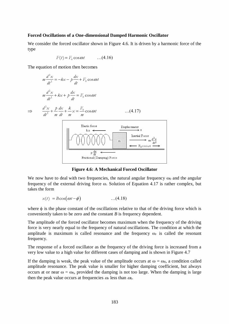
183

Forced Oscillations of a One-dimensional Damped Harmonic Oscillator

We consider the forced oscillator shown in Figure 4.6. It is driven by a harmonic force of the

type

0( ) cosF t F t …(4.16)

The equation of motion then becomes

2

02cos

d x dxm kx p F tdt dt

2

02cos

d x dxm kx p F tdt dt

2

0

2cos

Fd x p dx kx t

dt m dt m m …(4.17)

Figure 4.6: A Mechanical Forced Oscillator

We now have to deal with two frequencies, the natural angular frequency 0 and the angular

frequency of the external driving force . Solution of Equation 4.17 is rather complex, but

takes the form

( ) cosx t B t …(4.18)

where is the phase constant of the oscillations relative to that of the driving force which is

conveniently taken to be zero and the constant B is frequency dependent.

The amplitude of the forced oscillator becomes maximum when the frequency of the driving

force is very nearly equal to the frequency of natural oscillations. The condition at which the

amplitude is maximum is called resonance and the frequency r is called the resonant

frequency.

The response of a forced oscillator as the frequency of the driving force is increased from a

very low value to a high value for different cases of damping and is shown in Figure 4.7

If the damping is weak, the peak value of the amplitude occurs at = 0, a condition called

amplitude resonance. The peak value is smaller for higher damping coefficient, but always

occurs at or near = 0, provided the damping is not too large. When the damping is large

then the peak value occurs at frequencies r less than 0.

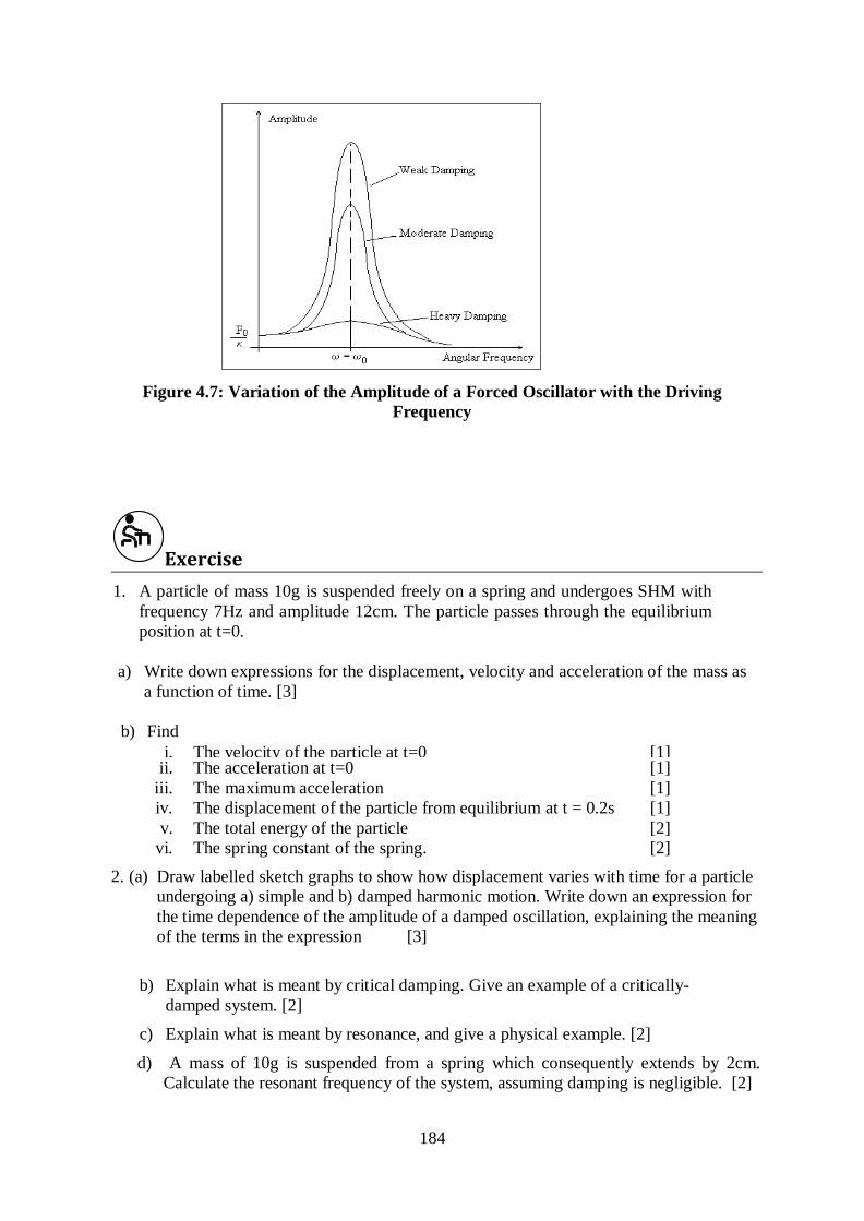
184

Figure 4.7: Variation of the Amplitude of a Forced Oscillator with the Driving

Frequency

Exercise 1. A particle of mass 10g is suspended freely on a spring and undergoes SHM with

frequency 7Hz and amplitude 12cm. The particle passes through the equilibrium

position at t=0.

a) Write down expressions for the displacement, velocity and acceleration of the mass as

a function of time. [3]

b) Find

i. The velocity of the particle at t=0 [1] ii. The acceleration at t=0 [1]

iii. The maximum acceleration [1]

iv. The displacement of the particle from equilibrium at t = 0.2s [1]

v. The total energy of the particle [2]

vi. The spring constant of the spring.

[2]

2. (a) Draw labelled sketch graphs to show how displacement varies with time for a particle

undergoing a) simple and b) damped harmonic motion. Write down an expression for

the time dependence of the amplitude of a damped oscillation, explaining the meaning

of the terms in the expression [3]

b) Explain what is meant by critical damping. Give an example of a critically-

damped system. [2]

c) Explain what is meant by resonance, and give a physical example. [2]

d) A mass of 10g is suspended from a spring which consequently extends by 2cm.

Calculate the resonant frequency of the system, assuming damping is negligible. [2]

185

e) Draw a sketch graph to show how the amplitude of oscillation of the system in d)

varies with the frequency of the driving force. How would the graph change if the

mass were suspended in water rather than air? [2]

3. A particle moving with simple harmonic motion of amplitude 10cm has a time period

of 25ms. What is its angular frequency? Calculate a) its phase, b) its velocity and c) its

phase when the displacement is 3cm from the equilibrium position.

186

4. A 1.5kg block is attached to a horizontal spring with spring constant 3000Nm-1

. Initially,

the block is at rest on a frictionless surface. A 10g bullet is fired into the block into the end

opposite the spring, and it sticks. If the subsequent oscillations of the spring have an

amplitude of 15cm, what was the initial velocity of the bullet? How would the amplitude

and frequency of the oscillations change if :

a) The same bullet were fired at a higher velocity into the block b) A heavier bullet were fired into the block at the original velocity.

5. (a) The end of a stretched string is forced to vibrate with a transverse displacement y (in

metres) = 0.3sin9t, where t is in seconds. If the tension in the string is 4N, and the mass per unit length of the string is 1.25gm

-1, calculate:

(i) The wave velocity (ii) The frequency (iii) The wavelength (iv) The displacement of the wave at (a)2m from the source, (b) 3m from the

source at a time 100ms after the oscillations commence.

(b) An astronaut on the Moon wishes to measure the local value of g by timing pulses

travelling down a 1.6m long wire of mass 4g, with a 3kg mass suspended from it. If a

pulse takes 36.1ms to traverse the total length of the string, calculate g.

6. What is Simple Harmonic Motion?

7. Describe Simple Harmonic Motion of a pendulum.

8. Describe Simple Harmonic Motion of an object attached to a horizontal spring.

9. Describe Simple Harmonic Motion of an object attached to a vertical spring.

10. Describe Simple Harmonic Motion of an object attached to a spring system in parallel.

11. Describe Simple Harmonic Motion of an object attached to a spring system in series.

12. Describe How potential energy and kinetic energy change in simple harmonic motion.

13. Describe Damping - light, hard and critical scenarios

187

Summary Damping forces are forces that restrain the vibratory motion, such as mechanical oscillations,

noise, and alternating electric currents, by dissipation of energy. Different kinds of damping

forces include viscous damping, Coulomb friction (ordinary friction) and structural damping

(internal friction). In a damped oscillator the mechanical energy is not constant but decreases

with time.

Two effects of damping on free simple harmonic oscillations are the exponential decay, with

time, of the amplitude and the slight reduction of the angular frequency of oscillation.

References

Gottys,W., Keller, F.J. and Skove, M.J, Physics Classical and Modern, 1989. McGraw

Hill.


E.F. Redish, Teaching Introductory Physics with the Physics Suite, 2003. John Wiley &

Sons.


188

Lecture 17: Wave Motion

17.1 Introduction

Wave motion appears in almost every branch of physics and is an important phenomenon in life.

For example, sound and light waves are essential for our contact and perception of our

environment, surface waves are a common feature on

water-bodies, electromagnetic waves are playing an increasingly important role in local and

global communication, and the structure of atoms and nuclei can be understood via the wavelike

properties of their constituent particles. Mobile phone signals, microwave ovens, ultrasound

machines all use energy carried by waves. Earthquakes and tsunamis are destructive waves of

energy.

Lecture Objectives At the end of this lecture, you should be able to do the following:

(i) Define waves

(ii) Differentiate waves from oscillations.

(iii) Describe mechanical waves.

(iv) Explain the characteristics of waves.

(v) Define wavelength as a variable characteristic of wave motion.

(vi) Write the wave equation.

(vii) Describe interference of waves

(viii) Describe standing waves

Definition of waves

A wave is a pulse of energy. Waves carry energy away from a central transmitter. Mechanical

waves such as sound waves need some medium of transmission. Electromagnetic waves, for

example, radio waves can carry energy through a vacuum. If a mechanical wave is travelling

through a medium, the particles of the medium do not move along. They simply vibrate about

their equilibrium position, and the energy is transmitted through the interaction of neighbouring

particles.

Waves can be classified into two broad classes: mechanical waves and electromagnetic waves.

Mechanical waves travel in deformable or elastic media whereas electromagnetic waves do not

require a medium for their propagation. Despite the differences in the nature of the waves, the

physical and mathematical descriptions are similar.

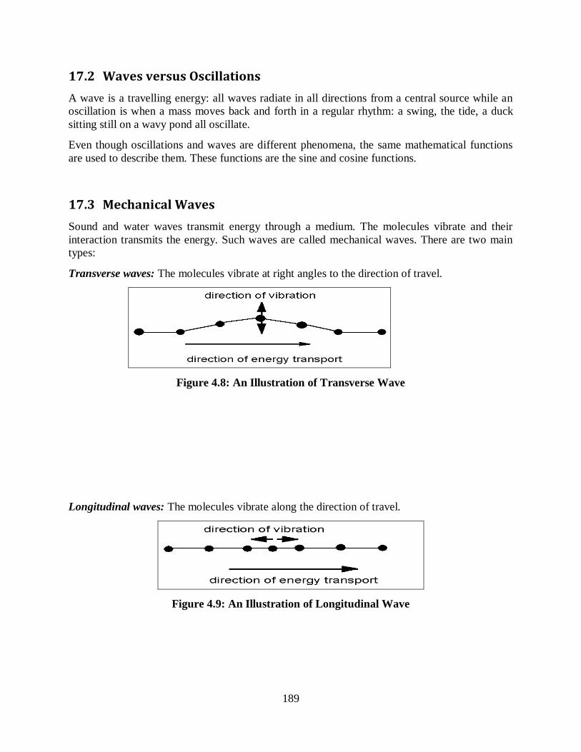
189

17.2 Waves versus Oscillations

A wave is a travelling energy: all waves radiate in all directions from a central source while an

oscillation is when a mass moves back and forth in a regular rhythm: a swing, the tide, a duck

sitting still on a wavy pond all oscillate.

Even though oscillations and waves are different phenomena, the same mathematical functions

are used to describe them. These functions are the sine and cosine functions.

17.3 Mechanical Waves

Sound and water waves transmit energy through a medium. The molecules vibrate and their

interaction transmits the energy. Such waves are called mechanical waves. There are two main

types:

Transverse waves: The molecules vibrate at right angles to the direction of travel.

Figure 4.8: An Illustration of Transverse Wave

Longitudinal waves: The molecules vibrate along the direction of travel.

Figure 4.9: An Illustration of Longitudinal Wave

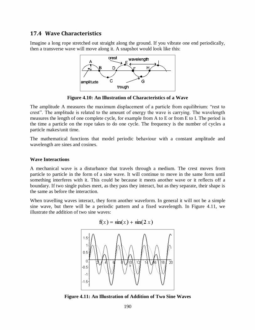
190

17.4 Wave Characteristics

Imagine a long rope stretched out straight along the ground. If you vibrate one end periodically,

then a transverse wave will move along it. A snapshot would look like this:

Figure 4.10: An Illustration of Characteristics of a Wave

The amplitude A measures the maximum displacement of a particle from equilibrium: “rest to

crest”. The amplitude is related to the amount of energy the wave is carrying. The wavelength

measures the length of one complete cycle, for example from A to E or from E to I. The period is

the time a particle on the rope takes to do one cycle. The frequency is the number of cycles a

particle makes/unit time.

The mathematical functions that model periodic behaviour with a constant amplitude and

wavelength are sines and cosines.

Wave Interactions

A mechanical wave is a disturbance that travels through a medium. The crest moves from

particle to particle in the form of a sine wave. It will continue to move in the same form until

something interferes with it. This could be because it meets another wave or it reflects off a

boundary. If two single pulses meet, as they pass they interact, but as they separate, their shape is

the same as before the interaction.

When travelling waves interact, they form another waveform. In general it will not be a simple

sine wave, but there will be a periodic pattern and a fixed wavelength. In Figure 4.11, we

illustrate the addition of two sine waves:

Figure 4.11: An Illustration of Addition of Two Sine Waves

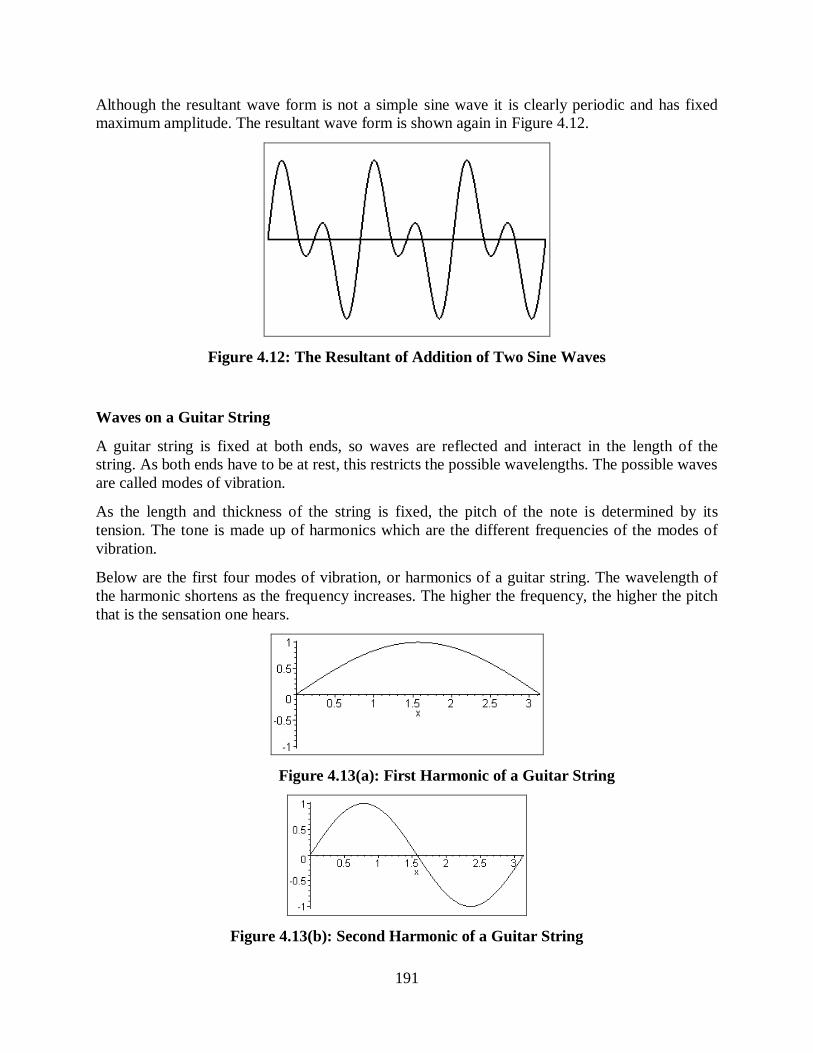
191

Although the resultant wave form is not a simple sine wave it is clearly periodic and has fixed

maximum amplitude. The resultant wave form is shown again in Figure 4.12.

Figure 4.12: The Resultant of Addition of Two Sine Waves

Waves on a Guitar String

A guitar string is fixed at both ends, so waves are reflected and interact in the length of the

string. As both ends have to be at rest, this restricts the possible wavelengths. The possible waves

are called modes of vibration.

As the length and thickness of the string is fixed, the pitch of the note is determined by its

tension. The tone is made up of harmonics which are the different frequencies of the modes of

vibration.

Below are the first four modes of vibration, or harmonics of a guitar string. The wavelength of

the harmonic shortens as the frequency increases. The higher the frequency, the higher the pitch

that is the sensation one hears.

Figure 4.13(a): First Harmonic of a Guitar String

Figure 4.13(b): Second Harmonic of a Guitar String

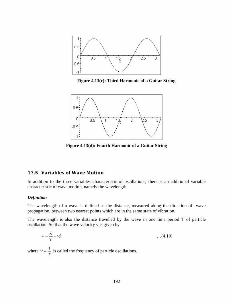
192

Figure 4.13(c): Third Harmonic of a Guitar String

Figure 4.13(d): Fourth Harmonic of a Guitar String

17.5 Variables of Wave Motion

In addition to the three variables characteristic of oscillations, there is an additional variable

characteristic of wave motion, namely the wavelength.

Definition

The wavelength of a wave is defined as the distance, measured along the direction of wave

propagation, between two nearest points which are in the same state of vibration.

The wavelength is also the distance travelled by the wave in one time period T of particle

oscillation. So that the wave velocity v is given by

vT

…(4.19)

where 1

T is called the frequency of particle oscillations.

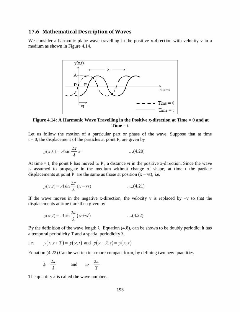
193

17.6 Mathematical Description of Waves

We consider a harmonic plane wave travelling in the positive x-direction with velocity v in a

medium as shown in Figure 4.14.

Figure 4.14: A Harmonic Wave Travelling in the Positive x-direction at Time = 0 and at

Time = t

Let us follow the motion of a particular part or phase of the wave. Suppose that at time

t = 0, the displacement of the particles at point P, are given by

2( , 0) siny x A x

…(4.20)

At time = t, the point P has moved to P', a distance vt in the positive x-direction. Since the wave

is assumed to propagate in the medium without change of shape, at time t the particle

displacements at point P' are the same as those at position (x – vt), i.e.

2( , ) sin ( v )y x t A x t

.....(4.21)

If the wave moves in the negative x-direction, the velocity v is replaced by –v so that the

displacements at time t are then given by

2

( , ) sin vy x t A x t

....(4.22)

By the definition of the wave length , Equation (4.8), can be shown to be doubly periodic; it has

a temporal periodicity T and a spatial periodicity .

i.e. , ,y x t T y x t and , ,y x t y x t

Equation (4.22) Can be written in a more compact form, by defining two new quantities

2k

and

2

T

The quantity k is called the wave number.

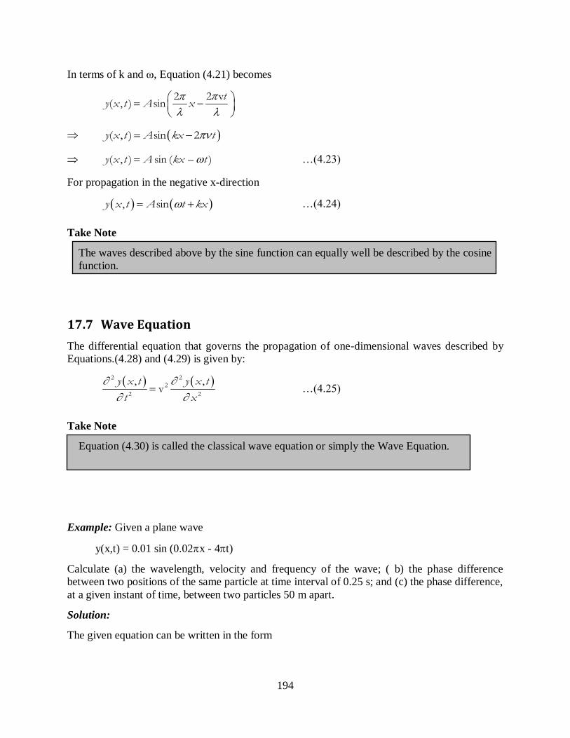
194

In terms of k and , Equation (4.21) becomes

2 v2( , ) sin

ty x t A x

( , ) sin 2y x t A kx t

( , ) sin ( – )y x t A kx t …(4.23)

For propagation in the negative x-direction

, siny x t A t kx …(4.24)

Take Note

The waves described above by the sine function can equally well be described by the cosine

function.

17.7 Wave Equation

The differential equation that governs the propagation of one-dimensional waves described by

Equations.(4.28) and (4.29) is given by:

2 2

2

2 2

, ,v

y x t y x t

t x

…(4.25)

Take Note

Equation (4.30) is called the classical wave equation or simply the Wave Equation.

Example: Given a plane wave

y(x,t) = 0.01 sin (0.02x - 4t)

Calculate (a) the wavelength, velocity and frequency of the wave; ( b) the phase difference

between two positions of the same particle at time interval of 0.25 s; and (c) the phase difference,

at a given instant of time, between two particles 50 m apart.

Solution:

The given equation can be written in the form

195

2( , ) 0.01sin 200

100y x t x t

Comparing with the wave equation

2( , ) sin vy x t A x t

We have,

the wavelength = 100 m

the wave velocity v = 200 m/s

and the frequency = v/ = 2.0 Hz

The phase change in a time interval t is

2. 2 . 2 .2.0.25t t

The phase difference for the path difference of x is

2 2. .50

100x

17.8 Interference of Waves

When two or more waves combine at a particular point, they are said to interfere and the

phenomenon is called interference.

There are two cases of interference:

1. Constructive interference in which the waves reinforce each other giving rise to a

resultant wave having an amplitude equal to the sum of the individual wave amplitudes.

2. Destructive interference in which the waves tend to cancel each other out giving rise to a

resultant wave having an amplitude close to zero.

Let us consider two waves of the same frequency and amplitude but different phase constants

both traveling in the +x-direction.

1 1( , ) siny x t A kx t …(4.26)

2 2( , ) siny x t A kx t …(4.27)

These waves could be propagating in any medium. Interference arises from the superposition of

the two waves. Thus adding Equations (4.26) and (4.27) we have

1 2( , ) ( , ) ( , )y x t y x t y x t

196

1 2sin sinA kx t A kx t

From the trigonometric identity

sinP +sinQ = 2sin½(P+Q)cos½(P–Q)

We obtain

1 2 2 1

1 1( , ) 2 sin 2 2 cos

2 2y x t A kx t

2 1 1 2

1 12 cos sin

2 2A kx t

1

( , ) 2 cos sin2

y x t A kx t …(4.28)

where

1 2

1

2 and 2 1

The quantity is called the phase difference between the two waves.

Equation (4.28) corresponds to a new wave having the same frequency but with an amplitude

2Acos(/2). If is very small in comparison with 180, the resultant amplitude is nearly

2A, twice the amplitude of either wave, this is constructive interference; on the other hand if

is close to 180 the resultant amplitude is nearly zero, this is destructive interference.

Two waves are said to be in phase when = 0 and are out of phase when = 180.

If the individual wave amplitudes are A1 and A2, the resultant wave amplitude is A1 + A2 if the

waves are in phase, while the resultant amplitude is A1 – A2 if they are out of phase.

Example: Two waves travel in the same direction along a string and interfere. The waves have

the same wavelength and travel with the same speed. The amplitude of each wave is 9.7 mm and

there is a phase difference of 110 between them. Calculate the amplitude of the combined wave

resulting from the interference of the two waves.

Solution:

The amplitude of the combined wave is given by

( , ) 2 cos ( , ) 2(9.7) cos(110/2) 11.1y x t A y x t mm

197

17.9 Standing Waves

When two or more waves travelling along the same direction combine they may interfere

destructively or constructively. On the other hand when the waves travel in opposite directions

the superposition gives rise to standing waves.

We consider two waves of equal amplitude and frequency moving in opposite direction a string.

1( , ) sin( )y x t A kx t

2( , ) sin( )y x t A kx t

Superposition gives rise to

1 2( , ) ( , ) ( , )y x t y x t y x t

sin( ) sin( )A kx t A kx t

( , ) 2 sin cosy x t A kx t …(4.29)

Take Note

Equation (4.34) is an equation of a Standing wave because the space and time variables, x

and t, do not appear as argument of the same trigonometric function as required for a

travelling wave.

In a travelling wave, each particle of the string vibrates with the same amplitude. In a standing

wave, the amplitude is not the same for different particles but varies for different location x of

the particle.

In Equation (4.29), the amplitude, 2Asinkx, is maximum at positions where

3 5; ; ......2 2 2

kx

Or 3 5; ; ........4 4 4

x

…(4.30)

Points of maximum amplitude in a standing wave are called antinodes. They are spaced one-half

wavelength apart.

On the other hand, the amplitude of the standing wave is minimum with value zero at positions

where

, 2 ,3 ....kx

or 3

, , , ......2 2

x

…(4.31)

198

Points of minimum amplitude in a standing wave are called nodes. They are also spaced one-half

wavelength apart. Hence, the separation between nodes and antinodes is a quarter wavelength.

Summary

i. A wave is a pulse of energy. Waves carry energy away from a central transmitter.

ii. Waves can be classified into mechanical waves and electromagnetic waves.

iii. Mechanical waves such as sound waves need some medium of transmission.

Electromagnetic waves, for example, radio waves can carry energy through a vacuum.

iv. When two or more waves travelling along the same direction combine they may interfere

destructively or constructively

v. In an oscillating system, the force always acts in a direction opposite to the displacement

of the particle from the equilibrium point.

The point of maximum displacement is defined as the amplitude of the oscillation.

Period of oscillation denotes the time it takes for an oscillating particle to return to its initial

position.

Frequency is defined as the number of cycles per unit time

Exercise 1. A wave has an amplitude of 2 cm and a frequency of 12 Hz, and the distance from a crest

to the nearest trough is measured to be 5 cm. Determine the period of such a wave.

2. A fly flaps its wings back and forth 150 times each second. Determine the period of a

wing flap.

3. A transverse wave is found to have a distance of 8 cm from a trough to a crest, a

frequency of 12 Hz, and a distance of 6 cm from a crest to the nearest trough. Determine

the amplitude, period, and wavelength of such a wave.

4. An ocean wave has an amplitude of 2.5 m. Weather conditions suddenly change such that

the wave has an amplitude of 5.0 m. Determine the amount of energy transported by the

wave.

5. In Figure 1, determine the time required for the waves, v = 340 m/s to travel from the

tuning fork to point P is

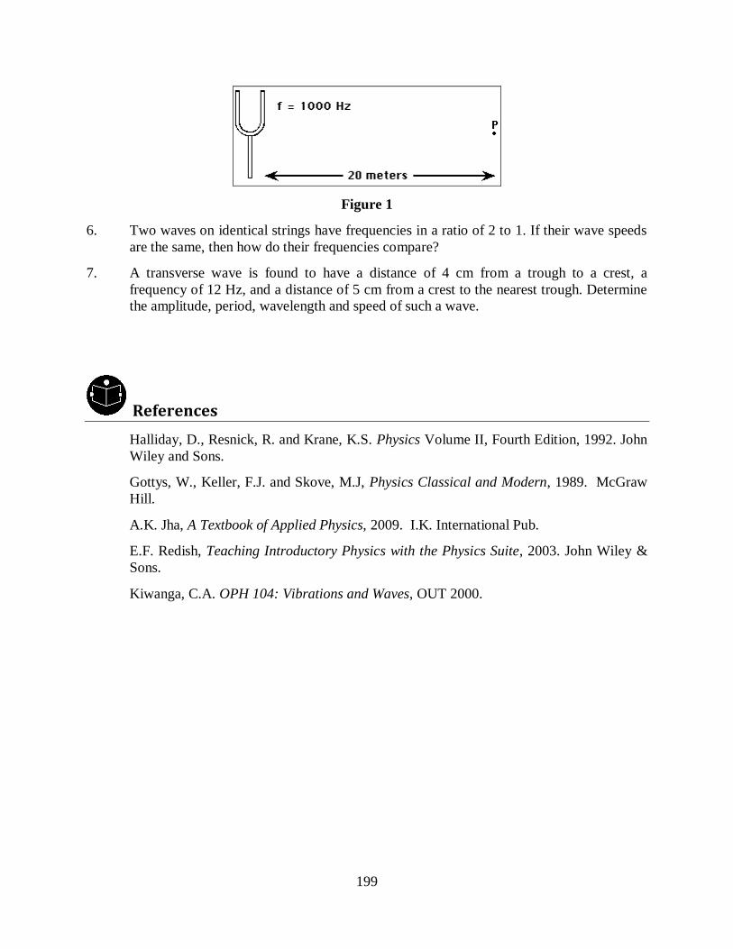
199

Figure 1

6. Two waves on identical strings have frequencies in a ratio of 2 to 1. If their wave speeds

are the same, then how do their frequencies compare?

7. A transverse wave is found to have a distance of 4 cm from a trough to a crest, a

frequency of 12 Hz, and a distance of 5 cm from a crest to the nearest trough. Determine

the amplitude, period, wavelength and speed of such a wave.

References

Halliday, D., Resnick, R. and Krane, K.S. Physics Volume II, Fourth Edition, 1992. John

Wiley and Sons.

Gottys, W., Keller, F.J. and Skove, M.J, Physics Classical and Modern, 1989. McGraw

Hill.


E.F. Redish, Teaching Introductory Physics with the Physics Suite, 2003. John Wiley &

Sons.


200

SECTION SIX:

ELECTRONICS

Lecture 18: Electronics

18.1 Introduction

Summary of the valve history

The vacuum tube or thermionic valve brought the dawn of the age of electronics. Its invention

enabled the wireless technology of the day to move forward.

The history of the vacuum tube or thermionic valve brings many individual discoveries together

that enable the invention to be made.

The history of the thermionic valve also moves on to tell of the further developments that were

made.

All these individual elements take their place in the overall history of the thermionic valve or

vacuum tube.

Lecture Objectives At the end of this lecture, you should be able to do the following:

(i) Outline the origins of the valve or vacuum tube.

(ii) Describe the diode valve.

(iii)Describe the diode rectification.

(iv) Describe the common examples of semiconductors.

(v) Describe features of intrinsic and extrinsic semiconductors.

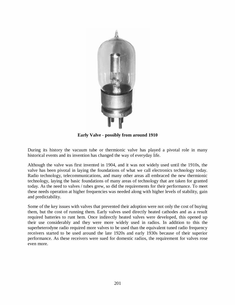
201

Early Valve - possibly from around 1910

During its history the vacuum tube or thermionic valve has played a pivotal role in many

historical events and its invention has changed the way of everyday life.

Although the valve was first invented in 1904, and it was not widely used until the 1910s, the

valve has been pivotal in laying the foundations of what we call electronics technology today.

Radio technology, telecommunications, and many other areas all embraced the new thermionic

technology, laying the basic foundations of many areas of technology that are taken for granted

today. As the need to valves / tubes grew, so did the requirements for their performance. To meet

these needs operation at higher frequencies was needed along with higher levels of stability, gain

and predictability.

Some of the key issues with valves that prevented their adoption were not only the cost of buying

them, but the cost of running them. Early valves used directly heated cathodes and as a result

required batteries to runt hem. Once indirectly heated valves were developed, this opened up

their use considerably and they were more widely used in radios. In addition to this the

superheterodyne radio required more valves to be used than the equivalent tuned radio frequency

receivers started to be used around the late 1920s and early 1930s because of their superior

performance. As these receivers were sued for domestic radios, the requirement for valves rose

even more.

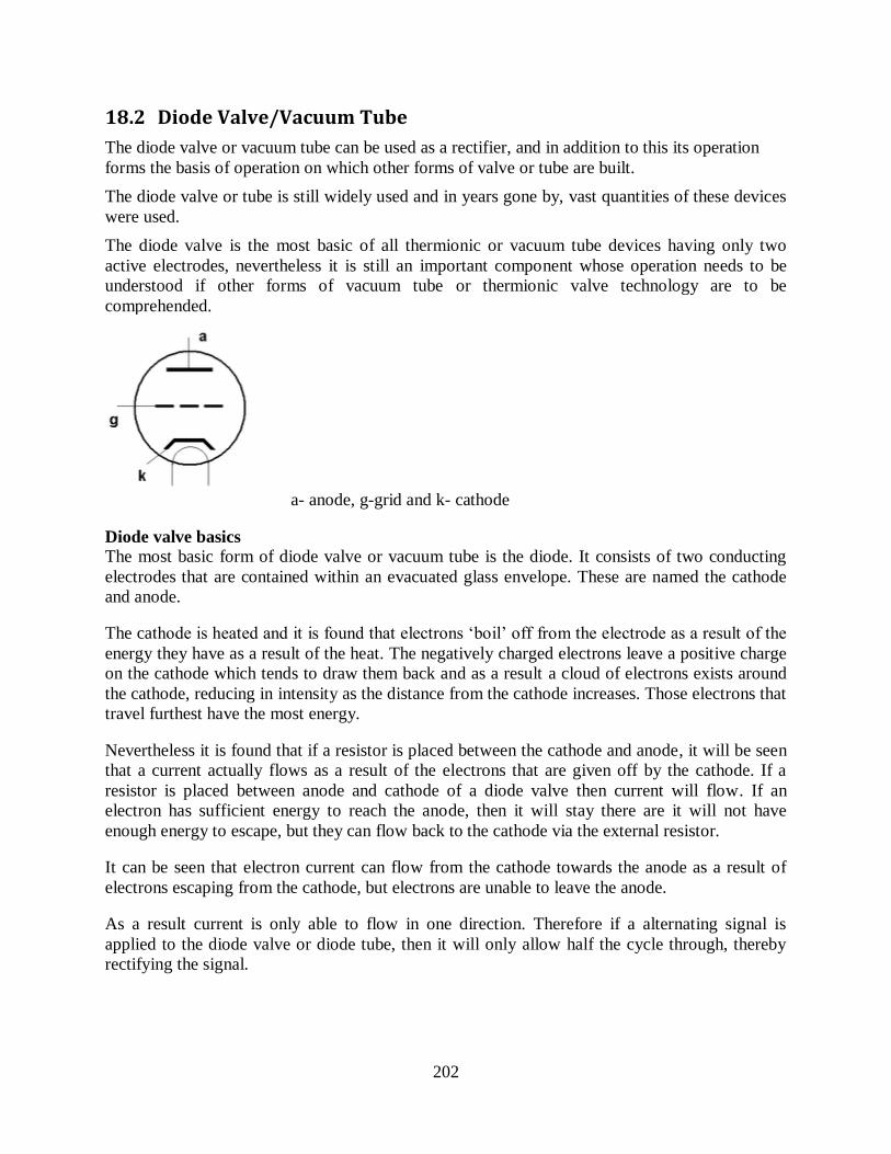
202

18.2 Diode Valve/Vacuum Tube

The diode valve or vacuum tube can be used as a rectifier, and in addition to this its operation

forms the basis of operation on which other forms of valve or tube are built.

The diode valve or tube is still widely used and in years gone by, vast quantities of these devices

were used.

The diode valve is the most basic of all thermionic or vacuum tube devices having only two

active electrodes, nevertheless it is still an important component whose operation needs to be

understood if other forms of vacuum tube or thermionic valve technology are to be

comprehended.

a- anode, g-grid and k- cathode

Diode valve basics

The most basic form of diode valve or vacuum tube is the diode. It consists of two conducting

electrodes that are contained within an evacuated glass envelope. These are named the cathode

and anode.

The cathode is heated and it is found that electrons ‘boil’ off from the electrode as a result of the

energy they have as a result of the heat. The negatively charged electrons leave a positive charge

on the cathode which tends to draw them back and as a result a cloud of electrons exists around

the cathode, reducing in intensity as the distance from the cathode increases. Those electrons that

travel furthest have the most energy.

Nevertheless it is found that if a resistor is placed between the cathode and anode, it will be seen

that a current actually flows as a result of the electrons that are given off by the cathode. If a

resistor is placed between anode and cathode of a diode valve then current will flow. If an

electron has sufficient energy to reach the anode, then it will stay there are it will not have

enough energy to escape, but they can flow back to the cathode via the external resistor.

It can be seen that electron current can flow from the cathode towards the anode as a result of

electrons escaping from the cathode, but electrons are unable to leave the anode.

As a result current is only able to flow in one direction. Therefore if a alternating signal is

applied to the diode valve or diode tube, then it will only allow half the cycle through, thereby

rectifying the signal.

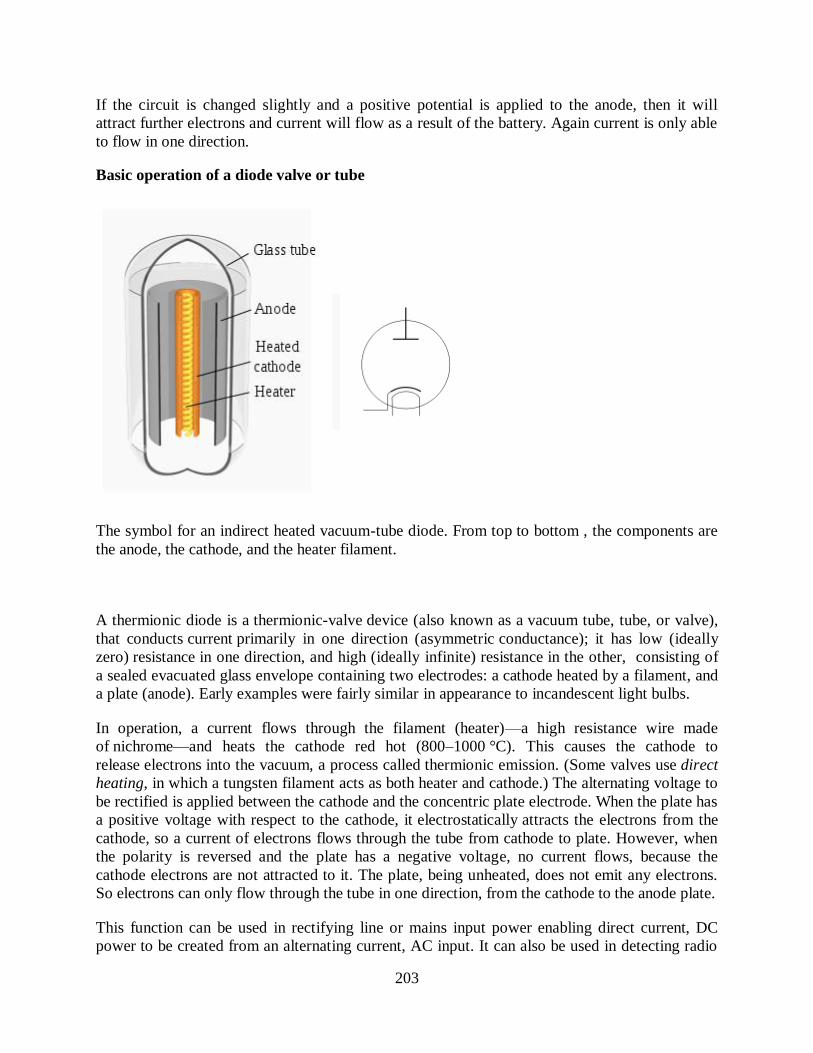
203

If the circuit is changed slightly and a positive potential is applied to the anode, then it will

attract further electrons and current will flow as a result of the battery. Again current is only able

to flow in one direction.

Basic operation of a diode valve or tube

The symbol for an indirect heated vacuum-tube diode. From top to bottom , the components are

the anode, the cathode, and the heater filament.

A thermionic diode is a thermionic-valve device (also known as a vacuum tube, tube, or valve),

that conducts current primarily in one direction (asymmetric conductance); it has low (ideally

zero) resistance in one direction, and high (ideally infinite) resistance in the other, consisting of

a sealed evacuated glass envelope containing two electrodes: a cathode heated by a filament, and

a plate (anode). Early examples were fairly similar in appearance to incandescent light bulbs.

In operation, a current flows through the filament (heater)—a high resistance wire made

of nichrome—and heats the cathode red hot (800–1000 °C). This causes the cathode to

release electrons into the vacuum, a process called thermionic emission. (Some valves use direct

heating, in which a tungsten filament acts as both heater and cathode.) The alternating voltage to

be rectified is applied between the cathode and the concentric plate electrode. When the plate has

a positive voltage with respect to the cathode, it electrostatically attracts the electrons from the

cathode, so a current of electrons flows through the tube from cathode to plate. However, when

the polarity is reversed and the plate has a negative voltage, no current flows, because the

cathode electrons are not attracted to it. The plate, being unheated, does not emit any electrons.

So electrons can only flow through the tube in one direction, from the cathode to the anode plate.

This function can be used in rectifying line or mains input power enabling direct current, DC

power to be created from an alternating current, AC input. It can also be used in detecting radio

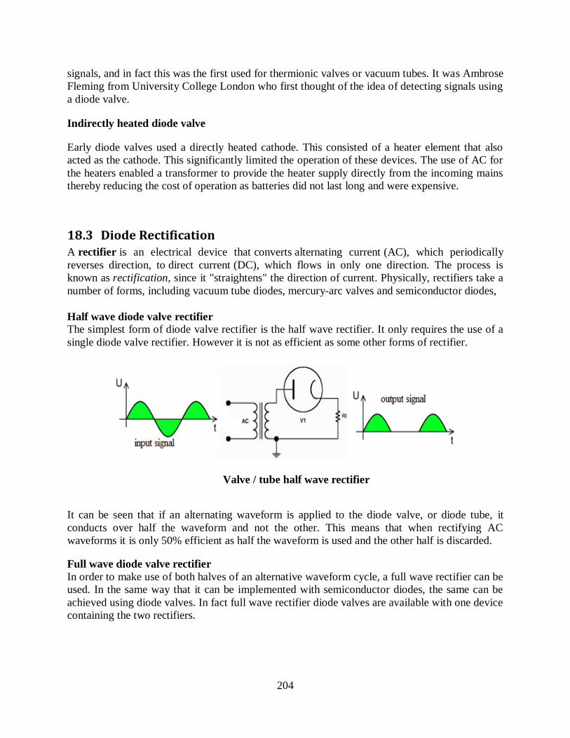
204

signals, and in fact this was the first used for thermionic valves or vacuum tubes. It was Ambrose

Fleming from University College London who first thought of the idea of detecting signals using

a diode valve.

Indirectly heated diode valve

Early diode valves used a directly heated cathode. This consisted of a heater element that also

acted as the cathode. This significantly limited the operation of these devices. The use of AC for

the heaters enabled a transformer to provide the heater supply directly from the incoming mains

thereby reducing the cost of operation as batteries did not last long and were expensive.

18.3 Diode Rectification A rectifier is an electrical device that converts alternating current (AC), which periodically

reverses direction, to direct current (DC), which flows in only one direction. The process is

known as rectification, since it "straightens" the direction of current. Physically, rectifiers take a

number of forms, including vacuum tube diodes, mercury-arc valves and semiconductor diodes,

Half wave diode valve rectifier

The simplest form of diode valve rectifier is the half wave rectifier. It only requires the use of a

single diode valve rectifier. However it is not as efficient as some other forms of rectifier.

Valve / tube half wave rectifier

It can be seen that if an alternating waveform is applied to the diode valve, or diode tube, it

conducts over half the waveform and not the other. This means that when rectifying AC

waveforms it is only 50% efficient as half the waveform is used and the other half is discarded.

Full wave diode valve rectifier

In order to make use of both halves of an alternative waveform cycle, a full wave rectifier can be

used. In the same way that it can be implemented with semiconductor diodes, the same can be

achieved using diode valves. In fact full wave rectifier diode valves are available with one device

containing the two rectifiers.

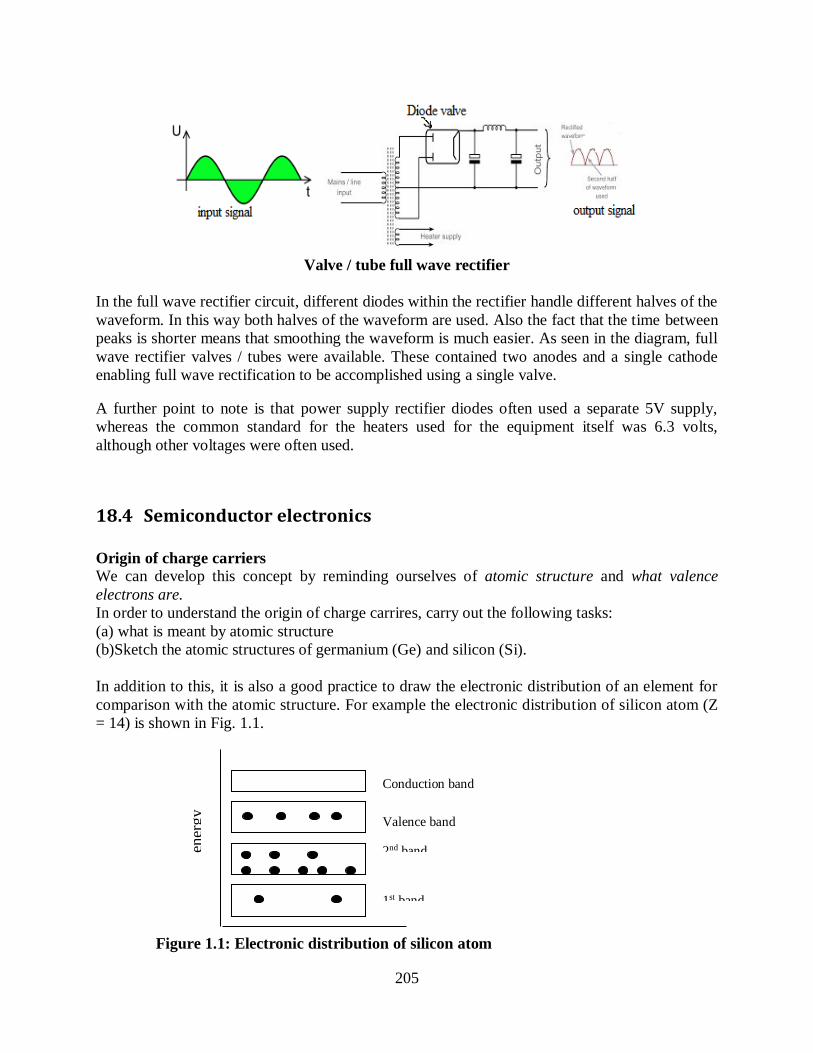
205

Valve / tube full wave rectifier

In the full wave rectifier circuit, different diodes within the rectifier handle different halves of the

waveform. In this way both halves of the waveform are used. Also the fact that the time between

peaks is shorter means that smoothing the waveform is much easier. As seen in the diagram, full

wave rectifier valves / tubes were available. These contained two anodes and a single cathode

enabling full wave rectification to be accomplished using a single valve.

A further point to note is that power supply rectifier diodes often used a separate 5V supply,

whereas the common standard for the heaters used for the equipment itself was 6.3 volts,

although other voltages were often used.

18.4 Semiconductor electronics

Origin of charge carriers

We can develop this concept by reminding ourselves of atomic structure and what valence

electrons are.

In order to understand the origin of charge carrires, carry out the following tasks:

(a) what is meant by atomic structure

(b)Sketch the atomic structures of germanium (Ge) and silicon (Si).

In addition to this, it is also a good practice to draw the electronic distribution of an element for

comparison with the atomic structure. For example the electronic distribution of silicon atom (Z

= 14) is shown in Fig. 1.1.

Figure 1.1: Electronic distribution of silicon atom

1st band

2nd band

Valence band

Conduction band

ener

gy

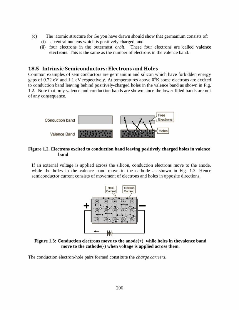
206

(c) The atomic structure for Ge you have drawn should show that germanium consists of:

(i) a central nucleus which is positively charged, and

(ii) four electrons in the outermost orbit. These four electrons are called valence

electrons. This is the same as the number of electrons in the valence band.

18.5 Intrinsic Semiconductors: Electrons and Holes Common examples of semiconductors are germanium and silicon which have forbidden energy

gaps of 0.72 eV and 1.1 eV respectively. At temperatures above 00K some electrons are excited

to conduction band leaving behind positively-charged holes in the valence band as shown in Fig.

1.2. Note that only valence and conduction bands are shown since the lower filled bands are not

of any consequence.

Figure 1.2. Electrons excited to conduction band leaving positively charged holes in valence

band

If an external voltage is applied across the silicon, conduction electrons move to the anode,

while the holes in the valence band move to the cathode as shown in Fig. 1.3. Hence

semiconductor current consists of movement of electrons and holes in opposite directions.

Figure 1.3: Conduction electrons move to the anode(+), while holes in thevalence band

move to the cathode(-) when voltage is applied across them.

The conduction electron-hole pairs formed constitute the charge carriers.

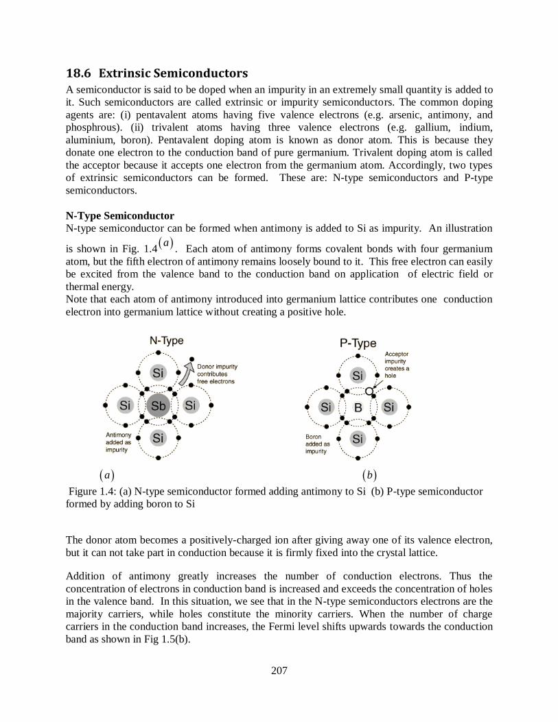
207

18.6 Extrinsic Semiconductors A semiconductor is said to be doped when an impurity in an extremely small quantity is added to

it. Such semiconductors are called extrinsic or impurity semiconductors. The common doping

agents are: (i) pentavalent atoms having five valence electrons (e.g. arsenic, antimony, and

phosphrous). (ii) trivalent atoms having three valence electrons (e.g. gallium, indium,

aluminium, boron). Pentavalent doping atom is known as donor atom. This is because they

donate one electron to the conduction band of pure germanium. Trivalent doping atom is called

the acceptor because it accepts one electron from the germanium atom. Accordingly, two types

of extrinsic semiconductors can be formed. These are: N-type semiconductors and P-type

semiconductors.

N-Type Semiconductor

N-type semiconductor can be formed when antimony is added to Si as impurity. An illustration

is shown in Fig. 1.4 a

. Each atom of antimony forms covalent bonds with four germanium

atom, but the fifth electron of antimony remains loosely bound to it. This free electron can easily

be excited from the valence band to the conduction band on application of electric field or

thermal energy.

Note that each atom of antimony introduced into germanium lattice contributes one conduction

electron into germanium lattice without creating a positive hole.

a

b

Figure 1.4: (a) N-type semiconductor formed adding antimony to Si (b) P-type semiconductor

formed by adding boron to Si

The donor atom becomes a positively-charged ion after giving away one of its valence electron,

but it can not take part in conduction because it is firmly fixed into the crystal lattice.

Addition of antimony greatly increases the number of conduction electrons. Thus the

concentration of electrons in conduction band is increased and exceeds the concentration of holes

in the valence band. In this situation, we see that in the N-type semiconductors electrons are the

majority carriers, while holes constitute the minority carriers. When the number of charge

carriers in the conduction band increases, the Fermi level shifts upwards towards the conduction

band as shown in Fig 1.5(b).

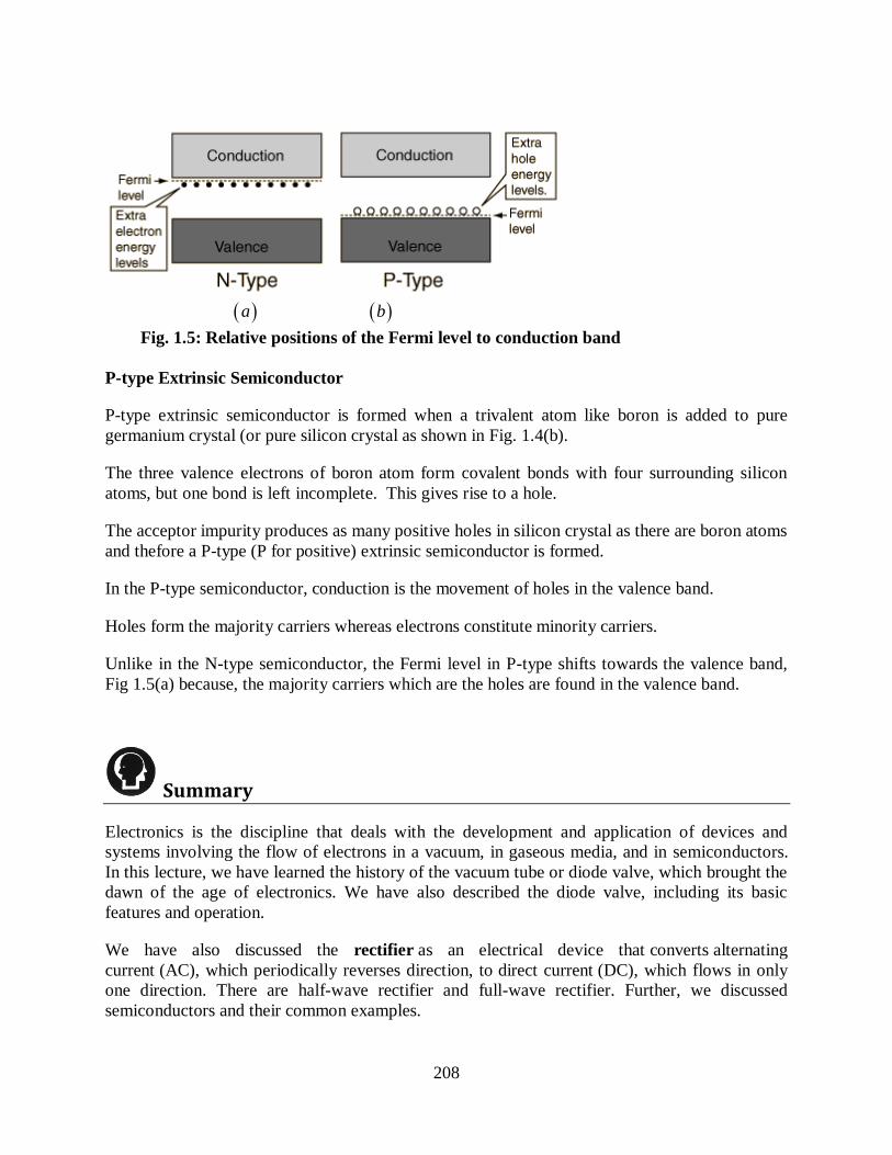
208

a

b

Fig. 1.5: Relative positions of the Fermi level to conduction band

P-type Extrinsic Semiconductor

P-type extrinsic semiconductor is formed when a trivalent atom like boron is added to pure

germanium crystal (or pure silicon crystal as shown in Fig. 1.4(b).

The three valence electrons of boron atom form covalent bonds with four surrounding silicon

atoms, but one bond is left incomplete. This gives rise to a hole.

The acceptor impurity produces as many positive holes in silicon crystal as there are boron atoms

and thefore a P-type (P for positive) extrinsic semiconductor is formed.

In the P-type semiconductor, conduction is the movement of holes in the valence band.

Holes form the majority carriers whereas electrons constitute minority carriers.

Unlike in the N-type semiconductor, the Fermi level in P-type shifts towards the valence band,

Fig 1.5(a) because, the majority carriers which are the holes are found in the valence band.

Summary

Electronics is the discipline that deals with the development and application of devices and

systems involving the flow of electrons in a vacuum, in gaseous media, and in semiconductors.

In this lecture, we have learned the history of the vacuum tube or diode valve, which brought the

dawn of the age of electronics. We have also described the diode valve, including its basic

features and operation.

We have also discussed the rectifier as an electrical device that converts alternating

current (AC), which periodically reverses direction, to direct current (DC), which flows in only

one direction. There are half-wave rectifier and full-wave rectifier. Further, we discussed

semiconductors and their common examples.

209

References

Chattopadhyay, D., Rakshit, P. C. and Saha, B. (2009). Foundations of Electronics,

Revised Second Ed. New Age International Publishers: India

ofp 010 physics - The Open University of Tanzania-Library

Documents