1 Offshore pumped hydropower storage Technical feasibility study on a large energy storage facility on the Dogger Bank L.H. de Vilder Master thesis

Welcome message from author
This document is posted to help you gain knowledge. Please leave a comment to let me know what you think about it! Share it to your friends and learn new things together.
Transcript
1
Offshore pumped hydropower storage Technical feasibility study on a large energy storage facility
on the Dogger Bank
L.H. de Vilder Master thesis

2
III
Offshore Pumped Hydropower Storage
Technical feasibility study on a large energy storage facility on the Dogger Bank
By
Lucas de Vilder
To obtain the degree of
Master of Science
In Hydraulic Engineering
Specialization in Hydraulic Structures and Flood Risk
Faculty of Civil Engineering and Geosciences Delft University of Technology
The Netherlands
16th October 2017
Graduation committee
Chairman Prof. Dr. Ir. S.N. Jonkman Supervisor Prof. Ir. A.Q.C. van der Horst Supervisor Ir. J.D. Bricker Supervisor Ir. W.F. Molenaar Company supervisor Ir. E.J. van Druten

IV

V
Preface This report presents my graduation work to conclude my Master Hydraulic Engineering and
specialisation Hydraulic Structures and Flood Risk at the Delft University of Technology. The topic of
this research is to develop a better understanding of how an offshore pumped hydropower storage
facility scales with its storage and power capacity by using existing construction technologies. The
research has been conducted in cooperation with the engineering and consulting agency
Witteveen+Bos.
First of all, I would like to express my gratitude towards the members of my graduation committee. I
would like to thank Bas Jonkman for your extensive feedback after every single meeting and Jeremy
Bricker for always being available whenever I needed some guidance. Thanks to Wilfred Molenaar for
always expressing your concerns and safeguarding the principles of hydraulic engineering. Aad van
der Horst, thank you for joining the committee and enthusiasm to deal with the challenges of
execution.
A special thanks to Emiel van Druten, your fascination for civil engineering and supervision on the
graduation process has truly been inspiring. To all the colleagues of Witteveen+Bos, thank you for
the opportunity to work alongside you and your willingness to assist every time I needed your
expertise. Thanks to the other graduates for the enjoyable time and good atmosphere in the office.
Finally, I would like to thank my family, friends, flatmates and girlfriend for your support during my
entire study.
Lucas de Vilder
Delft, October 2017

VI
VII
Summary To combat global warming a transition towards renewable energy sources (RES) is essential.
Although RES have much lower life-cycle emissions, they do not offer a continuous and fully
predictable output like their fossil-fuelled counterparts. Energy storage is paramount in order to
include the growing share of these intermittent sources into the grid and provide a reliable supply of
energy.
In 2016 a long term vision which involves the creation of an artificial island on the Dogger Bank in the
North Sea was presented. The island would act as the central spill in an interconnected future
economy fuelled by RES. Currently there are no competitive energy storage technologies under
consideration that could contribute to this ‘energy hub’.
In Europe pumped hydropower storage (PHS) represents over 90% of the grid-connected storage
capacity and continues to be identified as the most cost-efficient energy storage technology available
today and in the future. Unfortunately, conventional PHS is restricted to mountainous areas and the
remaining potential (2291GWh) does not suffice to future demand (estimated at 3596GWh).
The plans of developing a large wind farm via the construction of an island made it an attractive base
to test the contribution and feasibility of a substitute to conventional PHS: inverse offshore pumped
hydropower storage (IOPHS). It relies on the same principles as conventional PHS, only the process is
inverted. When the wind farm generates a surplus of energy, the excess power is used to drive
hydraulic turbines which pump the water out of the artificially created lake into the surrounding sea.
Then when there is a higher demand for energy than the wind farm generates at that time, the sea
water is allowed to flow back into the interior lake driving the same turbines.
Although the idea of inverse offshore pumped hydropower storage has been around for years, it has
never been constructed. The objective of this research is to identify the possible design alternatives
and determine how the costs of an offshore pumped hydropower storage facility scale with the
power and storage capacity, using existing construction technologies.
The construction of the storage plant consists of four main elements: the dam, dredging works,
turbines and the turbine housing. For the dam and dredging process that collectively are responsible
for the creation of the storage capacity, it was found that when thick clay layers are present the costs
are dominated by:
1. Maximum practically achievable reservoir depth
2. Armouring of the dam to cope with the wave conditions
3. Combination of inner slope stability and uplift of the inner toe
4. Dredging equipment and the operational waves during the excavation of the stiff clay
5. Sealing of the underlying sand layer
The costs of the power capacity depend on the turbines and the housing that are governed by:
1. Construction method of the turbine housing and connecting penstock and tailrace
2. Type and size of turbines
3. Maintenance costs of the electrical and mechanical parts
4. Preventive measures against cavitation from the turbine runners

VIII
When all costs are combined (except for planning and design costs) the expenditure scales as
estimated in Table 1. The dedicated equipment is required to enable an efficient dredging process in
the offshore conditions.
Element Capital costs (m€) Operational and maintenance costs (m€/yr)
Dedicated equipment 310 -
Storage reservoir (E=GWh) 103 x 0.7209 x E0.389 10 x 0.7209 x E0.389
Power generation (P=GW) 103 x 0.8746 x P0.9118 40 x 0.8746 x P0.9118 Table 1: Total costs of an offshore pumped hydropower storage plant in the North Sea with a maximum head difference of 40 metres. The operational cost of the dredging equipment is included in the storage capacity
It should be noted that the results are certainly not limited to a single location on the Dogger Bank,
rather they are universally applicable. The stated design choices and relative costs components may
act as guidance from which the given formulae and factors could easily be transposed to any other
site. By doing so it can quickly be assessed if an inverse PHS system is possible and whether it
provides a profitable business case.
The computed costs were obtained in a deterministic way. After a selection of future scenarios and
uncertainties were taken into account, the levelised cost of storage (LCOS) was estimated. For a
25GWh storage capacity and 2.65GW of installed power the LCOS may vary from 68.2€/MWh to
19.0€/MWh of which 40€/MWh is found the most realistic.
In the worst case scenario the offshore pumped hydropower variant would remarkably be just as
competitive as a conventional PHS plant. More importantly the studied alternative is a factor 3 to 18
times less expensive than batteries or power to gas (both are currently under consideration to
incorporate the large shares of wind energy from the North Sea).
The considered reservoir is expected to have a Net Present Value of 610 million euros and a payback
period of 23 years, which in favourable conditions could become 2.9 billion euros. Consequently it
was not only found that constructing an inverse offshore pumped hydropower storage facility in the
middle of the North Sea that can cope with the discussed failure mechanisms is possible. In addition
the operation would be highly profitable.
This research presents a viable offshore pumped hydropower storage facility that is undoubtedly
worthwhile, without relying on potential revenues or investments from other functions. Thereby it
may offer a valuable link in the transition towards a green economy and within the development of
large scale offshore wind energy in the North Sea.
The idea of Luc Lievense about artificially creating an energy storage reservoir has been laying on the
shelf for nearly four decades. At the time wind energy did not develop as quickly as initially ex pected
and the project lost interest. Nowadays offshore wind is being installed and planned on an
unprecedented scale, making the business case for energy storage more lucrative than it has ever
been before. Therefore the time to initiate the realisation of inverse pumped hydropower storage is
now.

IX
10
Content Preface ......................................................................................................................................... V
Summary .................................................................................................................................... VII
1. Introduction .............................................................................................................................15
1.1 Climate action ....................................................................................................................15
1.2 Integrating renewable energy into the grid...........................................................................17
1.3 Long term plan: ‘Energy hub in the North Sea’ ......................................................................19
1.3.1 Contribution of energy storage to the ‘energy hub’ ........................................................20
1.4 Problem definition ..............................................................................................................22
1.5 Reading guide .....................................................................................................................23
2. Analysis on energy storage........................................................................................................25
2.1 Energy storage outlook .......................................................................................................25
2.1.1 Global ..........................................................................................................................25
2.1.2 European Union ...........................................................................................................26
2.1.3 The Netherlands ...........................................................................................................27
2.1.4 Overview .....................................................................................................................27
2.2 Future demand for energy storage.......................................................................................28
2.2.1 Future energy demand..................................................................................................28
2.2.2 Future renewable energy market share .........................................................................29
2.2.3 Required energy storage capacity ..................................................................................30
2.2.4 Types of energy storage services ...................................................................................31
2.3 Energy storage technologies ................................................................................................32
2.3.1 Pumped hydropower storage ........................................................................................32
2.3.2 Compressed air energy storage .....................................................................................35
2.3.3 Batteries ......................................................................................................................37
2.3.4 Vehicle to grid ..............................................................................................................39
2.3.5 Power to gas ................................................................................................................40
2.3.6 Comparison of energy storage technologies ...................................................................42
2.3.7 Concluding remarks on energy storage technologies ......................................................45
2.4 Potentially realisable pumped hydro storage ........................................................................46
2.5 Future demand versus potentially realisable energy storage .................................................48
2.5.1 Need for alternative energy storage technologies...........................................................48
2.6 Overview of energy storage islands ......................................................................................49
11
3. Technical design approach ........................................................................................................51
3.1 Boundary conditions ...........................................................................................................52
3.2 Functional requirements .....................................................................................................52
3.3 Failure tree .........................................................................................................................52
3.4 Principal scaling of reservoir dimensions ..............................................................................55
3.5 Volume balance ..................................................................................................................58
4. Dam design ..............................................................................................................................60
4.1 Sea defence ........................................................................................................................61
4.2 Inner slope .........................................................................................................................65
4.2.1 Protection against waves ..............................................................................................65
4.2.3 Phreatic line .................................................................................................................69
4.3 Water retaining measures ...................................................................................................70
4.3.1 Slurry bentonite wall.....................................................................................................70
4.3.2 Sheet piles ...................................................................................................................71
4.3.3 Jet-grouting..................................................................................................................71
4.3.4 Replacement of sand layer ............................................................................................72
4.3.5 Choice of measure ........................................................................................................72
4.4 Failure mechanisms ............................................................................................................74
4.4.1 Macro stability .............................................................................................................76
4.4.2 Micro stability ..............................................................................................................80
4.4.3 Piping ..........................................................................................................................81
4.4.4 Seepage .......................................................................................................................82
4.4.5 Bursting of the clay layer...............................................................................................84
4.4.6 Overtopping .................................................................................................................85
4.5 Final design and concluding remarks ....................................................................................86
5. Dredging works ........................................................................................................................90
5.1 Selection of dredger............................................................................................................90
5.2 Dredging operation .............................................................................................................91
5.3 Specifications and costs.......................................................................................................95
5.4 Environmental measures ................................................................................................... 100
6. Power generation ................................................................................................................... 102
6.1 Selection of turbine........................................................................................................... 102
6.2 Runner diameter............................................................................................................... 104
6.3 Cavitation prevention........................................................................................................ 107
12
6.4 Pump-turbine characteristics ............................................................................................. 107
7. Housing of turbines ................................................................................................................ 109
7.1 Construction method ........................................................................................................ 110
7.1.1 In-situ: pneumatic caisson ........................................................................................... 111
7.1.2 In-situ: open caisson ................................................................................................... 112
7.1.3 Prefab: modular box caissons ...................................................................................... 113
7.1.4 Hybrid: prefab bottom caisson + in-situ superstructure................................................. 115
7.1.5 Choice of method ....................................................................................................... 116
7.2 Main dimensions and volumes........................................................................................... 117
8. Costs & benefits ..................................................................................................................... 120
8.1 Dam costs......................................................................................................................... 120
8.1.1 Water retaining costs.................................................................................................. 121
8.2 Dredging costs .................................................................................................................. 122
8.3 Pump-turbine costs........................................................................................................... 123
8.4 Housing of turbine costs.................................................................................................... 125
8.5 Operational and maintenance costs ................................................................................... 126
8.6 Total costs ........................................................................................................................ 127
8.7 Levelised cost of storage ................................................................................................... 129
8.7.1 Comparison with other energy storage technologies .................................................... 131
8.8 Benefits............................................................................................................................ 132
8.8.1 Hypothetical revenues and payback period .................................................................. 133
8.8.2 Contribution of energy storage to the ‘Energy hub’ in the North Sea ............................. 135
9. Discussion .............................................................................................................................. 137
9.1 Storage capacity ............................................................................................................... 137
9.2 Power capacity ................................................................................................................. 139
9.3 Levelised cost of storage ................................................................................................... 140
9.4 Comparison with previous literature .................................................................................. 141
9.5 Remarkable findings.......................................................................................................... 142
10. Conclusion ........................................................................................................................... 145
10.1 Dam design..................................................................................................................... 147
10.2 Dredging process ............................................................................................................ 147
10.3 Power generation ........................................................................................................... 148
10.4 Housing of turbines ......................................................................................................... 149
10.5 Scaling of an offshore pumped hydropower storage facility ............................................... 150
13
11. Recommendations................................................................................................................ 152
Bibliography .............................................................................................................................. 155
List of figures ............................................................................................................................. 161
List of tables .............................................................................................................................. 169
Appendices ................................................................................................................................ 173
Appendix A: Options to help integrating intermittent renewables ............................................. 174
Appendix B: Alternative pumped hydropower storage systems ................................................. 175
B.1 Plan Lievense ................................................................................................................ 175
B.2 Energy Island ................................................................................................................ 177
B.3 Slufter .......................................................................................................................... 180
B.4 Taiwan Integrated Energy and Service Island .................................................................. 182
B.5 Underground pumped hydro storage ............................................................................. 185
B.6 Stored Energy in Sea...................................................................................................... 187
Appendix C: Scalars of energy storage islands .......................................................................... 189
Appendix D: Dogger Bank conditions ....................................................................................... 191
Appendix E: Risks associated to inverse offshore pumped hydro storage ................................... 195
Appendix F: Influence of toe material on slope stability ............................................................ 196
Appendix G: Seepage and bursting mechanism for a closed aquifer........................................... 198
G.1 Seepage ....................................................................................................................... 198
G.2 Bursting........................................................................................................................ 200
Appendix H: Construction method of the dam ......................................................................... 204
Appendix I: Location of the powerhouse and penstock design................................................... 206
Appendix J: Connecting box caissons with Gina gaskets ............................................................ 210

14
15
1. Introduction Firstly an outline on the challenges of the future energy supply will be given, explaining climate
change as a driver for switching to renewables, which bring their own challenges. Furthermore, the
alternatives for energy storage will be discussed as interconnectivity, flexible demand and generation
or the curtailment that would follow when these flexibility options are not sufficiently implemented.
Lastly a long term vision is presented, that involves the creation of an artificial island in the middle of
the North Sea. The island would act as the central spill in an interconnected future economy that is
fuelled by renewable energy sources (RES). For that future situation it will ultimately lead to the
question how energy storage can contribute to this multifunctional concept.
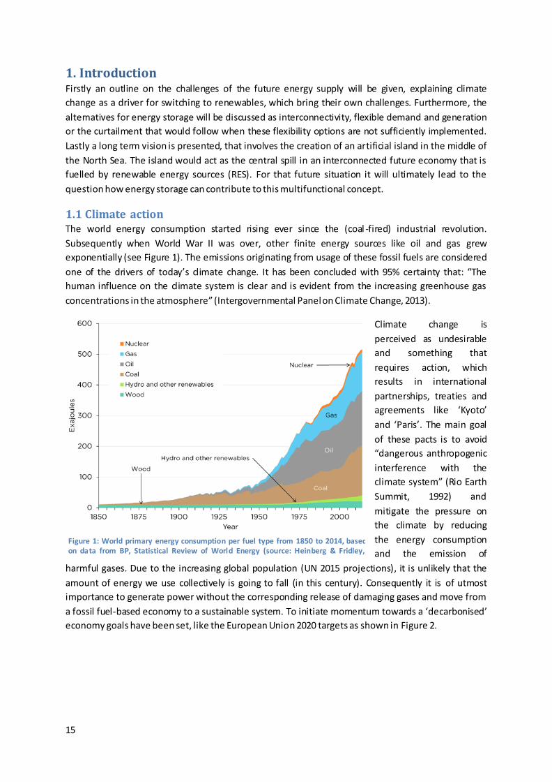
1.1 Climate action The world energy consumption started rising ever since the (coal -fired) industrial revolution.
Subsequently when World War II was over, other finite energy sources like oil and gas grew
exponentially (see Figure 1). The emissions originating from usage of these fossil fuels are considered
one of the drivers of today’s climate change. It has been concluded with 95% certainty that: “The
human influence on the climate system is clear and is evident from the increasing greenhouse gas
concentrations in the atmosphere” (Intergovernmental Panel on Climate Change, 2013).
Climate change is
perceived as undesirable
and something that
requires action, which
results in international
partnerships, treaties and
agreements like ‘Kyoto’
and ‘Paris’. The main goal
of these pacts is to avoid
“dangerous anthropogenic
interference with the
climate system” (Rio Earth
Summit, 1992) and
mitigate the pressure on
the climate by reducing
the energy consumption
and the emission of
harmful gases. Due to the increasing global population (UN 2015 projections), it is unlikely that the
amount of energy we use collectively is going to fall (in this century). Consequently it is of utmost
importance to generate power without the corresponding release of damaging gases and move from
a fossil fuel-based economy to a sustainable system. To initiate momentum towards a ‘decarbonised’
economy goals have been set, like the European Union 2020 targets as shown in Figure 2.
Figure 1: World primary energy consumption per fuel type from 1850 to 2014, based on data from BP, Statistical Review of World Energy (source: Heinberg & Fridley, 2016)
16
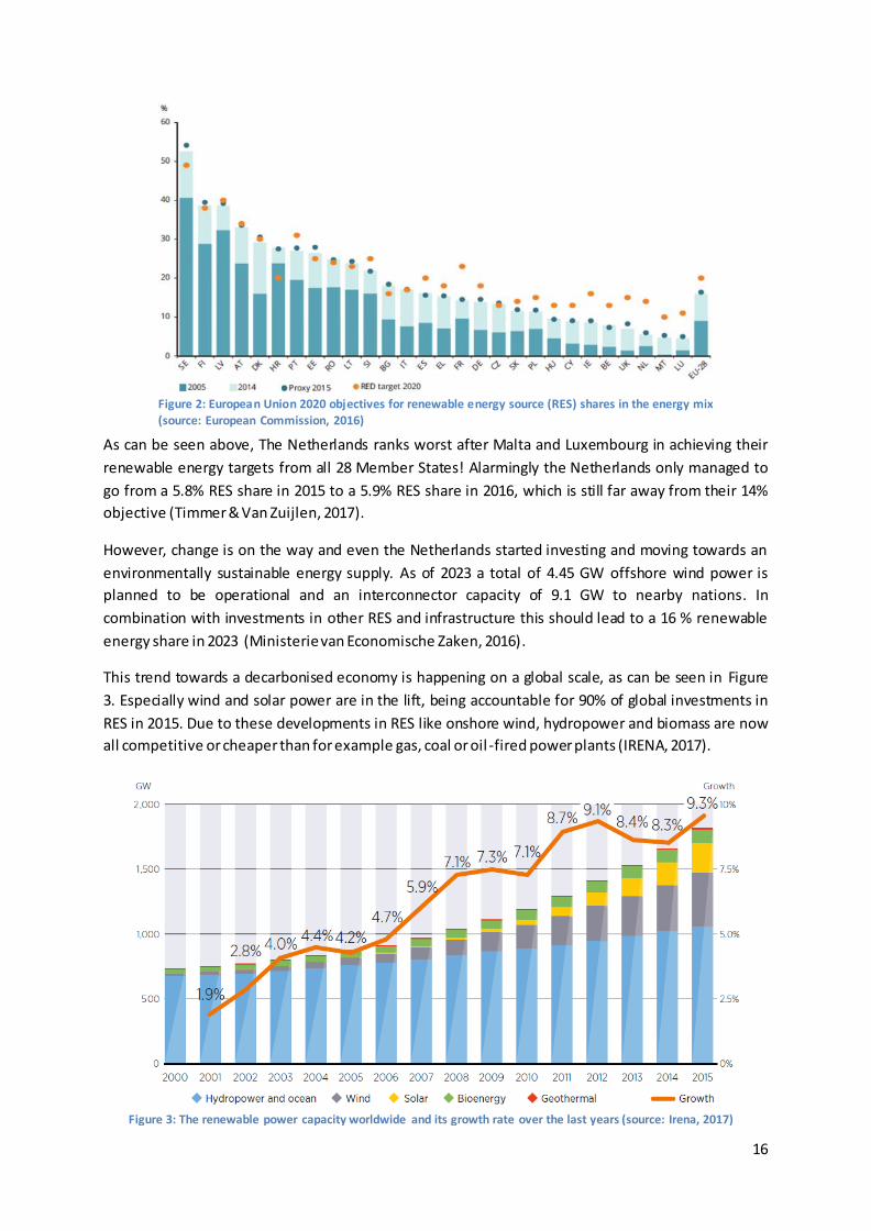
As can be seen above, The Netherlands ranks worst after Malta and Luxembourg in achieving their
renewable energy targets from all 28 Member States! Alarmingly the Netherlands only managed to
go from a 5.8% RES share in 2015 to a 5.9% RES share in 2016, which is still far away from their 14%
objective (Timmer & Van Zuijlen, 2017).
However, change is on the way and even the Netherlands started investing and moving towards an
environmentally sustainable energy supply. As of 2023 a total of 4.45 GW offshore wind power is
planned to be operational and an interconnector capacity of 9.1 GW to nearby nations. In
combination with investments in other RES and infrastructure this should lead to a 16 % renewable
energy share in 2023 (Ministerie van Economische Zaken, 2016).
This trend towards a decarbonised economy is happening on a global scale, as can be seen in Figure
3. Especially wind and solar power are in the lift, being accountable for 90% of global investments in
RES in 2015. Due to these developments in RES like onshore wind, hydropower and biomass are now
all competitive or cheaper than for example gas, coal or oil -fired power plants (IRENA, 2017).
Figure 2: European Union 2020 objectives for renewable energy source (RES) shares in the energy mix
(source: European Commission, 2016)
Figure 3: The renewable power capacity worldwide and its growth rate over the last years (source: Irena, 2017)
17
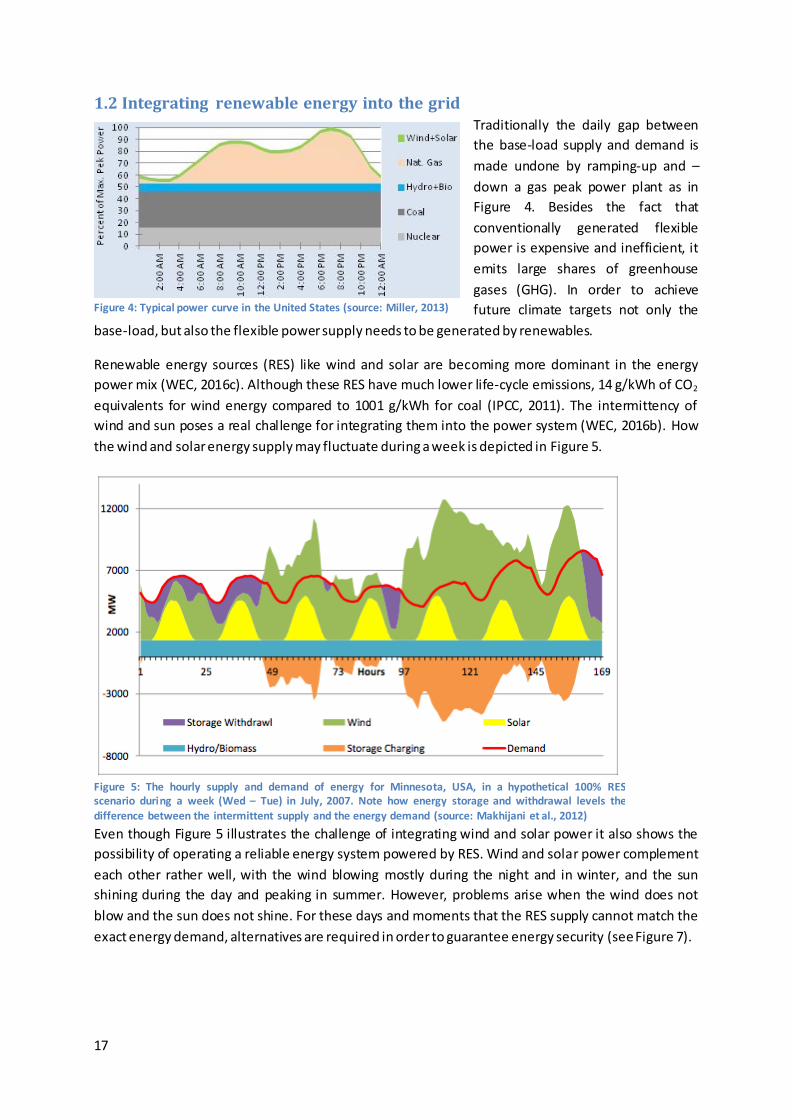
1.2 Integrating renewable energy into the grid Traditionally the daily gap between
the base-load supply and demand is
made undone by ramping-up and –
down a gas peak power plant as in
Figure 4. Besides the fact that
conventionally generated flexible
power is expensive and inefficient, it
emits large shares of greenhouse
gases (GHG). In order to achieve
future climate targets not only the
base-load, but also the flexible power supply needs to be generated by renewables.
Renewable energy sources (RES) like wind and solar are becoming more dominant in the energy
power mix (WEC, 2016c). Although these RES have much lower life-cycle emissions, 14 g/kWh of CO2
equivalents for wind energy compared to 1001 g/kWh for coal (IPCC, 2011). The intermittency of
wind and sun poses a real challenge for integrating them into the power system (WEC, 2016b). How
the wind and solar energy supply may fluctuate during a week is depicted in Figure 5.
Even though Figure 5 illustrates the challenge of integrating wind and solar power it also shows the
possibility of operating a reliable energy system powered by RES. Wind and solar power complement
each other rather well, with the wind blowing mostly during the night and in winter, and the sun
shining during the day and peaking in summer. However, problems arise when the wind does not
blow and the sun does not shine. For these days and moments that the RES supply cannot match the
exact energy demand, alternatives are required in order to guarantee energy security (see Figure 7).
Figure 5: The hourly supply and demand of energy for Minnesota, USA, in a hypothetical 100% RES scenario during a week (Wed – Tue) in July, 2007. Note how energy storage and withdrawal levels the difference between the intermittent supply and the energy demand (source: Makhijani et al., 2012)
Figure 4: Typical power curve in the United States (source: Miller, 2013)
18
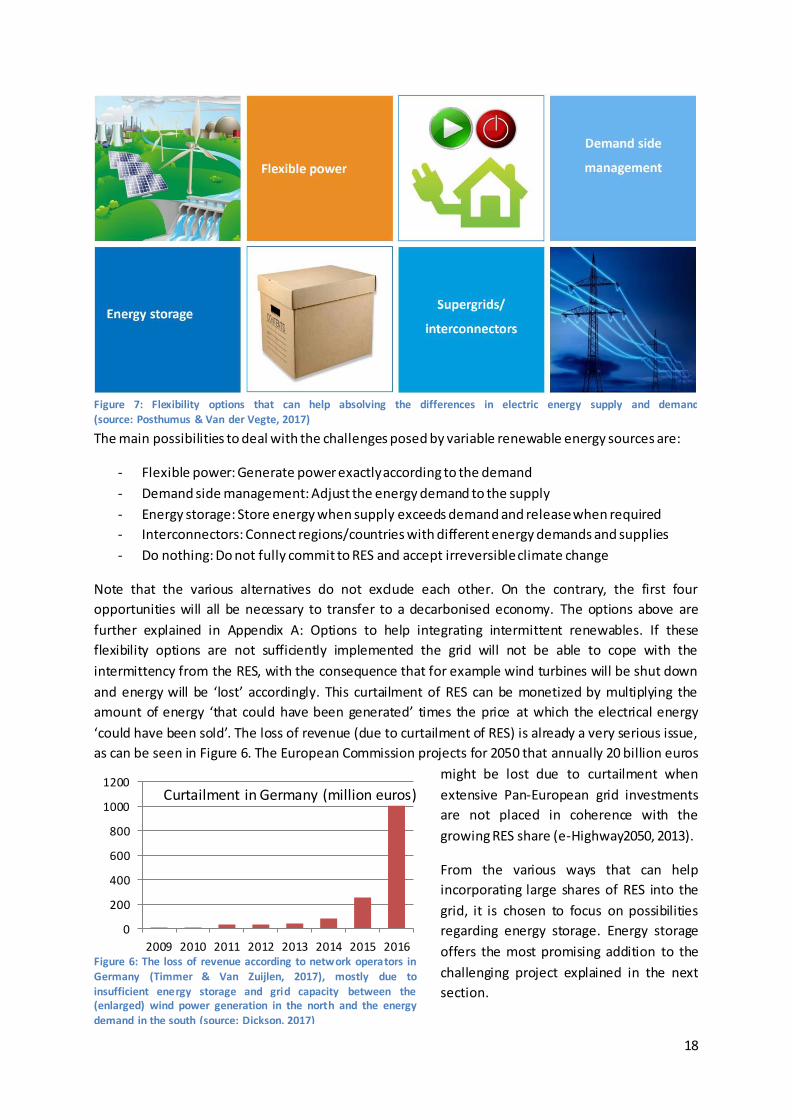
The main possibilities to deal with the challenges posed by variable renewable energy sources are:
- Flexible power: Generate power exactly according to the demand
- Demand side management: Adjust the energy demand to the supply
- Energy storage: Store energy when supply exceeds demand and release when required
- Interconnectors: Connect regions/countries with different energy demands and supplies
- Do nothing: Do not fully commit to RES and accept irreversible climate change
Note that the various alternatives do not exclude each other. On the contrary, the first four
opportunities will all be necessary to transfer to a decarbonised economy. The options above are
further explained in Appendix A: Options to help integrating intermittent renewables. If these
flexibility options are not sufficiently implemented the grid will not be able to cope with the
intermittency from the RES, with the consequence that for example wind turbines will be shut down
and energy will be ‘lost’ accordingly. This curtailment of RES can be monetized by multiplying the
amount of energy ‘that could have been generated’ times the price at which the electrical energy
‘could have been sold’. The loss of revenue (due to curtailment of RES) is already a very serious issue,
as can be seen in Figure 6. The European Commission projects for 2050 that annually 20 billion euros
might be lost due to curtailment when
extensive Pan-European grid investments
are not placed in coherence with the
growing RES share (e-Highway2050, 2013).
From the various ways that can help
incorporating large shares of RES into the
grid, it is chosen to focus on possibilities
regarding energy storage. Energy storage
offers the most promising addition to the
challenging project explained in the next
section.
Figure 7: Flexibility options that can help absolving the differences in electric energy supply and demand
(source: Posthumus & Van der Vegte, 2017)
0
200
400
600
800
1000
1200
2009 2010 2011 2012 2013 2014 2015 2016
Curtailment in Germany (million euros)
Figure 6: The loss of revenue according to network operators in Germany (Timmer & Van Zuijlen, 2017), mostly due to
insufficient energy storage and grid capacity between the (enlarged) wind power generation in the north and the energy demand in the south (source: Dickson, 2017)
19
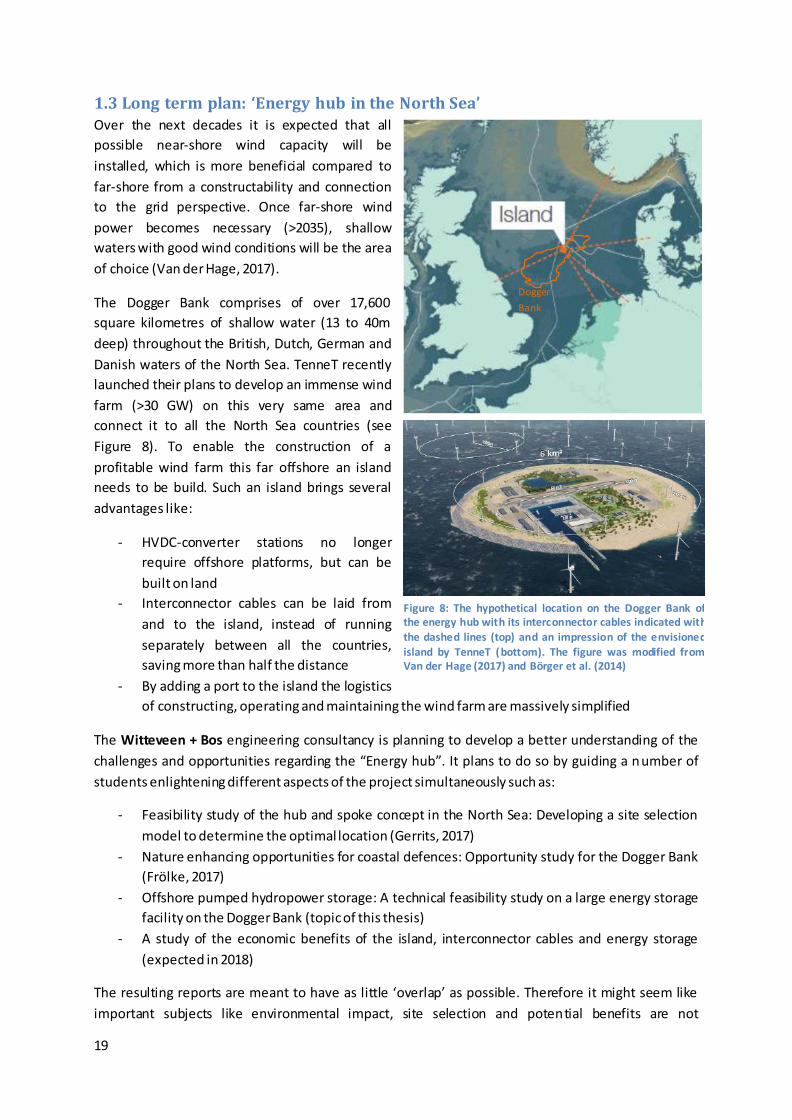
1.3 Long term plan: ‘Energy hub in the North Sea’ Over the next decades it is expected that all
possible near-shore wind capacity will be
installed, which is more beneficial compared to
far-shore from a constructability and connection
to the grid perspective. Once far-shore wind
power becomes necessary (>2035), shallow
waters with good wind conditions will be the area
of choice (Van der Hage, 2017).
The Dogger Bank comprises of over 17,600
square kilometres of shallow water (13 to 40m
deep) throughout the British, Dutch, German and
Danish waters of the North Sea. TenneT recently
launched their plans to develop an immense wind
farm (>30 GW) on this very same area and
connect it to all the North Sea countries (see
Figure 8). To enable the construction of a
profitable wind farm this far offshore an island
needs to be build. Such an island brings several
advantages like:
- HVDC-converter stations no longer
require offshore platforms, but can be
built on land
- Interconnector cables can be laid from
and to the island, instead of running
separately between all the countries,
saving more than half the distance
- By adding a port to the island the logistics
of constructing, operating and maintaining the wind farm are massively simplified
The Witteveen + Bos engineering consultancy is planning to develop a better understanding of the
challenges and opportunities regarding the “Energy hub”. It plans to do so by guiding a number of
students enlightening different aspects of the project simultaneously such as:
- Feasibility study of the hub and spoke concept in the North Sea: Developing a site selection
model to determine the optimal location (Gerrits, 2017)
- Nature enhancing opportunities for coastal defences: Opportunity study for the Dogger Bank
(Frölke, 2017)
- Offshore pumped hydropower storage: A technical feasibility study on a large energy storage
facility on the Dogger Bank (topic of this thesis)
- A study of the economic benefits of the island, interconnector cables and energy storage
(expected in 2018)
The resulting reports are meant to have as little ‘overlap’ as possible. Therefore it might seem like
important subjects like environmental impact, site selection and potential benefits are not
Dogger
Bank
Figure 8: The hypothetical location on the Dogger Bank of the energy hub with its interconnector cables indicated with the dashed lines (top) and an impression of the envisioned island by TenneT (bottom). The figure was modified from Van der Hage (2017) and Börger et al. (2014)
20
sufficiently addressed in this report. However, as can be deducted from the previously stated parallel
projects, those topics are thoroughly investigated in the other studies. Additionally has to be
mentioned that, unless otherwise stated, all the work presented in this report originates from the
author itself.
1.3.1 Contribution of energy storage to the ‘energy hub’
Within the plans of creating a central spill in the North Sea, to develop large-scale wind power, it is
thought that energy storage could be a valuable asset within the whole project. When the artificial
island, interconnector cables and wind turbines are in place, all ingredients an energy storage facility
could wish for are present:
- The interconnector cables between the North Sea countries allow for buying and selling of
energy to many different markets.
- By being right next to the wind power source, the storage facility can stock wind energy
directly at times of abundance and provide energy once required, when otherwise the
energy would be lost (avoided curtailment and security of supply).
- The ability of storing energy locally for later moments also results in deferral of
disproportional grid investments, since they do not need to cope with the maximum wind
power capacity. To put it into perspective: by avoiding 300 kilometres of a 700 MW
interconnector cable, 600 million euros are saved.
- With all the wind power generation and electrical infrastructure to transform alternating
current (AC) to direct current (DC), there will be a large demand for frequency control
services, which energy storage might fulfil.
- The presence of a port on the ‘energy hub’ enables an easy way of transporting equipment
and materials that are necessary for the construction and operation of the storage facility.
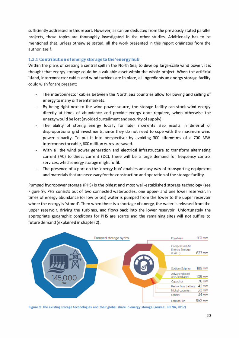
Pumped hydropower storage (PHS) is the oldest and most well -established storage technology (see
Figure 9). PHS consists out of two connected waterbodies, one upper- and one lower reservoir. In
times of energy abundance (or low prices) water is pumped from the lower to the upper reservoir
where the energy is ‘stored’. Then when there is a shortage of energy, the water is released from the
upper reservoir, driving the turbines, and flows back into the lower reservoir. Unfortunately the
appropriate geographic conditions for PHS are scarce and the remaining sites will not suffice to
future demand (explained in chapter 2).
Figure 9: The existing storage technologies and their global share in energy storage (source: IRENA, 2017)
21
The lack of mountains in the Netherlands did not stop Luc Lievense in trying to use the efficient
pumped hydro technology so he conceived a way to ‘artificially’ create the required hydraulic head
difference that enables power generation. Lievense launched his idea in 1979 in a response to the
prior oil boycott from the Middle-East and resistance against nuclear energy. The energy storage
system would reduce the dependency on foreign policies and help integrating renewable energy into
the grid. By erecting a circular dam a higher inner reservoir would be created of which the water
level could be adjusted to either store or withdraw energy.
At the time there was a lot of resistance due to the risk of a flood when the dam would break.
Additionally, wind energy did not develop as quickly as was first expected, reducing the need for
large investments in energy storage.
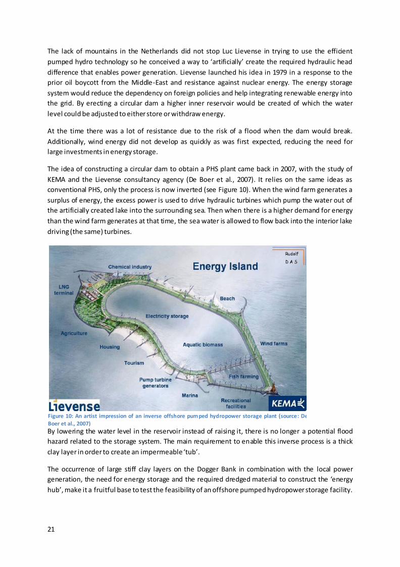
The idea of constructing a circular dam to obtain a PHS plant came back in 2007, with the study of
KEMA and the Lievense consultancy agency (De Boer et al., 2007). It relies on the same ideas as
conventional PHS, only the process is now inverted (see Figure 10). When the wind farm generates a
surplus of energy, the excess power is used to drive hydraulic turbines which pump the water out of
the artificially created lake into the surrounding sea. Then when there is a higher demand for energy
than the wind farm generates at that time, the sea water is allowed to flow back into the interior lake
driving (the same) turbines.
By lowering the water level in the reservoir instead of raising it, there is no longer a potential flood
hazard related to the storage system. The main requirement to enable this inverse process is a thick
clay layer in order to create an impermeable ‘tub’.
The occurrence of large stiff clay layers on the Dogger Bank in combination with the local power
generation, the need for energy storage and the required dredged material to construct the ‘energy
hub’, make it a fruitful base to test the feasibility of an offshore pumped hydropower storage facility.
Figure 10: An artist impression of an inverse offshore pumped hydropower storage plant (source: De Boer et al., 2007)
22
1.4 Problem definition Although the idea of “inverse pumped hydro storage” has been around for years, it has never been
executed. Therefore many uncertainties and challenges still cloud the feasibility of such a project. In
the handful of studies that have been performed certain design choices remained rather unclear, like
the head difference between reservoirs, storage and power capacity, water retaining measures and
the dam design. This particular thesis will try to identify the possible design alternatives and answer
the question: “How do the costs of an offshore pumped hydropower storage facility on the Dogger
Bank scale with the power and storage capacity, using existing construction technologies?”
The main research question will be answered step-by-step with dividing it into the following sub-
questions:
1. What are the construction method alternatives, considering the Dogger Bank geology and
bathymetry, for the dam to cope with seepage, piping, overtopping and stability issues and
what is the maximum head difference achievable?
2. What is the preferred dredging strategy to obtain the required depth following from
question 1.?
3. What is the ideal turbine setup to deliver the necessary power with the given head
difference?
4. What is the most cost effective construction method for the housing of the turbines, in-situ,
prefab or a hybrid alternative?
5. What are the benefits of energy storage, for both storage and power services?
23
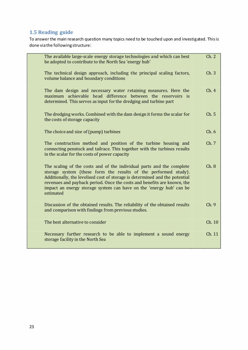
1.5 Reading guide To answer the main research question many topics need to be touched upon and investigated. This is
done via the following structure:
The available large-scale energy storage technologies and which can best be adopted to contribute to the North Sea ‘energy hub’
Ch. 2
The technical design approach, including the principal scaling factors, volume balance and boundary conditions
Ch. 3
The dam design and necessary water retaining measures. Here the maximum achievable head difference between the reservoirs is determined. This serves as input for the dredging and turbine part
Ch. 4
The dredging works. Combined with the dam design it forms the scalar for the costs of storage capacity
Ch. 5
The choice and size of (pump) turbines Ch. 6
The construction method and position of the turbine housing and connecting penstock and tailrace. This together with the turbines results in the scalar for the costs of power capacity
Ch. 7
The scaling of the costs and of the individual parts and the complete storage system (these form the results of the performed study). Additionally, the levelised cost of storage is determined and the potential revenues and payback period. Once the costs and benefits are known, the impact an energy storage system can have on the ‘energy hub’ can be estimated
Ch. 8
Discussion of the obtained results. The reliability of the obtained results and comparison with findings from previous studies.
Ch. 9
The best alternative to consider Ch. 10
Necessary further research to be able to implement a sound energy storage facility in the North Sea
Ch. 11

24
25
2. Analysis on energy storage This chapter gives an overview of developments and technologies to store energy. At the end of this
chapter it should be clear what the best alternative to investigate is for the Netherlands to cope with
energy security and the difference between energy demand and supply. The answer is obtained via a
set of sub-questions:
- What are the views and trends regarding energy storage on a global, European and national level?
§2.1
- What is the future demand for energy storage and which are the types of storage services?
§2.2
- What are the large scale energy storage alternatives and how do these compare?
§2.3
- How do the future demand and potentially realisable energy storage match?
§2.5
- What is the best alternative to consider? §2.6
2.1 Energy storage outlook In this section there is elaborated on the prospect of energy storage from different angles narrowed
down from a global level to the European Union to the view of the Netherlands.
2.1.1 Global
The International Renewable Energy Agency (IRENA) expects electricity storage to become a vital
part of power systems with high renewable shares (IRENA, 2012). With the fast growing renewable
energy market, the global investment in grid-connected storage is estimated to rise from USD 1.5
billion in 2010 to around USD 35 billion in 2020. Where today’s grid stability in networks with a high
share of renewable energy is safeguarded by an elaborate interconnection system, which allows
more than e.g. 20% of wind energy, this might become insufficient when the renewable energy share
grows in all regions (IRENA, 2012). The International Energy Agency (IEA) states in their World Energy
Outlook 2016 that energy storage becomes essential after the share of wind and solar output
surpasses one-quarter of the power mix. In case no investments are made curtailment of wind and
solar energy in times of abundance, could idle the equivalent of up to 30% of the investment in the
wind farms and solar parks (IEA, 2016).
Simulations taking into account a high renewable energy share indicate that in Western Europe a
storage capacity of about 90 GW would be required by 2050, with 30% of wind power generation.
Globally storage need to be provided for the usage of wind power between 190 GW and 300 GW
(IRENA, 2012).
Pumped hydro power is the only large scale option which is regarded as commercially viable at
present. Other storage technologies, such as hydrogen- or large scale battery storage, need further
development to become competitive (IRENA, 2012).
26
2.1.2 European Union
The European Energy Directive (EED) regards energy storage as an essential element to facilitate the
transition towards a sustainable electricity network (European Commission, 2012). Many values of
electricity storage are identified such as: allowing a large share of renewable sources in the energy
mix, letting base-load plants (nuclear, coal) run at higher efficiency by storing their output at times of
low demand, avoiding the curtailment of wind and solar power, increased flexibility and reliability on
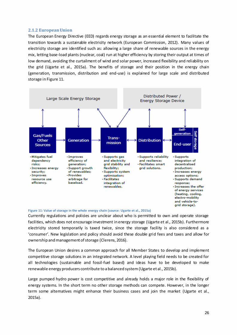
the grid (Ugarte et al., 2015a). The benefits of storage and their position in the energy chain
(generation, transmission, distribution and end-use) is explained for large scale and distributed
storage in Figure 11.
Currently regulations and policies are unclear about who is permitted to own and operate storage
facilities, which does not encourage investment in energy storage (Ugarte et al., 2015b). Furthermore
electricity stored temporarily is taxed twice, since the storage facility is also considered as a
‘consumer’. New legislation and policy should avoid these double grid fees and taxes and allow for
ownership and management of storage (Clerens, 2016).
The European Union desires a common approach for all Member States to develop and implement
competitive storage solutions in an integrated network. A level playing field needs to be created for
all technologies (sustainable and fossil-fuel based) and ideas have to be developed to make
renewable energy producers contribute to a balanced system (Ugarte et al., 2015b).
Large pumped hydro power is cost competitive and already holds a major role in the flexibility of
energy systems. In the short term no other storage methods can compete. However, in the longer
term some alternatives might enhance their business cases and join the market (Ugarte et al.,
2015a).
Figure 11: Value of storage in the whole energy chain (source: Ugarte et al., 2015a)
27
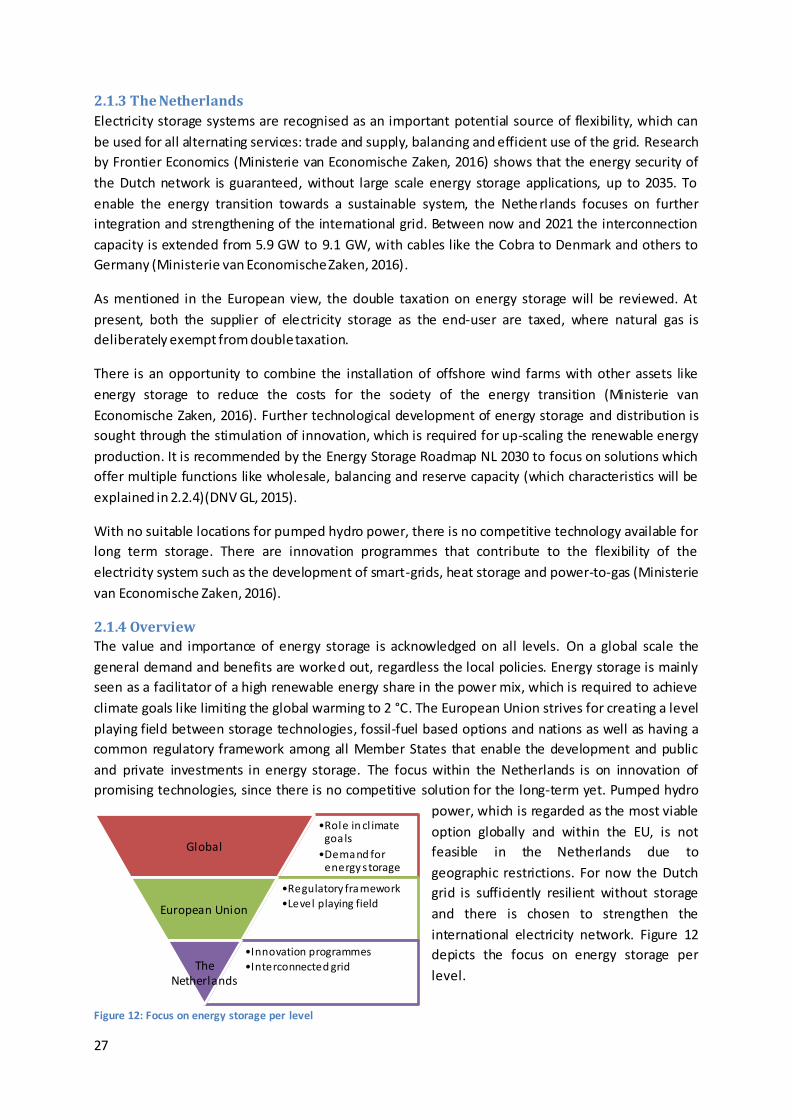
•Role in cl imate goals
•Demand for energy s torage
Global
•Regulatory framework
•Level playing field European Union
•Innovation programmes
•Interconnected grid The Netherlands
Figure 12: Focus on energy storage per level
2.1.3 The Netherlands
Electricity storage systems are recognised as an important potential source of flexibility, which can
be used for all alternating services: trade and supply, balancing and efficient use of the grid. Research
by Frontier Economics (Ministerie van Economische Zaken, 2016) shows that the energy security of
the Dutch network is guaranteed, without large scale energy storage applications, up to 2035. To
enable the energy transition towards a sustainable system, the Netherlands focuses on further
integration and strengthening of the international grid. Between now and 2021 the interconnection
capacity is extended from 5.9 GW to 9.1 GW, with cables like the Cobra to Denmark and others to
Germany (Ministerie van Economische Zaken, 2016).
As mentioned in the European view, the double taxation on energy storage will be reviewed. At
present, both the supplier of electricity storage as the end-user are taxed, where natural gas is
deliberately exempt from double taxation.
There is an opportunity to combine the installation of offshore wind farms with other assets like
energy storage to reduce the costs for the society of the energy transition (Ministerie van
Economische Zaken, 2016). Further technological development of energy storage and distribution is
sought through the stimulation of innovation, which is required for up-scaling the renewable energy
production. It is recommended by the Energy Storage Roadmap NL 2030 to focus on solutions which
offer multiple functions like wholesale, balancing and reserve capacity (which characteristics will be
explained in 2.2.4)(DNV GL, 2015).
With no suitable locations for pumped hydro power, there is no competitive technology available for
long term storage. There are innovation programmes that contribute to the flexibility of the
electricity system such as the development of smart-grids, heat storage and power-to-gas (Ministerie
van Economische Zaken, 2016).
2.1.4 Overview
The value and importance of energy storage is acknowledged on all levels. On a global scale the
general demand and benefits are worked out, regardless the local policies. Energy storage is mainly
seen as a facilitator of a high renewable energy share in the power mix, which is required to achieve
climate goals like limiting the global warming to 2 °C. The European Union strives for creating a level
playing field between storage technologies, fossil-fuel based options and nations as well as having a
common regulatory framework among all Member States that enable the development and public
and private investments in energy storage. The focus within the Netherlands is on innovation of
promising technologies, since there is no competitive solution for the long-term yet. Pumped hydro
power, which is regarded as the most viable
option globally and within the EU, is not
feasible in the Netherlands due to
geographic restrictions. For now the Dutch
grid is sufficiently resilient without storage
and there is chosen to strengthen the
international electricity network. Figure 12
depicts the focus on energy storage per
level.
28
2.2 Future demand for energy storage The prospective need for energy storage is computed through three steps. The time horizon is set on
2050 and the scope is set on North- and West-Europe, since this area is well (inter) connected and
fits within the area of influence of the project. Firstly the future energy demand is worked out, when
secondly the share of energy from renewable sources in this future scenario is determined. Once the
amount of renewable energy that will be generated is known, the corresponding need for energy
storage to facilitate the integration of fluctuating sources is defined. Afterwards the various services
that energy storage can provide are introduced.
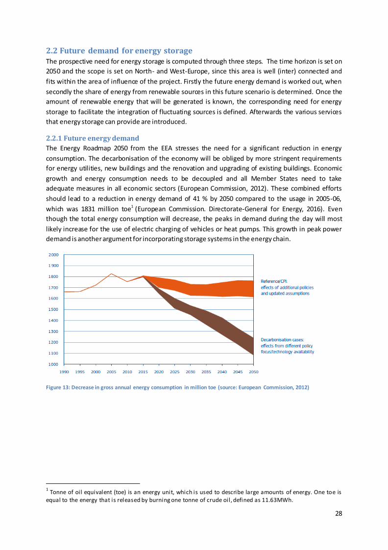
2.2.1 Future energy demand
The Energy Roadmap 2050 from the EEA stresses the need for a significant reduction in energy
consumption. The decarbonisation of the economy will be obliged by more stringent requirements
for energy utilities, new buildings and the renovation and upgrading of existing buildings. Economic
growth and energy consumption needs to be decoupled and all Member States need to take
adequate measures in all economic sectors (European Commission, 2012). These combined efforts
should lead to a reduction in energy demand of 41 % by 2050 compared to the usage in 2005-06,
which was 1831 million toe1 (European Commission. Directorate-General for Energy, 2016). Even
though the total energy consumption will decrease, the peaks in demand during the day will most
likely increase for the use of electric charging of vehicles or heat pumps. This growth in peak power
demand is another argument for incorporating storage systems in the energy chain.
Figure 13: Decrease in gross annual energy consumption in million toe (source: European Commission, 2012)
1 Tonne of oil equivalent (toe) is an energy unit, which is used to describe large amounts of energy. One toe is
equal to the energy that is released by burning one tonne of crude oil, defined as 11.63MWh.
29
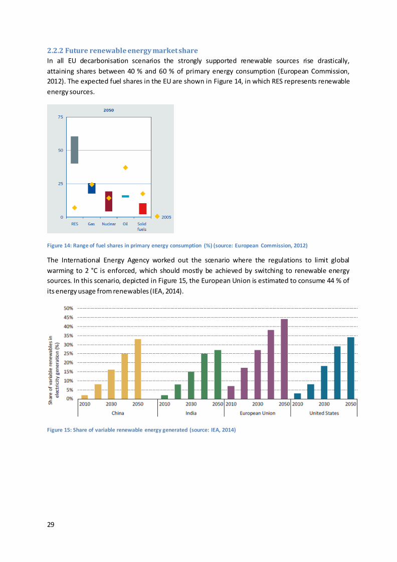
2.2.2 Future renewable energy market share
In all EU decarbonisation scenarios the strongly supported renewable sources rise drastically,
attaining shares between 40 % and 60 % of primary energy consumption (European Commission,
2012). The expected fuel shares in the EU are shown in Figure 14, in which RES represents renewable
energy sources.
Figure 14: Range of fuel shares in primary energy consumption (%) (source: European Commission, 2012)
The International Energy Agency worked out the scenario where the regulations to limit global
warming to 2 °C is enforced, which should mostly be achieved by switching to renewable energy
sources. In this scenario, depicted in Figure 15, the European Union is estimated to consume 44 % of
its energy usage from renewables (IEA, 2014).
Figure 15: Share of variable renewable energy generated (source: IEA, 2014)
30
2.2.3 Required energy storage capacity
There is no definite answer to the amount of energy storage that is required to integrate a significant
amount of variable renewable energy into the system. The necessary storage is highly dependent on
other aspects within the energy chain like the size of the system, the quality of the grid, regulation on
the demand side, the other generation technologies and interconnectivity with neighbouring
systems. This vast number of factors of influence results in a wide range from 20 % to 60 % of
expected need for energy storage per renewable energy share according to comprehensible studies
by Fraunhofer, BET and IRENA (Ugarte et al., 2015a). These estimates are in line with the experience
gained from a pilot project that combined a wind farm with sodium-sulfur batteries in Minnesota,
USA. The project found that for each MW of wind generated, 0.2 MW to 0.4 MW of storage would be
required (Himelic & Novacheck, 2011).
Combining the reduced energy demand with 41 % by 2050, a renewable energy share between 40 %
to 60 %, and the need for energy storage ranging from 20 % to 60 %, leads to a required storage
power output of 115 GW as lower boundary and 516 GW as upper boundary for the EU-28.
Considering storage facilities need to be charged before they can generate, the installed capacity
needs to increase to allow for the charging time. Assuming e.g. a capacity factor/generation ratio of
0.45, the required storage power varies from 255 GW to 1148 GW.
Within the scope for North- and West-Europe, including Switzerland and Norway, where the largest
energy demand originates (European Commission. Directorate-General for Energy, 2016), the
respective need for storage ranges from 221 GW to 996 GW. Observing the future well
interconnected grid and ambitions for very high usage of renewable energy sources; a scenario with
60 % of RES and 20 % of required storage per share of RES is found most probable, resulting in a
required capacity of 3584 GWh and an output of 332 GW by 2050. To put it into perspective: globally
the installed energy storage withheld 143 GW in 2015 (IRENA, 2015).
31
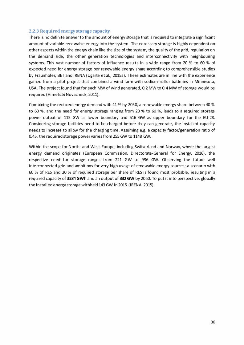
2.2.4 Types of energy storage services
In order to assess the value and make a distinction between various storage technologies, first the
different types of functionalities are introduced. The applications depend on the required time of
discharge and the amount of power. The terminology among sources may vary, but a common
distinction between services is: long-term storage, short-term storage and distributed battery (self)
storage (IEA, 2014).
2.2.4.1 Long-term storage
This service is mostly provided by bulk-storage technologies, which can provide power for a long
period of time (hours to days or for seasonal purposes). It is used to decouple the moment of
generation and consumption of electric energy (Rahman, 2012). A typical application is arbitrage,
where low-priced energy is bought and stored during periods of low demand and sold again during
peak hours when prices are high.
2.2.4.2 Short-term storage
These applications operate for a period of seconds to minutes to assure the continuity of power by
frequency regulation, voltage support and to enable switching between energy sources, while
safeguarding the supply (Rahman, 2012), (IEA, 2014).
2.2.4.3 Distributed battery (self) storage
Batteries have a widespread application field; they can be deployed in both distributed and
centralised systems, mobile or fixed and either connected to the grid or ‘behind the meter’ for self-
consumption (IEA, 2014). The latter is done by end users with for example combining solar panels
and storage. Although this ‘self-optimisation’ of energy usage is not necessarily the most efficient
(when considering the total system) this distributed storage share is likely to grow , driven by the
desire of the consumer to be self-reliant (DNV GL, 2015). When connected to the grid the battery
storage could, besides the integration of renewables, serve as frequency regulation and add
flexibility on the ‘demand-side’ for energy (IEA, 2014).
A more comprehensive explanation of the applications is given in the Technology Roadmap Energy
Storage (2014) by the International Energy Agency. Figure 16 illustrates the services storage can
provide.
Figure 16: Energy storage applications categorised by their power output, time of discharge and their location in the energy chain (source: IEA, 2014)
32
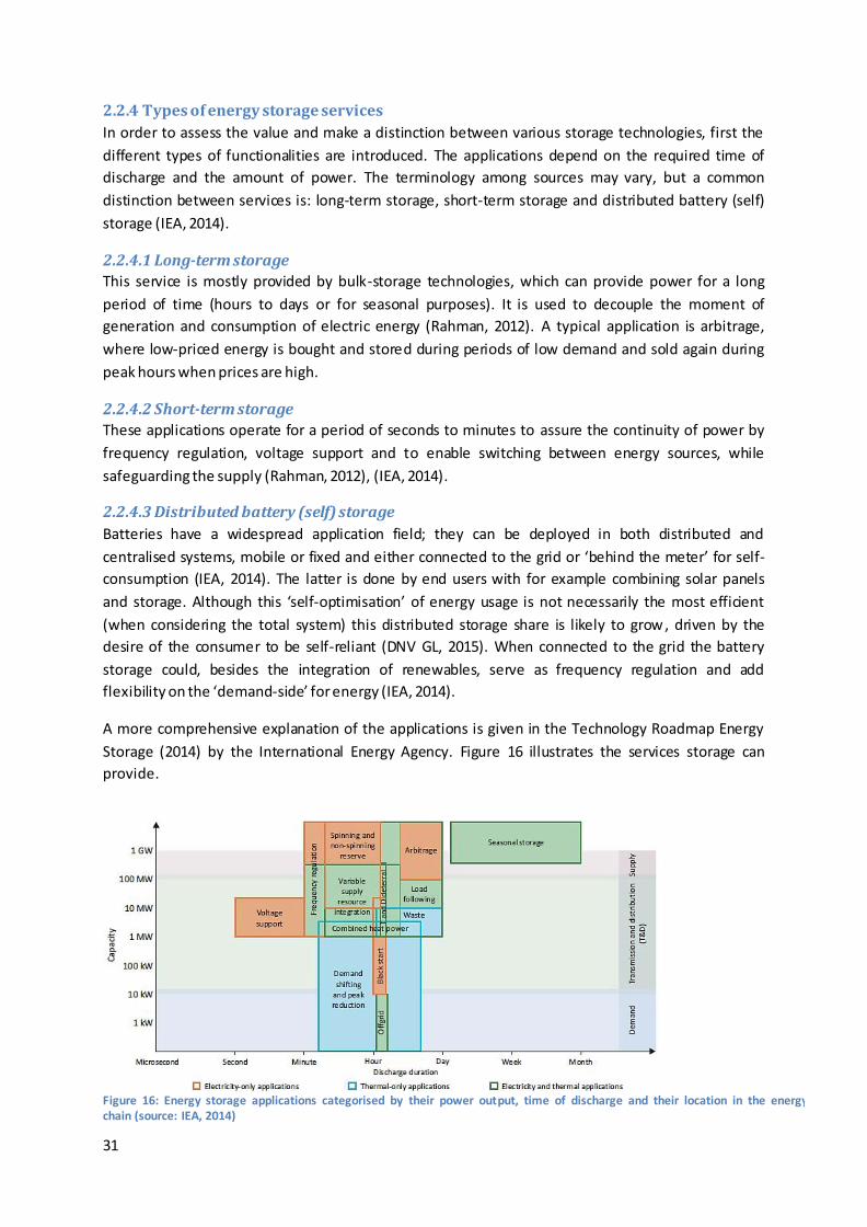
Figure 17: Schematisation of a PHS system (left) and the development of PHS in the EU (right) (source: Letcher, 2016 and Pérez-Díaz et al., 2014)
2.3 Energy storage technologies In this section options are reviewed that have the potential of storing large amounts of energy and
who can help integrating large shares of renewable energy into the grid.
2.3.1 Pumped hydropower storage
Pumped hydropower storage (PHS) consists out of two connected waterbodies, one upper- and one
lower reservoir. In times of energy abundance (or low prices) water is pumped from the lower to the
upper reservoir where the energy is ‘stored’. Then when there is a shortage of energy, the water is
released from the upper reservoir, driving the turbines, and flows back into the lower reservoir.
Europe has around 230 PHS facilities that have a combined capacity of 41 GW. Most of these storage
systems were built in the 1970s and 80s out of energy security concerns and alongside the
development of nuclear power plants (to provide peak power on top of the baseload power from the
nuclear plants and black starts). Nowadays PHS is making a revival with the growing share of
intermittent renewable energy and their responsive need for storage, see Figure 17.
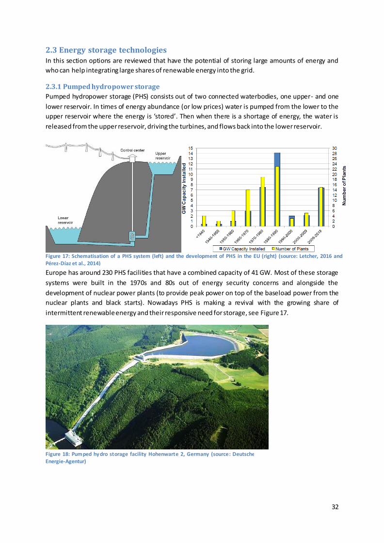
Figure 18: Pumped hydro storage facility Hohenwarte 2, Germany (source: Deutsche Energie-Agentur)
33
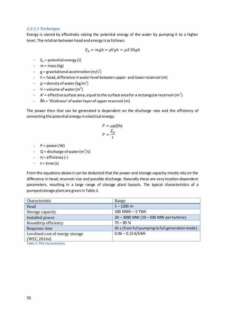
2.3.1.1 Technique
Energy is stored by effectively raising the potential energy of the water by pumping it to a higher
level. The relation between head and energy is as follows:
𝐸𝑝 = 𝑚𝑔ℎ = 𝜌𝑉𝑔ℎ = 𝜌𝐴′𝛿ℎ𝑔ℎ
- Ep = potential energy (J)
- m = mass (kg)
- g = gravitational acceleration (m/s2)
- h = head, difference in water level between upper- and lower reservoir (m)
- ρ = density of water (kg/m3)
- V = volume of water (m3)
- A’ = effective surface area, equal to the surface area for a rectangular reservoir (m 2)
- δh = ‘thickness’ of water layer of upper reservoir (m)
The power then that can be generated is dependent on the discharge rate and the efficiency of
converting the potential energy in electrical energy:
𝑃 = 𝜌𝑔𝑄ℎ𝜂
𝑃 =𝐸𝑝
𝑡
- P = power (W)
- Q = discharge of water (m3/s)
- η = efficiency (-)
- t = time (s)
From the equations above it can be deducted that the power and storage capacity mostly rely on the
difference in head, reservoir size and possible discharge. Naturally these are very location dependent
parameters, resulting in a large range of storage plant layouts. The typical characteristics of a
pumped storage plant are given in Table 2.
Characteristic Range
Head 5 – 1200 m
Storage capacity 100 MWh – 5 TWh
Installed power 20 – 3000 MW (10 – 500 MW per turbine)
Roundtrip efficiency 75 – 85 %
Response time 45 s (from full pumping to full generation mode)
Levelised cost of energy storage (WEC, 2016a)
0.06 – 0.13 €/kWh
Table 2: PHS characteristics
34
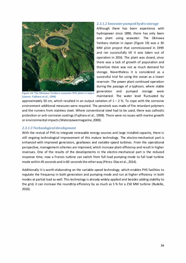
Figure 19: The Okinawa Yanbaru seawater PHS plant in Japan (source: Fujihara et al., 1998)
2.3.1.2 Seawater pumped hydro storage
Although there has been experience with
hydropower since 1890, there has only been
one plant using seawater. The Okinawa
Yanbaru station in Japan (Figure 19) was a 30
MW pilot project that commissioned in 1999
and ran successfully till it was taken out of
operation in 2016. The plant was closed, since
there was a lack of growth of population and
therefore there was not as much demand for
storage. Nevertheless it is considered as a
successful trial for using the ocean as a lower
reservoir. The power plant continued operation
during the passage of a typhoon, where stable
generation and pumped storage were
maintained. The water level fluctuated by
approximately 50 cm, which resulted in an output variation of 1 – 2 %. To cope with the corrosive
environment additional measures were required. The penstock was made of fire retardant polymers
and the runners from stainless steel. Where conventional steel had to be used, there was cathodic
protection or anti-corrosion coatings (Fujihara et al., 1998). There were no issues with marine growth
or environmental impacts (Waterpowermagazine, 2000).
2.3.1.3 Technological development
With the revival of PHS to integrate renewable energy sources and large installed capacity, there is
still ongoing technological improvement of this mature technology. The electro-mechanical part is
enhanced with improved generators, gearboxes and variable-speed turbines. From the operational
perspective, management schemes are improved, which increase plant efficiency and result in higher
revenues. One of the results of the developments in the electro-mechanical part is the reduced
response time, now a Francis turbine can switch from full load pumping mode to full load turbine
mode within 45 seconds and in 60 seconds the other way (Pérez-Díaz et al., 2014).
Additionally it is worth elaborating on the variable-speed technology, which enables PHS facilities to
regulate the frequency in both generation and pumping mode and run at higher efficiency in both
modes at partial load as well. This technology is already widely applied and besides adding stability to
the grid, it can increase the roundtrip efficiency by as much as 5 % for a 250 MW turbine (Rudelle,
2016).
35
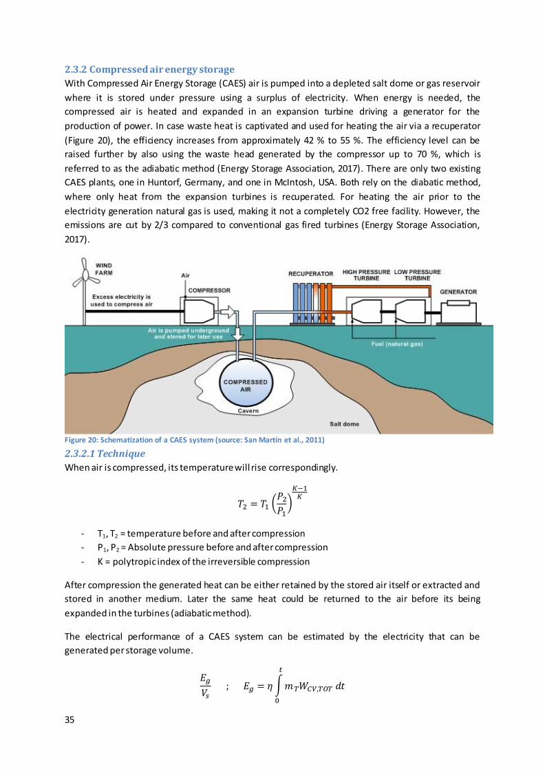
2.3.2 Compressed air energy storage
With Compressed Air Energy Storage (CAES) air is pumped into a depleted salt dome or gas reservoir
where it is stored under pressure using a surplus of electricity. When energy is needed, the
compressed air is heated and expanded in an expansion turbine driving a generator for the
production of power. In case waste heat is captivated and used for heating the air via a recuperator
(Figure 20), the efficiency increases from approximately 42 % to 55 %. The efficiency level can be
raised further by also using the waste head generated by the compressor up to 70 %, which is
referred to as the adiabatic method (Energy Storage Association, 2017). There are only two existing
CAES plants, one in Huntorf, Germany, and one in McIntosh, USA. Both rely on the diabatic method,
where only heat from the expansion turbines is recuperated. For heating the air prior to the
electricity generation natural gas is used, making it not a completely CO2 free facility. However, the
emissions are cut by 2/3 compared to conventional gas fired turbines (Energy Storage Association,
2017).
2.3.2.1 Technique
When air is compressed, its temperature will rise correspondingly.
𝑇2 = 𝑇1 (𝑃2𝑃1)
𝐾−1𝐾
- T1, T2 = temperature before and after compression
- P1, P2 = Absolute pressure before and after compression
- K = polytropic index of the irreversible compression
After compression the generated heat can be either retained by the stored air itself or extracted and
stored in another medium. Later the same heat could be returned to the air before its being
expanded in the turbines (adiabatic method).
The electrical performance of a CAES system can be estimated by the electricity that can be
generated per storage volume.
𝐸𝑔
𝑉𝑠 ; 𝐸𝑔 = 𝜂∫𝑚𝑇𝑊𝐶𝑉,𝑇𝑂𝑇 𝑑𝑡
𝑡
0
Figure 20: Schematization of a CAES system (source: San Martín et al., 2011)
36
- Eg = energy generated
- Vs = volume of storage reservoir
- η = efficiency
- t = time required to empty the storage reservoir
- mT = air mass flow rate
- WCV,TOT = total mechanical work, per unit mass
Based on the above equations it can be deducted that the performance of CAES depends largely on
what is being done with the ‘waste’ heat and to what level the air can be compressed. Some typical
numbers belonging to a CAES system are shown in Table 3.
Characteristic Range
Storage capacity 1.5 – 3.0 GWh
Installed power 100 – 500 MW
Roundtrip efficiency 40 – 55 % (60 – 70 % planned)
Response time 5 - 15 min
Levelised cost of energy storage (WEC, 2016a)
0.08 – 0.15 €/kWh
Table 3: CAES characteristics
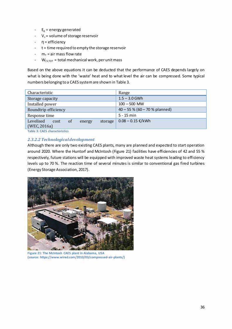
2.3.2.2 Technological development
Although there are only two existing CAES plants, many are planned and expected to start operation
around 2020. Where the Huntorf and McIntosh (Figure 21) facilities have efficiencies of 42 and 55 %
respectively, future stations will be equipped with improved waste heat systems leading to efficiency
levels up to 70 %. The reaction time of several minutes is similar to conventional gas fired turbines
(Energy Storage Association, 2017).
Figure 21: The McIntosh CAES plant in Alabama, USA (source: https://www.wired.com/2010/03/compressed-air-plants/)
37
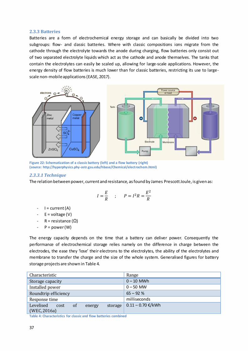
2.3.3 Batteries
Batteries are a form of electrochemical energy storage and can basically be divided into two
subgroups: flow- and classic batteries. Where with classic compositions ions migrate from the
cathode through the electrolyte towards the anode during charging, flow batteries only consist out
of two separated electrolyte liquids which act as the cathode and anode themselves. The tanks that
contain the electrolytes can easily be scaled up, allowing for large-scale applications. However, the
energy density of flow batteries is much lower than for classic batteries, restricting its use to large-
scale non-mobile applications (EASE, 2017).
2.3.3.1 Technique
The relation between power, current and resistance, as found by James Prescott Joule, is given as:
𝐼 =𝐸
𝑅 ; 𝑃 = 𝐼2𝑅 =
𝐸2
𝑅
- I = current (A)
- E = voltage (V)
- R = resistance (Ω)
- P = power (W)
The energy capacity depends on the time that a battery can deliver power. Consequently the
performance of electrochemical storage relies namely on the difference in charge between the
electrodes, the ease they ‘lose’ their electrons to the electrolytes, the ability of the electrolytes and
membrane to transfer the charge and the size of the whole system. Generalised figures for battery
storage projects are shown in Table 4.
Characteristic Range
Storage capacity 0 – 10 MWh
Installed power 0 – 50 MW
Roundtrip efficiency 65 – 92 %
Response time milliseconds
Levelised cost of energy storage (WEC, 2016a)
0.11 – 0.70 €/kWh
Table 4: Characteristics for classic and flow batteries combined
Figure 22: Schematization of a classic battery (left) and a flow battery (right) (source: http://hyperphysics.phy-astr.gsu.edu/hbase/Chemical/electrochem.html)
38
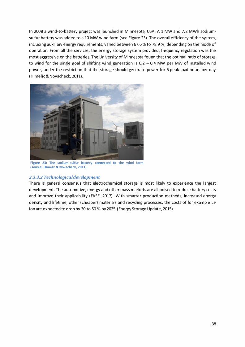
In 2008 a wind-to-battery project was launched in Minnesota, USA. A 1 MW and 7.2 MWh sodium-
sulfur battery was added to a 10 MW wind farm (see Figure 23). The overall efficiency of the system,
including auxiliary energy requirements, varied between 67.6 % to 78.9 %, depending on the mode of
operation. From all the services, the energy storage system provided, frequency regulation was the
most aggressive on the batteries. The University of Minnesota found that the optimal ratio of storage
to wind for the single goal of shifting wind generation is 0.2 – 0.4 MW per MW of installed wind
power, under the restriction that the storage should generate power for 6 peak load hours per day
(Himelic & Novacheck, 2011).
2.3.3.2 Technological development
There is general consensus that electrochemical storage is most likely to experience the largest
development. The automotive, energy and other mass markets are all poised to reduce battery costs
and improve their applicability (EASE, 2017). With smarter production methods, increased energy
density and lifetime, other (cheaper) materials and recycling processes, the costs of for example Li-
Ion are expected to drop by 30 to 50 % by 2025 (Energy Storage Update, 2015).
Figure 23: The sodium-sulfur battery connected to the wind farm (source: Himelic & Novacheck, 2011)
39
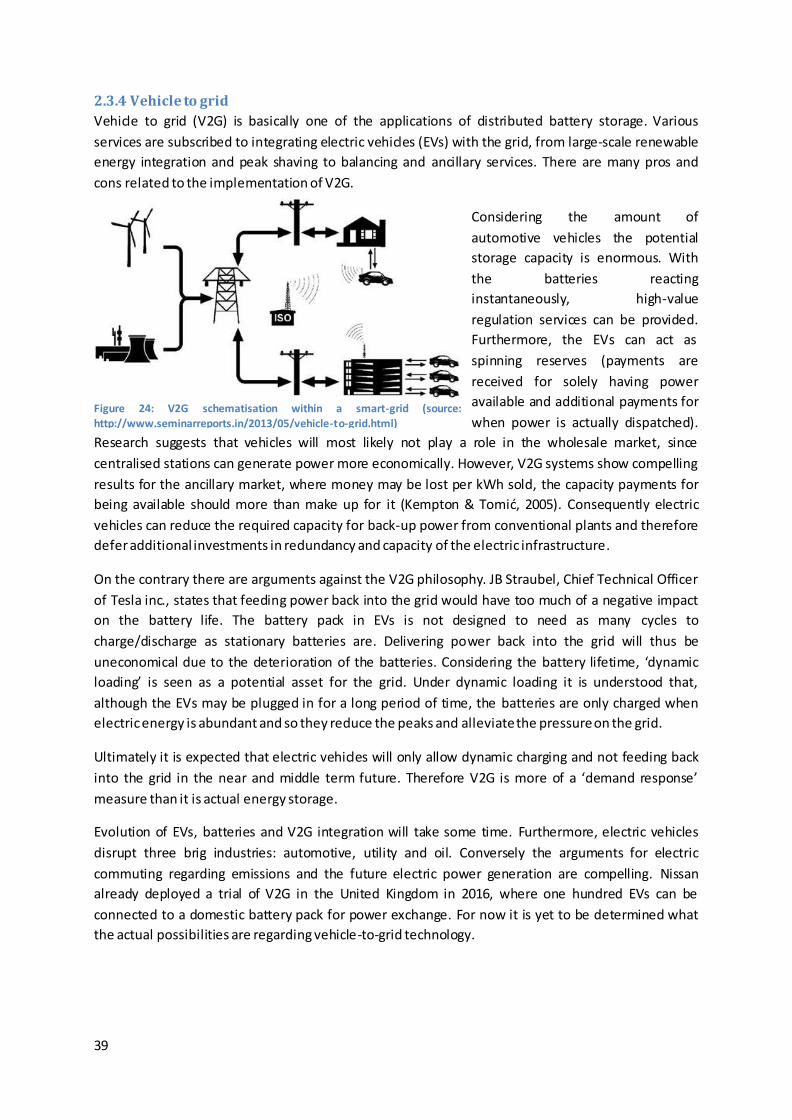
Figure 24: V2G schematisation within a smart-grid (source: http://www.seminarreports.in/2013/05/vehicle-to-grid.html)
2.3.4 Vehicle to grid
Vehicle to grid (V2G) is basically one of the applications of distributed battery storage. Various
services are subscribed to integrating electric vehicles (EVs) with the grid, from large-scale renewable
energy integration and peak shaving to balancing and ancillary services. There are many pros and
cons related to the implementation of V2G.
Considering the amount of
automotive vehicles the potential
storage capacity is enormous. With
the batteries reacting
instantaneously, high-value
regulation services can be provided.
Furthermore, the EVs can act as
spinning reserves (payments are
received for solely having power
available and additional payments for
when power is actually dispatched).
Research suggests that vehicles will most likely not play a role in the wholesale market, since
centralised stations can generate power more economically. However, V2G systems show compelling
results for the ancillary market, where money may be lost per kWh sold, the capacity payments for
being available should more than make up for it (Kempton & Tomić, 2005). Consequently electric
vehicles can reduce the required capacity for back-up power from conventional plants and therefore
defer additional investments in redundancy and capacity of the electric infrastructure.
On the contrary there are arguments against the V2G philosophy. JB Straubel, Chief Technical Officer
of Tesla inc., states that feeding power back into the grid would have too much of a negative impact
on the battery life. The battery pack in EVs is not designed to need as many cycles to
charge/discharge as stationary batteries are. Delivering power back into the grid will thus be
uneconomical due to the deterioration of the batteries. Considering the battery lifetime, ‘dynamic
loading’ is seen as a potential asset for the grid. Under dynamic loading it is understood that,
although the EVs may be plugged in for a long period of time, the batteries are only charged when
electric energy is abundant and so they reduce the peaks and alleviate the pressure on the grid.
Ultimately it is expected that electric vehicles will only allow dynamic charging and not feeding back
into the grid in the near and middle term future. Therefore V2G is more of a ‘demand response’
measure than it is actual energy storage.
Evolution of EVs, batteries and V2G integration will take some time. Furthermore, electric vehicles
disrupt three brig industries: automotive, utility and oil. Conversely the arguments for electric
commuting regarding emissions and the future electric power generation are compelling. Nissan
already deployed a trial of V2G in the United Kingdom in 2016, where one hundred EVs can be
connected to a domestic battery pack for power exchange. For now it is yet to be determined what
the actual possibilities are regarding vehicle-to-grid technology.
40
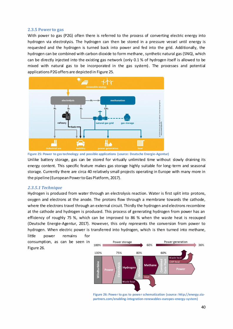
Figure 26: Power to gas to power schematization (source: http://energy.sia-partners.com/enabling-integration-renewables-europes-energy-system)
Figure 25: Power to gas technology and possible applications (source: Deutsche Energie-Agentur)
2.3.5 Power to gas
With power to gas (P2G) often there is referred to the process of converting electric energy into
hydrogen via electrolysis. The hydrogen can then be stored in a pressure vessel until energy is
requested and the hydrogen is turned back into power and fed into the grid. Additionally, the
hydrogen can be combined with carbon dioxide to form methane, synthetic natural gas (SNG), which
can be directly injected into the existing gas network (only 0.1 % of hydrogen itself is allowed to be
mixed with natural gas to be incorporated in the gas system). The processes and potential
applications P2G offers are depicted in Figure 25.
Unlike battery storage, gas can be stored for virtually unlimited time without slowly draining its
energy content. This specific feature makes gas storage highly suitable for long-term and seasonal
storage. Currently there are circa 40 relatively small projects operating in Europe with many more in
the pipeline (European Power to Gas Platform, 2017).
2.3.5.1 Technique
Hydrogen is produced from water through an electrolysis reaction. Water is first split into protons,
oxygen and electrons at the anode. The protons flow through a membrane towards the cathode,
where the electrons travel through an external circuit. Thirdly the hydrogen and electrons recombine
at the cathode and hydrogen is produced. This process of generating hydrogen from power has an
efficiency of roughly 75 %, which can be improved to 86 % when the waste heat is recouped
(Deutsche Energie-Agentur, 2017). However, this only represents the conversion from power to
hydrogen. When electric power is transferred into hydrogen, which is then turned into methane,
little power remains for
consumption, as can be seen in
Figure 26.
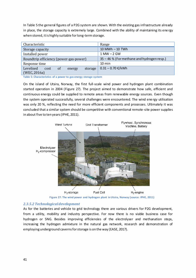
41
In Table 5 the general figures of a P2G system are shown. With the existing gas infrastructure already
in place, the storage capacity is extremely large. Combined with the ability of maintaining its ene rgy
when stored, it is highly suitable for long-term storage.
Characteristic Range
Storage capacity 10 MWh – 10 TWh
Installed power 1 MW – 2 GW
Roundtrip efficiency (power-gas-power) 35 – 46 % (For methane and hydrogen resp.)
Response time 10 min
Levelised cost of energy storage (WEC, 2016a)
0.31 – 0.70 €/kWh
Table 5: Characteristics of a power to gas energy storage system
On the island of Utsira, Norway, the first full -scale wind power and hydrogen plant combination
started operation in 2004 (Figure 27). The project aimed to demonstrate how safe, efficient and
continuous energy could be supplied to remote areas from renewable energy sources. Even though
the system operated successfully, several challenges were encountered. The wind ene rgy utilisation
was only 20 %, reflecting the need for more efficient components and processes. Ultimately it was
concluded that a similar system should be competitive with conventional remote -site power supplies
in about five to ten years (IPHE, 2011).
2.3.5.2 Technological development
As for the batteries and vehicle to grid technology there are various drivers for P2G development,
from a utility, mobility and industry perspective. For now there is no viable business case for
hydrogen or SNG. Besides improving efficiencies of the electrolyser and methanation steps,
increasing the hydrogen admixture in the natural gas network, research and demonstration of
employing underground caverns for storage is on the way (EASE, 2017).
Figure 27: The wind power and hydrogen plant in Utsira, Norway (source: IPHE, 2011)
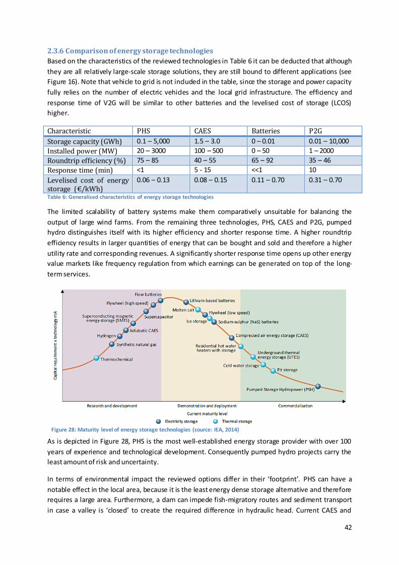
42
2.3.6 Comparison of energy storage technologies
Based on the characteristics of the reviewed technologies in Table 6 it can be deducted that although
they are all relatively large-scale storage solutions, they are still bound to different applications (see
Figure 16). Note that vehicle to grid is not included in the table, since the storage and power capacity
fully relies on the number of electric vehicles and the local grid infrastructure. The efficiency and
response time of V2G will be similar to other batteries and the levelised cost of storage (LCOS)
higher.
Characteristic PHS CAES Batteries P2G
Storage capacity (GWh) 0.1 – 5,000 1.5 – 3.0 0 – 0.01 0.01 – 10,000
Installed power (MW) 20 – 3000 100 – 500 0 – 50 1 – 2000
Roundtrip efficiency (%) 75 – 85 40 – 55 65 – 92 35 – 46
Response time (min) <1 5 - 15 <<1 10
Levelised cost of energy storage (€/kWh)
0.06 – 0.13 0.08 – 0.15 0.11 – 0.70 0.31 – 0.70
Table 6: Generalised characteristics of energy storage technologies
The limited scalability of battery systems make them comparatively unsuitable for balancing the
output of large wind farms. From the remaining three technologies, PHS, CAES and P2G, pumped
hydro distinguishes itself with its higher efficiency and shorter response time. A higher roundtrip
efficiency results in larger quantities of energy that can be bought and sold and therefore a higher
utility rate and corresponding revenues. A significantly shorter response time opens up other energy
value markets like frequency regulation from which earnings can be generated on top of the long-
term services.
As is depicted in Figure 28, PHS is the most well-established energy storage provider with over 100
years of experience and technological development. Consequently pumped hydro projects carry the
least amount of risk and uncertainty.
In terms of environmental impact the reviewed options differ in their ‘footprint’. PHS can have a
notable effect in the local area, because it is the least energy dense storage alternative and therefore
requires a large area. Furthermore, a dam can impede fish-migratory routes and sediment transport
in case a valley is ‘closed’ to create the required difference in hydraulic head. Current CAES and
Figure 28: Maturity level of energy storage technologies (source: IEA, 2014)
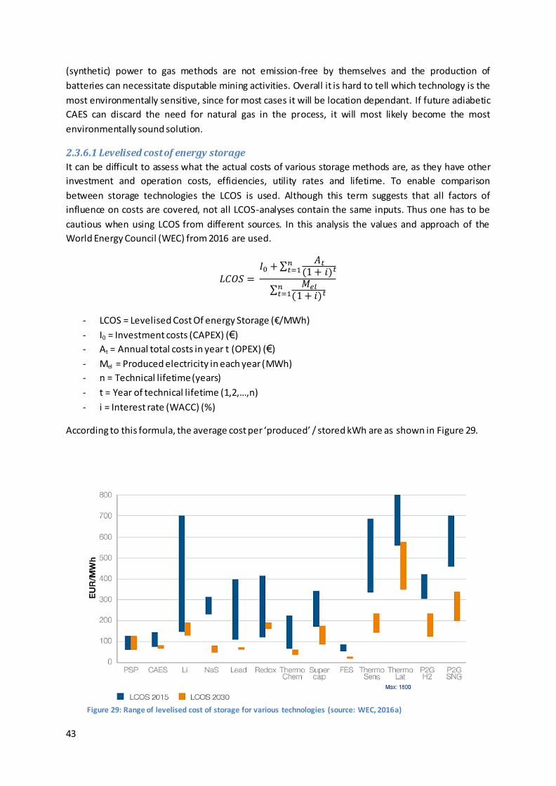
43
(synthetic) power to gas methods are not emission-free by themselves and the production of
batteries can necessitate disputable mining activities. Overall it is hard to tell which technology is the
most environmentally sensitive, since for most cases it will be location dependant. If future adiabetic
CAES can discard the need for natural gas in the process, it will most likely become the most
environmentally sound solution.
2.3.6.1 Levelised cost of energy storage
It can be difficult to assess what the actual costs of various storage methods are, as they have other
investment and operation costs, efficiencies, utility rates and lifetime. To enable comparison
between storage technologies the LCOS is used. Although this term suggests that all factors of
influence on costs are covered, not all LCOS-analyses contain the same inputs. Thus one has to be
cautious when using LCOS from different sources. In this analysis the values and approach of the
World Energy Council (WEC) from 2016 are used.
𝐿𝐶𝑂𝑆 = 𝐼0 +∑
𝐴𝑡(1+ 𝑖)𝑡
𝑛𝑡=1
∑𝑀𝑒𝑙
(1+ 𝑖)𝑡𝑛𝑡=1
- LCOS = Levelised Cost Of energy Storage (€/MWh)
- I0 = Investment costs (CAPEX) (€)
- At = Annual total costs in year t (OPEX) (€)
- Mel = Produced electricity in each year (MWh)
- n = Technical lifetime (years)
- t = Year of technical lifetime (1,2,…,n)
- i = Interest rate (WACC) (%)
According to this formula, the average cost per ‘produced’ / stored kWh are as shown in Figure 29.
Figure 29: Range of levelised cost of storage for various technologies (source: WEC, 2016a)
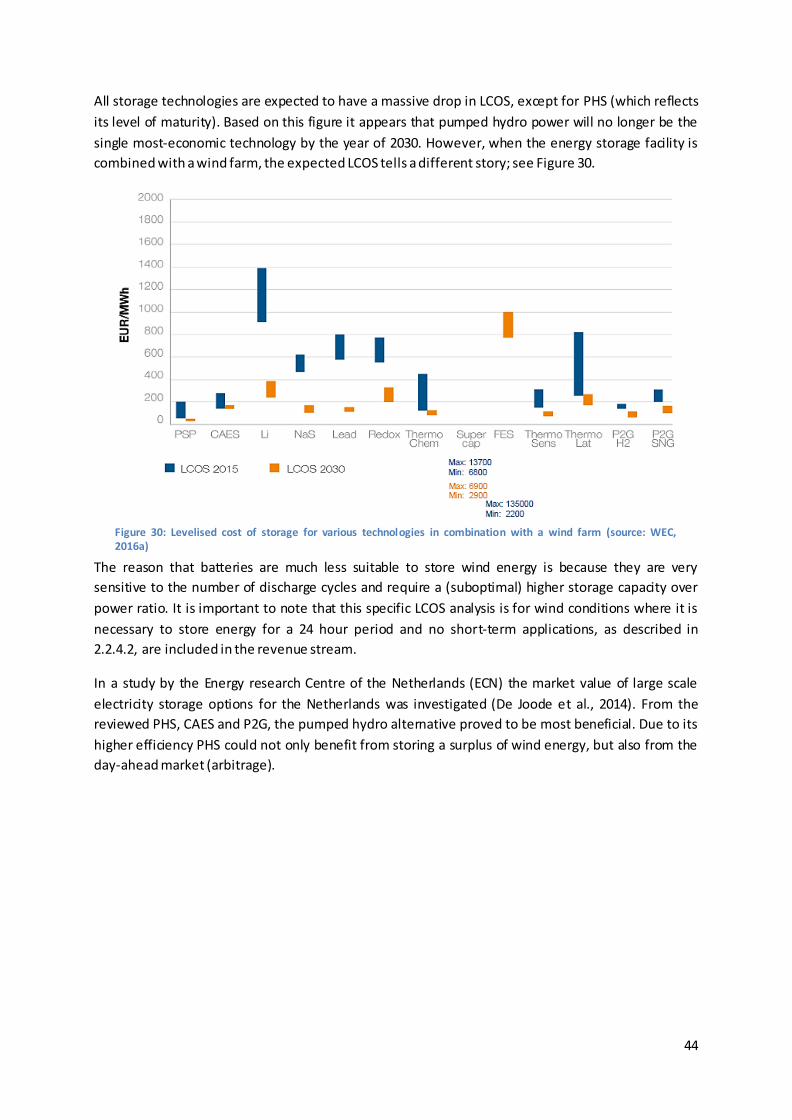
44
All storage technologies are expected to have a massive drop in LCOS, except for PHS (which reflects
its level of maturity). Based on this figure it appears that pumped hydro power will no longer be the
single most-economic technology by the year of 2030. However, when the energy storage facility is
combined with a wind farm, the expected LCOS tells a different story; see Figure 30.
The reason that batteries are much less suitable to store wind energy is because they are very
sensitive to the number of discharge cycles and require a (suboptimal) higher storage capacity over
power ratio. It is important to note that this specific LCOS analysis is for wind conditions where it is
necessary to store energy for a 24 hour period and no short-term applications, as described in
2.2.4.2, are included in the revenue stream.
In a study by the Energy research Centre of the Netherlands (ECN) the market value of large scale
electricity storage options for the Netherlands was investigated (De Joode et al., 2014). From the
reviewed PHS, CAES and P2G, the pumped hydro alternative proved to be most beneficial. Due to its
higher efficiency PHS could not only benefit from storing a surplus of wind energy, but also from the
day-ahead market (arbitrage).
Figure 30: Levelised cost of storage for various technologies in combination with a wind farm (source: WEC, 2016a)
45
2.3.7 Concluding remarks on energy storage technologies
In Europe pumped hydro storage represents circa 90 % of the grid-connected storage capacity and
continues to be identified as being the most cost-efficient large-scale energy storage technology
available today (Pérez-Díaz et al., 2014) and in the future (WEC, 2016a).
CAES is a good alternative, but also restricted to suitable sites. For heating the air prior to the
electricity generation natural gas is used, making it not a completely CO2 free facility (emissions are
cut by 2/3 compared to gas turbines). New CAES facilities that are being developed hope to raise the
roundtrip efficiency from a mere 55 % to 70 % by taking additional heat recovery measures. In case
future demonstration projects manage to exclude the usage of natural gas altogether, this
technology can become a valuable link in a sustainable energy chain.
Battery costs are expected to fall in the near future (WEC, 2016a). The sodium-sulfur flow battery
looks especially suitable for stationary ‘large-scale’ applications, where the lithium-ion battery seems
most appropriate for mobile applications (considering its energy density compared to a lead -acid
battery). Nevertheless it is unlikely that batteries will provide long-term and bulk energy storage
services, due to its physical constraints.
As is explained in 2.3.4 Vehicle to grid, it is expected that electric vehicles will only allow dynamic
charging and not feeding back into the grid in the near and middle term future. Therefore V2G is
more of a ‘demand response’ measure than it is actual energy storage. Yet it is a technology prone to
extensive research, considering the large interest of the automotive industry. Consequently current
beliefs might turn out different in the future.
Hydrogen storage and usage is inevitably related to safety issues, especially for the transportation
sector. Converting power to gas to power is simply too uneconomical on a day-to-day basis. Using
existing gas infrastructure is one of the main advantages of P2G and for synthetic natural gas
especially. However, the carbon that is added to hydrogen for making SNG will eventually be emitted
anyway; counteracting the initial gains from carbon capture from e.g. coal fired power plants.
Therefore this type of P2G is not sufficiently sustainable to meet climate change goals.
Considering investments to be made in new infrastructure it is likely that a single energy carrier will
dominate the market in the future. Whether this will become gas or electric power is yet to be seen.
In terms of efficiency it is preferable to have an economy (power generation, industrial-,
transportation- and domestic use) running on a single type of energy, to minimise energy
conversions and their corresponding losses. Where power to gas has a slight advantage with its
infrastructure already in place, an all-electric system has the upper hand with higher efficiencies,
safety in mobile applications and sustainability. Along this line of reasoning it is favourable to have an
energy storage system with electric power as its output too.
Based on the literature reviewed, data obtained and future developments taken into account, it is
concluded that pumped hydro is the best storage alternative to incorporate large shares from
renewable energy sources into the energy market.
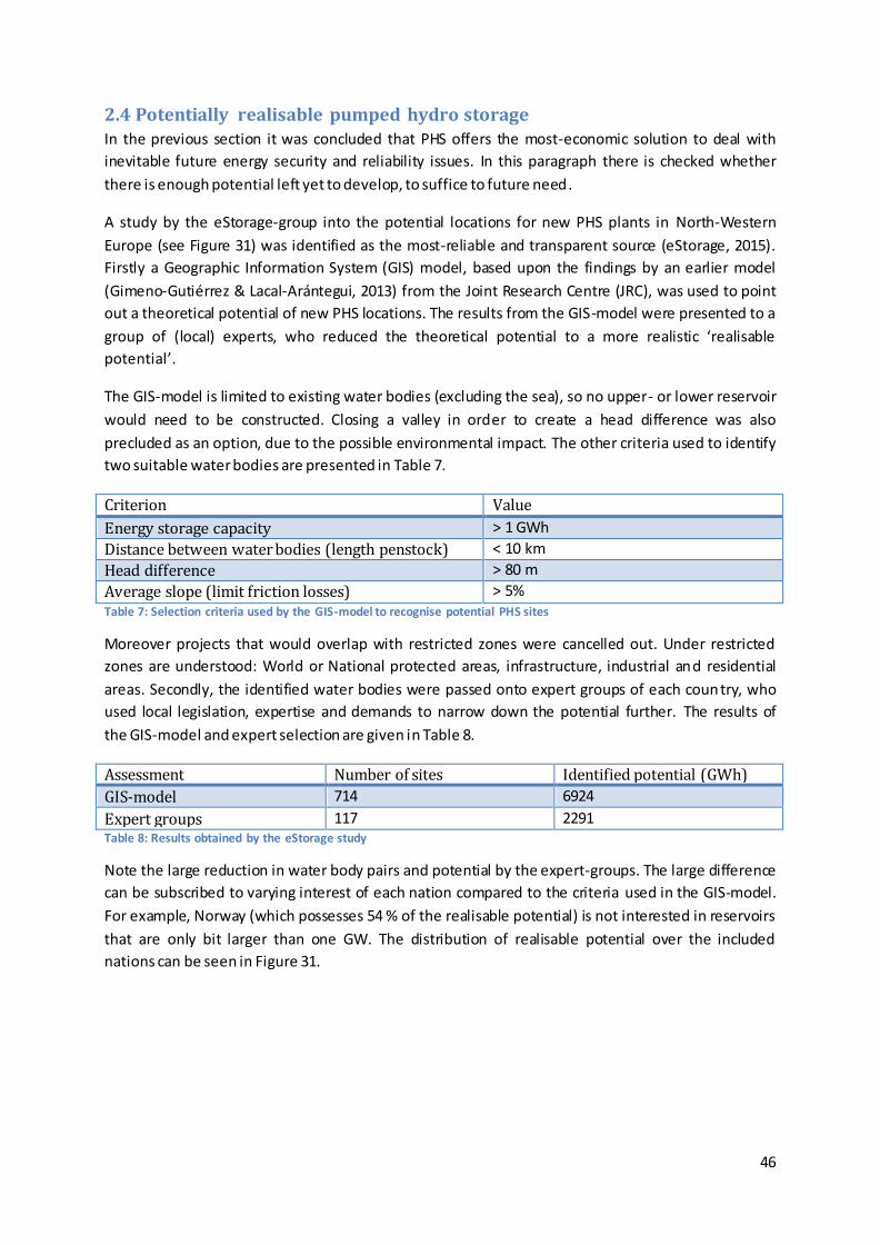
46
2.4 Potentially realisable pumped hydro storage In the previous section it was concluded that PHS offers the most-economic solution to deal with
inevitable future energy security and reliability issues. In this paragraph there is checked whether
there is enough potential left yet to develop, to suffice to future need.
A study by the eStorage-group into the potential locations for new PHS plants in North-Western
Europe (see Figure 31) was identified as the most-reliable and transparent source (eStorage, 2015).
Firstly a Geographic Information System (GIS) model, based upon the findings by an earlier model
(Gimeno-Gutiérrez & Lacal-Arántegui, 2013) from the Joint Research Centre (JRC), was used to point
out a theoretical potential of new PHS locations. The results from the GIS-model were presented to a
group of (local) experts, who reduced the theoretical potential to a more realistic ‘realisable
potential’.
The GIS-model is limited to existing water bodies (excluding the sea), so no upper- or lower reservoir
would need to be constructed. Closing a valley in order to create a head difference was also
precluded as an option, due to the possible environmental impact. The other criteria used to identify
two suitable water bodies are presented in Table 7.
Criterion Value
Energy storage capacity > 1 GWh
Distance between water bodies (length penstock) < 10 km
Head difference > 80 m
Average slope (limit friction losses) > 5% Table 7: Selection criteria used by the GIS-model to recognise potential PHS sites
Moreover projects that would overlap with restricted zones were cancelled out. Under restricted
zones are understood: World or National protected areas, infrastructure, industrial and residential
areas. Secondly, the identified water bodies were passed onto expert groups of each country, who
used local legislation, expertise and demands to narrow down the potential further. The results of
the GIS-model and expert selection are given in Table 8.
Assessment Number of sites Identified potential (GWh)
GIS-model 714 6924
Expert groups 117 2291 Table 8: Results obtained by the eStorage study
Note the large reduction in water body pairs and potential by the expert-groups. The large difference
can be subscribed to varying interest of each nation compared to the criteria used in the GIS-model.
For example, Norway (which possesses 54 % of the realisable potential) is not interested in reservoirs
that are only bit larger than one GW. The distribution of realisable potential over the included
nations can be seen in Figure 31.
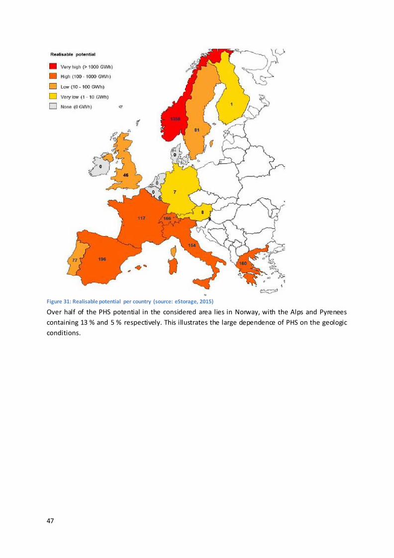
47
Over half of the PHS potential in the considered area lies in Norway, with the Alps and Pyrenees
containing 13 % and 5 % respectively. This illustrates the large dependence of PHS on the geologic
conditions.
Figure 31: Realisable potential per country (source: eStorage, 2015)
48
2.5 Future demand versus potentially realisable energy storage Today PHS is the only competitive and commercially viable large scale energy storage technology.
Therefore it is assumed that saying the remaining PHS left to develop is equal to the potentially
realisable energy storage capacity is a just first estimation.
The future demand for energy storage (as worked out in 2.2.3) was determined for North- and West-
Europe through the following steps:
1. Energy demand in 2050: 59 % of the usage in 2005-06
2. Renewable energy share: 40 - 60 % of energy demand
3. Required energy storage: 20 – 60 % of renewable energy share
From these ranges, a scenario with 60 % of renewable energy and 20 % required storage per
renewable share was chosen, for this particular region. Those assumptions led to a future storage
demand of 3584 GWh for North-Western Europe (including Norway and Switzerland) by the year of
2050.2
In the previous section the remaining potential for PHS was identified. For the same region a
realisable potential of 2291 GWh exists. Although this already fulfils a large part of the required
future storage capacity, it is not nearly enough. Furthermore it is unlikely that all the identified sites
will be realised, due to potential political and local opposition and the fact that the available
locations for new PHS do not coincide with the source of energy storage demand.
2.5.1 Need for alternative energy storage technologies
Since the ‘first’ option, conventional pumped hydro storage, does not suffice to the energy storage
demand, it is worth to look into the second-best alternative. The main drawback of conventional PHS
is the limited occurrence of two suitable existing water bodies (see Figure 31). Other than that, it is
the preferred storage method in combination with a wind farm (Figure 30). Therefore there is chosen
to look into alternative energy storage options, which rely on the same principles and technology as
the proven PHS. Between the alternatives there is sought for innovative solutions that pump water
from one reservoir to the other just the same, using identical equipment, but are not restricted to
the same geologic conditions. Appendix B contains six of these ideas that could complement the
conventional PHS in order to enable a secure energy supply.
2 Energy usage of North- and West-Europe in 2005-06 was 18477 TWh/yr. With the mentioned percentages this
results in a required energy storage capacity of: 0,59*0,6*0,2*18477 = 1308 TWh/yr. This is equal to 3584 GWh per day.
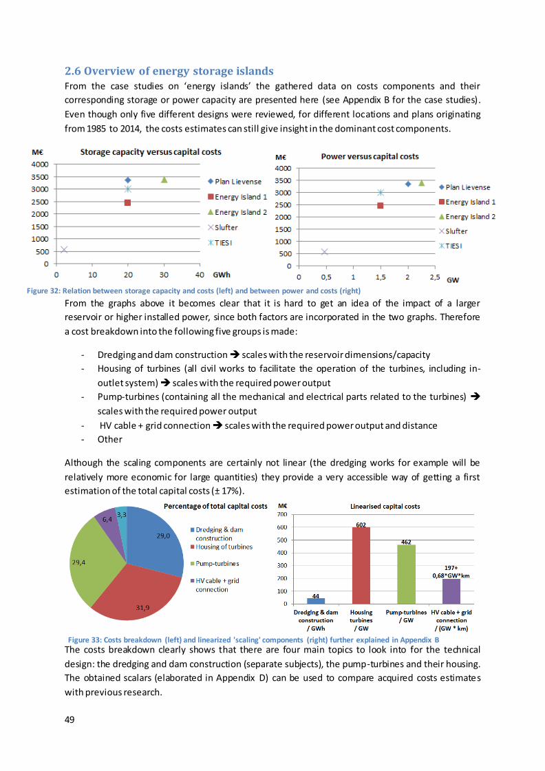
49
Figure 33: Costs breakdown (left) and linearized 'scaling' components (right) further explained in Appendix B
2.6 Overview of energy storage islands From the case studies on ‘energy islands’ the gathered data on costs components and their
corresponding storage or power capacity are presented here (see Appendix B for the case studies).
Even though only five different designs were reviewed, for different locations and plans originating
from 1985 to 2014, the costs estimates can still give insight in the dominant cost components.
From the graphs above it becomes clear that it is hard to get an idea of the impact of a larger
reservoir or higher installed power, since both factors are incorporated in the two graphs. Therefore
a cost breakdown into the following five groups is made:
- Dredging and dam construction scales with the reservoir dimensions/capacity
- Housing of turbines (all civil works to facilitate the operation of the turbines, including in-
outlet system) scales with the required power output
- Pump-turbines (containing all the mechanical and electrical parts related to the turbines)
scales with the required power output
- HV cable + grid connection scales with the required power output and distance
- Other
Although the scaling components are certainly not linear (the dredging works for example will be
relatively more economic for large quantities) they provide a very accessible way of getting a first
estimation of the total capital costs (± 17%).
The costs breakdown clearly shows that there are four main topics to look into for the technical
design: the dredging and dam construction (separate subjects), the pump-turbines and their housing.
The obtained scalars (elaborated in Appendix D) can be used to compare acquired costs estimates
with previous research.
Figure 32: Relation between storage capacity and costs (left) and between power and costs (right)

50
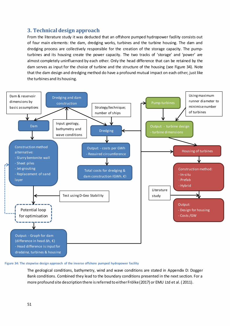
51
3. Technical design approach From the literature study it was deducted that an offshore pumped hydropower facility consists out
of four main elements: the dam, dredging works, turbines and the turbine housing. The dam and
dredging process are collectively responsible for the creation of the storage capacity. The pump-
turbines and its housing create the power capacity. The two tracks of ‘storage’ and ‘power’ are
almost completely uninfluenced by each other. Only the head difference that can be retained by the
dam serves as input for the choice of turbine and the structure of the housing (see Figure 34). Note
that the dam design and dredging method do have a profound mutual impact on each other, just like
the turbines and its housing.
The geological conditions, bathymetry, wind and wave conditions are stated in Appendix D: Dogger
Bank conditions. Combined they lead to the boundary conditions presented in the next section. For a
more profound site description there is referred to either Frölke (2017) or EMU Ltd et al. ( 2011).
Dredging and dam
construction
Dam
Construction method
alternative:
- Slurry bentonite wall
- Sheet piles
- Jet-grouting
- Replacement of sand
layer
Dam & reservoir
dimensions by
basic assumptions
Input: geology,
bathymetry and
wave conditions
Potential loop
for optimisation
Output: - Graph for dam
(difference in head Δh, €)
- Head difference is input for
dredging, turbines & housing
Dredging
Strategy/technique;
number of ships
Test using D-Geo Stability
Output: - costs per GWh
- Required circumference
Total costs for dredging &
dam construction (GWh, €)
Pump-turbines
Output: - turbine design
- turbine dimensions
Using maximum
runner diameter to
minimise number
of turbines
Housing of turbines
Construction method:
- In-situ
- Prefab
- Hybrid
Output:
- Design for housing
- Costs /GW
Literature
study
Figure 34: The stepwise design approach of the inverse offshore pumped hydropower facility
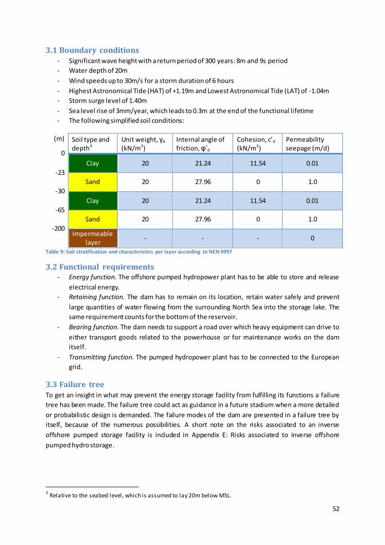
52
3.1 Boundary conditions - Significant wave height with a return period of 300 years: 8m and 9s period
- Water depth of 20m
- Wind speeds up to 30m/s for a storm duration of 6 hours
- Highest Astronomical Tide (HAT) of +1.19m and Lowest Astronomical Tide (LAT) of -1.04m
- Storm surge level of 1.40m
- Sea level rise of 3mm/year, which leads to 0.3m at the end of the functional lifetime
- The following simplified soil conditions:
(m) Soil type and depth3
Unit weight, γd (kN/m3)
Internal angle of friction, φ’d
Cohesion, c’d (kN/m2)
Permeability seepage (m/d)
0
Clay 20 21.24 11.54 0.01
-23
Sand 20 27.96 0 1.0
-30
Clay 20 21.24 11.54 0.01
-65
Sand 20 27.96 0 1.0
-200 Impermeable
layer - - - 0
Table 9: Soil stratification and characteristics per layer according to NEN 9997
3.2 Functional requirements - Energy function. The offshore pumped hydropower plant has to be able to store and release
electrical energy.
- Retaining function. The dam has to remain on its location, retain water safely and prevent
large quantities of water flowing from the surrounding North Sea into the storage lake. The
same requirement counts for the bottom of the reservoir.
- Bearing function. The dam needs to support a road over which heavy equipment can drive to
either transport goods related to the powerhouse or for maintenance works on the dam
itself.
- Transmitting function. The pumped hydropower plant has to be connected to the European
grid.
3.3 Failure tree To get an insight in what may prevent the energy storage facility from fulfilling its functions a failure
tree has been made. The failure tree could act as guidance in a future stadium when a more detailed
or probabilistic design is demanded. The failure modes of the dam are presented in a failure tree by
itself, because of the numerous possibilities. A short note on the risks associated to an inverse
offshore pumped storage facility is included in Appendix E: Risks associated to inverse offshore
pumped hydro storage.
3 Relative to the seabed level, which is assumed to lay 20m below MSL.
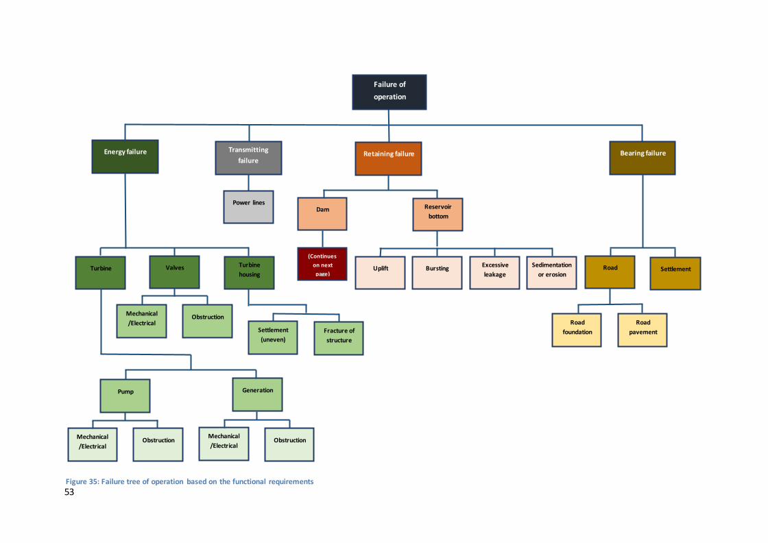
53
Figure 35: Failure tree of operation based on the functional requirements
Failure of
operation
Energy failure Bearing failure Retaining failure Transmitting
failure
Settlement Road
Power lines Dam Reservoir
bottom
(Continues
on next
page) Bursting Turbine Valves
Mechanical
/Electrical Obstruction
Uplift Turbine
housing
Settlement
(uneven)
Fracture of
structure
Pump Generation
Mechanical
/Electrical Obstruction
Mechanical
/Electrical Obstruction
Road
foundation
Road
pavement
Excessive
leakage Sedimentation
or erosion
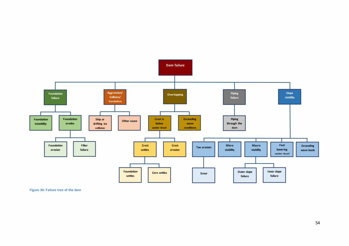
54
Dam failure
Foundation
failure
Slope
stability Overtopping Piping
failure
Other cause
Crest
settles
Crest
erosion
Foundation
settles Core settles
Foundation
instability
Foundation
erodes
Foundation
erosion
Filter
failure
Macro
stability
Micro
stability Toe erosion
Scour Outer slope
failure
Inner slope
failure
Exceeding
wave loads
Aggression/
Collision/
Vandalism
Piping
through the
dam
Fast
lowering
water level
Exceeding
wave
conditions
Crest is
below
water level
Ship or
drifting ice
collision
Figure 36: Failure tree of the dam
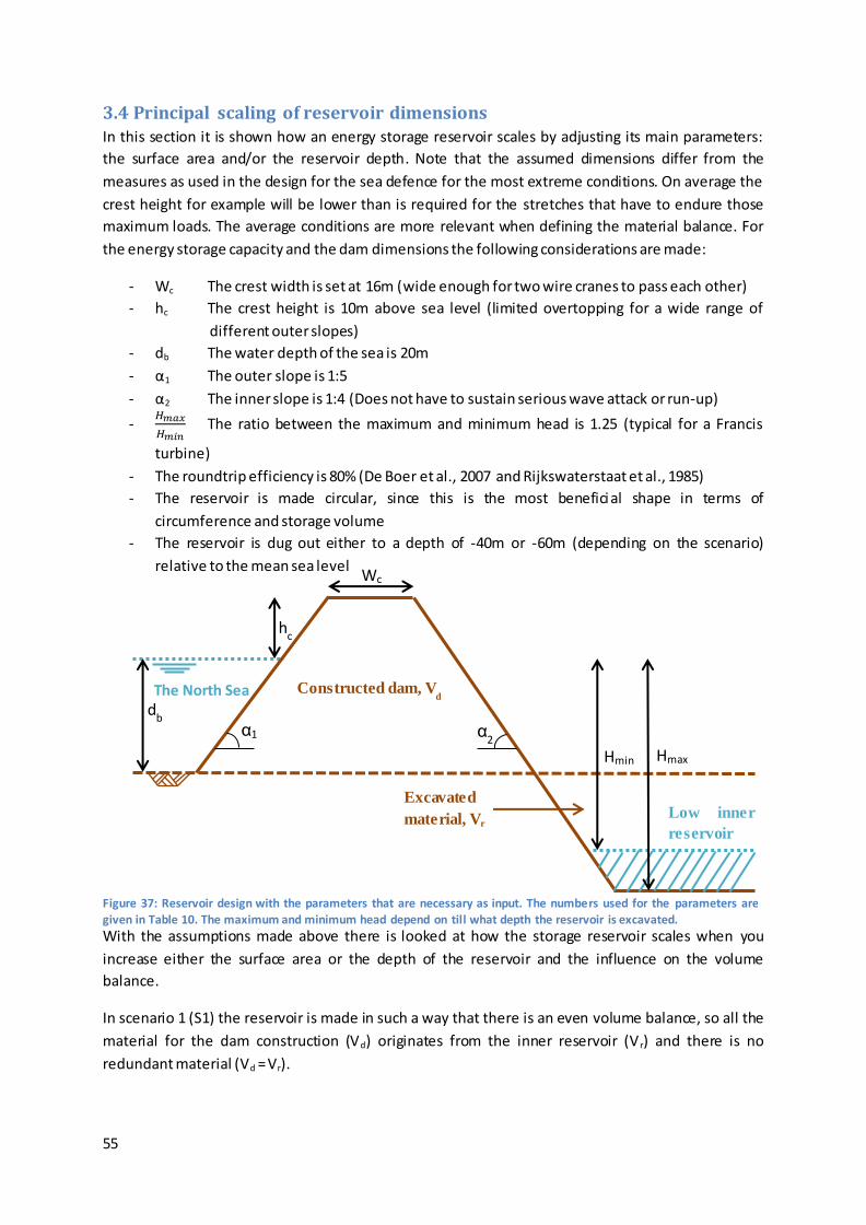
55
3.4 Principal scaling of reservoir dimensions In this section it is shown how an energy storage reservoir scales by adjusting its main parameters:
the surface area and/or the reservoir depth. Note that the assumed dimensions differ from the
measures as used in the design for the sea defence for the most extreme conditions. On average the
crest height for example will be lower than is required for the stretches that have to endure those
maximum loads. The average conditions are more relevant when defining the material balance. For
the energy storage capacity and the dam dimensions the following considerations are made:
- Wc The crest width is set at 16m (wide enough for two wire cranes to pass each other)
- hc The crest height is 10m above sea level (limited overtopping for a wide range of
different outer slopes)
- db The water depth of the sea is 20m
- α1 The outer slope is 1:5
- α2 The inner slope is 1:4 (Does not have to sustain serious wave attack or run-up)
- 𝐻𝑚𝑎𝑥
𝐻𝑚𝑖𝑛 The ratio between the maximum and minimum head is 1.25 (typical for a Francis
turbine)
- The roundtrip efficiency is 80% (De Boer et al., 2007 and Rijkswaterstaat et al., 1985)
- The reservoir is made circular, since this is the most beneficial shape in terms of
circumference and storage volume
- The reservoir is dug out either to a depth of -40m or -60m (depending on the scenario)
relative to the mean sea level
With the assumptions made above there is looked at how the storage reservoir scales when you
increase either the surface area or the depth of the reservoir and the influence on the volume
balance.
In scenario 1 (S1) the reservoir is made in such a way that there is an even volume balance, so all the
material for the dam construction (Vd) originates from the inner reservoir (V r) and there is no
redundant material (Vd = Vr).
Low inner
reservoir
Wc
db
hc
Hmin Hmax
α1 α2
The North Sea
Excavated
material, Vr
Constructed dam, Vd
Figure 37: Reservoir design with the parameters that are necessary as input. The numbers used for the parameters are given in Table 10. The maximum and minimum head depend on till what depth the reservoir is excavated.
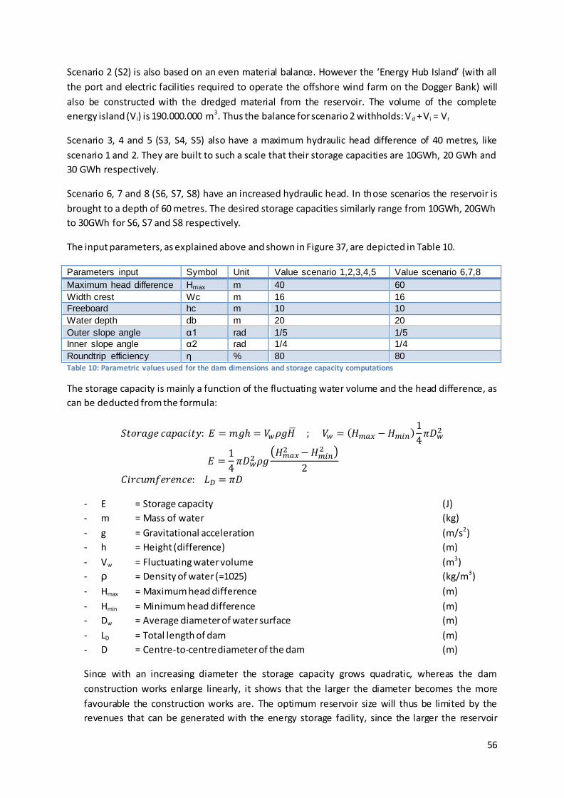
56
Scenario 2 (S2) is also based on an even material balance. However the ‘Energy Hub Island’ (with all
the port and electric facilities required to operate the offshore wind farm on the Dogger Bank) will
also be constructed with the dredged material from the reservoir. The volume of the complete
energy island (V i) is 190.000.000 m3. Thus the balance for scenario 2 withholds: Vd + Vi = Vr
Scenario 3, 4 and 5 (S3, S4, S5) also have a maximum hydraulic head difference of 40 metres, like
scenario 1 and 2. They are built to such a scale that their storage capacities are 10GWh, 20 GWh and
30 GWh respectively.
Scenario 6, 7 and 8 (S6, S7, S8) have an increased hydraulic head. In those scenarios the reservoir is
brought to a depth of 60 metres. The desired storage capacities similarly range from 10GWh, 20GWh
to 30GWh for S6, S7 and S8 respectively.
The input parameters, as explained above and shown in Figure 37, are depicted in Table 10.
Parameters input Symbol Unit Value scenario 1,2,3,4,5 Value scenario 6,7,8
Maximum head difference Hmax m 40 60
Width crest Wc m 16 16
Freeboard hc m 10 10
Water depth db m 20 20
Outer slope angle α1 rad 1/5 1/5
Inner slope angle α2 rad 1/4 1/4
Roundtrip efficiency η % 80 80
Table 10: Parametric values used for the dam dimensions and storage capacity computations
The storage capacity is mainly a function of the fluctuating water volume and the head difference, as
can be deducted from the formula:
𝑆𝑡𝑜𝑟𝑎𝑔𝑒 𝑐𝑎𝑝𝑎𝑐𝑖𝑡𝑦: 𝐸 = 𝑚𝑔ℎ = 𝑉𝑤𝜌𝑔𝐻 ; 𝑉𝑤 = (𝐻𝑚𝑎𝑥 −𝐻𝑚𝑖𝑛)1
4𝜋𝐷𝑤
2
𝐸 =1
4𝜋𝐷𝑤
2 𝜌𝑔(𝐻𝑚𝑎𝑥
2 −𝐻𝑚𝑖𝑛2 )
2
𝐶𝑖𝑟𝑐𝑢𝑚𝑓𝑒𝑟𝑒𝑛𝑐𝑒: 𝐿𝐷 = 𝜋𝐷
- E = Storage capacity (J)
- m = Mass of water (kg)
- g = Gravitational acceleration (m/s2)
- h = Height (difference) (m)
- Vw = Fluctuating water volume (m3)
- ρ = Density of water (=1025) (kg/m3)
- Hmax = Maximum head difference (m)
- Hmin = Minimum head difference (m)
- Dw = Average diameter of water surface (m)
- LD = Total length of dam (m)
- D = Centre-to-centre diameter of the dam (m)
Since with an increasing diameter the storage capacity grows quadratic, whereas the dam
construction works enlarge linearly, it shows that the larger the diameter becomes the more
favourable the construction works are. The optimum reservoir size will thus be limited by the
revenues that can be generated with the energy storage facility, since the larger the reservoir
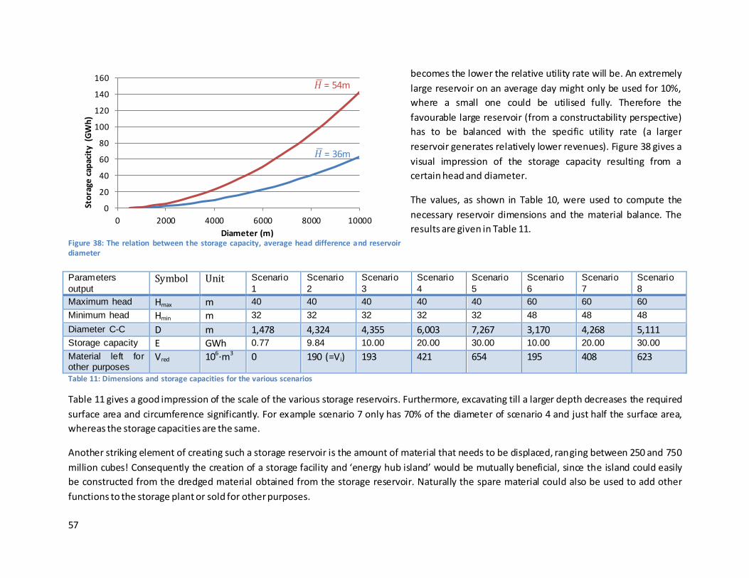
57
becomes the lower the relative utility rate will be. An extremely
large reservoir on an average day might only be used for 10%,
where a small one could be utilised fully. Therefore the
favourable large reservoir (from a constructability perspective)
has to be balanced with the specific utility rate (a larger
reservoir generates relatively lower revenues). Figure 38 gives a
visual impression of the storage capacity resulting from a
certain head and diameter.
The values, as shown in Table 10, were used to compute the
necessary reservoir dimensions and the material balance. The
results are given in Table 11.
Parameters
output Symbol Unit Scenario
1
Scenario
2
Scenario
3
Scenario
4
Scenario
5
Scenario
6
Scenario
7
Scenario
8
Maximum head Hmax m 40 40 40 40 40 60 60 60
Minimum head Hmin m 32 32 32 32 32 48 48 48
Diameter C-C D m 1,478 4,324 4,355 6,003 7,267 3,170 4,268 5,111 Storage capacity E GWh 0.77 9.84 10.00 20.00 30.00 10.00 20.00 30.00
Material left for other purposes
Vred 106∙m3 0 190 (=Vi) 193 421 654 195 408 623
Table 11: Dimensions and storage capacities for the various scenarios
Table 11 gives a good impression of the scale of the various storage reservoirs. Furthermore, excavating till a larger depth decreases the required
surface area and circumference significantly. For example scenario 7 only has 70% of the diameter of scenario 4 and just half the surface area,
whereas the storage capacities are the same.
Another striking element of creating such a storage reservoir is the amount of material that needs to be displaced, ranging between 250 and 750
million cubes! Consequently the creation of a storage facility and ‘energy hub island’ would be mutually beneficial, since the island could easily
be constructed from the dredged material obtained from the storage reservoir. Naturally the spare material could also be used to add other
functions to the storage plant or sold for other purposes.
0
20
40
60
80
100
120
140
160
0 2000 4000 6000 8000 10000
Sto
rage
cap
acit
y (G
Wh
)
Diameter (m)
𝐻 = 54m
𝐻 = 36m
Figure 38: The relation between the storage capacity, average head difference and reservoir diameter
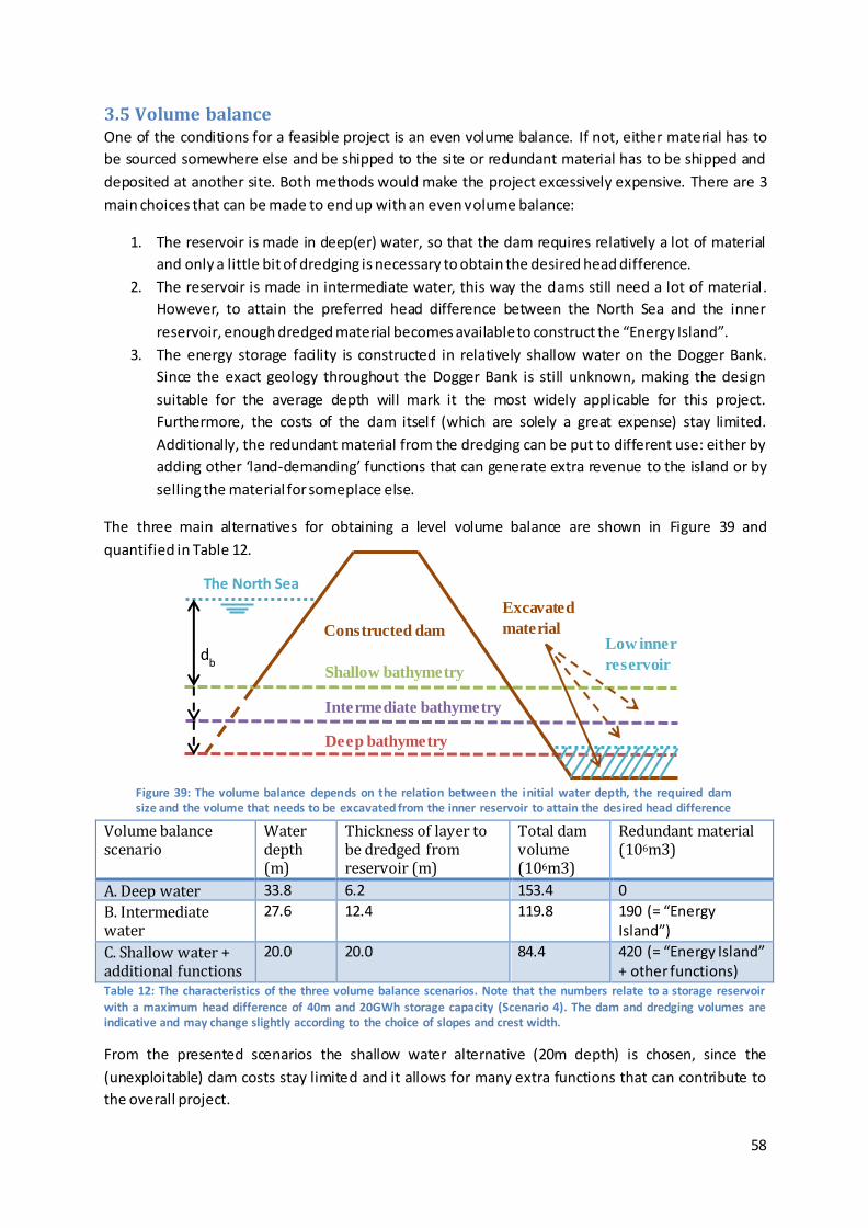
58
Shallow bathymetry
Intermediate bathymetry
Deep bathymetry
Excavated
material
db
The North Sea
Low inner
reservoir
Constructed dam
3.5 Volume balance One of the conditions for a feasible project is an even volume balance. If not, either material has to
be sourced somewhere else and be shipped to the site or redundant material has to be shipped and
deposited at another site. Both methods would make the project excessively expensive. There are 3
main choices that can be made to end up with an even volume balance:
1. The reservoir is made in deep(er) water, so that the dam requires relatively a lot of material
and only a little bit of dredging is necessary to obtain the desired head difference.
2. The reservoir is made in intermediate water, this way the dams still need a lot of material.
However, to attain the preferred head difference between the North Sea and the inner
reservoir, enough dredged material becomes available to construct the “Energy Island”.
3. The energy storage facility is constructed in relatively shallow water on the Dogger Bank.
Since the exact geology throughout the Dogger Bank is still unknown, making the design
suitable for the average depth will mark it the most widely applicable for this project.
Furthermore, the costs of the dam itself (which are solely a great expense) stay limited.
Additionally, the redundant material from the dredging can be put to different use: either by
adding other ‘land-demanding’ functions that can generate extra revenue to the island or by
selling the material for someplace else.
The three main alternatives for obtaining a level volume balance are shown in Figure 39 and
quantified in Table 12.
Volume balance scenario
Water depth (m)
Thickness of layer to be dredged from reservoir (m)
Total dam volume (106m3)
Redundant material (106m3)
A. Deep water 33.8 6.2 153.4 0
B. Intermediate water
27.6 12.4 119.8 190 (= “Energy Island”)
C. Shallow water + additional functions
20.0 20.0 84.4 420 (= “Energy Island” + other functions)
Table 12: The characteristics of the three volume balance scenarios. Note that the numbers relate to a storage reservoir with a maximum head difference of 40m and 20GWh storage capacity (Scenario 4). The dam and dredging volumes are indicative and may change slightly according to the choice of slopes and crest width.
From the presented scenarios the shallow water alternative (20m depth) is chosen, since the
(unexploitable) dam costs stay limited and it allows for many extra functions that can contribute to
the overall project.
Figure 39: The volume balance depends on the relation between the initial water depth, the required dam size and the volume that needs to be excavated from the inner reservoir to attain the desired head difference

59
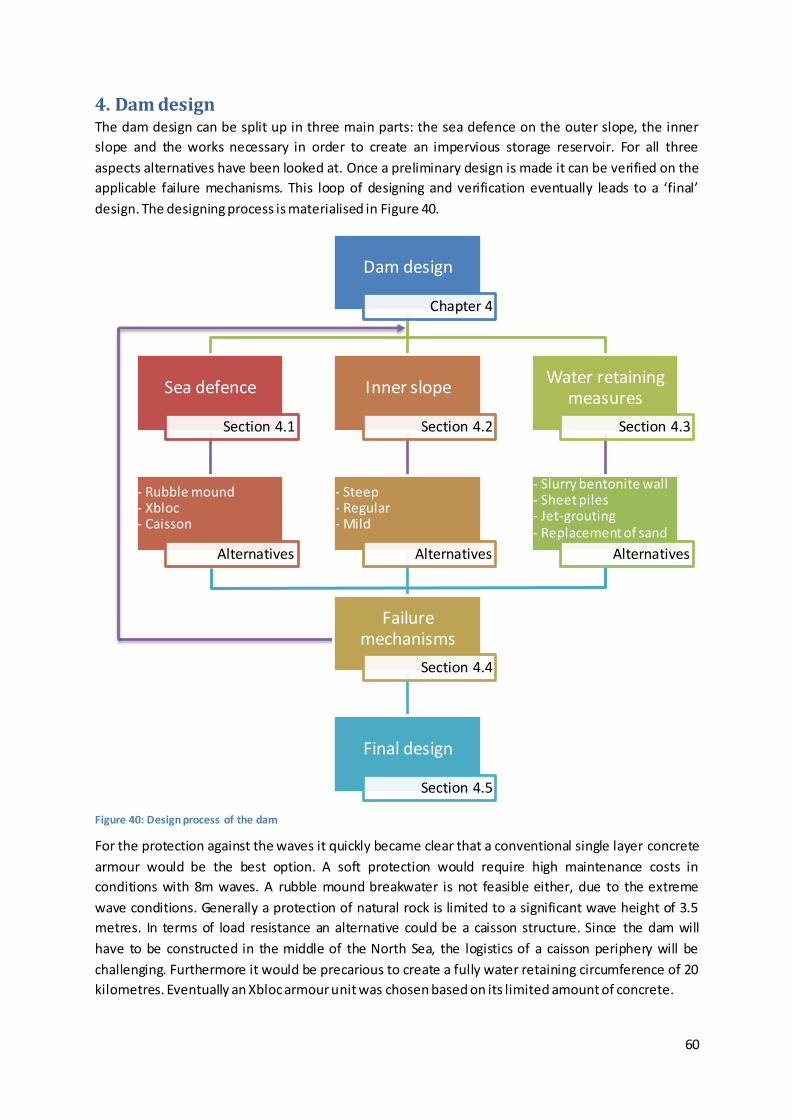
60
4. Dam design The dam design can be split up in three main parts: the sea defence on the outer slope, the inner
slope and the works necessary in order to create an impervious storage reservoir. For all three
aspects alternatives have been looked at. Once a preliminary design is made it can be verified on the
applicable failure mechanisms. This loop of designing and verification eventually leads to a ‘final’
design. The designing process is materialised in Figure 40.
For the protection against the waves it quickly became clear that a conventional single layer concrete
armour would be the best option. A soft protection would require high maintenance costs in
conditions with 8m waves. A rubble mound breakwater is not feasible either, due to the extreme
wave conditions. Generally a protection of natural rock is limited to a significant wave height of 3.5
metres. In terms of load resistance an alternative could be a caisson structure. Since the dam will
have to be constructed in the middle of the North Sea, the logistics of a caisson periphery will be
challenging. Furthermore it would be precarious to create a fully water retaining circumference of 20
kilometres. Eventually an Xbloc armour unit was chosen based on its limited amount of concrete.
Dam design
Chapter 4
Sea defence
Section 4.1
- Rubble mound - Xbloc - Caisson
Alternatives
Inner slope
Section 4.2
- Steep - Regular - Mild
Alternatives
Failure mechanisms
Section 4.4
Final design
Section 4.5
Water retaining measures
Section 4.3
- Slurry bentonite wall - Sheet piles - Jet-grouting - Replacement of sand
Alternatives
Figure 40: Design process of the dam
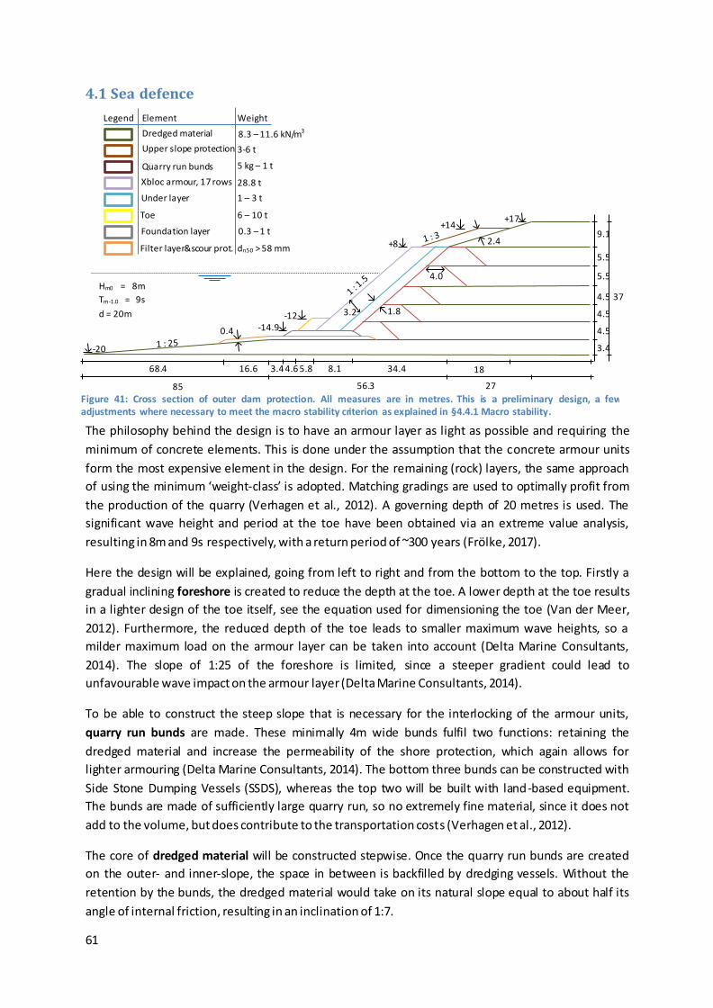
61
4.1 Sea defence
The philosophy behind the design is to have an armour layer as light as possible and requiring the
minimum of concrete elements. This is done under the assumption that the concrete armour units
form the most expensive element in the design. For the remaining (rock) layers, the same approach
of using the minimum ‘weight-class’ is adopted. Matching gradings are used to optimally profit from
the production of the quarry (Verhagen et al., 2012). A governing depth of 20 metres is used. The
significant wave height and period at the toe have been obtained via an extreme value analysis,
resulting in 8m and 9s respectively, with a return period of ~300 years (Frölke, 2017).
Here the design will be explained, going from left to right and from the bottom to the top. Firstly a
gradual inclining foreshore is created to reduce the depth at the toe. A lower depth at the toe results
in a lighter design of the toe itself, see the equation used for dimensioning the toe (Van der Meer,
2012). Furthermore, the reduced depth of the toe leads to smaller maximum wave heights, so a
milder maximum load on the armour layer can be taken into account (Delta Marine Consultants,
2014). The slope of 1:25 of the foreshore is limited, since a steeper gradient could lead to
unfavourable wave impact on the armour layer (Delta Marine Consultants, 2014).
To be able to construct the steep slope that is necessary for the interlocking of the armour units,
quarry run bunds are made. These minimally 4m wide bunds fulfil two functions: retaining the
dredged material and increase the permeability of the shore protection, which again allows for
lighter armouring (Delta Marine Consultants, 2014). The bottom three bunds can be constructed with
Side Stone Dumping Vessels (SSDS), whereas the top two will be built with land-based equipment.
The bunds are made of sufficiently large quarry run, so no extremely fine material, since it does not
add to the volume, but does contribute to the transportation costs (Verhagen et al., 2012).
The core of dredged material will be constructed stepwise. Once the quarry run bunds are created
on the outer- and inner-slope, the space in between is backfilled by dredging vessels. Without the
retention by the bunds, the dredged material would take on its natural slope equal to about half its
angle of internal friction, resulting in an inclination of 1:7.
Figure 41: Cross section of outer dam protection. All measures are in metres. This is a preliminary design, a few adjustments where necessary to meet the macro stability criterion as explained in §4.4.1 Macro stability.
Legend Element Weight
Dredged material
Upper slope protection
Quarry run bunds
Xbloc armour, 17 rows
Under layer
Toe
Foundation layer
Filter layer&scour prot.
8.3 – 11.6 kN/m3
3-6 t
5 kg – 1 t
28.8 t
1 – 3 t
6 – 10 t
0.3 – 1 t
dn50 > 58 mm
37 4.5
9.1
5.5
5.5
4.5
4.5
3.4
85 56.3 27
18 34.4 68.4 16.6 3.4 4.6 5.8 8.1
0.4 -14.9 -12
+8
+14 +17
2.4
4.0
1.8 3.2
-20
Hm0 = 8m
Tm-1.0 = 9s
d = 20m
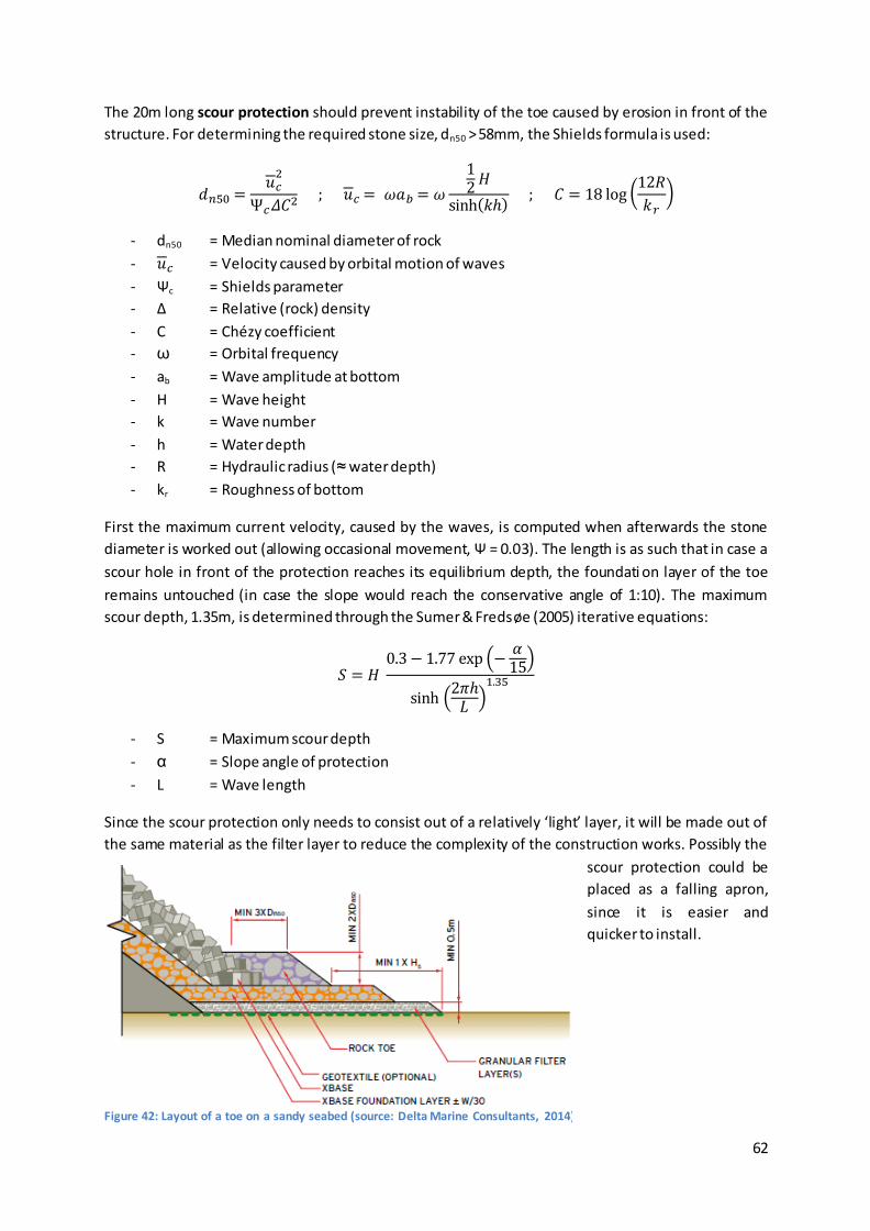
62
Figure 42: Layout of a toe on a sandy seabed (source: Delta Marine Consultants, 2014)
The 20m long scour protection should prevent instability of the toe caused by erosion in front of the
structure. For determining the required stone size, dn50 > 58mm, the Shields formula is used:
𝑑𝑛50 =𝑢𝑐2
Ѱ𝑐𝛥𝐶2 ; 𝑢𝑐 = 𝜔𝑎𝑏 = 𝜔
12𝐻
sinh(𝑘ℎ) ; 𝐶 = 18 log (
12𝑅
𝑘𝑟)
- dn50 = Median nominal diameter of rock
- 𝑢𝑐 = Velocity caused by orbital motion of waves
- Ѱc = Shields parameter
- Δ = Relative (rock) density
- C = Chézy coefficient
- ω = Orbital frequency
- ab = Wave amplitude at bottom
- H = Wave height
- k = Wave number
- h = Water depth
- R = Hydraulic radius (≈ water depth)
- kr = Roughness of bottom
First the maximum current velocity, caused by the waves, is computed when afterwards the stone
diameter is worked out (allowing occasional movement, Ѱ = 0.03). The length is as such that in case a
scour hole in front of the protection reaches its equilibrium depth, the foundati on layer of the toe
remains untouched (in case the slope would reach the conservative angle of 1:10). The maximum
scour depth, 1.35m, is determined through the Sumer & Fredsøe (2005) iterative equations:
𝑆 = 𝐻 0.3− 1.77 exp (−
𝛼15)
sinh (2𝜋ℎ𝐿)1.35
- S = Maximum scour depth
- α = Slope angle of protection
- L = Wave length
Since the scour protection only needs to consist out of a relatively ‘light’ layer, it will be made out of
the same material as the filter layer to reduce the complexity of the construction works. Possibly the
scour protection could be
placed as a falling apron,
since it is easier and
quicker to install.
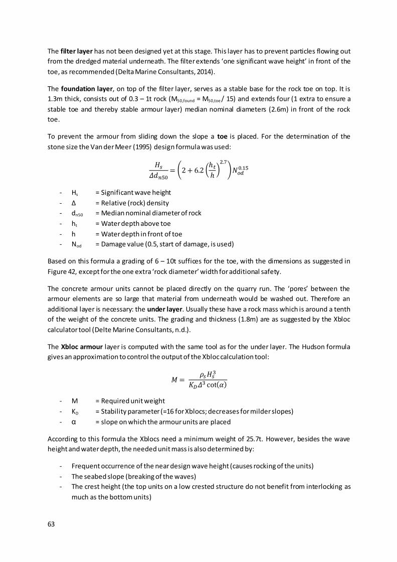
63
The filter layer has not been designed yet at this stage. This layer has to prevent particles flowing out
from the dredged material underneath. The filter extends ‘one significant wave height’ in front of the
toe, as recommended (Delta Marine Consultants, 2014).
The foundation layer, on top of the filter layer, serves as a stable base for the rock toe on top. It is
1.3m thick, consists out of 0.3 – 1t rock (M50,found = M50,toe / 15) and extends four (1 extra to ensure a
stable toe and thereby stable armour layer) median nominal diameters (2.6m) in front of the rock
toe.
To prevent the armour from sliding down the slope a toe is placed. For the determination of the
stone size the Van der Meer (1995) design formula was used:
𝐻𝑠𝛥𝑑𝑛50
= (2+ 6.2 (ℎ𝑡ℎ)2.7
)𝑁𝑜𝑑0.15
- Hs = Significant wave height
- Δ = Relative (rock) density
- dn50 = Median nominal diameter of rock
- ht = Water depth above toe
- h = Water depth in front of toe
- Nod = Damage value (0.5, start of damage, is used)
Based on this formula a grading of 6 – 10t suffices for the toe, with the dimensions as suggested in
Figure 42, except for the one extra ‘rock diameter’ width for additional safety.
The concrete armour units cannot be placed directly on the quarry run. The ‘pores’ between the
armour elements are so large that material from underneath would be washed out. Therefore an
additional layer is necessary: the under layer. Usually these have a rock mass which is around a tenth
of the weight of the concrete units. The grading and thickness (1.8m) are as suggested by the Xbloc
calculator tool (Delte Marine Consultants, n.d.).
The Xbloc armour layer is computed with the same tool as for the under layer. The Hudson formula
gives an approximation to control the output of the Xbloc calculation tool:
𝑀= 𝜌𝑠𝐻𝑠
3
𝐾𝐷𝛥3 cot(𝛼)
- M = Required unit weight
- KD = Stability parameter (=16 for Xblocs; decreases for milder slopes)
- α = slope on which the armour units are placed
According to this formula the Xblocs need a minimum weight of 25.7t. However, besides the wave
height and water depth, the needed unit mass is also determined by:
- Frequent occurrence of the near design wave height (causes rocking of the units)
- The seabed slope (breaking of the waves)
- The crest height (the top units on a low crested structure do not benefit from interlocking as
much as the bottom units)

64
- The core permeability (a permeable structure allows for some transmission of the wave
energy, instead of reflecting back on the armour)
- The slope (a steeper slope increases the interlocking between the armour units, which leads
to enhanced stability4)
For the chosen wave height and the design high water level of +1.5m the tool advises to use 28.8t
heavy elements, which are 3.3m high. First an Xbase unit (see Figure 42) is placed on top of the
foundation layer when afterwards the armour can be constructed, using land-based wire cranes,
from the bottom up. For the whole armour layer 17 rows of randomly placed Xblocs are required.
The Xbloc armour continues till ‘one significant wave height’ above still water level. The remaining
dam does not need to continue with, a difficult to realise, 1:1.5 slope, since the rock on the upper
slope protection does not rely on interlocking. A three-to-six tonne grading is chosen for the double
layer, 2.4m high, to complete the protection of the dam. The protection runs until +14m, slightly
above the limit that recommends armouring till 0.5 times the run-up that would be present on a
smooth slope (Van der Meer, 2002)5.
The crest level was initially set at +16m, which would allow an overtopping discharge of 10 litres per
second per metre according the Van der Meer (2002) formula:
𝑅𝑐 =
ln
(
𝑞
0.2√𝑔𝐻𝑚03
)
𝐻𝑚03 𝛾𝑓𝛾𝛽
−2.3
- Rc = Free crest height above still water line
- q = Overtopping discharge (in this case 10l/s/m)
- g = gravitational acceleration
- Hm0 = Significant wave height at the toe
- γf = Roughness reduction factor (weighted average for Xblocs and upper protection)
- γβ = Angle of incidence reduction factor (=1 for waves approaching perpendicular to the
structure)
One metre is finally added to the crest height for safety reasons and to counter future settlement of
the dam body (Bezuyen, 2012).
The presented preliminary design is entirely feasible and there is a lot of experience in constructing
such a structure. The many different layers and gradings do make it logistically challenging. The
relatively large usage of dredged material for the core and the proven concept of the Xblocs causes
that this conventional design remains to be preferred and used for later cost computations.
4 The opposite is true for non-interlocking concrete armour units or rock. These elements rely on gravi ty only and the
armour does not act as a whole as i t does for interlocking units . Therefore the s tability diminishes with an increasing slope for rock or concrete (antifer) cubes. 5 In order to take the maximum allowable influence (reduction) factors into account for the effect of roughness on the slope, certain restrictions apply. Fi rs t one has to compute the hypothetical run -up if the slope(s) would be perfectly smooth (in this case 26.5m). Secondly one is allowed to use the roughness ‘reduction’ factor in case the ‘roughness creating
elements’ are placed 0.25 * Run-upsmooth below the water line (=6.6m) and 0.5 * Run-upsmooth above the water line (=13.3m). Therefore there is chosen to apply the slope protection till +14m (The theoretical background of this method is rather unclear, however in practise this methodology i s widely accepted and applied, see Van der Meer (2002)).
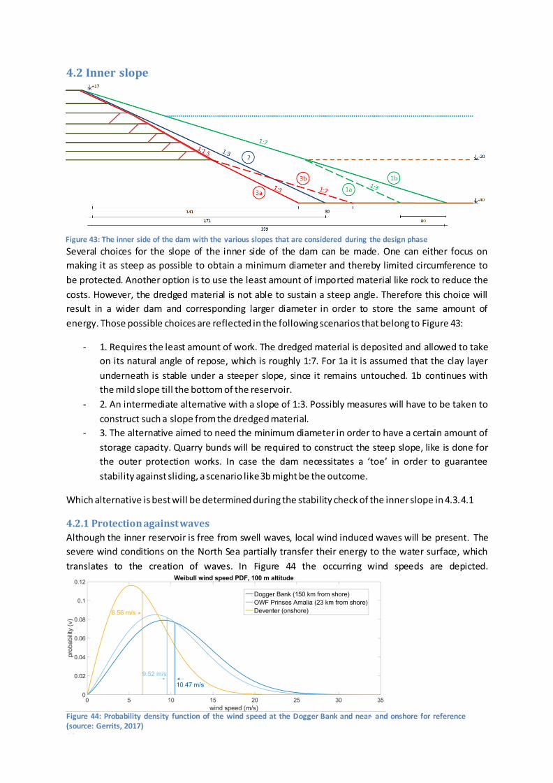
65
4.2 Inner slope
Several choices for the slope of the inner side of the dam can be made. One can either focus on
making it as steep as possible to obtain a minimum diameter and thereby limited circumference to
be protected. Another option is to use the least amount of imported material like rock to reduce the
costs. However, the dredged material is not able to sustain a steep angle. Therefore this choice will
result in a wider dam and corresponding larger diameter in order to store the same amount of
energy. Those possible choices are reflected in the following scenarios that belong to Figure 43:
- 1. Requires the least amount of work. The dredged material is deposited and allowed to take
on its natural angle of repose, which is roughly 1:7. For 1a it is assumed that the clay layer
underneath is stable under a steeper slope, since it remains untouched. 1b continues with
the mild slope till the bottom of the reservoir.
- 2. An intermediate alternative with a slope of 1:3. Possibly measures will have to be taken to
construct such a slope from the dredged material.
- 3. The alternative aimed to need the minimum diameter in order to have a certain amount of
storage capacity. Quarry bunds will be required to construct the steep slope, like is done for
the outer protection works. In case the dam necessitates a ‘toe’ in order to guarantee
stability against sliding, a scenario like 3b might be the outcome.
Which alternative is best will be determined during the stability check of the inner slope in 4.3.4.1
4.2.1 Protection against waves
Although the inner reservoir is free from swell waves, local wind induced waves will be present. The
severe wind conditions on the North Sea partially transfer their energy to the water surface, which
translates to the creation of waves. In Figure 44 the occurring wind speeds are depicted.
Figure 43: The inner side of the dam with the various slopes that are considered during the design phase
Figure 44: Probability density function of the wind speed at the Dogger Bank and near- and onshore for reference (source: Gerrits, 2017)
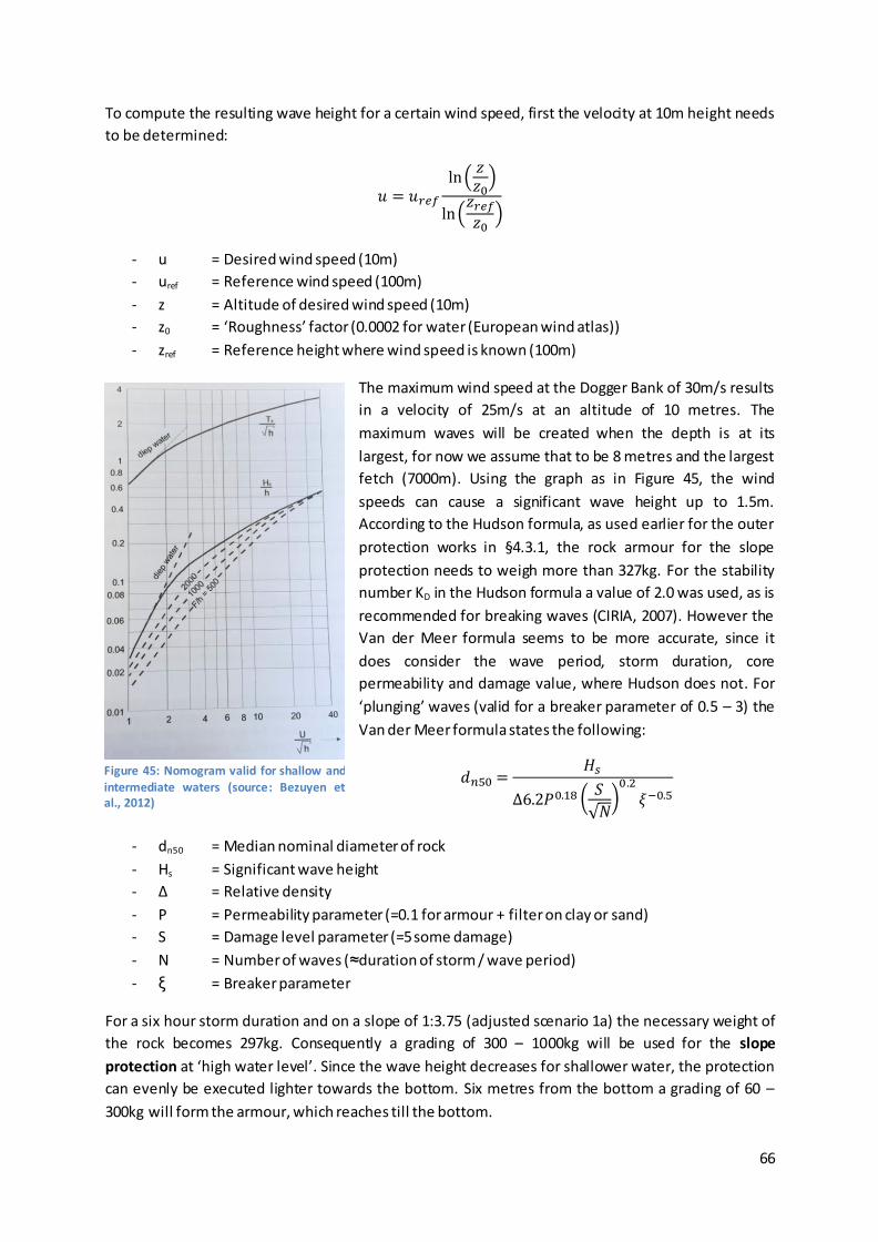
66
To compute the resulting wave height for a certain wind speed, first the velocity at 10m height needs
to be determined:
𝑢 = 𝑢𝑟𝑒𝑓
ln(𝑧𝑧0)
ln(𝑧𝑟𝑒𝑓𝑧0)
- u = Desired wind speed (10m)
- uref = Reference wind speed (100m)
- z = Altitude of desired wind speed (10m)
- z0 = ‘Roughness’ factor (0.0002 for water (European wind atlas))
- zref = Reference height where wind speed is known (100m)
The maximum wind speed at the Dogger Bank of 30m/s results
in a velocity of 25m/s at an altitude of 10 metres. The
maximum waves will be created when the depth is at its
largest, for now we assume that to be 8 metres and the largest
fetch (7000m). Using the graph as in Figure 45, the wind
speeds can cause a significant wave height up to 1.5m.
According to the Hudson formula, as used earlier for the outer
protection works in §4.3.1, the rock armour for the slope
protection needs to weigh more than 327kg. For the stability
number KD in the Hudson formula a value of 2.0 was used, as is
recommended for breaking waves (CIRIA, 2007). However the
Van der Meer formula seems to be more accurate, since it
does consider the wave period, storm duration, core
permeability and damage value, where Hudson does not. For
‘plunging’ waves (valid for a breaker parameter of 0.5 – 3) the
Van der Meer formula states the following:
𝑑𝑛50 =𝐻𝑠
∆6.2𝑃0.18 (𝑆
√𝑁)0.2
𝜉−0.5
- dn50 = Median nominal diameter of rock
- Hs = Significant wave height
- Δ = Relative density
- P = Permeability parameter (=0.1 for armour + filter on clay or sand)
- S = Damage level parameter (=5 some damage)
- N = Number of waves (≈duration of storm / wave period)
- ξ = Breaker parameter
For a six hour storm duration and on a slope of 1:3.75 (adjusted scenario 1a) the necessary weight of
the rock becomes 297kg. Consequently a grading of 300 – 1000kg will be used for the slope
protection at ‘high water level’. Since the wave height decreases for shallower water, the protection
can evenly be executed lighter towards the bottom. Six metres from the bottom a grading of 60 –
300kg will form the armour, which reaches till the bottom.
Figure 45: Nomogram valid for shallow and intermediate waters (source: Bezuyen et al., 2012)
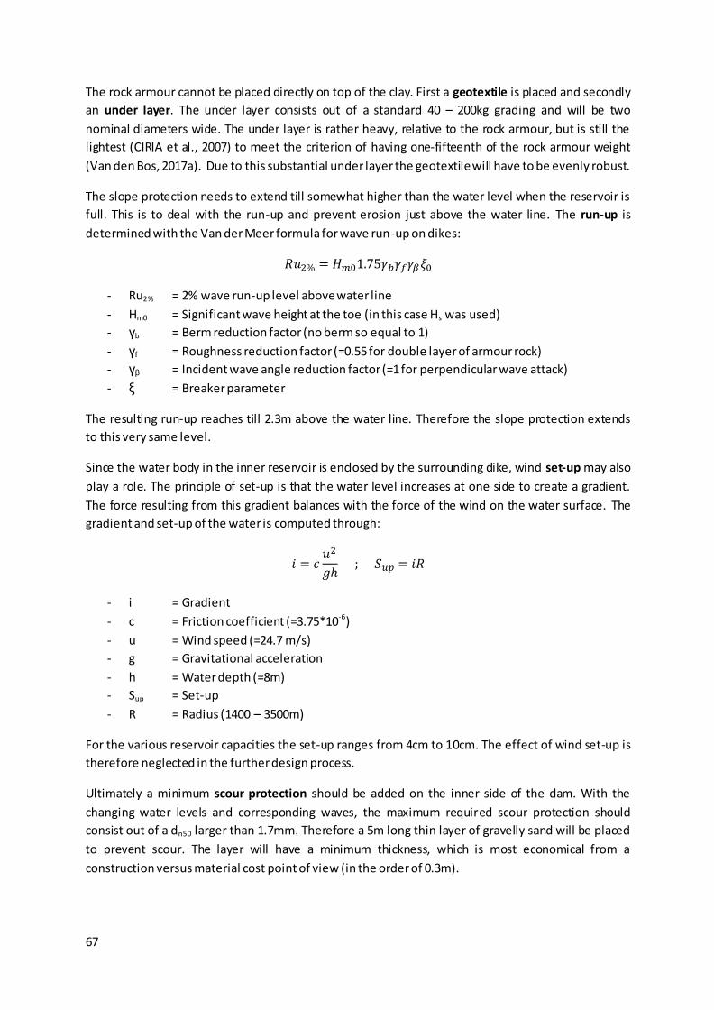
67
The rock armour cannot be placed directly on top of the clay. First a geotextile is placed and secondly
an under layer. The under layer consists out of a standard 40 – 200kg grading and will be two
nominal diameters wide. The under layer is rather heavy, relative to the rock armour, but is still the
lightest (CIRIA et al., 2007) to meet the criterion of having one-fifteenth of the rock armour weight
(Van den Bos, 2017a). Due to this substantial under layer the geotextile will have to be evenly robust.
The slope protection needs to extend till somewhat higher than the water level when the reservoir is
full. This is to deal with the run-up and prevent erosion just above the water line. The run-up is
determined with the Van der Meer formula for wave run-up on dikes:
𝑅𝑢2% = 𝐻𝑚01.75𝛾𝑏𝛾𝑓𝛾𝛽𝜉0
- Ru2% = 2% wave run-up level above water line
- Hm0 = Significant wave height at the toe (in this case Hs was used)
- γb = Berm reduction factor (no berm so equal to 1)
- γf = Roughness reduction factor (=0.55 for double layer of armour rock)
- γβ = Incident wave angle reduction factor (=1 for perpendicular wave attack)
- ξ = Breaker parameter
The resulting run-up reaches till 2.3m above the water line. Therefore the slope protection extends
to this very same level.
Since the water body in the inner reservoir is enclosed by the surrounding dike, wind set-up may also
play a role. The principle of set-up is that the water level increases at one side to create a gradient.
The force resulting from this gradient balances with the force of the wind on the water surface. The
gradient and set-up of the water is computed through:
𝑖 = 𝑐𝑢2
𝑔ℎ ; 𝑆𝑢𝑝 = 𝑖𝑅
- i = Gradient
- c = Friction coefficient (=3.75*10-6)
- u = Wind speed (=24.7 m/s)
- g = Gravitational acceleration
- h = Water depth (=8m)
- Sup = Set-up
- R = Radius (1400 – 3500m)
For the various reservoir capacities the set-up ranges from 4cm to 10cm. The effect of wind set-up is
therefore neglected in the further design process.
Ultimately a minimum scour protection should be added on the inner side of the dam. With the
changing water levels and corresponding waves, the maximum required scour protection should
consist out of a dn50 larger than 1.7mm. Therefore a 5m long thin layer of gravelly sand will be placed
to prevent scour. The layer will have a minimum thickness, which is most economical from a
construction versus material cost point of view (in the order of 0.3m).
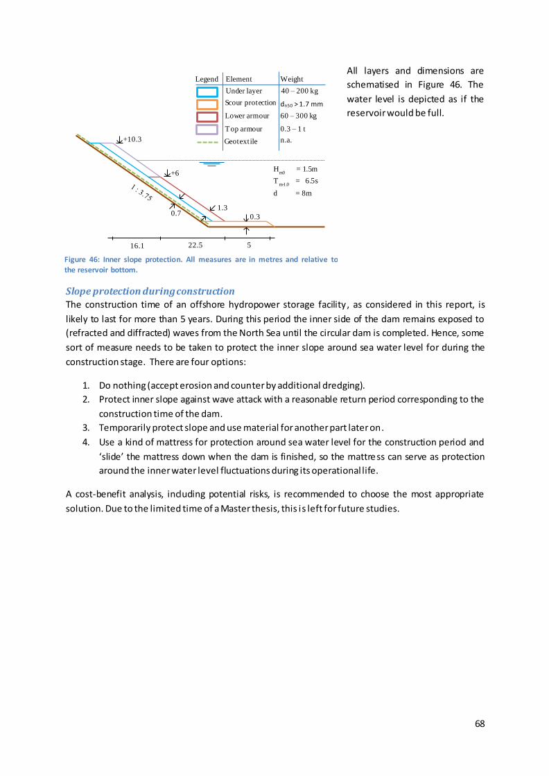
68
All layers and dimensions are
schematised in Figure 46. The
water level is depicted as if the
reservoir would be full.
Slope protection during construction
The construction time of an offshore hydropower storage facility, as considered in this report, is
likely to last for more than 5 years. During this period the inner side of the dam remains exposed to
(refracted and diffracted) waves from the North Sea until the circular dam is completed. Hence, some
sort of measure needs to be taken to protect the inner slope around sea water level for during the
construction stage. There are four options:
1. Do nothing (accept erosion and counter by additional dredging).
2. Protect inner slope against wave attack with a reasonable return period corresponding to the
construction time of the dam.
3. Temporarily protect slope and use material for another part later on.
4. Use a kind of mattress for protection around sea water level for the construction period and
‘slide’ the mattress down when the dam is finished, so the mattress can serve as protection
around the inner water level fluctuations during its operational life.
A cost-benefit analysis, including potential risks, is recommended to choose the most appropriate
solution. Due to the limited time of a Master thesis, this is left for future studies.
Hm0
= 1.5m
Tm-1.0
= 6.5s
d = 8m
+10.3
+6
1.3 0.7
0.3
Legend Element Weight
Scour protection
Lower armour
Top armour Geotextile
40 – 200 kg
dn50 > 1.7 mm
60 – 300 kg
0.3 – 1 t n.a.
Under layer
5 16.1 22.5
Figure 46: Inner slope protection. All measures are in metres and relative to
the reservoir bottom.
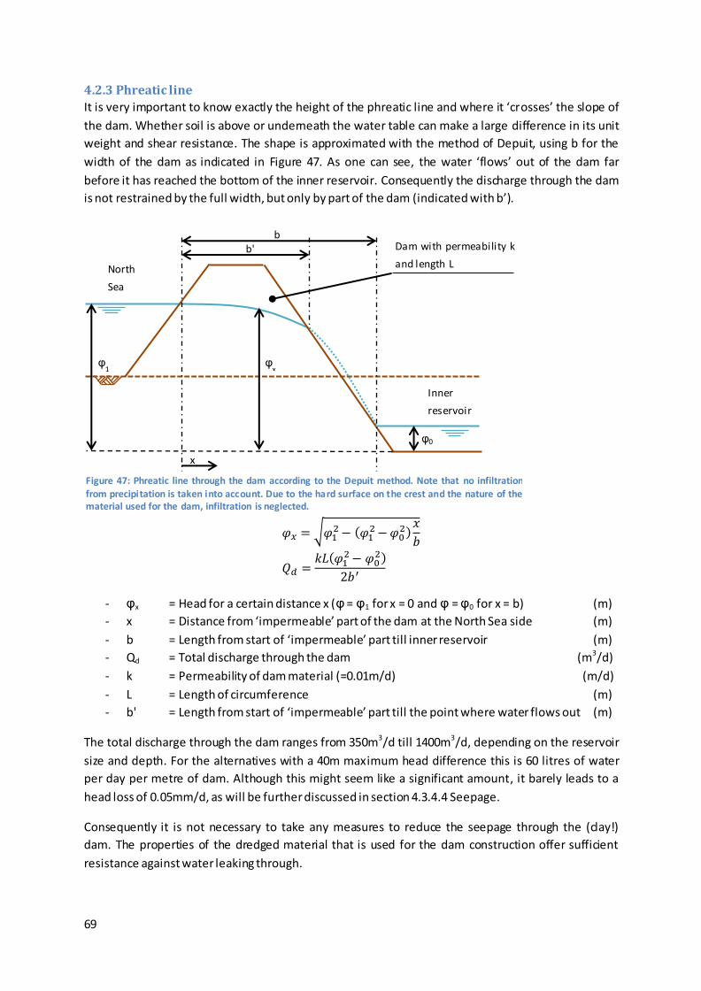
69
4.2.3 Phreatic line
It is very important to know exactly the height of the phreatic line and where it ‘crosses’ the slope of
the dam. Whether soil is above or underneath the water table can make a large difference in its unit
weight and shear resistance. The shape is approximated with the method of Depuit, using b for the
width of the dam as indicated in Figure 47. As one can see, the water ‘flows’ out of the dam far
before it has reached the bottom of the inner reservoir. Consequently the discharge through the dam
is not restrained by the full width, but only by part of the dam (indicated with b’).
𝜑𝑥 = √𝜑12− (𝜑1
2−𝜑02)𝑥
𝑏
𝑄𝑑 =𝑘𝐿(𝜑1
2− 𝜑02)
2𝑏′
- φx = Head for a certain distance x (φ = φ1 for x = 0 and φ = φ0 for x = b) (m)
- x = Distance from ‘impermeable’ part of the dam at the North Sea side (m)
- b = Length from start of ‘impermeable’ part till inner reservoir (m)
- Qd = Total discharge through the dam (m3/d)
- k = Permeability of dam material (=0.01m/d) (m/d)
- L = Length of circumference (m)
- b' = Length from start of ‘impermeable’ part till the point where water flows out (m)
The total discharge through the dam ranges from 350m3/d till 1400m3/d, depending on the reservoir
size and depth. For the alternatives with a 40m maximum head difference this is 60 litres of water
per day per metre of dam. Although this might seem like a significant amount, it barely leads to a
head loss of 0.05mm/d, as will be further discussed in section 4.3.4.4 Seepage.
Consequently it is not necessary to take any measures to reduce the seepage through the (clay!)
dam. The properties of the dredged material that is used for the dam construction offer sufficient
resistance against water leaking through.
b
φ1
φ0
φx
x
b' Dam with permeability k
and length L
Inner
reservoir
North
Sea
Figure 47: Phreatic line through the dam according to the Depuit method. Note that no infiltration from precipitation is taken into account. Due to the hard surface on the crest and the nature of the material used for the dam, infiltration is neglected.
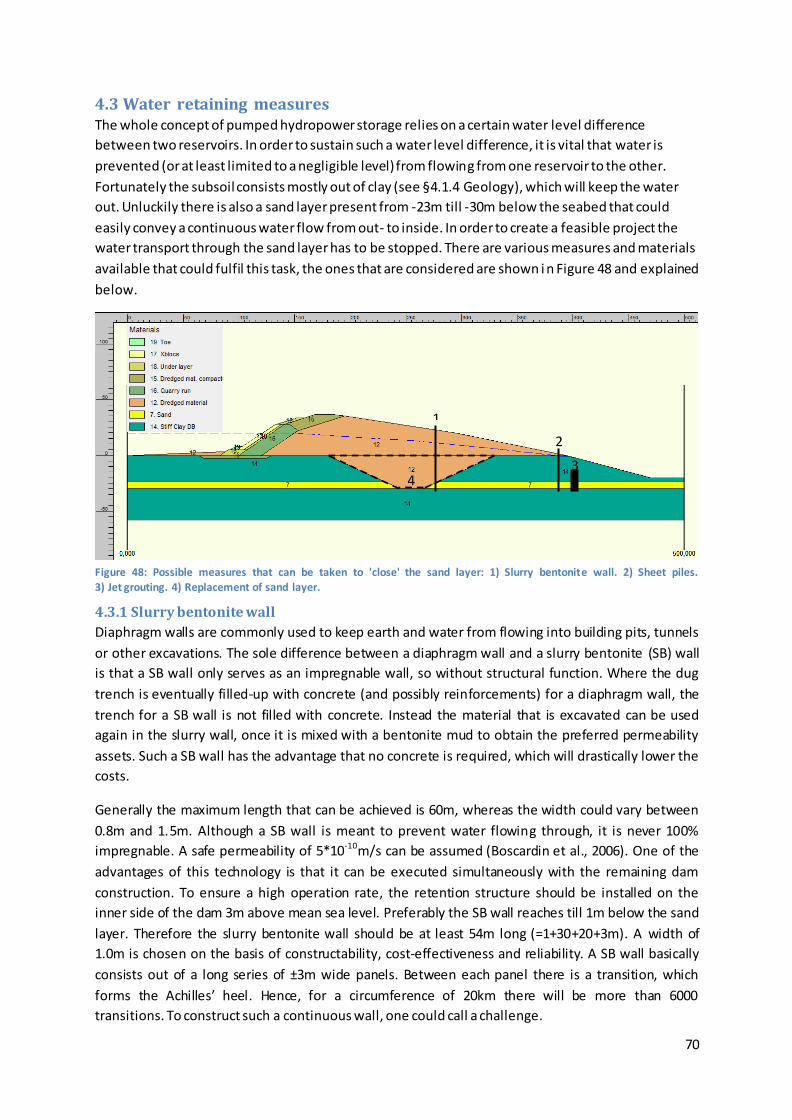
70
1
2
3 4
Figure 48: Possible measures that can be taken to 'close' the sand layer: 1) Slurry bentonite wall. 2) Sheet piles. 3) Jet grouting. 4) Replacement of sand layer.
4.3 Water retaining measures The whole concept of pumped hydropower storage relies on a certain water level difference
between two reservoirs. In order to sustain such a water level difference, it is vital that water is
prevented (or at least limited to a negligible level) from flowing from one reservoir to the other.
Fortunately the subsoil consists mostly out of clay (see §4.1.4 Geology), which will keep the water
out. Unluckily there is also a sand layer present from -23m till -30m below the seabed that could
easily convey a continuous water flow from out- to inside. In order to create a feasible project the
water transport through the sand layer has to be stopped. There are various measures and materials
available that could fulfil this task, the ones that are considered are shown i n Figure 48 and explained
below.
4.3.1 Slurry bentonite wall
Diaphragm walls are commonly used to keep earth and water from flowing into building pits, tunnels
or other excavations. The sole difference between a diaphragm wall and a slurry bentonite (SB) wall
is that a SB wall only serves as an impregnable wall, so without structural function. Where the dug
trench is eventually filled-up with concrete (and possibly reinforcements) for a diaphragm wall, the
trench for a SB wall is not filled with concrete. Instead the material that is excavated can be used
again in the slurry wall, once it is mixed with a bentonite mud to obtain the preferred permeability
assets. Such a SB wall has the advantage that no concrete is required, which will drastically lower the
costs.
Generally the maximum length that can be achieved is 60m, whereas the width could vary between
0.8m and 1.5m. Although a SB wall is meant to prevent water flowing through, it is never 100%
impregnable. A safe permeability of 5*10-10m/s can be assumed (Boscardin et al., 2006). One of the
advantages of this technology is that it can be executed simultaneously with the remaining dam
construction. To ensure a high operation rate, the retention structure should be installed on the
inner side of the dam 3m above mean sea level. Preferably the SB wall reaches till 1m below the sand
layer. Therefore the slurry bentonite wall should be at least 54m long (=1+30+20+3m). A width of
1.0m is chosen on the basis of constructability, cost-effectiveness and reliability. A SB wall basically
consists out of a long series of ±3m wide panels. Between each panel there is a transition, which
forms the Achilles’ heel. Hence, for a circumference of 20km there will be more than 6000
transitions. To construct such a continuous wall, one could call a challenge.
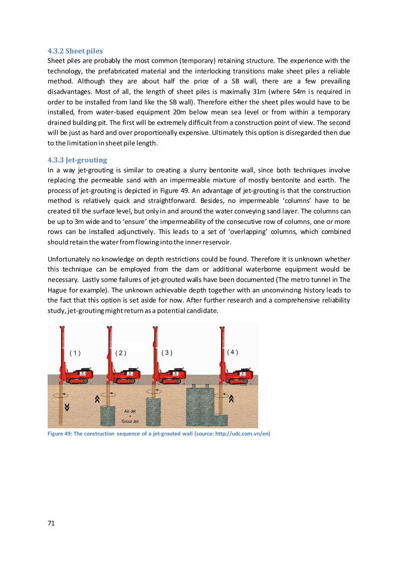
71
4.3.2 Sheet piles
Sheet piles are probably the most common (temporary) retaining structure. The experience with the
technology, the prefabricated material and the interlocking transitions make sheet piles a reliable
method. Although they are about half the price of a SB wall, there are a few prevailing
disadvantages. Most of all, the length of sheet piles is maximally 31m (where 54m i s required in
order to be installed from land like the SB wall). Therefore either the sheet piles would have to be
installed, from water-based equipment 20m below mean sea level or from within a temporary
drained building pit. The first will be extremely difficult from a construction point of view. The second
will be just as hard and over proportionally expensive. Ultimately this option is disregarded then due
to the limitation in sheet pile length.
4.3.3 Jet-grouting
In a way jet-grouting is similar to creating a slurry bentonite wall, since both techniques involve
replacing the permeable sand with an impermeable mixture of mostly bentonite and earth. The
process of jet-grouting is depicted in Figure 49. An advantage of jet-grouting is that the construction
method is relatively quick and straightforward. Besides, no impermeable ‘columns’ have to be
created till the surface level, but only in and around the water conveying sand layer. The columns can
be up to 3m wide and to ‘ensure’ the impermeability of the consecutive row of columns, one or more
rows can be installed adjunctively. This leads to a set of ‘overlapping’ columns, which combined
should retain the water from flowing into the inner reservoir.
Unfortunately no knowledge on depth restrictions could be found. Therefore it is unknown whether
this technique can be employed from the dam or additional waterborne equipment would be
necessary. Lastly some failures of jet-grouted walls have been documented (The metro tunnel in The
Hague for example). The unknown achievable depth together with an unconvincing history leads to
the fact that this option is set aside for now. After further research and a comprehensive reliability
study, jet-grouting might return as a potential candidate.
Figure 49: The construction sequence of a jet-grouted wall (source: http://udc.com.vn/en)
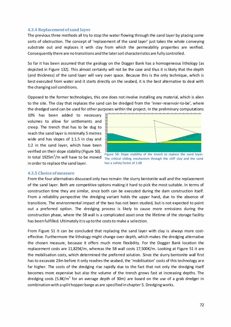
72
4.3.4 Replacement of sand layer
The previous three methods all try to stop the water flowing through the sand layer by placing some
sorts of obstruction. The concept of ‘replacement of the sand layer’ just takes the whole conveying
substrate out and replaces it with clay from which the permeability properties are verified.
Consequently there are no transitions and the later soil characteristics are fully controlled.
So far it has been assumed that the geology on the Dogger Bank has a homogeneous lithology (as
depicted in Figure 132). This almost certainly will not be the case and thus it is likely that the depth
(and thickness) of the sand layer will vary over space. Because this is the only technique, which is
best executed from water and it starts directly on the seabed, it is the best alternative to deal with
the changing soil conditions.
Opposed to the former technologies, this one does not involve installing any material, which is alien
to the site. The clay that replaces the sand can be dredged from the ‘inner-reservoir-to-be’, where
the dredged sand can be used for other purposes within the project. In the preliminary computations
10% has been added to necessary
volumes to allow for settlements and
creep. The trench that has to be dug to
reach the sand layer is minimally 5 metres
wide and has slopes of 1:1.5 in clay and
1:2 in the sand layer, which have been
verified on their slope stability (Figure 50).
In total 1925m3/m will have to be moved
in order to replace the sand layer.
4.3.5 Choice of measure
From the four alternatives discussed only two remain: the slurry bentonite wall and the replacement
of the sand layer. Both are competitive options making it hard to pick the most suitable. In terms of
construction time they are similar, since both can be executed during the dam construction itself.
From a reliability perspective the dredging variant holds the upper hand, due to the absence of
transitions. The environmental impact of the two has not been studied, but is not expected to point
out a preferred option. The dredging process is likely to cause more emissions during the
construction phase, where the SB wall is a complicated asset once the lifetime of the storage facility
has been fulfilled. Ultimately it is up to the costs to make a selection.
From Figure 51 it can be concluded that replacing the sand layer with clay is always more cost-
effective. Furthermore the lithology might change over depth, which makes the dredging alternative
the chosen measure, because it offers much more flexibility. For the Dogger Bank location the
replacement costs are 11,825€/m, whereas the SB wall costs 17,500€/m. Looking at Figure 51 it are
the mobilisation costs, which determined the preferred solution. Since the slurry bentonite wall first
has to excavate 23m before it only reaches the seabed, the ‘mobilisation’ costs of this technology are
far higher. The costs of the dredging rise rapidly due to the fact that not only the dredging itself
becomes more expensive but also the volume of the trench grows fast at increasing depths. The
dredging costs (5.8€/m3 for an average depth of 30m) are based on the use of a grab dredger in
combination with a split hopper barge as are specified in chapter 5. Dredging works.
Figure 50: Slope stability of the trench to replace the sand layer. The critical sliding mechanism through the stiff clay and the sand has a safety factor of 1.08
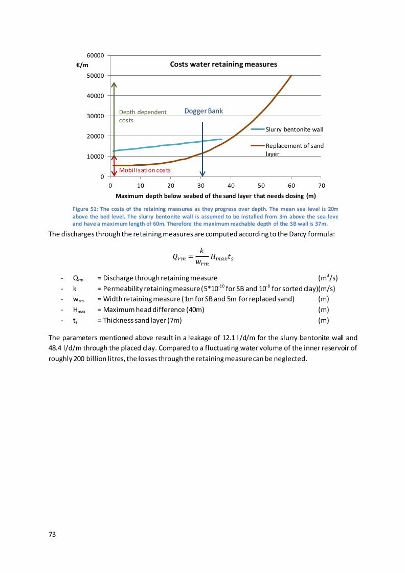
73
The discharges through the retaining measures are computed according to the Darcy formula:
𝑄𝑟𝑚 =𝑘
𝑤𝑟𝑚𝐻𝑚𝑎𝑥𝑡𝑠
- Qrm = Discharge through retaining measure (m3/s)
- k = Permeability retaining measure (5*10-10 for SB and 10-8 for sorted clay)(m/s)
- wrm = Width retaining measure (1m for SB and 5m for replaced sand) (m)
- Hmax = Maximum head difference (40m) (m)
- ts = Thickness sand layer (7m) (m)
The parameters mentioned above result in a leakage of 12.1 l /d/m for the slurry bentonite wall and
48.4 l/d/m through the placed clay. Compared to a fluctuating water volume of the inner reservoir of
roughly 200 billion litres, the losses through the retaining measure can be neglected.
Figure 51: The costs of the retaining measures as they progress over depth. The mean sea level is 20m above the bed level. The slurry bentonite wall is assumed to be installed from 3m above the sea level and have a maximum length of 60m. Therefore the maximum reachable depth of the SB wall is 37m.
0
10000
20000
30000
40000
50000
60000
0 10 20 30 40 50 60 70
€/m
Maximum depth below seabed of the sand layer that needs closing (m)
Costs water retaining measures
Slurry bentonite wall
Replacement of sandlayer
Mobilisation costs
Depth dependent costs
Dogger Bank
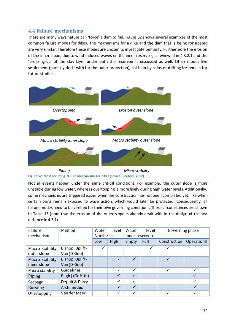
74
4.4 Failure mechanisms There are many ways nature can ‘force’ a dam to fail. Figure 52 shows several examples of the most
common failure modes for dikes. The mechanisms for a dike and the dam that is being considered
are very similar. Therefore these modes are chosen to investigate primarily. Furthermore the erosion
of the inner slope, due to wind-induced waves on the inner reservoir, is reviewed in 4.3.2.1 and the
‘breaking-up’ of the clay layer underneath the reservoir is discussed as well. Other modes like
settlement (partially dealt with for the outer protection), collision by ships or drifting ice remain for
future studies.
Not all events happen under the same critical conditions. For example, the outer slope is more
unstable during low water, whereas overtopping is more likely during high water levels. Additionally,
some mechanisms are triggered easier when the construction has not been completed yet, like when
certain parts remain exposed to wave action, which would later be protected. Consequently, all
failure modes need to be verified for their own governing conditions. These circumstances are shown
in Table 13 (note that the erosion of the outer slope is already dealt with in the design of the sea
defence in 4.3.1).
Failure mechanism
Method Water level North Sea
Water level inner reservoir
Governing phase
Low High Empty Full Construction Operational
Macro stability outer slope
Bishop, Uplift-Van (D-Geo)
Macro stability inner slope
Bishop, Uplift-Van (D-Geo)
Micro stability Guidelines
Piping Bligh (+Griffith)
Seepage Depuit & Darcy
Bursting Archimedes
Overtopping Van der Meer
Overtopping Erosion outer slope
Macro stability inner slope Macro stability outer slope
Micro stability Piping Figure 52: Most occurring failure mechanisms for dikes (source: Peeters, 2012)
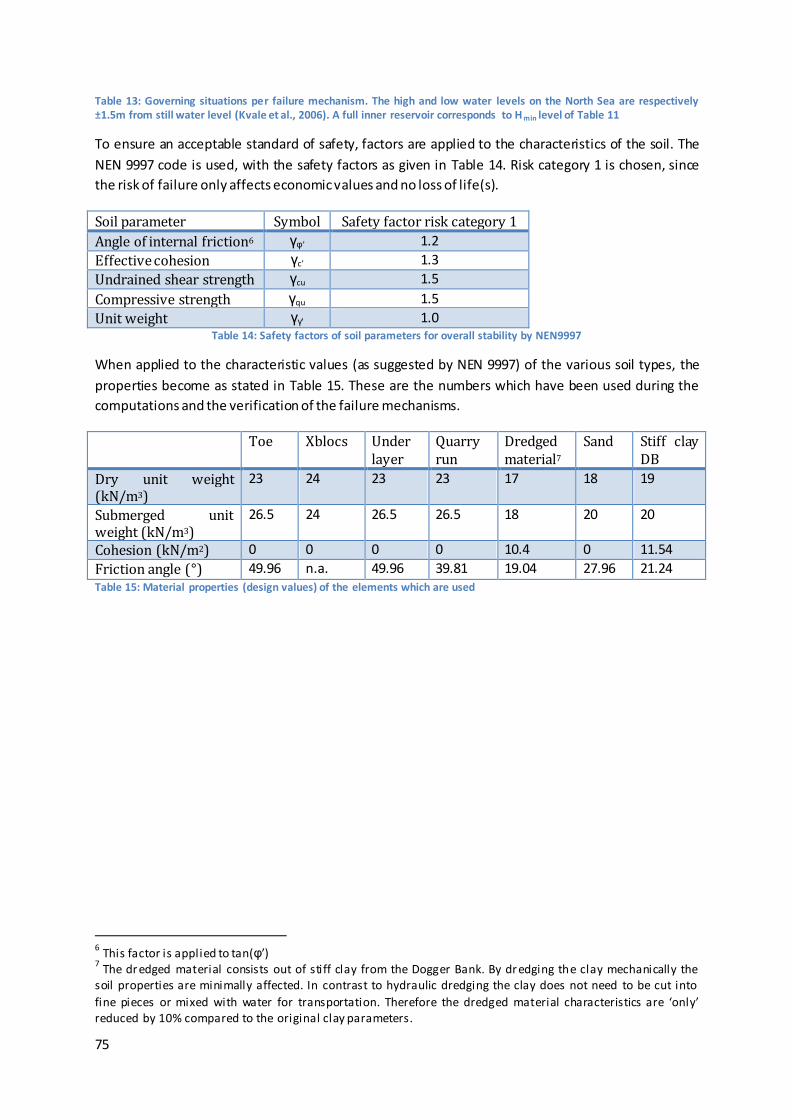
75
Table 13: Governing situations per failure mechanism. The high and low water levels on the North Sea are respectively ±1.5m from still water level (Kvale et al., 2006). A full inner reservoir corresponds to Hmin level of Table 11
To ensure an acceptable standard of safety, factors are applied to the characteristics of the soil. The
NEN 9997 code is used, with the safety factors as given in Table 14. Risk category 1 is chosen, since
the risk of failure only affects economic values and no loss of life(s).
Soil parameter Symbol Safety factor risk category 1
Angle of internal friction6 γφ’ 1.2
Effective cohesion γc’ 1.3
Undrained shear strength γcu 1.5
Compressive strength γqu 1.5
Unit weight γγ' 1.0 Table 14: Safety factors of soil parameters for overall stability by NEN9997
When applied to the characteristic values (as suggested by NEN 9997) of the various soil types, the
properties become as stated in Table 15. These are the numbers which have been used during the
computations and the verification of the failure mechanisms.
Toe Xblocs Under layer
Quarry run
Dredged material7
Sand Stiff clay DB
Dry unit weight (kN/m3)
23 24 23 23 17 18 19
Submerged unit weight (kN/m3)
26.5 24 26.5 26.5 18 20 20
Cohesion (kN/m2) 0 0 0 0 10.4 0 11.54
Friction angle (°) 49.96 n.a. 49.96 39.81 19.04 27.96 21.24 Table 15: Material properties (design values) of the elements which are used
6 This factor is applied to tan(φ’)
7 The dredged material consists out of stiff clay from the Dogger Bank. By dredging the clay mechanically the
soil properties are minimally affected. In contrast to hydraulic dredging the clay does not need to be cut into
fine pieces or mixed with water for transportation. Therefore the dredged material characteristics are ‘only’ reduced by 10% compared to the original clay parameters.
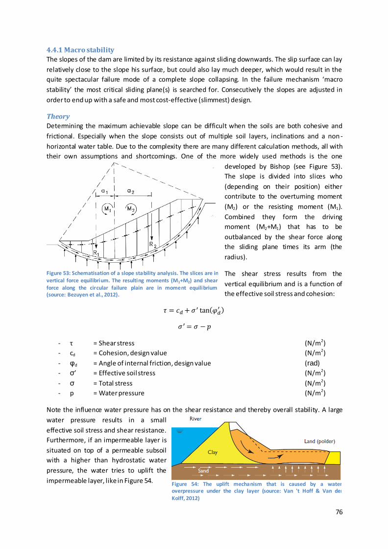
76
4.4.1 Macro stability
The slopes of the dam are limited by its resistance against sliding downwards. The slip surface can lay
relatively close to the slope his surface, but could also lay much deeper, which would result in the
quite spectacular failure mode of a complete slope collapsing. In the failure mechanism ‘macro
stability’ the most critical sliding plane(s) is searched for. Consecutively the slopes are adjusted in
order to end up with a safe and most cost-effective (slimmest) design.
Theory
Determining the maximum achievable slope can be difficult when the soils are both cohesive and
frictional. Especially when the slope consists out of multiple soil layers, inclinations and a non -
horizontal water table. Due to the complexity there are many different calculation methods, all with
their own assumptions and shortcomings. One of the more widely used methods is the one
developed by Bishop (see Figure 53).
The slope is divided into slices who
(depending on their position) either
contribute to the overturning moment
(M2) or the resisting moment (M1).
Combined they form the driving
moment (M2+M1) that has to be
outbalanced by the shear force along
the sliding plane times its arm (the
radius).
The shear stress results from the
vertical equilibrium and is a function of
the effective soil stress and cohesion:
𝜏 = 𝑐𝑑+𝜎′ tan(𝜑𝑑
′ )
𝜎 ′= 𝜎 −𝑝
- τ = Shear stress (N/m2)
- cd = Cohesion, design value (N/m2)
- φd = Angle of internal friction, design value (rad)
- σ’ = Effective soil stress (N/m2)
- σ = Total stress (N/m2)
- p = Water pressure (N/m2)
Note the influence water pressure has on the shear resistance and thereby overall stability. A large
water pressure results in a small
effective soil stress and shear resistance.
Furthermore, if an impermeable layer is
situated on top of a permeable subsoil
with a higher than hydrostatic water
pressure, the water tries to uplift the
impermeable layer, like in Figure 54.
Figure 53: Schematisation of a slope stability analysis. The slices are in vertical force equilibrium. The resulting moments (M1+M2) and shear force along the circular failure plain are in moment equilibrium (source: Bezuyen et al., 2012).
Figure 54: The uplift mechanism that is caused by a water overpressure under the clay layer (source: Van 't Hoff & Van der Kolff, 2012)
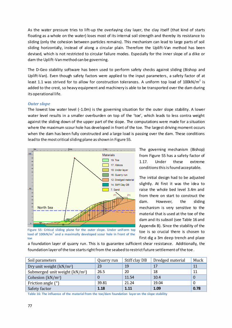
77
As the water pressure tries to lift-up the overlaying clay layer, the clay itself (that kind of starts
floating as a whole on the water) loses most of its internal soil strength and thereby its resistance to
sliding (only the cohesion between particles remains). This mechanism can lead to large parts of soil
sliding horizontally, instead of along a circular plain. Therefore the Uplift-Van method has been
devised, which is not restricted to circular failure modes. Especially for the inner slope of a dike or
dam the Uplift-Van method can be governing.
The D-Geo stability software has been used to perform safety checks against sliding (Bishop and
Uplift-Van). Even though safety factors were applied to the input parameters, a safety factor of at
least 1.1 was strived for to allow for construction tolerances. A uniform top load of 100kN/m2 is
added to the crest, so heavy equipment and machinery is able to be transported over the dam during
its operational life.
Outer slope
The lowest low water level (-1.0m) is the governing situation for the outer slope stability. A lower
water level results in a smaller overburden on top of the ‘toe’, which leads to less contra weight
against the sliding down of the upper part of the slope. The computations were made for a situation
where the maximum scour hole has developed in front of the toe. The largest driving moment occurs
when the dam has been fully constructed and a large load is passing over the dam. These conditions
lead to the most critical sliding plane as shown in Figure 55.
The governing mechanism (Bishop)
from Figure 55 has a safety factor of
1.17. Under these extreme
conditions this is found acceptable.
The initial design had to be adjusted
slightly. At first it was the idea to
raise the whole bed level 3.4m and
from there on start to construct the
dam. However, the sliding
mechanism is very sensitive to the
material that is used at the toe of the
dam and its subsoil (see Table 16 and
Appendix B). Since the stability of the
toe is so crucial there is chosen to
first dig a 3m deep trench and place
a foundation layer of quarry run. This is to guarantee sufficient shear resistance. Additionally, the
foundation layer of the toe starts right from the seabed to restrict future settlement of the toe .
Soil parameters Quarry run Stiff clay DB Dredged material Muck
Dry unit weight (kN/m3) 23 19 17 11
Submerged unit weight (kN/m3) 26.5 20 18 11
Cohesion (kN/m2) 0 11.54 10.4 0
Friction angle (°) 39.81 21.24 19.04 0
Safety factor 1.18 1.11 1.09 0.78 Table 16: The influence of the material from the toe/dam foundation layer on the slope stability
Figure 55: Critical sliding plane for the outer slope. Under uniform top load of 100kN/m2 and a maximally developed scour hole in front of the toe
North Sea
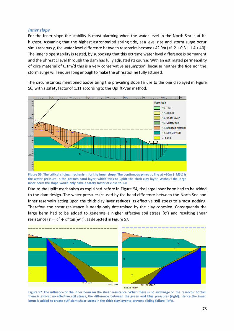
78
Figure 57: The influence of the inner berm on the shear resistance. When there is no surcharge on the reservoir bottom there is almost no effective soil stress, the difference between the green and blue pressures (right). Hence the inner berm is added to create sufficient shear stress in the thick clay layer to prevent sliding failure (left).
Inner slope
For the inner slope the stability is most alarming when the water level in the North Sea is at its
highest. Assuming that the highest astronomical spring tide, sea level rise and storm surge occur
simultaneously, the water level difference between reservoirs becomes 42.9m (=1.2 + 0.3 + 1.4 + 40).
The inner slope stability is tested, by supposing that this extreme water level difference is permanent
and the phreatic level through the dam has fully adjusted its course. With an estimated permeabili ty
of core material of 0.1m/d this is a very conservative assumption, because neither the tide nor the
storm surge will endure long enough to make the phreatic line fully attuned.
The circumstances mentioned above bring the prevailing slope failure to the one displayed in Figure
56, with a safety factor of 1.11 according to the Uplift-Van method.
Due to the uplift mechanism as explained before in Figure 54, the large inner berm had to be added
to the dam design. The water pressure (caused by the head difference between the North Sea and
inner reservoir) acting upon the thick clay layer reduces its effective soil stress to almost nothing.
Therefore the shear resistance is nearly only determined by the clay cohesion. Consequently the
large berm had to be added to generate a higher effective soil stress (σ’) and resulting shear
resistance (𝜏 = 𝑐′+ 𝜎 ′tan (𝜑′)), as depicted in Figure 57.
Figure 56: The critical sliding mechanism for the inner slope. The continuous phreatic line at +20m (=MSL) is
the water pressure in the bottom sand layer, which tries to uplift the thick clay layer. Without the large inner berm the slope would only have a safety factor of close to 1.0
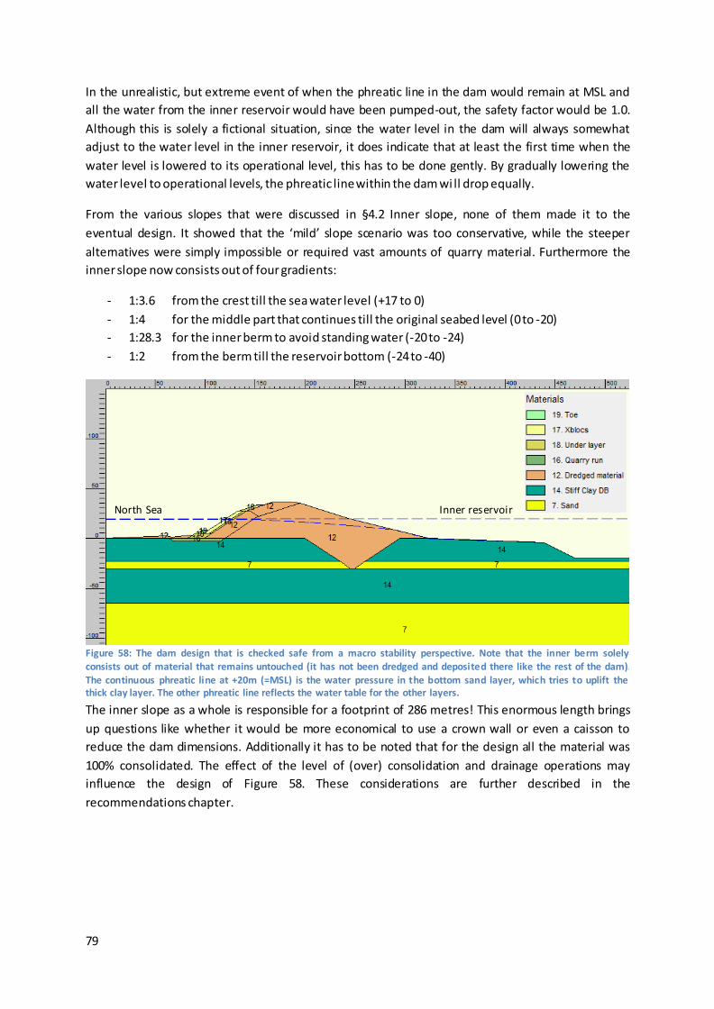
79
In the unrealistic, but extreme event of when the phreatic line in the dam would remain at MSL and
all the water from the inner reservoir would have been pumped-out, the safety factor would be 1.0.
Although this is solely a fictional situation, since the water level in the dam will always somewhat
adjust to the water level in the inner reservoir, it does indicate that at least the first time when the
water level is lowered to its operational level, this has to be done gently. By gradually lowering the
water level to operational levels, the phreatic line within the dam wi ll drop equally.
From the various slopes that were discussed in §4.2 Inner slope, none of them made it to the
eventual design. It showed that the ‘mild’ slope scenario was too conservative, while the steeper
alternatives were simply impossible or required vast amounts of quarry material. Furthermore the
inner slope now consists out of four gradients:
- 1:3.6 from the crest till the sea water level (+17 to 0)
- 1:4 for the middle part that continues till the original seabed level (0 to -20)
- 1:28.3 for the inner berm to avoid standing water (-20 to -24)
- 1:2 from the berm till the reservoir bottom (-24 to -40)
The inner slope as a whole is responsible for a footprint of 286 metres! This enormous length brings
up questions like whether it would be more economical to use a crown wall or even a caisson to
reduce the dam dimensions. Additionally it has to be noted that for the design all the material was
100% consolidated. The effect of the level of (over) consolidation and drainage operations may
influence the design of Figure 58. These considerations are further described in the
recommendations chapter.
Figure 58: The dam design that is checked safe from a macro stability perspective. Note that the inner berm solely consists out of material that remains untouched (it has not been dredged and deposited there like the rest of the dam). The continuous phreatic line at +20m (=MSL) is the water pressure in the bottom sand layer, which tries to uplift the thick clay layer. The other phreatic line reflects the water table for the other layers.
North Sea Inner reservoir
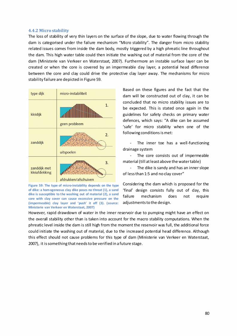
80
4.4.2 Micro stability
The loss of stability of very thin layers on the surface of the slope, due to water flowing through the
dam is categorised under the failure mechanism “Micro stability”. The danger from micro stability
related issues comes from inside the dam body, mostly triggered by a high phreatic line throughout
the dam. This high water table could then initiate the washing out of material from the core of the
dam (Ministerie van Verkeer en Waterstaat, 2007). Furthermore an instable surface layer can be
created or when the core is covered by an impermeable clay layer, a potential head difference
between the core and clay could drive the protective clay layer away. The mechanisms for micro
stability failure are depicted in Figure 59.
Based on these figures and the fact that the
dam will be constructed out of clay, it can be
concluded that no micro stability issues are to
be expected. This is stated once again in the
guidelines for safety checks on primary water
defences, which says: “A dike can be assumed
‘safe’ for micro stability when one of the
following conditions is met:
- The inner toe has a well-functioning
drainage system
- The core consists out of impermeable
material (till at least above the water table)
- The dike is sandy and has an inner slope
of less than 1:5 and no clay cover”
Considering the dam which is proposed for the
‘final’ design consists fully out of clay, this
failure mechanism does not require
adjustments to the design.
However, rapid drawdown of water in the inner reservoir due to pumping might have an effect on
the overall stability other than is taken into account for the macro stability computations. When the
phreatic level inside the dam is still high from the moment the reservoir was full, the additional force
could initiate the washing out of material, due to the increased potential head difference. Although
this effect should not cause problems for this type of dam (Ministerie van Verkeer en Waterstaat,
2007), it is something that needs to be verified in a future stage.
Figure 59: The type of micro-instability depends on the type of dike: a homogeneous clay dike poses no threat (1), a sand dike is susceptible to the washing out of material (2), a sand core with clay cover can cause excessive pressure on the
(impermeable) clay layer and ‘push’ it off (3). (source: Ministerie van Verkeer en Waterstaat, 2007)
1.
2.
3.
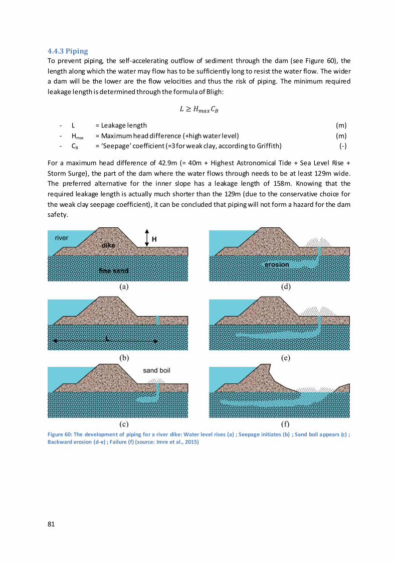
81
4.4.3 Piping
To prevent piping, the self-accelerating outflow of sediment through the dam (see Figure 60), the
length along which the water may flow has to be sufficiently long to resist the water flow. The wider
a dam will be the lower are the flow velocities and thus the risk of piping. The minimum required
leakage length is determined through the formula of Bligh:
𝐿 ≥ 𝐻𝑚𝑎𝑥𝐶𝐵
- L = Leakage length (m)
- Hmax = Maximum head difference (+high water level) (m)
- CB = ‘Seepage’ coefficient (=3 for weak clay, according to Griffith) (-)
For a maximum head difference of 42.9m (= 40m + Highest Astronomical Tide + Sea Level Rise +
Storm Surge), the part of the dam where the water flows through needs to be at least 129m wide.
The preferred alternative for the inner slope has a leakage length of 158m. Knowing that the
required leakage length is actually much shorter than the 129m (due to the conservative choice for
the weak clay seepage coefficient), it can be concluded that piping will not form a hazard for the dam
safety.
Figure 60: The development of piping for a river dike: Water level rises (a) ; Seepage initiates (b) ; Sand boil appears (c) ; Backward erosion (d-e) ; Failure (f) (source: Imre et al., 2015)
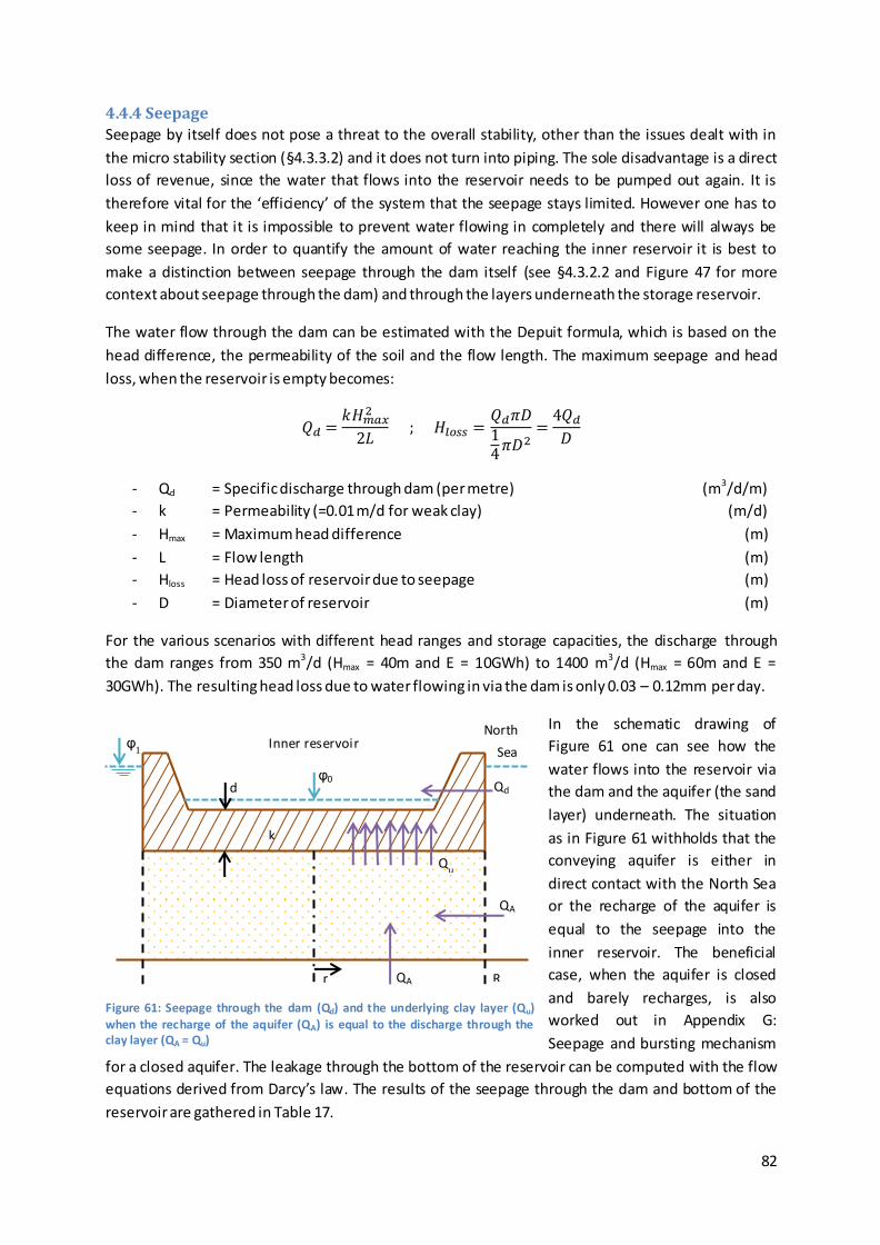
82
4.4.4 Seepage
Seepage by itself does not pose a threat to the overall stability, other than the issues dealt with in
the micro stability section (§4.3.3.2) and it does not turn into piping. The sole disadvantage is a direct
loss of revenue, since the water that flows into the reservoir needs to be pumped out again. It is
therefore vital for the ‘efficiency’ of the system that the seepage stays limited. However one has to
keep in mind that it is impossible to prevent water flowing in completely and there will always be
some seepage. In order to quantify the amount of water reaching the inner reservoir it is best to
make a distinction between seepage through the dam itself (see §4.3.2.2 and Figure 47 for more
context about seepage through the dam) and through the layers underneath the storage reservoir.
The water flow through the dam can be estimated with the Depuit formula, which is based on the
head difference, the permeability of the soil and the flow length. The maximum seepage and head
loss, when the reservoir is empty becomes:
𝑄𝑑 =𝑘𝐻𝑚𝑎𝑥
2
2𝐿 ; 𝐻𝑙𝑜𝑠𝑠 =
𝑄𝑑𝜋𝐷14𝜋𝐷2
=4𝑄𝑑𝐷
- Qd = Specific discharge through dam (per metre) (m3/d/m)
- k = Permeability (=0.01 m/d for weak clay) (m/d)
- Hmax = Maximum head difference (m)
- L = Flow length (m)
- Hloss = Head loss of reservoir due to seepage (m)
- D = Diameter of reservoir (m)
For the various scenarios with different head ranges and storage capacities, the discharge through
the dam ranges from 350 m3/d (Hmax = 40m and E = 10GWh) to 1400 m3/d (Hmax = 60m and E =
30GWh). The resulting head loss due to water flowing in via the dam is only 0.03 – 0.12mm per day.
In the schematic drawing of
Figure 61 one can see how the
water flows into the reservoir via
the dam and the aquifer (the sand
layer) underneath. The situation
as in Figure 61 withholds that the
conveying aquifer is either in
direct contact with the North Sea
or the recharge of the aquifer is
equal to the seepage into the
inner reservoir. The beneficial
case, when the aquifer is closed
and barely recharges, is also
worked out in Appendix G:
Seepage and bursting mechanism
for a closed aquifer. The leakage through the bottom of the reservoir can be computed with the flow
equations derived from Darcy’s law. The results of the seepage through the dam and bottom of the
reservoir are gathered in Table 17.
Figure 61: Seepage through the dam (Qd) and the underlying clay layer (Qu) when the recharge of the aquifer (QA) is equal to the discharge through the clay layer (QA = Qu)
Qd d φ0
φ1
Qu
R r
Inner reservoir North
Sea
k
QA
QA
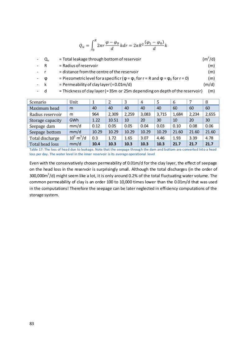
83
𝑄𝑢 = ∫ 2𝜋𝑟𝜑−𝜑0𝑑
𝑘𝑑𝑟𝑅
0= 2𝜋𝑅2
(𝜑1 − 𝜑0)
𝑑𝑘
- Qu = Total leakage through bottom of reservoir (m3/d)
- R = Radius of reservoir (m)
- r = distance from the centre of the reservoir (m)
- φ = Piezometric level for a specific r (φ = φ1 for r = R and φ = φ0 for r = 0) (m)
- k = Permeability of clay layer (= 0.01m/d) (m/d)
- d = Thickness of clay layer (= 35m or 25m depending on depth of the reservoir) (m)
Scenario Unit 1 2 3 4 5 6 7 8
Maximum head m 40 40 40 40 40 60 60 60
Radius reservoir m 964 2,309 2,259 3,083 3,715 1,684 2,234 2,655
Storage capacity GWh 1.22 10.51 10 20 30 10 20 30
Seepage dam mm/d 0.12 0.05 0.05 0.04 0.03 0.10 0.08 0.06
Seepage bottom mm/d 10.29 10.29 10.29 10.29 10.29 21.60 21.60 21.60
Total discharge 105 m3/d 0.3 1.72 1.65 3.07 4.46 1.93 3.39 4.78
Total head loss mm/d 10.4 10.3 10.3 10.3 10.3 21.7 21.7 21.7 Table 17: The loss of head due to leakage. Note that the seepage through the dam and bottom are converted into a head
loss per day. The water level in the inner reservoir is its average operational level
Even with the conservatively chosen permeability of 0.01m/d for the clay layer, the effect of seepage
on the head loss in the reservoir is surprisingly small. Although the total discharges (in the order of
300,000m3/d) might seem like a lot, it is only around 0.2% of the total fluctuating water volume. The
common permeability of clay is an order 100 to 10,000 times lower than the 0.01m/d that was used
in the computations! Therefore the seepage can be later neglected in efficiency computations of the
storage system.
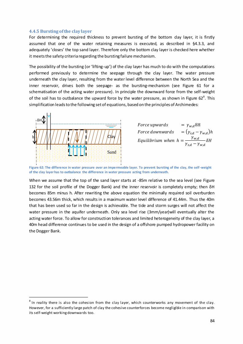
84
4.4.5 Bursting of the clay layer
For determining the required thickness to prevent bursting of the bottom clay layer, it is firstly
assumed that one of the water retaining measures is executed, as described in §4.3.3, and
adequately ‘closes’ the top sand layer. Therefore only the bottom clay layer is checked here whether
it meets the safety criteria regarding the bursting failure mechanism.
The possibility of the bursting (or ‘lifting-up’) of the clay layer has much to do with the computations
performed previously to determine the seepage through the clay layer. The water pressure
underneath the clay layer, resulting from the water level difference between the North Sea and the
inner reservoir, drives both the seepage- as the bursting-mechanism (see Figure 61 for a
schematisation of the acting water pressure). In principle the downward force from the self-weight
of the soil has to outbalance the upward force by the water pressure, as shown in Figure 628. This
simplification leads to the following set of equations, based on the principles of Archimedes:
𝐹𝑜𝑟𝑐𝑒 𝑢𝑝𝑤𝑎𝑟𝑑𝑠 = 𝛾𝑤,𝑑δH
𝐹𝑜𝑟𝑐𝑒 𝑑𝑜𝑤𝑛𝑤𝑎𝑟𝑑𝑠 = (𝛾𝑠,𝑑 −𝛾𝑤,𝑑)ℎ
𝐸𝑞𝑢𝑖𝑙𝑖𝑏𝑟𝑖𝑢𝑚 𝑤ℎ𝑒𝑛 ℎ =𝛾𝑤,𝑑
𝛾𝑠,𝑑 −𝛾𝑤,𝑑𝛿𝐻
When we assume that the top of the sand layer starts at -85m relative to the sea level (see Figure
132 for the soil profile of the Dogger Bank) and the inner reservoir is completely empty; then δH
becomes 85m minus h. After rewriting the above equation the minimally required soil overburden
becomes 43.56m thick, which results in a maximum water level difference of 41.44m. Thus the 40m
that has been used so far in the design is achievable. The tide and storm surges will not affect the
water pressure in the aquifer underneath. Only sea level rise (3mm/year)will eventually alter the
acting water force. To allow for construction tolerances and limited heterogeneity of the clay layer, a
40m head difference continues to be used in the design of a offshore pumped hydropower facility on
the Dogger Bank.
8 In reality there is also the cohesion from the clay layer, which counterworks any movement of the clay.
However, for a sufficiently large patch of clay the cohesive counterforces become negligible in comparison with its self-weight working downwards too.
δH
h Clay
Sand
Figure 62: The difference in water pressure over an impermeable layer. To prevent bursting of the clay, the self -weight of the clay layer has to outbalance the difference in water pressure acting from underneath.
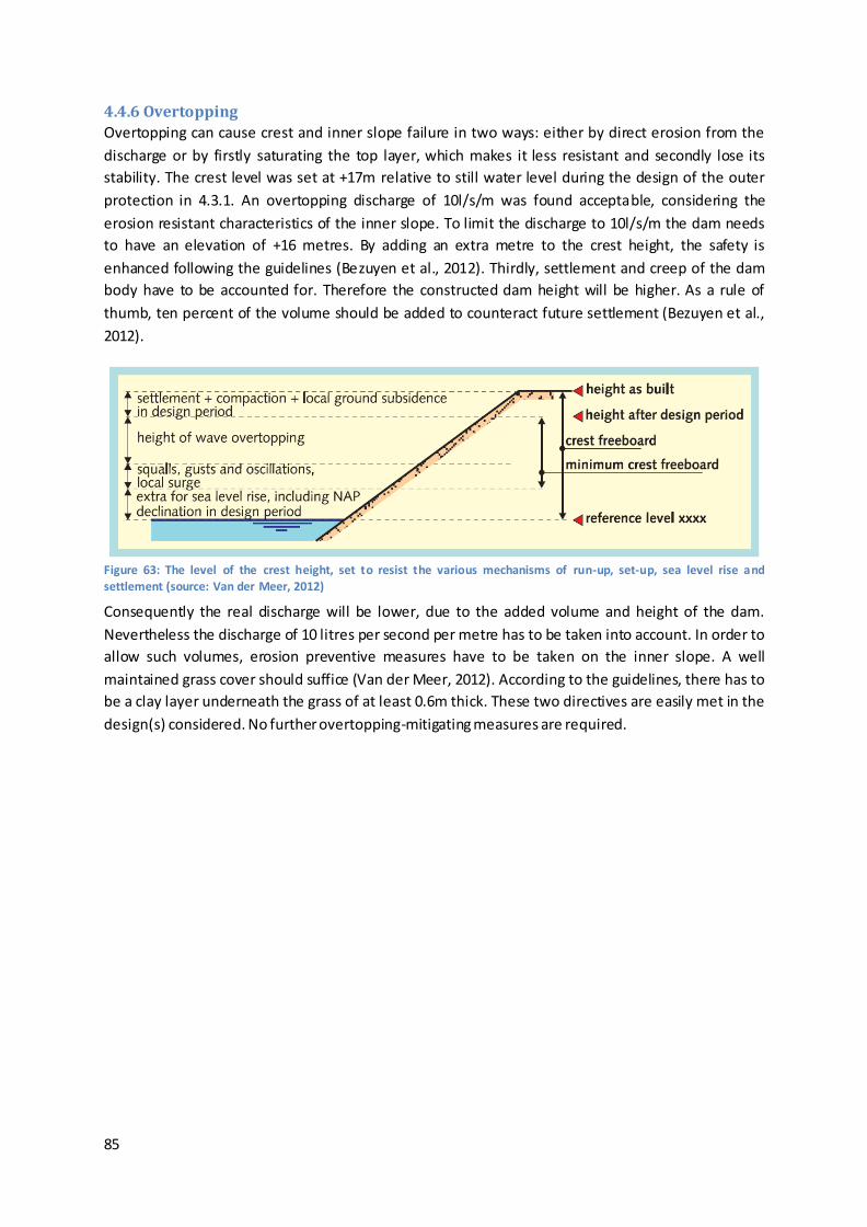
85
4.4.6 Overtopping
Overtopping can cause crest and inner slope failure in two ways: either by direct erosion from the
discharge or by firstly saturating the top layer, which makes it less resistant and secondly lose its
stability. The crest level was set at +17m relative to still water level during the design of the outer
protection in 4.3.1. An overtopping discharge of 10l/s/m was found acceptable, considering the
erosion resistant characteristics of the inner slope. To limit the discharge to 10l/s/m the dam needs
to have an elevation of +16 metres. By adding an extra metre to the crest height, the safety is
enhanced following the guidelines (Bezuyen et al., 2012). Thirdly, settlement and creep of the dam
body have to be accounted for. Therefore the constructed dam height will be higher. As a rule of
thumb, ten percent of the volume should be added to counteract future settlement (Bezuyen et al.,
2012).
Consequently the real discharge will be lower, due to the added volume and height of the dam.
Nevertheless the discharge of 10 litres per second per metre has to be taken into account. In order to
allow such volumes, erosion preventive measures have to be taken on the inner slope. A well
maintained grass cover should suffice (Van der Meer, 2012). According to the guidelines, there has to
be a clay layer underneath the grass of at least 0.6m thick. These two directives are easily met in the
design(s) considered. No further overtopping-mitigating measures are required.
Figure 63: The level of the crest height, set to resist the various mechanisms of run-up, set-up, sea level rise and settlement (source: Van der Meer, 2012)
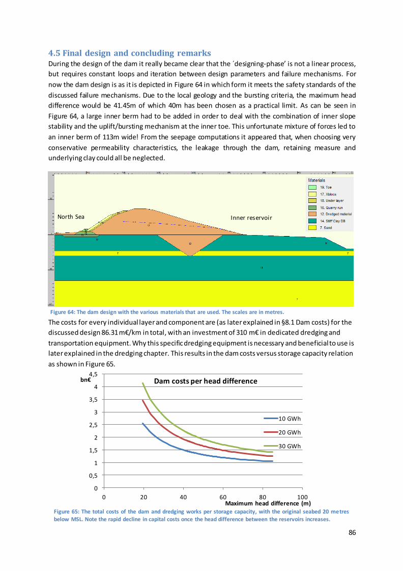
86
Figure 65: The total costs of the dam and dredging works per storage capacity, with the original seabed 20 metres below MSL. Note the rapid decline in capital costs once the head difference between the reservoirs increases.
0
0,5
1
1,5
2
2,5
3
3,5
4
4,5
0 20 40 60 80 100
bn€
Maximum head difference (m)
Dam costs per head difference
10 GWh
20 GWh
30 GWh
4.5 Final design and concluding remarks During the design of the dam it really became clear that the ´designing-phase’ is not a linear process,
but requires constant loops and iteration between design parameters and failure mechanisms. For
now the dam design is as it is depicted in Figure 64 in which form it meets the safety standards of the
discussed failure mechanisms. Due to the local geology and the bursting criteria, the maximum head
difference would be 41.45m of which 40m has been chosen as a practical limit. As can be seen in
Figure 64, a large inner berm had to be added in order to deal with the combination of inner slope
stability and the uplift/bursting mechanism at the inner toe. This unfortunate mixture of forces led to
an inner berm of 113m wide! From the seepage computations it appeared that, when choosing very
conservative permeability characteristics, the leakage through the dam, retaining measure and
underlying clay could all be neglected.
The costs for every individual layer and component are (as later explained in §8.1 Dam costs) for the
discussed design 86.31 m€/km in total, with an investment of 310 m€ in dedicated dredging and
transportation equipment. Why this specific dredging equipment is necessary and beneficial to use is
later explained in the dredging chapter. This results in the dam costs versus storage capacity relation
as shown in Figure 65.
Figure 64: The dam design with the various materials that are used. The scales are in metres.
North Sea Inner reservoir
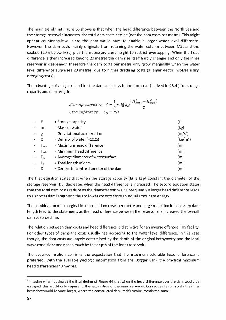
87
The main trend that Figure 65 shows is that when the head difference between the North Sea and
the storage reservoir increases, the total dam costs decline (not the dam costs per metre). This might
appear counterintuitive, since the dam would have to enable a larger water level difference.
However, the dam costs mainly originate from retaining the water column between MSL and the
seabed (20m below MSL) plus the necessary crest height to restrict overtopping. When the head
difference is then increased beyond 20 metres the dam size itself hardly changes and only the inner
reservoir is deepened.9 Therefore the dam costs per metre only grow marginally when the water
level difference surpasses 20 metres, due to higher dredging costs (a larger depth involves rising
dredging costs).
The advantage of a higher head for the dam costs lays in the formulae (derived in §3.4 ) for storage
capacity and dam length:
𝑆𝑡𝑜𝑟𝑎𝑔𝑒 𝑐𝑎𝑝𝑎𝑐𝑖𝑡𝑦: 𝐸 =1
4𝜋𝐷𝑤
2 𝜌𝑔(𝐻𝑚𝑎𝑥
2 −𝐻𝑚𝑖𝑛2 )
2
𝐶𝑖𝑟𝑐𝑢𝑚𝑓𝑒𝑟𝑒𝑛𝑐𝑒: 𝐿𝐷 = 𝜋𝐷
- E = Storage capacity (J)
- m = Mass of water (kg)
- g = Gravitational acceleration (m/s2)
- ρ = Density of water (=1025) (kg/m3)
- Hmax = Maximum head difference (m)
- Hmin = Minimum head difference (m)
- Dw = Average diameter of water surface (m)
- LD = Total length of dam (m)
- D = Centre-to-centre diameter of the dam (m)
The first equation states that when the storage capacity (E) is kept constant the diameter of the
storage reservoir (Dw) decreases when the head difference is increased. The second equation states
that the total dam costs reduce as the diameter shrinks. Subsequently a larger head difference leads
to a shorter dam length and thus to lower costs to store an equal amount of energy.
The combination of a marginal increase in dam costs per metre and large reduction in necessary dam
length lead to the statement: as the head difference between the reservoirs is increased the overall
dam costs decline.
The relation between dam costs and head difference is distinctive for an inverse offshore PHS facility.
For other types of dams the costs usually rise according to the water level difference. In this case
though, the dam costs are largely determined by the depth of the original bathymetry and the local
wave conditions and not so much by the depth of the inner reservoir.
The acquired relation confirms the expectation that the maximum tolerable head difference is
preferred. With the available geologic information from the Dogger Bank the practical maximum
head difference is 40 metres.
9 Imagine when looking at the final design of Figure 64 that when the head difference over the dam would be
enlarged, this would only require further excavation of the inner reservoir. Consequently it is solely the inner berm that would become larger, where the constructed dam itself remains mostly the same.
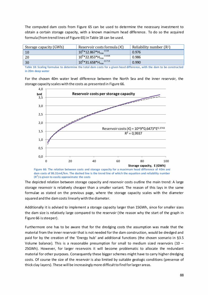
88
Reservoir costs (€) = 10^9*0,6473*E0,3743 R² = 0,9937
0,0
0,5
1,0
1,5
2,0
2,5
3,0
3,5
4,0
0 20 40 60 80 100
bn€
Storage capacity, E (GWh)
Reservoir costs per storage capacity
Figure 66: The relation between costs and storage capacity for a maximum head difference of 40m and dam costs of 86.31m€/km. The dashed line is the trend line of which the equation and reliability number (R2) is given to easily approximate the costs
The computed dam costs from Figure 65 can be used to determine the necessary investment to
obtain a certain storage capacity, with a known maximum head difference. To do so the acquired
formula (from trend lines of Figure 65) in Table 18 can be used.
Storage capacity (GWh) Reservoir costs formula (€) Reliability number (R2)
10 109*12.867*Hmax-0.58 0.976
20 109*22.853*Hmax-0.668 0.986
30 109*31.658*Hmax-0.713 0.990
Table 18: Scaling formulae to determine the total dam costs for a given head difference, with the dam to be constructed in 20m deep water
For the chosen 40m water level difference between the North Sea and the inner reservoir, the
storage capacity scales with the costs as presented in Figure 66.
The depicted relation between storage capacity and reservoir costs outline the main trend: A large
storage reservoir is relatively cheaper than a smaller variant. The reason of this lays in the same
formulae as stated on the previous page, where the storage capacity scales with the diameter
squared and the dam costs linearly with the diameter.
Additionally it is advised to implement a storage capacity larger than 15GWh, since for smaller sizes
the dam size is relatively large compared to the reservoir (the reason why the start of the graph in
Figure 66 is steeper).
Furthermore one has to be aware that for the dredging costs the assumption was made that the
material from the inner reservoir that is not needed for the dam construction, would be dredged and
paid for by the creation of the ‘Energy hub’ and additional functions (the chosen scenario in §3.5
Volume balance). This is a reasonable presumption for small to medium sized reservoirs (10 –
25GWh). However, for larger reservoirs it will become problematic to allocate the redundant
material for other purposes. Consequently these bigger schemes might have to carry higher dredging
costs. Of course the size of the reservoir is also limited by suitable geologic conditions (presence of
thick clay layers). These will be increasingly more difficult to find for larger areas.

89
From the dam design for an offshore pumped hydropower storage facility on the Dogger Bank three
main conclusions can be drawn:
1. Constructing a dam that can cope with the discussed failure mechanisms is possible.
2. As the head difference between the reservoirs is increased the overall (not per metre) dam
costs decline.
3. A large storage reservoir is more economical compared to a smaller one from a civil costs
perspective.
Now a preliminary design for the dam is made and the maximum achievable head difference is
known (40 metres), this provides the input for the necessary dredging works and the choice and
housing of turbines.
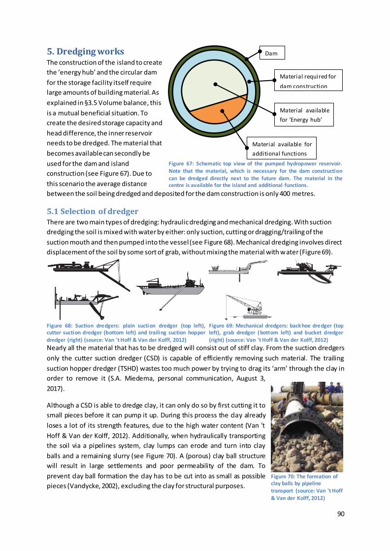
90
Figure 68: Suction dredgers: plain suction dredger (top left), cutter suction dredger (bottom left) and trailing suction hopper dredger (right) (source: Van 't Hoff & Van der Kolff, 2012)
Figure 69: Mechanical dredgers: backhoe dredger (top left), grab dredger (bottom left) and bucket dredger (right) (source: Van 't Hoff & Van der Kolff, 2012)
5. Dredging works The construction of the island to create
the ‘energy hub’ and the circular dam
for the storage facility itself require
large amounts of building material. As
explained in §3.5 Volume balance, this
is a mutual beneficial situation. To
create the desired storage capacity and
head difference, the inner reservoir
needs to be dredged. The material that
becomes available can secondly be
used for the dam and island
construction (see Figure 67). Due to
this scenario the average distance
between the soil being dredged and deposited for the dam construction is only 400 metres.
5.1 Selection of dredger There are two main types of dredging: hydraulic dredging and mechanical dredging. With suction
dredging the soil is mixed with water by either: only suction, cutting or dragging/trailing of the
suction mouth and then pumped into the vessel (see Figure 68). Mechanical dredging involves direct
displacement of the soil by some sort of grab, without mixing the material with water (Figure 69).
Nearly all the material that has to be dredged will consist out of stiff clay. From the suction dredgers
only the cutter suction dredger (CSD) is capable of efficiently removing such material. The trailing
suction hopper dredger (TSHD) wastes too much power by trying to drag its ‘arm’ through the clay in
order to remove it (S.A. Miedema, personal communication, August 3,
2017).
Although a CSD is able to dredge clay, it can only do so by first cutting it to
small pieces before it can pump it up. During this process the clay already
loses a lot of its strength features, due to the high water content (Van 't
Hoff & Van der Kolff, 2012). Additionally, when hydraulically transporting
the soil via a pipelines system, clay lumps can erode and turn into clay
balls and a remaining slurry (see Figure 70). A (porous) clay ball structure
will result in large settlements and poor permeability of the dam. To
prevent clay ball formation the clay has to be cut into as small as possible
pieces (Vandycke, 2002), excluding the clay for structural purposes.
Dam
Material required for
dam construction
Material available
for ‘Energy hub’
Material available for
additional functions
Figure 67: Schematic top view of the pumped hydropower reservoir.
Note that the material, which is necessary for the dam construction can be dredged directly next to the future dam. The material in the centre is available for the island and additional functions.
Figure 70: The formation of clay balls by pipeline transport (source: Van 't Hoff
& Van der Kolff, 2012)

91
Figure 72: A backhoe with a maximum dredging depth of 32m (left) (source: http://www.jandenul.com/en/ equipment/fleet/backhoe-dredger) and a split hopper barge (middle and right) (source: Van den Bos, 2017b; https://www.vanoord.com/activities/hopper-barge-and-pushbuster)
All three mechanical dredging technologies are suitable to dredge clay. However, the backhoe - and
bucket dredger are both limited to a maximum dredging depth of more or less 30m. A grab dredger
(GD) on the contrary can excavate till extremely large depths (>500m), since it is only limited by the
length of its wires.
The dredging depth of maximally 40 metres and the stiff clay that needs to be displaced (but remain
intact!), make the grab dredger the preferred technology. Additionally it will not have any problems
when it encounters large boulder that are left from the various glacial ages.
With a dedicated clamshell it will be possible to obtain a 100% filling ratio of the grab. A conventional
grab will have problems dredging the stiff glacial clay, because the grab does not penetrate into the
seabed deep enough and thus it will only ‘shave-off’ the top layer. Therefore the dedicated grabber
should be designed to do exactly this: ‘shaving-off’ the top layer, but still in large quantities (in the
order of 50m3 per grab). This can be done with a very wide grab, so it will have a large ‘footprint’/
‘distance between cutting-teeth’ on the seabed when it is about to start grabbing (S.A. Miedema,
personal communication, August 3, 2017).
5.2 Dredging operation One of the conventional methods of using a grab dredger would be that the grabber would be
installed on its own pontoon/vessel, like in Figure 71 and dump the dredged material directly in a
barge. The barge would then sail to the area where the dam needs to be constructed and unload.
Since the dumped material will be reshaped afterwards by a backhoe, it does not require precise
dumping (Figure 72). Therefore a split hopper barge (SHB) will be the quickest and most efficient
barge for this process (Van den Bos, 2017b).
Figure 71: The largest grab dredger in the World: Gosho (200m3) used for a terminal reclamation project in Singapore (2016). It uses a counterweight system to reduce the energy consumption and simplify the hoisting mechanism (source: http://www.kk-kojimagumi.co.jp/english/news/excepteur_sint_occaecat_cupidatat_non.html)

92
Although there is a lot of experience using the mentioned process and equipment of using a grab for
dredging, split hopper barges for transport and a backhoe dredger for reshaping the dam. They all
have in common that they cannot cope very well with offshore wave conditions. The three of them
are limited to wave heights around 1.0 – 1.5 metres (Van den Bos, 2017b; Van 't Hoff & Van der Kolff,
2012). Partly this can be mitigated by upscaling the equipment (the larger the vessel, the larger its
limiting wave height/length). However, aligning a split hopper barge for loading next to the grab
dredger with larger waves will be a precarious enterprise. The mean wave heights from Table 20
ranging from 1.3m to 1.7m for the various directions will significantly reduce the workability of the
conventional dredging process (obtained by Frölke (2017) from Argos data: 55°N 3°E measured over
Jan 1992 – Dec 2016).
To ensure a quick and reliable
construction period a solution has to
be found to the vigorous waves on the
North Sea. Both in the oil and gas as in
the offshore wind industry, jack-up
systems are often deployed to get rid
of restricting wave conditions. By
hauling the hull or pontoon out of the
water the surface area that is in
contact with the attacking waves is
limited to its (four) spuds (see Figure
73). Consequently jack-up systems can
deal with much stronger wave
conditions.
Yet, when a grab dredger would be
installed on a jack-up platform, the
grab would dig away the soil on which
its own spuds are standing! This makes
a combination of dredging and a jack-
up system impossible.
Figure 73: An offshore wind turbine installation vessel performing its jack-up tests (top) and a working platform (bottom) (source: http://www.ziton.eu/wp-content/uploads/WIND-SERVER-jacked-03-low-res.jpg; http://www.thinkdefence.co.uk/ship-to-shore-logistics/ increment-2-pier/)
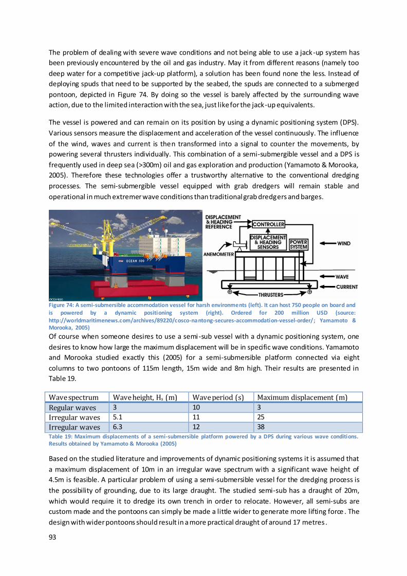
93
The problem of dealing with severe wave conditions and not being able to use a jack-up system has
been previously encountered by the oil and gas industry. May it from different reasons (namely too
deep water for a competitive jack-up platform), a solution has been found none the less. Instead of
deploying spuds that need to be supported by the seabed, the spuds are connected to a submerged
pontoon, depicted in Figure 74. By doing so the vessel is barely affected by the surrounding wave
action, due to the limited interaction with the sea, just like for the jack-up equivalents.
The vessel is powered and can remain on its position by using a dynamic positioning system (DPS).
Various sensors measure the displacement and acceleration of the vessel continuously. The influence
of the wind, waves and current is then transformed into a signal to counter the movements, by
powering several thrusters individually. This combination of a semi-submergible vessel and a DPS is
frequently used in deep sea (>300m) oil and gas exploration and production (Yamamoto & Morooka,
2005). Therefore these technologies offer a trustworthy alternative to the conventional dredging
processes. The semi-submergible vessel equipped with grab dredgers will remain stable and
operational in much extremer wave conditions than traditional grab dredgers and barges.
Of course when someone desires to use a semi-sub vessel with a dynamic positioning system, one
desires to know how large the maximum displacement will be in specific wave conditions. Yamamoto
and Morooka studied exactly this (2005) for a semi-submersible platform connected via eight
columns to two pontoons of 115m length, 15m wide and 8m high. Their results are presented in
Table 19.
Wave spectrum Wave height, Hs (m) Wave period (s) Maximum displacement (m)
Regular waves 3 10 3
Irregular waves 5.1 11 25
Irregular waves 6.3 12 38 Table 19: Maximum displacements of a semi-submersible platform powered by a DPS during various wave conditions. Results obtained by Yamamoto & Morooka (2005)
Based on the studied literature and improvements of dynamic positioning systems it is assumed that
a maximum displacement of 10m in an irregular wave spectrum with a significant wave height of
4.5m is feasible. A particular problem of using a semi-submersible vessel for the dredging process is
the possibility of grounding, due to its large draught. The studied semi-sub has a draught of 20m,
which would require it to dredge its own trench in order to relocate. However, all semi-subs are
custom made and the pontoons can simply be made a little wider to generate more lifting force . The
design with wider pontoons should result in a more practical draught of around 17 metres .
Figure 74: A semi-submersible accommodation vessel for harsh environments (left). It can host 750 people on board and is powered by a dynamic positioning system (right). Ordered for 200 million USD (source: http://worldmaritimenews.com/archives/89220/cosco-nantong-secures-accommodation-vessel-order/; Yamamoto & Morooka, 2005)
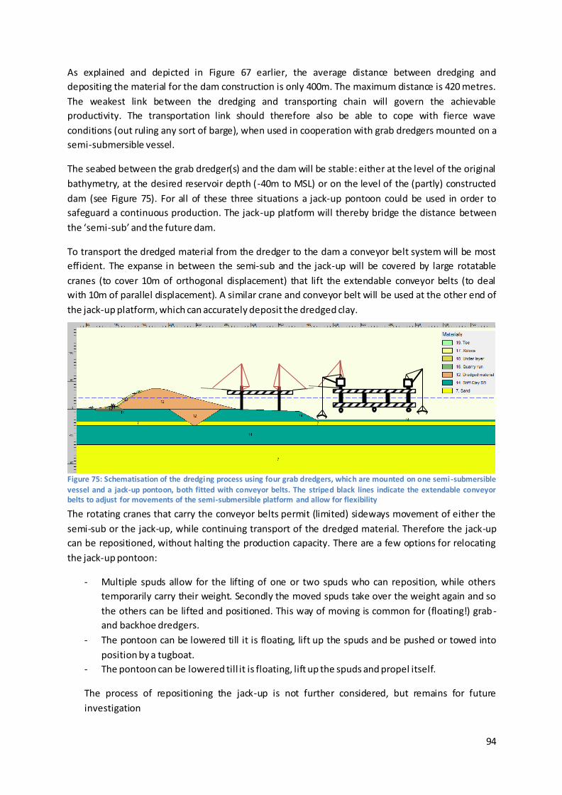
94
As explained and depicted in Figure 67 earlier, the average distance between dredging and
depositing the material for the dam construction is only 400m. The maximum distance is 420 metres.
The weakest link between the dredging and transporting chain will govern the achievable
productivity. The transportation link should therefore also be able to cope with fierce wave
conditions (out ruling any sort of barge), when used in cooperation with grab dredgers mounted on a
semi-submersible vessel.
The seabed between the grab dredger(s) and the dam will be stable: either at the level of the original
bathymetry, at the desired reservoir depth (-40m to MSL) or on the level of the (partly) constructed
dam (see Figure 75). For all of these three situations a jack-up pontoon could be used in order to
safeguard a continuous production. The jack-up platform will thereby bridge the distance between
the ‘semi-sub’ and the future dam.
To transport the dredged material from the dredger to the dam a conveyor belt system will be most
efficient. The expanse in between the semi-sub and the jack-up will be covered by large rotatable
cranes (to cover 10m of orthogonal displacement) that lift the extendable conveyor belts (to deal
with 10m of parallel displacement). A similar crane and conveyor belt will be used at the other end of
the jack-up platform, which can accurately deposit the dredged clay.
The rotating cranes that carry the conveyor belts permit (limited) sideways movement of either the
semi-sub or the jack-up, while continuing transport of the dredged material. Therefore the jack-up
can be repositioned, without halting the production capacity. There are a few options for relocating
the jack-up pontoon:
- Multiple spuds allow for the lifting of one or two spuds who can reposition, while others
temporarily carry their weight. Secondly the moved spuds take over the weight again and so
the others can be lifted and positioned. This way of moving is common for (floating!) grab-
and backhoe dredgers.
- The pontoon can be lowered till it is floating, lift up the spuds and be pushed or towed into
position by a tugboat.
- The pontoon can be lowered till it is floating, lift up the spuds and propel itself.
The process of repositioning the jack-up is not further considered, but remains for future
investigation
Figure 75: Schematisation of the dredging process using four grab dredgers, which are mounted on one semi-submersible
vessel and a jack-up pontoon, both fitted with conveyor belts. The striped black lines indicate the extendable conveyor belts to adjust for movements of the semi-submersible platform and allow for flexibility
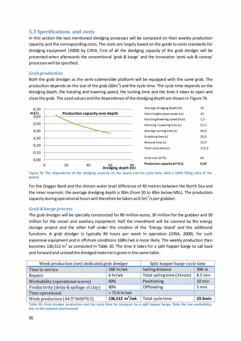
95
5.3 Specifications and costs In this section the two mentioned dredging processes will be compared on their weekly production
capacity and the corresponding costs. The costs are largely based on the guide to costs standards for
dredging equipment (2009) by CIRIA. First of all the dredging capacity of the grab dredger will be
presented when afterwards the conventional ‘grab & barge’ and the innovative ‘semi -sub & convey’
processes will be specified.
Grab production
Both the grab dredger as the semi-submersible platform will be equipped with the same grab. The
production depends on the size of the grab (60m3) and the cycle time. The cycle time depends on the
dredging depth, the hoisting and lowering speed, the turning time and the time it takes to open and
close the grab. The used values and the dependence of the dredging depth are shown in Figure 76.
Average dredging depth (m) 30
Hoist height above water (m) 10
Hoisting/lowering speed (m/s) 1,5
Hoisting + lowering time (s) 53,3
Average turning time (s) 40,0
Grabbing time (s) 20,0
Release time (s) 10,0
Total cycle time (s) 123,3
Grab size (m^3) 60
Production capacity (m^3/s) 0,49
Figure 76: The dependence of the dredging capacity on the depth and the cycle time, with a 100% filling ratio of the bucket
For the Dogger Bank and the chosen water level difference of 40 metres between the North Sea and
the inner reservoir, the average dredging depth is 30m (from 20 to 40m below MSL). The production
capacity during operational hours will therefore be taken as 0.5m3/s per grabber.
Grab & barge process
The grab dredger will be specially constructed for 80 million euros, 30 million for the grabber and 50
million for the vessel and auxiliary equipment. Half the investment will be covered by the energy
storage project and the other half under the creation of the ‘Energy Island’ and the additional
functions. A grab dredger is typically 84 hours per week in operation (CIRIA, 2009), for such
expensive equipment and in offshore conditions 168hr/wk is more likely. The weekly production then
becomes 136,512 m3 as computed in Table 20. The time it takes for a split hopper barge to sail back
and forward and unload the dredged material is given in the same table.
Week production (net) dedicated grab dredger Split hopper barge cycle time
Time in service 168 hr/wk Sailing distance 396 m
Repairs 6 hr/wk Total sailing time (3 knots) 8.5 min
Workability (operational waves) 60% Positioning 10 min
Productivity (delay & spillage of clay) 80% Offloading 5 min
Time operational = 75.8 hr/wk
Week production (44.5*3600*0.5) 136,512 m3/wk Total cycle time 23.5min Table 20: Grab dredger production and the cycle time for transport by a split hopper barge. Note the low workability, due to the exposed environment
0,00
0,10
0,20
0,30
0,40
0,50
0,60
0,70
0 20 40 60 80
m3/s
Dredging depth (m)
Production capacity over depth

96
According to Table 20 it takes the split hopper barge 23.5 min to complete its offloading cycle. To
allow for some minor discrepancies 25 minutes is used. In the same timespan the grab dredger is
capable of dredging 750m3 (=25*60*0.5). However, the original bathymetry is only 20m deep, which
results in the higher production capacity of 825m3 (as explained by Figure 76). To get rid of waiting
times between the grab dredger(s) and split hopper barge(s), two small SHBs can be combined with
one grab dredger or two medium sized SHBs with two grab dredgers. For the latter option the barge
needs to have a minimum capacity of 1650m3. Therefore split hopper barges of 2000m3 (a little
bigger to have some extra flexibility in the process) will be employed to take care of the transport of
the dredged material. This is common equipment and can simply be hired.
Furthermore a backhoe dredger is required to reshape the dam below water and a normal land-
based excavator to do the same above water level. As soon as the dam approaches the sea level,
construction will have to continue from land. Barges will sail to the dam, where they will be unloaded
and transport will continue via dump trucks. For a more detailed construction process of the dam,
see §Appendix H: . The project costs of the most advantageous arrangement of operating four grab
dredgers and four split hopper barges are given in Table 21.
Element OPEX (€/wk) CAPEX (€)
Grab dredger (60m3) (dredging) 4*350,000 4*0.5*80,000,000
Split hopper barge (2000m3) (transport) 4*100,000 -
Backhoe dredger (profiling) 250,000 -
Excavator (profiling) 10,000 -
Total 2,060,000 160,000,000 Table 21: Costs of 'grab & barge' process. The OPEX include depreciation, interest, maintenance, repairs, fuel, personnel and all other operating costs. The other half of the investments costs of the grab dredgers are carried by the ‘energy hub’
project.
The costs as in Table 21 are chosen on the conservative side. Especially for the grab dredger the costs
may be lower than indicated, since a large part of the OPEX is the depreciation of the equipment.
Thereby the depreciation is already discounted in the capital expenditure unde r the assumption that
the complete costs of the grab dredger will be covered by the dam and island construction, instead
of over its service life (CIRIA, 2009).
With the weekly production of a grab dredger and all corresponding costs known the unit price
becomes as presented in Table 22.
Week production (net) 546,048 m3/wk
Dam construction speed 103.6 m/wk
Operational costs 2,060,000 €/wk
Capital costs 160,000,000 €
Operational unit price 3.77 €/m3
‘Constructed’ unit price (*1.5) 5.66 €/m3
Unit price including capital costs (for 20GWh) 8.00 €/m3 Table 22: Unit price for grab & barge process. The 'constructed' unit price includes all project related costs like site investigation, monitoring, design, profit, uncertainty and risk. This in combination with the capital costs can be used to
determine the overall dredging costs. The bottom unit price is an example of where the CAPEX is already included for a 20GWh storage system with a 40m head difference
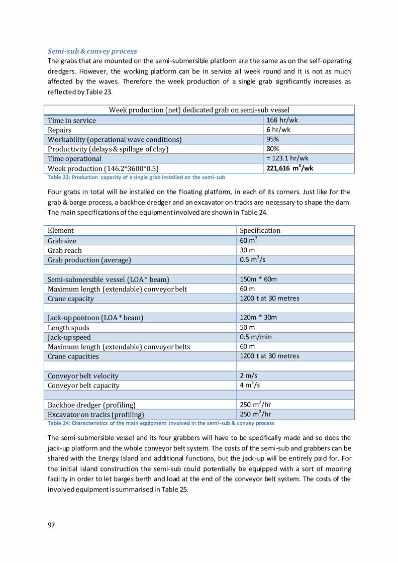
97
Semi-sub & convey process
The grabs that are mounted on the semi-submersible platform are the same as on the self-operating
dredgers. However, the working platform can be in service all week round and it is not as much
affected by the waves. Therefore the week production of a single grab significantly increases as
reflected by Table 23.
Week production (net) dedicated grab on semi-sub vessel
Time in service 168 hr/wk
Repairs 6 hr/wk
Workability (operational wave conditions) 95%
Productivity (delays & spillage of clay) 80%
Time operational = 123.1 hr/wk
Week production (146.2*3600*0.5) 221,616 m3/wk Table 23: Production capacity of a single grab installed on the semi-sub
Four grabs in total will be installed on the floating platform, in each of its corners. Just like for the
grab & barge process, a backhoe dredger and an excavator on tracks are necessary to shape the dam.
The main specifications of the equipment involved are shown in Table 24.
Element Specification
Grab size 60 m3
Grab reach 30 m
Grab production (average) 0.5 m3/s
Semi-submersible vessel (LOA * beam) 150m * 60m
Maximum length (extendable) conveyor belt 60 m
Crane capacity 1200 t at 30 metres
Jack-up pontoon (LOA * beam) 120m * 30m
Length spuds 50 m
Jack-up speed 0.5 m/min
Maximum length (extendable) conveyor belts 60 m
Crane capacities 1200 t at 30 metres
Conveyor belt velocity 2 m/s
Conveyor belt capacity 4 m3/s
Backhoe dredger (profiling) 250 m2/hr
Excavator on tracks (profiling) 250 m2/hr Table 24: Characteristics of the main equipment involved in the semi-sub & convey process
The semi-submersible vessel and its four grabbers will have to be specifically made and so does the
jack-up platform and the whole conveyor belt system. The costs of the semi-sub and grabbers can be
shared with the Energy Island and additional functions, but the jack-up will be entirely paid for. For
the initial island construction the semi-sub could potentially be equipped with a sort of mooring
facility in order to let barges berth and load at the end of the conveyor belt system. The costs of the
involved equipment is summarised in Table 25.
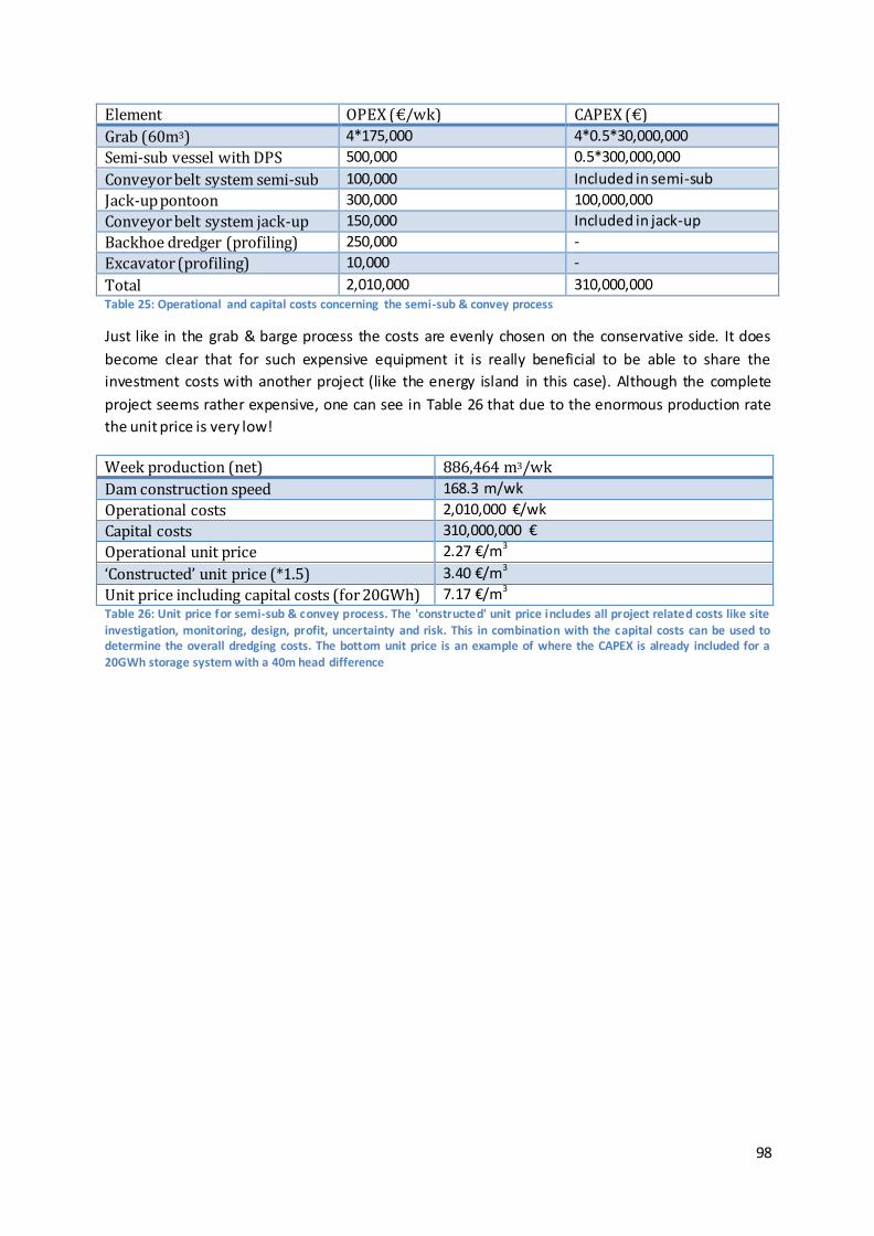
98
Element OPEX (€/wk) CAPEX (€)
Grab (60m3) 4*175,000 4*0.5*30,000,000
Semi-sub vessel with DPS 500,000 0.5*300,000,000
Conveyor belt system semi-sub 100,000 Included in semi-sub
Jack-up pontoon 300,000 100,000,000
Conveyor belt system jack-up 150,000 Included in jack-up
Backhoe dredger (profiling) 250,000 -
Excavator (profiling) 10,000 -
Total 2,010,000 310,000,000 Table 25: Operational and capital costs concerning the semi-sub & convey process
Just like in the grab & barge process the costs are evenly chosen on the conservative side. It does
become clear that for such expensive equipment it is really beneficial to be able to share the
investment costs with another project (like the energy island in this case). Although the complete
project seems rather expensive, one can see in Table 26 that due to the enormous production rate
the unit price is very low!
Week production (net) 886,464 m3/wk
Dam construction speed 168.3 m/wk
Operational costs 2,010,000 €/wk
Capital costs 310,000,000 €
Operational unit price 2.27 €/m3
‘Constructed’ unit price (*1.5) 3.40 €/m3
Unit price including capital costs (for 20GWh) 7.17 €/m3 Table 26: Unit price for semi-sub & convey process. The 'constructed' unit price includes all project related costs like site
investigation, monitoring, design, profit, uncertainty and risk. This in combination with the capital costs can be used to determine the overall dredging costs. The bottom unit price is an example of where the CAPEX is already included for a 20GWh storage system with a 40m head difference
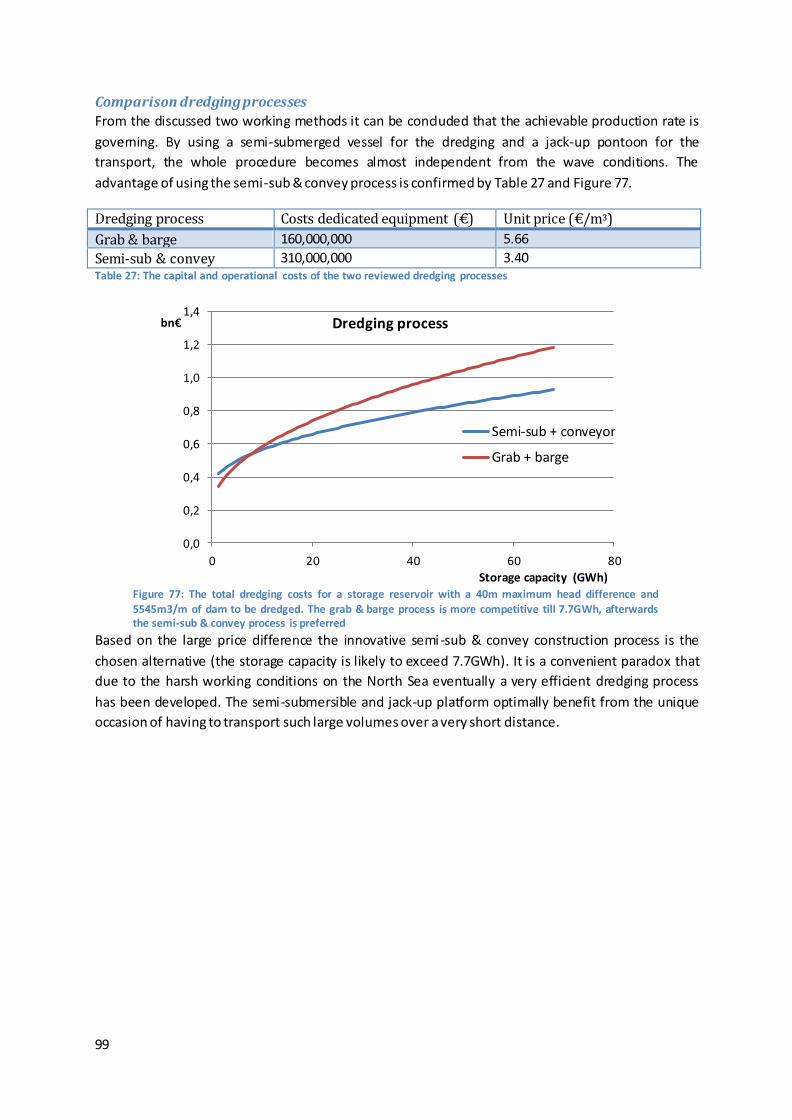
99
Comparison dredging processes
From the discussed two working methods it can be concluded that the achievable production rate is
governing. By using a semi-submerged vessel for the dredging and a jack-up pontoon for the
transport, the whole procedure becomes almost independent from the wave conditions. The
advantage of using the semi-sub & convey process is confirmed by Table 27 and Figure 77.
Dredging process Costs dedicated equipment (€) Unit price (€/m3)
Grab & barge 160,000,000 5.66
Semi-sub & convey 310,000,000 3.40 Table 27: The capital and operational costs of the two reviewed dredging processes
Based on the large price difference the innovative semi-sub & convey construction process is the
chosen alternative (the storage capacity is likely to exceed 7.7GWh). It is a convenient paradox that
due to the harsh working conditions on the North Sea eventually a very efficient dredging process
has been developed. The semi-submersible and jack-up platform optimally benefit from the unique
occasion of having to transport such large volumes over a very short distance.
Figure 77: The total dredging costs for a storage reservoir with a 40m maximum head difference and 5545m3/m of dam to be dredged. The grab & barge process is more competitive till 7.7GWh, afterwards the semi-sub & convey process is preferred
0,0
0,2
0,4
0,6
0,8
1,0
1,2
1,4
0 20 40 60 80
bn€
Storage capacity (GWh)
Dredging process
Semi-sub + conveyor
Grab + barge
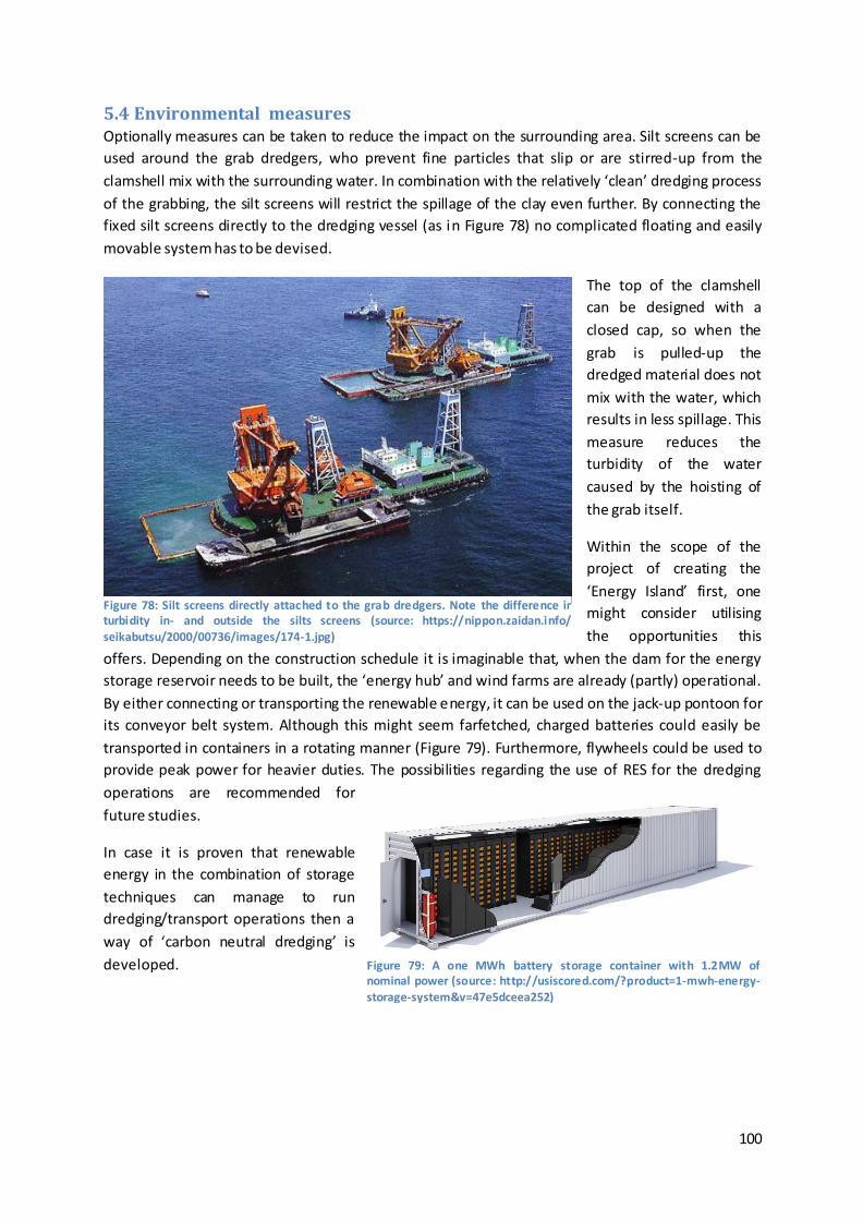
100
5.4 Environmental measures Optionally measures can be taken to reduce the impact on the surrounding area. Silt screens can be
used around the grab dredgers, who prevent fine particles that slip or are stirred-up from the
clamshell mix with the surrounding water. In combination with the relatively ‘clean’ dredging process
of the grabbing, the silt screens will restrict the spillage of the clay even further. By connecting the
fixed silt screens directly to the dredging vessel (as in Figure 78) no complicated floating and easily
movable system has to be devised.
The top of the clamshell
can be designed with a
closed cap, so when the
grab is pulled-up the
dredged material does not
mix with the water, which
results in less spillage. This
measure reduces the
turbidity of the water
caused by the hoisting of
the grab itself.
Within the scope of the
project of creating the
‘Energy Island’ first, one
might consider utilising
the opportunities this
offers. Depending on the construction schedule it is imaginable that, when the dam for the energy
storage reservoir needs to be built, the ‘energy hub’ and wind farms are already (partly) operational.
By either connecting or transporting the renewable energy, it can be used on the jack-up pontoon for
its conveyor belt system. Although this might seem farfetched, charged batteries could easily be
transported in containers in a rotating manner (Figure 79). Furthermore, flywheels could be used to
provide peak power for heavier duties. The possibilities regarding the use of RES for the dredging
operations are recommended for
future studies.
In case it is proven that renewable
energy in the combination of storage
techniques can manage to run
dredging/transport operations then a
way of ‘carbon neutral dredging’ is
developed.
Figure 78: Silt screens directly attached to the grab dredgers. Note the difference in turbidity in- and outside the silts screens (source: https://nippon.zaidan.info/ seikabutsu/2000/00736/images/174-1.jpg)
Figure 79: A one MWh battery storage container with 1.2MW of nominal power (source: http://usiscored.com/?product=1-mwh-energy-storage-system&v=47e5dceea252)

101
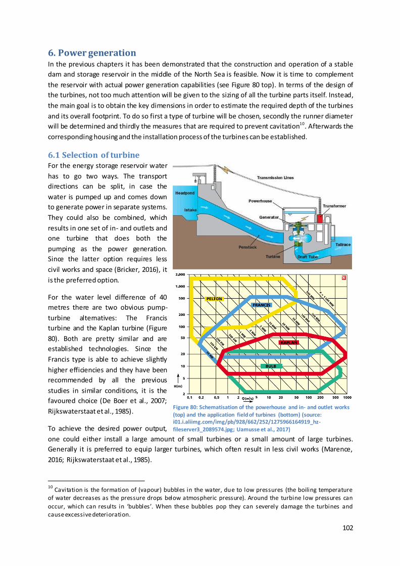
102
6. Power generation In the previous chapters it has been demonstrated that the construction and operation of a stable
dam and storage reservoir in the middle of the North Sea is feasible. Now it is time to complement
the reservoir with actual power generation capabilities (see Figure 80 top). In terms of the design of
the turbines, not too much attention will be given to the sizing of all the turbine parts itself. Instead,
the main goal is to obtain the key dimensions in order to estimate the required depth of the turbines
and its overall footprint. To do so first a type of turbine will be chosen, secondly the runner diameter
will be determined and thirdly the measures that are required to prevent cavitation10. Afterwards the
corresponding housing and the installation process of the turbines can be established.
6.1 Selection of turbine For the energy storage reservoir water
has to go two ways. The transport
directions can be split, in case the
water is pumped up and comes down
to generate power in separate systems.
They could also be combined, which
results in one set of in- and outlets and
one turbine that does both the
pumping as the power generation.
Since the latter option requires less
civil works and space (Bricker, 2016), it
is the preferred option.
For the water level difference of 40
metres there are two obvious pump-
turbine alternatives: The Francis
turbine and the Kaplan turbine (Figure
80). Both are pretty similar and are
established technologies. Since the
Francis type is able to achieve slightly
higher efficiencies and they have been
recommended by all the previous
studies in similar conditions, it is the
favoured choice (De Boer et al., 2007;
Rijkswaterstaat et al., 1985).
To achieve the desired power output,
one could either install a large amount of small turbines or a small amount of large turbines.
Generally it is preferred to equip larger turbines, which often result in less civil works (Marence,
2016; Rijkswaterstaat et al., 1985).
10
Cavitation is the formation of (vapour) bubbles in the water, due to low pressures (the boiling temperature of water decreases as the pressure drops below atmospheric pressure). Around the turbine low pressures can
occur, which can results in ‘bubbles’. When these bubbles pop they can severely damage the turbines and cause excessive deterioration.
Figure 80: Schematisation of the powerhouse and in- and outlet works (top) and the application field of turbines (bottom) (source: i01.i.aliimg.com/img/pb/928/662/252/1275966164919_hz-fileserver3_2089574.jpg; Uamusse et al., 2017)
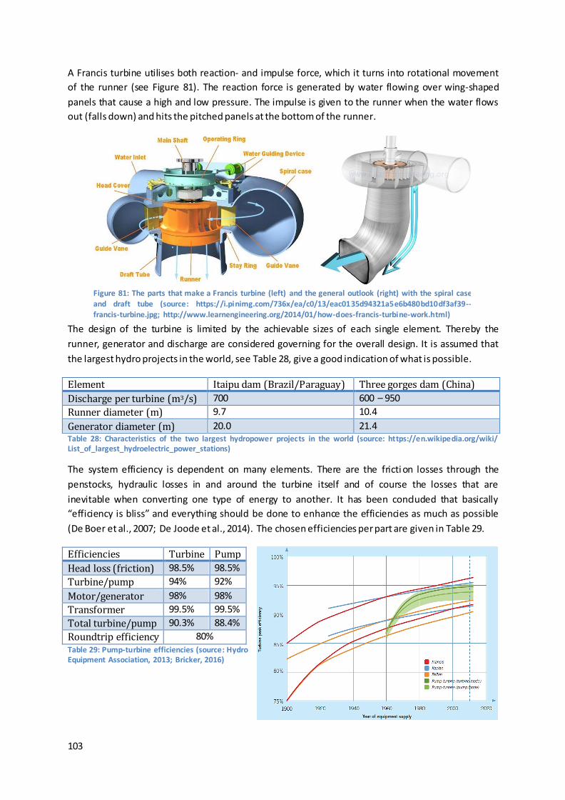
103
A Francis turbine utilises both reaction- and impulse force, which it turns into rotational movement
of the runner (see Figure 81). The reaction force is generated by water flowing over wing-shaped
panels that cause a high and low pressure. The impulse is given to the runner when the water flows
out (falls down) and hits the pitched panels at the bottom of the runner.
The design of the turbine is limited by the achievable sizes of each single element. Thereby the
runner, generator and discharge are considered governing for the overall design. It is assumed that
the largest hydro projects in the world, see Table 28, give a good indication of what is possible.
Element Itaipu dam (Brazil/Paraguay) Three gorges dam (China)
Discharge per turbine (m3/s) 700 600 – 950
Runner diameter (m) 9.7 10.4
Generator diameter (m) 20.0 21.4 Table 28: Characteristics of the two largest hydropower projects in the world (source: https://en.wikipedia.org/wiki/ List_of_largest_hydroelectric_power_stations)
The system efficiency is dependent on many elements. There are the fricti on losses through the
penstocks, hydraulic losses in and around the turbine itself and of course the losses that are
inevitable when converting one type of energy to another. It has been concluded that basically
“efficiency is bliss” and everything should be done to enhance the efficiencies as much as possible
(De Boer et al., 2007; De Joode et al., 2014). The chosen efficiencies per part are given in Table 29.
Efficiencies Turbine Pump
Head loss (friction) 98.5% 98.5%
Turbine/pump 94% 92%
Motor/generator 98% 98%
Transformer 99.5% 99.5%
Total turbine/pump 90.3% 88.4%
Roundtrip efficiency 80% Table 29: Pump-turbine efficiencies (source: Hydro Equipment Association, 2013; Bricker, 2016)
Figure 81: The parts that make a Francis turbine (left) and the general outlook (right) with the spiral case and draft tube (source: https://i.pinimg.com/736x/ea/c0/13/eac0135d94321a5e6b480bd10df3af39--francis-turbine.jpg; http://www.learnengineering.org/2014/01/how-does-francis-turbine-work.html)
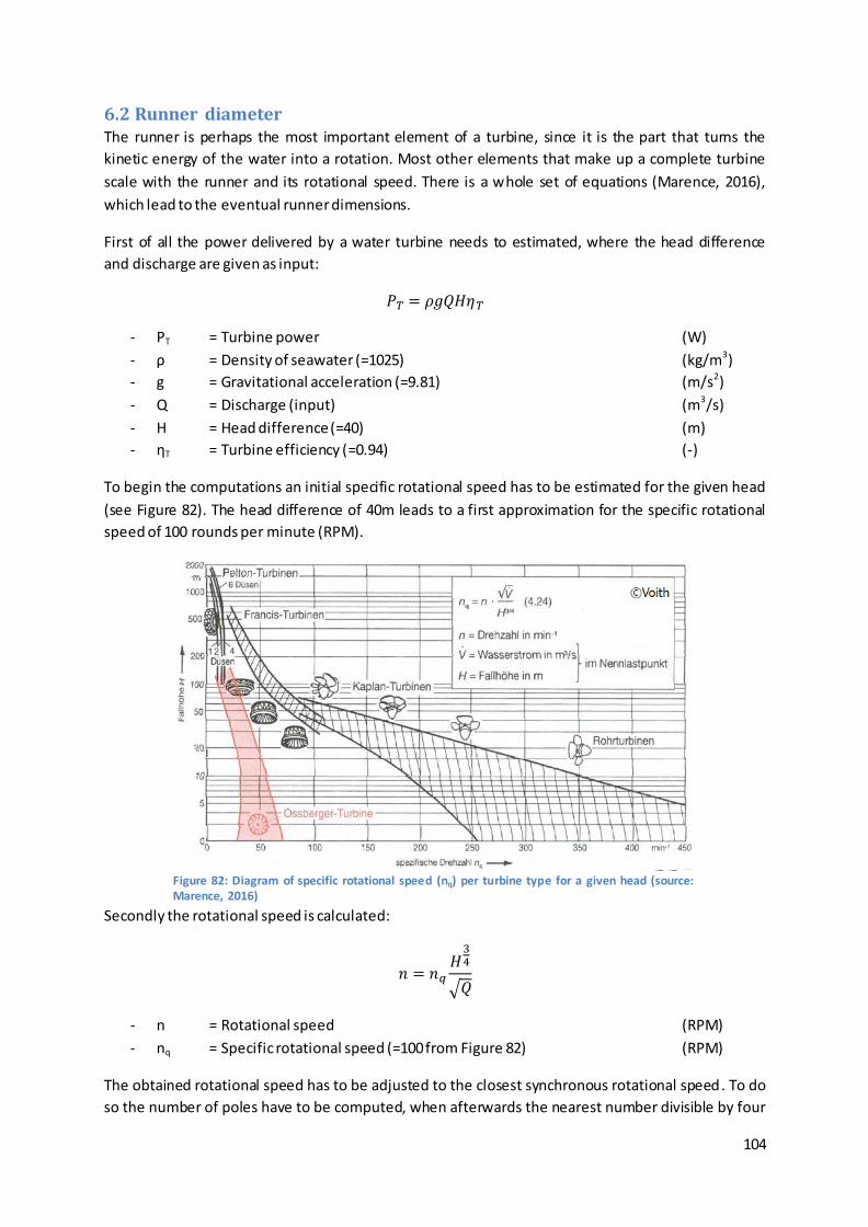
104
6.2 Runner diameter The runner is perhaps the most important element of a turbine, since it is the part that turns the
kinetic energy of the water into a rotation. Most other elements that make up a complete turbine
scale with the runner and its rotational speed. There is a whole set of equations (Marence, 2016),
which lead to the eventual runner dimensions.
First of all the power delivered by a water turbine needs to estimated, where the head difference
and discharge are given as input:
𝑃𝑇 = 𝜌𝑔𝑄𝐻𝜂𝑇
- PT = Turbine power (W)
- ρ = Density of seawater (=1025) (kg/m3)
- g = Gravitational acceleration (=9.81) (m/s2)
- Q = Discharge (input) (m3/s)
- H = Head difference (=40) (m)
- ηT = Turbine efficiency (=0.94) (-)
To begin the computations an initial specific rotational speed has to be estimated for the given head
(see Figure 82). The head difference of 40m leads to a first approximation for the specific rotational
speed of 100 rounds per minute (RPM).
Secondly the rotational speed is calculated:
𝑛 = 𝑛𝑞𝐻34
√𝑄
- n = Rotational speed (RPM)
- nq = Specific rotational speed (=100 from Figure 82) (RPM)
The obtained rotational speed has to be adjusted to the closest synchronous rotational speed. To do
so the number of poles have to be computed, when afterwards the nearest number divisible by four
Figure 82: Diagram of specific rotational speed (nq) per turbine type for a given head (source: Marence, 2016)
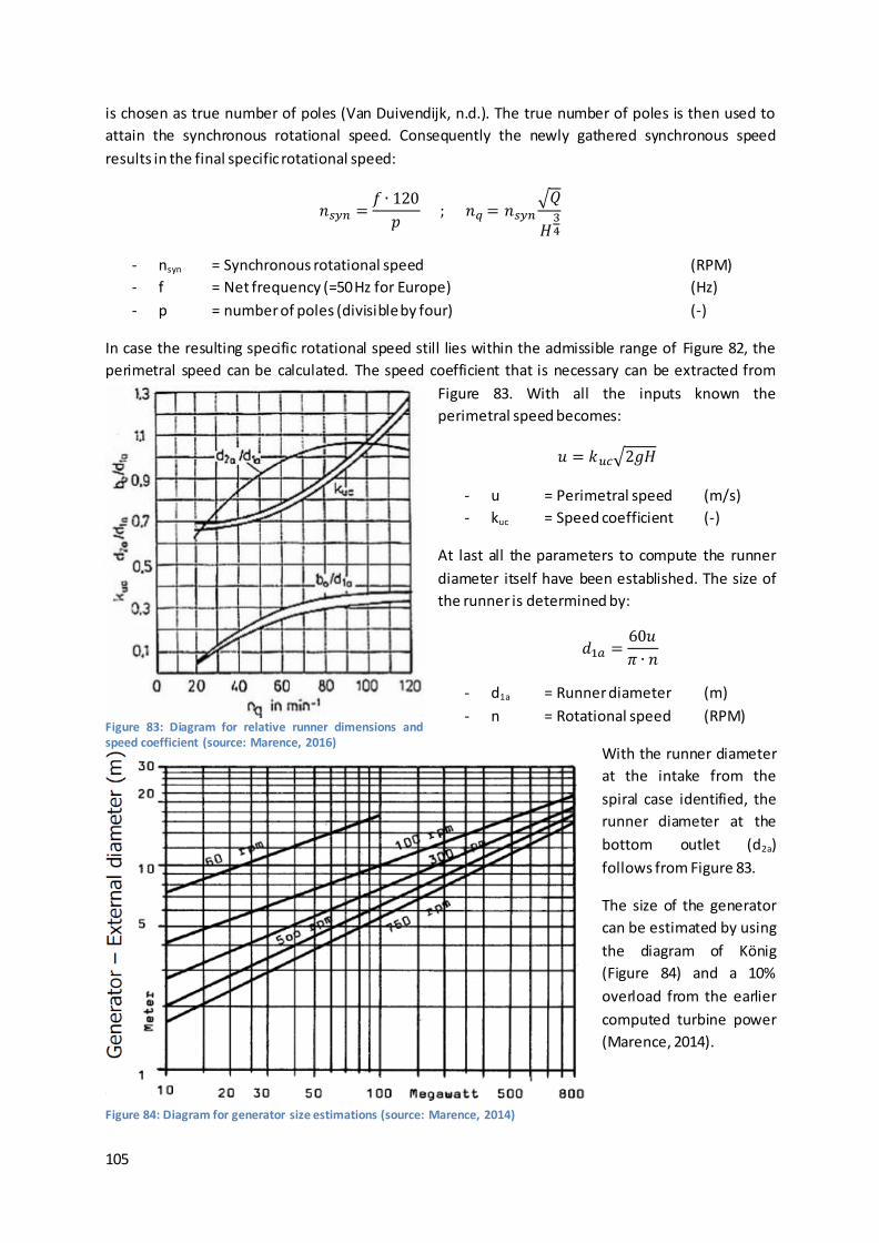
105
is chosen as true number of poles (Van Duivendijk, n.d.). The true number of poles is then used to
attain the synchronous rotational speed. Consequently the newly gathered synchronous speed
results in the final specific rotational speed:
𝑛𝑠𝑦𝑛 =𝑓 ∙ 120
𝑝 ; 𝑛𝑞 = 𝑛𝑠𝑦𝑛
√𝑄
𝐻34
- nsyn = Synchronous rotational speed (RPM)
- f = Net frequency (=50 Hz for Europe) (Hz)
- p = number of poles (divisible by four) (-)
In case the resulting specific rotational speed still lies within the admissible range of Figure 82, the
perimetral speed can be calculated. The speed coefficient that is necessary can be extracted from
Figure 83. With all the inputs known the
perimetral speed becomes:
𝑢 = 𝑘𝑢𝑐√2𝑔𝐻
- u = Perimetral speed (m/s)
- kuc = Speed coefficient (-)
At last all the parameters to compute the runner
diameter itself have been established. The size of
the runner is determined by:
𝑑1𝑎 =60𝑢
𝜋 ∙ 𝑛
- d1a = Runner diameter (m)
- n = Rotational speed (RPM)
With the runner diameter
at the intake from the
spiral case identified, the
runner diameter at the
bottom outlet (d2a)
follows from Figure 83.
The size of the generator
can be estimated by using
the diagram of König
(Figure 84) and a 10%
overload from the earlier
computed turbine power
(Marence, 2014).
Figure 83: Diagram for relative runner dimensions and speed coefficient (source: Marence, 2016)
Figure 84: Diagram for generator size estimations (source: Marence, 2014)
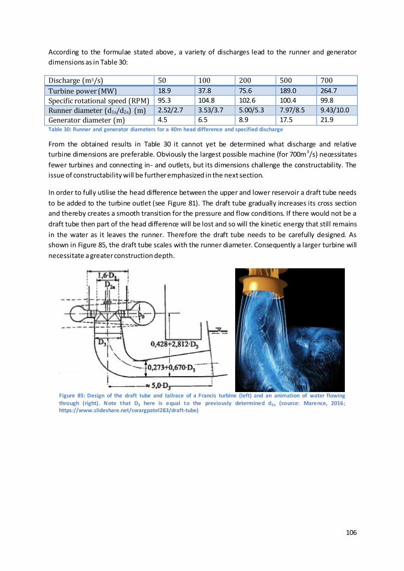
106
According to the formulae stated above, a variety of discharges lead to the runner and generator
dimensions as in Table 30:
Discharge (m3/s) 50 100 200 500 700
Turbine power (MW) 18.9 37.8 75.6 189.0 264.7
Specific rotational speed (RPM) 95.3 104.8 102.6 100.4 99.8
Runner diameter (d1a/d2a) (m) 2.52/2.7 3.53/3.7 5.00/5.3 7.97/8.5 9.43/10.0
Generator diameter (m) 4.5 6.5 8.9 17.5 21.9 Table 30: Runner and generator diameters for a 40m head difference and specified discharge
From the obtained results in Table 30 it cannot yet be determined what discharge and relative
turbine dimensions are preferable. Obviously the largest possible machine (for 700m3/s) necessitates
fewer turbines and connecting in- and outlets, but its dimensions challenge the constructability. The
issue of constructability will be further emphasized in the next section.
In order to fully utilise the head difference between the upper and lower reservoir a draft tube needs
to be added to the turbine outlet (see Figure 81). The draft tube gradually increases its cross section
and thereby creates a smooth transition for the pressure and flow conditions. If there would not be a
draft tube then part of the head difference will be lost and so will the kinetic energy that still remains
in the water as it leaves the runner. Therefore the draft tube needs to be carefully designed. As
shown in Figure 85, the draft tube scales with the runner diameter. Consequently a larger turbine will
necessitate a greater construction depth.
Figure 85: Design of the draft tube and tailrace of a Francis turbine (left) and an animation of water flowing
through (right). Note that D3 here is equal to the previously determined d2a (source: Marence, 2016; https://www.slideshare.net/swargpatel283/draft-tube)
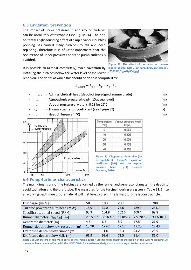
107
Figure 87: Diagram to determine (by extrapolation) Thoma's caviation coefficient (left) and the vapour pressure head (right) (source: Marence, 2016)
6.3 Cavitation prevention The impact of under pressures in and around turbines
can be absolutely catastrophic (see Figure 86). The not-
so-tantalisingly-sounding effect of simple vapour bubbles
popping has caused many turbines to fail and need
replacing. Therefore it is of utter importance that the
occurrence of under pressures near the pump-turbines is
avoided.
It is possible to (almost completely) avoid cavitation by
installing the turbines below the water level of the lower
reservoir. The depth at which this should be done is computed by:
ℎ𝑆,𝑎𝑑𝑚 = ℎ𝑎𝑡−ℎ𝑣− 𝜎𝑐 ⋅ ℎ𝑓
- hS,adm = Admissible draft head (depth of top edge of runner blade) (m)
- hat = Atmospheric pressure head (=10 at sea level) (m)
- hv = Vapour pressure of water (=0.18 for 15°C) (m)
- σc = Thoma’s cavitation coefficient (see Figure 87) (-)
- hf = Head difference (=40) (m)
6.4 Pump-turbine characteristics The main dimensions of the turbines are formed by the runner and generator diameter, the depth to
avoid cavitation and the draft tube. The measures for the turbine housing are given in Table 31. Since
all working depths are problematic, it will first be explored if the largest turbine is constructible.
Discharge (m3/s) 50 100 200 500 700
Turbine power for 40m head (MW) 18.9 37.8 75.6 189.0 264.7
Specific rotational speed (RPM) 95.3 104.8 102.6 100.4 99.8
Runner diameter (d1a/d2a) (m) 2.52/2.7 3.53/3.7 5.00/5.3 7.97/8.5 9.43/10.0
Generator diameter (m) 4.5 6.5 8.9 17.5 21.9
Runner depth below low reservoir (m) 13.98 17.62 17.17 17.20 17.43
Draft tube depth below runner (m) 7.9 11.0 15.3 24.2 28.5
Draft tube depth below MSL (m) 61.9 68.6 72.5 81.4 86.0 Table 31: Dimensions of the main parts of the Francis pump-turbines to be used for the design of the turbine housing. All measures have been verified with the UNESCO-IHE HydroPower design tool and are equal to the centimetre.
Figure 86: The effect of cavitation on runner blades (source: http://authors.library.caltech.edu /25019/1/figs/fig604.jpg)

108
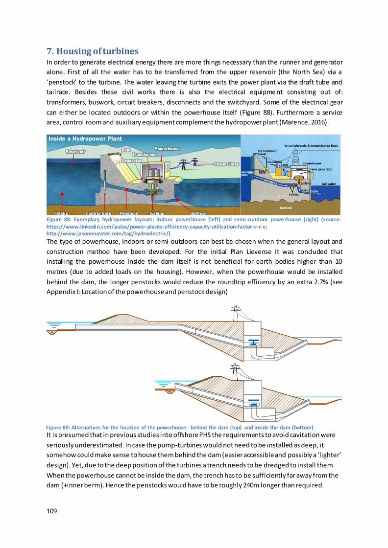
109
7. Housing of turbines In order to generate electrical energy there are more things necessary than the runner and generator
alone. First of all the water has to be transferred from the upper reservoir (the North Sea) via a
‘penstock’ to the turbine. The water leaving the turbine exits the power plant via the draft tube and
tailrace. Besides these civil works there is also the electrical equipment consisting out of:
transformers, buswork, circuit breakers, disconnects and the switchyard. Some of the electrical gear
can either be located outdoors or within the powerhouse itself (Figure 88). Furthermore a service
area, control room and auxiliary equipment complement the hydropower plant (Marence, 2016).
The type of powerhouse, indoors or semi-outdoors can best be chosen when the general layout and
construction method have been developed. For the initial Plan Lievense it was concluded that
installing the powerhouse inside the dam itself is not beneficial for earth bodies higher than 10
metres (due to added loads on the housing). However, when the powerhouse would be installed
behind the dam, the longer penstocks would reduce the roundtrip efficiency by an extra 2.7% (see
Appendix I: Location of the powerhouse and penstock design)
It is presumed that in previous studies into offshore PHS the requirements to avoid cavitation were
seriously underestimated. In case the pump-turbines would not need to be installed as deep, it
somehow could make sense to house them behind the dam (easier accessible and possibly a ‘lighter’
design). Yet, due to the deep position of the turbines a trench needs to be dredged to install them.
When the powerhouse cannot be inside the dam, the trench has to be sufficiently far away from the
dam (+inner berm). Hence the penstocks would have to be roughly 240m longer than required.
Figure 88: Exemplary hydropower layouts: indoor powerhouse (left) and semi-outdoor powerhouse (right) (source: https://www.linkedin.com/pulse/power-plants-efficiency-capacity-utilization-factor-v-r-v; http://www.jasonmunster.com/tag/hydroelectric/)
Figure 89: Alternatives for the location of the powerhouse: behind the dam (top) and inside the dam (bottom)
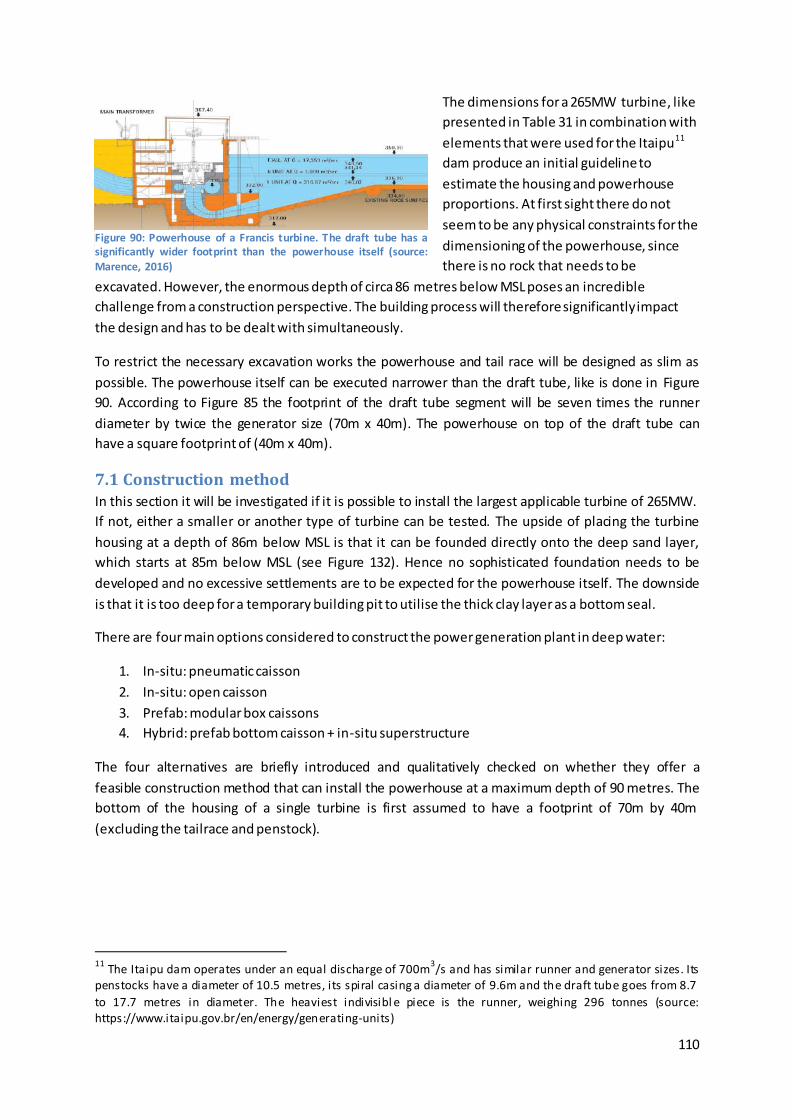
110
The dimensions for a 265MW turbine, like
presented in Table 31 in combination with
elements that were used for the Itaipu11
dam produce an initial guideline to
estimate the housing and powerhouse
proportions. At first sight there do not
seem to be any physical constraints for the
dimensioning of the powerhouse, since
there is no rock that needs to be
excavated. However, the enormous depth of circa 86 metres below MSL poses an incredible
challenge from a construction perspective. The building process will therefore significantly impact
the design and has to be dealt with simultaneously.
To restrict the necessary excavation works the powerhouse and tail race will be designed as slim as
possible. The powerhouse itself can be executed narrower than the draft tube, like is done in Figure
90. According to Figure 85 the footprint of the draft tube segment will be seven times the runner
diameter by twice the generator size (70m x 40m). The powerhouse on top of the draft tube can
have a square footprint of (40m x 40m).
7.1 Construction method In this section it will be investigated if it is possible to install the largest applicable turbine of 265MW.
If not, either a smaller or another type of turbine can be tested. The upside of placing the turbine
housing at a depth of 86m below MSL is that it can be founded directly onto the deep sand layer,
which starts at 85m below MSL (see Figure 132). Hence no sophisticated foundation needs to be
developed and no excessive settlements are to be expected for the powerhouse itself. The downside
is that it is too deep for a temporary building pit to utilise the thick clay layer as a bottom seal.
There are four main options considered to construct the power generation plant in deep water:
1. In-situ: pneumatic caisson
2. In-situ: open caisson
3. Prefab: modular box caissons
4. Hybrid: prefab bottom caisson + in-situ superstructure
The four alternatives are briefly introduced and qualitatively checked on whether they offer a
feasible construction method that can install the powerhouse at a maximum depth of 90 metres. The
bottom of the housing of a single turbine is first assumed to have a footprint of 70m by 40m
(excluding the tailrace and penstock).
11
The Itaipu dam operates under an equal discharge of 700m3/s and has similar runner and generator sizes. Its
penstocks have a diameter of 10.5 metres, its spiral casing a diameter of 9.6m and the draft tube goes from 8.7
to 17.7 metres in diameter. The heaviest indivisibl e piece is the runner, weighing 296 tonnes (source: https://www.itaipu.gov.br/en/energy/generating-units)
Figure 90: Powerhouse of a Francis turbine. The draft tube has a significantly wider footprint than the powerhouse itself (source: Marence, 2016)
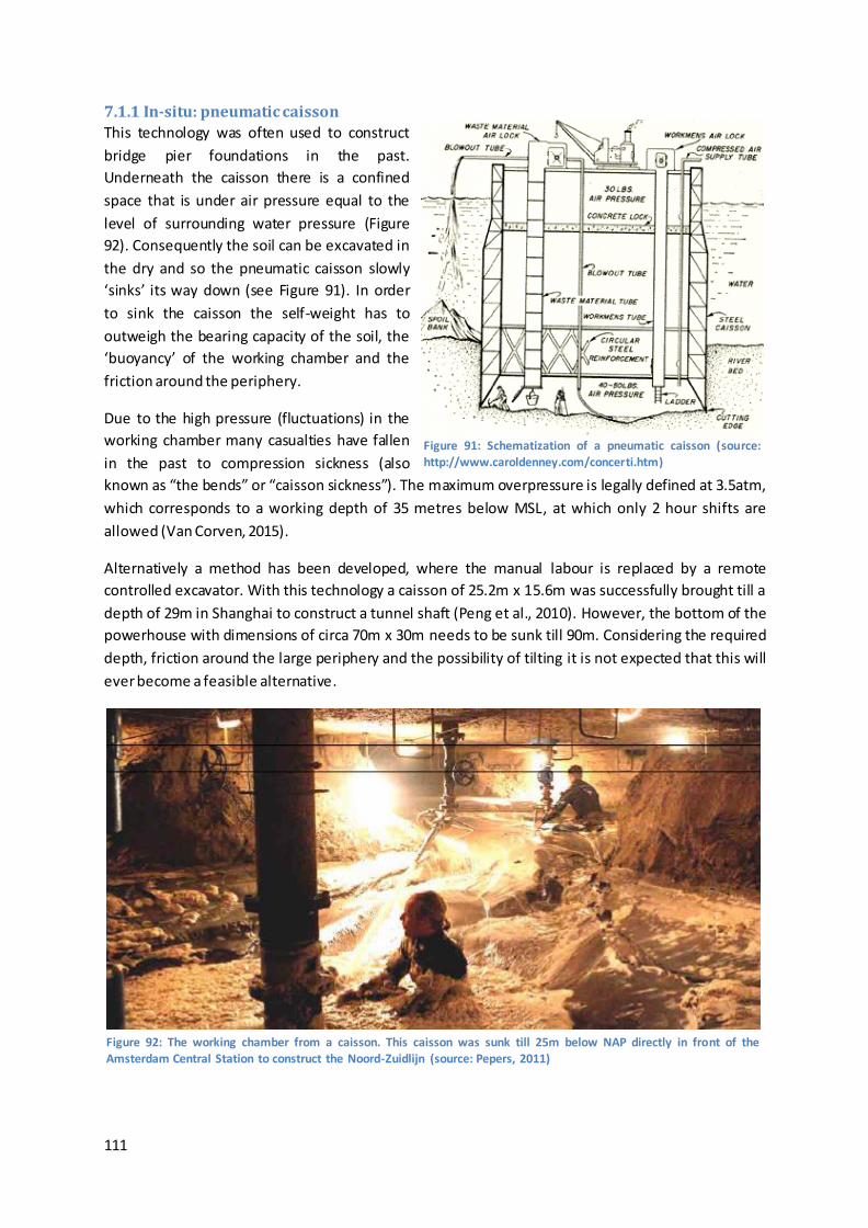
111
7.1.1 In-situ: pneumatic caisson
This technology was often used to construct
bridge pier foundations in the past.
Underneath the caisson there is a confined
space that is under air pressure equal to the
level of surrounding water pressure (Figure
92). Consequently the soil can be excavated in
the dry and so the pneumatic caisson slowly
‘sinks’ its way down (see Figure 91). In order
to sink the caisson the self-weight has to
outweigh the bearing capacity of the soil, the
‘buoyancy’ of the working chamber and the
friction around the periphery.
Due to the high pressure (fluctuations) in the
working chamber many casualties have fallen
in the past to compression sickness (also
known as “the bends” or “caisson sickness”). The maximum overpressure is legally defined at 3.5atm,
which corresponds to a working depth of 35 metres below MSL, at which only 2 hour shifts are
allowed (Van Corven, 2015).
Alternatively a method has been developed, where the manual labour is replaced by a remote
controlled excavator. With this technology a caisson of 25.2m x 15.6m was successfully brought till a
depth of 29m in Shanghai to construct a tunnel shaft (Peng et al., 2010). However, the bottom of the
powerhouse with dimensions of circa 70m x 30m needs to be sunk till 90m. Considering the required
depth, friction around the large periphery and the possibility of tilting it is not expected that this will
ever become a feasible alternative.
Figure 91: Schematization of a pneumatic caisson (source:
http://www.caroldenney.com/concerti.htm)
Figure 92: The working chamber from a caisson. This caisson was sunk till 25m below NAP directly in front of the Amsterdam Central Station to construct the Noord-Zuidlijn (source: Pepers, 2011)
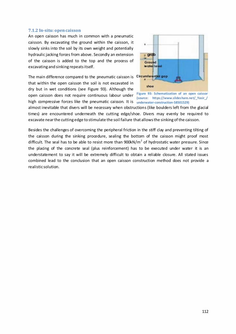
112
7.1.2 In-situ: open caisson
An open caisson has much in common with a pneumatic
caisson. By excavating the ground within the caisson, it
slowly sinks into the soil by its own weight and potentially
hydraulic jacking forces from above. Secondly an extension
of the caisson is added to the top and the process of
excavating and sinking repeats itself.
The main difference compared to the pneumatic caisson is
that within the open caisson the soil is not excavated in
dry but in wet conditions (see Figure 93). Although the
open caisson does not require continuous labour under
high compressive forces like the pneumatic caisson. It is
almost inevitable that divers will be necessary when obstructions (like boulders left from the glacial
times) are encountered underneath the cutting edge/shoe. Divers may evenly be required to
excavate near the cutting edge to stimulate the soil failure that allows the sinking of the caisson.
Besides the challenges of overcoming the peripheral friction in the stiff clay and preventing tilting of
the caisson during the sinking procedure, sealing the bottom of the caisson might proof most
difficult. The seal has to be able to resist more than 900kN/m2 of hydrostatic water pressure. Since
the placing of the concrete seal (plus reinforcement) has to be executed under water it is an
understatement to say it will be extremely difficult to obtain a reliable closure. All stated issues
combined lead to the conclusion that an open caisson construction method does not provide a
realistic solution.
Figure 93: Schematization of an open caisson (source: https://www.slideshare.net/_Yasir_/ underwater-construction-58501529)
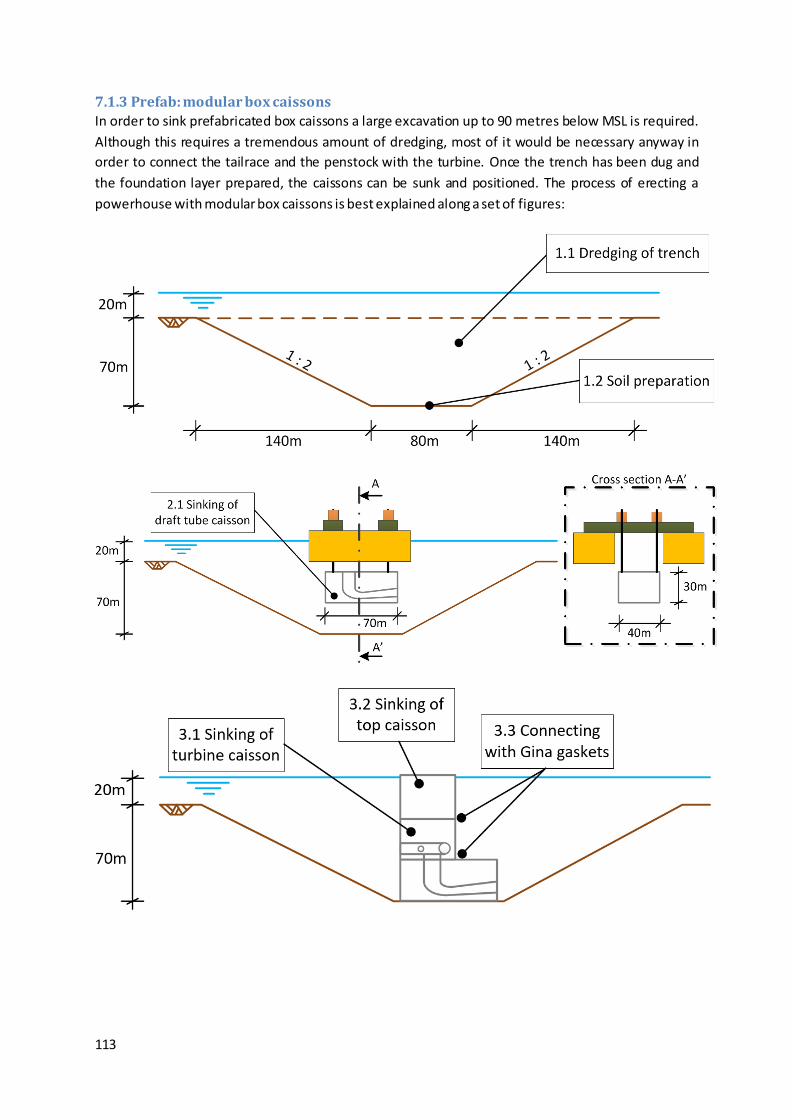
113
7.1.3 Prefab: modular box caissons
In order to sink prefabricated box caissons a large excavation up to 90 metres below MSL is required.
Although this requires a tremendous amount of dredging, most of it would be necessary anyway in
order to connect the tailrace and the penstock with the turbine. Once the trench has been dug and
the foundation layer prepared, the caissons can be sunk and positioned. The process of erecting a
powerhouse with modular box caissons is best explained along a set of figures:
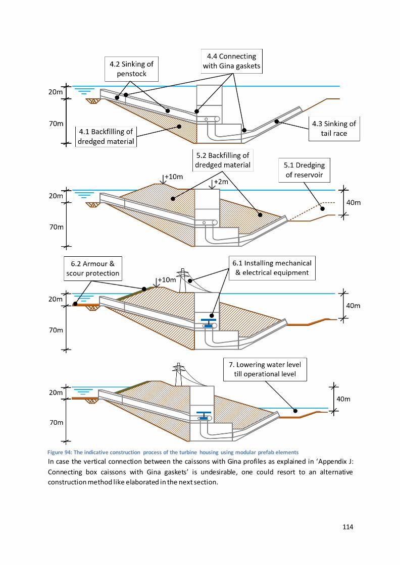
114
In case the vertical connection between the caissons with Gina profiles as explained in ‘Appendix J:
Connecting box caissons with Gina gaskets’ is undesirable, one could resort to an alternative
construction method like elaborated in the next section.
Figure 94: The indicative construction process of the turbine housing using modular prefab elements
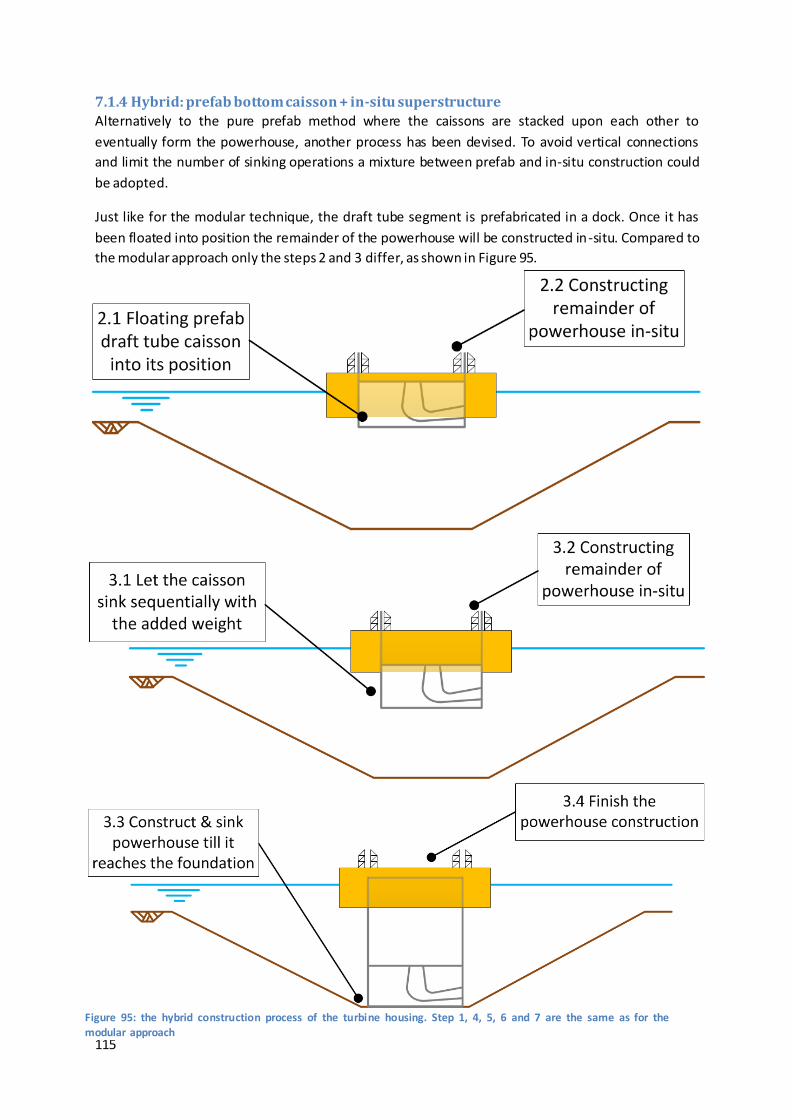
115
7.1.4 Hybrid: prefab bottom caisson + in-situ superstructure
Alternatively to the pure prefab method where the caissons are stacked upon each other to
eventually form the powerhouse, another process has been devised. To avoid vertical connections
and limit the number of sinking operations a mixture between prefab and in-situ construction could
be adopted.
Just like for the modular technique, the draft tube segment is prefabricated in a dock. Once it has
been floated into position the remainder of the powerhouse will be constructed in-situ. Compared to
the modular approach only the steps 2 and 3 differ, as shown in Figure 95.
Figure 95: the hybrid construction process of the turbine housing. Step 1, 4, 5, 6 and 7 are the same as for the modular approach
116
7.1.5 Choice of method
From the discussed four options it has been concluded that:
- A pneumatic caisson cannot be used to install the powerhouse at 90m below MSL
- An open caisson construction would be extremely difficult to successfully sink and seal and
should be avoided
- The modular box caisson method seems viable at first sight and is the preferred technique
- The hybrid scheme could theoretically work, but may be challenging to realise
The use of modular box caissons is chosen as best applicable. By dredging till the required depth the
slopes that are necessary for the tailrace and penstocks are simultaneously created. For the in-situ
options dredging would be needed to install the in- and outlets anyway.
The pure prefab method has the advantage over the hybrid method that everything can be built at
one main construction site. Furthermore the balancing during construction of the floating
powerhouse seems precarious. Most likely both alternatives need a (temporary) dam to shield the
construction process from the surrounding wave climate. Even when the whole dam around the
storage reservoir would already have been completed, the powerhouse installation would still need
protection from locally induced wind waves (who can exceed 2 metres, see Figure 45).
Preferably the housing of the turbines would be placed in deep water. The necessary dredging works
would be limited and the flow velocities at the in- and outtake lower. Hence the scour protection
could be executed ‘lighter’.
All things considered, an excavation with box caissons is the mostly likely option to be feasible. The
technology has been widely applied in for example immersed tunnelling projects12 and breakwaters.
There are many things yet to investigate besides the actual design of the caissons like: best suitable
location of the construction dock (conventional or floating) , type of formwork and the number of
elements to be produced per submerging and transport cycle.
To obtain insight in the main volumes and dimensions of the turbine housing some initial
computations are performed in the next section. These could provide a little guidance to estimate
the costs.
Finally it should be stated that this powerhouse construction differs from most PHS plants in the way
that there is no lateral transport possible between the several pump-turbines. This is due to the
caisson structure. Therefore all transport of people and equipment takes place vertically.
12
World’s deepest immersed tunnel segments have been installed in the Marmaray link that connects Europe and Asia via the Bosperus. The segments are 150m long, sunk till a maximum depth of 60m and total a length
of 1,387m. For the new Fehmarn connection between Germany and Denmark a 17.6km long immersed tunnel is planned that reaches ti l l 40m below MSL (source: https://en.wikipedia.org/wiki/Fehmarn_Belt_Fixed_Link).
117
7.2 Main dimensions and volumes Critical for the execution of the prefab methodology is the vertical stability of the caissons during
transport, sinking and in their final position. As a rule of thumb: with the (floating) transportation the
weight of the caisson should be no more than 99% of the maximum buoyancy force, including
bulkheads and sinking equipment. In the final position the weight needs to be 107.5% of the uplift
force caused by the displaced water (Bakker, 2014). Subsequently it will be necessary to increase the
ballast of the caissons once they are positioned. This can be done by either adding more concrete or
by locally sourced material. The latter is preferred since it is much cheaper. Hence the caissons
should be designed in such a way that they can incorporate dredged material. By using the
Archimedes principle of displaced water the necessary concrete and reinforcement (estimated at 1%)
volumes can be computed:
𝑉𝑟𝑐 = 𝑉𝑐𝑎𝑖𝑠𝑠𝑜𝑛𝛾𝑤𝛾𝑐0.99
𝑉𝑐𝑜𝑛𝑐 = 0.99𝑉𝑟𝑐
𝑉𝑟𝑒𝑖𝑛 = 0.01𝑉𝑟𝑐
𝑉𝑓𝑖𝑙𝑙 = 0.085𝑉𝑐𝑎𝑖𝑠𝑠𝑜𝑛𝛾𝑤𝛾𝑠
- Vrc = Volume reinforced concrete (m3)
- Vcaisson = Volume caisson (m3)
- Vconc = Volume concrete (m3)
- Vrein = Volume reinforcement (m3)
- Vfill = Volume dredged backfill (m3)
- γw = Volumetric weight sea water (=1025) (kg/m3)
- γc = Volumetric weight reinforced concrete (=2400) (kg/m3)
- γw = Volumetric weight dredged material (=2000) (kg/m3)
Caisson Dimensions (l*w*h) (m)
Volume concrete (m3)
Volume reinforcement (m3)
Volume dredged backfill (m3)
Draft tube 70*40*30 35,161 355 3,659
Turbine 40*40*30 20,092 203 2,091
Top 40*40*30 20,092 203 2,091 Table 32: Volume and material characteristics of modular box caissons
The volumes stated in Table 32 can be used for a first approximation of the powerhouse costs. The
costs of the penstocks, tailrace, excavation, backfi ll and in- and outlet need to be added to obtain a
full estimation of turbine housing costs.
The maximum height of the box caisson is practically limited by the bathymetry. As a rule of thumb a
caisson would be able to float halfway out of the water (A.Q.C. van der Horst, personal
communication, September 12, 2017). A 30 metre high caisson could therefore have a draught of
only 15 metres. To allow for some movements and irregularities this should be acceptable for the
Dogger Bank where the average depth is around 20m.
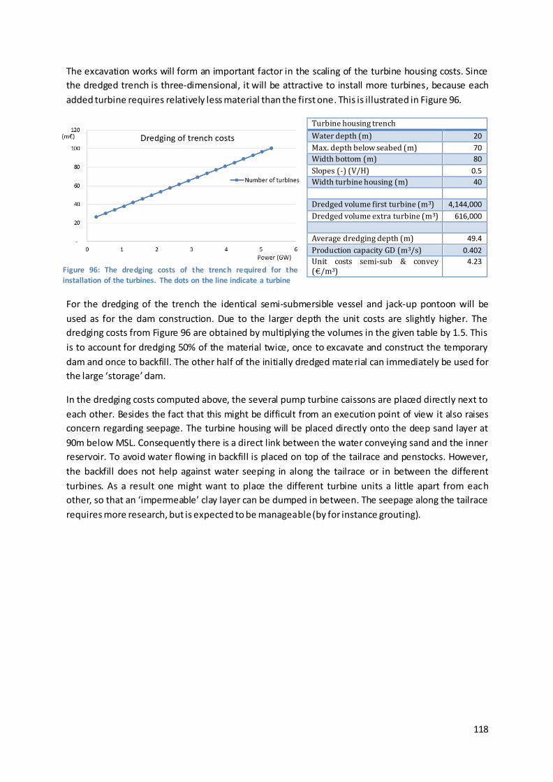
118
The excavation works will form an important factor in the scaling of the turbine housing costs. Since
the dredged trench is three-dimensional, it will be attractive to install more turbines, because each
added turbine requires relatively less material than the first one. This is illustrated in Figure 96.
Turbine housing trench
Water depth (m) 20
Max. depth below seabed (m) 70
Width bottom (m) 80
Slopes (-) (V/H) 0.5
Width turbine housing (m) 40
Dredged volume first turbine (m3) 4,144,000
Dredged volume extra turbine (m3) 616,000
Average dredging depth (m) 49.4
Production capacity GD (m3/s) 0.402
Unit costs semi-sub & convey (€/m3)
4.23
For the dredging of the trench the identical semi-submersible vessel and jack-up pontoon will be
used as for the dam construction. Due to the larger depth the unit costs are slightly higher. The
dredging costs from Figure 96 are obtained by multiplying the volumes in the given table by 1.5. This
is to account for dredging 50% of the material twice, once to excavate and construct the temporary
dam and once to backfill. The other half of the initially dredged material can immediately be used for
the large ‘storage’ dam.
In the dredging costs computed above, the several pump turbine caissons are placed directly next to
each other. Besides the fact that this might be difficult from an execution point of view it also raises
concern regarding seepage. The turbine housing will be placed directly onto the deep sand layer at
90m below MSL. Consequently there is a direct link between the water conveying sand and the inner
reservoir. To avoid water flowing in backfill is placed on top of the tailrace and penstocks. However,
the backfill does not help against water seeping in along the tailrace or in between the different
turbines. As a result one might want to place the different turbine units a little apart from each
other, so that an ‘impermeable’ clay layer can be dumped in between. The seepage along the tailrace
requires more research, but is expected to be manageable (by for instance grouting).
Figure 96: The dredging costs of the trench required for the installation of the turbines. The dots on the line indicate a turbine

119
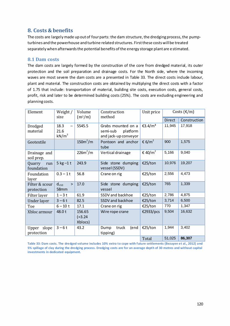
120
8. Costs & benefits The costs are largely made up out of four parts: the dam structure, the dredging process, the pump-
turbines and the powerhouse and turbine related structures. First these costs will be treated
separately when afterwards the potential benefits of the energy storage plant are e stimated.
8.1 Dam costs The dam costs are largely formed by the construction of the core from dredged material, its outer
protection and the soil preparation and drainage costs. For the North side, where the incoming
waves are most severe the dam costs are a presented in Table 33. The direct costs include labour,
plant and material. The construction costs are obtained by multiplying the direct costs with a factor
of 1.75 that include: transportation of material, building site costs, execution costs, general costs,
profit, risk and later to be determined building costs (25%). The costs are excluding engineering and
planning costs.
Element Weight / size
Volume (m3/m)
Construction method
Unit price Costs (€/m)
Direct Construction
Dredged material
18.3 – 21.6 kN/m3
5545.5 Grabs mounted on a semi-sub platform and jack-up conveyor
€3.4/m³ 11,945 17,918
Geotextile 150m2/m Pontoon and anchor tube
€ 6/m2 900 1,575
Drainage and soil prep.
226m2/m Vertical drainage € 40/m2 5,166 9,040
Quarry run foundation
5 kg –1 t 243.9 Side stone dumping vessel (SSDV)
€25/ton 10,976 19,207
Foundation layer
0.3 – 1 t 56.8 Crane on rig €25/ton 2,556 4,473
Filter & scour protection
dn50 > 58mm
17.0 Side stone dumping vessel
€25/ton 765 1,339
Filter layer 1 – 3 t 61.9 SSDV and backhoe €25/ton 2,786 4,875
Under layer 3 – 6 t 82.5 SSDV and backhoe €25/ton 3,714 6,500
Toe 6 – 10 t 17.1 Crane on rig €25/ton 770 1,347
Xbloc armour 48.0 t 156.65 (=3.24 Xblocs)
Wire rope crane €2933/pcs 9,504 16,632
Upper slope protection
3 – 6 t 43.2 Dump truck (end tipping)
€25/ton 1,944 3,402
Total 51,025 86,307
Table 33: Dam costs. The dredged volume includes 10% extra to cope with future settlements (Bezuyen et al., 2012) and 5% spillage of clay during the dredging process. Dredging costs are for an average depth of 30 metres and without capital investments in dedicated equipment.
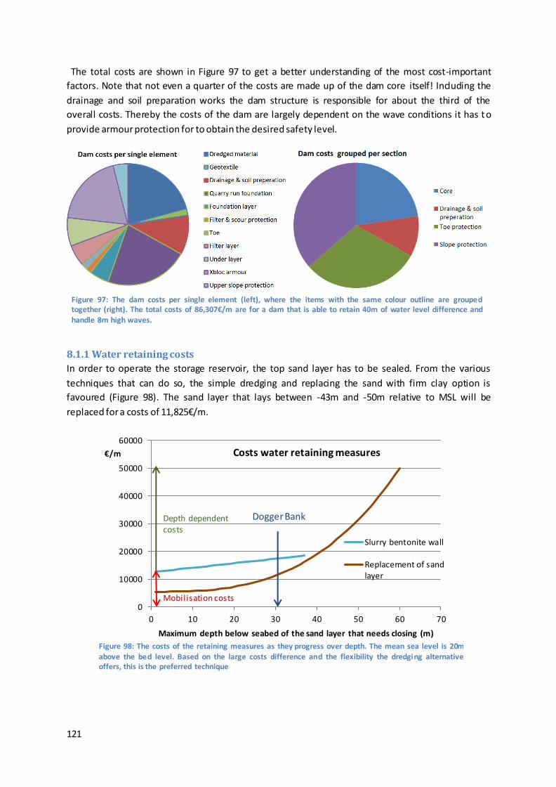
121
The total costs are shown in Figure 97 to get a better understanding of the most cost-important
factors. Note that not even a quarter of the costs are made up of the dam core itself! Including the
drainage and soil preparation works the dam structure is responsible for about the third of the
overall costs. Thereby the costs of the dam are largely dependent on the wave conditions it has to
provide armour protection for to obtain the desired safety level.
8.1.1 Water retaining costs
In order to operate the storage reservoir, the top sand layer has to be sealed. From the various
techniques that can do so, the simple dredging and replacing the sand with firm clay option is
favoured (Figure 98). The sand layer that lays between -43m and -50m relative to MSL will be
replaced for a costs of 11,825€/m.
0
10000
20000
30000
40000
50000
60000
0 10 20 30 40 50 60 70
€/m
Maximum depth below seabed of the sand layer that needs closing (m)
Costs water retaining measures
Slurry bentonite wall
Replacement of sandlayer
Mobilisation costs
Depth dependent costs
Figure 98: The costs of the retaining measures as they progress over depth. The mean sea level is 20m above the bed level. Based on the large costs difference and the flexibility the dredging alternative offers, this is the preferred technique
Dogger Bank
Figure 97: The dam costs per single element (left), where the items with the same colour outline are grouped together (right). The total costs of 86,307€/m are for a dam that is able to retain 40m of water level difference and
handle 8m high waves.
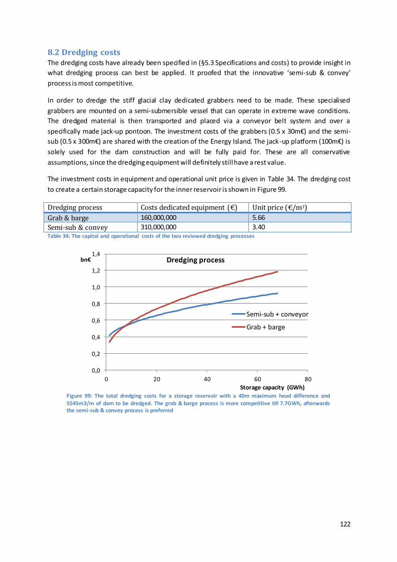
122
8.2 Dredging costs The dredging costs have already been specified in (§5.3 Specifications and costs) to provide insight in
what dredging process can best be applied. It proofed that the innovative ‘semi-sub & convey’
process is most competitive.
In order to dredge the stiff glacial clay dedicated grabbers need to be made. These specialised
grabbers are mounted on a semi-submersible vessel that can operate in extreme wave conditions.
The dredged material is then transported and placed via a conveyor belt system and over a
specifically made jack-up pontoon. The investment costs of the grabbers (0.5 x 30m€) and the semi-
sub (0.5 x 300m€) are shared with the creation of the Energy Island. The jack-up platform (100m€) is
solely used for the dam construction and will be fully paid for. These are all conservative
assumptions, since the dredging equipment will definitely still have a rest value.
The investment costs in equipment and operational unit price is given in Table 34. The dredging cost
to create a certain storage capacity for the inner reservoir is shown in Figure 99.
Dredging process Costs dedicated equipment (€) Unit price (€/m3)
Grab & barge 160,000,000 5.66
Semi-sub & convey 310,000,000 3.40 Table 34: The capital and operational costs of the two reviewed dredging processes
Figure 99: The total dredging costs for a storage reservoir with a 40m maximum head difference and 5545m3/m of dam to be dredged. The grab & barge process is more competitive till 7.7GWh, afterwards the semi-sub & convey process is preferred
0,0
0,2
0,4
0,6
0,8
1,0
1,2
1,4
0 20 40 60 80
bn€
Storage capacity (GWh)
Dredging process
Semi-sub + conveyor
Grab + barge
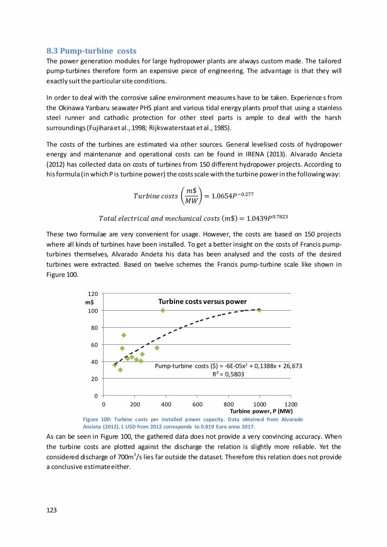
123
8.3 Pump-turbine costs The power generation modules for large hydropower plants are always custom made. The tailored
pump-turbines therefore form an expensive piece of engineering. The advantage is that they will
exactly suit the particular site conditions.
In order to deal with the corrosive saline environment measures have to be taken. Experience s from
the Okinawa Yanbaru seawater PHS plant and various tidal energy plants proof that using a stainless
steel runner and cathodic protection for other steel parts is ample to deal with the harsh
surroundings (Fujihara et al., 1998; Rijkswaterstaat et al., 1985).
The costs of the turbines are estimated via other sources. General levelised costs of hydropower
energy and maintenance and operational costs can be found in IRENA (2013). Alvarado Ancieta
(2012) has collected data on costs of turbines from 150 different hydropower projects. According to
his formula (in which P is turbine power) the costs scale with the turbine power in the following way:
𝑇𝑢𝑟𝑏𝑖𝑛𝑒 𝑐𝑜𝑠𝑡𝑠 (𝑚$
𝑀𝑊) = 1.0654𝑃−0.277
𝑇𝑜𝑡𝑎𝑙 𝑒𝑙𝑒𝑐𝑡𝑟𝑖𝑐𝑎𝑙 𝑎𝑛𝑑 𝑚𝑒𝑐ℎ𝑎𝑛𝑖𝑐𝑎𝑙 𝑐𝑜𝑠𝑡𝑠 (𝑚$) = 1.0439𝑃0.7823
These two formulae are very convenient for usage. However, the costs are based on 150 projects
where all kinds of turbines have been installed. To get a better insight on the costs of Francis pump-
turbines themselves, Alvarado Ancieta his data has been analysed and the costs of the desired
turbines were extracted. Based on twelve schemes the Francis pump-turbine scale like shown in
Figure 100.
As can be seen in Figure 100, the gathered data does not provide a very convincing accuracy. When
the turbine costs are plotted against the discharge the relation is slightly more reliable. Yet the
considered discharge of 700m3/s lies far outside the dataset. Therefore this relation does not provide
a conclusive estimate either.
Pump-turbine costs ($) = -6E-05x2 + 0,1388x + 26,673 R² = 0,5803
0
20
40
60
80
100
120
0 200 400 600 800 1000 1200
m$
Turbine power, P (MW)
Turbine costs versus power
Figure 100: Turbine costs per installed power capacity. Data obtained from Alvarado Ancieta (2012). 1 USD from 2012 corresponds to 0.819 Euro anno 2017.
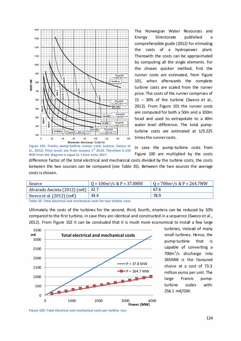
124
Figure 102: Total electrical and mechanical costs per turbine size
0
500
1000
1500
2000
2500
3000
3500
0 1000 2000 3000 4000
m€
Power (MW)
Total electrical and mechanical costs
P = 37.8 MW
P = 264.7 MW
The Norwegian Water Resources and
Energy Directorate published a
comprehensible guide (2012) for etimating
the costs of a hydropower plant.
Therewith the costs can be approximated
by computing all the single elements. For
the chosen quicker method, first the
runner costs are estimated, from Figure
101, when afterwards the complete
turbine costs are scaled from the runner
price. The costs of the runner comprises of
15 – 30% of the turbine (Sweco et al.,
2012). From Figure 101 the runner costs
are computed for both a 50m and a 100m
head and used to extrapolate to a 40m
water level difference. The total pump-
turbine costs are estimated at 1/0.225
times the runner costs.
In case the pump-turbine costs from
Figure 100 are multiplied by the costs
difference factor of the total electrical and mechanical costs divided by the turbine costs, the costs
between the two sources can be compared (see Table 35). Between the two sources the average
costs is chosen.
Source Q = 100m3/s & P = 37.8MW Q = 700m3/s & P = 264.7MW
Alvarado Ancieta (2012) (m€) 32.7 67.6
Sweco et al. (2012) (m€) 34.4 78.9 Table 35: Total electrical and mechanical costs for two turbine sizes
Ultimately the costs of the turbines for the second, third, fourth, etcetera can be reduced by 10%
compared to the first turbine, in case they are identical and constructed in a sequence (Sweco et al.,
2012). From Figure 102 it can be concluded that it is much more economical to install a few large
turbines, instead of many
small turbines. Hence, the
pump-turbine that is
capable of converting a
700m3/s discharge into
265MW is the favoured
choice at a cost of 73.3
million euros per unit. The
large Francis pump-
turbine scales with:
256.1 m€/GW.
Figure 101: Franics pump-turbine runner costs (source: Sweco et
al., 2012). Price levels are from January 1st
2010. Therefore 0.133 NOK from the diagram is equal to 1 Euro anno 2017.
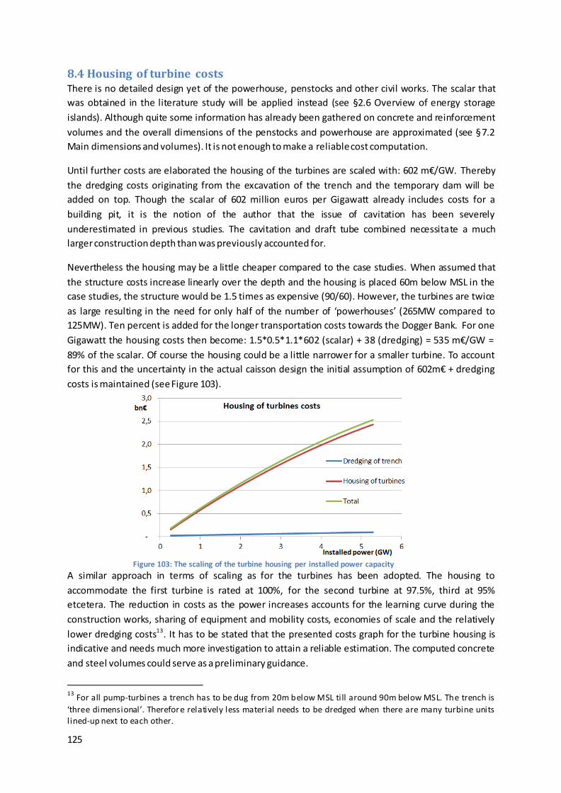
125
Figure 103: The scaling of the turbine housing per installed power capacity
8.4 Housing of turbine costs There is no detailed design yet of the powerhouse, penstocks and other civil works. The scalar that
was obtained in the literature study will be applied instead (see §2.6 Overview of energy storage
islands). Although quite some information has already been gathered on concrete and reinforcement
volumes and the overall dimensions of the penstocks and powerhouse are approximated (see §7.2
Main dimensions and volumes). It is not enough to make a reliable cost computation.
Until further costs are elaborated the housing of the turbines are scaled with: 602 m€/GW. Thereby
the dredging costs originating from the excavation of the trench and the temporary dam will be
added on top. Though the scalar of 602 million euros per Gigawatt already includes costs for a
building pit, it is the notion of the author that the issue of cavitation has been severely
underestimated in previous studies. The cavitation and draft tube combined necessitate a much
larger construction depth than was previously accounted for.
Nevertheless the housing may be a little cheaper compared to the case studies. When assumed that
the structure costs increase linearly over the depth and the housing is placed 60m below MSL in the
case studies, the structure would be 1.5 times as expensive (90/60). However, the turbines are twice
as large resulting in the need for only half of the number of ‘powerhouses’ (265MW compared to
125MW). Ten percent is added for the longer transportation costs towards the Dogger Bank. For one
Gigawatt the housing costs then become: 1.5*0.5*1.1*602 (scalar) + 38 (dredging) = 535 m€/GW =
89% of the scalar. Of course the housing could be a little narrower for a smaller turbine. To account
for this and the uncertainty in the actual caisson design the initial assumption of 602m€ + dredging
costs is maintained (see Figure 103).
A similar approach in terms of scaling as for the turbines has been adopted. The housing to
accommodate the first turbine is rated at 100%, for the second turbine at 97.5%, third at 95%
etcetera. The reduction in costs as the power increases accounts for the learning curve during the
construction works, sharing of equipment and mobility costs, economies of scale and the relatively
lower dredging costs13. It has to be stated that the presented costs graph for the turbine housing is
indicative and needs much more investigation to attain a reliable estimation. The computed concrete
and steel volumes could serve as a preliminary guidance.
13
For all pump-turbines a trench has to be dug from 20m below MSL till around 90m below MSL. The trench is
‘three dimensional’. Therefore relatively less material needs to be dredged when there are many turbine units l ined-up next to each other.
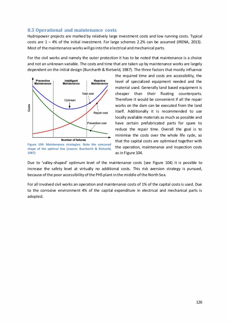
126
8.5 Operational and maintenance costs Hydropower projects are marked by relatively large investment costs and low running costs. Typical
costs are 1 – 4% of the initial investment. For large schemes 2.2% can be assumed (IRENA, 2013).
Most of the maintenance works will go into the electrical and mechanical parts.
For the civil works and namely the outer protection it has to be noted that maintenance is a choice
and not an unknown variable. The costs and time that are taken up by maintenance works are largely
dependent on the initial design (Burcharth & Rietveld, 1987). The three factors that mostly influence
the required time and costs are accessibility, the
level of specialized equipment needed and the
material used. Generally land based equipment is
cheaper than their floating counterparts.
Therefore it would be convenient if all the repair
works on the dam can be executed from the land
itself. Additionally it is recommended to use
locally available materials as much as possible and
have certain prefabricated parts for spare to
reduce the repair time. Overall the goal is to
minimise the costs over the whole life cycle, so
that the capital costs are optimised together with
the operation, maintenance and inspection costs
as in Figure 104.
Due to ‘valley-shaped’ optimum level of the maintenance costs (see Figure 104) it is possible to
increase the safety level at virtually no additional costs. This risk aversion strategy is pursued,
because of the poor accessibility of the PHS plant in the middle of the North Sea.
For all involved civil works an operation and maintenance costs of 1% of the capital costs is used. Due
to the corrosive environment 4% of the capital expenditure in electrical and mechanical parts is
adopted.
Figure 104: Maintenance strategies. Note the concaved shape of the optimal line (source: Burcharth & Rietveld, 1987)
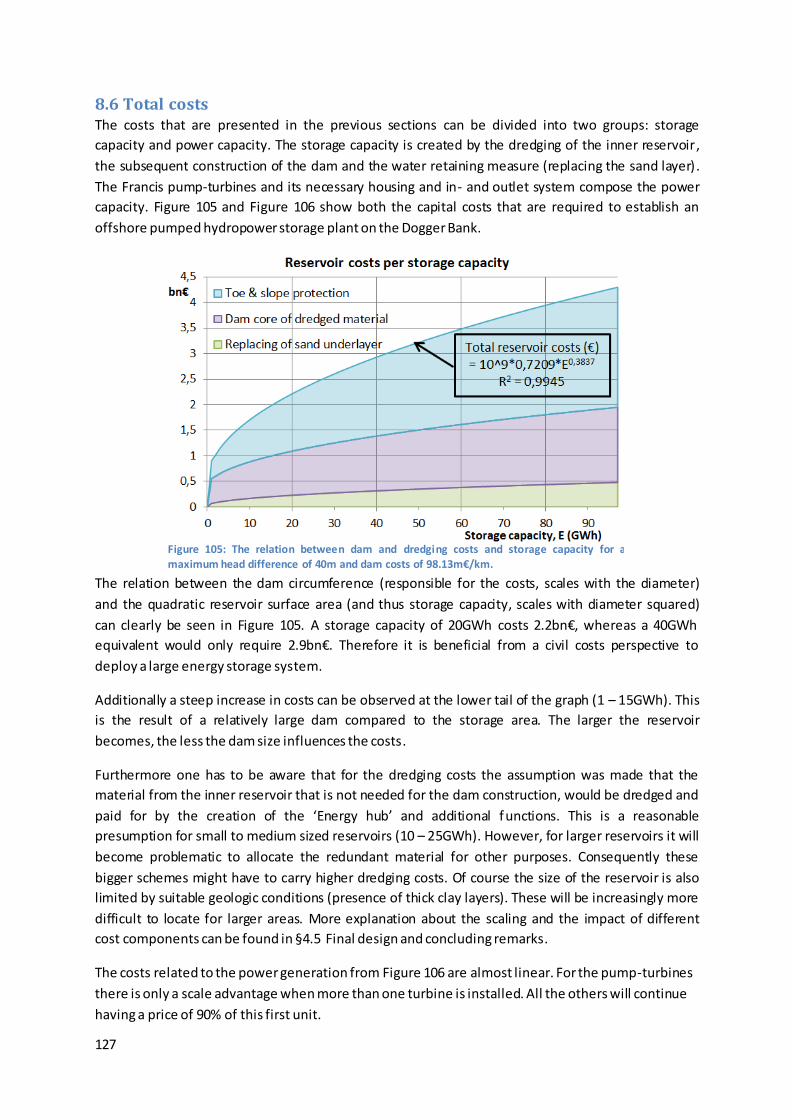
127
8.6 Total costs The costs that are presented in the previous sections can be divided into two groups: storage
capacity and power capacity. The storage capacity is created by the dredging of the inner reservoir,
the subsequent construction of the dam and the water retaining measure (replacing the sand layer).
The Francis pump-turbines and its necessary housing and in- and outlet system compose the power
capacity. Figure 105 and Figure 106 show both the capital costs that are required to establish an
offshore pumped hydropower storage plant on the Dogger Bank.
The relation between the dam circumference (responsible for the costs, scales with the diameter)
and the quadratic reservoir surface area (and thus storage capacity, scales with diameter squared)
can clearly be seen in Figure 105. A storage capacity of 20GWh costs 2.2bn€, whereas a 40GWh
equivalent would only require 2.9bn€. Therefore it is beneficial from a civil costs perspective to
deploy a large energy storage system.
Additionally a steep increase in costs can be observed at the lower tail of the graph (1 – 15GWh). This
is the result of a relatively large dam compared to the storage area. The larger the reservoir
becomes, the less the dam size influences the costs.
Furthermore one has to be aware that for the dredging costs the assumption was made that the
material from the inner reservoir that is not needed for the dam construction, would be dredged and
paid for by the creation of the ‘Energy hub’ and additional functions. This is a reasonable
presumption for small to medium sized reservoirs (10 – 25GWh). However, for larger reservoirs it will
become problematic to allocate the redundant material for other purposes. Consequently these
bigger schemes might have to carry higher dredging costs. Of course the size of the reservoir is also
limited by suitable geologic conditions (presence of thick clay layers). These will be increasingly more
difficult to locate for larger areas. More explanation about the scaling and the impact of different
cost components can be found in §4.5 Final design and concluding remarks.
The costs related to the power generation from Figure 106 are almost linear. For the pump-turbines
there is only a scale advantage when more than one turbine is installed. All the others will continue
having a price of 90% of this first unit.
Figure 105: The relation between dam and dredging costs and storage capacity for a maximum head difference of 40m and dam costs of 98.13m€/km.
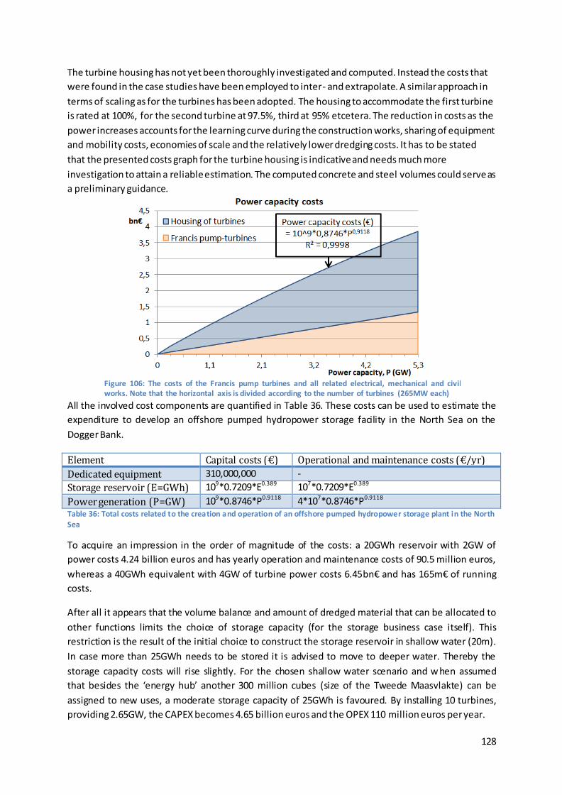
128
Figure 106: The costs of the Francis pump turbines and all related electrical, mechanical and civil works. Note that the horizontal axis is divided according to the number of turbines (265MW each)
The turbine housing has not yet been thoroughly investigated and computed. Instead the costs that
were found in the case studies have been employed to inter- and extrapolate. A similar approach in
terms of scaling as for the turbines has been adopted. The housing to accommodate the first turbine
is rated at 100%, for the second turbine at 97.5%, third at 95% etcetera. The reduction in costs as the
power increases accounts for the learning curve during the construction works, sharing of equipment
and mobility costs, economies of scale and the relatively lower dredging costs. It has to be stated
that the presented costs graph for the turbine housing is indicative and needs much more
investigation to attain a reliable estimation. The computed concrete and steel volumes could serve as
a preliminary guidance.
All the involved cost components are quantified in Table 36. These costs can be used to estimate the
expenditure to develop an offshore pumped hydropower storage facility in the North Sea on the
Dogger Bank.
Element Capital costs (€) Operational and maintenance costs (€/yr)
Dedicated equipment 310,000,000 -
Storage reservoir (E=GWh) 109*0.7209*E0.389 107*0.7209*E0.389
Power generation (P=GW) 109*0.8746*P0.9118 4*107*0.8746*P0.9118 Table 36: Total costs related to the creation and operation of an offshore pumped hydropower storage plant in the North Sea
To acquire an impression in the order of magnitude of the costs: a 20GWh reservoir with 2GW of
power costs 4.24 billion euros and has yearly operation and maintenance costs of 90.5 million euros,
whereas a 40GWh equivalent with 4GW of turbine power costs 6.45bn€ and has 165m€ of running
costs.
After all it appears that the volume balance and amount of dredged material that can be allocated to
other functions limits the choice of storage capacity (for the storage business case itself). This
restriction is the result of the initial choice to construct the storage reservoir in shallow water (20m).
In case more than 25GWh needs to be stored it is advised to move to deeper water. Thereby the
storage capacity costs will rise slightly. For the chosen shallow water scenario and w hen assumed
that besides the ‘energy hub’ another 300 million cubes (size of the Tweede Maasvlakte) can be
assigned to new uses, a moderate storage capacity of 25GWh is favoured. By installing 10 turbines,
providing 2.65GW, the CAPEX becomes 4.65 billion euros and the OPEX 110 million euros per year.
129
8.7 Levelised cost of storage To be able to compare different storage technologies the levelised cost of storage (LCOS) can be
used, just like the levelised cost of energy (LCOE) is used for power plants. It must be clearly
understood that the LCOS does not cover the true benefits of energy storage: energy security and
allowing large shares of renewable energy sources to be integrated into the grid. These and other
benefits will be discussed in the next section.
Although the LCOS suggests that all factors of influence on costs are covered, not all LCOS-analyses
contain the same inputs. Thus one has to be cautious when using LCOS from different sources. In this
analysis the same approach of the World Energy Council (WEC) from 2016 is adopted that was also
used for the comparison between storage technologies earlier in §2.3.6 Comparison of energy
storage technologies:
𝐿𝐶𝑂𝑆 = 𝐼0 +∑
𝐴𝑡(1+ 𝑖)𝑡
𝑛𝑡=1
∑𝑀𝑒𝑙
(1+ 𝑖)𝑡𝑛𝑡=1
- LCOS = Levelised Cost Of energy Storage (€/MWh)
- I0 = Investment costs (CAPEX) (€)
- At = Annual total costs in year t (OPEX) (€)
- Mel = Produced electricity in each year (MWh)
- n = Technical lifetime (years)
- t = Year of technical lifetime (1,2,…,n) (-)
- i = Interest rate (WACC14 = 6.4315) (%)
To get a better insight in how these parameters influence the LCOS and what would be a reasonable
assumption ten scenarios are presented. First a basic situation when afterwards a single parameter is
changed at the time.
- Standard: Power is produced on average for a morning peak of 3 hours and in
the afternoon peak for another 3 hours. The preferred alternative of 25GWh and 2.65GW is
operational for 95% of the time. The lifetime is 50 years, till the pump-turbines and
electrical-mechanical equipment are deteriorated. The interest rate is 6.43% as was
suggested by previous research (De Boer et al., 2007).
- Long lifetime: The operational life is elongated till 80 years, without refurbishment.
- Refurbishment E&M: The operational life is elongated till 80 years, with a full revision of
the turbines and all other electrical and mechanical equipment at a cost of 667m€.
- Low interest: The interest rate is lowered to 5%.
- High generation: Besides the peak-shaving additional power is generated due to the
charging of a surplus of wind energy and discharging at times of shortage. This almost
continuous cycle of buying and selling leads to an electricity production of 10 hours a day.
- Grid deferral: By adding the energy storage facility to the ‘Energy hub’ on the
North Sea, the amount of interconnector cable (IC) capacity can be restricted. The exact ratio
14
WACC = Weighted Average Cost of Capital 15
As was determined by the study for the Energy Island by KEMA and Lievense. This value includes taxes and was found acceptable for an investment made by a governmental body (De Boer et al., 2007).
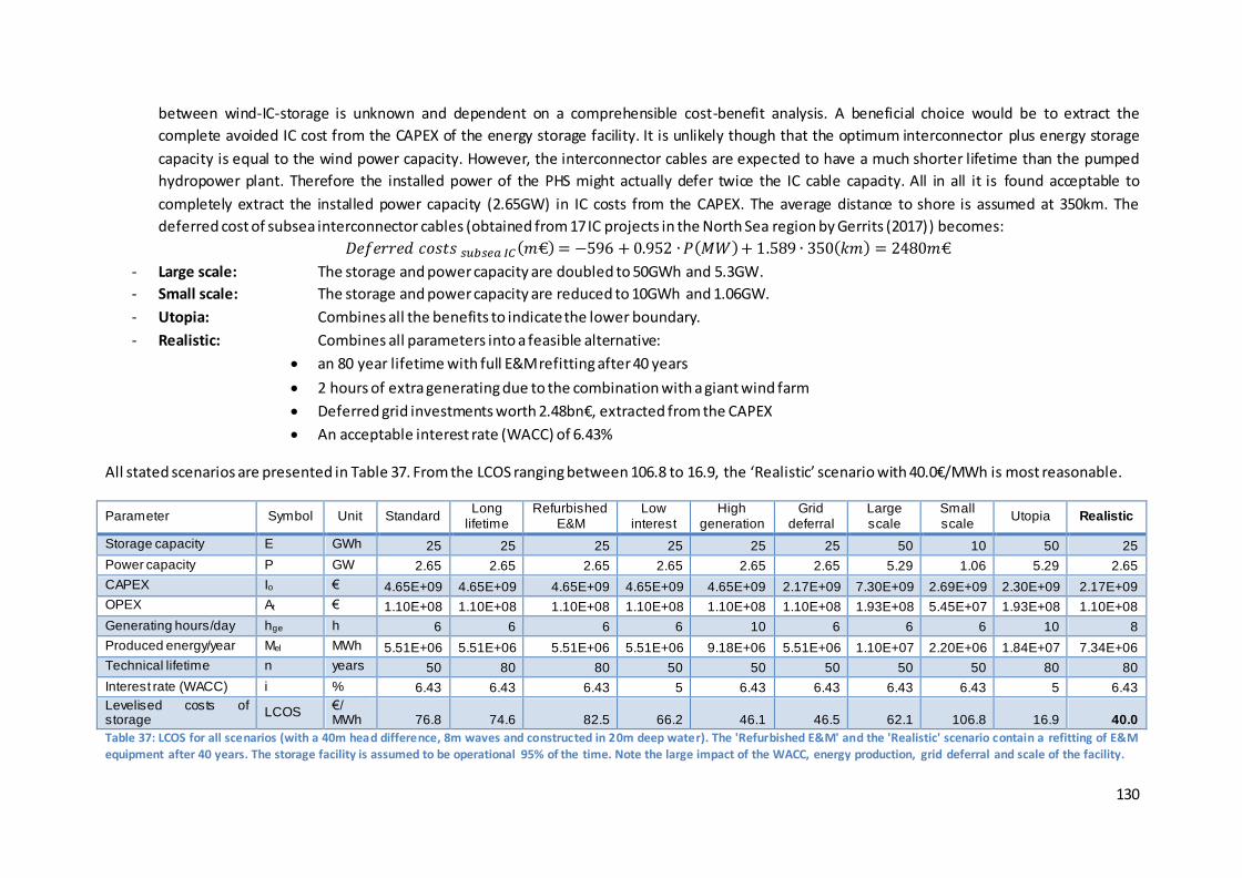
130
between wind-IC-storage is unknown and dependent on a comprehensible cost-benefit analysis. A beneficial choice would be to extract the
complete avoided IC cost from the CAPEX of the energy storage facility. It is unlikely though that the optimum interconnector plus energy storage
capacity is equal to the wind power capacity. However, the interconnector cables are expected to have a much shorter lifetime than the pumped
hydropower plant. Therefore the installed power of the PHS might actually defer twice the IC cable capacity. All in all it is found acceptable to
completely extract the installed power capacity (2.65GW) in IC costs from the CAPEX. The average distance to shore is assumed at 350km. The
deferred cost of subsea interconnector cables (obtained from 17 IC projects in the North Sea region by Gerrits (2017)) becomes:
𝐷𝑒𝑓𝑒𝑟𝑟𝑒𝑑 𝑐𝑜𝑠𝑡𝑠 𝑠𝑢𝑏𝑠𝑒𝑎 𝐼𝐶(𝑚€)= −596 + 0.952 ∙ 𝑃(𝑀𝑊)+1.589 ∙ 350(𝑘𝑚) = 2480𝑚€
- Large scale: The storage and power capacity are doubled to 50GWh and 5.3GW.
- Small scale: The storage and power capacity are reduced to 10GWh and 1.06GW.
- Utopia: Combines all the benefits to indicate the lower boundary.
- Realistic: Combines all parameters into a feasible alternative:
an 80 year lifetime with full E&M refitting after 40 years
2 hours of extra generating due to the combination with a giant wind farm
Deferred grid investments worth 2.48bn€, extracted from the CAPEX
An acceptable interest rate (WACC) of 6.43%
All stated scenarios are presented in Table 37. From the LCOS ranging between 106.8 to 16.9, the ‘Realistic’ scenario with 40.0€/MWh is most reasonable.
Parameter Symbol Unit Standard Long
lifetime Refurbished
E&M Low
interest High
generation Grid
deferral Large scale
Small scale
Utopia Realistic
Storage capacity E GWh 25 25 25 25 25 25 50 10 50 25
Power capacity P GW 2.65 2.65 2.65 2.65 2.65 2.65 5.29 1.06 5.29 2.65
CAPEX Io € 4.65E+09 4.65E+09 4.65E+09 4.65E+09 4.65E+09 2.17E+09 7.30E+09 2.69E+09 2.30E+09 2.17E+09
OPEX At € 1.10E+08 1.10E+08 1.10E+08 1.10E+08 1.10E+08 1.10E+08 1.93E+08 5.45E+07 1.93E+08 1.10E+08
Generating hours/day hge h 6 6 6 6 10 6 6 6 10 8
Produced energy/year Mel MWh 5.51E+06 5.51E+06 5.51E+06 5.51E+06 9.18E+06 5.51E+06 1.10E+07 2.20E+06 1.84E+07 7.34E+06
Technical lifetime n years 50 80 80 50 50 50 50 50 80 80
Interest rate (WACC) i % 6.43 6.43 6.43 5 6.43 6.43 6.43 6.43 5 6.43
Levelised costs of storage
LCOS €/ MWh 76.8 74.6 82.5 66.2 46.1 46.5 62.1 106.8 16.9 40.0
Table 37: LCOS for all scenarios (with a 40m head difference, 8m waves and constructed in 20m deep water). The 'Refurbished E&M' and the 'Realistic' scenario contain a refitting of E&M
equipment after 40 years. The storage facility is assumed to be operational 95% of the time. Note the large impact of the WACC, energy production, grid deferral and scale of the facility.
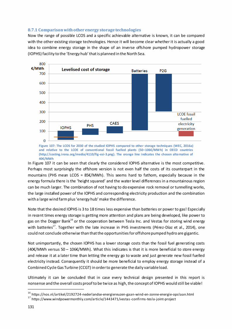
131
8.7.1 Comparison with other energy storage technologies
Now the range of possible LCOS and a specific achievable alternative is known, it can be compared
with the other existing storage technologies. Hence it will become clear whether it is actually a good
idea to combine energy storage in the shape of an inverse offshore pumped hydropower storage
(IOPHS) facility to the ‘Energy hub’ that is planned in the North Sea.
In Figure 107 it can be seen that clearly the considered IOPHS alternative is the most competitive.
Perhaps most surprisingly the offshore version is not even half the costs of its counterpart in the
mountains (PHS mean LCOS = 85€/MWh). This seems hard to fathom, especially because in the
energy formula there is the ‘height squared’ and the water level differences in a mountainous region
can be much larger. The combination of not having to do expensive rock removal or tunnelling works,
the large installed power of the IOPHS and corresponding electricity production and the combination
with a large wind farm plus ‘energy hub’ make the difference.
Note that the desired IOPHS is 3 to 18 times less expensive than batteries or power to gas! Especially
in recent times energy storage is getting more attention and plans are being developed, like power to
gas on the Dogger Bank16 or the cooperation between Tesla Inc. and Vestas for storing wind energy
with batteries17. Together with the late increase in PHS investments (Pérez-Díaz et al., 2014), one
could not conclude otherwise than that the opportunities for offshore pumped hydro are gigantic.
Not unimportantly, the chosen IOPHS has a lower storage costs than the fossil fuel generating costs
(40€/MWh versus 50 – 106€/MWh). What this indicates is that it is more beneficial to store energy
and release it at a later time than letting the energy go to waste and just generate new fossil fuelled
electricity instead. Consequently it should be more beneficial to employ energy storage instead of a
Combined Cycle Gas Turbine (CCGT) in order to generate the daily variable load.
Ultimately it can be concluded that in case every technical design presented in this report is
nonsense and the overall costs proof to be twice as high, the concept of IOPHS would still be viable!
16
https://nos.nl/artikel/2192724-nederlandse-energiereuzen-gaan-wind-en-zonne-energie-opslaan.html 17
https://www.windpowermonthly.com/article/1443471/vestas -confirms-tesla-joint-project
Figure 107: The LCOS for 2030 of the studied IOPHS compared to other storage techniques (WEC, 2016a) and relative to the LCOE of conventional fossil fuelled plants (50–106€/MWh) in OECD countries (http://costing.irena.org/media/4110/fig-esi-3.png). The orange line indicates the chosen alternative of
40€/MWh
132
8.8 Benefits The value of energy storage lies above all in providing energy security. Secondly it enables the
integration of intermittent RES into the grid. Regardless how much wind or solar capacity would be
installed, without energy storage conventional fossil fuelled plants would have to take over when the
wind is not blowing and the sun not shining. Hence the desired reduction in carbon output of 80 –
95% could never be achieved.
Besides these social advantages of safeguarding the electricity supply and allowing the transition
from a fossil fuel based economy to a sustainable market, there are of course also the economic
benefits. Pumped hydro storage is typically profitable in the daily storage cycle, where electricity is
generated for one till ten hours a day. Lately with the development of variable -speed pump-turbines
it is possible to adjust the power output to the second for both the pumping and generating mode.
This possibility opens up a whole new market for PHS in the short-term energy world. Together a
modern PHS facility can thus cover almost all revenue creating applications (see Figure 16 for all
services). Only seasonal storage is not beneficial, due to its low utility rate (Rauwerda, 2017).
To accurately compute the benefits of the energy storage system on the Dogger Bank would be
extremely challenging, because of all the uncertainties in future energy prices, installed wind capacity
and all the connected countries with their own policies and power generation units. As was
concluded in the LCOS section, the business case for offshore PHS is as good as a storage technology
has ever been. Based on this fact and the current trend of developing all kinds of lesser (in costs)
storage alternatives, it could safely be assumed that the studied storage method will be profitable.
In order to get a little bit of an insight in the revenue streams and the payback period, a few future
scenarios are presented in the next section.
Additionally other functions could be added to the energy storage reservoir itself (besides other uses
that can contribute via the redundant material). Some of the possibilities that directl y originate from
the existence of the storage facility are:
- The inner slopes and berm (250m) could be covered in solar panels. Imagine a spatial
coverage of 70% and a 25GWh system (6830m diameter), then the surface covered by
photovoltaic (PV) panels becomes:
0.7 ∙1
4(𝜋 ∙ 𝐷2− 𝜋 ∙ (𝐷 − 250)2) = 1.84𝑘𝑚2 𝑤𝑖𝑡ℎ 0.35
𝐺𝑊
𝑘𝑚→ 0.65𝐺𝑊 𝑜𝑓 𝑃𝑉 𝑐𝑎𝑝𝑎𝑐𝑖𝑡𝑦18
With a 10% capacity factor the annually produced electricity from PV would be 569GWh. This
is equivalent to 5% of the solar production of 2016 in the Netherlands.
- Aquaculture. The inner reservoir could be used to grow mussels, oysters and possibly fish.
Since there is some redundancy in the reservoir depth (40m, where 41.5m is possible) it
could be considered to locally dredge a little deeper to create a minimum water level.
- Biomass. The growing of seaweed to use as biomass for electricity generation offers a lot of
potential19. Just as for the aquaculture it needs to be investigated if the proper (tidal)
conditions are present.
18
0.35GW/km obtained from https://www.deingenieur.nl/artikel/heel -nederland-groen 19
See http://www.wur.nl/nl/show/Seaweed -as-a-source-of-biofuels-and-chemicals.htm for a description of why exactly seaweed is so promising
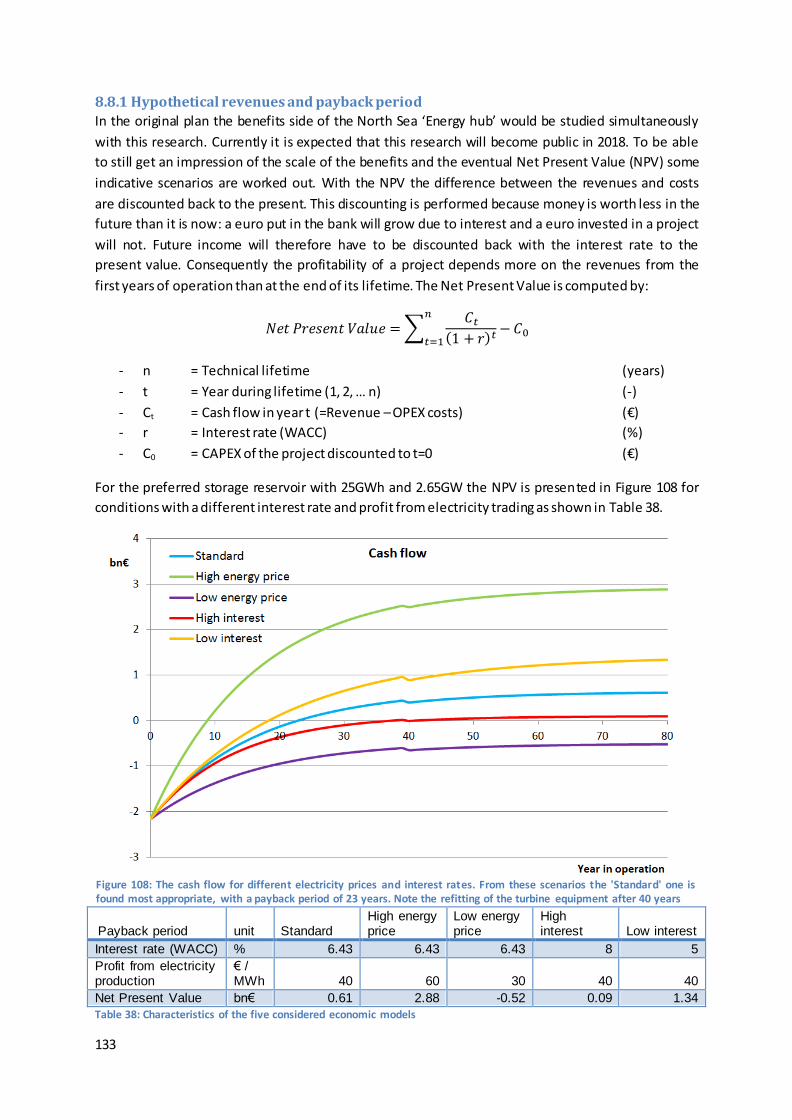
133
8.8.1 Hypothetical revenues and payback period
In the original plan the benefits side of the North Sea ‘Energy hub’ would be studied simultaneously
with this research. Currently it is expected that this research will become public in 2018. To be able
to still get an impression of the scale of the benefits and the eventual Net Present Value (NPV) some
indicative scenarios are worked out. With the NPV the difference between the revenues and costs
are discounted back to the present. This discounting is performed because money is worth less in the
future than it is now: a euro put in the bank will grow due to interest and a euro invested in a project
will not. Future income will therefore have to be discounted back with the interest rate to the
present value. Consequently the profitability of a project depends more on the revenues from the
first years of operation than at the end of its lifetime. The Net Present Value is computed by:
𝑁𝑒𝑡 𝑃𝑟𝑒𝑠𝑒𝑛𝑡 𝑉𝑎𝑙𝑢𝑒 =∑𝐶𝑡
(1 + 𝑟)𝑡−𝐶0
𝑛
𝑡=1
- n = Technical lifetime (years)
- t = Year during lifetime (1, 2, … n) (-)
- Ct = Cash flow in year t (=Revenue – OPEX costs) (€)
- r = Interest rate (WACC) (%)
- C0 = CAPEX of the project discounted to t=0 (€)
For the preferred storage reservoir with 25GWh and 2.65GW the NPV is presented in Figure 108 for
conditions with a different interest rate and profit from electricity trading as shown in Table 38.
Payback period unit Standard High energy price
Low energy price
High interest Low interest
Interest rate (WACC) % 6.43 6.43 6.43 8 5
Profit from electricity production
€ / MWh 40 60 30 40 40
Net Present Value bn€ 0.61 2.88 -0.52 0.09 1.34
Table 38: Characteristics of the five considered economic models
Figure 108: The cash flow for different electricity prices and interest rates. From these scenarios the 'Standard' one is found most appropriate, with a payback period of 23 years. Note the refitting of the turbine equipment after 40 years
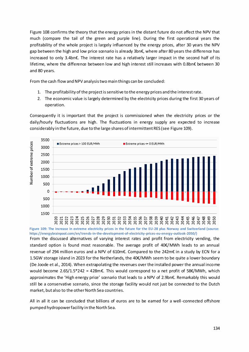
134
Figure 108 confirms the theory that the energy prices in the distant future do not affect the NPV that
much (compare the tail of the green and purple line). During the first operational years the
profitability of the whole project is largely influenced by the energy prices, after 30 years the NPV
gap between the high and low price scenario is already 3bn€, where after 80 years the difference has
increased to only 3.4bn€. The interest rate has a relatively larger impact in the second half of its
lifetime, where the difference between low and high interest still increases with 0.8bn€ between 30
and 80 years.
From the cash flow and NPV analysis two main things can be concluded:
1. The profitability of the project is sensitive to the energy prices and the interest rate.
2. The economic value is largely determined by the electricity prices during the first 30 years of
operation.
Consequently it is important that the project is commissioned when the electricity prices or the
daily/hourly fluctuations are high. The fluctuations in energy supply are expected to increase
considerably in the future, due to the large shares of intermittent RES (see Figure 109).
From the discussed alternatives of varying interest rates and profit from electricity vending, the
standard option is found most reasonable. The average profit of 40€/MWh leads to an annual
revenue of 294 million euros and a NPV of 610m€. Compared to the 242m€ in a study by ECN for a
1.5GW storage island in 2023 for the Netherlands, the 40€/MWh seem to be quite a lower boundary
(De Joode et al., 2014). When extrapolating the revenues over the installed power the annual income
would become 2.65/1.5*242 = 428m€. This would correspond to a net profit of 58€/MWh, which
approximates the ‘High energy price’ scenario that leads to a NPV of 2.9bn€. Remarkably this would
still be a conservative scenario, since the storage facility would not just be connected to the Dutch
market, but also to the other North Sea countries.
All in all it can be concluded that billions of euros are to be earned for a well -connected offshore
pumped hydropower facility in the North Sea.
Figure 109: The increase in extreme electricity prices in the future for the EU-28 plus Norway and Switzerland (source: https://energybrainpool.com/en/trends-in-the-development-of-electricity-prices-eu-energy-outlook-2050/)
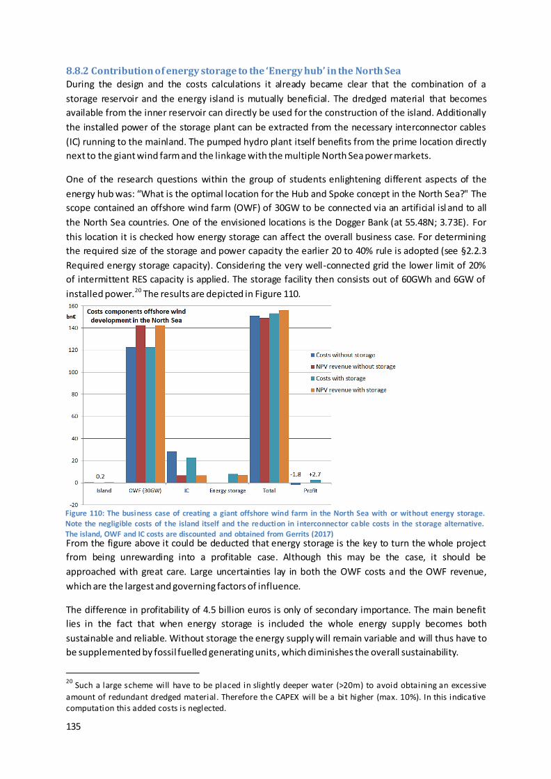
135
Figure 110: The business case of creating a giant offshore wind farm in the North Sea with or without energy storage.
Note the negligible costs of the island itself and the reduction in interconnector cable costs in the storage alternative. The island, OWF and IC costs are discounted and obtained from Gerrits (2017)
8.8.2 Contribution of energy storage to the ‘Energy hub’ in the North Sea
During the design and the costs calculations it already became clear that the combination of a
storage reservoir and the energy island is mutually beneficial. The dredged material that becomes
available from the inner reservoir can directly be used for the construction of the island. Additionally
the installed power of the storage plant can be extracted from the necessary interconnector cables
(IC) running to the mainland. The pumped hydro plant itself benefits from the prime location directly
next to the giant wind farm and the linkage with the multiple North Sea power markets.
One of the research questions within the group of students enlightening different aspects of the
energy hub was: “What is the optimal location for the Hub and Spoke concept in the North Sea?" The
scope contained an offshore wind farm (OWF) of 30GW to be connected via an artificial isl and to all
the North Sea countries. One of the envisioned locations is the Dogger Bank (at 55.48N; 3.73E). For
this location it is checked how energy storage can affect the overall business case. For determining
the required size of the storage and power capacity the earlier 20 to 40% rule is adopted (see §2.2.3
Required energy storage capacity). Considering the very well-connected grid the lower limit of 20%
of intermittent RES capacity is applied. The storage facility then consists out of 60GWh and 6GW of
installed power.20 The results are depicted in Figure 110.
From the figure above it could be deducted that energy storage is the key to turn the whole project
from being unrewarding into a profitable case. Although this may be the case, it should be
approached with great care. Large uncertainties lay in both the OWF costs and the OWF revenue,
which are the largest and governing factors of influence.
The difference in profitability of 4.5 billion euros is only of secondary importance. The main benefit
lies in the fact that when energy storage is included the whole energy supply becomes both
sustainable and reliable. Without storage the energy supply will remain variable and will thus have to
be supplemented by fossil fuelled generating units, which diminishes the overall sustainability.
20
Such a large scheme will have to be placed in slightly deeper water (>20m) to avoid obtaining an excessive
amount of redundant dredged material. Therefore the CAPEX will be a bit higher (max. 10%). In this indicative computation this added costs is neglected.

136
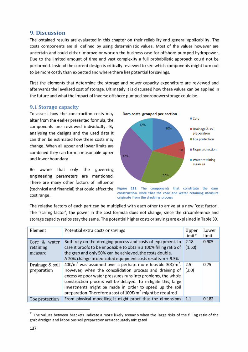
137
9. Discussion The obtained results are evaluated in this chapter on their reliability and general applicability. The
costs components are all defined by using deterministic values. Most of the values however are
uncertain and could either improve or worsen the business case for offshore pumped hydropower.
Due to the limited amount of time and vast complexity a full probabilistic approach could not be
performed. Instead the current design is critically reviewed to see which components might turn out
to be more costly than expected and where there lies potential for savings.
First the elements that determine the storage and power capacity expenditure are reviewed and
afterwards the levelised cost of storage. Ultimately it is discussed how these values can be applied in
the future and what the impact of inverse offshore pumped hydropower storage could be.
9.1 Storage capacity To assess how the construction costs may
alter from the earlier presented formula, the
components are reviewed individually. By
analysing the designs and the used data it
can then be estimated how these costs may
change. When all upper and lower limits are
combined they can form a reasonable upper
and lower boundary.
Be aware that only the governing
engineering parameters are mentioned.
There are many other factors of influence
(technical and financial) that could affect the
cost range.
The relative factors of each part can be multiplied with each other to arrive at a new ‘cost factor’.
The ‘scaling factor’, the power in the cost formula does not change, since the circumference and
storage capacity ratios stay the same. The potential higher costs or savings are explained in Table 39.
Element Potential extra costs or savings Upper limit21
Lower limit
Core & water retaining measure
Both rely on the dredging process and costs of equipment. In case it proofs to be impossible to obtain a 100% filling ratio of the grab and only 50% can be achieved, the costs double. A 20% change in dedicated equipment costs results in +-9.5%
2.18 (1.50)
0.905
Drainage & soil preparation
40€/m2 was assumed over a perhaps more feasible 30€/m2. However, when the consolidation process and draining of excessive poor water pressures runs into problems, the whole construction process will be delayed. To mitigate this, large investments might be made in order to speed up the soil preparation. Therefore a cost of 100€/m2 might be required
2.5 (2.0)
0.75
Toe protection From physical modelling it might proof that the dimensions 1.1 0.182
21
The values between brackets indicate a more likely scenario when the large risks of the fi lling ratio of the grab dredger and laborious soil preparation are adequately mitigated
Figure 111: The components that constitute the dam construction. Note that the core and water retaining measure originate from the dredging process
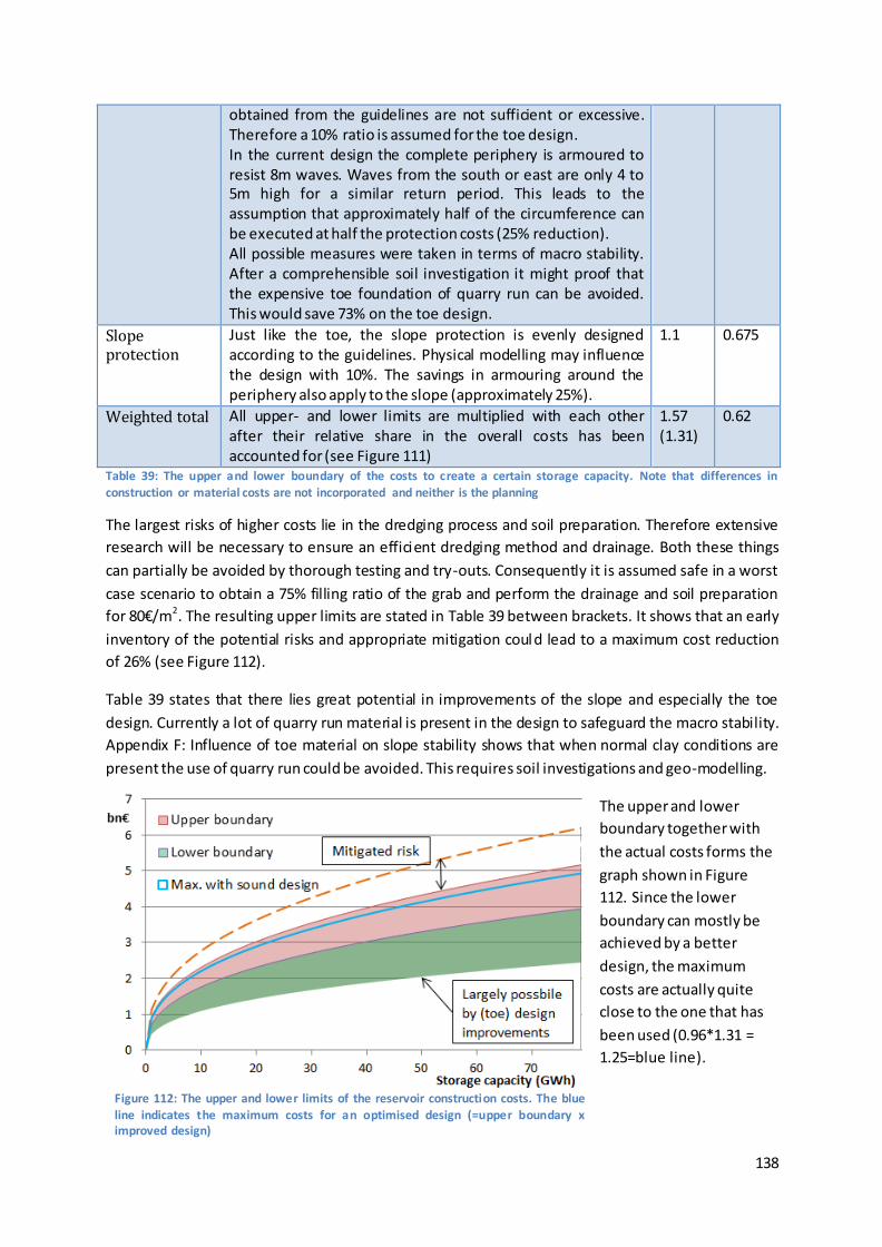
138
Figure 112: The upper and lower limits of the reservoir construction costs. The blue line indicates the maximum costs for an optimised design (=upper boundary x improved design)
obtained from the guidelines are not sufficient or excessive. Therefore a 10% ratio is assumed for the toe design. In the current design the complete periphery is armoured to resist 8m waves. Waves from the south or east are only 4 to 5m high for a similar return period. This leads to the assumption that approximately half of the circumference can be executed at half the protection costs (25% reduction). All possible measures were taken in terms of macro stability. After a comprehensible soil investigation it might proof that the expensive toe foundation of quarry run can be avoided. This would save 73% on the toe design.
Slope protection
Just like the toe, the slope protection is evenly designed according to the guidelines. Physical modelling may influence the design with 10%. The savings in armouring around the periphery also apply to the slope (approximately 25%).
1.1 0.675
Weighted total All upper- and lower limits are multiplied with each other after their relative share in the overall costs has been accounted for (see Figure 111)
1.57 (1.31)
0.62
Table 39: The upper and lower boundary of the costs to create a certain storage capacity. Note that differences in construction or material costs are not incorporated and neither is the planning
The largest risks of higher costs lie in the dredging process and soil preparation. Therefore extensive
research will be necessary to ensure an efficient dredging method and drainage. Both these things
can partially be avoided by thorough testing and try-outs. Consequently it is assumed safe in a worst
case scenario to obtain a 75% filling ratio of the grab and perform the drainage and soil preparation
for 80€/m2. The resulting upper limits are stated in Table 39 between brackets. It shows that an early
inventory of the potential risks and appropriate mitigation could lead to a maximum cost reduction
of 26% (see Figure 112).
Table 39 states that there lies great potential in improvements of the slope and especially the toe
design. Currently a lot of quarry run material is present in the design to safeguard the macro stability.
Appendix F: Influence of toe material on slope stability shows that when normal clay conditions are
present the use of quarry run could be avoided. This requires soil investigations and geo-modelling.
The upper and lower
boundary together with
the actual costs forms the
graph shown in Figure
112. Since the lower
boundary can mostly be
achieved by a better
design, the maximum
costs are actually quite
close to the one that has
been used (0.96*1.31 =
1.25=blue line).
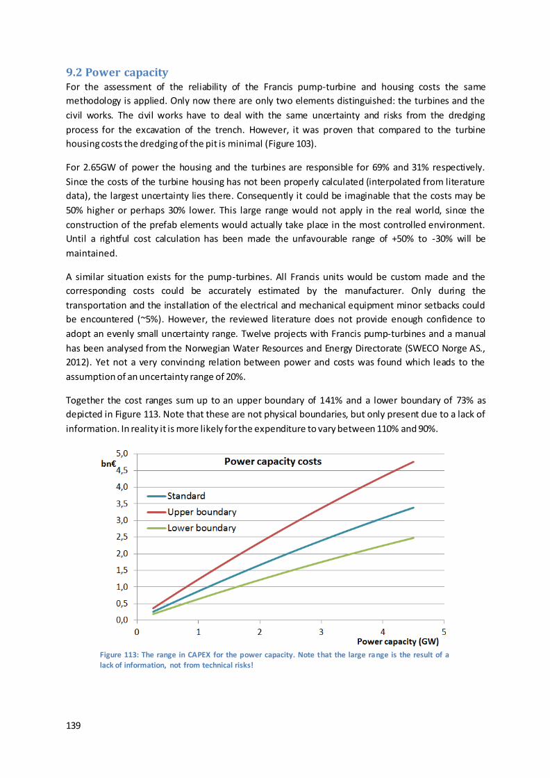
139
9.2 Power capacity For the assessment of the reliability of the Francis pump-turbine and housing costs the same
methodology is applied. Only now there are only two elements distinguished: the turbines and the
civil works. The civil works have to deal with the same uncertainty and risks from the dredging
process for the excavation of the trench. However, it was proven that compared to the turbine
housing costs the dredging of the pit is minimal (Figure 103).
For 2.65GW of power the housing and the turbines are responsible for 69% and 31% respectively.
Since the costs of the turbine housing has not been properly calculated (interpolated from literature
data), the largest uncertainty lies there. Consequently it could be imaginable that the costs may be
50% higher or perhaps 30% lower. This large range would not apply in the real world, since the
construction of the prefab elements would actually take place in the most controlled environment.
Until a rightful cost calculation has been made the unfavourable range of +50% to -30% will be
maintained.
A similar situation exists for the pump-turbines. All Francis units would be custom made and the
corresponding costs could be accurately estimated by the manufacturer. Only during the
transportation and the installation of the electrical and mechanical equipment minor setbacks could
be encountered (~5%). However, the reviewed literature does not provide enough confidence to
adopt an evenly small uncertainty range. Twelve projects with Francis pump-turbines and a manual
has been analysed from the Norwegian Water Resources and Energy Directorate (SWECO Norge AS.,
2012). Yet not a very convincing relation between power and costs was found which leads to the
assumption of an uncertainty range of 20%.
Together the cost ranges sum up to an upper boundary of 141% and a lower boundary of 73% as
depicted in Figure 113. Note that these are not physical boundaries, but only present due to a lack of
information. In reality it is more likely for the expenditure to vary between 110% and 90%.
Figure 113: The range in CAPEX for the power capacity. Note that the large range is the result of a lack of information, not from technical risks!
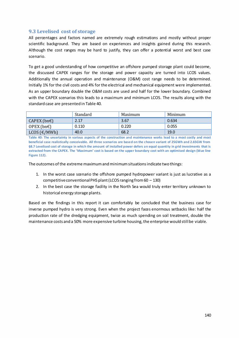
140
9.3 Levelised cost of storage All percentages and factors named are extremely rough estimations and mostly without proper
scientific background. They are based on experiences and insights gained during this research.
Although the cost ranges may be hard to justify, they can offer a potential worst and best case
scenario.
To get a good understanding of how competitive an offshore pumped storage plant could become,
the discussed CAPEX ranges for the storage and power capacity are turned into LCOS values.
Additionally the annual operation and maintenance (O&M) cost range needs to be determined.
Initially 1% for the civil costs and 4% for the electrical and mechanical equipment were implemented.
As an upper boundary double the O&M costs are used and half for the lower boundary. Combined
with the CAPEX scenarios this leads to a maximum and minimum LCOS. The results along with the
standard case are presented in Table 40.
Standard Maximum Minimum
CAPEX (bn€) 2.17 3.67 0.634
OPEX (bn€) 0.110 0.220 0.055
LCOS (€/MWh) 40.0 68.2 19.0 Table 40: The uncertainty in various aspects of the construction and maintenance works lead to a most costly and most
beneficial case realistically conceivable. All three scenarios are based on the chosen variant of 25GWh and 2.65GW from §8.7 Levelised cost of storage in which the amount of installed power defers an equal quantity in grid investments that is extracted from the CAPEX. The ‘Maximum’ cost is based on the upper boundary cost with an optimised design (blue line Figure 112).
The outcomes of the extreme maximum and minimum situations indicate two things:
1. In the worst case scenario the offshore pumped hydropower variant is just as lucrative as a
competitive conventional PHS plant (LCOS ranging from 60 – 130)
2. In the best case the storage facility in the North Sea would truly enter territory unknown to
historical energy storage plants.
Based on the findings in this report it can comfortably be concluded that the business case for
inverse pumped hydro is very strong. Even when the project faces enormous setbacks like: half the
production rate of the dredging equipment, twice as much spending on soil treatment, double the
maintenance costs and a 50% more expensive turbine housing, the enterprise would still be viable.
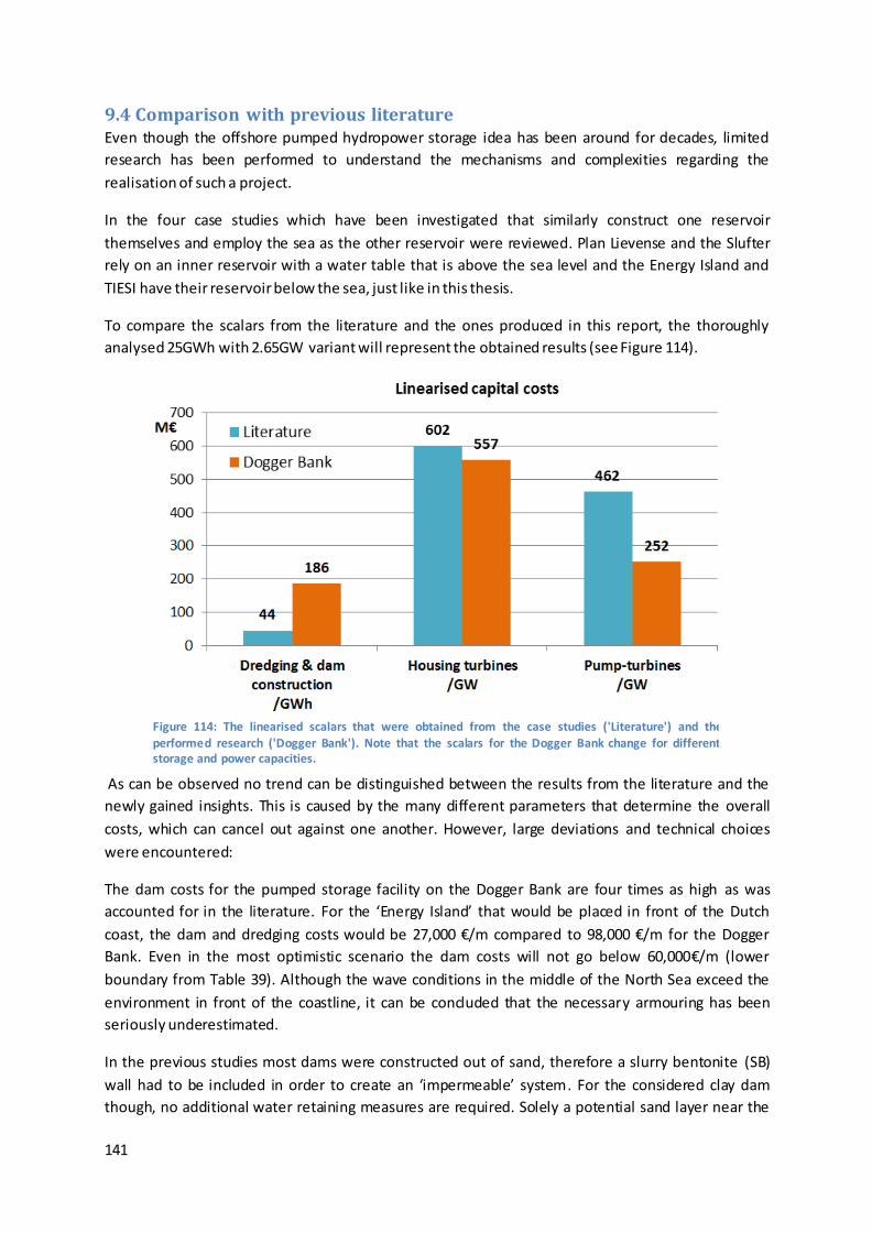
141
9.4 Comparison with previous literature Even though the offshore pumped hydropower storage idea has been around for decades, limited
research has been performed to understand the mechanisms and complexities regarding the
realisation of such a project.
In the four case studies which have been investigated that similarly construct one reservoir
themselves and employ the sea as the other reservoir were reviewed. Plan Lievense and the Slufter
rely on an inner reservoir with a water table that is above the sea level and the Energy Island and
TIESI have their reservoir below the sea, just like in this thesis.
To compare the scalars from the literature and the ones produced in this report, the thoroughly
analysed 25GWh with 2.65GW variant will represent the obtained results (see Figure 114).
As can be observed no trend can be distinguished between the results from the literature and the
newly gained insights. This is caused by the many different parameters that determine the overall
costs, which can cancel out against one another. However, large deviations and technical choices
were encountered:
The dam costs for the pumped storage facility on the Dogger Bank are four times as high as was
accounted for in the literature. For the ‘Energy Island’ that would be placed in front of the Dutch
coast, the dam and dredging costs would be 27,000 €/m compared to 98,000 €/m for the Dogger
Bank. Even in the most optimistic scenario the dam costs will not go below 60,000€/m (lower
boundary from Table 39). Although the wave conditions in the middle of the North Sea exceed the
environment in front of the coastline, it can be concluded that the necessary armouring has been
seriously underestimated.
In the previous studies most dams were constructed out of sand, therefore a slurry bentonite (SB)
wall had to be included in order to create an ‘impermeable’ system . For the considered clay dam
though, no additional water retaining measures are required. Solely a potential sand layer near the
Figure 114: The linearised scalars that were obtained from the case studies ('Literature') and the performed research ('Dogger Bank'). Note that the scalars for the Dogger Bank change for different storage and power capacities.
142
reservoir bottom would need sealing. This can best be executed by dredging and replacing the
conveying material with selected clay.
The turbine housing component is nearly equal, since the costs were estimated by this scalar
obtained from the case studies. The small difference is caused by the assumption that the CAPEX
decline for the housing with 2.5% per installed turbine. The reduction in costs as the power increases
accounts for the learning curve during the construction works, sharing of equipment and mobility
costs, economies of scale and the relatively lower dredging costs. Until a more detailed construction
method and cost computation is made it cannot be said whether the literature over- or
underestimated the costs. It is likely that the housing costs will be lower, because the employed
turbines are twice the size, necessitating only half the number of ‘powerhouses’, penstocks and
tailraces.
The pump-turbines are clearly less costly than previously thought. This is the result of using a turbine
twice as large, 265MW instead of 125MW. Thereby it is proven that it was a misconception that the
costs of a turbine do not relatively decline as the power is increased.
9.5 Remarkable findings In general another few remarkable characteristics were discovered that were either not identified or
ignored in previous research:
A very large inner berm has to be added to overcome the combination of macro slope stability and
uplift at the inner toe.
The optimum depth of the reservoir does not lie between 30 and 40 metres, but much deeper.
Effectively only the water level between the MSL and the seabed needs to be retained by the dam
(which does needs to be high enough to restrict the overtopping). In case the inner reservoir is
excavated below the original seabed, the water level that the dam has to resist remains the
difference between MSL and the seabed. The water level difference between the bottom of the inner
reservoir and the seabed is simply retained by the existing soil (underneath the constructed dam).
The use of a grab dredger takes away the limitation of the practical maximum dredging depth of a
suction dredger. Since the storage capacity is a function of the head difference squared, a deeper
reservoir is preferred, because it will shorten the necessary dam length. For an inverse offshore
pumped hydro storage reservoir the optimal depth will rather approach 60 metres.
The need for shallow water to enable the implementation of an offshore storage system is not as
correct as would be first assumed. Naturally the dam costs will increase when it is located in deeper
water. However, the dam costs only form about a third of the total capital expenditure. In case a
storage system larger than 25GWh is desired the facility should gradually move to deeper waters. If
not, it is likely that the amount of material that becomes available (>500 million cubic metres) cannot
be allocated to other purposes (the ‘energy hub’ requires about 200 million cubic metres). The
depositing and transporting of left over material is unwanted and it would be favourable to move to
deeper water instead.
A larger reservoir (>25GWh) does benefit from its scale compared to smaller alternatives. This scaling
advantage counters the added dam costs induced by the larger water depth. Consequently the
relation exists: “the larger the reservoir, the deeper the water depth should be”. Therefore the

143
inverse storage plant is not limited to depths of maximally 20 metres, but more likely to 40 metres
(afterwards the dam and armouring costs will counter all scale benefits). Ultimately the concept of
inverse pumped hydropower storage has a much wider application range than was until recently
believed.
The influence of cavitation on the design for the turbine housing is immense. To avoid this
catastrophic phenomenon the turbines need to be installed at depths far below the bottom of the
storage reservoir (14 – 18 metres). Additionally a draft tube that enables the maximum use of the
head difference between the reservoirs is necessary. This draft tube reaches a depth of roughly three
times the runner diameter. For a 40m head difference the maximum depth of the powerhouse
extends till 90 metres below mean sea level.
The challenges regarding the turbine housing were not clearly identified and pose a critical obstacle
in the realisation of the whole energy storage scheme. The proposed construction method with
modular box caissons is deemed appropriate to deal with the circumstances and consequently
enable the implementation of an inverse offshore pumped hydropower storage facility.
It should be noted that the results are certainly not l imited to a single case on the Dogger Bank,
rather they are universally applicable. The stated design choices and relative costs components may
act as guidance from which the given formulae and factors could easily be transposed to any other
case. By doing so it can quickly be assessed if an inverse PHS system is possible and whether it
provides a profitable business case.

144
145
10. Conclusion Billions of euros lay for the taking in the newly emerged storage market. Therefore the offshore
pumped hydropower storage plant does not only offer environmental benefits (integrating large
shares of RES to combat climate change) or societal benefits (employing thousands of people) it is
also extremely lucrative from an economic perspective.
In this chapter the main conclusions of the performed research are first briefly stated when
afterwards the choice and the scaling of the four building blocks of the storage facility ( dam,
dredging, turbines and housing) are elaborated. Thereby the research question: “How do the costs of
an offshore pumped hydropower storage facility on the Dogger Bank scale with the power and
storage capacity, using existing construction technologies?” will be answered and reflected upon.
Regarding the technical characteristics and scaling it was found that:
- Constructing an inverse offshore pumped hydropower storage facility in the middle of the
North Sea that can cope with the discussed failure mechanisms is possible.
- As the head difference between the reservoirs is increased the overall (not per metre) dam
costs decline. This is characteristic for inverse offshore pumped hydropower.
- The optimum depth of the reservoir does not lie between 30 and 40 metres, but will rather
approach 60 metres (enabled by the use of a grab dredger).
- A large storage reservoir is more economical compared to a smaller one from a civil costs
perspective. Storage systems smaller than 10GWh should be avoided.
- In case the pumped hydro system is built in 20 metre deep water a storage capacity of
25GWh is preferred for the wind development plans in the North Sea. In case a storage
system larger than 25GWh is desired the facility should gradually move to deeper waters to
limit the amount of material that becomes available.
- The inverse storage plant is not limited to depths of maximally 20 metres, but more likely to
40 metres for reservoirs larger than 40GWh (afterwards the dam and armouring costs will
counter all scale benefits).
Concerning the costs and benefits an alternative with a 25GWh reservoir and 2.65GW of installed
power has been researched, which showed:
- The levelised cost of storage for various (economic) conditions is estimated to vary between
16.9 and 106.8€/MWh of which 40€/MWh appears most reasonable for an energy storage
system connected to the North Sea countries and a large wind farm (~10GW).
- Due to technical uncertainties in the present soil conditions, equipment and design the LCOS
of 40€/MWh may range from 68.2€/MWh to 19.0€/MWh in the relative worst and best case
scenario.
- In the worst case scenario the offshore pumped hydropower variant is just as lucrative as a
competitive conventional PHS plant (LCOS ranging from 60 – 130)
- In the best case the storage facility in the North Sea would truly enter territory unknown to
any historical energy storage plant.
- The 40€/MWh would make offshore PHS 3 to 18 times less expensive than batteries or
power to gas (both are currently under consideration to incorporate the large shares of wind
energy from the North Sea).
146
- It is more beneficial to store energy and release it at a later time than letting the energy go to
waste and just generate new fossil fuelled electricity instead. This is caused by the fact that
the chosen facility has a lower storage costs than fossil fuel generating costs (40€/MWh
versus 50 – 106€/MWh).
- The considered reservoir is expected to have a Net Present Value of 610 million euros, which
could reasonably become 2.9 billion euros.
- The profitability of the project is sensitive to the energy prices and the interest rate.
- The economic value is largely determined by the electricity prices during the first 30 years of
operation.
The whole research into energy storage was instigated by the plans for the development of a massive
wind farm (>30GW) on the Dogger Bank via an artificially created island. The cost of the island,
offshore wind farm and the interconnector cables were acquired simultaneously by Gerrits (2017).
Therefore a scenario with and without storage could be developed. Although large uncertainties lay
in especially the wind farm costs and revenues, it did show promising results: For a 30GW wind farm
and all related costs the NPV ended up at minus 1.8 billion euros. By adding an adequate storage
system (6GW of installed power) the value turned into a plus of 2.7 billion euros.
All signs and gathered results point in the same direction: the opportunities for offshore pumped
hydropower storage are immense. There are first-mover advantages while largely relying on late-
mover technology. In other words: operating such a large scale storage facility, without comparable
competition (monopoly), could lead to large profits. While the research and development costs,
which are usually exceptionally high for pioneering concepts, stay limited since almost all technology
used has been long proven.
Though it is certainly helpful, the profitability of adding storage to a renewable energy powered
economy is only of secondary importance. The main benefit lies in the fact that when energy storage
is included the whole energy supply can become both sustainable and reliable. Without storage the
energy supply will remain variable and will thus have to be supplemented by fossil fuelled generating
units, which diminishes the overall sustainability.
This research presents the first viable offshore pumped hydropower storage facility that is
undoubtedly lucrative, without relying on potential revenues or investments from other functions.
Thereby it may offer a valuable link in the transition towards a green economy and within the
development of large scale offshore wind energy in the North Sea.
147
In the following sections the general conclusions from the technical design of the four building blocks
are stated. It should be noted that the scalars are certainly not limited to a single case on the Dogger
Bank, rather they are universally applicable. With the stated design choices and relative costs
components, combined with some engineering judgement, the given formulae and factors could
easily be transposed to any other case.
10.1 Dam design The design of the dam roughly consists out of three aspects: The outer protection against waves, the
inner slope and the water retaining measure that is used to seal the underlying water conveying sand
layer.
An Xbloc design was made for the sea defence, because of its ability to deal with extreme wave
conditions, large dependence on locally sourced core material and a less-brittle failure mode than a
caisson structure. It proofed that for the whole dam the costs are for two-thirds shaped by the
armouring against the severe wave environment. Therefore massive savings can be accomplished
when the pumped storage plant would be located in calmer waters.
Due to the local geology and the bursting criteria, the maximum head difference would be 41.45m of
which 40 metres was chosen as a practical limit. A large inner berm was added in order to deal with
the combination of inner slope stability and the uplift/bursting mechanism at the inner toe. This
mixture of forces led to an inner berm of 113m wide!
In order to operate the storage reservoir, the top sand layer has to be sealed. From the various
techniques that can do so, the simple dredging and replacing the sand with firm clay option i s
favoured. The sand layer that lays between -43m and -50m relative to MSL will be replaced with the
‘work with work’ method for a costs of 11,825€/m.
From the seepage computations it appeared that, when choosing very conservative permeability
characteristics, the leakage through the dam, retaining measure and underlying clay could all be
neglected. The final design passed all the safety criteria that were considered. The dam costs
including the sealing measure are estimated at 98,130€/m. This clay dam is able to resist a water
level difference of 40m and waves of 8m.
10.2 Dredging process In order to reuse the dredged clay directly in the core of the dam it was found that the clay has to be
dredged mechanically. Hydraulic dredging would destroy the good qualities of clay and turn it into an
impractical slurry. From the discussed two working methods it can be concluded that the achievable
production rate is governing. The conventional grad dredgers and barges can only operate in calm
waters, which would be an exception for the North Sea. By using a semi-submerged vessel for the
dredging and a jack-up pontoon for the transport, the whole procedure becomes almost
independent from the wave conditions.
In order to dredge the stiff glacial clay dedicated grabbers need to be made. These specialised
grabbers are mounted on a semi-submersible vessel that is powered by a dynamic positioning system
to maintain its location. The dredged material is then transported and placed via a conveyor belt
system and over a specifically made jack-up pontoon. The investment costs of the grabbers (0.5 x
30m€) and the semi-sub (0.5 x 300m€) are shared with the creation of the Energy Island. The jack-up

148
platform (100m€) is solely used for the dam construction and will be fully paid for. These are all
conservative assumptions, since the dredging equipment will definitely still have a rest value.
Based on the large price difference the innovative ‘semi-sub & convey’ construction process is the
chosen alternative. It is a convenient paradox that due to the harsh working conditions on the North
Sea eventually a very efficient dredging process was developed. The semi-submersible and jack-up
platform optimally benefit from the unique occasion of having to transport such large volumes over a
very short distance. In total 310 million euros are required to invest in dedicated dredging equipment
to construct the dam. For a storage reservoir on the Dogger Bank with a 40m head difference the
dredging unit price is 3.4€/m3.
10.3 Power generation To limit the need for civil works a turbine was chosen that can both generate power and pump water
back up. Since the Francis type is able to achieve slightly higher efficiencies than the Kaplan
equivalent and the Francis one was recommended by all the previous studies in similar conditions, it
is the preferred choice.
It was discovered that it is much more economical to install a few large turbines, instead of many
small turbines. Hence, the largest pump-turbine (which is feasible today) and capable of converting a
700m3/s discharge into 265MW is the favoured choice at an estimated cost of 73.3 million euros per
unit (excluding the additional costs for a stainless steel runner and cathodic protection). The
discharges and dimensions are comparable to the two largest hydropower projects in the world: The
Three Gorges Dam in China and the Itaipu Dam on the border of Brazil and Paraguay.
The effect of cavitation managed to have a drastic impact on the turbine design. To prevent
disastrous under pressures in and around the turbines, the units need to be placed sufficiently far
below the lower reservoir level. Since the installation depths for all turbine sizes were problematic,
the largest turbine was chosen anyway. Although the civil works are more costly per turbine the
number of required penstocks and tailraces decrease, leading to an overall saving.
In order to deal with the corrosive saline environment measures had to be taken. Experience from
the Okinawa Yanbaru seawater PHS plant and various tidal energy plants proof that using a stainless
steel runner, and cathodic protection for other steel parts is ample to deal with the harsh
surroundings (Fujihara et al., 1998; Rijkswaterstaat et al., 1985).
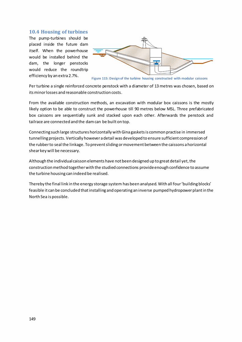
149
10.4 Housing of turbines The pump-turbines should be
placed inside the future dam
itself. When the powerhouse
would be installed behind the
dam, the longer penstocks
would reduce the roundtrip
efficiency by an extra 2.7%.
Per turbine a single reinforced concrete penstock with a diameter of 13 metres was chosen, based on
its minor losses and reasonable construction costs.
From the available construction methods, an excavation with modular box caissons is the mostly
likely option to be able to construct the powerhouse till 90 metres below MSL. Three prefabricated
box caissons are sequentially sunk and stacked upon each other. Afterwards the penstock and
tailrace are connected and the dam can be built on top.
Connecting such large structures horizontally with Gina gaskets is common practise in immersed
tunnelling projects. Vertically however a detail was developed to ensure sufficient compression of
the rubber to seal the linkage. To prevent sliding or movement between the caissons a horizontal
shear key will be necessary.
Although the individual caisson elements have not been designed up to great detail yet, the
construction method together with the studied connections provide enough confidence to assume
the turbine housing can indeed be realised.
Thereby the final link in the energy storage system has been analysed. With all four ‘building blocks’
feasible it can be concluded that installing and operating an inverse pumped hydropower plant in the
North Sea is possible.
Figure 115: Design of the turbine housing constructed with modular caissons
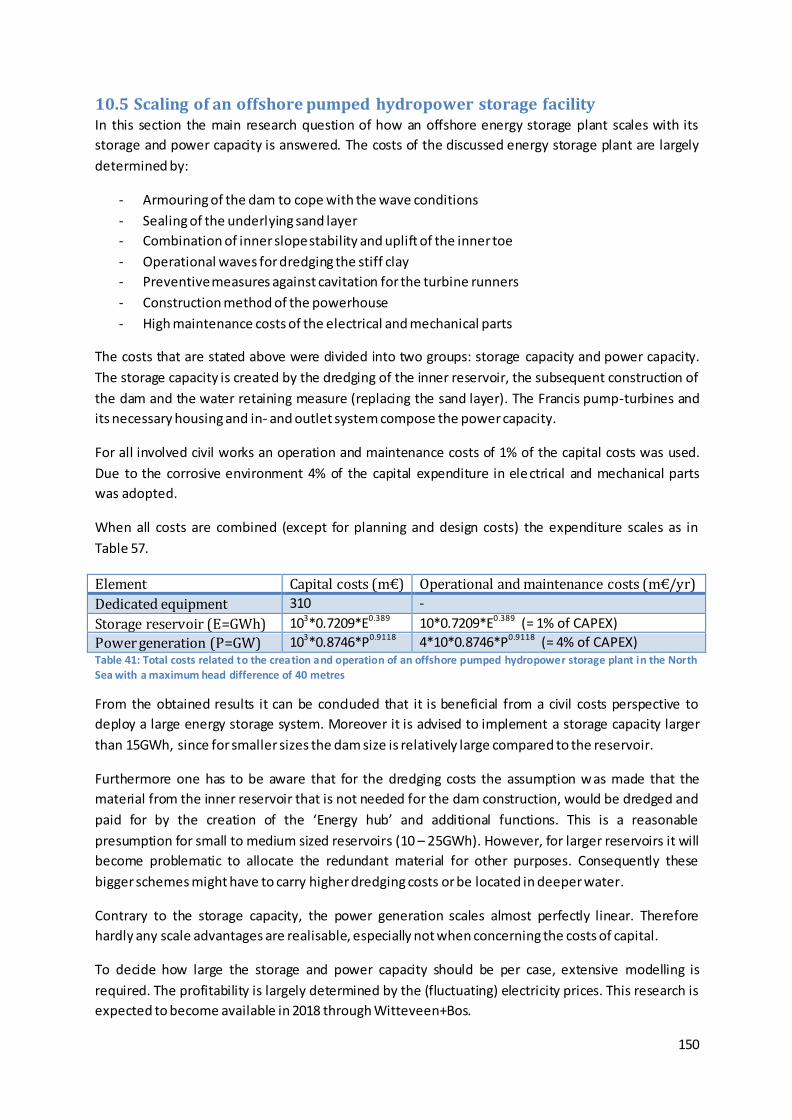
150
10.5 Scaling of an offshore pumped hydropower storage facility In this section the main research question of how an offshore energy storage plant scales with its
storage and power capacity is answered. The costs of the discussed energy storage plant are largely
determined by:
- Armouring of the dam to cope with the wave conditions
- Sealing of the underlying sand layer
- Combination of inner slope stability and uplift of the inner toe
- Operational waves for dredging the stiff clay
- Preventive measures against cavitation for the turbine runners
- Construction method of the powerhouse
- High maintenance costs of the electrical and mechanical parts
The costs that are stated above were divided into two groups: storage capacity and power capacity.
The storage capacity is created by the dredging of the inner reservoir, the subsequent construction of
the dam and the water retaining measure (replacing the sand layer). The Francis pump-turbines and
its necessary housing and in- and outlet system compose the power capacity.
For all involved civil works an operation and maintenance costs of 1% of the capital costs was used.
Due to the corrosive environment 4% of the capital expenditure in electrical and mechanical parts
was adopted.
When all costs are combined (except for planning and design costs) the expenditure scales as in
Table 57.
Element Capital costs (m€) Operational and maintenance costs (m€/yr)
Dedicated equipment 310 -
Storage reservoir (E=GWh) 103*0.7209*E0.389 10*0.7209*E0.389 (= 1% of CAPEX)
Power generation (P=GW) 103*0.8746*P0.9118 4*10*0.8746*P0.9118 (= 4% of CAPEX) Table 41: Total costs related to the creation and operation of an offshore pumped hydropower storage plant in the North Sea with a maximum head difference of 40 metres
From the obtained results it can be concluded that it is beneficial from a civil costs perspective to
deploy a large energy storage system. Moreover it is advised to implement a storage capacity larger
than 15GWh, since for smaller sizes the dam size is relatively large compared to the reservoir.
Furthermore one has to be aware that for the dredging costs the assumption w as made that the
material from the inner reservoir that is not needed for the dam construction, would be dredged and
paid for by the creation of the ‘Energy hub’ and additional functions. This is a reasonable
presumption for small to medium sized reservoirs (10 – 25GWh). However, for larger reservoirs it will
become problematic to allocate the redundant material for other purposes. Consequently these
bigger schemes might have to carry higher dredging costs or be located in deeper water.
Contrary to the storage capacity, the power generation scales almost perfectly linear. Therefore
hardly any scale advantages are realisable, especially not when concerning the costs of capital.
To decide how large the storage and power capacity should be per case, extensive modelling is
required. The profitability is largely determined by the (fluctuating) electricity prices. This research is
expected to become available in 2018 through Witteveen+Bos.

151
152
11. Recommendations The idea of Luc Lievense about artificially creating an energy storage reservoir has been laying on the
shelf for nearly four decades. At the time wind energy did not develop as quickly as initially expected
and the project lost interest. Nowadays offshore wind is being installed and planned on an
unprecedented scale, making the business case for energy storage more lucrative than it has ever
been before. Therefore the time to initiate the realisation of inverse pumped hydropower storage is
now.
The performed research proves that energy storage can be a valuable contribution to the planned
North Sea ‘energy hub’. Although at first the location was planned at the Dogger Bank, Gerrits (2017)
found that it may be more advantageous to commence the whole wind project further into Danish
waters. Thereby the sensitive natural area of the Dogger Bank would be avoided. The obtained
results show that the storage system is versatile and could evenly be constructed in deeper water (up
to 40 metres). The sole restriction is the presence of an appropriate clay layer.
In order to attain more profound knowledge of the optimal dam design, best time of investment and
required storage and power capacities, some recommendations are made. They are stated in the
same order of: dam, dredging, turbines, housing and benefits.
Dam & reservoir
Most important to realise the offshore pumped hydropower storage facility is a detailed soil
investigation. The presence and condition of the clay can determine whether the project is practically
feasible. Slight differences in soil properties between the assumed and actual values can already
result in large savings or additional expenses for the dam design.
Other failure modes like settlement (partially dealt with for the outer protection), collision by ships
or drifting ice should be investigated. The drifting ice loads both from the North Sea as from the inner
reservoir need to be quantified. The Dogger Bank sea water temperature varies from 5°C to 15°C
(Eisma, 2006). Therefore only drifting ice may pose a threat.
From guidelines it was concluded that micro stability for embankments with a clay core does not
pose a threat. However rapid drawdown of the water table in the inner reservoir should still be
regarded.
The effect of infiltration on the phreatic line in the dam has to be analysed. A raised water table leads
to lower effective soil stresses and thereby shear resistance.
The inner slope protection of the dam for during the construction phase is yet to be optimised. See
§Slope protection during construction.
Possibly a crown wall against run-up may be advantageous. Adding a crown wall to limit the run-up
and corresponding discharge over the crest might be more economical than a high dam (plus its
larger inner berm required for the stability).
The dam closure operation needs special attention. No serious problems are expected since the tidal
differences and flow velocities are relatively limited (compared to for example the Deltawerken in
the Netherlands).
153
The unknown achievable depth together with an unconvincing history led to the fact that jet-
grouting was set aside. After further research and a comprehensive reliability study, jet-grouting
might become a potential candidate to seal an underlying sand layer.
Effects of an offshore energy storage facility and the in- and outflow on surrounding morphology.
Similarly the occurrence of sedimentation or erosion of the inner reservoir needs studying. The
sequential in- and outflow may cause the formation of gullies and channels in the reservoir bottom.
In an extreme case this might affect the stability of the clay layer, which would result in a restriction
of maintaining a minimum water level to reduce local flow velocities. Therefore it could lead to a
reduction in effective storage capacity.
How the water quality in the inner reservoir is affected by (temporary) stagnation of the water table.
Dredging
The possibilities regarding the use of RES for dredging operations are recommended for future
studies (using the neighbouring energy hub for the construction of the dam).
The influence the conveying transportation method and the dropping of clay above the water level
have on the clay properties.
Turbines
It can be interesting to research the possibility of using a Kaplan pump-turbine. In case it can be
positioned higher than the Francis alternative or the draft tube would not need to be as deep then it
might be more competitive, since it requires less excavation and civil works. Alternatively the use of
horizontally placed axis Francis turbines or inverted Francis turbine could reduce the necessary
runner and draft tube depth. The extra costs that come with these options, due to smaller turbine
sizes, can then be weighed against the reduced housing costs per turbine.
Housing of turbines
Better insight in turbine housing costs and the proposed construction method. A question that
remains is whether it is possible to apply the same construction process for a deeper reservoir
(~60m). In case there proofs to be a (practical) limit the statement of: “the largest achievable head
difference is recommended” might have to be adjusted.
In order to achieve the desired lifetime of the pumped hydropower plant, the presence of sulphates
and other chemicals in the clay or soil that can harm concrete should be investigated.
Benefits
The benefits of energy storage on both a societal and financial level need further understanding.
Compared to electricity generating plants, storage provides other advantages like energy security or
the integration of large shares of RES. Those assets are hard to quantify and monetise.
Energy price modelling is required to estimate the revenues and best time of commissioning.
Thereby the expected peak in prices around 2025 – 2035 needs to be weighed against the larger
fluctuations and spot prices around 2050 and afterwards.
Ultimately the contribution of other functions to the storage facility need studying like solar panels
on the inner slope and berm, aquaculture and biomass inside the reservoir, natural areas, port and
marina facilities, recreation and housing.

154
155
Bibliography Abadal, A. M., Dornhelm, E., Elakel, M., Feys, C., & Naderi, N. (2017). Energy hub in the North Sea. TU
Delft.
Alvarado-Ancieta, C. A. (2012). Kostenschätzung 2012 für die elektrische und mechanische
Ausrüstung des Krafthauses in Wasserkraft- und Pumpspeicher-Projekten. Wasserkraft & Energie, 22-
35.
Anastasopoulos, I., Gerolymos, N., Drosos, V., Kourkoulis, R., Georgarakos, T., & Gazetas, G. (2007).
Nonlinear Response of Deep Immersed Tunnel to Strong Seismic Shaking. Journal of Geotechnical
and Geoenvironmental Engineering, 133(9), 1067-1090. doi:10.1061/(asce)1090-
0241(2007)133:9(1067)
Bakker, K. J. (2014, September). Immersed tunnels [PDF].
Barends, F. B.J., & Uffink, G. J.M. (2006). Groundwater mechanics, flow and transport.
Beurskens, J., De Haan, S., Bauer, P., & Dieleman, R. (2014). Taiwan integrated energy storage island.
Alliander.
Bezuyen, K. G., Stive, M. J.F., Vaes, G. J.C., Vrijling, J. K., & Zitman, T. J. (2012). Inleiding
waterbouwkunde. Delft, The Netherlands: TU Delft.
Börger, T., Hattam, C., Burdon, D., Atkins, J. P., & Austen, M. C. (2014). Valuing conservation benefits
of an offshore marine protected area. Ecological Economics, 108, 229-241.
doi:10.1016/j.ecolecon.2014.10.006
Boscardin, M., Patterson, C., Landis, M., Younan, J. C., & Aghjayan, D. (2006). Evaluation of
permeability of containment slurry walls. In GeoCongress 2006: Geotechnical Engineering in the
Information Technology Age. Atlanta, GA: American Society of Civil Engineers.
Bricker, J. (2016, June 1). Pumped storage power [PDF].
Burcharth, H. F., & Rietveld, C. F. W. (1987). Construction, Maintenance and Repair as Elements in
Rubble Mound Breakwater Design. Paper presented at The 2nd international Conference on Coastal
and Port Engineering In Developing Countries, Beijing, China.
CIRIA, CUR, CETMEF (2007). The Rock Manual. The use of rock in hydraulic engineering (2nd edition).
C683, CIRIA, London
CIRIA. (2009). A guide to costs standards for dredging equipment. London, UK: Author.
Clerens, P. (2016). An overview on energy storage - what are the prerequisites for its European
integration? EASE
Van Corven, T. A. W. (2015). Construction of the new lock in Terneuzen using pneumatic caissons: A
construction alternative to conventional construction methods (Master's thesis, TU Delft, Delft, The
Netherlands). Retrieved from https://repository.tudelft.nl/islandora/object/uuid:5f203b83-fe87-
4221-8912-1c9a1aa095ae/datastream/OBJ
156
De Boer, W. W., Verheij, F. J., Moldovan, N., Van der Veen, W., Groeman, F., Schrijner, M., …
Zwemmer, D. (2007). Energie-eiland, de haalbaarheid van drie verschillende opties van energieopslag
voor Nederland. KEMA Consulting/Lievense.
De Ingenieur. (2015). Lievense, de man van het opslagbekken. De Ingenieur. Retrieved from
https://www.deingenieur.nl/artikel/lievense-de-man-van-het-opslagbekken
De Ingenieur. (2016, June 13). [Schematisation of North Sea (wind) infrastructure]. Retrieved from
https://www.deingenieur.nl/artikel/gigantisch-stopcontact-op-eiland-doggersbank
De Joode, J., Özdemir, Ö., & Van Hout, M. (2014). The market value of large scale electricity storage
options (ECN-E--14-042). ECN.
Delta Marine Consultants. (2014). Guidelines for Xbloc concept designs. Retrieved from
http://www.xbloc.com/downloads/brochures-and-drawings-and-videos/xbloc-design-
guidelines/item556
Delte Marine Consultants. (n.d.). Calculator | Armour Layer Design Tool for Xbloc® Breakwater Units.
Retrieved from http://www.xbloc.com/technical-information/calculator/item697
Deutsche Energie-Agentur. (2017). Power to gas. Retrieved from
http://www.powertogas.info/power-to-gas/
DNV GL. (2015). Energy storage roadmap NL 2030. KEMA
Dickson, G. (2017, June). European wind power. Opening&keynotes. Symposium conducted at
WindDays, Amsterdam.
EASE. (2017). Energy storage technologies. Retrieved from http://ease-storage.eu/energy-
storage/technologies/
Eisma, D. (2006). Dredging in coastal waters. London, UK: Taylor & Francis.
Energy Storage Association. (2017). Compressed Air Energy Storage (CAES). Retrieved from
http://energystorage.org/compressed-air-energy-storage-caes
EMU Ltd, SKM Enviros, RPS Energy, BTO, Anatec Ltd, Brown & May Marine Ltd, & Cork Ecology.
(2011). Dogger Bank zonal characterisation (11/J/1/06/1761/1218). Forewind.
eStorage. (2015). Overview of potential locations for new pumped storage plants in EU 15,
Switzerland and Norway (D4.2 Final Report).
European Commission. (2012). Energy roadmap 2050
European Commission. Directorate-General for Energy. (2016). EU energy in figures: Statistical
pocketbook
European Power to Gas Platform. (2017). Power to gas. Retrieved from
http://www.europeanpowertogas.com/index
Forewind. (2015). The geology of Dogger Bank: Geological factsheet.
157
Frölke, G. (2017). Nature enhancing opportunities for coastal defences: Opportunity study for the
Dogger Bank (Master's thesis, TU Delft, Delft, The Netherlands).
Fujihara, T., Imano, H., & Oshima, K. (1998). Development of pump turbine for seawater pumped-
storage power plant (5). Hitachi Review
Garg, A., Lay, C., & Füllmann, R. (2012). Stored energy in sea: The feasibility of an underwater pumped
hydro storage system [Powerpoint slides]. Retrieved from http://docplayer.net/8559477-Stensea-
stored-energy-in-sea-the-feasibility-of-an-underwater-pumped-hydro-storage-system-dr-andreas-
garg-christoph-lay-robert-fullmann.html
Gerrits, S. B. J. (2017). Feasibilty study of the hub and spoke concept in the North Sea: Developing a
site selection model to determine the optimal location (Master's thesis, TU Delft, Delft, The
Netherlands).
Gimeno-Gutiérrez, M., & Lacal-Arántegui, R. (2013). Assessment of the European potential for
pumped hydropower energy storage: A GIS-based assessment of pumped hydropower storage
potential. Luxembourg: Publications Office of the European Union.
Heinberg, R., & Fridley, D. (2016). Our renewable future: Laying the path for 100% clean energy .
Himelic, J., & Novachek, F. (2011). Sodium sulfur battery energy storage and its potential to enable
further integration of wind (wind-to-battery project) (Final Report). Retrieved from Xcel website:
https://www.xcelenergy.com/staticfiles/xe-
responsive/Energy%20Portfolio/Renewable%20Energy/Renewable%20Development%20Fund/rdf-
completed-wind-projects-milestone-final-report.pdf
Hydro Equipment Association. (2013). Hydro equipment technology roadmap. Retrieved from
http://www.thehea.org/roadmap
Imre, E., Nagy, L., Lőrincz, J., Rahemi, N., Schanz, T., Singh, V., & Fityus, S. (2015). Some comments on
the entropy-based criteria for piping. Entropy, 17(4), 2281-2303. doi:10.3390/e17042281
Intergovernmental Panel on Climate Change. (2013). IPCC Fifth Assessment Report (AR5). Geneva:
WMO, IPCC Secretariat.
International Energy Agency (IEA). (2014). Technology roadmap: Energy storage
International Energy Agency (IEA). (2016). World Energy Outlook 2016
International Partnership for Hydrogen and Fuel Cells in the Economy (IPHE). (2011). Utsira wind
power and hydrogen plant. Retrieved from http://www.statoil.com/en/NewsAnd-
Media/Multimedia/features/Pages/ HydrogenSociety.aspx
IRENA. (2017). REthinking Energy: Accelerating the global energy transformation . Abu Dhabi:
International Renewable Energy Agency.
IRENA. (2013). Renewable power generation costs in 2012: An overview.
158
Kempener, R., & De Vivero, G. (2015). Renewables and electricity storage. A technology roadmap for
REmap 2030. IRENA.
Kempton, W., & Tomić, J. (2005). Vehicle-to-grid power fundamentals: Calculating capacity and net
revenue. Power Sources, 144, 268-279.
Kibrit, B. (2013). Pumped hydropower storage in the Netherlands (Master's thesis, TU Delft, Delft, The
Netherlands). Retrieved from http://repository.tudelft.nl/islandora/object/uuid%3A6f98d3d5-6454-
4e20-af5e-5b8615dcaba0?collection=education
Kvale, E. P. (2006). The origin of neap–spring tidal cycles. Marine Geology, 235(1-4), 5-18.
doi:10.1016/j.margeo.2006.10.001
Lazard. (2015). Lazard's levelized cost of storage analysis (Version 1.0). Retrieved from
https://www.lazard.com/media/2391/lazards-levelized-cost-of-storage-analysis-10.pdf
Letcher, T. M. (2016). Pumped hydroelectric storage. In Storing energy: with special reference to
renewable energy sources (pp. 25-38).
Makhijani, A., Mills, C., & Ramana, M. V. (2012). Renewable Minnsesota: A technical and economic
analysis of a 100% renewable energy-based electricity system for Minnesota. Institute for Energy and
Environmental Research.
Marence, M. (2016, May). Powerhouse and M&E equipment [PDF].
Marence, M. (2014). Storage and hydropower: Exercise - turbine design [PowerPoint slides].
Miller, J. (2013, January 29). Typical U.S. power supply and demand load curves [Graph]. Retrieved
from http://www.theenergycollective.com/jemiller_ep/178096/expanded-wind-and-solar-power-
increase-need-natural-gas
Ministerie van Economische Zaken. (2016). Energieagenda: Naar een CO2-arme energievoorziening.
Ministerie van Verkeer en Waterstaat. (2007). Voorschrift Toetsen op Veiligheid Primaire
Waterkeringen. Den Haag: Author.
Nederlands Normalisatie-instituut. (2016). NEN 9997-1 Geotechnisch ontwerp van constructies - Deel
1: Algemene regels.
NIOZ, Deltares, IMARES, & Rijkswaterstaat. (2015). De staat van de Noordzee. Noordzeedagen.
Peeters, P. (2012). Integratie toetsing, inspectie en monitoring [Powerpoint slides]. Retrieved from
https://www.slideshare.net/Waterbouwkundiglaboratorium/eerste-stappen
Peng, F., Wang, H., Tan, Y., Xu, Z., & Li, Y. (2011). Field Measurements and Finite-Element Method
Simulation of a Tunnel Shaft Constructed by Pneumatic Caisson Method in Shanghai Soft Ground.
Journal of Geotechnical and Geoenvironmental Engineering, 137(5), 516-524.
doi:10.1061/(asce)gt.1943-5606.0000460
Pepers, R. (2011, October). Pneumatische caissons Noord-Zuidlijn Amsterdam. KOersief, 85, 16.
159
Pérez-Díaz, J.I., Cavazzini, G., Blázquez, F., Platero, C., Fraile-Ardanuy, J., Sánchez, J.A. and Chazarra,
M. (2014). Technological developments for pumped-hydro energy storage, Technical Report,
Mechanical Storage Subprogramme, Joint Programme on Energy Storage, European Energy Research
Alliance
Posthumus, A., & Van der Vegte, H. (2017, June). WindStock: Haalbaarheid windmolens,
energieopslag en zonnepanelen. Windenergie en energieopslag: Een veel belovende kans. Symposium
conducted at WindDays, Amsterdam.
Rauwerda, A. (2017, June). A sustainable energy future will be hybridized. R&D projects and required
technical developments. Symposium conducted at WindDays, Amsterdam.
Rahman, F., Rehman, S., & Abdul-Majeed, M. A. (2012). Overview of energy storage systems for
storing electricity from renewable energy sources in Saudi Arabia. Renewable and Sustainable Energy
Reviews, 16(1), 274-283. doi:10.1016/j.rser.2011.07.153
Rijkswaterstaat, Hollandsche Beton Groep NV, Ballast Nedam Groep NV, & Raadg. Ing. Bur. Lievense.
(1985). Pomp accumulatie centrale Noordzeekust (Hoofdrapportage fase 1).
Rudelle, G. (2016). eStorage project update [Powerpoint slides]. Retrieved from
http://www.estorage-project.eu/wp-content/uploads/2013/06/3-eStorage-WS4-2016-GE-Project-
presentation.pdf
San Martín, J. I., Zamora, I., San Martín, J. J., Aperribay, V., & Eguía, P. (2011). Energy storage
technologies for electric applications. In International conference on renewable energies and power
quality (ICREPQ'11). Las Palmas de Gran Canaria, Spain: Author.
Schiereck, G. J. (2004). Introduction to bed, bank and shore protection, Engineering the interface of
soil and water. Delft, The Netherlands: VSSD.
Simbolotti, G., & Kempener, R. (2012). Electricity storage technology brief (E18). Retrieved from
IRENA website: http://www.irena.org/Publications
Sündermann, J., & Pohlmann, T. (2011). A brief analysis of North Sea physics. Oceanologia, 53(3),
663-689. doi:10.5697/oc.53-3.663
Sumer, B. M., & Fredsøe, J. (2005). The mechanics of scour in the marine environment. Singapore:
World Scientific.
SWECO Norge AS. (2012). Cost base for hydropower plants. Retrieved from Norwegian Water
Resources and Energy Directorate website: http://www.nve.no
Timmer, H., & Van Zuijlen, E. (2017, June). Opening & Keynotes. Symposium conducted at WindDays,
Amsterdam.
Trelleborg Ridderkerk BV. (n.d.). Gina Gasket. Retrieved from www.trelleborg.com/infrastructure
Uamusse, M. M., Aljaradin, M., & Persson, K. M. (2017). Micro-hydropower plant - Energy solution
used in rural areas, Mozambique. Sustainable Resources Management, 1(1).
doi:10.5281/zenodo.255257

160
Ugarte, S., Larkin, J., Van der Ree, B., Swinkels, V., Voogt, M., Friedrichsen, N., … Michaelis, J.
(2015a). Energy storage: Which market designs and regulatory incentives are needed? Retrieved from
European Parliament website: http://www.europarl.europa.eu/studies
Ugarte, S., Larkin, J., Van der Ree, B., Swinkels, V., Voogt, M., Friedrichsen, N., … Michaelis, J.
(2015b). At a glance. Energy storage: Which market designs and regulatory incentives are
needed? Retrieved from European Parliament website: http://www.europarl.europa.eu/studies
Van den Bos, J. P. (2017a, March 10). Breakwaters and closure dams: Breakwaters cross-sectional
design [PDF].
Van den Bos, J. P. (2017b, March 17). Breakwaters and closure dams: Constructability and project
execution [PDF].
Van der Hage, R. (2017, June). Offshore grid roll out. Trends in the offshore wind system. Symposium
conducted at WindDays, Amsterdam.
Van der Meer, J. W. (2002). Technical report wave run-up and wave overtopping at dikes. Technical
Advisory Committee on Flood Defence, The Netherlands.
Van Duivendijk, J. (n.d.). Water power engineering: Principles and characteristics [PDF].
Van 't Hoff, J., & Van der Kolff, A. N. (2012). Hydraulic fill manual: For dredging and reclamation
works (1st edition). Boca Raton, FL: CRC Press/Balkema Taylor & Francis Group.
Vandycke, S. (2002). Dredging stiff to very stiff clay in the Wielingen using the DRACULA system on a
hopper dredger. Terra et Aqua, 89.
Verhagen, H. J., D'Angremond, K., & Van Roode, F. (2012). Breakwaters and closure dams (Second
edition). Delft, The Netherlands: VSSD.
Waterpowermagazine. (2000, August 14). Japanese pumped storage embraces the ocean waves.
Retrieved from http://www.waterpowermagazine.com/features/featurejapanese-pumped-storage-
embraces-the-ocean-waves/
World Energy Council (WEC). (2016a). E-storage: Shifting from cost to value wind and solar
applications. Retrieved from http://www.europeanpowertogas.com/documents
World Energy Council (WEC). (2016b). Variable renewable energy sources integration in electricity
systems: How to get it right. Retrieved from www.worldenergy.org
World Energy Council (WEC). (2016c). World energy scenarios: The grand transition. Retrieved from
www.worldenergy.org
Yamamoto, M., & Morooka, C. K. (2005). Dynamic positioning system of semi-submersible platform
using fuzzy control. Journal of the Brazilian Society of Mechanical Sciences and Engineering , 27(4),
449-455. doi:10.1590/s1678-58782005000400014
161
List of figures Figure 1: World primary energy consumption per fuel type from 1850 to 2014, based on data from
BP, Statistical Review of World Energy (source: Heinberg & Fridley, 2016) ...................................... 15
Figure 2: European Union 2020 objectives for renewable energy source (RES) shares in the energy
mix (source: European Commission, 2016) ................................................................................... 16
Figure 3: The renewable power capacity worldwide and its growth rate over the last years (source:
Irena, 2017) ................................................................................................................................. 16
Figure 4: Typical power curve in the United States (source: Miller, 2013) ........................................ 17
Figure 5: The hourly supply and demand of energy for Minnesota, USA, in a hypothetical 100% RES
scenario during a week (Wed – Tue) in July, 2007. Note how energy storage and withdrawal levels
the difference between the intermittent supply and the energy demand (source: Makhijani et al.,
2012) .......................................................................................................................................... 17
Figure 6: The loss of revenue according to network operators in Germany (Timmer & Van Zuijlen,
2017), mostly due to insufficient energy storage and grid capacity between the (enlarged) wind
power generation in the north and the energy demand in the south (source: Dickson, 2017) ........... 18
Figure 7: Flexibility options that can help absolving the differences in electric energy supply and
demand (source: Posthumus & Van der Vegte, 2017)....................................................... 18
Figure 8: The hypothetical location on the Dogger Bank of the energy hub with its interconnector
cables indicated with the dashed lines (top) and an impression of the envisioned island by TenneT
(bottom). The figure was modified from Van der Hage (2017) and Börger et al. (2014) .................... 19
Figure 9: The existing storage technologies and their global share in energy storage (source: IRENA,
2017) .......................................................................................................................................... 20
Figure 10: An artist impression of an inverse offshore pumped hydropower storage plant (source: De
Boer et al., 2007) ......................................................................................................................... 21
Figure 11: Value of storage in the whole energy chain (source: Ugarte et al., 2015a) ....................... 26
Figure 12: Focus on energy storage per level ................................................................................. 27
Figure 13: Decrease in gross annual energy consumption in million toe (source: European
Commission, 2012) ...................................................................................................................... 28
Figure 14: Range of fuel shares in primary energy consumption (%) (source: European Commission,
2012) .......................................................................................................................................... 29
Figure 15: Share of variable renewable energy generated (source: IEA, 2014) ................................. 29
Figure 16: Energy storage applications categorised by their power output, time of discharge and their
location in the energy chain (source: IEA, 2014) ............................................................................. 31
Figure 17: Schematisation of a PHS system (left) and the development of PHS in the EU (right)
(source: Letcher, 2016 and Pérez-Díaz et al., 2014) ........................................................................ 32
Figure 18: Pumped hydro storage facility Hohenwarte 2, Germany (source: Deutsche Energie-
Agentur)...................................................................................................................................... 32
Figure 19: The Okinawa Yanbaru seawater PHS plant in Japan (source: Fujihara et al., 1998) ............ 34
Figure 20: Schematization of a CAES system (source: San Martín et al., 2011).................................. 35
Figure 21: The McIntosh CAES plant in Alabama, USA (source:
https://www.wired.com/2010/03/compressed-air-plants/) ........................................................... 36
Figure 22: Schematization of a classic battery (left) and a flow battery (right) (source:
http://hyperphysics.phy-astr.gsu.edu/hbase/Chemical/electrochem.html) 37
Figure 23: The sodium-sulfur battery connected to the wind farm (source: Himelic & Novacheck,
2011) .......................................................................................................................................... 38
162
Figure 24: V2G schematisation within a smart-grid (source:
http://www.seminarreports.in/2013/05/vehicle-to-grid.html) ....................................................... 39
Figure 25: Power to gas technology and possible applications (source: Deutsche Energie -Agentur) .. 40
Figure 26: Power to gas to power schematization (source: http://energy.sia-partners.com/enabling-
integration-renewables-europes-energy-system)........................................................................... 40
Figure 27: The wind power and hydrogen plant in Utsira, Norway (source: IPHE, 2011) .................... 41
Figure 28: Maturity level of energy storage technologies (source: IEA, 2014) ................................... 42
Figure 29: Range of levelised cost of storage for various technologies (source: WEC, 2016a) ............ 43
Figure 30: Levelised cost of storage for various technologies in combination with a wind farm (source:
WEC, 2016a) ................................................................................................................................ 44
Figure 31: Realisable potential per country (source: eStorage, 2015) .............................................. 47
Figure 32: Relation between storage capacity and costs (left) and between power and costs (right) . 49
Figure 33: Costs breakdown (left) and linearized 'scaling' components (right) further explained in
Appendix B .................................................................................................................................. 49
Figure 34: The stepwise design approach of the inverse offshore pumped hydropower facility ........ 51
Figure 39: Failure tree of operation based on the functional requirements...................................... 53
Figure 40: Failure tree of the dam ................................................................................................. 54
Figure 41: Reservoir design with the parameters that are necessary as input. The numbers used for
the parameters are given in Table 10. The maximum and minimum head depend on till what depth
the reservoir is excavated............................................................................................................. 55
Figure 42: The relation between the storage capacity, average head difference and reservoir
diameter ..................................................................................................................................... 57
Figure 43: The volume balance depends on the relation between the initial water depth, the required
dam size and the volume that needs to be excavated from the inner reservoir to attain the desired
head difference ........................................................................................................................... 58
Figure 44: Design process of the dam ............................................................................................ 60
Figure 45: Cross section of outer dam protection. All measures are in metres. This is a preliminary
design, a few adjustments where necessary to meet the macro stability criterion as explained in
§4.3.4.1 Macro stability. ............................................................................................................... 61
Figure 46: Layout of a toe on a sandy seabed (source: Delta Marine Consultants, 2014) ................... 62
Figure 47: The inner side of the dam with the various slopes that are considered during the design
phase .......................................................................................................................................... 65
Figure 48: Probability density function of the wind speed at the Dogger Bank and near- and onshore
for reference (source: Gerrits, 2017) ............................................................................................. 65
Figure 49: Nomogram valid for shallow and intermediate waters (source: Bezuyen et al., 2012) ....... 66
Figure 50: Inner slope protection. All measures are in metres and relative to the reservoir bottom. . 68
Figure 51: Phreatic line through the dam according to the Depuit method. Note that no infiltration
from precipitation is taken into account. Due to the hard surface on the crest and the nature of the
material used for the dam, infiltration is neglected. ....................................................................... 69
Figure 52: Possible measures that can be taken to 'close' the sand layer: 1) Slurry bentonite wall. 2)
Sheet piles. 3) Jet grouting. 4) Replacement of sand layer. ............................................................. 70
Figure 53: The construction sequence of a jet-grouted wall (source: http://udc.com.vn/en)............. 71
Figure 54: Slope stability of the trench to replace the sand layer. The critical sliding mechanism
through the stiff clay and the sand has a safety factor of 1.08 ........................................................ 72
163
Figure 55: The costs of the retaining measures as they progress over depth. The mean sea level is
20m above the bed level. The slurry bentonite wall is assumed to be installed from 3m above the sea
level and have a maximum length of 60m. Therefore the maximum reachable depth of the SB wall is
37m. ........................................................................................................................................... 73
Figure 56: Most occurring failure mechanisms for dikes (source: Peeters, 2012) .............................. 74
Figure 57: Schematisation of a slope stability analysis. The slices are in vertical force equilibrium. The
resulting moments (M1+M2) and shear force along the circular failure plain are in moment
equilibrium (source: Bezuyen et al., 2012). .................................................................................... 76
Figure 58: The uplift mechanism that is caused by a water overpressure under the clay layer (source:
Van 't Hoff & Van der Kolff, 2012) ................................................................................................. 76
Figure 59: Critical sliding plane for the outer slope. Under uniform top load of 100kN/m2 and a
maximally developed scour hole in front of the toe ....................................................................... 77
Figure 60: The critical sliding mechanism for the inner slope. The continuous phreatic line at +20m
(=MSL) is the water pressure in the bottom sand layer, which tries to uplift the thick clay layer.
Without the large inner berm the slope would only have a safety factor of close to 1.0 ................... 78
Figure 61: The influence of the inner berm on the shear resistance. When there is no surcharge on
the reservoir bottom there is almost no effective soil stress, the difference between the green and
blue pressures (right). Hence the inner berm is added to create sufficient shear stress in the thick clay
layer to prevent sliding failure (left). ............................................................................................. 78
Figure 62: The dam design that is checked safe from a macro stability perspective. Note that the
inner berm solely consists out of material that remains untouched (it has not been dredged and
deposited there like the rest of the dam). The continuous phreatic line at +20m (=MSL) is the water
pressure in the bottom sand layer, which tries to uplift the thick clay layer. The other phreatic line
reflects the water table for the other layers. ................................................................................. 79
Figure 63: The type of micro-instability depends on the type of dike: a homogeneous clay dike poses
no threat (1), a sand dike is susceptible to the washing out of material (2), a sand core with clay cover
can cause excessive pressure on the (impermeable) clay layer and ‘push’ it off (3). (source: Ministerie
van Verkeer en Waterstaat, 2007) ................................................................................................ 80
Figure 64: The development of piping for a river dike: Water level rises (a) ; Seepage initiates (b) ;
Sand boil appears (c) ; Backward erosion (d-e) ; Failure (f) (source: Imre et al., 2015)....................... 81
Figure 65: Seepage through the dam (Qd) and the underlying clay layer (Qu) when the recharge of the
aquifer (QA) is equal to the discharge through the clay layer (QA = Qu)............................................. 82
Figure 66: The difference in water pressure over an impermeable layer. To prevent bursting of the
clay, the self-weight of the clay layer has to outbalance the difference in water pressure acting from
underneath. ................................................................................................................................ 84
Figure 67: The level of the crest height, set to resist the various mechanisms of run-up, set-up, sea
level rise and settlement (source: Van der Meer, 2012).................................................................. 85
Figure 68: The dam design with the various materials that are used. The scales are in metres. ......... 86
Figure 69: The total costs of the dam and dredging works per storage capacity, with the original
seabed 20 metres below MSL. Note the rapid decline in capital costs once the head difference
between the reservoirs increases.................................................................................................. 86
Figure 70: The relation between costs and storage capacity for a maximum head difference of 40m
and dam costs of 86.31m€/km. The dashed line is the trend line of which the equation and reliability
number (R2) is given to easily approximate the costs...................................................................... 88
164
Figure 71: Schematic top view of the pumped hydropower reservoir. Note that the material, which is
necessary for the dam construction can be dredged directly next to the future dam. The material in
the centre is available for the island and additional functions. ........................................................ 90
Figure 72: Suction dredgers: plain suction dredger (top left), cutter suction dredger (bottom left) and
trailing suction hopper dredger (right) (source: Van 't Hoff & Van der Kolff, 2012) ........................... 90
Figure 73: Mechanical dredgers: backhoe dredger (top left), grab dredger (bottom left) and bucket
dredger (right) (source: Van 't Hoff & Van der Kolff, 2012).............................................................. 90
Figure 74: The formation of clay balls by pipeline transport (source: Van 't Hoff & Van der Kolff, 2012)
................................................................................................................................................... 90
Figure 75: The largest grab dredger in the World: Gosho (200m3) used for a terminal reclamation
project in Singapore (2016). It uses a counterweight system to reduce the energy consumption and
simplify the hoisting mechanism (source: http://www.kk-
kojimagumi.co.jp/english/news/excepteur_sint_occaecat_cupidatat_non.html) ............................. 91
Figure 76: A backhoe with a maximum dredging depth of 32m (left) (source:
http://www.jandenul.com/en/ equipment/fleet/backhoe-dredger) and a split hopper barge (middle
and right) (source: Van den Bos, 2017b; https://www.vanoord.com/activities/hopper-barge-and-
pushbuster) ................................................................................................................................. 91
Figure 77: An offshore wind turbine installation vessel performing its jack-up tests (top) and a
working platform (bottom) (source: http://www.ziton.eu/wp-content/uploads/WIND-SERVER-jacked-
03-low-res.jpg; http://www.thinkdefence.co.uk/ship-to-shore-logistics/ increment-2-pier/) ............ 92
Figure 78: A semi-submersible accommodation vessel for harsh environments (left). It can host 750
people on board and is powered by a dynamic positioning system (right). Ordered for 200 million
USD (source: http://worldmaritimenews.com/archives/89220/cosco-nantong-secures-
accommodation-vessel-order/; Yamamoto & Morooka, 2005)........................................................ 93
Figure 79: Schematisation of the dredging process using four grab dredgers, which are mounted on
one semi-submersible vessel and a jack-up pontoon, both fitted with conveyor belts. The striped
black lines indicate the extendable conveyor belts to adjust for movements of the semi-submersible
platform and allow for flexibility ................................................................................................... 94
Figure 76: The dependence of the dredging capacity on the depth and the cycle time, with a 100%
filling ratio of the bucket .............................................................................................................. 95
Figure 81: The total dredging costs for a storage reservoir with a 40m maximum head difference and
5545m3/m of dam to be dredged. The grab & barge process is more competitive till 7.7GWh,
afterwards the semi-sub & convey process is preferred ................................................................. 99
Figure 82: Silt screens directly attached to the grab dredgers. Note the difference in turbidity in- and
outside the silts screens (source: https://nippon.zaidan.info/ seikabutsu/2000/00736/images/174-
1.jpg) ........................................................................................................................................ 100
Figure 83: A one MWh battery storage container with 1.2MW of nominal power (source:
http://usiscored.com/?product=1-mwh-energy-storage-system&v=47e5dceea252) ...................... 100
Figure 84: Schematisation of the powerhouse and in- and outlet works (top) and the application field
of turbines (bottom) (source: i01.i.aliimg.com/img/pb/928/662/252/1275966164919_hz-
fileserver3_2089574.jpg; Uamusse et al., 2017) ........................................................................... 102
Figure 85: The parts that make a Francis turbine (left) and the general outlook (right) with the spiral
case and draft tube (source:
https://i.pinimg.com/736x/ea/c0/13/eac0135d94321a5e6b480bd10df3af39--francis-turbine.jpg;
http://www.learnengineering.org/2014/01/how-does-francis-turbine-work.html) ........................ 103
165
Figure 86: Diagram of specific rotational speed (nq) per turbine type for a given head (source:
Marence, 2016) ......................................................................................................................... 104
Figure 87: Diagram for relative runner dimensions and speed coefficient (source: Marence, 2016) 105
Figure 88: Diagram for generator size estimations (source: Marence, 2014) .................................. 105
Figure 89: Design of the draft tube and tailrace of a Francis turbine (left) and an animation of water
flowing through (right). Note that D3 here is equal to the previously determined d2a (source:
Marence, 2016; https://www.slideshare.net/swargpatel283/draft-tube) ...................................... 106
Figure 90: The effect of cavitation on runner blades (source: http://authors.library.caltech.edu
/25019/1/figs/fig604.jpg) ........................................................................................................... 107
Figure 91: Diagram to determine (by extrapolation) Thoma's caviation coefficient (left) and the
vapour pressure head (right) (source: Marence, 2016) ................................................................. 107
Figure 92: Exemplary hydropower layouts: indoor powerhouse (left) and semi-outdoor powerhouse
(right) (source: https://www.linkedin.com/pulse/power-plants-efficiency-capacity-utilization-factor-
v-r-v; http://www.jasonmunster.com/tag/hydroelectric/)............................................................ 109
Figure 93: Alternatives for the location of the powerhouse: behind the dam (top) and inside the dam
(bottom) ................................................................................................................................... 109
Figure 94: Powerhouse of a Francis turbine. The draft tube has a significantly wider footprint than the
powerhouse itself (source: Marence, 2016) ................................................................................. 110
Figure 95: Schematization of a pneumatic caisson (source:
http://www.caroldenney.com/concerti.htm) .............................................................................. 111
Figure 96: The working chamber from a caisson. This caisson was sunk till 25m below NAP directly in
front of the Amsterdam Central Station to construct the Noord-Zuidlijn (source: Pepers, 2011) ..... 111
Figure 97: Schematization of an open caisson (source: https://www.slideshare.net/_Yasir_/
underwater-construction-58501529) .......................................................................................... 112
Figure 98: The indicative construction process of the turbine housing using modular prefab elements
................................................................................................................................................. 114
Figure 99: the hybrid construction process of the turbine housing. Step 1, 4, 5, 6 and 7 are the same
as for the modular approach ...................................................................................................... 115
Figure 100: The dredging costs of the trench required for the installation of the turbines. The dots on
the line indicate a turbine........................................................................................................... 118
Figure 101: The dam costs per single element (left), where the items with the same colour outline are
grouped together (right). The total costs of 86,307€/m are for a dam that is abl e to retain 40m of
water level difference and handle 8m high waves. ....................................................................... 121
Figure 102: The costs of the retaining measures as they progress over depth. The mean sea level is
20m above the bed level. Based on the large costs difference and the flexibility the dredging
alternative offers, this is the preferred technique ........................................................................ 121
Figure 103: The total dredging costs for a storage reservoir with a 40m maximum head difference
and 5545m3/m of dam to be dredged. The grab & barge process is more competitive till 7.7GWh,
afterwards the semi-sub & convey process is preferred ............................................................... 122
Figure 104: Turbine costs per installed power capacity. Data obtained from Alvarado Ancieta (2012).
1 USD from 2012 corresponds to 0.819 Euro anno 2017. .............................................................. 123
Figure 105: Franics pump-turbine runner costs (source: Sweco et al., 2012). Price levels are from
January 1st 2010. Therefore 0.133 NOK from the diagram is equal to 1 Euro anno 2017. ................ 124
Figure 106: Total electrical and mechanical costs per turbine size ................................................. 124
Figure 107: The scaling of the turbine housing per installed power capacity .................................. 125
166
Figure 108: Maintenance strategies. Note the concaved shape of the optimal line (source: Burcharth
& Rietveld, 1987) ....................................................................................................................... 126
Figure 109: The relation between dam and dredging costs and storage capacity for a maximum head
difference of 40m and dam costs of 98.13m€/km. ....................................................................... 127
Figure 110: The costs of the Francis pump turbines and all related electrical, mechanical and civil
works. Note that the horizontal axis is divided according to the number of turbines (265MW each)
................................................................................................................................................. 128
Figure 111: The LCOS for 2030 of the studied IOPHS compared to other storage techniques (WEC,
2016a) and relative to the LCOE of conventional fossil fuelled plants (50–106€/MWh) in OECD
countries (http://costing.irena.org/media/4110/fig-esi-3.png). The orange line indicates the chosen
alternative of 40€/MWh ............................................................................................................. 131
Figure 112: The cash flow for different electricity prices and interest rates. From these scenarios the
'Standard' one is found most appropriate, with a payback period of 23 years. Note the refitting of the
turbine equipment after 40 years ............................................................................................... 133
Figure 113: The increase in extreme electricity prices in the future for the EU-28 plus Norway and
Switzerland (source: https://energybrainpool.com/en/trends-in-the-development-of-electricity-
prices-eu-energy-outlook-2050/) ................................................................................................ 134
Figure 114: The business case of creating a giant offshore wind farm in the North Sea with or without
energy storage. Note the negligible costs of the island itself and the reduction in interconnector cable
costs in the storage alternative. The island, OWF and IC costs are discounted and obtained from
Gerrits (2017) ............................................................................................................................ 135
Figure 115: The components that constitute the dam construction. Note that the core and water
retaining measure originate from the dredging process ............................................................... 137
Figure 116: The upper and lower limits of the reservoir construction costs. The blue line indicates the
maximum costs for an optimised design (=upper boundary x improved design)............................. 138
Figure 117: The range in CAPEX for the power capacity. Note that the large range is the result of a
lack of information, not from technical risks!............................................................................... 139
Figure 118: The linearised scalars that were obtained from the case studies ('Literature') and the
performed research ('Dogger Bank'). Note that the scalars for the Dogger Bank change for different
storage and power capacities. .................................................................................................... 141
Figure 119: Design of the turbine housing constructed with modular caissons............................... 149
Figure 120: Most favourable design for the Haringvliet location, using "wet" dikes (source:
Rijkswaterstaat, 1985) ................................................................................................................ 175
Figure 121: Artist impression of the Energy island and its multifunctional purposes (source: De Boer
et al., 2007) ............................................................................................................................... 177
Figure 122: Impression of the design of the waterpower plant (source: De Boer et al., 2007) ......... 177
Figure 123: The old silt-depot: the Slufter (source: portofrotterdam.com)..................................... 180
Figure 124: Cross-section of dam design for the Slufter ................................................................ 180
Figure 121: Artist impression of the multifunctional island by Reinout Prins (Source: Beurskens et al.,
2014) ........................................................................................................................................ 182
Figure 126: Impression of the various components belonging to an underground PHS facility (source:
http://www.sogecom.nl/energy.html) ........................................................................................ 185
Figure 127: Concept of Stored Energy in Sea (source: http://forschung-
energiespeicher.info/en/projektschau/gesamtliste/projekt-
einzelansicht/95/Kugelpumpspeicher_unter_Wasser/) ................................................................ 187
167
Figure 128: Cross-section of concrete sphere (source: http://forschung-
energiespeicher.info/en/projektschau/gesamtliste/projekt-
einzelansicht/95/Kugelpumpspeicher_unter_Wasser/) ................................................................ 188
Figure 129: The 1:10 pilot being installed (source:
https://www.energiesystemtechnik.iwes.fraunhofer.de/en/projekte/search/laufende/stensea.html)
................................................................................................................................................. 188
Figure 130: Shares of total costs per component ......................................................................... 189
Figure 131: Scalars of linearised costs per component of a PHS facility.......................................... 190
Figure 132: Sea level rise in the North Sea (mm/year). Local differences can be explained by storm
surges, sensitivity to water set-up and subsidence of the land. From this figure a sea level rise of
3mm/year is assumed for the Dogger Bank (source: NIOZ et al., 2015). ......................................... 192
Figure 133: Storm surge levels in the North Sea (cm) obtained via a schematic storm with a constant
northerly wind of 23.2m/s and real bathymetry (Sündermann & Pohlmann, 2011). For the Dogger
Bank a storm surge of 1.2 – 1.4m will be taken into account......................................................... 192
Figure 134: Illustration of the amphidromic points in the North Sea. The Co-range lines indicate lines
of equal tidal range (high water level is thus in the order of half the range!). The outline of the
Dogger Bank is depicted in red and the Dutch part of the bank has a blue perimeter. The figure was
modified from Börger et al. (2014) and Kvale (2006). ................................................................... 192
Figure 135: Extreme value analysis on the wave return period (source: Frölke, 2017) .................... 193
Figure 38: Soil profile taken from Dutch part of the Dogger Bank. Leem = mud/loam, Klei = clay, Zand
fijne categorie = fine sand category, Zand grove categorie = coarse sand category. Coordinates:
530958, 6172188 (source: https://www.dinoloket.nl/ondergrondgegevens) ................................. 194
Figure 136: The outer slope stability with a quarry run toe foundation. The safety factor is 1.18. Note
that the length of the critical slip surface through the quarry run is minimal since it causes a lot of
friction ...................................................................................................................................... 196
Figure 137: The outer slope stability with a stiff clay toe foundation. The safety factor is 1.11. ....... 196
Figure 138: The outer slope protection with a weak muck layer underneath the toe structure. The
resulting safety factor is 0.78 ...................................................................................................... 197
Figure 139: The outer slope protection with the existing seabed replaced with dredged material. The
safety factor is 1.09. ................................................................................................................... 197
Figure 140: Seepage through the dam (Qd) and the underlying clay layer (Qu) in case the aquifer is
barely recharged through the surrounding environment (QA < Qu) ................................................ 198
Figure 141: Potential head in a semi-confined aquifer. Note the influence that the leakage factor λ
has on how quick the head decreases towards the centre of the reservoir (source: Barends & Uffink,
2006). ....................................................................................................................................... 200
Figure 142: The process of how the soil parameters eventually affect the (savings on) dam length. See
Figure 143 for the quantitative relation between the leakage factor and savings. .......................... 201
Figure 143: The green line indicates the relation between the leakage factor and achievable depth of
the reservoir, which ultimately determines the potential savings in the dam circumference (in
comparison with scenario 4, with 40m water pressure under the whole reservoir , 20GWh storage
capacity and dam costs of 136.88m€/km). The black striped line shows the trend of the relation
between the soil characteristics and savings on the dam length. The R2 value shows the level of
reliability of the given ‘Savings’ approximation (the maximum R2 is 1, therefore the given formula is
very accurate)............................................................................................................................ 202

168
Figure 144: The stability of the clay layer against bursting for an infinitely long strip. Note that this is a
conservative assumption, since the cohesive forces will also act along the ‘δx’sides. ..................... 203
Figure 145: The vertical stability of the clay layer. The x-axis depicts the distance from where the
inner dam slope intersects with the reservoir bottom (x=0) till 300m towards the centre of the basin.
The equilibrium of forces is computed for an infinitely long strip and a conservative leakage length of
5000m. The blue line reflects the maximum achievable depth. The red line portrays the chosen
excavation depth. ...................................................................................................................... 203
Figure 146: Construction sequence of a breakwater. The process for the dam construction will be
mostly similar, except for the core construction and lack of a crown element and heavy inner
protection (source: Van den Bos, 2017b) ..................................................................................... 204
Figure 147: The serial construction process of the dam in the longitudinal direction. First the core has
to be placed, when after the under layers and final armour layer can be positioned (source: Van den
Bos, 2017b) ............................................................................................................................... 205
Figure 148: Alternatives for the location of the powerhouse: behind the dam (top) and inside the
dam (bottom) ............................................................................................................................ 206
Figure 149: Head loss through penstocks for different scenarios................................................... 207
Figure 150: Head loss for a short and long single penstock with a 700m3/s discharge .................... 209
Figure 151: The procedure of connecting two immersed tunnel units explained above and a detail of
the connection below (source: Trelleborg Ridderkerk BV, n.d. ;
https://www.researchgate.net/figure/234044892_fig5_Fig-5-Aseismic-design-of-the-immersed-
section-of-the-proposed-railway-link) ......................................................................................... 210
Figure 152: Geometric and deformation characteristics of existing Gina gaskets (Type-A) and
projected profiles (Type-B). Both have been tested and verified on half-scale tests (source:
Anastasopoulos et al., 2007) ....................................................................................................... 211
Figure 153: The vertical connection between the box caissons. Instead of the whole top structure
weighing down on the Gina gaskets, a small recess in the top caisson ensures a watertight seal while
the downward forces are simply transmitted via the concrete structure ....................................... 211
169
List of tables Table 1: Total costs of an offshore pumped hydropower storage plant in the North Sea with a
maximum head difference of 40 metres. The operational cost of the dredging equipment is included
in the storage capacity ............................................................................................................... VIII
Table 2: PHS characteristics .......................................................................................................... 33
Table 3: CAES characteristics ........................................................................................................ 36
Table 4: Characteristics for classic and flow batteries combined ..................................................... 37
Table 5: Characteristics of a power to gas energy storage system ................................................... 41
Table 6: Generalised characteristics of energy storage technologies ............................................... 42
Table 7: Selection criteria used by the GIS-model to recognise potential PHS sites ........................... 46
Table 8: Results obtained by the eStorage study ............................................................................ 46
Table 9: Soil stratification and characteristics per layer according to NEN 9997 ............................... 52
Table 10: Parametric values used for the dam dimensions and storage capacity computations......... 56
Table 11: Dimensions and storage capacities for the various scenarios............................................ 57
Table 12: The characteristics of the three volume balance scenarios. Note that the numbers relate to
a storage reservoir with a maximum head difference of 40m and 20GWh storage capacity (Scenario
4). The dam and dredging volumes are indicative and may change slightly according to the choice of
slopes and crest width.................................................................................................................. 58
Table 13: Governing situations per failure mechanism. The high and low water levels on the North
Sea are respectively ±1.5m from still water level (Kvale et al., 2006). A full inner reservoir
corresponds to Hmin level of Table 11 ............................................................................................ 75
Table 14: Safety factors of soil parameters for overall stability by NEN9997 .................................... 75
Table 15: Material properties (design values) of the elements which are used................................. 75
Table 16: The influence of the material from the toe/dam foundation layer on the slope stability .... 77
Table 17: The loss of head due to leakage. Note that the seepage through the dam and bottom are
converted into a head loss per day. The water level in the inner reservoir is its average operational
level ............................................................................................................................................ 83
Table 18: Scaling formulae to determine the total dam costs for a given head dif ference, with the
dam to be constructed in 20m deep water .................................................................................... 88
Table 19: Maximum displacements of a semi-submersible platform powered by a DPS during various
wave conditions. Results obtained by Yamamoto & Morooka (2005) .............................................. 93
Table 20: Grab dredger production and the cycle time for transport by a split hopper barge. Note the
low workability, due to the exposed environment ......................................................................... 95
Table 21: Costs of 'grab & barge' process. The OPEX include depreciation, interest, maintenance,
repairs, fuel, personnel and all other operating costs. The other half of the investments costs of the
grab dredgers are carried by the ‘energy hub’ project. ................................................................... 96
Table 22: Unit price for grab & barge process. The 'constructed' unit price includes all project related
costs like site investigation, monitoring, design, profit, uncertainty and risk. This in combination with
the capital costs can be used to determine the overall dredging costs. The bottom unit price is an
example of where the CAPEX is already included for a 20GWh storage system with a 40m head
difference.................................................................................................................................... 96
Table 23: Production capacity of a single grab installed on the semi-sub ......................................... 97
Table 24: Characteristics of the main equipment involved in the semi-sub & convey process ........... 97
Table 25: Operational and capital costs concerning the semi-sub & convey process......................... 98
170
Table 26: Unit price for semi-sub & convey process. The 'constructed' unit price includes all project
related costs like site investigation, monitoring, design, profit, uncertainty and risk. This in
combination with the capital costs can be used to determine the overall dredging costs. The bottom
unit price is an example of where the CAPEX is already included for a 20GWh storage system with a
40m head difference .................................................................................................................... 98
Table 27: The capital and operational costs of the two reviewed dredging processes....................... 99
Table 28: Characteristics of the two largest hydropower projects in the world (source:
https://en.wikipedia.org/wiki/ List_of_largest_hydroelectric_power_stations) ............................. 103
Table 29: Pump-turbine efficiencies (source: Hydro Equipment Association, 2013; Bricker, 2016) ... 103
Table 30: Runner and generator diameters for a 40m head difference and specified discharge ...... 106
Table 31: Dimensions of the main parts of the Francis pump-turbines to be used for the design of the
turbine housing. All measures have been verified with the UNESCO-IHE HydroPower design tool and
are equal to the centimetre. ....................................................................................................... 107
Table 32: Volume and material characteristics of modular box caissons ........................................ 117
Table 33: Dam costs. The dredged volume includes 10% extra to cope with future settlements
(Bezuyen et al., 2012) and 5% spillage of clay during the dredging process. Dredging costs are for an
average depth of 30 metres and without capital investments in dedicated equipment. ................. 120
Table 34: The capital and operational costs of the two reviewed dredging processes..................... 122
Table 35: Total electrical and mechanical costs for two turbine sizes ............................................ 124
Table 36: Total costs related to the creation and operation of an offshore pumped hydropower
storage plant in the North Sea .................................................................................................... 128
Table 37: LCOS for all scenarios (with a 40m head difference, 8m waves and constructed in 20m deep
water). The 'Refurbished E&M' and the 'Realistic' scenario contain a refitting of E&M equipment after
40 years. The storage facility is assumed to be operational 95% of the time. Note the large impact of
the WACC, energy production, grid deferral and scale of the facility. ............................................ 130
Table 38: Characteristics of the five considered economic models ................................................ 133
Table 39: The upper and lower boundary of the costs to create a certain storage capacity. Note that
differences in construction or material costs are not incorporated and neither is the planning....... 138
Table 40: The uncertainty in various aspects of the construction and maintenance works lead to a
most costly and most beneficial case realistically conceivable. All three scenarios are based on the
chosen variant of 25GWh and 2.65GW from §8.7 Levelised cost of storage in which the amount of
installed power defers an equal quantity in grid investments that is extracted from the CAPEX. The
‘Maximum’ cost is based on the upper boundary cost with an optimised design (blue line Figure 116).
................................................................................................................................................. 140
Table 41: Total costs related to the creation and operation of an offshore pumped hydropower
storage plant in the North Sea with a maximum head difference of 40 metres .............................. 150
Table 42: Characteristics of Haringvliet design ............................................................................. 176
Table 43: Costs of Haringvliet pumped accumulation plant........................................................... 176
Table 44: Characteristics energy islands ...................................................................................... 178
Table 45: Costs and benefits of both energy storage islands ......................................................... 178
Table 46: Benefits for the various storage options after 40 years (source: adapted from De Boer et al.,
2007) ........................................................................................................................................ 179
Table 47: Characteristics of energy storage system the Slufter...................................................... 181
Table 48: Costs and benefits of the Slufter................................................................................... 181
Table 49: TIESI reservoir characteristics ....................................................................................... 183
171
Table 50: TIESI costs and benefits ............................................................................................... 183
Table 51: Characteristics of an underground pumped hydro storage facility .................................. 186
Table 52: Characteristics of a single sphere placed at a depth of 700m.......................................... 187
Table 53: Target costs of STENSEA .............................................................................................. 188
Table 54: Energy storage island properties and costs. Note that all costs are discounted to 2015
values with http://www.iisg.nl/hpw/calculate-nl.php .................................................................. 189
Table 55: Dogger Bank conditions and properties (source: EMU Ltd et al., 2011). Directional mean
wave heights, to be used as operational waves, are obtained from Frölke (2017) and tidal elevations
from Abadal et al. (2017) ............................................................................................................ 191
Table 56: Risk levels for a pumped hydropower plant in the Netherlands (source: Rijkswaterstaat et
al., 1985) ................................................................................................................................... 195
Table 57: The influence of the material from the toe foundation layer on the slope stability .......... 197
Table 58: The loss of head due to leakage. Note that the seepage through the dam and bottom are
converted into a head loss per day. The potential head at the centre is basically the ‘pressure’ that
remains from the water level difference...................................................................................... 199
Table 59: The impact of the soil characteristics on the achievable depth of the reservoir and
respective savings on the necessary dam circumference. Note that the ranges of soil parameters are
all fully possible (only the clay is assumed to be homogeneously 35m thick). The potential head is the
additional water pressure acting upon the clay layer at the inner toe (most critical point), resulting
from a water level difference of 40m. The values between brackets indicate the potential head when
the reservoir would be excavated till the maximum depth. The maximum reservoir depth is equal to
the achievable water level difference between the North Sea and the inner reservoir (with a safety
factor for bursting of 1). The savings on dam length refer to the dam costs of scenario 4, with 40m
water pressure under the whole reservoir, 20GWh storage capacity and dam costs of 136.88m€/km.
................................................................................................................................................. 201
Table 60: Head loss through the 400.4m long double penstock with 350m3/s per penstock ........... 208
Table 61: Head loss through the 400.4m long single penstock with 700m3/s per penstock............. 208
Table 62: Head loss through the 160.4m long double penstock with 350m3/s per penstock ........... 208
Table 63: Head loss through the 160.4m long single penstock with 700m3/s per penstock............. 208

172

173
Appendices
Appendix A: Options to help integrating intermittent renewables
Appendix B: Alternative pumped hydropower storage systems
Appendix C: Scalars of energy storage islands
Appendix D: Dogger Bank conditions
Appendix E: Risks associated to inverse offshore pumped hydro storage
Appendix F: Influence of toe material on slope stability
Appendix G: Seepage and bursting mechanism for a closed aquifer
Appendix H: Construction method of the dam
Appendix I: Location of the powerhouse and penstock design
Appendix J: Connecting box caissons with Gina gaskets
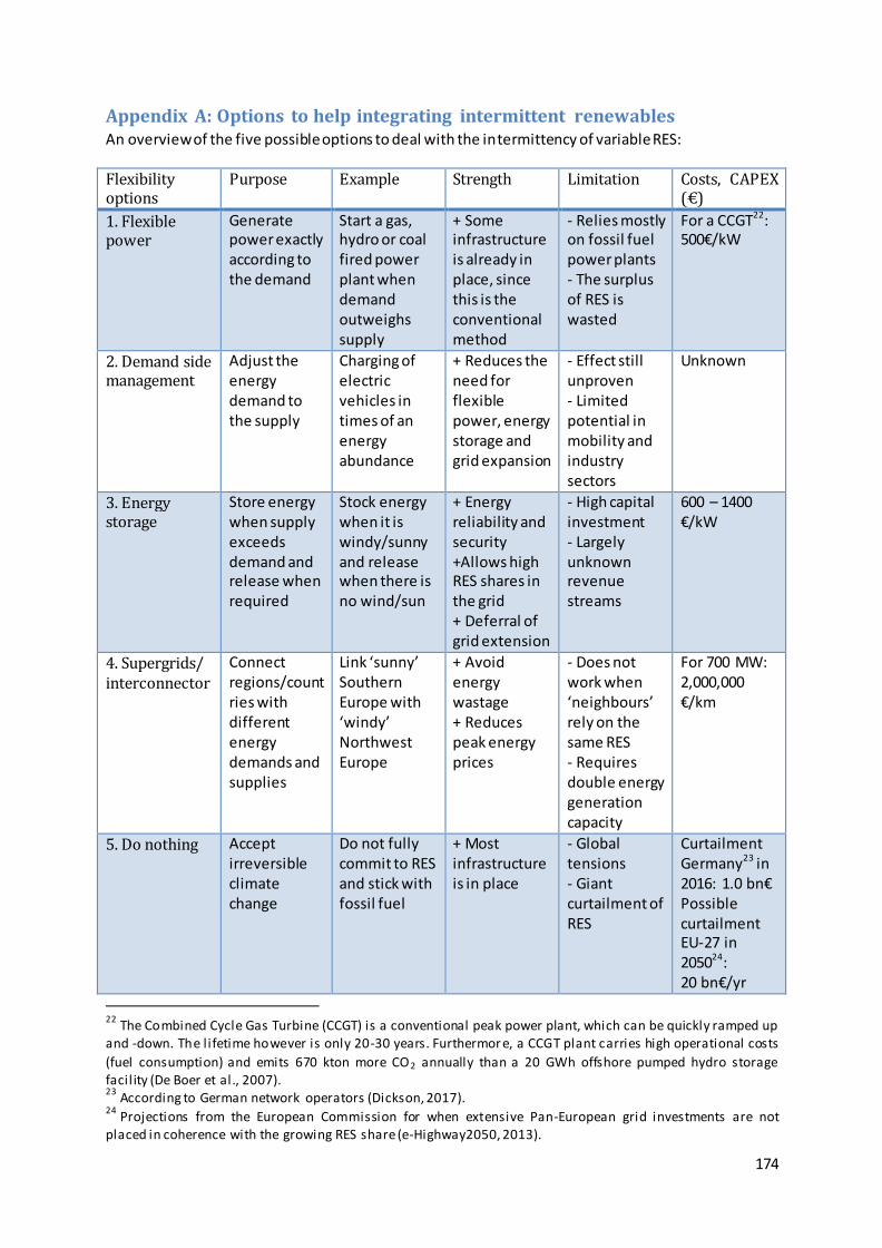
174
Appendix A: Options to help integrating intermittent renewables An overview of the five possible options to deal with the intermittency of variable RES:
Flexibility options
Purpose Example Strength Limitation Costs, CAPEX (€)
1. Flexible power
Generate power exactly according to the demand
Start a gas, hydro or coal fired power plant when demand outweighs supply
+ Some infrastructure is already in place, since this is the conventional method
- Relies mostly on fossil fuel power plants - The surplus of RES is wasted
For a CCGT22: 500€/kW
2. Demand side management
Adjust the energy demand to the supply
Charging of electric vehicles in times of an energy abundance
+ Reduces the need for flexible power, energy storage and grid expansion
- Effect still unproven - Limited potential in mobility and industry sectors
Unknown
3. Energy storage
Store energy when supply exceeds demand and release when required
Stock energy when it is windy/sunny and release when there is no wind/sun
+ Energy reliability and security +Allows high RES shares in the grid + Deferral of grid extension
- High capital investment - Largely unknown revenue streams
600 – 1400 €/kW
4. Supergrids/ interconnector
Connect regions/countries with different energy demands and supplies
Link ‘sunny’ Southern Europe with ‘windy’ Northwest Europe
+ Avoid energy wastage + Reduces peak energy prices
- Does not work when ‘neighbours’ rely on the same RES - Requires double energy generation capacity
For 700 MW: 2,000,000 €/km
5. Do nothing Accept irreversible climate change
Do not fully commit to RES and stick with fossil fuel
+ Most infrastructure is in place
- Global tensions - Giant curtailment of RES
Curtailment Germany23 in 2016: 1.0 bn€ Possible curtailment EU-27 in 205024: 20 bn€/yr
22
The Combined Cycle Gas Turbine (CCGT) is a conventional peak power plant, which can be quickly ramped up and -down. The lifetime however is only 20-30 years. Furthermore, a CCGT plant carries high operational costs
(fuel consumption) and emits 670 kton more CO2 annually than a 20 GWh offshore pumped hydro storage facil ity (De Boer et al., 2007). 23
According to German network operators (Dickson, 2017). 24
Projections from the European Commission for when extensive Pan-European grid investments are not placed in coherence with the growing RES share (e-Highway2050, 2013).
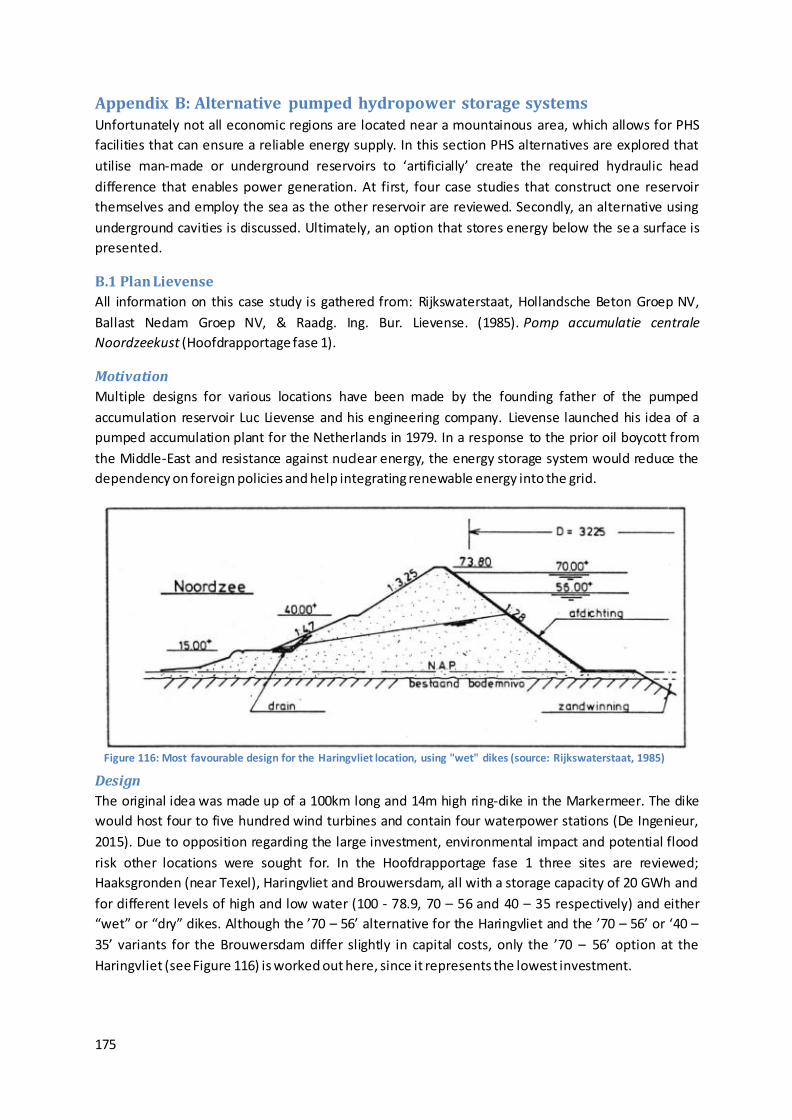
175
Appendix B: Alternative pumped hydropower storage systems Unfortunately not all economic regions are located near a mountainous area, which allows for PHS
facilities that can ensure a reliable energy supply. In this section PHS alternatives are explored that
utilise man-made or underground reservoirs to ‘artificially’ create the required hydraulic head
difference that enables power generation. At first, four case studies that construct one reservoir
themselves and employ the sea as the other reservoir are reviewed. Secondly, an alternative using
underground cavities is discussed. Ultimately, an option that stores energy below the se a surface is
presented.
B.1 Plan Lievense
All information on this case study is gathered from: Rijkswaterstaat, Hollandsche Beton Groep NV,
Ballast Nedam Groep NV, & Raadg. Ing. Bur. Lievense. (1985). Pomp accumulatie centrale
Noordzeekust (Hoofdrapportage fase 1).
Motivation
Multiple designs for various locations have been made by the founding father of the pumped
accumulation reservoir Luc Lievense and his engineering company. Lievense launched his idea of a
pumped accumulation plant for the Netherlands in 1979. In a response to the prior oil boycott from
the Middle-East and resistance against nuclear energy, the energy storage system would reduce the
dependency on foreign policies and help integrating renewable energy into the grid.
Design
The original idea was made up of a 100km long and 14m high ring-dike in the Markermeer. The dike
would host four to five hundred wind turbines and contain four waterpower stations (De Ingenieur,
2015). Due to opposition regarding the large investment, environmental impact and potential flood
risk other locations were sought for. In the Hoofdrapportage fase 1 three sites are reviewed;
Haaksgronden (near Texel), Haringvliet and Brouwersdam, all with a storage capacity of 20 GWh and
for different levels of high and low water (100 - 78.9, 70 – 56 and 40 – 35 respectively) and either
“wet” or “dry” dikes. Although the ’70 – 56’ alternative for the Haringvliet and the ’70 – 56’ or ‘40 –
35’ variants for the Brouwersdam differ slightly in capital costs, only the ’70 – 56’ option at the
Haringvliet (see Figure 116) is worked out here, since it represents the lowest investment.
Figure 116: Most favourable design for the Haringvliet location, using "wet" dikes (source: Rijkswaterstaat, 1985)
176
The reservoir has a circular shape, since this has the most optimal capacity versus circumference
ratio. A variation of 1.25 between high and low water is maintained to enable optimal performance
from the Francis turbines. From the optimal failure probabilities; economic 3*10-3/yr., personal 10-
4/yr. and societal 10-3/yr., the normative personal acceptable risk level was used for the design. The
in-outlet works for a discharge of 3000 – 7000 m3/s would need to be 500m wide and 10m deep. For
all scenario’s the turbine clusters would be placed outside the dike, ‘sheltered’ from the dominant
storm direction and disembogue in a deep (old) flow channel. Sixty percent of the sand necessary to
construct the dikes could be sourced from within the reservoir. The ring-dike itself would have an
impermeable layer on the inner-slope that continues for only a bit on the reservoir bottom, resulting
in a high phreatic line in the dike. Under normal operation 20cm of water would be lost daily, due to
seepage.
Unit Quantity
Storage capacity GWh 20
Power output GW 2.0 (2.9 pumping power)
Surface area reservoir km2 11.95
Head range m 70 – 56
Turbines (Francis) MW 15 * 134
Roundtrip efficiency % 80 Table 42: Characteristics of Haringvliet design
Costs & benefits
Costs are given in the original Dutch guilders and discounted to their 2015 value in euros (by the
Internationaal instituut voor sociale geschiedenis, http://www.iisg.nl/hpw/calculate-nl.php). No data
on the operation and maintenance were reported, nor were the benefits. The costs for the
Haringvliet project are given in Table 43.
Costs (mfl. / m€)
Dredging & dam construction 1473 / 1,160
Housing of pumps etc. 1,202 / 946
Pumps, generators etc. 1,401 / 1,103
HV cable + grid connection 200 / 157
Total capital costs 4,276 / 3,367 Table 43: Costs of Haringvliet pumped accumulation plant
Why is it not constructed?
During the years that the feasibility of an artificial PHS facility for the Netherlands was analysed, the
wind energy technology did not develop as quickly as initially expected. Additionally, the electric
infrastructure could handle a far greater share of wind energy than was first thought (20%), reducing
the need for storage. Ultimately the discussion moved towards nuclear energy and interest in PHS
was lost.
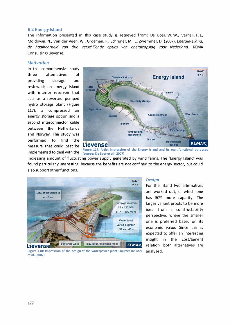
177
Figure 118: Impression of the design of the waterpower plant (source: De Boer et al., 2007)
B.2 Energy Island
The information presented in this case study is retrieved from: De Boer, W. W., Verheij, F. J.,
Moldovan, N., Van der Veen, W., Groeman, F., Schrijner, M., … Zwemmer, D. (2007). Energie-eiland,
de haalbaarheid van drie verschillende opties van energieopslag voor Nederland. KEMA
Consulting/Lievense.
Motivation
In this comprehensive study
three alternatives of
providing storage are
reviewed; an energy island
with interior reservoir that
acts as a reversed pumped
hydro storage plant (Figure
117), a compressed air
energy storage option and a
second interconnector cable
between the Netherlands
and Norway. The study was
performed to find the
measure that could best be
implemented to deal with the
increasing amount of fluctuating power supply generated by wind farms. The ‘Energy Island’ was
found particularly interesting, because the benefits are not confined to the energy sector, but could
also support other functions.
Design
For the island two alternatives
are worked out, of which one
has 50% more capacity. The
larger variant proofs to be more
ideal from a constructability
perspective, where the smaller
one is preferred based on its
economic value. Since this is
expected to offer an interesting
insight in the cost/benefit
relation, both alternatives are
analysed.
Figure 117: Artist impression of the Energy island and its multifunctional purposes (source: De Boer et al., 2007)
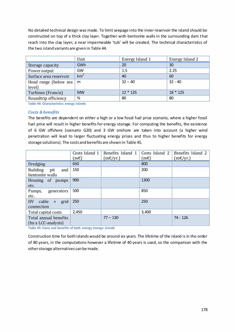
178
No detailed technical design was made. To limit seepage into the inner reservoir the island should be
constructed on top of a thick clay layer. Together with bentonite walls in the surrounding dam that
reach into the clay layer, a near impermeable ‘tub’ will be created. The technical characteristics of
the two island variants are given in Table 44.
Unit Energy Island 1 Energy Island 2
Storage capacity GWh 20 30
Power output GW 1.5 2.25
Surface area reservoir km2 40 60
Head range (below sea level)
m 32 – 40 32 - 40
Turbines (Francis) MW 12 * 125 18 * 125
Roundtrip efficiency % 80 80 Table 44: Characteristics energy islands
Costs & benefits
The benefits are dependent on either a high or a low fossil fuel price scenario, where a higher fossil
fuel price will result in higher benefits for energy storage. For computing the benefits, the existence
of 6 GW offshore (scenario G20) and 3 GW onshore are taken into account (a higher wind
penetration will lead to larger fluctuating energy prices and thus to higher benefits for energy
storage solutions). The costs and benefits are shown in Table 45.
Costs Island 1 (m€)
Benefits Island 1 (m€/yr.)
Costs Island 2 (m€)
Benefits Island 2 (m€/yr.)
Dredging 650 800
Building pit and bentonite walls
150 200
Housing of pumps etc.
900 1300
Pumps, generators etc.
500 850
HV cable + grid connection
250 250
Total capital costs 2,450 3,400
Total annual benefits (by a LCC-analysis)
77 – 130 74 - 126
Table 45: Costs and benefits of both energy storage islands
Construction time for both islands would be around six years. The lifetime of the island is in the order
of 80 years, in the computations however a lifetime of 40 years is used, so the comparison with the
other storage alternatives can be made.

179
Benefit of storage system compared to conventional peak power (CCGT) plant (discounted over 40yr.)
Low fossil fuel price scenario, including dredging costs (m€)
High fossil fuel price scenario, excluding dredging costs (m€)
CAES +1,300 +1,300
Energy Island 1 (20GWh) +0.0 +800
Energy Island 2 (30GWh) -400 +300
NorNed 2nd interconnector +900 +1300 Table 46: Benefits for the various storage options after 40 years (source: adapted from De Boer et al., 2007)
In Table 46 the ‘benefits’ are compared to a conventional peak-power plant. Note the large impact a
higher gas-coal price would have on the indicative benefits for the pumped hydro storage systems. In
case the dredging costs would be paid by adding other functions to the island, the payback period
would be 17 years in the high fossil fuel price scenario for the smaller variant. When no other
revenue creating assets contribute to the island and with the low fossil fuel price scenario, the
payback period would be 40 years.
Why is it not constructed?
Even though there did not seem to be a technical or environmental showstopper, no actions have
been taken to realise the project. The lack of commitment can most likely be subscribed to the
absence of an urgent need for energy storage capacity.
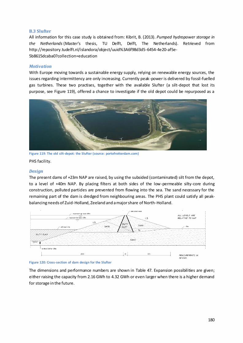
180
B.3 Slufter
All information for this case study is obtained from: Kibrit, B. (2013). Pumped hydropower storage in
the Netherlands (Master's thesis, TU Delft, Delft, The Netherlands). Retrieved from
http://repository.tudelft.nl/islandora/object/uuid%3A6f98d3d5-6454-4e20-af5e-
5b8615dcaba0?collection=education
Motivation
With Europe moving towards a sustainable energy supply, relying on renewable energy sources, the
issues regarding intermittency are only increasing. Currently peak-power is delivered by fossil-fuelled
gas turbines. These two practises, together with the available Slufter (a silt-depot that lost its
purpose, see Figure 119), offered a chance to investigate if the old depot could be repurposed as a
PHS facility.
Design
The present dams of +23m NAP are raised, by using the subsided (contaminated) silt from the depot,
to a level of +40m NAP. By placing filters at both sides of the low-permeable silty-core during
construction, polluted particles are prevented from flowing into the sea. The sand necessary for the
remaining part of the dam is dredged from neighbouring areas. The PHS plant could satisfy all peak-
balancing needs of Zuid-Holland, Zeeland and a major share of North-Holland.
The dimensions and performance numbers are shown in Table 47. Expansion possibilities are given;
either raising the capacity from 2.16 GWh to 4.32 GWh or even larger when there is a higher demand
for storage in the future.
Figure 119: The old silt-depot: the Slufter (source: portofrotterdam.com)
Figure 120: Cross-section of dam design for the Slufter
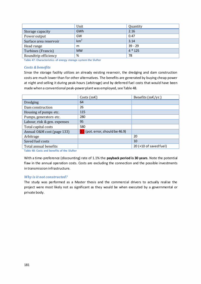
181
Unit Quantity
Storage capacity GWh 2.16
Power output GW 0.47
Surface area reservoir km2 3.14
Head range m 39 - 29
Turbines (Francis) MW 4 * 125
Roundtrip efficiency % 78 Table 47: Characteristics of energy storage system the Slufter
Costs & benefits
Since the storage facility utilizes an already existing reservoir, the dredging and dam construction
costs are much lower than for other alternatives. The benefits are generated by buying cheap power
at night and selling it during peak-hours (arbitrage) and by deferred fuel costs that would have been
made when a conventional peak-power plant was employed, see Table 48.
Costs (m€) Benefits (m€/yr.)
Dredging 64
Dam construction 26
Housing of pumps etc. 115
Pumps, generators etc. 280
Labour, risk & gen. expenses 95
Total capital costs 580
Annual O&M cost (page 133) 0.5 (pot. error, should be 46.9)
Arbitrage 20
Saved fuel costs 10
Total annual benefits 20 (+10 of saved fuel) Table 48: Costs and benefits of the Slufter
With a time-preference (discounting) rate of 1.1% the payback period is 30 years. Note the potential
flaw in the annual operation costs. Costs are excluding the connection and the possible investments
in transmission infrastructure.
Why is it not constructed?
The study was performed as a Master thesis and the commercial drivers to actually realise the
project were most likely not as significant as they would be when executed by a governmental or
private body.
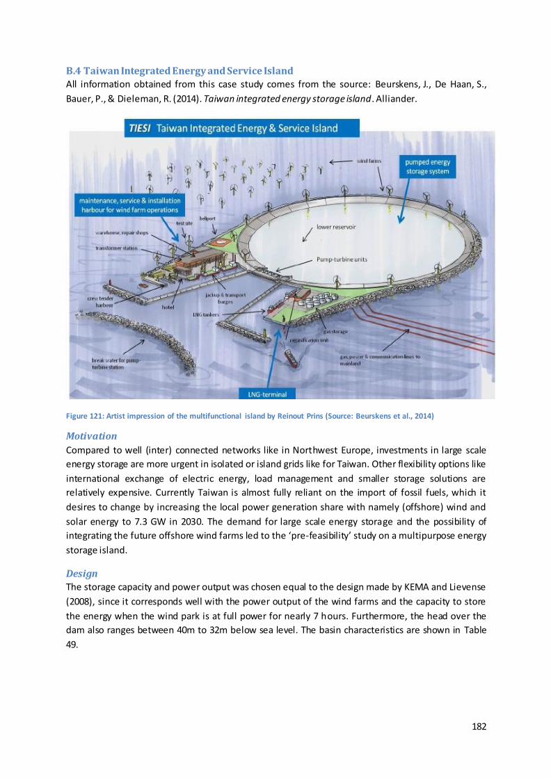
182
B.4 Taiwan Integrated Energy and Service Island
All information obtained from this case study comes from the source: Beurskens, J., De Haan, S.,
Bauer, P., & Dieleman, R. (2014). Taiwan integrated energy storage island. Alliander.
Figure 121: Artist impression of the multifunctional island by Reinout Prins (Source: Beurskens et al., 2014)
Motivation
Compared to well (inter) connected networks like in Northwest Europe, investments in large scale
energy storage are more urgent in isolated or island grids like for Taiwan. Other flexibility options like
international exchange of electric energy, load management and smaller storage solutions are
relatively expensive. Currently Taiwan is almost fully reliant on the import of fossil fuels, which it
desires to change by increasing the local power generation share with namely (offshore) wind and
solar energy to 7.3 GW in 2030. The demand for large scale energy storage and the possibility of
integrating the future offshore wind farms led to the ‘pre-feasibility’ study on a multipurpose energy
storage island.
Design
The storage capacity and power output was chosen equal to the design made by KEMA and Lievense
(2008), since it corresponds well with the power output of the wind farms and the capacity to store
the energy when the wind park is at full power for nearly 7 hours. Furthermore, the head over the
dam also ranges between 40m to 32m below sea level. The basin characteristics are shown in Table
49.
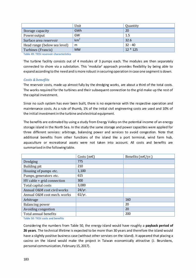
183
Unit Quantity
Storage capacity GWh 20
Power output GW 1.5
Surface area reservoir km2 32.6
Head range (below sea level) m 32 - 40
Turbines (Francis) MW 12 * 125 Table 49: TIESI reservoir characteristics
The turbine facility consists out of 4 modules of 3 pumps each. The modules are then separately
connected to shore via a substation. This ‘modular’ approach provides flexibility by being able to
expand according to the need and is more robust in securing operation in case one segment is down.
Costs & benefits
The reservoir costs, made up almost fully by the dredging works, are about a third of the total costs.
The works required for the turbines and their subsequent connection to the grid make up the rest of
the capital investment.
Since no such system has ever been built, there is no experience with the respective operation and
maintenance costs. As a rule of thumb, 1% of the initial civil engineering costs are used and 10% of
the initial investment in the turbine and electrical equipment.
The benefits are estimated by using a study from Energy Valley on the potential income of an energy
storage island in the North Sea. In the study the same storage and power capacities were applied for
three different services: arbitrage, balancing power and services to avoid congestion. Note that
additional benefits from other functions of the island like a port terminal, wind farm hub,
aquaculture or recreational assets were not taken into account. All costs and benefits are
summarised in the following table.
Costs (m€) Benefits (m€/yr.)
Dredging 775
Building pit 210
Housing of pumps etc. 1,100
Pumps, generators etc. 615
HV cable + grid connection 300
Total capital costs 3,000
Annual O&M cost civil works 24/yr.
Annual O&M cost mech. works 61/yr.
Arbitrage 160
Balancing power 20
Avoiding congestion 20
Total annual benefits 200 Table 50: TIESI costs and benefits
Considering the numbers from Table 50, the energy island would have roughly a payback period of
26 years. The technical lifetime is expected to be more than 30 years and therefore the island would
have a slightly positive business case (without other services on the island). It appeared that placing a
casino on the island would make the project in Taiwan economically attractive (J. Beurskens,
personal communication, February 15, 2017).

184
Potential environmental impact
Several potential impacts are mentioned, mostly regarding the effects of the change in morphology,
salinity, hydrodynamics and land use on fish (larvae), benthos, birds and marine mammals like
dolphins and seals.
Attention need to be paid to what extend the water in the reservoir is mixed, resulting from the
filling and emptying of the waterbody. If insufficient, stratification of the stagnant water will occur
and the lower water layer will be depleted from oxygen, due to the rotting of organic material on the
bottom. Consequently the water would be unsuitable for marine life. On the contrary, a ‘healthy’
water reservoir offers opportunities for commercial fish, shellfish or bio-mass purposes.
The (hard) protection on the exterior side of the reservoir could offer a substrate for benthic species,
which in their turn attract fish and so increase biodiversity. The in- and outlet system has to be
designed in such a way that fish will not be harmed by the turbines. During the feasibility study there
did not seem to be any environmental constraints and the island could even form a base for nature
development.
Why is it not constructed?
Eventually the decision makers did not see the shear need for energy storage on the short-term.
Perhaps the project could be realised in the future (in circa twenty years), but then there should be a
reference project to proof the concept (J. Beurskens, personal communication, February 15, 2017).
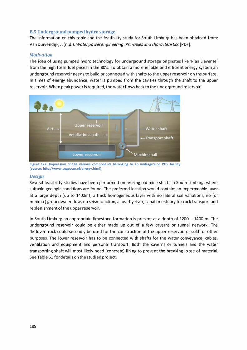
185
B.5 Underground pumped hydro storage
The information on this topic and the feasibility study for South Limburg has been obtained from:
Van Duivendijk, J. (n.d.). Water power engineering: Principles and characteristics [PDF].
Motivation
The idea of using pumped hydro technology for underground storage originates like ‘Plan Lievense’
from the high fossil fuel prices in the 80’s. To obtain a more reliable and efficient energy system an
underground reservoir needs to build or connected with shafts to the upper reservoir on the surface.
In times of energy abundance, water is pumped from the cavities through the shaft to the upper
reservoir. When peak power is required, the water flows back to the underground reservoir.
Design
Several feasibility studies have been performed on reusing old mine shafts in South Limburg, where
suitable geologic conditions are found. The preferred location would contain: an impermeable layer
at a large depth (up to 1400m), a thick homogeneous layer with no lateral soil variations, no (or
minimal) groundwater flow, no seismic action, a nearby river, canal or estuary for rock transport and
replenishment of the upper reservoir.
In South Limburg an appropriate limestone formation is present at a depth of 1200 – 1400 m. The
underground reservoir could be either made up out of a few caverns or tunnel network. The
‘leftover’ rock could secondly be used for the construction of the upper reservoir or sold for other
purposes. The lower reservoir has to be connected with shafts for the water conveyance, cables,
ventilation and equipment and personal transport. Both the caverns or tunnels and the water
transporting shaft will most likely need (concrete) lining to prevent the breaking loose of material.
See Table 51 for details on the studied project.
Figure 122: Impression of the various components belonging to an underground PHS facility (source: http://www.sogecom.nl/energy.html)
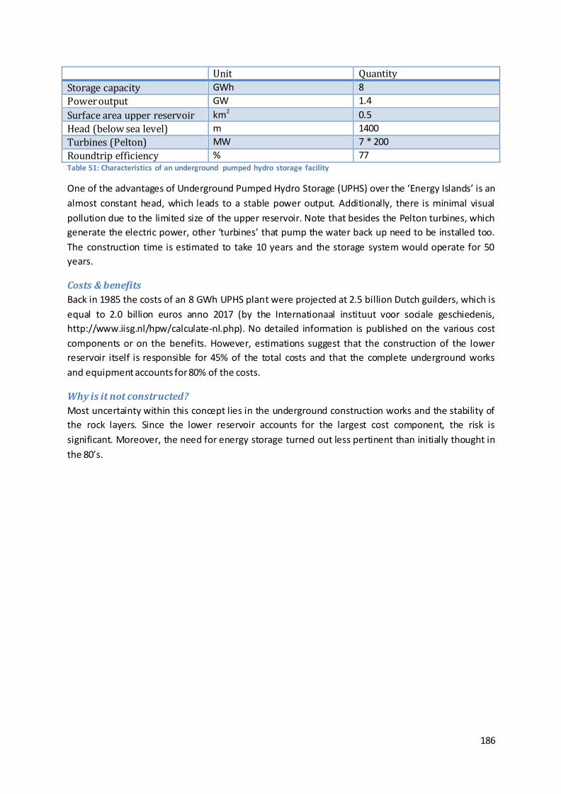
186
Unit Quantity
Storage capacity GWh 8
Power output GW 1.4
Surface area upper reservoir km2 0.5
Head (below sea level) m 1400
Turbines (Pelton) MW 7 * 200
Roundtrip efficiency % 77 Table 51: Characteristics of an underground pumped hydro storage facility
One of the advantages of Underground Pumped Hydro Storage (UPHS) over the ‘Energy Islands’ is an
almost constant head, which leads to a stable power output. Additionally, there is minimal visual
pollution due to the limited size of the upper reservoir. Note that besides the Pelton turbines, which
generate the electric power, other ‘turbines’ that pump the water back up need to be installed too.
The construction time is estimated to take 10 years and the storage system would operate for 50
years.
Costs & benefits
Back in 1985 the costs of an 8 GWh UPHS plant were projected at 2.5 billion Dutch guilders, which is
equal to 2.0 billion euros anno 2017 (by the Internationaal instituut voor sociale geschiedenis,
http://www.iisg.nl/hpw/calculate-nl.php). No detailed information is published on the various cost
components or on the benefits. However, estimations suggest that the construction of the lower
reservoir itself is responsible for 45% of the total costs and that the complete underground works
and equipment accounts for 80% of the costs.
Why is it not constructed?
Most uncertainty within this concept lies in the underground construction works and the stability of
the rock layers. Since the lower reservoir accounts for the largest cost component, the risk is
significant. Moreover, the need for energy storage turned out less pertinent than initially thought in
the 80’s.
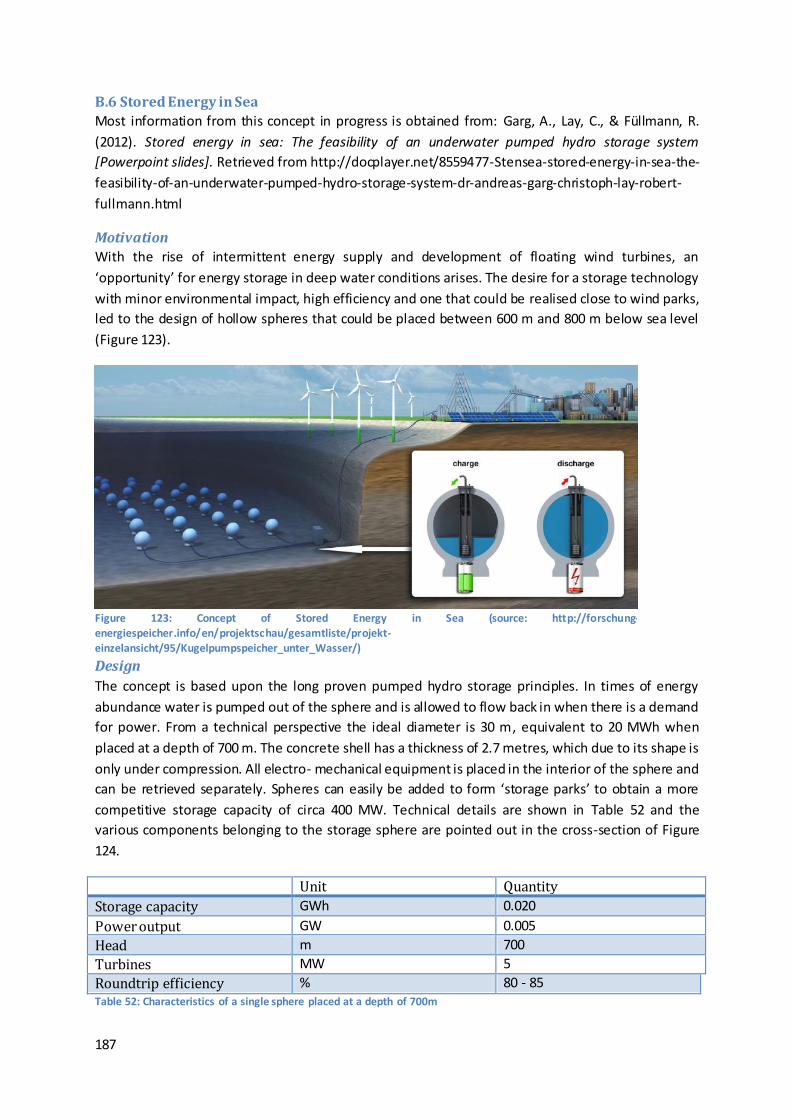
187
B.6 Stored Energy in Sea
Most information from this concept in progress is obtained from: Garg, A., Lay, C., & Füllmann, R.
(2012). Stored energy in sea: The feasibility of an underwater pumped hydro storage system
[Powerpoint slides]. Retrieved from http://docplayer.net/8559477-Stensea-stored-energy-in-sea-the-
feasibility-of-an-underwater-pumped-hydro-storage-system-dr-andreas-garg-christoph-lay-robert-
fullmann.html
Motivation
With the rise of intermittent energy supply and development of floating wind turbines, an
‘opportunity’ for energy storage in deep water conditions arises. The desire for a storage technology
with minor environmental impact, high efficiency and one that could be realised close to wind parks,
led to the design of hollow spheres that could be placed between 600 m and 800 m below sea level
(Figure 123).
Design
The concept is based upon the long proven pumped hydro storage principles. In times of energy
abundance water is pumped out of the sphere and is allowed to flow back in when there is a demand
for power. From a technical perspective the ideal diameter is 30 m, equivalent to 20 MWh when
placed at a depth of 700 m. The concrete shell has a thickness of 2.7 metres, which due to its shape is
only under compression. All electro- mechanical equipment is placed in the interior of the sphere and
can be retrieved separately. Spheres can easily be added to form ‘storage parks’ to obtain a more
competitive storage capacity of circa 400 MW. Technical details are shown in Table 52 and the
various components belonging to the storage sphere are pointed out in the cross-section of Figure
124.
Unit Quantity
Storage capacity GWh 0.020
Power output GW 0.005
Head m 700
Turbines MW 5
Roundtrip efficiency % 80 - 85 Table 52: Characteristics of a single sphere placed at a depth of 700m
Figure 123: Concept of Stored Energy in Sea (source: http://forschung-energiespeicher.info/en/projektschau/gesamtliste/projekt-einzelansicht/95/Kugelpumpspeicher_unter_Wasser/)
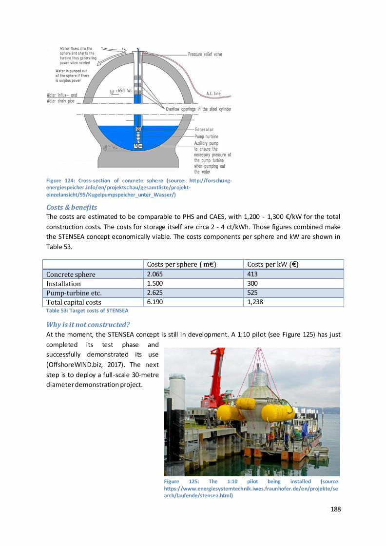
188
Costs & benefits
The costs are estimated to be comparable to PHS and CAES, with 1,200 - 1,300 €/kW for the total
construction costs. The costs for storage itself are circa 2 - 4 ct/kWh. Those figures combined make
the STENSEA concept economically viable. The costs components per sphere and kW are shown in
Table 53.
Costs per sphere ( m€) Costs per kW (€)
Concrete sphere 2.065 413
Installation 1.500 300
Pump-turbine etc. 2.625 525
Total capital costs 6.190 1,238 Table 53: Target costs of STENSEA
Why is it not constructed?
At the moment, the STENSEA concept is still in development. A 1:10 pilot (see Figure 125) has just
completed its test phase and
successfully demonstrated its use
(OffshoreWIND.biz, 2017). The next
step is to deploy a full-scale 30-metre
diameter demonstration project.
Figure 124: Cross-section of concrete sphere (source: http://forschung-energiespeicher.info/en/projektschau/gesamtliste/projekt-einzelansicht/95/Kugelpumpspeicher_unter_Wasser/)
Figure 125: The 1:10 pilot being installed (source: https://www.energiesystemtechnik.iwes.fraunhofer.de/en/projekte/search/laufende/stensea.html)
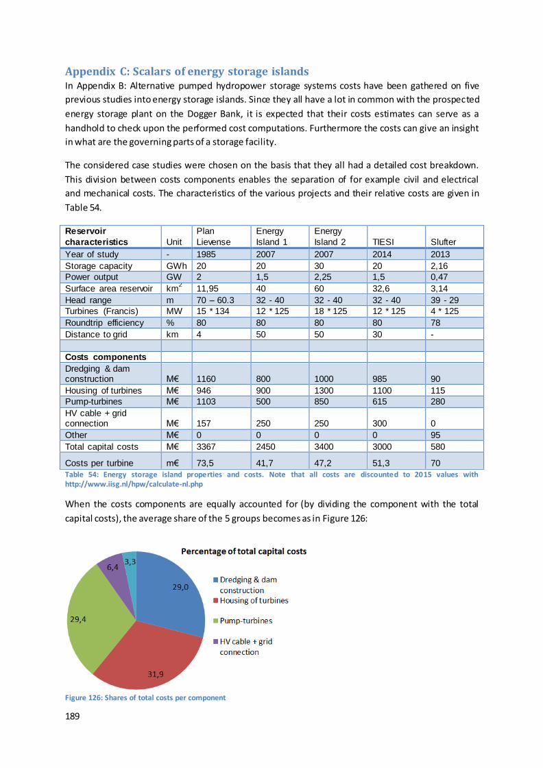
189
Figure 126: Shares of total costs per component
Appendix C: Scalars of energy storage islands In Appendix B: Alternative pumped hydropower storage systems costs have been gathered on five
previous studies into energy storage islands. Since they all have a lot in common with the prospected
energy storage plant on the Dogger Bank, it is expected that their costs estimates can serve as a
handhold to check upon the performed cost computations. Furthermore the costs can give an insight
in what are the governing parts of a storage facility.
The considered case studies were chosen on the basis that they all had a detailed cost breakdown.
This division between costs components enables the separation of for example civil and electrical
and mechanical costs. The characteristics of the various projects and their relative costs are given in
Table 54.
Reservoir
characteristics Unit
Plan
Lievense
Energy
Island 1
Energy
Island 2 TIESI Slufter
Year of study - 1985 2007 2007 2014 2013
Storage capacity GWh 20 20 30 20 2,16
Power output GW 2 1,5 2,25 1,5 0,47
Surface area reservoir km2 11,95 40 60 32,6 3,14
Head range m 70 – 60.3 32 - 40 32 - 40 32 - 40 39 - 29
Turbines (Francis) MW 15 * 134 12 * 125 18 * 125 12 * 125 4 * 125
Roundtrip efficiency % 80 80 80 80 78
Distance to grid km 4 50 50 30 -
Costs components
Dredging & dam construction M€ 1160 800 1000 985 90
Housing of turbines M€ 946 900 1300 1100 115
Pump-turbines M€ 1103 500 850 615 280
HV cable + grid connection M€ 157 250 250 300 0
Other M€ 0 0 0 0 95
Total capital costs M€ 3367 2450 3400 3000 580
Costs per turbine m€ 73,5 41,7 47,2 51,3 70
Table 54: Energy storage island properties and costs. Note that all costs are discounted to 2015 values with http://www.iisg.nl/hpw/calculate-nl.php
When the costs components are equally accounted for (by dividing the component with the total
capital costs), the average share of the 5 groups becomes as in Figure 126:
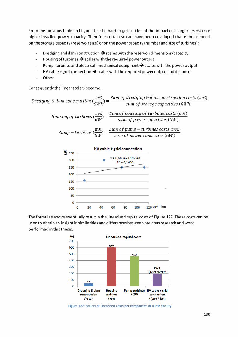
190
From the previous table and figure it is still hard to get an idea of the impact of a larger reservoir or
higher installed power capacity. Therefore certain scalars have been developed that either depend
on the storage capacity (reservoir size) or on the power capacity (number and size of turbines):
- Dredging and dam construction scales with the reservoir dimensions/capacity
- Housing of turbines scales with the required power output
- Pump-turbines and electrical- mechanical equipment scales with the power output
- HV cable + grid connection scales with the required power output and distance
- Other
Consequently the linear scalars become:
𝐷𝑟𝑒𝑑𝑔𝑖𝑛𝑔 & 𝑑𝑎𝑚 𝑐𝑜𝑛𝑠𝑡𝑟𝑢𝑐𝑡𝑖𝑜𝑛 (𝑚€
𝐺𝑊ℎ)=
𝑆𝑢𝑚 𝑜𝑓 𝑑𝑟𝑒𝑑𝑔𝑖𝑛𝑔 & 𝑑𝑎𝑚 𝑐𝑜𝑛𝑠𝑡𝑟𝑢𝑐𝑡𝑖𝑜𝑛 𝑐𝑜𝑠𝑡𝑠 (𝑚€)
𝑠𝑢𝑚 𝑜𝑓 𝑠𝑡𝑜𝑟𝑎𝑔𝑒 𝑐𝑎𝑝𝑎𝑐𝑖𝑡𝑖𝑒𝑠 (𝐺𝑊ℎ)
𝐻𝑜𝑢𝑠𝑖𝑛𝑔 𝑜𝑓 𝑡𝑢𝑟𝑏𝑖𝑛𝑒𝑠 (𝑚€
𝐺𝑊) =
𝑆𝑢𝑚 𝑜𝑓 ℎ𝑜𝑢𝑠𝑖𝑛𝑔 𝑜𝑓 𝑡𝑢𝑟𝑏𝑖𝑛𝑒𝑠 𝑐𝑜𝑠𝑡𝑠 (𝑚€)
𝑠𝑢𝑚 𝑜𝑓 𝑝𝑜𝑤𝑒𝑟 𝑐𝑎𝑝𝑎𝑐𝑖𝑡𝑖𝑒𝑠 (𝐺𝑊)
𝑃𝑢𝑚𝑝− 𝑡𝑢𝑟𝑏𝑖𝑛𝑒𝑠 (𝑚€
𝐺𝑊) =
𝑆𝑢𝑚 𝑜𝑓 𝑝𝑢𝑚𝑝− 𝑡𝑢𝑟𝑏𝑖𝑛𝑒𝑠 𝑐𝑜𝑠𝑡𝑠 (𝑚€)
𝑠𝑢𝑚 𝑜𝑓 𝑝𝑜𝑤𝑒𝑟 𝑐𝑎𝑝𝑎𝑐𝑖𝑡𝑖𝑒𝑠 (𝐺𝑊)
The formulae above eventually result in the linearised capital costs of Figure 127. These costs can be
used to obtain an insight in similarities and differences between previous research and work
performed in this thesis.
Figure 127: Scalars of linearised costs per component of a PHS facility
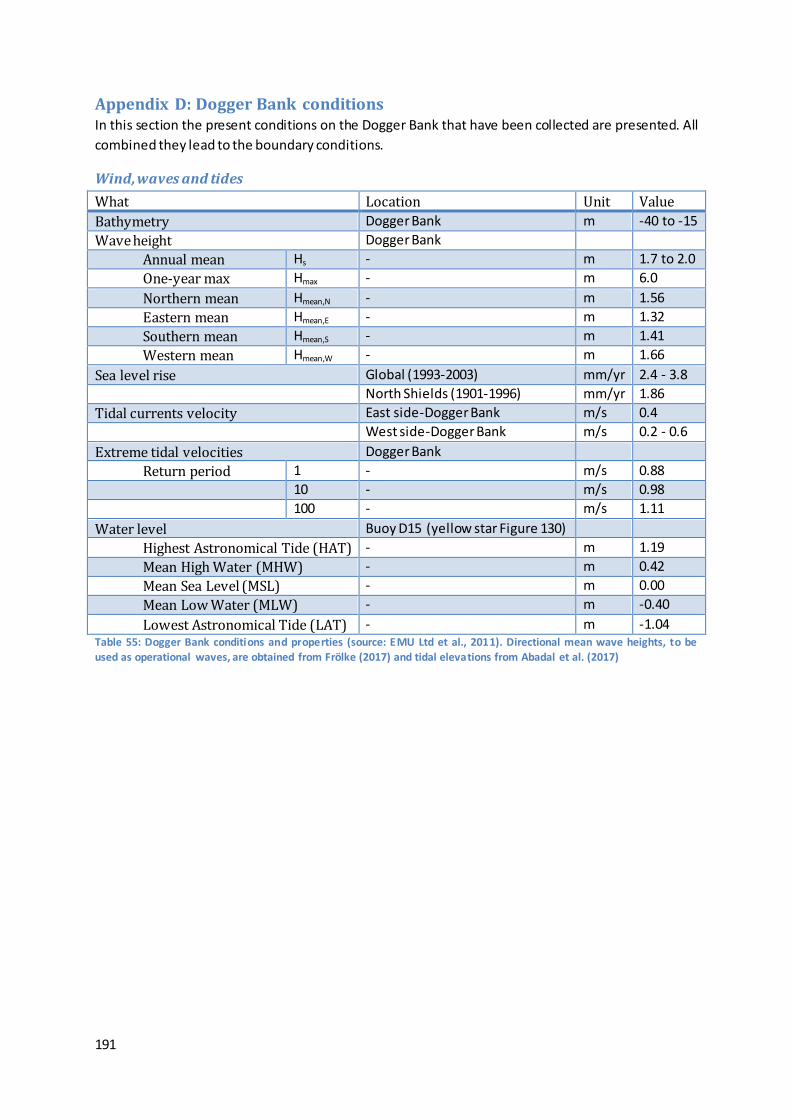
191
Appendix D: Dogger Bank conditions In this section the present conditions on the Dogger Bank that have been collected are presented. All
combined they lead to the boundary conditions.
Wind, waves and tides
What Location Unit Value
Bathymetry Dogger Bank m -40 to -15
Wave height Dogger Bank
Annual mean Hs - m 1.7 to 2.0
One-year max Hmax - m 6.0
Northern mean Hmean,N - m 1.56
Eastern mean Hmean,E - m 1.32
Southern mean Hmean,S - m 1.41
Western mean Hmean,W - m 1.66
Sea level rise Global (1993-2003) mm/yr 2.4 - 3.8
North Shields (1901-1996) mm/yr 1.86
Tidal currents velocity East side-Dogger Bank m/s 0.4
West side-Dogger Bank m/s 0.2 - 0.6
Extreme tidal velocities Dogger Bank
Return period 1 - m/s 0.88
10 - m/s 0.98
100 - m/s 1.11
Water level Buoy D15 (yellow star Figure 130)
Highest Astronomical Tide (HAT) - m 1.19
Mean High Water (MHW) - m 0.42
Mean Sea Level (MSL) - m 0.00
Mean Low Water (MLW) - m -0.40
Lowest Astronomical Tide (LAT) - m -1.04 Table 55: Dogger Bank conditions and properties (source: EMU Ltd et al., 2011). Directional mean wave heights, to be used as operational waves, are obtained from Frölke (2017) and tidal elevations from Abadal et al. (2017)
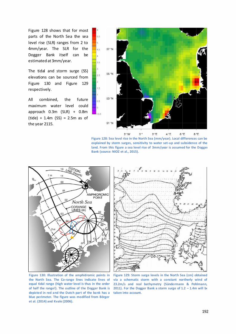
192
Figure 128 shows that for most
parts of the North Sea the sea
level rise (SLR) ranges from 2 to
4mm/year. The SLR for the
Dogger Bank itself can be
estimated at 3mm/year.
The tidal and storm surge (SS)
elevations can be sourced from
Figure 130 and Figure 129
respectively.
All combined, the future
maximum water level could
approach 0.3m (SLR) + 0.8m
(tide) + 1.4m (SS) = 2.5m as of
the year 2115.
Figure 128: Sea level rise in the North Sea (mm/year). Local differences can be explained by storm surges, sensitivity to water set-up and subsidence of the
land. From this figure a sea level rise of 3mm/year is assumed for the Dogger Bank (source: NIOZ et al., 2015).
Figure 129: Storm surge levels in the North Sea (cm) obtained
via a schematic storm with a constant northerly wind of 23.2m/s and real bathymetry (Sündermann & Pohlmann, 2011). For the Dogger Bank a storm surge of 1.2 – 1.4m will be taken into account.
Figure 130: Illustration of the amphidromic points in
the North Sea. The Co-range lines indicate lines of equal tidal range (high water level is thus in the order of half the range!). The outline of the Dogger Bank is depicted in red and the Dutch part of the bank has a blue perimeter. The figure was modified from Börger
et al. (2014) and Kvale (2006).
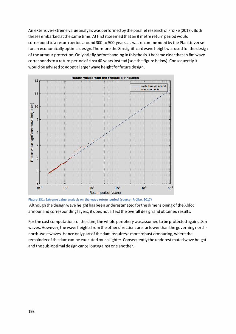
193
An extensive extreme value analysis was performed by the parallel research of Frölke (2017). Both
theses embarked at the same time. At first it seemed that an 8 metre return period would
correspond to a return period around 300 to 500 years, as was recommended by the Plan Lievense
for an economically optimal design. Therefore the 8m significant wave height was used for the design
of the armour protection. Only briefly before handing in this thesis it became clear that an 8m wave
corresponds to a return period of circa 40 years instead (see the figure below). Consequently it
would be advised to adopt a larger wave height for future design.
Although the design wave height has been underestimated for the dimensioning of the Xbloc
armour and corresponding layers, it does not affect the overall design and obtained results.
For the cost computations of the dam, the whole periphery was assumed to be protected against 8m
waves. However, the wave heights from the other directions are far lower than the governing north-
north-west waves. Hence only part of the dam requires a more robust armouring, where the
remainder of the dam can be executed much lighter. Consequently the underestimated wave height
and the sub-optimal design cancel out against one another.
Figure 131: Extreme value analysis on the wave return period (source: Frölke, 2017)
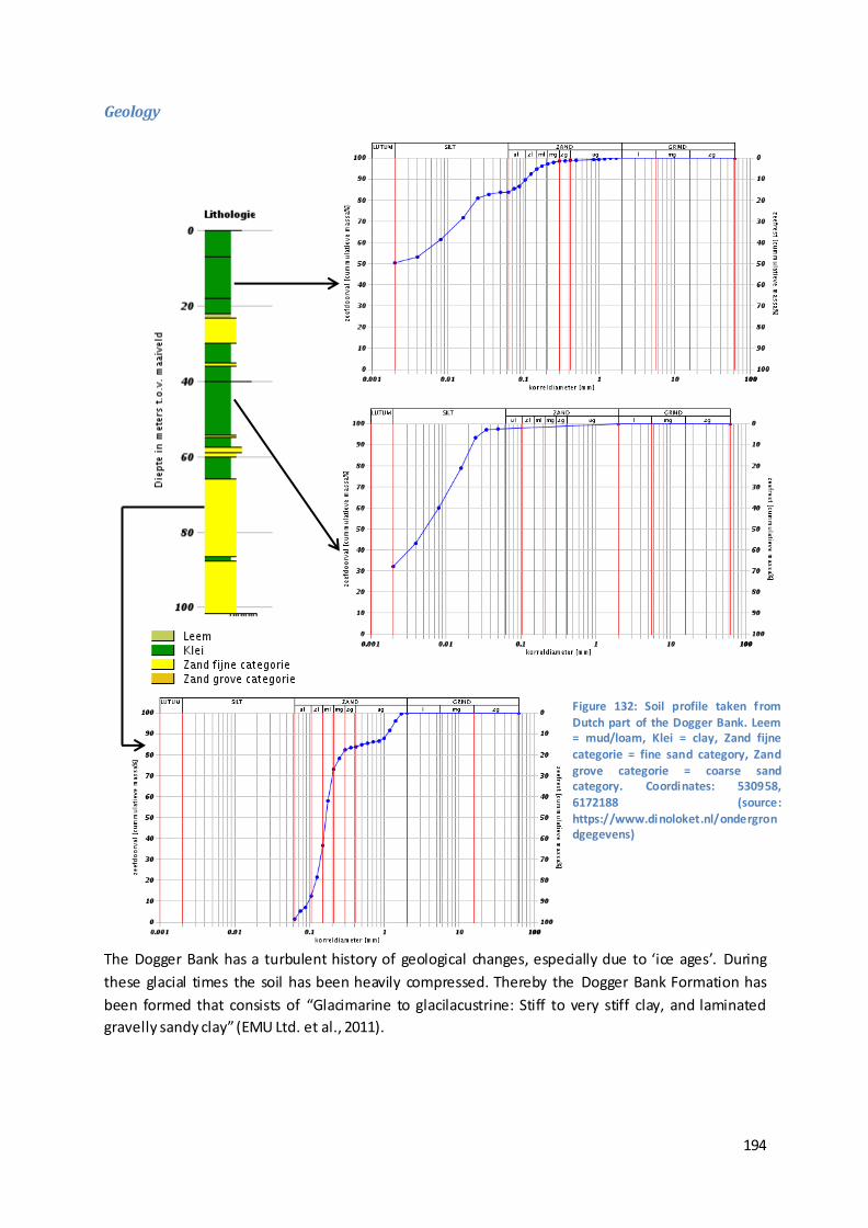
194
Geology
The Dogger Bank has a turbulent history of geological changes, especially due to ‘ice ages’. During
these glacial times the soil has been heavily compressed. Thereby the Dogger Bank Formation has
been formed that consists of “Glacimarine to glacilacustrine: Stiff to very stiff clay, and laminated
gravelly sandy clay” (EMU Ltd. et al., 2011).
Figure 132: Soil profile taken from Dutch part of the Dogger Bank. Leem = mud/loam, Klei = clay, Zand fijne categorie = fine sand category, Zand grove categorie = coarse sand category. Coordinates: 530958, 6172188 (source: https://www.dinoloket.nl/ondergrondgegevens)

195
Appendix E: Risks associated to inverse offshore pumped hydro storage One of the key advantages of an inverse offshore hydropower storage plant is that there is no
potential flood risk posed by the storage facility. In fact: when the dam would break through the
inner reservoir would be filled, instead of the reservoir flooding the surrounding area. The only
threat is then the economic loss of damage to the dam and filling-up of the inner reservoir.
Since for the energy storage function no human activities are necessary within the storage reservoir,
there is no risk for loss of life(s). This significantly reduces the demanded safety factor for the system.
It is even possible to imagine that when a storm is forecasted of unprecedented magnitude, which
could potentially breach the dam, the inner reservoir is filled-up to prevent a destructive flood wave
coming in. This risk and damage mitigation measure is an interesting asset of the offshore energy
storage system. In case other functions are added to the island the acceptable risk might change,
which results in stricter requirements for the dam structure. Hence, the value and benefit of
potential extra functions has to be weighed against the influence on the needed safety level (and
thus added costs).
For the Plan Lievense in front of the Dutch coast a detailed risk analysis was performed that resulted
in the risk levels as presented in Table 56.
Perspective acceptable risk Optimal failure probability per year
Economic (minimal costs over the lifetime) 3.10-3
Personal (loss of lives) 10-4 Table 56: Risk levels for a pumped hydropower plant in the Netherlands (source: Rijkswaterstaat et al., 1985)
Since the Plan Lievense contained an inner reservoir higher than the lower reservoir (the North Sea)
a dam break through would cause a flood wave endangering the loss of lives. Therefore the
‘personal’ risk level from Table 56 was governing, with a failure probability of 1/10,000 years.
As the inverse offshore PHS has its reservoir below the North Sea, it does not imperil the surrounding
area. Consequently the more competitive failure probability of 1/333 years can be applied. This
economic risk level should result in the lowest costs of the storage facility over its lifetime (CAPEX +
OPEX). Due to the similar structures and investments compared to the Plan Lievense it is expected
that the economic acceptable risk is evenly alike for the inverse offshore PHS plant on the Dogger
Bank. Consequently a design that meets the optimal failure probability of 1/333 years is
recommended.
The design has not been executed in a probabilistic approach. This would be vastly more
complicated, due to all the correlations between the failure mechanisms. Furthermore it would be
overly detailed compared to the desired insight in the scaling of an energy storage facility. The
economic risk level has only been used to choose design wave heights and safety factors.
The technical failure mechanisms are depicted in Figure 35 and Figure 36. The shown failure modes
are purely technical. There are also financial and societal risks. Financial risks can encompass
fluctuations in energy prices and the cost of capital. Societal risks contain mostly changes in policy
and support by the government(s), the public or non-governmental organisations. The focus of this
report lies within the technical part and no further attention is given to the financial and societal
risks.
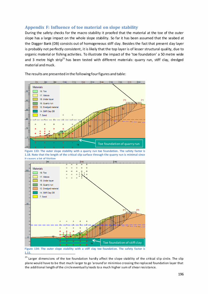
196
Appendix F: Influence of toe material on slope stability During the safety checks for the macro stability it proofed that the material at the toe of the outer
slope has a large impact on the whole slope stability. So far it has been assumed that the seabed at
the Dogger Bank (DB) consists out of homogeneous stiff clay. Besides the fact that present clay layer
is probably not perfectly consistent, it is likely that the top layer is of lesser structural quality, due to
organic material or fishing activities. To illustrate the impact of the ‘toe foundation’ a 50 metre wide
and 3 metre high strip25 has been tested with different materials: quarry run, stiff clay, dredged
material and muck.
The results are presented in the following four figures and table:
25
Larger dimensions of the toe foundation hardly affect the slope stability of the critical sl ip circle. The slip
plane would have to be that much larger to go ‘around’or minimise crossing the replaced foundation layer that the additional length of the circle eventually leads to a much higher sum of shear resistance.
Figure 133: The outer slope stability with a quarry run toe foundation. The safety factor is 1.18. Note that the length of the critical slip surface through the quarry run is minimal since
it causes a lot of friction
Toe foundation of quarry run
Figure 134: The outer slope stability with a stiff clay toe foundation. The safety factor is 1.11.
Toe foundation of stiff clay
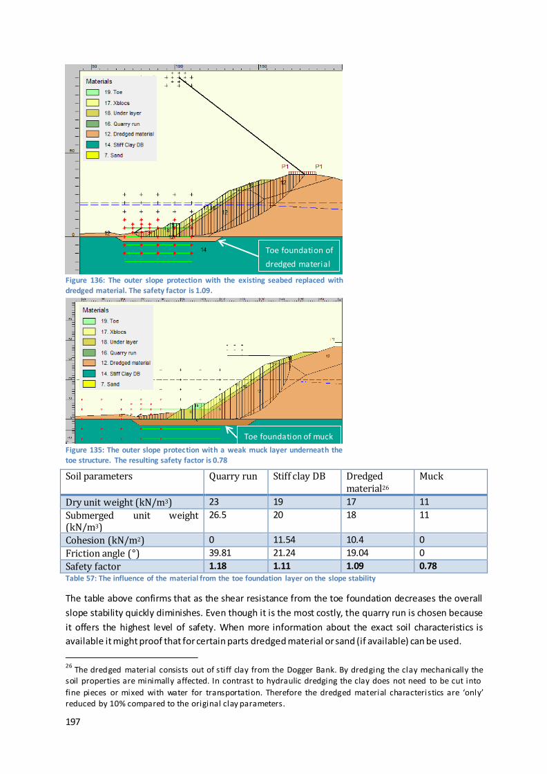
197
Soil parameters Quarry run Stiff clay DB Dredged material26
Muck
Dry unit weight (kN/m3) 23 19 17 11
Submerged unit weight (kN/m3)
26.5 20 18 11
Cohesion (kN/m2) 0 11.54 10.4 0
Friction angle (°) 39.81 21.24 19.04 0
Safety factor 1.18 1.11 1.09 0.78 Table 57: The influence of the material from the toe foundation layer on the slope stability
The table above confirms that as the shear resistance from the toe foundation decreases the overall
slope stability quickly diminishes. Even though it is the most costly, the quarry run is chosen because
it offers the highest level of safety. When more information about the exact soil characteristics is
available it might proof that for certain parts dredged material or sand (if available) can be used.
26
The dredged material consists out of stiff clay from the Dogger Bank. By dredging the clay mechanically the soil properties are minimally affected. In contrast to hydraulic dredging the clay does not need to be cut into
fine pieces or mixed with water for transportation. Therefore the dredged material characteristics are ‘only’ reduced by 10% compared to the original clay parameters.
Figure 136: The outer slope protection with the existing seabed replaced with
dredged material. The safety factor is 1.09.
Toe foundation of
dredged material
Figure 135: The outer slope protection with a weak muck layer underneath the toe structure. The resulting safety factor is 0.78
Toe foundation of muck
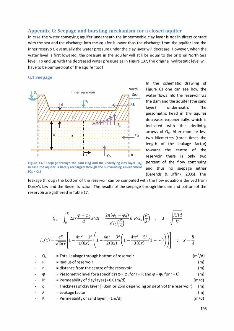
198
Appendix G: Seepage and bursting mechanism for a closed aquifer In case the water conveying aquifer underneath the impermeable clay layer is not in direct contact
with the sea and the discharge into the aquifer is lower than the discharge from the aquifer into the
inner reservoir, eventually the water pressure under the clay layer will decrease. However, when the
water level is first lowered, the pressure in the aquifer will still be equal to the original North Sea
level. To end up with the decreased water pressure as in Figure 137, the original hydrostatic level will
have to be pumped out of the aquifer too!
G.1 Seepage
In the schematic drawing of
Figure 61 one can see how the
water flows into the reservoir via
the dam and the aquifer (the sand
layer) underneath. The
piezometric head in the aquifer
decreases exponentially, which is
indicated with the declining
arrows of Qu. After more or less
two kilometres (three times the
length of the leakage factor)
towards the centre of the
reservoir there is only two
percent of the flow continuing
and thus no seepage either
(Barends & Uffink, 2006). The
leakage through the bottom of the reservoir can be computed with the flow equations derived from
Darcy’s law and the Bessel function. The results of the seepage through the dam and bottom of the
reservoir are gathered in Table 17.
𝑄𝑢 = ∫ 2𝜋𝑟𝜑 −𝜑0𝑑
𝑘′𝑑𝑟𝑅
0=2𝜋(𝜑1 −𝜑0)
𝑑𝐼0 (𝑅𝜆)
𝑘′𝑅𝜆𝐼1 (𝑅
𝜆) ; 𝜆 = √
𝐾𝐻𝑑
𝑘′
𝐼𝑛(𝑥) =𝑒𝑥
√2𝜋𝑥[1−
4𝑛2 −12
1(8𝑥)(1−
4𝑛2 −32
2(8𝑥)(1 −
4𝑛2 −52
3(8𝑥)(1 −⋯)))] ; 𝑥 =
𝑅
𝜆
- Qu = Total leakage through bottom of reservoir (m3/d)
- R = Radius of reservoir (m)
- r = distance from the centre of the reservoir (m)
- φ = Piezometric level for a specific r (φ = φ1 for r = R and φ = φ0 for r = 0) (m)
- k’ = Permeability of clay layer (= 0.01m/d) (m/d)
- d = Thickness of clay layer (= 35m or 25m depending on depth of the reservoir) (m)
- λ = Leakage factor (m)
- K = Permeability of sand layer (= 1m/d) (m/d)
Figure 137: Seepage through the dam (Qd) and the underlying clay layer (Qu) in case the aquifer is barely recharged through the surrounding environment (QA < Qu)
Qd d φ0
φ1
Qu
R r
H
Inner reservoir North
Sea
k'
K QA
QA

199
- H = Thickness of sand layer27 (= 135m) (m)
- In = Asymptotic approximation of modified Bessel function (for I0 n = 0 and for I1 n = 1)
- x = Leakage penetration factor (-)
Scenario Unit 1 2 3 4 5 6 7 8
Maximum head m 40 40 40 40 40 60 60 60
Pot. head centre m 26.88 7.29 7.16 2.57 1.14 10.20 4.69 2.50
Storage capacity GWh 0.77 9.84 10 20 30 10 20 30
Seepage dam mm/d 0.83 0.28 0.28 0.21 0.17 1.06 0.79 0.66
Seepage bottom mm/d 5.78 5.98 5.95 4.59 3.89 13.92 11.12 9.58
Total discharge 104 m3/d 1.13 9.20 9.28 13.57 16.84 11.82 17.04 21.00
Total head loss mm/d 6.6 6.3 6.2 4.8 4.1 15.0 11.9 10.2 Table 58: The loss of head due to leakage. Note that the seepage through the dam and bottom are converted into a head loss per day. The potential head at the centre is basically the ‘pressure’ that remains from the water level difference
Even with the conservatively chosen permeability of 0.01m/d for the clay layer, the effect of seepage
on the head loss in the reservoir is surprisingly small. Furthermore, the values presented in Table 17
form the upper boundary, since they are computed with a continuously empty inner reservoir.
Although the total discharges (in the order of 150,000m3/d) might seem like a lot, it is only around
0.1% of the total fluctuating water volume!
27
The sand layer thickness is estimated at 135m based on the soil profile (which indicates that the sand layer starts at -65m relative to the seabed) and the geological conditions presented by the Forewind consortium who
state that the Yarmouth Roads formation (“Marine and non-marine sands and plant debris with intertidal sand and mud rhythmites”) extends ti l l roughly -200m below the seabed (Emu Ltd. et al., 2011)
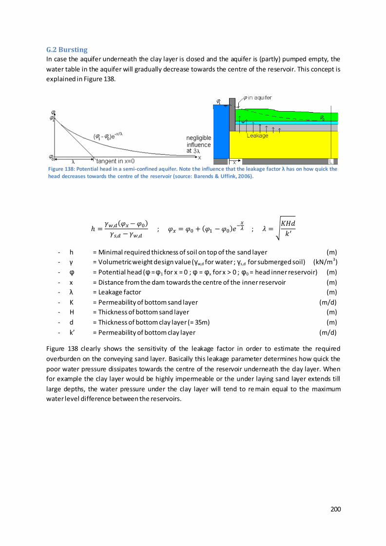
200
G.2 Bursting
In case the aquifer underneath the clay layer is closed and the aquifer is (partly) pumped empty, the
water table in the aquifer will gradually decrease towards the centre of the reservoir. This concept is
explained in Figure 138.
ℎ =𝛾𝑤,𝑑(𝜑𝑥−𝜑0)
𝛾𝑠,𝑑 −𝛾𝑤,𝑑 ; 𝜑𝑥 = 𝜑0 + (𝜑1 −𝜑0)𝑒
−𝑥𝜆 ; 𝜆 = √
𝐾𝐻𝑑
𝑘′
- h = Minimal required thickness of soil on top of the sand layer (m)
- γ = Volumetric weight design value (γw,d for water ; γs,d for submerged soil) (kN/m3)
- φ = Potential head (φ = φ1 for x = 0 ; φ = φx for x > 0 ; φ0 = head inner reservoir) (m)
- x = Distance from the dam towards the centre of the inner reservoir (m)
- λ = Leakage factor (m)
- K = Permeability of bottom sand layer (m/d)
- H = Thickness of bottom sand layer (m)
- d = Thickness of bottom clay layer (= 35m) (m)
- k’ = Permeability of bottom clay layer (m/d)
Figure 138 clearly shows the sensitivity of the leakage factor in order to estimate the required
overburden on the conveying sand layer. Basically this leakage parameter determines how quick the
poor water pressure dissipates towards the centre of the reservoir underneath the clay layer. When
for example the clay layer would be highly impermeable or the under laying sand layer extends till
large depths, the water pressure under the clay layer will tend to re main equal to the maximum
water level difference between the reservoirs.
Figure 138: Potential head in a semi-confined aquifer. Note the influence that the leakage factor λ has on how quick the head decreases towards the centre of the reservoir (source: Barends & Uffink, 2006).
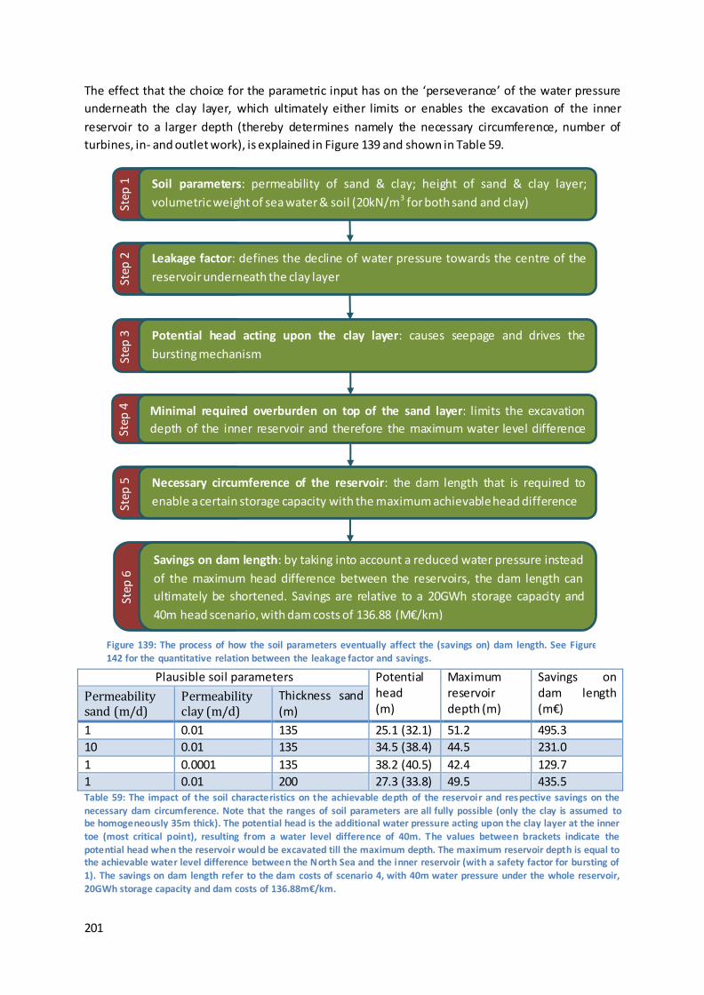
201
The effect that the choice for the parametric input has on the ‘perseverance’ of the water pressure
underneath the clay layer, which ultimately either limits or enables the excavation of the inner
reservoir to a larger depth (thereby determines namely the necessary circumference, number of
turbines, in- and outlet work), is explained in Figure 139 and shown in Table 59.
Plausible soil parameters Potential head (m)
Maximum reservoir depth (m)
Savings on dam length (m€)
Permeability sand (m/d)
Permeability clay (m/d)
Thickness sand (m)
1 0.01 135 25.1 (32.1) 51.2 495.3
10 0.01 135 34.5 (38.4) 44.5 231.0
1 0.0001 135 38.2 (40.5) 42.4 129.7
1 0.01 200 27.3 (33.8) 49.5 435.5 Table 59: The impact of the soil characteristics on the achievable depth of the reservoir and respective savings on the
necessary dam circumference. Note that the ranges of soil parameters are all fully possible (only the clay is assumed to be homogeneously 35m thick). The potential head is the additional water pressure acting upon the clay layer at the inner
toe (most critical point), resulting from a water level difference of 40m. The values between brackets indicate the potential head when the reservoir would be excavated till the maximum depth. The maximum reservoir depth is equal to the achievable water level difference between the North Sea and the inner reservoir (with a safety factor for bursting of
1). The savings on dam length refer to the dam costs of scenario 4, with 40m water pressure under the whole reservoir, 20GWh storage capacity and dam costs of 136.88m€/km.
Soil parameters: permeability of sand & clay; height of sand & clay layer;
volumetric weight of sea water & soil (20kN/m3 for both sand and clay) Step
1
Leakage factor: defines the decline of water pressure towards the centre of the
reservoir underneath the clay layer Step
2
Potential head acting upon the clay layer: causes seepage and drives the
bursting mechanism Step
3
Minimal required overburden on top of the sand layer: limits the excavation
depth of the inner reservoir and therefore the maximum water level difference
Step
4
Necessary circumference of the reservoir: the dam length that is required to
enable a certain storage capacity with the maximum achievable head difference Step
5
Savings on dam length: by taking into account a reduced water pressure instead
of the maximum head difference between the reservoirs, the dam length can
ultimately be shortened. Savings are relative to a 20GWh storage capacity and
40m head scenario, with dam costs of 136.88 (M€/km)
Step
6
Figure 139: The process of how the soil parameters eventually affect the (savings on) dam length. See Figure 142 for the quantitative relation between the leakage factor and savings.
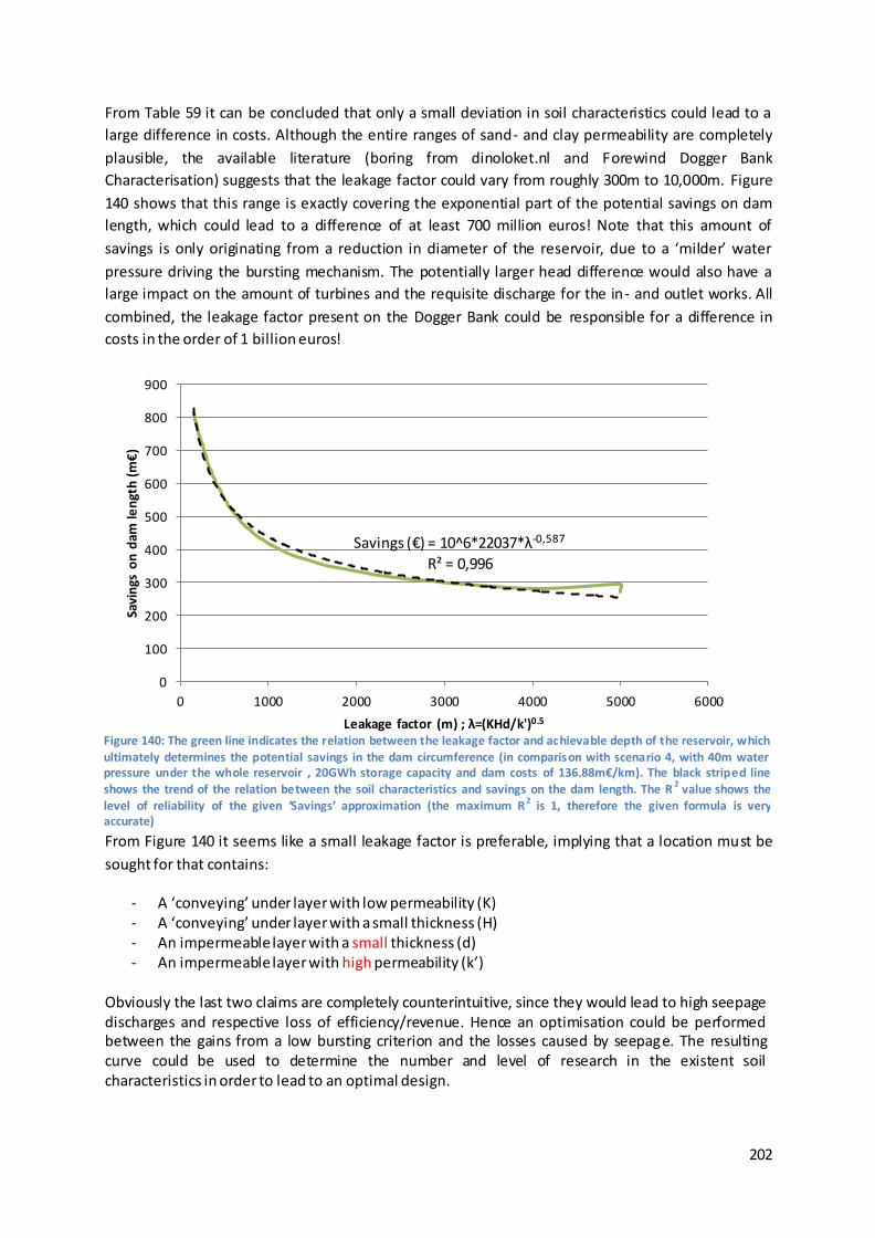
202
From Table 59 it can be concluded that only a small deviation in soil characteristics could lead to a
large difference in costs. Although the entire ranges of sand- and clay permeability are completely
plausible, the available literature (boring from dinoloket.nl and Forewind Dogger Bank
Characterisation) suggests that the leakage factor could vary from roughly 300m to 10,000m. Figure
140 shows that this range is exactly covering the exponential part of the potential savings on dam
length, which could lead to a difference of at least 700 million euros! Note that this amount of
savings is only originating from a reduction in diameter of the reservoir, due to a ‘milder’ water
pressure driving the bursting mechanism. The potentially larger head difference would also have a
large impact on the amount of turbines and the requisite discharge for the in- and outlet works. All
combined, the leakage factor present on the Dogger Bank could be responsible for a difference in
costs in the order of 1 billion euros!
From Figure 140 it seems like a small leakage factor is preferable, implying that a location must be
sought for that contains:
- A ‘conveying’ under layer with low permeability (K) - A ‘conveying’ under layer with a small thickness (H) - An impermeable layer with a small thickness (d) - An impermeable layer with high permeability (k’)
Obviously the last two claims are completely counterintuitive, since they would lead to high seepage discharges and respective loss of efficiency/revenue. Hence an optimisation could be performed between the gains from a low bursting criterion and the losses caused by seepage. The resulting curve could be used to determine the number and level of research in the existent soil characteristics in order to lead to an optimal design.
Savings (€) = 10^6*22037*λ-0,587
R² = 0,996
0
100
200
300
400
500
600
700
800
900
0 1000 2000 3000 4000 5000 6000
Savi
ngs
on
dam
len
gth
(m
€)
Leakage factor (m) ; λ=(KHd/k')0.5 Figure 140: The green line indicates the relation between the leakage factor and achievable depth of the reservoir, which ultimately determines the potential savings in the dam circumference (in comparison with scenario 4, with 40m water pressure under the whole reservoir , 20GWh storage capacity and dam costs of 136.88m€/km). The black striped line
shows the trend of the relation between the soil characteristics and savings on the dam length. The R2 value shows the
level of reliability of the given ‘Savings’ approximation (the maximum R 2 is 1, therefore the given formula is very accurate)
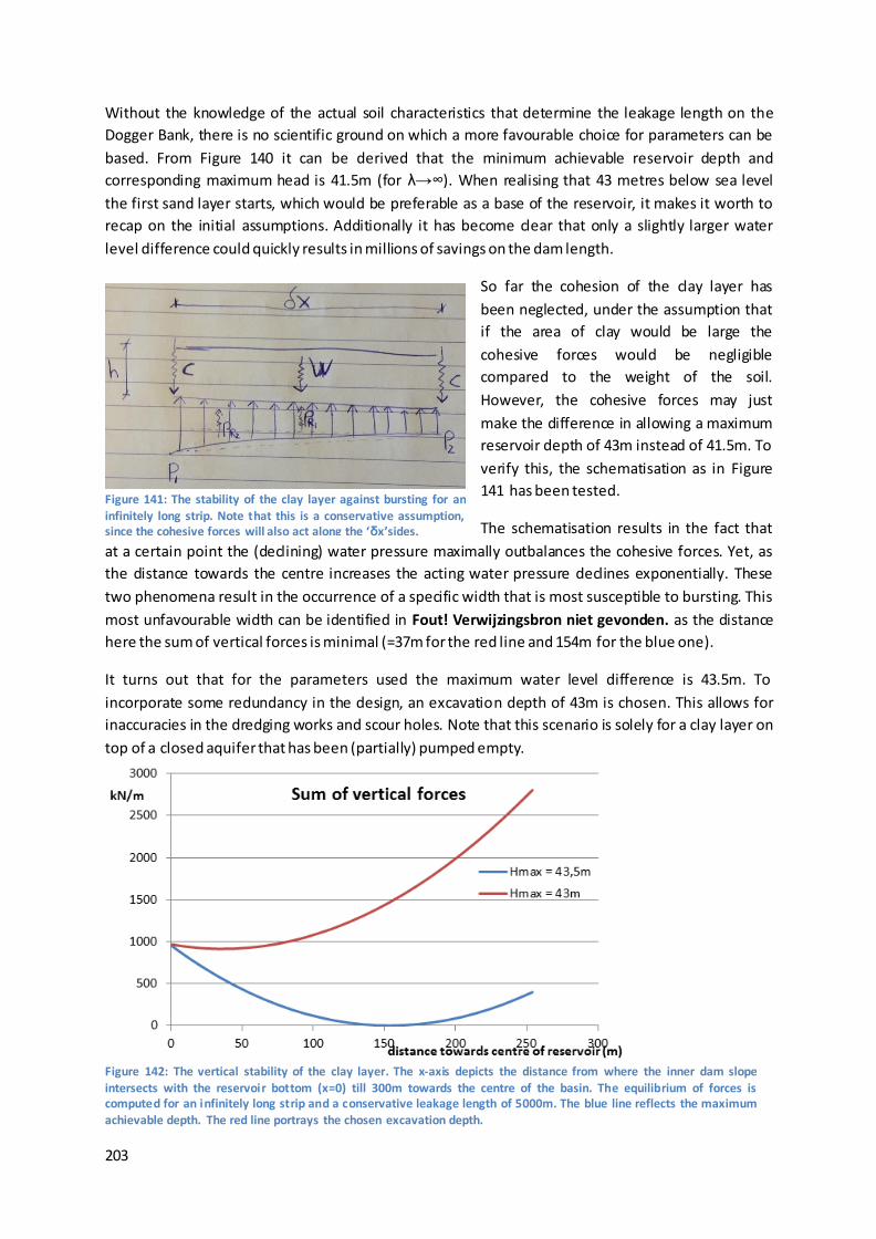
203
Figure 142: The vertical stability of the clay layer. The x-axis depicts the distance from where the inner dam slope intersects with the reservoir bottom (x=0) till 300m towards the centre of the basin. The equilibrium of forces is computed for an infinitely long strip and a conservative leakage length of 5000m. The blue line reflects the maximum
achievable depth. The red line portrays the chosen excavation depth.
Without the knowledge of the actual soil characteristics that determine the leakage length on the
Dogger Bank, there is no scientific ground on which a more favourable choice for parameters can be
based. From Figure 140 it can be derived that the minimum achievable reservoir depth and
corresponding maximum head is 41.5m (for λ→∞). When realising that 43 metres below sea level
the first sand layer starts, which would be preferable as a base of the reservoir, it makes it worth to
recap on the initial assumptions. Additionally it has become clear that only a slightly larger water
level difference could quickly results in millions of savings on the dam length.
So far the cohesion of the clay layer has
been neglected, under the assumption that
if the area of clay would be large the
cohesive forces would be negligible
compared to the weight of the soil.
However, the cohesive forces may just
make the difference in allowing a maximum
reservoir depth of 43m instead of 41.5m. To
verify this, the schematisation as in Figure
141 has been tested.
The schematisation results in the fact that
at a certain point the (declining) water pressure maximally outbalances the cohesive forces. Yet, as
the distance towards the centre increases the acting water pressure declines exponentially. These
two phenomena result in the occurrence of a specific width that is most susceptible to bursting. This
most unfavourable width can be identified in Fout! Verwijzingsbron niet gevonden. as the distance
here the sum of vertical forces is minimal (=37m for the red line and 154m for the blue one).
It turns out that for the parameters used the maximum water level difference is 43.5m. To
incorporate some redundancy in the design, an excavation depth of 43m is chosen. This allows for
inaccuracies in the dredging works and scour holes. Note that this scenario is solely for a clay layer on
top of a closed aquifer that has been (partially) pumped empty.
Figure 141: The stability of the clay layer against bursting for an infinitely long strip. Note that this is a conservative assumption, since the cohesive forces will also act along the ‘δx’sides.
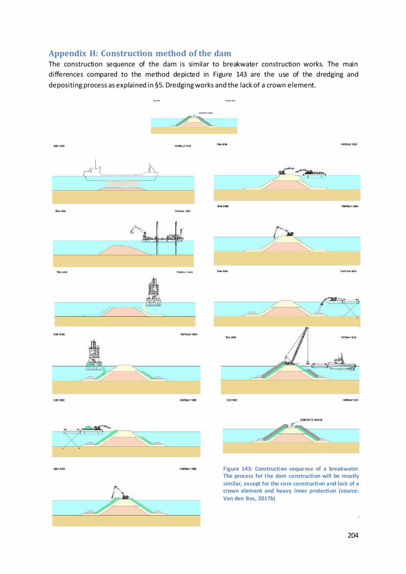
204
Appendix H: Construction method of the dam The construction sequence of the dam is similar to breakwater construction works. The main
differences compared to the method depicted in Figure 143 are the use of the dredging and
depositing process as explained in §5. Dredging works and the lack of a crown element.
Figure 143: Construction sequence of a breakwater. The process for the dam construction will be mostly similar, except for the core construction and lack of a crown element and heavy inner protection (source:
Van den Bos, 2017b)
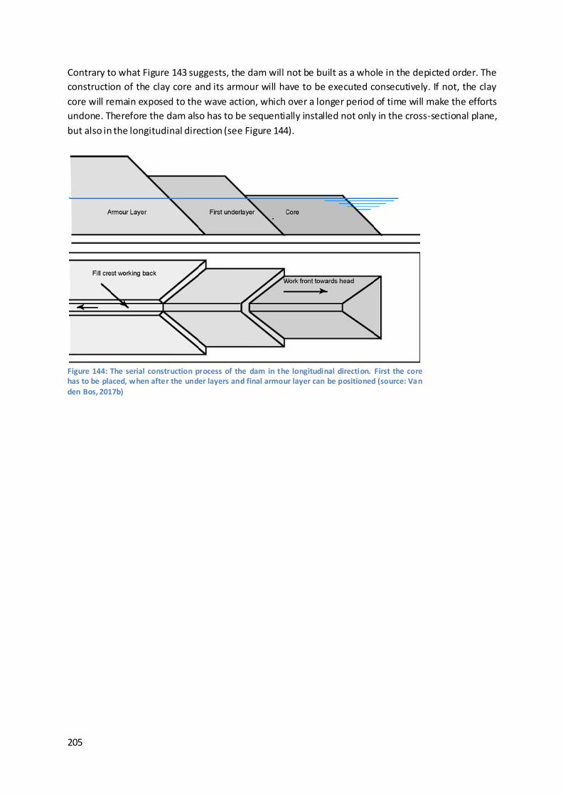
205
Contrary to what Figure 143 suggests, the dam will not be built as a whole in the depicted order. The
construction of the clay core and its armour will have to be executed consecutively. If not, the clay
core will remain exposed to the wave action, which over a longer period of time will make the efforts
undone. Therefore the dam also has to be sequentially installed not only in the cross-sectional plane,
but also in the longitudinal direction (see Figure 144).
Figure 144: The serial construction process of the dam in the longitudinal direction. First the core has to be placed, when after the under layers and final armour layer can be positioned (source: Van den Bos, 2017b)
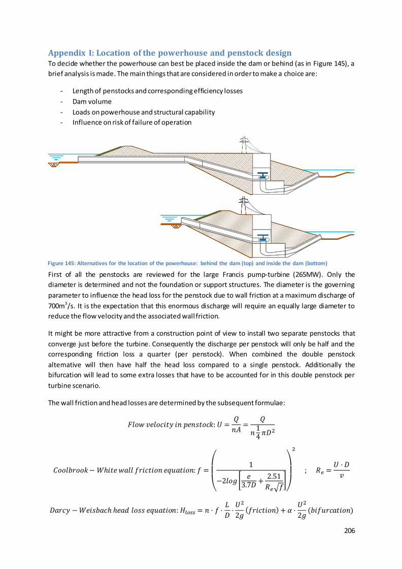
206
Appendix I: Location of the powerhouse and penstock design To decide whether the powerhouse can best be placed inside the dam or behind (as in Figure 145), a
brief analysis is made. The main things that are considered in order to make a choice are:
- Length of penstocks and corresponding efficiency losses
- Dam volume
- Loads on powerhouse and structural capability
- Influence on risk of failure of operation
First of all the penstocks are reviewed for the large Francis pump-turbine (265MW). Only the
diameter is determined and not the foundation or support structures. The diameter is the governing
parameter to influence the head loss for the penstock due to wall friction at a maximum discharge of
700m3/s. It is the expectation that this enormous discharge will require an equally large diameter to
reduce the flow velocity and the associated wall friction.
It might be more attractive from a construction point of view to install two separate penstocks that
converge just before the turbine. Consequently the discharge per penstock will only be half and the
corresponding friction loss a quarter (per penstock). When combined the double penstock
alternative will then have half the head loss compared to a single penstock. Additionally the
bifurcation will lead to some extra losses that have to be accounted for in this double penstock per
turbine scenario.
The wall friction and head losses are determined by the subsequent formulae:
𝐹𝑙𝑜𝑤 𝑣𝑒𝑙𝑜𝑐𝑖𝑡𝑦 𝑖𝑛 𝑝𝑒𝑛𝑠𝑡𝑜𝑐𝑘: 𝑈 =𝑄
𝑛𝐴=
𝑄
𝑛14𝜋𝐷2
𝐶𝑜𝑜𝑙𝑏𝑟𝑜𝑜𝑘− 𝑊ℎ𝑖𝑡𝑒 𝑤𝑎𝑙𝑙 𝑓𝑟𝑖𝑐𝑡𝑖𝑜𝑛 𝑒𝑞𝑢𝑎𝑡𝑖𝑜𝑛: 𝑓 =
(
1
−2𝑙𝑜𝑔[𝑒3.7𝐷
+2.51
𝑅𝑒√𝑓])
2
; 𝑅𝑒 =𝑈 ⋅ 𝐷
𝑣
𝐷𝑎𝑟𝑐𝑦 −𝑊𝑒𝑖𝑠𝑏𝑎𝑐ℎ ℎ𝑒𝑎𝑑 𝑙𝑜𝑠𝑠 𝑒𝑞𝑢𝑎𝑡𝑖𝑜𝑛: 𝐻𝑙𝑜𝑠𝑠 = 𝑛 ⋅ 𝑓 ⋅𝐿
𝐷⋅𝑈2
2𝑔(𝑓𝑟𝑖𝑐𝑡𝑖𝑜𝑛) + 𝛼 ⋅
𝑈2
2𝑔(𝑏𝑖𝑓𝑢𝑟𝑐𝑎𝑡𝑖𝑜𝑛)
Figure 145: Alternatives for the location of the powerhouse: behind the dam (top) and inside the dam (bottom)
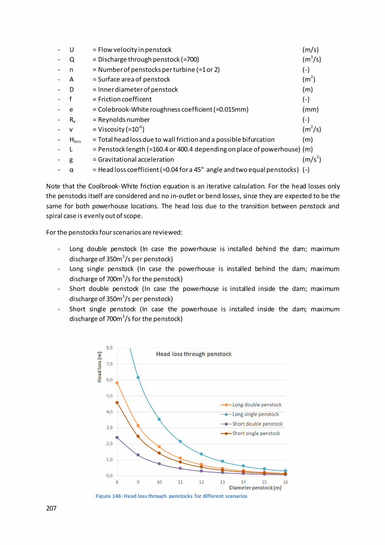
207
- U = Flow velocity in penstock (m/s)
- Q = Discharge through penstock (=700) (m3/s)
- n = Number of penstocks per turbine (=1 or 2) (-)
- A = Surface area of penstock (m2)
- D = Inner diameter of penstock (m)
- f = Friction coefficent (-)
- e = Colebrook-White roughness coefficient (=0.015mm) (mm)
- Re = Reynolds number (-)
- v = Viscosity (=10-6) (m2/s)
- Hloss = Total head loss due to wall friction and a possible bifurcation (m)
- L = Penstock length (=160.4 or 400.4 depending on place of powerhouse) (m)
- g = Gravitational acceleration (m/s2)
- α = Head loss coefficient (=0.04 for a 45° angle and two equal penstocks) (-)
Note that the Coolbrook-White friction equation is an iterative calculation. For the head losses only
the penstocks itself are considered and no in-outlet or bend losses, since they are expected to be the
same for both powerhouse locations. The head loss due to the transition between penstock and
spiral case is evenly out of scope.
For the penstocks four scenarios are reviewed:
- Long double penstock (In case the powerhouse is installed behind the dam; maximum
discharge of 350m3/s per penstock)
- Long single penstock (In case the powerhouse is installed behind the dam; maximum
discharge of 700m3/s for the penstock)
- Short double penstock (In case the powerhouse is installed inside the dam; maximum
discharge of 350m3/s per penstock)
- Short single penstock (In case the powerhouse is installed inside the dam; maximum
discharge of 700m3/s for the penstock)
Figure 146: Head loss through penstocks for different scenarios
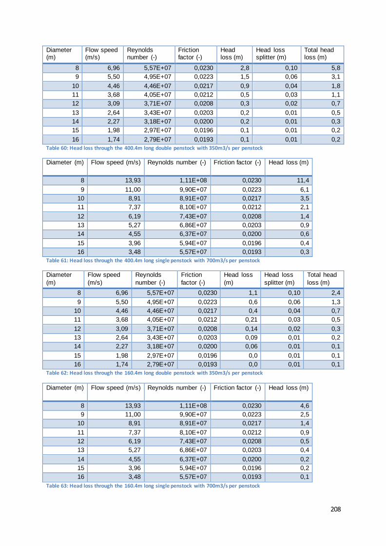
208
Diameter (m)
Flow speed (m/s)
Reynolds number (-)
Friction factor (-)
Head loss (m)
Head loss splitter (m)
Total head loss (m)
8 6,96 5,57E+07 0,0230 2,8 0,10 5,8
9 5,50 4,95E+07 0,0223 1,5 0,06 3,1
10 4,46 4,46E+07 0,0217 0,9 0,04 1,8
11 3,68 4,05E+07 0,0212 0,5 0,03 1,1
12 3,09 3,71E+07 0,0208 0,3 0,02 0,7
13 2,64 3,43E+07 0,0203 0,2 0,01 0,5
14 2,27 3,18E+07 0,0200 0,2 0,01 0,3
15 1,98 2,97E+07 0,0196 0,1 0,01 0,2
16 1,74 2,79E+07 0,0193 0,1 0,01 0,2
Table 60: Head loss through the 400.4m long double penstock with 350m3/s per penstock
Diameter (m) Flow speed (m/s) Reynolds number (-) Friction factor (-) Head loss (m)
8 13,93 1,11E+08 0,0230 11,4
9 11,00 9,90E+07 0,0223 6,1
10 8,91 8,91E+07 0,0217 3,5
11 7,37 8,10E+07 0,0212 2,1
12 6,19 7,43E+07 0,0208 1,4
13 5,27 6,86E+07 0,0203 0,9
14 4,55 6,37E+07 0,0200 0,6
15 3,96 5,94E+07 0,0196 0,4
16 3,48 5,57E+07 0,0193 0,3
Table 61: Head loss through the 400.4m long single penstock with 700m3/s per penstock
Diameter
(m)
Flow speed
(m/s)
Reynolds
number (-)
Friction
factor (-)
Head loss
(m)
Head loss
splitter (m)
Total head
loss (m)
8 6,96 5,57E+07 0,0230 1,1 0,10 2,4
9 5,50 4,95E+07 0,0223 0,6 0,06 1,3
10 4,46 4,46E+07 0,0217 0,4 0,04 0,7
11 3,68 4,05E+07 0,0212 0,21 0,03 0,5
12 3,09 3,71E+07 0,0208 0,14 0,02 0,3
13 2,64 3,43E+07 0,0203 0,09 0,01 0,2
14 2,27 3,18E+07 0,0200 0,06 0,01 0,1
15 1,98 2,97E+07 0,0196 0,0 0,01 0,1
16 1,74 2,79E+07 0,0193 0,0 0,01 0,1
Table 62: Head loss through the 160.4m long double penstock with 350m3/s per penstock
Diameter (m) Flow speed (m/s) Reynolds number (-) Friction factor (-) Head loss (m)
8 13,93 1,11E+08 0,0230 4,6
9 11,00 9,90E+07 0,0223 2,5
10 8,91 8,91E+07 0,0217 1,4
11 7,37 8,10E+07 0,0212 0,9
12 6,19 7,43E+07 0,0208 0,5
13 5,27 6,86E+07 0,0203 0,4
14 4,55 6,37E+07 0,0200 0,2
15 3,96 5,94E+07 0,0196 0,2
16 3,48 5,57E+07 0,0193 0,1
Table 63: Head loss through the 160.4m long single penstock with 700m3/s per penstock
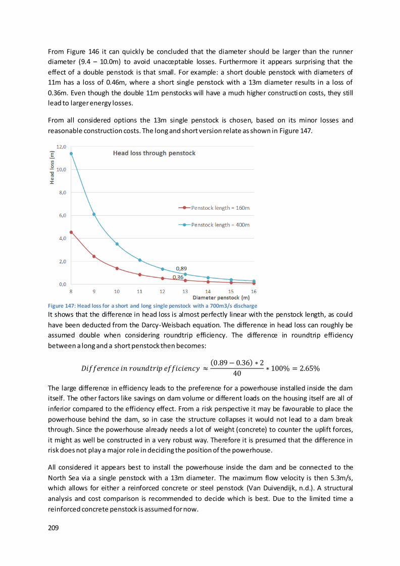
209
From Figure 146 it can quickly be concluded that the diameter should be larger than the runner
diameter (9.4 – 10.0m) to avoid unacceptable losses. Furthermore it appears surprising that the
effect of a double penstock is that small. For example: a short double penstock with diameters of
11m has a loss of 0.46m, where a short single penstock with a 13m diameter results in a loss of
0.36m. Even though the double 11m penstocks will have a much higher constructi on costs, they still
lead to larger energy losses.
From all considered options the 13m single penstock is chosen, based on its minor losses and
reasonable construction costs. The long and short version relate as shown in Figure 147.
It shows that the difference in head loss is almost perfectly linear with the penstock length, as could
have been deducted from the Darcy-Weisbach equation. The difference in head loss can roughly be
assumed double when considering roundtrip efficiency. The difference in roundtrip efficiency
between a long and a short penstock then becomes:
𝐷𝑖𝑓𝑓𝑒𝑟𝑒𝑛𝑐𝑒 𝑖𝑛 𝑟𝑜𝑢𝑛𝑑𝑡𝑟𝑖𝑝 𝑒𝑓𝑓𝑖𝑐𝑖𝑒𝑛𝑐𝑦 ≈(0.89− 0.36) ∗ 2
40∗ 100% = 2.65%
The large difference in efficiency leads to the preference for a powerhouse installed inside the dam
itself. The other factors like savings on dam volume or different loads on the housing itself are all of
inferior compared to the efficiency effect. From a risk perspective it may be favourable to place the
powerhouse behind the dam, so in case the structure collapses it would not lead to a dam break
through. Since the powerhouse already needs a lot of weight (concrete) to counter the uplift forces,
it might as well be constructed in a very robust way. Therefore it is presumed that the difference in
risk does not play a major role in deciding the position of the powerhouse.
All considered it appears best to install the powerhouse inside the dam and be connected to the
North Sea via a single penstock with a 13m diameter. The maximum flow velocity is then 5.3m/s,
which allows for either a reinforced concrete or steel penstock (Van Duivendijk, n.d.). A structural
analysis and cost comparison is recommended to decide which is best. Due to the limited time a
reinforced concrete penstock is assumed for now.
Figure 147: Head loss for a short and long single penstock with a 700m3/s discharge
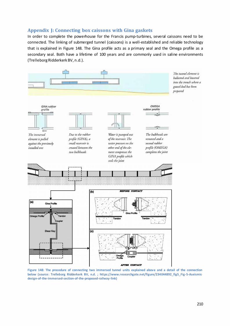
210
Appendix J: Connecting box caissons with Gina gaskets In order to complete the powerhouse for the Francis pump-turbines, several caissons need to be
connected. The linking of submerged tunnel (caissons) is a well-established and reliable technology
that is explained in Figure 148. The Gina profile acts as a primary seal and the Omega profile as a
secondary seal. Both have a lifetime of 100 years and are commonly used in saline environments
(Trelleborg Ridderkerk BV, n.d.).
Figure 148: The procedure of connecting two immersed tunnel units explained above and a detail of the connection below (source: Trelleborg Ridderkerk BV, n.d. ; https://www.researchgate.net/figure/234044892_fig5_Fig-5-Aseismic-design-of-the-immersed-section-of-the-proposed-railway-link)
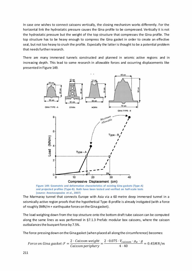
211
In case one wishes to connect caissons vertically, the closing mechanism works differently. For the
horizontal link the hydrostatic pressure causes the Gina profile to be compressed. Vertically it is not
the hydrostatic pressure but the weight of the top structure that compresses the Gina profile. The
top structure has to be heavy enough to compress the Gina gasket in order to create an effective
seal, but not too heavy to crush the profile. Especially the latter is thought to be a potential problem
that needs further research.
There are many immersed tunnels constructed and planned in seismic active regions and in
increasing depth. This lead to some research in allowable forces and occurring displacements like
presented in Figure 149.
The Marmaray tunnel that connects Europe with Asia via a 60 metre deep immersed tunnel in a
seismically active region proofs that the hypothetical Type-B profile is already instigated (with a force
of roughly 3MN/m + earthquake forces on the Gina gasket).
The load weighing down from the top structure onto the bottom draft tube caisson can be computed
along the same lines as was performed in §7.1.3 Prefab: modular box caissons, where the caisson
outbalances the buoyant force by 7.5%.
The force pressing down on the Gina gasket (when placed all along the circumference) becomes:
𝐹𝑜𝑟𝑐𝑒 𝑜𝑛 𝐺𝑖𝑛𝑎 𝑔𝑎𝑠𝑘𝑒𝑡:𝐹 =2 ⋅ 𝐶𝑎𝑖𝑠𝑠𝑜𝑛 𝑤𝑒𝑖𝑔ℎ𝑡
𝐶𝑎𝑖𝑠𝑠𝑜𝑛 𝑝𝑒𝑟𝑖𝑝ℎ𝑒𝑟𝑦=2 ⋅ 0.075 ⋅ 𝑉𝑐𝑎𝑖𝑠𝑠𝑜𝑛 ⋅ 𝜌𝑤 ⋅ 𝑔
4 ⋅ 40= 0.45𝑀𝑁/𝑚
Figure 149: Geometric and deformation characteristics of existing Gina gaskets (Type-A) and projected profiles (Type-B). Both have been tested and verified on half-scale tests (source: Anastasopoulos et al., 2007)
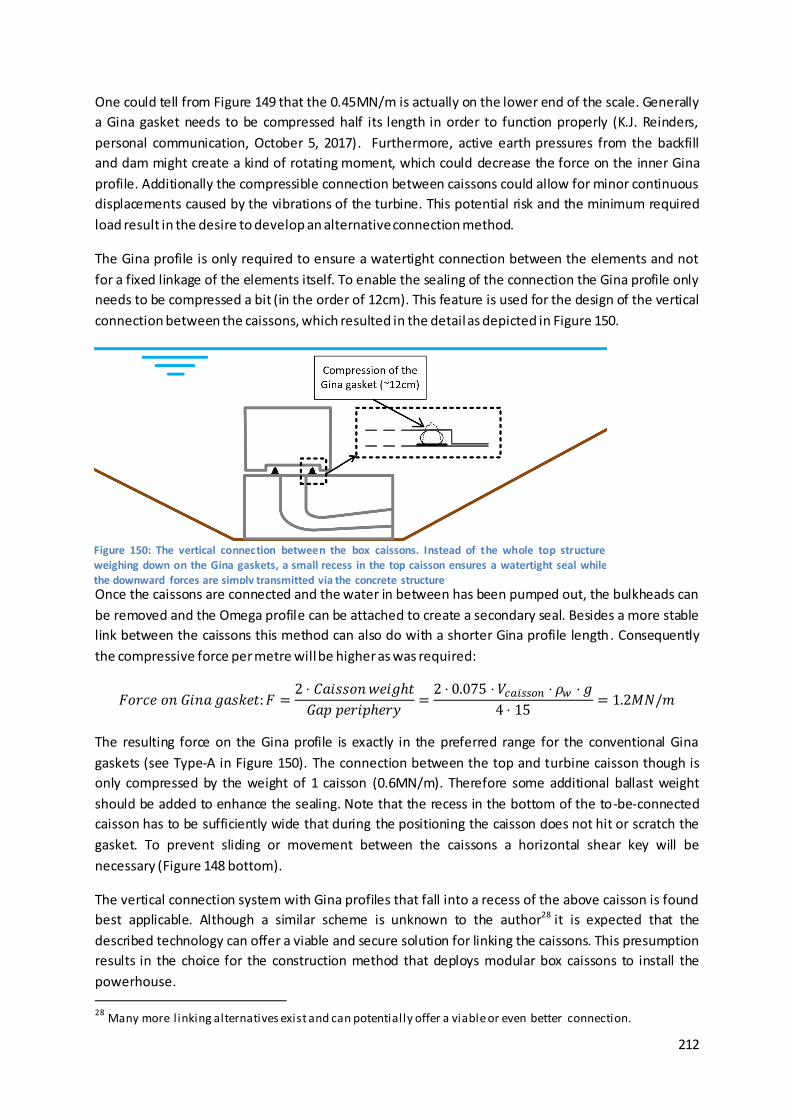
212
One could tell from Figure 149 that the 0.45MN/m is actually on the lower end of the scale. Generally
a Gina gasket needs to be compressed half its length in order to function properly (K.J. Reinders,
personal communication, October 5, 2017). Furthermore, active earth pressures from the backfill
and dam might create a kind of rotating moment, which could decrease the force on the inner Gina
profile. Additionally the compressible connection between caissons could allow for minor continuous
displacements caused by the vibrations of the turbine. This potential risk and the minimum required
load result in the desire to develop an alternative connection method.
The Gina profile is only required to ensure a watertight connection between the elements and not
for a fixed linkage of the elements itself. To enable the sealing of the connection the Gina profile only
needs to be compressed a bit (in the order of 12cm). This feature is used for the design of the vertical
connection between the caissons, which resulted in the detail as depicted in Figure 150.
Once the caissons are connected and the water in between has been pumped out, the bulkheads can
be removed and the Omega profile can be attached to create a secondary seal. Besides a more stable
link between the caissons this method can also do with a shorter Gina profile length. Consequently
the compressive force per metre will be higher as was required:
𝐹𝑜𝑟𝑐𝑒 𝑜𝑛 𝐺𝑖𝑛𝑎 𝑔𝑎𝑠𝑘𝑒𝑡:𝐹 =2 ⋅ 𝐶𝑎𝑖𝑠𝑠𝑜𝑛 𝑤𝑒𝑖𝑔ℎ𝑡
𝐺𝑎𝑝 𝑝𝑒𝑟𝑖𝑝ℎ𝑒𝑟𝑦=2 ⋅ 0.075 ⋅ 𝑉𝑐𝑎𝑖𝑠𝑠𝑜𝑛 ⋅ 𝜌𝑤 ⋅ 𝑔
4 ⋅ 15= 1.2𝑀𝑁/𝑚
The resulting force on the Gina profile is exactly in the preferred range for the conventional Gina
gaskets (see Type-A in Figure 150). The connection between the top and turbine caisson though is
only compressed by the weight of 1 caisson (0.6MN/m). Therefore some additional ballast weight
should be added to enhance the sealing. Note that the recess in the bottom of the to-be-connected
caisson has to be sufficiently wide that during the positioning the caisson does not hit or scratch the
gasket. To prevent sliding or movement between the caissons a horizontal shear key will be
necessary (Figure 148 bottom).
The vertical connection system with Gina profiles that fall into a recess of the above caisson is found
best applicable. Although a similar scheme is unknown to the author28 it is expected that the
described technology can offer a viable and secure solution for linking the caissons. This presumption
results in the choice for the construction method that deploys modular box caissons to install the
powerhouse. 28
Many more linking alternatives exist and can potentially offer a viable or even better connection.
Figure 150: The vertical connection between the box caissons. Instead of the whole top structure weighing down on the Gina gaskets, a small recess in the top caisson ensures a watertight seal while the downward forces are simply transmitted via the concrete structure

213
214
Related Documents


