Copy No. Guide for Mechanistic-Empirical Design OF NEW AND REHABILITATED PAVEMENT STRUCTURES FINAL DOCUMENT APPENDIX II-1: CALIBRATION OF FATIGUE CRACKING MODELS FOR FLEXIBLE PAVEMENTS NCHRP Prepared for National Cooperative Highway Research Program Transportation Research Board National Research Council Submitted by ARA, Inc., ERES Division 505 West University Avenue Champaign, Illinois 61820 February 2004

Welcome message from author
This document is posted to help you gain knowledge. Please leave a comment to let me know what you think about it! Share it to your friends and learn new things together.
Transcript

Copy No.
Guide for Mechanistic-Empirical Design OF NEW AND REHABILITATED PAVEMENT
STRUCTURES
FINAL DOCUMENT
APPENDIX II-1: CALIBRATION OF FATIGUE CRACKING MODELS FOR
FLEXIBLE PAVEMENTS
NCHRP
Prepared for National Cooperative Highway Research Program
Transportation Research Board National Research Council
Submitted by ARA, Inc., ERES Division
505 West University Avenue Champaign, Illinois 61820
February 2004

i
Acknowledgment of Sponsorship This work was sponsored by the American Association of State Highway and Transportation Officials (AASHTO) in cooperation with the Federal Highway Administration and was conducted in the National Cooperative Highway Research Program which is administered by the Transportation Research Board of the National Research Council. Disclaimer This is the final draft as submitted by the research agency. The opinions and conclusions expressed or implied in this report are those of the research agency. They are not necessarily those of the Transportation Research Board, the National Research Council, the Federal Highway Administration, AASHTO, or the individual States participating in the National Cooperative Highway Research program. Acknowledgements The research team for NCHRP Project 1-37A: Development of the 2002 Guide for the Design of New and Rehabilitated Pavement Structures consisted of Applied Research Associates, Inc., ERES Consultants Division (ARA-ERES) as the prime contractor with Arizona State University (ASU) as the primary subcontractor. Fugro-BRE, Inc., the University of Maryland, and Advanced Asphalt Technologies, LLC served as subcontractors to either ARA-ERES or ASU along with several independent consultants. Research into the subject area covered in this Appendix was conducted at ASU. The authors of this Appendix are Dr. M.W. Witczak and Mr. M. M. El-Basyouny. Foreword This appendix is the first in a series of three volumes on Calibration of Fatigue Cracking Models for Flexible Pavements. This volume concentrates on the selection, development, of calibration and validation aspects of the fatigue cracking models selected for the Design Guide. Both types of fatigue cracking (bottom up and top down) are discussed separately in the following sections. The fatigue cracking discussion will consist of: an overview of two widely used fatigue models evaluated for inclusion in the Design Guide. For each model evaluated, fatigue-cracking comparisons of data collected from the LTPP database will be discussed. Finally the calibration of the final fatigue cracking model and the reliability of the model selected are explained in detail. The other volumes are: Appendix II-2: Sensitivity Analysis for Asphalt Concrete Fatigue Alligator Cracking Appendix II-3: Sensitivity Analysis for Asphalt Concrete Fatigue Longitudinal Surface
Cracking

ii
Table of Contents
Appendix II-1
Calibration of Fatigue Cracking Models for Flexible Pavements
Page
Annex A- 2 Calibration of Fatigue Cracking Models for Flexible Pavements
Annex B- 83
Bottom-Up Alligator Fatigue Cracking Shell Oil Model Calibration Results Annex C- 113
Bottom-Up Alligator Fatigue Cracking MS-1 Model Calibration Results Annex D- 143
Top-Down Longitudinal Fatigue Cracking Shell Oil Model Calibration Results Annex E- 172
Top-Down Longitudinal Fatigue Cracking MS-1 Model Calibration Results
1
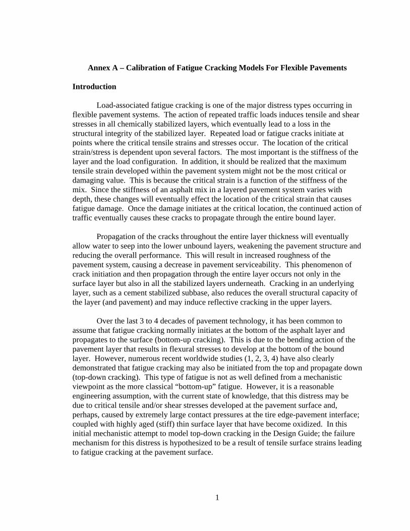
Annex A – Calibration of Fatigue Cracking Models For Flexible Pavements
Introduction Load-associated fatigue cracking is one of the major distress types occurring in
flexible pavement systems. The action of repeated traffic loads induces tensile and shear stresses in all chemically stabilized layers, which eventually lead to a loss in the structural integrity of the stabilized layer. Repeated load or fatigue cracks initiate at points where the critical tensile strains and stresses occur. The location of the critical strain/stress is dependent upon several factors. The most important is the stiffness of the layer and the load configuration. In addition, it should be realized that the maximum tensile strain developed within the pavement system might not be the most critical or damaging value. This is because the critical strain is a function of the stiffness of the mix. Since the stiffness of an asphalt mix in a layered pavement system varies with depth, these changes will eventually effect the location of the critical strain that causes fatigue damage. Once the damage initiates at the critical location, the continued action of traffic eventually causes these cracks to propagate through the entire bound layer.
Propagation of the cracks throughout the entire layer thickness will eventually
allow water to seep into the lower unbound layers, weakening the pavement structure and reducing the overall performance. This will result in increased roughness of the pavement system, causing a decrease in pavement serviceability. This phenomenon of crack initiation and then propagation through the entire layer occurs not only in the surface layer but also in all the stabilized layers underneath. Cracking in an underlying layer, such as a cement stabilized subbase, also reduces the overall structural capacity of the layer (and pavement) and may induce reflective cracking in the upper layers.
Over the last 3 to 4 decades of pavement technology, it has been common to
assume that fatigue cracking normally initiates at the bottom of the asphalt layer and propagates to the surface (bottom-up cracking). This is due to the bending action of the pavement layer that results in flexural stresses to develop at the bottom of the bound layer. However, numerous recent worldwide studies (1, 2, 3, 4) have also clearly demonstrated that fatigue cracking may also be initiated from the top and propagate down (top-down cracking). This type of fatigue is not as well defined from a mechanistic viewpoint as the more classical “bottom-up” fatigue. However, it is a reasonable engineering assumption, with the current state of knowledge, that this distress may be due to critical tensile and/or shear stresses developed at the pavement surface and, perhaps, caused by extremely large contact pressures at the tire edge-pavement interface; coupled with highly aged (stiff) thin surface layer that have become oxidized. In this initial mechanistic attempt to model top-down cracking in the Design Guide; the failure mechanism for this distress is hypothesized to be a result of tensile surface strains leading to fatigue cracking at the pavement surface.

2
This chapter concentrates on the selection, development, of calibration and validation aspects of the fatigue cracking models selected for the Design Guide. Both types of fatigue cracking (bottom up and top down) are discussed separately in the following sections. The fatigue cracking discussion will consist of: an overview of two widely used fatigue models evaluated for inclusion in the Design Guide. For each model evaluated, fatigue-cracking comparisons of data collected from the LTPP database will be discussed. Finally the calibration of the final fatigue cracking model and the reliability of the model selected are explained in detail.
Asphalt Mixture Fatigue Cracking Models
Fatigue cracking prediction is normally based on the cumulative damage concept
given by Miner’s (5). The damage is calculated as the ratio of the predicted number of traffic repetitions to the allowable number of load repetitions (to some failure level) as shown in equation 1. Theoretically, fatigue cracking should occur at an accumulated damage value of 1. If a normal distribution is assumed for the damage ratio calculated, the percentage of area cracked can be computed and checked with field performance.
1
Ti
i i
nDN=
= ∑ (1)
where:
D = damage. T = total number of periods. ni = actual traffic for period i. Ni = allowable failure repetitions under conditions prevailing in period i.
The fatigue life of an asphalt concrete mixture is influenced by many factors. Several key mix properties such as asphalt type, asphalt content and air-void content are well known to influence fatigue. Other factors such as temperature, frequency, and rest periods of the applied load also are known to influence fatigue life. Other material properties may also affect the fatigue life. It is obvious that mix properties need to be carefully balanced to optimize fatigue cracking of any mixtures.
In the literature, the most commonly used model form to predict the number of
load repetitions to fatigue cracking is a function of the tensile strain and mix stiffness (modulus). The critical locations of the tensile strains may either be at the surface (result in top-down cracking) or at the bottom of the asphaltic layer (result in bottom-up cracking).
The general mathematical form of the number of load repetitions used in the
literature is shown in equation 2. The form of the model is a function of the tensile strains at a given location and modulus of the asphalt layer.

3
32 111
kk
tf E
CkN ⎟⎠⎞
⎜⎝⎛
⎟⎟⎠
⎞⎜⎜⎝
⎛=
ε (2)
where: Nf = Number of repetitions to fatigue cracking. εt = Tensile strain at the critical location. E = Stiffness of the material. k1, k2, k3 = Laboratory regression coefficients. C = Laboratory to field adjustment factor. The most commonly used fatigue cracking models are those developed by Shell
Oil (6) and the Asphalt Institute (MS-1) (7). The overall general form of each model is the same mathematical model form shown above. However, the difference is in the laboratory regression coefficients in the equation and the laboratory to field adjustment factor. In the following section these two models will be discussed, showing the difference between the two models and the effect of the laboratory testing procedure on the models.
It has to be noted that the fatigue-cracking model, which calculates the number of
cycles to failure is only expressing the stage of fatigue cracking described as the crack initiation stage. The second stage, or vertical crack propagation stage, is accounted for in these models by using the field adjustment factor. Other models in the literature use two different equations to express each stage of the fatigue cracking. For example, Lytton et al. (8) used fracture mechanics based upon the Paris law to model the crack propagation stage in his development of the theoretical Superpave Model. Finally, another (third) stage of fatigue fracture is associated with the growth in longitudinal area, in which fatigue cracking occurs. In general, true field fatigue failure is generally associated with a percentage of fatigue cracking along the roadway.
Constant Stress Vs Constant Strain Analysis
In the laboratory, two types of controlled loading are generally applied for fatigue characterization: constant stress and constant strain. In constant stress (load) testing, the applied stress during the fatigue testing remains constant. As the repetitive load causes damage in the test specimen, the stiffness of the mix is decreased due to the micro cracking observed. This, in turn, leads to an increase in tensile strain with load repetitions. In the constant strain test, the strain remains constant with the number of repetitions. Because of specimen damage due to the repetitive loading; the stress must be reduced to obtain the same strain. This leads to a reduced stiffness as a function of repetitions. The constant stress and constant strain phenomena are shown in Figure 1.

4
Constant Stress Constant Strain
Number of Cycles
Stiff
ness
Number of Cycles
Stre
ss
Number of Cycles
Stra
in
Number of Cycles
Stiff
ness
Number of Cycles
Stre
ss
Number of Cycles
Stra
in
Figure 1 Constant Stress and Constant Strain Phenomena
The constant stress type of loading is generally considered applicable to thick
asphalt pavement layers usually more than 8 inches. In this type of structure, the thick asphalt layer is the main load-carrying component and the strain increases, as the material gets weaker under repeated loading. However, with the reduction in the stiffness, because of the thickness, changes in the stress are not significant and this fact leads to a constant stress situation.
The constant strain type of loading is considered more applicable to thin asphalt
pavement layers usually less than 2 inches. The pavement layer is not the main load-carrying component. The strain in the asphalt layer is governed by the underlying layers and is not greatly affected by the change in the asphalt layer stiffness. This situation is conceptually more related to the category of constant strain. However, for intermediate thicknesses, fatigue life is generally governed by a situation that is a combination of constant stress and constant strain.

5
Shell Oil Model
Because of the known impact between stress states and damage mechanism for different thicknesses of asphalt layers, the Shell Oil Co. has developed fatigue damage prediction equations for the two major forms of laboratory fatigue testing. The equations developed are summarized below (6):
Constant Strain
8.155]112.00454.0)(0085.017.0[ −−−+−= EVVPIPIAN tbbff ε (3a) Constant Stress
4.155]0167.000673.0)(00126.00252.0[ −−−+−= EVVPIPIAN tbbff ε (3b) In the above equation PI is the penetration index as is defined by the following
equations:
AAPI
50150020
+−
= (4a)
“A” is the temperature susceptibility, which is the slope of the logarithm of
penetration versus temperature plot. Mathematically, this is expressed as:
21
21 )log()log(TT
TatpenTatpenA−−
= (4b)
T1 and T2 are temperatures in centigrade (oC), at which penetrations are measured.
In addition to the above equation, A can also be obtained from the following equation.
BRTT
TatpenA&
800log)log(−
−= (4c)
TR&B is the softening point or the Ring & Ball temperature as specified by
AASHTO (T53-84). Softening point temperature is the reference temperature (equi-viscous) at which all bitumens have the same consistency (viscosity or penetration). Tests have shown that at the TR&B temperature, the penetration of all bitumens is near 800. Replacing T2 in equation 4b by TR&B and pen at T2 by 800 results in equation 4c.
In developing an implementation scheme for equation 3, Witczak hypothesized
that the constant strain case was applicable for asphalt layer thickness of 2-inch or less and that the constant stress case was applicable for asphalt layer thickness of 8-inch or more. No relationship was available for intermediate thicknesses (thickness value

6
between 2 and 8 inches), which are the most common asphaltic thickness values used in the majority of flexible pavement construction.
In order to overcome this problem, a numerical transition approach was developed
by M. W. Witczak and M. W. Mirza (9) during the NCHRP 1-37A research to come-up with a generalized fatigue equation applicable to a broad range of thickness values. The methodology developed is based upon the constant stress and constant strain equations presented earlier (equation 3). Comparing equations 3a and 3b, it is apparent that the K1 factor represents the volumetric and the binder characteristics of the mix. Further examination of equations 4a and 4b reveals that for all practical purposes; each parameter coefficient ratio within the K1 term is:
i
i
aStressConstaStrainConst
.
.=α (5a)
746.6
0252.017.0
1 ==PI
PIα (5b)
746.6
)(00126.0)(0085.0
2 ==b
b
VPIVPI
α (5c)
746.6
00673.00454.0
3 ==b
b
VV
α (5d)
707.6
0167.0112.0
4 ==α (5e)
Thus, the average α for the four factors is 6.74. That is, the K1 values in the two
fatigue equations differ by a factor of α5 = 6.745 = 13,909. Another difference observed between the constant stress and constant strain equations is the power of the modulus term (E). A value of k3 = 1.8 occurs for the constant strain (hac ≤ 2 inch) condition, while 1.4 is present for constant stress (hac ≥ 8 inch). Based upon these findings, a generalized (modified) Shell Oil based fatigue equation for each mode of loading is given by:
Constant Strain: 8.15
1113909 −
⎟⎟⎠
⎞⎜⎜⎝
⎛= EKAN
tff εαε (6a)
Constant Stress: 4.15
11 −
⎟⎟⎠
⎞⎜⎜⎝
⎛= EKAN
tff εασ (6b)

7
It should be noted that the K1 value in the above equations is replaced by the K1α
value. The K1α represents the K1 value for the constant stress situation. Taking the ratio of these two equations results in the following relationship.
4.0*13909 −== ENN
Ff
f
σ
ε (7a)
That is:
σε ff NFN *= (7b) In the above equation F represents the ratio between the constant strain and
constant stress and is a function of the modulus (E) of asphalt layer. Estimated values of F as a function of the modulus of the mix are given in Table 1. It is to be noted that the value of F is always one for the constant stress situation. That is, for a modulus value of 1,000,000 psi, F-value for constant strain situation is 55.3. This means that under the constant strain situation, the fatigue life of an asphalt mix, at a mix stiffness of 1,000,000 psi, is 55.3 times that predicted under constant stress conditions.
Table 1 only provides F-values for the two extreme conditions, constant strain
(thickness <= 2 inch) and constant stress situation (thickness => 8 inch). In order to have a continuous function between constant strain and stress conditions, it was assumed that a sigmoidal relationship, between the two F conditions and all intermediate thickness (2 inches to 8 inches), would be applicable. Thus, a sigmoidal function of "F was defined
Table 1 Calculated F Values for Constant Strain and Constant Stress Situation
Modulus (E), psi Constant Strain
(hac ≤ 2 inch)
Constant Stress
(hac ≥ 8 inch)
50,000 183.4 1.0
100,000 139.0 1.0
500,000 73.0 1.0
1,000,00 55.3 1.0
5,000,00 29.0 1.0

8
(developed) to be given by:
)408.5354.1(exp1
1" −++=
ach
FF (8)
Equation 8 provides "F -values as a function of the F-value (Equation 7a) and the
thickness, providing a continuous fatigue relationship. This function is shown in Equation 9.
4.15
11" −
⎟⎟⎠
⎞⎜⎜⎝
⎛= EKFAN
tff εσ (9)
The sigmoidal relationship shown in the above equation is also graphically shown in Figure 2. The "F -values shown are noted to be functions of the stiffness of the mix. It is important to note that the "F -value decreases with increasing modulus. This implies that the difference in fatigue life between constant strain and constant stress decreases as the stiffness increases. The overall generalized equation developed based upon the above analysis is presented in Table 2
0
20
40
60
80
100
120
140
160
180
200
0 2 4 6 8 10 12 14
AC Layer Thickness, inch
Thic
knes
s A
djus
tmen
t Fac
tor
- F"
50 ksi 100 ksi 500 ksi 1,000 ksi 5,000 ksi
Figure 2 Sigmoidal Fit to Fatigue Equation Parameters

9
Table 2 Generalized Shell Oil Fatigue Equations 4.1
*
55
)408.5354.1(
4.0 11)0167.000673.0)(00126.00252.0(exp1
1139091−
−
−
⎟⎠⎞
⎜⎝⎛
⎟⎟⎠
⎞⎜⎜⎝
⎛−+−⎟⎟
⎠
⎞⎜⎜⎝
⎛+
−+=
EVVPIPIEAN
tbbhff ac ε
where
)408.5354.1(
4.0
exp11139091" −
−
+−
+=ach
EF
5
1 ]0167.000673.0)(00126.00252.0[ −+−= bb VVPIPIK α Af = laboratory to field adjustment factor (default = 1.0)

10
Asphalt Institute (MS-1) Model The Asphalt Institute’s (7) fatigue equation is based upon modifications to
constant stress laboratory fatigue criteria. Because the approach developed by Witczak and Shook (10) was applicable to thicker full-depth asphalt pavements, use of any type of controlled strain results were not incorporated. The number of load repetitions to failure is expressed in the same mathematical form as the Shell Oil model and it is given by:
854.0291.3
1100432.0 ⎟⎠⎞
⎜⎝⎛
⎟⎟⎠
⎞⎜⎜⎝
⎛=
ECN
tf ε
MC 10=
⎟⎟⎠
⎞⎜⎜⎝
⎛−
+= 69.084.4
ba
b
VVV
M (10)
where: Vb = effective binder content (%). Va = air voids (%). This equation (model), developed by Witczak et al (7) for the Ninth Edition of
MS-1, utilized the basic fatigue relationship developed under NCHRP 1-10 by Fred Finn et al. (11) and modified by Witczak to incorporate mixture volumetric adjustments developed by Monismith et al.
The Asphalt Institute Ninth Edition of the MS-1 design manual (7) used a field
calibration factor of 18.4 to adjust for the effect of the laboratory to field differences. This correction factor was developed for a 20% level cracking in the wheel path and was that recommended by Finn in his classic NCHRP 1-10 study (11).
Comparing the Shell Oil model to the MS-1 model will lead to the conclusion that
both models are exactly the same form. However, the coefficients are less for the MS-1 model compared to the Shell Oil. This would be reasonable to accept because the Shell Oil relationships are based upon laboratory testing while the MS-1 equation (derived from NCHRP 1-10) was heavily based upon actual field calibration studies.
While there are many other available fatigue models, which are found in the
literature, the dissertation (and implementation into the Design Guide) focused only on the Shell Oil and the MS-1 models. This was accomplished because it was the opinion of the NCHRP 1-37A team, that these two models represented the most powerful and accurate state of the art fatigue models for potential inclusion into the final Design guide. Calibration of Fatigue Cracking Models
The asphalt concrete mix fatigue-cracking models (both bottom-up cracking and
top-down cracking) were calibrated following the process noted below:

11
1. Calibration (performance) data was collected from the LTPP database for
each field section. 2. Simulation (predictive) runs were done using the 2002 Design Guide
software and using a different set of calibration coefficients in the number of load repetition model.
3. The predicted damage from each calibration coefficient combination was compared to the measured cracking observed in the field. The coefficient combination with the least scatter of the data and the correct trends was selected.
4. The predicted damage was correlated to the measured cracking in the field by minimizing the square of the errors.
The calibration data collection was done at the same time for both types of fatigue
cracking as the same sections were used for both bottom-up and top-down cracking calibration. In the following sections each step of the above listed calibration steps is discussed in details. The calibration data will be presented in a general section for both fatigue- cracking types, and then each fatigue cracking model calibration will be discussed separately.
Calibration Data
The main source used to obtain performance data for the calibration of the fatigue
cracking was the LTPP database. Data were mainly obtained from the General Pavement Sites (GPS) and the Special Pavement Sites (SPS) (12). Appendix EE includes a detailed listing of the sections and the section data used in the calibration process, as well as any assumptions made for some of these sections to replace missing data. In a limited number of cases some parameters were not found. These values were assumed using a default value based on experience and the literature review. Appendix EE1 includes the data for the new pavement sections (13), while Appendix EE-2 includes the data for the rehabilitation pavement sections (14). It has to be noted that the rehabilitation data is included in the dissertation. However, the calibration of the rehabilitation sections is not an inherent part of this dissertation. The rehabilitation section calibration, however, is included as a part of the NCHRP 1-37A final reports and publications.
Two requirements for calibrating the performance prediction models are to ensure
that all major factors that influence the development of pavement distress are included and to ensure that the selected test pavements span the expected range of each factor. The approach used in the plan for model calibration was to select the desired number of field sections as well as desirable attribute values (ranges) of key factors; following generally accepted experimental statistical concepts. The approach emphasizes the recognition of key parameters for the factors of interest, selection of the appropriate number of levels for a factor, and the selection of the number of replicates within each cell of the experiment design. These experiments were designed to:
12
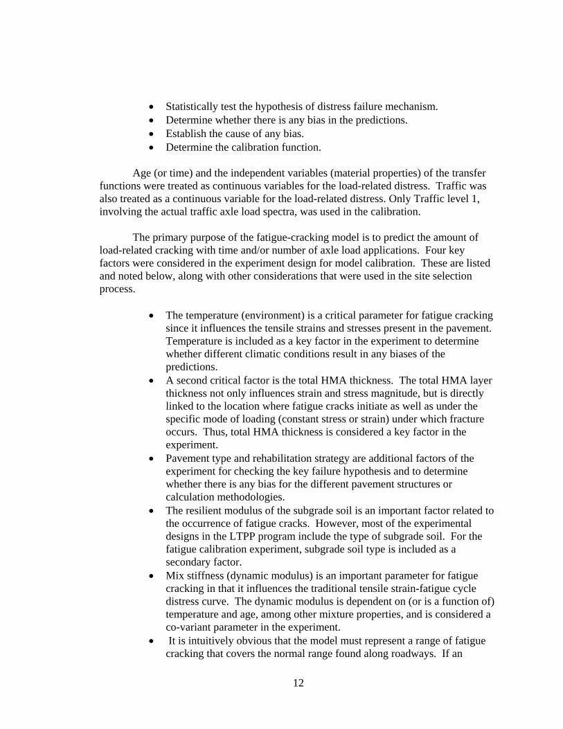
• Statistically test the hypothesis of distress failure mechanism. • Determine whether there is any bias in the predictions. • Establish the cause of any bias. • Determine the calibration function.
Age (or time) and the independent variables (material properties) of the transfer
functions were treated as continuous variables for the load-related distress. Traffic was also treated as a continuous variable for the load-related distress. Only Traffic level 1, involving the actual traffic axle load spectra, was used in the calibration.
The primary purpose of the fatigue-cracking model is to predict the amount of
load-related cracking with time and/or number of axle load applications. Four key factors were considered in the experiment design for model calibration. These are listed and noted below, along with other considerations that were used in the site selection process.
• The temperature (environment) is a critical parameter for fatigue cracking
since it influences the tensile strains and stresses present in the pavement. Temperature is included as a key factor in the experiment to determine whether different climatic conditions result in any biases of the predictions.
• A second critical factor is the total HMA thickness. The total HMA layer thickness not only influences strain and stress magnitude, but is directly linked to the location where fatigue cracks initiate as well as under the specific mode of loading (constant stress or strain) under which fracture occurs. Thus, total HMA thickness is considered a key factor in the experiment.
• Pavement type and rehabilitation strategy are additional factors of the experiment for checking the key failure hypothesis and to determine whether there is any bias for the different pavement structures or calculation methodologies.
• The resilient modulus of the subgrade soil is an important factor related to the occurrence of fatigue cracks. However, most of the experimental designs in the LTPP program include the type of subgrade soil. For the fatigue calibration experiment, subgrade soil type is included as a secondary factor.
• Mix stiffness (dynamic modulus) is an important parameter for fatigue cracking in that it influences the traditional tensile strain-fatigue cycle distress curve. The dynamic modulus is dependent on (or is a function of) temperature and age, among other mixture properties, and is considered a co-variant parameter in the experiment.
• It is intuitively obvious that the model must represent a range of fatigue cracking that covers the normal range found along roadways. If an

13
adequate range of cracking extent or magnitude is not included, the accuracy of the model over a wide range will be questionable. Thus, the distress magnitude is the fourth important factor considered in the calibration process. Field sections with varying levels of fatigue cracks were included in the experimental plan to cover the range of conditions. However, due to the availability of time-series distress data for each test section, the range in fatigue cracking was not included as a key factor in the experiment. Fatigue cracking magnitude was used in selecting the test sections for the individual cells.
The field sections were selected randomly to ensure that a well-balanced matrix
of salient pavement parameters and fatigue cracking was present in the experiment. The models were evaluated based on bias, precision, and accuracy, as defined below,
• Bias – An effect that deprives predictions of simulating “real world”
observations by systematically distorting it, as distinct from a random error that may distort on any one occasion but balances out on the average.
• Precision – The ability of a model to give repeated estimates that are very close together.
• Accuracy – The closeness of predictions to the “true” or “actual” value. The concept of accuracy encompasses both precision and bias.
Site Selection Criteria and Considerations The following lists and briefly defines the criteria that were considered in
selecting and prioritizing sites for use in the calibration and validation of the Design Guide distress prediction models for flexible pavements.
• Consistency of Measurements – It is imperative that a consistent
definition and measurement of the surface distresses and other data be used and maintained throughout the calibration and validation process. All data used to establish the inputs for the models (including, material test results, climatic data, and traffic data) and performance monitoring, are collected or measured in accordance with the FHWA LTPP publication Data Collection Guide For Long Term Pavement Performance (15) or with an equivalent method.
• Time-Series Distress Data – Projects or test sections that have three or more distress surveys or observations within their analysis life were given a high priority in the site selection process.
• Materials Characterization and Testing – Materials tests or properties were required for each input level. However, material testing (level 1 type) is outside the scope of this research work. Thus, test sections for which the material properties have already been measured are required for

14
use to calibrate the distress prediction models. The material properties of the pavement layers must be measured with the same test protocols to ensure that the results are compatible between different projects and test sections.
• Number of Layers – The test sections with the fewest number of structural layers and materials (e.g., one or two asphalt concrete layers, one unbound base layer, and one subbase layer) were given a higher priority to reduce the data collection requirements, as well as the complexity of the analysis.
• Traffic –The recommended traffic data collection frequency is one week per quarter year, or during periods of peak truck traffic. First priority in the selection of field sections for the calibration experiments was given to those in the LTPP inventory equipped with continuous WIM. Unfortunately, many LTPP test sections do not have continuous WIM data, even for a limited number of years. Thus, a second priority in the selection of field sections was given to those test sections with seasonal WIM monitoring with the greatest frequency of sampling and continuous AVC sampling for multiple years.
• Rehabilitation and New Construction – The computation methodology (incremental damage accumulation) to simulate a distress mechanism for both new construction (original pavement surfaces) and rehabilitation (overlays) will be different for some distresses. As a result, test sections with and without overlays were needed for the calibration and validation experiments.
• Maximum Use of Test Sections Between Model Studies – Coordination of field activities between projects can substantially reduce the number of test sections that will be required if each project were conducted independently from the others. Those projects or test sections that are planned for use on other research projects were given a higher priority for use in the calibration-validation process of the Design Guide distress prediction models.
• Non-Conventional Mixtures – Those test sections that include non-conventional mixtures or layers were given a higher priority for the site selection process. These non-conventional mixtures include: SMA, modified HMA, and open-graded drainage layers. However, open-graded drainage layers were the only non-conventional material that was used in the GPS and SPS-1 and 5 experiments. Thus, it can be stated that the calibration process was principally based upon conventional dense graded type of asphalt mixtures.
• Experimental Optimization/Efficiency – The test sections for the calibration and validation studies came from the SPS and GPS sites included in the LTPP program. Fewer number of sections was used because of the cost and time required for data collection and review.

15
Those test sections that were used for multiple factorials were given a higher priority for the site selection process.
Identification of Test Sections The first activity of the site selection process was to categorize all test sections
applicable for both the calibration experiments based on the data requirements. The following LTPP studies meet the general criteria listed above:
• GPS, • SPS-1, Structural Factors for Flexible Pavements. • SPS-5, Rehabilitation of Asphalt Concrete Pavements.
In summary, these projects include varying climates, traffic levels, subgrade soils,
and pavement structural cross sections. The specific sites used in the calibration process are shown in Figure 3 and Figure 4. There were 136 LTPP test sections (94 new sections and 42 overlay sections) used for the calibration. As previously noted, the specific details for each test section are summarized in Appendix EE.
These test sections cover a diverse range of site features. All data required for
executing the models, including the model inputs and measures of fatigue distress, were extracted, reviewed for accuracy and completeness, and incorporated into a project database. These data elements included performance observations (measurements of distress), material properties, traffic and climatic characteristics, pavement cross-section, foundation and many others.
The LTPP database provided the fatigue cracking data according to its severity
level (low, medium and high severity) for each LTPP section. The LTPP sections had a length of 500 feet. In this research project, it was decided, by the NCHRP Panel over viewing the study, that the summation of the three fatigue cracking severity values would be added arithmetically and used as the total fatigue cracking, without using any weights for each severity category.

16
Figure 3 Location of the Sections used in the New Pavement Calibration

17
Figure 4 Location of the Sections used in the Rehabilitation Calibration Simulation Process

18
For the bottom-up cracking, the summation of the measured alligator cracking was divided by the total area of the lane (12’*500’ = 6000 ft2) to calculate the percentage area cracked. However, for the longitudinal cracking (top-down), the summation of the measured longitudinal fatigue cracking, in the LTPP database, was multiplied by 10.56 to convert the value from longitudinal feet per 500 feet to longitudinal feet per mile. It should be recognized that a very important set of assumptions is contained in the above description of cracking. Implicit within the distress magnitude is the fact that bottom-up fatigue cracking results in “alligator cracking” distress alone and surface-down fatigue cracking is associated with “longitudinal cracking”. These are important assumptions that need to be remembered during the field calibration process.
Simulation Process
After selecting the sections suitable to be used for the calibration and collecting
all the data needed to analysis each pavement section, the next step in the calibration process was to run the Design Guide software for all available sections. The output from the software was the accumulated damage for each section at the surface (or 0.5 inch deep) for top-down fatigue cracking and at the bottom of the asphalt layer (for the bottom-up cracking) for each month of the design life. However, before discussing the simulation runs, it is better first to discuss the procedure for the prediction of the fatigue cracking damage using the Design Guide software.
Fatigue Damage Prediction Procedure The Design Guide software is user-friendly software, however the analysis part of
the software is a complicated process. The design starts with inputting the data using the windows based input screens, then the analysis is run and finally the output is presented in excel worksheets. The procedure, which is needed to predict cracking for flexible pavements follows certain steps, these steps are summarized below:
• Tabulate input data: summarize all inputs needed. • Process traffic data: the processed traffic data needs to be further
processed to determine equivalent number of single, tandem, and tridem axles produced by each passing of tandem, tridem, and quad axles.
• Process pavement temperature profile data: the hourly pavement temperature profiles generated using EICM (nonlinear distribution) need to be converted to distribution of equivalent linear temperature differences to compute temperature gradients by calendar month.
• Process monthly moisture conditions data: the effects of seasonal changes in moisture conditions on base and subgrade modulus.
• Sub layering of Pavement Structure: the pavement structure is subdivided into smaller sublayers to account for changes in temperature

19
and frequency in the asphalt layers, as well as significant moisture content changes in unbound layers.
• Calculate stress and strain states: calculate tensile strains corresponding to each load, load level, load position, and temperature difference for each month within the design period at the surface and bottom of each asphalt layer. These depth positions (surface and bottom) are used in the top down (longitudinal) fatigue: surface and the bottom up (alligator) fatigue: bottom. Using material modulus and Poisson’s ratio; determine the elastic strains at each computational point. Calculate damage for each sub-season and sum to determine accumulated damage in each asphalt layer.
• Calculate fatigue cracking: calculate the cracking for each layer from the damage calculated.
A detailed step-by-step procedure is given below: Step 1: Tabulate input data All input data required for the prediction of fatigue cracking is presented in detail
in Appendix EE. Step 2: Process traffic data The traffic inputs are first processed to determine the expected number of single,
tandem, tridem, and quad axles in each month within the design period. As previously mentioned, Level-1 traffic is used in the calibration process. Level-1 traffic includes the actual traffic load axle spectra data for each section from the LTPP database.
Step 3: Process temperature profile data A base unit of one month is typically used for damage computations in the
flexible pavement analysis. In situations where the pavement is exposed to freezing and thawing cycles, the base unit of one month is changed to 15-days (half month) duration to account for rapid changes in the pavement material properties during frost/thaw periods. While damage computations are based on a two-week or monthly average temperature; the influence of extreme temperatures, upon AC stiffness, above and below the average, are directly accounted for in the design analysis. In order to include the extreme temperatures during a computational analysis period, the following approach is used in the analysis scheme.
The solution sequence from the EICM provides temperature data at intervals of
0.1 hours (6 minutes) over the analysis period. This temperature distribution for a given month (or 15-days) can be represented by a normal distribution with a certain mean value (µ) and the standard deviation (σ), N(µ,σ) as shown in Figure 5.

20
The frequency distribution of temperature data obtained using EICM is assumed to be normally distributed as depicted in Figure 5. The frequency diagram obtained from the EICM represents the distribution at a specific depth and time. Temperatures in a given month (or bi-monthly for frost/thaw) may have extreme temperatures (even at a low frequency of occurrence) that could be significant for fatigue cracking.
Using the average temperature value within a given analysis period, will not
capture the damage caused by these extreme temperatures. In order to account for the extreme temperatures, upon fatigue, the temperatures over a given interval are divided into five different sub-seasons. For each sub-season, the sub-layer temperature is defined by a temperature that represents 20 % of the frequency distribution of the pavement temperature. This sub-season will also represent those conditions when 20% of the monthly traffic will occur. This is accomplished by computing pavement temperatures corresponding to standard normal deviates of -1.2816, -0.5244, 0, 0.5244 and 1.2816. These values correspond to accumulated frequencies of 10, 30, 50, 70 and 90 % within a given month.
Step 4: Process monthly moisture conditions data EICM calculates the moisture content and corrects for the moisture change in all
unbound layers (base / subbase / subgrade). Refer to NCHRP 1-37A documentations (16) for a detailed explanation of the method used to correct the unbound layer modulus.
0
0.05
0.1
0.15
0.2
0.25
0 2
4 6 8 1 0 1 2 1 4 1 6 1 8
z = 0 z = 1.2816z = 0.5244z = -0.5244z -1.2816
20 %
20 %
20 %
20 %
20 %
f(x)
Figure 5 Temperature Distribution for a Given Analysis Period

21
Step 5: Pavement Sub layering The pavement structure is sub divided into smaller sublayers to account for the
changes in the temperature and frequency in the asphalt layers, as well as, the changes in the moisture content in the unbound base, subbase and subgrade layers. The pavement sublayer scheme is shown in Figure 6.
The first 1-inch of the asphalt layer is subdivided into two 0.5 and 0.5 inch
sublayers. Then the asphalt layer is further subdivided into 1-inch sublayers to a depth of 4 inches. If the thickness of the asphalt layer is greater than 4 inches then a sublayer is added with a maximum thickness of 4 inches, which makes the total asphalt thickness to be 8 inches. The remaining thickness of the asphalt layer is taken as one final AC sublayer. For example if the AC layer thickness was 10 inches; then the asphalt sublayers would be 0.5, 0.5, 1,1,1,4 and 2 inches. All base, subbase and subgrade layers are subdivided as shown in Figure 6. If there is a chemically stabilized layer, these layers are not subdivided. Finally, it is important to recognize that no sublayering is conducted for any layer material greater than 8 feet from the surface. The maximum number of AC layers that can be used in the new design process is three; the maximum number of layers that can be input is 10 and the maximum number of sublayers, used in stress- strain computations, is 19.
Step 6: Calculate strain It is necessary to use the pavement response model for the layered pavement
structure to calculate potentially critical strains for all cases that needs to be analyzed.
The number of cases depends on the damage increment. The following increments are considered:
• Pavement age – by year. • Season – by month or semi-month. • Load configuration – axle type. • Load level – discrete load levels in 1,000 to 3,000 lb increments,
depending on axle type. • Temperature – pavement temperature for the HMA dynamic modulus.
For damage computation, it is mandatory to “guess” all of the locations in the
pavement system that may result in a critical response value. This is a very difficult problem to solve. For several different combinations of axle configurations, it is not possible to specify one location that will result in a maximum damage. To overcome this problem and to insure that the critical location is utilized in the damage analysis, the program internally specifies several computational points depending upon the axle type. It should be noted that the solution uses a maximum of four different axle types for design and analysis. Based upon the type of axles in the traffic mix, the program pre-defines the analysis locations where the maximum damage could occur because of mixed

22
traffic. Once these locations are defined, the incremental damage is calculated at these locations for performance prediction within each computational analysis period to estimate the maximum damage.
Compacted Subgrade
Natural Subgrade
Bedrock
Unbound Sub-base
Unbound Base}6"{2 ≥Bhif
"64)2(int >⎟
⎠⎞⎜
⎝⎛ −= B
BB hforhn
"84int ≥⎟⎠⎞⎜
⎝⎛= SB
SBSB hforhn
"1212int >⎟⎠⎞⎜
⎝⎛= CSG
CSGCSG hforhnCompacted Subgrade
Natural Subgrade
Bedrock
Unbound Sub-base
Unbound Base}6"{2 ≥Bhif
"64)2(int >⎟
⎠⎞⎜
⎝⎛ −= B
BB hforhn
"84int ≥⎟⎠⎞⎜
⎝⎛= SB
SBSB hforhn
"1212int >⎟⎠⎞⎜
⎝⎛= CSG
CSGCSG hforhnCompacted Subgrade
Natural Subgrade
Bedrock
Unbound Sub-base
Unbound Base}6"{2 ≥Bhif
"64)2(int >⎟
⎠⎞⎜
⎝⎛ −= B
BB hforhn
"84int ≥⎟⎠⎞⎜
⎝⎛= SB
SBSB hforhn
"1212int >⎟⎠⎞⎜
⎝⎛= CSG
CSGCSG hforhn
"1212int >⎟⎠⎞⎜
⎝⎛= SG
SGSG hforhn "1212int >⎟
⎠⎞⎜
⎝⎛= SG
SGSG hforhn "1212int >⎟
⎠⎞⎜
⎝⎛= SG
SGSG hforhn
Asphalt Concrete"5.0
"5.0−= ACAC hhAsphalt Concrete
"5.0
"5.0−= ACAC hhAsphalt Surface
"5.0
"5.0−= ACAC hh’
Asphalt ConcreteAsphalt ConcreteAsphalt Base No Sub-Layering
Compacted Subgrade
Natural Subgrade
Bedrock
Unbound Sub-base
Unbound Base}6"{2 ≥Bhif
"64)2(int >⎟
⎠⎞⎜
⎝⎛ −= B
BB hforhn
"84int ≥⎟⎠⎞⎜
⎝⎛= SB
SBSB hforhn
"1212int >⎟⎠⎞⎜
⎝⎛= CSG
CSGCSG hforhnCompacted Subgrade
Natural Subgrade
Bedrock
Unbound Sub-base
Unbound Base}6"{2 ≥Bhif
"64)2(int >⎟
⎠⎞⎜
⎝⎛ −= B
BB hforhn
"84int ≥⎟⎠⎞⎜
⎝⎛= SB
SBSB hforhn
"1212int >⎟⎠⎞⎜
⎝⎛= CSG
CSGCSG hforhnCompacted Subgrade
Natural Subgrade
Bedrock
Unbound Sub-base
Unbound Base}6"{2 ≥Bhif
"64)2(int >⎟
⎠⎞⎜
⎝⎛ −= B
BB hforhn
"84int ≥⎟⎠⎞⎜
⎝⎛= SB
SBSB hforhn
"1212int >⎟⎠⎞⎜
⎝⎛= CSG
CSGCSG hforhn
"1212int >⎟⎠⎞⎜
⎝⎛= SG
SGSG hforhn "1212int >⎟
⎠⎞⎜
⎝⎛= SG
SGSG hforhn "1212int >⎟
⎠⎞⎜
⎝⎛= SG
SGSG hforhn "1212int >⎟
⎠⎞⎜
⎝⎛= SG
SGSG hforhn "1212int >⎟
⎠⎞⎜
⎝⎛= SG
SGSG hforhn "1212int >⎟
⎠⎞⎜
⎝⎛= SG
SGSG hforhn
Asphalt Concrete"5.0
"5.0−= ACAC hhAsphalt Concrete
"5.0
"5.0−= ACAC hhAsphalt Surface
"5.0
"5.0−= ACAC hh’Asphalt Concrete
"5.0
"5.0−= ACAC hhAsphalt Concrete
"5.0
"5.0−= ACAC hhAsphalt Surface
"5.0
"5.0−= ACAC hh’
Asphalt ConcreteAsphalt ConcreteAsphalt Base No Sub-Layering
Figure 6 Layered Pavement Cross-Section for Flexible Pavement Systems (No Sub layering beyond 8 Feet).
0.5” 1” increments till depth of 4” 4” till 8” Whatever is left

23
The analysis location defined below is applicable for both the layer elastic analysis (JULEA) and the FEM approach. However, the computation of responses at these critical locations depends upon the pavement response model. For the layered elastic analysis (JULEA), the principle of superposition is used to account for axles within the specific axle type (single, tandem, tridem, or quad). Because, for any axle type, the response in only obtained for dual wheels on the single axle and the effect of other wheels within the axle configuration is obtained by superposition. This is done to obviously minimize the number of JULEA runs for the layer elastic analysis. The only restriction with this approach is that all wheels in the gear assembly have the same load and tire pressure. Figure 7 shows the analysis locations for the four axle types used for the general traffic analysis. In addition, the figure also shows the approach used for the estimation of critical response.
Before explaining the approach used for determination of critical response, it is
important to understand the location of the analysis points. Below is the description of “X” and “Y” locations shown in Figure 7.
X-Axis Locations
X1 = 0.0 {center of dual tires/tire spacing} X2 = ((Tspacing/2) - Tradius)/2 {Tspacing = tire spacing; Tradius = tire contact radius} X3 = (Tspacing/2) - Tradius X4 = Tspacing/2 X5 = (Tspacing/2) + Tradius X6 = (Tspacing/2) + Tradius + 4 in X7 = (Tspacing/2) + Tradius + 8 in X8 = (Tspacing/2) + Tradius + 16 in X9 = (Tspacing/2) + Tradius + 24 in X10 = (Tspacing/2) + Tradius + 32 in
Y-Axis Locations
Y1: y = 0.0 {center of dual tires/tire spacing} Y2: y = Standem {tandem axle spacing} Y3: y = Standem/2 Y4: y = Stridem {tridem/quad axle spacing) Y5: y = Stridem/2 Y6: y = Stridem3/2 Y7: y = Stridem4/2

24
Y2 (y = Standem) and Y4 (y = Stridem)
Y3 (y = Standem/2) and Y5 (y = Strid em/2)
x
y
8 in 8 in 8 inSx
Sy
CL
X1 X2 X3 X4 X5 X6 X7 X8 X9 X1 0
4 in4 in
Sx/2
Sy/2
Y1 (y = 0.0)
Y7 (y = 4/2 Stridem)
Y6 (y = 3/2 Stridem)
Computed Responses
• Single• Response 1 = Y1
•Tandem• Response 1 = Y1 + Y2• Response 2 = 2 * Y3
•Tridem• Response 1 = Y1 + 2 * Y4• Response 2 = 2 * Y5 + Y6
•Quad• Response 1 = Y1 + 2 * Y4 + Y7• Response 2 = 2 * Y5 + 2 * Y6
Y
X
Figure 7 Schematics for Horizontal Analysis Locations Regular Traffic
25
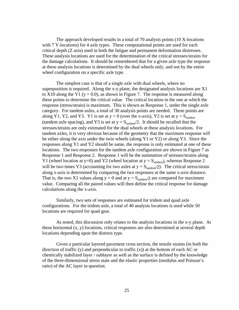
The approach developed results in a total of 70 analysis points (10 X-locations with 7 Y-locations) for 4 axle types. These computational points are used for each critical depth (Z axis) used in both the fatigue and permanent deformation distresses. These analysis locations are used for the determination of the critical stresses/strains for the damage calculations. It should be remembered that for a given axle type the response at these analysis locations is determined by the dual wheels only, and not by the entire wheel configuration on a specific axle type.
The simplest case is that of a single axle with dual wheels, where no
superposition is required. Along the x-y plane, the designated analysis locations are X1 to X10 along the Y1 (y = 0.0), as shown in Figure 7. The response is measured along these points to determine the critical value. The critical location in the one at which the response (stress/strain) is maximum. This is shown as Response 1, under the single axle category. For tandem axles, a total of 30 analysis points are needed. These points are along Y1, Y2, and Y3. Y1 is set at y = 0 (over the x-axis), Y2 is set at y = Standem (tandem axle spacing), and Y3 is set at y = Standem/2. It should be recalled that the stresses/strains are only estimated for the dual wheels at these analysis locations. For tandem axles, it is very obvious because of the geometry that the maximum response will be either along the axis under the twin wheels (along Y1 or Y2) or along Y3. Since the responses along Y1 and Y2 should be same, the response is only estimated at one of these locations. The two responses for the tandem axle configuration are shown in Figure 7 as Response 1 and Response 2. Response 1 will be the summation of stresses/strains along Y1 (wheel location at y=0) and Y2 (wheel location at y = Standem), whereas Response 2 will be two times Y3 (accounting for two axles at y = Standem/2). The critical stress/strain along x-axis is determined by comparing the two responses at the same x-axis distance. That is, the two X1 values along y = 0 and at y = Standem/2 are compared for maximum value. Comparing all the paired values will then define the critical response for damage calculations along the x-axis.
Similarly, two sets of responses are estimated for tridem and quad axle
configurations. For the tridem axle, a total of 40 analysis locations is used while 50 locations are required for quad gear.
As noted, this discussion only relates to the analysis locations in the x-y plane. At
these horizontal (x, y) locations, critical responses are also determined at several depth locations depending upon the distress type.
Given a particular layered pavement cross section, the tensile strains (in both the
direction of traffic (y) and perpendicular to traffic (x)) at the bottom of each AC or chemically stabilized layer / sublayer as well as the surface is defined by the knowledge of the three-dimensional stress state and the elastic properties (modulus and Poisson’s ratio) of the AC layer in question.

26
The complex moduli of asphalt mixtures are employed in the Design Guide via a master curve. Thus, E* is expressed as a function of the mix properties, temperature, and time of the load pulse. Knowledge of the predicted tensile strain at any point, along with the layer dynamic modulus and Nf repetition relationship, allows for the direct calculation of the damage for any asphalt layer, after N repetitions of load, to be computed.
Estimation of fatigue damage is based upon Miner’s Law, which states that
damage is given by the following relationship.
fi
iT
ii N
nD =∑
=1
(11)
where: D = damage T = total number of periods ni = traffic for period i Ni = allowable failure repetitions under conditions prevailing in period i Wander Effect One of the inputs required in the design process is the lateral vehicle wander, in
inches. Wander is the lateral traffic distribution over a pavement cross section, and it accounts for the fact that not all vehicles stress the pavement surface at the exact same point. The amount of lateral wander directly affects the fatigue and the permanent deformation within the pavement system. An increase in wander will result in more fatigue life and less permanent deformation within the pavement system. It is not practical to assess the exact distribution of wander; however, a good approximation is to assume that the wander is normally distributed. The standard deviation for the normal distribution plot represents the wander in inches.
Because Miner’s Law is linear with traffic, damage distribution, considering
wander, is computed from the fatigue damage profile obtained that has no wander (wander = 0 inch). The approach is better explained in Figure 8.
In Figure 8, plot “A” shows the pavement structure with a dual wheel centered at
location 1. In this example, 5 points are used to define the damage profile due to wander effect (locations 1, 2, 3, 4, and 5 on the figure); however, within the Design Guide program 11 points are used to define the damage profile. As mentioned earlier, 10 lateral points (Figure 7) are used for damage calculations. These points are sufficient to define the damage profile. Plot “B” shows the actual damage profile for a wander value of zero predicted by the design program.

27
z =
1.28
155
* Sd
X
X
Damage
5 4 321 Analysis
X, z
Wander Normal Distribution
z =
-1.2
8155
* S
d
z = -0
.524
4 *
Sd
z = 0
z =
0.5
244
* Sd
Damage
A
C
B
D1 X, z
X, z
X, z
X, z
X, z H
F
G
E
D
D2
D3
D4
D5
20% of Traffic
20% of Traffic
20% of Traffic
20% of Traffic
20% of Traffic
Figure 8 Fatigue Analysis Wander Approach.

28
If no wander is used, the maximum value from this damage will define the fatigue life. Plot “C” in this figure shows the wander distribution and is assumed to be normally distributed. The spread of the distribution is dependent upon the standard deviation value entered by the user.
A higher standard deviation or higher wander value will result in a larger spread.
In this plot (normal distribution plot) the area under the curve can be divided into five quintiles, each representing 20 percent of the total distribution. For each of these areas, a representative x-coordinate is found by multiplying the standard normal deviate “z” by the wander (standard deviation). Each of the normal deviates will represent accumulated areas equivalent to 10, 30, 50, 70, and 90 percent of the distribution.
Therefore, it is assumed that, for 20 percent of the traffic, damage distribution
will be centered at location equal to –1.28155 Sd, where Sd is the wander. For this situation (plot D), damage at location 3 is D1. Since D1 is 0 for this case, no fatigue damage occurs at location 3. The next plots (plots E through H) show damage distribution centered at z = -0.5244, 0, 0.5244, and 1.28155. Each represents the situation occurring for 20 percent of the traffic. Damage for cases is D2, D3, D4, and D5, respectively. Thus, the total damage at location 3 can be computed as:
∑=
×=×+×+×+×+×=5
154321 2.02.02.02.02.02.0
iiDDDDDDD (12)
Di (each analysis location) is determined using polynomial or linear interpolation.
Simulation Runs
In establishing the fundamental fatigue model that was to be used for the field calibration-validation study, the fatigue failure model has three coefficients, as shown in equation 13. Table 3 shows the two models considered in the study.
3322 )()(11
kktff
ff EkN ββεβ −−= (13)
where: Nf = Number of repetitions to fatigue cracking. εt = Tensile strain at the critical location. E = Stiffness (dynamic modulus) of the material. k1, k2, k3 = Laboratory regression coefficients. βf1, βf2, βf3 = Calibration parameters.

29
Table 3 Fatigue Cracking Models used in the Study
Factor Shell Oil Asphalt Institute MS-1
k1
5
)408.5354.1(
4.0
)0167.000673.0)(00216.00252.0(
*exp1
1139091
−+−
⎟⎟⎠
⎞⎜⎜⎝
⎛+
−+ −
−
bb
h
VVPIPI
Eac
⎟⎟⎠
⎞⎜⎜⎝
⎛−
+69.084.4
10
*004325.0
ba
b
VVV
k2 5 3.291 k3 1.4 0.854

30
For each coefficient factor, a calibration factor (βfi) was introduced to eliminate the bias and scatter in the predictions. It is these calibration factors, βfi, which are used to calibrate the fatigue-cracking model to actual field performance.
The simulation runs were done by running the software for a combination of
values of the calibration factors βf2, βf3. Then the reasonable solution was optimized using βf1 as a function of the total asphalt concrete layer thickness. This last correction was used to compensate for the crack propagation phase of the fatigue cracking phenomena.
The runs using the MS-1 model were conducted for values of 0.8, 1.0 and 1.2 for
the calibration factor on the strain (βf2), while the values of 0.8, 1.5 and 2.5 were used for the modulus calibration factor (βf3). Additional runs were used in the simulation to check on the sensitivity of the factors such as using the original factors of the equation (using calibration factors of 1.0 on both the strain and the modulus). For the Shell Oil model βf2 and βf3 had the same values of 0.9, 1.0 and 1.1. These values for the two calibration factors were somewhat guided based on available fatigue models in the literature. The lab regression coefficients (k2, k3) (not the calibration factors) ranges, found in the literature, were from 2.5 to 5 for the strain and from 0.8 to 2 for the modulus.
The simulation runs were completed on both the Shell Oil and the Asphalt
Institute (MS-1) fatigue models. Both models were evaluated in the calibration process to ascertain which model form (equation) methodology would provide the most accurate solution for the field calibration process. Annex B and Annex C provides plots / data of the simulation runs for the bottom-up fatigue cracking using both Shell Oil and MS-1 models for all combinations of the strain and the modulus calibration factors grouped by total asphalt layer thickness. Annex B shows the bottom-up cracking damage predictions using the Shell Oil equation, while, Annex C shows the bottom-up cracking predicted damage using the MS-1 equation. Similarly Annex D and Annex E shows the predictions for the top-down fatigue damage, where Annex D provides the Shell Oil equation results, while Annex E shows the MS-1 model results. In the following section the results will be discussed and analyzed for the final step of the calibration process.
82 sections out of the 94 new (LTPP) sections were selected for the fatigue
simulation as they contained fatigue-cracking data in the database. The 82 sections were located in 24 different states with different climatic location. The average running time of the program was 1.5 min per year within the design life using a 2 GHz Pentium 4 processor. This averaged about half an hour running time per section. This, in turn, resulted in a total computer running time of approximately 820 hours (2 models *10 simulations *82 sections *0.5 hour) for a single calibration trial for fatigue. This does not include the time taken to input the data in the program.
It must be noted that the calibration process was not really a single run of 820
hours. Many, sets of calibration runs were conducted. Many factors were responsible for

31
the numerous runs conducted. The majority of these individual calibration runs were caused by bugs/errors in the program or erroneous input data (like traffic). These problems, which were subsequently discovered after the “Final” calibration, necessitated that the results be completely disregarded and the calibration process be redone. Obviously, all of the results shown here are the results of the last final set of runs after fixing all the bugs and errors.
Coefficient Selection
Ten different simulation runs were done using the 82 fatigue sections. Detailed
plots showing the results of each run grouped by asphalt thickness for bottom-up fatigue by both the Shell Oil model and the MS-1 model are given in Annex B and C. Annex D and E provides simulation data /plots for top-down cracking.
The Shell Oil runs were done using the modified model (equation 8) for both
constant stress and constant strain. However, the MS-1 model was used in its original form without any modification for all thickness of asphalt. The MS-1 fatigue model, modified with the appropriate βfi factors, was used to calculate the damage percentage. These predicted damage percentage estimates were then plotted against the measured fatigue cracking in the field for each section.
A very important parameter was studied, which is the percentage damage when
the cracking starts to appear. As explained earlier in this chapter, the cracking phenomena is divided into two stages: cracking initiation and crack propagation. During the crack initiation stage the damage increase while no cracking is observed. However, when the damage reached a certain percentage the crack can be seen and starts to propagate in the asphalt layer. Another set of variables studied were the range of the predicted damage and the scatter of the damage by AC layer thickness.
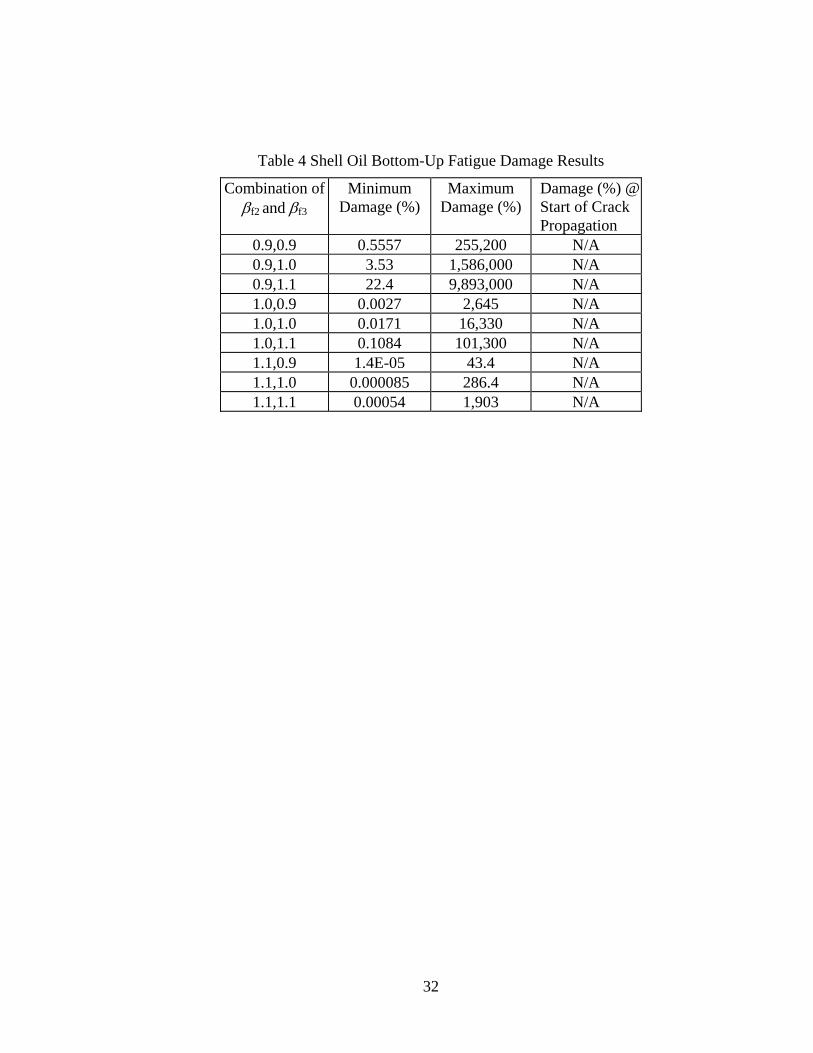
The results of the simulation runs for the Shell Oil bottom-up fatigue cracking are
shown in Table 4. From the tables it can be seen that changing the βf2 and βf3 coefficients result in a big shift in the predicted damage values. This shift can be as large as 106 for the damage percentage.
The simulations runs results for the Shell Oil model, Table 4, show that the range
of the damage values was very high. Also, the damage percentage at which the cracking would start propagating in the asphalt layer could not be identified and it was also found to depend greatly on the thickness of the AC layer. This can also be confirmed from Figure 9, which shows the plot of the predicted percentage damage using the Shell Oil model versus the measured percentage alligator cracking. All the calibration factors (βf1, βf2 and βf3) used for prediction of the damage shown in Figure 9 were 1.0.
32
Table 4 Shell Oil Bottom-Up Fatigue Damage Results
Combination of βf2 and βf3
Minimum Damage (%)
Maximum Damage (%)
Damage (%) @ Start of Crack Propagation
0.9,0.9 0.5557 255,200 N/A 0.9,1.0 3.53 1,586,000 N/A 0.9,1.1 22.4 9,893,000 N/A 1.0,0.9 0.0027 2,645 N/A 1.0,1.0 0.0171 16,330 N/A 1.0,1.1 0.1084 101,300 N/A 1.1,0.9 1.4E-05 43.4 N/A 1.1,1.0 0.000085 286.4 N/A 1.1,1.1 0.00054 1,903 N/A

33
0
10
20
30
40
50
60
70
80
90
100
0.01 0.1 1 10 100 1000 10000 100000Predicted Bottom-Up Damage (%)
Alli
gato
r Cra
ckin
g (%
of T
otal
Lan
e A
rea)
AC Thickness <2" AC Thicknes 2 - 5" AC Thickness 5-8"AC Thickness 8-12" AC Thickness >12"
Figure 9 Shell Oil Predicted Damage vs. Measured Alligator Cracking (βf1 = 1.0, βf2 = 1.0, βf3 = 1.0) (Lane Area = 6000 ft2)

34
From the initial analysis, the MS-1 fatigue model showed promising trends as seen in Table 5, the range of the predicted bottom-up damage is still high, but the percentage damage at which the cracking starts was easily identified. The combination of calibration factors of βf2 = 1.2 and βf3 = 1.5 provided a damage percentage of about 100 % when the cracking starts to propagate.
For the MS-1 model, the original data appeared to indicate that there were two
separate groups in the plot: a group with thickness less than 4 inches and the other with asphalt thickness greater than 4 inch. This finding was very important as it confirmed the fact that constant strain (less than 4 inches) was necessary to be incorporated into the MS-1 constant stress model. Figure 10 shows the plot of the initial percentage damage versus the measured alligator fatigue cracking for the MS-1 model form (without the constant strain modification). The “outliers” for the thin AC sections are very evident in the figure and pointed out the necessity to adjust the MS-1 model for thinner AC layers. In Figure 10 the βfi calibration factors used for the MS-1 model were βf1 = 1.0, βf2 = 1.2 and βf3 = 1.5. The results of the other simulation runs are provided in Annex C.
By examining both the preliminary results of the Shell Oil and the MS-1 models it was clear that the Shell Oil model possessed more scatter and did not possess any definite trends to follow. However, the MS-1 model had much less scatter and resulted in a definite trend between damage and cracking for sections greater that 4” –6” AC layers and thin AC sections (less than 4”). Based upon this initial study, it was concluded that MS-1 model was a more acceptable model for the prediction of the fatigue damage percentage for the 2002 Design Guide.
Table 5 MS-1 Bottom-Up Fatigue Damage Results
Combination of βf2 and βf3
Minimum Damage (%)
Maximum Damage (%)
Damage (%) @ Start of Crack Propagation
0.8,0.8 30.5 2,497,000 7,000 0.8,1.5 80,110 9.5E+09 2.0E+07 0.8,2.5 6.3E+09 1.6E+15 5.0E+12 1.0,0.8 0.025 9,771 10 1.0,1.0 0.24 102,000 200 1.0,1.5 65 37,540,000 50,000 1.0,2.5 5,020,000 6.1E+12 7.0e+09 1.2,0.8 2.2E-05 43.6 0.02 1.2,1.5 0.055575 124,042 100 1.2,2.5 4,267 2.4E+10 1.0E+07

35
0
10
20
30
40
50
60
70
80
90
100
0.01 0.1 1 10 100 1000 10000 100000 1000000
Predicted Bottom-Up Damage (%)
Alli
gato
r Cra
ckin
g (%
of T
otal
Lan
e A
rea)
AC Thickness <2" AC Thicknes 2 - 4" AC Thickness 4-6" AC Thickness 6-8"AC Thickness 8-10" AC Thickness 10-12" AC Thickness >12"
Figure 10 Asphalt Institute (MS-1) Predicted Damage vs. Measured Alligator Cracking (βf1 = 1.0, βf2 = 1.2, βf3 = 1.5) (Lane Area = 6000 ft2)

36
Identical conclusions were found for the top-down cracking when the Shell Oil and MS-1 models were compared as shown in Figure 11 and Figure 12 (using the same calibration factors βf1, βf2 and βf3 as mentioned earlier for the alligator cracking). The scatter of the predicted surface-down damage is much less in the MS-1 model than when using the Shell Oil model. The surface-down cracking mechanism used in this study has been noted to be hypothesized as a similar tensile strain fatigue failure as the more classical alligator cracking. That is why the same fatigue cracking model and calibration factors used for the bottom-up cracking were used for the surface-down cracking. However, the shift function (as a function of the AC layer thickness) is needed to correct for the constant strain effect, which is not included in the MS-1 model.
0
1000
2000
3000
4000
5000
6000
7000
8000
9000
10000
1E-07 1E-06 1E-05 0.0001 0.001 0.01 0.1 1 10 100 1000 10000Predicted Surface-Down Damage (%)
Long
itudi
nal C
rack
ing
(ft /
Mile
)
AC Thickness <2" AC Thicknes 2 - 5" AC Thickness 5-8"AC Thickness 8-12" AC Thickness >12"
Figure 11 Shell Oil Predicted Damage vs. Measured Longitudinal Cracking (βf1 = 1.0, βf2
= 1.0, βf3 = 1.0)

37
0
1000
2000
3000
4000
5000
6000
7000
8000
9000
10000
0.00001 0.0001 0.001 0.01 0.1 1 10 100 1000Predicted Surface-Down Damage (%)
Long
itudi
nal C
rack
ing
(ft /
mile
)
AC Thickness <2" AC Thicknes 2 - 4" AC Thickness 4-6" AC Thickness 6-8"AC Thickness 8-10" AC Thickness 10-12" AC Thickness >12"
Figure 12 Asphalt Institute (MS-1) Predicted Damage vs. Measured Longitudinal Cracking (βf1 = 1.0, βf2 = 1.2, βf3 = 1.5)

38
Bottom-Up Fatigue Cracking Calibration Once the initial model form was selected, the next step of the calibration process
was to find the most accurate transfer function, which will predict damage relative to the measured field cracking observed. This section presents the final calibration of the bottom-up (alligator) cracking while the top-down cracking (longitudinal) is discussed in the following section. The final step of the calibration includes the analysis of field cracking data to check the factors and the trends of the alligator cracking measured in the field. The shift function, to correct for the constant strain in the fatigue-cracking model for thin AC sections is then presented. Finally the final transfer function, which correlates predicted damage to the measured alligator cracking, is presented. Analysis of Measured Alligator Cracking Data
To calibrate distress models, field data must be checked for general
reasonableness and any trends from these data should be examined. Any trends with the measured data should be compared to the calibration results trends to assess the reasonableness of the calibrated model. The database from the LTPP (12) (Long Term Pavement Performance) provided the capability to do these comparisons. The data was extracted from the LTPP database provided in the DataPave (version 3) software.
Alligator fatigue cracking data was collected from all available new sections
having fatigue cracking in the LTPP database. The total number of sections used was 640 sections. Each section contained multiple data points as a time series of alligator cracking. The total number of points used in the forgoing study was 1897 data points. The LTPP database provided fatigue-cracking data according to severity level (low, medium and high severity) in each LTPP section. Each LTPP section has a length of 500 feet. In this research work, as mentioned earlier, the researchers were instructed to utilize the total of all three-fatigue cracking severity values, without using any weighting scheme. This value was then divided by the total area of the lane (12’*500’ = 6000 ft2) to calculate the percentage area cracked. At the same time, the thickness of all the asphalt concrete layers, for each section, was extracted from the database. The thickness was then added to get the total thickness of asphalt concrete layers for each section.
The frequency of the total asphalt layer thickness for the LTPP sections analyzed
is plotted in Figure 13. The frequency of the asphalt layer thickness indicates that the 66 % of the sections built have a total asphalt layers thickness between 2 and 10 inches. Only 6% were less than 2 inches in thickness while 28 % were built with thicknesses greater than 10 inches.
Figure 14 shows the plot of the total alligator cracking percentage from the 640
LTPP sections to the total asphalt thickness. Figure 14 also shows that the alligator cracking in all of the LTPP sections analyzed, reaches a maximum damage (cracking) level at an asphalt layer thickness of 4 – 6 inches. This analysis also indicates a high

39
percentage of fatigue cracking for thin (AC = 2 inches) sections. The percent cracking is very high and reaches a value of about 65% cracking (based on 117 sections).
Figure 15 shows the frequency distribution of the percentage alligator cracking.
About 85% of the data points found in the database had alligator cracking less than 10%. This is primarily due to the fact that many highway agencies do not allow roadways to reach any significant level of cracking before some kind of maintenance will be performed to repair the cracking. In addition it should also be noted, that the numbers shown in the analysis represent time series of cracking early in the life of the pavement where fatigue cracking would not be expected.
Another major factor that affects fatigue cracking is the mean annual air temperature (MAAT). As shown in Figure 16 and Figure 17, the MAAT for the LTPP sections evaluated, ranges from about 29 ºF to about 77 ºF. The general expectation of the alligator cracking was that more cracking usually occurs in cold regions and less cracking in hot regions. However, the plots indicate that the occurrence and the amount of alligator cracking are very close for all regions and independent of the MAAT (site environment). Thus, the MAAT appears to have little to no significant influence on the measured alligator cracking reported in the LTPP database. The inference here is that pavement structures and material properties are more important in the fatigue process than MAAT. However, perhaps what is most critical to fatigue cracking is the interaction (dependency) of AC mix stiffness and the climatic condition at the design site. Thus by the proper selection of material quality (stiffness) the influence of temperature is mitigated or normalized as a salient design variable.
6
1 41 6
1 91 6
1 1
5 53 2
1 1 00
5
10
15
20
25
30
35
40
45
50
< 2 2 -4 4 -6 6 -8 8 -10 10 -12 12 -14 14 -16 16 -18 18 -20 20 -22 22 -24 24 -26
T o ta l A sp h a lt La ye r T h ickn e ss (in )
Freq
uenc
y (%
)
Figure 13 Frequency Distribution for the Total Asphalt Layer Thickness.

40
0
10
20
30
40
50
60
70
80
90
100
0 5 10 15 20 25 30
Total Asphalt Layer Thickness (in)
Allig
ator
Fat
giue
Cra
ckin
g (%
of L
ane
Area
)
Figure 14 LTPP Alligator Cracking Data vs. Asphalt Layer Thickness
5 3 2 2 1 1 0 0 0
87
0
10
20
30
40
50
60
70
80
90
100
10 20 30 40 50 60 70 80 90 100
Alligator Cracking (% Based on 6000 ft2)
Freq
uenc
y (%
)
Figure 15 Frequency Distribution of Percentage Alligator Cracking

41
0
10
20
30
40
50
60
70
80
90
100
0 10 20 30 40 50 60 70 80 90
MAAT (oF)
Tota
l Allig
ator
Cra
ckin
g (%
)
Figure 16 Alligator Cracking vs. Mean Annual Air Temperature
83
73
8288
65
0
10
20
30
40
50
60
70
80
90
100
<40 40-50 50-60 60-70 >70
MAAT (oF)
Max
imum
Alli
gato
r Cra
ckin
g (%
)
Figure 17 Maximum Alligator Cracking vs. Site Mean Annual Air Temperature Ranges Calibration of the Fatigue Alligator Cracking Model

42
The next step of the calibration process is to derive an appropriate shift function relating asphalt thickness to damage and the cracking. The following section will discuss these two steps using only the MS-1 model selected in the initial study stage as the model of choice in the analysis. The MS-1 model is shown in equation 14
32 *854.0*291.3
111**00432.0
ff
ECN
tff
ββ
εβ ⎟
⎠⎞
⎜⎝⎛
⎟⎟⎠
⎞⎜⎜⎝
⎛= (14)
In the previous equation (14) there are three calibration factors (βf1, βf2 and βf3),
these factors needs to be estimated by minimizing the error in the prediction of the damage. βf1 would be a function of the AC layers thickness to shift the thin sections (constant strain). In addition to the estimation of these three alligator fatigue cracking calibration factors, a transfer function between the predicted damage and measured cracking is required to complete the calibration process.
The fatigue cracking – damage transfer function used in the calibration of the
Design Guide alligator (bottom-up) fatigue cracking was assumed to take on the form of a mathematical sigmoidal function. The model form selected is in the form given in equation 15
⎟⎠⎞
⎜⎝⎛
⎟⎠⎞
⎜⎝⎛
+= − 60
1*1
6000.. *21 LogDCCeCF (15)
where: F.C. = fatigue cracking (% of lane area) D = Damage in percentage C1, C2 = regression coefficients
The 6000 in the alligator cracking – damage function is the total area of the lane
(12 feet wide and 500 feet length). The (1/60) value is a conversion to obtain the cracking in percentage, not in square feet.
To find the regression coefficients C1 and C2 a Microsoft Solver numerical
optimization routine was used. The optimization was set by first predicting the damage for each alligator cracking data point. An initial value was assumed for C1 and C2. Then by using the equation form given in equation 15, fatigue cracking was calculated from the predicted damage percentage. The predicted alligator fatigue cracking was then compared to the measured alligator cracking by finding the error between the two values. The errors are then squared and summed to get the total sum of squared error. Microsoft Excel Solver was then run to minimize the sum of squared errors by changing the C1 and C2 values for the first iteration. The new C1 and C2 values are then used as the input for the second iteration, and the same steps are repeated till the solution converges and the minimum total sum of squared errors is obtained. Finally, the Microsoft Solver is used

43
again to set the arithmetic sum of errors to zero (by changing the C1 and C2 values again). This is done in order to eliminate any bias in the prediction. This optimization approach has been previously presented in Chapter 2 of this dissertation.
The alligator fatigue cracking calibration process can be summarized in the
following steps:
1. Estimation of βf2 and βf3 2. Finding the alligator fatigue cracking – damage transfer function by
minimizing the error to get a final value of C1 and C2. 3. Finally, shifting thin sections to match with the thick sections. This is
accomplished by associating βf1 to a function having the AC layers thickness as an independent variable.
In the following sections a step-by-step details of all the alligator cracking
calibration process are discussed.
Estimation of βf2 and βf3 As shown earlier ten simulation runs were conducted using different values and
combinations of βf2 and βf3 as shown in Table 5. To compare these runs for different βf2 and βf3 values, a quick optimization was done to optimize the error in the alligator cracking – damage transfer function given in equation 15 using the bottom-up damage percentage predicted for each combination of βf2 and βf3 and the corresponding measured alligator cracking for each LTPP section used in this study. Table 6 shows the standard error calculated from each simulation run. The fitting of the predicted damage to calculate the alligator fatigue cracking, in this step, was done without any AC thickness shift for the damage.
Table 6 shows that as βf2 and βf3 value increased the standard error is reduced.
The simulation run, which had a βf2 equal to 1.2 and βf3 equal to 1.5, provided a realistic prediction, in which the cracking starts to appear and propagate in the AC layer at a bottom-up predicted damage percentage of 100 %, the range of the damage was in the realistic range and the standard error is minimum. Accordingly, the calibration factors βf2 and βf3 were set at 1.2 and 1.5 respectively. However, the calibration factor βf1 still needed to be adjusted to shift the thin AC layer (constant strain sections less than 4 inches) to match the constant stress sections (greater than 4 inches AC thickness). The mathematical approach used to accomplish this objective will be explained later in this chapter.

44
Table 6 MS-1 Bottom-Up Fatigue Damage Standard Error
Combination of βf2 and βf3
Standard Error
0.8,0.8 282.36 0.8,1.5 282.28 0.8,2.5 282.06 1.0,0.8 279.56 1.0,1.0 279.56 1.0,1.5 279.51 1.0,2.5 279.23 1.2,0.8 275.98 1.2,1.5 275.91 1.2,2.5 275.68

45
The revised MS-1 alligator fatigue-cracking model can then be written as shown in the following equation:
281.19492.3
111**00432.0 ⎟
⎠⎞
⎜⎝⎛
⎟⎟⎠
⎞⎜⎜⎝
⎛=
ECN
tff ε
β (16)
where: '1
'11 * kff ββ =
='1fβ Numeric value
='1k Function of the AC layer thickness
In this equation the parameter βf1 has been introduced to provide a correction for
thin asphalt layer thickness effects. However, before finding the relationship that represents βf1 as a function of the AC layers thickness, the function describing the measured alligator cracking – predicted bottom-up damage transfer function was found first using thick sections (AC layer thickness greater than 4 inches).
Alligator Fatigue Cracking – Damage Relationship
The correlation between the alligator cracking and damage was based on two
assumptions:
• A sigmoidal function form is the best representative of the relationship between cracking and damage. This is an extremely reasonable assumption as the relationship must be “bounded” by 0 ft2 cracking as a minimum and 6,000 ft2 cracking as a maximum.
• The alligator cracking is 50% cracking of the total area of the lane (6000 ft2) at a damage percentage of 100%.
The cracking – damage correlation was obtained using only sections, which had
an AC thickness greater than 4 inches. This was because the MS-1 fatigue model was developed using the constant stress theory (thick AC sections). Also, it can be seen in Figure 10 that AC thicknesses greater than 4 inches were grouped together while sections with AC thickness less than 4 inches had a higher damage percentage. Sections, which have AC layer thickness less than 4 inches, were eventually shifted using the βf1 as a function of the AC thickness.
The sigmoidal function form given in equation 15 was used to correlate the
fatigue cracking to the damage of an AC pavement. This function form has two coefficients (C1 and C2). In order to satisfy the second assumption previously noted the C1 value must be equal to twice the value of C2 but with a negative sign as shown in equation 17.

46
21 *2 CC −= (17)
Also, the second assumption implied that the damage values should be multiplied by a factor of 0.004 in order to set 50% cracking at 100% damage. The main objective of this step is to find the values of C1 and C2 while satisfying the above listed two assumptions. In reality, only C2 is needed and from equation 17, C1 can be easily obtained.
The rate at which the crack initiates and then propagates in the pavement structure
depends mainly on the thickness of the AC layers. That is why the relationship that correlates the fatigue cracking to the damage in the pavement should include the effect of the rate (slope) of cracking, which is a function of the AC layer thickness. C2 was obtained from the relationship between the rate of cracking and the thickness of the AC layers.
0
10000
20000
30000
40000
50000
60000
0 2 4 6 8 10 12 14 16
AC Thickness (in)
Bot
tom
-Up
Cra
ckin
g / l
og D
amag
e
Figure 18 Ratio Between Bottom-up Cracking and Log Damage vs. AC Thickness

47
The rate of cracking was calculated from only 26 sections (from 82 sections) that developed significant cracking. Using two cracking values (a low and high cracking) and the time between these two crack levels, the rate of cracking was calculated, as shown Figure 18. A model was fitted in these data. The final form of this model is the C2.
The final fitted model for C2 is shown in the following equation
( ) 85609.22 1*748.3940874.2 −+−−= achC (18)
By finding the C2 then the transfer function is set and the only remaining issue is
to shift thin section performance to match the thick ones.
Shifting Thin Sections To find the equation for βf1 as a function of the AC layers thickness, the sections
were first sorted by AC layers thickness. Four groups were identified:
1. Sections with an AC thickness less than 2 inches, 2. Sections with an AC thickness between 2 and 3 inches, 3. Sections with an AC thickness between 3 and 4 inches, 4. Sections with an AC thickness greater than 4 inches.
βf1 was divided into two parameter β'
f1 and 1'k , as given in equation 19. The β'f1
is a number; it is not a function of any variable. However, 1'k is a function of the AC layer thickness.
'1
'11 * kff ββ = (19)
As mentioned earlier, sections with AC layer thickness greater than 4 inches
typically had a shift factor of 0.004. The remaining three groups had a higher damage value, with the highest damage for sections less than 2 inches thickness. Table 7 shows the maximum and minimum damage values predicted for the different AC thickness.
A shift factor was used to shift the damage for each of the thickness groups to
match the fourth group (AC thickness greater than 4 inches). This shift factor was found manually for each group to satisfy the assumption that 50 % of the fatigue cracking occurs at 100 % damage. The shift factors adopted for each thickness group are shown in Table 7.
A sigmoidal function was then fitted for the shift factors obtained for each AC
thickness group with the AC layer thickness as an independent variable. Figure 19 shows the sigmoidal function used to shift the thin sections for the calibration of the alligator fatigue (bottom up) cracking.

48
For the alligator fatigue (bottom up) cracking the “ 1'k ” parameter is given by the
following equation:
hac)*3.49-(11.02
1
e1003602.00.000398
1'
++
=k (20)
where: hac = Total thickness of the asphalt concrete layers. The statistical summary for this model is:
Sum of error square = 1.92E-07 Standard error (Se) = 0.00017
Table 7 Minimum and Maximum Damage (%) by AC Thickness
AC Thickness Minimum Damage (%) Maximum Damage (%) Shift Factor<2 3.4E+02 1.2E+05 0.000398 2-3 2.3E+02 3.2E+04 0.000524 2-4 5.0E+01 1.9E+04 0.002934 4-6 2.8E+01 3.2E+04 0.004 6-8 5.1E+00 2.7E+03 0.004 8-10 9.0E-01 1.3E+03 0.004 10-12 1.5E+00 4.3E+03 0.004 >12 5.6E-02 2.6E+02 0.004

49
0
0.0005
0.001
0.0015
0.002
0.0025
0.003
0.0035
0.004
0.0045
0 2 4 6 8 10 12 14 16
AC Layer Thickness (in)
k'1
Figure 19 Sigmoidal Shift Function 1'k

50
Alligator Fatigue (Bottom-Up) Cracking Conclusion
The alligator fatigue (bottom up) cracking calibration process went through three main steps: estimation of coefficients βf2 and βf3 for the MS-1 number of load repetitions fatigue model; then finding the correlation between the alligator fatigue cracking and the damage using only sections with AC layer thickness greater than 4 inches; and finally shifting the thin sections using the “ 1'k ” parameter as a function of the AC layer thickness.
The final transfer function to calculate the fatigue cracking from the fatigue
damage is based on the assumption that the fatigue cracking would be 50 % at a damage of 100 %. The calibrated model for the bottom-up fatigue cracking (% of total lane area) is expressed as follows:
⎟⎠⎞
⎜⎝⎛
⎟⎠⎞
⎜⎝⎛
+= + 60
1*e1
6000.. 100))*log10(D**C'C*C'(C 2211CF (21)
where: C1 = 1.0 C2 = 1.0 856.2
2 )1(*748.3940874.2' −+−−= hacC C’1= -2 * C’2. Number of observations = 461 observations. Sum of error square = 17663.91 Standard error (Se) = 6.2 %. Se/Sy = 0.947. The bottom-up cracking is calculated as a percentage of the total lane area, based
on the assumption that the lane is 500 ft long by 12 ft wide. It should be recalled that the measured cracking used in the calibration is the total summation of the high, medium and low severity cracking reported in the LTPP database. Figure 20 shows the graph of the calibration of the measured alligator cracking to the predicted bottom-up cracking, while Figure 21 shows the error (predicted – measured) in the prediction of the bottom-up fatigue cracking.
The 2002 Design Guide is based on mechanistic principles that provided a
fundamental basis for the structural design of pavements structures. However, without calibration, the results of the mechanistic predictions cannot be confidently used to predict fatigue cracking with the confidence and assurance that it will model field behavior as accurately as possible. While the mathematical optimization techniques used in the error minimization approach are one form of field verification, an equally important component of the overall model verification is to insure that the final model

51
developed provides extremely reasonable correlations to known impacts of significant variables in the fatigue process. In order to insure that this added verification effort did indeed occur, an extensive sensitivity analysis was run using different levels of key variable that are known to have an impact upon alligator (bottom-up) cracking. The results and discussions of this study are contained in Appendix II2. This sensitivity study contains a very detailed investigation as well as discussion of results for each major set of variables investigated.
0
10
20
30
40
50
60
70
80
90
100
-4 -3 -2 -1 0 1 2 3
Log Damage (%)
Alli
gato
r Cra
ckin
g (%
of T
otal
Lan
e A
rea)
Figure 20 Bottom-Up Cracking vs. Fatigue Damage at Bottom of HMA layer

52
-50
-40
-30
-20
-10
0
10
20
30
-4 -3 -2 -1 0 1 2
Log Damage (%)
Erro
r (P
redi
cted
-Mea
sure
d)
Figure 21 Error (Predicted – Measured Cracking) vs. Damage (%) for the Bottom-Up
Fatigue Cracking.
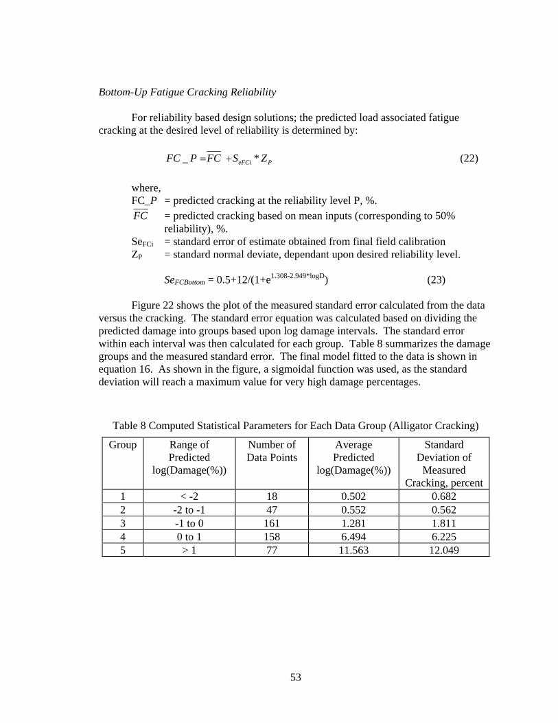
53
Bottom-Up Fatigue Cracking Reliability For reliability based design solutions; the predicted load associated fatigue
cracking at the desired level of reliability is determined by:
PeFCi ZSFCPFC *_ += (22)
where, FC_P = predicted cracking at the reliability level P, %. FC = predicted cracking based on mean inputs (corresponding to 50%
reliability), %. SeFCi = standard error of estimate obtained from final field calibration ZP = standard normal deviate, dependant upon desired reliability level.
SeFCBottom = 0.5+12/(1+e1.308-2.949*logD) (23)
Figure 22 shows the plot of the measured standard error calculated from the data
versus the cracking. The standard error equation was calculated based on dividing the predicted damage into groups based upon log damage intervals. The standard error within each interval was then calculated for each group. Table 8 summarizes the damage groups and the measured standard error. The final model fitted to the data is shown in equation 16. As shown in the figure, a sigmoidal function was used, as the standard deviation will reach a maximum value for very high damage percentages.
Table 8 Computed Statistical Parameters for Each Data Group (Alligator Cracking)
Group Range of Predicted
log(Damage(%))
Number of Data Points
Average Predicted
log(Damage(%))
Standard Deviation of
Measured Cracking, percent
1 < -2 18 0.502 0.682 2 -2 to -1 47 0.552 0.562 3 -1 to 0 161 1.281 1.811 4 0 to 1 158 6.494 6.225 5 > 1 77 11.563 12.049

54
0
2
4
6
8
10
12
14
-3 -2 -1 0 1 2 3Log Damage (%)
Alli
gato
r Cra
ckin
g St
anda
rd E
rror
(%)
Figure 22 Standard Deviation of the Predicted Bottom-Up Cracking

55
Top-Down Fatigue Cracking Calibration Similar to the bottom-up alligator fatigue cracking analysis, the ultimate goal of
the top-down longitudinal surface cracking calibration is to find the transfer function, which will correlate predicted damage to measured cracking with the minimum amount of error. This section focuses on the top-down fatigue cracking distress. The final stage of the calibration, include the analysis of field cracking data to check the factors and trends of the longitudinal cracking measured in the field; model adjustment (development) of a shift function to correct for the constant strain (AC thickness effect) in the MS-1 fatigue-cracking model and finally optimizing the transfer function, to correlate the predicted damage to the measured longitudinal cracking with minimum error and maximum accuracy.
The top-down longitudinal cracking is a distress that starts at the surface of the
pavement then propagates in the asphalt layer. As noted throughout this report, the mechanism hypothesized for this distress was due to excessive tensile strains at, or near, the pavement surface. At the beginning of the study, it was assumed that surface fatigue cracking could be a result of the combination of strains occurring at the surface of the pavement due to both environmental conditions (thermal) as well as load associated. In order to thoroughly investigate the feasibility of such a hypothesis, different combinations of the surface strains, were used in the prediction of the damage for longitudinal (top-down) cracking.
Different scenarios were tested for the prediction of the surface – down cracking.
These scenarios were different in the way the surface strains were obtained. Tensile strains that occur at the surface due to traffic loads were always included. However, the strains induced from thermal changes in cooler climatic zones were initially investigated in the calibration study. Several scenarios using combined thermal and load strains were investigated. These scenarios included use of the maximum tensile strains in an analysis period or using the average thermally induced strains. Another approach also investigated was to totally ignore the temperature induced strains.
Another important initial consideration was evaluated due to the fact that the
longitudinal cracking mechanism is not very well understood (compared to the alligator cracking). In the initial study phases, the strains for the longitudinal cracking were calculated at two different depths: at the surface and at 0.5” below the surface. The logic in determining tensile strains at the 0.5” depth was to assess if the aged hardened upper 1” AC layer was being “fatigued” due to the aging phenomenon. All of these scenarios were evaluated in an attempt to better understand how the longitudinal cracking develops and how it should be correctly modeled.
Once the final tensile strain scenario for the longitudinal cracking was selected,
the calibration process followed similar steps as the calibration process of the alligator (bottom-up) fatigue cracking. In the following sections, the different scenarios for the
56
longitudinal fatigue cracking will be discussed and the calibration process will be explained. The discussion will start with the analysis of some trends of longitudinal cracking from the LTPP database.
Analysis of Measured Longitudinal Cracking Data
The general approach used for the calibration of top-down fatigue cracking was
conceptually identical to the approach used for the bottom-up alligator cracking. The database from the LTPP (12) was used to calibrate the distress models, and to compare field data trends to the calibration results trends to guide the calibration process. All data was extracted from the LTPP database provided in the DataPave (version 3) software.
Longitudinal fatigue cracking data was collected from all available new LTPP
sections indicating the presence of longitudinal cracking. The total number of sections used was 640 sections. Each section had a multiple data point as a time series. The total number of time- distress –sections points used was 1897. The LTPP database provided the longitudinal cracking data according to severity level (low, medium and high severity) for each LTPP section. The LTPP sections have a length of 500 feet. In this research work, as mentioned earlier, it was decided by the NCHRP panel overviewing this study, that the three fatigue cracking severity values would be added arithmetically, without any weighting coefficients, and used as the total fatigue cracking. A factor of 10.56 was then used to convert the longitudinal cracking from feet per 500 feet into feet per mile. It is to be noted that the prediction of the longitudinal surface fatigue cracking is a lineal measure, in contrast to the areal measure, used for the bottom-up alligator cracking.
At the same time, the thickness of all asphalt concrete layers, for each section, was extracted from the database. The thickness was then added to get the total thickness of asphalt concrete layers for each section. Figure 23 shows the frequency distribution of the longitudinal cracking. About 95% of the data points found in the database have longitudinal cracking less than 500 ft/mile. There are several hypothesized reasons for this limit. First, it is because the roadways are maintained if the distress reaches a certain level of cracking. Additionally it is logical that after a certain level of longitudinal cracking, the longitudinal cracking may become interconnected and become integrated into alligator cracking. Finally it should be recalled that a time series of distress was used in the database. Thus a majority of points will be in the early stages of distress, which will alter the apparent conclusions.

57
80.6
7.23.5 2.2 2.1 1.0 0.9 0.3 0.3 0.3 0.6 0.2 0.9
0
10
20
30
40
50
60
70
80
90
100
0-500 500-1000
1000-1500
1500-2000
2000-2500
2500-3000
3000-3500
3500-4000
4000-4500
4500-5000
5000-5500
5500-6000
6000-10000
Longitudinal Cracking (ft/mile)
Freq
uenc
y (%
)
Figure 23 Frequency Distribution of Longitudinal Cracking

58
Figure 24 shows the plot of the total longitudinal cracking, from the 640 sections,
to the total asphalt thickness. Figure 24 also shows that the longitudinal cracking in 640 sections at different asphalt thickness peaks at an asphalt layer thickness of 4 – 7 inches. Also, the figure shows that for thick asphalt layers, the longitudinal cracking definitely decreased. This provides some credulence to the consideration that the longitudinal cracking is, indeed, related to some structural properties of the pavement system. The same sections used for the alligator cracking were used in the longitudinal cracking. This is why the frequency of the total asphalt layer thickness is the same as shown in Figure 13. Quite candidly, the trends showing a decrease in longitudinal cracking, as the AC thickness increased, was opposite to initial views of the research team for longitudinal cracking. It was thought that more longitudinal cracking would occur with thick asphalt sections and less with thin sections. Obviously this was an erroneous initial impression.
0
2000
4000
6000
8000
10000
12000
0 5 10 15 20 25 30
AC Layer Thickness (in)
Long
itudi
nal C
rack
ing
(ft/m
ile)
Figure 24 LTPP Longitudinal Cracking Data vs. Asphalt Layer Thickness

59
Another major factor that was investigated was the effect of the mean annual air temperature (MAAT) upon longitudinal cracking. As shown in Figure 25 and Figure 26, the MAAT ranges from about 29 ºF to about 77 ºF. Initially, it was the general expectation of research team that the longitudinal cracking would be more prevalent in cold regions, with less cracking in hot regions. However, the figures show that the longitudinal cracking appears to reach a maximum value at a MAAT near 60 to 70 ºF. When the MAAT was greater than 70 ºF or less than 50 ºF, the average longitudinal cracking decreased.
Another factor, which appears to have an impact on the longitudinal cracking, is
the subgrade soil type. Figure 27 shows that more longitudinal cracking is observed in the field for stronger (sandy) subgrade soils. This finding lends some credulence to the final distress methodology developed in that stronger (higher) moduli foundations will tend to cause higher surfacial tensile strains in the pavement systems. This in turn, should result in a greater degree of surface cracking to occur.
0
2000
4000
6000
8000
10000
12000
20 30 40 50 60 70 80
MAAT (oF)
Long
itudi
nal C
rack
ing
(ft /m
ile)
Figure 25 Longitudinal Cracking vs. Mean Annual Air Temperature

60
439
291
561
494
204
0
100
200
300
400
500
600
< 40 40-50 50-60 60-70 > 70
M AAT (oF)
Ave
rage
Lon
gitu
dina
l Cra
ckin
g (ft
/mile
)
Figure 26 Average Longitudinal Cracking vs. Mean Annual Air Temperature Ranges
592
396
483 490
0
100
200
300
400
500
600
700
Clean Sand Silty Sand Clay All
Subgrade Soil Type
Mea
n Lo
ngitu
dina
l Cra
ckin
g (ft
/mile
)
Figure 27 Average Longitudinal Cracking vs. Subgrade Soil type

61
Calibration of the Fatigue Longitudinal Cracking Model The calibration process goal for the longitudinal cracking is to find the shift
function for asphalt thickness and then to find the sigmoidal function relating the damage and the cracking. The following section will discuss these two steps using only the MS-1 model. The general MS-1 model is given in the following equation:
32 *854.0*291.3
111**00432.0
ff
ECN
tff
ββ
εβ ⎟
⎠⎞
⎜⎝⎛
⎟⎟⎠
⎞⎜⎜⎝
⎛= (24)
It has to be noted that the same fatigue model (MS-1) was selected to be used for the damage prediction of both the top-down and bottom-up procedures. In fact, the decision to use the MS-1 and not the Shell Oil model was taken based on the results obtained from the bottom-up cracking. Since the fatigue damage is being calculated for distress types (longitudinal and alligator cracking) the same model should be used.
Similar to the alligator cracking, there are three calibration factors (βf1, βf2 and
βf3) that need to be evaluated. βf1 would be a function of the AC layers thickness. In addition to the estimation of these three alligator fatigue cracking calibration factors, a transfer function between the predicted damage and measured cracking is required to complete the calibration process.
The tensile strains, which are used to calculate the longitudinal cracking, were
calculated at two depths, at the surface and at 0.5 inch below the pavement surface. However, in 100% of every analysis conducted in the entire study, tensile strains at the surface were much higher (more critical) than those strains calculated at 0.5” deep. This finding appears to suggest that long-term aging of the upper thin AC layer does not play a significant role in the longitudinal surface cracking process. Accordingly, it was decided to only use tensile strains at the surface (Z = 0) for the longitudinal cracking calibration process. The tensile strains for the damage prediction were calculated at different horizontal (x – y) locations as explained in and earlier section. The maximum tensile strain at the 10 locations is used in the analysis. In the majority of cases evaluated, the maximum location was found between the dual tires and at the AC surface.
The fatigue cracking – damage transfer function used in the calibration of the
Design Guide for longitudinal (surface-down) fatigue cracking is in the form shown in equation 25.
( )56.10*1
1000.. *21⎟⎠⎞
⎜⎝⎛
+=
− LogDCCeCF (25)
where: F.C. = fatigue cracking (ft / mile) D = Damage in percentage

62
C1, C2 = regression coefficients
The “1000” is the maximum length of linear cracking which can occur in two wheel paths of a 500 feet section (2 * 500 feet length). The (10.56) factor is a conversion to feet per mile units.
The regression coefficients C1 and C2 were evaluated using a Microsoft Solver
numerical optimization routine. The optimization was set by first predicting the surface damage using the MS-1 model. An initial value was assumed for C1 and C2. Then by using the equation form given in equation 25, fatigue cracking was calculated from the predicted damage percentage. The predicted longitudinal fatigue cracking was then compared to the measured cracking. The Microsoft Excel Solver was then run to minimize the sum of squared errors by changing the C1 and C2 values for the first iteration. The new C1 and C2 values are then used as the input for the second iteration, and the same steps repeated until the solution converges and the minimum total sum of squared errors is obtained. Finally, the Microsoft Solver is used again to set the arithmetic sum of errors to zero (by changing the C1 and C2 values again). This is done in order to eliminate any bias in the prediction. The same assumption assumed for the alligator cracking was assumed for the longitudinal cracking; in that the cracking would be 50% at a damage of 100%.
The longitudinal fatigue cracking calibration process can be summarized in the
following steps:
1. Estimation of βf2 and βf3 2. Finding βf1 as a function of the AC layers thickness. 3. Finally, the longitudinal fatigue cracking – damage transfer function is
optimized by minimizing the error to get a final value of C1 and C2. For the longitudinal surface cracking fatigue subsystem, there was an interaction
between step 2 (finding βf1) and step 3 (finding the longitudinal cracking transfer function). This is in contrast to the alligator cracking, for which the two steps were independent and completed separately. That is why, step 2 and 3 for the longitudinal cracking calibration was repeated by trial and error to find the minimum error.
In the following sections, a step-by-step solution of the longitudinal (surface)
cracking calibration process is presented.
Estimation of βf2 and βf3 For the longitudinal cracking, the MS-1 fatigue model was selected to be
consistent with the bottom-up fatigue cracking predictions. Also, the lack of a well-founded and accepted distress methodology for the longitudinal cracking mechanism led to the assumption to use the same model and calibration coefficients as the alligator

63
bottom-up cracking. Accordingly the same values were used for the calibration coefficients βf2 and βf3. The calibration factors βf2 and βf3 were set at 1.2 and 1.5 respectively. The MS-1 model used for the longitudinal cracking calibration process is as follows:
'
111 *' kff ββ = βf2 = 1.2 βf3 = 1.5
281.19492.3
'11
11**'*00432.0 ⎟⎠⎞
⎜⎝⎛
⎟⎟⎠
⎞⎜⎜⎝
⎛=
ECkN
tff ε
β (26)
where:
='1fβ Numeric value
='1k Function of the AC layer thickness
Longitudinal Damage Tensile Strains
As mentioned earlier, the initial surface (top-down) fatigue study utilized
different combinations of load-associated strains and low temperature-induced strains to predict the damage for the longitudinal cracking. The load-associated strains are the strains that were produced from the effect of the traffic load. Low temperature (thermal) strains are the strains induced in the pavement, especially near the surface, due to quick temperature drops that lead to thermal induced stresses and strains due to the frictional restraint of the pavement and the relaxation and tensile properties of the AC surface mix. The thermal strains are generally of consequence in relatively cool temperature periods and increase as the temperature becomes well below freezing. In a pavement system, the primary mode of stress – strain development is parallel to the long axis of the road. In other words, thermal strains due to temperature drops are only of a practical consequence in the direction of travel.
In contrast, load-associated horizontal tensile strains are calculated in two
directions: the traffic direction and perpendicular to the traffic direction. However, the temperature strains are calculated in only one direction, which is the direction perpendicular to the traffic. In the investigation to assess if thermal strains needed to be incorporated in the fatigue model, thermal tensile strains were added to the load strains parallel to traffic, and then the summed value compared to the load strains in the direction perpendicular to traffic. The most critical strain of the two was used for the damage calculation in the preliminary study.
The incremental prediction period for the damage calculation is two weeks when
freezing and thawing exists and one month if no freezing / thawing is present. However,

64
the temperature measurement provided in the Design Guide is an hourly temperature. This is required input format for the solution of the thermal fracture module for asphalt pavement system. In order, to use the predicted thermal strains for the longitudinal cracking prediction, direct use of the thermal fracture subsystem was used.
The specific combinations investigated were:
1. Load associated strains plus the average thermal tensile strain within the analysis period.
2. Load associated strains plus the maximum thermal tensile strain within the analysis period.
3. Load associated strains only. All of these combinations were evaluated using the calibration factors of 1.2 and
1.5 for the βf2 and βf3. A complete calibration was conducted on each of these three combinations to assess the accuracy of the prediction model by comparing the standard error for each calibration. Figure 28, Figure 29 and Figure 30 show the plots of the predicted damage versus the measured longitudinal cracking for the three tensile strains combinations respectively. The standard error for each calibration process is shown in Table 9.
From Table 9 it is clear that only using the load associated tensile strains provides
the least standard error (1242.25 ft / mile) and the lowest Se/Sy (1.388). The use of adding either the average or the maximum thermal tensile strain to the load associated strains, yields a very close standard error for both combinations (2113.4 and 2028.6 respectively). However, these values are much higher than the load associated tensile strains alone.
The results of this initial study allowed one to clearly conclude that the best
methodology with the least error was the one in which only the load-associated strains were used. Adding the temperature strains introduced a larger degree of variability and scatter in the predicted values, leading to very high errors.

65
0
1000
2000
3000
4000
5000
6000
7000
8000
9000
10000
-5 -4 -3 -2 -1 0 1 2 3
log Damage (%)
Long
itudi
nal C
rack
ing
(ft/m
ile)
Se = 2113.4Se/Sy= 1.663
Figure 28 Longitudinal Cracking vs. Damage Using Load Associated and Average
Thermal Tensile Strains
0
1000
2000
3000
4000
5000
6000
7000
8000
9000
10000
-5 -4 -3 -2 -1 0 1 2 3
log Damage (%)
Long
itudi
nal C
rack
ing
(ft/m
ile)
Se = 2028.6Se/Sy= 1.596
Figure 29 Longitudinal Cracking vs. Damage Using Load Associated and Maximum Thermal Tensile Strains
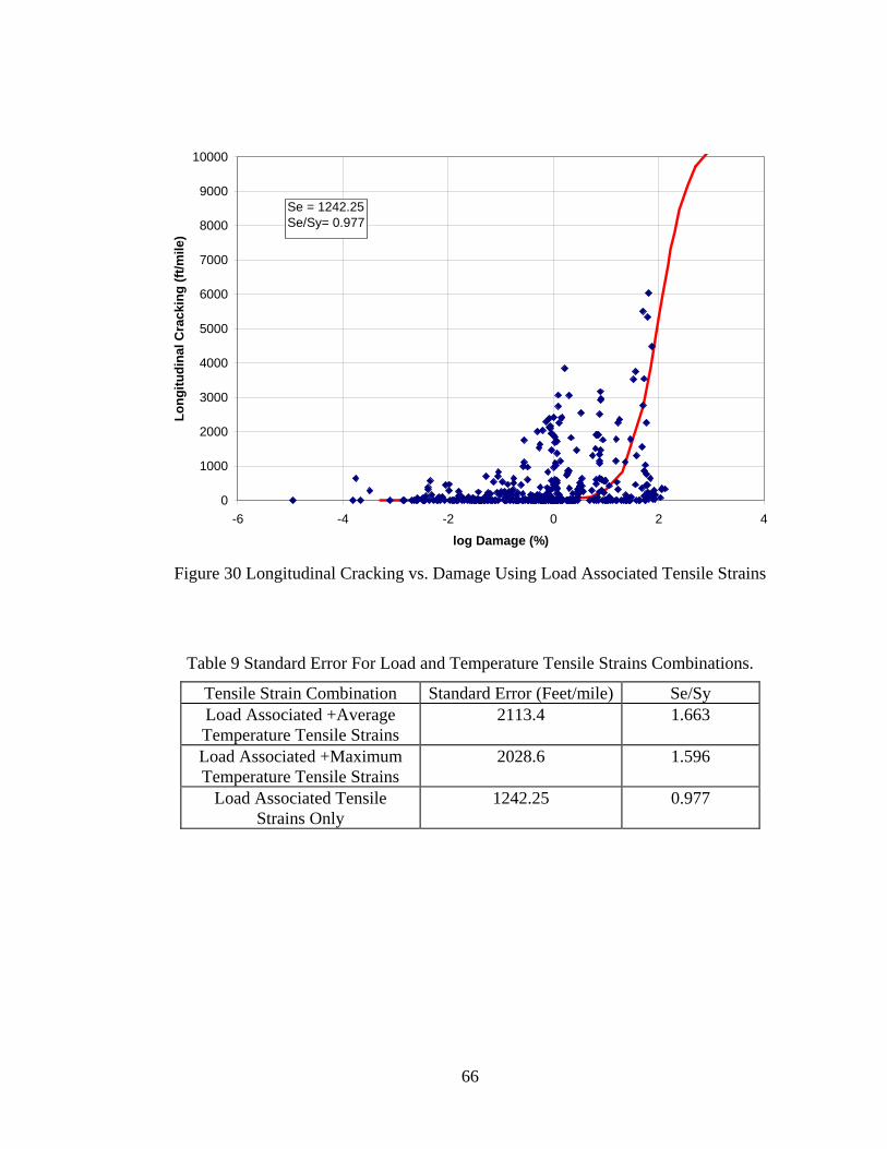
66
0
1000
2000
3000
4000
5000
6000
7000
8000
9000
10000
-6 -4 -2 0 2 4
log Damage (%)
Long
itudi
nal C
rack
ing
(ft/m
ile)
Se = 1242.25Se/Sy= 0.977
Figure 30 Longitudinal Cracking vs. Damage Using Load Associated Tensile Strains
Table 9 Standard Error For Load and Temperature Tensile Strains Combinations.
Tensile Strain Combination Standard Error (Feet/mile) Se/Sy Load Associated +Average Temperature Tensile Strains
2113.4 1.663
Load Associated +Maximum Temperature Tensile Strains
2028.6 1.596
Load Associated Tensile Strains Only
1242.25 0.977

67
Estimation of '1k Function and C1/ C2 values
Using only the tensile strains associated with the applied traffic, the final stage of
the calibration was to find the transfer function between the longitudinal cracking and the damage. However, before getting into that stage a check was done on the distribution of the measured cracking versus the thickness of the AC layers.
A transfer function was optimized using the Microsoft Solver to find the values of C1 and C2 from equation 25 without doing any shift or correction for the AC layer thickness. Figure 31 shows a bar chart of the average longitudinal cracking versus the AC layer thickness. Figure 31 shows that if the cracking was done without any thickness shift (using the original form of the equation and setting the “ '
1k ” factor to 1) the top-down cracking prediction would be higher for thinner sections and will decrease as the asphalt layer thickness increase. This contrasts the findings described in an earlier section, which clearly showed that the longitudinal cracking peaks at an AC thickness of 4-7 inches and that it significantly decreases outside this range.
0
1000
2000
3000
4000
5000
6000
7000
8000
9000
10000
1.5 2.5 3.5 4.5 5.5 6.5 7.5 8.5 9.5 10.5 11.5 15.0
Ac Thickness (in)
Long
itudi
nal C
rack
ing
(ft /m
ile)
Predicted Measured Figure 31 Measured and Predicted Longitudinal Cracking vs. Asphalt Concrete
Thickness without using Thickness Shift Factor
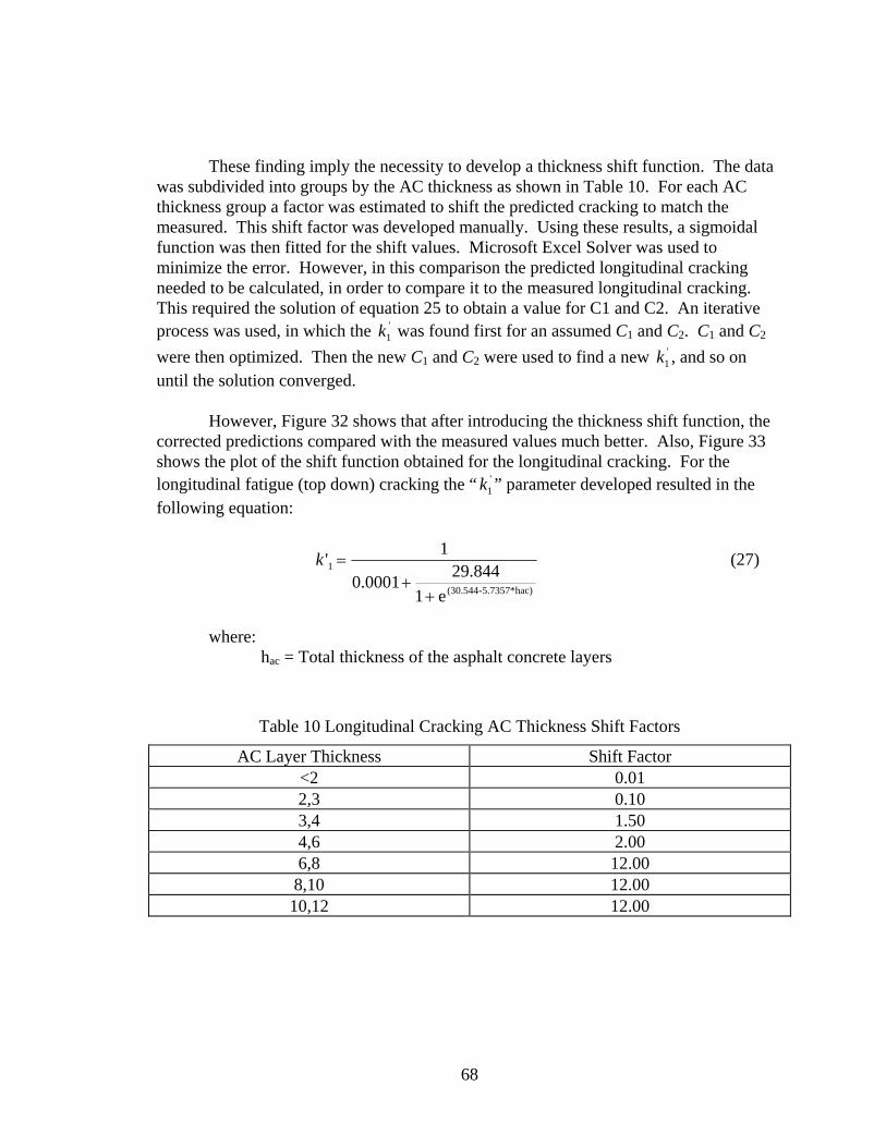
68
These finding imply the necessity to develop a thickness shift function. The data
was subdivided into groups by the AC thickness as shown in Table 10. For each AC thickness group a factor was estimated to shift the predicted cracking to match the measured. This shift factor was developed manually. Using these results, a sigmoidal function was then fitted for the shift values. Microsoft Excel Solver was used to minimize the error. However, in this comparison the predicted longitudinal cracking needed to be calculated, in order to compare it to the measured longitudinal cracking. This required the solution of equation 25 to obtain a value for C1 and C2. An iterative process was used, in which the '
1k was found first for an assumed C1 and C2. C1 and C2 were then optimized. Then the new C1 and C2 were used to find a new '
1k , and so on until the solution converged.
However, Figure 32 shows that after introducing the thickness shift function, the
corrected predictions compared with the measured values much better. Also, Figure 33 shows the plot of the shift function obtained for the longitudinal cracking. For the longitudinal fatigue (top down) cracking the “ '
1k ” parameter developed resulted in the following equation:
hac)5.7357*-(30.544
1
e1844.290.0001
1'
++
=k (27)
where: hac = Total thickness of the asphalt concrete layers
Table 10 Longitudinal Cracking AC Thickness Shift Factors
AC Layer Thickness Shift Factor <2 0.01 2,3 0.10 3,4 1.50 4,6 2.00 6,8 12.00 8,10 12.00 10,12 12.00

69
0
1000
2000
3000
4000
5000
6000
7000
8000
9000
10000
1.5 2.5 3.5 4.5 5.5 6.5 7.5 8.5 9.5 10.5 11.5 15
AC Thickness (in)
Long
itudi
nal C
rack
ing
(ft /m
ile)
Predicted Measured Figure 32 Measured and Predicted Longitudinal Cracking vs. Asphalt Concrete
Thickness using Thickness Shift Factor
0
2
4
6
8
10
12
14
0 1 2 3 4 5 6 7 8 9 10 11 12 13 14 15
AC Layer Thickness (inch)
Shi
ft Fa
ctor
Figure 33 Longitudinal Cracking Shift Function

70
The final transfer function to correlate the longitudinal fatigue cracking from the fatigue damage is based on the assumption that the longitudinal surface fatigue cracking would be 5000 ft /mile at a damage of 100 %. The calibrated model is expressed as following:
For the top-down cracking (feet/mile)
( ) 56.10*1
1000.. )100*(10*log5.37 ⎟⎠⎞
⎜⎝⎛
+= − De
CF (28)
Number of observations = 414 observations. Sum of error square = 6.37e8 Standard error (Se) = 1242.25 ft/mile. Se/Sy = 0.977. The top-down cracking is calculated as linear feet in the wheel path. The
measured cracking used in the calibration is the unweighted sum of the high, medium and low severity cracking reported in the LTPP database. Figure 30 (previously shown) indicates the final calibration model of the measured to predicted top-down longitudinal cracking. Figure 34 shows the error (predicted – measured) in the prediction of the top-down fatigue cracking.
To ensure that the calibrated model is as accurate as possible and that the
predicted model trends are as close as possible to what experience, practical knowledge and reasonable engineering judgment of the performance of the asphalt concrete pavements allows; an extensive sensitivity analysis was conducted using a wide variety of salient variables that were felt to have an impact on top-down fatigue cracking. The results of the sensitivity analysis for the top-down fatigue cracking are given in Appendix II3. This appendix contains an in-depth detailed analysis for the entire sensitivity study.

71
-6000
-4000
-2000
0
2000
4000
6000
8000
-6 -5 -4 -3 -2 -1 0 1 2 3
Log Damage (%)
Erro
r (Pr
edic
ted
-Mea
sure
d) L
ongi
tudi
nal C
rack
ing
(ft/m
ile)
Figure 34 Error (Predicted – Measured Cracking) vs. Damage (%) for Top-Down Fatigue
Cracking.

72
Top-Down Fatigue Cracking Reliability
The reliability design is obtained by determining the predicted load associated
fatigue cracking at the desired level of reliability as follows:
PeFCi ZSFCPFC *_ += (29)
where, FC_P = predicted cracking at the reliability level P, ft/mile. FC = predicted cracking based on mean inputs (corresponding to 50%
reliability), ft/mile. SeFCi = standard error of cracking at the predicted level of mean cracking ZP = standard normal deviate, based upon desired reliability level.
STDFCTop = 200+2300/(1+e1.072-2.1654*logD) (30) Figure 35 shows the plot of the measured standard deviation calculated from the
data versus the cracking damage. The final model fitted to the data is shown in equation 30. As seen, a sigmoidal function is used, as the standard deviation will reach a maximum value for very high damage percentages. The standard error equation was calculated based on dividing the predicted damage into groups, then calculating the standard error for each group. Table 11 shows damage groups and the measured standard error.
Table 11 Computed Statistical Parameters for Each Data Group (Longitudinal Cracking).
Group Range of Predicted
log(Damage(%))
Number of Data Points
Average Predicted
log(Damage(%))
Standard Error for Predicted
Longitudinal Cracking, ft/mi
1 < -2 33 -2.655 204.8 2 -2 to -1 69 -1.476 200.2 3 -1 to 0 118 -0.413 702.9 4 0 to 1 125 0.428 1104.7 5 > 1 69 1.561 2497.5

73
0
500
1000
1500
2000
2500
3000
-4 -3 -2 -1 0 1 2 3 4 5
Log Damage (%)
Long
itudi
nal C
rack
ing
Stan
dard
Err
or (f
t/mile
)
Figure 35 Standard Deviation of the Predicted Top-Down Cracking

74
Fatigue Cracking Calibration Conclusions
Two distinct types of fatigue cracking phenomena were considered. The first was the classical bottom-up cracking; which was assumed to be related to conventional alligator cracking. The alligator cracking was reported as a percentage of the total pavement area exhibiting alligator cracking. The total pavement area was defined by a 12-foot wide lane width by 500-foot long sections (geometric dimensions from LTPP database). This maximum percent alligator cracking is associated with an area of 6000 ft2. Alligator fatigue cracking is assumed to be initiated from horizontal tensile strains occurring at the bottom of the asphalt layers.
The second type of fatigue cracking was the surface (top-down) cracking. This
distress was related to the longitudinal cracking in the pavement system. This fatigue distress type is characterized as the magnitude of longitudinal cracking in feet per mile. LTPP distresses, used in the calibration effort, were adjusted from the 500-foot LTPP section length, to reflect distress reported on a per mile basis of road length. The mechanism that was eventually selected to provide the best agreement to field observations, was a fatigue model related to the tensile strain occurring at the surface of the asphalt layer system. Maximum tensile strain values (and hence fatigue damage) were found to be always associated with the surface tensile strains between the set of dual wheels within a single, tandem, tridem or quad gear configuration.
Based upon the fatigue calibration study, it can be summarized that:
• The fatigue cracking calculations were based on using Miner’s law for
cumulative damage.
1
Ti
i i
nDN=
= ∑
• The general basic form of the fatigue damage prediction model was initially
defined by:
32 111
kk
tf E
kN ⎟⎠⎞
⎜⎝⎛
⎟⎟⎠
⎞⎜⎜⎝
⎛=
ε • The final Design Guide methodology incorporated two types of fatigue
cracking prediction models based on the thickness of the AC layer: constant stress fatigue conditions were assumed to be applicable with thick AC sections while constant strain principles were adopted for thin sections.
• For the fatigue cracking distress, two existing AC models were initially
considered as viable potential candidates in the calibration: the Shell Oil model and the Asphalt Institute (MS-1) model.

75
• The Shell Oil (6) model contains two separate fatigue relationships: one for
the constant stress conditions (thick sections greater than 8 inches) and another for constant strain conditions (thin sections less than 2 inches). These equations are:
Constant Strain
8.155]112.00454.0)(0085.017.0[ −−−+−= EVVPIPIAN tbbff ε
Constant Stress
4.155]0167.000673.0)(00126.00252.0[ −−−+−= EVVPIPIAN tbbff ε
• A general model representing the Shell Oil was developed by fitting a
sigmoidal function between the two models to transition asphalt thicknesses between 2 – 8 inches. The final fatigue model for Shell Oil that was used in the original calibration effort is given by:
4.1
*
55
)408.5354.1(
4.0 11)0167.000673.0)(00126.00252.0(exp1
1139091−
−
−
⎟⎠⎞
⎜⎝⎛
⎟⎟⎠
⎞⎜⎜⎝
⎛−+−⎟⎟
⎠
⎞⎜⎜⎝
⎛+
−+=
EVVPIPIEAN
tbbhff ac ε
where
)408.5354.1(
4.0
exp11139091" −
−
+−
+=ach
EF
5
1 ]0167.000673.0)(00126.00252.0[ −+−= bb VVPIPIK α
Af = laboratory to field adjustment factor (default = 1.0)
• The second existing model used in the calibration evaluation was the Asphalt
Institute MS-1 fatigue model. It is defined by:
854.0291.31100432.0 ⎟
⎠⎞
⎜⎝⎛
⎟⎟⎠
⎞⎜⎜⎝
⎛=
ECN
tf ε
MC 10=

76
⎟⎟⎠
⎞⎜⎜⎝
⎛−
+= 69.084.4
ba
b
VVV
M
• In the actual fatigue calibration work, 82 sections out of the 94 sections
collected for this study, had fatigue data. The quantification of the fatigue distress was as follows.
• The cracking (alligator and longitudinal) reported in the LTPP database is
reported based on the severity level (low, medium and high). According to the panel supervising this project, it was recommended to use the arithmetic summation of the three levels without applying any weighing factor. This was followed by the research team, for both types of fatigue cracking.
• Alligator cracking was reported as percentage of the total pavement area (12
feet width by 500 feet length = 6000 ft2). While the longitudinal cracking was reported as the total longitudinal cracking in feet per mile.
• For the bottom-up cracking, the distress was found to occur at a maximum
asphalt layer thickness of 3-5 inches. A shift function was obtained for the bottom-up cracking to shift the thin sections from the constant strain state to match with the model, which was developed using the constant stress state.
• Alligator cracking showed no significant difference at different MAAT. In
fact, the alligator cracking appeared to be the same for a wide range in temperature.
• The Design Guide computer code calculates the tensile strains for the damage
computation at the bottom of every asphalt layer to assess the damage caused by alligator (bottom-up) cracking. For the longitudinal (surface down) cracking, tensile strains were calculated at the surface of the pavement (Z=0”) and at 0.5” deep from the surface. It was concluded (without question) that tensile strains and hence fatigue damage, were greatest at pavement surface directly between the dual tire of any gear type.
• An analysis of the calibration results for the Shell Oil model showed that this
model had more scatter. No definite trends, at all, were found for the longitudinal cracking. A comparison of the initial accuracy of both model approaches (Shell Oil and the Asphalt Institute) led to the decision to abandon the Shell Oil approach from further consideration and only concentrate upon enhancing the Asphalt Institute’s MS-1 approach.
• The MS-1 model was found to have better trends and less scatter in the data
than the Shell Oil model. However, because the MS-1 is essentially a constant stress model; it was deemed necessary to apply (develop) corrections for the thinner sections by applying a shift factor to match with the thicker

77
asphalt thickness. This adjustment can simply be viewed as an empirical, adjustment to account for constant strain conditions.
• The final values of the fatigue calibration factors were the βf2 = 1.2 on the
tensile strain coefficient and βf2 = 1.5 on the modulus (E) coefficient. These calibration factors were found to be applicable for both the top-down and the bottom-up cracking due to the fact that both of the two distresses showed the least sum of error square for this combination of the distress model coefficients in the final optimization process.
• Thin AC sections were shifted for the alligator cracking calibration process
using an adjustment equation including a function of the AC layer thickness.
281.19492.3
111**00432.0 ⎟
⎠⎞
⎜⎝⎛
⎟⎟⎠
⎞⎜⎜⎝
⎛=
ECN
tff ε
β
'1
'11 * kff ββ =
hac)*3.49-(11.02
1
e1003602.00.000398
1'
++
=k
where:
hac = Total thickness of the asphalt concrete layers.
In the calibration analysis, it was determined that the most appropriate value of the '
1fβ value turned to be '1fβ = 1.0.
The statistical summary for the final Nf model is:
Sum of error square = 1.92E-07 Standard error (Se) = 0.00017
• The final alligator field calibrated cracking model was fund to be:
⎟⎠⎞
⎜⎝⎛
⎟⎠⎞
⎜⎝⎛
+= + 60
1*e1
6000.. 100))*log10(D**C'C*C'(C 2211CF
where: C1 = 1.0 C2 = 1.0 856.2
2 )1(*748.3940874.2' −+−−= hacC

78
C’1= -2 * C’2.
Number of observations = 461 observations. Sum of error square = 17663.91 Standard error (Se) = 6.2 %. Se/Sy = 0.947.
• The standard deviation of the alligator cracking error was correlated to the
predicted damage for the calculation of the reliability as given in the following equation:
SeFCBottom = 0.5+12/(1+e1.308-2.949*logD)
• An analysis of the LTPP database showed that longitudinal surface cracking, hypothesized to initiate due to surface tensile strains, appeared to be maximized at AC thickness of 5-7 inches. A shift function was developed for the top-down cracking in order for the predicted cracking to match the measured cracking from the LTPP database at different asphalt layer thickness.
• The effect of longitudinal cracking was found to be greater at higher mean
annual air temperatures (MAAT) (about 50-60 ºF) than was expected. In addition, it was found that the foundation stiffness slightly influenced the degree of top-down cracking. The stiffer the foundation layer, the greater the amount of longitudinal cracking distress.
• In the initial study of top down cracking, two different depths were used to
assess the damage. These depths were at the surface of the pavement and at a 0.5 inch deep in the surface layer. Further studies clearly showed that the tensile strain at the 0.5-inch deep strains were always less than the surface. As a consequence, only the surface tensile strains (between the tires) were eventually used in the calibration process.
• Three different methods of calculating the longitudinal cracking were initially
investigated to assess which approach would provide the most accurate methodology. In all three approaches, the load-associated strains at the surface (in a direction parallel to traffic) were added to a thermal strain computed from: the maximum thermal strain, the average thermal strain and a null case where no thermal strains were added. The maximum damage (tensile strain) in both directions to traffic (parallel and normal) was evaluated. It was concluded that the best correlation and least scatter occurred for the case when thermal strain were not considered in the analysis.
• The top-down cracking final calibration model developed was:
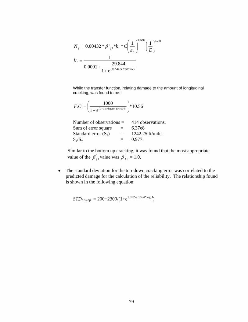
79
281.19492.3'11
11**'*00432.0 ⎟⎠⎞
⎜⎝⎛
⎟⎟⎠
⎞⎜⎜⎝
⎛=
ECkN
tff ε
β
hac)5.7357*-(30.544
1
e1844.290.0001
1'
++
=k
While the transfer function, relating damage to the amount of longitudinal cracking, was found to be:
( ) 56.10*1
1000.. )100*(10*log5.37 ⎟⎠⎞
⎜⎝⎛
+= − De
CF
Number of observations = 414 observations. Sum of error square = 6.37e8 Standard error (Se) = 1242.25 ft/mile. Se/Sy = 0.977.
Similar to the bottom up cracking, it was found that the most appropriate value of the '
1fβ value was '1fβ = 1.0.
• The standard deviation for the top-down cracking error was correlated to the
predicted damage for the calculation of the reliability. The relationship found is shown in the following equation:
STDFCTop = 200+2300/(1+e1.072-2.1654*logD)

80
REFERENCES
1. Dauzats, M. and Rampal, A. Mechanism of Surface Cracking in Wearing Courses. Proceedings, 6th International Conference Structural Design of Asphalt Pavements, The University of Michigan, Ann Arbor, Michigan, July 1987, pp. 232-247.
2. Craus, J., Chen, A., Sousa, J. and Monismith, C. Development of Failure Curves
and Investigation of Asphalt Concrete Pavement Cracking From Super-Overloaded Vehicles. Report to Division of New Technology, Materials, and Research, California Department of Transportation. Sacramento, CA, 1994.
3. Myers, L.A., Roque, R., and Ruth B.E. Mechanisms of Surface-Initiated
Longitudinal Wheel Path Cracks in High-Type Bituminous Pavements. Proceedings, Volume 67, Association of Asphalt Paving Technologists. 1998.
4. Uhlmeyer, J.S., Willoughby, K., Pierce, L.M. and Mahoney, J.P. Top-Down
Cracking in Washington State Asphalt Concrete Wearing Courses. Transportation Research Record 1730. Transportation Research Board, National Research Council, Washington, D.C., January 2000, pp. 110-116.
5. Yang H. H. Pavement Analysis and Design. Prentice Hall, Englewood Cliffs,
New Jersey 1993.
6. Bonnaure, F., Gravois, A., and Udron, J. A New Method of Predicting the Fatigue Life of Bituminous Mixes. Journal of the Association of Asphalt Paving Technologist, Volume 49, 1980.
7. Asphalt Institute. Research and Development of the Asphalt Institute’s Thickness
Design Manual (MS-1), 9th edition. Research Report 82-2, 1982.
8. Lytton, L.R., Uzan, J., Fernando, E. G., Roque, R., Hiltunen, D., and Stoffels, S.M. Development and validation of performance prediction models and specifications for asphalt binders and paving mixes. SHRP-A-357 Report. Strategic Highway Research Program, National Research Council, Washington D.C., 1993.
9. Witczak, M. W., and Mirza, M. W. AC Fatigue Analysis for 2002 Design Guide.
Research Report for NCHRP 1-37A Project. Arizona State University, Tempe, Arizona, 2000
10. Shook, J. F., Finn, F. N., Witczak, M. W., and Monismith, C. L. Thickness
Design of Asphalt Pavements – The Asphalt Institute Method. 5th International Conference on the Structural Design of Asphalt Pavements, Volume 1, 1982.

81
11. Hudson, W. R., Finn, F. N., McCullough, B.F., Nair, K., and Vallerga, B.A.
Systems Approach to Pavement Systems Formulation, Performance Definition and Materials Characterization. Final Report, NCHRP Project 1-10, Materials Research and Development, Inc., March 1968.
12. Federal Highway Administration. LTPP DataPave. Washington D.C. 2000.
13. Witczak, M. W., Zapata, C., and El-Basyouny, M. M. Input Data for the
Calibration and Validation of the 2002 Design Guide for New Constructed Flexible Pavement Sections. Research Report for NCHRP 1-37A Project. Arizona State University, Tempe, Arizona, December 2003
14. Witczak, M. W., Zapata, C., El-Basyouny, M. M., and Konareddy, P. Input Data
for the Calibration and Validation of the 2002 Design Guide for Rehabilitated Pavement Sections with HMA Overlays. Research Report for NCHRP 1-37A Project. Arizona State University, Tempe, Arizona, December 2003
15. Strategic Highway Research Program. Distress Identification Manual for the
Long-Term Pavement Performance Project. National Research Council. Washington D.C. 1993
16. NCHRP 1-37A Draft Document. 2002 Guide for the Design of New and
Rehabilitated Pavement Structures. ERES Division of ARA Inc., Champaign Illinois, May 2002.

Annex B
Bottom-Up Alligator Fatigue Cracking Shell Oil Model Calibration

83
Table B-1 Measured Alligator Cracking Fatigue Cracking and Predicted Bottom-up Damage Using Shell Oil Model.
Section Total
Asphalt Thickness
Date Time Measured Alligator Cracking (ft^2)
Predicted Bottom-Up Damage (%) (At Different βf2 and βf3)
Low Medium High Total 0.9,0.9 0.9,1.0 0.9,1.1 1.0,0.9 1.0,1.0 11001 3.2 Sep-91 132 8 0 0 8 10700 68740 445000 148.5 942.6 11001 3.2 Apr-92 139 13 0 0 13 11390 73410 477200 157.1 1001 11001 3.2 Jul-92 142 13 0 0 13 11700 75320 488900 161.7 1029 11001 3.2 Jan-93 148 45 0 0 45 12280 79170 514700 169.4 1079 11019 6.7 May-89 32 0 0 0 0 9490 54380 313100 120 683.6 11019 6.7 Apr-90 43 0 0 0 0 12840 73530 423300 161.3 918.2 11019 6.7 Jan-91 52 0 0 0 0 15680 89530 513900 197.1 1118 11019 6.7 Jun-91 57 800 0 0 800 17400 99320 570000 218.5 1239 11019 6.7 Mar-92 66 0 0 0 0 20360 116400 669000 254.6 1446 11019 6.7 Mar-93 78 1112 0 0 1112 24530 140200 804900 306.4 1739 11019 6.7 Jul-95 106 2554 0 0 2554 34800 198300 1136000 435.1 2462 11019 6.7 Jan-98 136 0 1461 233 1693 45940 262000 1502000 572.5 3243 14126 13.1 Jun-89 15 0 0 0 0 239.1 1405 8285 1.751 10.21 14126 13.1 Mar-91 36 0 0 0 0 625.9 3660 21500 4.621 26.8 14126 13.1 Mar-93 60 0 0 0 0 1100 6437 37840 8.113 47.11 14126 13.1 Apr-94 73 0 0 0 0 1388 8133 47840 10.24 59.47 14126 13.1 Dec-95 93 6 22 0 28 1904 11140 65430 14.08 81.75 14126 13.1 Dec-97 117 81 0 0 81 2485 14560 85660 18.34 106.6 21001 3 May-90 83 0 0 0 0 38.45 280.1 2049 0.421 3.043 21001 3 Aug-91 98 0 0 0 0 46.21 335.8 2451 0.5076 3.66 21001 3 Aug-93 122 0 0 0 0 57.98 421.7 3081 0.6368 4.595 21001 3 Jun-95 144 0 0 0 0 67.69 493.5 3614 0.7406 5.356 21001 3 Aug-97 170 0 0 0 0 80.79 588.8 4311 0.8841 6.392 21001 3 Aug-98 182 0 3 0 3 86.6 631.1 4620 0.9479 6.853 21002 3.3 May-90 68 0 0 0 0 5.11 37.74 280.2 0.05174 0.3783 21002 3.3 Aug-91 83 0 0 0 0 6.519 48.03 355.7 0.06628 0.4836 21002 3.3 Aug-93 107 0 0 0 0 8.424 62.17 461.1 0.08547 0.6244 21002 3.3 Jun-95 129 0 0 0 0 10.02 74.15 551.4 0.1013 0.7414 21002 3.3 Aug-97 155 0 0 0 0 12.27 90.73 674.4 0.1241 0.908 21002 3.3 May-98 164 0 0 0 0 12.74 94.4 703.1 0.1283 0.9411 40113 4.5 Feb-95 19 11 0 0 11 661.1 4102 25710 7.601 46.42 40113 4.5 Mar-95 20 11 0 0 11 701.9 4368 27450 8.034 49.23 40113 4.5 Aug-95 25 11 0 0 11 948 5797 35800 11.13 67.07 40113 4.5 Nov-95 28 11 0 0 11 1107 6756 41620 13.02 78.4 40113 4.5 Feb-96 31 11 0 0 11 1197 7388 46030 13.86 84.22 40113 4.5 Apr-96 33 11 0 0 11 1300 8032 50100 15.02 91.43 40113 4.5 Jul-96 36 11 0 0 11 1477 9036 55800 17.32 104.4 40113 4.5 Aug-96 37 11 0 0 11 1542 9394 57800 18.18 109.2 40113 4.5 Jan-98 54 11 0 0 11 2415 14890 92840 27.98 169.7 40113 4.5 Apr-98 57 11 10 0 20 2566 15900 99570 29.51 179.8 40113 4.5 Jun-98 59 11 10 0 20 2714 16760 104600 31.36 190.6 40113 4.5 Oct-98 63 11 10 0 20 3038 18620 115400 35.49 214.2 40114 6.8 Feb-95 19 11 0 0 11 2868 18030 114100 30.11 186.9 40114 6.8 Mar-95 20 11 0 0 11 2965 18700 118800 30.94 192.6 40114 6.8 Aug-95 25 11 0 0 11 4458 27840 174800 47.37 292.6

84
Table B-1 (Cont’d) Measured Alligator Cracking Fatigue Cracking and Predicted Bottom-
up Damage Using Shell Oil Model. Section Total
Asphalt Thickness
Date Time Measured Alligator Cracking (ft^2)
Predicted Bottom-Up Damage (%) (At Different βf2 and βf3)
Low Medium High Total 0.9,0.9 0.9,1.0 0.9,1.1 1.0,0.9 1.0,1.0 40114 6.8 Nov-95 28 11 0 0 11 5200 32520 204400 55.08 340.9 40114 6.8 Feb-96 31 11 0 0 11 5327 33450 211200 56 347.6 40114 6.8 Apr-96 33 11 0 0 11 5667 35690 226100 59.22 368.7 40114 6.8 Jul-96 36 11 0 0 11 6841 42820 269400 72.27 447.7 40114 6.8 Aug-96 37 11 0 0 11 7302 45580 286000 77.48 478.9 40114 6.8 Jan-98 54 11 0 0 11 10810 67810 427800 113.6 704.8 40114 6.8 Apr-98 57 11 46 0 57 11150 70160 444100 116.5 724.6 40114 6.8 Jun-98 59 11 52 0 62 11950 75100 474800 125 777.2 40114 6.8 Oct-98 63 11 114 0 125 13960 87450 550500 147.1 912.1 40115 15.1 Feb-95 19 11 0 0 11 13.86 81.9 486.1 0.09003 0.5272 40115 15.1 Mar-95 20 11 25 0 36 14.13 83.71 498.2 0.09137 0.536 40115 15.1 Jan-98 54 11 0 0 11 47.93 282.9 1676 0.3106 1.819 40116 16.2 Feb-95 19 11 0 0 11 11.42 69.84 428.9 0.06596 0.3998 40116 16.2 Mar-95 20 11 0 0 11 11.63 71.3 439 0.06687 0.406 40116 16.2 Jan-98 54 11 0 0 11 39.83 243.3 1492 0.2297 1.392 40117 11.8 Feb-95 19 11 0 0 11 218.1 1313 7938 1.807 10.79 40117 11.8 Mar-95 20 11 0 0 11 221.4 1336 8089 1.826 10.92 40117 11.8 Jan-98 54 11 0 0 11 804.9 4855 29380 6.62 39.65 40118 11.7 Feb-95 19 11 0 0 11 106.5 656.7 4066 0.7833 4.784 40118 11.7 Mar-95 20 11 0 0 11 109 674.1 4186 0.7978 4.883 40118 11.7 Jan-98 54 11 0 0 11 401.3 2470 15260 2.971 18.14 41007 6.5 Sep-91 162 38 0 0 38 4066 24170 144500 46.06 271 41007 6.5 Feb-93 163 44 16 0 60 4113 24450 146200 46.57 274 41007 6.5 Sep-94 198 70 132 0 202 5646 33570 200800 63.9 376.1 41024 10.8 Nov-89 149 0 0 0 0 59030 342700 1996000 581.9 3354 41024 10.8 Aug-90 158 0 0 0 0 64100 372400 2171000 630.9 3638 41024 10.8 Oct-92 184 0 0 0 0 82320 478800 2795000 807.5 4664 41024 10.8 Mar-95 213 0 0 0 0 103200 600100 3502000 1014 5851 41024 10.8 Jul-95 217 0 0 0 0 108100 628300 3666000 1061 6125 41024 10.8 Aug-95 218 12 0 0 12 109900 638900 3727000 1079 6230 41024 10.8 Nov-95 221 0 10 0 10 112300 653200 3814000 1101 6357 41024 10.8 Feb-96 224 0 0 0 0 112400 654200 3821000 1101 6362 41024 10.8 Apr-96 226 16 0 0 16 113300 659900 3857000 1109 6410 41024 10.8 Jun-96 228 118 0 0 118 117200 682000 3985000 1147 6632 41024 10.8 Aug-96 230 161 0 0 161 122900 714300 4165000 1208 6973 41024 10.8 Apr-98 250 0 398 529 927 136900 797400 4662000 1338 7738 41024 10.8 Jun-98 252 0 397 530 927 141000 821400 4801000 1380 7978 41024 10.8 Oct-98 256 0 414 529 943 149700 870700 5081000 1468 8477 81029 4.2 Oct-91 233 27 15 0 42 48.49 329.8 2263 0.572 3.828 81029 4.2 Jul-94 266 0 0 0 0 55.16 375.4 2578 0.6492 4.347 81029 4.2 Sep-95 280 464 0 0 464 58.45 397.8 2731 0.6877 4.605 81053 4.6 Oct-89 60 0 0 0 0 41.91 276.2 1838 0.5014 3.253 81053 4.6 Jul-90 69 0 0 0 0 49.72 328.6 2192 0.5921 3.848 81053 4.6 Apr-93 102 3 0 0 3 82.54 547.2 3663 0.9742 6.349 81053 4.6 Nov-93 109 0 0 0 0 93.2 615.3 4101 1.106 7.18 81053 4.6 Dec-93 110 23 0 0 23 93.4 616.9 4113 1.107 7.191
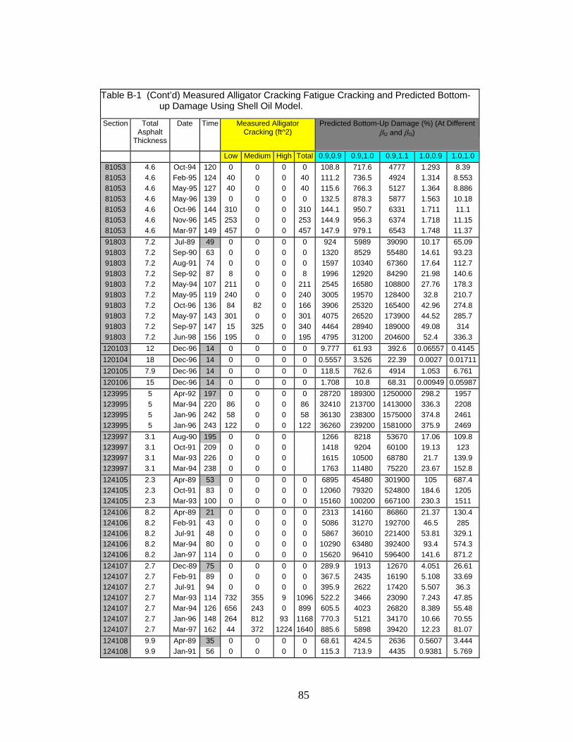
85
Table B-1 (Cont’d) Measured Alligator Cracking Fatigue Cracking and Predicted Bottom-
up Damage Using Shell Oil Model.
Section Total Asphalt
Thickness
Date Time Measured Alligator Cracking (ft^2)
Predicted Bottom-Up Damage (%) (At Different βf2 and βf3)
Low Medium High Total 0.9,0.9 0.9,1.0 0.9,1.1 1.0,0.9 1.0,1.0 81053 4.6 Oct-94 120 0 0 0 0 108.8 717.6 4777 1.293 8.39 81053 4.6 Feb-95 124 40 0 0 40 111.2 736.5 4924 1.314 8.553 81053 4.6 May-95 127 40 0 0 40 115.6 766.3 5127 1.364 8.886 81053 4.6 May-96 139 0 0 0 0 132.5 878.3 5877 1.563 10.18 81053 4.6 Oct-96 144 310 0 0 310 144.1 950.7 6331 1.711 11.1 81053 4.6 Nov-96 145 253 0 0 253 144.9 956.3 6374 1.718 11.15 81053 4.6 Mar-97 149 457 0 0 457 147.9 979.1 6543 1.748 11.37 91803 7.2 Jul-89 49 0 0 0 0 924 5989 39090 10.17 65.09 91803 7.2 Sep-90 63 0 0 0 0 1320 8529 55480 14.61 93.23 91803 7.2 Aug-91 74 0 0 0 0 1597 10340 67360 17.64 112.7 91803 7.2 Sep-92 87 8 0 0 8 1996 12920 84290 21.98 140.6 91803 7.2 May-94 107 211 0 0 211 2545 16580 108800 27.76 178.3 91803 7.2 May-95 119 240 0 0 240 3005 19570 128400 32.8 210.7 91803 7.2 Oct-96 136 84 82 0 166 3906 25320 165400 42.96 274.8 91803 7.2 May-97 143 301 0 0 301 4075 26520 173900 44.52 285.7 91803 7.2 Sep-97 147 15 325 0 340 4464 28940 189000 49.08 314 91803 7.2 Jun-98 156 195 0 0 195 4795 31200 204600 52.4 336.3 120103 12 Dec-96 14 0 0 0 0 9.777 61.93 392.6 0.06557 0.4145 120104 18 Dec-96 14 0 0 0 0 0.5557 3.526 22.39 0.0027 0.01711120105 7.9 Dec-96 14 0 0 0 0 118.5 762.6 4914 1.053 6.761 120106 15 Dec-96 14 0 0 0 0 1.708 10.8 68.31 0.00949 0.05987123995 5 Apr-92 197 0 0 0 0 28720 189300 1250000 298.2 1957 123995 5 Mar-94 220 86 0 0 86 32410 213700 1413000 336.3 2208 123995 5 Jan-96 242 58 0 0 58 36130 238300 1575000 374.8 2461 123995 5 Jan-96 243 122 0 0 122 36260 239200 1581000 375.9 2469 123997 3.1 Aug-90 195 0 0 0 1266 8218 53670 17.06 109.8 123997 3.1 Oct-91 209 0 0 0 1418 9204 60100 19.13 123 123997 3.1 Mar-93 226 0 0 0 1615 10500 68780 21.7 139.9 123997 3.1 Mar-94 238 0 0 0 1763 11480 75220 23.67 152.8 124105 2.3 Apr-89 53 0 0 0 0 6895 45480 301900 105 687.4 124105 2.3 Oct-91 83 0 0 0 0 12060 79320 524800 184.6 1205 124105 2.3 Mar-93 100 0 0 0 0 15160 100200 667100 230.3 1511 124106 8.2 Apr-89 21 0 0 0 0 2313 14160 86860 21.37 130.4 124106 8.2 Feb-91 43 0 0 0 0 5086 31270 192700 46.5 285 124106 8.2 Jul-91 48 0 0 0 0 5867 36010 221400 53.81 329.1 124106 8.2 Mar-94 80 0 0 0 0 10290 63480 392400 93.4 574.3 124106 8.2 Jan-97 114 0 0 0 0 15620 96410 596400 141.6 871.2 124107 2.7 Dec-89 75 0 0 0 0 289.9 1913 12670 4.051 26.61 124107 2.7 Feb-91 89 0 0 0 0 367.5 2435 16190 5.108 33.69 124107 2.7 Jul-91 94 0 0 0 0 395.9 2622 17420 5.507 36.3 124107 2.7 Mar-93 114 732 355 9 1096 522.2 3466 23090 7.243 47.85 124107 2.7 Mar-94 126 656 243 0 899 605.5 4023 26820 8.389 55.48 124107 2.7 Jan-96 148 264 812 93 1168 770.3 5121 34170 10.66 70.55 124107 2.7 Mar-97 162 44 372 1224 1640 885.6 5898 39420 12.23 81.07 124108 9.9 Apr-89 35 0 0 0 0 68.61 424.5 2636 0.5607 3.444 124108 9.9 Jan-91 56 0 0 0 0 115.3 713.9 4435 0.9381 5.769

86
Table B-1 (Cont’d) Measured Alligator Cracking Fatigue Cracking and Predicted Bottom-
up Damage Using Shell Oil Model.
Section Total Asphalt
Thickness
Date Time Measured Alligator Cracking (ft^2)
Predicted Bottom-Up Damage (%) (At Different βf2 and βf3)
Low Medium High Total 0.9,0.9 0.9,1.0 0.9,1.1 1.0,0.9 1.0,1.0 124108 9.9 Oct-91 65 0 0 0 0 143.2 885.4 5490 1.169 7.178 124108 9.9 Mar-94 94 0 0 0 0 203.9 1267 7899 1.645 10.15 124108 9.9 Aug-94 99 0 0 0 0 227.4 1409 8760 1.845 11.35 124108 9.9 Jan-96 116 0 0 0 0 265.2 1648 10270 2.137 13.18 124135 1.4 Dec-89 227 1112 86 0 1198 117100 786100 5314000 2155 14340 124135 1.4 Jan-91 240 2045 355 0 2400 123600 830500 5617000 2271 15120 131031 11.1 Apr-91 119 0 0 0 289.5 1776 10950 2.307 14.02 131031 11.1 Jul-92 134 0 0 0 366.7 2248 13840 2.922 17.75 131031 11.1 Jan-93 140 0 0 0 391.4 2401 14800 3.115 18.93 131031 11.1 Apr-94 155 0 0 0 473.7 2907 17920 3.765 22.89 131031 11.1 Oct-94 161 0 0 0 541.6 3312 20350 4.328 26.24 131031 11.1 Aug-95 171 0 0 0 602.2 3690 22720 4.795 29.12 131031 11.1 Jan-96 176 0 0 0 623.6 3826 23590 4.953 30.12 131031 11.1 Apr-96 179 0 0 0 633.4 3891 24030 5.018 30.55 134111 8.7 Mar-89 101 0 0 0 0 603.1 3781 23860 6.666 41.33 134111 8.7 Mar-91 125 0 0 0 0 923.6 5801 36660 10.17 63.21 134111 8.7 Feb-92 136 316 0 0 316 1098 6889 43490 12.11 75.19 134112 15.9 May-89 144 0 0 0 0 420.8 2469 14540 3.619 21.06 134112 15.9 Feb-91 165 0 0 0 0 526.6 3094 18250 4.514 26.31 134112 15.9 Apr-91 167 0 0 0 0 533.3 3136 18510 4.563 26.62 134112 15.9 Feb-94 201 0 0 0 0 740.7 4345 25600 6.363 37.03 134112 15.9 Oct-94 209 0 0 0 0 809 4744 27920 6.956 40.47 134112 15.9 Jan-96 224 0 0 0 0 892.6 5244 30930 7.643 44.56 134112 15.9 Feb-97 237 0 0 0 0 985.2 5784 34090 8.448 49.2 134112 15.9 Apr-98 251 0 0 0 0 1077 6331 37380 9.202 53.68 134113 15.2 May-89 144 0 0 0 0 1866 10830 63080 17.56 101.1 134113 15.2 Feb-91 165 0 0 0 0 2268 13180 76840 21.29 122.7 134113 15.2 Apr-91 167 0 0 0 0 2293 13330 77800 21.48 123.9 134113 15.2 Feb-94 201 0 0 0 0 3057 17740 103400 28.75 165.5 134113 15.2 Oct-94 209 0 0 0 0 3306 19180 111700 31.11 179.1 134113 15.2 Jan-96 224 0 0 0 0 3604 20940 122100 33.79 194.8 134113 15.2 Feb-97 237 47 0 0 47 3933 22840 133100 36.93 212.7 134113 15.2 Apr-98 251 44 0 0 44 4255 24740 144400 39.83 229.8 161001 3.7 Jul-89 192 0 0 0 0 620.2 4559 33880 6.207 44.64 161001 3.7 Aug-90 205 0 0 0 0 689.7 5065 37610 6.906 49.62 161001 3.7 Jun-93 239 36 0 0 36 866.6 6387 47590 8.604 62.05 161001 3.7 Aug-94 253 16 0 0 16 961.9 7074 52600 9.581 68.96 161001 3.7 May-95 262 0 0 0 0 1004 7403 55210 9.943 71.76 161001 3.7 Jul-97 288 3 611 0 615 1184 8724 64990 11.74 84.66 161001 3.7 Sep-98 302 0 434 99 533 1290 9497 70680 12.8 92.26 161009 10.4 Sep-89 180 0 0 0 65.81 424.7 2756 0.4587 2.927 161009 10.4 Jul-90 190 0 0 0 70.66 456.3 2964 0.492 3.141 161009 10.4 Jul-92 214 0 0 0 85.09 550 3577 0.5912 3.778 161009 10.4 Oct-93 229 0 0 0 97.49 629.5 4090 0.6787 4.333 161009 10.4 Jun-96 261 0 0 0 120.4 779 5069 0.8362 5.346 161009 10.4 Jul-97 274 0 0 0 133.8 864.6 5622 0.9298 5.941

87
Table B-1 (Cont’d) Measured Alligator Cracking Fatigue Cracking and Predicted Bottom-
up Damage Using Shell Oil Model.
Section Total Asphalt
Thickness
Date Time Measured Alligator Cracking (ft^2)
Predicted Bottom-Up Damage (%) (At Different βf2 and βf3)
Low Medium High Total 0.9,0.9 0.9,1.0 0.9,1.1 1.0,0.9 1.0,1.0 161021 5.9 Sep-89 48 0 0 0 0 24.34 156.4 1014 0.2408 1.524 161021 5.9 Oct-90 61 0 0 0 0 30.73 197.9 1286 0.3029 1.92 161021 5.9 Aug-91 71 0 0 0 0 35.24 226.6 1470 0.3483 2.205 161021 5.9 Aug-93 95 0 0 0 0 47.73 307.6 2000 0.4701 2.98 161021 5.9 Sep-95 120 0 0 0 0 60.98 392.7 2552 0.6009 3.807 161021 5.9 Jun-96 129 0 0 0 0 63.73 411.4 2680 0.6259 3.973 161021 5.9 Jul-97 142 0 0 0 0 71.5 461.2 3003 0.7027 4.458 169034 9.2 Jul-89 10 0 0 0 0 10.62 69.68 460 0.08236 0.5331 169034 9.2 Aug-90 23 0 0 0 0 31.34 200.1 1286 0.2559 1.613 169034 9.2 Jun-93 57 0 0 0 0 67.77 436.2 2827 0.5441 3.456 169034 9.2 Aug-94 71 0 0 0 0 90.88 581.1 3740 0.7392 4.666 169034 9.2 May-95 80 0 0 0 0 95.65 613.9 3968 0.7725 4.891 169034 9.2 Jul-97 106 25 0 0 25 131.2 840.2 5418 1.064 6.722 169034 9.2 Sep-98 120 0 0 25 25 151.9 971.3 6253 1.234 7.79 201009 11.1 Aug-88 44 10 0 0 10 10.15 62.72 389 0.07557 0.4635 201009 11.1 May-89 53 0 0 0 0 11.11 68.92 429.3 0.08198 0.5045 201009 11.1 Dec-90 72 42 0 0 42 16.36 101.1 626.7 0.1216 0.7451 201009 11.1 Oct-91 82 1 13 0 14 18.94 117.1 726.8 0.1404 0.8612 201009 11.1 Apr-93 100 6 18 16 41 22.41 138.5 859.6 0.1662 1.019 201009 11.1 Apr-95 124 2 54 0 56 27.75 171.8 1067 0.2047 1.257 201009 11.1 Apr-96 136 0 0 0 0 30.44 188.5 1172 0.2243 1.377 201009 11.1 Jan-99 168 0 1643 0 1643 39.61 245 1522 0.2919 1.792 251003 6.6 Aug-89 180 0 0 0 0 2800 18520 123300 30.44 198.5 251003 6.6 Sep-90 193 0 0 0 0 3060 20250 134900 33.22 216.7 251003 6.6 Aug-91 204 28 0 0 28 3273 21670 144500 35.49 231.7 251003 6.6 Sep-92 217 56 93 0 149 3593 23760 158300 39.05 254.6 251003 6.6 Oct-95 254 45 75 0 121 4388 29070 193900 47.52 310.3 251003 6.6 Oct-96 266 1314 0 0 1314 4675 30970 206600 50.59 330.4 251003 6.6 Jun-98 286 1062 62 0 1125 5135 34040 227200 55.54 362.8 251004 9.6 Aug-89 178 0 0 0 0 1395 8941 57530 15.21 96.58 251004 9.6 Sep-90 191 0 0 0 0 1573 10080 64850 17.14 108.9 251004 9.6 Aug-91 202 0 0 0 0 1704 10920 70270 18.58 118 251004 9.6 Sep-92 215 0 0 0 0 1889 12110 77970 20.56 130.6 251004 9.6 Oct-95 252 0 0 0 0 2495 16000 103000 27.16 172.6 251004 9.6 Jun-97 272 56 0 0 56 2778 17840 115000 30.14 191.7 251004 9.6 Jun-98 284 0 0 0 0 3035 19480 125600 32.94 209.5 261001 2.2 Jul-88 203 0 0 0 0 51.73 381.4 2837 0.6647 4.831 261001 2.2 Sep-89 217 0 0 0 0 55.26 407 3024 0.7112 5.164 261001 2.2 Jul-90 227 0 0 0 0 57.56 424.4 3157 0.7395 5.374 261001 2.2 Jul-91 239 33 0 0 33 60.8 448.4 3335 0.781 5.677 261001 2.2 Sep-91 241 28 0 0 28 61.42 452.7 3366 0.7894 5.736 261001 2.2 Sep-92 253 40 0 0 40 64.33 474.5 3531 0.8257 6.004 261001 2.2 Jun-93 262 0 81 0 81 66.63 491.9 3663 0.8544 6.217 261001 2.2 Jun-93 263 76 0 0 76 66.96 494.1 3678 0.8592 6.249 261001 2.2 May-95 285 58 0 0 58 72.13 532.6 3967 0.9247 6.729 261001 2.2 Jul-96 299 83 0 0 83 76.02 561 4177 0.9753 7.094
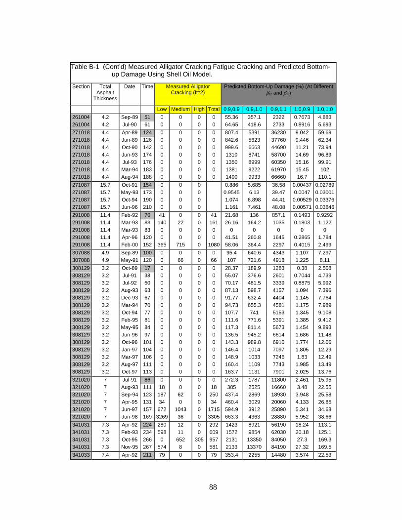
88
Table B-1 (Cont’d) Measured Alligator Cracking Fatigue Cracking and Predicted Bottom-
up Damage Using Shell Oil Model.
Section Total Asphalt
Thickness
Date Time Measured Alligator Cracking (ft^2)
Predicted Bottom-Up Damage (%) (At Different βf2 and βf3)
Low Medium High Total 0.9,0.9 0.9,1.0 0.9,1.1 1.0,0.9 1.0,1.0 261004 4.2 Sep-89 51 0 0 0 0 55.36 357.1 2322 0.7673 4.883 261004 4.2 Jul-90 61 0 0 0 0 64.65 418.6 2733 0.8916 5.693 271018 4.4 Apr-89 124 0 0 0 0 807.4 5391 36230 9.042 59.69 271018 4.4 Jun-89 126 0 0 0 0 842.6 5623 37760 9.446 62.34 271018 4.4 Oct-90 142 0 0 0 0 999.6 6663 44690 11.21 73.94 271018 4.4 Jun-93 174 0 0 0 0 1310 8741 58700 14.69 96.89 271018 4.4 Jul-93 176 0 0 0 0 1350 8999 60350 15.16 99.91 271018 4.4 Mar-94 183 0 0 0 0 1381 9222 61970 15.45 102 271018 4.4 Aug-94 188 0 0 0 0 1490 9933 66660 16.7 110.1 271087 15.7 Oct-91 154 0 0 0 0.886 5.685 36.58 0.00437 0.02789271087 15.7 May-93 173 0 0 0 0.9545 6.13 39.47 0.0047 0.03001271087 15.7 Oct-94 190 0 0 0 1.074 6.898 44.41 0.00529 0.03376271087 15.7 Jun-96 210 0 0 0 1.161 7.461 48.08 0.00571 0.03646291008 11.4 Feb-92 70 41 0 0 41 21.68 136 857.1 0.1493 0.9292 291008 11.4 Mar-93 83 140 22 0 161 26.16 164.2 1035 0.1803 1.122 291008 11.4 Mar-93 83 0 0 0 0 0 0 0 0 0 291008 11.4 Apr-96 120 0 0 0 0 41.51 260.8 1645 0.2865 1.784 291008 11.4 Feb-00 152 365 715 0 1080 58.06 364.4 2297 0.4015 2.499 307088 4.9 Sep-89 100 0 0 0 0 95.4 640.6 4343 1.107 7.297 307088 4.9 May-91 120 0 66 0 66 107 721.6 4918 1.225 8.11 308129 3.2 Oct-89 17 0 0 0 0 28.37 189.9 1283 0.38 2.508 308129 3.2 Jul-91 38 0 0 0 0 55.07 376.6 2601 0.7044 4.739 308129 3.2 Jul-92 50 0 0 0 0 70.17 481.5 3339 0.8875 5.992 308129 3.2 Aug-93 63 0 0 0 0 87.13 598.7 4157 1.094 7.396 308129 3.2 Dec-93 67 0 0 0 0 91.77 632.4 4404 1.145 7.764 308129 3.2 Mar-94 70 0 0 0 0 94.73 655.3 4581 1.175 7.989 308129 3.2 Oct-94 77 0 0 0 0 107.7 741 5153 1.345 9.108 308129 3.2 Feb-95 81 0 0 0 0 111.6 771.6 5391 1.385 9.412 308129 3.2 May-95 84 0 0 0 0 117.3 811.4 5673 1.454 9.893 308129 3.2 Jun-96 97 0 0 0 0 136.5 945.2 6614 1.686 11.48 308129 3.2 Oct-96 101 0 0 0 0 143.3 989.8 6910 1.774 12.06 308129 3.2 Jan-97 104 0 0 0 0 146.4 1014 7097 1.805 12.29 308129 3.2 Mar-97 106 0 0 0 0 148.9 1033 7246 1.83 12.49 308129 3.2 Aug-97 111 0 0 0 0 160.4 1109 7743 1.985 13.49 308129 3.2 Oct-97 113 0 0 0 0 163.7 1131 7901 2.025 13.76 321020 7 Jul-91 86 0 0 0 0 272.3 1787 11800 2.461 15.95 321020 7 Aug-93 111 18 0 0 18 385 2525 16660 3.48 22.55 321020 7 Sep-94 123 187 62 0 250 437.4 2869 18930 3.948 25.58 321020 7 Apr-95 131 34 0 0 34 460.4 3029 20060 4.133 26.85 321020 7 Jun-97 157 672 1043 0 1715 594.9 3912 25890 5.341 34.68 321020 7 Jun-98 169 3269 36 0 3305 663.3 4363 28880 5.952 38.66 341031 7.3 Apr-92 224 280 12 0 292 1423 8921 56190 18.24 113.1 341031 7.3 Feb-93 234 598 11 0 609 1572 9854 62030 20.18 125.1 341031 7.3 Oct-95 266 0 652 305 957 2131 13350 84050 27.3 169.3 341031 7.3 Nov-95 267 574 8 0 581 2133 13370 84190 27.32 169.5 341033 7.4 Apr-92 211 79 0 0 79 353.4 2255 14480 3.574 22.53

89
Table B-1 (Cont’d) Measured Alligator Cracking Fatigue Cracking and Predicted Bottom-
up Damage Using Shell Oil Model.
Section Total Asphalt
Thickness
Date Time Measured Alligator Cracking (ft^2)
Predicted Bottom-Up Damage (%) (At Different βf2 and βf3)
Low Medium High Total 0.9,0.9 0.9,1.0 0.9,1.1 1.0,0.9 1.0,1.0 341033 7.4 Feb-93 221 6 0 0 6 374.2 2388 15330 3.782 23.84 341033 7.4 Nov-95 254 15 0 0 15 447.4 2852 18290 4.531 28.54 341033 7.4 Jul-97 274 0 0 0 0 486.6 3104 19920 4.923 31.02 341034 11.1 Oct-89 48 0 0 0 0 55.31 362.1 2380 0.3461 2.247 341034 11.1 Sep-90 59 0 0 0 0 70.16 459.1 3016 0.4391 2.85 341034 11.1 Apr-92 78 0 0 0 0 88.96 583.7 3846 0.5533 3.597 341034 11.1 Feb-93 88 0 0 0 0 104.3 683.8 4503 0.6487 4.216 341034 11.1 Nov-95 121 0 0 0 0 160.5 1052 6916 0.9998 6.492 341034 11.1 Jul-97 141 129 75 0 205 194.1 1272 8366 1.21 7.852 350101 7.2 May-97 19 0 0 0 0 4229 26630 168600 50.37 313.4 350102 4.8 May-97 19 0 0 0 0 2864 18790 124200 38.01 245.9 350103 12.5 May-97 19 0 0 0 0 8266 50770 312900 83.78 510.2 350104 19.2 May-97 19 0 0 0 0 451.1 2750 16820 3.39 20.5 350105 9.9 May-97 19 0 0 0 0 93270 567000 3462000 1088 6548 350106 15.6 May-97 19 0 0 0 0 1699 10340 63150 14.66 88.45 351005 8.9 Oct-89 73 0 0 0 0 243.3 1548 9891 2.394 15.1 351005 8.9 Mar-91 90 0 0 0 0 325.8 2070 13200 3.226 20.3 351005 8.9 Oct-92 109 0 0 0 0 448.8 2856 18250 4.423 27.9 351005 8.9 Feb-94 125 0 0 0 0 546.1 3474 22190 5.387 33.95 351005 8.9 Mar-95 138 0 0 0 0 641.7 4088 26150 6.311 39.82 351005 8.9 Apr-97 163 0 0 0 0 869.9 5541 35440 8.556 53.98 351022 6.3 Oct-89 37 0 0 0 0 160.7 1044 6824 1.737 11.14 351022 6.3 Mar-91 54 0 0 0 0 227 1489 9835 2.404 15.53 351022 6.3 Oct-92 73 0 0 0 0 374.4 2436 15960 3.994 25.63 351022 6.3 Feb-94 89 0 0 0 0 465.7 3046 20070 4.92 31.71 351022 6.3 Mar-95 102 0 0 0 0 571.2 3733 24590 6.028 38.81 351022 6.3 Apr-97 127 0 0 0 0 791 5177 34150 8.303 53.53 351112 6.3 Dec-89 67 0 0 0 0 1009 6287 39370 11.56 71.31 351112 6.3 Jan-91 80 0 0 0 0 1177 7348 46120 13.41 82.87 351112 6.3 Mar-91 82 0 0 0 0 1183 7392 46440 13.46 83.22 351112 6.3 Jan-93 104 0 0 0 0 1546 9660 60670 17.56 108.6 351112 6.3 Feb-94 117 0 0 0 0 1717 10750 67610 19.45 120.4 351112 6.3 Oct-94 125 0 0 0 0 1880 11760 73950 21.27 131.7 351112 6.3 Mar-95 130 9 0 0 9 1899 11900 74950 21.43 132.8 351112 6.3 Apr-95 131 0 0 0 0 1906 11950 75270 21.49 133.2 351112 6.3 Jun-95 133 0 0 0 0 1952 12240 77100 22.01 136.5 351112 6.3 Nov-96 150 0 0 0 0 2254 14110 88760 25.45 157.7 351112 6.3 Apr-97 155 0 0 0 0 2280 14290 90040 25.68 159.2 351112 6.3 Sep-97 160 0 0 0 0 2415 15130 95190 27.25 168.8 371024 4.8 Nov-89 109 167 0 0 167 17.78 116.4 768.1 0.2128 1.371 371024 4.8 Mar-91 125 889 89 0 978 20.43 134.2 889.1 0.2427 1.568 371024 4.8 Apr-92 138 1442 308 342 2093 23.25 152.9 1014 0.2755 1.782 371802 4.5 Mar-91 66 36 0 0 36 3276 20450 128600 60.42 371.9 371802 4.5 Oct-92 85 51 36 0 86 4433 27560 172700 82.26 504.8 371802 4.5 Apr-94 103 1521 0 0 1521 5321 33230 209200 98.1 604.2 371802 4.5 Jul-95 118 1739 70 0 1809 6239 38910 244600 115.3 709.3

90
Table B-1 (Cont’d) Measured Alligator Cracking Fatigue Cracking and Predicted Bottom-
up Damage Using Shell Oil Model.
Section Total Asphalt
Thickness
Date Time Measured Alligator Cracking (ft^2)
Predicted Bottom-Up Damage (%) (At Different βf2 and βf3)
Low Medium High Total 0.9,0.9 0.9,1.0 0.9,1.1 1.0,0.9 1.0,1.0 371802 4.5 Apr-96 127 2608 206 0 2814 6695 41820 263400 123.4 760.1 371992 2.4 Mar-91 14 0 0 0 0 113.7 789.2 5514 1.641 11.27 371992 2.4 Oct-92 33 2 0 0 2 312.5 2127 14590 4.649 31.31 371992 2.4 Apr-94 51 0 0 0 0 524.7 3640 25450 7.592 52.03 371992 2.4 Feb-96 73 0 0 0 0 846.9 5864 40950 12.29 84.06 404087 10.1 Jan-90 43 0 0 0 0 134 802.9 4833 1.567 9.306 404087 10.1 Oct-91 64 0 0 0 0 232.9 1391 8345 2.735 16.2 404087 10.1 Nov-92 77 0 0 0 0 278.3 1669 10060 3.241 19.27 404087 10.1 Feb-93 80 0 0 0 0 279.1 1675 10100 3.246 19.31 404087 10.1 Nov-94 101 0 0 0 0 407 2438 14670 4.744 28.18 404087 10.1 Feb-95 104 32 0 0 32 407.9 2445 14730 4.75 28.22 404087 10.1 Aug-95 110 0 0 0 0 450.7 2704 16300 5.24 31.16 404087 10.1 Jun-97 132 67 207 0 273 559.6 3370 20390 6.456 38.52 404163 11.5 Jan-90 34 0 0 0 0 865.9 5221 31570 8.476 50.73 404163 11.5 Mar-91 48 0 0 0 0 1113 6739 40940 10.77 64.7 404163 11.5 Oct-91 55 0 0 0 0 1469 8845 53420 14.37 85.91 404163 11.5 Nov-92 68 0 0 0 0 1748 10550 63860 17 101.8 404163 11.5 Mar-93 72 0 0 0 0 1756 10600 64260 17.04 102.1 404163 11.5 Nov-94 92 0 0 0 0 2372 14300 86550 23.04 138 404163 11.5 Apr-96 109 27 0 0 27 2674 16160 97960 25.86 155.1 404163 11.5 Aug-97 125 0 0 0 0 3150 19040 115500 30.41 182.5 404163 11.5 Jan-99 141 13 0 0 13 3458 20940 127200 33.21 199.6 404165 8.1 Jan-90 68 0 0 0 0 1367 8491 53000 12.82 78.97 404165 8.1 Mar-91 82 0 0 0 0 1604 9998 62610 14.95 92.36 404165 8.1 Oct-91 89 0 0 0 0 1904 11820 73700 17.88 110.1 404165 8.1 Nov-92 102 0 0 0 0 2176 13530 84550 20.36 125.5 404165 8.1 Mar-93 106 0 0 0 0 2188 13620 85240 20.43 126 404165 8.1 Oct-94 125 1 2 0 3 2693 16780 105100 25.08 154.9 404165 8.1 Nov-94 126 0 0 0 0 2702 16850 105500 25.14 155.3 404165 8.1 Apr-95 131 3 0 0 3 2722 17000 106600 25.27 156.3 404165 8.1 Jun-95 133 3 0 0 3 2794 17460 109600 25.92 160.4 404165 8.1 Apr-96 143 0 0 0 0 2980 18630 117000 27.59 170.8 404165 8.1 Nov-96 150 0 0 0 0 3306 20600 129000 30.77 190.1 404165 8.1 May-97 156 32 0 0 32 3359 20970 131600 31.18 192.8 404165 8.1 Sep-97 160 40 0 0 40 3578 22300 139700 33.31 205.7 421599 12.3 Aug-89 25 0 0 0 0 53.71 326.9 1997 0.4042 2.441 421599 12.3 Sep-90 38 0 0 0 0 80.63 492.9 3025 0.5998 3.638 421599 12.3 Mar-93 68 0 0 0 0 144.2 882.9 5430 1.072 6.502 421599 12.3 Sep-94 86 0 0 0 0 203.5 1244 7637 1.515 9.183 421599 12.3 Jun-95 95 0 0 0 0 220.9 1352 8317 1.642 9.968 421599 12.3 Jul-96 108 0 0 0 0 264.3 1616 9928 1.969 11.94 421599 12.3 Mar-98 128 9 0 0 9 321.6 1970 12120 2.389 14.5 451011 3.2 Mar-92 69 0 0 0 0 776 5096 33730 9.786 63.5 451011 3.2 Oct-92 76 0 0 0 0 874.2 5707 37550 11.13 71.8 451011 3.2 Jun-93 84 1101 0 0 1101 965.3 6325 41770 12.22 79.11 451011 3.2 Jan-96 115 11 46 0 57 1331 8740 57840 16.79 108.9

91
Table B-1 (Cont’d) Measured Alligator Cracking Fatigue Cracking and Predicted Bottom-
up Damage Using Shell Oil Model.
Section Total Asphalt
Thickness
Date Time Measured Alligator Cracking (ft^2)
Predicted Bottom-Up Damage (%) (At Different βf2 and βf3)
Low Medium High Total 0.9,0.9 0.9,1.0 0.9,1.1 1.0,0.9 1.0,1.0 451011 3.2 Jun-97 132 1729 41 150 1919 1536 10100 66910 19.34 125.6 451011 3.2 Feb-99 150 1203 612 254 2070 1767 11610 76830 22.28 144.6 473104 1.3 Aug-89 39 0 74 0 74 75.11 528.5 3753 1.639 11.36 473104 1.3 Nov-89 42 0 0 0 0 76.59 539.6 3837 1.661 11.53 473104 1.3 May-91 60 52 0 0 52 86.05 611.8 4390 1.805 12.63 473104 1.3 Aug-91 63 451 0 0 451 86.33 613.7 4403 1.809 12.66 473104 1.3 Oct-92 77 140 19 0 159 93.52 667.6 4808 1.92 13.49 473104 1.3 Aug-93 87 370 0 0 370 99.85 716.2 5183 2.016 14.22 473104 1.3 Nov-95 114 124 300 292 716 120.2 870.4 6353 2.338 16.65 473104 1.3 Oct-96 125 159 1217 407 1784 128.5 933.1 6830 2.467 17.63 480001 2.4 Apr-89 1 0 0 0 0 49.48 299.1 1814 0.9553 5.752 480001 2.4 Oct-90 19 0 0 0 0 1050 6274 37750 20.59 121.8 480001 2.4 May-91 26 0 0 0 0 1541 9407 57850 29.34 177.2 480001 2.4 Feb-93 47 0 0 0 0 3242 19880 123000 61.35 371.5 480001 2.4 Apr-93 49 0 0 0 0 3441 21120 130800 65 394.2 480001 2.4 Feb-95 71 0 0 0 0 5791 35550 220200 109.3 663.2 480001 2.4 Mar-95 72 0 0 0 0 5909 36310 225000 111.4 676.5 480001 2.4 May-97 98 0 18 0 18 9414 57990 360200 176.8 1076 480001 2.4 Mar-98 108 0 27 0 27 10930 67330 418500 205.1 1248 481060 7.5 Jun-90 52 0 0 0 45750 283200 1759000 479.6 2948 481060 7.5 Feb-91 60 0 0 0 0 55990 346600 2153000 586.3 3604 481060 7.5 Apr-91 62 0 0 0 0 58030 360000 2241000 605.1 3727 481060 7.5 Mar-92 73 0 0 0 0 74610 462400 2876000 779.1 4795 481060 7.5 Feb-93 84 8 0 0 8 92560 573900 3572000 965.4 5944 481060 7.5 Mar-93 85 0 0 0 0 93290 579000 3606000 971.5 5986 481060 7.5 Oct-94 104 0 0 0 0 136800 847400 5266000 1429 8793 481060 7.5 Feb-95 108 0 0 0 0 139200 863800 5381000 1448 8925 481060 7.5 Mar-95 109 0 0 0 0 140100 869900 5422000 1455 8976 481060 7.5 Mar-95 112 0 0 0 0 147300 915500 5709000 1529 9436 481060 7.5 Jun-95 134 0 0 0 0 195900 1218000 7606000 2028 12520 481060 7.5 Apr-97 137 0 0 0 0 208000 1292000 8056000 2158 13320 481060 7.5 Jul-97 139 12 0 0 12 217300 1348000 8393000 2261 13940 481060 7.5 Sep-97 154 0 0 0 0 255200 1586000 9893000 2645 16330 481077 5.1 Apr-89 88 0 0 0 0 747.8 4838 31600 7.392 47.08 481077 5.1 Nov-91 119 0 0 0 0 1072 6911 44980 10.64 67.54 481077 5.1 Oct-92 130 0 0 0 0 1190 7672 49930 11.8 74.95 481077 5.1 May-93 137 0 0 0 0 1241 8036 52530 12.23 77.95 481077 5.1 Oct-94 154 10 0 0 10 1447 9334 60790 14.34 91.07 481077 5.1 Mar-95 159 0 0 0 0 1477 9557 62440 14.57 92.75 481077 5.1 Apr-95 160 0 0 0 0 1489 9635 62970 14.68 93.46 481077 5.1 Jun-95 162 0 0 0 0 1519 9821 64140 14.98 95.36 481077 5.1 Aug-95 164 0 0 0 0 1553 10020 65320 15.37 97.65 481077 5.1 Jun-96 174 0 0 0 0 1652 10690 69880 16.28 103.7 481077 5.1 May-97 185 13 0 0 13 1773 11480 75120 17.43 111.1 481077 5.1 Jul-97 187 56 0 0 56 1807 11690 76380 17.81 113.4 481077 5.1 Sep-97 189 50 0 0 50 1842 11900 77630 18.19 115.7

92
Table B-1 (Cont’d) Measured Alligator Cracking Fatigue Cracking and Predicted Bottom-
up Damage Using Shell Oil Model.
Section Total Asphalt
Thickness
Date Time Measured Alligator Cracking (ft^2)
Predicted Bottom-Up Damage (%) (At Different βf2 and βf3)
Low Medium High Total 0.9,0.9 0.9,1.0 0.9,1.1 1.0,0.9 1.0,1.0 481077 5.1 Mar-98 195 41 0 0 41 1889 12240 80070 18.57 118.4 481109 6.5 Jan-90 68 0 0 0 0 2443 12250 61640 49.64 247.5 481109 6.5 Sep-90 76 0 0 0 0 2832 14180 71180 57.7 287.3 481109 6.5 May-91 84 0 0 0 0 3130 15740 79350 63.31 316.6 481109 6.5 Feb-93 105 73 0 0 73 4100 20650 104400 82.6 413.9 481109 6.5 Jul-93 110 0 0 0 0 4389 22080 111400 88.59 443.4 481109 6.5 Feb-95 129 186 0 0 186 5313 26830 135800 106.6 535.2 481109 6.5 May-95 132 74 0 0 74 5488 27710 140300 110.1 552.8 481109 6.5 Aug-96 147 150 0 0 150 6369 32130 162600 127.9 641.8 481169 1.1 Feb-90 211 0 0 0 0 4734 28890 177400 81.68 497.9 481169 1.1 Mar-90 212 0 0 0 0 4761 29050 178300 82.16 500.6 481169 1.1 Sep-90 218 0 0 0 0 4820 29370 180100 83.19 506.3 481169 1.1 Jan-91 222 0 0 0 0 5026 30680 188400 86.72 528.5 481169 1.1 Mar-91 224 0 0 0 0 5100 31130 191100 88.01 536.4 481169 1.1 Jun-91 227 0 0 0 0 5132 31310 192100 88.57 539.4 481169 1.1 Jan-92 234 0 0 0 0 5373 32800 201500 92.71 565.1 481169 1.1 Feb-93 247 0 0 0 0 5772 35250 216500 99.58 607.2 481169 1.1 Aug-93 253 0 0 0 0 5846 35660 218900 100.9 614.5 481169 1.1 Mar-95 272 0 0 0 0 6507 39740 244100 112.3 684.6 481169 1.1 Jul-95 276 0 0 0 0 6549 39970 245400 113 688.6 481169 1.1 Jul-97 300 0 0 0 0 7288 44490 273300 125.7 766.5 481174 4.7 Oct-90 186 0 0 0 0 462.2 2864 17850 5.754 35.33 481174 4.7 Feb-91 190 0 0 0 0 467.6 2903 18120 5.808 35.7 481174 4.7 Apr-91 192 0 16 0 16 472.1 2932 18310 5.858 36.03 481174 4.7 Mar-92 203 0 0 0 0 500.8 3110 19430 6.213 38.22 481174 4.7 Feb-93 214 22 0 0 22 529.1 3286 20530 6.565 40.38 481174 4.7 Mar-93 215 58 0 0 58 531 3299 20620 6.586 40.52 481174 4.7 Feb-95 238 28 0 0 28 589.8 3665 22900 7.315 45.01 481174 4.7 Mar-95 239 109 0 0 109 591.8 3678 22990 7.336 45.15 481174 4.7 Jan-96 249 154 0 0 154 618 3839 23990 7.664 47.15 481174 4.7 Apr-97 264 492 6 0 498 655.4 4076 25490 8.116 49.98 481174 4.7 Mar-98 275 422 61 0 483 683.1 4248 26570 8.458 52.09 481178 8.5 Feb-91 32 0 0 0 0 38.41 222.5 1295 0.4225 2.427 481178 8.5 May-91 33 0 0 0 0 39.25 227.8 1328 0.4303 2.476 481178 8.5 Feb-93 56 0 0 0 0 73.08 424.4 2476 0.8014 4.616 481178 8.5 Jul-93 61 0 0 0 0 82.66 480.3 2803 0.9058 5.222 481178 8.5 Feb-95 80 9 0 0 9 114.1 664.1 3884 1.247 7.199 481178 8.5 Mar-95 81 9 0 0 9 114.8 669 3916 1.253 7.241 481183 5.7 Sep-90 188 0 0 0 1130 6731 40340 20.42 120.1 481183 5.7 Mar-91 194 0 0 0 1157 6909 41540 20.8 122.6 481183 5.7 Oct-91 201 0 0 0 1302 7765 46620 23.45 138.1 481183 5.7 Nov-91 202 0 0 0 1303 7778 46710 23.46 138.2 481183 5.7 Jan-93 216 0 0 0 1519 9048 54240 27.46 161.4 481183 5.7 Jul-93 222 0 0 0 1627 9700 58200 29.36 172.7 481183 5.7 Apr-94 231 0 0 0 1746 10430 62700 31.4 185
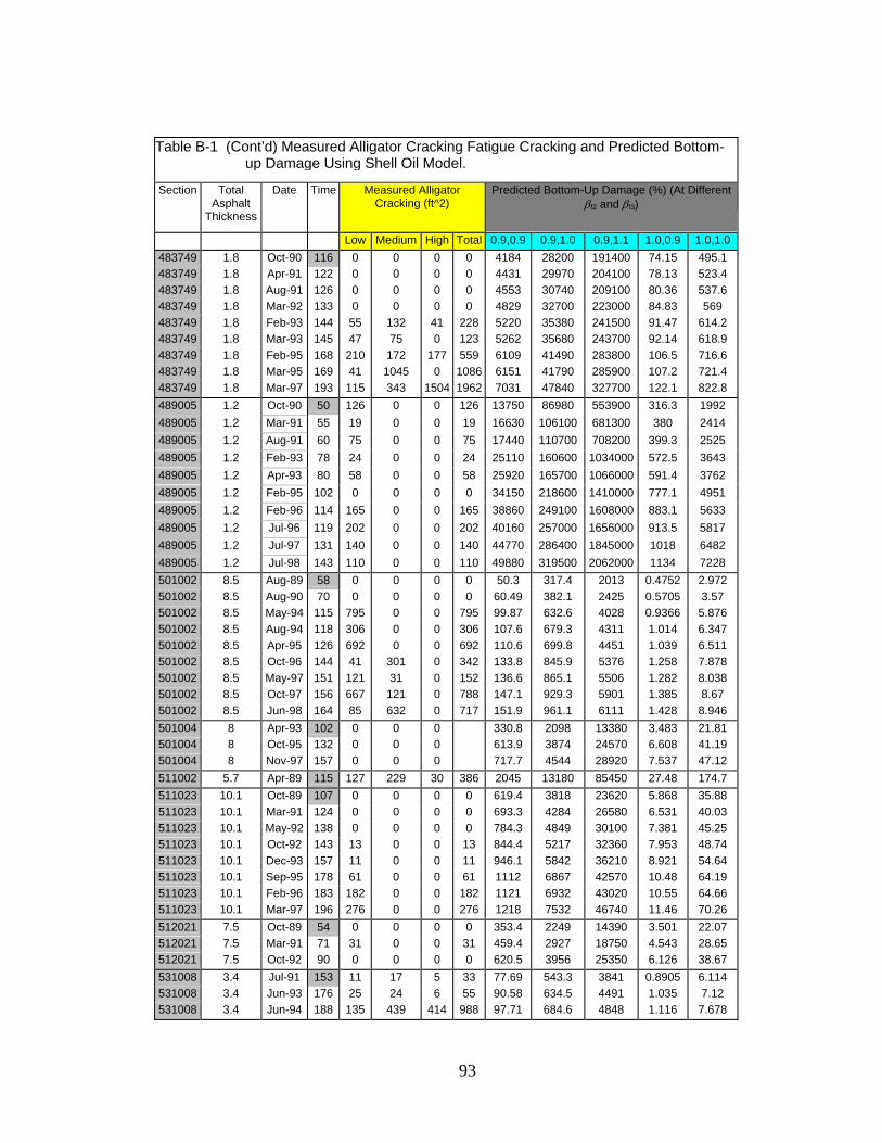
93
Table B-1 (Cont’d) Measured Alligator Cracking Fatigue Cracking and Predicted Bottom-
up Damage Using Shell Oil Model.
Section Total Asphalt
Thickness
Date Time Measured Alligator Cracking (ft^2)
Predicted Bottom-Up Damage (%) (At Different βf2 and βf3)
Low Medium High Total 0.9,0.9 0.9,1.0 0.9,1.1 1.0,0.9 1.0,1.0 483749 1.8 Oct-90 116 0 0 0 0 4184 28200 191400 74.15 495.1 483749 1.8 Apr-91 122 0 0 0 0 4431 29970 204100 78.13 523.4 483749 1.8 Aug-91 126 0 0 0 0 4553 30740 209100 80.36 537.6 483749 1.8 Mar-92 133 0 0 0 0 4829 32700 223000 84.83 569 483749 1.8 Feb-93 144 55 132 41 228 5220 35380 241500 91.47 614.2 483749 1.8 Mar-93 145 47 75 0 123 5262 35680 243700 92.14 618.9 483749 1.8 Feb-95 168 210 172 177 559 6109 41490 283800 106.5 716.6 483749 1.8 Mar-95 169 41 1045 0 1086 6151 41790 285900 107.2 721.4 483749 1.8 Mar-97 193 115 343 1504 1962 7031 47840 327700 122.1 822.8 489005 1.2 Oct-90 50 126 0 0 126 13750 86980 553900 316.3 1992 489005 1.2 Mar-91 55 19 0 0 19 16630 106100 681300 380 2414 489005 1.2 Aug-91 60 75 0 0 75 17440 110700 708200 399.3 2525 489005 1.2 Feb-93 78 24 0 0 24 25110 160600 1034000 572.5 3643 489005 1.2 Apr-93 80 58 0 0 58 25920 165700 1066000 591.4 3762 489005 1.2 Feb-95 102 0 0 0 0 34150 218600 1410000 777.1 4951 489005 1.2 Feb-96 114 165 0 0 165 38860 249100 1608000 883.1 5633 489005 1.2 Jul-96 119 202 0 0 202 40160 257000 1656000 913.5 5817 489005 1.2 Jul-97 131 140 0 0 140 44770 286400 1845000 1018 6482 489005 1.2 Jul-98 143 110 0 0 110 49880 319500 2062000 1134 7228 501002 8.5 Aug-89 58 0 0 0 0 50.3 317.4 2013 0.4752 2.972 501002 8.5 Aug-90 70 0 0 0 0 60.49 382.1 2425 0.5705 3.57 501002 8.5 May-94 115 795 0 0 795 99.87 632.6 4028 0.9366 5.876 501002 8.5 Aug-94 118 306 0 0 306 107.6 679.3 4311 1.014 6.347 501002 8.5 Apr-95 126 692 0 0 692 110.6 699.8 4451 1.039 6.511 501002 8.5 Oct-96 144 41 301 0 342 133.8 845.9 5376 1.258 7.878 501002 8.5 May-97 151 121 31 0 152 136.6 865.1 5506 1.282 8.038 501002 8.5 Oct-97 156 667 121 0 788 147.1 929.3 5901 1.385 8.67 501002 8.5 Jun-98 164 85 632 0 717 151.9 961.1 6111 1.428 8.946 501004 8 Apr-93 102 0 0 0 330.8 2098 13380 3.483 21.81 501004 8 Oct-95 132 0 0 0 613.9 3874 24570 6.608 41.19 501004 8 Nov-97 157 0 0 0 717.7 4544 28920 7.537 47.12 511002 5.7 Apr-89 115 127 229 30 386 2045 13180 85450 27.48 174.7 511023 10.1 Oct-89 107 0 0 0 0 619.4 3818 23620 5.868 35.88 511023 10.1 Mar-91 124 0 0 0 0 693.3 4284 26580 6.531 40.03 511023 10.1 May-92 138 0 0 0 0 784.3 4849 30100 7.381 45.25 511023 10.1 Oct-92 143 13 0 0 13 844.4 5217 32360 7.953 48.74 511023 10.1 Dec-93 157 11 0 0 11 946.1 5842 36210 8.921 54.64 511023 10.1 Sep-95 178 61 0 0 61 1112 6867 42570 10.48 64.19 511023 10.1 Feb-96 183 182 0 0 182 1121 6932 43020 10.55 64.66 511023 10.1 Mar-97 196 276 0 0 276 1218 7532 46740 11.46 70.26 512021 7.5 Oct-89 54 0 0 0 0 353.4 2249 14390 3.501 22.07 512021 7.5 Mar-91 71 31 0 0 31 459.4 2927 18750 4.543 28.65 512021 7.5 Oct-92 90 0 0 0 0 620.5 3956 25350 6.126 38.67 531008 3.4 Jul-91 153 11 17 5 33 77.69 543.3 3841 0.8905 6.114 531008 3.4 Jun-93 176 25 24 6 55 90.58 634.5 4491 1.035 7.12 531008 3.4 Jun-94 188 135 439 414 988 97.71 684.6 4848 1.116 7.678

94
Table B-1 (Cont’d) Measured Alligator Cracking Fatigue Cracking and Predicted Bottom-
up Damage Using Shell Oil Model.
Section Total Asphalt
Thickness
Date Time Measured Alligator Cracking (ft^2)
Predicted Bottom-Up Damage (%) (At Different βf2 and βf3)
Low Medium High Total 0.9,0.9 0.9,1.0 0.9,1.1 1.0,0.9 1.0,1.0 561007 2.8 Jul-90 121 0 0 0 0 42.14 292.5 2051 0.5401 3.692 561007 2.8 May-91 131 0 0 0 0 45.54 316.7 2224 0.5824 3.987 561007 2.8 Aug-91 134 0 0 0 0 46.9 325.6 2282 0.6013 4.109 561007 2.8 Aug-93 158 0 0 0 0 55.1 382.7 2686 0.7056 4.825 561007 2.8 Oct-93 160 0 0 0 0 55.85 388 2722 0.715 4.89 561007 2.8 Dec-93 162 5 0 0 5 56.34 391.7 2751 0.72 4.928 561007 2.8 Mar-94 165 8 0 0 8 57.06 397.1 2792 0.7283 4.989 561007 2.8 Apr-94 166 0 0 0 0 57.61 401 2820 0.7354 5.039 561007 2.8 Aug-94 170 6 0 0 6 59.39 412.8 2898 0.7595 5.197 561007 2.8 Feb-95 176 0 0 0 0 60.31 419.5 2947 0.7702 5.274 561007 2.8 May-95 179 0 0 0 0 61.6 428.8 3015 0.7862 5.387 561007 2.8 Sep-95 183 0 0 0 0 63.32 439.7 3084 0.8109 5.543 561007 2.8 Jun-96 192 12 0 0 12 66.27 460.9 3238 0.8466 5.796 561007 2.8 Oct-96 196 0 0 0 0 67.87 471.7 3311 0.8676 5.936 561007 2.8 Nov-96 197 0 0 0 0 68.09 473.4 3325 0.8698 5.953 561007 2.8 Mar-97 201 0 0 0 0 68.29 475 3337 0.8719 5.969 561007 2.8 Aug-97 206 0 0 0 0 70.95 493.1 3462 0.9075 6.209 561007 2.8 Sep-97 207 0 0 0 0 71.37 495.9 3480 0.9131 6.246

95
Table B-2 Measured Alligator Cracking Fatigue Cracking and Predicted Bottom-up Damage Using Shell Oil Model.
Section Total
Asphalt Thickness
Date Time Measured Alligator Cracking (ft^2)
Predicted Bottom-Up Damage (%) (At Different βf2 and βf3)
Low Medium High Total 1.0,1.1 1.1,0.9 1.1,1.0 1.1,1.111001 3.2 Sep-91 132 8 0 0 8 6031 2.127 13.36 84.54 11001 3.2 Apr-92 139 13 0 0 13 6429 2.239 14.11 89.62 11001 3.2 Jul-92 142 13 0 0 13 6602 2.31 14.54 92.22 11001 3.2 Jan-93 148 45 0 0 45 6933 2.415 15.22 96.64 11019 6.7 May-89 32 0 0 0 0 3911 1.552 8.79 49.99 11019 6.7 Apr-90 43 0 0 0 0 5250 2.073 11.73 66.64 11019 6.7 Jan-91 52 0 0 0 0 6371 2.532 14.28 80.84 11019 6.7 Jun-91 57 800 0 0 800 7060 2.804 15.8 89.48 11019 6.7 Mar-92 66 0 0 0 0 8249 3.253 18.36 104.1 11019 6.7 Mar-93 78 1112 0 0 1112 9914 3.912 22.05 124.9 11019 6.7 Jul-95 106 2554 0 0 2554 14000 5.557 31.25 176.5 11019 6.7 Jan-98 136 0 1461 233 1693 18460 7.286 41.01 231.9 14126 13.1 Jun-89 15 0 0 0 0 59.7 0.01351 0.07827 0.454614126 13.1 Mar-91 36 0 0 0 0 156 0.03594 0.2071 1.197 14126 13.1 Mar-93 60 0 0 0 0 274.5 0.06304 0.3637 2.104 14126 13.1 Apr-94 73 0 0 0 0 346.7 0.0795 0.4588 2.655 14126 13.1 Dec-95 93 6 22 0 28 476.1 0.1096 0.6322 3.657 14126 13.1 Dec-97 117 81 0 0 81 621.5 0.1424 0.8224 4.762 21001 3 May-90 83 0 0 0 0 22.1 0.00478 0.03428 0.247 21001 3 Aug-91 98 0 0 0 0 26.51 0.00578 0.04134 0.297121001 3 Aug-93 122 0 0 0 0 33.31 0.00725 0.0519 0.373321001 3 Jun-95 144 0 0 0 0 38.92 0.0084 0.06028 0.434521001 3 Aug-97 170 0 0 0 0 46.43 0.01003 0.07194 0.518421001 3 Aug-98 182 0 3 0 3 49.77 0.01076 0.07714 0.555821002 3.3 May-90 68 0 0 0 0 2.78 0.00055 0.00395 0.0287621002 3.3 Aug-91 83 0 0 0 0 3.546 0.0007 0.00507 0.0368321002 3.3 Aug-93 107 0 0 0 0 4.585 0.0009 0.00654 0.0475121002 3.3 Jun-95 129 0 0 0 0 5.457 0.00107 0.00773 0.0563121002 3.3 Aug-97 155 0 0 0 0 6.68 0.00131 0.00947 0.0689921002 3.3 May-98 164 0 0 0 0 6.936 0.00135 0.00978 0.0713740113 4.5 Feb-95 19 11 0 0 11 286.3 0.09065 0.5456 3.313 40113 4.5 Mar-95 20 11 0 0 11 304.5 0.09536 0.5759 3.509 40113 4.5 Aug-95 25 11 0 0 11 407.8 0.1352 0.8041 4.821 40113 4.5 Nov-95 28 11 0 0 11 476 0.1583 0.9413 5.64 40113 4.5 Feb-96 31 11 0 0 11 516.4 0.1663 0.9963 6.019 40113 4.5 Apr-96 33 11 0 0 11 561.5 0.1798 1.079 6.533 40113 4.5 Jul-96 36 11 0 0 11 635.1 0.2101 1.25 7.499 40113 4.5 Aug-96 37 11 0 0 11 661.5 0.2216 1.314 7.853 40113 4.5 Jan-98 54 11 0 0 11 1040 0.3363 2.011 12.13 40113 4.5 Apr-98 57 11 10 0 20 1107 0.3523 2.115 12.82 40113 4.5 Jun-98 59 11 10 0 20 1170 0.3759 2.251 13.6 40113 4.5 Oct-98 63 11 10 0 20 1305 0.4296 2.557 15.35 40114 6.8 Feb-95 19 11 0 0 11 1167 0.3284 2.016 12.44 40114 6.8 Mar-95 20 11 0 0 11 1206 0.3356 2.066 12.78 40114 6.8 Aug-95 25 11 0 0 11 1816 0.5203 3.185 19.57

96
Table B-2 (Cont’d) Measured Alligator Cracking Fatigue Cracking and
Predicted Bottom-up Damage Using Shell Oil Model. Section Total
Asphalt Thickness
Date Time Measured Alligator Cracking (ft^2)
Predicted Bottom-Up Damage (%) (At Different βf2 and βf3)
Low Medium High Total 1.0,1.1 1.1,0.9 1.1,1.0 1.1,1.140114 6.8 Nov-95 28 11 0 0 11 2119 0.6026 3.698 22.78 40114 6.8 Feb-96 31 11 0 0 11 2168 0.6094 3.747 23.14 40114 6.8 Apr-96 33 11 0 0 11 2307 0.6408 3.952 24.47 40114 6.8 Jul-96 36 11 0 0 11 2786 0.7886 4.843 29.86 40114 6.8 Aug-96 37 11 0 0 11 2972 0.8483 5.2 31.99 40114 6.8 Jan-98 54 11 0 0 11 4393 1.235 7.592 46.85 40114 6.8 Apr-98 57 11 46 0 57 4529 1.261 7.766 48.04 40114 6.8 Jun-98 59 11 52 0 62 4854 1.354 8.339 51.55 40114 6.8 Oct-98 63 11 114 0 125 5678 1.601 9.839 60.7 40115 15.1 Feb-95 19 11 0 0 11 3.097 0.0006 0.00352 0.0204940115 15.1 Mar-95 20 11 25 0 36 3.156 0.00061 0.00356 0.0207840115 15.1 Jan-98 54 11 0 0 11 10.68 0.00208 0.01208 0.0704840116 16.2 Feb-95 19 11 0 0 11 2.431 0.00039 0.00237 0.014340116 16.2 Mar-95 20 11 0 0 11 2.474 0.0004 0.0024 0.0144940116 16.2 Jan-98 54 11 0 0 11 8.463 0.00137 0.00822 0.0496740117 11.8 Feb-95 19 11 0 0 11 64.56 0.0155 0.0919 0.546140117 11.8 Mar-95 20 11 0 0 11 65.45 0.01561 0.09268 0.551440117 11.8 Jan-98 54 11 0 0 11 238 0.05619 0.3346 1.996 40118 11.7 Feb-95 19 11 0 0 11 29.33 0.00595 0.03609 0.219440118 11.7 Mar-95 20 11 0 0 11 30.01 0.00604 0.03666 0.223340118 11.7 Jan-98 54 11 0 0 11 111.1 0.02266 0.1375 0.836741007 6.5 Sep-91 162 38 0 0 38 1602 0.5372 3.133 18.36 41007 6.5 Feb-93 163 44 16 0 60 1621 0.5429 3.168 18.56 41007 6.5 Sep-94 198 70 132 0 202 2225 0.7445 4.346 25.47 41024 10.8 Nov-89 149 0 0 0 0 19380 5.902 33.82 194.2 41024 10.8 Aug-90 158 0 0 0 0 21040 6.387 36.63 210.5 41024 10.8 Oct-92 184 0 0 0 0 27010 8.146 46.79 269.3 41024 10.8 Mar-95 213 0 0 0 0 33860 10.25 58.79 338.1 41024 10.8 Jul-95 217 0 0 0 0 35450 10.72 61.53 353.9 41024 10.8 Aug-95 218 12 0 0 12 36050 10.9 62.58 359.9 41024 10.8 Nov-95 221 0 10 0 10 36820 11.1 63.74 366.9 41024 10.8 Feb-96 224 0 0 0 0 36860 11.1 63.77 367.1 41024 10.8 Apr-96 226 16 0 0 16 37160 11.17 64.18 369.7 41024 10.8 Jun-96 228 118 0 0 118 38430 11.56 66.44 382.7 41024 10.8 Aug-96 230 161 0 0 161 40340 12.22 70.1 403.1 41024 10.8 Apr-98 250 0 398 529 927 44870 13.46 77.38 446 41024 10.8 Jun-98 252 0 397 530 927 46250 13.88 79.81 459.9 41024 10.8 Oct-98 256 0 414 529 943 49090 14.79 84.96 489.1 81029 4.2 Oct-91 233 27 15 0 42 25.81 0.00711 0.04691 0.311781029 4.2 Jul-94 266 0 0 0 0 29.32 0.00805 0.05316 0.353381029 4.2 Sep-95 280 464 0 0 464 31.06 0.00852 0.05627 0.374 81053 4.6 Oct-89 60 0 0 0 0 21.28 0.00639 0.0409 0.263681053 4.6 Jul-90 69 0 0 0 0 25.23 0.00752 0.0482 0.311181053 4.6 Apr-93 102 3 0 0 3 41.74 0.01228 0.07887 0.510481053 4.6 Nov-93 109 0 0 0 0 47.02 0.01399 0.08957 0.5777

97
Table B-2 (Cont’d) Measured Alligator Cracking Fatigue Cracking and
Predicted Bottom-up Damage Using Shell Oil Model. Section Total
Asphalt Thickness
Date Time Measured Alligator Cracking (ft^2)
Predicted Bottom-Up Damage (%) (At Different βf2 and βf3)
Low Medium High Total 1.0,1.1 1.1,0.9 1.1,1.0 1.1,1.181053 4.6 Dec-93 110 23 0 0 23 47.11 0.014 0.08966 0.578481053 4.6 Oct-94 120 0 0 0 0 54.9 0.01638 0.1048 0.675781053 4.6 Feb-95 124 40 0 0 40 56.16 0.01657 0.1063 0.687181053 4.6 May-95 127 40 0 0 40 58.41 0.01717 0.1103 0.713581053 4.6 May-96 139 0 0 0 0 66.91 0.01967 0.1263 0.817281053 4.6 Oct-96 144 310 0 0 310 72.66 0.02167 0.1387 0.893781053 4.6 Nov-96 145 253 0 0 253 73.04 0.02173 0.1391 0.897281053 4.6 Mar-97 149 457 0 0 457 74.65 0.02205 0.1414 0.913791803 7.2 Jul-89 49 0 0 0 0 419 0.1179 0.7465 4.75 91803 7.2 Sep-90 63 0 0 0 0 598.3 0.1701 1.075 6.819 91803 7.2 Aug-91 74 0 0 0 0 724 0.2052 1.297 8.234 91803 7.2 Sep-92 87 8 0 0 8 904.2 0.255 1.614 10.26 91803 7.2 May-94 107 211 0 0 211 1153 0.3196 2.029 12.96 91803 7.2 May-95 119 240 0 0 240 1362 0.3778 2.398 15.31 91803 7.2 Oct-96 136 84 82 0 166 1768 0.4981 3.151 20.03 91803 7.2 May-97 143 301 0 0 301 1845 0.5135 3.257 20.77 91803 7.2 Sep-97 147 15 325 0 340 2021 0.5687 3.599 22.89 91803 7.2 Jun-98 156 195 0 0 195 2172 0.6041 3.833 24.44 120103 12 Dec-96 14 0 0 0 0 2.623 0.00045 0.00285 0.01802120104 18 Dec-96 14 0 0 0 0 0.1084 1.3E-05 8.5E-05 0.00054120105 7.9 Dec-96 14 0 0 0 0 43.45 0.00961 0.06155 0.3947120106 15 Dec-96 14 0 0 0 0 0.378 5.4E-05 0.00034 0.00215123995 5 Apr-92 197 0 0 0 0 12870 3.208 20.97 137.4 123995 5 Mar-94 220 86 0 0 86 14530 3.615 23.64 154.9 123995 5 Jan-96 242 58 0 0 58 16200 4.027 26.34 172.7 123995 5 Jan-96 243 122 0 0 122 16250 4.038 26.42 173.2 123997 3.1 Aug-90 195 0 0 0 710.6 0.2385 1.522 9.767 123997 3.1 Oct-91 209 0 0 0 796.1 0.2675 1.706 10.95 123997 3.1 Mar-93 226 0 0 0 907.8 0.3025 1.935 12.44 123997 3.1 Mar-94 238 0 0 0 991.9 0.3298 2.111 13.58 124105 2.3 Apr-89 53 0 0 0 0 4526 1.654 10.74 70.2 124105 2.3 Oct-91 83 0 0 0 0 7906 2.922 18.92 123.2 124105 2.3 Mar-93 100 0 0 0 0 9969 3.621 23.56 154.2 124106 8.2 Apr-89 21 0 0 0 0 797 0.2047 1.245 7.589 124106 8.2 Feb-91 43 0 0 0 0 1750 0.4411 2.695 16.49 124106 8.2 Jul-91 48 0 0 0 0 2017 0.5119 3.121 19.07 124106 8.2 Mar-94 80 0 0 0 0 3537 0.8799 5.393 33.11 124106 8.2 Jan-97 114 0 0 0 0 5370 1.333 8.173 50.21 124107 2.7 Dec-89 75 0 0 0 0 175.5 0.058 0.3795 2.491 124107 2.7 Feb-91 89 0 0 0 0 223 0.07278 0.478 3.149 124107 2.7 Jul-91 94 0 0 0 0 240.1 0.07853 0.5154 3.394 124107 2.7 Mar-93 114 732 355 9 1096 317.3 0.103 0.6775 4.472 124107 2.7 Mar-94 126 656 243 0 899 368.2 0.1192 0.7846 5.183 124107 2.7 Jan-96 148 264 812 93 1168 468.6 0.1513 0.9967 6.59 124107 2.7 Mar-97 162 44 372 1224 1640 539.3 0.1732 1.143 7.567

98
Table B-2 (Cont’d) Measured Alligator Cracking Fatigue Cracking and
Predicted Bottom-up Damage Using Shell Oil Model. Section Total
Asphalt Thickness
Date Time Measured Alligator Cracking (ft^2)
Predicted Bottom-Up Damage (%) (At Different βf2 and βf3)
Low Medium High Total 1.0,1.1 1.1,0.9 1.1,1.0 1.1,1.1124108 9.9 Apr-89 35 0 0 0 0 21.21 0.00479 0.02926 0.179 124108 9.9 Jan-91 56 0 0 0 0 35.57 0.00798 0.04878 0.2988124108 9.9 Oct-91 65 0 0 0 0 44.19 0.00996 0.06085 0.3723124108 9.9 Mar-94 94 0 0 0 0 62.75 0.01387 0.08505 0.5226124108 9.9 Aug-94 99 0 0 0 0 70.04 0.01564 0.09566 0.5866124108 9.9 Jan-96 116 0 0 0 0 81.57 0.018 0.1104 0.6786124135 1.4 Dec-89 227 1112 86 0 1198 96050 41.29 272.2 1808 124135 1.4 Jan-91 240 2045 355 0 2400 101300 43.4 286.4 1903 131031 11.1 Apr-91 119 0 0 0 85.58 0.01924 0.1161 0.7027131031 11.1 Jul-92 134 0 0 0 108.3 0.02435 0.1469 0.8887131031 11.1 Jan-93 140 0 0 0 115.5 0.02592 0.1564 0.947 131031 11.1 Apr-94 155 0 0 0 139.7 0.03129 0.1889 1.144 131031 11.1 Oct-94 161 0 0 0 159.7 0.03613 0.2176 1.314 131031 11.1 Aug-95 171 0 0 0 177.6 0.0399 0.2406 1.456 131031 11.1 Jan-96 176 0 0 0 183.8 0.04113 0.2483 1.503 131031 11.1 Apr-96 179 0 0 0 186.7 0.04158 0.2513 1.523 134111 8.7 Mar-89 101 0 0 0 0 257.7 0.07675 0.4716 2.911 134111 8.7 Mar-91 125 0 0 0 0 394.8 0.1167 0.7187 4.446 134111 8.7 Feb-92 136 316 0 0 316 469.2 0.1392 0.8563 5.292 134112 15.9 May-89 144 0 0 0 0 123 0.03229 0.1866 1.082 134112 15.9 Feb-91 165 0 0 0 0 153.9 0.04013 0.2323 1.349 134112 15.9 Apr-91 167 0 0 0 0 155.9 0.04049 0.2346 1.364 134112 15.9 Feb-94 201 0 0 0 0 216.3 0.05672 0.3278 1.9 134112 15.9 Oct-94 209 0 0 0 0 236.3 0.06202 0.3584 2.078 134112 15.9 Jan-96 224 0 0 0 0 260.6 0.06787 0.393 2.282 134112 15.9 Feb-97 237 0 0 0 0 287.6 0.07517 0.4347 2.522 134112 15.9 Apr-98 251 0 0 0 0 314.2 0.08161 0.4727 2.747 134113 15.2 May-89 144 0 0 0 0 584.1 0.1716 0.9811 5.626 134113 15.2 Feb-91 165 0 0 0 0 709.8 0.2073 1.187 6.818 134113 15.2 Apr-91 167 0 0 0 0 717.5 0.2089 1.197 6.88 134113 15.2 Feb-94 201 0 0 0 0 956.3 0.2807 1.605 9.203 134113 15.2 Oct-94 209 0 0 0 0 1034 0.3038 1.737 9.96 134113 15.2 Jan-96 224 0 0 0 0 1127 0.3288 1.883 10.82 134113 15.2 Feb-97 237 47 0 0 47 1230 0.3599 2.059 11.82 134113 15.2 Apr-98 251 44 0 0 44 1330 0.3872 2.218 12.74 161001 3.7 Jul-89 192 0 0 0 0 324.5 0.06592 0.4643 3.304 161001 3.7 Aug-90 205 0 0 0 0 360.5 0.07333 0.5161 3.67 161001 3.7 Jun-93 239 36 0 0 36 452.4 0.09055 0.6396 4.565 161001 3.7 Aug-94 253 16 0 0 16 501.8 0.1011 0.7128 5.078 161001 3.7 May-95 262 0 0 0 0 523.6 0.1044 0.7378 5.27 161001 3.7 Jul-97 288 3 611 0 615 617.2 0.1232 0.8706 6.215 161001 3.7 Sep-98 302 0 434 99 533 672.1 0.1344 0.9496 6.774 161009 10.4 Sep-89 180 0 0 0 18.76 0.0033 0.02087 0.1325161009 10.4 Jul-90 190 0 0 0 20.14 0.00354 0.02238 0.1421161009 10.4 Jul-92 214 0 0 0 24.25 0.00424 0.02686 0.1707

99
Table B-2 (Cont’d) Measured Alligator Cracking Fatigue Cracking and
Predicted Bottom-up Damage Using Shell Oil Model. Section Total
Asphalt Thickness
Date Time Measured Alligator Cracking (ft^2)
Predicted Bottom-Up Damage (%) (At Different βf2 and βf3)
Low Medium High Total 1.0,1.1 1.1,0.9 1.1,1.0 1.1,1.1161009 10.4 Oct-93 229 0 0 0 27.79 0.00488 0.03086 0.196 161009 10.4 Jun-96 261 0 0 0 34.34 0.00599 0.03798 0.2415161009 10.4 Jul-97 274 0 0 0 38.13 0.00667 0.04225 0.2686161021 5.9 Sep-89 48 0 0 0 0 9.719 0.00249 0.01556 0.09788161021 5.9 Oct-90 61 0 0 0 0 12.26 0.00312 0.01954 0.123 161021 5.9 Aug-91 71 0 0 0 0 14.06 0.0036 0.02251 0.1415161021 5.9 Aug-93 95 0 0 0 0 19.04 0.00485 0.03032 0.1909161021 5.9 Sep-95 120 0 0 0 0 24.3 0.0062 0.03874 0.2438161021 5.9 Jun-96 129 0 0 0 0 25.42 0.00644 0.04031 0.2541161021 5.9 Jul-97 142 0 0 0 0 28.5 0.00723 0.04526 0.2851169034 9.2 Jul-89 10 0 0 0 0 3.469 0.00067 0.00429 0.0276169034 9.2 Aug-90 23 0 0 0 0 10.22 0.00219 0.01364 0.08549169034 9.2 Jun-93 57 0 0 0 0 22.07 0.00458 0.02877 0.1816169034 9.2 Aug-94 71 0 0 0 0 29.6 0.00629 0.03932 0.2467169034 9.2 May-95 80 0 0 0 0 31.13 0.00654 0.04095 0.2577169034 9.2 Jul-97 106 25 0 0 25 42.71 0.00903 0.05648 0.3548169034 9.2 Sep-98 120 0 0 25 25 49.44 0.01049 0.06556 0.4115201009 11.1 Aug-88 44 10 0 0 10 2.851 0.00059 0.00357 0.02181201009 11.1 May-89 53 0 0 0 0 3.113 0.00063 0.00385 0.02362201009 11.1 Dec-90 72 42 0 0 42 4.579 0.00094 0.00573 0.03496201009 11.1 Oct-91 82 1 13 0 14 5.298 0.00108 0.0066 0.04033201009 11.1 Apr-93 100 6 18 16 41 6.264 0.00128 0.00782 0.04773201009 11.1 Apr-95 124 2 54 0 56 7.739 0.00157 0.0096 0.05867201009 11.1 Apr-96 136 0 0 0 0 8.484 0.00172 0.0105 0.06422201009 11.1 Jan-99 168 0 1643 0 1643 11.03 0.00224 0.01366 0.08349251003 6.6 Aug-89 180 0 0 0 0 1302 0.3478 2.241 14.51 251003 6.6 Sep-90 193 0 0 0 0 1423 0.3788 2.443 15.83 251003 6.6 Aug-91 204 28 0 0 28 1521 0.4045 2.61 16.92 251003 6.6 Sep-92 217 56 93 0 149 1670 0.446 2.874 18.61 251003 6.6 Oct-95 254 45 75 0 121 2038 0.5407 3.49 22.63 251003 6.6 Oct-96 266 1314 0 0 1314 2171 0.5756 3.715 24.1 251003 6.6 Jun-98 286 1062 62 0 1125 2384 0.6316 4.077 26.45 251004 9.6 Aug-89 178 0 0 0 0 615 0.1746 1.101 6.956 251004 9.6 Sep-90 191 0 0 0 0 693.3 0.1967 1.24 7.839 251004 9.6 Aug-91 202 0 0 0 0 751.2 0.2132 1.344 8.495 251004 9.6 Sep-92 215 0 0 0 0 832.1 0.2355 1.486 9.393 251004 9.6 Oct-95 252 0 0 0 0 1099 0.3112 1.963 12.41 251004 9.6 Jun-97 272 56 0 0 56 1223 0.3445 2.175 13.76 251004 9.6 Jun-98 284 0 0 0 0 1336 0.3766 2.377 15.04 261001 2.2 Jul-88 203 0 0 0 0 35.42 0.00906 0.06493 0.4694261001 2.2 Sep-89 217 0 0 0 0 37.82 0.00971 0.0695 0.5019261001 2.2 Jul-90 227 0 0 0 0 39.41 0.01008 0.07221 0.522 261001 2.2 Jul-91 239 33 0 0 33 41.63 0.01064 0.07628 0.5515261001 2.2 Sep-91 241 28 0 0 28 42.04 0.01076 0.07711 0.5572261001 2.2 Sep-92 253 40 0 0 40 44.04 0.01124 0.08059 0.5829

100
Table B-2 (Cont’d) Measured Alligator Cracking Fatigue Cracking and
Predicted Bottom-up Damage Using Shell Oil Model. Section Total
Asphalt Thickness
Date Time Measured Alligator Cracking (ft^2)
Predicted Bottom-Up Damage (%) (At Different βf2 and βf3)
Low Medium High Total 1.0,1.1 1.1,0.9 1.1,1.0 1.1,1.1261001 2.2 Jun-93 262 0 81 0 81 45.64 0.01162 0.08339 0.6036261001 2.2 Jun-93 263 76 0 0 76 45.85 0.01169 0.08387 0.6068261001 2.2 May-95 285 58 0 0 58 49.41 0.01257 0.09023 0.6531261001 2.2 Jul-96 299 83 0 0 83 52.06 0.01327 0.09521 0.6888261004 4.2 Sep-89 51 0 0 0 0 31.29 0.01127 0.07094 0.449 261004 4.2 Jul-90 61 0 0 0 0 36.61 0.01305 0.08233 0.5227271018 4.4 Apr-89 124 0 0 0 0 396.2 0.1044 0.6828 4.486 271018 4.4 Jun-89 126 0 0 0 0 413.6 0.1091 0.7137 4.689 271018 4.4 Oct-90 142 0 0 0 0 490 0.1296 0.847 5.558 271018 4.4 Jun-93 174 0 0 0 0 642.7 0.1698 1.109 7.284 271018 4.4 Jul-93 176 0 0 0 0 662 0.1754 1.145 7.513 271018 4.4 Mar-94 183 0 0 0 0 676.8 0.1783 1.165 7.654 271018 4.4 Aug-94 188 0 0 0 0 729.8 0.1929 1.26 8.269 271087 15.7 Oct-91 154 0 0 0 0.1784 2.2E-05 0.00014 0.0009271087 15.7 May-93 173 0 0 0 0.192 2.4E-05 0.00015 0.00097271087 15.7 Oct-94 190 0 0 0 0.216 2.7E-05 0.00017 0.00109271087 15.7 Jun-96 210 0 0 0 0.2335 2.9E-05 0.00019 0.00118291008 11.4 Feb-92 70 41 0 0 41 5.801 0.00107 0.00664 0.04116291008 11.4 Mar-93 83 140 22 0 161 7.005 0.0013 0.00803 0.04975291008 11.4 Mar-93 83 0 0 0 0 0 0 0 0 291008 11.4 Apr-96 120 0 0 0 0 11.15 0.00207 0.01278 0.07927291008 11.4 Feb-00 152 365 715 0 1080 15.61 0.0029 0.01794 0.1112307088 4.9 Sep-89 100 0 0 0 0 48.53 0.01364 0.08856 0.5793307088 4.9 May-91 120 0 66 0 66 54.17 0.01494 0.09729 0.6387308129 3.2 Oct-89 17 0 0 0 0 16.7 0.00534 0.0348 0.2287308129 3.2 Jul-91 38 0 0 0 0 32.2 0.0095 0.06294 0.421 308129 3.2 Jul-92 50 0 0 0 0 40.87 0.01184 0.07871 0.5283308129 3.2 Aug-93 63 0 0 0 0 50.52 0.0145 0.09647 0.6483308129 3.2 Dec-93 67 0 0 0 0 53.18 0.01509 0.1007 0.6783308129 3.2 Mar-94 70 0 0 0 0 54.92 0.01539 0.1029 0.696 308129 3.2 Oct-94 77 0 0 0 0 62.3 0.01775 0.1182 0.7957308129 3.2 Feb-95 81 0 0 0 0 64.66 0.01815 0.1213 0.8199308129 3.2 May-95 84 0 0 0 0 68.03 0.01904 0.1274 0.8621308129 3.2 Jun-96 97 0 0 0 0 79.03 0.02199 0.1473 0.9976308129 3.2 Oct-96 101 0 0 0 0 82.78 0.0232 0.1551 1.048 308129 3.2 Jan-97 104 0 0 0 0 84.62 0.02351 0.1575 1.066 308129 3.2 Mar-97 106 0 0 0 0 86.11 0.02377 0.1595 1.082 308129 3.2 Aug-97 111 0 0 0 0 92.65 0.02594 0.1734 1.172 308129 3.2 Oct-97 113 0 0 0 0 94.53 0.02645 0.1769 1.195 321020 7 Jul-91 86 0 0 0 0 103.9 0.02316 0.1487 0.9582321020 7 Aug-93 111 18 0 0 18 146.8 0.03276 0.2102 1.354 321020 7 Sep-94 123 187 62 0 250 166.6 0.03712 0.2382 1.534 321020 7 Apr-95 131 34 0 0 34 175.3 0.03869 0.2488 1.607 321020 7 Jun-97 157 672 1043 0 1715 226.4 0.04998 0.3213 2.074 321020 7 Jun-98 169 3269 36 0 3305 252.4 0.05565 0.3579 2.311

101
Table B-2 (Cont’d) Measured Alligator Cracking Fatigue Cracking and
Predicted Bottom-up Damage Using Shell Oil Model. Section Total
Asphalt Thickness
Date Time Measured Alligator Cracking (ft^2)
Predicted Bottom-Up Damage (%) (At Different βf2 and βf3)
Low Medium High Total 1.0,1.1 1.1,0.9 1.1,1.0 1.1,1.1341031 7.3 Apr-92 224 280 12 0 292 703.9 0.2464 1.515 9.345 341031 7.3 Feb-93 234 598 11 0 609 778.3 0.2727 1.677 10.34 341031 7.3 Oct-95 266 0 652 305 957 1054 0.3681 2.266 13.98 341031 7.3 Nov-95 267 574 8 0 581 1055 0.3683 2.267 13.99 341033 7.4 Apr-92 211 79 0 0 79 142.6 0.03831 0.2392 1.498 341033 7.4 Feb-93 221 6 0 0 6 151 0.04051 0.253 1.585 341033 7.4 Nov-95 254 15 0 0 15 180.6 0.0486 0.3033 1.899 341033 7.4 Jul-97 274 0 0 0 0 196.3 0.05275 0.3293 2.063 341034 11.1 Oct-89 48 0 0 0 0 14.63 0.00227 0.01463 0.09458341034 11.1 Sep-90 59 0 0 0 0 18.55 0.00288 0.01854 0.1199341034 11.1 Apr-92 78 0 0 0 0 23.46 0.00361 0.02329 0.1507341034 11.1 Feb-93 88 0 0 0 0 27.49 0.00423 0.0273 0.1766341034 11.1 Nov-95 121 0 0 0 0 42.28 0.00652 0.04205 0.2719341034 11.1 Jul-97 141 129 75 0 205 51.14 0.0079 0.05091 0.329 350101 7.2 May-97 19 0 0 0 0 1959 0.6325 3.898 24.11 350102 4.8 May-97 19 0 0 0 0 1602 0.5313 3.394 21.82 350103 12.5 May-97 19 0 0 0 0 3116 0.8942 5.41 32.8 350104 19.2 May-97 19 0 0 0 0 124.4 0.02669 0.1605 0.9667350105 9.9 May-97 19 0 0 0 0 39550 13.37 79.89 478.5 350106 15.6 May-97 19 0 0 0 0 535.1 0.1328 0.7956 4.777 351005 8.9 Oct-89 73 0 0 0 0 95.5 0.02448 0.1532 0.9614351005 8.9 Mar-91 90 0 0 0 0 128.1 0.0332 0.2073 1.297 351005 8.9 Oct-92 109 0 0 0 0 176.5 0.04525 0.2833 1.778 351005 8.9 Feb-94 125 0 0 0 0 214.6 0.0552 0.3453 2.165 351005 8.9 Mar-95 138 0 0 0 0 252.1 0.06448 0.4038 2.535 351005 8.9 Apr-97 163 0 0 0 0 341.6 0.0874 0.5473 3.436 351022 6.3 Oct-89 37 0 0 0 0 71.82 0.01957 0.1242 0.7917351022 6.3 Mar-91 54 0 0 0 0 101 0.02663 0.17 1.091 351022 6.3 Oct-92 73 0 0 0 0 165.5 0.04444 0.2821 1.799 351022 6.3 Feb-94 89 0 0 0 0 205.6 0.05434 0.346 2.215 351022 6.3 Mar-95 102 0 0 0 0 251.5 0.06648 0.4229 2.705 351022 6.3 Apr-97 127 0 0 0 0 347.3 0.09108 0.5801 3.715 351112 6.3 Dec-89 67 0 0 0 0 441.4 0.1376 0.8412 5.16 351112 6.3 Jan-91 80 0 0 0 0 514 0.1588 0.9725 5.976 351112 6.3 Mar-91 82 0 0 0 0 516.6 0.1592 0.9755 5.997 351112 6.3 Jan-93 104 0 0 0 0 674.1 0.2071 1.27 7.808 351112 6.3 Feb-94 117 0 0 0 0 748.4 0.2287 1.403 8.64 351112 6.3 Oct-94 125 0 0 0 0 818.7 0.2497 1.533 9.444 351112 6.3 Mar-95 130 9 0 0 9 826.7 0.2511 1.543 9.51 351112 6.3 Apr-95 131 0 0 0 0 829.5 0.2516 1.547 9.536 351112 6.3 Jun-95 133 0 0 0 0 849.8 0.2576 1.584 9.767 351112 6.3 Nov-96 150 0 0 0 0 980.4 0.2982 1.831 11.28 351112 6.3 Apr-97 155 0 0 0 0 991.4 0.3003 1.846 11.38 351112 6.3 Sep-97 160 0 0 0 0 1050 0.3188 1.959 12.07 371024 4.8 Nov-89 109 167 0 0 167 8.899 0.00267 0.01698 0.1087

102
Table B-2 (Cont’d) Measured Alligator Cracking Fatigue Cracking and
Predicted Bottom-up Damage Using Shell Oil Model. Section Total
Asphalt Thickness
Date Time Measured Alligator Cracking (ft^2)
Predicted Bottom-Up Damage (%) (At Different βf2 and βf3)
Low Medium High Total 1.0,1.1 1.1,0.9 1.1,1.0 1.1,1.1371024 4.8 Mar-91 125 889 89 0 978 10.21 0.00303 0.01928 0.1237371024 4.8 Apr-92 138 1442 308 342 2093 11.61 0.00343 0.02186 0.1404371802 4.5 Mar-91 66 36 0 0 36 2306 1.167 7.1 43.46 371802 4.5 Oct-92 85 51 36 0 86 3120 1.597 9.691 59.17 371802 4.5 Apr-94 103 1521 0 0 1521 3748 1.895 11.53 70.62 371802 4.5 Jul-95 118 1739 70 0 1809 4395 2.233 13.57 83.02 371802 4.5 Apr-96 127 2608 206 0 2814 4717 2.383 14.51 88.85 371992 2.4 Mar-91 14 0 0 0 0 77.94 0.02477 0.1685 1.154 371992 2.4 Oct-92 33 2 0 0 2 212.4 0.07239 0.4824 3.238 371992 2.4 Apr-94 51 0 0 0 0 359.5 0.1152 0.7804 5.328 371992 2.4 Feb-96 73 0 0 0 0 579.6 0.1873 1.265 8.614 404087 10.1 Jan-90 43 0 0 0 0 55.46 0.01923 0.1135 0.6711404087 10.1 Oct-91 64 0 0 0 0 96.31 0.0337 0.1983 1.17 404087 10.1 Nov-92 77 0 0 0 0 115 0.03961 0.2339 1.385 404087 10.1 Feb-93 80 0 0 0 0 115.3 0.03964 0.2342 1.387 404087 10.1 Nov-94 101 0 0 0 0 167.9 0.05803 0.3423 2.025 404087 10.1 Feb-95 104 32 0 0 32 168.3 0.05806 0.3426 2.027 404087 10.1 Aug-95 110 0 0 0 0 186 0.0639 0.3775 2.236 404087 10.1 Jun-97 132 67 207 0 273 230.6 0.07821 0.4633 2.752 404163 11.5 Jan-90 34 0 0 0 0 304.4 0.08869 0.5279 3.148 404163 11.5 Mar-91 48 0 0 0 0 389.7 0.1114 0.6656 3.984 404163 11.5 Oct-91 55 0 0 0 0 514.9 0.15 0.8923 5.317 404163 11.5 Nov-92 68 0 0 0 0 611.4 0.1766 1.052 6.278 404163 11.5 Mar-93 72 0 0 0 0 613.7 0.1769 1.054 6.292 404163 11.5 Nov-94 92 0 0 0 0 828.1 0.2391 1.424 8.494 404163 11.5 Apr-96 109 27 0 0 27 932.2 0.2674 1.594 9.522 404163 11.5 Aug-97 125 0 0 0 0 1098 0.3136 1.871 11.19 404163 11.5 Jan-99 141 13 0 0 13 1203 0.3408 2.037 12.19 404165 8.1 Jan-90 68 0 0 0 0 487.9 0.1265 0.7735 4.742 404165 8.1 Mar-91 82 0 0 0 0 572.3 0.1466 0.8991 5.528 404165 8.1 Oct-91 89 0 0 0 0 679.7 0.1765 1.079 6.613 404165 8.1 Nov-92 102 0 0 0 0 776.4 0.2003 1.226 7.526 404165 8.1 Mar-93 106 0 0 0 0 780.3 0.2007 1.229 7.55 404165 8.1 Oct-94 125 1 2 0 3 960.1 0.2455 1.506 9.26 404165 8.1 Nov-94 126 0 0 0 0 963.1 0.2459 1.509 9.282 404165 8.1 Apr-95 131 3 0 0 3 970 0.2468 1.515 9.327 404165 8.1 Jun-95 133 3 0 0 3 996 0.2528 1.553 9.568 404165 8.1 Apr-96 143 0 0 0 0 1062 0.2687 1.652 10.18 404165 8.1 Nov-96 150 0 0 0 0 1178 0.3012 1.847 11.36 404165 8.1 May-97 156 32 0 0 32 1197 0.3044 1.869 11.51 404165 8.1 Sep-97 160 40 0 0 40 1275 0.3259 1.999 12.29 421599 12.3 Aug-89 25 0 0 0 0 14.79 0.00316 0.01896 0.1141421599 12.3 Sep-90 38 0 0 0 0 22.13 0.00464 0.02794 0.1688421599 12.3 Mar-93 68 0 0 0 0 39.59 0.00829 0.04994 0.3017421599 12.3 Sep-94 86 0 0 0 0 55.85 0.01173 0.07064 0.4264

103
Table B-2 (Cont’d) Measured Alligator Cracking Fatigue Cracking and
Predicted Bottom-up Damage Using Shell Oil Model. Section Total
Asphalt Thickness
Date Time Measured Alligator Cracking (ft^2)
Predicted Bottom-Up Damage (%) (At Different βf2 and βf3)
Low Medium High Total 1.0,1.1 1.1,0.9 1.1,1.0 1.1,1.1421599 12.3 Jun-95 95 0 0 0 0 60.71 0.01271 0.07659 0.4628421599 12.3 Jul-96 108 0 0 0 0 72.61 0.01526 0.09188 0.5546421599 12.3 Mar-98 128 9 0 0 9 88.29 0.01848 0.1113 0.6724451011 3.2 Mar-92 69 0 0 0 0 415 0.1286 0.8248 5.328 451011 3.2 Oct-92 76 0 0 0 0 466.6 0.1474 0.9411 6.047 451011 3.2 Jun-93 84 1101 0 0 1101 516 0.161 1.031 6.649 451011 3.2 Jan-96 115 11 46 0 57 711.7 0.2206 1.415 9.14 451011 3.2 Jun-97 132 1729 41 150 1919 821.7 0.2537 1.629 10.53 451011 3.2 Feb-99 150 1203 612 254 2070 945.1 0.2928 1.879 12.14 473104 1.3 Aug-89 39 0 74 0 74 79.57 0.03751 0.2565 1.771 473104 1.3 Nov-89 42 0 0 0 0 80.84 0.03786 0.2591 1.79 473104 1.3 May-91 60 52 0 0 52 89.2 0.04008 0.276 1.919 473104 1.3 Aug-91 63 451 0 0 451 89.39 0.04015 0.2764 1.922 473104 1.3 Oct-92 77 140 19 0 159 95.63 0.0419 0.2895 2.02 473104 1.3 Aug-93 87 370 0 0 370 101.3 0.04337 0.3007 2.106 473104 1.3 Nov-95 114 124 300 292 716 119.7 0.04856 0.3399 2.402 473104 1.3 Oct-96 125 159 1217 407 1784 127.1 0.05062 0.3554 2.52 480001 2.4 Apr-89 1 0 0 0 0 34.74 0.01887 0.1131 0.6805480001 2.4 Oct-90 19 0 0 0 0 725.5 0.4158 2.438 14.39 480001 2.4 May-91 26 0 0 0 0 1078 0.5767 3.449 20.77 480001 2.4 Feb-93 47 0 0 0 0 2269 1.201 7.19 43.38 480001 2.4 Apr-93 49 0 0 0 0 2410 1.27 7.615 46.01 480001 2.4 Feb-95 71 0 0 0 0 4055 2.136 12.81 77.41 480001 2.4 Mar-95 72 0 0 0 0 4140 2.174 13.05 78.93 480001 2.4 May-97 98 0 18 0 18 6602 3.435 20.68 125.4 480001 2.4 Mar-98 108 0 27 0 27 7661 3.983 23.97 145.4 481060 7.5 Jun-90 52 0 0 0 18180 5.206 31.82 195 481060 7.5 Feb-91 60 0 0 0 0 22220 6.36 38.87 238.1 481060 7.5 Apr-91 62 0 0 0 0 23030 6.537 40.02 245.7 481060 7.5 Mar-92 73 0 0 0 0 29600 8.427 51.56 316.3 481060 7.5 Feb-93 84 8 0 0 8 36710 10.43 63.83 391.7 481060 7.5 Mar-93 85 0 0 0 0 36990 10.48 64.19 394.1 481060 7.5 Oct-94 104 0 0 0 0 54270 15.43 94.47 579.7 481060 7.5 Feb-95 108 0 0 0 0 55180 15.59 95.58 587.2 481060 7.5 Mar-95 109 0 0 0 0 55530 15.66 96 590.1 481060 7.5 Mar-95 112 0 0 0 0 58410 16.42 100.8 620 481060 7.5 Jun-95 134 0 0 0 0 77590 21.74 133.5 821.7 481060 7.5 Apr-97 137 0 0 0 0 82420 23.18 142.2 874.7 481060 7.5 Jul-97 139 12 0 0 12 86130 24.34 149.2 916.5 481060 7.5 Sep-97 154 0 0 0 0 101100 28.37 174.1 1072 481077 5.1 Apr-89 88 0 0 0 0 302.4 0.07668 0.4817 3.049 481077 5.1 Nov-91 119 0 0 0 0 432.4 0.1107 0.6935 4.377 481077 5.1 Oct-92 130 0 0 0 0 479.9 0.1227 0.7691 4.855 481077 5.1 May-93 137 0 0 0 0 501.1 0.1265 0.7951 5.036 481077 5.1 Oct-94 154 10 0 0 10 583.2 0.1491 0.9339 5.895
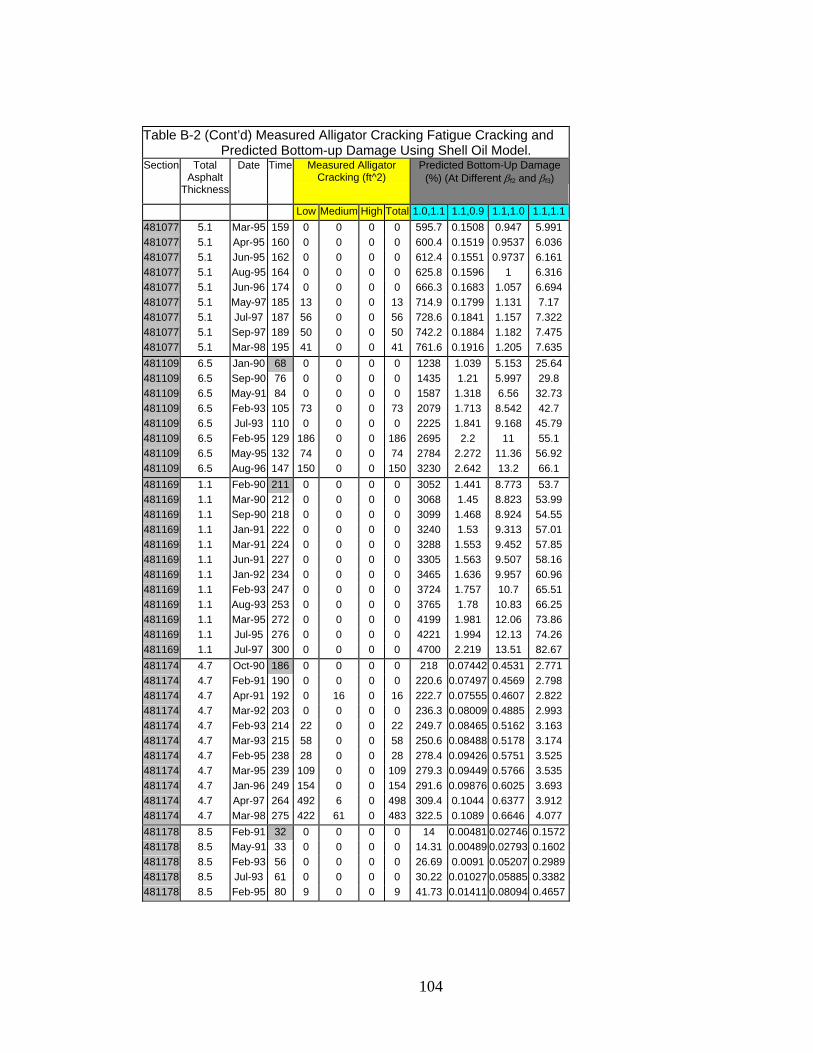
104
Table B-2 (Cont’d) Measured Alligator Cracking Fatigue Cracking and
Predicted Bottom-up Damage Using Shell Oil Model. Section Total
Asphalt Thickness
Date Time Measured Alligator Cracking (ft^2)
Predicted Bottom-Up Damage (%) (At Different βf2 and βf3)
Low Medium High Total 1.0,1.1 1.1,0.9 1.1,1.0 1.1,1.1481077 5.1 Mar-95 159 0 0 0 0 595.7 0.1508 0.947 5.991 481077 5.1 Apr-95 160 0 0 0 0 600.4 0.1519 0.9537 6.036 481077 5.1 Jun-95 162 0 0 0 0 612.4 0.1551 0.9737 6.161 481077 5.1 Aug-95 164 0 0 0 0 625.8 0.1596 1 6.316 481077 5.1 Jun-96 174 0 0 0 0 666.3 0.1683 1.057 6.694 481077 5.1 May-97 185 13 0 0 13 714.9 0.1799 1.131 7.17 481077 5.1 Jul-97 187 56 0 0 56 728.6 0.1841 1.157 7.322 481077 5.1 Sep-97 189 50 0 0 50 742.2 0.1884 1.182 7.475 481077 5.1 Mar-98 195 41 0 0 41 761.6 0.1916 1.205 7.635 481109 6.5 Jan-90 68 0 0 0 0 1238 1.039 5.153 25.64 481109 6.5 Sep-90 76 0 0 0 0 1435 1.21 5.997 29.8 481109 6.5 May-91 84 0 0 0 0 1587 1.318 6.56 32.73 481109 6.5 Feb-93 105 73 0 0 73 2079 1.713 8.542 42.7 481109 6.5 Jul-93 110 0 0 0 0 2225 1.841 9.168 45.79 481109 6.5 Feb-95 129 186 0 0 186 2695 2.2 11 55.1 481109 6.5 May-95 132 74 0 0 74 2784 2.272 11.36 56.92 481109 6.5 Aug-96 147 150 0 0 150 3230 2.642 13.2 66.1 481169 1.1 Feb-90 211 0 0 0 0 3052 1.441 8.773 53.7 481169 1.1 Mar-90 212 0 0 0 0 3068 1.45 8.823 53.99 481169 1.1 Sep-90 218 0 0 0 0 3099 1.468 8.924 54.55 481169 1.1 Jan-91 222 0 0 0 0 3240 1.53 9.313 57.01 481169 1.1 Mar-91 224 0 0 0 0 3288 1.553 9.452 57.85 481169 1.1 Jun-91 227 0 0 0 0 3305 1.563 9.507 58.16 481169 1.1 Jan-92 234 0 0 0 0 3465 1.636 9.957 60.96 481169 1.1 Feb-93 247 0 0 0 0 3724 1.757 10.7 65.51 481169 1.1 Aug-93 253 0 0 0 0 3765 1.78 10.83 66.25 481169 1.1 Mar-95 272 0 0 0 0 4199 1.981 12.06 73.86 481169 1.1 Jul-95 276 0 0 0 0 4221 1.994 12.13 74.26 481169 1.1 Jul-97 300 0 0 0 0 4700 2.219 13.51 82.67 481174 4.7 Oct-90 186 0 0 0 0 218 0.07442 0.4531 2.771 481174 4.7 Feb-91 190 0 0 0 0 220.6 0.07497 0.4569 2.798 481174 4.7 Apr-91 192 0 16 0 16 222.7 0.07555 0.4607 2.822 481174 4.7 Mar-92 203 0 0 0 0 236.3 0.08009 0.4885 2.993 481174 4.7 Feb-93 214 22 0 0 22 249.7 0.08465 0.5162 3.163 481174 4.7 Mar-93 215 58 0 0 58 250.6 0.08488 0.5178 3.174 481174 4.7 Feb-95 238 28 0 0 28 278.4 0.09426 0.5751 3.525 481174 4.7 Mar-95 239 109 0 0 109 279.3 0.09449 0.5766 3.535 481174 4.7 Jan-96 249 154 0 0 154 291.6 0.09876 0.6025 3.693 481174 4.7 Apr-97 264 492 6 0 498 309.4 0.1044 0.6377 3.912 481174 4.7 Mar-98 275 422 61 0 483 322.5 0.1089 0.6646 4.077 481178 8.5 Feb-91 32 0 0 0 0 14 0.00481 0.02746 0.1572481178 8.5 May-91 33 0 0 0 0 14.31 0.00489 0.02793 0.1602481178 8.5 Feb-93 56 0 0 0 0 26.69 0.0091 0.05207 0.2989481178 8.5 Jul-93 61 0 0 0 0 30.22 0.01027 0.05885 0.3382481178 8.5 Feb-95 80 9 0 0 9 41.73 0.01411 0.08094 0.4657

105
Table B-2 (Cont’d) Measured Alligator Cracking Fatigue Cracking and
Predicted Bottom-up Damage Using Shell Oil Model. Section Total
Asphalt Thickness
Date Time Measured Alligator Cracking (ft^2)
Predicted Bottom-Up Damage (%) (At Different βf2 and βf3)
Low Medium High Total 1.0,1.1 1.1,0.9 1.1,1.0 1.1,1.1481178 8.5 Mar-95 81 9 0 0 9 42.01 0.01417 0.08132 0.4682481183 5.7 Sep-90 188 0 0 0 709.4 0.393 2.287 13.37 481183 5.7 Mar-91 194 0 0 0 726 0.3989 2.326 13.61 481183 5.7 Oct-91 201 0 0 0 817 0.4497 2.622 15.34 481183 5.7 Nov-91 202 0 0 0 818.1 0.4499 2.623 15.35 481183 5.7 Jan-93 216 0 0 0 953.3 0.5289 3.077 17.97 481183 5.7 Jul-93 222 0 0 0 1021 0.5643 3.285 19.21 481183 5.7 Apr-94 231 0 0 0 1096 0.6022 3.51 20.54 483749 1.8 Oct-90 116 0 0 0 0 3329 1.475 9.762 65.04 483749 1.8 Apr-91 122 0 0 0 0 3531 1.547 10.27 68.62 483749 1.8 Aug-91 126 0 0 0 0 3622 1.592 10.56 70.46 483749 1.8 Mar-92 133 0 0 0 0 3845 1.673 11.12 74.43 483749 1.8 Feb-93 144 55 132 41 228 4153 1.8 11.97 80.19 483749 1.8 Mar-93 145 47 75 0 123 4187 1.811 12.05 80.78 483749 1.8 Feb-95 168 210 172 177 559 4856 2.083 13.89 93.26 483749 1.8 Mar-95 169 41 1045 0 1086 4890 2.096 13.98 93.87 483749 1.8 Mar-97 193 115 343 1504 1962 5586 2.377 15.88 106.8 489005 1.2 Oct-90 50 126 0 0 126 12630 7.49 47 296.9 489005 1.2 Mar-91 55 19 0 0 19 15430 8.946 56.59 360.3 489005 1.2 Aug-91 60 75 0 0 75 16080 9.42 59.32 376.1 489005 1.2 Feb-93 78 24 0 0 24 23350 13.44 85.2 543.5 489005 1.2 Apr-93 80 58 0 0 58 24090 13.9 88.03 561.3 489005 1.2 Feb-95 102 0 0 0 0 31770 18.22 115.6 738.2 489005 1.2 Feb-96 114 165 0 0 165 36190 20.68 131.3 839.6 489005 1.2 Jul-96 119 202 0 0 202 37310 21.41 135.7 866.5 489005 1.2 Jul-97 131 140 0 0 140 41560 23.87 151.3 965.3 489005 1.2 Jul-98 143 110 0 0 110 46420 26.56 168.5 1077 501002 8.5 Aug-89 58 0 0 0 0 18.66 0.0047 0.02921 0.1819501002 8.5 Aug-90 70 0 0 0 0 22.43 0.00564 0.03503 0.2183501002 8.5 May-94 115 795 0 0 795 37.01 0.00921 0.05737 0.3584501002 8.5 Aug-94 118 306 0 0 306 39.86 0.01003 0.06228 0.3881501002 8.5 Apr-95 126 692 0 0 692 40.97 0.01024 0.0637 0.3974501002 8.5 Oct-96 144 41 301 0 342 49.55 0.01239 0.07708 0.4809501002 8.5 May-97 151 121 31 0 152 50.61 0.01261 0.0785 0.4902501002 8.5 Oct-97 156 667 121 0 788 54.49 0.01367 0.08497 0.5297501002 8.5 Jun-98 164 85 632 0 717 56.27 0.01408 0.08753 0.546 501004 8 Apr-93 102 0 0 0 137.1 0.03925 0.2433 1.513 501004 8 Oct-95 132 0 0 0 257.8 0.076 0.4694 2.908 501004 8 Nov-97 157 0 0 0 295.8 0.08473 0.5247 3.259 511002 5.7 Apr-89 115 127 229 30 386 1117 0.3884 2.443 15.43 511023 10.1 Oct-89 107 0 0 0 0 220 0.0577 0.3506 2.136 511023 10.1 Mar-91 124 0 0 0 0 246 0.06392 0.3892 2.375 511023 10.1 May-92 138 0 0 0 0 278.3 0.07218 0.4396 2.684 511023 10.1 Oct-92 143 13 0 0 13 299.6 0.07778 0.4737 2.892 511023 10.1 Dec-93 157 11 0 0 11 335.7 0.08735 0.5317 3.244

106
Table B-2 (Cont’d) Measured Alligator Cracking Fatigue Cracking and
Predicted Bottom-up Damage Using Shell Oil Model. Section Total
Asphalt Thickness
Date Time Measured Alligator Cracking (ft^2)
Predicted Bottom-Up Damage (%) (At Different βf2 and βf3)
Low Medium High Total 1.0,1.1 1.1,0.9 1.1,1.0 1.1,1.1511023 10.1 Sep-95 178 61 0 0 61 394.5 0.1025 0.6242 3.809 511023 10.1 Feb-96 183 182 0 0 182 397.6 0.103 0.6276 3.833 511023 10.1 Mar-97 196 276 0 0 276 432 0.112 0.6822 4.165 512021 7.5 Oct-89 54 0 0 0 0 139.7 0.03604 0.2255 1.416 512021 7.5 Mar-91 71 31 0 0 31 181.4 0.0468 0.2926 1.835 512021 7.5 Oct-92 90 0 0 0 0 245 0.06293 0.394 2.475 531008 3.4 Jul-91 153 11 17 5 33 42.45 0.01082 0.07289 0.4968531008 3.4 Jun-93 176 25 24 6 55 49.51 0.01254 0.08464 0.5778531008 3.4 Jun-94 188 135 439 414 988 53.41 0.01352 0.09124 0.6229561007 2.8 Jul-90 121 0 0 0 0 25.5 0.00743 0.05004 0.3403561007 2.8 May-91 131 0 0 0 0 27.58 0.008 0.05391 0.3672561007 2.8 Aug-91 134 0 0 0 0 28.37 0.00827 0.0557 0.3787561007 2.8 Aug-93 158 0 0 0 0 33.33 0.0097 0.06533 0.4444561007 2.8 Oct-93 160 0 0 0 0 33.78 0.00983 0.06618 0.4502561007 2.8 Dec-93 162 5 0 0 5 34.07 0.00988 0.0666 0.4534561007 2.8 Mar-94 165 8 0 0 8 34.54 0.00998 0.06734 0.459 561007 2.8 Apr-94 166 0 0 0 0 34.88 0.01008 0.06802 0.4636561007 2.8 Aug-94 170 6 0 0 6 35.92 0.01043 0.07028 0.4784561007 2.8 Feb-95 176 0 0 0 0 36.48 0.01056 0.07121 0.4851561007 2.8 May-95 179 0 0 0 0 37.3 0.01077 0.0727 0.4956561007 2.8 Sep-95 183 0 0 0 0 38.28 0.01115 0.07505 0.5103561007 2.8 Jun-96 192 12 0 0 12 40.09 0.01161 0.0783 0.5333561007 2.8 Oct-96 196 0 0 0 0 41.03 0.01191 0.08024 0.5461561007 2.8 Nov-96 197 0 0 0 0 41.17 0.01193 0.08042 0.5475561007 2.8 Mar-97 201 0 0 0 0 41.29 0.01196 0.08059 0.5489561007 2.8 Aug-97 206 0 0 0 0 42.92 0.01246 0.08398 0.5716561007 2.8 Sep-97 207 0 0 0 0 43.16 0.01255 0.0845 0.575

107
0
1000
2000
3000
4000
5000
6000
0.1 1 10 100 1000 10000 100000 1000000Damage (%)
Alli
gato
r Cra
ckin
g (ft
2 /500
ft)
AC Thickness <2" AC Thicknes 2 - 5" AC Thickness 5-8"AC Thickness 8-12" AC Thickness >12"
Figure B-1 Alligator Cracking vs. Predicted Bottom-Up Damage (AC 1,0.9,0.9)
0
1000
2000
3000
4000
5000
6000
1 10 100 1000 10000 100000 1000000 10000000Damage (%)
Alli
gato
r Cra
ckin
g (ft
2 /500
ft)
AC Thickness <2" AC Thicknes 2 - 5" AC Thickness 5-8"AC Thickness 8-12" AC Thickness >12"
Figure B-2 Alligator Cracking vs. Predicted Bottom-Up Damage (AC 1,0.9,1.0)
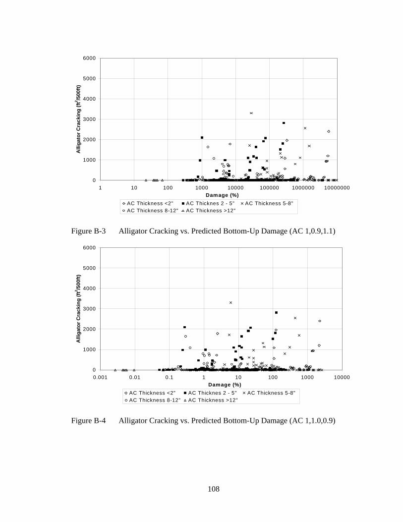
108
0
1000
2000
3000
4000
5000
6000
1 10 100 1000 10000 100000 1000000 10000000Damage (%)
Alli
gato
r Cra
ckin
g (ft
2 /500
ft)
AC Thickness <2" AC Thicknes 2 - 5" AC Thickness 5-8"AC Thickness 8-12" AC Thickness >12"
Figure B-3 Alligator Cracking vs. Predicted Bottom-Up Damage (AC 1,0.9,1.1)
0
1000
2000
3000
4000
5000
6000
0.001 0.01 0.1 1 10 100 1000 10000Damage (%)
Alli
gato
r Cra
ckin
g (ft
2 /500
ft)
AC Thickness <2" AC Thicknes 2 - 5" AC Thickness 5-8"AC Thickness 8-12" AC Thickness >12"
Figure B-4 Alligator Cracking vs. Predicted Bottom-Up Damage (AC 1,1.0,0.9)

109
0
1000
2000
3000
4000
5000
6000
0.01 0.1 1 10 100 1000 10000 100000Damage (%)
Alli
gato
r Cra
ckin
g (ft
2 /500
ft)
AC Thickness <2" AC Thicknes 2 - 5" AC Thickness 5-8"AC Thickness 8-12" AC Thickness >12"
Figure B-5 Alligator Cracking vs. Predicted Bottom-Up Damage (AC 1,1.0,1.0)
0
1000
2000
3000
4000
5000
6000
0.1 1 10 100 1000 10000 100000 1000000Damage (%)
Alli
gato
r Cra
ckin
g (ft
2 /500
ft)
AC Thickness <2" AC Thicknes 2 - 5" AC Thickness 5-8"AC Thickness 8-12" AC Thickness >12"
Figure B-6 Alligator Cracking vs. Predicted Bottom-Up Damage (AC 1,1.0,1.1)

110
0
1000
2000
3000
4000
5000
6000
0.00001 0.0001 0.001 0.01 0.1 1 10 100Damage (%)
Alli
gato
r Cra
ckin
g (ft
2 /500
ft)
AC Thickness <2" AC Thicknes 2 - 5" AC Thickness 5-8"AC Thickness 8-12" AC Thickness >12"
Figure B-7 Alligator Cracking vs. Predicted Bottom-Up Damage (AC 1,1.1,0.9)
0
1000
2000
3000
4000
5000
6000
0.00001 0.0001 0.001 0.01 0.1 1 10 100 1000Damage (%)
Alli
gato
r Cra
ckin
g (ft
2 /500
ft)
AC Thickness <2" AC Thicknes 2 - 5" AC Thickness 5-8"AC Thickness 8-12" AC Thickness >12"
Figure B-8 Alligator Cracking vs. Predicted Bottom-Up Damage (AC 1,1.1,1.0)

111
0
1000
2000
3000
4000
5000
6000
0.0001 0.001 0.01 0.1 1 10 100 1000 10000Damage (%)
Alli
gato
r Cra
ckin
g (ft
2 /500
ft)
AC Thickness <2" AC Thicknes 2 - 5" AC Thickness 5-8"AC Thickness 8-12" AC Thickness >12"
Figure B-9 Alligator Cracking vs. Predicted Bottom-Up Damage (AC 1,1.1,1.1)

ANNEX C
Bottom-Up Alligator Cracking Fatigue Cracking MS-1 MODEL CALIBRATION

113
Table C-1 Measured Alligator Fatigue Cracking and Predicted Bottom-up Damage Using MS1 Model.
Section Total
Asphalt Thickness
Date Time Measured Alligator Cracking (ft^2)
Predicted Bottom-Up Damage (%) (At Different βf2 and βf3)
Low Medium High Total 0.8,0.8 0.8,1.5 0.8,2.5 1.0,0.8 1.0,1.011001 3.2 Sep-91 132 8 0 0 8 579200 2E+09 3E+14 1607 15960 11001 3.2 Apr-92 139 13 0 0 13 608300 2.1E+09 3.3E+14 1677 16730 11001 3.2 Jul-92 142 13 0 0 13 624200 2.2E+09 3.3E+14 1726 17180 11001 3.2 Jan-93 148 45 0 0 45 653000 2.3E+09 3.5E+14 1805 17970 11019 6.7 May-89 32 0 0 0 0 41600 1.1E+08 1E+13 90.52 837.7 11019 6.7 Apr-90 43 0 0 0 0 55680 1.5E+08 1.4E+13 121.5 1121 11019 6.7 Jan-91 52 0 0 0 0 67900 1.7E+08 1.6E+13 149.7 1373 11019 6.7 Jun-91 57 800 0 0 800 74280 1.9E+08 1.8E+13 163.3 1501 11019 6.7 Mar-92 0 0 0 84480 2.2E+08 2.1E+13 185 1703 11019 6.7 Mar-93 78 1112 0 0 1112 99340 2.6E+08 2.6E+13 216.9 2000 11019 6.7 Jul-95 106 2554 0 0 2554 158900 4E+08 3.7E+13 370.7 3380 11019 6.7 Jan-98 136 0 1461 233 1693 202900 5.2E+08 4.9E+13 473.5 4323 14126 13.1 Jun-89 15 0 0 0 0 1038 3364000 3.5E+11 0.9166 9.229 14126 13.1 Mar-91 36 0 0 0 0 2622 8474000 8.7E+11 2.329 23.44 14126 13.1 Mar-93 60 0 0 0 0 4563 1.5E+07 1.5E+12 4.065 40.87 14126 13.1 Apr-94 73 0 0 0 0 5697 1.8E+07 1.9E+12 5.086 51.11 14126 13.1 Dec-95 93 6 22 0 28 7558 2.4E+07 2.5E+12 6.767 67.96 14126 13.1 Dec-97 117 81 0 0 81 9905 3.2E+07 3.2E+12 8.88 89.13 21001 3 May-90 83 0 0 0 0 8665 4.3E+07 9.8E+12 19.97 221.4 21001 3 Aug-91 98 0 0 0 0 10760 5.3E+07 1.2E+13 25.3 278.7 21001 3 Aug-93 122 0 0 0 0 13190 6.6E+07 1.5E+13 30.67 339.2 21001 3 Jun-95 144 0 0 0 0 15850 8E+07 1.8E+13 36.79 408.5 21001 3 Aug-97 170 0 0 0 0 18890 9.5E+07 2.2E+13 43.82 486 21001 3 Aug-98 182 0 3 0 3 20200 1E+08 2.3E+13 46.85 520.1 21002 3.3 May-90 68 0 0 0 0 2412 1.2E+07 2.7E+12 5.207 56.8 21002 3.3 Aug-91 83 0 0 0 0 2974 1.4E+07 3.2E+12 6.509 70.38 21002 3.3 Aug-93 107 0 0 0 0 3896 1.9E+07 4.3E+12 8.487 92.06 21002 3.3 Jun-95 129 0 0 0 0 4666 2.3E+07 5.3E+12 10.13 110 21002 3.3 Aug-97 155 0 0 0 0 5626 2.7E+07 6.3E+12 12.21 132.7 21002 3.3 May-98 164 0 0 0 0 5931 2.9E+07 6.9E+12 12.77 139.4 40113 4.5 Feb-95 19 0 0 0 0 46470 1.6E+08 2.3E+13 106.1 1039 40113 4.5 Mar-95 20 0 0 0 0 48540 1.7E+08 2.5E+13 110 1082 40113 4.5 Aug-95 25 0 0 0 0 66400 2.1E+08 2.9E+13 155.2 1503 40113 4.5 Nov-95 28 0 0 0 0 76030 2.5E+08 3.3E+13 177.3 1720 40113 4.5 Feb-96 31 0 0 0 0 80290 2.7E+08 3.9E+13 184 1798 40113 4.5 Apr-96 33 0 0 0 0 85620 2.9E+08 4.2E+13 195.3 1914 40113 4.5 Jul-96 36 0 0 0 0 98790 3.2E+08 4.4E+13 230.5 2232 40113 4.5 Aug-96 37 0 0 0 0 103700 3.3E+08 4.4E+13 243.7 2352 40113 4.5 Jan-98 54 0 0 0 0 154200 5.1E+08 7.4E+13 357 3467 40113 4.5 Apr-98 57 10 0 0 10 160300 5.4E+08 8.1E+13 367.7 3586 40113 4.5 Jun-98 59 10 0 0 10 168700 5.7E+08 8.4E+13 388 3781 40113 4.5 Oct-98 63 10 0 0 10 188500 6.2E+08 8.8E+13 438.1 4246 40114 6.8 Feb-95 19 0 0 0 0 25810 8E+07 1E+13 51.56 492.4 40114 6.8 Mar-95 20 0 0 0 0 26840 8.4E+07 1.1E+13 53.18 509.8 40114 6.8 Aug-95 25 0 0 0 0 37260 1.1E+08 1.3E+13 75.86 718.2

114
Table C-1 (Cont’d) Measured Alligator Fatigue Cracking and Predicted Bottom-up
Damage Using MS1 Model. Section Total
Asphalt Thickness
Date Time Measured Alligator Cracking (ft^2)
Predicted Bottom-Up Damage (%) (At Different βf2 and βf3)
Low Medium High Total 0.8,0.8 0.8,1.5 0.8,2.5 1.0,0.8 1.0,1.040114 6.8 Nov-95 28 0 0 0 0 42730 1.3E+08 1.4E+13 86.75 822.6 40114 6.8 Feb-96 31 0 0 0 0 44520 1.4E+08 1.6E+13 89.03 848.8 40114 6.8 Apr-96 33 0 0 0 0 47280 1.4E+08 1.8E+13 93.94 898.4 40114 6.8 Jul-96 36 0 0 0 0 55240 1.6E+08 1.9E+13 112.2 1062 40114 6.8 Aug-96 37 0 0 0 0 58330 1.7E+08 1.9E+13 119.4 1126 40114 6.8 Jan-98 54 0 0 0 0 85890 2.6E+08 3.1E+13 173.9 1647 40114 6.8 Apr-98 57 46 0 0 46 88640 2.7E+08 3.4E+13 177.9 1691 40114 6.8 Jun-98 59 52 0 0 52 93410 2.8E+08 3.5E+13 187.6 1783 40114 6.8 Oct-98 63 114 0 0 114 105000 3.1E+08 3.7E+13 213.1 2016 40115 15.1 Feb-95 19 0 0 0 0 472.7 1362000 1.5E+11 0.4743 4.459 40115 15.1 Mar-95 20 25 0 0 25 488.4 1426000 1.6E+11 0.4858 4.582 40115 15.1 Jan-98 54 0 0 0 0 1615 4485000 4.9E+11 1.651 15.4 40116 16.2 Feb-95 19 0 0 0 0 442.4 1286000 1.5E+11 0.3974 3.745 40116 16.2 Mar-95 20 0 0 0 0 457 1346000 1.5E+11 0.407 3.848 40116 16.2 Jan-98 54 0 0 0 0 1505 4209000 4.6E+11 1.379 12.88 40117 11.8 Feb-95 19 0 0 0 0 667.3 2179000 2.9E+11 0.717 6.99 40117 11.8 Mar-95 20 0 0 0 0 691.5 2287000 3.1E+11 0.7369 7.209 40117 11.8 Jan-98 54 0 0 0 0 2266 7123000 9.2E+11 2.485 24.01 40118 11.7 Feb-95 19 0 0 0 0 1506 4405000 5.1E+11 2.155 20.3 40118 11.7 Mar-95 20 0 0 0 0 1550 4592000 5.4E+11 2.198 20.77 40118 11.7 Jan-98 54 0 0 0 0 5136 1.5E+07 1.6E+12 7.427 69.6 41007 6.5 Sep-91 162 38 0 0 38 35430 9.6E+07 1E+13 68.3 629.2 41007 6.5 Feb-93 163 44 16 0 60 35630 9.7E+07 1.1E+13 68.59 632.3 41007 6.5 Sep-94 198 70 132 0 202 48060 1.3E+08 1.4E+13 92.18 851.6 41024 10.8 Nov-89 149 0 0 0 0 248500 5.9E+08 5.2E+13 452.3 4023 41024 10.8 Aug-90 158 0 0 0 0 272500 6.4E+08 5.7E+13 497.4 4418 41024 10.8 Oct-92 184 0 0 0 0 344400 8.1E+08 7.3E+13 627.8 5577 41024 10.8 Mar-95 213 0 0 0 0 422700 1E+09 9.4E+13 763.2 6801 41024 10.8 Jul-95 217 0 0 0 0 445100 1.1E+09 9.6E+13 806.8 7180 41024 10.8 Aug-95 218 12 0 0 12 452800 1.1E+09 9.7E+13 822.8 7316 41024 10.8 Nov-95 221 0 10 0 10 462900 1.1E+09 9.9E+13 839.7 7470 41024 10.8 Feb-96 224 0 0 0 464800 1.1E+09 1E+14 841.3 7489 41024 10.8 Apr-96 226 16 0 0 16 468000 1.1E+09 1E+14 845.2 7530 41024 10.8 Jun-96 228 118 0 0 118 477500 1.1E+09 1.1E+14 862.1 7682 41024 10.8 Aug-96 230 161 0 0 161 495700 1.2E+09 1.1E+14 901.3 8010 41024 10.8 Apr-98 250 0 398 529 927 560000 1.3E+09 1.2E+14 1011 9007 41024 10.8 Jun-98 252 0 397 530 927 571900 1.4E+09 1.3E+14 1033 9203 41024 10.8 Oct-98 256 0 414 529 943 598800 1.4E+09 1.3E+14 1083 9644 81029 4.2 Oct-91 233 27 15 0 42 9471 3.4E+07 5.9E+12 24.53 239.5 81029 4.2 Jul-94 266 0 0 0 10860 3.9E+07 6.9E+12 28.01 273.9 81029 4.2 Sep-95 280 464 0 0 464 11520 4.1E+07 7.3E+12 29.71 290.3 81053 4.6 Oct-89 60 0 0 0 0 4724 1.6E+07 2.3E+12 14.44 139.3 81053 4.6 Jul-90 69 0 0 0 0 5163 1.7E+07 2.7E+12 15.39 149.1 81053 4.6 Apr-93 102 3 0 0 3 8872 3E+07 4.8E+12 26.63 257.6 81053 4.6 Nov-93 109 0 0 0 11370 3.7E+07 5.5E+12 35.85 343.3 81053 4.6 Dec-93 110 23 0 0 23 11400 3.7E+07 5.5E+12 35.89 343.8 81053 4.6 Oct-94 120 0 0 0 14090 4.5E+07 6.6E+12 45.11 432

115
Table C-1 (Cont’d) Measured Alligator Fatigue Cracking and Predicted Bottom-up
Damage Using MS1 Model. Section Total
Asphalt Thickness
Date Time Measured Alligator Cracking (ft^2)
Predicted Bottom-Up Damage (%) (At Different βf2 and βf3)
Low Medium High Total 0.8,0.8 0.8,1.5 0.8,2.5 1.0,0.8 1.0,1.081053 4.6 Feb-95 124 40 0 0 40 14270 4.7E+07 7E+12 45.39 435.4 81053 4.6 May-95 127 40 0 0 40 14480 4.8E+07 7.2E+12 45.82 439.9 81053 4.6 May-96 139 0 0 0 15450 5.1E+07 7.9E+12 48.01 461.9 81053 4.6 Oct-96 144 310 0 0 310 16070 5.3E+07 8.1E+12 49.58 476.9 81053 4.6 Nov-96 145 253 0 0 253 16120 5.3E+07 8.1E+12 49.65 477.8 81053 4.6 Mar-97 149 457 0 0 457 16380 5.5E+07 8.7E+12 50.12 483.4 91803 7.2 Jul-89 49 0 0 0 0 2389 1E+07 2.2E+12 4.239 44.45 91803 7.2 Sep-90 63 0 0 0 0 3329 1.4E+07 3E+12 5.932 62.09 91803 7.2 Aug-91 74 0 0 0 0 4073 1.8E+07 3.8E+12 7.264 75.96 91803 7.2 Sep-92 87 8 0 0 8 5024 2.2E+07 4.7E+12 8.886 93.28 91803 7.2 May-94 107 211 0 0 211 6467 2.9E+07 6.6E+12 11.27 119.1 91803 7.2 May-95 119 240 0 0 240 7614 3.4E+07 7.8E+12 13.26 140.1 91803 7.2 Oct-96 136 84 82 0 166 9824 4.3E+07 9.5E+12 17.35 182.1 91803 7.2 May-97 143 301 0 0 301 10290 4.6E+07 1.1E+13 17.95 189.5 91803 7.2 Sep-97 147 15 325 0 340 11120 4.9E+07 1.1E+13 19.55 205.7 91803 7.2 Jun-98 156 195 0 0 195 11980 5.4E+07 1.2E+13 20.87 220.4 120103 12 Dec-96 14 0 0 0 0 146 394400 3.2E+10 0.1718 1.635 120104 18 Dec-96 14 0 0 0 0 30.49 80110 6.3E+09 0.02478 0.234 120105 7.9 Dec-96 14 0 0 0 0 614.1 1767000 1.6E+11 1.009 9.76 120106 15 Dec-96 14 0 0 0 0 54.58 145300 1.2E+10 0.05075 0.4808123995 5 Apr-92 197 0 0 0 1949000 5.1E+09 4.2E+14 4385 40990 123995 5 Mar-94 220 86 0 0 2226000 5.8E+09 4.8E+14 5011 46830 123995 5 Jan-96 242 58 0 0 2486000 6.5E+09 5.4E+14 5597 52310 123995 5 Jan-96 243 122 0 0 2497000 6.5E+09 5.4E+14 5618 52520 123997 3.1 Aug-90 195 2000 0 0 2000 187100 5.5E+08 6.1E+13 546.3 5208 123997 3.1 Oct-91 209 0 3000 0 3000 208300 6.1E+08 6.8E+13 607.5 5797 123997 3.1 Mar-93 226 0 4680 0 4680 233200 7E+08 8E+13 676 6475 123997 3.1 Mar-94 238 0 5047 0 5047 254100 7.6E+08 8.6E+13 737.3 7060 124105 2.3 Apr-89 53 0 0 0 0 210200 6.8E+08 8.7E+13 707.7 6946 124105 2.3 Oct-91 83 0 0 0 0 331800 1.1E+09 1.3E+14 1123 10990 124105 2.3 Mar-93 100 0 0 0 0 397000 1.3E+09 1.7E+14 1333 13120 124106 8.2 Apr-89 21 0 0 0 0 36480 8.7E+07 6.2E+12 62.33 571 124106 8.2 Feb-91 43 0 0 0 0 72590 1.8E+08 1.3E+13 122.8 1130 124106 8.2 Jul-91 48 0 0 0 0 81270 2E+08 1.4E+13 137.6 1265 124106 8.2 Mar-94 80 0 0 0 0 132000 3.3E+08 2.5E+13 221.1 2043 124106 8.2 Jan-97 114 0 0 0 0 186000 4.6E+08 3.5E+13 310.6 2874 124107 2.7 Dec-89 75 0 0 0 0 21790 7.1E+07 8.5E+12 69.27 688.6 124107 2.7 Feb-91 89 0 0 0 0 26680 8.8E+07 1.1E+13 84.4 841.9 124107 2.7 Jul-91 94 0 0 0 0 28590 9.4E+07 1.1E+13 90.61 902.8 124107 2.7 Mar-93 114 732 355 9 1096 36220 1.2E+08 1.5E+13 114.1 1141 124107 2.7 Mar-94 126 656 243 0 899 41330 1.4E+08 1.8E+13 130.1 1302 124107 2.7 Jan-96 148 264 812 93 1168 51430 1.7E+08 2.2E+13 161.5 1620 124107 2.7 Mar-97 162 44 372 1224 1640 58280 2E+08 2.5E+13 182.7 1834 124108 9.9 Apr-89 35 0 0 0 0 3400 7231000 4.9E+11 5.259 45.81 124108 9.9 Jan-91 56 0 0 0 0 5477 1.2E+07 8.2E+11 8.49 73.73 124108 9.9 Oct-91 65 0 0 0 0 6532 1.4E+07 9.5E+11 10.16 88.1 124108 9.9 Mar-94 94 0 0 0 0 9477 2E+07 1.5E+12 14.6 127

116
Table C-1 (Cont’d) Measured Alligator Fatigue Cracking and Predicted Bottom-up
Damage Using MS1 Model. Section Total
Asphalt Thickness
Date Time Measured Alligator Cracking (ft^2)
Predicted Bottom-Up Damage (%) (At Different βf2 and βf3)
Low Medium High Total 0.8,0.8 0.8,1.5 0.8,2.5 1.0,0.8 1.0,1.0124108 9.9 Aug-94 99 0 0 0 0 10210 2.2E+07 1.5E+12 15.77 137 124108 9.9 Jan-96 116 0 0 0 0 12000 2.6E+07 1.9E+12 18.43 160.6 124135 1.4 Dec-89 227 1112 86 0 1198 2242000 9E+09 1.5E+15 9282 96800 124135 1.4 Jan-91 240 2045 355 0 2400 2364000 9.5E+09 1.6E+15 9771 102000131031 11.1 Apr-91 119 0 0 0 0 2633 7799000 9.6E+11 3.815 36.13 131031 11.1 Jul-92 134 0 0 0 0 3387 9872000 1.2E+12 4.94 46.68 131031 11.1 Jan-93 140 0 0 0 0 3646 1.1E+07 1.3E+12 5.32 50.24 131031 11.1 Apr-94 155 0 0 0 0 4345 1.3E+07 1.6E+12 6.312 59.69 131031 11.1 Oct-94 161 0 0 0 0 4840 1.4E+07 1.7E+12 7.044 66.6 131031 11.1 Aug-95 171 0 0 0 0 5448 1.6E+07 1.9E+12 7.954 75.09 131031 11.1 Jan-96 176 0 0 0 0 5701 1.7E+07 2E+12 8.285 78.34 131031 11.1 Apr-96 179 0 0 0 0 5784 1.7E+07 2.1E+12 8.365 79.22 134111 8.7 Mar-89 101 0 0 0 0 8295 2.2E+07 2.5E+12 20.21 185.3 134111 8.7 Mar-91 125 0 0 0 0 12460 3.4E+07 3.8E+12 30.31 278.1 134111 8.7 Feb-92 136 316 0 0 316 14530 3.9E+07 4.4E+12 35.31 324 134112 15.9 May-89 144 0 0 0 0 15190 3.4E+07 2.4E+12 21.92 193.4 134112 15.9 Feb-91 165 0 0 0 0 18840 4.2E+07 3E+12 27.2 239.9 134112 15.9 Apr-91 167 0 0 0 0 19110 4.2E+07 3.1E+12 27.52 243 134112 15.9 Feb-94 201 0 0 0 0 26380 5.8E+07 4.2E+12 38 335.4 134112 15.9 Oct-94 209 0 0 0 0 28560 6.3E+07 4.5E+12 41.24 363.8 134112 15.9 Jan-96 224 0 0 0 0 31670 7E+07 5.1E+12 45.63 402.7 134112 15.9 Feb-97 237 0 0 0 0 34900 7.7E+07 5.6E+12 50.24 443.5 134112 15.9 Apr-98 251 0 0 0 0 38620 8.6E+07 6.2E+12 55.53 490.4 134113 15.2 May-89 144 0 0 0 0 22370 5.4E+07 4.4E+12 32.42 294.1 134113 15.2 Feb-91 165 0 0 0 0 26890 6.6E+07 5.5E+12 38.98 353.4 134113 15.2 Apr-91 167 0 0 0 0 27210 6.7E+07 5.6E+12 39.36 357.2 134113 15.2 Feb-94 201 0 0 0 0 35950 8.8E+07 7.3E+12 52 471.8 134113 15.2 Oct-94 209 0 0 0 0 38540 9.4E+07 7.6E+12 55.85 506.4 134113 15.2 Jan-96 224 0 0 0 0 42140 1E+08 8.6E+12 60.96 553 134113 15.2 Feb-97 237 47 0 0 47 45870 1.1E+08 9.4E+12 66.3 601.6 134113 15.2 Apr-98 251 44 0 0 44 50120 1.2E+08 1E+13 72.36 657 161001 3.7 Jul-89 192 0 0 0 0 377700 1.6E+09 3E+14 1167 11890 161001 3.7 Aug-90 205 0 0 0 0 437100 1.8E+09 3.4E+14 1369 13910 161001 3.7 Jun-93 239 36 0 0 36 541400 2.2E+09 4.4E+14 1674 17070 161001 3.7 Aug-94 253 16 0 0 16 595500 2.4E+09 4.8E+14 1844 18780 161001 3.7 May-95 262 0 0 0 627500 2.6E+09 5.2E+14 1929 19720 161001 3.7 Jul-97 288 3 611 0 615 754000 3.1E+09 6.1E+14 2345 23880 161001 3.7 Sep-98 302 0 434 99 533 796400 3.3E+09 6.4E+14 2454 25030 161009 10.4 Sep-89 180 0 0 0 0 3109 8951000 1.2E+12 3.994 36.7 161009 10.4 Jul-90 190 0 0 0 0 3347 9725000 1.3E+12 4.283 39.44 161009 10.4 Jul-92 214 23 0 0 23 4060 1.2E+07 1.6E+12 5.193 47.8 161009 10.4 Oct-93 229 0 0 0 4640 1.3E+07 1.8E+12 5.96 54.75 161009 10.4 Jun-96 261 0 0 0 5746 1.7E+07 2.4E+12 7.309 67.47 161009 10.4 Jul-97 274 4 0 4 9 6362 1.9E+07 2.6E+12 8.131 74.87 161021 5.9 Sep-89 48 0 0 0 0 2625 9007000 1.5E+12 4.924 47.62 161021 5.9 Oct-90 61 0 0 0 0 3309 1.1E+07 1.9E+12 6.213 60.04 161021 5.9 Aug-91 71 0 0 0 0 3845 1.3E+07 2.2E+12 7.208 69.66

117
Table C-1 (Cont’d) Measured Alligator Fatigue Cracking and Predicted Bottom-up
Damage Using MS1 Model. Section Total
Asphalt Thickness
Date Time Measured Alligator Cracking (ft^2)
Predicted Bottom-Up Damage (%) (At Different βf2 and βf3)
Low Medium High Total 0.8,0.8 0.8,1.5 0.8,2.5 1.0,0.8 1.0,1.0161021 5.9 Aug-93 95 0 0 0 0 5154 1.8E+07 3.1E+12 9.625 93.13 161021 5.9 Sep-95 120 0 0 0 0 6622 2.3E+07 3.9E+12 12.38 119.8 161021 5.9 Jun-96 129 0 0 0 0 7029 2.5E+07 4.3E+12 13.05 126.6 161021 5.9 Jul-97 142 0 0 0 0 7828 2.8E+07 4.8E+12 14.55 141.1 169034 9.2 Jul-89 10 0 0 0 0 159.7 618600 1.1E+11 0.1984 2.01 169034 9.2 Aug-90 23 0 0 0 0 421.6 1480000 2.4E+11 0.5622 5.509 169034 9.2 Jun-93 57 0 0 0 0 942.8 3496000 6.2E+11 1.22 12.1 169034 9.2 Aug-94 71 0 0 0 0 1216 4403000 7.6E+11 1.596 15.73 169034 9.2 May-95 80 0 0 0 0 1313 4870000 8.7E+11 1.701 16.86 169034 9.2 Jul-97 106 25 0 0 25 1777 6500000 1.2E+12 2.323 22.93 169034 9.2 Sep-98 120 0 0 25 25 2023 7375000 1.3E+12 2.647 26.12 201009 11.1 Aug-88 44 10 0 0 10 502.3 1350000 1.5E+11 0.6331 5.809 201009 11.1 May-89 53 0 0 0 572.3 1583000 1.8E+11 0.7104 6.556 201009 11.1 Dec-90 72 42 0 0 42 811 2203000 2.5E+11 1.017 9.343 201009 11.1 Oct-91 82 1 13 0 14 950.2 2550000 2.8E+11 1.199 10.98 201009 11.1 Apr-93 100 6 18 16 41 1110 3067000 3.6E+11 1.379 12.7 201009 11.1 Apr-95 124 2 54 0 56 1413 3878000 4.5E+11 1.765 16.21 201009 11.1 Apr-96 136 0 0 0 1554 4282000 5E+11 1.937 17.81 201009 11.1 Jan-99 168 0 1643 0 2005 5472000 6.3E+11 2.507 23.01 251003 6.6 Aug-89 180 0 0 0 0 29330 1.1E+08 1.8E+13 59.3 594.2 251003 6.6 Sep-90 193 0 0 0 0 31870 1.2E+08 2E+13 64.2 644.4 251003 6.6 Aug-91 204 28 0 0 28 34150 1.3E+08 2.1E+13 68.76 690.1 251003 6.6 Sep-92 217 56 93 0 149 37360 1.4E+08 2.3E+13 75.53 756.7 251003 6.6 Oct-95 254 45 75 0 121 45700 1.7E+08 2.8E+13 91.87 922.6 251003 6.6 Oct-96 266 1314 0 0 1314 48710 1.8E+08 3E+13 97.99 983.8 251003 6.6 Jun-98 286 1062 62 0 1125 53580 2E+08 3.4E+13 107.7 1081 251004 9.6 Aug-89 178 0 0 0 0 10400 3.9E+07 6.9E+12 17.96 181.1 251004 9.6 Sep-90 191 0 0 0 0 11610 4.4E+07 7.7E+12 20.06 202.3 251004 9.6 Aug-91 202 0 0 0 0 12630 4.8E+07 8.5E+12 21.8 219.9 251004 9.6 Sep-92 215 0 0 0 0 14140 5.4E+07 9.4E+12 24.46 246.5 251004 9.6 Oct-95 252 0 0 0 0 18430 7E+07 1.2E+13 31.73 320.3 251004 9.6 Jun-97 272 56 0 0 56 20870 8E+07 1.4E+13 35.79 361.6 251004 9.6 Jun-98 284 0 0 0 22670 8.7E+07 1.6E+13 38.89 392.9 261001 2.2 Jul-88 203 0 0 0 0 19320 8.5E+07 1.7E+13 53.97 572 261001 2.2 Sep-89 217 0 0 0 0 20680 9.1E+07 1.8E+13 57.82 612.1 261001 2.2 Jul-90 227 0 0 0 0 21540 9.5E+07 1.9E+13 60.14 637.4 261001 2.2 Jul-91 239 33 0 0 33 22650 1E+08 2E+13 63.25 670.2 261001 2.2 Sep-91 241 28 0 0 28 22850 1E+08 2E+13 63.87 676.3 261001 2.2 Sep-92 253 40 0 0 40 23960 1.1E+08 2.1E+13 66.89 708.7 261001 2.2 Jun-93 262 0 81 0 81 24870 1.1E+08 2.2E+13 69.35 735.9 261001 2.2 Jun-93 263 76 0 0 76 24980 1.1E+08 2.2E+13 69.7 739 261001 2.2 May-95 285 58 0 0 58 26980 1.2E+08 2.4E+13 75.19 797.9 261001 2.2 Jul-96 299 83 0 0 83 28310 1.2E+08 2.5E+13 78.97 837.2 261004 4.2 Sep-89 51 0 0 0 0 7972 3.2E+07 5.9E+12 18.76 192.7 261004 4.2 Jul-90 61 0 0 0 0 9566 3.9E+07 7.5E+12 22.39 230.9 271018 4.4 Apr-89 124 0 0 0 0 129900 4.6E+08 7.4E+13 314.8 3103 271018 4.4 Jun-89 126 0 0 0 0 134700 4.7E+08 7.5E+13 327.9 3226

118
Table C-1 (Cont’d) Measured Alligator Fatigue Cracking and Predicted Bottom-up
Damage Using MS1 Model. Section Total
Asphalt Thickness
Date Time Measured Alligator Cracking (ft^2)
Predicted Bottom-Up Damage (%) (At Different βf2 and βf3)
Low Medium High Total 0.8,0.8 0.8,1.5 0.8,2.5 1.0,0.8 1.0,1.0271018 4.4 Oct-90 142 0 0 0 0 162000 5.6E+08 8.8E+13 395.5 3884 271018 4.4 Jun-93 174 0 0 0 0 211900 7.5E+08 1.2E+14 513.2 5060 271018 4.4 Jul-93 176 0 0 0 0 218000 7.6E+08 1.2E+14 530.9 5217 271018 4.4 Mar-94 183 0 0 0 0 224100 7.9E+08 1.3E+14 542.7 5345 271018 4.4 Aug-94 188 0 0 0 0 238700 8.4E+08 1.3E+14 581.4 5714 271087 15.7 Oct-91 154 0 0 0 0 379.8 1220000 1.6E+11 0.2847 2.763 271087 15.7 May-93 173 0 0 0 0 415.1 1345000 1.8E+11 0.3096 3.01 271087 15.7 Oct-94 190 0 3 0 3 462.6 1489000 2E+11 0.346 3.36 271087 15.7 Jun-96 210 13 0 0 13 506.5 1640000 2.2E+11 0.3778 3.672 291008 11.4 Feb-92 70 41 0 0 41 387.8 1102000 1.3E+11 0.4881 4.56 291008 11.4 Mar-93 83 140 22 0 161 460.8 1321000 1.6E+11 0.5759 5.391 291008 11.4 465.1 1338000 1.6E+11 0.5799 5.433 291008 11.4 Apr-96 120 0 0 0 704.9 2030000 2.5E+11 0.8789 8.23 291008 11.4 Feb-00 152 365 715 0 967.7 2765000 3.3E+11 1.209 11.31 307088 4.9 Sep-89 100 0 0 0 0 13260 5.2E+07 1E+13 32.17 321.6 307088 4.9 May-91 120 0 66 0 66 16060 6.4E+07 1.3E+13 38.67 388.1 308129 3.2 Oct-89 17 0 0 0 0 6017 2.6E+07 5.2E+12 14.94 156.3 308129 3.2 Jul-91 38 0 0 0 0 15580 7.2E+07 1.6E+13 39.33 420.1 308129 3.2 Jul-92 50 0 0 0 0 20320 9.6E+07 2.2E+13 50.62 542.9 308129 3.2 Aug-93 63 0 0 0 0 25680 1.2E+08 2.8E+13 63.54 681.1 308129 3.2 Dec-93 67 0 0 0 0 26990 1.3E+08 3E+13 66.39 712.9 308129 3.2 Mar-94 70 0 0 0 0 28390 1.4E+08 3.3E+13 69.33 749.5 308129 3.2 Oct-94 77 0 0 0 0 34280 1.6E+08 3.7E+13 86.52 926.7 308129 3.2 Feb-95 81 0 0 0 0 35770 1.7E+08 4.1E+13 89.36 962.7 308129 3.2 May-95 84 0 0 0 0 36890 1.8E+08 4.3E+13 91.7 989.8 308129 3.2 Jun-96 97 0 0 0 0 42830 2.1E+08 5E+13 105.8 1142 308129 3.2 Oct-96 101 0 0 0 0 45130 2.2E+08 5.1E+13 111.9 1204 308129 3.2 Jan-97 104 0 0 0 0 46050 2.2E+08 5.4E+13 113.5 1225 308129 3.2 Mar-97 106 0 0 0 0 46790 2.3E+08 5.5E+13 114.8 1242 308129 3.2 Aug-97 111 0 0 0 0 49810 2.4E+08 5.7E+13 122.9 1323 308129 3.2 Oct-97 113 0 0 0 0 50820 2.4E+08 5.8E+13 125.3 1349 321020 7 Jul-91 86 0 0 0 0 4976 1.7E+07 2.7E+12 9.157 89.42 321020 7 Aug-93 111 18 0 0 18 6869 2.4E+07 3.8E+12 12.65 123.4 321020 7 Sep-94 123 187 62 0 250 7837 2.7E+07 4.3E+12 14.41 140.6 321020 7 Apr-95 131 34 0 0 34 8257 2.9E+07 4.8E+12 15.02 147.2 321020 7 Jun-97 157 672 1043 0 10730 3.7E+07 6.2E+12 19.55 191.5 321020 7 Jun-98 169 3269 36 0 11820 4.1E+07 6.9E+12 21.48 210.6 341031 7.3 Apr-92 224 280 12 0 292 17460 5.3E+07 7.2E+12 41.28 388.7 341031 7.3 Feb-93 234 598 11 0 609 19250 5.8E+07 7.8E+12 45.62 429.3 341031 7.3 Oct-95 266 0 652 305 957 26060 7.8E+07 1E+13 61.8 581.1 341031 7.3 Nov-95 267 574 8 0 581 26130 7.9E+07 1E+13 61.89 582.2 341033 7.4 Apr-92 211 79 0 0 79 8149 2.6E+07 3.8E+12 13.98 134 341033 7.4 Feb-93 221 6 0 0 6 8628 2.8E+07 4E+12 14.82 142 341033 7.4 Nov-95 254 15 0 0 15 10140 3.3E+07 4.7E+12 17.42 166.8 341033 7.4 Jul-97 274 0 0 0 10950 3.6E+07 5.2E+12 18.71 179.6 341034 11.1 Oct-89 48 0 0 0 0 1324 4447000 6.3E+11 1.35 13.27 341034 11.1 Sep-90 59 0 0 0 0 1668 5576000 8E+11 1.712 16.77

119
Table C-1 (Cont’d) Measured Alligator Fatigue Cracking and Predicted Bottom-up
Damage Using MS1 Model. Section Total
Asphalt Thickness
Date Time Measured Alligator Cracking (ft^2)
Predicted Bottom-Up Damage (%) (At Different βf2 and βf3)
Low Medium High Total 0.8,0.8 0.8,1.5 0.8,2.5 1.0,0.8 1.0,1.0341034 11.1 Apr-92 78 0 0 0 0 2124 7380000 1.1E+12 2.135 21.06 341034 11.1 Feb-93 88 0 0 0 0 2499 8578000 1.3E+12 2.529 24.88 341034 11.1 Nov-95 121 0 0 0 0 3793 1.3E+07 1.9E+12 3.859 37.89 341034 11.1 Jul-97 141 129 75 0 205 4550 1.6E+07 2.4E+12 4.609 45.33 350101 7.2 May-97 19 0 0 0 0 20630 6.3E+07 7.5E+12 47.7 454.1 350102 4.8 May-97 19 0 0 0 0 51290 1.8E+08 2.6E+13 134.7 1333 350103 12.5 May-97 19 0 0 0 0 10160 2.8E+07 2.8E+12 18.66 173.4 350104 19.2 May-97 19 0 0 0 0 1929 5097000 4.8E+11 2.421 22.27 350105 9.9 May-97 19 0 0 0 0 32310 8.2E+07 7.6E+12 70.29 634.8 350106 15.6 May-97 19 0 0 0 0 3376 9126000 9.1E+11 4.72 43.56 351005 8.9 Oct-89 73 0 0 0 0 1658 5689000 8.5E+11 2.571 25.33 351005 8.9 Mar-91 90 0 0 0 0 2058 7345000 1.2E+12 3.131 31.07 351005 8.9 Oct-92 109 0 0 0 0 2812 9915000 1.6E+12 4.295 42.57 351005 8.9 Feb-94 125 0 0 0 0 3422 1.2E+07 2E+12 5.206 51.65 351005 8.9 Mar-95 138 0 0 0 0 4118 1.5E+07 2.3E+12 6.309 62.35 351005 8.9 Apr-97 163 0 0 0 0 5442 2E+07 3.2E+12 8.23 81.82 351022 6.3 Oct-89 37 0 0 0 0 2653 9472000 1.5E+12 5.22 51.88 351022 6.3 Mar-91 54 0 0 0 0 4186 1.5E+07 2.6E+12 8.192 81.38 351022 6.3 Oct-92 73 0 0 0 0 6716 2.4E+07 4E+12 13.28 131.5 351022 6.3 Feb-94 89 0 0 0 0 8673 3.2E+07 5.5E+12 16.99 168.7 351022 6.3 Mar-95 102 0 0 0 0 10690 3.9E+07 6.8E+12 20.88 207.6 351022 6.3 Apr-97 127 0 0 0 0 15250 5.5E+07 9.6E+12 30.02 297.3 351112 6.3 Dec-89 67 0 0 0 0 27900 7.2E+07 7.5E+12 66.1 598.2 351112 6.3 Jan-91 80 0 0 0 0 32630 8.5E+07 9E+12 76.56 695.6 351112 6.3 Mar-91 82 0 0 0 0 33070 8.7E+07 9.3E+12 77.29 703.3 351112 6.3 Jan-93 104 0 0 0 0 41870 1.1E+08 1.2E+13 97.77 889.5 351112 6.3 Feb-94 117 0 0 0 0 47010 1.2E+08 1.3E+13 109.7 998 351112 6.3 Oct-94 125 0 0 0 0 51400 1.3E+08 1.4E+13 120.5 1094 351112 6.3 Mar-95 130 9 0 0 9 52270 1.4E+08 1.5E+13 121.9 1109 351112 6.3 Apr-95 131 0 0 0 0 52640 1.4E+08 1.5E+13 122.6 1116 351112 6.3 Jun-95 133 0 0 0 0 53820 1.4E+08 1.5E+13 125.5 1142 351112 6.3 Nov-96 150 0 0 0 0 61130 1.6E+08 1.7E+13 142.4 1296 351112 6.3 Apr-97 155 0 0 0 0 61960 1.6E+08 1.8E+13 143.6 1310 351112 6.3 Sep-97 160 0 0 0 0 65240 1.7E+08 1.9E+13 152 1383 371024 4.8 Nov-89 109 167 0 0 167 3635 1.2E+07 1.6E+12 8.802 84.43 371024 4.8 Mar-91 125 889 89 0 4225 1.4E+07 1.9E+12 10.12 97.52 371024 4.8 Apr-92 138 1442 308 342 4793 1.6E+07 2.2E+12 11.44 110.4 371802 4.5 Mar-91 66 36 0 0 36 118500 3.5E+08 4.4E+13 485.4 4596 371802 4.5 Oct-92 85 51 36 0 86 156400 4.6E+08 5.6E+13 646 6093 371802 4.5 Apr-94 103 1521 0 0 1521 185300 5.6E+08 7E+13 757.5 7181 371802 4.5 Jul-95 118 1739 70 0 1809 216000 6.4E+08 8E+13 888.9 8397 371802 4.5 Apr-96 127 2608 206 0 2814 230000 6.9E+08 8.8E+13 942 8919 371992 2.4 Mar-91 14 0 0 0 0 13640 5.2E+07 8.5E+12 37.76 388.2 371992 2.4 Oct-92 33 2 0 0 2 35710 1.3E+08 1.9E+13 102.5 1027 371992 2.4 Apr-94 51 0 0 0 0 57920 2.2E+08 3.5E+13 163.1 1653 371992 2.4 Feb-96 73 0 0 0 0 90340 3.4E+08 5.7E+13 253.5 2573 404087 10.1 Jan-90 43 0 0 0 0 3111 7294000 6.6E+11 7.66 67.85

120
Table C-1 (Cont’d) Measured Alligator Fatigue Cracking and Predicted Bottom-up
Damage Using MS1 Model. Section Total
Asphalt Thickness
Date Time Measured Alligator Cracking (ft^2)
Predicted Bottom-Up Damage (%) (At Different βf2 and βf3)
Low Medium High Total 0.8,0.8 0.8,1.5 0.8,2.5 1.0,0.8 1.0,1.0404087 10.1 Oct-91 64 0 0 0 0 5015 1.2E+07 1.1E+12 12.27 108.9 404087 10.1 Nov-92 77 0 0 0 0 6140 1.5E+07 1.3E+12 14.89 132.4 404087 10.1 Feb-93 80 0 0 0 0 6183 1.5E+07 1.4E+12 14.93 132.9 404087 10.1 Nov-94 101 0 0 0 0 8491 2E+07 1.9E+12 20.36 181.7 404087 10.1 Feb-95 104 32 0 0 32 8533 2.1E+07 2E+12 20.4 182.2 404087 10.1 Aug-95 110 9689 2.3E+07 2.2E+12 23.41 208.3 404087 10.1 Jun-97 132 67 207 0 273 12340 3E+07 2.9E+12 29.58 263.7 404163 11.5 Jan-90 34 0 0 0 0 4917 1.2E+07 1.2E+12 7.846 71.04 404163 11.5 Mar-91 48 0 0 0 0 6546 1.7E+07 1.8E+12 10.36 93.98 404163 11.5 Oct-91 55 0 0 0 0 7802 2E+07 2E+12 12.35 112.1 404163 11.5 Nov-92 68 0 0 0 0 9524 2.4E+07 2.5E+12 15.15 137.1 404163 11.5 Mar-93 72 0 0 0 0 9634 2.5E+07 2.6E+12 15.23 138.1 404163 11.5 Nov-94 92 0 0 0 0 12510 3.2E+07 3.3E+12 19.74 179.1 404163 11.5 Apr-96 109 27 0 0 27 14030 3.7E+07 4E+12 21.93 199.5 404163 11.5 Aug-97 125 16780 4.3E+07 4.6E+12 26.56 240.4 404163 11.5 Jan-99 141 13 0 0 13 18640 4.8E+07 5.2E+12 29.37 266.2 404165 8.1 Jan-90 68 0 0 0 0 10330 2.9E+07 3.7E+12 16.16 150.3 404165 8.1 Mar-91 82 0 0 0 0 12300 3.6E+07 4.5E+12 19.07 178 404165 8.1 Oct-91 89 0 0 0 0 13910 4E+07 4.8E+12 21.7 202.1 404165 8.1 Nov-92 102 0 0 0 0 15670 4.5E+07 5.7E+12 24.27 226.7 404165 8.1 Mar-93 106 0 0 0 0 15840 4.6E+07 6E+12 24.41 228.4 404165 8.1 Oct-94 125 1 2 0 3 19770 5.7E+07 7.1E+12 30.86 287.1 404165 8.1 Nov-94 126 0 0 0 19830 5.7E+07 7.2E+12 30.91 287.7 404165 8.1 Apr-95 131 3 0 0 3 20170 5.9E+07 7.6E+12 31.25 291.5 404165 8.1 Jun-95 133 3 0 0 3 20630 6E+07 7.7E+12 31.94 298.2 404165 8.1 Apr-96 143 0 0 0 22160 6.5E+07 8.4E+12 34.25 319.9 404165 8.1 Nov-96 150 0 0 0 23820 6.9E+07 8.7E+12 36.95 344.6 404165 8.1 May-97 156 32 0 0 32 24280 7.1E+07 9.2E+12 37.46 350.1 404165 8.1 Sep-97 160 40 0 0 40 25480 7.4E+07 9.4E+12 39.45 368.3 421599 12.3 Aug-89 25 0 0 0 0 2527 7295000 8.6E+11 3.47 32.59 421599 12.3 Sep-90 38 0 0 0 0 3454 1E+07 1.3E+12 4.54 42.99 421599 12.3 Mar-93 68 0 0 0 0 5506 1.7E+07 2.4E+12 6.833 65.52 421599 12.3 Sep-94 86 0 0 0 0 7259 2.3E+07 3E+12 8.93 85.52 421599 12.3 Jun-95 95 0 0 0 0 7866 2.5E+07 3.4E+12 9.546 91.86 421599 12.3 Jul-96 108 0 0 0 0 9138 2.9E+07 4E+12 11.03 106.1 421599 12.3 Mar-98 128 9 0 0 9 11100 3.6E+07 5E+12 13.27 127.9 451011 3.2 Mar-92 69 0 0 0 0 127700 4.2E+08 5.9E+13 339.3 3320 451011 3.2 Oct-92 76 0 0 0 0 143000 4.6E+08 6.3E+13 382.6 3728 451011 3.2 Jun-93 84 1101 0 0 1101 155200 5.2E+08 7.2E+13 410.9 4029 451011 3.2 Jan-96 115 11 46 0 57 214600 7.1E+08 9.9E+13 569.8 5579 451011 3.2 Jun-97 132 1729 41 150 1919 244900 8.2E+08 1.2E+14 647.6 6356 451011 3.2 Feb-99 150 1203 612 254 2070 279400 9.3E+08 1.3E+14 738.8 7252 473104 1.3 Aug-89 39 0 74 0 1142 5145000 1E+12 4.449 48.04 473104 1.3 Nov-89 42 0 0 0 1203 5429000 1.1E+12 4.642 50.17 473104 1.3 May-91 60 52 0 0 1749 8427000 1.8E+12 6.481 71.49 473104 1.3 Aug-91 63 451 0 0 1788 8545000 1.8E+12 6.609 72.75 473104 1.3 Oct-92 77 140 19 0 2147 1E+07 2.2E+12 7.797 86.1
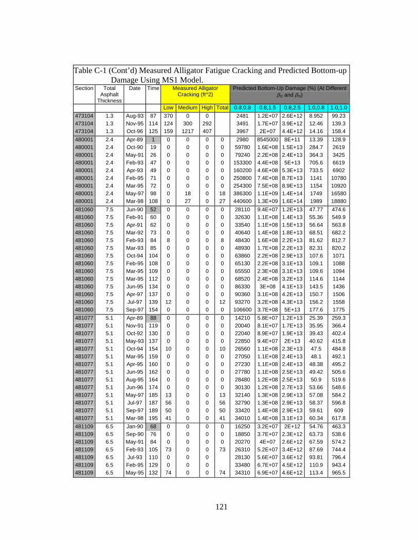
121
Table C-1 (Cont’d) Measured Alligator Fatigue Cracking and Predicted Bottom-up
Damage Using MS1 Model. Section Total
Asphalt Thickness
Date Time Measured Alligator Cracking (ft^2)
Predicted Bottom-Up Damage (%) (At Different βf2 and βf3)
Low Medium High Total 0.8,0.8 0.8,1.5 0.8,2.5 1.0,0.8 1.0,1.0473104 1.3 Aug-93 87 370 0 0 2481 1.2E+07 2.6E+12 8.952 99.23 473104 1.3 Nov-95 114 124 300 292 3491 1.7E+07 3.9E+12 12.46 139.3 473104 1.3 Oct-96 125 159 1217 407 3967 2E+07 4.4E+12 14.16 158.4 480001 2.4 Apr-89 1 0 0 0 0 2980 8545000 8E+11 13.39 128.9 480001 2.4 Oct-90 19 0 0 0 0 59780 1.6E+08 1.5E+13 284.7 2619 480001 2.4 May-91 26 0 0 0 0 79240 2.2E+08 2.4E+13 364.3 3425 480001 2.4 Feb-93 47 0 0 0 0 153300 4.4E+08 5E+13 705.6 6619 480001 2.4 Apr-93 49 0 0 0 0 160200 4.6E+08 5.3E+13 733.5 6902 480001 2.4 Feb-95 71 0 0 0 0 250800 7.4E+08 8.7E+13 1141 10780 480001 2.4 Mar-95 72 0 0 0 0 254300 7.5E+08 8.9E+13 1154 10920 480001 2.4 May-97 98 0 18 0 18 386300 1.1E+09 1.4E+14 1749 16580 480001 2.4 Mar-98 108 0 27 0 27 440600 1.3E+09 1.6E+14 1989 18880 481060 7.5 Jun-90 52 0 0 0 0 28110 9.4E+07 1.2E+13 47.77 474.6 481060 7.5 Feb-91 60 0 0 0 0 32630 1.1E+08 1.4E+13 55.36 549.9 481060 7.5 Apr-91 62 0 0 0 0 33540 1.1E+08 1.5E+13 56.64 563.8 481060 7.5 Mar-92 73 0 0 0 0 40640 1.4E+08 1.8E+13 68.51 682.2 481060 7.5 Feb-93 84 8 0 0 8 48430 1.6E+08 2.2E+13 81.62 812.7 481060 7.5 Mar-93 85 0 0 0 0 48930 1.7E+08 2.2E+13 82.31 820.2 481060 7.5 Oct-94 104 0 0 0 0 63860 2.2E+08 2.9E+13 107.6 1071 481060 7.5 Feb-95 108 0 0 0 0 65130 2.2E+08 3.1E+13 109.1 1088 481060 7.5 Mar-95 109 0 0 0 0 65550 2.3E+08 3.1E+13 109.6 1094 481060 7.5 Mar-95 112 0 0 0 0 68520 2.4E+08 3.2E+13 114.6 1144 481060 7.5 Jun-95 134 0 0 0 0 86330 3E+08 4.1E+13 143.5 1436 481060 7.5 Apr-97 137 0 0 0 0 90360 3.1E+08 4.2E+13 150.7 1506 481060 7.5 Jul-97 139 12 0 0 12 93270 3.2E+08 4.3E+13 156.2 1558 481060 7.5 Sep-97 154 0 0 0 0 106600 3.7E+08 5E+13 177.6 1775 481077 5.1 Apr-89 88 0 0 0 0 14210 5.8E+07 1.2E+13 25.39 259.3 481077 5.1 Nov-91 119 0 0 0 0 20040 8.1E+07 1.7E+13 35.95 366.4 481077 5.1 Oct-92 130 0 0 0 0 22040 8.9E+07 1.9E+13 39.43 402.4 481077 5.1 May-93 137 0 0 0 0 22850 9.4E+07 2E+13 40.62 415.8 481077 5.1 Oct-94 154 10 0 0 10 26560 1.1E+08 2.3E+13 47.5 484.8 481077 5.1 Mar-95 159 0 0 0 0 27050 1.1E+08 2.4E+13 48.1 492.1 481077 5.1 Apr-95 160 0 0 0 0 27230 1.1E+08 2.4E+13 48.38 495.2 481077 5.1 Jun-95 162 0 0 0 0 27780 1.1E+08 2.5E+13 49.42 505.6 481077 5.1 Aug-95 164 0 0 0 0 28480 1.2E+08 2.5E+13 50.9 519.6 481077 5.1 Jun-96 174 0 0 0 0 30130 1.2E+08 2.7E+13 53.66 548.6 481077 5.1 May-97 185 13 0 0 13 32140 1.3E+08 2.9E+13 57.08 584.2 481077 5.1 Jul-97 187 56 0 0 56 32790 1.3E+08 2.9E+13 58.37 596.8 481077 5.1 Sep-97 189 50 0 0 50 33420 1.4E+08 2.9E+13 59.61 609 481077 5.1 Mar-98 195 41 0 0 41 34010 1.4E+08 3.1E+13 60.34 617.8 481109 6.5 Jan-90 68 0 0 0 0 16250 3.2E+07 2E+12 54.76 463.3 481109 6.5 Sep-90 76 0 0 0 0 18850 3.7E+07 2.3E+12 63.73 538.6 481109 6.5 May-91 84 0 0 0 0 20270 4E+07 2.6E+12 67.59 574.2 481109 6.5 Feb-93 105 73 0 0 73 26310 5.2E+07 3.4E+12 87.69 744.4 481109 6.5 Jul-93 110 0 0 0 28130 5.6E+07 3.6E+12 93.81 796.4 481109 6.5 Feb-95 129 0 0 0 33480 6.7E+07 4.5E+12 110.9 943.4 481109 6.5 May-95 132 74 0 0 74 34310 6.9E+07 4.6E+12 113.4 965.5
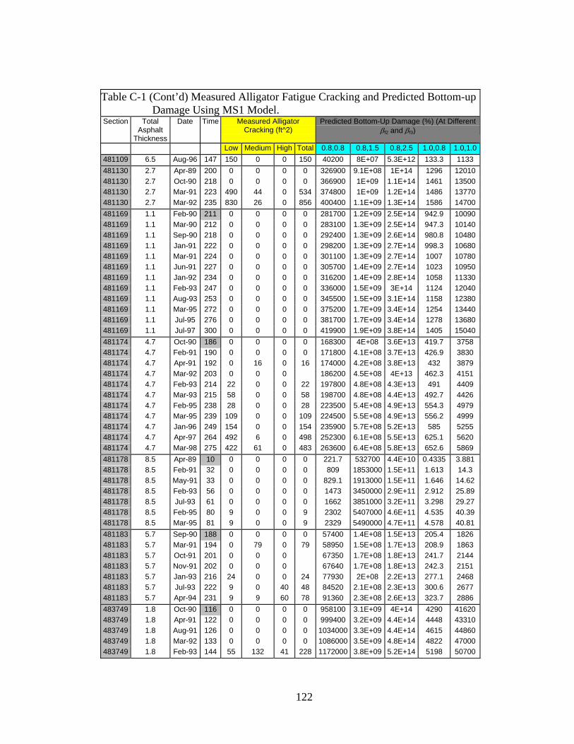
122
Table C-1 (Cont’d) Measured Alligator Fatigue Cracking and Predicted Bottom-up
Damage Using MS1 Model. Section Total
Asphalt Thickness
Date Time Measured Alligator Cracking (ft^2)
Predicted Bottom-Up Damage (%) (At Different βf2 and βf3)
Low Medium High Total 0.8,0.8 0.8,1.5 0.8,2.5 1.0,0.8 1.0,1.0481109 6.5 Aug-96 147 150 0 0 150 40200 8E+07 5.3E+12 133.3 1133 481130 2.7 Apr-89 200 0 0 0 0 326900 9.1E+08 1E+14 1296 12010 481130 2.7 Oct-90 218 0 0 0 0 366900 1E+09 1.1E+14 1461 13500 481130 2.7 Mar-91 223 490 44 0 534 374800 1E+09 1.2E+14 1486 13770 481130 2.7 Mar-92 235 830 26 0 856 400400 1.1E+09 1.3E+14 1586 14700 481169 1.1 Feb-90 211 0 0 0 0 281700 1.2E+09 2.5E+14 942.9 10090 481169 1.1 Mar-90 212 0 0 0 0 283100 1.3E+09 2.5E+14 947.3 10140 481169 1.1 Sep-90 218 0 0 0 0 292400 1.3E+09 2.6E+14 980.8 10480 481169 1.1 Jan-91 222 0 0 0 0 298200 1.3E+09 2.7E+14 998.3 10680 481169 1.1 Mar-91 224 0 0 0 0 301100 1.3E+09 2.7E+14 1007 10780 481169 1.1 Jun-91 227 0 0 0 0 305700 1.4E+09 2.7E+14 1023 10950 481169 1.1 Jan-92 234 0 0 0 0 316200 1.4E+09 2.8E+14 1058 11330 481169 1.1 Feb-93 247 0 0 0 0 336000 1.5E+09 3E+14 1124 12040 481169 1.1 Aug-93 253 0 0 0 0 345500 1.5E+09 3.1E+14 1158 12380 481169 1.1 Mar-95 272 0 0 0 0 375200 1.7E+09 3.4E+14 1254 13440 481169 1.1 Jul-95 276 0 0 0 0 381700 1.7E+09 3.4E+14 1278 13680 481169 1.1 Jul-97 300 0 0 0 0 419900 1.9E+09 3.8E+14 1405 15040 481174 4.7 Oct-90 186 0 0 0 0 168300 4E+08 3.6E+13 419.7 3758 481174 4.7 Feb-91 190 0 0 0 0 171800 4.1E+08 3.7E+13 426.9 3830 481174 4.7 Apr-91 192 0 16 0 16 174000 4.2E+08 3.8E+13 432 3879 481174 4.7 Mar-92 203 0 0 0 186200 4.5E+08 4E+13 462.3 4151 481174 4.7 Feb-93 214 22 0 0 22 197800 4.8E+08 4.3E+13 491 4409 481174 4.7 Mar-93 215 58 0 0 58 198700 4.8E+08 4.4E+13 492.7 4426 481174 4.7 Feb-95 238 28 0 0 28 223500 5.4E+08 4.9E+13 554.3 4979 481174 4.7 Mar-95 239 109 0 0 109 224500 5.5E+08 4.9E+13 556.2 4999 481174 4.7 Jan-96 249 154 0 0 154 235900 5.7E+08 5.2E+13 585 5255 481174 4.7 Apr-97 264 492 6 0 498 252300 6.1E+08 5.5E+13 625.1 5620 481174 4.7 Mar-98 275 422 61 0 483 263600 6.4E+08 5.8E+13 652.6 5869 481178 8.5 Apr-89 10 0 0 0 0 221.7 532700 4.4E+10 0.4335 3.881 481178 8.5 Feb-91 32 0 0 0 0 809 1853000 1.5E+11 1.613 14.3 481178 8.5 May-91 33 0 0 0 0 829.1 1913000 1.5E+11 1.646 14.62 481178 8.5 Feb-93 56 0 0 0 0 1473 3450000 2.9E+11 2.912 25.89 481178 8.5 Jul-93 61 0 0 0 0 1662 3851000 3.2E+11 3.298 29.27 481178 8.5 Feb-95 80 9 0 0 9 2302 5407000 4.6E+11 4.535 40.39 481178 8.5 Mar-95 81 9 0 0 9 2329 5490000 4.7E+11 4.578 40.81 481183 5.7 Sep-90 188 0 0 0 0 57400 1.4E+08 1.5E+13 205.4 1826 481183 5.7 Mar-91 194 0 79 0 79 58950 1.5E+08 1.7E+13 208.9 1863 481183 5.7 Oct-91 201 0 0 0 67350 1.7E+08 1.8E+13 241.7 2144 481183 5.7 Nov-91 202 0 0 0 67640 1.7E+08 1.8E+13 242.3 2151 481183 5.7 Jan-93 216 24 0 0 24 77930 2E+08 2.2E+13 277.1 2468 481183 5.7 Jul-93 222 9 0 40 48 84520 2.1E+08 2.3E+13 300.6 2677 481183 5.7 Apr-94 231 9 9 60 78 91360 2.3E+08 2.6E+13 323.7 2886 483749 1.8 Oct-90 116 0 0 0 0 958100 3.1E+09 4E+14 4290 41620 483749 1.8 Apr-91 122 0 0 0 0 999400 3.2E+09 4.4E+14 4448 43310 483749 1.8 Aug-91 126 0 0 0 0 1034000 3.3E+09 4.4E+14 4615 44860 483749 1.8 Mar-92 133 0 0 0 0 1086000 3.5E+09 4.8E+14 4822 47000 483749 1.8 Feb-93 144 55 132 41 228 1172000 3.8E+09 5.2E+14 5198 50700
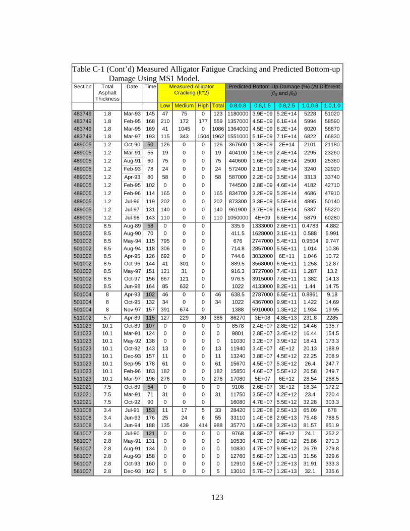
123
Table C-1 (Cont’d) Measured Alligator Fatigue Cracking and Predicted Bottom-up
Damage Using MS1 Model. Section Total
Asphalt Thickness
Date Time Measured Alligator Cracking (ft^2)
Predicted Bottom-Up Damage (%) (At Different βf2 and βf3)
Low Medium High Total 0.8,0.8 0.8,1.5 0.8,2.5 1.0,0.8 1.0,1.0483749 1.8 Mar-93 145 47 75 0 123 1180000 3.9E+09 5.2E+14 5228 51020 483749 1.8 Feb-95 168 210 172 177 559 1357000 4.5E+09 6.1E+14 5994 58590 483749 1.8 Mar-95 169 41 1045 0 1086 1364000 4.5E+09 6.2E+14 6020 58870 483749 1.8 Mar-97 193 115 343 1504 1962 1551000 5.1E+09 7.1E+14 6822 66830 489005 1.2 Oct-90 50 126 0 0 126 367600 1.3E+09 2E+14 2101 21180 489005 1.2 Mar-91 55 19 0 0 19 404100 1.5E+09 2.4E+14 2295 23260 489005 1.2 Aug-91 60 75 0 0 75 440600 1.6E+09 2.6E+14 2500 25360 489005 1.2 Feb-93 78 24 0 0 24 572400 2.1E+09 3.4E+14 3240 32920 489005 1.2 Apr-93 80 58 0 0 58 587000 2.2E+09 3.5E+14 3313 33740 489005 1.2 Feb-95 102 0 0 0 744500 2.8E+09 4.6E+14 4182 42710 489005 1.2 Feb-96 114 165 0 0 165 834700 3.2E+09 5.2E+14 4686 47910 489005 1.2 Jul-96 119 202 0 0 202 873300 3.3E+09 5.5E+14 4895 50140 489005 1.2 Jul-97 131 140 0 0 140 961900 3.7E+09 6.1E+14 5387 55220 489005 1.2 Jul-98 143 110 0 0 110 1050000 4E+09 6.6E+14 5879 60280 501002 8.5 Aug-89 58 0 0 0 335.9 1333000 2.6E+11 0.4783 4.882 501002 8.5 Aug-90 70 0 0 0 411.5 1628000 3.1E+11 0.588 5.991 501002 8.5 May-94 115 795 0 0 676 2747000 5.4E+11 0.9504 9.747 501002 8.5 Aug-94 118 306 0 0 714.8 2857000 5.5E+11 1.014 10.36 501002 8.5 Apr-95 126 692 0 0 744.6 3032000 6E+11 1.046 10.72 501002 8.5 Oct-96 144 41 301 0 889.5 3568000 6.9E+11 1.258 12.87 501002 8.5 May-97 151 121 31 0 916.3 3727000 7.4E+11 1.287 13.2 501002 8.5 Oct-97 156 667 121 0 976.5 3915000 7.6E+11 1.382 14.13 501002 8.5 Jun-98 164 85 632 0 1022 4133000 8.2E+11 1.44 14.75 501004 8 Apr-93 102 46 0 0 46 638.5 2787000 6.5E+11 0.8861 9.18 501004 8 Oct-95 132 34 0 0 34 1022 4367000 9.9E+11 1.422 14.69 501004 8 Nov-97 157 391 674 0 1388 5910000 1.3E+12 1.934 19.95 511002 5.7 Apr-89 115 127 229 30 386 86270 3E+08 4.8E+13 231.8 2285 511023 10.1 Oct-89 107 0 0 0 0 8578 2.4E+07 2.8E+12 14.46 135.7 511023 10.1 Mar-91 124 0 0 0 0 9801 2.8E+07 3.4E+12 16.44 154.5 511023 10.1 May-92 138 0 0 0 0 11030 3.2E+07 3.9E+12 18.41 173.3 511023 10.1 Oct-92 143 13 0 0 13 11940 3.4E+07 4E+12 20.13 188.9 511023 10.1 Dec-93 157 11 0 0 11 13240 3.8E+07 4.5E+12 22.25 208.9 511023 10.1 Sep-95 178 61 0 0 61 15670 4.5E+07 5.3E+12 26.4 247.7 511023 10.1 Feb-96 183 182 0 0 182 15850 4.6E+07 5.5E+12 26.58 249.7 511023 10.1 Mar-97 196 276 0 0 276 17080 5E+07 6E+12 28.54 268.5 512021 7.5 Oct-89 54 0 0 0 0 9108 2.6E+07 3E+12 18.34 172.2 512021 7.5 Mar-91 71 31 0 0 31 11750 3.5E+07 4.2E+12 23.4 220.4 512021 7.5 Oct-92 90 0 0 0 16080 4.7E+07 5.5E+12 32.28 303.3 531008 3.4 Jul-91 153 11 17 5 33 28420 1.2E+08 2.5E+13 65.09 678 531008 3.4 Jun-93 176 25 24 6 55 33110 1.4E+08 2.9E+13 75.48 788.5 531008 3.4 Jun-94 188 135 439 414 988 35770 1.6E+08 3.2E+13 81.57 851.9 561007 2.8 Jul-90 121 0 0 0 0 9768 4.3E+07 9E+12 24.1 252.2 561007 2.8 May-91 131 0 0 0 0 10530 4.7E+07 9.8E+12 25.86 271.3 561007 2.8 Aug-91 134 0 0 0 0 10830 4.7E+07 9.9E+12 26.79 279.8 561007 2.8 Aug-93 158 0 0 0 0 12760 5.6E+07 1.2E+13 31.56 329.6 561007 2.8 Oct-93 160 0 0 0 0 12910 5.6E+07 1.2E+13 31.91 333.3 561007 2.8 Dec-93 162 5 0 0 5 13010 5.7E+07 1.2E+13 32.1 335.6

124
Table C-1 (Cont’d) Measured Alligator Fatigue Cracking and Predicted Bottom-up
Damage Using MS1 Model. Section Total
Asphalt Thickness
Date Time Measured Alligator Cracking (ft^2)
Predicted Bottom-Up Damage (%) (At Different βf2 and βf3)
Low Medium High Total 0.8,0.8 0.8,1.5 0.8,2.5 1.0,0.8 1.0,1.0561007 2.8 Mar-94 165 8 0 0 8 13210 5.8E+07 1.2E+13 32.48 340.3 561007 2.8 Apr-94 166 0 0 0 13300 5.9E+07 1.2E+13 32.7 342.8 561007 2.8 Aug-94 170 6 0 0 6 13690 6E+07 1.3E+13 33.77 353.2 561007 2.8 Feb-95 176 0 0 0 14110 6.2E+07 1.3E+13 34.67 363.5 561007 2.8 May-95 179 0 0 0 14360 6.4E+07 1.3E+13 35.28 370.1 561007 2.8 Sep-95 183 0 0 0 14740 6.5E+07 1.4E+13 36.33 380.2 561007 2.8 Jun-96 192 12 0 0 12 15400 6.8E+07 1.4E+13 37.82 396.8 561007 2.8 Oct-96 196 0 0 0 15770 6.9E+07 1.5E+13 38.85 406.6 561007 2.8 Nov-96 197 0 0 0 15830 7E+07 1.5E+13 38.97 408 561007 2.8 Mar-97 201 0 0 0 16110 7.1E+07 1.5E+13 39.55 415 561007 2.8 Aug-97 206 0 0 0 16590 7.3E+07 1.5E+13 40.93 428 561007 2.8 Sep-97 207 0 0 0 16680 7.3E+07 1.5E+13 41.18 430.4

125
Table C-2 Measured Alligator Fatigue Cracking and Predicted Bottom-up Damage Using MS1 Model.
Section Total
Asphalt Thickness
Date Time Measured Alligator Cracking (ft^2)
Predicted Bottom-Up Damage (%) (At Different βf2 and βf3)
Low Medium High Total 1.0,1.5 1.0,2.5 1.2,0.8 1.2,1.5 1.2,2.5 11001 3.2 Sep-91 132 8 0 0 8 5232000 7.1E+11 4.775 16779.4 1.821E+0911001 3.2 Apr-92 139 13 0 0 13 5553000 7.8E+11 4.953 17662.7 1.97E+09 11001 3.2 Jul-92 142 13 0 0 13 5668000 7.8E+11 5.116 18091.5 1.995E+0911001 3.2 Jan-93 148 45 0 0 45 5936000 8.2E+11 5.345 18936.3 2.092E+0911019 6.7 May-89 32 0 0 0 0 225400 1.9E+10 0.21 498.252 38530000 11019 6.7 Apr-90 43 0 0 0 0 300200 2.5E+10 0.2828 665.003 51070000 11019 6.7 Jan-91 52 0 0 0 0 362500 3E+10 0.3519 810.503 60820000 11019 6.7 Jun-91 57 800 0 0 800 397500 3.3E+10 0.3829 886.753 66890000 11019 6.7 Mar-92 0 0 0 453300 3.8E+10 0.4325 1006.25 76940000 11019 6.7 Mar-93 78 1112 0 0 1112 535900 4.6E+10 0.5059 1185 92180000 11019 6.7 Jul-95 106 2554 0 0 2554 877900 7.1E+10 0.931 2086.26 15060000011019 6.7 Jan-98 136 0 1461 233 1693 1127000 9.3E+10 1.192 2677.51 19530000014126 13.1 Jun-89 15 0 0 0 0 2969 3.1E+08 0.00086 13.6275 289400 14126 13.1 Mar-91 36 0 0 0 0 7527 7.8E+08 0.00221 33.65 736000 14126 13.1 Mar-93 60 0 0 0 0 13100 1.3E+09 0.00387 55.4 1279000 14126 13.1 Apr-94 73 0 0 0 0 16360 1.7E+09 0.00485 68.925 1597000 14126 13.1 Dec-95 93 6 22 0 28 21720 2.2E+09 0.00647 92.3 2121000 14126 13.1 Dec-97 117 81 0 0 81 28450 2.9E+09 0.0085 117.425 2775000 21001 3 May-90 83 0 0 0 0 94440 2E+10 0.05063 194.19 44620000 21001 3 Aug-91 98 0 0 0 0 117000 2.4E+10 0.06556 234.287 54580000 21001 3 Aug-93 122 0 0 0 0 143700 3E+10 0.07859 292.218 67690000 21001 3 Jun-95 144 0 0 0 0 174800 3.7E+10 0.09412 343.679 83700000 21001 3 Aug-97 170 0 0 0 0 207500 4.4E+10 0.1121 412.858 98770000 21001 3 Aug-98 182 0 3 0 3 222400 4.7E+10 0.1198 440.425 10640000021002 3.3 May-90 68 0 0 0 0 23600 5E+09 0.01249 50.4254 9993000 21002 3.3 Aug-91 83 0 0 0 0 28680 5.9E+09 0.01585 62.1408 11880000 21002 3.3 Aug-93 107 0 0 0 0 37850 7.9E+09 0.02057 81.3252 15910000 21002 3.3 Jun-95 129 0 0 0 0 45460 9.6E+09 0.02452 97.4765 19240000 21002 3.3 Aug-97 155 0 0 0 0 54800 1.2E+10 0.02949 117.154 23150000 21002 3.3 May-98 164 0 0 0 0 58180 1.3E+10 0.03063 123.599 24860000 40113 4.5 Feb-95 19 0 0 0 0 329200 4.2E+10 0.2622 577.508 83590000 40113 4.5 Mar-95 20 0 0 0 0 345800 4.5E+10 0.2701 603.219 88620000 40113 4.5 Aug-95 25 0 0 0 0 460500 5.5E+10 0.3903 825.551 11190000040113 4.5 Nov-95 28 0 0 0 0 527500 6.2E+10 0.4441 945.287 12760000040113 4.5 Feb-96 31 0 0 0 0 564100 7.1E+10 0.4553 994.19 14090000040113 4.5 Apr-96 33 0 0 0 0 603900 7.6E+10 0.4805 1059.73 15160000040113 4.5 Jul-96 36 0 0 0 0 683800 8.1E+10 0.5782 1222.07 16570000040113 4.5 Aug-96 37 0 0 0 0 713200 8.3E+10 0.6155 1282.57 17080000040113 4.5 Jan-98 54 0 0 0 0 1073000 1.3E+11 0.8917 1900.15 26580000040113 4.5 Apr-98 57 10 0 0 10 1124000 1.4E+11 0.9121 1972.75 28310000040113 4.5 Jun-98 59 10 0 0 10 1181000 1.5E+11 0.9629 2077.36 29560000040113 4.5 Oct-98 63 10 0 0 10 1307000 1.6E+11 1.097 2321.37 32060000040114 6.8 Feb-95 19 0 0 0 0 145100 1.6E+10 0.1118 291.501 27360000 40114 6.8 Mar-95 20 0 0 0 0 151600 1.7E+10 0.1145 302.251 28870000 40114 6.8 Aug-95 25 0 0 0 0 206000 2.1E+10 0.1665 423.001 37380000 40114 6.8 Nov-95 28 0 0 0 0 236200 2.4E+10 0.1894 484.501 42730000

126
Table C-2 (Cont’d) Measured Alligator Fatigue Cracking and Predicted Bottom-up Damage
Using MS1 Model. Section Total
Asphalt Thickness
Date Time Measured Alligator Cracking (ft^2)
Predicted Bottom-Up Damage (%) (At Different βf2 and βf3)
Low Medium High Total 1.0,1.5 1.0,2.5 1.2,0.8 1.2,1.5 1.2,2.5 40114 6.8 Feb-96 31 0 0 0 0 248000 2.6E+10 0.1925 500.001 45930000 40114 6.8 Apr-96 33 0 0 0 0 264500 2.8E+10 0.2018 530.001 49310000 40114 6.8 Jul-96 36 0 0 0 0 304100 3E+10 0.2453 623.252 54890000 40114 6.8 Aug-96 37 0 0 0 0 319300 3.1E+10 0.263 660.002 56960000 40114 6.8 Jan-98 54 0 0 0 0 473100 4.9E+10 0.3797 965.253 86040000 40114 6.8 Apr-98 57 46 0 0 46 490900 5.2E+10 0.3862 992.003 90610000 40114 6.8 Jun-98 59 52 0 0 52 517100 5.4E+10 0.407 1046.5 95080000 40114 6.8 Oct-98 63 114 0 0 114 576600 5.9E+10 0.4656 1179.5 10410000040115 15.1 Feb-95 19 0 0 0 0 1254 1.2E+08 0.00052 1.281 106700 40115 15.1 Mar-95 20 25 0 0 25 1300 1.3E+08 0.00053 1.31675 111700 40115 15.1 Jan-98 54 0 0 0 0 4227 3.9E+08 0.00182 4.41 350000 40116 16.2 Feb-95 19 0 0 0 0 1060 1E+08 0.00039 0.96875 82210 40116 16.2 Mar-95 20 0 0 0 0 1100 1.1E+08 0.00039 0.99575 86110 40116 16.2 Jan-98 54 0 0 0 0 3555 3.3E+08 0.00136 3.32 267100 40117 11.8 Feb-95 19 0 0 0 0 2154 2.5E+08 0.00084 2.3645 236400 40117 11.8 Mar-95 20 0 0 0 0 2241 2.6E+08 0.00085 2.4405 248500 40117 11.8 Jan-98 54 0 0 0 0 7205 7.9E+08 0.00294 8.085 767000 40118 11.7 Feb-95 19 0 0 0 0 5732 5.6E+08 0.00337 8.38 695500 40118 11.7 Mar-95 20 0 0 0 0 5913 5.8E+08 0.00342 8.565 723300 40118 11.7 Jan-98 54 0 0 0 0 19280 1.8E+09 0.01163 28.525 2277000 41007 6.5 Sep-91 162 38 0 0 38 169600 1.6E+10 0.1412 327.753 26390000 41007 6.5 Feb-93 163 44 16 0 60 170800 1.6E+10 0.1416 329.503 26650000 41007 6.5 Sep-94 198 70 132 0 202 231100 2.2E+10 0.1896 444.503 36240000 41024 10.8 Nov-89 149 0 0 0 0 979800 7.1E+10 0.8862 1808 11250000041024 10.8 Aug-90 158 0 0 0 0 1073000 7.8E+10 0.9769 1985.75 12290000041024 10.8 Oct-92 184 0 0 0 0 1355000 9.8E+10 1.233 2505 15530000041024 10.8 Mar-95 213 0 0 0 0 1668000 1.2E+11 1.487 3050 19310000041024 10.8 Jul-95 217 0 0 0 0 1753000 1.3E+11 1.576 3220 20200000041024 10.8 Aug-95 218 12 0 0 12 1782000 1.3E+11 1.61 3280 20460000041024 10.8 Nov-95 221 0 10 0 10 1822000 1.3E+11 1.64 3350 20930000041024 10.8 Feb-96 224 0 0 0 1831000 1.4E+11 1.641 3357.5 21130000041024 10.8 Apr-96 226 16 0 0 16 1845000 1.4E+11 1.647 3375 21350000041024 10.8 Jun-96 228 118 0 0 118 1883000 1.4E+11 1.678 3442.5 21770000041024 10.8 Aug-96 230 161 0 0 161 1949000 1.4E+11 1.765 3590 22370000041024 10.8 Apr-98 250 0 398 529 927 2208000 1.7E+11 1.972 4035 25570000041024 10.8 Jun-98 252 0 397 530 927 2255000 1.7E+11 2.015 4125 26090000041024 10.8 Oct-98 256 0 414 529 943 2358000 1.7E+11 2.111 4322.5 27170000081029 4.2 Oct-91 233 27 15 0 42 77130 1.1E+10 0.07199 233.31 24690000 81029 4.2 Jul-94 266 0 0 0 88660 1.3E+10 0.08181 266.91 28530000 81029 4.2 Sep-95 280 464 0 0 464 93780 1.4E+10 0.0868 282.265 30100000 81053 4.6 Oct-89 60 0 0 0 0 42140 5E+09 0.05161 201.072 13450000 81053 4.6 Jul-90 69 0 0 0 0 45760 5.7E+09 0.05401 235.673 14740000 81053 4.6 Apr-93 102 3 0 0 3 79030 9.9E+09 0.09429 400.584 25570000 81053 4.6 Nov-93 109 0 0 0 102200 1.2E+10 0.1324 471.749 32410000 81053 4.6 Dec-93 110 23 0 0 23 102500 1.2E+10 0.1324 472.503 32560000 81053 4.6 Oct-94 120 0 0 0 128300 1.5E+10 0.1683 547.44 40950000 81053 4.6 Feb-95 124 40 0 0 40 130200 1.5E+10 0.1687 551.966 41970000

127
Table C-2 (Cont’d) Measured Alligator Fatigue Cracking and Predicted Bottom-up Damage
Using MS1 Model. Section Total
Asphalt Thickness
Date Time Measured Alligator Cracking (ft^2)
Predicted Bottom-Up Damage (%) (At Different βf2 and βf3)
Low Medium High Total 1.0,1.5 1.0,2.5 1.2,0.8 1.2,1.5 1.2,2.5 81053 4.6 May-95 127 40 0 0 40 131900 1.6E+10 0.1697 567.808 42520000 81053 4.6 May-96 139 0 0 0 139300 1.7E+10 0.1754 653.055 44760000 81053 4.6 Oct-96 144 310 0 0 310 143700 1.7E+10 0.1797 717.933 45790000 81053 4.6 Nov-96 145 253 0 0 253 144100 1.7E+10 0.1799 720.196 45980000 81053 4.6 Mar-97 149 457 0 0 457 147000 1.8E+10 0.1808 726.734 47500000 91803 7.2 Jul-89 49 0 0 0 0 16630 3E+09 0.00869 31.325 4832000 91803 7.2 Sep-90 63 0 0 0 0 23090 4.1E+09 0.01218 43.675 6646000 91803 7.2 Aug-91 74 0 0 0 0 28260 5.1E+09 0.01496 53.45 8182000 91803 7.2 Sep-92 87 8 0 0 8 35010 6.4E+09 0.01815 65.7 10210000 91803 7.2 May-94 107 211 0 0 211 45520 8.7E+09 0.02278 83.9751 13610000 91803 7.2 May-95 119 240 0 0 240 53610 1E+10 0.02678 98.8251 16050000 91803 7.2 Oct-96 136 84 82 0 166 68530 1.3E+10 0.03541 128.2 20110000 91803 7.2 May-97 143 301 0 0 301 72440 1.4E+10 0.0363 133.575 21710000 91803 7.2 Sep-97 147 15 325 0 340 77760 1.5E+10 0.03975 144.85 22940000 91803 7.2 Jun-98 156 195 0 0 195 84280 1.6E+10 0.04216 155.5 25220000 120103 12 Dec-96 14 0 0 0 0 459.2 3.7E+07 0.00022 0.59125 45680 120104 18 Dec-96 14 0 0 0 0 64.47 5020000 2.2E-05 0.05558 4267 120105 7.9 Dec-96 14 0 0 0 0 2861 2.5E+08 0.00178 5.06 433300 120106 15 Dec-96 14 0 0 0 0 133.6 1.1E+07 5.1E-05 0.1317 10280 123995 5 Apr-92 197 0 0 0 1.1E+07 8.9E+11 10.73 25862.5 2.043E+09123995 5 Mar-94 220 86 0 0 1.3E+07 1E+12 12.27 28891.9 2.331E+09123995 5 Jan-96 242 58 0 0 1.4E+07 1.1E+12 13.7 31746 2.604E+09123995 5 Jan-96 243 122 0 0 1.4E+07 1.1E+12 13.75 31846.2 2.618E+09123997 3.1 Aug-90 195 2000 0 0 2000 1521000 1.6E+11 1.719 4581.87 434300000123997 3.1 Oct-91 209 0 3000 0 3000 1696000 1.7E+11 1.909 5107.48 485300000123997 3.1 Mar-93 226 0 4680 0 4680 1915000 2E+11 2.114 5726.72 557700000123997 3.1 Mar-94 238 0 5047 0 5047 2086000 2.2E+11 2.307 6241.93 606600000124105 2.3 Apr-89 53 0 0 0 0 2186000 2.6E+11 2.571 7624.95 846500000124105 2.3 Oct-91 83 0 0 0 0 3432000 4E+11 4.101 12028.7 1.318E+09124105 2.3 Mar-93 100 0 0 0 0 4165000 5.1E+11 4.833 14470.9 1.638E+09124106 8.2 Apr-89 21 0 0 0 0 146600 1E+10 0.1137 263.25 17780000 124106 8.2 Feb-91 43 0 0 0 0 293400 2.1E+10 0.2218 521 36040000 124106 8.2 Jul-91 48 0 0 0 0 328000 2.3E+10 0.2486 583 40160000 124106 8.2 Mar-94 80 0 0 0 0 536400 3.9E+10 0.3959 943.5 66780000 124106 8.2 Jan-97 114 0 0 0 0 757500 5.6E+10 0.5543 1327.25 94800000 124107 2.7 Dec-89 75 0 0 0 0 220000 2.5E+10 0.2359 523.502 79760000 124107 2.7 Feb-91 89 0 0 0 0 271400 3.2E+10 0.2863 643.552 99830000 124107 2.7 Jul-91 94 0 0 0 0 290100 3.4E+10 0.3078 688.744 106200000124107 2.7 Mar-93 114 732 355 9 1096 371200 4.4E+10 0.3856 876.484 138700000124107 2.7 Mar-94 126 656 243 0 899 424000 5.1E+10 0.4396 1000.42 158600000124107 2.7 Jan-96 148 264 812 93 1168 529400 6.4E+10 0.5444 1248.28 198900000124107 2.7 Mar-97 162 44 372 1224 1640 602000 7.3E+10 0.6143 1416.51 227700000124108 9.9 Apr-89 35 0 0 0 0 10560 6.5E+08 0.00889 16.9875 951100 124108 9.9 Jan-91 56 0 0 0 0 16920 1.1E+09 0.01441 27.225 1523000 124108 9.9 Oct-91 65 0 0 0 0 20120 1.2E+09 0.01728 32.5 1797000 124108 9.9 Mar-94 94 0 0 0 0 29320 1.9E+09 0.02466 46.85 2662000 124108 9.9 Aug-94 99 0 0 0 0 31520 2E+09 0.02668 50.575 2843000
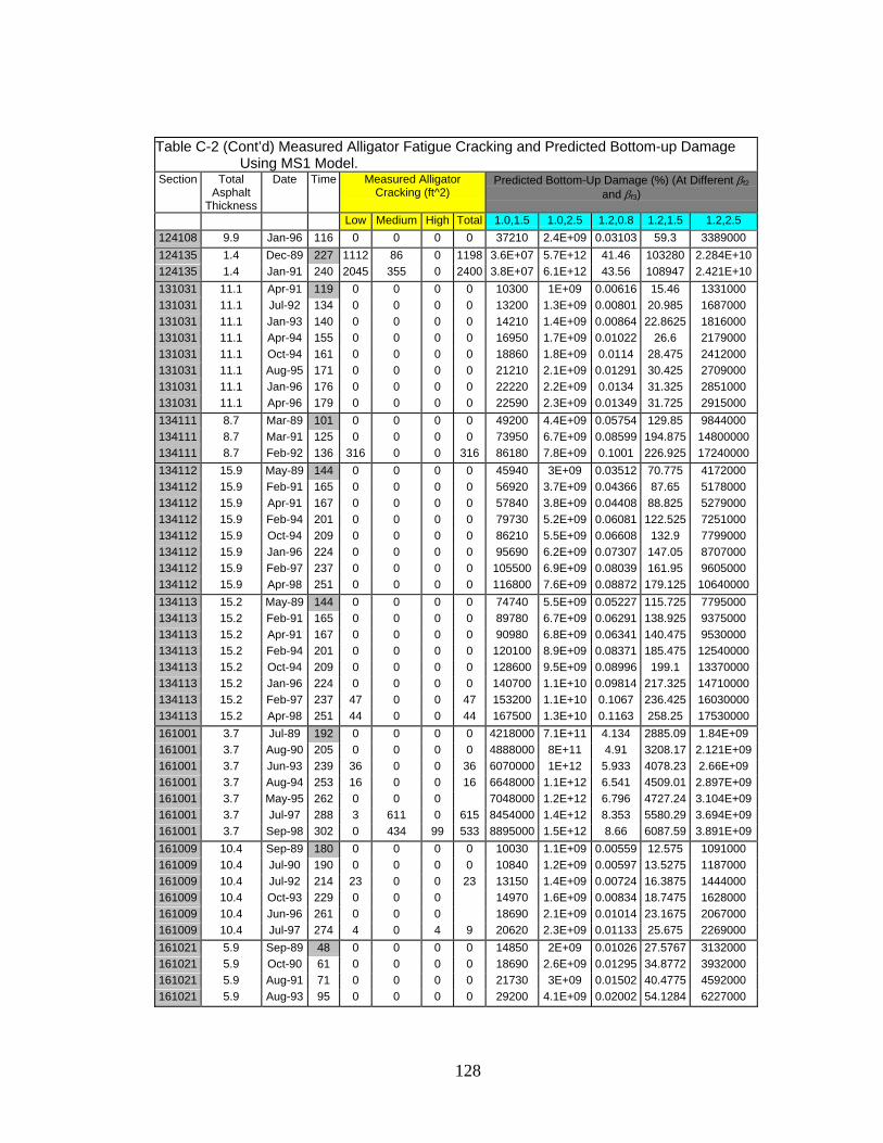
128
Table C-2 (Cont’d) Measured Alligator Fatigue Cracking and Predicted Bottom-up Damage
Using MS1 Model. Section Total
Asphalt Thickness
Date Time Measured Alligator Cracking (ft^2)
Predicted Bottom-Up Damage (%) (At Different βf2 and βf3)
Low Medium High Total 1.0,1.5 1.0,2.5 1.2,0.8 1.2,1.5 1.2,2.5 124108 9.9 Jan-96 116 0 0 0 0 37210 2.4E+09 0.03103 59.3 3389000 124135 1.4 Dec-89 227 1112 86 0 1198 3.6E+07 5.7E+12 41.46 103280 2.284E+10124135 1.4 Jan-91 240 2045 355 0 2400 3.8E+07 6.1E+12 43.56 108947 2.421E+10131031 11.1 Apr-91 119 0 0 0 0 10300 1E+09 0.00616 15.46 1331000 131031 11.1 Jul-92 134 0 0 0 0 13200 1.3E+09 0.00801 20.985 1687000 131031 11.1 Jan-93 140 0 0 0 0 14210 1.4E+09 0.00864 22.8625 1816000 131031 11.1 Apr-94 155 0 0 0 0 16950 1.7E+09 0.01022 26.6 2179000 131031 11.1 Oct-94 161 0 0 0 0 18860 1.8E+09 0.0114 28.475 2412000 131031 11.1 Aug-95 171 0 0 0 0 21210 2.1E+09 0.01291 30.425 2709000 131031 11.1 Jan-96 176 0 0 0 0 22220 2.2E+09 0.0134 31.325 2851000 131031 11.1 Apr-96 179 0 0 0 0 22590 2.3E+09 0.01349 31.725 2915000 134111 8.7 Mar-89 101 0 0 0 0 49200 4.4E+09 0.05754 129.85 9844000 134111 8.7 Mar-91 125 0 0 0 0 73950 6.7E+09 0.08599 194.875 14800000 134111 8.7 Feb-92 136 316 0 0 316 86180 7.8E+09 0.1001 226.925 17240000 134112 15.9 May-89 144 0 0 0 0 45940 3E+09 0.03512 70.775 4172000 134112 15.9 Feb-91 165 0 0 0 0 56920 3.7E+09 0.04366 87.65 5178000 134112 15.9 Apr-91 167 0 0 0 0 57840 3.8E+09 0.04408 88.825 5279000 134112 15.9 Feb-94 201 0 0 0 0 79730 5.2E+09 0.06081 122.525 7251000 134112 15.9 Oct-94 209 0 0 0 0 86210 5.5E+09 0.06608 132.9 7799000 134112 15.9 Jan-96 224 0 0 0 0 95690 6.2E+09 0.07307 147.05 8707000 134112 15.9 Feb-97 237 0 0 0 0 105500 6.9E+09 0.08039 161.95 9605000 134112 15.9 Apr-98 251 0 0 0 0 116800 7.6E+09 0.08872 179.125 10640000 134113 15.2 May-89 144 0 0 0 0 74740 5.5E+09 0.05227 115.725 7795000 134113 15.2 Feb-91 165 0 0 0 0 89780 6.7E+09 0.06291 138.925 9375000 134113 15.2 Apr-91 167 0 0 0 0 90980 6.8E+09 0.06341 140.475 9530000 134113 15.2 Feb-94 201 0 0 0 0 120100 8.9E+09 0.08371 185.475 12540000 134113 15.2 Oct-94 209 0 0 0 0 128600 9.5E+09 0.08996 199.1 13370000 134113 15.2 Jan-96 224 0 0 0 0 140700 1.1E+10 0.09814 217.325 14710000 134113 15.2 Feb-97 237 47 0 0 47 153200 1.1E+10 0.1067 236.425 16030000 134113 15.2 Apr-98 251 44 0 0 44 167500 1.3E+10 0.1163 258.25 17530000 161001 3.7 Jul-89 192 0 0 0 0 4218000 7.1E+11 4.134 2885.09 1.84E+09 161001 3.7 Aug-90 205 0 0 0 0 4888000 8E+11 4.91 3208.17 2.121E+09161001 3.7 Jun-93 239 36 0 0 36 6070000 1E+12 5.933 4078.23 2.66E+09 161001 3.7 Aug-94 253 16 0 0 16 6648000 1.1E+12 6.541 4509.01 2.897E+09161001 3.7 May-95 262 0 0 0 7048000 1.2E+12 6.796 4727.24 3.104E+09161001 3.7 Jul-97 288 3 611 0 615 8454000 1.4E+12 8.353 5580.29 3.694E+09161001 3.7 Sep-98 302 0 434 99 533 8895000 1.5E+12 8.66 6087.59 3.891E+09161009 10.4 Sep-89 180 0 0 0 0 10030 1.1E+09 0.00559 12.575 1091000 161009 10.4 Jul-90 190 0 0 0 0 10840 1.2E+09 0.00597 13.5275 1187000 161009 10.4 Jul-92 214 23 0 0 23 13150 1.4E+09 0.00724 16.3875 1444000 161009 10.4 Oct-93 229 0 0 0 14970 1.6E+09 0.00834 18.7475 1628000 161009 10.4 Jun-96 261 0 0 0 18690 2.1E+09 0.01014 23.1675 2067000 161009 10.4 Jul-97 274 4 0 4 9 20620 2.3E+09 0.01133 25.675 2269000 161021 5.9 Sep-89 48 0 0 0 0 14850 2E+09 0.01026 27.5767 3132000 161021 5.9 Oct-90 61 0 0 0 0 18690 2.6E+09 0.01295 34.8772 3932000 161021 5.9 Aug-91 71 0 0 0 0 21730 3E+09 0.01502 40.4775 4592000 161021 5.9 Aug-93 95 0 0 0 0 29200 4.1E+09 0.02002 54.1284 6227000

129
Table C-2 (Cont’d) Measured Alligator Fatigue Cracking and Predicted Bottom-up Damage
Using MS1 Model. Section Total
Asphalt Thickness
Date Time Measured Alligator Cracking (ft^2)
Predicted Bottom-Up Damage (%) (At Different βf2 and βf3)
Low Medium High Total 1.0,1.5 1.0,2.5 1.2,0.8 1.2,1.5 1.2,2.5 161021 5.9 Sep-95 120 0 0 0 0 37540 5.3E+09 0.02575 69.5294 8010000 161021 5.9 Jun-96 129 0 0 0 0 40070 5.7E+09 0.02699 73.6796 8652000 161021 5.9 Jul-97 142 0 0 0 0 44560 6.4E+09 0.03015 82.1052 9601000 169034 9.2 Jul-89 10 0 0 0 0 689.8 1E+08 0.00028 0.9005 111400 169034 9.2 Aug-90 23 0 0 0 0 1749 2.3E+08 0.00084 2.432 263200 169034 9.2 Jun-93 57 0 0 0 0 3976 5.8E+08 0.00178 5.3575 623100 169034 9.2 Aug-94 71 0 0 0 0 5084 7.2E+08 0.00236 6.955 782900 169034 9.2 May-95 80 0 0 0 0 5531 8.1E+08 0.00249 7.4625 866800 169034 9.2 Jul-97 106 25 0 0 25 7448 1.1E+09 0.00342 10.135 1156000 169034 9.2 Sep-98 120 0 0 25 25 8468 1.2E+09 0.0039 11.54 1311000 201009 11.1 Aug-88 44 10 0 0 10 1541 1.4E+08 0.00088 2.68 150700 201009 11.1 May-89 53 0 0 0 1769 1.7E+08 0.00098 3.005 176700 201009 11.1 Dec-90 72 42 0 0 42 2489 2.3E+08 0.00141 4.2925 244900 201009 11.1 Oct-91 82 1 13 0 14 2902 2.6E+08 0.00168 5.06 282800 201009 11.1 Apr-93 100 6 18 16 41 3413 3.2E+08 0.00191 5.82 339600 201009 11.1 Apr-95 124 2 54 0 56 4332 4E+08 0.00245 7.435 429000 201009 11.1 Apr-96 136 0 0 0 4770 4.5E+08 0.00268 8.1675 473200 201009 11.1 Jan-99 168 0 1643 0 6129 5.7E+08 0.00348 10.5575 602900 251003 6.6 Aug-89 180 0 0 0 0 198900 2.8E+10 0.1379 419.002 52090000 251003 6.6 Sep-90 193 0 0 0 0 216500 3.1E+10 0.1487 454.752 56900000 251003 6.6 Aug-91 204 28 0 0 28 232000 3.3E+10 0.1593 487.003 61030000 251003 6.6 Sep-92 217 56 93 0 149 253300 3.6E+10 0.1756 533.253 66370000 251003 6.6 Oct-95 254 45 75 0 121 310600 4.5E+10 0.2125 651.004 81840000 251003 6.6 Oct-96 266 1314 0 0 1314 330900 4.8E+10 0.2268 694.254 87100000 251003 6.6 Jun-98 286 1062 62 0 1125 364500 5.3E+10 0.2491 763.004 96260000 251004 9.6 Aug-89 178 0 0 0 0 60760 8.6E+09 0.03664 133.575 13320000 251004 9.6 Sep-90 191 0 0 0 0 67890 9.6E+09 0.0409 148.825 14890000 251004 9.6 Aug-91 202 0 0 0 0 73830 1E+10 0.04445 161.775 16200000 251004 9.6 Sep-92 215 0 0 0 0 82580 1.2E+10 0.04996 181.375 18080000 251004 9.6 Oct-95 252 0 0 0 0 107700 1.5E+10 0.06454 234.975 23680000 251004 9.6 Jun-97 272 56 0 0 56 122100 1.8E+10 0.0726 265 26960000 251004 9.6 Jun-98 284 0 0 0 132700 1.9E+10 0.07895 288 29280000 261001 2.2 Jul-88 203 0 0 0 0 222700 4.2E+10 0.1689 653.312 114000000261001 2.2 Sep-89 217 0 0 0 0 237800 4.5E+10 0.1811 698.222 121400000261001 2.2 Jul-90 227 0 0 0 0 248200 4.7E+10 0.1881 727.587 126900000261001 2.2 Jul-91 239 33 0 0 33 260800 4.9E+10 0.1978 765.012 133300000261001 2.2 Sep-91 241 28 0 0 28 262700 4.9E+10 0.2 770.962 133900000261001 2.2 Sep-92 253 40 0 0 40 275800 5.2E+10 0.2092 808.963 140900000261001 2.2 Jun-93 262 0 81 0 81 287400 5.4E+10 0.2166 841.398 147500000261001 2.2 Jun-93 263 76 0 0 76 288200 5.4E+10 0.2179 844.469 147700000261001 2.2 May-95 285 58 0 0 58 311800 5.9E+10 0.2347 912.218 160100000261001 2.2 Jul-96 299 83 0 0 83 326300 6.1E+10 0.2468 956.169 167100000261004 4.2 Sep-89 51 0 0 0 0 68840 1.1E+10 0.05051 162.731 24240000 261004 4.2 Jul-90 61 0 0 0 0 83420 1.4E+10 0.06009 196.613 29950000 271018 4.4 Apr-89 124 0 0 0 0 1007000 1.4E+11 0.8283 2436.34 292900000271018 4.4 Jun-89 126 0 0 0 0 1042000 1.4E+11 0.8661 2531.96 301200000271018 4.4 Oct-90 142 0 0 0 0 1247000 1.7E+11 1.047 3042.9 357800000

130
Table C-2 (Cont’d) Measured Alligator Fatigue Cracking and Predicted Bottom-up Damage
Using MS1 Model. Section Total
Asphalt Thickness
Date Time Measured Alligator Cracking (ft^2)
Predicted Bottom-Up Damage (%) (At Different βf2 and βf3)
Low Medium High Total 1.0,1.5 1.0,2.5 1.2,0.8 1.2,1.5 1.2,2.5 271018 4.4 Jun-93 174 0 0 0 0 1644000 2.3E+11 1.349 3971.2 478400000271018 4.4 Jul-93 176 0 0 0 0 1681000 2.3E+11 1.403 4082.5 484700000271018 4.4 Mar-94 183 0 0 0 0 1733000 2.4E+11 1.427 4186.2 503200000271018 4.4 Aug-94 188 0 0 0 0 1841000 2.5E+11 1.536 4472.03 530600000271087 15.7 Oct-91 154 0 0 0 0 838 9.4E+07 0.00024 0.54975 63290 271087 15.7 May-93 173 0 0 0 0 918.2 1E+08 0.00026 0.5995 69800 271087 15.7 Oct-94 190 0 3 0 3 1021 1.1E+08 0.00029 0.66725 77190 271087 15.7 Jun-96 210 13 0 0 13 1119 1.3E+08 0.00031 0.73 84960 291008 11.4 Feb-92 70 41 0 0 41 1258 1.2E+08 0.00069 1.52775 132600 291008 11.4 Mar-93 83 140 22 0 161 1497 1.4E+08 0.00081 1.74425 158500 291008 11.4 1512 1.5E+08 0.00081 1.7565 160500 291008 11.4 Apr-96 120 0 0 0 2288 2.2E+08 0.00123 2.4615 243000 291008 11.4 Feb-00 152 365 715 0 3133 3E+08 0.00169 3.275 330700 307088 4.9 Sep-89 100 0 0 0 0 109300 1.8E+10 0.08934 167.569 35380000 307088 4.9 May-91 120 0 66 0 66 133300 2.2E+10 0.1068 200.587 43780000 308129 3.2 Oct-89 17 0 0 0 0 58740 1.1E+10 0.04035 189.106 24200000 308129 3.2 Jul-91 38 0 0 0 0 167000 3.4E+10 0.1094 406.555 77630000 308129 3.2 Jul-92 50 0 0 0 0 218400 4.6E+10 0.1392 541.159 102700000308129 3.2 Aug-93 63 0 0 0 0 274000 5.8E+10 0.1735 690.814 128500000308129 3.2 Dec-93 67 0 0 0 0 288000 6.1E+10 0.1804 727.692 135400000308129 3.2 Mar-94 70 0 0 0 0 308200 6.7E+10 0.1871 757.28 149200000308129 3.2 Oct-94 77 0 0 0 0 371500 7.7E+10 0.2416 849.045 176100000308129 3.2 Feb-95 81 0 0 0 0 392100 8.4E+10 0.2474 879.92 189800000308129 3.2 May-95 84 0 0 0 0 404900 8.8E+10 0.2527 913.367 196400000308129 3.2 Jun-96 97 0 0 0 0 468200 1E+11 0.2896 1078.46 226800000308129 3.2 Oct-96 101 0 0 0 0 489300 1E+11 0.3069 1139.35 234200000308129 3.2 Jan-97 104 0 0 0 0 501400 1.1E+11 0.3099 1165.08 242000000308129 3.2 Mar-97 106 0 0 0 0 511300 1.1E+11 0.3126 1188.23 248400000308129 3.2 Aug-97 111 0 0 0 0 539000 1.2E+11 0.3357 1271.85 258300000308129 3.2 Oct-97 113 0 0 0 0 548800 1.2E+11 0.3422 1300.15 262200000321020 7 Jul-91 86 0 0 0 0 27970 3.6E+09 0.01856 41.4501 5566000 321020 7 Aug-93 111 18 0 0 18 38560 5E+09 0.02569 57.1501 7678000 321020 7 Sep-94 123 187 62 0 250 44030 5.7E+09 0.02924 65.1751 8803000 321020 7 Apr-95 131 34 0 0 34 46700 6.3E+09 0.03025 68.4751 9499000 321020 7 Jun-97 157 672 1043 0 60580 8.1E+09 0.03937 88.9751 12250000 321020 7 Jun-98 169 3269 36 0 66800 8.9E+09 0.04314 97.8751 13540000 341031 7.3 Apr-92 224 280 12 0 292 110800 1.2E+10 0.1118 273.75 23900000 341031 7.3 Feb-93 234 598 11 0 609 122000 1.3E+10 0.1237 302.5 26220000 341031 7.3 Oct-95 266 0 652 305 957 164700 1.7E+10 0.1674 409 35190000 341031 7.3 Nov-95 267 574 8 0 581 165300 1.7E+10 0.1676 409.75 35380000 341033 7.4 Apr-92 211 79 0 0 79 40120 4.8E+09 0.02746 134.45 7118000 341033 7.4 Feb-93 221 6 0 0 6 42450 5E+09 0.02913 142.125 7517000 341033 7.4 Nov-95 254 15 0 0 15 49890 5.9E+09 0.03425 167.525 8843000 341033 7.4 Jul-97 274 0 0 0 54020 6.5E+09 0.03664 180.075 9641000 341034 11.1 Oct-89 48 0 0 0 0 4159 5E+08 0.00153 4.4175 458500 341034 11.1 Sep-90 59 0 0 0 0 5227 6.3E+08 0.00195 5.5825 574500 341034 11.1 Apr-92 78 0 0 0 0 6709 8.6E+08 0.0024 7.0025 758000

131
Table C-2 (Cont’d) Measured Alligator Fatigue Cracking and Predicted Bottom-up Damage
Using MS1 Model. Section Total
Asphalt Thickness
Date Time Measured Alligator Cracking (ft^2)
Predicted Bottom-Up Damage (%) (At Different βf2 and βf3)
Low Medium High Total 1.0,1.5 1.0,2.5 1.2,0.8 1.2,1.5 1.2,2.5 341034 11.1 Feb-93 88 0 0 0 0 7861 9.9E+08 0.00286 8.2625 879200 341034 11.1 Nov-95 121 0 0 0 0 11890 1.5E+09 0.00438 12.575 1319000 341034 11.1 Jul-97 141 129 75 0 205 14300 1.8E+09 0.00521 15.0425 1597000 350101 7.2 May-97 19 0 0 0 0 132200 1.4E+10 0.1239 317.75 28550000 350102 4.8 May-97 19 0 0 0 0 432100 5.7E+10 0.3899 1168.9 136000000350103 12.5 May-97 19 0 0 0 0 47170 4.1E+09 0.03855 90.95 6949000 350104 19.2 May-97 19 0 0 0 0 5895 4.8E+08 0.00341 7.785 561800 350105 9.9 May-97 19 0 0 0 0 161900 1.3E+10 0.1717 366.5 25260000 350106 15.6 May-97 19 0 0 0 0 11690 1E+09 0.00738 17.0275 1293000 351005 8.9 Oct-89 73 0 0 0 0 8037 1E+09 0.00439 12.755 1386000 351005 8.9 Mar-91 90 0 0 0 0 10080 1.4E+09 0.00528 15.6625 1790000 351005 8.9 Oct-92 109 0 0 0 0 13730 1.8E+09 0.00725 21.4625 2412000 351005 8.9 Feb-94 125 0 0 0 0 16750 2.3E+09 0.00878 26.025 2969000 351005 8.9 Mar-95 138 0 0 0 0 20040 2.7E+09 0.01071 31.35 3521000 351005 8.9 Apr-97 163 0 0 0 0 26690 3.6E+09 0.01381 41.25 4763000 351022 6.3 Oct-89 37 0 0 0 0 16930 2.3E+09 0.01127 23.5704 3941000 351022 6.3 Mar-91 54 0 0 0 0 26780 3.8E+09 0.01773 36.9006 6385000 351022 6.3 Oct-92 73 0 0 0 0 42680 5.9E+09 0.02893 59.3759 9972000 351022 6.3 Feb-94 89 0 0 0 0 55420 8E+09 0.03682 76.2512 13210000 351022 6.3 Mar-95 102 0 0 0 0 68410 9.9E+09 0.04511 93.8765 16320000 351022 6.3 Apr-97 127 0 0 0 0 97080 1.4E+10 0.06538 134.002 23010000 351112 6.3 Dec-89 67 0 0 0 0 154000 1.3E+10 0.1709 370.006 26670000 351112 6.3 Jan-91 80 0 0 0 0 180900 1.6E+10 0.1962 430.257 31640000 351112 6.3 Mar-91 82 0 0 0 0 183800 1.6E+10 0.1975 435.007 32330000 351112 6.3 Jan-93 104 0 0 0 0 232200 2E+10 0.2494 549.259 40820000 351112 6.3 Feb-94 117 0 0 0 0 260800 2.3E+10 0.2797 616.01 45930000 351112 6.3 Oct-94 125 0 0 0 0 284100 2.5E+10 0.3083 675.01 49560000 351112 6.3 Mar-95 130 9 0 0 9 290000 2.6E+10 0.3105 684.511 51140000 351112 6.3 Apr-95 131 0 0 0 0 292300 2.6E+10 0.3122 689.261 51590000 351112 6.3 Jun-95 133 0 0 0 0 298600 2.6E+10 0.3194 705.011 52570000 351112 6.3 Nov-96 150 0 0 0 0 338900 3E+10 0.3617 799.512 59510000 351112 6.3 Apr-97 155 0 0 0 0 344400 3.1E+10 0.3639 808.263 61000000 351112 6.3 Sep-97 160 0 0 0 0 361400 3.2E+10 0.3862 853.013 63450000 371024 4.8 Nov-89 109 167 0 0 167 25410 3E+09 0.02372 116.664 6448000 371024 4.8 Mar-91 125 889 89 0 29720 3.6E+09 0.02706 135.619 7666000 371024 4.8 Apr-92 138 1442 308 342 33810 4.2E+09 0.03051 153.998 8777000 371802 4.5 Mar-91 66 36 0 0 36 1333000 1.4E+11 2.224 5369.23 533500000371802 4.5 Oct-92 85 51 36 0 86 1746000 1.8E+11 2.979 7146.37 688600000371802 4.5 Apr-94 103 1521 0 0 1521 2089000 2.3E+11 3.464 8472.29 841200000371802 4.5 Jul-95 118 1739 70 0 1809 2421000 2.6E+11 4.091 9921.74 965700000371802 4.5 Apr-96 127 2608 206 0 2814 2589000 2.8E+11 4.319 10557 1.043E+09371992 2.4 Mar-91 14 0 0 0 0 137800 2.1E+10 0.114 397 55870000 371992 2.4 Oct-92 33 2 0 0 2 343100 4.7E+10 0.321 1022.56 129900000371992 2.4 Apr-94 51 0 0 0 0 572300 8.6E+10 0.5025 1670.26 229100000371992 2.4 Feb-96 73 0 0 0 0 896300 1.4E+11 0.7799 2607.42 362700000404087 10.1 Jan-90 43 0 0 0 0 16340 1.2E+09 0.0218 21.355 2639000 404087 10.1 Oct-91 64 0 0 0 0 26260 1.9E+09 0.03463 34.8 4235000

132
Table C-2 (Cont’d) Measured Alligator Fatigue Cracking and Predicted Bottom-up Damage
Using MS1 Model. Section Total
Asphalt Thickness
Date Time Measured Alligator Cracking (ft^2)
Predicted Bottom-Up Damage (%) (At Different βf2 and βf3)
Low Medium High Total 1.0,1.5 1.0,2.5 1.2,0.8 1.2,1.5 1.2,2.5 404087 10.1 Nov-92 77 0 0 0 0 32210 2.3E+09 0.04169 42.625 5238000 404087 10.1 Feb-93 80 0 0 0 0 32480 2.4E+09 0.04174 42.9 5320000 404087 10.1 Nov-94 101 0 0 0 0 44590 3.3E+09 0.05645 59 7309000 404087 10.1 Feb-95 104 32 0 0 32 44870 3.4E+09 0.05649 59.225 7396000 404087 10.1 Aug-95 110 50750 3.8E+09 0.06532 67.35 8270000 404087 10.1 Jun-97 132 67 207 0 273 64650 4.9E+09 0.08207 86.05 10600000 404163 11.5 Jan-90 34 0 0 0 0 18100 1.4E+09 0.01439 31.225 2117000 404163 11.5 Mar-91 48 0 0 0 0 24120 2E+09 0.0189 41.2 2851000 404163 11.5 Oct-91 55 0 0 0 0 28690 2.3E+09 0.02245 49.1 3361000 404163 11.5 Nov-92 68 0 0 0 0 34920 2.8E+09 0.02769 59.975 4081000 404163 11.5 Mar-93 72 0 0 0 0 35420 3E+09 0.02776 60.375 4184000 404163 11.5 Nov-94 92 0 0 0 0 45900 3.8E+09 0.03586 78.15 5397000 404163 11.5 Apr-96 109 27 0 0 27 51660 4.4E+09 0.03952 87 6157000 404163 11.5 Aug-97 125 61420 5.1E+09 0.04839 104.825 7213000 404163 11.5 Jan-99 141 13 0 0 13 68290 5.7E+09 0.05328 115.925 8049000 404165 8.1 Jan-90 68 0 0 0 0 41420 4.1E+09 0.02849 67.9 5613000 404165 8.1 Mar-91 82 0 0 0 0 49630 5.1E+09 0.03339 80.55 6825000 404165 8.1 Oct-91 89 0 0 0 0 55840 5.5E+09 0.0381 91.375 7569000 404165 8.1 Nov-92 102 0 0 0 0 63170 6.4E+09 0.04238 102.575 8656000 404165 8.1 Mar-93 106 0 0 0 0 64080 6.7E+09 0.0425 103.375 8882000 404165 8.1 Oct-94 125 1 2 0 3 79260 7.9E+09 0.05432 129.6 10780000 404165 8.1 Nov-94 126 0 0 0 79540 8E+09 0.05436 129.85 10840000 404165 8.1 Apr-95 131 3 0 0 3 81230 8.4E+09 0.05475 131.675 11200000 404165 8.1 Jun-95 133 3 0 0 3 83120 8.5E+09 0.05589 134.75 11440000 404165 8.1 Apr-96 143 0 0 0 89400 9.3E+09 0.05985 144.525 12350000 404165 8.1 Nov-96 150 0 0 0 95780 9.7E+09 0.06471 155.6 13120000 404165 8.1 May-97 156 32 0 0 32 98000 1E+10 0.06537 158.175 13560000 404165 8.1 Sep-97 160 40 0 0 40 102600 1E+10 0.06896 166.375 14080000 421599 12.3 Aug-89 25 0 0 0 0 9166 9.1E+08 0.00524 12.545 1105000 421599 12.3 Sep-90 38 0 0 0 0 12360 1.3E+09 0.00657 19.115 1492000 421599 12.3 Mar-93 68 0 0 0 0 19560 2.2E+09 0.0094 33.525 2427000 421599 12.3 Sep-94 86 0 0 0 0 25390 2.9E+09 0.01211 47.45 3089000 421599 12.3 Jun-95 95 0 0 0 0 27670 3.2E+09 0.0128 51.55 3421000 421599 12.3 Jul-96 108 0 0 0 0 31950 3.7E+09 0.01468 61.25 3929000 421599 12.3 Mar-98 128 9 0 0 9 38720 4.6E+09 0.01751 75.475 4790000 451011 3.2 Mar-92 69 0 0 0 0 1044000 1.3E+11 0.9784 2818.14 315100000451011 3.2 Oct-92 76 0 0 0 0 1159000 1.4E+11 1.11 3154.76 344200000451011 3.2 Jun-93 84 1101 0 0 1101 1274000 1.6E+11 1.181 3426.2 387400000451011 3.2 Jan-96 115 11 46 0 57 1757000 2.2E+11 1.643 4742.65 531400000451011 3.2 Jun-97 132 1729 41 150 1919 2015000 2.5E+11 1.86 5411.59 614600000451011 3.2 Feb-99 150 1203 612 254 2070 2299000 2.9E+11 2.122 6179.16 701300000473104 1.3 Aug-89 39 0 74 0 19400 3.8E+09 0.01938 336.803 15270000 473104 1.3 Nov-89 42 0 0 0 20300 4E+09 0.02005 369.765 15900000 473104 1.3 May-91 60 52 0 0 30350 6.4E+09 0.0268 612.392 24720000 473104 1.3 Aug-91 63 451 0 0 30730 6.5E+09 0.02725 635.936 24860000 473104 1.3 Oct-92 77 140 19 0 36610 7.8E+09 0.03155 816.357 29510000 473104 1.3 Aug-93 87 370 0 0 42540 9.1E+09 0.0359 976.456 34590000

133
Table C-2 (Cont’d) Measured Alligator Fatigue Cracking and Predicted Bottom-up Damage
Using MS1 Model. Section Total
Asphalt Thickness
Date Time Measured Alligator Cracking (ft^2)
Predicted Bottom-Up Damage (%) (At Different βf2 and βf3)
Low Medium High Total 1.0,1.5 1.0,2.5 1.2,0.8 1.2,1.5 1.2,2.5 473104 1.3 Nov-95 114 124 300 292 60820 1.3E+10 0.04919 1527.14 50540000 473104 1.3 Oct-96 125 159 1217 407 69330 1.5E+10 0.05585 1768.77 57890000 480001 2.4 Apr-89 1 0 0 0 0 37620 3.4E+09 0.06372 225.736 15520000 480001 2.4 Oct-90 19 0 0 0 0 700000 6.1E+10 1.451 4396.98 270400000480001 2.4 May-91 26 0 0 0 0 970900 9.6E+10 1.8 5847.47 407700000480001 2.4 Feb-93 47 0 0 0 0 1876000 1.9E+11 3.498 11269.5 797900000480001 2.4 Apr-93 49 0 0 0 0 1971000 2E+11 3.62 11781.3 845700000480001 2.4 Feb-95 71 0 0 0 0 3116000 3.3E+11 5.596 18476.4 1.361E+09480001 2.4 Mar-95 72 0 0 0 0 3168000 3.4E+11 5.649 18727.6 1.391E+09480001 2.4 May-97 98 0 18 0 18 4827000 5.2E+11 8.543 28491.7 2.129E+09480001 2.4 Mar-98 108 0 27 0 27 5527000 6.1E+11 9.699 32463.3 2.465E+09481060 7.5 Jun-90 52 0 0 0 0 151300 1.8E+10 0.08844 267.75 28330000 481060 7.5 Feb-91 60 0 0 0 0 175600 2.1E+10 0.1025 309.75 32980000 481060 7.5 Apr-91 62 0 0 0 0 181000 2.1E+10 0.1044 317.75 34210000 481060 7.5 Mar-92 73 0 0 0 0 219200 2.6E+10 0.126 384.25 41420000 481060 7.5 Feb-93 84 8 0 0 8 260900 3.1E+10 0.15 457.25 49230000 481060 7.5 Mar-93 85 0 0 0 0 263900 3.1E+10 0.151 461.5 49900000 481060 7.5 Oct-94 104 0 0 0 0 343300 4E+10 0.1975 601.5 64510000 481060 7.5 Feb-95 108 0 0 0 0 351400 4.2E+10 0.1992 611 66760000 481060 7.5 Mar-95 109 0 0 0 0 354000 4.3E+10 0.1999 614.5 67440000 481060 7.5 Mar-95 112 0 0 0 0 370000 4.5E+10 0.2089 642.75 70360000 481060 7.5 Jun-95 134 0 0 0 0 466900 5.7E+10 0.2603 806 89310000 481060 7.5 Apr-97 137 0 0 0 0 487700 5.9E+10 0.2741 845.25 92780000 481060 7.5 Jul-97 139 12 0 0 12 502300 6E+10 0.2848 873.75 95060000 481060 7.5 Sep-97 154 0 0 0 0 575300 7E+10 0.3224 995.25 109500000481077 5.1 Apr-89 88 0 0 0 0 92140 1.6E+10 0.0495 226.056 23810000 481077 5.1 Nov-91 119 0 0 0 0 129200 2.2E+10 0.07025 316.073 33020000 481077 5.1 Oct-92 130 0 0 0 0 142400 2.5E+10 0.07684 346.605 36520000 481077 5.1 May-93 137 0 0 0 0 148500 2.6E+10 0.0788 358.367 38620000 481077 5.1 Oct-94 154 10 0 0 10 171600 3E+10 0.0926 415.675 44060000 481077 5.1 Mar-95 159 0 0 0 0 175600 3.1E+10 0.09338 422.432 45620000 481077 5.1 Apr-95 160 0 0 0 0 176800 3.1E+10 0.09386 425.185 45980000 481077 5.1 Jun-95 162 0 0 0 0 180300 3.2E+10 0.09588 433.944 46710000 481077 5.1 Aug-95 164 0 0 0 0 184100 3.2E+10 0.09918 444.955 47340000 481077 5.1 Jun-96 174 0 0 0 0 195300 3.5E+10 0.1043 469.731 50610000 481077 5.1 May-97 185 13 0 0 13 208700 3.7E+10 0.1107 500.012 54380000 481077 5.1 Jul-97 187 56 0 0 56 212500 3.8E+10 0.1134 510.522 55100000 481077 5.1 Sep-97 189 50 0 0 50 216300 3.8E+10 0.1159 520.282 55820000 481077 5.1 Mar-98 195 41 0 0 41 221100 4E+10 0.1169 528.29 57780000 481109 6.5 Jan-90 68 0 0 0 0 99290 5.4E+09 0.2033 349.253 16790000 481109 6.5 Sep-90 76 0 0 0 0 115000 6.2E+09 0.2369 406.003 19360000 481109 6.5 May-91 84 0 0 0 0 124400 6.9E+09 0.2485 432.753 21290000 481109 6.5 Feb-93 105 73 0 0 73 161100 9E+09 0.322 559.754 27490000 481109 6.5 Jul-93 110 0 0 0 172200 9.6E+09 0.3443 599.005 29350000 481109 6.5 Feb-95 129 0 0 0 205100 1.2E+10 0.405 708.505 35180000 481109 6.5 May-95 132 74 0 0 74 210600 1.2E+10 0.4129 725.506 36250000 481109 6.5 Aug-96 147 150 0 0 150 246100 1.4E+10 0.4864 851.007 42070000

134
Table C-2 (Cont’d) Measured Alligator Fatigue Cracking and Predicted Bottom-up Damage
Using MS1 Model. Section Total
Asphalt Thickness
Date Time Measured Alligator Cracking (ft^2)
Predicted Bottom-Up Damage (%) (At Different βf2 and βf3)
Low Medium High Total 1.0,1.5 1.0,2.5 1.2,0.8 1.2,1.5 1.2,2.5 481130 2.7 Apr-89 200 0 0 0 0 3335000 3.4E+11 5.727 14931.6 1.227E+09481130 2.7 Oct-90 218 0 0 0 0 3724000 3.7E+11 6.473 16793.1 1.357E+09481130 2.7 Mar-91 223 490 44 0 534 3824000 3.9E+11 6.562 17151.4 1.408E+09481130 2.7 Mar-92 235 830 26 0 856 4092000 4.1E+11 6.998 18326 1.511E+09481169 1.1 Feb-90 211 0 0 0 0 3988000 7.6E+11 3.364 13280.5 2.444E+09481169 1.1 Mar-90 212 0 0 0 0 4013000 7.7E+11 3.378 13357.8 2.462E+09481169 1.1 Sep-90 218 0 0 0 0 4123000 7.8E+11 3.506 13749.6 2.511E+09481169 1.1 Jan-91 222 0 0 0 0 4223000 8.1E+11 3.562 14051.6 2.589E+09481169 1.1 Mar-91 224 0 0 0 0 4273000 8.2E+11 3.589 14208.8 2.627E+09481169 1.1 Jun-91 227 0 0 0 0 4331000 8.3E+11 3.651 14415.9 2.656E+09481169 1.1 Jan-92 234 0 0 0 0 4478000 8.5E+11 3.776 14902.5 2.747E+09481169 1.1 Feb-93 247 0 0 0 0 4763000 9.1E+11 4.01 15855.7 2.924E+09481169 1.1 Aug-93 253 0 0 0 0 4885000 9.3E+11 4.134 16279.9 2.987E+09481169 1.1 Mar-95 272 0 0 0 0 5331000 1E+12 4.468 17729.8 3.283E+09481169 1.1 Jul-95 276 0 0 0 0 5411000 1E+12 4.558 18009.2 3.319E+09481169 1.1 Jul-97 300 0 0 0 0 5957000 1.1E+12 5.009 19820.9 3.661E+09481174 4.7 Oct-90 186 0 0 0 0 943000 7.4E+10 1.117 2491.01 169200000481174 4.7 Feb-91 190 0 0 0 0 966900 7.7E+10 1.133 2532.93 175000000481174 4.7 Apr-91 192 0 16 0 16 980400 7.8E+10 1.145 2558.03 177600000481174 4.7 Mar-92 203 0 0 0 1049000 8.4E+10 1.226 2706.14 189800000481174 4.7 Feb-93 214 22 0 0 22 1115000 8.9E+10 1.301 2846.72 202200000481174 4.7 Mar-93 215 58 0 0 58 1121000 9E+10 1.305 2856.76 203600000481174 4.7 Feb-95 238 28 0 0 28 1261000 1E+11 1.468 3155.49 229300000481174 4.7 Mar-95 239 109 0 0 109 1267000 1E+11 1.472 3168.05 230800000481174 4.7 Jan-96 249 154 0 0 154 1330000 1.1E+11 1.55 3306.11 241500000481174 4.7 Apr-97 264 492 6 0 498 1425000 1.1E+11 1.654 3506.94 259000000481174 4.7 Mar-98 275 422 61 0 483 1490000 1.2E+11 1.726 3639.99 271800000481178 8.5 Apr-89 10 0 0 0 0 968.6 7.3E+07 0.00092 1.93325 130100 481178 8.5 Feb-91 32 0 0 0 0 3461 2.4E+08 0.00348 7.07 445200 481178 8.5 May-91 33 0 0 0 0 3559 2.5E+08 0.00353 7.2375 460600 481178 8.5 Feb-93 56 0 0 0 0 6334 4.6E+08 0.00624 12.8025 830000 481178 8.5 Jul-93 61 0 0 0 0 7120 5.1E+08 0.00708 14.465 924500 481178 8.5 Feb-95 80 9 0 0 9 9911 7.3E+08 0.00967 19.975 1301000 481178 8.5 Mar-95 81 9 0 0 9 10040 7.4E+08 0.00975 20.1925 1322000 481183 5.7 Sep-90 188 0 0 0 0 452200 3.8E+10 0.8522 2052.26 116100000481183 5.7 Mar-91 194 0 79 0 79 466900 4E+10 0.8614 2083.01 122000000481183 5.7 Oct-91 201 0 0 0 529200 4.4E+10 1.005 2382.3 135400000481183 5.7 Nov-91 202 0 0 0 532000 4.4E+10 1.007 2387.55 136600000481183 5.7 Jan-93 216 24 0 0 24 615500 5.3E+10 1.145 2705.34 159700000481183 5.7 Jul-93 222 9 0 40 48 667300 5.6E+10 1.241 2920.37 172600000481183 5.7 Apr-94 231 9 9 60 78 723000 6.2E+10 1.335 3130.39 188700000483749 1.8 Oct-90 116 0 0 0 0 1.3E+07 1.5E+12 21.93 61826.5 6.737E+09483749 1.8 Apr-91 122 0 0 0 0 1.4E+07 1.7E+12 22.62 64528.8 7.178E+09483749 1.8 Aug-91 126 0 0 0 0 1.4E+07 1.7E+12 23.52 66718.6 7.35E+09 483749 1.8 Mar-92 133 0 0 0 0 1.5E+07 1.8E+12 24.47 70073.1 7.826E+09483749 1.8 Feb-93 144 55 132 41 228 1.6E+07 2E+12 26.33 75594.2 8.467E+09483749 1.8 Mar-93 145 47 75 0 123 1.6E+07 2E+12 26.47 76083.4 8.536E+09

135
Table C-2 (Cont’d) Measured Alligator Fatigue Cracking and Predicted Bottom-up Damage
Using MS1 Model. Section Total
Asphalt Thickness
Date Time Measured Alligator Cracking (ft^2)
Predicted Bottom-Up Damage (%) (At Different βf2 and βf3)
Low Medium High Total 1.0,1.5 1.0,2.5 1.2,0.8 1.2,1.5 1.2,2.5 483749 1.8 Feb-95 168 210 172 177 559 1.8E+07 2.3E+12 30.24 87451.6 9.907E+09483749 1.8 Mar-95 169 41 1045 0 1086 1.9E+07 2.3E+12 30.36 87894.2 9.981E+09483749 1.8 Mar-97 193 115 343 1504 1962 2.1E+07 2.7E+12 34.29 99891.5 1.142E+10489005 1.2 Oct-90 50 126 0 0 126 7220000 1E+12 13.01 42748.9 5.79E+09 489005 1.2 Mar-91 55 19 0 0 19 8041000 1.2E+12 14.13 47252.8 6.587E+09489005 1.2 Aug-91 60 75 0 0 75 8783000 1.3E+12 15.37 51557.5 7.214E+09489005 1.2 Feb-93 78 24 0 0 24 1.1E+07 1.7E+12 19.88 66985 9.4E+09 489005 1.2 Apr-93 80 58 0 0 58 1.2E+07 1.8E+12 20.28 68876.1 9.777E+09489005 1.2 Feb-95 102 0 0 0 1.5E+07 2.3E+12 25.48 87389 1.259E+10489005 1.2 Feb-96 114 165 0 0 165 1.7E+07 2.6E+12 28.54 98188.2 1.422E+10489005 1.2 Jul-96 119 202 0 0 202 1.8E+07 2.8E+12 29.76 103040 1.503E+10489005 1.2 Jul-97 131 140 0 0 140 2E+07 3.1E+12 32.73 113591 1.66E+10 489005 1.2 Jul-98 143 110 0 0 110 2.1E+07 3.3E+12 35.7 124042 1.812E+10501002 8.5 Aug-89 58 0 0 0 1703 2.7E+08 0.00078 2.55 338300 501002 8.5 Aug-90 70 0 0 0 2083 3.3E+08 0.00096 3.13 413000 501002 8.5 May-94 115 795 0 0 3450 5.6E+08 0.00153 5.0975 697700 501002 8.5 Aug-94 118 306 0 0 3628 5.8E+08 0.00164 5.41 724700 501002 8.5 Apr-95 126 692 0 0 3798 6.2E+08 0.00168 5.6025 769300 501002 8.5 Oct-96 144 41 301 0 4519 7.3E+08 0.00203 6.72 904500 501002 8.5 May-97 151 121 31 0 4673 7.7E+08 0.00207 6.895 945300 501002 8.5 Oct-97 156 667 121 0 4959 8E+08 0.00223 7.3775 991900 501002 8.5 Jun-98 164 85 632 0 5203 8.5E+08 0.00232 7.7025 1048000 501004 8 Apr-93 102 46 0 0 46 3373 6.3E+08 0.00141 6.685 736400 501004 8 Oct-95 132 34 0 0 34 5340 9.7E+08 0.00227 10.995 1141000 501004 8 Nov-97 157 391 674 0 7230 1.3E+09 0.00309 15.08 1539000 511002 5.7 Apr-89 115 127 229 30 386 730300 9.6E+10 0.7124 2078.51 229100000511023 10.1 Oct-89 107 0 0 0 0 37800 3.6E+09 0.02664 65.45 5326000 511023 10.1 Mar-91 124 0 0 0 0 43290 4.2E+09 0.03022 74.475 6157000 511023 10.1 May-92 138 0 0 0 0 48800 4.8E+09 0.03366 83.575 6974000 511023 10.1 Oct-92 143 13 0 0 13 52620 5E+09 0.03709 91.025 7428000 511023 10.1 Dec-93 157 11 0 0 11 58350 5.6E+09 0.04094 100.65 8264000 511023 10.1 Sep-95 178 61 0 0 61 69030 6.6E+09 0.0486 119.325 9752000 511023 10.1 Feb-96 183 182 0 0 182 69930 6.8E+09 0.04882 120.3 9940000 511023 10.1 Mar-97 196 276 0 0 276 75480 7.4E+09 0.05222 129.3 10780000 512021 7.5 Oct-89 54 0 0 0 0 48350 4.7E+09 0.04064 100 8491000 512021 7.5 Mar-91 71 31 0 0 31 62770 6.5E+09 0.05156 127.95 11290000 512021 7.5 Oct-92 90 0 0 0 85530 8.5E+09 0.07142 176.1 15150000 531008 3.4 Jul-91 153 11 17 5 33 255800 4.7E+10 0.1678 596.213 98680000 531008 3.4 Jun-93 176 25 24 6 55 299300 5.6E+10 0.1937 694.554 116100000531008 3.4 Jun-94 188 135 439 414 988 323400 6E+10 0.2093 750.407 125500000561007 2.8 Jul-90 121 0 0 0 0 96590 1.9E+10 0.06642 245.627 41950000 561007 2.8 May-91 131 0 0 0 0 104600 2E+10 0.07094 264.855 45730000 561007 2.8 Aug-91 134 0 0 0 0 106800 2E+10 0.074 271.846 46240000 561007 2.8 Aug-93 158 0 0 0 0 125800 2.4E+10 0.08716 320.373 54490000 561007 2.8 Oct-93 160 0 0 0 0 127200 2.4E+10 0.08808 323.952 55100000 561007 2.8 Dec-93 162 5 0 0 5 128500 2.5E+10 0.08844 326.615 55800000 561007 2.8 Mar-94 165 8 0 0 8 130900 2.5E+10 0.08926 331.942 57240000

136
Table C-2 (Cont’d) Measured Alligator Fatigue Cracking and Predicted Bottom-up Damage
Using MS1 Model. Section Total
Asphalt Thickness
Date Time Measured Alligator Cracking (ft^2)
Predicted Bottom-Up Damage (%) (At Different βf2 and βf3)
Low Medium High Total 1.0,1.5 1.0,2.5 1.2,0.8 1.2,1.5 1.2,2.5 561007 2.8 Apr-94 166 0 0 0 132000 2.6E+10 0.08985 334.523 57800000 561007 2.8 Aug-94 170 6 0 0 6 135300 2.6E+10 0.09308 343.845 58840000 561007 2.8 Feb-95 176 0 0 0 140100 2.7E+10 0.09521 354.666 61360000 561007 2.8 May-95 179 0 0 0 142700 2.8E+10 0.09683 361.241 62520000 561007 2.8 Sep-95 183 0 0 0 145800 2.8E+10 0.1 370.147 63450000 561007 2.8 Jun-96 192 12 0 0 12 153000 3E+10 0.1038 387.127 66990000 561007 2.8 Oct-96 196 0 0 0 155900 3E+10 0.107 395.534 67870000 561007 2.8 Nov-96 197 0 0 0 156600 3E+10 0.1073 396.949 68210000 561007 2.8 Mar-97 201 0 0 0 160100 3.1E+10 0.1085 404.607 70260000 561007 2.8 Aug-97 206 0 0 0 163900 3.2E+10 0.1129 415.843 71370000 561007 2.8 Sep-97 207 0 0 0 164700 3.2E+10 0.1136 418.008 71610000

137
0
1000
2000
3000
4000
5000
6000
1 10 100 1000 10000 100000 1000000 10000000
Damage (%)
Alli
gato
r Cra
ckin
g (ft
2 /500
ft)
AC Thickness <2" AC Thicknes 2 - 4" AC Thickness 4-6" AC Thickness 6-8"AC Thickness 8-10" AC Thickness 10-12" AC Thickness >12"
Figure C-1 Alligator Cracking vs. Predicted Bottom-Up Damage (AC 1,0.8,0.8)
0
1000
2000
3000
4000
5000
6000
1 10 100 1000 10000 100000 1000000
1E+07 1E+08 1E+09 1E+10
Dam age (%)
Alli
gato
r Cra
ckin
g (ft
2 /500
ft)
AC Thickness <2" AC Thicknes 2 - 4" AC Thickness 4-6" AC Thickness 6-8"AC Thickness 8-10" AC Thickness 10-12" AC Thickness >12"
Figure C-2 Alligator Cracking vs. Predicted Bottom-Up Damage (AC 1, 0.8,1.5)

138
0
1000
2000
3000
4000
5000
6000
1 100 10000 1000000 100000000
1E+10 1E+12 1E+14 1E+16
Damage (%)
Alli
gato
r Cra
ckin
g (ft
2 /500
ft)
AC Thickness <2" AC Thicknes 2 - 4" AC Thickness 4-6" AC Thickness 6-8"AC Thickness 8-10" AC Thickness 10-12" AC Thickness >12"
Figure C-3 Alligator Cracking vs. Predicted Bottom-Up Damage (AC 1, 0.8,2.5)
0
1000
2000
3000
4000
5000
6000
0.01 0.1 1 10 100 1000 10000
Damage (%)
Alli
gato
r Cra
ckin
g (ft
2 /500
ft)
AC Thickness <2" AC Thicknes 2 - 4" AC Thickness 4-6" AC Thickness 6-8"AC Thickness 8-10" AC Thickness 10-12" AC Thickness >12"
Figure C-4 Alligator Cracking vs. Predicted Bottom-Up Damage (AC 1,1.0, 0.8)
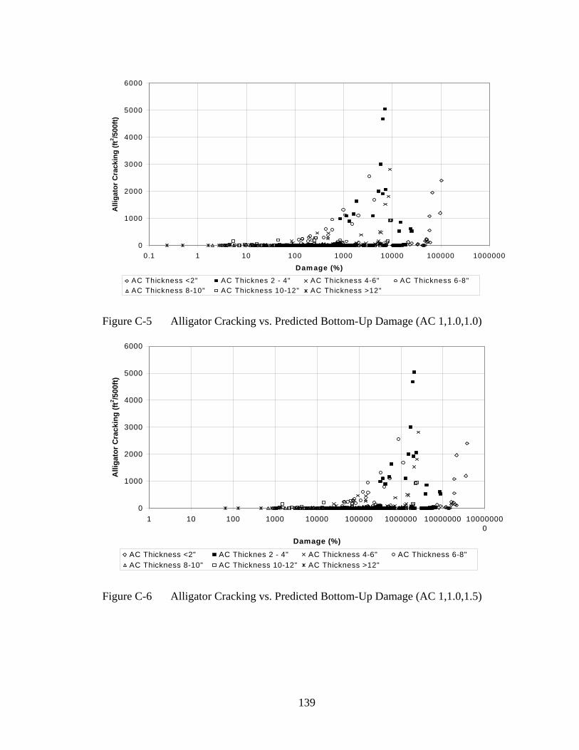
139
0
1000
2000
3000
4000
5000
6000
0.1 1 10 100 1000 10000 100000 1000000
Dam age (%)
Alli
gato
r Cra
ckin
g (ft
2 /500
ft)
AC Thickness <2" AC Thicknes 2 - 4" AC Thickness 4-6" AC Thickness 6-8"AC Thickness 8-10" AC Thickness 10-12" AC Thickness >12"
Figure C-5 Alligator Cracking vs. Predicted Bottom-Up Damage (AC 1,1.0,1.0)
0
1000
2000
3000
4000
5000
6000
1 10 100 1000 10000 100000 1000000 10000000 100000000
Damage (%)
Alli
gato
r Cra
ckin
g (ft
2 /500
ft)
AC Thickness <2" AC Thicknes 2 - 4" AC Thickness 4-6" AC Thickness 6-8"AC Thickness 8-10" AC Thickness 10-12" AC Thickness >12"
Figure C-6 Alligator Cracking vs. Predicted Bottom-Up Damage (AC 1,1.0,1.5)
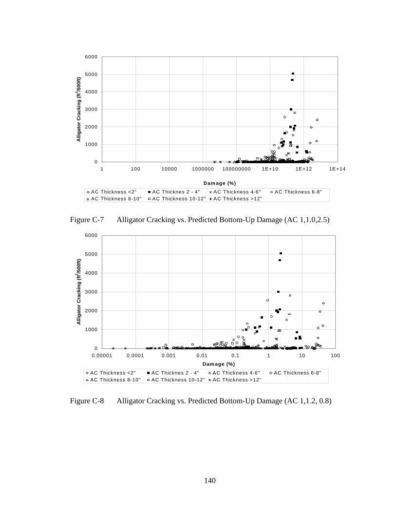
140
0
1000
2000
3000
4000
5000
6000
1 100 10000 1000000 100000000 1E+10 1E+12 1E+14
Dam age (%)
Alli
gato
r Cra
ckin
g (ft
2 /500
ft)
AC Thickness <2" AC Thicknes 2 - 4" AC Thickness 4-6" AC Thickness 6-8"AC Thickness 8-10" AC Thickness 10-12" AC Thickness >12"
Figure C-7 Alligator Cracking vs. Predicted Bottom-Up Damage (AC 1,1.0,2.5)
0
1000
2000
3000
4000
5000
6000
0.00001 0.0001 0.001 0.01 0.1 1 10 100
Damage (%)
Alli
gato
r Cra
ckin
g (ft
2 /500
ft)
AC Thickness <2" AC Thicknes 2 - 4" AC Thickness 4-6" AC Thickness 6-8"AC Thickness 8-10" AC Thickness 10-12" AC Thickness >12"
Figure C-8 Alligator Cracking vs. Predicted Bottom-Up Damage (AC 1,1.2, 0.8)

141
0
1000
2000
3000
4000
5000
6000
0.01 0.1 1 10 100 1000 10000 100000 1000000
Dam age (%)
Alli
gato
r Cra
ckin
g (ft
2 /500
ft)
AC Thickness <2" AC Thicknes 2 - 4" AC Thickness 4-6" AC Thickness 6-8"AC Thickness 8-10" AC Thickness 10-12" AC Thickness >12"
Figure C-9 Alligator Cracking vs. Predicted Bottom-Up Damage (AC 1,1.2,1.5)
0
1000
2000
3000
4000
5000
6000
1 100 10000 1000000 100000000 10000000000 1E+12
Damage (%)
Alli
gato
r Cra
ckin
g (ft
2 /500
ft)
AC Thickness <2" AC Thicknes 2 - 4" AC Thickness 4-6" AC Thickness 6-8"AC Thickness 8-10" AC Thickness 10-12" AC Thickness >12"
Figure C-10 Alligator Cracking vs. Predicted Bottom-Up Damage (AC 1,1.2,2.5)

Annex D
Top-Down Longitudinal Fatigue Cracking Shell Oil Model Calibration

143
Table D-1 Measured Longitudinal Fatigue Cracking and Predicted Top-Down Damage Using Shell Oil Model.
Section Total
Asphalt Thick
Date Time Measured Longitudinal Cracking (ft)
Predicted Top-Down Damage (%) (At Different βf2 and βf3)
Low Medium High Total 0.9,0.9 0.9,1.0 0.9,1.1 1.0,0.9 1.0,1.0
11001 3.2 Sep-91 132 0 0 0 0 0.4687 3.14 21.34 0.00327 0.0212811001 3.2 Apr-92 139 16 0 0 16 0.4827 3.246 22.14 0.00334 0.0217911001 3.2 Jul-92 142 14 0 0 14 0.4955 3.327 22.66 0.00344 0.0223911001 3.2 Jan-93 148 30 0 0 30 0.519 3.496 23.9 0.00358 0.0234 11019 6.7 May-89 32 0.1526 0.9351 5.771 0.001 0.0060411019 6.7 Apr-90 43 0.2051 1.26 7.795 0.00133 0.0080911019 6.7 Jan-91 52 0.248 1.523 9.417 0.00161 0.0097711019 6.7 Jun-91 57 4 0 0 4 0.2729 1.676 10.36 0.00177 0.0107411019 6.7 Mar-92 66 0.3144 1.936 12 0.00203 0.0123511019 6.7 Mar-93 78 139 0 0 139 0.3711 2.287 14.19 0.00239 0.0145611019 6.7 Jul-95 106 0 0 0 0 0.5047 3.112 19.31 0.00324 0.0197711019 6.7 Jan-98 136 0 0 0 0 0.6437 3.981 24.78 0.00411 0.0251514126 13.1 Jun-89 15 0 0 0 0 0.0016 0.0098 0.06034 1E-05 6.3E-0514126 13.1 Mar-91 36 0 0 0 0 0.00396 0.02504 0.1599 2.5E-05 0.0001514126 13.1 Mar-93 60 0 0 0 0 0.00572 0.03673 0.2383 3.4E-05 0.0002214126 13.1 Apr-94 73 0 0 0 0 0.00679 0.04355 0.2816 4.1E-05 0.0002614126 13.1 Dec-95 93 0 0 0 0 0.00816 0.05235 0.3385 4.9E-05 0.0003114126 13.1 Dec-97 117 0 0 0 0 0.0099 0.06389 0.4161 5.8E-05 0.0003721001 3 May-90 83 0 0 0 0 3.853 30.76 245.6 0.03875 0.3094 21001 3 Aug-91 98 0 0 0 0 3.877 30.95 247.1 0.03891 0.3107 21001 3 Aug-93 122 27 0 0 27 4.806 38.36 306.3 0.04823 0.3851 21001 3 Jun-95 144 0 0 0 0 5.721 45.67 364.6 0.05742 0.4584 21001 3 Aug-97 170 0 0 0 0 6.643 53.03 423.4 0.06667 0.5323 21001 3 Aug-98 182 0 0 0 0 7.547 60.25 481 0.07584 0.6055 21002 3.3 May-90 68 0 0 0 0 0.2927 2.416 19.95 0.00243 0.0201 21002 3.3 Aug-91 83 6 0 0 6 0.3407 2.813 23.22 0.00283 0.0234 21002 3.3 Aug-93 107 0 0 0 0 0.4368 3.606 29.78 0.00363 0.0299921002 3.3 Jun-95 129 0 0 0 0 0.533 4.4 36.33 0.00443 0.0366 21002 3.3 Aug-97 155 0 0 0 0 0.6297 5.198 42.92 0.00524 0.0432221002 3.3 May-98 164 0 0 0 0 0.6781 5.599 46.23 0.00564 0.0465540113 4.5 Feb-95 19 0 0 0 0 1.319 7.593 44.65 0.01168 0.0645740113 4.5 Mar-95 20 11 0 0 11 1.331 7.673 45.22 0.01172 0.0649 40113 4.5 Aug-95 25 0 0 0 0 1.974 11.29 65.69 0.0174 0.0963740113 4.5 Nov-95 28 0 0 0 0 2.131 12.22 71.21 0.01855 0.103 40113 4.5 Feb-96 31 0 0 0 0 2.191 12.67 74.57 0.01879 0.1048 40113 4.5 Apr-96 33 0 0 0 0 2.237 12.96 76.48 0.01906 0.1065 40113 4.5 Jul-96 36 0 0 0 0 2.75 15.85 92.82 0.02353 0.1314 40113 4.5 Aug-96 37 0 0 0 0 2.986 17.18 100.4 0.0256 0.143 40113 4.5 Jan-98 54 53 17 0 70 4.525 26.54 158.4 0.03773 0.2137 40113 4.5 Apr-98 57 17 65 0 82 4.586 26.98 161.6 0.03799 0.2155 40113 4.5 Jun-98 59 24 59 0 83 4.856 28.51 170.4 0.04025 0.2283

144
Table D-1 (Cont’d) Measured Longitudinal Fatigue Cracking and Predicted Top-Down Damage Using Shell Oil Model.
Section Total Asphalt Thick
Date Time Measured Longitudinal Cracking (ft)
Predicted Top-Down Damage (%) (At Different βf2 and βf3)
Low Medium High Total 0.9,0.9 0.9,1.0 0.9,1.1 1.0,0.9 1.0,1.0
40113 4.5 Oct-98 63 0 173 0 173 5.524 32.35 192.6 0.04574 0.2595 40114 6.8 Feb-95 19 0 0 0 0 0.5028 3.326 22.22 0.00276 0.0179 40114 6.8 Mar-95 20 31 0 0 31 0.518 3.433 22.97 0.00282 0.0183940114 6.8 Aug-95 25 0 0 0 0 0.846 5.564 36.9 0.0047 0.0304740114 6.8 Nov-95 28 0 0 0 0 0.9953 6.56 43.58 0.00551 0.0357840114 6.8 Feb-96 31 7 0 0 7 1.007 6.644 44.21 0.00555 0.0360840114 6.8 Apr-96 33 9 0 0 9 1.067 7.052 47 0.00585 0.0381140114 6.8 Jul-96 36 44 0 0 44 1.326 8.736 57.99 0.00734 0.0476840114 6.8 Aug-96 37 0 0 0 0 1.432 9.42 62.43 0.00795 0.0516240114 6.8 Jan-98 54 33 40 26 98 2.104 13.91 92.65 0.01158 0.0754540114 6.8 Apr-98 57 0 41 0 41 2.147 14.21 94.76 0.01178 0.0768240114 6.8 Jun-98 59 0 42 0 42 2.311 15.28 101.8 0.01269 0.0827440114 6.8 Oct-98 63 38 23 0 61 2.709 17.9 119.1 0.01491 0.0971940115 15.1 Feb-95 19 0 0 0 0 0.00983 0.05843 0.3506 5.5E-05 0.0003240115 15.1 Mar-95 20 33 0 0 33 0.00984 0.05846 0.3508 5.5E-05 0.0003240115 15.1 Jan-98 54 0 0 0 0 0.02136 0.1298 0.7967 0.00011 0.0006540116 16.2 Feb-95 19 0 0 0 0 0.01907 0.114 0.6868 0.00011 0.0006640116 16.2 Mar-95 20 18 0 0 18 0.01909 0.1141 0.6876 0.00011 0.0006640116 16.2 Jan-98 54 0 0 0 0 0.04171 0.2551 1.573 0.00022 0.0013140117 11.8 Feb-95 19 0 0 0 0 0.01388 0.08951 0.5865 5.9E-05 0.0003740117 11.8 Mar-95 20 14 0 0 14 0.01389 0.08957 0.5869 5.9E-05 0.0003740117 11.8 Jan-98 54 0 0 0 0 0.04383 0.2843 1.866 0.00018 0.0011340118 11.7 Feb-95 19 0 0 0 0 0.00259 0.01843 0.1346 8.5E-06 5.8E-0540118 11.7 Mar-95 20 15 0 0 15 0.00259 0.01843 0.1346 8.5E-06 5.8E-0540118 11.7 Jan-98 54 0 0 0 0 0.00699 0.04967 0.3612 2.2E-05 0.0001541007 6.5 Sep-91 162 0 0 0 0 1.06 6.925 45.56 0.00608 0.0392141007 6.5 Feb-93 163 57 0 0 57 1.074 7.017 46.17 0.00616 0.0397441007 6.5 Sep-94 198 167 0 0 167 1.463 9.566 63 0.00837 0.0540941024 10.8 Nov-89 149 1.826 11.15 68.48 0.00899 0.0542341024 10.8 Aug-90 158 1.975 12.07 74.23 0.0097 0.0585741024 10.8 Oct-92 184 0 0 0 0 2.487 15.24 93.9 0.01214 0.0735141024 10.8 Mar-95 213 9 0 0 9 3.125 19.16 118.1 0.01528 0.0926 41024 10.8 Jul-95 217 23 0 0 23 3.268 20.04 123.6 0.01596 0.0967841024 10.8 Aug-95 218 127 0 0 127 3.326 20.41 125.9 0.01623 0.0984441024 10.8 Nov-95 221 109 0 0 109 3.365 20.65 127.4 0.0164 0.0994741024 10.8 Feb-96 224 61 0 0 61 3.365 20.65 127.4 0.0164 0.0994741024 10.8 Apr-96 226 79 0 23 102 3.376 20.72 127.9 0.01645 0.0997741024 10.8 Jun-96 228 59 0 0 59 3.497 21.47 132.4 0.01704 0.1034 41024 10.8 Aug-96 230 59 0 0 59 3.719 22.82 140.8 0.01816 0.1102 41024 10.8 Apr-98 250 49 0 4 53 4.034 24.8 153.3 0.01959 0.119 41024 10.8 Jun-98 252 49 0 4 53 4.162 25.59 158.1 0.02021 0.1228 41024 10.8 Oct-98 256 50 0 4 54 4.439 27.3 168.8 0.02155 0.131 81029 4.2 Oct-91 233 0 25 0 25 0.2851 2.373 19.77 0.00204 0.0169981029 4.2 Jul-94 266 44 0 0 44 0.3238 2.696 22.47 0.00229 0.0191

145
Table D-1 (Cont’d) Measured Longitudinal Fatigue Cracking and Predicted Top-Down Damage Using Shell Oil Model. Section Total
Asphalt Thick
Date Time Measured Longitudinal Cracking (ft)
Predicted Top-Down Damage (%) (At Different βf2 and βf3)
Low Medium High Total 0.9,0.9 0.9,1.0 0.9,1.1 1.0,0.9 1.0,1.0
81029 4.2 Sep-95 280 11 0 0 11 0.3284 2.734 22.78 0.00232 0.0193 81053 4.6 Oct-89 60 2.285 18.29 146.4 0.02051 0.1642 81053 4.6 Jul-90 69 2.288 18.31 146.6 0.02052 0.1643 81053 4.6 Apr-93 102 92 0 0 92 4.028 32.24 258.1 0.03633 0.291 81053 4.6 Nov-93 109 18 0 0 18 4.068 32.56 260.6 0.03656 0.2928 81053 4.6 Dec-93 110 33 0 0 33 4.069 32.57 260.7 0.03657 0.2928 81053 4.6 Oct-94 120 108 0 0 108 4.078 32.64 261.3 0.03661 0.2932 81053 4.6 Feb-95 124 228 0 0 228 4.08 32.66 261.4 0.03662 0.2932 81053 4.6 May-95 127 229 0 0 229 4.081 32.66 261.4 0.03662 0.2932 81053 4.6 May-96 139 0 0 0 0 4.124 32.99 264 0.03689 0.2953 81053 4.6 Oct-96 144 0 0 0 0 4.843 38.36 304 0.04336 0.3436 81053 4.6 Nov-96 145 33 0 0 33 4.844 38.36 304.1 0.04336 0.3436 81053 4.6 Mar-97 149 45 0 0 45 4.844 38.37 304.1 0.04336 0.3436 91803 7.2 Jul-89 49 6.112 49.57 402.1 0.06723 0.5453 91803 7.2 Sep-90 63 6.97 56.53 458.5 0.07437 0.6032 91803 7.2 Aug-91 74 7 0 0 7 13.99 113.5 920.6 0.1554 1.26 91803 7.2 Sep-92 87 5 0 0 5 14.27 115.8 939 0.1576 1.278 91803 7.2 May-94 107 103 0 0 103 24.96 202.4 1642 0.2771 2.248 91803 7.2 May-95 119 207 7 0 214 25.34 205.5 1667 0.2801 2.272 91803 7.2 Oct-96 136 364 0 0 364 25.6 207.7 1684 0.2819 2.286 91803 7.2 May-97 143 557 0 0 557 26.92 218.3 1771 0.2923 2.371 91803 7.2 Sep-97 147 74 0 0 74 26.92 218.3 1771 0.2923 2.371 91803 7.2 Jun-98 156 279 11 0 290 40.73 330.4 2679 0.4517 3.664 120103 12 Dec-96 14 0 0 0 0 4.8E-05 0.00033 0.00222 1.4E-07 9.3E-07120104 18 Dec-96 14 0 0 0 0 0.00033 0.00212 0.01374 1.4E-06 8.9E-06120105 7.9 Dec-96 14 0 0 0 0 0.00387 0.02545 0.1681 1.7E-05 0.00011120106 15 Dec-96 14 0 0 0 0 0.00025 0.00162 0.01034 1.1E-06 6.8E-06123995 5 Apr-92 197 34 0 0 34 5.39 39.56 291.3 0.02211 0.1616 123995 5 Mar-94 220 82 0 0 82 6.065 44.56 328.5 0.02485 0.1819 123995 5 Jan-96 242 215 0 0 215 6.703 49.25 363.1 0.02745 0.201 123995 5 Jan-96 243 72 0 0 72 6.736 49.5 365.1 0.02758 0.202 123997 3.1 Aug-90 195 1.855 11.7 74.28 0.01558 0.09673123997 3.1 Oct-91 209 2.077 13.11 83.21 0.01745 0.1084 123997 3.1 Mar-93 226 2.279 14.41 91.63 0.01906 0.1186 123997 3.1 Mar-94 238 2.459 15.56 99.02 0.02053 0.1278 124105 2.3 Apr-89 53 0 0 0 0 68.3 428.8 2706 0.7973 4.942 124105 2.3 Oct-91 83 0 0 0 0 115.9 729.5 4615 1.349 8.387 124105 2.3 Mar-93 100 0 0 0 0 135 851.9 5403 1.562 9.733 124106 8.2 Apr-89 21 0.0439 0.292 1.95 0.00017 0.00112124106 8.2 Feb-91 43 0.1039 0.6965 4.688 0.0004 0.00264124106 8.2 Jul-91 48 0 0 0 0 0.1195 0.8005 5.383 0.00046 0.00304124106 8.2 Mar-94 80 10 0 0 10 0.2103 1.419 9.612 0.00079 0.00532124106 8.2 Jan-97 114 50 0 0 50 0.3117 2.109 14.32 0.00117 0.00788124107 2.7 Dec-89 75 0 0 0 0 1.006 6.532 42.56 0.00925 0.05946124107 2.7 Feb-91 89 261 0 0 261 1.183 7.711 50.43 0.01075 0.06938

146
Table D-1 (Cont’d) Measured Longitudinal Fatigue Cracking and Predicted Top-Down Damage Using Shell Oil Model. Section Total
Asphalt Thick
Date Time Measured Longitudinal Cracking (ft)
Predicted Top-Down Damage (%) (At Different βf2 and βf3)
Low Medium High Total 0.9,0.9 0.9,1.0 0.9,1.1 1.0,0.9 1.0,1.0
124107 2.7 Jul-91 94 343 0 0 343 1.283 8.363 54.67 0.01168 0.07536124107 2.7 Mar-93 114 18 0 0 18 1.61 10.52 68.9 0.01457 0.09419124107 2.7 Mar-94 126 37 13 0 51 1.808 11.83 77.66 0.01627 0.1054 124107 2.7 Jan-96 148 67 0 0 67 2.239 14.67 96.44 0.02007 0.1302 124107 2.7 Mar-97 162 0 0 0 0 2.503 16.42 108.1 0.02235 0.1451 124108 9.9 Apr-89 35 0 0 0 0 0.00389 0.02491 0.1619 2.4E-05 0.00015124108 9.9 Jan-91 56 0 0 0 0 0.00494 0.03164 0.205 2.9E-05 0.00018124108 9.9 Oct-91 65 0 0 0 0 0.00706 0.04675 0.3134 4.1E-05 0.00026124108 9.9 Mar-94 94 7 0 0 7 0.00824 0.0544 0.3635 4.6E-05 0.0003 124108 9.9 Aug-94 99 0 0 0 0 0.01048 0.07062 0.4812 5.8E-05 0.00039124108 9.9 Jan-96 116 0 0 0 0 0.01116 0.07508 0.5108 6.1E-05 0.00041124135 1.4 Dec-89 227 99 199 0 298 13450 91930 635300 227.1 1538 124135 1.4 Jan-91 240 412 271 0 683 13970 95340 658100 235.3 1592 131031 11.1 Apr-91 119 0.00681 0.05514 0.4469 3E-05 0.00024131031 11.1 Jul-92 134 0.00688 0.05562 0.4503 3E-05 0.00024131031 11.1 Jan-93 140 0.00981 0.07945 0.6442 4.3E-05 0.00035131031 11.1 Apr-94 155 0.01198 0.09702 0.7868 5.2E-05 0.00043131031 11.1 Oct-94 161 0.01203 0.09739 0.7892 5.3E-05 0.00043131031 11.1 Aug-95 171 0.01209 0.09776 0.7919 5.3E-05 0.00043131031 11.1 Jan-96 176 0.01631 0.1321 1.072 7.2E-05 0.00058131031 11.1 Apr-96 179 0.01631 0.1321 1.072 7.2E-05 0.00058134111 8.7 Mar-89 101 27 0 0 27 0.01282 0.1038 0.8428 5.2E-05 0.00042134111 8.7 Mar-91 125 291 0 0 291 0.022 0.1786 1.453 8.7E-05 0.00071134111 8.7 Feb-92 136 477 0 0 477 0.02222 0.1799 1.461 8.8E-05 0.00071134112 15.9 May-89 144 0 0 0 0 0.02868 0.1692 1.003 0.00027 0.00154134112 15.9 Feb-91 165 17 0 0 17 0.03227 0.1914 1.14 0.00029 0.0017 134112 15.9 Apr-91 167 0 0 0 0 0.03228 0.1915 1.141 0.00029 0.0017 134112 15.9 Feb-94 201 0 0 0 0 0.04852 0.2885 1.723 0.00044 0.00257134112 15.9 Oct-94 209 0 0 0 0 0.05106 0.3043 1.821 0.00046 0.00269134112 15.9 Jan-96 224 0 0 0 0 0.05353 0.3195 1.915 0.00048 0.0028 134112 15.9 Feb-97 237 0 0 0 0 0.06179 0.3687 2.209 0.00055 0.00325134112 15.9 Apr-98 251 0 0 0 0 0.06446 0.3853 2.312 0.00057 0.00337134113 15.2 May-89 144 0 0 0 0 0.08602 0.4907 2.811 0.00088 0.00497134113 15.2 Feb-91 165 0 0 0 0 0.09493 0.544 3.13 0.00096 0.0054 134113 15.2 Apr-91 167 0 0 0 0 0.09496 0.5442 3.132 0.00096 0.0054 134113 15.2 Feb-94 201 0 0 0 0 0.1389 0.7989 4.61 0.0014 0.00795134113 15.2 Oct-94 209 0 0 0 0 0.1456 0.8387 4.849 0.00146 0.00828134113 15.2 Jan-96 224 0 0 0 0 0.1519 0.8761 5.073 0.00151 0.0086 134113 15.2 Feb-97 237 31 0 0 31 0.1735 1.001 5.798 0.00173 0.00987134113 15.2 Apr-98 251 37 0 0 37 0.1809 1.045 6.059 0.0018 0.01024161001 3.7 Jul-89 192 155 0 0 155 3.553 29.76 249.8 0.02209 0.1854 161001 3.7 Aug-90 205 193 0 0 193 3.836 32.12 269.5 0.0237 0.1989 161001 3.7 Jun-93 239 78 0 0 78 4.827 40.44 339.4 0.02955 0.248 161001 3.7 Aug-94 253 199 0 0 199 5.092 42.63 357.6 0.03091 0.2593

147
Table D-1 (Cont’d) Measured Longitudinal Fatigue Cracking and Predicted Top-Down Damage Using Shell Oil Model. Section Total
Asphalt Thick
Date Time Measured Longitudinal Cracking (ft)
Predicted Top-Down Damage (%) (At Different βf2 and βf3)
Low Medium High Total 0.9,0.9 0.9,1.0 0.9,1.1 1.0,0.9 1.0,1.0
161001 3.7 May-95 262 183 2 0 185 5.843 48.99 411.5 0.03576 0.3003 161001 3.7 Jul-97 288 67 63 44 175 6.275 52.55 441 0.03788 0.3179 161001 3.7 Sep-98 302 0 159 5 164 7.16 60 503.7 0.0435 0.3653 161009 10.4 Sep-89 180 1.32 10.43 82.44 0.01175 0.09283161009 10.4 Jul-90 190 1.599 12.63 99.84 0.01401 0.1108 161009 10.4 Jul-92 214 0 0 0 0 1.651 13.04 103.1 0.01435 0.1134 161009 10.4 Oct-93 229 8 0 0 8 1.994 15.75 124.5 0.01715 0.1355 161009 10.4 Jun-96 261 1 0 0 1 2.109 16.67 131.7 0.01787 0.1413 161009 10.4 Jul-97 274 0 0 0 0 2.549 20.14 159.2 0.02145 0.1695 161021 5.9 Sep-89 48 0.06179 0.4932 3.939 0.00046 0.0037 161021 5.9 Oct-90 61 0 0 0 0 0.06304 0.5027 4.013 0.00047 0.00374161021 5.9 Aug-91 71 0 0 0 0 0.1229 0.982 7.848 0.00093 0.00743161021 5.9 Aug-93 95 0 0 0 0 0.1252 0.9993 7.983 0.00094 0.0075 161021 5.9 Sep-95 120 0 0 0 0 0.1886 1.506 12.04 0.00142 0.01137161021 5.9 Jun-96 129 5 0 0 5 0.1893 1.512 12.08 0.00143 0.01139161021 5.9 Jul-97 142 0 0 0 0 0.1907 1.523 12.17 0.00143 0.01144169034 9.2 Jul-89 10 0.00216 0.01664 0.1293 8.1E-06 6.2E-05169034 9.2 Aug-90 23 0.03494 0.2771 2.202 0.00019 0.00154169034 9.2 Jun-93 57 12 0 0 12 0.2764 2.206 17.61 0.00183 0.01457169034 9.2 Aug-94 71 146 0 0 146 0.4801 3.833 30.6 0.00324 0.02588169034 9.2 May-95 80 0.4821 3.848 30.73 0.00325 0.02594169034 9.2 Jul-97 106 217 0 0 217 0.7135 5.696 45.48 0.00482 0.03846169034 9.2 Sep-98 120 156 52 18 226 0.7162 5.716 45.63 0.00483 0.03853201009 11.1 Aug-88 44 0 0 0 0 23 190.6 1580 0.2424 2.009 201009 11.1 May-89 53 11 0 0 11 23.27 192.8 1598 0.2441 2.023 201009 11.1 Dec-90 72 210 5 0 215 41.29 342.2 2836 0.4415 3.659 201009 11.1 Oct-91 82 6 1 0 7 45.08 373.5 3096 0.4778 3.959 201009 11.1 Apr-93 100 9 0 0 9 60.91 504.7 4183 0.6528 5.41 201009 11.1 Apr-95 124 16 28 0 43 72.59 601.6 4985 0.767 6.356 201009 11.1 Apr-96 136 0 0 0 0 73.18 606.5 5026 0.7716 6.394 201009 11.1 Jan-99 168 0 0 0 0 85.64 709.7 5881 0.887 7.35 251003 6.6 Aug-89 180 758 0 0 758 1.99 15.88 126.7 0.02022 0.1613 251003 6.6 Sep-90 193 691 0 0 691 2.401 19.16 152.9 0.02425 0.1935 251003 6.6 Aug-91 204 556 1 0 557 2.418 19.29 153.9 0.02435 0.1944 251003 6.6 Sep-92 217 600 0 0 600 2.469 19.69 157.1 0.02474 0.1974 251003 6.6 Oct-95 254 563 0 0 563 2.951 23.54 187.8 0.02936 0.2343 251003 6.6 Oct-96 266 39 0 0 39 3.008 23.99 191.4 0.02978 0.2377 251003 6.6 Jun-98 286 32 9 0 41 3.514 28.03 223.6 0.0347 0.2769 251004 9.6 Aug-89 178 0 0 0 0 0.5757 4.496 35.13 0.00446 0.03485251004 9.6 Sep-90 191 19 0 0 19 0.6286 4.909 38.36 0.00483 0.03771251004 9.6 Aug-91 202 16 0 0 16 0.7356 5.746 44.9 0.00566 0.04419251004 9.6 Sep-92 215 0 0 0 0 0.738 5.763 45.02 0.00567 0.04428251004 9.6 Oct-95 252 0 0 0 0 1.071 8.362 65.35 0.00819 0.06399251004 9.6 Jun-97 272 3 0 0 3 1.152 8.998 70.31 0.00875 0.06836
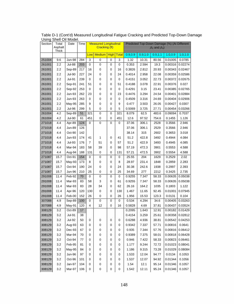
148
Table D-1 (Cont’d) Measured Longitudinal Fatigue Cracking and Predicted Top-Down Damage Using Shell Oil Model. Section Total
Asphalt Thick
Date Time Measured Longitudinal Cracking (ft)
Predicted Top-Down Damage (%) (At Different βf2 and βf3)
Low Medium High Total 0.9,0.9 0.9,1.0 0.9,1.1 1.0,0.9 1.0,1.0
251004 9.6 Jun-98 284 3 0 0 3 1.32 10.31 80.56 0.01005 0.0785 261001 2.2 Jul-88 203 0 0 0 0 0.353 2.594 19.3 0.00316 0.02274261001 2.2 Sep-89 217 16 0 0 16 0.3826 2.812 20.93 0.00343 0.02467261001 2.2 Jul-90 227 24 0 0 24 0.4014 2.958 22.08 0.00359 0.02586261001 2.2 Jul-91 239 0 0 0 0 0.4151 3.052 22.73 0.00372 0.02675261001 2.2 Sep-91 241 51 0 0 51 0.4188 3.078 22.91 0.00376 0.027 261001 2.2 Sep-92 253 0 0 0 0 0.4291 3.15 23.41 0.00385 0.02765261001 2.2 Jun-93 262 23 0 0 23 0.4476 3.294 24.54 0.00401 0.02884261001 2.2 Jun-93 263 0 0 0 0 0.4509 3.316 24.69 0.00404 0.02906261001 2.2 May-95 285 9 0 0 9 0.477 3.503 26.05 0.00427 0.0307 261001 2.2 Jul-96 299 5 0 0 5 0.5069 3.725 27.71 0.00454 0.03266261004 4.2 Sep-89 51 321 0 0 321 8.079 62.5 483.6 0.09094 0.7037 261004 4.2 Jul-90 61 451 0 0 451 12.6 97.52 754.6 0.1455 1.126 271018 4.4 Apr-89 124 0 0 0 0 37.06 306.1 2528 0.3566 2.946 271018 4.4 Jun-89 126 37.06 306.1 2529 0.3566 2.946 271018 4.4 Oct-90 142 38.14 315 2602 0.3653 3.018 271018 4.4 Jun-93 174 41 1 0 41 51.2 422.8 3492 0.4944 4.084 271018 4.4 Jul-93 176 7 51 0 57 51.2 422.9 3493 0.4945 4.085 271018 4.4 Mar-94 183 58 39 0 98 57.19 472.3 3901 0.5553 4.588 271018 4.4 Aug-94 188 131 0 0 131 57.21 472.5 3902 0.5554 4.588 271087 15.7 Oct-91 154 0 0 0 0 25.55 204 1629 0.2529 2.02 271087 15.7 May-93 173 8 0 0 8 28.97 231.4 1848 0.2859 2.283 271087 15.7 Oct-94 190 24 0 0 24 30.38 242.6 1938 0.2997 2.393 271087 15.7 Jun-96 210 25 0 0 25 34.69 277 2212 0.3425 2.735 291008 11.4 Feb-92 70 0 0 0 0 0.9255 7.347 58.33 0.00635 0.05038291008 11.4 Mar-93 83 58 3 0 61 0.9255 7.347 58.33 0.00635 0.05038291008 11.4 Mar-93 83 28 34 0 62 26.16 164.2 1035 0.1803 1.122 291008 11.4 Apr-96 120 130 0 0 130 1.467 11.65 92.45 0.01001 0.07945291008 11.4 Feb-00 152 26 0 0 26 1.956 15.53 123.3 0.0131 0.104 307088 4.9 Sep-89 100 0 0 0 0 0.534 4.294 34.6 0.00405 0.03263307088 4.9 May-91 120 4 12 0 16 0.5828 4.69 37.81 0.00437 0.03524308129 3.2 Oct-89 17 0.2095 1.643 12.91 0.00182 0.01429308129 3.2 Jul-91 38 0.4154 3.259 25.61 0.00358 0.02812308129 3.2 Jul-92 50 0 0 0 0 0.6288 4.936 38.81 0.00542 0.04253308129 3.2 Aug-93 63 0 0 0 0 0.9342 7.337 57.71 0.00816 0.0641 308129 3.2 Dec-93 67 0 0 0 0 0.935 7.344 57.76 0.00816 0.06412308129 3.2 Mar-94 70 0 0 0 0 0.9389 7.375 58.01 0.00818 0.06428308129 3.2 Oct-94 77 0 0 0 0 0.946 7.422 58.33 0.00823 0.06461308129 3.2 Feb-95 81 0 0 0 0 1.177 9.244 72.72 0.01023 0.08041308129 3.2 May-95 84 0 0 0 0 1.186 9.315 73.28 0.01029 0.08084308129 3.2 Jun-96 97 0 0 0 0 1.533 12.04 94.77 0.0134 0.1053 308129 3.2 Oct-96 101 0 0 0 0 1.537 12.07 94.92 0.01344 0.1056 308129 3.2 Jan-97 104 0 0 0 0 1.54 12.1 95.14 0.01346 0.1057 308129 3.2 Mar-97 106 0 0 0 0 1.542 12.11 95.24 0.01346 0.1057

149
Table D-1 (Cont’d) Measured Longitudinal Fatigue Cracking and Predicted Top-Down Damage Using Shell Oil Model. Section Total
Asphalt Thick
Date Time Measured Longitudinal Cracking (ft)
Predicted Top-Down Damage (%) (At Different βf2 and βf3)
Low Medium High Total 0.9,0.9 0.9,1.0 0.9,1.1 1.0,0.9 1.0,1.0
308129 3.2 Aug-97 111 0 0 0 0 1.549 12.16 95.57 0.01352 0.1061 308129 3.2 Oct-97 113 0 0 0 0 1.55 12.16 95.6 0.01352 0.1061 321020 7 Jul-91 86 34 0 0 34 6.581 54.74 455.3 0.06323 0.526 321020 7 Aug-93 111 138 0 0 138 10.68 88.82 738.8 0.1039 0.864 321020 7 Sep-94 123 29 20 0 49 11.04 91.85 764 0.1065 0.8857 321020 7 Apr-95 131 242 0 0 242 11.28 93.78 780.1 0.1079 0.898 321020 7 Jun-97 157 9 0 0 9 14.19 118 981.8 0.1332 1.108 321020 7 Jun-98 169 0 0 0 0 14.46 120.3 1000 0.1349 1.122 341031 7.3 Apr-92 224 333 1 0 333 7.638 59.57 466 0.06787 0.5304 341031 7.3 Feb-93 234 322 31 3 356 7.721 60.11 469.7 0.06849 0.5344 341031 7.3 Oct-95 266 0 352 170 522 8.155 63.16 491.3 0.0715 0.5553 341031 7.3 Nov-95 267 232 30 0 261 10.54 82.13 641.9 0.09229 0.7203 341033 7.4 Apr-92 211 52 2 0 54 0.1531 1.233 9.937 0.00113 0.00908341033 7.4 Feb-93 221 32 11 0 44 0.1579 1.272 10.25 0.00116 0.00931341033 7.4 Nov-95 254 55 0 0 55 0.1985 1.599 12.89 0.00146 0.01173341033 7.4 Jul-97 274 260 0 0 260 0.2036 1.64 13.22 0.00149 0.01198341034 11.1 Oct-89 48 0 0 0 0 3.808 30.53 244.7 0.03281 0.263 341034 11.1 Sep-90 59 0 0 0 0 3.81 30.54 244.8 0.03282 0.2631 341034 11.1 Apr-92 78 0 0 0 0 6.113 49 392.8 0.05179 0.4152 341034 11.1 Feb-93 88 0 0 0 0 6.115 49.02 393 0.0518 0.4152 341034 11.1 Nov-95 121 3 0 0 3 8.824 70.73 567 0.07411 0.5941 341034 11.1 Jul-97 141 0 15 0 15 11.62 93.15 746.8 0.09732 0.7802 350101 7.2 May-97 19 0 0 0 0 0.4642 3.491 26.68 0.00261 0.01935350102 4.8 May-97 19 0 0 0 0 1.322 10.13 78.43 0.00777 0.05922350103 12.5 May-97 19 0 0 0 0 0.05354 0.4397 3.611 0.00022 0.00185350104 19.2 May-97 19 0 0 0 0 0.00022 0.0013 0.00762 1.1E-06 6.6E-06350105 9.9 May-97 19 0 0 0 0 0.08719 0.7126 5.834 0.00038 0.00313350106 15.6 May-97 19 0 0 0 0 0.03823 0.3054 2.44 0.00016 0.0013 351005 8.9 Oct-89 73 0 0 0 0 0.1388 1.109 8.912 0.00081 0.00644351005 8.9 Mar-91 90 0 0 0 0 0.2307 1.853 14.97 0.00136 0.01089351005 8.9 Oct-92 109 0 0 0 0 0.2498 1.994 16.02 0.00145 0.01159351005 8.9 Feb-94 125 0 0 0 0 0.2785 2.217 17.77 0.0016 0.01272351005 8.9 Mar-95 138 0 0 0 0 0.4027 3.228 26.02 0.00234 0.01871351005 8.9 Apr-97 163 0 0 0 0 0.4518 3.6 28.88 0.00258 0.02056351022 6.3 Oct-89 37 0 0 0 0 0.2029 1.625 13.06 0.00139 0.01116351022 6.3 Mar-91 54 0 0 0 0 0.5071 4.101 33.23 0.00351 0.02844351022 6.3 Oct-92 73 0 0 0 0 0.5259 4.231 34.15 0.00361 0.0291 351022 6.3 Feb-94 89 0 0 0 0 0.9359 7.569 61.34 0.00645 0.05226351022 6.3 Mar-95 102 0 0 0 0 0.9492 7.664 62.03 0.00652 0.05272351022 6.3 Apr-97 127 0 0 0 0 1.818 14.74 119.6 0.01274 0.1035 351112 6.3 Dec-89 67 0.2074 1.456 10.33 0.00105 0.00729351112 6.3 Jan-91 80 0.2468 1.739 12.37 0.00125 0.00866351112 6.3 Mar-91 82 0 0 0 0 0.2486 1.753 12.47 0.00126 0.00872351112 6.3 Jan-93 104 0 0 0 0 0.3237 2.279 16.2 0.00164 0.01136351112 6.3 Feb-94 117 0 0 0 0 0.3632 2.562 18.25 0.00183 0.01274
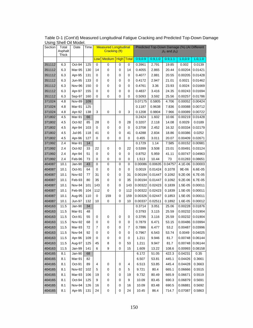
150
Table D-1 (Cont’d) Measured Longitudinal Fatigue Cracking and Predicted Top-Down Damage Using Shell Oil Model. Section Total
Asphalt Thick
Date Time Measured Longitudinal Cracking (ft)
Predicted Top-Down Damage (%) (At Different βf2 and βf3)
Low Medium High Total 0.9,0.9 0.9,1.0 0.9,1.1 1.0,0.9 1.0,1.0
351112 6.3 Oct-94 125 0 0 0 0 0.3961 2.791 19.85 0.002 0.0139 351112 6.3 Mar-95 130 14 0 0 14 0.4055 2.865 20.44 0.00204 0.01421351112 6.3 Apr-95 131 0 0 0 0 0.4077 2.881 20.55 0.00205 0.01428351112 6.3 Jun-95 133 0 0 0 0 0.4172 2.947 21.01 0.0021 0.01462351112 6.3 Nov-96 150 0 0 0 0 0.4761 3.36 23.93 0.0024 0.01669351112 6.3 Apr-97 155 0 0 0 0 0.4837 3.416 24.35 0.00243 0.01694351112 6.3 Sep-97 160 0 0 0 0 0.5093 3.592 25.56 0.00257 0.01786371024 4.8 Nov-89 109 0.07175 0.5805 4.706 0.00052 0.00424371024 4.8 Mar-91 125 0.1187 0.9638 7.836 0.00088 0.00712371024 4.8 Apr-92 138 3 0 0 3 0.1208 0.9804 7.966 0.00089 0.00722371802 4.5 Mar-91 66 0.2424 1.602 10.66 0.00219 0.01428371802 4.5 Oct-92 85 28 0 0 28 0.3207 2.118 14.08 0.0029 0.0189 371802 4.5 Apr-94 103 0 0 0 0 0.3708 2.452 16.32 0.00334 0.02179371802 4.5 Jul-95 118 41 0 0 41 0.4288 2.834 18.86 0.00386 0.0252 371802 4.5 Apr-96 127 0 0 0 0 0.455 3.011 20.07 0.00409 0.02671371992 2.4 Mar-91 14 0.1729 1.14 7.585 0.00152 0.00981371992 2.4 Oct-92 33 22 0 0 22 0.5399 3.508 23.01 0.00491 0.03124371992 2.4 Apr-94 51 0 0 0 0 0.8752 5.959 41.11 0.00747 0.04963371992 2.4 Feb-96 73 0 0 0 0 1.513 10.44 73 0.01283 0.08651404087 10.1 Jan-90 43 0 0 0 0 0.00086 0.00635 0.04757 4.1E-06 0.00003404087 10.1 Oct-91 64 0 0 0 0 0.0019 0.01424 0.1078 9E-06 6.6E-05404087 10.1 Nov-92 77 31 0 0 31 0.00194 0.01447 0.1092 9.2E-06 6.7E-05404087 10.1 Feb-93 80 35 0 0 35 0.00194 0.01447 0.1092 9.2E-06 6.7E-05404087 10.1 Nov-94 101 143 0 0 143 0.00322 0.02423 0.1839 1.5E-05 0.00011404087 10.1 Feb-95 104 112 0 0 112 0.00322 0.02423 0.1839 1.5E-05 0.00011404087 10.1 Aug-95 110 0 159 0 159 0.00326 0.02447 0.1853 1.5E-05 0.00011404087 10.1 Jun-97 132 10 0 0 10 0.00337 0.02511 0.1892 1.6E-05 0.00012404163 11.5 Jan-90 34 0.3714 3.051 25.06 0.00228 0.01876404163 11.5 Mar-91 48 0.3793 3.115 25.59 0.00232 0.01904404163 11.5 Oct-91 55 0 0 0 0 0.3795 3.116 25.59 0.00232 0.01904404163 11.5 Nov-92 68 0 0 0 0 0.7879 6.471 53.15 0.00486 0.03994404163 11.5 Mar-93 72 7 0 0 7 0.7886 6.477 53.2 0.00487 0.03996404163 11.5 Nov-94 92 0 0 0 0 0.7967 6.543 53.74 0.0049 0.04025404163 11.5 Apr-96 109 0 0 0 0 1.211 9.946 81.7 0.00748 0.06144404163 11.5 Aug-97 125 45 8 0 53 1.211 9.947 81.7 0.00748 0.06144404163 11.5 Jan-99 141 6 9 0 15 1.609 13.22 108.6 0.00993 0.08158404165 8.1 Jan-90 68 6.172 51.05 422.3 0.04231 0.35 404165 8.1 Mar-91 82 6.507 53.81 445.1 0.04426 0.3661 404165 8.1 Oct-91 89 4 0 0 4 6.513 53.85 445.4 0.04428 0.3663 404165 8.1 Nov-92 102 5 0 0 5 9.721 80.4 665.1 0.06666 0.5515 404165 8.1 Mar-93 106 19 0 0 19 9.732 80.49 665.9 0.06671 0.5519 404165 8.1 Oct-94 125 9 0 0 9 10.09 83.45 690.3 0.06879 0.5691 404165 8.1 Nov-94 126 16 0 0 16 10.09 83.48 690.5 0.06881 0.5692 404165 8.1 Apr-95 131 24 0 0 24 10.45 86.4 714.7 0.07087 0.5863

151
Table D-1 (Cont’d) Measured Longitudinal Fatigue Cracking and Predicted Top-Down Damage Using Shell Oil Model. Section Total
Asphalt Thick
Date Time Measured Longitudinal Cracking (ft)
Predicted Top-Down Damage (%) (At Different βf2 and βf3)
Low Medium High Total 0.9,0.9 0.9,1.0 0.9,1.1 1.0,0.9 1.0,1.0
404165 8.1 Jun-95 133 25 0 0 25 10.45 86.41 714.7 0.07088 0.5863 404165 8.1 Apr-96 143 25 0 0 25 13.88 114.8 950 0.09483 0.7846 404165 8.1 Nov-96 150 60 0 0 60 13.89 114.9 950.2 0.09486 0.7848 404165 8.1 May-97 156 26 0 0 26 13.9 115 951.1 0.09491 0.7852 404165 8.1 Sep-97 160 24 0 0 24 13.91 115 951.3 0.09493 0.7853 421599 12.3 Aug-89 25 11.92 97.97 805.4 0.1252 1.029 421599 12.3 Sep-90 38 19.32 158.8 1306 0.2061 1.695 421599 12.3 Mar-93 68 0 0 0 0 42.25 347.3 2855 0.4507 3.705 421599 12.3 Sep-94 86 0 0 0 0 42.71 351.1 2886 0.4539 3.731 421599 12.3 Jun-95 95 8 0 0 8 59.15 486.3 3997 0.6282 5.164 421599 12.3 Jul-96 108 4 0 0 4 69.65 572.5 4707 0.743 6.108 421599 12.3 Mar-98 128 2 0 0 2 70.77 581.7 4782 0.7508 6.172 451011 3.2 Mar-92 69 0 0 0 0 1.043 6.627 42.44 0.00809 0.05027451011 3.2 Oct-92 76 0 0 0 0 1.235 7.82 49.92 0.00964 0.05986451011 3.2 Jun-93 84 0 0 0 0 1.301 8.262 52.91 0.01007 0.06266451011 3.2 Jan-96 115 16 0 0 16 1.755 11.18 71.8 0.01353 0.0844 451011 3.2 Jun-97 132 0 0 0 0 1.984 12.66 81.42 0.01522 0.09512451011 3.2 Feb-99 150 0 0 0 0 2.296 14.65 94.22 0.01765 0.1103 473104 1.3 Aug-89 39 2.953 18.99 123 0.06208 0.3923 473104 1.3 Nov-89 42 2.988 19.24 124.8 0.06252 0.3954 473104 1.3 May-91 60 3.181 20.62 134.8 0.0649 0.4123 473104 1.3 Aug-91 63 3.216 20.85 136.3 0.06538 0.4154 473104 1.3 Oct-92 77 3.418 22.27 146.4 0.06798 0.4336 473104 1.3 Aug-93 87 3.559 23.29 153.7 0.06976 0.4461 473104 1.3 Nov-95 114 4.126 27.32 182.5 0.07729 0.499 473104 1.3 Oct-96 125 4.354 28.92 194 0.08027 0.5198 480001 2.4 Apr-89 1 0.2568 1.481 8.594 0.00344 0.01955480001 2.4 Oct-90 19 9.736 55.7 320.6 0.1383 0.7795 480001 2.4 May-91 26 0 0 0 0 11.03 63.7 370.4 0.153 0.8687 480001 2.4 Feb-93 47 0 0 0 0 22.91 133 777.7 0.3149 1.799 480001 2.4 Apr-93 49 0 0 0 0 23.53 136.8 801 0.322 1.842 480001 2.4 Feb-95 71 0 0 0 0 37.23 218.2 1287 0.5002 2.886 480001 2.4 Mar-95 72 0 0 0 0 37.46 219.7 1296 0.5026 2.901 480001 2.4 May-97 98 34 0 0 34 54.66 322.7 1917 0.7203 4.187 480001 2.4 Mar-98 108 34 0 0 34 63.33 374.2 2224 0.8338 4.851 481060 7.5 Jun-90 52 0 0 0 0 10.25 65.28 417.7 0.05783 0.3644 481060 7.5 Feb-91 60 0 0 0 0 12.38 78.93 505.7 0.06967 0.4396 481060 7.5 Apr-91 62 0 0 0 0 12.73 81.26 521.4 0.07133 0.4506 481060 7.5 Mar-92 73 12 0 0 12 16.06 102.6 658.4 0.08994 0.5686 481060 7.5 Feb-93 84 19 0 0 19 19.51 124.8 801.8 0.1091 0.6904 481060 7.5 Mar-93 85 23 0 0 23 19.6 125.4 806 0.1095 0.6931 481060 7.5 Oct-94 104 14 0 0 14 27.79 178 1146 0.1548 0.9821 481060 7.5 Feb-95 108 28 0 0 28 28.04 179.8 1158 0.1559 0.9897 481060 7.5 Mar-95 109 0 0 0 0 28.15 180.5 1163 0.1564 0.9929

152
Table D-1 (Cont’d) Measured Longitudinal Fatigue Cracking and Predicted Top-Down Damage Using Shell Oil Model. Section Total
Asphalt Thick
Date Time Measured Longitudinal Cracking (ft)
Predicted Top-Down Damage (%) (At Different βf2 and βf3)
Low Medium High Total 0.9,0.9 0.9,1.0 0.9,1.1 1.0,0.9 1.0,1.0
481060 7.5 Mar-95 112 14 0 0 14 29.46 189 1219 0.1634 1.038 481060 7.5 Jun-95 134 8 0 0 8 37.8 242.9 1568 0.209 1.33 481060 7.5 Apr-97 137 31 0 0 31 40.02 257.1 1659 0.2216 1.409 481060 7.5 Jul-97 139 31 2 0 33 41.77 268.2 1730 0.2316 1.473 481060 7.5 Sep-97 154 32 0 0 32 47.93 308.2 1991 0.2648 1.686 481077 5.1 Apr-89 88 1.715 13.22 102.1 0.01095 0.08462481077 5.1 Nov-91 119 0 0 0 0 2.55 19.67 151.9 0.01632 0.1261 481077 5.1 Oct-92 130 28 0 0 28 2.82 21.75 167.9 0.01794 0.1387 481077 5.1 May-93 137 124 0 0 124 2.841 21.91 169.1 0.01802 0.1393 481077 5.1 Oct-94 154 143 0 0 143 2.883 22.21 171.3 0.01819 0.1405 481077 5.1 Mar-95 159 47 0 0 47 3.603 27.8 214.7 0.02279 0.1762 481077 5.1 Apr-95 160 181 0 0 181 3.605 27.81 214.8 0.02279 0.1762 481077 5.1 Jun-95 162 181 0 0 181 3.609 27.84 215 0.02281 0.1763 481077 5.1 Aug-95 164 181 0 0 181 3.613 27.86 215.1 0.02283 0.1764 481077 5.1 Jun-96 174 181 0 0 181 3.643 28.09 216.8 0.02294 0.1773 481077 5.1 May-97 185 228 10 0 238 3.675 28.33 218.5 0.02307 0.1782 481077 5.1 Jul-97 187 300 0 0 300 3.679 28.35 218.7 0.02309 0.1783 481077 5.1 Sep-97 189 276 0 0 276 3.683 28.37 218.9 0.0231 0.1784 481077 5.1 Mar-98 195 281 0 0 281 4.482 34.58 267 0.02822 0.2182 481109 6.5 Jan-90 68 2.502 14.02 79.3 0.02236 0.1234 481109 6.5 Sep-90 76 2.836 15.91 89.94 0.02522 0.1394 481109 6.5 May-91 84 123 0 0 123 3.21 18.13 103.2 0.02826 0.1573 481109 6.5 Feb-93 105 148 0 0 148 4.217 23.98 137.4 0.03657 0.2054 481109 6.5 Jul-93 110 336 0 0 336 4.456 25.32 144.9 0.03861 0.2168 481109 6.5 Feb-95 129 502 3 0 505 5.477 31.32 180.3 0.04696 0.2656 481109 6.5 May-95 132 571 0 0 571 5.642 32.26 185.7 0.04835 0.2735 481109 6.5 Aug-96 147 425 0 0 425 6.485 37.13 213.9 0.05533 0.3136 481169 1.1 Feb-90 211 319.3 1954 12050 4.287 26.09 481169 1.1 Mar-90 212 321.2 1966 12120 4.313 26.25 481169 1.1 Sep-90 218 327.6 2001 12320 4.404 26.75 481169 1.1 Jan-91 222 0 0 0 0 338.5 2072 12780 4.545 27.66 481169 1.1 Mar-91 224 343.1 2100 12950 4.605 28.03 481169 1.1 Jun-91 227 0 0 0 0 346.4 2119 13060 4.653 28.3 481169 1.1 Jan-92 234 360.7 2208 13620 4.841 29.47 481169 1.1 Feb-93 247 0 0 0 0 385.7 2363 14580 5.175 31.52 481169 1.1 Aug-93 253 0 0 0 0 392.9 2404 14820 5.277 32.1 481169 1.1 Mar-95 272 7 0 0 7 432.9 2653 16380 5.807 35.38 481169 1.1 Jul-95 276 0 0 0 0 437.5 2678 16520 5.872 35.74 481169 1.1 Jul-97 300 0 0 0 0 484.4 2967 18310 6.499 39.58 481174 4.7 Oct-90 186 0.1774 1.196 8.113 0.00091 0.00609481174 4.7 Feb-91 190 0.1792 1.21 8.21 0.00092 0.00615481174 4.7 Apr-91 192 201 0 0 201 0.1809 1.221 8.292 0.00093 0.00621481174 4.7 Mar-92 203 204 0 0 204 0.1912 1.292 8.773 0.00098 0.00656481174 4.7 Feb-93 214 138 0 0 138 0.2014 1.36 9.237 0.00103 0.00691

153
Table D-1 (Cont’d) Measured Longitudinal Fatigue Cracking and Predicted Top-Down Damage Using Shell Oil Model. Section Total
Asphalt Thick
Date Time Measured Longitudinal Cracking (ft)
Predicted Top-Down Damage (%) (At Different βf2 and βf3)
Low Medium High Total 0.9,0.9 0.9,1.0 0.9,1.1 1.0,0.9 1.0,1.0
481174 4.7 Mar-93 215 185 0 0 185 0.2021 1.366 9.275 0.00104 0.00694481174 4.7 Feb-95 238 220 10 0 229 0.2233 1.509 10.26 0.00115 0.00766481174 4.7 Mar-95 239 179 0 0 179 0.2241 1.514 10.29 0.00115 0.00768481174 4.7 Jan-96 249 160 0 0 160 0.2333 1.577 10.71 0.0012 0.008 481174 4.7 Apr-97 264 0 0 0 0 0.2467 1.668 11.34 0.00126 0.00846481174 4.7 Mar-98 275 49 0 0 49 0.2564 1.734 11.79 0.00131 0.00879481178 8.5 Feb-91 32 0.00023 0.00132 0.00749 1.2E-06 6.5E-06481178 8.5 May-91 33 48 0 0 48 0.00023 0.00132 0.00753 1.2E-06 6.6E-06481178 8.5 Feb-93 56 44 0 0 44 0.00043 0.00242 0.01389 2.1E-06 1.2E-05481178 8.5 Jul-93 61 94 0 0 94 0.00047 0.00268 0.01539 2.3E-06 1.3E-05481178 8.5 Feb-95 80 92 0 0 92 0.00062 0.00355 0.02041 3E-06 1.7E-05481178 8.5 Mar-95 81 57 0 0 57 0.00062 0.00355 0.02042 3E-06 1.7E-05481183 5.7 Sep-90 188 0 0 0 0 0.3568 2.304 15 0.00313 0.01992481183 5.7 Mar-91 194 0 0 0 0 0.3658 2.369 15.47 0.0032 0.02035481183 5.7 Oct-91 201 4 0 0 4 0.4117 2.664 17.38 0.0036 0.02294481183 5.7 Nov-91 202 11 0 0 11 0.4123 2.669 17.42 0.00361 0.02296481183 5.7 Jan-93 216 19 0 0 19 0.4789 3.095 20.18 0.0042 0.02672481183 5.7 Jul-93 222 3 0 0 3 0.5146 3.326 21.67 0.00452 0.02872481183 5.7 Apr-94 231 3 0 0 3 0.553 3.582 23.4 0.00483 0.0308 483749 1.8 Oct-90 116 0 0 0 0 2.372 15.47 101.6 0.02239 0.1438 483749 1.8 Apr-91 122 0 0 0 0 2.427 15.86 104.3 0.02278 0.1466 483749 1.8 Aug-91 126 0 0 0 0 2.485 16.24 106.8 0.02325 0.1496 483749 1.8 Mar-92 133 2.552 16.71 110.1 0.02374 0.153 483749 1.8 Feb-93 144 0 0 0 0 2.679 17.57 115.9 0.02471 0.1595 483749 1.8 Mar-93 145 0 0 0 0 2.688 17.63 116.4 0.02477 0.1599 483749 1.8 Feb-95 168 2.943 19.36 128.2 0.02671 0.173 483749 1.8 Mar-95 169 0 0 0 0 2.953 19.43 128.7 0.02678 0.1734 483749 1.8 Mar-97 193 2 0 0 2 3.222 21.25 141.1 0.02883 0.1872 489005 1.2 Oct-90 50 169 0 0 169 902.6 5558 34470 17.41 106.4
489005 1.2 Mar-91 55 215 0 0 215 1010 6268 39160 19.32 119
489005 1.2 Aug-91 60 223 0 0 223 1093 6755 42030 20.99 128.7
489005 1.2 Feb-93 78 106 0 0 106 1454 9032 56500 27.73 170.9
489005 1.2 Apr-93 80 240 0 0 240 1498 9309 58240 28.57 176.1
489005 1.2 Feb-95 102 169 0 0 169 1907 11860 74310 36.24 223.7
489005 1.2 Feb-96 114 274 0 0 274 2130 13260 83100 40.4 249.5
489005 1.2 Jul-96 119 253 0 0 253 2221 13810 86460 42.18 260.2
489005 1.2 Jul-97 131 325 0 0 325 2459 15290 95760 46.66 288
489005 1.2 Jul-98 143 278 0 0 278 2692 16750 105000 51.06 315.3 501002 8.5 Aug-89 58 1.78 13.94 109.1 0.01544 0.1209 501002 8.5 Aug-90 70 2.951 23.12 181.2 0.02637 0.2067 501002 8.5 May-94 115 2 0 0 2 4.653 36.46 285.7 0.04141 0.3246 501002 8.5 Aug-94 118 0 0 0 0 4.655 36.48 285.8 0.04143 0.3247 501002 8.5 Apr-95 126 8 0 0 8 4.738 37.12 290.9 0.04199 0.3292

154
Table D-1 (Cont’d) Measured Longitudinal Fatigue Cracking and Predicted Top-Down Damage Using Shell Oil Model. Section Total
Asphalt Thick
Date Time Measured Longitudinal Cracking (ft)
Predicted Top-Down Damage (%) (At Different βf2 and βf3)
Low Medium High Total 0.9,0.9 0.9,1.0 0.9,1.1 1.0,0.9 1.0,1.0
501002 8.5 Oct-96 144 16 0 0 16 5.178 40.58 318 0.04568 0.3581 501002 8.5 May-97 151 66 125 0 191 7.446 58.37 457.5 0.06957 0.5454 501002 8.5 Oct-97 156 10 5 0 14 7.447 58.37 457.5 0.06957 0.5454 501002 8.5 Jun-98 164 10 26 0 36 7.533 59.05 462.9 0.07015 0.55 501004 8 Apr-93 102 11.95 99.79 833 0.1234 1.03 501004 8 Oct-95 132 12.19 101.7 849.3 0.125 1.043 501004 8 Nov-97 157 20.29 169.4 1414 0.2086 1.742 511002 5.7 Apr-89 115 1.951 16.64 142.2 0.01571 0.1343 511023 10.1 Oct-89 107 0.1758 1.368 10.69 0.00105 0.0082 511023 10.1 Mar-91 124 0.3075 2.411 18.95 0.00184 0.01448511023 10.1 May-92 138 0 0 0 0 0.3095 2.423 19.03 0.00185 0.01454511023 10.1 Oct-92 143 21 0 0 21 0.3108 2.432 19.08 0.00186 0.01458511023 10.1 Dec-93 157 0 0 0 0 0.3939 3.086 24.25 0.00236 0.01854511023 10.1 Sep-95 178 105 0 0 105 0.3973 3.107 24.38 0.00238 0.01864511023 10.1 Feb-96 183 167 0 0 167 0.3974 3.108 24.38 0.00238 0.01864511023 10.1 Mar-97 196 4 0 0 4 0.4897 3.836 30.13 0.00294 0.02306512021 7.5 Oct-89 54 0.2437 1.944 15.54 0.00171 0.01371512021 7.5 Mar-91 71 0.4522 3.622 29.06 0.00328 0.02636512021 7.5 Oct-92 90 21 0 0 21 0.4926 3.936 31.52 0.00351 0.02812531008 3.4 Jul-91 153 6 0 0 6 0.2363 1.783 13.58 0.00159 0.01184531008 3.4 Jun-93 176 66 0 0 67 0.2655 2.003 15.25 0.00177 0.01319531008 3.4 Jun-94 188 8 5 8 21 0.2908 2.196 16.73 0.00194 0.01447561007 2.8 Jul-90 121 1.742 13.74 108.6 0.01673 0.132 561007 2.8 May-91 131 0 0 0 0 1.956 15.44 122 0.01876 0.1481 561007 2.8 Aug-91 134 1.958 15.45 122 0.01878 0.1482 561007 2.8 Aug-93 158 13 0 0 13 2.306 18.19 143.7 0.0224 0.1767 561007 2.8 Oct-93 160 26 0 0 26 2.313 18.24 144.1 0.02244 0.1771 561007 2.8 Dec-93 162 4 0 0 4 2.498 19.72 155.8 0.02426 0.1915 561007 2.8 Mar-94 165 6 0 0 6 2.517 19.87 157 0.02441 0.1926 561007 2.8 Apr-94 166 0 0 0 0 2.518 19.87 157 0.02441 0.1927 561007 2.8 Aug-94 170 6 0 0 6 2.52 19.88 157.1 0.02443 0.1928 561007 2.8 Feb-95 176 7 0 0 7 2.833 22.37 176.8 0.02779 0.2195 561007 2.8 May-95 179 0 0 0 0 2.834 22.37 176.9 0.0278 0.2195 561007 2.8 Sep-95 183 0 0 0 0 2.839 22.4 177 0.02785 0.2198 561007 2.8 Jun-96 192 5 0 0 5 2.872 22.67 179.1 0.0281 0.2218 561007 2.8 Oct-96 196 0 0 0 0 2.882 22.74 179.7 0.02817 0.2223 561007 2.8 Nov-96 197 2 0 0 2 2.902 22.9 180.9 0.02832 0.2235 561007 2.8 Mar-97 201 0 0 0 0 3.073 24.26 191.7 0.02997 0.2366 561007 2.8 Aug-97 206 3 0 0 3 3.077 24.28 191.9 0.03 0.2368 561007 2.8 Sep-97 207 0 0 0 0 3.077 24.28 191.9 0.03 0.2368

155
Table D-2 Measured Longitudinal Fatigue Cracking and Predicted Top-Down Damage Using Shell Oil Model.
Section Total
Asphalt Thick
Date Time Measured Longitudinal Cracking (ft)
Predicted Top-Down Damage (%) (At Different βf2 and βf3)
Low Medium High Total 1.0,1.1 1.1,0.9 1.1,1.0 1.1,1.1 11001 3.2 Sep-91 132 0 0 0 0 0.1401 2.5E-05 0.00016 0.00102 11001 3.2 Apr-92 139 16 0 0 16 0.144 2.5E-05 0.00016 0.00103 11001 3.2 Jul-92 142 14 0 0 14 0.1478 2.6E-05 0.00017 0.00106 11001 3.2 Jan-93 148 30 0 0 30 0.155 2.7E-05 0.00017 0.00111 11019 6.7 May-89 32 0.03687 6.7E-06 4E-05 0.00024 11019 6.7 Apr-90 43 0.0495 8.8E-06 5.3E-05 0.00032 11019 6.7 Jan-91 52 0.05976 1.1E-05 6.4E-05 0.00039 11019 6.7 Jun-91 57 4 0 0 4 0.06573 1.2E-05 7.1E-05 0.00043 11019 6.7 Mar-92 66 0.07575 1.3E-05 8.1E-05 0.00049 11019 6.7 Mar-93 78 139 0 0 139 0.08938 1.6E-05 9.5E-05 0.00058 11019 6.7 Jul-95 106 0 0 0 0 0.1214 2.1E-05 0.00013 0.00078 11019 6.7 Jan-98 136 0 0 0 0 0.155 2.7E-05 0.00016 0.00099 14126 13.1 Jun-89 15 0 0 0 0 0.00038 7.1E-08 4.3E-07 2.6E-06 14126 13.1 Mar-91 36 0 0 0 0 0.00096 1.6E-07 1E-06 6.2E-06 14126 13.1 Mar-93 60 0 0 0 0 0.00137 2.2E-07 1.4E-06 8.6E-06 14126 13.1 Apr-94 73 0 0 0 0 0.00163 2.7E-07 1.7E-06 1E-05 14126 13.1 Dec-95 93 0 0 0 0 0.00194 3.1E-07 1.9E-06 1.2E-05 14126 13.1 Dec-97 117 0 0 0 0 0.00235 3.7E-07 2.3E-06 1.5E-05 21001 3 May-90 83 0 0 0 0 2.471 0.0004 0.00316 0.02522 21001 3 Aug-91 98 0 0 0 0 2.481 0.0004 0.00317 0.02528 21001 3 Aug-93 122 27 0 0 27 3.075 0.00049 0.00392 0.03134 21001 3 Jun-95 144 0 0 0 0 3.661 0.00059 0.00467 0.03731 21001 3 Aug-97 170 0 0 0 0 4.251 0.00068 0.00543 0.04332 21001 3 Aug-98 182 0 0 0 0 4.835 0.00077 0.00618 0.04932 21002 3.3 May-90 68 0 0 0 0 0.166 2E-05 0.00017 0.00139 21002 3.3 Aug-91 83 6 0 0 6 0.1932 2.4E-05 0.0002 0.00162 21002 3.3 Aug-93 107 0 0 0 0 0.2477 3E-05 0.00025 0.00208 21002 3.3 Jun-95 129 0 0 0 0 0.3022 3.7E-05 0.00031 0.00253 21002 3.3 Aug-97 155 0 0 0 0 0.3569 4.4E-05 0.00036 0.00299 21002 3.3 May-98 164 0 0 0 0 0.3844 4.7E-05 0.00039 0.00322 40113 4.5 Feb-95 19 0 0 0 0 0.3625 0.00011 0.00061 0.00332 40113 4.5 Mar-95 20 11 0 0 11 0.3649 0.00011 0.00061 0.00333 40113 4.5 Aug-95 25 0 0 0 0 0.5402 0.00017 0.0009 0.00493 40113 4.5 Nov-95 28 0 0 0 0 0.5786 0.00018 0.00095 0.00522 40113 4.5 Feb-96 31 0 0 0 0 0.5924 0.00018 0.00096 0.00528 40113 4.5 Apr-96 33 0 0 0 0 0.6026 0.00018 0.00097 0.00534 40113 4.5 Jul-96 36 0 0 0 0 0.7422 0.00022 0.0012 0.00659 40113 4.5 Aug-96 37 0 0 0 0 0.8072 0.00024 0.0013 0.00718 40113 4.5 Jan-98 54 53 17 0 70 1.226 0.00034 0.0019 0.01061 40113 4.5 Apr-98 57 17 65 0 82 1.239 0.00035 0.00191 0.01067 40113 4.5 Jun-98 59 24 59 0 83 1.311 0.00037 0.00202 0.01129 40113 4.5 Oct-98 63 0 173 0 173 1.489 0.00041 0.00229 0.0128 40114 6.8 Feb-95 19 0 0 0 0 0.1174 1.6E-05 0.0001 0.00065 40114 6.8 Mar-95 20 31 0 0 31 0.1207 1.6E-05 0.0001 0.00067 40114 6.8 Aug-95 25 0 0 0 0 0.1988 2.7E-05 0.00017 0.00112
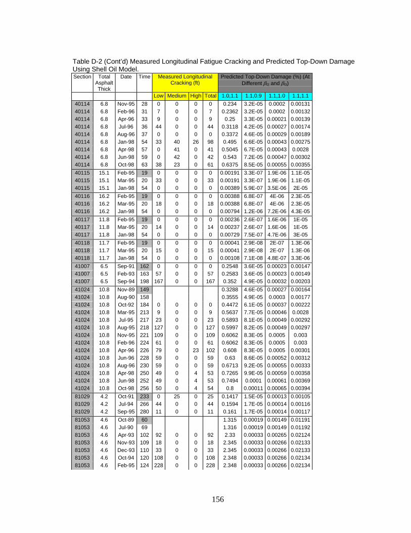
156
Table D-2 (Cont’d) Measured Longitudinal Fatigue Cracking and Predicted Top-Down Damage Using Shell Oil Model. Section Total
Asphalt Thick
Date Time Measured Longitudinal Cracking (ft)
Predicted Top-Down Damage (%) (At Different βf2 and βf3)
Low Medium High Total 1.0,1.1 1.1,0.9 1.1,1.0 1.1,1.1 40114 6.8 Nov-95 28 0 0 0 0 0.234 3.2E-05 0.0002 0.00131 40114 6.8 Feb-96 31 7 0 0 7 0.2362 3.2E-05 0.0002 0.00132 40114 6.8 Apr-96 33 9 0 0 9 0.25 3.3E-05 0.00021 0.00139 40114 6.8 Jul-96 36 44 0 0 44 0.3118 4.2E-05 0.00027 0.00174 40114 6.8 Aug-96 37 0 0 0 0 0.3372 4.6E-05 0.00029 0.00189 40114 6.8 Jan-98 54 33 40 26 98 0.495 6.6E-05 0.00043 0.00275 40114 6.8 Apr-98 57 0 41 0 41 0.5045 6.7E-05 0.00043 0.0028 40114 6.8 Jun-98 59 0 42 0 42 0.543 7.2E-05 0.00047 0.00302 40114 6.8 Oct-98 63 38 23 0 61 0.6375 8.5E-05 0.00055 0.00355 40115 15.1 Feb-95 19 0 0 0 0 0.00191 3.3E-07 1.9E-06 1.1E-05 40115 15.1 Mar-95 20 33 0 0 33 0.00191 3.3E-07 1.9E-06 1.1E-05 40115 15.1 Jan-98 54 0 0 0 0 0.00389 5.9E-07 3.5E-06 2E-05 40116 16.2 Feb-95 19 0 0 0 0 0.00388 6.8E-07 4E-06 2.3E-05 40116 16.2 Mar-95 20 18 0 0 18 0.00388 6.8E-07 4E-06 2.3E-05 40116 16.2 Jan-98 54 0 0 0 0 0.00794 1.2E-06 7.2E-06 4.3E-05 40117 11.8 Feb-95 19 0 0 0 0 0.00236 2.6E-07 1.6E-06 1E-05 40117 11.8 Mar-95 20 14 0 0 14 0.00237 2.6E-07 1.6E-06 1E-05 40117 11.8 Jan-98 54 0 0 0 0 0.00729 7.5E-07 4.7E-06 3E-05 40118 11.7 Feb-95 19 0 0 0 0 0.00041 2.9E-08 2E-07 1.3E-06 40118 11.7 Mar-95 20 15 0 0 15 0.00041 2.9E-08 2E-07 1.3E-06 40118 11.7 Jan-98 54 0 0 0 0 0.00108 7.1E-08 4.8E-07 3.3E-06 41007 6.5 Sep-91 162 0 0 0 0 0.2548 3.6E-05 0.00023 0.00147 41007 6.5 Feb-93 163 57 0 0 57 0.2583 3.6E-05 0.00023 0.00149 41007 6.5 Sep-94 198 167 0 0 167 0.352 4.9E-05 0.00032 0.00203 41024 10.8 Nov-89 149 0.3288 4.6E-05 0.00027 0.00164 41024 10.8 Aug-90 158 0.3555 4.9E-05 0.0003 0.00177 41024 10.8 Oct-92 184 0 0 0 0 0.4472 6.1E-05 0.00037 0.00222 41024 10.8 Mar-95 213 9 0 0 9 0.5637 7.7E-05 0.00046 0.0028 41024 10.8 Jul-95 217 23 0 0 23 0.5893 8.1E-05 0.00049 0.00292 41024 10.8 Aug-95 218 127 0 0 127 0.5997 8.2E-05 0.00049 0.00297 41024 10.8 Nov-95 221 109 0 0 109 0.6062 8.3E-05 0.0005 0.003 41024 10.8 Feb-96 224 61 0 0 61 0.6062 8.3E-05 0.0005 0.003 41024 10.8 Apr-96 226 79 0 23 102 0.608 8.3E-05 0.0005 0.00301 41024 10.8 Jun-96 228 59 0 0 59 0.63 8.6E-05 0.00052 0.00312 41024 10.8 Aug-96 230 59 0 0 59 0.6713 9.2E-05 0.00055 0.00333 41024 10.8 Apr-98 250 49 0 4 53 0.7265 9.9E-05 0.00059 0.00358 41024 10.8 Jun-98 252 49 0 4 53 0.7494 0.0001 0.00061 0.00369 41024 10.8 Oct-98 256 50 0 4 54 0.8 0.00011 0.00065 0.00394 81029 4.2 Oct-91 233 0 25 0 25 0.1417 1.5E-05 0.00013 0.00105 81029 4.2 Jul-94 266 44 0 0 44 0.1594 1.7E-05 0.00014 0.00116 81029 4.2 Sep-95 280 11 0 0 11 0.161 1.7E-05 0.00014 0.00117 81053 4.6 Oct-89 60 1.315 0.00019 0.00149 0.01191 81053 4.6 Jul-90 69 1.316 0.00019 0.00149 0.01192 81053 4.6 Apr-93 102 92 0 0 92 2.33 0.00033 0.00265 0.02124 81053 4.6 Nov-93 109 18 0 0 18 2.345 0.00033 0.00266 0.02133 81053 4.6 Dec-93 110 33 0 0 33 2.345 0.00033 0.00266 0.02133 81053 4.6 Oct-94 120 108 0 0 108 2.348 0.00033 0.00266 0.02134 81053 4.6 Feb-95 124 228 0 0 228 2.348 0.00033 0.00266 0.02134

157
Table D-2 (Cont’d) Measured Longitudinal Fatigue Cracking and Predicted Top-Down Damage Using Shell Oil Model. Section Total
Asphalt Thick
Date Time Measured Longitudinal Cracking (ft)
Predicted Top-Down Damage (%) (At Different βf2 and βf3)
Low Medium High Total 1.0,1.1 1.1,0.9 1.1,1.0 1.1,1.1 81053 4.6 May-95 127 229 0 0 229 2.348 0.00033 0.00266 0.02134 81053 4.6 May-96 139 0 0 0 0 2.364 0.00033 0.00268 0.02144 81053 4.6 Oct-96 144 0 0 0 0 2.725 0.00039 0.00312 0.02471 81053 4.6 Nov-96 145 33 0 0 33 2.725 0.00039 0.00312 0.02471 81053 4.6 Mar-97 149 45 0 0 45 2.725 0.00039 0.00312 0.02471 91803 7.2 Jul-89 49 4.423 0.00075 0.00612 0.04961 91803 7.2 Sep-90 63 4.893 0.00081 0.0066 0.05356 91803 7.2 Aug-91 74 7 0 0 7 10.22 0.00175 0.01423 0.1154 91803 7.2 Sep-92 87 5 0 0 5 10.37 0.00177 0.01437 0.1165 91803 7.2 May-94 107 103 0 0 103 18.23 0.00313 0.02538 0.2058 91803 7.2 May-95 119 207 7 0 214 18.42 0.00315 0.02556 0.2073 91803 7.2 Oct-96 136 364 0 0 364 18.54 0.00316 0.02567 0.2082 91803 7.2 May-97 143 557 0 0 557 19.23 0.00325 0.02634 0.2137 91803 7.2 Sep-97 147 74 0 0 74 19.23 0.00325 0.02634 0.2137 91803 7.2 Jun-98 156 279 11 0 290 29.72 0.0051 0.04136 0.3355 120103 12 Dec-96 14 0 0 0 0 6.3E-06 4.2E-10 2.8E-09 1.9E-08 120104 18 Dec-96 14 0 0 0 0 5.8E-05 6.2E-09 4E-08 2.5E-07 120105 7.9 Dec-96 14 0 0 0 0 0.00071 7.4E-08 4.8E-07 3.1E-06 120106 15 Dec-96 14 0 0 0 0 4.3E-05 4.7E-09 3E-08 1.9E-07 123995 5 Apr-92 197 34 0 0 34 1.186 9.3E-05 0.00068 0.00496 123995 5 Mar-94 220 82 0 0 82 1.336 0.0001 0.00076 0.00558 123995 5 Jan-96 242 215 0 0 215 1.476 0.00012 0.00084 0.00616 123995 5 Jan-96 243 72 0 0 72 1.484 0.00012 0.00085 0.00619 123997 3.1 Aug-90 195 0.6035 0.00014 0.00086 0.0053 123997 3.1 Oct-91 209 0.6765 0.00016 0.00097 0.00595 123997 3.1 Mar-93 226 0.7412 0.00017 0.00105 0.00649 123997 3.1 Mar-94 238 0.7994 0.00018 0.00113 0.00699 124105 2.3 Apr-89 53 0 0 0 0 30.78 0.00984 0.06032 0.3714 124105 2.3 Oct-91 83 0 0 0 0 52.39 0.01658 0.102 0.6302 124105 2.3 Mar-93 100 0 0 0 0 60.95 0.01909 0.1177 0.7291 124106 8.2 Apr-89 21 0.00742 6.8E-07 4.4E-06 2.9E-05 124106 8.2 Feb-91 43 0.01765 1.6E-06 1E-05 6.9E-05 124106 8.2 Jul-91 48 0 0 0 0 0.0203 1.8E-06 1.2E-05 7.9E-05 124106 8.2 Mar-94 80 10 0 0 10 0.03583 3.1E-06 2.1E-05 0.00014 124106 8.2 Jan-97 114 50 0 0 50 0.05316 4.6E-06 3.1E-05 0.0002 124107 2.7 Dec-89 75 0 0 0 0 0.3834 9E-05 0.00057 0.00365 124107 2.7 Feb-91 89 261 0 0 261 0.449 0.0001 0.00066 0.00423 124107 2.7 Jul-91 94 343 0 0 343 0.4876 0.00011 0.00072 0.0046 124107 2.7 Mar-93 114 18 0 0 18 0.6107 0.00014 0.00089 0.00573 124107 2.7 Mar-94 126 37 13 0 51 0.6844 0.00015 0.00099 0.00638 124107 2.7 Jan-96 148 67 0 0 67 0.8469 0.00019 0.00122 0.00787 124107 2.7 Mar-97 162 0 0 0 0 0.9453 0.00021 0.00136 0.00875 124108 9.9 Apr-89 35 0 0 0 0 0.00096 1.6E-07 9.9E-07 6.2E-06 124108 9.9 Jan-91 56 0 0 0 0 0.00117 1.9E-07 1.2E-06 7.3E-06 124108 9.9 Oct-91 65 0 0 0 0 0.00174 2.5E-07 1.6E-06 1E-05 124108 9.9 Mar-94 94 7 0 0 7 0.00198 2.8E-07 1.8E-06 1.2E-05 124108 9.9 Aug-94 99 0 0 0 0 0.0026 3.5E-07 2.3E-06 1.5E-05 124108 9.9 Jan-96 116 0 0 0 0 0.00273 3.6E-07 2.4E-06 1.6E-05

158
Table D-2 (Cont’d) Measured Longitudinal Fatigue Cracking and Predicted Top-Down Damage Using Shell Oil Model. Section Total
Asphalt Thick
Date Time Measured Longitudinal Cracking (ft)
Predicted Top-Down Damage (%) (At Different βf2 and βf3)
Low Medium High Total 1.0,1.1 1.1,0.9 1.1,1.0 1.1,1.1 124135 1.4 Dec-89 227 99 199 0 298 10540 3.985 26.7 181.2 124135 1.4 Jan-91 240 412 271 0 683 10890 4.122 27.6 187.1 131031 11.1 Apr-91 119 0.00196 1.3E-07 1.1E-06 8.7E-06 131031 11.1 Jul-92 134 0.00197 1.3E-07 1.1E-06 8.7E-06 131031 11.1 Jan-93 140 0.00284 1.9E-07 1.6E-06 1.3E-05 131031 11.1 Apr-94 155 0.00345 2.3E-07 1.9E-06 1.5E-05 131031 11.1 Oct-94 161 0.00346 2.3E-07 1.9E-06 1.5E-05 131031 11.1 Aug-95 171 0.00347 2.3E-07 1.9E-06 1.5E-05 131031 11.1 Jan-96 176 0.00473 3.2E-07 2.6E-06 2.1E-05 131031 11.1 Apr-96 179 0.00473 3.2E-07 2.6E-06 2.1E-05 134111 8.7 Mar-89 101 27 0 0 27 0.00338 2.1E-07 1.7E-06 1.4E-05 134111 8.7 Mar-91 125 291 0 0 291 0.00574 3.5E-07 2.8E-06 2.3E-05 134111 8.7 Feb-92 136 477 0 0 477 0.00577 3.5E-07 2.8E-06 2.3E-05 134112 15.9 May-89 144 0 0 0 0 0.00898 2.7E-06 1.5E-05 8.8E-05 134112 15.9 Feb-91 165 17 0 0 17 0.00999 2.9E-06 1.7E-05 9.5E-05 134112 15.9 Apr-91 167 0 0 0 0 0.00999 2.9E-06 1.7E-05 9.5E-05 134112 15.9 Feb-94 201 0 0 0 0 0.01513 4.3E-06 2.5E-05 0.00014 134112 15.9 Oct-94 209 0 0 0 0 0.01585 4.4E-06 2.6E-05 0.00015 134112 15.9 Jan-96 224 0 0 0 0 0.01655 4.6E-06 2.7E-05 0.00016 134112 15.9 Feb-97 237 0 0 0 0 0.01919 5.3E-06 3.1E-05 0.00018 134112 15.9 Apr-98 251 0 0 0 0 0.01995 5.5E-06 3.2E-05 0.00019 134113 15.2 May-89 144 0 0 0 0 0.02803 9.9E-06 5.5E-05 0.0003 134113 15.2 Feb-91 165 0 0 0 0 0.0306 1E-05 5.8E-05 0.00033 134113 15.2 Apr-91 167 0 0 0 0 0.03061 1E-05 5.8E-05 0.00033 134113 15.2 Feb-94 201 0 0 0 0 0.04527 1.5E-05 8.6E-05 0.00048 134113 15.2 Oct-94 209 0 0 0 0 0.04722 1.6E-05 8.9E-05 0.0005 134113 15.2 Jan-96 224 0 0 0 0 0.04909 1.6E-05 9.1E-05 0.00052 134113 15.2 Feb-97 237 31 0 0 31 0.0564 1.9E-05 0.00011 0.00059 134113 15.2 Apr-98 251 37 0 0 37 0.05861 1.9E-05 0.00011 0.00061 161001 3.7 Jul-89 192 155 0 0 155 1.559 0.00014 0.00121 0.01017 161001 3.7 Aug-90 205 193 0 0 193 1.672 0.00015 0.00129 0.01084 161001 3.7 Jun-93 239 78 0 0 78 2.086 0.00019 0.00159 0.01339 161001 3.7 Aug-94 253 199 0 0 199 2.18 0.0002 0.00165 0.01389 161001 3.7 May-95 262 183 2 0 185 2.527 0.00023 0.00192 0.01618 161001 3.7 Jul-97 288 67 63 44 175 2.672 0.00024 0.00201 0.01692 161001 3.7 Sep-98 302 0 159 5 164 3.072 0.00028 0.00232 0.01954 161009 10.4 Sep-89 180 0.7338 0.00011 0.00084 0.00666 161009 10.4 Jul-90 190 0.8756 0.00013 0.00099 0.00782 161009 10.4 Jul-92 214 0 0 0 0 0.8964 0.00013 0.00101 0.00795 161009 10.4 Oct-93 229 8 0 0 8 1.071 0.00015 0.00119 0.00938 161009 10.4 Jun-96 261 1 0 0 1 1.116 0.00015 0.00122 0.00967 161009 10.4 Jul-97 274 0 0 0 0 1.34 0.00018 0.00146 0.0115 161021 5.9 Sep-89 48 0.02961 3.5E-06 2.8E-05 0.00023 161021 5.9 Oct-90 61 0 0 0 0 0.02992 3.6E-06 2.9E-05 0.00023 161021 5.9 Aug-91 71 0 0 0 0 0.05942 7.1E-06 5.7E-05 0.00046 161021 5.9 Aug-93 95 0 0 0 0 0.05998 7.2E-06 5.7E-05 0.00046 161021 5.9 Sep-95 120 0 0 0 0 0.09091 1.1E-05 8.7E-05 0.0007 161021 5.9 Jun-96 129 5 0 0 5 0.09109 1.1E-05 8.7E-05 0.0007

159
Table D-2 (Cont’d) Measured Longitudinal Fatigue Cracking and Predicted Top-Down Damage Using Shell Oil Model. Section Total
Asphalt Thick
Date Time Measured Longitudinal Cracking (ft)
Predicted Top-Down Damage (%) (At Different βf2 and βf3)
Low Medium High Total 1.0,1.1 1.1,0.9 1.1,1.0 1.1,1.1 161021 5.9 Jul-97 142 0 0 0 0 0.09145 1.1E-05 8.7E-05 0.0007 169034 9.2 Jul-89 10 0.00048 3.1E-08 2.4E-07 1.8E-06 169034 9.2 Aug-90 23 0.01224 1.1E-06 8.7E-06 6.9E-05 169034 9.2 Jun-93 57 12 0 0 12 0.1164 1.2E-05 9.8E-05 0.00078 169034 9.2 Aug-94 71 146 0 0 146 0.2067 2.2E-05 0.00018 0.00141 169034 9.2 May-95 80 0.2072 2.2E-05 0.00018 0.00141 169034 9.2 Jul-97 106 217 0 0 217 0.3072 3.3E-05 0.00026 0.0021 169034 9.2 Sep-98 120 156 52 18 226 0.3078 3.3E-05 0.00026 0.0021 201009 11.1 Aug-88 44 0 0 0 0 16.65 0.00258 0.02135 0.1769 201009 11.1 May-89 53 11 0 0 11 16.76 0.00259 0.02144 0.1777 201009 11.1 Dec-90 72 210 5 0 215 30.32 0.00476 0.03942 0.3267 201009 11.1 Oct-91 82 6 1 0 7 32.81 0.00511 0.04231 0.3506 201009 11.1 Apr-93 100 9 0 0 9 44.83 0.00705 0.05844 0.4843 201009 11.1 Apr-95 124 16 28 0 43 52.67 0.00817 0.06773 0.5613 201009 11.1 Apr-96 136 0 0 0 0 52.99 0.00821 0.06803 0.5638 201009 11.1 Jan-99 168 0 0 0 0 60.91 0.00928 0.07694 0.6376 251003 6.6 Aug-89 180 758 0 0 758 1.288 0.00021 0.00168 0.01337 251003 6.6 Sep-90 193 691 0 0 691 1.544 0.00025 0.00199 0.01591 251003 6.6 Aug-91 204 556 1 0 557 1.551 0.00025 0.002 0.01596 251003 6.6 Sep-92 217 600 0 0 600 1.576 0.00025 0.00202 0.01615 251003 6.6 Oct-95 254 563 0 0 563 1.87 0.0003 0.00238 0.01901 251003 6.6 Oct-96 266 39 0 0 39 1.897 0.0003 0.00241 0.01921 251003 6.6 Jun-98 286 32 9 0 41 2.21 0.00035 0.00279 0.02229 251004 9.6 Aug-89 178 0 0 0 0 0.2724 3.5E-05 0.00027 0.00213 251004 9.6 Sep-90 191 19 0 0 19 0.2948 3.8E-05 0.00029 0.00229 251004 9.6 Aug-91 202 16 0 0 16 0.3454 4.4E-05 0.00034 0.00269 251004 9.6 Sep-92 215 0 0 0 0 0.346 4.4E-05 0.00034 0.00269 251004 9.6 Oct-95 252 0 0 0 0 0.5002 6.3E-05 0.00049 0.00387 251004 9.6 Jun-97 272 3 0 0 3 0.5344 6.7E-05 0.00053 0.0041 251004 9.6 Jun-98 284 3 0 0 3 0.6137 7.7E-05 0.0006 0.00472 261001 2.2 Jul-88 203 0 0 0 0 0.1655 3.1E-05 0.00021 0.00153 261001 2.2 Sep-89 217 16 0 0 16 0.1797 3.3E-05 0.00023 0.00166 261001 2.2 Jul-90 227 24 0 0 24 0.1888 3.5E-05 0.00024 0.00174 261001 2.2 Jul-91 239 0 0 0 0 0.1949 3.6E-05 0.00025 0.0018 261001 2.2 Sep-91 241 51 0 0 51 0.1966 3.6E-05 0.00026 0.00182 261001 2.2 Sep-92 253 0 0 0 0 0.2011 3.7E-05 0.00026 0.00186 261001 2.2 Jun-93 262 23 0 0 23 0.2103 3.9E-05 0.00027 0.00194 261001 2.2 Jun-93 263 0 0 0 0 0.2118 3.9E-05 0.00027 0.00195 261001 2.2 May-95 285 9 0 0 9 0.2234 4.1E-05 0.00029 0.00206 261001 2.2 Jul-96 299 5 0 0 5 0.2378 4.4E-05 0.00031 0.0022 261004 4.2 Sep-89 51 321 0 0 321 5.445 0.00104 0.00805 0.06232 261004 4.2 Jul-90 61 451 0 0 451 8.712 0.0017 0.01318 0.102 271018 4.4 Apr-89 124 0 0 0 0 24.34 0.00347 0.02866 0.2368 271018 4.4 Jun-89 126 24.34 0.00347 0.02866 0.2368 271018 4.4 Oct-90 142 24.93 0.00354 0.02924 0.2416 271018 4.4 Jun-93 174 41 1 0 41 33.74 0.00484 0.03995 0.3301 271018 4.4 Jul-93 176 7 51 0 57 33.74 0.00484 0.03995 0.3301 271018 4.4 Mar-94 183 58 39 0 98 37.9 0.00546 0.04513 0.3729

160
Table D-2 (Cont’d) Measured Longitudinal Fatigue Cracking and Predicted Top-Down Damage Using Shell Oil Model. Section Total
Asphalt Thick
Date Time Measured Longitudinal Cracking (ft)
Predicted Top-Down Damage (%) (At Different βf2 and βf3)
Low Medium High Total 1.0,1.1 1.1,0.9 1.1,1.0 1.1,1.1 271018 4.4 Aug-94 188 131 0 0 131 37.9 0.00546 0.04514 0.3729 271087 15.7 Oct-91 154 0 0 0 0 16.13 0.00253 0.0202 0.1613 271087 15.7 May-93 173 8 0 0 8 18.23 0.00285 0.02277 0.1819 271087 15.7 Oct-94 190 24 0 0 24 19.11 0.00299 0.02386 0.1906 271087 15.7 Jun-96 210 25 0 0 25 21.84 0.00342 0.02729 0.2179 291008 11.4 Feb-92 70 0 0 0 0 0.3999 4.4E-05 0.00035 0.00277 291008 11.4 Mar-93 83 58 3 0 61 0.3999 4.4E-05 0.00035 0.00277 291008 11.4 Mar-93 83 28 34 0 62 7.005 0.0013 0.00803 0.04975 291008 11.4 Apr-96 120 130 0 0 130 0.6307 6.9E-05 0.00055 0.00434 291008 11.4 Feb-00 152 26 0 0 26 0.8257 8.8E-05 0.0007 0.00558 307088 4.9 Sep-89 100 0 0 0 0 0.2634 3.2E-05 0.00025 0.00206 307088 4.9 May-91 120 4 12 0 16 0.2847 3.4E-05 0.00027 0.0022 308129 3.2 Oct-89 17 0.1123 1.6E-05 0.00013 0.00099 308129 3.2 Jul-91 38 0.221 3.1E-05 0.00025 0.00194 308129 3.2 Jul-92 50 0 0 0 0 0.3344 4.7E-05 0.00037 0.00293 308129 3.2 Aug-93 63 0 0 0 0 0.5042 7.2E-05 0.00057 0.00447 308129 3.2 Dec-93 67 0 0 0 0 0.5044 7.2E-05 0.00057 0.00447 308129 3.2 Mar-94 70 0 0 0 0 0.5057 7.2E-05 0.00057 0.00448 308129 3.2 Oct-94 77 0 0 0 0 0.5078 7.3E-05 0.00057 0.00449 308129 3.2 Feb-95 81 0 0 0 0 0.6327 9E-05 0.00071 0.00558 308129 3.2 May-95 84 0 0 0 0 0.6361 9.1E-05 0.00071 0.00561 308129 3.2 Jun-96 97 0 0 0 0 0.8291 0.00012 0.00093 0.00736 308129 3.2 Oct-96 101 0 0 0 0 0.8303 0.00012 0.00094 0.00737 308129 3.2 Jan-97 104 0 0 0 0 0.8314 0.00012 0.00094 0.00737 308129 3.2 Mar-97 106 0 0 0 0 0.8319 0.00012 0.00094 0.00738 308129 3.2 Aug-97 111 0 0 0 0 0.8341 0.00012 0.00094 0.00739 308129 3.2 Oct-97 113 0 0 0 0 0.8343 0.00012 0.00094 0.00739 321020 7 Jul-91 86 34 0 0 34 4.376 0.00062 0.00513 0.04269 321020 7 Aug-93 111 138 0 0 138 7.189 0.00102 0.00851 0.07076 321020 7 Sep-94 123 29 20 0 49 7.369 0.00104 0.00866 0.07208 321020 7 Apr-95 131 242 0 0 242 7.471 0.00105 0.00874 0.07273 321020 7 Jun-97 157 9 0 0 9 9.216 0.00127 0.01057 0.08795 321020 7 Jun-98 169 0 0 0 0 9.334 0.00128 0.01066 0.0887 341031 7.3 Apr-92 224 333 1 0 333 4.157 0.00062 0.00482 0.03783 341031 7.3 Feb-93 234 322 31 3 356 4.183 0.00062 0.00485 0.03803 341031 7.3 Oct-95 266 0 352 170 522 4.33 0.00064 0.005 0.03906 341031 7.3 Nov-95 267 232 30 0 261 5.64 0.00082 0.00644 0.05052 341033 7.4 Apr-92 211 52 2 0 54 0.07319 8.4E-06 6.8E-05 0.00054 341033 7.4 Feb-93 221 32 11 0 44 0.07511 8.6E-06 6.9E-05 0.00056 341033 7.4 Nov-95 254 55 0 0 55 0.09457 1.1E-05 8.7E-05 0.0007 341033 7.4 Jul-97 274 260 0 0 260 0.09659 1.1E-05 8.9E-05 0.00071 341034 11.1 Oct-89 48 0 0 0 0 2.109 0.00029 0.00229 0.01832 341034 11.1 Sep-90 59 0 0 0 0 2.109 0.00029 0.00229 0.01833 341034 11.1 Apr-92 78 0 0 0 0 3.328 0.00044 0.00355 0.02843 341034 11.1 Feb-93 88 0 0 0 0 3.329 0.00044 0.00355 0.02843 341034 11.1 Nov-95 121 3 0 0 3 4.763 0.00063 0.00503 0.04031 341034 11.1 Jul-97 141 0 15 0 15 6.255 0.00082 0.00658 0.05274 350101 7.2 May-97 19 0 0 0 0 0.1463 1.5E-05 0.00011 0.00083
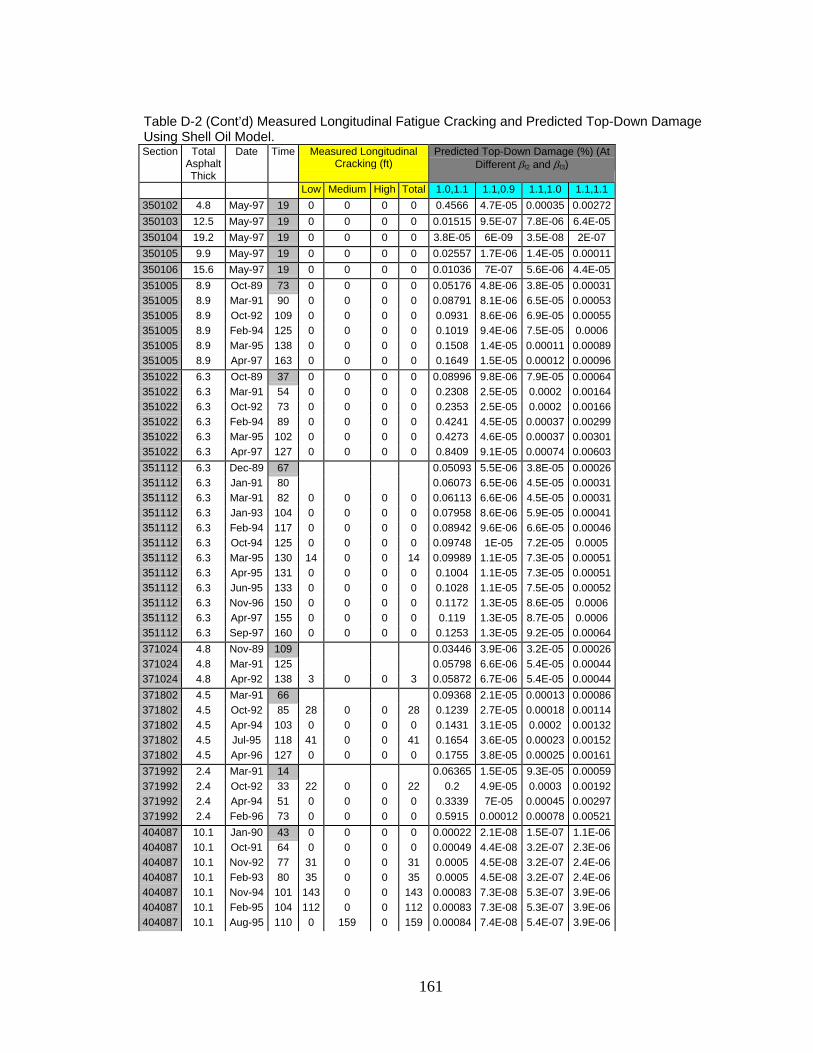
161
Table D-2 (Cont’d) Measured Longitudinal Fatigue Cracking and Predicted Top-Down Damage Using Shell Oil Model. Section Total
Asphalt Thick
Date Time Measured Longitudinal Cracking (ft)
Predicted Top-Down Damage (%) (At Different βf2 and βf3)
Low Medium High Total 1.0,1.1 1.1,0.9 1.1,1.0 1.1,1.1 350102 4.8 May-97 19 0 0 0 0 0.4566 4.7E-05 0.00035 0.00272 350103 12.5 May-97 19 0 0 0 0 0.01515 9.5E-07 7.8E-06 6.4E-05 350104 19.2 May-97 19 0 0 0 0 3.8E-05 6E-09 3.5E-08 2E-07 350105 9.9 May-97 19 0 0 0 0 0.02557 1.7E-06 1.4E-05 0.00011 350106 15.6 May-97 19 0 0 0 0 0.01036 7E-07 5.6E-06 4.4E-05 351005 8.9 Oct-89 73 0 0 0 0 0.05176 4.8E-06 3.8E-05 0.00031 351005 8.9 Mar-91 90 0 0 0 0 0.08791 8.1E-06 6.5E-05 0.00053 351005 8.9 Oct-92 109 0 0 0 0 0.0931 8.6E-06 6.9E-05 0.00055 351005 8.9 Feb-94 125 0 0 0 0 0.1019 9.4E-06 7.5E-05 0.0006 351005 8.9 Mar-95 138 0 0 0 0 0.1508 1.4E-05 0.00011 0.00089 351005 8.9 Apr-97 163 0 0 0 0 0.1649 1.5E-05 0.00012 0.00096 351022 6.3 Oct-89 37 0 0 0 0 0.08996 9.8E-06 7.9E-05 0.00064 351022 6.3 Mar-91 54 0 0 0 0 0.2308 2.5E-05 0.0002 0.00164 351022 6.3 Oct-92 73 0 0 0 0 0.2353 2.5E-05 0.0002 0.00166 351022 6.3 Feb-94 89 0 0 0 0 0.4241 4.5E-05 0.00037 0.00299 351022 6.3 Mar-95 102 0 0 0 0 0.4273 4.6E-05 0.00037 0.00301 351022 6.3 Apr-97 127 0 0 0 0 0.8409 9.1E-05 0.00074 0.00603 351112 6.3 Dec-89 67 0.05093 5.5E-06 3.8E-05 0.00026 351112 6.3 Jan-91 80 0.06073 6.5E-06 4.5E-05 0.00031 351112 6.3 Mar-91 82 0 0 0 0 0.06113 6.6E-06 4.5E-05 0.00031 351112 6.3 Jan-93 104 0 0 0 0 0.07958 8.6E-06 5.9E-05 0.00041 351112 6.3 Feb-94 117 0 0 0 0 0.08942 9.6E-06 6.6E-05 0.00046 351112 6.3 Oct-94 125 0 0 0 0 0.09748 1E-05 7.2E-05 0.0005 351112 6.3 Mar-95 130 14 0 0 14 0.09989 1.1E-05 7.3E-05 0.00051 351112 6.3 Apr-95 131 0 0 0 0 0.1004 1.1E-05 7.3E-05 0.00051 351112 6.3 Jun-95 133 0 0 0 0 0.1028 1.1E-05 7.5E-05 0.00052 351112 6.3 Nov-96 150 0 0 0 0 0.1172 1.3E-05 8.6E-05 0.0006 351112 6.3 Apr-97 155 0 0 0 0 0.119 1.3E-05 8.7E-05 0.0006 351112 6.3 Sep-97 160 0 0 0 0 0.1253 1.3E-05 9.2E-05 0.00064 371024 4.8 Nov-89 109 0.03446 3.9E-06 3.2E-05 0.00026 371024 4.8 Mar-91 125 0.05798 6.6E-06 5.4E-05 0.00044 371024 4.8 Apr-92 138 3 0 0 3 0.05872 6.7E-06 5.4E-05 0.00044 371802 4.5 Mar-91 66 0.09368 2.1E-05 0.00013 0.00086 371802 4.5 Oct-92 85 28 0 0 28 0.1239 2.7E-05 0.00018 0.00114 371802 4.5 Apr-94 103 0 0 0 0 0.1431 3.1E-05 0.0002 0.00132 371802 4.5 Jul-95 118 41 0 0 41 0.1654 3.6E-05 0.00023 0.00152 371802 4.5 Apr-96 127 0 0 0 0 0.1755 3.8E-05 0.00025 0.00161 371992 2.4 Mar-91 14 0.06365 1.5E-05 9.3E-05 0.00059 371992 2.4 Oct-92 33 22 0 0 22 0.2 4.9E-05 0.0003 0.00192 371992 2.4 Apr-94 51 0 0 0 0 0.3339 7E-05 0.00045 0.00297 371992 2.4 Feb-96 73 0 0 0 0 0.5915 0.00012 0.00078 0.00521 404087 10.1 Jan-90 43 0 0 0 0 0.00022 2.1E-08 1.5E-07 1.1E-06 404087 10.1 Oct-91 64 0 0 0 0 0.00049 4.4E-08 3.2E-07 2.3E-06 404087 10.1 Nov-92 77 31 0 0 31 0.0005 4.5E-08 3.2E-07 2.4E-06 404087 10.1 Feb-93 80 35 0 0 35 0.0005 4.5E-08 3.2E-07 2.4E-06 404087 10.1 Nov-94 101 143 0 0 143 0.00083 7.3E-08 5.3E-07 3.9E-06 404087 10.1 Feb-95 104 112 0 0 112 0.00083 7.3E-08 5.3E-07 3.9E-06 404087 10.1 Aug-95 110 0 159 0 159 0.00084 7.4E-08 5.4E-07 3.9E-06

162
Table D-2 (Cont’d) Measured Longitudinal Fatigue Cracking and Predicted Top-Down Damage Using Shell Oil Model. Section Total
Asphalt Thick
Date Time Measured Longitudinal Cracking (ft)
Predicted Top-Down Damage (%) (At Different βf2 and βf3)
Low Medium High Total 1.0,1.1 1.1,0.9 1.1,1.0 1.1,1.1 404087 10.1 Jun-97 132 10 0 0 10 0.00086 7.8E-08 5.6E-07 4.1E-06 404163 11.5 Jan-90 34 0.1541 1.4E-05 0.00012 0.00095 404163 11.5 Mar-91 48 0.1564 1.4E-05 0.00012 0.00096 404163 11.5 Oct-91 55 0 0 0 0 0.1564 1.4E-05 0.00012 0.00096 404163 11.5 Nov-92 68 0 0 0 0 0.3281 3E-05 0.00025 0.00204 404163 11.5 Mar-93 72 7 0 0 7 0.3282 3E-05 0.00025 0.00204 404163 11.5 Nov-94 92 0 0 0 0 0.3306 3E-05 0.00025 0.00205 404163 11.5 Apr-96 109 0 0 0 0 0.5047 4.6E-05 0.00038 0.00313 404163 11.5 Aug-97 125 45 8 0 53 0.5047 4.6E-05 0.00038 0.00313 404163 11.5 Jan-99 141 6 9 0 15 0.6701 6.2E-05 0.00051 0.00416 404165 8.1 Jan-90 68 2.896 0.00029 0.00242 0.02002 404165 8.1 Mar-91 82 3.029 0.0003 0.00251 0.0208 404165 8.1 Oct-91 89 4 0 0 4 3.03 0.0003 0.00252 0.02081 404165 8.1 Nov-92 102 5 0 0 5 4.563 0.00046 0.00381 0.03155 404165 8.1 Mar-93 106 19 0 0 19 4.566 0.00046 0.00382 0.03157 404165 8.1 Oct-94 125 9 0 0 9 4.708 0.00047 0.00392 0.0324 404165 8.1 Nov-94 126 16 0 0 16 4.709 0.00047 0.00392 0.0324 404165 8.1 Apr-95 131 24 0 0 24 4.851 0.00049 0.00402 0.03324 404165 8.1 Jun-95 133 25 0 0 25 4.851 0.00049 0.00402 0.03324 404165 8.1 Apr-96 143 25 0 0 25 6.492 0.00065 0.00541 0.04474 404165 8.1 Nov-96 150 60 0 0 60 6.493 0.00065 0.00541 0.04475 404165 8.1 May-97 156 26 0 0 26 6.497 0.00065 0.00541 0.04476 404165 8.1 Sep-97 160 24 0 0 24 6.497 0.00065 0.00541 0.04476 421599 12.3 Aug-89 25 8.459 0.00133 0.01093 0.08985 421599 12.3 Sep-90 38 13.93 0.00222 0.01828 0.1503 421599 12.3 Mar-93 68 0 0 0 0 30.46 0.00486 0.03996 0.3285 421599 12.3 Sep-94 86 0 0 0 0 30.67 0.00488 0.04015 0.33 421599 12.3 Jun-95 95 8 0 0 8 42.45 0.00675 0.05545 0.4559 421599 12.3 Jul-96 108 4 0 0 4 50.21 0.00802 0.06589 0.5416 421599 12.3 Mar-98 128 2 0 0 2 50.73 0.00807 0.06634 0.5453 451011 3.2 Mar-92 69 0 0 0 0 0.3146 6.8E-05 0.00042 0.00255 451011 3.2 Oct-92 76 0 0 0 0 0.374 8.1E-05 0.0005 0.00305 451011 3.2 Jun-93 84 0 0 0 0 0.3924 8.4E-05 0.00052 0.00318 451011 3.2 Jan-96 115 16 0 0 16 0.5299 0.00011 0.00069 0.00428 451011 3.2 Jun-97 132 0 0 0 0 0.5981 0.00013 0.00078 0.00481 451011 3.2 Feb-99 150 0 0 0 0 0.6938 0.00015 0.0009 0.00559 473104 1.3 Aug-89 39 2.495 0.0014 0.0087 0.0545 473104 1.3 Nov-89 42 2.517 0.0014 0.00874 0.05478 473104 1.3 May-91 60 2.637 0.00143 0.00895 0.05629 473104 1.3 Aug-91 63 2.657 0.00144 0.009 0.05658 473104 1.3 Oct-92 77 2.785 0.00147 0.00924 0.05826 473104 1.3 Aug-93 87 2.874 0.0015 0.0094 0.05941 473104 1.3 Nov-95 114 3.248 0.0016 0.01013 0.06448 473104 1.3 Oct-96 125 3.394 0.00164 0.01041 0.06642 480001 2.4 Apr-89 1 0.1116 4.9E-05 0.00027 0.00154 480001 2.4 Oct-90 19 4.419 0.00207 0.01152 0.06448 480001 2.4 May-91 26 0 0 0 0 4.962 0.00225 0.0126 0.07093 480001 2.4 Feb-93 47 0 0 0 0 10.34 0.00458 0.02584 0.1465

163
Table D-2 (Cont’d) Measured Longitudinal Fatigue Cracking and Predicted Top-Down Damage Using Shell Oil Model. Section Total
Asphalt Thick
Date Time Measured Longitudinal Cracking (ft)
Predicted Top-Down Damage (%) (At Different βf2 and βf3)
Low Medium High Total 1.0,1.1 1.1,0.9 1.1,1.0 1.1,1.1 480001 2.4 Apr-93 49 0 0 0 0 10.6 0.00467 0.02635 0.1495 480001 2.4 Feb-95 71 0 0 0 0 16.74 0.00711 0.04054 0.232 480001 2.4 Mar-95 72 0 0 0 0 16.83 0.00714 0.0407 0.233 480001 2.4 May-97 98 34 0 0 34 24.47 0.01005 0.05773 0.3329 480001 2.4 Mar-98 108 34 0 0 34 28.37 0.01162 0.06681 0.3856 481060 7.5 Jun-90 52 0 0 0 0 2.307 0.00034 0.00211 0.01325 481060 7.5 Feb-91 60 0 0 0 0 2.786 0.00041 0.00254 0.01596 481060 7.5 Apr-91 62 0 0 0 0 2.861 0.00042 0.0026 0.01633 481060 7.5 Mar-92 73 12 0 0 12 3.612 0.00052 0.00328 0.0206 481060 7.5 Feb-93 84 19 0 0 19 4.39 0.00063 0.00397 0.02499 481060 7.5 Mar-93 85 23 0 0 23 4.408 0.00063 0.00398 0.02507 481060 7.5 Oct-94 104 14 0 0 14 6.258 0.00089 0.00562 0.03549 481060 7.5 Feb-95 108 28 0 0 28 6.31 0.0009 0.00566 0.03572 481060 7.5 Mar-95 109 0 0 0 0 6.332 0.0009 0.00567 0.03582 481060 7.5 Mar-95 112 14 0 0 14 6.624 0.00094 0.00592 0.03741 481060 7.5 Jun-95 134 8 0 0 8 8.498 0.0012 0.00756 0.04786 481060 7.5 Apr-97 137 31 0 0 31 9.005 0.00127 0.00802 0.05076 481060 7.5 Jul-97 139 31 2 0 33 9.405 0.00133 0.00839 0.05308 481060 7.5 Sep-97 154 32 0 0 32 10.78 0.00152 0.00957 0.06066 481077 5.1 Apr-89 88 0.6544 7.2E-05 0.00055 0.00429 481077 5.1 Nov-91 119 0 0 0 0 0.9757 0.00011 0.00083 0.0064 481077 5.1 Oct-92 130 28 0 0 28 1.073 0.00012 0.0009 0.007 481077 5.1 May-93 137 124 0 0 124 1.077 0.00012 0.00091 0.00701 481077 5.1 Oct-94 154 143 0 0 143 1.086 0.00012 0.00091 0.00705 481077 5.1 Mar-95 159 47 0 0 47 1.363 0.00015 0.00114 0.00883 481077 5.1 Apr-95 160 181 0 0 181 1.363 0.00015 0.00114 0.00883 481077 5.1 Jun-95 162 181 0 0 181 1.364 0.00015 0.00114 0.00884 481077 5.1 Aug-95 164 181 0 0 181 1.365 0.00015 0.00114 0.00884 481077 5.1 Jun-96 174 181 0 0 181 1.371 0.00015 0.00115 0.00886 481077 5.1 May-97 185 228 10 0 238 1.378 0.00015 0.00115 0.00889 481077 5.1 Jul-97 187 300 0 0 300 1.379 0.00015 0.00115 0.0089 481077 5.1 Sep-97 189 276 0 0 276 1.379 0.00015 0.00115 0.0089 481077 5.1 Mar-98 195 281 0 0 281 1.688 0.00018 0.00141 0.01089 481109 6.5 Jan-90 68 0.6876 0.00021 0.00114 0.00626 481109 6.5 Sep-90 76 0.7775 0.00024 0.00128 0.00703 481109 6.5 May-91 84 123 0 0 123 0.8839 0.00026 0.00143 0.00791 481109 6.5 Feb-93 105 148 0 0 148 1.163 0.00033 0.00184 0.01024 481109 6.5 Jul-93 110 336 0 0 336 1.227 0.00035 0.00193 0.01079 481109 6.5 Feb-95 129 502 3 0 505 1.514 0.00042 0.00234 0.01315 481109 6.5 May-95 132 571 0 0 571 1.558 0.00043 0.00241 0.01354 481109 6.5 Aug-96 147 425 0 0 425 1.79 0.00049 0.00274 0.01548 481169 1.1 Feb-90 211 160 0.0589 0.3564 2.174 481169 1.1 Mar-90 212 160.9 0.05926 0.3586 2.187 481169 1.1 Sep-90 218 163.8 0.06057 0.3659 2.228 481169 1.1 Jan-91 222 0 0 0 0 169.6 0.06243 0.3778 2.304 481169 1.1 Mar-91 224 171.9 0.06326 0.3829 2.335 481169 1.1 Jun-91 227 0 0 0 0 173.4 0.06394 0.3867 2.357 481169 1.1 Jan-92 234 180.8 0.06649 0.4025 2.455

164
Table D-2 (Cont’d) Measured Longitudinal Fatigue Cracking and Predicted Top-Down Damage Using Shell Oil Model. Section Total
Asphalt Thick
Date Time Measured Longitudinal Cracking (ft)
Predicted Top-Down Damage (%) (At Different βf2 and βf3)
Low Medium High Total 1.0,1.1 1.1,0.9 1.1,1.0 1.1,1.1 481169 1.1 Feb-93 247 0 0 0 0 193.5 0.07104 0.4303 2.626 481169 1.1 Aug-93 253 0 0 0 0 196.7 0.0725 0.4386 2.673 481169 1.1 Mar-95 272 7 0 0 7 217.2 0.07969 0.4829 2.948 481169 1.1 Jul-95 276 0 0 0 0 219.2 0.08063 0.4881 2.977 481169 1.1 Jul-97 300 0 0 0 0 242.9 0.08921 0.5403 3.297 481174 4.7 Oct-90 186 0.0409 5E-06 3.3E-05 0.00022 481174 4.7 Feb-91 190 0.04132 5E-06 3.3E-05 0.00022 481174 4.7 Apr-91 192 201 0 0 201 0.0417 5E-06 3.3E-05 0.00022 481174 4.7 Mar-92 203 204 0 0 204 0.0441 5.3E-06 3.5E-05 0.00023 481174 4.7 Feb-93 214 138 0 0 138 0.04645 5.6E-06 3.7E-05 0.00025 481174 4.7 Mar-93 215 185 0 0 185 0.04662 5.6E-06 3.7E-05 0.00025 481174 4.7 Feb-95 238 220 10 0 229 0.05152 6.2E-06 4.1E-05 0.00027 481174 4.7 Mar-95 239 179 0 0 179 0.05168 6.2E-06 4.1E-05 0.00027 481174 4.7 Jan-96 249 160 0 0 160 0.05381 6.5E-06 4.3E-05 0.00028 481174 4.7 Apr-97 264 0 0 0 0 0.0569 6.8E-06 4.5E-05 0.0003 481174 4.7 Mar-98 275 49 0 0 49 0.05914 7.1E-06 4.7E-05 0.00031 481178 8.5 Feb-91 32 3.7E-05 6.1E-09 3.4E-08 1.9E-07 481178 8.5 May-91 33 48 0 0 48 3.7E-05 6.1E-09 3.4E-08 1.9E-07 481178 8.5 Feb-93 56 44 0 0 44 6.7E-05 1.1E-08 6.1E-08 3.4E-07 481178 8.5 Jul-93 61 94 0 0 94 7.4E-05 1.2E-08 6.6E-08 3.7E-07 481178 8.5 Feb-95 80 92 0 0 92 9.8E-05 1.5E-08 8.7E-08 4.9E-07 481178 8.5 Mar-95 81 57 0 0 57 9.8E-05 1.5E-08 8.7E-08 4.9E-07 481183 5.7 Sep-90 188 0 0 0 0 0.1275 2.9E-05 0.00018 0.00116 481183 5.7 Mar-91 194 0 0 0 0 0.1306 3E-05 0.00019 0.00118 481183 5.7 Oct-91 201 4 0 0 4 0.1471 3.4E-05 0.00021 0.00133 481183 5.7 Nov-91 202 11 0 0 11 0.1473 3.4E-05 0.00021 0.00133 481183 5.7 Jan-93 216 19 0 0 19 0.1712 3.9E-05 0.00025 0.00155 481183 5.7 Jul-93 222 3 0 0 3 0.184 4.2E-05 0.00026 0.00167 481183 5.7 Apr-94 231 3 0 0 3 0.1977 4.5E-05 0.00028 0.00179 483749 1.8 Oct-90 116 0 0 0 0 0.9297 0.00025 0.00159 0.01013 483749 1.8 Apr-91 122 0 0 0 0 0.9489 0.00025 0.00161 0.01029 483749 1.8 Aug-91 126 0 0 0 0 0.9689 0.00026 0.00164 0.01047 483749 1.8 Mar-92 133 0.9921 0.00026 0.00167 0.01066 483749 1.8 Feb-93 144 0 0 0 0 1.036 0.00027 0.00173 0.01104 483749 1.8 Mar-93 145 0 0 0 0 1.039 0.00027 0.00173 0.01107 483749 1.8 Feb-95 168 1.127 0.00029 0.00184 0.01183 483749 1.8 Mar-95 169 0 0 0 0 1.13 0.00029 0.00185 0.01185 483749 1.8 Mar-97 193 2 0 0 2 1.223 0.00031 0.00197 0.01266 489005 1.2 Oct-90 50 169 0 0 169 655.2 0.3471 2.107 12.88 489005 1.2 Mar-91 55 215 0 0 215 737.4 0.3822 2.336 14.38 489005 1.2 Aug-91 60 223 0 0 223 794.6 0.4164 2.536 15.55 489005 1.2 Feb-93 78 106 0 0 106 1060 0.5467 3.346 20.61 489005 1.2 Apr-93 80 240 0 0 240 1093 0.5632 3.447 21.24 489005 1.2 Feb-95 102 169 0 0 169 1390 0.7122 4.365 26.93 489005 1.2 Feb-96 114 274 0 0 274 1551 0.7926 4.861 30.01 489005 1.2 Jul-96 119 253 0 0 253 1616 0.8282 5.075 31.29 489005 1.2 Jul-97 131 325 0 0 325 1789 0.9158 5.614 34.63 489005 1.2 Jul-98 143 278 0 0 278 1960 1.001 6.142 37.91

165
Table D-2 (Cont’d) Measured Longitudinal Fatigue Cracking and Predicted Top-Down Damage Using Shell Oil Model. Section Total
Asphalt Thick
Date Time Measured Longitudinal Cracking (ft)
Predicted Top-Down Damage (%) (At Different βf2 and βf3)
Low Medium High Total 1.0,1.1 1.1,0.9 1.1,1.0 1.1,1.1 501002 8.5 Aug-89 58 0.9474 0.00014 0.00107 0.00838 501002 8.5 Aug-90 70 1.62 0.00024 0.00188 0.01472 501002 8.5 May-94 115 2 0 0 2 2.545 0.00037 0.00294 0.02304 501002 8.5 Aug-94 118 0 0 0 0 2.545 0.00037 0.00294 0.02304 501002 8.5 Apr-95 126 8 0 0 8 2.58 0.00038 0.00297 0.02328 501002 8.5 Oct-96 144 16 0 0 16 2.807 0.00041 0.00322 0.02522 501002 8.5 May-97 151 66 125 0 191 4.277 0.00066 0.00521 0.04087 501002 8.5 Oct-97 156 10 5 0 14 4.277 0.00066 0.00521 0.04087 501002 8.5 Jun-98 164 10 26 0 36 4.312 0.00067 0.00524 0.04112 501004 8 Apr-93 102 8.601 0.0013 0.01083 0.0904 501004 8 Oct-95 132 8.708 0.00131 0.01092 0.09112 501004 8 Nov-97 157 14.54 0.00218 0.01823 0.1522 511002 5.7 Apr-89 115 1.15 0.00013 0.00111 0.00948 511023 10.1 Oct-89 107 0.06425 6.3E-06 5E-05 0.00039 511023 10.1 Mar-91 124 0.114 1.1E-05 8.7E-05 0.00069 511023 10.1 May-92 138 0 0 0 0 0.1143 1.1E-05 8.8E-05 0.00069 511023 10.1 Oct-92 143 21 0 0 21 0.1146 1.1E-05 8.8E-05 0.00069 511023 10.1 Dec-93 157 0 0 0 0 0.1459 1.4E-05 0.00011 0.00088 511023 10.1 Sep-95 178 105 0 0 105 0.1465 1.4E-05 0.00011 0.00089 511023 10.1 Feb-96 183 167 0 0 167 0.1465 1.4E-05 0.00011 0.00089 511023 10.1 Mar-97 196 4 0 0 4 0.1814 1.8E-05 0.00014 0.0011 512021 7.5 Oct-89 54 0.1099 1.2E-05 9.9E-05 0.0008 512021 7.5 Mar-91 71 0.212 2.4E-05 0.0002 0.00158 512021 7.5 Oct-92 90 21 0 0 21 0.2258 2.6E-05 0.00021 0.00166 531008 3.4 Jul-91 153 6 0 0 6 0.0893 1.1E-05 8.3E-05 0.00061 531008 3.4 Jun-93 176 66 0 0 67 0.09943 1.2E-05 9.1E-05 0.00068 531008 3.4 Jun-94 188 8 5 8 21 0.1091 1.4E-05 0.0001 0.00074 561007 2.8 Jul-90 121 1.043 0.00016 0.00129 0.0102 561007 2.8 May-91 131 0 0 0 0 1.17 0.00018 0.00145 0.01144 561007 2.8 Aug-91 134 1.171 0.00018 0.00145 0.01144 561007 2.8 Aug-93 158 13 0 0 13 1.396 0.00022 0.00175 0.01383 561007 2.8 Oct-93 160 26 0 0 26 1.399 0.00022 0.00175 0.01385 561007 2.8 Dec-93 162 4 0 0 4 1.513 0.00024 0.0019 0.01499 561007 2.8 Mar-94 165 6 0 0 6 1.522 0.00024 0.00191 0.01506 561007 2.8 Apr-94 166 0 0 0 0 1.523 0.00024 0.00191 0.01506 561007 2.8 Aug-94 170 6 0 0 6 1.523 0.00024 0.00191 0.01507 561007 2.8 Feb-95 176 7 0 0 7 1.735 0.00028 0.0022 0.01736 561007 2.8 May-95 179 0 0 0 0 1.735 0.00028 0.0022 0.01736 561007 2.8 Sep-95 183 0 0 0 0 1.737 0.00028 0.0022 0.01738 561007 2.8 Jun-96 192 5 0 0 5 1.753 0.00028 0.00222 0.0175 561007 2.8 Oct-96 196 0 0 0 0 1.757 0.00028 0.00222 0.01753 561007 2.8 Nov-96 197 2 0 0 2 1.766 0.00028 0.00223 0.0176 561007 2.8 Mar-97 201 0 0 0 0 1.87 0.0003 0.00236 0.01861 561007 2.8 Aug-97 206 3 0 0 3 1.871 0.0003 0.00236 0.01862 561007 2.8 Sep-97 207 0 0 0 0 1.871 0.0003 0.00236 0.01862

166
0
100
200
300
400
500
600
700
800
900
1000
0.00001 0.0001 0.001 0.01 0.1 1 10 100 1000 10000 100000Damage (%)
Long
itudi
nal C
rack
ing
(ft/5
00ft)
AC Thickness <2" AC Thicknes 2 - 5" AC Thickness 5-8"AC Thickness 8-12" AC Thickness >12"
Figure D-1 Longitudinal Cracking vs. Predicted Top-Down Damage (AC 1,0.9,0.9)
0
100
200
300
400
500
600
700
800
900
1000
0.0001 0.001 0.01 0.1 1 10 100 1000 10000 100000Damage (%)
Long
itudi
nal C
rack
ing
(ft/5
00ft)
AC Thickness <2" AC Thicknes 2 - 5" AC Thickness 5-8"AC Thickness 8-12" AC Thickness >12"
Figure D-2 Longitudinal Cracking vs. Predicted Top-Down Damage (AC 1,0.9,1.0)
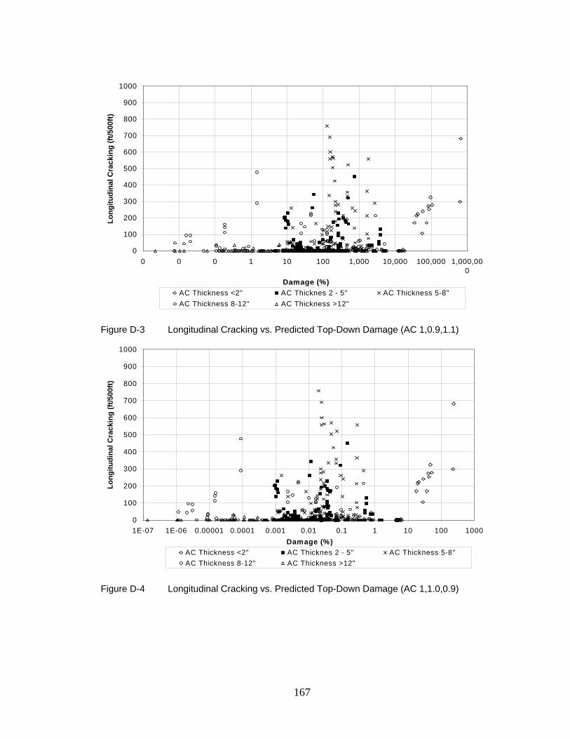
167
0
100
200
300
400
500
600
700
800
900
1000
0 0 0 1 10 100 1,000 10,000 100,000 1,000,000
Damage (%)
Long
itudi
nal C
rack
ing
(ft/5
00ft)
AC Thickness <2" AC Thicknes 2 - 5" AC Thickness 5-8"AC Thickness 8-12" AC Thickness >12"
Figure D-3 Longitudinal Cracking vs. Predicted Top-Down Damage (AC 1,0.9,1.1)
0
100
200
300
400
500
600
700
800
900
1000
1E-07 1E-06 0.00001 0.0001 0.001 0.01 0.1 1 10 100 1000Damage (%)
Long
itudi
nal C
rack
ing
(ft/5
00ft)
AC Thickness <2" AC Thicknes 2 - 5" AC Thickness 5-8"AC Thickness 8-12" AC Thickness >12"
Figure D-4 Longitudinal Cracking vs. Predicted Top-Down Damage (AC 1,1.0,0.9)
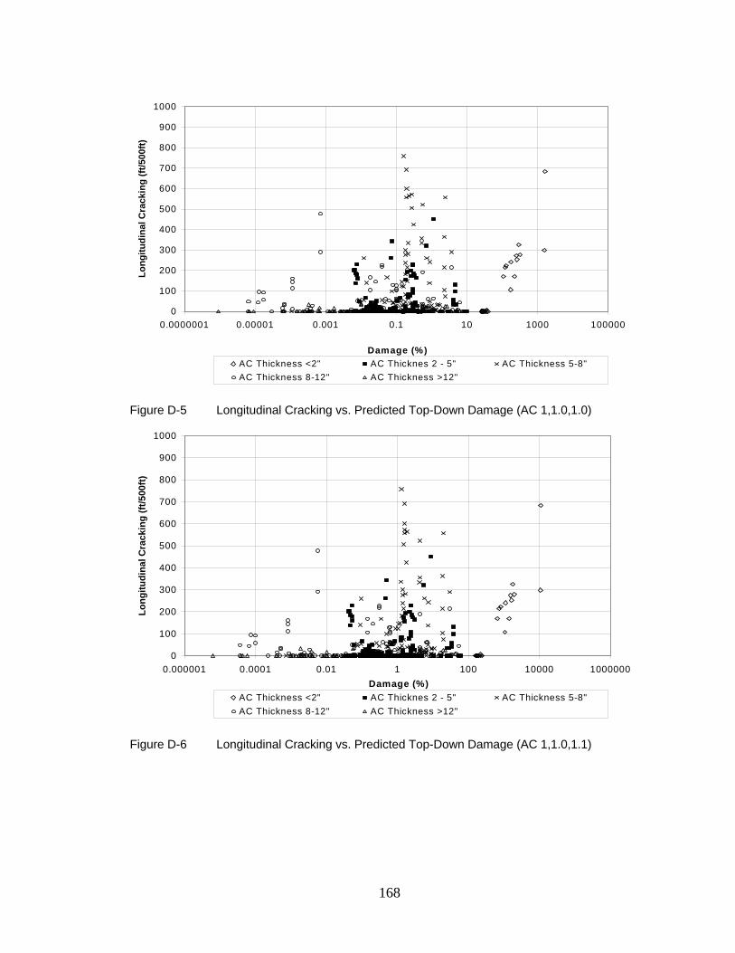
168
0
100
200
300
400
500
600
700
800
900
1000
0.0000001 0.00001 0.001 0.1 10 1000 100000
Damage (%)
Long
itudi
nal C
rack
ing
(ft/5
00ft)
AC Thickness <2" AC Thicknes 2 - 5" AC Thickness 5-8"AC Thickness 8-12" AC Thickness >12"
Figure D-5 Longitudinal Cracking vs. Predicted Top-Down Damage (AC 1,1.0,1.0)
0
100
200
300
400
500
600
700
800
900
1000
0.000001 0.0001 0.01 1 100 10000 1000000Damage (%)
Long
itudi
nal C
rack
ing
(ft/5
00ft)
AC Thickness <2" AC Thicknes 2 - 5" AC Thickness 5-8"AC Thickness 8-12" AC Thickness >12"
Figure D-6 Longitudinal Cracking vs. Predicted Top-Down Damage (AC 1,1.0,1.1)

169
0
100
200
300
400
500
600
700
800
900
1000
1E-10 0.00000001 0.000001 0.0001 0.01 1 100Damage (%)
Long
itudi
nal C
rack
ing
(ft/5
00ft)
AC Thickness <2" AC Thicknes 2 - 5" AC Thickness 5-8"AC Thickness 8-12" AC Thickness >12"
Figure D-7 Longitudinal Cracking vs. Predicted Top-Down Damage (AC 1,1.1,0.9)
0
100
200
300
400
500
600
700
800
900
1000
0.000000001 0.0000001 0.00001 0.001 0.1 10 1000Damage (%)
Long
itudi
nal C
rack
ing
(ft/5
00ft)
AC Thickness <2" AC Thicknes 2 - 5" AC Thickness 5-8"AC Thickness 8-12" AC Thickness >12"
Figure D-8 Longitudinal Cracking vs. Predicted Top-Down Damage (AC 1,1.1,1.0)

170
0
100
200
300
400
500
600
700
800
900
1000
0.00000001 0.000001 0.0001 0.01 1 100 10000Damage (%)
Long
itudi
nal C
rack
ing
(ft/5
00ft)
AC Thickness <2" AC Thicknes 2 - 5" AC Thickness 5-8"AC Thickness 8-12" AC Thickness >12"
Figure D-9 Longitudinal Cracking vs. Predicted Top-Down Damage (AC 1,1.1,1.1)

171
ANNEX E
Top-Down Longitudinal Fatigue Cracking MS-1 Model Calibration

172
Table E-1 Measured Longitudinal Fatigue Cracking and Predicted Top-Down Damage Using MS1 Model.
Section Total
Asphalt Thick
Date Time Measured Longitudinal Cracking (ft)
Predicted Top-Down Damage (%) (At Different βf2 and βf3)
Low Medium High Total 0.8,0.8 0.8,1.5 0.8,2.5 1.0,0.8 1.0,1.0 1.0,1.5
11001 3.2 Sep-91 132 0 0 0 0 1900 6481000 9.7E+11 1.95 18.98 6048 11001 3.2 Apr-92 139 16 0 0 16 1991 6923000 1.1E+12 2.027 19.83 6410 11001 3.2 Jul-92 142 14 0 0 14 2050 7063000 1.1E+12 2.097 20.46 6567 11001 3.2 Jan-93 148 30 0 0 30 2141 7399000 1.1E+12 2.185 21.35 6869 11019 6.7 May-89 32 133 496500 7.8E+10 0.1046 1.064 366.9 11019 6.7 Apr-90 43 176.9 662900 1E+11 0.139 1.414 488.5 11019 6.7 Jan-91 52 213.6 791600 1.2E+11 0.1687 1.711 586.1 11019 6.7 Jun-91 57 4 0 0 4 234 870700 1.4E+11 0.1845 1.873 643.8 11019 6.7 Mar-92 265.6 999100 1.6E+11 0.2083 2.121 733.8 11019 6.7 Mar-93 78 139 0 0 139 313.4 1193000 1.9E+11 0.245 2.502 872.8 11019 6.7 Jul-95 106 0 0 0 498.3 1877000 3E+11 0.4088 4.168 1444 11019 6.7 Jan-98 136 0 0 0 635.9 2418000 3.9E+11 0.5213 5.328 1857 14126 13.1 Jun-89 15 0 0 0 0 29.28 47640 2.2E+09 0.05181 0.4184 78.45 14126 13.1 Mar-91 36 0 0 0 0 55.15 93340 4.5E+09 0.09163 0.748 144.2 14126 13.1 Mar-93 60 0 0 0 0 75.5 132700 6.9E+09 0.1187 0.9785 193.2 14126 13.1 Apr-94 73 0 0 0 0 87.8 156600 8.2E+09 0.1347 1.115 222.6 14126 13.1 Dec-95 93 0 0 0 0 109.1 197800 1.1E+10 0.1628 1.354 273.6 14126 13.1 Dec-97 117 0 0 0 0 130.3 240100 1.3E+10 0.1892 1.581 323.4 21001 3 May-90 83 0 0 0 0 127.6 725800 1.9E+11 0.1123 1.284 596.5 21001 3 Aug-91 98 0 0 0 0 160.3 896100 2.3E+11 0.1432 1.63 747.2 21001 3 Aug-93 122 27 0 0 27 196.6 1113000 2.9E+11 0.175 2.002 929.3 21001 3 Jun-95 144 0 0 0 0 239.2 1382000 3.7E+11 0.212 2.447 1158 21001 3 Aug-97 170 0 0 0 0 287 1646000 4.4E+11 0.256 2.946 1384 21001 3 Aug-98 182 0 0 0 0 307.1 1772000 4.8E+11 0.2737 3.159 1495 21002 3.3 May-90 68 0 0 0 0 29.21 159100 4.2E+10 0.02423 0.2664 115.2 21002 3.3 Aug-91 83 6 0 0 6 37.24 197400 5.1E+10 0.03212 0.3488 146.9 21002 3.3 Aug-93 107 0 0 0 0 48.29 256400 6.7E+10 0.04168 0.4521 190.1 21002 3.3 Jun-95 129 0 0 0 0 60.59 325800 8.7E+10 0.05295 0.5771 245.9 21002 3.3 Aug-97 155 0 0 0 0 71.04 382600 1E+11 0.06127 0.6694 286.2 21002 3.3 May-98 164 0 0 0 0 75.99 417200 1.1E+11 0.06507 0.7169 312.6 40113 4.5 Feb-95 19 0 0 0 0 564.8 2661000 6.4E+11 0.413 4.35 1734 40113 4.5 Mar-95 20 11 0 0 11 591.8 2819000 6.9E+11 0.4295 4.544 1828 40113 4.5 Aug-95 25 0 0 0 0 762 3436000 7.9E+11 0.5625 5.867 2269 40113 4.5 Nov-95 28 0 0 0 0 855.1 3863000 8.8E+11 0.625 6.541 2541 40113 4.5 Feb-96 31 0 0 0 0 942.7 4461000 1.1E+12 0.6764 7.177 2888 40113 4.5 Apr-96 33 0 0 0 0 1002 4776000 1.1E+12 0.7141 7.603 3081 40113 4.5 Jul-96 36 0 0 0 0 1125 5147000 1.2E+12 0.8183 8.599 3373 40113 4.5 Aug-96 37 0 0 0 0 1171 5282000 1.2E+12 0.8576 8.973 3482 40113 4.5 Jan-98 54 53 17 0 70 1776 8426000 2E+12 1.263 13.45 5440 40113 4.5 Apr-98 57 17 65 0 82 1880 9106000 2.2E+12 1.326 14.21 5838 40113 4.5 Jun-98 59 24 59 0 83 1957 9425000 2.3E+12 1.38 14.77 6047

173
Table E-1 (Cont’d) Measured Longitudinal Fatigue Cracking and Predicted Top-Down Damage Using MS-1 Model. Section Total
Asphalt Thick
Date Time Measured Longitudinal Cracking (ft)
Predicted Top-Down Damage (%) (At Different βf2 and βf3)
Low Medium High Total 0.8,0.8 0.8,1.5 0.8,2.5 1.0,0.8 1.0,1.0 1.0,1.5
40113 4.5 Oct-98 63 0 173 0 173 2146 1E+07 2.4E+12 1.528 16.25 6541 40114 6.8 Feb-95 19 0 0 0 0 591.6 2184000 3.7E+11 0.4941 4.921 1633 40114 6.8 Mar-95 20 31 0 0 31 612.9 2289000 3.9E+11 0.5082 5.076 1697 40114 6.8 Aug-95 25 0 0 0 0 872.9 3147000 5.1E+11 0.7407 7.361 2416 40114 6.8 Nov-95 28 0 0 0 0 1003 3650000 5.9E+11 0.847 8.449 2797 40114 6.8 Feb-96 31 7 0 0 7 1033 3828000 6.4E+11 0.8623 8.628 2883 40114 6.8 Apr-96 33 9 0 0 9 1096 4097000 6.9E+11 0.91 9.129 3069 40114 6.8 Jul-96 36 44 0 0 44 1298 4717000 7.6E+11 1.098 10.95 3619 40114 6.8 Aug-96 37 0 0 0 1373 4948000 7.9E+11 1.168 11.63 3825 40114 6.8 Jan-98 54 33 40 26 98 1999 7329000 1.2E+12 1.685 16.86 5610 40114 6.8 Apr-98 57 0 41 0 41 2051 7587000 1.3E+12 1.719 17.23 5759 40114 6.8 Jun-98 59 0 42 0 42 2170 8026000 1.3E+12 1.82 18.25 6104 40114 6.8 Oct-98 63 38 23 0 61 2458 9008000 1.5E+12 2.074 20.77 6918 40115 15.1 Feb-95 19 0 0 0 0 372.8 677400 3.6E+10 0.5021 4.175 845.4 40115 15.1 Mar-95 20 33 0 0 33 374.8 683100 3.6E+10 0.5033 4.186 848.8 40115 15.1 Jan-98 54 0 0 0 0 1039 2072000 1.2E+11 1.241 10.6 2301 40116 16.2 Feb-95 19 0 0 0 0 106 223400 1.4E+10 0.1152 1.001 226.1 40116 16.2 Mar-95 20 18 0 0 18 106.5 225300 1.5E+10 0.1155 1.004 227 40116 16.2 Jan-98 54 0 0 0 0 280.6 649100 4.7E+10 0.2662 2.376 574.1 40117 11.8 Feb-95 19 0 0 0 0 97.64 210600 1.5E+10 0.09658 0.8389 189.3 40117 11.8 Mar-95 20 14 0 0 14 97.99 211900 1.5E+10 0.09669 0.8401 189.7 40117 11.8 Jan-98 54 0 0 0 0 264.7 631300 5E+10 0.2245 2.005 486.1 40118 11.7 Feb-95 19 0 0 0 0 46.63 103700 7.4E+09 0.03416 0.2996 69.67 40118 11.7 Mar-95 20 15 0 0 15 46.67 103800 7.4E+09 0.03417 0.2997 69.7 40118 11.7 Jan-98 54 0 0 0 0 129.1 319000 2.6E+10 0.08078 0.7312 184.4 41007 6.5 Sep-91 162 0 0 0 0 423.7 1785000 3.6E+11 0.2531 2.637 982.2 41007 6.5 Feb-93 163 57 0 0 57 426.8 1803000 3.6E+11 0.2547 2.656 991 41007 6.5 Sep-94 198 167 0 0 167 575.4 2453000 5E+11 0.3412 3.571 1343 41024 10.8 Nov-89 149 3079 8327000 8.1E+11 2.247 20.83 5627 41024 10.8 Aug-90 158 3403 9214000 8.9E+11 2.483 23.04 6233 41024 10.8 Oct-92 184 0 0 0 0 4269 1.2E+07 1.1E+12 3.104 28.87 7850 41024 10.8 Mar-95 213 9 0 0 9 5119 1.4E+07 1.4E+12 3.688 34.39 9414 41024 10.8 Jul-95 217 23 0 0 23 5440 1.5E+07 1.5E+12 3.921 36.57 10010 41024 10.8 Aug-95 218 127 0 0 127 5566 1.5E+07 1.5E+12 4.014 37.45 10260 41024 10.8 Nov-95 221 109 0 0 109 5661 1.6E+07 1.5E+12 4.073 38.02 10430 41024 10.8 Feb-96 224 61 0 0 61 5661 1.6E+07 1.5E+12 4.073 38.02 10430 41024 10.8 Apr-96 226 79 0 23 102 5672 1.6E+07 1.5E+12 4.079 38.07 10440 41024 10.8 Jun-96 228 59 0 0 59 5781 1.6E+07 1.6E+12 4.151 38.75 10640 41024 10.8 Aug-96 230 59 0 0 59 6102 1.7E+07 1.6E+12 4.402 41.08 11260 41024 10.8 Apr-98 250 49 0 4 53 6764 1.9E+07 1.8E+12 4.865 45.45 12490 41024 10.8 Jun-98 252 49 0 4 53 6915 1.9E+07 1.9E+12 4.97 46.44 12760 41024 10.8 Oct-98 256 50 0 4 54 7244 2E+07 2E+12 5.185 48.51 13380 81029 4.2 Oct-91 233 0 25 0 25 113.2 618000 1.7E+11 0.09184 1.031 474 81029 4.2 Jul-94 266 44 0 0 44 130.1 716200 1.9E+11 0.1049 1.181 547
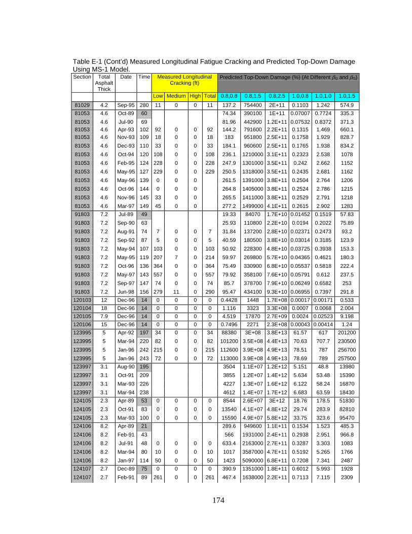
174
Table E-1 (Cont’d) Measured Longitudinal Fatigue Cracking and Predicted Top-Down Damage Using MS-1 Model. Section Total
Asphalt Thick
Date Time Measured Longitudinal Cracking (ft)
Predicted Top-Down Damage (%) (At Different βf2 and βf3)
Low Medium High Total 0.8,0.8 0.8,1.5 0.8,2.5 1.0,0.8 1.0,1.0 1.0,1.5
81029 4.2 Sep-95 280 11 0 0 11 137.2 754400 2E+11 0.1103 1.242 574.9 81053 4.6 Oct-89 60 74.34 390100 1E+11 0.07007 0.7724 335.3 81053 4.6 Jul-90 69 81.96 442900 1.2E+11 0.07532 0.8372 371.3 81053 4.6 Apr-93 102 92 0 0 92 144.2 791600 2.2E+11 0.1315 1.469 660.1 81053 4.6 Nov-93 109 18 0 0 18 183 951800 2.5E+11 0.1758 1.929 828.7 81053 4.6 Dec-93 110 33 0 0 33 184.1 960600 2.5E+11 0.1765 1.938 834.2 81053 4.6 Oct-94 120 108 0 0 108 236.1 1210000 3.1E+11 0.2323 2.538 1078 81053 4.6 Feb-95 124 228 0 0 228 247.9 1301000 3.5E+11 0.242 2.662 1152 81053 4.6 May-95 127 229 0 0 229 250.5 1318000 3.5E+11 0.2435 2.681 1162 81053 4.6 May-96 139 0 0 0 261.5 1391000 3.8E+11 0.2504 2.764 1206 81053 4.6 Oct-96 144 0 0 0 264.8 1405000 3.8E+11 0.2524 2.786 1215 81053 4.6 Nov-96 145 33 0 0 265.5 1411000 3.8E+11 0.2529 2.791 1218 81053 4.6 Mar-97 149 45 0 0 277.2 1499000 4.1E+11 0.2615 2.902 1283 91803 7.2 Jul-89 49 19.33 84070 1.7E+10 0.01452 0.1519 57.83 91803 7.2 Sep-90 63 25.93 110800 2.2E+10 0.0194 0.2022 75.89 91803 7.2 Aug-91 74 7 0 0 7 31.84 137200 2.8E+10 0.02371 0.2473 93.2 91803 7.2 Sep-92 87 5 0 0 5 40.59 180500 3.8E+10 0.03014 0.3185 123.9 91803 7.2 May-94 107 103 0 0 103 50.92 228300 4.8E+10 0.03725 0.3938 153.3 91803 7.2 May-95 119 207 7 0 214 59.97 269800 5.7E+10 0.04365 0.4621 180.3 91803 7.2 Oct-96 136 364 0 0 364 75.49 330900 6.8E+10 0.05537 0.5818 222.4 91803 7.2 May-97 143 557 0 0 557 79.92 358100 7.6E+10 0.05791 0.612 237.5 91803 7.2 Sep-97 147 74 0 0 74 85.7 378700 7.9E+10 0.06249 0.6582 253 91803 7.2 Jun-98 156 279 11 0 290 95.47 434100 9.3E+10 0.06955 0.7397 291.8 120103 12 Dec-96 14 0 0 0 0 0.4428 1448 1.7E+08 0.00017 0.00171 0.533 120104 18 Dec-96 14 0 0 0 0 1.116 3323 3.3E+08 0.0007 0.0068 2.004 120105 7.9 Dec-96 14 0 0 0 0 4.519 17870 2.7E+09 0.0024 0.02523 9.198 120106 15 Dec-96 14 0 0 0 0 0.7496 2271 2.3E+08 0.00043 0.00414 1.24 123995 5 Apr-92 197 34 0 0 34 88380 3E+08 3.8E+13 61.57 617 201200 123995 5 Mar-94 220 82 0 0 82 101200 3.5E+08 4.4E+13 70.63 707.7 230500 123995 5 Jan-96 242 215 0 0 215 112600 3.9E+08 4.9E+13 78.51 787 256700 123995 5 Jan-96 243 72 0 0 72 113000 3.9E+08 4.9E+13 78.69 789 257500 123997 3.1 Aug-90 195 3504 1.1E+07 1.2E+12 5.151 48.8 13980 123997 3.1 Oct-91 209 3855 1.2E+07 1.4E+12 5.634 53.48 15390 123997 3.1 Mar-93 226 4227 1.3E+07 1.6E+12 6.122 58.24 16870 123997 3.1 Mar-94 238 4612 1.4E+07 1.7E+12 6.683 63.59 18430 124105 2.3 Apr-89 53 0 0 0 0 8544 2.6E+07 3E+12 18.76 178.5 51830 124105 2.3 Oct-91 83 0 0 0 0 13540 4.1E+07 4.8E+12 29.74 283.9 82810 124105 2.3 Mar-93 100 0 0 0 0 15590 4.9E+07 5.8E+12 33.75 323.6 95470 124106 8.2 Apr-89 21 289.6 949600 1.1E+11 0.1534 1.523 485.3 124106 8.2 Feb-91 43 566 1931000 2.4E+11 0.2938 2.951 966.8 124106 8.2 Jul-91 48 0 0 0 0 633.4 2163000 2.7E+11 0.3287 3.303 1083 124106 8.2 Mar-94 80 10 0 0 10 1017 3587000 4.7E+11 0.5192 5.265 1766 124106 8.2 Jan-97 114 50 0 0 50 1423 5090000 6.8E+11 0.7208 7.341 2487 124107 2.7 Dec-89 75 0 0 0 0 390.9 1351000 1.8E+11 0.6012 5.993 1928 124107 2.7 Feb-91 89 261 0 0 261 467.4 1638000 2.2E+11 0.7113 7.115 2309

175
Table E-1 (Cont’d) Measured Longitudinal Fatigue Cracking and Predicted Top-Down Damage Using MS-1 Model. Section Total
Asphalt Thick
Date Time Measured Longitudinal Cracking (ft)
Predicted Top-Down Damage (%) (At Different βf2 and βf3)
Low Medium High Total 0.8,0.8 0.8,1.5 0.8,2.5 1.0,0.8 1.0,1.0 1.0,1.5
124107 2.7 Jul-91 94 343 0 0 343 503.9 1762000 2.4E+11 0.7682 7.683 2492 124107 2.7 Mar-93 114 18 0 0 18 624.3 2215000 3E+11 0.9424 9.453 3092 124107 2.7 Mar-94 126 37 13 0 51 709.3 2523000 3.5E+11 1.069 10.73 3516 124107 2.7 Jan-96 148 67 0 0 67 866.2 3115000 4.3E+11 1.291 13.01 4297 124107 2.7 Mar-97 162 0 0 0 973 3520000 5E+11 1.443 14.56 4829 124108 9.9 Apr-89 35 0 0 0 0 12.69 33830 3.7E+09 0.01203 0.1078 27.17 124108 9.9 Jan-91 56 0 0 0 0 20.72 55500 6.1E+09 0.02032 0.1818 45.64 124108 9.9 Oct-91 65 0 0 0 0 24.08 65410 7.2E+09 0.023 0.207 52.75 124108 9.9 Mar-94 94 7 0 0 7 34.46 96310 1.1E+10 0.0327 0.2963 76.87 124108 9.9 Aug-94 99 0 0 0 0 36.74 103100 1.2E+10 0.03447 0.3132 81.75 124108 9.9 Jan-96 116 0 0 0 0 41.69 119300 1.4E+10 0.03817 0.3488 92.37 124135 1.4 Dec-89 227 99 199 0 298 250600 9.6E+08 1.5E+14 856.8 8764 3046000124135 1.4 Jan-91 240 412 271 0 683 263100 1E+09 1.6E+14 897.1 9186 3200000131031 11.1 Apr-91 119 0 0 0 0 44.99 127700 1.3E+10 0.03012 0.2822 78.64 131031 11.1 Jul-92 134 0 0 0 0 58.68 166800 1.8E+10 0.03928 0.3686 103 131031 11.1 Jan-93 140 0 0 0 0 63.18 179600 1.9E+10 0.04238 0.3976 111.1 131031 11.1 Apr-94 155 0 0 0 0 74.64 213100 2.3E+10 0.04989 0.4687 131.3 131031 11.1 Oct-94 161 0 0 0 0 83.35 239100 2.5E+10 0.05549 0.5222 146.9 131031 11.1 Aug-95 171 0 0 0 0 94.69 271100 2.9E+10 0.06322 0.595 167.3 131031 11.1 Jan-96 176 4 0 0 4 97.99 281900 3E+10 0.06521 0.6142 173.2 131031 11.1 Apr-96 179 23 0 0 23 98.44 283800 3.1E+10 0.06539 0.6161 173.8 134111 8.7 Mar-89 101 27 0 0 27 34.3 101300 1.1E+10 0.02841 0.2696 77.27 134111 8.7 Mar-91 125 291 0 0 291 50.98 152700 1.7E+10 0.04178 0.3983 115.4 134111 8.7 Feb-92 136 477 0 0 477 59.21 178000 2E+10 0.04838 0.462 134.3 134112 15.9 May-89 144 0 0 0 0 146.3 354700 2.9E+10 0.1825 1.634 403.1 134112 15.9 Feb-91 165 17 0 0 17 181.9 446000 3.7E+10 0.2255 2.028 504.9 134112 15.9 Apr-91 167 0 0 0 0 182.3 447400 3.7E+10 0.2258 2.031 505.8 134112 15.9 Feb-94 201 0 0 0 0 245.7 611500 5.2E+10 0.3009 2.719 684.6 134112 15.9 Oct-94 209 0 0 0 0 263.6 659300 5.6E+10 0.3202 2.898 732.7 134112 15.9 Jan-96 224 0 0 0 0 292.8 731500 6.2E+10 0.3572 3.235 818.3 134112 15.9 Feb-97 237 0 0 0 0 319.8 800400 6.7E+10 0.3897 3.532 894.9 134112 15.9 Apr-98 251 0 0 0 0 349.4 876600 7.4E+10 0.4246 3.853 978.1 134113 15.2 May-89 144 0 0 0 0 382.8 862300 6.4E+10 0.5006 4.387 1024 134113 15.2 Feb-91 165 0 0 0 0 456.1 1041000 7.9E+10 0.5906 5.199 1226 134113 15.2 Apr-91 167 0 0 0 0 457.1 1044000 7.9E+10 0.5912 5.205 1228 134113 15.2 Feb-94 201 0 0 0 0 589.3 1367000 1E+11 0.7538 6.671 1593 134113 15.2 Oct-94 209 0 0 0 0 627.7 1461000 1.1E+11 0.7978 7.072 1695 134113 15.2 Jan-96 224 0 0 0 0 684.5 1594000 1.2E+11 0.8716 7.734 1857 134113 15.2 Feb-97 237 31 0 0 31 738.4 1724000 1.3E+11 0.9389 8.34 2007 134113 15.2 Apr-98 251 37 0 0 37 798.8 1869000 1.4E+11 1.015 9.021 2175 161001 3.7 Jul-89 192 155 0 0 155 8142 4.4E+07 1.1E+13 8.538 96.5 43980 161001 3.7 Aug-90 205 193 0 0 193 9320 5E+07 1.3E+13 9.844 111 50340 161001 3.7 Jun-93 239 78 0 0 78 11730 6.4E+07 1.7E+13 12.3 139.3 63750 161001 3.7 Aug-94 253 199 0 0 199 12810 7E+07 1.8E+13 13.44 151.9 69250

176
Table E-1 (Cont’d) Measured Longitudinal Fatigue Cracking and Predicted Top-Down Damage Using MS-1 Model. Section Total
Asphalt Thick
Date Time Measured Longitudinal Cracking (ft)
Predicted Top-Down Damage (%) (At Different βf2 and βf3)
Low Medium High Total 0.8,0.8 0.8,1.5 0.8,2.5 1.0,0.8 1.0,1.0 1.0,1.5
161001 3.7 May-95 262 183 2 0 185 13770 7.6E+07 2E+13 14.4 163.4 75090 161001 3.7 Jul-97 288 67 63 44 175 16270 8.9E+07 2.3E+13 17.09 193.5 88410 161001 3.7 Sep-98 302 0 159 5 164 17260 9.4E+07 2.4E+13 18.05 204.5 93620 161009 10.4 Sep-89 180 34.65 130400 2.5E+10 0.02238 0.2209 74.75 161009 10.4 Jul-90 190 36.59 137400 2.7E+10 0.02343 0.2312 78.06 161009 10.4 Jul-92 214 0 0 0 0 45.07 171700 3.4E+10 0.02888 0.2863 98.09 161009 10.4 Oct-93 229 8 0 0 8 51.11 191500 3.7E+10 0.03279 0.3234 108.9 161009 10.4 Jun-96 261 1 0 0 1 60.69 229100 4.4E+10 0.03803 0.376 127 161009 10.4 Jul-97 274 0 0 0 0 69.94 268500 5.3E+10 0.04435 0.4408 151.8 161021 5.9 Sep-89 48 36.66 192900 5.3E+10 0.0244 0.2623 113.1 161021 5.9 Oct-90 61 0 0 0 0 48.09 257400 7.1E+10 0.03186 0.3455 151.4 161021 5.9 Aug-91 71 0 0 0 0 54.89 293900 8.1E+10 0.03594 0.3897 170.6 161021 5.9 Aug-93 95 0 0 0 0 74.93 405200 1.1E+11 0.04938 0.5379 237.9 161021 5.9 Sep-95 120 0 0 0 0 96.86 526600 1.5E+11 0.06338 0.6927 308 161021 5.9 Jun-96 129 5 0 0 5 102.8 563700 1.6E+11 0.06643 0.7287 326.3 161021 5.9 Jul-97 142 0 0 0 0 113 615700 1.7E+11 0.07302 0.798 354.6 169034 9.2 Jul-89 10 5.219 20030 3.9E+09 0.00306 0.02976 9.498 169034 9.2 Aug-90 23 16.37 57020 1E+10 0.01108 0.1048 31.13 169034 9.2 Jun-93 57 12 0 0 12 34.02 131500 2.7E+10 0.0211 0.206 67.3 169034 9.2 Aug-94 71 146 0 0 146 43.65 165100 3.2E+10 0.02705 0.2634 84.88 169034 9.2 May-95 80 46.24 179100 3.6E+10 0.02816 0.2759 90.46 169034 9.2 Jul-97 106 217 0 0 217 62.92 245000 5E+10 0.03815 0.3755 124.7 169034 9.2 Sep-98 120 156 52 18 226 71.04 276400 5.6E+10 0.04277 0.4211 139.7 201009 11.1 Aug-88 44 0 0 0 0 5.739 25500 6.9E+09 0.00385 0.03963 15.63 201009 11.1 May-89 53 11 0 0 11 6.657 31810 9.1E+09 0.0043 0.04514 18.68 201009 11.1 Dec-90 72 210 5 0 215 9.766 47580 1.4E+10 0.00631 0.06687 28.22 201009 11.1 Oct-91 82 6 1 0 7 10.86 50960 1.4E+10 0.007 0.07334 30.07 201009 11.1 Apr-93 100 9 0 0 9 12.54 60970 1.7E+10 0.00799 0.08486 35.88 201009 11.1 Apr-95 124 16 28 0 43 16.6 82180 2.4E+10 0.01053 0.1124 48.15 201009 11.1 Apr-96 136 0 0 0 17.33 84820 2.4E+10 0.01091 0.1162 49.34 201009 11.1 Jan-99 168 0 0 0 21.69 105300 3E+10 0.01347 0.1432 60.41 251003 6.6 Aug-89 180 758 0 0 758 73.37 368800 8.6E+10 0.06355 0.7041 303.2 251003 6.6 Sep-90 193 691 0 0 691 80.03 403800 9.4E+10 0.06919 0.7677 331.5 251003 6.6 Aug-91 204 556 1 0 557 85.6 432100 1E+11 0.07392 0.8202 354.2 251003 6.6 Sep-92 217 600 0 0 600 93.16 468400 1.1E+11 0.08059 0.8928 384.4 251003 6.6 Oct-95 254 563 0 0 563 115 582500 1.4E+11 0.09922 1.102 477.7 251003 6.6 Oct-96 266 39 0 0 39 122.2 618800 1.5E+11 0.1054 1.171 507.2 251003 6.6 Jun-98 286 32 9 0 41 135.1 687000 1.6E+11 0.1165 1.295 562.7 251004 9.6 Aug-89 178 0 0 0 0 29.77 105100 1.7E+10 0.02765 0.272 86.91 251004 9.6 Sep-90 191 19 0 0 19 33.04 116300 1.8E+10 0.03071 0.3019 96.2 251004 9.6 Aug-91 202 16 0 0 16 35.76 125100 1.9E+10 0.0333 0.3271 103.8 251004 9.6 Sep-92 215 0 0 0 40.05 139500 2.1E+10 0.03736 0.3666 116 251004 9.6 Oct-95 252 0 0 0 52.18 184500 2.9E+10 0.04833 0.4758 152 251004 9.6 Jun-97 272 3 0 0 3 58.44 205900 3.2E+10 0.05411 0.5324 169.6
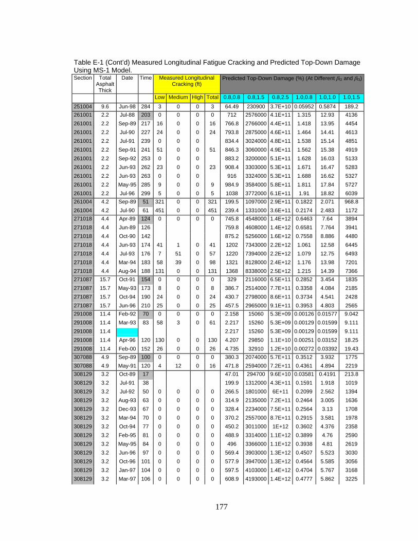
177
Table E-1 (Cont’d) Measured Longitudinal Fatigue Cracking and Predicted Top-Down Damage Using MS-1 Model. Section Total
Asphalt Thick
Date Time Measured Longitudinal Cracking (ft)
Predicted Top-Down Damage (%) (At Different βf2 and βf3)
Low Medium High Total 0.8,0.8 0.8,1.5 0.8,2.5 1.0,0.8 1.0,1.0 1.0,1.5
251004 9.6 Jun-98 284 3 0 0 3 64.49 230900 3.7E+10 0.05952 0.5874 189.2 261001 2.2 Jul-88 203 0 0 0 0 712 2576000 4.1E+11 1.315 12.93 4136 261001 2.2 Sep-89 217 16 0 0 16 766.8 2766000 4.4E+11 1.418 13.95 4454 261001 2.2 Jul-90 227 24 0 0 24 793.8 2875000 4.6E+11 1.464 14.41 4613 261001 2.2 Jul-91 239 0 0 0 834.4 3024000 4.8E+11 1.538 15.14 4851 261001 2.2 Sep-91 241 51 0 0 51 846.3 3060000 4.9E+11 1.562 15.38 4919 261001 2.2 Sep-92 253 0 0 0 883.2 3200000 5.1E+11 1.628 16.03 5133 261001 2.2 Jun-93 262 23 0 0 23 908.4 3303000 5.3E+11 1.671 16.47 5283 261001 2.2 Jun-93 263 0 0 0 916 3324000 5.3E+11 1.688 16.62 5327 261001 2.2 May-95 285 9 0 0 9 984.9 3584000 5.8E+11 1.811 17.84 5727 261001 2.2 Jul-96 299 5 0 0 5 1038 3772000 6.1E+11 1.91 18.82 6039 261004 4.2 Sep-89 51 321 0 0 321 199.5 1097000 2.9E+11 0.1822 2.071 968.8 261004 4.2 Jul-90 61 451 0 0 451 239.4 1331000 3.6E+11 0.2174 2.483 1172 271018 4.4 Apr-89 124 0 0 0 0 745.8 4548000 1.4E+12 0.6463 7.64 3894 271018 4.4 Jun-89 126 759.8 4608000 1.4E+12 0.6581 7.764 3941 271018 4.4 Oct-90 142 875.2 5256000 1.6E+12 0.7558 8.886 4480 271018 4.4 Jun-93 174 41 1 0 41 1202 7343000 2.2E+12 1.061 12.58 6445 271018 4.4 Jul-93 176 7 51 0 57 1220 7394000 2.2E+12 1.079 12.75 6493 271018 4.4 Mar-94 183 58 39 0 98 1321 8128000 2.4E+12 1.176 13.98 7201 271018 4.4 Aug-94 188 131 0 0 131 1368 8338000 2.5E+12 1.215 14.39 7366 271087 15.7 Oct-91 154 0 0 0 0 329 2116000 6.5E+11 0.2852 3.454 1835 271087 15.7 May-93 173 8 0 0 8 386.7 2514000 7.7E+11 0.3358 4.084 2185 271087 15.7 Oct-94 190 24 0 0 24 430.7 2798000 8.6E+11 0.3734 4.541 2428 271087 15.7 Jun-96 210 25 0 0 25 457.5 2965000 9.1E+11 0.3953 4.803 2565 291008 11.4 Feb-92 70 0 0 0 0 2.158 15060 5.3E+09 0.00126 0.01577 9.042 291008 11.4 Mar-93 83 58 3 0 61 2.217 15260 5.3E+09 0.00129 0.01599 9.111 291008 11.4 2.217 15260 5.3E+09 0.00129 0.01599 9.111 291008 11.4 Apr-96 120 130 0 0 130 4.207 29850 1.1E+10 0.00251 0.03152 18.25 291008 11.4 Feb-00 152 26 0 0 26 4.735 32910 1.2E+10 0.00272 0.03392 19.43 307088 4.9 Sep-89 100 0 0 0 0 380.3 2074000 5.7E+11 0.3512 3.932 1775 307088 4.9 May-91 120 4 12 0 16 471.8 2594000 7.2E+11 0.4361 4.894 2219 308129 3.2 Oct-89 17 47.01 294700 9.6E+10 0.03581 0.4191 213.8 308129 3.2 Jul-91 38 199.9 1312000 4.3E+11 0.1591 1.918 1019 308129 3.2 Jul-92 50 0 0 0 0 266.5 1801000 6E+11 0.2099 2.562 1394 308129 3.2 Aug-93 63 0 0 0 0 314.9 2135000 7.2E+11 0.2464 3.005 1636 308129 3.2 Dec-93 67 0 0 0 0 328.4 2234000 7.5E+11 0.2564 3.13 1708 308129 3.2 Mar-94 70 0 0 0 0 370.2 2557000 8.7E+11 0.2915 3.581 1978 308129 3.2 Oct-94 77 0 0 0 0 450.2 3011000 1E+12 0.3602 4.376 2358 308129 3.2 Feb-95 81 0 0 0 0 488.9 3314000 1.1E+12 0.3899 4.76 2590 308129 3.2 May-95 84 0 0 0 0 496 3366000 1.1E+12 0.3938 4.81 2619 308129 3.2 Jun-96 97 0 0 0 0 569.4 3903000 1.3E+12 0.4507 5.523 3030 308129 3.2 Oct-96 101 0 0 0 0 577.9 3947000 1.3E+12 0.4564 5.585 3056 308129 3.2 Jan-97 104 0 0 0 0 597.5 4103000 1.4E+12 0.4704 5.767 3168 308129 3.2 Mar-97 106 0 0 0 0 608.9 4193000 1.4E+12 0.4777 5.862 3225

178
Table E-1 (Cont’d) Measured Longitudinal Fatigue Cracking and Predicted Top-Down Damage Using MS-1 Model. Section Total
Asphalt Thick
Date Time Measured Longitudinal Cracking (ft)
Predicted Top-Down Damage (%) (At Different βf2 and βf3)
Low Medium High Total 0.8,0.8 0.8,1.5 0.8,2.5 1.0,0.8 1.0,1.0 1.0,1.5
308129 3.2 Aug-97 111 0 0 0 0 622.2 4255000 1.4E+12 0.4887 5.976 3269 308129 3.2 Oct-97 113 0 0 0 0 626.1 4277000 1.4E+12 0.4913 6.004 3281 321020 7 Jul-91 86 34 0 0 34 118.3 563800 1.4E+11 0.08031 0.8596 349 321020 7 Aug-93 111 138 0 0 138 166.6 811600 2.1E+11 0.1133 1.221 506 321020 7 Sep-94 123 29 20 0 49 189.4 921900 2.3E+11 0.1283 1.383 571.9 321020 7 Apr-95 131 242 0 0 242 200.2 986400 2.5E+11 0.1345 1.454 605.5 321020 7 Jun-97 157 9 0 0 256.6 1253000 3.2E+11 0.1721 1.856 766.6 321020 7 Jun-98 169 0 0 0 288.9 1440000 3.7E+11 0.1938 2.105 886 341031 7.3 Apr-92 224 333 1 0 333 815.3 3031000 4.9E+11 0.8026 8.041 2688 341031 7.3 Feb-93 234 322 31 3 356 894.5 3312000 5.4E+11 0.8828 8.836 2946 341031 7.3 Oct-95 266 0 352 170 522 1203 4449000 7.2E+11 1.186 11.88 3961 341031 7.3 Nov-95 267 232 30 0 261 1207 4471000 7.2E+11 1.188 11.9 3974 341033 7.4 Apr-92 211 52 2 0 54 19.61 87080 1.9E+10 0.01219 0.1283 49.05 341033 7.4 Feb-93 221 32 11 0 44 20.71 91710 1.9E+10 0.01289 0.1355 51.7 341033 7.4 Nov-95 254 55 0 0 55 24.2 107100 2.3E+10 0.01504 0.1581 60.28 341033 7.4 Jul-97 274 260 0 0 260 26.18 117000 2.5E+10 0.01618 0.1706 65.56 341034 11.1 Oct-89 48 0 0 0 0 29.45 90900 1.2E+10 0.02175 0.2057 58.6 341034 11.1 Sep-90 59 0 0 0 0 37.29 114700 1.5E+10 0.02737 0.2591 73.93 341034 11.1 Apr-92 78 0 0 0 0 44.9 140900 1.9E+10 0.03236 0.3075 88.74 341034 11.1 Feb-93 88 0 0 0 0 52.92 166000 2.2E+10 0.03781 0.36 104.2 341034 11.1 Nov-95 121 3 0 0 3 79.44 252700 3.4E+10 0.05571 0.533 156.2 341034 11.1 Jul-97 141 0 15 0 15 94.06 300600 4E+10 0.06543 0.6272 184.5 350101 7.2 May-97 19 0 0 0 0 262.8 833800 1.1E+11 0.2516 2.409 715.2 350102 4.8 May-97 19 0 0 0 0 283.1 1183000 2.3E+11 0.2222 2.301 842.8 350103 12.5 May-97 19 0 0 0 0 0.04618 150 3.6E+07 1.5E-05 0.00014 0.03902350104 19.2 May-97 19 0 0 0 0 7.649 15170 8.9E+08 0.00625 0.05379 11.78 350105 9.9 May-97 19 0 0 0 0 15.48 31760 2E+09 0.01116 0.09666 21.63 350106 15.6 May-97 19 0 0 0 0 1.518 2846 1.8E+08 0.00106 0.00896 1.891 351005 8.9 Oct-89 73 0 0 0 0 20.95 82120 1.6E+10 0.01261 0.1272 44.12 351005 8.9 Mar-91 90 0 0 0 0 25.61 105200 2.2E+10 0.01512 0.1543 55.41 351005 8.9 Oct-92 109 0 0 0 0 33.72 137100 2.8E+10 0.01974 0.2012 71.88 351005 8.9 Feb-94 125 0 0 0 0 40.58 167100 3.5E+10 0.02362 0.2414 86.94 351005 8.9 Mar-95 138 0 0 0 0 50.03 208600 4.4E+10 0.02915 0.299 109 351005 8.9 Apr-97 163 0 0 0 0 63.26 264600 5.6E+10 0.03636 0.3735 136.1 351022 6.3 Oct-89 37 0 0 0 0 33.24 152900 3.5E+10 0.02265 0.2404 95.12 351022 6.3 Mar-91 54 0 0 0 0 51.31 237300 5.6E+10 0.03466 0.3673 145 351022 6.3 Oct-92 73 0 0 0 0 84.32 393300 9.4E+10 0.0574 0.6106 243.8 351022 6.3 Feb-94 89 0 0 0 0 107.7 505700 1.2E+11 0.07285 0.776 310.7 351022 6.3 Mar-95 102 0 0 0 0 131.7 615800 1.5E+11 0.08891 0.9462 377.3 351022 6.3 Apr-97 127 0 0 0 0 189.9 892400 2.1E+11 0.1287 1.371 549.7 351112 6.3 Dec-89 67 565.5 2174000 4E+11 0.4634 4.613 1581 351112 6.3 Jan-91 80 662.2 2591000 4.9E+11 0.5343 5.36 1866 351112 6.3 Mar-91 82 0 0 0 0 675.1 2659000 5E+11 0.543 5.457 1909 351112 6.3 Jan-93 104 0 0 0 0 846.1 3369000 6.4E+11 0.6714 6.79 2403 351112 6.3 Feb-94 117 0 0 0 0 946.5 3788000 7.2E+11 0.7466 7.568 2690

179
Table E-1 (Cont’d) Measured Longitudinal Fatigue Cracking and Predicted Top-Down Damage Using MS-1 Model. Section Total
Asphalt Thick
Date Time Measured Longitudinal Cracking (ft)
Predicted Top-Down Damage (%) (At Different βf2 and βf3)
Low Medium High Total 0.8,0.8 0.8,1.5 0.8,2.5 1.0,0.8 1.0,1.0 1.0,1.5
351112 6.3 Oct-94 125 0 0 0 0 1022 4064000 7.7E+11 0.8069 8.172 2895 351112 6.3 Mar-95 130 14 0 0 14 1051 4238000 8.2E+11 0.825 8.387 3001 351112 6.3 Apr-95 131 0 0 0 0 1060 4276000 8.2E+11 0.8314 8.455 3028 351112 6.3 Jun-95 133 0 0 0 0 1080 4348000 8.4E+11 0.8472 8.615 3082 351112 6.3 Nov-96 150 0 0 0 0 1219 4917000 9.4E+11 0.9508 9.692 3479 351112 6.3 Apr-97 155 0 0 0 0 1244 5062000 9.8E+11 0.9668 9.875 3564 351112 6.3 Sep-97 160 0 0 0 0 1296 5236000 1E+12 1.009 10.29 3698 371024 4.8 Nov-89 109 37.16 162500 3.2E+10 0.03087 0.3274 127.2 371024 4.8 Mar-91 125 42.92 191200 3.9E+10 0.03518 0.3751 147.7 371024 4.8 Apr-92 138 3 0 0 3 48.53 217400 4.5E+10 0.03958 0.4227 167.2 371802 4.5 Mar-91 66 996 3164000 4E+11 1.604 15.48 4690 371802 4.5 Oct-92 85 28 0 0 28 1317 4154000 5.2E+11 2.129 20.54 6200 371802 4.5 Apr-94 103 0 0 0 1547 4961000 6.4E+11 2.481 24.02 7323 371802 4.5 Jul-95 118 41 0 0 41 1804 5732000 7.3E+11 2.909 28.09 8513 371802 4.5 Apr-96 127 0 0 0 1913 6124000 7.8E+11 3.071 29.71 9047 371992 2.4 Mar-91 14 294.3 972100 1.3E+11 0.4589 4.445 1351 371992 2.4 Oct-92 33 22 0 0 22 905.8 2817000 3.5E+11 1.507 14.4 4220 371992 2.4 Apr-94 51 0 0 0 0 1384 4414000 5.7E+11 2.279 21.85 6476 371992 2.4 Feb-96 73 0 0 0 0 2146 6894000 9E+11 3.534 33.96 10120 404087 10.1 Jan-90 43 0 0 0 0 3.621 7854 5.2E+08 0.00343 0.03018 7.067 404087 10.1 Oct-91 64 0 0 0 0 5.471 12200 8.3E+08 0.00505 0.04486 10.72 404087 10.1 Nov-92 77 31 0 0 31 6.425 14460 1E+09 0.00589 0.05245 12.62 404087 10.1 Feb-93 80 35 0 0 35 6.425 14460 1E+09 0.00589 0.05245 12.62 404087 10.1 Nov-94 101 143 0 0 143 8.303 19010 1.3E+09 0.00748 0.06697 16.32 404087 10.1 Feb-95 104 112 0 0 112 8.303 19010 1.3E+09 0.00748 0.06697 16.32 404087 10.1 Aug-95 110 0 159 0 159 9.779 22500 1.6E+09 0.00879 0.07882 19.29 404087 10.1 Jun-97 132 10 0 0 10 11.93 27760 2E+09 0.01062 0.09558 23.57 404163 11.5 Jan-90 34 1.815 4375 3.6E+08 0.00102 0.00917 2.273 404163 11.5 Mar-91 48 2.368 5802 4.9E+08 0.00132 0.01192 2.991 404163 11.5 Oct-91 55 0 0 0 0 2.742 6805 5.8E+08 0.0015 0.01363 3.452 404163 11.5 Nov-92 68 0 0 0 0 3.469 8657 7.4E+08 0.00191 0.01738 4.429 404163 11.5 Mar-93 72 7 0 0 7 3.478 8728 7.6E+08 0.00191 0.0174 4.443 404163 11.5 Nov-94 92 0 0 0 0 4.412 11220 9.8E+08 0.0024 0.02194 5.663 404163 11.5 Apr-96 109 0 0 0 0 4.764 12210 1.1E+09 0.00257 0.02351 6.098 404163 11.5 Aug-97 125 45 8 0 53 6.02 15520 1.4E+09 0.00326 0.0299 7.799 404163 11.5 Jan-99 141 6 9 0 15 6.55 17020 1.6E+09 0.00352 0.03239 8.492 404165 8.1 Jan-90 68 97.84 358100 6.4E+10 0.06452 0.6303 201.7 404165 8.1 Mar-91 82 114.5 425900 7.7E+10 0.07432 0.7301 236.7 404165 8.1 Oct-91 89 4 0 0 4 129 477300 8.5E+10 0.08345 0.821 266.5 404165 8.1 Nov-92 102 5 0 0 5 143.8 542900 9.9E+10 0.09159 0.9063 298.7 404165 8.1 Mar-93 106 19 0 0 19 144.9 551100 1E+11 0.09192 0.9104 301.1 404165 8.1 Oct-94 125 9 0 0 9 180.8 680600 1.2E+11 0.1151 1.14 375.2 404165 8.1 Nov-94 126 16 0 0 16 181.2 683200 1.2E+11 0.1152 1.141 376 404165 8.1 Apr-95 131 24 0 0 24 183.6 698100 1.3E+11 0.1162 1.152 381.5

180
Table E-1 (Cont’d) Measured Longitudinal Fatigue Cracking and Predicted Top-Down Damage Using MS-1 Model. Section Total
Asphalt Thick
Date Time Measured Longitudinal Cracking (ft)
Predicted Top-Down Damage (%) (At Different βf2 and βf3)
Low Medium High Total 0.8,0.8 0.8,1.5 0.8,2.5 1.0,0.8 1.0,1.0 1.0,1.5
404165 8.1 Jun-95 133 25 0 0 25 187.4 713500 1.3E+11 0.1184 1.175 389.7 404165 8.1 Apr-96 143 25 0 0 25 201.1 771900 1.4E+11 0.1263 1.257 419.2 404165 8.1 Nov-96 150 60 0 0 60 215.6 824300 1.5E+11 0.1354 1.347 449.1 404165 8.1 May-97 156 26 0 0 26 219.1 843300 1.6E+11 0.137 1.365 456.8 404165 8.1 Sep-97 160 24 0 0 24 229 878200 1.6E+11 0.143 1.425 477 421599 12.3 Aug-89 25 8.385 28040 4.5E+09 0.00518 0.05013 16.28 421599 12.3 Sep-90 38 11.57 42060 7.3E+09 0.00699 0.0695 24.13 421599 12.3 Mar-93 68 0 0 0 0 20.72 80750 1.5E+10 0.01252 0.1267 45.92 421599 12.3 Sep-94 86 0 0 0 0 27.04 103400 1.9E+10 0.01649 0.1659 59.2 421599 12.3 Jun-95 95 8 0 0 8 30.15 118600 2.2E+10 0.01817 0.1844 67.14 421599 12.3 Jul-96 108 4 0 0 4 33.07 125000 2.3E+10 0.02018 0.202 71.12 421599 12.3 Mar-98 128 2 0 0 2 42.37 161000 2.9E+10 0.02626 0.2627 92.55 451011 3.2 Mar-92 69 0 0 0 0 1939 6609000 9.9E+11 2.338 22.61 6906 451011 3.2 Oct-92 76 0 0 0 0 2203 7422000 1.1E+12 2.678 25.87 7860 451011 3.2 Jun-93 84 0 0 0 0 2321 7997000 1.2E+12 2.771 26.88 8274 451011 3.2 Jan-96 115 16 0 0 16 3226 1.1E+07 1.7E+12 3.853 37.46 11570 451011 3.2 Jun-97 132 0 0 0 0 3637 1.3E+07 1.9E+12 4.313 42.01 13050 451011 3.2 Feb-99 150 0 0 0 0 4135 1.4E+07 2.2E+12 4.886 47.67 14850 473104 1.3 Aug-89 39 125.3 460200 7.6E+10 0.4149 4.12 1366 473104 1.3 Nov-89 42 132.2 489200 8.2E+10 0.4336 4.316 1439 473104 1.3 May-91 60 178.3 712100 1.3E+11 0.5534 5.624 1982 473104 1.3 Aug-91 63 186.9 738000 1.3E+11 0.5793 5.875 2058 473104 1.3 Oct-92 77 226.3 902600 1.6E+11 0.6874 7.004 2479 473104 1.3 Aug-93 87 259.5 1049000 1.9E+11 0.78 7.987 2859 473104 1.3 Nov-95 114 357.2 1489000 2.8E+11 1.053 10.9 4005 473104 1.3 Oct-96 125 406.7 1699000 3.2E+11 1.198 12.42 4582 480001 2.4 Apr-89 1 40.86 114000 1.1E+10 0.07134 0.6641 181.7 480001 2.4 Oct-90 19 1167 2867000 2.7E+11 2.541 22.43 5439 480001 2.4 May-91 26 0 0 0 0 1382 3711000 4.1E+11 2.836 25.42 6476 480001 2.4 Feb-93 47 0 0 0 0 2716 7409000 8.5E+11 5.577 50.18 12900 480001 2.4 Apr-93 49 0 0 0 0 2791 7703000 9E+11 5.677 51.21 13260 480001 2.4 Feb-95 71 0 0 0 0 4209 1.2E+07 1.5E+12 8.272 75.49 20120 480001 2.4 Mar-95 72 0 0 0 0 4243 1.2E+07 1.5E+12 8.309 75.89 20280 480001 2.4 May-97 98 34 0 0 34 6329 1.9E+07 2.3E+12 12.22 112.2 30370 480001 2.4 Mar-98 108 34 0 0 34 7215 2.1E+07 2.7E+12 13.86 127.5 34720 481060 7.5 Jun-90 52 0 0 0 0 1590 5283000 6.9E+11 1.254 12.29 3847 481060 7.5 Feb-91 60 0 0 0 0 1827 6093000 8E+11 1.437 14.11 4427 481060 7.5 Apr-91 62 0 0 0 0 1867 6259000 8.3E+11 1.463 14.38 4525 481060 7.5 Mar-92 73 12 0 0 12 2243 7575000 1E+12 1.748 17.23 5456 481060 7.5 Feb-93 84 19 0 0 19 2657 9016000 1.2E+12 2.065 20.38 6479 481060 7.5 Mar-93 85 23 0 0 23 2679 9112000 1.2E+12 2.078 20.52 6533 481060 7.5 Oct-94 104 14 0 0 14 3479 1.2E+07 1.6E+12 2.691 26.64 8518 481060 7.5 Feb-95 108 28 0 0 28 3513 1.2E+07 1.6E+12 2.707 26.83 8597 481060 7.5 Mar-95 109 0 0 0 3528 1.2E+07 1.6E+12 2.715 26.91 8631

181
Table E-1 (Cont’d) Measured Longitudinal Fatigue Cracking and Predicted Top-Down Damage Using MS-1 Model. Section Total
Asphalt Thick
Date Time Measured Longitudinal Cracking (ft)
Predicted Top-Down Damage (%) (At Different βf2 and βf3)
Low Medium High Total 0.8,0.8 0.8,1.5 0.8,2.5 1.0,0.8 1.0,1.0 1.0,1.5
481060 7.5 Mar-95 112 14 0 0 14 3690 1.3E+07 1.7E+12 2.837 28.14 9035 481060 7.5 Jun-95 134 8 0 0 8 4599 1.6E+07 2.2E+12 3.508 34.91 11290 481060 7.5 Apr-97 137 31 0 0 31 4833 1.7E+07 2.3E+12 3.694 36.75 11880 481060 7.5 Jul-97 139 31 2 0 33 5005 1.7E+07 2.4E+12 3.835 38.13 12310 481060 7.5 Sep-97 154 32 0 0 32 5679 2E+07 2.7E+12 4.327 43.11 13980 481077 5.1 Apr-89 88 374.1 1633000 3.3E+11 0.2127 2.25 873.5 481077 5.1 Nov-91 119 0 0 0 0 514.7 2235000 4.5E+11 0.2919 3.085 1194 481077 5.1 Oct-92 130 28 0 0 28 566.8 2471000 5E+11 0.3208 3.395 1318 481077 5.1 May-93 137 124 0 0 124 594.6 2620000 5.3E+11 0.3349 3.555 1390 481077 5.1 Oct-94 154 143 0 0 143 679.7 2972000 6E+11 0.3834 4.061 1579 481077 5.1 Mar-95 159 47 0 0 47 700.2 3089000 6.3E+11 0.3935 4.179 1635 481077 5.1 Apr-95 160 181 0 0 181 705.6 3114000 6.3E+11 0.3965 4.212 1648 481077 5.1 Jun-95 162 181 0 0 181 717.4 3157000 6.4E+11 0.4035 4.284 1673 481077 5.1 Aug-95 164 181 0 0 181 728.6 3189000 6.4E+11 0.4105 4.35 1693 481077 5.1 Jun-96 174 181 0 0 181 775.1 3416000 6.9E+11 0.4353 4.622 1807 481077 5.1 May-97 185 228 10 0 238 831.2 3684000 7.5E+11 0.466 4.956 1946 481077 5.1 Jul-97 187 300 0 0 300 843.3 3724000 7.6E+11 0.4733 5.029 1969 481077 5.1 Sep-97 189 276 0 0 276 855.3 3765000 7.6E+11 0.4804 5.101 1994 481077 5.1 Mar-98 195 281 0 0 281 879.7 3910000 8E+11 0.4922 5.239 2061 481109 6.5 Jan-90 68 636.1 2124000 3E+11 0.7427 7.24 2261 481109 6.5 Sep-90 76 737.3 2454000 3.4E+11 0.8627 8.411 2624 481109 6.5 May-91 84 123 0 0 123 796 2703000 3.9E+11 0.9212 9.026 2853 481109 6.5 Feb-93 105 148 0 0 148 1031 3517000 5.1E+11 1.191 11.69 3708 481109 6.5 Jul-93 110 336 0 0 336 1104 3762000 5.4E+11 1.276 12.53 3975 481109 6.5 Feb-95 129 502 3 0 505 1314 4521000 6.6E+11 1.511 14.88 4750 481109 6.5 May-95 132 571 0 0 571 1349 4656000 6.8E+11 1.548 15.26 4883 481109 6.5 Aug-96 147 425 0 0 425 1579 5437000 7.9E+11 1.814 17.89 5722 481130 2.7 Apr-89 200 0 0 0 0 4147 1E+07 9.1E+11 8.725 77.27 18700 481130 2.7 Oct-90 218 0 0 0 0 4703 1.1E+07 1E+12 9.897 87.69 21230 481130 2.7 Mar-91 223 15 0 0 15 4739 1.2E+07 1E+12 9.937 88.11 21380 481130 2.7 Mar-92 235 35 0 0 35 5030 1.2E+07 1.1E+12 10.52 93.35 22690
481169 1.1 Feb-90 211 37120 1.6E+08 3.3E+13 91.28 973.3 380700 481169 1.1 Mar-90 212 37290 1.7E+08 3.3E+13 91.65 977.7 382700 481169 1.1 Sep-90 218 38600 1.7E+08 3.4E+13 95.11 1013 394600 481169 1.1 Jan-91 222 0 0 0 0 39270 1.7E+08 3.5E+13 96.53 1030 402700 481169 1.1 Mar-91 224 0 0 0 0 39610 1.8E+08 3.5E+13 97.26 1038 406900 481169 1.1 Jun-91 227 0 0 0 0 40250 1.8E+08 3.6E+13 98.93 1055 413000 481169 1.1 Jan-92 234 0 0 0 0 41630 1.8E+08 3.7E+13 102.3 1091 427000 481169 1.1 Feb-93 247 0 0 0 0 44210 2E+08 3.9E+13 108.6 1159 454000 481169 1.1 Aug-93 253 0 0 0 0 45510 2E+08 4E+13 111.9 1193 466400 481169 1.1 Mar-95 272 7 0 0 7 49250 2.2E+08 4.4E+13 120.8 1290 506800 481169 1.1 Jul-95 276 0 0 0 0 50160 2.2E+08 4.4E+13 123.1 1315 515300 481169 1.1 Jul-97 300 0 0 0 0 55120 2.4E+08 4.9E+13 135.2 1444 566700
481174 4.7 Oct-90 186 611.6 2207000 3.3E+11 0.3966 3.995 1348

182
Table E-1 (Cont’d) Measured Longitudinal Fatigue Cracking and Predicted Top-Down Damage Using MS-1 Model. Section Total
Asphalt Thick
Date Time Measured Longitudinal Cracking (ft)
Predicted Top-Down Damage (%) (At Different βf2 and βf3)
Low Medium High Total 0.8,0.8 0.8,1.5 0.8,2.5 1.0,0.8 1.0,1.0 1.0,1.5
481174 4.7 Feb-91 190 620.7 2250000 3.4E+11 0.4018 4.053 1372 481174 4.7 Apr-91 192 201 0 0 201 627.1 2277000 3.4E+11 0.4057 4.094 1387 481174 4.7 Mar-92 203 204 0 0 204 665.7 2418000 3.7E+11 0.43 4.34 1472 481174 4.7 Feb-93 214 138 0 0 138 701.9 2552000 3.9E+11 0.4525 4.569 1550 481174 4.7 Mar-93 215 185 0 0 185 704.1 2562000 3.9E+11 0.4538 4.583 1556 481174 4.7 Feb-95 238 220 10 0 229 783.3 2852000 4.3E+11 0.5035 5.086 1728 481174 4.7 Mar-95 239 179 0 0 179 785.8 2863000 4.3E+11 0.5049 5.102 1734 481174 4.7 Jan-96 249 160 0 0 160 822.2 2994000 4.5E+11 0.5278 5.333 1812 481174 4.7 Apr-97 264 0 0 0 873.1 3187000 4.8E+11 0.5595 5.658 1926 481174 4.7 Mar-98 275 49 0 0 49 907.6 3317000 5E+11 0.5808 5.876 2002
481178 8.5 Apr-89 10 78 0 0 78 4.13 6721 3.3E+08 0.00441 0.03486 6.305 481178 8.5 Feb-91 32 61 0 0 61 11.26 21420 1.3E+09 0.00949 0.07836 15.91 481178 8.5 May-91 33 48 0 0 48 11.32 21590 1.3E+09 0.00951 0.0786 15.98 481178 8.5 Feb-93 56 44 0 0 44 17.73 36040 2.3E+09 0.01361 0.1149 24.62 481178 8.5 Jul-93 61 94 0 0 94 19.79 40700 2.6E+09 0.01491 0.1264 27.39 481178 8.5 Feb-95 80 92 0 0 92 25.35 53700 3.6E+09 0.01834 0.157 34.91 481178 8.5 Mar-95 81 57 0 0 57 25.41 53880 3.6E+09 0.01836 0.1573 34.99
481183 5.7 Sep-90 188 0 0 0 0 1438 4487000 5.8E+11 1.754 16.82 5033 481183 5.7 Mar-91 194 0 0 0 0 1463 4604000 6.1E+11 1.777 17.07 5128 481183 5.7 Oct-91 201 4 0 0 4 1676 5214000 6.8E+11 2.044 19.59 5849 481183 5.7 Nov-91 202 11 0 0 11 1680 5236000 6.8E+11 2.047 19.62 5864 481183 5.7 Jan-93 216 19 0 0 19 1914 6012000 7.9E+11 2.323 22.31 6698 481183 5.7 Jul-93 222 3 0 0 3 2073 6512000 8.5E+11 2.515 24.17 7261 481183 5.7 Apr-94 231 3 0 0 3 2223 7006000 9.2E+11 2.69 25.86 7782
483749 1.8 Oct-90 116 0 0 0 0 15160 4.6E+07 5.5E+12 29.68 280.5 80490 483749 1.8 Apr-91 122 0 0 0 0 15560 4.8E+07 5.8E+12 30.22 286.3 82620 483749 1.8 Aug-91 126 0 0 0 0 16190 4.9E+07 6E+12 31.47 298 85880 483749 1.8 Mar-92 133 0 0 0 0 16750 5.2E+07 6.4E+12 32.32 306.7 88860 483749 1.8 Feb-93 144 0 0 0 0 17960 5.6E+07 6.9E+12 34.51 327.8 95250 483749 1.8 Mar-93 145 0 0 0 0 18040 5.6E+07 6.9E+12 34.63 329 95660 483749 1.8 Feb-95 168 0 0 0 0 20490 6.4E+07 8E+12 38.97 371.1 108500 483749 1.8 Mar-95 169 0 0 0 0 20560 6.4E+07 8.1E+12 39.06 372.1 108900 483749 1.8 Mar-97 193 2 0 0 2 23060 7.3E+07 9.2E+12 43.44 414.8 122100
489005 1.2 Oct-90 50 169 0 0 169 27920 9E+07 1.2E+13 117.7 1143 351700
489005 1.2 Mar-91 55 215 0 0 215 29950 9.9E+07 1.3E+13 125.3 1220 378900
489005 1.2 Aug-91 60 223 0 0 223 32490 1.1E+08 1.5E+13 135.5 1321 411500
489005 1.2 Feb-93 78 106 0 0 106 41640 1.4E+08 1.9E+13 172.3 1686 529700
489005 1.2 Apr-93 80 240 0 0 240 42260 1.4E+08 2E+13 174.3 1708 538500 489005 1.2 Feb-95 102 169 0 0 169 52680 1.8E+08 2.5E+13 215.3 2118 673000
489005 1.2 Feb-96 114 274 0 0 274 58520 2E+08 2.8E+13 238.6 2349 748000
489005 1.2 Jul-96 119 253 0 0 253 60630 2.1E+08 2.9E+13 246.3 2429 776500
489005 1.2 Jul-97 131 325 0 0 325 66470 2.3E+08 3.2E+13 269.3 2659 852700
489005 1.2 Jul-98 143 278 0 0 278 72320 2.5E+08 3.6E+13 292.4 2890 929300

183
Table E-1 (Cont’d) Measured Longitudinal Fatigue Cracking and Predicted Top-Down Damage Using MS-1 Model. Section Total
Asphalt Thick
Date Time Measured Longitudinal Cracking (ft)
Predicted Top-Down Damage (%) (At Different βf2 and βf3)
Low Medium High Total 0.8,0.8 0.8,1.5 0.8,2.5 1.0,0.8 1.0,1.0 1.0,1.5
501002 8.5 Aug-89 58 39.34 226400 6.1E+10 0.02785 0.3285 163.8 501002 8.5 Aug-90 70 48.54 279700 7.6E+10 0.03427 0.4044 201.7 501002 8.5 May-94 115 2 0 0 2 85.43 501200 1.4E+11 0.06118 0.7267 366.8 501002 8.5 Aug-94 118 0 0 0 0 87.57 509200 1.4E+11 0.06249 0.7403 371.6 501002 8.5 Apr-95 126 8 0 0 8 91.13 531200 1.4E+11 0.0646 0.7658 384.6 501002 8.5 Oct-96 144 16 0 0 16 115.6 677000 1.8E+11 0.08382 0.9962 501.8 501002 8.5 May-97 151 66 125 0 191 116.6 681800 1.8E+11 0.08427 1.001 503.8 501002 8.5 Oct-97 156 10 5 0 14 124.1 721100 1.9E+11 0.08937 1.059 530.6 501002 8.5 Jun-98 164 10 26 0 36 126.3 730900 2E+11 0.09049 1.071 535.2
501004 8 Apr-93 102 34 11 0 44 17.02 123400 4.3E+10 0.01351 0.1711 99.5 501004 8 Oct-95 132 8 4 0 12 22.89 163400 5.6E+10 0.01704 0.2147 123.7 501004 8 Nov-97 157 7 3 0 9 33.84 242900 8.4E+10 0.02523 0.3186 184.1
511002 5.7 Apr-89 115 9 42 59 110 585.7 2489000 4.8E+11 0.5969 6.258 2355
511023 10.1 Oct-89 107 0 0 0 0 115 341600 3.7E+10 0.07796 0.7445 215.7 511023 10.1 Mar-91 124 0 0 0 0 130 386900 4.2E+10 0.08804 0.8414 244.2 511023 10.1 May-92 138 0 0 0 0 144.6 432900 4.7E+10 0.09735 0.9321 271.7 511023 10.1 Oct-92 143 21 0 0 21 159.8 477900 5.2E+10 0.108 1.034 301.4 511023 10.1 Dec-93 157 0 0 0 175.6 525900 5.7E+10 0.1187 1.136 331.3 511023 10.1 Sep-95 178 105 0 0 105 208.5 626500 6.8E+10 0.1405 1.348 394.2 511023 10.1 Feb-96 183 167 0 0 167 208.9 628400 6.9E+10 0.1407 1.349 394.9 511023 10.1 Mar-97 196 4 0 0 4 223.3 674000 7.4E+10 0.1498 1.439 422.2
512021 7.5 Oct-89 54 180.6 719800 1.3E+11 0.1481 1.517 537.9 512021 7.5 Mar-91 71 230.3 934000 1.7E+11 0.1869 1.921 687.3 512021 7.5 Oct-92 90 21 0 0 21 316.4 1276000 2.3E+11 0.2582 2.654 947.5
531008 3.4 Jul-91 153 6 0 0 6 349.2 1453000 3E+11 0.3589 3.539 1193 531008 3.4 Jun-93 176 66 0 0 67 399.4 1679000 3.5E+11 0.4054 4.012 1365 531008 3.4 Jun-94 188 8 5 8 21 432.2 1819000 3.8E+11 0.438 4.338 1478
561007 2.8 Jul-90 121 162.7 620700 1.2E+11 0.2106 2.031 643.5 561007 2.8 May-91 131 0 0 0 0 173.7 671400 1.3E+11 0.2226 2.154 689.6 561007 2.8 Aug-91 134 0 0 0 0 183.4 694400 1.4E+11 0.2395 2.304 726.2 561007 2.8 Aug-93 158 13 0 0 13 214.2 808100 1.6E+11 0.2802 2.694 846.6 561007 2.8 Oct-93 160 26 0 0 26 216.2 817400 1.6E+11 0.2822 2.716 854.7 561007 2.8 Dec-93 162 4 0 0 4 218 829200 1.6E+11 0.2835 2.731 863.3 561007 2.8 Mar-94 165 6 0 0 6 220.7 847900 1.7E+11 0.2855 2.756 877 561007 2.8 Apr-94 166 0 0 0 221.6 852700 1.7E+11 0.2862 2.764 880.5 561007 2.8 Aug-94 170 6 0 0 6 229.2 875000 1.7E+11 0.2975 2.87 909.6 561007 2.8 Feb-95 176 7 0 0 7 235.2 908800 1.8E+11 0.303 2.931 937.1 561007 2.8 May-95 179 0 0 0 237.7 919800 1.8E+11 0.3055 2.957 946.6 561007 2.8 Sep-95 183 0 0 0 245.8 942700 1.9E+11 0.3177 3.07 977.3 561007 2.8 Jun-96 192 5 0 0 5 254.3 983400 2E+11 0.3266 3.163 1013 561007 2.8 Oct-96 196 0 0 0 263.6 1008000 2E+11 0.3421 3.302 1048 561007 2.8 Nov-96 197 2 0 0 2 264.1 1010000 2E+11 0.3424 3.305 1050 561007 2.8 Mar-97 201 0 0 0 266.5 1026000 2E+11 0.3439 3.324 1059 561007 2.8 Aug-97 206 3 0 0 3 278.9 1058000 2.1E+11 0.3645 3.509 1106

184
561007 2.8 Sep-97 207 0 0 0 280.6 1063000 2.1E+11 0.3669 3.532 1113

185
Table E-2 Measured Longitudinal Fatigue Cracking and Predicted Top-Down Damage Using MS1 Model.
Section Total
AC Thick
Date Time Measured Longitudinal Cracking (ft)
Predicted Top-Down Damage (%) (At Different βf2 and βf3)
Low Med High Total 1.0,2.5 1.2,0.8 1.2,1.5 (Ave
Thermal)
1.2,1.5 (No
Thermal)
1.2,1.5 (max
Thermal)
1.2,2.5
11001 3.2 Sep-91 132 0 0 0 0 8.2E+08 0.00223 6.201 5.93698 6.321 74890011001 3.2 Apr-92 139 16 0 0 16 9E+08 0.0023 6.512 6.25489 6.659 80980011001 3.2 Jul-92 142 14 0 0 14 9.1E+08 0.00239 6.705 6.42577 6.852 82240011001 3.2 Jan-93 148 30 0 0 30 9.5E+08 0.00249 7 6.71189 7.174 86250011019 6.7 May-89 32 5.2E+07 8.7E-05 0.2887 0.28546 0.3495 37880 11019 6.7 Apr-90 43 7E+07 0.00012 0.3837 0.37945 0.4595 50560 11019 6.7 Jan-91 52 8.3E+07 0.00014 0.4631 0.45789 0.5527 59960 11019 6.7 Jun-91 57 4 0 0 4 9.2E+07 0.00015 0.5079 0.50214 0.601 66110 11019 6.7 Mar-92 1.1E+08 0.00017 0.5759 0.56951 0.6788 75900 11019 6.7 Mar-93 78 139 0 0 139 1.3E+08 0.0002 0.6826 0.6751 0.8047 91520 11019 6.7 Jul-95 106 0 0 0 2.1E+08 0.00036 1.191 1.1769 1.374 15650011019 6.7 Jan-98 136 0 0 0 2.7E+08 0.00046 1.531 1.51278 1.758 20310014126 13.1 Jun-89 15 0 0 0 0 2961000 0.0001 0.1514 0.04933 0.02122 5212 14126 13.1 Mar-91 36 0 0 0 0 5756000 0.00017 0.2615 0.1209 0.2954 9504 14126 13.1 Mar-93 60 0 0 0 0 8147000 0.00021 0.3326 0.1721 0.4433 12670 14126 13.1 Apr-94 73 0 0 0 0 9584000 0.00024 0.3741 0.2057 0.7572 14560 14126 13.1 Dec-95 93 0 0 0 0 1.2E+07 0.00028 0.4471 0.2713 0.7591 17820 14126 13.1 Dec-97 117 0 0 0 0 1.5E+07 0.00032 0.5144 0.3278 0.9258 21000 21001 3 May-90 83 0 0 0 0 1.5E+08 0.00011 0.553 0.36955 534.1 12960021001 3 Aug-91 98 0 0 0 0 1.8E+08 0.00015 0.7012 0.45136 552.6 16010021001 3 Aug-93 122 27 0 0 27 2.3E+08 0.00018 0.874 0.55591 728.2 20500021001 3 Jun-95 144 0 0 0 0 3E+08 0.00021 1.087 0.64433 728.3 26490021001 3 Aug-97 170 0 0 0 0 3.5E+08 0.00026 1.305 0.7688 728.5 31360021001 3 Aug-98 182 0 0 0 0 3.9E+08 0.00028 1.412 0.82482 728.6 34430021002 3.3 May-90 68 0 0 0 0 2.8E+07 2.5E-05 0.09913 0.08125 52.52 20190 21002 3.3 Aug-91 83 6 0 0 6 3.4E+07 3.4E-05 0.1315 0.10731 76.5 25550 21002 3.3 Aug-93 107 0 0 0 0 4.4E+07 4.5E-05 0.1702 0.14205 79.86 32800 21002 3.3 Jun-95 129 0 0 0 0 5.9E+07 5.8E-05 0.2238 0.17453 104.3 45000 21002 3.3 Aug-97 155 0 0 0 0 6.8E+07 6.6E-05 0.2572 0.20306 104.4 51840 21002 3.3 May-98 164 0 0 0 0 7.7E+07 6.9E-05 0.2797 0.21084 104.4 58980 40113 4.5 Feb-95 19 0 0 0 0 3.8E+08 0.00034 1.234 1.00236 7.324 24180040113 4.5 Mar-95 20 11 0 0 11 4.1E+08 0.00035 1.293 1.0427 7.626 25700040113 4.5 Aug-95 25 0 0 0 0 4.8E+08 0.00047 1.637 1.34506 8.32 30180040113 4.5 Nov-95 28 0 0 0 0 5.3E+08 0.00051 1.819 1.47914 8.543 33640040113 4.5 Feb-96 31 0 0 0 0 6.4E+08 0.00054 2.027 1.62744 11.38 40090040113 4.5 Apr-96 33 0 0 0 0 6.9E+08 0.00057 2.149 1.71312 11.75 42930040113 4.5 Jul-96 36 0 0 0 0 7.2E+08 0.00066 2.403 1.95823 12.02 452700

186
Table E-2 (Cont’d) Measured Longitudinal Fatigue Cracking and Predicted Top-Down Damage Using MS-1 Model. Section Total
AC Thick
Date Time Measured Longitudinal Cracking (ft)
Predicted Top-Down Damage (%) (At Different βf2 and βf3)
Low Med High Total 1.0,2.5 1.2,0.8 1.2,1.5 (Ave
Thermal)
1.2,1.5 (No
Thermal)
1.2,1.5 (max
Thermal)
1.2,2.5
40113 4.5 Aug-96 37 0 0 0 0 7.3E+08 0.0007 2.499 2.05274 12.12 46110040113 4.5 Jan-98 54 53 17 0 70 1.2E+09 0.001 3.794 3.06125 19.25 75560040113 4.5 Apr-98 57 17 65 0 82 1.3E+09 0.00104 4.035 3.23375 20.79 82710040113 4.5 Jun-98 59 24 59 0 83 1.4E+09 0.00108 4.181 3.34555 20.99 85070040113 4.5 Oct-98 63 0 173 0 173 1.4E+09 0.0012 4.57 3.69478 21.4 90020040114 6.8 Feb-95 19 0 0 0 0 2.3E+08 0.00045 1.358 1.38517 4.714 16560040114 6.8 Mar-95 20 31 0 0 31 2.5E+08 0.00046 1.401 1.43008 4.955 17340040114 6.8 Aug-95 25 0 0 0 0 3.3E+08 0.00068 2.046 2.08161 5.958 24280040114 6.8 Nov-95 28 0 0 0 0 3.9E+08 0.00077 2.358 2.39699 6.286 28420040114 6.8 Feb-96 31 7 0 0 7 4.1E+08 0.00078 2.403 2.44793 7.762 29480040114 6.8 Apr-96 33 9 0 0 9 4.4E+08 0.00082 2.544 2.59238 8.102 31580040114 6.8 Jul-96 36 44 0 0 44 5E+08 0.00101 3.058 3.10918 8.676 36660040114 6.8 Aug-96 37 0 0 0 5.2E+08 0.00107 3.252 3.30424 8.87 38550040114 6.8 Jan-98 54 33 40 26 98 7.8E+08 0.00154 4.736 4.81275 12.81 57180040114 6.8 Apr-98 57 0 41 0 41 8.1E+08 0.00156 4.834 4.91665 13.53 58860040114 6.8 Jun-98 59 0 42 0 42 8.6E+08 0.00165 5.127 5.21493 13.92 62520040114 6.8 Oct-98 63 38 23 0 61 9.6E+08 0.00189 5.849 5.93885 14.66 70670040115 15.1 Feb-95 19 0 0 0 0 3.8E+07 0.00075 1.206 1.196 2.48 48750 40115 15.1 Mar-95 20 33 0 0 33 3.8E+07 0.00075 1.209 1.198 2.492 48930 40115 15.1 Jan-98 54 0 0 0 0 1.2E+08 0.00165 2.908 2.878 7.305 13550040116 16.2 Feb-95 19 0 0 0 0 1.2E+07 0.00014 0.2618 0.2595 0.6168 13130 40116 16.2 Mar-95 20 18 0 0 18 1.3E+07 0.00014 0.2623 0.2599 0.6217 13180 40116 16.2 Jan-98 54 0 0 0 0 3.6E+07 0.00028 0.5791 0.5732 1.604 33340 40117 11.8 Feb-95 19 0 0 0 0 1.1E+07 0.00011 0.2046 0.1981 0.7893 10130 40117 11.8 Mar-95 20 14 0 0 14 1.1E+07 0.00011 0.2048 0.1982 0.8039 10150 40117 11.8 Jan-98 54 0 0 0 0 3.2E+07 0.00022 0.4514 0.4343 2.051 25760 40118 11.7 Feb-95 19 0 0 0 0 4233000 2.9E-05 0.05474 0.05394 0.403 2919 40118 11.7 Mar-95 20 15 0 0 15 4236000 2.9E-05 0.05475 0.05395 0.4096 2920 40118 11.7 Jan-98 54 0 0 0 0 1.3E+07 5.7E-05 0.1219 0.1197 1.126 7714 41007 6.5 Sep-91 162 0 0 0 0 1.8E+08 0.00016 0.5854 0.57635 0.6356 93330 41007 6.5 Feb-93 163 57 0 0 57 1.8E+08 0.00016 0.5901 0.58104 0.6403 94400 41007 6.5 Sep-94 198 167 0 0 167 2.4E+08 0.00022 0.795 0.783 0.8626 12870041024 10.8 Nov-89 149 4.8E+08 0.00178 4.169 4.166 12.56 31670041024 10.8 Aug-90 158 5.3E+08 0.00196 4.616 4.61 14.38 35190041024 10.8 Oct-92 184 0 0 0 0 6.7E+08 0.00244 5.797 5.796 18.57 44600041024 10.8 Mar-95 213 9 0 0 9 8.2E+08 0.00287 6.89 6.896 25.73 53660041024 10.8 Jul-95 217 23 0 0 23 8.7E+08 0.00305 7.33 7.334 26.18 57100041024 10.8 Aug-95 218 127 0 0 127 8.9E+08 0.00313 7.513 7.515 26.36 58570041024 10.8 Nov-95 221 109 0 0 109 9.1E+08 0.00317 7.621 7.626 26.92 59570041024 10.8 Feb-96 224 61 0 0 61 9.1E+08 0.00317 7.621 7.626 27.1 595700

187
Table E-2 (Cont’d) Measured Longitudinal Fatigue Cracking and Predicted Top-Down Damage Using MS-1 Model. Section Total
AC Thick
Date Time Measured Longitudinal Cracking (ft)
Predicted Top-Down Damage (%) (At Different βf2 and βf3)
Low Med High Total 1.0,2.5 1.2,0.8 1.2,1.5 (Ave
Thermal)
1.2,1.5 (No
Thermal)
1.2,1.5 (max
Thermal)
1.2,2.5
41024 10.8 Apr-96 226 79 0 23 102 9.1E+08 0.00317 7.63 7.636 27.15 59660041024 10.8 Jun-96 228 59 0 0 59 9.3E+08 0.00322 7.76 7.765 27.3 60720041024 10.8 Aug-96 230 59 0 0 59 9.8E+08 0.00343 8.251 8.253 27.79 64400041024 10.8 Apr-98 250 49 0 4 53 1.1E+09 0.00378 9.131 9.144 31.95 71630041024 10.8 Jun-98 252 49 0 4 53 1.1E+09 0.00386 9.327 9.339 32.15 73140041024 10.8 Oct-98 256 50 0 4 54 1.2E+09 0.00401 9.732 9.759 35.42 76840081029 4.2 Oct-91 233 0 25 0 25 1.2E+08 8.4E-05 0.3977 0.44921 1292 99960 81029 4.2 Jul-94 266 44 0 0 44 1.4E+08 9.5E-05 0.4563 0.51241 1458 11590081029 4.2 Sep-95 280 11 0 0 11 1.5E+08 9.9E-05 0.4783 0.53816 1511 12140081053 4.6 Oct-89 60 8.1E+07 7.4E-05 0.322 0.66249 367.3 70250 81053 4.6 Jul-90 69 9.3E+07 7.8E-05 0.3484 0.78522 385.1 79040 81053 4.6 Apr-93 102 92 0 0 92 1.7E+08 0.00013 0.6138 1.35658 743.6 14260081053 4.6 Nov-93 109 18 0 0 18 2E+08 0.00019 0.8077 1.54624 744.5 17280081053 4.6 Dec-93 110 33 0 0 33 2E+08 0.00019 0.8113 1.55343 746.3 17410081053 4.6 Oct-94 120 108 0 0 108 2.5E+08 0.00026 1.074 1.80151 768.7 22390081053 4.6 Feb-95 124 228 0 0 228 2.8E+08 0.00026 1.138 1.83639 1141 24690081053 4.6 May-95 127 229 0 0 229 2.8E+08 0.00027 1.144 1.91182 1144 24880081053 4.6 May-96 139 0 0 0 3E+08 0.00027 1.173 2.20611 1238 25800081053 4.6 Oct-96 144 0 0 0 3E+08 0.00027 1.179 2.38705 1238 25900081053 4.6 Nov-96 145 33 0 0 3E+08 0.00027 1.18 2.40231 1238 25950081053 4.6 Mar-97 149 45 0 0 3.2E+08 0.00028 1.232 2.45245 1247 27780091803 7.2 Jul-89 49 1.1E+07 1.2E-05 0.04484 0.03515 452.7 7731 91803 7.2 Sep-90 63 1.4E+07 1.6E-05 0.05861 0.04845 458.2 9692 91803 7.2 Aug-91 74 7 0 0 7 1.7E+07 2E-05 0.07144 0.05871 530.1 11890 91803 7.2 Sep-92 87 5 0 0 5 2.4E+07 2.5E-05 0.09528 0.07211 1108 17120 91803 7.2 May-94 107 103 0 0 103 3E+07 3.1E-05 0.116 0.09111 1137 20620 91803 7.2 May-95 119 207 7 0 214 3.5E+07 3.6E-05 0.1356 0.10683 1244 24090 91803 7.2 Oct-96 136 364 0 0 364 4.2E+07 4.6E-05 0.1684 0.13889 1252 28590 91803 7.2 May-97 143 557 0 0 557 4.6E+07 4.7E-05 0.1774 0.14409 1416 30950 91803 7.2 Sep-97 147 74 0 0 74 4.8E+07 5.1E-05 0.1902 0.15689 1416 32500 91803 7.2 Jun-98 156 279 11 0 290 5.8E+07 5.7E-05 0.2203 0.16791 2471 40240 120103 12 Dec-96 14 0 0 0 0 55360 8E-08 0.00023 0.00021 0.00024 22.09 120104 18 Dec-96 14 0 0 0 0 182100 5E-07 0.00137 0.00137 0.00137 118.1 120105 7.9 Dec-96 14 0 0 0 0 1340000 1.4E-06 0.00511 0.00532 0.00527 710.5 120106 15 Dec-96 14 0 0 0 0 116200 2.7E-07 0.00077 0.00077 0.00077 68.46 123995 5 Apr-92 197 34 0 0 34 2.4E+10 0.04782 149.3 23.2063 23.68 1.7E+07123995 5 Mar-94 220 82 0 0 82 2.7E+10 0.05499 171.4 25.9236 26.43 1.9E+07123995 5 Jan-96 242 215 0 0 215 3.1E+10 0.061 190.6 28.4485 29.02 2.1E+07123995 5 Jan-96 243 72 0 0 72 3.1E+10 0.06112 191.1 28.5485 29.14 2.1E+07123997 3.1 Aug-90 195 1.4E+09 0.00887 22.07 22.2806 22.26 1845000
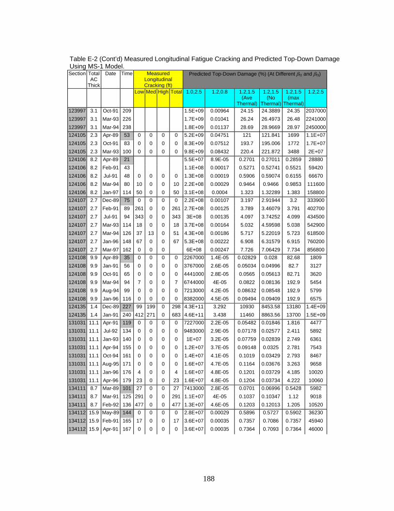
188
Table E-2 (Cont’d) Measured Longitudinal Fatigue Cracking and Predicted Top-Down Damage Using MS-1 Model. Section Total
AC Thick
Date Time Measured Longitudinal Cracking (ft)
Predicted Top-Down Damage (%) (At Different βf2 and βf3)
Low Med High Total 1.0,2.5 1.2,0.8 1.2,1.5 (Ave
Thermal)
1.2,1.5 (No
Thermal)
1.2,1.5 (max
Thermal)
1.2,2.5
123997 3.1 Oct-91 209 1.5E+09 0.00964 24.15 24.3889 24.35 2037000123997 3.1 Mar-93 226 1.7E+09 0.01041 26.24 26.4973 26.48 2241000123997 3.1 Mar-94 238 1.8E+09 0.01137 28.69 28.9669 28.97 2450000124105 2.3 Apr-89 53 0 0 0 0 5.2E+09 0.04751 121 121.841 1699 1.1E+07124105 2.3 Oct-91 83 0 0 0 0 8.3E+09 0.07512 193.7 195.006 1772 1.7E+07124105 2.3 Mar-93 100 0 0 0 0 9.8E+09 0.08432 220.4 221.872 3488 2E+07 124106 8.2 Apr-89 21 5.5E+07 8.9E-05 0.2701 0.27011 0.2859 28880 124106 8.2 Feb-91 43 1.1E+08 0.00017 0.5271 0.52741 0.5521 59420 124106 8.2 Jul-91 48 0 0 0 0 1.3E+08 0.00019 0.5906 0.59074 0.6155 66670 124106 8.2 Mar-94 80 10 0 0 10 2.2E+08 0.00029 0.9464 0.9466 0.9853 111600124106 8.2 Jan-97 114 50 0 0 50 3.1E+08 0.0004 1.323 1.32289 1.383 158800124107 2.7 Dec-89 75 0 0 0 0 2.2E+08 0.00107 3.197 2.91944 3.2 333900124107 2.7 Feb-91 89 261 0 0 261 2.7E+08 0.00125 3.789 3.46079 3.791 402700124107 2.7 Jul-91 94 343 0 0 343 3E+08 0.00135 4.097 3.74252 4.099 434500124107 2.7 Mar-93 114 18 0 0 18 3.7E+08 0.00164 5.032 4.59598 5.038 542900124107 2.7 Mar-94 126 37 13 0 51 4.3E+08 0.00186 5.717 5.22019 5.723 618500124107 2.7 Jan-96 148 67 0 0 67 5.3E+08 0.00222 6.908 6.31579 6.915 760200124107 2.7 Mar-97 162 0 0 0 6E+08 0.00247 7.726 7.06429 7.734 856800124108 9.9 Apr-89 35 0 0 0 0 2267000 1.4E-05 0.02829 0.028 82.68 1809 124108 9.9 Jan-91 56 0 0 0 0 3767000 2.6E-05 0.05034 0.04996 82.7 3127 124108 9.9 Oct-91 65 0 0 0 0 4441000 2.8E-05 0.0565 0.05613 82.71 3620 124108 9.9 Mar-94 94 7 0 0 7 6744000 4E-05 0.0822 0.08136 192.9 5454 124108 9.9 Aug-94 99 0 0 0 0 7213000 4.2E-05 0.08632 0.08548 192.9 5799 124108 9.9 Jan-96 116 0 0 0 0 8382000 4.5E-05 0.09494 0.09409 192.9 6575 124135 1.4 Dec-89 227 99 199 0 298 4.3E+11 3.292 10930 8453.58 13180 1.4E+09124135 1.4 Jan-91 240 412 271 0 683 4.6E+11 3.438 11460 8863.56 13700 1.5E+09131031 11.1 Apr-91 119 0 0 0 0 7227000 2.2E-05 0.05482 0.01846 1.816 4477 131031 11.1 Jul-92 134 0 0 0 0 9483000 2.9E-05 0.07178 0.02577 2.411 5892 131031 11.1 Jan-93 140 0 0 0 0 1E+07 3.2E-05 0.07759 0.02839 2.749 6361 131031 11.1 Apr-94 155 0 0 0 0 1.2E+07 3.7E-05 0.09148 0.0325 2.781 7543 131031 11.1 Oct-94 161 0 0 0 0 1.4E+07 4.1E-05 0.1019 0.03429 2.793 8467 131031 11.1 Aug-95 171 0 0 0 0 1.6E+07 4.7E-05 0.1164 0.03676 3.263 9658 131031 11.1 Jan-96 176 4 0 0 4 1.6E+07 4.8E-05 0.1201 0.03729 4.185 10020 131031 11.1 Apr-96 179 23 0 0 23 1.6E+07 4.8E-05 0.1204 0.03734 4.222 10060 134111 8.7 Mar-89 101 27 0 0 27 7413000 2.8E-05 0.0701 0.06996 0.5428 5982 134111 8.7 Mar-91 125 291 0 0 291 1.1E+07 4E-05 0.1037 0.10347 1.12 9018 134111 8.7 Feb-92 136 477 0 0 477 1.3E+07 4.6E-05 0.1203 0.12013 1.205 10520 134112 15.9 May-89 144 0 0 0 0 2.8E+07 0.00029 0.5896 0.5727 0.5902 36230 134112 15.9 Feb-91 165 17 0 0 17 3.6E+07 0.00035 0.7357 0.7086 0.7357 45940 134112 15.9 Apr-91 167 0 0 0 0 3.6E+07 0.00035 0.7364 0.7093 0.7364 46000

189
Table E-2 (Cont’d) Measured Longitudinal Fatigue Cracking and Predicted Top-Down Damage Using MS-1 Model. Section Total
AC Thick
Date Time Measured Longitudinal Cracking (ft)
Predicted Top-Down Damage (%) (At Different βf2 and βf3)
Low Med High Total 1.0,2.5 1.2,0.8 1.2,1.5 (Ave
Thermal)
1.2,1.5 (No
Thermal)
1.2,1.5 (max
Thermal)
1.2,2.5
134112 15.9 Feb-94 201 0 0 0 0 4.9E+07 0.00046 0.9886 0.9495 0.9883 62900 134112 15.9 Oct-94 209 0 0 0 0 5.3E+07 0.00049 1.05 1.009 1.049 67350 134112 15.9 Jan-96 224 0 0 0 0 5.9E+07 0.00055 1.179 1.134 1.179 75630 134112 15.9 Feb-97 237 0 0 0 0 6.5E+07 0.0006 1.289 1.241 1.29 82920 134112 15.9 Apr-98 251 0 0 0 0 7.1E+07 0.00065 1.406 1.355 1.407 90780 134113 15.2 May-89 144 0 0 0 0 6.4E+07 0.00082 1.564 1.488 1.567 85630 134113 15.2 Feb-91 165 0 0 0 0 7.8E+07 0.00096 1.859 1.772 1.86 103800134113 15.2 Apr-91 167 0 0 0 0 7.8E+07 0.00096 1.861 1.773 1.862 103900134113 15.2 Feb-94 201 0 0 0 0 1E+08 0.00121 2.394 2.289 2.395 136600134113 15.2 Oct-94 209 0 0 0 0 1.1E+08 0.00127 2.533 2.424 2.535 145600134113 15.2 Jan-96 224 0 0 0 0 1.2E+08 0.00139 2.783 2.667 2.786 160400134113 15.2 Feb-97 237 31 0 0 31 1.3E+08 0.0015 3.006 2.884 3.012 173900134113 15.2 Apr-98 251 37 0 0 37 1.4E+08 0.00162 3.259 3.114 3.265 189000161001 3.7 Jul-89 192 155 0 0 155 1.1E+10 0.00975 46.6 7.63222 3275 1.1E+07161001 3.7 Aug-90 205 193 0 0 193 1.2E+10 0.01132 53.63 8.4377 3295 1.2E+07161001 3.7 Jun-93 239 78 0 0 78 1.6E+10 0.01402 67.52 10.6735 4261 1.6E+07161001 3.7 Aug-94 253 199 0 0 199 1.7E+10 0.01533 73.38 11.8764 5395 1.7E+07161001 3.7 May-95 262 183 2 0 185 1.9E+10 0.01635 79.41 12.3568 5408 1.9E+07161001 3.7 Jul-97 288 67 63 44 175 2.2E+10 0.01953 93.85 14.5782 5546 2.2E+07161001 3.7 Sep-98 302 0 159 5 164 2.3E+10 0.02053 99.04 15.9616 7496 2.3E+07161009 10.4 Sep-89 180 1.3E+07 1.8E-05 0.05175 0.03825 543.1 8271 161009 10.4 Jul-90 190 1.4E+07 1.8E-05 0.0536 0.04016 630.9 8473 161009 10.4 Jul-92 214 0 0 0 0 1.8E+07 2.2E-05 0.06714 0.04876 636.4 10980 161009 10.4 Oct-93 229 8 0 0 8 1.9E+07 2.5E-05 0.07463 0.05649 637.3 11650 161009 10.4 Jun-96 261 1 0 0 1 2.2E+07 2.9E-05 0.08482 0.06562 850.2 13110 161009 10.4 Jul-97 274 0 0 0 0 2.8E+07 3.4E-05 0.1023 0.07489 852.2 16750 161021 5.9 Sep-89 48 2.9E+07 2E-05 0.07713 0.05469 325.1 18040 161021 5.9 Oct-90 61 0 0 0 0 4E+07 2.6E-05 0.1025 0.06904 470.8 24560 161021 5.9 Aug-91 71 0 0 0 0 4.5E+07 2.9E-05 0.1139 0.07943 592.2 27170 161021 5.9 Aug-93 95 0 0 0 0 6.3E+07 4E-05 0.1615 0.10779 788.5 39280 161021 5.9 Sep-95 120 0 0 0 0 8.2E+07 5.1E-05 0.2067 0.13673 976.4 50530 161021 5.9 Jun-96 129 5 0 0 5 8.8E+07 5.3E-05 0.2163 0.14514 1115 53240 161021 5.9 Jul-97 142 0 0 0 0 9.4E+07 5.8E-05 0.2345 0.16207 1178 56930 169034 9.2 Jul-89 10 1394000 2.3E-06 0.00586 0.00513 1.666 626.1 169034 9.2 Aug-90 23 4158000 9.5E-06 0.02237 0.01913 26.25 2144 169034 9.2 Jun-93 57 12 0 0 12 1.1E+07 1.6E-05 0.04369 0.03431 69.65 5582 169034 9.2 Aug-94 71 146 0 0 146 1.3E+07 2.1E-05 0.05505 0.04423 71.18 6709 169034 9.2 May-95 80 1.5E+07 2.1E-05 0.05755 0.0457 95.76 7296 169034 9.2 Jul-97 106 217 0 0 217 2.1E+07 2.8E-05 0.07888 0.06108 135.1 10520 169034 9.2 Sep-98 120 156 52 18 226 2.3E+07 3.2E-05 0.08769 0.06866 139.2 11550
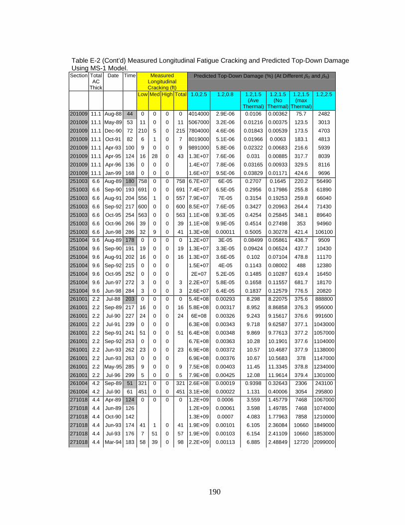
190
Table E-2 (Cont’d) Measured Longitudinal Fatigue Cracking and Predicted Top-Down Damage Using MS-1 Model.
Section Total AC
Thick
Date Time Measured Longitudinal Cracking (ft)
Predicted Top-Down Damage (%) (At Different βf2 and βf3)
Low Med High Total 1.0,2.5 1.2,0.8 1.2,1.5 (Ave
Thermal)
1.2,1.5 (No
Thermal)
1.2,1.5 (max
Thermal)
1.2,2.5
201009 11.1 Aug-88 44 0 0 0 0 4014000 2.9E-06 0.0106 0.00362 75.7 2482 201009 11.1 May-89 53 11 0 0 11 5067000 3.2E-06 0.01216 0.00375 123.5 3013 201009 11.1 Dec-90 72 210 5 0 215 7804000 4.6E-06 0.01843 0.00539 173.5 4703 201009 11.1 Oct-91 82 6 1 0 7 8019000 5.1E-06 0.01966 0.0063 183.1 4813 201009 11.1 Apr-93 100 9 0 0 9 9891000 5.8E-06 0.02322 0.00683 216.6 5939 201009 11.1 Apr-95 124 16 28 0 43 1.3E+07 7.6E-06 0.031 0.00885 317.7 8039 201009 11.1 Apr-96 136 0 0 0 1.4E+07 7.8E-06 0.03165 0.00933 329.5 8116 201009 11.1 Jan-99 168 0 0 0 1.6E+07 9.5E-06 0.03829 0.01171 424.6 9696 251003 6.6 Aug-89 180 758 0 0 758 6.7E+07 6E-05 0.2707 0.1645 220.2 56490 251003 6.6 Sep-90 193 691 0 0 691 7.4E+07 6.5E-05 0.2956 0.17986 255.8 61890 251003 6.6 Aug-91 204 556 1 0 557 7.9E+07 7E-05 0.3154 0.19253 259.8 66040 251003 6.6 Sep-92 217 600 0 0 600 8.5E+07 7.6E-05 0.3427 0.20963 264.4 71430 251003 6.6 Oct-95 254 563 0 0 563 1.1E+08 9.3E-05 0.4254 0.25845 348.1 89640 251003 6.6 Oct-96 266 39 0 0 39 1.1E+08 9.9E-05 0.4514 0.27498 353 94960 251003 6.6 Jun-98 286 32 9 0 41 1.3E+08 0.00011 0.5005 0.30278 421.4 106100251004 9.6 Aug-89 178 0 0 0 0 1.2E+07 3E-05 0.08499 0.05861 436.7 9509 251004 9.6 Sep-90 191 19 0 0 19 1.3E+07 3.3E-05 0.09424 0.06524 437.7 10430 251004 9.6 Aug-91 202 16 0 0 16 1.3E+07 3.6E-05 0.102 0.07104 478.8 11170 251004 9.6 Sep-92 215 0 0 0 1.5E+07 4E-05 0.1143 0.08002 488 12380 251004 9.6 Oct-95 252 0 0 0 2E+07 5.2E-05 0.1485 0.10287 619.4 16450 251004 9.6 Jun-97 272 3 0 0 3 2.2E+07 5.8E-05 0.1658 0.11557 681.7 18170 251004 9.6 Jun-98 284 3 0 0 3 2.6E+07 6.4E-05 0.1837 0.12579 776.5 20820 261001 2.2 Jul-88 203 0 0 0 0 5.4E+08 0.00293 8.298 8.22075 375.6 888800261001 2.2 Sep-89 217 16 0 0 16 5.8E+08 0.00317 8.952 8.86858 376.3 956000261001 2.2 Jul-90 227 24 0 0 24 6E+08 0.00326 9.243 9.15617 376.6 991600261001 2.2 Jul-91 239 0 0 0 6.3E+08 0.00343 9.718 9.62587 377.1 1043000261001 2.2 Sep-91 241 51 0 0 51 6.4E+08 0.00348 9.869 9.77613 377.2 1057000261001 2.2 Sep-92 253 0 0 0 6.7E+08 0.00363 10.28 10.1901 377.6 1104000261001 2.2 Jun-93 262 23 0 0 23 6.9E+08 0.00372 10.57 10.4687 377.9 1138000261001 2.2 Jun-93 263 0 0 0 6.9E+08 0.00376 10.67 10.5683 378 1147000261001 2.2 May-95 285 9 0 0 9 7.5E+08 0.00403 11.45 11.3345 378.8 1234000261001 2.2 Jul-96 299 5 0 0 5 7.9E+08 0.00425 12.08 11.9614 379.4 1301000261004 4.2 Sep-89 51 321 0 0 321 2.6E+08 0.00019 0.9398 0.32643 2306 243100261004 4.2 Jul-90 61 451 0 0 451 3.1E+08 0.00022 1.131 0.40006 3054 295800271018 4.4 Apr-89 124 0 0 0 0 1.2E+09 0.0006 3.559 1.45779 7468 1067000271018 4.4 Jun-89 126 1.2E+09 0.00061 3.598 1.49785 7468 1074000271018 4.4 Oct-90 142 1.3E+09 0.0007 4.083 1.77963 7858 1210000271018 4.4 Jun-93 174 41 1 0 41 1.9E+09 0.00101 6.105 2.36084 10660 1849000271018 4.4 Jul-93 176 7 51 0 57 1.9E+09 0.00103 6.154 2.41109 10660 1853000271018 4.4 Mar-94 183 58 39 0 98 2.2E+09 0.00113 6.885 2.48849 12720 2099000

191
Table E-2 (Cont’d) Measured Longitudinal Fatigue Cracking and Predicted Top-Down Damage Using MS-1 Model.
Section Total AC
Thick
Date Time Measured Longitudinal Cracking (ft)
Predicted Top-Down Damage (%) (At Different βf2 and βf3)
Low Med High Total 1.0,2.5 1.2,0.8 1.2,1.5 (Ave
Thermal)
1.2,1.5 (No
Thermal)
1.2,1.5 (max
Thermal)
1.2,2.5
271018 4.4 Aug-94 188 131 0 0 131 2.2E+09 0.00117 7.022 2.63108 12720 2125000271087 15.7 Oct-91 154 0 0 0 0 5.6E+08 0.00026 1.678 0.1206 27820 514900271087 15.7 May-93 173 8 0 0 8 6.7E+08 0.00031 2 0.128 31660 617400271087 15.7 Oct-94 190 24 0 0 24 7.5E+08 0.00034 2.221 0.1434 35830 685300271087 15.7 Jun-96 210 25 0 0 25 7.9E+08 0.00036 2.34 0.1554 38210 721100291008 11.4 Feb-92 70 0 0 0 0 3210000 8.1E-07 0.00585 0.00015 66.32 2087 291008 11.4 Mar-93 83 58 3 0 61 3220000 8.2E-07 0.00588 0.00017 67.35 2090 291008 11.4 3220000 8.2E-07 0.00588 0.00017 67.35 2091 291008 11.4 Apr-96 120 130 0 0 130 6511000 1.6E-06 0.01198 0.00024 134.6 4300 291008 11.4 Feb-00 152 26 0 0 26 6883000 1.7E-06 0.01247 0.00032 148.6 4449 307088 4.9 Sep-89 100 0 0 0 0 4.6E+08 0.00036 1.672 0.65907 2696 398600307088 4.9 May-91 120 4 12 0 16 5.8E+08 0.00045 2.091 0.80108 3631 500600308129 3.2 Oct-89 17 6.9E+07 3.1E-05 0.173 0.28791 198.7 53760 308129 3.2 Jul-91 38 3.3E+08 0.00014 0.8541 0.71093 442 270100308129 3.2 Jul-92 50 0 0 0 0 4.6E+08 0.00018 1.162 0.91598 843.3 380800308129 3.2 Aug-93 63 0 0 0 0 5.4E+08 0.00021 1.357 1.08169 1095 446000308129 3.2 Dec-93 67 0 0 0 0 5.7E+08 0.00022 1.415 1.11825 1291 466600308129 3.2 Mar-94 70 0 0 0 0 6.7E+08 0.00025 1.655 1.19097 1359 553400308129 3.2 Oct-94 77 0 0 0 0 7.7E+08 0.00031 1.993 1.24144 1359 642500308129 3.2 Feb-95 81 0 0 0 0 8.6E+08 0.00034 2.182 1.30423 1389 712000308129 3.2 May-95 84 0 0 0 0 8.7E+08 0.00034 2.199 1.34754 1389 717900308129 3.2 Jun-96 97 0 0 0 0 1E+09 0.00039 2.538 1.53551 1838 838100308129 3.2 Oct-96 101 0 0 0 0 1E+09 0.00039 2.556 1.55895 1838 841900308129 3.2 Jan-97 104 0 0 0 0 1.1E+09 0.0004 2.642 1.61896 2036 874400308129 3.2 Mar-97 106 0 0 0 0 1.1E+09 0.00041 2.681 1.68016 2160 888700308129 3.2 Aug-97 111 0 0 0 0 1.1E+09 0.00042 2.718 1.71791 2160 895100308129 3.2 Oct-97 113 0 0 0 0 1.1E+09 0.00042 2.727 1.73182 2160 896900321020 7 Jul-91 86 34 0 0 34 7.8E+07 5.9E-05 0.236 0.1702 117.5 47610 321020 7 Aug-93 111 138 0 0 138 1.2E+08 8.3E-05 0.3443 0.23427 252.3 73540 321020 7 Sep-94 123 29 20 0 49 1.3E+08 9.4E-05 0.3874 0.26811 261.6 82030 321020 7 Apr-95 131 242 0 0 242 1.4E+08 9.8E-05 0.4065 0.28463 262.2 86690 321020 7 Jun-97 157 9 0 0 1.8E+08 0.00013 0.5131 0.36794 263.2 106500321020 7 Jun-98 169 0 0 0 2.1E+08 0.00014 0.5952 0.40581 512.3 130000341031 7.3 Apr-92 224 333 1 0 333 3.8E+08 0.00089 2.737 2.809 338.3 330800341031 7.3 Feb-93 234 322 31 3 356 4.1E+08 0.00098 3.008 3.08812 343.1 361700341031 7.3 Oct-95 266 0 352 170 522 5.5E+08 0.00132 4.041 4.16173 346.8 485800341031 7.3 Nov-95 267 232 30 0 261 5.5E+08 0.00132 4.048 4.16843 357.8 487700341033 7.4 Apr-92 211 52 2 0 54 9256000 8.7E-06 0.03193 0.07771 0.1925 5286 341033 7.4 Feb-93 221 32 11 0 44 9711000 9.2E-06 0.03369 0.0823 0.1955 5552 341033 7.4 Nov-95 254 55 0 0 55 1.1E+07 1.1E-05 0.03925 0.09711 0.2147 6441

192
Table E-2 (Cont’d) Measured Longitudinal Fatigue Cracking and Predicted Top-Down Damage Using MS-1 Model.
Section Total AC
Thick
Date Time Measured Longitudinal Cracking (ft)
Predicted Top-Down Damage (%) (At Different βf2 and βf3)
Low Med High Total 1.0,2.5 1.2,0.8 1.2,1.5 (Ave
Thermal)
1.2,1.5 (No
Thermal)
1.2,1.5 (max
Thermal)
1.2,2.5
341033 7.4 Jul-97 274 260 0 0 260 1.2E+07 1.2E-05 0.04246 0.10401 0.2308 7073 341034 11.1 Oct-89 48 0 0 0 0 5956000 2E-05 0.04772 0.04661 36.45 3906 341034 11.1 Sep-90 59 0 0 0 0 7416000 2.4E-05 0.05974 0.05858 37.09 4880 341034 11.1 Apr-92 78 0 0 0 0 9195000 2.8E-05 0.07036 0.0688 70.8 5894 341034 11.1 Feb-93 88 0 0 0 0 1.1E+07 3.3E-05 0.0818 0.0802 72.46 6876 341034 11.1 Nov-95 121 3 0 0 3 1.7E+07 4.7E-05 0.12 0.1174 83.91 10400 341034 11.1 Jul-97 141 0 15 0 15 2E+07 5.5E-05 0.1405 0.1375 84.58 12260 350101 7.2 May-97 19 0 0 0 0 7.8E+07 0.00027 0.7078 0.71574 2.548 66490 350102 4.8 May-97 19 0 0 0 0 1.4E+08 0.00019 0.6728 0.70497 3.805 101100350103 12.5 May-97 19 0 0 0 0 6772 6.5E-09 1.4E-05 1.1E-05 0.249 1.542 350104 19.2 May-97 19 0 0 0 0 599900 5.8E-06 0.01064 0.01064 0.3927 504.7 350105 9.9 May-97 19 0 0 0 0 1172000 8.9E-06 0.01669 0.01668 0.4905 832.9 350106 15.6 May-97 19 0 0 0 0 93060 8.3E-07 0.00146 0.00145 0.4271 64.98 351005 8.9 Oct-89 73 0 0 0 0 7422000 8.5E-06 0.02665 0.02382 840.8 3850 351005 8.9 Mar-91 90 0 0 0 0 1E+07 1E-05 0.03279 0.02762 1303 5194 351005 8.9 Oct-92 109 0 0 0 0 1.3E+07 1.3E-05 0.04225 0.03619 1596 6539 351005 8.9 Feb-94 125 0 0 0 0 1.6E+07 1.5E-05 0.05073 0.04289 2490 8009 351005 8.9 Mar-95 138 0 0 0 0 2E+07 1.9E-05 0.06356 0.05231 2721 10420 351005 8.9 Apr-97 163 0 0 0 0 2.5E+07 2.3E-05 0.07845 0.06584 3742 12660 351022 6.3 Oct-89 37 0 0 0 0 2E+07 1.7E-05 0.0649 0.03548 506.9 12350 351022 6.3 Mar-91 54 0 0 0 0 3.1E+07 2.6E-05 0.09779 0.05438 599.4 18400 351022 6.3 Oct-92 73 0 0 0 0 5.3E+07 4.3E-05 0.1659 0.08748 2235 32370 351022 6.3 Feb-94 89 0 0 0 0 6.7E+07 5.4E-05 0.2103 0.11217 2419 41070 351022 6.3 Mar-95 102 0 0 0 0 8.1E+07 6.6E-05 0.2549 0.13884 2519 48970 351022 6.3 Apr-97 127 0 0 0 0 1.2E+08 9.5E-05 0.3726 0.19558 4293 72950 351112 6.3 Dec-89 67 2.6E+08 0.00043 1.272 1.22121 841.6 181200351112 6.3 Jan-91 80 3.1E+08 0.00048 1.48 1.42738 842.5 215500351112 6.3 Mar-91 82 0 0 0 0 3.2E+08 0.00049 1.509 1.45631 842.6 221600351112 6.3 Jan-93 104 0 0 0 0 4.1E+08 0.00059 1.879 1.80407 1301 281400351112 6.3 Feb-94 117 0 0 0 0 4.6E+08 0.00065 2.091 2.01327 1303 315400351112 6.3 Oct-94 125 0 0 0 0 4.9E+08 0.0007 2.253 2.17168 1304 337200351112 6.3 Mar-95 130 14 0 0 14 5.2E+08 0.00072 2.321 2.22852 1312 354800351112 6.3 Apr-95 131 0 0 0 0 5.2E+08 0.00072 2.341 2.24803 1312 358200351112 6.3 Jun-95 133 0 0 0 0 5.3E+08 0.00073 2.384 2.29074 1312 363900351112 6.3 Nov-96 150 0 0 0 0 6E+08 0.00082 2.681 2.582 1313 410000351112 6.3 Apr-97 155 0 0 0 0 6.2E+08 0.00083 2.734 2.63514 1313 422200351112 6.3 Sep-97 160 0 0 0 0 6.4E+08 0.00086 2.843 2.74142 1313 435200371024 4.8 Nov-89 109 2.4E+07 2.8E-05 0.1073 0.3606 0.1483 18680 371024 4.8 Mar-91 125 2.8E+07 3.1E-05 0.1229 0.42311 0.1805 21920 371024 4.8 Apr-92 138 3 0 0 3 3.2E+07 3.5E-05 0.1384 0.48133 0.2005 24860 371802 4.5 Mar-91 66 5.2E+08 0.00288 7.835 10.3732 10.69 780600

193
Table E-2 (Cont’d) Measured Longitudinal Fatigue Cracking and Predicted Top-Down Damage Using MS-1 Model.
Section Total AC
Thick
Date Time Measured Longitudinal Cracking (ft)
Predicted Top-Down Damage (%) (At Different βf2 and βf3)
Low Med High Total 1.0,2.5 1.2,0.8 1.2,1.5 (Ave
Thermal)
1.2,1.5 (No
Thermal)
1.2,1.5 (max
Thermal)
1.2,2.5
371802 4.5 Oct-92 85 28 0 0 28 6.9E+08 0.00383 10.41 14.0077 14.48 1028000371802 4.5 Apr-94 103 0 0 0 8.3E+08 0.00444 12.19 16.5856 17.22 1227000371802 4.5 Jul-95 118 41 0 0 41 9.5E+08 0.00523 14.25 19.5247 20.36 1417000371802 4.5 Apr-96 127 0 0 0 1E+09 0.0055 15.08 20.7195 21.61 1513000371992 2.4 Mar-91 14 1.5E+08 0.00084 2.264 2.23258 2.642 214800371992 2.4 Oct-92 33 22 0 0 22 4.3E+08 0.00291 7.503 7.3743 8.15 666900371992 2.4 Apr-94 51 0 0 0 0 6.9E+08 0.00438 11.41 11.0792 30.26 1035000371992 2.4 Feb-96 73 0 0 0 0 1.1E+09 0.00679 17.84 17.1456 51.11 1632000404087 10.1 Jan-90 43 0 0 0 0 423600 3.8E-06 0.00761 0.00227 0.2893 421.9 404087 10.1 Oct-91 64 0 0 0 0 667400 5.5E-06 0.01127 0.00347 0.2989 650.3 404087 10.1 Nov-92 77 31 0 0 31 795700 6.4E-06 0.01317 0.00408 0.4075 769.9 404087 10.1 Feb-93 80 35 0 0 35 795700 6.4E-06 0.01317 0.00408 0.4078 769.9 404087 10.1 Nov-94 101 143 0 0 143 1053000 8E-06 0.01674 0.00526 0.7112 1003 404087 10.1 Feb-95 104 112 0 0 112 1053000 8E-06 0.01674 0.00526 0.7156 1003 404087 10.1 Aug-95 110 0 159 0 159 1253000 9.3E-06 0.01974 0.00618 0.7241 1193 404087 10.1 Jun-97 132 10 0 0 10 1556000 1.1E-05 0.0239 0.00765 0.8968 1468 404163 11.5 Jan-90 34 160400 6.6E-07 0.00138 0.00136 0.1047 85.81 404163 11.5 Mar-91 48 215500 8.4E-07 0.0018 0.00178 0.2743 114.6 404163 11.5 Oct-91 55 0 0 0 0 252700 9.5E-07 0.00204 0.00202 0.2747 132.4 404163 11.5 Nov-92 68 0 0 0 0 326000 1.2E-06 0.00264 0.00261 0.311 172.8 404163 11.5 Mar-93 72 7 0 0 7 330900 1.2E-06 0.00264 0.00261 0.3802 173.8 404163 11.5 Nov-94 92 0 0 0 0 428200 1.5E-06 0.00333 0.00329 0.3824 223.9 404163 11.5 Apr-96 109 0 0 0 0 466100 1.6E-06 0.00355 0.00351 0.5878 241 404163 11.5 Aug-97 125 45 8 0 53 601500 2E-06 0.00456 0.00451 0.6583 313.1 404163 11.5 Jan-99 141 6 9 0 15 663200 2.2E-06 0.00494 0.00488 0.7633 342.2 404165 8.1 Jan-90 68 2.9E+07 5.1E-05 0.1386 0.13477 13.03 15610 404165 8.1 Mar-91 82 3.5E+07 5.8E-05 0.1601 0.15615 13.13 18470 404165 8.1 Oct-91 89 4 0 0 4 3.8E+07 6.5E-05 0.1797 0.17558 13.15 20750 404165 8.1 Nov-92 102 5 0 0 5 4.4E+07 7E-05 0.1979 0.19247 20.42 23620 404165 8.1 Mar-93 106 19 0 0 19 4.5E+07 7E-05 0.1987 0.19317 21.07 23880 404165 8.1 Oct-94 125 9 0 0 9 5.5E+07 8.7E-05 0.2487 0.24179 23.99 29600 404165 8.1 Nov-94 126 16 0 0 16 5.6E+07 8.7E-05 0.249 0.24209 24.06 29680 404165 8.1 Apr-95 131 24 0 0 24 5.7E+07 8.8E-05 0.2513 0.24441 24.65 30220 404165 8.1 Jun-95 133 25 0 0 25 5.8E+07 8.9E-05 0.2562 0.2492 24.66 30920 404165 8.1 Apr-96 143 25 0 0 25 6.4E+07 9.5E-05 0.2738 0.26595 27.61 33490 404165 8.1 Nov-96 150 60 0 0 60 6.8E+07 0.0001 0.2934 0.28532 27.64 35790 404165 8.1 May-97 156 26 0 0 26 7E+07 0.0001 0.297 0.28884 27.69 36510 404165 8.1 Sep-97 160 24 0 0 24 7.2E+07 0.00011 0.3099 0.30157 27.71 38050 421599 12.3 Aug-89 25 2544000 3.6E-06 0.01046 0.00867 537.3 1535 421599 12.3 Sep-90 38 4109000 4.7E-06 0.01513 0.01142 768.5 2454

194
Table E-2 (Cont’d) Measured Longitudinal Fatigue Cracking and Predicted Top-Down Damage Using MS-1 Model.
Section Total AC
Thick
Date Time Measured Longitudinal Cracking (ft)
Predicted Top-Down Damage (%) (At Different βf2 and βf3)
Low Med High Total 1.0,2.5 1.2,0.8 1.2,1.5 (Ave
Thermal)
1.2,1.5 (No
Thermal)
1.2,1.5 (max
Thermal)
1.2,2.5
421599 12.3 Mar-93 68 0 0 0 0 8243000 8.5E-06 0.02869 0.01963 1580 4870 421599 12.3 Sep-94 86 0 0 0 0 1E+07 1.1E-05 0.03732 0.02793 1876 6185 421599 12.3 Jun-95 95 8 0 0 8 1.2E+07 1.2E-05 0.04181 0.0295 1968 7106 421599 12.3 Jul-96 108 4 0 0 4 1.2E+07 1.4E-05 0.0449 0.0354 2001 7262 421599 12.3 Mar-98 128 2 0 0 2 1.6E+07 1.9E-05 0.05922 0.04492 2938 9532 451011 3.2 Mar-92 69 0 0 0 0 8.2E+08 0.00336 8.849 8.70677 11.28 850000451011 3.2 Oct-92 76 0 0 0 0 9.2E+08 0.00386 10.16 9.97444 12.6 964600451011 3.2 Jun-93 84 0 0 0 0 1E+09 0.00395 10.5 10.3122 13.24 1024000451011 3.2 Jan-96 115 16 0 0 16 1.4E+09 0.00548 14.7 14.4172 18.32 1439000451011 3.2 Jun-97 132 0 0 0 0 1.6E+09 0.0061 16.47 16.1578 20.82 1631000451011 3.2 Feb-99 150 0 0 0 0 1.8E+09 0.00688 18.69 18.3355 23.74 1861000473104 1.3 Aug-89 39 2E+08 0.00164 4.852 15.1196 4.874 597100473104 1.3 Nov-89 42 2.1E+08 0.00169 5.062 16.3095 5.085 629700473104 1.3 May-91 60 3.2E+08 0.00205 6.576 22.0194 8.09 918200473104 1.3 Aug-91 63 3.3E+08 0.00214 6.825 24.0893 8.339 942900473104 1.3 Oct-92 77 4E+08 0.00248 8.06 31.1491 9.577 1139000473104 1.3 Aug-93 87 4.7E+08 0.00277 9.194 36.549 10.73 1331000473104 1.3 Nov-95 114 6.9E+08 0.00364 12.62 53.2085 16.05 1927000473104 1.3 Oct-96 125 7.9E+08 0.00413 14.43 61.9083 17.86 2220000480001 2.4 Apr-89 1 1.6E+07 0.00014 0.3351 0.45085 0.3375 25690 480001 2.4 Oct-90 19 4.1E+08 0.00654 12.52 16.9191 12.63 759700480001 2.4 May-91 26 0 0 0 0 5.6E+08 0.00701 14 18.81 14.2 945100480001 2.4 Feb-93 47 0 0 0 0 1.1E+09 0.01378 27.92 37.3639 28.72 1921000480001 2.4 Apr-93 49 0 0 0 0 1.2E+09 0.01393 28.42 37.9942 29.23 1985000480001 2.4 Feb-95 71 0 0 0 0 1.9E+09 0.0196 41.63 55.5239 42.78 3082000480001 2.4 Mar-95 72 0 0 0 0 2E+09 0.01964 41.82 55.7504 42.98 3115000480001 2.4 May-97 98 34 0 0 34 3E+09 0.02848 61.8 82.0942 63.89 4713000480001 2.4 Mar-98 108 34 0 0 34 3.5E+09 0.03213 70.22 93.1241 72.6 5431000481060 7.5 Jun-90 52 0 0 0 0 4.5E+08 0.00109 3.118 3.10921 3.631 323500481060 7.5 Feb-91 60 0 0 0 0 5.1E+08 0.00125 3.583 3.57195 4.143 373300481060 7.5 Apr-91 62 0 0 0 0 5.3E+08 0.00127 3.649 3.63897 4.241 382300481060 7.5 Mar-92 73 12 0 0 12 6.4E+08 0.0015 4.38 4.37279 5.066 463700481060 7.5 Feb-93 84 19 0 0 19 7.7E+08 0.00177 5.186 5.18369 5.948 552900481060 7.5 Mar-93 85 23 0 0 23 7.8E+08 0.00178 5.219 5.21719 5.993 557900481060 7.5 Oct-94 104 14 0 0 14 1E+09 0.00229 6.79 6.80882 7.831 731200481060 7.5 Feb-95 108 28 0 0 28 1E+09 0.0023 6.83 6.85238 7.925 738400481060 7.5 Mar-95 109 0 0 0 1E+09 0.00231 6.85 6.87249 7.966 741400481060 7.5 Mar-95 112 14 0 0 14 1.1E+09 0.0024 7.163 7.19081 8.296 777100481060 7.5 Jun-95 134 8 0 0 8 1.4E+09 0.00295 8.891 8.93323 10.21 977400481060 7.5 Apr-97 137 31 0 0 31 1.4E+09 0.00311 9.37 9.41239 10.69 1029000

195
Table E-2 (Cont’d) Measured Longitudinal Fatigue Cracking and Predicted Top-Down Damage Using MS-1 Model.
Section Total AC
Thick
Date Time Measured Longitudinal Cracking (ft)
Predicted Top-Down Damage (%) (At Different βf2 and βf3)
Low Med High Total 1.0,2.5 1.2,0.8 1.2,1.5 (Ave
Thermal)
1.2,1.5 (No
Thermal)
1.2,1.5 (max
Thermal)
1.2,2.5
481060 7.5 Jul-97 139 31 2 0 33 1.5E+09 0.00324 9.729 9.77428 11.05 1065000481060 7.5 Sep-97 154 32 0 0 32 1.7E+09 0.00363 11 11.061 12.55 1214000481077 5.1 Apr-89 88 1.6E+08 0.00013 0.4936 1.37429 14.2 86870 481077 5.1 Nov-91 119 0 0 0 0 2.2E+08 0.00018 0.673 1.87841 16.87 117500481077 5.1 Oct-92 130 28 0 0 28 2.5E+08 0.00019 0.7419 2.06034 20.22 130100481077 5.1 May-93 137 124 0 0 124 2.6E+08 0.0002 0.7786 2.1412 20.98 138300481077 5.1 Oct-94 154 143 0 0 143 3E+08 0.00023 0.886 2.4553 21.55 155800481077 5.1 Mar-95 159 47 0 0 47 3.1E+08 0.00023 0.914 2.50973 21.89 162500481077 5.1 Apr-95 160 181 0 0 181 3.1E+08 0.00024 0.9216 2.52839 21.9 163800481077 5.1 Jun-95 162 181 0 0 181 3.2E+08 0.00024 0.9365 2.57815 21.91 165900481077 5.1 Aug-95 164 181 0 0 181 3.2E+08 0.00024 0.9488 2.62635 21.93 167000481077 5.1 Jun-96 174 181 0 0 181 3.4E+08 0.00026 1.01 2.77563 25.25 179200481077 5.1 May-97 185 228 10 0 238 3.7E+08 0.00028 1.085 2.95911 28.43 194300481077 5.1 Jul-97 187 300 0 0 300 3.8E+08 0.00028 1.1 3.01198 28.44 196000481077 5.1 Sep-97 189 276 0 0 276 3.8E+08 0.00029 1.114 3.06174 28.46 197800481077 5.1 Mar-98 195 281 0 0 281 4E+08 0.00029 1.147 3.12394 29.5 206000481109 6.5 Jan-90 68 2.8E+08 0.00095 2.676 2.67743 3.037 287000481109 6.5 Sep-90 76 3.2E+08 0.00111 3.116 3.11657 3.503 332700481109 6.5 May-91 84 123 0 0 123 3.6E+08 0.00117 3.35 3.35107 3.805 366800481109 6.5 Feb-93 105 148 0 0 148 4.6E+08 0.00151 4.35 4.35112 4.925 478600481109 6.5 Jul-93 110 336 0 0 336 5E+08 0.00162 4.667 4.66647 5.25 513000481109 6.5 Feb-95 129 502 3 0 505 6E+08 0.00191 5.551 5.55212 6.379 617000481109 6.5 May-95 132 571 0 0 571 6.2E+08 0.00195 5.697 5.69973 6.524 635900481109 6.5 Aug-96 147 425 0 0 425 7.2E+08 0.00229 6.688 6.68939 7.776 744800481130 2.7 Apr-89 200 0 0 0 0 1.3E+09 0.02206 43.16 45.702 43.45 2538000481130 2.7 Oct-90 218 0 0 0 0 1.5E+09 0.02498 49.02 51.9718 49.33 2884000481130 2.7 Mar-91 223 15 0 0 15 1.5E+09 0.02503 49.2 52.1651 49.54 2908000481130 2.7 Mar-92 235 35 0 0 35 1.6E+09 0.02644 52.11 55.2309 52.46 3091000
481169 1.1 Feb-90 211 7.1E+10 0.241 950 883.692 884.7 1.6E+08481169 1.1 Mar-90 212 7.1E+10 0.2419 954.6 887.992 889.1 1.7E+08481169 1.1 Sep-90 218 7.3E+10 0.2516 987 917.792 918.9 1.7E+08481169 1.1 Jan-91 222 0 0 0 0 7.5E+10 0.2548 1005 934.892 936 1.7E+08481169 1.1 Mar-91 224 0 0 0 0 7.6E+10 0.2565 1014 943.592 944.7 1.8E+08481169 1.1 Jun-91 227 0 0 0 0 7.7E+10 0.2611 1030 958.491 959.7 1.8E+08481169 1.1 Jan-92 234 0 0 0 0 8E+10 0.27 1065 990.991 992.2 1.8E+08481169 1.1 Feb-93 247 0 0 0 0 8.5E+10 0.2864 1132 1052.99 1054 2E+08 481169 1.1 Aug-93 253 0 0 0 0 8.7E+10 0.2955 1164 1082.99 1085 2E+08 481169 1.1 Mar-95 272 7 0 0 7 9.5E+10 0.3179 1262 1173.99 1176 2.2E+08481169 1.1 Jul-95 276 0 0 0 0 9.6E+10 0.3246 1285 1194.99 1197 2.2E+08481169 1.1 Jul-97 300 0 0 0 0 1.1E+11 0.3562 1412 1313.99 1316 2.5E+08
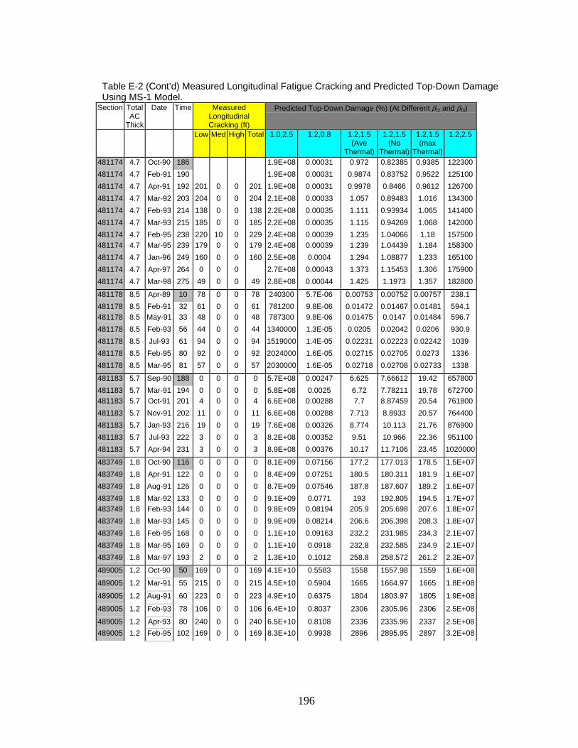
196
Table E-2 (Cont’d) Measured Longitudinal Fatigue Cracking and Predicted Top-Down Damage Using MS-1 Model.
Section Total AC
Thick
Date Time Measured Longitudinal Cracking (ft)
Predicted Top-Down Damage (%) (At Different βf2 and βf3)
Low Med High Total 1.0,2.5 1.2,0.8 1.2,1.5 (Ave
Thermal)
1.2,1.5 (No
Thermal)
1.2,1.5 (max
Thermal)
1.2,2.5
481174 4.7 Oct-90 186 1.9E+08 0.00031 0.972 0.82385 0.9385 122300481174 4.7 Feb-91 190 1.9E+08 0.00031 0.9874 0.83752 0.9522 125100481174 4.7 Apr-91 192 201 0 0 201 1.9E+08 0.00031 0.9978 0.8466 0.9612 126700481174 4.7 Mar-92 203 204 0 0 204 2.1E+08 0.00033 1.057 0.89483 1.016 134300481174 4.7 Feb-93 214 138 0 0 138 2.2E+08 0.00035 1.111 0.93934 1.065 141400481174 4.7 Mar-93 215 185 0 0 185 2.2E+08 0.00035 1.115 0.94269 1.068 142000481174 4.7 Feb-95 238 220 10 0 229 2.4E+08 0.00039 1.235 1.04066 1.18 157500481174 4.7 Mar-95 239 179 0 0 179 2.4E+08 0.00039 1.239 1.04439 1.184 158300481174 4.7 Jan-96 249 160 0 0 160 2.5E+08 0.0004 1.294 1.08877 1.233 165100481174 4.7 Apr-97 264 0 0 0 2.7E+08 0.00043 1.373 1.15453 1.306 175900481174 4.7 Mar-98 275 49 0 0 49 2.8E+08 0.00044 1.425 1.1973 1.357 182800
481178 8.5 Apr-89 10 78 0 0 78 240300 5.7E-06 0.00753 0.00752 0.00757 238.1 481178 8.5 Feb-91 32 61 0 0 61 781200 9.8E-06 0.01472 0.01467 0.01481 594.1 481178 8.5 May-91 33 48 0 0 48 787300 9.8E-06 0.01475 0.0147 0.01484 596.7 481178 8.5 Feb-93 56 44 0 0 44 1340000 1.3E-05 0.0205 0.02042 0.0206 930.9 481178 8.5 Jul-93 61 94 0 0 94 1519000 1.4E-05 0.02231 0.02223 0.02242 1039 481178 8.5 Feb-95 80 92 0 0 92 2024000 1.6E-05 0.02715 0.02705 0.0273 1336 481178 8.5 Mar-95 81 57 0 0 57 2030000 1.6E-05 0.02718 0.02708 0.02733 1338
481183 5.7 Sep-90 188 0 0 0 0 5.7E+08 0.00247 6.625 7.66612 19.42 657800481183 5.7 Mar-91 194 0 0 0 0 5.8E+08 0.0025 6.72 7.78211 19.78 672700481183 5.7 Oct-91 201 4 0 0 4 6.6E+08 0.00288 7.7 8.87459 20.54 761800481183 5.7 Nov-91 202 11 0 0 11 6.6E+08 0.00288 7.713 8.8933 20.57 764400481183 5.7 Jan-93 216 19 0 0 19 7.6E+08 0.00326 8.774 10.113 21.76 876900481183 5.7 Jul-93 222 3 0 0 3 8.2E+08 0.00352 9.51 10.966 22.36 951100481183 5.7 Apr-94 231 3 0 0 3 8.9E+08 0.00376 10.17 11.7106 23.45 1020000
483749 1.8 Oct-90 116 0 0 0 0 8.1E+09 0.07156 177.2 177.013 178.5 1.5E+07483749 1.8 Apr-91 122 0 0 0 0 8.4E+09 0.07251 180.5 180.311 181.9 1.6E+07483749 1.8 Aug-91 126 0 0 0 0 8.7E+09 0.07546 187.8 187.607 189.2 1.6E+07483749 1.8 Mar-92 133 0 0 0 0 9.1E+09 0.0771 193 192.805 194.5 1.7E+07483749 1.8 Feb-93 144 0 0 0 0 9.8E+09 0.08194 205.9 205.698 207.6 1.8E+07483749 1.8 Mar-93 145 0 0 0 0 9.9E+09 0.08214 206.6 206.398 208.3 1.8E+07483749 1.8 Feb-95 168 0 0 0 0 1.1E+10 0.09163 232.2 231.985 234.3 2.1E+07483749 1.8 Mar-95 169 0 0 0 0 1.1E+10 0.0918 232.8 232.585 234.9 2.1E+07483749 1.8 Mar-97 193 2 0 0 2 1.3E+10 0.1012 258.8 258.572 261.2 2.3E+07
489005 1.2 Oct-90 50 169 0 0 169 4.1E+10 0.5583 1558 1557.98 1559 1.6E+08
489005 1.2 Mar-91 55 215 0 0 215 4.5E+10 0.5904 1665 1664.97 1665 1.8E+08
489005 1.2 Aug-91 60 223 0 0 223 4.9E+10 0.6375 1804 1803.97 1805 1.9E+08
489005 1.2 Feb-93 78 106 0 0 106 6.4E+10 0.8037 2306 2305.96 2306 2.5E+08
489005 1.2 Apr-93 80 240 0 0 240 6.5E+10 0.8108 2336 2335.96 2337 2.5E+08489005 1.2 Feb-95 102 169 0 0 169 8.3E+10 0.9938 2896 2895.95 2897 3.2E+08

197
Table E-2 (Cont’d) Measured Longitudinal Fatigue Cracking and Predicted Top-Down Damage Using MS-1 Model.
Section Total AC
Thick
Date Time Measured Longitudinal Cracking (ft)
Predicted Top-Down Damage (%) (At Different βf2 and βf3)
Low Med High Total 1.0,2.5 1.2,0.8 1.2,1.5 (Ave
Thermal)
1.2,1.5 (No
Thermal)
1.2,1.5 (max
Thermal)
1.2,2.5
489005 1.2 Feb-96 114 274 0 0 274 9.2E+10 1.099 3212 3211.95 3213 3.5E+08
489005 1.2 Jul-96 119 253 0 0 253 9.7E+10 1.131 3323 3322.95 3324 3.7E+08
489005 1.2 Jul-97 131 325 0 0 325 1.1E+11 1.234 3641 3640.94 3641 4.1E+08
489005 1.2 Jul-98 143 278 0 0 278 1.2E+11 1.336 3960 3959.94 3961 4.4E+08
501002 8.5 Aug-89 58 4.5E+07 2.2E-05 0.132 0.01552 1928 37000 501002 8.5 Aug-90 70 5.6E+07 2.7E-05 0.1611 0.01894 2244 45140 501002 8.5 May-94 115 2 0 0 2 1E+08 4.9E-05 0.2977 0.03078 3907 84240 501002 8.5 Aug-94 118 0 0 0 0 1E+08 5E-05 0.3009 0.03276 3909 84680 501002 8.5 Apr-95 126 8 0 0 8 1.1E+08 5.1E-05 0.3091 0.03374 4359 86840 501002 8.5 Oct-96 144 16 0 0 16 1.4E+08 6.7E-05 0.4096 0.04065 4769 114800501002 8.5 May-97 151 66 125 0 191 1.4E+08 6.7E-05 0.4105 0.04155 4776 115000501002 8.5 Oct-97 156 10 5 0 14 1.4E+08 7.1E-05 0.4295 0.0446 4959 119400501002 8.5 Jun-98 164 10 26 0 36 1.5E+08 7.2E-05 0.4321 0.04651 4975 119800
501004 8 Apr-93 102 34 11 0 44 3.5E+07 1.2E-05 0.08733 0.00088 1173 30790 501004 8 Oct-95 132 8 4 0 12 4.3E+07 1.4E-05 0.1027 0.00145 1512 35960 501004 8 Nov-97 157 7 3 0 9 6.4E+07 2E-05 0.1511 0.002 2070 52970
511002 5.7 Apr-89 115 9 42 59 110 4.1E+08 0.00067 2.461 2.14831 42.54 392600
511023 10.1 Oct-89 107 0 0 0 0 2.1E+07 5.8E-05 0.1507 0.1504 1.158 13020 511023 10.1 Mar-91 124 0 0 0 0 2.3E+07 6.5E-05 0.1705 0.1702 1.368 14780 511023 10.1 May-92 138 0 0 0 0 2.6E+07 7.2E-05 0.1886 0.1883 1.428 16470 511023 10.1 Oct-92 143 21 0 0 21 2.9E+07 8E-05 0.2099 0.2096 1.45 18330 511023 10.1 Dec-93 157 0 0 0 3.2E+07 8.8E-05 0.2308 0.2305 1.945 20170 511023 10.1 Sep-95 178 105 0 0 105 3.8E+07 0.0001 0.274 0.2736 2.092 24090 511023 10.1 Feb-96 183 167 0 0 167 3.8E+07 0.0001 0.2742 0.2739 2.2 24130 511023 10.1 Mar-97 196 4 0 0 4 4.1E+07 0.00011 0.2921 0.2918 2.269 25830
512021 7.5 Oct-89 54 8.5E+07 0.00013 0.4441 0.43795 56.96 61660 512021 7.5 Mar-91 71 1.1E+08 0.00017 0.5618 0.55422 69.27 79350 512021 7.5 Oct-92 90 21 0 0 21 1.5E+08 0.00023 0.7794 0.76934 106.4 109500
531008 3.4 Jul-91 153 6 0 0 6 2E+08 0.00048 1.285 1.2593 1750 160600531008 3.4 Jun-93 176 66 0 0 67 2.3E+08 0.00054 1.452 1.42431 1769 184000531008 3.4 Jun-94 188 8 5 8 21 2.5E+08 0.00058 1.57 1.53893 2370 199800
561007 2.8 Jul-90 121 9.9E+07 0.00035 0.8719 0.77803 575 97420 561007 2.8 May-91 131 0 0 0 0 1.1E+08 0.00036 0.9246 0.81966 671.5 105600561007 2.8 Aug-91 134 0 0 0 0 1.1E+08 0.0004 0.9931 0.88645 671.6 109800561007 2.8 Aug-93 158 13 0 0 13 1.3E+08 0.00046 1.162 1.04778 709.7 127300561007 2.8 Oct-93 160 26 0 0 26 1.3E+08 0.00047 1.17 1.05472 721.7 128600561007 2.8 Dec-93 162 4 0 0 4 1.3E+08 0.00047 1.177 1.05646 745.5 130700561007 2.8 Mar-94 165 6 0 0 6 1.4E+08 0.00047 1.188 1.06166 782.3 133900561007 2.8 Apr-94 166 0 0 0 1.4E+08 0.00047 1.191 1.06426 782.4 134500561007 2.8 Aug-94 170 6 0 0 6 1.4E+08 0.00049 1.237 1.10763 782.4 138100

198
Table E-2 (Cont’d) Measured Longitudinal Fatigue Cracking and Predicted Top-Down Damage Using MS-1 Model.
Section Total AC
Thick
Date Time Measured Longitudinal Cracking (ft)
Predicted Top-Down Damage (%) (At Different βf2 and βf3)
Low Med High Total 1.0,2.5 1.2,0.8 1.2,1.5 (Ave
Thermal)
1.2,1.5 (No
Thermal)
1.2,1.5 (max
Thermal)
1.2,2.5
561007 2.8 Feb-95 176 7 0 0 7 1.5E+08 0.0005 1.263 1.12411 896.7 143900561007 2.8 May-95 179 0 0 0 1.5E+08 0.0005 1.274 1.13365 896.7 145300561007 2.8 Sep-95 183 0 0 0 1.5E+08 0.00052 1.324 1.18049 896.8 149100561007 2.8 Jun-96 192 5 0 0 5 1.6E+08 0.00053 1.363 1.21258 925.7 155400561007 2.8 Oct-96 196 0 0 0 1.6E+08 0.00056 1.426 1.27503 925.8 159600561007 2.8 Nov-96 197 2 0 0 2 1.6E+08 0.00056 1.427 1.2759 926.3 159900561007 2.8 Mar-97 201 0 0 0 1.6E+08 0.00056 1.434 1.28111 934.6 161800561007 2.8 Aug-97 206 3 0 0 3 1.7E+08 0.0006 1.517 1.36437 934.7 167300561007 2.8 Sep-97 207 0 0 0 1.7E+08 0.00061 1.527 1.37391 934.7 168100

199
0
100
200
300
400
500
600
700
800
900
1000
0.01 0.1 1 10 100 1000 10000 100000 1000000Damage (%)
Long
itudi
nal C
rack
ing
(ft/5
00ft)
AC Thickness <2" AC Thicknes 2 - 4" AC Thickness 4-6" AC Thickness 6-8"AC Thickness 8-10" AC Thickness 10-12" AC Thickness >12"
Figure E-1 Longitudinal Cracking vs. Predicted Top-Down Damage (AC 1,0.8,0.8)
0
100
200
300
400
500
600
700
800
900
1000
1 10 100 1000 10000 100000 1000000 10000000 1E+08 1E+09Damage (%)
Long
itudi
nal C
rack
ing
(ft/5
00ft)
AC Thickness <2" AC Thicknes 2 - 4" AC Thickness 4-6" AC Thickness 6-8"AC Thickness 8-10" AC Thickness 10-12" AC Thickness >12"
Figure E-2 Longitudinal Cracking vs. Predicted Top-Down Damage (AC 1, 0.8,1.5)

200
0
100
200
300
400
500
600
700
800
900
1000
1 100 10000 1000000 100000000 10000000000 1E+12 1E+14Damage (%)
Long
itudi
nal C
rack
ing
(ft/5
00ft)
AC Thickness <2" AC Thicknes 2 - 4" AC Thickness 4-6" AC Thickness 6-8"AC Thickness 8-10" AC Thickness 10-12" AC Thickness >12"
Figure E-3 Longitudinal Cracking vs. Predicted Top-Down Damage (AC 1, 0.8,2.5)
0
100
200
300
400
500
600
700
800
900
1000
0.00001 0.0001 0.001 0.01 0.1 1 10 100 1000Damage (%)
Long
itudi
nal C
rack
ing
(ft/5
00ft)
AC Thickness <2" AC Thicknes 2 - 4" AC Thickness 4-6" AC Thickness 6-8"AC Thickness 8-10" AC Thickness 10-12" AC Thickness >12"
Figure E-4 Longitudinal Cracking vs. Predicted Top-Down Damage (AC 1,1.0, 0.8)

201
0
100
200
300
400
500
600
700
800
900
1000
0.0001 0.001 0.01 0.1 1 10 100 1000Damage (%)
Long
itudi
nal C
rack
ing
(ft/5
00ft)
AC Thickness <2" AC Thicknes 2 - 4" AC Thickness 4-6" AC Thickness 6-8"AC Thickness 8-10" AC Thickness 10-12" AC Thickness >12"
Figure E-5 Longitudinal Cracking vs. Predicted Top-Down Damage (AC 1,1.0,1.0)
0
100
200
300
400
500
600
700
800
900
1000
0.01 0.1 1 10 100 1000 10000 100000 1000000Damage (%)
Long
itudi
nal C
rack
ing
(ft/5
00ft)
AC Thickness <2" AC Thicknes 2 - 4" AC Thickness 4-6" AC Thickness 6-8"AC Thickness 8-10" AC Thickness 10-12" AC Thickness >12"
Figure E-6 Longitudinal Cracking vs. Predicted Top-Down Damage (AC 1,1.0,1.5)

202
0
100
200
300
400
500
600
700
800
900
1000
1 10 100 1000 10000 100000 1000000 1E+07 1E+08 1E+09 1E+10 1E+11Damage (%)
Long
itudi
nal C
rack
ing
(ft/5
00ft)
AC Thickness <2" AC Thicknes 2 - 4" AC Thickness 4-6" AC Thickness 6-8"AC Thickness 8-10" AC Thickness 10-12" AC Thickness >12"
Figure E-7 Longitudinal Cracking vs. Predicted Top-Down Damage (AC 1,1.0,2.5)
0
100
200
300
400
500
600
700
800
900
1000
1E-09 1E-08 1E-07 1E-06 1E-05 0.0001 0.001 0.01 0.1 1 10 100 1000Damage (%)
Long
itudi
nal C
rack
ing
(ft/5
00ft)
AC Thickness <2" AC Thicknes 2 - 4" AC Thickness 4-6" AC Thickness 6-8"AC Thickness 8-10" AC Thickness 10-12" AC Thickness >12"
Figure E-8 Longitudinal Cracking vs. Predicted Top-Down Damage (AC 1,1.2, 0.8)

203
0
100
200
300
400
500
600
700
800
900
1000
0.00001 0.0001 0.001 0.01 0.1 1 10 100 1000Damage (%)
Long
itudi
nal C
rack
ing
(ft/5
00ft)
AC Thickness <2" AC Thicknes 2 - 4" AC Thickness 4-6" AC Thickness 6-8"AC Thickness 8-10" AC Thickness 10-12" AC Thickness >12"
Figure E-9 Longitudinal Cracking vs. Predicted Top-Down Damage (AC 1,1.2,1.5)
0
100
200
300
400
500
600
700
800
900
1000
1 10 100 1000 10000 100000 1000000 10000000 100000000Damage (%)
Long
itudi
nal C
rack
ing
(ft/5
00ft)
AC Thickness <2" AC Thicknes 2 - 4" AC Thickness 4-6" AC Thickness 6-8"AC Thickness 8-10" AC Thickness 10-12" AC Thickness >12"
Figure E-10 Longitudinal Cracking vs. Predicted Top-Down Damage (AC 1,1.2,2.5)

204
0
100
200
300
400
500
600
700
800
900
1000
0.00001 0.0001 0.001 0.01 0.1 1 10 100 1000Damage (%)
Long
itudi
nal C
rack
ing
(ft/5
00ft)
AC Thickness <2" AC Thicknes 2 - 4" AC Thickness 4-6" AC Thickness 6-8"AC Thickness 8-10" AC Thickness 10-12" AC Thickness >12"
Figure E-12 Longitudinal Cracking vs. Predicted Top-Down Damage (AC 1,1.2,1.5) (No Thermal Strain added)
0
100
200
300
400
500
600
700
800
900
1000
0.0001 0.001 0.01 0.1 1 10 100 1000 10000 100000Damage (%)
Long
itudi
nal C
rack
ing
(ft/5
00ft)
AC Thickness <2" AC Thicknes 2 - 4" AC Thickness 4-6" AC Thickness 6-8"AC Thickness 8-10" AC Thickness 10-12" AC Thickness >12"
Figure E-13 Longitudinal Cracking vs. Predicted Top-Down Damage (AC 1,1.2,1.5) (Max Thermal Strain added)

Copy No.
Guide for Mechanistic-Empirical Design OF NEW AND REHABILITATED PAVEMENT
STRUCTURES
FINAL DOCUMENT
APPENDIX II-2: SENSITIVITY ANALYSIS FOR ASPHALT CONCRETE
FATIGUE ALLIGATOR CRACKING
NCHRP
Prepared for National Cooperative Highway Research Program
Transportation Research Board National Research Council
Submitted by ARA, Inc., ERES Division
505 West University Avenue Champaign, Illinois 61820
February 2004

i
Acknowledgment of Sponsorship This work was sponsored by the American Association of State Highway and Transportation Officials (AASHTO) in cooperation with the Federal Highway Administration and was conducted in the National Cooperative Highway Research Program which is administered by the Transportation Research Board of the National Research Council. Disclaimer This is the final draft as submitted by the research agency. The opinions and conclusions expressed or implied in this report are those of the research agency. They are not necessarily those of the Transportation Research Board, the National Research Council, the Federal Highway Administration, AASHTO, or the individual States participating in the National Cooperative Highway Research program. Acknowledgements The research team for NCHRP Project 1-37A: Development of the 2002 Guide for the Design of New and Rehabilitated Pavement Structures consisted of Applied Research Associates, Inc., ERES Consultants Division (ARA-ERES) as the prime contractor with Arizona State University (ASU) as the primary subcontractor. Fugro-BRE, Inc., the University of Maryland, and Advanced Asphalt Technologies, LLC served as subcontractors to either ARA-ERES or ASU along with several independent consultants. Research into the subject area covered in this Appendix was conducted at ASU. The authors of this Appendix are Dr. M.W. Witczak, Mr. M. M. El-Basyouny, and Mr. S. El-Badawy. Foreword This appendix is the second in a series of three volumes on Calibration of Fatigue Cracking Models for Flexible Pavements. This volume concentrates on the sensitivity analysis for asphalt concrete fatigue alligator cracking. The other volumes are: Appendix II-1: Calibration of Fatigue Cracking Models for Flexible Pavements Appendix II-3: Sensitivity Analysis for Asphalt Concrete Fatigue Longitudinal Surface
Cracking

ii
TABLE OF CONTENT
Appendix II-2
Sensitivity Analysis for AC Fatigue Alligator Cracking
Page
1. Introduction and Objectives 2
2. Major Program Input Parameters Used in Study 4
3. Sensitivity Analysis for AC Fatigue Alligator Cracking 14

1
APPENDIX II-2: SENSITIVITY ANALYSIS FOR AC FATIGUE ALLIGATOR CRACKING
1 Introduction and Objectives The objective of this major component of the overall Design Procedure sensitivity study is to
investigate how the prediction of fatigue cracking is influenced by changes in magnitude of
several different key input variables. To study the sensitivity of these input parameters on
fatigue cracking the Design Guide computer program was run using several factorial
combinations of the input parameters shown in Table E1-2.1 of this appendix. Unless noted in
the specific sensitivity write-up; most of the computer runs used parameters that were
typically related to the "Medium" input levels shown in the table.
In general, the sensitivity study of fatigue cracking was not intended to cover a complete full
factorial matrix of all parameters. Rather, the intent was to investigate the effect of varying
one parameter at a time, while keeping as many of the other variables to be constant input
parameters.
The independent parameter that is used for the Design Guide prediction for the fatigue
distress is the amount of cracking. For the classic bottom-ups alligator fatigue cracking
distress, the specific value used as the program output for the distress is described as follows:
• Alligator cracking (bottom up) is computed in the program as the area of
cracking (in ft 2 / 500 ft / lane). Thus, the maximum area of alligator cracking
that can be predicted would be 12ft x 500 ft = 6000 ft 2. Alligator cracking is
expressed as a percent value, between 0% and 100%, relative to the predicted
area of cracking. As an example, if the program would predict an alligator
cracking value of 1000 ft 2 / 500 ft / lane; then the percent alligator cracking
would be 1000 ft 2 / 6000 ft 2 = 16.7%.
In order to investigate the overall sensitivity of key parameters to alligator fatigue cracking; a
series of individual studies were performed. Each separate study had it's own unique

2
parametric objective. The sensitivity analysis for fatigue cracking covered the following items
shown below. The paragraph where the sensitivity study outcome is reported and discussed is
also shown in the following list:
Paragraph - Study ID
3.1 Influence of AC Mix Stiffness upon Fatigue (Alligator) Cracking (Thin AC Layers)
3.2 Influence of AC Mix Stiffness upon Fatigue (Alligator) Cracking (Thick AC Layers)
3.3 Influence of AC Thickness upon Fatigue (Alligator) Cracking
3.4 Influence of Subgrade Modulus upon Fatigue (Alligator) Cracking
3.5 Influence of AC Mix Air Voids upon Fatigue (Alligator) Cracking
3.6 Influence of Asphalt Content (Effective Bitumen Volume) upon Fatigue (Alligator) Cracking
3.7 Influence of Depth to GWT on Fatigue (Alligator) Cracking
3.8 Influence of Truck Traffic Volume upon Fatigue (Alligator) Cracking
3.9 Influence of Traffic Speed upon Fatigue (Alligator) Cracking
3.10 Influence of Traffic Analysis Level upon Fatigue (Alligator) Cracking
3.11 Influence of MAAT upon Fatigue (Alligator) Cracking
3.12 Influence of Bedrock Depth upon Fatigue (Alligator) Cracking
Prior to presenting the sensitivity report results; the following section of this report describes
the general input parameters (and ranges of variables) that have been utilized in the study.

3
2 Major Program Input Parameters Used in Study
2.1 Introduction To study the effect of the desired sensitivity input parameter on alligator fatigue cracking, the
major pavement design input parameters were usually selected from one of three different
levels of the parameter under study (Low, Medium and High). In certain special cases, a
fourth level was employed to insure that an adequate range of the variable examined could be
evaluated for the sensitivity study. In general, the majority of program runs were conducted
using the "Medium levels" of all of the input variables, while varying the major parameter
whose sensitivity was being examined. However, in some cases, traffic levels using a "High
approach" were used to insure that adequate quantitative cracking levels would be obtained in
the sensitivity runs. Table 2.1 shows the different input parameters used in this study and the
three to four different levels for each parameter that were eventually investigated. Specifics
concerning all of these input values are explained in the following sections.
2.2 Design Parameters and Pavement Structure For the alligator fatigue cracking sensitivity analysis, only the deterministic analysis was used
in the study. The design life selected for each program run was 10 years. This was simply
selected to minimize the computational running time required for the entire sensitivity effort.
The granular base construction completion date was set two months earlier than the asphalt
construction completion date for all problems, while the traffic opening date was set to be the
same as the asphalt construction completion date.
A simple conventional flexible pavement cross-section was used in the study. The structure is
a three-layer pavement system with a single asphalt concrete layer, an unbound granular base
layer (10 inches thick) and a subgrade. Figure 2.1 shows the pavement structure used in the
study. The asphalt layer thickness was varied from 1 - 12 inches to study the effect of AC
thickness on alligator fatigue cracking. However, the thickness of the unbound granular base
was fixed at 10 inch, for all problems analyzed.

4
2.3 Traffic Two traffic methods were eventually used in the study: a general traffic module using the load
spectrum (Level 1 type of analysis) and a classical 18 kip ESAL approach. The traffic volume
was expressed by the average annual daily truck traffic (AADTT) selected to represent a very
high traffic volume (50,000 daily truck), high truck traffic (7000 daily trucks), medium high
traffic (4000 daily trucks), medium traffic (1000 daily trucks) and a low traffic (100 daily
trucks). The general 10-year E18KSAL repetitions for these traffic levels are approximately:
100 million, 15 million, 8 million, 2 million and 200,000. The rest of the traffic parameters
were set to the default values given by the software.
Tables 2.2 to 2.5 show the values of the various traffic parameter inputs used in this study.
Information regarding the general traffic parameters (Table 2.2), AADTT distributions by
vehicle class (Table 2.3), number of axles per truck (Table 2.4) and the axle configurations
(Table 2.5) is illustrated. The monthly adjustment factors for traffic were set at 1; while the
standard deviation of traffic wander was taken to be 10 inches. Finally, no traffic growth was
considered in the study.
2.4 Climate Three different climatic regions were selected in the sensitivity study of fatigue cracking. The
climatic stations were selected to cover a broad range of US temperature conditions (cold,
intermediate and hot region). One city was selected from each region to represent the climatic
region. The cities were Minneapolis (Minnesota) for the cold climate, Oklahoma City
(Oklahoma) for the intermediate climate and Phoenix (Arizona) for the hot weather. The
mean annual air temperatures (MAAT) for these three stations were 46.1, 60.7 and 74.4 ºF,
respectively.

5
Table 2.1 Parameters Used in the Sensitivity Runs
Very Low Low (L) Medium
(M) Medium
High High (H) Very
High Traffic Volume – AADTT (Vehicle/Day)
100 1000 4000 7000 50,000
(10 years) 18 Kips ESALs
2*105 2*106 8*106 1.5*107 1.0*108
Facility Type (Operating Speed (mph))
Intersection (2.0)
Urban Streets (25)
State Primary
(45)
Interstate (60)
Location (MAAT)
Minnesota (46.1ºF)
Oklahoma (60.7ºF)
Phoenix (74.4ºF)
GWT depth (ft) 2 7 15 AC Thickness (in) 1 4 12 AC Stiffness (See Table 2.6)
Low Mix Med Mix High Mix
AC Air Voids (@ time of Construction For Med Mix)
4 7 10
AC Effective Binder Content
8 11 15
SG Modulus (psi) (Plasticity index)
3,000 (45)
8,000 (30)
15,000 (15)
30,000 (0)
AC
GB
SG
10” A-1-b (38,000 psi)
Figure 2.1 Pavement Structure

6
Table 2.2 Traffic Parameters used in the Study
Number of lanes in design direction 2 Percent of trucks in design direction (%) 50 Percent of trucks in design lane (%) 95 Design lane (ft) 12 Standard deviation of Traffic Wander (inch) 10
Table 2.3 AADTT Distributions by Vehicle Class
Table 2.4 Number of Axles per Truck
Vehicle Class
Single Axle
Tandem Axle
Tridem Axle
Quad Axle
Class 4 1.62 0.39 0.00 0.00 Class 5 2.00 0.00 0.00 0.00 Class 6 1.02 0.99 0.00 0.00 Class 7 1.00 0.26 0.83 0.00 Class 8 2.38 0.67 0.00 0.00 Class 9 1.13 1.93 0.00 0.00 Class 10 1.19 1.09 0.89 0.00 Class 11 4.29 0.26 0.06 0.00 Class 12 3.52 1.14 0.06 0.00 Class 13 2.15 2.13 0.35 0.00
Class 4 1.8% Class 5 24.6% Class 6 7.6% Class 7 0.5% Class 8 5.0% Class 9 31.3% Class 10 9.8% Class 11 0.8% Class 12 3.3% Class 13 15.3%

7
Table 2.5 Axle Configurations
Average axle width (edge-to-edge) outside dimensions, ft) 8.5 Dual tire spacing (in) 12 Single Tire (psi) 120 Dual Tire (psi) 120 Axle Spacing - Tandem axle (in) 51.6 Axle Spacing - Tridem axle (in) 49.2 Axle Spacing - Quad axle (in) 49.2
2.5 Depth to Ground Water Table / Bedrock For the majority of problems conducted, the ground water table depth (GWT) was set at the
Medium level (7 ft), shown in Table 2.1. For the special case, where the effect of the GWT
was analyzed for the sensitivity study parameter, it was varied as shown in Table 2.1 to have
values of: 2 ft, 7 ft and 15 ft. The presence of a bedrock (stiff) layer was not considered as a
variable in any of the studies, except for 3.15 and 3.16, which evaluated the influence of
bedrock layers (1 to 20 ft) upon fatigue cracking. The GWT depth and the depth to bedrock
are measured from the surface of the pavement.
2.6 Material Characterizations
2.6.1 Asphalt Concrete Mixtures
Three different asphalt concrete mixtures were used in this study. The range of E* master
curves (mix stiffnesses) selected was based upon using as broad a range in stiffness of historic
AC mixtures as possible. Table 2.6 shows the typical mixture properties as well as typical
binder grade and properties. The mixture E* master curves chosen are representative of
mixtures utilizing PG 46-34; PG 58-28 and PG 76-16 binders.
Figure 2.2 shows the master curve for the three mixtures. These plots are typically defined, in
mathematical models, by use of a sigmoidal function. Table 2.7 shows the dynamic modulus

8
equation parameters (sigmoidal function) for the three AC mixtures utilized in the sensitivity
study. The intermediate mixture was selected as the base mixture for the studies in which the
air voids and the effective binder content were changed when to study the effect of these two
parameters on the AC fatigue cracking.
Table 2.8 summarizes the creep compliance values at different loading time and the tensile
strength calculated for the three different asphalt concrete mixtures.
2.6.2 Unbound Layers Material
The unbound granular base properties were the same for all computer runs used in this study.
However, the material properties for the subgrade soil were changed to reflect a very broad
range of support values, from "very low" (Mr=3000 psi) to "high" (Mr=30,000 psi)
conditions. These input values represent the "Design Conditions" for input into the program.
Table 2.9 summarizes the input properties of the granular base and the four different subgrade
soils used in this study.

9
Table 2.6 Asphalt Mixture properties
Variable Low Mix Med Mix High Mix
Air Voids (%) 7 7 8 Effective Binder content (%) 12 11 10
VFA (%) 63 61 55 % Retained ¾” 0 11.62 30
% Retained 3/8” 1.16 35.3 47 % Retained # 4 27.65 52.64 52.8
% Passing # 200 11.12 7.28 8.38 PG Grade 46-34 58-28 76-16 Binder A 11.504 11.01 10.015
Binder VTS -3.901 -3.701 -3.315
Table 2.7 Asphalt Concrete Dynamic Modulus Parameters (Sigmoidal Model Form)
Dynamic Modulus Parameters Low Mixture Med Mixture High Mixture
Delta 2.8657 2.8234 -0.6719 Alpha 3.8185 3.9435 4.1776 Beta -0.4236 -0.7920 -1.2554
Gamma 0.313351 0.313351 0.313351 C 1.255882 1.255882 1.255882

10
Table 2.8 Creep Compliance and Tensile Strength for each AC Mixture.
Low Mix
Creep Compliance (1/psi) Loading Time (sec) Temp (-20 oC) Temp (-10 oC) Temp (0 oC) 1 2.928E-07 3.955E-07 5.342E-07 2 3.681E-07 5.670E-07 8.732E-07 5 4.984E-07 9.128E-07 1.672E-06 10 6.267E-07 1.309E-06 2.733E-06 20 7.880E-07 1.876E-06 4.467E-06 50 1.067E-06 3.021E-06 8.554E-06 100 1.341E-06 4.331E-06 1.398E-05
Tensile Strength (psi) 467.4 Med Mix
Creep Compliance (1/psi) Loading Time (sec) Temp (-20 oC) Temp (-10 oC) Temp (0 oC) 1 2.981E-07 4.027E-07 5.440E-07 2 3.302E-07 4.835E-07 7.081E-07 5 3.779E-07 6.157E-07 1.003E-06 10 4.185E-07 7.393E-07 1.306E-06 20 4.634E-07 8.876E-07 1.700E-06 50 5.303E-07 1.130E-06 2.409E-06 100 5.873E-07 1.357E-06 3.136E-06
Tensile Strength (psi) 413.44 High Mix
Creep Compliance (1/psi) Loading Time (sec) Temp (-20 oC) Temp (-10 oC) Temp (0 oC) 1 3.284E-07 4.437E-07 5.993E-07 2 3.568E-07 5.023E-07 7.069E-07 5 3.982E-07 5.917E-07 8.794E-07 10 4.326E-07 6.698E-07 1.037E-06 20 4.700E-07 7.583E-07 1.223E-06 50 5.244E-07 8.934E-07 1.522E-06 100 5.697E-07 1.011E-06 1.795E-06
Tensile Strength (psi) 392.5

11
1.E+03
1.E+04
1.E+05
1.E+06
1.E+07
-10 -5 0 5 10
Log Reduced Time
Dyn
amic
Mod
ulus
(psi
)Low E*Medium E *High E*
Figure 2.2 Asphalt Concrete Mixtures Master Curves

12
Table 2.9 Unbound Material Properties
Layer GB SG Very
low SG Low SG Med High
Classification A–1–b CL A–7–6 A – 6 A – 3 Modulus (psi) 38,000 3,000 8,000 15,000 30,000
Plasticity Index – PI (%) 0 45 30 15 0 % Passing # 4 40 100 100 95 85
% Passing # 200 3 97 80 50 7 D60 (mm) 2 0.01 0.02 0.1 0.3
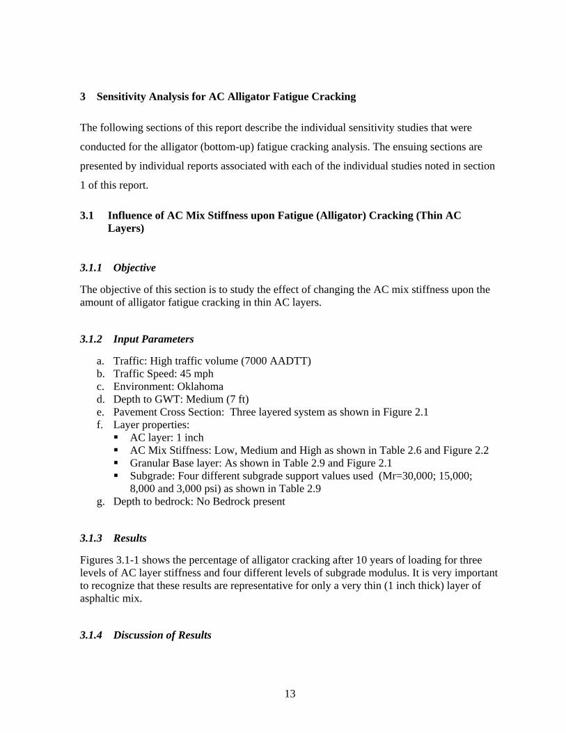
13
3 Sensitivity Analysis for AC Alligator Fatigue Cracking The following sections of this report describe the individual sensitivity studies that were
conducted for the alligator (bottom-up) fatigue cracking analysis. The ensuing sections are
presented by individual reports associated with each of the individual studies noted in section
1 of this report.
3.1 Influence of AC Mix Stiffness upon Fatigue (Alligator) Cracking (Thin AC Layers)
3.1.1 Objective
The objective of this section is to study the effect of changing the AC mix stiffness upon the amount of alligator fatigue cracking in thin AC layers.
3.1.2 Input Parameters
a. Traffic: High traffic volume (7000 AADTT) b. Traffic Speed: 45 mph c. Environment: Oklahoma d. Depth to GWT: Medium (7 ft) e. Pavement Cross Section: Three layered system as shown in Figure 2.1 f. Layer properties: AC layer: 1 inch AC Mix Stiffness: Low, Medium and High as shown in Table 2.6 and Figure 2.2 Granular Base layer: As shown in Table 2.9 and Figure 2.1 Subgrade: Four different subgrade support values used (Mr=30,000; 15,000;
8,000 and 3,000 psi) as shown in Table 2.9 g. Depth to bedrock: No Bedrock present
3.1.3 Results
Figures 3.1-1 shows the percentage of alligator cracking after 10 years of loading for three levels of AC layer stiffness and four different levels of subgrade modulus. It is very important to recognize that these results are representative for only a very thin (1 inch thick) layer of asphaltic mix.
3.1.4 Discussion of Results

14
The results shown in the figure are very important for the reader to comprehend. First of all, as is intuitive, regardless of the AC modulus value (E* stiffness range); alligator cracking decreases with increasing subgrade support (modulus). However, the most important lesson to be drawn from this sensitivity analysis is related to the fundamental fact that, for very thin AC layers, the best AC mixture is one that exhibits a very low stiffness Master Curve. As the mixture becomes more and more stiff, the amount of alligator cracking, due to bottoms up fatigue fracture, greatly increases. In essence, if very thin AC layers are used, the engineer must insure that a very soft (i.e. high AC% mix, small nominal aggregate size, soft - low viscosity binder) mixture is used. If a very stiff mixture is placed in a thin layer, the probability of obtaining excessive fatigue cracking is very likely. Finally, it is important to understand that the AC mixture stiffness principles, presented for this one-inch thick AC layer, will change as the thickness of the AC layer is changed.
3.1.5 Summary and Conclusions
For very thin AC layers, alligator (fatigue cracking) will greatly be increased as the stiffness of the AC mix becomes larger. The rate of change in alligator cracking is small at low to medium ranges of mixture stiffness, but increases significantly as very high mix stiffnesses are used in the pavement structure.

15
0%
10%
20%
30%
40%
50%
60%
70%
80%
90%
100%
Low E* Med E* Hi E*
AC Mix Stiffness
Alli
gato
r Bot
tom
Up
% C
rack
ing
Ref
eren
ce B
ased
Upo
n 60
00 ft
2 / 500
ft
SG Mr= 3 ksi SG Mr= 8 ksi SG Mr= 15 ksi SG Mr= 30 ksi
Figure 3.1-1 Effect of AC Mix Stiffness on Alligator Cracking, (Hac = 1 in)

16
3.2 Influence of AC Mix Stiffness upon Fatigue (Alligator) Cracking (Thick AC Layers)
3.2.1 Objective
The objective of this section is to study the effect of changing the AC mix stiffnesses on the amount of alligator fatigue (bottom up) cracking for thick AC layers.
3.2.2 Input Parameters
a. Traffic: High traffic volume (7000 AADTT) b. Traffic Speed: 45 mph c. Environment: Oklahoma d. Depth to GWT: Medium (7 ft) e. Pavement Cross Section: Three layered system as shown in Figure 2.1 f. Layer properties: AC layer: 10 inch AC Mix Stiffness: Low, Medium and High as shown in Table 2.6 and Figure 2.2 Granular Base layer: As shown in Table 2.9 and Figure 2.1 Subgrade: Four different subgrade support values used (Mr=30,000; 15,000; 8,000
and 3,000 psi) as shown in Table 2.9 g. Depth to bedrock: No Bedrock present
3.2.3 Results
Figures 3.2-1 shows the percentage of alligator fatigue cracking after 10 years of loading for three levels of AC layer stiffness.
3.2.4 Discussion of Results
As would be expected, the fatigue cracking decreases with an increase in the subgrade modulus. This is due to the fact that tensile strains, and hence fatigue damage, are reduced as the subgrade modulus is increased. However, a most important trend and conclusion is noted relative to the influence of AC stiffness upon alligator cracking. It is observed that for very thick AC sections, fatigue damage (cracking) is increased for low stiffness AC mixtures. This is 180 degrees opposite to the findings of mix stiffness - fatigue damage for very thin AC layers. The influence of AC mix stiffness is more significant as the foundation support decreases. In general, for very large AC thicknesses, low E* mixtures would tend to show more damage (cracking).
3.2.5 Summary and Conclusions

17
As the AC mix stiffness of thick AC layers increases the amount of alligator fatigue cracking decreases. The higher the subgrade modulus, the lower the alligator cracking would be.
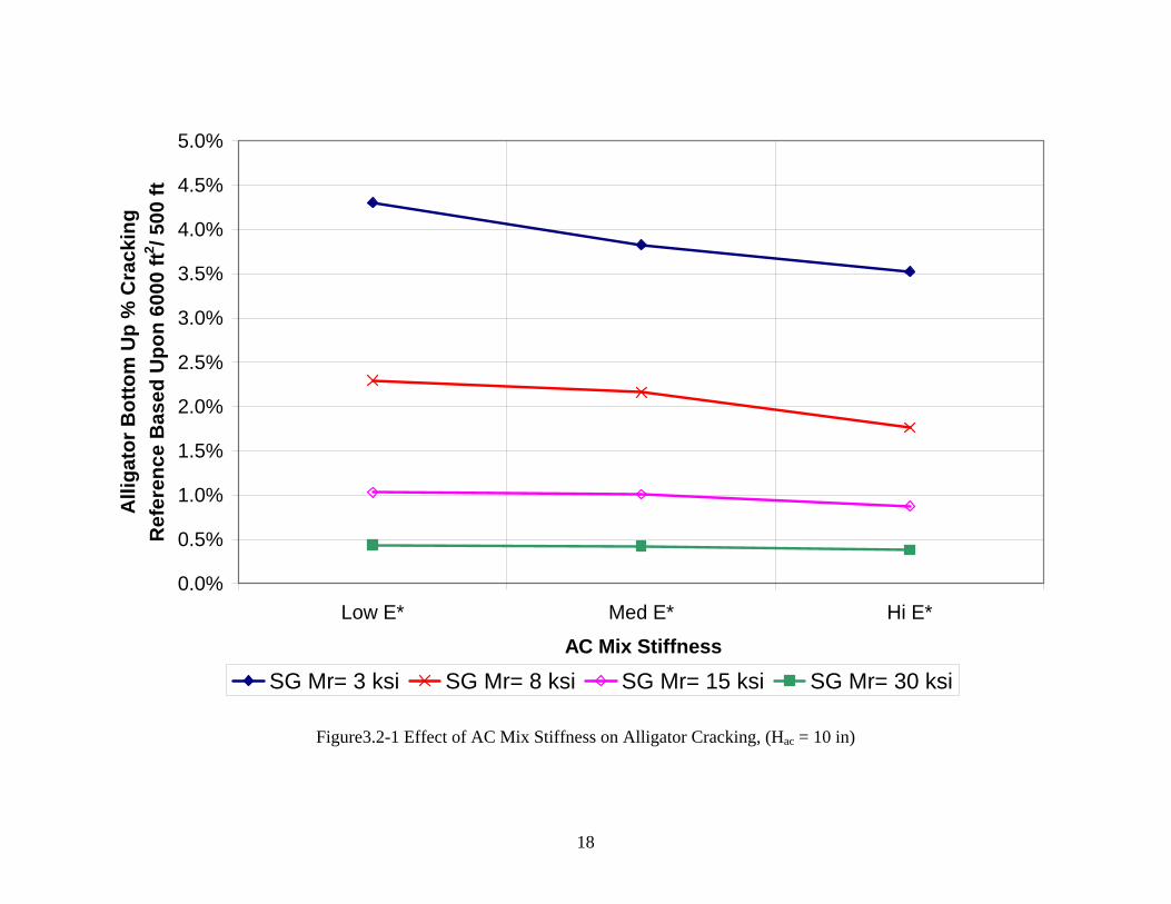
18
0.0%
0.5%
1.0%
1.5%
2.0%
2.5%
3.0%
3.5%
4.0%
4.5%
5.0%
Low E* Med E* Hi E*
AC Mix Stiffness
Alli
gato
r Bot
tom
Up
% C
rack
ing
Ref
eren
ce B
ased
Upo
n 60
00 ft
2 / 500
ft
SG Mr= 3 ksi SG Mr= 8 ksi SG Mr= 15 ksi SG Mr= 30 ksi
Figure3.2-1 Effect of AC Mix Stiffness on Alligator Cracking, (Hac = 10 in)

19
3.3 Influence of AC Thickness Upon Fatigue (Alligator) Cracking
3.3.1 Objective
The objective of this section is to study the effect of AC layer thickness on the amount of alligator fatigue cracking.
3.3.2 Input Parameters
a. Traffic: High traffic volume (7000 AADTT) b. Traffic Speed: 45 mph c. Environment: Oklahoma d. Depth to GWT: medium (7 ft) e. Pavement Cross-Section: Three layered system as shown in Figure 2.1 f. Layer properties: AC layer: 1, 2, 4, 6, 8, 10 and 12 inches AC Mix Stiffness: Medium Stiff Mixture as shown in Table 2.6 and Figure 2.2 Granular Base layer: As shown in Table 2.9and Figure 2.1 Subgrade: Six different subgrade support values used (Mr=30,000; 25,000; 20,000;
15,000; 8,000 and 3,000 psi) as shown in Table 2.9 g. Depth to bedrock: No Bedrock present
3.3.3 Results
Figure 3.3-1 illustrates the influence of the percentage of alligator fatigue cracking after 10 years of loading, as a function of the AC layer thickness, for various levels of subgrade support.
3.3.4 Discussion of Results
The relationship shown in the figure illustrates another extremely important fundamental fact regarding the distribution of alligator fatigue cracking for flexible pavement systems. First of all, for all levels of AC thickness, it can be clearly observed that the magnitude of alligator cracking is increased as the subgrade support is decreased. It can also be observed that the sensitivity, or impact of the subgrade support upon alligator cracking, is directly related to the thickness of the AC layer. Perhaps the most important fundamental conclusion that can be drawn from the figure is that for good performance, the proper thickness of AC layers must be either as thin as practical or as thick as possible. It reinforces the adage of old time flexible pavement experts who inferred that " …if you build a pavement thin, it should be thin…if you build it thick, then it should be built thick". The figure clearly indicates that the greatest potential for fatigue fracture is really associated with AC layers that are typically in the 3" to 5" thick range.
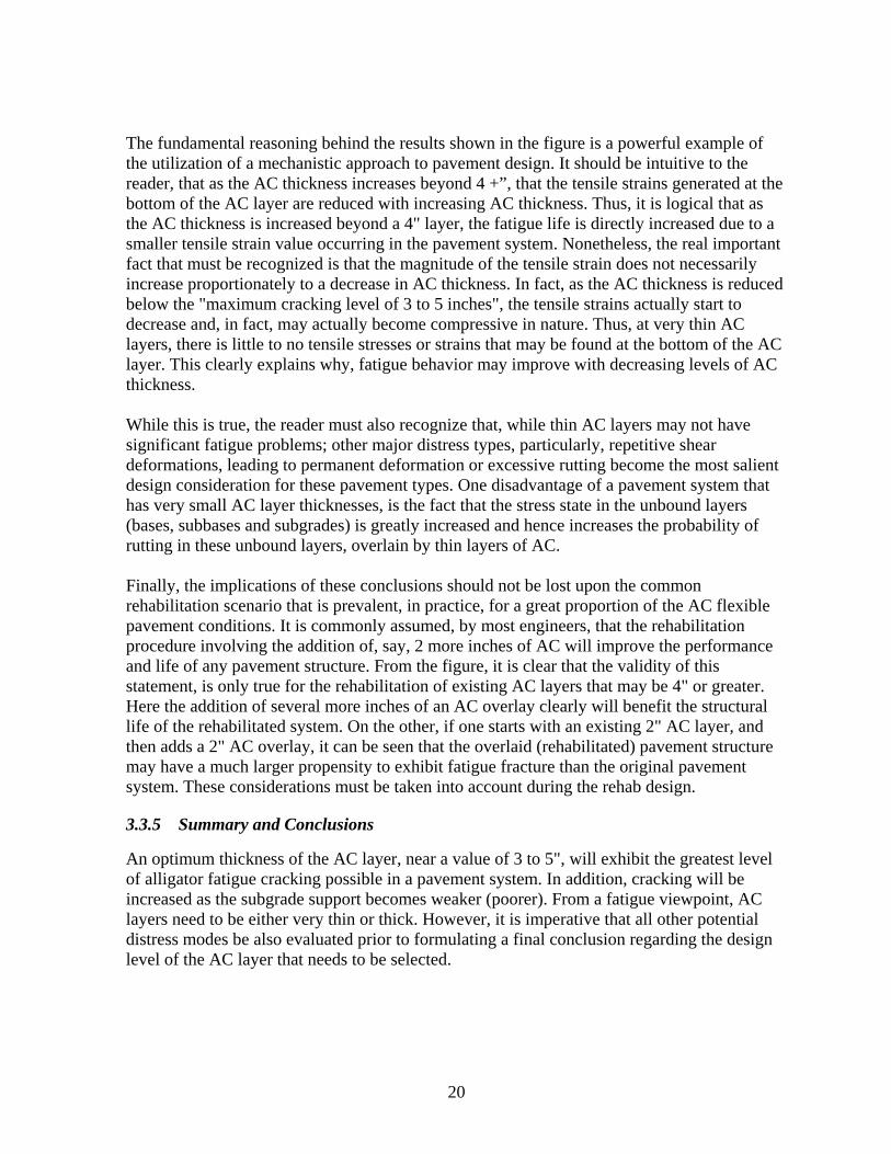
20
The fundamental reasoning behind the results shown in the figure is a powerful example of the utilization of a mechanistic approach to pavement design. It should be intuitive to the reader, that as the AC thickness increases beyond 4 +”, that the tensile strains generated at the bottom of the AC layer are reduced with increasing AC thickness. Thus, it is logical that as the AC thickness is increased beyond a 4" layer, the fatigue life is directly increased due to a smaller tensile strain value occurring in the pavement system. Nonetheless, the real important fact that must be recognized is that the magnitude of the tensile strain does not necessarily increase proportionately to a decrease in AC thickness. In fact, as the AC thickness is reduced below the "maximum cracking level of 3 to 5 inches", the tensile strains actually start to decrease and, in fact, may actually become compressive in nature. Thus, at very thin AC layers, there is little to no tensile stresses or strains that may be found at the bottom of the AC layer. This clearly explains why, fatigue behavior may improve with decreasing levels of AC thickness. While this is true, the reader must also recognize that, while thin AC layers may not have significant fatigue problems; other major distress types, particularly, repetitive shear deformations, leading to permanent deformation or excessive rutting become the most salient design consideration for these pavement types. One disadvantage of a pavement system that has very small AC layer thicknesses, is the fact that the stress state in the unbound layers (bases, subbases and subgrades) is greatly increased and hence increases the probability of rutting in these unbound layers, overlain by thin layers of AC. Finally, the implications of these conclusions should not be lost upon the common rehabilitation scenario that is prevalent, in practice, for a great proportion of the AC flexible pavement conditions. It is commonly assumed, by most engineers, that the rehabilitation procedure involving the addition of, say, 2 more inches of AC will improve the performance and life of any pavement structure. From the figure, it is clear that the validity of this statement, is only true for the rehabilitation of existing AC layers that may be 4" or greater. Here the addition of several more inches of an AC overlay clearly will benefit the structural life of the rehabilitated system. On the other, if one starts with an existing 2" AC layer, and then adds a 2" AC overlay, it can be seen that the overlaid (rehabilitated) pavement structure may have a much larger propensity to exhibit fatigue fracture than the original pavement system. These considerations must be taken into account during the rehab design.
3.3.5 Summary and Conclusions
An optimum thickness of the AC layer, near a value of 3 to 5", will exhibit the greatest level of alligator fatigue cracking possible in a pavement system. In addition, cracking will be increased as the subgrade support becomes weaker (poorer). From a fatigue viewpoint, AC layers need to be either very thin or thick. However, it is imperative that all other potential distress modes be also evaluated prior to formulating a final conclusion regarding the design level of the AC layer that needs to be selected.
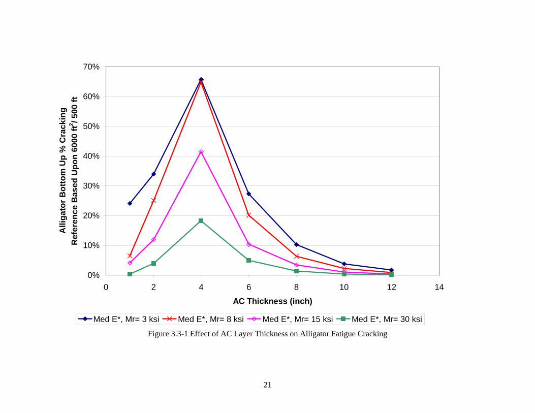
21
0%
10%
20%
30%
40%
50%
60%
70%
0 2 4 6 8 10 12 14
AC Thickness (inch)
Alli
gato
r Bot
tom
Up
% C
rack
ing
Ref
eren
ce B
ased
Upo
n 60
00 ft
2 / 500
ft
Med E*, Mr= 3 ksi Med E*, Mr= 8 ksi Med E*, Mr= 15 ksi Med E*, Mr= 30 ksi
Figure 3.3-1 Effect of AC Layer Thickness on Alligator Fatigue Cracking

22
3.4 Influence of Subgrade Modulus Upon Fatigue (Alligator) Cracking
3.4.1 Objective
The objective of this section is to study the effect of subgrade modulus on the amount of alligator fatigue cracking.
3.4.2 Input Parameters
a. Traffic: High traffic volume (7000 AADTT) b. Traffic Speed: 45 mph c. Environment: Oklahoma d. Depth to GWT: medium (7 ft) e. Pavement Cross-Section: Three layered system as shown in Figure 2.1 f. Layer properties: AC layer: 4 inches AC Mix Stiffness: Medium Stiff Mixture as shown in Table 2.6 and Figure 2.2 Granular Base layer: As shown in Table 2.9 and Figure 2.1 Subgrade: Four different subgrade support values used (Mr=30,000; 15,000; 8,000
and 3,000 psi) as shown in Table 2.9 g. Depth to bedrock: No Bedrock present
3.4.3 Results
Figure 3.4-1 shows the percentage of alligator fatigue cracking after 10 years of loading for the four levels of subgrade modulus used in the sensitivity study.
3.4.4 Discussion of Results
The figure clearly illustrates the fundamental fact that the stronger the foundation (subgrade) support of the pavement system becomes; the less the amount of alligator fatigue cracking that will occur. The relative sensitivity of the rate of alligator cracking, due to variable subgrade support, is a function of many other design variables, such as: traffic, site climatic condition and thickness of the AC layer used in the cross section.
3.4.5 Summary and Conclusions
Increasing the subgrade support modulus will result in a decreased level of alligator fatigue cracking in any pavement system. The sensitivity of subgrade support to the magnitude of alligator cracking is also a function of many other design input parameters as well.

23
0%
10%
20%
30%
40%
50%
60%
70%
80%
90%
100%
0 5000 10000 15000 20000 25000 30000 35000
Subgrade Modulus (psi)
Alli
gato
r Bot
tom
Up
% C
rack
ing
Ref
eren
ce B
ased
Upo
n 60
00 ft
2/ 5
00 ft
Figure3.4-1 Effect of Subgrade Modulus on Alligator Cracking

24
3.5 Influence of AC Mix Air Voids Upon Fatigue (Alligator) Cracking
3.5.1 Objective
The objective of this section is to study the effect of the in-situ AC air voids on alligator fatigue cracking.
3.5.2 Input Parameters
a. Traffic: Medium traffic volume (7000 AADTT) b. Traffic Speed: 45 mph c. Environment: Oklahoma d. Depth to GWT: medium (7 ft) e. Pavement Cross-Section: Three layered system as shown in Figure 2.1 f. Layer properties: AC layer: 4 inches AC Mix Stiffness: Medium Stiff Mixture as shown in Table 2.6 and Figure 2.2 AC Mix Air Voids: 4, 7, and 10% Granular Base layer: As shown in Table 2.9 and Figure 2.1 Subgrade: Medium Support (Mr=15,000 psi) as shown in Table 2.9
g. Depth to bedrock: No Bedrock present
3.5.3 Results
Figure 3.5-1 shows the percentage of alligator fatigue cracking after 10 years of loading for the three levels of AC mix air voids used in the sensitivity study. The range of air voids used in the study reflects a very real range under typical construction conditions (4% to 10%).
3.5.4 Discussion of Results
The results shown in the figure clearly reflect the critical importance of air voids upon fatigue cracking. The greater the in-place air voids of an asphalt mixture are; the greater the degree of cracking that may be expected. This effect is directly attributable to the volumetric mix term incorporated into both the controlled strain (thin AC layers) and controlled stress (thick AC layers) fatigue equation for bottoms up cracking. In reality, it is the mix Voids Filled with Bitumen parameter that directly influences the fatigue cracking. As this parameter is increased, the cracking is greatly reduced. Thus, this sensitivity study is directly tied to air voids and the AC content. (Also see Study 3.6)
3.5.5 Summary and Conclusions
In summary, the air voids within an AC mixture are an important parameter to influence fatigue cracking. Increasing the amount of air voids in the AC mix may significantly increase the amount of alligator fatigue cracking.

25
0%
10%
20%
30%
40%
50%
60%
70%
80%
90%
100%
0 2 4 6 8 10 12
AC Mix Air Voids (%)
Alli
gato
r Bot
tom
Up
% C
rack
ing
Ref
eren
ce B
ased
Upo
n 60
00 ft
2/ 5
00 ft
Figure 3.5-1 Effect of Percent AC Mix Air Voids on Alligator Fatigue Cracking

26
3.6 Influence of Asphalt Content (Effective Bitumen Volume) Upon Fatigue (Alligator) Cracking
3.6.1 Objective
The objective of this section is to study the influence of the magnitude of the effective bitumen volume present in an AC mixture upon the amount of alligator cracking.
3.6.2 Input Parameters
a. Traffic: Medium traffic volume (7000 AADTT) b. Traffic Speed: 45 mph c. Environment: Oklahoma d. Depth to GWT: medium (7 ft) e. Pavement Cross-Section: Three layered system as shown in Figure 2.1 f. Layer properties: AC layer: 4 inches AC Mix Stiffness: Medium Stiff Mixture as shown in Table 2.6 and Figure 2.2 AC Mix Effective Binder Content: 8, 11 and 15% Granular Base layer: As shown in Table 2.9 and Figure 2.1 Subgrade: Medium Support (Mr=15,000 psi) as shown in Table 2.9
g. Depth to bedrock: No Bedrock present
3.6.3 Results
Figure 3.6-1 shows the percentage of alligator fatigue cracking after 10 years of loading for three assumed values of effective bitumen volume (Vbe). This parameter is approximately 2.0 to 2.2 times the numerical value of the AC content, in percentage form. Thus the ranges of Vbe = 8, 11 and 15 %, translate into approximate AC % values of 4%, 5+% and 7+%.
3.6.4 Discussion of Results
Like the previous study presented on the influence of mixture air voids, the influence of the amount of asphalt present in a mix also has a significant influence upon the amount of alligator cracking that may occur. It is observed from the figure that there is a decrease in the amount of alligator fatigue cracking as the amount of the effective binder volume increases. This is a direct consequence of the Vfb term used in the Fatigue Damage equation. As the asphalt content (effective bitumen content) is increased; the Voids filled with bitumen are also increased. This results in a greater resistance of the mixture to fracture under fatigue damage.
3.6.5 Summary and Conclusions
In summary, the amount of asphalt binder present in a mixture will directly influence the amount of fatigue cracking that will occur in the field. When the effective bitumen volume (amount of asphalt) is increased in a mix; the amount of alligator cracking will be decreased.

27
0%
10%
20%
30%
40%
50%
60%
70%
80%
90%
100%
6 7 8 9 10 11 12 13 14 15 16
AC Mix Effective Binder Content By Volume (%)
Alli
gato
r Bot
tom
Up
% C
rack
ing
Ref
eren
ce B
ased
Upo
n 60
00 ft
2/ 5
00 ft
Figure 3.6-1 Effect of Percent AC Binder by volume on Alligator Fatigue Cracking

28
3.7 Influence of Depth to GWT on Fatigue (Alligator) Cracking
3.7.1 Objective
The objective of this section is to study the effect of depth to GWT on the amount of alligator (bottom- up) cracking.
3.7.2 Input Parameters
a. Traffic: High traffic volume (1000 AADTT) b. Traffic Speed: 45 mph c. Environment: Phoenix d. Depth to GWT: 2, 4, 7 and 15 ft e. Pavement Cross-Section: Three layered system as shown in Figure 2.1 f. Layer properties: AC layer: 4 inches AC Mix Stiffness: High Stiff Mixture as shown in Table 2.6 and Figure 2.2 Granular Base layer: Constant modulus = 38,000 psi. Subgrade: Five different subgrade support values used (above GWT/ below GWT)
(Mr=34,000/17,600; 25,000/13075; 18,000/10260, 10,000/5,860 and 6,000/2250 psi).
g. Depth to bedrock: No Bedrock present
3.7.3 Results
Figure 3.7-1 shows the percentage of alligator fatigue cracking after 10 years of loading for four levels of depth to GWT, for a variety of subgrade modulus materials.
3.7.4 Discussion of Results
These runs were conducted on pavement sections in which the granular base and subgrade moduli were fixed at the values shown above (i.e. no correction of moisture content using EICM). However, a subgrade layer was added below the GWT depth to reflect the saturated conditions of the subgrade. The saturated values were estimated from prior analysis of runs using the EICM models. As a general observation, as would be expected, the alligator cracking distress decreases as the depth of the ground water table is increased. Also, as explained in a previous comparison, the alligator bottom-up cracking decreases as the subgrade modulus is increased. It can be observed that the most significant impact upon fatigue damage will occur when high GWT are found in weaker, clayey subgrades. There appears to be little impact of GWT location upon the magnitude of alligator cracking for higher subgrade modulus. For the problem input parameters, it appears that GWT depths, greater than 5 feet to 7 feet will not impact upon fatigue damage.

29
Higher GWT depth leads to saturation of the subgrade and hence reduces the subgrade modulus. If the difference between the saturated modulus below the GWT and the unsaturated modulus above the GWT is large enough, the GWT depth will cause significant changes in the alligator fatigue cracking. One of the facts, the engineer should consider is that the sensitivity of subgrade support (modulus) to alligator cracking as large compared to the sensitivity of support modulus to permanent deformation (rutting). This is very much consistent to the sensitivity of PCC fatigue cracking to Westergaard's modulus of subgrade reaction value (k). As a consequence, even though the presence of the GWT does influence the in-situ moisture and hence modulus of the unbound base/subbase and subgrade materials; the resultant change of the in-situ unbound material modulus profile may be small, and it's impact upon the overall support modulus, and eventual fatigue cracking, is not overly sensitive to the final value. The sensitivity, however, will increase with poorer (lower) subgrade support values.
3.7.5 Summary and Conclusions
In general, the sensitivity of GWT to alligator cracking will be dependent upon the subgrade support encountered. As a general statement, fatigue damage will increase as the GWT moves closer to the surface. At depths greater than 5 feet to 7 feet, the influence of the GWT becomes very low. Finally, the impact of GWT is most significant for low modulus subgrade materials.

30
0%
5%
10%
15%
20%
25%
30%
35%
0 2 4 6 8 10 12 14 16
Ground Water Table Depth (ft)
Alli
gato
r Bot
tom
Up
% C
rack
ing
Ref
eren
ce B
ased
Upo
n 60
00 ft
2/ 5
00 ft
SG Modulus = 6000 SG Modulus = 10000 SG Modulus = 18000 SG Modulus = 25000 SG Modulus = 34000
Figure 3.7-1 Effect of Depth to GWT on Alligator Fatigue Cracking
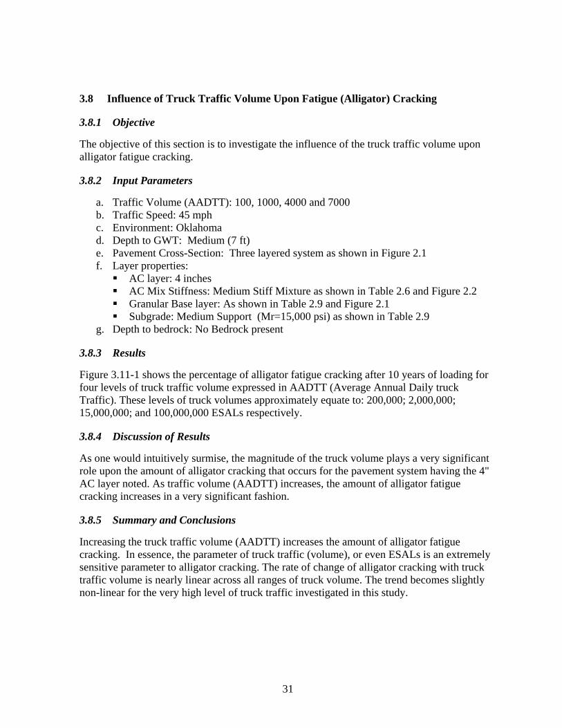
31
3.8 Influence of Truck Traffic Volume Upon Fatigue (Alligator) Cracking
3.8.1 Objective
The objective of this section is to investigate the influence of the truck traffic volume upon alligator fatigue cracking.
3.8.2 Input Parameters
a. Traffic Volume (AADTT): 100, 1000, 4000 and 7000 b. Traffic Speed: 45 mph c. Environment: Oklahoma d. Depth to GWT: Medium (7 ft) e. Pavement Cross-Section: Three layered system as shown in Figure 2.1 f. Layer properties: AC layer: 4 inches AC Mix Stiffness: Medium Stiff Mixture as shown in Table 2.6 and Figure 2.2 Granular Base layer: As shown in Table 2.9 and Figure 2.1 Subgrade: Medium Support (Mr=15,000 psi) as shown in Table 2.9
g. Depth to bedrock: No Bedrock present
3.8.3 Results
Figure 3.11-1 shows the percentage of alligator fatigue cracking after 10 years of loading for four levels of truck traffic volume expressed in AADTT (Average Annual Daily truck Traffic). These levels of truck volumes approximately equate to: 200,000; 2,000,000; 15,000,000; and 100,000,000 ESALs respectively.
3.8.4 Discussion of Results
As one would intuitively surmise, the magnitude of the truck volume plays a very significant role upon the amount of alligator cracking that occurs for the pavement system having the 4" AC layer noted. As traffic volume (AADTT) increases, the amount of alligator fatigue cracking increases in a very significant fashion.
3.8.5 Summary and Conclusions
Increasing the truck traffic volume (AADTT) increases the amount of alligator fatigue cracking. In essence, the parameter of truck traffic (volume), or even ESALs is an extremely sensitive parameter to alligator cracking. The rate of change of alligator cracking with truck traffic volume is nearly linear across all ranges of truck volume. The trend becomes slightly non-linear for the very high level of truck traffic investigated in this study.
32
0%
10%
20%
30%
40%
50%
60%
70%
80%
90%
100%
0 10000 20000 30000 40000 50000 60000
Traffic Volume (AADTT)
Alli
gato
r Bot
tom
Up
% C
rack
ing
Ref
eren
ce B
ased
Upo
n 60
00 ft
2/ 5
00 ft
Figure 3.8-1 Effect of Truck Traffic Volume on Alligator Fatigue Cracking (Hac=4 in)

33
3.9 Influence of Traffic Speed Upon Fatigue (Alligator) Cracking
3.9.1 Objective
The objective of this section is to study the effect of traffic speed on alligator fatigue cracking.
3.9.2 Input Parameters
a. Traffic: High traffic volume (7000 AADTT) b. Traffic Speed: 2, 25, 45 and 60 mph c. Environment: Oklahoma (for variable level subgrade support study); Minnesota (for
supplemental studies of Hac thickness effect) d. Depth to GWT: Medium (7 ft) e. Pavement Cross-Section: Three layered system as shown in Figure 2.1 f. Layer properties: AC layer: 4 inches AC Mix Stiffness: Medium Stiff Mixture as shown in Table 2.6 and Figure 2.2 Granular Base layer: As shown in Table 2.9 and Figure 2.1 Subgrade: Four different subgrade support values for variable support study
(Mr=30,000; 15,000; 8,000 and 3,000 psi) as shown in Table 2.9; Mr=15,000 psi used in supplementary Hac thickness study)
g. Depth to bedrock: No Bedrock present
3.9.3 Results
Figure 3.9-1(a thru c) show the results of the sensitivity study relative to traffic speed upon alligator cracking. Figure 3.9-1a contains results of the percentage of alligator fatigue cracking after 10 years of loading for the four levels of traffic speed (2 mph to 60 mph), and the four levels of subgrade support noted in section 3.9.2. Figures 3.9-1b and c, provide the results of the study for two different thickness levels of AC: 1" and 8" for the cold temperature condition associated with a subgrade modulus of 15,000 psi and the use of a "medium" AC stiffness.
3.9.4 Discussion of Results
Hac=4"; Multiple Subgrade Support Study: For the 4" AC layer pavement system, it can be observed that the influence of operational vehicle speed has a very minor effect upon the alligator cracking observed, across all levels of subgrade support. One can detect, however, a very minor decrease in alligator cracking as the vehicle speed is increased. This result is fundamentally correct, especially as the thickness of the AC layer is increased. The reason for this is as follows. As the vehicle speed is increased, the load time of the stress pulse acting on the AC layer becomes smaller. Thus, with a higher speed, the time of the stress load is diminished, at a given temperature. This leads to a slight increase in the E* of the AC layer material (refer to AC Master Curve). As the E* is

34
increased, a slightly lower tensile strain then occurs in the AC bound layer. This slightly lower tensile strain will then lead to a slightly reduced degree of damage, and hence a slight increase in the fatigue resistance of the mix. This aspect is eventually translated to a small decrease in alligator cracking (slightly less damage) as the vehicle operational speed is increased. This phenomenon is clearly shown in the figure. While the previous discussion is based upon the events surrounding a 4" AC layer; it is important to also understand the implications of increased vehicle speed upon fracture of very thin (e.g. 1") AC layers. Referring to Figure 3.1-1 for the alligator cracking of thin AC layers; it can be seen that, for both conditions of cracking, the presence of very stiff (high E*) mixtures leads to a greater degree of cracking. Since increases in the vehicle speed will cause an increase in the E* of the AC layer, the consequence of this is the fact that a greater degree of damage may occur within the thin AC layer as the vehicle speed is increased. This is verified in the ensuing paragraphs.
Hac=1" and 8"; Cold Climatic Site Figures 3.9-1b and c reflect the results for the influence of traffic speed upon alligator cracking for a thin AC layer (Fig 3.9-1b) as well as a thicker 8" AC layer (Fig 3.9-1c), for a single subgrade support modulus of Mr=15,000 psi in a cold environmental site. For the 1" thin AC layer; it can be seen that increasing the traffic speed tends to increase the alligator cracking (slight increase for the example inputs used in the study). This is a very logical result due to the fact that thin AC layers, anything that will cause an increase in the E* of the AC mixture, will cause an increase in the fatigue damage and cracking that is observed. Increasing the traffic speed actually results in a shorter load stress pulse (time of loading) in the AC layer. This has a tendency, at any given temperature, to increase the mix E* (refer to master curve and reduced time effect upon the E*). As the AC layer thickness is substantially increased (Hac=8" in Fig.3.9-1c); it can be observed that the amount of alligator damage and cracking, decreases with increasing speed. This reverse trend from the thin 1" AC layer, is also logical, as increasing the vehicular speed causes an increase in the E*, a decrease in the tensile strain and less damage (alligator cracking) to the pavement system. Finally, it should be noted that the sensitivity of speed to fatigue damage is not overly significant. In all actuality, the specific changes in fatigue damage is a complex mechanism and very much a function of the specific input parameters of a given pavement system.
3.9.5 Summary and Conclusions
As a general conclusion, changes in the vehicular operational speed on the amount of alligator cracking in a pavement system may not be very large. For very thin AC layer pavement systems, the amount of fatigue damage and cracking will increase as the speed of the loading system is also increased. For very thick pavements, the reverse will occur and slightly less fatigue damage may be present at higher vehicle speeds.

35
At intermediate (4" AC layer thicknesses); the influence of traffic speed upon fatigue damage is not overly significant, particularly across a broad range of AC layer thicknesses.

36
0%
10%
20%
30%
40%
50%
60%
70%
80%
90%
100%
0 10 20 30 40 50 60 70
Traffic Speed (mph)
Alli
gato
r Bot
tom
Up
% C
rack
ing
Ref
eren
ce B
ased
Upo
n 60
00 ft
2/ 5
00 ft
SG Mr= 3 ksi SG Mr= 8 ksi SG Mr= 15 ksi SG Mr= 30 ksi
Figure 3.9-1a Effect of Traffic Speed on Alligator Fatigue Cracking (Hac =4”, Moderate Climate)

37
0%
1%
2%
3%
4%
5%
6%
7%
8%
9%
10%
0 10 20 30 40 50 60 70
Traffic Speed (mph)
Alli
gato
r Bot
tom
Up
% C
rack
ing
Ref
eren
ce B
ased
Upo
n 60
00 ft
2/ 5
00 ft
Figure 3.9-1b Effect of Traffic Speed on Alligator Fatigue Cracking (Hac =1”, Cold Climate)

38
0%
1%
2%
3%
4%
5%
6%
7%
8%
9%
10%
0 10 20 30 40 50 60 70
Traffic Speed (mph)
Alli
gato
r Bot
tom
Up
% C
rack
ing
Ref
eren
ce B
ased
Upo
n 60
00 ft
2/ 5
00 ft
Figure 3.9-1c Effect of Traffic Speed on Alligator Fatigue Cracking (Hac =8”, Cold Climate)

39
3.10 Influence of Traffic Analysis Level Upon Fatigue (Alligator) Cracking
3.10.1 Objective
The objective of this section is to investigate the influence of Hierarchical Traffic Level used in the analysis upon the amount of alligator fatigue cracking.
3.10.2 Input Parameters
a. Traffic Volume: See discussion in 3.13.3 "Results" section below b. Traffic Speed: 45 mph c. Environment: Oklahoma (61 deg F) d. Depth to GWT: Medium (7 ft) e. Pavement Cross-Section: Three layered system as shown in Figure 2.1 f. Layer properties: AC layer: 4 inches AC Mix Stiffness: Medium Stiff Mixture as shown in Table 2.6 and Figure 2.2 Granular Base layer: As shown in Table 2.9 and Figure 2.1 Subgrade: Medium Support (Mr=15,000 psi) as shown in Table 2.9
g. Depth to bedrock: No Bedrock present
3.10.3 Results
Figure 3.10-1 shows the impact of the Hierarchical Traffic Level selected upon the relationship of the percentage of alligator fatigue cracking (after 10 years of loading) for a range of traffic volumes (distributions). In this plot, four specific traffic distributions (volumes) were investigated. For the Traffic Level 1 approach, the actual traffic load axle spectrums were used as input into the program. The load spectrum approach used the input traffic assumptions noted in Tables 2.2 to 2.5. The cracking results using the Level 1 approach, for each of the four traffic volumes, is denoted as the "Load Spectra" results in the plot. For each of the four axle load spectrum distributions; the mixture axle type- load combinations were then transformed into Equivalent 18 Kip Single Axle Load repetitions (ESALs) through the use of conventional AASHTO truck damage factors, defined at a pt=2.5 and SN=5. The approximate cumulative 10-year ESAL values have been noted in Table 2.1.
3.10.4 Discussion of Results
The alligator fatigue cracking results shown in Figure 3.10-1 clearly indicate that the use of actual traffic load spectra, in the structural distress prediction model, results in a difference in predicted cracking, compared to the use of the empirical ESAL approach to traffic that has been historically used in pavement design. For the problem investigated, the traffic axle load spectra approach (Level 1) appears to yield about 3% to 7% more cracking compared to the use of E18KSAL's. This implies that the level 1 approach, based upon the actual load spectra, provides more damaging (fatigue) predictions than the conventional ESAL approach.

40
3.10.5 Summary and Conclusions
The use of a Level 1 traffic approach, based upon the actual traffic load spectra, yields a higher level of alligator cracking compared to the classical use of E18KSAL's.

41
0%
10%
20%
30%
40%
50%
60%
70%
80%
90%
100%
1.00E+04 1.00E+05 1.00E+06 1.00E+07 1.00E+08
Total Number of Esals (10 years)
Alli
gato
r Bot
tom
Up
% C
rack
ing
Ref
eren
ce B
ased
Upo
n 60
00 ft
2/ 5
00 ft
ESALs Load Spectra
Figure 3.10-1 Effect of Traffic Analysis Level upon Alligator Fatigue Cracking

42
3.11 Influence of MAAT Upon Fatigue (Alligator) Cracking
3.11.1 Objective
The objective of this section is to study the effect of MAAT (actual site environment) on the alligator fatigue cracking.
3.11.2 Input Parameters
a. Traffic Volume: Medium (7000 AADTT) b. Traffic Speed: 45 mph c. Environment: (MAAT): Minnesota (46 deg F); Oklahoma (61 deg F) and Phoenix (74
deg F) d. Depth to GWT: Medium (7 ft) e. Pavement Cross-Section: Three layered system as shown in Figure 2.1 f. Layer properties: AC layer: 1,4, 8 and 12 inches AC Mix Stiffness: High, Medium and Low Mixture Stiffnesses as shown in Table
2.6 and Figure 2.2 Granular Base layer: As shown in Table 2.9 and Figure 2.1 Subgrade: Medium Support (Mr=15,000 psi) as shown in Table 2.9
g. Depth to bedrock: No Bedrock present
3.11.3 Results
The full results of this sensitivity analysis are shown in Figures 3.11-1(a thru d). Each figure represents the relationship of predicted alligator cracking as a function of a specific level of AC layer thickness (Hac= 1, 4, 8 and 12"). The percentage of alligator fatigue cracking shown reflects 10 years of loading for the three levels of MAAT investigated.
3.11.4 Discussion of Results
The results shown are quite important relative to the selection of the appropriate level of AC mix stiffness (E*) as a function of the thickness of the AC layer. Theses results can best be interpreted for each AC thickness level presented in the analysis. Hac=1": Referring to Figure 3.11-1a (Hac=1"); it can be observed that the amount of fatigue cracking (damage) is always increased as the MAAT is also increased. This is true for all mixture stiffness values (E*). This result is very logical because as the MAAT increases, larger pavement temperatures will occur. This is turn, will lead to lower in-situ AC stiffnesses (dynamic moduli), which in turn causes greater tensile strains, a lower number of repetitions to failure (Nf) and a greater degree of damage (alligator cracking), regardless of the original AC mix stiffness master curve (E*).
43
The second significant finding shown in the figure supports the discussion of study 3.1. As can be observed, the degree of alligator cracking that occurs is extremely sensitive to the AC mixture stiffness (E*). For thin AC layers, the greater the mixture stiffness, the greater the degree of alligator cracking. In fact, for the very thin AC layer, it can be observed that there is a very strong degree of sensitivity of the AC E* stiffness to the amount of cracking that occurs. Hac=4": The influence of increasing the AC thickness from a 1" layer to a 4" layer is illustrated in Figure 3.11-1b. It is observed that an identical conclusion, relative to the significance of the MAAT upon cracking, is noted for the 4" AC layer, compared to the 1" AC layer. The explanation of this result is the same as what was presented for the 1' AC layer. All increasing the temperature at the site will accomplish is to increase the tensile strains, regardless of the mixture stiffness. In regards to the impact of the AC mixture stiffness level at the 4" layer thickness level , it can be observed that the sensitivity of E* to the amount of alligator cracking, is nowhere near as significant as it was for the 1" layer thickness. Nonetheless, even at the 4" AC thickness level, there is a slight, but noticeable, trend of the mixture E* value upon cracking. For the conditions noted in this example, it is observed that more alligator cracking will occur with the stiffer (higher) E* AC mixtures, compared to the mixtures with a lower E* stiffness relationship. Hac=8": As the thickness of the AC layer is increased from 4" to 8"; the sensitivity of E* and MAAT is shown in Figure 3.11-1c. It is again obvious that the influence of warmer design sites upon an increased level of alligator cracking is identical to the conclusion already noted for the 1" and 4" AC layers. As previously noted, this is not surprising and the explanation provided in the previous paragraphs are truly applicable for any level of AC thickness. At the Hac=8" level; it can be noted that there is very little, if any effect of the AC mixture stiffness upon the amount of alligator cracking observed. Hac=12": The influence of the MAAT and E*, upon alligator cracking for the thick (12") AC layer; is presented in Figure 3.11-1d. It is observed that increasing the MAAT will lead to an increase in the amount of alligator cracking; an identical conclusion noted for all of the three prior thickness levels. Regarding the influence of the E* upon the degree of cracking, it can be observed that the influence of E* tends to reverse itself from the previous thickness levels and that a high E* value generally tends to yield less damage than mixtures with lower stiffnesses. However, the relative change in damage may be “academic” because damage and hence fatigue cracking, will be very small at relatively large thicknesses of AC.
3.11.5 Summary and Conclusions

44
Regardless of the thickness of the AC layer, the amount of fatigue damage and alligator cracking will increase with increasing Mean Annual Air Temperature at the design site. This is true for whatever level of AC mixture stiffness is utilized in the pavement structure. However, the actual thickness of the AC layer tends to play a very critical role in defining the optimum benefit (lowest amount of alligator cracking damage) for the specific mix in question. As a general rule, for very thin AC layers; the use of a very stiff AC mixture will result in maximum fatigue damage and cracking. As the AC layer thickness is increased to levels of 10" - 12+", the use of stiff mixtures (high E* values) is preferable and will lead to a minimum of fatigue damage and alligator cracking.

45
0%
10%
20%
30%
40%
50%
60%
40 45 50 55 60 65 70 75 80
MAAT (oF)
Alli
gato
r Bot
tom
Up
% C
rack
ing
Ref
eren
ce B
ased
Upo
n 60
00 ft
2 / 500
ft
Low AC E* Medium AC E* High AC E*
Figure 3.11-1a Effect of MAAT on Alligator Fatigue Cracking (Hac =1”)

46
0%
10%
20%
30%
40%
50%
60%
0 10 20 30 40 50 60 70 80
MAAT (oF)
Alli
gato
r Bot
tom
Up
% C
rack
ing
Ref
eren
ce B
ased
Upo
n 60
00 ft
2/ 5
00 ft
Low AC E* Medium AC E* High AC E*
Figure 3.11-1b Effect of MAAT on Alligator Fatigue Cracking (Hac =4”)

47
0%
2%
4%
6%
8%
10%
12%
14%
16%
18%
20%
40 45 50 55 60 65 70 75 80
MAAT (oF)
Alli
gato
r Bot
tom
Up
% C
rack
ing
Ref
eren
ce B
ased
Upo
n 60
00 ft
2 / 500
ft
Low AC E* Medium AC E* High AC E*
Figure 3.11-1c Effect of MAAT on Alligator Fatigue Cracking (Hac =8”)

48
0%
1%
2%
3%
4%
5%
6%
7%
8%
9%
10%
0 10 20 30 40 50 60 70 80
MAAT (oF)
Alli
gato
r Bot
tom
Up
% C
rack
ing
Ref
eren
ce B
ased
Upo
n 60
00 ft
2/ 5
00 ft
Low AC E* Medium AC E* High AC E*
Figure 3.11-1d Effect of MAAT on Alligator Fatigue Cracking (Hac =12”)

49
3.12 Influence of Bedrock Depth upon Fatigue (Alligator) Cracking
3.12.1 Objective
The objective of this section is to study the effect of changing the depth of bedrock under a flexible pavement upon the amount of alligator fatigue cracking.
3.12.2 Input Parameters
a. Traffic: High traffic volume (7000 AADTT) b. Traffic Speed: 45 mph c. Environment: Oklahoma d. Depth to GWT: medium (7 ft) for bedrock depths 10 and 20 ft; GWT at top of
Bedrock for all depths less than 5 ft e. Pavement Cross-Section: Three layered system as shown in Figure 2.1 f. Layer properties: AC layer: 4 inch AC Mix Stiffness: Medium as shown in Table 2.6 and Figure 2.2 Granular Base layer: As shown in Table 2.9 and Figure 2.1 Subgrade: Two subgrade support values used (Mr=30,000 and 3,000 psi) as shown
in Table 2.9 g. Depth to bedrock: 3', 4', 5', 6’,7’, 12' and 22' (from top of pavement): Ebr= 750,000 psi
3.12.3 Results
Figures 3.12-1 shows the percentage of alligator fatigue cracking (after 10 years of loading) as a function of the depth of the Bedrock layer, for the two levels of subgrade support evaluated.
3.12.4 Discussion of Results
The results presented in the figure very clearly demonstrate that the presence of bedrock near the surface of the pavement can have a very significant effect upon the alligator fatigue cracking that may occur in a pavement system. While the figure is applicable for only one specific pavement cross-section example; it can be seen that the bedrock will generally influence softer subgrade support values (Mr=3,000 psi) to greater depths. For the example shown, a bedrock layer within 10 to 12' of the subgrade surface, for a subgrade Mr= 3000 psi, appears to be a typical bedrock depth that one would have to be concerned about. It can be observed that for the case of a much stronger subgrade support value (Mr=30,000 psi); this effective bedrock depth decreases to about 2 to 3'. As the bedrock layer is closer to the surface, the deep stiff bedrock layer will tend to start decreasing the tensile strains at the bottom of the AC layer. In fact, as the bedrock layer gets to within several feet of the subgrade; it is apparent that the neutral axis of the composite pavement may actually shift below the last AC layer and cause a compressive state of stress

50
(strain), rather than tension to exist at the bottom of the AC layer. Once this occurs, this phenomenon will result in having little to no alligator cracking present in the pavement system.
3.12.5 Summary and Conclusions
The presence of bedrock within a flexible pavement cross-section may influence the magnitude of alligator fatigue cracking that may occur. In general, the closer a bedrock layer comes to the subgrade surface, the less fatigue fracture that may occur. The "critical bedrock depth", at which there is no more influence upon fatigue cracking will vary as a function of many properties of the cross-section. For example, a pavement with a 4" AC layer, will have a "critical bedrock depth" of only 2' to 3" for a subgrade support value of Mr=30,000 psi. In contrast, this "effective bedrock depth" will increase to as large as 10' to 12' if the subgrade support is decreased to Mr=3,000 psi.

51
0%
1%
2%
3%
4%
5%
6%
7%
8%
9%
10%
0 5 10 15 20 25
Bedrock Depth (ft)
Alli
gato
r B
otto
m U
p %
Cra
ckin
g R
efer
ence
Bas
ed U
pon
6000
ft2/
500
ft
SG Mr = 3,000 SG Mr = 30,000
Figure 3.12-1 Effect of Bedrock Depth Upon Alligator Fatigue Cracking (Hac=4", Moderate Climate
Copy No.
Guide for Mechanistic-Empirical Design OF NEW AND REHABILITATED PAVEMENT STRUCTURES
FINAL DOCUMENT
APPENDIX II-3: SENSITIVITY ANALYSIS FOR ASPHALT CONCRETE
FATIGUE LONGITUDINAL SURFACE CRACKING
NCHRP
Prepared for National Cooperative Highway Research Program
Transportation Research Board National Research Council
Submitted by ARA, Inc., ERES Division
505 West University Avenue Champaign, Illinois 61820
February 2004

i
Acknowledgment of Sponsorship This work was sponsored by the American Association of State Highway and Transportation Officials (AASHTO) in cooperation with the Federal Highway Administration and was conducted in the National Cooperative Highway Research Program which is administered by the Transportation Research Board of the National Research Council. Disclaimer This is the final draft as submitted by the research agency. The opinions and conclusions expressed or implied in this report are those of the research agency. They are not necessarily those of the Transportation Research Board, the National Research Council, the Federal Highway Administration, AASHTO, or the individual States participating in the National Cooperative Highway Research program. Acknowledgements The research team for NCHRP Project 1-37A: Development of the 2002 Guide for the Design of New and Rehabilitated Pavement Structures consisted of Applied Research Associates, Inc., ERES Consultants Division (ARA-ERES) as the prime contractor with Arizona State University (ASU) as the primary subcontractor. Fugro-BRE, Inc., the University of Maryland, and Advanced Asphalt Technologies, LLC served as subcontractors to either ARA-ERES or ASU along with several independent consultants. Research into the subject area covered in this Appendix was conducted at ASU. The authors of this Appendix are Dr. M.W. Witczak, Mr. M. M. El-Basyouny, and Mr. S. El-Badawy. Foreword This appendix is the third in a series of three volumes on Calibration of Fatigue Cracking Models for Flexible Pavements. This volume concentrates on the sensitivity analysis for asphalt concrete fatigue longitudinal surface cracking. The other volumes are: Appendix II-1: Calibration of Fatigue Cracking Models for Flexible Pavements Appendix II-2: Sensitivity Analysis for Asphalt Concrete Fatigue Alligator
Cracking

ii
General Table of Content
Appendix II-3
Sensitivity Analysis for AC Fatigue Longitudinal Surface Cracking
Page
1. Introduction and Objectives 2
2. Major Program Input Parameters Used in Study 4
3. Sensitivity Analysis for AC Fatigue Longitudinal Surface Cracking 14

1
APPENDIX II-3: SENSITIVITY ANALYSIS FOR AC FATIGUE LONGITUDINAL SURFACE CRACKING
1 Introduction and Objectives The objective of this major component of the overall Design Procedure sensitivity study
is to investigate how the prediction of longitudinal surface (top down) fatigue cracking is
influenced by changes in magnitude of several different key input variables. To study the
sensitivity of these input parameters on fatigue cracking the Design Guide computer
program was run using several factorial combinations of the input parameters shown in
Table 2.1. Unless specifically noted in the specific sensitivity write-up; most of the
computer runs used parameters that were typically related to the "Medium" levels shown
in the table.
In general, the sensitivity study of fatigue cracking was not intended to cover a complete
full factorial of all parameters, but rather to investigate the effect of varying one
parameter at a time, while keeping as many of the other variables to be constant input
parameters.
The independent parameter that is used for the Design Guide prediction for the
longitudinal surface (top down) fatigue distress is the amount of cracking. The specific
value used as the program output for the longitudinal fatigue cracking is described as
follows:
• Longitudinal cracking (top down) is computed in the program as the
length (in ft) of longitudinal cracking, per 500 ft / lane, in both wheel
paths. Thus the maximum amount of cracking would be 1000 ft / 500 ft /
lane. The cracking percentage limits vary between 0 and 100%. As an
example, if the program would predict a longitudinal cracking value of
400 ft / 500 ft / lane; then the percent longitudinal cracking (percent
damage) would be 400 ft / 1000 ft = 40.0%.
2
In order to investigate the overall sensitivity of key parameters to fatigue cracking; a
series of individual studies were performed. Each separate study had it's own unique
parametric objective. The sensitivity analysis for fatigue cracking covered the following
items shown below. The paragraph where the sensitivity study outcome is reported and
discussed is also shown in the following list:
Paragraph - Study ID
3.1 Influence of AC Mix Stiffness upon Fatigue (Longitudinal) Cracking (Thin AC Layers)
3.2 Influence of AC Mix Stiffness upon Fatigue (Longitudinal) Cracking (Thick AC Layers)
3.3 Influence of AC Thickness upon Fatigue (Longitudinal) Cracking
3.4 Influence of Subgrade Modulus upon Fatigue (Longitudinal) Cracking
3.5 Influence of AC Mix Air Voids upon Fatigue (Longitudinal) Cracking
3.6 Influence of Asphalt Content (Effective Bitumen Volume) upon Fatigue (Longitudinal) Cracking
3.7 Influence of Depth to GWT on Fatigue (Longitudinal) Cracking
3.8 Influence of Truck Traffic Volume upon Fatigue (Longitudinal) Cracking
3.9 Influence of Traffic Speed upon Fatigue (Longitudinal) Cracking
3.10 Influence of Traffic Analysis Level upon Fatigue (Longitudinal) Cracking
3.11 Influence of MAAT upon Fatigue (Longitudinal) Cracking
3.12 Influence of Bedrock Depth upon Fatigue (Longitudinal) Cracking
Prior to presenting the sensitivity report results; the following section of this report
describes the general input parameters (and ranges of variables) that have been utilized in
the study.

3
2 Major Program Input Parameters Used in Study
2.1 Introduction To study the effect of the desired sensitivity input parameter on top-down fatigue
cracking, the major pavement design parameters were usually selected from one of three
different levels of the parameter under study (Low, Medium and High). In certain special
cases, a fourth level was employed to insure that an adequate range of the variable
examined could be evaluated for the sensitivity study. In general, the majority of program
runs were conducted using the "Medium levels" of all of the input variables, while
varying the major parameter whose sensitivity was being examined. However, in some
cases, traffic levels using a "High approach" were used to insure that adequate
quantitative cracking levels would be obtained in the sensitivity runs. Table 2.1 shows the
different input parameters used in this study and the three to four different levels for each
parameter that were eventually investigated. Specifics concerning all of these input
values are explained in the following sections.
2.2 Design Parameters and Pavement Structure For the longitudinal surface fatigue sensitivity analysis, only the deterministic analysis
was used in the study. The design life selected for each program run was 10 years. This
was simply selected to minimize the computational running time required for the entire
sensitivity effort. The granular base construction completion date was set two months
earlier than the asphalt construction completion date for all problems, while the traffic
opening date was set to be the same as the asphalt construction completion date.
A simple conventional flexible pavement structure was used in the study. The structure is
a three-layer pavement system with a single asphalt concrete layer, an unbound granular
base layer (10 inches thick) and a subgrade. Figure 2.1 shows the pavement structure
used in the study. The asphalt layer thickness was varied from 1 - 12 inches to study the

4
effect of AC thickness on the fatigue cracking. However, the thickness of the unbound
granular base was fixed at 10 inch, for all problems analyzed.
2.3 Traffic Two traffic methods were eventually used in the study: a general traffic module using the
load spectrum (Level 1 type of analysis) and a classical 18 kip ESAL approach. The
traffic volume was expressed by the average annual daily truck traffic (AADTT) selected
to represent a very high traffic volume (50,000 daily truck), high truck traffic (7000 daily
trucks), medium high traffic (4000 daily trucks), medium traffic (1000 daily trucks) and a
low traffic (100 daily trucks). The general 10-year E18KSAL repetitions for these traffic
levels are approximately: 100 million, 15 million, 8 million, 2 million and 200,000. The
rest of the traffic parameters were set to the default values given by the software.
Tables 2.2 to 2.5 show the values of the various traffic parameter inputs used in this
study. Information regarding the general traffic parameters (Table 2.2), AADTT
distributions by vehicle class (Table 2.3), number of axles per truck (Table 2.4) and the
axle configurations (Table 2.5) is illustrated. The monthly adjustment factors for traffic
were set at 1; while the standard deviation of traffic wander was taken to be 10 inches.
Finally, no traffic growth was considered in the study.
2.4 Climate Three different climatic regions were selected in the sensitivity study of fatigue cracking.
The climatic stations were selected to cover a broad range of US temperature conditions
(cold, intermediate and hot region). One city was selected from each region to represent
the climatic region. The cities were Minneapolis (Minnesota) for the cold climate,
Oklahoma City (Oklahoma) for the intermediate climate and Phoenix (Arizona) for the
hot weather. The mean annual air temperatures (MAAT) for these three stations were
46.1, 60.7 and 74.4 ºF, respectively.

5
Table 2.1 Parameters Used in the Sensitivity Runs
Very Low Low (L) Medium
(M) Medium
High High (H) Very
High Traffic Volume – AADTT (Vehicle/Day)
100 1000 4000 7000 50,000
(10 years) 18 Kips ESALs
2*105 2*106 8*106 1.5*107 1.0*108
Facility Type (Operating Speed (mph))
Intersection (2.0)
Urban Streets (25)
State Primary
(45)
Interstate (60)
Location (MAAT)
Minnesota (46.1ºF)
Oklahoma (60.7ºF)
Phoenix (74.4ºF)
GWT depth (ft) 2 7 15 AC Thickness (in) 1 6 12 AC Stiffness (See Table 2.6)
Low Mix Med Mix High Mix
AC Air Voids (@ time of Construction For Med Mix)
4 7 10
AC Effective Binder Content
8 11 15
SG Modulus (psi) (Plasticity index)
3,000 (45)
8,000 (30)
15,000 (15)
30,000 (0)
AC
GB
SG
10” A-1-b (38,000 psi)
Figure 2.1 Pavement Structure

6
Table 2.2 Traffic Parameters used in the Study
Number of lanes in design direction 2 Percent of trucks in design direction (%) 50 Percent of trucks in design lane (%) 95 Design lane (ft) 12 Standard deviation of Traffic Wander (inch) 10
Table 2.3 AADTT Distributions by Vehicle Class
Table 2.4 Number of Axles per Truck
Vehicle Class
Single Axle
Tandem Axle
Tridem Axle
Quad Axle
Class 4 1.62 0.39 0.00 0.00 Class 5 2.00 0.00 0.00 0.00 Class 6 1.02 0.99 0.00 0.00 Class 7 1.00 0.26 0.83 0.00 Class 8 2.38 0.67 0.00 0.00 Class 9 1.13 1.93 0.00 0.00 Class 10 1.19 1.09 0.89 0.00 Class 11 4.29 0.26 0.06 0.00 Class 12 3.52 1.14 0.06 0.00 Class 13 2.15 2.13 0.35 0.00
Class 4 1.8% Class 5 24.6% Class 6 7.6% Class 7 0.5% Class 8 5.0% Class 9 31.3% Class 10 9.8% Class 11 0.8% Class 12 3.3% Class 13 15.3%
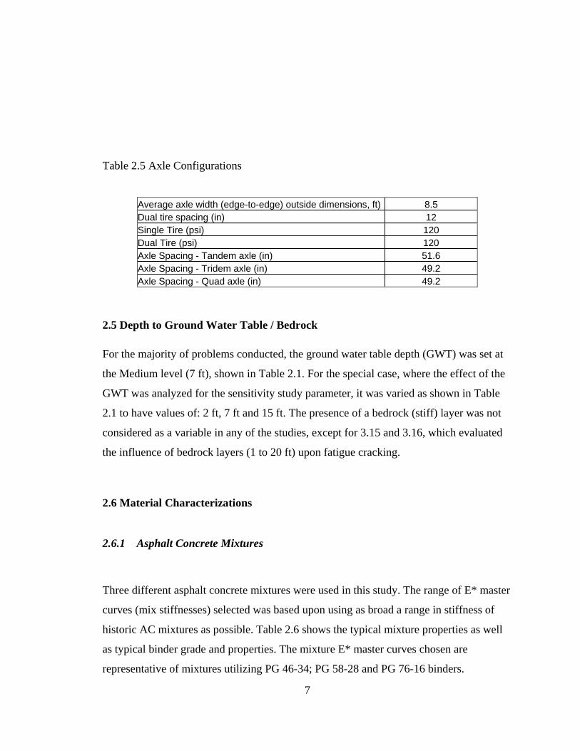
7
Table 2.5 Axle Configurations
Average axle width (edge-to-edge) outside dimensions, ft) 8.5 Dual tire spacing (in) 12 Single Tire (psi) 120 Dual Tire (psi) 120 Axle Spacing - Tandem axle (in) 51.6 Axle Spacing - Tridem axle (in) 49.2 Axle Spacing - Quad axle (in) 49.2
2.5 Depth to Ground Water Table / Bedrock For the majority of problems conducted, the ground water table depth (GWT) was set at
the Medium level (7 ft), shown in Table 2.1. For the special case, where the effect of the
GWT was analyzed for the sensitivity study parameter, it was varied as shown in Table
2.1 to have values of: 2 ft, 7 ft and 15 ft. The presence of a bedrock (stiff) layer was not
considered as a variable in any of the studies, except for 3.15 and 3.16, which evaluated
the influence of bedrock layers (1 to 20 ft) upon fatigue cracking.
2.6 Material Characterizations
2.6.1 Asphalt Concrete Mixtures
Three different asphalt concrete mixtures were used in this study. The range of E* master
curves (mix stiffnesses) selected was based upon using as broad a range in stiffness of
historic AC mixtures as possible. Table 2.6 shows the typical mixture properties as well
as typical binder grade and properties. The mixture E* master curves chosen are
representative of mixtures utilizing PG 46-34; PG 58-28 and PG 76-16 binders.

8
Figure 2.2 shows the master curve for the three mixtures. These plots are typically
defined, in mathematical models, by use of a sigmoidal function. Table 2.7 shows the
dynamic modulus equation parameters (sigmoidal function) for the three AC mixtures
utilized in the sensitivity study. The intermediate mixture was selected as the base
mixture for the studies in which the air voids and the effective binder content were
changed when to study the effect of these two parameters on the AC fatigue cracking.
The regression models for predicting the creep compliance and tensile strengths for use in
this study are based upon the Level 3 thermal fracture analysis. Table 2.8 summarizes the
creep compliance values at different loading time and the tensile strength calculated for
the three different asphalt concrete mixtures.
2.6.2 Unbound Layers Material
The unbound granular base properties were the same for all computer runs used in this
study. However, the material properties for the subgrade soil were changed to reflect a
very broad range of support values, from "very low" (Mr=3000 psi) to "high"
(Mr=30,000 psi) conditions. These input values represent the "Design Conditions" for
input into the program. Table 2.9 summarizes the input properties of the granular base
and the four different subgrade soils used in this study.

9
Table 2.6 Asphalt Mixture properties
Variable Low Mix Med Mix High Mix
Air Voids (%) 7 7 8 Effective Binder content (%) 12 11 10
VFA (%) 63 61 55 % Retained ¾” 0 11.62 30
% Retained 3/8” 1.16 35.3 47 % Retained # 4 27.65 52.64 52.8
% Passing # 200 11.12 7.28 8.38 PG Grade 46-34 58-28 76-16 Binder A 11.504 11.01 10.015
Binder VTS -3.901 -3.701 -3.315
Table 2.7 Asphalt Concrete Dynamic Modulus Parameters (Sigmoidal Model Form)
Dynamic Modulus Parameters Low Mixture Med Mixture High Mixture
Delta 2.8657 2.8234 -0.6719 Alpha 3.8185 3.9435 4.1776 Beta -0.4236 -0.7920 -1.2554
Gamma 0.313351 0.313351 0.313351 C 1.255882 1.255882 1.255882

10
Table 2.8 Creep Compliance and Tensile Strength for each AC Mixture.
Low Mix
Creep Compliance (1/psi) Loading Time (sec) Temp (-20 oC) Temp (-10 oC) Temp (0 oC) 1 2.928E-07 3.955E-07 5.342E-07 2 3.681E-07 5.670E-07 8.732E-07 5 4.984E-07 9.128E-07 1.672E-06 10 6.267E-07 1.309E-06 2.733E-06 20 7.880E-07 1.876E-06 4.467E-06 50 1.067E-06 3.021E-06 8.554E-06 100 1.341E-06 4.331E-06 1.398E-05
Tensile Strength (psi) 467.4 Med Mix
Creep Compliance (1/psi) Loading Time (sec) Temp (-20 oC) Temp (-10 oC) Temp (0 oC) 1 2.981E-07 4.027E-07 5.440E-07 2 3.302E-07 4.835E-07 7.081E-07 5 3.779E-07 6.157E-07 1.003E-06 10 4.185E-07 7.393E-07 1.306E-06 20 4.634E-07 8.876E-07 1.700E-06 50 5.303E-07 1.130E-06 2.409E-06 100 5.873E-07 1.357E-06 3.136E-06
Tensile Strength (psi) 413.44 High Mix
Creep Compliance (1/psi) Loading Time (sec) Temp (-20 oC) Temp (-10 oC) Temp (0 oC) 1 3.284E-07 4.437E-07 5.993E-07 2 3.568E-07 5.023E-07 7.069E-07 5 3.982E-07 5.917E-07 8.794E-07 10 4.326E-07 6.698E-07 1.037E-06 20 4.700E-07 7.583E-07 1.223E-06 50 5.244E-07 8.934E-07 1.522E-06 100 5.697E-07 1.011E-06 1.795E-06
Tensile Strength (psi) 392.5
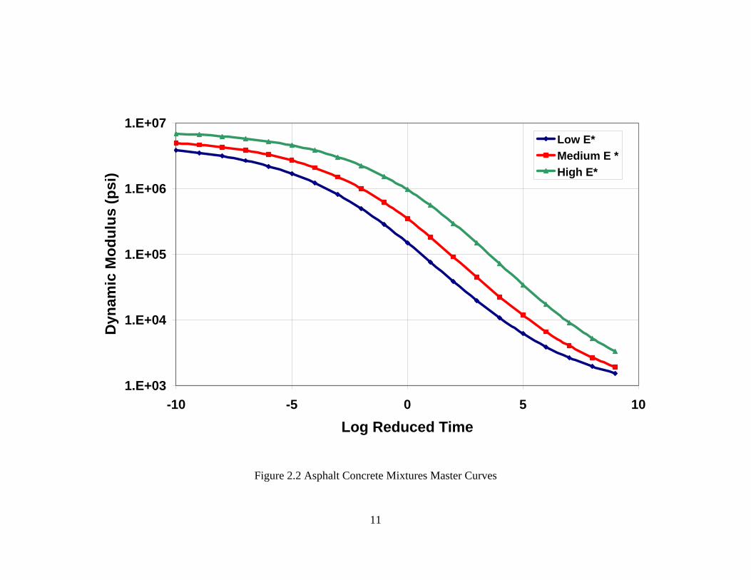
11
1.E+03
1.E+04
1.E+05
1.E+06
1.E+07
-10 -5 0 5 10
Log Reduced Time
Dyn
amic
Mod
ulus
(psi
)
Low E*Medium E *High E*
Figure 2.2 Asphalt Concrete Mixtures Master Curves

12
Table 2.9 Unbound Material Properties
Layer GB High SG Med SG Low SG Very
low Classification A–1–b A – 3 A – 6 A–7–6 CL Modulus (psi) 38,000 30,000 15,000 8,000 3,000
Plasticity Index – PI (%) 0 0 15 30 45 % Passing # 4 40 85 95 100 100
% Passing # 200 3 7 50 80 97 D60 (mm) 2 0.3 0.1 0.02 0.01
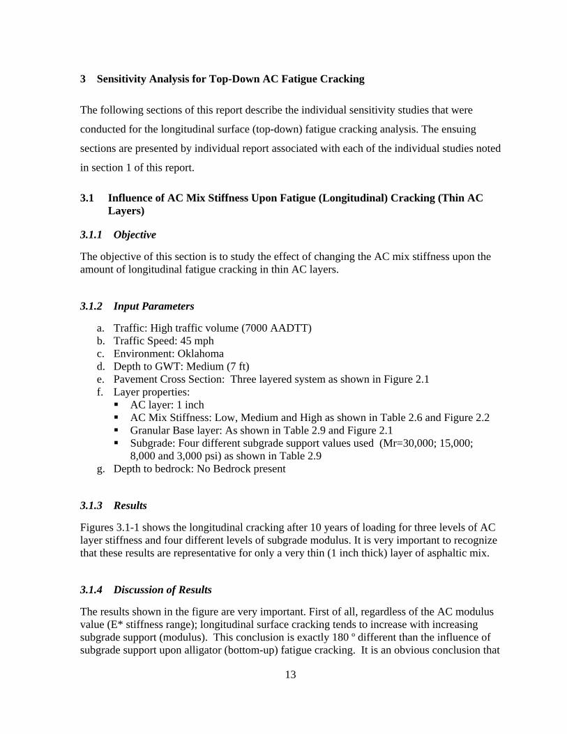
13
3 Sensitivity Analysis for Top-Down AC Fatigue Cracking The following sections of this report describe the individual sensitivity studies that were
conducted for the longitudinal surface (top-down) fatigue cracking analysis. The ensuing
sections are presented by individual report associated with each of the individual studies noted
in section 1 of this report.
3.1 Influence of AC Mix Stiffness Upon Fatigue (Longitudinal) Cracking (Thin AC Layers)
3.1.1 Objective
The objective of this section is to study the effect of changing the AC mix stiffness upon the amount of longitudinal fatigue cracking in thin AC layers.
3.1.2 Input Parameters
a. Traffic: High traffic volume (7000 AADTT) b. Traffic Speed: 45 mph c. Environment: Oklahoma d. Depth to GWT: Medium (7 ft) e. Pavement Cross Section: Three layered system as shown in Figure 2.1 f. Layer properties: AC layer: 1 inch AC Mix Stiffness: Low, Medium and High as shown in Table 2.6 and Figure 2.2 Granular Base layer: As shown in Table 2.9 and Figure 2.1 Subgrade: Four different subgrade support values used (Mr=30,000; 15,000;
8,000 and 3,000 psi) as shown in Table 2.9 g. Depth to bedrock: No Bedrock present
3.1.3 Results
Figures 3.1-1 shows the longitudinal cracking after 10 years of loading for three levels of AC layer stiffness and four different levels of subgrade modulus. It is very important to recognize that these results are representative for only a very thin (1 inch thick) layer of asphaltic mix.
3.1.4 Discussion of Results
The results shown in the figure are very important. First of all, regardless of the AC modulus value (E* stiffness range); longitudinal surface cracking tends to increase with increasing subgrade support (modulus). This conclusion is exactly 180 º different than the influence of subgrade support upon alligator (bottom-up) fatigue cracking. It is an obvious conclusion that

14
the stronger the subgrade the subgrade modulus, the greater the tensile strains will be at the pavement surface (Z=0). This will lead to a greater surface fatigue cracking effect. Another important lesson to be drawn from this sensitivity analysis is related to the fundamental fact that, for very thin AC layers, the best AC mixture is one that exhibits a very low stiffness Master Curve. As the mixture becomes more and more stiff, the amount of longitudinal cracking, due to top-down fatigue fracture, greatly increases (almost doubled). The results shown in the figure clearly indicate that the probability of having longitudinal surface cracking is greatly increased when thin stiff AC mixtures and stronger (stiffer) subgrade support values are encountered. This is explained by the fact that the surface tensile strains occurring at the top of the AC layer become greater for stiffer foundation supports, compared to lower (weak - low Mr subgrade supports). Hence, the larger tensile strains are more prone to have fatigue fracture originate at the surface with the stronger subgrade support conditions.
3.1.5 Summary and Conclusions
For very thin AC layers, the design engineer should use as low an AC mixture stiffness as possible to eliminate and / or minimize fatigue cracking. A higher probability of top down cracking appears to exist when pavements are constructed over stiff subgrade materials. If the subgrade has a weak support condition, it is highly likely that alligator fatigue cracking will be observed. Finally, it is very important to understand that the conclusions and inferences made are very much a function of the thickness of the AC layer used in the pavement design.

15
0
50
100
150
200
250
300
350
400
450
500
Low E* Med E* Hi E*
AC Mix Stiffness
Long
itudi
nal S
urfa
ce C
rack
ing
Ref
eren
ce B
ased
Upo
n 1
ft/ 5
00 ft
SG Mr= 3 ksi SG Mr= 8 ksi SG Mr= 15 ksi SG Mr= 30 ksi
Figure 3.1-1 Effect of AC Mix Stiffness on Longitudinal Cracking, (Hac = 1 in)

16
3.2 Influence of AC Mix Stiffness Upon Fatigue (Longitudinal) Cracking (Thick AC Layers)
3.2.1 Objective
The objective of this section is to study the effect of changing the AC mix stiffnesses on the amount of longitudinal fatigue cracking for thick AC layers.
3.2.2 Input Parameters
a. Traffic: High traffic volume (7000 AADTT) b. Traffic Speed: 45 mph c. Environment: Oklahoma d. Depth to GWT: Medium (7 ft) e. Pavement Cross Section: Three layered system as shown in Figure 2.1 f. Layer properties: AC layer: 8 inch AC Mix Stiffness: Low, Medium and High as shown in Table 2.6 and Figure 2.2 Granular Base layer: As shown in Table 2.9 and Figure 2.1 Subgrade: Four different subgrade support values used (Mr=30,000; 15,000; 8,000
and 3,000 psi) as shown in Table 2.9 g. Depth to bedrock: No Bedrock present
3.2.3 Results
Figures 3.2-1 shows the longitudinal fatigue cracking after 10 years of loading for three levels of AC layer stiffness.
3.2.4 Discussion of Results
One of the more critical results shown in the figure relates to the fact that longitudinal cracking is increased as the foundation (subgrade) modulus is increased. The presence of stiffer subgrade causes a larger surface tensile strain (and hence surface fatigue damage). Secondly, the interactive importance of the AC mixture stiffness is also readily apparent. For low E* mix stiffness, longitudinal cracking is greatly increased, primarily at stiff foundation (subgrade) conditions.
3.2.5 Summary and Conclusions
As the AC mix stiffness increases the amount of longitudinal surface fatigue cracking decreases. At high levels of AC mix stiffness there is almost no longitudinal surface fatigue cracking. In addition, surface cracking is increased as the subgrade (foundation) stiffness is increased.

17
0
50
100
150
200
250
300
350
400
450
Low E* Med E* Hi E*
AC Mix Stiffness
Long
itudi
nal S
urfa
ce C
rack
ing
(ft/5
00ft)
SG Mr= 3 ksi SG Mr= 8 ksi SG Mr= 15 ksi SG Mr= 30 ksi
Figure3.2-1 Effect of AC Mix Stiffness on Longitudinal Cracking, (Hac = 8 in)
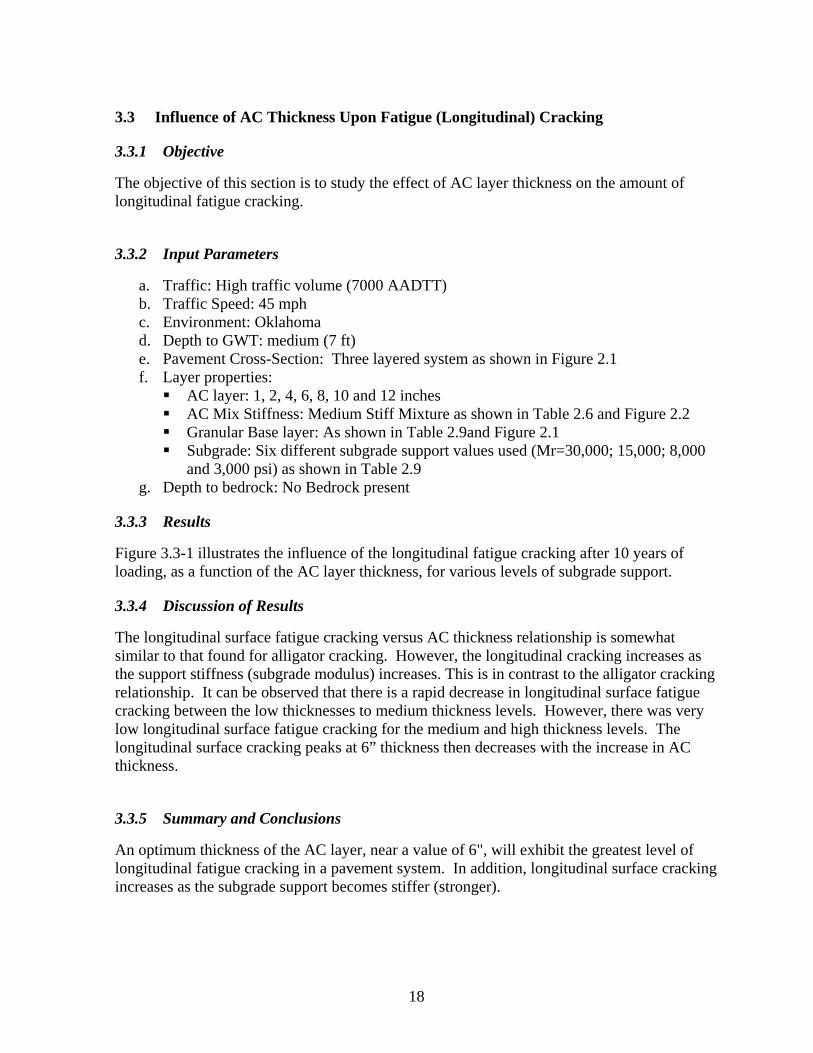
18
3.3 Influence of AC Thickness Upon Fatigue (Longitudinal) Cracking
3.3.1 Objective
The objective of this section is to study the effect of AC layer thickness on the amount of longitudinal fatigue cracking.
3.3.2 Input Parameters
a. Traffic: High traffic volume (7000 AADTT) b. Traffic Speed: 45 mph c. Environment: Oklahoma d. Depth to GWT: medium (7 ft) e. Pavement Cross-Section: Three layered system as shown in Figure 2.1 f. Layer properties: AC layer: 1, 2, 4, 6, 8, 10 and 12 inches AC Mix Stiffness: Medium Stiff Mixture as shown in Table 2.6 and Figure 2.2 Granular Base layer: As shown in Table 2.9and Figure 2.1 Subgrade: Six different subgrade support values used (Mr=30,000; 15,000; 8,000
and 3,000 psi) as shown in Table 2.9 g. Depth to bedrock: No Bedrock present
3.3.3 Results
Figure 3.3-1 illustrates the influence of the longitudinal fatigue cracking after 10 years of loading, as a function of the AC layer thickness, for various levels of subgrade support.
3.3.4 Discussion of Results
The longitudinal surface fatigue cracking versus AC thickness relationship is somewhat similar to that found for alligator cracking. However, the longitudinal cracking increases as the support stiffness (subgrade modulus) increases. This is in contrast to the alligator cracking relationship. It can be observed that there is a rapid decrease in longitudinal surface fatigue cracking between the low thicknesses to medium thickness levels. However, there was very low longitudinal surface fatigue cracking for the medium and high thickness levels. The longitudinal surface cracking peaks at 6” thickness then decreases with the increase in AC thickness.
3.3.5 Summary and Conclusions
An optimum thickness of the AC layer, near a value of 6", will exhibit the greatest level of longitudinal fatigue cracking in a pavement system. In addition, longitudinal surface cracking increases as the subgrade support becomes stiffer (stronger).

19
0
50
100
150
200
250
300
350
400
450
500
0 2 4 6 8 10 12 14
AC Thickness (inch)
Long
itudi
nal S
urfa
ce C
rack
ing
(ft/5
00ft)
Mr= 3 ksi Mr= 8 ksi Mr= 15 ksi Mr= 30 ksi
Figure 3.3-1 Effect of AC Layer Thickness on Longitudinal Fatigue Cracking

20
3.4 Influence of Subgrade Modulus Upon Fatigue (Longitudinal) Cracking
3.4.1 Objective
The objective of this section is to study the effect of subgrade modulus on the amount of longitudinal fatigue cracking.
3.4.2 Input Parameters
a. Traffic: High traffic volume (7000 AADTT) b. Traffic Speed: 45 mph c. Environment: Oklahoma d. Depth to GWT: medium (7 ft) e. Pavement Cross-Section: Three layered system as shown in Figure 2.1 f. Layer properties: AC layer: 6 inches AC Mix Stiffness: Medium Stiff Mixture as shown in Table 2.6 and Figure 2.2 Granular Base layer: As shown in Table 2.9 and Figure 2.1 Subgrade: Four different subgrade support values used (Mr=30,000; 15,000; 8,000
and 3,000 psi) as shown in Table 2.9 g. Depth to bedrock: No Bedrock present
3.4.3 Results
Figure 3.4-1 shows the longitudinal fatigue cracking after 10 years of loading for the four levels of subgrade modulus used in the sensitivity study.
3.4.4 Discussion of Results
The figure clearly illustrates the fundamental fact that the stronger the foundation (subgrade) support of the pavement system becomes; the greater the amount of longitudinal fatigue cracking that will occur. This is a direct result of the fact that larger surface tensile strains will occur when the foundation layer increases in modulus. The relative sensitivity of the rate of longitudinal cracking, due to variable subgrade support, is a function of many other design variables, such as: traffic, site climatic condition and thickness of the AC layer used in the cross section.
3.4.5 Summary and Conclusions
Increasing the subgrade support modulus will result in a increased level of longitudinal fatigue cracking in any pavement system. The sensitivity of subgrade support to the magnitude of longitudinal cracking is also a function of many other design input parameters as well.

21
0
50
100
150
200
250
300
350
400
450
500
0 5000 10000 15000 20000 25000 30000 35000
Subgrade Modulus (psi)
Long
itudi
nal S
urfa
ce C
rack
ing
(ft/5
00ft)
Figure3.4-1 Effect of Subgrade Modulus on Longitudinal Cracking

22
3.5 Influence of AC Mix Air Voids Upon Fatigue (Longitudinal) Cracking
3.5.1 Objective
The objective of this section is to study the effect of the in-situ AC air voids on longitudinal fatigue cracking.
3.5.2 Input Parameters
a. Traffic: Medium traffic volume (7000 AADTT) b. Traffic Speed: 45 mph c. Environment: Oklahoma d. Depth to GWT: medium (7 ft) e. Pavement Cross-Section: Three layered system as shown in Figure 2.1 f. Layer properties: AC layer: 6 inches AC Mix Stiffness: Medium Stiff Mixture as shown in Table 2.6 and Figure 2.2 AC Mix Air Voids: 4, 7, and 10% Granular Base layer: As shown in Table 2.9 and Figure 2.1 Subgrade: Medium Support (Mr=15,000 psi) as shown in Table 2.9
g. Depth to bedrock: No Bedrock present
3.5.3 Results
Figure 3.5-1 shows the longitudinal fatigue cracking after 10 years of loading for the three levels of AC mix air voids used in the sensitivity study. The range of air voids used in the study reflects a very real range under typical construction conditions (4% to 10%).
3.5.4 Discussion of Results
The results shown in the figure clearly reflect the critical importance of air voids upon fatigue cracking, regardless of whether bottom up-alligator or top-down longitudinal cracking is being considered. The greater the in-place air voids of an asphalt mixture are; the greater the degree of cracking that may be expected. This effect is directly attributable to the volumetric mix term incorporated into both the controlled strain (thin AC layers) and controlled stress (thick AC layers) fatigue equation for top-down cracking. In reality, it is the mix Voids Filled with Bitumen parameter that directly influences the fatigue cracking. As this parameter is increased, the cracking is greatly reduced. Thus, this sensitivity study is directly tied to air voids and the AC content. (Also see Study 3.6)
3.5.5 Summary and Conclusions
In summary, the air voids within an AC mixture are an important parameter to influence fatigue cracking. Increasing the amount of air voids in the AC mix may significantly increase the amount of longitudinal fatigue cracking.
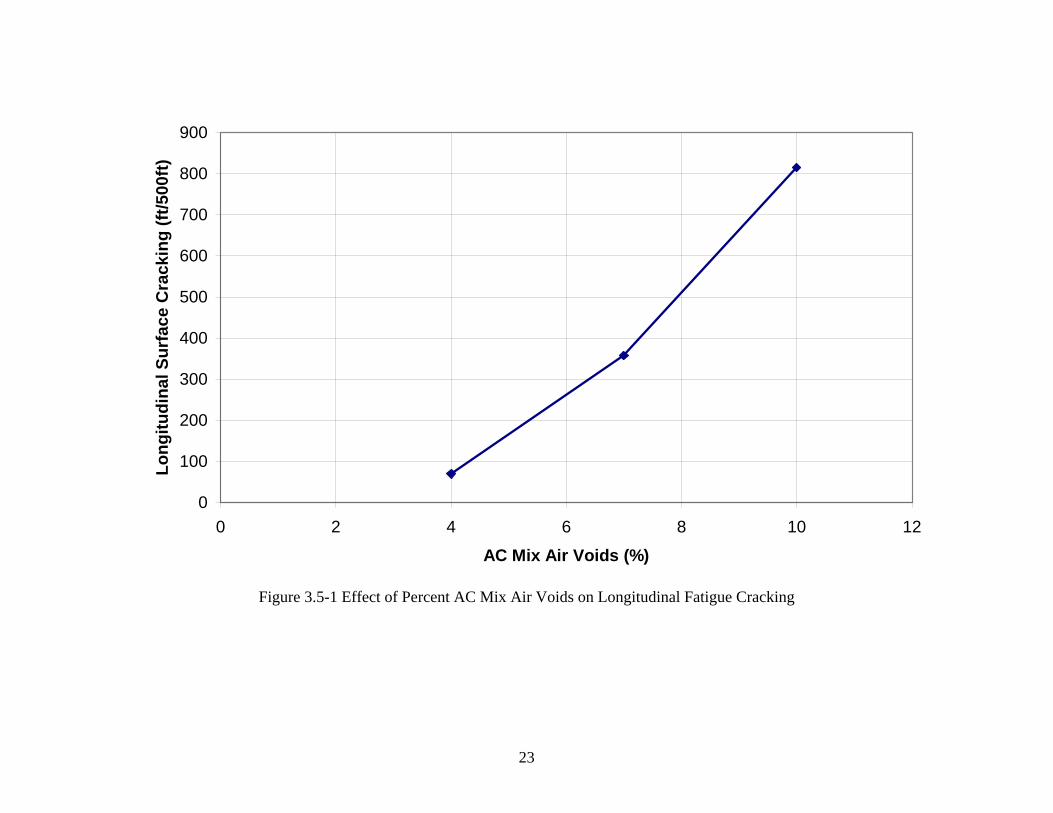
23
0
100
200
300
400
500
600
700
800
900
0 2 4 6 8 10 12
AC Mix Air Voids (%)
Long
itudi
nal S
urfa
ce C
rack
ing
(ft/5
00ft)
Figure 3.5-1 Effect of Percent AC Mix Air Voids on Longitudinal Fatigue Cracking

24
3.6 Influence of Asphalt Content (Effective Bitumen Volume) Upon Fatigue (Longitudinal) Cracking
3.6.1 Objective
The objective of this section is to study the influence of the magnitude of the effective bitumen volume present in an AC mixture upon the amount of longitudinal cracking.
3.6.2 Input Parameters
a. Traffic: Medium traffic volume (7000 AADTT) b. Traffic Speed: 45 mph c. Environment: Oklahoma d. Depth to GWT: medium (7 ft) e. Pavement Cross-Section: Three layered system as shown in Figure 2.1 f. Layer properties: AC layer: 6 inches AC Mix Stiffness: Medium Stiff Mixture as shown in Table 2.6 and Figure 2.2 AC Mix Effective Binder Content: 8, 11 and 15% Granular Base layer: As shown in Table 2.9 and Figure 2.1 Subgrade: Medium Support (Mr=15,000 psi) as shown in Table 2.9
g. Depth to bedrock: No Bedrock present
3.6.3 Results
Figure 3.6-1 shows the longitudinal fatigue cracking after 10 years of loading for three assumed values of effective bitumen volume (Vbe). This parameter is approximately 2.0 to 2.2 times the numerical value of the AC content, in percentage form. Thus the ranges of Vbe = 8, 11 and 15 %, translate into approximate AC % values of 4%, 5+% and 7+%.
3.6.4 Discussion of Results
Like the previous study presented on the influence of mixture air voids, the influence of the amount of asphalt present in a mix also has a significant influence upon the amount of longitudinal cracking that may occur. It is observed from the figure that there is a decrease in the amount of longitudinal fatigue cracking as the amount of the effective binder volume increases. This is a direct consequence of the Vfb term used in the Fatigue Damage equation. As the asphalt content (effective bitumen content) is increased; the Voids filled with bitumen are also increased. This results in a greater resistance of the mixture to fracture under fatigue damage.
3.6.5 Summary and Conclusions
In summary, the amount of asphalt binder present in a mixture will directly influence the amount of fatigue cracking that will occur in the field. When the effective bitumen volume (amount of asphalt) is increased in a mix; the amount of longitudinal cracking will be decreased.

25
0
100
200
300
400
500
600
700
800
6 7 8 9 10 11 12 13 14 15 16
AC Mix Effective Binder Content By Volume (%)
Long
itudi
nal S
urfa
ce C
rack
ing
(ft/5
00ft)
Figure 3.6-1 Effect of Percent AC Binder by volume on Longitudinal Fatigue Cracking

26
3.7 Influence of Depth to GWT on Fatigue (Longitudinal) Cracking
3.7.1 Objective
The objective of this section is to study the effect of depth to GWT on the amount of longitudinal cracking.
3.7.2 Input Parameters
a. Traffic: High traffic volume (1000 AADTT) b. Traffic Speed: 45 mph c. Environment: Phoenix d. Depth to GWT: 2, 4, 7 and 15 ft e. Pavement Cross-Section: Three layered system as shown in Figure 2.1 f. Layer properties: AC layer: 6 inches AC Mix Stiffness: High Stiff Mixture as shown in Table 2.6 and Figure 2.2 Granular Base layer: Constant modulus = 38,000 psi. Subgrade: Five different subgrade support values used (above GWT/ below GWT)
(Mr=34,000/17,600; 25,000/13075; 18,000/10260, 10,000/5,860 and 6,000/2250 psi).
g. Depth to bedrock: No Bedrock present
3.7.3 Results
Figure 3.7-1 shows the longitudinal surface fatigue cracking after 10 years of loading for four levels of depth to GWT, for low to high subgrade modulus materials.
3.7.4 Discussion of Results
As the GWT depth decreases (comes closer to the surface) the longitudinal fatigue cracking in the AC layer decreased. It can also be observed that as the subgrade modulus is increased the quantity of longitudinal cracking is also, increased. Thus, the GWT effect is clearly mirrored to the technical fact that any activity that will tent to increase the subgrade support (i.e. increasing the depth to GWT) will result in an increased level of surface longitudinal cracking. This due to the fact that as the GWT depth increases the subgrade becomes dryer and the subgrade modulus will increase, which in turn leads to a higher longitudinal cracking. The rate of at which the longitudinal cracking increases as GWT depth changes is the almost the same for all levels of the subgrade modulus. The rate of increase is higher at shallow GWT depths, and then starts to increase at a lower rate as the GWT increases. As the GWT becomes large, it would be anticipated that the influence upon fatigue damage would become insignificant.
3.7.5 Summary and Conclusions
Greater depths of the GWT will result in more longitudinal cracking due to the increased subgrade stiffness that will occur. Longitudinal cracking will almost double from a GWT

27
depth of 2 feet to a GWT depth of 7 feet. As would be expected, longitudinal cracking will tend to increase for stiffer foundations.

28
0
50
100
150
200
250
300
350
0 2 4 6 8 10 12 14 16Ground Water Table Depth (ft)
Long
itudi
nal S
urfa
ce C
rack
ing
(ft/5
00ft)
SG Modulus = 6000 SG Modulus = 10000 SG Modulus = 18000 SG Modulus = 25000 SG Modulus = 34000
Figure 3.7-1 Effect of Depth to GWT on Longitudinal Fatigue Cracking

29
3.8 Influence of Truck Traffic Volume Upon Fatigue (Longitudinal) Cracking
3.8.1 Objective
The objective of this section is to investigate the influence of the truck traffic volume upon longitudinal fatigue cracking.
3.8.2 Input Parameters
a. Traffic Volume (AADTT): 100, 1000, 4000, 7000 and 50,0000 b. Traffic Speed: 45 mph c. Environment: Oklahoma d. Depth to GWT: Medium (7 ft) e. Pavement Cross-Section: Three layered system as shown in Figure 2.1 f. Layer properties: AC layer: 6 inches AC Mix Stiffness: Medium Stiff Mixture as shown in Table 2.6 and Figure 2.2 Granular Base layer: As shown in Table 2.9 and Figure 2.1 Subgrade: Medium Support (Mr=15,000 psi) as shown in Table 2.9
g. Depth to bedrock: No Bedrock present
3.8.3 Results
Figure 3.8-1 shows the longitudinal fatigue cracking after 10 years of loading for four levels of truck traffic volume expressed in AADTT (Average Annual Daily truck Traffic). These levels of truck volumes approximately equate to: 200,000; 2,000,000; 8,000,000; 15,000,000; and 100,000,000 ESALs respectively.
3.8.4 Discussion of Results
As one would intuitively surmise, the magnitude of the truck volume plays a very significant role upon the amount of longitudinal cracking that occurs for the pavement system having the 6" AC layer noted. As traffic volume (AADTT) increases, the amount of longitudinal fatigue cracking increases in a very significant fashion.
3.8.5 Summary and Conclusions
Increasing the truck traffic volume (AADTT) increases the amount of longitudinal fatigue cracking. In essence, the parameter of truck traffic (volume), or even ESALs is an extremely sensitive parameter to longitudinal cracking. The rate of change of longitudinal cracking with truck traffic volume is nearly linear across all ranges of truck volume. The trend becomes slightly non-linear for the very high level of truck traffic investigated in this study.
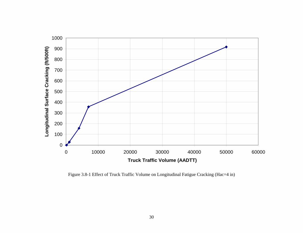
30
0
100
200
300
400
500
600
700
800
900
1000
0 10000 20000 30000 40000 50000 60000
Truck Traffic Volume (AADTT)
Long
itudi
nal S
urfa
ce C
rack
ing
(ft/5
00ft)
Figure 3.8-1 Effect of Truck Traffic Volume on Longitudinal Fatigue Cracking (Hac=4 in)
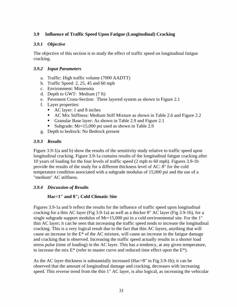
31
3.9 Influence of Traffic Speed Upon Fatigue (Longitudinal) Cracking
3.9.1 Objective
The objective of this section is to study the effect of traffic speed on longitudinal fatigue cracking.
3.9.2 Input Parameters
a. Traffic: High traffic volume (7000 AADTT) b. Traffic Speed: 2, 25, 45 and 60 mph c. Environment: Minnesota d. Depth to GWT: Medium (7 ft) e. Pavement Cross-Section: Three layered system as shown in Figure 2.1 f. Layer properties: AC layer: 1 and 8 inches AC Mix Stiffness: Medium Stiff Mixture as shown in Table 2.6 and Figure 2.2 Granular Base layer: As shown in Table 2.9 and Figure 2.1 Subgrade: Mr=15,000 psi used as shown in Table 2.9
g. Depth to bedrock: No Bedrock present
3.9.3 Results
Figure 3.9-1(a and b) show the results of the sensitivity study relative to traffic speed upon longitudinal cracking. Figure 3.9-1a contains results of the longitudinal fatigue cracking after 10 years of loading for the four levels of traffic speed (2 mph to 60 mph). Figures 3.9-1b provide the results of the study for a different thickness level of AC: 8" for the cold temperature condition associated with a subgrade modulus of 15,000 psi and the use of a "medium" AC stiffness.
3.9.4 Discussion of Results
Hac=1" and 8"; Cold Climatic Site Figures 3.9-1a and b reflect the results for the influence of traffic speed upon longitudinal cracking for a thin AC layer (Fig 3.9-1a) as well as a thicker 8" AC layer (Fig 3.9-1b), for a single subgrade support modulus of Mr=15,000 psi in a cold environmental site. For the 1" thin AC layer; it can be seen that increasing the traffic speed tends to increase the longitudinal cracking. This is a very logical result due to the fact that thin AC layers, anything that will cause an increase in the E* of the AC mixture, will cause an increase in the fatigue damage and cracking that is observed. Increasing the traffic speed actually results in a shorter load stress pulse (time of loading) in the AC layer. This has a tendency, at any given temperature, to increase the mix E* (refer to master curve and reduced time effect upon the E*). As the AC layer thickness is substantially increased (Hac=8" in Fig.3.9-1b); it can be observed that the amount of longitudinal damage and cracking, decreases with increasing speed. This reverse trend from the thin 1" AC layer, is also logical, as increasing the vehicular

32
speed causes an increase in the E*, a decrease in the tensile strain and less damage (longitudinal cracking) to the pavement system. Finally, it should be noted that the sensitivity of speed to fatigue damage is not overly significant.
3.9.5 Summary and Conclusions
As a general conclusion, changes in the vehicular operational speed on the amount of longitudinal cracking in a pavement system may not be very large. For very thin AC layer pavement systems, the amount of fatigue damage and cracking will increase as the speed of the loading system is also increased. For very thick pavements, the reverse will occur and slightly less fatigue damage may be present at higher vehicle speeds.

33
86
88
90
92
94
96
98
100
102
104
106
108
0 10 20 30 40 50 60 70
Traffic Speed (mph)
Long
itudi
nal S
urfa
ce C
rack
ing
(ft/5
00ft)
Figure 3.9-1a Effect of Traffic Speed on Longitudinal Fatigue Cracking (Hac =1”, Cold Climate)
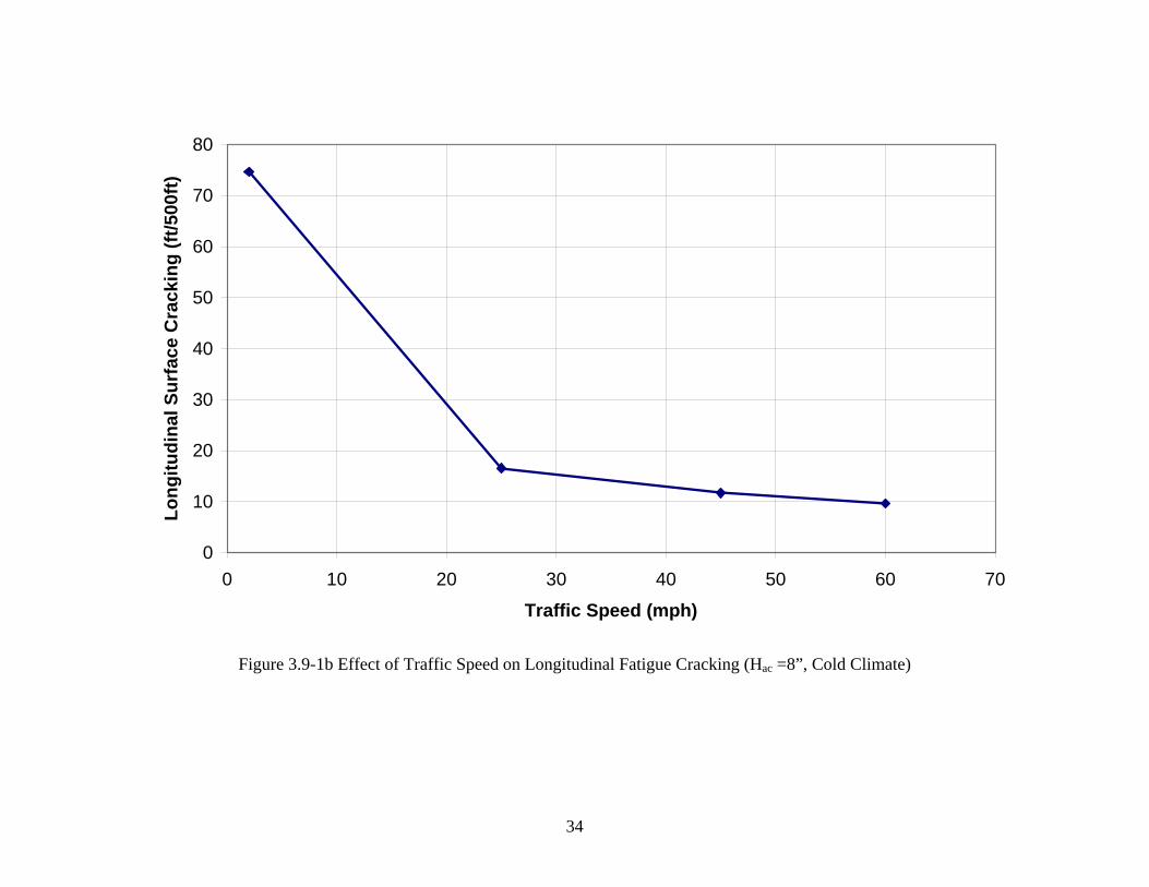
34
0
10
20
30
40
50
60
70
80
0 10 20 30 40 50 60 70
Traffic Speed (mph)
Long
itudi
nal S
urfa
ce C
rack
ing
(ft/5
00ft)
Figure 3.9-1b Effect of Traffic Speed on Longitudinal Fatigue Cracking (Hac =8”, Cold Climate)

35
3.10 Influence of Traffic Analysis Level Upon Fatigue (Longitudinal) Cracking
3.10.1 Objective
The objective of this section is to investigate the influence of Hierarchical Traffic Level used in the analysis upon the amount of longitudinal fatigue cracking.
3.10.2 Input Parameters
a. Traffic Volume: See discussion in 3.10.3 "Results" section below b. Traffic Speed: 45 mph c. Environment: Oklahoma (61 deg F) d. Depth to GWT: Medium (7 ft) e. Pavement Cross-Section: Three layered system as shown in Figure 2.1 f. Layer properties: AC layer: 6 inches AC Mix Stiffness: Medium Stiff Mixture as shown in Table 2.6 and Figure 2.2 Granular Base layer: As shown in Table 2.9 and Figure 2.1 Subgrade: Medium Support (Mr=15,000 psi) as shown in Table 2.9
g. Depth to bedrock: No Bedrock present
3.10.3 Results
Figure 3.10-1 shows the impact of the Hierarchical Traffic Level selected upon the relationship of the longitudinal fatigue cracking (after 10 years of loading) for a range of traffic volumes (distributions). In this plot, five specific traffic distributions (volumes) were investigated. For the Traffic Level 1 approach, the actual traffic load axle spectrums were used as input into the program. The load spectrum approach used the input traffic assumptions noted in Tables 2.2 to 2.5. The cracking results using the Level 1 approach, for each of the five traffic volumes, is denoted as the "Load Spectra" results in the plot. For each of the five axle load spectrum distributions; the mixture axle type- load combinations were then transformed into Equivalent 18 Kip Single Axle Load repetitions (ESALs) through the use of conventional AASHTO truck damage factors, defined at a pt=2.5 and SN=5. The approximate cumulative 10-year ESAL values have been noted in Table 2.1.
3.10.4 Discussion of Results
The longitudinal fatigue cracking results shown in Figure 3.10-1 clearly indicate that the use of actual traffic load spectra, in the structural distress prediction model, results in a very significant difference in predicted cracking, compared to the use of the empirical ESAL approach to traffic that has been historically used in pavement design. For the problem investigated, the traffic axle load spectra approach (Level 1) yield more cracking compared to the use of E18KSAL's specially at higher traffic. It can be seen that the predicted difference between the two approaches tends to dramatically increase with increasing traffic. At traffic levels approaching 1 million ESALs this difference is near 30 to 50 ft/500ft; for traffic in the 10 million ESALs range, this difference is near 300 ft/500ft, while for 108 ESALs the predicted difference is near 700 ft/500ft.

36
3.10.5 Summary and Conclusions
The use of a Level 1 traffic approach, based upon the actual traffic load spectra, yields a much higher level of longitudinal cracking compared to the classical use of E18KSAL's.

37
0
100
200
300
400
500
600
700
800
900
1000
10000 100000 1000000 10000000 100000000
Total Number of Esals (10 years)
Long
itudi
nal S
urfa
ce C
rack
ing
(ft/5
00ft)
ESALs Load Spectra
Figure 3.10-1 Effect of Traffic Analysis Level upon Longitudinal Fatigue Cracking

38
3.11 Influence of MAAT Upon Fatigue (Longitudinal) Cracking
3.11.1 Objective
The objective of this section is to study the effect of MAAT on the longitudinal fatigue cracking.
3.11.2 Input Parameters
a. Traffic Volume: Medium (7000 AADTT) b. Traffic Speed: 45 mph c. Environment: (MAAT): Minnesota (46 deg F); Oklahoma (61 deg F) and Phoenix (74
deg F) d. Depth to GWT: Medium (7 ft) e. Pavement Cross-Section: Three layered system as shown in Figure 2.1 f. Layer properties: AC layer: 1,4, 8 and 12 inches AC Mix Stiffness: High, Medium and Low Mixture Stiffnesses as shown in Table
2.6 and Figure 2.2 Granular Base layer: As shown in Table 2.9 and Figure 2.1 Subgrade: Medium Support (Mr=15,000 psi) as shown in Table 2.9
g. Depth to bedrock: No Bedrock present
3.11.3 Results
The full results of this sensitivity analysis are shown in Figures 3.11-1(a thru d). Each figure represents the relationship of predicted longitudinal cracking as a function of a specific level of AC layer thickness (Hac= 1, 4, 8 and 12"). The longitudinal fatigue cracking shown reflects 10 years of loading for the three levels of MAAT investigated.
3.11.4 Discussion of Results
The results shown are quite important relative to the selection of the appropriate level of AC mix stiffness (E*) as a function of the thickness of the AC layer. Theses results can best be interpreted for each AC thickness level presented in the analysis. Hac=1": Referring to Figure 3.11-1a (Hac=1"); it can be observed that the amount of longitudinal fatigue cracking is always increased as the MAAT is also increased. This is true for all mixture stiffness values (E*). This result is very logical because as the MAAT increases, higher pavement temperatures will occur. This is turn, will lead to lower in-situ AC stiffnesses (dynamic moduli), which in turn will cause greater tensile strains, a lower number of repetitions to failure (Nf) and a greater degree of damage (longitudinal cracking), regardless of the original AC mix stiffness master curve (E*). The second significant finding shown in the figure supports the discussion of study 3.1. As can be observed, the degree of longitudinal cracking that occurs is extremely sensitive to the

39
AC mixture stiffness (E*). For thin AC layers, the greater the mixture stiffness, the greater the degree of longitudinal cracking. In fact, for the very thin AC layer, it can be observed that there is a very strong degree of sensitivity of the AC E* stiffness to the amount of cracking that occurs. Hac=4": The influence of increasing the AC thickness from a 1" layer to a 4" layer is illustrated in Figure 3.11-1b. It is observed that an identical conclusion, relative to the significance of the MAAT upon cracking, is noted for the 4" AC layer, compared to the 1" AC layer. The explanation of this result is the same as what was presented for the 1” AC layer. Increasing the temperature at the site will increase the tensile strains, regardless of the mixture stiffness. However, the longitudinal cracking values are much less and the change is not significant. Hac=8": As the thickness of the AC layer is increased from 4" to 8"; the sensitivity of E* and MAAT is shown in Figure 3.11-1c. It is again obvious that the influence of warmer design sites upon an increased level of longitudinal cracking is identical to the conclusion already noted for the 1" and 4" AC layers. As previously noted, this is not surprising and the explanation provided in the previous paragraphs are applicable for any level of AC thickness. At the Hac=8" level; it can be observed that a major change in the influence of AC mix stiffness occurs. Unlike the effect for the Hac = 1” and 4” conditions; it can be observed that at thicker HMA layers, the lower the mix stiffness; the greater the amount of longitudinal surface cracking. This conclusion is entirely opposite to what was found at the thinner AC layer thickness. Hac=12": The influence of the MAAT and E*, upon longitudinal cracking for the thick (12") AC layer; is presented in Figure 3.11-1d. It is observed that increasing the MAAT will lead to an increase in the amount of longitudinal cracking; an identical conclusion noted for all of the three prior thickness levels. It should also be noted that the amount of cracking is greatly decreased as the AC thickness increases. At the Hac=12" level; it can be noted that there is very little, if any, effect of the AC mixture between medium and high stiffness upon the amount of longitudinal cracking observe. However like the Hac = 8” conditions; the low stiffness had a much higher cracking.
3.11.5 Summary and Conclusions
Regardless of the thickness of the AC layer, the amount of longitudinal cracking will increase with increasing Mean Annual Air Temperature at the design site. This is true for whatever level of AC mixture stiffness is utilized in the pavement structure and thickness of the HMA layer. However, the actual thickness of the AC layer tends to play a very critical role in defining the optimum benefit (lowest amount of longitudinal cracking damage) for the specific mix in question. As a general rule, for very thin AC layers; the use of a very stiff AC mixture will result in maximum fatigue damage and cracking. As previously noted, it appears that

40
maximum fatigue damage will occur with HMS layer thickness near 6”. As the AC layer thickness is increased to levels of 10" - 12+", the use of stiff mixtures (high E* values) is preferable and will lead to a minimum of fatigue damage and longitudinal cracking.

41
0
50
100
150
200
250
300
350
400
450
40 45 50 55 60 65 70 75 80
MAAT (oF)
Long
itudi
nal S
urfa
ce C
rack
ing
(ft/5
00ft)
Low AC E* Medium AC E* High AC E*
Figure 3.11-1a Effect of MAAT on Longitudinal Fatigue Cracking (Hac =1”)

42
0
5
10
15
20
25
30
35
40 45 50 55 60 65 70 75 80
MAAT (oF)
Long
itudi
nal S
urfa
ce C
rack
ing
(ft/5
00ft)
Low AC E* Medium AC E* High AC E*
Figure 3.11-1b Effect of MAAT on Longitudinal Fatigue Cracking (Hac =4”)

43
0
100
200
300
400
500
600
700
40 45 50 55 60 65 70 75 80
MAAT (oF)
Long
itudi
nal S
urfa
ce C
rack
ing
(ft/5
00ft)
Low AC E* Medium AC E* High AC E*
Figure 3.11-1c Effect of MAAT on Longitudinal Fatigue Cracking (Hac =8”)

44
0
20
40
60
80
100
120
140
160
180
200
40 45 50 55 60 65 70 75 80
MAAT (oF)
Long
itudi
nal S
urfa
ce C
rack
ing
(ft/5
00ft)
Low AC E* Medium AC E* High AC E*
Figure 3.11-1d Effect of MAAT on Longitudinal Fatigue Cracking (Hac =12”)

45
3.12 Influence of Bedrock Depth upon Fatigue (Longitudinal) Cracking
3.12.1 Objective
The objective of this section is to study the effect of changing the depth of bedrock under a flexible pavement upon the amount of longitudinal fatigue cracking.
3.12.2 Input Parameters
a. Traffic: High traffic volume (7000 AADTT) b. Traffic Speed: 45 mph c. Environment: Oklahoma d. Depth to GWT: medium (7 ft) for bedrock depths 10 and 20 ft; GWT at top of
Bedrock for all depths less than 5 ft e. Pavement Cross-Section: Three layered system as shown in Figure 2.1 f. Layer properties: AC layer: 6 inch AC Mix Stiffness: Medium as shown in Table 2.6 and Figure 2.2 Granular Base layer: As shown in Table 2.9 and Figure 2.1 Subgrade: Two subgrade support values used (Mr=30,000 and 3,000 psi) as shown
in Table 2.9 g. Depth to bedrock: 3', 4', 5', 6’, 7’, 12' and 20' (from top of pavement): Ebr= 750,000 psi
3.12.3 Results
Figures 3.12-1 shows the longitudinal fatigue cracking (after 10 years of loading) as a function of the depth of the Bedrock layer, for two levels of subgrade support evaluated.
3.12.4 Discussion of Results
The figure illustrates the fact, that regardless of the subgrade support value, the presence of a bedrock layer at depths greater than 6' to 7' below the pavement surface will have very little, if any, influence upon the surface longitudinal cracking that is observed. On the other hand, if the bedrock layer comes within several feet of the subgrade surface, its presence may be directly responsible for the development of significant levels of surface cracking to be observed. This result is totally consistent with the influence of subgrade (foundation) stiffness upon longitudinal cracking previously discussed. Again, the reason for this can be easily explained through layered response models and results. If the effective foundation support of a pavement system is very soft and there is no bedrock present, the magnitude of any surface tensile strains induced by vehicular traffic is very small. This would lead to little, if any, surface fatigue cracking to occur on the facility. However, as the "effective foundation support" is dramatically increased, (due to an increase in subgrade Mr and/or the presence of bedrock layer near the surface); a significant increase in the surface tensile strains will occur. This impact, results in a much greater probability of

46
surface fatigue cracking to occur. For surface cracking, the presence of a stiffer subgrade, in combination with the stiff bedrock layer, will result in a more damaging surface condition than if a low support subgrade where present.
3.12.5 Summary and Conclusions
Depth of bedrock may also influence the amount of longitudinal surface cracking that may be present in a pavement system. For the example pavement evaluated, it appears that the "effective zone of influence of the bedrock layer" must be within 6' to 7' of the pavement surface to influence the amount of surface fatigue cracking that may occur.

47
0
100
200
300
400
500
600
0 5 10 15 20 25
BedRock Depth (ft)
Long
itudi
nal S
urfa
ce C
rack
ing
(ft/5
00ft)
SG Mr = 3,000 SG Mr = 30,000
Figure 3.12-1 Effect of Bedrock Depth Upon Longitudinal Fatigue Cracking
Related Documents