Volume 5 Number 19 EJTP Electronic Journal of Theoretical Physics ISSN 1729-5254 Copyright © 2008 Fariel Shafee, All rights reserved. Editors Ammar Sakaji Ignazio Licata http://www.ejtp.com October, 2008 E-mail:[email protected]

Welcome message from author
This document is posted to help you gain knowledge. Please leave a comment to let me know what you think about it! Share it to your friends and learn new things together.
Transcript

Volume 5 Number 19
EJTPElectronic Journal of Theoretical Physics
ISSN 1729-5254
Copyright © 2008 Fariel Shafee, All rights reserved.
Editors
Ammar Sakaji Ignazio Licata
http://www.ejtp.com October, 2008 E-mail:[email protected]
Volume 5 Number 19
EJTPElectronic Journal of Theoretical Physics
ISSN 1729-5254
Copyright © 2008 Fariel Shafee, All rights reserved.
Editors
Ammar Sakaji Ignazio Licata
http://www.ejtp.com October, 2008 E-mail:[email protected]

Editor in Chief
A. J. Sakaji
EJTP Publisher P. O. Box 48210 Abu Dhabi, UAE [email protected] [email protected]
Editorial Board
Co-Editor
Ignazio Licata,Foundations of Quantum Mechanics Complex System & Computation in Physics and Biology IxtuCyber for Complex Systems Sicily – Italy
[email protected]@ejtp.info [email protected]
Wai-ning Mei Condensed matter Theory Physics Department University of Nebraska at Omaha,
Omaha, Nebraska, USA e-mail: [email protected] [email protected]
Richard Hammond General Relativity High energy laser interactions with charged particles Classical equation of motion with radiation reaction Electromagnetic radiation reaction forces Department of Physics University of North Carolina at Chapel Hill e.mail: [email protected]
F.K. DiakonosStatistical Physics Physics Department, University of Athens Panepistimiopolis GR 5784 Zographos, Athens, Greece e-mail: [email protected]
Tepper L. Gill Mathematical Physics, Quantum Field Theory Department of Electrical and Computer Engineering Howard University, Washington, DC, USA e-mail: [email protected]
José Luis Lopez-Bonilla Special and General Relativity, Electrodynamics of classical charged particles, Mathematical Physics, National Polytechnic Institute, SEPI-ESIME-Zacatenco, Edif. 5, CP 07738, Mexico city, Mexico e-mail:jlopezb[AT]ipn.mx lopezbonilla[AT]ejtp.info
Nicola Yordanov Physical Chemistry Bulgarian Academy of Sciences, BG-1113 Sofia, Bulgaria Telephone: (+359 2) 724917 , (+359 2) 9792546
e-mail: [email protected]
ndyepr[AT]bas.bg
S.I. ThemelisAtomic, Molecular & Optical Physics Foundation for Research and Technology - Hellas P.O. Box 1527, GR-711 10 Heraklion, Greece e-mail: [email protected]
T. A. HawaryMathematics Department of Mathematics Mu'tah University P.O.Box 6 Karak- Jordan e-mail: [email protected]
Arbab Ibrahim Theoretical Astrophysics and Cosmology Department of Physics, Faculty of Science, University of Khartoum, P.O. Box 321, Khartoum 11115, Sudan
e-mail: [email protected] [email protected]

Sergey Danilkin Instrument Scientist, The Bragg Institute Australian Nuclear Science and Technology Organization PMB 1, Menai NSW 2234 AustraliaTel: +61 2 9717 3338 Fax: +61 2 9717 3606
e-mail: [email protected]
Robert V. Gentry The Orion Foundation P. O. Box 12067 Knoxville, TN 37912-0067 USAe-mail: gentryrv[@orionfdn.org
Attilio Maccari Nonlinear phenomena, chaos and solitons in classic and quantum physics Technical Institute "G. Cardano" Via Alfredo Casella 3 00013 Mentana RM - ITALY
e-mail: [email protected]
Beny Neta Applied Mathematics Department of Mathematics Naval Postgraduate School 1141 Cunningham Road Monterey, CA 93943, USA
e-mail: [email protected]
Haret C. Rosu Advanced Materials Division Institute for Scientific and Technological Research (IPICyT) Camino a la Presa San José 2055 Col. Lomas 4a. sección, C.P. 78216 San Luis Potosí, San Luis Potosí, México
e-mail: [email protected]
A. AbdelkaderExperimental Physics Physics Department, AjmanUniversity Ajman-UAE e-mail: [email protected]
Leonardo Chiatti Medical Physics Laboratory ASL VT Via S. Lorenzo 101, 01100 Viterbo (Italy) Tel : (0039) 0761 236903 Fax (0039) 0761 237904
e-mail: [email protected]
Zdenek Stuchlik Relativistic Astrophysics Department of Physics, Faculty of Philosophy and Science, Silesian University, Bezru covo n´am. 13, 746 01 Opava, Czech Republic
e-mail: [email protected]
Copyright © 2003-2008 Electronic Journal of Theoretical Physics (EJTP) All rights reserved

Table of Contents
No
Articles Page
1 Quantum Computing Through Quaternions
J. P. Singh, and S. Prabakaran 1
2 Constructible Models of Orthomodular Quantum Logics
Piotr WILCZEK 9
3 Quantum Size Effect of Two Couple Quantum Dots
Gihan H. Zaki, Adel H. Phillips and Ayman S. Atallah
33
4 Quantum Destructive Interference
A.Y. Shiekh 43
5 Quantized Fields Around Field Defects
Bakonyi G. 47
6 Path Integral Quantization of Brink-Schwarz Superparticle
N. I. Farahat, and H. A. Eleglay 57
7 Noncommutative Geometry and Modified Gravity
N. Mebarki and F. Khelili 65

8 Classification of Electromagnetic Fields in non- Relativistic Mechanics
N. Sukhomlin and M. Arias 79
9 Magnetized Bianchi Type V I0 Barotropic Massive String Universe with Decaying Vacuum Energy Density
Anirudh Pradhan and Raj Bali 91
10 Bianchi Type V Magnetized String Dust Universe with Variable Magnetic Permeability
Raj Bali 105
11 Dynamics of Shell With a Cosmological Constant
A. Eid 115
12 Discrete Cosmological Self-Similarity and Delta Scuti Variable Stars
Robert L. Oldershaw 123
13 Neutrino Mixings and Magnetic Moments Due to Planck Scale Effects
Bipin Singh Koranga 133
14 Casimir Force in Confined Crosslinked Polymer Blends
M. Benhamou, A. Agouzouk, H. Kaidi, M. Boughou and S. El Fassi A. Derouiche
141
15 Transport Properties of Thermal Shot Noise Through Superconductor-Ferromagnetic /2DEG Junction
Attia A. AwadAlla, and Adel H. Phillips 163

16 On the Genuine Bound States of a Non-Relativistic Particle in a Linear Finite Range Potential
Nagalakshmi A. Rao and B. A. Kagali 169
17 Exact Non-traveling Wave and Coe±cient Function Solutions for (2+1)-Dimensional Dispersive Long Wave Equations
Sheng Zhang, Wei Wang, and Jing-Lin Tong 177

EJTP 5, No. 19 (2008) 1–8 Electronic Journal of Theoretical Physics
Quantum Computing Through Quaternions
J. P. Singh1∗, and S. Prabakaran2†
1Department of Management Studies, Indian Institute of Technology Roorkee,Roorkee 247667, India
2University of Petroleum & Energy Studies, Gurgaon, India
Received 6 April 2008, Accepted 16 August 2008, Published 10 October 2008
Abstract: Using quaternions, we study the geometry of the single and two qubit states ofquantum computing. Through the Hopf fibrations, we identify geometric manifestations of theseparability and entanglement of two qubit quantum systems.c© Electronic Journal of Theoretical Physics. All rights reserved.
Keywords: Quantum Mechanics; Quantum Computing; QuaternionsPACS (2008): 03.65.-w; 03.67.Pp; 03.67.-a
1. Introduction
Ever since the invention of “quaternions [1-6]” in 1843 by Sir William Hamilton to model
the three dimensional motion of rigid bodies, these magic numbers have fascinated math-
ematicians and physicists worldwide with application growing by the day. Quaternions
have provided a successful and elegant means for the representation of three dimensional
rotations, Lorentz transformations of special relativity, robotics, computer vision, prob-
lems of electrical engineering and so on. Quaternionic Quantum Mechanics has aso shown
potential of possible unification with General Relativity. In fact, there is belief in some
schools of thought that the conventional quantum mechanics in complex spacetime is an
asymptotic version of the Quaternionic Quantum Mechanics.
In this paper, an attempt is made to apply these “quaternions” in quantum informa-
tion processing.
∗ Jatinder [email protected] and [email protected]† [email protected]
2 Electronic Journal of Theoretical Physics 5, No. 19 (2008) 1–8
2. What are “Quaternions [1-6]”
We summarize below the salient properties of the “quaternion algebra” to facilate com-
pleteness and continuity in this article.
The “quaternions” are generalized complex numbers of the formq = w+xi+yj+zkwith
w, x, y, z ∈ R, the set of real numbers and i, j,k being imaginary units that satisfy the
quaternionic algebrai2 = j2 = k2 = ijk = −1.
Furthermore, Req = 12(q + q) = w, Imq = 1
2(q − q) = xi + yj + zk, where q =
Req − Imq is the conjugate of q = Req + Imq.
Quaternionic multiplication is associative and distributive but not commutative. In
fact, we have, for any two quaternions x = x0 + x1i+ x2j+ x3k, y = y0 + y1i+ y2j+ y3k
xy = (x0y0 − x1y1 − x2y2 − x3y3) + (x0y1 + x1y0 + x2y3 − x3y2) i
+ (x0y2 + x2y0 + x3y1 − x1y3) j + (x0y3 + x3y0 + x1y2 − x3y2)k
which can be succinctly expressed as xy = x0y0−x.y+x0y+xy0+x × y. For pure quater-
nions i.e. quaternions withReq = 0, this simplifies to xy = −x.y + x × y. Furthermore,
since x × y = −y × x, we also have 12(xy + yx) = x0y0 −x.y + x0y +xy0,
12(xy − yx) =
x × ywith the corresponding values for pure quaternions being 12(xy + yx) = −x.y,
12(xy − yx) = x × y.The product of two quaternions is again a quaternion being the sum
of a real number (x.y) and a pure quaternion (x × y). The cross product x × yalso sat-
isfies the Jacobi identity that makes the vector space �3with the bilinear map �3×�3 →�3 : (x,y) �→ x × y into a Lie algebra.
We define the norm of a quaternion as N (q) = ‖q‖ = (qq)1/2 = w2 + x2 + y2 + z2.
The inverse of a quaternion is naturally defined by q−1 = q
‖q‖2 .
Writing the quaternions asq = Req + Imq, we can split the quaternion algebra Qinto
the direct sum of two orthogonal subspaces Q ≡ R ⊕ R3where the real part of the
quaternion maps onto the straight line Rand the imaginary part maps onto the orthogonal
three dimensional real plane.
The quaternion algebra also provides a representation of the group of symplectic
transformations Sp (1)(defined as the group of all linear quaternion transformations φ
that leave the origin unchanged and preserve the real valued scalar product defined below)
[7].
For this purpose, we define, in the quaternion algebra, a real valued symmetric scalar
product as 〈x | y〉 = Rexy which coincides with the conventional dot product of vectors
i.e. 〈x | y〉 =3∑
i=0
xiyi as is easily verified. To explicitly set out the representation of the
symplectic group Sp (1), we identify the quaternion algebra Q with the complex space C2
by writing an arbitrary quaternion q ∈ Qas q = (q0 + q1i) + j (q2 − q3i) = qα + jqβwith
qα = (q0 + q1i) , qβ = (q2 + q3i) ∈ C. Under this canonical identification, the quater-
nion valued form 〈x | y〉Q = xy, x, y ∈ Q becomes 〈x | y〉Q = xy = (xαyα + xβ yβ) +
(xβyα − xαyβ) j = 〈x | y〉C + (x, y)C with the former form being hermitian and the latter
skew-symmetric. It can be shown that a transformation that preserves the scalar product

Electronic Journal of Theoretical Physics 5, No. 19 (2008) 1–8 3
〈x | y〉 = Rexy = Re 〈x | y〉Q also preserves the scalar product 〈x | y〉Q = xy and vice
versa. This follows from the fact that a transformation preserving 〈x | y〉Q = xy would,
obviously, preserve the real and imaginary components of the scalar product separately.
Conversely, let a quaternionic transformation φ ∈ Sp (1) preserve the real valued product
so that 〈φx | φy〉 = 〈x | y〉 = Re 〈x | y〉Q. Since this expression holds for quaternionic vec-
tors of the form |ix〉as well, we have Re 〈ix | y〉Q = Re 〈φ (ix) | Qy〉Q. Now, since, for the
transformation φ ∈ Sp (1), we have φ (ix) = iφ (x) so that Re 〈ix | y〉Q = Re 〈iφ (x) | φy〉Qwhich implies that the ith component of the quaternionic product is preserved if the real
part is preserved by the transformation φ ∈ Sp (1). Similarly, the j,kth components
can also be shown to be preserved. It follows that if a quaternionic transformation
φ ∈ Sp (1)preserves the real product, then it also preserves the imaginary part and hence
the complete quaternionic product.
With the identification of Q with C2, the group Sp (1)is embedded as a subgroup
in U (2). This follows from the fact that every quaternion transformation φ ∈ Sp (1)
preserves the quaternionic product 〈x | y〉Q = 〈x | y〉C + (x, y)C > therefore, such trans-
formation must necessarily preserve the hermitian complex form 〈x | y〉C and also the
skew symmetric form (x, y)C. Hence, φ ∈ Sp (1) is a unitary transformation in C2 and so
it belongs to U (2).
Any element φ ∈ Sp (1) can, therefore, be written as a 2 × 2 unitary matrix, say
φ =
⎛⎜⎝ a b
c d
⎞⎟⎠. Then, the unitary and symplectic nature of φ ∈ Sp (1) translate to the
constraints φEφT = E, φ† = φT = φ−1 or φE = E(φT )−1 = E(φ−1)T = Eφ∗ where
E =
⎛⎜⎝ 0 −1
1 0
⎞⎟⎠so that b = −c, d = a,with a, b being determined from the unitarity
conditions aa + bb = 1 and ab = ba. In the case of an infinitesimal φ ∈ Sp (1), we can
write it in the neighborhood of the identity transformation as φ = I + ε
⎛⎜⎝α β
χ γ
⎞⎟⎠. The
constraints on the transformation φ ∈ Sp (1) translate into the following constraints on
α, β, χ, γ viz. γ = α, χ = −β and α = −α.
The fact that the group of quaternions is isomorphic to Sp (1) and also to the sphere
S3in R4, then follows from the fact that elements of the group Sp (1)act on the space Q
of quaternions as φq = qafor q ∈ Q and a ∈ Qbeing determined by the transformation
φ ∈ Sp (1). Since φ ∈ Sp (1) preserves the quaternionic product, we have 〈x | y〉Q =
xy = xaay = ‖a‖2 xy whence ‖a‖ = 1. Since the identity ‖ab‖ = ‖a‖ ‖b‖ holds for all
quaternions, it follows that the group Sp (1) is isomorphic to the group of unit quaternions
that form a sphere S3in R4for 1 = ‖a‖2 = a20 + a2
1 + a22 + a2
3.
4 Electronic Journal of Theoretical Physics 5, No. 19 (2008) 1–8
3. The Geometry of a Single Qubit
The “quantum bit” or “qubit” plays the role of a “bit” in quantum computing [8] and
constitutes a unit of quantum information [8-9]. It is represented by a state vector of
a two-level quantum system. The representation space is, therefore, a two dimensional
Hilbert space of the complex numbers and the basis vectors are usually chosen as |0〉 ≡(1 0
)T
and |1〉 ≡(
0 1
)T
, being the eigenvectors of the “spin” operator σ3 in the
direction of the zaxis.
The fundamental difference between the “classical bit” and the “qubit” is that the
former can have only two possible values viz. 0,1. The “qubit”, on the other hand, can
occur in an infinite number of states being the superposition of the “pure states” repre-
sented by the basis vectors. We can, therefore, express a qubit as a linear combination of
the two basis states as |ψ〉 = α |0〉+β |1〉. α, β ∈ C are the probability amplitudes whose
squares provide a measure of the probability of the qubit being in state |0〉 and state |1〉respectively. We must, therefore, have |α|2 + |β|2 = 1
The state space of a single qubit quantum register admits a geometrical representation
as a Bloch sphere [10]. This is established as follows:-
The state space of a two level quantum system is conventionally taken as the Hilbert
space H ≡ C ⊗ C [11]. Now, if two physical states |ψ〉 , |φ〉that differ merely by a phase
i.e. a complex number of unit magnitude i.e. |ψ〉 = eiω |φ〉, then they represent the same
physical state. It follows, therefore, that the proper space for a two level quantum system
is the above Hilbert space H ≡ C ⊗ Cquotiented by the equivalence relation |ψ〉 ∼ |φ〉iff |ψ〉 = eiω |φ〉. It will, thus, be the projective Hilbert space created by this equivalence
relation and may be defined as Π (H) = H/ ∼. Sets of points in Hdiffering only in
phase (i.e. the same quantum ray) will be mapped onto the same point in Π (H). Thus,
ψ �→ Π (ψ) =: |ψ〉〈ψ|〈ψ|ψ〉 . Now, the complex space C2 has already been identified with the
algebra of quaternions Q through the symplectic decomposition of an arbitrary quaternion
q ∈ Q as q = (q0 + q1i) + j (q2 − q3i) = qα + jqβ qα = (q0 + q1i), qβ = (q2 + q3i) ∈ C.
The set of normalized quaternions i.e. quaternions with unit modulus get mapped into
a sphere S3 embedded in R4. It, therefore, follows that normalized state vectors in
C2 can also be canonically identified with the sphere S3 embedded in R4. Quotienting
C2by the equivalence relation |ψ〉 ∼ |φ〉 iff |ψ〉 = eiω |φ〉 to get the projective Hilbert
spaceΠ (H) = H/ ∼, amounts to constructing the complex projective space CP (1) i.e.
S3/U (1) which yields the sphere S2usually referred to in the literature as the Bloch
sphere. In other words, the geometry of the two level quantum system (qubits) can be
conveniently represented by the Bloch sphere.
4. The Hopf Map
The identification of S3in R4 with the Bloch sphere (S2) is done through the well studied
Hopf map. As a by product of the Hopf analysis, one also recovers the association between
the geometry of qubits [12-15] and quaternions. To construct the Hopf map, we recall that

Electronic Journal of Theoretical Physics 5, No. 19 (2008) 1–8 5
the sphere S3 is the group manifold of the special unitary group of matrices SU (2)i.e.
matrices with unit determinant that is isomorphic to the symplectic group Sp (1) of
transformations that preserve the quaternionic form. Elements on S3 can be expressed
in terms of quaternions q ≡ (zα, zβ) through the symplectic decomposition q = zα + jzβ,
zα, zβ ∈ C or equivalently by matrices qm =
⎛⎜⎝ zα zβ
−zβ zα
⎞⎟⎠with zαzα + zβ zβ = 1 for, writing
zα = q0 + iq1, zβ = q2 + iq3, we obtain q20 + q2
1 + q22 + q2
3 = 1. confirming that q ≡ (zα, zβ)
lies on the sphere S3.
To obtain explicit expressions for the Hopf map, we make use of the canonical repre-
sentation of the quaternion units by the well known Pauli matrices σ1 =
⎛⎜⎝ 0 1
1 0
⎞⎟⎠, σ2 =
⎛⎜⎝ 0 −i
i 0
⎞⎟⎠, σ3 =
⎛⎜⎝ 1 0
0 −1
⎞⎟⎠ as i ≡ −iσ1, j ≡ −iσ2,i ≡ −iσ3. In terms of these matrices,
acting as the basis, the Hopf mapping is defined by x = π (q) =
(zα zβ
)σ
(zα zβ
)T
yielding
x =(zβzα + zαzβ, i (zβzα − zβ zα) , |zα|2 − |zβ|2
)=(2 (q0q2 + q1q3) , 2 (q0q3 − q1q2) , q2
0 + q21 − q2
2 − q23
).
Let us take an element of the unitary group U (1), say, ϕ =
⎛⎜⎝ η 0
0 η
⎞⎟⎠ = λI + μσ3. We,
then, have π (qϕ) = (qϕ)† σqϕ = ϕ†xϕ = x confirming, thereby that π (q) = π (qϕ)
for ϕ ∈ U (1) and hence, establishing the projective nature of the Hopf map taking all
elements of S3 connected through a unitary transformation to a single image. The image
set is confirmed to be S2since x2 = 1as can be easily verified. Thus, the Hopf map creates
a principal bundle structure for S3 with the base manifold being S2 and the fibres being
circles S1 (members of the unitary group U (1).
To obtain the local charts and the transition functions for the Hopf map, we parame-
terize the sphere S3 by the stereographic projection coordinates. Let (X,Y )be the stere-
ographic projection coordinates of a point in the southern hemisphere USof S2 from the
North Pole. Consider a complex plane that contains the equator of S2. Then, Z = X+iY
lies within the circle of unit radius on the plane. Further, from the standard expressions
for stereographic coordinates, we have Z = x1+ix2
1−x3= q0−iq1
q2−iq3= zα
zβ. The projective nature of
the Hopf map again manifests itself here as the invariance of Zunder the transformation
(zα, zβ) → (λzα, λzβ) for |λ| = 1. Similarly, the stereographic coordinates of (U, V ) of
a point in the northern hemisphere UNwith respect to the South Pole will be given by
W = U + iV =zβ
zα.
We can, now, define the fibre bundle structure of the Hopf map. The local trivializa-
tions in the northern and southern hemisphere are respectively given by:-
6 Electronic Journal of Theoretical Physics 5, No. 19 (2008) 1–8
(i) φ−1N : π−1 (UN) → UN × U (1) by (zα, zβ) �→
(zβ
zα, zα
|zα|
)(ii) φ−1
S : π−1 (US) → US × U (1) by (zα, zβ) �→(
zα
zβ,
zβ
|zβ|
)(Both these trivializations are well defined on the respective charts for, in the northern
hemisphere zα �= 0 and in the southern hemisphere zβ �= 0).
(iii) On the equator, x3 = 0 so that |zα| = |zβ| = 2−1/2, whence, on the equator, the
local trivializations become φ−1N : (zα, zβ) �→
(zβ
zα,√
2zα
)and φ−1
N : (zα, zβ) �→(
zα
zβ,√
2zβ
)leading to the equatorial transition function tNS = zα
zβ.
5. The Geometry of Two Qubit States & Quantum Entangle-
ment
The Hopf map described above can easily be generalized to π : S7 → S4. This motivates
us to examine the geometry of a two qubit quantum state using the formalism of the Hopf
map. However, when addressing multiple qubit states, one needs to carefully consider
the issue of quantum entanglement. The “quaternions” again come in handy in studying
the two qubit state.
The Hilbert space for the compound system Hwill be the tensor product of the indi-
vidual Hilbert spaces HA, HB of the two qubits and the basis vectors will be the direct
product of the bases of the two spaces. We can, therefore, write a pure state of a two qubit
system as |Φ〉 = α |00〉+ β |01〉+ χ |10〉+ δ |11〉 where |ij〉 ≡ |i〉⊗ |j〉, |i〉 ∈ HA, |j〉 ∈ HB,
α, β, χ, δ ∈ C, α = αRe + iαIm, β = βRe + iβIm,χ = χRe + iχIm and δ = δRe + iδIm,
|α|2 + |β|2 + |χ|2 + |δ|2 = 1. This normalization condition translates to a sphere S7
embedded in R8. Now, if the two qubit state is a composition is two one qubit states,
then it should be possible to write the composite state as the tensor product of the two
single qubit states. Writing |φ〉A = a1 |0〉A + a2 |1〉A, |φ〉B = b1 |0〉B + b2 |1〉B, we have, for
separable states |Φ〉 = |φ〉A ⊗ |φ〉B = a1b1 |00〉 + a1b2 |01〉 + a2b1 |10〉 + a2b2 |11〉 whence,
the separability condition can be inferred as αδ − βχ = 0.
To introduce the Hopf fibration π : S7 → S4through the quaternions, we write the
probability amplitudes α, β, χ, δ ∈ C in the form of two quaternions using the symplectic
decomposition as q1 = αRe + αImi + βRej + βImk and q2 = χRe + χImi + δRej + δImk.
Obviously, the normalization condition implies that |q1|2 + |q2|2 = 1. Parametrizing
the sphere S4as5∑
l=1
ξ2l = 1, we obtain the Hopf map π : S7 → S4 by the mapping
ξ1 = Q0, ξ2 = Q1,ξ3 = Q2, ξ4 = Q3 and ξ5 =√(
1 − |Q|2)
whereπ (q1, q2) = Q =
Q0+Q1i+Q2j+Q3k = 2 (q1q2). Explicit computation using the values of the quaternions
q1 and q2 yield
ξ1 = 2 (αReχRe + βReδRe + αImχIm + βImχIm)
ξ2 = 2 (αReχIm − αImχRe + βReδIm − βImδRe)
ξ3 = 2 (αReδRe − αImδIm − βReχRe + βImχIm)

Electronic Journal of Theoretical Physics 5, No. 19 (2008) 1–8 7
ξ3 = 2 (αReδIm + αImδRe − βReχIm − βImχRe)
ξ5 = 1 − 2 |q1q2|
The Hopf map π : S7 → S4is equivalent to the mapping of S7onto a fibre bundle with
the base space being the unit sphere S4and the fibres being spheres S3(this is evidenced
by the invariance of this map under the transformation (q1, q2) �→ (λq1, λq2),|λ| = 1)
A perusal of the above expressions reveals an intriguing feature of the Hopf map. If
the two qubit states are separable i.e. αδ − βχ = 0, then ξ3 = ξ4 = 0and the base space
reduces to S2which is the Bloch sphere discussed in the earlier section of this manuscript.
This Bloch sphere (the base space) constitutes the state space of one of the qubits of the
two qubit separable system. The obvious question to be posed, then is – What about the
state space of the other qubit of this separable system? A possible solution is to introduce
a second Hopf map that fibres out the fibrings of the first Hopf map. As mentioned earlier
the fibres of the map π : S7 → S4 consist of spheres S3attached to the base space S4.
By means of another Hopf map π′ : S3 → S2 we can further, fibrate the fibres of the
first map into a base space (the two sphere S2) and fibres (being the one dimensional
sphere). This creates another Bloch sphere that can be considered as the state space of
the second qubit in the two qubit separable composite system. It needs be emphasized
here that such a construction is not permissible in an entangled system because of the
non vanishing of the coordinates ξ3, ξ4.
Conclusion
It is shown that the “quaternions” provide an attractive and efficient machinery to study
the geometry of the one qubit and two qubit systems. One is led to the conclusion, through
the Hopf map π : S3 → S2, that the one qubit system has a geometrical representation
as the Bloch sphere S2 which the base space of a principal bundle with fibres consisting
of the one dimensional sphere S1. In the case of the two qubit composite system, a
similar over fibration π : S7 → S4 implies that the system has the geometry of a fibre
bundle with the base space being the four dimensional sphere S4 fibres consisting of S3.
As a fallout of the Hopf map analysis, we also find that unentangled two qubit systems
admit a geometry as adirect product of two Bloch spheres as is intuitively to be expected.
However, the Bloch sphere corresponding to one of the qubits in an unentangled system
must be extracted from the S3fibres of the π : S7 → S4 by invoking a second Hopf
fibration of these S3fibres as π : S3 → S2.
References
[1] S L Altmann, Rotations, Quaternions & Double Groups, Oxford University Press,Oxford, 1986;
[2] Pertti Lounesto, Clifford Algebras & Spinors, Cambridge University Press,Cambridge, 2003;
8 Electronic Journal of Theoretical Physics 5, No. 19 (2008) 1–8
[3] K Imeada, Quaternionic Formulation of Classical Electrodynamics, OkayamaUniversity of Science, 1983;
[4] Chris Doran & Anthony Lasenby, Geometric Algebra for Physicists, CambridgeUniversity Press, Cambridge, 2003;
[5] E B Corrochano & G Sobczyk, Geometric Algebra with Applications in Science &Engineering, Birkhauser, Boston 2001;
[6] Stephen L Adler, Quaternionic Quantum Mechanics & Quantum Fields, OxfordUniversity Press, Oxford, 1995;
[7] A T Fomenko, Symplectic Geometry, Gordon & Breach Publishers, Luxembourg,1995;
[8] Michael A Nielsen & Issac L Chuang, Quantum Computation & QuantumInformation, Cambridge University Press, Cambridge, 2002;
[9] D Bouwmeester, A Eckert & A Zeilinger, ThePhysics of Quantum Information,Springer, 2000;
[10] Norman Steenrod, The Topology of Fibre Bundles, Princeton University Press,Princeton, 1957;
[11] A Peres, Quantum Theory – Concepts & Methods, Kluwer, 1994;
[12] W K Wootters, Phys Rev Lett, 80, 2245, 1998;
[13] D C Brody & L P Hughston, J Geom Phys, 38, 2001;
[14] I Bengtsson, Preprint quant-ph/0109064;
[15] H Urbanke, Am J Phys, 59, 53, 1991.

EJTP 5, No. 19 (2008) 9–32 Electronic Journal of Theoretical Physics
Constructible Models of OrthomodularQuantum Logics
Piotr WILCZEK∗
Department of Functional and Numerical Analysis, Institute of Mathematics, PoznanUniversity of Technology, ul. Piotrowo 3a, 60-965 Poznan, Poland
Received 15 July 2008, Accepted 16 August 2008, Published 10 October 2008
Abstract: We continue in this article the abstract algebraic treatment of quantum sententiallogics [39]. The Notions borrowed from the field of Model Theory and Abstract Algebraic Logic- AAL (i.e., consequence relation, variety, logical matrix, deductive filter, reduced product,ultraproduct, ultrapower, Frege relation, Leibniz congruence, Suszko congruence, Leibnizoperator) are applied to quantum logics. We also proved several equivalences between stateproperty systems (Jauch-Piron-Aerts line of investigations) and AAL treatment of quantumlogics (corollary 18 and 19). We show that there exist the uniquely defined correspondencebetween state property system and consequence relation defined on quantum logics. We alsosignalize that a metalogical property - Lindenbaum property does not hold for the set of quantumlogics.c© Electronic Journal of Theoretical Physics. All rights reserved.
Keywords: Abstract Algebraic Logic (AAL); Model Theory; Consequence Relation; LogicalMatrix; Sasaki Deductive Filter; State of Experimental Provability; State Property System;Orthogonality Relation; Lindenbaum PropertyPACS (2008): 02.10.-v; 02.10.Ab; 02.10.De; 02.20.-a; 02.20.Uw
1. Introduction
Quantum logics (just like classical logic) can be considered as a kind of propositional logic.
A set of formulae of quantum sentential logics constitutes a complete formal description
of physical systems. They describe the quantum entity in the terms of its actual and
potential properties – or dually – in terms of its states [1].
The general idea of quantum logics is based on the isomorphism relation between
the set of self-adjoint projection operators defined on a Hilbert space and the set of
properties of physical system. The set of all self-adjoint projection operators defined on

10 Electronic Journal of Theoretical Physics 5, No. 19 (2008) 9–32
a Hilbert space form – in the algebraic terms – the orthomodular lattice. Above idea can
be traced back to the work of von Neumann and G. Birkhoff [2]. In our considerations
concerning the foundations of quantum mechanics, we will follow the approach developed
by Geneva-Brussels School of quantum logic.
There exist two different and competitive ways of understanding the notion of logic.
Historically speaking, the old style is to understand a logic as a set of valid formulae
(these formulae are also forced to satisfy certain presupposed conditions, for instance the
invariance under substitutions). In this case one can identify a logic S with a set of
theorems [20]. The second manner of conceiving logic S is to define this concept as a
consequence relation between sets of formulae and the formula denoted by �S . In this
case, a set of formulae is also forced to fulfill a set of certain specific conditions, for
example the invariance under substitutions or finitarity. The consequences of the empty
set of assumptions are called theorems and they constitute a logic in the old style. Above
sketched second definition of logic is called Tarski style and belongs to the heritage of
Lvov-Warsaw School of Logic [20]. This view constitutes the basis for the development of
the so-called Abstract Algebraic Logic [21] . This kind of research is preferred especially
by algebraically oriented logicians. In this paper, we follow this path of investigations.
Modern scientists – mainly theoretic physicists – are interested not only in one de-
scription of quantum (or cosmological) phenomena, but they are going to construct a
whole set of possible models which correspond to possible pathway of the evolution of
the investigated system. This model-theoretic approach is widespread among contem-
porary scientists and is advised by methodologists and philosophers of science [14, 15].
Basing on above hints concerning the qualitative face of investigations, one can get the
complete knowledge indicating the possible ways of the evolution of the investigated phys-
ical system. Above methodological requirements prompted us to use the model-theoretic
approach in the investigating of the realm of quantum logics.
This article tries to explore the models of quantum logics. In case of classical logic, and
more popular and widespread non-classical logics (e.g., intuitionistic, modal and many-
valued logics), the model-theoretic problems are well understood and deeply elaborated.
However in the case of quantum logics, our knowledge concerning the possible models of
this sentential logics is very poor [39]. This article is planned to bridge this gap.
Firstly, we define quantum sentential logic as an absolutely free algebra (section 2).
We also define structural consequence operations on this algebra (section 2). The main
results of this paper are included in section 3 − 7 where we construct several models of
quantum logics and give main theorems characterizing these models. The section 8 is
devoted to concluding remarks.
2. Preliminary Remarks
All algebras which are considered in this paper have the signature 〈A,≤,∩,∪,0,1〉 and
are of similarity type 〈2, 2, 1, 0, 0〉. All abstract algebras, such as algebraic structures,
are labeled with a set of boldface complexes of letters beginning with a capitalized Latin
Electronic Journal of Theoretical Physics 5, No. 19 (2008) 9–32 11
characters, e.g., A,B,Fm, ... and their universes by the corresponding lightface characters
A,B, Fm, .... All our classes of algebra are varieties (varieties of algebras are defined as an
equationally definable classes of algebras closed under formation of Cartesian products,
ultraproducts, subalgebras and homomorphic images [3]). The fact that the given class
of algebras K is equationally definable means that there exists a set of equations Σ which
are satisfied by all members of the class K [21].
Definition 1. An orthomodular lattice is an algebraic structure U = 〈A,≤,∩,∪, (.)′,0,1〉if it satisfies the following conditions:
1) 〈A,≤,∩,∪,0,1〉 is a bounded lattice with the least element 0 and the greatest
element 1.
2) (.)′ is a unary antitone and an idempotent operator (called orthocomplementation)
on A which satisfies the following conditions:
a) for any x ∈ A, x′′ = x
b) for any x, y ∈ A,if x ≤ y then y′ ≤ x′
c) for any x ∈ A, x ∩ x′ = 0
3) orthomodular law.
We also supposed that all orthomodular lattices considered here are complete. When
one removes the orthomodular law from the above definition, one gets the definition of
ortholattice. All classes of algebras we mention here are varieties being subvarieties of
OL (the variety of all ortholattices). One can symbolically depict the relation between
algebraic structures which are mentioned in this paper as follows:
BA ⊆ MOL ⊆ OML ⊆ OL.
Above abbreviations mean: BA – the variety of all Boolean algebras, MOL – the
variety of all modular ortholattices, OML – the variety of all orthomodular lattices, OL
– the variety of all ortholattices.
Undoubtedly, one can define many other subvarieties of OL, but these algebraic struc-
tures are not mentioned here.
In our investigations, we work in the frame of binary orthologic introduced by Gold-
blatt [24]. The definition of binary orthologic corresponding to the OL variety can be
found in our previous paper [39]. The reader can also find there the listed axiom schemes
and inference rules for this logic. The definitions of orthomodular logics (OML) and the
modular orthologic (MOL) are also included in [39].
In our investigation of different models of quantum propositional logics, we follow
the path taken by algebraically oriented logicians. We use the definition of the senten-
tial language as an absolutely free algebra [38, 40, 41, 39]. Fm denotes the algebra of
formulae which is supposed to be absolutely free algebra of type L over a denumerable
set of generators V ar = {p, q, r, ...}. The set of free generators is identical with the in-
finite countable set of propositional variables. Inductive definition of formula describing
quantum entities can be found in [39].

12 Electronic Journal of Theoretical Physics 5, No. 19 (2008) 9–32
The algebra of terms Fm is endowed with finitely many finitary operations (in sen-
tential language – connectives) F1, F2, ..., Fn. The structure Fm = 〈Fm, F1, F2, ..., Fn〉 is
called the algebra of formulae – or equivalently – the algebra of terms [40, 41, 21]. It was
stated explicitly in our previous paper that the notion of quantum logic can be identified
with the structural consequence operation [29, 39]. The concept of logic or – more gen-
erally – the concept of deductive system in the language of type L is defined as a pair
S = 〈Fm,�S〉 where Fm is the algebra of formulae of type L, and �S is a substitution-
invariant consequence relation on Fm. More precisely, the consequence relation is defined
as a: �S P(Fm)×Fm satisfying the formal conditions stated in [38, 40, 41, 39]. (P(Fm)
denotes the power set of Fm ). We also explicitly postulate that for every X ⊆ Fm and
every α ∈ Fm, the subsequent equivalence holds:
X �Cn α iff α ∈ Cn(X).
In our paper it is supposed that all considered logics are finite, i.e., structural conse-
quence operations are finitary [39].
By a model for quantum sentential logics we mean a couple M = 〈A, F 〉 where A is
an algebra of the same similarity type as the algebra of terms of a given propositional
language, and F is a subset of the universe of the algebra A, i.e., F ⊆ A, and F is
called the set of designated elements of M. The structure M = 〈A, F 〉 is termed logical
matrix and can be understood as a semantical model of the given sentential logic. The
notion of logical matrix is regarded as a fundamental notion of Abstract Algebraic Logic
[38, 40, 41, 21]. Every logical matrix consists of an algebra which is homomorphic with
the algebra of formulae of a considered propositional logic. Logical matrices adequate
(see part 5) for quantum logics are formed of a variety of OL or OML. These varieties
are considered as canonical classes of homomorphic algebras forming logical matrices. To
every formula ϕ of the language of quantum logic, one can ascribe a unique interpretation
in the algebra A which depends on the values in A that are assigned to variables of this
formula [38, 40, 41].
Since Fm is absolutely free algebra freely generated by a set of variables (i.e., the set
of free generators) and A is an algebra of the same similarity type as Fm, then there
exists a function f : V ar → A and exactly one function hf : Fm → A which is the
extension of the function f , i.e., hf (p) = f(p) for each p ∈ V ar. Above function is
the homomorphism from the algebra of the terms into the algebra A constituting logical
matrix M = 〈A, F 〉 [40, 41, 21].
Using logical matrix as a basic tool in the algebraic treatment of logic, one can identify
the interpretation of a given formula ϕ of Fm with h(ϕ) where h is a homomorphism from
Fm to A that maps each variable of ϕ into its algebraic counterpart, i.e., into its assigned
value. If we represent a formula of quantum logic in the form ϕ(x0, x1, ..., xn−1) in order to
indicate that each of its variables occur in the list x0, x1, ..., xn−1 then ϕA(a0, a1, ..., an−1)
denotes the algebraic translation of this formula for a given homomorphism h(ϕ) such
Electronic Journal of Theoretical Physics 5, No. 19 (2008) 9–32 13
that h(xi) = ai for all i < ω. Considering a quantum logic S in the language of the
type L, we can say that matrix M = 〈A, F 〉 is a semantic model of S iff for every
h ∈ HomS(Fm,A) and every Γ ∪ {ϕ}:
If h[Γ] ⊆ F and Γ �S ϕ then h(ϕ) ∈ F.
In this case, the set F is called a deductive filter of the logic S – or alternatively –
Sasaki deductive filter of this logic [35, 38, 40, 41, 4]. By h ∈ HomS(Fm,A) we mean
a homomorphism from the algebra of formulae into the variety of algebra constituting
logical matrix for quantum logics. For a given quantum logics one can define a whole set
of Sasaki deductive filters. This set is partially ordered (by the set-theoretic relation of
inclusion) and is denoted by FiSA. The class of logical models (i.e., logical matrices) for
quantum propositional logics is denoted by ModS [21, 39].
As a starting point of our investigations in this paper we assume the corollaries in-
cluded in [39]. The strong version of the consequence operation is determined by the
class of models of quantum logics as follows [24]:
Γ �S ϕ iff ∀A ∈ OML, ∀h ∈ Hom(Fm,A),∀a ∈ A if a ≤ h(β),∀β ∈ Γ then a ≤ h(ϕ).
Corollary 2. The class of matrices:
ModS = {〈A, [a)〉 : A ∈ ModS, a ∈ A}.
is a matrix semantics for the strong version of quantum logic. [a) is a principal filter
of the form {x ∈ A : x ≥ a} [24].
In this paper our attention will be focused mainly on above defined Sasaki deductive
filters. If it is not stated otherwise F denotes Sasaki deductive filter of the form [a) =
{x ∈ A : x ≥ a} [29, 39].
Corollary 3. The class of matrices:
ModS= { 〈A, {1}〉 : A ∈ ModS}.
is a matrix semantics for the weak version of quantum logic [26, 29, 39].
The Sasaki deductive filters defined by these versions of quantum logics are one-
element subsets of OML, i.e., F = {1} [26]. This kind of Sasaki deductive filters will be
mentioned only occasionally.
14 Electronic Journal of Theoretical Physics 5, No. 19 (2008) 9–32
3. Simple Models for Quantum Sentential Logics
By a simple model for quantum sentential logics we mean an ordered pair M = 〈A, F 〉where A denotes variety of algebra associated with algebra of formulae of quantum logics,
i.e., the variety of OL or OML, and F denotes the Sasaki deductive filter of this algebra
(also called a deductive filter). It was mentioned in the previous section that by a logic
one can understand a structural consequence operation. This is a purely logical definition
of a deductive system. Nevertheless, in case of quantum logics (identified with structural
consequence operations defined on an algebra of formulae expressing properties of a given
quantum system), there exists also the physical interpretation of such conceived notion
of logic (i.e., the structural consequence operation).
In the realm of quantum mechanics, the rays of a Hilbert space are understood as
a mathematical representation of (pure) states of a physical system [18]. In this paper
we supposed that there exists a bijection between rays of the Hilbert space (formal rep-
resentation of quantum entity) and the structural consequence operations defined on a
corresponding orthomodular lattice (i.e., the lattice of the properties of quantum entity).
Basing on the excellent paper of K. Engesser and D. M. Gabbay, [18] one can assume that
the physical state of a quantum system can be understood as a “ state of provability” or
more adequately as a “ state of experimental provability”. Such conceived correspondence
between the logical notion of structural consequence operation and physical concept of
state can be simply illustrated. Let x denote pure state, A and B denote two observables,
for instance energy and momentum of an elementary particle. It is not supposed that
observables must be “ sharp” in x. It is said that a given observable with a value λ in
the state x is sharp if a measurement yields the value λ with probability equal 1. Our
considerations are conducted in the language containing atomic formulae which have the
following meaning: A = λ,B = ρ, .... It is supposed that observable A is not sharp in
state x. By α we denote the proposition A = λ, and by β the proposition B = ρ. We
measure A and the outcome is equal λ. If we end up our measurement (experiment), then
the quantum entity is in a state y (xA→ y) in which observable A is sharp (projection
postulate of quantum mechanics). In the state y, observable B is sharp with value ρ
(subsequent assumption). Shortly, it can be said “ if in the state x a measurement of
A yields λ, then, after measurement, the system is in a state in which observable B is
sharp with value ρ” [18]. Symbolically it can be expressed: α �x β.
The relation �x is considered as a consequence relation since it has all formal properties
of consequence operator (the whole example is borrowed from [18]).
4. Model-Theoretic Operations on Single Models
As it was explained in the first part of this article, by a simple model for quantum
sentential logics we mean an ordered pair M = 〈A, F 〉 where A is a homomorphic
algebra with regard to a quantum sentential language, and F is a Sasaki deductive filter
of this algebra. Basing on the classical results from Model Theory obtained by Tarski,

Electronic Journal of Theoretical Physics 5, No. 19 (2008) 9–32 15
Malcev, Robinson, �Los, Chang, Keisler and other ([38, 28, 36, 27, 7]) one can define several
different constructible models adequate for quantum sentential logics and operation on
them.
Let M = 〈OML, F 〉 and N = 〈OML, G〉 be similar matrices. Suppose that F
and G are two Sasaki deductive filters. A mapping h : M → N is called a matrix
homomorphism from M into N , symbolically h ∈ HomS(M,N ), when:
if a ∈ OML and a ∈ F then h(a) ∈ G.
One-to-one matrix homomorphisms are called isomorphic embeddings. When an iso-
morphic embedding h is onto, then h is termed an isomorphism. If h ∈ HomS(M,N )
is onto, then N is called a matrix homomorphic image under h. We use the notation
M ∼= N when matrices M and N are isomorphic.
Let M =⟨OMLM, F
⟩and N =
⟨OMLN , G
⟩be similar matrices. M is said to be
a submatrix (submodel) of N (in symbol M ⊆ N ) if OMLM is a subalgebra of OMLN
and M = OMLM ∩N .
Let Mi = 〈OMLi, Fi〉, i ∈ I, be a family of similar matrices. By the direct product
of matrices Mi, i ∈ I, we understand the matrix∏i∈I
Mi = 〈OML, F 〉 where OML =∏i∈I
OMLi is the direct product of algebras , i ∈ I, and F =∏i∈I
Fi, i.e., is the direct
product of Sasaki deductive filters. The elements of the set∏i∈I
OMLi are denoted by
〈f(i) : i ∈ I〉, 〈g(i) : i ∈ I〉 if all matrices Mi are the same, then∏i∈I
Mi is called a direct
power of M. It is denoted by MI .
Considering classes of algebras and classes of logical matrices we may introduce the
standard class operator symbols I, H,←−H , S, P, PS, PU , PR, PRm . They means, respec-
tively, for the formation of isomorphic and homomorphic images, homomorphic counter-
images, subalgebras, direct and subdirect products, and ultraproducts. PR , PRσ stand
for the reduced products and σ−reduced products, respectively, where σ is a regular
cardinal number [34]. The class of all matrix/algebraic homomorphic counterimages of
member of K (i.e., the class of algebras or logical matrices) is defined:
M ∈←−H (K) iff there exists a matrix N ∈K and a matrix homomorphism h : M → N .
Additionally, the class operator U =UV ar is defined:
U(K) = {A : every subalgebra of A generated by ≤ |V ar| free generators belongs to K} .
16 Electronic Journal of Theoretical Physics 5, No. 19 (2008) 9–32
Definition 4. The class of OML algebras is termed ISP−class if it is closed under
I, S and P [40, 41, 34].
ISP-class is termed a UISP-class if it is closed under U. This is a quasivariety if it
is closed under PU and a variety if it is closed under H. For every class OML of the
orthomodular algebras it follows that:
ISP(OML) ⊆ UISP(OML) ⊆ ISPPU(OML) ⊆ HSP(OML)
These symbols stand for the smallest ISP-class, the smallest UISP-class, the smallest
quasivariety and the smallest variety containing OML, respectively.
Applying the standard procedure of the models’ construction, one can also define
reduced products of elementary matrices. If {Mi}i∈I is an indexed family of matrices of
the same type, Mi = 〈OMLi, Fi〉 and ∇ is a filter (proper filter) over the set of indexes
I, then the reduced product of matrices {Mi}i∈I modulo ∇ is denoted by∏i∈I
Mi/∇
More precisely, the matrix∏i∈I
Mi is defined in the following manner. On the Cartesian
product C =∏i∈I
OMLi , we define the relation =∇ of ∇-equivalence by the condition:
for f, g ∈ C, f = g iff {i ∈ I : f(i) = g(i)} ∈ ∇. The relation of ∇-equivalence is a
congruence of the algebra∏i∈I
OMLi. It follows from the definition that∏i∈I
Mi/∇ =
〈OML∇, F∇〉 where OML∇ =∏i∈I
OMLi/∇ and F∇ =∏i∈I
F/∇. The members of∏i∈I
Mi
are denoted by f∇, g∇ or 〈f(i) : i ∈ I〉∇ , 〈g(i) : i ∈ I〉∇. If Mi = M for all i ∈ I, then
the reduced product may be written∏i∈I
M/∇ or simply MI/∇ and is called the reduced
power of {Mi}i∈I modulo ∇.
If filter ∇ is an non-principal ultrafilter over I, denoted by U , then∏i∈I
Mi/U is
termed the ultraproduct of matrices {Mi}i∈I . If Mi = M for all i ∈ I, then the
ultraproduct may be written∏i∈I
M/U or simply MI/U . We suppose that this ultrafilter
is non-principal and countably incomplete. The ultrafilter U defined on the set of natural
numbers is termed countably incomplete if there is a sequence of elements of U satisfying
for every J ∈ U :
J1 ⊇ J2 ⊇ ....,
∞⋂k=1
Jk = ∅.
Theorem 4 (cf. [40, 41]). For each standard consequence operation defined on the
quantum sentential language, the class Matr(C) is closed under I, S, P, H, HC , PR and
PU .

Electronic Journal of Theoretical Physics 5, No. 19 (2008) 9–32 17
Proof : see [40, 41]. �In above theorem, the symbol Matr(C) denotes the algebraic semantics for quantum
logics. A good behaviour of a given logic – from semantical point of view – is often
indicated by stipulation that this logic must satisfy the so-called Czelakowski’s theorem
([40, 12]).
Theorem 5 ([12, 40]). Let Cn be a standard consequence operation, and let Cn = CMfor some matrix semantics K. Then:
Matr(C) =←−H HSPRσ(K).
Moreover, if Cn is finitary and σ = ℵ0 then
Matr(C) = HCHSPR(K) =←−H HSPU(K).
Proof : see [40, 41]. �
5. Adequacy of Single Logical Matrices for Quantum Logics
As it was stated in the author’s previous paper, all logical matrices constituting a model
for quantum sentential logics determine not only the set of their own tautologies, but
mainly the so-called matrix consequence operation – CM [39].
For all logical matrices M = 〈OML, F 〉 and for arbitrary X ⊆ Fm and α ∈ Fm, the
operation CM is defined:
α ∈ CM(X) ↔ (h(X) ⊆ F → h(α) ∈ F ) where h ∈ HomS(Fm,OML).
Such operator CM can be understood as a structural consequence operation. Basing
on above considerations, one can generalize the notion of CM and introduce the operator
CK. The symbol K denotes the class of matrices. The operator CK is defined: for
arbitrary X ⊆ Fm and for arbitrary α ∈ Fm it is the case that:
α ∈ CK(X) iff ∀M ∈ K(α ∈ CM(X)).
Above introduced operator CK is named the consequence operator determined by the
class K of matrices. The consequence operators CM constitute the complete lattice. In
the lattice-theoretic term, the operator CK can be defined as follows:

18 Electronic Journal of Theoretical Physics 5, No. 19 (2008) 9–32
CK = inf{CM : M ∈ K}.
Definition 6 ([27, 40, 41]). The class K of matrices is termed adequate for sentential
calculus iff for arbitrary X ⊆ Fm and α ∈ Fm subsequent conditions are satisfied:
α ∈ Cn(X) iff for every α ∈ CK(X).
or shortly:
Cn = CK
Definition 7 ([40, 41]). Logical matrix is termed Cn-matrix if for every set of
formulae X ⊆ Fm it follows that:
Cn(X) ⊆ CM(X).
Such matrix M is called Cn-matrix if the consequence operator determined by this
matrix - CM – is not weaker than consequence operator Cn. Symbolically:
Cn ≤ CM.
In [39] several algebraic and semantical conditions were presented in the form of
theorems so that the subsequent equality for quantum logic was satisfied:
Cn = CM
Such posed question concerning the sentential logics belongs to the core problems
of Abstract Algebraic Logic and was studied from the early beginnings of this branch of
logic. In modern terminology, above sketched problem can be expressed as follows: To
give necessary and sufficient conditions (having synctactical and algebraic characters)
which must be satisfied by a given logic 〈Fm,�S〉 in order to indicate a single matrix
which is strongly adequate for this logic. A matrix is termed strongly adequate for a given
logic if the following equality is satisfied:
Cn = CM.
Electronic Journal of Theoretical Physics 5, No. 19 (2008) 9–32 19
The first investigations into the problem of the adequacy of logical matrices for quan-
tum sentential logics were carried out by Malinowski [29]. Historically speaking, the
problem of the existence of strongly adequate models for a given propositional logics can
be regarded as a generalization of the problem of the so-called weak adequacy for logics.
This topic constitutes the problem of finding a single matrix – for a given structural
consequence operation Cn – so that the subsequent equality was satisfied :
Cn(∅) = E(M).
In this notation E(M)is a set of logical tautologies determined by a given logical
matrices. Matrix which satisfied above equality is termed weakly adequate matrix for a
given sentential logic. Every weakly adequate logical matrix for quantum sentential logic
determines the set of tautologies of this logic. The formula which are satisfied in a matrix
under the given homomorphism are denoted by Sath(M).
In the case of quantum logic, subsequent equalities take place:
α ∈ Sath(M) ↔ h(α) ∈ F.
Sath(M) = h−1(F ).
The set of formulae which are satisfied under the homomorphism h is a counterimage of
a set of designated values (in this case, the only designated value is 1) with regards to this
homomorphism. The tautologies of quantum logics are identified with a set of formulae
which are satisfied for every valuations (i.e., for every homomorphisms) of sentential
variables of the term algebra – Fm. Above set is designated by E(M). The following
equality takes place:
E(M) =⋂h
Sath(M) where h ∈ HomS(Fm,OML).
Basing on Geneva-Brussels approach to the foundation of quantum mechanics, the
subsequent theorem can be deduced:
Theorem 8. In the case of quantum sentential logics weakly adequate matrices (i.e.,
the sets of formulae determined by these matrices) can be identified with the so-called
trivial question.

20 Electronic Journal of Theoretical Physics 5, No. 19 (2008) 9–32
Definition 9 ([31, 37]). Trivial question in the framework of Geneva-Brussels paradigm
is identified with the following definite experimental procedure:”Do whatever you wish
with the system and assign the response ”yes”” [31].
Above experimental situation also encompasses doing nothing with the physical sys-
tem. We can call this experimental procedure certain iff the physical entity exists. The
trivial question is true always when we are certain of obtaining the positive answer (i.e.,
“ yes”) were we to perform this question. The only condition – and indeed, ontological
(existential) condition – of the trivial question is that we have a physical system to begin
with.
Proof of the theorem 8 . From the definition of weakly adequate matrices it follows
that for all α ∈ Sath(M) ↔ h(α) ∈ F for all α ∈ Sath(M) ←→ h(α) ∈ F for all
h ∈ HomS(Fm,OML). Now, consider two arbitrarily chosen Sasaki deductive filters
determined by the strong version of quantum logic, i.e., they have the form:
F1 = [a1) = {x1 ∈ OML : x1 ≥ a1} and F2 = [a2) = {x2 ∈ OML : x2 ≥ a2} (Corol-
lary 2). From these definitions of filters it is obvious that they must have at least one
common element, i.e., top element of OML. This top element is identified with 1. Hence,
in order to be sure that a given formula is always true we choose such homomorphisms
h ∈ HomS(Fm,OML) that h(α) = 1 ∈Fi for arbitrary i. Such defined formula α is a
trivial question in the sense of definition 9. �
Theorem 10.There must exists at least one quantum entity.
Proof : Above theorem belongs to the so-called ontological presuppositions of quan-
tum logics. The tautologies (i.e., Cn(∅) = E(M)) of classical logic are satisfied even
in the empty domain. Since tautologies of quantum logics are satisfied under the pre-
suppositions that there exists at least one quantum entity to answer the trivial question
positively, i.e., h(α) ∈ F . �
The problem of ontological assumptions of quantum logics will be discussed in full
elsewhere.
In this article it is only signalized that such model-theoretic constructions as reduced
products and ultraproducts can be used to describe not only separated quantum entities
but also entangled ones.
6. Pasting of Single Models of Quantum Logics
Subsequent model-theoretic construction useful in the studying of quantum sentential
logics is the so-called {0, 1}-pasting (Bruns and Kalmbach 1971, 1972, Ptak and
Pulmannova 1991, Miyazaki 2005)[5, 6, 33, 30].
Definition 11 ([30]). Let A = 〈A,≤,∩,∪, (.)′,0A,1A〉and B = 〈B,≤,∩,∪,0B,1B〉are two non-trivial orthomodular lattices. By {0, 1}-pasting of these lattices one

Electronic Journal of Theoretical Physics 5, No. 19 (2008) 9–32 21
understands the structure A + B = 〈(A ∪ B)/≡,≤,∩,∪,0,1〉 where ≡ is an equiva-
lence relation defined ≡=df {(x, x) | x ∈ A∪B}∪{(0A, 0B), (0B,0A), (1A,1B ), (1B,1A)}.The
relation of order ≤ and other operations ∩,∪, (.)′ are inherited from original orthomodular
lattices A and B.
In the literature one can find two alternative concepts naming this construction:
{0, 1}-pasting ([5, 6]) and the term ‘horizontal sum’ ([33]). It is a well known facts,
from the theory of orthomodular lattices that {0, 1}-pasting of Boolean algebras is an
orthomodular lattice [30]. The horizontal sum of finitely or infinitely many ortholattices
or orthomodular lattices -∑
Ai – is defined in a similar way. Basically, for given ortho-
modular lattices A and B, {0, 1}-pasting A+B is an orthomodular lattice where 0A and
0B are identical to the new smallest element 0A+B and 1A and 1B are identical to the
new largest element 1A+B. Other elements are the same as in the original lattices A and
B.
From the definition of variety it does not follow that variety must be closed with
regards to the operation of {0, 1}-pasting. In fact, there are varieties which are closed
under this operation and varieties which are not closed with regards to horizontal sum.
Observation 12 ([30]). The variety OML is closed under {0, 1}-pasting. As it can
be deduced from the figure below, neither variety MOL nor BA is closed under {0, 1}-pasting.
Fig. 1 {0, 1}−pasting of two Boolean algebras ([30]).
7. Congruences of Orthomodular Lattices and State Property
System
The set of all congruences of an algebra A is denoted by CoA. Considering the set of all
congruences of the orthomodular lattices CoOML it is stated that this set constitutes a
distributive and Brouwerian lattices [8].
Definition 13 ([12, 22]). Let θ ∈ CoOML and F ⊆ OML. It is defined that θ is
compatible with F , symbolically θcompF when for all a, b ∈ F, if 〈a, b〉 ∈ θ and a ∈ F
then b ∈ F .
22 Electronic Journal of Theoretical Physics 5, No. 19 (2008) 9–32
The congruence θ is compatible with F iff F is a union of equivalence classes of θ
[12, 21, 22]. Above relationship can be also expressed using the projection mapping π :
OML → OML/θ, it is the case that θcompF iff F = π−1[G] for some G ⊆ A/θ [21, 22].
Congruences of an algebra OML compatible with F are also termed congruences of the
matrix M = 〈OML, F 〉 (or alternatively – the strict congruences of M = 〈OML, F 〉).Above introduced the projection mapping π is canonical surjective homomorphism. When
θ is compatible with F it can be assumed that:
F = {a/θ : a ∈ F} .
The largest congruence of OML which is compatible with F can be always indicated.
This congruence is called the Leibniz congruence of the matrix M = 〈OML, F 〉 and
is denoted by ΩOMLF (the notion of the Leibniz congruence belongs to the field of
Abstract Algebraic Logic and is also used when other algebras (logics) are considered)
[12, 21, 22]. In the general case, the Leibniz congruence is denoted by ΩAF . The
congruences of the matrix constitute the principal ideal of the lattice CoOML generated
by ΩOMLF . The matrix M = 〈OML, F 〉 is called reduced – or Leibniz reduced – when
its Leibniz congruence is the identity on OML, i.e., ΩOML = id. For an arbitrary matrix
M = 〈OML, F 〉 its reduction is equivalent to its quotient by its Leibniz congruence,
i.e., the matrix of the form M∗ = 〈OML/ΩOMLF, F/ΩOMLF 〉. The definition of the
Leibniz congruence is absolutely independent of any logic (i.e., structural consequence
operation). It is intrinsic to OML and F [12, 21, 22].
The class of reduced matrix models of a logic S is symbolized by Mod∗S. The class
of algebraic reducts of the reduced models of S i.e., the class of algebras that is associated
with a logic S is denoted by OML∗S (in a general case : A lg∗ S) [12, 21, 22]. Formally,
the class OML∗S can be defined as follows:
OML∗S = {OML : ∃F ∈ FiSOML and ΩOMLF = id } .
The subsequent useful tool to study logical matrices for quantum logics is a Frege
relation of a matrix M = 〈OML, F 〉 relative to the logic S [12, 21, 22]. This relation is
denoted by ΛOMLS F and is defined on OML by:
ΛOMLS F = {〈a, b〉 ∈ OML × OML : ∀G ∈ FiSOML, F ⊆ G → (a ∈ G ↔ b ∈ G)} .
Above relation means that 〈a, b〉 ∈ ΛOMLS iff a and b belong to the same Sasaki
deductive filter of an algebra OML which include F . Alternatively, it can be expressed:
〈a, b〉 ∈ ΛOMLS F iff FiOML
S (F ∪ {a}) = FiOMLS (F ∪ {b}).

Electronic Journal of Theoretical Physics 5, No. 19 (2008) 9–32 23
One can also introduce the notion of the Suszko congruence of the matrix M =
〈OML, F 〉 relative to S – it is the largest congruence included in ΛOMLS F . The Suszko
congruence is denoted by∼Ω
OML
S . Formally, the Suszko congruence for every Sasaki de-
ductive filter F on the algebra OML is defined:
∼Ω
OML
S F =⋂
{ΩOMLG : G is a Sasaki deductive filter of OML and F ⊆ G} .
Contrary to the Leibniz congruence, the notion of Suszko congruence is not intrinsic
to OML and F but it depends on the whole logic S, i.e., all Sasaki deductive filters
embracing a given F [12, 13, 21, 22]. Explicitely, it can be expressed that the Suszko
congruence relative to a logic S of a matrix 〈OML, F 〉 ∈ ModS depends not only on
the Sasaki deductive filter F but also on the whole family of these filters which include
F :
[F )S = {G ∈ F iSOML : F ⊆ G} .
This collection of the Sasaki deductive filters is a closure system (or closed-set system)
on the universe of OML. The Suszko congruence can be conceived as a function of the
family of models for the quantum logics, i.e., {〈OML, G〉 : G ∈ [F )S} ,or equivalently of
the pair 〈OML, [F )S〉 [21, 22].
In the operational approach to algebraic logic, the notion of Leibniz operator is in-
troduced [12, 21, 22]. The Leibniz operator Ω is a function which assigns to each Sasaki
deductive filter the largest congruence θ of the term algebra compatible with F . Compat-
ibility of the largest congruence of OML with arbitrary Sasaki deductive filter is defined
as a congruence of OML such that for all a ∈ OML we have:
either a/θ ⊆ F or (a/θ) ∩ F = ∅.
.
If two elements a, b ∈ OML are orthogonal (written a ⊥ b), i.e., a ≤ b′, then they can
not simultaneously belong to the same Sasaki deductive filter. Alternatively, there does
not exist deductive filter (i.e., S−theory) which embraces these two elements.
Theorem 14. Let a, b ∈ OML. It follows that:
if a ⊥ b then ¬∃F such that a, b ∈ F where F is an arbitrary Sasaki deductive filter.
In words, there does not exist the deductive filter i.e., the logical theory, which simul-
taneously realizes two orthogonal properties.
24 Electronic Journal of Theoretical Physics 5, No. 19 (2008) 9–32
Proof: Simple, from definitions. If a ⊥ b then there does not exist congruence relation
θ such that 〈a, b〉 ∈ θ and θ would be compatible with F . �
In the considerations of the foundation of quantum mechanics the problem of the
orthogonal states arises. In the operational approach to orthogonality relation developed
mainly in the Geneva-Brussels School the following definition can be formulated ([1]):
Definition 15 [37]. Two quantum states p, q ∈ Σ are orthogonal, written p ⊥ q, if
there exists a definite experimental project α such that α is certain for p and impossible
for q.
In the seminal works of Aerts it was stated explicitly that the complete description
of the quantum particle (the quantum entity) can be identified with the so-called state
property system, i.e., the ordered triple (Σ,L, ξ) [1]. In this notation, Σ denotes the set of
states, L is a set of properties (the so-called property lattice) and ξ is a function from Σ to
P(L). Conceptually, a state is an abstract name for a singular realization of the particular
physical system [31]. Equivalently, a state (or more precisely a state of provability or a
state of experimental provability, cf. section 3 of this article) can be identified with the
consequence operation defined on the property lattice. Above equivalence can be deduced
from the fact that according to the Geneva-Brussels School, a state is a dual notion with
regards to the concept of property. To each state p we can associate the family ξ(p) of
all of its actual properties, and conversely, to each property a we can associate the family
κ(a) of all states in which this property is actual. In order to formulate above sketched
duality, one can introduce the mapping ξ : Σ −→ P(L). The set of all properties which
are actual in a given state p ∈ Σ are denoted by ξ (p) ∈ P(L). Dually, if (Σ,L, ξ) is a
state property system, then its Cartan map is the mapping κ : L → P(Σ) defined ([1]):
κ : L → P(Σ) : a → κ(a) = {p ∈ Σ | a ∈ ξ(p)} .
Theorem 16. If the property lattice L is atomistic and orthomodular, then to each
state p ∈ Σ one can attribute the unique Sasaki deductive filter (of above lattice). The
mapping between the definite state p and F defined on the property lattice is injective.
Proof and comments : Basing on the mapping ξ : Σ −→ P(L) in the Geneva-Brussels
School notation, it can be deduced that a given state p ∈ Σ is identified with the unique
subset of property lattice, i.e., with the set of all properties which are actual in this state -
ξ(p). In our terminology, the set of all actual properties (or more precisely – their algebraic
counterparts in orthomodular lattices) is identified with the Sasaki deductive filter defined
on L. Hence, for the definite state p ∈ Σ there exists the unique Sasaki deductive filter of
L. Above defined correspondence is not surjective since not all possible Sasaki deductive
filters must be realized by the considered quantum entity T . The injectivity of this
correspondence derives form the fact that there does not exist two non-equivalent states
p1, p2 such that p1 �= p2 and ξ(p1) = ξ(p2). �
Electronic Journal of Theoretical Physics 5, No. 19 (2008) 9–32 25
Corollary 17. Any state p of the quantum entity T can be uniquely represented
as a particular Sasaki deductive filter F defined on L. Equivalently, any state p can be
identified with a particular Sasaki deductive filter F defined on a term algebra. It can be
expressed by the following equality:
ξ(p) = F ⊆ OML.
Let us recall that a S-theory of quantum logic is an arbitrary set of sentences describing
the quantum entity of the fixed language. If this set is closed under a consequence
operation C, i.e., if X = C(X), or equivalently if X = C(Y ) for some Y , then X is called
a S-theory of C [38, 39]. In equivalent terminology, C(X) is also called a deductive
system or, simply, a system of C. C(X) is the least S-theory of C that contain X and
C(∅) and is the system of all logically provable or - equivalently speaking - logically valid
sentences of C. It can be stated that :
if ϕ ∈ C(X) then ϕ ∈ X.
One can say that the deductively closed set C(X) is termed a S-theory. The set of all
S-theories of a given quantum logic is denoted by ThS. This set of all S-theories defined
on one given logic is ordered by set-theoretic inclusion and it constitutes a complete
lattice ThS= 〈ThS,⋂
,⋃〉 [38, 12, 11, 39]. Considering an algebraic semantics for this
quantum logic (i.e., logical matrices - M = 〈OML, F 〉) it can be stated that any S-theory
has its algebraic counterpart in the form of Sasaki deductive filters {Fi}i∈I defined on
OML, i.e., property lattice L. The different S-theories correspond to different Sasaki
deductive filters. Hence, if F has the form [a) = {x ∈ OML : x ≥ a} (corollary 2) then it
corresponds to one S-theory C(X) defined in an orthomodular quantum logic S. The set
of all Sasaki deductive filters is denoted by FiSOML and if these filters have the form [a)
then their set constitute a complete lattice. If X ⊆ OML then one can always indicates
the least Sasaki deductive filter of OML which contains X. This filter is generated by
X and is denoted by FiOMLS (X). The largest S-theory is the set Fm of all formulae
- and dually - the smallest S-theory is the set of all S-theorems (i.e., the formulae ϕ
such that �S , where �Smeans that ∅ �S ϕ). For any two S-theories T ,S we have
T ∪ S =⋂
{R ∈ ThS : T ∪ S ⊆ R}. So it is possible to define a deductive system as
the pair 〈Fm,ThS〉 .
Corollary 18. The lattice of all S-theories ThS = 〈ThS,⋂
,⋃〉 defined on Fm
(i.e., on the term algebra describing quantum entity) is isomorphic to the lattice of all
Sasaki deductive filters FiSOML.
Summing up above considerations (sections 3 and 7) one can claim that every quan-
tum state (p) can be identified with the particular set of its actual properties i.e., ξ(p).

26 Electronic Journal of Theoretical Physics 5, No. 19 (2008) 9–32
These sets of actual properties are proper subsets of the property lattice L. By an iden-
tification of L with an algebraic semantics for orthomodular quantum logics, i.e., OML,
one can deduce that above proper subsets of L are exactly the Sasaki deductive filters of
an algebra constituting above mentioned algebraic semantics for these logics. The deduc-
tive filters in Abstract Algebraic Logic (AAL) correspond to the deductively closed sets
named S−theories. Every deductively closed set, i.e., every S−theory, corresponds to a
quantum consequence operation C defined on a term algebra of quantum logics S deeply
studied in [24, 18, 29, 39]. An algebraic treatment of logical systems gives a general and
uniform understanding of the deductive relationship between different terms and between
sets of these terms [38, 28, 40, 41, 19, 21, 12, 39].
Hence, there exist the well-defined one-to-one correspondence between the different
consequence operations defined on OML (which determine the Sasaki deductive filters -
corollary 1 and 2) and the different S−theories (i.e., different deductively closed sets on
OML). Any structural consequence operation can be understood as a separate sentential
logic. It brings about that one can say that there exist plenty of quantum logics on the
same OML. Any quantum logic is identified with a separate deductive Sasaki filter. A
consequence operation C defined on OML is additionally termed a structural consequence
operation if C also satisfies the following condition:
e(C(X)) ⊆ C(e(X)) for X ⊆ Fm.
Here, e denotes any substitution in the universe of the term algebra Fm. From a
purely algebraic point of view a substitution in quantum logic can be regarded as a function:
e : V ar → Fm.
Based on above fact and assuming that the algebra of terms is the free algebra this
function e can be extended to an endomorphism:
he : Fm → Fm.
Or under assumption that there exist the set of homomorphisms h : Fm → OML one
can introduce a composition of two functions namely h ◦ e which is defined:
h ◦ e : Fm → OML.
In the author’s opinion the process of identification of a single quantum state with
one consequence operation on OML- or alternatively - with one Sasaki deductive filter
Electronic Journal of Theoretical Physics 5, No. 19 (2008) 9–32 27
(or with one S−theory) is a fundamental concept bringing together the logical notion
of provability or deducibility with the physical notion of a quantum state. One can see
that there exist the uniquely determined one-to-one correspondence between the Geneva-
Brussel approach to the foundation of quantum theory and the above algebraic treatment
of quantum sentential logic. In a common opinion the notion of logic understood as a
structural consequence operation is the most important logical concept. Regarding logic
as a structural consequence operation is the contribution of Lvov-Warsaw school of logic
and initiates the development of the so-called abstract algebraic logic (AAL) and model
theory of propositional logic.
One can state two following theorems:
Corollary 18. A logical matrix (i.e.,a logical model) constituting of OML and
of Sasaki deductive filter F , i.e., M = 〈OML, F 〉, can be understood as a particular
realization of one quantum state p∈ Σ .
Corollary 19. Following conditions are equivalent:
a) there is a one-to-one correspondence between the set of all quantum states Σ
which are allowed for one quantum entity T and the family of all logical matrices Mi =
〈OML, Fi〉 (where i ∈ I) adequate for quantum logic describing this entity.
b) the family of all Sasaki deductive filters {Fi}i∈I is in a one-to-one correspondence
with the set of all quantum states Σ which are allowed for this quantum entity T .
c) the set of all theories of quantum logic S denoted by ThS is in a one-to-one
correspondence with the set of all quantum states Σ which are allowed for this quantum
entity T .
d) the set of all theories of quantum logic S denoted by ThS is in a one-to-one
correspondence with the closed set system defined on the property lattice L.
e) if there exist a sequence (finite or infinite) of quantum states p1, p2, p3, ... de-
scribing the evolution of quantum entity then there exist the corresponding sequence
of logical matrices (i.e., the models) M1 = 〈OML, F1〉 , M2 = 〈OML, F2〉 ,M3 =
〈OML, F3〉 , ...which differ by their Sasaki deductive filters.
f) the lattices FiSOML and ThS = 〈ThS,⋂
,⋃〉 are isomorphic.
Using above sketched formalism the theorem characterizing the orthogonal quantum
states can be formulated (cf. definition 15):
Theorem 20. If two quantum states p, q ∈ Σ are orthogonal (i.e., p ⊥ q) then two
Sasaki deductive filters Fp and Fq which correspond to these states have at most one
common element. It means that their intersection constitute of a one-element set. This
one-element set is 1 - the top element of OML lattice. Formally,
Fp ∩ Fq = {1} .
Proof: Two Sasaki deductive filters which correspond to the orthogonal quantum
states have the form
Fp = [ap) = {xp ∈ OML : ap ≤ xp ≤ 1p} and Fq = [aq) = {xq ∈ OML : aq ≤ xq ≤ 1q}
28 Electronic Journal of Theoretical Physics 5, No. 19 (2008) 9–32
where 1p and 1q are the maximal elements of these filters. Basing on the Zorn lemma
it is obvious that 1p = 1q. It means that these two quantum states answer in the same
manner to definite experimental project consisting only of a trivial question. �
The orthogonality relation is symmetric and antireflexive [1, 37]:
If p ⊥ q then q ⊥ p and p �= q.
It can be easily observed that a physical condition of symmetricity of this relation
can be translated into the language of quantum logics in the form of a filter distributivity
property of these deductive systems. The filter distributivity property is a metalogical
property deeply investigated in AAL [12, 21, 22].
Proposition 21. If the orthogonality relation between two different states is symmet-
ric then two Sasaki deductive filters corresponding to these states commutes. It can be
alternatively stated that the lattice of all Sasaki deductive filters (FiSOML) which can
be defined on the same OML is distributive. The logic with this property is termed a
filter-distributive logic.
The class of the filter-distributive logics is very wide and includes also all orthomodular
quantum logics. This property is shared by all those logics which have a disjunction. The
fact that the lattice FiSOML is distributive has its purely algebraic counterpart in the
observation that OML has the property of congruence-distributivity.
The Lindenbaum property states that any semantically consistent set of terms admits
a semantically consistent complete extension [23]. It is well known that a S−theory in
AAL can be equivalently considered as a set of non-contradictory formulae. A complete
S−theory (denoted by T ) is characterized by the following formal condition:
∀β(β ∈ T or ¬β ∈ T ).
The Lindenbaum property asserts that any S−theory can be extended to a complete,
maximal non-contradictory S−theory. Formally:
T ⊆ Tmax.
In [23] it was proved that the orthomodular quantum logics does not satisfies the
Lindenbaum property. It means that there does not exist a complete, maximal S−theory
formulated in the quantum logic language. Here we give an alternative proof for this fact.
Basing on the previous corollaries it is known that any S−theory can be equivalently
represented as a Sasaki deductive filters defined on OML. Supposing that any formula
of quantum logic is uniquely represented as a single element of OML, formally:

Electronic Journal of Theoretical Physics 5, No. 19 (2008) 9–32 29
h(ϕ) = a ∈ OML where h ∈ HomS(Fm,OML).
then a complete, maximal S−theory of quantum logic is represented as a Sasaki
deductive filter which is an ultrafilter.
Claim 22. In the case of the orthomodular quantum logics the Lindenbaum property
is equivalent to the Ultrafilter lemma.
The Ultrafilter lemma asserts that every filter on a set X can be extended to some
ultrafilter on X.
Basing on the claim 22 it can be deduced that a complete, maximal S−theory on
OML is represented by a Sasaki deductive ultrafilter on OML.
Theorem 23. In the orthomodular quantum logics the Lindenbaum property does not
hold - or equivalently - there does not exist the Sasaki deductive ultrafilters on OML.
Proof and comments : From the definition of an ultrafilter U defined on a set X it
follows that if A is a subset of X then either A or X\A is an element of U . In the
language of AAL it is equal to the fact that for any formula ϕ, ϕ or ¬ϕ has its algebraic
counterpart, i.e., a or a′, belonging to U defined on OML. Formally, if S−theory is
complete and maximal then
∀ϕ(ϕ ∈ T or ¬ϕ ∈ T ).
Algebraically such S−theory corresponds to an ultrafilter U defined on OML. Sup-
pose that if h(ϕ) = a where h ∈ HomS(Fm,OML) then
a ∈ OML or a′ ∈ OML.
From the theorem 14 concerning the orthogonal properties we know that if a ⊥ b are
two orthogonal properties represented by two elements a, b ∈ OML then there does not
exist the Sasaki deductive filter embracing these two elements (a and a′ are trivially
orthogonal). Now choose such a, b ∈ OML which are in the relation of non-trivial
orthogonality, i.e., a ⊥ b and a′ �= b then there does not exist the Sasaki deductive
ultrafilter embracing these two orthogonal elements, i.e.,
¬∃U such that if a ⊥ b then a, b ∈ U where a′ �= b.
Undoubtedly, if a and b are trivially orthogonal, i.e., a′ = b, then it is trivially true
that there does not exist such U that a, a′ ∈ U . �
Subsequent property which can be expressed in the language of AAL applied to quan-
tum logics is the property of equivalent quantum states:
30 Electronic Journal of Theoretical Physics 5, No. 19 (2008) 9–32
Definition 24. We call states p, q ∈ Σ equivalent and denote them by p ≈ q iff
ξ(p) = ξ(q).
In the AAL treatment we know that any quantum state may be identified with a
single Sasaki deductive filter (corollary 19), i.e., ξ(p) = Fp ⊆ OML.
Hence, if we suppose that two states are equivalent, i.e., ξ(p) = ξ(q), then their Sasaki
deductive filters must be equivalent, i.e., Fp = Fq. From the fact that a deductive filter
correspond to a deductively closed set of formulae we obtain the following relationship:
if p ≈ q then C(Xp) = C(Xq).
Above equality means that two set of terms Xp, Xq ∈ Fm describing the properties
of quantum entity are equivalent with respect to a given logic C if their closures, i.e.,
C(Xp) and C(Xq) are equal.
Concluding Remarks
Contrary to other non-classical logics (just like many-valued logics, modal logics and in-
tuitionistic logics) quantum logic is not well elaborated from the view point of Abstract
Algebraic Logic (AAL). This article constitutes a author’s second attempt to applying a
machinery of AAL and Model Theory to quantum logic and inference rules encountered
in this logic [39]. We also shown that there exist a one-to-one correspondence between
approach based on the notion of state property system (Jauch-Piron-Aerts line of in-
vestigations) and our attitudes which use the sophisticated tools derived from two core
branches of modern mathematical logic – AAL and Model Theory.
References
[1] Aerts, D. (1999). Foundations of quantum physics: a general realistic and operationalapproach. Internat. J. Theoret. Phys. 38, 289-358.
[2] Birkhoff, G., and von Neumann, J. (1936). The logic of quantum mechanics. Ann. ofMath. (2) 37, 823-843.
[3] Brown, D. J., and Suszko, R. (1973). Abstract logics. Dissertationes Math. (RozprawyMat.) 102, 9-42.
[4] Brunet, O. (2006). A priori knowledge and the Kochen-Specker theorem. Preprint.
[5] Bruns, G., and Kalmbach, G. (1971). Varieties of orthomodular lattices I.Canad. J.Math. 24, 802-810.
[6] Bruns, G., and Kalmbach, G. (1972). Varieties of orthomodular lattices II. Canad.J. Math. 24, 328-337.
[7] Chang, C. C., and Keisler, H. J. (1977). Model Theory. Stud. Logic Found. Math.73, North-Holland. Amsterdam-New York-Oxford.
Electronic Journal of Theoretical Physics 5, No. 19 (2008) 9–32 31
[8] Chevalier, G. (1998). Congruence relations in orthomodular lattices. Tatra Mt. Math.Publ. 15, 197-225.
[9] Czelakowski, J. (1980). Reduced Products of Logical Matrices. Studia Logica 39,19-43.
[10] Czelakowski, J. (1981). Equivalential Logics (I), (II). Studia Logica 40, 227-236,355-372.
[11] Czelakowski, J. (1985). Key Notions of Tarski’s s Methodology of Deductive Systems.Studia Logica 44, 321-351.
[12] Czelakowski, J. (2001). Protoalgebraic Logics. Trends in Logic 10, Studia LogicaLibrary. Kluwer Academic Publishers, Dordrecht.
[13] Czelakowski, J. (2003). The Suszko operator. Part I. Studia Logica 74, 181-231.
[14] Da Costa, N., and French, S. (2000). Models, Theories, and Structures: Thirty YearsOn. Philosophy of Science 67, Supplement, S116-127.
[15] Da Costa, N., and French, S. (2003) Science and Partial Truth: A Unitary Approachto Models and Scientific Reasoning. Oxford University Press, Oxford.
[16] Dunn, J. M., and Hardegree, G. M. (2001). Algebraic Methods in Philosophical Logic.Oxford Logic Guides 10, Oxford Science Publications, Oxford.
[17] Dziobiak, W. The Lattice of Strengthenings of a Strongly Finite ConsequenceOperation. Studia Logica 40, 177-193.
[18] Engesser, K., and Gabbay, D. M. (2002). Quantum logic, Hilbert space, revisiontheory. Artificial Intelligence 136 (1), 61-100.
[19] Font, J. M., and Jansana, R. (1996). A General Algebraic Semantics for SententialLogics. Lecture Notes in Logic 7. Springer-Verlag.
[20] Font, J. M. (2003). Generalized Matrices in Abstract Algebraic Logic in Trends inLogic 21, edited by V. F. Hendricks and J. Malinowski, Studia Logica Library. KluwerAcademic Publishers, Dordrecht. 57-86.
[21] Font, J. M., Jansana, R., and Pigozzi, D. (2003). A survey of abstract algebraic logic.Studia Logica 74, 13-97.
[22] Font, J. M., Jansana, R., and Pigozzi, D. (2006). On the closure properties of theclass of full g-models of a deductive system. Studia Logica 83, 215-278.
[23] Giuntini, R. (1987). Quantum logics and Lindenbaum property. Studia Logica 46,17-35.
[24] Goldblatt, R. (1974). Semantic analysis of orthologic. J. Philos. Logic 3, 19-35.
[25] Jauch, J. M., and Piron, C. (1969). On the structure of quantal proposition systems.Helv. Phys. Acta 42, 842-848.
[26] Kalmbach, G. (1983). Orthomodular lattices. Academic Press, London.
[27] �Los, J. (1955). Quelques remarques, theoremes et problemes sur les classesdefinissables d’algebres. Mathematical Interpretation of Formal System, Stud. LogicFound. Math., Amsterdam, 98-113.
[28] Mal’cev, A. I. (1971). The Metamathematics of Algebraic Systems. Collected Papers1936-1967. North-Holland, Amsterdam.
[29] Malinowski, J. (1992). Strong versus weak quantum consequence operations. StudiaLogica 1, 113-123.

32 Electronic Journal of Theoretical Physics 5, No. 19 (2008) 9–32
[30] Miyazaki, Y. (2005). Some properties of orthologics. Studia Logica 80, 75-93.
[31] Moore, D. J. (1999). On state spaces and property lattices. Stud. Hist. Philos. Sci.B Stud. Hist. Philos. Modern Phys. 30, 61-83
[32] Piron, C. (1976). Foundations of Quantum Physics. WA Benjamin, Reading, Mass.
[33] Ptak, P., and Pulmannova, S. (1991). Orthomodular Structures as Quantum Logics.Kluwer Academic Publishers.
[34] Raftery, J. G. (2006). The Equational Definability of Truth Predicates. Rep. Math.Logic 41, 95-149.
[35] Rasiowa, H. (1974). An Algebraic Approach to Non-Classical Logics. Stud. Hist.Philos. Sci. B Stud. Hist. 78, North-Holland, Amsterdam.
[36] Robinson, A. (1963). Introduction to Model Theory and to Metamathematics ofAlgebra. North-Holland, Amsterdam.
[37] Smets, S. (2003). In defence of operational quantum logic. Logic Log. Philos. 11,191-212.
[38] Tarski, A. (1983). Logic, Semantics, Metamathematics. Paper from 1923 to 1938edited by J. Corcoran, Hackett Pub. Co., 2nd edn., Indianapolis, Indiana.
[39] Wilczek, P. (2006). Model-theoretic investigations into consequence operation (Cn)in quantum logics: an algebraic approach. Internat. J. Theoret. Phys. 45, 679-689.
[40] Wojcicki, R. ( 1984 ). Lectures on Propositional Calculi. Ossolineum. Wroc�law.
[41] Wojcicki, R. (1988). Theory of Logical Calculi. Basic Theory of ConsequenceOperations. Synthese Lib. 199. Reidel, Dordrecht.
EJTP 5, No. 19 (2008) 33–42 Electronic Journal of Theoretical Physics
Quantum Size Effect of Two Couple Quantum Dots
Gihan H. Zaki(1)∗, Adel H. Phillips(2)and Ayman S. Atallah(3)
(1)Faculty of Science, Cairo University, Giza, Egypt(2)Faculty of Engineering, Ain-Shams University, Cairo, Egypt(3)Faculty of Science, Beni- Suef University, Beni-Suef, Egypt
Received 18 February 2008, Accepted 16 August 2008, Published 10 October 2008
Abstract: The quantum transport characteristics are studied for double quantum dotsencountered by quantum point contacts. An expression for the conductance is derived usingLandauer - Buttiker formula. A numerical calculation shows the following features: (i) Tworesonance peaks appear for the dependence of normalized conductance, G, on the bias voltage,V0, for a certain value of the inter barrier thickness between the dots. As this barrier thicknessincreases the separation between the peaks decreases. (ii) For the dependence of, G, on, Vo,the peak heights decrease as the outer barrier thickness increases. (iii) The conductance, G,decreases as the temperature increases and the calculated activation energy of the electronincreases as the dimension, b, increases. Our results were found concordant with those in theliterature.c© Electronic Journal of Theoretical Physics. All rights reserved.
Keywords: Quantum Dots; Landauer - Buttiker FormulaPACS (2008): 73.21.La; 68.65.Hb; 61.46.Df
1. Introduction
Interest in low dimensional quantum confined structures has been fueled by the richness
of fundamental phenomena therein and the potential device applications [1-4]. In partic-
ular, ideal quantum dots can provide three-dimensional carrier confinement and resulting
discrete states for electrons and holes [5]. Interesting electronic properties related to the
transport of carriers through the bound states and the trapping of quasi-particles can
be used to realize a new class of devices such as the single electron transistor, multilevel
logic element, memory element, etc. [6-8]. Because of its high switching speed, low power
consumption, and reduced complexity to implement a given function, resonant tunneling

34 Electronic Journal of Theoretical Physics 5, No. 19 (2008) 33–42
diodes (RTDs) have candidates for digital circuit application [9]. Quantum dots can be
built as single-electron transistors [10], a charge Quantum bit and double quantum charge
qubit [11, 12]. They can serve as artificial atoms (quantum dots) and artificial molecules
(coupled quantum dots) [13-15]. In parallel to technological efforts aimed toward search-
ing compact circuit architecture, great deal of attention has been dedicated to model and
simulate RTDs [16-18], as a way to optimize device design and fabrication [19] and also
to understand mesoscopic transport properties of these devices. In the present paper, it
is desired to investigate the quantum size effect on the electron transport of mesoscopic
devices whose dimensions are less than the mean free path of electrons. Such a device will
be modeled as two series-coupled quantum dots based semiconductor - heterostructure
separated by an inner barrier of width, c. These quantum dots are coupled weakly to two
conducting leads via quantum point contact. As we shall see from the treatment of this
model, that such device will operate as a resonant tunneling device.
2. The Model
The resonant tunneling device could be constructed as two series coupled quantum dots,
each of diameter, a, and separated by an inner barrier of width, c. Also, these quantum
dots are separated from two leads by outer tunnel barriers from the corresponding sides,
each of width, b. Electron transport through these quantum dots could be affected by
the phenomenon of Coulomb blockade [20]. An expression for the conductance, G, of the
present device could be derived using Landauer- Buttiker formula [21]:
G =4e2
h
∫dE |Γ(E)|· (− ∂f
∂E) sin φ (1)
Where Γ (E) is the tunneling probability, φ is the phase angle of the tunneled electrons,
h is Planck’s constant and e is the electron charge. The derivative of the Fermi-Dirac
distribution is given by:
− ∂f
∂E= (4kBT )−1 cosh−2
[(E − EF )
2kBT
](2)
Where EF is the Fermi Energy, kB is Boltzmann’s constant and T is the absolute tem-
perature. The tunneling probability, Γ (E) of electrons through such device could be
determined by using the method of a transfer matrix [22] as follows: The Schrodinger
equation describing electron transport in the jth region is given by [21]:
− �2
2m∗d2ψj
dx2+
(Vj +
e2N2
4C
)ψj = Eψj (3)
Where m* is the effective mass of the electron, Vj is the potential energy of the jth
region, e2N2/4C is the charging energy of each quantum dot [18,20,21], in which C is
its capacitance and N is the number of electrons entering each quantum dot. The eigen-
functions ψj(x) in the jth region corresponding to the Schrodinger equation (3) is expressed
as [18, 21, and 23]:
Electronic Journal of Theoretical Physics 5, No. 19 (2008) 33–42 35
ψj(x) = Aj exp(ikj.x) + Bj exp(−ikj.x) (4)
Where:
kj =[2m∗(E − Vj − e2N2/4C)]1/2
�(5)
� is Planck’s constant divided by 2π. The coefficients Aj and Bj are determined by
matching the wave functions ψj and their first derivatives at the subsequent interface.
Now, using the transfer matrix, we get the coefficients Aj and Bj as:⎛⎜⎝Al
Bl
⎞⎟⎠ =∏j=1
Rj
⎛⎜⎝Ar
Br
⎞⎟⎠ (6)
Where the notations (l, r) denote left and, right regions. In Eq. (6), the coefficients
Rj in the jth region is given by:
Rj =1
2kj
⎛⎜⎝ (kj + kj+1) exp[i(kj+1 − kj)xj]
(kj − kj+1) exp[i(kj+1 + kj)xj]
(kj − kj+1) exp[i(kj+1 + kj)xj]
(kj + kj+1) exp[i(kj+1 − kj)xj]
⎞⎟⎠ (7)
According to the present model of the device, the corresponding wave vectors in the
regions where the barriers exist are given by:
κ =
[2m∗
(Vo + Vb + e2N2
4C
)]1/2
�(8)
Where, Vb is the barrier height. And also, the wave vectors in the quantum dots are
expressed as:
κ =[2m∗E]1/2
�(9)
Now, the tunneling probability, Γ (E), is given by solving Eq. (6) [22] and we get:
Γ(E) =1
1 + A2B2(10)
Where:
A =
(Vo + Vb + e2N2
4C
)· sinh (κb)(
E(Vo + Vb + e2N2
4C
)− E
)1/2 (11)
and
B = D1D2 −sinh (κ (2b − c))
sinh (κb)(12)
in which the expression for D1 and D2 are:
D1 = 2 cosh (κb) . cos (ka) −
(2E − Vo − Vb − e2N2
4C
)sinh (κb) sin (ka)(
E(Vo + Vb + e2N2
4C− E
))1/2 (13)
36 Electronic Journal of Theoretical Physics 5, No. 19 (2008) 33–42
and
D2 = 2 cosh (κc) cos (ka) −
(2E − Vo − Vb − e2N2
4C
)sinh (κc) sin (ka)(
E(Vo + Vb + e2N2
4C− E
))1/2 (14)
Now, by substituting Eq. (10) for the tunneling probability, Γ (E), into Eq. (1),
taking into consideration eqs. (11-14), and performing the integration numerically( using
Mathemtica-4), one can calculate the conductance.
3. Numerical Calculation and Discussion
In order to show that the present mesoscopic junction operates as a resonant tunneling
device, we perform a numerical calculation of the tunneling probability Γ (E) (Eq.10).
1- Figure 1 shows the variation of the tunneling probability Γ (E), with the bias voltage,
Vo, in energy units (eV) which have two main resonant peaks at certain values of Vo.
voltage. These main peaks are due to the sequential resonant tunneling of the electron
from the ground state of the 1st quantum dot to the 1st and the 2nd excited states of the
adjacent quantum dot. It is noticed from figure (1) that the tunneling probability has
different behaviors when the dimensions of the device [c, b, and a] are varied as follows:
i) The peak separation decreases as the inter barrier width, c, increases and at certain
value of c, we have only one peak, (see fig. 1-a).
ii) The resonant peak heights decrease as the outer tunnel barrier width, b, increases
without any shift in peak position (see fig. 1-b).
iii) The peak heights decrease with an observable shift in peak positions to higher
bias voltages as the diameter of the quantum dot, a, increases (see fig. 1-c). Behavior of
the tunneling probability, Γ (E), has been observed by other authors [16, 24].
2-a: Fig. 2 Shows the variation of the normalized conductance with the bias voltage,
Vo, measured at different values of the inner barrier width between the two quantum
dots, c. It is noticed from the figure that the peaks separation decreases as the barrier
width, c, increases. At a certain value of, c, the two peaks becomes one. This may be
attributed to the decrease in the degree of splitting of the conductance-energy state as
the inner barrier width, c, increases and at a certain value of, c, the presented double
quantum dot system becomes a system of two isolated quantum dots rather than coupled
or superlattice system [25]. The same behavior is also noticed for the dependence of the
conductance on the diameter of the dot, a, calculated at different values of the parameter,
c.
b: The dependence of the conductance, G, on the bias voltage, Vo, at different values
of the outer barrier width, b, between the reservoirs and the quantum dots is shown in
fig. 3. No shift for the peak positions occurs, but the peak heights decrease as the value
of the barrier width, b, increases. A similar behavior is also noticed for the dependence of
the conductance on the diameter of the quantum dot, a, for different values of the outer
barrier width, b.
c: The dependence of the normalized conductance, G, on the bias voltage, Vo, cal-
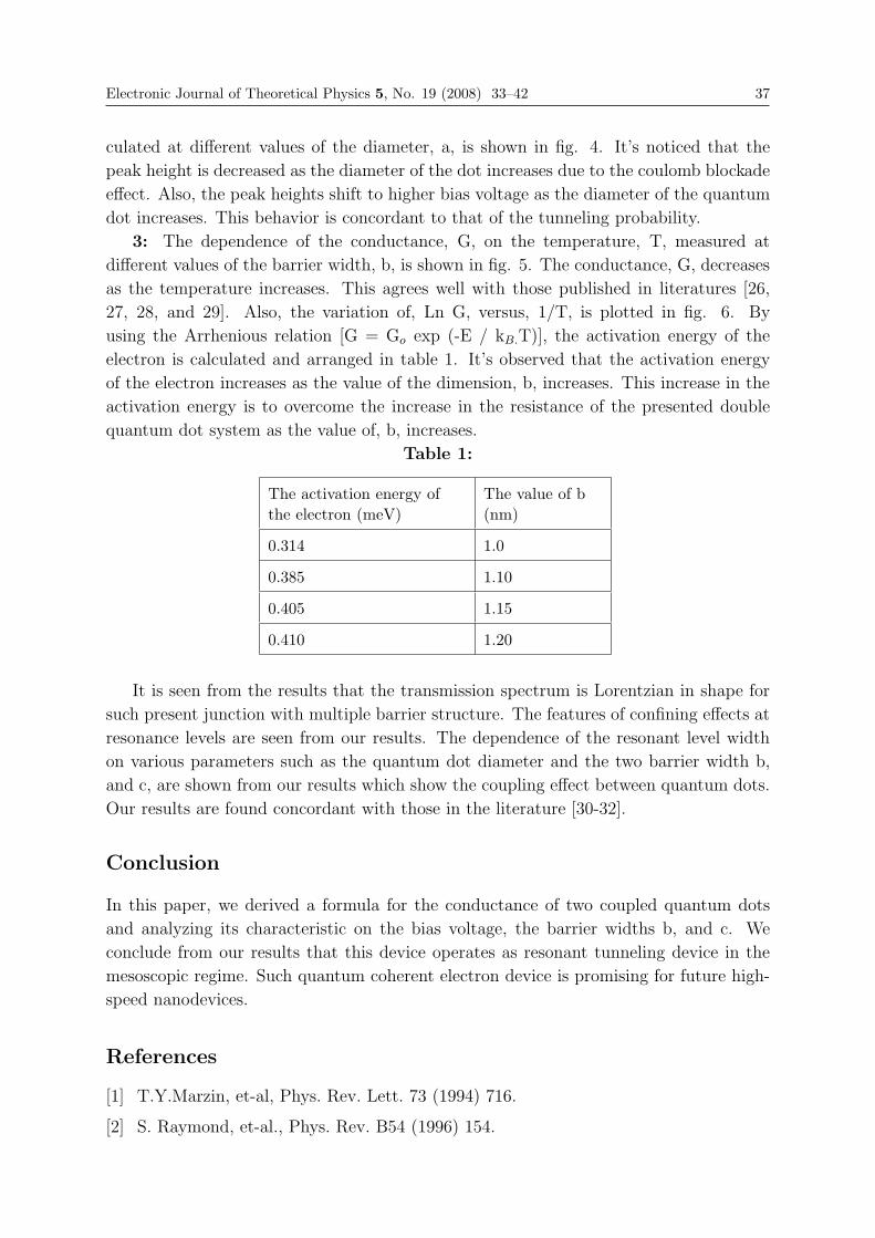
Electronic Journal of Theoretical Physics 5, No. 19 (2008) 33–42 37
culated at different values of the diameter, a, is shown in fig. 4. It’s noticed that the
peak height is decreased as the diameter of the dot increases due to the coulomb blockade
effect. Also, the peak heights shift to higher bias voltage as the diameter of the quantum
dot increases. This behavior is concordant to that of the tunneling probability.
3: The dependence of the conductance, G, on the temperature, T, measured at
different values of the barrier width, b, is shown in fig. 5. The conductance, G, decreases
as the temperature increases. This agrees well with those published in literatures [26,
27, 28, and 29]. Also, the variation of, Ln G, versus, 1/T, is plotted in fig. 6. By
using the Arrhenious relation [G = Go exp (-E / kB.T)], the activation energy of the
electron is calculated and arranged in table 1. It’s observed that the activation energy
of the electron increases as the value of the dimension, b, increases. This increase in the
activation energy is to overcome the increase in the resistance of the presented double
quantum dot system as the value of, b, increases.
Table 1:
The activation energy ofthe electron (meV)
The value of b(nm)
0.314 1.0
0.385 1.10
0.405 1.15
0.410 1.20
It is seen from the results that the transmission spectrum is Lorentzian in shape for
such present junction with multiple barrier structure. The features of confining effects at
resonance levels are seen from our results. The dependence of the resonant level width
on various parameters such as the quantum dot diameter and the two barrier width b,
and c, are shown from our results which show the coupling effect between quantum dots.
Our results are found concordant with those in the literature [30-32].
Conclusion
In this paper, we derived a formula for the conductance of two coupled quantum dots
and analyzing its characteristic on the bias voltage, the barrier widths b, and c. We
conclude from our results that this device operates as resonant tunneling device in the
mesoscopic regime. Such quantum coherent electron device is promising for future high-
speed nanodevices.
References
[1] T.Y.Marzin, et-al, Phys. Rev. Lett. 73 (1994) 716.
[2] S. Raymond, et-al., Phys. Rev. B54 (1996) 154.

38 Electronic Journal of Theoretical Physics 5, No. 19 (2008) 33–42
[3] M. Grundmann, et-al., Appl.Phys. Lett. 68 (1996) 979.
[4] H. Jiang et-al., Phys. Rev.B56 (1997) 4696.
[5] M. Rontani, et-al. Appl. Phys. Lett. 72 (1998) 957.
[6] M. A. Kastner, Rev. Mod. Phys. 64 (1992) 849.
[7] K. Nakazato, et-al., Electron. Lett. 29 (1992) 384.
[8] S. Tiwari, et-al., Appl. Phys. Lett., 69 (1996) 1232.
[9] P. Mazumder, et-al, Proc. IEEE 86 (1998) 664.
[10] Gergley Zarond at al., arxiv: cond-mat / 0607255V2 (18 Oct2006).
[11] Xiufeng Cao and Hang Zheng, arxiv: cond-mat / 0701581V1 (24 Jan2007).
[12] J. Gorman et al., Phys. Rev. Lett., 95 (2005) 090502.
[13] S. Sasaki et al., Phys. Rev. Lett., 93, 017205 (2004).
[14] P. Jarillo-Herreror et al., Nature 434, 484 (2005).
[15] A. Kogan et al., Phys. Rev. B, 67 (2003) 113309.
[16] L. Yang, et-al., J. Appl. Phys. 68 (1990) 2997.
[17] J. Sune, et-al. Microelectron. Eng. 36 (1997) 125.
[18] A. A. Awadalla, A.M.Hegazy, Adel H. Philips and R. Kamel, Egypt. J. Phys. 31(2000) 289.
[19] J. S. Sun, et-al., Proc. IEEE 86(1998)641.
[20] U. Meirav, et-al., Phys. Rev. Lett. 65 (1990)771.
[21] Y. Imry, Introduction to mesoscopic physics (Oxford University, New York, 1997).
[22] H. Kroemer, Quantum Mechanics, (Prentice Hall, Englewood Cliffs, New Jersey,07632 (1994)).
[23] C.W.J. Beenakker, in : Mesoscopic physics, eds. E. Ackermann’s, G. Montambaisand J. L. Pickard (North-Holland, Amsterdam, 1994).
[24] R. Ugajin, Appl. Phys. Lett. 68 (1996) 2657.
[25] D. K. Ferry and S. M. Goodnick in ”Transport in Nanostructures” CambridgeUniversity first edition 1997.
[26] Arafa H. Aly, Adel H. Phillips and R. Kamel, Egypt J. Physics, 30 (1999) 32.
[27] W.M. Van Hufflen, T. M.Klapwijk, D.R.Heslinga, Phys.Rev. B, 47 (1993) 5170.
[28] Aziz N. Mina, Adel H. Phillips, F. Shahin and N.S. Adel-Gwad, Physica C 341-348(2000).
[29] J. M. Kinaret, Physica B, 189 (1993) 142.
[30] H. Yamamoto, et-al, Appl. Phys. A50 (1990) 577.
[31] H.Yamamoto, et-al, Jpn. J. Appl. Phys. 34 (1995) 4529.
[32] Y. C. Kang, et-al. Jpn. J. Appl. Phys. 34(1995)4417.
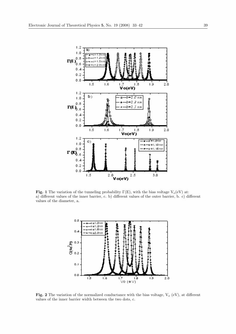
Electronic Journal of Theoretical Physics 5, No. 19 (2008) 33–42 39
Fig. 1 The variation of the tunneling probability Γ(E), with the bias voltage Vo(eV) at:a) different values of the inner barrier, c. b) different values of the outer barrier, b. c) differentvalues of the diameter, a.
Fig. 2 The variation of the normalized conductance with the bias voltage, Vo (eV), at differentvalues of the inner barrier width between the two dots, c.
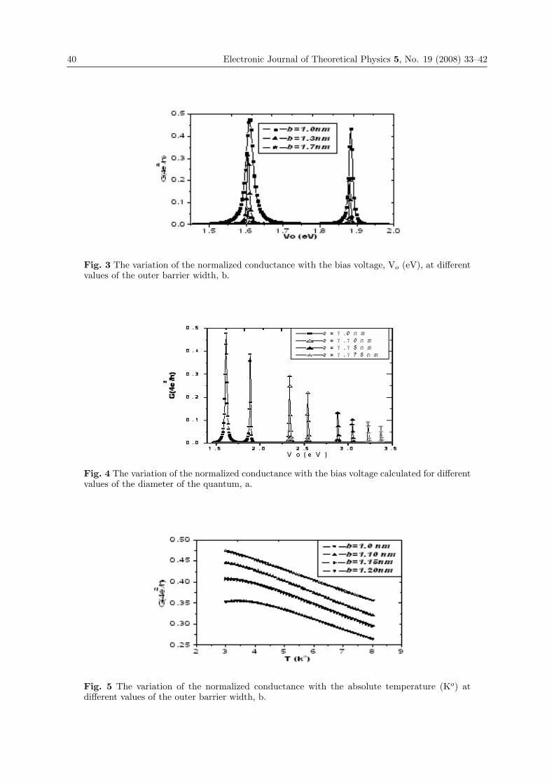
40 Electronic Journal of Theoretical Physics 5, No. 19 (2008) 33–42
Fig. 3 The variation of the normalized conductance with the bias voltage, Vo (eV), at differentvalues of the outer barrier width, b.
Fig. 4 The variation of the normalized conductance with the bias voltage calculated for differentvalues of the diameter of the quantum, a.
Fig. 5 The variation of the normalized conductance with the absolute temperature (Ko) atdifferent values of the outer barrier width, b.

Electronic Journal of Theoretical Physics 5, No. 19 (2008) 33–42 41
Fig. 6 The variation of the logarithm of the normalized conductance, Ln G, with the reciprocalof the absolute temperature, 1/T, at different values of the outer barrier width, b.

EJTP 5, No. 19 (2008) 43–46 Electronic Journal of Theoretical Physics
Quantum Destructive Interference
A.Y. Shiekh∗
Dine College, Tsaile, Arizona, U.S.A.
Received 8 August 2008, Accepted 16 September 2008, Published 10 October 2008
Abstract: An apparent paradox for unitarity non-conservation is investigated for the case ofdestructive quantum interference.c© Electronic Journal of Theoretical Physics. All rights reserved.
Keywords: Quantum Mechanics; Quantum Interference; Wave-functionPACS (2008): 03.65.-w; 03.67.-a; 03.67.Hk; 42.25.Hz
1. Introduction
Destructive quantum interference might at first seem to potentially threaten unitarity
since it seems to imply a reduction of the wave-function. Since this mechanism has been
exploited for a variety of applications [1, 2, 3], this motivates a deeper investigation into
the seeming paradox of unitary conservation.
2. Quantum Interference
An extreme example of destructive quantum interference is where two arms are brought
into overlap, having first arranged for them to be in anti-phase
Destructive Interference
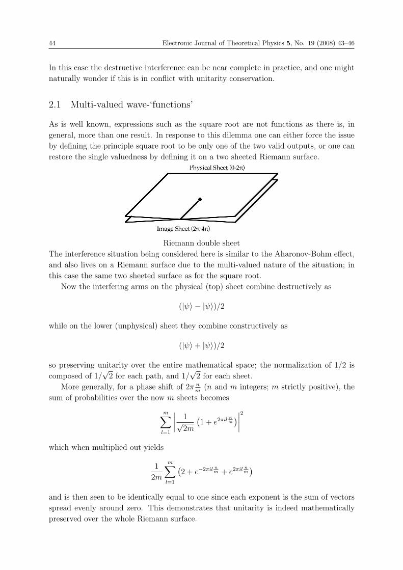
44 Electronic Journal of Theoretical Physics 5, No. 19 (2008) 43–46
In this case the destructive interference can be near complete in practice, and one might
naturally wonder if this is in conflict with unitarity conservation.
2.1 Multi-valued wave-‘functions’
As is well known, expressions such as the square root are not functions as there is, in
general, more than one result. In response to this dilemma one can either force the issue
by defining the principle square root to be only one of the two valid outputs, or one can
restore the single valuedness by defining it on a two sheeted Riemann surface.
Riemann double sheet
The interference situation being considered here is similar to the Aharonov-Bohm effect,
and also lives on a Riemann surface due to the multi-valued nature of the situation; in
this case the same two sheeted surface as for the square root.
Now the interfering arms on the physical (top) sheet combine destructively as
(|ψ〉 − |ψ〉)/2
while on the lower (unphysical) sheet they combine constructively as
(|ψ〉 + |ψ〉)/2
so preserving unitarity over the entire mathematical space; the normalization of 1/2 is
composed of 1/√
2 for each path, and 1/√
2 for each sheet.
More generally, for a phase shift of 2π nm
(n and m integers; m strictly positive), the
sum of probabilities over the now m sheets becomes
m∑l=1
∣∣∣∣ 1√2m
(1 + e2πil n
m
)∣∣∣∣2which when multiplied out yields
1
2m
m∑l=1
(2 + e−2πil n
m + e2πil nm
)and is then seen to be identically equal to one since each exponent is the sum of vectors
spread evenly around zero. This demonstrates that unitarity is indeed mathematically
preserved over the whole Riemann surface.

Electronic Journal of Theoretical Physics 5, No. 19 (2008) 43–46 45
Conclusion
The seeming paradox of lost unitarity is resolved by the realization that mathemati-
cally, over the whole Riemann surface, unitarity is actually preserved; while destructive
interference can take place on the single physical sheet.
However, since the particle cannot actually be lost, the wave-function needs to be
renormalized on the physical sheet, and this constitutes the mechanism that is being
exploited for quantum computation and communication [1, 2, 3].
The use of Riemann surfaces to carry physical problems can be of great utility [4].
References
[1] A. Y. Shiekh, The role of Quantum Interference in Quantum Computing, Int. Jour.Theo. Phys., 45, 1653, 2006 [arXiv:cs.CC/0507003]
[2] A. Y. Shiekh, The Quantum Interference Computer: Error Correction and anExperimental Proposal, Int. Jour. Theo. Phys., 47, 2176, 2008 [arXiv:quant-ph/0611052], [arXiv:0704.2033]
[3] A. Y. Shiekh, Faster than light quantum communication, Electr. Jour. of Theor.Phys., 18, 105, 2008 [arXiv:0710.1367]
[4] A. Y. Shiekh, (with C. DeWitt-Morette, S. G. Low, and L. S. Schulman) Wedges I,Found. Phys., 16, 311, 1986, a festschrift for J. Wheeler.

EJTP 5, No. 19 (2008) 47–56 Electronic Journal of Theoretical Physics
Quantized Fields Around Field Defects
Bakonyi G.∗
H-1039 Budapest III. Czetz J. u. 13, Hungary
Received 3 March 2008, Accepted 20 August 2008, Published 10 October 2008
Abstract: A heuristic exercise exploring analogies between different field theories. Similaritiesbetween the crystal defects and other various fields help to create a model to quantize thesefields. The charge of the electromagnetic field, and the electromagnetic waves are used asexamples.c© Electronic Journal of Theoretical Physics. All rights reserved.
Keywords: Quantum Field Theory; Electrodynamics; Magnetic MonopolesPACS (2008): 03.70.+k, 11.10.-z, 03.50.De, 14.80.Hv
1. Introduction
1.1 Physical Introduction
We can observe similarities between the phenomena appearing in solid states and in
electrodynamics or particle physics. In the crystal lattice of the solid states various kinds
of crystal defects can exist, for instance the line-defects such as the edge dislocations and
the screw dislocations. [1][2] Around the crystal defects, the bulk material is intact all
over, and inside these materials we can use such simple formulas which become unusable
and invalid at the place of the figurable lattice defects. Drawing a parallel between these,
we will consider a field in which in the ”solid” domain we can use some rule, except
of some ”figurable” field defects. The ”solid” domain works in a way, that the initial
conditions and the boundary conditions determines the inside of the domain. On the
other hand, the ”figurable” domain can easily fit every kind of initial and boundary
conditions, and the continuation in time and space is hardly predictable. Of course there
are some rules existing in this domain too, but applying these rules, we get near chaos
results. If the boundary of this kind of ”solid” field is over determined, then it will
inevitably contain ”figurable” field defects. Since the ”figurable” field defects have very
48 Electronic Journal of Theoretical Physics 5, No. 19 (2008) 47–56
unpredictable behavior, we will try to characterize them using the ”solid” field encircling
them.
1.2 Mathematical introduction
1.2.1 Quantized integrals
Let there be a field described by two physical properties: C, S. and let there be a soft
constraint condition between them:
C2 + S2 = 1 (1)
(I use the expression: ”soft constraint”, if the constraint criterion is not too stiff, and valid
only mostly and approximately.) C2 + S2 is mainly equal to 1 but not allways. In some
regions, the equation is not valid. We can close out the most invalid points of our region,
so we will use multiply-connected regions, where the constraint-criterion is approximately
valid. The C and S properties depends on each others. In a simply-connected region,
we can describe our field with a phase of a vawe. Lets be C = cos(φ) and S = sin(φ).
We know the two originally used properties, and we want to calculate the phase. We will
create a vector from the following determinants :
vi = Det
⎡⎢⎣C; ∂iC
S; ∂iS
⎤⎥⎦ (2)
The determinants are created from the properties of the field and its partial derivatives
with respect to space variables.
vi = Det
⎡⎢⎣cos(φ); −sin(φ)∂iφ
sin(φ); cos(φ)∂iφ
⎤⎥⎦ = (cos2(φ) + sin2(φ))∂iφ = ∂iφ (3)
We can calculate the phase difference between two points:
Δφ =
∫vidxi =
∫∂iφdxi (4)
In a simply-connected region, if we calculate the integral on a closed curve, we will get
zero, but in the case of multiply-connected regions we will get quantized results. The
result can be 2π ∗ n, where n is a positive or negative or zero whole number.
1.2.2 Additions of fields with defects
We have defects, and we would like to have the field of the sum of the defects. If we are
in the case of line surrounded defects, and our trajectory in the mapped field consists of

Electronic Journal of Theoretical Physics 5, No. 19 (2008) 47–56 49
only a single loop, let’s create two times two rotational operators for the mapped space.
These operators are constitute closed group [3].
U =
⎡⎢⎣C; −S
S; C
⎤⎥⎦ (5)
The field with two defects can be generated from the single fields multiplying by the
operators which represent the single fields. The result represents a field with multiple
defects. We can repeat this procedure several times, so we can create fields with multiple
defects. Of course we can multiply the result with the operators of the defectless field. In
this two dimensional case the operators are commutative. In general: If we can project the
subspace of the soft constraint condition to a grid, where the cell of the grid corresponds
to the single encircling, then we can use vectors in the space of the grid. The defects are
similar to the well known up and down counting operators [4].
2.
2.1 Line surrounded defects.
If we are on a surface, we can walk around a point-defect always staying inside the ”solid”
field. If we are in a three-dimensional space, we can walk around a line-defect on a curved
line, while if we are in a time and space, we can walk around a surface or a moving curve.
We will try to create properties similar to the Burgers-vectors [5] in this field. We would
like any optional closed curve integrals which walk around inside the ”solid” field to be
quantized, and in a defectless case the result must be zero. Let there be a field described
by a vector composed of two physical properties. It creates a two dimensional mapped
space.
Ψ = (A,B) (6)
and let there be a soft constraint condition between them:
C(Ψ) = 0 (7)
vi = Det
⎡⎢⎣FA(A,B); ∂iA
FB(A,B); ∂iB
⎤⎥⎦ (8)
Where FA(A,B) and FB(A, B) are functions. The determinants are created from the
properties of the field and its partial derivatives with respect to space variables. The curl

50 Electronic Journal of Theoretical Physics 5, No. 19 (2008) 47–56
[6][7] of this vector is the following:
curlv = ∇ × v
= (gn × gm)Det
⎡⎢⎣∂nFA(A,B); ∂mA
∂nFB(A,B); ∂mB
⎤⎥⎦= δnm
pq (gp ⊗ gq)Det
⎡⎢⎣∂nFA(A,B); ∂mA
∂nFB(A,B); ∂mB
⎤⎥⎦(9)
Where the gi is a contravariant base-vector, and δ is the Kronecker’s symbol. We will
see, that the result of a curve line integral around a defect is quantized:
∮vidxi =
∮Det
⎡⎢⎣FA(A,B); ∂iA
FB(A,B); ∂iB
⎤⎥⎦ dxi
=
∮Det
⎡⎢⎣FA(A, B); ∂iAdxi
FB(A,B); ∂iBdxi
⎤⎥⎦ =
∮Det
⎡⎢⎣FA(A,B); dA
FB(A,B); dB
⎤⎥⎦(10)
Every point of our space is connected to a point of the mapped space, so while we walk
around on a curve in our real space, it is a closed curve line at the same time in the
mapped space too, which can walk around multiple times. The result of the closed line
integral is equal with the integral made in the mapped space. For example the curve
determined by the soft constraint condition in the mapped space can contain a loop.
If it is without a loop, our integral has to be zero, but otherwise, it can be quantized.
The size of the quantum step or steps depend on the loop curve determined by the soft
constraint condition in the mapped space. The closed curve integral is the multiple of
the single loop integral of the projected mapped space, in consequence of the fact, that
the projected closed curve can be not only a single times encircled line, but a multiplied
times encircled closed curve, so the result of the integral can be the result of the single
times encirled case multiplied by a positive or negative or zero whole number.
2.2 Defect surrounded by surfaces.
2.2.1 Example: The Electric displacement field
In a three dimensional space a closed surface can encircle a point defect, or in a four di-
mensional spacetime it can encircle a trajectory. We will try to create quantized integrals.
Let there be
β = (β1, β2, β3) (11)
a three dimensional property mapped field. Let there be a soft constraint condition again:
C(β) = 0 (12)

Electronic Journal of Theoretical Physics 5, No. 19 (2008) 47–56 51
Let’s create the following electric displacement vectors in the spacetime:
D = δjknm
1
2(gn ⊗ gm)Det
⎡⎢⎢⎢⎢⎣F1(β); ∂jβ1; ∂kβ1
F2(β); ∂jβ2; ∂kβ2
F3(β); ∂jβ3; ∂kβ3
⎤⎥⎥⎥⎥⎦ (13)
Where F1(β), F2(β) and F3(β) are functions.
Dij = Det(F (β), ∂iβ, ∂jβ) (14)
In our model the electric and magnetic field transforms according to the general relaitvity.
A relativistic four-tensor describes the electromagnetic field.
D =
⎡⎢⎢⎢⎢⎢⎢⎢⎣
0; Hx; Hy; Hz
−Hx; 0; Dz; −Dy
−Hy; −Dz; 0; Dx
−Hz; Dy; −Dx; 0
⎤⎥⎥⎥⎥⎥⎥⎥⎦(15)
So the closed surface integral:
∮Dnmdanm =
∮Det
⎡⎢⎢⎢⎢⎣F1(β); ∂jβ1; ∂kβ1
F2(β); ∂jβ2; ∂kβ2
F3(β); ∂jβ3; ∂kβ3
⎤⎥⎥⎥⎥⎦ dajk (16)
in this model is quantized. Every point of our real space is connected to a point of the
mapped space, so while we integral around on a closed surface in our real space, it is a
closed surface integral in the mapped space too. The result of the closed surface integral
is equal with the integral made in the mapped space. If the surface of the mapped space
is closed, the integral can differ from zero. In the case of certain kind of surface, it is
possible to wrap around the defect in the mapped space multiple too. The size of the
quantum step depends on the surface of property space determined by the soft constraint
condition. In this case in a similar way as in the two dimensional case:
J = ∇ × D = δijkpnm
1
2(gp ⊗ gn ⊗ gm)Det
⎡⎢⎢⎢⎢⎣∂iF1(β); ∂jβ1; ∂kβ1
∂iF2(β); ∂jβ2; ∂kβ2
∂iF3(β); ∂jβ3; ∂kβ3
⎤⎥⎥⎥⎥⎦ (17)
We can create a pseudo-vector for the four-vector electric current density, which is the
following:
Js =1
6
1√
gεsijkJijk =
1
2
1√
gεsijk∇iDjk (18)

52 Electronic Journal of Theoretical Physics 5, No. 19 (2008) 47–56
Where ∇j represents the covariant differential, and g is the determinant of the metric-
tensor divided by −c2.
In details:
J = (ρ; Jx; Jy; Jz) (19)
Of course this satisfies the electric charge continuity [8], a trivial way, as we can see it
using the equation (17):
∇ J = ∇sJs = ∂sJ
s + JsΓnns = 0 (20)
2.3 Defect encircled by volume
2.3.1 The pure theory
In a four dimensional spacetime one closed volume can encircle one event defect. We will
try to make quantized the event defect. Let there be
γ = Det(γ1, γ2, γ3, γ4) (21)
a four-vector in the mapped space, where we project our field. Let there be a soft
constraint condition again, which decreases the four dimensinal freedom in the mapped
space to three: C(γ) = 0 Now, we create the following three-indexed tensor in the real
spacetime:
v = δijknml(g
n ⊗ gm ⊗ gl)Det
⎡⎢⎢⎢⎢⎢⎢⎢⎣
F0; ∂jγ0; ∂kγ0; ∂lγ0
F1; ∂jγ1; ∂kγ1; ∂lγ1
F2; ∂jγ2; ∂kγ2; ∂lγ2
F3; ∂jγ3; ∂kγ3; ∂lγ3
⎤⎥⎥⎥⎥⎥⎥⎥⎦(22)
The quantized event count can be calculated based on the volume-boundary integral
encircling the event The event count will be the particle count difference:
ΔN =
∮vijkdV ijk (23)
2.3.2 The Magnetic induction field
Till now, in our model of the electromagnetic field, it was not possible to create a vec-
torpotential. We will create the electric intensity vector E and the magnetic induction
vector B from the following vectorpotential and scalarpotential.
A =1
2giDet(G(α); ∂iα) (24)
Where G(α) is function of α. The vectorpotencial in four-vector form is [9]:
A = (Φ, Ax, Ay, Az) (25)
Electronic Journal of Theoretical Physics 5, No. 19 (2008) 47–56 53
In the usual way, if let there be: The magnetic induction field as a tensor derived from
the vectorpotential:
B = ∇ × A (26)
Bmn =1
2Det(∂mG(α); ∂nα) − 1
2Det(∂nG(α); ∂mα) (27)
(There is a soft constraint condition too: E = D and B = H.)
B =
⎡⎢⎢⎢⎢⎢⎢⎢⎣
0; −Ex; −Ey; −Ez
Ex; 0; Bz; −By
Ey; −Bz; 0; Bx
Ez; By; −Bx; 0
⎤⎥⎥⎥⎥⎥⎥⎥⎦(28)
In this case, as a trivial result, the magnetic induction field is charge free.
∇ × B = 0 (29)
The magnetic flux:
Φ =
∫Bij daij =
∮Ai dsi (30)
In parallel with the method used at the electric field due to the switched on soft constraint
condition, we can move only on a loop in the mapped space, and if we suppose, that the
magnetic field likes the magnetic induction vector and the electric intensity vector to be
zero, then the magnetic flux is quantized. Then it is the same case as studied before,
at the chapter ”Line surrounded defects.” We know, that the magnetic flux can really
be quantized, for example in supraconductors, where neither electric intensity vector nor
magnetic induction vector is present. It is the Josephson-effect [10]. The flux quantum
seems to be independent of the type of the material.
2.3.3 Boundary integral of the Event-current-density
To have quantized integrals, our boundary circle integrals of the real spacetime are needed
to be boundary circle integrals in the mapped space too. For example the following
expression complies this requirement.
L = ED − BH + JA − Φρ = div(H × A − DΦ) − ∂t(DA) (31)
(This is a soft constraint condition.) In this case:∫(∂nLn)dx4 =
∮LndVn (32)
L ∝ εnijk∂nDet
∣∣∣∣∣∣∣F (β); 0; ∂iβ; ∂jβ; ∂kβ
0; G(α); ∂iα; ∂jα; ∂kα
∣∣∣∣∣∣∣ (33)
54 Electronic Journal of Theoretical Physics 5, No. 19 (2008) 47–56
This integral may be quantized.
ΔN =
∮LndVn (34)
The event-current-density pseudo-vector:
Ls = −1
2
1√
gεsijkAiDjk (35)
2.3.4 The Energy-impulse tensor
If we use (18) and (35) then the supposed Energy-Impulse tensor can be written in the
following indexed form:
T pq = ∇qL
p − JpAq + δpq (J
sAs −∇sLs) (36)
where the upper index is pseudo. The energy-impulse tensor needn’t to be symmetrical,
because it is only a subsystem, and shouldn’t be symmetrical, due to the photon count
change. The force density of the electromagnetic field can be derived from the Energy-
Impulse tensor:
fi = ∇jTji = BisJ
s + As∇iJs (37)
The expression of the change of the impulse:
ΔPk =
∮T j
kdVj (38)
So the impulse is on an infinite volume:
Pk =
∫T j
kdVj =
∫∇kL
s − JsAk + δsk(J
jAj −∇jLj)dVs (39)
Without the members which are proportional to the currents or the events, we will get
the photon impulse:
P[photon]k =
∫∇kL
sdVs (40)
2.3.5 The moment of momentum
The torque causes the change of the moment of momentum. The torque density derived
from (37) with an additional torque density is:
M = x × f + A × J = gj∂j(·gpT p
i (x × gi)) + T ji (gi × g
j) + A × J
= gj∂j(·gpT p
i (x × gi)) + (∇ × L)(41)
The first member is the change of the orbital moment of momentum. The second member
is the change of the spin of the photon.
A corresponding operator was found for the spin. It was derived from a quantized property
with the help of a rotational operator.
As we can see, in our model both the Energy-impulse and the Spin of the photon, can
be derived from the quantized integral of the Event-current-density.
Electronic Journal of Theoretical Physics 5, No. 19 (2008) 47–56 55
3. Conclusion
The soft constraint criterions in the mapped space can cause quantized integrals, where
the quantum step depends on the subspaces which depend on the soft constraint criteri-
ons. The members of the Energy-Impulse tensors derived from the event-current-density
are similar to the Bosons contrasted with the members derived from the current-densities.
It was possible to use the method in the simple example of the electromagnetic field. As
a result of our model, the electric charge, magnetic flux and the photon-properties are
quantized, and magnetic monopoles are not exists.
References
[1] C. Kittel: Introduction to Solid State Physics,- Hungarian translation - Bevezetes aszilardtest fizikaba. (Muszaki Konyvkiado, Budapest 1966. ) p. 632.
[2] C. Kittel: Introduction to Solid State Physics,- Hungarian translation - Bevezetes aszilardtest fizikaba. (Muszaki Konyvkiado, Budapest 1981. ) p. 620.
[3] G.G. Hall: Applied Group Theory - Hungarian translation - AlkalmazottCsoportelmelet ( Muszaki Konyvkiado, Budapest 1975) p. 137.
[4] Modern Fizikai Kisenciklopedia, I. Fenyes ( Gondolat Konyvkiado, Budapest 1971)p. 212.
[5] C. Kittel: Introduction to Solid State Physics,- Hungarian translation - Bevezetes aszilardtest fizikaba. (Muszaki Konyvkiado, Budapest 1966. ) p. 635.
[6] L., Janossy - P. Tasnadi: Vektorszamıtas II. ( Tankonyvkiado, Budapest, 1982) p.90.
[7] J. G. Simmonds: A Brief of Tensor Analysis - Hungarian translation - TenzoranalızisDiohejban (Muszaki Konyvkiado, Budapest, 1985) p.101.
[8] K., Nagy: Elektrodinamika (Budapest 1968) p. 42.
[9] J. D. Jackson: Classical Electrodynamics - Hungarian translation Klasszikuselektrodinamika (TypoTEX Budapest 2004) p. 280.
[10] Modern Fizikai Kisenciklopedia, I. Fenyes ( Gondolat Konyvkiado, Budapest 1971)p. 641.

EJTP 5, No. 19 (2008) 57–64 Electronic Journal of Theoretical Physics
Path Integral Quantization of Brink-SchwarzSuperparticle
N. I. Farahat∗, and H. A. Elegla†
Physics Department, Islamic University of Gaza, P.O. Box 108 Gaza, Palestine
Received 31 March 2008, Accepted 16 August 2008, Published 10 September 2008
Abstract: The quantization of the Brink-Schwarz superparticle is performed by canonicalphase-space path integral.The supersymmetric particle is treated as a constrained system usingthe Hamilton-Jacobi approach. Since the equations of motion are obtained as total differentialequations in many variables, we obtained the canonical phase space coordinates and the phasespace Hamiltonian with out introducing Lagrange multipliers and with out any additional gaugefixing condition.c© Electronic Journal of Theoretical Physics. All rights reserved.
Keywords: Field Theory; Path Integral, Constrained Systems, Hamilton-Jacobi Formalism,Supersymmetric, SuperparticlePACS (2008): 11.10.-z; 11.10.Ef; 31.15.xk; 03.70.+k
1. Introduction
Systems described by singular Lagrangians are called singular systems and this kind of
systems contain inherent constraints [1, 2]. In a lot of physical domains, there extensively
exist different singular systems, such as gauge field theories, gravitational field theory,
supersymmetric theory, supergravity, superstring theory. A standard consistent way of
dealing with singular systems was first formulated by Dirac [3]. In Dirac’s method, when
a singular Lagrangian in configuration space is transformed into a singular Lagrangian
in phase space, the set of constraints would be generated, which are called primary con-
straints [4, 5]. Through the consistency conditions, using these primary constraints may
generate more new constraints, which are called secondary constraints. Following Dirac,
one classifies the constraints as being first or second class constraints. According to
Dirac’s conjecture each first class constraint generates a corresponding gauge symmetry,
58 Electronic Journal of Theoretical Physics 5, No. 19 (2008) 57–64
while second class constraints require for their implementation the replacement of Poisson
brackets by Dirac brackets [6, 7, 8]. The quantization scheme for constrained systems is
the path integral quantization. It is important because it serves as a basis to develop
perturbation theory and to find out the Feynman rules. The path integral quantization
of singular theories with first class constrains in canonical gauge was given by Faddeev
and Popov [9, 10]. The generalization of the method to theories with second class con-
straints is given by Senjanovic [11]. Moreover, Fradkin and Vilkovisky [12, 13] considered
quantization to bosonic theories with first class constraints and it is extension to include
fermions in the canonical gauge. When the constrained dynamical systems possesses
some second class constraints there exists another method given by Batalain and Frad-
kin [14]: the BFV- BRST operator quantization method. Which implies to extend the
initial phase space by auxiliary variables to convert the original second class constraints
into effective first class ones in the extended manifold. Recently, a new scheme of path
integral quantization [19]-[22], depend on the Hamilton-Jacobi treatment of constrained
systems [17]-[24]. According to Hamilton-Jacobi formalism the equations of motion are
obtained as total differential equations in many variables which require to investigate the
integrability conditions. The canonical path integral quantization is obtained directly
as an integration over the canonical phase-space coordinates without any need to en-
large the initial phase-space by introducing extra-unphysical variables. The advantage
of the Hamilton-Jacobi formalism is that we have no difference between first and second
class constraints and we do not need gauge-fixing term to reduce or enlarge the physical
phase-space. The better understanding of this features aries by applying the Hamilton-
Jacobi formalism for supersymmetric constraint systems[25], which are subject to mixed
fermionic first and second class constraints in an arbitrary space-time dimension. The
main aim of this paper is to apply the Hamilton-Jacobi technique to discuss the classical
dynamics of the Brink-Schwarz superparticle, then we try to quantize it by using the
canonical path integral method.
The material presented in this paper is divided as follows: In the next section the
Hamilton-Jacobi formulation is presented. Section 3, is devoted to analyze the mas-
sive Brink-Schwarz superparticle model [26] by using Hamilton-Jacobi formalism. The
conclusion is given in section 4.
2. Hamilton-Jacobi Formalism Of Constrained Systems
The system that is described by singular Lagrangian L(qi, qi, t) with i = 1, ..., N , has a
rank of Hess matrix
Aij =∂2L
∂qi∂qj
, i, j = 1, . . . , N, (1)
equal to (N − p) , p < N . In this case we have p momenta which are dependent on each
other. The generalized momenta Pi corresponding to the generalized coordinates qi are

Electronic Journal of Theoretical Physics 5, No. 19 (2008) 57–64 59
defined as,
Pa =∂L
∂qa
, a = 1, . . . , N − p, (2)
Pμ =∂L
∂qμ
, μ = N − p + 1, . . . , N. (3)
Since, the rank of the Hess matrix is (N − p), one may solve (2) for qa as
qa = qa (qi, qμ, Pb) ≡ ωa. (4)
Substituting (4) into (3), we obtain relations in qi, Pa, qν and t in the form
Pμ =∂L
∂qμ
∣∣∣∣qa=ωa
≡ −Hμ(qi, qν , qa = ωa, Pa, t), ν = N − p + 1, . . . , N. (5)
By mean of (4) and (5) the canonical Hamiltonian H0 is defined as
H0 = −L(qi, qμ, qa = ωa, t
)+ Paωa + qμPμ
∣∣Pν=−Hν
. (6)
The set of Hamilton-Jacobi partial differential equations (HJPDE) is expressed as
H ′α
(qβ; qa; Pa =
∂S
∂qa
; Pμ =∂S
∂qμ
)= 0, α, β = 0, 1, . . . , p. (7)
where
H ′0 = P0 + H0; (8)
and
H ′μ = Pμ + Hμ. (9)
with q0 ≡ t and S being the action. The equations of motion are obtained as total
differential equations in many variables such as,
dqa =∂H ′
α
∂Pa
dtα, (10)
dPr = −(−1)nrnα∂H ′
α
∂qr
dtα, r = 0, 1, . . . , N, (11)
dZ =
(−Hα + Pa
∂H ′α
∂Pa
)dtα, (12)
where ni = 0 , 1, (i = r , α) define the Grassmann parity of the corresponding quantity,
and Z = S (tα, qa). These equations are integrable if and only if [27, 28]
dH ′0 = 0, (13)
and
dH ′μ = 0, μ = N − p + 1, . . . , N. (14)
If the conditions (13) and (14) are not satisfied identically, we consider them as new
constraints and we examine their variations. Thus repeating this procedure, one may
60 Electronic Journal of Theoretical Physics 5, No. 19 (2008) 57–64
obtain a set of constraints such that all the variations vanish, then we may solve the
equations of motion (10) and (11) to get the canonical phase-space coordinates as
qa ≡ qa(t, tμ), pa ≡ pa(t, tμ), μ = 1, . . . , p. (15)
In this case the path integral representation may be written as
〈Out | S | In〉 =
∫ n−r∏a=1
dqadpa exp
[i
∫ t′α
tα
(−Hα + pa
∂H ′α
∂pa
)dtα
], (16)
a = 1, . . . , n − p, α = 0, n − p + 1, . . . , n.
We should notice that the integral (16) is an integration over the canonical phase space
coordinates (qa, pa).
3. Hamilton-Jacobi Formulation of Brink-Schwarz Superparti-
cle
One may write an action for a particle moving in a superspace; which is an extension
of ordinary 4 D spacetime to include extra anticommuting coordinates in the form of N
two-components Weyl spinors θ, θ , where θ is the conjugate of θ. Such action, firstly is
written by Brink-Schwarz with simple supersymmetry N = 1 [26] by the Lagrangian
L =1
2[e−1(xμ − iθγμθ)2 + em2]. (17)
The singularity of the the Lagrangian follows from the fact that the rank of the Hessian
matrix Aij is one.
The canonical momenta defined in (2) and (3) read as
Pμ =∂L
∂xμ= e−1
(xμ − iθγμθ
), (18)
πθ =∂rL
∂θ= −iθPμγ
μ = −Hθ, (19)
πθ =∂rL
∂ ˙θ= 0 = −Hθ, (20)
Pe =∂L
∂e= 0 = −He. (21)
Since the rank of the Hessian matrix is one, we can solve (18) for xμ in terms of Pμ and
other coordinates, in the form
xμ = ePμ + iθγμθ. (22)
The canonical Hamiltonian H0 is
H0 =1
2e[P 2 − m2]. (23)
Electronic Journal of Theoretical Physics 5, No. 19 (2008) 57–64 61
The set of HJPDE’s are
H ′0 = P0 +
1
2e[P 2 − m2], (24)
H ′θ = Pθ + iθPμγ
μ, (25)
H ′θ = Pθ, (26)
H ′e = Pe. (27)
Therefore, the total differential equations for the characteristics read as
dxμ = ePμdτ + iθγμdθ, , (28)
dPμ = 0, (29)
dPθ = 0, (30)
dPθ = (−iPμγμ)dθ, (31)
dPe = −1
2[P 2 − m2]dt. (32)
To check whether the set of (28) to (32) are integrable or not, let us consider the total
variations of the set of (HJPDE)’s. The variation of
dH ′0 = 0, (33)
dH ′θ = 0, (34)
dH ′θ = 0, (35)
are identically zero, whereas
dH ′e = −(
1
2[P 2 − m2])dt = H ′′
e dt. (36)
where
H ′′e =
1
2[P 2 − m2] = 0. (37)
is a new constraint. We notice that the total differential of H ′′e vanish identically, i.e.
dH ′′e = 0. (38)
Thus the set of equations (28)-(32) with (41) are integrable.According to (12) the action
can be written as
dZ = −H0dτ − Hθdθ − Hθdθ − Hede + Pμdxμ
=
{−1
2e
(P 2 − m2
)+ Pμ
(x − iθγμθ
)}dτ,
(39)
and the canonical action integral becomes
S =
∫ {1
2e
(P 2 + m2
)}dτ. (40)
62 Electronic Journal of Theoretical Physics 5, No. 19 (2008) 57–64
By using (40) and (16) the canonical path integral quantization of Brink-Schwarz super-
particle is expressed as
⟨xμ, τ ; x′
μ, τ′⟩ =
∫dxμ dpμexp
[i
∫ {1
2e(P 2 + m2
)}dτ
](41)
This path integral representation as an integration over the canonical phase-space with
no need to introduce any gauge fixing to reduce or enlarge the phase-space as in covariant
quantization of Brink-Schwarz superparticle described in references [29, 30, 31].
Conclusion
In this work we presented Brink-Schwarz Superparticle as a singular system, and its
Hamiltonian treatment contains all kinds of constraints (primary and secondary, first
and second class ones). This model is very illustrative, since it allows a comparison
between all features of Diracs and Hamilton-Jacobi formalisms. In Dirac’s formalism,
we must reduce any constrained singular system to one with first-class constraints only,
we must call attention to the presence of arbitrary variables in some of the Hamiltonian
equations of motion due to the fact that we have gauge dependent variables and we have
made a gauge fixing. This does not occur in Hamilton-Jacobi formalism since it provides a
gauge-independent description of the systems evolution due to the fact that the Hamilton-
Jacobi function S contains all the solutions that are related by gauge transformations.
The canonical path integral quantization of Brink-Schwarz Superparticle is done, since
the system is integrable, and the integration is taken over the canonical phase space.
References
[1] Henneaux M., Teitelboim C. , Quantization of Gauge Systems, Princeton UniversityPress, New Jersey, 1992.
[2] Li Z.P. , Jiang J.H. , Symmetries in Constrained Canonical Systems, Science Press,New York, 2002.
[3] Dirac P.A.M., Lectures on Quantum Mechanics, Yeshiva University Press, New York,1964.
[4] Anderson J.L., Bergmann P.G., Phys. Rev. 83 (1951) 1018.
[5] Bergmann P.G. , Goldberg J. , Phys. Rev. 98 (1955) 531.
[6] Sundermeyer K., Lecture notes in physics, Spring-Verlag, Berlin, (1982).
[7] Jan Govaerts, Hamiltonian Quantisation and Constrsined Dynamics, Volume 4,Leuven University Press, (1991).
[8] Gitman D. M. and Tyutin I. V., Quantization of Fields with Constraints (Spring-Verlag, Berlin, Heidelbag) (1990).
[9] Faddeev L. D., Theor. Math. Phys., 1 (1970)1.
[10] Faddeev L. D. and Popov V. M., Phys. Lett. B, 24 (1967)29.

Electronic Journal of Theoretical Physics 5, No. 19 (2008) 57–64 63
[11] Senjanovic P., Ann. Phys. N. Y., 100 (1976) 227.
[12] Fradkin E. S. and Vilkovisky G. A., Phys. Rev. D, 8 (1973) 4241.
[13] Fradkin E. S. and Vilkovisky G. A., Phys. Lett. B, 55 (1975) 241.
[14] Batalin I. A. and Fradkin E. S., Nucl. Phys. B, 270 (1968) 514.
[15] Muslih S. I., Nuovo Cimento B, 115 (2000)1.
[16] Muslih S. I., Nuovo Cimento B, 115 (2000)7.
[17] Farahat N. I. and Guler Y., Nuovo Cimento B111, (1996) 513.
[18] Rabei E.M., and Tawfiq S., Hadronic J, 20, (1997) 2399.
[19] Muslih S. I., General Relativity and Gravitation, 34, (2002) 1059.
[20] Farahat N. I. and Nassar Z., Islamic University Journal, 13, (2005) 239.
[21] Farahat N. I. and Nassar Z., Hadronic Journal 25, (2002) 239.
[22] Muslih S. I. and Guler Y., Nuovo Cimento B113, (1998) 277.
[23] Muslih S. I. and Guler Y., Nuovo Cimento B112,(1997) 97.
[24] Muslih S. I., Nuovo Cimento B117, (2002)4.
[25] Farahat N. I. and Elegla H. A., Turkish Journal of Physics ,30, (2006) 473.
[26] Brink L. and Schwarz J. H. , Phys. Lett. 100B, (1981) 310.
[27] Muslih S. I., Nuovo Cimento B118 (2003) 505.
[28] Muslih S. I., S. I. Muslih, Modern Physics Letter A, 19, (2004) 863.
[29] Deriglazov A.A. ,Galajinsky A.V., Lyakhovich S.L., Nuclear Physics B 473 (1996)245.
[30] Grassi P.A. , Policastro G., van Nieuwenhuizen P. ,Physics Letters B 553 (2003) 96.
[31] Jarvis P.D.; van Holten J.W., Kowalski-Glikman J., Physics Letters B (427),(1998),47.


EJTP 5, No. 19 (2008) 65–78 Electronic Journal of Theoretical Physics
Noncommutative Geometry and Modified Gravity
N. Mebarki and F. Khelili ∗
Laboratoire de Physique Mathematique etSubatomique, Mentouri University, Constantine, Algeria
Received 17 April 2008, Accepted 16 August 2008, Published 6 October 2008
Abstract: Using noncommutative deformed canonical commutation relations, a model ofgravity is constructed and a schwarchild like static solutions are obtained. As a consequence, theNewtonian potential is modified and it is shown to have a form similar to the one postulatedby Fishbach et al. to explain the proposed fifth force. More interesting is the form of thegravitational acceleration expression proposed in the modified Newtonian dynamics theories(MOND) which is obtained explicitly in our model without any ad hoc asymptions.c© Electronic Journal of Theoretical Physics. All rights reserved.
Keywords: General Relativity; Gravity Models; Modified theories of gravity; NoncommutativeGeometryPACS (2008): 02.40.Gh; 04.20.-q, 04.50.kd; 04.25.-g
1. Introduction
Some physicists think that the Einstein gravitation theory has to be modified at small
as well as large scales. In fact, there are certain cosmological and astrophysical argu-
ments suggesting the modification of general relativity. Studying the galaxies cluster
mass, Zwicky has noticed that the resulted mass deduced from the measurement of the
galaxies velocity is 10 to 100 times greater than the observed matter mass. Moreover,
other cosmological problems such as galaxies curvature anomalies, gravitational mirage,
galaxy formation, homogeneous and uniform structure of our universe, flatness, horizon
problem, etc...[1] − [6] suggest that either the Newtonian gravitation theory is not ap-
plicable at the cosmological scale or 90% of the universe mass is not observable (about
25% dark matter and 71% dark energy which do not have electromagnetic interactions)
and does manifest only by gravitational effects. Determining the nature of these dark
matter and energy [17] − [19] is one of the problems and tasks of the modern cosmol-

66 Electronic Journal of Theoretical Physics 5, No. 19 (2008) 65–78
ogy and particle physics. Instead of admitting the existence of dark matter and energy
some theoreticians believe that these cosmological anomalies are due essentially to the
fact that the Newtonian gravitation is incomplete. To account for these observations at
large scales, the gravitational force has to be much bigger than the one given by the
Newton approximation. For this, some models such as the Modified Newtonian Dynam-
ics (MOND)[20] − [22], Tensor-Vector-Scalar (TeVeS) [23] etc...,were proposed allowing
the reproduction of spiral galaxies rotational curves without recourse to the dark matter
scenario. It is important to mention that within Einstein Gravitational theory it was pos-
sible to develop relative astrophysics and cosmology in Riemann spacetime successfully
describing the basic structures of observable Universe. However the difficulties of classical
theoretical cosmology and up-to date state of art in observation cosmology result in new
problems of fundamental physics. One way to solve these problems suggested by many
authors is to generalize Gravitation theory. Moreover, Einstein’s theory of relativity has
not been tested on cosmological scales, and so one might contemplate if the observed
acceleration could be the first direct indication of our lack of understanding of grav-
ity. The goal of this paper is to study and understand some qualitative aspects of the
space noncommutativity through a gravity model based on noncommutative deformed
canonical commutation relations. In section2, we present the formalism, construct the
noncommutative action and derive the noncommutative Schwarchild like static solutions.
In section3, we discuss the modified Newtonian potential and finally in section4, we give
some of qualitative results and draw our conclusions.
2. Formalism
In what follows, we take � = c = 1 and consider a noncommutative geometry, char-
acterized by the space-time coordinates xμ and momenta pμ which are non commuting
operators satisfying the following matrices valued commutation relations:
[xμ , xν ] = 0 (1)
[xμ , pν ] = i(δμνI + θμν) (2)
and
[pμ , pν ] = 0 (3)
(I is 4X4 identity matrix ) where θμν are matrices valued tensor under ordinary general
coordinates transformations and taken to be proportional to the Dirac matrices γμν in a
curved space-time such that:
θμν =1
4ξ(x)γμν =
1
4ξ(x) [γμ, γν ] (4)
Electronic Journal of Theoretical Physics 5, No. 19 (2008) 65–78 67
(here ξ(x) is a scalar function of the space-time variable xμ ). Notice that although
the above commutation relations do not fit into the case where the noncommutativity
parameters are c-numbers, there is nothing fundamentally wrong with this choice.
2.1 Non commutative Gravity Model
The operators xνand pν have as representations:
xν = xν , pν = −i∂ν (5)
where the noncommutative matrix derivative ∂ν has as expression
∂ν = ∂ν + iθνα∂α (6)
and
∂α = gμα∂μ (7)
(xν and ∂ν are the ordinary coordinates and derivative respectively). gμα is the inverse
of the noncommutative symmetric metric gμα (which is not a matrix) such that
gνμgμα = δα
ν (8)
The modified affine connection (which is not Riemannian) denoted by Γνμλ takes the
form:
Γμαβ =
1
2gμν
(∂β gνα + ∂αgνβ − ∂ν gαβ
)(9)
which can be rewritten as:
Γμαβ = Γ
μ
αβ + Γμαβ (10)
where
Γμ
αβ =1
2gμν (∂β gνα + ∂αgνβ − ∂ν gαβ) (11)
and
Γμαβ =
i
2gμν (θβσ∂
σgνα + θασ∂σgνβ − θνσ∂
σgαβ) (12)
Here Γμαβ represents a non metricity like a tensor. We remind the reader that in differential
geometry, the affine connection on a differential manifold with a metric can be always
decomposed into the sum of a Levi-Civita (metric) connection, a non metricity tensor
and a torsion. This is the case of theories with more complicated geometrical structure
like the Riemann-Cartan space with general metric-affine spaces (curvature, torsion and
non-metricity) and the Weyl-Cartan space which is a connected differentiable manifold
with a Lorenz metric obeying the Weyl non-metricity condition. In the Riemannian space
68 Electronic Journal of Theoretical Physics 5, No. 19 (2008) 65–78
of general relativity the metric and the connection (which are considered respectively as
a potential and strength of the gravitational field) are linked through the requirement of
metric homogeneity (metricity condition). The latter assures that the length of a vector
transported parallel in any direction remains invariant. Regarding the noncommutative
matrices curvature and Ricci tensors Rσλμν and Rμν , they are given by:
Rμαβλ = ∂βΓμ
αλ − ∂λΓμαβ + Γμ
σβΓσαλ − Γμ
σλΓσαβ (13)
and
Rμν = Rλμλν = ∂νΓ
λμλ − ∂λΓ
λμν + Γλ
μσΓσλν − Γσ
μνΓλσλ (14)
We can also define a noncommutative matrix Einstein tensor Gμν as:
Gμν = Rμν −1
2gμνR (15)
and where the non commutative matrix scalar curvature R is defined as:
R = gμνRμν (16)
Now, we define the noncommutative Hilbert-Einstein INCG by
INCG =1
64πκ
∫d4x
√ggμν TrRμν (17)
Where κ is the gravitational constant , g stands for |det (gμν)|and Tr is the trace over the
gamma Dirac matrices. Since Trθβσ = 0 , thus the terms linear in θβσ do not contribute
in the expression of TrRμαβλ and therefore:
Rμν ≡ TrRαλ = Rαλ + TrRαλ (18)
where Rμν and Rμν are given by:
Rμν =(iθβσ∂
σΓβμν − iθνσ∂
σΓβμβ + Γβ
σβΓσμν − Γβ
σνΓσμβ
)(19)
and
Rμν = 4(∂νΓλ
μλ − ∂λΓλ
μν + Γλ
μσΓσ
λν − Γσ
μνΓλ
σλ) (20)
It is worth to mention that the principle of a least action leads to the following noncom-
mutative Einstein field equation in the vacuum:
Gμν ≡ Rμν −1
2δμνRα
α = 0 (21)
which is equivalent to:
Gμν = κTμν (22)
Electronic Journal of Theoretical Physics 5, No. 19 (2008) 65–78 69
where Gμνhas the form:
Gμν = Rμν −1
2δμνR
αα (23)
and Tμν is an effective matter energy-momentum tensor induced by the non commutativity
of the space and has as expression:
Tμν =−1
κ(TrR μν −
1
2δμνTrRα
α) (24)
This means that the non commutativity deform the space and generate a more complex
structure with a non metricity contributing to the field equations and induce an effective
macroscopic matter energy-momentum tensor as an additional source of gravity. This is
not surprising about the role of the deformed canonical commutation relations in quantum
mechanics where it was shown in ref.[27], that there exist an intimate connection to the
curved space. Moreover, a suitable choice of the position-momentum commutator can
elegantly describe many features of gravity, including the IR/UV correspondence and
dimensional reduction (holography)[28]. In what follows, we set:
ξ2 (x) = 4η2σ (x) (25)
( η # 1 is a constant parameter which characterizes the noncommutativity). Since gνα
is a solution of the field equations, we assume to have the form:
gνα = gνα + η2g(1)να (26)
where gναis the classical Einstein Riemanian metric and g(1)να is a non commutative cor-
rection to be determined later. Furthermore, to simplify our calculation, we assume that
the only non vanishing matrix valued parameters are θ01(of course our qualitative results
remain valid in the general case). Then, it is easy to show that at the O(η2), one has:
1
4Trθ01θ01 ≈ η2σ (x) (g01g01 − g00g11) (27)
It is important to mention that the noncommutative Hilbert-Einstein action given in
eq.(17) is invariant under general coordinate transformations.
2.2 Nocommutative Schwarzchild metric
In the case of Schwarzchild metric, one has in spherical coordinates system (where 0 → t,
1 → r, etc..): g01 = 0 and g00.g11 = −1. Therefore, eq. (27) takes the simple form:
1
4Trθ01θ01 ≈ η2σ (x) (28)
For static solutions, tedious but straightforward calculations lead to the following non
vanishing components of Tr Rαλ :
TrR00 = −1
2η2e−2λσ
{−λ′′ +
1
2λ′2 +
4
rλ′ +
1
2λ′ν ′ +
2
rν ′}
+1
4η2e−2λσ′
(λ′ +
4
r
)(29)
70 Electronic Journal of Theoretical Physics 5, No. 19 (2008) 65–78
TrR11 = −1
2η2e−(λ+ν)σ
{λ′′ − 1
2λ′2 +
2
rλ′ − 1
2λ′ν ′
}− 1
4η2e−(λ+ν)σ′λ′ (30)
TrR22 = −1
2η2e−2λe−νσ {2 − rλ′ − rν ′} − 1
2η2e−2λe−νσ′r (31)
TrR33 = TrR22 sin2 θ (32)
Using a perturbative expansion around the classical solutions λ0 and ν0at the O(η2):
λ ≈ λ0 + η2λ1 ν ≈ ν0 + η21ν1 (33)
Direct calculations give the following noncommutative Einstein equations in the vaccum:
−1
2ν ′′
1 − 1
rν ′
1 −1
4(3ν ′
1 − λ′1) ν ′
0 − σ
(1
2ν ′′
0 − 1
rν ′
0
)+
1
4
(4
r− ν ′
0
)σ′ = 0 (34)
1
2ν ′′
1 − 1
rλ′
1 +1
4(3ν ′
1 − λ′1) ν ′
0 + σ
(1
2ν ′′
0 +1
rν ′
0
)+
1
4ν ′
0σ′ = 0 (35)
and
λ′1 − ν ′
1 +2
r − bλ1 +
2
rσ + σ′ = 0 (36)
where ν0and λ0 are given by the classical Schwarchild like static solutions that is:
eν0 = e−λ0 = 1 − b
r(37)
from eqs.(34) and (35) we get:
λ′1 + ν ′
1 − 2ν ′0σ − σ′ = 0 (38)
Now, eqs.(36) and (37) lead to:
λ′1 +
1
r − bλ1 +
(2
r− 1
r − b
)σ = 0 (39)
and its solution has the form:
λ1 =C
r − b− 1
r − b
∫ (1 − 2b
r
)σdr (40)
from eq.(38) we deduce that:
ν1 = −λ1 + 2
∫ν ′
0σdr + σ + D (41)
Using eq.(40) we obtain the following second order differential equation:
[(r − b) ν1]′′ = (r − b) σ′ + 3σ′′ + 2ν ′
0σ (42)
Electronic Journal of Theoretical Physics 5, No. 19 (2008) 65–78 71
(the notation ’′′’ means space coordinates second derivative). Eq.(34) together with the
differential equation of the classical solution ν0:
1
2ν ′′
0 +1
2ν ′2
0 +1
rν ′
0 = 0 (43)
imply that:
[(r − b) ν1]′′ =
2
r(r − b) σ′ − 2 (r − b) ν ′′
0σ (44)
Moreover, as the classical solutions give:
2 (r − b) ν ′′0 =
2
r2(r − b) − 2
(r − b)(45)
eqs.(40), (44) and (45) lead to the following second order differential equation:
(r − b) σ′′ +(
1 +2b
r
)σ′ − 2b
r2σ = 0 (46)
where the general solution has the form:
σ (r) = Ar2
(r − b)2 + Br
(r − b)2 (r ln r + b) (47)
If we set the integration constant B = 0 (for the sake of simplicity), eqs.(40) and (41)
read:
λ1 = −A +C − Ab
r − b− Ab2
(r − b)2 (48)
and
ν1 = 2A + D − C − Ab
r − b+
Ab2
(r − b)2 (49)
where A,C, D are integration constants and:
b = 2κM. (50)
(κ and M are the Newton constant and the body mass producing the gravitational field).
Thus, in the noncommutative space, the Schwarzchild metric takes the final form:
ds2 = −(
1 − b
r
)eη2ν1dt2 +
(1 − b
r
)−1
eη2λ1dr2 + r2(dθ2 + sin2 θdϕ2
)(51)
Notice that in the classical limit where η → 0, eq.(51 ) is reduced to the classical
Schwarzchild metric.
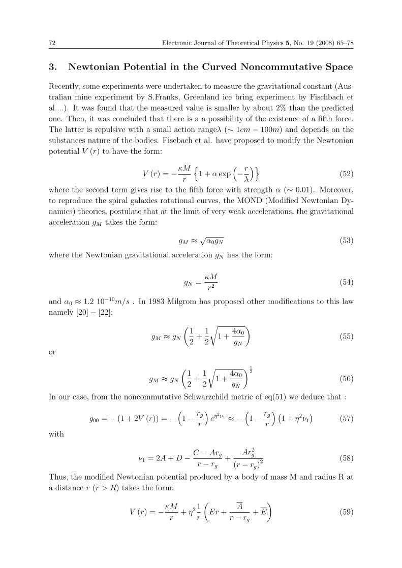
72 Electronic Journal of Theoretical Physics 5, No. 19 (2008) 65–78
3. Newtonian Potential in the Curved Noncommutative Space
Recently, some experiments were undertaken to measure the gravitational constant (Aus-
tralian mine experiment by S.Franks, Greenland ice bring experiment by Fischbach et
al....). It was found that the measured value is smaller by about 2% than the predicted
one. Then, it was concluded that there is a a possibility of the existence of a fifth force.
The latter is repulsive with a small action rangeλ (∼ 1cm − 100m) and depends on the
substances nature of the bodies. Fiscbach et al. have proposed to modify the Newtonian
potential V (r) to have the form:
V (r) = −κM
r
{1 + α exp
(− r
λ
)}(52)
where the second term gives rise to the fifth force with strength α (∼ 0.01). Moreover,
to reproduce the spiral galaxies rotational curves, the MOND (Modified Newtonian Dy-
namics) theories, postulate that at the limit of very weak accelerations, the gravitational
acceleration gM takes the form:
gM ≈ √α0gN (53)
where the Newtonian gravitational acceleration gN has the form:
gN =κM
r2(54)
and α0 ≈ 1.2 10−10m/s . In 1983 Milgrom has proposed other modifications to this law
namely [20] − [22]:
gM ≈ gN
(1
2+
1
2
√1 +
4α0
gN
)(55)
or
gM ≈ gN
(1
2+
1
2
√1 +
4α0
gN
) 12
(56)
In our case, from the noncommutative Schwarzchild metric of eq(51) we deduce that :
g00 = − (1 + 2V (r)) = −(1 − rg
r
)eη2ν1 ≈ −
(1 − rg
r
) (1 + η2ν1
)(57)
with
ν1 = 2A + D − C − Arg
r − rg
+Ar2
g
(r − rg)2 (58)
Thus, the modified Newtonian potential produced by a body of mass M and radius R at
a distance r (r > R) takes the form:
V (r) = −κM
r+ η2 1
r
(Er +
A
r − rg
+ E
)(59)
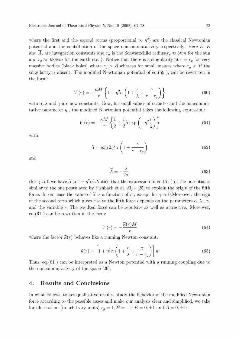
Electronic Journal of Theoretical Physics 5, No. 19 (2008) 65–78 73
where the first and the second terms (proportional to η2) are the classical Newtonian
potential and the contribution of the space noncommutativity respectively. Here E, E
and A, are integration constants and rg is the Schwarzchild radius(rg ≈ 3km for the sun
and rg ≈ 0.88cm for the earth etc..). Notice that there is a singularity at r = rg for very
massive bodies (black holes) where rg > R,whereas for small masses where rg < R the
singularity is absent. The modified Newtonian potential of eq.(59 ), can be rewritten in
the form:
V (r) = −κM
r
{1 + η2α
(1 +
r
λ+
γ
r − rg
)}(60)
with α, λ and γ are new constants. Now, for small values of α and γ and the noncommu-
tative parameter η , the modified Newtonian potential takes the following expression:
V (r) = −κM
r
{1
2+
1
2α exp
(−η2 r
λ
)}(61)
with
α = exp 2η2α
(1 +
γ
r − rg
)(62)
and
λ = − λ
2α(63)
(for γ ≈ 0 we have α ≈ 1 + η2α).Notice that the expression in eq.(61 ) of the potential is
similar to the one postulated by Fishbach et al.[23]− [25] to explain the origin of the fifth
force. In our case the value of α is a function of r , except for γ ≈ 0.Moreover, the sign
of the second term which gives rise to the fifth force depends on the parameters α, λ , γ,
and the variable r. The resulted force can be repulsive as well as attractive. Moreover,
eq.(61 ) can be rewritten in the form:
V (r) = − κ(r)M
r(64)
where the factor κ(r) behaves like a running Newton constant.
κ(r) =
[1 + η2α
(1 +
r
λ+
γ
r − rg
)]κ (65)
Thus, eq.(61 ) can be interpreted as a Newton potential with a running coupling due to
the noncommutativity of the space [26].
4. Results and Conclusions
In what follows, to get qualitative results, study the behavior of the modified Newtonian
force according to the possible cases and make our analysis clear and simplified, we take
for illustration (in arbitrary units) rg = 1, E = −1, E = 0,±1 and A = 0,±1:

74 Electronic Journal of Theoretical Physics 5, No. 19 (2008) 65–78
4.1 η2 = 0, or E = 0, A = 0:
In this case, the noncommutative Newtonian potential is reduced to the classical one.
Figure(1) displays the behavior of the Newtonian force F (r) acting on a body of mass
unity (m = 1) as a function of the distance r (F (r) = − 1r2 ) .
Fig. 1
4.2 E > 0, A > 0:
In this case and in arbitrary units, the behavior of the noncommutative Newtonian
potential V (r) is presented in fig.2 and the corresponding Newtonian force F (r) acting
on a body of mass m = 1 is displayed in fig.3. We distinguish eight main regions:
a)For 0 ≤ r ≤ r1(r1 ≈ 0.9), the non commutative Newtonian potential (NCNP) is
negative. It is an increasing function of r . It varies from V (0) ≈ −∞ to V (r1) ≈ −1.223
. The related non commutative force (NCF) is attractive and its intensity decreases from
|F (0)| = +∞ to |F (r1)| ≈ 0.
b)For r1 ≤ r ≤ r1(r1 ≈ 0.92), the NCNP is negative. It is an increasing function of r
until a maximum value V (r1) ≈ −1.222. The NCF is repulsive and its intensity increases
from |F (r1)| = 0 to |F (r1)| ≈ 0.16.
c)For r1 ≤ r ≤ rg, the NCNP remains negative but a decreasing function of r and
gives a repulsive NCF where the intensity increases form |F (r1)| ≈ 3.3 to |F (rg)| = +∞,
d)For rg ≤ r ≤ r2(r2 ≈ 1.01), the NCNP is positive. It is a decreasing function of r
and it vanishes at a distance r2 ≈ 1.01. The NCF is a repulsive force where the intensity
increases from |F (rg)| = +∞ to |F (r2)| ≈ 97.03.
e) For r2 ≤ r ≤ r3(r3 ≈ 1.09), the NCNP is negative. It is a decreasing function of
r.It varies from V (r2) = 0 to a minimal value V (r3) ≈ −1.02. The corresponding NCF
is repulsive where the intensity decreases from |F (r2)| ≈ 97.03. to |F (r3)| ≈ 0.19.
f) For r3 ≤ r ≤ r4(r4 ≈ 1.1), the NCNP is negative. It is an increasing function of
r.It varies from V (r3) ≈ −1.02 to valueV (r4) ≈ −0.99. The NCF is a repulsive force
with an intensity decreasing from |F (r3)| ≈ 0.19 to |F (r4)| ≈ 0.
g) For r4 ≤ r ≤ r5(r5 ≈ 1.25), the NCNP is negative. It is an increasing function of
r.It varies from V (r4) ≈ −0.99 to V (r5) ≈ −0.83. The NCF is an attractive force and

Electronic Journal of Theoretical Physics 5, No. 19 (2008) 65–78 75
its intensity increases from |F (r4)| ≈ 0 to |F (r5)| ≈ 0.46.
h)For r5 ≤ r ≤ +∞, the NCNP has a behavior which looks like the classical Newto-
nian one. Thus, it is negative and increasing function of r. It gives an attractive NCF
with an intensity decreasing from |F (r5)| ≈ 0.46 to |F (+∞)| = 0.
Fig. 2
Fig. 3
4.3 E > 0, A < 0:
In this case and in arbitrary units, the behavior of the NCNP is presented in fig.4
and the corresponding Newtonian force F (r) acting on a body of m = 1 is displayed in
fig.5.We distinguish four main regions:
a) for 0 ≤ r ≤ r6 (r6 ≈ 0.82 ), the NCNP is negative and an increasing function of r.
It varies from V (0) = −∞ to V (r6) ≈ −1.15. This gives an attractive NCF where the
intensity decreases from |F (0)| = +∞ to |F (r6)| ≈ 1.79.
b) for r6 ≤ r ≤ r7 (r7 ≈ 0.99 ), the NCNP is negative and an increasing function of r.
It varies from V (r6) ≈ −1.15 to V (r7) ≈ 0. This will give an attractive NCF where the
intensity increases from |F (r6)| ≈ 1.79. to |F (r7)| ≈ 101.02.
c) for r7 ≤ r ≤ rg, the NCNP is positive and an icreasing function of r . It varies from
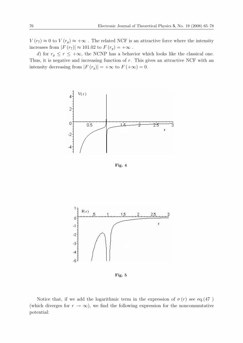
76 Electronic Journal of Theoretical Physics 5, No. 19 (2008) 65–78
V (r7) ≈ 0 to V (rg) ≈ +∞ . The related NCF is an attractive force where the intensity
increases from |F (r7)| ≈ 101.02 to F (rg) = +∞ .
d) for rg ≤ r ≤ +∞, the NCNP has a behavior which looks like the classical one.
Thus, it is negative and increasing function of r. This gives an attractive NCF with an
intensity decreasing from |F (rg)| = +∞ to F (+∞) = 0.
Fig. 4
Fig. 5
Notice that, if we add the logarithmic term in the expression of σ (r) see eq.(47 )
(which diverges for r → ∞), we find the following expression for the noncommutative
potential:
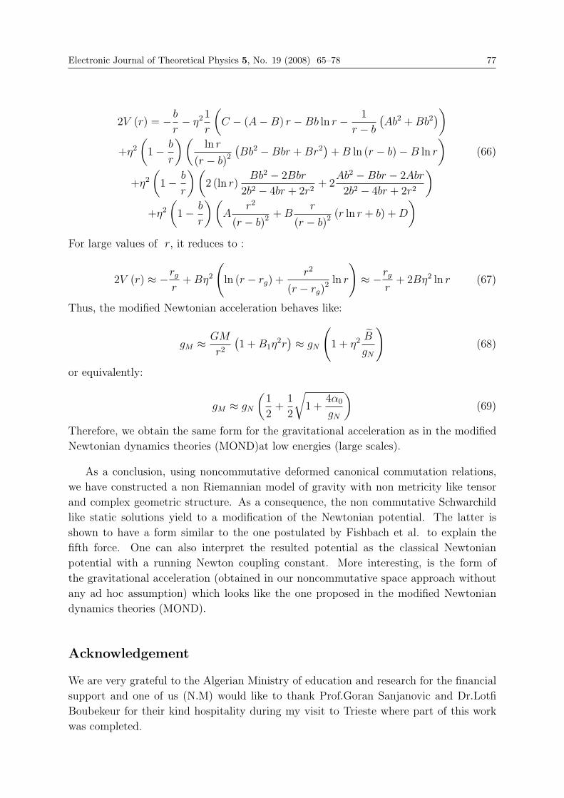
Electronic Journal of Theoretical Physics 5, No. 19 (2008) 65–78 77
2V (r) = − b
r− η2 1
r
(C − (A − B) r − Bb ln r − 1
r − b
(Ab2 + Bb2
))+η2
(1 − b
r
)(ln r
(r − b)2
(Bb2 − Bbr + Br2
)+ B ln (r − b) − B ln r
)(66)
+η2
(1 − b
r
)(2 (ln r)
Bb2 − 2Bbr
2b2 − 4br + 2r2+ 2
Ab2 − Bbr − 2Abr
2b2 − 4br + 2r2
)+η2
(1 − b
r
)(A
r2
(r − b)2 + Br
(r − b)2 (r ln r + b) + D
)For large values of r, it reduces to :
2V (r) ≈ −rg
r+ Bη2
(ln (r − rg) +
r2
(r − rg)2 ln r
)≈ −rg
r+ 2Bη2 ln r (67)
Thus, the modified Newtonian acceleration behaves like:
gM ≈ GM
r2
(1 + B1η
2r)≈ gN
(1 + η2 B
gN
)(68)
or equivalently:
gM ≈ gN
(1
2+
1
2
√1 +
4α0
gN
)(69)
Therefore, we obtain the same form for the gravitational acceleration as in the modified
Newtonian dynamics theories (MOND)at low energies (large scales).
As a conclusion, using noncommutative deformed canonical commutation relations,
we have constructed a non Riemannian model of gravity with non metricity like tensor
and complex geometric structure. As a consequence, the non commutative Schwarchild
like static solutions yield to a modification of the Newtonian potential. The latter is
shown to have a form similar to the one postulated by Fishbach et al. to explain the
fifth force. One can also interpret the resulted potential as the classical Newtonian
potential with a running Newton coupling constant. More interesting, is the form of
the gravitational acceleration (obtained in our noncommutative space approach without
any ad hoc assumption) which looks like the one proposed in the modified Newtonian
dynamics theories (MOND).
Acknowledgement
We are very grateful to the Algerian Ministry of education and research for the financial
support and one of us (N.M) would like to thank Prof.Goran Sanjanovic and Dr.Lotfi
Boubekeur for their kind hospitality during my visit to Trieste where part of this work
was completed.
78 Electronic Journal of Theoretical Physics 5, No. 19 (2008) 65–78
References
[1] J. Oort, Bull. Astron. Soc. Neth.6 (1932) 249 ; ibid 15 (1960) 45.
[2] F. Zwicky, Helv. Phys. Acta 6 (1933) 110.
[3] S. Smith, Astrophys. Journ. 83 (1936) 23.
[4] C. Munoz, Int. J. Mod. Phys. A 19 (2004) 3093 .
[5] V. V. Zhytnikov and J. M. Nester, Phys. Rev. Lett.73 (1994) 950.
[6] A. Edery, Phys. Rev. Lett. 83 (1999) 3990.
[7] J. D. Bekenstein, M. Milgrom and R. H. Sanders, Phys. Rev. Lett. 85 (2000) 1346.
[8] M. E. Soussa and R. P. Woodard, Class. Quant. Grav. 20 (2003) 2737.
[9] M. E. Soussa and R. P. Woodard, Phys. Lett. B 578 (2004) 253.
[10] A. Aguirre, C. P. Burgess, A. Friedland and D.Nolte, Class. Quant. Grav. 8 (2001)223.
[11] S. Perlmutter, G. Aldering , G. Goldhaber et al , Astrophys. J. 517 (1999) 565.
[12] S. Perlmutter, M. S. Urner and M.White, Phys. Rev. Lett. 83 (1999) 670.
[13] M. E. Soussa and R. P. Woodard, Class. Quant. Grav. 20 (2003) 2737.
[14] R. H. Sanders and S. S. McGaugh, Annu. Rev. Astron. Astrophys.40 (2002) 263.
[15] A. Lue, R. Scoccimari and G. Starkman, Phys. Rev. D69 (2004) 044005.
[16] S. M. Carroll, V. Duvvuri , M. Trodden and M. S. Turner, Phys.Rev.D70(2004)043528 .
[17] D. N. Spergel et al, Astrophys. J. Suppl. 148 (2003) 175.
[18] J. Jungman, M. Kamionkowski and K. Griest, Phys. Rep. 267 (1996) 195.
[19] R. R. Caldwell, Phys. Lett. B545 (2002) 23.
[20] M. Milgrom, Astrophys. Journ. 270 (1983) 365.
[21] M. Milgrom, Astrophys. Journ. 270 (1983) 371.
[22] M. Milgrom, Astrophys. Journ. 270 (1983) 384.
[23] J. D. Bekenstein, Phys. Rev. D70 (2004) 083509; Erratum-ibid. D71 (2005) 069901.
[24] E. Fischbach, H. T. Kloor, C. Talmadge, S. H. Aronson and G. T. Gillies, Phys. Rev.Lett. 60 (1988) 74.
[25] E. Fischbach, D. Sudarsky, A. Szafer, C. Talmage and S. H. Aronson, Phys. Rev.Lett. 56 (1986) 3.
[26] S. Reynaud and M. T. Jaekel, Int. J. Mod. Phys. A 20 (2005) 2294.
[27] C. Quesne, V. M. Tkachuk, J. Phys. A 37 (2004) 4267.
[28] M. G. Jackson, Int. J. Mod. Phys. D 14 (2005) 2239.
EJTP 5, No. 19 (2008) 79–90 Electronic Journal of Theoretical Physics
Classification of Electromagnetic Fields innon-Relativist Mechanics
N. Sukhomlin1 ∗ and M. Arias2
1 Department of Physics, Autonomous University of Santo Domingo, Santo Domingo,Dominican Republic
2 Department of Physics-Mathematics, University of Puerto Rico at Cayey,Puerto Rico 00736
Received 18 July 2008, Accepted 16 August 2008, Published 10 October 2008
Abstract: We study the classification of electromagnetic fields using the equivalence relationon the set of all 4-potentials of the Schrodinger equation. In the general case we find therelations among the equivalent fields, currents, and charge densities. Particularly, we study thefields equivalent to the null field. We show that the non-stationary state function for a particlein arbitrary uniform time-dependent magnetic field is equivalent to a plane wave. We presentthat the known coherent states of a free particle are equivalent to the stationary states of anisotropic oscillator. We reveal that the only constant magnetic field is not equivalent to the nullfield (contrary to a constant electrical field) and we find other fields that are equivalent to theconstant magnetic field. We establish that one particular transformation of the free Schrodingerequation puts a plane wave and Green’s function in a equivalence relation.c© Electronic Journal of Theoretical Physics. All rights reserved.
Keywords: Schrodinger Equation, Intrinsic Characteristics, Equivalent Fields, the ShapovalovGroupPACS (2008): 03.65.-w; 03.50.-z; 03.50.De; 02.90.+p
1. Exposition of the Problem
It is known that the Schrodinger equation for a particle in the electromagnetic field in
Cartesian coordinates
ı�∂Ψ
∂t= HΨ with H =
1
2m
[−ı�∇− e �A (t, �r)
]2
+ eϕ (t, �r) . (1)
must be completed with the following known characteristics: a physical interpretation of
the wave function and the fact that the 4-potential must be real so that the Hamilton
∗ Corresponding Author: [email protected]

80 Electronic Journal of Theoretical Physics 5, No. 19 (2008) 79–90
operator is hermitian (if not the normalization integrals could not be constant). These
characteristics are intrinsic of the physics problem.
The Schrodinger equation completed by their intrinsic characteristics we call a physi-
cal problem in non-Relativist Mechanics. In this paper we realize the classification on the
set of all physical problems using the Shapovalov’s approach [1]. It is evident that for dif-
ferent intrinsic characteristics we obtain different equivalence relations and, consequently,
different classifications.
Traditional studies add to the list of known intrinsic characteristics the structure of
the electromagnetic field: �E and �B must be fixed. This imposition reduces the group
of equivalence to the Cartesian product of the gauge invariance group and the Galilean
transformations group (see, for example, [2]).
On the contrary, Shapovalov’s approach does not include the structure of the electro-
magnetic field in the intrinsic characteristics. This allows us to find a broader equivalence
group, and gives the new exact solutions of different physical problems.
The following theorem defines the equivalence group of the Schrodinger equation (we
call it The Shapovalov group):
Shapovalov’s Theorem 1. The Schrodinger equation in the Euclidian space com-
pleted by mentioned intrinsic characteristics admits following equivalence group: Gsh =
R ⊗ T ⊗ V ⊗ Γ ⊗ Y. Where Γ is the gauge invariance group and
R (θ1 (t), θ2 (t) , θ3 (t)); T (c1 (t), c2 (t), c3 (t)) and V (s (t)) are the rotations, trans-
lations, and scale change groups. The Shapovalov group contains 7 arbitrary time-
dependent functions: s (t) , θi (t) , ci (t) and dt′dt
:= s2 > 0, and Y is the discrete
invariance group of the Schrodinger equation from Section 4.5.
The Shapovalov group is very effective for finding new solutions. We note that the
traditional equivalence group is a subgroup of the Gsh : θi, ci, s = const.
For a specification of the Shapovalov group, we compare two Schrodinger equations
such as (1) with different 4-potentials: { �A(t, �r ), ϕ(t, �r )} and { �A′ (t, �r ) ,
ϕ′ (t, �r )}. Additionally, we designate {t′, �r′} to be the variables of the second equation,
this allows us to distinguish equivalent fields. The equivalence relations must conserve
the structure (1) of the Schrodinger equation. When using only this imposition we found
[1] that the Shapovalov group of the Schrodinger equation is the following :
t′ = t′ (t)[dt′
dt:= s2 > 0
](2)
�r′ = s (t) a (t)�r + c (t) (3)
Ψ′ (t′, �r′) = Ψ (t, �r) s−3/2. (4)
The seven arbitrary time-dependent functions of the Shapovalov group mean the follow-
ing: s(t) represents a freedom of time-scale and the coordinate-scale choice. Three
functions ci(t) define three independent displacements with arbitrary time-dependent
linear velocities. The orthogonal matrix a(t) describes the rotations with three arbitrary
time-dependent angular velocities. In Section 4 we study the subclasses of the null field
equivalence class generated by each one of these three types of equivalence relations.
Electronic Journal of Theoretical Physics 5, No. 19 (2008) 79–90 81
If a reference system were inertial, the Shapovalov group puts it in equivalence with
the non-inertial systems. This fact is used frequently, for example, to describe the circular
movement of a classic particle with a constant linear velocity. After being transferred to
a rotating reference system, this physical problem is reduced to a free particle (see, for
instance, [3], [4]). We emphasize that in the traditional approach such obvious equivalence
does not exist. At least, this fact shows a need for extension of the traditional equivalence
group.
2. Equivalent Potentials and Fields
Using the fact that the form (1) of the Schrodinger equation must be invariant and the
equivalence relations of the Shapovalov group (2), (3) and (4), we obtain the equivalent
potentials:
A′k = s−1
∑j
akjAj −m
es−2xk, (5)
ϕ′ =1
s2ϕ +
∑k,j
1
s3x′
kakjAj −∑
k
m
2e
1
s4x′
kx′k, (6)
where x′k :=
∂x′k
∂t. Rigorously, the Shapovalov group is specified through formulas (2),
(3), (4), (5), (6), and (39). Now, we can easily calculate the relation among equivalent
electromagnetic fields:
s2B′i (t
′, �r′) =∑
k
aikBk(t, �r) +m
e
∑l,k,j
εilkalj(t)akj(t), (7)
s2 �E ′(t′, �r′) =1
sa �E(t, �r) − �r′ × �B′ +
m
e
(�r′
s2
)·
. (8)
For a compact presentation, we introduce Larmor’s notation: ω := eB2m
and the magnetic
field’s anti-symmetrical 3 × 3 matrix: Fij :=∑
k εijkωk. The relation (7) between
equivalent magnetic fields in matrix form appears as:
s2F ′(t′, �r′) = aF (t, �r)aT + aaT . (9)
If, for example, we have only time-dependent magnetic fields: B′ = B′(t′) and B =
B(t) they both are equivalent (a is an orthogonal matrix):
a(t) = s2F ′(t′)a − aF (t). (10)
Particularly, if both magnetic fields are constant, the following orthogonal matrix provides
the equivalent relations:
a(t) = exp {F ′t′(t) − Ft} ; t′(0) = 0. (11)

82 Electronic Journal of Theoretical Physics 5, No. 19 (2008) 79–90
Then we observe that naturally the equivalent fields (7) and (8) simultaneously verify the
first pair of the Maxwell equations. It is easy to find that:
s3∇′ · �B′ = ∇ · �B, s5
[∇′ × �E ′ +
∂ �B′
∂t′
]= sa
[∇× �E +
∂ �B
∂t
]−(div �B
)�r′.
If one referential system does not have a “magnetic charge”, than no other equivalent
system will have it. The second pair of the Maxwell equations gives the relations between
the equivalent densities of charge and current:
s4
(ρ′(t′, �r′)
ε0
− 2m
e�ω′2)
=ρ(t, �r)
ε0
− 2m
e�ω2 + s2� ′r rot′ �B′ − 3m
ef(t), (12)
�J ′(t′, �r′) + ε0∂ �E ′
∂t′=
1
s3a
(�J(t, �r) + ε0
∂ �E
∂t
). (13)
Where ω(t) is the Larmor frequency, �E and �E ′ verify (8) and
f(t) := s
(1
s
)··. (14)
3. Fields Equivalent to the Null Field
Here we study the null field equivalence class. If �E ′ = �B′ = 0, then relations (7), (8),
and (10) allow us to describe all fields of this equivalence class:
�B = �B(t)
defined by (7)
a = −aF (t); (15)
�E(t, �r) =m
e
[b(t)�r + �d(t)
], (16)
where we denote the matrix:
b(t) := −saT
[(sa)·
s2
]·= f(t)I + F − F 2, (17)
with f(t) from (14) , I unity matrix, and the vector
�d(t) := −saT
[�c
s2
]·. (18)
We conclude from (15) and (16) that the widest field equivalent to the null field can
contain an arbitrary time-dependent magnetic field, whereas the electric field is linear
related to �r (with the matrix of time-dependent coefficients) :
�B = �B(t) (19)
Electronic Journal of Theoretical Physics 5, No. 19 (2008) 79–90 83
�E(t, �r) =(m
e
) [�r × �ω + (�ω × �r) × �ω + f(t)�r + d(t)
], (20)
where the second term of �E has the form of the centrifugal force. We observe that the
class has non-orthogonal fields �E · �B �= 0, but all are equivalent to one orthogonal. From
(12) and (13) we find the null equivalent densities of charge and current:
eρ(t) = 2mε0ω2(t) + 3mε0f(t), (21)
�J(t, �r) = −ε0∂ �E
∂t= −ε0m
e
[b�r + �d
]. (22)
4. Particular Cases
4.1 Exclusively Rotation Equivalence (s = 1, �c = 0)
Now we treat the subclass of the fields which are equivalent to the null field using only
the rotating equivalent reference systems. From (19) and (20) we have:
�B = �B(t), (23)
�E(t, �r) =(m
e
)�r × �ω +
(m
e
)(�ω × �r) × �ω. (24)
The following 4-potential creates such a field:
�A =(m
e
)(�ω × �r) , ϕ = −
(m
2e
)(�ω × �r)2 ,
where the scalar potential represents the centrifugal energy. We observe that the electric
and magnetic fields are not orthogonal in the general case: �E · �B =(
12
) (�B × �B
)·�r, but
they are if, for example, �B ‖ �B. Hamilton’s operator of this system has the form:
H = − �2
2mΔ − �ω(t) · �L, (25)
where Δ is the Laplacian and �L := �r × �p is the operator of the angular momentum. The
formula (25) corresponds exactly to the classic mechanics theorem of transformation of
energy after passing from an inertial reference system to a system in rotation: Erotation =
Einertial − �ω · �L (see for instance [4]). If the field (23) and (24) is equivalent to the null
field, then the system with Hamilton’s operator (25) has a symmetry that corresponds
to one of a free particle. The first integrals of motion of (25) are:
�X1 = a(t)�p, �X2 = a(t)
[− t
m�p + �r
], �X1 = a(t)�L. (26)
These first order operators of symmetry are unique for the system and constitute the
base of all superior-order symmetry operators. The corresponding integrals of motion of

84 Electronic Journal of Theoretical Physics 5, No. 19 (2008) 79–90
a free particle are: �X ′i = aT �Xi (i = 1, 2, 3). It is known that the eigenvectors of the linear
momentum and the initial coordinate operators
�X ′1 = � ′p, �X ′
2 = −(
t′
m
)� ′p + � ′r, (27)
are respectively a plane wave and Green’s function (we remove the primes on top of wave
functions and variables):
Ψplane wave = C exp
[−ı
E
�+ ı
�p
�· �r]
; ΨGreen =C
t3/2exp
[ım(�r − �λ)2
2�t
]. (28)
In Section 4.5 we show that an equivalence exists among these functions and among the
operators (27). Now, using the known solutions (28), we can construct new solutions to
the Schrodinger equation for the field (23) and (24) for an arbitrary �B(t). The first
operator of (26) �X1 has the following eigenfunction:
Ψ(t, �r) = C exp
[ı�λT a(t)�r
�− ı
λ2
2m�t
]. (29)
This solution describes a non-stationary state, it is equivalent to a plane wave for a
free particle (stationary state function). The constant λ2
2mis quasi-energy, the expres-
sion �p0 := aT (t)λ is understood to be a quasi-momentum. We did not need to solve the
Schrodinger equation for a particle in an arbitrary time-dependent field (23), (24). But
we directly wrote its solution (29) without solving this equation, only using an equiva-
lence relation of the Shapovalov group. We observe that contrary to the null field, for a
particle in the field (23) and (24) the vector momentum is not a first integral of motion.
The Hamilton’s operator (25) and the vector operator �X2 of (26) provide the solution
of the Schrodinger equation that corresponds to the Green’s function:
Ψ(t, �r) =C
t3/2exp
[ım(�r − �r0(t))
2
2�t
], (30)
where �r0(t) := aT (t)�λ, �λ is the initial coordinate in the inertial reference system; �r0(t) is
the same initial coordinate in a rotating reference system. The vector λ is an arbitrary
constant vector (eigenvalue of �X2). An orthogonal matrix a(t) verifies (15) with the
arbitrary vector function �ω(t). It is known that the solution (30) can be orthonormalized
to the Dirac delta function, but its interpretation is difficult. It is a case of equivalence
of a non-stationary solution to another non-stationary one.
The third vector operator of symmetry (26) �X3 does not allow a direct construction
of a solution because as its components do not commute, it is necessary to use the set
equivalent to: H ′, �L′2, L′z.
Electronic Journal of Theoretical Physics 5, No. 19 (2008) 79–90 85
4.2 Exclusively Euclidean Translational Equivalence (the Unity Matrix
a = I and s = 1)
The subclass of the Euclidean translational displacements (�c �= 0) relates to the equiva-
lence between reference systems moving with arbitrary linear velocities. For example, the
only time-dependent uniform electrical field (16) defined by vector �d(t) from (18), with
the uniform corresponding current (22) is equivalent to the null field without a current.
Naturally, Galileo’s equivalence belongs to the Shapovalov group (see Section 4.5).
4.3 Isotropic Oscillator (Exclusively Time Scale Equivalence: the Unity
Matrix a = I and �c = 0)
Let be �B = 0 =⇒ b(t) is a constant matrix. Using formulas (19 and 20), for �c =
0 and �ω = 0, we find the field of the isotropic oscillator: E =(
me
)f(t)r. In case
of f(t) = const, it corresponds to the potential energy U =mω2
0r2
2, with ω0 = const. We
note that constant ω0 does not have any relation to the Larmor frequency ω (which
is null here). From this form of potential energy and definition (14) we obtain the well
known relation: (1
s
)··+ ω2
0
(1
s
)= 0.
Solving it, we find the time-scale equivalence (scale change group of Shapovalov’s theo-
rem):dt′
dt:= s2 = sec2(ω0t) =⇒ ω0t
′ = tan(ω0t), �r′ = s(t)�r. (31)
This equivalence relation provides an equivalence between the free Schrodinger equation
ı�∂Ψ′
∂t′= H ′Ψ′ = − �
2
2mΔ′Ψ′, (32)
and the equation for the isotropic oscillator:
ı�∂ψnlm(t, �r)
∂t= Hψnlm(t, �r) :=
[− �
2
2mΔ +
mω20r
2
2
]ψnlm(t, �r).
The solutions of the last equation are known (for instance, [5], [7]). We observe that these
states are defined by the following set of integrals of movement: H, � 2L, Lz. In addition,
in the equivalence relation (31), it is necessary to use gauge invariance:
Ψ′nlm(t′, �r′) =
ψnlm(t, �r)
s3/2exp
[ım
2�
s
sr2
]; (33)
with the wave function:
ψnlm(t, �r) = ϕnlm(�r) exp
[−ı
Enl
�t
]; (34)

86 Electronic Journal of Theoretical Physics 5, No. 19 (2008) 79–90
Enl = �ω0
[2n + l +
3
2
]; n, l = 0, 2, ...; m = 0, ±1, ..., ±l;
ϕnlm(r, θ, φ) =1
ξRnl(ξ)Ylm(θ, φ); ξ := r
√mω0
�.
Here the functions Ylm(θ, φ) are the spherical harmonics and Rnl(ξ) are the radial
functions expressed by confluent hypergeometric functions. The non-stationary solu-
tions Ψ′ (33) of the free Schrodinger equation (32) are known as coherent states and are
equivalent to the stationary states of the isotropic oscillator. For example, the function
of the fundamental state that verifies the equation (32) can be written (we abandon the
primes on top of the variables and the wave function):
Ψ000(t, �r) =C
√4π (1 + ω2
0t2)
3/4exp
[−mω0
2�
1
1 + ıω0t�r2 − ı
3
2arctan(ω0t)
]. (35)
We observe that to establish the equivalence of the free particle’s coherent states to
the stationary states of an isotropic oscillator, the time scale equivalence relation (31) is
indispensable. For another equivalent solution to (35) of the free Schrodinger equation see
(40). The equivalence between a free particle and an isotropic oscillator of one dimension
is discussed in [8].
If f(t) from (14) is not a constant, we have an arbitrary time-dependent radial dilation.
In this case, new solutions of other physical problems can be constructed.
4.4 Constant Magnetic Field
In the null field equivalent class (15) and (16), we find a field with a constant magnetic
component:
�B = (0, 0, B) = const; �E(t, �r) =m
e
[f(t)�r + ω2 (x1, x2, 0)
]+ �ε(t). (36)
Here f(t) is defined by (14), �ε(t) is an arbitrary time-dependent vector function.
The first term of the electrical component corresponds to an arbitrary time-dependent
dilation; particularly to an isotropic oscillator from Section 4.3 with an arbitrary time-
dependent frequency. The second term corresponds to the constant centrifugal force field
and the third term results from Euclidean translational freedom (c(t) �= 0). Here are two
particular cases of interest:
if f = 0 (s = 1) =⇒ �B = (0, 0, B) ; �E(t, �r) =mω2
e(x1, x2, 0) ; (37)
if f := s
(1
s
)··= −ω2
0 =⇒ �B = (0, 0, B) ; �E(t, �r) = −mω2
e(0, 0, x3) .
We can see that only constant magnetic field does not belong to the null field equivalent
class, but always some electrical component of the field is present. By using formulas (7)
Electronic Journal of Theoretical Physics 5, No. 19 (2008) 79–90 87
and (8), we find that only constant magnetic field is equivalent to the constant centripetal
force field:
�B′ = (0, 0, B′) = const; �E ′ = 0 ⇔ �B = 0; �E(t, �r) = −mω′2
e(x1, x2, 0) .
(38)
This result explains the formula (37). If f = const, �ε = const, the field (36) defines the
widest stationary field equivalent to the null field.
4.5 Free Schrodinger Equation’s Nucleus
It is interesting to find the set of equivalence relations that put the null field in equivalence
to itself (see also [6]). By choosing �E ′ = �B′ = �E = �B = 0, we easily find that such a
nucleus is the Galilean group:
t′ = α2t + β; �r′ = αa�r + �ν0t + �r0; Ψ′ = α−3/2Ψ
with arbitrary constants α, β, �ν0, �r0, and a constant orthogonal matrix a. In addi-
tion, one isolated equivalence operation exists and leaves the free Schrodinger equation
invariant:
t′ = −1
t; �r′ =
1
t�r; Ψ′(t′, �r′) = Ψ(t, �r)t3/2 exp
[−ı
m
2�
r2
t
], (39)
t
Ψ
[i�
∂
∂t+
�2
2mΔ
]Ψ = − t′
Ψ′
[i�
∂
∂t′+
�2
2mΔ′]
Ψ′.
Let us denote this transformation e. It is easy to show that {e, e2, e3, e4} constitutes the
discrete invariance group of the Schrodinger equation Y from the Shapovalov’s theorem.
This transformation has a very interesting property: it transforms Green’s function (28)
to the plane wave propagating in the direction −�λ :
Ψ′(t′, �r′) = C ′ exp[−ıω′t′ − ı�k′�r′
], �ω′ :=
mλ2
2; ��k′ := m�λ.
And inversely, the equivalence relation (39) transforms a plane wave into Green’s func-
tion. Of course, the relation (39) also puts in equivalence the operator of linear momen-
tum �p′ and the operator of initial coordinate: −( tm
)�p + �r (see formula (27)). This
operation is similar to passing to momentum space. This transformation does not make
sense if �λ = 0.
We easily find that relation (39) does not change the angular momentum: �L =
� ′L. Consequently, the well-known states of a free particle with a constant angular
momentum are invariant in respect to relation (39).
Another example, relation (39) puts the coherent state (35) in equivalence with the
following function:
Ψ′000(t
′, �r′) =C
√4π (ω2
0 + t′2)3/4exp
[−m
2�
1
ω0 + ıt′�r′2 − ı
3
2arctan(
ω0
t′)
]. (40)
88 Electronic Journal of Theoretical Physics 5, No. 19 (2008) 79–90
It is a new solution of the free Schrodinger equation (32).
Also, we can note that formula (33) with the relations dt′dt
:= s2(t) and �r′ =
s(t)�r contains the operation of equivalence (39) if we just impose the transformation
of the Green’s function to a plane wave or inverse.
4.6 Classic Particle
The Shapovalov group was found by Shapovalov and Sukhomlin (1974) [1] who also
enumerated all cases of separation of variables in a parabolic equation and proved that
all of these cases recur in quantum mechanic and in classical Hamilton Jacobi approach.
In 1980, S. Benenti and M. Francaviglia [9] applied the Shapovalov group to the
Hamilton-Jacobi equation and G. Reid [10] extended it in 1986 to the space of n-dimensions.
A study of the Hamilton-Jacobi equation gives the same equivalence group that the
Schrodinger equation (2), (3), (4) does. In fact, the equivalent potentials and the fields
are the same as (5), (6) and (7), (8).
In particular, we refer to the results to the equivalence study in some cases. Using
(31) we establish the relation between equivalent actions as in Section 4.3:
W ′(t′, �r′) = W (t, �r) +m
2
s
s�r2, (41)
where W (t, �r) corresponds to the isotropic oscillator and W ′(t′, �r′) to coherent states of
a free particle.
Finally:
W ′(t′, r′) = − α
ω0
cos−1
(√1
2α
mω20
1 + ω20t
′2 r′)
+mω0
2r′√
1
1 + ω20t
′2
(2α
mω20
− r′2
1 + ω20t
′2
)+
mω0
2
t′
1 + ω20t
′2 r′2 − α
ω0
arctan(ω0t′). (42)
Here α is energy. As in Section 4.5 we can verify that the nucleus of the Hamilton-Jacobi
equation is specified by the same relation (39) as gauge invariance:
W ′(t′, �r′) = W (t, �r) − m
2
r2
t, (43)
where W (t, �r) is (42) without the primes. The solution of Hamilton-Jacobi that corre-
sponds to (40), presents:
W ′(t′, r′) = − α
ω0
cos−1
(√1
2α
mω20
ω20 + t′2
r′)
+mω0
2r′√
1
ω20 + t′2
(2α
mω20
− r′2
ω20 + t′2
)+
mω0
2t′r′2
ω20 + t′2
− α
ω0
arctan(ω0
t′). (44)
Electronic Journal of Theoretical Physics 5, No. 19 (2008) 79–90 89
Conclusions
(1) The null field is equivalent to the uniform magnetic field with arbitrary time depen-
dence. The corresponding electric component (linear related to �r) is defined by (16)
or (20). The equivalence relation between such a magnetic field and the null field
is similar to the passing from an initial reference system to one which is in rotation
defined by an orthogonal matrix from (15).
(2) The null field equivalence class has several non-orthogonal fields.
(3) The arbitrary-uniform charge distribution (time-dependent or not) is equivalent to
the null charge density according to (21). Its time dependence comes from two types
of equivalence: one from rotation of a reference system and the other from time scale
equivalence. It is possible to have a null charge distribution simultaneously for both
fields: one of type (15), (16) and the null field. Its current densities can be null also.
The widest current density equivalent to the null current is linear related to �r (22).
(4) The time scale equivalence (s �= 0) has an important role in the equivalence relations
on all physical problem sets (see the isotropic oscillator, Section 4.3). Particularly it
is known that the non-stationary coherent states of a free particle (33) are equivalent
to the stationary states of a harmonic oscillator (34). Another example is when
concrete relations establish the equivalence between a non-dissipative wave packet
and one with dissipation [5].
(5) Only Euclidean translational equivalence (�c(t) �= 0) establishes a correspondence
between arbitrary time-dependent uniform electrical fields and the null field (see
Section 4.2).
(6) Since the free Schrodinger equation has both stationary and non-stationary solutions,
in the null field equivalence class we find four types of equivalence relations: the
stationary wave functions equivalent to stationary or non-stationary states. Also
non-stationary states could be equivalent to one other stationary or non-stationary
wave functions. For example, the non-stationary wave function (29) is equivalent to
a stationary one (plane wave (28)); the non-stationary function (30) is equivalent to
another non-stationary one (Green’s function of the free Schrodinger equation (28)).
(7) The widest stationary field equivalent to the null field is defined by formula (36)
with conditions f = const, �ε = const.
(8) The formulas (36) and (38) show that only a constant magnetic field does not belong
to the null field equivalent class (contrary to a constant electrical field).
(9) The known isolated equivalence relation (39) puts the free Schrodinger equation
in equivalence to itself. The plane wave is equivalent by means of this relation to
Green’s function. It is similar to the rotation in a phase space.

90 Electronic Journal of Theoretical Physics 5, No. 19 (2008) 79–90
Acknowledgements
The authors are grateful to Prof. Franklin Garcia Fermin and to the UASD Department
of Physics for their cooperation. Also, the authors express their gratitude to the Editor
in Chief of the EJTP and to anonymous reviewers.
References
[1] V. Shapovalov, N. Sukhomlin, Separation of the variables in the non-stationarySchrodinger equation, Izv. Vyss. Ucheb. Zaved., Physika, 12, 100 (1974) (Sov. Phys.Journ., 17, 1718 (1976)).
[2] R. Zhdanov, A. Zhalij, On separable Schrodinger equation, Journal of MathematicalPhysics,40, 6319 (1999).
[3] H. Goldstein, C. Poole, J. Safko, Classical Mechanics, Addison-Wesley, 3rd ed., 134(2002).
[4] L. D. Landau, E. M. Lifshitz, Course of Theoretical Physics, Mechanics, 1, 3rd ed.,Oxford: Pergamon press, 126 (1976).
[5] M. Moshinsky, D. Schuch, A. Suarez-Moreno, Motion of wave packets withdissipation, Revista Mexicana de Fisica, 47, 7 (2001).
[6] C. Boyer , The maximal kinematical invariance group for an arbitrary potential, Helv.Phys. Acta, 47, 589 (1974).
[7] S. Flugge, Practical Quantum Mechanics, vol. I, Springer-Verlag, Berlin, Heidelberg,New York (1971); problem 65.
[8] W. Miller Jr, Symmetry and Separation of variables, Addison-Wesley, London (1977);Chapter 2.
[9] S. Benenti, M. Francaviglia, The Theory of Separability of the Hamilton-JacobiEquation and its Applications to General Relativity, A General Relativity andGravitation, Berne, Switz, 393 (1980).
[10] G. Reid, R-Separation for Heat and Schrodinger Equations I, SIAM, 17 Issue 3,646(1986).

EJTP 5, No. 19 (2008) 91–104 Electronic Journal of Theoretical Physics
Magnetized Bianchi Type V I0 Barotropic MassiveString Universe with Decaying Vacuum Energy
Density Λ
Anirudh Pradhan ∗1 and Raj Bali†2
1Department of Mathematics, Hindu Post-graduate College, Zamania-232 331,Ghazipur, India
2Department of Mathematics, University of Rajasthan, Jaipur-302 004, India
Received 8 August 2008, Accepted 16 September 2008, Published 10 October 2008
Abstract: Bianchi type V I0 massive string cosmological models using the technique givenby Letelier (1983) with magnetic field are investigated. To get the deterministic models, weassume that the expansion (θ) in the model is proportional to the shear (σ) and also the fluidobeys the barotropic equation of state. It was found that vacuum energy density Λ ∝ 1
t2which
matches with natural units. The behaviour of the models from physical and geometrical aspectsin presence and absence of magnetic field is also discussed.c© Electronic Journal of Theoretical Physics. All rights reserved.
Keywords: Massive String, Bianchi type V I0 Universe, Magnetic FieldPACS (2008): 11.10.-z; 98.80.Cq, 04.20.-q; 98.80.-k
1. Introduction
The problem of the cosmological constant is one of the most salient and unsettled prob-
lems in cosmology. The smallness of the effective cosmological constant recently observed
(Λ0 ≤ 10−56cm−2) constitutes the most difficult problems involving cosmology and ele-
mentary particle physics theory. To explain the striking cancelation between the “bare”
cosmological constant and the ordinary vacuum energy contributions of the quantum
fields, many mechanisms have been proposed during last few years [1]. The “cosmologi-
cal constant problem” can be expressed as the discrepancy between the negligible value
of Λ has for the present universe (as can be seen by the successes of Newton’s theory
of gravitation [2]) and the values 1050 larger expected by the Glashow-Salam-Weinberg
92 Electronic Journal of Theoretical Physics 5, No. 19 (2008) 91–104
model [3] or by grand unified theory (GUT) where it should be 10107 larger [4]. The
cosmological term Λ is then small at the present epoch. The problem in this approach
is to determine the right dependence of Λ upon S or t. Recent observations of Type
Ia supernovae (Perlmutter et al. [5], Riess et al. [6]) and measurements of the cosmic
microwave background [7] suggest that the universe is an accelerating expansion phase [8].
Several ansatz have been proposed in which the Λ term decays with time (see Refs.
Gasperini [9], Berman [10]−[12], Berman et al. [13]−[15], Freese et al. [16], Ozer and
Taha [17], Ratra and Peebles [18], Chen and Hu [19], Abdussattar and Vishwakarma [20],
Gariel and Le Denmat [21], Pradhan et al. [22]). Of the special interest is the ansatz
Λ ∝ S−2 (where S is the scale factor of the Robertson-Walker metric) by Chen and Wu
[19], which has been considered/modified by several authors ( Abdel-Rahaman [23], Car-
valho et al. [24], Silveira and Waga [25], Vishwakarma [26]).
One of the outstanding problems in cosmology today is developing a more precise
understanding of structure formation in the universe, that is, the origin of galaxies and
other large-scale structures. Existing theories for the structure formation of the Universe
fall into two categories, based either upon the amplification of quantum fluctuations in
a scalar field during inflation, or upon symmetry breaking phase transition in the early
Universe which leads to the formation of topological defects such as domain walls, cosmic
strings, monopoles, textures and other ’hybrid’ creatures. Cosmic strings play an impor-
tant role in the study of the early universe. These arise during the phase transition after
the big bang explosion as the temperature goes down below some critical temperature
as predicted by grand unified theories (see Refs. Zel’dovich et al. [27], Kibble [28, 29],
Everett [30], Vilenkin [31]). It is believed that cosmic strings give rise to density pertur-
bations which lead to formation of galaxies (Zel’dovich [32]). These cosmic strings have
stress energy and couple to the gravitational field. Therefore, it is interesting to study
the gravitational effect which arises from strings. The general treatment of strings was
initiated by Letelier [33, 34] and Stachel [35].
The occurrence of magnetic fields on galactic scale is well-established fact today, and
their importance for a variety of astrophysical phenomena is generally acknowledged.
Several authors (Zeldovich [36], Harrison [37], Misner, Thorne and Wheeler [38], Asseo
and Sol [39], Pudritz and Silk [40], Kim, Tribble, and Kronberg [41], Perley, and Taylor
[42], Kronberg, Perry, and Zukowski [43], Wolfe, Lanzetta and Oren [44], Kulsrud, Cen,
Ostriker and Ryu [45] and Barrow [46]) have pointed out the importance of magnetic
field in different context. As a natural consequences, we should include magnetic fields in
the energy-momentum tensor of the early universe. The string cosmological models with
a magnetic field are also discussed by Benerjee et al. [47], Chakraborty [48], Tikekar and
Patel ([49, 50], Patel and Maharaj [51] Singh and Singh [52].
Electronic Journal of Theoretical Physics 5, No. 19 (2008) 91–104 93
Recently, Bali et al. [53]−[57], Pradhan et al. [58] − [60], Yadav et al. [61] and
Pradhan [62] have investigated Bianchi type I, II, III, V,IX and cylindrically symmetric
magnetized string cosmological models in presence and absence of magnetic field. Tikekar
and Patel [50] have investigated some solutions for Bianchi type V I0 cosmology in presence
and absence of magnetic field. In this paper we have derived some Bianchi type V I0 string
cosmological models for perfect fluid distribution in presence and absence of magnetic field
and discussed the variation of Λ with time. This paper is organized as follows: The metric
and field equations are presented in Section 2. In Section 3, we deal with the solution of
the field equations in presence of magnetic field. In Section 4, we have described some
geometric and physical behavior of the model. Section 5 includes the solution in absence
of magnetic field. In Section 6, we have discussed the variation of cosmological constant
Λ with time in presence and absence of magnetic field. In the last Section 7, concluding
remarks are given.
2. The Metric and Field Equations
We consider the Bianchi Type V I0 metric in the form
ds2 = −dt2 + A2(t)dx2 + B2(t)e2xdy2 + C2(t)e−2xdz2. (1)
The energy-momentum tensor for a cloud of strings in presence of magnetic field is taken
into the form
Tik = (ρ + p)vivk + pgik − λxixk + [glmFilFkm − 1
4gikFlmF lm], (2)
where vi and xi satisfy conditions
vivi = −xixi = −1, vixi = 0. (3)
In equations (2), p is isotropic pressure, ρ is rest energy density for a cloud strings, λ is
the string tension density, Fij is the electromagnetic field tensor, xi is a unit space-like
vector representing the direction of string, and vi is the four velocity vector satisfying the
relation
gijvivj = −1. (4)
Here, the co-moving coordinates are taken to be v1 = 0 = v2 = v3 and v4 = 1 and
xi = ( 1A, 0, 0, 0). The Maxwell’s equations
Fij;k + Fjk;i + Fki;j = 0, (5)
F ik;k = 0, (6)
are satisfied by
F23 = K(say) = constant, (7)
where a semicolon (;) stands for covariant differentiation.
94 Electronic Journal of Theoretical Physics 5, No. 19 (2008) 91–104
The Einstein’s field equations (with 8πGc4
= 1)
Rji −
1
2Rgj
i = −T ji − Λgj
i , (8)
for the line-element(1) lead to the following system of equations:
B44
B+
C44
C+
B4C4
BC+
1
A2= −
[p − λ − K2
2B2C2
]− Λ, (9)
A44
A+
C44
C+
A4C4
AC− 1
A2= −
[p +
K2
2B2C2
]− Λ, (10)
A44
A+
B44
B+
A4B4
AB− 1
A2= −
[p +
K2
2B2C2
]− Λ, (11)
A4B4
AB+
B4C4
BC+
C4A4
CA− 1
A2=
[ρ +
K2
2B2C2
]− Λ, (12)
1
A
[C4
C− B4
B
]= 0, (13)
where the sub indice 4 in A, B, C denotes ordinary differentiation with respect to t. The
velocity field vi is irrotational. The scalar expansion θ and components of shear σij are
given by
θ =A4
A+
B4
B+
C4
C, (14)
σ11 =A2
3
[2A4
A− B4
B− C4
C
], (15)
σ22 =B2
3
[2B4
B− A4
A− C4
C
], (16)
σ33 =C2
3
[2C4
C− A4
A− B4
B
], (17)
σ44 = 0. (18)
Therefore
σ2 =1
2
[(σ1
1)2 + (σ2
2)2 + (σ3
3)2 + (σ4
4)2
],
which leads to
σ2 =1
3
[A2
4
A2+
B24
B2+
C24
C2− A4B4
AB− B4C4
BC− C4A4
CA
].
Above relation after using (13) reduces to
σ =1√3
(A4
A− B4
B
). (19)

Electronic Journal of Theoretical Physics 5, No. 19 (2008) 91–104 95
3. Solutions of the Field Equations
The field equations (9)-(13) are a system of five equations with seven unknown parameters
A, B, C, ρ, p, λ and Λ. We need two additional conditions to obtain explicit solutions
of the system.
Equation (13) leads to
C = mB, (20)
where m is an integrating constant.
We first assume that the expansion (θ) in the model is proportional to shear (σ).
The motive behind assuming this condition is explained with reference to Thorne [63],
the observations of the velocity-red-shift relation for extragalactic sources suggest that
Hubble expansion of the universe is isotropic today within ≈ 30 per cent [64, 65]. To put
more precisely, red-shift studies place the limit
σ
H≤ 0.3
on the ratio of shear, σ, to Hubble constant, H, in the neighborhood of our Galaxy today.
Collins et al. [66] have pointed out that for spatially homogeneous metric, the normal
congruence to the homogeneous expansion satisfies that the condition σθ
is constant. This
condition and Eq. (20) lead to
1√3
(A4
A− B4
B
)= l
(A4
A+
2B4
B
)(21)
which yields toA4
A= n
B4
B, (22)
where n = (2l√
3+1)
(1−l√
3)and l are constants. Eq. (22), after integration, reduces to
A = βBn, (23)
where β is a constant of integration. Eqs. (10) and (12) lead to
p = − K2
2B2C2−(
A44
A+
C44
C+
A4C4
AC− 1
A2
)− Λ, (24)
and
ρ =A4B4
AB+
B4C4
BC+
C4A4
CA− 1
A2− K2
2B2C2+ Λ, (25)
respectively. Now let us consider that the fluid obeys the barotropic equation of state
p = γρ, (26)
where γ(γ ≤ 0 ≤ 1) is a constant. Eqs. (24) to (26) lead to
96 Electronic Journal of Theoretical Physics 5, No. 19 (2008) 91–104
A44
A+
C44
C+ (1 + γ)
A4C4
AC+ γ
(A4B4
AB+
B4C4
BC
)− (1 + γ)
1
A2+
(1 − γ)K2
2B2C2+ (1 + γ)Λ = 0. (27)
Eq. (27) with the help of (20) and (23) reduces to
2B44 +2(n2 + 2γn + γ)
(n + 1)
B24
B2=
2(1 + γ)
β2B2n−1+
(1 − γ)K2
m2B3+ 2l0B, (28)
where l0 = (1 + γ)Λ.
Let us consider B4 = f(B) and f ′ = dfdB
. Hence Eq. (28) takes the form
d
df(f2) +
2α
Bf 2 =
2(1 + γ)
β2B2n−1+
(1 − γ)K2
m2B3+ 2l0B, (29)
where α = (n2+2nγ+γ)(n+1)
. Eq. (29) after integrating reduces to
f 2 =2(1 + γ)B−2n+2
β2(2α − 2n + 2)+
(1 − γ)K2
2m2(α − 1)+
l0B2
(α + 1)+ MB−2α, γ �= 1, (30)
where M is an integrating constant. To get deterministic solution in terms of cosmic
string t, we suppose M = 0 without any loss of generality. In this case Eq. (30) takes
the form
f 2 = aB−2(n−1) + bB−2 + kB2, (31)
where
a =2(1 + γ)
β2(2α − 2n + 2), b =
(1 − γ)K2
2m2(α − 1), k =
(1 + γ)Λ
(α + 1).
Therefore, we havedB√
aB−2(n−1) + bB−2 + kB2= dt. (32)
To get deterministic solution, we assume n = 2. In this case integrating Eq. (32), we
obtain
B2 =√
(a + b)sinh (2
√kt)√
k. (33)
Hence, we have
C2 = m2√
(a + b)sinh (2
√kt)√
k, (34)
A2 = β2(a + b)sinh2 (2
√kt)
k, (35)
where k > 0 without any loss of generality.
Therefore, the metric (1), in presence of magnetic field, reduces to the form
ds2 = −dt2 + β2(a + b)sinh2 (2
√kt)
kdx2+
√(a + b)
sinh (2√
kt)√k
e2x dy2 + m2√
(a + b)sinh (2
√kt)√
ke−2x dz2. (36)
Electronic Journal of Theoretical Physics 5, No. 19 (2008) 91–104 97
4. The Geometric and Physical Significance of Model
The pressure (p), energy density (ρ), the string tension density (λ), the particle density
(ρp), the scalar of expansion (θ), the shear tensor (σ) and the proper volume (V 3) for the
model (36) are given by
p =
[k
β2(a + b)− K2k
2m2(a + b)
]coth2 (2
√kt)+
[K2
2m(a + b)− 1
β2(a + b)− 8
]k − Λ, (37)
ρ =
[5k − k
(a + b)
(K2
2m2+
1
β2
)]coth2 (2
√kt)+
k
(a + b)
(K2
2m2+
1
β2
)+ Λ, (38)
where p = γρ is satisfied by (27).
λ =
[2k
β2(a + b)− K2k
m2(a + b)− k
]coth2 (2
√kt)+
{K2k
m2(a + b)− 2k
β2(a + b)− 4k
}, (39)
ρp = ρ − λ =
[K2k
2m2(a + b)− 3k
β2(a + b)+ k
]coth2 (2
√kt)
+9k +
{3k
β2(a + b)− K2
2m2(a + b)
}, (40)
θ = 4√
k coth (2√
kt), (41)
σ =
√k
3coth (2
√kt), (42)
V 3 =βm(a + b)
ksinh2 (2
√kt). (43)
From Eqs. (30) and (31), we obtain
σ
θ= constant. (44)
The deceleration parameter is given by
q = − R/R
R2/R2= −
[8k3− 8k
9coth2 (2
√kt)
16k9
coth2 (2√
kt)
]. (45)
From (45), we observe that
q < 0 if coth2 (2√
kt) < 3
98 Electronic Journal of Theoretical Physics 5, No. 19 (2008) 91–104
and
q > 0 if coth2 (2√
kt) > 3.
From (38), ρ ≥ 0 implies that
coth2 (2√
kt) ≤[ k
(a+b)
(K2
2m2 + 1β2
)+ Λ
k(a+b)
(K2
2m2 + 1β2
)− 5k
]. (46)
Also from (40), ρp ≥ 0 implies that
coth2 (2√
kt) ≤[
3kβ2(a+b)
− K2
2m2(a+b)+ 9k
3kβ2(a+b)
− K2k2m2(a+b)
− k
]. (47)
Thus the energy conditions ρ ≥ 0, ρp ≥ 0 are satisfied under conditions given by (46)
and (47).
The model (36) starts with a big bang at t = 0. The expansion in the model de-
creases as time increases. The proper volume of the model increases as time increases.
Since σθ
= constant, hence the model does not approach isotropy. Since ρ, λ, θ, σ tend
to infinity and V 3 → 0 at initial epoch t = 0, therefore, the model (36) for massive
string in presence of magnetic field has Line-singularity (Banerjee et al. [47]). For the
condition coth2 (2√
kt) < 3, the solution gives accelerating model of the universe. It can
be easily seen that when coth2 (2√
kt) > 3, our solution represents decelerating model of
the universe.
5. Solutions in Absence of Magnetic Field
In absence of magnetic field, i.e. when b → 0 i.e. K → 0, we obtain
B2 = 2√
2sinh (2
√kt)
2√
k,
C2 = 2m2√
asinh (2
√kt)
2√
k,
A2 = 4aβ2 sinh2 (2√
kt)
4k. (48)
Hence, in this case, the geometry of the universe (36) reduces to
ds2 = −dt2 + 4β2asinh2 (2
√kt)
4kdx2+
2√
2sinh (2
√kt)
2√
ke2x dy2 + 2m2
√a
sinh (2√
kt)
2√
ke−2x dz2. (49)
Electronic Journal of Theoretical Physics 5, No. 19 (2008) 91–104 99
The pressure (p), energy density (ρ), the string tension density (λ), the particle density
(ρp), the scalar of expansion (θ), the shear tensor (σ) and the proper volume (V 3) for the
model (49) are given by
p =k
aβ2coth2 (2
√kt) −
(1
aβ2+ 8
)k − Λ, (50)
ρ =
(5k − k
aβ2
)coth2 (2
√kt) +
k
aβ2+ Λ, (51)
λ =
[2k
aβ2− k
]coth2 (2
√kt) −
{2k
aβ2+ 4k
}, (52)
ρp = ρ − λ =
[k − 3k
aβ2
]coth2 (2
√kt) + 9k +
3k
β2a, (53)
θ = 4√
k coth (2√
kt), (54)
σ =
√k
3coth (2
√kt), (55)
V 3 =βma
ksinh2 (2
√kt). (56)
From Eqs. (54) and (55), we obtain
σ
θ= constant. (57)
From (51), ρ ≥ 0 implies that
coth2 (2√
kt) ≤[
kaβ2 + Λk
aβ2 − 5k
]. (58)
Also from (53), ρp ≥ 0 implies that
coth2 (2√
kt) ≤[
3kaβ2 + ak3kaβ2 − k
]. (59)
Thus the energy conditions ρ ≥ 0, ρp ≥ 0 are satisfied under conditions given by (58)
and (59).
The model (49) starts with a big bang at t = 0 and the expansion in the model
decreases as time increases. The spatial volume of the model increases as time increases.
Since σθ
= constant, hence the anisotropy is maintained throughout. Since ρ, λ, θ, σ tend
to infinity and V 3 → 0 at initial epoch t = 0, therefore, the model (49) for massive string
in absence of magnetic field has Line-singularity [47].
100 Electronic Journal of Theoretical Physics 5, No. 19 (2008) 91–104
6. Variation of Λ with time
Equations (37) and (38) with the use of (26) reduce to
coth2 (2√
kt) =
[� + α + 1
� − 5γ
], (60)
where
� =(1 + γ)
β2(a + b)− K2(1 − γ)
2m2(a + b). (61)
Thus � decreases as magnetic field increases. From equation (60), we obtain
2√
kt = coth−1
[� + α + 1
� − 5γ
] 12
, (62)
where � + α + 1 > �− 5γ implies that α + 1 + 5γ > 0 which is true. Putting the value of
k in (62), we obtain
√Λt =
√1 + α
2√
1 + γcoth−1
[� + α + 1
� − 5γ
] 12
= constant, (63)
which implies that
Λ =L
t2, (64)
where L is constant. Here we observe that when t → 0 then Λ → ∞ and when t → ∞then Λ → 0. Here Λ ∝ 1
t2which gives fundamental condition supported by observations.
In absence of magnetic field i.e. when K → 0 then
� → (1 + γ)
β2(a + b)= s (say). (65)
In this case equations (37) and (38) with the use of (26) reduce to
coth2 (2√
kt) =
[s + α + 1
s − 5γ
], (66)
Putting the value of k in (66), we obtain
√Λt =
√1 + α
2√
1 + γcoth−1
[s + α + 1
s − 5γ
] 12
= constant, (67)
which implies that
Λ =Q
t2, (68)
where Q is constant. Here we observe that when t → 0 then Λ → ∞ and when t → ∞then Λ → 0. Here Λ ∝ 1
t2which gives fundamental condition supported by observations.
A number of authors have argued in favor of the dependence Λ → t−2 in different context.
It has also be found, by several authors, that when one supposes variable gravitational
and cosmological “constant” in Brans-Dicke theories one finds the relation like equations
Electronic Journal of Theoretical Physics 5, No. 19 (2008) 91–104 101
(64) and (68). Berman and Som [13] pointed out that the relation Λ → t−2 seems to play
a major role in cosmology. In fact, Berman, Som, and Gomide [14] found this relation
in Brans-Dicke static models; Berman [10] found it in a static universe with Endo-Fukui
modified Brans-Dicke cosmology; Berman and Som [13] found it again in general Brans-
Dicke models which obey the perfect gas equation of state [11, 12]. Berman [15] also
found this relation in general relativity. We have derived the same variation of Λ with
time in massive string cosmology in this article.
7. Concluding Remarks
Some Bianchi type V I0 massive string cosmological models with a perfect fluid as the
source of matter are obtained in presence and absence of magnetic field. Generally,
the models are expanding, shearing and non-rotating. In presence of perfect fluid it
represents an accelerating universe during the span of time mentioned below equation
(45) as decelerating factor q < 0 and it represents decelerating universe as q > 0. All
the two massive string cosmological models obtained in the present study have Line-
singularity (Banerjee et al. [47]) at the initial epoch t = 0. The variation of cosmological
term in presence and absence of magnetic field is consistent with recent observations. To
solve the age parameter and density parameter, one requires the cosmological constant
to be positive or equivalently the deceleration parameter to be negative. The nature of
the cosmological constant Λ and the energy density ρ have been examined. We have
found that the cosmological parameter Λ varies inversely with the square of time, which
matches its natural units. This supports the views in favour of the dependence Λ → t−2
first expressed by Bertolami [67, 68] and later on observed by several authors [9]−[22].
The density is easily adjustable to what we observe today, so that there is no need to have
recourse to any critical density, and the Λ → t−2 law guarantees that we may explain
why the present value of Λ is negligible in comparison with the early universe values as
required by particle physics.
We have also observed that the magnetic field gives positive contribution to expansion,
shear and the free gravitational field which die out for large value of t at a slower rate
than the corresponding quantities in the absence of magnetic field.
Acknowledgements
One of the authors (A. P. ) would like to thank the Harish-Chandra Research Institute,
Allahabad, India for providing facility where the part of this work was carried out.
References
[1] S. Weinberg, Rev. Mod. Phys. 61, 1 (1989).
[2] S. Weinberg, Gravitation and Cosmology, Wiley, New York, 1972.
[3] E. S. Abers and B. W. Lee, Phys. Rep. 9, 1 (1973).
102 Electronic Journal of Theoretical Physics 5, No. 19 (2008) 91–104
[4] P. Langacker, Phys. Rep. 72, 185 (1981).
[5] S. Perlmutter et al., Astrophys. J. 483, 565 (1997) (astro-ph/9608192).S. Perlmutter et al., Nature 391, 51 (1998) (astro-ph/9712212);S. Perlmutter et al., Astrophys. J. 517, 5 (1999)(astro-ph/9812133).
[6] A. G. Riess et al., Astron. J. 116 (1998) 1009 (astro-ph/9805201).A. G. Riess: PASP, 114 1284 (2000).
[7] P. De Bernardis et al., Ap. J. 564, 559 (2002).
[8] S. M. Caroll, astro-ph/0310342 (2003).
[9] M. Gasperini, Phys. Lett. B 194, 347 (1987).M. Gasperini, Class. Quant. Grav. 5, 521 (1988).
[10] M. S. Berman, Int. J. Theor. Phys. 29, 567 (1990).
[11] M. S. Berman, Int. J. Theor. Phys. 29, 1419 (1990).
[12] M. S. Berman, Phys. Rev. D 43, 75 (1991).
[13] M. S. Berman and M. M. Som, Int. J. Theor. Phys. 29, 1411 (1990).
[14] M. S. Berman, M. M. Som and F. M. Gomide, Gen. Rel. Grav. 21, 287 (1989).
[15] M. S. Berman, Gen. Rel. Grav. 23, 465 (2001).
[16] K. Freese, F. C. Adams, J. A. Frieman and E. Motta, ibid. B 287, 1797 (1987).
[17] M. Ozer and M. O. Taha, Nucl. Phys. B 287, 776 (1987).
[18] B. Ratra and P. J. E. Peebles, Phys. Rev. D 37, 3406 (1988).
[19] W. Chen and Y. S. Wu, Phys. Rev. D 41, 695 (1990).
[20] Abdussattar and R. G. Vishwakarma, Pramana J. Phys. 47, 41 (1996).
[21] J. Gariel and G. Le Denmat, Class. Quant. Grav. 16, 149 (1999).
[22] A. Pradhan and A. Kumar, Int. J. Mod. Phys. D 10, 291 (2001).A. Pradhan and V. K. Yadav, Int J. Mod Phys. D 11, 983 (2002).
[23] A.-M. M. Abdel-Rahaman, Gen. Rel. Grav. 22, 655 (1990).A.-M. M. Abdel-Rahaman, Phys. Rev. D 45, 3492 (1992).
[24] J. C. Carvalho, J. A. S. Lima and I. Waga, Phys. Rev. D 46,2404 (1992).
[25] V. Silviera and I. Waga, ibid. D 50, 4890 (1994).
[26] R. G. Vishwakarma, Class. Quant. Grav. 17, 3833 (2000).
[27] Ya. B. Zel’dovich, I. Yu. Kobzarev, and L. B. Okun, Zh. Eksp. Teor. Fiz. 67, 3(1975).Ya. B. Zel’dovich, I. Yu. Kobzarev, and L. B. Okun, Sov. Phys.-JETP 40, 1 (1975).
[28] T. W. B. Kibble, J. Phys. A: Math. Gen. 9, 1387 (1976).
[29] T. W. B. Kibble, Phys. Rep. 67, 183 (1980).
[30] A. E. Everett, Phys. Rev. 24, 858 (1981).
[31] A. Vilenkin, Phys. Rev. D 24, 2082 (1981).
Electronic Journal of Theoretical Physics 5, No. 19 (2008) 91–104 103
[32] Ya. B. Zel’dovich, Mon. Not. R. Astron. Soc. 192, 663 (1980).
[33] P. S. Letelier, Phys. Rev. D 20, 1294 (1979).
[34] P. S. Letelier, Phys. Rev. D 28, 2414 (1983).
[35] J. Stachel, Phys. Rev. D 21, 2171 (1980).
[36] Ya. B. Zel’dovich, Magnetic field in Astrophysics, New York, Gordon and Breach(1993).
[37] E. R. Harrison, Phys. Rev. Lett. 30, 188 (1973).
[38] C. W. Misner, K. S. Thorne and J. A. Wheeler, Gravitation, W. H. Freeman, NewYork (1973).
[39] E. Asseo and H. Sol, Phys. Rep. 6, 148 (1987).
[40] R. Pudritz and J. Silk, Astrophys. J. 342, 650 (1989).
[41] K. T. Kim, P. G. Tribble and P. P. Kronberg, Astrophys. J. 379, 80 (1991)
[42] R. Perley and G. Taylor, Astrophys. J. 101, 1623 (1991).
[43] P. P. Kronberg, J. J. Perry and E. L. Zukowski, Astrophys. J. 387, 528 (1991).
[44] A. M. Wolfe, K. Lanzetta and A. L. Oren, Astrophys. J. 388, 17 (1992).
[45] R. Kulsrud, R. Cen, J. P. Ostriker and D. Ryu, Astrophys. J. 380, 481 (1997).
[46] J. D. Barrow, Phys. Rev. D 55, 7451 (1997).
[47] A. Banerjee, A. K. Sanyal and S. Chakraborty, Pramana-J. Phys. 34, 1 (1990).
[48] S. Chakraborty, Ind. J. Pure Appl. Phys.29, 31 (1980).
[49] R. Tikekar and L. K. Patel, Gen. Rel. Grav. 24, 397 (1992).
[50] R. Tikekar and L. K. Patel, Pramana-J. Phys. 42, 483 (1994).
[51] L. K. Patel and S. D. Maharaj, Pramana-J. Phys. 47, 1 (1996).
[52] G. P. Singh and T. Singh, Gen. Rel. Grav. 31, 371 (1999).
[53] R. Bali and S. Dave, Pramana - J. Phys., 56, 513 (2001).
[54] R. Bali and R. D. Upadhaya, Astrophys. Space Sci. 283, 97 (2003).
[55] R. Bali and D. K. Singh, Astrophys. Space Sci. 300, 387 (2005).
[56] R. Bali and Anjali, Astrophys. Space Sci. 302, 201 (2006).
[57] R. Bali, U. K. Pareek and A. Pradhan, Chin. Phys. Lett., 24, 2455 (2007).
[58] A. Pradhan, A. Rai and S. K. Singh, Astrophys. Space Sci. 312, 261 (2007).
[59] A. Pradhan, K. Jotania and A. Singh, Braz. J. Phys. 38, 167 (2008).
[60] A. Pradhan, V. Rai and K. Jotania, Commun. Theor. Phys. 50, 279 (2008).
[61] M. Y. Yadav, A. Pradhan and S. K. Singh, Astrophys. Space Sci. 311, 423 (2007).
[62] A. Pradhan, Fizika B (Zagreb), 16, 205 (2007).
[63] Thorne, K.S.: Astrophys. J. 148, 51 (1967)

104 Electronic Journal of Theoretical Physics 5, No. 19 (2008) 91–104
[64] Kantowski, R., Sachs, R.K.: J. Math. Phys. 7, 433 (1966)
[65] J. Kristian, J., Sachs, R.K.: Astrophys. J. 143, 379 (1966)
[66] Collins, C.B., Glass, E.N., Wilkinson, D.A.: Gen. Rel. Grav. 12, 805 (1980)
[67] O. Bertolami, Nuovo Cimento, 93, 36 (1986).
[68] O. Bertolami, Fortschr. Phys. 34, 829 (1986).
EJTP 5, No. 19 (2008) 105–114 Electronic Journal of Theoretical Physics
Bianchi Type V Magnetized String Dust Universewith Variable Magnetic Permeability
Raj Bali ∗
Department of Mathematics, University of Rajasthan, Jaipur-302004, India
Received 18 August 2008, Accepted 20 September 2008, Published 10 October 2008
Abstract: Bianchi Type V magnetized string dust universe with variable magnetic permeabilityis investigated. The magnetic field is due to an electric current produced along x-axis. Thus F23
is the only non-vanishing component of electro-magnetic field tensor Fij . Maxwell’s equationsF[ij;k] = 0, F ij
;j = 0 are satisfied by F23 = constant. The physical and geometrical aspects ofthe model with singularity in the model are discussed.The physical implications of the modelare also explained.c© Electronic Journal of Theoretical Physics. All rights reserved.
Keywords: Bianchi V, Magnetized, String Dust, Variable Magnetic PermeabilityPACS (2008): 11.10.-z; 98.80.Cq, 04.20.-q; 98.80.-k
1. Introduction
Bianchi Type V universes are the natural generalization of FRW (Friedmann-Robertson-
Walker) models with negative curvature. These open models are favoured by the available
evidences for low density universes (Gott et al [1]). Bianchi Type V cosmological model
where matter moves orthogonally to the hyper surface of homogeneity, has been studied
by Heckmann and Schucking[2]. Exact tilted solutions for the Bianchi Type V space-time
are obtained by Hawking[3], Grishchuk et al. [4]. Ftaclas and Cohen[5] have investigated
LRS (Locally Rotationally Symmetric) Bianchi Type V universes containing stiff matter
with electromagnetic field. Lorentz[6] has investigated LRS Bianchi Type V tilted models
with stiff perfect fluid and electromagnetic field. Roy and Singh [7] have investigated a
Bianchi Type V universe with stiff fluid and a source free electromagnetic field. Banerjee
and Sanyal [8] have investigated Bianchi Type V cosmological models with viscosity and
heat flow. Coley [9] has investigated Biachi type V imperfect fluid cosmological models in
General Relativity. Nayak and Sahoo [10] have investigated Bianchi type V models with
106 Electronic Journal of Theoretical Physics 5, No. 19 (2008) 105–114
matter distribution admitting anisotropic pressure and heat flow. Bali and Meena[11]
have investigated Bianchi Type V tilted cosmological model for stiff perfect fluid distri-
bution.
Cosmic string play a significant role in the study of the early universe. These strings
arise during the phase transitions after the big-bang explosion. Linde [12]conjectured
that universe might have experienced a number of phase transitions after the big-bang
explosions. The phase transitions produce vacuum domain structure such as domain
walls, strings and monopoles(Kibble[13], Zel’dovich[14]). Cosmic strings create a consid-
erable interest as these act as a gravitational lenses and give rise to density perturbations
leading to the formation of galaxies (Vilekin[15]). These strings have stress energy and
they can be classified as massive and geometrical strings. Each massive string is formed
by geometric string with particles attached along its extension. This is the interesting
situations wherein we have particles and strings together. The pioneering work in the for-
mulation of the energy-momentum tensor for classical massive strings is due to Letelier[16]
Who explained that the massive strings are formed by geometric string(Stachel[17]) with
particles attached along its extension. Letelier[18] first used this idea in finding some
cosmological solutions for massive strings for Bianchi Type I and Kantowski-Sachs space-
time. Melvin[19] in his cosmological solution for dust and electromagnetic field suggested
that during the evolution of the universe, the matter was in a highly ionized state and
is smoothly coupled with the field. Hence the presence of magnetic field in string dust
universe is not unrealistic. Banerjee et al.[20] have investigated an axially symmetric
Bianchi Type I string dust cosmological model in presence and absence of magnetic field.
A class of cosmological solutions of massive strings has been derived by Chakraborty[21]
for Bianchi Type V I0space-time. Tikekar and Patel [22,23]have investigated cosmologi-
cal models in Biachi Type III and V I0 space-times in presence and absence of magnetic
field. Patel and Maharaj[24] investigated stationary rotating world model with magnetic
field. Singh and Singh [25] have investigated string cosmological models with magnetic
field in the context of space-time with G3 symmetry. Wang [26] has investigated massive
string cosmological model in presence of magnetic field in the context of Bianchi Type
III space-time.Bali and Upadhaya [27]have investigated LRS(Locally Rotationally Sym-
metric)Bianchi Type I string dust magnetized cosmological models using the condition
that σ (shear) is proportional to the expansion (θ). Bali and Anjali [28]have investi-
gated Bianchi Type I magnetized string dust cosmological model using supplementary
condition between metric potentials A,B,Cas A = (BC)n, n being a constant. Recently
Bali et al.[29]have investigated Bianchi Type I massive string cosmological model with
magnetic field for Barotropic perfect fluid distribution. In the above mentioned studies,
the magnetic permeability where it is considered, is assumed as constant quantity. In
this paper, we have investigated Bianchi Type V string dust universe in the presence of
magnetic field with variable magnetic permeability. To get the deterministic model, we
have assumed thatF23 is the only non-vanishing component ofFij. The physical implica-
tions of the model are also discussed.
Electronic Journal of Theoretical Physics 5, No. 19 (2008) 105–114 107
2. Formation of Field Equations
We consider Bianchi Type V space-time in the form
ds2 = −dt2 + A2dx2 + B2e2xdy2 + C2e2xdz2 (1)
where A, B,C are functions of t. The energy-momentum tensor (T ji ) for a cloud of string
is given by Letelier[16]
T ji = ρviv
j − λxixj + Ej
i (2)
where viand xi satisfy the conditions
vivi = −xix
i = −1, vixi = 0,
x1 �= 0, x2 = x3 = x4 (3)
ρ being the proper energy density for a cloud of string with particles attached to them,λ
the string tension density, vi the four-velocity of the particles and xi is a unit space-like
vector representing the direction of string. If the particle density of the configuration is
denoted by ρp then we have
ρ = ρp + λ (4)
In a comoving coordinate system, we have
vi = (0, 0, 0, 1), xi = (1/A, 0, 0, 0) (5)
E is electromagnetic field given by Lichnerowicz [30] as
Eji = μ
[|h|2
(viv
j + 1/2gji
)− hih
j]
(6)
with
hi =
√−g
2μεijklF
klvj (7)
Where hi is the magnetic flux vector, εijkl the Levi-Civita tensor, F klthe electromagnetic
field tensor, μ the magnetic permeability and |h|2 = hlhl, gij the metric tensor. We assume
that magnetic field is due to an electric current produced along x-axis. Thus F23 is the only
non-vanishing component of electromagnetic field tensorFij and h1 �= 0, h2 = 0 = h3 = h4.
Maxwell’s equations Fij;k + Fjk;i + Fki;j = o and F ij;j = 0 are satisfied by
F23 = H(constant) (8)
We also find that F14 = 0 = F24 = F34due to the assumption of infinite electrical
conductivity(Roy Maartens[31]). From equation (7), we find that
h1 =AHe−2x
μBC(9)

108 Electronic Journal of Theoretical Physics 5, No. 19 (2008) 105–114
Using equation (9) in (6), we have
E11 = − H2e−4x
2μB2C2= −E2
2 = −E33 = E4
4 (10)
The Einstein’s field equations
Rji − 1/2Rgj
i = −8πT ji (11)
for the line-element (1) with equations (2), (5) and (10) lead to the following system of
equations
B44
B+
C44
C+
B4C4
BC− 1
A2= 8π
(H2
2B2C2+ λ
)(12)
A44
A+
C44
C+
A4C4
AC− 1
A2= −8π
(H2
2B2C2
)(13)
A44
A+
B44
B+
A4B4
AB− 1
A2= −8π
(H2
2B2C2
)(14)
A4B4
AB+
A4C4
AC+
B4C4
BC− 3
A2= 8π
(ρ +
H2
2B2C2
)(15)
2A4
A− B4
B− C4
C= 0 (16)
where we have assumed that magnetic permeability is a variable quantity and assumed
as
μ = e−4x (17)
Thus μ → 0 as x → ∞ and μ = 1 when x → 0, Zel’dovich[14] in his investigation has
explained that ρs/ρc ∼ 2.5 × 10⁻³ where ρsis the mass density and ρcthe critical density
then strings frozen in plasma would change their density like a−2 i.e. like t−1 in the ra-
diation dominated universe where a is the radius of the universe. In this approximation,
the strings would soon be dominant and the tension along the string (λ) is equal to its
energy density (ρ) per unit length and the particle density (ρp) of the configuration is
zero. Thus from equation (4) we have string dust condition as
ρ = λ
3. Solution of Field Equations
Equations (12) and (15) after using string dust condition ρ = λ lead to
B44
B+
C44
C− A4
A
(B4
B+
C4
C
)+
2
A2= 0 (18)
Equation (16) leads toA4
A=
1
2
(B4
B+
C4
C
)(19)

Electronic Journal of Theoretical Physics 5, No. 19 (2008) 105–114 109
which on integration leads to
A = L√
BC (20)
where L is the constant of integration. Equation (19) leads to
2A44
A=
B44
B+
C44
C− 1
2
B24
B2− 1
2
C24
C2+
B4C4
BC(21)
From equations (13) and (14), we have
2A44
A+
B44
B+
C44
C+
A4
A
(B4
B+
C4
C
)− 2
A2= − K
B2C2(22)
where
K = 8πH2 (23)
Using equations (20) and (21) in (22), we have
B44
B+
C44
C+
B4C4
BC− 1
L2BC= − K
B2C2(24)
Let us assume
BC = μ,B
C= ν (25)
Using equation (25)in (18)and (24), we have
μ44
2μ− μ2
4
2μ2+
ν24
4ν2+
1
L2μ= 0 (26)
andμ44
μ− μ2
4
4μ2+
ν24
4ν2− 1
L2μ= − K
2μ2(27)
Equations (26) and (27) lead to
2μ44 + 1/4μ24 =
8
L2− 2K
μ(28)
which leads to
f 2 = (dμ
dt)2 =
4
L2μ − 2K +
N
μ(29)
where μ4 = f(μ), μ44 = ff ′, f ′ = dfdμ
and N is the constant of integration.
From equations (13), (14) and (19), we have
B44
B− C44
C+
1
2
(B4
B+
C4
C
)(B4
B− C4
C
)= 0 (30)
which after using the condition (25)leads to
ν4
ν=
l
Lμ3/2(31)
110 Electronic Journal of Theoretical Physics 5, No. 19 (2008) 105–114
which again leads todν
ν=
l
Lμ3/2
dt
dμdμ (32)
where l is the constant of integration. Equation (32) after using (29) leads to
ν = M
[α + tan θ/2 − 4γ
L2K
α − tan θ/2 + 4γL2K
]2l/L2αK
(33)
where tan θ/2 is determined by
tan θ/2 =
√(4T − L2K)2 + (L4K2 + 4NL2) − 1
(4T − L2K)(34)
and
K =1
L2(35)
Hence the metric (1) reduces to the form
ds2 = −(
dt
dμ
)2
dμ2 + L2μdx2 + μνe2xdy2 +μ
νe2xdz2
= − dT 2
4TL2 − 2K + N
T
+ TdX2 + Tνe2XL dY 2 +
T
νe
2XL dZ2 (36)
where Lx = X, y = Y, z = Z, μ = T and ν is given by (33).
In the absence of magnetic field i.e. when K → 0 then the metric (36) reduces to the
form
ds2 = − dT 2
4TL2 + N
T
+ TdX2 + Tνe2XL dY 2 +
T
νe
2XL dZ2 (37)
where ν is determined by (33)in absence of magnetic field as
ν = M
[α + tan θ/2 − 4γ
α − tan θ/2 + 4γ
]2l/α
(38)
and tan θ/2 in the absence of magnetic field is given by (34) as
tan θ/2 =
√16T 2 + 4NL2 − 1
4T(39)
The energy density (ρ), the string tension density (λ),the scalar of expansion(θ) and
the shear (σ) for the model (36) in the presence of magnetic field, are given by
8πρ =
(3N
4− M2
4
)1
T 3− 2K
T 2
= 8πλ (40)
θ =A4
A+
B4
B+
C4
C
= 3
√4
L2T+
N
T 3− 2K
T 2(41)
σ =l
2LT 3/2(42)

Electronic Journal of Theoretical Physics 5, No. 19 (2008) 105–114 111
The energy condition ρ ≥ 0 leads to
0 < T ≤ 3N−M2
64πK
Conclusions
The model (36) starts with a big-bang at T = 0 and the expansion in the model decreases
as time increases. When T → 0 then ρ → ∞ and when T → ∞ then ρ → 0. Since σ → 0
when T → ∞ then the model isotropizes for large values of T . There is a Point type
singularity in the model (36) at T = 0 (MacCallum[32]). The scale factor R is given by
R3 = ABCe2x = Le2xT 3/2
Thus R increases as T increases. The deceleration parameter (q) is given by
q = − R/R
R2/R2
= −(2K − 4N
T
)(4TL2 − 2K + N
T
) (43)
The decelaration parameter approaches the value -1 as in de-Sitter universe when5NT
+ 4TL2 = 4K
In the absence of magnetic field i.e. when K → 0,The energy density (ρ), the string
tension density (λ),the scalar of expansion (θ) and the shear (σ) for the model (37), are
given by
8πρ =
(3N
4− M2
4
)1
T 3
= 8πλ (44)
θ = 3
√4
L2T+
N
T 3(45)
σ =l
2LT 3/2(46)
The energy condition ρ ≥ 0 leads to 3N ≥ M2.
The model (37) in the absence of magnetic field, starts with a big-bang at T = 0
and the expansion in the model decreases as time increases. Since σ → 0 when T → ∞.
Therefore the model isotropizes for large values of T .The scale factor R is given by
R3 = Le2xT 3/2
Thus R increases as T increases. The deceleration parameter (q) in the absence of mag-
netic field is given by
q = − R/R
R2/R2 = 4N/T4TL2 +N
T
Thus the decelaration parameter approaches the value -1 as in de-Sitter universe if 5NL2+
4T 2 = 0.
112 Electronic Journal of Theoretical Physics 5, No. 19 (2008) 105–114
Acknowledgement
The author is thankful to the Inter-University Center for Astronomy and Astrophysics
(IUCAA), Pune, India for providing facility and support where this work was carried out.
References
[1] Gott, J.R., Gunn, J.E., Schramn, D.N. and Tinsley,B.M. 1974 Astrophys. J. 194 543
[2] Heckmann,O. and Schucking, E.1962 , In Gravitation:An Introduction to CurrentResearch ed.Witten,L.(John Wiley, NewYork)
[3] Hawking, S.W. 1969 Mon. Not. R. Astron. Soc. 142 129
[4] Grishchuk, L.P., Doroshkevich, A.G. and Novikov, I.D. 1969 Sov.Phys. JETP 28 1214
[5] Ftaclas, C. and Cohen, J.M. 1978 Phys. Rev D 18 4373
[6] Lorentz, D. 1981 Gen. Relat. Gravit. 13, 795
[7] Roy, S.R. and Singh, J.P. 1985 Aust. J. Phys. 38 763
[8] Banerjee, A. and Sanyal,A.K. 1988 Gen.Relati. Grav.20 103
[9] Coley,A.A. 1990 Gen.Relati.Grav.22 3
[10] Nayak, B.K. and Sahoo, B.K. 1996 Gen.Relati.Grav.28 251
[11] Bali, R. and Meena, B.L. 2005 Proc. Nat. Acad. Sci. India, 75(A) IV 273
[12] Linde,A.B. 1979 Rep.Prog.Phys. 42 25
[13] Kibble, T.W.B. 1976 J. Phys. A.:Math. Gen. 9 1387
[14] Zel’dovich, Ya.B. 1980 Mon.Not.Roy.Astron.Soc.192 663
[15] Velenkin, A. 1982 Phys. Rev D 24 2082
[16] Letelier, P.S. 1979 Phys. Rev D 20 1249
[17] Stachel, J. 1980 Phys. Rev D 21 2171
[18] Letelier, P.S. 1983 Phys. Rev D 28 2414
[19] Melvin, M.A. 1975 Ann. New York Acad.Sci 262 253
[20] Banerjee, A.,Sanyal, A.K. and Chakravorty,S. 1990 Pamana - J. Phys. 34 1
[21] Chakravorty, S. 1991 Ind. J. Pure and Applied Phys. 29 31
[22] Tikekar, R. and Patel, L.K. 1992 Gen. Rel. Grav. 24 397
[23] Tikekar, R. and Patel, L.K. 1994 Pramana - J. Phys. 42 483
[24] Patel, L.K. and Maharaj, S.D. 1996 Pramana - J. Phys. 47 1
[25] Singh, G.P. and Singh, T. 1999 Gen. Rel. Grav. 31 371
[26] Wang, X.X. 2006 Chin. Phys. Lett. 23 1702
[27] Bali,R. and Upadhaya, R.D. 2003 Astrophys. and Space-Science 283 97

Electronic Journal of Theoretical Physics 5, No. 19 (2008) 105–114 113
[28] Bali, R. and Anjali 2006 Astrophys. and Space-Science 302 201
[29] Bali, R., Pareek, U.K. and Pradhan, A. 2007 Chin.Phys. Lett. 24 2455
[30] Lichnerowicz,A. 1967 Relativistic Hydrodynamics and Magneto Hydrodynamics,Benjamin, NewYork, p.13
[31] Roy, Maartens 2000 Pramana-J.Phys. 55 575
[32] MacCallum, M.A.H. 1971 Comm. Math.Phys. 20 57.


EJTP 5, No. 19 (2008) 115–122 Electronic Journal of Theoretical Physics
Dynamics of Shell With a Cosmological Constant
A. Eid∗
Department of Astronomy, Faculty of Science, Cairo University, Egypt
Received 12 December 2007, Accepted 16 August 2008, Published 10 October 2008
Abstract: Spherically symmetric thin shell in the presence of a cosmological constant areconstructed, applying the Darmois-Israel formalism. An equation governing the behavior of theradial pressure across the junction surface is deduced. The cosmological constant term slowsdown the collapse of matter. The spherical N-shell model with an appropriate initial conditionimitates the FRW universe with Λ �= 0 , quite well.c© Electronic Journal of Theoretical Physics. All rights reserved.
Keywords: Cosmology; Darmois-Israel formalism; Cosmological Constant; SphericallySymmetric ShellPACS (2008): 98.80.-k; 95.30.Sf; 98.80.Es
1. Introduction
The possible existence of a cosmological constant is one of the most important challenges
in high energy physics today [1]. However, a surprising recent result coming from the
analysis of high redshift supernovae, indicating that the universe may be accelerating
now [2]. This suggests that there is in fact a cosmological constant, that dominates the
content of energy of the universe today. The cosmological implication of the existence
of a cosmological constant today are enormous, concerning not only the evolution of the
universe but also the structure formation and age problems. The gravitational collapse is
one example of these extreme physical conditions where black holes seem to be formed.
The general relativistic treatment of an infinitely thin shell has been given by Israel
[3]. The motion of a shell is described as a timelike hypersurface between two different
given space- times. This metric junction method was generalized to include a non vacuum
metric. The compact stellar objects such as white dwarf and neutron star are formed by
a period of gravitational collapse. It is interesting to consider the appropriate geometry
of interior and exterior regions and determine proper junction conditions which allow the

116 Electronic Journal of Theoretical Physics 5, No. 19 (2008) 115–122
matching of these regions. Most of the problems related to gravitational collapse have
been discussed by considering spherically symmetric system. The gravitational collapse
of dust was first shown by Oppenheimer and Snyder [4], the evolution of bubbles and
domain walls in cosmological settings [5], and shells around black hole solutions [6].
An interesting application to the motion of dust shell with a cosmological constant
was done in [7, 8]. The effect of a positive cosmological constant on spherically symmetric
collapse with perfect fluid has been studied in [9].
The goal of this work is to extend the study of the gravitational collapse in the presence
of a cosmological constant. This paper is organized as follows. In Section 2 the Darmois-
Israel thin shell formalism is briefly reviewed. Match an interior Schwarzschild de-Sitter
solution to an exterior Schwarzschild de-Sitter solution and the expression governing the
behavior of the radial pressure across the junction boundary are given in Section 3. The
equations of motion of thin shell and the general form of this equations in N-shell are
deduced in Section 4. Finally, some concluding remarks are made in Section 5. Also
adopt the units such that c = G = 1.
2. The Darmois – Israel Formalism
Consider two distinct spacetime manifolds M+ and M− with metrics given by g+μν(x
μ+)
and SijKij =[−Tμνn
μnν − Λ8π
]+−, in terms of independently defined coordinate systems
xμ±. The manifolds are bounded by hypersurfaces Σ+ and Σ−, respectively, with induced
metrics g±ij . The hypersurfaces are isometric, i.e. g+
ij(ξ) = g−ij(ξ) = gij(ξ), in terms of the
intrinsic coordinates, invariant under the isometry. A single manifold M is obtained by
gluing together M+ and M− at their boundaries, i.e. M = M+ ∪ M−, with the natural
identification of the boundaries Σ = Σ+ = Σ−. The basic vectors eμ = ∂∂ξa tangent to
Σ have the components eμa± =
∂xμ±
∂ξa , with respect to the two four dimensional coordinate
systems in M±. The second fundamental forms (extrinsic curvature) associated with the
two sides of the shell are:
K±ij = −n±
γ (∂2xγ
∂ξi∂ξj+ Γγ
αβ
∂xα
∂ξi
∂xβ
∂ξj)...Σ (1)
where n±γ are the unit normal 4-vector to Σ in M , with nμn
μ = 1 and nμeμi = 0. The
Israel formalism requires that the normal point from M−to M+. For the case of a thin
shell Kij is not continuous across Σ, so that, the discontinuity in the second fundamental
form is defined as [Kij] = K+ij − K−
ij . The Einstein equation determines the relations
between the extrinsic curvature and the three dimensional intrinsic energy momentum
tensor are given by The Lanczos equations,
Sij =−1
8π([Kij] − [K] gij) (2)
where [K] is the trace of [Kij] and Sij is the surface stress-energy tensor on Σ. The first
contracted Gauss- Kodazzi equation or the “Hamiltonian” constraint
Gμνnμnν =
1
2(K2 − KijK
ij − 3R), (3)

Electronic Journal of Theoretical Physics 5, No. 19 (2008) 115–122 117
with the Einstein equations provide the evolution identity
SijKij =
[−Tμνn
μnν − Λ
8π
]+
−. (4)
The convention, [X] = X+ −X−, and X = 12(X+ + X−), is used. The second contracted
Gauss- Kodazzi equation or the “ADM” constraint,
Gμνeμi n
ν = Kji;j − K,i (5)
With the Lanczos equations gives the conservation identity
Sij;i = [Tμνe
μi n
ν ]+− . (6)
The surface stress-energy tensor may be written in terms of the surface energy density
σ, and surface pressure p: Sij = diag · (−σ, p, p).
For spherically symmetric thin shell, the Lanczos equations reduce to
σ =−1
4π
[Kθ
θ
](7)
p =1
8π
([Kτ
τ ] +[Kθ
θ
]). (8)
If the surface stress-energy terms are zero, the junction is denoted as a boundary surface.
If surface stress terms are present, the junction is called a thin shell.
3. Generic Dynamic Spherically Symmetric Thin Shell
The matching of two Schwarzschild de-Sitter space-times of M±, given by the following
line elements:
ds2± = −F (r)dt2 + F−1(r)dr2 + r2(dθ2 + sin2 θdφ2) (9)
with
F± = 1 − 2m±R
− 1
3Λ±R2 (10)
where m± and Λ±are the gravitational mass and the cosmological constant outside and
inside the shell. The suffix ‘+’ denotes a quantity evaluated just outside the shell and
‘-‘ just inside the shell. Let r be the area radius, i.e. the radial coordinate such that
A = 4πr2is the area of the spheres of symmetry at constant r. The area radius is
continuous across Σ, which is not true for the time coordinates. Let τ be the proper time
parameter along the lines element of constant angular coordinates in Σ. Let the equation
of the shell be r± = R±(τ), the history of the shell is described by the hypersurface
xα± = xα
±(τ, θ, φ), in the regions M±, respectively; the function R(τ)describes the time
evolution of the shell.
Using the Einstein field equation in an orthogonal reference frame, the stress-energy
tensor components are given by
ρ(R) =−1
8π
[− 1
R2+
F
R2+
F ′
R
]+
−(11)

118 Electronic Journal of Theoretical Physics 5, No. 19 (2008) 115–122
Pr(R) =1
8π
[1
R2− F
R2− F ′
R
]+
−(12)
Pt(R) =1
8π
[−F ′′
2− F ′
R
]+
−(13)
where ρ(R)is the energy density, Pr(R)is the radial pressure, and Pt(R)is the lateral
pressure measured in the orthogonal direction to the radial direction; the prim denotes a
derivative with respect to R. The four velocity is given by
Uμ± = (F−1
±
√F± + R2, R, 0, 0) (14)
where the overdot denotes a derivative with respect to τ . The unit normal to the junction
surface is
nμ± = (RF−1
± ,
√F± + R2, 0, 0). (15)
Using equation (1), the non-trivial components of the extrinsic curvature are given by:
Kθ±θ = Kφ±
φ =1
R
√F± + R2 (16)
Kτ±τ =
1√F± + R2
(m±R2
− 1
3Λ±R + R) (17)
Therefore, the Lanczos equations (7)-(8), with the extrinsic curvature equations (16)-(17),
are given by
σ =−1
4πR
[√F + R2
]+
−(18)
p =1
8πR
[1 − m
R− 2
3ΛR2 + R2 + RR√F + R2
]+
−(19)
Taking into account the transparency condition, [GμνUμnν ]+− = 0, the conservation iden-
tity, equation (6), provides the simple relationship:
σ =−2R
R(σ + P) (20)
where the first term represents the variation of the internal energy of the shell, and the
second term is the work done by the shell’s internal force.
In general case, the conservation identity provides the following relationship:
σ′ =−2
R(σ + P) + H (21)
where H is the momentum flux given by
H =1
4πR2
[√F + R2
]+
−(22)

Electronic Journal of Theoretical Physics 5, No. 19 (2008) 115–122 119
This flux term vanishes in the particular case of P = −ρ. Taking into account these
relationship
σ + p =1
8πR
[−1 + 3m
R− R2 + RR√
F + R2
]+
−, (23)
σ =−R
4πR2
[−1 + 3m
R− R2 + RR√
F + R2
]+
−, (24)
σ′ =1
4πR2
[1 − 3m
R+ R2 − RR√F + R2
]+
−. (25)
For the static solution R0, with R = R = 0, equation (25), reduced to
σ′(R0) =1
4πR20
[1 − 3m
R0√F (R0)
]+
−. (26)
Using the surface mass of the shell, M = 4πR2σ, and taking into account the radial
derivative of σ′, equation (21) can be rearranged to provide the following relationship(M
2R
)?
=4π
R(σ + P) + 2πRH ′ − 4πσ′η (27)
with the parameter η defined as η = P′σ′ .
One may obtain an equation governing the behavior of the radial pressure in terms
of the surface stresses at the junction boundary from the following identity:
[Tμνnμnν ] =
1
2(K i+
j + Ki−j )Si
j. (28)
The tension acting on the shell is, by definition, the normal component of the stress-
energy tensor, −Ξ = Tμνnμnν ≡ Pr(R), then the pressure balance equation is
−Ξ+ + Ξ− = −σ
2
⎛⎝ m+
R2 − 13Λ+R + R√
F+ + R2
+m−R2 − 1
3Λ−R + R√
F− + R2
⎞⎠+P
RN (29)
where , N =
(√F+ + R2 +
√F− + R2
).
This equation relates the difference of the radial tension across the shell in terms of
a combination of the surface stresses, σand P, given by equations (18)-(19), respectively,
and the geometrical quantities. For the exterior vacuum solution Ξ+=0. For the case
of a null surface energy density σ = 0, and considering that the interior and exterior
cosmological constants are equal Λ− = Λ+, equation (29) reduces to
Ξ−(R) =2P
R
√1 − 2m±
R− 1
3ΛR2. (30)
For a radial tension Ξ−(R) ' 0, acting on the shell from the interior, a tangential surface
pressure, P ' 0, is needed to hold the thin shell form collapsing. For a radial interior
pressure Ξ−(R) ≺ 0, then a tangential surface tension, P ≺ 0, is needed to hold the
structure form expansion.

120 Electronic Journal of Theoretical Physics 5, No. 19 (2008) 115–122
4. The Motion of Dust Shell
Rearranging equation (18) into the form
4πσR =
√F− + R2 −
√F+ + R2 ≡ M
R(31)
where M = 4πσR2is the rest mass of the shell. Equation (31) can be written in the form
R2 = −1 +M2
4R2+
(m+ − m−
M
)2
+
(m− + m+
R
)+
R2
4M2Γ (32)
where
Γ =R4
9(Λ+ − Λ−)2 +
2
3M2(Λ+ + Λ−) +
4R2
3
(m+ − m−
R
)(Λ+ − Λ−)
From equation (31), the total gravitational mass of the shell is
m ≡ m+ − m− =R3
6(Λ− − Λ+) − M2
2R+ M
√1 − 2m−
R− 1
3Λ−R2 + R2
If the discontinuity of Λacross the thin shell , [Λ] = 0, then
R2 = −1 +M2
4R2+
(m+ − m−
M
)2
+
(m− + m+
R
)+
ΛR2
3(33)
It represents the energy equation of the shell, and can be called the expansion law of the
dust shell.
Generalize this equation of motion for a sequence of shells, by defining a number
of spherically symmetric shells with a common center at R = 0. The innermost shell
is called the first shell, the next one is called the second shell, and so on. The region
enclosed by the (i + 1)th shell and ith shell is called the ith region. The general form of
the energy equation for ith shell is
R2i = −1 +
M2i
4R2i
+ E2i +
2mi
Ri
+ΛR2
i
3(34)
where
Ei =mi+1 − mi
Mi
,
mi =1
2(mi+1 + mi),
Mi = 4πσiR2i .
For Λ = 0, equation (34), reduced to the energy equation of N-shell in the Schwarzschild
space-time. Therefore, the thin shell’s equation of motion will be written in the form
R2i + V (R) = 0 (35)

Electronic Journal of Theoretical Physics 5, No. 19 (2008) 115–122 121
where
V (R) = 1 − M2i
4R2i
− E2i −
2mi
Ri
− ΛR2i
3(36)
is an effective potential that determines the motion of the shells. From (34) the expansion
law of the dust shells can be written as(Ri
Ri
)2
=M2
i
4R4i
+E2
i − 1
R2i
+2mi
R3i
+Λ
3(37)
To compare this equation with the Friedmann equation in the Friedmann universe, let
yibe the initial circumferential radius of the ithshell, and the difference between these
shells is defined by the interval Δyi. Let the radius of the ithshell be
Ri = yiai(τ), (38)
where a(τ)is a dimensionless scale (expansion) factor depending on the time τ , called the
radius of the universe. Inserting (38) into (37) to get(ai
ai
)2
=E2
i − 1
y2i a
2i
+2mi
y3i a
3i
+M2
i
4y4i a
4i
+Λ
3(39)
Define the density ρiof the ithshell by
4π
3ρi =
mi
y3i a
3i
and the curvature kiby
ki =1
y2i
(1 − E2i )
Therefore, equation (39) will be
a2i = −ki +
8π
3ρia
2i +
M2i
4y4i a
2i
+Λa2
i
3(40)
This represents the motion of the ithshell in the Friedmann universe with Λ �= 0, where
the first term corresponds to the curvature, the second term behaves like a non-relativistic
matter term in the Friedmann universe, and the third term behaves like a radiation source,
and the last term corresponds to the effect of cosmological constant. For great a , the
third term is neglected and the expansion law is equivalent to the Friedmann equation
with Λ �= 0,
a2i = −ki +
8π
3ρia
2i +
Λa2i
3(41)
Therefore, the spherical N-shell model with an appropriate initial condition imitates the
Friedmann- Robertson-Walker (FRW) universe with Λ �= 0, quite well.

122 Electronic Journal of Theoretical Physics 5, No. 19 (2008) 115–122
Conclusion
By using the Darmois-Israel formalism technique, thin shell in the presence of a cosmo-
logical constant is constructed. General solution by matching an interior Schwarzschild
de-Sitter space-time to a Schwarzschild de-Sitter space-time exterior solution at a junction
surface was constructed.
An equation governing the behavior of the radial pressure across the shell was de-
termined. The pressure term creates a bound for the cosmological constant to act as a
repulsive force. It is mentioned here that if P = 0, the results reduce to the dust case. The
cosmological constant can slow down the collapse initially, but at later times the sphere’s
Self gravity dominates entirely and eventually pulls the sphere into the final singularity.
An FRW model with Λ �= 0can be considered as a limiting case of dust shell model.
Therefore, the non-homogeneities are more important in earlier phases of the expansion
because they are represented by a term similar to the addition term in the expansion
law. The spherical N-shell model with an appropriate initial condition imitates the FRW
universe with Λ �= 0, quite well.
References
[1] Weinberg S., astro - ph/9610044, (1996).
[2] Cohn J.D., astro - ph/9807128, (1998).
[3] Israel W., Nuovo Cimento 44B (1966) 1.
[4] Oppenheimer J.R. and Snyder H., Phys. Rev. 56 (1939) 455.
[5] Berezin V.A, Kuzmin V.A. and Tkachev I.I., Phys.Rev.D 36 (1987) 2919.
[6] Brady P.R., Louko J. and PoissonE., Phys. Rev. D 44 (1991) 1891.
[7] Yamanaka Y., Nakao K. and Sato H., Prog. Theor. Phys. 88 (1992) 1097.
[8] Lake K., gr-qc/0002044, (2000).
[9] Cissoko M, Fabris J.C., Gariel J., Denmat G.L. and Santos N.O., gr-qc/9809057,(1998).

EJTP 5, No. 19 (2008) 123–132 Electronic Journal of Theoretical Physics
Discrete Cosmological Self-Similarity andDelta Scuti Variable Stars
Robert L. Oldershaw∗
Amherst College, Amherst, MA 01002, USA
Received 3 November 2007, Accepted 20 August 2008, Published 10 October 2008
Abstract: Within the context of a fractal paradigm that emphasizes nature’s well-stratifiedhierarchical organization, the δ Scuti class of variable stars is investigated for evidence of discretecosmological self-similarity. Methods that were successfully applied to the RR Lyrae class ofvariable stars are used to identify Atomic Scale analogues of δ Scuti stars and their relevantrange of energy levels. The mass, pulsation mode and fundamental oscillation period of awell-studied δ Scuti star are then shown to be quantitatively self-similar to the counterpartparameters of a uniquely identified Atomic Scale analogue. Several additional tests confirm thespecificity of the discrete fractal relationship.c© Electronic Journal of Theoretical Physics. All rights reserved.
Keywords: Self-Similarity; Fractals; δ Scuti stars; Variable Stars; Rydberg Atoms; CosmologyPACS (2008): 05.45.Df; 32.80.Ee; 97.30.Dg; 98.80.-k
1. Introduction
In two previous papers (Oldershaw, 2008a, b) evidence was presented for discrete fractal
phenomena associated with RR Lyrae variable stars. The masses, radii and oscillation
periods of RR Lyrae stars were shown to have a discrete self-similar relationship to the
masses, radii and transition periods of their Atomic Scale counterparts: helium atoms in
moderately excited Rydberg states undergoing single-level transitions. The techniques
that were used to achieve these unique results are applied here to a distinctly different
class of variable stars: δ Scuti stars. The new results contain some interesting surprises,
but they are in general agreement with the discrete fractal paradigm and offer additional
evidence for the principle of discrete cosmological self-similarity.
Briefly, the Self-Similar Cosmological Paradigm (SSCP) proposes that nature is or-
dered in a transfinite hierarchy of discrete cosmological Scales, of which we can currently
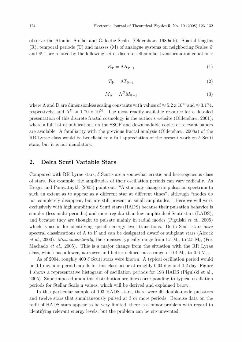
124 Electronic Journal of Theoretical Physics 5, No. 19 (2008) 123–132
observe the Atomic, Stellar and Galactic Scales (Oldershaw, 1989a,b). Spatial lengths
(R), temporal periods (T) and masses (M) of analogue systems on neighboring Scales Ψ
and Ψ-1 are related by the following set of discrete self-similar transformation equations:
RΨ = ΛRΨ−1 (1)
TΨ = ΛTΨ−1 (2)
MΨ = ΛDMΨ−1 (3)
where Λ and D are dimensionless scaling constants with values of ≈ 5.2 x 10¹⁷ and ≈ 3.174,
respectively, and ΛD ≈ 1.70 x 1056. The most readily available resource for a detailed
presentation of this discrete fractal cosmology is the author’s website (Oldershaw, 2001),
where a full list of publications on the SSCP and downloadable copies of relevant papers
are available. A familiarity with the previous fractal analysis (Oldershaw, 2008a) of the
RR Lyrae class would be beneficial to a full appreciation of the present work on δ Scuti
stars, but it is not mandatory.
2. Delta Scuti Variable Stars
Compared with RR Lyrae stars, δ Scutis are a somewhat erratic and heterogeneous class
of stars. For example, the amplitudes of their oscillation periods can vary radically. As
Breger and Pamyatnykh (2005) point out: “A star may change its pulsation spectrum to
such an extent as to appear as a different star at different times”, although “modes do
not completely disappear, but are still present at small amplitudes.” Here we will work
exclusively with high amplitude δ Scuti stars (HADS) because their pulsation behavior is
simpler (less multi-periodic) and more regular than low amplitude δ Scuti stars (LADS),
and because they are thought to pulsate mainly in radial modes (Pigulski et al., 2005)
which is useful for identifying specific energy level transitions. Delta Scuti stars have
spectral classifications of A to F and can be designated dwarf or subgiant stars (Alcock
et al., 2000). Most importantly, their masses typically range from 1.5 M� to 2.5 M� (Fox
Machado et al., 2005). This is a major change from the situation with the RR Lyrae
class, which has a lower, narrower and better-defined mass range of 0.4 M� to 0.6 M�.
As of 2004, roughly 400 δ Scuti stars were known. A typical oscillation period would
be 0.1 day, and period cutoffs for this class occur at roughly 0.04 day and 0.2 day. Figure
1 shows a representative histogram of oscillation periods for 193 HADS (Pigulski et al.,
2005). Superimposed upon this distribution are lines corresponding to typical oscillation
periods for Stellar Scale n values, which will be derived and explained below.
In this particular sample of 193 HADS stars, there were 40 double-mode pulsators
and twelve stars that simultaneously pulsed at 3 or more periods. Because data on the
radii of HADS stars appear to be very limited, there is a minor problem with regard to
identifying relevant energy levels, but the problem can be circumvented.
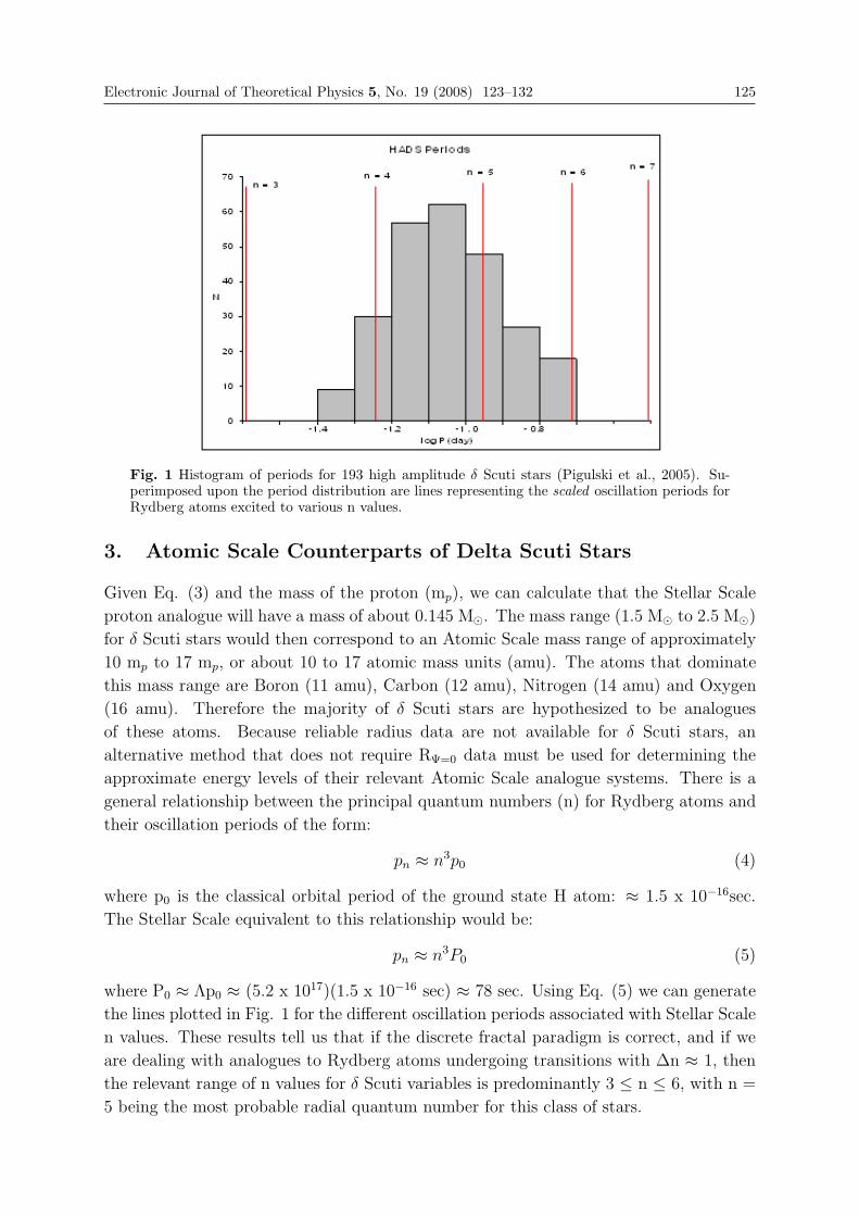
Electronic Journal of Theoretical Physics 5, No. 19 (2008) 123–132 125
Fig. 1 Histogram of periods for 193 high amplitude δ Scuti stars (Pigulski et al., 2005). Su-perimposed upon the period distribution are lines representing the scaled oscillation periods forRydberg atoms excited to various n values.
3. Atomic Scale Counterparts of Delta Scuti Stars
Given Eq. (3) and the mass of the proton (mp), we can calculate that the Stellar Scale
proton analogue will have a mass of about 0.145 M�. The mass range (1.5 M� to 2.5 M�)
for δ Scuti stars would then correspond to an Atomic Scale mass range of approximately
10 mp to 17 mp, or about 10 to 17 atomic mass units (amu). The atoms that dominate
this mass range are Boron (11 amu), Carbon (12 amu), Nitrogen (14 amu) and Oxygen
(16 amu). Therefore the majority of δ Scuti stars are hypothesized to be analogues
of these atoms. Because reliable radius data are not available for δ Scuti stars, an
alternative method that does not require RΨ=0 data must be used for determining the
approximate energy levels of their relevant Atomic Scale analogue systems. There is a
general relationship between the principal quantum numbers (n) for Rydberg atoms and
their oscillation periods of the form:
pn ≈ n3p0 (4)
where p0 is the classical orbital period of the ground state H atom: ≈ 1.5 x 10⁻¹⁶sec.
The Stellar Scale equivalent to this relationship would be:
pn ≈ n3P0 (5)
where P0 ≈ Λp0 ≈ (5.2 x 10¹⁷)(1.5 x 10⁻¹⁶ sec) ≈ 78 sec. Using Eq. (5) we can generate
the lines plotted in Fig. 1 for the different oscillation periods associated with Stellar Scale
n values. These results tell us that if the discrete fractal paradigm is correct, and if we
are dealing with analogues to Rydberg atoms undergoing transitions with Δn ≈ 1, then
the relevant range of n values for δ Scuti variables is predominantly 3 ≤ n ≤ 6, with n =
5 being the most probable radial quantum number for this class of stars.
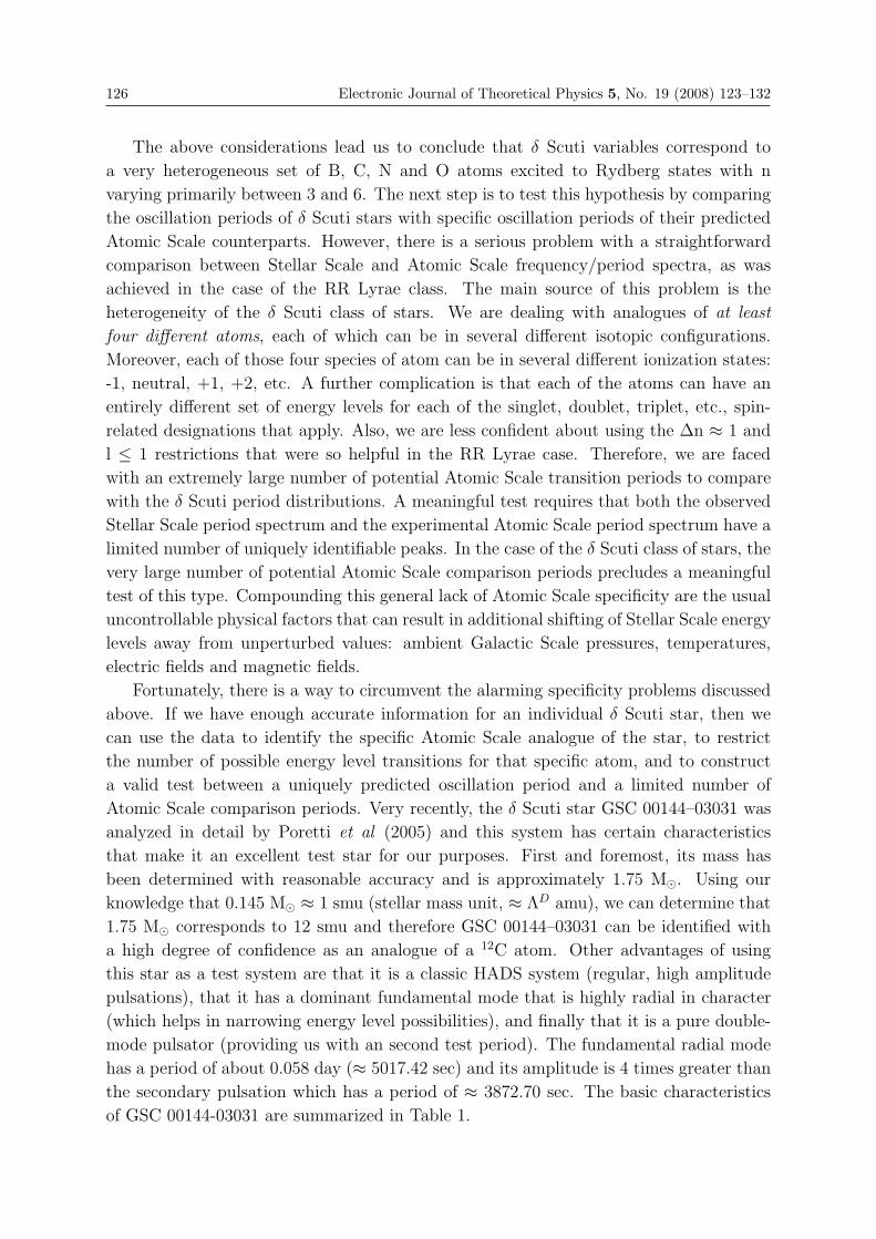
126 Electronic Journal of Theoretical Physics 5, No. 19 (2008) 123–132
The above considerations lead us to conclude that δ Scuti variables correspond to
a very heterogeneous set of B, C, N and O atoms excited to Rydberg states with n
varying primarily between 3 and 6. The next step is to test this hypothesis by comparing
the oscillation periods of δ Scuti stars with specific oscillation periods of their predicted
Atomic Scale counterparts. However, there is a serious problem with a straightforward
comparison between Stellar Scale and Atomic Scale frequency/period spectra, as was
achieved in the case of the RR Lyrae class. The main source of this problem is the
heterogeneity of the δ Scuti class of stars. We are dealing with analogues of at least
four different atoms, each of which can be in several different isotopic configurations.
Moreover, each of those four species of atom can be in several different ionization states:
-1, neutral, +1, +2, etc. A further complication is that each of the atoms can have an
entirely different set of energy levels for each of the singlet, doublet, triplet, etc., spin-
related designations that apply. Also, we are less confident about using the Δn ≈ 1 and
l ≤ 1 restrictions that were so helpful in the RR Lyrae case. Therefore, we are faced
with an extremely large number of potential Atomic Scale transition periods to compare
with the δ Scuti period distributions. A meaningful test requires that both the observed
Stellar Scale period spectrum and the experimental Atomic Scale period spectrum have a
limited number of uniquely identifiable peaks. In the case of the δ Scuti class of stars, the
very large number of potential Atomic Scale comparison periods precludes a meaningful
test of this type. Compounding this general lack of Atomic Scale specificity are the usual
uncontrollable physical factors that can result in additional shifting of Stellar Scale energy
levels away from unperturbed values: ambient Galactic Scale pressures, temperatures,
electric fields and magnetic fields.
Fortunately, there is a way to circumvent the alarming specificity problems discussed
above. If we have enough accurate information for an individual δ Scuti star, then we
can use the data to identify the specific Atomic Scale analogue of the star, to restrict
the number of possible energy level transitions for that specific atom, and to construct
a valid test between a uniquely predicted oscillation period and a limited number of
Atomic Scale comparison periods. Very recently, the δ Scuti star GSC 00144–03031 was
analyzed in detail by Poretti et al (2005) and this system has certain characteristics
that make it an excellent test star for our purposes. First and foremost, its mass has
been determined with reasonable accuracy and is approximately 1.75 M�. Using our
knowledge that 0.145 M� ≈ 1 smu (stellar mass unit, ≈ ΛD amu), we can determine that
1.75 M� corresponds to 12 smu and therefore GSC 00144–03031 can be identified with
a high degree of confidence as an analogue of a 12C atom. Other advantages of using
this star as a test system are that it is a classic HADS system (regular, high amplitude
pulsations), that it has a dominant fundamental mode that is highly radial in character
(which helps in narrowing energy level possibilities), and finally that it is a pure double-
mode pulsator (providing us with an second test period). The fundamental radial mode
has a period of about 0.058 day (≈ 5017.42 sec) and its amplitude is 4 times greater than
the secondary pulsation which has a period of ≈ 3872.70 sec. The basic characteristics
of GSC 00144-03031 are summarized in Table 1.
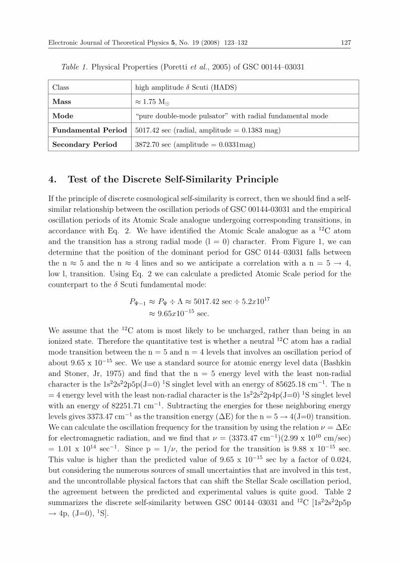
Electronic Journal of Theoretical Physics 5, No. 19 (2008) 123–132 127
Table 1. Physical Properties (Poretti et al., 2005) of GSC 00144–03031
Class high amplitude δ Scuti (HADS)
Mass ≈ 1.75 M�
Mode “pure double-mode pulsator” with radial fundamental mode
Fundamental Period 5017.42 sec (radial, amplitude = 0.1383 mag)
Secondary Period 3872.70 sec (amplitude = 0.0331mag)
4. Test of the Discrete Self-Similarity Principle
If the principle of discrete cosmological self-similarity is correct, then we should find a self-
similar relationship between the oscillation periods of GSC 00144-03031 and the empirical
oscillation periods of its Atomic Scale analogue undergoing corresponding transitions, in
accordance with Eq. 2. We have identified the Atomic Scale analogue as a 12C atom
and the transition has a strong radial mode (l = 0) character. From Figure 1, we can
determine that the position of the dominant period for GSC 0144–03031 falls between
the n ≈ 5 and the n ≈ 4 lines and so we anticipate a correlation with a n = 5 → 4,
low l, transition. Using Eq. 2 we can calculate a predicted Atomic Scale period for the
counterpart to the δ Scuti fundamental mode:
PΨ−1 ≈ PΨ ÷ Λ ≈ 5017.42 sec ÷ 5.2x10¹⁷
≈ 9.65x10⁻¹⁵ sec.
We assume that the 12C atom is most likely to be uncharged, rather than being in an
ionized state. Therefore the quantitative test is whether a neutral 12C atom has a radial
mode transition between the n = 5 and n = 4 levels that involves an oscillation period of
about 9.65 x 10⁻¹⁵ sec. We use a standard source for atomic energy level data (Bashkin
and Stoner, Jr, 1975) and find that the n = 5 energy level with the least non-radial
character is the 1s22s22p5p(J=0) 1S singlet level with an energy of 85625.18 cm−1. The n
= 4 energy level with the least non-radial character is the 1s22s22p4p(J=0) 1S singlet level
with an energy of 82251.71 cm−1. Subtracting the energies for these neighboring energy
levels gives 3373.47 cm−1 as the transition energy (ΔE) for the n = 5 → 4(J=0) transition.
We can calculate the oscillation frequency for the transition by using the relation ν = ΔEc
for electromagnetic radiation, and we find that ν = (3373.47 cm−1)(2.99 x 1010 cm/sec)
= 1.01 x 10¹⁴ sec−1. Since p = 1/ν, the period for the transition is 9.88 x 10⁻¹⁵ sec.
This value is higher than the predicted value of 9.65 x 10⁻¹⁵ sec by a factor of 0.024,
but considering the numerous sources of small uncertainties that are involved in this test,
and the uncontrollable physical factors that can shift the Stellar Scale oscillation period,
the agreement between the predicted and experimental values is quite good. Table 2
summarizes the discrete self-similarity between GSC 00144–03031 and 12C [1s22s22p5p
→ 4p, (J=0), 1S].
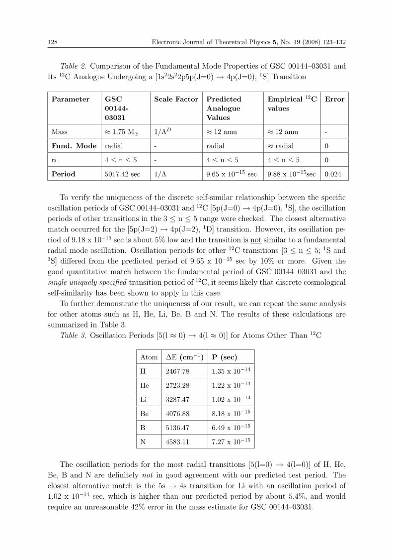
128 Electronic Journal of Theoretical Physics 5, No. 19 (2008) 123–132
Table 2. Comparison of the Fundamental Mode Properties of GSC 00144–03031 and
Its 12C Analogue Undergoing a [1s22s22p5p(J=0) → 4p(J=0), 1S] Transition
Parameter GSC00144-03031
Scale Factor PredictedAnalogueValues
Empirical 12Cvalues
Error
Mass ≈ 1.75 M� 1/ΛD ≈ 12 amu ≈ 12 amu -
Fund. Mode radial - radial ≈ radial 0
n 4 ≤ n ≤ 5 - 4 ≤ n ≤ 5 4 ≤ n ≤ 5 0
Period 5017.42 sec 1/Λ 9.65 x 10⁻¹⁵ sec 9.88 x 10⁻¹⁵sec 0.024
To verify the uniqueness of the discrete self-similar relationship between the specific
oscillation periods of GSC 00144–03031 and 12C [5p(J=0) → 4p(J=0), 1S], the oscillation
periods of other transitions in the 3 ≤ n ≤ 5 range were checked. The closest alternative
match occurred for the [5p(J=2) → 4p(J=2), 1D] transition. However, its oscillation pe-
riod of 9.18 x 10⁻¹⁵ sec is about 5% low and the transition is not similar to a fundamental
radial mode oscillation. Oscillation periods for other 12C transitions [3 ≤ n ≤ 5; 1S and3S] differed from the predicted period of 9.65 x 10−15 sec by 10% or more. Given the
good quantitative match between the fundamental period of GSC 00144–03031 and the
single uniquely specified transition period of 12C, it seems likely that discrete cosmological
self-similarity has been shown to apply in this case.
To further demonstrate the uniqueness of our result, we can repeat the same analysis
for other atoms such as H, He, Li, Be, B and N. The results of these calculations are
summarized in Table 3.
Table 3. Oscillation Periods [5(l ≈ 0) → 4(l ≈ 0)] for Atoms Other Than 12C
Atom ΔE (cm−1) P (sec)
H 2467.78 1.35 x 10⁻¹⁴
He 2723.28 1.22 x 10⁻¹⁴
Li 3287.47 1.02 x 10⁻¹⁴
Be 4076.88 8.18 x 10⁻¹⁵
B 5136.47 6.49 x 10⁻¹⁵
N 4583.11 7.27 x 10⁻¹⁵
The oscillation periods for the most radial transitions [5(l=0) → 4(l=0)] of H, He,
Be, B and N are definitely not in good agreement with our predicted test period. The
closest alternative match is the 5s → 4s transition for Li with an oscillation period of
1.02 x 10⁻¹⁴ sec, which is higher than our predicted period by about 5.4%, and would
require an unreasonable 42% error in the mass estimate for GSC 00144–03031.
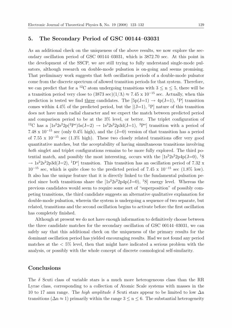
Electronic Journal of Theoretical Physics 5, No. 19 (2008) 123–132 129
5. The Secondary Period of GSC 00144–03031
As an additional check on the uniqueness of the above results, we now explore the sec-
ondary oscillation period of GSC 00144–03031, which is 3872.70 sec. At this point in
the development of the SSCP, we are still trying to fully understand single-mode pul-
sators, although research on double-mode pulsation is on-going and seems promising.
That preliminary work suggests that both oscillation periods of a double-mode pulsator
come from the discrete spectrum of allowed transition periods for that system. Therefore,
we can predict that for a 12C atom undergoing transitions with 3 ≤ n ≤ 5, there will be
a transition period very close to (3873 sec)(1/Λ) ≈ 7.45 x 10⁻¹⁵ sec. Actually, when this
prediction is tested we find three candidates. The [5p(J=1) → 4p(J=1), 1P] transition
comes within 4.4% of the predicted period, but the [(J=1), 1P] nature of this transition
does not have much radial character and we expect the match between predicted period
and comparison period to be at the 3% level, or better. The triplet configuration of12C has a [1s22s22p(2Po)5s(J=2) → 1s22s22p3d(J=1), 3Po] transition with a period of
7.48 x 10⁻¹⁵ sec (only 0.4% high), and the (J=0) version of that transition has a period
of 7.55 x 10⁻¹⁵ sec (1.3% high). These two closely related transitions offer very good
quantitative matches, but the acceptability of having simultaneous transitions involving
both singlet and triplet configurations remains to be more fully explored. The third po-
tential match, and possibly the most interesting, occurs with the [1s22s22p4p(J=0), 1S
→ 1s22s22p3d(J=2), 1Do] transition. This transition has an oscillation period of 7.32 x
10−15 sec, which is quite close to the predicted period of 7.45 x 10⁻¹⁵ sec (1.8% low).
It also has the unique feature that it is directly linked to the fundamental pulsation pe-
riod since both transitions share the [1s22s22p4p(J=0), 1S] energy level. Whereas the
previous candidates would seem to require some sort of “superposition” of possibly com-
peting transitions, the third candidate suggests an alternative qualitative explanation for
double-mode pulsation, wherein the system is undergoing a sequence of two separate, but
related, transitions and the second oscillation begins to activate before the first oscillation
has completely finished.
Although at present we do not have enough information to definitively choose between
the three candidate matches for the secondary oscillation of GSC 00144–03031, we can
safely say that this additional check on the uniqueness of the primary results for the
dominant oscillation period has yielded encouraging results. Had we not found any period
matches at the < 5% level, then that might have indicated a serious problem with the
analysis, or possibly with the whole concept of discrete cosmological self-similarity.
Conclusions
The δ Scuti class of variable stars is a much more heterogeneous class than the RR
Lyrae class, corresponding to a collection of Atomic Scale systems with masses in the
10 to 17 amu range. The high amplitude δ Scuti stars appear to be limited to low Δn
transitions (Δn ≈ 1) primarily within the range 3 ≤ n ≤ 6. The substantial heterogeneity
130 Electronic Journal of Theoretical Physics 5, No. 19 (2008) 123–132
of this class interferes with a simple comparison of sizeable samples of empirical δ Scuti
oscillation periods with predicted periods derived from Atomic Scale data, although this
may be possible in principle. However, we have achieved the specificity required for a
meaningful test of discrete cosmological self-similarity by focusing on an individual, well-
characterized δ Scuti star. Based purely on physical data for GSC 00144–03031, we have
identified:
(1) a specific Atomic Scale analogue (12C),
(2) a most likely energy level transition (1s22s22p5p → 4p, J=0, 1S), and
(3) a uniquely matching self-similar oscillation period (agreement at the 97.6% level).
These new results, combined with the previous successful demonstration (Oldershaw,
2008a,b) of discrete self-similarity between RR Lyrae stars and He atoms undergoing
Δn = 1 Rydberg state transitions, lend further support to our contention that discrete
cosmological self-similarity is a fundamental property of nature. It can be predicted that
the same methods that have been applied here, and in the case of the RR Lyrae stars,
can be successfully applied to other δ Scuti stars if the following criteria are met. The
stellar mass must be known to an accuracy of ≤ 0.05 M�, so that the correct Atomic
Scale analogue can be identified. Ideally the star should pulsate in a single dominant
oscillation mode, although double-mode pulsators can also be analyzed by our methods.
Multi-mode pulsators with three or more low-amplitude periods appear to be analogous
to excited, highly perturbed, atomic systems that are oscillating at several potential
transition periods, but are not yet undergoing single specific transitions between energy
levels, as will be discussed in a forthcoming paper (Oldershaw, 2008c) on the class of ZZ
Ceti variable stars. At any rate, the higher the amplitude of the dominant oscillation
period of the δ Scuti star, the more likely it is that we are observing an event that is
self-similar to a full-fledged transition between discrete energy levels. Although we may
be getting a bit ahead of ourselves here, it is conceivable that a typical single-mode HADS
star evolves from a multi-mode LADS star when the latter absorbs a sufficient amount of
energy at an appropriate frequency in order to trigger a genuine energy level transition.
References
[1] Alcock, C., et al., Astrophys. J. 536, 798-815, 2000.
[2] Bashkin, S. and Stoner, Jr., J.O., Atomic Energy Levels and Grotrian Diagrams
(Vol. I. Hydrogen I – Phosphorus XV), North-Holland Pub. Co., Amsterdam;
American Elsevier Pub. Co., Inc., New York, 1975.
[3] Breger, M. and Pamyatnykh, A.A., preprint, arXiv:astro-ph/0509666 v1, available at
http://www.arXiv.org, 2005.
[4] Fox Machado, L., et al., preprint, arXiv:astro-ph/0510484 v1, submitted to Astron.
and Astrophys., available at http://www.arXiv.org, 2005.
[5] Oldershaw, R.L., Internat. J. Theoretical Physics, 12, 669, 1989a.
[6] Oldershaw, R.L., Internat. J. Theoretical Physics, 12, 1503, 1989b.
Electronic Journal of Theoretical Physics 5, No. 19 (2008) 123–132 131
[7] Oldershaw, R.L., http://www.amherst.edu/∼rloldershaw , 2001.
[8] Oldershaw, R.L., Electron. J. Theoretical Physics, 5(17), 207, 2008a; also availableathttp://www.arxiv.org/ftp/astro-ph/papers/0510/0510147.pdf .
[9] Oldershaw, R. L., Complex Systems, submitted, 2008b; also available athttp://www.arxiv.org/ftp/astro-ph/papers/0606/0606128.pdf .
[10] Oldershaw, R.L., in preparation, 2008c; also available at
http://www.arxiv.org/ftp/astro-ph/papers/0602/0602451.pdf .
[11] Pigulski, A., et al., preprint, arXiv:astro-ph/0509523 v1, available at
http://www.arXiv.org, 2005.
[12] Poretti, E., et al., Astron. and Astrophys., 440, 1097-1104, 2005; also see preprint,arXiv:astro-ph/0506266 v1, available at http://www.arXiv.org, 2005.

EJTP 5, No. 19 (2008) 133–140 Electronic Journal of Theoretical Physics
Neutrino Mixings and Magnetic Moments Due toPlanck Scale Effects
Bipin Singh Koranga∗
Department of Physics, Indian Institute of Technology Bombay, Mumbai 400076, India
Received 2 July 2008, Accepted 16 August 2008, Published 10 September 2008
Abstract: In this paper, we consider the effect of Planck scale operators on neutrino magneticmoments. We assume that the main part of neutrino masses and mixings arise throughGUT scale operators. We further assume that additional discrete symmetries make theneutrino mixing bi-maximal. Quantum gravitational (Planck scale) effects lead to an effectiveSU(2)L×U(1) invariant dimension-5 Lagrangian involving neutrino and Higgs fields, which givesrise to additional terms in neutrino mass matrix. These additional terms can be consideredto be perturbation of the GUT scale bi-maximal neutrino mass matrix. We assume thatthe gravitational interaction is flavor blind and we study the neutrino mixings and magneticmoments due to the physics above the GUT scale.c© Electronic Journal of Theoretical Physics. All rights reserved.
Keywords: Quantum Gravity; Planck Scale; Neutrino Mixings; Neutrino Magnetic MomentsPACS (2008): 04.60.-m; 04.90.+e; 26.35.+c; 26.60.-c
1. Introduction
Neutrino magnetic moments is proportional to the neutrino mass as required by the sym-
metry principles. At present the solar, atmospheric, reactor and accelerator experiments
indicates the existence of non zero neutrino masses. Its indicates that neutrino has a mag-
netic moment. A minimal extension of solar model yields a neutrino magnetic moment
[1]
μν =3eGF mν
8π2√
2=
3GF memν
4π2√
2μB, (1)
where μB = e/2m is the Bohr magnetron, me is the electron mass and mν is the
neutrino mass.

134 Electronic Journal of Theoretical Physics 5, No. 19 (2008) 133–140
The fundamental magnetic moment are associated with the mass eigenstates in the
mass eigenstates basis. Dirac neutrino can have diagonal or off diagonal moment, while
Majorana neutrino can have transition magnetic moments [2, 3, 4]. The experimental
value of neutrino magnetic moment can be determined by only in the recoil electron
spectrum from neutrino electron spectrum [5, 6]. In this paper, we study, how Planck
scale effects the neutrino magnetic moments. Magnetic moment of neutrinos, in principle,
depend on the distance from its source [4]
μ2e =
∑i
|∑
j
Uejμijexp(−iEjL)|2, (2)
where μij is the fundamental constant in term of unit μB that characterize the coupling
of the neutrino mass eigenstate to the electromagnetic field. The expression for μ2e in the
case of Dirac neutrino, with only diagonal magnetic moment (μij = μiδij); this is used
by the Particle Data Group [4]
μ2e =
∑j
|Uej|2|μj|2, (3)
In this expression, there is no dependence of L and neutrino energy E. In this one can
say the neutrino magnetic moments depend on neutrino mixings. In the case of Majorana
neutrino, and we assume three mass eigenstates. Then
μ′2e = (|μ12|2 + |μ13|2)(|Ue2|2 + |Ue3|2). (4)
For the Dirac case this implies that at least nondoagonal magnetic moment is as large
as the diagonal ones. In the case of Majorana, it implies that two different nondiagonal
magnetic moment are of a similar magnitude [16]. Correction to neutrino mixing and
neutrino magnetic moments are given in Section 2. In section 3 give the results on
neutrino mixing and magnetic moments.
2. Corrections to Mixing Angles and Neutrino Magnetic Mo-
ments
The neutrino mass matrix is assumed to be generated by the see saw mechanism [7, 8,
9]. Here we will assume that the dominant part of neutrino mass matrix arises due to
GUT scale operators and they lead to bi-maximal mixing. The effective gravitational
interaction of neutrinos with Higgs field can be expressed as SU(2)L × U(1) invariant
dimension-5 operator [10],
Lgrav =λαβ
Mpl
(ψAαεACψC)C−1ab (ψBbβεBDψD) + h.c. (5)
Here and every where below we use Greek indices α, β..for the flavor states and Latin
indices i, j, k for the mass states. In the above equation ψα = (να, lα) is the lepton
doublet , φ = (φ+, φ0) is the Higgs doublet and Mpl = 1.2× 10¹⁹GeV is the Planck mass.

Electronic Journal of Theoretical Physics 5, No. 19 (2008) 133–140 135
λ is a 3 × 3 matrix in flavour space with each element O(1). In eq(4), all indices are
explicitly shown. The Lorentz indices a, b = 1, 2, 3, 4 are contracted with the charge
conjugation matrix C and the SU(2)L isospin indices A, B, C, D = 1, 2 are contracted with
ε, the Levi-Civita symbol in two dimensions. After spontaneous electroweak symmetry
breaking the Lagrangian in eq(4) generates additional terms of neutrino mass matrix
Lmass =v2
Mpl
λαβναC−1νβ, (6)
where v=174 GeV is the VEV of electroweak symmetry breaking.
We assume that the gravitational interaction is “flavour blind” , that is λαβ is
independent of α, β indices. Thus the Planck scale contribution to the neutrino mass
matrix is
μ λ = μ
⎛⎜⎜⎜⎜⎝1 1 1
1 1 1
1 1 1
⎞⎟⎟⎟⎟⎠ , (7)
where the scale μ is
μ =v2
Mpl
= 2.5 × 10⁻⁶eV. (8)
In our calculation, we take eq(6) as a perturbation to the main part of the neutrino
mass matrix, that is generated by GUT dynamics. We compute the changes in neutrino
mass eigenvalues and mixing angles induced by this perturbation. We assume that GUT
scale operators give rise to the light neutrino mass matrix, which in mass eigenbasis,
takes the form M = diag(M1,M2, M3), where Mi are real and non negative. We take
these to be the unperturbed (0th − order) masses. Let U be the neutrino mixing matrix
at 0th − order. Then the corresponding 0th − order mass matrix M in flavour space is
given by
M = U∗MU †. (9)
The 0th − order MNS matrix U is given in this form
U =
⎛⎜⎜⎜⎜⎝Ue1 Ue2 Ue3
Uμ1 Uμ2 Uμ3
Uτ1 Uτ2 Uτ3
⎞⎟⎟⎟⎟⎠ , (10)
where the nine elements are functions of three mixing angles, one Dirac phase and
two Majorana phases. In terms of the above elements, the mixing angles are defined by
|Ue2
U e1
| = tanθ12,Uμ3
Uτ3
| = tanθ23, |Ue3| = sinθ13. (11)

136 Electronic Journal of Theoretical Physics 5, No. 19 (2008) 133–140
In terms of the above mixing angles, the mixing matrix is written as
U = diag(eif1, eif2, eif3)R(θ23)ΔR(θ13)Δ∗R(θ12)diag(eia1, eia2, 1). (12)
The matrix Δ = diag(eiδ2 , 1, e
−iδ2 ) contains the Dirac phase δ. This leads to CP viola-
tion in neutrino oscillations. a1 and a2 are the so called Majorana phases, which affect
the neutrinoless double beta decay. f1, f2 and f3 are usually absorbed as a part of the
definition of the charge lepton field. It is possible to rotate these phases away, if the mass
matrix eq(5) is the complete mass matrix. However, since we are going to add another
contribution to this mass matrix, these phases of the zeroth order mass matrix can have
an impact on the complete mass matrix and thus must be retained. By the same token,
the Majorana phases which are usually redundant for oscillations have a dynamical role to
play now. Planck scale effects will add other contributions to the mass matrix. Including
the Planck scale mass terms, the mass matrix in flavour space is modified as
M → M′= M + μλ, (13)
with λ being a matrix whose elements are all 1 as discussed in eq(3). Since μ is small,
we treat the second term (the Planck scale mass terms) in the above equation as a per-
turbation to the first term (the GUT scale mass terms). The impact of the perturbation
on the neutrino masses and mixing angles can be seen by forming the hermitian matrix
M′†M
′=(M + μλ)†(M + μλ), (14)
which is the matrix relevant for oscillation physics. To the first order in the small
parameter μ, the above matrix is
M†M + μλ†M + M†μλ. (15)
This hermitian matrix is diagonalized by a new unitary matrix U′. The corresponding
diagonal matrix M′2, correct to first order in μ, is related to the above matrix by U
′M
′2U
′†.
Rewriting M in the above expression in terms of the diagonal matrix M we get
U′M
′2U
′†= U(M2 + m†M + Mm)U † (16)
where
m = μU tλU. (17)
Here M and M′
are the diagonal matrices with neutrino masses correct to 0th and
1th order in μ. It is clear from eq(15) that the new mixing matrix can be written as:
U′= U(1 + iδΘ),

Electronic Journal of Theoretical Physics 5, No. 19 (2008) 133–140 137
=
⎛⎜⎜⎜⎜⎝Ue1 Ue2 Ue3
Uμ1 Uμ2 Uμ3
Uτ1 Uτ2 Uτ3
⎞⎟⎟⎟⎟⎠+
⎛⎜⎜⎜⎜⎝Ue2δΘ
∗12 + Ue3δΘ
∗23, Ue1δΘ12 + Ue3δΘ
∗23, Ue1δΘ13 + Ue3δΘ
∗23)
Uμ2δΘ∗12 + Uμ3δΘ
∗13, Uμ1δΘ12 + Uμ3δΘ
∗23, Uμ1δΘ13 + Uμ3δΘ
∗23
Uτ2δΘ∗12 + Uτ3δΘ
∗13, Uτ1δΘ12 + Uτ3θΘ
∗23, Uτ1δΘ13 + Uτ3δΘ
∗23
⎞⎟⎟⎟⎟⎠ , (18)
where δθ is a hermitian matrix that is first order in μ. From eq(15) we obtain
M2 + m†M + Mm = M′′2
+ [iδΘ,M′2]. (19)
Therefore to first order in μ, the mass squared difference ΔM2ij = M2
i − M2j get
modified [11, 13] as:
ΔM′2ij = ΔM2
ij + 2(MiRe[mii] − MjRe[mjj]). (20)
The change in the elements of the mixing matrix, which we parameterized by δΘ, is
given by
δΘij =iRe(mij)(Mi + Mj)
ΔM′2ij
− Im(mij)(Mi − Mj)
ΔM′2ij
. (21)
The above equation determines only the off diagonal elements of matrix δΘij. The
diagonal elements of δΘ can be set to zero by phase invariance.
The new Majorana neutrino magnetic moments due to Planck scale is given by
μ′2x =
∑j
∑k
|U ′xj|2|μjk|2, (22)
where (x = e, μ τ) is the flavour indices. In the case of three flavour, the magnetic
moment of Majorana electron neutrinos is given by
μ′2e = (|μ12|2 + |μ13|2)(|U
′e2|2 + |U ′
e3|2). (23)
and there is no dependence on the distance L or neutrino energy.
3. Results and Discussions
We assume the largest allowed value of 2 eV for degenerate neutrino mass which comes
from tritium beta decay [12]. We also assume normal neutrino mass hierarchy. Thus we
have M1 =2 eV, M2 =√
M21 + Δ21 and M3 =
√M2
1 + Δ31. As in the case of 0thorder
mixing angles, we can compute 1st order mixing angles in terms of 1st order mixing

138 Electronic Journal of Theoretical Physics 5, No. 19 (2008) 133–140
matrix elements [14]. We expect the mixing angles coming from GUT scale operators to
be determined by some symmetries. For simplicity, here we assume a bi-maximal mixing
pattern, θ12 = θ23 = π/4 and θ13 = 0. We compute the modified mixing angles for the
degenerate neutrino mass of 2 eV. We have taken Δ31 = 0.0025eV 2 and Δ21 = 0.00008eV 2
. For simplicity we have set the charge lepton phases f1 = f2 = f3 = 0. We have checked
that non-zero values for these phases do not change our results. Since we have set θ13 = 0,
the Dirac phase δ drops out of the 0th order mixing matrix. We consider the Planck scale
effects on neutrino mixing and we get the given range of mixing parameter of MNS matrix
U′= R(θ23 + ε3)Uphase(δ)R(θ13 + ε2)R(θ12 + ε1), (24)
In Planck scale, only θ12(ε1 = ±3o)have reasonable deviation and θ13, θ23 deviation
is very small less than 0.3o [14]. In the new mixing at Planck scale we get the given
moments of Majorana neutrinos
μ′2e = (|μ12|2 + |μ13|2)(|U
′e2|2 + |U ′
e3|2). (25)
μ′2μ = (|μ21|2 + |μ23|2)(|U
′μ1|2 + |U ′
μ3|2). (26)
μ′2τ = (|μ31|2 + |μ32|2)(|U
′eτ2|2 + |U ′
eτ3|2). (27)
The best direct limit on the neutrino magnetic moment, μe ≤ 1.8 × 10⁻¹⁰μB at 90%
CL [15], coming from neutrino electron scattering with anti-neutrino. However, the limit
obtained using the SK data [4], μe ≤ 1.5 × 10⁻¹⁰μB.Due to Planck scale effects, mixing
angle θ12 and θ13 will contributes the magnetic moments of neutrinos.
conclusions
We assumed that the main part of neutrino masses and mixings arise from GUT scale
operators. We considered these to be 0th order quantities. We further assumed that
GUT scale symmetries constrain the neutrino mixing angles to be either bi-maximal or
tri-bi-maximal. The gravitational interaction of lepton fields with SM Higgs field gives
rise to an SU(2)L × U(1) invariant dimension-5 effective lagrangian, given originally by
Weinberg [10]. On electroweak symmetry breaking this operator leads to additional mass
terms. We consider these to be a perturbation of GUT scale mass terms. We compute
the first order corrections to neutrino mass eigenvalues and mixing angles. In [11], it
was shown that the change in θ13, due to this perturbation, is small. Here we show that
the change in θ23 also is small (less than 0.3o) but the change in θ12 can be substantial
(about ±3o). The changes in all three mixing angles are proportional to the neutrino mass
eigenvalues. To maximize the change we assumed degenerate neutrino masses ) 2.0 eV.
For degenerate neutrino masses, the changes in θ13 and θ23 are inversely proportional
to Δ31 and Δ32 respectively, whereas the change in θ12 is inversely proportional to Δ21.
Since Δ31∼= Δ32 * Δ21, the change in θ12 is much larger than the changes in θ13 and
Electronic Journal of Theoretical Physics 5, No. 19 (2008) 133–140 139
θ23. In this paper, we write the neutrino magnetic moment expression for three flavour
neutrino mixing. For majarona neutrino two non diagonal moment, these expression are
Eq(4.0) for vacuum mixing. For majorana neutrino with three flavour, the expression is
μ′2e = (|μ12|2 + |μ13|2)(|Ue2|2 + |Ue3|2). In this paper, finally we wish make a important
comment. Due to Planck scale effects mixing angle θ12 and θ13 contribute the magnetic
moments of neutrinos.
References
[1] W. J Marciano and A. I. Sanda, Phys. Lett. B 67, 303-305 (1977).
[2] R. E. Shrock, Nucl. Phys. B 206, 359 (1982).
[3] B. Kayser, Phys. Rev, 1662 (1982).
[4] C. Caso et al., Eur. Phys. J. C3, 1 (1998).
[5] P. Vogel and J. Engel, Phys. Rev. D 39, 3378 (1989).
[6] A. V. Kyuldjiev, Nucl. Phys. B 243, 387 (1984).
[7] A. Gouvea and J. W. F Valle, Phys. Lett. B 501 (2001) 115.
[8] R. N Mohapatra and G. Senjanovic, Phys. Rev. Lett. 44 (1980) 912.
[9] R. N Mohapatra and G. Senjanovic, Phys. Rev. D 23 (1981) 165.
[10] S .Weinberg, Phys. Rev. Lett. 43 (1979) 1566.
[11] F. Vissani, M. Narayan and V. Berezinsky, Phys. Lett. B 571, 209-216, 2003.
[12] Ch. Weinheimer et al, . Phys. Lett. B 460, 219 (1999) ; V. M. Lobashev et al, .Phys. Lett. B 460, 227 (1999).
[13] Bipin Singh Koranga, M. Narayan and S Uma Sankar, arXiv: hep-ph/0607274(Accepted in Phy.Lett B).
[14] Bipin Singh Koranga, M. Narayan and S Uma Sankar, arXiv: hep-ph/0611186.
[15] A. I. Derbin et al, . JETP. Lett. 57, 768 (1993).
[16] J. F. Becaom and P. Vogel, Phys. Rev. Lett. 83, 5222-5225 (1999).

EJTP 5, No. 19 (2008) 141–162 Electronic Journal of Theoretical Physics
Casimir Force in Confined CrosslinkedPolymer Blends
M. Benhamou∗, A. Agouzouk, H. Kaidi, M. Boughou and S. El Fassi,A. Derouiche
Laboratoire de Physique des Polymeres et Phenomenes CritiquesFaculte des Sciences Ben M’sik, B.P. 7955, Casablanca, Morocco
Received 2 May 2008, Accepted 16 August 2008, Published 10 October 2008
Abstract: The physical system we consider is a crosslinked polymer blend (or aninterpenetrating polymer network), made of two chemically incompatible polymers, whichare confined to two parallel plates that are a finite distance L apart, that is L < ξ∗. Here,ξ∗ ∼ aD−1/2 (a being the monomer size and D the reticulation dose) denotes the size of themicrodomains (mesh size). We assume that these strongly adsorb one or the two polymers, nearthe spinodal temperature (critical adsorption). The strong fluctuations of composition give riseto an induced force between the walls we are interested in. To compute this force, as a functionof the separation L, we elaborate a field model, of which the free energy is a functional of thecomposition fluctuation (order parameter). Within the framework of this extended de Gennestheory, we exactly compute this induced force, for two special boundary conditions (symmetricand asymmetric plates). Symmetric plates mean that these have the same preference to adsorbone polymer, while asymmetric ones correspond to the situation where one polymer adsorbs ontothe first plate and the other onto the second one. Using the phase portrait method, we first showthat the induced force is attractive, for symmetric plates, and repulsive, for asymmetric ones.Second, we demonstrate that the force satisfies the scaling laws : Πa = Π0
a.Ωa (L/ξ∗) (symmetricplates) and Πr = Π0
r .Ωr (L/ξ∗) (asymmetric plates). Here, Ωa (x) and Ωr (x) are known universalscaling functions, where Π0
a = −EaL−4 and Π0
r = ErL−4 are the induced forces relative to an
uncrosslinked polymer blend confined to the same geometry (Ea and Er are known amplitudes).For very small distances compared to the mesh size ξ∗, we show that, in any case, the forcedecays exponentially, that is : Πa ) −EaL
−4 exp{−L2/ξ∗ 2
}and Πr ) ErL
−4 exp{−L2/ξ∗ 2
}.
Finally, this work must be regarded as a natural extension of that relative to the uncrosslinkedpolymer blends.c© Electronic Journal of Theoretical Physics. All rights reserved.
Keywords: Casimir Force; Crosslinked Polymer Blends; MaterialsPACS (2008): 28.52.Fa; 61.25.-f; 61.25.Hq ; - 64.75.+g ; 82.70.Gg
∗ Author for correspondence: E-mail: [email protected]
142 Electronic Journal of Theoretical Physics 5, No. 19 (2008) 141–162
1. Introduction
The crosslinked polymer blends (CPBs) and interpenetrating polymer networks (IPNs)
constitute new materials that have many potential applications. Among these, we can
quote the crosslinked epoxy adhesives, the crosslinked mixtures of bacterial and sea-
weed polysaccharides gellan and agarose [1], the polysiloxane interpenetrating networks
[2], and the IPNs made of polypropylene/poly(n-butyl acrylate) [3]. For example, the
formers possess a great resistance to acids, bases and many solvents, and exhibit high
glass transition temperatures and thermal resistance, while the second ones are used as
electronic device encapsulants.
The CPBs and IPNs are made of two chemically incompatible polymers A and B.
Their common feature is that, when they cooled down, below some critical temperature,
one assists to the appearance of microdomains alternatively rich in A and B-polymers.
This is the so-called microphase separation (MPS), which results from a competition
between the tendency that the polymer mixture phase separates completely and the
elasticity of the gel that resists to such a separation.
The pioneered theory of MPS was introduced by Gennes [4], followed by several
extended works [5 − 21]. The de Gennes’ trick was an analogy between the CPB and a
dielectric medium. The theoretical predictions were confirmed experimentally by Briber
and Bauer [22] by small-angle neutron-scattering experiment on the PS-PVME mixture,
which was crosslinked by γ–ray irradiation techniques [23].
Usually, the CPBs and IPNs are trapped not in infinite space but rather in a finite
volume. In other words, they are in the presence of geometrical boundaries. To simplify
their investigation, we assume that these are confined to two parallel walls. In addition,
we suppose that these plates strongly adsorb one or the two crosslinked polymers. This
preferential adsorption, termed critical adsorption in literature [24 − 40], takes place in
the vicinity of le spinodal temperature. Around this temperature, the thermal fluctu-
ations of composition yields an induced force (critical Casimir force) we are interested
in.
The Casimir effect is one of the fundamental discoveries of the last century. This effect
that has been predicted, for the first time, by Hendrick Casimir in 1948 [41], stipulates
that the vacuum quantum fluctuations of a confined electromagnetic field induce an
attractive force between two parallel uncharged conducting plates. The Casimir effect
has been confirmed in more recent experiments by Lamoreaux [42] and by Mohideen and
Roy [43].
Thereafter, Fisher and de Gennes [24] pointed out in a short note that the Casimir
effect also appears in the context of the critical systems (fluids, simple liquid mixtures,
polymer blends, liquid 4He, liquid-crystals), confined to restricted geometries or in the
presence of colloidal particles. For these systems, the critical fluctuations of the order
parameter play the role of the vacuum quantum fluctuations, and then, they lead to
long-ranged forces between the confining walls or between immersed colloids [44].
The Casimir effect related to the critical systems that are confined between two

Electronic Journal of Theoretical Physics 5, No. 19 (2008) 141–162 143
parallel walls or in the presence of immersed colloidal particles, has been the subject
of numerous theoretical and experimental investigations [24, 25, 44 − 70]. Very recently,
these studies were generalized to the critical polymer blends or ternary polymer solutions
[71 − 84].
In this paper, we consider a polymer mixture of two polymers A and B of different
chemical nature, confined to two parallel plates 1 and 2 that are a finite distance L apart.
This mixture is crosslinked in the one-phase region, that is at high-temperature. The
system is prepared in such a way that, near the spinodal temperature, the plates strongly
adsorb one or the two polymers (critical adsorption) [85]. Near criticality, the crosslinked
mixture presents as microdomains, of size ξ∗ ∼ aD−1/2 (a being the monomer size and D
the reticulation dose), which are alternatively rich in A and B-polymers. Therefore, the
length ξ∗ must be compared to the film thickness L. Since the critical fluctuations occurs
in domains of size ξ∗, the Casimir effect is relevant only when the latter is much greater
than L, that is L < ξ∗. The critical adsorption and thermal fluctuations of composition
have as consequence to generate an effective force between plates.
In this work, we are interested in the computation of such a force. For the sake of
simplicity, we will be concerned only by two boundary conditions, depending on wether
the plates have the same preference to attract one polymer (symmetric plates) or they
have an opposite preference (asymmetric plates). The latter boundary condition means
that the plate 1 adsorbs the polymer A and plate 2 the polymer B.
To determine the induced force, we elaborate an extended model taking into account
the plate-polymer interaction. The associated free energy is a functional of the compo-
sition fluctuation ϕ = ΦA − ΦB, where ΦA and ΦB denote the compositions of A and
B-polymers, respectively. With the help of the phase portrait method [71 − 74], we com-
pute the resulting force (per unit area), Π, as a function of separation L. This force is
attractive for symmetric plates and repulsive for asymmetric ones. For the two boundary
conditions, at the spinodal temperature Ts, we find an exact form for the expected force :
Πa = Π0a.Ωa (L/ξ∗) (symmetric plates) and Πr = Π0
r.Ωr (L/ξ∗) (asymmetric plates), with
known universal scaling functions Ωa (x) and Ωr (x). Here, Π0a = (N/kBTs) Δ++ (L/a)−4
(Δ++ ) −7) and Π0r = (N/kBTs) Δ+− (L/a)−4 (Δ+− ) 28) are the induced forces for an
uncrosslinked polymer blend confined to the same geometry, and N the common poly-
merization degree of the crosslinked polymer chains A and B. These scaling forms become
simpler when one is concerned with very small distances compared to the mesh size ξ∗,that is : Πa ) Π0
a exp {−L2/ξ∗ 2} and Πr ) Π0r exp {−L2/ξ∗ 2}. These closer forms indi-
cate that the induced force corresponding to CPBs is less important than that relative to
uncrosslinked ones. This result is natural, since the presence of crosslinks considerably
reduces the critical fluctuations of composition.
The remaining presentation proceeds as follows. In Sec. II, we briefly recall the
essential of the de Gennes theory of MPS of CPBs of infinite extent. The presentation of
the used model and computation of the Casimir force are the aim of Sec. III. We draw
some concluding remarks in the last section.
144 Electronic Journal of Theoretical Physics 5, No. 19 (2008) 141–162
2. MPS Theory
Consider two polymers A and B of different chemical nature, which are crosslinked in their
one-phase region (at high temperature). When the temperature of the system is lowered,
below some critical temperature, one assists to the appearance of microdomains alterna-
tively rich in A and B-polymers. In fact, this MPS is the consequence of a competition
between the usual macrophase separation and the elasticity of the polymer network.
To investigate the MPS, the starting point is the de Gennes (bulk) free energy [4]
Fb [ϕ]
kBT= a−3
∫d3r
(t
2ϕ2 +
u
4ϕ4 + κ(∇ϕ)2 − C
2ϕΔ−1ϕ
), (1)
with T the absolute temperature and kB the Boltzmann constant. The temperature
parameter t is
t =1
2(χc − χ) . (2)
The latter is then proportional to the distance from the consolute point, where χ denotes
the standard Flory interaction parameter, and χc = 2/N represents its critical value
(N being the common polymerization degree of A and B-chains), when the mixture is
uncrosslinked. Notice that the parameter χ has the form : χ = α + β/T , where the
constants α and β depend on the chemical nature of the components A and B. The
gradient term takes into account the interfacial energy between A and B-rich phases,
with the coefficient κ = a2/9 (a is the monomer size). There, u = 1/3N accounts for
the coupling constant, and the field or order parameter ϕ (r) for the local fluctuation of
composition
ϕ (r) = Φ (r) − Φc , (3)
where Φ is the composition of one component of the mixture, say A, and Φc = 1/2 its
critical value. We recall that the first two terms in relation (1) constitute the expansion
of the usual Flory-Huggins free energy [86, 87] around the critical composition, and the
third one describes the gel elasticity. According to de Gennes [4], the internal rigidity
constant C is given by
C ∼ n−2a−2 , (4)
where n is the average number of monomers per strand (section of chains between consec-
utive crosslinks). In Eq. (1), the term −ϕΔ−1ϕ plays the role of the squared polarization
of the dielectric medium in de Gennes’ analogy [4], where Δ−1 represents the inverse of
the Laplacian operator.
The structure factor, S (q), can be obtained keeping only the quadratic terms in field
ϕ. We simply recall its expression [4]
S (q) =1
2κq2 + t + Cq2
, (5)
with q = (4π/λ) sin (θ/2) the module of the wave-vector, where λ is the wavelength of the
incident radiation and θ the scattering-angle. This structure factor exhibits a maximum
Electronic Journal of Theoretical Physics 5, No. 19 (2008) 141–162 145
for
q∗ =
(C
2κ
)1/4
∼ a−1n−1/2 , (6)
of which the inverse q∗ −1 ≡ ξ∗ = (C/2κ)−1/4∼ a
√n represents the size of microdomains
or mesh size. The maximal value, S (q∗), of the structure factor diverges at the spinodal
point for [4]
ts = −2√
2κC ∼ n−1 . (7)
In the following section, we will be interested in the computation of the Casimir force
between two parallel plates delimitating a CPB.
3. Casimir Forces
3.1 Field Model
Consider a CPB that is confined between two parallel adsorptive plates, separated by a
finite distance L. We suppose that, near the spinodal temperature, the plates strongly
adsorb one or the two crosslinked polymers. Then, one is in the critical adsorption regime.
As noted before, the critical adsorption and thermal fluctuations of composition generate
a Casimir force between the parallel plates. The purpose of this work is precisely the
computation of such a force, as a function of thickness L. Since the critical fluctuations
occur inside microdomains, the expected force is significant only for distances smaller
than the mesh size ξ∗ (L < ξ∗).To compute the induced force, we start form the free energy (per unit area) that
describes the confined CPB
F [ϕ]
AkBT=
g
2
2∑i=1
ϕ2i −h
2∑i=1
ϕi+
∫ L
0
dz
a3
[t
2ϕ2 +
u
4ϕ4 + κ
(dϕ
dz
)2
− C
2ϕ
(d2
dz2
)−1
ϕ
], (8)
which is a generalization of that relative to an uncrosslinked one [72]. In the above
definition, A is the common area of plates, t, κ and C are those bulk parameters defined
above, g represents the surface coupling constant measuring the interaction strength
between the crosslinked mixture and the two plates, and the field h is the surface chemical
potentials difference of polymers A and B (reduced by kBT ). There, u = 1/3N is
the coupling constant, and ϕ and ϕi’s are the bulk and surfaces fields, respectively.
The critical adsorption emerges in the limit h → ∞, at fixed coupling constant [36].
This is equivalent to impose the condition that the order parameter at surface goes to
infinity : ϕ0 → ∞, which is the fixed point of the normal transition [36, 37, 88], in the
Renormalization-Group (RG) sense. We have ϕ1 = ϕ2 ≡ ϕ0, for the symmetric plates,
and ϕ1 = ϕ2 = −ϕ0, for the asymmetric ones. Notice that, because of the homogeneity
property of the two plates, the order parameter ϕ depends only on the perpendicular
distance z ∈ [0, L] from one plate taken as origin.
146 Electronic Journal of Theoretical Physics 5, No. 19 (2008) 141–162
The next step consists in the computation of the induced force experienced by the
parallel plates.
3.2 Induced Forces
To determine such a force, we will need the knowledge of the properties of the equilibrium
profile, ϕ (z). The latter can be obtained through a standard minimization of the above
total free energy, that is δF/δϕ = 0. Then, the profile is solution to the following
non-linear differential equation
tϕ + uϕ3 − 2κd2ϕ
dz2− C
(d2
dz2
)−1
ϕ = 0 , (9)
together with the boundary conditions
2a−3κ
[dϕ
dz
]z=0
= gϕ0 − h , 2a−3κ
[dϕ
dz
]z=L
= −gϕ0 + h , (10a)
for the symmetric plates, and
2a−3κ
[dϕ
dz
]z=0
= gϕ0 − h , 2a−3κ
[dϕ
dz
]z=L
= gϕ0 − h , (10b)
for the asymmetric ones.
As pointed out in a very recent work [85], it is difficult to extract the necessary
information directly from the differential equation (9) due to the non-local character
of the inverse Laplacian operator (d2/dz2)−1
. But, when one is interested in distances
smaller than the mesh size ξ∗ (z < ξ∗), it has been shown [85] that the reticulation term
in Eq. (9) can be replaced by
C
(d2
dz2
)−1
ϕ ∼ Cξ∗ 2ϕ . (11)
With these considerations, at the spinodal temperature (t ∼ −ξ∗ −2), the differential equa-
tion (9) becomes
t∗ϕ + uϕ3 − 2κd2ϕ
dz2= 0 , (12)
with the critical temperature parameter t∗ = −α0 (ξ∗/a)−2∼ n−1, where α0 is a positive
numerical coefficient of the order of unity. We have used the fact that C ∼ a−2 (ξ∗/a)−4.
Now, to compute the expected force, the starting point is the first integral of the
above differential equation
κ
(dϕ
dz
)2
= G (ϕ) + K , (13)
with the notation
G (ϕ) =t∗
2ϕ2 +
u
4ϕ4 . (14)
In formula (13), K is an integration constant that depends on the bulk parameters (t∗, u),
the surface ones (c, h) and the separation L.

Electronic Journal of Theoretical Physics 5, No. 19 (2008) 141–162 147
3.2.1 Symmetric Plates
In this case, it is easy to see that the expected profile ϕ (z) exhibits a minimum point at
the middle of the film [73, 75], that is at z = L/2. In this case, the integration constant
K is directly related to the minimal value of the bulk free energy density G (ϕ), that is
K = −G (ϕm). Here, ϕm = ϕ (L/2) is the minimal value of the equilibrium profile.
We have now all necessary ingredients for the computation of the Casimir force orig-
inating from the thermal fluctuations of composition, which are strong near the spinodal
temperature. The key of the problem is the first integral (13), with K = −G (ϕm). It is
easy to see, from this first integral, that the minimal value ϕm of the equilibrium profile
is given by the quadrature formula
L = 2√
κ
∫ ϕ0
ϕm
dϕ√G (ϕ) − G (ϕm)
. (15)
This relationship then expresses the dependence of the minimal value ϕm on separation
L and surface composition ϕ0. On the other hand, the attractive force (per unit area),
Πa, is given by the first derivative of the total free energy, with respect to separation L,
that is Πa = − (1/AkBT ) ∂F/∂L. As in confined uncrosslinked polymer mixtures case
[73, 75], this force is simply given by
Πa = −kBTs
a3G (ϕm) . (16)
(The subscript a on Πa is for attractive). Since the quantity G (ϕm) is positive definite
[73, 75], the force is attractive. Therefore, the induced force is completely determined by
the knowledge of the minimal value ϕm of the profile.
In the critical adsorption limit, the upper bound of the integral in Eq. (15) goes to
infinity (ϕ0 → ∞), and the quadrature formula then reduces to
L = 2√
κ
∫ ∞
ϕm
dϕ√G (ϕ) − G (ϕm)
. (17)
Explicitly, we have
L = 4
√κ
u
∫ ∞
ϕm
dϕ√(ϕ2 − ϕ2
m) (ϕ2 + ϕ2m − ϕ∗ 2)
. (18)
In this equality, the quantity ϕ∗ ≡√
−2t∗/u is nothing else but the non-zero value of the
order parameter ϕ that solves G (ϕ∗) = 0. Therefore, ϕm > ϕ∗ =√
−2t∗/u, to ensure
the condition that G (ϕm) > 0. Making the variable change : ϕ → x = ϕ/ϕm yields
L =4
ϕm
√κ
u
∫ ∞
1
dx√(x2 − 1)
(x2 + 1 − ϕ∗ 2
ϕ2m
) . (19)
Mathematically speaking, the above integral defines an elliptic function [89]. To get
more information about the variation of the expected induced force, we introduce the

148 Electronic Journal of Theoretical Physics 5, No. 19 (2008) 141–162
dimensionless parameter
η =ϕ∗
ϕm
. (20)
Of course, η belongs to the interval ]0, 1[. In term of this parameter, formulae (16) and
(19) rewrite
Πa = Π0afa (η) , (21a)
L
ξ∗= ga (η) , (21b)
with the η-dependent functions
fa (η) =(1 − η2
)⎛⎝∫∞1
dx√(x2−1)(x2+1−η2)∫∞1
dx√x4−1
⎞⎠4
, (21c)
ga (η) = η
∫ ∞
1
dx√(x2 − 1) (x2 + 1 − η2)
. (21d)
The notation
Π0a =
NkBTs
a3
Δ++
(L/a)4 < 0 (21e)
means the Casimir force in uncrosslinked polymer blends case, at the critical temperature
that is identical to the spinodal one Ts. In the above relation, the amplitude Δ++ is such
that [73, 75] : Δ++ ) −7. There, ξ∗ ∼ an1/2 accounts for the mesh size.
Come back to the parametric equations (21a) and (21b) and notice that they give
the exact form for the induced force upon separation L, by simple elimination of the
parameter η. Also, these relations show that the force obeys the following scaling law
Πa = Π0a.Ωa
(L
ξ∗
), L < ξ∗ . (22)
Here, the universal scaling function Ωa (x) identifies to fa (η), where the parameter η can
be determined by inversion of relation (21b).
To have an idea about the magnitude of the expected force, we expand the two
parametric equations (21a) and (21b), to second order, around η = 0. After elimination
of η between these equations, we find that
Πa = Π0a
[1 −
(1 − 2
J
I
)L2
ξ∗ 2+ O
(L4
ξ∗ 4
)], (23)
with the constants
I =
∫ ∞
1
dx√x4 − 1
, J =
∫ ∞
1
dx
(x2 + 1)√
x4 − 1. (24)
The ratio J/I equals 0.27. Of course, there is no difficulty to compute high-order pertur-
bation terms.
Electronic Journal of Theoretical Physics 5, No. 19 (2008) 141–162 149
By an exponentiation of series (23), we find the closer form for the induced force
Πa ) Π0a exp
{− L2
ξ∗ 2
}. (25)
We have rescaled the mesh size ξ∗ as follows : ξ∗ →√
1 − 2J/I ξ∗. This simple formula
calls the following comments.
Firstly, the induced force is attractive, because Π0a < 0.
Secondly, the ratio of the force Πa to the usual one Π0a is a universal scaling function of
the renormalized separation L/ξ∗, independently on the chemical details of the crosslinked
polymer chains and physical nature of plates.
Thirdly, as it should be, the induced force is directly proportional to the polymeriza-
tion degree of the chains before they are crosslinked (through Π0a, relation (21e)).
Fourthly, formula (25) suggests that the induced force in confined CPBs is expo-
nentially small in comparison to that of their homologous with C = 0 (no crosslinks).
As a matter of fact, this is not surprising, since the presence of permanent crosslinks
considerably reduces the critical fluctuations of composition.
Fifthly, at fixed distance, the force is significant only for weakly CPBs (small reticu-
lation dose).
Sixthly, the force vanishes beyond the scale ξ∗, due to the absence of the critical
fluctuations of composition.
Finally, in the limit C = 0 (ξ∗ → ∞), we naturally recover the usual force, that is
Πa → Π0a.
The variation of the attractive force Πa is depicted in Fig. 1, as a function of thickness
L (expressed in a unit). This curve is drawn with the ratio ξ∗/a = 50.
In Fig. 2, we make a comparison between the computed attractive force (C �= 0) and
that relative to an uncrosslinked polymer mixture (C = 0). For the former, the chosen
reticulation dose is such that ξ∗/a = 50. The fact that the curve with C �= 0 is above
that relative to the C = 0 case reflects the discussion made before.
Fig. 3 shows a superposition of the variations of the attractive force, for two values of
the reticulation dose corresponding to the mesh sizes ξ∗1 = 50a and ξ∗2 = 80a. Of course,
the curve with ξ∗ = ξ∗1 is above that with ξ∗ = ξ∗2 . Indeed, the first case corresponds to
a tightly CPB, while the second to a weakly one.
3.2.2 Asymmetric Plates
In this case, it is easy to see that the expected profile ϕ (z) is a monotonous decreasing
function from z = 0 to z = L. The induced force experienced by the asymmetric plates
is rather repulsive, and exactly identifies to the integration constant K, that is
Πr =kBTs
a3K . (26)
150 Electronic Journal of Theoretical Physics 5, No. 19 (2008) 141–162
(The subscript r on Πr is for repulsive). On the other hand, we show that the thickness
L can be given by the following quadrature formula
L = 2√
κ
∫ ∞
0
dϕ√G (ϕ) + K
, (27)
with G (ϕ) that quantity defined in Eq. (14).
Some algebra yields the two parametric equations defining the induced force
Πr = Π0r.fr (η) , (28a)
L
ξ∗= ηgr (η) , (28b)
with the functions
fr (η) =
⎛⎝∫∞0
dx√x4+η2x2+1∫∞
0dx√x4+1
⎞⎠4
, (28c)
gr (η) = η
∫ ∞
0
dx√x4 + η2x2 + 1
, (28d)
where the new parameter η is defined by : η = (4K/u)−1/4√
t∗/2 < 1. There, the
quantity
Π0r =
NkBTs
a3
Δ+−(L/a)4 > 0 (28e)
denotes the Casimir force for an uncrosslinked polymer blend, at the critical temperature
that is identical to the spinodal one Ts, with the amplitude [73, 75] : Δ+− ) 28.
As for symmetric plates, the induced force rewrites on the scaling form
Πr = Π0rΩr
(L
ξ∗
), L < ξ∗ , (29)
with the universal scaling function Ωr (x) that identifies to fr (η), where the parameter η
can be determined by inversion of relation (28b). To second order in L/ξ∗, we find
Πr = Π0r
[1 − 2
J ′
I ′L2
ξ∗ 2+ O
(L4
ξ∗ 4
)], (30)
with the constants
I ′ =
∫ ∞
0
dx√x4 + 1
, J ′ =
∫ ∞
0
x2
(x4 + 1)3/2dx . (31)
Numerically, the ratio J ′/I ′ equals 0.30.
As for symmetric plates, we propose the following closer form for the expected induced
force
Πr ) Π0r exp
{− L2
ξ∗ 2
}. (32)
Electronic Journal of Theoretical Physics 5, No. 19 (2008) 141–162 151
We have rescaled the mesh size ξ∗ as follows : ξ∗ → 2√
J ′/I ′ ξ∗. The above scaling
law tells us that the Casimir force in confined CPBs is exponentially small, when it is
compared to its homologous in the absence of crosslinks.
Emphasize that similar comments could be made for asymmetric plates. In addition,
we note that, as for confined uncrosslinked polymer mixtures, the repulsive force remains
more important that the attractive one. This fact is explained in Refs. [73] and [75].
In Fig. 4, we report the variation of the repulsive force Πr upon separation L (ex-
pressed in a unit). This curve is drawn with the ratio ξ∗/a = 50.
Fig. 5 shows a comparison between the computed repulsive force (C �= 0) and that
relative to an uncrosslinked polymer mixture (C = 0). For the former, the chosen retic-
ulation dose is such that ξ∗/a = 50. Of course, the curve with C �= 0 is below that with
C = 0, since the thermal fluctuations of composition are reduced due to the presence of
permanent reticulations.
In Fig. 6, we superpose the variations of the repulsive force, for two values of the
reticulation dose corresponding to the mesh sizes ξ∗1 = 50a and ξ∗2 = 80a. The fact that
the curve with ξ∗ = ξ∗1 is below that with ξ∗ = ξ∗2 is a natural tendency, since the critical
fluctuations of the order parameter are less important when one is interested in tightly
CPBs.
Conclusions
The goal of the present work was the computation of the Casimir force between two
parallel plates delimitating a critical CPB. Near the spinodal temperature, the plates
strongly adsorb one or the two polymers. The critical fluctuations of composition imply an
induced force between the parallel walls. Within the framework of an extended de Gennes
theory, we exactly computed this force, for two special boundary conditions (symmetric
and asymmetric plates).
With the help of the phase portrait method, we have shown, first, that the induced
force is attractive for symmetric plates and repulsive for asymmetric ones. Second, we
found that the force obeys the scaling laws : Πa = Π0a.Ωa (L/ξ∗) (symmetric plates)
and Πr = Π0r.Ωr (L/ξ∗) (asymmetric plates), with known universal scaling functions
Ωa (x) and Ωr (x). Here, Π0a ∼ −L−4 and Π0
r ∼ L−4 account for the induced force of
an uncrosslinked polymer blend confined to the same geometry. For very small distances
compared to the mesh size ξ∗ ∼ aD−1/2 (a being the monomer size and D = 1/n the
reticulation dose), we have shown that the force obeys an exponential decay, that is :
Πa ∼ −L−4 exp {−L2/ξ∗ 2} and Πr ∼ L−4 exp {−L2/ξ∗ 2}, with known amplitudes.
We note that these results also remain valid for confined IPNs. Therefore, the expres-
sion of the Casimir force does not depend on the nature of reticulations.
Emphasize that the used model is a mean-field theory, which is reliable only for high-
molecular-weight polymer mixture, as demonstrated, many years ago, by de Gennes [90].
For low-molecular-weight polymer mixtures, however, the mean-field theory is no longer
valid. To go beyond this approach, and in order to get correct results, it would be
152 Electronic Journal of Theoretical Physics 5, No. 19 (2008) 141–162
necessary to use the RG-techniques [91, 92].
Also, we point out that it would be interesting to introduce a good solvent as a third
component and study its effects on the induced force. As a matter of fact, the solvent
adds new fluctuations of composition, and then, a drastic change of the force expression
is expected.
Finally, this work must be considered as a natural extension of that relative to un-
crosslinked polymer blends [73, 75].
Acknowledgments
We are much indebted to Professor M. Daoud for fruitful discussions, and to Professors
S. Dietrich, E. Eisenriegler and M. Krech for useful correspondences.
References
[1] E. Amici, A.H. Clark, V. Normand, and N.B. Johnson, Biomacromolecules 1, 721(2000).
[2] G. J. Gibbons and D. Holland, J. Sol-Gel Sci. & Techn. 8, 599 (1997).
[3] C. Zhao, M. Xu, W. Zhu, and X. Luo, Polymer 39, 275 (1998).
[4] P.-G. de Gennes, J. Phys. Lett. (Paris) 40, 69 (1979).
[5] A. Bettachy, A. Derouiche, M. Benhamou, and M. Daoud, J. Phys. II (Paris) 1, 153(1991).
[6] A. Derouiche, A. Bettachy, M. Benhamou, and M. Daoud, Macromolecules 25, 7188(1992).
[7] T. A. Vilgis, M. Benmouna, M. Daoud, M. Benhamou, A. Bettachy, and A.Derouiche, Polym. Network Blends 3, 59 (1993).
[8] M. Benhamou, Int. J. Mod. Phys. A 8, 2581 (1993).
[9] M. Benmouna, T.A. Vilgis, M. Daoud, and M. Benhamou, Macromolecules 27, 1172(1994).
[10] M. Benmouna, T.A. Vilgis, M. Benhamou, A. Babaoui, and M. Daoud, Macromol.:Theory Simul. 3, 557 (1994).
[11] A. Bettachy, A. Derouiche, M. Benhamou, M. Benmouna, T.A. Vilgis, and M. Daoud,Macromol.: Theory Simul. 4, 67 (1995).
[12] M. Benhamou, J. Chem. Phys. 102, 5854 (1995).
[13] D. J. Read, M.G. Brereton, and T.C.B. McLeish, J. Phys. II (Paris) 5, 1679 (1995).
[14] A. Bettachy, Ph.D thesis, University of Hassan II-Mohammedia, 1995.
[15] A. Derouiche, Ph.D thesis, University of Hassan II-Mohammedia, 1995.
[16] A. Babaoui, Ph.D thesis, University of Hassan II-Mohammedia, 1995.
[17] M. Riva and V.G. Benza, J. Phys. II (Paris) 7, 285 (1997).

Electronic Journal of Theoretical Physics 5, No. 19 (2008) 141–162 153
[18] M. Benhamou, A. Derouiche, and A. Bettachy, J. Chem. Phys. 106, 2513 (1997).
[19] M. Riva and V.G. Benza, J. Phys. II (Paris) 7, 285 (1997).
[20] A. Derouiche, M. Benhamou, and A. Bettachy, Eur. Phys. J. E 13, 353 (2005).
[21] M. Benhamou and M. Chahid, Physica A 373, 153 (2007).
[22] R.M. Briber and B.J. Bauer, Macromolecules 21, 3296 (1988).
[23] M. Dole, The Radiation Chemistry of Macromolecules, Vols. I and II, Academic Press,New York, 1972.
[24] M. E. Fisher and P.-G. de Gennes, C. R. Acad. Sci. (Paris) Ser. B 287, 207 (1978).
[25] P.-G. de Gennes, C. R. Acad. Sci. (Paris) II 292, 701 (1981).
[26] J. Rudnik and D. Jasnow, Phys. Rev. Lett. 48, 1059 (1982).
[27] S. Leibler and L. Peliti, J. Phys. C 15, L–403 (1982).
[28] D. Beysens and S. Leibler, J. Phys. Lett. (Paris) 43, L–133 (1982).
[29] C. Franck and S.E. Schnatterly, Phys. Rev. Lett. 48, 763 (1982).
[30] L. Peliti and S. Leibler, J. Phys. C 16, L–2635 (1983).
[31] E. Brezin and S. Leibler, Phys. Rev. B 27, 594 (1983).
[32] S. Leibler, Ph.D thesis, University Paris XI, 1984.
[33] J. A. Dixon, M. Schlossman, X.-L. Wu, and C. Franck, Phys. Rev. B 31, 1509 (1985).
[34] M. Schlossman, X.-L. Wu, and C. Franck, Phys. Rev. B 31, 1478 (1985).
[35] S. Blumel and G.H. Findenegg, Phys. Rev. Lett. 54, 447 (1985).
[36] H. W. Diehl, in Phase Transitions and Critical Phenomena, Vol. 10, edited by C.Domb and J.L. Lebowitz, Academic Press, London, 1986.
[37] S. Dietrich, in Phase Transitions and Critical Phenomena, Vol. 12, edited by C. Domband J.L. Lebowitz, Academic Press, London, 1988.
[38] H. Zhao et al., Phys Rev. Lett. 75, 1977 (1995).
[39] A. Hanke, M. Krech, F. Schlesener, and S. Dietrich, Phys. Rev. E 60, 5163 (1999).
[40] Critical adsorption on curved objects, such as single spherical and rod-like colloidalparticles, has been investigated in : A. Hanke and S. Dietrich, Phys. Rev. E 59, 5081(1999) ; A. Hanke, Phys. Rev. Lett. 84, 2180 (2000).
[41] H.B.G. Casimir, Proc. Kon. Ned. Akad. Wetenschap B 51, 793 (1948).
[42] S. K. Lamoreaux, Phys. Rev. Lett. 78, 5 (1997).
[43] U. Mohideen and A. Roy, Phys. Rev. Lett. 81, 4549 (1998).
[44] M. Krech, The Casimir Effect in Critical Systems, World Scientific, Singapore, 1994.
[45] K. Symanzik, Nucl. Phys. B 190 [FS], 1 (1981).
[46] E. Brezin, J. Phys. (Paris) 43, 15 (1982).
[47] N.M. Barber, in Phase Transitions and Critical Phenomena, edited by C. Domb andM.S. Green, Vol. 8, Academic Press, New York, 1983.
154 Electronic Journal of Theoretical Physics 5, No. 19 (2008) 141–162
[48] D. Beysens and D. Esteve, Phys. Rev. Lett. 54, 2123 (1985).
[49] K. K. Mon, Phys. Rev. Lett. 54, 2671 (1985).
[50] J. L. Cardy, Nucl. Phys. B 275, 200 (1986).
[51] I. Affleck, Phys. Rev. Lett. 56, 746 (1986).
[52] H. W. J. Blote, J.L. Cardy, and M.P. Nightingale, Phys. Rev. Lett. 56, 742 (1986).
[53] V. Gurfein, D. Beysens, and F. Perrot, Phys. Rev. A 40, 2543 (1989).
[54] V. Privman, in Finite Size Scaling and Numerical Simulation of Statistical Systems,edited by V. Privman, World Scientific, Singapore, 1990.
[55] M. Krech and S. Dietrich, Phys. Rev. Lett. 66, 345 (1991).
[56] T. W. Burkhardt and T. Xue, Phys. Rev. Lett. 66, 895 (1991).
[57] T. W. Burkhardt and T. Xue, Nucl. Phys. B 345, 653 (1991).
[58] M. Krech and S. Dietrich, Phys. Rev. Lett. 67, 1055 (1991).
[59] M. Krech and S. Dietrich, Phys. Rev. A 46, 1886 (1992).
[60] M. Krech and S. Dietrich, Phys. Rev. A 46, 1922 (1992).
[61] M. L. Broide, Y. Garrabos, and D. Beysens, Phys. Rev. E 47, 3768 (1993).
[62] T. Narayanan, A. Kumar, E.S.R. Gopal, D. Beysens, P. Guenoun, and G. Zalczer,Phys. Rev. E 48, 1989 (1993).
[63] T. W. Burkhardt and E. Eisenriegler, Nucl. Phys. B 424 [FS], 487 (1994).
[64] E. Eisenriegler and M. Stapper, Phys. Rev. B 50, 10009 (1994).
[65] T. W. Burkhardt and E. Eisenriegler, Phys. Rev. Lett. 74, 3189 (1995).
[66] E. Eisenriegler and U. Ritschel, Phys. Rev. B 51, 13717 (1995).
[67] M. Krech and D.P. Landau, Phys. Rev. E 53, 4414 (1996).
[68] R. R. Netz, Phys. Rev. Lett. 76, 3646 (1996).
[69] M. Krech, Phys. Rev. E 56, 1642 (1997).
[70] F. Schlesener, A. Hanke, and S. Dietrich, J. Stat. Phys. 110, 981 (2003).
[71] R. Cherrabi, Ph.D thesis, University of Hassan II-Mohammedia, 1998.
[72] A. Saout Elhak, R. Cherrabi, M. Benhamou, and M. Daoud, J. Chem. Phys. 111,8174 (1999).
[73] R. Cherrabi, A. Saout Elhak, M. Benhamou, and M. Daoud, Phys. Rev. E 62, 6795(2000).
[74] A. Saout Elhak, Ph.D thesis, University of Hassan II-Mohammedia, 2000.
[75] E.-K. Hachem, M. Benhamou, and M. Daoud, J. Chem. Phys. 116, 8168 (2002).
[76] H. Ridouane, E.-K. Hachem, and M. Benhamou, J. Chem. Phys. 118, 10780 (2003).
[77] H. Ridouane, E.-K. Hachem, and M. Benhamou, Cond. Matter Phys. 7, 63 (2004).
[78] H. Ridouane, Thesis, Hassan II-Mohammedia University, 2004.
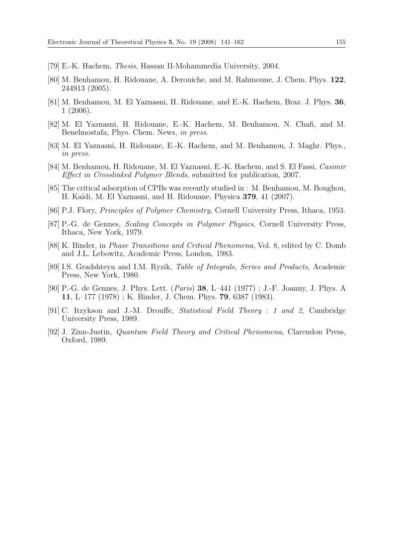
Electronic Journal of Theoretical Physics 5, No. 19 (2008) 141–162 155
[79] E.-K. Hachem, Thesis, Hassan II-Mohammedia University, 2004.
[80] M. Benhamou, H. Ridouane, A. Derouiche, and M. Rahmoune, J. Chem. Phys. 122,244913 (2005).
[81] M. Benhamou, M. El Yaznasni, H. Ridouane, and E.-K. Hachem, Braz. J. Phys. 36,1 (2006).
[82] M. El Yaznasni, H. Ridouane, E.-K. Hachem, M. Benhamou, N. Chafi, and M.Benelmostafa, Phys. Chem. News, in press.
[83] M. El Yaznasni, H. Ridouane, E.-K. Hachem, and M. Benhamou, J. Maghr. Phys.,in press.
[84] M. Benhamou, H. Ridouane, M. El Yaznasni, E.-K. Hachem, and S. El Fassi, CasimirEffect in Crosslinked Polymer Blends, submitted for publication, 2007.
[85] The critical adsorption of CPBs was recently studied in : M. Benhamou, M. Boughou,H. Kaıdi, M. El Yaznasni, and H. Ridouane, Physica 379, 41 (2007).
[86] P.J. Flory, Principles of Polymer Chemistry, Cornell University Press, Ithaca, 1953.
[87] P.-G. de Gennes, Scaling Concepts in Polymer Physics, Cornell University Press,Ithaca, New York, 1979.
[88] K. Binder, in Phase Transitions and Critical Phenomena, Vol. 8, edited by C. Domband J.L. Lebowitz, Academic Press, London, 1983.
[89] I.S. Gradshteyn and I.M. Ryzik, Table of Integrals, Series and Products, AcademicPress, New York, 1980.
[90] P.-G. de Gennes, J. Phys. Lett. (Paris) 38, L–441 (1977) ; J.-F. Joanny, J. Phys. A11, L–177 (1978) ; K. Binder, J. Chem. Phys. 79, 6387 (1983).
[91] C. Itzykson and J.-M. Drouffe, Statistical Field Theory : 1 and 2, CambridgeUniversity Press, 1989.
[92] J. Zinn-Justin, Quantum Field Theory and Critical Phenomena, Clarendon Press,Oxford, 1989.
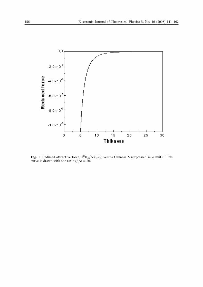
156 Electronic Journal of Theoretical Physics 5, No. 19 (2008) 141–162
Fig. 1 Reduced attractive force, a3Πa/NkBTs, versus thikness L (expressed in a unit). Thiscurve is drawn with the ratio ξ∗/a = 50.
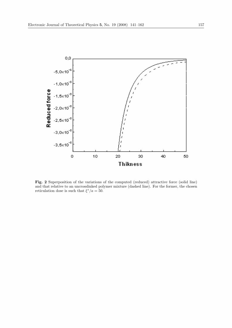
Electronic Journal of Theoretical Physics 5, No. 19 (2008) 141–162 157
Fig. 2 Superposition of the variations of the computed (reduced) attractive force (solid line)and that relative to an uncrosslinked polymer mixture (dashed line). For the former, the chosenreticulation dose is such that ξ∗/a = 50.
158 Electronic Journal of Theoretical Physics 5, No. 19 (2008) 141–162
Fig. 3 Superposition of the variations of the computed (reduced) attractive force upon thiknessL (expressed in a unit), for two reticulation doses corresponding to the mesh sizes : ξ∗1 = 50a(solid line) and ξ∗2 = 80a (dashed line).

Electronic Journal of Theoretical Physics 5, No. 19 (2008) 141–162 159
Fig. 4 Reduced repulsive force, a3Πr/NkBTs, versus thikness L (expressed in a unit). Thiscurve is drawn with the ratio ξ∗/a = 50.

160 Electronic Journal of Theoretical Physics 5, No. 19 (2008) 141–162
Fig. 5 Superposition of the variations of the computed (reduced) repulsive force (solid line) andthat relative to an uncrosslinked polymer mixture (dashed line). For the former, the chosenreticulation dose is such that ξ∗/a = 50

Electronic Journal of Theoretical Physics 5, No. 19 (2008) 141–162 161
Fig. 6 Superposition of the variations of the computed (reduced) repulsive force upon thiknessL (expressed in a unit), for two reticulation doses corresponding to the mesh sizes : ξ∗1 = 50a(solid line) and ξ∗2 = 80a (dashed line).


EJTP 5, No. 19 (2008) 163–168 Electronic Journal of Theoretical Physics
Transport Properties of Thermal Shot NoiseThrough Superconductor-Ferromagnetic /2DEG
Junction
Attia A. Awad Alla1∗, and Adel H. Phillips2
1Physics Department, Faculty of Science, Beni-Suef University, Beni-Suef, Egypt2Faculty of Engineering, Ain-Shams University, Cairo, Egypt
Received 29 December 2007, Accepted 20 August 2008, Published 10 October 2008
Abstract: We study transport properties of thermal shot noise, thermo power and thermalconductance through superconductor-ferromagnetic /2DEG junction under the effect of Fermienergy, number of open channels and excitation energy. Thermal shot noise, PThermal is directlyrelated to the conductance through the fluctuation- dissipation theorem; the model consists ofa 2DEG region inserted between two identical superconductor electrodes. Ferromagnetic stripsare placed onto top of each superconductor/2DEG junction and voltage applied across themodel. The results show an oscillatory behavior of the dependence of the thermal shot noise onFermi energy. These results agree with existing experiments. This research is very importantfor using a model as a high-frequency shot noise detector.c© Electronic Journal of Theoretical Physics. All rights reserved.
Keywords: Ferromagnetic Strips; Excitation Energy; Andreev Reflections; Thermal Shot Noise;Thermo PowerPACS (2008): -73.23.-b; 73.40.-c; 73.63.-b
1. Introduction
On chip noise detection schemes, where device and detector are coactively coupled within
sub millimeter length scales, can benefit from large frequency bandwidths. This results
in a good sensitivity and allows one to study the quantum limit of noise, where an asym-
metry can occur in the spectrum between positive and negative frequencies [1, 2]. Shot
noise measurements allow us to access the dynamical properties of a resonant tunneling
device which are not accessible by measuring solely the average current [2]. Shot noise
is more interesting, because it contains information on the temporal correlation of the

164 Electronic Journal of Theoretical Physics 5, No. 19 (2008) 163–168
electrons which is not contained in the conductance [3-4].
In this paper we study transport properties of thermal shot noise, thermo power and
the thermal conductance through superconductor-ferromagnetic /2DEG junction.
2. Method of Calculation
The model consists of a 2DEG region inserted between two identical superconductor elec-
trodes. Ferromagnetic strips are placed onto top of each superconductor/2DEG junction
and voltage applied across the model [4]. In order to study electron transport in the
model we make us of the Bogolubove-de Gennes equation [5]. Within the Landauer-
Buttiker scattering approach, the conductance thought the system biased at the across
applied voltage Va can be written as [6]
G(ε) =( e
h
)∫ ∞
−∞dεγ(ε)
(−∂f(ε − eVa)
∂ε
)(1)
Where γ(ε)is tunneling probability and given by
γ(ε) = [N(ε) − R0(ε) + RA(ε)] (2a)
and (−∂f(ε − eVa
∂ε
)= (4KBT )−1Cosh
(ε − εF − eVa
2KBT
)(2b)
Where R0(ε) and RA(ε) are normal, Andreev reflection and N(ε) is the number of open
channels in the system, Va applied voltage, f is the Fermi distribution temperature, ε
is the excitation energy, Δ0( Niobium)=0.0015 eV is the superconducting energy gap ,
critical temperature Tc(Niobium)= 9.3 K, critical magnetic field Bc(Niobium)= 0.1985
Tesla and coherence length ξ0 (Niobium)=38 nm.
Thermal shot noise, PThermal is directly related to the conductance through the
fluctuation- dissipation theorem [7]
PThermal = (4KBT )( e
h
)∫ ∞
−∞dεγ(ε)
(−∂f(ε − eVa)
∂ε
)(3)
Thermal shot noise is more interesting, because it contains information on the temporal
correlation of the electrons which is not contained in the conductance. The thermo power
S, of the system is given by [8]
S = −L/G (4)
Where L, is thermo-electric coefficient and G, is the conductance.
The thermal conductance, K, is given by
K(ε) = −(
π2k2B
3e
)(T
h
)∫ ∞
−∞dεγ(ε)
(−∂f(ε − eVa)
∂ε
)(5)

Electronic Journal of Theoretical Physics 5, No. 19 (2008) 163–168 165
3. Results and Discussions
The thermal shot noise, PThermal, thermo power, S, and the thermal conductance, K,
Eqs. 3, 4 and 5 has been computed respectively over Fermi energy, excitation energy,
magnetic field and applied voltage. The calculations were performed for the cases: Fig.
(1) Show that thermal shot noise as a function of the Fermi energy at different value
of the temperature, this results show an oscillatory behavior of the dependence of the
thermal shot noise on Fermi energy, the coincidence of peaks in the thermal shot noise
with steps in the Fermi energy is clearly visible; these oscillations are due to Coulomb
blockade effect [9-11]. Fig. (2) Show that Periodic suppression of thermal conductance
as a function of the number of open channels at different applied voltage, the value of
thermal conductance it is very high with the increasing the number of open channels. Fig.
(3) Show that thermo power as a function of the magnetic field at different temperatures,
the value of thermo power decreasing with increasing the magnetic field, the results show
an oscillatory behavior of the dependence of the thermo power on magnetic field [11, 12].
Fig. (4) Show that thermo power as a function of the excitation energy, ε, a crossover
from the quantization behavior of the thermo power to a δ–function behavior, might
be explained as the probability for normal reflections R0(ε) be more dominant over the
Andreev reflections RA(ε) for large numbers of open channels in the system N(ε) [12-14].
Our results are in good concordant with those in the literature [12-18].
Conclusion
In this paper we study transport properties of thermal shot noise, thermal conductance
and thermo power through superconductor-ferromagnetic /2DEG junction under the ef-
fect of Fermi energy, number of open channels and excitation energy. These results agree
with existing experiments. This research is very important for using a model as a high-
frequency shot noise detector.
References
[1] R. Aguado and L. P. Kouwenhoven, Phys. Rev. Lett.84, 1986(2000).
[2] G. B. Lesovik, JETP Lett. 49, 592 (1989).
[3] M. Reznikov, M. Heiblum, H. Shtrikman, D. Mahalu, Phys. Rev. Lett. 75, 3340(1995).
[4] Attia A. Awad Alla, Applied Science, 8, 23 (2006).
[5] P. G. de Gennes, Superconductivity of Metals and Alloys (Addison-Wesley, NewYork, 1989).
[6] R. Landauer, Philos. Mag. 21, 863 (1970); M. Buttiker, Phys. Rev. Lett. 57, 1761(1986).
[7] I. Hapke-Wurst, U. Zeitler, H. Frahm, A.G.M. Jansen, R.J. Haug, and K. Pierz,Phys. Rev. B, 62, 12621(2000).

166 Electronic Journal of Theoretical Physics 5, No. 19 (2008) 163–168
[8] G. Williamson, L. P. Kouwenhoven, D. van der Marel, C. T. Foxon, Phys. Rev Lett.,60, 848 (1988); Phys. Rev. B 43, 12431(1991).
[9] A. Nauen, F. Hohls , N. Maire, K. Pierz, and R.J. Haug, Phys. Rev. B,70,033305(2004).
[10] Attia A. Awad Alla, Arafa H. Aly, and Adel H. Phillips, International Journal ofNanoscience, Vol. 6, No. 1,41-44 (2007).
[11] F. Zhou, J. H. Seol, A. L. Moore, Q. L. Ye, and R. Scheffler, J. Phys.: CondenseMatter 18, 9651–9657 (2006).
[12] Attia A. Awad Alla, and Adel H. Phillips, International Journal of Modern PhysicsB, 21, No.31, 1-6 (2007).
[13] Mesoscopic Phenomena in Solids, edited by B. L. Atshuler, P.A. Lee and R. A. Webb(Elsevier, Amestrdam,1991).
[14] J. Ankerhold, Europhys. Lett 67, 280 (2004).
[15] Arafa H. Aly, Attia A. Awad Alla, Adel H. Phillips, Ayman S. Atallah, InternationalJournal of Mathematics and Computer Science, 1,173 (2006).
[16] S. Camalet, J. Lehmann, S. Kohler, and P. Hanggi, Phys. Rev. Lett. 90, 210602(2003).
[17] G. Kiesslich, A. Wacker, and E. Scholl, Phys. Rev. B, 68, 17, 125320(2003).
[18] Attia A. Awad Alla and Adel H. Phillips, Chinese Physics Lett. , Vol. 24, No. 5,1339-1341(2007).

Electronic Journal of Theoretical Physics 5, No. 19 (2008) 163–168 167
Fig. 1 Thermal shot noise as a function of the Fermi energy.
Fig. 2 Thermal conductance as a function of the number of open channels at different appliedvoltage.

168 Electronic Journal of Theoretical Physics 5, No. 19 (2008) 163–168
Fig. 3 Thermo power as a function of the magnetic field at different temperatures.
Fig. 4 Thermo power as a function of the excitation energy, ε , a crossover from the quantizationbehavior of the thermo power to a δ –function behavior.
EJTP 5, No. 19 (2008) 169–176 Electronic Journal of Theoretical Physics
On the Genuine Bound States of a Non-RelativisticParticle in a Linear Finite Range Potential
Nagalakshmi A. Rao1∗ and B. A. Kagali2†
1Department of Physics, Government Science College,Bangalore-560001, Karnataka, India
2Department of Physics, Bangalore University, Bangalore-560056, India
Received 19 August 2008, Accepted 16 September 2008, Published 10 October 2008
Abstract: We explore the energy spectrum of a non-relativistic particle bound in a linearfinite range, attractive potential, envisaged as a quark-confining potential. The intricatetranscendental eigenvalue equation is solved numerically to obtain the explicit eigen-energies.The linear potential, which resembles the triangular well, has potential significance in particlephysics and exciting applications in electronicsc© Electronic Journal of Theoretical Physics. All rights reserved.
Keywords: Linear Potential, Eigenenergy, Airy Equation, Quark-ConfinementPACS (2008): 03.65.Ge; 02.10.Eb, 02.30.Gp, 14.65.-q
1. Introduction
A challenging problem in particle physics in recent years is that of quark confinement. It
is presently known that mesons are not elementary particles, but are composed of quarks,
as are the nucleons.
In literature, several approximation methods are available relating to quark confine-
ment. The lattice model [1] suggests that at large distance between quarks, the interac-
tion increases approximately linearly with separation. The bag model, where quarks and
gluons are confined in a bag, is not suitable for calculating the hadronic properties of
heavy quarks or in computing the energy levels of excited states. String model, on the
other hand, proposes quark-antiquark pair at the ends of an open string and creation
of quark-antiquark pair when the string breaks. In recent years, potential models [2] are
best justified theoretically to describe heavy quarkonia and seem to be most powerful in
170 Electronic Journal of Theoretical Physics 5, No. 19 (2008) 169–176
calculating the static properties.
Several authors [3 - 6] have addressed the bound states of various kinds of linear
potential. Chiu [7] has examined the quarkonium systems with the regulated linear
plus Coulomb potential in momentum space. Deloff [8] has used a semi-spectral Cheby-
shev method for numerically solving integral equations and has applied the same to the
quarkonium bound state problem in momentum space.
Rao and Kagali [9 - 11] have investigated extensively the bound states of both spin
and spinless particles in a screened Coulomb potential, having linear behaviour near the
origin. In the present work, we propose a finite, short-ranged linearly rising potential,
envisaged as a quark-confining potential and explore the non-relativistic bound states.
2. The Schrodinger Equation with the Linear Potential
Several attempts have been made to study the meson spectra using the non-relativistic
Schrodinger equation with a linear potential. Intuitively, we construct a simple linear
rising, finite range potential of the form [12]
V (x) = −V0
a(a − |x|) , (1)
in which the well depth V0 and range 2a are positive and adjustable parameters. The
linear potential with its boundary regions is illustrated in Fig.1 and owing to its shape,
this potential could also be called the triangular potential well.
Obviously in regions I and IV, the particle is free and the allowed solutions of the free
particle Schrodinger equation are
ψ1(x) = C1eαx −∞ < x ≤ −a (2)
ψ4(x) = C6e−αx a ≤ x < ∞, (3)
consistent with the requirement ψ(x) vanishes as |x| → ∞.
Here α2 = −2mE
�2 is implied. Since E < 0 for bound states, α is positive. To discuss
the nature of the soution within the potential region, −a < x < a, we insert the potential
described in Eqn.(1) in the celebrated Schrodinger equation and obtain
d2ψ
dx2+
2m
�2
[E + V0
(1 − |x|
a
)]ψ(x) = 0. (4)
Settingxa= y and defining E =
E�2/2ma2 and Vo =
Vo�2/2ma2 we obtain the dimensionless
form of the Schrodinger equation
d2ψ(y)
dy2+[E + V0(1 − y)
]ψ(y) = 0, (5)

Electronic Journal of Theoretical Physics 5, No. 19 (2008) 169–176 171
which may further be written as
d2ψ
dy2− Ayψ + Bψ = 0. (6)
The constants A = V0 and B = E + V0 are also dimensionless. Introducing an auxiliary
function
w = A13
(y − B
A
)(7)
yields
d2ψ
dw2− wψ = 0. (8)
The solutions of this differential equation are the well-known Airy functions Ai(w)
and Bi(w) [13], having oscillatory and damping nature.
The Eigenvalue Equation
The admissible solutions in the four regions, consistent with physical reality, are
ψ1(x) = C1eαx −∞ < x ≤ −a (9)
ψ2(x) = C2Ai(w) + C3Bi(w) − a ≤ x ≤ 0 (10)
ψ3(x) = C4Ai(−w) + C5Bi(−w) 0 ≤ x ≤ a (11)
ψ4(x) = C6e−αx a ≤ x < ∞ (12)
where C1 to C6 are the normalisation constants. Imposing on the solutions in equations
(9) to (12) the requirements that ψ anddψdx be continuous at the origin and also at the
potential boundaries (x = ±a) leads to the eigenvalue equation.
At x = −a, ψ1(x) = ψ2(x) anddψ1dx =
dψ2dx
This leads to
C1e−αa = C2 Ai(w1) + C3 Bi(w) (13)
αC1e−αa =
A13
a[C2 Ai′(w1) + C3 Bi′(w1)] (14)
where
w1 = A13
(−1 − B
A
)(15)
On simplification, we obtain
α =A
13
a
[P Ai′(w1) + Bi′(w1)
P Ai(w1) + Bi(w1)
](16)
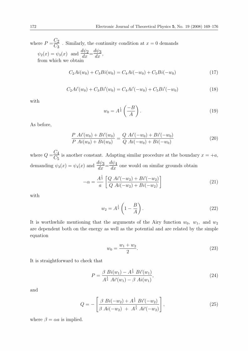
172 Electronic Journal of Theoretical Physics 5, No. 19 (2008) 169–176
where P =C2C3
. Similarly, the continuity condition at x = 0 demands
ψ2(x) = ψ3(x) anddψ2dx =
dψ3dx ,
from which we obtain
C2Ai(w0) + C3Bi(w0) = C4Ai(−w0) + C5Bi(−w0) (17)
C2Ai′(w0) + C3Bi′(w0) = C4Ai′(−w0) + C5Bi′(−w0) (18)
with
w0 = A13
(−B
A
). (19)
As before,
P Ai′(w0) + Bi′(w0)
P Ai(w0) + Bi(w0)=
Q Ai′(−w0) + Bi′(−w0)
Q Ai(−w0) + Bi(−w0)(20)
where Q =C4C5
is another constant. Adapting similar procedure at the boundary x = +a,
demanding ψ3(x) = ψ4(x) anddψ3dx =
dψ4dx one would on similar grounds obtain
−α =A
13
a
[Q Ai′(−w2) + Bi′(−w2)
Q Ai(−w2) + Bi(−w2)
](21)
with
w2 = A13
(1 − B
A
). (22)
It is worthwhile mentioning that the arguments of the Airy function w0, w1, and w2
are dependent both on the energy as well as the potential and are related by the simple
equation
w0 =w1 + w2
2. (23)
It is straightforward to check that
P =β Bi(w1) − A
13 Bi′(w1)
A13 Ai′(w1) − β Ai(w1)
, (24)
and
Q = −[
β Bi(−w2) + A13 Bi′(−w2)
β Ai(−w2) + A13 Ai′(−w2)
], (25)
where β = αa is implied.

Electronic Journal of Theoretical Physics 5, No. 19 (2008) 169–176 173
Formally on eliminating P and Q in Eqn.(20) we obtain the eigenvalue equation as
⎡⎣{
βBi (ω1) − A13 Bi′ (ω1)
}Ai′ (ω0) +
{A
13 Ai′ (ω1) − βAi (ω1)
}Bi′ (ω0){
βBi (ω1) − A13 Bi′ (ω1)
}Ai (ω0) +
{A
13 Ai′ (ω1) − βAi (ω1)
}Bi (ω0)
⎤⎦ =
⎡⎣{
βBi (−ω2)+A13 Bi′ (−ω2)
}Ai′ (−ω0)−
{A
13 Ai′ (−ω2)+βAi (−ω2)
}Bi′ (−ω0){
βBi (−ω2)+A13 Bi′ (−ω2)
}Ai (−ω0) −
{A
13 Ai′ (−ω2)+βAi (−ω2)
}Bi (−ω0)
⎤⎦ (26)
This intricate and fairly complicated transcendental eigenvalue equation involving
the Airy function and its derivatives is solved both graphically and numerically using
Mathematica[14]. The real roots, which correspond to the eigenenergies, are listed in
Table 1 for a typical value of the range parameter(a). Energy (E) and well-depth (V0)
are both expressed in units of�2
2ma2 .
3. Results and Discussion
One of the distinctive characteristics of quantum mechanics, in contrast to classical me-
chanics, is the existence of bound states corresponding to discrete energy levels. It is
well-known in quantum mechanics that bound states exist for all attractive potentials,
the exact number depending on the specific form of the potential and the dimensionality
of the space.
More specifically, as is seen from the spectrum of energies listed in Table 1, for a
finite range of the potential, deeper wells admit excited state energies, consistent with
the wisdom of quantum mechanics. Such studies, apart from being pedagogical in nature,
are potentially exciting and significant as it is concerned with quark confinement.
Quantum chromodynamics, which governs the quark-antiquark interaction is widely
accepted as a good theory of strongly interacting particles. One can explore the hadronic
properties by investigating the bound states of quarks. Our investigation concerning the
linear potential is seeming interesting and can be regarded as a model to describe the
quarkonia.
Further, the linear potential well or in other words, the triangular well has potential
applications in electronics. Interestingly, in many semiconductor devices, it is believed
that electrons are confined in almost triangular quantum wells [15]. Examples of such
devices are Si MOSFETs (Metal Oxide Semiconductor Field Effect Transistors) widely
used in digital applications and GaAs/AlGaAs MODFETs (Modulation Doped Field
Effect Transistors) used for high speed applications. The bound states of the linear
potential is a subject of renewed interest and intensive research and we have extended
the study of this naive potential to the relativistic domain, which will be reported shortly.

174 Electronic Journal of Theoretical Physics 5, No. 19 (2008) 169–176
Acknowledgements
This work was carried out under a grant and fellowship by the University Grants Com-
mission.
References
[1] Kogut J and Susskind L 1975 Hamiltonian formulation of Wilson’s lattice guagetheories Phys. Rev D 11 395
[2] Lichtenberg D B 1987 Energy levels of quarkonia in potential models Int. J. Mod.Phys. A 2 1669
[3] Antippa A F and Phares A J 1978 The linear potential: A solution in terms ofcombinatorics functions J.Math.Phys 19 308
[4] Antippa A F and Toan N K 1979 The linear potential eigen energy equation I Can.J. Phys. 57 417
[5] Plante G and Antippa A F 2005 Analytic solution of the Schrodinger equation forthe Coulomb plus linear potential - The wave functions J. Math. Phys. 46 062108
[6] Antonio de Castro 2003 Bound states by a pseudoscalar Coulomb potential in oneplus one dimension arXiv:hepth/0303 175v2
[7] Chiu T W 1986 Non-relativistic bound state problems in momentum space J. Phys.A Math. Gen.19 2537
[8] Deloff A 2007 Quarkonium bound state problem in momentum space revisted Ann.Phys. 322 2315
[9] Nagalakshmi A Rao and Kagali B A 2002 Spinless particles in a screened Coulombpotential Phys. Lett. A 296 192
[10] Nagalakshmi A Rao and Kagali B A 2002 Dirac bound states in a one-dimensionalscalar screened Coulomb potential Mod. Phys. Lett. A 17 2049
[11] Nagalakshmi A Rao and Kagali B A 2002 Bound states of Klein-Gordon particles inscalar screened Coulomb potential Int. J. Mod. Phys. A 17 4793
[12] Nagalakshmi A Rao 1996 A study of bound states in relativistic quantum mechanicsM. Phil Dissertation (Bangalore University)
[13] Abramowitz M and stegun I A 1965 Handbook of Mathematical Functions andFormulas, Graphs and Mathematical Tables (New York: Dover)
[14] Wolfram S 1996 The Mathematica Book (Cambridge: Cambridge University Press)
[15] Jasprit Singh 1997 Quantum Mechanics - Fundamentals and Applications toTechnology (New York: Wiley Interscience)

Electronic Journal of Theoretical Physics 5, No. 19 (2008) 169–176 175
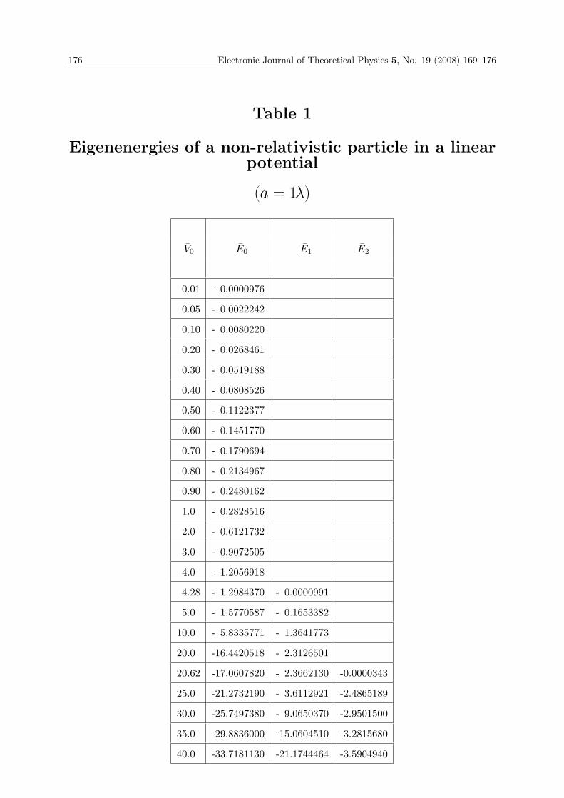
176 Electronic Journal of Theoretical Physics 5, No. 19 (2008) 169–176
Table 1
Eigenenergies of a non-relativistic particle in a linearpotential
(a = 1λ)
V0 E0 E1 E2
0.01 - 0.0000976
0.05 - 0.0022242
0.10 - 0.0080220
0.20 - 0.0268461
0.30 - 0.0519188
0.40 - 0.0808526
0.50 - 0.1122377
0.60 - 0.1451770
0.70 - 0.1790694
0.80 - 0.2134967
0.90 - 0.2480162
1.0 - 0.2828516
2.0 - 0.6121732
3.0 - 0.9072505
4.0 - 1.2056918
4.28 - 1.2984370 - 0.0000991
5.0 - 1.5770587 - 0.1653382
10.0 - 5.8335771 - 1.3641773
20.0 -16.4420518 - 2.3126501
20.62 -17.0607820 - 2.3662130 -0.0000343
25.0 -21.2732190 - 3.6112921 -2.4865189
30.0 -25.7497380 - 9.0650370 -2.9501500
35.0 -29.8836000 -15.0604510 -3.2815680
40.0 -33.7181130 -21.1744464 -3.5904940

EJTP 5, No. 19 (2008) 177–190 Electronic Journal of Theoretical Physics
Exact Non-traveling Wave and Coefficient FunctionSolutions for (2+1)-Dimensional Dispersive Long
Wave Equations
Sheng Zhang∗, Wei Wang, and Jing-Lin Tong
Department of Mathematics, Bohai University, Jinzhou 121000, PR China
Received 12 May 2008, Accepted 16 August 2008, Published 10 October 2008
Abstract: In this paper, a new generalized F-expansion method is proposed to seek exactsolutions of nonlinear evolution equations. With the aid of symbolic computation, we choosethe (2+1)-dimensional dispersive long wave equations to illustrate the validity and advantagesof the proposed method. As a result, many new and more general exact non-traveling waveand coefficient function solutions are obtained including single and combined non-degenerateJacobi elliptic function solutions, soliton-like solutions and trigonometric function solutions,each of which contains two arbitrary functions. The arbitrary functions provide us with enoughfreedom to discuss the behaviors of solutions. As an illustrative example, new spatial structuresof two solutions are shown. Compared with the most existing F-expansion methods, the newgeneralized F-expansion method gives not only more general exact solutions but also new formalexact solutions. The proposed method can also be applied to other nonlinear evolution equationsin mathematical physics.c© Electronic Journal of Theoretical Physics. All rights reserved.
Keywords: F-expansion Method, Jacobi Elliptic Function Solutions, Non-traveling Wave andCoefficient Function Solutions, Soliton-Like Solutions, Trigonometric Function SolutionsPACS (2008): 02.30.Jr; 04.20.Jb; 05.45.Yv
1. Introduction
Since the soliton phenomena were first observed by Scott Russell 1 in 1834 and the KdV
equation was solved by the inverse scattering method by Gardner et al. 2 in 1967, finding
exact solutions of nonlinear evolution equations (NLEEs) has become one of the most
exciting and extremely active areas of research investigation. Many effective methods
∗ Corresponding author. Tel.: +86 416 2889533; fax: +86 416 2889522. E-mail address:[email protected]
178 Electronic Journal of Theoretical Physics 5, No. 19 (2008) 177–190
for obtaining exact solutions of NLEEs have been presented such as Hirota’s bilinear
method, 3 Backlund transformation, 4 Painleve expansion, 5 sine-cosine method, 6 ho-
mogenous balance method, 7 homotopy perturbation method, 8−10 variational method,11−14 asymptotic methods, 15,16 non-perturbative methods, 17 Adomian Pade approxima-
tion, 18 tanh-function method, 19−32 algebraic method, 33−38 auxiliary equation method,39−45 Exp-function method, 46−55 and so on.
Recently, many exact solutions expressed by various Jacobi elliptic functions of many
NLEEs in mathematical physics have been obtained by Jacobi elliptic function expansion
method 56−58 and F-expansion method 59−61 which can be thought of as a generalization
of Jacobi elliptic function expansion method. F-expansion method was later extended in
different manners 62−70. Very recently, we proposed a generalized F-expansion method71−73 to obtain more general exact solutions which contain not only the results obtained
by using the methods 59−61,67−70 but also a series of new and more general exact solutions,
in which the restriction on ξ(x, y, z, . . . , t) as merely a linear function of x, y, z, . . . , t and
the restriction on the coefficients being constants are removed.
The present paper is motivated by the desire to further improve and develop our
method 71−73 by taking the (2+1)-dimensional dispersive long wave (DLW) equations
as an example. As a result, many new and more general exact non-traveling wave and
coefficient function solutions are obtained including single and combined non-degenerate
Jacobi elliptic function solutions, soliton-like solutions and trigonometric function solu-
tions, each of which contains two arbitrary functions.
The rest of this paper is organized as follows. In Section 2, we give the description
of the new generalized F-expansion method. In Section 3, we use this method to obtain
more general exact solutions of the (2+1)-dimensional DLW equations. In Section 4,
some conclusions are given.
2. Description of the New Generalized F-expansion Method
For a given NLEE with independent variables X = (x, y, z, . . . , t) and dependent variable
u:
F (u, ut, ux, uy, uz, . . . , uxt, uyt, uzt . . . , utt, uxx, uyy, uzz, . . . ) = 0, (1)
we seek its solutions in the new and more general form 71−73:
u = a0 +n∑
i=1
{aiF
i(ξ) + biF−i(ξ) + ciF
i−1(ξ)F ′(ξ) + diF−i(ξ)F ′(ξ)
}, (2)
where a0 = a0(X), ai = ai(X), bi = bi(X), ci = ci(X), di = di(X) (i = 1, 2, . . . , n) and
ξ = ξ(X) are undetermined functions, F (ξ) and F ′(ξ) in (2) satisfy
F ′2(ξ) = PF 4(ξ) + QF 2(ξ) + R, (3)

Electronic Journal of Theoretical Physics 5, No. 19 (2008) 177–190 179
and hence holds for F (ξ) and F ′(ξ)⎧⎪⎪⎪⎪⎪⎪⎪⎪⎪⎪⎪⎨⎪⎪⎪⎪⎪⎪⎪⎪⎪⎪⎪⎩
F ′′(ξ) = 2PF 3(ξ) + QF (ξ),
F ′′′(ξ) = (6PF 2(ξ) + Q)F ′(ξ),
F (4)(ξ) = 24P 2F 5(ξ) + 20PQF 3(ξ) + (Q2 + 12PR)F (ξ),
F (5)(ξ) = (120P 2F 4(ξ) + 60PQF 2(ξ) + Q2 + 12PR)F ′(ξ),
. . .
(4)
where P , Q and R are all parameters, the prime denotes d/dξ. Given different values of
P , Q and R, the different Jacobi elliptic function solutions F (ξ) can be obtained from
Eq. (3) (see Appendix A for its various Jacobi elliptic function solutions including some
new ones which have not been listed in the method 71−73). To determine u explicitly, we
take the following four steps:
Step 1. Determine the integer n by balancing the highest order nonlinear term(s) and
the highest order partial derivative term of u in Eq. (1).
Step 2. Substitute (2) along with (3) and (4) into Eq. (1) and collect all coefficients
of F ′i(ξ)F j(ξ) (i = 0, 1; j = 0,±1,±2, . . .), then set each coefficient to zero to derive a
set of over-determined partial differential equations for a0, bi, ci, di (i = 1, 2, . . . , n) and
ξ.
Step 3. Solve the system of over-determined partial differential equations obtained in
Step 2 for a0, ai, bi, ci, di and ξ by use of Mathematica.
Step 4. From Appendix A select P , Q, R and F (ξ), then substitute them along
with a0, ai, bi, ci, di and ξ obtained in Step 3 into (2) to obtain Jacobi elliptic function
solutions of Eq. (1) (see Appendix B for F ′(ξ)), from which soliton-like solutions and
trigonometric function solutions can be obtained when m → 1 and m → 0.
Remark 1. In order to determine the explicit solutions of the partial differential
equations derived in Step 2, we may choose special forms of a0, ai, bi, ci, di and ξ as we
do in Section 3.
3. Exact Solutions of the (2+1)-dimensional DLW Equations
uyt + vxx +1
2(u2)xy = 0, (5)
vt + (uv + u + uxy)x = 0. (6)
This system was firstly obtained by Boiti et al. 74 as a compatibility condition for
a “weak” Lax pair. Paquin and Winternitz 75 showed that the symmetry algebra of
it is infinite-dimensional and has a Kac–Moody–Virasoro structure. Lou 76 gave the
more general symmetry algebra, W∞ symmetry algebra. Lou 77 found nine types of
two-dimensional similarity reductions and thirteen types of ordinary differential equation
reductions. Though the model equation system is Lax or IST integrable, it does not pass

180 Electronic Journal of Theoretical Physics 5, No. 19 (2008) 177–190
the Painleve test. 78 Recently, He 14 established a variational model by the semi-inverse
method. We 68 obtained periodic wave solutions by using the extended F-expansion
method. Xia and Chen 79 obtained dromion solutions by means of the homogenous
balance method. Zhao and Bai 80 obtained non-traveling wave solutions via the extended
mapping transformation method.
According to Step 1, we get n1 = 1 for u and n2 = 2 for v. In order to search for
explicit solutions, we suppose that the solutions of Eqs. (5) and (6) can be expressed as:
u = a0 + a1F (ξ) + b1F−1(ξ) + c1F
′(ξ)F (ξ) + d1F′(ξ)F−1(ξ), (7)
v = A0 + A1F (ξ) + A2F2(ξ) + B1F
−1(ξ) + B2F−2(ξ) + C1F
′(ξ)
+C2F′(ξ)F (ξ) + D1F
′(ξ)F−1(ξ) + D2F′(ξ)F−2(ξ), (8)
where a0 = a0(y, t), a1 = a1(y, t), b1 = b1(y, t), c1 = c1(y, t), d1 = d1(y, t), A0 = A0(y, t),
A1 = A1(y, t), A2 = A2(y, t), B1 = B1(y, t), B2 = B2(y, t), C1 = C1(y, t), C2 = C2(y, t),
D1 = D1(y, t), D2 = D2(y, t), ξ = kx + η, η = η(y, t), k is a nonzero constant.
With the aid of Mathematica, substituting (7) and (8) along with (3) and (4) into Eqs.
(5) and (6), the left-hand sides of Eqs. (5) and (6) are converted into two polynomials
of F ′i(ξ)F j(ξ) (i = 0, 1; j = 0,±1,±2, · · · ), then setting each coefficient to zero, we get a
set of over-determined partial differential equations for a0, a1, b1, c1, d1, A0, A1, A2, B1,
B2, C1, C2, D1, D2 and η. Solving these over-determined partial differential equations
by use of Mathematica, we get the following results:
Case 1
a1 = ±k√
P , d1 = ±k, C1 = ±k√
Pf ′(y), D2 = ±k√
Rf ′(y),
a0 = −g′(t)k
, b1 = ±k√
R, A2 = −kPf ′(y), B2 = −kRf ′(y),
A0 = −1 ± 2k√
PRf ′(y), c1 = A1 = B1 = C2 = D1 = 0, η = f(y) + g(t),
where f(y) and g(t) are arbitrary functions of y and t respectively, f ′(y) = df(y)/dy,
g′(t) = dg(t)/dt. The sign “±” means that all possible combinations of “+” and “−” can
be taken in a1, d1, C1 and D2. If the same sign is used in d1 and D2, then “−” must be
used in b1, furthermore the different signs must be used in a1 and A0. If different signs
are used in d1 and D2, then “+” must be used in b1, furthermore the same sign must be
used in a1 and A0. Hereafter, the sign “±” always stands for this meaning in the similar
circumstances.
Case 2
a0 = −g′(t)k
, d1 = ±2k, A2 = −2kPf ′(y), B2 = −2kRf ′(y),
A0 = −1, a1 = b1 = c1 = A1 = B1 = C1 = C2 = D1 = D2 = 0, η = f(y) + g(t),
where f(y) and g(t) are arbitrary functions of y and t respectively, f ′(y) = df(y)/dy,
g′(t) = dg(t)/dt.
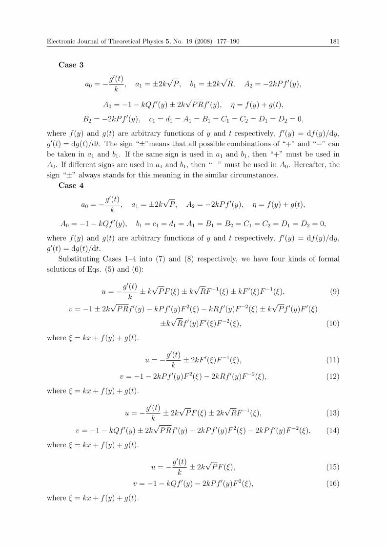
Electronic Journal of Theoretical Physics 5, No. 19 (2008) 177–190 181
Case 3
a0 = −g′(t)k
, a1 = ±2k√
P, b1 = ±2k√
R, A2 = −2kPf ′(y),
A0 = −1 − kQf ′(y) ± 2k√
PRf ′(y), η = f(y) + g(t),
B2 = −2kPf ′(y), c1 = d1 = A1 = B1 = C1 = C2 = D1 = D2 = 0,
where f(y) and g(t) are arbitrary functions of y and t respectively, f ′(y) = df(y)/dy,
g′(t) = dg(t)/dt. The sign “±”means that all possible combinations of “+” and “−” can
be taken in a1 and b1. If the same sign is used in a1 and b1, then “+” must be used in
A0. If different signs are used in a1 and b1, then “−” must be used in A0. Hereafter, the
sign “±” always stands for this meaning in the similar circumstances.
Case 4
a0 = −g′(t)k
, a1 = ±2k√
P , A2 = −2kPf ′(y), η = f(y) + g(t),
A0 = −1 − kQf ′(y), b1 = c1 = d1 = A1 = B1 = B2 = C1 = C2 = D1 = D2 = 0,
where f(y) and g(t) are arbitrary functions of y and t respectively, f ′(y) = df(y)/dy,
g′(t) = dg(t)/dt.
Substituting Cases 1–4 into (7) and (8) respectively, we have four kinds of formal
solutions of Eqs. (5) and (6):
u = −g′(t)k
± k√
PF (ξ) ± k√
RF−1(ξ) ± kF ′(ξ)F−1(ξ), (9)
v = −1 ± 2k√
PRf ′(y) − kPf ′(y)F 2(ξ) − kRf ′(y)F−2(ξ) ± k√
Pf ′(y)F ′(ξ)
±k√
Rf ′(y)F ′(ξ)F−2(ξ), (10)
where ξ = kx + f(y) + g(t).
u = −g′(t)k
± 2kF ′(ξ)F−1(ξ), (11)
v = −1 − 2kPf ′(y)F 2(ξ) − 2kRf ′(y)F−2(ξ), (12)
where ξ = kx + f(y) + g(t).
u = −g′(t)k
± 2k√
PF (ξ) ± 2k√
RF−1(ξ), (13)
v = −1 − kQf ′(y) ± 2k√
PRf ′(y) − 2kPf ′(y)F 2(ξ) − 2kPf ′(y)F−2(ξ), (14)
where ξ = kx + f(y) + g(t).
u = −g′(t)k
± 2k√
PF (ξ), (15)
v = −1 − kQf ′(y) − 2kPf ′(y)F 2(ξ), (16)
where ξ = kx + f(y) + g(t).
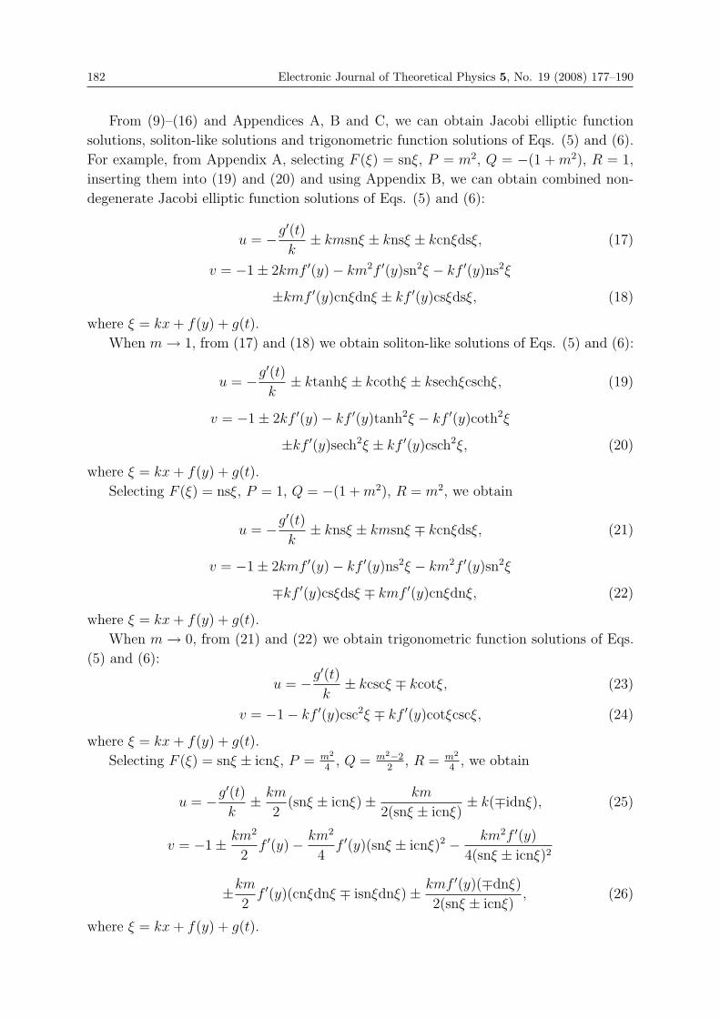
182 Electronic Journal of Theoretical Physics 5, No. 19 (2008) 177–190
From (9)–(16) and Appendices A, B and C, we can obtain Jacobi elliptic function
solutions, soliton-like solutions and trigonometric function solutions of Eqs. (5) and (6).
For example, from Appendix A, selecting F (ξ) = snξ, P = m2, Q = −(1 + m2), R = 1,
inserting them into (19) and (20) and using Appendix B, we can obtain combined non-
degenerate Jacobi elliptic function solutions of Eqs. (5) and (6):
u = −g′(t)k
± kmsnξ ± knsξ ± kcnξdsξ, (17)
v = −1 ± 2kmf ′(y) − km2f ′(y)sn2ξ − kf ′(y)ns2ξ
±kmf ′(y)cnξdnξ ± kf ′(y)csξdsξ, (18)
where ξ = kx + f(y) + g(t).
When m → 1, from (17) and (18) we obtain soliton-like solutions of Eqs. (5) and (6):
u = −g′(t)k
± ktanhξ ± kcothξ ± ksechξcschξ, (19)
v = −1 ± 2kf ′(y) − kf ′(y)tanh2ξ − kf ′(y)coth2ξ
±kf ′(y)sech2ξ ± kf ′(y)csch2ξ, (20)
where ξ = kx + f(y) + g(t).
Selecting F (ξ) = nsξ, P = 1, Q = −(1 + m2), R = m2, we obtain
u = −g′(t)k
± knsξ ± kmsnξ ∓ kcnξdsξ, (21)
v = −1 ± 2kmf ′(y) − kf ′(y)ns2ξ − km2f ′(y)sn2ξ
∓kf ′(y)csξdsξ ∓ kmf ′(y)cnξdnξ, (22)
where ξ = kx + f(y) + g(t).
When m → 0, from (21) and (22) we obtain trigonometric function solutions of Eqs.
(5) and (6):
u = −g′(t)k
± kcscξ ∓ kcotξ, (23)
v = −1 − kf ′(y)csc2ξ ∓ kf ′(y)cotξcscξ, (24)
where ξ = kx + f(y) + g(t).
Selecting F (ξ) = snξ ± icnξ, P = m2
4, Q = m2−2
2, R = m2
4, we obtain
u = −g′(t)k
± km
2(snξ ± icnξ) ± km
2(snξ ± icnξ)± k(∓idnξ), (25)
v = −1 ± km2
2f ′(y) − km2
4f ′(y)(snξ ± icnξ)2 − km2f ′(y)
4(snξ ± icnξ)2
±km
2f ′(y)(cnξdnξ ∓ isnξdnξ) ± kmf ′(y)(∓dnξ)
2(snξ ± icnξ), (26)
where ξ = kx + f(y) + g(t).

Electronic Journal of Theoretical Physics 5, No. 19 (2008) 177–190 183
When m → 1, from (25) and (26) we obtain soliton-like solutions of Eqs. (5) and (6):
u = −g′(t)k
± k
2(tanhξ ± isechξ) ± k
2(tanhξ ± isechξ)± k(±isechξ), (27)
v = −1 ± k
2f ′(y) − k
4f ′(y)(tanhξ ± isechξ)2 − kf ′(y)
4(tanhξ ± isechξ)2
±k
2f ′(y)(sech2ξ ∓ itanhξsechξ) ± kf ′(y)(±sechξ)
2(tanhξ ± isechξ), (28)
where ξ = kx + f(y) + g(t).
Selecting F (ξ) = snξ1±cnξ
, P = 14, Q = 1−2m2
2, R = 1
4, we obtain
u = −g′(t)k
± ksnξ
2(1 ± cnξ)± k(1 ± cnξ)
2snξ± k[cnξdnξ(1 ± cnξ) ± sn2ξdnξ]
snξ(1 ± cnξ), (29)
v = −1 ± kf ′(y)
2− kf ′(y)sn2ξ
4(1 ± cnξ)2− kf ′(y)(1 ± cnξ)2
4sn2ξ
±kf ′(y)[cnξdnξ(1 ± cnξ) ± sn2ξdnξ]
2(1 ± cnξ)2± kf ′(y)[cnξdnξ(1 ± cnξ) ± sn2ξdnξ]
2sn2ξ, (30)
where ξ = kx + f(y) + g(t).
When m → 1, from (29) and (30) we obtain soliton-like solutions of Eqs. (5) and (6):
u = −g′(t)k
± ktanhξ
2(1 ± sechξ)± k(1 ± sechξ)
2tanhξ± k[sech2ξ(1 ± sechξ) ± tanh2ξsechξ]
tanhξ(1 ± sechξ), (31)
v = −1 ± kf ′(y)
2− kf ′(y)tanh2ξ
4(1 ± sechξ)2− kf ′(y)(1 ± sechξ)2
4tanh2ξ
±kf ′(y)[sech2ξ(1 ± sechξ) ± tanh2ξsechξ]
2(1 ± sechξ)2
±kf ′(y)[sech2ξ(1 ± sechξ) ± tanh2ξsechξ]
2tanh2ξ, (32)
where ξ = kx + f(y) + g(t).
When m → 0, from (29) and (30) we obtain trigonometric function solutions of Eqs.
(5) and (6):
u = −g′(t)k
± ksinξ
2(1 ± cosξ)± k(1 ± cosξ)
2sinξ± k[cosξ(1 ± cosξ) ± sin2ξ]
sinξ(1 ± cosξ), (33)
v = −1 ± kf ′(y)
2− kf ′(y)sin2ξ
4(1 ± cosξ)2− kf ′(y)(1 ± cosξ)2
4sin2ξ
±kf ′(y)[cosξ(1 ± cosξ) ± sin2ξcosξ]
2(1 ± cosξ)2± kf ′(y)[cosξ(1 ± cosξ) ± sin2ξcosξ]
2sin2ξ, (34)
where ξ = kx + f(y) + g(t).
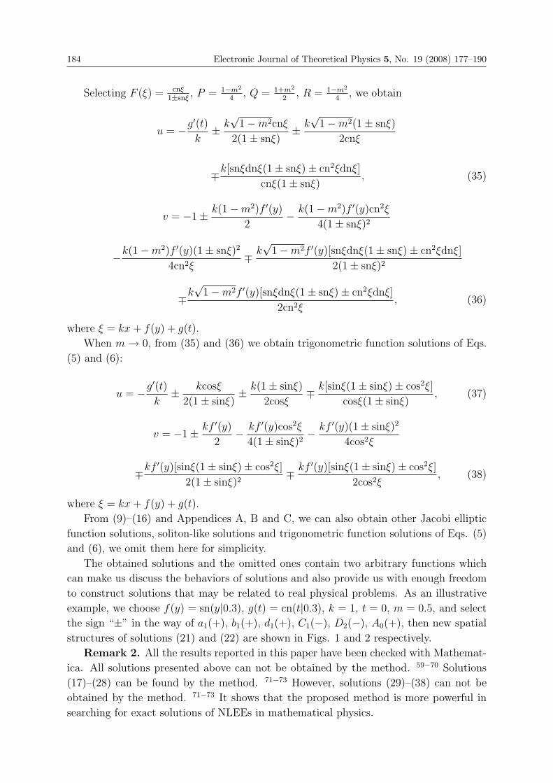
184 Electronic Journal of Theoretical Physics 5, No. 19 (2008) 177–190
Selecting F (ξ) = cnξ1±snξ
, P = 1−m2
4, Q = 1+m2
2, R = 1−m2
4, we obtain
u = −g′(t)k
± k√
1 − m2cnξ
2(1 ± snξ)± k
√1 − m2(1 ± snξ)
2cnξ
∓k[snξdnξ(1 ± snξ) ± cn2ξdnξ]
cnξ(1 ± snξ), (35)
v = −1 ± k(1 − m2)f ′(y)
2− k(1 − m2)f ′(y)cn2ξ
4(1 ± snξ)2
−k(1 − m2)f ′(y)(1 ± snξ)2
4cn2ξ∓ k
√1 − m2f ′(y)[snξdnξ(1 ± snξ) ± cn2ξdnξ]
2(1 ± snξ)2
∓k√
1 − m2f ′(y)[snξdnξ(1 ± snξ) ± cn2ξdnξ]
2cn2ξ, (36)
where ξ = kx + f(y) + g(t).
When m → 0, from (35) and (36) we obtain trigonometric function solutions of Eqs.
(5) and (6):
u = −g′(t)k
± kcosξ
2(1 ± sinξ)± k(1 ± sinξ)
2cosξ∓ k[sinξ(1 ± sinξ) ± cos2ξ]
cosξ(1 ± sinξ), (37)
v = −1 ± kf ′(y)
2− kf ′(y)cos2ξ
4(1 ± sinξ)2− kf ′(y)(1 ± sinξ)2
4cos2ξ
∓kf ′(y)[sinξ(1 ± sinξ) ± cos2ξ]
2(1 ± sinξ)2∓ kf ′(y)[sinξ(1 ± sinξ) ± cos2ξ]
2cos2ξ, (38)
where ξ = kx + f(y) + g(t).
From (9)–(16) and Appendices A, B and C, we can also obtain other Jacobi elliptic
function solutions, soliton-like solutions and trigonometric function solutions of Eqs. (5)
and (6), we omit them here for simplicity.
The obtained solutions and the omitted ones contain two arbitrary functions which
can make us discuss the behaviors of solutions and also provide us with enough freedom
to construct solutions that may be related to real physical problems. As an illustrative
example, we choose f(y) = sn(y|0.3), g(t) = cn(t|0.3), k = 1, t = 0, m = 0.5, and select
the sign “±” in the way of a1(+), b1(+), d1(+), C1(−), D2(−), A0(+), then new spatial
structures of solutions (21) and (22) are shown in Figs. 1 and 2 respectively.
Remark 2. All the results reported in this paper have been checked with Mathemat-
ica. All solutions presented above can not be obtained by the method. 59−70 Solutions
(17)–(28) can be found by the method. 71−73 However, solutions (29)–(38) can not be
obtained by the method. 71−73 It shows that the proposed method is more powerful in
searching for exact solutions of NLEEs in mathematical physics.

Electronic Journal of Theoretical Physics 5, No. 19 (2008) 177–190 185
-5
0
5x
-5
0
5
y
-5
0
5u
-5
0
5x
Fig. 1. Spatial structure of solution (21).
-5
0
5x
-5
0
5
y
-3-2-101
v
-5
0
5x
Fig. 2. Spatial structure of solution (22).
Conclusion
In this paper, we have proposed a new generalized F-expansion method to improve and
develop the most existing F-expansion method. Applying the proposed method to the
(2+1)-dimensional DLW equations, we have successfully obtained new and more gen-
eral exact non-traveling wave and coefficient function solutions including combined non-
degenerate Jacobi elliptic function solutions, soliton-like solutions and trigonometric func-
tion solutions, each of which contains two arbitrary functions. The arbitrary functions in
the obtained solutions imply that these solutions have rich local structures. To the best
of our knowledge, these solutions have not been reported in literature. It may be impor-
tant to explain some physical phenomena. Compared with the most existing F-expansion
methods [59–73], the new generalized F-expansion method gives both more general exact
solutions and new formal solutions. More importantly, the method with the help of sym-
bolic computation provides a powerful mathematical tool for solving a great many NLEEs
in mathematical physics, such as the (3+1)-dimensional Kadomtsev–Petviashvili (KP)
equation, the (2+1)-dimensional Broer–Kaup–Kupershmidt (BKK) equations, breaking
solition (BS) equations, Nizhnik–Novikov–VesselovIt (NNV) equations and so on. Its
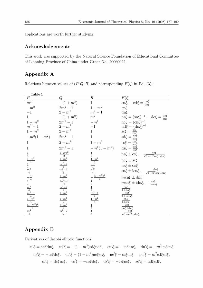
186 Electronic Journal of Theoretical Physics 5, No. 19 (2008) 177–190
applications are worth further studying.
Acknowledgements
This work was supported by the Natural Science Foundation of Educational Committee
of Liaoning Province of China under Grant No. 20060022.
Appendix A
Relations between values of (P,Q, R) and corresponding F (ξ) in Eq. (3):
Table 1P Q R F (ξ)m2 −(1 + m2) 1 snξ, cdξ = cnξ
dnξ
−m2 2m2 − 1 1 − m2 cnξ−1 2 − m2 m2 − 1 dnξ1 −(1 + m2) m2 nsξ = (snξ)−1, dcξ = dnξ
cnξ
1 − m2 2m2 − 1 −m2 ncξ = (cnξ)−1
m2 − 1 2 − m2 −1 ndξ = (dnξ)−1
1 − m2 2 − m2 1 scξ = snξcnξ
−m2(1 − m2) 2m2 − 1 1 sdξ = snξdnξ
1 2 − m2 1 − m2 csξ = cnξsnξ
1 2m2 − 1 −m2(1 − m2) dsξ = dnξsnξ
14
1−2m2
214
nsξ ± csξ, cnξ√1−m2snξ±dnξ
1−m2
41+m2
21−m2
4ncξ ± scξ
14
m2−22
m2
4nsξ ± dsξ
m2
4m2−2
2m2
4snξ ± icnξ, dnξ√
1−m2snξ±cnξ
−14
1+m2
2− (1−m2)2
4mcnξ ± dnξ
14
1−2m2
214
msnξ ± idnξ, snξ1±cnξ
m2
4m2−2
214
snξ1±dnξ
m2−14
1+m2
2m2−1
4dnξ
1±msnξ1−m2
41+m2
21−m2
4cnξ
1±snξ(1−m2)2
41+m2
214
snξcnξ±dnξ
m4
4m2−2
214
cnξ√1−m2±dnξ
Appendix B
Derivatives of Jacobi elliptic functions
sn′ξ = cnξdnξ, cd′ξ = −(1 − m2)sdξndξ, cn′ξ = −snξdnξ, dn′ξ = −m2snξcnξ,
ns′ξ = −csξdsξ, dc′ξ = (1 − m2)ncξscξ, nc′ξ = scξdcξ, nd′ξ = m2cdξsdξ,
sc′ξ = dcξncξ, cs′ξ = −nsξdsξ, ds′ξ = −csξnsξ, sd′ξ = ndξcdξ.

Electronic Journal of Theoretical Physics 5, No. 19 (2008) 177–190 187
Appendix C
Jacobi elliptic functions degenerate into hyperbolic functions when m → 1:
snξ → tanhξ, cnξ → sechξ, dnξ → sechξ, scξ → sinhξ,
sdξ → sinhξ, cdξ → 1, nsξ → cothξ, ncξ → coshξ,
ndξ → coshξ, csξ → cschξ, dsξ → cschξ, dcξ → 1.
Jacobi elliptic functions degenerate into trigonometric functions when m → 0:
snξ → sinξ, cnξ → cosξ, dnξ → 1, scξ → tanξ, sdξ → sinξ, cdξ → cosξ,
nsξ → cscξ, ncξ → secξ, ndξ → 1, csξ → cotξ, dsξ → cscξ, dcξ → secξ.
References
[1] M. J. Ablowitz and P. A. Clarkson, Soliton, Nonlinear Evolution Equations andInverse Scattering (Cambridge University Press, New York, 1991).
[2] C. S. Gardner, J. M. Greene and M. D. Kruskal, Phys. Rev. Lett. 19, 1095 (1967).
[3] R. Hirota, Phys. Rev. Lett. 27, 1192 (1971).
[4] M. R. Miurs, Backlund Transformation (Springer, Berlin 1978).
[5] J. Weiss, M. Tabor, and G. Carnevale, J. Math. Phys. 24, 522 (1983).
[6] C. T. Yan, Phys. Lett. A 224, 77 (1996).
[7] M. L. Wang, Phys. Lett. A 213, 279 (1996).
[8] M. El-Shahed, Int. J. Nonlinear Sci. Numer. Simul. 6, 163 (2005).
[9] J. H. He, Int. J. Nonlinear Sci. Numer. Simul. 6, 207 (2005).
[10] J. H. He, Chaos Solitons and Fractals 26, 695 (2005).
[11] J. H. He, Int. J. Nonlinear Mech. 34, 699 (1999).
[12] J. H. He, Appl. Math. Comput. 114, 115 (2000).
[13] J. H. He, Chaos Solitons and Fractals 19, 847 (2004).
[14] J. H. He, Phys. Lett. A 335, 182 (2005).
[15] J. H. He, Int. J. Modern Phys. B 20, 1141 (2006).
[16] J. H. He, Int. J. Modern Phys. B 20, 2561 (2006).
[17] J. H. He, Non-Perturbative Methods for Strongly Nonlinear Problems (Dissertation,de-Verlag im Internet GmbH, Berlin, 2006).
[18] T. A. Abassy, M. A. El-Tawil, and H. K. Saleh, Int. J. Nonlinear Sci. Numer. Simul.5, 327 (2004).
[19] W. Malfliet, Am. J. Phys. 60, 650 (1992).

188 Electronic Journal of Theoretical Physics 5, No. 19 (2008) 177–190
[20] W. X. Ma, Int. J. Nonlinear Mech. 31, 329 (1996).
[21] Y. T. Gao and B. Tian, Comput. Math. Appl. 33, 115 (1997).
[22] E. G. Fan, Phys. Lett. A 227, 212 (2000).
[23] Z. S. Lu and H. Q. Zhang, Commun. Theor. Phys. (Beijing, China) 39, 405 (2003).
[24] D. S. Li and H. Q. Zhang, Commun. Theor. Phys. (Beijing, China)40, 143 (2003).
[25] Y. Chen, B. Li, and H. Q. Zhang, Int. J. Mod. Phys. C 14, 471 (2003).
[26] Y. Chen, B. Li, and H. Q. Zhang, Int. J. Mod. Phys. C 14, 99 (2003).
[27] Y. Chen and Z. Yu, Int. J. Mod. Phys. C 14, 601 (2003).
[28] F. D. Xie, Y. Zhang, and Z. S. Lu, Chaos Solitons and Fractals 24, 257 (2005).
[29] S. Zhang and T. C. Xia, Commun. Theor. Phys. (Beijing, China) 45, 985 (2006).
[30] S. Zhang and T. C. Xia, Appl. Math. Comput. 181, 319 (2006).
[31] S. Zhang, Chaos Solitons and Fractals 31, 951 (2007).
[32] H. Zhao, Commun. Theor. Phys. (Beijing, China) 47, 200 (2007).
[33] Y. Chen and Q. Wang, Int. J. Mod. Phys. C 15, 595 (2004).
[34] Y. Chen, Q. Wang, and Y. Lang, Z. Naturforsch. 60a, 127 (2005).
[35] Y. Chen, Int. J. Mod. Phys. C 15, 1107 (2005).
[36] E. Yomba, Chaos Solitons and Fractals 27, 187 (2006).
[37] S. Zhang and T. C. Xia, Phys. Lett. A 356, 119 (2006).
[38] S. Zhang and T. C. Xia, Appl. Math. Comput. 182, 1651 (2006).
[39] Sirendaoreji and J. Sun, Phys. Lett. A 309, 387 (2003).
[40] S. Zhang and T. C. Xia, J. Phys. A: Math. Theor. 40, 227 (2007).
[41] S. Zhang and T. C. Xia, Phys. Lett. A 363, 356 (2007).
[42] S. Zhang, Phys. Lett. A 368, 470 (2007).
[43] S. Zhang, Appl. Math. Comput. 188, 1 (2007).
[44] S. Zhang, Appl. Math. Comput. 190, 510 (2007).
[45] S. Zhang, Comput. Math. Appl. 54, 1028 (2007).
[46] J. H. He and X. H. Wu, Chaos Solitons and Fractals 30, 700 (2006).
[47] J. H. He and M. A. Abdou, Chaos Solitons and Fractals 34, 1421 (2007).
[48] X. H. Wu and J. H. He, Comput. Math. Appl. 54, 966 (2007).
[49] M. A. Abdou, A. A. Soliman, and S.T. El-Basyony, Phys. Lett. A 369, 469 (2007).
[50] S. A. El-Wakil, M. A. Madkour, and M. A. Abdou, Phys. Lett. A 369, 62 (2007).
[51] S. Zhang, Phys. Lett. A 365, 448 (2007).
[52] S. Zhang, Phys. Lett. A 371, 65 (2007).
Electronic Journal of Theoretical Physics 5, No. 19 (2008) 177–190 189
[53] A. Ebaid, Phys. Lett. A 365, 213 (2007).
[54] S. D. Zhu, Int. J. Nonlinear Sci. Numer. Simul. 8, 461 (2007).
[55] S. D. Zhu, Int. J. Nonlinear Sci. Numer. Simul. 8, 465 (2007).
[56] S. K. Liu, Z. T. Fu, S. D. Liu, and Q. Zhao, Phys. Lett. A 289, 69 (2001).
[57] E. J. Parkes, B. R. Duffy, and P. C. Abbott, Phys. Lett. A 295, 280 (2002).
[58] Y. Chen, Q. Wang, and B. Li, Z. Naturforsch. 59a, 529 (2004).
[59] Y. B. Zhou, M. L. Wang, and Y. M. Wang, Phys. Lett. A 308, 31 (2003).
[60] M. L. Wang and Y. B. Zhou, Phys. Lett. A 318 (2003) 84.
[61] M. L. Wang, Y. M. Wang, and J. L. Zhang, Chin. Phys. 12, 13412 (2003).
[62] J. B. Liu and K. Q. Yang, Chaos Solitons and Fractals 22, 111 (2004).
[63] M. L. Wang and X. Z. Li, Chaos Solitons and Fractals 24, 1257(2005).
[64] H. Q. Zhang, Chaos Solitons and Fractals 26, 921 (2005).
[65] D. S. Wang and H. Q. Zhang, Chaos Solitons and Fractals 25, 601 (2005).
[66] Y. J. Ren and H. Q. Zhang, Chaos Solitons and Fractals 27, 959 (2006).
[67] S. Zhang, Chaos Solitons and Fractals 30, 1213 (2006).
[68] S. Zhang, Chaos Solitons and Fractals 32, 847 (2007).
[69] J. Chen, H. S. He, and K. Q. Yang, Commun. Theor. Phys. (Beijing, China) 44, 307(2005).
[70] S. Zhang, Chaos Solitons and Fractals 32, 1375 (2007).
[71] S. Zhang, Phys. Lett. A 358, 414 (2006).
[72] S. Zhang and T. C. Xia, Appl. Math. Comput. 183, 1190 (2006).
[73] S. Zhang, Appl. Math. Comput. 189, 836 (2007).
[74] M. Boiti, J. J. P. Leon, M. Manna, and F. Pempinelli, Inerse Problem 3, 25 (1987).
[75] G. Paquin and P. Winternitz, Physica D 358, 122 (1990).
[76] S. Y. Lou, J. Phys. A: Math. Gen. 27, 3235 (1994).
[77] S. Y. Lou, Math. Meth. Appl. Sci. 27, 789 (1995).
[78] S. Y. Lou, Phys. Lett. A 176, 96 (1993).
[79] T. C. Xia and D. Y. Chen, Chaos Solitons and Fractals 22, 577 (2004).
[80] H. Zhao and C. L. Bai, Commun. Theor. Phys. (Beijing, China) 44, 473 (2005).

Related Documents