ODE and Discrete Simulation or Mean Field Methods for Computer and Communication Systems

ODE and Discrete Simulationor

Mean Field Methods for Computer and Communication Systems

Jean-Yves Le Boudec

EPFLMLQA, Aachen, September 2011

1

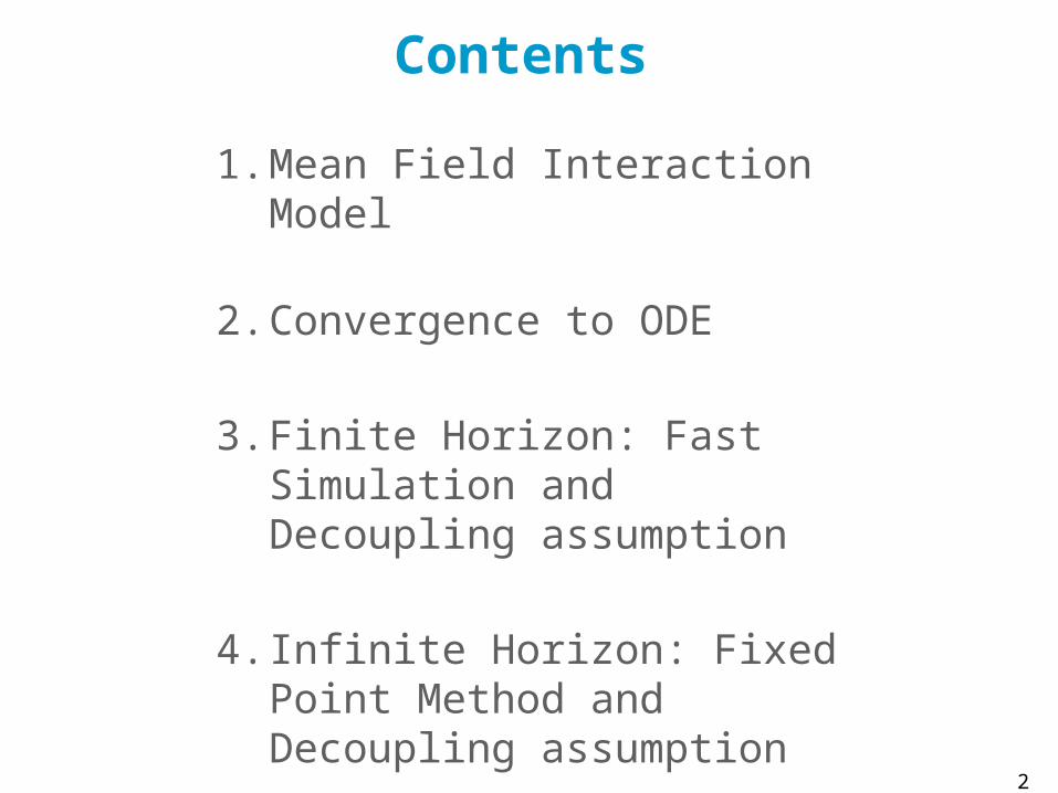
Contents

2

1. Mean Field Interaction Model

2. Convergence to ODE

3. Finite Horizon: Fast Simulation and Decoupling assumption

4. Infinite Horizon: Fixed Point Method and Decoupling assumption

MEAN FIELD INTERACTION MODEL1

3

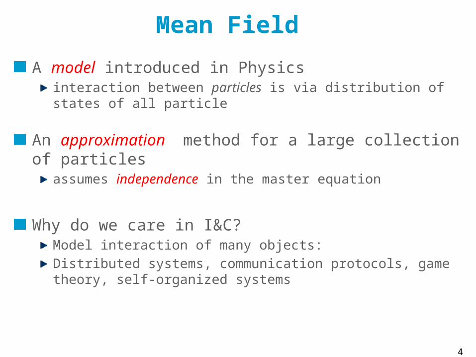
Mean Field

A model introduced in Physicsinteraction between particles is via distribution of states of all particle

An approximation method for a large collection of particlesassumes independence in the master equation

Why do we care in I&C?Model interaction of many objects: Distributed systems, communication protocols, game theory, self-organized systems

4

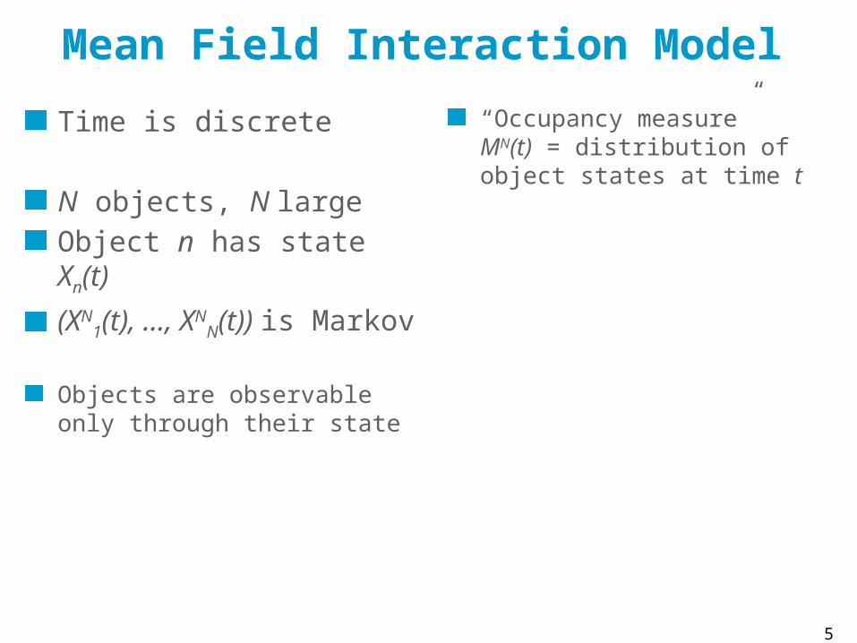
Mean Field Interaction Model

Time is discrete

N objects, N largeObject n has state Xn(t)

(XN1(t), …, XN

N(t)) is Markov

Objects are observable only through their state

“Occupancy measure”MN(t) = distribution of object states at time t

5

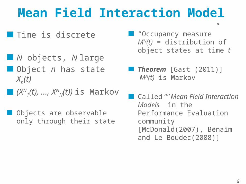
Mean Field Interaction Model

Time is discrete

N objects, N largeObject n has state Xn(t)

(XN1(t), …, XN

N(t)) is Markov

Objects are observable only through their state

“Occupancy measure”MN(t) = distribution of object states at time t

Theorem [Gast (2011)] MN(t) is Markov

Called “Mean Field Interaction Models” in the Performance Evaluation community[McDonald(2007), Benaïm and Le Boudec(2008)]

6

7

A Few Examples Where Applied

Never again !

E.L.

8

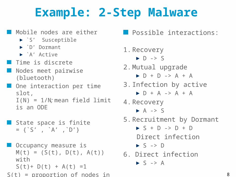
Example: 2-Step MalwareMobile nodes are either

`S’ Susceptible`D’ Dormant`A’ Active

Time is discreteNodes meet pairwise (bluetooth)One interaction per time slot, I(N) = 1/N; mean field limit is an ODE

State space is finite = {`S’ , `A’ ,`D’}

Occupancy measure isM(t) = (S(t), D(t), A(t)) with S(t)+ D(t) + A(t) =1

S(t) = proportion of nodes in state `S’

[Benaïm and Le Boudec(2008)]

Possible interactions:

1. RecoveryD -> S

2. Mutual upgrade D + D -> A + A

3. Infection by activeD + A -> A + A

4. RecoveryA -> S

5. Recruitment by DormantS + D -> D + D

Direct infectionS -> D

6. Direct infectionS -> A

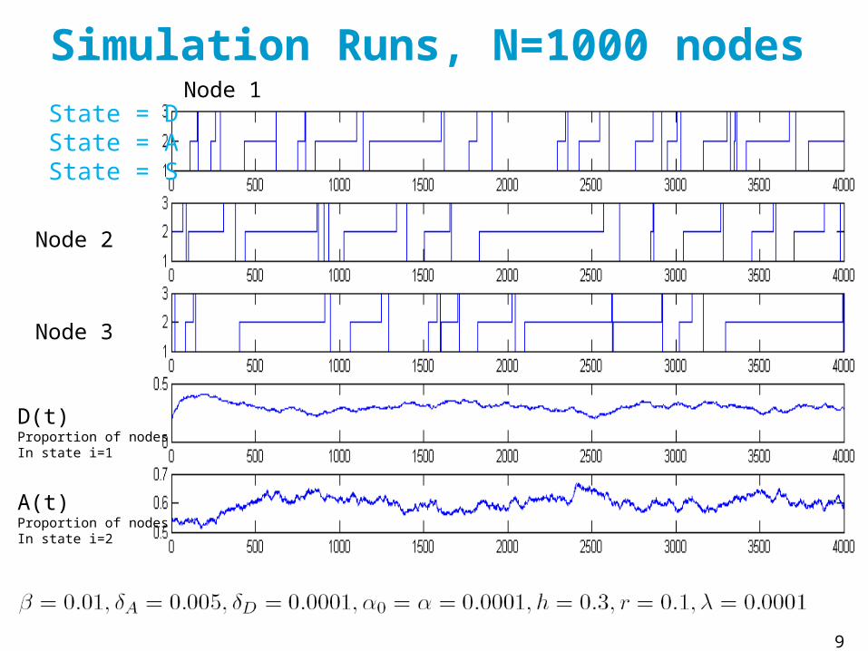
A(t)Proportion of nodes In state i=2

9

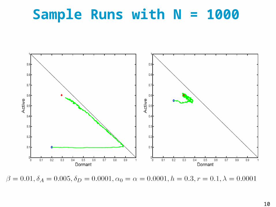
Simulation Runs, N=1000 nodesNode 1

Node 2

Node 3

D(t)Proportion of nodes In state i=1

State = DState = AState = S

10

Sample Runs with N = 1000

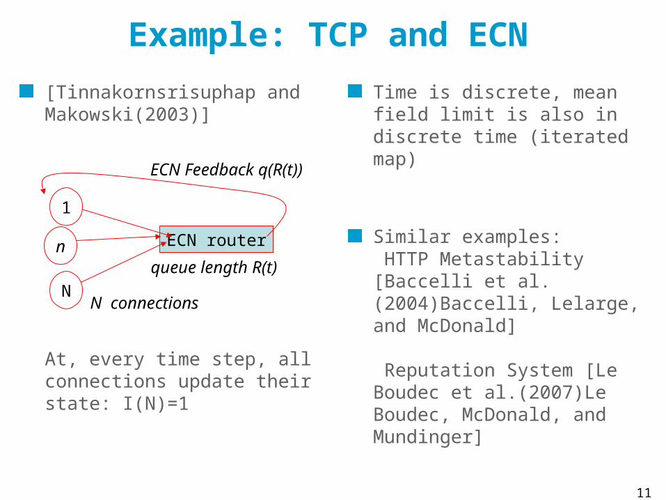
Example: TCP and ECN[Tinnakornsrisuphap and Makowski(2003)]

At, every time step, all connections update their state: I(N)=1

Time is discrete, mean field limit is also in discrete time (iterated map)

Similar examples: HTTP Metastability[Baccelli et al.(2004)Baccelli, Lelarge, and McDonald]

Reputation System [Le Boudec et al.(2007)Le Boudec, McDonald, and Mundinger]

11

ECN router

queue length R(t)

ECN Feedback q(R(t))

N connections

1

n

N

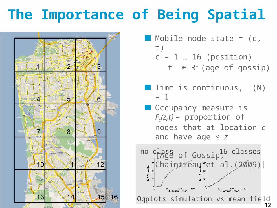
The Importance of Being SpatialMobile node state = (c, t)c = 1 … 16 (position)

t R∊ + (age of gossip)

Time is continuous, I(N) = 1Occupancy measure is Fc(z,t) = proportion of nodes that at location c and have age ≤ z

[Age of Gossip, Chaintreau et al.(2009)]

12Qqplots simulation vs mean field

no class 16 classes

13

What can we do with a Mean Field Interaction Model ?

Large N asymptotics, Finite Horizon

fluid limit of occupancy measure (ODE)decoupling assumption

(fast simulation)

IssuesWhen validHow to formulate the fluid limit

Large t asymptoticStationary approximation of occupancy measureDecoupling assumption

IssuesWhen valid

CONVERGENCE TO ODE

14

E. L.

2.

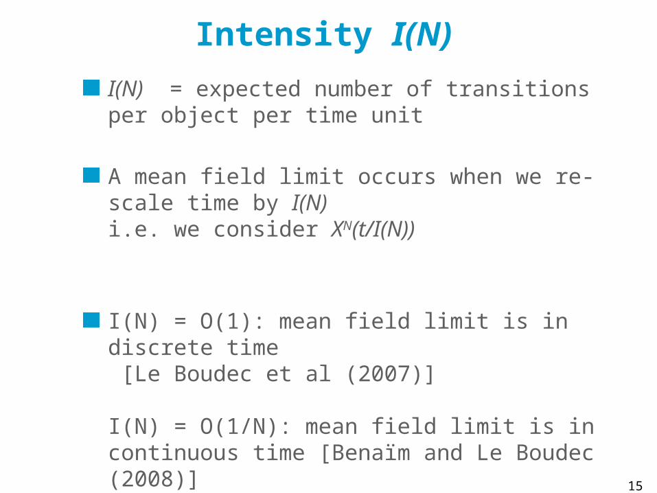
Intensity I(N)I(N) = expected number of transitions per object per time unit

A mean field limit occurs when we re-scale time by I(N)i.e. we consider XN(t/I(N))

I(N) = O(1): mean field limit is in discrete time [Le Boudec et al (2007)]

I(N) = O(1/N): mean field limit is in continuous time [Benaïm and Le Boudec (2008)]

15

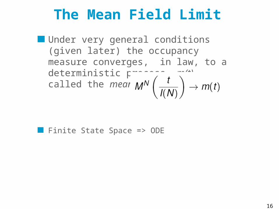
The Mean Field Limit

Under very general conditions (given later) the occupancy measure converges, in law, to a deterministic process, m(t), called the mean field limit

Finite State Space => ODE

16

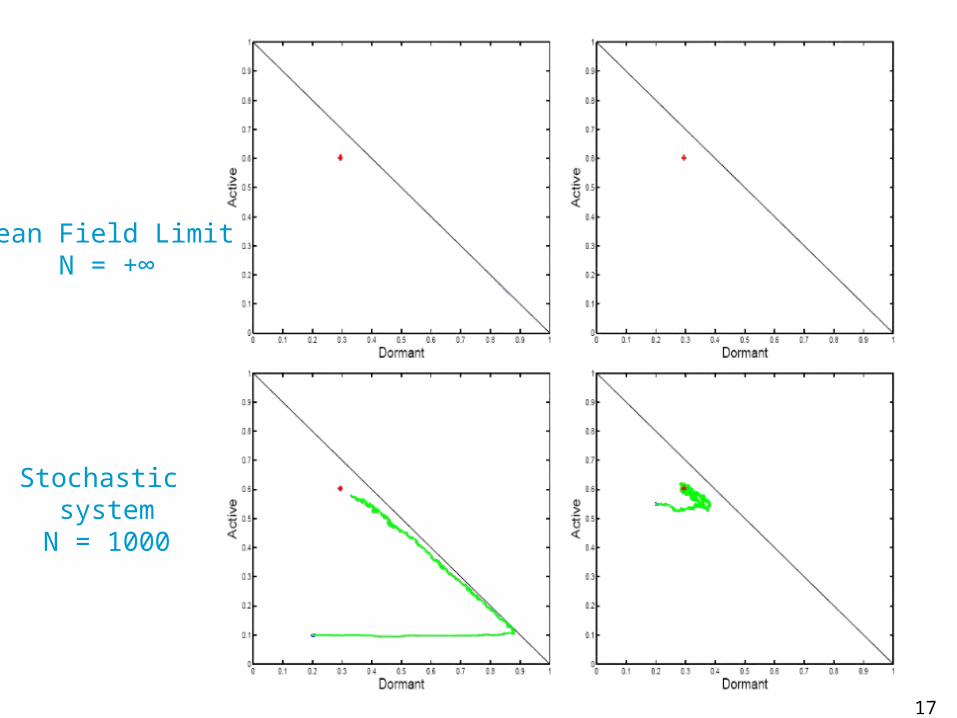
Mean Field LimitN = +∞

Stochastic system

N = 1000

17

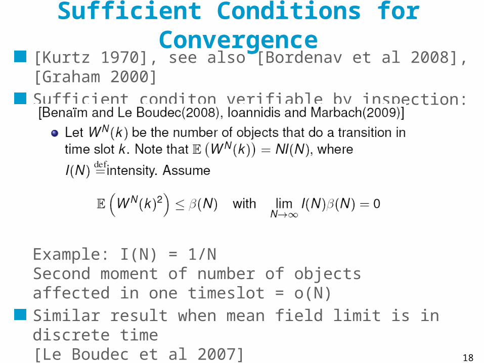
Sufficient Conditions for Convergence[Kurtz 1970], see also [Bordenav et al 2008], [Graham 2000]Sufficient conditon verifiable by inspection:

Example: I(N) = 1/NSecond moment of number of objects affected in one timeslot = o(N)Similar result when mean field limit is in discrete time [Le Boudec et al 2007]

18

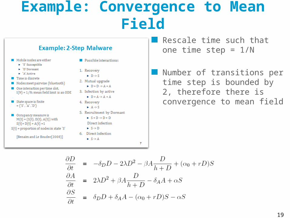
Example: Convergence to Mean FieldRescale time such that one time step = 1/N

Number of transitions per time step is bounded by 2, therefore there is convergence to mean field

19

=

=

=

Formulating the Mean Field Limit

20

drift =

=

=

=

Drift = sum over all transitions of proba of transition

xDelta to system state MN(t)

Re-scale drift by intensity

Equation for mean field limit is

dm/dt = limit of rescaled drift

Can be automated

http://icawww1.epfl.ch/IS/tsed

Convergence to Mean Field

For the finite state space case, there are many simple results, often verifiable by inspection

For example [Kurtz 1970] or [Benaim, Le Boudec 2008]

For the general state space, things may be more complex(fluid limitz is not an ODE, e.g. [Chaintreau et al, 2009])

21E.L.

E. L.

FINITE HORIZON :FAST SIMULATION AND DECOUPLING ASSUMPTION

3.

22

Convergence to Mean Field Limit is Equivalent to Propagation of Chaos

23

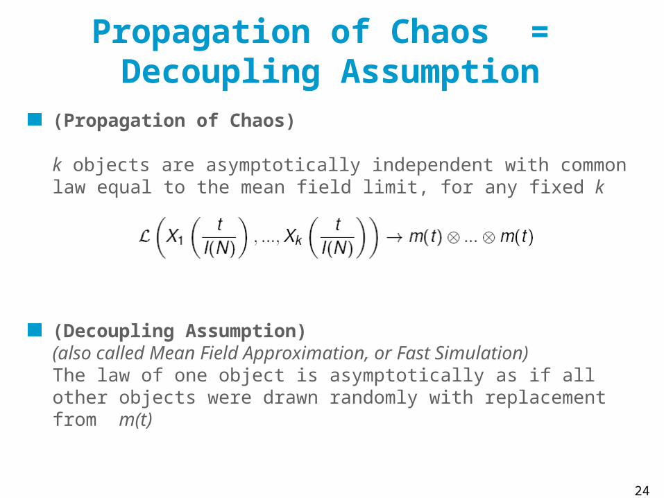
Propagation of Chaos = Decoupling Assumption

(Propagation of Chaos)

k objects are asymptotically independent with common law equal to the mean field limit, for any fixed k

(Decoupling Assumption) (also called Mean Field Approximation, or Fast Simulation) The law of one object is asymptotically as if all other objects were drawn randomly with replacement from m(t)

24

25

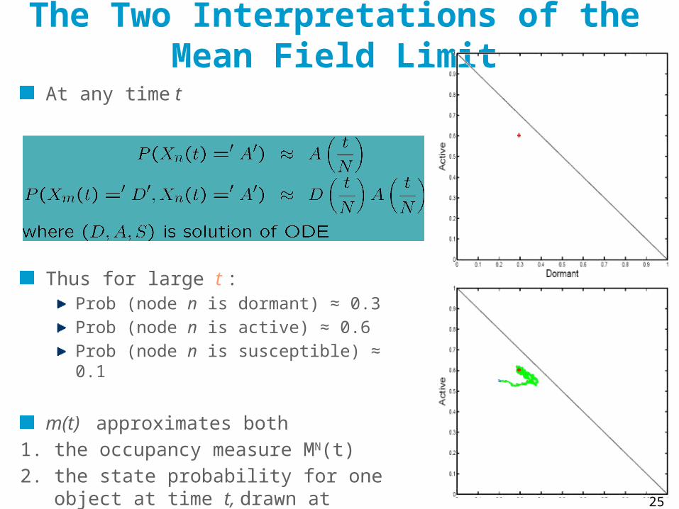
The Two Interpretations of the Mean Field Limit

At any time t

Thus for large t :Prob (node n is dormant) ≈ 0.3Prob (node n is active) ≈ 0.6 Prob (node n is susceptible) ≈ 0.1

m(t) approximates both1. the occupancy measure MN(t)2. the state probability for one object at time

t, drawn at random among N

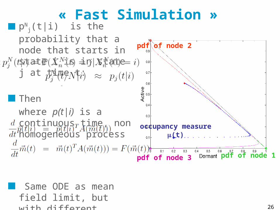
« Fast Simulation »

26

pdf of node 1

pdf of node 2

pdf of node 3

occupancy measure(t)

pNj(t|i) is the probability

that a node that starts in state i is in state j at time t:

Thenwhere p(t|i) is a continuous time, non homogeneous process

Same ODE as mean field limit, but with different initial condition

The Decoupling Assumption

The evolution for one object as if the other objects had a state drawn randomly and independently from the distribution m(t)

Is valid over finite horizon whenever mean field convergence occurs

Can be used to analyze or simulate evolution of k objects

27

INFINITE HORIZON: FIXED POINT METHOD AND DECOUPLING ASSUMPTION

4.

28

29

The Fixed Point MethodDecoupling assumption says distribution of prob for state of one object is approx. m(t) with

We are interested in stationary regime, i.e we do

This is the « Fixed Point Method »Example: in stationary regime:

Prob (node n is dormant) ≈ 0.3Prob (node n is active) ≈ 0.6 Prob (node n is susceptible) ≈ 0.1

Nodes m and n are independent

30

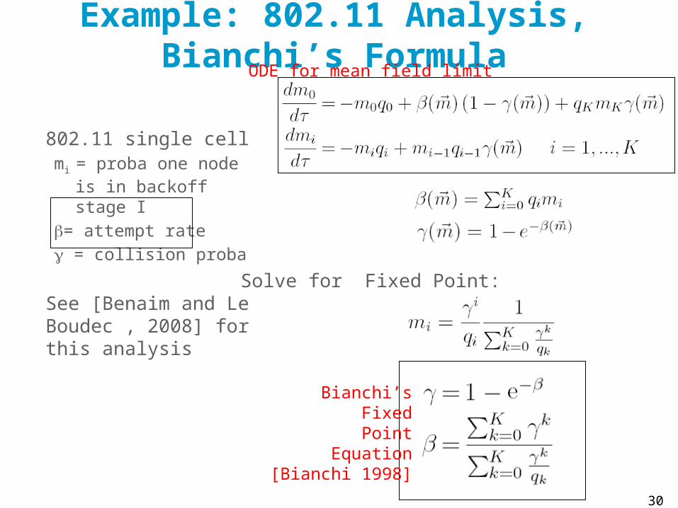
Example: 802.11 Analysis, Bianchi’s Formula

802.11 single cellmi = proba one node is in

backoff stage I= attempt rate = collision proba

See [Benaim and Le Boudec , 2008] for this analysis

Solve for Fixed Point:

Bianchi’sFixedPoint

Equation[Bianchi 1998]

ODE for mean field limit

31

2-Step Malware, Again

Same as before except for one parameter value : h = 0.1 instead of 0.3

The ODE does not converge to a unique attractor (limit cycle)The equation F(m) = 0has a unique solution (red cross) – but it is not the stationary regime !

32

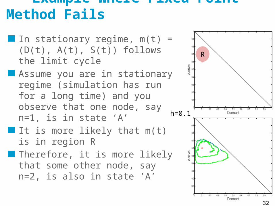
Example Where Fixed Point Method Fails

In stationary regime, m(t) = (D(t), A(t), S(t)) follows the limit cycleAssume you are in stationary regime (simulation has run for a long time) and you observe that one node, say n=1, is in state ‘A’It is more likely that m(t) is in region RTherefore, it is more likely that some other node, say n=2, is also in state ‘A’

This is synchronization

R

h=0.1

33

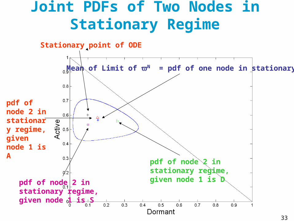
Joint PDFs of Two Nodes in Stationary Regime

Mean of Limit of N = pdf of one node in stationary regime

Stationary point of ODE

pdf of node 2 in stationary regime, given node 1 is D

pdf of node 2 in stationary regime, given node 1 is S

pdf of node 2 in stationary regime, given node 1 is A

34

Where is the Catch ?Decoupling assumption says that nodes m and n are asymptotically independent

There is mean field convergence for this example

But we saw that nodes may not be asymptotically independent

… is there a contradiction ?

The decoupling assumption may not hold in stationary regime, even for perfectly regular models

35

mi(t) mj(t) mi(t) mj(t)

Mean Field Convergence

Markov chain is ergodic

≠

Result 1: Fixed Point Method Holds under (H) Assume that

(H) ODE has a unique global stable point to which all trajectories converge

Theorem [e.g. Benaim et al 2008] : The limit of stationary distribution of MN is concentrated on this fixed pointThe decoupling assumption holds in stationary regime

36

37

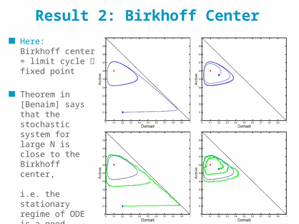
Here: Birkhoff center = limit cycle fixed point

Theorem in [Benaim] says that the stochastic system for large N is close to the Birkhoff center,

i.e. the stationary regime of ODE is a good approximation of the stationary regime of stochastic system

Result 2: Birkhoff Center

Stationary Behaviour of Mean Field Limit is not predicted by Structure of Markov Chain

MN(t) is a Markov chain on SN={(a, b, c) ≥ 0, a + b + c =1, a, b, c multiples of 1/N}

MN(t) is ergodic and aperiodic

Depending on parameter, there is or is not a limit cycle for m(t)

SN (for N = 200)

h = 0.3

h = 0.1

Example: 802.11 with Heterogeneous Nodes

[Cho et al, 2010]

Two classes of nodes with heterogeneous parameters (restransmission probability)

Fixed point equation has a unique solution, but this is not the stationary proba

There is a limit cycle

39

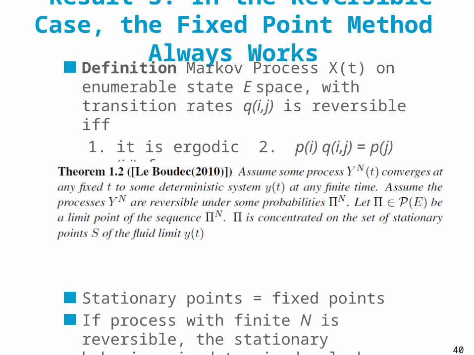
Result 3: In the Reversible Case, the Fixed Point Method Always Works

Definition Markov Process X(t) on enumerable state E space, with transition rates q(i,j) is reversible iff 1. it is ergodic 2. p(i) q(i,j) = p(j) q(j,i) for

some p

Stationary points = fixed points If process with finite N is reversible, the stationary behaviour is determined only by fixed points.

40

A Correct Method

1. Write dynamical system equations in transient regime

2. Study the stationary regime of dynamical system

if converges to unique stationary point m* then make fixed point assumptionelse objects are coupled in stationary regime by mean field limit m(t)

Hard to predict outcome of 2 (except for reversible case)

41

Conclusion

Mean field models are frequent in large scale systems

Validity of approach is often simple by inspection

Mean field is bothODE for fluid limitFast simulation using decoupling assumption

Decoupling assumption holds at finite horizon; may not hold in stationary regime.

Stationary regime is more than stationary points, in general(except for reversible case)

42

43

Thank You …

References

44

45

46

2

47

48