October 25, 2017 - arxiv.org · PDF fileBecause of the vast scales involved, conventional 3D reservoir simulation quickly ... Whereas most studies focus on depth-integration across

Multiresolution Coupled Vertical Equilibrium Model for Fast

Flexible Simulation of CO2 Storage

Olav Møyner and Halvor Møll Nilsen

October 25, 2017

Abstract

CO2 capture and storage is an important technology for mitigating climate change. Designof efficient strategies for safe, long-term storage requires the capability to efficiently simulateprocesses taking place on very different temporal and spatial scales. The physical laws describingCO2 storage are the same as for hydrocarbon recovery, but the characteristic spatial and temporalscales are quite different. Petroleum reservoirs seldom extend more than tens of kilometersand have operational horizons spanning decades. Injected CO2 needs to be safely containedfor hundreds or thousands of years, during which it can migrate hundreds or thousands ofkilometers. Because of the vast scales involved, conventional 3D reservoir simulation quicklybecomes computationally unfeasible. Large density difference between injected CO2 and residentbrine means that vertical segregation will take place relatively quickly, and depth-integratedmodels assuming vertical equilibrium (VE) often represents a better strategy to simulate long-term migration of CO2 in large-scale aquifer systems. VE models have primarily been formulatedfor relatively simple rock formations and have not been coupled to 3D simulation in a uniformway. In particular, known VE simulations have not been applied to models of realistic geologyin which many flow compartments may exist in-between impermeable layers. In this paper,we generalize the concept of VE models, formulated in terms of well-proven reservoir simulationtechnology, to complex aquifer systems with multiple layers and regions. We also introduce novelformulations for multi-layered VE models by use of both direct spill and diffuse leakage betweenindividual layers. This new layered 3D model is then coupled to a state-of-the-art, 3D black-oiltype model. The formulation of the full model is simple and exploits the fact that both modelscan be written in terms of generalized multiphase flow equations with particular choices of therelative permeabilities and capillary pressure functions. The resulting simulation framework isvery versatile and can be used to simulate CO2 storage for (almost) any combination of 3D andVE-descriptions, thereby enabling the governing equations to be tailored to the local structure.We demonstrate the simplicity of the model formulation by extending the standard flow-solversfrom the open-source Matlab Reservoir Simulation Toolbox (MRST), allowing immediate accessto upscaling tools, complex well modeling, and visualization features. We demonstrate thiscapability on both conceptual and industry-grade models from a proposed storage formation inthe North Sea. While the examples are taken specifically from CO2 storage applications, theframework itself is general and can be applied to many problems in which parts of the domainis dominated by gravity segregation. Such applications include gas storage and hydrocarbonrecovery from gas reservoirs with local layering structure.

1 Introduction

Most climate mitigation scenarios require large-scale CO2 storage as a part of carbon capture andsequestration (CCS) to mitigate global temperature increases beyond the target of two degrees Cel-sius. To be successful, large volumes of CO2 must be safely stored for thousands of years. Versatile

1

arX

iv:1

710.

0873

5v1

[ph

ysic

s.co

mp-

ph]

24

Oct

201

7

simulation tools play a vital role to optimize utilization of storage resources and ensure safe op-erations, but also play an integrated part in post-injection monitoring. In most cases, this meanssimulating a wide variety of probable scenarios, which means that simulators must be accurate,efficient, and robust. Standard simulators developed primarily for hydrocarbon recovery do un-fortunately not always meet these three criteria because of the vast differences in physical scalesinvolved in the study of long-term migration of CO2 in large-scale aquifer systems. The goal ofthis work is to present a new multiresolution framework in which the granularity of the flow modeladapts to the nature of the flow physics to accelerate overall simulation time. More specifically, wepropose to combine traditional flow models in regions where the flow has a complex 3D structure,with effective vertically-integrated models [54] in regions where the flow is primarily driven by buoy-ancy and consists of one or more layers of vertical equilibria. By use of a fully implicit formulationfor the discrete coupled system of equations, we ensure efficient simulation without sacrificing therobustness of state-of-the-art, well-proven simulation methods from the oil and gas industry.

During the injection process, we believe it is best to use standard methods for 3D reservoirsimulation to describe the flow in the near-well region. At high-flow rates, the flow is often dominatedby viscous forces and will generally have a 3D structure with comparable characteristic time scalesin the lateral/vertical directions, which makes the assumption of vertical-segregation less valid.Secondly, we want to utilize extensive work on advanced well-facility modeling done for hydrocarbonrecovery. In the near-well regions, our framework therefore utilizes standard 3D black-oil model withtwo-point flux approximations and mobility-upwind discretization (TPFA–MUP) [10], which is whatis used in most commercial simulators [56].

However, for segregated flow – which is expected in regions with long lateral distances andtime horizons – depth-integrated models assuming vertical equilibrium have been shown to moreefficient [6, 12] and in many cases more accurate [6, 12]. Gains in accuracy can be attributed to amore accurate description of the CO2 –water interface in the strongly segregated case [39, 45] Inaddition, the VE description is less sensitive to the choice of discretization. Recent extensions ofthe VE framework have focused on incorporating the most relevant physical effects for CO2 storageinto VE formulations. Early VE models used for CO2 storage problems assumed a sharp interfacebetween CO2 and brine and were posed in simple domains [53, 30, 18]. Later, these models have beenextended with compressibility [1], convective dissolution [19, 44], capillary fringe [52], retardationeffects caused by small-scale variations in caprock topography [50, 22, 21], various hysteretic effects[20, 15, 16], and heat transfer [23]. Whereas most studies focus on depth-integration across a singlerock layer, a few attempts have been made at simulation relatively simple examples of systems withmultiple geological layers [5, 7]. This family of depth-integrated models has also been extended tocases in which full segregation is not achieved, in particular with geological layering in the verticaldirection [25]. For such cases, the computational method is similar to gravity-splitting approachesused e.g., for streamline simulation [9, 17], but with a 2D pressure equation.

Most of the extensions mentioned above were first demonstrated with little emphasis on ex-ploiting know-how from robust simulation technology developed in the oil and gas industry. In aseries of papers [59, 49, 46, 38, 2], modern VE methods for CO2 sequestration were reinterpreted inthe classical formulations developed during the early period of reservoir simulation [40, 14, 41, 13],when time-step robustness and mass-conservation aspects using a limited computational budget wasthe primary focus. Similar formulations were also introduced in the commercial Eclipse simulatorto model thin layers of oil in the Troll field [29]. The resulting formulation is an extension of thetraditional pseudo-relative permeability and capillary pressure [32, 34, 60, 8], which unifies the 3Dand VE discretizations in a generalized model of multiphase flow with more complex functionaldependencies than in traditional models. It also provides a uniform framework which is suitablefore TPFA–MUP type discretization.

2

Our main contribution herein is to make the VE framework fully integrated in a general geologicalmodel. In particular, we show coupled, multilayered VE simulations on real formations for thefirst time, couple 3D and VE in a uniform and stable simulation framework, and introduce simple,extendable diffuse-leakage coupling between VE layers, which is fully consistent with the underlying3D description of the simulation model.

CO2 storage is not economically feasible without a global market environment in which thecost of greenhouse gas emissions is incorporated. At the time of writing, this has not yet beenachieved, but the simulation infrastructure should be available and proven well before commerciallarge-scale CCS becomes common. Given the time-constraint implicit in the climate challenge, webelieve that the only way robust and novel simulation software for the CO2 storage problem can bedeveloped and proven beyond doubt, is through collaboration and use of community software. Thenew framework is therefore developed by use of the Matlab Reservoir Simulation Toolbox (MRST)[43, 36, 35, 33], which is an open-source community software that can be freely downloaded andused under the GNU General Public License v3.0. The software offers reliable simulations of modelswith full industry-standard complexity, and enables interactive experimentation with various modelassumptions like boundary conditions, different fluid models and parameters, injection points andrates, geological parameters, etc. The software also offers a wide variety of computational methodsthe user can combine to quickly create models and tools of increasing fidelity and computationalcomplexity for modeling CO2 storage, e.g., as discussed by [38, 2]. These tools have previouslybeen applied to study ongoing injections at Sleipner, as well as many synthetic scenarios posed ongeological models of saline aquifers from the Norwegian Continental Shelf [26].

Our new framework will be constructed based on several modules from MRST. By use of func-tionality for upscaling and grid coarsening, we produce user-friendly workflow that takes a fine-grid3D simulation model as input and automatically converts it to a coupled 3D-VE model, with differ-ent regions automatically determined by the simulator. The only additional input is a specificationof which domains should be treated using 3D or VE discretizations. The hybrid 3D–VE grid is for-mulated as a simple partition of the underlying grid, and hence it is straightforward to also developstrategies in which the vertically averaged regions adapt dynamically to the migrating CO2 plume,as recently proposed by [28]; dynamic coarsening methods have previously been demonstrated inMRST, e.g., by [27]. To build a hybrid 3D–VE flow simulator, we utilize a combination of stan-dard black-oil equations, which have been implemented using automatic differentiation [33, 35],with functionality from MRST-co2lab for computing dynamic pseudo functions based on depth-integration and an assumption of vertical equilibrium [48, 47]. We demonstrate our new frameworkon geological models from the Utsira formation in the Norwegian North Sea, and verify large effi-ciency gains compared with fine-scale simulation. In fact, the gains are much larger than what canbe explained by the mere reduction in the number of degrees-of-freedom, which is consistent withobservations for simpler cases [6, 12].

The implementation described in this paper is not yet publicly available, but will be included inan upcoming release of MRST. Using this general framework opens up for many possible extensionsof the work presented herein. Use of automatic differentiation makes it straightforward to computegradients and parameter sensitivities, e.g., by use of an adjoint formulation. This enables users toeasily perform optimization and sensitivity studies with respect to parameters of interest, whichis essential to investigate optimal injection strategies and develop closed-loop strategies for CO2

storage management. Such strategies consist of regular assimilation of measured data, and couldrequire a coupling of flow simulations with, for example, time-dependent seismic, gravity, or othermonitoring data. We have previously demonstrated the usefulness of sensitivities for pure VE modelused as part of rigorous mathematical optimization of large-scale injection strategies [3, 37, 38, 46]or to match models with interpreted time time-lapse seismics [51]. Finally, we mention that our new

3

framework has been implemented using object-oriented techniques which should simplify subsequentextensions to include additional physics such as thermal, geochemical, and geomechanical effects,which are already available in the software.

2 Governing equations

To describe our method, we consider two immiscible phases that each contain a single component:the aqueous phase contains resident brine, whereas the vapor/supercritical phase contains the CO2

component. use two-component, two-phase flow in a porous medium. The governing equations forimmiscible, two-phase flow can be written as mass-conservation equations for each component orphase,

∂

∂t(φswρw) +∇ · (ρw~vw) = qw, (1)

∂

∂t(φsgρg) +∇ · (ρg~vg) = qg, (2)

where ρα(p) is the density of a phase, φ(p) the fraction of the medium available to flow, sα thefraction of the open pores occupied by phase α, and qα source terms. Phase velocity is determinedusing the standard multiphase extension of Darcy’s law,

~vα = −λαK∇(pα − ραg∆z), λα =krαµα

, (3)

where the relative permeability krα(sα) models reduction in flow rate due to the presence of theother phase as a function of saturation, µα is the fluid viscosity, and g is the gravity constant actingin the vertical direction for increasing depth. The phase mobility λα is the ratio between relativepermeability and viscosity. This equation, in addition to modified functions relating the phasepressures, will be generalized to account for the new models and couplings.

To close the system, we assume that the two phases fill up the available pore-volume,

sw + sg = 1, (4)

and that the difference between the phase pressures is given by the capillary pressure as a functionof saturation,

pg = pw + pwg(sg). (5)

We emphasize that the two-component immiscible flow was chosen to simplify the description ofour new framework. The underlying implementation seems to work equally well for more complexblack-oil models as well as a general compositional model with miscibility.

3 Discretization

In this section, we describe the discretization of the model equations. We begin by briefly discussingthe fine-scale and vertical equilibrium on discrete form that are used, before considering the tran-sition between different discretization regions, which is the main objective in this paper. Althoughthe fine-scale and VE equations should be fairly well-known to the reader, the specific notation usedherein is useful for the treatment of the coupling terms later on.

4

3.1 Fine-scale

For a fine-scale discretization of the mass-flux (1 multiplied by density), we employ a standard two-point flux approximation together with first-order mobility upwinding [10]. The temporal derivativeis discretized using backward Euler. For a given cell index i with a set of neighboring cell indicesN(i), we then obtain,

1

∆t

[(Φisαρα)n+1

i + (Φisαρα)ni]−∑j∈N(i)

fij(pn+1α ,ρn+1

α ,λn+1α , z) = (qα)n+1

i . (6)

In the flux, we have used z as the depths of the cell-centers. If we use a standard two-pointapproximation for the fluxes (3), we can obtain discrete phase flux given for an oriented interfaceij as,

fij(pα,ρα,λα, z) = − upw(ραλα,pα)ijTij [grad(p)ij − g favg(ρα)grad(z)ij ] . (7)

We remark that the mobility λiji can be considered as one value for each oriented face. Thisgeneralization is equivalent to considering tensor relative permeability in the discrete setting of atwo point flux mobility upwind discretization. For brevity, we neglect rock compressibility in thisdiscussion and assume that the source terms are known functions of pressure, saturation and time.By eliminating one saturation and one pressure using the closure relations (4) and (5) this formsa well-posed system of equations with one phase pressure and one phase saturation as primaryvariables.

We have introduced discrete operators grad, favg and upw to map values from cells to faces.For the transported quantities in the flux expression, we use the first-order upwind operator, whichis defined for a given cell-wise vector v and the discrete phase pressure p as,

upw(v,p)ij =

{vi if pi > pj

vj otherwise.(8)

The discrete gradient grad and the face average favg are, respectively, the difference in values overthe interface and the averaged value of the two cell values,

grad(v)ij = vj − vi, favg(v)ij =vi + vj

2. (9)

3.2 Vertical equilibrium

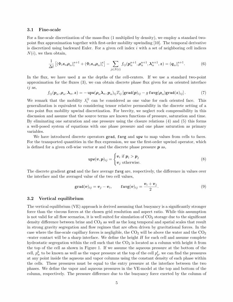
The vertical equilibrium (VE) approach is derived assuming that buoyancy is a significantly strongerforce than the viscous forces at the chosen grid resolution and aspect ratio. While this assumptionis not valid for all flow scenarios, it is well suited for simulation of CO2 storage due to the significantdensity difference between brine and CO2 as well as the long temporal and spatial scales that resultin strong gravity segregation and flow regimes that are often driven by gravitational forces. In thecase where the fine-scale capillary forces is negligible, the CO2 will be above the water and the CO2

-water contact will be a sharp interface. We define the height H for each cell and assume completehydrostatic segregation within the cell such that the CO2 is located as a column with height h fromthe top of the cell as shown in Figure 1. If we assume the aqueous pressure at the bottom of thecell, pbw to be known as well as the vapor pressure at the top of the cell ptg, we can find the pressuresat any point inside the aqueous and vapor columns using the constant density of each phase withinthe cells. These pressures must be equal to the entry pressure at the interface between the twophases. We define the vapor and aqueous pressures in the VE-model at the top and bottom of thecolumn, respectively. The pressure difference due to the buoyancy force exerted by the column of

5

T

B

pg = ptg

pg = ptg + ρg∆z1∆z1

pw − pg = pwg

pw = pbw − ρw∆z2∆z2

pw = pbw

h

H

Figure 1: Water and gas pressures inside a vertically segregated column with height H and constantdensities.

CO2 takes a form analogous to the fine-scale capillary force, resulting in the final pressure differencebetween the two phases in a VE zone as,

Pg = ptg, Pw = pbw, Pg = Pw + pwg(Sg) + hg(ρw − ρg)−Hgρw. (10)

This expression is found by inserting the definitions of VE pressures and solving for equal phasepressure at the fluid interface.

We have opted to use capital case to refer quantities under the VE assumption to differentiatethem from the fine-scale. In the above case there is now flowing water at the top and Pw is equalto the hydrostatic head of water at the bottom with respect the water pressure at the CO2 -waterinterface. Assuming a level, sharp interface between two phases, the height of the CO2 columncan be found from the saturation as h = HSg and the relative permeability will be equal to thesaturation. In more advanced models, for example models where capillary pressure modifies theinterface, the relations are more complicated, see e.g. [47]. We can now write the discrete VEsystem on the same form as (6), albeit with a slightly different interpretation of the variables,

1

∆t

[(ΦiSwρw)n+1

i + (ΦiSwρw)ni]− ∑

j∈N(i)

fij(Pn+1w ,ρn+1

w ,λn+1w , zb) = (Qw)n+1

i , (11)

1

∆t

[(ΦiSgρg)

n+1i + (ΦiSgρg)

ni

]− ∑

j∈N(i)

fij(Pn+1g ,ρn+1

g ,λn+1g , zt) = (Qg)

n+1i . (12)

In the above expression, zt and zb correspond to the top and bottom depths of the coarse cells. Thisis slightly different from the definitions in [48, 47] where only a single region of VE was considered.This definition is simpler to use in the general setting because the flow of the different phases aredefined at the point where they physically appear: The top, zt, for CO2 and the bottom, zb, forwater. The only complication is that the pressure at the point has to be reconstructed from thevariables defined as primary. In this work, we use the cell-center pressures for both primary variablesand property evaluations, requiring a small hydrostatic correction before fluxes are computed.

3.3 Discrete fluxes at the interfaces

We have in the previous sections introduced both a fine-scale and an upscaled system in a discretesetting. The VE approach is in general valid for cells where the gravity segregation due to buoyancyhappens on a much shorter time-scale than the transport induced by viscous forces. The most

6

(a) Transition from VE to fine (b) Transition from VE to VE

Figure 2: The two transition cases: From a zone with a VE discretization to a zone with a fine-scale discretization (left) and the transition from a single to two different VE zones, separated by aimpermeable layer.

restrictive of the VE assumptions are that of full gravity segregation, see [25] for a discussion ofa more advanced model. VE is well suited for the simulation of CO2 migration, where the time-scales are long and there exists a significant density difference. However, the formulation assumes asmooth top surface without significant vertical flow. This situation may occur, e.g. in the presenceof partially eroded impermeable shale layers between two regions of the reservoir.

In order to create a VE model fully suitable for general geomodels, we wish to both be able tocouple different VE regions characterized by a discontinuous top surface. In addition, the assumptionof vertical equilibrium will not be valid in high flow regions, for example near wells. In these partsof the domain, it may be required to use a fine grid resolution to resolve the flow pattern. Toovercome these challenges, we need expressions for fij at interfaces where i and j belong to differentdiscretization regions, either representing the transition between two VE zones or from one VE zoneto a fine-scale grid cell. Both cases are represented in Figure 2

3.3.1 Virtual cells with local saturations and pressure

Since the accumulation terms representing total mass in a cell and the source terms are inde-pendently defined per cell, transitioning between two discretizations comes down to defining thenumerical flux function (7) at the interface. In order to provide a relatively generic implementation,we will not modify the flux function directly, but rather choose the values of p, ρ, λ, z carefully. Fig-ure 3 shows the fine details near a single transition interface, between two VE cells corresponding todifferent layers. In this case, we will focus on the values in the left cell specifically as the treatmentof the right cell is analogous. In order to keep the discussion as simple as possible, we assume thatpillars are completely vertical with a flat top and bottom surface. For a given pillar, we have zt andzb as the z-depth of the top and bottom of the column, respectively. For a given interface betweenthe column and a neighboring column, we define zti and zbi for the column as the top and bottomof the neighboring column1.

The region inside our column delineated vertically by t and h defines a virtual cell. If we candetermine the saturations and pressure in this cell for both the fine-scale and VE discretizations,we can use the flux function directly to obtain a consistent flux. Since the parent cell of the virtualcell is assumed to be in vertical equilibrium with a sharp interface, we can write the virtual gas

1In our implementation, we exploit the fact that the grid is a coarse grid where the cells consist of agglomerations offine-cells. We look up the fine-scale cells at the interface, from which t, h can be retrieved directly. The pre-processordoes not need to take geometry into account, it simply uses the fine-grid depths.

7

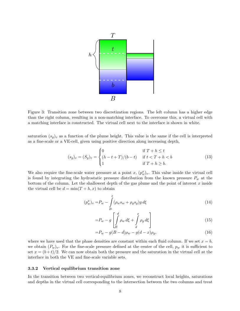
T

B

t

b

h

Figure 3: Transition zone between two discretization regions. The left column has a higher edgethan the right column, resulting in a non-matching interface. To overcome this, a virtual cell witha matching interface is constructed. The virtual cell next to the interface is shown in white.

saturation (sg)v as a function of the plume height. This value is the same if the cell is interpretedas a fine-scale or a VE-cell, given using positive direction along increasing depth,

(sg)v = (Sg)v =

0 if T + h ≤ t(h− t+ T )/(b− t) if t < T + h < b

1 if T + h ≥ b.(13)

We also require the fine-scale water pressure at a point x, (pxw)v. This value inside the virtual cellis found by integrating the hydrostatic pressure distribution from the known pressure Pw at thebottom of the column. Let the shallowest depth of the gas plume and the point of interest x insidethe virtual cell be d = min(T + h, x) to obtain

(pxw)v =Pw −x∫

B

(ρwsw + ρgsg)g dξ (14)

=Pw − g

d∫B

ρw dξ +

x∫d

ρg dξ

(15)

=Pw − g(B − d)ρw − g(d− x)ρg, (16)

where we have used that the phase densities are constant within each fluid column. If we set x = b,we obtain (Pw)v. For the fine-scale pressure defined at the center of the cell, pw it is sufficient toset x = (b+ t)/2. We can now obtain both the pressure and the saturation in the virtual cell at theinterface in both the VE and fine-scale variable sets.

3.3.2 Vertical equilibrium transition zone

In the transition between two vertical-equilibrium zones, we reconstruct local heights, saturationsand depths in the virtual cell corresponding to the intersection between the two columns and treat

8

the connection as VE-to-VE interface. We note that this choices gives a different form than theexpression obtained for the VE-to-VE for two cells of the same region, where the transition isdefined in terms of the saturations of the whole column. This is because the fine-scale situationis different. In the VE-to-VE interaction using the virtual cell we have assumed that the heightdifference between the columns are only due to a discontinuity, while in the VE-to-VE case of samelayer the top surface is assumed to be smoothly varying. These two interpretations can lead todifferent large scale behavior and can be related to the work in [22] on upscaling of top-surfacetopography. The two expressions represent the two limit cases of a smooth family of upscaledrelative permeabilities valid in different regimes. For example, the smooth version is the correctfor the discontinuous top surface in the limit where the viscous forces dominate buoyancy forcesand co-current flow dominates the counter-current segregation effects. For large scale simulations,the virtual cell treatment is appropriate where the model is expected to have a discontinuity in thesurface, e.g. over connecting fault lines. For VE-to-VE where more than one VE cells is involvedon one side the virtual cell concept is the only physically relevant approach, as any other treatmentwould allow for larger-than-unity relative permeability on the coarse-scale.

3.3.3 Fine-scale to VE transition

Cells connected to a transition zone which represent fine-scale cells have pressure defined at thecentroids rather than the top of the cell and we require an additional pressure correction. In suchcells we change the starting point of the integration in equation (14) to the cell centroid instead of thetop of the column. For purposes of the transition from fine to VE zones, the virtual cells belongingto vertically-equilibrated columns are treated as fine-scale cells, with reconstructed pressure andsaturations. The relative permeability is evaluated using the reconstructed fine-scale saturation.

3.3.4 Vertical flow between VE regions

Certain aquifer models contain nearly impermeable layers that compartmentalize the flow. Theselayers are of particular interested for CO2 storage, as the assumption of gravity segregation withineach column for long time-scales is challenged by almost impermeable layers. For connectionsbetween two VE-regions in the vertical direction, we reconstruct fine-scale virtual cells over thelayer and treat the flux as between two fine-scale cells. Specifically, this is required in the Utsiraexample, where the model uses translatability multipliers to account for diffusive leakage throughthin clay layers. This connection is treated separately in our implementation, allowing for the rapidincorporation of more advanced diffuse leakage models.

3.4 Coupled equations

In the preceding text, we used the v subscript to refer to a virtual cell since the discussion waslimited to a single interface. For the general discretization, we employ the notation viji to refer tothe virtual value of the discrete variable v in a cell i when considered at the interface ij. We assumethat this definition is unique per interface, viji = vjii . The virtual cell always belongs to a singlecoarse block-interface pair. We also need the notion of a column, i.e. a set of cells that are verticallylayered on top of each other, is found using the indicator C(i) which provides the column-index ofcell i.

We define the discrete indicator V (i) which gives the ve-region of cell i. If a cell is not governed

9

by the VE discretization, V (i) = Fine. We can write the discretization of the coupled system as,

1

∆t

[Θn+1i + Θn

i

]−∑j∈N(i)

fij(Πn+1α ) = Ψn+1

i , (17)

where we change accumulation terms based on the discretization for the individual cells,

Θi =

{Φisiρi if V (i) = Fine,

ΦiSiρi otherwise,Ψi =

{qi if V (i) = Fine,

Qi otherwise.(18)

There are four categories of flux variables to consider. We have already discussed the case forV (i) = V (j) = Fine, i.e. transition between two fine-scale cells. In the same vein, we have discussedthe case where two VE-columns of the same category cells exchange mass, V (i) = V (j) 6= Fine.The two remaining cases are the transitions between mixed categories V (i) 6= V (j). Depending onthe context, this transition is either treated as a fine-scale or a VE transition. In total, we have fivedifferent cases to consider:

1. Coupling between fine cells.2. Coupling between VE cells in the same VE layer: Figure 13. Coupling between two VE-columns of different category (VE-scale): Figure 2, right subplot,

blue to orange cells or Figure 3.4. Coupling in the vertical direction due to diffuse leakage (fine-scale): Figure 2, right subplot,

orange to yellow cells5. Coupling between fine-scale and VE-columns where C(i) = C(j) but V (i) 6= V (j) (fine-scale)

2, left subplot, blue to orange cells.We reconstruct the appropriate virtual values and apply the same flux expression for all cases.

The concise definition of the variables that must be reconstructed for all possible interfaces can thusbe written out,

Πij =

(p,ρ,λ, z) if V (i) = V (j) = Fine: Case 1,

(P ,ρ,λ,Z) if (V (i) = V (j)) ∧ (C(i) 6= C(j)) ∧ (V (i) 6= Fine) ∧ (V (j) 6= Fine): Case 2,

(P ,ρ,λ,Z)ij if (V (i) 6= V (j)) ∧ (C(i) 6= C(j)) ∧ (V (i) 6= Fine ∧ V (j) 6= Fine): Case 3,

(p,ρ,λ, z)ij otherwise: Cases 4 & 5.

Note that the coarse depth Z is assumed to take the top or bottom depending on the phase beingevaluated.

3.5 Automated selection of different regions

Applications of the proposed multi-region VE model to realistic reservoir models necessarily requiresautomated partitioning of the grid. Manually determining which regions must be separated intodistinct VE regions is not practical for grids with a large number of cells. Segmenting the domaininto different regions can be done using a simple two-step algorithm. We first define an indicatorNij to be 1 if cells i and j are connected with transmissibility below some threshold, or otherwisespecified by the user. We define a column-connectivity matrix Ac,

(Ac)ij =

{1 if Nij ∧ C(i) = C(j)

0 otherwise.(19)

Taking the disconnected components of Ac using a depth-first search from the Boost Graph Librarypackage [57, 24], will give us all columns of the grid, divided into sections where either missing

10

geometric connections or transmissibility below a defined threshold block flow as the vector cc. Wenow have a number of coarse blocks that each belong to a single column, with possibly multipleblocks that belong to the same column. Define G(i) to be the column number of block i and letM(i, j) be the number of blocks with column number j that block i is connected to with a non-zerotransmissibility. We define the block connectivity matrix,

(Ab)ij =

{1 if M(i, G(j)) = 1

0 otherwise,(20)

and take the block connected components cb. If we treat the original partition as a linear index intothis next connected components, cb(cc), we merge any columns that do not transition to more thanone column as seen in Figure 4 and obtain the discrete mapping V required in (3.4).

(a) Fine-scale grid with impermeablelayers before coarsening.

(b) Columns split into connected com-ponents in the vertical direction.

(c) Blocks with single column connec-tion merged together. These blocksshare top and bottom surface.

Figure 4: The grid with impermeable layers (left) is processed into connected sub-columns (middle)before all sub-columns with the same connectivity are assigned to the same category (right). Eachcolor corresponds in this final figure to a distinct region with uniform discretization.

4 Numerical examples

For the numerical examples, we will consider two conceptual problems and two corner-point fieldmodels. As property modeling is not the focus of the discussion, we will use the properties givenin Table 1 for CO2 and brine. All examples include the effect of compressibility, except for thefirst motivational example. All solvers use the same time-steps. These are generally chosen for thefine-scale reference, where very long time-steps can be challenging when column-segregation mustbe resolved.

Table 1: Fluid properties used in the examples. Reference densities are given at 100 bar pressure.

Pseudocomponent Compressibility Viscosity Reference density

Brine (liquid) 10−7 bar−1 0.80 cP 1200 kg/m3

CO2 (vapor) 10−4 bar−1 0.06 cP 760 kg/m3

4.1 A motivational example: Gravity-dominated displacement

As the first example, we will consider a simple problem where applying vertical-equilibrium resultsin considerable reduction in the number of degrees-of-freedom, without any loss of accuracy. We

11

will demonstrate the transition between fine-scale and VE discretizations and consider the effect ofrelative permeabilities on the simulation results.

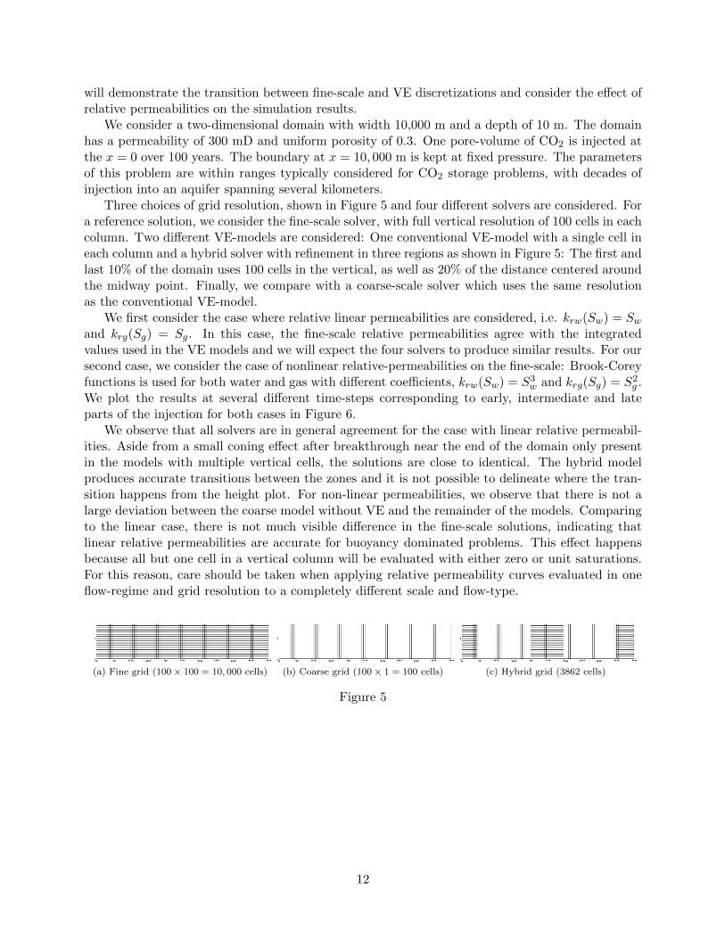
We consider a two-dimensional domain with width 10,000 m and a depth of 10 m. The domainhas a permeability of 300 mD and uniform porosity of 0.3. One pore-volume of CO2 is injected atthe x = 0 over 100 years. The boundary at x = 10, 000 m is kept at fixed pressure. The parametersof this problem are within ranges typically considered for CO2 storage problems, with decades ofinjection into an aquifer spanning several kilometers.

Three choices of grid resolution, shown in Figure 5 and four different solvers are considered. Fora reference solution, we consider the fine-scale solver, with full vertical resolution of 100 cells in eachcolumn. Two different VE-models are considered: One conventional VE-model with a single cell ineach column and a hybrid solver with refinement in three regions as shown in Figure 5: The first andlast 10% of the domain uses 100 cells in the vertical, as well as 20% of the distance centered aroundthe midway point. Finally, we compare with a coarse-scale solver which uses the same resolutionas the conventional VE-model.

We first consider the case where relative linear permeabilities are considered, i.e. krw(Sw) = Swand krg(Sg) = Sg. In this case, the fine-scale relative permeabilities agree with the integratedvalues used in the VE models and we will expect the four solvers to produce similar results. For oursecond case, we consider the case of nonlinear relative-permeabilities on the fine-scale: Brook-Coreyfunctions is used for both water and gas with different coefficients, krw(Sw) = S3

w and krg(Sg) = S2g .

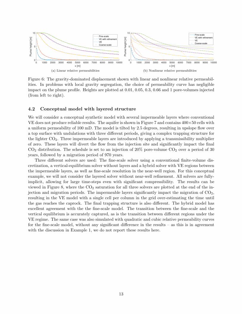
We plot the results at several different time-steps corresponding to early, intermediate and lateparts of the injection for both cases in Figure 6.

We observe that all solvers are in general agreement for the case with linear relative permeabil-ities. Aside from a small coning effect after breakthrough near the end of the domain only presentin the models with multiple vertical cells, the solutions are close to identical. The hybrid modelproduces accurate transitions between the zones and it is not possible to delineate where the tran-sition happens from the height plot. For non-linear permeabilities, we observe that there is not alarge deviation between the coarse model without VE and the remainder of the models. Comparingto the linear case, there is not much visible difference in the fine-scale solutions, indicating thatlinear relative permeabilities are accurate for buoyancy dominated problems. This effect happensbecause all but one cell in a vertical column will be evaluated with either zero or unit saturations.For this reason, care should be taken when applying relative permeability curves evaluated in oneflow-regime and grid resolution to a completely different scale and flow-type.

(a) Fine grid (100× 100 = 10, 000 cells) (b) Coarse grid (100× 1 = 100 cells) (c) Hybrid grid (3862 cells)

Figure 5

12

0 1000 2000 3000 4000 5000 6000 7000 8000 9000 10000

x [m]

0

5

10P

lum

e h

eig

ht

[m] Fine-scale

VE with refinement

VE

Coarse-scale

(a) Linear relative permeabilities

0 1000 2000 3000 4000 5000 6000 7000 8000 9000 10000

x [m]

0

5

10

Plu

me

he

igh

t [m

]

Fine-scale

VE with refinement

VE

Coarse-scale

(b) Nonlinear relative permeabilities

Figure 6: The gravity-dominated displacement shown with linear and nonlinear relative permeabil-ities. In problems with local gravity segregation, the choice of permeability curve has negligibleimpact on the plume profile. Heights are plotted at 0.01, 0.05, 0.3, 0.66 and 1 pore-volumes injected(from left to right).

4.2 Conceptual model with layered structure

We will consider a conceptual synthetic model with several impermeable layers where conventionalVE does not produce reliable results. The aquifer is shown in Figure 7 and contains 400×50 cells witha uniform permeability of 100 mD. The model is tilted by 2.5 degrees, resulting in upslope flow overa top surface with undulations with three different periods, giving a complex trapping structure forthe lighter CO2. Three impermeable layers are introduced by applying a transmissibility multiplierof zero. These layers will divert the flow from the injection site and significantly impact the finalCO2 distribution. The schedule is set to an injection of 20% pore-volume CO2 over a period of 30years, followed by a migration period of 970 years.

Three different solvers are used: The fine-scale solver using a conventional finite-volume dis-cretization, a vertical-equilibrium solver without layers and a hybrid solver with VE regions betweenthe impermeable layers, as well as fine-scale resolution in the near-well region. For this conceptualexample, we will not consider the layered solver without near-well refinement. All solvers are fully-implicit, allowing for large time-steps even with significant compressibility. The results can beviewed in Figure 8, where the CO2 saturation for all three solvers are plotted at the end of the in-jection and migration periods. The impermeable layers significantly impact the migration of CO2,resulting in the VE model with a single cell per column in the grid over-estimating the time untilthe gas reaches the caprock. The final trapping structure is also different. The hybrid model hasexcellent agreement with the the fine-scale model. The transition between the fine-scale and thevertical equilibrium is accurately captured, as is the transition between different regions under theVE regime. The same case was also simulated with quadratic and cubic relative permeability curvesfor the fine-scale model, without any significant difference in the results – as this is in agreementwith the discussion in Example 1, we do not report these results here.

13

(a) Fine-scale model (20,000 cells) (b) Hybrid model (1368 cells)

Figure 7: A synthetic 2D model with CO2 injection in the lower left corner and an open boundaryat the right-most part of the domain (left). The model is coarsened into multiple VE-zones (right),including a fine-scale near-well region shown in red.

(a) End of injection, fine-scale (b) End of injection, hybrid vertical-equilibrium

(c) End of injection, only vertical-equilibrium

(d) End of migration, fine-scale (e) End of migration, hybrid vertical-equilibrium

(f) End of migration, only vertical-equilibrium

Figure 8: Saturation plots for the conceptual model with impermeable layers. CO2 injection in thelower left corner migrates towards the open boundary at the right side of the domain. ConventionalVE models assume vertical equilibrium throughout the vertical direction and are unable to predictthe final trapping structure.

4.3 Refined subset of Sleipner model

The Sleipner field in the North Sea of Norway is a site for CO2 re-injection, where 16.5 milliontonnes of CO2 has been injected into the Utsira formation over the 20 years of operational history[11]. Since it was the first of the large scale injection for storage it has been used as benchmarkon simulation framework. In addition a model of the upper layer has been released to facilitateresearch on realistic data [58, 31]. The upper layer is of particular interest, since this is the region

14

the plume is visible on seismic data.In this example, we will study a complex layered structure with a large number of impermeable

barriers. In order to assess the accuracy of the hybrid VE solver, we will use a highly refined two-dimensional subset of the IEAGHG benchmark mode [58, 31]. The grid has logical dimensions of238× 215, resulting in 40,460 cells after inactive or pinched cells has been removed. We introduce alayering structure inspired by Figure 2 in [4] where intra-formational shales delay plume migrationto the caprock. Six impermeable layers are added, with 25% of the faces in each layer are leftopen to flow, representing fractures or eroded shale layers where gas can migrate through. Thedistribution of open faces in each layer is uniformly random, resulting in a highly complex structureof different flow compartments as shown in the top part of Figure 9.

10-2 100 102

Time [year]

0

0.1

0.2

0.3

0.4

0.5

0.6

0.7

0.8

Fra

ction o

f to

tal C

O2

Top

10-2 100 102

Time [year]

0.05

0.1

0.15

0.2

0.25

0.3

0.35

0.4

0.45

0.5

0.55

Fra

ctio

n o

f to

tal C

O2

Middle

10-2 100 102

Time [year]

0

0.1

0.2

0.3

0.4

0.5

0.6

0.7

0.8

0.9

Fra

ction o

f to

tal C

O2

Bottom

Figure 9: The setup of the Sleipner subset case. A number of impermeable layers are added to themodel, with a stochastic distribution of open segments. The model is divided in to three parts forpurposes of analyzing the migration behavior in the different discretized models.

We use a synthetic well configuration where three injection sites at the bottom of the formationinject a total of 0.75 pore-volumes over 50 years, followed by 4950 years of migration. While thisis a fairly large amount in terms of total pore-volume, it only corresponds to 5.7 megatonnes ofCO2 due to the thin width of the grid. The formation is open at x = min(x) and x = max(x) withhydrostatic boundary conditions.

The gas saturation at the end of the injection and migration periods is shown in Figure 10. Weobserve that all solvers produce sharp, horizontal interfaces at equilibrium, but the conventionalVE model (700 cells) predicts almost no trapped CO2 in the right part of the model. The hybridmodel with near-well refinement (2700 cells) and the vertical equilibrium with layers included (1776cells) both accurately predict the saturation distribution at the end of the migration and injectionperiods. Even insignificant traps of CO2 is predicted consistently across the fine-scale and the twomultiresolution VE-models. In terms of the migration behavior over time, we observe from Figure 9that the relative ranking of the four models persist, with agreement between all models which include

15

layers. If we consider the injector BHP, shown in Figure 11, we see that the hybrid model with fine-scale cells in the near-well region agrees with the fine-scale model in terms of pressure buildup. Themodels without fine-scale detail does not match the BHP, although a dedicated upscaling procedurefor the wells themselves may improve this result. For a real formation introducing specific treatmentfor the wells may be less practical than including the correct behavior using the fine grid aroundthe well. One would expect that the near-well is relatively stationary at later times and thus willnot contribute to the numerical complexity of solving the nonlinear system.

The number of nonlinear iterations used by the different solvers is reported in Figure 15. Weobserve that the VE solvers with and without layers use approximately the same low numberof iterations when compared to the fine-scale. The solver with near-well refinement uses moreiterations, as the segregation process near the well must be resolved by the Newton-Rapshon solver.Relative speed-up by applying VE varies from 548 to 52, depending on the solver used.

(a) End of injection, fine-scale (b) End of migration, fine-scale

(c) End of injection, hybrid (d) End of migration, hybrid

(e) End of injection, vertical-equilibrium (f) End of migration, vertical-equilibrium

(g) End of injection, vertical-equilibrium (without layers) (h) End of migration, vertical-equilibrium (without layers)

Figure 10: Reconstructed CO2 saturation for the four different solvers for the same problem. Theleft column represents the end of the injection period, while the right column is the stationarysolution after 1000 years of subsequent migration.

16

100

105

Time [days]

30

35

40

45

50B

HP

[bar]

Fine-scale

VE (near-well refinement)

VE (no layers)

VE (with layers)

(a) BHP, injector 1

100

105

Time [days]

30

35

40

45

50

BH

P [bar]

Fine-scale

VE (near-well refinement)

VE (no layers)

VE (with layers)

(b) BHP, injector 2

100

105

Time [days]

30

35

40

45

50

BH

P [bar]

Fine-scale

VE (near-well refinement)

VE (no layers)

VE (with layers)

(c) BHP, injector 3

Figure 11: Bottom hole pressures for the injectors in the Sleipner example during the injectionperiod

4.4 Layered Utsira model

The final example is a 3D model with logical dimensions 64×240×15 and 111,162 active cells. Thegeometry, permeability, well configuration and layering structure is taken from one of the Utsiramodels considered in [55]. The model has a uniform permeability of 1000 mD, with three semi-permeable layers as shown in Figure 12. The corresponding faces in the vertical connections has atransmissibility multiplier of 10−4. 140.89 megatonnes of CO2 is injected over 50 years, followed bya migration period until 8000 years in total has passed. The boundaries of the reservoir is consideredto be closed. Due to the coarseness of the vertical layers and fairly long time-steps, we considerlinear relative permeability curves to be a reasonable choice to ensure correct segregation speed.

Unlike the previous example, the fine-scale model does not have sufficient resolution to beconsidered fully resolved. It is therefore not necessarily given that the fine-scale model is moreaccurate than the different VE solvers, which represent the plume depth continuously within eachcolumn. Four models are considered: The fine-scale model (111,162 cells), VE without layering(11,680 cells), VE with layers (42,877 cells) and hybrid-VE with fine-scale near the wells (44,215).The ratio between fine-scale and VE models is lower in this example, as the original model is alreadyvery coarse. In this sense, the VE models do not significantly reduce the number of cells, but theypotentially increase the accuracy of the predicted CO2 distribution.

From the thresholded saturation profiles in Figure 13, we observe that all four models giveessentially the same trapping structure after 8000 years. As only the top surface is truly imper-meable, the long term migration is less impacted by the inclusion of the layers. In the short andmedium-term in Figure 12), however, we note that the inclusion of layers is necessary to estimatewhich depths of the reservoir contains mobile CO2 . We also observe that the hybrid model exactlymatches the fine-scale distribution, while the layered model without near-well refinement deviatessomewhat. We emphasize that the hybrid model will represent the near-well flow exactly as in thefine-scale model, including any discretization error made by using large grid blocks. This is againreflected in the well curves, shown in Figure 14, where the hybrid model accurately predicts BHP.

The right subfigure in Figure 15 contains the iteration numbers and relative speedups. As themodel is already fairly coarse, the effect of applying VE is not as significant as in the Sleipner subsetexample. However, we still observe an order-of-magnitude speedup and a halving of the number ofnonlinear iterations when compared to the fine-scale.

17

10 -2 10 0 10 2

Time [year]

0

0.1

0.2

0.3

0.4

0.5

0.6

0.7

0.8

0.9

1F

ractio

n o

f to

tal C

O2

Layers 1 to 3

10 -2 10 0 10 2

Time [year]

0

0.05

0.1

0.15

0.2

Fra

ctio

n o

f to

tal C

O2

Layers 4 to 5

10 -2 10 0 10 2

Time [year]

0

0.05

0.1

0.15

0.2

0.25

0.3

0.35

Fra

ctio

n o

f to

tal C

O2

Layers 6 to 7

10 -2 10 0 10 2

Time [year]

0

0.1

0.2

0.3

0.4

0.5

0.6

Fra

ctio

n o

f to

tal C

O2

Layers 8 to Inf

Figure 12: The Utsira model. Four different flow compartments are defined, with semi-permeablelayers in-between shown in black. These shales cover the entire layer, but allow for diffusive leakagewith a small rate compared to the vertical flow during injection.

18

(a) End of injection, fine-scale (b) End of migration, fine-scale

(c) End of injection, hybrid (d) End of migration, hybrid

(e) End of injection, vertical-equilibrium (f) End of migration, vertical-equilibrium

(g) End of injection, vertical-equilibrium (withoutlayers)

(h) End of migration, vertical-equilibrium (withoutlayers)

Figure 13: Gas saturation in the Utsira example. A thresholding of sg > 0.1 was used to visualizethe plume.

19

100

102

104

Time [days]

95

100

105

110

115

120

125

BH

P [bar]

Fine-scale

VE with refinement

VE without layers

VE without refinement

(a) BHP, injector 1

100

102

104

Time [days]

95

100

105

110

115

120

125

BH

P [bar]

Fine-scale

VE with refinement

VE without layers

VE without refinement

(b) BHP, injector 2

100

102

104

Time [days]

95

100

105

110

115

120

125

BH

P [bar]

Fine-scale

VE with refinement

VE without layers

VE without refinement

(c) BHP, injector 3

100

102

104

Time [days]

95

100

105

110

115

120

125

BH

P [bar]

Fine-scale

VE with refinement

VE without layers

VE without refinement

(d) BHP, injector 4

Figure 14: Bottom hole pressures for the injectors in the Utsira example during the injection period

1.00

52.68

548.11 165.32

Fine-scale VE (near-well refinement) VE (no layers) VE (with layers)0

1000

2000

3000

4000

5000

Nu

mb

er

of

no

nlin

ea

r ite

ratio

ns

Injection

Migration

(a) Sleipner subset

1.00

9.53156.25

13.77

Fine-scale VE with refinement VE without layers VE without refinement0

500

1000

1500

Num

ber

of nonlin

ear

itera

tion

s

Injection

Migration

(b) Utsira model

Figure 15: Nonlinear iterations used in the Sleipner and Utsira examples. The number of iterationsspent is divided between injection and migration, and relative speed-up compared to the fine-scaleis shown as a number over each column.

20

5 Conclusion

We have presented a uniform framework for coupling VE models with general layered structurewith traditional 3D reservoir models. In addition we have devices a general strategy for obtainingthe model from a underlaying 3D reservoir model in industry standard format. In doing so we haveintroduced to our knowledge introduced new coupling terms between 3D models and VE model,between VE layers and a new diffuse leakage calculation consistent with the underlying 3D model.The model is implemented in the MRST AD-OO framework with state of the art robust implicitTPFA-MUP discretization including possibilities for adjoint calculations. This makes the modelpresented in this paper suited for use in optimization and data integration applications.

A major contribution of the paper is the uniform representation of the model in terms of pseudorelative permeabilities and capillary pressure, which highlights the need for relative permeabilitiesassociated with oriented faces for upscaled model. This can bee seen as a discrete representation ofgeneral tensor mobilities.

VE models which have shown great promise for evaluating long-term aquifer-scale CO2 storageand this work is an important step towards applying these models to general industry-grade modelswith layered structure, complex well models and non-VE flow regions. As the discretization isbased on a underlying 3D detailed description it is always possible to check the validity of a coarsemodel by adding more parts of the model in the 3D region. The proposed treatment results ina practical and efficient simulation model for optimization and data integration in the setting ofCO2 storage. However, we believe the methodology is well suited for other sub-surface simulationproblems where segregated flow dominates large parts of the domain, for example gas storage andpetroleum reservoirs with large gravity differences and large distances between wells.

The model including examples of this paper will be made public under the GPLv3 with the nextrelease of the Matlab Reservoir Simulation Toolbox [42].

6 Acknowledgements

This work was funded in part by the Research Council of Norway through grant no. 243729 (Sim-ulation and optimization of large-scale, aquifer-wide CO2 injection in the North Sea) and NCCS– Industry Driven Innovation for Fast Track CCS Deployment grant no. 257579. Olav Møyner isfunded by VISTA, which is a basic research programme funded by Statoil and conducted in closecollaboration with The Norwegian Academy of Science and Letters.

Statoil and the Sleipner License are acknowledged for provision of the Sleipner 2010 Referencedataset. Any conclusions in this paper concerning the Sleipner field are the authors’ own opinionsand do not necessarily represent the views of Statoil.

We also acknowledge The Norwegian Petroleum Directorate for providing the model accompa-nying the paper [55] used in Example 4.

21

References

[1] Odd Andersen, Sara Gasda, and Halvor M. Nilsen. Vertically averaged equations with variabledensity for CO2 flow in porous media. Transp. Porous Media, 107:95–127, 2015.

[2] Odd Andersen, Knut-Andreas Lie, and Halvor Møll Nilsen. An open-source toolchain forsimulation and optimization of aquifer-wide CO2 storage. Energy Procedia, :1–10, 2015. The8th Trondheim Conference on Capture, Transport and Storage.

[3] Odd Andersen, Halvor Møll Nilsen, and Knut-Andreas Lie. Reexamining CO2 storage capacityand utilization of the Utsira Formation. In ECMOR XIV – 14th European Conference on theMathematics of Oil Recovery, Catania, Sicily, Italy, 8-11 September 2014. EAGE, 2014.

[4] J. Cavanagh Andrew, R. Stuart Haszeldine, and Bamshad Nazarian. The sleipner co2 storagesite: using a basin model to understand reservoir simulations of plume dynamics. First Break,33(6):61–68, 2015.

[5] Karl W Bandilla, Michael A Celia, Thomas R Elliot, Mark Person, Kevin M Ellett, John ARupp, Carl Gable, and Yipeng Zhang. Modeling carbon sequestration in the illinois basin usinga vertically-integrated approach. Comput. Vis. Sci., 15(1):39–51, 2012.

[6] Karl W. Bandilla, Michael A. Celia, and Evan Leister. Impact of model complexity on CO2

plume modeling at Sleipner. Energy Procedia, 63:3405–3415, 2014. 12th International Confer-ence on Greenhouse Gas Control Technologies, GHGT-12.

[7] Karl W Bandilla, Stephen R Kraemer, and Jens T Birkholzer. Using semi-analytic solutionsto approximate the area of potential impact for carbon dioxide injection. Int. J. Greenh. GasControl, 8:196–204, 2012.

[8] John Barker and Sylvain Thibeau. A critical review of the use of pseudorelative permeabilitiesfor upscaling. SPE Reservoir Engineering, 12(2):138–143, 1997.

[9] R. P. Batyck, J. M. Blunt, and M. R. Thiele. A 3d field-scale streamline-based reservoirsimulator. Society of Petroleum Engineers, 12, 1997.

[10] Yann Brenier and Jerome Jaffre. Upstream differencing for multiphase flow in reservoir simu-lation. SIAM J. Numer. Anal., 28(3):685–696, 1991.

[11] Andrew J Cavanagh, R Stuart Haszeldine, and Bamshad Nazarian. The Sleipner CO2 storagesite: using a basin model to understand reservoir simulations of plume dynamics. First Break,33(June):61–68, 2015.

[12] M. A. Celia, S. Bachu, J. M. Nordbotten, and K. W. Bandilla. Status of CO2 storage indeep saline aquifers with emphasis on modeling approaches and practical simulations. WaterResources Research, 51(9), 2015.

[13] K. H. Coats, J. R. Dempsey, and J. H. Henderson. The use of vertical equilibrium in two-dimensional simulation of three-dimensional reservoir preformance. Soc. Pet. Eng. J., Mar:68–71, 1971.

[14] K. H. Coats, R. L. Nielsen, M. H. Terune, and A. G.Weber. Simulation of three-dimensional,two-phase flow in oil and gas reservoirs. Soc. Pet. Eng. J., Dec:377–388, 1967.

22

[15] F. Doster, J. M. Nordbotten, and M. A. Celia. Hysteretic upscaled constitutive relationshipsfor vertically integrated porous media flow. Comput. Visual. Sci., 15:147–161, 2012.

[16] F. Doster, J.M. Nordbotten, and M.A. Celia. Impact of capillary hysteresis and trapping onvertically integrated models for CO2 storage. Adv. Water Resour., 62, Part C:465–474, 2013.

[17] Kristin Guldbrandsen Froysa, Johnny Froyen, and Magne S. Espedal. Simulation of 3d flowwith gravity forces in a porous medium. Computing and Visualization in Science, 3(3):121–131,Aug 2000.

[18] S. E. Gasda, J. M. Nordbotten, and M. A. Celia. Vertical equilibrium with sub-scale analyticalmethods for geological C02 sequestration. Comput. Geosci., 13(4):469–481, 2009.

[19] S. E. Gasda, J. M. Nordbotten, and M. A. Celia. Vertically-averaged approaches to CO2injection with solubility trapping. Water Resources Research, 47:W05528, 2011.

[20] Sarah E. Gasda, Elsa du Plessis, and Helge K. Dahle. Upscaled models for modeling CO2injection and migration in geological systems. In Peter Bastian, Johannes Kraus, RobertScheichl, and Mary Wheeler, editors, Simulation of Flow in Porous Media, volume 12 of RadonSeries on Computational and Applied Mathematics, pages 1–38. De Gruyter, Berlin, Boston,2013.

[21] Sarah E. Gasda, Halvor M. Nilsen, and Helge K. Dahle. Impact of structural heterogeneityon upscaled models for large-scale CO2 migration and trapping in saline aquifers. Adv. WaterResour., 62, Part C(0):520–532, 2013.

[22] Sarah E. Gasda, Halvor M. Nilsen, Helge K. Dahle, and William G. Gray. Effective modelsfor CO2 migration in geological systems with varying topography. Water Resour. Res., 48(10),2012.

[23] S.E. Gasda, A.F. Stephansen, I. Aavatsmark, and H.K. Dahle. Upscaled modeling of CO2injection and migration with coupled thermal processes. Energy Procedia, 40:384–391, 2013.

[24] David Gleich. Matlabbgl – a matlab graph library, October 2008.

[25] Bo Guo, Karl W. Bandilla, Florian Doster, Eirik Keilegavlen, and Michael A. Celia. A verticallyintegrated model with vertical dynamics for co2 storage. Water Resources Research, 50(8):6269–6284, 2014.

[26] Eva K. Halland, Jasminka Mujezinovic, and Fridtjof Riis, editors. CO2 Storage Atlas: Norwe-gian Continental Shelf. Norwegian Petroleum Directorate, P.O. Box 600, NO-4003 Stavanger,Norway, 2014.

[27] Vera Louise Hauge, Knut-Andreas Lie, and Jostein R. Natvig. Flow-based coarsening formultiscale simulation of transport in porous media. Comput. Geosci., 16(2):391–408, 2012.

[28] Rainer Helmig. Adaptive vertical equilibrium concept for energy storage in subsurface systems.SIAM Conference on Mathematical and Computational Issues in the Geosciences, September11–14, 2017, Erlangen, Germany.

[29] A. Henriquez, O. J. Apeland, O. Lie, and I. & Cheshire. Novel simulation techniques used ina gas reservoir with a thin oil zone. Society of Petroleum Engineers, 1992.

23

[30] Mark A. Hesse, Franklin M. Orr, and Hamdi A. Tchelepi. Gravity currents with residualtrapping. J. Fluid. Mech., 611:35–60, 2008.

[31] International Energy Agency. Sleipner benchmark model, 2012.

[32] Hugh H. Jacks, Owen J. E. Smith, and C. C. Mattax. The modeling of a three-dimensionalreservoir with a two-dimensional reservoir simulator – the use of dynamic pseudo functions.Soc. Pet. Eng. J., 13(3):175–185, 1973.

[33] Stein Krogstad, Knut-Andreas Lie, Olav Møyner, Halvor Møll Nilsen, Xavier Raynaud, andBard Skaflestad. MRST-AD – an open-source framework for rapid prototyping and evaluationof reservoir simulation problems. In SPE Reservoir Simulation Symposium, 23–25 February,Houston, Texas, 2015.

[34] Jo Ro Kyte and D W Berry. New pseudo functions to control numerical dispersion. Soc. Pet.Eng. J., 15(4):269–276, 1975.

[35] Knut-Andreas Lie. An Introduction to Reservoir Simulation Using MATLAB: User guide forthe Matlab Reservoir Simulation Toolbox (MRST). SINTEF ICT, http://www.sintef.no/Projectweb/MRST/publications, 2nd edition, December 2015.

[36] Knut-Andreas Lie, Stein Krogstad, Ingeborg S. Ligaarden, Jostein R. Natvig, Halvor MøllNilsen, and Bard Skaflestad. Open source MATLAB implementation of consistent discretisa-tions on complex grids. Comput. Geosci., 16:297–322, 2012.

[37] Knut-Andreas Lie, Halvor Møll Nilsen, Odd Andersen, and Olav Møyner. A simulation work-flow for large-scale CO2 storage in the Norwegian North Sea. In ECMOR XIV – 14th EuropeanConference on the Mathematics of Oil Recovery, Catania, Sicily, Italy, 8-11 September 2014.EAGE, 2014.

[38] Knut-Andreas Lie, Halvor Møll Nilsen, Odd Andersen, and Olav Møyner. A simulation work-flow for large-scale CO2 storage in the Norwegian North Sea. Comput. Geosci., :1–16, 2015.

[39] Ingeborg S. Ligaarden and Halvor Møll Nilsen. Numerical aspects of using vertical equilib-rium models for simulating CO2 sequestration. In Proceedings of ECMOR XII–12th EuropeanConference on the Mathematics of Oil Recovery, Oxford, UK, 6–9 September 2010. EAGE.

[40] J. C. Martin. Some mathematical aspects of two phase flow with application to flooding andgravity segregation. Prod. Monthly, 22(6):22–35, 1958.

[41] J. C. Martin. Partial integration of equation of multiphase flow. Soc. Pet. Eng. J., Dec:370–380,1968.

[42] The MATLAB Reservoir Simulation Toolbox, version 2011a, 2011.

[43] The MATLAB Reservoir Simulation Toolbox, version 2017a, 6 2017.http://www.sintef.no/MRST/.

[44] Trine S. Mykkeltvedt and Jan M. Nordbotten. Estimating effective rates of convective mixingfrom commercial-scale injection. Environ. Earth Sci., 67(2):527–535, 2012.

24

[45] Halvor Møll Nilsen, Paulo A. Herrera, Meisam Ashraf, Ingeborg Ligaarden, Martin Iding,Christian Hermanrud, Knut-Andreas Lie, Jan M. Nordbotten, Helge K. Dahle, and Eirik Kei-legavlen. Field-case simulation of CO2-plume migration using vertical-equilibrium models.Energy Procedia, 4(0):3801–3808, 2011.

[46] Halvor Møll Nilsen, Knut-Andreas Lie, and Odd Andersen. Analysis of CO2 trapping capacitiesand long-term migration for geological formations in the Norwegian North Sea using MRST-co2lab. Computers & Geoscience, 79:15–26, 2015.

[47] Halvor Møll Nilsen, Knut-Andreas Lie, and Odd Andersen. Fully implicit simulation of vertical-equilibrium models with hysteresis and capillary fringe. Comput. Geosci., :, 2015.

[48] Halvor Møll Nilsen, Knut-Andreas Lie, and Odd Andersen. Robust simulation of sharp-interfacemodels for fast estimation of CO2 trapping capacity. Computational Geosciences, pages 1–21,2015.

[49] Halvor Møll Nilsen, Knut-Andreas Lie, Olav Møyner, and Odd Andersen. Spill-point anal-ysis and structural trapping capacity in saline aquifers using MRST-co2lab. Computers &Geoscience, 75:33–43, 2015.

[50] Halvor Møll Nilsen, Anne Randi Syversveen, Knut-Andreas Lie, Jan Tveranger, and Jan M.Nordbotten. Impact of top-surface morphology on CO2 storage capacity. Int. J. Greenh. GasControl, 11(0):221–235, 2012.

[51] Halvor Mll Nilsen, Stein Krogstad, Odd Andersen, Rebecca Allen, and Knut-Andreas Lie.Using sensitivities and vertical-equilibrium models for parameter estimation of co2 injectionmodels with application to sleipner data. Energy Procedia, 114(Supplement C):3476 – 3495,2017. 13th International Conference on Greenhouse Gas Control Technologies, GHGT-13, 14-18November 2016, Lausanne, Switzerland.

[52] J. M. Nordbotten and H. K. Dahle. Impact of the capillary fringe in vertically integratedmodels for CO2 storage. Water Resour. Res., 47(2):W02537, 2011.

[53] Jan M. Nordbotten and Michael A. Celia. Similarity solutions for fluid injection into confinedaquifers. J. Fluid Mech., 561:307–327, 8 2006.

[54] Jan M. Nordbotten and Michael A. Celia. Geological Storage of CO2: Modeling Approachesfor Large-Scale Simulation. John Wiley & Sons, Hoboken, New Jersey, 2012.

[55] VTH Pham, F Riis, IT Gjeldvik, EK Halland, IM Tappel, and P Aagaard. Assessment of co 2injection into the south utsira-skade aquifer, the north sea, norway. Energy, 55:529–540, 2013.

[56] Schlumberger. Eclipse Technical Description Manual. Schlumberger, 2009.2 edition, 2009.

[57] Jeremy G Siek, Lie-Quan Lee, and Andrew Lumsdaine. The Boost Graph Library: User Guideand Reference Manual, Portable Documents. Pearson Education, 2001.

[58] Varunendra Singh, Andrew Cavanagh, Hilde Hansen, Bamshad Nazarian, Martin Iding, andPhilip Ringrose. Reservoir modeling of CO2 plume behavior calibrated against monitoring datafrom Sleipner, Norway. In SPE Annual Technical Conference and Exhibition, Florence, Italy,2010.

25

[59] SINTEF ICT. The MATLAB Reservoir Simulation Toolbox: Numerical CO2 laboratory, Oc-tober 2014.

[60] H. L. Stone. Rigorous black oil pseudo functions. In SPE Symposium on Reservoir Simulation,17-20 February, Anaheim, California. Society of Petroleum Engineers, 1991.

26