SLAC-PUB-819 , October 1970 WV QUANTUM ELECTRODYNAMICS AT INFINITE MOMENTUM: SCATTERING FROM AN EXTERNAL FIELDt James D. Bjorken, John B. Kogut* and Davison E. Soper Stanford Linear Accelerator Center Stanford University, Stanford, California 94305 ABSTRACT Using a formulation of quantum electrodynamics in the infinite momentum frame, we develop a theory to describe the scattering of energetic electrons or >” photons off an external field. A physical picture emerges which proves to be a realization of Feymnan’s lfparton” ideas. In this picture the incoming electron is composed of bare constituents (the quanta of the Schroedinger fields) which, at high laboratory energies, interact slowly with one another: Each bare constituent ” is scattered from the external field in a simple way, then the constituents again interact among themselves to form the final state. This formalism is applied to elastic electron and photon scattering, bremsstrahlung and pair production, and deep inelastic electroproduction of lepton pairs, and the results of Cheng and Wu andothers are recovered in a simple way. In these applications, perturbation theory is used to construct the wave functions of the constituents in the initial and final states. (Submitted to Phys. Rev. ) t‘ Work supported by the U. S. Atomic Energy Commission. * NSF Predoctoral Fellow.

Welcome message from author
This document is posted to help you gain knowledge. Please leave a comment to let me know what you think about it! Share it to your friends and learn new things together.
Transcript

SLAC-PUB-819 , October 1970 WV
QUANTUM ELECTRODYNAMICS AT INFINITE MOMENTUM:
SCATTERING FROM AN EXTERNAL FIELDt
James D. Bjorken, John B. Kogut* and Davison E. Soper
Stanford Linear Accelerator Center Stanford University, Stanford, California 94305
ABSTRACT
Using a formulation of quantum electrodynamics in the infinite momentum
frame, we develop a theory to describe the scattering of energetic electrons or >”
photons off an external field. A physical picture emerges which proves to be a
realization of Feymnan’s lfparton” ideas. In this picture the incoming electron is
composed of bare constituents (the quanta of the Schroedinger fields) which, at
high laboratory energies, interact slowly with one another: Each bare constituent ”
is scattered from the external field in a simple way, then the constituents again
interact among themselves to form the final state. This formalism is applied to
elastic electron and photon scattering, bremsstrahlung and pair production, and
deep inelastic electroproduction of lepton pairs, and the results of Cheng and Wu
andothers are recovered in a simple way. In these applications, perturbation
theory is used to construct the wave functions of the constituents in the initial and
final states.
(Submitted to Phys. Rev. )
t‘ Work supported by the U. S. Atomic Energy Commission.
* NSF Predoctoral Fellow.

I. INTRODUCTION
Recently considerable progress has been made in evaluating amplitudes for
high energy electromagnetic processes. Various authors’ have found, using con-
ventional calculational techniques and considerable labor, that these amplitudes
have several unifying features. First, when two electromagnetic particles having
large relative momenta exchange a fixed amount of momentum, the interaction
can be viewed as occurring between the bare quanta which compose the incoming
and outgoing scattering states. And furthermore, the interaction between these
constituents is ‘simply a relativistic generalization of the eikonal amplitude familiar
from nonrelativistic scattering processes. 2 Thus, a physical picture for these
scattering processes emerges which is similar to Feynman’s “parton” ideas. 3
. . We wish to show in this paper that these interesting features can be easily under-
stood and derived from a recent formulation of quantum electrodynamics in the . . . . 1. . b 1
t 4 *f. infinite momentum frame developed by two of the authors.
The motivation for developing a formal theory of quantum electrodynamics
in the infinite momentum frame, hereafter referred to as I., was the hope that
this exact theory would lead to an approximate ultrarelativistic theory which could
provide a simple description of extremely high energy phenomena, just as non-
relativistic field theories provide understanding of low energy phenomena. For
example, the nonrelativistic limit of quantum electrodynamics possesses tremen-
dous computational simplifications and intuitive insights into low energy electro-
magnetic processes. It was shown in I. that quantum electrodynamics in the
infinite momentum frame, although formally equivalent to quantum electrodynamics
developed in an ordinary reference frame, possesses several simplifying features
itself. These include the formal absence of vacuum pair creation, computational
simplicities, and a nonrelativistic analogy which should become a basis for intuition
-l-

into high energy phenomena. However, just as the nonrelativistic limit of quantum
electrodynamics has certain deficiencies, its ultrarelativistic limit will inherit
several limitations already contained in I. For example, the renormalization
procedure becomes more difficult, old-fashioned perturbation theory must be
used, and manifest covariance is lost. Nonetheless, we will see in this article .
that for a limited range of applications, specifically the calculation of high energy
amplitudes, the formulation of quantum electrodynamics in the infinite momentum
frame possesses distinct advantages over the conventional theory.
The plan of this paper will be to review the formalism of quantum electro-
dynamics in the infinite momentum frame developed in I. , and present a heuristic
derivation of the salient features of that paper in a ‘nonrelativistic” fashion. We
next introduce an external field into the theory and derive a closed form for the
scattering operator, formally valid as the energies of incident and produced
partidles tend to infinity. We then apply this formalism to several electrodynamic
processes and obtain the results of Cheng and Wu and others. \
II. REVIEW OF THE INFINITE-MOMENTUM FORMALISM
The trajectories of particles in nonrelativistic processes cluster about a
single direction in space-time, which is generally taken to be the time axis. The
trajectories in extreme-relativistic processes likewise cluster about a direction
in space-time, which can be conventionally taken to be a nu.II vector in the t-z
plane. It is sensible to describe nonrelativistic processes in the coordinate
system (t, x, y,&. It is likewise sensible to describe extreme-relativistic pro-
cesses using the coordinates 7 = 2 42 (t’z), x;y,g = 2-1’2(t- z), since in this
coordinate system the particle trajectories cluster about the new g%irne’J axis.
-2-

In I. , quantum electrodynamics was reformulated in this new coordinate system
$ = (7,x1,x2,g)==c;~v =gPVkv , 1
with xv the usual space-time coordinates and
(II. 1)
The corresponding momenta are H = p. = 2 -l’2(E - p,), ? = p3 = 2-1’2(E + p,), and
; = (P,,P,). s ince H generates T-translations, it plays the role of a Hamiltonian.
In brief, the procedure used in I. is:
1. Change variables in the Lagrangian. The equations of motion, being
form-invariant, remain unchanged.
2. Choose the gauge A0 = A3 = 0.
3; Identify the independent field components and quantize them with the known . . . _ : \‘_ 6 : . equal-7 commutation relations satisfied by the corresponding free field com-
ponents. . Only the two transverse components of the electromagnetic potential
are independent variables; the component A3 is zero by the gauge choice, and
the component A0 is eliminated in a way similar to that of conventional Coulomb-
gauge electrodynamics. In a similar way, we find that only two of the four com-
ponents of the Dirac field ~7 are independent. Once the equal-7 commutation
relations among the independent field components have been specified, all of
the equal-7 ‘commutators in the theory can be calculated using Maxwell’s
equations and the Dirac equation.
4. Construct the Hamiltonian.
5. For the perturbation expansion of the S-matrix, use “old-fashioned” Heitler
perturbation theory. This procedure is seen to give a perturbative solution to
the field theory identical to the more familiar Feynman expansion.
-3-

The infinite momentum analysis of I. led naturally to the use of four-component
spinors and polarization vectors which, when boosted to (almost) the speed of light
in the z-direction, became eigenstates of helicity as measured in the lab. (Thus,
if we choose to describe processes involving particles with almost infinite mo-
mentum in the +z direction, this notion of infinite momentum helicity coincides
with the familiar description of helicity.) It turns out that the matrix elements of
the Hamiltonian of I. are remarkably simple if one chooses the incoming and out-
going particles to be in infinite momentum helicity states.
Instead of simply evaluating the relevant matrix elements in the context of I.,
we find it instructive and intriguing to rederive these results in a simple heuristic
fashion which takes full advantage of the nonrelativistic structure present in the
infinite momentum frame. (The connection between the formalism of I. and the
formalism. to be presented here is given in the Appendix. )
We begin with the mass shell condition for a free electron, pPpP = m2, or
2qH - p2 = m2. * If we make the usual identification pP-iaP we arrive at the
equation of motion for the free electron field (the Klein-Gordon equation):
I i 9.,U(x) = 1 5 (g2 -f- m2) P(X) , (II. 3)
where l/7 is the integral operator
c 1 +p (x) = & J- df e-0 w->&O (II. 4)
As we will see, it suffices to let w(x) have only two components. The two components
are postulated to satisfy the equal-T anticommutation relations
= sap S(p9’) S2(g g’) . w- 5)
Free photons are described by the two transverse components b(x) of the
electromagnetic potential. As in paper I, we use the infinite momentum gauge,
A0 = A3 = 0. The equal-r commutation relations satisfied by s(x)
/J-a-

are
(II. 6)
The free photon Hamiltonian is
H 2’ =-
Y dg dz Ak(x) g2 Ak(x) . (II. 7)
Using the commutation relations (II. 6), this Hamiltonian leads to the expected
equation of motion,
p(x), HA= id0 Ak(x) = 4 $ Ak(x) . w* 8)
The natural two component spinors w(s) and polarization vectors g(h) in this
description are
.w(+1/2) = ; 0
S(G) = 2 -1’2(i, i)
w(-l/2) = 1” 0
$1) = 2 -l’?(l, -i), (II. 9)
where the arguments s,h refer to the infinite momentum helicity discussed earlier.
Using these wave functions, the Fourier expansion of the fields a’, A take the form5
W(x) = (W -yd$$@& ${&w(s) e~ip’xb(p,s)+fi~(-s)e+iP’Xdt(p,s)},
(II. 10)
&(x) = (2~)w3$$ g(h) emiP ’ xa(p, h) -t- g(h)* e+ip ’ x a?(p, h)) . (II. 11)
The operator b T (p, s), t t d (p, s), and a (p, s) are creation operators for electrons,
positrons, and photons respectively. They satisfy the commutation relations
{ WP, s), &pr, sl)> = $&m3 2rl w - rl’) ~2tg-&1)
{d(p, s), dh?‘, St)} = tSss,(2q3 277 6(q -q,‘) a2(g-g’,
(II. 12)
L’- ”

The electrodynamic interaction can be introduced into this formalism by
writing the free electron wave equation in the form6
iao*= (m-ig.g) $j (m*ig.g)II/ , (II. 13)
then making the gauge-&variant substitution pF. pP - e AP. Then, using the
gauge choice A3 = 0, the wave equation with interactions becomes
iao# = eAom+ (m- Q-e g-eg)&(m+i_asI;E-e&j)* (II. 14)
The dependent variable A0 is eliminated with the help of ‘Maxwell’s equations,
#F w
= aP$AV - a, #A, = JV . Choosing V= 3 and recalling that A3 = 0, we
find that -a,(a,A, -l l 9) = J3. From I. , we find that J3 = Jo = cl/l% . Therefore
Ao’. 1 q2
(II. 15)
where l/q2 is the integral operator
(II. 16)
Now the equation of motion for &V reads
e2 i~oIJf=*-IJ.f’;JI+ qY2 ~.&+(m-i~~L~-e~~) f (rn+is*z-es,)* 712 (II. 17)
Finally, from Eqs. (II. 5),(II. 17), and the Heisenberg relation [iH,@] = So@, we
can conjecture that the Hamiltonian for the theory is
(II. 18)
Akg2Ak
=ho+hI (II. 19)
with ho= HemO.
As we have mentioned, the matrix elements of H are very simple when taken
between the “infinite momentum helicity” states created by the operators
-6-

<e-(p’, s’) Y(% A)lHI e?p, s))
b (p, s), d’(p, s), P “f a (p,h). The matrix elements are easily calculated using the
expansions (II. 10) and (II. 11) of the fields:
1) Single photon emission (Fig. la):
where &
w WMP’ PI l ~*@c) w(s)
*; :1
= w (s’)
{ Tq 2 l z*(a) - g*gyh) [2@ g-’ p
-g-g’ [2~‘]-l~* g*(h) - + im g. ,$*(A) 7 [ t-1 - Tl]} w(s) ,.
In Table I, we list all of the possible matrix elements w’s* f*w.”
The matrix elements for other processes involving two fermions and one
(II. 21)
E photon can be obtained by the usual substitution rules. For instance, the matrix
.j element for y - e-e+ is
<e-O?‘, W &?, @IHI W& W):
X e w (s’) j(P’, wky -,p’ ’ $*(-3 N-s) (II. 22)
2) Instantaneous electron exchange (Fig. lb):
<e-(pq~ s4) ?‘(P3J3) iHI e-(pl, sl) Y(p2, h2)> .
= tzaJ3 *lqo& -?in> “2(gout - ,Pin) [2T4J1’2 C2713 ‘I2
x e2 4s,)g*L(h2) [27-lopg.f*(h3) w(sl) . The spinor product is very simple:
(II. 23)
l/7() if all the particles are right handed or if all the particles are left handed =
0 otherwise (II. 24)
-7-

3) Instantaneous scalar photon exchange (Fig. lc) :
e2(q0)-2* s1s36 ‘2’4
’ + contribution from crossed diagram . (II. 25)
The veteran field theorist, armed with this information, will be able to con-
struct the rules for oldXashioned perturbation diagrams by whatever formal
methods suit his taste:
1) A factor (Hf - H + i:) -1 for each intermediate state;
2) An overac factor -2ai 8(Hf - Hi) ;
3) For each internal line, a sum over spins and an integration
4) For each vertex,
a) a factor (27r)3 8(vout - 7’in) ’ (,Pout - ,Pin) ) l/2 b) a factor $2,, for each fermi08 line entering.or leaving the vertex
(the factors [271Jl’~ associated with each internal fermion line have the
effect of removing the factor 1/(2q) from the phase space integral),
c) t. a simple matrix element (e.g. , ew 2. E *w) .
5) These rules give the S-matrix element? <fjSli> . One obtains the differential
cross section from the S-matrix in the conventional fashion.
The heuristic approach presented here shows that with some imagination and
a little guesswork (along with considerable hindsight), one can obtain these simple
results in a simple way.

TABLE1
IbATRIXELEMENTSFORPHOTONEMISSION
I l/2 112 1
172 1'2 -1
1’2 -1'2 1
1’2 -1'2 -1
4'2 1’2 1
p = 2-m 2 * (p rt ip2) , q = p-p’
-1'2 1'2 -1
-1'2 -1'2 1
-1'2 -1'2 -1
Jiq$P',P) l t*(h) w(s)
(qhq) - (Pyr')
Cs,'?,, - (P+'d
-2-l/2 im 71qiW9~) 0
0
-2-l/2 im qq/(qqf)
cqhql - (P-h)
CL .A) - (pyr ')

III. HIGH ENERGY SCATTERING FROM AN EXTERNAL POTENTIAL
The reformulation of quantum electrodynamics described in I. and above was
motivated by a desire to develop limiting theories to describe high energy scat-
tering. We will develop here such a theory to describe the scattering of high
energy electrons and photons. in a prescribed external electromagnetic potential
acl(x). We have derived the results of this section using the complete canonical
formalism of I. with the external potential included in the Lagrangian. However,
the same results can be obtained by extending the heuristic discussion of Section
II. Since the heuristic method is somewhat simpler, we present it here.
Begin by introducing the potential ap into the electron wave. equation (II. 14)
according to the gauge-invariant substitution p -p - ea . Then the equation P P fQ
of motion reads , 4
. (i s 0 -TAO - eao)@ = m - i&g (,P-e&-eaj ’
w J 2(, -ea3) m+ i&s (g- e3 - ea) ‘*. 9*- (III. 1)
Here 17 - ea3r1 is the integral operator
Now, just as in Section HI, we can eliminate the dependent variable A0 using
Maxwell’s equations and find the Hamiltonian H which gives i[H,@] = a,@ .
The result is
- 10 -

It will be convenient to imagine writing H in the form H(T) = Ho(r) + V(T), where
Ho(~) is given by (III. 3) with a = 0 and P
V(T) = H(T) - Ho(~) ww
Thus Ho is the full Hamiltonian for quantum electrodynamics with no external
potential, and V gives the additional effect of the potential.
Now let us look at the scattering matrix in the interaction picture with V as the
interaction Hamiltonian. Define the interaction picture fields by
!b$-,q,& = exp(+iHot%-) ‘@(G+I) exp(-$otOh)
$&,xA = em(+iHo(OLr) #O,XT,S) exp( -~i~,(O)7) , w. 5)
and let V$T) be given by (III. 3) and (III. 4) with wI(xi and x) substituted for a(x)
and A(x). Then it is a familiar exercise to show that the scattering matrix can be ,’
written in the form
sfi= \f’T exp(-i, &VI(T)j,i) ,
.
(III. 6)
where T indicates T-ordering and If) and i) are appropriate eigenstates of
Ho(O) (which may be evaluated in perturbation theory).
We are interested in the high energy limit of Sfi as qi, nf - -: To study
this limit we let lie) and If,) b e f - ioK
ixed states and calculate Sfi between the high
energy states I i )- = e Ii,) and If) = eBiaK3 If,), where Kg is the generator
of Lorentz boosts in the z direction. Thus we want to calculate
‘fi = <fOle iwK3
T j exp ( -iJdr VI(T)) 1 e-‘OX3 1 i.
We recall from I. that the boost operator K3 is given by
(III. 8)
- 11 -

and that the fields transform very simply under boosts:
e iWK3
@p,g,& e - ioK
_ = e o/2 eIt e”“7, g, e%
e im? &(7,r,g) Lio3 = &(e+7,g,eag) . W-9)
It is thus easy to calculate the effect of the boost operator on V$T). The term
eaoP t ~JP remain& finite in the limit o -) 00 and the rest of the terms are of order
e ma ; we indeed find that
(III. 10) Upon going to the limit the operators are all evaluated at 7 = 0, so the T-OrderiIIg
can be ignored. (This may be checked by examining the power series expansion. ) ,
Thus we obtain as Y or
, Sfi = “fb’p io’ + O(e+)
= <f(D?G>i- O(e-“> , ‘(III. 11)
where
and
This (formally) closed expression for the limiting form of the scattering
operator is in fact the eikonal approximation, and also establishes a connection
with parton ideas. The initial state Ii) is an eigenstate of Ho, the Hamiltonian
for quantum electrodymmics with no external field. Thus it is a l&essed7’
- 12 -

electron, photon, or whatever. Imagine expanding Ii) in terms of the %are”
quanta associated with the fields ty(O,g,g), &(O,~,& at time r= 0:
x bt(p1’“12 S1) d-!g2,712, s2) lo>+ l 0 - . (III. 15)
Here, for example, htgl,+ sl;g2~3n2, s2) is the amplitude for the state Ii) to
contain a bare electron with momentum~l,~l and spin s 1, and a bare positron
with momentum d,p ,q2 and spin s2 0
We also imagine the final scattering state If) to be expanded in terms of
bare quanta (“partons”) in the same way. If we know all the amplitudes g, h, etc.,
we can then evaluate S . by moving m to the right past all of the parton creation fl
operators until F acts on the vacuum state 01. That is, we write
[Fbtoo~aT(() =~b~~-‘ooo~afp-‘p(() . (ID. 16)
We note that F is -invariant under ,$-translations, -and-thus commutes with the
momentum operator 7, Since 10 > is the only state with 7 = 0, we conclude that
JFIO = IO>. (This result can be formally assured by considering the operators
in p(x) to be normal-ordered.) The effect of IF on the creation operators P t b , d ,
a’ is easily calculated using the equd-T commutation relations (IL 5). We find
first that
t p @(0,3f,g)‘F1 = y(W) Ilib, &A * (III. 17)
Upon Fourier-transforming this’ relation we obtain the convolution integral
IFb’(g,q ;s) p-l = s
-$- b’tg’m) Tdp’-@ , (III. 18)
- 13 -

where
(III. 19)
Thus when a high energy bare electron passes through the potential at position
5, the only effect of the potential is to multiply the electron wave function by an’
eikonal phase factor exp(-iX($). (Note that the phase X&J is simply the integral
of the potential along the trajectory of the electron.) The momentum component
?J of the bare electron and its infinite momentum helicity s are conserved in the
process, and no pairs are created.
The effect of F on the positron creation operators is equally simple. In
passing through the potential each bare positron receives the opposite phase:
where
Fe(s) = JQ e-i%’ H eii ’ (@ .
Finally, we find that the bare photons are unaffected by the potential:
D? at(g,q ;A) IF-l = a’Q,q ;h) .
(III. 20)
(III. 21)
(III. 22)
After we have moved F to the right past all of the parton creation operators,
we are left with an expansion of the state 1~1i) in terms of parton states (similar
to the expansion (III. 15) of Ii ) ). Assuming that the expansion of the final state
If ) is also known, it is then a simple matter to compute the overlap Sfi of If)
with IFli).
Of course we do not in fact know the amplitudes involved in the expansions
of the states Ii> and If) in terms of bare particle states. In the examples treated
in the next section we are forced to use approximate amplitudes calculated from
perturbation theory. What we wish to emphasize here is the physical picture
- 14 -

\
that emerges from the present discussion: I
1) The scattering of high energy physical particles from the external potential
is not simple. For example, it is not described by a single eikonal phase.
2) The physical particles can be viewed as being composed of certain con-
stituent particles (called partons in the, language of Feynman). In the
present case the partons are the ‘*bare” quanta created by the fields 11 /
and3 atr= 0.
3) The scattering of high energy partons from the potential is simple.
4) The interaction of the partons among themselves is complicated, but
at high energies these interactions are slowed down by relativistic time
dilation. Therefore no parton-parton interactions take place during the
finite time interval during which the partons interact with the external
field.
Thus the scattering of high energy particles from the external field occurs
in three steps. First the partons in the initial state interact among themselves
during the infinite time interval -aO<T < 0. Then each individual parton scatters
in a simple way from the external potential. Finally, the partons again interact
among themselves during the infinite time interval 0 < 7.~ ao.
IV. EXAMPLES
In this section we calculate the high energy limits of the cross sections for
several interesting scattering processes. As we have seen, the contribution to -’
the high energy limit of the S-matrix from the scattering of the individual partons
off the external field can be calculated exactly. However, the interac Cons among
the partons in the initial and final states do not simplify in the high energy limit.
Thus we include these interactions only to a finite order in perturbation theory.
-15-

Nevertheless, the required calculations in perturbation theory are quite easy
because of the simple form of the matrix elements of the Hamiltonian in the
infinite momentum frame.
We begin with a short discussion of the methods involved in the calculations,
then proceed to the calculation of cross sections. for electron scattering with
second order vertex corrections, bremsstrahlung, pair production, Delbruck
/ scattering, and electroproduction of p-pairs in an external field.
A. Calculational Methods
In all of our applications we must compute the amplitudes involved in the
expansions (III, 15) of the initial and final states in terms of bare particle states. ,:.
To do this, we recall the definition of the unitary evolution operator U(T', 7) =
exp(ihoT ‘) exp(-irhO + h12T7 r - r ) eXp(-ihoT), where ho is the free particle
Hamiltonian and ho + hI is the full Hamiltonain for quantum electrodynamics ,
with no external potential. The final physical scattering state (f(b),. consisting
of outgoing particles with momenta and helicities labeled by ‘b’ is related to the
corresponding bare particle state 1 b> by f(b) I = <bJU(m, 0). Similarly, the
physical initial state Ii(a),> is related to the corresponding bare particle state
Ia) by Ii@)) = W,-+>. Thus the high energy limit of the scattering matrix,
Eq. (III. ll), can be written as
<II b S a> = ~f(b)llFli(a)> = ( blU(a, 0) lFU(0, -=)la> . w 1)
We need the expansion (III. 15) of If(b), - in terms of bare particle states
In> : <f(b)1 = C(blU(oo, O)(n) KnI. The amplitudes (blU(s, O)(n) can be n
calculated to a finite order in perturbation theory using the familiar perturbation
- 16 -

expansion of U(o0 , 0):
cftb)l = <b + c <blhIb) Hf _ in+iE (nl n
I- c <bthItm> Hf- km+, <mlhI’n’ 1 Hf- Hn+ie < nl+ . . . .
m,n (I=9
where Hf is the energy of the final state and hoI* = Hmlm) .
Similarly, the initial state can be written as
lital, = C\$ <niu(o, -oo)(a’ = Ia) +zt< H-H ‘+ic
n n i n <++) + - l -
However, since the initial state in our examples is always a one particle state,
it is convenient to factor the wave function renormalization constant /$a out of
this expansion9 : /
lw> = Jqla>+ C’IJQ j&j- <n qa> n. i n
’ -I- m hIta‘ -+ . . . n m . '(rv.3)
If 1 a> is, say, a one electron state then the sums c ’ exclude one electron
states; the ie terms in the energy denominators are then irrelevant. Since U(0, -00)
is unitary, the renormalization constant fi can be determined from the require-
ment 0
<i(a)li(a’)) = (ala’) . (~4
Let us return now to the formula (IV. 1) for (b,S a>.tit will prove convenient
to explicitly separate the uninteresting “no scattering’” term (b(a) from <blSla)
before doing any calculations. This can be accomplished by noting that
<dU(~, 0) 31 UP, -4b> = <b(U(aJ, -m) I a > is the S-matrix for quantum elec tro-
dynamics with no external potential, which is simply <blU(oo, +)(a> = <bla> if la> is
a (stable) one particle state. Thus
<blSla> = (b/a> + (blU(m, 0) [IF - I]U(O, -=)/a> . tfv- 5)
-

It is, of course, only the second term in (IV. 5) which is related to cross
sections. With the normalization conventions used in this paper, the exact re-
lationship is 10
i 1 91 dY du= -
“I& dr, 213
. . . a (2n)3 277N
where the transition amplitude <bpYla> is defined by
;b(U(=, 0) [lF - 11 U(0, -m)la> = (2~) 8(qa- 74 <b’gI& .
12, (TV4
w* 7)
B. Electron Scattering
We wish to calculate the amplitude
‘fi - *fi = (e-(p,’ , s-‘)pJ(% 0) [IF - 13 UP,- o)le’@, s)> W-8)
for high energy electron scattering off an external field. We will calculate the
amplitude to second order in the structure of the physical electron. Using the
expansion (IV. 3) for ‘e-lU( , 0) and U(O,-0~) e-; and keeping terms to order e2
we find with the help of (III. 18) that
Sfi - afi = (27q 6(rl-71’) 2rl z2 FQ’ -8, - (27q2 a2Q’ -e,3
‘dq x I. 6 ’ + f2r)-3j$2 4 ss’
0 e2
1
[H(P’) - WI?’ - I’,) - o(p2)] [H(P) - H(P - p2) - w(P,)- 1 w. 9)
Here H(P) = (g2 + m2)/2q is the free electron Hamiltonian, w(p) = ~~‘277 is the
free photon Hamiltonian, and Z2 is the electron wave function renormalization
constant (to be calculated to order ;e2). The two terms in Eq. (IV. 9) are
represented by r-ordered diagrams in Fig. 2a and 2b. The figures also clarify
the kinematic notation chosen here. The black dots in the diagrams refer to the
eikonal factor [F(,P’ -8) - (2n)2 a2Qr -cp)].
-18-

In order to discuss the general form of the scattering amplitude, let us
write (IV. 9) in the abbreviated form
where 8 = plct - p”. One important result which we notice immediately is that
the second order vertex correction does not destroy the proportionality between
the scattering amplitude and the eikonal factor that one finds if the electron
structure is neglected altogether.’ However, it should be pointed out that if the
scattering amplitude were calculated to fourth order in the structure of the
electron, a diagram like Fig, 3 would appear and this proportionality would be
lost.11
The effects of the electron structure are contained in the factor w t Mw. It
will come as no surprise that the four matrix elements of ‘M are simply related
to two invariant form factors Fl, ,(q2). It is instruct$ve to derive this relation
using the invariance principles which appear naturally in the infinite momentum
frame. Using Eq. (IV. 10) and the table of matrix elements, Table I, then we
can easily verify that w t Mw is invariant under the following symmetry operations:
1) Lorentz z-boosts: momenta transform according to (q,g) -(ewrl,@,
helicities remain unchanged.
2) llGalilean boosts”: momenta transform according to (9,~) -c (7,~ -t-vu),
helicities remain unchanged.
3) Rotations in the (x1, x2)-plane.
4) “Parity”: momenta transform according to (q, p’, p2) - (q, pl, - p2),
helicities are reversed.
For q f 0, the four matrices 11, CJ.~, 3”~ = q102 - q201, uz are linearly independent.
Thus M can be written in the form
M(p’,p) = a II + b q. cr+ cqxo+ dcz . pk.* bb me
(Iv. 11)
- 19 -

The coefficients a, b, c, d will then be functions of p’ and p, or, equivalently, of
.Il(=r)‘h p+rp, 0, = tanD1(q2/q1), and p. l&t the invariance of w f Mw under
Lorentz z-boosts implies that the coefficients are independent of r] ; invariance
under “Galilean boosts” implies that they are independent of 8’ + g; and rotational
invariance implies that they are independent of ,@ cl’
Thus each coefficient is a
function of ,4” only. Finally, invariance of w f Mw under the ‘parity” operation
imp’lies that c($)= -c(d) and d(g2) = -d(g2); hence c = d= 0. The remaining
form factors a and b are functions of q2 ; lrrr but since qq = 0,
q2z qpqp = 271 H q ,-z2=-q2 (Iv. 12) w
Therefore the expansion of M takes the form
M(P’ , P) = a(q2) 11 + b(q2) 2 l ,” (Iv. 13)
This analysis can be compared to the general analysis of electron scattering
from a weak external field which concludes that the S-matrix, calculated to first
. order in the external potential and all orders in the structure of the electron,
takes the form
Sfi - Sfi = -i d4x e$(x) eiq l x \
X E(p’, s’) yl’l F,(q2) + & (r@’ g, F2ts2,} UP, s) . (Iv. 14)
In the high energy limit, Eq. (IV. 14) becomes
Sfi - Sfi = -27fi 6(7j’ - 7j) 1% e-5! ’ 5Jd~ ea0(7 ,a 0) [ I
z(p’, s’) {y” F,(q2) + & coV g, F,ts2,} VP, s) l
When this result is converted to the notation used in this paper, it reads
Sfi - ‘fi = (2n) S(Y’ -7) 2rl [-iS$ XQ$ exp(-ig $1
1 + &- F2(q2) gr+v(s).
- 20-

Comparison of this result with (IV. 10) and (IV. 13) shows that the form factor
a(q2) can be identified with Fl(q2) and b(q2) can be identified with -i/(2m)]F2(q2).
Thus our result is
sfi - ‘fi = (2’) ‘(77’ - 77) ‘rl [F(~ - (2~)~ s2(~]
x w’(s’) F,(q2) ll + & F2(q2) q/g w(s). 1 >
(IV. 16)
Apparently the amplitude for scattering with no change in helicity is proportional
to Fl(q2), whereas the helicity flip amplitudes are proportional to F2(q2). For
instance
Sfi(&$ s;;) = ‘fi + (2’) ‘(7’ -7) 2qrF(s) - t2’j2 fi2t$] F,(q2) Iv. 17) .
( 1 1 Sfi s’= -ps=3 )= Pb3W -71) 27.1 F&J - WI2 a2($ .l& F2ts2) 9, (IV. 18)
where s = 2 -l’2(q1 f iq2).
We are now in a position to return to Eq. (IV. 9) in order to calculate the
electron form factors. We begine with the helicity flip amplitude and the form
factor F2. It is convenient to choose a coordinate system (by transforming the
coordinates with a “GaMean boost” if necessary) so that ^
P = (rt, -&H), P’~ = (T,,P’,H), q’ = (0,2$‘,0’) .
Then the energy denominators in (TV. 9) become
[
(yp2 - Pg1)2 +P2m2 H(P’) - H(P’ - P,) - u(p2) = - 6
PC1 - PI I
[
t,p2 +p,P’)2 +P2m2 H(P) - H(P - P,) - w(p2> = - &
B(l-PI 1 , (Iv. 19)
where
p = 712/77 l
- 21 -

The numerator factor in the helicity flip amplitude is trivially calculated with
the aid of Table I:
If we insert these results (IV. 19) and (IV. 20) back into (IV. 9) and use (IV. 18)
to identify F2(q2) we find 12
The integrals are elementary and we find without difficulty
F2(Z2) = 3 [
2m2
12’ ($+4m 2 l/2 log
) (W)] l
(Iv. 22)
w
We recognize this equation as a familiar expression for the second order con- 2 13 tribution ot F2(q ). Letting q2 0, we obtain L
F2P) = 2 (IV. 23)
which is the famous anomalous magnetic moment of the electron.
Before turning to consider the form factor F,(q2), we shall point out the
calculational advantages that the formulation of infinite momentum perturbation
theory used here has over others that have appeared in the literature. 14 First,
no high energy approximation has to be used to extract the important pieces of
the energy denominators and vertices. This occurs because of the simple scaling
behavior our kinematic variables have under boosts in the z-direction. Secondly,
I - 22 -

the electrodynamic vertices between infinite momentum helicity states are so i
simple that traces can be altogether avoided.
We now turn our attention to the helicity nonflip amplitude and the form
factor F1. Using Table I, we calculate the numerator factor in the amplitude
(Iv. 9):-
C wf(+l/2) j *
V2
5 w wfi * ;* w(+1/2) 8, w
p2+
(
p:-p2+ = L_- >(
p2- + p!. + 4--
>
+;e Ag-IY-(!&,:; v(;fq2)J
= [2q2 ~2(1-~)2]-1{(& - p f2)(1+(l-@~) -k m2p4
- 2i(np’X1*p2) P2@ - P),
where we have used the fact that 2k+p = k. - rm
(IV. 24)
Jf we substitute the expressions (IV. 24) and (IV. 19) for the numerator and
energy denominators in (IV. 9) and use (IV. 17) to identify F,(q2), we find
Flts2) = Z2(1 + Itc~~)h (IV. 25)
where I
IQ21 =
X [(&+p2[m2*~~]~-p2~2.cJ2]-1 (TV. 26)
In (IV.26) we have used the fact that the term in the numerator proportional to
p2x CJ will not contribute to the integral.
The integral defining I(q2) diverges as PLO and asgi ----do. However
these divergences are cancelled by corresponding divergences in Z2, just as in
conventional treatments of the second order vertex. Tf we calculate Z 2 to order
- 23 -

a using
we find easily that
z2 = (1+1(o))-l .
Thus Fl(z2)$ calculated to order a, is
Flts21 = (1 ‘W))-1 (1 + IQ2,, = 1 + (wJ2) - YO)) (Iv.29)
The integral defining ~~~~~~~~~~~~~~~~~ = IQ2) - I(0) is now better defined: the
P-integral converges for fixed (EZ and the ,p2 -integral converges for fixed p. How-
(TV. 27)
(Iv. 28)
ever, the integral still has the familiar infrared divergence coming from the
region near /3 = 0, & 0. In an explicit evaluation of F,(s2), this infrared divergence
could be eliminated by inserting a small photon mass in the energy denominators.
Before proceeding to the next example, we should point out that the use of
the eikonal approximation in (IV. 8) is self-consistent, even though Fig. 2b
includes a loop. This is true because the loop integrals are well behaved in the
region p = 1, where the electron in the intermediate state is no longer a “right
mover. ‘I If the integrals had diverged at the endpoint p = 1, the claim that
Eq. (IV. 8) closely approximates the effect of external field on the physical
particle would have been unjustified.
C. Bremsstrahlung
In this section we shall calculate the helicity amplitudes for the experimentally
interesting process of bremsstrahlung off an external field. The,matrix element
of interest is then,
- 24 -

‘fi= < eW~sk4k~) I U(co,O)(IF-l)U(O,-co)1 e(p,s) > . (N.30)
If we insert our expression for the physical states from Section IV.A accurate
to terms of order e, we readily find
Sfi = (2s)6(q-77’-qk)2 ‘l~&-(2,)~6~($ +
f x e w (s’)&(p’,p’ -t-k)= c(h)w(s) + w f (s’)&(p-k,p). d(h) w(s) H@‘)+ w(k) - H(p’ + k) H(p)- w(k)-H(p-k)
I
l
The terms in this expression can be visualized with the aid of Fig. 4a and b
respectively.
In order to discuss bremsstrahlung conveniently we choose a coordinate
system with its z-axis along the direction of the outgoing photon. The energy .
denominators in Eq. (IIL32) become,
(Iv.31)
‘k H(P’) + O(k) - H(p’ + k) = m (?;6q2 -I- m2)
‘k H(p) -u(k) - H@-k) =a~ (p2+m2) .
Finally; if we choose definite helicities for the incoming and outgoing particles
we obtain, with the aid of Table 1, the infinite momentum helicity amplitudes
for bremsstrahlung,
- 25 -
rl

@+&ml) = -I- 2
Pi-
p +m2 iun
(IV.32 )
M(+ -+,l) =JZ im ‘- ,-+---2-+ \ p1 +m
awI *
M<+-,-+,-l) zz o .
These results should prove useful in detailed calculations with specified external
fields. For cases in which the external field can be treated perturbatively, one
can easily show that Eqs. (4.32) lead to the high energy limit of the Bethe-Heitler
formula.
D. Pair Reduction
We wish to calculate the scattering amplitude
‘fi = < e @I, S1) e+(P2, 5) I UP ,O>[F-lr] wbm)I y(k,w>, (rv.33)
Proceeding along familiar lines, we insert perturbation expansions of the physical
states accurate to first order in e and find
- 26 -

x [ VP~-E) Fc(p2 + E -kJ - (23462~l-;)“2$2 -I- t -9 I , &I
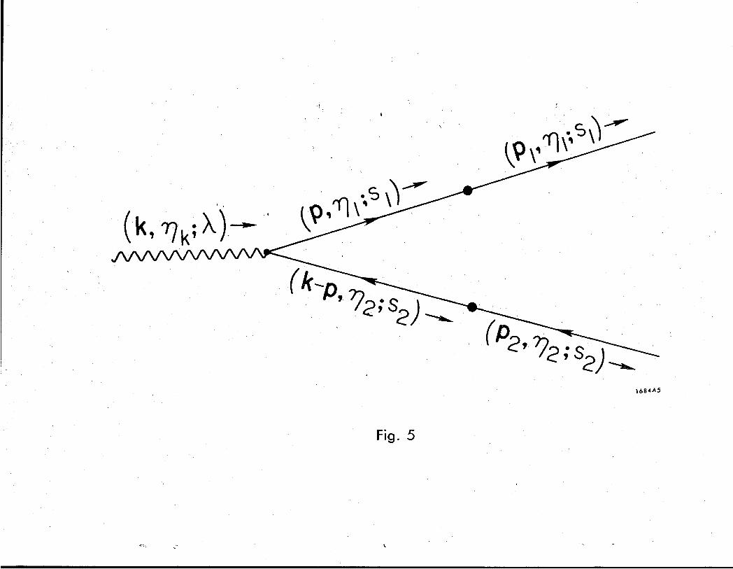
which can be visualized with the aid of Fig. 5.
If we now choose the z-axis along the direction of the photon and calculate
helicity amplitudes, we find
‘fi = t2n>s hk-??l-r]$ 2 9712 [ 1 i- e tW -2 d; M(h-+sl, s2>
x C WP~--) -Fc (p2 +$I - (2d462,@l-~:) 62($2 +$’ 9 Al 1 where
M(l+$,&) =
It is interesting to convert the momentum integration in (IV. 35) to an inte-
gration in coordinate space in order to appreciate the two-dimensional Galilean
(IV.34)
(rV.35)
- 27 -

I invariance group which manifests itself in the infinite momentum frame. To
begin, we drop the special requirement that the transverse momentum &of the
photon be zero and return to the energy denominator in (lV.34):
This is a rather messy function of the momentum p of the electron and the awl momentum $-E) of the positron in the intermediate state. As is usual with two
body problems in llnon-relativistic’r quantum mechanics, it pays to change vari-
ables to the total momentum, 5, of the two particles and their relative momentum.
Since r) plays the role of particle mass in the nonrelativistic analogy, the rela-
tive momentum is
where
is the 11 reduced mass” of the pair. When written as a function of k and q, the Il(tl @WI
energy denominator is independent of k: rknt
wCkv7)k)-Hb?? )-HE-z,r12) =-(25)-l z2+m2 ml [ I
(IV.36)
(IV.37)
(In non-relativistic terms, this is minus the ‘*internal energy” of the pair. )
P Similarly, the vertex matrix element w j E* w in (lV.34) is a function of the rela- WV
tive momentum q only. After a little algebra we obtain the explicit form,

f ew ts&.i~ ~sl;P-k,-172)*~(h)w(-s2) - -~--t.- ,: w~,171,\-H(~,rll)-H~-~,r12) = w.(Sl)~(5?;91’~2)W(-S2)*f(h) ,
hw?,\ _ (IV.3 8)
^. LJ r)l I Gtwh, 77,) = 41 “, ‘) q-i(q X2) o-+im_o} (qa+mY)-’ ,
I where q x%’ = (q”,-q”). *
Using these results, we can write (IV.34) as a coordinate- space integral.
Let 3, h be the coordinates of the electron and positron respectively in the
Fourier expansions (III.19) and (III.20) of the eikonal factors, and define
R= Q 071% coordinate of the center of f7massf1 of + T2&) = the pair
r = 21-g = relative coordinate. w
(IV.39)
Then we find
.I. (IV.40) x w’(S14$gfq~ r2 )w(-s2) l g(h)eq*g ,
where
gQyp2) = (270 -2 d~ei~‘~$($~1,~2) . /
It is interesting to interpret the various factors in (IV.40). First,
E (A) exp (i$RJ is the wave function of the initial bare photon. 49 Multiplying this
by Q(E) tells us the composition of the physical photon in terms of its consti- 15 tuents, which, to first order, are an electron and a positron. Hence we might
- 29 -
,_I

refer to E(r) 0 s(h) exp (ig*IX) as the first order approximation to the wave function
of the physical photon. The I1 internalff wave function C$J satisfies a two-
dimensional Schroedinger equation with a point source,
The solution of this equation which vanishes as I r I -+ =Q is simply related to the
modified Bessel functionXo :
rl2-3 ,G(-r) =& -i- ii 1 ‘k
~-(;~~~~fi.mg i
KO(ml 21).
The next factor in Eq. (IV.40), the eikonal phase factor, tells us how the
constituents of the physical photon interact with the external field. Finally, the
factors ~~(“1) exp(- i&. 3) and w(- s2) exp(- ig2* g) are the wave functions of the
final electron and positron (calculated to zeroth order). Evaluation of the S-
matrix is completed by integrating over the coordinates a and-x of the electron
and positron and multiplying by (2 71) times an q -conserving delta function and by
a fermion normalization factor (2?71)& (27~~)~ .
E, Delbruck Scattering
Let us turn our attention now to the problem of photon scattering off an external
field. We shall see that our scattering theory gives a clear and concise derivation
of the amplitude for this process.
The matrix element we wish to calculate is .
‘fi- ‘fi = <y(P’J’) 1 D(%O) IF-llU(O,-00) 1 y(p,h) > l (IV.41)
I - 30-

If we insert the expansion of the physical photon state into (IV.41) and calculate
to order e2, we find
Sfi-6fi = e 2 (27r) -4 W ‘-7) l dql/dgldr$ c sl’ s2
X [Ft&$-,4) FJP&-E~) - (2~‘462(~l-~p~~~-&,] w
(IV.42)
x &,l).J (Pl7P2)’ ,~(~JW-s2)w+(-s2)j (-p$,pi)’ E*(A’)W(Sl)
x - H(P~)- H(p2) I [ -’ ~(Pi)-H(Pi)-Hcp;~-l
where
This formula is visualized, and its kinematics are defined, in the T- ordered
diagram Fig. 6.
We are now faced with two related problems. First, the integrand in (IV.42)
is a very messy function of the independent momenta ,pl and a. Second, the
momentum integration is divergent: if the integrals are cut off in an arbitrary
non-covariant fashion,, the result will depend on the cutoff parameter. The remedy
is simple. Since Sfi is invariant under the Galilean symmetry group,discussed in
I and in Section IV.B, it will be to our advantage to use integration variables which
are invariant under this group.
- 31-

We choose to make use of four Galilean-invariant momenta I.+, q, &and g IMr The momenta s and 2 are defined so that the momentum transfer from the external
potential to the electron in the intermediate state is r + q, and the momentum R* )r*
transfer to the positron is r I - q: wl w
The momenta L and 2 are de
positron pair is i-2 before
the interaction:
Q m
where 77 = 771~~1 rl is the l’r
integration variables instead
by the external momenta: 2;
in terms of L and q by y*c
where we have defined
led so that the I1 relative momentumff of the electron-
e interaction with the external field, and I! + Q after ?a. Ivr
(IV.44)
duced massI of the pair. We will use 2 and &as
rf $1 and $9 The momentum .s is, of course, fixed
= E’ -9. We find with a little algebra that Q is given mn
(IV.45)
Q = ?71/rl l (IV.46)
- 32 -

When this change of variables has been made, the scattering matrix takes
the form
where
MA(c&~;Lh’) = jdrr/d.$ c 0 s1s2
W t (Sl)A (PI9 ‘P2)’ f (A) w(- s2) w’(- s2)i (-Pi, Pi )* dew (IV.48)
C W(P) - H(g) - H(p2) 1” k(P’)-H(Pi)-H(Pi)l ,
Eq. (IV.47) has the attractive property that the integrand of the q-integration w
decomposes into two factors: one describing the interaction with the external
field, and a second, called the photon impact factor by Cheng and Wu16, describing
the composition of the physical photon as a bare pair.
A technical complication arises because the impact factor M depends on
a cutoff A in the &- integration. However, we will see that the cutoff does not
affect the scattering amplitude, and therefore has no physical significance.
It is quite easy to write down the explicit form of MA using the variables
P and Q w m =$ (;+c&q9 The energy denominators are
W(P) - H(P~) - H(p2) = - (2F)*’ [$+J)~ + m2] = -~TJ a(1 - (pi]-’ [$-G&)2 +- m2]
W(P’) - H(Pi) - H(P2) = - (25)-l [(i+GJ” + m2 ] = -[29c~(l-@j-’ [@+G$+m2
-33-

By making use of the Galilean invariance of the numerator factors w’j w, we can m
write them in terms of&and C& immediately:
wt(s,)j(p,,,~p,)w(-s,) = w’(s,)j (Q-Q,rl,;Q-Q,-rl,)w(-s,) Y
Thus MA takes the form
where
nf.$($LW = C s1s2
WT(S1)A(&- 2, ‘I&$, - 7&4*~ Gw(- 9
(N.50)
Let us consider the helicity flip case first. Reading from Table I, we find
n($9;1, - 1) = -2(171172)-l(Q+-Q+)(e,+Q+) = -2f2 [&I - c$~[Q+Q+-Q+Q+] . W-51)
Thus
M*($,T, + 1, - 1) = - 8 jd”“(1-~~~d~~+~+-Q+Q~[~~-~~2~m2]-1 [(a+Q)2+m2]-1 l
0 tee?*
(IV. 52)
-34-

The helicity non-flip amplitude is also quite simple. The helicity non-flip amplitude is also quite simple. Reading from Reading from
Table I, we find Table I, we find
n(JJf$+L+l) = n(JJf$+L+l) = [ [ -2 -2
y-l1 y-l1 + 7?i2 +77i2 1 1 2--2 2--2 (Q+-Q$@- + Q-J + 8 m r (Q+-Q$@- + Q-J + 8 m r =& [To$l-.;13( [a2+ (l-0$] $-$-2iiXC$ +m2j .
(IV.53) (IV.53)
The term proportional toi X CGJ can be dropped since it will not contribute to MA . The term proportional toi X CGJ can be dropped since it will not contribute to MA .
Thus we obtain Thus we obtain
A M (c&x;+ 1, + 1) = 2 M (z,;;+ 1, + 1) = 2
i/F da d& (02+ p - o12)(i- GJ2) + m2] ki-Cj2+m2]-1 [(;+$)2+ m2]-‘. p - 0i12)(.4f- g2) + m2] k.p($2+m2]-1 [(;+$12+ m23” l
(IV.54) (IV.54)
As mentioned earlier, the impact factors MA given in(IV.52) and (IV.54)
depend on the cutoff parameter A used to avoid the logarithmic divergence in the
ifi- integration. However, we can verify that the cutoff does not affect the scattering
amplitude in the limit A- CO by writing MA in the form
As mentioned earlier, the impact factors MA given in(IV.52) and (IV.54)
depend on the cutoff parameter A used to avoid the logarithmic divergence in the
ifi- integration. However, we can verify that the cutoff does not affect the scattering
amplitude in the limit A- CO by writing MA in the form
The term %Adefined by (IV.55) is evidently finite in the limit A-00. If we use
the simple observation that
M,KL~ am = GA(~E;h,af) +MAt;,gpm . (IV.55)
The term %Adefined by (IV.55) is evidently finite in the limit A-00. If we use
the simple observation that
I c dz F($+$ FJ;-$- (W462(~+$62t&-$ = 0 3 1 we see that the cutoff dependent part of MA(q, r;a ,a’), namely MAk,$h ,a’), does
a?i not contribute to the scattering amplitude (IV.47) and therefore has no,special
significance. 14’
.: ,:.- .> .>
we see that the cutoff dependent part of MA(q, r;a ,a’), namely MAk,$h ,a’), does a?i
not contribute to the scattering amplitude (IV.47) and therefore has no,special
significance. 14’
-35- - 35 -

In addition, we may note that because of its definition EA(a,;;h ,a’) is zero
at%=;. Itisalsozeroatz=-r w. (Indeed, it is an even function of 2 as can
be verified by making the change of variables Q! +(l- o) in (N.52) and (IV.54). )
Thus the scattering amplitude (IV.47) remains finite even if the eikonal factors
are singular at q = f r, as they are in the case that Ap(x) is a static Coulomb *
potential. The renormalized impact factors ‘%,($,$;a ,A’) are identical (aside
from a factor - e4(2 a)-“) to the impact factors for the photon found by other
techniques by Cheng and Wu. 16
G. Electroproduction of ,u Pairs; Scaling
We wish to discuss here a “rnodell” calculation which,’ hopefully, has im-
portant features in common with electron-nucleon inelastic scattering. We
imagine the process pictured in Figs. 7a and 7b: a virtual photon, produced by
the scattered electron, creates a pair of muons which diffract through an external
field (e. g. a nucleus). In the spirit of inelastic electron-nucleon scattering we put
eikonal phases only on the members of the pair and treat all particles as distin-
guishable.
One purpose of the model is to investigate the scaling property recently dis-
covered in electron-nucleon l7 scattering. To do this, we assume that only the
final electron is observed and construct the cross section dc/dQ2dv, where Q2 :
is the four-momentum transfer from the electron line and v is the energy transfer.
We then ask whether the diffractive mechanism envisioned here leads to scale
invariant expressions for the form factors oT and us in the limit Q2- a0 18
.
I
- 36 -

To begin, we construct the scattering amplitude corresponding to Figs. ?a - - - L
and 7b:
S,: = ez(27r)6(q-ql-q,-q,) 12172rlt217,2r7,1’ I --% I1 .
1 ZAW’(S1)i @‘3P)’ E*(a) Wts) w’(sl)A(Pi 3 -Ph)‘_f,@) w(- s2) , .-2 _ c 0
S',SOS I’- s2
X rHcp)-H(p’)-H~(Pi)-Hu(P;;I-’ 1 F~l-~)Fc$2-8i)-(29462(~l-~i)62~2-~~-.’ (
I
L a- - I -I LA -- .- ~_ a)] ’
(IV. 56) I where where
%=P-P’ 9 %=P-P’ 9 q4 q4 = q-q’ = q-q’
‘W ‘Jwr ‘W ‘Jwr
:i :i ‘-xi+9 9 ‘-xi+9 9 ‘71’ = r]l 9 7; = rl2 l ‘71’ = r]l 9 7; = rl2 l
The first term in braces in (IV.56) corresponds to exchange of transverse. photons The first term in braces in (IV.56) corresponds to exchange of transverse. photo Ins . 1 1 ’ ’
(Fig. 7a); the second term corresponds to the exchange of a “scalar photorifT (Fig. 7a); the second term corresponds to the exchange of a “scalar photorifT
(Fig. 7b). (Fig. 7b). The function HP(p) refers to the free muon Hamiltonian (s2+ h2)/277, The function HP(p) refers to the free muon Hamiltonian (s2+ p2)/2q,
where /J is the muon mass. where /J is the muon mass.
Before proceeding further, it is convenient (as usual) to change variables in Before proceeding further, it is convenient (as usual) to change variables in
the momentum integration from J$ the momentum integration from J$ to ,k , where h is the ‘1 relative momentuml’ to ,k , where h is the l1 relative momentuml’ of of
the virtual p-pair: the virtual p-pair:
(IV. (IV.
where where
Q = qrlq * o! = qrlq * (IV. (IV.
-37- -37-
I I
57)
58)

It is also convenient to let - Q2 stand for the square of the 4-momentum trans-
ferred from the electron line:
I,
-Q2 = (P -PY (P-P’), l (Iv. 59)
In terms of these variables, the energy denominators in (IV.56) have the simple In terms of these variables, the energy denominators in (IV.56) have the simple
forms forms
H(P) -IUP’) - w(q) = -Q2/‘tWq) , H(P) -IUP’) - w(q) = -Q2/‘tWq) 9
(IV.60) (IV.60)
H(P) -H(P’) -Hh(Pi) -HF(P$ H(P) -H(P’) -Hh(Pi) -HF(P$ = - $ - - qq 2 2
q 2q1q2% +p ) l l
The numerator functions The numerator functions t. t. w i.&*w w i.&*w t. t. > >
w z 5,~ can be read from Table I, and are w z 5,~ can be read from Table I, and are
a* simple functions of $. a* simple functions of $. .
We are now prepared to write out Sfi in a form suitable for calculating the We are now prepared to write out Sfi in a form suitable for calculating the
l cross section. cross see tion. Let us choose the z-axis in the direction of the beam, SOE = 0, Let us choose the z-axis in the direction of the beam, SOE = 0,
and consider S . for the choice of spins s = s’ = s and consider S . for the choice of spins s = s’ = s fl fl 1 1 = *, s2 = -4 . = *, s2 = -4 . Then when we Then when we
substitute the expressions from Table I and Eq. (IV.60) into (IV.56) we obtain substitute the expressions from Table I and Eq. (IV.60) into (IV.56) we obtain
where where
~(B,P2) ) ~(B,P2) , w w (IV.61) (IV.61)
- 38 - - 38 -

and
= d+-pi ~-ct]k- + a(l-a)Q2 cz(l-ol)Q2+p 2 -1 I .
The three terms in f(k) arise from exchange of a right handed photon, a left handed
photon, and a If scalar photon’? respectively.
The physics of the amplitude l$pl, p,) is more apparent if we write it as a
Fourier transform by inserting the expansions of the eikonal factors into (IV.62).
The resulting structure of %(~1,~2), and its physical interpretation will be familiar
from the discussion of pair production by real photons in Set tion IV.D. We find
. = P-3 m.d32e
- $fg - jg23 e [expt-i+Y$.i,i exp(+iX(jf&))-l]fg-22) eili6’)
where I$ = qil(qla + q2z2) and f(r) is the Fourier transfsrm of F(Ix)~ Explicit
evaluation gives the wave function of the virtual muon pair, f($, in terms of
modified Bessel functions K. and FL’
f(g) = (277)-2 dk e%g FB(&) + FL(k) +Fs (IV.6 5)
- 39 -

-&P;O-o) ~$-a)& ‘~1 [ 2 zgr- r:
f&J = +v a(1 - a)Q2 K. .‘
We will see in the sequel that, for our purposes, this expression for f(r) is not
as formidable as it seems.
With a useable expression for Sfi now at hand, we are ready to construct
the cross section da integrated over the unobserved momenta of the muon pair,
Using (IV.61) in Eq. (IV.6) we obtain
da = ’ dq’ I $P,,P,, 1’ l (IV.67)
Since M(I,Xl,s2) is simpler than &p1,g2), we write thezl, s2-integral as
= dgl f($ I [2 -2 cos (X(p+p X(b@-$I-))]
Assuming that the potential has cylindrical symmetry about the z-axis, we can
replace I f(r) I 2 by I fK(;) I2 + I fL(rJ I2 + I fs(rJ I 2 in (IV.68), since the various
cross terms will vanish when the integration over the angle of L is performed.
Thus the cross section separates into a part due to the exchange of a ‘I transverse
-4o-

photon??, doT = daR + daI,, and a part due to the exchange of a If scalar photon??,
daS. If we substitute the expressions for I fE I 2, I fL12, and I fS I 2 obtained
from (IV.66) into (IV.68) and (IV.67) and interchange the roles of a! and (1- Q) in
dcI,, we obtain
da = doT + dos 1
(IV.69)
This expression gives the cross section in the high energy limit discussed
in Section III, i. e. in the limit q , q ‘??J with q/q 1 and Q2 fixed. It remains now
to evaluate do in the limit Q2*oo. To take this limit we have only to note that the
modified Bessel functions appearing in (IV.69) are large only for small values of
their arguments, so that the main contribution to the h-integral comes from the
.
Physically, this means that for large Q2 the transverse separation r between
the muons as they pass through the external potential is small. If the separation
were zero the two muons would receive exactly opposite eikonal phases; thus for
small r the net phase received by the muon pair is proportional not to X but to VX .
Mathematically, this means that the Q2 -co limit of da can be obtained by
substituting for the h-integral in (IV.69) its limiting form as r-0. 19
This
limiting form is easily evaluated:
-41-
,/ ;’

( X
(rv.70)
(In the last step we have used the assumed cyliqdrical symmetry of X(@. )
Once the limiting form (lV.70) of thek-integral has been substituted into
(IV.69), the &-integral can be evaluated using the formula”
s-l = 2s-3 [ I rt+s> 2 tbs + JU-(is- J) Iv) l
This leads to
da = dzldqf
Evaluating the a-integrals in the limit Q2-cm, we find
da = doT + das
m ’ dq’ 2e4 3(2n)5Q4q
q
2 l (Iv. 71)
(IV.72)
- 42 -

We recall that this is the cross section for the choice of spins s = s’ = 4 ,
sl=*, s2=+ It is not difficult to see that the choice s = s’ = 4 , s1 = -8 ,
s2 = +& leads to the same cross section. Each of the other six possible choices
for the spins of the final particles gives a cross section das = 0 and a cross
set tion daT which is small compared to the cross section in (IV.72) as Q2- 00. 21
Thus the limiting cross section for s = 3 (or s = -4 ), summed over final spins,
is two times the cross section in (IV. 72).
In order to make contact with standard notation and identify the form factors
aT(Q 2
,V), us(Q 2
, V), let us define
E = lab energy of the incident electron = 2-& I: li + H(ti;
E’ = lab energy of the scattered electron = 2-& [q’ + HM] (N.73)
u =E-E’ .
Apparently in the high energy limit
q zz$E, q’ = &’ , qq =&, l (rv.74)
We recall also the definition of Q2:
2
Q2 = - (P- P’?(P- P’)~ = -211q(H(p) -H@‘)) +P’~ = + p’2 + 2’ m2 . (IV.75)
Thus in the high energy limit, and neglecting m2 compared to Q2, we can replace
,p12 by
,p =gQ2. ‘2 (IV. 76)

When we make these replacements we find for the cross section summed
over final spins,
da
dQ2dv dQ2dv
’ ;;d$E;;& log@, + l/~d~,~x
(IV.77)
Using (XV.77) we can extract the form factors us and uT 22 .
us(Q2, v/Q2) - z
(IV.78)
uT(Q2, dQ2, - $j? -+ &
It is interesting to compare the behavior of us and aT in the present model
with the famous scaling behavior of the same form factors for deep inelastic
electron-nucleon scattering. 23 In this model, us(Q2, v/Q2) is scale invariant:
for large v and Q2 2 , Q us is a function of (v/Q2) only. However, the factor
log(Q2/p2) spoils the scaling behavior of (rT.24
In the somewhat hypothetical limit of an external field which varies in space
slowly compared the lepton Compton-wavelength (l/X 17j4e p -l), the formula I
(R-71) for os/uT is valid for all Q2. The direct evaluation is shown
in Fig. 8; we see that us,uT is never larger than 0.26.
It is not clear what direct connection these calculations have with respect to
hadron electroproduction. While there appears to be a diffractive 25 mechanism
operating in both cases, the details (e.g., the scaling behavior of uT) are different.
However it may be that some features of the process, such as the importance of
bxdl transverse distances (Ax)” d Qw2 at large Q2 are common to both.
-44-

V. FUTURE PROBLEMS AND POSSIBLE LIMITATIONS
Throughout this paper we have found support for a sim.ple physical picture
for high energy scattering processes. However, this picture is couched in per-
turbation theory, and one may wonder whether it is generally valid. For example,
to what extent does this picture apply to strong coupling field theories? Or, more
modestly, will this picture survive higher order calculations in quantum electro-
dynamics ?
Studies of diagrams such as shown in Fig. 9 indicate that the complete 26 situation is not as simple as we suggest in’this paper. Using these or other methods
it is not difficult to find that this diagram diverges logarithmically as r) -00 , where
17 refers to the incoming electron. The, logarithm comes from a loop integral and
receives a large contribution from that region of phase space in which the internal
partons are (almost) “wee”. This example raises two problems. First, if we
apply perturbation theory to very high orders, we must be equipped to deal with
such logarithms,which in sufficiently high order violate s-channel unitarity. And
secondly, since the internal photons in this example are (almost) “wee, If one can
question the applicability of the eikonal approximation to this diagram. The true
situation may be somewhat like using purely nonrelativistic methods to calculate
the Lamb shift: they work up to a certain point, and contribute a great deal of
insight into the physics. However beyond that point they fail utterly. In the present
case there is very likely a similar boundary, associated with wee partons, beyond
which the simple methods of this paper fail. It remains for the future to see how
much of the physics lies on the simple side of the boundary and how sharply the
properties of the boundary region can be delineated.
- 45 -

APPENDIX
The two component formalism described in Section II suggests, in the
interest of overall simplicity and uniformity, a change in notation, mainly in
normalization factors, from that used in Paper I. This appendix is devoted to
clarifying the connection between the old and new formalism.
We begin by discussing the electromagnetic potential. The operator h(x),
as discussed in (11.6) and below, may be directly identified withhT(x), of I.
new efW = aT(x) old . (A4
However, the plane wave expansion(II.11) of (x) differs from Eq. (IV.37) of I by
a factor 2 (%o 3* I ; the comparison yields
62) new a(p, ) = a(p, .) old l
The connection between the new 2-component electron field V(x) an8 the old
4-component I&X) is more disagreeable. Not only is there a change in normalization
but also there is a unitary rotation. The essential connection is between
(A-3)
and the independent dynamical variables of I.,
(A-4)
- 46 -

By comparing the anticommutation relations (IV.36) of I. with (11.5) of this
paper, we see that the normalizations of the field operators differ by a relative
factor 2*. If we choose phases such that
new $1(x] = 2i @l(x) old , (A-5)
then we find it is best to make the identification
new $2(x} = i2a a4(x) old , (A.6)
We verify the connection by comparing the equations of motion for w+ and $.
Elimination of @- from Eq. (IV.18) of I. produces
(A-7)
Using the y-matrices (IV.9) of I. , we see that, as 2 x 2 matrices acting on the
first and fourth components of !P+, the matrices y1 and y2 are
yl = ( 0 -1 1 0 1 y2 = ( 0 i i0 ) ’
If we combine (A.5) into the two component spinor relation
$(x) = 2* u #y(x)
1 0
0 i )
ow
-47-
/. ;

and insert this relation into (A.7) we obtain
(ia,-eAo)$ = [-(g- ,
But
[ $-e$)*UyI++m
rwa 1 tcI. (A.9)
uyb -l = iaj , (A.10)
so that (A.9) is identical to the equation of motion (11.14) for $.
The unitary matrix U introduces relative phases in the comparison of the
elements of the plane wave e’xpansions of II/ and w+. By definition, the new
spinors w(s) appearing in the expansion (11.10) of $J are equal to the old two com-
ponent spinors w(s) appearing in the expansion (IV.32) of !J$, in I. Thus the
creation and distruction operators in (11.10) must absorb, in addition to a normali-
zation, the phase introduced by the presence of U. The comparison between (11.10)
and (IV.32) of I, using Eq. (A.8), yields
new b(p, +8 ) = [ 1 2(2nj3 ’ b(p, + 8 ) old
new b(p, -4)
new dt(p, + $) = i 2(2~)~]* dt(p, T & ) old
t newd (p, -$) = [ 1 2 tm 3 ’ dt(p, -+) old.
This completes the correspondence-relations between the old and new notations.
It is now straightforward to check that the new formalism is consistent with the
old, including rules for diagrams.
We must apologize for changing notation in midstream. However, many
disagreeable factors of &, (2n) 3/2 , etc. have thereby been purged, and a consistent
mnemonic now exists for the factors “2tf occuring in the rules for perturbation
- 48 -

diagrams at the end of Section II: for every factor “r a factor 2, for every
factor q a factor 2.
ACKNOWLEDGEMENTS
Many of the ideas in this paper have been independently found by the experts
in this field; in particular we thank R. P. Feynman and T. T. Wu for interesting
and informative discussions. We also thank our colleagues at SLAC for dis-
cussions and criticism.
‘- 49 -

1. H. Cheng and T. T. Wu, Phys. Rev. Letters 24, 1456 (1970). See the
bibliography of this article for additional references by these authors.
S. J. Chang and S. K. Ma, Phys. Rev. 180, 1506 (1969); 188, 2385 (1969);
Phys. Rev. Letters 22, 1334 (1969); H. Abarbanel and C. Itzykson, Phys.
Rev. Letters% 53 (1969); Y. P. Yao, Phys. Rev. Dl, 2316 (1970); B. Lee,
Phys. Rev. D& 2361 (1970).
2. R. J. Glauber, Lectures in Theoretical Physics, edited by W. E. Britten et al.,
3.
(Wiley-Interscience Inc., New York, 1959), Vol. 1.
R. P. Feynman, invited paper at the Third Topical Conf. on High Energy
Collisions of Hadrons, Stony Brook, New York, Sept. 1969; Phys. Rev.
Letters 23, 1415 (1969).
4.
5.
J. B, Kogut and D. E, Soper, Phys. Rev. Dl, 2901 (1970).
Note that $ d /2r is the Lorentz-invariant surface element dpxdpydpz/2E
on the mass shell. The q-integration runs from 0 to Ed, thus covering the
forward mass shell..
6. RecaIl‘that the nonrelativistic equation of motion is written iao$= &- l ELLS C
before introducing the minimal substitution in order to obtain the correct
7. Readers familiar with the discussion in I. of the Galilean subgroup of the
Lorentz group will note that such combinations in Table I as (@q) - (g/7] )
transform under this subgroup like (momentum/mass) - (momentum/mass)
and are therefore invariant under “Galilean boosts. I’ This invariance can
8.
often be used to practical advantage in calcuIations.
With the present normalization conventions, t f IS i > = (2n)484(pf - pi)M, where
M is the invariant amplitude calculated with the conventions of Bjorken and
REFERENCES

16.
17.
18.
19.
Drell using Dirac spinors normalized to iIu = 2m. See J. D. Bjorken and
S. D. Drell, Relativistic Quantum Fields, (McGraw Hill, New York, 1965);
Appendix B.
We also use this formula for a one particle final state.
This relationship can be obtained by using a wave packet for the initial state
(cf. , M. L. Goldberger and K. M. Watson, Collision Theory (John Wiley,
New York, 1964) ; Sec. 3.3)). In the high energy limit in which 7-d E
this reduces to the more familiar result with 17 replaced everywhere by E
in (IV. 6) and (IV. 7).
Cf., H. Cheng and T. T. Wu, Phys. Rev. 184, 1868 (1969).
To calculate F2 to order e2, we can use the value Z2 = 1, which is correct
to order e”.
S. J. Chang and S. K. Ma have used different infinite momentum techniques
to obtain this result, Phys. Rev. 180, 1506 (1969).
S. D. Drell, D. J. Levy, T. M. Yan, Phys. Rev. Letters 22, 744 (1969);
H. Cheng and T. T. Wu, Phys. Rev. E, 1069 (1970); S. J. Chang and
S. K. Ma, s.cit. -
The amplitude ~a? a physical photon to be a bare photon is 1 to lowest
order, but does not, of course, contribute to pair production.
H. Cheng and T. T. Wu, Phys. Rev. 182, 1852 (1969).
E. Bloom et al. , Report No. SLAC-PUB-642, Stanford Linear Accelerator
Center.
Note that the limit v -Q) is already implicit in our formalism.
More precisely: let d& be the limiting form of d, so obtained. Then it is
not difficult to prove that dus = d. iI-1 + O(l/Q2)], du T = do+ 1 + O(l/log Q2),
as Q2- 00, assuming that the potential is sufficiently well behaved.
+
.

20. A. Erdelyi, ed., Tables of Integral Transforms, (McGraw Hill , New York,
1954); Vol. 1, pg. 334.
21. If the helicity is flipped on the electron line dcqT is suppressed by a factor
(m2/Q2) as Q2- 00. If the helicity is flipped on the muon line, dcqT is
suppressed by a factor [l/log (Q2/p2)].
22. J. D. Bjorken, Phys. Rev. Dl, 1376 (1970).
23, J. D. Bjorken, Phys. Rev. , 1547 (1969).
24. Strictly speaking, scale invariance for gT means that Q2 rT approaches a
finite limit as Q2 -00 with @/Q2) held constant. However, we have evaluated
oT in this model in the limit (v/d)- ~a with Q2 held constant, and then we
have let Q2 -0 . It is not impossible for a;r to exhibit scale invariance
in the limit Q2--- a~, (v/Q2) = con&. , but not in the reversed limit used here.
25. B. L. Ioffe, Phys. Letters s, 123 (1969).
26. G. V. Frolov, V. N. Gribov, L. N. Lipatov, Phys. Letters e, 34 (1970);
H. Cheng and T. T. Wu, Phys. Rev. Dl, 2775 (1970).

FIGURE CAPTIONS
1. Vertices in the infinite momentum frame,
2. Electron scattering off an external field. (a) Zeroth order in electron
structure, (b) second order in electron structure.
3. Higher order contribution to electron scattering off an external field.
4. Bremsstrahlung off an external field.
5. Pair production on an external field.
6. Delbruck scattering.
-7. Muon pair production off an external field.
8. as/‘dT for high energy electroproduction of lepton pairs from a slowly
varying external field.
9. Electron scattering diagram contributing qlog 7 term to the S-matrix.

La) . .
’
Ud
Fig. 1

m-
ci
-i2 U

.;
1684A3 .
Fig. 3

u c
4 . .
0
1684A5
Fig. 5
\ .

i
1684A6 c

d -
I m
- ‘co ?i t m
d
U
n zj, .- LL
u
U

0 0 0 -
a .L U
0 6

Y
l
Fig. 9
Related Documents