Oceanic circumpolar habitats of Antarctic krill

MARINE ECOLOGY PROGRESS SERIESMar Ecol Prog Ser

Vol. 362: 1–23, 2008doi: 10.3354/meps07498

Published June 30

INTRODUCTION

Studying micronekton in the open ocean

In ecology, our paradigms are often governed by tech-nical constraints on methodology. A prime example inthe oceans is the issue over bottom–up or top–down con-trol, with an emphasis on the former because it is easierto quantify than predation (Ohman & Wood 1995, Verity& Smetacek 1996). However, a basic ecological trade-offexists between occupying habitats that are risky, but re-warding, and those that are safer, but food-poor (e.g.Suhonen 1993). While this risk–reward concept is wellaccepted in the pelagic marine environment (e.g. for diel

© Inter-Research 2008 · www.int-res.com*Email: [email protected]

FEATURE ARTICLE

Oceanic circumpolar habitats of Antarctic krill

A. Atkinson1,*, V. Siegel2, E. A. Pakhomov3, 4, P. Rothery5, V. Loeb6, R. M. Ross7, L. B. Quetin7, K. Schmidt1, P. Fretwell1, E. J. Murphy1, G. A. Tarling1, A. H. Fleming1

1British Antarctic Survey, Natural Environment Research Council, High Cross, Madingley Road, Cambridge CB3 0ET, UK2Sea Fisheries Institute, Palmaille 9, 22767 Hamburg, Germany

3Department of Earth and Ocean Sciences, University of British Columbia, 6339 Stores Road, Vancouver, BC V6T 1Z4, Canada 4Department of Zoology, Faculty of Science and Technology, University of Fort Hare, Private Bag X1314, Alice 5700, South Africa

5Centre for Ecology and Hydrology, CEH Monks Wood, Abbots Ripton, Huntingdon PE28 2LS, UK6Moss Landing Marine Laboratories, 8272 Moss Landing Road, Moss Landing, California 95039, USA

7Marine Science Institute, University of California at Santa Barbara, Santa Barbara, California 93106-6150, USA

ABSTRACT: Surveys of Euphausia superba often target lo-calised shelves and ice edges where their growth rates andpredation losses are atypically high. Emphasis on these ar-eas has led to the current view that krill require high foodconcentrations, with a distribution often linked to shelves.For a wider, circumpolar perspective, we compiled allavailable net-based density data on postlarvae from 8137mainly summer stations from 1926 to 2004. Unlike Antarc-tic zooplankton, the distribution of E. superba is highly un-even, with 70% of the total stock concentrated betweenlongitudes 0° and 90° W. Within this Atlantic sector, krillare abundant over both continental shelf and ocean. At theAntarctic Peninsula they are found mainly over the innershelf, whereas in the Indian–Pacific sectors krill prevail inthe ocean within 200 to 300 km of the shelf break. Overall,87% of the total stock lives over deep oceanic water(>2000 m), and krill occupy regions with moderate foodconcentrations (0.5 to 1.0 mg chl a m–3). Advection modelssuggest some northwards loss from these regions and intothe low chlorophyll belts of the Antarctic Circumpolar Cur-rent (ACC). We found possible evidence for a compensat-ing southwards migration, with an increasing proportion ofkrill found south of the ACC as the season progresses. Theretention of krill in moderately productive oceanic habitatsis a key factor in their high total production. While growthrates are lower than over shelves, the ocean provides arefuge from shelf-based predators. The unusual circumpo-lar distribution of krill thus reflects a balance between ad-vection, migration, top–down and bottom–up processes.

KEY WORDS: Euphausiid · Circumpolar · Distribution ·Growth · Mortality · Predation · Risk · Bottom–up control ·Top–down control

Resale or republication not permitted without written consent of the publisher

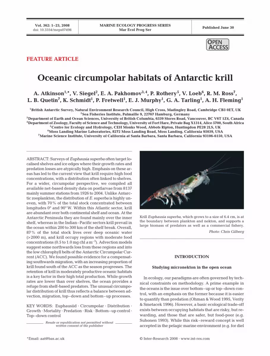
Krill Euphausia superba, which grows to a size of 6.4 cm, is atthe boundary between plankton and nekton, and supports alarge biomass of predators as well as a commercial fishery.

Photo: Chris Gilberg

OPENPEN ACCESSCCESS

Mar Ecol Prog Ser 362: 1–23, 20082

vertical migration), it is rarely extended to horizontaldistribution studies (e.g. Alonzo et al. 2003, Pepin et al.2003).

Technical constraints are also behind the difficulty inclassifying the mechanisms of large-scale movement inpelagic organisms. Some consider micronekton as pas-sive drifters at large scales, even though they can bestrong swimmers. Swimming behaviour is very hard toquantify in dynamic environments (Hamner & Hamner2000), while the availability of advection models hasled to much work on micronekton distribution as dic-tated by current flow (Fach et al. 2006, Sourisseau et al.2006, Thorpe et al. 2007). Insects, by contrast, have afascinating variety of behaviours that can be examinedand quantified more easily (e.g. Shashar et al. 2005).

Antarctic krill Euphausia superba, hereafter ‘krill’,epitomise these problems with methodology. We havenot yet fully incorporated predation into our mainlybottom–up-based view of their biology (Alonzo &Mangel 2001, Alonzo et al. 2003, Ainley etal. 2006). Growing to >6 cm and living for>5 yr, krill are at the awkward boundarybetween plankton and nekton. Advanceshave been made in understanding the ad-vective forces governing their distribution(Hofmann & Murphy 2004, Murphy et al.2004, Thorpe et al. 2007). However, theseauthors stress that it is the whole life cycle(of which advection and swimming behav-iour are just 2 parts) which dictates thelarge-scale distribution of krill (Murphy etal. 2007). Clearly though, we need to knowthe position of krill along the spectra fromtop–down to bottom–up control (Ainleyet al. 2006, Nicol et al. 2007) and from ad-vection- to migration-dictated distribution(Nicol 2003, 2006, Murphy et al. 2007).

Polar regions are warming rapidly(Vaughan et al. 2003), and their endemicpelagic invertebrates are stenothermal,with life cycles potentially sensitive to envi-ronmental change. To predict the future, weneed to understand mechanisms behind thepresent-day success of key species such askrill. Suggested factors for krill include itslarge size, longevity, flexible diet, schoolingbehaviour, use of winter sea ice and starva-tion resistance (Daly & Macaulay 1991,Quetin et al. 1994, Quetin & Ross 2003). Itsasymmetrical circumpolar distribution is alsoextraordinary and atypical of Antarcticzooplankton. In this paper we focus on thedistribution of post-larval krill during thespring to autumn (October–April) period inrelation to its overall success.

Circumpolar distribution of krill

The ‘Discovery’ Investigations (1926 to 1939) laidthe foundations for our understanding of Antarcticplankton distributions. Indeed, Marr’s (1962) circum-polar map of krill (Fig. 1) remains the prime referenceon their distribution today (Tynan 1998, Nicol et al.2000a, Hofmann & Hüsrevoglu 2003). This map, likeall those following it, was based on multiple seasonsof sampling with different methods. The conversionfactors used by Marr (1962) were soon adjusted(Mackintosh 1973) and since then, a series of circum-polar maps of krill distribution have been created (e.g.Maslennikov 1980, Voronina 1998, Everson 2000).Without a quantitative scale, these maps are hard tointerpret. Only recently have there been attempts atcreating more quantitative maps using data fromacoustic and net surveys (Atkinson et al. 2004, Siegel2005).

Fig. 1. Euphausia superba. Summer distribution of postlarvae (Fig. 135 fromMarr 1962). This map was based on 970 stations sampled with both obliqueand horizontal 1 m ring nets. It shows the distribution of highest recordeddensities mainly between 20 and 60° W, and high catches in both near-shelfand oceanic areas, congruent with our analysis. However, because samplecoverage is very uneven and the circles obscure each other, relative krill

densities are not possible to quantify from this map

Atkinson et al.: Oceanic circumpolar krill distribution

Several of these maps show the strongly asymmetriccircumpolar distribution of krill that is atypical of otherzooplankton species. Nicol et al. (2000a) estimatedfrom acoustic measurements that biomass densities inthe SW Atlantic sector were 10-fold those in the Indiansector, and Atkinson et al. (2004) calculated that 50 to70% of the total stock were within the sector 10° to80° W. By contrast, Fig. 2 shows much more even cir-

cumpolar distributions for other zooplankters, a findingsince supported by specific studies on copepods(Andrews 1966) and salps (Foxton 1966, Pakhomov etal. 2002, Atkinson et al. 2004). Likewise, total meso-zooplankton catch volumes differ little between sectors(Fig. 3). Has the unusual distribution of krill got a partto play in their success?

Our synthesis is based on net samples, incorporatingthose from Marr (1962) (excluding the horizontalhauls) and all available data since then. This database,KRILLBASE, builds on that used by Atkinson et al.(2004), with additional recent data and standardisationto a common sampling method (see Appendix 1 ‘Stan-dardisation of densities within KRILLBASE’, availablein MEPS Supplementary Material at www.int-res.com/articles/suppl/m362p001_app.pdf). KRILLBASE isrestricted to post-larval krill from non-targeted haulsexecuted between October and April, although mostrecords are from the summer months (Appendix 1). Thisdataset yields the best available picture of the relativedistribution pattern of krill (Fig 4). Based on the areaof each grid cell and its krill density, 70% of the totalkrill stock live between 0 and 90° W. Thus, nearlythree-quarters of the population are concentrated intoone-quarter of the longitude.

Top–down and bottom–up controls on krill ecology

Many explanations for the circumpolar distributionof krill have been proposed, including sea ice (Mackin-tosh 1973, Brierley et al. 2002), gyres (Marr 1962,Pakhomov 2000, Nicol 2006), fronts (Spiridonov 1996,Witek et al. 1988, Tynan 1998), shelf edges (Siegel2005, Nicol 2006) and high food concentrations (Con-stable et al. 2003, Atkinson et al. 2004). However, noneof these fully accounts for the distribution patterns, asexceptions apply to each. One common factor, how-ever, is that all are bottom–up interpretations, whichrelate krill to areas of enhanced food. Fig. 5 shows thismodern concept that krill are a species mainly of shelfedges and their vicinity (Trathan et al. 2003, Reid et al.2004, Nicol 2006).

3

Euphausia superba

Euphausia frigida

Euphausia triacantha

Thysanoessa spp.

Salps

Eukrohnia hamata

Themisto gaudichaudii

Limacina helicina

Inci

den

ce (%

)

40–

60°W

0–

20°W

20–

40°E

60–

80°E

100

–120

°E

140

–160

°E

160

–180

°W

120

–140

°W

80–1

00°W

120100806040200

100806040200

120100806040200

100806040200

120100806040200

100806040200

100806040200

100806040200

Fig. 2. Euphausia superba. Circumpolar distribution relativeto other major zooplankton and micronekton species, plottedas percentage incidence in available hauls within each sector

(redrawn from Fig. 4 of Baker 1954)

Total zooplankton volume

Volu

me

(ml s

ampl

e–1)

0–60°W 0°

15

10

5

020°E 20–120°E 120–180°E 180–60°W

Fig. 3. Total volume of zooplankton caught with 70 cm modi-fied Nansen net, integrated over the top 1000 m (redrawn

from Fig. 17 of Foxton 1956)

http://www.int-res.com/articles/suppl/m362p001_app.pdf

http://www.int-res.com/articles/suppl/m362p001_app.pdf


Few krill studies, by contrast, deal both with the abil-ity to find food and to avoid predation. Mortality isclearly a prime force in krill population dynamics (e.g.Pakhomov 2000, Murphy & Reid 2001), with >100 mil-lion tonnes (Mt) of krill being removed annually bypredators—a value similar to their total biomass(Miller & Hampton 1989, Mori & Butterworth 2006).Near islands with breeding predator colonies, preda-tion is especially intense (Croxall et al. 1984, Fraser &Hofmann 2003). The concept of a ‘krill surplus’ follow-ing the removal of large predators through whalingduring the last century reflects this top–down view ofcontrol (Mackintosh 1973, Laws 1985, Ainley et al.2006). Ecologists studying higher krill predators oftenemphasise predation as a controlling factor (e.g. Reid& Croxall 2001, Fraser & Hofmann 2003, Ainley et al.

2006), whilst others highlight food resources (e.g.Atkinson et al. 2004, Siegel 2005). Clearly, these 2approaches must be integrated (Daly & Macaulay1991, Alonzo & Mangel 2001, Ainley et al. 2006).

Advection and migration controls on krill distribution

Are krill more like a planktonic drifter or more like asmall pelagic fish? On the one hand, krill have beentreated as drifters at the circumpolar scale, since advec-tion probably plays a major part in their lives (Hofmannet al. 1998, Murphy et al. 2004, Fach et al. 2006). On theother hand, attributes more akin to those of small pelagicfish have been argued. As well as size and lifespan(Quetin et al. 1994, Quetin & Ross 2003), these attributesinclude cruising speeds of ~20 cm s–1 (Kils 1982), school-ing (Daly & Macaulay 1991, Hamner & Hamner 2000) andhorizontal migrations (Kanda et al. 1982, Siegel 1988,Sprong & Schalk 1992, Lascara et al. 1999). Despite theseattributes, questions remain over the degree to whichswimming controls the circumpolar distribution of krill.

Modern models emphasise both migration (Fig. 6)and advection (Fig. 7) in determining the distributionof krill. Clearly, the processes work at different scales,with the ontogenetic seasonal migration model apply-ing to the Antarctic Peninsula area, whereas theadvection model is circumpolar. However, there isneed to integrate processes at both of these scales,because small differences in behaviour can have majoreffects on advection tracks (Hofmann et al. 1998, Mur-phy et al. 2004, Cresswell et al. 2007).

4

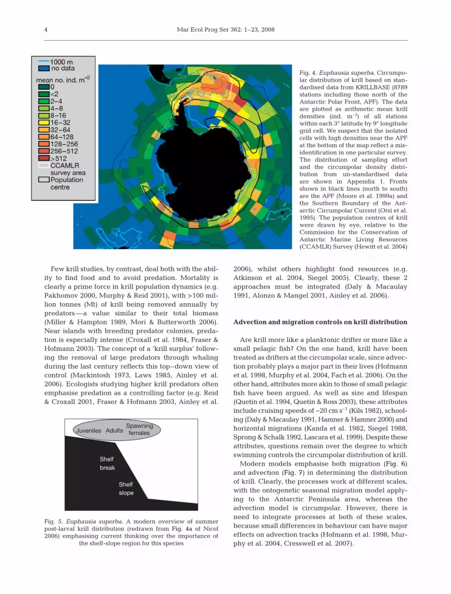
Fig. 4. Euphausia superba. Circumpo-lar distribution of krill based on stan-dardised data from KRILLBASE (8789stations including those north of theAntarctic Polar Front, APF). The dataare plotted as arithmetic mean krilldensities (ind. m–2) of all stationswithin each 3° latitude by 9° longitudegrid cell. We suspect that the isolatedcells with high densities near the APFat the bottom of the map reflect a mis-identification in one particular survey.The distribution of sampling effortand the circumpolar density distri-bution from un-standardised dataare shown in Appendix 1. Frontsshown in black lines (north to south)are the APF (Moore et al. 1999a) andthe Southern Boundary of the Ant-arctic Circumpolar Current (Orsi et al.1995). The population centres of krillwere drawn by eye, relative to theCommission for the Conservation ofAntarctic Marine Living Resources(CCAMLR) Survey (Hewitt et al. 2004)

Shelfbreak

AdultsJuvenilesSpawningfemales

Shelfslope

Fig. 5. Euphausia superba. A modern overview of summerpost-larval krill distribution (redrawn from Fig. 4a of Nicol2006) emphasising current thinking over the importance of

the shelf-slope region for this species


Aim and structure of this synthesis

Many overviews of krill biology have appearedrecently (Nicol 2003, 2006, Hofmann & Murphy 2004,Siegel 2005, Smetacek & Nicol 2005, Ainley et al.2006, Murphy et al. 2007, Nicol et al. 2007). Thesehave taken a variety of standpoints over the relativeimportance of top–down or bottom–up processesand the influence of advection or migration on distri-bution. Our meta-analysis attempts to rationalisethese issues. Our central thesis is that the above con-trols are not mutually exclusive and that the uniquedistribution of krill reflects them all operatingtogether.

This synthesis departs from a conventional review inseveral key features. We do not synthesise the resultsof past studies, but rather synthesise and re-analysethe raw data behind them. The number of such meta-analyses is increasing, following the realisation thatnations must pool their datasets to address circumpolarissues (www.iced.ac.uk). KRILLBASE contains >70times the number of stations of even the largest sur-veys, so circumpolar questions beyond the scope ofindividual campaigns can be tackled. In this synthesis,we relate krill to multiple features of their environ-

ment. After defining the potential habitats anddescribing the main patterns of krill distribution,we explore the concept of ‘good habitat’. Do krillinhabit areas with optimal temperature-foodcombinations for growth? We introduce top–down controls with a simple trade-off model foroccupying risky, high growth habitats vs. thosethat are safe, but food-poor. The next sectionexamines the roles of advection and migration incausing the observed distribution.

Finally, we discuss the issue of net samplingmethodology, which is critical to our interpreta-tions of distribution. Methods are described fullyin Appendix 1. We then rationalise the views oftop–down, bottom–up, advection and migrationcontrols of distribution, to speculate on some ofthe mechanisms for the success of krill. The dif-ferent views are examined in the context of cli-mate change, with some promising researchavenues suggested for the future.

KRILL HABITAT

Bathymetry, fronts and the seasonal ice zone

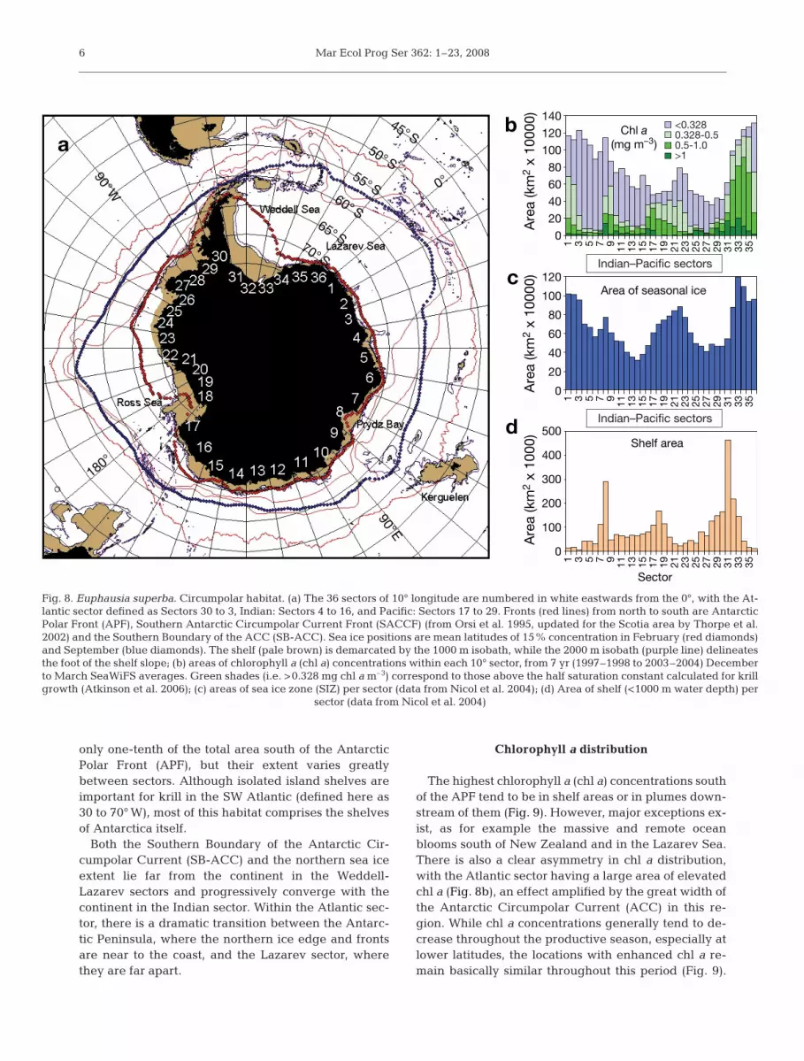
In Fig. 8a, we delineate shelf areas as thosehabitats that are not covered by permanent iceand which are shallower than 1000 m. The shelf isdeep, with most areas >200 m. Shelves comprise

5

MayMarJanNovSep

Shelfbreak

Adult

Immat

Dis

tanc

e fr

om c

ontin

ent

She

lfO

cean

ic

Juvenile

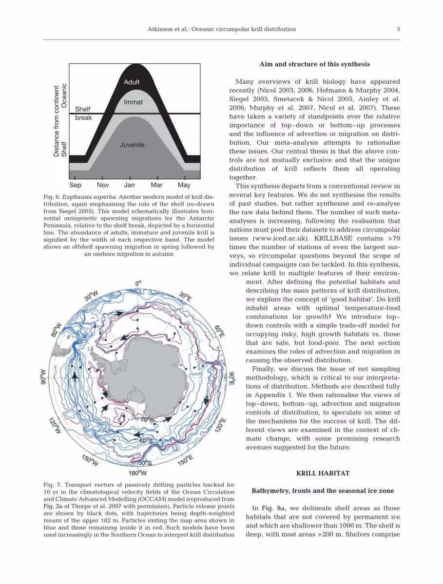
Fig. 6. Euphausia superba. Another modern model of krill dis-tribution, again emphasising the role of the shelf (re-drawnfrom Siegel 2005). This model schematically illustrates hori-zontal ontogenetic spawning migrations for the AntarcticPeninsula, relative to the shelf break, depicted by a horizontalline. The abundance of adults, immature and juvenile krill issignified by the width of each respective band. The modelshows an offshelf spawning migration in spring followed by

an onshore migration in autumn

Fig. 7. Transport vectors of passively drifting particles tracked for10 yr in the climatological velocity fields of the Ocean Circulationand Climate Advanced Modelling (OCCAM) model (reproduced fromFig. 2a of Thorpe et al. 2007 with permission). Particle release pointsare shown by black dots, with trajectories being depth-weightedmeans of the upper 182 m. Particles exiting the map area shown inblue and those remaining inside it in red. Such models have beenused increasingly in the Southern Ocean to interpret krill distribution


only one-tenth of the total area south of the AntarcticPolar Front (APF), but their extent varies greatlybetween sectors. Although isolated island shelves areimportant for krill in the SW Atlantic (defined here as30 to 70° W), most of this habitat comprises the shelvesof Antarctica itself.

Both the Southern Boundary of the Antarctic Cir-cumpolar Current (SB-ACC) and the northern sea iceextent lie far from the continent in the Weddell-Lazarev sectors and progressively converge with thecontinent in the Indian sector. Within the Atlantic sec-tor, there is a dramatic transition between the Antarc-tic Peninsula, where the northern ice edge and frontsare near to the coast, and the Lazarev sector, wherethey are far apart.

Chlorophyll a distribution

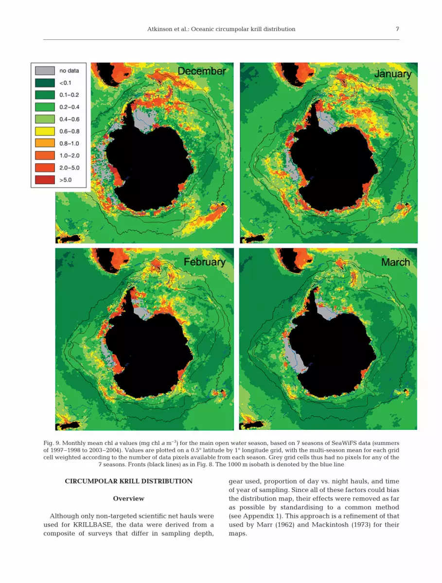
The highest chlorophyll a (chl a) concentrations southof the APF tend to be in shelf areas or in plumes down-stream of them (Fig. 9). However, major exceptions ex-ist, as for example the massive and remote oceanblooms south of New Zealand and in the Lazarev Sea.There is also a clear asymmetry in chl a distribution,with the Atlantic sector having a large area of elevatedchl a (Fig. 8b), an effect amplified by the great width ofthe Antarctic Circumpolar Current (ACC) in this re-gion. While chl a concentrations generally tend to de-crease throughout the productive season, especially atlower latitudes, the locations with enhanced chl a re-main basically similar throughout this period (Fig. 9).

6

Chl a(mg m–3)

140

120

100

80

60

40

20

0

120

100

80

60

40

20

0

500

400

300

200

100

01 3 5 7 9 11 13 15 17 19 21 23 25 27 29 31 33 35

1 3 5 7 9 11 13 15 17 19 21 23 25 27 29 31 33 35

1 3 5 7 9 11 13 15 17 19 21 23 25 27 29 31 33 35

Are

a (k

m2

x 10

000)

Are

a (k

m2

x 10

000)

Are

a (k

m2

x 10

00)

<0.3280.328-0.50.5-1.0>1

Area of seasonal ice

ab

c

d

0°

90°E

90°W

180°

45° S50° S

55° S60° S

65° S70° S Indian–Pacific sectors

Indian–Pacific sectors

Sector

Shelf area

Fig. 8. Euphausia superba. Circumpolar habitat. (a) The 36 sectors of 10° longitude are numbered in white eastwards from the 0°, with the At-lantic sector defined as Sectors 30 to 3, Indian: Sectors 4 to 16, and Pacific: Sectors 17 to 29. Fronts (red lines) from north to south are AntarcticPolar Front (APF), Southern Antarctic Circumpolar Current Front (SACCF) (from Orsi et al. 1995, updated for the Scotia area by Thorpe et al.2002) and the Southern Boundary of the ACC (SB-ACC). Sea ice positions are mean latitudes of 15% concentration in February (red diamonds)and September (blue diamonds). The shelf (pale brown) is demarcated by the 1000 m isobath, while the 2000 m isobath (purple line) delineatesthe foot of the shelf slope; (b) areas of chlorophyll a (chl a) concentrations within each 10° sector, from 7 yr (1997–1998 to 2003–2004) Decemberto March SeaWiFS averages. Green shades (i.e. >0.328 mg chl a m–3) correspond to those above the half saturation constant calculated for krillgrowth (Atkinson et al. 2006); (c) areas of sea ice zone (SIZ) per sector (data from Nicol et al. 2004); (d) Area of shelf (<1000 m water depth) per

sector (data from Nicol et al. 2004)


CIRCUMPOLAR KRILL DISTRIBUTION

Overview

Although only non-targeted scientific net hauls wereused for KRILLBASE, the data were derived from acomposite of surveys that differ in sampling depth,

gear used, proportion of day vs. night hauls, and timeof year of sampling. Since all of these factors could biasthe distribution map, their effects were removed as faras possible by standardising to a common method(see Appendix 1). This approach is a refinement of thatused by Marr (1962) and Mackintosh (1973) for theirmaps.

7

Fig. 9. Monthly mean chl a values (mg chl a m–3) for the main open water season, based on 7 seasons of SeaWiFS data (summersof 1997–1998 to 2003–2004). Values are plotted on a 0.5° latitude by 1° longitude grid, with the multi-season mean for each gridcell weighted according to the number of data pixels available from each season. Grey grid cells thus had no pixels for any of the

7 seasons. Fronts (black lines) as in Fig. 8. The 1000 m isobath is denoted by the blue line


Our standardised data (Fig. 4) show a concentrationof krill in the SW Atlantic sector and a tail extendingaround Antarctica, closer to the continent. As shownpreviously (Marr 1962, Mackintosh 1973, Nicol et al.2000a, Siegel 2005), this tail is of much lower densitythan in the SW Atlantic. We have tentatively markedthe core of the distribution in Fig. 4 to highlight 2further features:

Within the SW Atlantic, the highest mean densitiesare not at the Antarctic Peninsula but further east andnorth, in Sectors 32 to 35 (marked in Fig. 8). Indeed,the Antarctic Peninsula-Scotia Sea system does notcontain most of the krill, even within the Atlantic sec-tor. Based on the areas and krill densities within eachgrid cell in Fig. 4, the CCAMLR Synoptic Survey area(Hewitt et al. 2004) contains only 26% of the total cir-cumpolar stock (this value is 28% if the densities arestratified on a finer-scale 2° by 6° grid, A. Atkinson etal. unpubl.). By comparison, the whole 0° to 90° W sec-tor contains 70% of the total stock. These calculationsassume conservatively that the unsampled (blue) gridcells in Fig. 4 contain no krill.

The data suggest 2 population centres betweenSectors 34 and 4 (see Fig. 8 for sectors). One aligns withthe ACC stream and the other is in the counter-currentnear the continent. This result also holds for individualsurveys in the area, for example those in 1934 and2004. Like so many aspects of krill biology, this patternhas already been proposed many years ago (Mackin-tosh 1973, Makarov & Spiridonov 1993). KRILLBASEsuggests a connection between the northern popula-tion (the main ‘stock’ in the Atlantic sector) and theremaining 30% of the stock. This connection is madetentatively, given the paucity of sampling here—theregion clearly demands a more focussed survey effort.

Long-term change in density and distribution

The standardised data in Fig. 4 are a composite ofdata spanning 80 yr, during which krill density withinthe SW Atlantic sector has declined over the period1976 to 2003. This observation was based on subsets ofun-standardised data, causing concerns over possiblesampling artefacts (Quetin et al. 2007). However,Fig. 10 shows that, even after applying our standardis-ation procedure, the decline persists.

This decline in krill within the SW Atlantic sector isaccompanied by a regional increase in water tempera-ture (Meredith & King 2005) and decrease in sea ice(Parkinson 2002) and follows larger-scale and longer-term changes (de la Mare 1997, Gille 2002, Cotté &Guinette 2007, Whitehouse et al. in press). Conse-quently, an overall change in krill abundance is plau-sible within a 30 yr period, taking into account that the

population can fluctuate greatly from year to year.However, in the context of this synthesis, the questionis: Has this been accompanied by a re-distribution?Within the limits of the available data, we found noconvincing evidence for any change in krill distribu-tion between the ‘Discovery’ expeditions and recentyears, so the ‘climatology’ in Fig. 4 is a reasonableoverall picture.

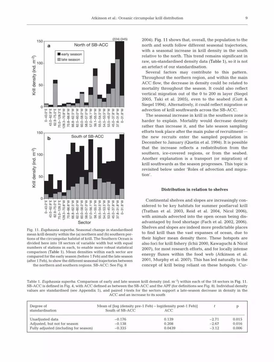
Seasonal change in distribution

Our standardisation procedure (see Appendix 1)revealed that krill density peaks in the middle ofsummer (January) and declines thereafter. This re-flects the pulse of recruitment from larvae duringspring–summer and subsequent mortality. However,there is a latitudinal difference in this simple picture.We illustrate this with a plot of density anomalies(Fig. 11), calculated from standardised densities, andcomparing seasonal trends in density between thenorthern and southern parts of the krill distributionrange. In our analysis, we have divided the 8137 sam-pling stations into a standard sample size, a nominaln = 36 groups of stations, to make it compatible to arecent circumpolar habitat-based analysis (Nicol et al.

8

2.5

2

1.5

1

0.5

1928

1931

1934

1937

1940

1978

1981

1984

1987

1990

1993

1996

1999

2002

YearLo

g 10

(kril

l den

sity

, ind

. m–2

)Fig. 10. Euphausia superba. Change in mean density (ind. m–2)within the SW Atlantic sector (30 to 70° W), based on stan-dardised densities, for comparison with Fig. 2a of Atkinson etal. (2004) based on un-standardised values. Only years with>50 stations are plotted. The vertical line separates the 1926to 1939 and post-1976 eras. Based on the post-1976 datasetthere is a significant decline: log10 (krill density) = 60.07 –

0.0294 (yr); R2 = 31%, p = 0.007, n = 22 yr


2004). Fig. 11 shows that, overall, the population to thenorth and south follow different seasonal trajectories,with a seasonal increase in krill density in the southrelative to the north. This trend remains significant inraw, un-standardised density data (Table 1), so it is notan artefact of our standardisation.

Several factors may contribute to this pattern.Throughout the northern region, and within the mainACC flow, the decrease in density could be related tomortality throughout the season. It could also reflectvertical migration out of the 0 to 200 m layer (Siegel2005, Taki et al. 2005), even to the seabed (Gutt &Siegel 1994). Alternatively, it could reflect migration oradvection of krill southwards across the SB-ACC.

The seasonal increase in krill in the southern zone isharder to explain. Mortality would decrease densityrather than increase it, and the late season samplingefforts took place after the main pulse of recruitment—the new recruits enter the sampled population inDecember to January (Quetin et al. 1994). It is possiblethat the increase reflects a redistribution from thesouthern, ice-covered regions, or from the seabed.Another explanation is a transport (or migration) ofkrill southwards as the season progresses. This topic isrevisited below under ‘Roles of advection and migra-tion’.

Distribution in relation to shelves

Continental shelves and slopes are increasingly con-sidered to be key habitats for summer postlarval krill(Trathan et al. 2003, Reid et al. 2004, Nicol 2006),with animals advected into the open ocean being dis-advantaged by food shortage (Fach et al. 2002, 2006).Shelves and slopes are indeed more predictable placesto find krill than the vast expanses of ocean, due totheir higher mean density there. These hotspots arealso foci for krill fishery (Ichii 2000, Kawaguchi & Nicol2007), for most research efforts, and for locally intenseenergy fluxes within the food web (Atkinson et al.2001, Murphy et al. 2007). This has led naturally to theconcept of krill being reliant on these hotspots. Cur-

9

North of SB-ACC

South of SB-ACC

0–4

3.0°

E43

.0–6

2.9°

E62

.9–7

5.0°

E75

.0–1

28.3

°E12

8.3

–70.

8°W

70.8

–66.

8°W

66.8

–62.

5°W

62.5

–60.

0°W

60.0

–58.

0°W

58.0

–57.

0°W

57.0

–56.

1°W

56.1

–55.

5°W

55.5

–54.

5°W

54.5

–53.

5°W

53.5

–45.

0°W

45.0

–37.

8°W

37.8

–31.

8°W

0–3

1.8°

W

Sector

0–4

3.0°

E43

.0–6

2.9°

E62

.9–7

5.0°

E75

.0–1

28.3

°E12

8.3

–70.

8°W

70.8

–66.

8°W

66.8

–62.

5°W

62.5

–60.

0°W

60.0

–58.

0°W

58.0

–57.

0°W

57.0

–56.

1°W

56.1

–55.

5°W

55.5

–54.

5°W

54.5

–53.

5°W

53.5

–45.

0°W

45.0

–37.

8°W

37.8

–31.

8°W

0–3

1.8°

W

Kril

l den

sity

(ind

. m–2

)K

rill d

ensi

ty (i

nd. m

–2)

early season

late season

(224) (345)150

100

50

0

150

100

50

0

a

b

Fig. 11. Euphausia superba. Seasonal change in standardisedmean krill density within the (a) northern and (b) southern por-tions of the circumpolar habitat of krill. The Southern Ocean isdivided here into 18 sectors of variable width but with equalnumbers of stations in each, to enable more robust statisticalcomparison (Table 1). Mean densities within each sector arecompared for the early season (before 1 Feb) and the late season(after 1 Feb), to show the different seasonal trajectories between

the northern and southern regions. SB-ACC: See Fig. 8

Table 1. Euphausia superba. Comparison of early and late season krill density (ind. m–2) within each of the 18 sectors in Fig. 11.SB-ACC is defined in Fig. 4, with ACC defined as between the SB-ACC and the APF (for definitions see Fig. 8). Individual densityvalues are standardised (see Appendix 1), and paired t-tests for the sectors support a late-season decrease in density in the

ACC and an increase to its south

Degree of Mean of [log (density pre-1 Feb) – log(density post-1 Feb)] t pstandardisation South of SB-ACC ACC

Unadjusted data –0.176 0.139 –2.71 0.015Adjusted, but not for season –0.138 0.208 –2.67 0.016Fully adjusted (including for season) –0.335 0.0439 –3.12 0.006


rent models of their seasonal distribution (Siegel 2005,Nicol 2006) infer shelves to be a key part of the sum-mer habitat for postlarvae (Figs. 5 & 6).

Our circumpolar scale view, however, provides aradically different picture. Based on all net samplingstations south of the APF, mean krill density over shelf-slope areas (water depth <2000 m) is only 1.65 timesthat over deep ocean. This relatively slight differencein krill density from the shallowest to deepest watercan also be seen from acoustic data taken from Reid etal. (2004) and re-plotted in Fig. 12. By stratifying thedensity estimates by area, we calculate (see Appen-dix 1) that 87% of the total krill population live overwater depths >2000 m. This reflects the rather smalldensity gradient and the 10-fold greater habitat area.

Plotting krill density in relation to distance from theshelf break also shows the same basic picture. At a cir-cumpolar scale (Fig. 13a), there is a decline in krilldensity from onshore to offshore, but the relativelysmall density difference and 10-fold greater area ofocean mean that most of the population are oceanic.Based on both types of analysis, the finding that only13% of the global krill stock live in the shelf-slopehabitat shows that krill are mainly an oceanic species.

This overall pattern, however, obscures major differ-ences between sectors. Prior analysis revealed 3 broadpatterns of distribution found in the Antarctic Penin-sula area, the main Atlantic sector, and the Indian–Pacific sector. These sub-areas (Fig. 13b–d) are plot-ted on the same scale to show the much lower densityin the Indian-Pacific sector and the scarcity over its

10

3

2

1

0

1

0

–1

–2

0 1000 2000 3000 4000 5000 6000Depth (m)

Log 1

0 (k

rill d

ensi

ty, i

nd. m

–3)

Log 1

0 (b

iom

ass

per

inte

grat

ion

per

iod

)

Fig. 12. Euphausia superba. Krill density (left axis, filled cir-cles, solid regression line) in relation to water depth. Datafrom all 8137 net stations south of the APF were first ranked inorder of increasing water depth and then divided into 36groups of 226 stations. The mean krill density for each groupis plotted here against the respective mean water depth. Re-gression statistics (but with both predictor and response vari-ables logged) are presented in Table 2. Also plotted is relativeacoustically derived biomass vs. water depth (right axis, opensquares, broken regression line) with data recalculated from

Reid et al. (2004)

3

2

1

0

–1

3

2

1

0

–1

3

2

1

0

–1

3

2

1

0

–1

–200 0 200 400 600 800

–200 0 200 400 600 800

–200 0 200 400

Circumpolar (all data)

Antarctic Peninsula

Atlantic sector

Indian-Pacific sector

Distance from shelf break (km)

600 800

–200 0 200 400 600 800

Log 1

0 (k

rill d

ensi

ty, i

nd. m

–2)

d

c

b

a

Fig. 13. Euphausia superba. Distribution in relation to theshelf break; (a) Circumpolar density data (8137 stations southof APF) in relation to distance from the nearest shelf break(defined as any 1000 m isobath occurring south of the APF).Shelf stations are assigned with negative distances; (b)Antarctic Peninsula data only (3992 stations from 50 to 70° W;Sectors 30 to 31) Log10 (krill density) = 1.5 – 0.0047 (distancefrom shelf break, km), R2 = 0.628, p < 0.01, n = 36; (c) Atlanticsector only (2142 stations from 50° W to 30° E; Sectors 32 to 3;(d) Indian-Pacific sector only (2003 stations from 30° E to70° W; Sectors 4 to 29). Trend lines in Panels (a,c,d) represent10-sample running means. We used our standard protocol ofdividing each subset of data into 36 groups with equalised

samples sizes


shelves (Fig. 13d). Here, krill density is often maximalwithin a few hundred kilometres of the shelf break,with a general decline further offshore. This pattern,with maximum densities south of the SB-ACC, hasbeen observed in detailed surveys within this sector(Hosie 1994, Nicol et al. 2000b,c).

The Antarctic Peninsula, by contrast, shows a com-pletely different pattern with highest densities oftenclose inshore near the islands and the convolutedcoastline (Fig. 13b). Clearly, the shelf here is betterkrill habitat than its high latitude counterpart aroundthe main continent. The latter, with heavier ice cover,is inhabited by its congener Euphausia crystalloro-phias (Hosie 1994).

While the oceanic habitat near the Antarctic Penin-sula is narrow, unproductive and contains few krill, theoceanic Atlantic sector is productive and much moreextensive, and high krill densities occur within theACC remote from land (Fig. 13c). In this sector, there isalso a concentration close to and over shelves, but theshelf–ocean difference in density is not great. Becausekrill abundance is highest in this main Atlantic sector itdominates the overall circumpolar pattern.

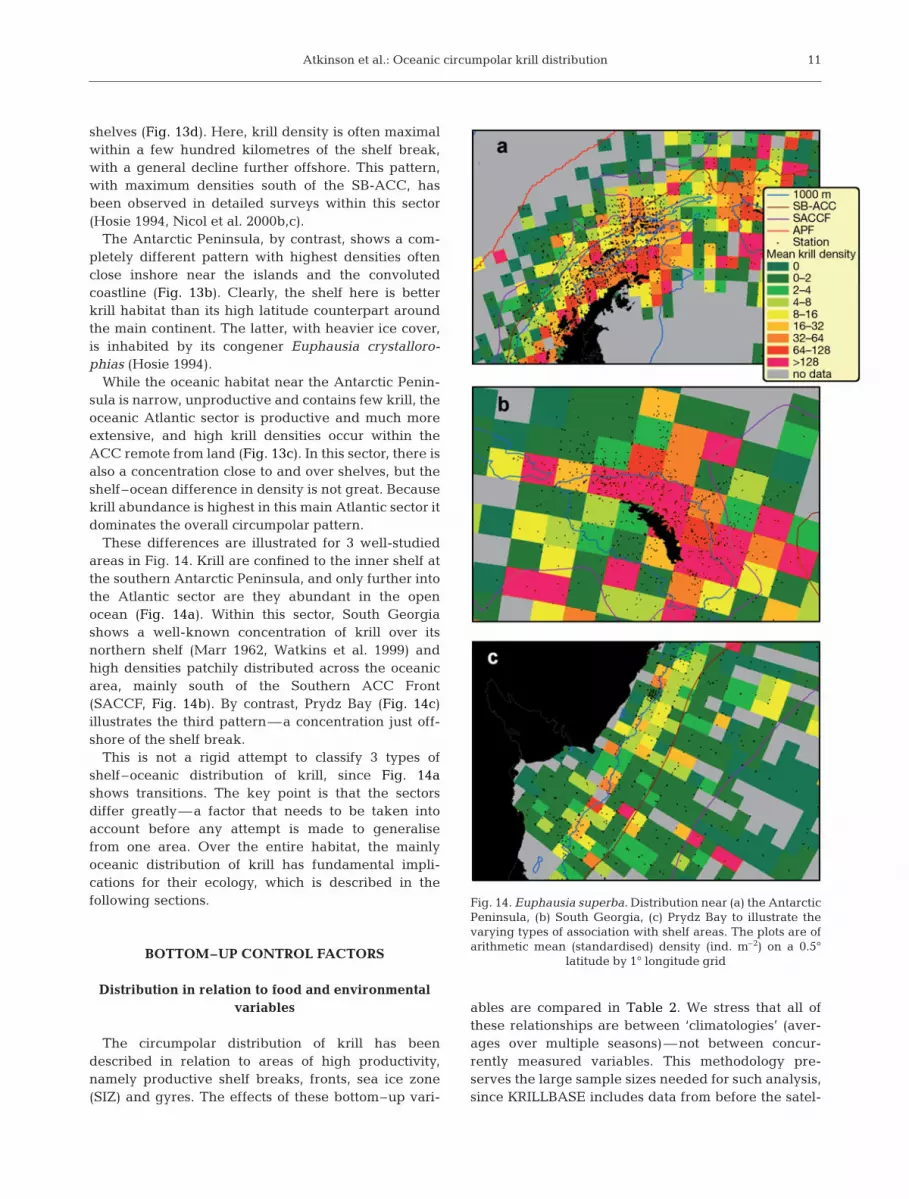
These differences are illustrated for 3 well-studiedareas in Fig. 14. Krill are confined to the inner shelf atthe southern Antarctic Peninsula, and only further intothe Atlantic sector are they abundant in the openocean (Fig. 14a). Within this sector, South Georgiashows a well-known concentration of krill over itsnorthern shelf (Marr 1962, Watkins et al. 1999) andhigh densities patchily distributed across the oceanicarea, mainly south of the Southern ACC Front(SACCF, Fig. 14b). By contrast, Prydz Bay (Fig. 14c)illustrates the third pattern—a concentration just off-shore of the shelf break.

This is not a rigid attempt to classify 3 types ofshelf–oceanic distribution of krill, since Fig. 14ashows transitions. The key point is that the sectorsdiffer greatly—a factor that needs to be taken intoaccount before any attempt is made to generalisefrom one area. Over the entire habitat, the mainlyoceanic distribution of krill has fundamental impli-cations for their ecology, which is described in thefollowing sections.

BOTTOM–UP CONTROL FACTORS

Distribution in relation to food and environmentalvariables

The circumpolar distribution of krill has beendescribed in relation to areas of high productivity,namely productive shelf breaks, fronts, sea ice zone(SIZ) and gyres. The effects of these bottom–up vari-

ables are compared in Table 2. We stress that all ofthese relationships are between ‘climatologies’ (aver-ages over multiple seasons)—not between concur-rently measured variables. This methodology pre-serves the large sample sizes needed for such analysis,since KRILLBASE includes data from before the satel-

11

Fig. 14. Euphausia superba. Distribution near (a) the AntarcticPeninsula, (b) South Georgia, (c) Prydz Bay to illustrate thevarying types of association with shelf areas. The plots are ofarithmetic mean (standardised) density (ind. m–2) on a 0.5°

latitude by 1° longitude grid


lite era, and the records do not include concurrentlymeasured environmental data.

After dividing the Southern Ocean south of the APFinto 36 sectors of 10° longitude, no relationship wasfound between mean krill density per sector and itsarea of shelf, the SIZ, or area south of the SB-ACC.Some of these relationships (for example between krilldensity and area south of the SB-ACC) hold for partsof the circumpolar habitat (Nicol et al. 2000b,c), but notfor all of it. Krill density and recruitment are linked tosea ice extent, but this is a temporal relationship forthe SW Atlantic (Kawaguchi & Sataki 1994, Siegel &Loeb 1995, Loeb et al. 1997, Atkinson et al. 2004) andis not seen at circumpolar scales (Constable et al. 2003,Table 2, this paper).

However, krill density relates significantly both tofood and to water depth. These co-vary, but multiple

regression (Table 2) teases apart the 2 effects—we findno significant effect of water depth after allowingfor the effect of food. Indeed, the relationship withfood concentration (Fig. 15a) is non-linear and muchstronger than that with water depth (Table 2). Thus,variation in krill density between sectors is more influ-enced by their areas of enhanced food than by shelfareas within the sectors (Table 2, Fig. 13b).

Our reappraisal of what constitutes good krill habitathelps interpret their concentration in the SW Atlantic.Factors invoked previously include its larger shelfarea, retention by the Weddell Gyre and convergenceof currents (Reid et al. 2004, Nicol 2006, Thorpe et al.2007). However, Fig. 4 suggests a scarcity of krillaround the Weddell Sea (see also Siegel 2005), andkrill density per sector does not relate to its area ofshelf. Fig. 15b shows the SW Atlantic simply as part of

12

Table 2. Euphausia superba. Circumpolar-scale relationships between log10 of krill density (ind. m–2) and physical–biologicalenvironment and Gross Growth Potential (GGP). For definitions of APF, SIZ and SB-ACC see Fig. 8. N = 36 for all regressions,which use all available data (>8000 stations) pooled into 36 groups either of equal sample size or into sectors of 10° longitude.

ns: not significant (p > 0.05)

Relationship Predictor (x) variable Regression R2 (%)(All logged) (of logged predictor and response variables)

Food Mean chl a (mg m–3) y = 1.76 + 0.304x / (1 + 0.991x ) 48(chl a data in Fig. 17a, regression shown in Fig. 15a)a

Area of chl a > 0.5 mg m–3 y = –1.96 + 1.11x 30in 10° sector (1000 km2)(chl a data in Fig. 8b, regression in Fig. 15b)

Mean chl a in 10° sector ns –(mg m–3)

Water depth Mean water depth (m) y = 2.54 – 0.31x 23(data derived from Fig. 12)

Area from coast to 1000 m ns –isobath in 10° sector (1000 km2)(data from Nicol et al. 2004, presented in Fig. 8d)

Distance from Distance (km) from any 1000 m ns –shelf break isobath south of APF (km)

(data in Fig. 13a)

Food and Water depth Mean chl a, C y = 2.39 – 0.135 C + 0.201 Z – 1.75 C 2 58mean depth, Z (C 2 is the only significant term: p = 0.004)

GGP GGP y = 0.513 + 0.382x – 0.0300x2 28(data from Fig. 16a)

Area of SIZ Maximum minus minimum sea ice ns –extent in 10° sector (1000 km2)(data from Nicol et al. 2004, presented in Fig. 8c)

Area south of SB-ACC Area from coast to SB-ACC ns –in 10° sector (km2)(data from Nicol et al. 2004)

aA hyperbolic relationship provides a statistically better fit (F1, 33 = 14.36, p = 0.001) than a straight line. A quadratic relation-ship provides an even better fit (R2 = 61%), but the effects at highest chl a concentrations are uncertain


the circumpolar relationship between krill density andthe area of suitable feeding grounds. Clearly, this areamust also support the whole life cycle. For example, itslower latitudes may receive enough winter light to pro-mote pelagic- and ice-derived food for overwintering,larval growth and early spawning (Murphy et al. 2007,Quetin et al. 2007).

The issue of scale is central to these analyses. Giventhe complex interactions between predator and prey,the sign and type of relationship observed betweenthem depends on the scale of analysis (Rose & Leggett1990). We therefore repeated the krill–food analysis,but at a smaller scale, by pairing each krill record withSeaWiFS data for the same year and month of sam-pling and extracting the mean chl a value from within50 km of the station (n = 1943 stations). Like the clima-

tology analysis, this also produced a dome-shapedrelationship, with highest krill densities at moderatechl a values. However, the explanations might not bethe same. For example, the larger scale relationshipreflects the high-chl a Antarctic shelf being south ofthe main range of krill, while at the smaller scale highdensities of krill could have grazed down their food.

Distribution in relation to growth potential

A circumpolar prediction of successful spawninghabitats exists (Hofmann & Hüsrevoglu 2003), butnone for predicting habitats ideal for growth. Anempirical model of summer growth rates now allowsthis (Atkinson et al. 2006), being designed for large-scale, satellite-derivable food and temperature indices.While there are caveats to any predictive model,Fig. 16 is a first numerical attempt to explore how foodand temperature interact to dictate the circumpolargrowth habitats for krill.

We defined different growth habitats by their GrossGrowth Potential (GGP), which is the body mass of akrill at the end of March divided by that at the be-ginning of December (see Appendix 1 for calculationmethod). The growth rate decreases as krill get longer,so the GGP is higher for smaller starting sizes of krill(Fig. 16a,b). Each season varies in its conditions, andthus in its ability to support high growth rates. This isillustrated in Fig. 16c,d—a high chl a season (summer1999–2000) supports much higher growth rates thanone with low chl a (2002–2003).

To check these predictions, we obtained an overallmean GGP for the Southern Ocean by weighting thecell-specific GGPs (Fig. 16a) with their respective krilldensities. This provides a GGP of 3.7. For comparison,a quadrupling of krill mass from December to March(i.e. a GGP of 4) equates to a 30 mm krill growing at0.1 mm d–1. This is close to respective values of0.11 mm d–1 and 0.06 to 1.2 mm d–1 from studies usingthe Instantaneous Growth Rate (IGR) method in theIndian-Atlantic sectors (Kawaguchi et al. 2006) and theAntarctic Peninsula (Ross et al. 2000), and to growthrates of field populations (Rosenberg et al. 1986, Siegel& Nicol 2000).

All of these model outputs show starvation (shrink-age) north of the APF, while rapid growth follows theavailability of chl a in habitats south of the APF. Theinteraction of food and temperature in dictatinggrowth is illustrated in Fig. 17. The shrinkage north ofthe APF is probably due to adverse effects of high tem-perature. The upper temperature limit for krill survivalis ~8°C (Naumov & Chekunova 1980) and their normalnorthern limit is the APF. The model on which the GGPvalues are based (Atkinson et al. 2006) yields maximal

13

10–1

2

1

0

2

1

0

–1

–21 2 3

a

b

Log 1

0 (k

rill d

ensi

ty, i

nd. m

–2)

Log 1

0 (m

ean

krill

den

sity

, ind

. m–2

)

Log10 (chl a concentration, mg chl a m–3)

Log10 (1000 km2 of chl a >0.5 mg m–3)

Fig. 15. Euphausia superba. Log–log relationships betweenclimatologies (i.e. multi-season means) of krill density andsimple indices of their food availability. (a) Krill density vs.food concentration, based on our standard division of all 8137sampling stations into 36 groups of equal size; (b) krill densitywithin each of the 36 sectors vs. its area of elevated chl a (arbi-trarily defined as >0.5 mg chl a m–2). The SW Atlantic-Penin-sula sectors (here defined as 10 to 80° W) are shown with

filled symbols. Regressions are in Table 2


growth at 0.5 to 1°C and a progressive decline athigher temperatures. It is possible that the warmwaters near the APF in the SW Atlantic are viable krillhabitat because the costs from high water tempera-tures are offset by the rewards from abundant food(Fig. 15).

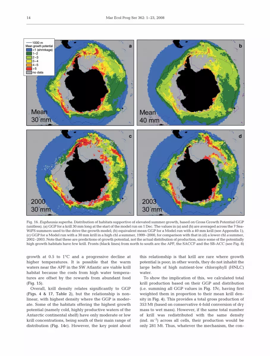
Overall, krill density relates significantly to GGP(Figs. 4 & 17, Table 2), but the relationship is non-linear, with highest density where the GGP is moder-ate. Some of the habitats offering the highest growthpotential (namely cold, highly productive waters of theAntarctic continental shelf) have only moderate or lowkrill concentrations, being south of their main range ofdistribution (Fig. 14c). However, the key point about

this relationship is that krill are rare where growthpotential is poor; in other words, they do not inhabit thelarge belts of high nutrient-low chlorophyll (HNLC)water.

To show the implication of this, we calculated totalkrill production based on their GGP and distribution(i.e. summing all GGP values in Fig. 17c, having firstweighted them in proportion to their mean krill den-sity in Fig. 4). This provides a total gross production of353 Mt (based on conservative 4-fold conversion of drymass to wet mass). However, if the same total numberof krill was redistributed with the same density(ind. m–2) across all cells, their production would beonly 281 Mt. Thus, whatever the mechanism, the con-

14

Fig. 16. Euphausia superba. Distribution of habitats supportive of elevated summer growth, based on Gross Growth Potential GGP(unitless). (a) GGP for a krill 30 mm long at the start of the model run on 1 Dec. The values in (a) and (b) are averaged across the 7 Sea-WiFS summers used to the drive the growth model; (b) equivalent mean GGP for a Model run with a 40 mm krill (see Appendix 1);(c) GGP for a Model run with a 30 mm krill in a high chl a summer, 1999–2000, for comparison with that in (d) a lower chl a summer,2002–2003. Note that these are predictions of growth potential, not the actual distribution of production, since some of the potentiallyhigh growth habitats have few krill. Fronts (black lines) from north to south are the APF, the SACCF and the SB-ACC (see Fig. 8)


centration of krill in enhanced growth habitats booststheir production by 72 Mt.

To sum up, the distribution of summer post-larvalkrill does indeed relate to bottom–up factors. How-ever, the highest krill densities coincide with interme-diate food concentrations and growth potential, ratherthan with the highest values for both factors. We sug-gest that this is due to reduced predation risk in suchareas.

TOP–DOWN CONTROL FACTORS

Risk–reward model of habitat suitability

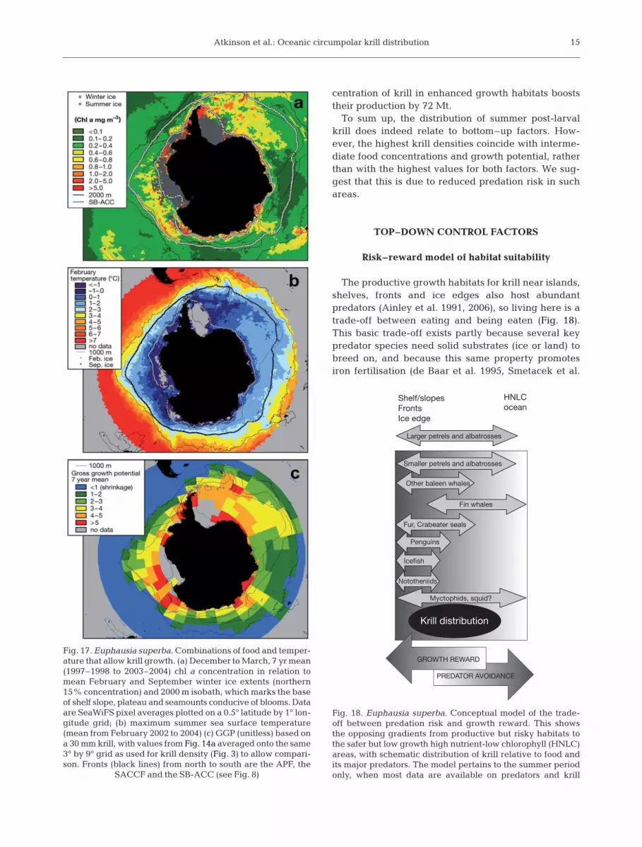
The productive growth habitats for krill near islands,shelves, fronts and ice edges also host abundantpredators (Ainley et al. 1991, 2006), so living here is atrade-off between eating and being eaten (Fig. 18).This basic trade-off exists partly because several keypredator species need solid substrates (ice or land) tobreed on, and because this same property promotesiron fertilisation (de Baar et al. 1995, Smetacek et al.

15

Fig. 17. Euphausia superba. Combinations of food and temper-ature that allow krill growth. (a) December to March, 7 yr mean(1997–1998 to 2003–2004) chl a concentration in relation tomean February and September winter ice extents (northern15% concentration) and 2000 m isobath, which marks the baseof shelf slope, plateau and seamounts conducive of blooms. Dataare SeaWiFS pixel averages plotted on a 0.5° latitude by 1° lon-gitude grid; (b) maximum summer sea surface temperature(mean from February 2002 to 2004) (c) GGP (unitless) based ona 30 mm krill, with values from Fig. 14a averaged onto the same3° by 9° grid as used for krill density (Fig. 3) to allow compari-son. Fronts (black lines) from north to south are the APF, the

SACCF and the SB-ACC (see Fig. 8)

Icefish

Penguins

Myctophids, squid?

Fur, Crabeater seals

Smaller petrels and albatrosses

Shelf/slopesFrontsIce edge

HNLCocean

Larger petrels and albatrosses

Other baleen whales

Fin whales

Krill distribution

Nototheniids

GROWTH REWARD

PREDATOR AVOIDANCE

Fig. 18. Euphausia superba. Conceptual model of the trade-off between predation risk and growth reward. This showsthe opposing gradients from productive but risky habitats tothe safer but low growth high nutrient-low chlorophyll (HNLC)areas, with schematic distribution of krill relative to food andits major predators. The model pertains to the summer periodonly, when most data are available on predators and krill


2004). Many non-land breeders such as icefish (Koch etal. 1994) and whales (Reilly et al. 2004, Friedlaender etal. 2006) also concentrate in chl a-rich habitats, whilethe distribution of others relative to chl a is unknown(e.g. squid or myctophid fish).

The best approach to explore this trade-off numeri-cally would be to relate growth potential and predationrisk to chl a, but we are unaware of predation dataexpressed in this form. Instead, we related both growthand predation risk to water depth, since this is a rea-sonable proxy for chl a concentration (Fig. 19a) and is atractable means of describing trends in predator distri-butions. The environmental data (Fig. 19a), combinedwith the growth model, generate an onshore–offshoregradient in growth potential for an individual krill(Fig. 19b). This quantifies the potential benefit in theextreme scenario of optimising individual growth andignoring mortality risk.

However, krill predators also track these hotspots.This is shown in Fig. 19c for the land-breeding compo-nent in relation to water depth. Predation risk isdepicted here both by predator densities (Reid et al.2004) and by estimates of krill consumption (Murphy1995). The changes in predator densities and con-sumption estimates with water depth are substantial,and certainly in line with the differences in predationrisk that are calculated to balance growth (Fig. 19d).

These opposing gradients in growth potential andpredation risk have a cancelling effect in calculationsof net production. The krill consumption estimates inFig. 19c provide a more specific illustration of this

16

Fig. 19. Euphausia superba. Risks and benefits for krill cal-culated for January-February, all in relation to water depth.(a) Overall average relationships are food concentration C(mg chl a m–3) vs. depth Z (m): Log10 C = –0.00268 – 0.00012 Z(R2 = 28%, p < 0.001, n = 10338 grid cells of 0.5° by 1° south ofthe APF). Temperature T (°C): T = 0.496 + 0.000344 Z (R2 =8%, p < 0.001, n = 10338); (b) predicted mass gains of 3 sizesof krill over 9 wk, from the relationships above and thegrowth model (Eq. 9 in Appendix 1); (c) left axis, logarithmicscale: relative densities of major krill predators across the SWAtlantic sector (data recalculated from Reid et al. 2004); rightaxis: calculated krill consumption by seabirds at Bird Island,South Georgia (data from Murphy 1995); (d) predation calcu-lated to balance exactly the mass increase from growth pre-dicted in Panel (b) (i.e. to yield 0 net growth). This simplecalculation shows the ‘balance point’ for the counteractingrisk–reward trade-off for comparison with predator observa-tions in Panel (c) (see Appendix 1); (e) predicted net produc-tion (g wet mass m–2) after 9 wk, based on an evenly distrib-uted starting population of 40 mm krill on 1 Jan with growthin Panel (b) and mortality based on Murphy’s (1995) values inPanel (c). Model sensitivity to mortality is examined bydoubling and halving the predation rates of Murphy (1995);negative net production (values below the horizontal line)equates to greater consumption rates than can be supported

by growth


trade-off for the South Georgia area. The predationestimates are conservative for this region, comprisingonly the seabird fraction of the total predators, andbeing calculated pro-rata from annual rates. Neverthe-less, a simple sensitivity analysis (Fig. 19e) shows thatnet krill production is very sensitive to predation loss,implying the importance of top–down control.

The period for which krill data is available, from1926 to 2004, follows a major perturbation of theirpredators, with a large proportion of fur seals, southernright, humpback and blue whales removed before1926 (Laws 1985, Moore et al. 1999b). These compriseboth shelf-based and pelagic foragers, so it is hard topredict how their removal might affect krill distribu-tion. While krill density relates significantly (p < 0.05)and negatively to water depth in both eras of samplingefforts included in KRILLBASE (1926 to 1939 and1976 to 2004, see Appendix 1) with a substantialshelf–ocean difference for the 1926 to 1939 era, nosignificant difference in the slopes of the regressionswas detected.

In summary, our risk–reward analysis shows that thebest feeding grounds for krill may not be best for netpopulation growth. The exercise is not to infer that krillhave necessarily evolved a risk-balancing strategy—the krill we observe are those remaining after preda-tion has operated. In other words, a reduced predationrisk may be the implication of the observed distributionand not its cause. Notwithstanding this caveat, theconcept of risk and reward allows us to rationalise thesurprising finding that 87% of the krill population liveover deep ocean. Here, krill are growing at sub-maxi-mal rates, but they are sheltered from the most intensepredation.

Efficient growth in low-risk areas

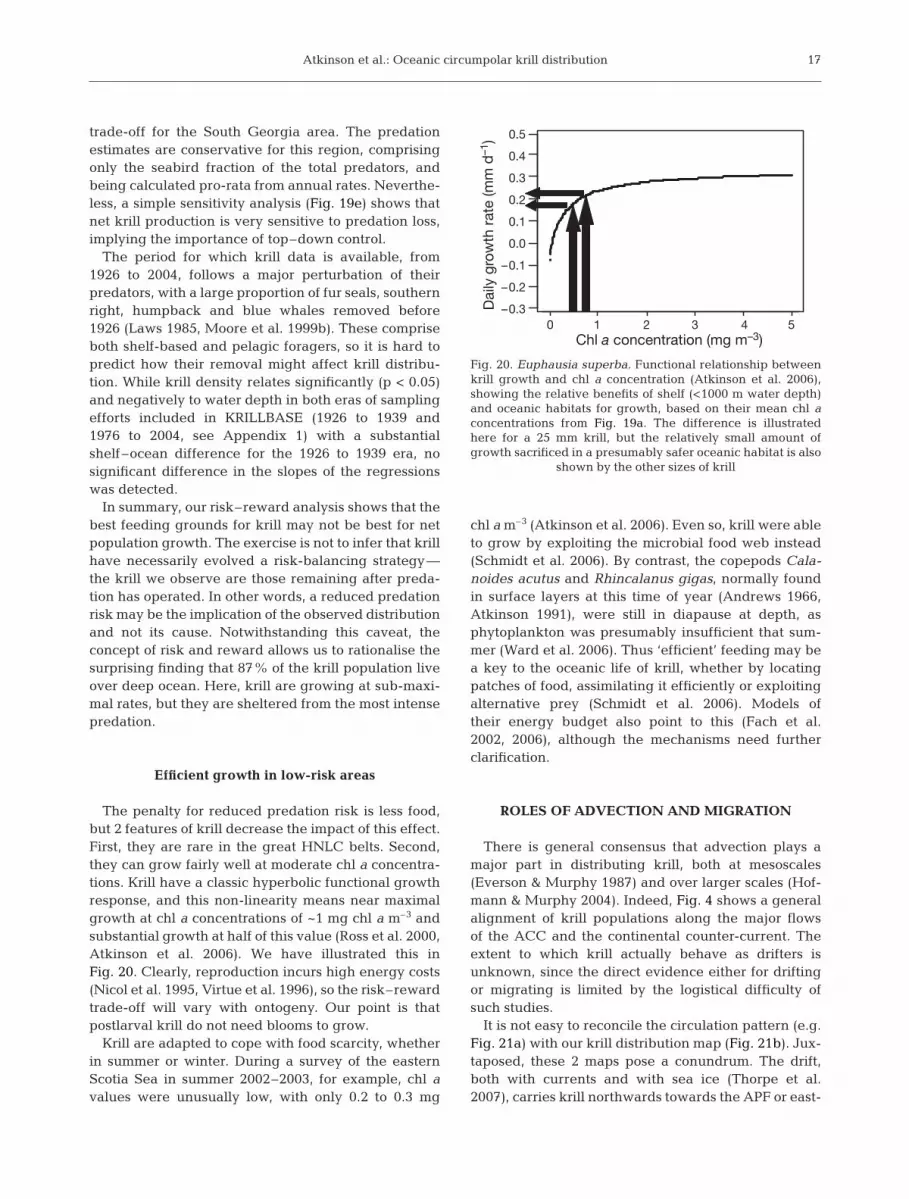
The penalty for reduced predation risk is less food,but 2 features of krill decrease the impact of this effect.First, they are rare in the great HNLC belts. Second,they can grow fairly well at moderate chl a concentra-tions. Krill have a classic hyperbolic functional growthresponse, and this non-linearity means near maximalgrowth at chl a concentrations of ~1 mg chl a m–3 andsubstantial growth at half of this value (Ross et al. 2000,Atkinson et al. 2006). We have illustrated this inFig. 20. Clearly, reproduction incurs high energy costs(Nicol et al. 1995, Virtue et al. 1996), so the risk–rewardtrade-off will vary with ontogeny. Our point is thatpostlarval krill do not need blooms to grow.

Krill are adapted to cope with food scarcity, whetherin summer or winter. During a survey of the easternScotia Sea in summer 2002–2003, for example, chl avalues were unusually low, with only 0.2 to 0.3 mg

chl a m–3 (Atkinson et al. 2006). Even so, krill were ableto grow by exploiting the microbial food web instead(Schmidt et al. 2006). By contrast, the copepods Cala-noides acutus and Rhincalanus gigas, normally foundin surface layers at this time of year (Andrews 1966,Atkinson 1991), were still in diapause at depth, asphytoplankton was presumably insufficient that sum-mer (Ward et al. 2006). Thus ‘efficient’ feeding may bea key to the oceanic life of krill, whether by locatingpatches of food, assimilating it efficiently or exploitingalternative prey (Schmidt et al. 2006). Models oftheir energy budget also point to this (Fach et al.2002, 2006), although the mechanisms need furtherclarification.

ROLES OF ADVECTION AND MIGRATION

There is general consensus that advection plays amajor part in distributing krill, both at mesoscales(Everson & Murphy 1987) and over larger scales (Hof-mann & Murphy 2004). Indeed, Fig. 4 shows a generalalignment of krill populations along the major flowsof the ACC and the continental counter-current. Theextent to which krill actually behave as drifters isunknown, since the direct evidence either for driftingor migrating is limited by the logistical difficulty ofsuch studies.

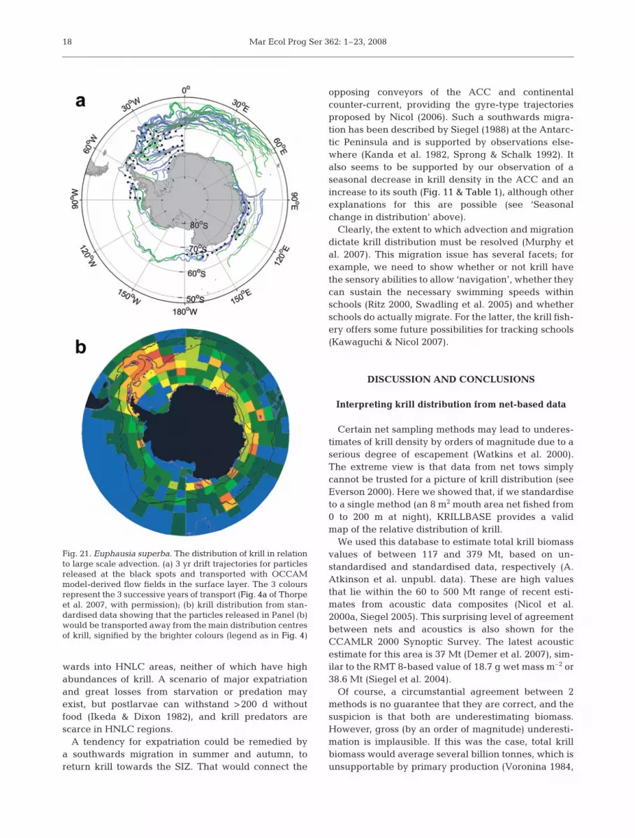
It is not easy to reconcile the circulation pattern (e.g.Fig. 21a) with our krill distribution map (Fig. 21b). Jux-taposed, these 2 maps pose a conundrum. The drift,both with currents and with sea ice (Thorpe et al.2007), carries krill northwards towards the APF or east-

17

543210

0.5

0.4

0.3

0.2

0.1

0.0

–0.1

–0.2

–0.3Dai

ly g

row

th r

ate

(mm

d–1

)

Chl a concentration (mg m–3)

Fig. 20. Euphausia superba. Functional relationship betweenkrill growth and chl a concentration (Atkinson et al. 2006),showing the relative benefits of shelf (<1000 m water depth)and oceanic habitats for growth, based on their mean chl aconcentrations from Fig. 19a. The difference is illustratedhere for a 25 mm krill, but the relatively small amount ofgrowth sacrificed in a presumably safer oceanic habitat is also

shown by the other sizes of krill


wards into HNLC areas, neither of which have highabundances of krill. A scenario of major expatriationand great losses from starvation or predation mayexist, but postlarvae can withstand >200 d withoutfood (Ikeda & Dixon 1982), and krill predators arescarce in HNLC regions.

A tendency for expatriation could be remedied bya southwards migration in summer and autumn, toreturn krill towards the SIZ. That would connect the

opposing conveyors of the ACC and continentalcounter-current, providing the gyre-type trajectoriesproposed by Nicol (2006). Such a southwards migra-tion has been described by Siegel (1988) at the Antarc-tic Peninsula and is supported by observations else-where (Kanda et al. 1982, Sprong & Schalk 1992). Italso seems to be supported by our observation of aseasonal decrease in krill density in the ACC and anincrease to its south (Fig. 11 & Table 1), although otherexplanations for this are possible (see ‘Seasonalchange in distribution’ above).

Clearly, the extent to which advection and migrationdictate krill distribution must be resolved (Murphy etal. 2007). This migration issue has several facets; forexample, we need to show whether or not krill havethe sensory abilities to allow ‘navigation’, whether theycan sustain the necessary swimming speeds withinschools (Ritz 2000, Swadling et al. 2005) and whetherschools do actually migrate. For the latter, the krill fish-ery offers some future possibilities for tracking schools(Kawaguchi & Nicol 2007).

DISCUSSION AND CONCLUSIONS

Interpreting krill distribution from net-based data

Certain net sampling methods may lead to underes-timates of krill density by orders of magnitude due to aserious degree of escapement (Watkins et al. 2000).The extreme view is that data from net tows simplycannot be trusted for a picture of krill distribution (seeEverson 2000). Here we showed that, if we standardiseto a single method (an 8 m2 mouth area net fished from0 to 200 m at night), KRILLBASE provides a validmap of the relative distribution of krill.

We used this database to estimate total krill biomassvalues of between 117 and 379 Mt, based on un-standardised and standardised data, respectively (A.Atkinson et al. unpubl. data). These are high valuesthat lie within the 60 to 500 Mt range of recent esti-mates from acoustic data composites (Nicol et al.2000a, Siegel 2005). This surprising level of agreementbetween nets and acoustics is also shown for theCCAMLR 2000 Synoptic Survey. The latest acousticestimate for this area is 37 Mt (Demer et al. 2007), sim-ilar to the RMT 8-based value of 18.7 g wet mass m–2 or38.6 Mt (Siegel et al. 2004).

Of course, a circumstantial agreement between 2methods is no guarantee that they are correct, and thesuspicion is that both are underestimating biomass.However, gross (by an order of magnitude) underesti-mation is implausible. If this was the case, total krillbiomass would average several billion tonnes, which isunsupportable by primary production (Voronina 1984,

18

Fig. 21. Euphausia superba. The distribution of krill in relationto large scale advection. (a) 3 yr drift trajectories for particlesreleased at the black spots and transported with OCCAMmodel-derived flow fields in the surface layer. The 3 coloursrepresent the 3 successive years of transport (Fig. 4a of Thorpeet al. 2007, with permission); (b) krill distribution from stan-dardised data showing that the particles released in Panel (b)would be transported away from the main distribution centresof krill, signified by the brighter colours (legend as in Fig. 4)


1998, Tseitlin 1989, Priddle et al. 1998). To sum up, wehave combated a variable degree of underestimationof krill density within KRILLBASE by standardising toa single, relatively efficient method. Energy flow con-siderations suggest that the residual under-estimationcannot be too serious, and this is reassurance that ourmaps capture real trends in krill distribution.

Facets to the success of Euphausia superba

Clearly, a variety of factors involving the completeseasonal life cycle must be involved in the success ofkrill (Spiridonov 1996). Nevertheless, our focus onsummer postlarvae sheds light on one part of the lifecycle involving high energy fluxes. That postlarvae aremainly oceanic, that ‘source regions’ at the AntarcticPeninsula do not have the highest densities, and thatkrill can grow without blooms are surprising assess-ments, but they can be rationalised in our habitat-based approach.

The unusual asymmetrical distribution of krill reflectstheir concentration in specific regions that enhancetheir growth. This finding is non-trivial, as they couldtheoretically circumnavigate Antarctica if carriedpassively (Hofman & Murphy 2004), spreading themacross HNLC as well as productive sectors (Fig. 19).While their concentration in habitats of enhancedgrowth boosts total production, the mainly oceanicdistribution would reduce mortality loss. How thisremarkable distribution is achieved appears to be ablend of top–down, bottom–up, migration and advec-tion controls. Krill have meshed their life cycle intri-cately with the Southern Ocean circulation, and nowwe need to learn exactly how this is achieved (Hof-mann & Murphy 2004, Murphy et al. 2007).

Krill are often described as a species of extremes,for instance in their size, biomass, lifespan, schoolsize, food requirements or predation loss. While thisis true for some of these traits, our analysis suggeststhat they are not simply a ‘boom or bust’ species withhigh food requirements and high mortality. On thecontrary, the main habitat of krill is in lower-riskenvironments with moderate food levels. By analogywith investment, their high production (i.e. ‘overallprofit’) is based on a high biomass (high ‘capital’)because most of their population inhabit low-riskoceanic areas with little erosion of this capital. Theyare also rare in the unprofitable HNLC belts or thephysiologically costly zone north of the APF. Never-theless, their large distributional range spans a widespectrum of risk and reward, thus spreading risk.This presents a more subtle picture than one simplyof ‘risky stocks’ with high gains and high potentiallosses.

Implications of climate change

While krill are successful at present, the fact thatthey are stenothermal and have a life cycle keyed tosea ice makes them potentially sensitive to climaticchange. At the Antarctic Peninsula, for example,recent rapid loss of sea ice and a warming ocean coin-cided with a decline in krill (Loeb et al. 1997, Atkinsonet al. 2004). However, such studies provide only alimited capacity to predict the future—we also need toexamine the mechanisms for the present day success ofkrill, and to relate these to longer-term environmentalchanges.

Krill have survived for millennia in much warmerand colder conditions than today (Spiridonov 1996,Jarman et al. 2000). The great temperature oscillationsover the last 20 millenia produced a periodic shrinkageand expansion of suitable krill habitat (Spiridonov1996). In cold eras, when ice closed off Antarctica’sshelves, the only shallow water would have been nearjust a few isolated islands—very different to today. Incontrast, the basic ACC circulation is bathymetricallyconstrained (Orsi et al. 1995) and appears to have per-sisted.

In such a changeable climate, adapting to flows link-ing specific shelves is too narrow a repertoire for a suc-cessful circumpolar euphausiid. More logical is a lifecycle keyed to the wider ACC circulation (Spiridonov1996), with deep sinking eggs (Marr 1962, Quetin &Ross 1984, Hofmann & Hüsrevoglu 2003), mainlyoceanic larvae (Marr 1962, Brinton 1985, Hosie 1991)and mainly oceanic summer postlarvae, able to grow inmoderate food concentrations. This may provide someof the context for the present-day oceanic distributionof krill. Their flexibility, for example in feeding, over-wintering and use of sea ice, is often stated as anotherkey to their success (see Quetin et al. 1994). To predicthow resilient their populations are to rapid, regionalclimate change, we now need to progress towardslearning some of the mechanisms involved.

Perspectives

This millennium has seen a renaissance in krill bio-logy, with rejuvenated interest for example in larvae(e.g. Meyer et al. 2003, Pakhomov et al. 2004), growth(Ross et al. 2000, Atkinson et al. 2006, Kawaguchi et al.2006) and overwintering strategies (Daly 2004, Ashjianet al. 2008, Lawson et al. 2008). Likewise, our analysisfollows several recent studies of large-scale distribu-tion (e.g. Siegel 2005, Thorpe et al. 2007), all of whichraise questions over the degree of connection betweenkrill stocks, the role of migration and advection or,more broadly: how krill are maintained within a suit-

19


able habitat. These all converge on a central issue: thetrajectories of individual krill over periods of >1 wk.

Tackling this issue of ‘krill flux’ requires a divers-ity of approaches (Nicol 2003, Hofmann & Murphy2004, Murphy et al. 2007). Genetic analyses are beingrefined (Zane et al. 1998), but even if no genetic isola-tion of ‘stocks’ is found, the connection between sub-populations is still germane to fisheries management(Constable et al. 2000, Nicol 2003). Length-frequencydistributions can act as population tracers (Watkins etal. 1999), and fishery data can provide time series(Kawaguchi & Nicol 2007). The contrasting onshelf–offshelf distributions of krill between the AntarcticPeninsula, Atlantic and Indian sectors are tantalisingin this respect—are they separate stocks that evolvedwith different solutions to their environment, and howelse do they differ?

These issues must be resolved before we can modela realistic circumpolar distribution of krill. Such mod-els, in turn, are a precursor to further models thatembed the whole life cycle of krill in oceanic circula-tion patterns, similar to that for Calanus finmarchicusin the north Atlantic (Spiers et al. 2006). While thedevelopment of such a model can realistically be ex-pected within the next decade, observational data willalways be a key element in validation. KRILLBASE hasshown the value of multinational collaboration to pooldatasets, but this sort of approach needs to be ex-panded to validate whole life cycle models.

A further benefit of such data composites is that theytell us where to sample in future. For example, the sec-tor between 20° W and 50° E has been neglected,despite containing a large part of the krill stock andrepresenting a potential connection between the 2 pos-tulated subpopulations. New programmes, for exam-ple during the International Polar Year, are samplingsome of these areas. This is indeed an exciting time inkrill biology.

Acknowledgements. We thank S. Nicol for discussions thatgreatly improved this analysis. A. Hirst, M. Whitehouse, K.Reid, S. Hill, M. Jessopp and S. Fielding provided further con-structive comment on the manuscript. We are grateful to G.Hosie and R. Anadón for providing data. A. Wood ran theday/night algorithm. Satellite data were provided courtesy ofNASA GSFC, the SeaWiFS Project and NOAA. Collection ofthe Palmer LTER net data included in this analysis wasfunded by the US National Science Foundation, OPP awardnos. 901197, 9632763 and 0217282. This is a contribution tothe British Antarctic Survey DISCOVERY 2010 Programme.

LITERATURE CITED

Ainley DG, Fraser WR, Smith WO, Smith J, Hopkins TL, Tor-res JJ (1991) The structure of upper level pelagic foodwebs in the Antarctic: effect of phytoplankton distribution.J Mar Syst 2:111–122

Ainley DG, Ballard G, Dugger KM (2006) Competition amongpenguins and cetaceans reveal trophic cascades in theWestern Ross Sea, Antarctica. Ecology 87:2080–2093

Ainley DG, Ballard G, Ackley S, Blight LK and others (2007)Paradigm lost, or is top–down forcing no longer significantin the Antarctic marine ecosystem? Antarct Sci 19:283–290

Alonzo SH, Mangel M (2001) Survival strategies and growthof krill: avoiding predators in space and time. Mar EcolProg Ser 209:203–217

Alonzo SH, Switzer PV, Mangel M (2003) Ecological gamesin space and time: the distribution and abundance ofAntarctic krill and penguins. Ecology 84:1598–1607

Andrews KJH (1966) The distribution and life history of Cala-noides acutus (Giesbrecht). ‘Discovery’ Rep 34:117–162

Ashjian CJ, Davis CS, Gallager SM, Wiebe PH, Lawson GL(2008) Distribution of larval krill and zooplankton in asso-ciation with hydrography in Marguerite Bay, AntarcticPeninsula, in austral fall and winter 2001 described usinga Video Plankton Recorder. Deep-Sea Res II 55:455–471

Atkinson A (1991) Life cycles of Calanoides acutus, Calanussimillimus and Rhincalanus gigas (Copepoda: Calanoida)within the Scotia Sea. Mar Biol 109:79–91

Atkinson A, Whitehouse MJ, Priddle J, Cripps GC, Ward P,Brandon MA (2001) South Georgia, Antarctica: a produc-tive, cold water, pelagic ecosystem. Mar Ecol Prog Ser 216:279–308

Atkinson A, Siegel V, Pakhomov EA, Rothery P (2004) Long-term decline in krill stock and increase in salps within theSouthern Ocean. Nature 432:100–103

Atkinson A, Shreeve RS, Hirst AG, Rothery P and others(2006) Natural growth rates of Antarctic krill (Euphausiasuperba): II. Predictive models based on food, temperature,body length, sex, and maturity stage. Limnol Oceanogr 51:973–987

Baker A de C (1954) The circumpolar continuity of Antarcticplankton species. ‘Discovery’ Rep 27:201–218

Brierley AS, Fernandes PG, Brandon MA, Armstrong F andothers (2002) Antarctic krill under sea ice: elevated abun-dance in a narrow band just south of the ice edge. Science295:1890–1892

Brinton E (1985) The oceanographic structure of the easternScotia Sea. III. Distributions of euphausiid species andtheir developmental stages in 1981 in relation to hydro-graphy. Deep-Sea Res 32:1153–1180

Constable AJ, de la Mare WK, Agnew DJ, Everson I, MillerDGM (2000) Managing fisheries to conserve the Antarcticmarine ecosystem: practical implementation of the Con-vention for the Conservation of Antarctic Marine LivingResources (CCAMLR). ICES J Mar Sci 57:778–791

Constable AJ, Nicol S, Strutton PG (2003) Southern Oceanproductivity in relation to spatial and temporal variationin the physical environment. J Geophys Res Oceans 108:C4,8079

Cotté C, Guinett C (2007) Historical whaling records revealmajor regional retreat of Antarctic sea ice. Deep-Sea Res I54:243–252

Cresswell KA, Tarling GA, Burrows MT (2007) Behaviouraffects local-scale distributions of krill around SouthGeorgia. Mar Ecol Prog Ser 343:193–206

Croxall JP, Ricketts C, Prince PA (1984) The impacts ofseabirds on marine resources, especially krill, at SouthGeorgia. In: Whittow GC, Rahn H (eds) Seabird energet-ics. Plenum, New York p 285–318

Daly K (2004) Overwintering growth and development of lar-val Euphausia superba: an interannual comparison undervarying environmental conditions west of the AntarcticPeninsula. Deep-Sea Res II 51:2139–2168

20


Daly KL, Macaulay MC (1991) Influence of physical and bio-logical mesoscale dynamics on the seasonal distributionand behaviour of Euphausia superba in the AntarcticMarginal Ice-Zone. Mar Ecol Prog Ser 79:37–66

de Baar HJW, de Jong J, Bakker DC, Löscher BM, Veth C,Bathmann U, Smetacek V (1995) Importance of blooms forplankton blooms and carbon dioxide drawdown in theSouthern Ocean. Nature 373:412–415

de la Mare W (1997) Abrupt mid-twentieth century declinein Antarctic sea-ice extent from whaling records. Nature389:57–60

Demer DA, Cossio AM, Reiss CS (2007) CCAMLR 2000revisited. CCAMLR WG-EMM-07/30 Rev. 1

Everson I (2000) Distribution and standing stock—the South-ern Ocean. In: Everson I (ed) Krill biology, ecology andfisheries. Blackwell, Cambridge, p 63–79

Everson I, Murphy E (1987) Mesoscale variability in the distri-bution of krill Euphausia superba. Mar Ecol Prog Ser 40:53–60

Fach BA, Hofmann EE, Murphy EJ (2002) Modeling studies ofAntarctic krill Euphausia superba survival during trans-port across the Scotia Sea. Mar Ecol Prog Ser 231:187–203

Fach BA, Hofmann EE, Murphy EJ (2006) Transport of Antarc-tic krill (Euphausia superba) across the Scotia Sea. II: krillgrowth and survival. Deep-Sea Res I 53:1011–1043

Foxton P (1956) Distribution of the standing stock of zooplank-ton in the Southern Ocean. ‘Discovery’ Rep 28:191–236

Foxton P (1966) The distribution and life-history of Salpathompsoni Foxton with observations on a related species,Salpa gerlachei Foxton. ‘Discovery’ Rep 34:1–116

Fraser WR, Hofmann EE (2003) A predator’s perspective oncausal links between climate change, physical forcing andecosystem response. Mar Ecol Prog Ser 265:1–15

Friedlaender AS, Halpin PN, Qian SS, Lawson GL, Wiebe PH,Thiele D, Read AJ (2006) Whale distribution in relation toprey abundance and oceanographic processes in shelfwaters of the Western Antarctic Peninsula. Mar Ecol ProgSer 317:297–310

Gille ST (2002) Warming of the Southern Ocean since the1950s. Science 295:1275–1277

Gutt J, Siegel V (1994) Benthopelagic aggregations of krill(Euphausia superba) on the deeper shelf of the WeddellSea (Antarctica). Deep-Sea Res 141:169–178

Hamner WM, Hamner PP (2000) Behavior of Antarctic krill(Euphausia superba): schooling, foraging, and antipreda-tory behaviour. Can J Fish Aquat Sci 57:192–202

Hewitt RP, Watkins J, Naganobu M, Sushin V and others(2004) Biomass of Antarctic krill in the Scotia Sea in Janu-ary/February 2000 and its use in revising an estimate ofprecautionary yield. Deep-Sea Res II 51:1215–1236

Hofmann EE, Hüsrevoglu YS (2003) A circumpolar modellingstudy of habitat control of Antarctic krill (Euphausiasuperba) reproductive success. Deep-Sea Res II 50:3121–3142

Hofmann EE, Murphy EJ (2004) Advection, krill, and Ant-arctic marine ecosystems. Antarct Sci 16:487–499

Hofmann EE, Klinck JM, Locarnini RA, Fach BA, Murphy EJ(1998) Krill transport in the Scotia Sea and environs.Antarct Sci 10:406–415

Hosie GW (1991) Distribution and abundance of euphausiidlarvae in the Prydz Bay region, Antarctica. Antarct Sci 3:167–180

Hosie GW (1994) The macroplankton communities in the PrydzBay region, Antarctica. in: El Sayed SZ (ed) SouthernOcean ecology: the BIOMASS perspective. CambridgeUniversity Press, Cambridge, p165–184

Ichii T (2000) Krill harvesting. In: Everson I (ed) Krill bio-

logy, ecology and fisheries. Blackwell Science, Londonp 228–261

Ikeda T, Dixon P (1982) Body shrinkage as a possible over-wintering mechanism of the Antarctic krill, Euphausiasuperba Dana. J Exp Mar Biol Ecol 62:143–151

Jarman SN, Elliot NG, Nicol S, McMinn A (2000) Molecularphylogenetics of circumglobal Euphausia species (Eu-phausiacea: Crustacea). Can J Fish Aquat Sci 57:51–58

Kanda K, Takagi K, Seki Y (1982) Movement of the largerswarms of Antarctic krill, Euphausia superba off EnderbyLand during 1976-77 season. J Tokyo Univ Fish 68:24–42

Kawaguchi S, Nicol S (2007) Learning about Antarctic krillfrom the fishery. Antarct Sci 19:219–230

Kawaguchi S, Sataki M (1994) Relationship between recruit-ment of Antarctic krill and the degree of ice cover near theSouth Shetland Islands. Fish Sci 60:123–124

Kawaguchi S, Candy SG, King R, Naganobu M, Nicol S (2006)Modelling growth of Antarctic krill. I. Growth trends withsex, length, season and region. Mar Ecol Prog Ser 306:1–15

Kils U (1982) Swimming behaviour, swimming performanceand energy balance of Antarctic krill Euphausia superba.BIOMASS Sci Ser 3:1–122

Kock KH, Wilhelms S, Everson I, Groger J (1994) Variationsin the diet composition and feeding intensity of Mackerelicefish Champsocephalus gunnari at South Georgia (Ant-arctic). Mar Ecol Prog Ser 108:43–57

Lascara CM, Hofmann EE, Ross RM, Quetin LB (1999)Seasonal variability in the distribution of Antarctic krill,Euphausia superba, west of the Antarctic Peninsula.Deep-Sea Res I 46:951–984

Laws RM (1985) The ecology of the Southern Ocean. Am Sci73:26–40

Lawson GL, Wiebe PH, Ashjian CJ, Stanton TK (2008)Euphausiid distribution along the Western AntarcticPeninsula—Part B: distribution of euphausiid aggrega-tions and biomass, and associations with environmentalfeatures. Deep-Sea Res II 55:432–454

Loeb V, Siegel V, Holm Hansen O, Hewitt R, Fraser W, Trivel-piece W, Trivelpiece S (1997) Effects of sea-ice extent andkrill or salp dominance on the Antarctic food web. Nature387:897–900

Mackintosh N (1973) Distribution of post-larval krill in theAntarctic. ‘Discovery’ Rep 36:95–156

Makarov RR, Spiridonov VV (1993) Life cycle and distributionof the Antarctic krill. Some results of the studies andproblems. In: Voronina NM (ed) Pelagic ecosystems of theSouthern Ocean. Nauka Press, Moscow, p 158–168 (inRussian)

Marr JWS (1962) The natural history and geography of theAntarctic krill (Euphausia superba Dana). ‘Discovery’ Rep32:33–464

Maslennikov VV (1980) Modern concepts on the large-scalecirculation of Antarctic waters and routes of mass driftof krill. In: Makarov RR (ed) Biological resources ofthe Antarctic krill. VNIRO Publishers, Moscow, p 8–27 (inRussian)

Meredith MP, King JC (2005) Rapid climate change in theocean west of the Antarctic Peninsula during the secondhalf of the 20th century. Geophys Res Lett 32:1–5

Meyer B, Atkinson A, Blume B, Bathmann UV (2003) Feedingand energy budgets of larval Antarctic krill Euphausiasuperba in summer. Mar Ecol Prog Ser 257:167–178

Miller DGM, Hampton I (1989) Biology and ecology of theAntarctic krill (Euphausia superba Dana): a review. BIO-MASS Sci Ser 9:1–66

Moore JK, Abbott MR, Richman JG (1999a) Location and

21


dynamics of the Antarctic Polar Front from satellitesea surface temperature data. J Geophys Res C 104:3059–3073

Moore MJ, Berrow SD, Jensen BA, Carr P and others (1999b)Relative abundance of large whales around South Georgia(1979–1998). Mar Mamm Sci 15:1287–1302

Mori M, Butterworth DS (2006) A first step towards modellingthe krill–predator dynamics of the Antarctic ecosystem.CCAMLR Sci 13:217–277

Murphy EJ (1995) Spatial structure of the Southern Oceanecosystem—predator–prey linkages in Southern Oceanfood webs. J Anim Ecol 64:333–347

Murphy EJ, Reid K (2001) Modelling Southern Ocean krillpopulation dynamics: biological processes generatingfluctuations in the South Georgia ecosystem. Mar EcolProg Ser 217:175–189

Murphy EJ, Thorpe SE, Watkins JL, Hewitt R (2004) Modelingthe krill transport pathways in the Scotia Sea: spatial andenvironmental connections generating the seasonal distri-bution of krill. Deep-Sea Res II 51:1435–1456

Murphy EJ, Watkins JL, Trathan PN, Reid K and others (2007)Spatial and temporal operation of the Scotia Sea ecosys-tem: a review of large-scale links in a krill-centred foodweb. Phil Trans R Soc Lond B 362:113–148

Naumov AG, Chekunova VI (1980) The intensity of the oxy-gen exchange and bioenergetic requirements of Antarctickrill. In: Lubimova TG (ed) Biological resources of Ant-arctic krill. VNIRO Publ, Moscow, p 185–202 (in Russian)

Nicol S (2003) Krill and currents—physical and biologicalinteractions influencing the distribution of Euphausiasuperba. Ocean Polar Res 25:633–644

Nicol S (2006) Krill, currents, and sea ice: Euphausia superbaand its changing environment. Bioscience 56:111–120

Nicol S, de la Mare WK, Stolp M (1995) The energetic cost ofegg production in Antarctic krill (Euphausia superbaDana). Antarct Sci 7:25–30

Nicol S, Constable AJ, Pauly T (2000a) Estimates of circumpo-lar abundance of Antarctic krill based on recent acousticdensity measurements. CCAMLR Sci 7:87–99

Nicol S, Kitchener J, King R, Hosie G, de la Mare WK (2000b)Population structure and condition of Antarctic krill(Euphausia superba) off East Antarctica (80–150° E) dur-ing the austral summer of 1995/1996. Deep-Sea Res II47:2489–2517

Nicol S, Pauly T, Bindoff NL, Wright S and others (2000c)Ocean circulation off East Antarctica affects ecosystemstructure and sea-ice extent. Nature 406:504–507

Nicol S, Worby AP, Strutton PG, Trull TW (2004) Oceano-graphic influences on Antarctic ecosystems: observationsand insights from East Antarctica (0° to 150° E). In:Robinson AR, Brink KH (eds) The sea. The President andFellows of Harvard College, p 1491–1532

Nicol S, Croxall J, Trathan P, Gales N, Murphy E (2007) Para-digm misplaced? Antarctic marine ecosystems are affectedby climate change as well as biological processes andharvesting. Antarct Sci 19:291–295

Ohman MD, Wood SN (1995) The inevitability of mortality.ICES J Mar Sci 52:517–522

Orsi AH, Whitworth T, Nowlin WD (1995) On the meridionalextent and fronts of the Antarctic Circumpolar Current.Deep-Sea Res I 42:641–673

Pakhomov EA (2000) Demography and life cycle of Antarctickrill, Euphausia superba, in the Indian sector of the South-ern Ocean: long-term comparison between coastal andopen ocean regions. Can J Fish Aquat Sci 57:68–90

Pakhomov EA, Froneman PW, Perissinotto R (2002) Salp/krillinteractions in the Southern Ocean: spatial segregation

and implications for the carbon flux. Deep-Sea Res II 49:1881–1907

Pakhomov EA, Atkinson A, Meyer B, Oettl B, Bathmann UV(2004) Daily rations and growth of larval krill Euphausiasuperba in the Eastern Bellingshausen Sea during australautumn. Deep-Sea Res II 51:2185–2198

Parkinson CL (2002) Trends in the length of the SouthernOcean sea-ice seasons, 1979-99. Ann Glaciol 34:435–440

Pepin P, Dower JF, Davidson FJM (2003) A spatially explicitstudy of predator-prey interactions in larval fish: assessingthe influence of food and predator abundance on larvalgrowth and survival. Fish Oceanogr 12:19–33

Priddle J, Boyd IL, Whitehouse MJ, Murphy EJ, Croxall JP(1998) Estimates of Southern Ocean primary production—constraints from predator carbon demand and nutrientdrawdown. J Mar Syst 17:275–288

Quetin LB, Ross RM (1984) Depth distribution of developingEuphausia superba embryos predicted from sinking rates.Mar Biol 79:47–53

Quetin LB, Ross RM (2003) Episodic recruitment in Antarctickrill Euphausia superba in the Palmer LTER study region.Mar Ecol Prog Ser 259:185–200

Quetin LB, Ross RM, Clarke A (1994) Krill energetics: sea-sonal and environmental aspects of the physiology ofEuphausia superba. In: El Sayed SZ (ed) Southern Oceanecology: the BIOMASS perspective. Cambridge Univer-sity Press, Cambridge, p 165–184

Quetin LB, Ross RM, Fritsen CH, Vernet M (2007) Ecologicalresponses of Antarctic krill to environmental variability:can we predict the future? Antarct Sci 19:253–266

Reid K, Croxall JP (2001) Environmental response of uppertrophic-level predators reveals a system change in anAntarctic marine ecosystem. Proc R Soc Lond B Biol Sci268:377–384

Reid K, Sims M, White RW, Gillon KW (2004) Spatial distribu-tion of predator/prey interactions in the Scotia Sea: impli-cations for measuring predator/fisheries overlap. Deep-Sea Res II 51:1383–1396

Reilly S, Hedley S, Borberg J, Hewitt R, Thiele D, Watkins J,Naganobu M (2004) Biomass and energy transfer tobaleen whales in the South Atlantic sector of the SouthernOcean. Deep-Sea Res II 51:1397–1409

Ritz DA (2000) Is social aggregation in aquatic crustaceansa strategy to conserve energy? Can J Fish Aquat Sci 57:59–67

Rose GA, Leggett WC (1990) The importance of scale topredator–prey spatial correlations: an example of Atlanticfishes. Ecology 71:33–43

Rosenberg AA, Beddington JR, Basson M (1986) Growth andlongevity of krill during the first decade of pelagic whaling.Nature 324:152–153

Ross RM, Quetin LB, Baker KS, Vernet M, Smith RC (2000)Growth limitation in young Euphausia superba under fieldconditions. Limnol Oceanogr 45:31–43

Schmidt K, Atkinson A, Petzke KJ, Voss M, Pond DW (2006)Protozoans as a food source for Antarctic krill, Euphausiasuperba: Complementary insights from stomach content,fatty acids, and stable isotopes. Limnol Oceanogr 51:2409–2427

Shashar N, Sabbah S, Aharoni N (2005) Migrating locusts candetect polarized reflections to avoid flying over the sea.Biol Lett 1:472–475

Siegel V (1988) A concept of seasonal variation of krill (Euphau-sia superba) distribution and abundance west of the Ant-arctic Peninsula. In: Sahrhage D (ed) Antarctic Ocean andresources variability. Springer-Verlag, Berlin, p 219–230

Siegel V (2005) Distribution and population dynamics of Eu-

22


phausia superba: summary of recent findings. Polar Biol29:1–22

Siegel V, Loeb V (1995) Recruitment of Antarctic krill Euphau-sia superba and possible causes for its variability. Mar EcolProg Ser 123:45–56

Siegel V, Nicol S (2000) Population parameters. In: Everson I(ed) Krill biology, ecology and fisheries. Blackwell Science,London, p 103–149

Siegel V, Kawaguchi S, Ward P, Litvinov F, Sushin V, Loeb V,Watkins J (2004) Krill demography and large scale distrib-ution in the southwest Atlantic during January/February2000. Deep-Sea Res II 51:1253–1273

Smetacek V, Nicol S (2005) Polar ocean ecosystems in achanging world. Nature 437:362–368

Smetacek V, Assmy P, Henjes J (2004) The role of grazing instructuring Southern Ocean pelagic ecosystems and bio-geochemical cycles. Antarct Sci 16:541–558

Sourisseau M, Simard Y, Saucier FJ (2006) Krill aggregationin the St Lawrence system, and supply of krill to the whalefeeding grounds in the estuary from the gulf. Mar EcolProg Ser 314:257–270

Speirs DC, Gurney WSC, Heath MR, Horbelt W, Wood SN,de Cuevas BA (2006) Ocean-scale modelling of the distri-bution, abundance and seasonal dynamics of the copepodCalanus finmarchicus. Mar Ecol Prog Ser 313:173–192

Spiridonov VA (1996) Scenario of the late-Pleistocene-Holocene changes in the distributional range of Antarctickrill (Euphausia superba). PSZN I: Mar Ecol 17:519–541

Sprong I, Schalk P (1992) Acoustic observations on krill spring–summer migration and patchiness in the northern WeddellSea. Polar Biol 12:261–268

Suhonen J (1993) Predation risk influences the use of foragingsites by tits. Ecology 74:1197–1203

Swadling KM, Ritz DA, Nicol S, Osborn JE, Gurney LJ (2005)Respiration rate and cost of swimming for Antarctic krill,Euphausia superba, in large groups in the laboratory. MarBiol 146:1169–1175

Taki K, Hayashi T, Naganobu M (2005) Characteristics ofseasonal variation in diurnal vertical migration and ag-gregation of Antarctic krill (Euphausia superba) in theScotia Sea, using Japanese fishery data. CCAMLR Sci 12:163–172

Thorpe SE, Murphy EJ, Brandon MA, Stevens DP (2002) Vari-ability of the southern Antarctic circumpolar current frontnorth of South Georgia. J Mar Syst 37:87–105

Thorpe SE, Murphy EJ, Watkins JL (2007) Circumpolarconnections between Antarctic krill (Euphausia superbaDana) populations: investigating the roles of ocean and

sea ice transport. Deep-Sea Res I 54:792–810 Trathan PN, Brierley AS, Brandon MA, Bone DG and others

(2003) Oceanographic variability and changes in Antarctickrill (Euphausia superba) abundance at South Georgia.Fish Oceanogr 12:569–683

Tseitlin VB (1989) Biomass and production of the Antarctickrill. In: Ponomareva LA (ed) Complex investigations ofthe Southern Ocean pelagic zone. IORAN PublishingOffice, Moscow, p 118–122 (in Russian)

Tynan C (1998) Ecological importance of the Southern Bound-ary of the Antarctic Circumpolar Current. Nature 392:708–710

Vaughan DG, Marshall GJ, Connolley WM, Parkinson C andothers (2003) Recent rapid climate warming on the Ant-arctic Peninsula. Clim Change 60:243–274

Verity PG, Smetacek V (1996) Organism life cycles, preda-tion, and the structure of marine pelagic ecosystems. MarEcol Prog Ser 130:277–293

Virtue P, Nichols PD, Nicol S, Hosie G (1996) Reproductivetrade-off in male Antarctic krill, Euphausia superba. MarBiol 126:521–527

Voronina NM (1984) Pelagic ecosystems of the SouthernOcean. Nauka Press, Moscow (in Russian)

Voronina NM (1998) Comparative abundance and distribu-tion of major filter-feeders in the Antarctic pelagic zone.J Mar Syst 17:375–390

Ward P, Shreeve R, Atkinson A, Korb R and others (2006)Plankton community structure and variability in the ScotiaSea: austral summer 2003. Mar Ecol Prog Ser 309:75–91

Watkins JL, Murray AWA, Daly HI (1999) Variation in thedistribution of Antarctic krill Euphausia superba aroundSouth Georgia. Mar Ecol Prog Ser 188:149–160

Watkins J, Macaulay M, Everson I (2000) Sampling krill. In:Everson I (ed) Krill biology, ecology and fisheries. Black-well Science, London, p 8–39

Whitehouse MJ, Meredith MP, Rothery P, Atkinson A, WardP, Korb RE (in press) Long-term ocean warming at SouthGeorgia, Southern Ocean: physical characteristics andimplications for lower trophic levels. Deep-Sea Res I

Witek Z, Kalinowski J, Grelowski A (1988) Formation ofAntarctic krill concentrations in relation to hydrodynamicprocesses and social behaviour. In: Sahrhage D (ed) Ant-arctic Ocean and resources variability. Springer, Berlin,p 237–244

Zane L, Ostellarti L, Macatrozzo L, Bargelloni L, Battaglia B,Patarnello T (1998) Molecular evidence for genetic sub-division of Antarctic krill (Euphausia superba) popula-tions. Proc R Soc Lond B Biol Sci 265:2387–2391

23

Initial editorial responsibility: Howard Browman,Storebø,Norway; Final editorial responsibility: Hans Heinrich Janssen,Oldendorf/Luhe, Germany

Submitted: November 3, 2007; Accepted: March 27, 2008Proofs received from author(s): June 6, 2008

Oceanic circumpolar habitats of Antarctic krill

Documents