Ocean ensemble forecasting. Part II: Mediterranean Forecast System response

Quarterly Journal of the Royal Meteorological Society Q. J. R. Meteorol. Soc. 137: 879–893, April 2011 B

Ocean ensemble forecasting. Part II: Mediterranean ForecastSystem response

Nadia Pinardi,a Alessandro Bonazzi,b Srdjan Dobricic,c Ralph F. Milliff,d* Christopher K.Wiklee and L. Mark Berlinerf

aCIRSA, University of Bologna, Ravenna, ItalybOperational Oceanography Group, INGV, Bologna, Italy

cCentro EuroMediterraneo per i Cambiamenti Climatici, Bologna, ItalydNWRA, Colorado Research Associates Div., Boulder, CO, USA

eStatistics Department, University of Missouri, Columbia, MO, USAfStatistics Department, Ohio State University, Columbus, OH, USA

*Correspondence to: R. F. Milliff, NorthWest Research Associates, Colorado Research Associates Division, 3380 MitchellLane, Boulder, Colorado 80301, USA. E-mail: [email protected]

This article analyzes the ocean forecast response to surface vector wind (SVW)distributions generated by a Bayesian hierarchical model (BHM) developed in PartI of this series. A new method for ocean ensemble forecasting (OEF), the so-called BHM-SVW-OEF, is described. BHM-SVW realizations are used to produceand force perturbations in the ocean state during 14 day analysis and 10 dayforecast cycles of the Mediterranean Forecast System (MFS). The BHM-SVW-OEFocean response spread is amplified at the mesoscales and in the pycnocline ofthe eddy field. The new method is compared with an ensemble response forcedby European Centre for Medium-Range Weather Forecasts (ECMWF) ensembleprediction system (EEPS) surface winds, and with an ensemble forecast started fromperturbed initial conditions derived from an ad hoc thermocline intensified randomperturbation (TIRP) method. The EEPS-OEF shows spread on basin scales while theTIRP-OEF response is mesoscale-intensified as in the BHM-SVW-OEF response.TIRP-OEF perturbations fill more of the MFS domain, while the BHM-SVW-OEFperturbations are more location-specific, concentrating ensemble spread at the siteswhere the ocean-model response to uncertainty in the surface wind forcing is largest.Copyright c© 2011 Royal Meteorological Society

Key Words: forecast uncertainty; wind perturbations; model error structure; mesoscales; upper oceanvariability; Bayesian hierarchical methods

Received 13 November 2009; Revised 16 February 2011; Accepted 28 February 2011; Published online in WileyOnline Library 3 May 2011

Citation: Pinardi N, Bonazzi A, Dobricic S, Milliff RF, Wikle CK, Berliner LM. 2011. Ocean ensembleforecasting. Part II: Mediterranean Forecast System response. Q. J. R. Meteorol. Soc. 137: 879–893.DOI:10.1002/qj.816

1. Introduction

The aims of this article are (1) to analyze the impact of theBayesian hierarchical model (BHM) surface vector winds(SVW), hereafter BHM-SVW, derived in Part I of thisseries (Milliff et al., 2011) on the ocean ensemble forecast

(OEF) response and (2) to compare the response with otherensemble-forecast-generating methods. The assessment willbe carried out for the short-term, open-ocean MediterraneanForecasting System (MFS: Pinardi et al., 2003; Pinardi andCoppini, 2010). The MFS produces deterministic ten-dayocean forecasts starting from ocean analyses that incorporate

Copyright c© 2011 Royal Meteorological Society

880 N. Pinardi et al.

both satellite and in situ data. The MFS ocean forecastingmodel is eddy-resolving and mesoscale variability dominatesthe flow field on weekly time-scales. Phase and amplitudeerrors associated with the growth, decay and propagation ofthe eddies are the main causes of forecast predictability loss.Forecast errors in temperature, salinity and sea level doubleon time-scales of a few days (Tonani et al., 2009).

Given that the predictability limit of short-term oceanforecasting is associated with oceanic mesoscale eddies,any ocean ensemble forecasting method should considerboth initial conditions and atmospheric forcing errors. Theimpacts of high-resolution and high-intensity scatterometerwinds on the ocean response have been documentedin prior work (Milliff et al., 1999, 2001), showing thathigh-resolution winds affect both the mesoscale and thetime-mean circulation. In particular, the high-resolutionproperties of scatterometer winds are necessary to force deepmixing events, ocean upwelling and ocean-eddy variability(Kersale et al., 2010) accurately. Thus, we hypothesizethat inputs from scatterometer winds are essential in thedevelopment of a probabilistic ensemble ocean forecastsystem, focused on ocean mesoscales. Starting from theuncertainty in atmospheric SVW fields, Part I of this articleconstructed an ensemble of initial conditions consistent withthe assimilation of ocean observations and atmospheric winderrors during the analysis cycle of the MFS. This article willnow study the characteristics of the ten-day OEF standarddeviation, i.e. the spread, derived from ensemble initialconditions and BHM-SVW forecast wind realizations.

The BHM-SVW-OEF spread will be compared withthe ensemble standard deviation produced with (1) windrealizations coming from the European Centre for Medium-Range Weather Forecasts (ECMWF) Ensemble PredictionSystem (EEPS) and (2) a fixed initial-condition perturbationmethod, already shown to be efficient for producing spreadon ocean mesoscales (Pinardi et al., 2008). The EEPS forcingmembers display large-scale differences (Buizza, 2006), whilethe differences in BHM-SVW realizations are broad-bandand include high wave-number signals. These differences areexplored in greater detail in section 3.3 of this article. Thesensitivity of the OEF spread to the ocean forecast modelhorizontal resolution will also be studied for both the BHM-SVW and ECMWF EPS ensemble-generating methods.

The impact of wind forcing errors on ocean ensembleforecasts has been studied by other authors. Andreu-Burilloet al. (2002) developed a pseudo-random perturbationmethod for winds and performed 100 forecasts with thesame initial condition, generating an ensemble spread inthe mixed layer (first 100 m). Auclair et al. (2003) againused pseudo-random perturbations of the winds, initialdensity, lateral boundary conditions and river inputs, for acoastal model domain. They showed that the model responsespread is sensitive to each perturbation type depending onthe dominant ocean-current regime. Lucas et al. (2008)perturbed winds, air temperature and incoming solarradiation fields, deducing the errors from the comparisonof the ECWMF re-analysis forcing fields with data from theCo-ordinated Ocean-Ice Reference Experiments (CORE).Again, the perturbations to the ECMWF re-analysis fieldswere modelled in a pseudo-random way and the oceanresponse peaked in the eddy field of the Gulf Streamand tropical regions of the North Atlantic. However, theperturbations at 100 m needed several months to grow,limiting the utility for real-time daily ensemble forecasting

systems. These previous attempts did not use realisticestimates of the atmospheric wind errors such as we havedeveloped with the BHM-SVW method and they did not usemodel-adjusted initial-condition perturbations, as we haveshown in Part I of this article (Milliff et al., 2011).

In section 2 we describe the main characteristics of theMFS operational ocean forecasting system and the differentresolution models used in this article. Section 3 describesthe two ensemble-generating methods from BHM-SVW andEEPS winds and section 4 offers the comparison of ensembleresponses with the two methods. Section 5 describes analternative initial-condition perturbation method and acomparison with the previous ensemble results. Section6 describes the vertical temperature and salinity structureof the ensemble variance generated by the BHM-SVW-OEFmethod and section 7 provides a summary and conclusions.

2. The Mediterranean Forecasting System: assimilationscheme and models

The MFS∗ is composed of a large observational network, anumerical prediction model and a data-assimilation scheme.The observational network consists of real-time satelliteand in situ data. The latter include temperature verticalprofiles down to 700 m provided by a ‘ship of opportunity’programme (Manzella et al., 2007) and temperature andsalinity profiles down to 700 and 2000 m implemented bythe MedArgo program (Poulain et al., 2007). The real-time satellite measurements include along-track sea-levelanomaly (SLA) from altimetry (Le Traon et al., 2003) andsea-surface temperature (SST: Buongiorno-Nardelli et al.,2003).

The MFS ocean model is described in Tonani et al.(2008) and here we outline only its main characteristics.The model has 71 non-uniform z-coordinate levels and ahorizontal resolution of 1/16◦ × 1/16◦. The model domaincovers the Mediterranean Sea and a portion of the AtlanticOcean where an Atlantic box is designed to parametrizecoupling between the Mediterranean and the Atlantic. Theoperational model is forced by ECMWF surface fields usinginteractive air–sea physics (Pinardi et al., 2003). A lowerresolution implementation of the MFS numerical oceanmodel, with 71 vertical levels and a horizontal resolution of1/4◦ × 1/4◦, is also used in this article. The geographicaldomain of the low-resolution model is the same as that ofthe high-resolution model except for the Atlantic box, whichis taken from previous investigations at the lower resolution(Korres et al., 2000; Brankart and Pinardi, 2001). In thefollowing, the high- and low-resolution versions of the MFSmodels are referred to as MFS1671 and MFS471 respectively.The MFS471 model is initialized from MFS1671 fields usingbilinear interpolation.

The atmospheric forcing used in the MFS is derivedfrom the ECMWF analysis fields and the ten-day ECMWFsingle deterministic forecast fields, starting at 1200 UTC.Deterministic forecast winds are generated twice a day bythe ECMWF atmospheric model starting from an analyzedinitial condition and integrating forward in time for thenext ten days. In addition to this deterministic system, theECMWF operational model once a day runs a 51 memberensemble prediction system that will be described in

∗http://gnoo.bo.ingv.it/mfs

Copyright c© 2011 Royal Meteorological Society Q. J. R. Meteorol. Soc. 137: 879–893 (2011)

Mediterranean Forecast System response 881

section 3.2. The ECMWF forecast model has a spectralrepresentation with a triangular truncation of 511 wavesin the horizontal and 60 levels in the vertical (T511L60),which means a nominal horizontal resolution of 40 km.The surface fields are utilized in a reduced regular grid of0.5 × 0.5 degrees of latitude and longitude. The ECMWFsurface winds, mean sea-level pressure, air temperature,relative humidity and cloud cover are used in bulk formulae(Pettenuzzo et al., 2010) that, combined with the model SST,provide momentum and heat fluxes to the ocean model.The ocean operational outputs that use the deterministicECMWF SVW analysis and forecast fields will hereafter becalled the control.

All the real-time data are assimilated in both oceanmodels using a reduced-order optimal interpolationscheme adapted by Dobricic et al. (2007) to produce dailyocean analyses. Ocean state analyses are constructed usingECMWF surface-analysis forcing fields and by assimilatingavailable ocean data using a one-day temporal window. Theerror-covariance matrix is a reduced-order, multivariatematrix, described in detail in Dobricic et al. (2005).The order reduction results from the decomposition ofthe error covariance into leading vertical and horizontalmodes. The vertical modes are multivariate temperature,salinity and sea-surface height (SSH) empirical orthogonalfunctions (EOFs) for different regions and seasons in theMediterranean Sea. The assimilation scheme is sequentialand at the end of each day the error-covariance matrix isused to correct the background model fields, producing ananalysis snapshot, considered as initial condition for thenext day’s analysis or forecast.

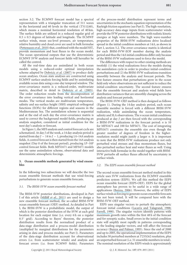
In Figure 1, the MFS analysis and control forecast cycle areschematized. At day J of the week, a 14 day analysis period isstarted from day J − 14 to J − 1, producing 1A–14A analysisfields. A control forecast is then started from the 14A analysissnapshot (Day 0 of the forecast period), producing 1F–10Fcontrol forecast fields. Both MFS1671 and MFS471 modelsuse the same assimilation scheme, observational data anddeterministic atmospheric forcings.

3. Ocean ensemble methods generated by wind ensem-bles

In the following two subsections we will describe the twoocean ensemble forecast methods that use wind-forcingperturbations to generate ocean ensemble forecasts.

3.1. The BHM-SVW ocean ensemble forecast method

The BHM-SVW posterior distributions, developed in PartI of this article (Milliff et al., 2011) are used to design anew ensemble forecast method, the so-called BHM-SVWocean ensemble forecast (OEF) method. As detailed in PartI, the BHM-SVW is a probabilistic model, the output ofwhich is the posterior distribution of the SVW at each gridlocation for each output time (i.e. every 6 h on a regular0.5◦ grid). According to Bayes’ theorem, the posteriordistribution results from the normalized product of adata-stage distribution and a process-model distribution(multiplied by marginal distributions for the parametersarising in data and process models; see Part I). Parametersof the data-stage distribution account for observationalerrors (i.e. from scatterometer winds) and analysis andforecast errors (i.e. from ECMWF fields). Parameters

of the process-model distribution represent terms anduncertainties in the stochastic equation representation of theRayleigh friction equations (see Part I). The high-resolution,high-accuracy data-stage inputs from scatterometer windsprovide the SVW posterior distributions with realistic kineticenergies at high wave numbers. The high wave-numberproperties of the BHM-SVW realizations drive localizedspread in the initial condition members at 14A, as shown inPart I, section 5.2. The error-covariance matrix is identicalfor each BHM-SVW-EOF member during the analysisperiod and thus the 14A initial conditions differ only becauseof the BHM-SVW realizations used to force the model.

The differences with respect to other existing methods aretwofold: (1) the wind realizations force the models duringthe assimilation cycle in order to produce initial-conditionperturbations and (2) the BHM-SVW realizations transitionsmoothly between the analysis and forecast periods. Thefirst feature ensures that perturbations grow in the oceanfield only where observations are not sufficient to reduce theinitial-condition uncertainty. The second feature ensuresthat the ensemble forecast and analysis wind fields havedistribution variances that are smoothly changing across theanalysis and forecast periods.

The BHM-SVW-OEF method is then designed as follows(Figure 1). During the 14 day analysis period, each oceanensemble member is forced with a different BHM-SVWrealization, while assimilating the ocean temperature,salinity and SLA observations. The n ocean initial conditionsproduced at day J are then forced with the correspondingn BHM-SVW realizations in the forecast period: n is 10for MFS1671 and 100 for MFS471. The cost of integratingMFS1671 constrains the ensemble size even though thegreater number of degrees of freedom in the higher-resolution model might justify a larger n. It is importantto note that the BHM-SVW realizations produce not onlyperturbed wind stresses and thus momentum fluxes, butalso perturbed surface heat and water fluxes as well. Usinginteractive bulk formulae in the model together with BHM-SVW perturbs all surface fluxes affected by uncertainty insurface winds.

3.2. The EEPS ocean ensemble forecast method

The second ocean ensemble forecast method studied in thisarticle uses SVW realizations from the ECMWF ensembleprediction system (EEPS). We call this method the EEPSocean ensemble forecast (EEPS-OEF). EEPS for the globalatmosphere has proven to be useful in a wide range ofapplications (Buizza, 2006). However, the utility of EEPSsurface winds as forcing to generate ocean ensemble forecastshas not been tested. It will be compared here with theBHM-SVW-OEF method.

EEPS uses singular vectors to perturb the atmosphericforecast initial conditions (Lacarra and Talagrand, 1988;Farrell, 1990). The singular vectors identify patterns withmaximum growth rates within the first 48 h of the forecastand for synoptic scales. Small errors in the initial-conditionstate will amplify most rapidly in patterns correspondingto the leading singular vectors, and will affect the forecastaccuracy (Buizza and Palmer, 1995). Since the end of 2000and up to 2005, the operational implementation of the EEPSincludes 50 perturbed members at T255L62 resolution, plusan unperturbed forecast (i.e. 51 ensemble members in total).The nominal resolution of the EEPS winds is approximately

Copyright c© 2011 Royal Meteorological Society Q. J. R. Meteorol. Soc. 137: 879–893 (2011)

882 N. Pinardi et al.

Figure 1. Schematic of the MFS analysis and forecast control cycle and the BHM-SVW-OEF method: J indicates the day at which the forecasts start,1A–14A and 1F–10F indicate analysis and forecast days respectively. The n BHM-SVW realizations are used to force OEF members starting from differentanalysis initial conditions created at 14A.

80 km, i.e. two times lower than the deterministic ECMWFforecast winds.

The EEPS-OEF method makes use of a single analysis fieldsnapshot at 14A as the initial condition for the ocean forecast.For the high-resolution model, MFS1671, 10 forecasts areforced by EEPS wind members. For the low-resolutionmodel, MFS471, all 51 members of the EEPS are used. TheEEPS-OEF method has a clear disadvantage in terms ofproducing useful spread in the ensemble forecast, since itstarts from an unperturbed initial condition.

3.3. Comparison between BHM and EEPS SVW distribu-tions

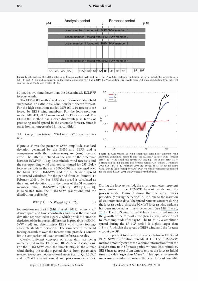
Figure 2 shows the posterior SVW amplitude standarddeviation generated by the BHM and EEPS, and acomparison with the root-mean-square (rms) forecasterror. The latter is defined as the rms of the differencebetween ECMWF 10 day deterministic wind forecasts andthe corresponding wind analyses, computed for 255 10 dayforecast periods in the years 2000–2004 and averaged overthe basin. The BHM-SVW and the EEPS wind spreadare instead calculated for the period from 25 January–17February 2005 only. For EEPS the spread is calculated asthe standard deviation from the mean of the 51 ensemblemembers. The BHM-SVW amplitude, W(x, y, t) = |U|,is calculated from the BHM-SVW realizations and thedistribution is given by

W(x, y, t) ∼ N[Wmean(x, y, t), σ 2W ]; (1)

for notation see Part I (Milliff et al., 2011), where x, y, tdenote space and time coordinates and σW is the standarddeviation represented in Figure 2, which provides a succinctdepiction of the important differences in probabilistic BHM-SVW (red) and deterministic EEPS wind (blue) forcing-ensemble standard deviations. The variances in the windforcing ensembles over the forecast time provide a contextfor the comparison of ocean ensemble forecast results.

Clearly, different concepts of uncertainty are beingimplemented in the EEPS and BHM-SVW distributions.For the BHM-SVW case, the uncertainties in the surfacewind during the analysis period derive from parametersselected to represent observational errors (i.e. for QuikSCATand ECMWF analysis winds) and process-model errors.

Figure 2. Comparison of wind amplitude spread for different windensemble-generating methods and the ECMWF surface wind forecasterrors. (a) Wind amplitude spread σW (see Eq. (1)) of the BHM-SVWdistribution during analysis and forecast periods (25 January–7 February2005 (1A–14A), 8–17 February 2005 (1F–10F)). b) As (a) but for EEPSwinds during the forecast period. (c) ECMWF rms forecast error computedfor the period 2000–2004 and averaged over the basin.

During the forecast period, the error parameters representuncertainties in the ECMWF forecast winds and theprocess model. Figure 2 shows that the spread variesperiodically during the period 1A–14A due to the insertionof scatteromenter data. The spread remains constant duringthe forecast period, since the ECMWF forecast wind variancehas been modelled as time-independent (see Milliff et al.,2011). The EEPS wind spread (blue curve) instead mimicsthe growth of the forecast error (black curve), albeit offsetto lower amplitude after day 6F. The BHM-SVW amplitudespread during the 1F–10F period is slightly larger than1.5 m s−1, which is the spread of EEPS winds and the forecasterror at day 5F.

It is important to note the difference between EEPS andBHM SVW distribution spreads at 1F. The BHM-SVWmethod smoothly carries the variance information from theanalysis time to the forecast period without discontinuities.EEPS instead grows from almost zero at the forecast initialtime to a value larger than 2.5 m s−1. This rapid error growthmay cause unwanted response in the ocean forecast ensemble

Copyright c© 2011 Royal Meteorological Society Q. J. R. Meteorol. Soc. 137: 879–893 (2011)

Mediterranean Forecast System response 883

and contamination by ocean surface gravity waves, as hasbeen shown in other articles (Powell et al., 2009).

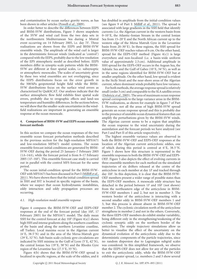
In order better to describe the differences between EEPSand BHM-SVW distributions, Figure 3 shows snapshotsof the SVW and wind curl from the two data sets inthe northwestern Mediterranean Sea during a Mistralevent occurring on 14 February 2005, i.e. day 7F. Threerealizations are shown from the EEPS and BHM-SVWensemble winds. The amplitude of the wind curl is largerin the deterministic forecast winds (indicated as ‘control’)compared with the EEPS, probably due to the low resolutionof the EPS atmospheric model as described before. EEPSmembers differ in synoptic-scale patterns while the BHM-SVW are different at finer spatial scales, i.e. subsynopticor atmospheric mesoscales. The scales of uncertainty givenby these two wind ensembles are not overlapping, sincethe EEPS distributions focus on the error growth inthe 500 hPa geopotential height field while the BHM-SVW distributions focus on the surface wind errors ascharacterized by QuikSCAT. Our analyses indicate that thesurface atmospheric flow field exhibits finer spatial scaleerrors, probably due to orographic effects and land–seatemperature and humidity differences. In the sections below,we will show that the smaller-scale uncertainties in the wind-field realizations are important in generating an ensembleresponse at the ocean mesoscale.

4. Comparison of BHM-SVW and EEPS ocean ensembleforecast methods

In this section we compare the ocean responses of the twoensemble ocean forecast perturbation methods describedin the previous section for the high-resolution MFS1671and low-resolution MFS471 model systems. The oceanensemble forecast initial conditions are generated by BHM-SVW-OEF during the period 25 January–7 February 2005(1A–14A), while the forecast period is from 8–17 February2005 (1F–10F). This ensemble forecast case study is carriedout in parallel with the control MFS forecast for the sameperiod.

The ocean initial-condition spread for the BHM-SVW-OEF with MFS1671 has been discussed in Part I (Milliff et al.,2011). We have shown there that the initial-condition spreadin SSH and SST is located in specific regions of the basin,where we suspect that ocean hydrodynamic instabilities,eddy interaction and eddy propagation processes areoccurring.

4.1. High-resolution model ensemble response

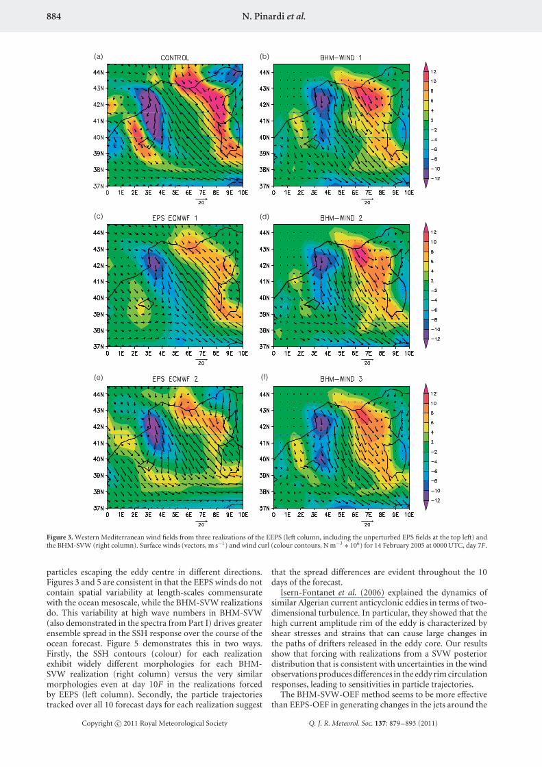
Figure 4 compares the BHM-SVW-OEF and EEPS-OEFresponses at the end of the forecast period (day 10F, 17February 2005) for the MFS1671 model. The daily meanSSH for the control forecast at day 10F (Figure 4(a)) showshigh SSH and intense gradients along the southern coastlinesof the basin and along the northern Levantine coastline,off Turkey. Local maxima occur in the Algerian current(6◦E, 38.5◦N) and in the area of the Mersa-Matruh gyre(29◦E, 32◦N). Sub-basin-scale cyclonic gyre circulations areindicated by SSH minima in the Gulf of Lyon (5◦E, 42◦N),the central Ionian Sea (19◦E, 38◦N) and the Rhodes Gyreregion of the Levantine Sea (27.5◦E, 35◦N).

Figure 4(b) shows that the BHM-SVW-OEF spread islocalized in specific regions, at the scale of the eddies, and it

has doubled in amplitude from the initial-condition values(see figure 9 of Part I: Milliff et al., 2011). The spread isassociated with large gradients in the SSH field that identifycurrents (i.e. the Algerian current in the western basin from0–10◦E, the Atlantic–Ionian Stream in the central IonianSea from 15–20◦E and the North African current up to thewestern edge of the Mersa Matruh Gyre in the Levantinebasin from 20–30◦E). In these regions, the SSH spread forBHM-SVW-OEF reaches values of 6 cm. On the other hand,spread for the EEPS-OEF method (Figure 4(c)) is largeeverywhere and non-localized (i.e. a basin-wide uniformvalue of approximately 2.5 cm). Additional amplitude inSSH spread for the EEPS-OEF occurs in the Aegean Sea, theAdriatic Sea and the Gulf of Gabes (10◦E, 34◦N), as well asin the same regions identified for BHM-SVW-OEF but atsmaller amplitude. On the other hand, low spread is evidentin the Sicily Strait and the near-shore areas of the Algeriancurrent, where dominant winds probably have low variance.

For both methods, the average response spread is relativelysmall (order 3 cm) and comparable to the SLA satellite errors(Dobricic et al., 2005). The area of maximum ocean responsespread corresponds to the large-variance areas in the BHM-SVW realizations, as shown for example in figure 7 of PartI. However, not all the areas of high BHM-SVW spreadgenerate an ocean response spread and this is probably dueto the presence of unstable ocean dynamical features that canamplify the perturbations given by the BHM-SVW winds.The Algerian current seems to be a region that amplifiesthe ocean response to the wind uncertainty during theassimilation and the forecast periods we have analyzed (seePart I and Part II of this article respectively).

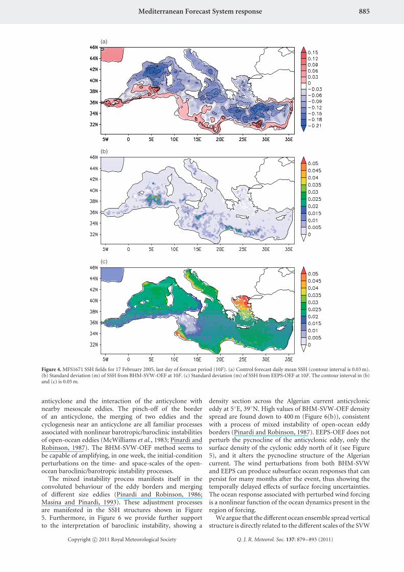
The highest ensemble variance values are observed inboth the BHM-SVW-OEF and EEPS-OEF responses at thelocation of the Algerian current anticyclonic eddies, oneof which during this period is centred at 6◦E, 38.5◦N.Figure 5 shows how this structure is represented in theensemble responses to both the BHM-SVW-OEF and EEPS-OEF. Figure 5 also depicts the effect of evolving currents inthree ensemble members for each method on the simulatedtrajectories of six drifters released at the centre of theanticyclone in each member at day 1F and tracked throughday 10F. In this depiction, it is clear that the BHM-SVW-OEF members present a wider range of possible states thanthe EEPS-OEF members. A mesoscale eddy structure hasdetached in the period between 1F and 10F (not shown)from the northeastern edge of the anticyclone in BHM-SVW-OEF members 1 and 2, but not in member 3. Thewestern border of the anticyclone is interacting with asecond smaller eddy in BHM-SVW-OEF members 1 and3, but this process is almost absent in BHM-SVW-OEFmember 2. The cyclonic circulation north of the anticyclonestrengthens in member 2 and not in the others. Conversely,the three EEPS-OEF members do exhibit similar variability,being different only in the strengthening/weakening of thecyclonic synoptic eddy on the northern border of theanticyclone. The simple trajectory simulations allow usbetter to visualize the effect of the uncertainty on thedynamical evolution of the anticyclonic eddy due to thedeterministic components of the particle trajectories, sinceno random dispersion due to Lagrangian subgrid scaleswas considered. In this simplified framework, we observethat the EEPS-OEF does not allow for any of the particlesto exit the anticyclonic eddy, while the BHM-SVW-OEFexhibits a greater spread, i.e. members 2 and 3 show several

Copyright c© 2011 Royal Meteorological Society Q. J. R. Meteorol. Soc. 137: 879–893 (2011)

884 N. Pinardi et al.

Figure 3. Western Mediterranean wind fields from three realizations of the EEPS (left column, including the unperturbed EPS fields at the top left) andthe BHM-SVW (right column). Surface winds (vectors, m s−1) and wind curl (colour contours, N m−3 ∗ 106) for 14 February 2005 at 0000 UTC, day 7F.

particles escaping the eddy centre in different directions.Figures 3 and 5 are consistent in that the EEPS winds do notcontain spatial variability at length-scales commensuratewith the ocean mesoscale, while the BHM-SVW realizationsdo. This variability at high wave numbers in BHM-SVW(also demonstrated in the spectra from Part I) drives greaterensemble spread in the SSH response over the course of theocean forecast. Figure 5 demonstrates this in two ways.Firstly, the SSH contours (colour) for each realizationexhibit widely different morphologies for each BHM-SVW realization (right column) versus the very similarmorphologies even at day 10F in the realizations forcedby EEPS (left column). Secondly, the particle trajectoriestracked over all 10 forecast days for each realization suggest

that the spread differences are evident throughout the 10days of the forecast.

Isern-Fontanet et al. (2006) explained the dynamics ofsimilar Algerian current anticyclonic eddies in terms of two-dimensional turbulence. In particular, they showed that thehigh current amplitude rim of the eddy is characterized byshear stresses and strains that can cause large changes inthe paths of drifters released in the eddy core. Our resultsshow that forcing with realizations from a SVW posteriordistribution that is consistent with uncertainties in the windobservations produces differences in the eddy rim circulationresponses, leading to sensitivities in particle trajectories.

The BHM-SVW-OEF method seems to be more effectivethan EEPS-OEF in generating changes in the jets around the

Copyright c© 2011 Royal Meteorological Society Q. J. R. Meteorol. Soc. 137: 879–893 (2011)

Mediterranean Forecast System response 885

Figure 4. MFS1671 SSH fields for 17 February 2005, last day of forecast period (10F). (a) Control forecast daily mean SSH (contour interval is 0.03 m).(b) Standard deviation (m) of SSH from BHM-SVW-OEF at 10F. (c) Standard deviation (m) of SSH from EEPS-OEF at 10F. The contour interval in (b)and (c) is 0.05 m.

anticyclone and the interaction of the anticyclone withnearby mesoscale eddies. The pinch-off of the borderof an anticyclone, the merging of two eddies and thecyclogenesis near an anticyclone are all familiar processesassociated with nonlinear barotropic/baroclinic instabilitiesof open-ocean eddies (McWilliams et al., 1983; Pinardi andRobinson, 1987). The BHM-SVW-OEF method seems tobe capable of amplifying, in one week, the initial-conditionperturbations on the time- and space-scales of the open-ocean baroclinic/barotropic instability processes.

The mixed instability process manifests itself in theconvoluted behaviour of the eddy borders and mergingof different size eddies (Pinardi and Robinson, 1986;Masina and Pinardi, 1993). These adjustment processesare manifested in the SSH structures shown in Figure5. Furthermore, in Figure 6 we provide further supportto the interpretation of baroclinic instability, showing a

density section across the Algerian current anticycloniceddy at 5◦E, 39◦N. High values of BHM-SVW-OEF densityspread are found down to 400 m (Figure 6(b)), consistentwith a process of mixed instability of open-ocean eddyborders (Pinardi and Robinson, 1987). EEPS-OEF does notperturb the pycnocline of the anticyclonic eddy, only thesurface density of the cyclonic eddy north of it (see Figure5), and it alters the pycnocline structure of the Algeriancurrent. The wind perturbations from both BHM-SVWand EEPS can produce subsurface ocean responses that canpersist for many months after the event, thus showing thetemporally delayed effects of surface forcing uncertainties.The ocean response associated with perturbed wind forcingis a nonlinear function of the ocean dynamics present in theregion of forcing.

We argue that the different ocean ensemble spread verticalstructure is directly related to the different scales of the SVW

Copyright c© 2011 Royal Meteorological Society Q. J. R. Meteorol. Soc. 137: 879–893 (2011)

886 N. Pinardi et al.

Figure 5. MFS1671 SSH mean daily fields at day 10F (17 February 2005) and six simulated particle trajectories (black lines) for EEPS-OEF members 1–3(panels (a), (c), (e)) and for BHM-SVW-OEF members 1–3 (panels (b), (d), (f)). The contour interval is 0.01 m. Trajectories depict simulated drifterpaths from 1F–10F.

fields. In the BHM-SVW-OEF case, the spread is amplifiedaround the unstable eddy jets, enabling multiple realizationsof a process of barotropic/baroclinic instability, while inthe EEPS-OEF case the spread is at lower amplitude andsuggestive of large-scale, surface-intensified modes.

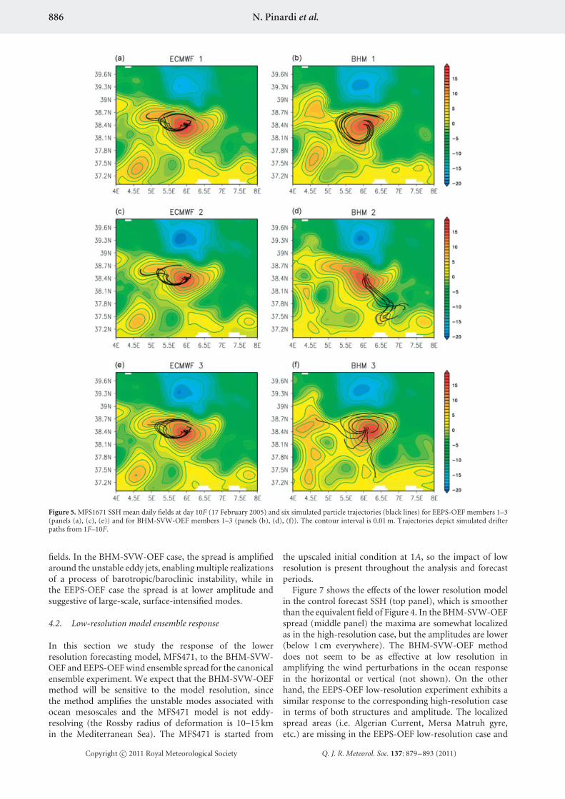
4.2. Low-resolution model ensemble response

In this section we study the response of the lowerresolution forecasting model, MFS471, to the BHM-SVW-OEF and EEPS-OEF wind ensemble spread for the canonicalensemble experiment. We expect that the BHM-SVW-OEFmethod will be sensitive to the model resolution, sincethe method amplifies the unstable modes associated withocean mesoscales and the MFS471 model is not eddy-resolving (the Rossby radius of deformation is 10–15 kmin the Mediterranean Sea). The MFS471 is started from

the upscaled initial condition at 1A, so the impact of lowresolution is present throughout the analysis and forecastperiods.

Figure 7 shows the effects of the lower resolution modelin the control forecast SSH (top panel), which is smootherthan the equivalent field of Figure 4. In the BHM-SVW-OEFspread (middle panel) the maxima are somewhat localizedas in the high-resolution case, but the amplitudes are lower(below 1 cm everywhere). The BHM-SVW-OEF methoddoes not seem to be as effective at low resolution inamplifying the wind perturbations in the ocean responsein the horizontal or vertical (not shown). On the otherhand, the EEPS-OEF low-resolution experiment exhibits asimilar response to the corresponding high-resolution casein terms of both structures and amplitude. The localizedspread areas (i.e. Algerian Current, Mersa Matruh gyre,etc.) are missing in the EEPS-OEF low-resolution case and

Copyright c© 2011 Royal Meteorological Society Q. J. R. Meteorol. Soc. 137: 879–893 (2011)

Mediterranean Forecast System response 887

Figure 6. Meridional section of σ = ρ − 1000 (kg m−3) at 5◦E (Algerian coast to the left, French coast to the right) for 17 February 2005 (10F). (a)MFS1671 daily mean σ for the control forecast at 10F. The contour interval is 0.1 kg m−3. b) σ standard deviation for BHM-SVW-OEF at 10F. (c) σ

standard deviation of EEPS-OEF at 10F. The contour interval in panels (b) and (c) is 0.01 kg m−3.

the large-scale uniform response is dominant. The overallresponse is less sensitive to the model resolution than in theBHM-SVW-OEF case. This result supports the notion thatthe new method, BHM-SVW-OEF, amplifies the uncertaintydue to winds on ocean mesoscales, while EEPS-OEF mainlychanges the uniform, large-scale SSH patterns.

5. Comparison with an initial-condition perturbationmethod

In this section we compare the wind ensemble perturbationmethods above with a more traditional initial-conditionperturbation method. Pinardi et al. (2008) have developeda thermocline intensified random perturbation oceanensemble forecast method (TIRP-OEF) that prescribesinitial perturbations with an ad hoc horizontal and verticalstructure.

The temperature and salinity perturbed initial conditions,Tp and Sp, are written as

Tp(x, y, z, t0) =T(x, y, z, t0) + p(x, y)M∑

j=1

ejfj(z), (2)

Sp(x, y, z, t0) =S(x, y, z, t0) + p(x, y)M∑

j=1

ejgj(z), (3)

where t0 is the initial time, T and S are the temperature andsalinity fields at 14A, p(x, y) is a two-dimensional horizontalstructure field with random amplitude and fj(z) and gj(z)are pre-defined vertical structure functions with amplitudesej. This method was originally used to generate Kalman-filter background-error ensembles in Evensen (2003) andextended by Pinardi et al. (2008) with vertical structurefunctions.

Copyright c© 2011 Royal Meteorological Society Q. J. R. Meteorol. Soc. 137: 879–893 (2011)

888 N. Pinardi et al.

Figure 7. MFS471 SSH fields for 17 February 2005, last forecast day (10F). (a) Daily mean SSH fields from the control forecast, contour interval is 0.05 m.(b) Standard deviation (m) of SSH for BHM-SVW-OEF. (c) Standard deviation (m) of SSH for EEPS-OEF . The contour interval in panel (b) is 0.0005 mand that in panel (c) is 0.005 m.

For this experiment, 20 vertical structure functions wereselected from a set of EOFs computed from the analysis ofthe variance of a long ocean model simulation. The ej are theexplained variances or eigenvalues for each mode. The EOFshave maximum amplitude at the depth of the thermocline,around 100–200 m, and they are discussed in Pinardi et al.(2008), Dobricic et al. (2005) and Sparnocchia et al. (2003).The p field at each grid point is modelled by a Gaussianfunction with a decay radius of 60 km that roughly mimicsthe size of large mesoscale eddies in the Mediterranean Sea.The amplitude of p was set in order to obtain horizontallyintegrated perturbations up to a value of ±0.2 cm in theSSH initial states. Initial perturbations of greater amplitudegenerate a noise signal in the forecast ensemble spread thatdoes not allow clear identification of dynamical patterns inthe forecast response (not shown).

The TIRP perturbations are clearly not consistent withdata assimilation, since each point in the domain has thesame probability to be perturbed, regardless of whetheror not an observation has been assimilated close by.Furthermore it is a method not strictly related to the wind-driven response and is ad hoc in that all free parameters (i.e.the number and type of EOFs, the horizontal structure radiusand the amplitude) are decided on the basis of experience.

The TIRP-OEF method implemented here produces 10perturbed initial T and S fields for the MFS1671 model. Theinitial-condition ensemble members are forced by the singledeterministic ECMWF wind forecast from 8–17 February2005.

In Figure 8 we show the TIRP-OEF spread at 10F.The values are relatively large, up to 4 cm, and theyare preferentially organized around mesoscale circulationstructures. Three maxima of SSH spread can be identified

Copyright c© 2011 Royal Meteorological Society Q. J. R. Meteorol. Soc. 137: 879–893 (2011)

Mediterranean Forecast System response 889

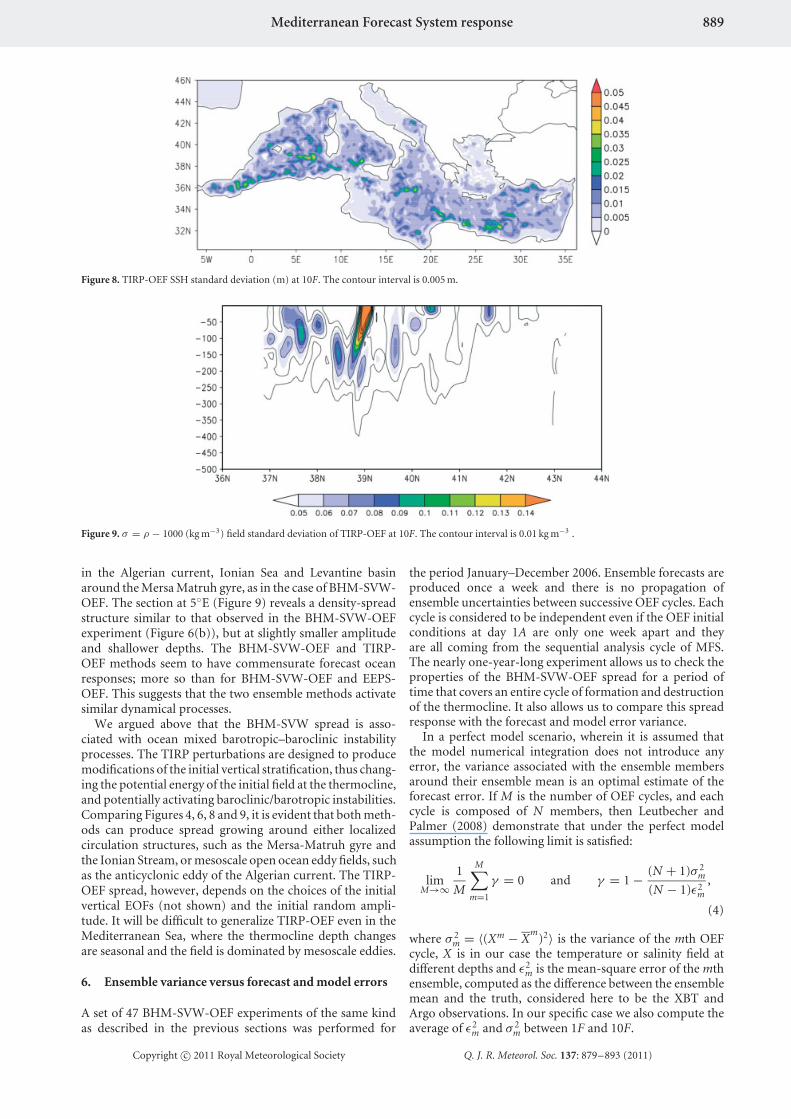
Figure 8. TIRP-OEF SSH standard deviation (m) at 10F. The contour interval is 0.005 m.

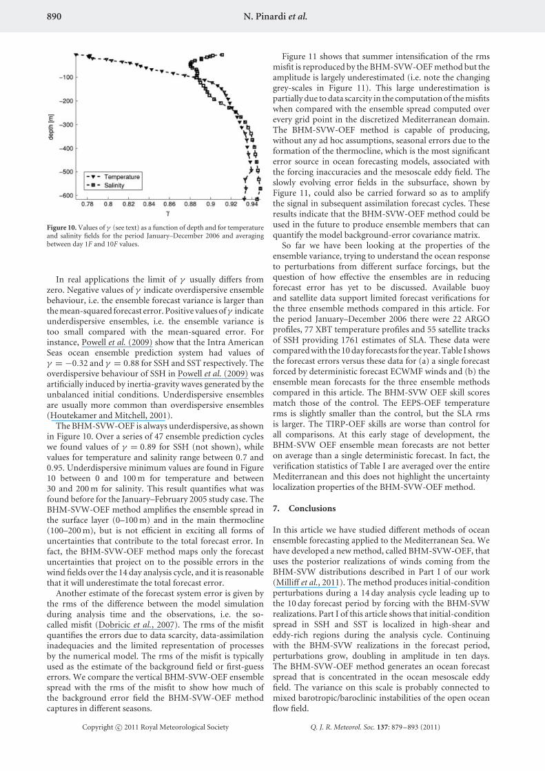
Figure 9. σ = ρ − 1000 (kg m−3) field standard deviation of TIRP-OEF at 10F. The contour interval is 0.01 kg m−3 .

in the Algerian current, Ionian Sea and Levantine basinaround the Mersa Matruh gyre, as in the case of BHM-SVW-OEF. The section at 5◦E (Figure 9) reveals a density-spreadstructure similar to that observed in the BHM-SVW-OEFexperiment (Figure 6(b)), but at slightly smaller amplitudeand shallower depths. The BHM-SVW-OEF and TIRP-OEF methods seem to have commensurate forecast oceanresponses; more so than for BHM-SVW-OEF and EEPS-OEF. This suggests that the two ensemble methods activatesimilar dynamical processes.

We argued above that the BHM-SVW spread is asso-ciated with ocean mixed barotropic–baroclinic instabilityprocesses. The TIRP perturbations are designed to producemodifications of the initial vertical stratification, thus chang-ing the potential energy of the initial field at the thermocline,and potentially activating baroclinic/barotropic instabilities.Comparing Figures 4, 6, 8 and 9, it is evident that both meth-ods can produce spread growing around either localizedcirculation structures, such as the Mersa-Matruh gyre andthe Ionian Stream, or mesoscale open ocean eddy fields, suchas the anticyclonic eddy of the Algerian current. The TIRP-OEF spread, however, depends on the choices of the initialvertical EOFs (not shown) and the initial random ampli-tude. It will be difficult to generalize TIRP-OEF even in theMediterranean Sea, where the thermocline depth changesare seasonal and the field is dominated by mesoscale eddies.

6. Ensemble variance versus forecast and model errors

A set of 47 BHM-SVW-OEF experiments of the same kindas described in the previous sections was performed for

the period January–December 2006. Ensemble forecasts areproduced once a week and there is no propagation ofensemble uncertainties between successive OEF cycles. Eachcycle is considered to be independent even if the OEF initialconditions at day 1A are only one week apart and theyare all coming from the sequential analysis cycle of MFS.The nearly one-year-long experiment allows us to check theproperties of the BHM-SVW-OEF spread for a period oftime that covers an entire cycle of formation and destructionof the thermocline. It also allows us to compare this spreadresponse with the forecast and model error variance.

In a perfect model scenario, wherein it is assumed thatthe model numerical integration does not introduce anyerror, the variance associated with the ensemble membersaround their ensemble mean is an optimal estimate of theforecast error. If M is the number of OEF cycles, and eachcycle is composed of N members, then Leutbecher andPalmer (2008) demonstrate that under the perfect modelassumption the following limit is satisfied:

limM→∞

1

M

M∑

m=1

γ = 0 and γ = 1 − (N + 1)σ 2m

(N − 1)ε2m

,

(4)

where σ 2m = 〈(Xm − X

m)2〉 is the variance of the mth OEF

cycle, X is in our case the temperature or salinity field atdifferent depths and ε2

m is the mean-square error of the mthensemble, computed as the difference between the ensemblemean and the truth, considered here to be the XBT andArgo observations. In our specific case we also compute theaverage of ε2

m and σ 2m between 1F and 10F.

Copyright c© 2011 Royal Meteorological Society Q. J. R. Meteorol. Soc. 137: 879–893 (2011)

890 N. Pinardi et al.

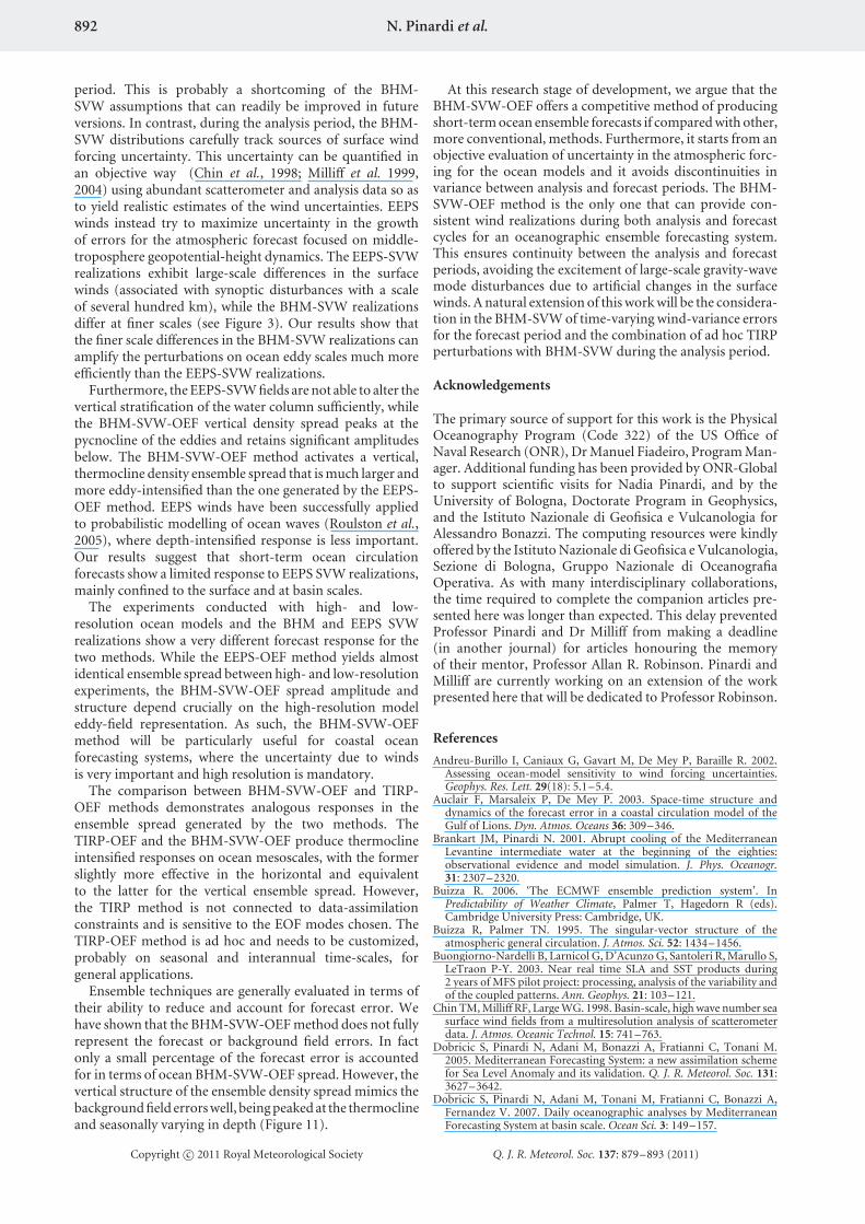
Figure 10. Values of γ (see text) as a function of depth and for temperatureand salinity fields for the period January–December 2006 and averagingbetween day 1F and 10F values.

In real applications the limit of γ usually differs fromzero. Negative values of γ indicate overdispersive ensemblebehaviour, i.e. the ensemble forecast variance is larger thanthe mean-squared forecast error. Positive values ofγ indicateunderdispersive ensembles, i.e. the ensemble variance istoo small compared with the mean-squared error. Forinstance, Powell et al. (2009) show that the Intra AmericanSeas ocean ensemble prediction system had values ofγ = −0.32 and γ = 0.88 for SSH and SST respectively. Theoverdispersive behaviour of SSH in Powell et al. (2009) wasartificially induced by inertia-gravity waves generated by theunbalanced initial conditions. Underdispersive ensemblesare usually more common than overdispersive ensembles(Houtekamer and Mitchell, 2001).

The BHM-SVW-OEF is always underdispersive, as shownin Figure 10. Over a series of 47 ensemble prediction cycleswe found values of γ = 0.89 for SSH (not shown), whilevalues for temperature and salinity range between 0.7 and0.95. Underdispersive minimum values are found in Figure10 between 0 and 100 m for temperature and between30 and 200 m for salinity. This result quantifies what wasfound before for the January–February 2005 study case. TheBHM-SVW-OEF method amplifies the ensemble spread inthe surface layer (0–100 m) and in the main thermocline(100–200 m), but is not efficient in exciting all forms ofuncertainties that contribute to the total forecast error. Infact, the BHM-SVW-OEF method maps only the forecastuncertainties that project on to the possible errors in thewind fields over the 14 day analysis cycle, and it is reasonablethat it will underestimate the total forecast error.

Another estimate of the forecast system error is given bythe rms of the difference between the model simulationduring analysis time and the observations, i.e. the so-called misfit (Dobricic et al., 2007). The rms of the misfitquantifies the errors due to data scarcity, data-assimilationinadequacies and the limited representation of processesby the numerical model. The rms of the misfit is typicallyused as the estimate of the background field or first-guesserrors. We compare the vertical BHM-SVW-OEF ensemblespread with the rms of the misfit to show how much ofthe background error field the BHM-SVW-OEF methodcaptures in different seasons.

Figure 11 shows that summer intensification of the rmsmisfit is reproduced by the BHM-SVW-OEF method but theamplitude is largely underestimated (i.e. note the changinggrey-scales in Figure 11). This large underestimation ispartially due to data scarcity in the computation of the misfitswhen compared with the ensemble spread computed overevery grid point in the discretized Mediterranean domain.The BHM-SVW-OEF method is capable of producing,without any ad hoc assumptions, seasonal errors due to theformation of the thermocline, which is the most significanterror source in ocean forecasting models, associated withthe forcing inaccuracies and the mesoscale eddy field. Theslowly evolving error fields in the subsurface, shown byFigure 11, could also be carried forward so as to amplifythe signal in subsequent assimilation forecast cycles. Theseresults indicate that the BHM-SVW-OEF method could beused in the future to produce ensemble members that canquantify the model background-error covariance matrix.

So far we have been looking at the properties of theensemble variance, trying to understand the ocean responseto perturbations from different surface forcings, but thequestion of how effective the ensembles are in reducingforecast error has yet to be discussed. Available buoyand satellite data support limited forecast verifications forthe three ensemble methods compared in this article. Forthe period January–December 2006 there were 22 ARGOprofiles, 77 XBT temperature profiles and 55 satellite tracksof SSH providing 1761 estimates of SLA. These data werecompared with the 10 day forecasts for the year. Table I showsthe forecast errors versus these data for (a) a single forecastforced by deterministic forecast ECWMF winds and (b) theensemble mean forecasts for the three ensemble methodscompared in this article. The BHM-SVW OEF skill scoresmatch those of the control. The EEPS-OEF temperaturerms is slightly smaller than the control, but the SLA rmsis larger. The TIRP-OEF skills are worse than control forall comparisons. At this early stage of development, theBHM-SVW OEF ensemble mean forecasts are not betteron average than a single deterministic forecast. In fact, theverification statistics of Table I are averaged over the entireMediterranean and this does not highlight the uncertaintylocalization properties of the BHM-SVW-OEF method.

7. Conclusions

In this article we have studied different methods of oceanensemble forecasting applied to the Mediterranean Sea. Wehave developed a new method, called BHM-SVW-OEF, thatuses the posterior realizations of winds coming from theBHM-SVW distributions described in Part I of our work(Milliff et al., 2011). The method produces initial-conditionperturbations during a 14 day analysis cycle leading up tothe 10 day forecast period by forcing with the BHM-SVWrealizations. Part I of this article shows that initial-conditionspread in SSH and SST is localized in high-shear andeddy-rich regions during the analysis cycle. Continuingwith the BHM-SVW realizations in the forecast period,perturbations grow, doubling in amplitude in ten days.The BHM-SVW-OEF method generates an ocean forecastspread that is concentrated in the ocean mesoscale eddyfield. The variance on this scale is probably connected tomixed barotropic/baroclinic instabilities of the open oceanflow field.

Copyright c© 2011 Royal Meteorological Society Q. J. R. Meteorol. Soc. 137: 879–893 (2011)

Mediterranean Forecast System response 891

Figure 11. Vertical distribution of temperature and salinity rms of misfits and BHM-SVW-OEF ensemble spread averaged for the whole Mediterranean Seafor the period June–December 2006. (a) Rms of misfit and (b) BHM-SVW-OEF spread for temperature in ◦C. (c) Rms of misfit and (d) BHM-SVW-OEFspread for salinity in PSU.

Table I. Root-mean-square (rms) errors of forecasts for the period January–December 2006 for temperature, salinity andsea-level anomaly (SLA). Units are◦C, psu and m. The rms is calculated as an average over the entire Mediterranean Sea

for all vertical levels (‘All’), at 30 and 100 m.

Forecast Temperature Salinity SLA

All 30 m 100 m All 30 m 100 m

Deterministic forecast 0.37 0.41 0.4 0.18 0.28 0.22 0.04

BHM-SVW-OEF 0.36 0.41 0.34 0.18 0.28 0.23 0.04EEPS-OEF 0.36 0.39 0.39 0.18 0.28 0.22 0.05TIRP-OEF 0.43 0.50 0.48 0.20 0.30 0.25 0.05

The new method has been compared with twomore traditional methods of generating ocean ensembleperturbations and forecasts. The first uses the EEPS surfacewinds starting from a single initial condition and forcing theocean forecast ensemble with 10 realizations. The secondis an ad hoc perturbation method for the T and S initial

condition fields, i.e. the so-called thermocline intensifiedrandom perturbation (TIRP).

BHM and EEPS winds differ substantially during theforecast time. EEPS wind ensemble spread mimics theforecast error growth in the ten-day forecast period whileBHM-SVW ensemble spread is constant over the same

Copyright c© 2011 Royal Meteorological Society Q. J. R. Meteorol. Soc. 137: 879–893 (2011)

892 N. Pinardi et al.

period. This is probably a shortcoming of the BHM-SVW assumptions that can readily be improved in futureversions. In contrast, during the analysis period, the BHM-SVW distributions carefully track sources of surface windforcing uncertainty. This uncertainty can be quantified inan objective way (Chin et al., 1998; Milliff et al. 1999,2004) using abundant scatterometer and analysis data so asto yield realistic estimates of the wind uncertainties. EEPSwinds instead try to maximize uncertainty in the growthof errors for the atmospheric forecast focused on middle-troposphere geopotential-height dynamics. The EEPS-SVWrealizations exhibit large-scale differences in the surfacewinds (associated with synoptic disturbances with a scaleof several hundred km), while the BHM-SVW realizationsdiffer at finer scales (see Figure 3). Our results show thatthe finer scale differences in the BHM-SVW realizations canamplify the perturbations on ocean eddy scales much moreefficiently than the EEPS-SVW realizations.

Furthermore, the EEPS-SVW fields are not able to alter thevertical stratification of the water column sufficiently, whilethe BHM-SVW-OEF vertical density spread peaks at thepycnocline of the eddies and retains significant amplitudesbelow. The BHM-SVW-OEF method activates a vertical,thermocline density ensemble spread that is much larger andmore eddy-intensified than the one generated by the EEPS-OEF method. EEPS winds have been successfully appliedto probabilistic modelling of ocean waves (Roulston et al.,2005), where depth-intensified response is less important.Our results suggest that short-term ocean circulationforecasts show a limited response to EEPS SVW realizations,mainly confined to the surface and at basin scales.

The experiments conducted with high- and low-resolution ocean models and the BHM and EEPS SVWrealizations show a very different forecast response for thetwo methods. While the EEPS-OEF method yields almostidentical ensemble spread between high- and low-resolutionexperiments, the BHM-SVW-OEF spread amplitude andstructure depend crucially on the high-resolution modeleddy-field representation. As such, the BHM-SVW-OEFmethod will be particularly useful for coastal oceanforecasting systems, where the uncertainty due to windsis very important and high resolution is mandatory.

The comparison between BHM-SVW-OEF and TIRP-OEF methods demonstrates analogous responses in theensemble spread generated by the two methods. TheTIRP-OEF and the BHM-SVW-OEF produce thermoclineintensified responses on ocean mesoscales, with the formerslightly more effective in the horizontal and equivalentto the latter for the vertical ensemble spread. However,the TIRP method is not connected to data-assimilationconstraints and is sensitive to the EOF modes chosen. TheTIRP-OEF method is ad hoc and needs to be customized,probably on seasonal and interannual time-scales, forgeneral applications.

Ensemble techniques are generally evaluated in terms oftheir ability to reduce and account for forecast error. Wehave shown that the BHM-SVW-OEF method does not fullyrepresent the forecast or background field errors. In factonly a small percentage of the forecast error is accountedfor in terms of ocean BHM-SVW-OEF spread. However, thevertical structure of the ensemble density spread mimics thebackground field errors well, being peaked at the thermoclineand seasonally varying in depth (Figure 11).

At this research stage of development, we argue that theBHM-SVW-OEF offers a competitive method of producingshort-term ocean ensemble forecasts if compared with other,more conventional, methods. Furthermore, it starts from anobjective evaluation of uncertainty in the atmospheric forc-ing for the ocean models and it avoids discontinuities invariance between analysis and forecast periods. The BHM-SVW-OEF method is the only one that can provide con-sistent wind realizations during both analysis and forecastcycles for an oceanographic ensemble forecasting system.This ensures continuity between the analysis and forecastperiods, avoiding the excitement of large-scale gravity-wavemode disturbances due to artificial changes in the surfacewinds. A natural extension of this work will be the considera-tion in the BHM-SVW of time-varying wind-variance errorsfor the forecast period and the combination of ad hoc TIRPperturbations with BHM-SVW during the analysis period.

Acknowledgements

The primary source of support for this work is the PhysicalOceanography Program (Code 322) of the US Office ofNaval Research (ONR), Dr Manuel Fiadeiro, Program Man-ager. Additional funding has been provided by ONR-Globalto support scientific visits for Nadia Pinardi, and by theUniversity of Bologna, Doctorate Program in Geophysics,and the Istituto Nazionale di Geofisica e Vulcanologia forAlessandro Bonazzi. The computing resources were kindlyoffered by the Istituto Nazionale di Geofisica e Vulcanologia,Sezione di Bologna, Gruppo Nazionale di OceanografiaOperativa. As with many interdisciplinary collaborations,the time required to complete the companion articles pre-sented here was longer than expected. This delay preventedProfessor Pinardi and Dr Milliff from making a deadline(in another journal) for articles honouring the memoryof their mentor, Professor Allan R. Robinson. Pinardi andMilliff are currently working on an extension of the workpresented here that will be dedicated to Professor Robinson.

References

Andreu-Burillo I, Caniaux G, Gavart M, De Mey P, Baraille R. 2002.Assessing ocean-model sensitivity to wind forcing uncertainties.Geophys. Res. Lett. 29(18): 5.1–5.4.

Auclair F, Marsaleix P, De Mey P. 2003. Space-time structure anddynamics of the forecast error in a coastal circulation model of theGulf of Lions. Dyn. Atmos. Oceans 36: 309–346.

Brankart JM, Pinardi N. 2001. Abrupt cooling of the MediterraneanLevantine intermediate water at the beginning of the eighties:observational evidence and model simulation. J. Phys. Oceanogr.31: 2307–2320.

Buizza R. 2006. ‘The ECMWF ensemble prediction system’. InPredictability of Weather Climate, Palmer T, Hagedorn R (eds).Cambridge University Press: Cambridge, UK.

Buizza R, Palmer TN. 1995. The singular-vector structure of theatmospheric general circulation. J. Atmos. Sci. 52: 1434–1456.

Buongiorno-Nardelli B, Larnicol G, D’Acunzo G, Santoleri R, Marullo S,LeTraon P-Y. 2003. Near real time SLA and SST products during2 years of MFS pilot project: processing, analysis of the variability andof the coupled patterns. Ann. Geophys. 21: 103–121.

Chin TM, Milliff RF, Large WG. 1998. Basin-scale, high wave number seasurface wind fields from a multiresolution analysis of scatterometerdata. J. Atmos. Oceanic Technol. 15: 741–763.

Dobricic S, Pinardi N, Adani M, Bonazzi A, Fratianni C, Tonani M.2005. Mediterranean Forecasting System: a new assimilation schemefor Sea Level Anomaly and its validation. Q. J. R. Meteorol. Soc. 131:3627–3642.

Dobricic S, Pinardi N, Adani M, Tonani M, Fratianni C, Bonazzi A,Fernandez V. 2007. Daily oceanographic analyses by MediterraneanForecasting System at basin scale. Ocean Sci. 3: 149–157.

Copyright c© 2011 Royal Meteorological Society Q. J. R. Meteorol. Soc. 137: 879–893 (2011)

Mediterranean Forecast System response 893

Evensen G. 2003. The Ensemble Kalman Filter: theoretical formulationand practical implementation. Ocean Dyn. 53: 343–367.

Farrell BF. 1990. Small error dynamics and the predictability ofatmospheric flow. J. Atmos. Sci. 47: 2191–2199.

Houtekamer PL, Mitchell HL. 2001. A sequential ensemble Kalman filterfor atmospheric data assimilation. Mon. Weather Rev. 129: 123–137.

Isern-Fontanet J, Garcıa-Ladona E, Font J. 2006.. The vortices of theMediterranean sea: an altimetric perspective. J. Phys. Ocean. 36:87–103.

Kersale M, Doglioli AM, Petrenko AA. 2010. Sensitivity study of windforcing in a numerical model of mesoscale eddies in the lee of Hawaiiislands. Ocean Sci. Discuss. 7: 477–500.

Korres G, Pinardi N, Lascaratos A. 2000. The ocean response to lowfrequency interannual atmospheric variability in the MediterraneanSea, Part I: Sensitivity experiments and energy analysis. J. Climate 13:705–731.

Lacarra J, Talagrand O. 1988. Short-range evolution of smallperturbations in a barotropic model. Tellus 40A: 81–95.

Le Traon PY, Nadal F, Ducet N. 2003. An improved mapping method ofmultisatellite altimeter data. J. Atmos. Oceanic Technol. 15: 522–533.

Leutbecher M, Palmer TN. 2008. Ensemble forecasting. J. Comput. Phys.227: 515–539.

Lucas M, Ayoub N, Penduff T, Barnier B, De Mey P. 2008. Stochasticstudy of the temperature response of the upper ocean to uncertaintiesin the atmospheric forcing in an Atlantic OGCM. Ocean Modelling 20:90–113. DOI:10.1016/j.ocemod.2007.07.006.

Manzella GMR, Reseghetti F, Coppini G, Borghini M, Cruzado A, Galli C,Gertman I, Gervais T, Hayes D, Millot C, Murashkovsky A, Ozsoy E,Tziavos C, Velasquez Z, Zodiatis G. 2007. The improvements of theships of opportunity program in MFS-TEP. Ocean Sci. 3: 245–258.

Masina S, Pinardi N. 1993. The halting effect of baroclinicity in vortexmerging. J. Phys. Oceanogr. 23: 1618–1637.

McWilliams JC, Brown ED, Bryden HL, Ebbesmeyer CC, Elliot BA,Heinmiller RH, Hua BL, Leaman KD, Lindstrom EJ, Luyten JR,McDowell SE, Owens WB, Perkins H, Price JF, Regier L, Riser SC,Rossby HT, Sanford TB, Shen CY, Taft BA, Van Leer JC. 1983.‘The local dynamics of eddies in the western North Atlantic’. InEddies in Marine Science, Robinson AR (ed). Springer-Verlag: Berlin,pp 92–113.

Milliff RF, Large WG, Morzel J, Danabasoglu G, Chin TM. 1999. Oceangeneral circulation model sensitivity to forcing from scatterometerwinds. J. Geophys. Res. 104: 11337–11358.

Milliff RF, Freilich MH, Liu WT, Atlas R, Large WG. 2001. ‘Global oceansurface wind vector observations from space’. In Observing the oceansin the 21st Century, Koblinsky CJ, Smith NR (eds). GODAE ProjectOffice and Bureau of Meteorology: Melbourne.

Milliff RF, Morzel J, Chelton DB, Freilich MH. 2004. Wind stress curland wind stress divergence biases from rain effects on QSCAT surfacewind retrievals. J. Atmos. Oceanic Technol. 21: 1216–1231.

Milliff RF, Bonazzi A, Wikle CK, Pinardi N, Berliner LM. 2011.Ocean ensemble forecasting. Part I: Ensemble Mediterranean windsfrom a Bayesian hierarchical model. Q. J. R. Meteorol. Soc. DOI:10.1002/qj.767.

Pettenuzzo D, Large WG, Pinardi N. 2010. On the corrections of ERA-40 surface flux products consistent with the Mediterranean heat andwater budgets and the connection between basin surface total heat fluxand NAO. J. Geophys. Res. 115: C06022. DOI:10.1029/2009JC005631.

Pinardi N, Coppini G. 2010. Operational oceanography in theMediterranean Sea: the second stage of development. Ocean Sci.6: 263–267.

Pinardi N, Robinson AR. 1986. Quasigeostrophic energetics of openocean regions. Dyn. Atmos. Oceans 10: 185–221.

Pinardi N, Robinson AR. 1987. Dynamics of deep thermocline jets inthe polymode region. J. Phys. Oceanogr. 17: 1163–1188.

Pinardi N, Allen I, Demirov E, DeMey P, Korres G, Lascaratos A,LeTraon P-Y, Maillard C, Manzella G, Tziavos C. 2003.The Mediterranean Ocean Forecasting System: first phase ofimplementation (1998–2001). Ann. Geophys. 21: 49–62.

Pinardi N, Bonazzi A, Scoccimarro E, Dobricic S, Navarra A, Ghiselli A,Veronesi P. 2008. Very large ensemble ocean forecasting experimentusing the grid computing infrastructure. Bull. Am. Meteorol. Soc. 89:799–804.

Poulain PM, Barbanti R, Font J, Cruzado A, Millot C, Gertman I,Griffa A, Molcard A, Rupolo V, Bras SL, de-la Villeon LP. 2007.Medargo: a drifting profiler program in the Mediterranean Sea. OceanSci. 3: 379–395.

Powell BS, Moore AM, Arango HG, DiLorenzo E, Milliff RF, Leben RR.2009. Near real time assimilation and prediction in the Intra-AmericanSea with Regional Ocean Modelling System. Dyn. Atmos. Oceans 48:46–68.

Roulston MS, Ellepola J, von Hardenberg J, Smith LA. 2005.. Forecastingwave height probabilities with numerical weather prediction models.Ocean Eng. 32: 1841–1863.

Sparnocchia S, Pinardi N, Demirov E. 2003. Multivariate empiricalorthogonal function analysis of the upper thermocline structure ofthe Mediterranean Sea from observations and model simulations.Ann. Geophys. 21: 167–187.

Tonani M, Pinardi N, Dobricic S, Pujol I, Fratianni C. 2008. A high-resolution free-surface model for the Mediterranean Sea. Ocean Sci.4: 1–14.

Tonani M, Pinardi N, Fratianni C, Pistoia J, Dobricic S. 2009. Forecastand analysis assessment through skill scores in the Mediterranean Sea.Ocean Sci. 5: 649–660.

Copyright c© 2011 Royal Meteorological Society Q. J. R. Meteorol. Soc. 137: 879–893 (2011)