Welcome message from author
This document is posted to help you gain knowledge. Please leave a comment to let me know what you think about it! Share it to your friends and learn new things together.
Transcript

R E S E R V E B A N K O F I N D I A
OCCASIONAL PAPERS
RESERVE BANK OF INDIA

RESERVE BANK OF INDIA
OCCASIONALPAPERSVOL. 31 NO. 1 SUMMER 2010
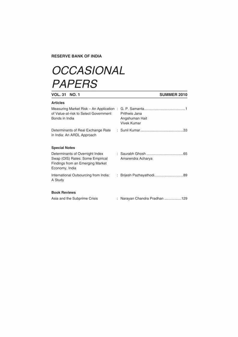
Articles
Measuring Market Risk – An Application : G. P. Samanta .........................................1of Value-at-risk to Select Government Prithwis JanaBonds in India Angshuman Hait Vivek Kumar
Determinants of Real Exchange Rate : Sunil Kumar ...........................................33in India: An ARDL Approach
Special Notes
Determinants of Overnight Index : Saurabh Ghosh .....................................65Swap (OIS) Rates: Some Empirical Amarendra AcharyaFindings from an Emerging Market Economy, India
International Outsourcing from India: : Brijesh Pazhayathodi .............................89A Study
Book Reviews
Asia and the Subprime Crisis : Narayan Chandra Pradhan .................129

Published by Deepak Mohanty for the Reserve Bank of India and printed by him at Alco Corporation, Gala No. 72, A-2, Shah and Nahar Industrial Estate, Lower Parel (W), Mumbai - 400 013.
Measuring Market Risk – An Application of Value-at-risk to Select Government
Bonds in India
G. P. Samanta, Prithwis Jana, Angshuman Hait and Vivek Kumar*
Value-at-Risk (VaR) is widely used as a tool for measuring the market risk of asset portfolios. Banks, who adopt ‘internal model approach’ (IMA) of the Basel Accord, require to quantify market risk through its own VaR model and minimum required capital for the quantifi ed risk would be determined by a rule prescribed by the concerned regulator. A challenging task before banks and risk managers, therefore, has been the selection of appropriate risk model from a wide and heterogeneous set of potential alternatives. In practice, selection of risk model for a portfolio has to be decided empirically. This paper makes an empirical attempt to select suitable VaR model for government security market in India. Our empirical results show that returns on these bonds do not follow normal distribution – the distributions possess fat-tails and at times, are skewed. The observed non-normality of the return distributions, particularly fat-tails, adds great diffi culty in estimation of VaR. The paper focuses more on demonstrating the steps involved in such a task with the help of select bonds. We have evaluated a number of competing models/methods for estimating VaR numbers for selected government bonds. We tried to address non-normality of returns suitably while estimating VaR, using a number of non-normal VaR models, such as, historical simulation, RiskMetric, hyperbolic distribution fi t, method based on tail-index. The accuracy of VaR estimates obtained from these VaR models are also assessed under several frameworks.
JEL Classifi cation : C13, G10
Keywords : Value-at-Risk, Transformations to Symmetry and Normality, Tail-Index
Reserve Bank of India Occasional PapersVol. 31, No.1, Summer 2010
* Dr. G. P. Samanta, currently a Member of Faculty at Reserve Bank Staff College, Chennai, is Director, Prithwis Jana and Angshuman Hait are Assistant Advisers and Vivek Kumar is Research Offi cer in the Department of Statistics and Information Management, Reserve Bank of India, Mumbai. Views expressed in the paper are purely personal and not necessarily of the organisation the authors belong to.
1. Introduction
The market risk amendment of 1988 Basel Accord in 1996, the advent of New Basel Accord (Basel II) in 2004, and subsequent revisions in the accord have brought about sea changes in risk
2 RESERVE BANK OF INDIA OCCASIONAL PAPERS
management framework adopted at banks globally in recent years. Regulators across the world today follow banking supervision systems broadly similar to the framework articulated in these documents. A key feature of this framework is the risk capital – the minimum amount of capital a bank requires to keep for its exposure to risk. It is argued that the risk capital acts as a cushion against losses, protecting depositors’ interest and increasing the resilience of the banking system in the event of crisis. Risk capital also makes the banks take risk on their own fund, thereby induces them to invest in prudent assets and curb their tendency to take excessive risk, which reduces the chances of bank runs greatly. So, the risk-based capital regulation has emerged as a tool to maintain stability of banking sector. Eventually, not only the banks but an increasing number of other fi nancial institutions and fi rms are also aligning their risk management framework in the similar line.
Two important changes are notable in the supervisory framework in recent years. First, determination of minimum required capital is now made more risk-sensitive (also more scientifi c) than earlier. Second, there has been an expansion in coverage of risk events in banks’ portfolio. In contrast to traditional focus solely on credit risk (BIS, 1988), the regulatory framework has gradually covered two more important risk categories, viz., market risk (BIS, 1996a, 1996b) and operational risk (BIS, 2004).
The Basel Accords and associated amendments/revisions provide broad guidelines to determine the level of minimum required capital a bank should maintain for all three types of fi nancial risks mentioned above. Under each risk category there have been a number of alternative approaches – starting from simple/basic to advanced in increasing level of sophistication. Also a distinction between basic and more advanced approach is that later emphasizes more on actual quantifi cation of risk.
In the case of ‘market risk’ the advanced approach is known as ‘internal model approach’ (IMA), wherein risk capital is determined based on the new risk measure, called value-at-risk (VaR). Higher the value of VaR, higher the level of market risk, thereby; larger the level
MEASURING MARKET RISK 3
of minimum required capital for market risk. Banks, who adopt IMA, subject to regulators’ approval, would quantify market risk through its own VaR model and minimum required capital for the quantifi ed risk would be determined by a rule prescribed by the concerned regulator.
The concept of VaR was fi rst introduced in the regulatory domain in 1996 (BIS, 1996) in the context of measuring market risk. However, post-1996 literature has given ample demonstration that the same concept is also applicable to much wider class of risk categories, including credit and operational risks. Today, VaR is considered as a unifi ed risk measure and a new benchmark for risk management. Interestingly, not only the regulators and banks but many private sector groups also have widely endorsed statistical-based risk management systems, such as, VaR.
As stated above, modern risk management practices at banks demand for proper assessment of risk and VaR concept is an infl uential tool for the purpose. The success of capital requirement regulation lies on determination of appropriate level of minimum required risk capital, which in turns depends on accuracy of quantifi ed risk. There has been a plethora of approaches in measuring VaR from data, each having some merits over others but suffering from some inherent limitations. Also, each approach covers a number of alternative techniques which are sometimes quite heterogeneous. A challenging task before banks and risk managers, therefore, has been the selection of appropriate risk model from a wide and heterogeneous set of potential alternatives. Ironically, theory does not help much in direct identifi cation of the best suitable risk model for a portfolio.
In practice, selection of risk model for a portfolio has to be based on empirical fi ndings. Against this backdrop, this paper makes an empirical attempt to select VaR model for government security market in India. The paper focuses more on demonstrating the steps involved in such a task with the help of select bonds. In reality, actual portfolio differs (say, in terms of composition) across investors/banks and the strategy demonstrated here can be easily replicated for any specifi c portfolio. The rest of the paper is organized as follows.
4 RESERVE BANK OF INDIA OCCASIONAL PAPERS
Section 2 presents the VaR concept and discusses some related issues. Section 3 summarises a number of techniques to estimate VaR using historical returns for a portfolio and Section 4 discusses criteria to evaluate alternative VaR models. Empirical results for select bonds are presented in Section 5. Finally, Section 6 presents the concluding remarks of the paper.
Section II
Value-at-Risk – The Concept, Usage and Relevant Issues
2.1 Defi ning Value-at-Risk
The VaR is a number indicating the maximum amount of loss, with certain specifi ed confi dence level, a fi nancial position may incur due to some risk events/factors, say, market swings (market risk) during a given future time horizon (holding period). If the value of a portfolio today is W, one can always argue that the entire value may be wiped out at some crisis phase so the maximum possible loss would be the today’s portfolio value itself. However, VaR does not refer to this trivial upper bound of the loss. The VaR concept is defi ned in a probabilistic framework, making it possible to determine a non-trivial upper bound (lower than trivial level) for loss at a specifi ed probability. Denoting L to represent loss of the portfolio over a specifi ed time horizon, the VaR for the portfolio, say V*, associated with a given probability, say p, 0 < p <1, is given by Prob[Loss > V*] = p, or equivalently, Prob[Loss < V*] = (1-p), where Prob[.] represents the probability measure. Usually, the terms ‘VaR for probability p’ refer to the defi nitional identity Prob[Loss > V*] = p, and the terms ‘VaR for 100*(1-p) per cent confi dence level’ are used to refer to the identity Prob[Loss < V*] = (1-p).
The VaR can be defi ned in terms of a threshold for change in value of the portfolio also. In order to illustrate this point, let Wt denotes the total value of underlying assets corresponding to a fi nancial position at time instance t, and the change in value of the position from time t to t+h is ∆Wt(h) = (Wt+h - Wt). At time point t, Wt+h is not known, so ∆Wt(k) is also unknown and can be considered a random variable. So, the value-at-risk V* would satisfy the identity Prob[∆Wt(h)
MEASURING MARKET RISK 5
< -V*] = p, or equivalently, as earlier, the identity can be expressed as Prob[∆Wt(h) > -V*] = (1-p).
It is important to note that any VaR number has two parameters, viz., holding period (i.e. time horizon) and probability/confi dence level. For a given portfolio, VaR number changes with these two parameters - while VaR decreases (increases) with the rise (fall) of probability level1, it changes in the same direction with changes in holding period.
2.2 Short and Long Financial Positions, and VaR
The holder of a short fi nancial position suffers a loss when the prices of underlying assets rise, and concentrates on upper-tail of the distribution while calculating her VaR (Tsay, 2002, pp. 258). Similarly, the holder of a long fi nancial position would model the lower-tail of return distribution as a negative return on underlying assets makes her suffer a loss.
2.3 Usage of VaR
Despite being a single number for a portfolio, VaR has several usages. First, VaR itself is a risk measure. Given probability level ‘p’ and holding period, larger VaR number would indicate greater risk in a portfolio. Thus, VaR has ability to rank portfolios in order of risk. The second, it gives a numerical maximal loss (probabilistic) for a portfolio. Unlike other common risk measures, this is an additional advantage in measuring risk through VaR concept. Third, VaR number is useful to determine the regulatory required capital for banks exposure to risk.
Apart from the general usages of VaR concept, it is also worthwhile to note a few points on its applicability to various risk categories. Though there has been criticism against it as being not a coherent risk measure and lacking some desirable properties (see for
6 RESERVE BANK OF INDIA OCCASIONAL PAPERS
instance, Artzner, et al., 1999), it is a widely accepted risk measure today. Though VaR was originally endorsed as a tool to measure market risk, it provides a unifi ed framework to deal with other risks, such as, credit risk, operation risk. As seen in the defi nition, the essence of VaR is that it is a percentile of loss/return distribution for a portfolio. So long as one has data to approximate/fi t the loss distribution, VaR being a characteristic of such distribution, can be estimated from the fi tted distribution.
2.4 Choice of Probability Level and Holding Period
The choice of ‘probability/confi dence level’ and ‘holding period’ would depend on the purpose of estimating the VaR measure. It is now a common practice, as also prescribed by the regulators, to compute VaR for probability level 0.01, i.e. 99% confi dence level. In addition, researchers sometimes consider assessment of risk for select other probability levels, such as, for probability 0.05.
A useful guideline for deciding ‘holding period’, is the liquidation period – the time required to liquidate a portfolio2. An alternative view is that the holding period would represent the ‘period over which the portfolio remains relatively stable’. Holding period may also relates to the time required to hedge the risk. Notably, a rise in holding period will increase the VaR number. One may also get same outcome by reducing probability level (i.e. increasing confi dence level) adequately (instead of changing holding period). In practice, regulators maintain uniformity in fi xing probability level at p=0.01 (equivalently, 99% confi dence level). Thus, holding period has to be decided based on some of the consideration stated above. It may be noted that VaR for market risk may have much shorter holding period as compared to say VaR for credit risk. Basel Accords suggests 10-day holding period for market risk, though country regulators may prescribe higher holding period. In case of credit risk, duration of holding period is generally one-year.
MEASURING MARKET RISK 7
2.5 VaR Expressed in Percentage and Other Forms
As seen, VaR is defi ned in terms of the change/loss in value of a portfolio. In practice, distribution of return (either percentage change or continuously-compounded/log-difference3) of the fi nancial position may actually be modeled and thus, VaR may be estimated based on percentile of the underlying return distribution. Sometimes percentiles of return distribution are termed as ‘relative VaR’ (see for instance, Wong, et al., 2003). On this perception, the VaR for change in value may be termed as ‘absolute/nominal VaR’.
Thus, the percentile ξp corresponding to left-tail probability p of distribution of k-period percentage change itself is the relative VaR (expressed in per cent) with specifi ed parameters and corresponding (absolute) VaR would be [(ξp/100)Wt]. Alternatively, if ξp represents the p-percentile for log-return (in per cent), then (absolute) VaR can be expressed as [{exp(ξp/100)-1}Wt]. In our paper, unless otherwise stated, we use the term VaR to indicate ‘relative VaR’ (expressed in per cent).
2.6 The h-period VaR from 1-period VaR
Another point to be noted relates to the estimation of multi-period VaR (i.e. VaR corresponding to multi-period ‘time horizon’, say h-day). In practice, given probability level ‘p’, 0<p<1, 1-period VaR are fi rst directly computed using 1-period return (say, daily return), and then they are converted to multi-period VaR using some approximation rule under certain assumptions about the market/portfolio. The widely used approximation relation between, say h-day VaR and 1-day VaR is given by
where VaR(h,p) denotes a VaR with probability level ‘p’ and h-day holding period.
It is important to note that above relationship between h-period VaR and 1-period VaR is not correct in general conditions. However,
8 RESERVE BANK OF INDIA OCCASIONAL PAPERS
for simplicity, this has been widely used in practice and regulators across the world has also subscribed to such approximation. Indeed, as per the regulators’ guidelines, banks adopting IMA for market risk require to compute 1-day VaR using daily returns and the validation of risk-model depends upon how accurately the models estimate 1-day VaR. However, minimum required capital is determined using multi-period VaR, say 10-day VaR numbers, which are generated from the 1-day VaR values.
Section III
Measurement of VaR – Select Techniques
The central to any VaR measurement exercise has been the estimation of suitable percentile of change in value or return of the portfolio. Following the earlier discussion, we focus here in estimating 1-period VaR (e.g., 1-day VaR using daily returns). Also, we shall be focusing only on estimating VaR directly from portfolio-level returns. As well known, a portfolio usually consists of several securities and fi nancial instruments/assests, and returns on each component of the portfolio would follow certain probability distribution. Portfolio value is the weighted sum of all components, changes in which can be assessed by studying the multivariate probability distribution considering returns on all components of the portfolio. In our study, such a strategy has not been followed. Instead, our analysis, as quite common in the literature, relies on historical portfolio-level returns and VaR estimation essentially requires to study the underlying univariate distribution.
3.1 Estimating VaR Under Normality of Unconditional Return Distribution
The normality assumption to portfolio return distribution simplifi es the task of VaR estimation greatly. A normal distribution is fully characterized by fi rst two moments, viz., mean (µ) and standard
MEASURING MARKET RISK 9
deviation (σ), and the percentile with left-tail probability p, 0<p<1, is given by zp = [ µ + τp σ ], where τp denotes the corresponding percentile for standard normal distribution. By defi nition, VaR for given probability p is the absolute value of zp, denoted by |zp|. Thus, if and denote the estimate of µ and σ, respectively, based on a sample of portfolio returns upto time t, the estimated VaR (with probability p, 0<p<1) for the next time point, i.e. time point (t+1), is given by
..... (2)
where the meaning of |.| remains same.
3.2 Non-Normality of Unconditional Return Distribution - Estimating VaR
The biggest practical problem of measuring VaR, however, is that the observed returns hardly follow normal distribution - the fi nancial market returns are known to exhibit ‘volatility clustering phenomena’ and follow ‘fat-tailed’ (leptokurtic) distribution with possibly substantial asymmetry. The deviation from normality intensifi es the complexity in modelling return distribution, hence estimation of required percentiles and VaR numbers.
A simple approach to handle non-normality has been to model return distribution non-parametrically, such as, employing the historical simulation approach. The non-parametric techniques do not assume any specifi c form of the return distribution and are quite robust over alternative distributional forms. Besides, these techniques are easy to understand and pose no diffi culty to implement. But inherent limitations of a non-parametric approach is well known.
The conventional parametric approaches to deal with non-normality can be classifi ed under four broad categories; (i) conditional heteroscedastic models - modeling conditional return distribution through RiskMetric approach, ARCH/GARCH or more advanced forms of such models; (ii) fi tting suitable non-normal or mixture distribution for unconditional distribution; and (iii) application of
10 RESERVE BANK OF INDIA OCCASIONAL PAPERS
extreme value theory (EVT) - modeling either the distribution of extreme return or only the tails of return distribution.
3.2.1 Non-Parametric Approach - Historical Simulation
The non-parametric approach, such as, historical simulation (HS), possess some specifi c advantages over the normal method, as it is not model based, although it is a statistical measure of potential loss. The main benefi t is that it can cope with all portfolios that are either linear or non-linear. The method does not assume any specifi c form of the distribution of price change/return. The method captures the characteristics of the price change distribution of the portfolio, as it estimates VaR based on the distribution actually observed. But one has to be careful in selecting past data. If the past data do not contain highly volatile periods, then HS method would not be able to capture the same. Hence, HS should be applied when one has very large data points to take into account all possible cyclical events. HS method takes a portfolio at a point of time and then revalues the same using the historical price series. Daily returns, calculated based on the price series, are then sorted in an ascending order and fi nd out the required data point at desired percentiles. Linear interpolation can be used to estimate required percentile if it falls in between two data points.
Another variant of HS method is a hybrid approach put forward by Boudhoukh, et al. (1997), that takes into account the exponentially weighing approach in HS for estimating the percentiles of the return directly. As described by Boudhoukh et al. (1997, pp. 3), “the approach starts with ordering the returns over the observation period just like the HS approach. While the HS approach attributes equal weights to each observation in building the conditional empirical distribution, the hybrid approach attributes exponentially declining weights to historical returns”. The process is simplifi ed as follows:
� Calculate the return series of past price data of the security or the portfolio.
� Fix a value δ from the interval (0,1). Usually δ is fi xed at =0.98.
� To each most recent k returns: R(t), R(t-1), …R(t-k+1) assign a
MEASURING MARKET RISK 11
weight proportional to 1, δ, δ2, …., δk-1, respectively. In order to make total weights sum to 1, the weights for R(t), R(t-1), …..,R(t-k+1) would be , respectively4.
� Sort the returns in ascending order.
� In order to obtain VaR of the portfolio for probability ‘p’, 0<p<1, start from the lowest return and keep accumulating the weights until ‘p’ is reached. The return corresponding with accumulated weight ‘p’ relates to VaR. Linear interpolation may be used, if necessary, to attain exact ‘p’ of the distribution.
3.2.2 Use of Conditional Heteroscedasticity Models
The ‘volatility clustering phenomenon’ implies that the conditional variance of return is not constant over time (i.e. heteroscedastic). This phenomenon is a potential source of observed fat-tail of unconditional return distributions. Interestingly, theory also proves that unconditional distribution of return will possess fat-tails even when returns follow normal distribution conditionally. These results give rise to the idea of modeling conditional heteroscedasticity of returns. Under normality of such conditional distributions, expression for VaR is |µt + σt τp|, where µt and σt are time-varying/conditional mean and standard deviation of return, respectively; ‘p’is the probability level attached with VaR number; τp is the tabulated value for standard normal distribution corresponding with the lower-tail probability ‘p’.
Using historical returns on a portfolio, one can estimate conditional mean and standard deviation at different time points. Accordingly estimated VaR numbers would be
.....(3)
12 RESERVE BANK OF INDIA OCCASIONAL PAPERS
where and , respectively, denote estimated conditional mean
and variance for time point t+1 (using information upto time t)5.
There exist several alternative models to estimate conditional mean and variance. The simplest form of conditional heteroscedastic model is the one like exponentially weighted moving average as used in RiskMetrics (J.P. Morgan/Reuters, 1996). This popular technique in effect models conditional variance as a weighted average of past variances and past returns, where exponential weighting scheme for past returns is used as follows;
....(4)
where and rt denote conditional variance and return at time t, respectively; denotes the variance at origin (i.e. time t=0); and the parameter λ, known as decay factor, satisfi es 0 < λ <1.
For daily data, the value of the decay parameter in the RiskMetric approach is generally fi xed at λ=0.94 (van den Goorberg and Vlaar, 1999). The accuracy in VaR estimates may also improve for alternative values for λ, such as, 0.96 or 0.98 (see for instance, Samanta and Nath, 2004).
More advanced models like ARCH, GARCH and so forth (Engle 1982; Bollerslev, 1986; Wong et al., 2003) can also be used for capturing conditional heteroscedasticity. Though conceptually appealing, the performance of the conditional heteroscedastic models in estimating VaR, however, is mixed. In a recent empirical study, Wong et al., (2003) found that the approaches, like, ARCH/GARCH, do not necessarily improve the quality of VaR estimates.
3.2.3 Fitting Non-Normal Distribution for Returns
Alternatively, one can simply fi t the parametric form of a suitable non-normal distribution to the observed returns. The class of
MEASURING MARKET RISK 13
distributional forms considered would be quite wide including, say, hyperbolic distribution, t-distribution, mixture of two or more normal distributions, Laplace distribution or so forth, (van den Goorbergh and Vlaar, 1999; Bauer 2000; Linden, 2001).
In our study we consider symmetric hyperbolic distribution as an alternative fat-tailed distribution for returns6. A d-dimensional random variable ‘r’ is said to follow a symmetric hyperbolic distribution if it has density function as below;
where, Kν is the modifi ed Bessel function of the third kind, the
parameters δ and ∆ are for multivariate scales, µ for location and ζ mainly changes the tails.
For the presence of Bessel functions in above density function, closed form expression for maximum likelihood estimators are not possible. Bauer (2000) suggests an approach to have maximum likelihood estimators7. Once estimates of the parameters become available, one can estimate the required percentile of the distribution following numerical iteration method.
3.2.4 Methods under Extreme Value Theory – Use of Tail-Index
The fat tails of unconditional return distribution can also be handled through extreme value theory using, say, tail-index, which measures the amount of tail fatness. One can therefore, estimate the tail-index and measure VaR based on the underlying distribution. The basic premise of this idea stems from the result that the tails of every fat-tailed distribution converge to the tails of Pareto distribution. In a simple case, upper tail of such a distribution can be modeled as,
14 RESERVE BANK OF INDIA OCCASIONAL PAPERS
Prob[X > x] ≈ Cα |x|–α (i.e. Prob[X ≤ x] ≈ 1 - Cα |x|-α); x>C ….. (6)
Where, C is a threshold above which the Pareto law holds; |x| denotes the absolute value of x and the parameter α is the tail-index.
Similarly, lower tail of a fat-tailed distribution can be modeled as
Prob[X > x] ≈1 - Cα x–α (i.e. Prob[X ≤ x] ≈ Cα x-α); x < C ….. (7)
Where, C is a threshold below which the Pareto law holds, and the parameter α, called as tail-index, measures the tail-fatness.
In practice, observations in upper tail of the return distribution are generally positive and those in lower tail are negative. The holder of a short fi nancial position suffers a loss in the event of a rise in values of underlying assets and therefore, concentrates on upper-tail of the distribution (i.e. Eqn. 6) for calculating VaR (Tsay, 2002, pp. 258). Similarly, the holder of a long fi nancial position would model the lower-tail of the underlying distribution (i.e. use Eqn. 7) as a fall in asset values makes her suffer a loss.
From Eqns.(6) and (7), it is clear that the estimation of VaR is crucially dependent on the estimation of tail-index α. There are several methods of estimating tail-index, such as, (i) Hill’s (1975) estimator and (ii) the estimator under ordinary least square (OLS) framework suggested by van den Goorbergh and Vlaar (1999). In this study, only the widely used Hill’s estimator of tail-index is considered.
Section IV
Selecting VaR Model – Evaluation Criteria
The accuracy of VaR estimates obtained from a VaR model can be assessed under several frameworks, such as, (i) regulators’ backtesting (henceforth simply called as backtesting); (ii) Kupiec’s test; (iii) loss-function based evaluation criteria. Under each framework, there would be several techniques and what follows is the summary of some of the widely used techniques.
MEASURING MARKET RISK 15
4.1 Backtesting
As recommended by Basel Committee, central banks do not specify any VaR model to the banks. Rather under the advanced ‘internal model approach’, banks are allowed to adopt their own VaR model. There is an interesting issue here. As known, VaR is being used for determining minimum required capital – larger the value of VaR, larger is the capital charge. Since larger capital charge may affect profi tability adversely, banks have an incentive to adopt a model that produces lower VaR estimate. In order to eliminate such inherent inertia of banks, Basel Committee has set out certain requirements on VaR models used by banks to ensure their reliability (Basel Committee, 1996a,b) as follows;
(i) 1-day and 10-day VaRs must be estimated based on the daily data of at least one year
(ii) Capital charge is equal to three times the 60-day moving average of 1% 10-day VaRs, or 1% 10-day VaR on the current day, which ever is higher. The multiplying factor (here 3) is known as ‘capital multiplier’.
Further, Basel Committee (1996b) provides following Backtesting criteria for an internal VaR model (see van den Goorbergh and Vlaar, 1999; Wong et al., 2003, among others)
(i) One-day VaRs are compared with actual one-day trading outcomes.
(ii) One-day VaRs are required to be correct on 99% of backtesting days. There should be at least 250 days (around one year) for backtesting.
(iii) A VaR model fails in Backtesting when it provides 5% or more incorrect VaRs.
If a bank provides a VaR model that fails in backtesting, it will have its capital multiplier adjusted upward, thus increasing the amount of capital charges. For carrying out the Backtesting of a VaR model, realized day-to-day returns of the portfolio are compared to the VaR of
16 RESERVE BANK OF INDIA OCCASIONAL PAPERS
the portfolio. The number of days, when actual portfolio loss is higher than VaR estimate, provides an idea about the accuracy of the VaR model. For a good 99% VaR model, this number would approximately be equal to the 1 per cent (i.e. 100 times of VaR probability) of back-testing days. If the number of VaR violations or failures (i.e. number of days when observed loss exceeds VaR estimate) is too high, a penalty is imposed by raising the multiplying factor (which is at least 3), resulting in an extra capital charge. The penalty directives provided by the Basel Committee for 250 back-testing trading days is as follows; multiplying factor remains at minimum (i.e. 3) for number of violations up to 4, increases to 3.4 for 5 violations, 3.5 for 6 violations, 3.65 for violations 7, 3.75 for violations 8, 3.85 for violations 9, and reaches at 4.00 for violations above 9 in which case the bank is likely to be obliged to revise its internal model for risk management (van den Goorbergh and Vlaar, 1999).
4.2 Statistical Tests of VaR Accuracy
The accuracy of a VaR model can also be assessed statistically by applying Kupiec’s (1995) test (see, for example, van den Goorbergh and Vlaar, 1999 for an application of the technique). The idea behind this test is that frequency of VaR- violation should be statistically consistent with the probability level for which VaR is estimated. Kupiec (1995) proposed to use a likelihood ratio statistics for testing the said hypothesis.
If z denotes the number of times the portfolio loss is worse than the VaR estimate in the sample (of size T, say) then z follows a Binomial distribution with parameters (T, p), where p is the probability level of VaR. Ideally, more the z/T closes to p, more accurate the estimated VaR is. Thus the null hypothesis z/T = p may be tested against the alternative hypothesis z/T ≠ p. The likelihood ratio (LR) statistic for testing the null hypothesis against the alternative hypothesis is
….. (8)
MEASURING MARKET RISK 17
Under the null hypothesis, LR-statistic follows a χ2-distribution with 1-degree of freedom.
The VaR estimates are also interval forecasts, which thus, can be evaluated conditionally or unconditionally. While the conditional evaluation considers information available at each time point, the unconditional assessment is made without reference to it. The test proposed by Kupiec provides only an unconditional assessment as it simply counts violations over the entire backtesting period (Lopez, 1998). In the presence of time-varying volatility, the conditional accuracy of VaR estimates assumes importance. Any interval forecast ignoring such volatility dynamics may have correct unconditional coverage but at any given time, may have incorrect conditional coverage. In such cases, the Kupiec’s test has limited use as it may classify inaccurate VaR as acceptably accurate.
A three-step testing procedure developed by Christoffersen (1998) involves a test for correct unconditional coverage (as Kupiec’s test), a test for ‘independence’, and a test for correct ‘conditional coverage’ (Christoffersen, 1998; Berkowitz and O’Brien, 2002; Sarma, et al., 2003). All these tests use Likelihood-Ratio (LR) statistics.
4.3 Evaluating VaR Models Using Penalty/Loss-Function
Tests mentioned above assess the frequency of VaR violations, either conditionally or unconditionally, during the backtesting trading days. These tests, however, do not look at the severity/magnitude of additional loss (i.e. loss in excess of estimated VaR) at the time of VaR violations. However, a portfolio manager may prefer the case of more frequent but little additional loss than the case of less frequent but huge additional loss. The underlying VaR model in the former case may fail in backtesting but still the total amount of loss (after adjusting for penalty on multiplying factor, if any) during the backtesting trading days may be less than that in later case. So long as this condition persists with a VaR model, a portfolio manager, particularly non-banks who are not required to comply with any regulatory requirement, may prefer to accept the VaR model even
18 RESERVE BANK OF INDIA OCCASIONAL PAPERS
if it fails in backtesting. This means that the objective function of a portfolio manager is not necessarily be the same as that provided by the backtesting. Each manager may set his own objective function and try to optimize that while managing market risk. But, loss-functions of individual portfolio managers are not available in public domain and thus, it would be impossible to select a VaR model appropriate for all managers. However, discussion on a systematic VaR selection framework by considering a few specifi c forms of loss-function would provide insight into the issue so as to help individual manager to select a VaR model on the basis of his own loss-function. On this perception, it would be interesting to illustrate the VaR selection framework with the help of some specifi c forms of loss-function.
The idea of using loss-function for selecting VaR model, perhaps, is proposed fi rst by Lopez (1998). He shows that the binomial distribution-based test is actually minimizing a typical loss-function – gives score 1 for a VaR violation and a score 0 otherwise. In other words, the implied loss-function in backtesting would be an indicator function It which assumes a value 1 at time t if the loss at t exceeds corresponding VaR estimate and assumes a value zero otherwise. However, it is hard to imagine an economic agent who has such a utility function: one which is neutral to all times with no VaR violation and abruptly shifts to score of 1 in the slightest failure and penalizes all failures equally (Sarma, et al., 2003). Lopez (1998) also considers a more generalised loss-function which can incorporate the regulatory concerns expressed in the multiplying factor and thus is analogous to the adjustment schedule for the multiplying factor for determining required capital. But, he himself observed that, like the simple binomial distribution-based loss-function, this loss-function is also based on only the number of violations in backtesting observations – with paying no attention to another concern, the magnitudes of loss at the time of failures. In order to handle this situation, Lopez (1998) also proposes a different loss-function addressing the magnitude of violation as follows;
..... (9)
MEASURING MARKET RISK 19
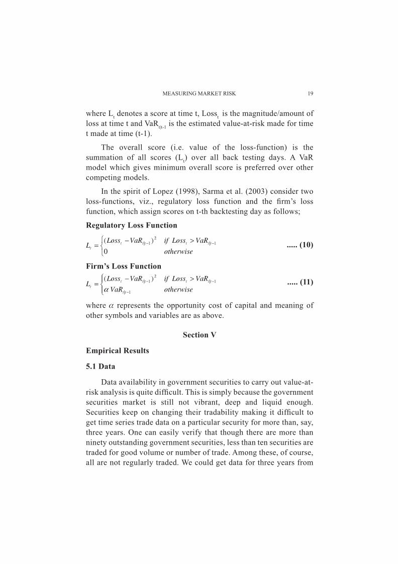
where Lt denotes a score at time t, Losst is the magnitude/amount of loss at time t and VaRt|t-1 is the estimated value-at-risk made for time t made at time (t-1).
The overall score (i.e. value of the loss-function) is the summation of all scores (Lt) over all back testing days. A VaR model which gives minimum overall score is preferred over other competing models.
In the spirit of Lopez (1998), Sarma et al. (2003) consider two loss-functions, viz., regulatory loss function and the fi rm’s loss function, which assign scores on t-th backtesting day as follows;
Regulatory Loss Function
..... (10)
Firm’s Loss Function
..... (11)
where α represents the opportunity cost of capital and meaning of other symbols and variables are as above.
Section V
Empirical Results
5.1 Data
Data availability in government securities to carry out value-at-risk analy sis is quite diffi cult. This is simply because the government securities market is still not vibrant, deep and liquid enough. Securities keep on changing their tradability making it diffi cult to get time series trade data on a particular security for more than, say, three years. One can easily verify that though there are more than ninety outstanding government securities, less than ten securities are traded for good volume or number of trade. Among these, of course, all are not regularly traded. We could get data for three years from
20 RESERVE BANK OF INDIA OCCASIONAL PAPERS
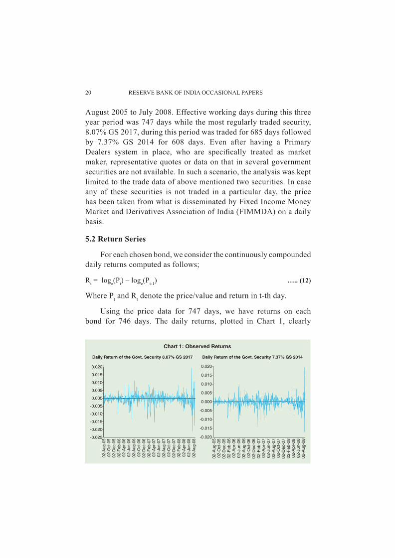
August 2005 to July 2008. Effective working days during this three year period was 747 days while the most regularly traded security, 8.07% GS 2017, during this period was traded for 685 days followed by 7.37% GS 2014 for 608 days. Even after having a Primary Dealers system in place, who are specifi cally treated as market maker, representative quotes or data on that in several government securities are not available. In such a scenario, the analysis was kept limited to the trade data of above mentioned two securities. In case any of these securities is not traded in a particular day, the price has been taken from what is disseminated by Fixed Income Money Market and Derivatives Association of India (FIMMDA) on a daily basis.
5.2 Return Series
For each chosen bond, we consider the continuously compounded daily returns computed as follows;
Rt = loge(Pt) – loge(Pt-1) ….. (12)
Where Pt and Rt denote the price/value and return in t-th day.
Using the price data for 747 days, we have returns on each bond for 746 days. The daily returns, plotted in Chart 1, clearly
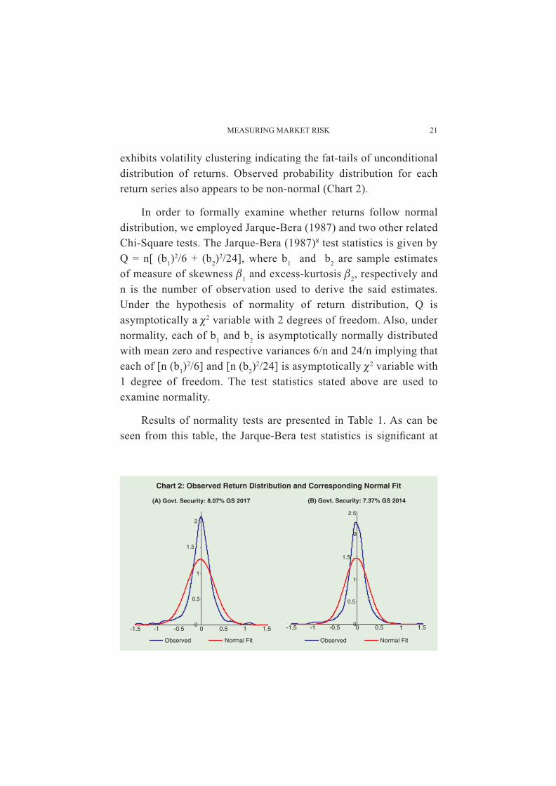
MEASURING MARKET RISK 21
exhibits volatility clustering indicating the fat-tails of unconditional distribution of returns. Observed probability distribution for each return series also appears to be non-normal (Chart 2).
In order to formally examine whether returns follow normal distribution, we employed Jarque-Bera (1987) and two other related Chi-Square tests. The Jarque-Bera (1987)8 test statistics is given by Q = n[ (b1)
2/6 + (b2)2/24], where b1 and b2 are sample estimates
of measure of skewness β1 and excess-kurtosis β2, respectively and n is the number of observation used to derive the said estimates. Under the hypothesis of normality of return distribution, Q is asymptotically a χ2 variable with 2 degrees of freedom. Also, under normality, each of b1 and b2 is asymptotically normally distributed with mean zero and respective variances 6/n and 24/n implying that each of [n (b1)
2/6] and [n (b2)2/24] is asymptotically χ2 variable with
1 degree of freedom. The test statistics stated above are used to examine normality.
Results of normality tests are presented in Table 1. As can be seen from this table, the Jarque-Bera test statistics is signifi cant at
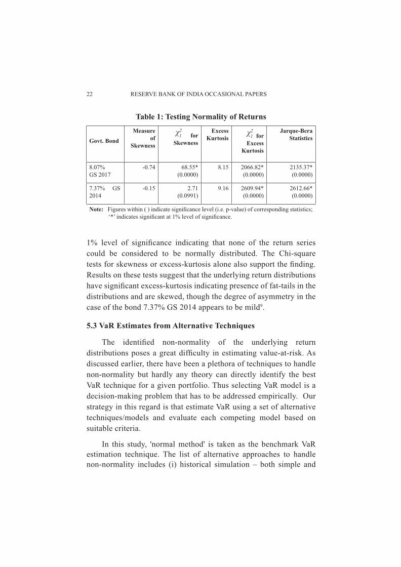
22 RESERVE BANK OF INDIA OCCASIONAL PAPERS
1% level of signifi cance indicating that none of the return series could be considered to be normally distributed. The Chi-square tests for skewness or excess-kurtosis alone also support the fi nding. Results on these tests suggest that the underlying return distributions have signifi cant excess-kurtosis indicating presence of fat-tails in the distributions and are skewed, though the degree of asymmetry in the case of the bond 7.37% GS 2014 appears to be mild9.
5.3 VaR Estimates from Alternative Techniques
The identifi ed non-normality of the underlying return distributions poses a great diffi culty in estimating value-at-risk. As discussed earlier, there have been a plethora of techniques to handle non-normality but hardly any theory can directly identify the best VaR technique for a given portfolio. Thus selecting VaR model is a decision-making problem that has to be addressed empirically. Our strategy in this regard is that estimate VaR using a set of alternative techniques/models and evaluate each competing model based on suitable criteria.
In this study, 'normal method' is taken as the benchmark VaR estimation technique. The list of alternative approaches to handle non-normality includes (i) historical simulation – both simple and
Table 1: Testing Normality of Returns
Govt. Bond
Measure of
Skewness
for
Skewness
Excess Kurtosis
for
Excess Kurtosis
Jarque-Bera Statistics
8.07% GS 2017
-0.74 68.55*(0.0000)
8.15 2066.82* (0.0000)
2135.37* (0.0000)
7.37% GS 2014
-0.15 2.71(0.0991)
9.16 2609.94*(0.0000)
2612.66* (0.0000)
Note: Figures within ( ) indicate signifi cance level (i.e. p-value) of corresponding statistics; ‘*’ indicates signifi cant at 1% level of signifi cance.
χ21 χ2
1
MEASURING MARKET RISK 23
hybrid; (ii) RiskMetric approach – using exponentially weighted sum of squares of past returns to capture the conditional heteroscedasticity in returns; (iii) symmetric hyperbolic distribution – a distribution having fat-tails; and (iv) tail-index based method – an approach under extreme value theory that measure tail fatness (through tail-index) and model tails of return distribution.
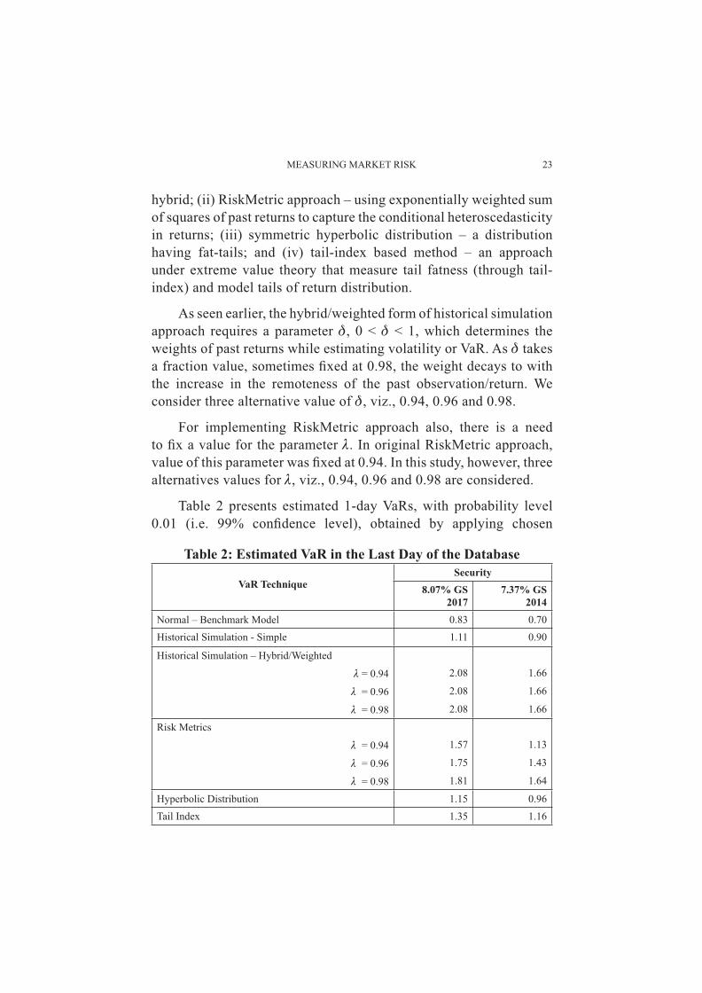
As seen earlier, the hybrid/weighted form of historical simulation approach requires a parameter δ, 0 < δ < 1, which determines the weights of past returns while estimating volatility or VaR. As δ takes a fraction value, sometimes fi xed at 0.98, the weight decays to with the increase in the remoteness of the past observation/return. We consider three alternative value of δ, viz., 0.94, 0.96 and 0.98.
For implementing RiskMetric approach also, there is a need to fi x a value for the parameter λ. In original RiskMetric approach, value of this parameter was fi xed at 0.94. In this study, however, three alternatives values for λ, viz., 0.94, 0.96 and 0.98 are considered.
Table 2 presents estimated 1-day VaRs, with probability level 0.01 (i.e. 99% confi dence level), obtained by applying chosen
Table 2: Estimated VaR in the Last Day of the Database
VaR TechniqueSecurity
8.07% GS 2017
7.37% GS 2014
Normal – Benchmark Model 0.83 0.70Historical Simulation - Simple 1.11 0.90
Historical Simulation – Hybrid/Weighted
λ = 0.94 2.08 1.66
λ = 0.96 2.08 1.66
λ = 0.98 2.08 1.66
Risk Metrics
λ = 0.94 1.57 1.13
λ = 0.96 1.75 1.43
λ = 0.98 1.81 1.64
Hyperbolic Distribution 1.15 0.96Tail Index 1.35 1.16
24 RESERVE BANK OF INDIA OCCASIONAL PAPERS
alternative techniques for the last day in our database. Noting that returns do not follow normal distribution, VaR number is likely to be underestimated by normal method. Our empirical results are consistent on this matter. As can be seen from Table 2, VaR estimates obtained from normal method are the lowest for selected bonds10.
Among the non-normal alternatives, historical simulation (simple) and hyperbolic distribution produces the lowest VaR numbers. On the other hand, the RiskMetric and hybrid historical simulation methods produce the highest VaR estimates. The tail-index based method results into VaR estimates some where in between these two sets of estimates.
5.4 Evaluation of Competing VaR Models
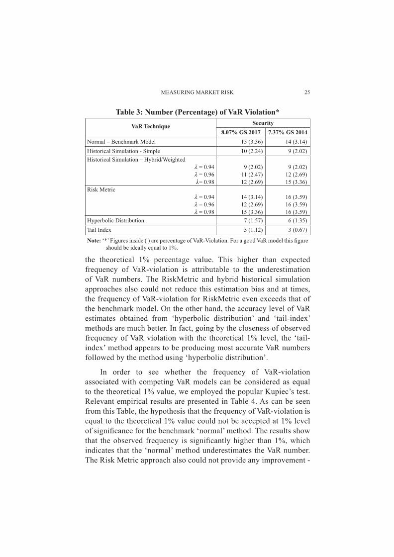
Competing VaR models were evaluated in terms of their accuracy in estimating VaR over last 447 days in the database. For each VaR model, we followed following steps: First, estimate 1-day VaR with 99% confi dence level (i.e. probability level 0.01) using the returns for fi rst 300 days. This estimate is then compared with the loss on 301st day. In case loss exceeds VaR, we say that an instance of VaR-violation has occurred. Second, estimate VaR for 302nd day using returns for past 300 days (covering the period from 2nd to 301st days). This estimate is then compared with the loss in 302nd day in the database to see whether any VaR-violation occurred. Third, the process is repeated until all data points are exhausted. Finally, count the number/percentage of VaR violation over the period of 447 days. For a good VaR model, percentage of VaR violation should be equal to the theoretical value 1% (corresponding with probability level 0.01 of estimated VaR numbers). In Table 3, the number/percentage of VaR violation over last 447 days in the database is given separately for each of the competing VaR models.
As can be seen from Table 3, percentage of VaR violation for the benchmark model ‘normal method’ is above 3% - far above
MEASURING MARKET RISK 25
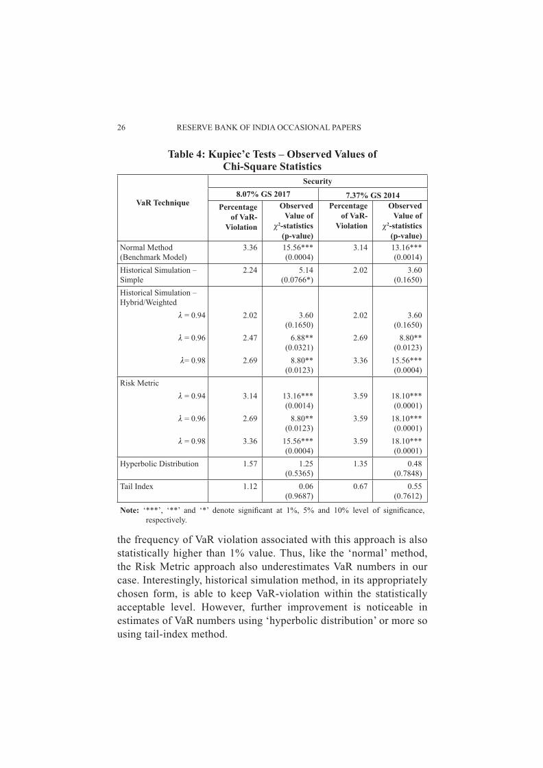
the theoretical 1% percentage value. This higher than expected frequency of VaR-violation is attributable to the underestimation of VaR numbers. The RiskMetric and hybrid historical simulation approaches also could not reduce this estimation bias and at times, the frequency of VaR-violation for RiskMetric even exceeds that of the benchmark model. On the other hand, the accuracy level of VaR estimates obtained from ‘hyperbolic distribution’ and ‘tail-index’ methods are much better. In fact, going by the closeness of observed frequency of VaR violation with the theoretical 1% level, the ‘tail-index’ method appears to be producing most accurate VaR numbers followed by the method using ‘hyperbolic distribution’.
In order to see whether the frequency of VaR-violation associated with competing VaR models can be considered as equal to the theoretical 1% value, we employed the popular Kupiec’s test. Relevant empirical results are presented in Table 4. As can be seen from this Table, the hypothesis that the frequency of VaR-violation is equal to the theoretical 1% value could not be accepted at 1% level of signifi cance for the benchmark ‘normal’ method. The results show that the observed frequency is signifi cantly higher than 1%, which indicates that the ‘normal’ method underestimates the VaR number. The Risk Metric approach also could not provide any improvement -
Table 3: Number (Percentage) of VaR Violation*
VaR Technique Security8.07% GS 2017 7.37% GS 2014
Normal – Benchmark Model 15 (3.36) 14 (3.14)Historical Simulation - Simple 10 (2.24) 9 (2.02)Historical Simulation – Hybrid/Weighted
λ = 0.94 9 (2.02) 9 (2.02)λ = 0.96 11 (2.47) 12 (2.69)λ= 0.98 12 (2.69) 15 (3.36)
Risk Metricλ = 0.94 14 (3.14) 16 (3.59)λ = 0.96 12 (2.69) 16 (3.59)λ = 0.98 15 (3.36) 16 (3.59)
Hyperbolic Distribution 7 (1.57) 6 (1.35)Tail Index 5 (1.12) 3 (0.67)
Note: ‘*’ Figures inside ( ) are percentage of VaR-Violation. For a good VaR model this fi gure should be ideally equal to 1%.
26 RESERVE BANK OF INDIA OCCASIONAL PAPERS
the frequency of VaR violation associated with this approach is also statistically higher than 1% value. Thus, like the ‘normal’ method, the Risk Metric approach also underestimates VaR numbers in our case. Interestingly, historical simulation method, in its appropriately chosen form, is able to keep VaR-violation within the statistically acceptable level. However, further improvement is noticeable in estimates of VaR numbers using ‘hyperbolic distribution’ or more so using tail-index method.
Table 4: Kupiec’c Tests – Observed Values of Chi-Square Statistics
VaR Technique
Security8.07% GS 2017 7.37% GS 2014
Percentage of VaR-
Violation
Observed Value of
χ2-statistics(p-value)
Percentage of VaR-
Violation
Observed Value of
χ2-statistics(p-value)
Normal Method (Benchmark Model)
3.36 15.56***(0.0004)
3.14 13.16*** (0.0014)
Historical Simulation – Simple
2.24 5.14 (0.0766*)
2.02 3.60 (0.1650)
Historical Simulation – Hybrid/Weighted
λ = 0.94 2.02 3.60 (0.1650)
2.02 3.60 (0.1650)
λ = 0.96 2.47 6.88** (0.0321)
2.69 8.80** (0.0123)
λ= 0.98 2.69 8.80**(0.0123)
3.36 15.56***(0.0004)
Risk Metricλ = 0.94 3.14 13.16***
(0.0014)3.59 18.10***
(0.0001)λ = 0.96 2.69 8.80**
(0.0123)3.59 18.10***
(0.0001)λ = 0.98 3.36 15.56***
(0.0004)3.59 18.10***
(0.0001)Hyperbolic Distribution 1.57 1.25
(0.5365)1.35 0.48
(0.7848)Tail Index 1.12 0.06
(0.9687)0.67 0.55
(0.7612)
Note: ‘***’, ‘**’ and ‘*’ denote signifi cant at 1%, 5% and 10% level of signifi cance, respectively.
MEASURING MARKET RISK 27
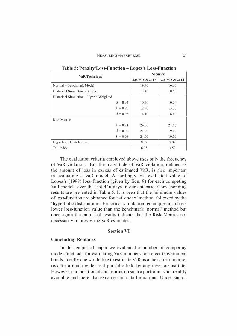
The evaluation criteria employed above uses only the frequency of VaR-violation. But the magnitude of VaR violation, defi ned as the amount of loss in excess of estimated VaR, is also important in evaluating a VaR model. Accordingly, we evaluated value of Lopez’s (1998) loss-function (given by Eqn. 9) for each competing VaR models over the last 446 days in our database. Corresponding results are presented in Table 5. It is seen that the minimum values of loss-function are obtained for ‘tail-index’ method, followed by the ‘hyperbolic distribution’. Historical simulation techniques also have lower loss-function value than the benchmark ‘normal’ method but once again the empirical results indicate that the Risk Metrics not necessarily improves the VaR estimates.
Section VI
Concluding Remarks
In this empirical paper we evaluated a number of competing models/methods for estimating VaR numbers for select Government bonds. Ideally one would like to estimate VaR as a measure of market risk for a much wider real portfolio held by any investor/institute. However, composition of and returns on such a portfolio is not readily available and there also exist certain data limitations. Under such a
Table 5: Penalty/Loss-Function – Lopez’s Loss-Function
VaR TechniqueSecurity
8.07% GS 2017 7.37% GS 2014Normal – Benchmark Model 19.90 16.60Historical Simulation - Simple 13.40 10.50Historical Simulation – Hybrid/Weighted
λ = 0.94 10.70 10.20λ = 0.96 12.90 13.30λ = 0.98 14.10 16.40
Risk Metricsλ = 0.94 24.00 21.00λ = 0.96 21.00 19.00λ = 0.98 24.00 19.00
Hyperbolic Distribution 9.07 7.02Tail Index 6.75 3.59
28 RESERVE BANK OF INDIA OCCASIONAL PAPERS
situation, we chose two most liquid Government bonds during the period from August 2005 to July 2008 and constructed daily return series on the chosen two assets for the period. Though not aimed at analyzing market risk (value-at-risk) of any real bond portfolio, the study is useful in a sense that it demonstrates various relevant issues in details, which can be easily mimicked for any given portfolio.
If returns were normally distributed, estimation of VaR would be made simply by using fi rst two moments of the distribution and the tabulated values of standard normal distribution. But the experience from empirical literature shows that the task is potentially diffi cult for the fact that the fi nancial market returns seldom follow normal distribution. The returns in our database are identifi ed to follow fat-tailed, also possibly skewed, distribution. This observed non-normality of returns has to be handled suitably while estimating VaR. Accordingly, we employed a number of non-normal VaR models, such as, historical simulation, RiskMetric, hyperbolic distribution fi t, method based on tail-index. Our empirical results show that the VaR estimates based on the conventional ‘normal’ method are usually biased downward (lower than actual) and the popular Risk Metric approach could not improve this level of underestimation. Interestingly, historical simulation method (in its suitable chosen form) can estimate VaR numbers more accurately. However, most accurate VaR estimates are obtained from the tail-index method followed by the method based on hyperbolic distribution fi t.
Notes1 This means VaR number increases (decreases) with the rise (fall) of confi dence level.2 In the case of market risk, a related view is that ‘holding period’ may be determined from the ‘time required to hedge’ the market risk.3 Note that ∆Wt(k) is the change in value of the assets in the fi nancial position from time point t to (t+k) and the k-period simple return would be measured by [100*{∆Wt(k)/Wt}]. Alternatively, k-period continuously compounded return, known as log-return, is defi ned by [100{loge(Wt+k) – loge(Wt)}]. Through out the article, the base of logarithmic transformation is ‘e’ and therefore, anti-log
MEASURING MARKET RISK 29
(i.e. the inverse of log-transformation) of a real number x is anti-log(x) = ex; sometimes denoted by exp(x).4 It may be noted that the simple HS method corresponds to δ =1, where each of the past k returns is assigned a constant weight 1/k.5 Conventionally, μt+1|t is considered to be zero, though one can model the return process to have estimates of time-varying/conditional means.6 The symmetric hyperbolic distribution is a special case of generalized hyperbolic distribution which depends on six parameters. For a discussion of hyperbolic distribution, generalized and symmetric, one may see Bauer (2000).7 For more discussions on fi tting symmetric hyperbolic distribution, one may see the papers referred by Bauer (2000), such as, Eberlein and Keller (1995).8 See, also, Gujarati (1995) for a discussion on the issues relating to Jarque-Bera (1987) test for normality.9 In this case the null hypothesis of zero skewness could be rejected only at 10% or higher level of signifi cance.10 For the sake of brevity, we present VaR estimates only for one day. But we have noticed the similar pattern in other days in our database also.
Select ReferencesArtzner, Philippe, Freddy Delbaen, Jean-Marc Eber and David Heath (1999), Coherent Measures of Risk, Mathematical Finance, Vol. 9, No. 3 (July), pp. 203-28.
Baillie, R. T., Bollerslev, T. and Mikkelsen, H. O. (1996a), "Fractionally Integrated Generalized Autoregressive Conditional Heteroskedasticity", Journal of Econometrics, 74, 3–30.
Basel Committee (1988), International Convergence of Capital Measurement and Capital Standards - Basel Capital Accord, Bank for International Settlements.
Basel Committee (1996a), Amendment to the Capital Accord to Incorporate Market Risks, Bank for International Settlements.
Basel Committee (1996b), Supervisory Framework for the Use of ‘Backtesting’ in Conjunction with Internal Models Approach to Market Risk, Bank for International Settlements.
Bauer, Christian (2000), “Value at Risk Using Hyperbolic Distributions”, Journal of Economics and Business, Vol. 52, pp. 455-67.
30 RESERVE BANK OF INDIA OCCASIONAL PAPERS
Berkowitz, Jeremy and James O’Brien (2002), “How Accurate are Value-at-Risk Models at Commercial Banks?”, Journal of Finance, Vol. LVII, No. 3, June, pp. 1093-111.
Bickel, P.J. and K.A. Doksum (1981), “An Analysis of Transformations Revisited”, Journal of American Statistical Association, vol. 76, pp. 296-311.
Billio, Monica and Loriana Pelizzon (2000), “Value-at-Risk: A Multivariate Switching Regime Approach”, Journal of Empirical Finance, Vol. 7, pp. 531-54.
Bollerslev, T. (1986), “Generalized Autoregressive Conditional Heteroskedasticity”, Journal of Econometrics, Vol. 31, pp. 307-27.
Box, G.E.P. and D.R. Cox (1964), “An Analysis of Transformations” (with Discussion), Journal of Royal Statistical Association, Vol. 76, pp. 296-311.
Boudoukh J., Matthew Richardson, and R. F. Whitelaw (1997), “The Best of both Worlds: A Hybrid Approach to Calculating Value at Risk”, Stern School of Business, NYU
Brooks, Chris and Gita Persand (2003), “Volatility Forecasting for Risk Management”, Journal of Forecasting, Vol. 22, pp. 1-22.
Burbidge John B., Lonnie Magee and A. Leslie Robb (1988), “Alternative Transformations to Handle Extreme Values of the Dependent Variable”, Journal of American Statistical Association, March, Vol. 83, No. 401, pp. 123-27.
Cebenoyan, A. Sinan and Philio E. Strahan (2004), “Risk Management, Capital Structure and Lending at Banks”, Journal of Banking and Finance, Vol. 28, pp. 19-43.
Christoffersen, P.F. (1998), “Evaluating Interval Forecasts”, International Economic Review, 39, pp. 841-62.
Christoffersen, P., Jinyong Hahn and Atsushi Inoue (2001), “Testing and Comparing Value-at-Risk Measures”, Journal of Empirical Finance, Vol. 8, No. 3, July, pp. 325-42.
Diamond, Douglas W. and Philip H. Dybvig (1983), “Bank Runs, Deposit Insurance, and Liquidity”, Journal of Political Economy, Vol. 91, No. 3, pp. 401-19.
Dowd, Kevin. (1998), Beyond Value at Risk: The New Science of Risk Management, (Reprinted, September 1998; January & August 1999; April 2000), Chichester, John Wiley & Sons Ltd.
MEASURING MARKET RISK 31
Eberlin, E. and U. Keller (1995), “Hyperbolic Distributions in Finance”, Bernoulli: Offi cial Journal of the Bernoulli Society of Mathematical Statistics and Probability, 1(3), pp. 281-99.
Engle, R. F. (1982), “Autoregressive Conditional Heteroscedasticity with Estimates of the Variance of United Kingdom Infl ation”, Econometrica, Vol. 50, No. 4, July, pp. 987-1007.
Hellmann, Thomas F., Kevin C. Murdock, and Joseph E. Stiglitz (2000), “Liberalisation, Moral Hazard in Banking, and Prudential Regulation: Are Capital Requirements Enough?”, The American Economic Review, Vol. 90, No. 1, Mar, pp. 147-165.
Hill, B.M. (1975), “A Simple General Approach to Inference About the Tail of a Distribution”, Annals of Statistics, 35, pp. 1163-73.
John, J.A. and N.R.Draper (1980), “An Alternative Family of Transformations”, Appl. Statist., Vol. 29, pp. 190-97.
Jorion, Philippe (2001), Value-at-Risk – The New Benchmark for Managing Financial Risk, Second Edition, McGraw Hill.
J.P.Morgan/Reuters (1996), RiskMetrics: Technical Document, Fourth Edition, New York, USA.
Kupiec, P.(1995), “Techniques for Verifying the Accuracy of Risk Measurement Models”, Journal of Derivatives, Vol. 2, pp. 73-84.
Linden, Mikael (2001), “A Model for Stock Return Distribution”, International Journal of Finance and Economics, April, Vol. 6, No. 2, pp. 159-69.
Lopez, Jose A. (1998), “Methods for Evaluating Value-at-Risk Estimates”, Federal Reserve Bank of New York Economic Policy Review, October, pp. 119-124.
Mills, Terence C. (1999), The Econometric Modelling of Financial Time Series, 2nd Edition, Cambridge University Press.
Nath, Golaka C. and G. P. Samanta (2003), “Value-at-Risk: Concepts and Its Implementation for Indian Banking System”, The Seventh Capital Market Conference, December 18-19, 2003, Indian Institute of Capital Markets, Navi Mumbai, India.
Robinson, P. M. and Zaffaroni, P. (1997), "Modelling Nonlinearity and Long Memory in Time Series", Fields Institute Communications, 11, 161–170.
32 RESERVE BANK OF INDIA OCCASIONAL PAPERS
Robinson, P. M. and Zaffaroni, P. (1998), "Nonlinear Time Series with Long Memory: A Model for Stochastic Volatility", Journal of Statistical Planning and Inference, 68, 359–371.
Samanta, G.P. (2003), “Measuring Value-at-Risk: A New Approach Based on Transformations to Normality”, The Seventh Capital Markets Conference, December 18-19, 2003, Indian Institute of Capital Markets, Vashi, New Mumbai.
Samanta, G. P. (2008), "Value-at-Risk using Transformations to Normality: An Empirical Analysis", in Jayaram, N. and R.S.Deshpande [Eds.] (2008), Footprints of Development and Change – Essays in Memory of Prof. V.K.R.V.Rao Commemorating his Birth Centenary, Academic Foundation, New Delhi. The Edited Volume is contributed by the V.K.R.V.Rao Chair Professors at Institute of Social and Economic Change (ISEC), Bangalore, and the scholars who have received the coveted V.K.R.V.Rao Award.
Samanta, G.P. and Golaka C. Nath (2004), “Selecting Value-at-Risk Models for Government of India Fixed Income Securities”, ICFAI Journal of Applied Finance, Vol. 10, No. 6, June, pp. 5-29.
Sarma, Mandira, Susan Thomas and Ajay Shah (2003), “Selection of Value-at-Risk Models”, Journal of Forecasting, 22(4), pp. 337-358.
Taylor, Jeremy, M. G. (1985), “Power Transformations to Symmetry”, Biometrika, Vol. 72, No. 1, pp. 145-52.
Tsay, Ruey S. (2002), Analysis of Financial Time Series, Wiley Series in Probability and Statistics, John Wiley & Sons, Inc.
van den Goorbergh, R.W.J. and P.J.G. Vlaar (1999), “Value-at-Risk Analysis of Stock Returns Historical Simulation, Variance Techniques or Tail Index Estimation?”, DNB Staff Reports, No. 40, De Nederlandsche Bank.
Wong, Michael Chak Sham, Wai Yan Cheng and Clement Yuk Pang Wong (2003), “Market Risk Management of Banks: Implications from the Accuracy of Value-at-Risk Forecasts”, Journal of Forecasting, 22, pp. 23-33.
Yeo, In-Kwon and Richard A. Johnson (2000), “A New Family of Power Transformations to Improve Normality or Symmetry”, Biometrika, Vol. 87, No. 4, pp. 954-59.
Determinants of Real Exchange Rate in India: An ARDL Approach
Sunil Kumar* This paper attempts to identify determinants of real exchange rate in India. Apart from providing theoretical background on possible determinants of real exchange rate, the paper tests their statistical signifi cance using autoregressive distributed lag (ARDL) modelling approach. It fi nds that among the identifi ed variables chosen a priori based on theoretical arguments as determinants of RER, productivity differential, external openness, terms of trade and net foreign assets turn out to be statistically signifi cant. The signs of the short-run dynamic impact have been found consistent with long-run coeffi cients and error correction term is negative and statistically signifi cant implying convergence to long-run equilibrium path. Since the fi tted RER is found to be quite closer to the actual behavior exhibited by RER, the variables identifi ed with certain lags could, therefore, serve as lead indicators of real exchange rate behaviour. On the basis of results, it may be noted that appreciation in RER should not always be seen as decline in international competitiveness of the traded sector as some of the factors contributing to the RER appreciation are attributed to higher growth refl ecting improvement in competitiveness.
JEL Classifi cation : E31, F31, C15.Keywords : Real Exchange Rate, Economic Growth, Balassa-Samuelson
hypothesis, Autoregressive Distributed Lag
Reserve Bank of India Occasional PapersVol. 31, No.1, Summer 2010
Introduction
Real exchange rate (RER) is considered as barometer of the competitiveness of an economy for international trade. The higher real exchange rate ceteris paribus entails country’s exports more expensive and imports relatively cheaper. Thus, affecting the prices of exports and imports, RER movements result in to variation in the allocation of internal production and consumption between traded and non-traded goods. RER assumes utmost importance in developing countries where non-tradable goods constitute a large segment of the goods market and only their prices are fl exible as prices of traded
* Assistant Adviser with Department of Economic Analysis and Policy, Reserve Bank of India. The views expressed in the paper are those of author and do not necessarily represent those of the RBI. Errors and omissions, if any, are the sole responsibility of the author. The author is extremely thankful to Dr. M.R. Aggarwal for providing valuable guidance in accomplishing this study.
34 RESERVE BANK OF INDIA OCCASIONAL PAPERS
goods are largely determined in world market. Therefore, the volatility in the prices of non-traded goods leads to misalignment of RER from its equilibrium level and supposedly, affects adversely the competitiveness and economic growth. In fact, recurrent and large misalignments are linked to lower growth rates and current account defi cits in the long run and very frequently with currency and fi nancial crisis. However, it has been debated for some times whether devaluations in RER are contractionary or expansionary. On the one hand, in the conventional textbook model, assuming the Marshall-Lerner condition holds, devaluations are supposed to increase competitiveness, increase production and exports of tradable goods, reduce imports, and thereby improve trade balance, GDP and employment. On the other hand, evidence from many countries reveals that currency appreciation results from accelerated economic development, whereas reverse is true in case of deceleration in economic development. Balassa-Samuelson hypothesis (1963), one of the most important hypotheses with respect to the equilibrium real exchange rate level, postulates that rapid economic growth is accompanied by real exchange rate appreciation because of differential productivity growth between tradable and non-tradable sectors. However, the analysis of the relationship between the level of economic development and real exchange rate, as was suggested by the seminal paper of Balassa-Samuelson, do not fi nd much of the place in the history of research. Nevertheless, open economy macroeconomics has provided with a framework on equilibrium exchange rate level compatible with overall economic equilibrium, as well as policy instruments necessary to correct the possible misalignment.
The fi ndings of various studies on the impact of real exchange rate on economic activities also differ distinctly. Aguirre and Calderon (2005) has found that large overvaluations and undervaluation in RER hurt growth, whereas small undervaluation can boost growth. On the other hand, Diaz-Alejandro (1963), Krugman and Taylor (1978), and Lizondo and Montiel (1989) have found that expansionary effect of real devaluations in tradable sector could be offset by contractionary impact in the non-tradable sector. Edwards (1989) investigated the
DETERMINANTS OF REAL EXCHANGE RATE IN INDIA: AN ARDL APPROACH 35
relationship between real exchange rate misalignment and economic performances and concludes that real exchange rate difference with regards to its equilibrium level has a negative effect. Cotti et al (1990) confi rms that for some Latin American countries real exchange rate instability has handicapped exportation growth, whereas Asian exportation growth has been for the most part accounted for by real exchange rate stability. According to Sekkat and Varoudakis (1998), the chronic misalignments of real exchange rate are a major factor of the weak economic performances of developing countries. Ghura and Grennes (1993) show on a panel of African countries that real exchange rate misalignment negatively affected economic growth, exports, investment and saving.
Even though, it is not very clear whether net impact of RER devaluations is positive or negative in an economy, several emerging market and developing economies have resisted devaluation in the last many years partly because of concerns that such policy would be contractionary. This view arises from the experience of countries such as Mexico, where real depreciations (increase) of the Peso have consistently been associated with declines in output, while real appreciations (decrease) have been linked to expansion (Villavicencio and Bara, 2006). Furthermore, real exchange rate stability and alignments have assumed critical importance in policy formulations particularly in EMEs to improve economic performance during recent years. Real exchange rate misalignment affects economic activity in developing countries mainly due to their dependence on imported capital goods and specialization in commodity exports. Evidence from developing countries is often quoted to support the view that the link between RER misalignment and economic performance is strong.
Given the fact that RER movements and economic growth have got some association positive or negative, the determinants of RER becomes more relevant from policy perspective. In fact, a number of researchers have also pointed out the importance of understanding the main determinants of real exchange rate (Edwards, 1989; Elbadawi and Soto, 1997; Ebadawi, 1994; and Ghura and Grennes, 1993).
36 RESERVE BANK OF INDIA OCCASIONAL PAPERS
Furthermore, this is well established that in most of the cases, especially in emerging market and developing economies, RER does not strictly converge to purchasing power parity (PPP) and even if it does in some cases in the long-run, the rate of convergence remains very slow resulting from underlying macroeconomic fundamentals. This implies that impulse response of RER to movements in macroeconomic fundamentals is very pronounced.
Therefore, the objective of this paper is to identify theoretically the determinants of RER and empirically investigate the link between RER and select determinants in case of India. The structure of the remainder of the paper is as follows. The theoretical framework and macroeconomic variables as determinants of RER has been given in section II, while Section III dwells upon the RER evolution in India. Section IV provides details on sources of data and research methodology. Empirical results have been discussed in section V. The concluding observations have been furnished in section VI.
Section IITheoretical Framework and Determinants
Theoretical framework
In order to specify the nature of the relation to be tested through econometrics techniques, the Balassa-Samuelson hypothesis has been taken as minimal theoretical framework for real exchange rate determination. For this purpose, a small open economy is considered, which is composed of a set of homogeneous fi rms. The representative fi rm produces two goods: a tradable commodity for the world market and a non-tradable one for domestic demand. The tradable goods production is presumed to require both capital and labour, while non-tradable goods production uses only labour. The competition is supposed to be perfect and it ensures that production factors are paid at their marginal productivity and at the same time, labour factor mobility ensures equal pay. Whereas labour supply is supposed to be constant and all variables are expressed in terms of tradable goods.
DETERMINANTS OF REAL EXCHANGE RATE IN INDIA: AN ARDL APPROACH 37
In this study, an extension of the benchmark model is used where the equilibrium real exchange rate is a path upon which an economy maintains both internal and external balances. The equilibrium real exchange rate depends not only on productivities but also on some other real variables. This model used in the present study is basically developed by Montiel (cited by Mkenda 2001). Real exchange rate is defi ned as the relative price of traded and non-traded goods. That is:
(1)
Where, PT is the world price for traded goods and PN is the price of non-traded ones. This defi nition is called internal real exchange rate and is appropriate for developing countries where exports are predominately primary products and law of one price holds. The law of one price entails that price of traded goods is equivalent across the countries in common currency. Edwards (1989) mentions that this defi nition provides a consistent index of the country’s tradable sector competitiveness and also infl uences resources allocation as an increase in q would cause a shift of resources away from the traded to the non traded sector. As per defi nition (1), the dynamics of the internal relative price of non tradable goods drives the movements in RER as law of one prices holds in case of traded goods and their prices amount equivalent to world prices, especially in emerging market and developing economies.
The defi nition of real exchange rate could be generalized and written in log form as follows.
(2)
Where, p and p* are respectively the national and foreign price indices, and assuming that log p and log p* can be split into traded and non traded prices as below.
(3)
(4)
38 RESERVE BANK OF INDIA OCCASIONAL PAPERS
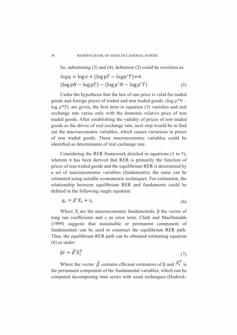
So, substituting (3) and (4), defi nition (2) could be rewritten as:
(5)
Under the hypothesis that the law of one price is valid for traded goods and foreign prices of traded and non traded goods, (log p*N – log p*T), are given, the fi rst term in equation (5) vanishes and real exchange rate varies only with the domestic relative price of non traded goods. After establishing the validity of prices of non traded goods as the driver of real exchange rate, next step would be to fi nd out the macroeconomic variables, which causes variations in prices of non traded goods. These macroeconomic variables could be identifi ed as determinants of real exchange rate.
Considering the RER framework detailed in equations (1 to 5), wherein it has been derived that RER is primarily the function of prices of non traded goods and the equilibrium RER is determined by a set of macroeconomic variables (fundaments), the same can be estimated using suitable econometric techniques. For estimation, the relationship between equilibrium RER and fundaments could be defi ned in the following single equation:
(6)
Where Xt are the macroeconomic fundamentals, β the vector of long run coeffi cients and εt an error term. Clark and MacDonalds (1999) suggests that sustainable or permanent component of fundamentals can be used to construct the equilibrium RER path. Thus, the equilibrium RER path can be obtained estimating equation (6) as under:
(7)
Where the vector contains effi cient estimators of β and is the permanent component of the fundamental variables, which can be computed decomposing time series with usual techniques (Hodrick-
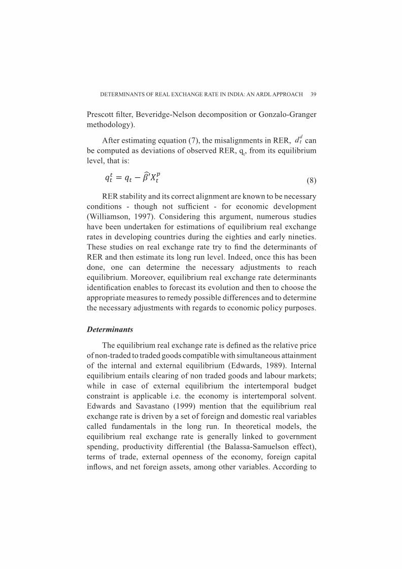
DETERMINANTS OF REAL EXCHANGE RATE IN INDIA: AN ARDL APPROACH 39
Prescott fi lter, Beveridge-Nelson decomposition or Gonzalo-Granger methodology).
After estimating equation (7), the misalignments in RER, can be computed as deviations of observed RER, qt, from its equilibrium level, that is:
(8)
RER stability and its correct alignment are known to be necessary conditions - though not suffi cient - for economic development (Williamson, 1997). Considering this argument, numerous studies have been undertaken for estimations of equilibrium real exchange rates in developing countries during the eighties and early nineties. These studies on real exchange rate try to fi nd the determinants of RER and then estimate its long run level. Indeed, once this has been done, one can determine the necessary adjustments to reach equilibrium. Moreover, equilibrium real exchange rate determinants identifi cation enables to forecast its evolution and then to choose the appropriate measures to remedy possible differences and to determine the necessary adjustments with regards to economic policy purposes.
Determinants
The equilibrium real exchange rate is defi ned as the relative price of non-traded to traded goods compatible with simultaneous attainment of the internal and external equilibrium (Edwards, 1989). Internal equilibrium entails clearing of non traded goods and labour markets; while in case of external equilibrium the intertemporal budget constraint is applicable i.e. the economy is intertemporal solvent. Edwards and Savastano (1999) mention that the equilibrium real exchange rate is driven by a set of foreign and domestic real variables called fundamentals in the long run. In theoretical models, the equilibrium real exchange rate is generally linked to government spending, productivity differential (the Balassa-Samuelson effect), terms of trade, external openness of the economy, foreign capital infl ows, and net foreign assets, among other variables. According to
40 RESERVE BANK OF INDIA OCCASIONAL PAPERS
Edwards (1989), both real and nominal variables affect equilibrium real exchange rate, where as it respond only to fundamentals in the long run. In view of above, the real exchange rate movements may be endogenously generated by variations in fundamentals and hence, not necessarily means disequilibrium situations.
The studies by Ghura and Grennes (1993), Aron et al (1997), Cotti et al (1990) and Elbadawi and Soto (1997) fi nd that real exchange rate determinants are mainly the terms of trade, the openness degree of the economy, imports and capital fl ows.
We have considered the determinants of RER in India on the basis of extant theoretical literature and numerous empirical studies undertaken in respect of other countries having somewhat similar economic structure. The Edwards model (1988), a theoretical framework for equilibrium RER used in various empirical studies on developing and EMEs, has been used in the present study. The macroeconomic fundaments, considered as possible determinants of RER in case of India, are productivity differential, government spending, terms of trade (TOT), external openness, capital fl ows and net foreign assets. The justifi cation for choosing these macroeconomic fundamentals as possible determinants of RER has been discussed below:
a. Productivity Differentials: The productivity differential impact refers to the Balassa-Samuelson model (Balassa, 1964; Samuelson, 1964). Balassa-Samuelson hypothesis presents that in an open economy, which is divided into two sectors i.e. traded and non-traded, the relative price of non-traded goods to traded goods infl uence the real exchange rate to large extent and productivity differentials in these sectors are refl ected in their relative price movements. When traded sector experience large productivity gains, the wage rates in this sector moves upward commensurately, but at the same time, wage rates in non-traded sector also increase equally, albeit productivity rise remains signifi cantly lower. Since wage increase in traded goods sector is matched by productivity improvement, the prices of traded goods
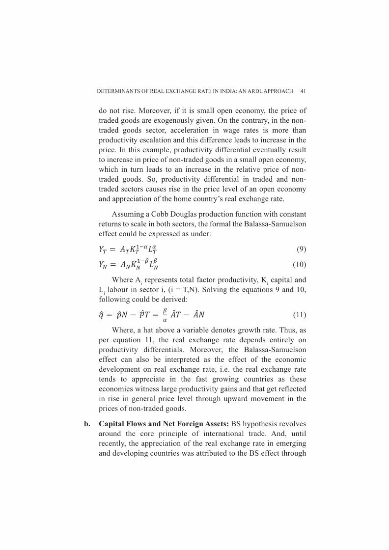
DETERMINANTS OF REAL EXCHANGE RATE IN INDIA: AN ARDL APPROACH 41
do not rise. Moreover, if it is small open economy, the price of traded goods are exogenously given. On the contrary, in the non-traded goods sector, acceleration in wage rates is more than productivity escalation and this difference leads to increase in the price. In this example, productivity differential eventually result to increase in price of non-traded goods in a small open economy, which in turn leads to an increase in the relative price of non-traded goods. So, productivity differential in traded and non-traded sectors causes rise in the price level of an open economy and appreciation of the home country’s real exchange rate.
Assuming a Cobb Douglas production function with constant returns to scale in both sectors, the formal the Balassa-Samuelson effect could be expressed as under:
(9)
(10)
Where Ai represents total factor productivity, Ki capital and Li labour in sector i, (i = T,N). Solving the equations 9 and 10, following could be derived:
(11)
Where, a hat above a variable denotes growth rate. Thus, as per equation 11, the real exchange rate depends entirely on productivity differentials. Moreover, the Balassa-Samuelson effect can also be interpreted as the effect of the economic development on real exchange rate, i.e. the real exchange rate tends to appreciate in the fast growing countries as these economies witness large productivity gains and that get refl ected in rise in general price level through upward movement in the prices of non-traded goods.
b. Capital Flows and Net Foreign Assets: BS hypothesis revolves around the core principle of international trade. And, until recently, the appreciation of the real exchange rate in emerging and developing countries was attributed to the BS effect through
42 RESERVE BANK OF INDIA OCCASIONAL PAPERS
increase in the relative prices of non-traded goods. The collapse of Bretton Woods system in early 1970s and heightened volatilities in foreign exchange markets across the world paved the way for capital fl ows. A large number of emerging and developing countries also introduced economic reforms comprising of macroeconomic stabililisation i.e. containing infl ation, fi scal defi cit and external debt and structural changes i.e. developing and strengthening money and fi nancial markets, globalization (enhancing external openness through trade and fi nancial fl ows), liberalization/ privatization etc. As a result, economic landscape underwent a transformation with increasing fi nancial fl ows across the countries following increasingly integration of international fi nancial markets during 1990s and 21st century.
Alongside increasing international fi nancial markets integration, it was debated that besides productivity differential, there is something else also which explains the recurrent deviations in exchange rate from its PPP level and jury was out with capital fl ows as one of the crucial factors behind the movements in exchange rate. Therefore, it is broadly accepted that trade and capital fl ows infl uence the exchange rate. A surge in capital fl ows leads to an increase in consumption demand for both traded and non-traded goods. In case of non-traded goods, excess demand generated by capital fl ows is not proportionately matched with rise in supply and hence, result into rise in the price of non-traded goods to reach to equilibrium. On the other hand, elevated demand for traded goods is met with imported goods without any affect on the price refl ecting law of one price (LOP) and this leads to widening trade defi cit. Accordingly, increase in the relative price of non-traded goods would entails an appreciation of the real exchange rate.
Generally, a country’s current account balance is matched with net capital fl ows. If, current account is in defi cit (surplus), then there would be net capital infl ows (outfl ows). However, there could also be a situation when net capital infl ows are more (less) than current account defi cit and lead to accretion (erosion)
DETERMINANTS OF REAL EXCHANGE RATE IN INDIA: AN ARDL APPROACH 43
of net foreign assets of the country. Thus, net foreign assets tend to infl uence a country’s exchange rate and that is why, foreign exchange balance is commonly used as one of the determinants of real exchange rate. Lane and Milessi-Ferreti (1999) investigate the theoretical relationship between the real exchange rate and net foreign assets and fi nds that the net foreign assets as an important determinant of the real exchange rate for developing and developed countries.
Net foreign assets infl uence the real exchange rate through various channels. The portfolio-balances considerations suggest that a defi cit in the current account creates an increase in the net foreign debt of a country, which has to be fi nanced by international investors and they demand for a higher yield to adjust their portfolio (Antonia and Bara, 2006). At given interest rate, this can only be achieved through a depreciation of the currency of the debtor country. Furthermore, the servicing of external debt accumulated through funding current account defi cit entails a country to generate addition foreign exchange through promoting exports of goods and services. Therefore, the country needs to depreciate its currency to increase competitiveness of its exports (balance of payments channel also requires that (Maeso-Fernandez, et al (2001)).
In sum, rising current account defi cit would be fi nanced with an increase in capital fl ows and excess capital fl ows would lead to appreciation in real exchange rate. In the process, either excess capital fl ows would result in appreciation of nominal exchange rate or rise in prices with increasing money supply in the system. It may be noted that if a country relies on foreign capital for high levels of domestic absorptions (investment), RER is bound to appreciate regardless of the exchange rate regime in vogue. Thus, the real exchange rate is expected to appreciate (depreciate) with rise (fall) in foreign assets of a country. Like other emerging and developing countries, capital fl ows are susceptible to infl uence the movement in real exchange rate in India1.
44 RESERVE BANK OF INDIA OCCASIONAL PAPERS
c. Government Spending: The Balassa-Samuelson model presumes that real exchange rate is supply side phenomenon, means demand factors do not have any impact on the real exchange rate. BS model also assumes certain conditions in vogue viz., prefect competition in goods market, free factors mobility between two sectors of production, international capital mobility, law of one price and constant returns to scale in both trade and non-traded sectors (Froot and Rogoff (1995) and De Gregorio et al. (1994)). However, in practice, all these conditions are diffi cult to be in existence especially in emerging and developing countries. Jorge and Restout (2008) mention that demand factors can have an effect on the relative price of non-traded goods if one of the above conditions is relaxed. In this regard, Aguirre and Calderon (2005) introduce monopolistic competition in the non-traded sector in Lane and Milesi-Ferretti’s (2004) model and consider demand factors to determine the real exchange rate. Institutively, it is believed that the government expenditure is disproportionately incurred on non-traded goods, which leads to upward pressure on relative price of non-traded goods and appreciation in exchange rate. Otherwise also, generally higher government expenditure tends to be infl ationary as it pushes the aggregate demand upward and supply response is not contemporaneous.
d. Terms of Trade: Terms of trade (ToT) affect the real exchange rate through income effect and substitution affect and net affect depends on the relative strength of these affects as both effects work in reverse direction to each other. Therefore, theoretical models although provide the importance of ToT disturbances as potential source of real exchange rate fl uctuations, their impact on the real exchange rate remains undefi ned. On the one hand, deterioration in ToT generates negative income effect through decline in the domestic purchasing power and adversely affects the private demand for non-traded goods and leads to decline in prices eventually resulting into real depreciation of the exchange rate. On the other hand, weakening ToT induces substitution
DETERMINANTS OF REAL EXCHANGE RATE IN INDIA: AN ARDL APPROACH 45
effect and makes the consumption of imported goods more expensive. The substitution effect result into shift of demand in favour of non-traded goods increasing their prices and real appreciation in exchange rate. As mentioned above, the total effect of a ToT worsening on real exchange rate would depend on the strength of the income and substitution effects. However, recent empirical studies have found that the income effect is predominant; hence, ToT improvements are associated with real appreciation in the long-run.
e. External openness: The extent of external openness of an economy infl uences the movement in real exchange rate in many ways. Firstly, increase in external openness through reduction in tariffs makes imports cheaper and shift the demand away from non-traded goods towards imported goods. The prices of non-traded goods decline and real exchange rate depreciates in this process to ensure equilibrium in non-traded goods segment. The second infl uence channel of external openness on real exchange rate has been provided in the model by Obstfeld and Rogoff (2002). As per their model, there exist a negative relationship between external openness and real exchange rate volatility. Basic tenet of their model is that monopoly/ monopolistic competition like market conditions prevail in non-traded goods segment and hence, promote the aggregate price rigidity. While traded goods allow the convergence of the domestic price indices. Because of aggregate price rigidity, a larger real exchange rate changes would be needed for a relatively closed economy to ensure equilibrium in domestic market. Hau (2002) mentions that more open countries behave more like fl exible prices economies with smaller real exchange rate fl uctuations since more imported goods provide a channel for quick adjustment of the national price indices. Using a panel of forty eight countries, Hau provids evidence of the negative relationship between real exchange rate volatility and trade openness. So, it is amply clear that increasing external sector openness leads to lower volatility as well as depreciation in real exchange rate.
46 RESERVE BANK OF INDIA OCCASIONAL PAPERS
Section IIIEvolution of Real Exchange Rate in India
The evolution of India’s real exchange rate may be viewed in line with the shifts in India’s exchange rate policies over the last few decades from a par value system to a basket-peg and further to a managed fl oat exchange rate system. During the period from 1947 to 1971, India followed the par value system of exchange rate. Initially, the rupee’s external par value was fi xed at 4.15 grains of fi ne gold. The Reserve Bank maintained the par value of the rupee within the permitted margin of ±1 per cent using pound sterling as the intervention currency. Since the sterling-dollar exchange rate was kept stable by the US monetary authority, the exchange rates of rupee in terms of gold as well as the dollar and other currencies were indirectly kept stable. The devaluation of rupee in September 1949 and June 1966 in terms of gold resulted in the reduction of the par value of rupee in terms of gold to 2.88 and 1.83 grains of fi ne gold, respectively. The exchange rate of the rupee remained unchanged between 1966 and 1971. Therefore, evolution of real exchange rate during this period was guided mainly by the changes in prices in India as well as its trading partners.
With the breakdown of the Bretton Woods System in 1971 and the fl oatation of major currencies, the rupee was also linked with pound sterling in December 1971. Since sterling was fi xed in terms of US dollar under the Smithsonian Agreement of 1971, the rupee also remained stable against dollar. In order to overcome the weaknesses associated with a single currency peg and to ensure stability of the exchange rate, the rupee, with effect from September 1975, was pegged to a basket of currencies. The currency selection and weights assigned were left to the discretion of the Reserve Bank. The currencies included in the basket as well as their relative weights were kept confi dential in order to discourage speculation. Indian rupee exchange rate continued to be pegged to the basket of currencies until early 1990s when market determined exchange rate was introduced.
During 1970s, changes in real exchange rate were largely conditioned by the prices in India and its trading partners as real
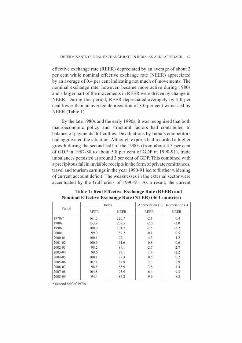
DETERMINANTS OF REAL EXCHANGE RATE IN INDIA: AN ARDL APPROACH 47
effective exchange rate (REER) depreciated by an average of about 2 per cent while nominal effective exchange rate (NEER) appreciated by an average of 0.4 per cent indicating not much of movements. The nominal exchange rate, however, became more active during 1980s and a larger part of the movements in REER were driven by change in NEER. During this period, REER depreciated averagely by 2.0 per cent lower than an average depreciation of 3.0 per cent witnessed by NEER (Table 1).
By the late 1980s and the early 1990s, it was recognised that both macroeconomic policy and structural factors had contributed to balance of payments diffi culties. Devaluations by India’s competitors had aggravated the situation. Although exports had recorded a higher growth during the second half of the 1980s (from about 4.3 per cent of GDP in 1987-88 to about 5.8 per cent of GDP in 1990-91), trade imbalances persisted at around 3 per cent of GDP. This combined with a precipitous fall in invisible receipts in the form of private remittances, travel and tourism earnings in the year 1990-91 led to further widening of current account defi cit. The weaknesses in the external sector were accentuated by the Gulf crisis of 1990-91. As a result, the current
Table 1: Real Effective Exchange Rate (REER) and Nominal Effective Exchange Rate (NEER) (36 Countries)
PeriodIndex Appreciation (+)/ Depreciation (-)
REER NEER REER NEER
1970s* 161.3 220.7 -2.1 0.41980s 153.9 208.5 -2.0 -3.01990s 100.9 101.7 -2.5 -5.22000s 99.9 89.2 -0.1 -0.52000-01 100.1 92.1 4.3 1.22001-02 100.9 91.6 0.8 -0.62002-03 98.2 89.1 -2.7 -2.72003-04 99.6 87.1 1.4 -2.22004-05 100.1 87.3 0.5 0.22005-06 102.4 89.9 2.3 2.92006-07 98.5 85.9 -3.8 -4.42007-08 104.8 93.9 6.4 9.32008-09 94.4 86.2 -9.9 -8.3
* Second half of 1970s.
48 RESERVE BANK OF INDIA OCCASIONAL PAPERS
account defi cit widened to 3.2 per cent of GDP in 1990-91 and the capital fl ows also dried up necessitating the adoption of exceptional corrective steps.
Against this backdrop, India embarked on stabilisation and structural reforms in the early 1990s of which trade policies, exchange rate policies and industrial policies formed an integrated policy framework to improve the overall productivity, competitiveness and effi ciency of the economic system, in general, and the external sector, in particular. As a stabilsation measure, a two step downward exchange rate adjustment by 9 per cent and 11 per cent between July 1 and 3, 1991 was resorted to counter the massive drawdown in the foreign exchange reserves, to instill confi dence among investors and to improve domestic competitiveness. A two-step adjustment of exchange rate in July 1991 effectively brought to close the regime of a pegged exchange rate. Following the recommendations of the High Level Committee on Balance of Payments (Chairman: Dr. C. Rangarajan) to move towards the market-determined exchange rate, the Liberalised Exchange Rate Management System (LERMS) was put in place in March 1992 initially involving a dual exchange rate system. Under the LERMS, all foreign exchange receipts on current account transactions (exports, remittances, etc.) were required to be surrendered to the Authorised Dealers (ADs) in full. The LERMS was essentially a transitional mechanism and a downward adjustment in the offi cial exchange rate took place in early December 1992 and ultimate convergence of the dual rates was made effective from March 1, 1993, leading to the introduction of a market-determined exchange rate regime. The dual exchange rate system was replaced by a unifi ed exchange rate system in March 1993, whereby all foreign exchange receipts could be converted at market determined exchange rates. On unifi cation of the exchange rates, the nominal exchange rate of the rupee against both the US dollar as also against a basket of currencies got adjusted lower, which almost nullifi ed the impact of the previous infl ation differential.
From March 1993 began a new chapter in the evolution of the real exchange rate of India wherein market determined nominal
DETERMINANTS OF REAL EXCHANGE RATE IN INDIA: AN ARDL APPROACH 49
exchange rate of the rupee started conditioning the real exchange rate besides relative prices. REER depreciated by an average of 2.5 per cent during 1990s signifi cantly lower that the average depreciation of 5.2 per cent in NEER indicating that transmission of NEER depreciation to REER was controlled to a large extent by relative higher rate of change in domestic prices. During 2000s, both REER and NEER witnessed a marginal average depreciation of 0.1 and 0.5 per cent, respectively.
Section IVData Description and Research Methodology
Data Description
The variables used in the present study are real exchange rate (REF) of Indian rupee against USA dollar, differential growth rate between India and USA (DG), government fi nal consumption expenditure as percentage of GDP (GC), foreign exchange assets (FX), terms of trade (TOT) and external openness (OP). Data series are quarterly ranging from Q2 of 1997 to Q2 of 2009. The RER has been calculated taking nominal exchange rate of rupee against US dollar, wholesale price index (WPI) of India and producers’ price index (PPI) of USA. We have used bilateral RER of rupee against US dollar keeping in view that India’s about 80 per cent of the international trade is invoiced in US dollar. Since nominal exchange rate has been taken as rupees per US dollar, increase/ decrease in RER mean depreciation/ appreciation. Due to non-availability of data on sectoral productivity, many studies have used the GDP per capita relative to trading partners as a proxy for the Balassa-Samuelson effect (productivity differential). In the present study, we have used difference in growth rate of India and USA to examine the Balassa-Samulson effect on the RER in the absence of quarterly GDP per capita. Higher growth differential, which has been presumed to be largely driven by traded goods sector, will lead to increase in prices of non-traded goods on account of Balassa-Samuelson effect. Foreign exchange assets have been considered to factor in the impact of capital fl ows and net foreign assets on the RER. The terms of trade
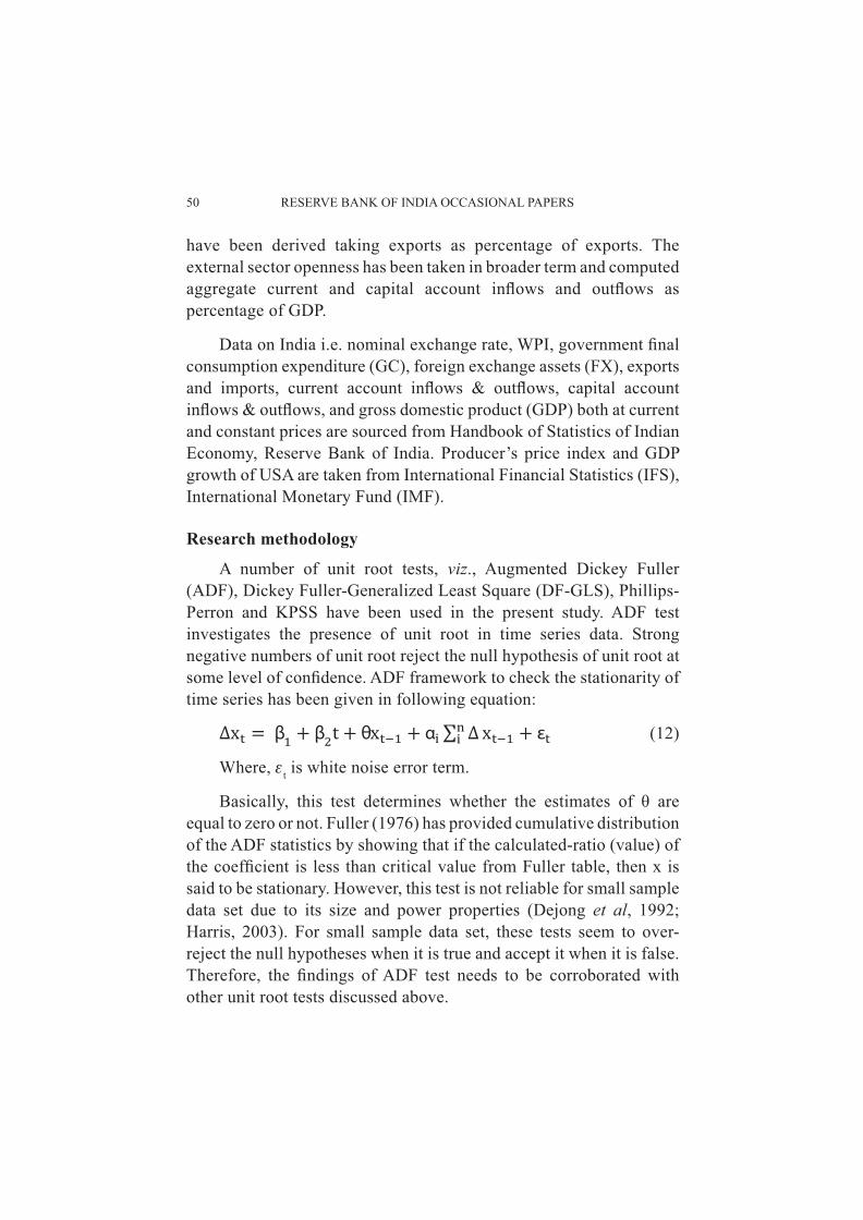
50 RESERVE BANK OF INDIA OCCASIONAL PAPERS
have been derived taking exports as percentage of exports. The external sector openness has been taken in broader term and computed aggregate current and capital account infl ows and outfl ows as percentage of GDP.
Data on India i.e. nominal exchange rate, WPI, government fi nal consumption expenditure (GC), foreign exchange assets (FX), exports and imports, current account infl ows & outfl ows, capital account infl ows & outfl ows, and gross domestic product (GDP) both at current and constant prices are sourced from Handbook of Statistics of Indian Economy, Reserve Bank of India. Producer’s price index and GDP growth of USA are taken from International Financial Statistics (IFS), International Monetary Fund (IMF).
Research methodology
A number of unit root tests, viz., Augmented Dickey Fuller (ADF), Dickey Fuller-Generalized Least Square (DF-GLS), Phillips-Perron and KPSS have been used in the present study. ADF test investigates the presence of unit root in time series data. Strong negative numbers of unit root reject the null hypothesis of unit root at some level of confi dence. ADF framework to check the stationarity of time series has been given in following equation:
(12)
Where, εt is white noise error term.
Basically, this test determines whether the estimates of θ are equal to zero or not. Fuller (1976) has provided cumulative distribution of the ADF statistics by showing that if the calculated-ratio (value) of the coeffi cient is less than critical value from Fuller table, then x is said to be stationary. However, this test is not reliable for small sample data set due to its size and power properties (Dejong et al, 1992; Harris, 2003). For small sample data set, these tests seem to over-reject the null hypotheses when it is true and accept it when it is false. Therefore, the fi ndings of ADF test needs to be corroborated with other unit root tests discussed above.
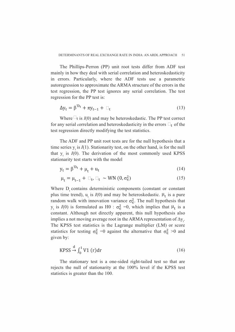
DETERMINANTS OF REAL EXCHANGE RATE IN INDIA: AN ARDL APPROACH 51
The Phillips-Perron (PP) unit root tests differ from ADF test mainly in how they deal with serial correlation and heteroskedasticity in errors. Particularly, where the ADF tests use a parametric autoregression to approximate the ARMA structure of the errors in the test regression, the PP test ignores any serial correlation. The test regression for the PP test is:
(13)
Where is I(0) and may be heteroskedastic. The PP test correct for any serial correlation and heteroskedasticity in the errors of the test regression directly modifying the test statistics.
The ADF and PP unit root tests are for the null hypothesis that a time series yt is I(1). Stationarity test, on the other hand, is for the null that yt is I(0). The derivation of the most commonly used KPSS stationarity test starts with the model
(14)
(15)
Where Dt contains deterministic components (constant or constant plus time trend), ut is I(0) and may be heteroskedastic. is a pure random walk with innovation variance . The null hypothesis that yt is I(0) is formulated as H0 : =0, which implies that is a constant. Although not directly apparent, this null hypothesis also implies a not moving average root in the ARMA representation of ∆yt. The KPSS test statistics is the Lagrange multiplier (LM) or score statistics for testing =0 against the alternative that >0 and given by:
(16)
The stationary test is a one-sided right-tailed test so that are rejects the null of stationarity at the 100% level if the KPSS test statistics is greater than the 100.
52 RESERVE BANK OF INDIA OCCASIONAL PAPERS
After testing for integrated order of data series, next logical step is to estimate the relationship with appropriate econometric techniques. Since present study deals with time series data and all the level variables are not stationary, it would be appropriate to apply some technique which can circumvent the problem of stationarity in the time series data. The data could be converted into stationary form taking fi rst difference and relationship could be estimated with ordinary least square (OLS) regression, but there would be greater loss of information and hence, estimates may not be that robust.
Econometric literature has abundant techniques to investigate relationships among non-stationary macroeconomic variables and prominent among them are univariate co-integration technique (Engle-Granger (1987)), multivariate co-integration technique (Johansen (1988); Johansen and Juselius (1990); and Johansen’s (1995)) and newly developed auto regressive distributed lag (ARDL) model (Pesaran and Shin, 1995, 1998; Pesaran et al., 1996; Pesaran et al., 2001). The recent studies indicate that the ARDL approach to cointegration is preferable to other conventional cointegration approaches such as Engle and Granger (1987), Johansen (1988) etc. mainly because of its applicability irrespective of whether the underlying regressors are purely I(0), purely I(1) or mutually co-integrated. The statistic underlying this procedure is the familiar Wald or F-statistic in a generalized Dickey-Fuller type regression, which is used to test the signifi cance of lagged levels of the variables under consideration in a conditional unrestricted equilibrium error correction model (ECM) (Pesaran, et al., 2001). Another reason for preferring the ARDL approach over other approaches is that it is more robust and performs better for small sample sizes.
In the present study, ARDL approach has been used for estimating long-run relationship and short-run dynamics because of the obvious reasons cited above for its preferability i.e. all the variables are not integrated of the same order and small sample is size. The ARDL approach involves estimating the conditional error correction version of the ARDL model for variables under estimation. The conditional VECM
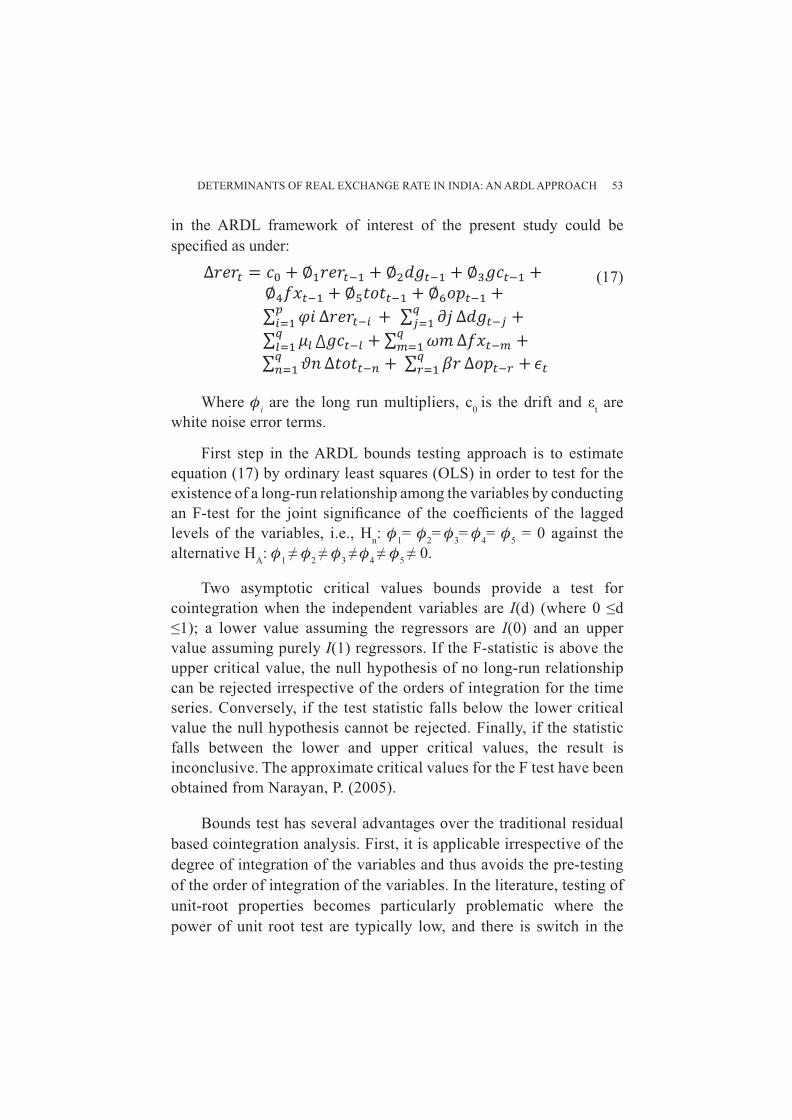
DETERMINANTS OF REAL EXCHANGE RATE IN INDIA: AN ARDL APPROACH 53
in the ARDL framework of interest of the present study could be specifi ed as under:
(17)
Where φi are the long run multipliers, c0 is the drift and εt are white noise error terms.
First step in the ARDL bounds testing approach is to estimate equation (17) by ordinary least squares (OLS) in order to test for the existence of a long-run relationship among the variables by conducting an F-test for the joint signifi cance of the coeffi cients of the lagged levels of the variables, i.e., Hn: φ1= φ2= φ3= φ4= φ5 = 0 against the alternative HA: φ1 ≠ φ2 ≠ φ3 ≠ φ4 ≠ φ5 ≠ 0.
Two asymptotic critical values bounds provide a test for cointegration when the independent variables are I(d) (where 0 ≤d ≤1); a lower value assuming the regressors are I(0) and an upper value assuming purely I(1) regressors. If the F-statistic is above the upper critical value, the null hypothesis of no long-run relationship can be rejected irrespective of the orders of integration for the time series. Conversely, if the test statistic falls below the lower critical value the null hypothesis cannot be rejected. Finally, if the statistic falls between the lower and upper critical values, the result is inconclusive. The approximate critical values for the F test have been obtained from Narayan, P. (2005).
Bounds test has several advantages over the traditional residual based cointegration analysis. First, it is applicable irrespective of the degree of integration of the variables and thus avoids the pre-testing of the order of integration of the variables. In the literature, testing of unit-root properties becomes particularly problematic where the power of unit root test are typically low, and there is switch in the
54 RESERVE BANK OF INDIA OCCASIONAL PAPERS
distribution function of the test statistics as one or more roots of the data series approach unity (Pesaran and Pesaran, 1997). Second, unlike residual based cointegration analysis, the unrestricted error correction model (UECM) employed in bound testing does not push the short-run dynamics into the residual terms (Banerjee et al., 1993). Third, the bounds test can be applied to small sample size. Fourth, it identifi es the exact variable to be normalised in the long-run relationship. A limitation of bounds test, however, is that it is not appropriate in situations where there may be more than one long-run relationship among the variables. In other words, the test is appropriate only when one variable is explained by the remaining variables and not vice versa.
In the second step, once cointegration is established, the conditional ARDL (p1 ,q1 , q2 ,q3 ,q4 ) long-run model for rert can be estimated as:
(18)
This involves selecting the orders of ARDL (p, q1, q2 , q3, q4, q5) model in the six variables using Schwarz Bayesian Criterion. Finally, the short-term dynamic parameters by estimating an error model associated with the long-run estimates can be estimated in the following specifi cation:
(19)
Where φ, , μ, ω, , β, and δ are the short-term dynamic coeffi cients of the model’s convergence to the equilibrium and is the speed of adjustment towards long term equilibrium path.
DETERMINANTS OF REAL EXCHANGE RATE IN INDIA: AN ARDL APPROACH 55
Section VEmpirical Results
The results reported in Table 2 show that null hypothesis of ADF unit root is accepted in case of all variables except for ToT but rejected in fi rst difference at 1% level of signifi cance. Similarly, null hypothesis of unit root could not be rejected by DF-GLS unit root test in the levels, while it was not accepted in fi rst difference except for GC and ToT. Both the unit root tests indicate that all the variables considered in the present study are difference stationary I(1) barring TOT which is level stationary I(0) only as per ADF test.
Phillips-Perron (PP) unit root test indicates that null hypothesis of unit root cannot be rejected in the level form in case of RER, DG, and OP, but discarded null hypothesis of unit root in GC and TOT in the level form. PP test, however, rejected the null hypothesis of unit root in the fi rst difference of the RER, DG, TOT and OP. The results of KPSS stationary test have rejected the null of stationary in the level of DG, GC, FX, and OP, while accepted the null in the level of RER
Table 2: Results of Unit Root/ Stationary TestsVariables ADF Test DF-GLS Test
Level 1st Difference Level 1st Difference
RER -1.79 -5.17*** -1.52 -5.15***DG -0.61 -5.87*** 0.38 -7.65***GC -0.74 -19.81*** -1.09 -0.70FX 2.91 -4.06*** 0.10 -3.99***TOT -2.83* -7.51*** 0.14 0.95OP 0.66 -8.72*** -0.37 -8.33***
Variables Phillips-Perron Test KPSS TestLevel 1st Difference Level 1st Difference
RER -2.05 -5.17*** 0.36* 0.15***DG -1.83 -9.92*** 0.91 0.03***GC -5.08*** -30.92*** 0.83 0.29***FX 0.40 -2.95*** 0.83 0.21***TOT -2.85* -19.17*** 0.63** 0.14***OP -0.38 -8.71*** 0.78 0.16***
Note: ***, **, and * denote statistical signifi cance at 1%, 5% and 10% levels, respectively.
56 RESERVE BANK OF INDIA OCCASIONAL PAPERS
and TOT. The KPSS results further have found that null of stationary was accepted in the fi rst difference of DG, GC, FX, and OP.
On the basis of the majority criteria, it has been inferred that variables, viz., RER, DG, GC, FX and OP are integrated of order one I(1), while TOT is integrated of order zero I(0). After seeing the unit root properties of the data series, cointegration among the variables have been tested using auto regressive distributed lag (ARDL) model has been used.
In order to test the presence of long-run relationship between RER and DG, GC, FX, and OP, equation (17) is estimated. A general-to-specifi c modeling approach guided by the short data span and SBC respectively to select a maximum lag order of 4 for the conditional ARDL-VECM is preferred because of quarterly frequency.
Firstly, an OLS regression is estimated for the fi rst differences part of equation and then tested for joint signifi cance of the parameters of the lagged level variables. The joint null hypothesis of the coeffi cients being equal to zero means no long-run relationship has been tested with F-statistics. The presence of cointegration between the variables is accepted if F-statistics reject the null at 95 per cent critical bound values generated by Narayan (2005) for small sample. The calculated F statistic presented in Table 3 is 4.8559 and is higher than the upper bound at 1% level of signifi cance. Thus, null hypothesis of no cointegration is rejected, implying that there exists a long-run relationship among the variables RER, DG, GC, FX, TOT, and OP, when the regression is normalized on RER. It may, however, be noted that null hypothesis of no cointegration is accepted at 95 per cent critical value when regression is normalised on variables other than RER. This implies that there exists only one long-run cointegrating relationship.
Having established that a long-run cointegration relationship exists between dependent variable RER and independent variables DG, GC, FX, TOT and OP, the long-run relationship has been estimated using the specifi cation defi ned in equation (18). The
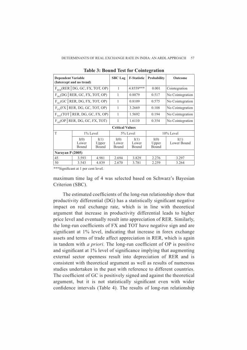
DETERMINANTS OF REAL EXCHANGE RATE IN INDIA: AN ARDL APPROACH 57
maximum time lag of 4 was selected based on Schwarz’s Bayesian Criterion (SBC).
The estimated coeffi cients of the long-run relationship show that productivity differential (DG) has a statistically signifi cant negative impact on real exchange rate, which is in line with theoretical argument that increase in productivity differential leads to higher price level and eventually result into appreciation of RER. Similarly, the long-run coeffi cients of FX and TOT have negative sign and are signifi cant at 1% level, indicating that increase in forex exchange assets and terms of trade affect appreciation in RER, which is again in tandem with a priori. The long-run coeffi cient of OP is positive and signifi cant at 1% level of signifi cance implying that augmenting external sector openness result into depreciation of RER and is consistent with theoretical argument as well as results of numerous studies undertaken in the past with reference to different countries. The coeffi cient of GC is positively signed and against the theoretical argument, but it is not statistically signifi cant even with wider confi dence intervals (Table 4). The results of long-run relationship
Table 3: Bound Test for CointegrationDependent Variable(Intercept and no trend)
SBC Lag F-Statistic Probability Outcome
FRER(RER│DG, GC, FX, TOT, OP) 1 4.8559*** 0.001 Cointegration
FDG(DG│RER, GC, FX, TOT, OP) 1 0.8879 0.517 No Cointegration
FGC(GC│RER, DG, FX, TOT, OP) 1 0.8109 0.575 No Cointegration
FFX(FX│RER, DG, GC, TOT, OP) 1 3.2669 0.108 No Cointegration
FTOT(TOT│RER, DG, GC, FX, OP) 1 1.5692 0.194 No Cointegration
FOP(OP│RER, DG, GC, FX, TOT) 1 1.6110 0.354 No Cointegration
Critical ValuesT 1% Level 5% Level 10% Level
I(0)Lower Bound
I(1)Upper Bound
I(0)Lower Bound
I(1)Lower Bound
I(0)Upper Bound
I(1)Lower Bound
Narayan P (2005)45 3.593 4.981 2.694 3.829 2.276 3.29750 3.543 4.839 2.670 3.781 2.259 3.264
***Signifi cant at 1 per cent level.
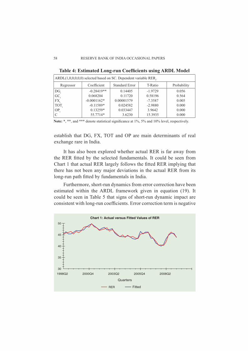
58 RESERVE BANK OF INDIA OCCASIONAL PAPERS
establish that DG, FX, TOT and OP are main determinants of real exchange rare in India.
It has also been explored whether actual RER is far away from the RER fi tted by the selected fundamentals. It could be seen from Chart 1 that actual RER largely follows the fi tted RER implying that there has not been any major deviations in the actual RER from its long-run path fi tted by fundamentals in India. Furthermore, short-run dynamics from error correction have been estimated within the ARDL framework given in equation (19). It could be seen in Table 5 that signs of short-run dynamic impact are consistent with long-run coeffi cients. Error correction term is negative
Table 4: Estimated Long-run Coeffi cients using ARDL ModelARDL(1,0,0,0,0,0) selected based on SC. Dependent variable RERt.
Regressor Coeffi cient Standard Error T-Ratio ProbabilityDGt -0.28419** 0.14405 -1.9729 0.056GCt 0.068204 0.11720 0.58196 0.564FXt -0.0001162* 0.00001579 -7.3587 0.005TOTt -0.11589* 0.024582 -2.9880 0.000OPt 0.13259* 0.033447 3.9642 0.000C 55.7714* 3.6230 15.3935 0.000
Note: *, **, and *** denote statistical signifi cance at 1%, 5% and 10% level, respectively.
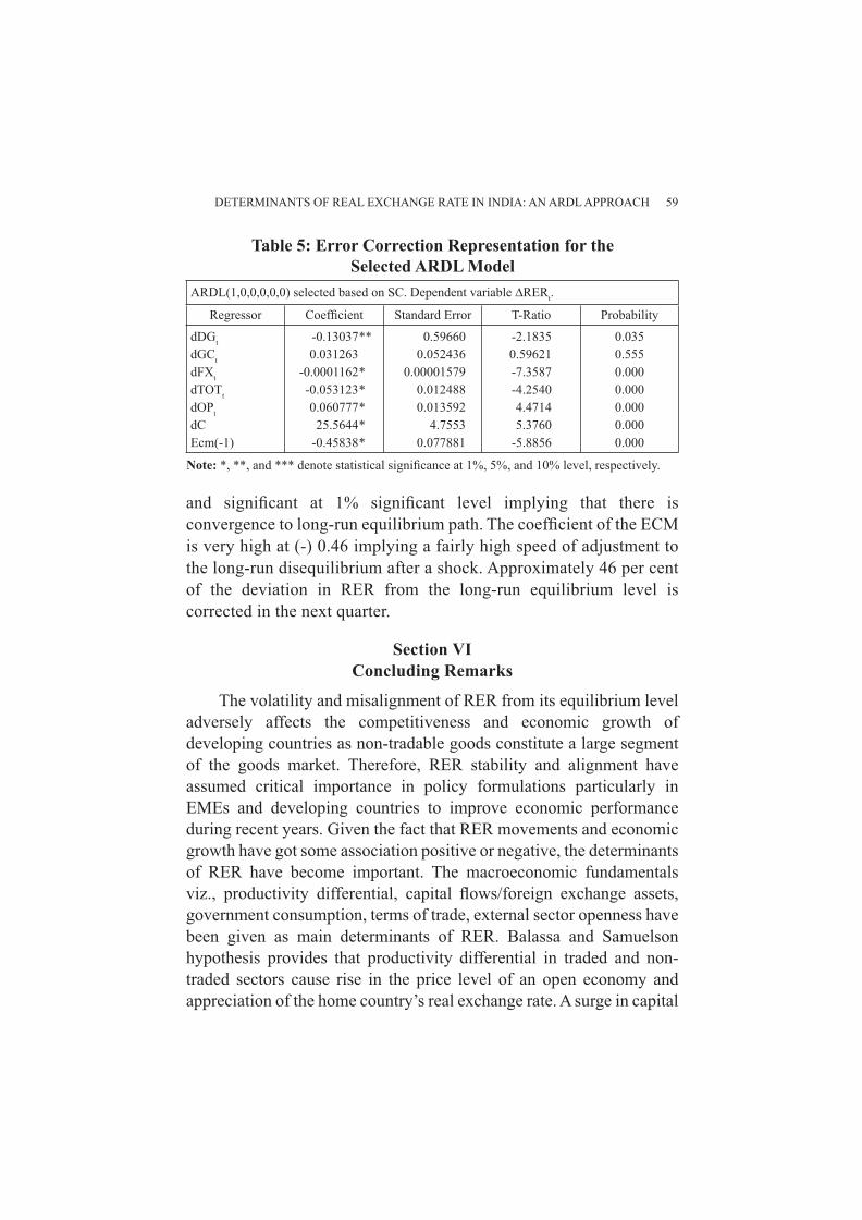
DETERMINANTS OF REAL EXCHANGE RATE IN INDIA: AN ARDL APPROACH 59
and signifi cant at 1% signifi cant level implying that there is convergence to long-run equilibrium path. The coeffi cient of the ECM is very high at (-) 0.46 implying a fairly high speed of adjustment to the long-run disequilibrium after a shock. Approximately 46 per cent of the deviation in RER from the long-run equilibrium level is corrected in the next quarter.
Section VIConcluding Remarks
The volatility and misalignment of RER from its equilibrium level adversely affects the competitiveness and economic growth of developing countries as non-tradable goods constitute a large segment of the goods market. Therefore, RER stability and alignment have assumed critical importance in policy formulations particularly in EMEs and developing countries to improve economic performance during recent years. Given the fact that RER movements and economic growth have got some association positive or negative, the determinants of RER have become important. The macroeconomic fundamentals viz., productivity differential, capital fl ows/foreign exchange assets, government consumption, terms of trade, external sector openness have been given as main determinants of RER. Balassa and Samuelson hypothesis provides that productivity differential in traded and non-traded sectors cause rise in the price level of an open economy and appreciation of the home country’s real exchange rate. A surge in capital
Table 5: Error Correction Representation for the Selected ARDL Model
ARDL(1,0,0,0,0,0) selected based on SC. Dependent variable ∆RERt.
Regressor Coeffi cient Standard Error T-Ratio Probability
dDGt -0.13037** 0.59660 -2.1835 0.035dGCt 0.031263 0.052436 0.59621 0.555dFXt -0.0001162* 0.00001579 -7.3587 0.000dTOTt -0.053123* 0.012488 -4.2540 0.000dOPt 0.060777* 0.013592 4.4714 0.000dC 25.5644* 4.7553 5.3760 0.000Ecm(-1) -0.45838* 0.077881 -5.8856 0.000
Note: *, **, and *** denote statistical signifi cance at 1%, 5%, and 10% level, respectively.
60 RESERVE BANK OF INDIA OCCASIONAL PAPERS
fl ows leads to an increase in aggregate demand and rise in the price of non-traded goods, which would eventually refl ect in appreciation of the real exchange rate. Furthermore, excess capital fl ows would lead to nominal appreciation in exchange rate. The government expenditure, which is disproportionately incurred on non-traded goods, leads to upward pressure on relative price of non-traded goods and appreciation in exchange rate. The deterioration in terms of trade generates negative income effect leading to decline in prices and eventually resulting into real depreciation of the exchange rate, while, at the same time it induces substitution effect in favour of non-traded goods increasing their prices and real appreciation in exchange rate. Increasing external openness of an economy may increase demand for imported goods and decline for demand of non-traded goods, which would result to decline in the prices of non-trade goods and real exchange rate depreciation. The impact of aforementioned macroeconomic fundamentals has been tested estimating ARDL cointegration model.
The bound tests of cointegration indicate that there exist a long-run relationship between RER and independent variables viz., differential growth, government consumption, net foreign assets, terms of trade and openness. The estimated coeffi cients of the long-run relationship show that productivity differential (differential growth), net foreign assets and terms of trade have negative sign and are signifi cant at 1% signifi cance level, indicating that increase in these variables lead to appreciation in RER. The long-run coeffi cient of openness is positive and signifi cant at 1% level of signifi cance implying that augmenting external sector openness result into depreciation of RER. The coeffi cient of government consumptions is, however, positively signed but it is not satistically signifi cant. Therefore, the results of long-run relationship establish that productivity differential, foreign assets, terms of trade and openness are main determinants of real exchange rare in India. Productivity differential exerts largest infl uence on the RER. Further, the signs of the short-run dynamic impact have been found consistent with long-run coeffi cients and error correction term is negative and signifi cant implying convergence to long-run equilibrium path. About 46 per cent at the deviation in the long-run equilibrium RER is corrected during the next quarter.
DETERMINANTS OF REAL EXCHANGE RATE IN INDIA: AN ARDL APPROACH 61
The appreciation in RER is generally seen as deterioration in the competitiveness of the traded goods sector. The results of present study, however, shows that appreciation in RER should not always be seen as decline in competitiveness as some of the factors contributing to appreciation in RER viz., increase in productivity differential and net foreign exchange assets and decline in terms of trade are attributed to higher growth refl ecting improvement in the traded goods sector competitiveness.
62 RESERVE BANK OF INDIA OCCASIONAL PAPERS
Notes:1 While theoretically, capital fl ows would equal to zero in the long-run, most less developed countries are expected to be capital importers for the future, therefore, most empirical studies of developing economies use a measure of sustainable capital fl ows rather than a zero capital account. Models of the RER in these countries often include capital fl ow as a determinant of the equilibrium real exchange rates (see Joyace and Kamas (2003)).
References:Aguirre and Calderon, (2005), “Real Exchange Rate Misalignments and Economic Performance,” Working Paper No. 316, Central Bank of Chile.Antonia, L.V. & Josep, L.R. Bara (2006), “The short and long-run determinants of the real exchange rate in Mexico,” Working Paper No. 0606, Department of Applied Economics at Universidad Autonoma of Barcelona.Antonia, L.V. (2006), “Real equilibrium exchange rates. A panel data approach for advanced and emerging economies,” Working Paper No. 0605, Department of Applied Economics at Universidad Autonoma of Barcelona.Balassa, B. (1964), “The purchasing power parity doctrine: a reappraisal”, The Journal of Political Economy, Vol.72, 584–96.Balassa, B. (1973), “Just how misleading are offi cial exchange rate conversions: a comment”, Economic Journal, 83, 1258–67.Clark, P. B, and MacDonald, R. (1998), “Exchange rates and economic fundamentals: a methodological comparison of BEERs and FEERs”, IMF Working Paper No. 67, International Monetary Fund, Washington D C.Clark, P. B, and MacDonald, R. (2000), “Filtering the BEER: a permanent and transitory decomposition”, IMF Working paper No. 144, International Monetary Fund, Washington D C.Clark, P. B, Bartolini, L., Bayoumi, T. & Symansky, S., (1994), “Exchange rates and economic fundamentals: a framework for analysis,” IMF Occasional Paper No. 115, International Monetary Fund, Washington D. C.Cottani, J.A., Cavallo, F. and Khan, Shahbaz (1990), ”Real Exchange Rate Behavior and Economic Performance in LDCs”, Economic Development and Cultural Change, Vol.39:61-76.De Gregorio J., Giovanni, A. and Wolf, H. C. (1994), “International evidence on tradables and non-tradables infl ation”, European Economic Journal, Vol. 38, 1225–44.
DETERMINANTS OF REAL EXCHANGE RATE IN INDIA: AN ARDL APPROACH 63
Diaz-Alejandro, Carlos F (1963), “A Note on the Impact of Devaluation and the Redistributive Effect,” The Journal of Political Economy, Vol.71 December.
Drine, Imed and Rault, Christophe (2005), “Can the Balassa-Samuelson theory explain long-run real exchange rate movements in OECD countries?”, Applied Financial Economics, Vol.15: 8, 519-530.
Edwards, Sebastian, (1989), “Real Exchange Rate, Devaluation and Adjustment”, The MIT Press, Cambridge.
Elbadawi, I., A. (1994), “Estimating Long-Run Equilibrium Exchange Rates” in Williamson, John, (eds), Estimating Equilibrium Exchange Rates, Institute for International Economics, Washington DC.
Elbadawi, Ibrahim, A. and Soto Raimundo, (1997), “Real Exchange Rates and Macroeconomic Adjustment in Sub-Saharan Africa and Other Developing Countries,” Journal of African Economies, Vol. 6(3), pages 74-120, Oxford University Press.
Froot, Kenneth A., and Kenneth Rogoff (1996), “Perspectives on PPP and Long-Run Real Exchange Rates,” NBER Working Paper No. 4952, April.
Ghura, D. and Grennes, T., J. (1993), “The Real Exchange Rate and Macroeconomic Performance in Sub-Saharan Africa”, Journal of Development Economics, Vol. 42: 155-174.
Hau, Harald (2006), “The Role of Transaction Costs for Financial Volatility: Evidence from the Paris Bourse,” Journal of the European Economic Association, MIT Press, vol. 4(4), pages 862-890, 06.
Hsieh, D., (1982), “The determination of the real exchange rate: the productivity approach”, Journal of International Economics, Vol. 12:355-24362.
Jorge Carrera and Romain Restout, (2008), “Long Run Determinants of Real Exchange Rates in Latin America,” Post-Print halshs-00276402_v1, HAL.
Krugman, Paul and Taylor, Lance (1978), “Contractionary effects of devaluation,” Journal of International Economics, Elsevier, Vol. 8(3), pages 445-456.
Krumm, K. (1993), “A Medium-Term Framework for Analysing the Real Exchange Rate, with Applications to the Philippines and Tanzania”, World Bank Economic Review, Vol. 7 : 219-49.
64 RESERVE BANK OF INDIA OCCASIONAL PAPERS
Lane, P., and G. Milessi-Ferreti (1999), “The External Wealth of Nations: Measures of Foreign assets and Liabilities for Industrial and Developing Countries,” CEPR Working Paper No. 2231.Lizondo, Saul and Peter J. Montiel (1989), “Contractionary Devaluation in Developing Countries: An Analytical Overview”, IMF Staff Papers, Vol. 36, pp. 182-227.Maeso-Fernandez, F., C. Osbat, and B. Schnatz (2001), “Determinants of the Euro Real Effective Exchange Rate: a BEER/PEER Approach,” European Central Bank Working Paper No. 85.Montiel, P.(1999a), “Determinants of the long run equilibrium real exchange rate: An analytical model”, in L. Hinkle and P. Montiel (eds.), Exchange rate misalignment: concepts and measurements for developing countries, World Bank, Washington D.C, pp. 264-290.Montiel, P. (1999b), “The long run equilibrium real exchange rate: Conceptual issues and empirical research”, in L. Hinkle & P. Montiel (eds.), Exchange rate misalignment: concepts and measurements for developing countries, World Bank, Washington D.C, pp. 219-263.Obstfeld, K. and Rogoff, P. (1996), “Foundation of International Macroeconomics”, MIT Press, Cambridge, MA.Pesaran, H.M and Pesaran, B (1997), “Working with Microfi t 4.0, Oxford University Press”, Oxford.Pesaran, H.M., Shin, Y. and Smith, R.J. (2000), “Structural analysis of vector error correction models with exogenous I(1) variables”, Journal of Econometrics, 97, pp. 293-343.Razin, O., and Collins, S. M.(1997), “Real exchange rate misalignment and growth”, Retrieved: March 2005”, available at http://econwpa.wustl.edu:80/eps/if/papers/9707/9707001.pdfRogoff, K. (1996), “The purchasing power parity puzzle”, Journal of Economic Literature, Vol.34, pp.647-668.Rosenberg, M. R.(2003), “The dollar’s equilibrium exchange rate: a market view”, in Dollar Overvaluation and the World Economy, Institute for International Economics, Washington, pp.35-55.Samuelson, P. (1964), “Theoretical notes and trade problems,” Review of Economics and Statistics, Vol. 46, pp.145-54.Sekkat, Khalid & Varoudakis, Aristomene (2000), “Exchange rate management and manufactured exports in Sub-Saharan Africa,” Journal of Development Economics, Elsevier, Vol. 61(1), pages 237-253, February.
Determinants of Overnight Index Swap (OIS) Rates: Some Empirical Findings from an
Emerging Market Economy, India
Saurabh Ghosh and Amarendra Acharya*
This paper uses the fi nancial sector variables over the last two years to analyse the determinants of the Overnight Index Swap (OIS) rates in India. Among the fi nancial variables considered, in the short run, Gsec rate and call rate had positive and signifi cant correlation with the OIS rate, while infl ation rate was not contemporaneously related with the OIS rate. The other factor that signifi cantly caused the OIS rate movement was the liquidity conditions in the Indian money market, measured by the difference between the call and repo rate. The above factors remained crucial even during and in the aftermath of the global fi nancial crisis. The impulse response functions indicated that the market was resilient to shocks. The long run equilibrium relationship between OIS, Gsec and Call rates was confi rmed by existence of at least one cointegrating vector. The coeffi cient of Gsec rate in the estimated cointegration was found to be positive and signifi cant. However, the coeffi cient of call rate was found to be negative (and low). It could indicate that a high (low) call rate today was expected to converge to the long term market expectation as indicated by the OIS rate. The error correction term, though negative, was not found to be statistically signifi cant at the conventional levels. This could be because of low volume in the OIS market, which is likely to pick up with further money market activities and future fi nancial product developments.
JEL Classifi cation : E40, G10, G31.
Keywords : Overnight Index Swap, OIS, Money Market, Yields, Overnight Rate, Infl ation.
Introduction
Interest risk management has assumed predominant importance in the management of any fi nancial institution after the deregulation of the interest rates. In the deregulated market, every fi nancial
* The authors are Assistant Adviser and Research Offi cer, respectively, in the Financial Markets Department of the RBI. Views expressed by the authors are their personal and not necessarily of the organization that they belong to. The suggestion of Shri Sudarsana Sahoo and Shri Puneet Pancholy, AGM, FMD are gratefully acknowledged.
Reserve Bank of India Occasional PapersVol. 31, No.1, Summer 2010
66 RESERVE BANK OF INDIA OCCASIONAL PAPERS
organization recognizes and quantifi es its risk-taking appetite. Banks and corporates face the risks on their investment portfolios, cost of raising working capital on account of the volatility in the movement of interest rates. One of the commonly used risk management practices is the use of overnight index swap (OIS). It is one type of interest rate swaps where the fl oating leg of the swap is linked to an overnight index, compounded every day over of the payment period. The parties agree to exchange the difference in the accrued interest arrived according to the fi xed and fl oating interest rates at the maturity on the notional principal amount.
Use of OIS generally brings many benefi ts to the fi nancial community. OIS helps in hedging the interest rate risks. Additional benefi ts include reduction of credit risk, creation of synthetic overnight-index-linked liability for corporates, etc.. It allows the fi nancial institutions the fl exibility to move to the interest rate basis of its choice, manage various features of their debt portfolios, the duration of its investment portfolio.
Research in money market microstructure is a relatively recent development and has mainly focused on developed markets. In contrast, research on emerging market economies (EMEs) is rather limited - perhaps because of the narrow and underdeveloped nature of the market in such economies. This paper makes an attempt to address this anomaly by analysis of relationship of the OIS rates with other fi nancial variables. In particular, we attempt an evaluation of the determinants of Overnight Index Swap (OIS) rate and the causal relation between OIS rate and different fi nancial variables, their short run and long run relationship. This paper is organized as follows: Section 2 concentrates on the cross country experience, Section 3 describes the data, Section 4 devotes itself to the empirical analysis and Section 5 concludes the major fi ndings. Finally, OIS and Call rates around the recent policy dates and the market expectations (gathered from different print media) are reported in Table A1 and A2 in Annex, respectively.
DETERMINANTS OF OVERNIGHT INDEX SWAP (OIS) RATES 67
Section II
Cross Country Experience While not many academic articles on OIS were available in the public domain, reasonable literature search on the subject found the following: In Australia the overnight index swap market started in late 1999, and has witnessed rapid growth in the subsequent years. The market is more liquid in relatively shorter end as compared with its longer counterpart. The liquidity in the OIS market makes it useful in forecasting the market expectations about the future movement of the Cash rate, though they are not perfect indicator of the same. In Australia, banks are the main players in the overnight interest rate swaps market. In view of its success, some Australian investment banks and fi xed-income brokers introduced the OIS in the New Zealand markets (February 2002). However, there were no formal price-making arrangements in the OIS market of New Zealand. Trades between banks and their institutional clients were also low. A few Australian investment banks dominated the market, and the domestic players were insignifi cant. The turnover in the OIS market was only around 10 per cent of the more established FRA and bank bills futures market in New Zealand. The trades were mostly for taking a view on the direction and magnitude of changes in the offi cial cash rate (OCR) so far. The OIS market remained more developed and broad-based in Australia as compared with New Zealand. In Japan the OIS was launched in mid-1997 but it remained shallow till recently. The main reasons were the prevailing effective zero overnight interest rates and very low short-term interest rates. As the bankers did not need to hedge against short-term interest rate risks, there was no need for the fi nancial institutions to operate in this OIS market. The OIS transactions began to grow as market participants expected the end of the Quantitative easing Policy before the crisis. Gradually, the OIS transaction volume exceeded that of all non-OIS interest rate swaps with terms of less than one year. The Japanese fi nancial institutions benefi ted from utilizing the OIS by directly managing the risk of a rise in overnight rates and from the possibility of arbitrage opportunities. As the Japanese money markets become more active and interest rates become more volatile, demands for hedging
68 RESERVE BANK OF INDIA OCCASIONAL PAPERS
and arbitrage operations are expected to grow further; and consequently the Japanese OIS market is expected to be more broad-based and liquid.
The ushering of the global economic crisis / sub-prime crisis brought to fore a new variable as a measure of fi nancial health. The measure is the spread between 3-month LIBOR and the 3-month Overnight Index Swap (OIS) rate. The OIS rate is a measure of market expectation of the money market rates. Expectations also play major roles on all term loans, inlcluding 3-month LIBOR. The difference between LIBOR and OIS rate thus captures factors other than interest rate expectations, such as credit and liquidity risks (Taylor 2008). An increase in the spread, holding the OIS constant, will increase the cost of such loans and have a contractionary effect on the economy. Bringing this spread down therefore became a major objective of monetary policy, as well as a measure of its success in dealing with the market turmoil.
The Interest rate swaps in India is relatively new, with the fi rst interest rate swap being traded in July 1999. Among the Interest rate swaps, the OIS is the most popular and liquid. As the name implies the benchmark here is the overnight rate. The fl oating benchmark is MIBOR (Mumbai inter-bank offered rate), against which the swap is settled. The fl oating leg of the transaction is compounded and settled only at pre-decided frequency (generally semi-annually). Though OIS are quoted in different maturities, anecdotal evidence indicates that tenors upto fi ve-year are liquid (according to the number of deals). In India the OIS market is generally dominated by the foreign banks and some of the segments of the OIS market remain quite illiquid.
Section III
Data and Descriptive Statistics
This study concentrates on the last two-and-half year daily data on one-year and fi ve-year OIS rates (from August 2007 to November 2009) and attempts to identify their determinants. The major data sources for this study are the Reuters database and Weekly Statistical Supplement. The rate / fi nancial sector variables considered for this study are as follows:
� 1-year FIMMDA generic yield (Gsec1);
DETERMINANTS OF OVERNIGHT INDEX SWAP (OIS) RATES 69
� 5-year FIMMDA generic yield (Gsec5);
� Call/notice money market rate(CALL);
� Repo Rate, Reverse Repo rate & Cash reserve ratio (CRR);
� Call money spread (call_spd) is the difference between the Call rate and the repo rate (Call_spd), and the increase in the same is an indicator of the stringent liquidity conditions in the inter-bank money market.
� Weekly WPI Infl ation Rate (the infl ation rate is repeated for other days of the week). For October and November 2009, the infl ation rate is repeated for all days in the month.
The choice of these variables was guided by opportunity cost and liquidity considerations, and supply/demand situation in the underlying and OIS market. From the cost angle 1-year and 5-year Government security yields were taken as measures of benchmark risk-free interest rates of one-year and fi ve-year maturities. The call rate and the call spread were included as indicators of overall liquidity in the system.
Trends in One-year and fi ve-year OIS rate
The trends in the one-year and fi ve-year OIS rates along with Gsec rate during the period under consideration are plotted in Chart 1.
As evident from the above chart, there have been three distinct phases in the OIS market. In the fi rst phase, i.e. from August 2007 to June 2008, the OIS rate followed an increasing trend in general, which refl ected the infl ationary pressures, cumulative increase in CRR and increase in the repo rate. Beginning July 2008, there was a change in the underlying trend and the OIS rate generally declined, perhaps refl ecting the global fi nancial crisis, expectations for the easing rate and liquidity conditions in the Indian money markets. Finally, from beginning of December 2008, the rate in the OIS market started increasing gradually. In the entire period under consideration the data indicated a close co-movement between OIS rates and Gsec
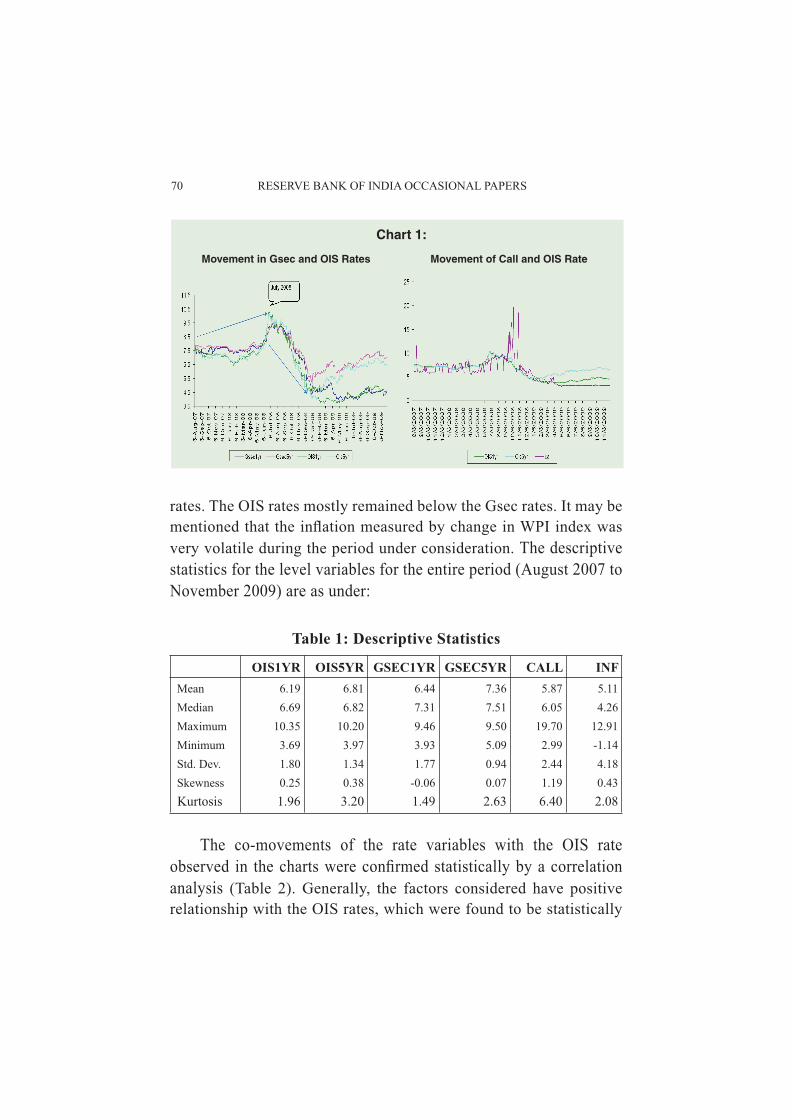
70 RESERVE BANK OF INDIA OCCASIONAL PAPERS
Table 1: Descriptive Statistics
OIS1YR OIS5YR GSEC1YR GSEC5YR CALL INF Mean 6.19 6.81 6.44 7.36 5.87 5.11 Median 6.69 6.82 7.31 7.51 6.05 4.26 Maximum 10.35 10.20 9.46 9.50 19.70 12.91 Minimum 3.69 3.97 3.93 5.09 2.99 -1.14 Std. Dev. 1.80 1.34 1.77 0.94 2.44 4.18 Skewness 0.25 0.38 -0.06 0.07 1.19 0.43 Kurtosis 1.96 3.20 1.49 2.63 6.40 2.08
rates. The OIS rates mostly remained below the Gsec rates. It may be mentioned that the infl ation measured by change in WPI index was very volatile during the period under consideration. The descriptive statistics for the level variables for the entire period (August 2007 to November 2009) are as under:
The co-movements of the rate variables with the OIS rate observed in the charts were confi rmed statistically by a correlation analysis (Table 2). Generally, the factors considered have positive relationship with the OIS rates, which were found to be statistically
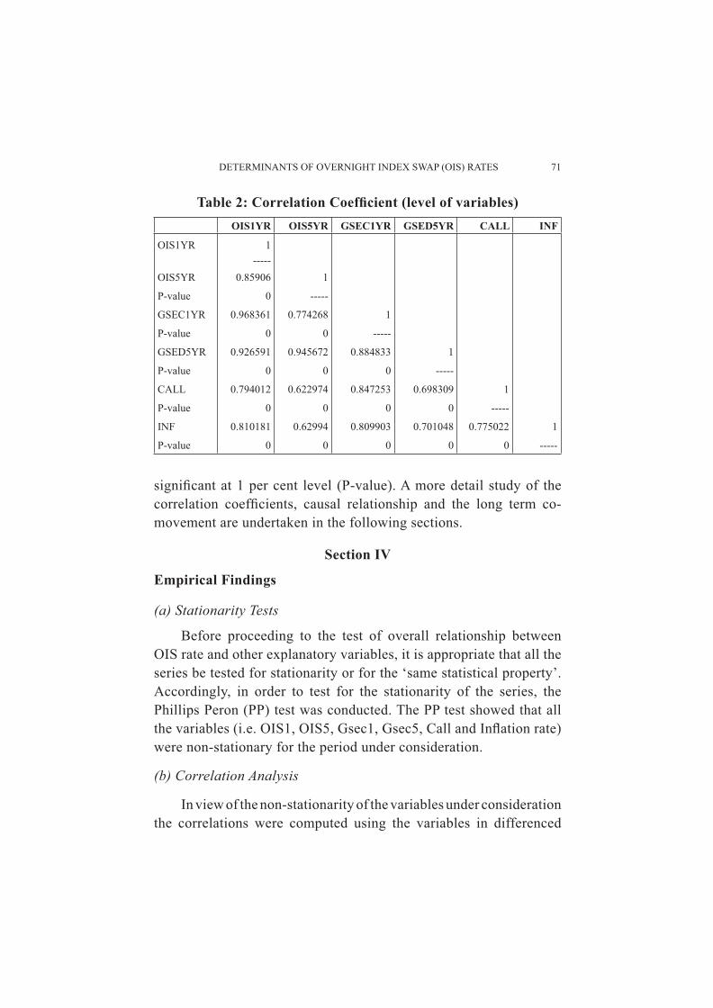
DETERMINANTS OF OVERNIGHT INDEX SWAP (OIS) RATES 71
signifi cant at 1 per cent level (P-value). A more detail study of the correlation coeffi cients, causal relationship and the long term co-movement are undertaken in the following sections.
Section IV
Empirical Findings
(a) Stationarity Tests
Before proceeding to the test of overall relationship between OIS rate and other explanatory variables, it is appropriate that all the series be tested for stationarity or for the ‘same statistical property’. Accordingly, in order to test for the stationarity of the series, the Phillips Peron (PP) test was conducted. The PP test showed that all the variables (i.e. OIS1, OIS5, Gsec1, Gsec5, Call and Infl ation rate) were non-stationary for the period under consideration.
(b) Correlation Analysis
In view of the non-stationarity of the variables under consideration the correlations were computed using the variables in differenced
Table 2: Correlation Coeffi cient (level of variables)OIS1YR OIS5YR GSEC1YR GSED5YR CALL INF
OIS1YR 1-----
OIS5YR 0.85906 1
P-value 0 -----
GSEC1YR 0.968361 0.774268 1
P-value 0 0 -----
GSED5YR 0.926591 0.945672 0.884833 1
P-value 0 0 0 -----
CALL 0.794012 0.622974 0.847253 0.698309 1
P-value 0 0 0 0 -----
INF 0.810181 0.62994 0.809903 0.701048 0.775022 1
P-value 0 0 0 0 0 -----
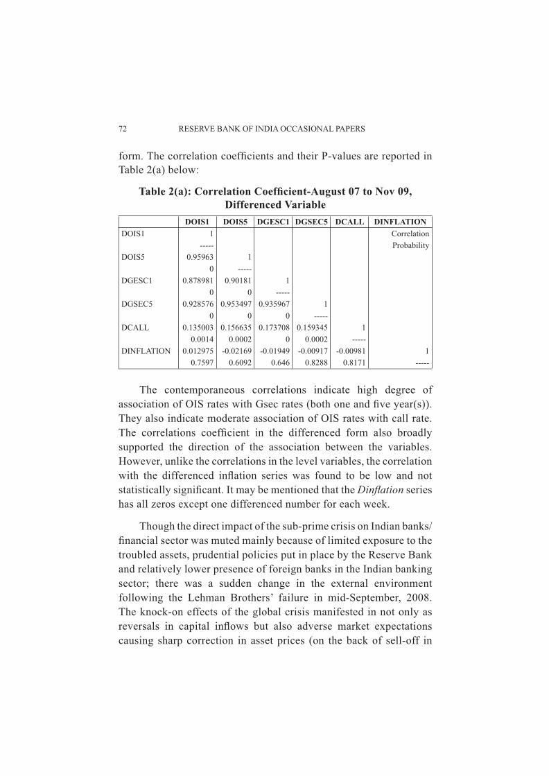
72 RESERVE BANK OF INDIA OCCASIONAL PAPERS
form. The correlation coeffi cients and their P-values are reported in Table 2(a) below:
Table 2(a): Correlation Coeffi cient-August 07 to Nov 09, Differenced Variable
DOIS1 DOIS5 DGESC1 DGSEC5 DCALL DINFLATIONDOIS1 1 Correlation
----- ProbabilityDOIS5 0.95963 1
0 -----DGESC1 0.878981 0.90181 1
0 0 -----DGSEC5 0.928576 0.953497 0.935967 1
0 0 0 -----DCALL 0.135003 0.156635 0.173708 0.159345 1
0.0014 0.0002 0 0.0002 -----DINFLATION 0.012975 -0.02169 -0.01949 -0.00917 -0.00981 1
0.7597 0.6092 0.646 0.8288 0.8171 -----
The contemporaneous correlations indicate high degree of association of OIS rates with Gsec rates (both one and fi ve year(s)). They also indicate moderate association of OIS rates with call rate. The correlations coeffi cient in the differenced form also broadly supported the direction of the association between the variables. However, unlike the correlations in the level variables, the correlation with the differenced infl ation series was found to be low and not statistically signifi cant. It may be mentioned that the Dinfl ation series has all zeros except one differenced number for each week.
Though the direct impact of the sub-prime crisis on Indian banks/fi nancial sector was muted mainly because of limited exposure to the troubled assets, prudential policies put in place by the Reserve Bank and relatively lower presence of foreign banks in the Indian banking sector; there was a sudden change in the external environment following the Lehman Brothers’ failure in mid-September, 2008. The knock-on effects of the global crisis manifested in not only as reversals in capital infl ows but also adverse market expectations causing sharp correction in asset prices (on the back of sell-off in
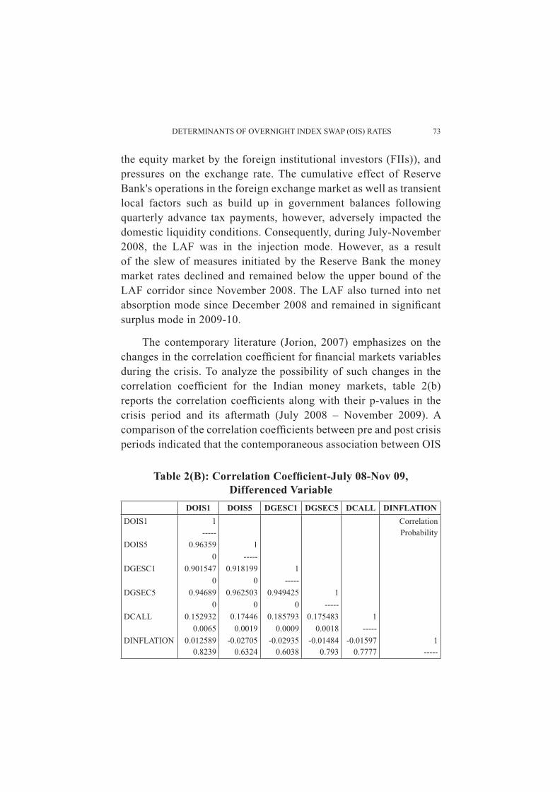
DETERMINANTS OF OVERNIGHT INDEX SWAP (OIS) RATES 73
the equity market by the foreign institutional investors (FIIs)), and pressures on the exchange rate. The cumulative effect of Reserve Bank's operations in the foreign exchange market as well as transient local factors such as build up in government balances following quarterly advance tax payments, however, adversely impacted the domestic liquidity conditions. Consequently, during July-November 2008, the LAF was in the injection mode. However, as a result of the slew of measures initiated by the Reserve Bank the money market rates declined and remained below the upper bound of the LAF corridor since November 2008. The LAF also turned into net absorption mode since December 2008 and remained in signifi cant surplus mode in 2009-10.
The contemporary literature (Jorion, 2007) emphasizes on the changes in the correlation coeffi cient for fi nancial markets variables during the crisis. To analyze the possibility of such changes in the correlation coeffi cient for the Indian money markets, table 2(b) reports the correlation coeffi cients along with their p-values in the crisis period and its aftermath (July 2008 – November 2009). A comparison of the correlation coeffi cients between pre and post crisis periods indicated that the contemporaneous association between OIS
Table 2(B): Correlation Coeffi cient-July 08-Nov 09, Differenced Variable
DOIS1 DOIS5 DGESC1 DGSEC5 DCALL DINFLATIONDOIS1 1 Correlation
----- ProbabilityDOIS5 0.96359 1
0 -----DGESC1 0.901547 0.918199 1
0 0 -----DGSEC5 0.94689 0.962503 0.949425 1
0 0 0 -----DCALL 0.152932 0.17446 0.185793 0.175483 1
0.0065 0.0019 0.0009 0.0018 -----DINFLATION 0.012589 -0.02705 -0.02935 -0.01484 -0.01597 1
0.8239 0.6324 0.6038 0.793 0.7777 -----
74 RESERVE BANK OF INDIA OCCASIONAL PAPERS
rate and Gsec rate generally remained unchanged. However, the sensitivity to changes in OIS rate and Gsec rates has increased in the second period (July 08–November 09) as compared with the entire period. There has also been marginal increase in association between OIS rate and call rate in the second period as compared with the entire period. The relationship between differenced infl ation and the other differenced variables, however, continues to remain small and insignifi cant.
(c) Causality Analysis
The sections above concentrated on the contemporaneous association between the variables. In an attempt to analyze the causal relationship among these variables (taking into account the lead & lagged effects) and the direction of such causality, we undertook pair-wise Granger causality test. In general, the test considers the lagged values of the dependent variable1 and the explanatory variable and evaluates the incremental explanatory power of the second set of variable on the fi rst. The different pair of variables considered for the causality test along with their F-Statistics and P-values are reported in the Table 3.
The F-Statistics and their P-values for the entire period under consideration indicate that the yield on Government securities (both 1 year and 5 year) were the major factors driving the OIS rate movements. But the reverse (i.e. the bi-directional) causality was not found to be statistically signifi cant. It may be mentioned that the number of participants are much larger in the Gsec market (as compared to the OIS market), as Gsec forms a part of the statutory requirement (SLR) in India. Moreover, the Gsec is a funding based instrument while OIS is more of a (notional principal) hedging instrument which is settled by netting the difference. Therefore, the rate discovery has taken place in the Gsec market and it has percolated to the OIS market and not vice-versa. The other factor, which caused the 5-year OIS for the entire period was the call spread (difference between Call rate and repo rate), an indicator of liquidity conditions.
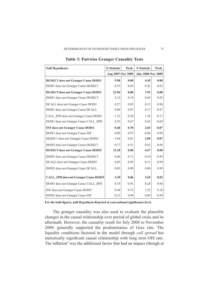
DETERMINANTS OF OVERNIGHT INDEX SWAP (OIS) RATES 75
The granger causality was also used to evaluate the plausible changes in the causal relationship over period of global crisis and its aftermath. However, the causality result for July 2008 to November 2009, generally supported the predominance of Gsec rate. The liquidity conditions factored in the model through call spread has statistically signifi cant causal relationship with long term OIS rate. The infl ation2 was the additional factor that had an impact (though at
Table 3: Pairwise Granger Causality Tests
Null Hypothesis: F-Statistic Prob. F-Statistic Prob.
Aug 2007-Nov 2009 July 2008-Nov 2009
DGSEC1 does not Granger Cause DOIS1 9.98 0.00 4.45 0.00
DOIS1 does not Granger Cause DGSEC1 0.55 0.65 0.42 0.83
DGSEC5 does not Granger Cause DOIS1 22.96 0.00 7.93 0.00
DOIS1 does not Granger Cause DGSEC5 2.12 0.10 0.45 0.82
DCALL does not Granger Cause DOIS1 0.27 0.85 0.15 0.98
DOIS1 does not Granger Cause DCALL 0.09 0.97 0.17 0.97
CALL_SPD does not Granger Cause DOIS1 1.33 0.26 1.58 0.17
DOIS1 does not Granger Cause CALL_SPD 0.52 0.67 0.62 0.69
INF does not Granger Cause DOIS1 0.48 0.70 2.03 0.07
DOIS1 does not Granger Cause INF 0.09 0.97 0.06 0.99
DGSEC1 does not Granger Cause DOIS5 3.64 0.01 2.09 0.07
DOIS5 does not Granger Cause DGSEC1 0.77 0.51 0.62 0.68
DGSEC5 does not Granger Cause DOIS5 12.18 0.00 4.67 0.00
DOIS5 does not Granger Cause DGSEC5 0.46 0.71 0.10 0.99
DCALL does not Granger Cause DOIS5 0.05 0.99 0.11 0.99
DOIS5 does not Granger Cause DCALL 0.03 0.99 0.08 0.99
CALL_SPD does not Granger Cause DOIS5 2.49 0.06 2.65 0.02
DOIS5 does not Granger Cause CALL_SPD 0.18 0.91 0.24 0.94
INF does not Granger Cause DOIS5 0.44 0.72 1.52 0.18
DOIS5 does not Granger Cause INF 0.13 0.94 0.09 0.99
For the bold fi gures, null Hypothesis Rejected at conventional signifi cance level.
76 RESERVE BANK OF INDIA OCCASIONAL PAPERS
lower confi dence level) on the long term OIS rate during July 2008 to November 2009. It may be mentioned that there was a large swing in the infl ation rate during the period under consideration, which could explain the observed causal relationship.
(d) Impulse Response Function
The above section indicated existence of causal relationship between changes in OIS rate to changes in Gsec rate, call rate, and infl ation. In this section we investigate the direction and magnitude of such change on OIS' rate in the short run. In particular we attempt to analyze the impact of a shock / impulse in call rate and Gsec rates on the OIS rates.
For analyzing the same a three equation Vector Auto Regression (VAR) model was estimated using differenced OIS rate, call rate, Gsec yields and their lagged (with three lags) values. Infl ation was used in their levels to minimize information loss. One of the major criticisms of unrestricted VAR models is that they are susceptible to ordering of variables. We tried to address this shortcoming by using Generalized Impulse Response function. Generalized Impulses, as described by Pesaran and Shin (1998), construct an orthogonal set of innovations that does not depend on the VAR ordering. The generalized impulse responses from an innovation to the j-th variable are derived by applying a variable specifi c Cholesky factor computed with the j-th variable at the top of the Cholesky ordering (Eviews User Guide).
Using the estimated set of equations, generalized impulse responses of a change in the above-mentioned three variables were plotted in Chart -3. The impulse response charts indicated the following:
� The impulse to infl ation has a miniscule impact on OIS. The impact of one standard deviation shock to call had more noticeable impact on the OIS rate in the fi rst period. The maximum impact was observed in the case of one SD generalized shock to the one-year Government Securities rate. These shocks had similar impact for one-year and fi ve-year OIS rates.
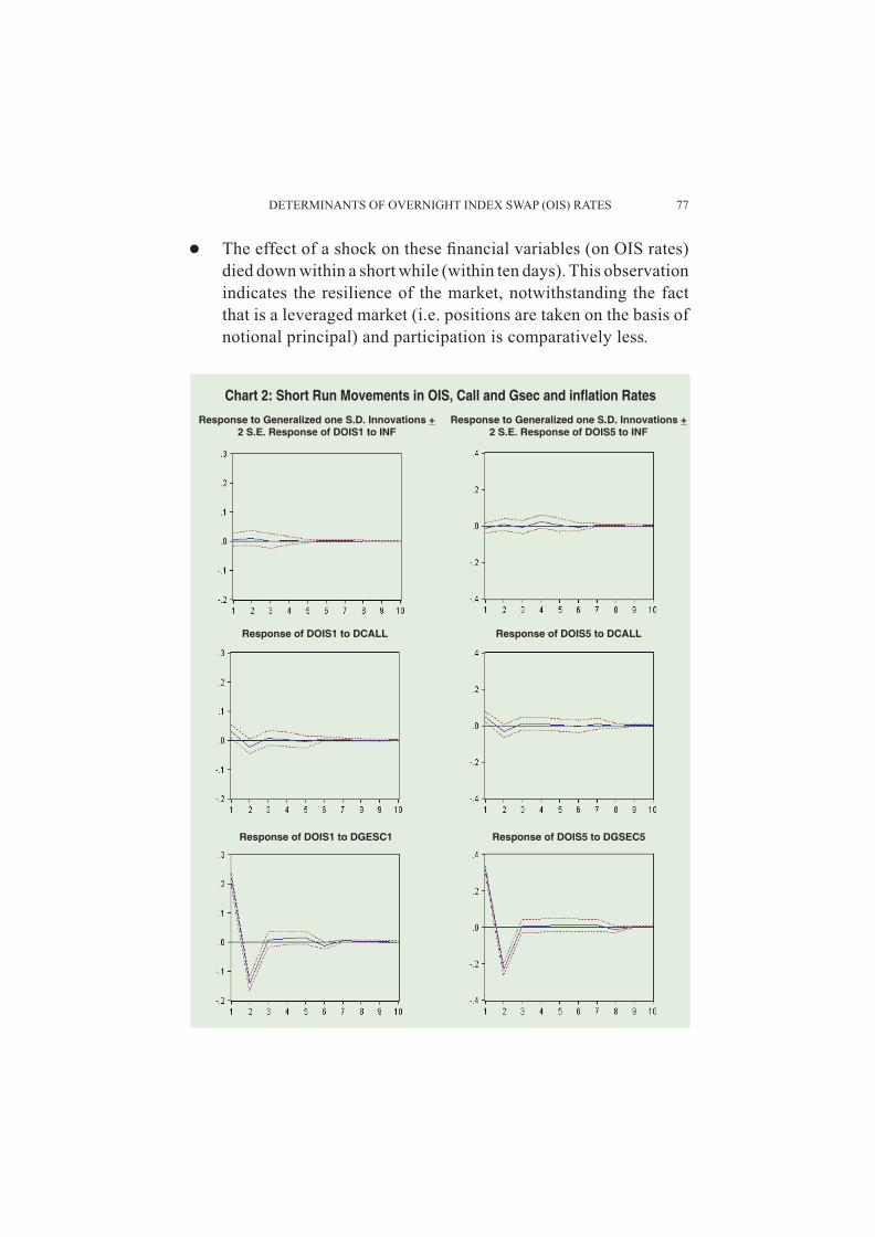
DETERMINANTS OF OVERNIGHT INDEX SWAP (OIS) RATES 77
� The effect of a shock on these fi nancial variables (on OIS rates) died down within a short while (within ten days). This observation indicates the resilience of the market, notwithstanding the fact that is a leveraged market (i.e. positions are taken on the basis of notional principal) and participation is comparatively less.
78 RESERVE BANK OF INDIA OCCASIONAL PAPERS
(e) Long Run Cointegration Analysis
So far we have analysed the short run impacts of other fi nancial market variables on the OIS rate. In this section we consider the possible long run co-movement of the rate variables. The OIS, Gsec, Call were found to be non-stationary. Therefore, the long run equilibrium relation among them is best established using cointegration approach. This involves testing for the null hypothesis that there are no cointegrating vectors. On the basis of sample data, if this null is rejected, then the cointegrating vector is estimated using a Vector Error Correction Model (VECM). Using the full sample period (August 2007 to November 2009) the estimated value for the test statistic leads to the rejection of the null hypothesis under different assumptions (both the trace and Max-eigenvalue test) and indicate existence of at least one cointegrating vector at 5 per cent level of signifi cance.
After confi rming the existence of contegrating vector, using the Johansen methodology (1991), the Vector error correction model was estimated. A dummy variable for the period July 2008 to November 2008 was introduced as an exogenous variable in the cointegrating VAR. The estimated long run cointegration vector is as follows (fi gures in the parenthesis report the t-statistic values).
OIS5= -9.06+ 2.94*Gsec5 - 0.99*Call; Error correction term = -0.002 (7.93) (5.96) (-0.63)
In the estimated cointegration equation, the Gsec yield has expected (positive) sign and is signifi cant at 1 per cent level, indicating co-movement of fi ve year OIS and Gsec rates. A negative relationship between call and OIS rate, on the other hand, may appear counterintuitive in nature. However, it could actually indicate the long term expectations of the market participants. The call rate today could be high (low) depending on the demand and supply conditions in the market; however the fi ve-year OIS rate adjust accordingly taking into account the long term expectation of the money market rates.
DETERMINANTS OF OVERNIGHT INDEX SWAP (OIS) RATES 79
The error correction term has the right (negative) sign. As expected, the magnitude of the same is low mainly because (as the study uses daily data) it represents daily adjustment to the disequilibrium. However, the coeffi cient is statistically insignifi cant at 10 per cent level. It makes the adjustment to the equilibrium path weak. The signifi cance could improve with the increase in depth and liquidity in the Indian OIS markets. It might be mentioned that the major market makers in the OIS market in India are the handful of foreign banks and the volume of trade are slowly picking up.
Section V
Conclusions
There haven’t been many published studies on the Overnight Index Swap (OIS) for an Emerging economy. This study is an attempt in this direction, which concentrated on India. In India, the overnight market started in July 1999 and gradually developed. Anecdotal evidences suggest that the volume in the OIS market has remained low as compared with the Gsec market and the private/foreign banks have remained the major players in this market.
Among the fi nancial variables considered in this study, the Gsec rate had high and signifi cant positive contemporaneous correlation with the OIS rate. The call rate was also found to have positive and signifi cant correlation with OIS rate. However, the infl ation rate was not found to be contemporaneously related with the OIS rate. The above correlation didn’t considerably change during the global fi nancial crisis or in its aftermath. This could be because of the fact that the global fi nancial crisis had a muted impact on the Indian economy.
The causality analysis generally indicated unidirectional causality from Gsec to OIS rate. The other factor that signifi cantly caused the OIS movement was the liquidity conditions in the Indian money market, measured by the difference between the call and repo rate. While the above factors remained crucial even during and in the aftermath of the global fi nancial crisis, infl ation became a factor causing one year OIS movement in the post-crisis period. It may be mentioned in this context that infl ation changed considerably during
80 RESERVE BANK OF INDIA OCCASIONAL PAPERS
and after the crisis period. Call rate didn’t signifi cantly cause the OIS rates or vice-versa. This could be because of the fact that the causality analysis results are indicative of a short period adjustment (as the lag length of three days is selected through HQ information criteria).
Anecdotal evidences suggested shocks to fi nancial variables affect OIS rate movement. To evaluate the impact of such impulses, the generalized impulse response functions were considered. In this framework, the one standard deviation shocks to infl ation, differenced gsec rate and differenced call rate positively impacted the OIS rate in the 1st period. However, the impact of such shocks died down over a ten working day period indicating the resilience of the OIS market.
Moving to the long-run equilibrium relationship between OIS rate, call rate and the Gsec rate, the test for cointegration indicated the presence of at least one conitegrating vector. The coeffi cient of Gsec rate in the estimated cointegration was found to be positive and signifi cant. However, the coeffi cient of call rate was found to be negative (and low). It could indicate that a high (low) call rate today was expected to coverage to the long term market expectation as indicated by the OIS rate. The error correction term, though negative, was not found to be statistically signifi cant at the conventional levels. This could be because of low volume in the OIS market, which is likely to pick up with further money market activities and future fi nancial product developments.
While this is just the beginning, the road ahead for some of the empirical research in this area includes (a) the issues relating to the predictive power of the OIS rate, (b) the behavior of the MIBOR-OIS spread for India during different phases and (c) the reasons for OIS rate being lower than the risk free GoI bond rate.
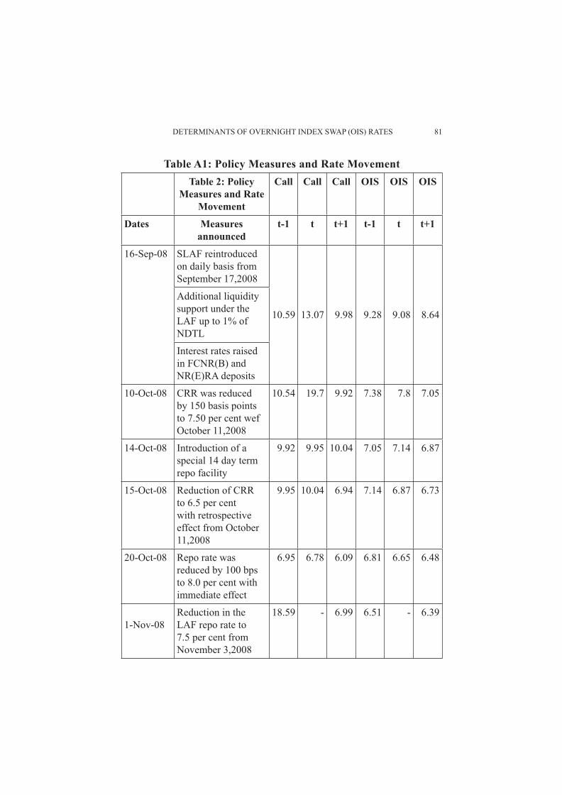
DETERMINANTS OF OVERNIGHT INDEX SWAP (OIS) RATES 81
Table A1: Policy Measures and Rate MovementTable 2: Policy
Measures and Rate Movement
Call Call Call OIS OIS OIS
Dates Measures announced
t-1 t t+1 t-1 t t+1
16-Sep-08 SLAF reintroduced on daily basis from September 17,2008
Additional liquidity support under the LAF up to 1% of NDTL
10.59 13.07 9.98 9.28 9.08 8.64
Interest rates raised in FCNR(B) and NR(E)RA deposits
10-Oct-08 CRR was reduced by 150 basis points to 7.50 per cent wef October 11,2008
10.54 19.7 9.92 7.38 7.8 7.05
14-Oct-08 Introduction of a special 14 day term repo facility
9.92 9.95 10.04 7.05 7.14 6.87
15-Oct-08 Reduction of CRR to 6.5 per cent with retrospective effect from October 11,2008
9.95 10.04 6.94 7.14 6.87 6.73
20-Oct-08 Repo rate was reduced by 100 bps to 8.0 per cent with immediate effect
6.95 6.78 6.09 6.81 6.65 6.48
1-Nov-08Reduction in the LAF repo rate to 7.5 per cent from November 3,2008
18.59 - 6.99 6.51 - 6.39
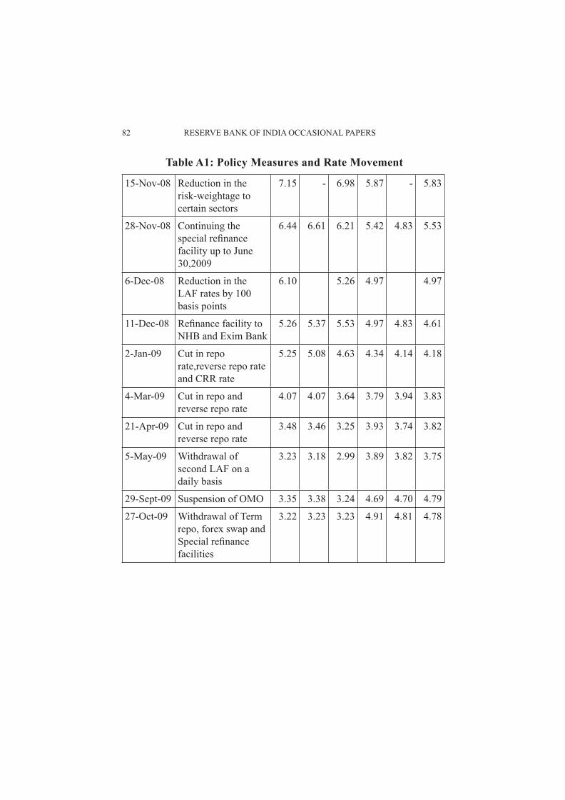
82 RESERVE BANK OF INDIA OCCASIONAL PAPERS
15-Nov-08 Reduction in the risk-weightage to certain sectors
7.15 - 6.98 5.87 - 5.83
28-Nov-08 Continuing the special refi nance facility up to June 30,2009
6.44 6.61 6.21 5.42 4.83 5.53
6-Dec-08 Reduction in the LAF rates by 100 basis points
6.10 5.26 4.97 4.97
11-Dec-08 Refi nance facility to NHB and Exim Bank
5.26 5.37 5.53 4.97 4.83 4.61
2-Jan-09 Cut in repo rate,reverse repo rate and CRR rate
5.25 5.08 4.63 4.34 4.14 4.18
4-Mar-09 Cut in repo and reverse repo rate
4.07 4.07 3.64 3.79 3.94 3.83
21-Apr-09 Cut in repo and reverse repo rate
3.48 3.46 3.25 3.93 3.74 3.82
5-May-09 Withdrawal of second LAF on a daily basis
3.23 3.18 2.99 3.89 3.82 3.75
29-Sept-09 Suspension of OMO 3.35 3.38 3.24 4.69 4.70 4.79
27-Oct-09 Withdrawal of Term repo, forex swap and Special refi nance facilities
3.22 3.23 3.23 4.91 4.81 4.78
Table A1: Policy Measures and Rate Movement
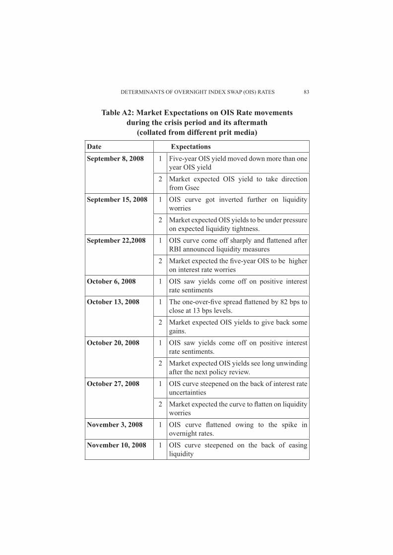
DETERMINANTS OF OVERNIGHT INDEX SWAP (OIS) RATES 83
Table A2: Market Expectations on OIS Rate movements during the crisis period and its aftermath
(collated from different prit media)
Date ExpectationsSeptember 8, 2008 1 Five-year OIS yield moved down more than one
year OIS yield2 Market expected OIS yield to take direction
from GsecSeptember 15, 2008 1 OIS curve got inverted further on liquidity
worries2 Market expected OIS yields to be under pressure
on expected liquidity tightness.September 22,2008 1 OIS curve come off sharply and fl attened after
RBI announced liquidity measures2 Market expected the fi ve-year OIS to be higher
on interest rate worriesOctober 6, 2008 1 OIS saw yields come off on positive interest
rate sentimentsOctober 13, 2008 1 The one-over-fi ve spread fl attened by 82 bps to
close at 13 bps levels.2 Market expected OIS yields to give back some
gains.October 20, 2008 1 OIS saw yields come off on positive interest
rate sentiments.2 Market expected OIS yields see long unwinding
after the next policy review.October 27, 2008 1 OIS curve steepened on the back of interest rate
uncertainties2 Market expected the curve to fl atten on liquidity
worriesNovember 3, 2008 1 OIS curve fl attened owing to the spike in
overnight rates.November 10, 2008 1 OIS curve steepened on the back of easing
liquidity
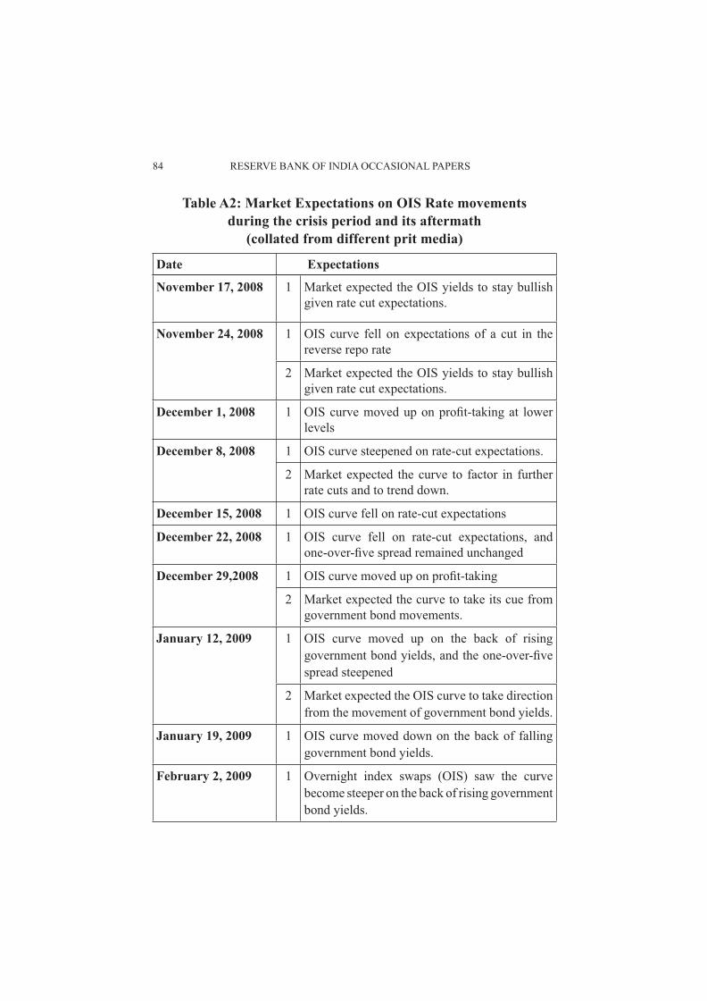
84 RESERVE BANK OF INDIA OCCASIONAL PAPERS
November 17, 2008 1 Market expected the OIS yields to stay bullish given rate cut expectations.
November 24, 2008 1 OIS curve fell on expectations of a cut in the reverse repo rate
2 Market expected the OIS yields to stay bullish given rate cut expectations.
December 1, 2008 1 OIS curve moved up on profi t-taking at lower levels
December 8, 2008 1 OIS curve steepened on rate-cut expectations.
2 Market expected the curve to factor in further rate cuts and to trend down.
December 15, 2008 1 OIS curve fell on rate-cut expectations
December 22, 2008 1 OIS curve fell on rate-cut expectations, and one-over-fi ve spread remained unchanged
December 29,2008 1 OIS curve moved up on profi t-taking
2 Market expected the curve to take its cue from government bond movements.
January 12, 2009 1 OIS curve moved up on the back of rising government bond yields, and the one-over-fi ve spread steepened
2 Market expected the OIS curve to take direction from the movement of government bond yields.
January 19, 2009 1 OIS curve moved down on the back of falling government bond yields.
February 2, 2009 1 Overnight index swaps (OIS) saw the curve become steeper on the back of rising government bond yields.
Table A2: Market Expectations on OIS Rate movements during the crisis period and its aftermath
(collated from different prit media)
Date Expectations
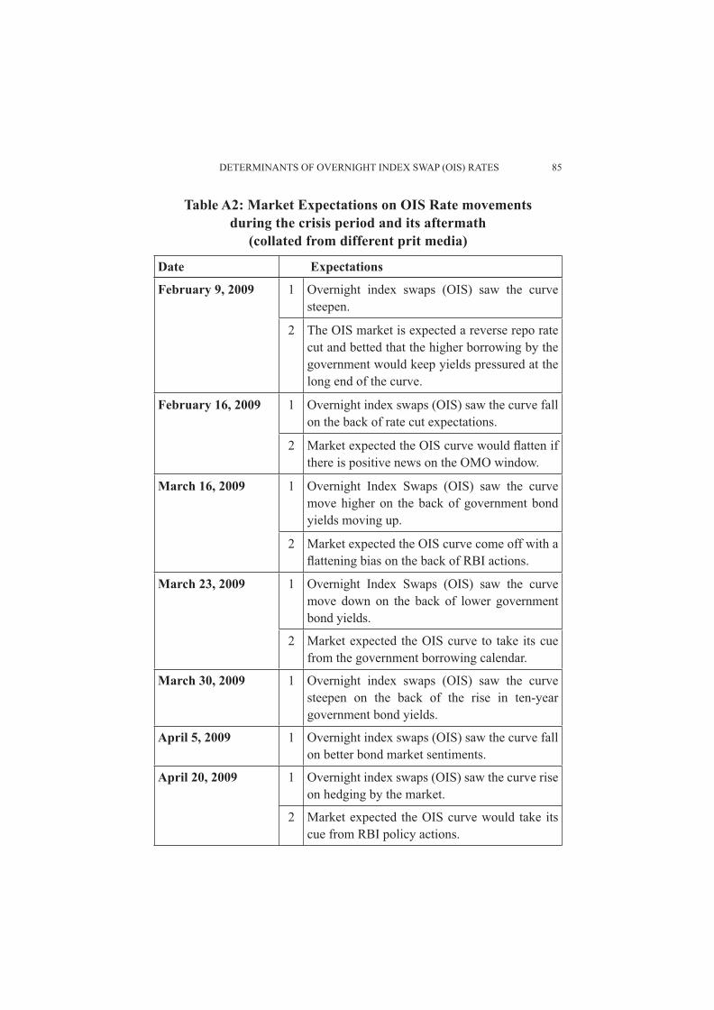
DETERMINANTS OF OVERNIGHT INDEX SWAP (OIS) RATES 85
February 9, 2009 1 Overnight index swaps (OIS) saw the curve steepen.
2 The OIS market is expected a reverse repo rate cut and betted that the higher borrowing by the government would keep yields pressured at the long end of the curve.
February 16, 2009 1 Overnight index swaps (OIS) saw the curve fall on the back of rate cut expectations.
2 Market expected the OIS curve would fl atten if there is positive news on the OMO window.
March 16, 2009 1 Overnight Index Swaps (OIS) saw the curve move higher on the back of government bond yields moving up.
2 Market expected the OIS curve come off with a fl attening bias on the back of RBI actions.
March 23, 2009 1 Overnight Index Swaps (OIS) saw the curve move down on the back of lower government bond yields.
2 Market expected the OIS curve to take its cue from the government borrowing calendar.
March 30, 2009 1 Overnight index swaps (OIS) saw the curve steepen on the back of the rise in ten-year government bond yields.
April 5, 2009 1 Overnight index swaps (OIS) saw the curve fall on better bond market sentiments.
April 20, 2009 1 Overnight index swaps (OIS) saw the curve rise on hedging by the market.
2 Market expected the OIS curve would take its cue from RBI policy actions.
Table A2: Market Expectations on OIS Rate movements during the crisis period and its aftermath
(collated from different prit media)
Date Expectations
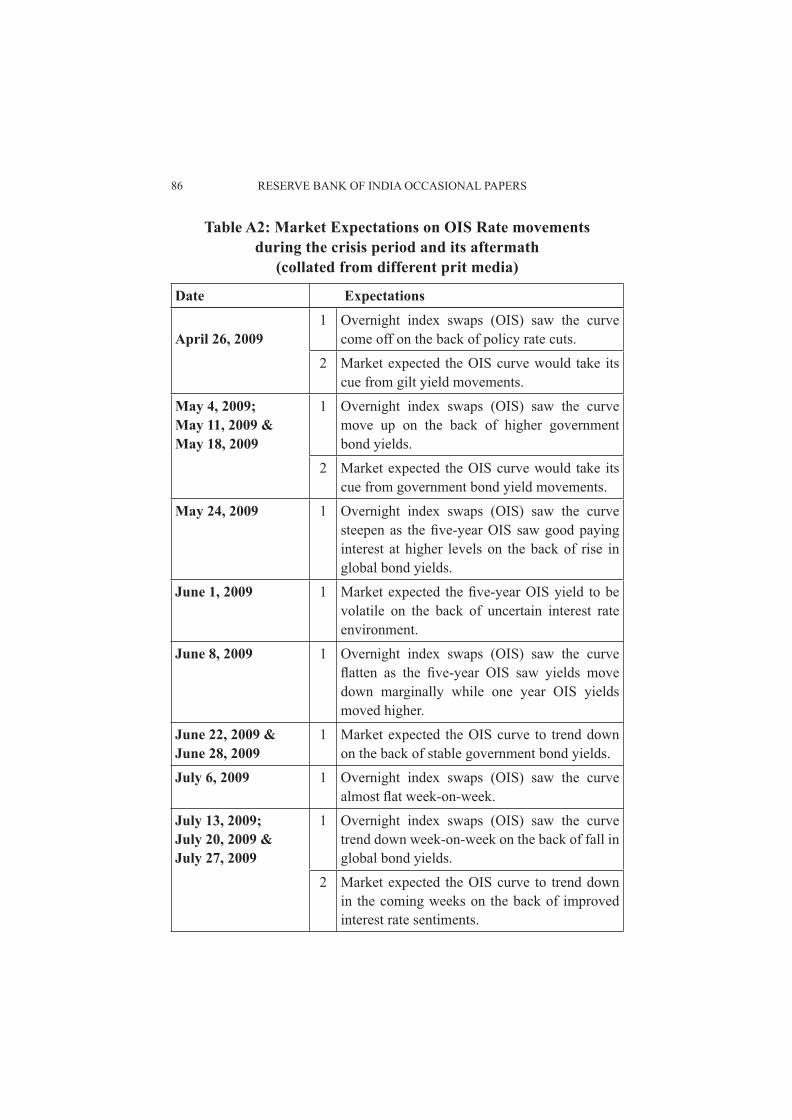
86 RESERVE BANK OF INDIA OCCASIONAL PAPERS
April 26, 20091 Overnight index swaps (OIS) saw the curve
come off on the back of policy rate cuts.
2 Market expected the OIS curve would take its cue from gilt yield movements.
May 4, 2009; May 11, 2009 & May 18, 2009
1 Overnight index swaps (OIS) saw the curve move up on the back of higher government bond yields.
2 Market expected the OIS curve would take its cue from government bond yield movements.
May 24, 2009 1 Overnight index swaps (OIS) saw the curve steepen as the fi ve-year OIS saw good paying interest at higher levels on the back of rise in global bond yields.
June 1, 2009 1 Market expected the fi ve-year OIS yield to be volatile on the back of uncertain interest rate environment.
June 8, 2009 1 Overnight index swaps (OIS) saw the curve fl atten as the fi ve-year OIS saw yields move down marginally while one year OIS yields moved higher.
June 22, 2009 & June 28, 2009
1 Market expected the OIS curve to trend down on the back of stable government bond yields.
July 6, 2009 1 Overnight index swaps (OIS) saw the curve almost fl at week-on-week.
July 13, 2009; July 20, 2009 & July 27, 2009
1 Overnight index swaps (OIS) saw the curve trend down week-on-week on the back of fall in global bond yields.
2 Market expected the OIS curve to trend down in the coming weeks on the back of improved interest rate sentiments.
Table A2: Market Expectations on OIS Rate movements during the crisis period and its aftermath
(collated from different prit media)
Date Expectations
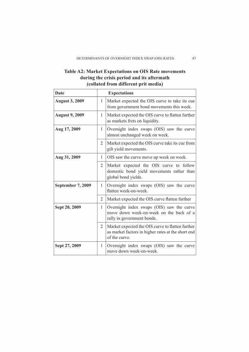
DETERMINANTS OF OVERNIGHT INDEX SWAP (OIS) RATES 87
August 3, 2009 1 Market expected the OIS curve to take its cue from government bond movements this week.
August 9, 2009 1 Market expected the OIS curve to fl atten further as markets frets on liquidity.
Aug 17, 2009 1 Overnight index swaps (OIS) saw the curve almost unchanged week on week.
2 Market expected the OIS curve take its cue from gilt yield movements.
Aug 31, 2009 1 OIS saw the curve move up week on week.
2 Market expected the OIS curve to follow domestic bond yield movements rather than global bond yields.
September 7, 2009 1 Overnight index swaps (OIS) saw the curve fl atten week-on-week.
2 Market expected the OIS curve fl atten further
Sept 20, 2009 1 Overnight index swaps (OIS) saw the curve move down week-on-week on the back of a rally in government bonds.
2 Market expected the OIS curve to fl atten further as market factors in higher rates at the short end of the curve.
Sept 27, 2009 1 Overnight index swaps (OIS) saw the curve move down week-on-week.
Table A2: Market Expectations on OIS Rate movements during the crisis period and its aftermath
(collated from different prit media)
Date Expectations
88 RESERVE BANK OF INDIA OCCASIONAL PAPERS
Notes:1 We selected the lag order on the basis of Hannan Quinn (HQ) information criteria, the optimal lag length was found to be 3 (days).2 Used in levels; it may be noted that the weekly WPI infl ation numbers were repeated for the days of the week as the differenced infl ation series actually incorporates the difference on Thursday / Friday leaving zero for all other days.
References:Bank of Japan (2006): Recent developments of OIS market in Japan; Review, www.boj.or.jp/en/type/ronbun/rev/data/rev06e04.pdf
BIS (2003) : The Euro Interest rate swaps market; Quarterly review, www.bis.org/publ/qtrpdf/r_qt0303f.pdf
British Bankers’ Association (2004): Sterling overnight Index Average, www.bba.org.uk, Benchmarks
Credit Suisse (2001): Material on Overnight Index swaps, www.acisuisse.ch/docs/dokumente/OIS_Note_CSFB_Zurich.pdf
FIMMDA, Circular on Overnight Index swaps, http://www.fi mmda.org/Information_Center/Circulars/Docs/Valuation%20Circular.pdf
IDBI Gilts: Interest rate swaps; A special Paper, www.idbigilts.com/interest_rate_swap.asp
John B. Taylor (2008), The Financial Crisis and the Policy Responses: An Empirical Analysis of What Went Wrong, Bank of Canada, November
Jorion Philippe (2007): Financial Risk Manager Handbook, Published by John Wiley & Sons, Inc., Hoboken, New Jersey, Fourth Edition
Reserve Bank of India: (2003): Report on Rupee Interest rate derivatives; www.rbi.org.in.
Reserve Bank of Australia (2002), Australian Financial Markets, Bulletin, June, www.rba.gov.au/publications/bulletin/2002/jun/pdf/bu-0602-2.pdf
Sukhdev Pavan K.(1997): Interest rate risk and derivatives, www.iief.com/policyage2-13.htm
Thomas S., Fixed Income Derivatives in India; Indira Gandhi Institute of Development Research, http://www.igidr.ac.in/~susant/DERBOOK/PAPERS/vs-outline.pdf
Reserve Bank of India Occasional PapersVol. 31, No.1, Summer 2010
International Outsourcing from India: A Study
Brijesh Pazhayathodi* World trade in services is growing at a much faster rate than trade in goods. Outsourcing of intermediate goods and business services are the most rapidly growing components of international trade. This paper analyzes the business service/IT outsourcing from India. The paper proves that India is having revealed comparative advantage in exports based on ITES-BPO services. The rapid rise in world trade in services would give a good opportunity to India to raise its share of world trade. The Government of India has already taken some initiatives in this regard by giving fi scal concessions to service sector. IT infrastructure and general business environment are two areas where India clearly lags behind other competitor countries in outsourcing arena. Another important fi nding is that even though there is lot of media attention on outsourcing sector in India and other developing countries, the maximum surplus in services trade is actually generated by developed countries. Even though India maintains its lead status as a source country for a variety of IT related services, there are number of emerging challenges like anti-outsourcing legislation and protectionism in western countries, rise of competitor countries etc. In short India has already made an impact in the outsourcing area. However, to maintain its lead and capture new markets and areas, Indian service industries should remain vigilant.
JEL Classifi cation : F13, F14.
Keywords : Outsourcing, Trade in Services
1. Introduction
Outsourcing of intermediate goods and business services is one of the most rapidly growing components of international trade. Companies are outsourcing an ever expanding set of activities, ranging from product design to assembly, from R&D to marketing, distribution
* The author is Research Offi cer in the Department of Economic Analysis and Policy of the Reserve Bank of India. Views expressed in this paper are those of the author and do not necessarily represents those of the RBI. The suggestions of Prof. Pushpa Trivedi, IIT Bombay are gratefully acknowledged. Errors and omissions, if any, are the sole responsibility of the author.
90 RESERVE BANK OF INDIA OCCASIONAL PAPERS
and after sales service. It may be noted that, many of the modern day fi rms have become “virtual” manufacturers, owning designs and plans for many products but making almost nothing themselves. Vertical disintegration is clearly evident in international trade. Annual report of the World Trade Organization (WTO) (1998) details, for example, the production of a particular American car as follows:-
“Thirty percent of the car’s value goes to Korea for assembly, 17.5 per cent to Japan for components and advanced technology, 7.5 per cent to Germany for design, 4 per cent to Taiwan and Singapore for minor parts, 2.5 per cent to the United Kingdom for advertising and marketing services, and 1.5 per cent to Ireland and Barbados for data processing. This means that only 37 per cent of the production value…is generated in the United States”.
Outsourcing of services could be within a country, from one state to another (inshore outsourcing), and also between countries (offshore outsourcing). Literature on outsourcing has given maximum attention on the effect on employment in developed countries. The objective of this study is to show the different facets of India’s Information Technology Enabled Services/Business Process Outsourcing (ITES/BPO). This study tries to capture comprehensive information on this topic by utilizing information/data from diverse source. The study also attempts a comparison between India’s and China’s ITES/BPO sector, the competitiveness of Indian ITES/BPO companies, the business environment existing in this regard in other competitor countries, emerging challenges etc.
This paper has been organized into 6 sections. Section 1 covers introduction and discusses the concepts related to outsourcing. Section 2 reviews the literature on outsourcing and spells out the methodology adopted in this study. Section 3 provides a cross country perspective of services exports and items closely related to outsourcing. It also discusses the major characteristics of India’s outsourcing sector and its importance for economic development. Section 4 attempts a comparison of outsourcing sector in India and
INTERNATIONAL OUTSOURCING FROM INDIA: AN ANALYSIS 91
its competitor countries. It also discusses Indian Government’s policy towards IT sector. Section 5 presents the emerging challenges for India’s outsourcing sector and Section 6 presents the conclusions emanating from the study.
There is no commonly accepted defi nition for outsourcing. Some of the interpretations of outsourcing as discussed in the literature are as follows.
The Oxford dictionary (1998) defi nes outsourcing as “obtain goods or a service by contract from an outside supplier. Outsourcing can dramatically lower total costs”. According to McKinsey study (2003), effective outsourcing implies identifying and managing the “natural owner” of every activity in the value chain. Bhagwati, Panagariya and Srinivasan (2004), have explained outsourcing as a process in which the innovating fi rms introduce a product in the domestic market and once the product matures, the production of this product is shifted to countries where it is cheaper to produce, with the innovating country eventually becoming an importer of the product. It could also consist of arm’s-length, or ‘long –distance’ purchase of services abroad, mainly via electronic mediums.
WTO under its General Agreement on Trade in Services (GATS), categorizes four different ways in which services can be traded. Mode 1, Mode 2, Mode 3 and Mode 4. In Mode 1, trade in services involves arm’s- length supply of services, with the supplier and buyer remaining in their respective locations. Mode 1 purchases have come into prominence because of the advances in electronic information and communication technology. Both individuals and fi rms can provide Mode 1 services. In the former category, independent designers, architects and consultants who sell their services to customers abroad electronically are included whereas latter consists of large fi rms that manage call centers, back offi ces and software programmers. It is said that, trade in Mode 1 services is what most economists have meant when they discuss “outsourcing” (Bhagwati, Panigariya and Srinavasan 2004). Mode 2 involves movement of the consumer to the location of the supplier. Under Mode 3, services are
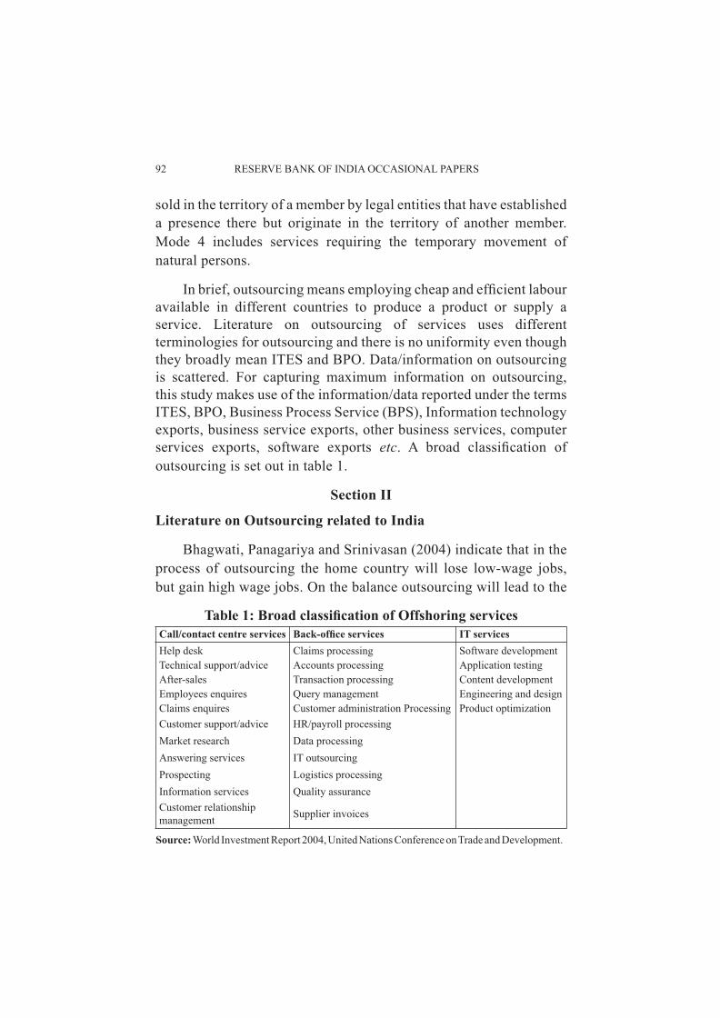
92 RESERVE BANK OF INDIA OCCASIONAL PAPERS
sold in the territory of a member by legal entities that have established a presence there but originate in the territory of another member. Mode 4 includes services requiring the temporary movement of natural persons.
In brief, outsourcing means employing cheap and effi cient labour available in different countries to produce a product or supply a service. Literature on outsourcing of services uses different terminologies for outsourcing and there is no uniformity even though they broadly mean ITES and BPO. Data/information on outsourcing is scattered. For capturing maximum information on outsourcing, this study makes use of the information/data reported under the terms ITES, BPO, Business Process Service (BPS), Information technology exports, business service exports, other business services, computer services exports, software exports etc. A broad classifi cation of outsourcing is set out in table 1.
Section II
Literature on Outsourcing related to India
Bhagwati, Panagariya and Srinivasan (2004) indicate that in the process of outsourcing the home country will lose low-wage jobs, but gain high wage jobs. On the balance outsourcing will lead to the
Table 1: Broad classifi cation of Offshoring servicesCall/contact centre services Back-offi ce services IT servicesHelp desk Claims processing Software developmentTechnical support/advice Accounts processing Application testingAfter-sales Transaction processing Content developmentEmployees enquires Query management Engineering and designClaims enquires Customer administration Processing Product optimizationCustomer support/advice HR/payroll processingMarket research Data processingAnswering services IT outsourcingProspecting Logistics processingInformation services Quality assuranceCustomer relationship management Supplier invoices
Source: World Investment Report 2004, United Nations Conference on Trade and Development.
INTERNATIONAL OUTSOURCING FROM INDIA: AN ANALYSIS 93
transition of the innovator country to a high-value job oriented country. The study also points out that, it is wrong to believe that most of the service jobs will be outsourced to India and China. This is because majority of the jobs in the US are in service industries, such as, retailing, restaurants, tourism, etc., that require both consumer and producer to be present at the same place, and, therefore, cannot be outsourced. In conclusion, this study points out that outsourcing is a relatively small phenomenon in the US labour market.
A study by Amiti and Wei (2004) brings out three interesting fi ndings: (1) the notion that large industrialized countries outsource more intensely is not correct; (ii) outsourcing does not lead to decline in employment in industrialized countries; and, (iii) in terms of economic size, it is the smaller economies which outsource intensively. This study shows that increases in service outsourcing in US manufacturing and services goes together with greater labour productivity. Manufacturing fi rms outsource business services in a large way. This is due to fi rms sourcing their least effi cient process of production from cheaper countries. Outsourcing may lead to shedding of labour but ultimately, the increased effi ciency could lead to higher production and an expansion of employment in other lines of work. However, the authors point out that there could be a change in the skill mix of jobs. The authors cite a study by McKinsey (2003), which indicates more than 69 per cent of workers who lost jobs due to imports in the USA between 1979 and 1999 were re-employed. These results suggest that service outsourcing would not induce a fall in aggregate employment.
Taganas and Kaul (2006) explore the strategies of fi rms in the Indian IT industry and their innovative behavior. The study concludes that India’s software industry has generally been weak to spur innovation within the industry. Most of the innovations are incremental rather than radical in nature. The pattern of innovation is market driven rather than based on fundamental technological research. Competition compels fi rms to cut costs and put emphasis on marketing
94 RESERVE BANK OF INDIA OCCASIONAL PAPERS
cooperation. The study point out that there is wide scope for IT fi rms to collaborate with the more technologically competent MNCs. It suggests that Indian IT fi rms should further increase their focus on R&D to sustain their growth.
The study by NASSCOM (2007) focuses on growth of IT software and services industry in China and India. It is based on a series of interactions with Chinese offi cials and interviews with IT software companies. The study indicates that Chinese IT-BPO has much to learn from India. Even though the Chinese IT sector is expected to continue growing at a rapid pace, it is unlikely to displace India in the near future. Strong Government support, excellent quality of infrastructure, rapid pace of growth of domestic economy, etc., are the major strength of Chinese IT-BPO sector. Further the geographical proximity and cultural similarity to advanced markets like Japan and Korea is a great help to Chinese IT-BPO sector. The average wage in China is signifi cantly lower than other competitor countries. However, lack of transparency in procedures and weak intellectual property protection are major weakness of China. The study puts forward a strong case for increased partnership between India and China to tap the growing IT-BPO market in the world.
There are some interesting studies on labour conditions and trade unions in ITES-BPO sector. Ramesh (2004) point out the vulnerabilities for laborers in India’s BPO sector. The study is based on fi eld survey of call centers. Firms often terminate the job to get rid of long-term commitments towards employees. Laborers, who work on voice processes, are forced to live as Indian during the day and Westerner after the sundown. Many a times, customers are irritatable and abusive. Further, odd working time confl icts with the natural rhythm of human body resulting in increased healthcare costs besides affecting personal and social life. Workers are not entitled for national / religious holidays, as the fi rms work with clients’ calendar. The study also observed workers developing poor eating habits, smoking, excessive drinking of coffee, etc., to cope up with the psychological and physical stress. The long-term opportunity costs of BPO work could be still
INTERNATIONAL OUTSOURCING FROM INDIA: AN ANALYSIS 95
higher as most of the young workers are burning out their best time for higher education working as “cyber coolies”. Further, Women’s scope in the job is extremely constrained due to odd timings of work. Sandhu (2006) examines the diffi culties of unionizing BPO sector. It point out that there have been attempts at unionizing the call centre industry since the year 2000. Information Technology Professionals’ Forum (ITPF) is the result of this, and it gained recognition as an offi cial organization from the Karnataka State Government as a society rather than a trade union. The study indicate BPO workers opposed unions because they associate it with the pre-1991 era of slow economic growth and limited opportunities. BPO workers associate their work with upward mobility, clean work clothes, shiny buildings, etc. In short, the study point out that even though BPO workers are overworked and stressed, they are not interested in unionization. Taylor et al (2008) examines the issue of working conditions and employee rights in ITES-BPO industry. The study suggests that there is a constituency for UNITES in Indian ITES-BPO. UNITES was formed in September 2005 on the foundations laid by the Centre for Business Processing Outsourcing Professionals (CBPOP) in 2004. UNITES has secured legal status under Trade Disputes Act (1926) and has been granted ‘provisional affi liation’ to Indian National Trades Union Congress (INTUC). The study collected information through questionnaires mainly from UNITES members. Majoriy of the respondents reported that UNITES is helping to improve work conditions. About 65 per cent of respondents indicated “working times” which include shift length, night-time work, etc., as crucial issues for them. In short, the study indicates that there are numerous work related concerns in Indian ITES-BPO industry.
It may be pointed out that, even though outsourcing has attracted much attention in the media, there is a dearth of comprehensive study on outsourcing from India. Most of the available studies focus on outsourcing and issues related to job loss. The study by Amiti and Wei (2004) is very relevant in the context of anti-outsourcing legislations in developed countries like the US. It points out that if we take into
96 RESERVE BANK OF INDIA OCCASIONAL PAPERS
account the size of the economy, developing countries like India not only export but also are a large importer of business services. This study is a coherent one and removes many misconceptions about outsourcing. Ahuja (2004) sets out the benefi ts from outsourcing, such as, cost reduction and suggests a tax on profi ts of benefi ciary fi rm so as to fund the relocation of workers who lose their jobs due to outsourcing. The Study by Ramesh (2004) is unique as it focuses on labour issues and harsh conditions of work in BPOs located in India and point out the negative side of employment in BPOs. However, the recent reports indicate that there are positive sides of employment in BPOs. Many BPOs had started taking measures for the welfare of their workers like, leisure trips, physical and mental exercises for destressing, social interaction programmes, fi nancial incentives, etc. Tata Indicom is planning to employ visually challenged individuals in its call centres which may boost the morale and employment opportunity of differently able people. In conclusion, it may be said that most of the literature points out that offshoring of IT and IT-enabled services will increase in the coming years without signifi cantly reducing the employment levels in the countries that offshore jobs. Nor will it dramatically change the overall employment situation in the countries providing the offshored services. In this context, World Trade Report (2005), indicates that the impact of offshoring services jobs is far stronger in the popular perception than on actual production, employment and trade patterns. The number of jobs affected by offshoring IT services is small when compared to the overall employment levels in the developed countries. It is also small in the countries which have started exporting IT services when compared to their total employment. However, many of the studies mention about initial loss of employment or change in skill mix due to outsourcing in the service importing country.
2.1 Methodology
Under Balance of Payments format, services come under invisibles. Services can be further subdivided into Travel, Transportation, Insurance, Government Not Included Elsewhere and
INTERNATIONAL OUTSOURCING FROM INDIA: AN ANALYSIS 97
Miscellaneous services (including IT/BPO exports). Outsourcing of ITES and Business Process has become prominent in recent years and therefore there is no uniform comparable data for outsourcing to and from different countries in the global context. But a broad comparison can be attempted using the IMF data. In its BoP statistics, the IMF reports services, which includes the categories most closely related to outsourcing- ‘computing and information services’ and ‘other business services’. According to IMF (2006), computer and information services comprise transactions between resident and nonresident related to hardware consultancy, software implementation, information services (data processing) etc,; the item ‘other business services’ covers transactions between residents and nonresidents relating to professional and technical services, miscellaneous business services, merchanting and other trade-related services.
Since a single source of data does not give a comprehensive picture, this study mainly uses three sets of data, viz., data compiled by Reserve Bank of India, under Balance of Payments Statistics, NASSCOM, and IMF.
The objectives and the scope of this study are as follows: Firstly, an analysis using the IMF data is attempted to fi nd out countries that dominate in service exports. Secondly, it computes Revealed Comparative Advantage (RCA) index for different countries to examine countries that have a comparative advantage in business services (proxied as BPOs) and computer software related exports. It also examines whether India has comparative advantage in merchandise goods exports or services exports. Thirdly, it uses fi rm level data from NASSCOM to study the specifi c characteristics of India’s ITES-BPO sector. Fourthly, it examines ITES-BPOs in India and China so as to fi nd out their relative strengths and weaknesses. Fifthly, it explores the weakness and emerging problems in India’s ITES-BPO exports. Finally, it also tries to fi nd out whether the global economic slowdown has had any impact on Software and business service export. Though this study have used the descriptive statistics for most of the stated objectives, it has used the Balassa
98 RESERVE BANK OF INDIA OCCASIONAL PAPERS
Index (1965) to measure the ‘Revealed Comparative Advantage’ (RCA). This is stated in equation 1.
RCA=(Xij/Xit)/(Xnj/Xnt)=(Xij/Xnj)/(Xit/Xnt) ….1
Where X represents exports, i is a country, j is a commodity (or industry), t is a set of commodities (or industries) and n is a set of countries. RCA measures a country’s exports of a commodity (or industry) relative to its total exports and to the corresponding exports of a set of countries. A comparative advantage is ‘revealed’, if RCA > 1. If RCA is less than unity, the country is said to have a comparative disadvantage in exports of the commodity/industry (Utkulu and Seymen, 2004).
Section III
Service Sector Exports: A Cross-Country Perspective
Since IT/BPO exports are included under service exports, this study present the broad trend in international trade in services. Over the last decade, international trade in services has been growing at a higher rate than trade in goods. The world economy has fast turned into a ‘service economy’ since the 1990s. Around 70 per cent of global GDP comprises of services. The growth of services sector has overtaken the growth in real GDP in a number of countries. While developed countries still account for a major share of services in world GDP and trade, developing countries are catching up in terms of increasing their share in global trade in services. In India, traditionally services relating to trade in goods, such as transportation and fi nancing were the major constituents, the rapid developments in telecommunications and information technology has facilitated the emergence of business and computer services as the main drivers of the export growth (RBI, 2010). This is evident from the rapid rise in India’s share of service exports in world which has shown steady growth from 0.6 per cent in 1994 to 2.7 per cent in 2008 (Ranked 12th in world, China stood 8th with a share of 3.8 per cent in 2008) (Table 2).
The share of India’s service exports in its total exports of goods and services has also shown a rapid rise from around 26.4 per cent in 2000-01 to 35.0 per cent in 2008-09 (Table 3).
INTERNATIONAL OUTSOURCING FROM INDIA: AN ANALYSIS 99
Amongst the different services sectors, trade in software services has witnessed rapid expansion in recent years. This is largely due to the increased demand from developed countries like US and EU,
Table 2: Top Service Exporting Countries (Share in World) (in per cent
1995 2000 2002 2003 2004 2005 2006 2007 2008 RankUnited States 17.7 19.5 17.6 15.9 15.3 15.1 15.0 14.5 14.1 1United Kingdom 6.5 7.9 8.3 8.4 8.7 8.1 8.2 8.2 7.4 2Germany 6.5 5.5 6.3 6.5 6.4 6.4 6.6 6.5 6.4 3Europe 4.9 4.8 4.8 5.1 5.3 5.6 5.7 6.0 6.7 4France 6.8 5.3 5.3 5.2 5.0 4.8 4.5 4.3 4.3 5Japan 5.3 4.6 4.0 4.1 4.3 4.3 4.1 3.7 3.9 6Spain 3.3 3.5 3.7 3.9 3.8 3.7 3.7 3.7 3.7 7China,P.R. 1.6 2.0 2.4 2.5 2.7 2.9 3.2 3.5 3.8 8Italy 5.0 3.7 3.7 3.8 3.7 3.5 3.4 3.2 3.2 9Netherlands 3.7 3.2 3.4 3.3 3.2 3.1 2.9 2.8 2.7 10Ireland 0.4 1.2 1.8 2.2 2.3 2.4 2.4 2.7 2.6 11India 0.6 1.1 1.2 1.3 1.7 2.1 2.4 2.5 2.7 12China,:HKong – 2.7 2.7 2.5 2.4 2.5 2.5 2.5 2.4 13Singapore 2.1 1.9 1.8 1.9 2.1 2.1 2.2 2.3 2.2 14Belgium – – 2.3 2.4 2.3 2.2 2.1 2.2 2.2 15
Source: Balance of Payments Statistics (February 2010), IMF.
Table 3: India’s Exports of Services (in US $ million)
1995-96 2000-01 2004-05 2005-06 2006-07 2007-08 2008-09Goods and Services 39,654 61,720 128,455 162,811 202,668 256,504 290,679Services Export 7,344 16,268 43,249 57,659 73,780 90,342 101,678Services export as per cent of goods and service export 18.5 26.4 33.7 35.4 36.4 35.2 35.0Computer and Information services .... 4,727 16,344 21,875 29,088 37,491 49,379Computer and Information services as per cent of Services export 29.1 37.8 37.9 39.4 41.5 48.6Computer services .... 4,633 16,204 21,711 28,787 37,032 48,626Computer services export as per cent of Services export 28.5 37.5 37.7 39.0 41.0 47.8Other business services 2,120 4,149 8,153 12,764 17,536 20,734 20,426Other business services export as per cent of Services export 28.9 25.5 18.9 22.1 23.8 23.0 20.1
Source: Monthly Bulletin, various issues, Reserve Bank of India (for goods and services exports) and Balance of Payments Statistics (February 2010) IMF.
100 RESERVE BANK OF INDIA OCCASIONAL PAPERS
which are outsourcing their non-core activities to take advantage of the low-cost high-skilled professionals from the developing countries like India. India exhibits a strong revealed comparative advantage (RCA) in services. India’s comparative advantage in this area has made India a favorable destination for outsourcing and also exports oriented FDI projects in IT and related area (Table 4).
A Report (2005) by United Nations Conference on Trade and Development (UNCTAD) points out that many of the poorest countries continue to have very low Information and Communication Technology (ICT) penetration rates, in particular those with a large rural population and relatively high-priced basic ICT infrastructure. Only 3.1 per cent
Table 4: Export oriented FDI projects in call centres, shared service centres, IT services and regional headquarters, by
destination, 2002-2003(Number and per cent)
Call centres Shared service centres
IT services Regional HQs
No of projects
Share of
total (%)
No of projects
Share of
total(%)
No of projects
Share of
total(%)
No of projects
Share of
total(%)
World 513 100 139 100 632 100 565 100Developed countries 279 54 48 35 293 46 339 60EU 169 33 38 27 198 31 185 33Developing economies 203 40 72 52 315 50 209 37Asia 167 33 66 47 283 45 195 35China 30 6 4 3 60 9 38 7Hong Kong, China 2 – – – 14 2 37 7India 60 12 43 31 118 19 7 1Korea, Rep. 5 1 5 1 6 1Malaysia 16 3 6 4 8 1 17 3Phillipines 12 2 1 1 9 1 4 1Singapore 16 3 8 6 35 6 36 6Taiwan 4 1 – – 9 1 4 1Hungary 11 2 7 5 4 1 4 1Ireland 29 6 19 14 14 2 15 3UK 43 8 7 5 73 12 64 11United States 15 3 2 1 26 4 80 14Canada 56 11 3 2 14 2 25 4Germany 20 4 1 1 34 5 22 4
Source: World Investment Report 2004, United Nations Conference on Trade and Development.
INTERNATIONAL OUTSOURCING FROM INDIA: AN ANALYSIS 101
of Africans had access to the Internet in 2004, compared with 62.6 per cent North Americans. In EU 15 country average is 50 per cent. This indicates a vast stock of potential outsourcing opportunities for countries like India once the ICT picks up in these regions.
3.1 Exports of Computer and Information Services
IMF data shows that during 2008, India ranks fi rst before industrialised countries like Ireland, UK, US and Germany in exports of computer and information services (Table 5). India’s surplus position in trade in computer and information services is rapidly rising (Chart 1). India is attractive because of its low cost of operations, high quality of products and services and availability of skilled manpower.
Further, India’s share of export of computer and information services in the total service exports is high compared to other countries (Table 6). This indicates the importance of this emerging sector within the growing services sector. Regarding import of computer and
Table 5: Exports of Computer and Information services (US $ million
1995 2000 2002 2003 2004 2005 2006 2007 2008 RankIndia .... 4,727 8,889 11,876 16,344 21,875 29,088 37,491 49,379 1Ireland .... 7,490 10,447 14,238 18,774 19,586 21,040 29,825 34,162 2U.K 1,250 4,320 5,930 8,160 11,260 10,820 12,560 14,210 13,580 3Germany 1,400 3,800 5,530 6,700 8,090 8,390 9,910 12,600 15,130 4U.S.A 2,420 5,620 5,390 6,250 6,700 7,320 10,080 11,640 12,600 5Sweden .... 1,191 1,472 1,993 2,537 2,688 3,585 6,526 7,647 6Netherlands 620 1,166 1,422 2,884 3,702 3,723 4,969 6,419 6,684 7Israel .... 4,246 4,180 3,409 4,407 4,529 5,289 5,809 6,852 8Spain 1,033 2,043 2,490 2,913 2,964 3,606 3,960 5,358 6,119 9Canada 1,011 2,428 2,266 2,796 3,014 3,600 4,296 4,597 4,642 10China,P.R. .... 356 638 1,102 1,637 1,840 2,958 4,345 6,252 11Belgium .... .... 1,774 2,132 2,441 2,581 2,869 2,982 3,616 12France 360 800 1,190 1,260 1,490 1,710 1,970 1,900 1,530 13Finland 743 203 503 566 755 1,511 1,475 1,846 8,250 14Austria 82 296 420 657 899 1,234 1,503 1,833 2,155 15
Source : Balance of Payments Statistics (February 2010), IMF.
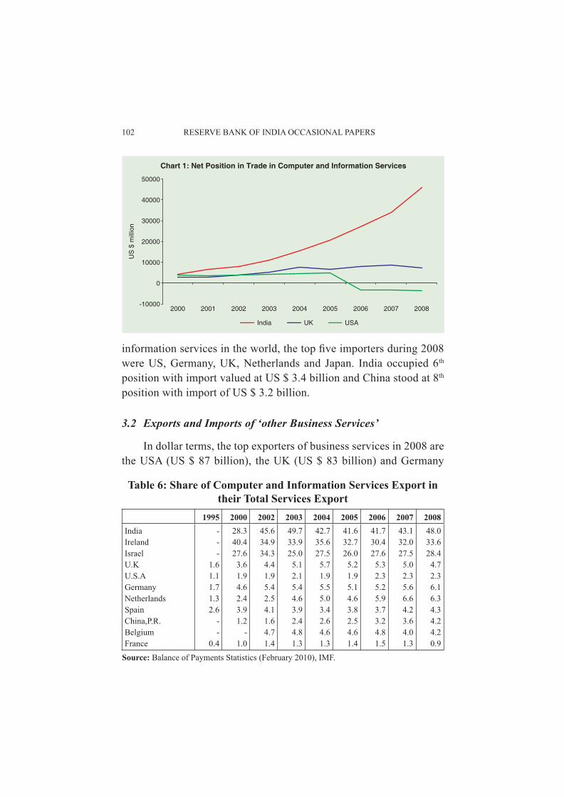
102 RESERVE BANK OF INDIA OCCASIONAL PAPERS
information services in the world, the top fi ve importers during 2008 were US, Germany, UK, Netherlands and Japan. India occupied 6th position with import valued at US $ 3.4 billion and China stood at 8th position with import of US $ 3.2 billion.
3.2 Exports and Imports of ‘other Business Services’
In dollar terms, the top exporters of business services in 2008 are the USA (US $ 87 billion), the UK (US $ 83 billion) and Germany
Table 6: Share of Computer and Information Services Export in their Total Services Export
1995 2000 2002 2003 2004 2005 2006 2007 2008India - 28.3 45.6 49.7 42.7 41.6 41.7 43.1 48.0Ireland - 40.4 34.9 33.9 35.6 32.7 30.4 32.0 33.6Israel - 27.6 34.3 25.0 27.5 26.0 27.6 27.5 28.4U.K 1.6 3.6 4.4 5.1 5.7 5.2 5.3 5.0 4.7U.S.A 1.1 1.9 1.9 2.1 1.9 1.9 2.3 2.3 2.3Germany 1.7 4.6 5.4 5.4 5.5 5.1 5.2 5.6 6.1Netherlands 1.3 2.4 2.5 4.6 5.0 4.6 5.9 6.6 6.3Spain 2.6 3.9 4.1 3.9 3.4 3.8 3.7 4.2 4.3China,P.R. - 1.2 1.6 2.4 2.6 2.5 3.2 3.6 4.2Belgium - - 4.7 4.8 4.6 4.6 4.8 4.0 4.2France 0.4 1.0 1.4 1.3 1.3 1.4 1.5 1.3 0.9
Source: Balance of Payments Statistics (February 2010), IMF.
INTERNATIONAL OUTSOURCING FROM INDIA: AN ANALYSIS 103
(US $ 80 billion). India, a country that has received the maximum attention as a recipient of outsourcing, is ranked 15th (US $ 20 billion) and China ranked 5th, receive contract worth US $ 46 billion (Table 7). It is interesting to note that eventhough India is highlighted in the media as one of the biggest exporters of business services in the world, there are many industrialized countries ahead of it.
Amiti and Wei (2004) shows that, the media reports indicating US and other developed countries alone outsource (or contract out services) to developing countries like India and China to take advantage of lower cost in these countries is not entirely correct. This is clear from an analysis of IMF data on import of other business services. Comparable data shows that top three importers of business services in 2008 are Germany, US and France. India and China- two countries that are major topic of discussion as major recipients of
Table 7: Exports of Other Business Services (US $ million)
1995 2000 2001 2003 2004 2005 2006 2007 2008 RankU.S.A 29,080 48,220 52,310 60,160 66,020 71,730 65,140 77,640 87,040 1U.K 17,200 33,880 35,770 47,300 57,010 60,450 68,880 81,160 83,370 2Germany 20,010 24,200 25,880 33,240 43,180 50,680 62,380 72,250 80,400 3China,P.R. 3,740 7,663 8,448 17,427 19,952 23,283 28,973 40,408 46,349 4Japan 24,440 17,710 16,240 18,040 21,910 27,280 30,680 32,920 41,130 5Italy 13,154 13,789 17,024 21,000 24,345 28,216 30,769 35,204 38,853 6France 23,710 19,300 20,010 24,130 24,930 29,410 29,570 31,630 38,560 7Netherlands 12,161 15,527 16,599 23,599 26,705 29,924 29,642 33,246 36,107 8Spain 4,289 8,018 9,385 13,407 16,081 17,886 21,884 27,456 32,862 9Ireland 1,389 1,908 4,386 7,862 10,498 16,232 18,724 28,279 31,355 10Singapore 6,689 8,318 8,343 14,378 18,371 21,219 24,732 30,676 30,242 11Belgium .... .... .... 14,714 16,501 17,577 17,462 23,342 29,457 12Switzerland 4,376 5,224 5,266 7,744 12,382 15,681 17,659 21,271 29,190 13Sweden 2,566 6,482 6,912 11,148 14,020 15,583 18,120 22,942 27,070 14India 2,120 4,149 2,349 2,229 8,153 12,764 17,536 20,734 20,426 15Canada 5,853 10,402 9,451 12,011 13,354 15,183 15,774 17,164 17,945 16Austria 11,836 5,384 6,341 8,254 9,618 11,423 12,635 14,362 16,652 17Brazil 1,249 4,568 4,613 4,133 4,938 6,722 8,568 11,064 14,331 18Norway 1,682 4,014 3,458 4,470 5,708 6,670 9,123 12,517 13,551 19Korea, Republic of 6,761 7,200 6,388 6,687 8,125 9,422 10,532 14,421 13,157 20
Source: Balance of Payments Statistics (February 2010), IMF.
104 RESERVE BANK OF INDIA OCCASIONAL PAPERS
outsourcing are themselves signifi cant outsourcers of business services (with a value of US $ 21 billion for India and US $ 38 billion for China, and ranked 13th and 7th in the world respectively. This clearly points out that the biggest importers in business services are leading developed countries like US and UK followed by emerging countries like India and China. Amiti and Wei 2004, pointed out that there is nothing unusual in larger economies like USA, UK etc, trading more than smaller ones. To get an idea of relative importance of outsourcing for an economy, it is important to know the share of imports in the economy, i.e imports as per cent of GDP. If one scales imports of business services by domestic GDP, smaller African economies like Angola, Congo etc. are much more outsourcing-intensive than developed countries like US and UK. In conclusion, we can say that even though industrialized countries outsource (contract work to other countries) more than developing countries in absolute terms, in terms of size of economy (GDP), it is poor countries which import more than developed countries. The belief that global service trade is dominated by lopsided one-way outsourcing from developed countries to developing countries is not supported by the available data. It is particularly important to note that developed countries like US and UK who are big exporters and importers of services are also gaining from trade in services. Short term job losses in these countries if any, due to outsourcing are well compensated by cost reduction and productivity gain made by these countries. The net result of outsourcing is that, both developing countries and developed countries are ultimately gaining. For example, while industrial countries gain in terms of productivity, cost reduction etc., developing countries gain in terms of employment, foreign exchange earning etc.
3.3 Revealed Comparative and Competitive Advantage in India’s Service Exports: An International Comparison
Tables 8 and 9 presented below gives the RCA indices calculated using IMF BoP statistics. A broad comparison clearly points out that India have advantage in exporting services which includes outsourcing
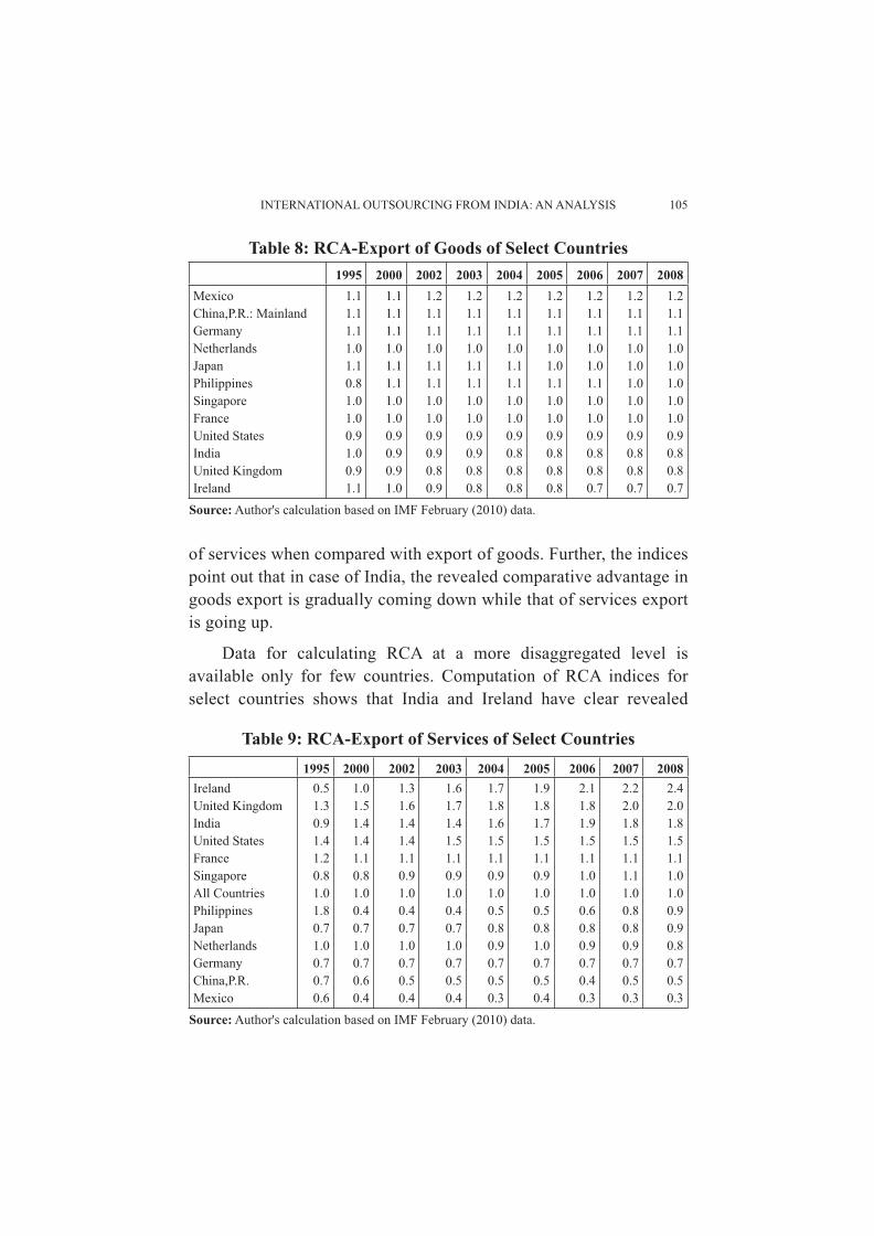
INTERNATIONAL OUTSOURCING FROM INDIA: AN ANALYSIS 105
of services when compared with export of goods. Further, the indices point out that in case of India, the revealed comparative advantage in goods export is gradually coming down while that of services export is going up.
Data for calculating RCA at a more disaggregated level is available only for few countries. Computation of RCA indices for select countries shows that India and Ireland have clear revealed
Table 8: RCA-Export of Goods of Select Countries1995 2000 2002 2003 2004 2005 2006 2007 2008
Mexico 1.1 1.1 1.2 1.2 1.2 1.2 1.2 1.2 1.2China,P.R.: Mainland 1.1 1.1 1.1 1.1 1.1 1.1 1.1 1.1 1.1Germany 1.1 1.1 1.1 1.1 1.1 1.1 1.1 1.1 1.1Netherlands 1.0 1.0 1.0 1.0 1.0 1.0 1.0 1.0 1.0Japan 1.1 1.1 1.1 1.1 1.1 1.0 1.0 1.0 1.0Philippines 0.8 1.1 1.1 1.1 1.1 1.1 1.1 1.0 1.0Singapore 1.0 1.0 1.0 1.0 1.0 1.0 1.0 1.0 1.0France 1.0 1.0 1.0 1.0 1.0 1.0 1.0 1.0 1.0United States 0.9 0.9 0.9 0.9 0.9 0.9 0.9 0.9 0.9India 1.0 0.9 0.9 0.9 0.8 0.8 0.8 0.8 0.8United Kingdom 0.9 0.9 0.8 0.8 0.8 0.8 0.8 0.8 0.8Ireland 1.1 1.0 0.9 0.8 0.8 0.8 0.7 0.7 0.7
Source: Author's calculation based on IMF February (2010) data.
Table 9: RCA-Export of Services of Select Countries1995 2000 2002 2003 2004 2005 2006 2007 2008
Ireland 0.5 1.0 1.3 1.6 1.7 1.9 2.1 2.2 2.4United Kingdom 1.3 1.5 1.6 1.7 1.8 1.8 1.8 2.0 2.0India 0.9 1.4 1.4 1.4 1.6 1.7 1.9 1.8 1.8United States 1.4 1.4 1.4 1.5 1.5 1.5 1.5 1.5 1.5France 1.2 1.1 1.1 1.1 1.1 1.1 1.1 1.1 1.1Singapore 0.8 0.8 0.9 0.9 0.9 0.9 1.0 1.1 1.0All Countries 1.0 1.0 1.0 1.0 1.0 1.0 1.0 1.0 1.0Philippines 1.8 0.4 0.4 0.4 0.5 0.5 0.6 0.8 0.9Japan 0.7 0.7 0.7 0.7 0.8 0.8 0.8 0.8 0.9Netherlands 1.0 1.0 1.0 1.0 0.9 1.0 0.9 0.9 0.8Germany 0.7 0.7 0.7 0.7 0.7 0.7 0.7 0.7 0.7China,P.R. 0.7 0.6 0.5 0.5 0.5 0.5 0.4 0.5 0.5Mexico 0.6 0.4 0.4 0.4 0.3 0.4 0.3 0.3 0.3
Source: Author's calculation based on IMF February (2010) data.
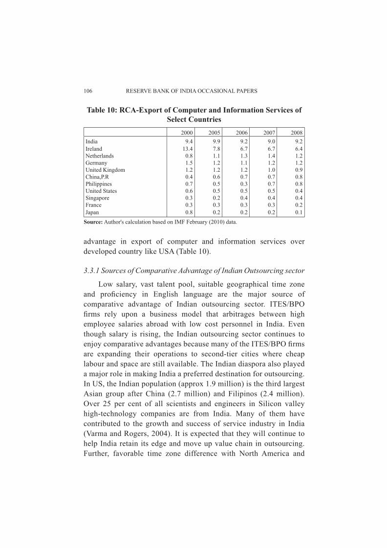
106 RESERVE BANK OF INDIA OCCASIONAL PAPERS
advantage in export of computer and information services over developed country like USA (Table 10).
3.3.1 Sources of Comparative Advantage of Indian Outsourcing sector
Low salary, vast talent pool, suitable geographical time zone and profi ciency in English language are the major source of comparative advantage of Indian outsourcing sector. ITES/BPO fi rms rely upon a business model that arbitrages between high employee salaries abroad with low cost personnel in India. Even though salary is rising, the Indian outsourcing sector continues to enjoy comparative advantages because many of the ITES/BPO fi rms are expanding their operations to second-tier cities where cheap labour and space are still available. The Indian diaspora also played a major role in making India a preferred destination for outsourcing. In US, the Indian population (approx 1.9 million) is the third largest Asian group after China (2.7 million) and Filipinos (2.4 million). Over 25 per cent of all scientists and engineers in Silicon valley high-technology companies are from India. Many of them have contributed to the growth and success of service industry in India (Varma and Rogers, 2004). It is expected that they will continue to help India retain its edge and move up value chain in outsourcing. Further, favorable time zone difference with North America and
Table 10: RCA-Export of Computer and Information Services of Select Countries
2000 2005 2006 2007 2008India 9.4 9.9 9.2 9.0 9.2Ireland 13.4 7.8 6.7 6.7 6.4Netherlands 0.8 1.1 1.3 1.4 1.2Germany 1.5 1.2 1.1 1.2 1.2United Kingdom 1.2 1.2 1.2 1.0 0.9China,P.R 0.4 0.6 0.7 0.7 0.8Philippines 0.7 0.5 0.3 0.7 0.8United States 0.6 0.5 0.5 0.5 0.4Singapore 0.3 0.2 0.4 0.4 0.4France 0.3 0.3 0.3 0.3 0.2Japan 0.8 0.2 0.2 0.2 0.1
Source: Author's calculation based on IMF February (2010) data.
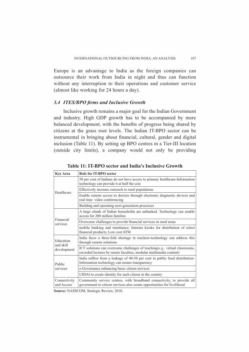
INTERNATIONAL OUTSOURCING FROM INDIA: AN ANALYSIS 107
Europe is an advantage to India as the foreign companies can outsource their work from India in night and thus can function without any interruption to their operations and customer service (almost like working for 24 hours a day).
3.4 ITES/BPO fi rms and Inclusive Growth
Inclusive growth remains a major goal for the Indian Government and industry. High GDP growth has to be accompanied by more balanced development, with the benefi ts of progress being shared by citizens at the grass root levels. The Indian IT-BPO sector can be instrumental in bringing about fi nancial, cultural, gender and digital inclusion (Table 11). By setting up BPO centres in a Tier-III location (outside city limits), a company would not only be providing
Table 11: IT-BPO sector and India's Inclusive GrowthKey Area Role for IT-BPO sector
Healthcare
50 per cent of Indians do not have access to primary healthcare-Information technology can provide it at half the costEffectively increase outreach to rural populationsEnable remote access to doctors through electronic diagnostic devices and real time video conferencingBuilding and operating next-generation processes
Financial services
A large chunk of Indian households are unbanked. Technology can enable access for 200 million familiesOvercome challenges to provide fi nancial services in rural areasmobile banking and remittance; Internet kiosks for distribution of select fi nancial products; Low cost ATM
Education and skill development
India faces a three-fold shortage in teachers-technology can address this through remote solutions ICT solutions can overcome challenges of teaching(e.g., virtual classrooms, recorded lectures by senior faculties, modular multimedia content)
Public services
India suffers from a leakage of 40-50 per cent in public food distribution- Information technology can ensure transparencye-Governance enhancing basic citizen servicesUIDAI to create identity for each citizen in the country
Connectivity and Access
Community service centres, with broadband connectivity, to provide all government to citizen services-also create opportunities for livelihood
Source: NASSCOM, Strategic Review, 2010.
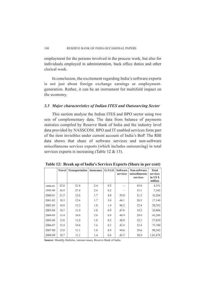
108 RESERVE BANK OF INDIA OCCASIONAL PAPERS
employment for the persons involved in the process work, but also for individuals employed in administration, back offi ce duties and other clerical work.
In conclusion, the excitement regarding India’s software exports is not just about foreign exchange earnings or employment-generation. Rather, it can be an instrument for multifold impact on the economy.
3.5 Major characteristics of Indian ITES and Outsourcing Sector
This section analyse the Indian ITES and BPO sector using two sets of complementary data. The data from balance of payments statistics compiled by Reserve Bank of India and the industry level data provided by NASSCOM. BPO and IT enabled services form part of the item invisibles under current account of India’s BoP. The RBI data shows that share of software services and non-software miscellaneous services exports (which includes outsourcing) in total services exports is increasing (Table 12 & 13).
Table 12: Break up of India's Services Exports (Share in per cent) Travel Transportation Insurance G.N.I.E Software
servicesNon-software miscellaneous
services
Total services in US $ million
1990-91 32.0 21.6 2.4 0.3 – 43.6 4,5511995-96 36.9 27.4 2.4 0.2 – 33.1 7,342
2000-01 21.5 12.6 1.7 4.0 39.0 21.3 16,268
2001-02 18.3 12.6 1.7 3.0 44.1 20.3 17,140
2002-03 16.0 12.2 1.8 1.4 46.2 22.4 20,763
2003-04 18.7 11.9 1.6 0.9 47.6 19.2 26,868
2004-05 15.4 10.8 2.0 0.9 40.9 29.9 43,249
2005-06 13.6 11.0 1.8 0.5 40.9 32.1 57,659
2006-07 12.4 10.8 1.6 0.3 42.4 32.4 73,780
2007-08 12.6 11.1 1.8 0.4 44.6 29.6 90,342
2008-09 10.7 11.1 1.4 0.4 45.5 30.9 1,01,678
Source: Monthly Bulletin, various issues, Reserve Bank of India.
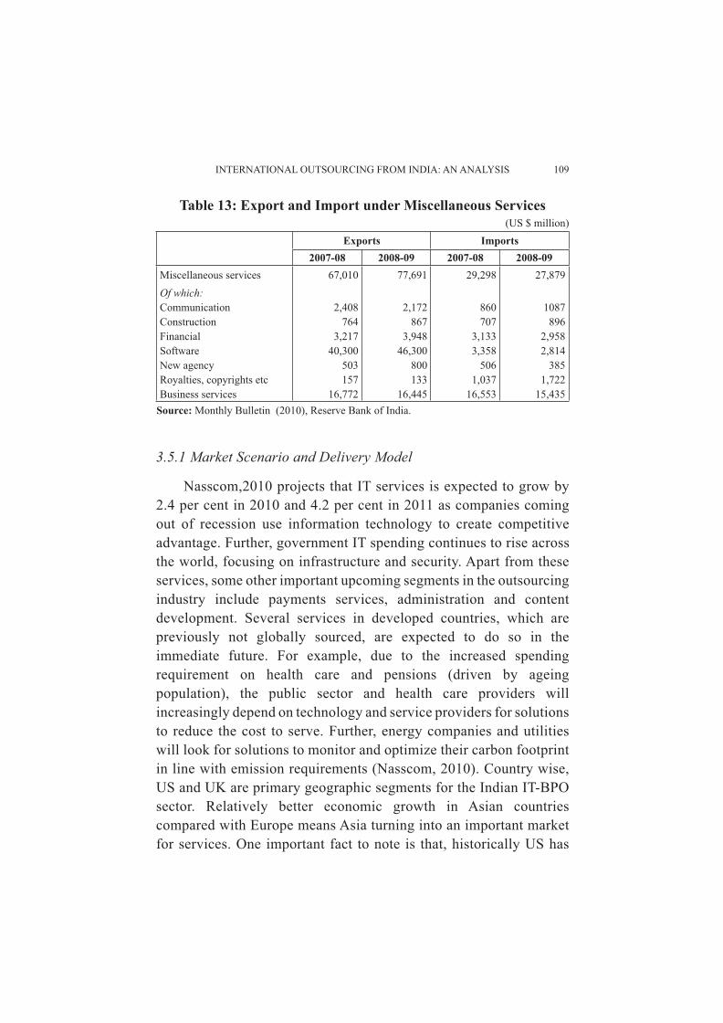
INTERNATIONAL OUTSOURCING FROM INDIA: AN ANALYSIS 109
3.5.1 Market Scenario and Delivery Model
Nasscom,2010 projects that IT services is expected to grow by 2.4 per cent in 2010 and 4.2 per cent in 2011 as companies coming out of recession use information technology to create competitive advantage. Further, government IT spending continues to rise across the world, focusing on infrastructure and security. Apart from these services, some other important upcoming segments in the outsourcing industry include payments services, administration and content development. Several services in developed countries, which are previously not globally sourced, are expected to do so in the immediate future. For example, due to the increased spending requirement on health care and pensions (driven by ageing population), the public sector and health care providers will increasingly depend on technology and service providers for solutions to reduce the cost to serve. Further, energy companies and utilities will look for solutions to monitor and optimize their carbon footprint in line with emission requirements (Nasscom, 2010). Country wise, US and UK are primary geographic segments for the Indian IT-BPO sector. Relatively better economic growth in Asian countries compared with Europe means Asia turning into an important market for services. One important fact to note is that, historically US has
Table 13: Export and Import under Miscellaneous Services (US $ million)
Exports Imports2007-08 2008-09 2007-08 2008-09
Miscellaneous services 67,010 77,691 29,298 27,879Of which:Communication 2,408 2,172 860 1087Construction 764 867 707 896Financial 3,217 3,948 3,133 2,958Software 40,300 46,300 3,358 2,814New agency 503 800 506 385Royalties, copyrights etc 157 133 1,037 1,722Business services 16,772 16,445 16,553 15,435
Source: Monthly Bulletin (2010), Reserve Bank of India.
110 RESERVE BANK OF INDIA OCCASIONAL PAPERS
displayed increased IT spending post recession, and this time it is not different. This is because US companies are following the strategy of cutting costs and increasing competitiveness through outsourcing to face recession (Nasscom, 2010). Indian vendors are now actively developing the Asia Pacifi c region as a potential market. Japan and Middle East also offer signifi cant untapped potential. Indian companies have increased their efforts to train their employees in various foreign languages and business culture, especially German and French. ITES/BPO companies are also following the strategy of recruiting local executives abroad for selling and marketing and other client-facing functions. Joint ventures and tie ups with local fi rms are also attempted. Besides the export market, strong growth of Indian economy may expand the domestic IT-BPO services market. Nasscom, 2010 indicate that domestic BPO segment is expected to grow at a compound annual growth rate of 21 per cent in 2011.
Regarding delivery model, there is a trend towards growing share of offshore development, compared with on-site services. Onsite services are performed at client location/country by sending professionals abroad while offshore services are performed at software development centers located in India. Billing rates for offshore software development are lower than onsite billing rates. The Services performed onsite generate higher revenues per-capita, but a lower gross margins in percentage as compared to the services performed at own development centres (Infosys 2009-10).
Section IV
Competitor Countries: A Comparative Study with China in Focus
Any study involving a comparison between India and China is very relevant as China is generally considered as a major competitor of India. The BPS and ITS sectors in China are predominantly serving the domestic market. China’s domestic markets for BPS and ITS are rapidly growing due to increasing demand from Chinese and foreign-owned multinationals that operate in China.
Structure and scale: According to a Nasscom whitepaper (2007), China’s IT/BPO growth is being driven by its domestic market while
INTERNATIONAL OUTSOURCING FROM INDIA: AN ANALYSIS 111
India is having predominantly an export led growth. The domestic market accounts for over 85 per cent in China.
Export destination: Indian IT –BPO exports are predominantly serving the US and the UK markets, which together account for more than 80 per cent of the total exports. On the other hand, China’s key export markets are Japan and Korea, where it has certain inherent linguistic / cultural advantages.
Service Portfolio: The portfolio of IT-BPO services exports from China is dominated by application development, coding/testing and localization services. The portfolio of services sourced from India is more broad based including, application management, infrastructure services, offshore product development and engineering services.
In short, the IT-BPO sectors in India and China are at different stages of evolution and are following different trajectories of growth. Many Indian BPS and ITS companies had approached China as an opportunity rather than a competitive threat. Leading Indian companies had established branch offi ces in China to take advantage of cultural similarities to serve clients in neighboring Japan and Korea. The rapidly growing domestic market in China also provides good opportunity. Further, China’s reforms in the banking sector will put pressure on domestic banks to increase productivity and computerization and this is expected to increase the market for BPS and ITS.
In this context it may be indicated that a report by ‘Deloitte’ (2003) found that among offshoring supply countries, India is still the distant leader (Table 14). The key factors considered while selecting an offshoring location are cost (38 per cent), profi ciency in language (22 per cent), industry expertise (18 per cent), technology infrastructure (9 per cent), time zone (5 per cent), political risk (4 per cent) and climate (1 per cent).
However, studies have shown that inadequate quality of infrastructure is one of the major disadvantages of Indian IT export
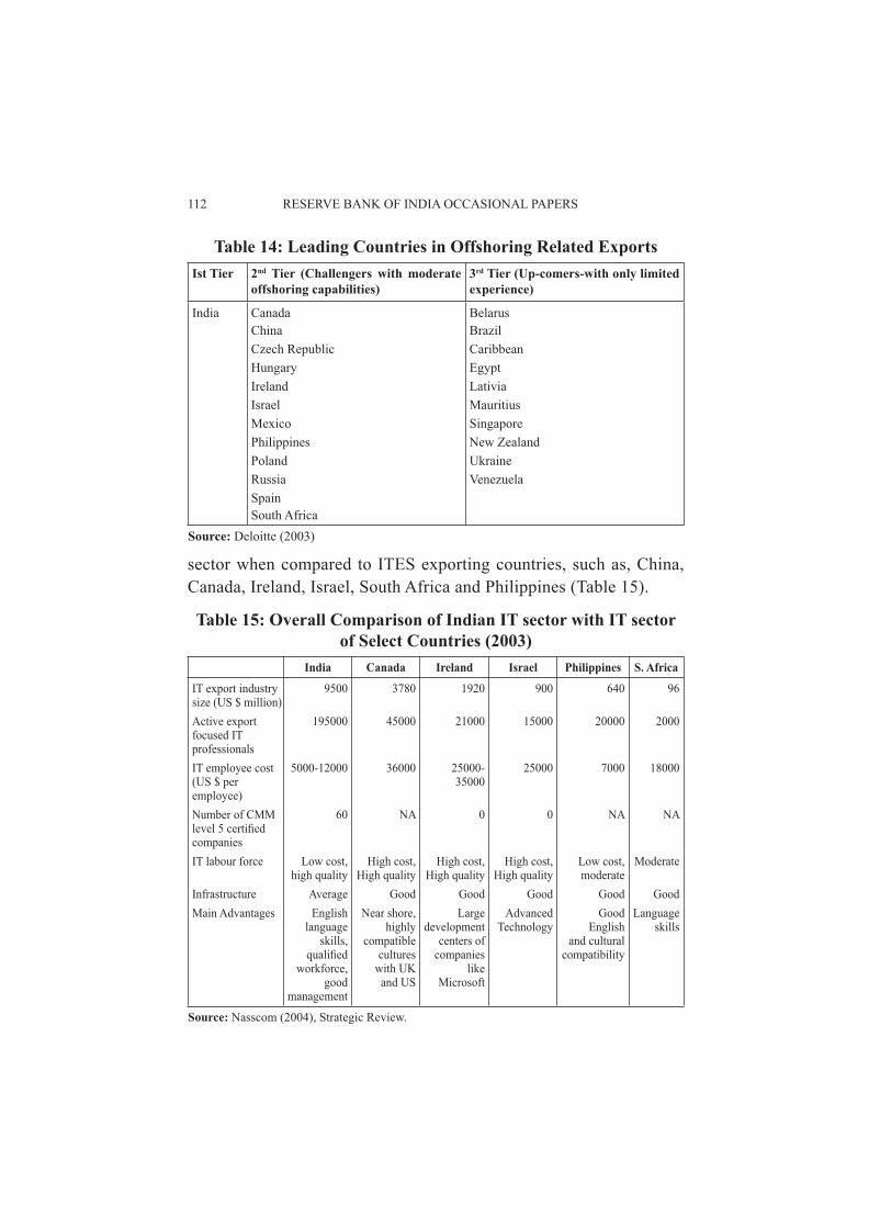
112 RESERVE BANK OF INDIA OCCASIONAL PAPERS
sector when compared to ITES exporting countries, such as, China, Canada, Ireland, Israel, South Africa and Philippines (Table 15).
Table 14: Leading Countries in Offshoring Related Exports Ist Tier 2nd Tier (Challengers with moderate
offshoring capabilities)3rd Tier (Up-comers-with only limited experience)
India Canada BelarusChina BrazilCzech Republic CaribbeanHungary EgyptIreland LativiaIsrael MauritiusMexico SingaporePhilippines New ZealandPoland UkraineRussia VenezuelaSpainSouth Africa
Source: Deloitte (2003)
Table 15: Overall Comparison of Indian IT sector with IT sector of Select Countries (2003)
India Canada Ireland Israel Philippines S. Africa
IT export industry size (US $ million)
9500 3780 1920 900 640 96
Active export focused IT professionals
195000 45000 21000 15000 20000 2000
IT employee cost (US $ per employee)
5000-12000 36000 25000-35000
25000 7000 18000
Number of CMM level 5 certifi ed companies
60 NA 0 0 NA NA
IT labour force Low cost, high quality
High cost, High quality
High cost, High quality
High cost, High quality
Low cost, moderate
Moderate
Infrastructure Average Good Good Good Good GoodMain Advantages English
language skills,
qualifi ed workforce,
good management
Near shore, highly
compatible cultures
with UK and US
Large development
centers of companies
like Microsoft
Advanced Technology
Good English
and cultural compatibility
Language skills
Source: Nasscom (2004), Strategic Review.
INTERNATIONAL OUTSOURCING FROM INDIA: AN ANALYSIS 113
4.1 Facing the Competition: Government Policy towards IT Sector
Supportive government policy has helped Indian outsourcing sector. The state funded IITs and other institutes of higher learning created a pool of skilled labour. The policy for construction of software technology parks allowed fi rms to increase revenues from offshore projects. The Export Oriented Units (EOUs) and units under Electronic Hardware Technology Parks (EHTPs), Software Technology Parks (STPs), Special Economic Zones (SEZs) and Bio-Technology Parks (BTPs) schemes are entitled to avail several facilities/benefi ts including exemption from payment of income tax under Section 10A and 10B of the Income Tax Act. Nasscom has called for the continuation of Software Technology Parks of India (STPI) scheme for a 10 year period as the number of start-up companies could decline in the absence of the scheme. The STPI scheme, allowed tax breaks to make IT business affordable for SMEs and start-ups.
Further, Government of India passed the IT Act 2000, which attempts to change outdated laws and provides ways to deal with cyber crimes. The Act offers the much-needed legal framework so that information is not denied legal effect, validity or enforceability, solely on the ground that i t i s in the form of e lec t ronic records (CYBERLAWSINDIA.net). In view of the growth in transactions and communications carried out through electronic records, the Act seeks to empower government departments to accept filing, creating and retention of offi cial documents in the digital format. The Act has also proposed a legal framework for the authentication and origin of electronic records / communications through digital signature. These measures are expected to help further growth of ITES-BPO services from India.
Section V
Emerging Challenges for India’s Outsourcing Sector
5.1 IT Exports and Exchange rate
The invoice in US dollar accounted for the maximum share of software services exports of India followed by Pound sterling and
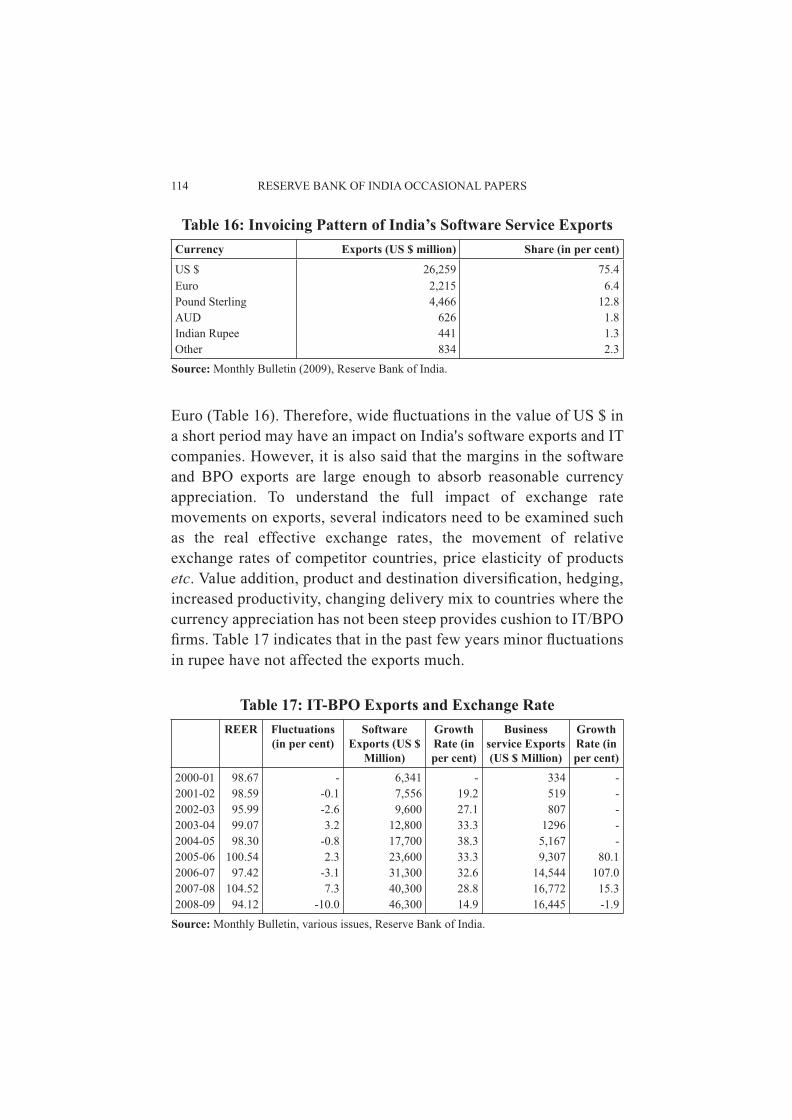
114 RESERVE BANK OF INDIA OCCASIONAL PAPERS
Euro (Table 16). Therefore, wide fl uctuations in the value of US $ in a short period may have an impact on India's software exports and IT companies. However, it is also said that the margins in the software and BPO exports are large enough to absorb reasonable currency appreciation. To understand the full impact of exchange rate movements on exports, several indicators need to be examined such as the real effective exchange rates, the movement of relative exchange rates of competitor countries, price elasticity of products etc. Value addition, product and destination diversifi cation, hedging, increased productivity, changing delivery mix to countries where the currency appreciation has not been steep provides cushion to IT/BPO fi rms. Table 17 indicates that in the past few years minor fl uctuations in rupee have not affected the exports much.
Table 16: Invoicing Pattern of India’s Software Service ExportsCurrency Exports (US $ million) Share (in per cent)
US $ 26,259 75.4Euro 2,215 6.4Pound Sterling 4,466 12.8AUD 626 1.8Indian Rupee 441 1.3Other 834 2.3
Source: Monthly Bulletin (2009), Reserve Bank of India.
Table 17: IT-BPO Exports and Exchange RateREER Fluctuations
(in per cent)Software
Exports (US $ Million)
GrowthRate (in per cent)
Business service Exports (US $ Million)
GrowthRate (in per cent)
2000-01 98.67 - 6,341 - 334 -2001-02 98.59 -0.1 7,556 19.2 519 -2002-03 95.99 -2.6 9,600 27.1 807 -2003-04 99.07 3.2 12,800 33.3 1296 -2004-05 98.30 -0.8 17,700 38.3 5,167 -2005-06 100.54 2.3 23,600 33.3 9,307 80.12006-07 97.42 -3.1 31,300 32.6 14,544 107.02007-08 104.52 7.3 40,300 28.8 16,772 15.32008-09 94.12 -10.0 46,300 14.9 16,445 -1.9
Source: Monthly Bulletin, various issues, Reserve Bank of India.
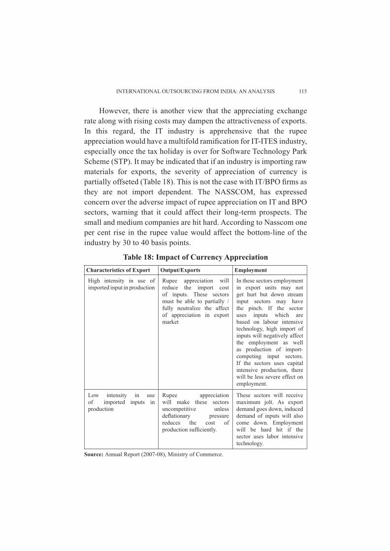
INTERNATIONAL OUTSOURCING FROM INDIA: AN ANALYSIS 115
However, there is another view that the appreciating exchange rate along with rising costs may dampen the attractiveness of exports. In this regard, the IT industry is apprehensive that the rupee appreciation would have a multifold ramifi cation for IT-ITES industry, especially once the tax holiday is over for Software Technology Park Scheme (STP). It may be indicated that if an industry is importing raw materials for exports, the severity of appreciation of currency is partially offseted (Table 18). This is not the case with IT/BPO fi rms as they are not import dependent. The NASSCOM, has expressed concern over the adverse impact of rupee appreciation on IT and BPO sectors, warning that it could affect their long-term prospects. The small and medium companies are hit hard. According to Nasscom one per cent rise in the rupee value would affect the bottom-line of the industry by 30 to 40 basis points.
Table 18: Impact of Currency AppreciationCharacteristics of Export Output/Exports Employment
High intensity in use of imported input in production
Rupee appreciation will reduce the import cost of inputs. These sectors must be able to partially / fully neutralize the affect of appreciation in export market
In these sectors employment in export units may not get hurt but down stream input sectors may have the pinch. If the sector uses inputs which are based on labour intensive technology, high import of inputs will negatively affect the employment as well as production of import-competing input sectors. If the sectors uses capital intensive production, there will be less severe effect on employment.
Low intensity in use of imported inputs in production
Rupee appreciation will make these sectors uncompetitive unless defl ationary pressure reduces the cost of production suffi ciently.
These sectors will receive maximum jolt. As export demand goes down, induced demand of inputs will also come down. Employment will be hard hit if the sector uses labor intensive technology.
Source: Annual Report (2007-08), Ministry of Commerce.
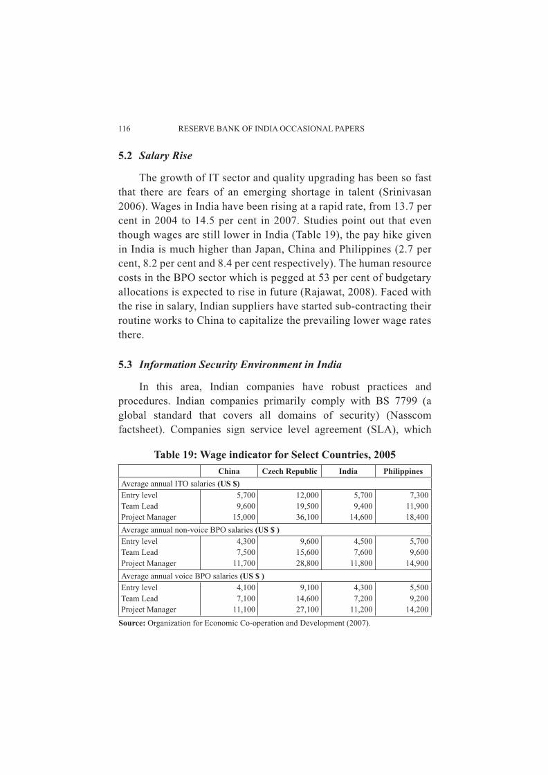
116 RESERVE BANK OF INDIA OCCASIONAL PAPERS
5.2 Salary Rise
The growth of IT sector and quality upgrading has been so fast that there are fears of an emerging shortage in talent (Srinivasan 2006). Wages in India have been rising at a rapid rate, from 13.7 per cent in 2004 to 14.5 per cent in 2007. Studies point out that even though wages are still lower in India (Table 19), the pay hike given in India is much higher than Japan, China and Philippines (2.7 per cent, 8.2 per cent and 8.4 per cent respectively). The human resource costs in the BPO sector which is pegged at 53 per cent of budgetary allocations is expected to rise in future (Rajawat, 2008). Faced with the rise in salary, Indian suppliers have started sub-contracting their routine works to China to capitalize the prevailing lower wage rates there.
5.3 Information Security Environment in India
In this area, Indian companies have robust practices and procedures. Indian companies primarily comply with BS 7799 (a global standard that covers all domains of security) (Nasscom factsheet). Companies sign service level agreement (SLA), which
Table 19: Wage indicator for Select Countries, 2005China Czech Republic India Philippines
Average annual ITO salaries (US $)Entry level 5,700 12,000 5,700 7,300Team Lead 9,600 19,500 9,400 11,900Project Manager 15,000 36,100 14,600 18,400Average annual non-voice BPO salaries (US $ )Entry level 4,300 9,600 4,500 5,700Team Lead 7,500 15,600 7,600 9,600Project Manager 11,700 28,800 11,800 14,900Average annual voice BPO salaries (US $ )Entry level 4,100 9,100 4,300 5,500Team Lead 7,100 14,600 7,200 9,200Project Manager 11,100 27,100 11,200 14,200
Source: Organization for Economic Co-operation and Development (2007).
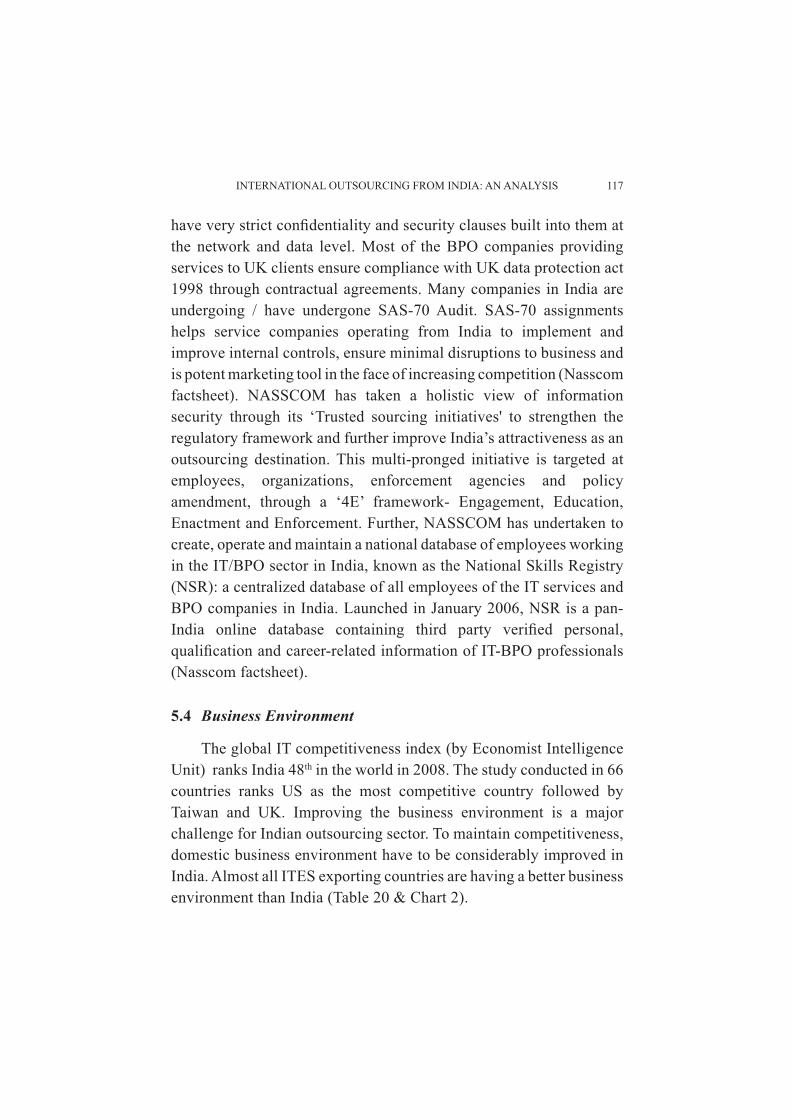
INTERNATIONAL OUTSOURCING FROM INDIA: AN ANALYSIS 117
have very strict confi dentiality and security clauses built into them at the network and data level. Most of the BPO companies providing services to UK clients ensure compliance with UK data protection act 1998 through contractual agreements. Many companies in India are undergoing / have undergone SAS-70 Audit. SAS-70 assignments helps service companies operating from India to implement and improve internal controls, ensure minimal disruptions to business and is potent marketing tool in the face of increasing competition (Nasscom factsheet). NASSCOM has taken a holistic view of information security through its ‘Trusted sourcing initiatives' to strengthen the regulatory framework and further improve India’s attractiveness as an outsourcing destination. This multi-pronged initiative is targeted at employees, organizations, enforcement agencies and policy amendment, through a ‘4E’ framework- Engagement, Education, Enactment and Enforcement. Further, NASSCOM has undertaken to create, operate and maintain a national database of employees working in the IT/BPO sector in India, known as the National Skills Registry (NSR): a centralized database of all employees of the IT services and BPO companies in India. Launched in January 2006, NSR is a pan-India online database containing third party verifi ed personal, qualifi cation and career-related information of IT-BPO professionals (Nasscom factsheet).
5.4 Business Environment
The global IT competitiveness index (by Economist Intelligence Unit) ranks India 48th in the world in 2008. The study conducted in 66 countries ranks US as the most competitive country followed by Taiwan and UK. Improving the business environment is a major challenge for Indian outsourcing sector. To maintain competitiveness, domestic business environment have to be considerably improved in India. Almost all ITES exporting countries are having a better business environment than India (Table 20 & Chart 2).
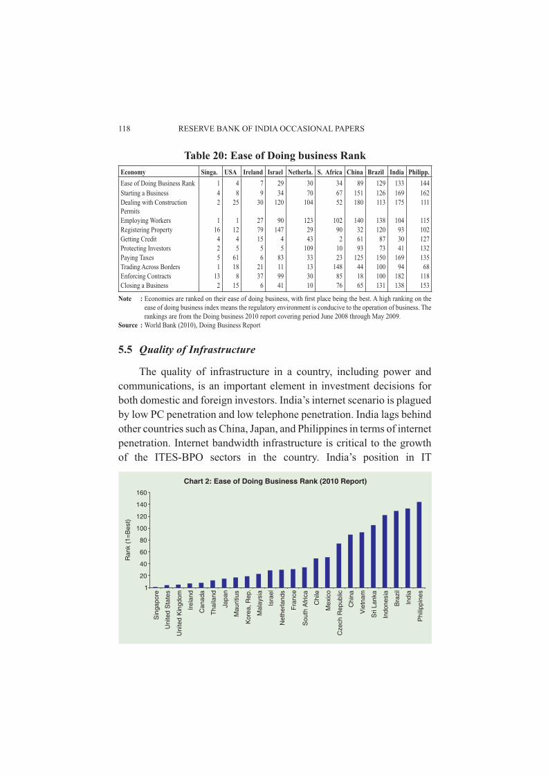
118 RESERVE BANK OF INDIA OCCASIONAL PAPERS
5.5 Quality of Infrastructure
The quality of infrastructure in a country, including power and communications, is an important element in investment decisions for both domestic and foreign investors. India’s internet scenario is plagued by low PC penetration and low telephone penetration. India lags behind other countries such as China, Japan, and Philippines in terms of internet penetration. Internet bandwidth infrastructure is critical to the growth of the ITES-BPO sectors in the country. India’s position in IT
Table 20: Ease of Doing business RankEconomy Singa. USA Ireland Israel Netherla. S. Africa China Brazil India Philipp.Ease of Doing Business Rank 1 4 7 29 30 34 89 129 133 144Starting a Business 4 8 9 34 70 67 151 126 169 162Dealing with Construction Permits
2 25 30 120 104 52 180 113 175 111
Employing Workers 1 1 27 90 123 102 140 138 104 115Registering Property 16 12 79 147 29 90 32 120 93 102Getting Credit 4 4 15 4 43 2 61 87 30 127Protecting Investors 2 5 5 5 109 10 93 73 41 132Paying Taxes 5 61 6 83 33 23 125 150 169 135Trading Across Borders 1 18 21 11 13 148 44 100 94 68Enforcing Contracts 13 8 37 99 30 85 18 100 182 118Closing a Business 2 15 6 41 10 76 65 131 138 153
Note : Economies are ranked on their ease of doing business, with fi rst place being the best. A high ranking on the ease of doing business index means the regulatory environment is conducive to the operation of business. The rankings are from the Doing business 2010 report covering period June 2008 through May 2009.
Source : World Bank (2010), Doing Business Report
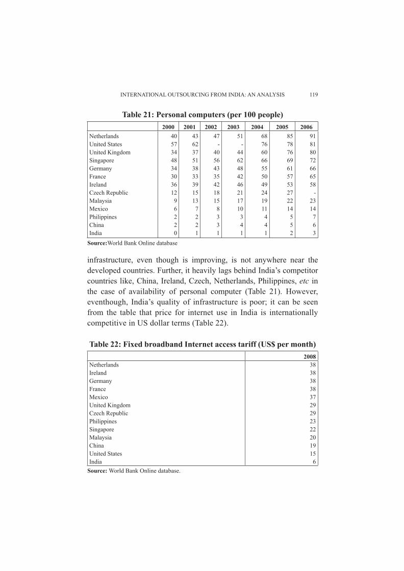
INTERNATIONAL OUTSOURCING FROM INDIA: AN ANALYSIS 119
infrastructure, even though is improving, is not anywhere near the developed countries. Further, it heavily lags behind India’s competitor countries like, China, Ireland, Czech, Netherlands, Philippines, etc in the case of availability of personal computer (Table 21). However, eventhough, India’s quality of infrastructure is poor; it can be seen from the table that price for internet use in India is internationally competitive in US dollar terms (Table 22).
Table 21: Personal computers (per 100 people)2000 2001 2002 2003 2004 2005 2006
Netherlands 40 43 47 51 68 85 91United States 57 62 - - 76 78 81United Kingdom 34 37 40 44 60 76 80Singapore 48 51 56 62 66 69 72Germany 34 38 43 48 55 61 66France 30 33 35 42 50 57 65Ireland 36 39 42 46 49 53 58Czech Republic 12 15 18 21 24 27 -Malaysia 9 13 15 17 19 22 23Mexico 6 7 8 10 11 14 14Philippines 2 2 3 3 4 5 7China 2 2 3 4 4 5 6India 0 1 1 1 1 2 3
Source:World Bank Online database
Table 22: Fixed broadband Internet access tariff (US$ per month)2008
Netherlands 38Ireland 38Germany 38France 38Mexico 37United Kingdom 29Czech Republic 29Philippines 23Singapore 22Malaysia 20China 19United States 15India 6
Source: World Bank Online database.
120 RESERVE BANK OF INDIA OCCASIONAL PAPERS
5.6 Free Trade Agreements
Multilateral or bilateral trade agreement in services sector would be helpful for strengthening existing markets and exploring new markets and new areas of trade. India may enter into bilateral free trade agreement in services to intensively explore the foreign markets. In this context, the comprehensive economic cooperation agreement (CECA) between India and Singapore are worth noting. India and Singapore signed a CECA under which both the countries guarantee access into each other’s market. Further, both the countries may not restrict access into their service market by imposing quantitative restrictions.
5.7 Anti-Outsourcing Legislations and protectionism
There is a rise in anti-outsourcing legislations world-wide. The Committee of European Banking Supervisors (CEBS) has put out a consultative paper proposing a total ban on outsourcing of strategic or core activities (Business Standard, 2004). However, it is also said that some of the anti-outsourcing bill in US may violate its international trade obligations and therefore will not be passed. But the fact that there is a general mood to prevent contracting of services to other countries under various pretext remains (Table 23).
Further, there are moves to impose restrictions on movement of professionals especially after the September 11, 2001 terror attack. Also, opposition to H1B quota of 65,000 exists due to growing unemployment in US (Varma and Rogers, 2004). Moreover, the Grossley-Durbin Bill in the US aims to set tougher wage standards (which may increase salaries of H-1 B workers) and also impose limits on the number of visa workers to 50 per cent of the workforce. This may force companies to hire more locals instead of professionals from India (Business Standard, 2009). In this context, it may also be noted that, a phenomenon known as ‘reverse outsourcing’ has begun to assert itself. For example, the Indian outsourcing fi rm Wipro has added many US based consultants to its staff.
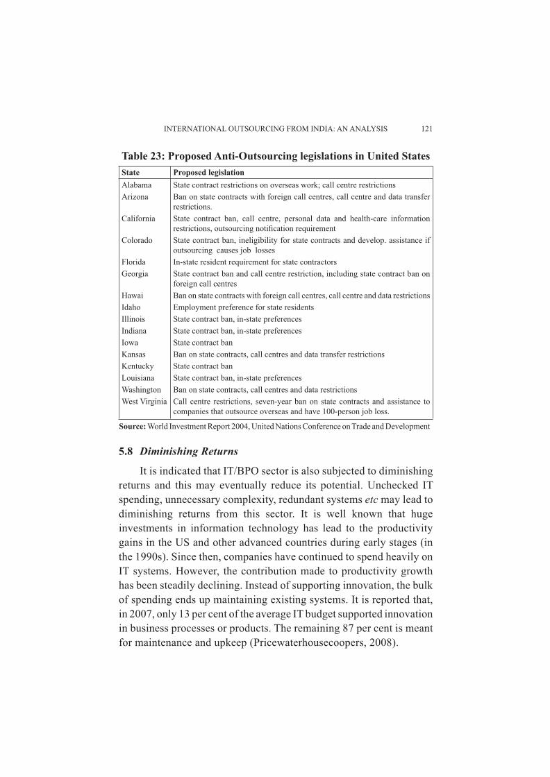
INTERNATIONAL OUTSOURCING FROM INDIA: AN ANALYSIS 121
5.8 Diminishing Returns
It is indicated that IT/BPO sector is also subjected to diminishing returns and this may eventually reduce its potential. Unchecked IT spending, unnecessary complexity, redundant systems etc may lead to diminishing returns from this sector. It is well known that huge investments in information technology has lead to the productivity gains in the US and other advanced countries during early stages (in the 1990s). Since then, companies have continued to spend heavily on IT systems. However, the contribution made to productivity growth has been steadily declining. Instead of supporting innovation, the bulk of spending ends up maintaining existing systems. It is reported that, in 2007, only 13 per cent of the average IT budget supported innovation in business processes or products. The remaining 87 per cent is meant for maintenance and upkeep (Pricewaterhousecoopers, 2008).
Table 23: Proposed Anti-Outsourcing legislations in United StatesState Proposed legislationAlabama State contract restrictions on overseas work; call centre restrictionsArizona Ban on state contracts with foreign call centres, call centre and data transfer
restrictions.California State contract ban, call centre, personal data and health-care information
restrictions, outsourcing notifi cation requirementColorado State contract ban, ineligibility for state contracts and develop. assistance if
outsourcing causes job lossesFlorida In-state resident requirement for state contractorsGeorgia State contract ban and call centre restriction, including state contract ban on
foreign call centresHawai Ban on state contracts with foreign call centres, call centre and data restrictionsIdaho Employment preference for state residentsIllinois State contract ban, in-state preferencesIndiana State contract ban, in-state preferencesIowa State contract banKansas Ban on state contracts, call centres and data transfer restrictionsKentucky State contract banLouisiana State contract ban, in-state preferencesWashington Ban on state contracts, call centres and data restrictionsWest Virginia Call centre restrictions, seven-year ban on state contracts and assistance to
companies that outsource overseas and have 100-person job loss.
Source: World Investment Report 2004, United Nations Conference on Trade and Development
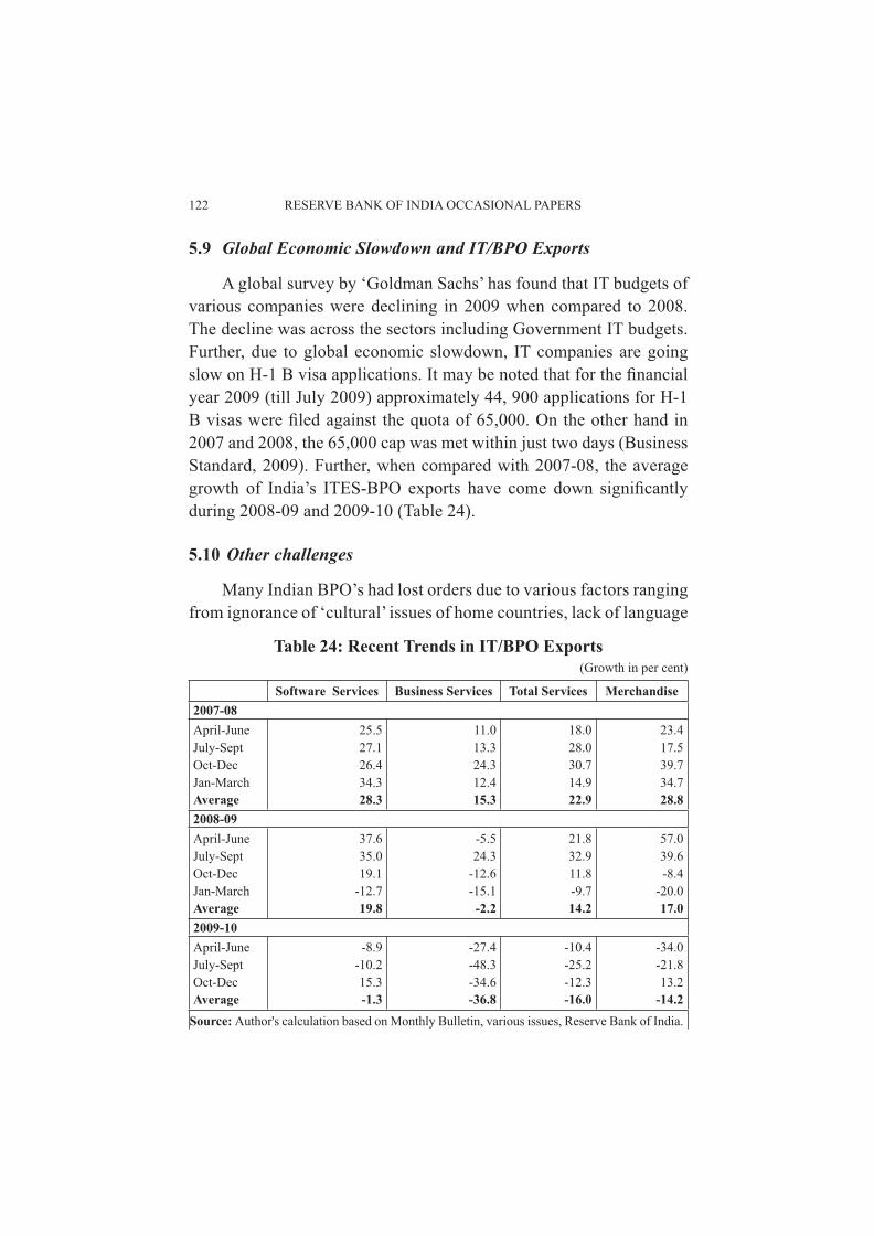
122 RESERVE BANK OF INDIA OCCASIONAL PAPERS
5.9 Global Economic Slowdown and IT/BPO Exports
A global survey by ‘Goldman Sachs’ has found that IT budgets of various companies were declining in 2009 when compared to 2008. The decline was across the sectors including Government IT budgets. Further, due to global economic slowdown, IT companies are going slow on H-1 B visa applications. It may be noted that for the fi nancial year 2009 (till July 2009) approximately 44, 900 applications for H-1 B visas were fi led against the quota of 65,000. On the other hand in 2007 and 2008, the 65,000 cap was met within just two days (Business Standard, 2009). Further, when compared with 2007-08, the average growth of India’s ITES-BPO exports have come down signifi cantly during 2008-09 and 2009-10 (Table 24).
5.10 Other challenges
Many Indian BPO’s had lost orders due to various factors ranging from ignorance of ‘cultural’ issues of home countries, lack of language
Table 24: Recent Trends in IT/BPO Exports(Growth in per cent)
Software Services Business Services Total Services Merchandise2007-08April-June 25.5 11.0 18.0 23.4July-Sept 27.1 13.3 28.0 17.5Oct-Dec 26.4 24.3 30.7 39.7Jan-March 34.3 12.4 14.9 34.7Average 28.3 15.3 22.9 28.82008-09April-June 37.6 -5.5 21.8 57.0July-Sept 35.0 24.3 32.9 39.6Oct-Dec 19.1 -12.6 11.8 -8.4Jan-March -12.7 -15.1 -9.7 -20.0Average 19.8 -2.2 14.2 17.02009-10April-June -8.9 -27.4 -10.4 -34.0July-Sept -10.2 -48.3 -25.2 -21.8Oct-Dec 15.3 -34.6 -12.3 13.2Average -1.3 -36.8 -16.0 -14.2
Source: Author's calculation based on Monthly Bulletin, various issues, Reserve Bank of India.
INTERNATIONAL OUTSOURCING FROM INDIA: AN ANALYSIS 123
abilities other than English, lack of technical profi ciency, credit card frauds and misuse of personal information. Further, some segments of outsourcing such as engineering services outsourcing has close links with manufacturing and it may be diffi cult for India to succeed in outsourcing sector without signifi cantly enhancing manufacturing capabilities. India’s weak engineering and physical infrastructures are likely to hamper the growth of services outsourcing in future.
Section VI
Conclusion
In conclusion, the study proves that India is having revealed comparative advantage in exports based on ITES-BPO services. World trade in services is growing at a much faster rate than trade in goods. This will give a good opportunity to India to raise its share of world trade if adequate attention is given to service sector especially to ITES-BPO sector. Government of India has already taken some initiatives in this regard by giving fi scal concessions to service sector. Regarding competition from China, as of today it is not a serious threat to outsourcing business of India. Indian companies had reasonably succeeded in maintaining an edge over Chinese companies in the quality and marketing of service exports. IT infrastructure and general business environment are two areas where India clearly lags behind almost all other competitors in outsourcing arena. Another important fi nding is that even though there is lot of media attention on outsourcing sector in India and other developing countries, especially regarding loss of employment in developed countries like US and UK due to contracting of services to abroad, the maximum gain from services trade is actually going towards these countries. McKinsey study revealed that more than three-fourth of the value being created in the global economy through offshoring goes to US and receiving countries like India get only 22 per cent (Dey 2004). Eventhough India maintain its lead status as a source country for a variety of IT related services, there are number of emerging challenges which require immediate attention. Anti-outsourcing legislation and growing protectionism in western countries need to be closely monitored.
124 RESERVE BANK OF INDIA OCCASIONAL PAPERS
There is an urgent need to diversify services export to other countries rather than concentrating only on US and Europe. In this regard, major Indian IT companies have adopted the strategy of acquisitions and alliances to increase the portfolio of services, and cater to new markets such as the Middle-east Asia, Singapore, etc. Indian service providers should move up the value chain to make up for the loss of rise in wage cost etc and to increase their profi tability. Setting up of overseas offi ces through joint ventures and collaboration with foreign companies and recruiting local talents from abroad is a strategy to bridge the gap in culture and language while exporting to non-English speaking countries. Free trade agreements in services with other countries may be attempted to further consolidate the gains India already made. In short, India has already made an impact in the outsourcing area. However, to maintain its lead and capture new markets and areas, Indian service industries should remain vigilant.
References
Ahuja, Rajeev (2004): “Outsourcing and Job Loss: A Protectionist Fallacy”, Indian Council for Research on International Economic Relations. Working paper No.136.
Amiti, Mary and Wei. Shang-Jin (2004): “Fear of Outsourcing: is it Justifi ed”, International Monetary Fund, Working Paper No. 04/186.
Balassa,B (1965): “Trade Liberalisation and ‘Revealed’ Comparative Advantage”, The Manchester School, 45.
Banga, Rashmi (2005): “Critical Issues in India’s Service-Led Growth”, Indian Council of Research in International Economic Research. Working Paper,171, October.
Bhagwati, Jadhish, Arvind Panagariya and T.N. Srinivasan (2004): “The Muddles Over Outsourcing”, Journal of Economic Perspectives, 18(1).
Business Standard (2004): “EU may put squeeze on outsourcing”, May 5.
Business Standard (2009): “IT companies go slow on H-1 B visas”, July 16.
Dey, Dipankar (2004): “Anxieties over offshoring: State Vs New Economy”, Economic and Political Weekly, June 12.
INTERNATIONAL OUTSOURCING FROM INDIA: AN ANALYSIS 125
Deloitte (2003): “Making the Offshore Call: The Road Map for Communications Operators”, Research report.
Engman, Michael (2007): “Explaining international supply chains: the role of emerging economies in providing IT and business process services”, OECD Trade Policy Working paper No.52.
Gordon,Jim and Poonam Gupta (2003): “Understanding India’s Services Revolution”,Paper prepared for the IMF-NCAER Conference, A Tale of Two Giants: India’s and China’s Experience with Reform, November 14-16, New Delhi.
Grossman, Gene M and Esteban Rossi-Hansberg (2006): “The Rise of Offshoring: It’s Not Wine for Cloth Anymore”, Paper prepared for the symposium sponsored by the Federal Reserve Bank of Kansas city, August.
Infosys (2009-10), Annual Report.
International Monetary Fund (2006): Balance of Payments Statistics Year Book.
International Monetary Fund (2010): Balance of Payments Statistics CD, February.
McKinsey Global Institute (2003): “Offshoring: is it a win-win Game”, San Francisco.
Ministry of Commerce (2007-2008): Annual Report, Government of India.
Mukherjee, Arpita and Paramita Deb Gupta (2006): “Prospects for IT-Enabled Services Under a Indo-US FTA”, Indian Council for Research on International Economic Relations. Working paper No.187.
Nasscom (2004): “Strategic Review".
Nasscom-IDC (2005): “Key highlights of the Nasscom-IDC study on the domestic services (IT-ITES) market opportunity”.
Nasscom (2007): “Tracing China’s IT Software and Services Industry Evolution”, White paper, August.
Nasscom Factsheet (undated): “Information security environment in India-Nasscom analysis”.
Nasscom (2010): “Strategic Review".
126 RESERVE BANK OF INDIA OCCASIONAL PAPERS
Pricewaterhousecoopers (2008): “Why isn’t IT spending creating more value?, June.
Rajawat, Yatish K (2008): "Behind The Scenes", Business World, February.
Ramesh, P Babu (2004): “Cyber Coolies’ in BPO – Insecurities and Vulnerabilities of Non-Standard Work”, Economic and Political Weekly, January 31.
Reserve Bank of India (2009): “Survey on Computer Software and Information Technology Services Exports 2007-08”, Monthly Bulletin, September.
Reserve Bank of India (2010): “Invisibles in India’s Balance of Payments: An Analysis of Trade in Services, Remittances and Income”, Monthly Bulletin, March.
Reserve Bank of India: Monthly Bulletin (Various issues).
Srinivasan, T.N (2006): “China, India and the World Economy”, Economic and Political Weekly, August 26.
Sandhu, Amandeep (2006): “Why Unions Fail in Organising India’s BPO-ITES Industry”, Economic and Political Weekly, October 14.
Taganas, Rey A.L and Kaul, Vijay Kumar (2006): “Innovation Systems in India’s IT Industry: An Empirical Investigation”, Economic and Political Weekly, September 30.
Taylor, Philip, E. Noronha, D. Scholarios and Premilla D’ Cruz (2008): “Employee Voice and Collective Formation in Indian ITES-BPO Industry” Economic and Political Weekly, May 31.
The New Oxford Dictionary of English (1998): OxfordUniversity Press, New Delhi.
United Nations (2004): World Investment Report: “The Shift towards Services”, United Nations Conference on Trade and Development.
United Nations (2005): "ICT and E-Business: Selected Trends and Issues on the ICT for Development Agenda" United Nations Conference on Trade and Development, December.
Utkulu, Utku and D. Seymen (2004): “Revealed Comparative Advantage and Competitiveness: Evidence for Turkey vis-à-vis the EU/15”, European Trade Study Group 6th Annual Conference, September.
INTERNATIONAL OUTSOURCING FROM INDIA: AN ANALYSIS 127
Varma, Roli and R.M. Everett (2004): “India Cyber Workers in US; Economic and Political Weekly, December 25.
World Bank (2006): World Development Report.
World Trade Organization (1998): Annual Report.
World Trade Organization (2005): World Trade Report.
http://www.cyberlawsindia.net/Information-technology-act-of-india.html
http://www.doingbusiness.org/economyrankings/
http://www.indiainfoline.com/Markets/News/Archieved

Asia and the Subprime Crisis, Chi Lo (Palgrave Macmillan: UK), 2009; pp XI+125, £60.
Many lessons can be learned from the recent subprime crisis. Those lessons have not been systematically addressed, perhaps because everyone has been busy with ‘fi ghting the fi re’. This is not a normal crisis period, and hence, no normal post-crisis recovery was expected. The fi nancial wizards seem to remain overly optimistic that the crisis will be followed by a normal economic recovery so that life can get back to normalcy. There was huge economic imbalances built up in the 1990s and early 2000s, all fi nanced by massive debt in the developed world. The advent of fi nancial derivatives, thanks to the deregulation, had only made these imbalances, making crisis more complicated. To unwind these imbalances from the web of complicated fi nancial instruments spread throughout the world will take a long time. The loss of public confi dence only adds diffi culties to fi nding a solution. There are also signifi cant implications of the crisis on the regulatory, macroeconomic and fi nancial fronts in the post-crisis era. In this book, the author has drawn parallels between fi nancial crisis of Asian emerging countries and developed countries of European Union and the USA. Though the analysis is China-centric, some sporadic focus on other emerging Asian countries to draw lessons from the crisis.
It is properly mentioned in the book that, the epicenter of the crisis has changed from Asia (Asian Financial Crisis of 1997) to Europe and the USA. The buzzwords have also changed, from currency pegs, excessive corporate borrowing and foreign debt in the Asian crisis to securitization, subprime mortgages, and collateral debt obligations in the subprime crisis. However, it is properly clarifi ed that the causes and symptoms of the subprime crisis are quite similar to those of the Asian crisis. So to say that the subprime crisis is an unexpected shock is a denial of human mistakes - greed is prevalent in both the subprime and Asian crises. Before the Asian crisis, massive foreign capital infl ows to the region signifi cantly boosted bank lending and corporate borrowing. Foreign investors were attracted by Asia’s high-yield securities in the blind faith that the regional currency pegs would hold forever and
Reserve Bank of India Occasional PapersVol. 31, No.1, Summer 2010
130 RESERVE BANK OF INDIA OCCASIONAL PAPERS
robust economic growth would support Asian Corporates’ payment ability forever. Similarly, massive capital infl ows fl ooded the USA and fi nanced its huge current account defi cit, fuelling excessive demand for credit and mortgage loans. The latter were repackaged into mortgage-backed securities and other credit derivatives like collateralized debt obligations (CDOs). Investors outside the USA were attracted by the high yields of these structured products in the blind faith that the underlying parties had AAA credit ratings. Imprudence follows greed. Ten years ago, the Asians indulged in imprudent lending to corporates based on relationship to mega projects and property development of dubious nature. Due diligence and commercial viability were totally ignored. In the subprime crisis, imprudence is seen in the proliferation of subprime mortgage loans and the so called ninja loans (no income, no jobs and no assets for backing).
Seed of the Subprime Crisis
The book has appropriately diagnosed the subprime crisis. It has mentioned that the global major central banks, such as, the US Federal Reserve, the Bank of England and the European Central Bank (ECB) in particular, had run an overly loose monetary policy in a dynamic, entrepreneurial, globalised and capitalist system, and ended up turning the original good economic policy intension into the seed of another shocking crisis. But that did not mean that capitalism had failed. Rather, the subprime crisis was a result of regulatory failure in the capitalist system.
The US monetary policy was not the only problem. The creation of the Euro zone in 1999, which centralized monetary policies of the member countries into ECB, also played a crucial role in creating the global credit bubble. Monetary union eliminates currency risk but not credit risk. With only one currency, the Euro, and one monetary policy, credit spreads in some Euroland countries should have risen to refl ect their underlying risks. But the ECB, in an attempt to ensure stability in the early days of the Euro, had kept an overly loose monetary policy for a long time. Thus, asset bubbles, fuelled
ASIA AND THE SUBPRIME CRISIS 131
by easy credit, emerged especially in the peripheral, smaller Euroland countries, such as, Ireland, Spain, Greece and Portugal.
Contesting Factors
The book has contested that the current subprime crisis is a ‘black swan’ event. The term black swan comes from the ancient western concept that all swans are white. In that context, a black swan was a metaphor for something that could not exist. Ever since black swans were discovered in Australia in the seventeenth century, the term black swan has been used to connote the actual happening of a highly unlikely event with unprecedented and devastating effects. The subprime crisis itself is not a black swan event, though the resultant credit crunch and confi dence crisis may qualify. This is because all the events and factors leading up to the current crisis were known. From a macro perspective, the Asian crisis and the subprime debacle have similarities in their causes and symptoms - namely a prolonged period of low interest rates leading to moral hazard, imprudent lending, regulatory oversight, excessive investment, and asset bubble. But the advent of fi nancial derivatives has made today’s subprime crisis more complicated.
The deepening of the US subprime crisis after September 2008, despite the Fed’s repeated massive liquidity injection, shows that the markets had failed to clear on their own and the global fi nancial system had stalled. There would be two possible outcomes of the crisis - either a global fi nancial meltdown or a full-scale government bailout. History and the Government actions suggest the latter. There is a confl ict of interest problem, which often takes the form of a principal-agent problem. In the Asian fi nancial crisis, bank managers just ignored shareholders and public interest and lent indiscriminately to companies and projects under political or infl uential business pressure. In the US subprime crisis, investors in mortgage based securities (MBS) and CDOs expected mortgage lenders and banks to keep their credit standards. But in the ‘originate and distribute’ model, in which the mortgage lenders and banks originate the loans and sell them off at once, they had little incentive to scrutinize and
132 RESERVE BANK OF INDIA OCCASIONAL PAPERS
keep the credit standards. Typically, mortgage lenders made the loans and at once sold them off to banks. The banks, in turn, securitized them and sold them off to investors throughout the world. The banks aimed at maximizing only their fee income from securitization but not the interest income from the loans. So they had the incentive to securitize and push the products off their books as soon as possible. Credit standards dropped sharply in the process, and no-one had any clues about the ultimate ownership of the underlying loans. So, when the US housing bubble burst, defaults surged, setting off a domino effect on the mortgage derivative instruments and shattering public confi dence in the banking system as a whole.
Hence, those who argue that the subprime crisis was a black swan event are either naive or in denial. Despite numerous analyses of the subprime crisis, its causes and impact are still misread in many cases, especially from the Asian perspective. As the subprime-induced credit crunch pulled down asset prices indiscriminately, what was at fi rst a liquidity crisis soon turned into a solvency crisis for individual banks, prompting the global authorities to employ radical measures such as partial bank nationalization, troubled-asset purchases and other forms of direct market interventions to contain the credit quake or fi nancial tsunami, as it is called in Asia. Asia’s policy response has remained relatively calm in this subprime debacle because it has learnt good lessons from the 1997-98 Asian fi nancial crisis.
Subprime Generalised
The word ‘subprime’ in relation to mortgages in the USA generally refers to those mortgages targeted at borrowers with impaired or low credit ratings and low income level who may fi nd it diffi cult to obtain fi nance through traditional sources, such as, prime mortgages and Alt-A. Subprime borrowers have the highest perceived default risk, as compared with Prime and Alt-A borrowers. In essence, subprime borrowers are those who have a history of loan delinquency or default, those with a record of bankruptcy, and those with low income levels relative to their mortgage payment ability.
ASIA AND THE SUBPRIME CRISIS 133
The US subprime crisis was quickly transmitted to Europe, as the European banks were some of the largest holders of the US mortgage-related derivative instruments. During the good times, they loaded up the MBS and CDOs with cheap US dollar funding. But when the sub-prime crisis broke, US$ funding sources of all sorts, including money market funds, bank depositors and other investors, withdrew cash en masse. European banks soon found their funding increasingly diffi cult and expensive to replace. When the credit market eventually seized up after the failure of Lehman Brothers in September 2008, the domino effect was quickly felt in Europe, pulling down big banks like Fortis and HBOS and forcing them into government hands for rescue.
When the fi nancial contagion hit Asia, it wreaked havoc in the regional fi nancial and currency markets, even though the regional banks had very limited exposure to the sub-prime toxic assets. However, the overall impact on the regional fi nancial system was relatively small. Asia’s strong fundamentals, including large current account surpluses, huge foreign reserves, low foreign debts and high savings rates, have helped shield its fi nancial systems from the fi nancial tsunami. However, the region’s heavy reliance on export growth has signifi cantly pushed its economies deep into recession as global demand contracts under the weight of the post-bubble adjustment in the developed world.
While Asian growth experienced a V-shaped rebound a year after the Asian crisis of 1997-98, thanks to its young and vibrant economic structure and a quick return of confi dence, don’t bet on the same happening in Europe and the USA. Even if the US Troubled Asset Relief Programme (TARP) manages to turn confi dence around and the European authorities fi nally wake up to reality and join in a concerted bailout effort, history shows that the post-bubble adjustment in developed economies will take a long time. Thus, to correct their mistakes, banks will have to become more boring, generating less profi t from fancy fi nancial engineering, and more heavily regulated relative to the past two decades. Granted, restrictions will hurt economic opportunities and profi tability in the next economic upswing, but
134 RESERVE BANK OF INDIA OCCASIONAL PAPERS
it will be a small price to pay for greater protection from another, perhaps bigger, banking crisis in the future.
The correct message from these failures should be that Asia should ensure that any move away from traditional banking practices towards more innovative techniques is accompanied by enhanced risk management. It will be extremely unfortunate if the wrong message gets out and delays or even deters further fi nancial liberalization in the developing world. Asian regulators should take the subprime crisis lesson seriously to improve their regulatory systems. As Asian fi nancial markets expand into new terrain, policymakers should put in place measures to deal with risks posed by fi nancial innovation, but should not shy away from fi nancial liberalization or suppress fi nancial innovation.
Bailout Approaches Converged
Before October 2008, there was no coordination between all the subprime crisis countries. They had only taken ad hoc steps to stem the crisis. Central banks had cut interest rates, governments had acted to strip toxic assets off bank balance sheets and regulators had injected capital into the banking sector. These moves were country-by-country solutions and had no broad coordination between governments, despite the fact that the global fi nancial system was linked. No wonder they had failed to calm the markets and prevent the crisis from deepening.
Asia does not have a fi nancial crisis, despite the global impact of the fi nancial tsunami stemming from the western world. This is mainly because the Asian banking systems, except Korea, have de-leveraged since the aftermath of the Asian crisis. This is in sharp contrast to the over-leveraging of the US and European systems, which sowed the seed for the subprime crisis. This difference in the banking system fundamentals between the east and the west is best summarized by the loan-to-deposit ratio. Since the Asian crisis, Asian banks, except Korea, have de-leveraged signifi cantly, while their western counterparts have indulged in lending.
ASIA AND THE SUBPRIME CRISIS 135
The Painful Lessons
Despite all these micro, macro and unconventional measures taken by the global authorities to tackle the global credit crisis, the root problem has yet to be dealt with effectively. That is because what the western policymakers have done is to sustain household leverage and consumption at any price, when the only exit from the ‘credit quack’ involved a return to thrift by the over-leveraged.
The book is properly timed and appropriately mentioned that the subprime crisis was rooted in the irresponsible social behaviour of the USA and most of the developed world in the past two decades, which prioritized the desire for current consumption over the ability to pay for it. Financial engineering and deregulation had encouraged borrowing and discouraged thrift to fi nance excess spending via a gigantic credit bubble. That, in turn, led to huge global economic imbalances and distortions. This root cause explains why it is so diffi cult to solve the crisis. Desperate to preserve the value of asset prices infl ated by this huge liquidity bubble, western policymakers have avoided the painful solution of allowing market clearing. The bailout programs, liquidity injections and fi scal stimulus packages are all meant to sustain asset prices, when these asset prices really need to fall to market levels so that they can be cleared.
Narayan Chandra Pradhan*
* Narayan Chandra Pradhan is Research Offi cer, Department of Economic Analysis and Policy, Reserve Bank of India.

Related Documents