Observer-Based Fuel Control Using Oxygen Measurement

Observer-Based Fuel Control Using Oxygen Measurement - A study based on a first- principles model of a pulverized coal fired Benson Boiler

Pa lie Andersen, Jan Dimon Bendtsen, Jan Henrik Mortensen, Rene Just Nielsen,

Observer-Based Fuel Control Using OxygenMeasurement

Observator-baseret Bransle Regiering ved SyreMatning

Palle Andersen, Jan Dimon Bendtsen, Jan Henrik Mortensen, Rene Just Nielsen, Tom Sondergaard Pedersen

P4-318

VARMEFORSK Service AB 101 53 STOCKHOLM • Tel 08-677 25 80

Januari 2005ISSN 0282-3772

VARMEFORSK

Preface

This project has been carried out in collaboration between the Department of Control Engineering, Aalborg University and Elsam Engineering A/S. It has been an interesting and instructive learning experience and has brought our research in this area forward. We hope that the proposed control concept will be found applicable in the power plant industry. We would like to thank everyone who gave input to this project, in particular

Hjalmar Hasselbalch Elsam Engineering A/SKlaus Trangb$k Aalborg University

Varmeforsks projektreferensgruppMartin Raberg Erik Dahlquist Erik Ramstrom Flemming Nielsen Kimmo Valiaho Kristian Sjostedt

Carl Bro AB Malardalens Hogskola TPS E2Foster Wheeler Alstom AB

Aalborg, November 2004

i

vArmeforsk

ii

VARMEFORSK

AbstractThis report describes an attempt to improve the existing control of coal mills used at the Danish power plant Nordjyllandsv$rket Unit 3. The coal mills are not equipped with coal flow sensors; thus, an observer-based approach is investigated. A nonlinear differential equation model of the boiler is constructed and validated against data obtained at the plant. A Kalman filter based on measurements of combustion air flow led into the furnace and oxygen concentration in the flue gas is designed to estimate the actual coal flow. With this estimate, it becomes possible to close an inner loop around the coal mill itself.

i

vArmeforsk

ii

VARMEFORSK

SammanfattningDenna rapport beskriver ett forsok att forbattra den existerande regleringen av kolkvarnar som anvands i det danska kraftverket Nordjyllandsv$rket Block 3. Kolkvarnarna maler kolstycken till ett fint pulver, som blases in i eldstaden. Dar forbranns kolet och utvecklar varme, som anvands till angproduktion. Med en battre reglering av kolkvarnarna skulle kraftverket kunna regleras mer effektivt vid lastandringar, med hogre tillganglighet och verkningsgrad som foljd. Ett av huvudproblemen, sett ur reglerteknisk synvinkel, ar att sensorer saknas for att mata den kolpulvermangd som faktiskt tillfors eldstaden. I projektet har en forhallandevis detaljerad ickelinjar modell av eldstaden och angkretsen utvecklats. Denna ar validerad mot matdata fran kraftverket och har visat sig aterge den viktigaste processdynamiken.

Denna modell har linjariserats kring ett antal arbetspunkter. Rapporten diskuterar linjariseringen och visar hur en linjar modell av en lagre ordning kan erhallas genom att ta bort tillstand som har liten paverkan pa den totala responsen. En anvandbar adaptiv regleringsstrategi skulle darmed kunna vara att ta fram regulatorer for var och en av dessa forenklade linjara modeller. Regulatorforstarkningarna skulle sedan anges som en funktion av last.

Med en sadan strategi blir dock inte variationer och osakerheter i kolkvarnarna direkt behandlade. En reglerstrategi undersoktes darfor i projektet dar ett Kalmanfilter baserat pa matningar av luftflodet till eldstaden och syrekoncentrationen i forbranningsgasen anvants for att uppskatta det faktiska kolflodet. Med hjalp av denna uppskattning blir det mojligt att ha en sluten inre reglerloop kring kvarnen. Detta ger battre storningsundertryckning vilket ocksa visas genom simuleringar.

Sokord: Bensonpanna, dynamisk modell, adaptiv/multi - vari ab el reglering, observator, storningsreducering

in

vArmeforsk

iv

VARMEFORSK

Summary

This report describes an attempt to improve the existing control of coal mills used at the Danish power plant Nordjyllandsv$rket Unit 3. The coal mills pulverize raw coal to a fine-grained powder, which is injected into the furnace of the power plant. In the furnace the coal is combusted, producing heat, which is used for steam production. With better control of the coal mills, the power plant can be controlled more efficiently during load changes, thus improving the overall availability and efficiency of the plant. One of the main difficulties from a control point of view is that the coal mills are not equipped with sensors that detect how much coal is injected into the furnace. During the project, a fairly detailed, nonlinear differential equation model of the furnace and the steam circuit was constructed and validated against data obtained at the plant. It was observed that this model was able to capture most of the important dynamics found in the data.

Based on this model, it is possible to extract linearized models in various operating points. The report discusses this approach and illustrates how the model can be linearized and reduced to a lower-order linear model that is valid in the vicinity of an operating point by removing states that have little influence on the overall response. A viable adaptive control strategy would then be to design controllers for each of these simplified linear models, i.e., the control loop that sets references to the coal mills and feedwater, and use the load as a separate input to the control. The control gains should then be scheduled according to the load.

However, the variations and uncertainties in the coal mill are not addressed directly in this approach. Another control approach was taken in this project, where a Kalman filter based on measurements of air flow blown into the furnace and the oxygen concentration in the flue gas is designed to estimate the actual coal flow injected into the furnace. With this estimate, it becomes possible to close an inner loop around the coal mill itself, thus giving it better disturbance rejection capabilities, as indicated through simulations.

Keywords: Benson boiler, dynamic model, adaptive/multi-variable control, observer, disturbance rejection

v

vArmeforsk

vi

vArmeforsk

Table of contents1 INTRODUCTION...........................................................................................................................1

1.1 Background...................................................................................................................... 11.2 The purpose of the research assignment and its role within the research area............... 11.3 Coal mills.......................................................................................................................... 21.4 The Benson boiler and steam circuit at njv3......................................................................51.5 Current control strategy................................................................................................ 61.6 Outline of the report....................................................................................................... 7

2 NONLINEAR MODEL OF ONCE-THROUGH BOILER AND STEAM CIRCUIT............... 8

2.1 Purpose of modeling......................................................................................................... 82.2 Overview of the power plant............................................................................................ 92.3 Coal mill model............................................................................................................... 102.4 Furnace model.................................................................................................................. 122.5 Flue gas duct model.........................................................................................................162.6 Oxygen controller..........................................................................................................172.7 Evaporator metal model.................................................................................................. 182.8 Evaporator model............................................................................................................ 192.9 Superheater metal model................................................................................................. 202.10 Superheater model...........................................................................................................212.11 Controller and attemporator model.............................................................................. 222.12 Summary and model structure......................................................................................... 23

3 VERIFICATION OF NONLINEAR MODEL.............................................................................26

3.1 High load experiments..................................................................................................... 263.2 Low load experiments...................................................................................................... 323.3 Summary........................................................................................................................... 37

4 MODEL LINEARIZATION......................................................................................................... 38

4.1 Linearization....................................................................................................................384.2 Linearized model validation............................................................................................ 404.3 Reduced linear model...................................................................................................... 424.4 Using a linearized model in an adaptive control concept................................................ 434.5 Summary........................................................................................................................... 44

5 STRATEGIES FOR ESTIMATION AND CONTROL............................................................. 45

5.1 General concept.............................................................................................................. 455.2 Observer design............................................................................................................... 455.3 Control strategy............................................................................................................485.4 Choice of control strategy............................................................................................ 495.5 Interaction between estimation and control..................................................................535.6 Summary........................................................................................................................... 53

6 RESULTS........................................................................................................................................ 54

6.1 Coal mill model estimation............................................................................................. 546.2 Verification of coal mill state estimation...................................................................... 556.3 Control........................................................................................................................... 586.4 Summary........................................................................................................................... 61

7 CONCLUSIONS............................................................................................................................. 62

8 SUGGESTIONS FOR CONTINUED RESEARCH...................................................................64

vii

VARMEFORSK

9 LITERATURE REFERENCES.....................................................................................................65

viii

VARMEFORSK

1 Introduction1.1 Background

In the power generation industry, the current trend toward market deregulation, cou­pled with increasing demands for maximization of natural resources and minimization of environmental impact, places greater and greater focus on effective plant-wide op­eration and control systems. Loadfollowing, i.e., the ability of the power plant to meet the power production demands at all times is becoming a major concern due to the growing competition between power companies and other market forces [7].

In this project, it is attempted to investigate and accomodate a subset of the factors that contribute to the difficulties in achieving efficient load following for coal-fired power plants such as the ones commonly used in Denmark, so-called once-through or Benson boilers. In particular, we wish to investigate the effects of variations in behavior of the coal mills found at modern power plants and attempt to devise methods to compensate for these variations. Currently, such variations, coupled with a lack of efficient coal flow measurement methods, are causing disturbances in the fuel input to the power plant, forcing the power plant control to be more cautious than what could be hoped for during load changes in order to avoid undesired transients, oscillations etc. If, on the other hand, the coal mills can be controlled precisely, it is possible to input exactly the required amount of coal into the furnace at the required time, thus improving the transient behavior during load changes and enabling the power plant to ”ramp up” (or down) to a new operating point in a rapid manner.

Normally, tight control of the coal mills would be possible by closing a local loop around the coal mills; under normal circumstances, however, there is no sensor equip­ment available to measure the coal flow leaving the mill and hence no local feedback can be made. Methods to detect the coal flow using the available sensors are thus de­sirable. Specific coal flow measurement equipment is available on the market, but is highly expensive and not straightforward to employ in practice.

1.2 The purpose of the research assignment and its role within the re­search area

The purpose of the present project is to investigate the development of an adaptive control strategy for the coal mills that can handle variations in the behavior of the coal mills found at a typical Danish power plant. The term ’adaptive’ here means to be able to estimate the varying dynamics involved in the input of fuel into the furnace online, i.e., during operation, based on available sensor measurements. The control law that regulates the operation of the coal mills may then be adjusted accordingly, such that it matches the current boiler dynamics at all times.

There are several benefits of being able to adjust the operation of the coal mills at all times; firstly, the transient behavior is improved as outlined above, which improves the load following capabilities of the plant. Secondly, undesired oscillations can be

1

VARMEFORSK

suppressed, which may improve the steady-state operation of the plant. Thirdly, better control improves the availablity of the plant, resulting in less risk of plant shutdowns in critical situations.

The scope of this project involves the coal supply system, the furnace and the steam circuit. Load following planning, power production via turbines, district heating, con­densation of steam, etc., are mentioned for the sake of completeness, but not included in the models.

The study will take its starting point in Nordjyllandsv$rket Unit 3 (hereinafter at times abbreviated as NJV3), which is situated at the outskirts of Nerresundby in Northern Jutland, Denmark [10]. The aim is to formulate models and control strategies that can be generalized to other power plants of similar type, but to adjust the models and validate them against data measured at NJV3.

Furthermore, the models derived and used in this project are created strictly for simu­lation and control purposes; they should not be seen as an attempt to perform a detailed modeling of the chemical reactions and flow patterns in the coal mills and furnace etc.

1.3 Coal mills

It is important to maintain close control of the size of the coal particles delivered to the burners. The finer the coal is, the more quickly and efficiently it burns, reducing carbon in the fly ash while maintaining low NOx emissions and increasing boiler efficiency. The coal mills are thus a crucial part of the fuel supply system at a fossil fuel plant.

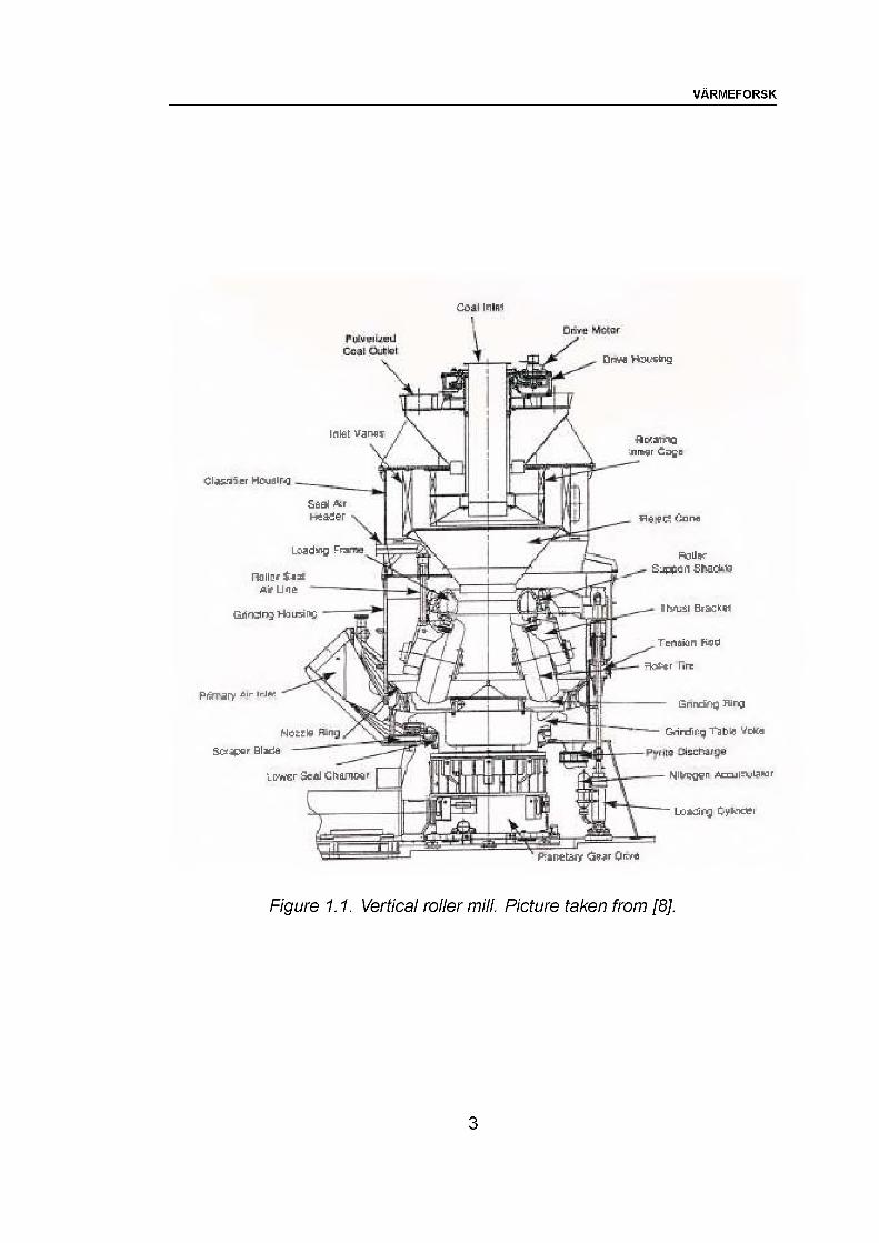
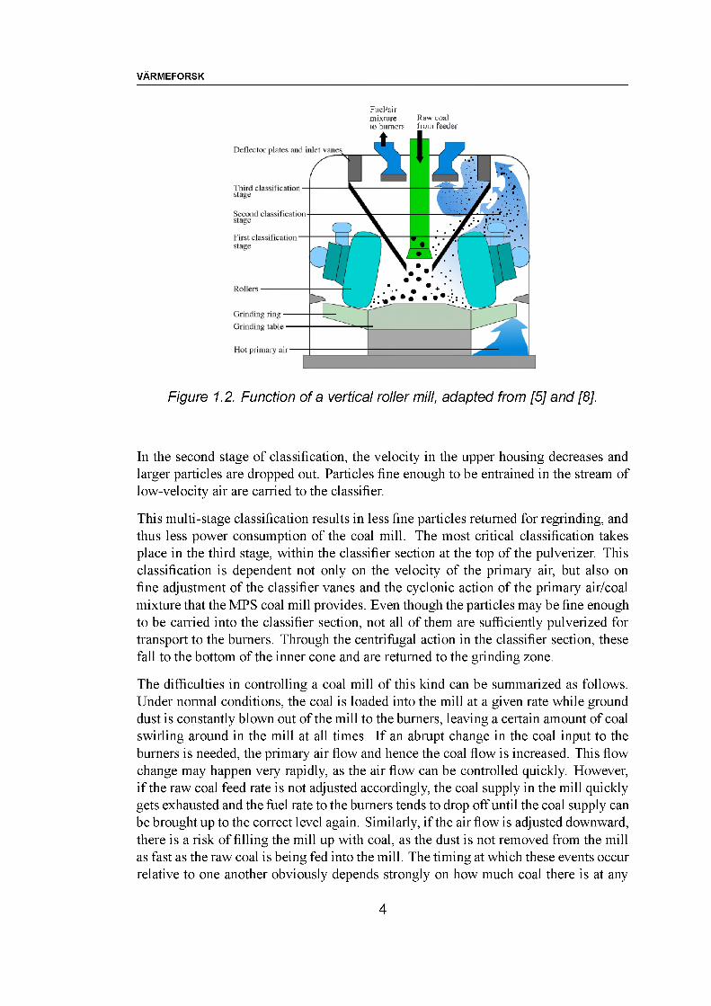
The coal mills used at Nordjyllandsv$rket Unit 3 are four Deutsche Babcock MPS mills [10]; see Figure 1.1. These MPS coal mills are of the so-called vertical spindle type, which operates in the following manner—see Figure 1.2. Raw coal is fed through a central coal inlet at the top of the mill and falls onto the rotating grinding table where it is mixed with classifier rejects returned for re-grinding. Centrifugal action forces the coal outward onto the grinding ring where it is pulverized between the ring and three grinding rollers.

The grinding load, transmitted from tension rods through a loading frame onto the roller assemblies, holds the rollers downward against the grinding ring. The rollers adjust their position vertically as the depth of the coal load increases or decreases.

A nozzle ring on the outside perimeter of the grinding ring feeds primary air to the pulverizer. Pyrites and tramp metal fall through the nozzle ring openings to be scraped into a rejects hopper.

In the separator and classifier sections, the large, heavy particles are separated from fine particles according to the following principle. Primary air enters the mill through an aerodynamically-ported nozzle, carrying the ground coal particles up toward the top of the mill; the developed swirl air flow induces larger particles to return to the grinding track. During this first stage of classification, fine particles are carried upward in the housing in the stream of air and coarser particles fall back to the table for regrinding.

2

VARMEFORSK

Coil Hlfli

Clr-v-ti hiru. -cng

P'iPeraiY (Se-pr Orve

Inlet Utisina niagr Cage

(ll.iir-. :!r Housing

£631 A;

Ar Liie Gritting !-i:u5.:%

Piifr^iy <"r hdw

PUttllMSo-jt^ir SIjlIb

uBWcr Seal Chamw

fleier t^cne

Aqlly£jpevn

!ln:sl g'^rkPi

Teristin I’^ci5=k?ltr fire

Gnrar,g Fling

Girding ~ghln Vck:

Nlirngnn Accui 'ijtimr

Lusting cye.iTfci

Figure 1.1. Vertical roller mill. Picture taken from [8],

3

VARMEFORSK

Fuel/airmixture Raw coalto burners from Feeder

Deflector plates and inlet varies^

Third classification stage

Second classification stage

First, classification stage

Rollers

Grinding ring - Grinding table

Hot primary air

Figure 1.2. Function of a vertical roller mill, adapted from [5] and [8].

In the second stage of classification, the velocity in the upper housing decreases and larger particles are dropped out. Particles fine enough to be entrained in the stream of low-velocity air are carried to the classifier.

This multi-stage classification results in less fine particles returned for regrinding, and thus less power consumption of the coal mill. The most critical classification takes place in the third stage, within the classifier section at the top of the pulverizer. This classification is dependent not only on the velocity of the primary air, but also on fine adjustment of the classifier vanes and the cyclonic action of the primary air/coal mixture that the MPS coal mill provides. Even though the particles may be fine enough to be carried into the classifier section, not all of them are sufficiently pulverized for transport to the burners. Through the centrifugal action in the classifier section, these fall to the bottom of the inner cone and are returned to the grinding zone.

The difficulties in controlling a coal mill of this kind can be summarized as follows. Under normal conditions, the coal is loaded into the mill at a given rate while ground dust is constantly blown out of the mill to the burners, leaving a certain amount of coal swirling around in the mill at all times. If an abrupt change in the coal input to the burners is needed, the primary air flow and hence the coal flow is increased. This flow change may happen very rapidly, as the air flow can be controlled quickly. However, if the raw coal feed rate is not adjusted accordingly, the coal supply in the mill quickly gets exhausted and the fuel rate to the burners tends to drop off until the coal supply can be brought up to the correct level again. Similarly, if the air flow is adjusted downward, there is a risk of filling the mill up with coal, as the dust is not removed from the mill as fast as the raw coal is being fed into the mill. The timing at which these events occur relative to one another obviously depends strongly on how much coal there is at any

4

VARMEFORSK

given time in the mill, and hence on the power plant load. Furthermore, wear and tear, coal congestion etc., cause the mechanical behavior to change over time. Finally, the quality of the raw coal itself varies, as the degree of humidity in the coal is not constant. These effects all have strong influences on the dynamic response of the coal mill and contibute to making the coal supply system tricky to control.

1.4 The Benson boiler and steam circuit at NJV3

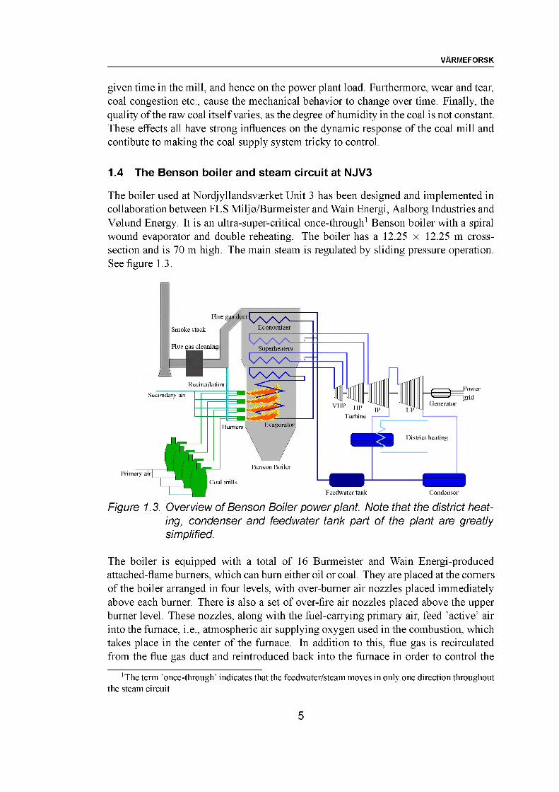
The boiler used at Nordjyllandsvserket Unit 3 has been designed and implemented in collaboration between FLS Miljo/Burmeister and Wain Energi, Aalborg Industries and Volund Energy. It is an ultra-super-critical once-through1 Benson boiler with a spiral wound evaporator and double reheating. The boiler has a 12.25 x 12.25 m cross- section and is 70 m high. The main steam is regulated by sliding pressure operation. See figure 1.3.

Hue gas duct

Smoke stack

Flue gas cleaning

r=B=n

RecirculationSecondary air

\

Economizer

—ESuperheaters

Generator

Figure 1.3. Overview of Benson Boiler power plant. Note that the district heat­ing, condenser and feedwater tank part of the plant are greatly simplified.

The boiler is equipped with a total of 16 Burmeister and Wain Energi-produced attached-flame burners, which can bum either oil or coal. They are placed at the comers of the boiler arranged in four levels, with over-burner air nozzles placed immediately above each burner. There is also a set of over-fire air nozzles placed above the upper burner level. These nozzles, along with the fuel-carrying primary air, feed ’active’ air into the furnace, i.e., atmospheric air supplying oxygen used in the combustion, which takes place in the center of the furnace. In addition to this, flue gas is recirculated from the flue gas duct and reintroduced back into the furnace in order to control the

1 The term ’once-through’ indicates that the feedwater/steam moves in only one direction throughout the steam circuit

5

VARMEFORSK

temperature in the combustion zone. The flue gas is led out of the furnace through the flue gas duct and through a cleaning system that handles removal of dust, NOx, SO2 and other harmful byproducts before being released into the atmosphere through the smoke stack.

The heating surfaces of the boiler are arranged to ensure efficient cooling of the flue gas; that is, heat is transferred from the combustion zone and flue gas to the boiler tubes placed on the walls of the furnace. In the boiler tubes, feedwater is evaporated under high pressure conditions, producing high-energy steam. The steam is superheated fur­ther, increasing the enthalpy in the steam and ensuring that the feedwater is completely evaporated before it is expanded through the turbine.

Large fluctuations in the steam temperature in the superheaters lead to heavy stress in the material used for the superheater pipes. These pipes are also easily corroded if the temperature becomes too high (about 600°C or more). Hence, a set of attemporators is placed at the inlets of each of the superheaters, injecting feedwater into the steam before it passes through the pipes. The injected feedwater evaporates immediately, thus cooling down the steam.

After the first superheater, the steam is expanded through the Very High Pressure (VHP) turbine stage from about 285 bar to about 80 bar, rotating the turbine shaft, which is connected to an electrical power generator. Following this, the steam is superheated again, then fed into the High Pressure (HP) turbine stage and expanded from about 75 bar to about 20 bar. This procedure is repeated for various Intermediate Pressure (IP) turbine stages, where the expansion takes place from about 19 bar down to about 7 bar. The inlet flow through the turbine at the IP stage is about 44 and the total net power output of NJV3 in full condensing mode is 411 MW [10]. The maximum electrical power output at full district heating production is 340 MW, and the maximum district heating production is 422 MJ/s.

Finally, the low-pressure, low-temperature steam is condensed to be reused as feed­water, and heat is exchanged with a district heat supply system to exploit the low- temperature enthalpy that cannot be used for electric power production.

1.5 Current control strategy

The overall control aims to supply the correct amounts of feedwater and fuel to deliver the desired steam flow and to evaporate and increase the enthalpy to the desired level. This level is governed by the energy production required of the plant, i.e., the load. The load is determined at a higher level, as a result of company-wide production distribution among the power plants connected to Elsam’s power grid etc.

Two interconnected loops control evaporator steam enthalpy and steam pressure using feedwater and coal flow as control inputs. Other loops control temperature (enthalpy) of superheated steam by injecting water into the steam. This is essentially a redistribution of feedwater in order to adapt to the actual heat transfer of individual heating surfaces.

6

VARMEFORSK

A local loop controls the feedwater pump, which delivers the required amount of feed­water to the evaporator in a fast and reliable manner. A similar local loop controlling the coal flow is not available, since it is not possible to measure the coal flow from the coal mills. Instead, the desired coal flow is used to guide the primary air flow, raw coal flow and speed of the grinding table of the mill in a feedforward fashion with the difficulties described in Section 1.3.

1.6 Outline of the report

In Chapter 2 a fairly detailed, nonlinear modeling of three subsystems of a power plant of the type described above within the scope of this project, namely the coal supply subsystem, the furnace and flue gas duct subsystem and the steam circuit subsystem, is carried out. These models, which are based on mass- and energy balance equations, yield first principles-based differential equation models that can be validated against actual data obtained from Nordjyllandsv$rket Unit 3. This is considered a significant contribution of this project.

Following that, in Chapter 4 the nonlinear model obtained in Chapter 2 is linearized in order to facilitate later estimator and control designs. It is furthermore investigated whether a reduced-order model is adequate to describe the behavior of the plant in various operating points.

Chapter 3 presents two open loop experiments carried out at NJV3 during the project period for the purpose of model validation and illustrates that the nonlinear model is able to simulate the observed plant behavior.

Chapter 5 presents the strategies for estimation and control of the coal flow employed in this project. It first presents the design of a state estimator for the actual coal flow. This estimator utilizes the total air flow and oxygen sensor measurement as inputs to a Kalman filter, which estimates the amount of coal combusted in the furnace. To the best of the authors’ knowledge, this is a novel development. Based on this estimated coal flow, it is chosen to close an inner loop around the coal mill to suppress disturbances.

In Chapter 6 it is shown that using the estimated coal flow as input to the furnace model, the modeling capabilities of the nonlinear model can be improved compared to using a system-identification-based model.

Finally, Chapters 7 and 8 sum up the work carried out in the project and considers the possibilities for further work opened up by this project.

7

vArmeforsk

2 Nonlinear Model of Once-Through Boiler and Steam Circuit

In this chapter a fairly detailed, nonlinear modeling of three subsystems of a once- through Benson boiler power plant, namely the coal supply subsystem, the furnace and flue gas duct subsystem and the steam circuit subsystem, is carried out. These models, which are based on mass- and energy balance equations, yield first principles-based differential equation models that can be validated against actual data obtained from Nordjyllandsv$rket Unit 3. 1

2.1 Purpose of Modeling

As mentioned in the introduction, the purpose of this project is to investigate variations in the coal mill dynamics and to propose a control strategy to cope with these varia­tions. The nonlinear model presented in this chapter is formulated for the purpose of describing the dynamics connecting the fuel and feedwater inputs to the enthalpy and pressure of the steam leaving the evaporator. With a good simulation model and the ac­companying understanding of the complex processes that take place in the power plant, it will (hopefully) be possible to evaluate the dynamics of the coal mill based on the available measurements. As pointed out in the introduction, no direct measurements of the coal flow are available, and various elements contribute to make the estimation of the coal mill dynamics difficult. It is thus necessary to have a good understanding of the combustion and heat transfer in the power plant in order to be able to utilize the available measurements and ’’calculate back” to the coal mill.

During the project period documented in this report, the model and the available data were reconsidered in an attempt to explain some of the missing dynamics and give addi­tions to the model. These changes were implemented in order to ensure that the model would be better able to describe the phenomena observed in the available measurement data. This is obviously highly desirable, since having a good simulation model means that control algorithms can be tested under reasonably realistic circumstances.

Also, linearizations can be performed in various operating points, and control designs can be performed, giving a fair degree of confidence that the design will perform as expected in the vicinity of these operating points.

The improvements have primarily been focused on the furnace side, with only a single addition on the steam circuit side compared to the first model. Some of the additions may be considered as disturbances in a control loop and may not be necessary in the control model. Others may be connected to control inputs via more or less complex paths and should ideally be included in the model.

1 Some of the modeling work presented here takes its starting point in work done in [3].

8

VARMEFORSK

2.2 Overview of the Power Plant

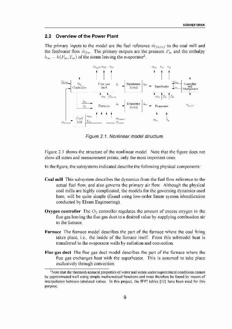
The primary inputs to the model are the fuel reference mfu,ref to the coal mill and the feedwater flow mfw. The primary outputs are the pressure Pse and the enthalpy hse = h(Pse, Tse) of the steam leaving the evaporator2.

CO2,fd mfd Tfd mss Pss Tss

fum fu.ref

CoalMill

Controller

EvaporatorMetal

SuperheaterMetal

Controllerand

AttemperatorSuperheater

Evaporator

Flue gas duct

Furnace

Figure 2.1. Nonlinear model structure.

Figure 2.1 shows the structure of the nonlinear model. Note that the figure does not show all states and measurement points, only the most important ones.

In the figure, the subsystems indicated describe the following physical components:

Coal mill This subsystem describes the dynamics from the fuel flow reference to the actual fuel flow, and also governs the primary air flow. Although the physical coal mills are highly complicated, the models for the governing dynamics used here, will be quite simple (found using low-order linear system identification conducted by Elsam Engineering).

Oxygen controller The O2 controller regulates the amount of excess oxygen in the flue gas leaving the flue gas duct to a desired value by supplying combustion air to the furnace.

Furnace The furnace model describes the part of the furnace where the coal firing takes place, i.e., the inside of the furnace itself. From this submodel heat is transferred to the evaporator walls by radiation and convection.

Flue gas duct The flue gas duct model describes the part of the furnace where the flue gas exchanges heat with the superheater. This is assumed to take place exclusively through convection.

2Note that the thermodynamical properties of water and steam under supercritical conditions cannot be approximated well using simple mathematical functions and must therefore be found by means of interpolation between tabulated values. In this project, the IF97 tables [12] have been used for this purpose.

9

VARMEFORSK

Evaporator metal The evaporator metal submodel represents the heat transfer dy­namics in the evaporator coil walls. In steady state this submodel can be ig­nored.

Evaporator In the evaporator, the feedwater is converted to steam with high enthalpy (pressure and temperature).

Superheater metal The superheater metal submodel represents the heat transfer dy­namics in the superheater tubes. As with the evaporator submodel, this submodel can be ignored in steady state.

Superheater The superheater model actually covers three physical superheaters. Here, the steam receives energy from the superheater pipes, increasing the en­thalpy of the steam even further. To be able to control the steam temperature at the superheater outlet, feedwater is injected into the steam at the superheater inlet through an attemporator system.

Controller and attemperator This part describes the attemporators, which regulate the temperature of the live steam by inj ecting feedwater with a lower temperature into the steam. The dynamics of this subsystem are composed of temperature sensor, PI controller and attemporator actuator dynamics.

It is noted that the recirculation air (mrecair) is included as an external, measurable disturbance input rather than as a controlled feedback. This is done primarily because the effects of the recirculation flow on the state of the Furnace submodel (see Section 2.4) were too large to be ignored, but the control system and process dynamics gov­erning the flow and temperature of the recirculation flow is quite complex and depends on many variables in the system, in particular the temperatures in the IP superheater, which was not included in the model. Similarly, the combustion air flow (ma) was first included as a measurable disturbance input, but in this case the O2 controller proved much easier to integrate in the model, and also turned out to be important for the fuel flow estimator.

In the following sections the dynamic models for the abovementioned physical com­ponents will be derived, leading to a complete description of the nonlinear simulation model used in the project.

2.3 Coal Mill Model

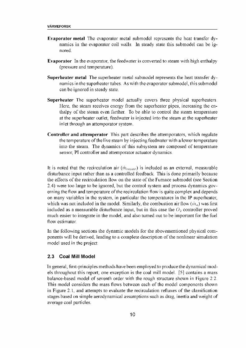
In general, first-principles methods have been employed to produce the dynamical mod­els throughout this report; one exception is the coal mill model. [5] contains a mass balance-based model of seventh order with the rough structure shown in Figure 2.2. This model considers the mass flows between each of the model components shown in Figure 2.1, and attempts to evaluate the recirculation refluxes of the classification stages based on simple aerodynamical assumptions such as drag, inertia and weight of average coal particles.

10

VARMEFORSK

Raw coalI

First and second classification stage

i

Motor

____I_____Grinding table and rollers

I

Bowl

Feeder Third classification stage

Fuel to burners

Figure 2.2. Rough coal mill model structure adapted from [5].

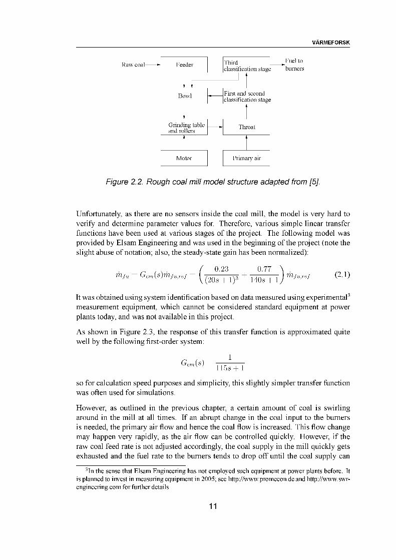
Unfortunately, as there are no sensors inside the coal mill, the model is very hard to verify and determine parameter values for. Therefore, various simple linear transfer functions have been used at various stages of the project. The following model was provided by Elsam Engineering and was used in the beginning of the project (note the slight abuse of notation; also, the steady-state gain has been normalized):

- _ z, r \ / 0-23 , 0.77 \ .(2.1)

It was obtained using system identification based on data measured using experimental3 measurement equipment, which cannot be considered standard equipment at power plants today, and was not available in this project.

As shown in Figure 2.3, the response of this transfer function is approximated quite well by the following first-order system:

Gcm(s)1

115s + 1

so for calculation speed purposes and simplicity, this slightly simpler transfer function was often used for simulations.

However, as outlined in the previous chapter, a certain amount of coal is swirling around in the mill at all times. If an abrupt change in the coal input to the burners is needed, the primary air flow and hence the coal flow is increased. This flow change may happen very rapidly, as the air flow can be controlled quickly. However, if the raw coal feed rate is not adjusted accordingly, the coal supply in the mill quickly gets exhausted and the fuel rate to the burners tends to drop off until the coal supply can

3In the sense that Elsam Engineering has not employed such equipment at power plants before. It is planned to invest in measuring equipment in 2005; see http://www.promecon.de and http://www.swr- engineering.com for further details

11

VARMEFORSK

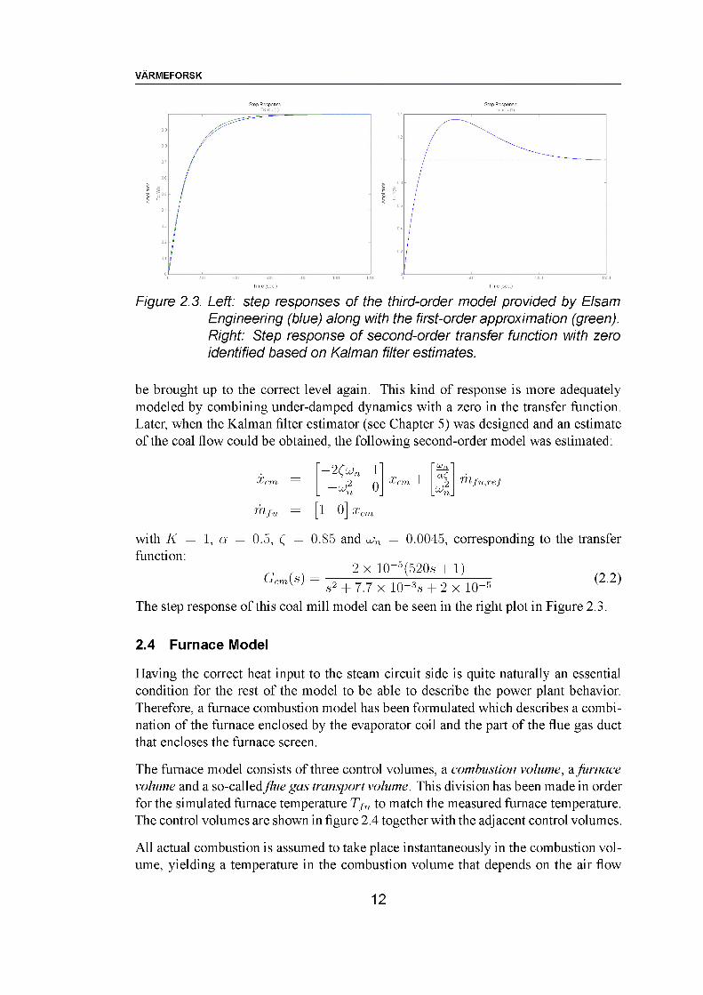
Figure 2.3. Left: step responses of the third-order model provided by Elsam Engineering (blue) along with the first-order approximation (green). Right: Step response of second-order transfer function with zero identified based on Kalman filter estimates.

be brought up to the correct level again. This kind of response is more adequately modeled by combining under-damped dynamics with a zero in the transfer function. Later, when the Kalman filter estimator (see Chapter 5) was designed and an estimate of the coal flow could be obtained, the following second-order model was estimated:

X'cm ,2

1"

0%cm "~h

"Wn ~

9~Un

rn,fUtref

[1 0] Xr

with K = 1, a = 0.5, ( = 0.85 and con = 0.0045, corresponding to the transfer function:

Gcm(s)2 x 10-5(520s + 1)

+ 7.7 x 10-3g + 2 x 10-5The step response of this coal mill model can be seen in the right plot in Figure 2.3.

(2.2)

2.4 Furnace Model

Having the correct heat input to the steam circuit side is quite naturally an essential condition for the rest of the model to be able to describe the power plant behavior. Therefore, a furnace combustion model has been formulated which describes a combi­nation of the furnace enclosed by the evaporator coil and the part of the flue gas duct that encloses the furnace screen.

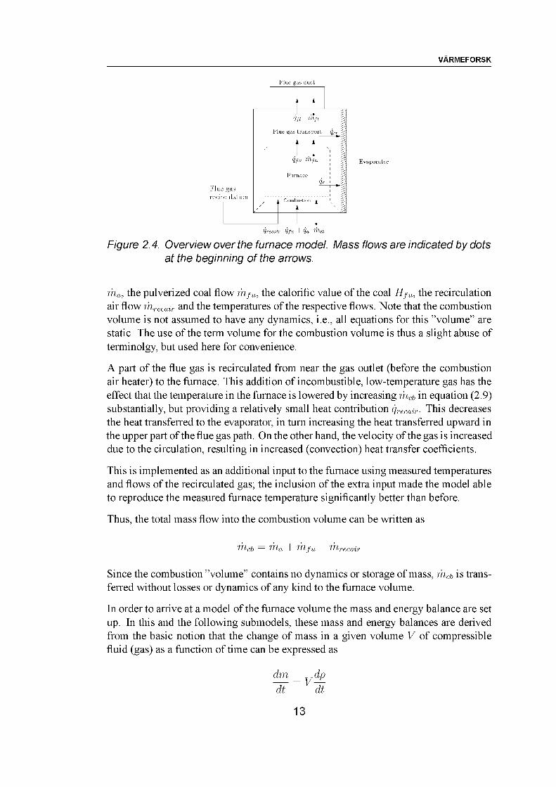
The furnace model consists of three control volumes, a combustion volume, a furnace volume and a so-called flue gas transport volume. This division has been made in order for the simulated furnace temperature 7/„ to match the measured furnace temperature. The control volumes are shown in figure 2.4 together with the adj acent control volumes.

All actual combustion is assumed to take place instantaneously in the combustion vol­ume, yielding a temperature in the combustion volume that depends on the air flow

12

VARMEFORSK

Flue gas duct

Flue gas recirculation

qfi m fi

Flue gas transport qcr

vh:

qfn m fn I

Furnace !qr i ^

i Combustion i 'n

Evaporator

qrecair qfu + qa m cb

Figure 2.4. Overview over the furnace model. Mass flows are indicated by dots at the beginning of the arrows.

ma, the pulverized coal flow mfu, the calorific value of the coal Hfu, the recirculation air flow mrecair and the temperatures of the respective flows. Note that the combustion volume is not assumed to have any dynamics, i.e., all equations for this ’’volume” are static. The use of the term volume for the combustion volume is thus a slight abuse of terminolgy, but used here for convenience.

A part of the flue gas is recirculated from near the gas outlet (before the combustion air heater) to the furnace. This addition of incombustible, low-temperature gas has the effect that the temperature in the furnace is lowered by increasing mcb in equation (2.9) substantially, but providing a relatively small heat contribution qrecair. This decreases the heat transferred to the evaporator, in turn increasing the heat transferred upward in the upper part of the flue gas path. On the other hand, the velocity of the gas is increased due to the circulation, resulting in increased (convection) heat transfer coefficients.

This is implemented as an additional input to the furnace using measured temperatures and flows of the recirculated gas; the inclusion of the extra input made the model able to reproduce the measured furnace temperature significantly better than before.

Thus, the total mass flow into the combustion volume can be written as

fflcb — m a + m fu + rhrecair

Since the combustion ’volume” contains no dynamics or storage of mass, mcb is trans­ferred without losses or dynamics of any kind to the furnace volume.

In order to arrive at a model of the furnace volume the mass and energy balance are set up. In this and the following submodels, these mass and energy balances are derived from the basic notion that the change of mass in a given volume V of compressible fluid (gas) as a function of time can be expressed as

dm _ dp dt dt

13

VARMEFORSK

where p is the density of the fluid (gas). Consequently, the mass balance in the furnace volume can be written as

Vfdpfr, t r dpfn dTfn .

(ft "9pfn dTfn

and likewise, for the flue gas transport volume:

dPfi dTfiVffi dTfi dt

TTfi — m/n - ^i

m/n - ^

dPfi dTfidTfi dt

(2.3)

(2.4)

Making the reasonable assumption that the pressure is constant throughout the volume, it is realized that the enthalpy becomes a function only of the temperature T. The energy balance for the furnace volume can thus be found by the following derivations:

dUfn d(mfnhfn)dt dt

d ( Vfnpfn hfn)(ft

T i „ dh/n dTfn dpfn dTfn-----IT- + y/m/Vm-dTfn dt dTfn dt

(2.5)

On the other hand, the change in energy in the volume is driven by the sum of the energy fluxes into and out of the volume:

dUfn(ft

qfu + qa + qrecair qr(fr — (ffn

— qfu + (fa + qrecair qr hfn\ mcb Vcb9p fn dTfn

(ft(2.6)

—Vm fn

where the expression for mfn obtained in equation (2.3) was used. Combining equa­tions (2.5) and (2.6) now yields the following state equation for the furnace volume:

dTffndt

(ffu + qa + qrecair — (Zr — ^fnTT^cb (2.7)

Similarly, the energy balance for the flue gas transport volume becomes

dUy^ . . . d(m/lh/l)

V/lp/l

dtdlh

(ft

— Qfn Qcf Qfl

— qfn qcf hfi fn fn

14

dt

(2.8)

VARMEFORSK

where each component can be written as

md,

(Z/u

qa

Qrecair

qr

(Zc/

p/n

P/i

m/u + a + W^recair (2.9)m/u(H/u + h/u ) m/u (H/u + c/uT/u) (2.10)

m aha — macp,aTa (2.11)W^recair (cp,/uTrecair + h0) (2.12)ar A/n [(T/n + 273)4 — (Tme + 273)4] + acrm ^ ^ A/n(T/n - T,(2.13)ac/ ^^c^ ̂^A/n (T/l — TLe ) (2.14)

{Tfn + 273 )R(2.15)

(T/f + 273)B (2.16)

In the expressions above, H/u = 25 x 106 J/kg is the calorific value of coal (i.e., the amount of energy released by burning 1 kg coal), R = 8.3145 is the ideal gas constant and, and M/ = 0.0299 kg/mol is the molar mass of the flue gas. Furthermore the assumption that the pressure in the furnace is constant and approximately equal to atmospheric pressure implies that P/n = P/f ~ 100, 000 Pa.

Equations (2.13) and (2.14) express the heat transfers that take place from the combus­tion volume and the flue gas transport volume to the evaporator, respectively. Here, it is assumed that heat is transferred via radiation and convection from the combustion volume and via convection only from the flue gas transport volume. ar and acr are heat transfer coefficients, whereas A/n is the inner area of the furnace walls. The heat trans­fer coefficients are highly empirical quantities that, among other things, reflect the ratio of heat transfer between the two volumes; in other words, these coefficients are con­sidered ’free’ variables that can be adjusted to make the model fit the measurements. They may e.g. be found through steady-state evaluations.

The average furnace temperature T/n was selected as a state variable although it can­not be measured directly as this would require a grid of temperature sensors situated inside the furnace. Instead, a measurement of the temperature just below the screen is available, which presumably reflects the dynamics of T/n well. For simplicity, the temperature T/i was selected as state variable in the flue gas transport volume equa­tions as they have the same structure as the combustion volume equations. Moreover, the dynamics reflected by the two mentioned state variables should be similar.

Having derived differential equations governing the temperature and mass flow in the furnace and flue gas transport volumes, it is possible to calculate the mass flow and temperature of the flue gas that leaves each volume. In equation (2.8) the mass flow m/n leaving the combustion volume can be expressed by the combustion temperature Ta as

m/nPlcbCp,/(Tcb "F 273) Qr

Cp,/(Tfn + 273)(2.17)

15

VARMEFORSK

where

TcbQfu T Qa T Qrecair

m cbcp,fh0

^P,f(2.18)

The combustion flue gas enthalpy as a function of the combustion temperature is ap­proximated using a straight line such that

hcb — cp,f Tcb + h0

Two points have been found in [1]

which gives

000 °C) = 1,147,800 ^

bd,(l,100°C) = 1,275,400 ^

hcb — 1,276Tb - 128,200

(2.19)

(2.20)

More generally, equation (2.20) can be written as

hf — 1,276Tf - 128,200 (2.21)

where the subscript (-)f indicates that the formula should only be used to calculate the enthalpy of a flue gas with a temperature Tf in the vicinity of 1,000-1,100 °C.

Finally, in the same way as for the combustion volume, the mass flow of flue gas leaving the flue gas transport volume can be expressed as

m ff'hlfnC-p,f(Tfn T 273) Qcr

(2.22)

2.5 Flue Gas Duct Model

The flue gas duct model describes the part of the flue gas duct that encloses the three high pressure superheaters HP1.1, HP1.2 and HP2. As stated earlier, heat from the flue gas is transferred to the metal of the mentioned superheaters through convection and the heat delivered to the superheater metal is passed on to the steam in the superheater model.

The constant pressure in the flue gas duct Pfd is taken to be the same as the furnace pressure Pfn. Analogously with the model of the furnace volume, the mass and energy balances are formulated for this volume.

Mass balance:

v,d dt " ^<07), dt m/d (2.23)

m fd (2.24)

16

VARMEFORSK

Similarly, the energy balance for the flue gas transport volume becomes

dUfd . . . d(mfdhfd)dt

Vfdpfdcp,dTffd

dt

(fff — qc — (ffd

— (ffd — (ff — hfd f^ff

dt

(2.25)f

As in the furnace model, the flue gas duct temperature Tfd was selected as the state variable. No measurements of Tfd are available but since the model structure is similar to that of the furnace the dynamics of Tfd are similar to those of Tfn and Tf.

The state equation of Tfd is given by equation (2.26).

dTVfdPfdcp,f ,, Qfi — Qc — hfdriifi (2.26)

The loss in the entire system leaves through the flue gas duct and can be identified as the term hfdmf in equation (2.26).

The remaining terms of (2.26) can be written as:

acmfd ^Ae ' (Tfd — Tme)

PfdMf(7)d + 273)E

and finally, the mass flow of flue gas leaving the volume is found as

qc —

Pf —

(2.27)

(2.28)

TM fdd^fiCpjiTfi + 273) — qc

+ 273)(2.29)

2.6 Oxygen Controller

The oxygen content in the flue gas was not considered in the first model and the amount of air supplied to the furnace was simply determined by a fixed air/fuel ratio. In practice, however, this air flow is controlled by an O2 controller, ensuring a specified amount of excess oxygen. This controller has been included in the new model.

The most immediate benefit of this inclusion is that the measurements of the oxygen concentration Co2 in the flue gas and the air flow are closely related to actual amount of coal being combusted. With these measurements available a state observer can be used to produce an estimate of the coal flow through the coal mill, as will be shown in a subsequent chapter.

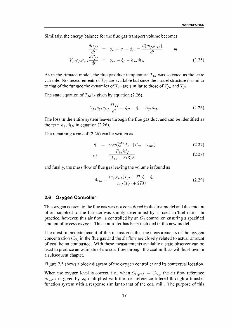
Figure 2.5 shows a block diagram of the oxygen controller and its contextual location.

When the oxygen level is correct, i.e., when Co2ref — Co2, the air flow reference ma,ref is given by A0 multiplied with the fuel reference filtered through a transfer function system with a response similar to that of the coal mill. The purpose of this

17

VARMEFORSK

m fu,ref

'a,ref

Air/fuel ratio

O2 controller

Figure 2.5. Block diagram of the O2 control loop.

filter is to ensure that the dynamics of the actual coal flow and air flow are in tune. When Co2ref = CO2 the controller contributes with a correction signal Acorr to the air/fuel ratio.

ma,ref is the reference signal to the air flow actuator of which the dynamics Ga are assumed to be quick (a first-order system with a time constant Ta of 1 s).

In the oxygen model GO2 the combustion is considered to take place immediately after the injection of coal in the furnace. The model of the oxygen content in the flue gas thus consists of a static model of the oxygen consumption by the combustion combined with mass balances for oxygen for the control volumes already included in the model of the flue gas path.

The concentration of oxygen right after the combustion CO2Cb is given by equation(2.30)

Cm r

O2C6

r CO2fd + ma CO2a — m/uAO2cbmcb

(2.30)

where CO2fd is the concentration of oxygen in the recirculated flue gas, CO2a is the concentration of oxygen in atmospheric air (0.233 kg/kg) and AO2cb is the oxygen ratio consumed in stoichiometric combustion per mass unit of coal.

The oxygen concentrations in the combustion volume O2,fn, flue gas transport volume O2fi and flue gas duct volume O2fd, respectively, are given by the mass balances in each of the control volumes. That is,

fficb(CO2cb CO2fn) (2.31)

A.

ffb fn(CO2fn — CO2fl) (2.32)

VidPid dt = ffi/l (CO2/l - CO2fd) (2.33)

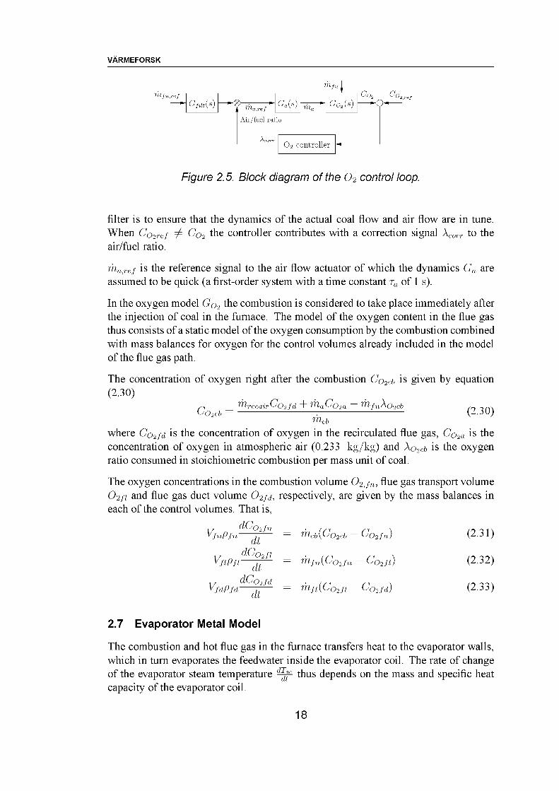
2.7 Evaporator Metal Model

The combustion and hot flue gas in the furnace transfers heat to the evaporator walls, which in turn evaporates the feedwater inside the evaporator coil. The rate of change of the evaporator steam temperature thus depends on the mass and specific heat capacity of the evaporator coil.

18

VARMEFORSK

Since no change of mass occurs in the metal an energy balance is enough to describe the metal temperature dynamics. The energy stored in the metal is given as Ume = mmeume = mmecmTme, and differentiating this leads to equation (2.34):

L/ me(ft

dTmTTlme Cm ~ dt qcr + qr — qn (2.34)

where the heat transmission from the metal to the evaporator steam can be expressed as [11]

Qme eAe ' (Tme — Tse)'~

The heat balance is illustrated in Figure 2.6.

(2.35)

m se

g

g

$

g; g;I g;

g

g

ng: g;

qfw m fw

q

q

Figure 2.6. Overview of the evaporator and evaporator metal models.

2.8 Evaporator Model

Figure 2.6 also illustrates the energy and mass flow in the evaporator. In this volume, the feedwater flow mfw is converted into steam mse. The high pressure is well beyond the critical point of water, which means that the mixture inside the evaporator is a super­critical water/steam mixture. In this region of operation there is no clearly defined transition from water to steam, so it has been chosen to regard the entire contents as dry steam since no information about the water/steam ratio (the so-called quality of the steam) is available. That is, the model does not include a separate control volume containing water.

Pse and Tse are chosen as state variables, as they can both be measured. The following mass and energy balances describe the dynamics of the evaporator. The mass balance is first formulated as:

dTnse dpse f 0pse dPse 0pse dTsem fw m se (2.36)

19

VARMEFORSK

since mse = pse Ve. Then, noting that Use = mseuse Ve (psehse — Pse), the energy balance can be written as:

df - d( df ^

, f 9Pse dPse dpse dTse

— Qme + Qfw Qse

mse ( hse Psevse) —

V’HT <2 37)

The remaining terms can be written as:

Qw -- m fw hfw (2.38)

Pfw f— P— 1 se (2.39)

Qse — dlsehge (2.40)

m se = ^ae\/ (2.41)

The dynamic steam flow mse out of the evaporator is calculated from the difference between Pse and the superheater pressure Pss. The orifice constant Kse in equation (2.41) has been calculated from steady-state measurements of mse, Pss and Pse.

The two state equations can be arranged in the matrix structure shown in equation (2.42)

V (n ahse + h — 1) V (n dhse , u

Ve

se& Pse V dpse

r dPsel r

dtdive.

. dt . L

(Zme + (Zfw — (ZsTTlfw m se

"(2.42)

which will be used in the final formulation of the total model.

2.9 Superheater Metal Model

The superheater metal model reflects the dynamics of the metal of the three super­heaters HP1.1, HP1.2 and HP2.

As with the model of the evaporator metal the heat transfer from the metal to the steam in the superheater is a function of the difference of Tss and Tms cubed [11]. The energy balance is given by

msdt

dTmdt qc Qms

which yields the state equation

dTmCflrns Cm " dt qc Qms

where the heat transmission to the superheater can be expressed as

(2.43)

Qms sAs ■ (Tms — Tss)3 (2.44)

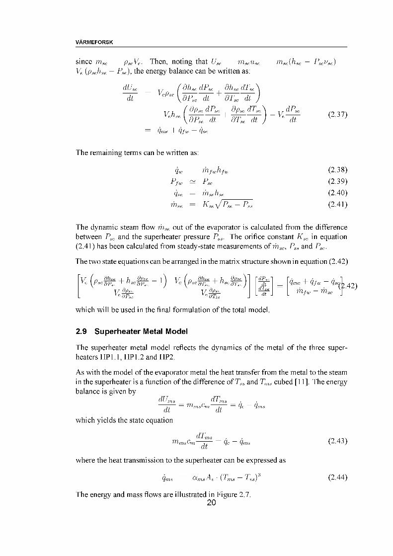
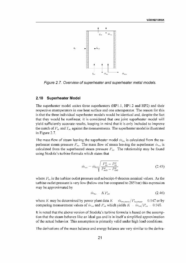
The energy and mass flows are illustrated in Figure 2.7.20

VARMEFORSK

fc

Ise m wa

Figure 2.7. Overview of superheater and superheater metal models.

2.10 Superheater Model

The superheater model unites three superheaters (HP1.1, HP1.2 and HP2) and their respective attemperators in one heat surface and one attemperator. The reason for this is that the three individual superheater models would be identical and, despite the fact that they would be nonlinear, it is considered that one joint superheater model will yield sufficiently accurate results, keeping in mind that it is only included to improve the match of Pse and Tse against the measurements. The superheater model is illustrated in Figure 2.7.

The mass flow of steam leaving the superheater model mss is calculated from the su­perheater steam pressure Pss. The mass flow of steam leaving the superheater mss is calculated from the superheated steam pressure Pss. The relationship may be found using Stodola’s turbine formula which states that

mss mopi - pi

p2 _ p2 Pss0 Pto0(2.45)

where Pto is the turbine outlet pressure and subscript-0 denotes nominal values. As the turbine outlet pressure is very low (below one bar compared to 285 bar) this expression may be approximated by

mss = KP,s (2.46)

where K may be determined by power plant data K = mssmax/Pss,max = 0.947 or by comparing measurement values of mss and Pss which yields K = mss/Pss = 0.945.

It is noted that the above version of Stodola’s turbine formula is based on the assump­tion that the steam behaves like an ideal gas and is in itself a simplified approximation of the actual behavior. This assumption is primarily valid under high load conditions.

The derivations of the mass balance and energy balance are very similar to the deriva-

21

VARMEFORSK

tions performed for the evaporator model.

dmss(ft

T T dPsS^ (ft

'mse + <mwa mss

/ 0pss dPss dpss dTSg^ (ft ^T,s (ft mse + mwa - mss (2.47)

and, since Uss mssUss m,ss{hss PssVss) Vspsshgs Vs Ps.

dUSi(ft

S'USS 7, fs'dh-ss dps

, 'dhss dPss dhss dT,sVgpgg ( —-----— +

dPsdt

dPss dt dTss dt(fms + (fse + (fwa — (fss

| ^ — Idf^,s dt dTss dt

- VsdPgg

(ft(2.48)

The remaining terms can be written as:

Qwa — mwahwa (2.49)Pwa 1— P— 1 w (2.50)

Qss -- mss hss (2.51)

mss — KPss (2.52)

The two state equations can be arranged in the matrix structure shown in equation (2.53)

V I n dhss + h 2^££. _ 1

V df>ss

V (n I h Ph

Vs dTs

r dpss idt (fms + (Zse + (Zwa — (tss

. dt . mse + mwa — mss(2.53)

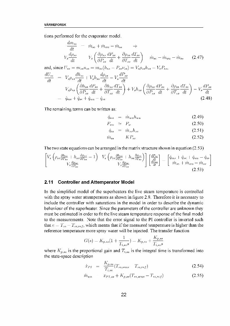
2.11 Controller and Attemperator Model

In the simplified model of the superheaters the live steam temperature is controlled with the spray water attemperators as shown in figure 2.8. Therefore it is necessary to include the controller with saturations in the model in order to describe the dynamic behaviour of the superheater. Since the parameters of the controller are unknown they must be estimated in order to fit the live steam temperature response of the final model to the measurements. Note that the error signal to the PI controller is inverted such that e — Tss — Tss,ref, which means that if the measured temperature is higher than the reference temperature more spray water will be injected. The transfer function

G(s) — Kp,ss (1 +1

TLsS) — Kp,ss +

Kp,ssTLsS

where Kp,ss is the proportional gain and Tiyss is the integral time is transformed into the state-space description

mmwa

Kp,ssT

(Ts — Tss.sens ss,ref)- «,ss

xPI,ss + Kp,ss(Ts —Tss,sens ^ ss,ref)

(2.54)

(2.55)

22

VARMEFORSK

Tss,ref Tss,sens ^ Temperature sensor

PI controller' Superheater

Spray water valveAttemperator

Figure 2.8. Model of the attemperator control loop.

Temperature Sensor DynamicsThe sensor measuring Tss for the PI controller has a time constant of approximately 20 s. This must be included in the model as well. The sensor dynamics are approxi­mated with a first-order filter:

T1

ss,sensTsenss + 1

-Ts

with Tsens = 20 s, which yields the following state-space form:

xsens

Ts

-1%sens

Tsens+ Ts.

1%sens

Tsens

(2.56)

(2.57)

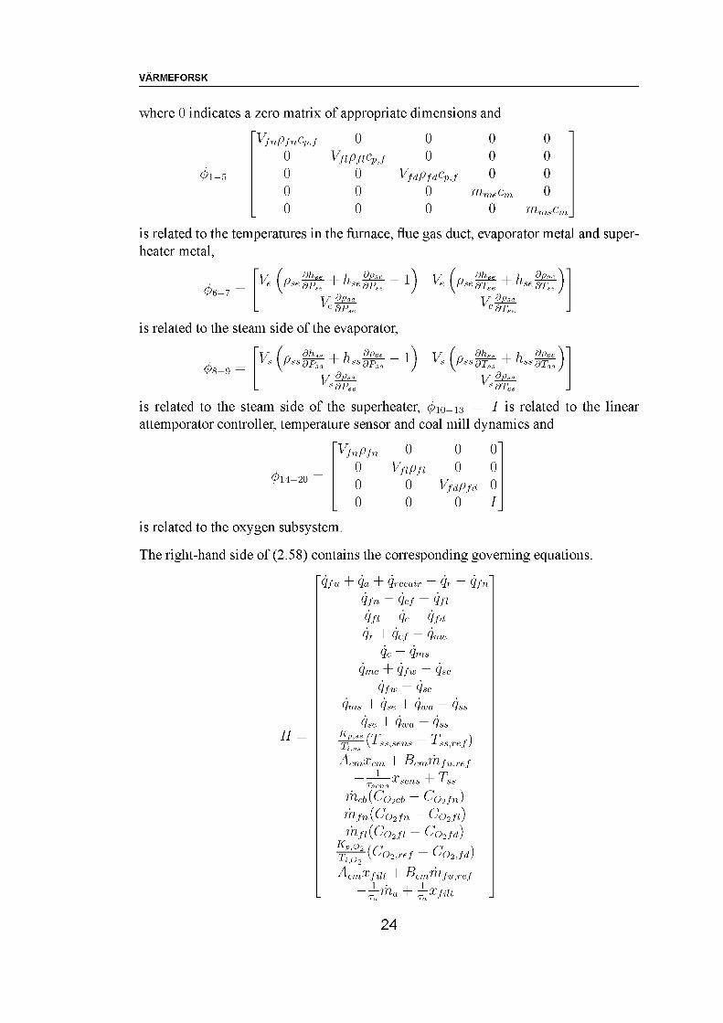
2.12 Summary and Model Structure

All the submodels described above are combined into a complete nonlinear model in the more compact matrix form:

= #(%,%) (2.58)

where x is the state vector of the complete system and u is a vector of external inputs, $(x) is a matrix that contains combinations of constants and functions of the states and H(x, u) is a vector that contains functions of the states and inputs. x is composed of the states identified in the submodels above:

x [ Tfn Tf: Tfd Tm, T,e T,, CO2f: CO2fd xP1,O2 ] T

$ has the structure

01-5 0 0 0 00 06-7 0 0 0

$ = 0 0 08-9 0 00 0 0 010-13 00 0 0 0 1 to o

(2.59)

23

VARMEFORSK

where 0 indicates a zero matrix of appropriate dimensions and

^1-5

^n^n Cp,f 0 0 0 00 Vfl p/lCp,/ 0 0 00 0 V/dpfdcp,f 0 00 0 0 m'me cm 00 0 0 0 mmscm

is related to the temperatures in the furnace, flue gas duct, evaporator metal and super­heater metal,

^6-7 =v (n ahse 4- h df>se — 1

V dpse

is related to the steam side of the evaporator,

^8-9 =V (n dhss 4- h df>ss — 1Kg ^aagp^ -T '^aagp^ ^

Vs dpst

V (n I h Spse

Ve dT,

v (n dhss 4- h ^Ka ^Kaag^^ 4" ^aag^_v dpss

is related to the steam side of the superheater, 01O-13 = I is related to the linear attemporator controller, temperature sensor and coal mill dynamics and

^14-20

Vfn Pfn 0 000 Vfipfi 0 00 0 VfdPfd 00 0 0 I

is related to the oxygen subsystem.

The right-hand side of (2.58) contains the corresponding governing equations:

H

(ffu + Qa + Qrecair — qr — (Zfn (ffn — (fcf — (ffl (ffl — (fc — (ffd Qr + (fcf — (fme

Qc Qms(fme + (Zfw — (Zse

Qfw — Qse(Zms + (Zse + (Zwa — (Zss

qse + qwa Qss- (VSS)Seras 7sa,r-e/)

+ Bcmmfu,ref'sens PPsens V Vss

mcb (CO2cb CO2fn)mfn (CO2/n — CO2/l) mfl (CO2fl — CO2/d)

Acm xfilt + Bcmmfu,ref-:r-ma +

Kp

Acm,x>cm^cm1

24

VARMEFORSK

These matrix equations are entered into the Matlab™ function ode15s, which is particularly suited for simulating stiff differential equations.

25

VARMEFORSK

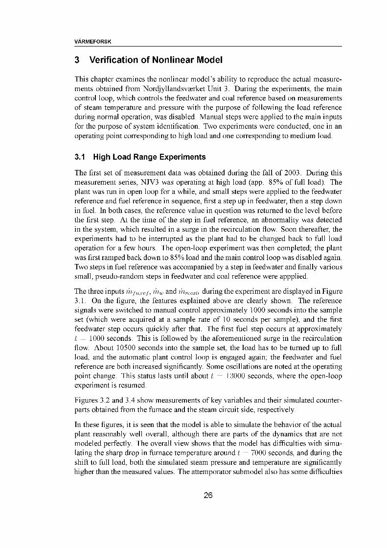
3 Verification of Nonlinear Model

This chapter examines the nonlinear model’s ability to reproduce the actual measure­ments obtained from Nordjyllandsv$rket Unit 3. During the experiments, the main control loop, which controls the feedwater and coal reference based on measurements of steam temperature and pressure with the purpose of following the load reference during normal operation, was disabled. Manual steps were applied to the main inputs for the purpose of system identification. Two experiments were conducted, one in an operating point corresponding to high load and one corresponding to medium load.

3.1 High Load Range Experiments

The first set of measurement data was obtained during the fall of 2003. During this measurement series, NJV3 was operating at high load (app. 85% of full load). The plant was run in open loop for a while, and small steps were applied to the feedwater reference and fuel reference in sequence, first a step up in feedwater, then a step down in fuel. In both cases, the reference value in question was returned to the level before the first step. At the time of the step in fuel reference, an abnormality was detected in the system, which resulted in a surge in the recirculation flow. Soon thereafter, the experiments had to be interrupted as the plant had to be changed back to full load operation for a few hours. The open-loop experiment was then completed; the plant was first ramped back down to 85% load and the main control loop was disabled again. Two steps in fuel reference was accompanied by a step in feedwater and finally various small, pseudo-random steps in feedwater and coal reference were appplied.

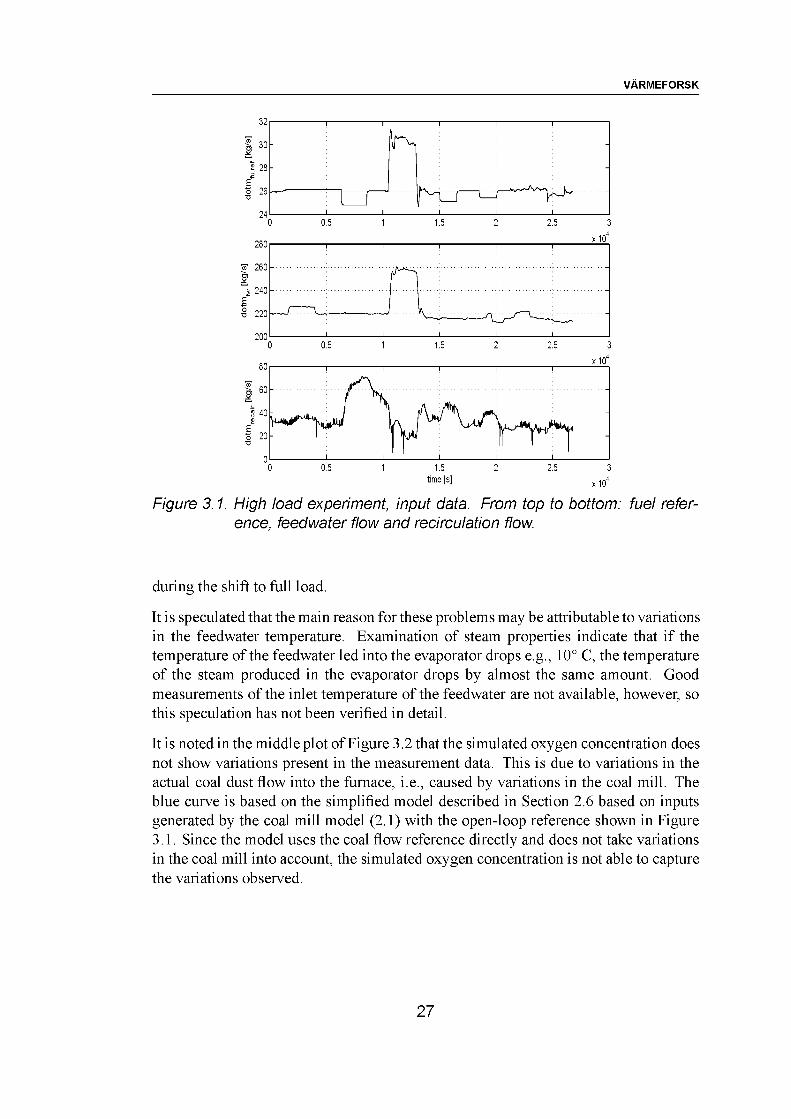
The three inputs m,fu,ref, mw and mrecair during the experiment are displayed in Figure 3.1. On the figure, the features explained above are clearly shown. The reference signals were switched to manual control approximately 1000 seconds into the sample set (which were acquired at a sample rate of 10 seconds per sample), and the first feedwater step occurs quickly after that. The first fuel step occurs at approximately t = 1000 seconds. This is followed by the aforementioned surge in the recirculation flow. About 10500 seconds into the sample set, the load has to be turned up to full load, and the automatic plant control loop is engaged again; the feedwater and fuel reference are both increased significantly. Some oscillations are noted at the operating point change. This status lasts until about t = 13000 seconds, where the open-loop experiment is resumed.

Figures 3.2 and 3.4 show measurements of key variables and their simulated counter­parts obtained from the furnace and the steam circuit side, respectively.

In these figures, it is seen that the model is able to simulate the behavior of the actual plant reasonably well overall, although there are parts of the dynamics that are not modeled perfectly. The overall view shows that the model has difficulties with simu­lating the sharp drop in furnace temperature around t = 7000 seconds, and during the shift to full load, both the simulated steam pressure and temperature are significantly higher than the measured values. The attemporator submodel also has some difficulties

26

VARMEFORSK

32

30-

28-

o 26

24

x 10280

■5T 260 -

■§ 220

200

x 1080

60 -

40-

20 -

00 1 2 3

time [s] x 104

Figure 3.1. High load experiment, input data. From top to bottom: fuel refer­ence, feedwater flow and recirculation flow.

during the shift to full load.

It is speculated that the main reason for these problems may be attributable to variations in the feedwater temperature. Examination of steam properties indicate that if the temperature of the feedwater led into the evaporator drops e.g., 10° C, the temperature of the steam produced in the evaporator drops by almost the same amount. Good measurements of the inlet temperature of the feedwater are not available, however, so this speculation has not been verified in detail.

It is noted in the middle plot of Figure 3.2 that the simulated oxygen concentration does not show variations present in the measurement data. This is due to variations in the actual coal dust flow into the furnace, i.e., caused by variations in the coal mill. The blue curve is based on the simplified model described in Section 2.6 based on inputs generated by the coal mill model (2.1) with the open-loop reference shown in Figure 3.1. Since the model uses the coal flow reference directly and does not take variations in the coal mill into account, the simulated oxygen concentration is not able to capture the variations observed.

27

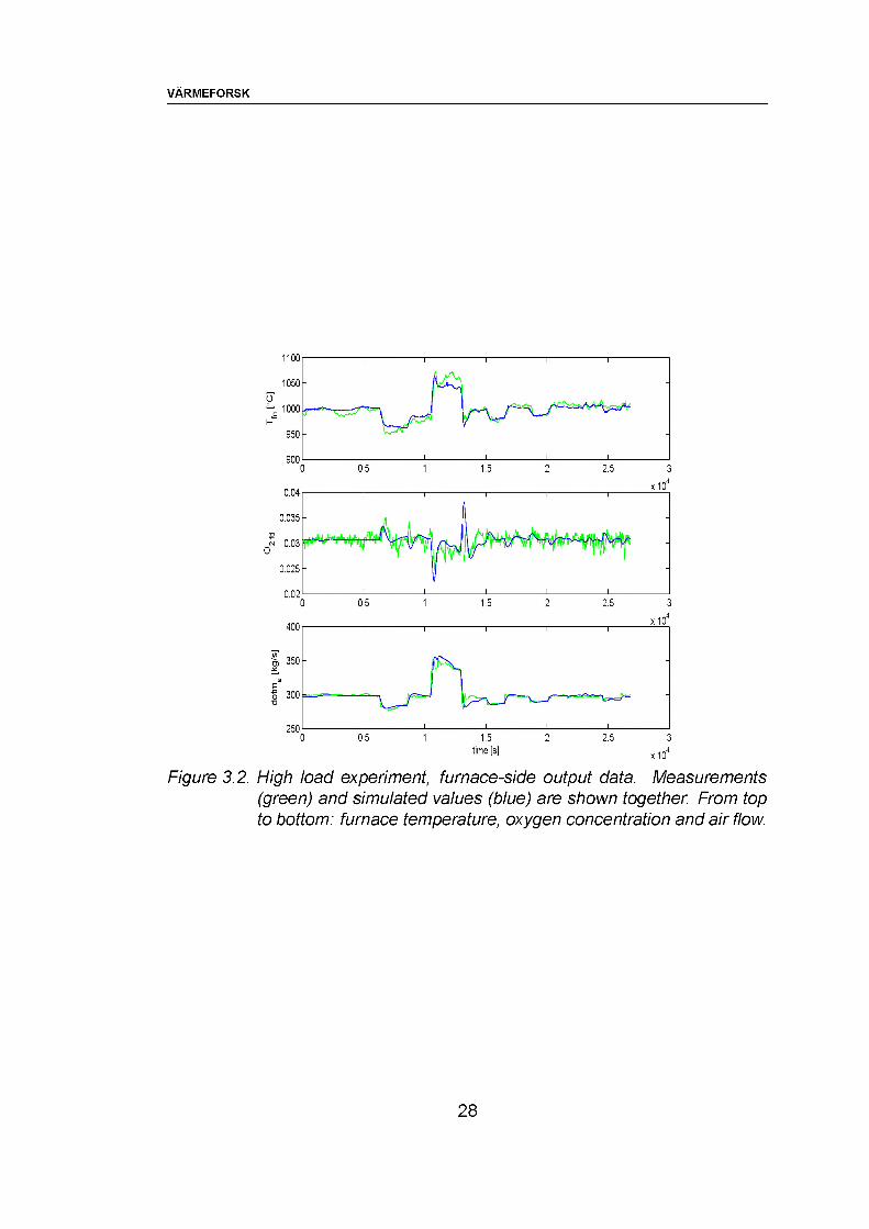
VARMEFORSK

Figure 3.2. High load experiment, furnace-side output data. Measurements (green) and simulated values (blue) are shown together. From top to bottom: furnace temperature, oxygen concentration and air flow.

28

VARMEFORSK

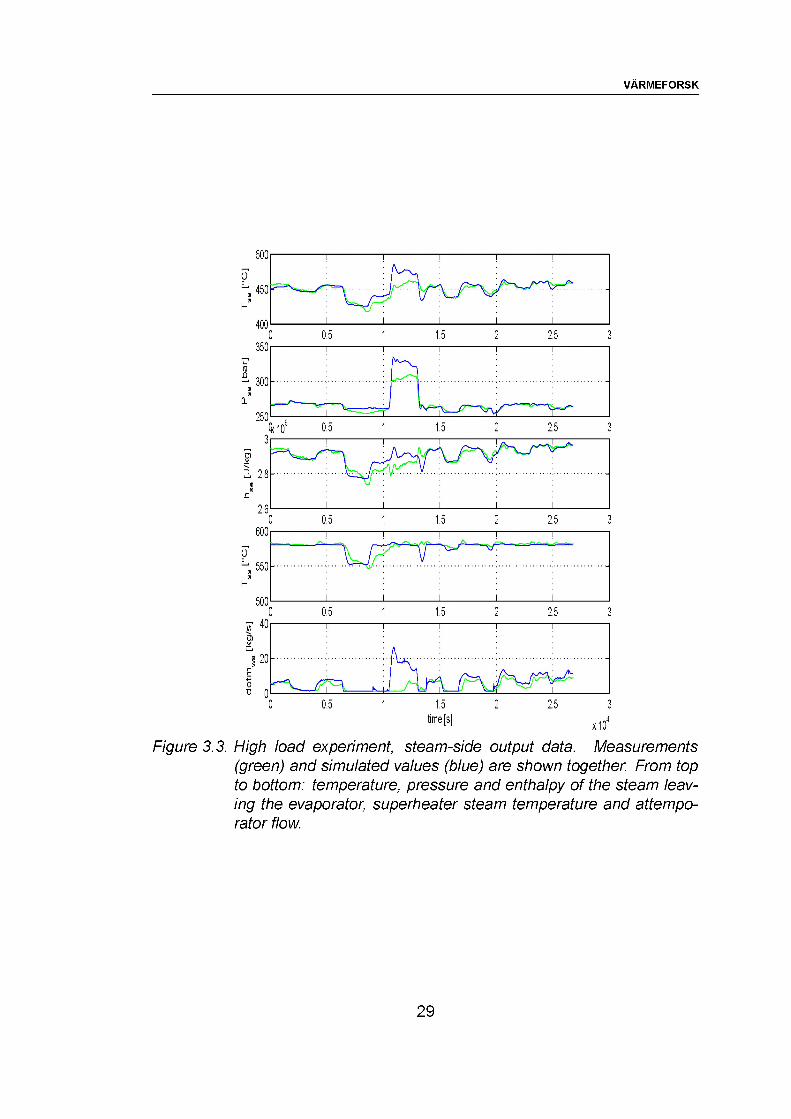
Figure 3.3. High load experiment, steam-side output data. Measurements (green) and simulated values (blue) are shown together. From top to bottom: temperature, pressure and enthalpy of the steam leav­ing the evaporator, superheater steam temperature and attempo- rator flow.

29

VARMEFORSK

0.035 -

0 0.03-—■..... ............... :...... :........ .

0.025 -

m 300 -

* 280 -

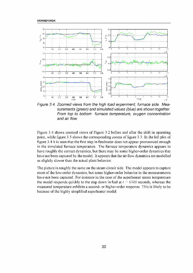
Figure 3.4. Zoomed views from the high load experiment, furnace side. Mea­surements (green) and simulated values (blue) are shown together. From top to bottom: furnace temperature, oxygen concentration and air flow.

Figure 3.4 shows zoomed views of Figure 3.2 before and after the shift in operating point, while figure 3.5 shows the corresponding zooms of figure 3.3. In the left plot of figure 3.4 it is seen that the first step in feedwater does not appear pronounced enough in the simulated furnace temperature. The furnace temperature dynamics appears to have roughly the correct dynamics, but there may be some higher-order dynamics that have not been captured by the model. It appears that the air flow dynamics are modelled as slightly slower than the actual plant behavior.

The picture is roughly the same on the steam circuit side. The model appears to capture most of the low-order dynamics, but some higher-order behavior in the measurements have not been captured. For instance in the case of the superheater steam temperature the model responds quickly to the step down in fuel at t = 6500 seconds, whereas the measured temperature exhibits a second- or higher-order response. This is likely to be because of the highly simplified superheater model.

30

VARMEFORSK

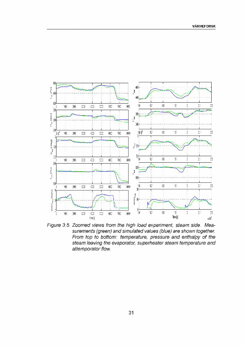
Figure 3.5. Zoomed views from the high load experiment, steam side. Mea­surements (green) and simulated values (blue) are shown together. From top to bottom: temperature, pressure and enthalpy of the steam leaving the evaporator, superheater steam temperature and attemporator flow.

31

VARMEFORSK

3.2 Low Load Experiment

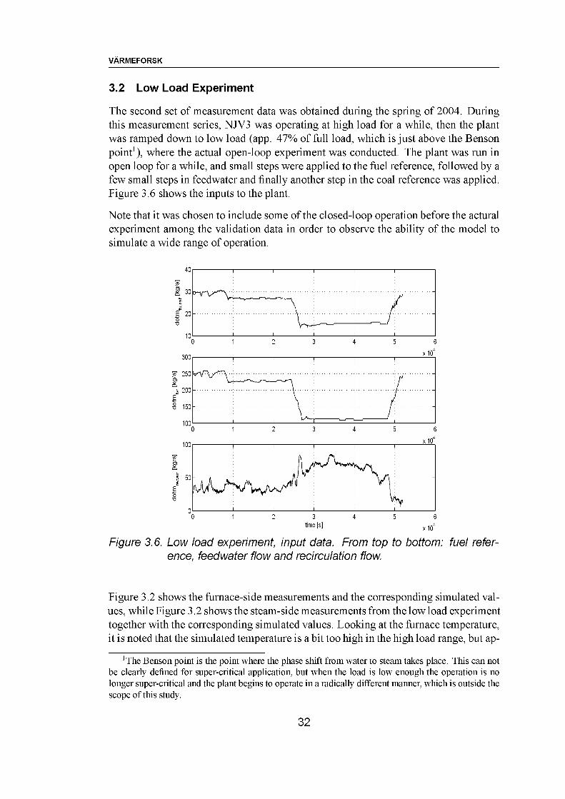
The second set of measurement data was obtained during the spring of 2004. During this measurement series, NJV3 was operating at high load for a while, then the plant was ramped down to low load (app. 47% of full load, which is just above the Benson point1), where the actual open-loop experiment was conducted. The plant was run in open loop for a while, and small steps were applied to the fuel reference, followed by a few small steps in feedwater and finally another step in the coal reference was applied. Figure 3.6 shows the inputs to the plant.

Note that it was chosen to include some of the closed-loop operation before the actural experiment among the validation data in order to observe the ability of the model to simulate a wide range of operation.

40

20 -

10

x 10300

250

200 -

150-

100

x 10100

50 -

00 1 2 3 4 5 6

time [s] x 104

Figure 3.6. Low load experiment, input data. From top to bottom: fuel refer­ence, feedwater flow and recirculation flow.

Figure 3.2 shows the furnace-side measurements and the corresponding simulated val­ues, while Figure 3.2 shows the steam-side measurements from the low load experiment together with the corresponding simulated values. Looking at the furnace temperature, it is noted that the simulated temperature is a bit too high in the high load range, but ap-

'The Benson point is the point where the phase shift from water to steam takes place. This can not be clearly defined for super-critical application, but when the load is low enough the operation is no longer super-critical and the plant begins to operate in a radically different manner, which is outside the scope of this study.

32

VARMEFORSK

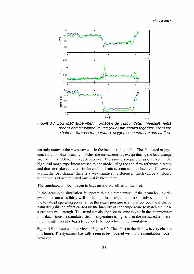
Figure 3.7. Low load experiment, furnace-side output data. Measurements (green) and simulated values (blue) are shown together From top to bottom: furnace temperature, oxygen concentration and air flow.

parently matches the measurements in the low operating point. The simulated oxygen concentration also basically matches the measurements, except during the load change around t = 25000 to t = 28000 seconds. The same discrepancies as observed in the high load range experiment caused by the model using the coal flow reference directly and does not take variations in the coal mill into account can be observed. Howevere, during the load change, there is a very significant difference, which can be attributed to the status of accumulated raw coal in the coal mill.

The simulated air flow is seen to have an obvious offset at low load.

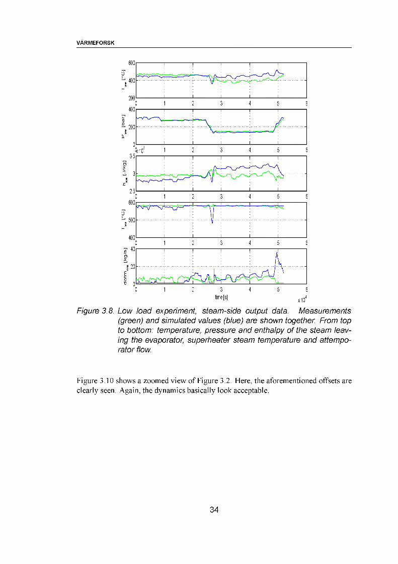
In the steam-side simulation, it appears that the temperature of the steam leaving the evaporator matches fairly well in the high-load range, but has a steady-state offset in the low-load operating point. Since the steam pressure is a little too low, the enthalpy naturally gains an offset caused by the inability of the temperature to match the mea­surements well enough. This trend can also be seen to some degree in the attemporator flow data; since the simulated steam temperature is higher than the measured tempera­ture, the attemporator has a tendency to be too active in the simulation.

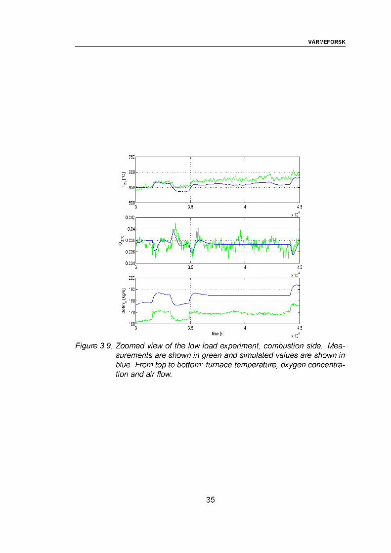
Figure 3.9 shows a zoomed view of Figure 3.2. The offset in the airflow is very clear in this figure. The dynamics basically seem to be modeled well by the simulation model, however.

33

VARMEFORSK

0 1 2 3 4 5 6

(jdoS 1 2 3 4 5 6

0 1 2 3 4 5 6

time [s]

Figure 3.8. Low load experiment, steam-side output data. Measurements (green) and simulated values (blue) are shown together From top to bottom: temperature, pressure and enthalpy of the steam leav­ing the evaporator, superheater steam temperature and attempo- rator flow.

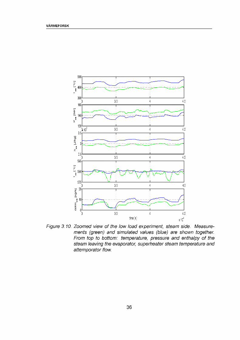
Figure 3.10 shows a zoomed view of Figure 3.2. Here, the aforementioned offsets are clearly seen. Again, the dynamics basically look acceptable.

34

VARMEFORSK

a 0.038

0.036 -

to 180 -

Figure 3.9. Zoomed view of the low load experiment, combustion side. Mea­surements are shown in green and simulated values are shown in blue. From top to bottom: furnace temperature, oxygen concentra­tion and air flow.

35

VARMEFORSK

3 3.5 4 4.5

Figure 3.10. Zoomed view of the low load experiment, steam side. Measure­ments (green) and simulated values (blue) are shown together. From top to bottom: temperature, pressure and enthalpy of the steam leaving the evaporator, superheater steam temperature and attemporator flow.

36

VARMEFORSK

3.3 Summary

This chapter describes the two open-loop experiments against which the nonlinear sim­ulation model formulated in the previous chapter was validated. The first experiment was run under high load conditions, and the second experiment was run under low load conditions.

Measurements were obtained from the plant on both the furnace and the steam side. Using the corresponding input samples, the simulation model simulated the plant oper­ation during the experiments, and the outputs were compared to the actual plant mea­surements. Some discrepancies were seen, particularly in the air flow in the low load experiment, but overall the model seemed to capture the prominent characteristics of the plant dynamics.

37

VARMEFORSK

4 Model Linearization

This chapter discusses linearization of the nonlinear model in various operating points and the potential usage of such linearized models for control purposes. Note that in this and the subsequent chapters it has been chosen to use the notation dx/dt for state derivatives in dynamical systems written on state space form in order to distinguish them from mass flows, changes in oxygen concentration etc.

4.1 Linearization

A linear model enables a number of methods for analyzing and controlling a system, some of which are listed below

Control Design: On the basis of a linear model it is possible to analyze and synthesize model-based multivariable controllers that control the evaporator steam pressure Pse and enthalpy hse using the coal flow reference mfu,ref and feedwater mfw as control signals.

Furthermore, linearization in several load points gives the opportunity to incor­porate the load variations in the control scheme, for instance by setting up a linear parameter varying model of the form

y = C (5)x + D(5)u

where x is the state and 5 is an external scheduling signal, for instance the load. Controllers scheduled according to the value of 5 can then be designed for this system.

Symbolic Solution: In contrast to most nonlinear models it is possible to evaluate the responses of linear models symbolically. For instance, for a given input an explicit formulation of the output may be found as a function of masses, heat transfer coefficients, operating points etc.

System Dynamics: The system dynamics can be interpreted in terms of time con­stants, damping factors, eigenvalues, poles and zeros etc. originating from linear systems theory.

Frequency Analysis: The information contained within the system’s differential equations can be presented as graphs (Bode plots). This is used in a number of control methods.

Model Reduction In linear systems theory a number of methods exist to reduce sys­tem order and at the same time preserving the dynamical properties of the sys­tem, pole-zero cancellation for example.

38

VARMEFORSK

Structural Properties: A linear description may make it easier to separate the dy­namics of the individual components of the system; for instance, the steam prop­erties may be approximated locally by simple gains, explaining the rough influ­ence of small increments and decrements of variables on the state of the system in an easy to understand manner.

A vector field f (x) describing a dynamical system on state-space form can be approx­imated in the vicinity of some f (x) using a first-order Taylor expansion as shown in(4.1).

f (x) f (x) +#/(x)

xi +x=x

#/(x)X2 +-------+

x=x

#/(x)xn

x=x(4.1)

where x = x — x is denoted the small-signal vector and x = [x1 x2 ■ ■ ■ xn]T denotes the operating point vector.

In the case discussed in Chapter 2, the nonlinear model is given by n equations having the general form:

f1,1(x) f1,2(x) f1,n(x)f2,1(x) f2,2(x) f2,n(x)

fn,1(x) fn,2(x) fn,n(x)

INi__ h1(x, __i

dx 2 dt =

u)i

r --

i____

dtH

(4.2)

with ^ through being the derivatives of the state vector x G E™ and h\(x,u) through hn(x, u) functions of the states and the inputs u G Rm.

Insertion of the operating point vector in each of the functions f1,1 (x) through fn,n(x) and changing the terms ^ to z 1 • • • n is sufficient to linearize the left hand side, that is:

f1,1(x)f2,1(x)

f1,2(x) "f2,2(x) "

' f1,n(x)' f2,n(x)

~ dx 1 'dx■),dt

h1 (x,u) h2 (x,u)

(4.3)

fn,1(x) fn,2(x) " ■ fn,n(x) dZn_ dt _ hn(x,u)

Linearization of each element on the right hand side of equation 4.2 reduces to

h(x,u) ^dh(x, u)

dxx +

dh(x,u)

x=x,u=u duu (4.4)

x=x,u=u

39

VARMEFORSK

since insertion of the operating points x in equation 4.2 gives zero, i.e. ^ = 0. Thus (abbreviating u) with h):

hn

dhi dhi&Cl 9z2dh>2 dh>2

&C2

dhn dhn . .

&C2

dhl

m203.

dhn03„

XiX2

+

Xn

dhi dhi0«1 0U2dh2 dh20«1 0U2

dhn_ dhn.0ui 0U2

Jh(u)

dhi

dUm

dhn0Urr

uiu2

um

(4.5)

where JH (x) and JH (u) are the Jacobians of H with respect to x and u, respectively.

After the linearization of the nonlinear model the equations are organized in a matrix structure as shown in equation 4.6.

Qdx

RX + Su

which in turn can be reorganized in standard state-space formalism

dx Q-1RX + Q-1 Su = AX + Bu1-1

(4.6)

(4.7)

This is carried out using Matlab™ ’s symbolic toolbox, resulting in a 20th-order MIMO model with the input vector

u [m fu,ref fu m fw Tss,ref 7arecair Trecair Ta Tw(4.8)

Subsequently, the numerical linear model can be calculated in various operating points resulting in different models. The number of linear models is determined by the desired accuracy and the extent of nonlinearities in the boiler model. With a sufficient number of linear models they can be combined in order to cover the entire range of operation in a linear parameter varying model.

4.2 Linearized Model Validation

Figure 4.1 shows a comparison of the nonlinear and linear responses where the linear model has been calculated at 84 % load. For better comparison saturations in the nonlinear model have been removed. The inaccuracies of the linearized model can be seen at the points where the attemperator flow hits the lower saturation value zero. A saturation of this kind must be dealt with in the specific design of a controller based on the linearized model.

The figure shows that the linear model reproduces the most significant dynamics of the nonlinear model to a satisfactory degree in a load operating range of approximately 85-100 %. Only when the states deviate too much from their operating points there is a slight mismatch in some of the gains. It is furthermore noted that the behaviors of the nonlinear and the linear deviate more as the load is decreased than when it is increased. This is likely due to the tendency of the super-critical steam to behave less like an ideal gas the closer when its state approaches the critical point.

40

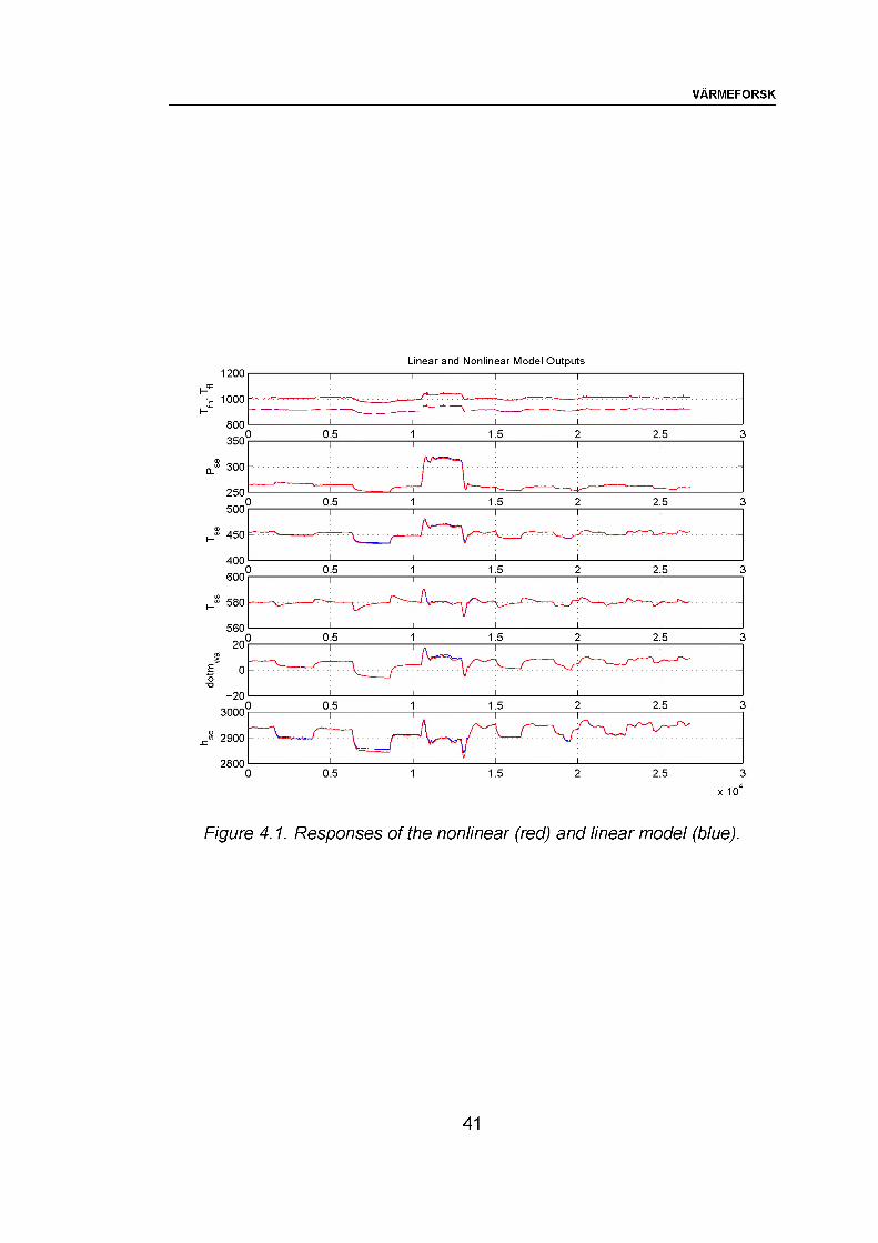
dotm

VARMEFORSK

Linear and Nonlinear Model OutputsI

...... . . . . i \-----1

----.------- '—__________I____________________1___________________800

300 -

x 104

Figure 4.1. Responses of the nonlinear (red) and linear model (blue).

41

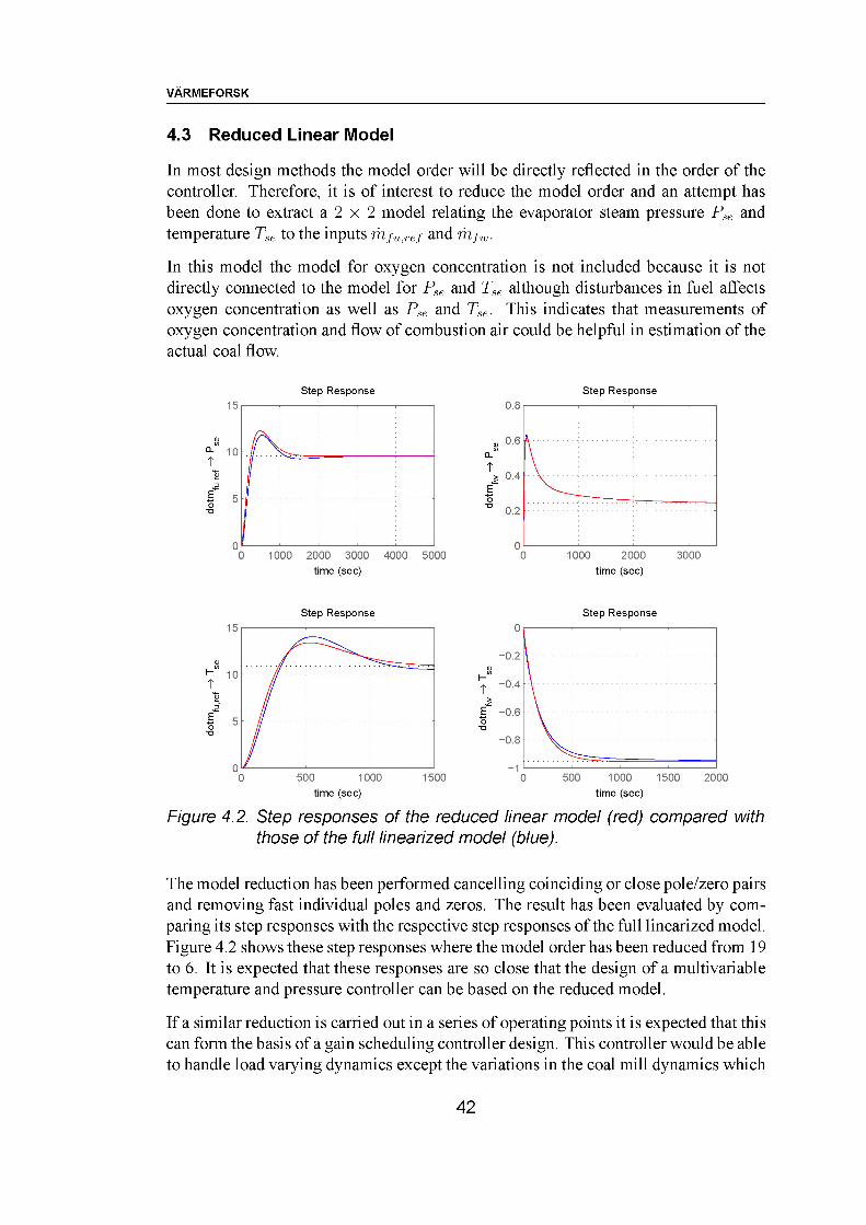
VARMEFORSK

4.3 Reduced Linear Model

In most design methods the model order will be directly reflected in the order of the controller. Therefore, it is of interest to reduce the model order and an attempt has been done to extract a 2 x 2 model relating the evaporator steam pressure Pse and temperature Tse to the inputs /i//„.r,/ and m,fw.

In this model the model for oxygen concentration is not included because it is not directly connected to the model for Pse and Tse although disturbances in fuel affects oxygen concentration as well as Pse and Tse. This indicates that measurements of oxygen concentration and flow of combustion air could be helpful in estimation of the actual coal flow.

Step Response

1000 2000 3000 4000 5000time (sec)

Step Response0.8

O'----------'---------- '--------- '—0 1000 2000 3000

time (sec)

Step Response

time (sec)

Step Response

2000time (sec)

Figure 4.2. Step responses of the reduced linear model (red) compared with those of the full linearized model (blue).

The model reduction has been performed cancelling coinciding or close pole/zero pairs and removing fast individual poles and zeros. The result has been evaluated by com­paring its step responses with the respective step responses of the full linearized model. Figure 4.2 shows these step responses where the model order has been reduced from 19 to 6. It is expected that these responses are so close that the design of a multivariable temperature and pressure controller can be based on the reduced model.

If a similar reduction is carried out in a series of operating points it is expected that this can form the basis of a gain scheduling controller design. This controller would be able to handle load varying dynamics except the variations in the coal mill dynamics which

42

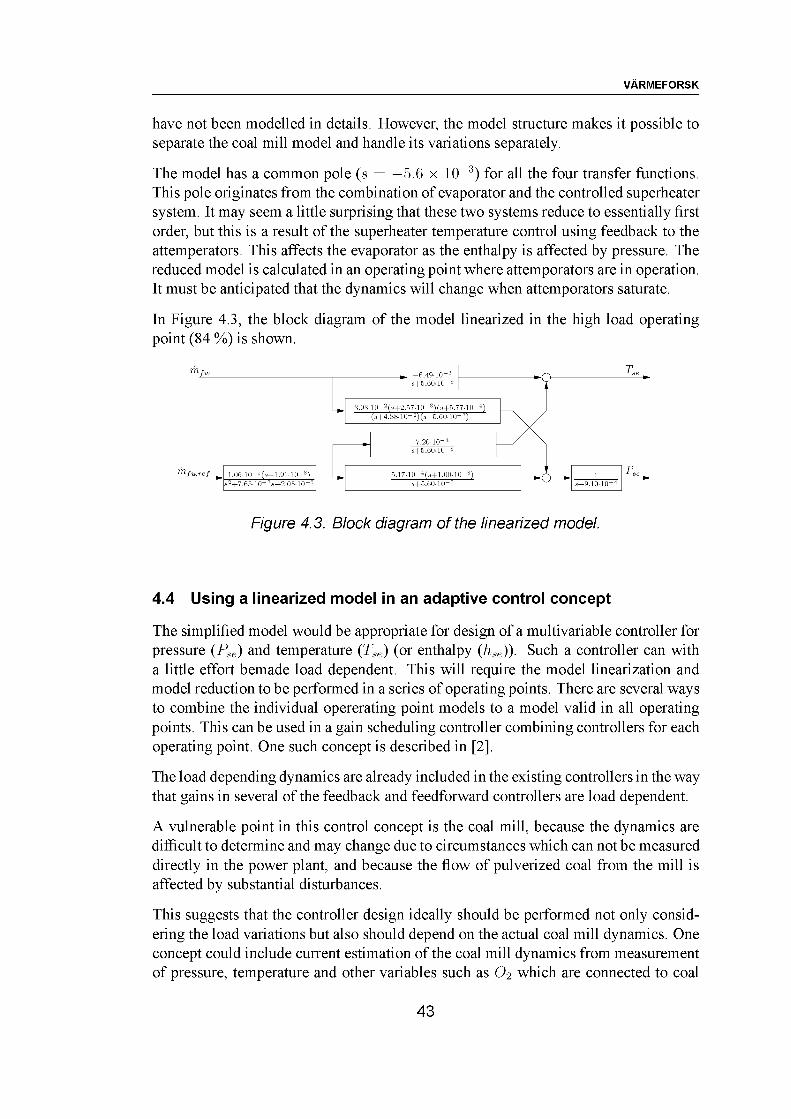
VARMEFORSK

have not been modelled in details. However, the model structure makes it possible to separate the coal mill model and handle its variations separately.

The model has a common pole (s = -5.6 x 10-3) for all the four transfer functions. This pole originates from the combination of evaporator and the controlled superheater system. It may seem a little surprising that these two systems reduce to essentially first order, but this is a result of the superheater temperature control using feedback to the attemperators. This affects the evaporator as the enthalpy is affected by pressure. The reduced model is calculated in an operating point where attemporators are in operation. It must be anticipated that the dynamics will change when attemporators saturate.

In Figure 4.3, the block diagram of the model linearized in the high load operating point (84 %) is shown.

Figure 4.3. Block diagram of the linearized model.

4.4 Using a linearized model in an adaptive control concept

The simplified model would be appropriate for design of a multivariable controller for pressure (Pse) and temperature (Tse) (or enthalpy (hse)). Such a controller can with a little effort bemade load dependent. This will require the model linearization and model reduction to be performed in a series of operating points. There are several ways to combine the individual opererating point models to a model valid in all operating points. This can be used in a gain scheduling controller combining controllers for each operating point. One such concept is described in [2].

The load depending dynamics are already included in the existing controllers in the way that gains in several of the feedback and feedforward controllers are load dependent.

A vulnerable point in this control concept is the coal mill, because the dynamics are difficult to determine and may change due to circumstances which can not be measured directly in the power plant, and because the flow of pulverized coal from the mill is affected by substantial disturbances.

This suggests that the controller design ideally should be performed not only consid­ering the load variations but also should depend on the actual coal mill dynamics. One concept could include current estimation of the coal mill dynamics from measurement of pressure, temperature and other variables such as O2 which are connected to coal

43

VARMEFORSK

flow. This will have the potential to improve stability and dynamic performance of the boiler, but still disturbance close to the coal mill have to be rejected through this relatively slow loop. Therefore it is natural to look for a measurement of the coal flow which can be used as a direct feedback around the coal mill.

4.5 Summary

In this chapter a linearized small-signal model valid in a neighbourhood of an operating point was calculated and tested against the nonlinear model. The results show that a linear model can approximate the boiler dynamics quite well in a neighbourhood around an operating point.

The model was reduced in order to facilitate controller design resulting in a sixth-order model from fuel and feedwater to evaporator pressure and temperature. An adaptive control concept using the sixth-order simplified model could then be suggested.

The full linearized model has an additional path from coal mill to oxygen concentration. This path gives an extra measurement, useful for estimation of the actual coal flow which may be disturbed by irregularities in the coal or the coal mill.

44

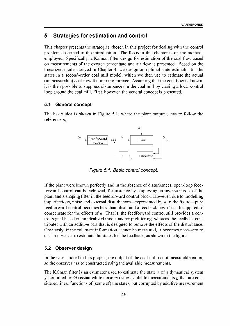
VARMEFORSK

5 Strategies for estimation and control

This chapter presents the strategies chosen in this project for dealing with the control problem described in the introduction. The focus in this chapter is on the methods employed. Specifically, a Kalman filter design for estimation of the coal flow based on measurements of the oxygen percentage and air flow is presented. Based on the linearized model derived in Chapter 4, we design an optimal state estimator for the states in a second-order coal mill model, which we then use to estimate the actual (unmeasurable) coal flow fed into the furnace. Assuming that the coal flow is known, it is then possible to suppress disturbances in the coal mill by closing a local control loop around the coal mill. First, however, the general concept is presented.

5.1 General concept

The basic idea is shown in Figure 5.1, where the plant output y has to follow the reference yr.

Figure 5.1. Basic control concept.

If the plant were known perfectly and in the absence of disturbances, open-loop feed­forward control can be achieved, for instance by employing an inverse model of the plant and a shaping filter in the feedforward control block. However, due to modelling imperfections, noise and external disturbances—represented by d in the figure—pure feedforward control becomes less than ideal, and a feedback law F can be applied to compensate for the effects of d. That is, the feedforward control still provides a con­trol signal based on an idealized model and/or prefiltering, whereas the feedback con­tributes with an additive part that is designed to remove the effects of the disturbance. Obviously, if the full state information cannot be measured, it becomes necessary to use an observer to estimate the states for the feedback, as shown in the figure.

5.2 Observer design

In the case studied in this project, the output of the coal mill is not measurable either, so the observer has to constructed using the available measurements.

The Kalman filter is an estimator used to estimate the state x of a dynamical system f perturbed by Gaussian white noise w using available measurements y that are con­sidered linear functions of (some of) the states, but corrupted by additive measurement

45

VARMEFORSK

noise v (also Gaussian white noise) as follows:

(5.1)

(5.2)

^ — f(x,u)+w

y = Cx + v

This is a reasonable representation for a great number of real-world systems, and it has the added advantage that for linear systems f (x, u) = Ax + Bu for which the covariance matrices Q0 and R0 of w and v, respectively, are known, a feedback gain can be found such that the estimates x approximate the true states optimally in a least squares sense. The general form of the Kalman filter is

— — /(%:,%) + %(%/ —C%)

y = cx

(5.3)

(5.4)

where K is the aforementioned Kalman gain. As can be seen, the Kalman gain essen­tially acts as a measurement feedback control driving the prediction error y — Cx to zero. The theory is well established, and will thus not be discussed any further here; refer to e.g., [9] for further treatment of the subject.

In the context of this application, the heart of the observer design is the oxygen mass balance in the furnace and flue gas duct, which are considered as a single volume in this context. This choice is made to keep the model as simple as possible; the time constants of the three individual flue gas volumes are each less than the sample time, and by considering the volumes as a single volume, the recirculation flue gas can be eliminated from the model equations.

The oxygen concentration in the flue gas duct, CO2, is influenced in the positive direc­tions by contributions from the inflow of recirculation air and primary air and in the negative direction by the (stoichiometric) combustion and the outflow of flue gas to the smoke stack. The oxygen mass balance can be written as

Vpfg CO2 mrecair CO2 + m a CO2a mfuCO2fu (mrecair + m a + mfu)CO2

= — (mfu + 77^)032 + ma CO2a — mfuCO2fu (5.5)

where V is the volume and pfg is the density of the flue gas. CO2a is the concentration of oxygen in atmospheric air, while CO2fu is the amount of oxygen consumed by stoi­chiometric combustion of 1 kg coal; these values are considered constants. mfu, mrecair and mair denote the mass flows of coal, recirculation air and total combustion air, re­spectively.

The observer is designed using the setup shown in Figure 5.2, which is an expansion of Figure 2.5. Ga(s) and GO2 (s) are simplified models of the air flow actuator and oxygen subsystem dynamics, respectively.

The model equations used for the observer design (i.e., corresponding to equations

46

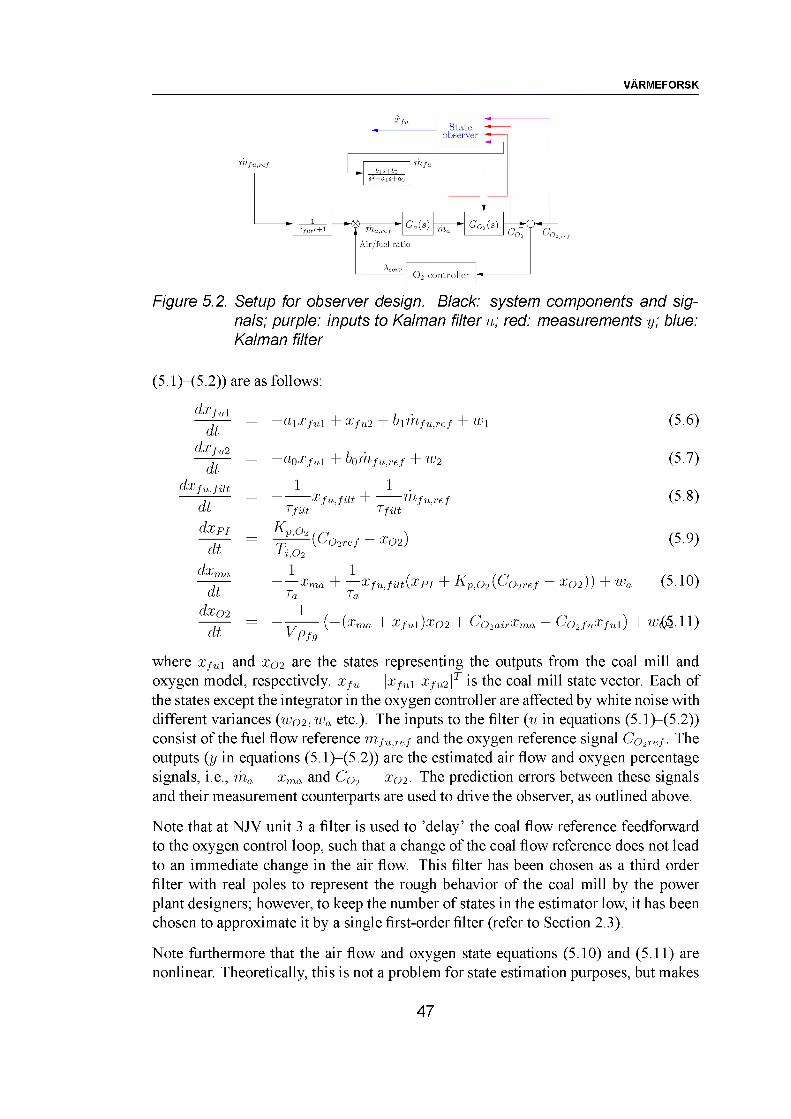
VARMEFORSK

A 'Wla,ref __

Air/fuel ratio

Stateobserver

O2 controller

Figure 5.2. Setup for observer design. Black: system components and sig­nals; purple: inputs to Kalman filter u; red: measurements y; blue: Kalman filter

(5.1)—(5.2)) are as follows:

dxfu 1dt

dx fu‘2

dtdx f uJilt

dt.dxpj

dtdxrn.n.

dt.(&P02

dt.

—ciiXfui + x.fu 2 + bim.fu.ref + W\

—cioXfui + bojm,fu.ref + w-2

1 1Xfilt 'Tfilt

(Cogre/ — #02)

~'m/-u,re/

Ap,02

---------- Xma H Xfujiit(x.pi + I\p02{Co2ref ~ X02)) + WaTa Ta

1

(5.6)

(5.7)

(5.8)

(5.9)

(5.10)

(—(Xma + Xfui)xo2 + ConairXma ~ ConfuXful) + "’(65 11)

where Xfui and x(yl are the states representing the outputs from the coal mill and oxygen model, respectively. xfu = [xfui xfu2]T is the coal mill state vector. Each of the states except the integrator in the oxygen controller are affected by white noise with different variances (u’02, etc ). The inputs to the filter (u in equations (5.1)—(5.2)) consist of the fuel flow reference m.fu.ref and the oxygen reference signal Co2ref■ The outputs (y in equations (5.1)—(5.2)) are the estimated air flow and oxygen percentage signals, i.e., m.a = xma and Cq2 = x(yl. The prediction errors between these signals and their measurement counterparts are used to drive the observer, as outlined above.

Note that at NJV unit 3 a filter is used to ’delay’ the coal flow reference feedforward to the oxygen control loop, such that a change of the coal flow reference does not lead to an immediate change in the air flow. This filter has been chosen as a third order filter with real poles to represent the rough behavior of the coal mill by the power plant designers; however, to keep the number of states in the estimator low, it has been chosen to approximate it by a single first-order filter (refer to Section 2.3).

Note furthermore that the air flow and oxygen state equations (5.10) and (5.11) are nonlinear. Theoretically, this is not a problem for state estimation purposes, but makes

47

VARMEFORSK

the subsequent Kalman filter design somewhat more complicated. Hence, a linearized version of (5.10) is used to obtain the Kalman filter gain.

5.3 Control strategy

This and the subsequent section discusses possible solutions to the control problem studied in this project, and the choice of control strategy made in the project is pre­sented.

In the existing control of the boiler the two important controlled outputs are the pres­sure at the inlet of the high pressure turbine Pss and the enthalpy at the outlet of the evaporator hse. These are essentially controlled using feedwater flow mfw and the flow of coal dust as inputs. In the following this enthalpy and pressure controller will be called the outer loop.

The feedwater flow is itself controlled by an internal flow controller. As mentioned, the coal flow cannot be directly measured and thus coal dust flow is controlled using the outer loop to set references to primary air flow, the raw coal feed rate and rotation speed of the grinding table. Deviations of the resulting coal dust flow must be corrected by the outer loop.

The model of the furnace and evaporator set up in the previous chapters are anticipated to be suitable for the design and analysis of the outer loop controller for Pse and Tse using mfu,ref and mfw as control signals.

The linearized models contain information about model variations depending on the varying load, giving the possibility of including these variations in the outer loop con­troller.

The main remaining problem in the control system is due to variations in the coal mill dynamics. These variations could be considered as disturbances or uncertainties in the coal mill model. From a control theoretical point of view, there are basically two control stategies for dealing with uncertainties: robust control and adaptive control. If the uncertainties in the model are ’large’ in some sense, adaptive control should be used, whereas better performance can be expected if the uncertainties are ’small’; this notion is made precise in e.g., [6], where a linear quadratic control performance measure taking the relative size of the plant and the uncertainties into account is analyzed.

One solution is to design the outer Pse/Tse controller adaptively, including variations in the coal mill dynamics.

Advantages: An adaptive controller aims to have a model updated currently from measurements giving the possibilities to optimize the controller to the currently observed conditions.

Disadvantages: The update of the model is dependent of a persistent exitation of the dynamics of the coal mill. In practice this will imply that the adaptation should

48

VARMEFORSK

be supervised in order to prevent windup problems in the model parameter es­timation. Furthermore, the adaptation of the Pse/Tse controller does not im­mediately improve the attenuation of disturbances close to the coal mill. This would require inclusion of the measurements facilitating estimates of the coal flow which, in fact, is the inner loop.

Another solution could be to design a linear controller which is robust against variations in the coal mill dynamics and capable of attenuating disturbances close to the coal mills. An obvious choice would be a cascade controller closing an inner loop around the coal mills using an estimate of the actual coal flow based on measurements of air flow ma and oxygen concentration CO2.

Advantages: An inner loop controller is able to reject variations caused by e.g., varia­tions in the humidity, grain size and calorific value. Secondly, it has a stabilizing effect on the outer control loop when the coal mill dynamics vary. Thirdly, it has the potential to provide a better performance than an adaptive controller when the disturbances and uncertainties are relatively small compared to the response of the nominal plant.

Disadvantages: In order to avoid that the coal mill saturates as a consequence of a too large closed-loop gain, one must ensure that the variations in the reference signal are limited, for instance by filtering the reference.

5.4 Choice of control strategy

One of the main practical hurdles in this project is the lacking possibility to measure the amount of coal dust leaving the coal mills. Furthermore, the two main aims of the controller are to suppress coal flow disturbances and variations in the coal mill dynamics.

Considering the advantages and disadvantages of each solution strategy outlined in the previous section, it is chosen in this project to design a robust cascade controller as an inner loop controller enclosing the coal mill. It is considered a significant disadvantage of the adaptive control concept that persistent excitation and good measurements are required to ensure good performance of an adaptive control concept, whereas a robust inner-loop control is likely to achieve better disturbance rejection performance based on the available plant setup and the coal flow observer.

An actual adaptive or linear parameter varying control concept is considered to be more appropriate for the outer loop.

Thus, the chosen strategy will be to insert a feedback controller (see figure 5.3) in a cascade configuration, as the nature of cascading is to reject disturbances and plant parameter variations.

49

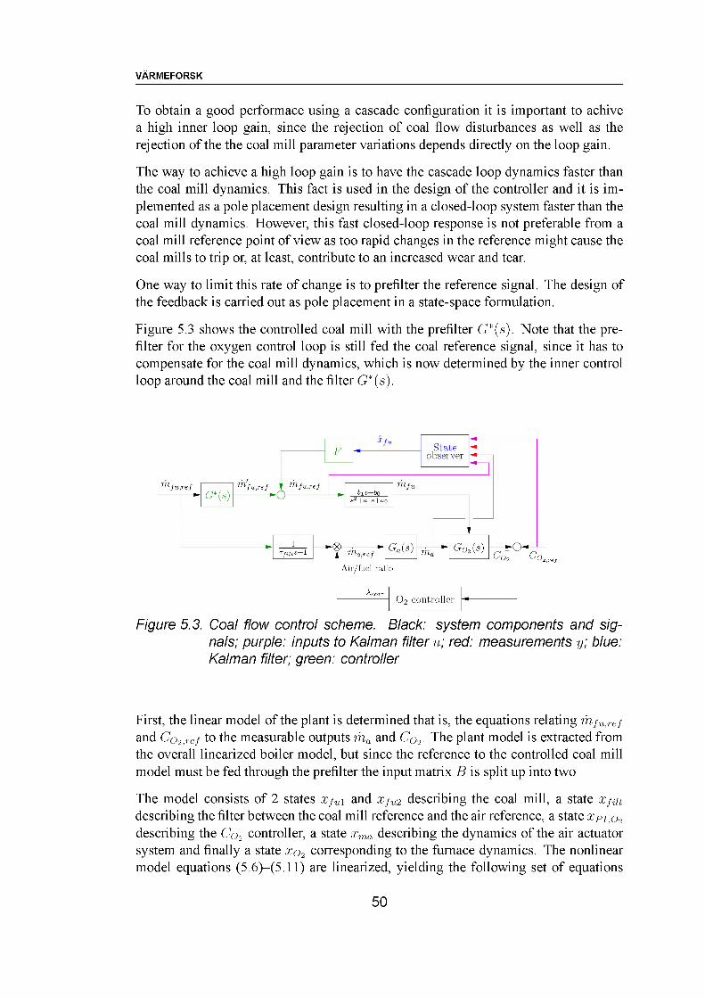
VARMEFORSK

To obtain a good performace using a cascade configuration it is important to achive a high inner loop gain, since the rejection of coal flow disturbances as well as the rejection of the the coal mill parameter variations depends directly on the loop gain.

The way to achieve a high loop gain is to have the cascade loop dynamics faster than the coal mill dynamics. This fact is used in the design of the controller and it is im­plemented as a pole placement design resulting in a closed-loop system faster than the coal mill dynamics. However, this fast closed-loop response is not preferable from a coal mill reference point of view as too rapid changes in the reference might cause the coal mills to trip or, at least, contribute to an increased wear and tear.

One way to limit this rate of change is to prefilter the reference signal. The design of the feedback is carried out as pole placement in a state-space formulation.

Figure 5.3 shows the controlled coal mill with the prefilter G*(s). Note that the pre­filter for the oxygen control loop is still fed the coal reference signal, since it has to compensate for the coal mill dynamics, which is now determined by the inner control loop around the coal mill and the filter G*(s).

ma,ref __

Air/fuel ratio

Stateobserver

02 controller

Figure 5.3. Coal flow control scheme. Black: system components and sig­nals; purple: inputs to Kalman filter u; red: measurements y; blue: Kalman filter; green: controller

First, the linear model of the plant is determined that is, the equations relating mfu.ref and C0n,ref to the measurable outputs ih„ and Cq2. The plant model is extracted from the overall linearized boiler model, but since the reference to the controlled coal mill model must be fed through the prefilter the input matrix B is split up into two

The model consists of 2 states Xfui and Xfu2 describing the coal mill, a state xfut describing the filter between the coal mill reference and the air reference, a state xPito2 describing the Co2 controller, a state xma describing the dynamics of the air actuator system and finally a state xo2 corresponding to the furnace dynamics. The nonlinear model equations (5.6)—(5.11) are linearized, yielding the following set of equations

50

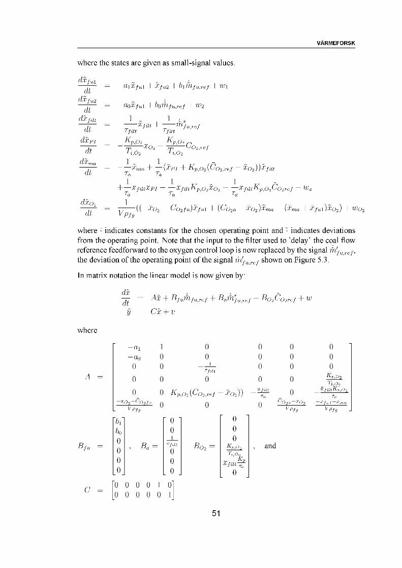
VARMEFORSK

where the states are given as small-signal values.

dx/uidt

dx fu 2dt

dx findt

dxpidt

dxmadt

d&Ogdt

— -a,lX/u1 + X/u2 + bi fh/u,re/ + Wi

= —ttoX/ui + bofh/u,re/ + W2

1 - 1— --------+ ------------ mfu,ref

T/ilt T/i1tKy,C>2 , Kp,P2

" rri ^02 “T rriT i,O2 T i,O2

aO2,re/

----- Xma d 02(^2,re/ — ^02))^/^Ta Ta1 1 _ 1 X

+—^/m^pr — —^/m-Kp,02^02 + "^/m-Kp,02Co2re/ + %

1

VP/"((—7O2 — CO2/u )X/ui + (CO2a — 7O2 )Xma — (7ma + 7/uI )XO2 ) + WO;

where 7 indicates constants for the chosen operating point and 7 indicates deviations from the operating point. Note that the input to the filter used to ’delay’ the coal flow reference feedforward to the oxygen control loop is now replaced by the signal m/u,re/, the deviation of the operating point of the signal m /u,re/ shown on Figure 5.3.

In matrix notation the linear model is now given by:

dXdt

A7 + B/um/u,re/ + Ba m/u,re/ + BO2 CO2re/ + w

ax + v

where

A

—ai—ao

0

0

0

- V7T3

100

0

0

0

00

___ ]_Tfilt0

KP,O2 (C7O2,re/

0

x7 O2 ))

[bi] 0 0

bo 0 00 1 0

B/u = 0 , Ba = Tfilt0 BO2 = ^P,02rr. ~

00

00 0

000010 0 0 0 0 0 1

000

0xfilt

Ta0

000

0

0Cc>2a x02

Vpfg

and

000

Kp,o 2-x filt*'-p,Q 2

Tax ful xrna^9

51

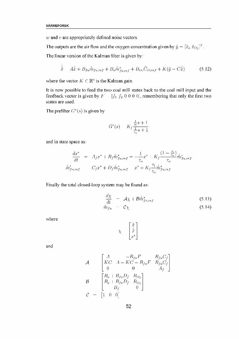
VARMEFORSK

w and v are appropriately defined noise vectors.

The outputs are the air flow and the oxygen concentration given by y = [Xa XO2]T.

The linear version of the Kalman filter is given by:

X = AxX + /u,re/ + Bam/u,re/ + BO2 C7O2re/ + K (y/ — CX) (5-12)

where the vector K G R6 is the Kalman gain.

It is now possible to feed the two coal mill states back to the coal mill input and the feedback vector is given by F = [fi f2 0 0 0 0], remembering that only the first two states are used.

The prefilter G* (s) is given by

G*(s)

and in state space as:

(ft

/u,re/

• 1 (!--)•A/a;* + z* + XT/——

Tn Tn

C/a;* + C/m^rg/ = a;* + XT/—m}^^/Tn

Finally the total closed-loop system may be found as:

where

and

m/u = C X

X

xXxXXx*

A

B

C

A —B/uF B/uC/KC A — KC — B/uF B/uC/

_ 0 0 A/

Ba + B/uD/ BO2

Ba + B/uD/ BO2

_ B/ 0 _C1 0 0]

(5.13)

(5.14)

52

VARMEFORSK

5.5 Interaction between estimation and control

The methods outlined so far in this chapter involve a state observer and a state feedback control law. In such designs, it is well-known (see e.g. [4]) that designing the estimator without taking the system zeros into consideration may result in an open loop with very small stability margins. That is, when an estimator designed as a Kalman filter is placed in a control loop together with a control law using the estimated states, the closed-loop behavior may get close to instability. To alleviate this, [4] suggests to modify the Kalman design by adding artificial noise on the input channels:

Q(q) = Qo + q2 BVBT, R = Ro

where q G R is a scaling factor to be chosen by the designer, B is the input matrix of the system and V is a positive definite symmetric matrix (typically an identity matrix). By following this approach, the open loop transfer functions for increasing values of q will approach the transfer function of the feedback loop that would have been obtained, if all the states were measurable and available for feedback.

5.6 Summary

This chapter presented a Kalman filter design used to estimate states representing the actual coal flow using the coal mill reference signal and measurements of oxygen in the flue gas and flow of combustion air. A control strategy using these estimates in feedback control law is proposed. This controller aims to reject disturbances in the coal flow as well as variations in the dynamic properties of the coal mill. In order to preserve the dynamics as seen from the outer pressure and temperature loop, a prefilter is inserted in the loop which can be seen as a model-following controller.

53

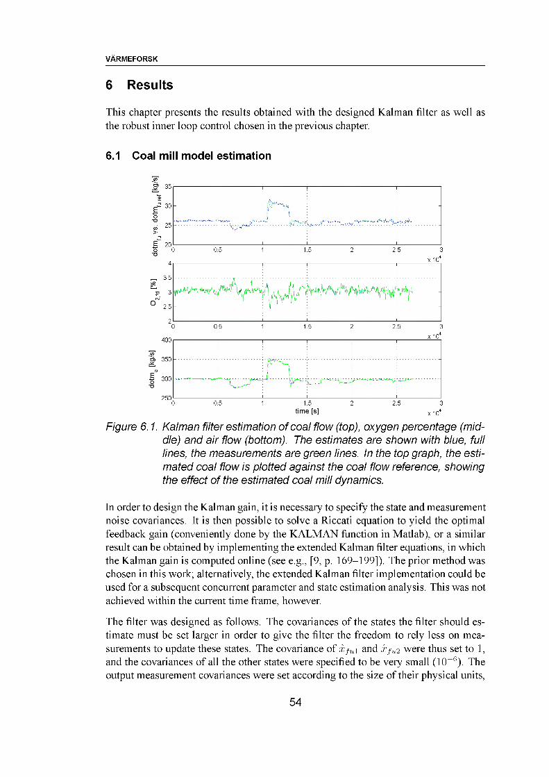
6 Results

This chapter presents the results obtained with the designed Kalman filter as well as the robust inner loop control chosen in the previous chapter.

VARMEFORSK

6.1 Coal mill model estimation

1.......... _

4

_ 3-5

2 3 2.5

2

0.5 1.5 2.5

x 10"

v#......... -r r" " ^

0.5 1.5 2.5

Figure 6.1. Kalman filter estimation of coal flow (top), oxygen percentage (mid­dle) and air flow (bottom). The estimates are shown with blue, full lines, the measurements are green lines. In the top graph, the esti­mated coal flow is plotted against the coal flow reference, showing the effect of the estimated coal mill dynamics.

In order to design the Kalman gain, it is necessary to specify the state and measurement noise covariances. It is then possible to solve a Riccati equation to yield the optimal feedback gain (conveniently done by the KALMAN function in Matlab), or a similar result can be obtained by implementing the extended Kalman filter equations, in which the Kalman gain is computed online (see e g., [9, p. 169-199]). The prior method was chosen in this work; alternatively, the extended Kalman filter implementation could be used for a subsequent concurrent parameter and state estimation analysis. This was not achieved within the current time frame, however.

The filter was designed as follows. The covariances of the states the filter should es­timate must be set larger in order to give the filter the freedom to rely less on mea­surements to update these states. The covariance of Xfu\ and Xfu2 were thus set to 1, and the covariances of all the other states were specified to be very small (10-6). The output measurement covariances were set according to the size of their physical units,

54

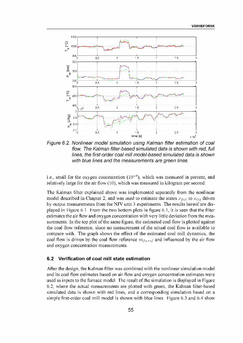
VARMEFORSK

Figure 6.2. Nonlinear model simulation using Kalman filter estimation of coal flow. The Kalman filter-based simulated data is shown with red, full lines, the first-order coal mill model-based simulated data is shown with blue lines and the measurements are green lines.

i.e., small for the oxygen concentration (10 6), which was measured in percent, and relatively large for the air flow (10), which was measured in kilogram per second.

The Kalman filter explained above was implemented separately from the nonlinear model described in Chapter 2, and was used to estimate the states Xfui to x02 driven by output measurements from the NJV unit 3 experiments. The results hereof are dis­played in Figure 6.1. From the two bottom plots in figure 6.1, it is seen that the filter estimates the air flow and oxygen concentration with very little deviation from the mea­surements. In the top plot of the same figure, the estimated coal flow is plotted against the coal flow reference, since no measurement of the actual coal flow is available to compare with. The graph shows the effect of the estimated coal mill dynamics; the coal flow is driven by the coal flow reference m,fu.ref and influenced by the air flow and oxygen concentration measurements.

6.2 Verification of coal mill state estimation

After the design, the Kalman filter was combined with the nonlinear simulation model and its coal flow estimates based on air flow and oxygen concentration estimates were used as inputs to the furnace model. The result of the simulation is displayed in Figure 6.2, where the actual measurements are plotted with green, the Kalman filter-based simulated data is shown with red lines, and a corresponding simulation based on a simple first-order coal mill model is shown with blue lines. Figure 6.3 and 6.4 show

55

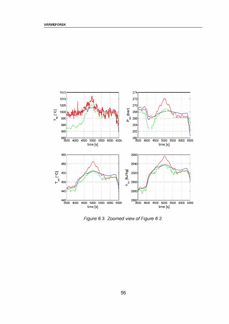
VARMEFORSK

O 1000

3500 4000 4500 5000 5500 6000 6500time [s]

3500 4000 4500 5000 5500 6000 6500time [s]

O 455

3500 4000 4500 5000 5500 6000 6500time [s]

3500 4000 4500 5000 5500 6000 6500time [s]

Figure 6.3. Zoomed view of Figure 6.2.

56

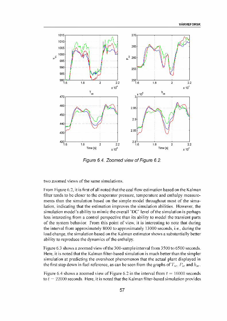
VARMEFORSK

Time [s]

“ 260

1.6 1.8 2 2.2 Time [s] 104

Figure 6.4. Zoomed view of Figure 6.2.

two zoomed views of the same simulations.

From Figure 6.2, it is first of all noted that the coal flow estimation based on the Kalman filter tends to be closer to the evaporator pressure, temperature and enthalpy measure­ments than the simulation based on the simple model throughout most of the simu­lation, indicating that the estimation improves the simulation abilities. However, the simulation model’s ability to mimic the overall ’DC’ level of the simulation is perhaps less interesting from a control perspective than its ability to model the transient parts of the system behavior. From this point of view, it is interesting to note that during the interval from approximately 8000 to approximately 13000 seconds, i.e., during the load change, the simulation based on the Kalman estimator shows a substantially better ability to reproduce the dynamics of the enthalpy.

Figure 6.3 shows a zoomed view of the 300-sample interval from 3500 to 6500 seconds. Here, it is noted that the Kalman filter-based simulation is much better than the simpler simulation at predicting the overshoot phenomenon that the actual plant displayed in the first step down in fuel reference, as can be seen from the graphs of 7. Pse and hse.

Figure 6.4 shows a zoomed view of Figure 6.2 in the interval from t = 16000 seconds tot = 22000 seconds. Here, it is noted that the Kalman filter-based simulation provides

57

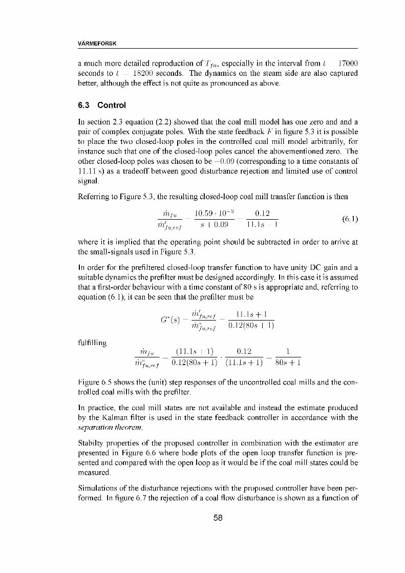
VARMEFORSK

a much more detailed reproduction of Tfn, especially in the interval from t = 17000 seconds to t = 18200 seconds. The dynamics on the steam side are also captured better, although the effect is not quite as pronounced as above.

6.3 Control

In section 2.3 equation (2.2) showed that the coal mill model has one zero and and a pair of complex conjugate poles. With the state feedback F in figure 5.3 it is possible to place the two closed-loop poles in the controlled coal mill model arbitrarily, for instance such that one of the closed-loop poles cancel the abovementioned zero. The other closed-loop poles was chosen to be -0.09 (corresponding to a time constants of 11.11 s) as a tradeoff between good disturbance rejection and limited use of control signal.

Referring to Figure 5.3, the resulting closed-loop coal mill transfer function is then

mfu _ 10.59- 10~3

^kre/ S + 0-090.12

ll.ls + 1(6.1)

where it is implied that the operating point should be subtracted in order to arrive at the small-signals used in Figure 5.3.

In order for the prefiltered closed-loop transfer function to have unity DC gain and a suitable dynamics the prefilter must be designed accordingly. In this case it is assumed that a first-order behaviour with a time constant of 80 s is appropriate and, referring to equation (6.1), it can be seen that the prefilter must be

r^*(a) = ^nfu<ref _ ll-ls + 1 ' ’n}vcf ~ 0.12(803+ 1)

fulfillingm/w _ (11.1s+ 1) 0.12 _ 1

m*furef ~ 0.12(80s + 1) ' (11.1s+ 1) “ 80s + 1

Figure 6.5 shows the (unit) step responses of the uncontrolled coal mills and the con­trolled coal mills with the prefilter.

In practice, the coal mill states are not available and instead the estimate produced by the Kalman filter is used in the state feedback controller in accordance with the separation theorem.

Stabilty properties of the proposed controller in combination with the estimator are presented in Figure 6.6 where bode plots of the open loop transfer function is pre­sented and compared with the open loop as it would be if the coal mill states could be measured.

Simulations of the disturbance rejections with the proposed controller have been per­formed. In figure 6.7 the rejection of a coal flow disturbance is shown as a function of

58

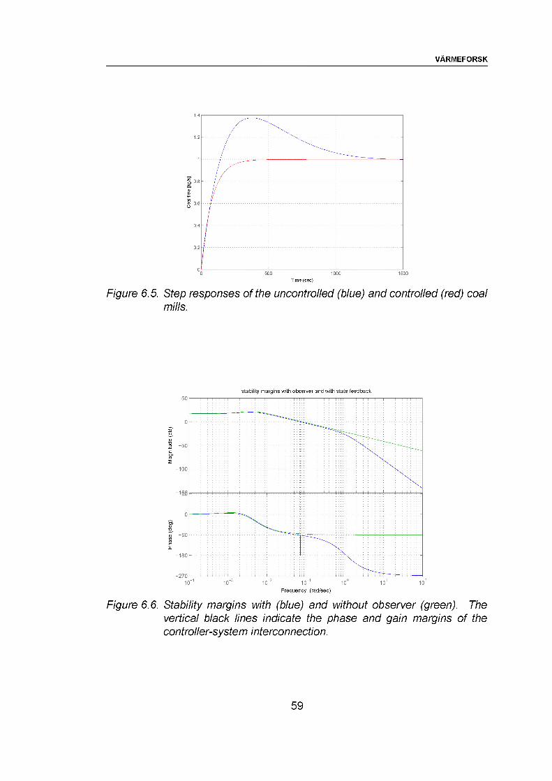
VARMEFORSK

Time (sec)

Figure 6.5. Step responses of the uncontrolled (blue) and controlled (red) coal mills.

stability margins with observer and with state feedback

3 "50

-100

o — •

-90 -

-180 -

-270

Frequency (rad/sec)

Figure 6.6. Stability margins with (blue) and without observer (green). The vertical black lines indicate the phase and gain margins of the controller-system interconnection.

59

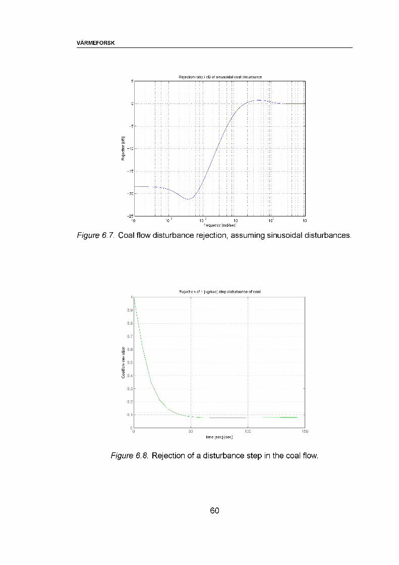
VARMEFORSK

Rejection ratio i dB of sinusoidal coal disturbance

-15 -

-20 -

frequency [rad/sec]

Figure 6.7. Coal flow disturbance rejection, assuming sinusoidal disturbances.

Rejection of 1 [kg/sec] step disturbance of coal

0.7 -

0.3 -

time [sec] (sec)

Figure 6.8. Rejection of a disturbance step in the coal flow.

60

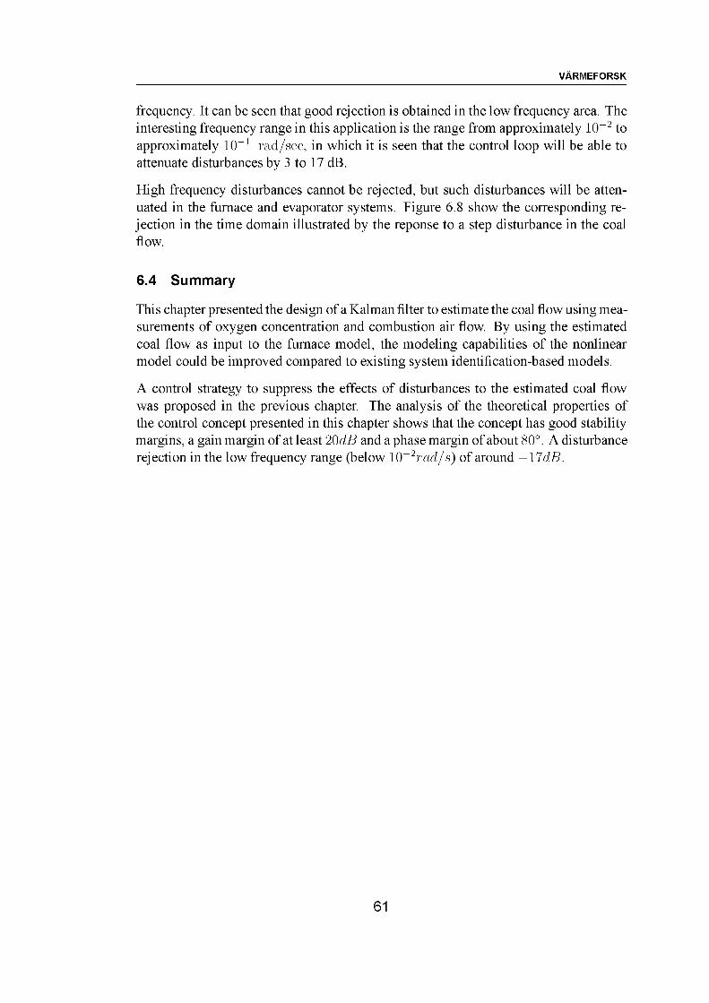
VARMEFORSK

frequency. It can be seen that good rejection is obtained in the low frequency area. The interesting frequency range in this application is the range from approximately 10-2 to approximately 10-1 rad/sec, in which it is seen that the control loop will be able to attenuate disturbances by 3 to 17 dB.

High frequency disturbances cannot be rejected, but such disturbances will be atten­uated in the furnace and evaporator systems. Figure 6.8 show the corresponding re­jection in the time domain illustrated by the reponse to a step disturbance in the coal flow.

6.4 Summary

This chapter presented the design of a Kalman filter to estimate the coal flow using mea­surements of oxygen concentration and combustion air flow. By using the estimated coal flow as input to the furnace model, the modeling capabilities of the nonlinear model could be improved compared to existing system identification-based models.

A control strategy to suppress the effects of disturbances to the estimated coal flow was proposed in the previous chapter. The analysis of the theoretical properties of the control concept presented in this chapter shows that the concept has good stability margins, a gain margin of at least 20dB and a phase margin of about 80°. A disturbance rejection in the low frequency range (below 10-2rod/s) of around -17dB.

61

VARMEFORSK

7 Conclusions

The purpose of the present project was to investigate the development of an adaptive control strategy for the coal mills that can handle variations in the behavior of the coal mills found at a Danish power plant.

If appropriate measurement equipment were available, tight control of the coal mills would be possible by closing a local loop around the coal mills; under normal circum­stances, however, no such sensor equipment is available and hence no local feedback can be made. This project thus attempted to find methods to detect the coal flow using the available sensors and use this information to close an inner loop around the coal mill to suppress disturbances and variations.

In Chapter 2 a fairly detailed, nonlinear modeling of three subsystems of a power plant within the scope of this project, namely the coal supply subsystem, the furnace and flue gas duct subsystem and the steam circuit subsystem, was carried out, and summed up for easy implementation in simulation software such as MATLABTM .

Chapter 3 described the two open-loop experiments against which the nonlinear sim­ulation model formulated in Chapter 2 was validated. The first experiment was run under high load conditions, and the second experiment was run under low load condi­tions. Measurements were obtained from the plant on both the furnace and the steam side. Using the corresponding input samples, the simulation model simulated the plant operation during the experiments, and the outputs were compared to the actual plant measurements. The simulation model showed good agreement with the measurements in a wide operating range.

Following that, in Chapter 4 the nonlinear model obtained in Chapter 2 was linearized in order to facilitate later estimator and control designs, as well as to obtain a better understanding of the model structure. It was found that a linear model of relatively low order describes the plant behavior quite well in the immediate vicinity of the operating points around which it was linearized.

Chapter 5 presented the design of a state estimator for the actual coal flow. This esti­mator utilized the coal flow reference, the oxygen sensor measurement and the total air flow measurement as input to a Kalman filter, and it was shown in Chapter 6 that using the estimated coal flow as input to the furnace model, the modeling capabilities of the nonlinear model could be improved compared to existing system identification-based models. To the best of the authors’ knowledge, this is a novel development.

Two control strategies to suppress the effects of disturbances to the estimated coal flow were proposed, an adaptive concept and a robust cascade concept. Considering the advantages and disadvantages of each concept, it was chosen in this project to de­sign a robust cascade controller as an inner loop controller enclosing the coal mill. It was considered a significant disadvantage of the adaptive control concept that persis­tent excitation and good measurements are required to ensure good performance of an adaptive control concept, whereas a robust inner-loop control is likely to achieve better

62

VARMEFORSK

disturbance rejection performance based on the available plant setup and the coal flow observer. An actual adaptive or linear parameter varying control concept is considered to be more appropriate for the outer loop.

The chosen design had the purpose of suppressing disturbances, effects of unmodeled dynamics etc., based on the estimated coal flow. Analysis of the theoretical properties of the control concept shows that the concept has good stability margins, a gain margin of at least 20dB and a phase margin of about 80°. A disturbance rejection in the low frequency range (below 10-2rod/s) of around -17dB. This is also considered a novel contribution, as it is based on the estimator work presented in the previous chapter.

Results from the reduced order linearized model suggest that it is possible to combine this controller with a gain-scheduling concept, and thus achieve adaptivity to operating point changes. However, this has not been investigated within the time frame of this project.

It is worthy of note that in plants containing several coal mills, the oxygen percentage and total air flow measurements give an average estimate of the coal mill behavior. Thus, in the proposed concept, if one coal mill behaves differently from the others, the other coal mills will compensate for this, as they are controlled via the average estimate. Whether this is acceptable, depends on the particular application.

The proposed concept may be used in other power plants or similar plants employing coal mills for fuel supply. To use the strategy, the oxygen content in the flue gas as well as the combustion air flow must be measurable in order to estimate the actual coal dust flow from the mill. This coal flow estimate may then be used in an appropriate control strategy.

63

VARMEFORSK

8 Suggestions for continued research

At this point, a satisfying nonlinear model of the furnace and evaporator subsystem at NJV3 has been developed and verified. As a follow-up to this, it is logical to attempt to construct a more sophisticated model of the coal mill, in order to investigate in greater detail the three internal control signals that the coal mill is actually controlled by. This can possibly be done by comparing the estimates from the estimator designed in this project with flow measurements obtained using new flow measurement equipment, which may be installed by Elsam Engineering in 2005.

Another interesting issue to address based on the modeling work done in this project include a more detailed modeling of the steam circuit at the power plant, especially in terms of the feedwater temperature, economizer, superheaters and intermediate/low pressure turbine steps. Doing so may remove some of the bias observed in the simula­tion models.

Regarding the estimator, it would be interesting to include more measurements in the filter design. Especially the furnace temperature and possibly the evaporator pressure and temperature may contain valuable information about the combustion.

In terms of control, it would obviously be very interesting to test the control concept on the real plant. The control concept has been designed in such a way that it is rea­sonably easy to implement as an addition to the existing feedforward coal mill control. Furthermore, it would be interesting to investigate linear parameter varying control of the evapotor pressure and temperature. Finally, system identification experiments may indicate whether true adaptivity of the coal mill control loop is indeed feasible.

64

VARMEFORSK

9 Literature references

[1] Andersen P, Hansen T, Pedersen T S, ”Kraftv$rksoverheder-dynamisk model, dataopsamling, modeltilpasning, sandtidssimulering”, Aalborg Universitet, Aalborg 1988

[2] Bendtsen J, Stoustrup J, Trangb$k K,; ’’Bumpless transfer between Advanced Controllers with Application to Power Plant Control”, Proc. Of 42nd Conference on Decision and Control, 2003

[3] Christensen S, Nielsen R; ’’Nonlinear Multivariable Model of a Benson Boiler”, Aalborg University, 2004

[4] Doyle J. C, Stein G ’Robustness with Observers”, IEEE trans. Automatic Control 21,1979

[5] Flynn D ed. ’Thermal Power Plant Simulation”, IEE, 1998[6] French, M. “An analytical comparison of the weighted LQ performance of a

robust and an adaptive backstepping design”, Proc. of the 38th IEEE Conference on Decision and Control, 1999

[7] Garduno-Ramirez R, Lee K ”Overall Control of Fossil-fuel Power Plants”, Proc. 2001 Winter Meeting IEEE Power Engineering Society, 2001

[8] Gilette R, Heath, T, Cardarelli, R ’’Advanced Milling System Technology Retrofit at New York State Electric and Gas Corp. Milliken Station”, Proc.POWER- GEN’94 Americas 1994

[9] Grewal M, Andrews A ’Kalman Filtering”,Prentice-Hall Inc., 1993[10] Inc.Babcock Power. http://www.babcockpower.com, 2003[11] Nordjyllandsv$rket I/S ”Nordjyllandsv$rket unit 3-advanced technology and high

efficiency”,1998[12] Usoro P, Wormley D ’Mathematical Modeling of Fossil Fuelled Steam Power

Plants under Normal and Emergency Operating Conditions”, Proc. 5 th Power Plant Dynamics, Control and Testing Symposium, 1983

[13] Wagner WEA ; ”The IAPWS Industrial Formulation 1997 for the thermodynamic Properties of Water and Steam”, ASME Journal of Eng. Gasturbines and Power 122, 2000

65

RAPPORTFORTECKNINGForteckning over tidigare publicerade rapporter, kan bestallas hos Varmeforsk.Telefax: 08-677 25 35Telefon: 08-677 27 54 http://www.varmeforsk.seSiffrorna mom parentes anger forskmngsgrupp/program:1 = Material- och kemiteknik2 = Miljo- och forbranningsteknik3 = Anlaggningsteknik6 = Tillampad forbranningsteknik

844 Forbranningsfbrhallanden vid omblandning i branslebaddar pa rorlig rost vid eldning av biobransle och sameldning med naturbranslen - etapp 1; Fbrsok i en kail anlaggningJurgen Jacoby, Asa Rodin november 2003 E2-003 (6)

845 Robust instrumentering Anders Wikdecember 2003 M9-829 (1)

846 Avvattning av aska franblandbranslen;Erfarenheter och resultat fran Tekninska Verken i Linkoping Ulf Carlsson, Anders Fredriksson, Inge Lindahl, Anna Arevius, Rolf Sjoblom december 2003 A9-835 (3)

847 Lagtemperaturkorrosion i pannor med SNCRBarbara Goldschmidtjanuari 2004 M4-218 (1)

848 Anvandning av energiaskor som fillermaterial vid betongtillverkning Hillevi Sundblomjanuari 2004 Q4-219 (10)

849 Forutsattningar for att askor kommer till anvandning i vagarErik Karrman, Denis Van Moeddaert, Henrik Bjurstrom, Magnus Berg, Bo Svedbergjanuari 2004 Q4-207 (10)

7 = Torkning av biobransle8 = Skogsindustriella programme!9 = Processtyming10= Miljoriktig anvandning av askor

850 Roterugn for bedomning av sintringbenagenhetJenny Larfeldt, Frank Zintl januari 2004 F4-208 (2)

851 Rening av baddmaterialFrank Zintl, Birgitta Stromberg, Jenny Larfeldt, Henrik Broden, Peter Sjovall januari 2004 F4-217 (2)

852 Pannsand som fillermaterial forfj arrvarmerorgravarRoger Pettersson, Pascal Suer, Jan Rogbeckjanuari 2004 Q4-220 (10)

853 Energieffektivisering av anlaggningar for stoftrening med slangfilterLars Eriksson, Karin Wikman, Magnus Bergjanuari 2004 A4-310 (3)

854 Experimentell studie av inverkan av trapulvers storleksfordelning pa forbranningsegenskaper Christian Fredrikssonjanuari 2004 F4-211 (2)

855 Askor och rotslam som tackskikt for gruvavfallMattias Backstrom, Inger Johansson januari 2004 Q4-146 (10)

856 En forenklad testmetodik for kvalitetssakring - etapp 1Henrik Bjurstrom, Magnus Berg, Maria Aim, Pascal Suer, Karsten Hakansson januari 2004 Q4-148 (10)

857 Databas inom delprogrammet ”Miljoriktig anvandning av askor”Henrik Bjurstrom, Camilla Rydstrand, Magnus Berg, Karin Wikman januari 2004 Q4-211 (10)

858 Naturliga koldmedierFramtida varmepumpar for fjarrvarme Paul Ingvarsson, Ingela Steen Ronnermark, Marcus Eriksson januari 2004 A4-303 (3)

859 Kvavgasbubbling i expansionskarl och lagertankar for spadvattenFredrik Wilgotson, Helen Hansson januari 2004 M4-214 (1)

860 Kallmodellstudie av en branslebadd pa en rorlig rostEtapp 1 - Parameterstudie av samspelet mellan rost-/pusherrorelser och branslebaddHenrik Broden, Jenny Larfeldt mars 2004 F4-310 (2)

861 Erfarenheter av samforbranning och kvalitetssakring av verksamhetsavfall i Sverige och EuropaElisabet Blom, Annika Ekvall, Lennart Gustavsson, Kerstin Robertsson, Jan-Olov Sundqvistapril 2004 F4-213 (2)

862 Anvandning av askor fran forbranning med returpapperslam inom gruvindustrin Erik Nordstrom, Mattias Holmstrom, Tomas Sandstromapril 2004 Q4-103 (10)

863 Z-phase in 9-12% Cr Steels Hilmar Danielsson, John Haldapril 2004 M4-313 (1)

864 Overhettarkorrosion - battre utnyttjande av projektresultatOlle Nystrom, Anders Kjork, Thomas Ehrstedtapril 2004 M4-211 (1)

865 Kontinuerlig styrning av matning och rosthastighet for en smaskalig forbranningsrostNader Padban, Erik Ramstrom, JennyLarfeldt och Niklas Bergeapril 2004 P4-309 (9)

866 Vagledning for klassificering av forbranningsrester enligt AvfallsforordningenPeter Adler, Jan-Erik Haglund, Rolf Sjoblommaj 2004 Q4-142 (10)

867 Kvalitetskriterier for bottenaskor till vag- och anlaggningsbyggnadEtapp 1 - inventering av provningsmetoder och funktionskrav Bo von Bahr, Annika Ekvall, Bjorn Schouenborgmaj 2004 Q4-143 (10)

868 Moderna panndata inom samforbranning Ola Thorsonmaj 2004 A4-217 (3)

869 Returbranslen - kopplingen mellan bransleberedning, forbranningsutrustning och askkvalitetMarianne Gyllenhammar, Inge Johansson juni 2004 A4-301 (3)

870 Flygaska i geotekniska anlaggningar Etapp 1 - inventering/tillganglighet Josef Macsik, Bo Svedberg, Stina Lenstromer, Thomas Nilssonjuli 2004 Q4-107 (10)

871 Utvardering av bark for rening av vatten vid biobransleeldade anlaggningar Christina Hansson, Helen Hansson och Soren Hanssonjuli 2004 M4-217 (1)

872 Arealer for skogsgodsling med traaska och torvaska pa organogena jordar i SverigeBjorn Hanellaugusti 2004 Q4-213 (10)

873 Modifierad sur konduktivitet Annika Stalenheimaugusti 2004 M4-203 (1)

874 Krypskador i svetsar av X 20 CrMoV 12 1 stal; Etapp 2Jan Storesund, Kjeld Borggreen, Weilin Zang, Henrik Nilsson, Ake Samuelson september 2004 M4-306 (1)

875 Funktion av allmetallseparatorer for avfallsbranslenJurgen Jacoby, Lars Wrangensten september 2004 A4-324 (3)

876 Pelletering med skogsbransle och Salix som ravaraLars Martinsson, Stefan Osterberg september 2004 A4-313 (3)

877 Larmsanering genom korrelationsanalys Tord Bergquist, Jonas Ahnlund, Bjorn Johansson, Lennart Gardman, Martin Rabergseptember 2004 P4-312 (9)

878 Sotningsmetodernas effektivitet och konsekvenser pa forbrannings- anlaggningar for olika typer av branslen Anders Eklund, Asa Rodinoktober 2004 A4-327 (3)

879 Miljoriktlinjer for nyttiggorande av askor i anlaggningsbyggande -del 1Karsten Hakansson, Ola Wik, David Bendz, Helena Helgesson, Bo Lind oktober 2004 Q4-104 (10)

880 Langsamupplosande askpellets - enjamforande studie av olika alternativ Maryam Mahmoudkhani, Hans Theliander oktober 2004 Q4-139 (10)

881 Torkning av biobranslen med spillvarme Inge Johansson, Sara Larsson, Olle Wennbergoktober 2004 A4-312 (3)

882 Bayesian networks applied to process diagnosticsBjorn Widarsson, Christer Karlsson, Thomas D. Nielsen, Finn V. Jensen, Erik Dahlqvistoktober 2004 P4-303 (9)

883 Lambdabaserad reglering -Borvardesoptimering och utvardering Mikael Svensson, Peter Brodin oktober 2004 P4-306 (9)

884 Sugpyrometern - en analys avinstrumentet och rad till anvandare Elisabet Blom, Peter Nyqvist, Dan Loyd oktober 2004 P4-305 (9)

885 Handbok for livslangdsarbete med energianlaggningarUtgava 2 Jan Storesundoktober 2004 A9-850/A4-209 (3)

886 Metodik for modellering av forbranningsrost med systemidentifiering, svart- och gralademodellerAstrid Lundgren, Jonas Sjoberg, Erik Ramstrom, Fredrik Sunnerstam oktober 2004 P4-301 (3)

887 Korrosion i avfallsforbrannings- anlaggningarAnnika Stalenheim, Pamela Henderson november 2004 M4-311 (1)

888 Fullskaleforsok med Hyttsand som badd-material i 12 MW avfallseldad BFB-panna Anders Eklund, Marcus Ohman november 2004 F4-319 (2)

889 Kvalitetssakring av automatiska emissionsmatsystem - analys och langtidsutvarderingHenrik Harnevie, Magnus Andersson,Lennart Gustavssonnovember 2004 F4-301 (2)

890 Effekten av fluidiseringshastighet och kornstorlek pa agglomereringsrisk vid biobransleeldning i FB-pannorMorgan Eriksson, Karin Wikman, MagnusBerg och Marcus Ohmannovember 2004 F4-305 (2)

891 Rokgaskondensering med varmepumpFredrik Axby, Camilla Pettersson november 2004 A4-316 (3)

892 Karaktarisering av gassensorer for matning av oforbranda amnen i nar- varmecentralerDavid Eskilsson och Marie Ronnback november 2004 F4-316 (2)

893 Basta mojliga overvakning av vatten- kemin i anlaggningar med angturbin Mats Hellmannovember 2004 M4-322 (1)

894 Praktiska konsekvenser for for- branningsanlaggningar vid inforandet av Vattendirektivet - Nya renings- tekniker och forbattringsatgarder vid utslapp till vattenFredrik Axby och Christina Hansson november 2004 M4-324 (1)

895 Avancerad rening av rokgaskondensat Fredrik Axby, Osten Ekengren, Jan-Erik Bjurhemnovember 2004 M4-302 (1)

896 Tidig detektering av utmattningssprickor genomoforstorande provning, OFP Mattias Broddegarddecember 2004 M4-305 (1)

897 Modellbaserade overvakningsfunktioner for sakrare och effektivare drift av fjarr- styrda anlaggningarThomas Bjorklund och Martin Raberg december 2004 P4-315 (3)

898 Produktionsplanering under osakerhet - Simulatorbaserad produktions- planering av medelstora kraftvarme- anlaggningarDaniel Haggstahl och Erik Dotzauer december 2004 P4-311 (3)

899 Indikation av forbranningssituationengenom bildanalys av rostens eldstad Anna Persson, Johan Helgesson december 2004 P4-319 (3)

900 Smaskalig kraftvarme medparallellkopplade tandemturbiner Pontus Steinwall, Urban Norstrom, Camilla Pettersson och Erik Osterlin december 2004 A4-321 (3)

901 Fosfatkemiprocesser i panntuber Magnus Nordlingdecember 2004 M4-309 (1)

902 Materialval vid rokgaskondenseringMagnus Nordling, Gunnar Bergman, Gustaf Back, Karin Jacobsson, Helen Pahverk, Stefanie Romhild december 2004 M4-303 (1)

903 Rosterovervakning med bildanalys Elisabet Blom, Bengt Gustafsson, Magnus Olssondecember 2004 P4-317 (3)

904 Biobranslebaserade energikombinat med tillverkning av drivmedel Barbara Goldschmidtjanuari 2005 A4-406 (3)

905 Materialegenskaper hos turbinskovlar av nickelbaslegeringen IN792 efter lang drifttidFredrik Karlssonjanuari 2005 M4-310 (1)

906 Observer-Based Fuel Control UsingOxygen Measurement - A study based on a first-principles model of a pulverized coal fired Benson Boiler Palle Andersen, Jan Dimon Bendtsen, Jan Henrik Mortensen, Rene Just Nielsen, Tom Sendergaard Pedersen februari 2005 P4-318 (3)

907 Betydelsen av jamnarebransle- fordelning av fastbransle till fluidbaddpannaJohan Helgesson, Christer Andersson, Anna Helgesson, Marcus Svanberg februari 2005 F4-335 (2)