Observations of distant supernovae and cosmological implications Rahman Amanullah Doctoral thesis in physics Department of Physics Stockholm University

Welcome message from author
This document is posted to help you gain knowledge. Please leave a comment to let me know what you think about it! Share it to your friends and learn new things together.
Transcript

Observations of distant
supernovae and cosmological
implications
Rahman Amanullah
Doctoral thesis in physicsDepartment of PhysicsStockholm University

Doctoral thesis in physicsDepartment of PhysicsStockholm UniversitySweden
c© Rahman Amanullah, 2006ISBN: 91-7155-250-2 pp i–x, 1–90
Typeset in LATEXPrinted by Universitetsservice US AB, Stockholm
Cover: An artist’s impression of a dark energydominated universe. Courtesy of SarahAmandusson.

Abstract
Type Ia supernovae can be used as distance indicators for probing theexpansion history of the Universe. The method has proved to be an effi-cient tool in cosmology and played a decisive role in the discovery of a yetunknown energy form, dark energy, that drives the accelerated expansionof the Universe. The work in this thesis addresses the nature of dark en-ergy, both by presenting existing data, and by predicting opportunitiesand difficulties related to possible future data.
Optical and infrared measurements of type Ia supernovae for differ-ent epochs in the cosmic expansion history are presented along with adiscussion of the systematic errors. The data have been obtained withseveral instruments, and an optimal method for measuring the lightcurveof a background contaminated source has been used. The procedure wasalso tested by applying it on simulated images.
The future of supernova cosmology, and the target precision of cos-mological parameters for the proposed snap satellite are discussed. Inparticular, the limits that can be set on various dark energy scenariosare investigated. The possibility of distinguishing between different in-verse power-law quintessence models is also studied. The predictions arebased on calculations made with the Supernova Observation Calcula-tor, a software package, introduced in the thesis, for simulating the lightpropagation from distant objects. This tool has also been used for inves-tigating how snap observations could be biased by gravitational lensing,and to what extent this would affect cosmology fitting. An alternativeapproach for estimating cosmological parameters, where lensing effectsare taken into account, is also suggested. Finally, it is investigated towhat extent strongly lensed core-collapse supernovae could be used as analternative approach for determining cosmological parameters.

Accompanying papers
Paper A. Supernovae and the nature of the dark energyM. Goliath, R. Amanullah, P. Astier, A. Goobar, and R. Pain
A&A 380, 6–18 (2001)
The target precision of the cosmological parameters for a future sn ex-periment of snap type is presented. The emphasis lies on the possibilityto differentiate between dark energy models by measuring the equationof state parameter w, parametrised as w(z) = w0 + w1z.
Paper B. Fitting inverse power-law quintessence models usingthe SNAP satelliteM. Eriksson and R. Amanullah
Phys. Rev. D 66, 023530 (2002)
The most commonly used quintessence model is the Peebles-Ratra in-verse power-law potential. In this paper the possibility of distinguishingbetween different values of the exponent by using the snap satellite isinvestigated.
Paper C. SNOC: A Monte-Carlo simulation package for high-zsupernova observationsA. Goobar, E. Mortsell, R. Amanullah, M. Goliath, L. Bergstrom, and T. Dahlen
A&A 392, 757–771 (2002)
The Supernova Observation Calculator (snoc), a software package forray-tracing optical and near-infrared photons from supernovae over cos-mological distances, is presented.
Paper D. Cosmological parameters from lensed supernovaeA. Goobar, E. Mortsell, R. Amanullah, and P. Nugent
A&A 393, 25–32 (2002)
The possibility of using core-collapse sne, that will be discovered bythe proposed snap satellite, for measuring cosmological parameters isinvestigated.
Paper E. Correcting for lensing bias in the Hubble diagramR. Amanullah, E. Mortsell, and A. Goobar
A&A 397, 819–823 (2003)
Gravitational lensing will be a major contributor to systematic errors inthe Hubble diagram for high-z sn observations. In this paper the effectsare quantified and a method for taking them into account in a cosmologyanalysis, is presented.

iii
Paper F. New Constraints on ΩM , ΩΛ and w from an indepen-dent set of 11 high-redshift supernovae observed with the Hub-ble Space TelescopeR. A. Knop, G. Aldering, R. Amanullah, P. Astier, G. Blanc, M. S. Burns, A. Con-
ley, S. E. Deustua, M. Doi, R. Ellis, S. Fabbro, G. Folatelli, A. S. Fruchter, G. Gar-
avini, S. Garmond, K. Garton, R. Gibbons, G. Goldhaber, A. Goobar, D. E. Groom,
D. Hardin, I. Hook, D. A. Howell, A. G. Kim, B. C. Lee, C. Lidman, J. Mendez,
S. Nobili, P. E. Nugent, R. Pain, N. Panagia, C. R. Pennypacker, S. Perlmut-
ter, R. Quimby, J. Raux, N. Regnault, P. Ruiz-Lapuente, G. Sainton, B. Schaefer,
K. Schahmaneche, E. Smith, A. L. Spadafora, V. Stanishev, M. Sullivan, N. A. Wal-
ton, L. Wang, W. M. Wood-Vasey, N. Yasuda ( scp)
ApJ 598, 102–137 (2003)
Cosmological results from a set of high-z supernovae are presented alongwith accurate colour measurements, that permit host galaxy extinctioncorrection directly.
Paper G. Restframe I-band Hubble diagram for type Ia super-novae up to redshift z ∼ 0.5S. Nobili, R. Amanullah, G. Garavini, A. Goobar, C. Lidman, V. Stanishev, G. Alde-
ring, P. Antilogus, P. Astier, M.S. Burns, A. Conley, S.E. Deutscha, R. Ellis, S. Fab-
bro, V. Fadeyev, G. Folatelli, R. Gibbons, G. Goldhaber, D.E. Groom, I. Hook, A. D.
Howell, A.G. Kim, R.A. Knop, P.E. Nugent, R. Pain, S. Perlmutter, R. Quim-
by, J. Raux, N.Regnault, P. Ruiz-Lapuente, G. Sainton, K.Schahmaneche, E. Smith,
A.L. Spadafora, R.C. Thomas, and L. Wang
A&A 437, 789–804 (2005)
Using the rest frame I-band for supernova cosmology is discussed. Bothfrom a technical point of view along with the advantages in terms ofminimising systematic effects.

Publications not included in the thesis
Paper 1. The Hubble diagram of type Ia supernovae as a func-tion of host galaxy morphologyM. Sullivan, R. S. Ellis, G. Aldering, R. Amanullah, P. Astier, G. Blanc, M. S. Burns,
A. Conley, S.E. Deustua, M. Doi, S. Fabbro, G. Folatelli, A. S. Fruchter, G. Garavini,
R. Gibbons, G. Goldhaber, A. Goobar, D. E. Groom, D. Hardin, I. Hook, D. A. Howell,
M. Irwin, A. G. Kim, R. A. Knop, C. Lidman, R. McMahon, J. Mendez, S. Nobili,
P. E. Nugent, R. Pain, N. Panagia, C. R. Pennypacker, S. Perlmutter, R. Quimby,
J. Raux, N. Regnault, P. Ruiz-Lapuente, B. Schaefer, K. Schahmaneche, A. L. Spa-
dafora, N. A. Walton, L. Wang, W. M. Wood-Vasey, N. Yasuda
MNRAS 340, 1057–1075 (2003)
Paper 2. Spectroscopic Observations and Analysis of the Pecu-liar SN 1999aaG. Garavini, G. Folatelli, A. Goobar, S. Nobili, G. Aldering, A. Amadon, R. Aman-
ullah, P. Astier, C. Balland, G. Blanc, M. S. Burns, A. Conley, T. Dahlen, S. E.
Deustua, R. Ellis, S. Fabbro, X. Fan, B. Frye, E. L. Gates, R. Gibbons, G. Gold-
haber, B. Goldman, D. E. Groom, J. Haissinski, D. Hardin, I. M. Hook, D. A. How-
ell, D. Kasen, S. Kent, A. G. Kim, R. A. Knop B. C. Lee, C. Lidman, J. Mendez,
G. J. Miller, M. Moniez, A. Mourao, H. Newberg, P. E. Nugent, R. Pain, O. Per-
dereau, S. Perlmutter, V. Prasad, R. Quimby, J. Raux, N. Regnault, J. Rich, G. T.
Richards, P. Ruiz-Lapuente, G. Sainton, B. E. Schaefer, K. Schahmaneche, E. Smith,
A. L. Spadafora, V. Stanishev, N. A. Walton, L. Wang, W. M. Wood-Vasey
AJ 128, 387–404 (2004)
Paper 3. No evidence for dark energy metamorphosis?J. Jonsson, A. Goobar, R. Amanullah, L. Bergstrom
JCAP 09, 007 (2004)
Paper 4. Spectroscopic confirmation of high-z supernovae withthe ESO VLT.C. Lidman, D. A. Howell, G. Folatelli, G. Garavini, S. Nobili, G. Aldering, R. Ama-
nullah, P. Antilogus, P. Astier, G. Blanc, M. S. Burns, A. Conley, S. E. Deustua,
M. Doi, R. Ellis, S. Fabbro, V. Fadeyev, R. Gibbons, G. Goldhaber, A. Goobar,
D. E. Groom, I. Hook, N. Kashikawa, A. G. Kim, R. A. Knop, B. C. Lee, J. Mendez,
T. Morokuma, K. Motohara, P. E. Nugent, R. Pain, S. Perlmutter, V. Prasad,

v
R. Quimby, J. Raux, N. Regnault, P. Ruiz-Lapuente, G. Sainton, B. E. Schaefer,
K. Schahmaneche, E. Smith, A. L. Spadafora, V. Stanishev, N. A. Walton, L. Wang,
W. M. Wood-Vasey, N. Yasuda (The Supernova Cosmology Project)
A&A 430, 843–851 (2005)
Paper 5. Spectroscopic Observations and Analysis of the Un-usual Type Ia SN 1999acG. Garavini, G. Aldering, G. Amadon, R. Amanullah, P. Astier, C. Balland, G.
Blanc, A. Conley, T. Dahlen, S. E. Deustua, R. Ellis, S. Fabbro, V. Fadeyev, X. Fan,
G. Folatelli, B. Frye, E. L. Gates, R. Gibbons, G. Goldhaber, B. Goldman, A. Goobar,
D. E. Groom, J. Haissinski, D. Hardin, I. Hook, D. A. Howell, S. Kent, A. G. Kim,
R. A. Knop, M. Kowalski, n. Kuznetsova, B. C. Lee, C. Lidman, J. Mendez, G. J.
Miller, M. Moniez, M. Mouchet, A. Mourao, H. Newberg, S. Nobili, P. E. Nugent,
R. Pain, O. Perdereau, S. Perlmutter, R. Quimby, N. Regnault, J. Rich, G. T.
Richards, P. Ruiz-Lapuente, B. E. Schaefer, K. Schahmaneche, E. Smith, A. L. Spa-
dafora, V. Stanishev, R. C. Thomas, N. A. Walton, L. Wang, W. M. Wood-Vasey
AJ 130, 2278–2292 (2005)
Paper 6. Spectra of High-Redshift Type Ia Supernovae and aComparison with Their Low-Redshift CounterpartsI. Hook, D. A. Howell, G. Aldering, R. Amanullah, M. S. Burns, A. Conley, S. E.
Deustua, R. Ellis, S. Fabbro, V. Fadeyev, G. Folatelli, G. Garavini, R. Gibbons,
G. Goldhaber, A. Goobar, D. E. Groom, A. G. Kim, R. A. Knop, M. Kowalski,
C. Lidman, S. Nobili, P. E. Nugent, R. Pain, C. R. Pennypacker, S. Perlmutter,
P. Ruiz-Lapuente, G. Sainton, B. E. Schaefer, E. Smith, A. L. Spadafora, V. Stani-
shev, R. C. Thomas, N. A. Walton, L. Wang, W. M. Wood-Vasey
AJ 130, 2788–2803 (2005)
Paper 7. Spectroscopy of twelve type Ia supernovae at inter-mediate redshiftC. Balland, M. Mouchet, R. Pain, N. A. Walton, R. Amanullah, P. Astier, R. S. El-
lis, S. Fabbro, A. Goobar, D. Hardin, I. M. Hook, M. J. Irwin, R. G. McMahon,
J. M. Mendez, P. Ruiz-Lapuente, G. Sainton, K. Schahmaneche, V. Stanishev
A&A 445, 387–402 (2006)

AcknowledgementsIt is often said that getting the right supervisor is far more importantthan choosing the right topic. During my doctoral studies, I have beenconstantly reminded that I could not have been more fortunate. ArielGoobar’s support and encouragement has been absolutely invaluable dur-ing the progress of this work. His scientific skills have always been asource of inspiration, and in addition to his outstanding tutoring, Arielhas often been the initiator of social activities, which also have had a verypositive impact on the scientific atmosphere in the Stockholm supernovacosmology group.
I would also like to give a special praise to my colleagues in thesnova group, Gabriele Garavini, Gaston Folatelli, Jakob Jonsson, JakobNordin, Karl Andersson, Linda Ostman, Pernilla Wahlin, Serena Nobili,Tomas Dahlen, and Vallery Stanishev. We have shared many frustratingmoments together, trying to find ghosts in our analysis or getting readyfor a deadline, but I will equally remember the less stressful momentstogether. Hiking in the Grand Canyon, skiing in the Alps or the orcasafari in Northern Norway are just a few of them.
The data analysis has been carried out together with members of theSupernova Cosmology Project and the European Supernova Consortium.I would especially like to thank Kyan Schahmaneche, Sebastien Fabbroand Pierre Astier for introducing me to the toads software, Chris Lid-man for his support in the analysis of infrared data, Rob Knop and RachelGibbons for their assistance with the hst data and for the time I spentwith them at Vanderbilt University during the scp 2004 search, and fi-nally Saul Perlmutter and Tony Spadafora for the very fruitful summerat Lawrence Berkeley National Laboratory.
Several members at the physics and astronomy departments of Stock-holm University deserve my deepest gratitude. For the assistance withthe simulations that is the basis of many of the results presented in thisthesis, I would like to thank Martin Goliath and Edvard Mortsell. MartinEriksson should have a commendation for his theoretical support. Thehelp from Christian Walck on some statistical issues has very valuable. Iam most grateful to all members of the cops and elpa groups for theirsupport, and in particular to Christofer Gunnarsson, Michael Gustafsson,Joakim Edsjo and Lars Bergstrom, and not to mention Hector Rubinsteinfor spicing up the lunch conversations. Ten points goes to the computersupport group consisting of Iouri Belokopytov, Alexander Agapow andTorbjorn Moa, for their liberal attitude and compliance.

vii
Part of my work has involved teaching support at Vetenskapslabora-toriet and setting up the Stockholm Centimetre Radio Telescopes, whichgave me the opportunity, and great pleasure, to collaborate with ChristerNilsson, Torsten Alm, Aage Sandqvist and Uno Wann.
I am very grateful to Per-Olof Hulth and the IceCube group for givingme the possibility to spend a season at the Amundsen-Scott South PoleStation on Antarctica. This was an experience that I will never forget,and I sincerely hope to get back there one day.
A group of people that always have a significant influence on a person,are the long line of teachers that follow us from elementary school to uni-versity. I think I have been particularly lucky in this case, and owe a greatdeal to, in chronological order, Britta Soderman, Britt-Marie Kaneteg,Gunnar Karlin, Kjell Bonander, Gunnar Edvinsson, and Barbro Asman.
Many of my friends have played an active role in shaping this thesisone way or the other. Sarah made the cover, Tomas is the one thatwill help you salvage your hard drive or give you a coding solution younever thought of, I will always have long, and often pointless, discussionswith Johan, and Georgios, together with the members of the swing dancecompany Shout’n Feel It, have been doing all they could to make surethat I spend as little time as possible at the physics department.
A final thought goes to the very foundation of life, my family. Myparents have been absolutely amazing during the past 29 years, and I of-ten wonder where they find their strength. And of course, Mona, who hasbeen absolutely fantastic, as always, in her support and encouragementduring the past months.

viii
Contents
1 Introduction 1
2 Standard cosmology 3
2.1 The expansion of the Universe . . . . . . . . . . . . . . . 3
2.2 Cosmological redshift . . . . . . . . . . . . . . . . . . . . . 4
2.3 A cosmological model . . . . . . . . . . . . . . . . . . . . 5
2.3.1 The energy content of the Universe . . . . . . . . . 6
2.4 Dark energy . . . . . . . . . . . . . . . . . . . . . . . . . . 7
2.4.1 The cosmological constant . . . . . . . . . . . . . . 7
2.4.2 Quintessence . . . . . . . . . . . . . . . . . . . . . 9
2.5 Measuring cosmological parameters . . . . . . . . . . . . . 9
2.5.1 The luminosity-distance relation . . . . . . . . . . 10
3 Cosmological parameters from supernovae 13
3.1 Type Ia supernovae as standard candles . . . . . . . . . . 13
3.1.1 The photometric system . . . . . . . . . . . . . . . 13
3.1.2 Homogeneity . . . . . . . . . . . . . . . . . . . . . 14
3.2 A supernova campaign in practise . . . . . . . . . . . . . . 15
3.2.1 Supernova search strategies . . . . . . . . . . . . . 15
3.2.2 Confirmation . . . . . . . . . . . . . . . . . . . . . 16
3.2.3 Photometric follow-up . . . . . . . . . . . . . . . . 17
3.3 Lightcurve building . . . . . . . . . . . . . . . . . . . . . . 17
3.3.1 The TOADS photometry package . . . . . . . . . . 18
3.3.2 A sanity check of the TOADS software . . . . . . . 21
3.3.3 Lightcurve building with HST WFPC2 data . . . . 25
3.3.4 Calibration . . . . . . . . . . . . . . . . . . . . . . 28
3.3.5 Multiple instruments . . . . . . . . . . . . . . . . . 30
3.4 Lightcurve fitting . . . . . . . . . . . . . . . . . . . . . . . 30
3.4.1 Lightcurve fitting in the I-band . . . . . . . . . . . 31
3.5 Estimating cosmological parameters . . . . . . . . . . . . 32
3.5.1 Grid search minimisation . . . . . . . . . . . . . . 32
3.5.2 The Davidon variance algorithm . . . . . . . . . . 34
3.5.3 Constraints of the cosmological estimators . . . . . 35
3.6 Observations and results . . . . . . . . . . . . . . . . . . . 36
3.7 Systematic errors . . . . . . . . . . . . . . . . . . . . . . . 38

x CONTENTS
3.7.1 Extinction . . . . . . . . . . . . . . . . . . . . . . . 383.7.2 Gravitational lensing . . . . . . . . . . . . . . . . . 39
4 The ESC 1999 campaign 414.1 The ESC 1999 campaign . . . . . . . . . . . . . . . . . . . 414.2 Lightcurve building . . . . . . . . . . . . . . . . . . . . . . 44
4.2.1 Residuals . . . . . . . . . . . . . . . . . . . . . . . 454.2.2 Quality of the fitted PSF . . . . . . . . . . . . . . 45
4.3 Instrumental wavelength response . . . . . . . . . . . . . . 474.4 Calibration and lightcurve fitting . . . . . . . . . . . . . . 524.5 Conclusions . . . . . . . . . . . . . . . . . . . . . . . . . . 52
5 The SCP 2001 high redshift campaign 555.1 The campaign . . . . . . . . . . . . . . . . . . . . . . . . . 555.2 Lightcurve building and calibration . . . . . . . . . . . . . 605.3 Preliminary results . . . . . . . . . . . . . . . . . . . . . . 60
5.3.1 SN2001hb . . . . . . . . . . . . . . . . . . . . . . . 605.3.2 SN2001gq . . . . . . . . . . . . . . . . . . . . . . . 625.3.3 Lightcurve fitting . . . . . . . . . . . . . . . . . . . 64
5.4 Unresolved supernovae . . . . . . . . . . . . . . . . . . . . 67
6 The future of supernova cosmology 696.1 The Supernova Observation Calculator . . . . . . . . . . . 706.2 The target precision of ΩM and ΩΛ . . . . . . . . . . . . . 72
6.2.1 The importance of a wide redshift range . . . . . . 726.3 The nature of dark energy . . . . . . . . . . . . . . . . . . 73
6.3.1 Fitting inverse power-law models . . . . . . . . . . 756.4 Gravitational lensing . . . . . . . . . . . . . . . . . . . . . 75
6.4.1 Dark matter halo models . . . . . . . . . . . . . . 766.4.2 Magnification and demagnification of type Ia SNe 776.4.3 Using lensing for cosmology fitting . . . . . . . . . 79
7 Summary 83

C h a p t e r 1
Introduction
Cosmologists have during the past decade lived in constant euphoria,feasting on a smorgasbord that is continuously being filled with new sci-entific results of various flavours. Somewhere, between chewing the latestcosmic background radiation map and a supernova Hubble diagram, thescientific community can happily announce to the rest of the world thatwe are all living in a flat accelerating dark energy dominant Universe, incontrast to a matter dominated which was the general belief ten yearsago.
When I, on rare occasions, happen to meet with my non-physicsfriends, and cosmology is politely being discussed, somebody may sc-ratch his or her head, and ask how we actually know all of this. Well,you see, we know this, since we can exclude the absence of dark energyat a high level of confidence. . . Surprisingly many are satisfied with thisanswer, probably because they realise that there is no point in pursuingit, and instead they tend to move on and ask why it is called dark energy.I excitedly try to explain that it is because we can not see it. This isusually followed by a short silence before someone is asking how far Ithink Sweden will make it in the World Cup this summer. This is one ofthe questions that will not be answered in this thesis.
The work presented here has mainly been carried out within the frameof three international collaborations: the Supernova Cosmology Project(scp), The European Supernova Consortium (esc) and the SupernovaAcceleration Probe (snap). During the past five years, I have had thebenefit to participate in almost all stages of a supernova campaign. I wasactively involved in the scp 2004 search campaign with the Hubble SpaceTelescope, and I have on several occasions taken part of both optical andinfrared, as well as spectroscopic follow-up of esc supernovae.
In some sense, I started my work in the Stockholm supernova cos-mology group from the wrong end. I began by participating in the de-velopment of a software package, the Supernova Observation Calculator(snoc), and the main result of my work was to make predictions of cos-mological results that could be obtained from future experiments like for
2 CHAPTER 1. INTRODUCTION
example the proposed snap satellite. The aim was primarily to under-stand to what extent different dark energy models could be constrained,and how gravitational lensing may affect cosmological parameter fitting.The main results from these studies are presented in Paper A–Paper Etogether with Paper 3. However, the cosmology fitter that was devel-oped has also been used for the existing data in Paper F.
As time went on, I got more involved in photometric data analysis,and started out by working on the infrared data of 2000fr, presentedin Paper G. A major part of my work has also involved optical data,obtained both with ground based observatories, and with the HubbleSpace Telescope.
This thesis will start with a brief introduction to standard cosmology,chapter 2, followed by a more detailed description of how cosmologicalparameters can be obtained from measurements of type Ia supernovaein chapter 3. This chapter introduces both the general concept as wellas more specific details concerning the methods used in the latter partof the thesis. Chapters 4 and 5 describe the preliminary, and ongoing,photometric analysis of two different data sets that have not yet beenpublished in a scientific journal. In chapter 6 the target precision ofcosmological parameters, and how gravitational lensing effects could biasthe estimators, are discussed. Finally, the thesis work is summarised inchapter 7.

C h a p t e r 2
Standard cosmology
Cosmology is the study of the evolving Universe as a whole. It is a youngscientific branch and was in fact not considered a separate study until thebeginning of the 20th century, when Einstein developed his general theoryof relativity. The reason for this was not specifically related to generalrelativity itself, but to the fact that the common opinion among scientiststhose days was that the Universe was static. Even Einstein himself had astatic Universe in mind when he first tried to build a cosmological modelfrom the relativistic equations. It was not until Edwin Hubble discoveredthat the galaxies in our vicinity are moving away from us, and thereforeconcluded that the cosmos is expanding, that the scientific communityadopted the idea of a dynamic Universe.
Today, the leading theory for the creation of the cosmos is the BigBang model, in which our observable Universe has been expanding eversince it started from a singularity ∼ 1010 years ago. One very strongargument in favour of this theory is the homogeneous microwave back-ground radiation that was first detected by A. Penzias and R. Wilson in1965, and has been measured more accurately by the cobe, boomerang,maxima and wmap projects. This radiation is very hard to explain bythe competing steady-state theories, but has a natural position in theBig Bang theory as a relic from the time when the Universe becametransparent to radiation.
2.1 The expansion of the Universe
All cosmological models are based on the cosmological principle, whichstates that our position in the Universe and what we observe, is verytypical and not at all a unique situation. This implies that the Universehas to be homogeneous and isotropic, except for local irregularities.
In 1929, Edwin Hubble published his discovery that galaxies in thelocal Universe are moving away from us with velocities that are propor-tional to their distances. This is called the Hubble law
v = H0 · d , (2.1)

4 CHAPTER 2. STANDARD COSMOLOGY
where the constant H0 is the Hubble constant. The expansion scenariowas in fact proposed already in 19221 by Alexander Friedmann, a youngRussian mathematician and meteorologist, but the belief in a static Uni-verse was so strongly rooted in the scientific community that his modelnever got general acceptance during his lifetime.2
If the Hubble law is to be consistent with the cosmological principle,all galaxies have to move away from each other. Hence all observerswill experience themselves as if they were located at the centre of theUniverse and that all galaxies are moving away from them.
It is very important to realise that the reason why the galaxies aremoving apart is not due to the same reason why particles move apartin an explosion, but it should instead be understood as if space itselfgrows. A very popular two-dimensional analogy to this is to imaginean expanding balloon where the galaxies are represented by dots on thesurface. The pattern of galaxies will always remain the same but thescale of the pattern changes as the balloon expands.
In other words, an expansion model can be implemented by assumingthat positions of galaxies and galaxy clusters are described by a num-ber of time independent co-moving coordinates, e.g. (ri, θi, φi), and thatall cosmological distances are stretched by a scale factor a(t). The dy-namic behaviour of the Universe can then be parametrised by the Hubbleparameter, defined as
H(t) ≡ a(t)
a(t),
where H0 = H(t0), is the present value of H. For distances within ourlocal Universe, which is what Hubble studied, H0 ≈ H is a sufficientapproximation, and the linearity of equation (2.1) holds.
The evolution of the Hubble parameter is determined by the energycontent of the Universe, and tracing this property backwards in time, isthe essence of this thesis.
2.2 Cosmological redshift
The scale factor ratio between the present, t0, and a given epoch, te, inthe cosmic history is something that can be measured with great accuracy
1 The expansion scenario was also independently formulated by the Belgian priestGeorges Edouard Lemaıtre in 1927.
2 It is a sad historical fact that Alexander Friedmann died in pneumonia at age 38in 1925, four years before Hubble’s discovery.

2.3. A COSMOLOGICAL MODEL 5
from studying the light emitted by distant objects. As the Universeexpands, the wavelength of the light from an object will be stretched bythe same factor as the Universe, and the cosmological redshift, z, can bedefined as
1 + z ≡ λ0
λe=
a(t0)
a(te), (2.2)
where λe and λ0 are the emitted and observed wavelengths respectively.In practise, the redshift is measured by identifying lines in the spectrumof a distant object and matching these with their rest frame counterparts.
2.3 A cosmological model
Building a model of a physical system requires knowledge of all forcesacting on the system, together with an adequate theory describing theinteractions between them. The model building is also simplified sig-nificantly if a suitable coordinate system is chosen, that takes existingsymmetries into account and does not introduce more parameters thannecessary.
Today, the best known theory that describes the relation betweenspace, time and energy, is Albert Einstein’s general theory of relativ-ity [22]. This is indeed, as the name suggests, a very extensive theory,that holds almost a century after its discovery, despite the revolutionduring recent decades in astrophysical observation techniques.
Homogeneous and isotropic space-time can be parametrised by us-ing the Friedmann Lemaıtre Robertson Walker (flrw) metric, whichin addition to the scale factor stretched, time independent, coordinates(ri, θi, φi), also is generalised to incorporate a space of constant curva-ture.
Finally, by recalling the cosmological principle, it can be assumed thatthe energy content of the Universe acts as a perfect fluid on cosmologicalscales and can then be described by its energy density, ρ, and pressure,p, which are related through the equation of state,3
p = w(z) · ρ . (2.3)
3 In most cases the physical properties of the energy content does not change withthe expansion of the Universe, but in order to allow for such exotic energy forms,the equation of state parameter, w(z), can be generalised to allow for a redshiftdependence.

6 CHAPTER 2. STANDARD COSMOLOGY
(a) Positive (b) Zero (c) Negative
Figure 2.1: Illustration of two-dimensional surfaces with different curvature.
If these three building bricks are combined, the Friedmann differentialequations,4
H2 =8π
3ρ − k
a2,
H2 = −8πp − 2a
a− k
a2,
(2.4)
describing the Hubble parameter, can be derived. Here the time depen-dence has been suppressed, and k originates from the flrw metric. Theequations have been constructed so that k only takes the values +1, 0or −1 depending on whether the constant curvature is positive, zero ornegative. These geometries are illustrated by two-dimensional analogiesin figure 2.1.
2.3.1 The energy content of the Universe
The total energy density, ρ, in equation (2.4) can consist of a number ofdifferent components, that each have their own equation of state param-eter, w. For example for radiation, ρr, w = 1/3, and for non-relativisticmatter, ρm, w = 0 is a very good approximation.
Requiring energy conservation leads to an equation,
pa3 =d
dt
(
a3 [ρ + p])
,
that will further constrain the cosmological model, which, together with
4 Geometrised units, i.e. GN = c = 1, are used throughout this thesis, where GN isNewton’s constant and c is the light speed in vacuum.

2.4. DARK ENERGY 7
equations (2.2) and (2.3) can be solved to give
ρ ∝ exp
[
3
∫ z
0
1 + w(z′)
1 + z′dz′]
= f(z) . (2.5)
For a constant and redshift independent w, this can be simplified as,
ρ ∝ (1 + z)−3·(1+w) . (2.6)
For non-relativistic matter, ρm, for instance, the energy density is in-versely proportional to the volume, a dependence that is expected in-tuitively. For radiation on the other hand, the relation becomes ρr ∝(1 + z)−4, which adds an extra factor (1 + z) in addition to the volumedependence due to the cosmological redshift. This also explains why ra-diation, that was the dominant energy component in the early Universe,hardly contributes at all to the present total energy density.
It is also interesting to see how the different energy flavours affectthe time evolution of the Universe. Subtracting the two expressions inequation (2.4) gives,
a
a= −4π
3(ρ + 3p) . (2.7)
Combining this with equation (2.3), the condition for a decelerating Uni-verse, can be derived as
w > −1/3 . (2.8)
In the introductory chapter it was briefly mentioned, that the to-tal energy density is dominated by an energy form that accelerates theUniverse. Since the nature of this dark energy, is unknown, measuringthe equation of state is a very tempting approach towards revealing itsorigin, and doing this is going to be a challenging task for observationalcosmology during the coming decade. Paper A and Paper B discussthe target precision of future measurements for different scenarios, whilePaper F give some results from existing data.
2.4 Dark energy
2.4.1 The cosmological constant
The simplest dark energy model is a cosmological constant, Λ, with anequation of state parameter w = −1, and the energy density
ρΛ =Λ
8π.

8 CHAPTER 2. STANDARD COSMOLOGY
A model of this kind is compatible with general relativity, and is alsowhat Einstein used to balance gravity in his static model of the Uni-verse. However, in an expanding Universe, a constant energy density(equation (2.6)) leads to the strange effect that the total dark energycontent of the Universe increases with the expansion. Since the densitiesof other energy components decrease with the expansion, dark energywill eventually come to dominate the Universe. Solving equation (2.7)with the anzats a ∼ eβ gives
a(t) ∝ exp[
t√
Λ/3]
,
i.e. a cosmological constant will lead to an exponentially expanding Uni-verse.
In the attempts to find a physical explanation for Λ, parallels can bedrawn to vacuum energy in quantum field theory. First of all, ρΛ hasthe same value in each point of the Universe, and secondly, the force hasthe same appearance as for a simple harmonic oscillator with a springconstant k = −Λ/3. Classically, the energy vanishes when the particle ismotion less, but in quantum mechanics however, the energy of the loweststate is E = 1
2~ω. For quantum field theory the situation is analogousand in this case the vacuum energy becomes very large. This does notmatter in the absence of gravity since only differences between energylevels have physical importance. However, in cosmology, gravity is indeedpresent and couples to any source of energy.
One argument against a cosmological constant, is that an attempt tocalculate the vacuum energy based on dimensional grounds results in adiscrepancy of 120 orders of magnitude [74] compared to the measuredvalue.
An additional dilemma is the so called coincidence problem. Accord-ing to equation (2.6), the density of different energy forms decreases atdifferent rates. Therefore, it seems incredibly unlikely that the energydensity of non-relativistic matter and dark energy happen to be of thesame order at the precise epoch when astrophysicists on this planet de-cide to measure it. In order for that to happen, the ratios between thedifferent energy forms have to be fine tuned in the early Universe.
The cosmological constant problem is one of the most interestingunsolved issues in fundamental physics today, and several alternativeexplanations for dark energy has been suggested to circumvent it.

2.5. MEASURING COSMOLOGICAL PARAMETERS 9
2.4.2 Quintessence
The considerations that were mentioned in the previous section motivatesa time-dependent dark energy density, that still must be constrained tohave negative pressure in accordance with equation (2.8). One way toobtain this is to introduce a minimally coupled scalar field Q, with energydensity and pressure given by,
ρQ =1
2Q2 + V (Q)
pQ =1
2Q2 − V (Q)
.
For this field, the equation of state parameter, wQ, will be negativein regions where the potential energy dominates over the kinetic. Thequintessence fields are also often constructed so to be insensitive to theinitial conditions in order to solve the coincidence problem. Anotherdesirable feature is for wQ to change slowly and to always be less thanthe equation of state parameter of the dominant energy component ofthe Universe. That is, according to equation (2.6), ρQ is always de-creasing slower than the background energy density, so that even thoughit is starting out as a negligible component, it will eventually come todominate the Universe.
Several different quintessence field potentials with the above men-tioned properties have been proposed, but one of the simplest is theinverse power-law potential introduced by Ratra and Peebles [55],
V (Q) =M4+α
Qα. (2.9)
There are no real constrains on the parameter α except that it should bepositive. For α = 0 the cosmological constant is retrieved. The parame-ter M determines the energy scale and is fixed by todays measurementsof the dark energy. The possibility of constraining the parameter α fromproposed future supernova experiments, is discussed in Paper B.
2.5 Measuring cosmological parameters
The evolution of the Universe can be described by the first of the equa-tions in (2.4) and is determined by the parameters on the right-hand sideof this expression. Assuming that the energy density, ρ, is completelydominated by matter, ρm, and dark energy, ρX , and that these quantities

10 CHAPTER 2. STANDARD COSMOLOGY
have a scale factor dependence given by equations (2.6) and (2.5), thetotal energy density can be written as
ρ(t) = ρm(t) + ρX(t) = ρm(t0) · (1 + z)3 + ρX(t0) · f(z) .
Further, expressing the energy densities of the present epoch, t0, as frac-tions of the critical density, ρcrit = 3H2
0/(8π), yields
ρ(t) =3H2
0
8π
[
ΩM (1 + z)3 + ΩX · f(z)]
,
where ΩM = ρm(t0)/ρcrit and ΩX = ρX(t0)/ρcrit. By also rewriting thegeometry factor as a(t0)ΩK = −k/ρcrit, the time-dependence of the right-hand side of equation (2.4) can be replaced by a redshift dependence, andthe final expression for the Friedmann equation becomes
H(z)2 = H20
[
ΩM (1 + z)3 + ΩX · f(z) + ΩK(1 + z)2]
. (2.10)
From an experimental point of view, this is quite an improvement sinceredshift is a property that can be measured with great accuracy. Theother half of the work consists of expressing H(z) in measurable quanti-ties, but before doing this, an important remark should be made aboutthe relation between the cosmological parameters. Setting, z = 0, in theequation above, gives
1 = ΩM + ΩX + ΩK ,
which can be interpreted as a geometry constraint from the energy con-tent of the Universe. This fact is of fundamental importance for drawingconclusions of the energy content from geometry measurements of thecosmic microwave background.
2.5.1 The luminosity-distance relation
Redshift measurements provide a tool for probing the cosmic evolution.If an equally powerful instrument would be available for connecting theexpansion history to real cosmological distances, the task of determiningthe parameters that drives the expansion would then, at least in theory,be rather straightforward.
One method for measuring cosmological distances is to look for socalled standard candles, i.e. light sources that all share the same intrin-sic brightness. The relative distances between such objects in a static

2.5. MEASURING COSMOLOGICAL PARAMETERS 11
Universe can then be determined by using the fact that the brightness de-creases with the inverse square of the distance. However, in an expandingUniverse, the redshift and the time dilation between two emitted photonsmust also be considered. The relation between the apparent, Lapp, andintrinsic, L, luminosities of an object then becomes
Lapp =L
4πa(t0)2r2(1 + z)2=
L
4πd2L
.
Here the luminosity distance, dL, can be expressed by integrating theflrw metric between the observer and the object at redshift z, andreplacing the time-dependence with a redshift-dependence, as
dL =
1+z√|ΩK |
sin
[
√
|ΩK |z∫
0
H(z′)−1 dz′]
if k > 0
(1 + z)z∫
0
H(z′)−1 dz′ if k = 0
1+z√|ΩK |
sinh
[
√
|ΩK |z∫
0
H(z′)−1 dz′]
if k < 0
. (2.11)
Due to the wide flux range of astronomical objects, it is customary tomeasure brightness in logarithmic units. The magnitude, m, of an objectis related to its luminosity distance as
m = M + 5 log10 dL + 25,
where M is the absolute magnitude of the object, i.e. the magnitude ata distance of 10 pc=32.6 ly from the source, and dL is measured in Mpc.Throughout this thesis however, the alternative expression
m(z) = 5 log10 DL(z) + M , (2.12)
will be used instead, where M is defined as M = M +25−5 log10 H0 andDL is the H0 reduced luminosity distance (compare with equation (2.10)).
Equation (2.12) together with equations (2.11) and (2.10) providethe requested cosmology dependent relation between the expansion his-tory and the distance for any given epoch, expressed in the measurablequantities, redshift, z, and standard candle brightness, m.
The problem is of course to find objects that seem to be reliablestandard candles, and that are bright enough to be observable over cos-mological distances. During the past 15 years, it has been shown thattype Ia supernovae appear to have exactly these properties.


C h a p t e r 3
Cosmological parameters from
supernovae
3.1 Type Ia supernovae as standard candles
Supernovae (sne) are exploding stars that for a short period often arebright enough to exceed the luminosity of their host galaxies. They aredivided into two main classes, type I and II, depending on whether theirspectra are hydrogen deficient or not. Further sub-classifications are alsopossible, where for instance type Ia objects are characterised by strongSi II absorption near 6150 A, type Ib supernovae have clear He I lines,and the absence of neither Si II nor He I features identifies a type Icobject.
All supernovae except for type Ia:s, are considered to be the resultof core collapsing massive stars at the end of their life cycles. Type Iasupernovae on the other hand are believed to come from thermonucleardisruptions of mass accreting white dwarfs, even though there are stillmany unanswered questions concerning this model [36, 29]. This theorydoes however offer a natural explanation to the homogeneity that hasbeen observed for type Ia sne, since all explosions would occur at moreor less the same mass. That is, when the white dwarfs have reached theChandrasekhar limit of 1.4M¯.
After a type Ia supernova explosion, it takes ∼ 20 days [59, 6] before itreaches maximum brightness. The lightcurve then declines quickly, andabout two weeks later it has diminished to ∼ 60 % of the peak brightness.One year after the explosion, the supernova has almost completely fadedaway.
3.1.1 The photometric system
Astronomical photometry is carried out using filters that block all in-coming light except for a limited wavelength window. This is needed inorder to accurately calibrate measurements and to compare observations

14 CHAPTER 3. COSMOLOGICAL PARAMETERS FROM SUPERNOVAE
Figure 3.1: Template spectrum (dashed) of a type Ia supernova spectrum at max-imum together with the Bessel filter system [15] (solid) and a typical atmospherictransmission curve (dotted, credit: The Isaac Newton Group of Telescopes).
obtained with different instruments at different locations. However, do-ing photometry in different filters can also be considered to be a crudeform of spectroscopy. Figure 3.1 shows a normalised template spectrumof a type Ia supernova at maximum brightness together with the Besselfilter system [15].
This figure reveals that most of the supernova light is emitted in theU and B filters. Since the atmospheric transmission is less favourablein the U -band (this is also often true for the quantum efficiency of thedetector and the mirror reflectivity), the B-band peak brightness hashistorically been used for standardising type Ia supernovae. The absolutepeak magnitude in this passband has been measured to MB = −19.18±0.06 mag [64], for H0 = 72 km s−1Mpc−1
3.1.2 Homogeneity
Type Ia supernovae have a measured intrinsic brightness dispersion, σ ∼0.3, in the B-band peak magnitude, and are therefore far from beingperfect standard candles. Some striking exceptions are for instance 1991t
and 1991bg. The peak magnitude in the B-band of 1991t is brighter thana normal type Ia supernova while 1991bg is ∼ 2.5 magnitudes too faint.
However, a correlation has been found [54] between the peak bright-ness and the lightcurve shape. This is identified by the B-band mag-nitude drop in the first 15 rest frame days past maximum, ∆m15(B),which reduces the intrinsic dispersion to σ ∼ 0.17 in B.1 Supernovae
1 Recent results [11] indicate that this dispersion can be decreased to as low as 0.12magnitudes.

3.2. A SUPERNOVA CAMPAIGN IN PRACTISE 15
-20 0 20 40 60
-17
-18
-19
-20
days
MV
– 5
log
(h/6
5)
-20 0 20 40 60
-17
-18
-19
-20
days
MV
– 5
log(h/6
5)
Figure 3.2: The intrinsic scatter of the peak brightness (left panel) can be reducedby fitting and applying a timescale stretch correction to the supernova lightcurves(right panel). This figure shows a set of nearby V -band lightcurves. Credit: [51]
with broad lightcurves, i.e. slow decline rates are on average brighterthan their narrow counter parts.
Alternative approaches for treating this relation are the multi-colourlightcurve shape [57] and the stretch [52, 26] methods. The latter one,which is used throughout this thesis, is illustrated in figure 3.2, and isbased on the idea of stretching the time evolution of the lightcurve witha factor, s. The corrected peak magnitude can then be calculated as
mcorrB = mB + α(s − 1) , (3.1)
where α is a nuisance parameter that must be fitted for an extended set oflightcurves. One advantage of the stretch method is that it considers thewhole lightcurve and not only two points as with the ∆m15(B)-method.
3.2 A supernova campaign in practise
It is the peak magnitude of the supernova that historically has beenused as a standardisble candle, but there are a series of steps involvedin obtaining these values for a set of supernovae. An overview with themain steps from supernova searching to cosmology fitting, is shown infigure 3.3.
3.2.1 Supernova search strategies
One difficulty involved in supernova studies is that the objects are onlyvisible for a limited amount of time, and it is impossible to know whereand when a supernova explosion is going to occur. In addition to this, the

16 CHAPTER 3. COSMOLOGICAL PARAMETERS FROM SUPERNOVAE
Search DiscoverySpectroscopicconfirmation
Photometricfollow-up
Referenceimage
Build and fitlightcurve
Cosmology
Figure 3.3: Main steps in a supernova campaign.
events are rather rare with a total rate of approximately one per centuryin a galaxy like the Milky Way. Unfortunately, the type Ia supernovaethat are of prime interest for cosmology, occur less frequently than thecore collapse events.
It was not until the beginning of the 1990’s that the scientific toolsfor systematic supernova search and follow-up became available. The Su-pernova Cosmology Project (scp) early developed a strategy that couldguarantee the discovery of a certain number of supernovae within a givenredshift range. The idea is to repeatedly observe a patch of the sky, us-ing a wide-field Charge-coupled device (ccd) camera, with an intervalthat approximately corresponds to the rise time of a type Ia supernova.The images are then compared by subtracting the early epoch with thelater, and candidates can be found on the resulting image. These areranked depending on the flux increase between the two epochs and thedistance from their hosts etc. This search strategy is in general verygood at discovering supernovae at early phases, before they reach theirmaximum brightness, which is a clear advantage when it comes to fittingthe lightcurve shape. The first discovery with this method was for 1992biat z = 0.458 [50].
During recent years, supernova cosmology is more and more becominga scientific industry with large scale projects running over several yearswith partially dedicated instruments. Under these conditions, so calledrolling searches have become very common. This search technique ismore expensive in terms of observation time, since each field is visitedevery few days, but it has the advantage that many supernovae can bediscovered and followed simultaneously.
3.2.2 Confirmation
The best way to confirm that a star-shaped flux increase in a search imageactually is a type Ia supernova, is by observing the object spectroscopi-

3.3. LIGHTCURVE BUILDING 17
cally. This also provides an accurate method for measuring the redshift ofthe candidate.2 Spectroscopy does however require long exposure times,especially for high redshift objects, and less accurate confirmation andredshift estimations can also be carried out through multi-band photom-etry.
3.2.3 Photometric follow-up
Photometric follow-up of the supernovae is required in at least one filterfor building the Hubble diagram, but it is often desirable to use morefilters in order to estimate extinction properties in the line of sight, whichcould systematically effect the final results.
In most situations it is also necessary to obtain a photometric refer-ence of the supernova-free host galaxy. If such images are not availableprior to the discovery, they are preferably obtained at least one yearafter the explosion, at which point the supernova has faded away. How-ever, note that references may not always be necessary. If the supernovaand the host galaxy separation is significant, and the background variessmoothly beneath the supernova, the galaxy contribution can be fittedwith an analytical expression. The analysis for one of the supernovaepresented in chapter 5 and for the majority of the data in Paper F, arefor example not using supernova-free reference images.
3.3 Lightcurve building
Estimating the varying supernova brightness on a set of images obtainedfor several epochs, so called lightcurve building, can often be a quitecomplicated task. Usually, standard point-source photometry can not beapplied, at least not until the contaminating host galaxy has been eitherremoved or taken into account. The most straightforward way of treat-ing this problem is to subtract a supernova-free reference image of thehost galaxy from the follow-up data, and then measure the supernovaflux on the resulting frame. However, it is very likely that the observa-tion conditions, primarily the seeing,3 are quite different at the different
2 It is preferable to use host galaxy lines for this task. These are narrower thanthose that originates from the fast-moving supernova ejecta, and therefore putmuch tighter constraints.
3 Seeing is the main factor that limits the resolution for ground based observations,and is caused by the thermal turbulence of the Earth’s atmosphere. Bad seeing willblur the objects on the acquired image, and since the incoming light is scattered

18 CHAPTER 3. COSMOLOGICAL PARAMETERS FROM SUPERNOVAE
epochs. This dilemma is often handled by convolving all images to theworst seeing image before carrying out the subtraction.
3.3.1 The TOADS photometry package
One disadvantage of doing photometry on subtracted frames, is that notall available information of the host galaxy is taken into account in theprocess. Only the data in the supernova-free reference images will beused for estimating the host contribution, while the galaxy light in thefollow-up images is ignored. On the other hand, this information canalso be taken into account by simultaneously fitting the galaxy back-ground and the supernova lightcurve. This is the approach of the TOolsfor Analysis and Detection of Supernovae (toads) software, that hasbeen developed by our French collaborators at the Institute national dephysique nucleaire et de physique des particules in Paris. The compo-nents specifically related to the lightcurve building were originally writ-ten by Sebastien Fabbro [23], with several modifications made by KyanSchahmanache for the telescopes and instruments used by the EuropeanSupernova Consortium (see chapter 4). The code is also the basis of thesnls analysis [11], although a lot of work has been done to adapt thecode for that specific project.
In the toads approach, described in figure 3.4, all images are firstgeometrically aligned to the image with the best seeing. This is per-formed by building an object catalogue using code from the SExtractorpackage [14]. An initial astrometric match is first carried out by takingadvantage of the celestial coordinate solution from the image headers.The transformation is then refined by fitting polynomials up to thirdorder between the two object catalogues through a χ2-fit. Each image isthen re-sampled using this transformation.
The best seeing image for each passband is chosen as photometricreference. A small patch is selected around the supernova, where psf
and background are not expected to have any spatial variation, and thefollowing model,
Ii(x, y) = fi · [Ki ⊗ psf] (x − x0, y − y0) + [Ki ⊗ G] (x, y) + Si , (3.2)
over a large surface this also means that a longer exposure time is required toobtain a sufficient signal to noise ratio. The seeing is quantified by the width(often the full width half maximum, fwhm) of the point spread function (psf)that is characterising for a stellar object.

3.3. LIGHTCURVE BUILDING 19
Night 1 . . . Night n
Image 11 Image 1kGeometric
referenceImage n1 Image nk
Cat. Cat. Cat. Cat. Cat.
Trns Trns Trns Trns
Resampled
Image 11
Resampled
Image 1i
Resampled
Image n1
Resampled
Image ni
Coadd Coadd
Night 1 Night nBest seeing
referenceCat. Cat.
Fiducial
Cat.
PSFAlard
Kernel
Simultaneous Fit
Lightcurve
Figure 3.4: The toads photometry pipeline. Object catalogues (cat.) are built foreach image (Image 11–nk) that enters the build, and used for fitting the transfor-mation (Trns) to the geometric reference. The images are re-sampled and coaddednightly for each instrument. A number of fiducial objects that appear on all imagesare chosen, and used for fitting convolution kernels between the best seeing imageand the others. The daophot package is used for fitting the psf on the best seeingreference, and finally equation (3.2) is used for simultaneously fitting the supernovalightcurve on all images.

20 CHAPTER 3. COSMOLOGICAL PARAMETERS FROM SUPERNOVAE
if fitted. Here, Ii(x, y) is the value in pixel (x, y) on image i, fi is thesupernova flux on image i, Ki is the fitted convolution kernel betweenthe best seeing image and image i, ⊗ is the convolution operator, psf
is the point spread function for the best seeing image, (x0, y0) is thesupernova position, G is the time independent galaxy model and Si isthe sky background on image i.
The psf of the best seeing image is fitted using the daophot soft-ware [71]. The convolution kernel, Ki, is modelled using a linear de-composition of Gaussian and polynomial basis functions in accordancewith the technique developed by Alard and Lupton [5, 4]. The kernelsare fitted by using small image patches centred around fiducial objectsacross the field. The integral of the fitted kernel provides a measurementof the photometric ratio between the images.
Once the best seeing psf and all kernels have been determined, theremaining parameters can be simultaneously fitted by minimising
χ2 =∑
i
∑
x,y
Wi(x, y) · [Di(x, y) − Ii(x, y)]2 ,
where Di(x, y) is the data value in pixel (x, y) on image patch i andWi(x, y) is the weight, estimated as the inverse of the variance in eachpixel. The Poisson noise as well as kernel and psf uncertainties areincluded in Wi. The χ2 function is minimised iteratively with respectto the fitting parameters, supernova position (x0, y0), fluxes fi, and thegalaxy model G(x, y).4 The number of fitting parameters is 2+N +k ·n,where N is the number of data patches with supernova light, and k × nare the patch dimensions.5
In order to break the degeneracy between the supernova psf and thebackground model, the supernova flux fi is set to fi = 0 on the referenceimages. It should also be noted, that it is rather important to have goodinitial values for the supernova position to assure convergence of thefit. An initial position is best estimated by subtracting the best seeingsupernova image6 and the best seeing supernova-free reference.
4 The galaxy is modelled with one value in each pixel on the best seeing image patch,i.e. a total of k × n parameters.
5 The patch dimensions are chosen based on the seeing of the images.
6 If there is not enough light in the best seeing epoch to get a reasonable positionestimate, it may have to be necessary to coadd several epochs.

3.3. LIGHTCURVE BUILDING 21
3.3.2 A sanity check of the TOADS software
A reliability test of the toads lightcurve building technique was carriedout by creating a set of simulated fake images with known properties.In order to mimic a real situation as much as possible, a series of realimages from the int wfs observations of 1999dy in the g-band, describedin chapter 4, were used as a template for this exercise. From this dataset, the dates, exposure time, zero points and sky background values wereborrowed. These values together with the int run-numbers are listed intable 3.1. The sky background was measured on the third chip of thewfc detector, and dimensions of the fake images were the same as forthe wfc chips, 2048 × 4096 pixels.
n Run Date Exp. Sky ZP
0 189252 1999-08-15 599.55 2632.53 24.641 194738 1999-09-08 239.85 913.49 25.062 194743 1999-09-08 239.87 929.41 25.063 194926 1999-09-10 599.39 2319.80 25.084 236595 2000-11-20 899.19 3730.56 25.045 236596 2000-11-20 898.62 3629.74 25.04
Table 3.1: int wfs observations of 1999dy in the g-band, together with the templatevalues used for the fake image simulations. Sky levels are in photo-electrons. Thezeropoints were measured by the wfs team, and are presented on their webpage. Seechapter 4 for a description of the data this table is based on.
First, the robustness and accuracy of the daophot allstar photo-metry was tested. For the work presented in chapter 4 it is essential thatthe psf photometry can be trusted over a wide magnitude range, and thatthe field stars can be used for calibrating the supernova lightcurve. Forthis purpose, 500 stars with a uniform magnitude distribution between16 < m < 24, were simulated and added to the image set in table 3.1. Thestars were randomly positioned across the chip, and a Moffat function[40],
PSF(r) = πα · (β − 1) ·[
1 + (r/α)2]−β
,
was used for the psf shape. The constants were chosen as β = 2.3, and
α = 0.7 · (1 + 0.1 · n) , (3.3)
where n is the image index from table 3.1. The last equation will simulatedifferent seeing conditions for the images, where the first is the best.

22 CHAPTER 3. COSMOLOGICAL PARAMETERS FROM SUPERNOVAE
Finally, the appropriate sky background was added to each individualimage, and shot-noise was simulated using a Poisson distribution.
A daophot allstar catalogue was then built for each image, and15 % of the objects in the catalogue were used to fit the zeropoint of theimage by comparing their measured magnitudes with the input simula-tion values (see the upper panel in figure 3.5). This offset should accountfor any possible multiplicative factor such as e.g. psf normalisation oraperture corrections. The fitted zeropoint was then used to calibratethe remaining sample, and these magnitudes were subtracted from theinput values to obtain a residual distribution (middle panel). The esti-mated mean and sigma of the residuals are then calculated within bins of0.4 magnitudes to make sure that the statistics is correct over the wholemagnitude range. This is illustrated by the lower panel of figure 3.5.The other images give very similar results, and the general conclusionthat can be drawn is that the photometric procedure does indeed seemto reproduce the expected results.
The actual lightcurve building procedure was tested by creating a newset of images with 250 field stars, using the same magnitude distributionas above. Additionally 50 galaxies, all hosting supernovae, were addedand where all supernovae shared the same magnitude in order to latersimplify the comparison between results. The galaxies, G, were modelledwith elliptical Gaussian functions,
G(x, y) = A · exp
[
− [(x − x0) · cos θ + (y − y0) · sin θ]2
2σ2x
−
− [(x − x0) · cos θ − (y − y0) · sin θ]2
2σ2y
]
,
where (x0, y0) were chosen randomly between 0.1–1.5×(σx, σy) from thesupernova position, and (σx, σy) were allowed to vary within 10 ≤ σx ≤12 and 4 ≤ σy ≤ 6 pixels respectively. The constant, A, was chosenso that the integrated magnitude, mG, was between 19.5 ≤ mG ≤ 20.5,and the angle θ was picked randomly. The galaxies were also convolvedwith the same Moffat psf that was used for the stars, in order to givea consistent seeing relation between the images. An example of a patchfrom one of these fake images is shown in figure 3.6. It should also bepointed out that the last two images in table 3.1 were used as supernova-free references, and only field stars and galaxies were added on these.

3.3. LIGHTCURVE BUILDING 23
Figure 3.5: Results from the psf and robustness test for image n = 1. The imageconsisted of 500 fake stars with a uniform magnitude distribution, 16 < m < 24,created by scaling a Moffat psf function. The upper panel shows the result fromthe zero point fit, while the residuals for the calibrated stars are presented in themiddle plot. The lower panel shows the deviation of the residual mean within bins of0.4 magnitudes, scaled with the expected uncertainty.
24 CHAPTER 3. COSMOLOGICAL PARAMETERS FROM SUPERNOVAE
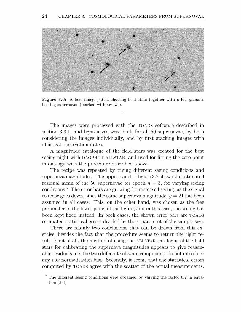
Figure 3.6: A fake image patch, showing field stars together with a few galaxieshosting supernovae (marked with arrows).
.
The images were processed with the toads software described insection 3.3.1, and lightcurves were built for all 50 supernovae, by bothconsidering the images individually, and by first stacking images withidentical observation dates.
A magnitude catalogue of the field stars was created for the bestseeing night with daophot allstar, and used for fitting the zero pointin analogy with the procedure described above.
The recipe was repeated by trying different seeing conditions andsupernova magnitudes. The upper panel of figure 3.7 shows the estimatedresidual mean of the 50 supernovae for epoch n = 3, for varying seeingconditions.7 The error bars are growing for increased seeing, as the signalto noise goes down, since the same supernova magnitude, g = 21 has beenassumed in all cases. This, on the other hand, was chosen as the freeparameter in the lower panel of the figure, and in this case, the seeing hasbeen kept fixed instead. In both cases, the shown error bars are toads
estimated statistical errors divided by the square root of the sample size.There are mainly two conclusions that can be drawn from this ex-
ercise, besides the fact that the procedure seems to return the right re-sult. First of all, the method of using the allstar catalogue of the fieldstars for calibrating the supernova magnitudes appears to give reason-able residuals, i.e. the two different software components do not introduceany psf normalisation bias. Secondly, it seems that the statistical errorscomputed by toads agree with the scatter of the actual measurements.
7 The different seeing conditions were obtained by varying the factor 0.7 in equa-tion (3.3)

3.3. LIGHTCURVE BUILDING 25
Figure 3.7: Mean of residuals from epoch n = 3 of 50 fitted supernova lightcurves.The (upper) panel shows how the residual mean varies with different seeing, while the(lower) illustrates the same property but for a fixed seeing and where the supernovamagnitude has been varied instead. The lower panel suggests that a small bias mayexist (no point is below zero), which was confirmed by additional tests on very brightobjects. The possible bias effect is however very small and will not affect any of themeasurements presented in this thesis.
Another observation that was made from the test is that the correla-tion between different epochs could be estimated to 0.2 < r < 0.5. Thestrength of this correlation depends on how well the background modelcan be determined.
3.3.3 Lightcurve building with HST WFPC2 data
It is not uncommon for high redshift supernova campaigns these daysto have both space and ground based photometric follow-up. This is forexample true both for the data presented in Paper F and in chapter 5,

26 CHAPTER 3. COSMOLOGICAL PARAMETERS FROM SUPERNOVAE
where the hst instrument wfpc2 was used. Due to the superior qualityand resolution of the hst wfpc2 data, it would be very unwise to do asimultaneous lightcurve build of both ground and hst data. Instead, thetwo sets are treated separately in the analysis, and with slightly differentapproaches.
For the hst analysis presented in this work, the data was reducedthrough the pipeline procedure provided by the Space Telescope ScienceInstitute (stsci). The wfpc2 images were then combined to reject cos-mic rays for each epoch with the crrej task which is part of the stsdas8 iraf 9 package.
The supernova can be found on the pc chip for all images obtainedwith wfpc2, and the properties of these images are quite different com-pared to the ground based data. A slightly modified method, originallydeveloped by the former scp member Prof. Robert A. Knop Jr., wasused for wfpc2 lightcurve building, where the relation,
Ii(x, y) = fi · PSFi(x − x0i, y − y0i)+
+ G(x − x0i, y − y0i, aj) + Si, (3.4)
was fitted to the image sequence. The psf of the wfpc2 pc chip isseverely under sampled, which is illustrated in figure 3.8 and fitting itusing the daophot approach explained in the previous section is not theoptimal approach. Instead the shape of the function can be simulated foreach filter using the Tiny Tim software [35]. Since the psf is extremelystable over time, no kernel fit is needed for combining different epochs,but the shape does however vary with pixel position, which motivates thei-index in equation (3.4). For all cases treated in this thesis, there wereonly minor position variations in time for each supernova, so in practisea single Tiny Tim psf was used for each object, and each filter.
In analogy with the ground based case, the transformations betweenimages of different epochs were determined by using other objects inthe wfpc2 field. However, the size of the wfpc2 field of view is only36.8′′ × 36.8′′, and the number of field stars is limited, so the transfor-mations could usually not be obtained better than to ∼< 1 pixel. Since
8 The Space Telescope Science Data Analysis System (stsdas) is a software packagefor reducing and analysing astronomical data. It provides general-purpose tools forastronomical data analysis as well as routines specifically designed for hst data.
9iraf is the Image Reduction and Analysis Facility, a general purpose softwaresystem for the reduction and analysis of astronomical data. iraf is written andsupported by the iraf programming group at the National Optical AstronomyObservatories (noao) in Tucson, Arizona.

3.3. LIGHTCURVE BUILDING 27
Figure 3.8: Histogram comparison between two different point spread functions. Theleft panel shows a daophot psf fit from one of the ground based int images discussedin chapter 4, while a typical Tiny Tim generated psf, in the F814w-band, for thewfpc2 pc chip is seen in the right panel. Each square represents one pixel.
the psf fwhm is of the same order (right panel of figure 3.8, the super-nova position is fitted on each frame, and by using the psf shape of theobject, the accuracy of the position can be improved by approximatelya factor 10. Note that this also has a disadvantage since it will biasthe results toward higher fluxes, that is the fit will favour positive noisefluctuations. On the other hand, in Paper F this was shown to be of mi-nor importance by studying the covariance between flux and supernovaposition.
One additional difference between equations (3.2) and (3.4) is thebackground model. While one parameter is used for each pixel in theformer, a smoothly varying analytical function defined by aj parametersis used in the latter. This can be carried out successfully, without re-quiring supernova-free references, when the supernova and host galaxycore are well separated. The procedure is particularly suitable for spacebased observations due to the high resolution.
One caveat, that should be mentioned here, is that the patch size mustbe chosen with care. In this thesis work only primitive parameterisationslike for example a plane, a paraboloid or an elliptical Gaussian havebeen used for modelling the background. These will only work if thereis no dramatic change in the background across the patch, which is anassumption that is likely to fail if the patch is too large and includesthe host galaxy core. On the other hand the patch must not be toosmall either, in order to successfully break the degeneracy between thesupernova and the background in the vicinity of (x0i, y0i). This topic isinvestigated further in section 5.3.2 on page 62.
28 CHAPTER 3. COSMOLOGICAL PARAMETERS FROM SUPERNOVAE
In order to cope with the properties of the under sampled psf prop-erly, the Tiny Tim psf has been 10 times subsampled. For each iterationin the fitting procedure, any shifts of the psf position is first applied inthe subsampled space. The psf is then re-binned to normal samplingand convolved with a charge diffusion kernel [35] before applying equa-tion (3.4). This is a physical effect that comes from the fact that ccd
pixels are defined by electromagnetic fields, created by an electrode struc-ture, rather than separate elements. An incoming photon is convertedto an electron, which is generally attracted to the closest electrode, butif a photon hits the detector far away from the electrode, where the fieldis weak, the electron may very well travel to an adjacent pixel instead.By convolving with the charge diffusion kernel the psf is smeared out tomimic this effect.
3.3.4 Calibration
The fitted lightcurve fluxes are expressed in terms of the psf used for thefit, which also must be used as the basis for the calibration. In the hst
case, the psf is stable and the instrument calibration is excellent, so it israther straightforward to obtain the instrumental supernova magnitudes.For ground based data, all lightcurve points are expressed in the bestseeing image, due to the procedure of using fitted kernels for translatingphotometry between images. A method for fitting the zeropoint, ZP , ofthis image, by using known measurements of the field stars was applied insection 3.3.2 and will be used in chapter 4. The instrumental magnitudes,mI , are then obtained as
mI = −2.5 log10 f + ZP , (3.5)
where f is the flux.The conversion between instrumental and standard magnitudes, mS ,
is in most cases sufficiently expressed by a linear colour term, cXY , as
mS = mI + cXY · (X − Y ) ,
where the colour is the magnitude difference (X − Y ) for an object be-tween two filters X and Y . This colour equation originates from thedifference in the combined instrumental wavelength response, caused byfactors such as atmospheric transmission (example shown in figure 3.1),filter response (illustrated in figure 4.5), the reflectivity of the mirrorsystem and the ccd quantum efficiency (see figure 3.9).

3.3. LIGHTCURVE BUILDING 29
Figure 3.9: Quantum efficiencies for a few different optical instruments at Observa-torio Roque de los Muchachos on the island of La Palma, together with the reflectanceof aluminium. Credit: Gemini report spe-te-g0043, Ruth Kneale.
The colour term is usually determined by observing stars over a widecolour range in several filters. The term is not expected to vary dra-matically over time so once cXY has been determined it can be usedto successfully calibrate other measurements. The drawback is that theequation can in principle only be used for objects that have a spectraldistribution similar to the stars that were used for obtaining the colourterm. For supernovae, where the spectrum deviates from the averagestar, the above relation is an approximation.
An alternative approach for colour correcting is to independentlymeasure the different properties that could affect the wavelength responseand combine them to an effective filter. The magnitude correction canthen be computed synthetically by integrating the object spectral energydistribution over the two filters and study the difference. The integralsmust also be normalised to a standard system, where the two most fre-quently used are the ab and Vega systems. For ab magnitudes, a flatspectral energy distribution is used, while for the Vega system, the pho-tometry is defined by the A0 star having zero magnitude in all passbands.One problem with this method is that accurate spectroscopy of the ob-ject is required, in order to do the analysis properly. This is expensivein terms of observation time and not feasible in practise.
In supernova cosmology, synthetic photometry is unavoidable, andmust be used for doing K-corrections between observed and rest framefilters, which is described in section 3.4. It is therefore often preferableto allow for this correction to also include the colour correction discussedabove, by K-correcting directly from instrumental filters to the rest framefilters. On the other hand, this requires very good knowledge of theinstrumental effective filters, which may not always be available.

30 CHAPTER 3. COSMOLOGICAL PARAMETERS FROM SUPERNOVAE
3.3.5 Multiple instruments
The lightcurve build and calibration are complicated further if severalinstruments are used together. The overall difference in sensitivity willbe handled correctly and is quantified by the integral of the fitted kernelbetween the images, but the difference in wavelength response is not con-sidered by the lightcurve building method described above. The optimalapproach would then be to build the lightcurves individually for each in-strument. On the other hand this would also require one supernova-freereference frame for each filter and each instrument, which is not feasiblesince observation time is expensive. The effect is to some extent includedin the uncertainty of the kernel fits. On the other hand, this depends onthe spectral distribution of the fiducial objects used for the fit. Furtherdiscussions on this topic can be found in chapter 4, where three differentground based telescopes were used for lightcurve building.
3.4 Lightcurve fitting
If calibrated lightcurves have been built in one or more filters, the peakmagnitude in each passband can be estimated by fitting lightcurve tem-plates to the real curve. However, it is the rest frame peak magnitudethat serves as the standard candle that is used for cosmology fits in equa-tion (2.12). Similarly, the lightcurve templates are constructed from verywell measured nearby type Ia supernovae, and thus, also these correspondto the rest frame spectral distribution, which was shown in figure 3.1.
When supernovae are observed at higher redshifts, the filters arechosen so that they approximately overlap with the corresponding restframe part of the spectrum, but this overlap is never perfect and a time-dependent generalised K-correction [34, 48] must be applied to the mea-sured lightcurve before its shape and peak brightness can be fitted. Thiscorrection, KXY , between the observed, Y , and the rest frame, X, filters,can be calculated as
KXY = − 2.5 · log10
[∫
Z(λ)SX(λ) dλ∫
Z(λ)SY (λ) dλ
]
+
+ 2.5 · log10
[∫
F (λ)SX(λ) dλ∫
F (λ′)SY (λ′(1 + z)) dλ′
]
(3.6)
where λ′ = λ/(1 + z). Here the first term is the filter zeropoint offsetincluding the spectral energy distribution, Z(λ), that defines the zero-points, and SX(λ), SY (λ) are the filter functions (see e.g., figure 3.1).
3.4. LIGHTCURVE FITTING 31
The second term is the cross-filter correction, where F (λ) is the super-nova spectral energy distribution and z is the redshift. For the case ofa perfect filter overlap, SY (λ′(1 + z)) = SX(λ), this term will drop outand only the zeropoint correction remains.
Note that the size of the correction will also vary with the supernovaspectrum that changes rapidly with time. In almost all cases the su-pernova will not be spectroscopically followed, and instead, a templatespectrum must be used for calculating the K-corrections. This will how-ever only introduce minor errors10 to the overall lightcurve fit, since thediversities between type Ia spectroscopic features do not remarkably af-fect the integrals in equation (3.6). A larger contribution to a potentialsystematic error, is a deviation from the expected supernova colour, e.g.in the case of reddening by dust in the host galaxy. This would lead to adisagreement of the general spectral shape. For multi-colour lightcurvefits presented in this thesis, an iterative approach have been used in orderto handle this. For each iteration, the spectrum is tilted to match themeasured colour excess, and the lightcurve is then refitted accordingly.The technique also takes a stretch-colour dependence into account, andis described in Paper F, although updated templates [47] have beenused for the results presented in chapters 4 and 5.
The actual fit is carried out on the K-corrected lightcurve with re-spect to the lightcurve stretch, s, explained in section 3.1.2, the peakbrightness in each filter, and the time of maximum in the rest frameB-band.
3.4.1 Lightcurve fitting in the I-band
In Paper G the rest frame I-band is discussed, and the type Ia lightcurveshape in this filter is rather different from the bluer bands, and shows asecond fainter peak. The fitting technique applied here was to use twoB-band templates, and then fit the two peaks, I1, I2, and the times, t1,t2 together with a stretch factor sI . This method gives satisfying results,except for the rising part of the lightcurve, which is discussed further inthe paper.
10 The systematic errors introduced are typically 0.02–0.05, depending on the filterand spectral overlap.

32 CHAPTER 3. COSMOLOGICAL PARAMETERS FROM SUPERNOVAE
3.5 Estimating cosmological parameters
The cosmological parameters can be fitted if equations (2.12) and (3.1)first are combined and then by minimising the χ2-sum
χ2 =∑
i
[mi + α(s − 1) −M− 5 log10 DL(ΩM , ΩX , w; zi)]2
σ2i
, (3.7)
where mi is the fitted B-band peak magnitude.However, some of the work presented in chapter 6 concerns possible
systematic effects due to gravitational lensing which can give rise toskew magnitude distributions. For this particular purpose a more generalcosmology fitter, based on the Maximum-Likelihood method, was writtenas a part of the snoc package introduced in Paper C and section 6.1.
The principle behind the maximum-likelihood method (ml) is to esti-mate the combination of parameter values that makes the measured dataset the most probable result for the applied model. This can be expressedas finding the parameters θ, that maximise the likelihood function
L(A|θ) =N∏
i=1
f(xi|θ) ,
for the data set A = xi where f is the probability density function.For numerical reasons, it is often common to rewrite this as the negativelog-likelihood function,
L(A|θ) = − ln L(A|θ) = − ln
(
N∏
i=1
f(xi|θ)
)
=N∑
i=1
− ln f(xi|θ) .
For a Gaussian probability distribution, L becomes
L(A|θ) =N∑
i=1
[xi − g(θ)]2
σ2i
+ ln(√
2π) ·N∑
i=1
ln σi .
which is equivalent to equation 3.7 with the exception of the last termthat has no importance for the fit (g(θ) is some arbitrary function of thefitting parameters).
3.5.1 Grid search minimisation
The minimisation problem described by equation (3.7) does not have asimple analytical solution. The most elementary minimisation procedure

3.5. ESTIMATING COSMOLOGICAL PARAMETERS 33
Lmax
e−0.5Lmax
θ
L
Lmin
Lmin + 0.5
θ
L
(a) One fitting parameter
θ1
θ2
PSfrag replacementsL
θ1
θ2
(b) 2D parameter space
Figure 3.10: Determination of parameter uncertainties from a grid search minimi-sation.
that can be applied to a situation like this is a grid search, where thelikelihood function is evaluated over an evenly spaced grid in the pa-rameter space. A plain grid search is simple and robust, but not veryefficient since the function is mapped with the same accuracy over thewhole parameter space, and the number of function evaluations increaseexponentially with the number of fitting parameters.
The uncertainty of the fitted parameter values can be determined byconsidering the likelihood function as a probability density function ofthe parameters. Consider for example a Gaussian likelihood function ofone parameter θ. The 1σ region can then be determined by finding the θfor which the likelihood function has decreased with a factor e−1/2 fromthe maximum value, L(max), illustrated in figure 3.10(a). This can beshown by solving the equation
exp
(
−1
2
)
L(max) =1√2πσ
exp
(
−(θ − θ)2
2σ2
)
⇔
⇔ exp
(
−1
2
)
= exp
(
−(θ − θ)2
2σ2
)
⇔ −1
2= −(θ − θ)2
2σ2⇔
⇔ θ = θ ± σ . (3.8)
For the negative log-likelihood function, L, the interval is instead foundby adding 0.5 to the minimum value.
In the two-dimensional case, the interval can be obtained in a similarmanner by studying the contour curve that appears in the intersectionbetween the negative log-likelihood function, L, and the plane that isdefined by L = Lmin + 1/2 (figure 3.10(b)). For a Gaussian likelihoodfunction the confidence contour becomes an ellipse, and the tangents of

34 CHAPTER 3. COSMOLOGICAL PARAMETERS FROM SUPERNOVAE
the contour parallel to the coordinate axes give a measurement of theaccuracy of the two estimators. The 1σ intervals obtained in this waycorrespond to a probability 0.683 of containing one of the parametersinside its interval when the value of the other is ignored.
If a joint probability of 0.683 for including both parameters in theirestimated intervals is requested, the contours appearing in the intersec-tion of the L = Lmin + 1.5152/2 [25] plane should be considered instead.The factor 1.515 is obtained by integrating a two-dimensional normaldistribution (bi-normal) and finding the level that gives 0.683 probabil-ity.
Note however, that in reality the likelihood functions are not alwaysbased on Gaussian distributions, and the parameter intervals correspond-ing to L = L(max)e−1/2 has to be treated with some care, and do onlyapproximately correspond to a probability of 0.68. The less elliptical theconfidence regions are, the weaker this approximation becomes.
3.5.2 The Davidon variance algorithm
If the derivatives of the likelihood function with respect to the fitting pa-rameters are taken into account, the number of calculations in the min-imisation procedure can be reduced dramatically. As it was establishedin the previous section, the variance of the estimated parameters can becomputed from the shape of the likelihood function. A narrow functionaround the extreme point, means small uncertainties of the fitting pa-rameters. Since the second derivatives of the function at the minimumgive a quantitative measurement of this narrowness, it is often assumedthat these derivatives give a measurement of the parameter uncertainties.For a multi-normal distributed likelihood function it can be shown [25]that the elements of the covariance matrix are given by
V −1ij (θ) =
∂2L∂θi∂θj
. (3.9)
The basic idea behind the Davidon variance algorithm [19] is to cal-culate the covariance matrix by an iterative algorithm. However, equa-tion (3.9) is not used to do this. Instead, the matrix is obtained by onlyusing the function values and the gradient, and the minimum value iscalculated simultaneously as the algorithm converges to the covariancematrix.
The Davidon variance algorithm is much more efficient than the pre-viously mentioned grid search, but one major drawback of the method

3.5. ESTIMATING COSMOLOGICAL PARAMETERS 35
is that the covariance matrix is always calculated under the assumptionthat the likelihood function is Gaussian, and will therefore give inaccu-rate error estimates when this approximation fails. However, for onlyobtaining the minimum of the likelihood function, that is estimating thecosmological parameters and disregarding their uncertainties, the Davi-don variance algorithm is always superior.
3.5.3 Constraints of the cosmological estimators
There are some constraints of the parameter space of the cosmologicalparameters, and certain areas are physically forbidden, e.g. ΩM < 0. Anadditional constraint [17] for a cosmological constant scenario is
ΩΛ < 4ΩM
coss
[
1
3coss−1
(
1 − ΩM
ΩM
)]3
,
where coss is defined as
coss(x)
cosh(x) if ΩM < 1/2cos(x) if ΩM > 1/2x if ΩM = 1/2
.
If this condition is not fulfilled, ΩΛ is too large for a Big Bang to evertake place. This cosmology would instead describe a bouncing modelwhere the Universe collapses from infinite size to a finite radius and thenre-expands. This constraint is shown as the grey area in the upper leftcorner of figure 7, Paper F.
In snoc, the non-physical constraints are treated by doing a gridsearch sampling of the likelihood function and then re-normalise it, ex-cluding the above mentioned regions. This will force the whole prob-ability density to lie within the physical region, which could bias theestimated limits if the true value is very close to a non-physical bound-ary. It can be argued to what extent this is the correct way to treat theseregions, and other methods have been suggested [24], and was used inprevious scp publications [53]. However, for present supernova data, theimpact of non-physical regions are only of minor importance.
On the other hand, this discussion does have relevance in a com-pletely different context in this thesis. It is often common to extinctioncorrect the magnitude of supernova that appear to be red, while blueobjects are assumed to be non-reddened. Type Ia supernovae do have anintrinsic colour scatter, and even if this was not the case, a measurement
36 CHAPTER 3. COSMOLOGICAL PARAMETERS FROM SUPERNOVAE
uncertainty would be expected. In other words, if extinction correctionsare applied blindly based on the object colour, the cosmological resultsfrom an extended data set, will be biased.
3.6 Observations and results
It was not until the ccd revolution in the early 1990’s that systematicsupernova searches became feasible. Type Ia supernova cosmology dur-ing this decade was dominated by two competing international collabora-tions, the Supernova Cosmology Project, (scp) and the High-Z SupernovaSearch Team (hzt).
The early scp data [50, 52] from the mid-1990’s contained only ahandful of supernovae and were consistent with the Einstein-de Sittermodel (ΩM = 1, Λ = 0), which at the time was believed to be the mostplausible model for the Universe. The following years both the scp andthe hzt rapidly increased both the statistics, and the redshift range oftheir data. For high redshifts the degeneracy between different cosmolog-ical models decreases [27], and at the end of 1998 both collaborations hadgathered enough evidence [53, 58] to conclude that the Universe is in factaccelerating, and that dark energy must exist. The striking agreementbetween the two independent measurements strengthened this conclu-sion.
Since then, the supernova community have pushed both statisticaland redshift limits considerably. The Hubble Space Telescope has beenabsolutely essential for the leap taken during the past five years, andthis is also the instrument that was used for the high-z data presentedin Paper F and chapter 5.
The latest scp data and results (Paper F) are shown in figure 3.11,and the best fitted cosmology from this data, assuming a flat universe,is
ΩM = 0.25+0.07−0.06 ± 0.04 , and w = −1.05+0.15
−0.20 ± 0.09 .
Other, independent, supernova campaigns have been able to pushtheir redshift limits beyond these data, where the degeneracy betweendifferent cosmological models decreases, and therefore managed to puteven tighter constraints [73, 62] on the cosmological parameters.
Meanwhile, several large scale supernova campaigns have entered thescene. What identifies these new projects is that they use partially ded-icated instruments operating in a rolling-search mode, and that multi-
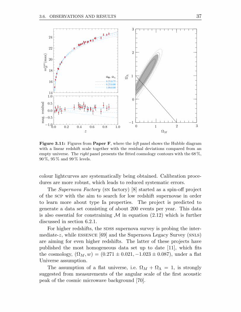
3.6. OBSERVATIONS AND RESULTS 37
z
MΩ ΩΛ,
0.25,0.750.25,0.001.00,0.00
PSfrag replacements
24
22
20
18
16
141.0
0.5
0.0
−0.5
−1.01.0
0.5
0.0 0.2 0.4 0.6 0.8
mco
rrB
(max
)m
ag.
resi
dual
ΩM
ΩM
PSfrag replacements
2422201816141.00.50.0
−0.5−1.0
1.00.50.00.20.40.60.8
mcorrB (max)
mag. residual
ΩM
ΩM
ΩM
ΩΛ
−10
0
1
1
2
2
3
3
Figure 3.11: Figures from Paper F, where the left panel shows the Hubble diagramwith a linear redshift scale together with the residual deviations compared from anempty universe. The right panel presents the fitted cosmology contours with the 68 %,90 %, 95% and 99 % levels.
colour lightcurves are systematically being obtained. Calibration proce-dures are more robust, which leads to reduced systematic errors.
The Supernova Factory (sn factory) [8] started as a spin-off projectof the scp with the aim to search for low redshift supernovae in orderto learn more about type Ia properties. The project is predicted togenerate a data set consisting of about 200 events per year. This datais also essential for constraining M in equation (2.12) which is furtherdiscussed in section 6.2.1.
For higher redshifts, the sdss supernova survey is probing the inter-mediate-z, while essence [69] and the Supernova Legacy Survey (snls)are aiming for even higher redshifts. The latter of these projects havepublished the most homogeneous data set up to date [11], which fitsthe cosmology, (ΩM , w) = (0.271 ± 0.021,−1.023 ± 0.087), under a flatUniverse assumption.
The assumption of a flat universe, i.e. ΩM + ΩΛ = 1, is stronglysuggested from measurements of the angular scale of the first acousticpeak of the cosmic microwave background [70].

38 CHAPTER 3. COSMOLOGICAL PARAMETERS FROM SUPERNOVAE
3.7 Systematic errors
The influence of systematic errors on cosmology fits is becoming impor-tant, as the statistical uncertainties are being reduced by the constantlygrowing supernova data set. Some of these effects have already beenmentioned, and a few others that have particular importance for thisthesis are summarised in this section.
3.7.1 Extinction
Extinction by dust particles along the line of sight has been proposedas an alternative to dark energy for explaining the observed dimming oftype Ia supernovae [63]. Even though it is very unlikely that extinctionwould account for the entire dimming effect, it will indeed add system-atics to the observed Hubble diagram, and it must be handled with care.
The extinction of an object can in general be determined by measur-ing the reddening, i.e. the difference in extinction between wavelengthbands. In practise, the colour of the supernova, e.g. B − V , is mea-sured and then compared with the expected intrinsic colour. It has beenshown [16] that it is a fair approximation to use one parameter, in thisexample RV , to describe the reddening,
RV =A(V )
E(B − V )=
A(V )
(B − V ) − (B − V )i,
where AV is the extinction integrated over the wavelength band V andB − V and (B − V )i are the measured and intrinsic colours respectively.
There are mainly three possible contributing environments to theextinction: dust in the host galaxy, intergalactic dust and dust in theMilky Way. The latter of these has been accurately measured [66] andobserved data can easily be corrected for it, while the effect from the twoformer is more uncertain.
In terms of host galaxy extinction, supernovae in late-type galaxies,with high star formation rates, are more likely to show signs of extinc-tion than those that occur in the supposedly dust-free early-type galaxies.This is also confirmed when the relation between the scatter in the Hub-ble diagram and the host type is studied (Paper 1). Observing type Iasupernovae in early-type galaxies also has another advantage, since it willminimise the contamination of non-Ia supernovae in the sample. Lookingexclusively at early-type galaxies is in fact the objective for an ongoingscp hst supernova search.
3.7. SYSTEMATIC ERRORS 39
It has been suggested [3, 2] that there could be a homogeneous inter-galactic dust medium with large grain sizes, > 0.1 µm. The reddeningproperties of this dust is much less significant, and it is therefore harderto detect it. The existence of such grey dust is still an open issue. Sometentative limits have been set [60, 46] by using the fact that grey dustis not entirely grey, but more multi-colour data at redshifts z > 0.5 isrequired in order to put narrower constraints.
One way of reducing the impact of dust, is to observe in longer wave-length bands. For example, for the dust properties observed in the MilkyWay, the extinction is less by a factor 2–3 between the B and I-filters,and the possibility of doing supernova cosmology in the latter of thesepassbands is discussed in Paper G. The drawback of this approach isthat type Ia supernova are intrinsically fainter in this passband (see thespectral distribution in figure 3.1 on page 14), and that ground basednear infrared observations are restricted by the strong atmospheric emis-sion at these wavelengths.
3.7.2 Gravitational lensing
Since the effects from gravitational lensing are highly redshift dependent,it is likely to be of more importance for possible future data rather thanfor the existing. In chapter 6 this topic will be introduced and discussedin detail. However, a handful of very high redshift supernovae havealready been observed, and the discussion has already begun [33, 28].For example the furthest known supernova up to date, 1997ff at z ∼ 1.7,that was discovered on hst images of the Hubble Deep Field [61], doesindeed appear to show evidence of lensing [43, 12]


C h a p t e r 4
The ESC 1999 campaign
The type Ia supernova Hubble diagram, shown in figure 3.6, reveals aredshift range around z ∼ 0.2–0.3, where the sampling is rather sparse.Adding data to this region is of great importance for several reasons. Forcosmology, this is an area where dark energy dominates, and the mea-sured supernova magnitude difference for different w-parameterisationswill show a redshift dependence, illustrated by figure 4.1. The relationflattens for higher redshifts, and would imply a systematic shift in theHubble diagram. However, if a redshift dependent trend is observed forlower redshifts, this would give much higher credibility for a measuredw-model, and is harder to discard as a systematic effect.
In addition to this, there are several important type Ia propertiesthat can be studied for these intermediate redshifts. The objects are stillclose enough to allow high precision measurements, and different featurescan be compared with similar quantities for nearby supernovae. Also forthese redshifts, the rest frame ultraviolet region of spectrum has beenredshifted into the visible wavelength area and can therefore be observedfrom the ground. This is a part of the type Ia spectrum that today isconnected with major uncertainties, and that often leads to significantdifficulties in the interpretation of high redshift data. A large data setin this area, of for example the type the sdss collaboration is presentlyobtaining, will be essential for an increased understanding of rest frameU -band properties.
In this chapter will the photometric analysis of five intermediate-zsupernovae discovered in 1999 will be discussed. The results presentedhere have not yet been published in a scientific journal and should beconsidered preliminary.
4.1 The ESC 1999 campaign
The European Supernova Consortium (esc) 1999 campaign was, to alarge extent, carried out as a piggyback project of the Isaac NewtonTelescope (int) Wide Field Survey (wfs) [39]. The wfs was initiated in

42 CHAPTER 4. THE ESC 1999 CAMPAIGN
Figure 4.1: Expected magnitude deviations from a cosmological constant differentequation of dark energy equation of states as a function of redshift. By courtesy ofAriel Goobar
1998, and has obtained multicolour data in the Gunn, u, g, r, i, z, filterset over a five year period, covering 200 square degrees with a depth ofr ≈ 24 and g ≈ 25. The 4k×2k Wide Field Camera (wfc) ccd mosaic,with a field of view of 0.27 square degrees, was used and the same areaof sky was observed repeatedly which also made the survey very suitablefor supernova searching.
The supernovae discussed in this section were discovered by com-paring two wfs data sets in g-band. The first observed in the middleof August 1999, and the second roughly one month later. The Augustdata consist of 600 s exposures, while two 240 s frames were obtained forthe September set. Altogether, three subtractions were made by bothconsidering the September discovery images individually, and by usingtheir coadded sum. Candidates were then selected by requiring detectionwithin 2 pixels on all three frames, in order to efficiently reject cosmicrays and fast-moving objects. In addition to this, it was demanded that
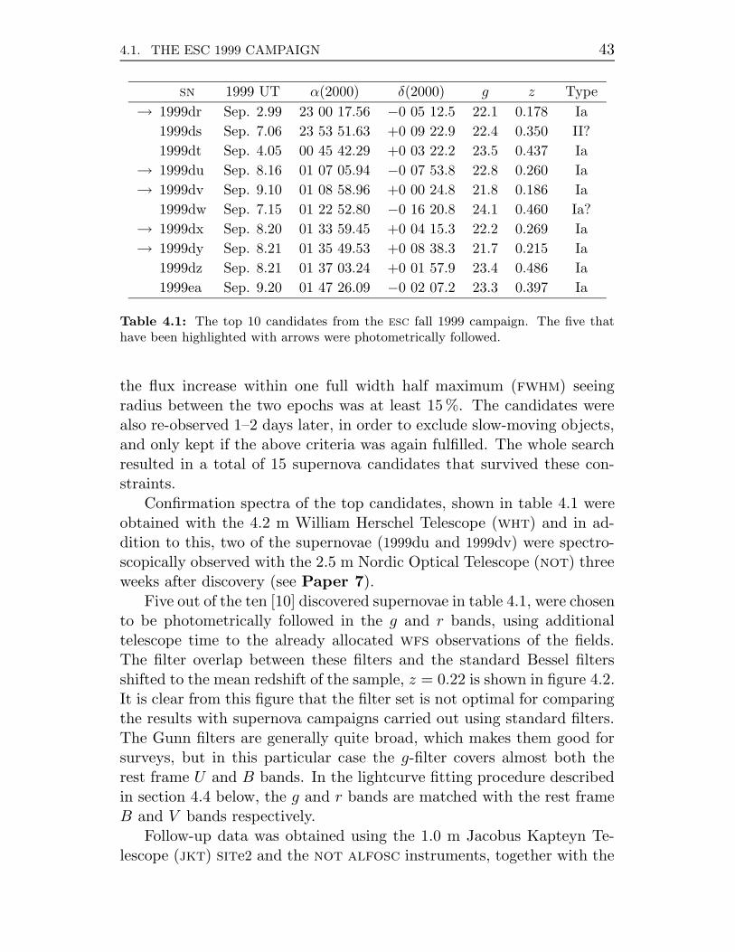
4.1. THE ESC 1999 CAMPAIGN 43
sn 1999 UT α(2000) δ(2000) g z Type
→ 1999dr Sep. 2.99 23 00 17.56 −0 05 12.5 22.1 0.178 Ia
1999ds Sep. 7.06 23 53 51.63 +0 09 22.9 22.4 0.350 II?
1999dt Sep. 4.05 00 45 42.29 +0 03 22.2 23.5 0.437 Ia
→ 1999du Sep. 8.16 01 07 05.94 −0 07 53.8 22.8 0.260 Ia
→ 1999dv Sep. 9.10 01 08 58.96 +0 00 24.8 21.8 0.186 Ia
1999dw Sep. 7.15 01 22 52.80 −0 16 20.8 24.1 0.460 Ia?
→ 1999dx Sep. 8.20 01 33 59.45 +0 04 15.3 22.2 0.269 Ia
→ 1999dy Sep. 8.21 01 35 49.53 +0 08 38.3 21.7 0.215 Ia
1999dz Sep. 8.21 01 37 03.24 +0 01 57.9 23.4 0.486 Ia
1999ea Sep. 9.20 01 47 26.09 −0 02 07.2 23.3 0.397 Ia
Table 4.1: The top 10 candidates from the esc fall 1999 campaign. The five thathave been highlighted with arrows were photometrically followed.
the flux increase within one full width half maximum (fwhm) seeingradius between the two epochs was at least 15 %. The candidates werealso re-observed 1–2 days later, in order to exclude slow-moving objects,and only kept if the above criteria was again fulfilled. The whole searchresulted in a total of 15 supernova candidates that survived these con-straints.
Confirmation spectra of the top candidates, shown in table 4.1 wereobtained with the 4.2 m William Herschel Telescope (wht) and in ad-dition to this, two of the supernovae (1999du and 1999dv) were spectro-scopically observed with the 2.5 m Nordic Optical Telescope (not) threeweeks after discovery (see Paper 7).
Five out of the ten [10] discovered supernovae in table 4.1, were chosento be photometrically followed in the g and r bands, using additionaltelescope time to the already allocated wfs observations of the fields.The filter overlap between these filters and the standard Bessel filtersshifted to the mean redshift of the sample, z = 0.22 is shown in figure 4.2.It is clear from this figure that the filter set is not optimal for comparingthe results with supernova campaigns carried out using standard filters.The Gunn filters are generally quite broad, which makes them good forsurveys, but in this particular case the g-filter covers almost both therest frame U and B bands. In the lightcurve fitting procedure describedin section 4.4 below, the g and r bands are matched with the rest frameB and V bands respectively.
Follow-up data was obtained using the 1.0 m Jacobus Kapteyn Te-lescope (jkt) site2 and the not alfosc instruments, together with the

44 CHAPTER 4. THE ESC 1999 CAMPAIGN
Figure 4.2: Overlap between rest frame (dashed) and observed, effective, int (solid)filters for the mean redshift, z = 0.22, of the follow-up sample. The dotted curve showsthe normalised spectral template distribution of a type Ia supernova. The effective gand r filter curves, consist of the measured filter response, the quantum efficiency ofthe wfs instrument, the expected atmospheric transmission at La Palma (airmass=1),and the reflectivity of the mirror.
int wfc. The int images were reduced through the wfs pipeline [32],while standard reduction, including bias subtraction and flat fielding,was performed on the not and jkt images, using the iraf software, bymembers of the Stockholm supernova cosmology group (Gaston Folatelliand Vallery Stanishev). Even after this procedure, a smoothly varyingmultiplicative factor appeared to remain on the jkt images. This prob-ably originated from slight filter offsets between when the flat fields andthe source images were acquired. The effect was corrected by fitting asurface to each image and then dividing the frame with it. The jkt datawas generally of quite poor quality, and several of the images had to beexcluded from the lightcurve build due to bad tracking, and even most ofthe images that were kept, show, what appears to be, filter dust marks.
4.2 Lightcurve building
The lightcurves for each of the five supernovae were built by applying thetechnique introduced in section 3.3.1. SExtractor catalogues, constructedfor each individual image, were used to align all frames, for a given filter,to the best seeing image. For the not alfosc images, with a plate scaleof 0.188′′/px, this also meant rescaling the images to 0.33′′/px, which isthe plate scale of both the int wfc and jkt site2 instruments.
Images obtained with the same instrument, in the same filter, and onthe same night, were coadded. For each of these images, a convolutionkernel is fitted between the image and the best seeing image in the sam-

4.2. LIGHTCURVE BUILDING 45
ple. As a test of the kernel quality, each image is subtracted with theconvolved best seeing reference in order to assure that the residuals areclean and that there are no remaining artifacts.
The model described by equation (3.2) is fitted to a set of imagepatches, centred on the initial supernova position. An example of imageand model patches, together with their resulting residuals, can be seenin figure 4.3 for increasing epochs.
4.2.1 Residuals
The residuals are in most cases clean, i.e. dominated by uncorrelatednoise, but over or under subtractions can occasionally occur. A possiblebias introduced by an unclean subtraction is quantified by measuringthe residual sum within one and two fwhm seeing residuals at the fit-ted sn position, and then compared to the total supernova count for thegiven epoch. From this exercise it can be concluded that this effect iscompletely negligible and is always well below the statistical uncertainty.However, note that for patches with supernova light, this is only a mea-surement of how the whole model fits the data, and it says nothing ofto what extent the degeneracy between the supernova and the galaxymodel is broken. If the separation between the supernova and the hostgalaxy is small, a large fraction of the supernova light could very wellbe included in the galaxy model rather than the supernova psf. Theresulting residuals would be the same, but the fitted supernova fluxesare in this case underestimated. It is therefore particularly importantto study any remaining residuals, once the galaxy model has been sub-tracted from the supernova-free reference images. Any remaining offsetin the residuals will affect all epochs but will have a larger impact onthe fainter points at the end of the lightcurve. However, this effect wasnot found to exceed the expected statistical fluctuations for any of thesupernovae described here.
4.2.2 Quality of the fitted PSF
Due to the construction of equation (3.2), all fitted fluxes fi will beexpressed in the system of the best seeing frame. This also means thatany possible normalisation or scaling of the psf fitted for this image, mustbe applied to all fitted fluxes. Furthermore, if the psf fit is unsatisfactoryon this specific image, it will affect the entire lightcurve, since the verysame psf is used for all epochs in a given filter.

46 CHAPTER 4. THE ESC 1999 CAMPAIGN
Figure 4.3: Data, model and residual triplets for a selection of epochs from theg-band lightcurve build of 1999dr. The last row shows the reference epoch, obtainedapproximately one year after discovery.

4.3. INSTRUMENTAL WAVELENGTH RESPONSE 47
Figure 4.4: Examples of comparison between aperture and psf measurements forincreasing magnitudes. The left panel shows the result when an erroneous psf is used,while this has been corrected, by refitting the psf, in the right panel. The ∆m offsetcomes from the use of different zeropoints, and is not physical.
In section 3.3.1 it was explained that the daophot package was usedfor psf fitting, and that the daophot allstar routine can be usedfor doing psf photometry on all stellar objects in the field. The psf
quality can then be checked by comparing this allstar catalogue withaperture photometry of the same objects for increasing magnitudes. Foran accurate psf the difference between these catalogues should be flat,while an erroneous psf will give a magnitude dependent trend of thekind shown in the left panel of figure 4.4.
This check turned out to be necessary since daophot is ran in apipeline mode and the psf fit was not always satisfactory. Refitting thepsf manually and rebuilding the allstar catalogue did, in these cases,remove the trend as shown in right panel of figure 4.4.
4.3 Instrumental wavelength response
Once the images have been re-sampled to the same plate scale, theyare treated equally in the lightcurve building process, and no concernis taken to the different instrumental sensitivity that may exist. Thisproblem was addressed in section 3.3.5, where also the reasons for thediscrepancy in wavelength response were explained.. The normalisedeffective filters, that take all these factors into account, have been plottedin figure 4.5 for int, not and jkt. Together with these, the responsecurves for the Sloan Digital Sky Survey (sdss) [1] have also been plotted.The sdss provides public object catalogues that overlap with all fieldsin the esc 1999 campaign. These catalogues can efficiently be used forcalibrating the supernova lightcurves in analogy with the procedure usedin section 3.3.2.

48 CHAPTER 4. THE ESC 1999 CAMPAIGN
Figure 4.5: Filter response comparison between the three instruments used for theesc 1999 campaign together with the function for the sdss Gunn filters. The filters arethe effective filters, i.e. the measured filter response times the quantum efficiency andthe mirror reflectivity. The filters have been normalised to have the same maximumtransmission in this figure.
The filter curves in figure 4.5 do suggest that a colour dependence ofthe type discussed in 3.3.4 can be expected. By using 16 photometricstandards, presented in [68], that also have spectral photometry [72], syn-thetic colour terms for transferring between the instrumental magnitudesand the sdss system can be calculated. This was done by integratingthe spectral energy distribution across the different effective filters, andcompare with the measured sdss magnitudes. Results are presented intable 4.2. This table also shows the corresponding measured1 values fromthe esc 1999 images.
In practise the measurements were carried out by building an all-
star catalogue for each available frame and match the object list withthe sdss catalogue. The matching was done by initially using the worldcoordinate solution of the individual files for the allstar catalogue, andthe R.A. and Dec. coordinates of the sdss list. The transformation wasthen refined by fitting a polynomial up to the second order, and thenrematching the lists. An example of an image patch with the two cata-logues and the matched objects marked, is shown in figure 4.6.
The offset between the allstar and the sdss magnitudes was fit-ted for each frame, together with a colour term, which in all cases waschosen to depend on gsdss − rsdss. Examples of a few representative in-dividual fits are shown in figure 4.7, while the combined values for eachfilter and instrument are presented in table 4.2. It should also be noted,
1 The wfs team also derived a set of colour terms for the int, available from theirwebpage, that are close to the ones measured here.

4.3. INSTRUMENTAL WAVELENGTH RESPONSE 49
Figure 4.6: A patch from the best seeing image in the g-band, the int night fromSep. 8, 1999 for 1999du. The circles mark the objects, with a brightness cut, fromthe allstar catalogue, while the triangles represent the sdss star catalogue for which16.0 < g < 22.0, and squares show objects that have been matched. In the left sideof the patch, a couple of object pairs can be seen, marked with arrows, that were notsuccessfully matches. This behaviour either motivates a higher order transformationfit in the iterative procedure, or a less conservative matching tolerance. In this specificcase the latter approach can be applied, but in some cases with crowded fields, thisleads to an increased number of false matches.
that extreme outliers were rejected in the fitting procedure, and that noevidence was found for a possible second order colour term or an airmassdependence.
The measured colour terms seem to correspond roughly to their syn-thetic counterparts in most cases, which suggests that the effective filtersadequately describe the physical systems. In the case of the not g-filter,this is however not the case, and the synthetic colour term is highlyincompatible with the data.
From a systematic error point of view, what is of interest in table 4.2is the discrepancy between colour terms for the different instruments.It is hard to estimate the propagation of this effect to the fitted super-nova fluxes, since it will influence the kernel fit between images. If, forexample, red stars are exclusively used for fitting the kernel, the fittedphotometric ratio, i.e. the kernel integral, would be different, comparedto if only blue stars were used. However, due to the similarity of theterms in this specific case, it is safe to assume that this will have a minorinfluence on the error budget, and an inter-instrument systematic errorof 0.02 magnitudes is assumed.

50 CHAPTER 4. THE ESC 1999 CAMPAIGN
(a) INT g, 0.14±0.01, χ2/dof = 1.03 (b) INT r, 0.00±0.01, χ2/dof = 1.09
(c) NOT g, 0.12 ± 0.02, χ2/dof =0.73
(d) NOT r, 0.01 ± 0.01, χ2/dof =0.72
(e) JKT g, 0.13±0.01, χ2/dof = 1.4(f) JKT r, 0.02 ± 0.01, χ2/dof =
1.70
Figure 4.7: Colour term fits for 1999dv. The difference between the measuredmagnitudes and the corresponding sdss values have been plotted against the sdss
colour of the stars. The scale on the y-axis is relative, and has no physical betweendifferent plots.

4.3. INSTRUMENTAL WAVELENGTH RESPONSE 51
Tel. c.t.
int 0.136 ± 0.005not 0.063 ± 0.005jkt 0.179 ± 0.005
(a) Synth. c.t. for g
Tel. c.t.
int 0.14 ± 0.01not 0.11 ± 0.02jkt 0.15 ± 0.02
(b) Meas. c.t. forg
Tel. c.t.
int 0.010 ± 0.005not 0.031 ± 0.005jkt 0.019 ± 0.005
(c) Synth. c.t. for r
Tel c.t.
int 0.00 ± 0.01not 0.02 ± 0.01jkt 0.02 ± 0.01
(d) Meas. c.t. forr
Table 4.2: Synthetic and measured colour terms for translating int, not and jkt in-strumental magnitudes to sdss magnitudes. No evidence for airmass dependent secondorder colour terms has been seen for these measurements. The synthetic colour termshave been calculated using the filter response functions presented in figure 4.5 for 16stars that both have accurate measured photometry [68] and spectra photometry [72](credit: Vallery Stanishev).

52 CHAPTER 4. THE ESC 1999 CAMPAIGN
4.4 Calibration and lightcurve fitting
The instrumental zeropoint for the best seeing night in each filter wasobtained by fitting the offset between the sdss and allstar object listsafter the measured colour terms had been taken into account. The sdss
stars are given in the ab system, and therefore, the calibrated supernovalightcurve will also be in this system. Supernova cosmology is historicallycarried out in the Vega system, but the conversion between these systemscan easily be calculated by computing the ab magnitude of Vega in thegiven filter.
The Vega lightcurves are then corrected for Milky Way extinction byusing the results from Schlegel et al. [66]. Iterative lightcurve fitting wasperformed with the technique described in section 3.4 and K-correctingbetween the instrumental effective filters and the corresponding standardrest frame filter. The results are presented in figure 4.8 and table 7.1.The stretch corrected rest frame B-band magnitudes at max have beenplotted in the Hubble diagram 7.1.
4.5 Conclusions
The most notable results in table 7.1, is the large scatter in colour excesspresented in the last column of the table. For example in the case of1999dr, the supernova show signs of significant reddening, which is re-markable. Figure 4.9 shows that the supernova appears to be locatedat the outer rim of its host galaxy, and an extinction of this magnitudewould therefore be very unlikely. However, it should be noted that theestimated colour excess for this supernova directly depends on the ex-trapolation based on one very late-time lightcurve point (see figure 4.8).
1999du, on the other hand, appears to be very blue. This supernovadoes seem to be quite peculiar. The lightcurve fit is not very satisfying,unless the time of max in the V band is allowed to float. In that casethe goodness of fit increases dramatically. A supernova with this oddbehaviour would probably not be used for cosmology fitting, irrespectiveof its strange colour.
Further, 1999dv and 1999dx both show signs of reddening. However,since both objects appear to be located very close to the core of the hostgalaxy, it is not unexpected to measure reddening in this case.
Finally, also 1999dy appears to be too blue, but it is still of the orderthat could be explained by the intrinsic colour dispersion of type Iasupernovae.

4.5. CONCLUSIONS 53
Figure 4.8: Lightcurve fits in g (left column) and r (middle column), where the xand y axes show days in observed frame and normalised flux respectively. The fits arebased on data from the int (triangle), not (square) and jkt (circle) telescopes. Theright column shows int patches (13.2”×13.2”) in the g band centred on the supernova.

54 CHAPTER 4. THE ESC 1999 CAMPAIGN
Figure 4.9: The left panel is centred on the supernova, and shows the closes lyingpixels to the line that runs through both the supernova the core of the host galaxy.The profile along this line has been plotted in the right panel along with a fittedexponential curve, exp(x/α), the expected decline rate. The separation between thesupernova and the host is determined to be ∼ 4.4α, which means that supernova wouldbe located at the outer rim of the galaxy. In physical units, the separation is 4.3′′,which for z = 0.183 and (ΩM = 0.28, ΩΛ = 72), corresponds to 12.8 kpc.
To summarise, the data-set is small and the interpretation of theresults is non-trivial, mainly due to broad filters used, and that theyoverlap a region of the rest frame spectrum where the type Ia propertiesstill are quite uncertain.

C h a p t e r 5
The SCP 2001 high redshift
campaign
5.1 The campaign
The scp search campaign during spring 2001 was carried out using the3.6 m Canadian French Hawaii Telescope (cfht) and the 4.0 m CerroTololo Inter-American Observatory (ctio) in Chile.
The 42′ × 28′ cfhk12k mosiac camera, which, at the time, was thelargest ccd mosaic camera in world, was used at the cfht to observetwo different fields in the I-band. Both fields were observed twice (3 hourexposures, limiting magnitude I ∼ 25.5) with a 25 day interval, whichresulted in the discovery of 13 candidates with S/N > 5 and a significantluminosity increase between the two epochs. Follow-up spectroscopy wasobtained for seven of the candidates using the 8.0 m Very Large Telescope(vlt) and the 10 m Keck telescope. Out of these, four could be classifiedas type Ia supernovae in the redshift range z = 0.45–1.12.
The ctio search on the other hand was carried out in a similar man-ner but with the addition that also R-band data were obtained. However,these exposures, 20 minutes, were not as deep as the I-band counterparts.This search resulted in the discovery of 14 candidates out of which 10could be classified as type Ia supernovae.
All 14 type Ia supernovae that were discovered from this search runhave been listed in table 5.1 [65, 7].
Five of these supernovae were photometrically followed both fromspace using the hst, and the ground using cfht, ctio, wht, the 3.6 mNew Technology Telescope (ntt), vlt and the 8 m Gemini telescope.The ground based follow-up data was obtained in the R, I and J pass-bands and have been reduced and analysed by members of the scp col-laboration.1
1 The ground based optical data have been, and is being, analysed by Julien Rauxand Linda Ostman using the technique described in chapters 3 and 4, while ChrisLidman and Pernilla Wahlin have been involved in the infrared analysis.

56 CHAPTER 5. THE SCP 2001 HIGH REDSHIFT CAMPAIGN
sn 2001 UT α(2000) δ(2000) m z
2001gm Apr. 15-20 14 01 51.18 + 5 05 38.5 I = 23.4 0.478
→ 2001gn Apr. 15-20 14 01 59.90 + 5 04 59.6 I = 25.0 1.1
→ 2001go Apr. 15-20 14 02 00.95 + 5 00 59.2 I = 23.7 0.552
→ 2001gq Apr. 15-20 14 01 51.38 + 4 53 12.4 I = 23.9 0.671
2001gr Apr. 18-20 10 04 23.27 + 7 40 48.3 I = 23.3 0.541
2001gt Apr. 18-20 10 02 39.31 + 7 16 33.0 I = 22.7 0.56?
2001gu Apr. 18-20 10 03 28.61 + 7 24 38.9 R = 23.7 0.32
2001gv Apr. 18-20 10 00 21.18 + 6 52 03.8 R = 23.7 0.661
2001gw Apr. 18-20 15 43 45.86 + 7 57 50.3 R = 22.0 0.363
→ 2001gy Apr. 18-20 13 57 04.54 + 4 30 59.8 I = 23.4 0.511
2001ha Apr. 18-20 10 06 33.50 + 7 38 03.2 R = 23.5 0.58
→ 2001hb Apr. 18-20 13 57 11.96 + 4 20 26.9 I = 24.8 1.05
2001hc Apr. 18-20 09 44 31.52 + 8 02 02.8 R = 21.4 0.35
2001hd Apr. 18-20 15 45 35.92 + 8 16 50.6 R = 22.8 0.511
Table 5.1: Summary of type Ia supernovae discovered in the scp Spring campaign.The supernovae that were photometrically followed with the hst have been highlightedwith arrows.
The hst follow-up data was obtained with the wfpc2 instrument,using the F675w, F814w and F850lp filters, which roughly correspondto the Cousins R and I-bands and the Gunn z-band. The filter overlapbetween redshifted standard filters and the observed filters are shown infigure 5.1 for two typical redshifts of the sample.
The wfpc2 camera consists of four chips (figure 5.2), out of whichthree are identical with a plate scale and field of view of 0.1′′/pixel and80′′×80′′ respectively. The fourth, pc chip, on the other hand, has muchhigher resolution, 0.046′′/pixel, but a smaller field of view, 37′′×37′′. Foreach observation in the scp spring 2001 run, the pointing of the hst waschosen so that the supernova landed on the pc chip of the camera.
In March 2002, during servicing mission 3B, a new instrument, theAdvanced Camera for Surveys (acs), was installed on the hst. This in-strument covers approximately the same wavelength range,2 as wfpc2,but it has a higher quantum efficiency (∼ 5 times higher in the I-band). The plate scale of the acs is 0.05′′/pixel, with a field of viewof 200′′× 204′′. Due to the higher sensitivity of the acs camera, it is lessexpensive in terms of exposure time to get the same S/N as for wfpc2.
2wfpc2 is sensitive in the range, 1200–11000 A, while acs covers 3500–11000 A.

5.1. THE CAMPAIGN 57
Figure 5.1: The filter overlap between redshifted standard filters (dotted), observedfilters used from ground (dashed) and space (solid). The upper panel shows the overlapfor z = 0.671 (2001gq), while the lower corresponds to z = 1.05 (2001hb). The filtershave been labelled by starting with the ground based observed filters on top, the spacebased filters in the middle, and the redshifted standard filters below these.
Therefore, the supernova-free reference images were obtained with theacs instrument. References were acquired for all supernova fields exceptfor 2001gq.
Patches of the five supernovae showing both the supernova and theacs reference are presented in figure 5.3. A few conclusions can be drawnimmediately. In the case of 2001hb, the deep reference image does notshow any trace of a visible host galaxy. In other words, the lightcurvebuilding of this supernova comes down to just measuring the variablebrightness of a point source, which simplifies the procedure considerably.
For 2001gq, the host galaxy and the supernova are well separated,and therefore no reference images are necessary. The follow-up imagesprovide enough information to determine the host background beneaththe object, and the procedure that was used in Paper F can be applied.This is however not the case for the remaining three supernovae for whichreference images are required.
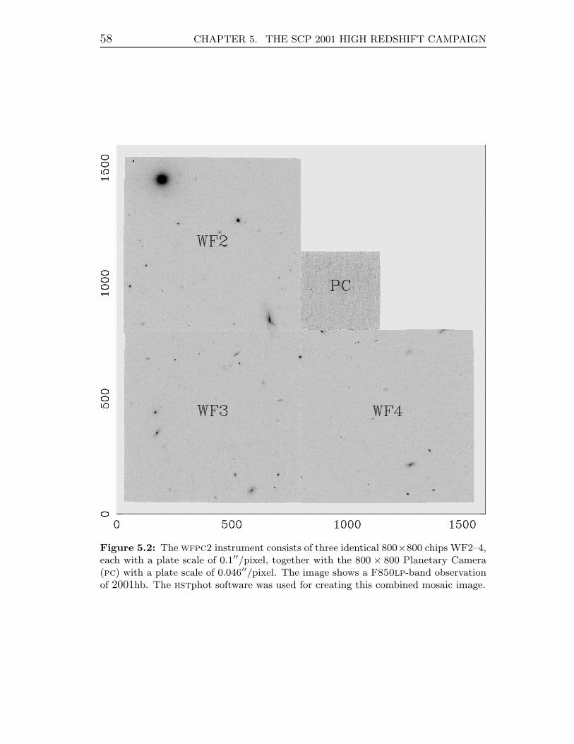
58 CHAPTER 5. THE SCP 2001 HIGH REDSHIFT CAMPAIGN
Figure 5.2: The wfpc2 instrument consists of three identical 800×800 chips WF2–4,each with a plate scale of 0.1′′/pixel, together with the 800 × 800 Planetary Camera(pc) with a plate scale of 0.046′′/pixel. The image shows a F850lp-band observationof 2001hb. The hstphot software was used for creating this combined mosaic image.

5.1. THE CAMPAIGN 59
(a) 2001gy
(b) 2001go
(c) 2001gn
(d) 2001hb
(e) 2001gq
Figure 5.3: The five supernovae from the scp Spring 2001 search campaign thatwere followed with the hst. Follow-up and reference images were obtained using thewfpc2 and acs instruments respectively. The follow-up images are shown to the leftin the left column, and at the top for 2001hb. All images shown here are in the F814w
passband.

60 CHAPTER 5. THE SCP 2001 HIGH REDSHIFT CAMPAIGN
The photometric analysis of the space-based data of 2001hb and2001gq is the main topic for this chapter. The problems related to the on-going analysis of the remaining three objects are discussed in section 5.4.
5.2 Lightcurve building and calibration
The significant differences in data properties between ground and spacebased observations were already discussed in section 3.3.3, and lead tothe alternative lightcurve building approach for wfpc2 images which wasintroduced in section 3.3.3.
Observing conditions in space are extremely stable over time, andhst photometry can be calibrated with very high accuracy by usingpublished zeropoints [30, 20, 67]. For wfpc2, the zeropoints are alwaysspecified for an aperture of 0.5′′. In order to use these, each Tiny Timgenerated psf must be normalised to this radius before equation (3.4)can be applied. Once this is accomplished, the zeropoints can be useddirectly for converting fluxes, fi, to instrumental magnitudes with thestandard flux-magnitude relation, equation (3.5) on page 28.
Lightcurves are fitted by applying the recipe developed in section 3.4.All K-corrections are calculated directly from instrumental to standardfilters, treating space and ground based observations independently.
5.3 Preliminary results
5.3.1 SN2001hb
As it has been pointed out earlier, building the lightcurve for 2001hb isparticularly easy due to the absence of any visible host galaxy. Because ofthis, 2001hb will be used to compare a few different photometric methods.The iraf apphot package was used to do aperture photometry on theimages, and the well tested hstphot package [21], designed for wfpc2
stellar photometry, was used along with the procedure from section 3.3.3to do psf photometry.
The hstphot software works directly on the pipeline reduced images,i.e. the crrej images were not used here. Instead there are a numberof preprocessing steps for masking bad pixels and subtracting the back-ground sky, within the package itself. There are three different optionsfor fitting the sky; either by using the mean value within an annulus foreach pixel and compute a sky map (sky), by measuring the sky value in agrid of pixel values and interpolate in between (sky 1), or by calculating

5.3. PRELIMINARY RESULTS 61
JD filter sky sky 1 sky 2
52037.06 F850lp 23.40± 0.06 23.42± 0.06 23.44± 0.0652041.15 F814w 23.77± 0.03 23.78± 0.03 23.79± 0.0352051.98 F814w 24.03± 0.04 24.04± 0.04 24.04± 0.0452065.23 F814w 24.55± 0.04 24.56± 0.04 24.56± 0.0452079.07 F814w 25.25± 0.07 25.27± 0.07 25.30± 0.07
JD filter sky sky 1 sky 2
52037.06 F850lp 23.49± 0.06 23.40± 0.06 23.41± 0.0652041.15 F814w 23.77± 0.03 23.76± 0.03 23.76± 0.0352051.98 F814w 24.02± 0.04 24.02± 0.03 24.02± 0.0352065.23 F814w 24.52± 0.04 24.52± 0.04 24.53± 0.0452079.07 F814w 25.24± 0.07 25.25± 0.07 25.27± 0.07
Table 5.2: Instrumental magnitudes for 2001hb obtained with hstphot. The uppertable shows the results when hstphot option 2 has been used, while the output fromoption 512 is presented in the lower table. The zeropoints used by the software areF814w = 20.839 and F850lp = 19.140 to get to the wfpc2 flight system. See thehstphot manual for details on the different sky and photometry options.
a single sky value for the whole chip. The latter of these, is probably themethod that best corresponds to the procedure used in the crrej task.
Further, there are also different sky options in the photometry pro-cess, where option 2 (“a local sky determination”) and 512 (“re-fittingthe sky before doing photometry”) in hstphot have been tested. Allmeasured magnitudes are presented in table 5.2.
The results by running hstltcv, described by equation (3.4), areshown in table 5.3. Here no background model has been used, but twosets of magnitudes are available depending on whether a pedestal offsethas been allowed or not. Examples of data and residual patches for oneof the lightcurve builds are presented in figure 5.4.
It can be concluded from the above results that the measured magni-tudes tend to vary roughly within one standard deviation, depending onhow the sky is treated, and, in the case for the hstltcv results, whethera pedestal offset is fitted or not.
A fair comparison between hstltcv and hstphot in terms of the skysubtraction procedure, and whether the local sky is determined or not,can be done by comparing the last column of table 5.3 with the lastcolumn of the upper table in 5.2, and the third column (Si = 0) oftable 5.3 with the last column of the lower table in 5.2.

62 CHAPTER 5. THE SCP 2001 HIGH REDSHIFT CAMPAIGN
JD filter Si = 0 free Si
52037.06 F850lp 23.34± 0.07 23.40± 0.0752041.15 F814w 23.78± 0.03 23.80± 0.0352051.98 F814w 24.02± 0.03 24.06± 0.0452065.23 F814w 24.57± 0.04 24.56± 0.0452079.07 F814w 25.27± 0.07 25.29± 0.07
Table 5.3: Instrumental magnitudes for 2001hb obtained by fitting a backgroundfree version of equation (3.4). For consistency the same zeropoint has been used as intable 5.2.
Figure 5.4: Data and residual pairs for increasing epochs after a hstltcv fitted TinyTim psf has been subtracted for 2001hb in the F814w-band. The patches have beencentred on the initial positions for the lightcurve fit.
To test the methods further, the magnitudes of a few field stars weremeasured, and compared with the corresponding results from aperturephotometry with the iraf apphot package. However, no deviations be-tween the methods could be found.
5.3.2 SN2001gq
SN 2001gq is well separated from the host galaxy core which is clear fromfigure 5.3(e). Lightcurve building for a case like this does not require anysupernova-free reference images for determining the galaxy background.In section 3.3.3, it was explained that the background can be fitted with a

5.3. PRELIMINARY RESULTS 63
1
2
3
4
5
6
7
8
Figure 5.5: The circles mark the randomly added fake supernovae, where the posi-tions where constrained to have the same aproximate distance to the galaxy core asthe real object. The magnitudes of the fake objects were set to mimic the expectedsupernova brightness for each epoch. The real supernova is the point source at thebottom of the patch between fake objects 1 and 4.
smooth and primitive surface parametrisation. However, concerns werealso raised regarding the robustness of this method, and it would bedesirable to know how sensitive the fitted supernova magnitudes are tothe choice of patch size and background model.
In order to be able to answer this question, a handful of fake super-novae were added around the host galaxy, which is shown in figure 5.5.The positions were randomly selected with the only constraint that theyobject-core distance were approximately the same as for the real super-nova. The fake objects were added to each image in the F814w band,and their magnitudes were set to be as close as possible to the real super-nova brightness for each epoch. The fake supernovae were modelled witha TinyTim generated psf, and several objects were also added randomlyto the image, in order to assure that they could be recovered accuratelyin the absence of a host galaxy.
The lightcurve for each of these supernovae was then built for differentbackground models and patch sizes. The mean residual plots presented infigure 5.6, show that ignoring the background, will lead to an expectedoverestimation of the supernova brightness. Similarly, it also confirms

64 CHAPTER 5. THE SCP 2001 HIGH REDSHIFT CAMPAIGN
JD F675w
52039.81 23.51± 0.0252048.04 23.77± 0.0352054.06 24.22± 0.0452066.90 25.19± 0.05
JD F814w
52039.87 23.08± 0.0352048.10 23.34± 0.0452054.12 23.63± 0.0452067.03 24.35± 0.05
Table 5.4: Instrumental magnitudes for 2001gq. The lightcurve was built with apatch width of 10 pixels, and fitting a paraboloid background model. The fluxes werecalibrated with the wfpc2 zeropoints published by Andrew Dolphin [20].
Telescope JD J
vlt 52048.2 23.24 ± 0.08Gemini 52051.6 23.39 ± 0.09
Table 5.5: Preliminary and unpublished, J-band magnitudes of 2001hb. Credit:Chris Lidman.
that primitive models of the galaxy shape will fail for large patches,while the paraboloid appears to satisfactory remove the background forall patch widths. It is also important to note that the last model doesnot lead to an underestimation of the supernova brightness, which couldhappen if a model with too much freedom is used without any supernova-free references to constrain it.
5.3.3 Lightcurve fitting
The lightcurves of the two supernovae discussed above were fitted, usingthe method presented in section 3.4. The data from table 5.4 and the lastcolumn of 5.3 were used for 2001gq and 2001hb respectively. In additionto this, ground based I-band data from [56], and the J-band points for2001hb from table 5.5 were included in the fits. The results are presentedin figure 5.8 and table 7.2, where the colour excess was estimated fromthe U and B passbands for 2001gq.
One notable result from this table is the remarkable high stretchof the supernovae, and specifically for 2001hb. However, for the latter,the stretch is determined by the pre-max points in the I-band whichcorrespond to the rest frame U -band. These points, and therefore thefitted stretch, will be highly sensitive to the uncertainty of the spectraltemplate in U .
The stretch corrected B-band magnitudes at max have been plottedin the Hubble diagram 7.1.

5.3. PRELIMINARY RESULTS 65
Figure 5.6: Results from studies with fake supernovae for different patch sizes andbackground models. Each point in the plot represents the mean of the residualsbetween the measured and input magnitude for all eight fake supernovae. The errorbars have been calculated as the estimated standard deviation of the residuals dividedby the square root of the number of points. The lower panel shows the result when nobackground model at all is assumed. For the middle panel a plane was used to modelthe host galaxy, while a paraboloid was used for the upper panel. All results presentedhere refer to the last epoch in the lightcurve build for the fake F814w data set.
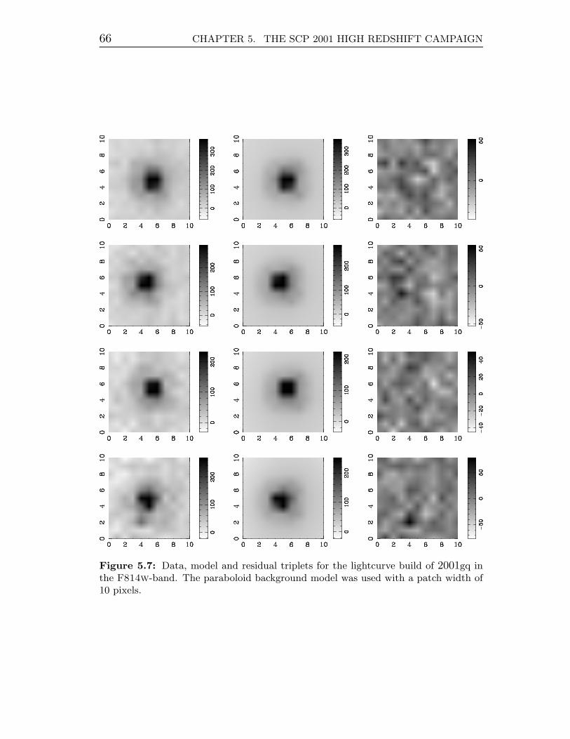
66 CHAPTER 5. THE SCP 2001 HIGH REDSHIFT CAMPAIGN
Figure 5.7: Data, model and residual triplets for the lightcurve build of 2001gq inthe F814w-band. The paraboloid background model was used with a patch width of10 pixels.

5.4. UNRESOLVED SUPERNOVAE 67
Figure 5.8: Lightcurve fits in, from left to right, the rest frame U , B and V passbands,where the observed filters are shown in the lower left corner of each plot. The x andy axes show days in observed frame and normalised flux respectively. The fits arebased on data from the hst (triangle), cfht (square), vlt (circle), ctio (diamond)and Gemini (cross) telescopes.
5.4 Unresolved supernovae
The three remaining supernovae of the sample can not be resolved fromtheir host galaxies (see the left column of figure 5.3), and the methodused in this chapter can not be applied to build these lightcurves. Thebackground model must be constrained by using supernova-free referenceimages, and an approach that first may come to mind, is to use thesame procedure as for the ground based data. There are, however, acouple of problems that arises when this method is tried. First of all, thefollow-up images and the references have been obtained with differentinstruments, so a transformation kernel must be used for subtracting thehost. Fitting this in the same manner as for ground based data turns outto be problematic due to the limited field of the wfpc2 pc chip. Veryfew objects appear in the fields, and only on rare occasions can a star befound on the images.
Another possible concern is the host galaxy model used in equa-tion (3.2), where one value is used for each pixel on the best seeingimage. This approach may not be feasible for the hst data. Due to thenarrow psf, it is desirable to have a model that works on sub pixel level,and an analytical model is therefore preferable. The best approach forsolving this could be to try to use shapelets, which have proved to be asuccessful method for fitting galaxy morphologies [18, 38].

68 CHAPTER 5. THE SCP 2001 HIGH REDSHIFT CAMPAIGN
To these problems, the general unpleasantness that always appears formulti-instrument lightcurves should also be added, namely the differencei wavelength response.
These difficulties are currently being addressed by the Stockholmsupernova cosmology group. It should also be added that more straight-forward methods, such as pixel-by-pixel subtraction and aperture pho-tometry comparison are also investigated.

C h a p t e r 6
The future of supernova cosmology
While the ongoing supernova surveys are successfully populating theHubble diagram for redshifts below one, there is still only a handful ofdata points above this limit. At the same time, these redshifts are veryinteresting since the separation between different cosmological models isbecoming more significant in this area [27] which, for example, is shownin figure 3.6. Additionally, while there are other successful methods formeasuring cosmology, type Ia supernovae currently provides one of thebest approaches for studying the expansion history of the Universe.
A large scale supernova survey for redshifts above one is simply notfeasible with todays instruments, other than a dedicated use of the hst.It is in fact only thanks to the hst that there are data at all in thispart of the Hubble diagram. For very high redshifts, a large part of thetype Ia spectrum lands in the infrared, where the atmospheric absorptionis severe, and will therefore not be visible from the ground. A supernovasurvey for z > 1, with exquisite control of systematics, would require aspace based wide-field imager with infrared capabilities like the proposedSupernova Acceleration Probe [9]. More than 2000 type Ia sne in the red-shift range 0.1 < z < 1.7 (table 6.1) will be discovered per year togetherwith a large number core-collapse supernovae. With a photometric ac-curacy at the percent level, even at the highest redshifts, a satellite ofthis kind would be an essential step towards revealing the nature of darkenergy. However, for these high precision measurements, it is of utterimportance that all possible systematic effects can be mapped and ac-counted for. Some of the effects that would have minor or no impact
z 0.1 0.2 0.3 0.4 0.5 0.6 0.7 0.8# 20 40 65 100 130 160 170 180
z 0.9 1.0 1.1 1.3 1.4 1.5 1.6 1.7# 170 160 140 120 115 100 90 70
Table 6.1: The redshift distribution of the sne that the snap satellite is predicted todetect during one year [9].

70 CHAPTER 6. THE FUTURE OF SUPERNOVA COSMOLOGY
Figure 6.1: The space in the line of sight between observer and source, is divided into cells. For each cell the effect of gravitational lensing and extinction is calculated.By courtesy of Edvard Mortsell.
for current data sets could lead to erroneous results for the snap data.In order to study exactly how elements of gravitational lensing, differentflavours of extinction, or even possible exotics like photon-axion interac-tion [41, 49], could affect the future of supernova cosmology, our groupat Stockholm University has developed a simulation package, exclusivelydesigned for this purpose.
6.1 The Supernova Observation Calculator
The Supernova Observation Calculator (snoc), described in Paper C, isa Monte-Carlo package for simulating supernova data. The main featureof this tool is that the emitted light is ray-traced between the observerand the source for each event, which makes it possible to study howdifferent physical processes could affect the light propagation .
The user specifies which type (or types) of supernova to study to-gether with the size of the data set and the redshift distribution. Thehost galaxy types depend on the object type that is generated. Type Iasne are produced in both early and late type galaxies, while core collapsesupernovae only occur in the latter. The inclination of the host galaxy,as well as the supernova position within it, are randomly generated, andthe extinction is calculated, based on chosen dust properties.
The ray-trace is done by first assuming a background flrw cosmol-ogy, described in chapter 2, and then using the method proposed by Holzand Wald [31] to account for gravitational lensing effects. The space be-tween observer and source is divided into spherical cells with sizes of theorder of intergalactic distances (figure 6.1). The cells have an average

6.1. THE SUPERNOVA OBSERVATION CALCULATOR 71
InputGenerate
sn z
Generateredshifted light
curve
Ray-tracing
Calculateextinctions
SearchCosmology fit
Figure 6.2: Overview of the snoc execution sequence. Each simulation is definedby an input file, where redshift distribution, dark matter and dust properties, etc. arespecified. In the output file the apparent supernova magnitude is given along with thesimulated contribution from each of the physical processes that have been simulated.
energy density1 corresponding to the chosen cosmology, but it is inhomo-geneously distributed inside the cells according to an arbitrary fractionof: point-masses, uniform spheres, singular isothermal spheres (sis) orthe Navarro-Frenk-White (nfw) density profile. The light beam is thentraced backward from the observer and for each cell an impact parame-ter is selected randomly and the deviation of the light ray is calculatedaccordingly. Finally the area of the light bundle in the source planecan be compared with the unaffected filled beam area to get the lensingmagnification.
After the ray-trace is completed the apparent supernova magnitudesare calculated in a user selected filter set, and to these, possible extinctionis added, taking into account the position of the supernova inside thehost and the morphology of the galaxy. Further, two random samplingsof the lightcurve are generated with a given time gap in order to simulatea search situation.
The results of the simulation can be analysed by the cosmology fitter,discussed in section 3.5, in order to study how sensitive the estimatedcosmological parameters may be to systematics introduced along the lineof sight. An overview of the whole execution sequence is shown in fig-ure 6.2. Figure 6.3 shows a simulated Hubble diagram for 2000 type Iasupernovae, distributed in accordance with table 6.1, together with a low-z sample of 200 type Ia objects uniformly distributed between 0.01 ≤ z ≤0.1. The latter is intended to correspond to what may come out of thesn-factory project [8]. For both simulations the cosmology ΩM = 0.3,ΩΛ = 0.7 and H0 = 65 km/(s·Mpc) has been used.
1 Each cell is also characterised by a dust density, which allows the study of extinctionfrom either grey dust or dust in intervening galaxies.

72 CHAPTER 6. THE FUTURE OF SUPERNOVA COSMOLOGY
PSfrag
replacem
entsmz
snap
simula
tion
sn-fa
ctory
simula
tion
Figure 6.3: Simulated supernova events corresponding to the predicted measure-ments for the snap and Supernova Factory projects.
6.2 The target precision of ΩM and ΩΛ
With snoc, it is very easy to study the accuracy of cosmology estimationsthat could be obtained from the data mentioned above. The result froma three parameter fit (ΩM , ΩΛ,M), where M has been treated as anuisance parameter, is shown in figure 6.4, and gives ΩM = 0.30 ± 0.02and ΩΛ = 0.70±0.06. The quoted uncertainties are for a joint probabilityof 68 % of including both parameters within the intervals, i.e. 1.51σ.
Target precisions for different fitting conditions and prior assumptionsis discussed further in Paper A.
6.2.1 The importance of a wide redshift range
The different cosmological models plotted in figure 3.6 on page 37, clearlyshows that the degeneracy between different models is broken at high red-shifts. However, it is important to point out that also a well sampledHubble diagram at low redshifts is important for cosmology fitting. Evenif M is treated as a nuisance parameter, constraining this means nar-rowing down the probability space also for the energy densities and thedark energy equation of state.
In figure 6.3 the same cosmology fit that was carried out for figure 6.4has been performed with and without considering the low-z sample. Bothcontours include the true values, (ΩM = 0.3, ΩΛ = 0.7), but when ∼10 %more data from the sn-factory simulation has been added the error in-tervals are dramatically decreased. Note, that the correlation betweenthe fitted parameters is also affected.
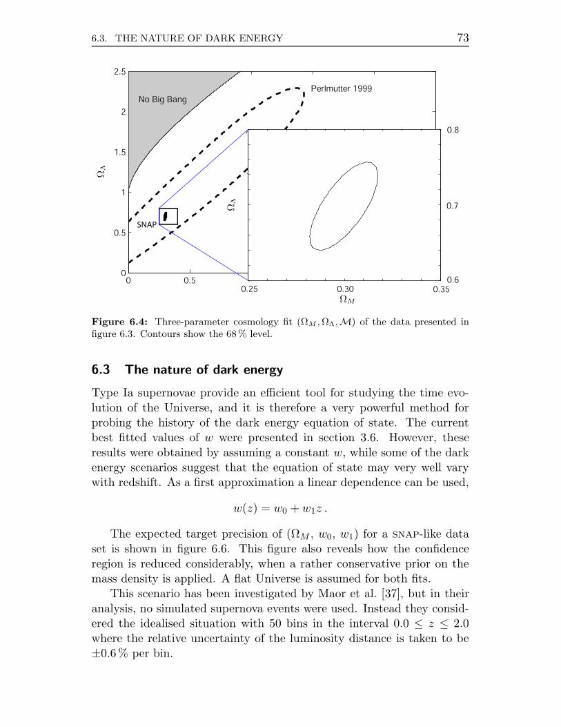
6.3. THE NATURE OF DARK ENERGY 73
0 0.50
0.5
1
1.5
2
2.5
No Big Bang
Perlmutter 1999
SNAP
Grid Search
Davidon min.
0.350.300.25
0.8
0.7
0.6
PSfrag replacements
ΩM
ΩΛ
ΩΛ
Figure 6.4: Three-parameter cosmology fit (ΩM , ΩΛ,M) of the data presented infigure 6.3. Contours show the 68 % level.
6.3 The nature of dark energy
Type Ia supernovae provide an efficient tool for studying the time evo-lution of the Universe, and it is therefore a very powerful method forprobing the history of the dark energy equation of state. The currentbest fitted values of w were presented in section 3.6. However, theseresults were obtained by assuming a constant w, while some of the darkenergy scenarios suggest that the equation of state may very well varywith redshift. As a first approximation a linear dependence can be used,
w(z) = w0 + w1z .
The expected target precision of (ΩM , w0, w1) for a snap-like dataset is shown in figure 6.6. This figure also reveals how the confidenceregion is reduced considerably, when a rather conservative prior on themass density is applied. A flat Universe is assumed for both fits.
This scenario has been investigated by Maor et al. [37], but in theiranalysis, no simulated supernova events were used. Instead they consid-ered the idealised situation with 50 bins in the interval 0.0 ≤ z ≤ 2.0where the relative uncertainty of the luminosity distance is taken to be±0.6 % per bin.

74 CHAPTER 6. THE FUTURE OF SUPERNOVA COSMOLOGY
0.2 0.25 0.3 0.35 0.4 0.45 0.50.5
0.55
0.6
0.65
0.7
0.75
0.8
0.85
0.9
PSfrag replacementssnap
snap and sn-factory
ΩM
ΩΛ
Figure 6.5: The 1.51σ (68%) contours for a three-parameter fits (ΩM , ΩΛ,M) basedon simulated data corresponding to the predicted snap data, and the predicted snap
and sn-factory data respectively.
−0.9 −0.85 −0.8 −0.75 −0.7 −0.65 −0.6 −0.55 −0.5−1.6
−1.4
−1.2
−1
−0.8
−0.6
−0.4
−0.2
0
0.2
0.4
w0
w1
Figure 6.6: Estimated ∼ 68 % and ∼ 95% confidence contours for a (ΩM ,w0,w1)fit with (dashed) and without (solid) a Gaussian prior (0.25 ± 0.1) on ΩM . A flatUniverse has been assumed for both fits, and they are based on a snoc simulationof 2300 snap + sn-factory type Ia supernovae. The simulations have been madeassuming w0 = −0.7 in order to correspond to the discussion in [37]. This value hashowever been excluded by recent results [62, 70].

6.4. GRAVITATIONAL LENSING 75
The conclusion that can be drawn is that even with this redshiftdependent equation of state parameter, it would be possible to make astatement on which of the models that is favourable from the measure-ments. This is only valid under the assumption that the geometry ofthe Universe and M are determined by other means though. It shouldhowever be noted that even under the assumption that M is known, it isstill of utter importance to have a wide redshift spread of the data whichis explained in Paper A.
6.3.1 Fitting inverse power-law models
Pushing one step further, it may be tempting to try to differentiate be-tween possible parameter values within a certain quintessence potential.One of the simplest potentials was presented in equation (2.9) on page 9,and in Paper B the possibility of fitting α together with ΩM from thesnap and sn-factory data sets has been investigated. It turns out thatit is possible to distinguish between the inverse power-law potential anda cosmological constant and put constraints on the power-law exponentif there are independent measurement of ΩM and M available.
6.4 Gravitational lensing
The measured brightness of a supernova may very well be affected if thereis matter present along the line of sight that could act as a gravitationallens system.
A simple lensing situation, often referred to as the Schwartzschildlens, is shown in figure 6.7, where the lens is spherically symmetric andhas a weak gravitational field. These constraints, which are fulfilled bye.g. a planet or a star, make the system particularly easy to treat andall calculations can be done in the planes defined by the source, the lensand the observer. The optical axis of the system is defined by the dottedline connecting the lens and the observer, and the positions of the sourceand image can then be specified by the angles β and θ respectively. Thelensing equation can be geometrically derived as
β = θ − αDds
Ds, (6.1)
where the distances are defined in figure 6.7, and the deflection angle, α,becomes
α =4M
ξ=
4M
θDd. (6.2)

76 CHAPTER 6. THE FUTURE OF SUPERNOVA COSMOLOGY
βθ
α
Ds
Dd Dds
F
ξ η
Figure 6.7: A simple lensing system
Here, M is the mass2of the lens, and the impact parameter ξ, is theshortest distance between the lens and the light path. Equation (6.1)has two solution, i.e. the lens give rise to two3 images located on eachside of the lens, and separated by an angle
∆θ = θ1 − θ2 =√
4α20 + β2 ≥ 2α0 . (6.3)
The magnification ratio between the two images can be calculated to be
r =
∣
∣
∣
∣
µ1
µ2
∣
∣
∣
∣
=
[
√
β2 + 4α20 + β
√
β2 + 4α20 − β
]2
. (6.4)
An additional interesting property of a lensing system, is that sincethe two images will take different paths to reach the observer, and sincethese paths are of different length, the two images will not reach theobserver at the same time. If the Schwartzschild metric is used, which isan excellent description of space-time around massive bodies, the timedelay between the two images can be calculated as,
∆t =a0
a(td)
DdDs
Ddsα2
0
(
θ22 − θ2
1
2|θ1θ2|+ ln
∣
∣
∣
∣
θ1
θ2
∣
∣
∣
∣
)
. (6.5)
6.4.1 Dark matter halo models
The point-mass model is very useful for planets or black holes but itdoes not do a very good job when the lens is constituted of a galaxy ora galaxy cluster. In these cases a matter density distribution function of
2 For this derivation, M is assumed to be a point mass.
3 In the special case when observer, lens and source are all aligned and β = 0, thesolution is an ”Einstein” ring around the lens.

6.4. GRAVITATIONAL LENSING 77
some sort is needed to describe the profile. The two mass-profiles thathave been used for the work in this thesis are the singular isothermalsphere (sis), and the The Navarro-Frenk-White density profile (nfw).
The sis model is based on the assumption that matter behave likeparticles in an ideal gas with a gravitational potential, and the densitydistribution becomes [44]
ρ(r) =σ2
v
2π
1
r2,
where σv is the one-dimensional velocity dispersion of the mass particles,and r is the distance from the centre.
The nfw model on the other hand is constructed from high-reso-lution N -body simulations of dark matter halo structure formation [45],giving the density profile
ρ(r) =ρ0
(r/rs)(1 + r/rs)2,
where ρ0 is a characteristic density, and rs a scale radius. The propertyof this density profile is similar to a sis model for r ∼ rs, while it issingular at the centre with ρ ∝ r−1, and proportional to r−3 for r À rs.The nfw model has been proved to be an adequate description over widedistance scales from dwarf galaxy halos to galaxy clusters.
6.4.2 Magnification and demagnification of type Ia SNe
The probability of a supernova being gravitationally magnified dependson the redshift of the source, since the further away it is, more potentiallenses are passed by the light before it reaches the observer. The mag-nification, or demagnification, is also strongly dependent on the darkmatter halo distribution model used for the intervening structures, andthe redshift of the lens. Figure 6.8 shows snoc computations of the mag-nitude deviation due to lensing for different redshifts and different halodistributions. The distributions are clearly asymmetric, but it should bekept in mind that for low redshifts, z < 1.0, this skewness will drowncompletely in the intrinsic scatter of ∼ 0.16 magnitudes.
However for higher redshifts these effects start to become important,and this issue is addressed in detail in Paper E. To study what ef-fects lensing would have on fitted cosmological parameters, a data setconsisting of 2300 type Ia sne with a uniform redshift distribution wassimulated. The dark matter halo model was parametrised to consist of

78 CHAPTER 6. THE FUTURE OF SUPERNOVA COSMOLOGY
PSfrag replacements
z = 1
z = 2
z = 3
∆m
1500
1000
1000
1000
500
500
500
00
0
0
−0.2 0.2 0.4
(a) sis-model
PSfrag replacements
z = 1
z = 2
z = 3
∆m
1500
1000
1000
1000
500
500
500
00
0
0
−0.2 0.2 0.4
(b) nfw-model
Figure 6.8: Simulated magnitude deviations due to gravitational lensing at threedifferent redshifts for a (ΩM = 0.3,ΩΛ = 0.7) cosmology. [13]
both compact objects, i.e. point masses, and a smooth matter distribu-tion described by the nfw profile. For the cosmology fits, the incorrectassumption of Gaussian magnitude distributions (identical to a χ2-fit)was first made in order to study possible bias effects. The result is pre-sented in left panel of figure 6.9.
The contour curves clearly show that gravitational lensing will pro-duce a bias in the estimations, and that the bias in ΩM increases withthe fraction of compact objects, while it seems to be less sensitive in ΩΛ.
The next step is to try to account for the lensing effects in the anal-ysis. A model for the asymmetric magnitude distribution is suggestedin Paper E,
f(m) = a · exp
[
−(m − m0)2
2σ2
]
for m ≥ 0 ,
f(m) = a · exp
[
−(m − m0)2
2σ2
]
+ b · |m| · 101.5m for m < 0 ,
where m0, a and b depend on the lensing model and the redshift. By using

6.4. GRAVITATIONAL LENSING 79
0.2 0.25 0.3 0.350.5
0.6
0.7
0.8
0.9
ΩM
ΩX
1.51σ, no lensing1.51σ for 0% c.o.1.51σ for 20% c.o.1.51σ for 40% c.o.
0.2 0.25 0.3 0.350.5
0.6
0.7
0.8
0.9
ΩM
ΩX
1.51σ, no lensing1.51σ, χ2−fit1.51σ, ML−fit for 15% c.o.1.51σ, ML−fit for 20% c.o.1.51σ, ML−fit for 25% c.o.
Figure 6.9: Confidence contours showing the joint 68% level for two parameters.The left panel shows χ2-fits, where gravitational lensing has not been considered, fordifferent dark matter scenarios. In the right panel, all fits are based on a Universewhere 20% of the dark matter consists of compact objects, but different compactobject assumptions have been made for the separate fits. All fits are based on asimulated sample of 2300 uniformly distributed type Ia sne.
the result of the χ2-fit as a first guess, these parameters can be estimatedfrom the magnitude residuals for this model. The estimation can then beused to simulate a large number of sne for each redshift, and further usethem to fit the parameters in the distribution function. Once the functionis known the cosmology can be re-fitted, and by applying this methoditeratively the bias is significantly reduced. The dash-dotted contour inthe right panel of figure 6.9 shows the result if the correct model is used,while the dotted contours give the result if an error of 5 % is made in thefraction of compact object estimate. This is approximately the accuracythat can be expected from the method [42].
6.4.3 Using lensing for cosmology fitting
Gravitational lensing is a physical property that up to this point hasbeen considered to be purely evil, but the Universe is not only black andwhite, and lensing can as a matter of fact also be used for doing good!
In some cases, when a massive matter distribution is located veryclose to the line of sight, the lensing model previously described in thissection is applicable, and multiple images can be observed. If equa-tions (6.3) and (6.4) are combined together with (6.5) and the redshiftrelation, the following cosmology dependent relation,
∆t = (1 + zd)DdDs
Dds· ∆θ2
2· r1/2 − r−1/2 + ln r
r1/2 − r−1/2 + 2,

80 CHAPTER 6. THE FUTURE OF SUPERNOVA COSMOLOGY
Figure 6.10: Fitted 68% contours based on 366 multiply lensed supernovae. Thedarker region is the result of a two parameter fit, where the nuisance parameter H0 isassumed to be known.
only including the observable quantities, r, ∆t and ∆θ, can be derived.In other words, this provides a method for measuring cosmological pa-rameters from multiply lensed objects. The main drawbacks are thatthis phenomenon is rather rare, and that the lensed source must have atime dependent lightcurve order to accurately determine ∆t. However,an experiment like the snap mission would, during its search for type Iasupernova, also discover a very large number of core collapse supernovaefor free. The snoc simulations presented in Paper D, resulted in ∼ 300strongly lensed objects, under snap-like conditions. A projection in the(ΩM , ΩΛ)-plane of a three-parameter fit (ΩM , ΩΛ, H0) of this data set ispresented in figure 6.10. The darker area gives the confidence region fora two parameter fit, (ΩM , ΩΛ), where H0 is assumed to be known byother measurements.
The accuracy of this method is far from the one obtained with theredshift-luminosity relation, but some things are however worth to notic-ing. First of all, the part of the confidence region that intersects withthe flat-universe line is quite narrow, so combining these measurements

6.4. GRAVITATIONAL LENSING 81
with a flatness prior from cmb experiments [70] will reduce the uncer-tainty dramatically. Secondly, the correlation between ΩM and ΩΛ isnegative for these fits, in contrast to the positive correlation for theredshift-magnitude case. This motivates the use of the multiple lensingtechnique as a complementary method to the type Ia studies.

C h a p t e r 7
Summary
The use of type Ia supernovae as distance indicators, is among the besttools available today for probing the expansion history of the Universe.Recent cosmological results by using this method have been presentedin Paper F, which also addresses the main source for systematic uncer-tainties, extinction due to dust along the line of sight. Supernova datacan be corrected for extinction by measuring the colour excess, but thisrequires accurately measured multi-colour lightcurves for each object andgood knowledge of the intrinsic colours.
The extinction dilemma can also be attacked by using longer wave-length bands for building the Hubble diagram. The possibility of usingthe rest frame I-band for this purpose is the topic of Paper G. Addi-tionally, in the paper, attempts are also made to set limits on possibleintergalactic grey dust by measuring the colour excess over a broad wave-length range. However, no tight constraints can be set from the existingdata.
The other end of the optical spectrum is also of great importancefor supernova cosmology. Type Ia supernovae emit a large fraction oftheir light in the rest frame U -band. This can not be measured from theground for nearby objects, due to the atmospheric absorption at thesewavelengths, and the knowledge of the type Ia spectrum in this rangeis therefore very limited. For higher redshifts the U -band part of thespectrum will often contribute to the observed brightness, and the cor-rections for translating to rest frame magnitudes are likely to introducesystematic errors. The preliminary data presented in chapters 4 and 5(see also tables 7.1-7.2 and figure 7.1), all have photometry that overlapthe rest frame U -band and the difficulties were also indeed recognised forthis data set as well as in Paper F.
Lightcurve building has been throughly discussed, and an optimalmethod for simultaneously fitting supernova fluxes for different epochsin a given filter has been used for all data presented throughout thethesis. The results from a series of sanity checks of this method, usingsimulated fake images, are also given in chapters 4 and 5.
The latter part of the thesis is mainly based on a series of simulations

84 CHAPTER 7. SUMMARY
carried out with the snoc software, introduced in Paper C. This pack-age simulates observed supernova data by ray-tracing the light beamsthrough space. Different potential systematic effects can be taken intoaccount one at a time, and the effect on the fitted cosmology can bestudied in detail.
The package is useful for answering questions regarding target pre-cision of the cosmological parameters for different data sets. It can beconcluded that, although the high redshift data is essential for breakingthe degeneracy between different cosmological scenarios, it is also impor-tant to obtain data at low and intermediate redshifts for constrainingcosmology, which was discussed in connection to figures 6.3 and 4.1.
Most of the simulation work is focused around a possible future dataset of the kind that is expected to be available from the proposed snap
satellite. The main task for cosmologists today, and also this specificinstrument, is to determine the origin of dark energy. The best approachto this is to study the evolution of its equation of state, which will revealwhether dark energy is explained by a cosmological constant or a moreexotic model. The target precision for the cosmological parameters ingeneral, and specifically w, is discussed in Paper A. Possible snap-limitsthat can be set on a Peebles-Ratra quintessence potential are presentedin Paper B.
The recipe for snap is to obtain high precision measurements of su-pernova lightcurves up to z ∼ 2, keeping systematic errors under control.For redshifts above one, the possibility increases that the obtained datacould be biased due to gravitational lensing. How this would affect thefitted cosmologies, together with how they can be taken into account, isthe topic for Paper E.
Finally, a satellite like snap will also discover a very large number ofcore-collapse supernovae. Some of these events could be strongly lensedand this data can in principle be used to give complementary cosmologyestimations of the kind discussed in Paper D.
In the introduction of this thesis, it was mentioned that experimentalcosmology has undergone a golden age during the past decade, and thereare no indications that this is going to stop any time soon. The snap
satellite is only one of many instruments that hopefully can be builtwithin a near future and that will have a major impact on cosmology.Instruments of this kind will help to pinpoint all parameters introducedin this thesis, but most importantly, they can probably also reveal someof the surprises that are awaiting us in a Universe where we still only canaccount for a few percent of its content.

85
sn z mg mB meffB Stretch E(B − V )g E(B − V )h
1999dr 0.183 21.64 21.52 ± 0.08 21.34 ± 0.19 0.859 ± 0.031 0.055 0.40 ± 0.11
1999du 0.260 21.20 21.32 ± 0.01 21.37 ± 0.16 1.044 ± 0.009 0.031 −0.21 ± 0.04
1999dv 0.186 20.81 20.81 ± 0.01 20.75 ± 0.16 0.958 ± 0.007 0.032 0.10 ± 0.03
1999dx 0.269 21.86 21.69 ± 0.01 21.62 ± 0.17 0.944 ± 0.029 0.037 0.21 ± 0.05
1999dy 0.202 20.82 20.90 ± 0.01 20.96 ± 0.16 1.048 ± 0.011 0.028 −0.10 ± 0.04
Table 7.1: Table summarising the results from the photometric follow-up of the esc 1999 campaign. The mg
are the observed peak magnitudes at the time of the B-maximum, mB . The mB = mg − KBg − Ag values havebeen K and mw-extinction corrected. The fitted stretch, s, has been applied to the meff
B magnitudes, usingα = 1.28 ± 0.28 from Paper F.
sn z mX mB meffB Stretch E(B − V )g E(B − V )h
2001gq 0.671 22.98 24.07 ± 0.02 24.27 ± 0.17 1.150 ± 0.005 0.027 0.24 ± 0.04
2001hb 1.055 23.34 24.74 ± 0.02 25.06 ± 0.18 1.251 ± 0.018 0.032 −0.04 ± 0.07
Table 7.2: Same as for table 7.1, but for the results from the photometric follow-up of the scp spring 2001campaign. The mX are the observed peak magnitudes at the time of the B-maximum, mB , where X = I for2001gq and X = f850lp for 2001hb. The mB = mX−KBX−AX values have been K and mw-extinction corrected.For 2001gq, the colour excess has been estimated by using the rest frame U and B, bands, while the B and Vbands were used for 2001hb.

86 CHAPTER 7. SUMMARY
Figure 7.1: Preliminary rest frame B-band Hubble diagram of the supernova datapresented in this thesis, where the z and meff
B columns from tables 7.1 and 7.2 havebeen plotted against each other. The solid line represents the concordance model withΩM = 0.28, ΩX = 0.72, w = −1, H0 = 72 km/s/Mpc.

Bibliography
[1] Adelman-McCarthy, J. K. et al., ApJS, 162 (2006) 38
[2] Aguirre, A., ApJ, 525 (1999) 583
[3] Aguirre, A. N., ApJ, 512 (1999) L19
[4] Alard, C., A&AS, 144 (2000) 363
[5] Alard, C. and Lupton, R. H., ApJ, 503 (1998) 325
[6] Aldering, G., Knop, R., and Nugent, P., AJ, 119 (2000) 2110
[7] Aldering, G. et al., IAU Circ., 7764 (2001) 1
[8] Aldering, G. et al. (2002). In J. A. Tyson and S. Wolff, editors,Survey and Other Telescope Technologies and Discoveries. Edited byTyson, J. Anthony; Wolff, Sidney. Proceedings of the SPIE , volume4836, pp. 61–72
[9] Aldering, G. et al. (2004). Supernova / Acceleration Probe:A satellite experiment to study the nature of the dark energy .[astro-ph/0405232]
[10] Astier, P. and Goobar, A., IAU Circ., 7258 (1999) 1
[11] Astier, P. et al., A&A, 447 (2006) 31
[12] Benıtez, N., et al., ApJ, 577 (2002) L1
[13] Bergstrom, L., Goliath, M., Goobar, A., and Mortsell, E., A&A,358 (2000) 13
[14] Bertin, E. and Arnouts, S., A&A Suppl., 117 (1996) 393
[15] Bessell, M. S., PASP, 102 (1990) 1181
[16] Cardelli, J. A., Clayton, G. C., and Mathis, J. S., The AstrophysicalJournal, 345 (1989) 245
[17] Carroll, S. M., Press, W. H., and Turner, E. L., ARA&A, 30 (1992)499

88 BIBLIOGRAPHY
[18] Chang, T.-C. and Refregier, A., ApJ, 570 (2002) 447
[19] Davidon, W. C., Computer Journal, 10 (1968) 406
[20] Dolphin, A. E., PASP, 112 (2000) 1397
[21] Dolphin, A. E., PASP, 112 (2000) 1383
[22] Einstein, A., Annalen der Physik, 49 (1916) 769
[23] Fabbro, S. (2001). PhD thesis. Ph.D. thesis, l’Universite Paris XIOrsay
[24] Feldman, G. J. and Cousins, R. D., Phys. Rev. D, 57 (1998) 3873
[25] Frodesen, A. G., Skjeggestad, O., and Tøfte, H. (1979). Probabilityand Statistics in Particle Physics. Universitetsforlaget, Bergen
[26] Goldhaber, G. et al., ApJ, 558 (2001) 359
[27] Goobar, A. and Perlmutter, S., ApJ, 450 (1995) 14
[28] Gunnarsson, C., et al., ApJ, 640 (2006) 417
[29] Hillebrandt, W. and Niemeyer, J. C., ARA&A, 38 (2000) 191
[30] Holtzman, J. A. et al., PASP, 107 (1995) 1065
[31] Holz, D. E. and Wald, R. M., Phys. Rev. D, 58(6) (1998) 063501
[32] Irwin, M. and Lewis, J., New Astronomy Review, 45 (2001) 105
[33] Jonsson, J., et al., ApJ, 639 (2006) 991
[34] Kim, A., Goobar, A., and Perlmutter, S., PASP, 108 (1996) 190
[35] Krist, R. N., John E.; Hook (2001). The tiny tim user’s guide
[36] Livio, M. (2000). Type Ia supernovae and their implications forcosmology . [astro-ph/0005344]
[37] Maor, I., Brustein, R., and Steinhardt, P. J., Physical Review Let-ters, 86 (2001) 6
[38] Massey, R., et al., MNRAS, 348 (2004) 214
[39] McMahon, R. G., et al., New Astronomy Review, 45 (2001) 97

BIBLIOGRAPHY 89
[40] Moffat, A. F. J., A&A, 3 (1969) 455
[41] Mortsell, E. and Goobar, A., JCAP, 0304 (2003) 003
[42] Mortsell, E., Goobar, A., and Bergstrom, L., ApJ, 559 (2001) 53
[43] Mortsell, E., Gunnarsson, C., and Goobar, A., ApJ, 561 (2001) 106
[44] Narayan, R. and Bartelmann, M. (1996). Lectures on gravitationallensing . [astro-ph/9606001]
[45] Navarro, J. F., Frenk, C. S., and White, S. D. M., ApJ, 490 (1997)493
[46] Nobili, S., Goobar, A., Knop, R., and Nugent, P., A&A, 404 (2003)901
[47] Nobili, S. et al. In prep.
[48] Nugent, P., Kim, A., and Perlmutter, S., PASP, 114 (2002) 803
[49] Ostman, L. and Mortsell, E., JCAP, 0502 (2005) 005
[50] Perlmutter, S. et al., ApJ, 440 (1995) L41
[51] Perlmutter, S. et al., Bulletin of the American Astronomical Society,29 (1997) 1351
[52] Perlmutter, S. et al., ApJ, 483 (1997) 565
[53] Perlmutter, S. et al., ApJ, 517 (1999) 565
[54] Phillips, M. M., ApJ, 413 (1993) L105
[55] Ratra, B. and Peebles, P. J. E., Phys. Rev. D, 37 (1988) 3406
[56] Raux, J. (2003). Photometrietrie differentielle de supernovae detype Ia lointaines (0.5 < z < 1.2) mesurees avec le telescope spatialHubble et estimation des parametres cosmologieques. Ph.D. thesis,l’Universite Paris XI Orsay
[57] Riess, A. G., Press, W. H., and Kirshner, R. P., ApJ, 473 (1996) 88
[58] Riess, A. G. et al., AJ, 116 (1998) 1009
[59] Riess, A. G., et al., AJ, 118 (1999) 2675

90 BIBLIOGRAPHY
[60] Riess, A. G. et al., ApJ, 536 (2000) 62
[61] Riess, A. G. et al., ApJ, 560 (2001) 49
[62] Riess, A. G. et al., ApJ, 607 (2004) 665
[63] Rowan-Robinson, M., MNRAS, 332 (2002) 352
[64] Sandage, A., et al. (2006). The hubble constant: A summary of thehst program for the luminosity calibration of type ia supernovae bymeans of cepheids. [astro-ph/0603647]
[65] Schahmaneche, K., IAU Circ., 7763 (2001) 1
[66] Schlegel, D. J., Finkbeiner, D. P., and Davis, M., ApJ, 500 (1998)525
[67] Sirianni, M. et al., PASP, 117 (2005) 1049
[68] Smith, J. A. et al., AJ, 123 (2002) 2121
[69] Sollerman, J., et al. (2005). Supernova cosmology and the essenceproject . [astro-ph/0510026]
[70] Spergel, D. N., et al. (2006). Wilkinson microwave anisotropyprobe (WMAP) three year results: Implications for cosmology .[astro-ph/0603449]
[71] Stetson, P. B., PASP, 99 (1987) 191
[72] Stritzinger, M., et al., PASP, 117 (2005) 810
[73] Tonry, J. L. et al., ApJ, 594 (2003) 1
[74] Weinberg, S., Reviews of Modern Physics, 61 (1989) 1
Related Documents


![arXiv:1811.02374v4 [astro-ph.CO] 10 May 2019FIRST COSMOLOGY RESULTS USING TYPE IA SUPERNOVAE FROM THE DARK ENERGY SURVEY: CONSTRAINTS ON COSMOLOGICAL PARAMETERS T. M. C. Abbott1, S.](https://static.cupdf.com/doc/110x72/5f14e71627fcb1459a61b600/arxiv181102374v4-astro-phco-10-may-2019-first-cosmology-results-using-type.jpg)