Department of Civil and Environmental Engineering University College Cork Observations and modelling of carbon Observations and modelling of carbon Observations and modelling of carbon Observations and modelling of carbon dioxide and energy fluxes from an Irish dioxide and energy fluxes from an Irish dioxide and energy fluxes from an Irish dioxide and energy fluxes from an Irish grassland for a two year campaign grassland for a two year campaign grassland for a two year campaign grassland for a two year campaign By Vesna Jaksic A Thesis submitted to the National University of Ireland In part candidature for the Degree of Master of Engineering Science May 2004

Welcome message from author
This document is posted to help you gain knowledge. Please leave a comment to let me know what you think about it! Share it to your friends and learn new things together.
Transcript
Department of Civil and Environmental Engineering
University College Cork
Observations and modelling of carbon Observations and modelling of carbon Observations and modelling of carbon Observations and modelling of carbon
dioxide and energy fluxes from an Irish dioxide and energy fluxes from an Irish dioxide and energy fluxes from an Irish dioxide and energy fluxes from an Irish
grassland for a two year campaigngrassland for a two year campaigngrassland for a two year campaigngrassland for a two year campaign
By
Vesna Jaksic
A Thesis submitted to the National University of Ireland
In part candidature for the Degree of Master of Engineering Science
May 2004
i
AcknowledgementsAcknowledgementsAcknowledgementsAcknowledgements
This thesis was developed at the department of Civil and Environmental Engineering
at the University College Cork from October 2001 to May 2003.
This work has been prepared as part of the Environmental Research Technological
Development which is managed by the Environmental Protection Agency and
financed by the Irish Government under the National Development Plan 2000-2006,
Project CELTICFLUX (Grant No. 2001-CC/CD-(5/7)).
I would like to thank Prof. Dr. J. P. J. O’Kane for the use of the facilities of the
Civil and Environmental Engineering Department.
I would like to express my profound thanks to Teagasc Walsh Fellowship
Programme and Dr. O. Carton and Dr. D. Fay, from Environment and Land Use
Department, Research Centre Johnstown Castle, for their support of the research
programme and encouragement to present my work at Walsh Flellowships Seminar in
Dublin (11th November 2003).
I would like to express my profound gratitude to my project supervisor Prof. Dr.
Gerard Kiely, who initiated experiment in July 2001. His interest and the exchange
of ideas were always stimulating and were encouraging me all the way throughout my
study. He also brought me in contact with many scientists and encouraged me to
participate at the AGU conference in Nice, France (April 2002) and at the Workshop
on IEA Bioenergy Implementing Agreement in Dublin (20th November 2003).
I would like to thank Dr. Gabriel Katul, Dr. Ram Oren and Dr. John D. Albertson
from Nicholas School of the Environment and Earth Science, Duke University, NC,
USA, for the stimulating e-mail discussions during preparation of this thesis and work
on the journal paper (to be submitted).
I would like to thank Dr. Cheng-I Hsieh, from Department of Bioenvironmental
Systems Engineering, National Taiwan University, Taipei, Taiwan, for his helpful
advice on the fetch subject.
I would like to acknowledge all who have contributed to this work with discussions,
ideas and moral support during this project, and especially Charlotte Le Bris, Ciaran
Lewis, Fahmida Khandokar, Adrian Birkby, Todd Scanlon, Niall Bourke,
Roberto Amboldi, Matteo Sottocornola, Marie Berthier, Gary Corcoran,

ii
Kenneth Byrne, Paul Leahy and Anna Laine, for their permanent help, and
friendship.
I also would like to thank my husband Aleksandar Jakšić for his support,
encouragement and love.
iii
AbstractAbstractAbstractAbstract
An eddy covariance (EC) system for CO2 fluxes was used continuously for
two years (2002 and 2003) to study the interannual variability of net ecosystem
exchange (NEE) and energy balance (EB) at a humid grassland site in South West
Ireland. The climate is temperate and humid with mean annual precipitation of about
1470 mm for the area. Over 90% of Irish agricultural land is under grassland,
suggesting the importance of quantifying the carbon fluxes in this ecosystem type.
The grassland type can be described as moderately high quality pasture and meadow
classified into the C3-grass category. The farmland management practices in both
years were similar, with intensely grazed (2.2 livestock units/ha) grassland fields
subject to nitrogen fertilisation rates of approximately 300 kg.N/ha per year. The
experimental grassland encompasses eight small dairy farms (of size 10 to 40ha each)
with approximately 2/3rd’s of the area grazed for eight months of the year while in the
other 1/3rd the grass was cut (harvested for winter feed) twice per year in June and
September. The year 2002 was wet (precipitation at 1785mm, ≈ 22% above average)
and 2003 was dry (precipitation at 1185mm, ≈ 15% below average). The annual
evapotranspiration (ET) was similar in both years, 370mm and 366mm in 2002 and
2003, respectively. We found that the wet year of 2002 had a NEE of -1.9 T.C/ha
(uptake) compared to -2.6 T.C/ha for the dry year of 2003 (a 27% difference). One
impact of 2002 being wet was that the first cut of silage was two weeks late (July 1)
by comparison with the more normal date of June 15 for 2003. The NEE for June
(July) 2002 was -75 (+2) g.C/m2 and for June (July) 2003 was -31 (-23) g.C/m2. The
sum of the NEE for the eight months (February to September) was -340 g.C/m2 for
2002 and -345 g.C/m2 for 2003. The difference in NEE between the years was in the
winter months (October to January) with 2002 having an NEE of +148 g.C/m2 and
2003 with an NEE of + 85 g.C/m2.The rainfall in these four months was 903mm in
2002 and 435mm in 2003. The rainfall of 2002 caused the soil moisture status to be
more frequently saturated than in 2003. This resulted in a wetter soil environment that
respired more. We conclude that the wetter winter of 2002 with its saturating effect on
soil moisture caused enhanced ecosystem respiration which was responsible for the
lower NEE of 2002.
Two semi-empirical models were then applied to simulate the net ecosystem
CO2 flux different time steps. The model proposed by Collatz et al [1991] considers
the full biochemical components of photosynthetic carbon assimilation from Farquhar
et al. [1980], and an empirical model of stomata conductance from Ball et al. [1987].
The model proposed by Jacobs [1994] is based on the empirical model of stomatal
conductance from Jarvis [1976], and on a less detailed assimilation model from
Goudriaan et al. [1985]. Both models satisfactorily predict CO2 fluxes over the
seasons for the grass catchment.
iv
ContentsContentsContentsContents
Acknowledgements ...................................................................................... i
Abstract ...................................................................................................... iii
Contents ..................................................................................................... iv
Chapter 1Chapter 1Chapter 1Chapter 1 IntroductionIntroductionIntroductionIntroduction
1.1 Some ecology terms……………………………………………….2
1.1.1 Global climate change…………………………………………………….2
1.1.2 Greenhouse gases…………………………………………………………2
1.1.3 Photosynthesis……………………………………………………………..2
1.1.4 The temperate grassland ecosystems………………………………….…3
1.1.5 C3 plants…………………………………………………………..….……3
1.1.6 Carbon cycle……………………………………………………………….3
1.1.7 Carbon source or carbon emission………………………………….……4
1.1.8 Carbon sink or carbon sequestration…………………………………….4
1.2 General Background……………………………………………...5
1.3 Methods……………………………………………………………6
1.3 Objectives………………………………………………………….7
1.4 Layout of thesis……………………………………………………8
v
Chapter 2Chapter 2Chapter 2Chapter 2 Data CollectionData CollectionData CollectionData Collection
2.1 Site description…………………………………………………..10
2.1.1 Location………………………………………………………………….10
2.1.2 Field history and Grassland management……………………………..11
2.1.3 Climate…………………………………………………………….……..13
2.2 Description of instruments………………………………….…..14
2.2.1 Weather station………………………………………………………….14
2.2.2 Net Radiometer………………………………………………………….16
2.2.3 Ultrasonic Anemometer…………………………..…………………….18
2.2.4 Open path CO2/H2O gas analyser……………………………………….19
2.2.5 PAR (Photosynthetic Active Radiation) sensor……………………….20
2.2.6 Humidity and temperature probe………………………………………21
2.2.7 Barometric Pressure Sensor PTB101B…………………………………22
2.2.8 Soil heat flux plates HFP01 Campbell………………………………….23
2.2.9 Soil temperature probes Model 107 Campbell………………………...23
2.2.10 Soil moisture monitors CS616 Campbell……...…..………………….24
2.2.11 Rain gauge ARG100 Campbell……………………………………….24
2.2.12 Stream flow……………………………………………………………..25
2.2.13 Datalogger CR23X Campbell…………………………………………25
2.2.14 Multiplexer AM 16/32 Campbell……………………………………...26
2.2.15 Telephone connection…………………………………………………26
vi
Chapter 3Chapter 3Chapter 3Chapter 3 The Eddy Covariance MethodThe Eddy Covariance MethodThe Eddy Covariance MethodThe Eddy Covariance Method
3.1 Basic theory…………………………………………………..…..28
3.2 Definition of flux………………………………………………...29
3.2.1 Latent heat flux and sensible heat flux…………………………………30
3.2.2 Carbon dioxide flux……………………………………………………...31
3.2.3 Webb correction…………………………………………………………31
3.3 Accuracy of Eddy Covariance measurements…………………32
3.3.1 Precipitation filter……………………………………………………….33
3.4 Footprint and fetch……………………………………………...34
3.4.1 Definition of footprint and fetch……………………………………….34
3.4.2 Footprint estimation…………………………………………………….35
Chapter 4Chapter 4Chapter 4Chapter 4 General meteorological dataGeneral meteorological dataGeneral meteorological dataGeneral meteorological data
4.1 Data collection.……………………………………………….….41
4.2 Precipitation……………………………………………………...41
4.2.1 Annual precipitation…………………………………………………….41
4.2.2 Monthly precipitation……………………………………………………42
4.2.3 Daily precipitation……………………………………………………….43
4.3 Soil moisture……………………………………………………..43
4.4 Relative air humidity and atmospheric pressure………………44
4.5 Air and soil temperature………………………………………...45
4.6 Photosynthetic photon flux (Qpar)……………………………...47
4.7 Wind velocity…………………………………………………….48
4.8 Cloudiness………………………………………………………..49
vii
Chapter 5Chapter 5Chapter 5Chapter 5 Energy BalanceEnergy BalanceEnergy BalanceEnergy Balance
5.1 Energy fluxes……………………………………………………..51
5.1.1 Net radiation (Rnet)………………………………………………………51
5.1.2 Soil heat flux (G)………………………………………………………...51
5.1.3 Sensible heat flux (H)…………………………………………………....53
5.1.4 Latent heat flux (LE)……………………………………………………54
5.1.5 Evapotranspiration (E)………………………………………………….54
Penman-Monteith equation…………………………………………………………..55
Priestley-Taylor equation……………………………………………………………..58
5.2 Estimation of H and LE…………………………………………59
5.2.1 Accuracy of Eddy covariance…………………………………………...60
5.3 Energy balance…………………………………………………...60
5.3.1 Energy balance closure………………………………………………….60
5.3.2 Energy balance fluxes……………………………………………………61
5.3.3 Bowen ratio………………………………………………………………65
5.4 Evapotranspiration………………………………………………66
5.4.1 Interannual variation in evapotranspiration…………………………...66
5.4.2 Measured and modelled evapotranspiration…………………………..69
viii
Chapter 6Chapter 6Chapter 6Chapter 6 Carbon dioxide Carbon dioxide Carbon dioxide Carbon dioxide fluxfluxfluxflux
6.1 Data analysis……………………………………………………..72
6.1.1 Eddy covariance…………………………………………………………72
6.1.2 Webb correction…………………………………………………………72
6.1.3 Defining the daytime and nighttime duration…………………………73
6.1.4 Precipitation filter……………………………………………………….74
6.1.5 Momentum flux filter……………………………………………………75
6.1.6 CO2 filter for nighttime…………………………………………………77
6.1.7 CO2 filter for daytime…………………………………………………...78
6.1.8 Quality of data…………………………………………………………...79
6.1.9 Contribution of Webb correction……………………………………….79
6.2 Gap filling………………………………………………………...80
6.2.1 Nighttime gap filling……………………………………………………..80
6.2.2 Daytime gap filling………………………………………………………83
6.3 Results and discussion…………………………………………..85
6.3.1 Daily flux…………………………………………………………………85
6.3.2 Monthly flux……………………………………………………………...87
6.3.3 Annual flux……………………………………………………………….94
6.3.4 Carbon balance…………………………………………………………..95
ix
Chapter 7Chapter 7Chapter 7Chapter 7 Modelling Modelling Modelling Modelling
7.1 Introduction……………………………………………………...98
7.1.1 Global processes…………………………………………………………98
Photosynthesis…………………………………………………………………………98
Dark respiration……………………………………………………………………….99
Photorespiration……………………………………………………………………...100
Soil respiration………………………………………………………………………..100
Plant categories………………………………………………………………………100
Stomata……………………………………………………………………………….100
7.1.2 Terminology…………………………………………………………….101
7.2 Models presentation……………………………………………102
7.2.1 Collatz’s Model…………………………………………………………102
Leaf-level assimilation model………………………………………..102
Temperature response……………………………………………….103
Stomatal conductance………………………………………………..103
7.2.2 Jacobs or A-gs Model…………………………………………………...104
Assimilation…………………………………………………………..105
Temperature response………………………………………………106
Stomatal conductance……………………………………………….107
7.3 Parameters……………………………………………………...108
7.3.1 Collatz’s model…………………………………………………………110
7.3.2 Jacobs’ model…………………………………………………………..111
7.4 Modelling results and comparisons…………………………...111
7.4.1 Daily flux………………………………………………………………..111
7.4.2 Monthly flux…………………………………………………………….117
7.4.3 Cumulative photosynthesis and global uptake………………………..118
x
Chapter 8Chapter 8Chapter 8Chapter 8 Conclusion Conclusion Conclusion Conclusion
8.1 Conclusion………………………………………………………123
8.2 Suggestion for further investigation…………………………...124
References………………………………………………………….127
Appendix 1………………………………………………………….138
Hsieh’s model matlab codes
Appendix 2.1………………………………………………………..141
Penman-Monteith equation matlab codes
Appendix 2.2………………………………………………………..144
Priestley-Taylor equation matlab codes
Appendix 3.…………………………………………………………145
Contribution of Webb correction to CO2 flux
Appendix 4.1………………………………………………………..148
Daytime fitting for 2002
Appendix 4.2………………………………………………………..155
Daytime fitting for 2003
Appendix 5………………………………………………………….162
Parameters for CO2 modeling
Appendix 6………………………………………………………….167
Wexford grassland
Appendix 7………………………………………………………….220
Complementary Production

1
Chapter 1 Introduction
2
Chapter 1Chapter 1Chapter 1Chapter 1 Introduction Introduction Introduction Introduction
1.1 Some ecology terms
1.1.1 Global climate change
The term 'climate change' is sometimes used to refer to all forms of climatic
inconsistency [Kyoto protocol, 1997; Hall et al., 2000; Schimel at al., 2000a;Schimel
at al., 2000b], but because the Earth's climate is never static, the term is more
properly used to imply a significant change from one climatic condition to another. In
some cases, 'climate change' has been used synonymously with the term, 'global
warming'. Scientists, however, tend to use the term in the wider sense to also include
natural changes in climate [Post at al., 1990; Royer at al., 2001, Sarmiento and
Gruber, 2002].
1.1.2 Greenhouse gases
Greenhouse gases include carbon dioxide (CO2), methane (CH4), nitrous oxide
(N2O), chlorofluorocarbons, and water vapour (H2O). Carbon dioxide, methane, and
nitrous oxide have significant natural and human sources while only industries
produce chlorofluorocarbons [Kiely, 1997]. Water vapour has the largest greenhouse
effect, but its concentration in the troposphere is determined within the climate
system. Water vapour will increase in response to global warming, which in turn may
further enhance global warming [Campbell and Norman, 1998].
Trace gases are both emitted and absorbed at the earth surface [Dabberdt et
al., 1993] and contribute to the greenhouse effect. Greenhouse gases (GHG) are
transparent to certain wavelengths of the sun's radiant energy, allowing them to
penetrate deep into the atmosphere or all the way to the Earth's surface [Kiely, 1997].
Greenhouse gases and clouds prevent some of infrared radiation from escaping,
trapping the heat near the Earth's surface where it warms the lower atmosphere [Kiely,
1997; Sarmiento and Gruber, 2002]. Alteration of this natural barrier of atmospheric
gases can raise or lower the mean global temperature of the Earth. This makes our
planet about 30 ºC warmer than if those gases were not present, warm enough to
support life as we know it [Campbell and Norman, 1998].
3
1.1.3 Photosynthesis
Photosynthesis, also called ‘primary production’, is the production of organic
molecules from inorganic molecules by the plants [Budyko, 1974]. In plants, cell
pigments called chlorophylls trap light from the sun. The photochemical reactions in
this first phase of photosynthesis produce energy-rich compounds and release oxygen.
In the second phase, enzymes in the plant use these compounds to ‘fix’ carbon
dioxide [Campbell and Norman, 1998] (see section 7.1.1). That is, they combine
atmospheric CO2 with these other compounds to form organic matter for plant
nutrition and growth. Much of this locked-up carbon is recycled into the soil as plant
matter. Leaves die and decay, as worms and microorganisms like bacteria break down
the organic matter [Batjes, 1999].
1.1.4 The temperate grassland ecosystems
Grassland biomes are large, rolling terrains of grasses, flowers and herbs.
Latitude, soil and local climates for the most part determine what kind of plants grow
in a particular grassland [Encyclopedia Britannica]. A grassland is a region where the
average annual precipitation is great enough to support grasses, and in some areas a
few trees [Encyclopedia Britannica]. Temperate grasslands are composed of a rich
mix of grasses and forbs and underlain by some of the world's most fertile soils. In
temperate grasslands the average rainfall per year ranges from 250-1000 mm [Radford
University, 2000]. The amount of rainfall is very important in determining which
areas are grasslands because it's hard for trees to compete with grasses in places where
the upper layers of soil are moist during part of the year but deeper layers of soil are
always dry [UC Berkeley, 2000].
1.1.5 C3 plants
Most plant species fall into one of the two major groupings (C3 and C4 plants)
with respect to carbon assimilation [Encyclopedia Britannica]. In the most common
group, the primary product of photosynthesis is a three-carbon sugar, so these species
are called C3 plants. The CO2 is directly introduced into the Calvin cycle [Kozaki and
Takeba, 1996]. C3 plants include most temperate plants, more than 95% of all earth’s
plants.
In our case, the metabolic pathway for carbon fixation is assumed to be a C3
Cycle [Le Bris, 2002] (see section 7.1.1).
4
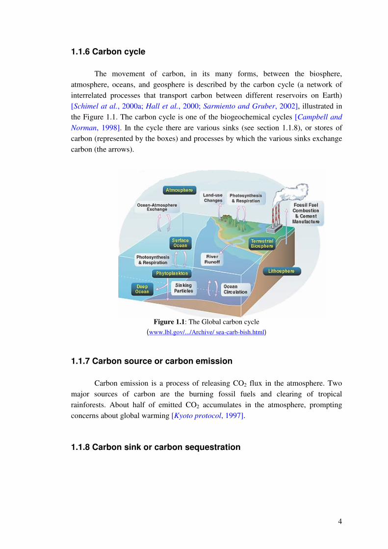
1.1.6 Carbon cycle
The movement of carbon, in its many forms, between the biosphere,
atmosphere, oceans, and geosphere is described by the carbon cycle (a network of
interrelated processes that transport carbon between different reservoirs on Earth)
[Schimel at al., 2000a; Hall et al., 2000; Sarmiento and Gruber, 2002], illustrated in
the Figure 1.1. The carbon cycle is one of the biogeochemical cycles [Campbell and
Norman, 1998]. In the cycle there are various sinks (see section 1.1.8), or stores of
carbon (represented by the boxes) and processes by which the various sinks exchange
carbon (the arrows).
Figure 1.1: The Global carbon cycle
(www.lbl.gov/.../Archive/ sea-carb-bish.html)
1.1.7 Carbon source or carbon emission
Carbon emission is a process of releasing CO2 flux in the atmosphere. Two
major sources of carbon are the burning fossil fuels and clearing of tropical
rainforests. About half of emitted CO2 accumulates in the atmosphere, prompting
concerns about global warming [Kyoto protocol, 1997].
1.1.8 Carbon sink or carbon sequestration
5
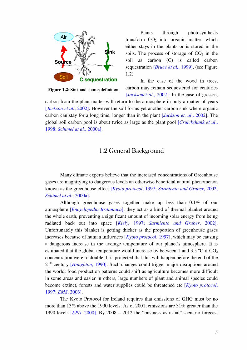
Plants through photosynthesis
transform CO2 into organic matter, which
either stays in the plants or is stored in the
soils. The process of storage of CO2 in the
soil as carbon (C) is called carbon
sequestration [Bruce et al., 1999], (see Figure
1.2).
In the case of the wood in trees,
carbon may remain sequestered for centuries
[Jacksonet al., 2002]. In the case of grasses,
carbon from the plant matter will return to the atmosphere in only a matter of years
[Jackson et al., 2002]. However the soil forms yet another carbon sink where organic
carbon can stay for a long time, longer than in the plant [Jackson et. al., 2002]. The
global soil carbon pool is about twice as large as the plant pool [Cruickshank et al.,
1998; Schimel at al., 2000a].
1.2 General Background
Many climate experts believe that the increased concentrations of Greenhouse
gases are magnifying to dangerous levels an otherwise beneficial natural phenomenon
known as the greenhouse effect [Kyoto protocol, 1997; Sarmiento and Gruber, 2002;
Schimel at al., 2000a].
Although greenhouse gases together make up less than 0.1% of our
atmosphere [Encyclopedia Britannica], they act as a kind of thermal blanket around
the whole earth, preventing a significant amount of incoming solar energy from being
radiated back out into space [Kiely, 1997; Sarmiento and Gruber, 2002].
Unfortunately this blanket is getting thicker as the proportion of greenhouse gases
increases because of human influences [Kyoto protocol, 1997], which may be causing
a dangerous increase in the average temperature of our planet’s atmosphere. It is
estimated that the global temperature would increase by between 1 and 3.5 ºC if CO2
concentration were to double. It is projected that this will happen before the end of the
21st century [Houghton, 1990]. Such changes could trigger major disruptions around
the world: food production patterns could shift as agriculture becomes more difficult
in some areas and easier in others, large numbers of plant and animal species could
become extinct, forests and water supplies could be threatened etc [Kyoto protocol,
1997; EMS, 2003].
The Kyoto Protocol for Ireland requires that emissions of GHG must be no
more than 13% above the 1990 levels. As of 2001, emissions are 31% greater than the
1990 levels [EPA, 2000]. By 2008 – 2012 the “business as usual” scenario forecast
Air
Soil
Source
Sink
C sequestrationC sequestration
Figure 1.2: Sink and source definition
Air
Soil
Source
Sink
C sequestrationC sequestration
Figure 1.2: Sink and source definition
6
(produced in 2000 based on 1998 data) is that emissions may be more than 37%
greater than the 1990 levels [EPA, 2003]. Agriculture is estimated to be responsible
for about 27% (soils 5.5%) of total emission in 2001 [EPA, 2003].
The earth’s vegetative cover is a key component in the global carbon cycle due
to its dynamic response to photosynthetic and respirative processes. The increase of
carbon emissions from fossil fuels into the atmosphere as well as deforestation
processes during the last century are accountable for most of the estimated 0.4 %
annual increase in concentration of atmospheric CO2 [IPCC, 1997; McGettigan and
Duffy, 2000]. Oceanic and forestry ecosystems have been studied in much detail
because of their significant carbon sink attributes [e.g., Post et al., 1990; Cruickshank
et al., 1998; Valentini et al., 2000; Berbigier et al., 2001; Falge et al., 2002]. Studies
of carbon fluxes in temperate grassland have been overlooked due to the perception
that this ecosystem is in equilibrium with regard to carbon fluxes [Hall et al., 2000;
Ham and Knapp, 1998; Hunt et al., 2002]. However, representing 32 % of earth’s
natural vegetation, the carbon fluxes of grasslands are now being revisited [Saigusa et
al., 1998; Frank and Dugas, 2001; Hunt et al., 2002; Jackson et al., 2002; Novick et
al., 2004] and may yet play a role in the missing global carbon sink [Ham & Knapp,
1998; Robert, 2001; Pacala et al., 2001; Goodale and Davidson, 2002] of the global
carbon balance. Grasslands are the dominant ecosystem in Ireland representing 45%
of the total landmass (with 26% for mountains and lakes, 17% for peat lands, 7% for
forests and only 5% for cultivated fields) [Gardiner and Radcliffe, 1980].
Several short-term studies have shown that grassland ecosystem can sequester
atmospheric CO2 [e.g. Bruce et al., 1999; Batjes, 1999; Conant et al., 2001; Soussana
et al., 2003], but few multi-annual data sets are available [Frank et al., 2001; Frank
and Dugas, 2001; Falge et al., 2002; Knapp et al., 2002; Novick et al., 2004]. To
quantify the source-sink potential of grasslands in different climatic zones, long-term
surface flux measurements are required [Goulden et al., 1996; Ham and Knapp, 1998;
Knapp et al., 2002; Baldocchi, 2003] to build and test models that represent the
biological and physical processes at the land surface interface. Such models (e.g.
BIOME3, Pnet, PaSim, Canveg) [Aber and Federer, 1992; Wilkinson and Janssen,
2001; Soussana et al., 2003] can be used to examine scenarios of changing land use
and management practices as well as climate change.
Many atmospheric, hydrological and biogeochemical processes are influenced
by the partitioning of available energy into the fluxes of sensible and latent heat from
the land surface [Humphreys et al., 2003]. A better understanding of how energy and
mass are partitioned at the earth’s surface is necessary for improving regional weather
and global climate models [Twine et al., 2000; Humphreys et al., 2003]. These models
are used to assess the impact of societal choices, such as abiding by the Kyoto
Protocol for carbon sequestration. Based on numerous measurements, carbon dioxide
fluxes which are measured by eddy covariance, are underestimated by the same factor
as eddy covariance evaporation measurements when energy balance closure is not
achieved [Twine et al., 2000; Wever, et al., 2002]. Therefore, dealing with lack of
7
energy balance closure should be also considered in the standards for a long term, flux
measurement networks even though it has received little attention so far [Baldocchi et
al., 1996; Twine et al., 2000].
1.3 Methods
The Dripsey flux site in Cork, Southwest Ireland, is a perennial ryegrass (C3
category) pasture, very typical of the vegetation of this part of the country, and is
grazed for approximately 8 months of the year. The lands are fertilised with
approximately 300kg/ha.year of nitrogen. The flux tower monitoring CO2, water
vapour and energy was established in June 2001 and we have continuous data since
then. The site also includes streamflow hydrology and stream water chemistry. We
present the results and analysis for CO2 for the years 2002 and 2003.The climate is
temperate with a small range of temperature during the year and abundant
precipitation. Several methods can be used to measure CO2 fluxes. Here, CO2 and
H2O fluxes between the ecosystem and the atmosphere as well as other
meteorological data were recorded continuously at 30 minutes intervals by an
aerodynamic method (Eddy Covariance method) over two years. No device has been
set up to measure specific soil respiration and LAI (Leaf Area Index). Once collected,
data were filtered and filled when found inadequate or suspect, as it is generally the
case with tower-based flux measurements.
Two different semi-empirical models were tested in comparison with the
measurements. The first is a model proposed by Collatz et al [1991] that considers the
full biochemical components of photosynthetic carbon assimilation from Farquhar et
al. [1980], and an empirical model of stomata conductance from Ball et al. [1987].
The second is a model proposed by Jacobs [1994], which is less demanding in terms
of inputs parameter and often linked with meteorological research [Calvet et al.,
1998]. It is based on the empirical model of stomatal conductance from Jarvis [1976],
and on a less detailed assimilation model from Goudriaan et al. [1985].
This work is part of a five-year (2002-2006) research project funded by the
Irish Environmental Protection Agency.
1.3 Objectives
The objective of the project was to determine the energy and CO2 fluxes over
two years (2002 and 2003) using an eddy covariance (EC) system to measure CO2 and
water vapour fluxes in a humid temperate grassland ecosystem in Ireland. The central
to this objective is investigation of seasonal, annual and interannual variation in
8
terrestrial (grassland ecosystem) CO2 and energy fluxes and to determine possible
meteorological and phonological controls on net CO2 and energy exchange. Long-
term measurements of this kind are essential for examining the seasonal and
interannual variability of carbon fluxes [Goulden et al., 1996; Baldocchi, 2003].
Another aim of this project was to study the interannual variability of CO2 flux
relative to the climatic and agricultural forcing.
The modelling part of this work is just the first step of what could be achieved
with such a tool. In this study, the models help to get a better understanding of
processes at work, and try to give a faithful description of the reality. The comparison
of two models is a good method to understand the most adapted description, and the
level of complexity needed to fit CO2 fluctuations.
1.4 Layout of thesis
Chapter 2 describes studied site and instruments used in experiment.
Chapter 3 describes eddy covariance method used for measuring CO2 and water
vapour fluxes.
Chapter 4 analyses the meteorological data measurements.
Chapter 5 provides estimates of the energy fluxes, energy balance closure and
evapotranspiration.
Chapter 6 contains a discussion and analysis of CO2 flux during two year
studies.
Chapter 7 contains modelling of CO2 flux using Jacobs’s (A-gs) and Collatz’s
models.
Chapter 8 presents the conclusions and recommendations and makes suggestions
for continuing research.
The Appendices include Hsieh’s model matlab codes, Penman-Monteith
equation matlab codes, Priestley-Taylor equation matlab codes, contribution of Webb
correction to CO2 flux, Daytime fitting for 2002 and 2003, parameters for CO2 flux
modelling, analyses of measurements of CO2 and energy fluxes for Wexford
grassland during 2003, and complementary production.

Chapter 2 Data Collection

Chapter 2 Data collection
10
Chapter 2Chapter 2Chapter 2Chapter 2 Data collection Data collection Data collection Data collection
2.1 Site description
2.1.1 Location
The Dripsey experimental grassland is located near the town of Donoughmore,
Co Cork in South West Ireland, 25 km northwest of Cork city (52º North latitude, 8º
30’ West longitude), (see Figure 2.1).
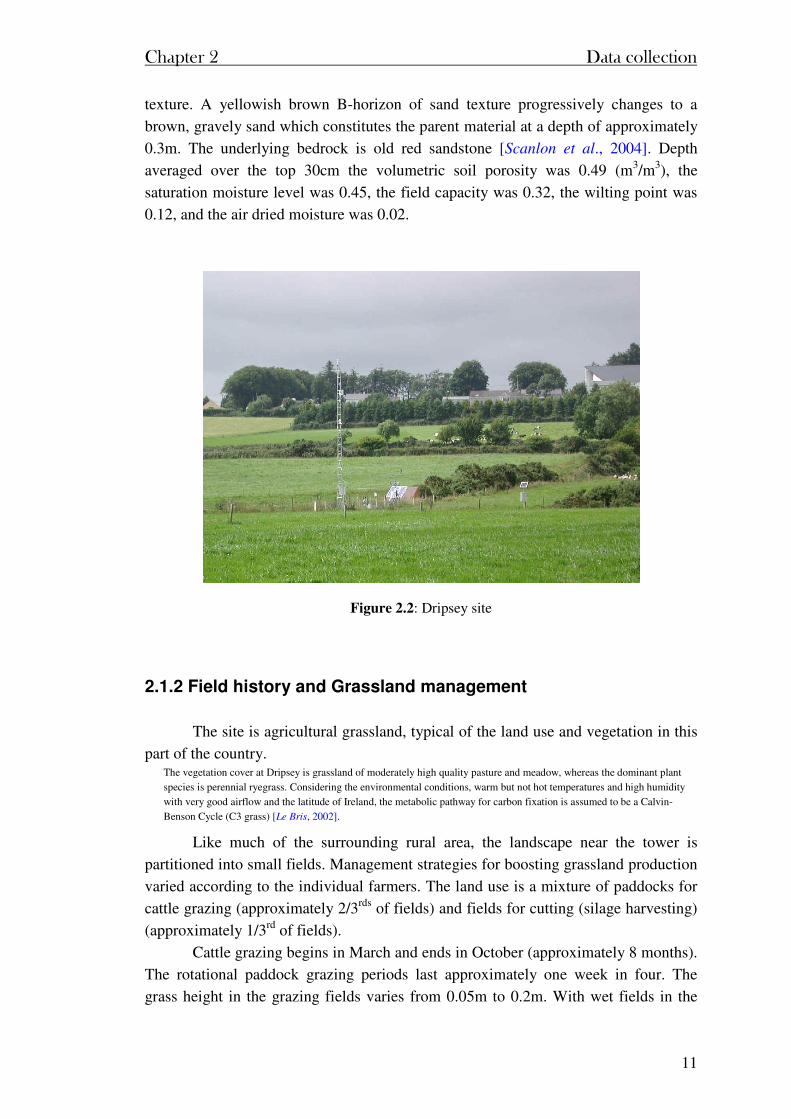
The Dripsey grassland at an elevation of 220 m above sea level has a gentle
slope to a stream of 3% grade (see Figure 2.2). The soil is classified as brown-grey
podzols [Daly, 1999]. The topsoil is rich in organic matter to a depth of about 15cm
(about 12% organic matter, [Daly, 1999]), overlying a dark brown B-horizon of sand
Figure 2.1: Location of the site area
Chapter 2 Data collection
11
texture. A yellowish brown B-horizon of sand texture progressively changes to a
brown, gravely sand which constitutes the parent material at a depth of approximately
0.3m. The underlying bedrock is old red sandstone [Scanlon et al., 2004]. Depth
averaged over the top 30cm the volumetric soil porosity was 0.49 (m3/m3), the
saturation moisture level was 0.45, the field capacity was 0.32, the wilting point was
0.12, and the air dried moisture was 0.02.
Figure 2.2: Dripsey site
2.1.2 Field history and Grassland management
The site is agricultural grassland, typical of the land use and vegetation in this
part of the country. The vegetation cover at Dripsey is grassland of moderately high quality pasture and meadow, whereas the dominant plant
species is perennial ryegrass. Considering the environmental conditions, warm but not hot temperatures and high humidity
with very good airflow and the latitude of Ireland, the metabolic pathway for carbon fixation is assumed to be a Calvin-
Benson Cycle (C3 grass) [Le Bris, 2002].
Like much of the surrounding rural area, the landscape near the tower is
partitioned into small fields. Management strategies for boosting grassland production
varied according to the individual farmers. The land use is a mixture of paddocks for
cattle grazing (approximately 2/3rds of fields) and fields for cutting (silage harvesting)
(approximately 1/3rd of fields).
Cattle grazing begins in March and ends in October (approximately 8 months).
The rotational paddock grazing periods last approximately one week in four. The
grass height in the grazing fields varies from 0.05m to 0.2m. With wet fields in the
Chapter 2 Data collection
12
autumn of 2002, cattle were not grazing (as cattle damage the fields in wet times) but
were housed indoors from early October leaving the standing biomass to its own
devices. By contrast, the autumn of 2003 was dry and cattle were grazing (at least
during the day) up to December.
Livestock density at the site is 2.2 LU/ha [Lewis, 2003], where Livestock
Units (LU) is the basis of comparison for different classes and species of stock. A
dairy caw is taken as the basic grazing livestock unit (1 LU) that requires
approximately 520 kg of good quality pasture dry matter per year.
In the cut fields the grass is harvested in the summer, first in May or June and
second time in September, and exported as silage from the pastureland for winter
feed. For the two years of the study, the first annual cutting was in July of 2002 and
June of 2003. The height of grass just before cutting in silage fields reaches about 0.5
m in summer, whereas it is down to 0.15 m in wintertime during the resting period.
Due to the mild climatic conditions the field stays green all year. No measurement of
the biomass or of the Leaf Area Index (LAI) of grass has been made on this site. The
annual yield of silage in the region has been 8 to 12 Tonnes of dry matter per hectare
per year depending on the weather. The dry matter is composed of 46% carbon
(Kiely, Teagasc, personal communication).
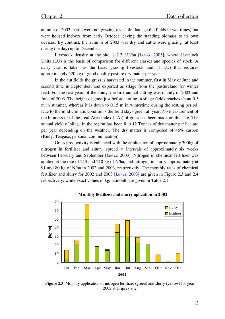
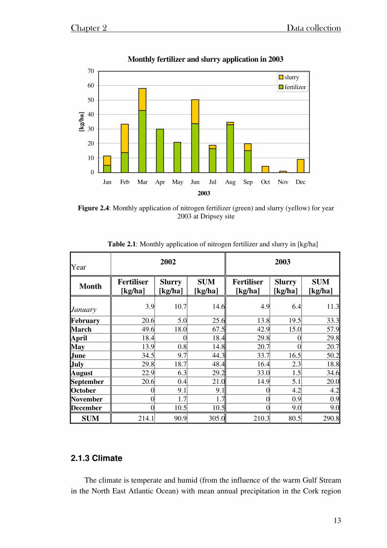
Grass productivity is enhanced with the application of approximately 300kg of
nitrogen in fertiliser and slurry, spread at intervals of approximately six weeks
between February and September [Lewis, 2003]. Nitrogen in chemical fertilizer was
applied at the rate of 214 and 210 kg of N/ha, and nitrogen in slurry approximately at
91 and 80 kg of N/ha in 2002 and 2003, respectively. The monthly rates of chemical
fertilizer and slurry for 2002 and 2003 [Lewis, 2003] are given in Figure 2.3 and 2.4
respectively, while exact values in kg/ha.month are given in Table 2.1.
Monthly fertilizer and slurry aplication in 2002
0
10
20
30
40
50
60
70
Jan Feb Mar Apr May Jun Jul Aug Sep Oct Nov Dec
2002
[kg
/ha]
slurry
fertilizer
Figure 2.3: Monthly application of nitrogen fertilizer (green) and slurry (yellow) for year
2002 at Dripsey site
Chapter 2 Data collection
13
Monthly fertilizer and slurry application in 2003
0
10
20
30
40
50
60
70
Jan Feb Mar Apr May Jun Jul Aug Sep Oct Nov Dec
2003
[kg/h
a]
slurry
fertilizer
Figure 2.4: Monthly application of nitrogen fertilizer (green) and slurry (yellow) for year 2003 at Dripsey site
Table 2.1: Monthly application of nitrogen fertilizer and slurry in [kg/ha]
2.1.3 Climate
The climate is temperate and humid (from the influence of the warm Gulf Stream
in the North East Atlantic Ocean) with mean annual precipitation in the Cork region
Year 2002
2003
Month Fertiliser
[kg/ha]
Slurry
[kg/ha]
SUM
[kg/ha]
Fertiliser
[kg/ha]
Slurry
[kg/ha]
SUM
[kg/ha]
January 3.9 10.7 14.6 4.9 6.4 11.3
February 20.6 5.0 25.6 13.8 19.5 33.3March 49.6 18.0 67.5 42.9 15.0 57.9April 18.4 0 18.4 29.8 0 29.8May 13.9 0.8 14.8 20.7 0 20.7June 34.5 9.7 44.3 33.7 16.5 50.2July 29.8 18.7 48.4 16.4 2.3 18.8August 22.9 6.3 29.2 33.0 1.5 34.6September 20.6 0.4 21.0 14.9 5.1 20.0October 0 9.1 9.1 0 4.2 4.2November 0 1.7 1.7 0 0.9 0.9December 0 10.5 10.5 0 9.0 9.0
SUM 214.1 90.9 305.0 210.3 80.5 290.8
Chapter 2 Data collection
14
of about 1200 mm. The rainfall regime is characterized by long duration events of low
intensity (values up to 40 mm/day). Short duration events of high intensity are more
seldom and occur in summer.
Daily air temperatures have a very small range of variation during the year, going
from a maximum of 20ºC to a minimum of 0ºC, with an average of 15ºC in summer
and 5ºC in winter. This part of Ireland is windy with a mean wind velocity of 4 m/s at
the site with peaks up to 16 m/s. The main wind comes from the southwest.
2.2 Description of instruments
The flux tower monitoring carbon dioxide, water vapour and energy was established in June 2001 and we have continuous
data since then. The site also includes streamflow hydrology and stream water chemistry. In this section we present an
overview of the sensors and techniques used for data collection.
2.2.1 Weather station
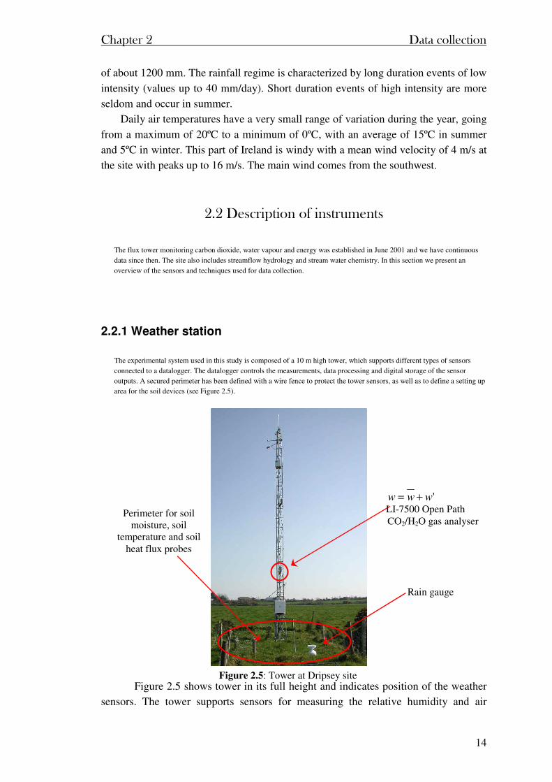
The experimental system used in this study is composed of a 10 m high tower, which supports different types of sensors
connected to a datalogger. The datalogger controls the measurements, data processing and digital storage of the sensor
outputs. A secured perimeter has been defined with a wire fence to protect the tower sensors, as well as to define a setting up
area for the soil devices (see Figure 2.5).
Figure 2.5 shows tower in its full height and indicates position of the weather
sensors. The tower supports sensors for measuring the relative humidity and air
'www += LI-7500 Open Path CO2/H2O gas analyser
Rain gauge
Perimeter for soil moisture, soil
temperature and soil heat flux probes
Figure 2.5: Tower at Dripsey site
Chapter 2 Data collection
15
temperature at 3 m and various types of sensors at 10 m (see Figure 2.6). The rain
gauge is located on the ground, while the soil moisture, soil heat flux plates and soil
temperature probes are underground near the tower. The white box near the foot of the
tower is called ‘Campbell environmental box’ and houses the datalogger, the
multiplexer, the barometric pressure sensor, as well as a modem connection.
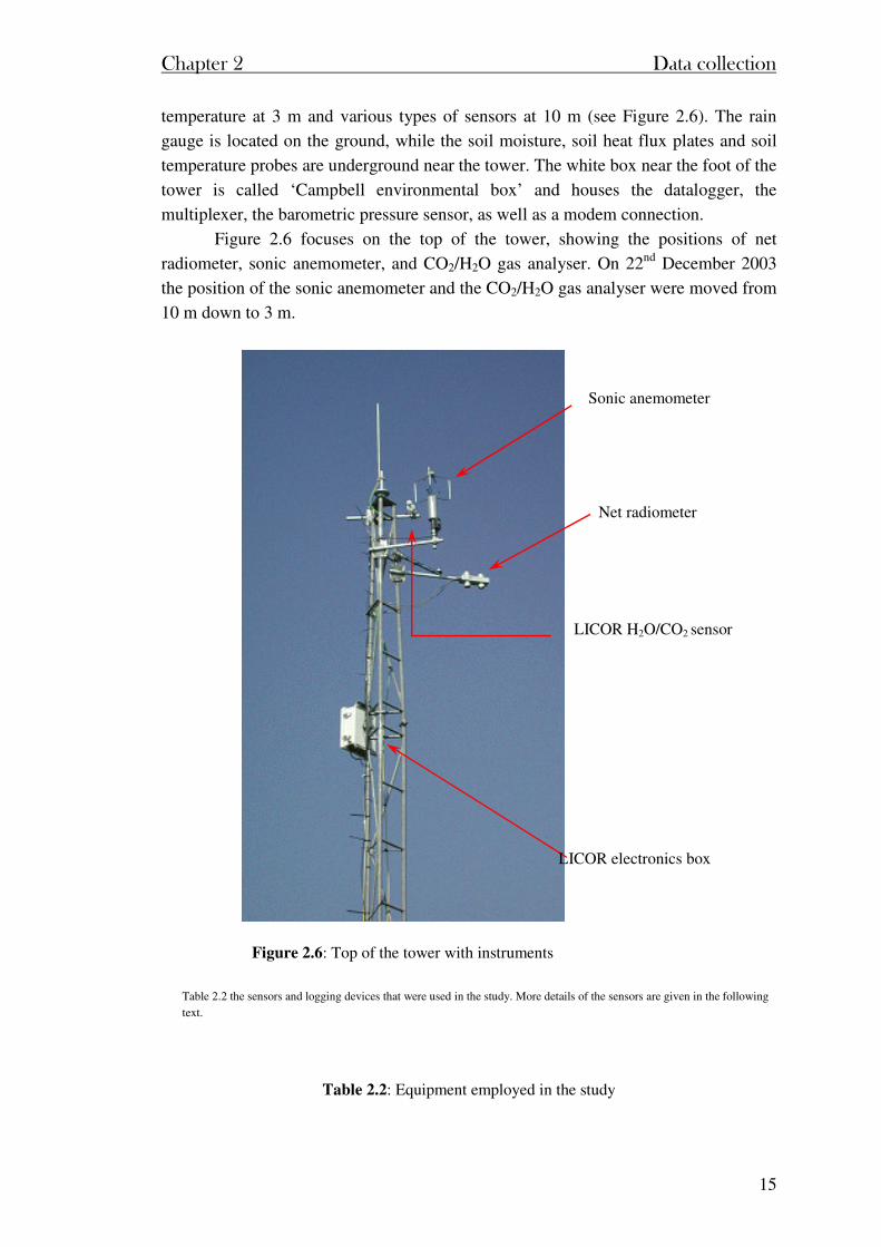
Figure 2.6 focuses on the top of the tower, showing the positions of net
radiometer, sonic anemometer, and CO2/H2O gas analyser. On 22nd December 2003
the position of the sonic anemometer and the CO2/H2O gas analyser were moved from
10 m down to 3 m.
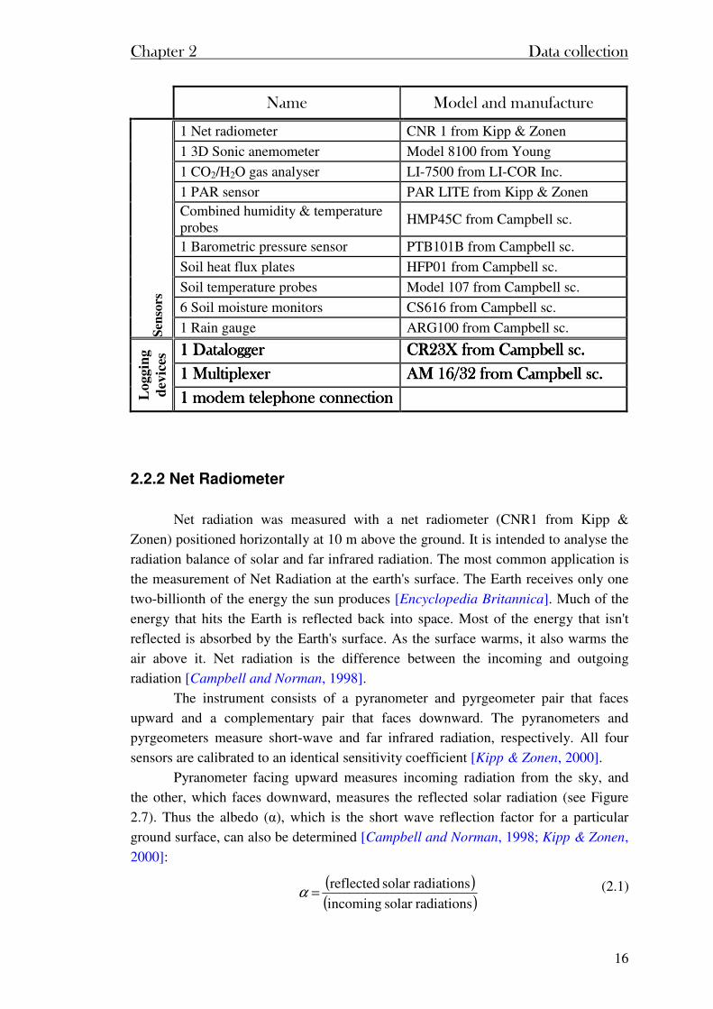
Table 2.2 the sensors and logging devices that were used in the study. More details of the sensors are given in the following
text.
Table 2.2: Equipment employed in the study
Figure 2.6: Top of the tower with instruments
Sonic anemometer
Net radiometer
LICOR electronics box
LICOR H2O/CO2 sensor
Chapter 2 Data collection
16
Name Model and manufacture
1 Net radiometer CNR 1 from Kipp & Zonen
1 3D Sonic anemometer Model 8100 from Young
1 CO2/H2O gas analyser LI-7500 from LI-COR Inc.
1 PAR sensor PAR LITE from Kipp & Zonen
Combined humidity & temperature probes
HMP45C from Campbell sc.
1 Barometric pressure sensor PTB101B from Campbell sc.
Soil heat flux plates HFP01 from Campbell sc.
Soil temperature probes Model 107 from Campbell sc.
6 Soil moisture monitors CS616 from Campbell sc.
Sen
sors
1 Rain gauge ARG100 from Campbell sc.
1 Datalogger1 Datalogger1 Datalogger1 Datalogger CR23X from Campbell sc.CR23X from Campbell sc.CR23X from Campbell sc.CR23X from Campbell sc.
1 Multiplexer1 Multiplexer1 Multiplexer1 Multiplexer AM 16/32 from Campbell AM 16/32 from Campbell AM 16/32 from Campbell AM 16/32 from Campbell sc.sc.sc.sc.
Lo
gg
ing
dev
ices
1 modem telephone connection1 modem telephone connection1 modem telephone connection1 modem telephone connection
2.2.2 Net Radiometer
Net radiation was measured with a net radiometer (CNR1 from Kipp &
Zonen) positioned horizontally at 10 m above the ground. It is intended to analyse the
radiation balance of solar and far infrared radiation. The most common application is
the measurement of Net Radiation at the earth's surface. The Earth receives only one
two-billionth of the energy the sun produces [Encyclopedia Britannica]. Much of the
energy that hits the Earth is reflected back into space. Most of the energy that isn't
reflected is absorbed by the Earth's surface. As the surface warms, it also warms the
air above it. Net radiation is the difference between the incoming and outgoing
radiation [Campbell and Norman, 1998].
The instrument consists of a pyranometer and pyrgeometer pair that faces
upward and a complementary pair that faces downward. The pyranometers and
pyrgeometers measure short-wave and far infrared radiation, respectively. All four
sensors are calibrated to an identical sensitivity coefficient [Kipp & Zonen, 2000].
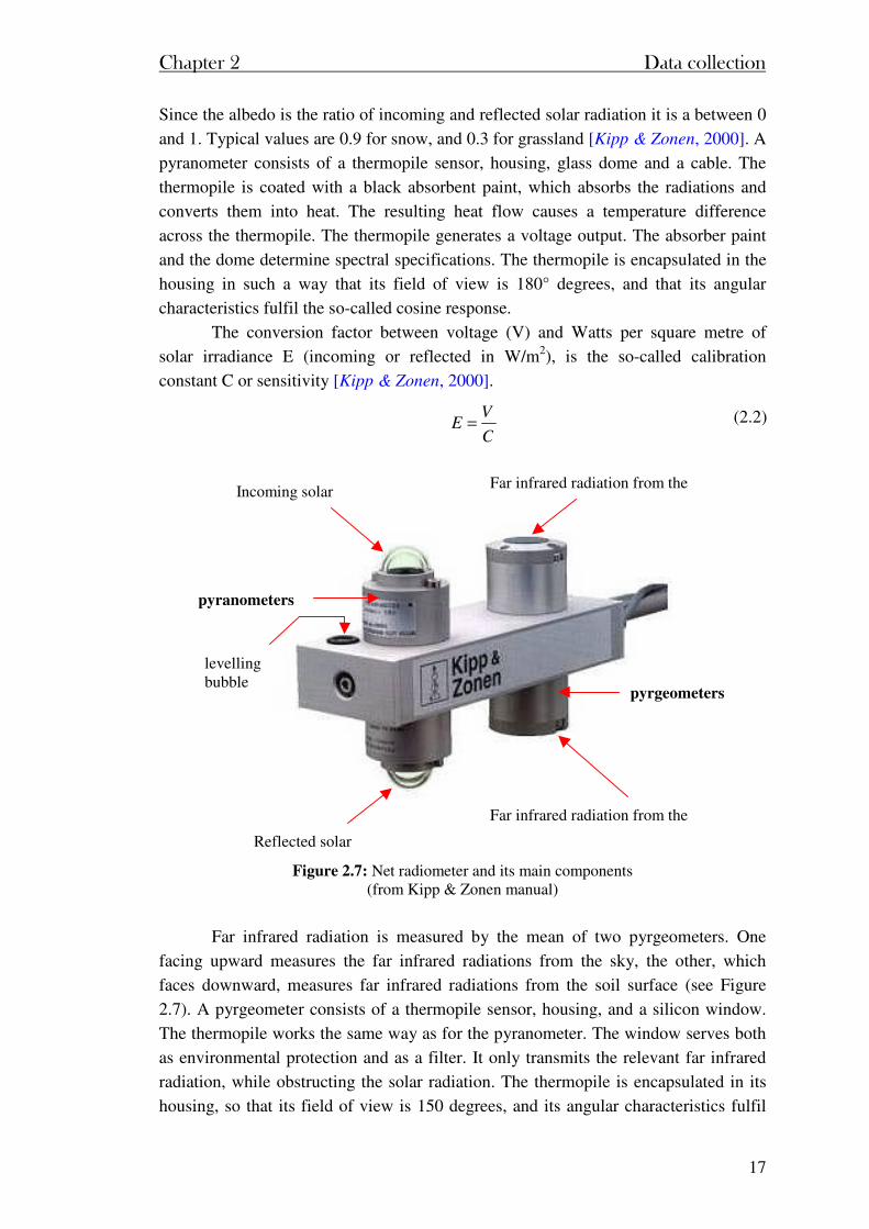
Pyranometer facing upward measures incoming radiation from the sky, and
the other, which faces downward, measures the reflected solar radiation (see Figure
2.7). Thus the albedo (α), which is the short wave reflection factor for a particular
ground surface, can also be determined [Campbell and Norman, 1998; Kipp & Zonen,
2000]:
( )( )radiationssolar incoming
radiationssolar reflected =α (2.1)
Chapter 2 Data collection
17
Since the albedo is the ratio of incoming and reflected solar radiation it is a between 0
and 1. Typical values are 0.9 for snow, and 0.3 for grassland [Kipp & Zonen, 2000]. A
pyranometer consists of a thermopile sensor, housing, glass dome and a cable. The
thermopile is coated with a black absorbent paint, which absorbs the radiations and
converts them into heat. The resulting heat flow causes a temperature difference
across the thermopile. The thermopile generates a voltage output. The absorber paint
and the dome determine spectral specifications. The thermopile is encapsulated in the
housing in such a way that its field of view is 180° degrees, and that its angular
characteristics fulfil the so-called cosine response.
The conversion factor between voltage (V) and Watts per square metre of
solar irradiance E (incoming or reflected in W/m2), is the so-called calibration
constant C or sensitivity [Kipp & Zonen, 2000].
Incoming solar radiation
Far infrared radiation from the sky
Reflected solar radiation
Far infrared radiation from the ground
pyranometers
pyrgeometers
levelling bubble
Figure 2.7: Net radiometer and its main components
(from Kipp & Zonen manual)
Far infrared radiation is measured by the mean of two pyrgeometers. One
facing upward measures the far infrared radiations from the sky, the other, which
faces downward, measures far infrared radiations from the soil surface (see Figure
2.7). A pyrgeometer consists of a thermopile sensor, housing, and a silicon window.
The thermopile works the same way as for the pyranometer. The window serves both
as environmental protection and as a filter. It only transmits the relevant far infrared
radiation, while obstructing the solar radiation. The thermopile is encapsulated in its
housing, so that its field of view is 150 degrees, and its angular characteristics fulfil
C
VE = (2.2)
Chapter 2 Data collection
18
the so-called cosine response as much as possible, in this field of view. The limited
field of view does not produce a large error because the missing part of the field of
view does not contribute significantly to the total, and is compensated for during
calibration [Kipp & Zonen, 2000]. The pyrgeometer temperature (T) in º K is needed
for estimating the far infrared radiation from the voltage (V). Hence, a temperature
sensor is located in the net radiometer body. The calculation of far infrared irradiance
(E) in W/m2 is given hereunder [Kipp & Zonen, 2000]:
481067.5 TC
VE ××+= − (2.3)
The calculation of the net total radiation (Rn) is performed automatically by the
instrument’s [Kipp & Zonen, 2000] user’s own processing software and is thus given
in as an output in W/m2:
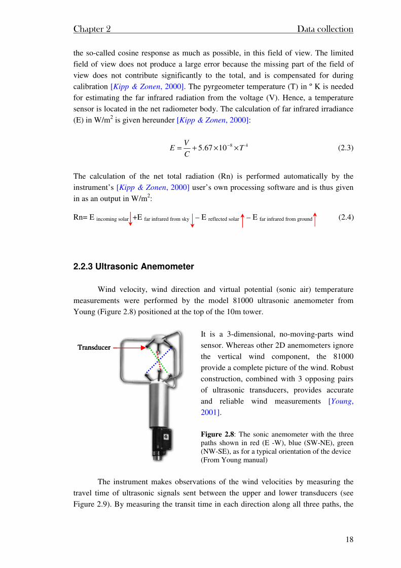
2.2.3 Ultrasonic Anemometer
Wind velocity, wind direction and virtual potential (sonic air) temperature
measurements were performed by the model 81000 ultrasonic anemometer from
Young (Figure 2.8) positioned at the top of the 10m tower.
It is a 3-dimensional, no-moving-parts wind
sensor. Whereas other 2D anemometers ignore
the vertical wind component, the 81000
provide a complete picture of the wind. Robust
construction, combined with 3 opposing pairs
of ultrasonic transducers, provides accurate
and reliable wind measurements [Young,
2001].
Figure 2.8: The sonic anemometer with the three paths shown in red (E -W), blue (SW-NE), green (NW-SE), as for a typical orientation of the device (From Young manual)
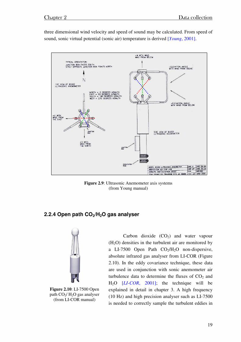
The instrument makes observations of the wind velocities by measuring the
travel time of ultrasonic signals sent between the upper and lower transducers (see
Figure 2.9). By measuring the transit time in each direction along all three paths, the
Rn= E incoming solar +E far infrared from sky – E reflected solar – E far infrared from ground (2.4)
TransducerTransducerTransducer
Chapter 2 Data collection
19
three dimensional wind velocity and speed of sound may be calculated. From speed of
sound, sonic virtual potential (sonic air) temperature is derived [Young, 2001].
Figure 2.9: Ultrasonic Anemometer axis systems (from Young manual)
2.2.4 Open path CO2/H2O gas analyser
Carbon dioxide (CO2) and water vapour
(H2O) densities in the turbulent air are monitored by
a LI-7500 Open Path CO2/H2O non-dispersive,
absolute infrared gas analyser from LI-COR (Figure
2.10). In the eddy covariance technique, these data
are used in conjunction with sonic anemometer air
turbulence data to determine the fluxes of CO2 and
H2O [LI-COR, 2001]; the technique will be
explained in detail in chapter 3. A high frequency
(10 Hz) and high precision analyser such as LI-7500
is needed to correctly sample the turbulent eddies in
Figure 2.10: LI-7500 Open path CO2/ H2O gas analyser
(from LI-COR manual)
Chapter 2 Data collection
20
the lower boundary layer [Garratt, 1992]. The sensor head has a smooth,
aerodynamic profile, in order to minimize flow disturbance.
The open path analyser eliminates time delays, pressure drops, and
sorption/desorption of water vapour on tubing employed with a closed path analyser
[LI-COR, 2001]. The LI-7500 is placed within about 20 cm of the centroid of the air
volume measured by the sonic anemometer.
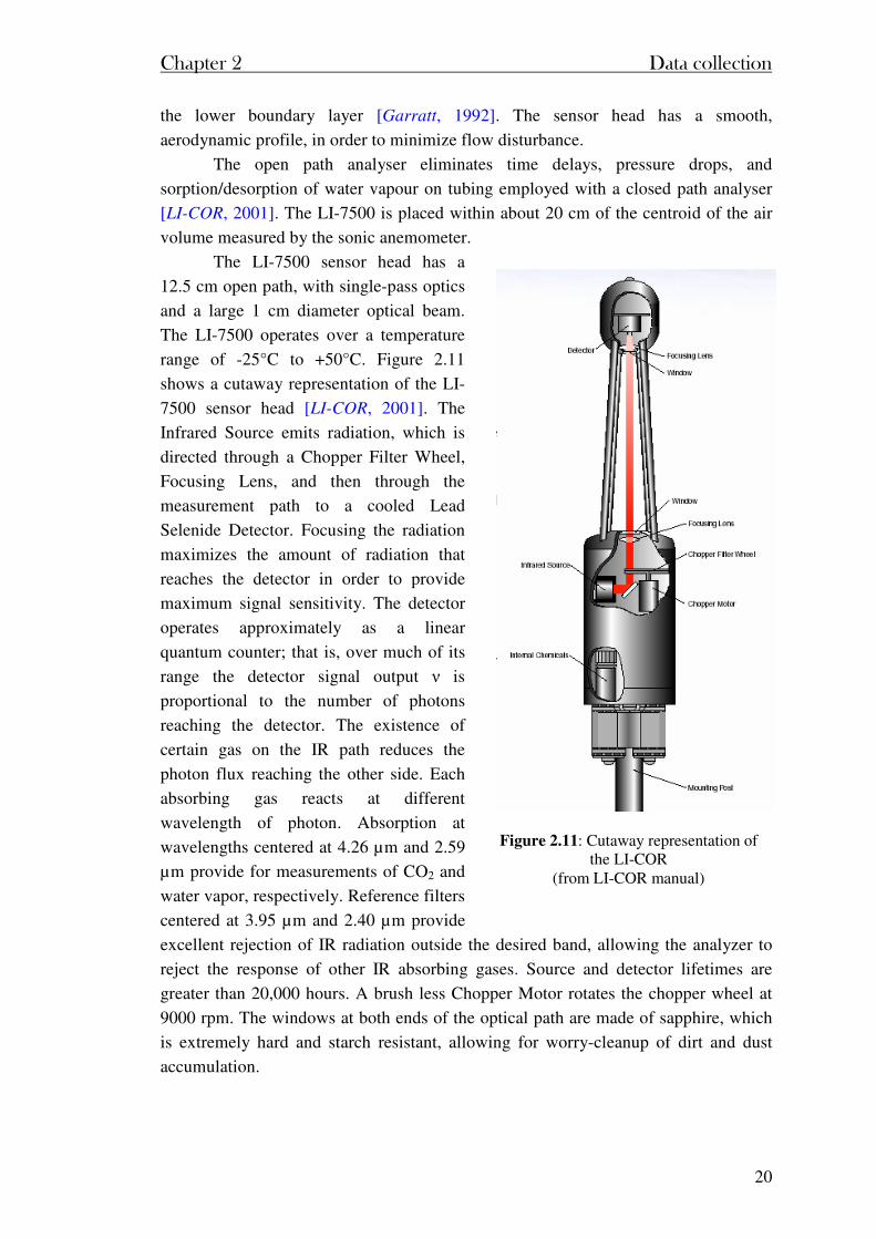
The LI-7500 sensor head has a
12.5 cm open path, with single-pass optics
and a large 1 cm diameter optical beam.
The LI-7500 operates over a temperature
range of -25°C to +50°C. Figure 2.11
shows a cutaway representation of the LI-
7500 sensor head [LI-COR, 2001]. The
Infrared Source emits radiation, which is
directed through a Chopper Filter Wheel,
Focusing Lens, and then through the
measurement path to a cooled Lead
Selenide Detector. Focusing the radiation
maximizes the amount of radiation that
reaches the detector in order to provide
maximum signal sensitivity. The detector
operates approximately as a linear
quantum counter; that is, over much of its
range the detector signal output ν is
proportional to the number of photons
reaching the detector. The existence of
certain gas on the IR path reduces the
photon flux reaching the other side. Each
absorbing gas reacts at different
wavelength of photon. Absorption at
wavelengths centered at 4.26 µm and 2.59
µm provide for measurements of CO2 and
water vapor, respectively. Reference filters
centered at 3.95 µm and 2.40 µm provide
excellent rejection of IR radiation outside the desired band, allowing the analyzer to
reject the response of other IR absorbing gases. Source and detector lifetimes are
greater than 20,000 hours. A brush less Chopper Motor rotates the chopper wheel at
9000 rpm. The windows at both ends of the optical path are made of sapphire, which
is extremely hard and starch resistant, allowing for worry-cleanup of dirt and dust
accumulation.
Figure 2.11: Cutaway representation of the LI-COR
(from LI-COR manual)
Chapter 2 Data collection
21
2.2.5 PAR (Photosynthetic Active Radiation) sensor
The photosynthetic photon flux or PAR can be easily calculated with the
incoming solar radiations, given some approximations [Campbell and Norman, 1998]:
the energy content of photons is the same for all wave lengths. It is equal to
the energy content of photons at the mean wavelength of the spectrum (green,
0.55µm) that is 3.6 10-19 J/photon (=0.217 J/µmol).
about 45% of the incoming solar radiations are in the PAR wave length.
Then,
( )
×=
×=
×=
sm
molµ
J
molµ
m
W
217.0
E45.022
gsolarmininco
PARQ (2.6)
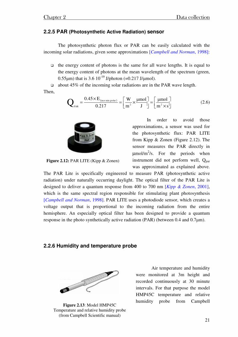
In order to avoid those
approximations, a sensor was used for
the photosynthetic flux: PAR LITE
from Kipp & Zonen (Figure 2.12). The
sensor measures the PAR directly in
µmol/m2/s. For the periods when
instrument did not perform well, Qpar
was approximated as explained above.
The PAR Lite is specifically engineered to measure PAR (photosynthetic active
radiation) under naturally occurring daylight. The optical filter of the PAR Lite is
designed to deliver a quantum response from 400 to 700 nm [Kipp & Zonen, 2001],
which is the same spectral region responsible for stimulating plant photosynthesis
[Campbell and Norman, 1998]. PAR LITE uses a photodiode sensor, which creates a
voltage output that is proportional to the incoming radiation from the entire
hemisphere. An especially optical filter has been designed to provide a quantum
response in the photo synthetically active radiation (PAR) (between 0.4 and 0.7µm).
2.2.6 Humidity and temperature probe
Air temperature and humidity
were monitored at 3m height and
recorded continuously at 30 minute
intervals. For that purpose the model
HMP45C temperature and relative
humidity probe from Campbell
Figure 2.12: PAR LITE (Kipp & Zonen)
Figure 2.13: Model HMP45C Temperature and relative humidity probe
(from Campbell Scientific manual)
Chapter 2 Data collection
22
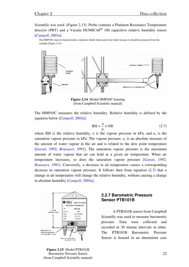
Scientific was used. (Figure 2.13). Probe contains a Platinum Resistance Temperature
detector (PRT) and a Vaisala HUMICAP® 180 capacitive relative humidity sensor
[Campell, 2003a]. The HMP45C must be housed inside a radiation shield when used in the fields because it should be protected from the
sunlight (Figure 2.14).
The HMP45C measures the relative humidity. Relative humidity is defined by the
equation below [Campell, 2003a]:
100e
eRH
s
×= (2.7)
where RH is the relative humidity, e is the vapour pressure in kPa, and es is the
saturation vapour pressure in kPa. The vapour pressure, e, is an absolute measure of
the amount of water vapour in the air and is related to the dew point temperature
[Garatt, 1992; Brutsaert, 1991]. The saturation vapour pressure is the maximum
amount of water vapour that air can hold at a given air temperature. When air
temperature increases, so does the saturation vapour pressure [Garatt, 1992;
Brutsaert, 1991]. Conversely, a decrease in air temperature causes a corresponding
decrease in saturation vapour pressure. It follows then from equation (2.7) that a
change in air temperature will change the relative humidity, without causing a change
in absolute humidity [Campell, 2003a].
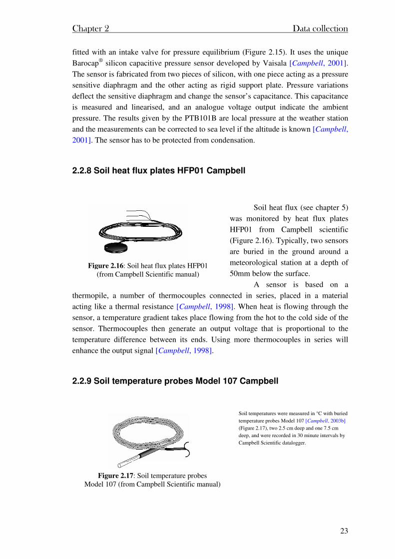
2.2.7 Barometric Pressure Sensor PTB101B
A PTB101B sensor from Campbell
Scientific was used to measure barometric
pressure. Data were collected and
recorded in 30 minute intervals in mbar.
The PTB101B Barometric Pressure
Sensor is housed in an aluminium case
Figure 2.15: Model PTB101B Barometric Pressure Sensor
(from Campbell Scientific manual)
Figure 2.14: Model HMP45C housing (from Campbell Scientific manual)
Chapter 2 Data collection
23
fitted with an intake valve for pressure equilibrium (Figure 2.15). It uses the unique
Barocap® silicon capacitive pressure sensor developed by Vaisala [Campbell, 2001].
The sensor is fabricated from two pieces of silicon, with one piece acting as a pressure
sensitive diaphragm and the other acting as rigid support plate. Pressure variations
deflect the sensitive diaphragm and change the sensor’s capacitance. This capacitance
is measured and linearised, and an analogue voltage output indicate the ambient
pressure. The results given by the PTB101B are local pressure at the weather station
and the measurements can be corrected to sea level if the altitude is known [Campbell,
2001]. The sensor has to be protected from condensation.
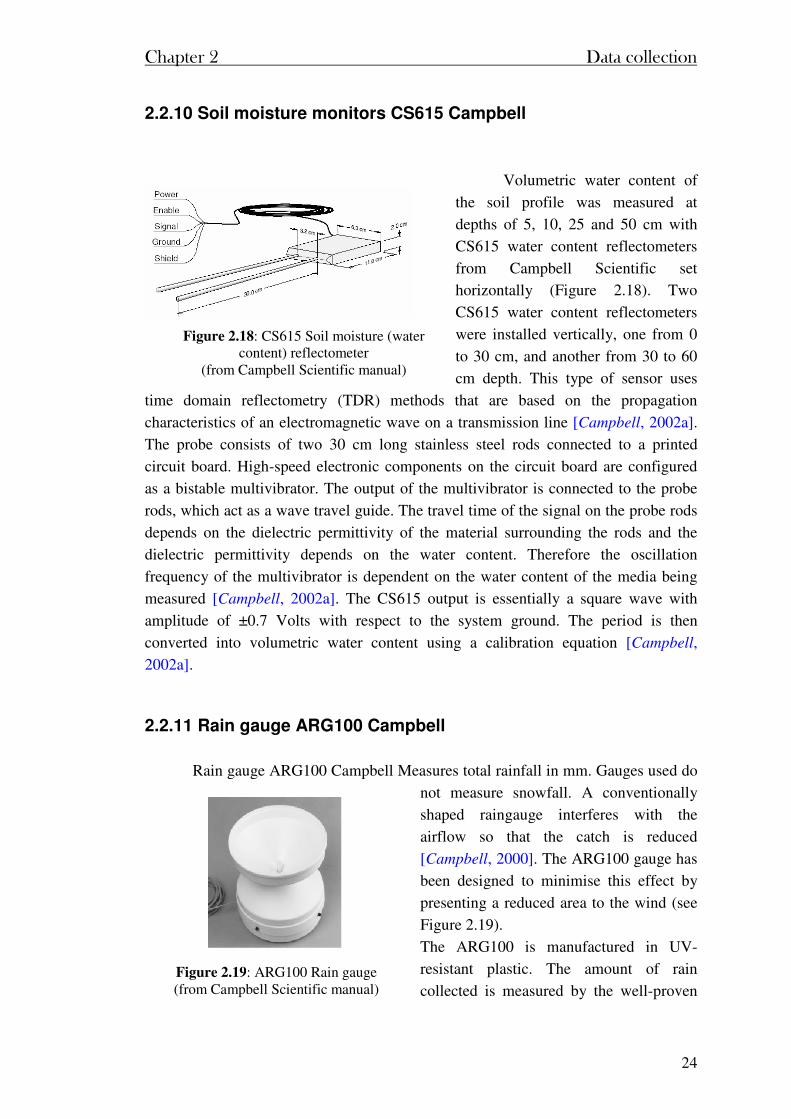
2.2.8 Soil heat flux plates HFP01 Campbell
Soil heat flux (see chapter 5)
was monitored by heat flux plates
HFP01 from Campbell scientific
(Figure 2.16). Typically, two sensors
are buried in the ground around a
meteorological station at a depth of
50mm below the surface.
A sensor is based on a
thermopile, a number of thermocouples connected in series, placed in a material
acting like a thermal resistance [Campbell, 1998]. When heat is flowing through the
sensor, a temperature gradient takes place flowing from the hot to the cold side of the
sensor. Thermocouples then generate an output voltage that is proportional to the
temperature difference between its ends. Using more thermocouples in series will
enhance the output signal [Campbell, 1998].
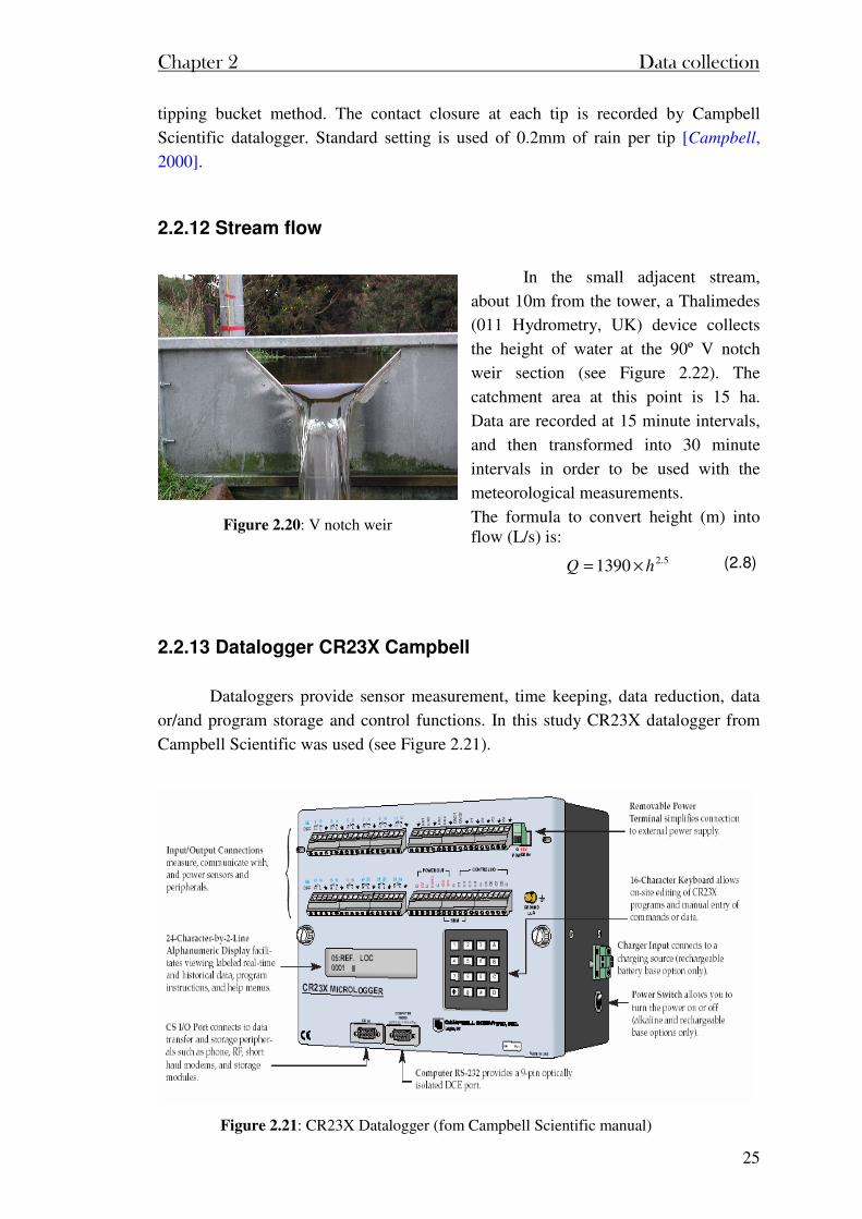
2.2.9 Soil temperature probes Model 107 Campbell
Soil temperatures were measured in °C with buried
temperature probes Model 107 [Campbell, 2003b]
(Figure 2.17), two 2.5 cm deep and one 7.5 cm
deep, and were recorded in 30 minute intervals by
Campbell Scientific datalogger.
Figure 2.16: Soil heat flux plates HFP01 (from Campbell Scientific manual)
Figure 2.17: Soil temperature probes Model 107 (from Campbell Scientific manual)
Chapter 2 Data collection
24
2.2.10 Soil moisture monitors CS615 Campbell
Volumetric water content of
the soil profile was measured at
depths of 5, 10, 25 and 50 cm with
CS615 water content reflectometers
from Campbell Scientific set
horizontally (Figure 2.18). Two
CS615 water content reflectometers
were installed vertically, one from 0
to 30 cm, and another from 30 to 60
cm depth. This type of sensor uses
time domain reflectometry (TDR) methods that are based on the propagation
characteristics of an electromagnetic wave on a transmission line [Campbell, 2002a].
The probe consists of two 30 cm long stainless steel rods connected to a printed
circuit board. High-speed electronic components on the circuit board are configured
as a bistable multivibrator. The output of the multivibrator is connected to the probe
rods, which act as a wave travel guide. The travel time of the signal on the probe rods
depends on the dielectric permittivity of the material surrounding the rods and the
dielectric permittivity depends on the water content. Therefore the oscillation
frequency of the multivibrator is dependent on the water content of the media being
measured [Campbell, 2002a]. The CS615 output is essentially a square wave with
amplitude of ±0.7 Volts with respect to the system ground. The period is then
converted into volumetric water content using a calibration equation [Campbell,
2002a].
2.2.11 Rain gauge ARG100 Campbell
Rain gauge ARG100 Campbell Measures total rainfall in mm. Gauges used do
not measure snowfall. A conventionally
shaped raingauge interferes with the
airflow so that the catch is reduced
[Campbell, 2000]. The ARG100 gauge has
been designed to minimise this effect by
presenting a reduced area to the wind (see
Figure 2.19).
The ARG100 is manufactured in UV-
resistant plastic. The amount of rain
collected is measured by the well-proven Figure 2.19: ARG100 Rain gauge (from Campbell Scientific manual)
Figure 2.18: CS615 Soil moisture (water content) reflectometer
(from Campbell Scientific manual)
Chapter 2 Data collection
25
tipping bucket method. The contact closure at each tip is recorded by Campbell
Scientific datalogger. Standard setting is used of 0.2mm of rain per tip [Campbell,
2000].
2.2.12 Stream flow
In the small adjacent stream,
about 10m from the tower, a Thalimedes
(011 Hydrometry, UK) device collects
the height of water at the 90º V notch
weir section (see Figure 2.22). The
catchment area at this point is 15 ha.
Data are recorded at 15 minute intervals,
and then transformed into 30 minute
intervals in order to be used with the
meteorological measurements.
The formula to convert height (m) into flow (L/s) is:
2.2.13 Datalogger CR23X Campbell
Dataloggers provide sensor measurement, time keeping, data reduction, data
or/and program storage and control functions. In this study CR23X datalogger from
Campbell Scientific was used (see Figure 2.21).
5.21390 hQ ×= (2.8)
Figure 2.20: V notch weir
Figure 2.21: CR23X Datalogger (fom Campbell Scientific manual)

Chapter 2 Data collection
26
2.2.14 Multiplexer AM 16/32 Campbell
Multiplexer device increases the number of sensors that
may be scanned by the dataloggers. For our needs AM
16/32 Multiplexer from Campbell Scientific was used (see
Figure 2.22).
2.2.15 Telephone connection
The weather station was connected by modem to a network, and was feeding
weather data into a retrieval system consisting of a personal computer and telephone
communications link.
Figure 2.22: AM 16/32 Multiplexer (From Campbell Scientific manual)
Chapter 3 The Eddy Covariance
Method
Chapter 3 The Eddy Covariance Method
28
Chapter 3Chapter 3Chapter 3Chapter 3 The Eddy Covariance Method The Eddy Covariance Method The Eddy Covariance Method The Eddy Covariance Method
3.1 Basic theory
The Eddy Covariance or Eddy Correlation (EC) method is a statistical tool,
used to analyse time series of Eddy high frequency wind and scalar atmospheric data
[Baldocchi, 2003], to yields values of fluxes of these properties representing quite
large areas [Campbell, 1998].
The atmosphere near the earth’s surface is almost always turbulent, and trace
gases are rapidly diffused to (or from) the surface by irregular or random motions
generated by wind shear and buoyancy forces [Dabberdt et al., 1993]. The boundary
layer defined by Garratt [1992], is the layer of air directly above the Earth’s surface in
which the effect of the surface (friction, heating and cooling) are felt directly on time
scales less than a day, and in which significant fluxes of momentum, heat or matter
are carried by turbulent motions on a scale of the order of the depth of the boundary
layer of less.
Transport in the boundary layer of heat, moisture, momentum and pollutants
are governed almost entirely by turbulence [Campbell, 1998]. Using the Reynolds
decomposition it is possible to quantify turbulent transport given a high enough
sampling rate and fast response instruments [Garatt, 1992].
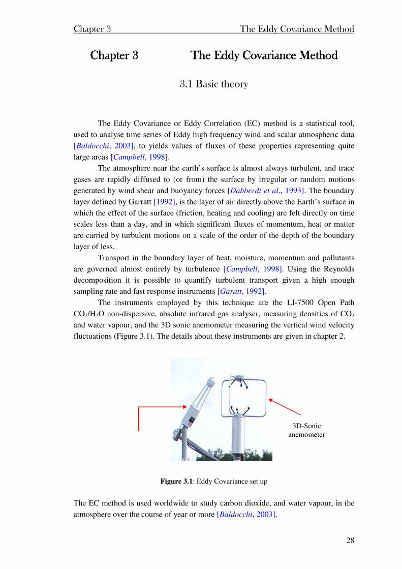
The instruments employed by this technique are the LI-7500 Open Path
CO2/H2O non-dispersive, absolute infrared gas analyser, measuring densities of CO2
and water vapour, and the 3D sonic anemometer measuring the vertical wind velocity
fluctuations (Figure 3.1). The details about these instruments are given in chapter 2.
Figure 3.1: Eddy Covariance set up
The EC method is used worldwide to study carbon dioxide, and water vapour, in the
atmosphere over the course of year or more [Baldocchi, 2003].
3D-Sonic anemometer
Chapter 3 The Eddy Covariance Method
29
3.2 Definition of flux
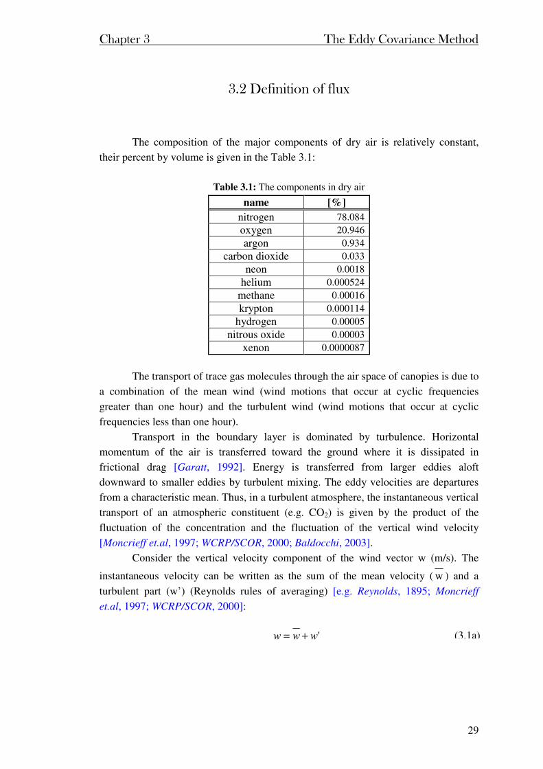
The composition of the major components of dry air is relatively constant,
their percent by volume is given in the Table 3.1:
Table 3.1: The components in dry air
name [%]
nitrogen 78.084
oxygen 20.946
argon 0.934
carbon dioxide 0.033
neon 0.0018
helium 0.000524
methane 0.00016
krypton 0.000114
hydrogen 0.00005
nitrous oxide 0.00003
xenon 0.0000087
The transport of trace gas molecules through the air space of canopies is due to
a combination of the mean wind (wind motions that occur at cyclic frequencies
greater than one hour) and the turbulent wind (wind motions that occur at cyclic
frequencies less than one hour).
Transport in the boundary layer is dominated by turbulence. Horizontal
momentum of the air is transferred toward the ground where it is dissipated in
frictional drag [Garatt, 1992]. Energy is transferred from larger eddies aloft
downward to smaller eddies by turbulent mixing. The eddy velocities are departures
from a characteristic mean. Thus, in a turbulent atmosphere, the instantaneous vertical
transport of an atmospheric constituent (e.g. CO2) is given by the product of the
fluctuation of the concentration and the fluctuation of the vertical wind velocity
[Moncrieff et.al, 1997; WCRP/SCOR, 2000; Baldocchi, 2003].
Consider the vertical velocity component of the wind vector w (m/s). The
instantaneous velocity can be written as the sum of the mean velocity ( w ) and a
turbulent part (w’) (Reynolds rules of averaging) [e.g. Reynolds, 1895; Moncrieff
et.al, 1997; WCRP/SCOR, 2000]:
'www += (3.1a)
Chapter 3 The Eddy Covariance Method
30
0''' === Tqw
The turbulent eddies from the specific humidity (q), carbon dioxide concentration
(CO2) and temperature (T) can be separated exactly in the same way [e.g. Reynolds,
1895].
In this study we are only interested in vertical fluxes. Since mean vertical wind
speeds in the boundary layer are very close to zero under most circumstances, the
vertical average value of turbulent parts is usually found to be very small. By
definition, the average value of the turbulent parts of the velocities and scalars equals
zero [Moncrieff et.al, 1997]:
(3.2)
If the site is horizontally uniform, and atmospheric conditions are assumed steady
over the averaging period (30 minutes), it is expected that: 0w = .
The measurement of a vertical flux by eddy correlation requires careful physical
alignment of the vertical velocity sensor (3D sonic anemometer) in the field and
analytical rotation of the coordinate axes during post processing of data [Dabberdt et
al., 1993]. This is necessary to avoid contamination of the vertical flux by the
streamwise flux, which is opposite in sign to the vertical flux and can be as much as
three times greater [Dabberdt et al., 1993].
In order to adjust measurements with eddy covariance basic principles, axis
rotation was performed with the raw data set [Guenther and Hills, 1998], i.e. mean
wind, its standard deviations, and all fluxes were rotated as follows:
First rotate axes so that +U is pointing north, and +V is pointing west (see
Figure 2.9 in chapter 2 for description of +U and +V).
Then rotate mean wind so that mean vertical wind velocity is set to zero.
3.2.1 Latent heat flux and sensible heat flux
The sensible heat flux H (W/m2) and the latent heat flux λE (W/m2) are not
measured directly but calculated using the eddy correlation technique with air
temperature and air specific humidity [WCRP/SCOR, 2000; Wever et al., 2002].
The product of the vertical wind speed w (m/s), and the density of moist air ρa
(kg/m3), is the mass flux of moist air, ρaw (kg/m2/s). With q the relative humidity and
λ the latent heat of vaporization (λ = 2450 kJ/kg), the latent heat flux can be written
λρawq (W/m2). The mass flux of air may be related, as well, to a specific property of
the air such as the specific heat per unit mass, cpT (J/kg), to give the sensible heat flux
ρawcpT (W/m2) with cp the specific heat capacity of moist air in J/kg/K.
'qqq += 'TTT += (3.1b, 3.1c & 3.1d) 'COCOCO 222 +=
Chapter 3 The Eddy Covariance Method
31
Considering the atmospheric density as constant for the lower part of the
atmospheric boundary layer (ρa =1.29kg/m3), and applying Reynolds averaging to the
property flux, the average flux of a constituent X can be written [Garatt, 1992]:
Then the average latent heat flux becomes:
And the average sensible heat flux
This equation is often simplified, considering cp as constant (cp=1005 J/kg/º K)
[Garatt, 1992]:
3.2.2 Carbon dioxide flux
In the eddy correlation method, the flux, Fc of gas is given by [Webb et al.,
1980; Guenther and Hills, 1998; Baldocchi, 2003]:
'' cc wF ρ−≅ (3.6)
where ρc’ is the density fluctuation of CO2 gas (mol/m3), measured with the LI-7500
at 10Hz speed, and w’ is the vertical wind velocity fluctuation (m/s) measured at 10
Hz speed, given by the sonic anemometer.
3.2.3 Webb correction
When the atmospheric turbulent flux of a minor constituent such as CO2 (or
water vapour) is measured by the eddy covariance technique, account may need to be
taken of variations of the constituent’s density due to the presence of a flux of heat
and/or water vapour [Webb et al., 1980; Kramm et al., 1995]. The total vertical flux of
any entity has contributions from two terms, an advection term (that is the product of
the average vertical velocity and the average flux concentration) and an eddy flux
term (that is the flux measured by eddy correlation) [Dabberdt et al., 1993]. The eddy
correlation method described above uses some close approximations to end up with
( )( )( ) ''''' XwXXwwwX aaaa ρρρρ =+++= (3.3)
'' qwE aλρλ = (3.4)
)'(' TcwH paρ= (3.5a)
''TwcH paρ= (3.5b)
Chapter 3 The Eddy Covariance Method
32
the simple equations (3.4, 3.5 and 3.6). So the advection term is neglected with
assumption that the average vertical velocity is zero at or near the surface, however
Webb et al. [1980] point out that the proper assumption is that the vertical flux of dry
air is zero at the surface. As a consequence, there is small nonzero average vertical
velocity equal to the negative of the eddy density flux divided by the density of dry
air, where the eddy density flux has contributions from the sensible heat and water
vapour fluxes.
Thus, the full equation for CO2 should be written [Webb et al., 1980]:
ccwebbcρw'ρ'wF ×−−= (3.7)
where the average wind velocity should be replaced by [Webb et al., 1980]:
( ) ( ) T
'T'w
ep
p
ep
TR
m
'ρ'ww
v
v ×−
+−
××= (3.8)
where p is the atmospheric pressure (in mbar), e the vapour pressure (in mbar), the air
temperature (in Kelvin), mv and ρv the molecular weight and density of water vapour
constituent, w’ the instantaneous wind velocity and R the gas constant.
So that the ‘Webb’ corrected expression of the CO2 flux is:
( ) ( )epT
ρ'T'wp'ρ'w
epm
ρTR'ρ'wF c
v
v
c
ccwebb−×
××−×
−×
××−−= (3.9)
The Webb correction is used to perform correction of the water vapour flux in the
same way [Webb et al., 1980; Foken and Wichura, 1996].
In CO2/H2O flux measurements, the magnitude of the correction will
commonly exceed that of the flux itself [Webb et al., 1980].
The Fcwebb best represents the surface flux for steady state, planar
homogeneous and well-developed turbulent flow [e.g. Goulden et al., 1996; Moncrieff
et al., 1997; Falge et al., 2001].
3.3 Accuracy of Eddy Covariance measurements
There are a number of diagnostic test statistics, which illustrate the correct
functioning of individual components of an eddy covariance technique [Gash et al.,
1999; Moncrieff et al., 1997]. Two useful statistics are the ratio of the standard
Chapter 3 The Eddy Covariance Method
33
deviation of vertical wind speed (σw) to the friction velocity (u*) and the ratio of
standard deviation of a scalar concentration (σc) to the relevant scalar concentration
(c*) [Moncrieff et al., 1997].
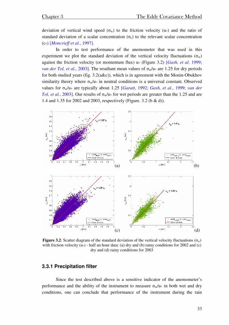
In order to test performance of the anemometer that was used in this
experiment we plot the standard deviation of the vertical velocity fluctuations (σw)
against the friction velocity (or momentum flux) u* (Figure 3.2) [Gash, et al. 1999;
van der Tol, et al., 2003]. The resultant mean values of σw/u* are 1.25 for dry periods
for both studied years (fig. 3.2(a&c)), which is in agreement with the Monin-Obukhov
similarity theory where σw/u* in neutral conditions is a universal constant. Observed
values for σw/u* are typically about 1.25 [Garatt, 1992; Gash, et al., 1999; van der
Tol, et al., 2003]. Our results of σw/u* for wet periods are greater than the 1.25 and are
1.4 and 1.35 for 2002 and 2003, respectively (Figure. 3.2 (b & d)).
(a) (b)
(c) (d) Figure 3.2: Scatter diagram of the standard deviation of the vertical velocity fluctuations (σw) with friction velocity (u*) - half an hour data: (a) dry and (b) rainy conditions for 2002 and (c)
dry and (d) rainy conditions for 2003
3.3.1 Precipitation filter
Since the test described above is a sensitive indicator of the anemometer’s
performance and the ability of the instrument to measure σw/u* in both wet and dry
conditions, one can conclude that performance of the instrument during the rain
Chapter 3 The Eddy Covariance Method
34
events was unsatisfactory. Raindrops on the open-path LI-COR can produce
unreliable signals (see section 2.2.4).
As described in section 2.2.11 precipitation was monitored by rain gauge set
on the ground which had resolution of 0.2 mm. Examining the half hour precipitation
measurements, it was noticed that on occasions in the early hours in the morning and
in the evening the rain gauge had registered 0.2 mm precipitation even when there
was no rain. It was concluded that the effect was condensation. Therefore threshold
for precipitation of 0.4 mm was adopted.
It should also be noted that approximately one hour was needed for the eddy
covariance set to dry out after rain events and thereby reestablish reliable
measurement by LI-COR. Therefore, the flux data (i.e. CO2 flux, latent heat flux
(LE), and sensible heat flux (H)) measured during the rain events and one hour
thereafter were treated as bad data and filtered out. Details about application of this
filter will be given in chapter 5 for LE and H and in chapter 6 for CO2.
3.4 Footprint and fetch
3.4.1 Definition of footprint and fetch
The eddy covariance method depends on turbulence to carry scalar entities
past the measurements sensors and roughly mix the air so that the scalar of interest
does not accumulate in the canopy air space [Campbell and Norman, 1998;
UMIST, 2002].
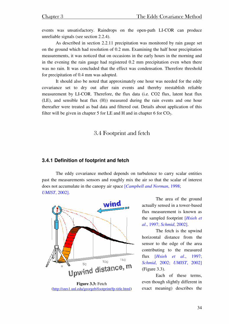
The area of the ground
actually sensed in a tower-based
flux measurement is known as
the sampled footprint [Hsieh et
al., 1997; Schmid, 2002].
The fetch is the upwind
horizontal distance from the
sensor to the edge of the area
contributing to the measured
flux [Hsieh et al., 1997;
Schmid, 2002; UMIST, 2002]
(Figure 3.3).
Each of these terms,
even though slightly different in
exact meaning) describes the Figure 3.3: Fetch
(http://snrs1.unl.edu/georgeb/footprint/fp-title.html)
Chapter 3 The Eddy Covariance Method
35
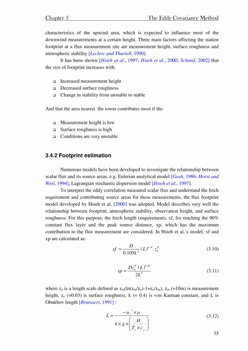
×××
×−=
pa
3
*
cT
Hgk
ρuL
characteristics of the upwind area, which is expected to influence most of the
downwind measurements at a certain height. Three main factors affecting the station
footprint at a flux measurement site are measurement height, surface roughness and
atmospheric stability [Leclerc and Thurtell, 1990].
It has been shown [Hsieh at al., 1997; Hsieh et al., 2000; Schmid, 2002] that
the size of footprint increases with:
Increased measurement height
Decreased surface roughness
Change in stability from unstable to stable
And that the area nearest the tower contributes most if the:
Measurement height is low
Surface roughness is high
Conditions are very unstable
3.4.2 Footprint estimation
Numerous models have been developed to investigate the relationship between
scalar flux and its source areas, e.g. Eulerian analytical model [Gash, 1986; Horst and
Weil, 1994], Lagrangian stochastic dispersion model [Hsieh et al., 1997].
To interpret the eddy correlation measured scalar flux and understand the fetch
requirement and contributing source areas for these measurements, the flux footprint
model developed by Hsieh et al. [2000] was adopted. Model describes very well the
relationship between footprint, atmospheric stability, observation height, and surface
roughness. For this purpose, the fetch length (requirement), xf, for reaching the 90%
constant flux layer and the peak source distance, xp, which has the maximum
contribution to the flux measurement are considered. In Hsieh et al.’s model, xf and
xp are calculated as:
P
u
PzL
k
Dxf
−= 1
2||
105.0 (3.10)
2
1
2
||
k
LDzxp
PP
u
−
= (3.11)
where zu is a length scale defined as zm(ln(zm/zo)-1+zo/zm), zm (=10m) is measurement
height, zo (=0.03) is surface roughness, k (= 0.4) is von Karman constant, and L is
Obukhov length [Brutsaert, 1991] :
(3.12)
Chapter 3 The Eddy Covariance Method
36
where u* is friction velocity (m/s), ρ is air density (1.2 kg/m3), g is gravity (9.81 m/s2),
H is sensible heat flux (W/m2), Ta is air temperature (K), and cp is specific heat for
dry air (1005 J/(kgK)). L is positive for stable, negative for unstable and infinitely
large for neutral conditions [Brutsaert, 1991].
In (3.10) and (3.11), D and P are constants [Hsieh et al., 2000] defined as:
a) D = 0.28; P = 0.59 for unstable condition;
b) D = 0.97; P = 1 for near neutral and neutral conditions; |zu/L| < 0.04;
c) D = 2.44; P = 1.33 for stable condition.
The stable condition of the boundary The stable condition of the boundary The stable condition of the boundary The stable condition of the boundary
layer forms over land in the evening as layer forms over land in the evening as layer forms over land in the evening as layer forms over land in the evening as
the ground cools, mixing is reduced and the ground cools, mixing is reduced and the ground cools, mixing is reduced and the ground cools, mixing is reduced and
concentrations of trace gases released concentrations of trace gases released concentrations of trace gases released concentrations of trace gases released
(or deposited) at (or deposited) at (or deposited) at (or deposited) at the surface are likely to the surface are likely to the surface are likely to the surface are likely to
be larger (or smaller) be larger (or smaller) be larger (or smaller) be larger (or smaller) [[[[Dabberdt et alDabberdt et alDabberdt et alDabberdt et al., ., ., ., 1993]1993]1993]1993]....
The xf values The xf values The xf values The xf values give an indicationgive an indicationgive an indicationgive an indication how how how how
far the eddyfar the eddyfar the eddyfar the eddy----correlation system can correlation system can correlation system can correlation system can
sense the scalar flux measurement from sense the scalar flux measurement from sense the scalar flux measurement from sense the scalar flux measurement from
the measurement towerthe measurement towerthe measurement towerthe measurement tower. The xp . The xp . The xp . The xp values values values values
give an indicationgive an indicationgive an indicationgive an indication how far the so how far the so how far the so how far the source urce urce urce
area, which has the maximum area, which has the maximum area, which has the maximum area, which has the maximum
contribution to the scalar flux contribution to the scalar flux contribution to the scalar flux contribution to the scalar flux
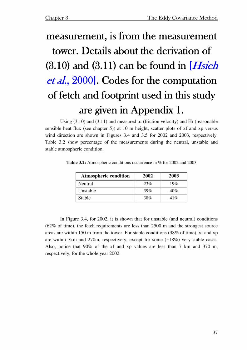
Chapter 3 The Eddy Covariance Method
37
measurement, is from the measurement measurement, is from the measurement measurement, is from the measurement measurement, is from the measurement
tower. tower. tower. tower. Details about Details about Details about Details about the the the the derivation of derivation of derivation of derivation of
((((3.103.103.103.10) and () and () and () and (3.113.113.113.11) can be found in ) can be found in ) can be found in ) can be found in [[[[Hsieh Hsieh Hsieh Hsieh et al.et al.et al.et al.,,,, 2000 2000 2000 2000]]]].... Codes for the computation Codes for the computation Codes for the computation Codes for the computation
of fetch and footprint used in thof fetch and footprint used in thof fetch and footprint used in thof fetch and footprint used in this study is study is study is study
are given in Appendix 1.are given in Appendix 1.are given in Appendix 1.are given in Appendix 1. Using (3.10) and (3.11) and measured u* (friction velocity) and Hr (reasonable
sensible heat flux (see chapter 5)) at 10 m height, scatter plots of xf and xp versus
wind direction are shown in Figures 3.4 and 3.5 for 2002 and 2003, respectively.
Table 3.2 show percentage of the measurements during the neutral, unstable and
stable atmospheric condition.
Table 3.2: Atmospheric conditions occurrence in % for 2002 and 2003
Atmospheric condition 2002 2003
Neutral 23% 19%
Unstable 39% 40%
Stable 38% 41%
In Figure 3.4, for 2002, it is shown that for unstable (and neutral) conditions
(62% of time), the fetch requirements are less than 2500 m and the strongest source
areas are within 150 m from the tower. For stable conditions (38% of time), xf and xp
are within 7km and 270m, respectively, except for some (~18%) very stable cases.
Also, notice that 90% of the xf and xp values are less than 7 km and 370 m,
respectively, for the whole year 2002.
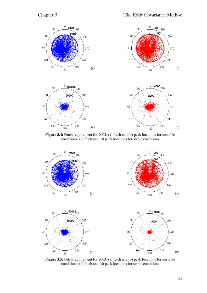
Chapter 3 The Eddy Covariance Method
38
Figure 3.4: Fetch requirement for 2002: (a) fetch and (b) peak locations for unstable
conditions; (c) fetch and (d) peak locations for stable conditions
Figure 3.5: Fetch requirement for 2003: (a) fetch and (b) peak locations for unstable
conditions; (c) fetch and (d) peak locations for stable conditions
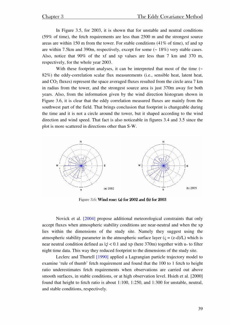
Chapter 3 The Eddy Covariance Method
39
In Figure 3.5, for 2003, it is shown that for unstable and neutral conditions
(59% of time), the fetch requirements are less than 2500 m and the strongest source
areas are within 150 m from the tower. For stable conditions (41% of time), xf and xp
are within 7.5km and 390m, respectively, except for some (~ 18%) very stable cases.
Also, notice that 90% of the xf and xp values are less than 7 km and 370 m,
respectively, for the whole year 2003.
With these footprint analyses, it can be interpreted that most of the time (~
82%) the eddy-correlation scalar flux measurements (i.e., sensible heat, latent heat,
and CO2 fluxes) represent the space averaged fluxes resulted from the circle area 7 km
in radius from the tower, and the strongest source area is just 370m away for both
years. Also, from the information given by the wind direction histogram shown in
Figure 3.6, it is clear that the eddy correlation measured fluxes are mainly from the
southwest part of the field. That brings conclusion that footprint is changeable during
the time and it is not a circle around the tower, but it shaped according to the wind
direction and wind speed. That fact is also noticeable in figures 3.4 and 3.5 since the
plot is more scattered in directions other than S-W.
Figure 3.6: Wind rose: (a) for 2002 and (b) for 2003 Wind rose: (a) for 2002 and (b) for 2003 Wind rose: (a) for 2002 and (b) for 2003 Wind rose: (a) for 2002 and (b) for 2003
Novick et al. [2004] propose additional meteorological constraints that only
accept fluxes when atmospheric stability conditions are near-neutral and when the xp
lies within the dimensions of the study site. Namely they suggest using the
atmospheric stability parameter in the atmospheric surface layer (ς = (z-d)/L) which is
near neutral condition defined as |ς| < 0.1 and xp (here 370m) together with u* to filter
night time data. This way they reduced footprint to the dimensions of the study site.
Leclerc and Thurtell [1990] applied a Lagrangian particle trajectory model to
examine ‘rule of thumb’ fetch requirement and found that the 100 to 1 fetch to height
ratio underestimates fetch requirements when observations are carried out above
smooth surfaces, in stable conditions, or at high observation level. Hsieh et al. [2000]
found that height to fetch ratio is about 1:100, 1:250, and 1:300 for unstable, neutral,
and stable conditions, respectively.
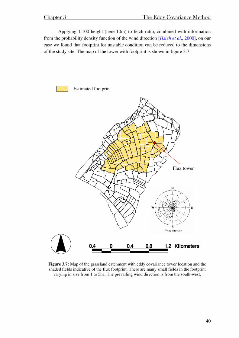
Chapter 3 The Eddy Covariance Method
40
Applying 1:100 height (here 10m) to fetch ratio, combined with information
from the probability density function of the wind direction [Hsieh et al., 2000], on our
case we found that footprint for unstable condition can be reduced to the dimensions
of the study site. The map of the tower with footprint is shown in figure 3.7.
Figure 3.7: Map of the grassland catchment with eddy covariance tower location and the shaded fields indicative of the flux footprint. There are many small fields in the footprint
varying in size from 1 to 5ha. The prevailing wind direction is from the south-west.
Estimated footprint
0 . 4 0 0 . 4 0 . 8 1 . 2 Kil o m e t e r s
Flux tower
Chapter 4 General meteorological data
Chapter 4 General meteorological data
41
Chapter 4Chapter 4Chapter 4Chapter 4 General meteorological data General meteorological data General meteorological data General meteorological data
4.1 Data collection
Meteorological data were monitored since July 2001 and we have continuous
data since then. In this thesis whole year data sets for years 2002 and 2003 were
analysed. Precipitation and meteorological measurements were read at one minute and
recorded at 30-minute intervals. The experimental system used in this study is
described in chapter 2.
For year 2002 we have whole data set without gaps, while in 2003 a gap
appears due to the electricity failure from 16th (00:00) to 19th (12:00) September.
Meteorological data for this period were filled following these steps:
Data from 15/09/03 were used to fill missing data for 16 and 17/09/03,
Gap for the first 12 hours of 19/09/03 were filled with data for the same
period from 20/09/03,
Missing data for 18/09/03 were filled up with data from 19/09/03.
Precipitation for this period was filled up with data from a nearby rain gauge.
4.2 Precipitation
4.2.1 Annual precipitation
The long-term annual average rainfall for Dripsey site is 1470mm. The year
2002 was wet, with an annual rainfall of 1785mm (~ 17 % above mean annual
precipitation) and 2003 was dry, with an annual rainfall of 1185mm (~ 19% less than
average). The first half of 2002 was particularly wet with 975mm compared to
610mm for 2003 (see Figure 4.1). It should be noted that there was no snow during
the study period.
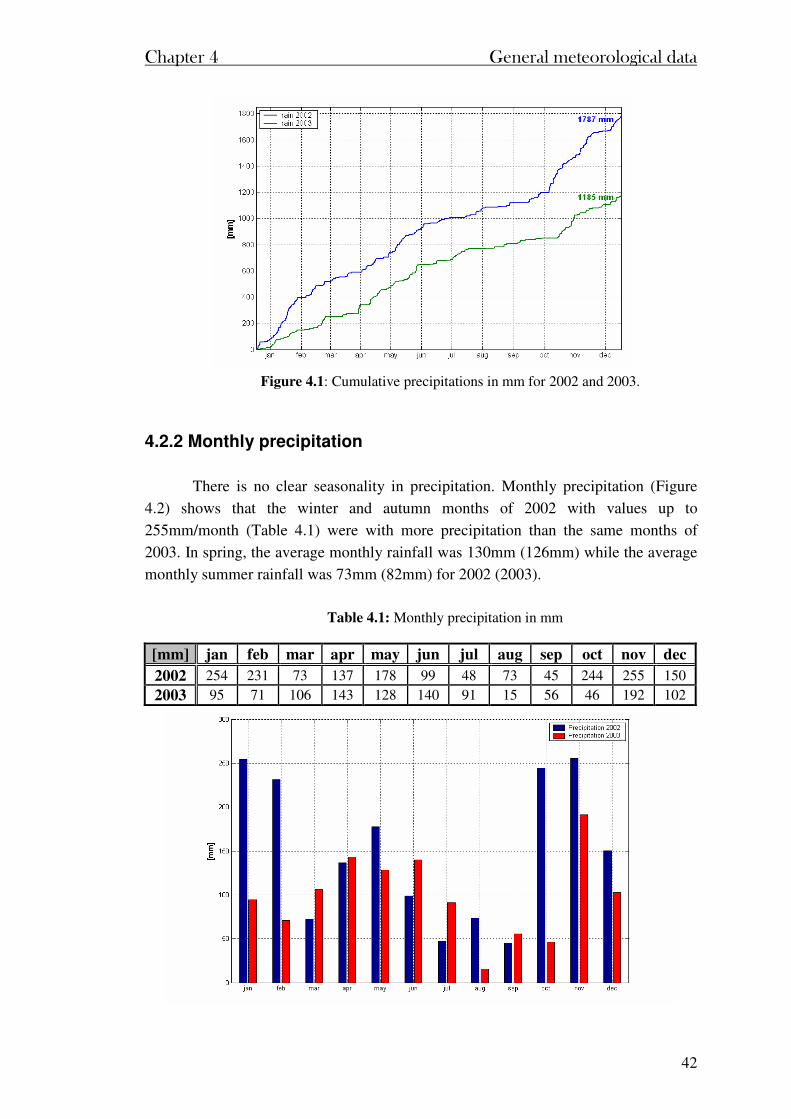
Chapter 4 General meteorological data
42
Figure 4.1: Cumulative precipitations in mm for 2002 and 2003.
4.2.2 Monthly precipitation
There is no clear seasonality in precipitation. Monthly precipitation (Figure
4.2) shows that the winter and autumn months of 2002 with values up to
255mm/month (Table 4.1) were with more precipitation than the same months of
2003. In spring, the average monthly rainfall was 130mm (126mm) while the average
monthly summer rainfall was 73mm (82mm) for 2002 (2003).
Table 4.1: Monthly precipitation in mm
[mm] jan feb mar apr may jun jul aug sep oct nov dec
2002 254 231 73 137 178 99 48 73 45 244 255 150
2003 95 71 106 143 128 140 91 15 56 46 192 102
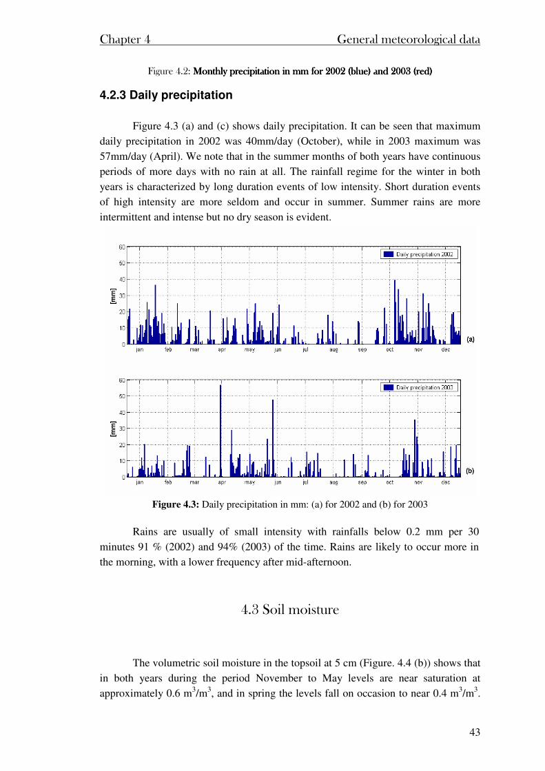
Chapter 4 General meteorological data
43
Figure 4.2: Monthly precipitation in mm for 2002 (blue) and 2003 (red) Monthly precipitation in mm for 2002 (blue) and 2003 (red) Monthly precipitation in mm for 2002 (blue) and 2003 (red) Monthly precipitation in mm for 2002 (blue) and 2003 (red)
4.2.3 Daily precipitation
Figure 4.3 (a) and (c) shows daily precipitation. It can be seen that maximum
daily precipitation in 2002 was 40mm/day (October), while in 2003 maximum was
57mm/day (April). We note that in the summer months of both years have continuous
periods of more days with no rain at all. The rainfall regime for the winter in both
years is characterized by long duration events of low intensity. Short duration events
of high intensity are more seldom and occur in summer. Summer rains are more
intermittent and intense but no dry season is evident.
Figure 4.3: Daily precipitation in mm: (a) for 2002 and (b) for 2003
Rains are usually of small intensity with rainfalls below 0.2 mm per 30
minutes 91 % (2002) and 94% (2003) of the time. Rains are likely to occur more in
the morning, with a lower frequency after mid-afternoon.
4.3 Soil moisture
The volumetric soil moisture in the topsoil at 5 cm (Figure. 4.4 (b)) shows that
in both years during the period November to May levels are near saturation at
approximately 0.6 m3/m3, and in spring the levels fall on occasion to near 0.4 m3/m3.
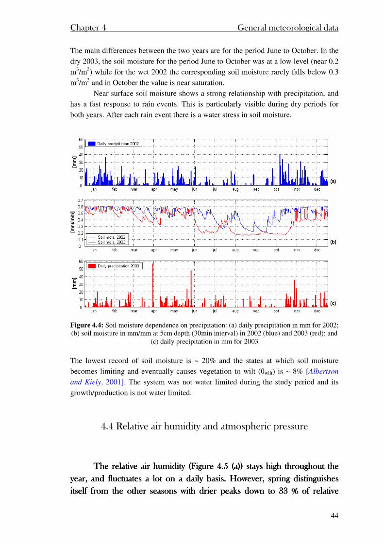
Chapter 4 General meteorological data
44
The main differences between the two years are for the period June to October. In the
dry 2003, the soil moisture for the period June to October was at a low level (near 0.2
m3/m3) while for the wet 2002 the corresponding soil moisture rarely falls below 0.3
m3/m3 and in October the value is near saturation.
Near surface soil moisture shows a strong relationship with precipitation, and
has a fast response to rain events. This is particularly visible during dry periods for
both years. After each rain event there is a water stress in soil moisture.
Figure 4.4: Soil moisture dependence on precipitation: (a) daily precipitation in mm for 2002; (b) soil moisture in mm/mm at 5cm depth (30min interval) in 2002 (blue) and 2003 (red); and
(c) daily precipitation in mm for 2003
The lowest record of soil moisture is ~ 20% and the states at which soil moisture
becomes limiting and eventually causes vegetation to wilt (θwilt) is ~ 8% [Albertson
and Kiely, 2001]. The system was not water limited during the study period and its
growth/production is not water limited.
4.4 Relative air humidity and atmospheric pressure
The relative air humidity (Figure 4.5 (a)) stays high throughout the The relative air humidity (Figure 4.5 (a)) stays high throughout the The relative air humidity (Figure 4.5 (a)) stays high throughout the The relative air humidity (Figure 4.5 (a)) stays high throughout the
year, and fluctuates a lot on a daily basis. However, spring dyear, and fluctuates a lot on a daily basis. However, spring dyear, and fluctuates a lot on a daily basis. However, spring dyear, and fluctuates a lot on a daily basis. However, spring distinguishes istinguishes istinguishes istinguishes
itself from the other seasons with drier peaks down to 33 % of relative itself from the other seasons with drier peaks down to 33 % of relative itself from the other seasons with drier peaks down to 33 % of relative itself from the other seasons with drier peaks down to 33 % of relative
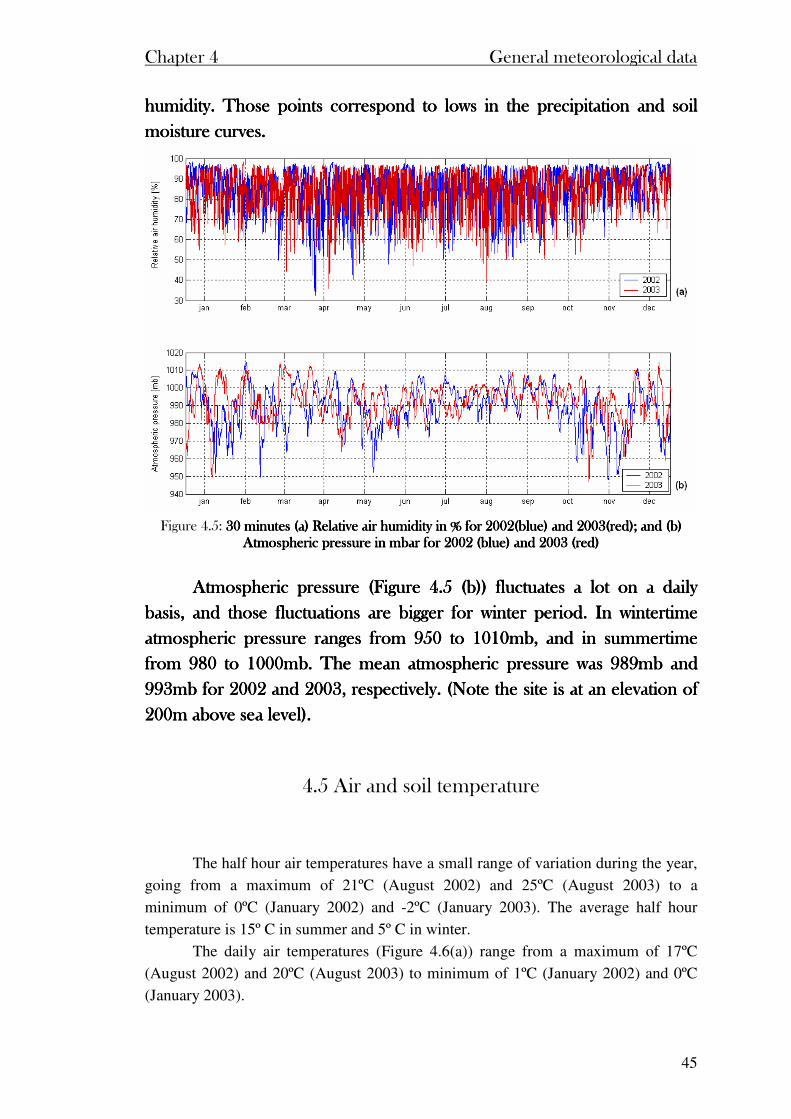
Chapter 4 General meteorological data
45
humidity. Those points correspond to lows in the precipitation and soil humidity. Those points correspond to lows in the precipitation and soil humidity. Those points correspond to lows in the precipitation and soil humidity. Those points correspond to lows in the precipitation and soil
moisture curves.moisture curves.moisture curves.moisture curves.
Figure 4.5: 30 minutes (a) Relative air humidity in % for 2002(blue) and 2003(re30 minutes (a) Relative air humidity in % for 2002(blue) and 2003(re30 minutes (a) Relative air humidity in % for 2002(blue) and 2003(re30 minutes (a) Relative air humidity in % for 2002(blue) and 2003(red); and (b) d); and (b) d); and (b) d); and (b)
Atmospheric pressure in mbar for 2002 (blue) and 2003 (red)Atmospheric pressure in mbar for 2002 (blue) and 2003 (red)Atmospheric pressure in mbar for 2002 (blue) and 2003 (red)Atmospheric pressure in mbar for 2002 (blue) and 2003 (red)
Atmospheric pressure (Figure 4.5 (b)) fluctuates a lot on a daily Atmospheric pressure (Figure 4.5 (b)) fluctuates a lot on a daily Atmospheric pressure (Figure 4.5 (b)) fluctuates a lot on a daily Atmospheric pressure (Figure 4.5 (b)) fluctuates a lot on a daily
basis, and those fluctuations are bigger for winter period. In wintertime basis, and those fluctuations are bigger for winter period. In wintertime basis, and those fluctuations are bigger for winter period. In wintertime basis, and those fluctuations are bigger for winter period. In wintertime
atmospheric pressure ranges from 950 to 10atmospheric pressure ranges from 950 to 10atmospheric pressure ranges from 950 to 10atmospheric pressure ranges from 950 to 1010mb, and in summertime 10mb, and in summertime 10mb, and in summertime 10mb, and in summertime
from 980 to 1000mb.from 980 to 1000mb.from 980 to 1000mb.from 980 to 1000mb. The mean atmospheric pressure was 989mb and The mean atmospheric pressure was 989mb and The mean atmospheric pressure was 989mb and The mean atmospheric pressure was 989mb and
993mb for 2002 and 2003, respectively. (Note the site is at an elevation of 993mb for 2002 and 2003, respectively. (Note the site is at an elevation of 993mb for 2002 and 2003, respectively. (Note the site is at an elevation of 993mb for 2002 and 2003, respectively. (Note the site is at an elevation of
200m above sea level).200m above sea level).200m above sea level).200m above sea level).
4.5 Air and soil temperature
The half hour air temperatures have a small range of variation during the year,
going from a maximum of 21ºC (August 2002) and 25ºC (August 2003) to a
minimum of 0ºC (January 2002) and -2ºC (January 2003). The average half hour
temperature is 15º C in summer and 5º C in winter.
The daily air temperatures (Figure 4.6(a)) range from a maximum of 17ºC
(August 2002) and 20ºC (August 2003) to minimum of 1ºC (January 2002) and 0ºC
(January 2003).
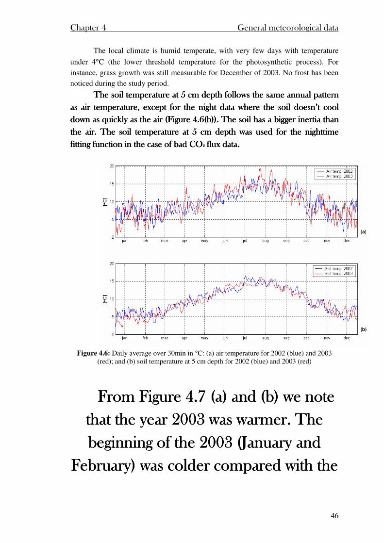
Chapter 4 General meteorological data
46
The local climate is humid temperate, with very few days with temperature
under 4°C (the lower threshold temperature for the photosynthetic process). For
instance, grass growth was still measurable for December of 2003. No frost has been
noticed during the study period.
The soil temperature at 5 cm depth follows the same annual pattern The soil temperature at 5 cm depth follows the same annual pattern The soil temperature at 5 cm depth follows the same annual pattern The soil temperature at 5 cm depth follows the same annual pattern
as air temperature, eas air temperature, eas air temperature, eas air temperature, except for the night data where the soil doesn’t cool xcept for the night data where the soil doesn’t cool xcept for the night data where the soil doesn’t cool xcept for the night data where the soil doesn’t cool
down as quickly as the air (Figure 4.6(b)).down as quickly as the air (Figure 4.6(b)).down as quickly as the air (Figure 4.6(b)).down as quickly as the air (Figure 4.6(b)). The soil has a bigger inertia than The soil has a bigger inertia than The soil has a bigger inertia than The soil has a bigger inertia than
the air.the air.the air.the air. The soil temperature at 5 cm depth was used for the nighttime The soil temperature at 5 cm depth was used for the nighttime The soil temperature at 5 cm depth was used for the nighttime The soil temperature at 5 cm depth was used for the nighttime
fitting function in the case of bad COfitting function in the case of bad COfitting function in the case of bad COfitting function in the case of bad CO2222 flux data. flux data. flux data. flux data.
Figure 4.6: Daily average over 30min in °C: (a) air temperature for 2002 (blue) and 2003
(red); and (b) soil temperature at 5 cm depth for 2002 (blue) and 2003 (red)
From Figure 4.7 (a) and (b) we note From Figure 4.7 (a) and (b) we note From Figure 4.7 (a) and (b) we note From Figure 4.7 (a) and (b) we note
that the year 2003 was warmer. The that the year 2003 was warmer. The that the year 2003 was warmer. The that the year 2003 was warmer. The
beginning of thbeginning of thbeginning of thbeginning of the 2003 (January and e 2003 (January and e 2003 (January and e 2003 (January and
February) was colder compared with the February) was colder compared with the February) was colder compared with the February) was colder compared with the
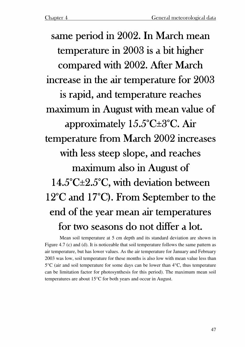
Chapter 4 General meteorological data
47
same period in 2002. In March mean same period in 2002. In March mean same period in 2002. In March mean same period in 2002. In March mean
temperature in 2003 is a bit higher temperature in 2003 is a bit higher temperature in 2003 is a bit higher temperature in 2003 is a bit higher
compared with 2002. After March compared with 2002. After March compared with 2002. After March compared with 2002. After March
increase in the air temperature for 2003 increase in the air temperature for 2003 increase in the air temperature for 2003 increase in the air temperature for 2003
is rapid, and temperature reaches is rapid, and temperature reaches is rapid, and temperature reaches is rapid, and temperature reaches
maximum in August wmaximum in August wmaximum in August wmaximum in August with mean value of ith mean value of ith mean value of ith mean value of
approximately 15.5°C±3°C. Air approximately 15.5°C±3°C. Air approximately 15.5°C±3°C. Air approximately 15.5°C±3°C. Air
temperature from March 2002 increases temperature from March 2002 increases temperature from March 2002 increases temperature from March 2002 increases
with less steep slope, and reaches with less steep slope, and reaches with less steep slope, and reaches with less steep slope, and reaches
maximum also in August of maximum also in August of maximum also in August of maximum also in August of
14.5°C±2.5°C, with deviation between 14.5°C±2.5°C, with deviation between 14.5°C±2.5°C, with deviation between 14.5°C±2.5°C, with deviation between
12°C and 17°C). From September to the 12°C and 17°C). From September to the 12°C and 17°C). From September to the 12°C and 17°C). From September to the
end of the year mean air temperatuend of the year mean air temperatuend of the year mean air temperatuend of the year mean air temperatures res res res
for two seasons do not differ a lot. for two seasons do not differ a lot. for two seasons do not differ a lot. for two seasons do not differ a lot. Mean soil temperature at 5 cm depth and its standard deviation are shown in
Figure 4.7 (c) and (d). It is noticeable that soil temperature follows the same pattern as
air temperature, but has lower values. As the air temperature for January and February
2003 was low, soil temperature for these months is also low with mean value less than
5°C (air and soil temperature for some days can be lower than 4°C, thus temperature
can be limitation factor for photosynthesis for this period). The maximum mean soil
temperatures are about 15°C for both years and occur in August.
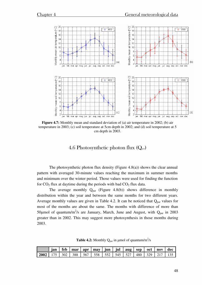
Chapter 4 General meteorological data
48
Figure 4.7: Monthly mean and standard deviation of (a) air temperature in 2002; (b) air
temperature in 2003; (c) soil temperature at 5cm depth in 2002; and (d) soil temperature at 5 cm depth in 2003.
4.6 Photosynthetic photon flux (Qpar)
The photosynthetic photon flux density (Figure 4.8(a)) shows the clear annual
pattern with averaged 30-minute values reaching the maximum in summer months
and minimum over the winter period. Those values were used for finding the function
for CO2 flux at daytime during the periods with bad CO2 flux data.
The average monthly Qpar (Figure 4.8(b)) shows difference in monthly
distribution within the year and between the same months for two different years.
Average monthly values are given in Table 4.2. It can be noticed that Qpar values for
most of the months are about the same. The months with difference of more than
50µmol of quantum/m2/s are January, March, June and August, with Qpar in 2003
greater than in 2002. This may suggest more photosynthesis in those months during
2003.
Table 4.2: Monthly Qpar in µmol of quantum/m2/s
jan feb mar apr may jun jul aug sep oct nov dec
2002 175 302 388 567 558 552 545 527 480 329 217 135
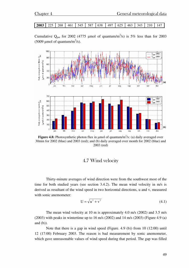
Chapter 4 General meteorological data
49
2003 225 268 461 545 587 638 497 625 463 343 210 147
Cumulative Qpar for 2002 (4775 µmol of quantum/m2/s) is 5% less than for 2003
(5009 µmol of quantum/m2/s).
Figure 4.8: Photosynthetic photon flux in µmol of quantum/m2/s: (a) daily averaged over
30min for 2002 (blue) and 2003 (red); and (b) daily averaged over month for 2002 (blue) and 2003 (red)
4.7 Wind velocity
Thirty-minute averages of wind direction were from the southwest most of the
time for both studied years (see section 3.4.2). The mean wind velocity in m/s is
derived as resultant of the wind speed in two horizontal directions, u and v, measured
with sonic anemometer: 22 vuU += (4.1)
The mean wind velocity at 10 m is approximately 4.0 m/s (2002) and 3.5 m/s
(2003) with peaks in wintertime up to 16 m/s (2002) and 14 m/s (2003) (Figure 4.9 (a)
and (b)).
Note that there is a gap in wind speed (Figure. 4.9 (b)) from 10 (12:00) until
12 (17:00) February 2003. The reason is bad measurement by sonic anemometer,
which gave unreasonable values of wind speed during that period. The gap was filled
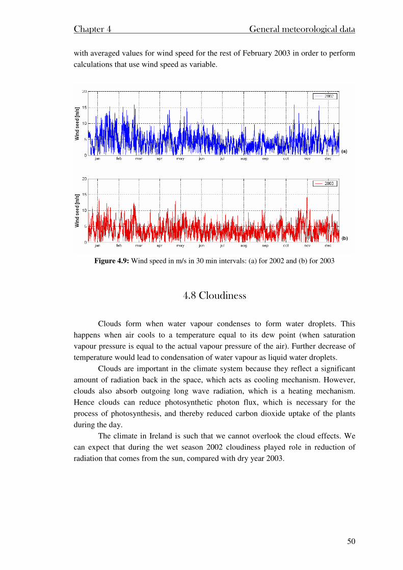
Chapter 4 General meteorological data
50
with averaged values for wind speed for the rest of February 2003 in order to perform
calculations that use wind speed as variable.
Figure 4.9: Wind speed in m/s in 30 min intervals: (a) for 2002 and (b) for 2003
4.8 Cloudiness
Clouds form when water vapour condenses to form water droplets. This
happens when air cools to a temperature equal to its dew point (when saturation
vapour pressure is equal to the actual vapour pressure of the air). Further decrease of
temperature would lead to condensation of water vapour as liquid water droplets.
Clouds are important in the climate system because they reflect a significant
amount of radiation back in the space, which acts as cooling mechanism. However,
clouds also absorb outgoing long wave radiation, which is a heating mechanism.
Hence clouds can reduce photosynthetic photon flux, which is necessary for the
process of photosynthesis, and thereby reduced carbon dioxide uptake of the plants
during the day.
The climate in Ireland is such that we cannot overlook the cloud effects. We
can expect that during the wet season 2002 cloudiness played role in reduction of
radiation that comes from the sun, compared with dry year 2003.

Chapter 5 Energy balance
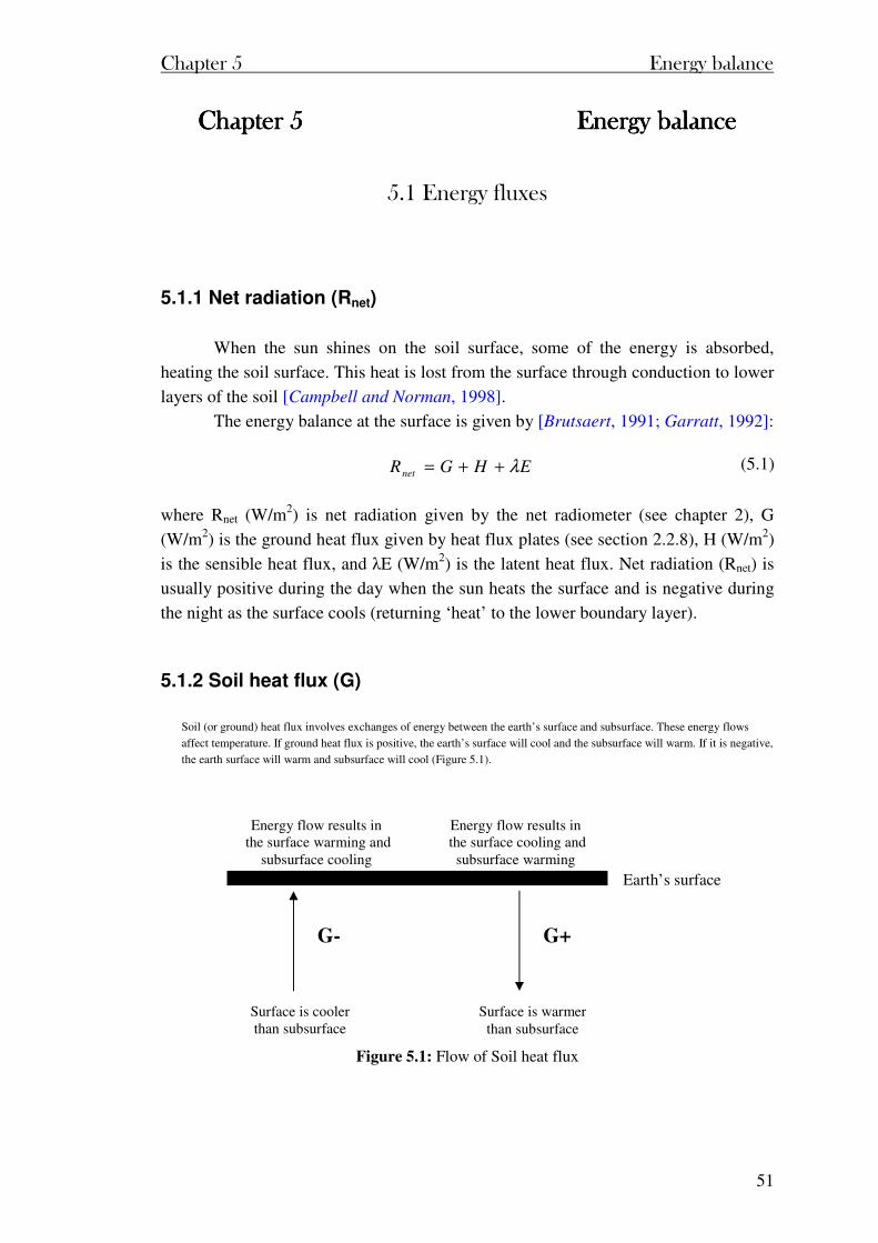
Chapter 5 Energy balance
51
Chapter 5Chapter 5Chapter 5Chapter 5 Energy balance Energy balance Energy balance Energy balance
5.1 Energy fluxes
5.1.1 Net radiation (Rnet)
When the sun shines on the soil surface, some of the energy is absorbed,
heating the soil surface. This heat is lost from the surface through conduction to lower
layers of the soil [Campbell and Norman, 1998].
The energy balance at the surface is given by [Brutsaert, 1991; Garratt, 1992]:
where Rnet (W/m2) is net radiation given by the net radiometer (see chapter 2), G
(W/m2) is the ground heat flux given by heat flux plates (see section 2.2.8), H (W/m2)
is the sensible heat flux, and λE (W/m2) is the latent heat flux. Net radiation (Rnet) is
usually positive during the day when the sun heats the surface and is negative during
the night as the surface cools (returning ‘heat’ to the lower boundary layer).
5.1.2 Soil heat flux (G)
Soil (or ground) heat flux involves exchanges of energy between the earth’s surface and subsurface. These energy flows
affect temperature. If ground heat flux is positive, the earth’s surface will cool and the subsurface will warm. If it is negative,
the earth surface will warm and subsurface will cool (Figure 5.1).
Figure 5.1: Flow of Soil heat flux
EHGRnet λ++= (5.1)
Surface is cooler than subsurface
G+ G-
Earth’s surface
Energy flow results in the surface warming and
subsurface cooling
Energy flow results in the surface cooling and
subsurface warming
Surface is warmer than subsurface
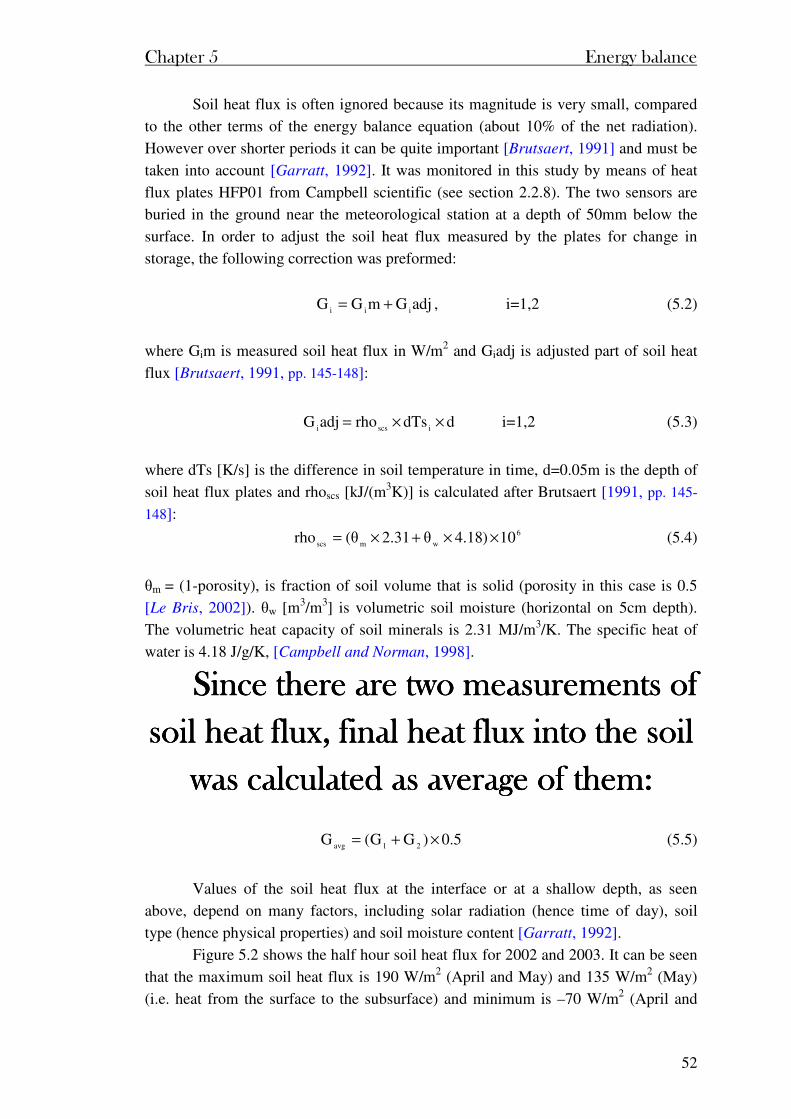
Chapter 5 Energy balance
52
Soil heat flux is often ignored because its magnitude is very small, compared
to the other terms of the energy balance equation (about 10% of the net radiation).
However over shorter periods it can be quite important [Brutsaert, 1991] and must be
taken into account [Garratt, 1992]. It was monitored in this study by means of heat
flux plates HFP01 from Campbell scientific (see section 2.2.8). The two sensors are
buried in the ground near the meteorological station at a depth of 50mm below the
surface. In order to adjust the soil heat flux measured by the plates for change in
storage, the following correction was preformed:
adjGmGG iii += , i=1,2 (5.2)
where Gim is measured soil heat flux in W/m2 and Giadj is adjusted part of soil heat
flux [Brutsaert, 1991, pp. 145-148]:
ddTsrhoadjG iscsi ××= i=1,2 (5.3)
where dTs [K/s] is the difference in soil temperature in time, d=0.05m is the depth of
soil heat flux plates and rhoscs [kJ/(m3K)] is calculated after Brutsaert [1991, pp. 145-
148]: 6
wmscs 10)18.4θ31.2θ(rho ××+×= (5.4)
θm = (1-porosity), is fraction of soil volume that is solid (porosity in this case is 0.5
[Le Bris, 2002]). θw [m3/m3] is volumetric soil moisture (horizontal on 5cm depth).
The volumetric heat capacity of soil minerals is 2.31 MJ/m3/K. The specific heat of
water is 4.18 J/g/K, [Campbell and Norman, 1998].
Since there are two measurements of Since there are two measurements of Since there are two measurements of Since there are two measurements of
soil heat fsoil heat fsoil heat fsoil heat flux, final heat flux into the soil lux, final heat flux into the soil lux, final heat flux into the soil lux, final heat flux into the soil
was calculated as average of them:was calculated as average of them:was calculated as average of them:was calculated as average of them:
5.0)GG(G 21avg ×+= (5.5)
Values of the soil heat flux at the interface or at a shallow depth, as seen
above, depend on many factors, including solar radiation (hence time of day), soil
type (hence physical properties) and soil moisture content [Garratt, 1992].
Figure 5.2 shows the half hour soil heat flux for 2002 and 2003. It can be seen
that the maximum soil heat flux is 190 W/m2 (April and May) and 135 W/m2 (May)
(i.e. heat from the surface to the subsurface) and minimum is –70 W/m2 (April and
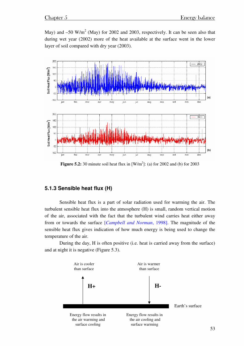
Chapter 5 Energy balance
53
May) and –50 W/m2 (May) for 2002 and 2003, respectively. It can be seen also that
during wet year (2002) more of the heat available at the surface went in the lower
layer of soil compared with dry year (2003).
Figure 5.2: 30 minute soil heat flux in [W/m2]: (a) for 2002 and (b) for 2003
5.1.3 Sensible heat flux (H)
Sensible heat flux is a part of solar radiation used for warming the air. The
turbulent sensible heat flux into the atmosphere (H) is small, random vertical motion
of the air, associated with the fact that the turbulent wind carries heat either away
from or towards the surface [Campbell and Norman, 1998]. The magnitude of the
sensible heat flux gives indication of how much energy is being used to change the
temperature of the air.
During the day, H is often positive (i.e. heat is carried away from the surface)
and at night it is negative (Figure 5.3).
Air is cooler than surface
Air is warmer than surface
H+ H-
Earth’s surface
Energy flow results in the air warming and
surface cooling
Energy flow results in the air cooling and
surface warming
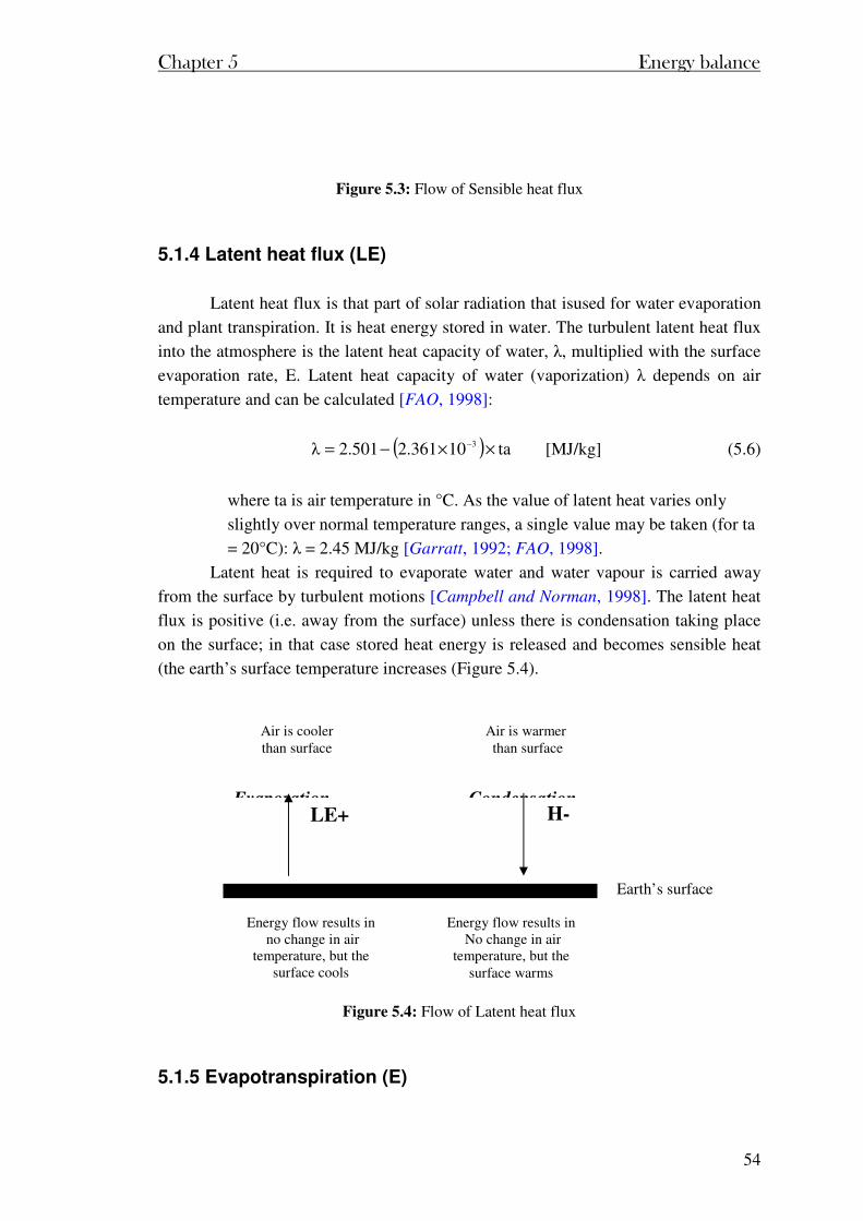
Chapter 5 Energy balance
54
Figure 5.3: Flow of Sensible heat flux
5.1.4 Latent heat flux (LE)
Latent heat flux is that part of solar radiation that isused for water evaporation
and plant transpiration. It is heat energy stored in water. The turbulent latent heat flux
into the atmosphere is the latent heat capacity of water, λ, multiplied with the surface
evaporation rate, E. Latent heat capacity of water (vaporization) λ depends on air
temperature and can be calculated [FAO, 1998]:
( ) ta10361.2501.2λ 3 ××−= − [MJ/kg] (5.6)
where ta is air temperature in °C. As the value of latent heat varies only
slightly over normal temperature ranges, a single value may be taken (for ta
= 20°C): λ = 2.45 MJ/kg [Garratt, 1992; FAO, 1998].
Latent heat is required to evaporate water and water vapour is carried away
from the surface by turbulent motions [Campbell and Norman, 1998]. The latent heat
flux is positive (i.e. away from the surface) unless there is condensation taking place
on the surface; in that case stored heat energy is released and becomes sensible heat
(the earth’s surface temperature increases (Figure 5.4).
Figure 5.4: Flow of Latent heat flux
5.1.5 Evapotranspiration (E)
Air is cooler than surface
Air is warmer than surface
LE+ H-
Earth’s surface
Energy flow results in no change in air
temperature, but the surface cools
Energy flow results in No change in air
temperature, but the surface warms
Evaporation Condensation
Chapter 5 Energy balance
55
Evapotranspiration is the collective term for all the processes by Evapotranspiration is the collective term for all the processes by Evapotranspiration is the collective term for all the processes by Evapotranspiration is the collective term for all the processes by
which watwhich watwhich watwhich water in the liquid or solid phase at or near the earth’s land surfaces er in the liquid or solid phase at or near the earth’s land surfaces er in the liquid or solid phase at or near the earth’s land surfaces er in the liquid or solid phase at or near the earth’s land surfaces
becomes atmospheric water vapour becomes atmospheric water vapour becomes atmospheric water vapour becomes atmospheric water vapour [[[[DingmanDingmanDingmanDingman, 1994], 1994], 1994], 1994]. Most of the water . Most of the water . Most of the water . Most of the water
‘lost’ via evapotranspiration is used to grow the plants that form the base of ‘lost’ via evapotranspiration is used to grow the plants that form the base of ‘lost’ via evapotranspiration is used to grow the plants that form the base of ‘lost’ via evapotranspiration is used to grow the plants that form the base of
the earth’s land ecosystems, and understthe earth’s land ecosystems, and understthe earth’s land ecosystems, and understthe earth’s land ecosystems, and understanding relations between anding relations between anding relations between anding relations between
evapotranspiration and ecosystem type is a requirement for predicting evapotranspiration and ecosystem type is a requirement for predicting evapotranspiration and ecosystem type is a requirement for predicting evapotranspiration and ecosystem type is a requirement for predicting
ecosystem response to climate change ecosystem response to climate change ecosystem response to climate change ecosystem response to climate change [[[[DingmanDingmanDingmanDingman, 1994], 1994], 1994], 1994]....
Evapotranspiration can be estimated using the PenmanEvapotranspiration can be estimated using the PenmanEvapotranspiration can be estimated using the PenmanEvapotranspiration can be estimated using the Penman----Monteith or Monteith or Monteith or Monteith or
PristleyPristleyPristleyPristley----Taylor equation.Taylor equation.Taylor equation.Taylor equation.
Penman-Monteith equation
The Penman-Monteith equation estimate the evapotranspiration rate from a
vegetated surface [Monteith, 1965; FAO, 1998].
( ) ( )
λr
r1γ∆
eer
cρGR∆
ET
a
s
as
a
pa
n
×
+×+
−×+−×
= (5.7)
where Rn [W/m2] is the net radiation, G [W/m2] is the soil heat flux, (es-ea) [kPa]
represents the vapour pressure deficit of the air, ρa [kg/m3] is the mean air density at
constant pressure (density of dry air is 1.29 kg/m3 [Brutsaert, 1991]), cp [MJ/kg/°C] is
specific heat of the air, ∆ [kPa/°C] represents the slope of the saturation vapour
pressure temperature relationship, γ [kPa/°C] is the psychrometric constant, and rs and
ra [s/m] are the (bulk) surface and aerodynamic resistances, respectively.
The saturation pressure can be calculated [FAO, 1998]:
+
××=
3.237t
t27.17exp6108.0e
a
a
s [kPa] (5.8)
where ta [°C] is air temperature.
Actual vapour pressure can be calculated using the relative humidity of the air
(RH) and saturation vapour pressure, calculated as in (5.8) [FAO, 1998]:
100
eRHe s
a
×= [kPa] (5.9)
Chapter 5 Energy balance
56
The vapour pressure deficit is the difference between the saturation vapour pressure
(es) and actual vapour pressure (ea) for a given time period.
Slope of saturation vapour pressure curve, represents the slope of the
relationship between saturation vapour pressure and temperature [FAO, 1998]:
( )2
a
s
3.237t
e4098∆
+
×= [kPa/°C] (5.10)
where es is saturation vapour pressure, calculated as in (5.8) and ta is air temperature
in [°C].
The psychrometric constant can be calculated [FAO, 1998]:
3ap 10λε
pcγ −×
×
×= [kPa/°C] (5.11)
where cp (= 1013 [J/kg/°C]) is specific heat of moist air, pa [kPa = 10 mbar] is
atmospheric pressure, ε (=0.622) is ratio of molecular weight of water vapour/dry air
and λ [MJ/kg] is latent heat of vaporization calculated as in (5.6).
The aerodynamic resistance is defined as:
2
2
oh
h
om
m
auk
z
dzln
z
dzln
r×
−×
−
= [s/m] (5.12)
where zm [m] is height of wind measurements, zh [m] is height of humidity
measurements, d = (2/3*h) [m] zero plane displacement height estimated from crop
height (h, which is in average from 0.12m to 0.15m for our case), zom = (0.123*h)
[m] is the roughness length governing momentum transfer, zoh = (0.1*zom) [m] is
roughness length governing transfer of heat and vapour, k = 0.41 is von Karman’s
constant, u2 [m/s] is wind speed at height z (= 2 [m] proposed by FAO).
To adjust wind speed data obtained from instruments placed at
elevations other than the standard height of 2m (in our case instrument is
placed at 10m height), logarithmic wind speed profile may be used for
measurements above a short grassed surface [FAO, 1998]:
)42.5z8.67ln(
87.4uu
m
z2−×
= [m/s] (5.13)
where u2 [m/s] is wind speed at 2m above ground surface, uz [m] is measured wind
speed at z [m] above ground surface, and zm [m] is height of measurement above
ground surface (in our case 10 m).
Chapter 5 Energy balance
57
The ‘bulk’ surface resistance describes the resistance of vapour flow trough
the transpiring crop and evaporating soil surface [FAO, 1998]:
active
l
sLAI
rr = [s/m] (5.14a)
where r1 [s/m] is bulk stomatal resistance of the well-illuminated leaf (it has a value of
about 100 s/m for a single leaf under well-watered conditions [FAO, 1998], as it is
case here) and LAIactive [m2 (leaf area)/m2(soil surface)] is active (sunlit) leaf area
index (for bulk surface resistance for a grass reference crop LAIactive = 0.5LAI [FAO,
1998]). For clipped grass generally LAI = 24*h (h is the crop height [m]). If we assume that study site is reference surface, the ‘bulk’ surface resistance can be calculated with approximations:
7012.0245.0
100rs ≈
××= s/m (5.14b)
The reference surface closely resembles an extensive surface of green grass of
uniform height, actively growing, completely shading the ground and with adequate
water [FAO, 1998]. The requirements that the grass surface should be extensive and
uniform results from the assumption that all fluxes are one-dimensional upwards
[FAO, 1998].
The ‘bulk’ surface resistance is highly dependant on the interactions (in many
cases non linear) of soil, plant genotype, and atmospheric factors [Ortega-Farias et.
al., 1996]. If the ‘bulk’ surface resistance (rs) is greater than zero and if we know its
actual value over time, then calculating Penman-Monteith equation (5.7) estimate the
the actual evapotranspiration or EA. Actual evapotranspiration is the quantity of water
that is actually removed from surface due to the process of evaporation and
transpiration [Dingman, 1994; Pidwirny, 2004].
If the ‘bulk’ surface resistance (rs) equals zero, then the Penman-Monteith
equation (5.7) estimates the potential evapotranspiartion or PE for open water surfaces
(e. g. sea, lake, pan). Potential evapotranspiration is a measure of the ability of the
atmosphere to remove water from the surface through the process of evaporation and
transpiration assuming no control on water supply [Dingman, 1994; Pidwirny, 2004].
Factors influencing potential evapotranspiration are energy from the sun (80%
variations in PE are caused by energy received from the sun) and wind (enables water
molecules to be removed from the ground surface by eddy diffusion).
The rate of evapotranspiration is associated with the vapour pressure deficit
(VPD). Vapour pressure deficit is the difference between actual and maximum vapour
pressure (saturation vapour pressure) [Nederhoff, 2004]:
( )1e100
RH)ee(VPD sas −×−=−= [kPa] (5.15)
Chapter 5 Energy balance
58
where ea is actual vapour pressure, RH [%] is relative humidity, and es is saturation
vapour pressure calculated by (5.8).
Low VPD means a high air humidity, and vice-versa. The higher the VPD the
stronger the drying effect, so the stronger the driving force on evapotranspiration.
The Matlab code for calculating Penman-Monteith equation is given in
Appendix 2.1.
Priestley-Taylor equation
The Priestley-Taylor equation is a simplification of the Penman-Monteith equation. It negates the need for any other measured data than the radiation for calculating potential evapotranspiration [Priestley and Taylor, 1972]. It assumes that air travelling over a saturated vegetation cover will become saturated and the actual rate of evaporation (AET) would be equal the Penman rate of potential evapotranspiration. Under those conditions evapotranspiration is referred to as equilibrium potential evapotranspiration (PETeq). The mass transfer term in the Penman-Monteith equation approaches zero and the radiation terms dominates. Priestley and Taylor [1972] found that AET from well watered vegetation was generally higher than the equilibrium potential rate and could be estimated by multiplying the PETeq by factor α (=1.26):
λ
1)GRn(
γ∆
∆αPET ×−×
+×= (5.16)
where ∆ [kPa/°C] is slope of saturation vapour pressure curve at air temperature, γ [kPa/°C] is psychrometric constant, Rn [W/m2] is net radiation, G [W/m2] is ground heat flux, λ [=2.45 MJ/kg] is latent heat of vaporization. The saturation vapour pressure curve is given by [Brutsaert, 1991]:
( )( )3
r
2
rr2
a
s t5196.0t9335.1t952.33185.1315.273t
e15.373∆ ×−×−×−×
+×= (5.17)
where ta [°C] is air temperature, es is saturation vapour pressure [Brutsaert, 1991]:
( )4
r
3
r
2
rrs t1299.0t6445.0t9760.1t3185.13exp25.1013e ×−×−×−××= (5.18)
where tr = 1-(373.15/(ta+273.15). (5.18a)
α is factor which value has been tested to be 1.26 over a wide range of
conditions for short vegetation [Garratt, 1992]. Over land, α varies with soil moisture
although at saturation it approaches the value 1.26 [Rind, 1997].
Actual evapotranspiration (AET) takes into account water supply limitations
and represents the amount of ET that occurs under field conditions. The most widely
used method to incorporate the effects of soil moisture on evapotranspiration is
through the use of soil moisture factor [Albertson and Kiely, 2001]:
Chapter 5 Energy balance
59
( ) PETθβPETa rel ×= (5.19)
where PETa is the actual evapotranspiration, PET is potential evapotranspiration
calculated in our case using the Priestley-Taylor equation and θrel is relative water
content, defined as:
( )∫=
zd
0
z
z
rel dzθd
1θ (5.20)
where z is depth of soil moisture measurements, so in our experiment
relative water content represents average of soil moisture measured on 5, 10
and 25 cm depths. Then reduction factor β is found to be [Albertson and
Kiely, 2001]:
( )
−
−==
,1
,θθ
θθ
,0
θββwiltlim
wiltrelrel
limrel
limrelwilt
wiltrel
θθ
θθθ
θθ
≥
<<
≤
(5.21)
where θlim and θwilt are parameters that define the states at which soil moisture
becomes limiting and eventually causes vegetation to wilt and transpiration to cease,
respectively [Albertson and Kiely, 2001]. In our case for θlim and θwilt values of 0.48
and 0.08 were adopted.
In this experiment it was found that reduction factor was never equal to zero,
so during the study period soil moisture was never limiting in terms of causing
vegetation to wilt. Only in 0.4% cases soil moisture was limiting in terms of case of
transpiration.
The Matlab code for calculating Priestley-Taylor equation is given in
Appendix 2.2.
5.2 Estimation of H and LE
H (W/mH (W/mH (W/mH (W/m2222), the sensible heat flux and ME (W/m), the sensible heat flux and ME (W/m), the sensible heat flux and ME (W/m), the sensible heat flux and ME (W/m2222), the latent heat flux ), the latent heat flux ), the latent heat flux ), the latent heat flux
are not measured directly by any device, but calculated using the eddy are not measured directly by any device, but calculated using the eddy are not measured directly by any device, but calculated using the eddy are not measured directly by any device, but calculated using the eddy
correlation technique with air temperature and air specific humidity, as it is correlation technique with air temperature and air specific humidity, as it is correlation technique with air temperature and air specific humidity, as it is correlation technique with air temperature and air specific humidity, as it is
explained in chapter 3. Webb correction was explained in chapter 3. Webb correction was explained in chapter 3. Webb correction was explained in chapter 3. Webb correction was applied to H and LE applied to H and LE applied to H and LE applied to H and LE
calculated by the eddy correlation technique. After this correction some calculated by the eddy correlation technique. After this correction some calculated by the eddy correlation technique. After this correction some calculated by the eddy correlation technique. After this correction some
bad points in H and LE data remained.bad points in H and LE data remained.bad points in H and LE data remained.bad points in H and LE data remained.
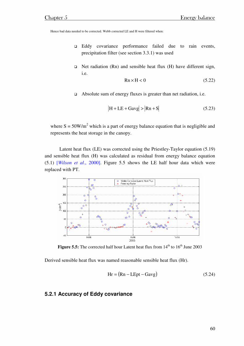
Chapter 5 Energy balance
60
Hence bad data needed to be corrected. Webb corrected LE and H were filtered when:
Eddy covariance performance failed due to rain events,
precipitation filter (see section 3.3.1) was used
Net radiation (Rn) and sensible heat flux (H) have different sign,
i.e.
0HRn <× (5.22)
Absolute sum of energy fluxes is greater than net radiation, i.e.
SRnGavgLEH +>++ (5.23)
where S = 50W/m2 which is a part of energy balance equation that is negligible and
represents the heat storage in the canopy.
Latent heat flux (LE) was corrected using the Priestley-Taylor equation (5.19)
and sensible heat flux (H) was calculated as residual from energy balance equation
(5.1) [Wilson et al., 2000]. Figure 5.5 shows the LE half hour data which were
replaced with PT.
Figure 5.5: The corrected half hour Latent heat flux from 14th to 16th June 2003
Derived sensible heat flux was named reasonable sensible heat flux (Hr).
( )GavgLEptRnHr −−= (5.24)
5.2.1 Accuracy of Eddy covariance
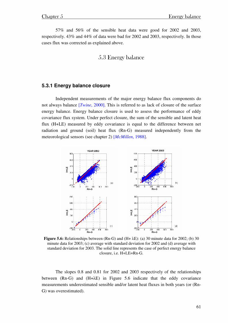
Chapter 5 Energy balance
61
57% and 56% of the sensible heat data were good for 2002 and 2003,
respectively. 43% and 44% of data were bad for 2002 and 2003, respectively. In those
cases flux was corrected as explained above.
5.3 Energy balance
5.3.1 Energy balance closure
Independent measurements of the major energy balance flux components do
not always balance [Twine, 2000]. This is referred to as lack of closure of the surface
energy balance. Energy balance closure is used to assess the performance of eddy
covariance flux system. Under perfect closure, the sum of the sensible and latent heat
flux (H+LE) measured by eddy covariance is equal to the difference between net
radiation and ground (soil) heat flux (Rn-G) measured independently from the
meteorological sensors (see chapter 2) [McMillen, 1988].
Figure 5.6: Relationships between (Rn-G) and (H+ λE): (a) 30 minute data for 2002; (b) 30
minute data for 2003; (c) average with standard deviation for 2002 and (d) average with standard deviation for 2003. The solid line represents the case of perfect energy balance
closure, i.e. H+LE=Rn-G.
The slopes 0.8 and 0.81 for 2002 and 2003 respectively of the relationships
between (Rn-G) and (H+λE) in Figure 5.6 indicate that the eddy covariance
measurements underestimated sensible and/or latent heat fluxes in both years (or (Rn-
G) was overestimated).
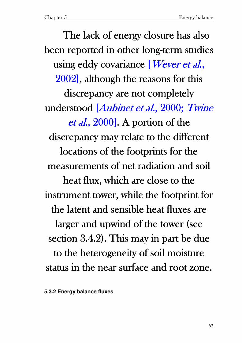
Chapter 5 Energy balance
62
The lack of energy closure has also The lack of energy closure has also The lack of energy closure has also The lack of energy closure has also
been reported in other longbeen reported in other longbeen reported in other longbeen reported in other long----term studies term studies term studies term studies
using eddy covariance using eddy covariance using eddy covariance using eddy covariance [[[[Wever et alWever et alWever et alWever et al., ., ., ., 2002]2002]2002]2002], although the reasons for this , although the reasons for this , although the reasons for this , although the reasons for this
discrepancy are not completely discrepancy are not completely discrepancy are not completely discrepancy are not completely
understood understood understood understood [[[[Aubinet et alAubinet et alAubinet et alAubinet et al...., 2000; , 2000; , 2000; , 2000; Twine Twine Twine Twine et alet alet alet al., 2000]., 2000]., 2000]., 2000]. A portion of the . A portion of the . A portion of the . A portion of the
discrepancy may relate to the different discrepancy may relate to the different discrepancy may relate to the different discrepancy may relate to the different
locations of the footprints for the locations of the footprints for the locations of the footprints for the locations of the footprints for the
measurements of net radiation and soil measurements of net radiation and soil measurements of net radiation and soil measurements of net radiation and soil
heat flux, which are close to the heat flux, which are close to the heat flux, which are close to the heat flux, which are close to the
instrument tower, while the footprint for instrument tower, while the footprint for instrument tower, while the footprint for instrument tower, while the footprint for
the latent and sensthe latent and sensthe latent and sensthe latent and sensible heat fluxes are ible heat fluxes are ible heat fluxes are ible heat fluxes are
larger and upwind of the tower (see larger and upwind of the tower (see larger and upwind of the tower (see larger and upwind of the tower (see
section 3.4.2). This may in part be due section 3.4.2). This may in part be due section 3.4.2). This may in part be due section 3.4.2). This may in part be due
to the heterogeneity of soil moisture to the heterogeneity of soil moisture to the heterogeneity of soil moisture to the heterogeneity of soil moisture
status in the near surface and root zone.status in the near surface and root zone.status in the near surface and root zone.status in the near surface and root zone.
5.3.2 Energy balance fluxes
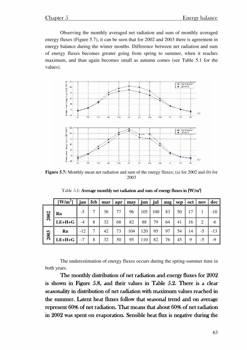
Chapter 5 Energy balance
63
Observing the monthly averaged net radiation and sum of monthly averaged
energy fluxes (Figure 5.7), it can be seen that for 2002 and 2003 there is agreement in
energy balance during the winter months. Difference between net radiation and sum
of energy fluxes becomes greater going from spring to summer, when it reaches
maximum, and than again becomes small as autumn comes (see Table 5.1 for the
values).
Figure 5.7: Monthly mean net radiation and sum of the energy fluxes; (a) for 2002 and (b) for
2003
Table 5.1: Average monthly net radiation and sum o Average monthly net radiation and sum o Average monthly net radiation and sum o Average monthly net radiation and sum of energy fluxes in [W/mf energy fluxes in [W/mf energy fluxes in [W/mf energy fluxes in [W/m2222]]]]
[W/m2] jan feb mar apr may jun jul aug sep oct nov dec
Rn -5 7 36 77 96 105 100 83 50 17 1 -10
20
02
LE+H+G -4 8 32 68 82 88 79 64 41 16 2 -6
Rn -12 7 42 73 104 120 95 97 54 14 -5 -13
20
03
LE+H+G -7 8 32 50 95 110 82 76 45 9 -5 -9
The underestimation of energy fluxes occurs during the spring-summer time in
both years.
The monthly distribution of net radiation and energy fluxes for 2002 The monthly distribution of net radiation and energy fluxes for 2002 The monthly distribution of net radiation and energy fluxes for 2002 The monthly distribution of net radiation and energy fluxes for 2002
is shown in Figure 5.8, and their values in Table 5.2. There is a clear is shown in Figure 5.8, and their values in Table 5.2. There is a clear is shown in Figure 5.8, and their values in Table 5.2. There is a clear is shown in Figure 5.8, and their values in Table 5.2. There is a clear
seasonality in seasonality in seasonality in seasonality in distribution of net radiation with maximum values reached in distribution of net radiation with maximum values reached in distribution of net radiation with maximum values reached in distribution of net radiation with maximum values reached in
the summer. Latent heat fluxes follow that seasonal trend and on average the summer. Latent heat fluxes follow that seasonal trend and on average the summer. Latent heat fluxes follow that seasonal trend and on average the summer. Latent heat fluxes follow that seasonal trend and on average
represent 60% of net radiation. That means that about 60% of net radiation represent 60% of net radiation. That means that about 60% of net radiation represent 60% of net radiation. That means that about 60% of net radiation represent 60% of net radiation. That means that about 60% of net radiation
in 2002 was spent on evaporation. Sensible heatin 2002 was spent on evaporation. Sensible heatin 2002 was spent on evaporation. Sensible heatin 2002 was spent on evaporation. Sensible heat flux is negative during the flux is negative during the flux is negative during the flux is negative during the
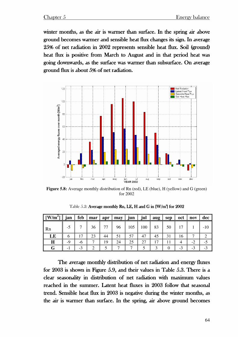
Chapter 5 Energy balance
64
winter months, as the air is warmer than surface. In the spring air above winter months, as the air is warmer than surface. In the spring air above winter months, as the air is warmer than surface. In the spring air above winter months, as the air is warmer than surface. In the spring air above
ground becomes warmer and sensible heat flux changes its sign. In average ground becomes warmer and sensible heat flux changes its sign. In average ground becomes warmer and sensible heat flux changes its sign. In average ground becomes warmer and sensible heat flux changes its sign. In average
25% of net radiation in 2002 represents sensible heat flux. Soil (ground) 25% of net radiation in 2002 represents sensible heat flux. Soil (ground) 25% of net radiation in 2002 represents sensible heat flux. Soil (ground) 25% of net radiation in 2002 represents sensible heat flux. Soil (ground)
heat heat heat heat flux is positive from March to August and in that period heat was flux is positive from March to August and in that period heat was flux is positive from March to August and in that period heat was flux is positive from March to August and in that period heat was
going downwards, as the surface was warmer than subsurface. On average going downwards, as the surface was warmer than subsurface. On average going downwards, as the surface was warmer than subsurface. On average going downwards, as the surface was warmer than subsurface. On average
ground flux is about 5% of net radiation.ground flux is about 5% of net radiation.ground flux is about 5% of net radiation.ground flux is about 5% of net radiation.
Figure 5.8: Average monthly distribution of Rn (red), LE (blue), H (yellow) and G (green)
for 2002
Table 5.2: Average monthly Rn, LE, H and G in [W/m Average monthly Rn, LE, H and G in [W/m Average monthly Rn, LE, H and G in [W/m Average monthly Rn, LE, H and G in [W/m2222] for 2002] for 2002] for 2002] for 2002
[W/m2] jan feb mar apr may jun jul aug sep oct nov dec
Rn -5 7 36 77 96 105 100 83 50 17 1 -10
LE 6 17 23 44 51 57 47 45 31 16 7 2
H -9 -6 7 19 24 25 27 17 11 4 -2 -5
G -1 -3 2 5 7 7 5 3 0 -3 -3 -3
The average monthly distribution of net radiation and energy fluxes The average monthly distribution of net radiation and energy fluxes The average monthly distribution of net radiation and energy fluxes The average monthly distribution of net radiation and energy fluxes
for 2003 is shown in Figure 5.9, and their values in Table 5.3. There is a for 2003 is shown in Figure 5.9, and their values in Table 5.3. There is a for 2003 is shown in Figure 5.9, and their values in Table 5.3. There is a for 2003 is shown in Figure 5.9, and their values in Table 5.3. There is a
clear seasonality in distribution of net radiation with maximum values clear seasonality in distribution of net radiation with maximum values clear seasonality in distribution of net radiation with maximum values clear seasonality in distribution of net radiation with maximum values
reachreachreachreached in the summer. Latent heat fluxes in 2003 follow that seasonal ed in the summer. Latent heat fluxes in 2003 follow that seasonal ed in the summer. Latent heat fluxes in 2003 follow that seasonal ed in the summer. Latent heat fluxes in 2003 follow that seasonal
trend. Sensible heat flux in 2003 is negative during the winter months, as trend. Sensible heat flux in 2003 is negative during the winter months, as trend. Sensible heat flux in 2003 is negative during the winter months, as trend. Sensible heat flux in 2003 is negative during the winter months, as
the air is warmer than surface. In the spring, air above ground becomes the air is warmer than surface. In the spring, air above ground becomes the air is warmer than surface. In the spring, air above ground becomes the air is warmer than surface. In the spring, air above ground becomes
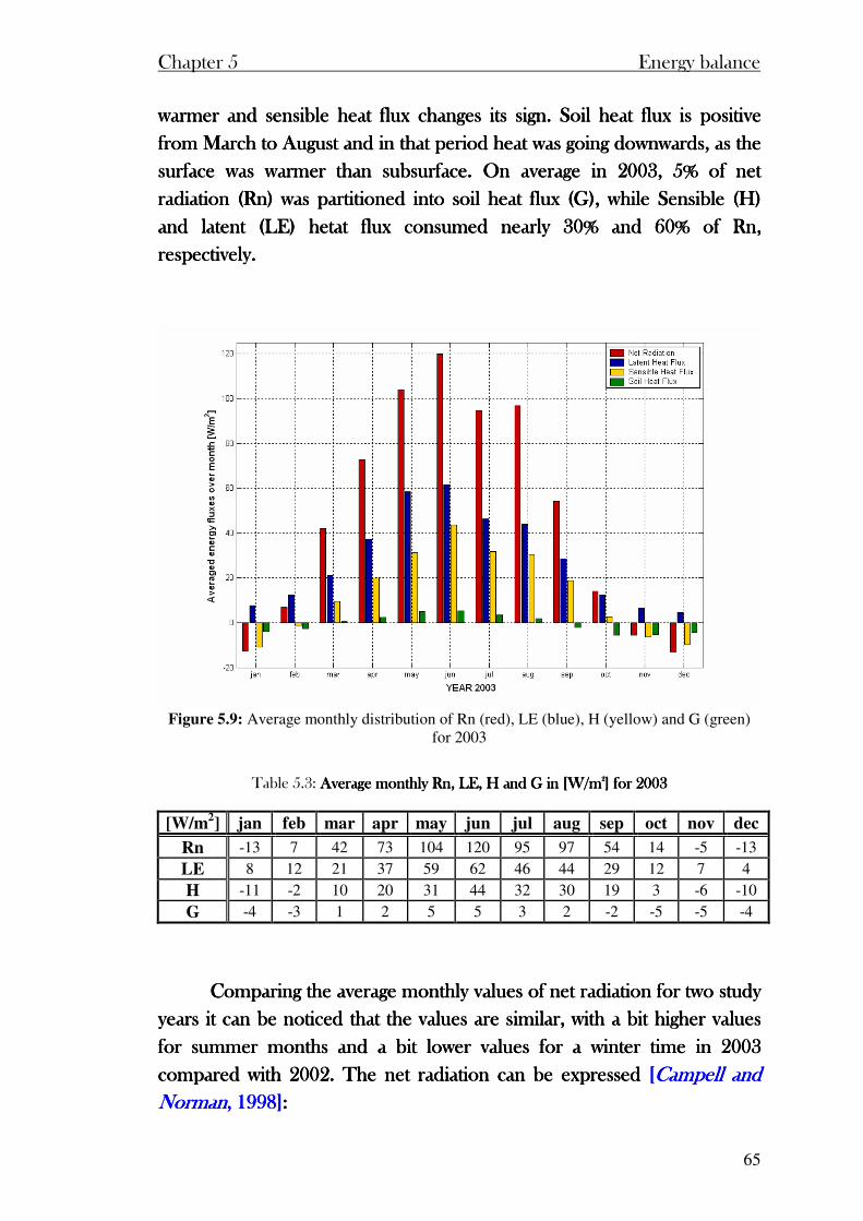
Chapter 5 Energy balance
65
warmer and sensible heat flux changes its swarmer and sensible heat flux changes its swarmer and sensible heat flux changes its swarmer and sensible heat flux changes its sign. Soil heat flux is positive ign. Soil heat flux is positive ign. Soil heat flux is positive ign. Soil heat flux is positive
from March to August and in that period heat was going downwards, as the from March to August and in that period heat was going downwards, as the from March to August and in that period heat was going downwards, as the from March to August and in that period heat was going downwards, as the
surface was warmer than subsurface. On average in 2003, 5% of net surface was warmer than subsurface. On average in 2003, 5% of net surface was warmer than subsurface. On average in 2003, 5% of net surface was warmer than subsurface. On average in 2003, 5% of net
radiation (Rn) was partitioned into soil heat flux (G), while Sensible (H) radiation (Rn) was partitioned into soil heat flux (G), while Sensible (H) radiation (Rn) was partitioned into soil heat flux (G), while Sensible (H) radiation (Rn) was partitioned into soil heat flux (G), while Sensible (H)
and latentand latentand latentand latent (LE) hetat flux consumed nearly 30% and 60% of Rn, (LE) hetat flux consumed nearly 30% and 60% of Rn, (LE) hetat flux consumed nearly 30% and 60% of Rn, (LE) hetat flux consumed nearly 30% and 60% of Rn,
respectively.respectively.respectively.respectively.
Figure 5.9: Average monthly distribution of Rn (red), LE (blue), H (yellow) and G (green)
for 2003
Table 5.3: Average monthly Rn, LE, H and G in [W/m Average monthly Rn, LE, H and G in [W/m Average monthly Rn, LE, H and G in [W/m Average monthly Rn, LE, H and G in [W/m2222] for 2003] for 2003] for 2003] for 2003
[W/m2] jan feb mar apr may jun jul aug sep oct nov dec
Rn -13 7 42 73 104 120 95 97 54 14 -5 -13
LE 8 12 21 37 59 62 46 44 29 12 7 4
H -11 -2 10 20 31 44 32 30 19 3 -6 -10
G -4 -3 1 2 5 5 3 2 -2 -5 -5 -4
Comparing the average monthly values of net radiation for two study Comparing the average monthly values of net radiation for two study Comparing the average monthly values of net radiation for two study Comparing the average monthly values of net radiation for two study
years it can be noticed that the values are similar, with a bit higher values years it can be noticed that the values are similar, with a bit higher values years it can be noticed that the values are similar, with a bit higher values years it can be noticed that the values are similar, with a bit higher values
for summer months and a bit lower values for a winter time in 2003 for summer months and a bit lower values for a winter time in 2003 for summer months and a bit lower values for a winter time in 2003 for summer months and a bit lower values for a winter time in 2003
compared with 2002. The net radiation can be expressed compared with 2002. The net radiation can be expressed compared with 2002. The net radiation can be expressed compared with 2002. The net radiation can be expressed [[[[Campell and Campell and Campell and Campell and NormanNormanNormanNorman, 1998], 1998], 1998], 1998]::::
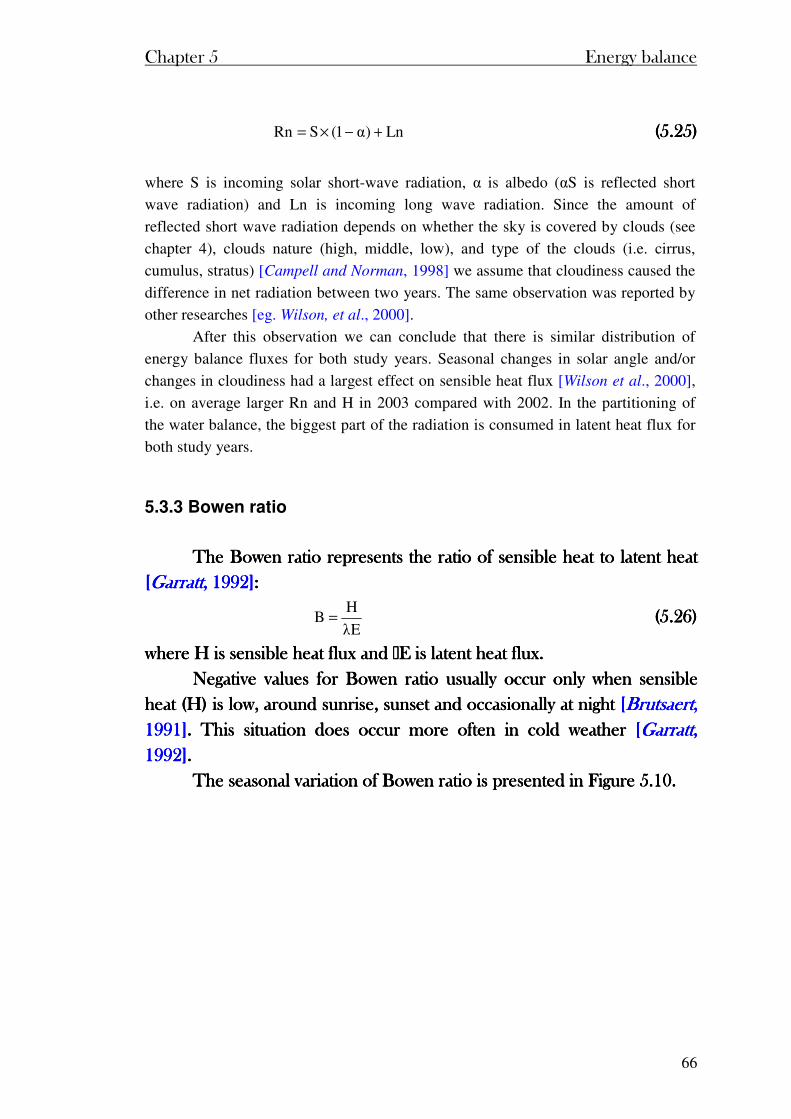
Chapter 5 Energy balance
66
Ln)α1(SRn +−×= (5.25) (5.25) (5.25) (5.25)
where S is incoming solar short-wave radiation, α is albedo (αS is reflected short
wave radiation) and Ln is incoming long wave radiation. Since the amount of
reflected short wave radiation depends on whether the sky is covered by clouds (see
chapter 4), clouds nature (high, middle, low), and type of the clouds (i.e. cirrus,
cumulus, stratus) [Campell and Norman, 1998] we assume that cloudiness caused the
difference in net radiation between two years. The same observation was reported by
other researches [eg. Wilson, et al., 2000].
After this observation we can conclude that there is similar distribution of
energy balance fluxes for both study years. Seasonal changes in solar angle and/or
changes in cloudiness had a largest effect on sensible heat flux [Wilson et al., 2000],
i.e. on average larger Rn and H in 2003 compared with 2002. In the partitioning of
the water balance, the biggest part of the radiation is consumed in latent heat flux for
both study years.
5.3.3 Bowen ratio
The Bowen ratio representsThe Bowen ratio representsThe Bowen ratio representsThe Bowen ratio represents the ratio of sensible heat to latent heat the ratio of sensible heat to latent heat the ratio of sensible heat to latent heat the ratio of sensible heat to latent heat
[[[[GarrattGarrattGarrattGarratt, 1992], 1992], 1992], 1992]::::
Eλ
HB = (5.26) (5.26) (5.26) (5.26)
where H is sensible heat flux and ME is latent heat flux.where H is sensible heat flux and ME is latent heat flux.where H is sensible heat flux and ME is latent heat flux.where H is sensible heat flux and ME is latent heat flux.
Negative values for Bowen ratio usually occur only when sensible Negative values for Bowen ratio usually occur only when sensible Negative values for Bowen ratio usually occur only when sensible Negative values for Bowen ratio usually occur only when sensible
heat (H) is low, around sunrise, sunset and occasionally at night heat (H) is low, around sunrise, sunset and occasionally at night heat (H) is low, around sunrise, sunset and occasionally at night heat (H) is low, around sunrise, sunset and occasionally at night [[[[BrutsaertBrutsaertBrutsaertBrutsaert, , , , 1991]1991]1991]1991]. This situation does occur more often in cold wea. This situation does occur more often in cold wea. This situation does occur more often in cold wea. This situation does occur more often in cold weather ther ther ther [[[[GarrattGarrattGarrattGarratt, , , , 1992]1992]1992]1992]....
The seasonal variation of Bowen ratio is presented in Figure 5.10. The seasonal variation of Bowen ratio is presented in Figure 5.10. The seasonal variation of Bowen ratio is presented in Figure 5.10. The seasonal variation of Bowen ratio is presented in Figure 5.10.
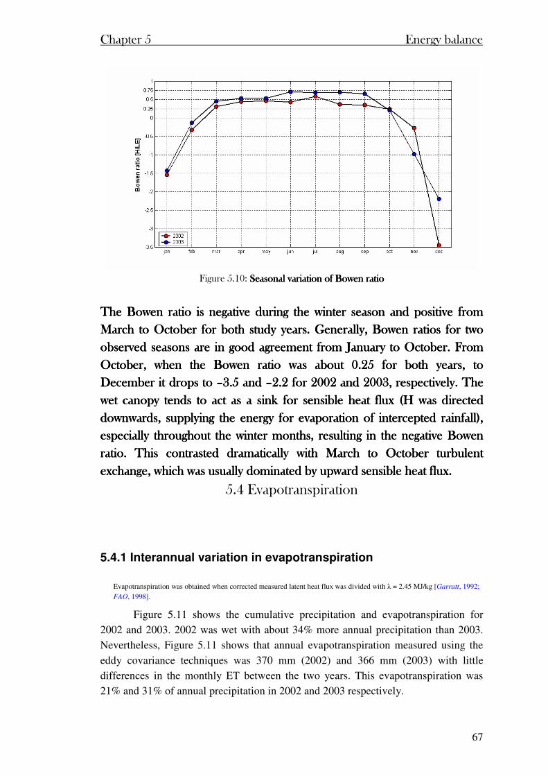
Chapter 5 Energy balance
67
Figure 5.10: Seasonal variation of Bowen ratio Seasonal variation of Bowen ratio Seasonal variation of Bowen ratio Seasonal variation of Bowen ratio
The Bowen ratio is negative during the winter season and positive from The Bowen ratio is negative during the winter season and positive from The Bowen ratio is negative during the winter season and positive from The Bowen ratio is negative during the winter season and positive from
March to October for both study years. GeneraMarch to October for both study years. GeneraMarch to October for both study years. GeneraMarch to October for both study years. Generally, Bowen ratios for two lly, Bowen ratios for two lly, Bowen ratios for two lly, Bowen ratios for two
observed seasons are in good agreement from January to October. From observed seasons are in good agreement from January to October. From observed seasons are in good agreement from January to October. From observed seasons are in good agreement from January to October. From
October, when the Bowen ratio was about 0.25 for both years, to October, when the Bowen ratio was about 0.25 for both years, to October, when the Bowen ratio was about 0.25 for both years, to October, when the Bowen ratio was about 0.25 for both years, to
December it drops to December it drops to December it drops to December it drops to ––––3.5 and 3.5 and 3.5 and 3.5 and ––––2.2 for 2002 and 2003, respectively. The 2.2 for 2002 and 2003, respectively. The 2.2 for 2002 and 2003, respectively. The 2.2 for 2002 and 2003, respectively. The
wet canopy tends to act awet canopy tends to act awet canopy tends to act awet canopy tends to act as a sink for sensible heat flux (H was directed s a sink for sensible heat flux (H was directed s a sink for sensible heat flux (H was directed s a sink for sensible heat flux (H was directed
downwards, supplying the energy for evaporation of intercepted rainfall), downwards, supplying the energy for evaporation of intercepted rainfall), downwards, supplying the energy for evaporation of intercepted rainfall), downwards, supplying the energy for evaporation of intercepted rainfall),
especially throughout the winter months, resulting in the negative Bowen especially throughout the winter months, resulting in the negative Bowen especially throughout the winter months, resulting in the negative Bowen especially throughout the winter months, resulting in the negative Bowen
ratio. This contrasted dramatically with March to October turratio. This contrasted dramatically with March to October turratio. This contrasted dramatically with March to October turratio. This contrasted dramatically with March to October turbulent bulent bulent bulent
exchange, which was usually dominated by upward sensible heat flux.exchange, which was usually dominated by upward sensible heat flux.exchange, which was usually dominated by upward sensible heat flux.exchange, which was usually dominated by upward sensible heat flux.
5.4 Evapotranspiration
5.4.1 Interannual variation in evapotranspiration
Evapotranspiration was obtained when corrected measured latent heat flux was divided with λ = 2.45 MJ/kg [Garratt, 1992;
FAO, 1998].
Figure 5.11 shows the cumulative precipitation and evapotranspiration for
2002 and 2003. 2002 was wet with about 34% more annual precipitation than 2003.
Nevertheless, Figure 5.11 shows that annual evapotranspiration measured using the
eddy covariance techniques was 370 mm (2002) and 366 mm (2003) with little
differences in the monthly ET between the two years. This evapotranspiration was
21% and 31% of annual precipitation in 2002 and 2003 respectively.
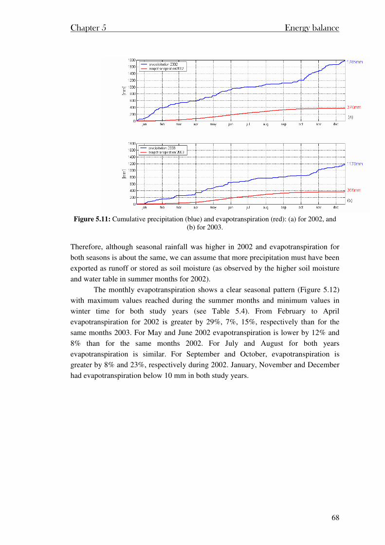
Chapter 5 Energy balance
68
Figure 5.11: Cumulative precipitation (blue) and evapotranspiration (red): (a) for 2002, and
(b) for 2003.
Therefore, although seasonal rainfall was higher in 2002 and evapotranspiration for
both seasons is about the same, we can assume that more precipitation must have been
exported as runoff or stored as soil moisture (as observed by the higher soil moisture
and water table in summer months for 2002).
The monthly evapotranspiration shows a clear seasonal pattern (Figure 5.12)
with maximum values reached during the summer months and minimum values in
winter time for both study years (see Table 5.4). From February to April
evapotranspiration for 2002 is greater by 29%, 7%, 15%, respectively than for the
same months 2003. For May and June 2002 evapotranspiration is lower by 12% and
8% than for the same months 2002. For July and August for both years
evapotranspiration is similar. For September and October, evapotranspiration is
greater by 8% and 23%, respectively during 2002. January, November and December
had evapotranspiration below 10 mm in both study years.
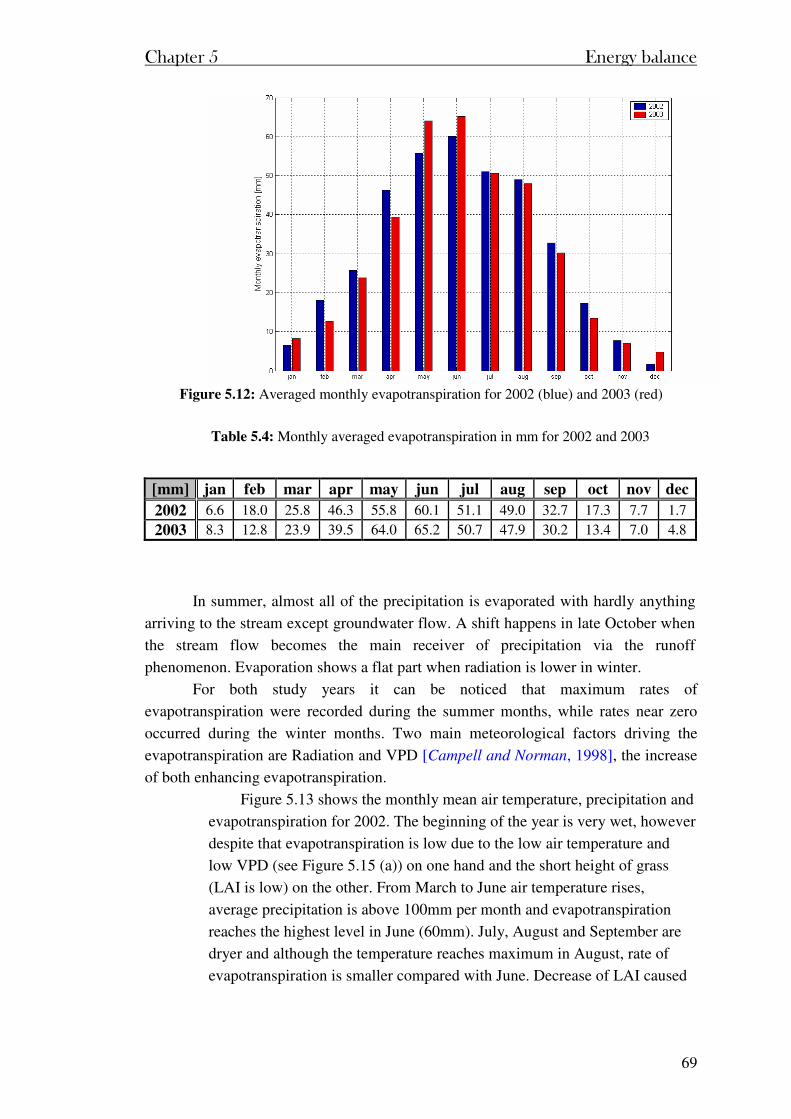
Chapter 5 Energy balance
69
Figure 5.12: Averaged monthly evapotranspiration for 2002 (blue) and 2003 (red)
Table 5.4: Monthly averaged evapotranspiration in mm for 2002 and 2003
[mm] jan feb mar apr may jun jul aug sep oct nov dec
2002 6.6 18.0 25.8 46.3 55.8 60.1 51.1 49.0 32.7 17.3 7.7 1.7
2003 8.3 12.8 23.9 39.5 64.0 65.2 50.7 47.9 30.2 13.4 7.0 4.8
In summer, almost all of the precipitation is evaporated with hardly anything
arriving to the stream except groundwater flow. A shift happens in late October when
the stream flow becomes the main receiver of precipitation via the runoff
phenomenon. Evaporation shows a flat part when radiation is lower in winter.
For both study years it can be noticed that maximum rates of
evapotranspiration were recorded during the summer months, while rates near zero
occurred during the winter months. Two main meteorological factors driving the
evapotranspiration are Radiation and VPD [Campell and Norman, 1998], the increase
of both enhancing evapotranspiration.
Figure 5.13 shows the monthly mean air temperature, precipitation and
evapotranspiration for 2002. The beginning of the year is very wet, however
despite that evapotranspiration is low due to the low air temperature and
low VPD (see Figure 5.15 (a)) on one hand and the short height of grass
(LAI is low) on the other. From March to June air temperature rises,
average precipitation is above 100mm per month and evapotranspiration
reaches the highest level in June (60mm). July, August and September are
dryer and although the temperature reaches maximum in August, rate of
evapotranspiration is smaller compared with June. Decrease of LAI caused
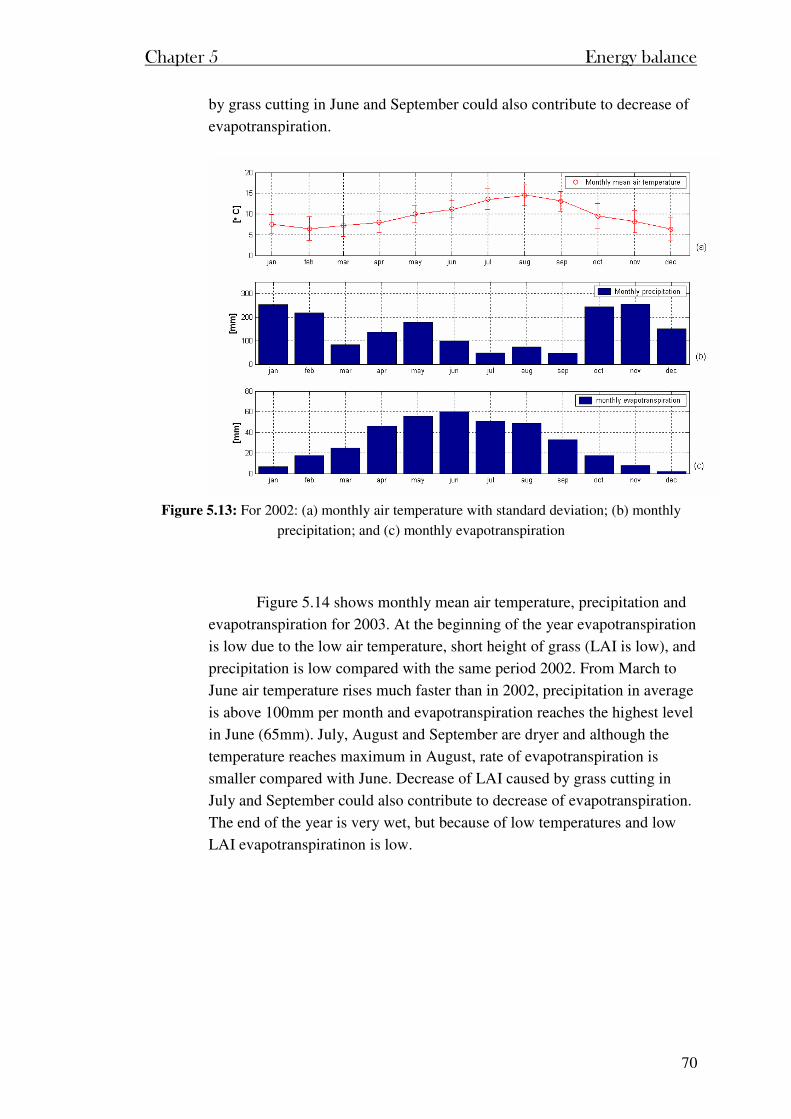
Chapter 5 Energy balance
70
by grass cutting in June and September could also contribute to decrease of
evapotranspiration.
Figure 5.13: For 2002: (a) monthly air temperature with standard deviation; (b) monthly
precipitation; and (c) monthly evapotranspiration
Figure 5.14 shows monthly mean air temperature, precipitation and
evapotranspiration for 2003. At the beginning of the year evapotranspiration
is low due to the low air temperature, short height of grass (LAI is low), and
precipitation is low compared with the same period 2002. From March to
June air temperature rises much faster than in 2002, precipitation in average
is above 100mm per month and evapotranspiration reaches the highest level
in June (65mm). July, August and September are dryer and although the
temperature reaches maximum in August, rate of evapotranspiration is
smaller compared with June. Decrease of LAI caused by grass cutting in
July and September could also contribute to decrease of evapotranspiration.
The end of the year is very wet, but because of low temperatures and low
LAI evapotranspiratinon is low.
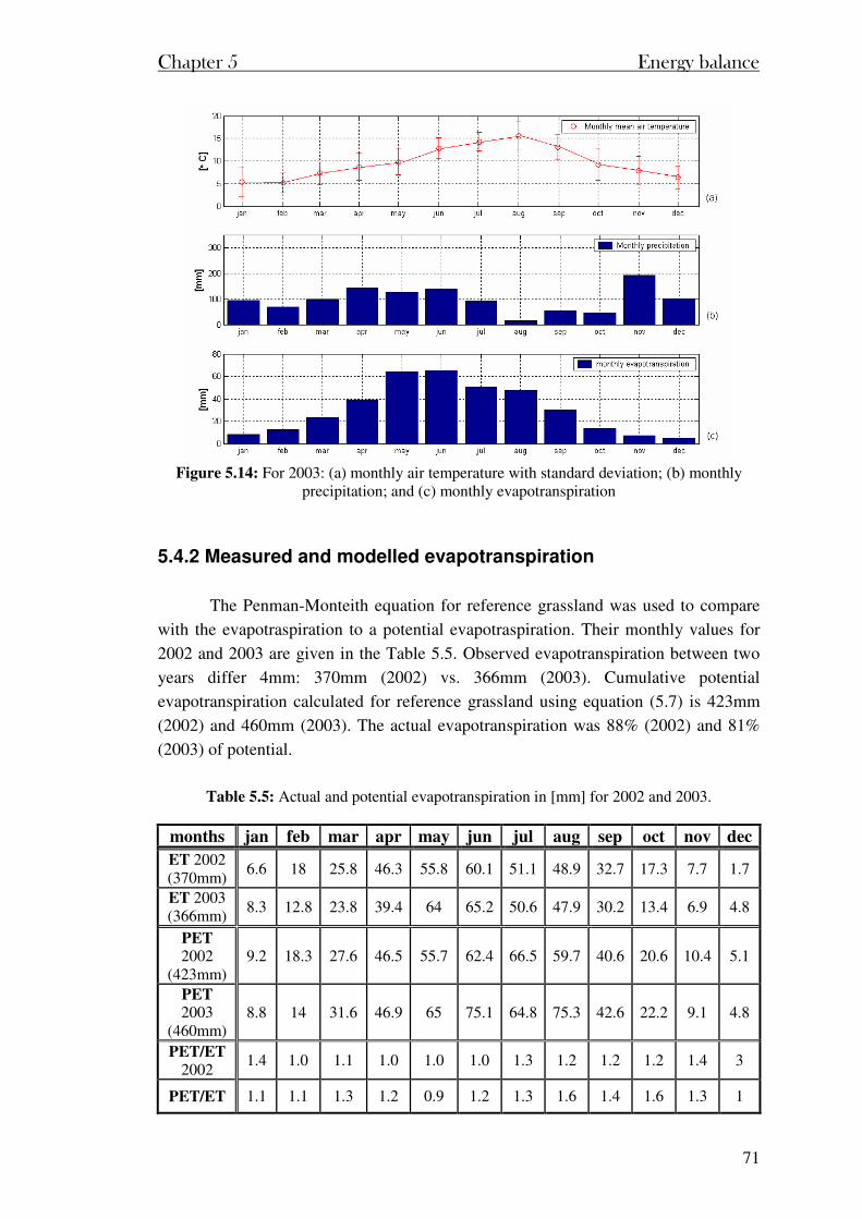
Chapter 5 Energy balance
71
Figure 5.14: For 2003: (a) monthly air temperature with standard deviation; (b) monthly
precipitation; and (c) monthly evapotranspiration
5.4.2 Measured and modelled evapotranspiration
The Penman-Monteith equation for reference grassland was used to compare
with the evapotraspiration to a potential evapotraspiration. Their monthly values for
2002 and 2003 are given in the Table 5.5. Observed evapotranspiration between two
years differ 4mm: 370mm (2002) vs. 366mm (2003). Cumulative potential
evapotranspiration calculated for reference grassland using equation (5.7) is 423mm
(2002) and 460mm (2003). The actual evapotranspiration was 88% (2002) and 81%
(2003) of potential.
Table 5.5: Actual and potential evapotranspiration in [mm] for 2002 and 2003.
months jan feb mar apr may jun jul aug sep oct nov dec
ET 2002 (370mm)
6.6 18 25.8 46.3 55.8 60.1 51.1 48.9 32.7 17.3 7.7 1.7
ET 2003 (366mm)
8.3 12.8 23.8 39.4 64 65.2 50.6 47.9 30.2 13.4 6.9 4.8
PET 2002
(423mm) 9.2 18.3 27.6 46.5 55.7 62.4 66.5 59.7 40.6 20.6 10.4 5.1
PET 2003
(460mm) 8.8 14 31.6 46.9 65 75.1 64.8 75.3 42.6 22.2 9.1 4.8
PET/ET 2002
1.4 1.0 1.1 1.0 1.0 1.0 1.3 1.2 1.2 1.2 1.4 3
PET/ET 1.1 1.1 1.3 1.2 0.9 1.2 1.3 1.6 1.4 1.6 1.3 1
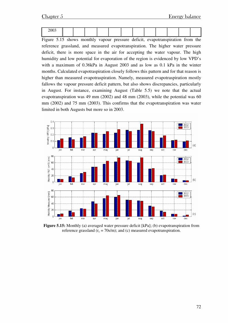
Chapter 5 Energy balance
72
2003
Figure 5.15 shows monthly vapour pressure deficit, evapotranspiration from the
reference grassland, and measured evapotranspiration. The higher water pressure
deficit, there is more space in the air for accepting the water vapour. The high
humidity and low potential for evaporation of the region is evidenced by low VPD’s
with a maximum of 0.36kPa in August 2003 and as low as 0.1 kPa in the winter
months. Calculated evapotraspiration closely follows this pattern and for that reason is
higher than measured evapotraspiration. Namely, measured evapotraspiration mostly
fallows the vapour pressure deficit pattern, but also shows discrepancies, particularly
in August. For instance, examining August (Table 5.5) we note that the actual
evapotranspiration was 49 mm (2002) and 48 mm (2003), while the potential was 60
mm (2002) and 75 mm (2003). This confirms that the evapotranspiration was water
limited in both Augusts but more so in 2003.
Figure 5.15: Monthly (a) averaged water pressure deficit [kPa]; (b) evapotranspiration from
reference grassland (rc = 70s/m); and (c) measured evapotranspiration.
Chapter 6 Carbon dioxide flux
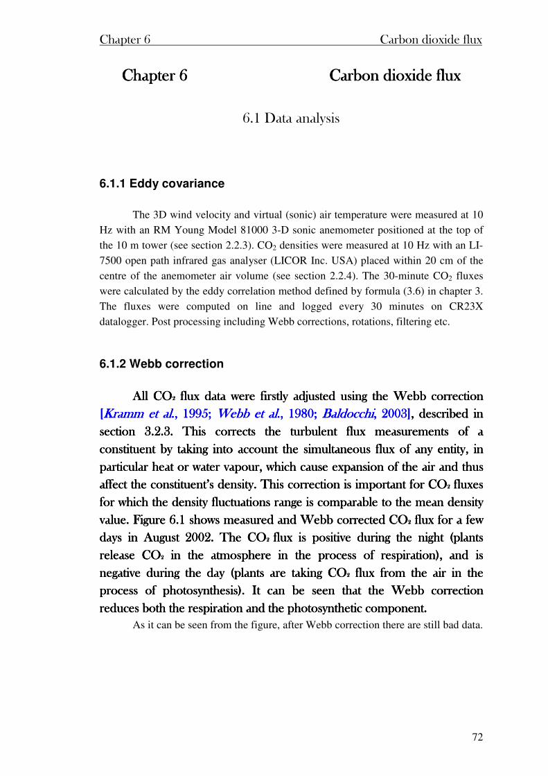
Chapter 6 Carbon dioxide flux
72
Chapter 6Chapter 6Chapter 6Chapter 6 Carbon dioxide flux Carbon dioxide flux Carbon dioxide flux Carbon dioxide flux
6.1 Data analysis
6.1.1 Eddy covariance
The 3D wind velocity and virtual (sonic) air temperature were measured at 10
Hz with an RM Young Model 81000 3-D sonic anemometer positioned at the top of
the 10 m tower (see section 2.2.3). CO2 densities were measured at 10 Hz with an LI-
7500 open path infrared gas analyser (LICOR Inc. USA) placed within 20 cm of the
centre of the anemometer air volume (see section 2.2.4). The 30-minute CO2 fluxes
were calculated by the eddy correlation method defined by formula (3.6) in chapter 3.
The fluxes were computed on line and logged every 30 minutes on CR23X
datalogger. Post processing including Webb corrections, rotations, filtering etc.
6.1.2 Webb correction
All COAll COAll COAll CO2222 flux data were firstly adjusted using the Webb correction flux data were firstly adjusted using the Webb correction flux data were firstly adjusted using the Webb correction flux data were firstly adjusted using the Webb correction
[[[[Kramm et alKramm et alKramm et alKramm et al., 1995;., 1995;., 1995;., 1995; Webb et alWebb et alWebb et alWebb et al., 1980; ., 1980; ., 1980; ., 1980; BaldocchiBaldocchiBaldocchiBaldocchi, 2003], 2003], 2003], 2003],,,, described in described in described in described in
section 3.2.3. This corrects the turbulent flux measurements of a section 3.2.3. This corrects the turbulent flux measurements of a section 3.2.3. This corrects the turbulent flux measurements of a section 3.2.3. This corrects the turbulent flux measurements of a
constconstconstconstituent by taking into account the simultaneous flux of any entity, in ituent by taking into account the simultaneous flux of any entity, in ituent by taking into account the simultaneous flux of any entity, in ituent by taking into account the simultaneous flux of any entity, in
particular heat or water vapour, which cause expansion of the air and thus particular heat or water vapour, which cause expansion of the air and thus particular heat or water vapour, which cause expansion of the air and thus particular heat or water vapour, which cause expansion of the air and thus
affect the constituent’s density. This correction is important for COaffect the constituent’s density. This correction is important for COaffect the constituent’s density. This correction is important for COaffect the constituent’s density. This correction is important for CO2222 fluxes fluxes fluxes fluxes
for which the density fluctuationfor which the density fluctuationfor which the density fluctuationfor which the density fluctuations range is comparable to the mean density s range is comparable to the mean density s range is comparable to the mean density s range is comparable to the mean density
value. Figure 6.1 shows measured and Webb corrected COvalue. Figure 6.1 shows measured and Webb corrected COvalue. Figure 6.1 shows measured and Webb corrected COvalue. Figure 6.1 shows measured and Webb corrected CO2222 flux for a few flux for a few flux for a few flux for a few
days in August 2002. The COdays in August 2002. The COdays in August 2002. The COdays in August 2002. The CO2 2 2 2 flux is positive during the night (plants flux is positive during the night (plants flux is positive during the night (plants flux is positive during the night (plants
release COrelease COrelease COrelease CO2222 in the atmosphere in the process of respiration), and is in the atmosphere in the process of respiration), and is in the atmosphere in the process of respiration), and is in the atmosphere in the process of respiration), and is
negnegnegnegative during the day (plants are taking COative during the day (plants are taking COative during the day (plants are taking COative during the day (plants are taking CO2222 flux from the air in the flux from the air in the flux from the air in the flux from the air in the
process of photosynthesis). It can be seen that the Webb correction process of photosynthesis). It can be seen that the Webb correction process of photosynthesis). It can be seen that the Webb correction process of photosynthesis). It can be seen that the Webb correction
reduces both the respiration and the photosynthetic component.reduces both the respiration and the photosynthetic component.reduces both the respiration and the photosynthetic component.reduces both the respiration and the photosynthetic component. As it can be seen from the figure, after Webb correction there are still bad data.
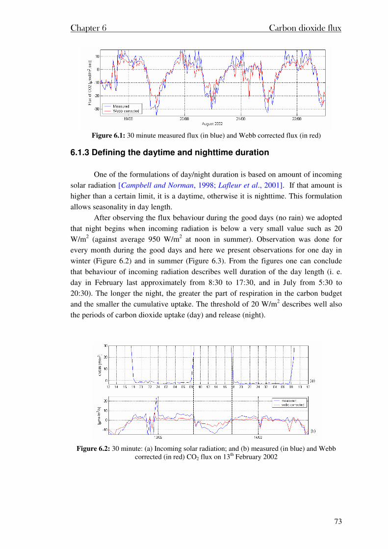
Chapter 6 Carbon dioxide flux
73
Figure 6.1: 30 minute measured flux (in blue) and Webb corrected flux (in red)
6.1.3 Defining the daytime and nighttime duration
One of the formulations of day/night duration is based on amount of incoming
solar radiation [Campbell and Norman, 1998; Lafleur et al., 2001]. If that amount is
higher than a certain limit, it is a daytime, otherwise it is nighttime. This formulation
allows seasonality in day length.
After observing the flux behaviour during the good days (no rain) we adopted
that night begins when incoming radiation is below a very small value such as 20
W/m2 (against average 950 W/m2 at noon in summer). Observation was done for
every month during the good days and here we present observations for one day in
winter (Figure 6.2) and in summer (Figure 6.3). From the figures one can conclude
that behaviour of incoming radiation describes well duration of the day length (i. e.
day in February last approximately from 8:30 to 17:30, and in July from 5:30 to
20:30). The longer the night, the greater the part of respiration in the carbon budget
and the smaller the cumulative uptake. The threshold of 20 W/m2 describes well also
the periods of carbon dioxide uptake (day) and release (night).
Figure 6.2: 30 minute: (a) Incoming solar radiation; and (b) measured (in blue) and Webb
corrected (in red) CO2 flux on 13th February 2002
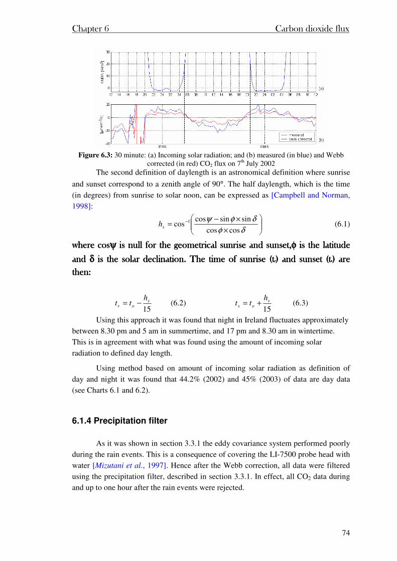
Chapter 6 Carbon dioxide flux
74
Figure 6.3: 30 minute: (a) Incoming solar radiation; and (b) measured (in blue) and Webb
corrected (in red) CO2 flux on 7th July 2002 The second definition of daylength is an astronomical definition where sunrise
and sunset correspond to a zenith angle of 90°. The half daylength, which is the time
(in degrees) from sunrise to solar noon, can be expressed as [Campbell and Norman,
1998]:
×
×−= −
δφ
δφψ
coscos
sinsincoscos 1
sh (6.1)
where coswhere coswhere coswhere cosψψψψ is null for the geometrical sunrise and sunset, is null for the geometrical sunrise and sunset, is null for the geometrical sunrise and sunset, is null for the geometrical sunrise and sunset,φφφφ is the latitude is the latitude is the latitude is the latitude
and and and and δδδδ is the solar declination. The time of sunrise (t is the solar declination. The time of sunrise (t is the solar declination. The time of sunrise (t is the solar declination. The time of sunrise (trrrr) and sunset (t) and sunset (t) and sunset (t) and sunset (tssss) are ) are ) are ) are
then:then:then:then:
15s
or
htt −= (6.2)
15s
os
htt += (6.3)
Using this approach it was found that night in Ireland fluctuates approximately
between 8.30 pm and 5 am in summertime, and 17 pm and 8.30 am in wintertime.
This is in agreement with what was found using the amount of incoming solar
radiation to defined day length.
Using method based on amount of incoming solar radiation as definition of
day and night it was found that 44.2% (2002) and 45% (2003) of data are day data
(see Charts 6.1 and 6.2).
6.1.4 Precipitation filter
As it was shown in section 3.3.1 the eddy covariance system performed poorly
during the rain events. This is a consequence of covering the LI-7500 probe head with
water [Mizutani et al., 1997]. Hence after the Webb correction, all data were filtered
using the precipitation filter, described in section 3.3.1. In effect, all CO2 data during
and up to one hour after the rain events were rejected.
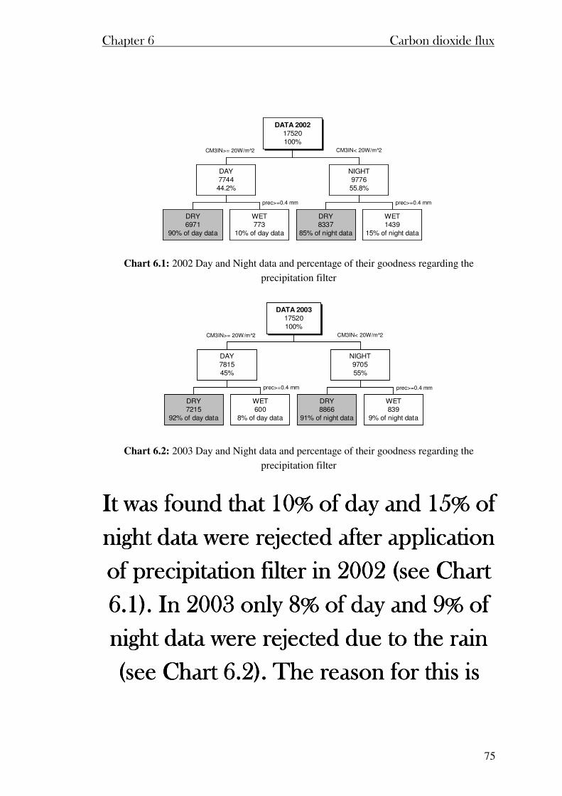
Chapter 6 Carbon dioxide flux
75
Chart 6.1: 2002 Day and Night data and percentage of their goodness regarding the
precipitation filter
CM3IN>= 20W/m 2
prec>=0.4 mm prec>=0.4 mm
CM3IN< 20W/m 2
DRY
7215
92% of day data
WET
600
8% of day data
DAY
7815
45%
DRY
8866
91% of night data
WET
839
9% of night data
NIGHT
9705
55%
DATA 2003
17520
100%
Chart 6.2: 2003 Day and Night data and percentage of their goodness regarding the
precipitation filter
It was found that 10% of day and 15% of It was found that 10% of day and 15% of It was found that 10% of day and 15% of It was found that 10% of day and 15% of
night data were rejected after application night data were rejected after application night data were rejected after application night data were rejected after application
of precipitation filtof precipitation filtof precipitation filtof precipitation filter in 2002 (see Chart er in 2002 (see Chart er in 2002 (see Chart er in 2002 (see Chart
6.1). In 2003 only 8% of day and 9% of 6.1). In 2003 only 8% of day and 9% of 6.1). In 2003 only 8% of day and 9% of 6.1). In 2003 only 8% of day and 9% of
night data were rejected due to the rain night data were rejected due to the rain night data were rejected due to the rain night data were rejected due to the rain
(see Chart 6.2). The reason for this is (see Chart 6.2). The reason for this is (see Chart 6.2). The reason for this is (see Chart 6.2). The reason for this is
CM3IN>= 20W/m 2
prec>=0.4 mm prec>=0.4 mm
CM3IN< 20W/m 2
DRY
6971
90% of day data
WET
773
10% of day data
DAY
7744
44.2%
DRY
8337
85% of night data
WET
1439
15% of night data
NIGHT
9776
55.8%
DATA 2002
17520
100%
Chapter 6 Carbon dioxide flux
76
less precipitation during the 2003 less precipitation during the 2003 less precipitation during the 2003 less precipitation during the 2003
season.season.season.season.
6.1.5 Momentum flux filter
The nocturnal period includes conditions such as cold air drainage, sporadic
mixing, and fluctuations in vertical wind too small to be resolved by the sonic
anemometer.
The eddy correlation method works best during windy periods [e.g., Goulden,
et al., 1996; Moncrieff et al., 1997; Falge et al., 2001]. During calm climatic
conditions the measured fluxes are underestimated:
1) as the fluctuations in the vertical wind speed are too small to be
resolved by the sonic anemometer [Goulden, et al., 1996] and
2) for nocturnal and very stable conditions, the flow statistics may be
dominated by transient phenomena or even lack of turbulence [Cava et
al., 2004].
Cava et al. [2004] found that when canopy waves dominate night-time runs,
the local CO2 production from ecosystem respiration and observed mean fluxes above
the canopy are, to a first order, de-coupled presumably through a storage term. What
is important here is that when canopy waves dominate, there is “gross” mass and heat
exchange between the canopy and the atmosphere; however, the net exchange over the
lifecycle of the wave is negligible. Occasionally, these waves are under-sampled
because of a short flux averaging period leading to an apparent and spurious
“photosynthesis” (or canopy C uptake) values at night in the case of CO2. Correcting
night-time fluxes with runs collected under high u* (or more precisely for near-neutral
to slightly stable conditions) ensures that the turbulent regime is fully-developed.
Another reason why runs with high friction velocity (momentum flux), u*, (or near-
neutral conditions) are preferred for night-time flux corrections is a much smaller (and
perhaps the more realistic) footprint.
Uncertainties in night-time fluxes have been examined by many researchers
[Falge et al., 2001; Pattey et. al., 2002; Baldocchi et al., 2003]. The nocturnal CO2
flux is a critical issue regarding poorly mixed periods, since small underestimations of
night-time CO2 fluxes (respiration) imply overestimations of the annual carbon uptake
[Goulden et al., 1996; Baldocchi et al., 1996; Moncrieff et al., 1996; Schmid et al.,
2000; Valentini et al., 2000]. In identifying calm conditions a lower boundary for u*
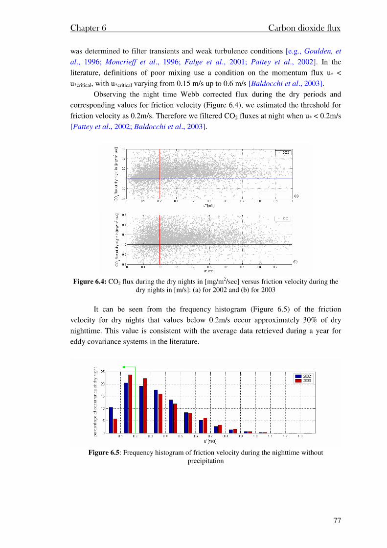
Chapter 6 Carbon dioxide flux
77
was determined to filter transients and weak turbulence conditions [e.g., Goulden, et
al., 1996; Moncrieff et al., 1996; Falge et al., 2001; Pattey et al., 2002]. In the
literature, definitions of poor mixing use a condition on the momentum flux u* <
u*critical, with u*critical varying from 0.15 m/s up to 0.6 m/s [Baldocchi et al., 2003].
Observing the night time Webb corrected flux during the dry periods and
corresponding values for friction velocity (Figure 6.4), we estimated the threshold for
friction velocity as 0.2m/s. Therefore we filtered CO2 fluxes at night when u* < 0.2m/s
[Pattey et al., 2002; Baldocchi et al., 2003].
Figure 6.4: CO2 flux during the dry nights in [mg/m2/sec] versus friction velocity during the
dry nights in [m/s]: (a) for 2002 and (b) for 2003
It can be seen from the frequency histogram (Figure 6.5) of the friction
velocity for dry nights that values below 0.2m/s occur approximately 30% of dry
nighttime. This value is consistent with the average data retrieved during a year for
eddy covariance systems in the literature.
Figure 6.5: Frequency histogram of friction velocity during the nighttime without
precipitation
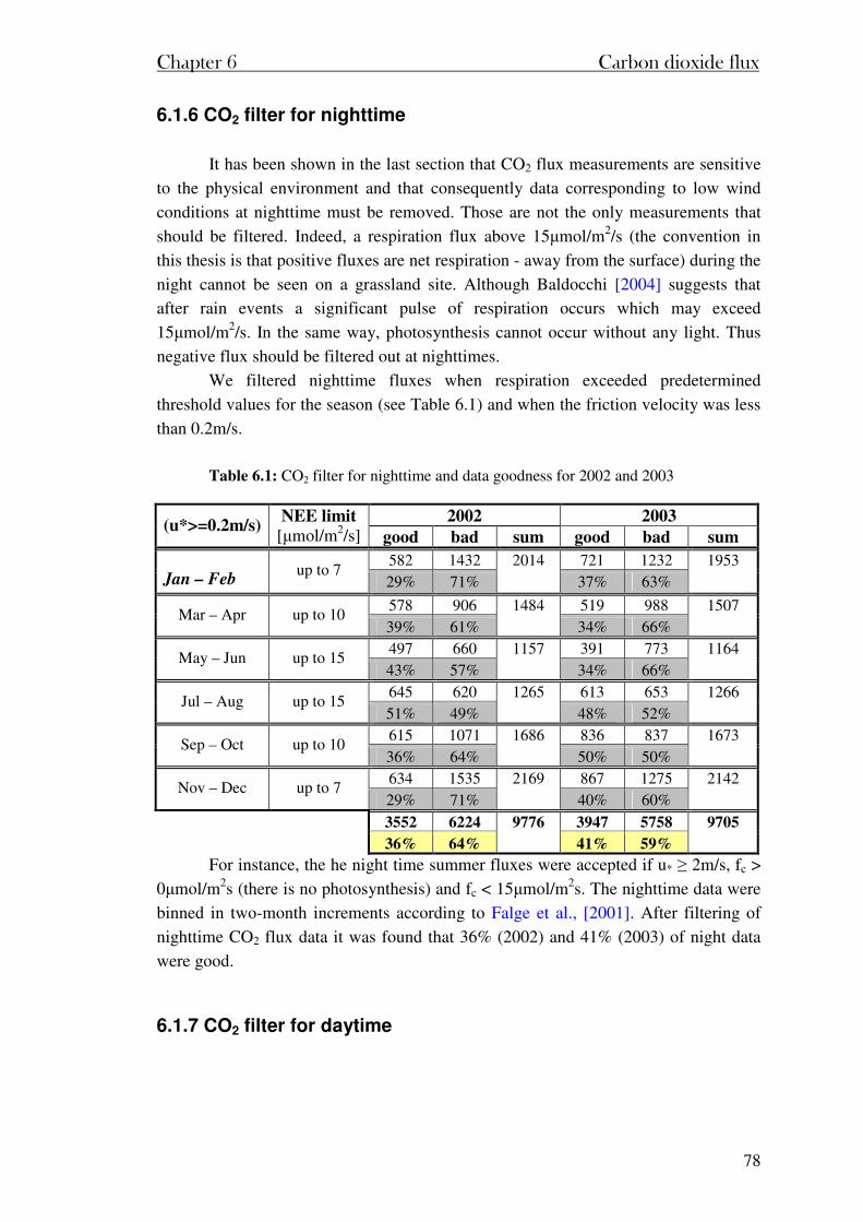
Chapter 6 Carbon dioxide flux
78
6.1.6 CO2 filter for nighttime
It has been shown in the last section that CO2 flux measurements are sensitive
to the physical environment and that consequently data corresponding to low wind
conditions at nighttime must be removed. Those are not the only measurements that
should be filtered. Indeed, a respiration flux above 15µmol/m2/s (the convention in
this thesis is that positive fluxes are net respiration - away from the surface) during the
night cannot be seen on a grassland site. Although Baldocchi [2004] suggests that
after rain events a significant pulse of respiration occurs which may exceed
15µmol/m2/s. In the same way, photosynthesis cannot occur without any light. Thus
negative flux should be filtered out at nighttimes.
We filtered nighttime fluxes when respiration exceeded predetermined
threshold values for the season (see Table 6.1) and when the friction velocity was less
than 0.2m/s.
Table 6.1: CO2 filter for nighttime and data goodness for 2002 and 2003
2002 2003 (u*>=0.2m/s)
NEE limit [µmol/m2/s] good bad sum good bad sum
582 1432 721 1232 Jan – Feb
up to 7 29% 71%
2014
37% 63%
1953
578 906 519 988 Mar – Apr up to 10
39% 61%
1484
34% 66%
1507
497 660 391 773 May – Jun up to 15
43% 57%
1157
34% 66%
1164
645 620 613 653 Jul – Aug up to 15
51% 49%
1265
48% 52%
1266
615 1071 836 837 Sep – Oct up to 10
36% 64%
1686
50% 50%
1673
634 1535 867 1275 Nov – Dec up to 7
29% 71%
2169
40% 60%
2142
3552 6224 3947 5758
36% 64%
9776
41% 59%
9705
For instance, the he night time summer fluxes were accepted if u* ≥ 2m/s, fc >
0µmol/m2s (there is no photosynthesis) and fc < 15µmol/m2s. The nighttime data were
binned in two-month increments according to Falge et al., [2001]. After filtering of
nighttime CO2 flux data it was found that 36% (2002) and 41% (2003) of night data
were good.
6.1.7 CO2 filter for daytime
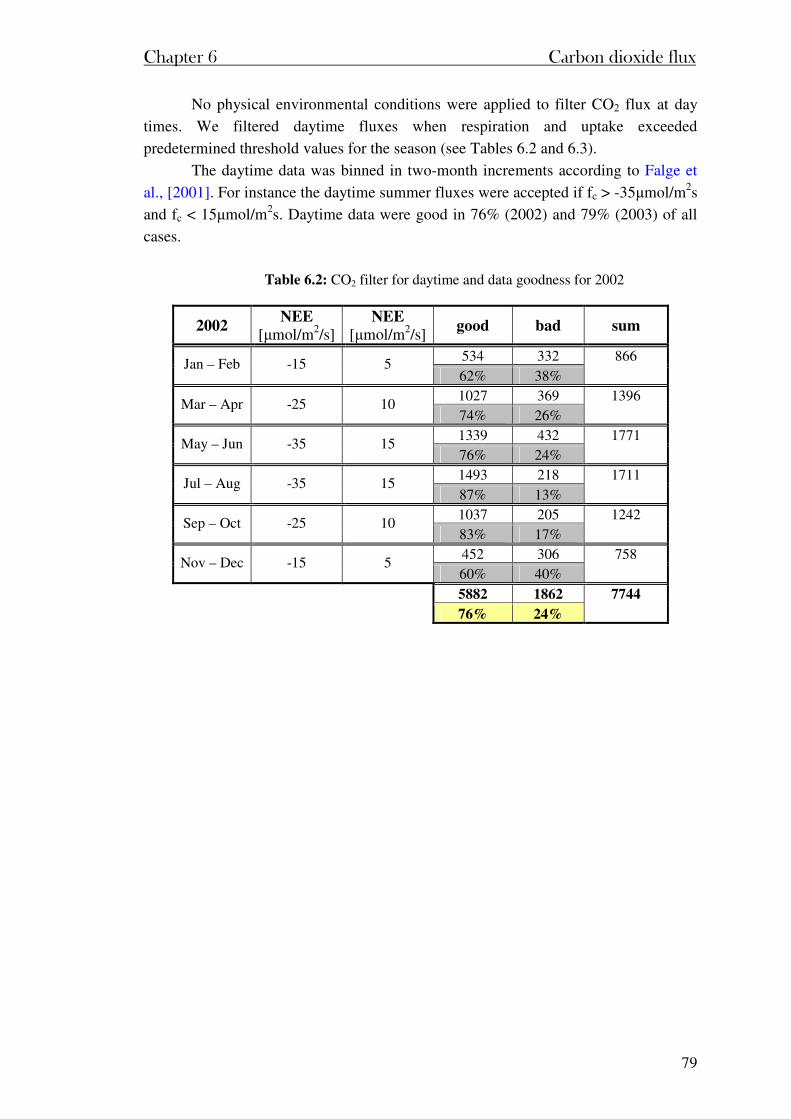
Chapter 6 Carbon dioxide flux
79
No physical environmental conditions were applied to filter CO2 flux at day
times. We filtered daytime fluxes when respiration and uptake exceeded
predetermined threshold values for the season (see Tables 6.2 and 6.3).
The daytime data was binned in two-month increments according to Falge et
al., [2001]. For instance the daytime summer fluxes were accepted if fc > -35µmol/m2s
and fc < 15µmol/m2s. Daytime data were good in 76% (2002) and 79% (2003) of all
cases.
Table 6.2: CO2 filter for daytime and data goodness for 2002
2002 NEE
[µmol/m2/s] NEE
[µmol/m2/s] good bad sum
534 332 Jan – Feb -15 5
62% 38%
866
1027 369 Mar – Apr -25 10
74% 26%
1396
1339 432 May – Jun -35 15
76% 24%
1771
1493 218 Jul – Aug -35 15
87% 13%
1711
1037 205 Sep – Oct -25 10
83% 17%
1242
452 306 Nov – Dec -15 5
60% 40%
758
5882 1862
76% 24%
7744
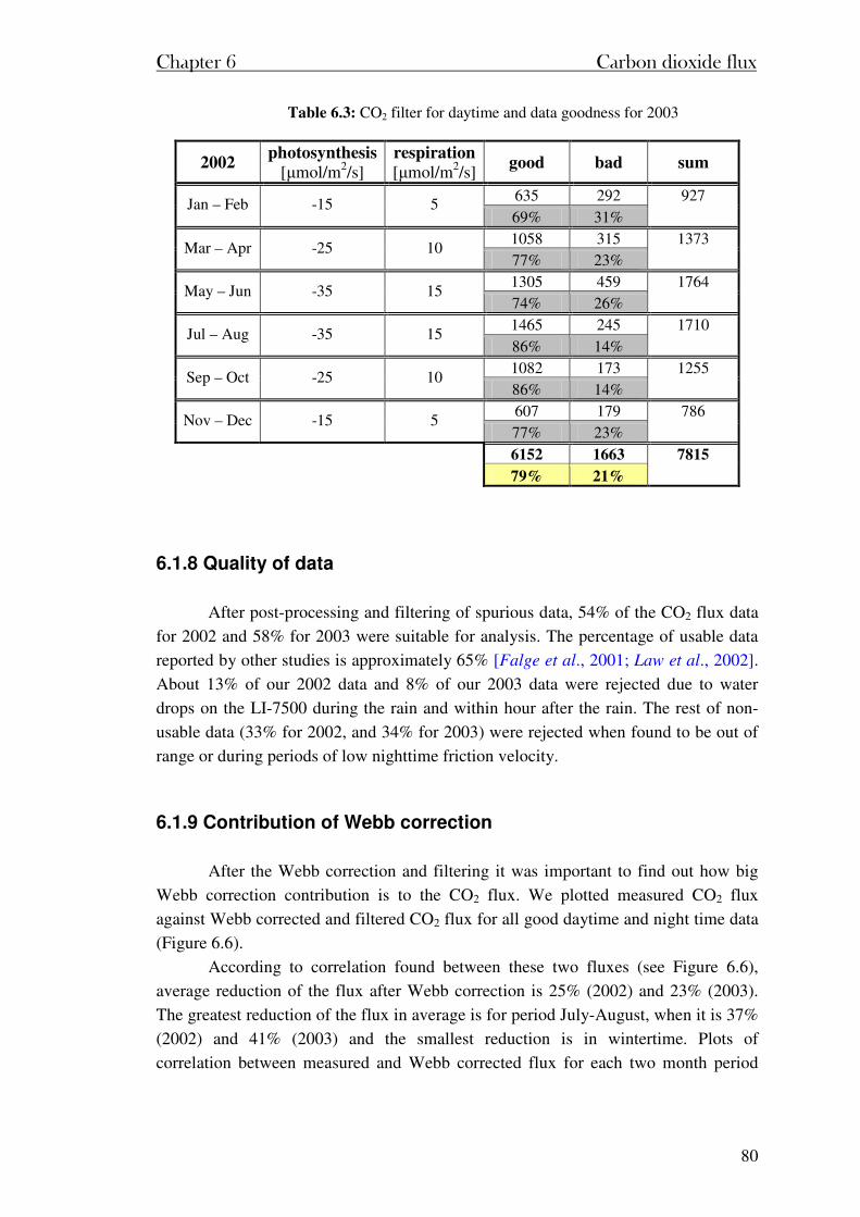
Chapter 6 Carbon dioxide flux
80
Table 6.3: CO2 filter for daytime and data goodness for 2003
2002 photosynthesis
[µmol/m2/s] respiration [µmol/m2/s]
good bad sum
635 292 Jan – Feb -15 5
69% 31%
927
1058 315 Mar – Apr -25 10
77% 23%
1373
1305 459 May – Jun -35 15
74% 26%
1764
1465 245 Jul – Aug -35 15
86% 14%
1710
1082 173 Sep – Oct -25 10
86% 14%
1255
607 179 Nov – Dec -15 5
77% 23%
786
6152 1663
79% 21%
7815
6.1.8 Quality of data
After post-processing and filtering of spurious data, 54% of the CO2 flux data
for 2002 and 58% for 2003 were suitable for analysis. The percentage of usable data
reported by other studies is approximately 65% [Falge et al., 2001; Law et al., 2002].
About 13% of our 2002 data and 8% of our 2003 data were rejected due to water
drops on the LI-7500 during the rain and within hour after the rain. The rest of non-
usable data (33% for 2002, and 34% for 2003) were rejected when found to be out of
range or during periods of low nighttime friction velocity.
6.1.9 Contribution of Webb correction
After the Webb correction and filtering it was important to find out how big
Webb correction contribution is to the CO2 flux. We plotted measured CO2 flux
against Webb corrected and filtered CO2 flux for all good daytime and night time data
(Figure 6.6).
According to correlation found between these two fluxes (see Figure 6.6),
average reduction of the flux after Webb correction is 25% (2002) and 23% (2003).
The greatest reduction of the flux in average is for period July-August, when it is 37%
(2002) and 41% (2003) and the smallest reduction is in wintertime. Plots of
correlation between measured and Webb corrected flux for each two month period
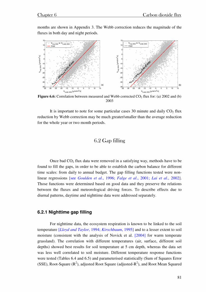
Chapter 6 Carbon dioxide flux
81
months are shown in Appendix 3. The Webb correction reduces the magnitude of the
fluxes in both day and night periods.
-35 -30 -25 -20 -15 -10 -5 0 5 10 15-35
-30
-25
-20
-15
-10
-5
0
5
10
15
fcw ebb
2002
[µmol/m2/s]
fcori
g 2
00
2 [
µm
ol/m
2/s
]
fcorig
2002
vs. fcw ebb
2002
linear
fc orig =
1.2
53*fc
webb
-0.2
72; R2 =0
.87
(a)
-35 -30 -25 -20 -15 -10 -5 0 5 10 15
-35
-30
-25
-20
-15
-10
-5
0
5
10
15
fcw ebb
2003
[µmol/m2/s]
fcori
g 2
00
3 [
µm
ol/m
2/s
]
fcorig
2003
vs. fcwebb
2003
linear
fc orig =
1.2
3*fcw
ebb-0
.45;
R2 =0
.83
(b)
Figure 6.6: Correlation between measured and Webb corrected CO2 flux for: (a) 2002 and (b)
2003
It is important to note for some particular cases 30 minute and daily CO2 flux
reduction by Webb correction may be much greater/smaller than the average reduction
for the whole year or two month periods.
6.2 Gap filling
Once bad CO2 flux data were removed in a satisfying way, methods have to be
found to fill the gaps, in order to be able to establish the carbon balance for different
time scales: from daily to annual budget. The gap filling functions tested were non-
linear regressions [see Goulden et al., 1996; Falge et al., 2001; Lai et al., 2002].
Those functions were determined based on good data and they preserve the relations
between the fluxes and meteorological driving forces. To describe effects due to
diurnal patterns, daytime and nighttime data were addressed separately.
6.2.1 Nighttime gap filling
For nighttime data, the ecosystem respiration is known to be linked to the soil
temperature [Lloyd and Taylor, 1994; Kirschbaum, 1995] and to a lesser extent to soil
moisture (consistent with the analysis of Novick et al. [2004] for warm temperate
grassland). The correlation with different temperatures (air, surface, different soil
depths) showed best results for soil temperature at 5 cm depth, whereas the data set
was less well correlated to soil moisture. Different temperature response functions
were tested (Tables 6.4 and 6.5) and parameterised statistically (Sum of Squares Error
(SSE), Root-Square (R2), adjusted Root Square (adjusted-R2), and Root Mean Squared
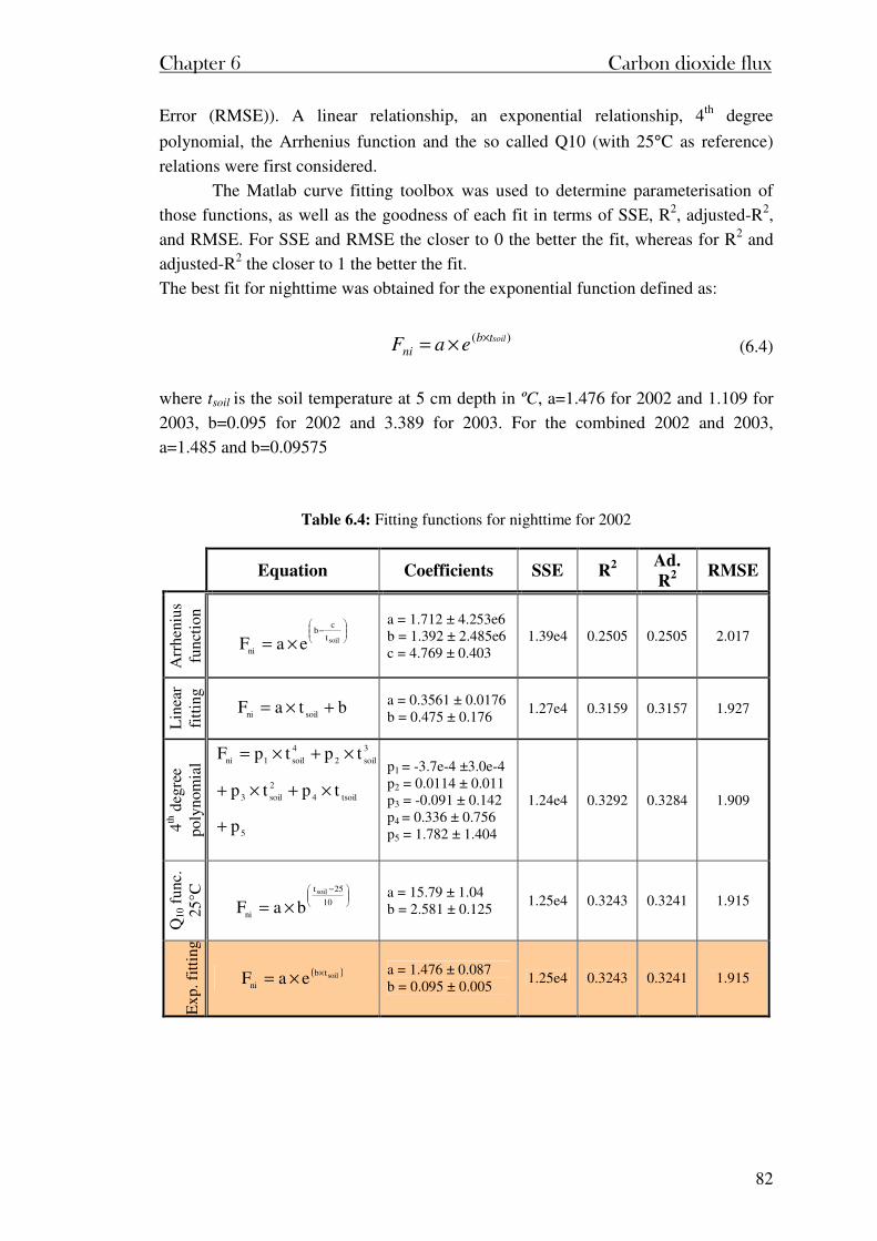
Chapter 6 Carbon dioxide flux
82
Error (RMSE)). A linear relationship, an exponential relationship, 4th degree
polynomial, the Arrhenius function and the so called Q10 (with 25°C as reference)
relations were first considered.
The Matlab curve fitting toolbox was used to determine parameterisation of
those functions, as well as the goodness of each fit in terms of SSE, R2, adjusted-R2,
and RMSE. For SSE and RMSE the closer to 0 the better the fit, whereas for R2 and
adjusted-R2 the closer to 1 the better the fit.
The best fit for nighttime was obtained for the exponential function defined as:
)( soiltbni eaF
××= (6.4)
where tsoil is the soil temperature at 5 cm depth in ºC, a=1.476 for 2002 and 1.109 for
2003, b=0.095 for 2002 and 3.389 for 2003. For the combined 2002 and 2003,
a=1.485 and b=0.09575
Table 6.4: Fitting functions for nighttime for 2002
Equation Coefficients SSE R
2
Ad.
R2 RMSE
Arr
heni
us
func
tion
−
×= soilt
cb
ni eaF
a = 1.712 ± 4.253e6 b = 1.392 ± 2.485e6 c = 4.769 ± 0.403
1.39e4 0.2505 0.2505 2.017
Lin
ear
fitt
ing
btaF soilni +×= a = 0.3561 ± 0.0176 b = 0.475 ± 0.176
1.27e4 0.3159 0.3157 1.927
4th d
egre
e po
lyno
mia
l
5
tsoil4
2
soil3
3
soil2
4
soil1ni
p
tptp
tptpF
+
×+×+
×+×=
p1 = -3.7e-4 ±3.0e-4 p2 = 0.0114 ± 0.011 p3 = -0.091 ± 0.142 p4 = 0.336 ± 0.756 p5 = 1.782 ± 1.404
1.24e4 0.3292 0.3284 1.909
Q10
fun
c.
25°C
−
×= 10
25t
ni
soil
baF a = 15.79 ± 1.04 b = 2.581 ± 0.125
1.25e4 0.3243 0.3241 1.915
Exp
. fit
ting
( )soiltb
ni eaF ××= a = 1.476 ± 0.087 b = 0.095 ± 0.005
1.25e4 0.3243 0.3241 1.915
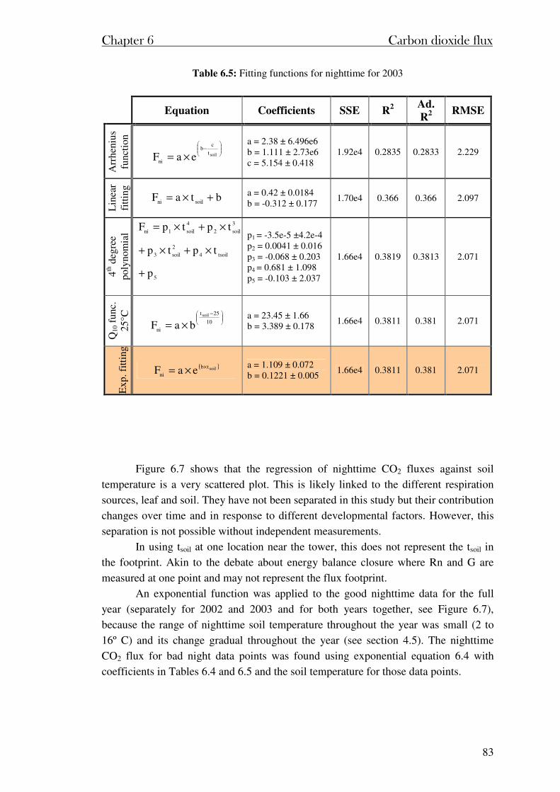
Chapter 6 Carbon dioxide flux
83
Table 6.5: Fitting functions for nighttime for 2003
Equation Coefficients SSE R
2
Ad.
R2 RMSE
Arr
heni
us
func
tion
−
×= soilt
cb
ni eaF
a = 2.38 ± 6.496e6 b = 1.111 ± 2.73e6 c = 5.154 ± 0.418
1.92e4 0.2835 0.2833 2.229
Lin
ear
fitt
ing
btaF soilni +×= a = 0.42 ± 0.0184 b = -0.312 ± 0.177
1.70e4 0.366 0.366 2.097
4th d
egre
e po
lyno
mia
l
5
tsoil4
2
soil3
3
soil2
4
soil1ni
p
tptp
tptpF
+
×+×+
×+×=
p1 = -3.5e-5 ±4.2e-4 p2 = 0.0041 ± 0.016 p3 = -0.068 ± 0.203 p4 = 0.681 ± 1.098 p5 = -0.103 ± 2.037
1.66e4 0.3819 0.3813 2.071
Q10
fun
c.
25°C
−
×= 10
25t
ni
soil
baF a = 23.45 ± 1.66 b = 3.389 ± 0.178
1.66e4 0.3811 0.381 2.071
Exp
. fit
ting
( )soiltb
ni eaF ××= a = 1.109 ± 0.072 b = 0.1221 ± 0.005
1.66e4 0.3811 0.381 2.071
Figure 6.7 shows that the regression of nighttime CO2 fluxes against soil
temperature is a very scattered plot. This is likely linked to the different respiration
sources, leaf and soil. They have not been separated in this study but their contribution
changes over time and in response to different developmental factors. However, this
separation is not possible without independent measurements.
In using tsoil at one location near the tower, this does not represent the tsoil in
the footprint. Akin to the debate about energy balance closure where Rn and G are
measured at one point and may not represent the flux footprint.
An exponential function was applied to the good nighttime data for the full
year (separately for 2002 and 2003 and for both years together, see Figure 6.7),
because the range of nighttime soil temperature throughout the year was small (2 to
16º C) and its change gradual throughout the year (see section 4.5). The nighttime
CO2 flux for bad night data points was found using exponential equation 6.4 with
coefficients in Tables 6.4 and 6.5 and the soil temperature for those data points.
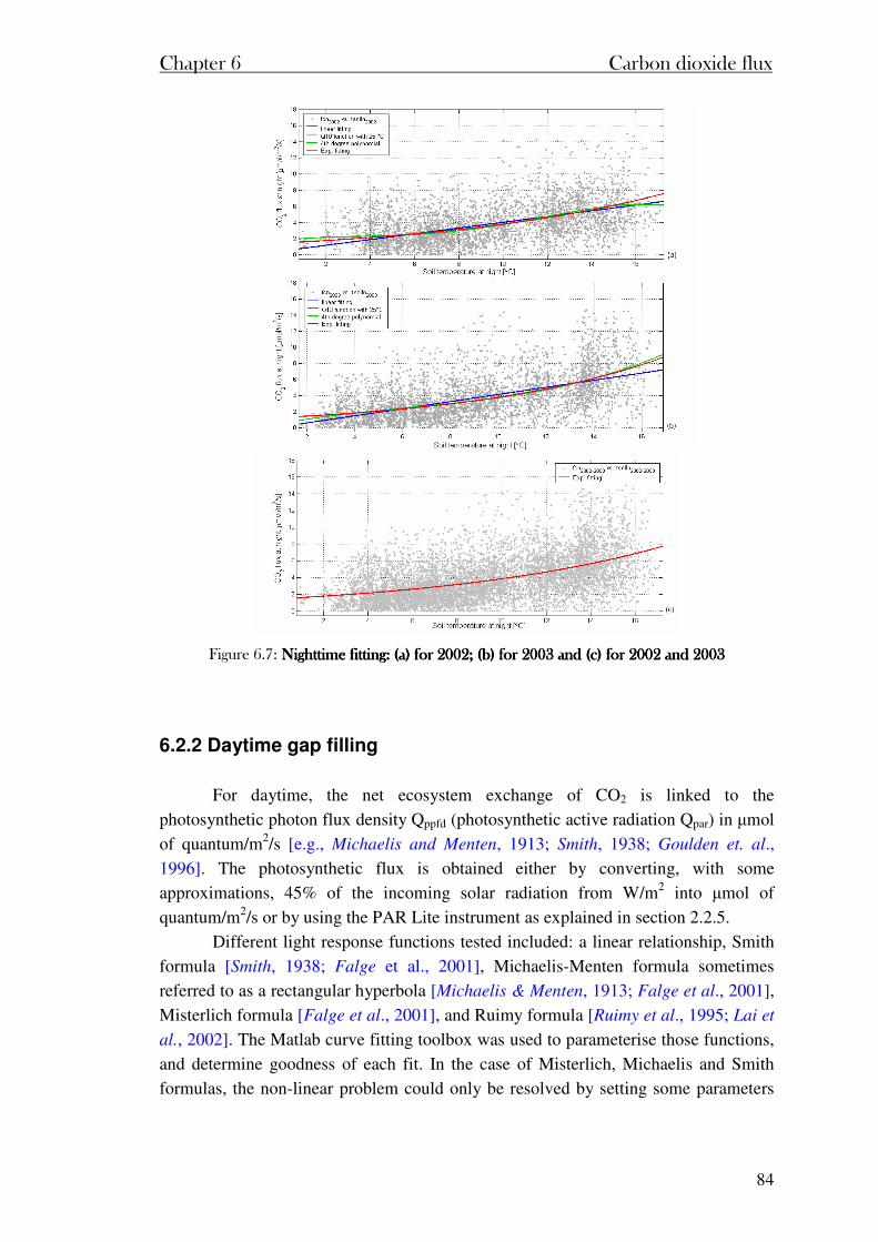
Chapter 6 Carbon dioxide flux
84
Figure 6.7: Nighttime fitting: (a) for 2002; (b) for 2003 and (c) for 2002 and 2003 Nighttime fitting: (a) for 2002; (b) for 2003 and (c) for 2002 and 2003 Nighttime fitting: (a) for 2002; (b) for 2003 and (c) for 2002 and 2003 Nighttime fitting: (a) for 2002; (b) for 2003 and (c) for 2002 and 2003
6.2.2 Daytime gap filling
For daytime, the net ecosystem exchange of CO2 is linked to the
photosynthetic photon flux density Qppfd (photosynthetic active radiation Qpar) in µmol
of quantum/m2/s [e.g., Michaelis and Menten, 1913; Smith, 1938; Goulden et. al.,
1996]. The photosynthetic flux is obtained either by converting, with some
approximations, 45% of the incoming solar radiation from W/m2 into µmol of
quantum/m2/s or by using the PAR Lite instrument as explained in section 2.2.5.
Different light response functions tested included: a linear relationship, Smith
formula [Smith, 1938; Falge et al., 2001], Michaelis-Menten formula sometimes
referred to as a rectangular hyperbola [Michaelis & Menten, 1913; Falge et al., 2001],
Misterlich formula [Falge et al., 2001], and Ruimy formula [Ruimy et al., 1995; Lai et
al., 2002]. The Matlab curve fitting toolbox was used to parameterise those functions,
and determine goodness of each fit. In the case of Misterlich, Michaelis and Smith
formulas, the non-linear problem could only be resolved by setting some parameters
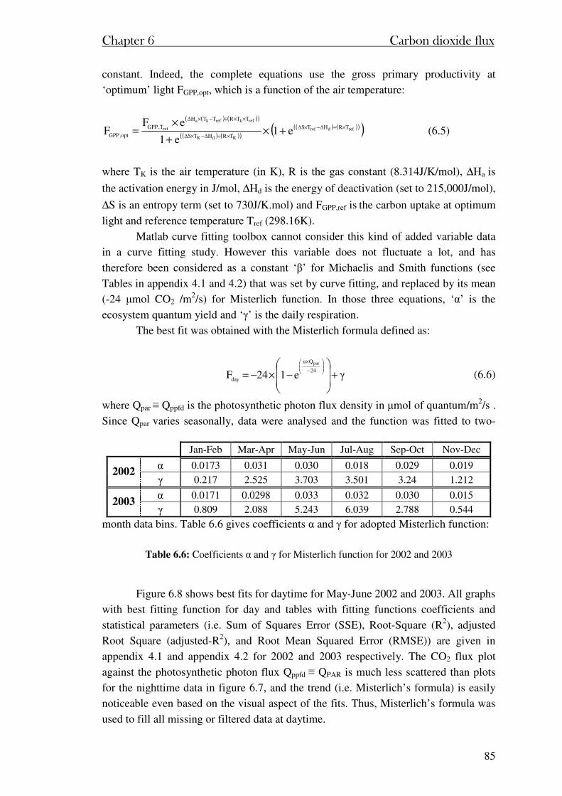
Chapter 6 Carbon dioxide flux
85
constant. Indeed, the complete equations use the gross primary productivity at
‘optimum’ light FGPP,opt, which is a function of the air temperature:
( ) ( )( )
( ) ( )( )( ) ( )( )( )refdref
KdK
refkrefka
ref TRH∆TS∆
TRH∆TS∆
TTRTTH∆
T,GPP
opt,GPP e1e1
eFF ×÷−×
×÷−×
××÷−×
+×+
×= (6.5)
where TK is the air temperature (in K), R is the gas constant (8.314J/K/mol), ∆Ha is
the activation energy in J/mol, ∆Hd is the energy of deactivation (set to 215,000J/mol),
∆S is an entropy term (set to 730J/K.mol) and FGPP,ref is the carbon uptake at optimum
light and reference temperature Tref (298.16K).
Matlab curve fitting toolbox cannot consider this kind of added variable data
in a curve fitting study. However this variable does not fluctuate a lot, and has
therefore been considered as a constant ‘β’ for Michaelis and Smith functions (see
Tables in appendix 4.1 and 4.2) that was set by curve fitting, and replaced by its mean
(-24 µmol CO2 /m2/s) for Misterlich function. In those three equations, ‘α’ is the
ecosystem quantum yield and ‘γ’ is the daily respiration.
The best fit was obtained with the Misterlich formula defined as:
γe124F24
Qα
day
par
+
−×−=
−
×
(6.6)
where Qpar ≡ Qppfd is the photosynthetic photon flux density in µmol of quantum/m2/s .
Since Qpar varies seasonally, data were analysed and the function was fitted to two-
month data bins. Table 6.6 gives coefficients α and γ for adopted Misterlich function:
Table 6.6: Coefficients α and γ for Misterlich function for 2002 and 2003
Figure 6.8 shows best fits for daytime for May-June 2002 and 2003. All graphs
with best fitting function for day and tables with fitting functions coefficients and
statistical parameters (i.e. Sum of Squares Error (SSE), Root-Square (R2), adjusted
Root Square (adjusted-R2), and Root Mean Squared Error (RMSE)) are given in
appendix 4.1 and appendix 4.2 for 2002 and 2003 respectively. The CO2 flux plot
against the photosynthetic photon flux Qppfd ≡ QPAR is much less scattered than plots
for the nighttime data in figure 6.7, and the trend (i.e. Misterlich’s formula) is easily
noticeable even based on the visual aspect of the fits. Thus, Misterlich’s formula was
used to fill all missing or filtered data at daytime.
Jan-Feb Mar-Apr May-Jun Jul-Aug Sep-Oct Nov-Dec
α 0.0173 0.031 0.030 0.018 0.029 0.019 2002
γ 0.217 2.525 3.703 3.501 3.24 1.212
α 0.0171 0.0298 0.033 0.032 0.030 0.015 2003
γ 0.809 2.088 5.243 6.039 2.788 0.544
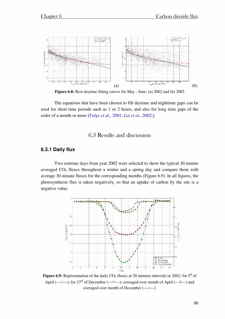
Chapter 6 Carbon dioxide flux
86
(a) (b) Figure 6.8: Best daytime fitting curves for May - June: (a) 2002 and (b) 2003
The equations that have been chosen to fill daytime and nighttime gaps can be
used for short time periods such as 1 or 2 hours, and also for long time gaps of the
order of a month or more [Falge et al., 2001; Lai et al., 2002;].
6.3 Results and discussion
6.3.1 Daily flux
Two extreme days from year 2002 were selected to show the typical 30 minute
averaged CO2 fluxes throughout a winter and a spring day and compare them with
average 30 minute fluxes for the corresponding months (Figure 6.9). In all figures, the
photosynthesis flux is taken negatively, so that an uptake of carbon by the site is a
negative value.
Figure 6.9: Representation of the daily CO2 fluxes at 30 minutes intervals in 2002: for 5th of
April (——); for 23rd of December (——); averaged over month of April (—◊—) and
averaged over month of December (——)
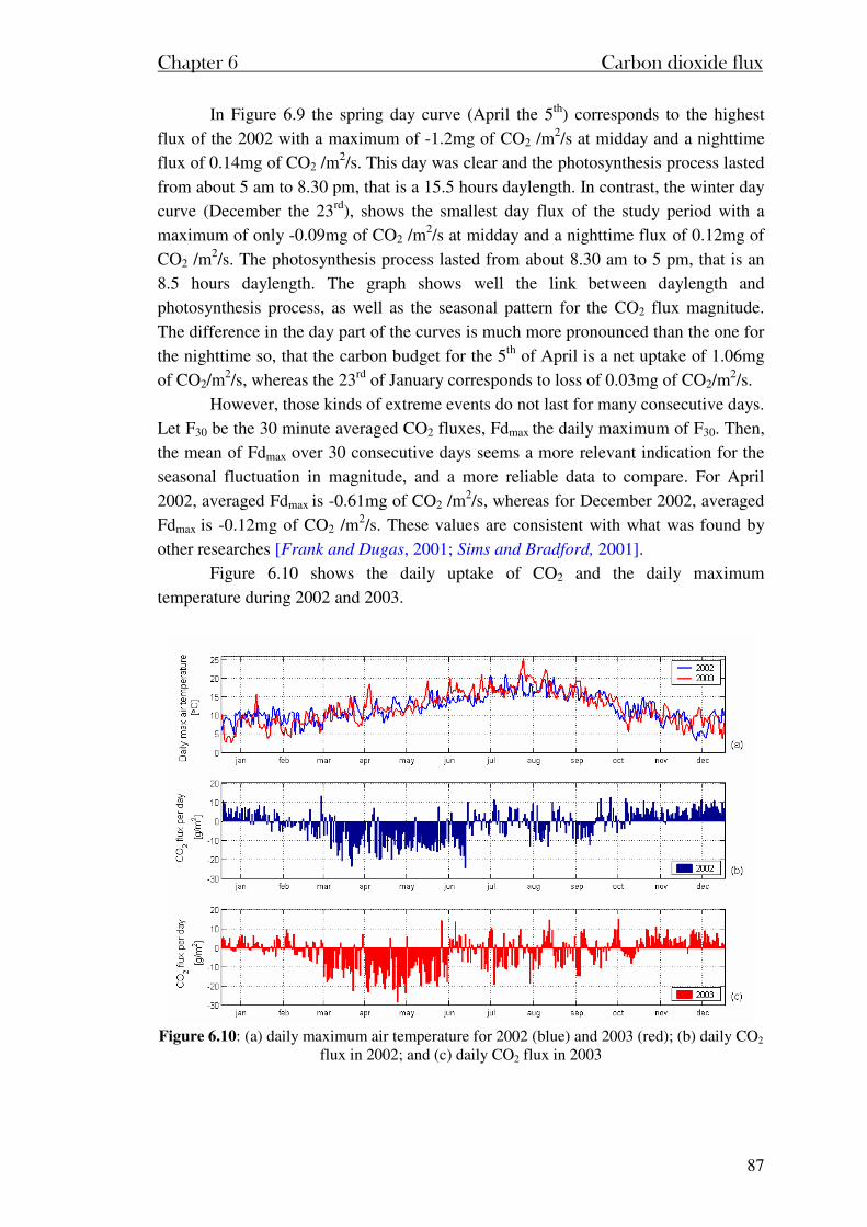
Chapter 6 Carbon dioxide flux
87
In Figure 6.9 the spring day curve (April the 5th) corresponds to the highest
flux of the 2002 with a maximum of -1.2mg of CO2 /m2/s at midday and a nighttime
flux of 0.14mg of CO2 /m2/s. This day was clear and the photosynthesis process lasted
from about 5 am to 8.30 pm, that is a 15.5 hours daylength. In contrast, the winter day
curve (December the 23rd), shows the smallest day flux of the study period with a
maximum of only -0.09mg of CO2 /m2/s at midday and a nighttime flux of 0.12mg of
CO2 /m2/s. The photosynthesis process lasted from about 8.30 am to 5 pm, that is an
8.5 hours daylength. The graph shows well the link between daylength and
photosynthesis process, as well as the seasonal pattern for the CO2 flux magnitude.
The difference in the day part of the curves is much more pronounced than the one for
the nighttime so, that the carbon budget for the 5th of April is a net uptake of 1.06mg
of CO2/m2/s, whereas the 23rd of January corresponds to loss of 0.03mg of CO2/m
2/s.
However, those kinds of extreme events do not last for many consecutive days.
Let F30 be the 30 minute averaged CO2 fluxes, Fdmax the daily maximum of F30. Then,
the mean of Fdmax over 30 consecutive days seems a more relevant indication for the
seasonal fluctuation in magnitude, and a more reliable data to compare. For April
2002, averaged Fdmax is -0.61mg of CO2 /m2/s, whereas for December 2002, averaged
Fdmax is -0.12mg of CO2 /m2/s. These values are consistent with what was found by
other researches [Frank and Dugas, 2001; Sims and Bradford, 2001].
Figure 6.10 shows the daily uptake of CO2 and the daily maximum
temperature during 2002 and 2003.
Figure 6.10: (a) daily maximum air temperature for 2002 (blue) and 2003 (red); (b) daily CO2
flux in 2002; and (c) daily CO2 flux in 2003
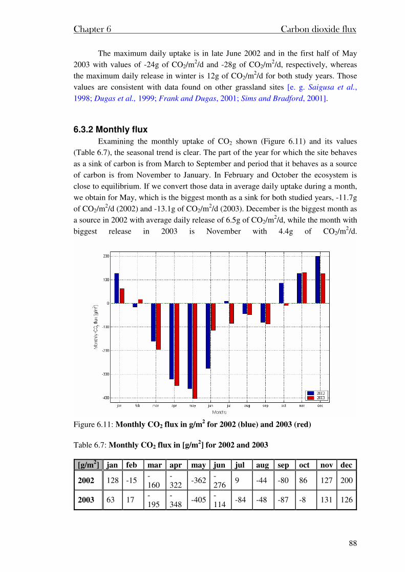
Chapter 6 Carbon dioxide flux
88
The maximum daily uptake is in late June 2002 and in the first half of May
2003 with values of -24g of CO2/m2/d and -28g of CO2/m
2/d, respectively, whereas
the maximum daily release in winter is 12g of CO2/m2/d for both study years. Those
values are consistent with data found on other grassland sites [e. g. Saigusa et al.,
1998; Dugas et al., 1999; Frank and Dugas, 2001; Sims and Bradford, 2001].
6.3.2 Monthly flux
Examining the monthly uptake of CO2 shown (Figure 6.11) and its values
(Table 6.7), the seasonal trend is clear. The part of the year for which the site behaves
as a sink of carbon is from March to September and period that it behaves as a source
of carbon is from November to January. In February and October the ecosystem is
close to equilibrium. If we convert those data in average daily uptake during a month,
we obtain for May, which is the biggest month as a sink for both studied years, -11.7g
of CO2/m2/d (2002) and -13.1g of CO2/m
2/d (2003). December is the biggest month as
a source in 2002 with average daily release of 6.5g of CO2/m2/d, while the month with
biggest release in 2003 is November with 4.4g of CO2/m2/d.
Figure 6.11: Monthly CO2 flux in g/m2 for 2002 (blue) and 2003 (red)
Table 6.7: Monthly CO2 flux in [g/m2] for 2002 and 2003
[g/m2] jan feb mar apr may jun jul aug sep oct nov dec
2002 128 -15 -160
-322
-362 -276
9 -44 -80 86 127 200
2003 63 17 -195
-348
-405 -114
-84 -48 -87 -8 131 126
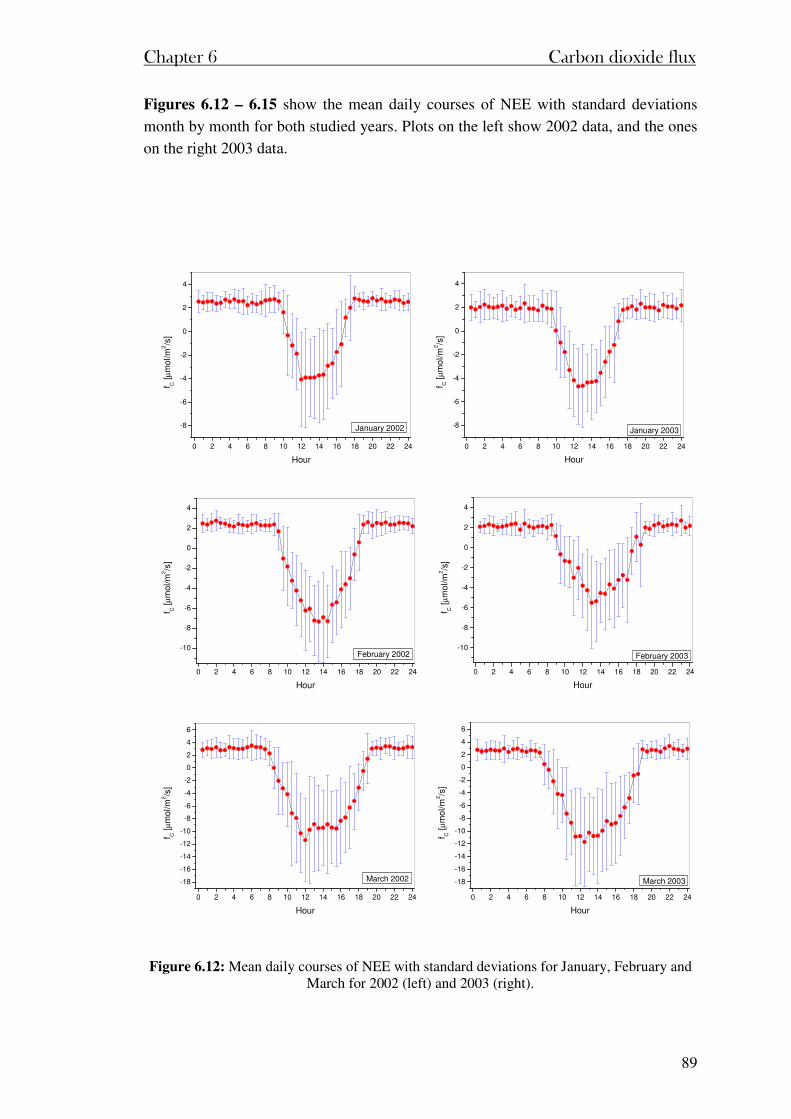
Chapter 6 Carbon dioxide flux
89
Figures 6.12 – 6.15 show the mean daily courses of NEE with standard deviations
month by month for both studied years. Plots on the left show 2002 data, and the ones
on the right 2003 data.
0 2 4 6 8 10 12 14 16 18 20 22 24
-8
-6
-4
-2
0
2
4
f C [
µm
ol/m
2/s
]
Hour
January 2002
0 2 4 6 8 10 12 14 16 18 20 22 24
-8
-6
-4
-2
0
2
4
f C [
µm
ol/m
2/s
]
Hour
January 2003
0 2 4 6 8 10 12 14 16 18 20 22 24
-10
-8
-6
-4
-2
0
2
4
f C [
µm
ol/m
2/s
]
Hour
February 2002
0 2 4 6 8 10 12 14 16 18 20 22 24
-10
-8
-6
-4
-2
0
2
4
f C [
µm
ol/m
2/s
]
Hour
February 2003
0 2 4 6 8 10 12 14 16 18 20 22 24
-18
-16
-14
-12
-10
-8
-6
-4
-2
0
2
4
6
f C [
µm
ol/m
2/s
]
Hour
March 2002
0 2 4 6 8 10 12 14 16 18 20 22 24
-18
-16
-14
-12
-10
-8
-6
-4
-2
0
2
4
6
f C [
µm
ol/m
2/s
]
Hour
March 2003
Figure 6.12: Mean daily courses of NEE with standard deviations for January, February and
March for 2002 (left) and 2003 (right).
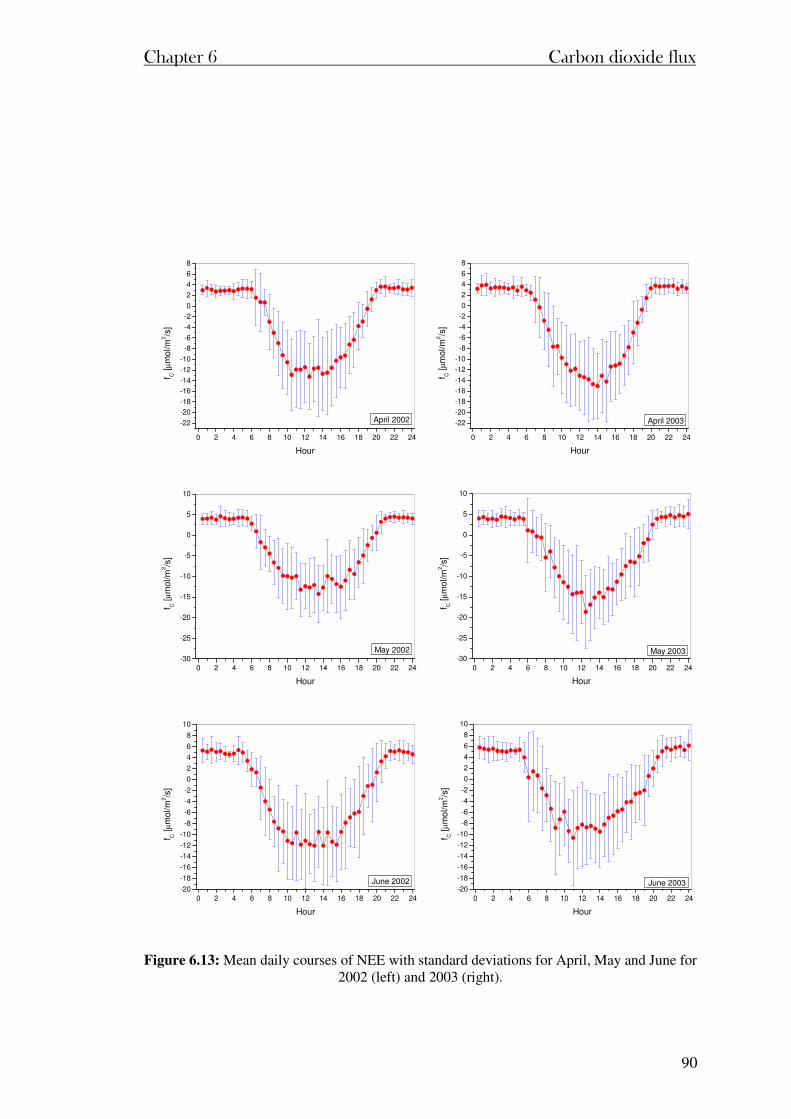
Chapter 6 Carbon dioxide flux
90
0 2 4 6 8 10 12 14 16 18 20 22 24
-22
-20
-18
-16
-14
-12
-10
-8
-6
-4
-2
0
2
4
6
8
f C [
µm
ol/m
2/s
]
Hour
April 2002
0 2 4 6 8 10 12 14 16 18 20 22 24
-22
-20
-18
-16
-14
-12
-10
-8
-6
-4
-2
0
2
4
6
8
f C [
µm
ol/m
2/s
]Hour
April 2003
0 2 4 6 8 10 12 14 16 18 20 22 24
-30
-25
-20
-15
-10
-5
0
5
10
f C [
µm
ol/m
2/s
]
Hour
May 2002
0 2 4 6 8 10 12 14 16 18 20 22 24
-30
-25
-20
-15
-10
-5
0
5
10
f C [
µm
ol/m
2/s
]
Hour
May 2003
0 2 4 6 8 10 12 14 16 18 20 22 24
-20
-18
-16
-14
-12
-10
-8
-6
-4
-2
0
2
4
6
8
10
f C [
µm
ol/m
2/s
]
Hour
June 2002
0 2 4 6 8 10 12 14 16 18 20 22 24
-20
-18
-16
-14
-12
-10
-8
-6
-4
-2
0
2
4
6
8
10
f C [
µm
ol/m
2/s
]
Hour
June 2003
Figure 6.13: Mean daily courses of NEE with standard deviations for April, May and June for
2002 (left) and 2003 (right).
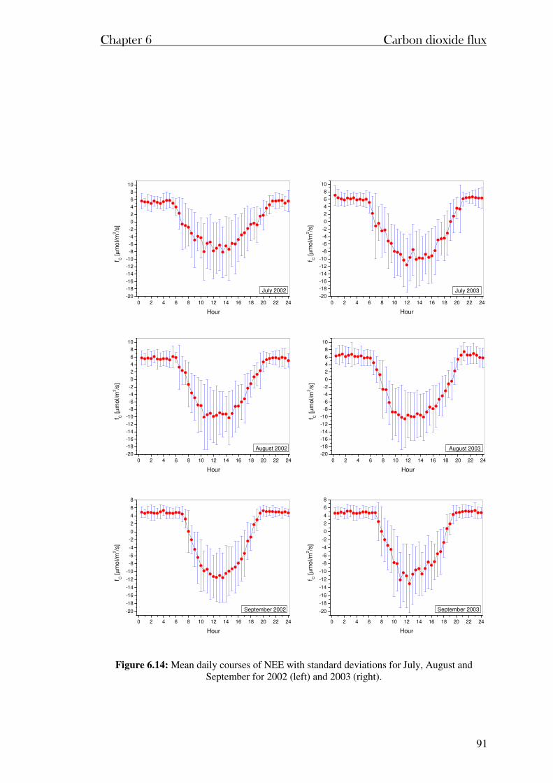
Chapter 6 Carbon dioxide flux
91
0 2 4 6 8 10 12 14 16 18 20 22 24
-20
-18
-16
-14
-12
-10
-8
-6
-4
-2
0
2
4
6
8
10
f C [
µm
ol/m
2/s
]
Hour
July 2002
0 2 4 6 8 10 12 14 16 18 20 22 24
-20
-18
-16
-14
-12
-10
-8
-6
-4
-2
0
2
4
6
8
10
f C [
µm
ol/m
2/s
]Hour
July 2003
0 2 4 6 8 10 12 14 16 18 20 22 24
-20
-18
-16
-14
-12
-10
-8
-6
-4
-2
0
2
4
6
8
10
f C [
µm
ol/m
2/s
]
Hour
August 2002
0 2 4 6 8 10 12 14 16 18 20 22 24
-20
-18
-16
-14
-12
-10
-8
-6
-4
-2
0
2
4
6
8
10
f C [
µm
ol/m
2/s
]
Hour
August 2003
0 2 4 6 8 10 12 14 16 18 20 22 24
-20
-18
-16
-14
-12
-10
-8
-6
-4
-2
0
2
4
6
8
f C [
µm
ol/m
2/s
]
Hour
September 2002
0 2 4 6 8 10 12 14 16 18 20 22 24
-20
-18
-16
-14
-12
-10
-8
-6
-4
-2
0
2
4
6
8
f C [
µm
ol/m
2/s
]
Hour
September 2003
Figure 6.14: Mean daily courses of NEE with standard deviations for July, August and September for 2002 (left) and 2003 (right).
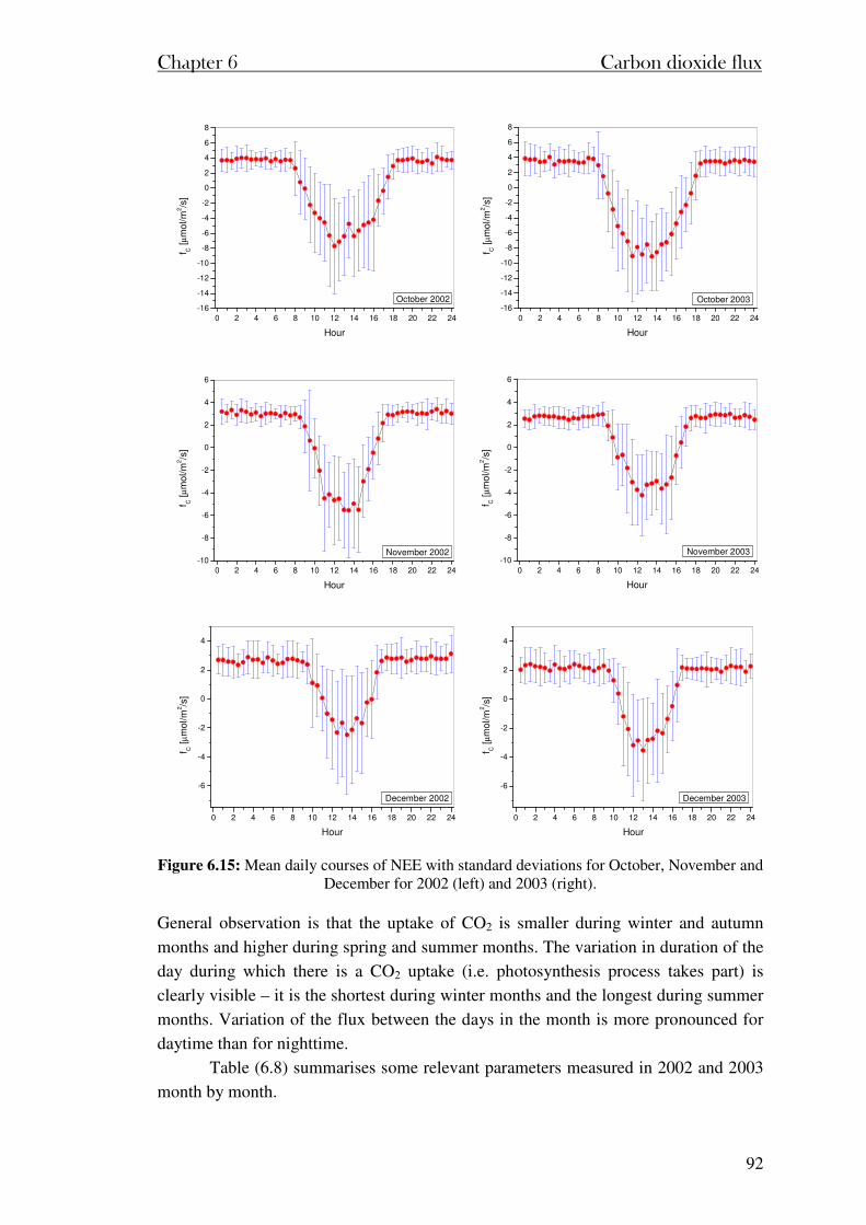
Chapter 6 Carbon dioxide flux
92
0 2 4 6 8 10 12 14 16 18 20 22 24
-16
-14
-12
-10
-8
-6
-4
-2
0
2
4
6
8
f C [
µm
ol/m
2/s
]
Hour
October 2002
0 2 4 6 8 10 12 14 16 18 20 22 24
-16
-14
-12
-10
-8
-6
-4
-2
0
2
4
6
8
f C [
µm
ol/m
2/s
]
Hour
October 2003
0 2 4 6 8 10 12 14 16 18 20 22 24
-10
-8
-6
-4
-2
0
2
4
6
f C [
µm
ol/m
2/s
]
Hour
November 2002
0 2 4 6 8 10 12 14 16 18 20 22 24
-10
-8
-6
-4
-2
0
2
4
6
f C [
µm
ol/m
2/s
]
Hour
November 2003
0 2 4 6 8 10 12 14 16 18 20 22 24
-6
-4
-2
0
2
4
f C [
µm
ol/m
2/s
]
Hour
December 2002
0 2 4 6 8 10 12 14 16 18 20 22 24
-6
-4
-2
0
2
4
f C [
µm
ol/m
2/s
]
Hour
December 2003
Figure 6.15: Mean daily courses of NEE with standard deviations for October, November and
December for 2002 (left) and 2003 (right). General observation is that the uptake of CO2 is smaller during winter and autumn
months and higher during spring and summer months. The variation in duration of the
day during which there is a CO2 uptake (i.e. photosynthesis process takes part) is
clearly visible – it is the shortest during winter months and the longest during summer
months. Variation of the flux between the days in the month is more pronounced for
daytime than for nighttime.
Table (6.8) summarises some relevant parameters measured in 2002 and 2003
month by month.
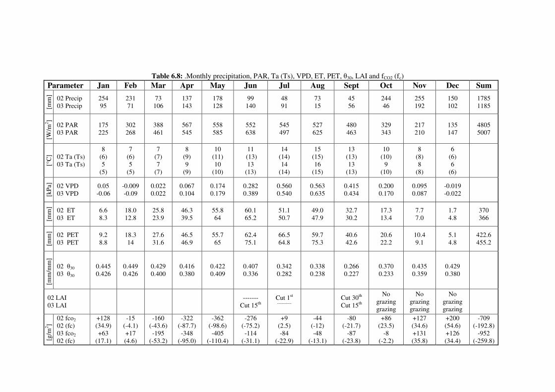
Table 6.8: .Monthly precipitation, PAR, Ta (Ts), VPD, ET, PET, θ30, LAI and fCO2 (fc)
Parameter Jan Feb Mar Apr May Jun Jul Aug Sept Oct Nov Dec Sum
[mm
]
02 Precip 03 Precip
254 95
231 71
73 106
137 143
178 128
99 140
48 91
73 15
45 56
244 46
255 192
150 102
1785 1185
[W/m
2 ]
02 PAR 03 PAR
175 225
302 268
388 461
567 545
558 585
552 638
545 497
527 625
480 463
329 343
217 210
135 147
4805 5007
[°C
] 02 Ta (Ts) 03 Ta (Ts)
8 (6) 5
(5)
7 (6) 5
(5)
7 (7) 7
(7)
8 (9) 9
(9)
10 (11) 10
(10)
11 (13) 13
(13)
14 (14) 14
(14)
15 (15) 16
(15)
13 (13) 13
(13)
10 (10)
9 (10)
8 (8) 8
(8)
6 (6) 6
(6)
[kP
a]
02 VPD 03 VPD
0.05 -0.06
-0.009 -0.09
0.022 0.022
0.067 0.104
0.174 0.179
0.282 0.389
0.560 0.540
0.563 0.635
0.415 0.434
0.200 0.170
0.095 0.087
-0.019 -0.022
[mm
]
02 ET 03 ET
6.6 8.3
18.0 12.8
25.8 23.9
46.3 39.5
55.8 64
60.1 65.2
51.1 50.7
49.0 47.9
32.7 30.2
17.3 13.4
7.7 7.0
1.7 4.8
370 366
[mm
]
02 PET 03 PET
9.2 8.8
18.3 14
27.6 31.6
46.5 46.9
55.7 65
62.4 75.1
66.5 64.8
59.7 75.3
40.6 42.6
20.6 22.2
10.4 9.1
5.1 4.8
422.6 455.2
[mm
/mm
]
02 θ30 03 θ30
0.445 0.426
0.449 0.426
0.429 0.400
0.416 0.380
0.422 0.409
0.407 0.336
0.342 0.282
0.338 0.238
0.266 0.227
0.370 0.233
0.435 0.359
0.429 0.380
02 LAI 03 LAI
-------
Cut 15th Cut 1st
----------
Cut 30th
Cut 15th
No grazing grazing
No grazing grazing
No grazing grazing
[g/m
2 ]
02 fco2
02 (fc)
03 fco2
02 (fc)
+128 (34.9) +63
(17.1)
-15 (-4.1) +17 (4.6)
-160 (-43.6) -195
(-53.2)
-322 (-87.7) -348
(-95.0)
-362 (-98.6) -405
(-110.4)
-276 (-75.2) -114
(-31.1)
+9 (2.5) -84
(-22.9)
-44 (-12) -48
(-13.1)
-80 (-21.7)
-87 (-23.8)
+86 (23.5)
-8 (-2.2)
+127 (34.6) +131 (35.8)
+200 (54.6) +126 (34.4)
-709 (-192.8)
-952 (-259.8)
Chapter 6 Carbon dioxide flux
94
The monthly magnitude of NEE varies between corresponding months in the
two years. The net release of CO2 in January 2002 of 128g/m2 compares to 63 g/m2 in
January 2003. The reason for a difference is higher air temperature in winter of 2002
that can be driving force for greater efflux.
The net uptake of CO2 in May 2002 of -362g/m2 compares to -405g/m2 in May
2003. The difference can be explained with more available photosynthetic flux during
this month in 2003 (according to higher precipitation during May 2002 it is expected
that cloudiness was reason for that) and air temperature in 2003 was higher.
The net uptake of CO2 in June 2002 of -276g/m2 compares to -114g/m2 in June
2003.
The reasons for the differences in NEE in June was twofold: one was, that part
of the grassland in the footprint was cut (harvested to within 5cm of the soil) in June
2003; and secondly, the last two weeks of June 2003 were dry and the soil moisture
consequently dropped from 0.6m3/m3 to 0.2m3/m3 whereas in June 2002 there was no
cutting and the rainfall was spread over the entire month keeping the soil moisture at
near saturation (see section4.3). Similar reasons explain why in July 2002 there was a
very small net respiration and in July 2003 a net uptake. July was dry in 2002 and
cutting was performed (enabled in the dry fields), while the grass that was cut in June
2003 was then emerging growth (approximately 0.2m in height) in July 2003. It has
been shown [Frank and Dugas, 2001] that short-term droughts during the growing
season reduce CO2 fluxes to near zero (photosynthesis balances respiration). Also, the
timing and magnitude of precipitation events influence the total growing season flux
and induce a considerable day-to-day variability in CO2 fluxes. Decreases in LAI
(Leaf Area Index) caused by the grass (silage) harvesting, reduce gross primary
productivity (GPP) [Budyko, 1974].
The NEE (uptake) in August and September 2002 was the same as August and
September 2003.
The sum of the NEE for the eight months (February to September) was –
1247g.CO2/m2 (-340 g.C/m2) for 2002 and –1265g.CO2/m
2 (-345 g.C/m2) for 2003.
The difference in NEE between the years was in the winter months (October to
January) with 2002 having an NEE of +543 g.CO2/m2 (+148 g.C/m2) and 2003 with
an NEE of +312 g.CO2/m2 (+ 85 g.C/m2). The rainfall in these four months was
903mm in 2002 and 435mm in 2003. The rainfall of 2002 caused the soil moisture
status to be more frequently saturated than in 2003. This resulted in a wetter soil
environment that respired more. In addition, in the drier year (2003), cattle grazed the
fields (during the daytime) during the parts of the months of October to January. By
contrast, in the wet winter (2002) cattle did not graze the fields because to do so, they
would have damaged the soil surface to an unacceptable level. So in the winter of
2002, there was a greater standing biomass (than in 2003), which enhanced the
respiration. This suggests that the wetter winter of 2002 with its saturating effect on
soil moisture, it’s higher standing biomass and enhanced ecosystem respiration was
responsible for the lower NEE of 2002.
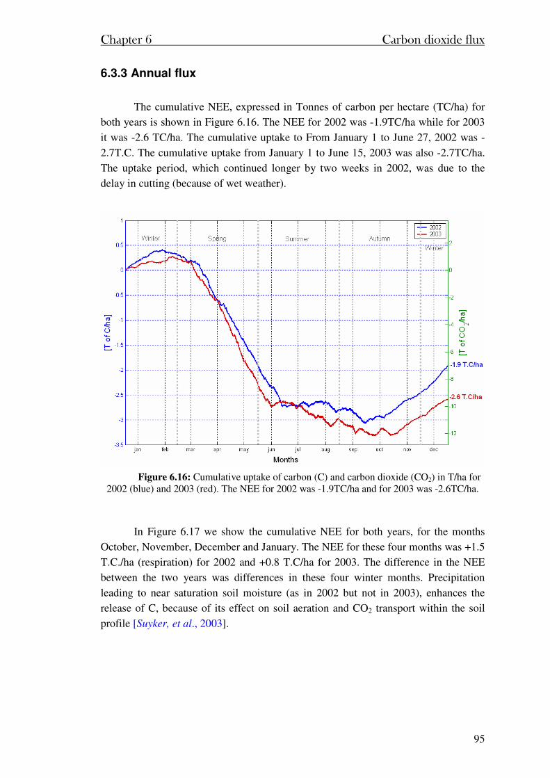
Chapter 6 Carbon dioxide flux
95
6.3.3 Annual flux
The cumulative NEE, expressed in Tonnes of carbon per hectare (TC/ha) for
both years is shown in Figure 6.16. The NEE for 2002 was -1.9TC/ha while for 2003
it was -2.6 TC/ha. The cumulative uptake to From January 1 to June 27, 2002 was -
2.7T.C. The cumulative uptake from January 1 to June 15, 2003 was also -2.7TC/ha.
The uptake period, which continued longer by two weeks in 2002, was due to the
delay in cutting (because of wet weather).
Figure 6.16: Cumulative uptake of carbon (C) and carbon dioxide (CO2) in T/ha for
2002 (blue) and 2003 (red). The NEE for 2002 was -1.9TC/ha and for 2003 was -2.6TC/ha.
In Figure 6.17 we show the cumulative NEE for both years, for the months
October, November, December and January. The NEE for these four months was +1.5
T.C./ha (respiration) for 2002 and +0.8 T.C/ha for 2003. The difference in the NEE
between the two years was differences in these four winter months. Precipitation
leading to near saturation soil moisture (as in 2002 but not in 2003), enhances the
release of C, because of its effect on soil aeration and CO2 transport within the soil
profile [Suyker, et al., 2003].
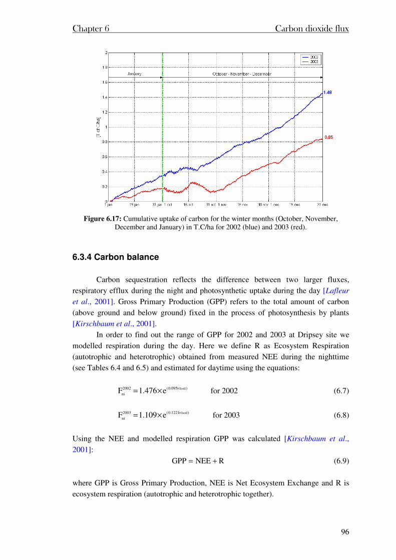
Chapter 6 Carbon dioxide flux
96
Figure 6.17: Cumulative uptake of carbon for the winter months (October, November,
December and January) in T.C/ha for 2002 (blue) and 2003 (red).
6.3.4 Carbon balance
Carbon sequestration reflects the difference between two larger fluxes,
respiratory efflux during the night and photosynthetic uptake during the day [Lafleur
et al., 2001]. Gross Primary Production (GPP) refers to the total amount of carbon
(above ground and below ground) fixed in the process of photosynthesis by plants
[Kirschbaum et al., 2001].
In order to find out the range of GPP for 2002 and 2003 at Dripsey site we
modelled respiration during the day. Here we define R as Ecosystem Respiration
(autotrophic and heterotrophic) obtained from measured NEE during the nighttime
(see Tables 6.4 and 6.5) and estimated for daytime using the equations:
)t095.0(2002
ni
soile476.1F ××= for 2002 (6.7)
)t1221.0(2003
ni
soile109.1F ××= for 2003 (6.8)
Using the NEE and modelled respiration GPP was calculated [Kirschbaum et al.,
2001]:
RNEEGPP += (6.9)
where GPP is Gross Primary Production, NEE is Net Ecosystem Exchange and R is
ecosystem respiration (autotrophic and heterotrophic together).
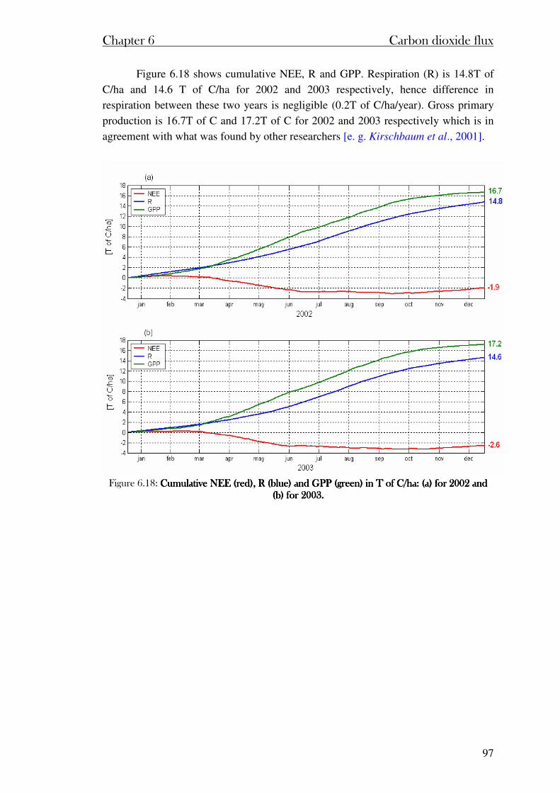
Chapter 6 Carbon dioxide flux
97
Figure 6.18 shows cumulative NEE, R and GPP. Respiration (R) is 14.8T of
C/ha and 14.6 T of C/ha for 2002 and 2003 respectively, hence difference in
respiration between these two years is negligible (0.2T of C/ha/year). Gross primary
production is 16.7T of C and 17.2T of C for 2002 and 2003 respectively which is in
agreement with what was found by other researchers [e. g. Kirschbaum et al., 2001].
Figure 6.18: Cumulative NEE (red), R (blue) and GPP (green) in T of C/ha: (a) for 2002 and Cumulative NEE (red), R (blue) and GPP (green) in T of C/ha: (a) for 2002 and Cumulative NEE (red), R (blue) and GPP (green) in T of C/ha: (a) for 2002 and Cumulative NEE (red), R (blue) and GPP (green) in T of C/ha: (a) for 2002 and
(b) for 2003.(b) for 2003.(b) for 2003.(b) for 2003.

Chapter 7
Modelling
98
Chapter 7Chapter 7Chapter 7Chapter 7 Modelling Modelling Modelling Modelling
7.1 Introduction
There are models that can then describe the main plant mechanisms involved
in the CO2 budget and their interactions; these models can be adjusted to fit each
specific environment. On the other hand, they constitute a basis to compare and adjust
variables in order to describe the observations and processes. With all the climatic
issues at present, proper predictions are needed of the effect on an ecosystem of
changes due to CO2 increasing concentration, or any other variable (precipitation, air
temperatures….).
In this study, modelling tools will be discussed in an effort to fit as well as
possible the CO2 fluxes during the year.
A wide range of models is nowadays available to estimate the exchange
between leaves and the atmosphere in terms of CO2. Biochemical models as proposed
by Farquhar et al. [1980] consider the full biochemical components of photosynthetic
carbon assimilation in plants and therefore require a large number of physiological
parameters that are not trivial to determine for a wide variety of species and sites. On
the opposite, empirical models for the stomata conductance calculation introduced by
Jarvis [1976] require few parameters but ignore well-known mechanisms. Models
proposed by Collatz et al [1991] and Jacobs [1994] are semi-empirical models
combining the two approaches. Thus, they require relatively few parameters and
retain the mechanisms of assimilation. After a brief presentation of the plant
physiological background, those two models will be presented and applied to seasonal
variation of CO2 fluxes in our study.
7.1.1 Global processes
Photosynthesis
The photosynthesis of green plants is a highly complicated set of interactive
reactions in which the energy of light is trapped and used to convert CO2 into
carbohydrates ((CH2O)n). Two groups of reactions can be distinguished: the light
reactions and the dark reactions.
In the light reactions, solar energy is trapped and stored into carriers of
chemical energy. Only the light in the visible wavelength range (400 nm to 700 nm) is
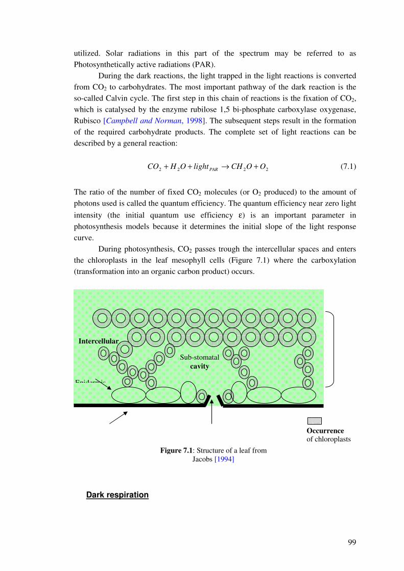
99
utilized. Solar radiations in this part of the spectrum may be referred to as
Photosynthetically active radiations (PAR).
During the dark reactions, the light trapped in the light reactions is converted
from CO2 to carbohydrates. The most important pathway of the dark reaction is the
so-called Calvin cycle. The first step in this chain of reactions is the fixation of CO2,
which is catalysed by the enzyme rubilose 1,5 bi-phosphate carboxylase oxygenase,
Rubisco [Campbell and Norman, 1998]. The subsequent steps result in the formation
of the required carbohydrate products. The complete set of light reactions can be
described by a general reaction:
2222 OOCHlightOHCO PAR +→++ (7.1)
The ratio of the number of fixed CO2 molecules (or O2 produced) to the amount of
photons used is called the quantum efficiency. The quantum efficiency near zero light
intensity (the initial quantum use efficiency ε) is an important parameter in
photosynthesis models because it determines the initial slope of the light response
curve.
During photosynthesis, CO2 passes trough the intercellular spaces and enters
the chloroplasts in the leaf mesophyll cells (Figure 7.1) where the carboxylation
(transformation into an organic carbon product) occurs.
Dark respiration
Sub-stomatal cavity
Intercellular
air space
Occurrence of chloroplasts
Epidermis
Figure 7.1: Structure of a leaf from Jacobs [1994]
100
The fixed carbon is used as an energy source for plant processes and as a
material to build structural dry matter. All these processes result in the release of CO2.
They are considered together under the name of dark respiration, because it takes
place in the dark. There are indications that dark respiration in leaves is suppressed by
light [Graham, 1979]. The equation is the counter reaction of photosynthesis.
Photorespiration
Because the carbon fixing enzyme of the Calvin cycle, Rubisco, is not only a
carboxylase but also an oxidase, CO2 and O2 compete for the same active site of
Rubisco. Therefore, photosynthesis will be inhibited in the presence of O2. At the
same time the oxidase activity of Rubisco will trigger a process that depends on the
availability of light and ultimately results in the release of previously fixed CO2. This
process is called photorespiration. C3 plants may loose up to 50 % of the newly fixed
CO2 by photorespiration. No clear function has been identified yet for this mechanism
so that it is often considered as a waste of energy.
Soil respiration
This release of CO2 corresponds to the plant root respiration and
decomposition of organic matter by micro-organisms.
Plant categories
In our case, the metabolic pathway for carbon fixation is assumed to be a C3
Cycle (see section 1.1.5).
Stomata
Stomata is a small opening on leaf surface through which plant communicate
with environment. The full mechanisms which control stomata aperture remain
unknown. However, it has been demonstrated that the stomata are sensitive to the
intercellular concentration of CO2, Ci, (and not to the concentration outside the leaf or
inside stomatal pores) and is influenced by light, leaf temperature, air humidity and
soil water content as well [Campbell and Norman, 1998]. Generally, stomata close in
the darkness and open if exposed to light. Higher temperatures increase the speed of
stomatal movements and the final aperture. Moreover, stomata tend to close if the
vapour pressure deficit of the surrounding air increases, and in response to the drying
101
of soil. In the latter case, closure starts only if the soil water potential drops down to
rather low values.
7.1.2 Terminology
Regarding the CO2 budget, fluxes have to be described separately for the plant
and the ecosystem. Let Pp be the plant photosynthetic flux, Rp the plant respiration
and Rs the soil respiration. Then Re, the ecosystem respiration is defined as
pse RRR += . The net primary productivity (NPP) for the plant is the quantity of CO2
absorbed when all processes have been taken into accounts:
pp RPNPP −= (7.2)
At the scale of the whole ecosystem, the soil respiration must be added for the net
ecosystem productivity (NEP):
epsppsRPRRPRNPPNEP −=−−=−= (7.3)
The NPP for each part of the plant depends on the efficiency of growth.
At the leaf level, the net assimilation, An, is balanced between the amount of
carbon fixed by photosynthesis (the gross assimilation rate Ag) and the losses due to
the dark respiration Rd:
dgn RAA −= (7.4)
The compensation point, Γ, is defined as the CO2 concentration at which no
assimilation occurs [Farquhar, 1980]. In the absence of ‘dark respiration’, that means
at light time, Γ increases linearly with the oxygen concentration in air (210000
µmol/mol), so that the light compensation point Γ* can be written:
τ2
CΓ oa* = (7.5)
where Coa is the oxygen concentration in the air and τ is the ratio describing the
partitioning between carboxylase and oxygenase reactions of Rubisco.
The common way of expressing the total leaf area in a forest canopy or any
other vegetation type is to use the leaf area index (LAI). It is the leaf surface per
square meter ground surface. It is expressed in m2/m2 and allows the scaling up of leaf
processes to a whole canopy.
Senescence is a productive form of aging leading to plant death. Plants age
productively; as tissues senesce they produce enzymes necessary to recycle
"expensive" materials and reroute the subunits to areas for use by active growth
102
elsewhere, in the next season, or by the next generation. This process is responsible
for the decrease in LAI in autumn.
7.2 Models presentation
7.2.1 Collatz’s Model
Leaf-level assimilation model
According to Farquhar et al. [1980], and later modified by Collatz et al. [1991]
and Campbell and Norman [1998], the gross photosynthetic rate at the leaf scale
depends on light, CO2 concentration, and leaf temperature. The light-limited
assimilation can be computed from:
( )*
*
2Γ+
Γ−×××=
i
ipmPAR
eC
CQeJ
α (7.6)
where αPAR is the leaf absorptivity for PAR, em is the maximum quantum efficiency
for leaf CO2 uptake (maximum number of CO2 molecules fixed per quantum of
radiation absorbed), Qp is the PAR photon flux density incident on the leaf
(µmol/m2/s), Ci is the intercellular CO2 concentration (see equation 7.15), and Γ* is
the light compensation point.
The Rubisco-limited assimilation rate is:
( )
+×+
Γ−×=
o
oa
ci
im
c
K
CKC
CVJ
1
*
(7.7)
where Vm is the maximum Rubisco capacity per unit leaf area [µmol/m2/s], Kc is the
Michaelis constant for CO2 fixation, and Ko is the Michaelis constant for oxygen
inhibition.
Finally, the last rate is controlled by the export and use of products of
photosynthesis. When sucrose builds up, the photosynthesis slows. It is considered as
the most likely rate-limiting step. The sucrose-limited assimilation is assumed, by
Collatz et al. [1991] to be just:
2m
s
VJ = (7.8)
The gross assimilation rate then is the minimum of those limiting-rates:
103
[ ]sceg JJJA ,,min= (7.9)
The net assimilation An is deduced from equation (7.9) minus the dark respiration.
dgn RAA −= (7.10)
Temperature response
The dark respiration and some other parameters of the model need a
temperature adjustment. Temperature dependence of kinetic variables is computed
following the equation in Campbell and Norman [1998]. For Kc, Ko and τ the
temperature dependence is an exponential relationship normalized with respect to
25°C (equation 7.11) whereas, for Vm and Rd, a high temperature cut-off is needed
(equations 7.12 and 7.13).
( )25)25(@)( −×= TqeXTX (7.11)
where q is the temperature coefficient for the parameter X and X(@25) is its value at
25°C. ( )
( )4129.0
25088.025,
1 −×
−×
+
×=
T
T
m
me
eVV (7.12)
( )
( )553.1
25069.025,
1 −×
−×
+
×=
T
T
d
de
eRR (7.13)
where Vm,25 and Rd,25 are values of Vm and Rd at 25°C, respectively [Campbell and
Norman, 1998].
Stomatal conductance
The stomatal conductance is deduced using the empirical formula from Ball et
al. [1987] when the net assimilation is known:
gs
s
sn
s bC
hAmg +
××= (7.14)
where m and bgs are constants, hs is the humidity at leaf surface (which is assumed to
be air humidity) and Cs is the CO2 concentration at leaf surface.
The third equation needed to solve the Ci/ An/ gs system is the Fick’s Law of
diffusion applied to CO2.
104
s
n
sig
ACC −= (7.15)
It has been assumed here that Cs is equal to the atmospheric CO2 concentration Ca
(380 ppm).
Equations (7.9), (7.14) and (7.15) constitute the core of the model as the
description of interactions between the internal concentration of CO2, the net
assimilation and the stomatal conductance. Being interdependent, they need to be
solved simultaneously.
In the light of those equations, this model has few inputs (PAR radiation, air
temperature, and air humidity) but about fifteen parameters depending on the plant
type. The full list of values chosen in our case is given in Appendix 5. However,
considering the works done by Collatz et al. [1991], Ball et al. [1987] and Farquhar et
al. [1980] as for C3 grass, only few of those parameters have been estimated for the
Dripsey site [Le Bris, 2002].
7.2.2 Jacobs or A-gs Model
Based on the empirical model from Jarvis [1976] for the stomatal
conductance, the A-gs model uses the model from Goudriaan et al. [1985] to describe
the photosynthesis part. Goudriaan’s model describes most of the essential
characteristics of photosynthesis. It is less detailed than Farquar’s model and therefore
needs less inputs parameters. This model is often linked to meteorological research
[Calvet et al., 1998; Calvet et al., 2001].
A correct model for stomatal behaviour must be able to include the effect of
short-term variations (light, temperature) as well as long-term changes (increase of
atmospheric CO2). The effects of those factors are combined, since it is known for
instance that an increase of atmospheric CO2 increases the plant sensitivity to light
and temperature and possibly to other factors too [Meidner and Mansfield, 1968].
However, Jarvis’s model, frequently used in meteorological research, does not take
into account synergistic effects between different stimuli. The alternative used in A-gs
is based on the observed correlation between the photosynthetic rate A, and the
stomatal conductance. At the cost of increased complexity, the responses to CO2 are
described including interactions between stimuli. Moreover, this model may be
expected to be more generally applicable since it relies more on the nature of plants
and less on statistics.
In Goudriaan et al. [1985] the photosynthetic rate does not only depend on the
biochemical processes of photosynthesis. The diffusion process which controls the
transport of CO2 from the atmosphere to the carboxylation sites inside the leaf, sets a
physical limit to the photosynthetic rate and is controlled by many conductances.
Some of these conductances are physical in nature. Others are related to chemical
processes and are called ‘conductance’ to allow a convenient comparison of
105
limitations imposed by chemical and physical processes. See figure 7.1 for location of
conductances described here:
The stomatal conductance (gsc for CO2 and gs for vapour water) describes
the diffusion through stomata pores. The difference in diffusivity has to be
accounted for so that scs gg ×= 6.1 .
The cuticular conductance describes the diffusion of water and CO2
through the waxy cuticle. For convenience, gc is usually assumed to be the
same for water and CO2. The total conductance through epidermis (see
Figure 7.1) can be calculated as csepidermis ggg += for water and with gsc
instead of gs for CO2. When stomata are widely open gc<< gs, whereas gc
may become larger than gs when they are closed.
The mesophyll conductance (gm), describes the transport of CO2 between
the sub-stomatal cavity and the site of carboxylation. gm includes a variety
of conductances from physical or chemical processes. Since the values of
those latter are not known for certain, gm is treated as one residual
resistance.
Assimilation
The modelling approach of A-gs directly relies on conductances to describe the
diffusion of CO2 between the air and chloroplasts. It is based on the distinction
between two different conditions:
the light-limiting factor.
the CO2 limiting factor.
If light is the limiting factor, An can be written as:
dan RIA −×= ε (7.16)
where Ia is the amount of absorbed PAR radiation, Rd is the dark respiration and ε is
the initial quantum use efficiency. The ε quantifies the slope of the light response
curve and is affected by photorespiration. It can be calculated as [Goudriaan et al.,
1985]:
Γ2C
ΓCεε
i
i
0+
−×= (7.17)
106
Γ is the compensation point [ppm], Ci is the internal concentration of CO2 and εo is
the maximum quantum use efficiency based on the theoretical efficiency of the Calvin
cycle. Equation (7.17) is derived from biochemical considerations and is similar to the
result obtained by Farquhar [1980].
In case that CO2 is the only limiting factor, the photosynthetic rate at light
saturation, Am, is linearly related to the CO2 concentration.
( ) cimm CgA ϕ×Γ−××= 001.0 (7.18)
Putting together equations (7.16) and (7.18), the final expression for An including
both the effect of limited light and CO2 is:
( ) d
RA
I
dmn ReRAA dm
a
−
−×+= +
×−ε
1 (7.19)
Here, the respiration rate Rd is simply defined as 9
m
d
AR = . (7.20)
In order to bound the photosynthetic rate at high light intensities and high CO2
concentrations, Am must be limited to a maximum value Am,max. A smooth transition
between equation (7.18) and Am,max is provided with:
( )
−×=
×Γ−××−
max,
001.0
max, 1 m
cim
A
Cg
mm eAA
ϕ
(7.20)
An and Am are calculated here in [mg/m2/s], gm is in [mm/s] and the concentrations are
in ppm [µmo/mol]. ϕc is a conversion factor transforming ppm to [mg/m3].
a
vaCO
cM
M ,2 ρϕ
×= (7.21)
where MCO2 and Ma are the molecular masses of CO2 and air (44 and 28.9 g/mol
respectively), and ρa is the density of air calculated thanks to the vapour content
×
−+××
=
100011
,q
R
RTR
P
a
v
a
vaρ (7.22)
where Rv and Ra are the gas constants for air and vapour pressure, P is the air pressure
in Pa, T is the air temperature [K] and q is the specific air humidity [kg/kg].
107
Temperature response
As for Collatz et al. [1991], the temperature dependence of photosynthesis is
accounted for through the temperature dependence of several parameters. The
response of those parameters is based on a Q10 function, which is a proportional
increase of a parameter for a 10°C increase in temperature [Berry and Raison, 1982].
For Γ, the equation (7.23) is used, whereas for gm and Am,max the function is modified
using an inhibition expression (equation (7.24)).
( ) ( ) 10
25
1025@−
×=T
QXTX (7.23)
X(T) is the value of any variable X at temperature T, with a reference value X(@25)
at 25°C.
( )( )( )( ) ( )( )TTTT
T
ee
QXTX
−−
−
+×+
×=
21 3.03.0
10
25
10
11
25@ (7.24)
T1 and T2 denote reference temperatures, which can be adjusted to mimic species-
specific features.
The reference values have been adapted from Jacobs [1994] and Bruse [2001].
The calibration process was done by Le Bris [2002] and the full list of parameters can
be found in Appendix 5.
Stomatal conductance
The effect of humidity on the stomatal response and internal CO2
concentration is parameterised using a factor f defined as:
×+
−×=
max
min
max
0 1D
Df
D
Dff ss (7.25)
Ds is the vapour pressure deficit of air at the plant surface [g/kg] and Dmax is its
maximum value. The fo is the value of f for Ds = 0 g/kg, and is around 0.85 for C3
plants. The minimum fmin is calculated from equation (7.26).
mc
c
gg
gf
+=min (7.26)
where gc is the cuticular conductance and gm is the mesophyll conductance.
The internal CO2 concentration, Ci, is then obtained from f, and the value of CO2
concentration at leaf surface:
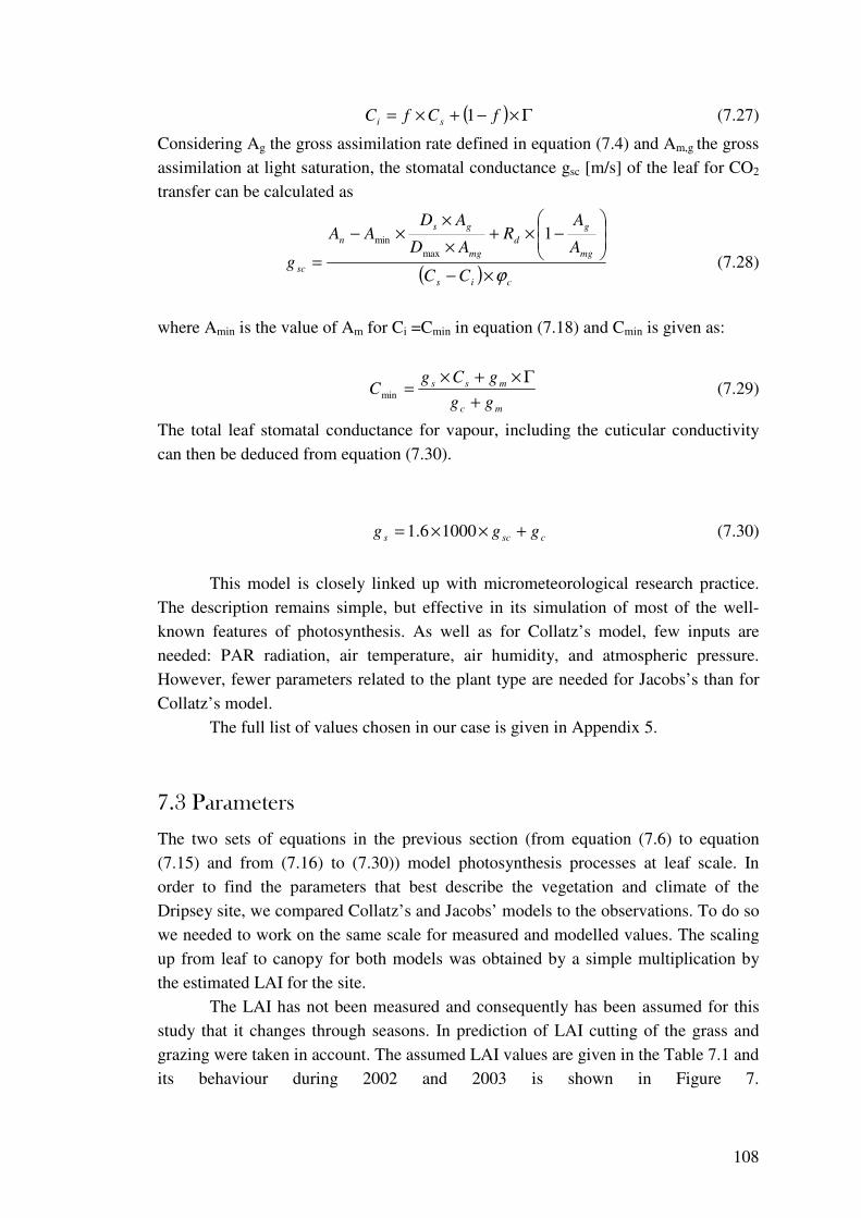
108
( ) Γ×−+×= fCfC si 1 (7.27)
Considering Ag the gross assimilation rate defined in equation (7.4) and Am,g the gross
assimilation at light saturation, the stomatal conductance gsc [m/s] of the leaf for CO2
transfer can be calculated as
( ) cis
mg
g
d
mg
gs
n
scCC
A
AR
AD
ADAA
gϕ×−
−×+
×
××−
=
1max
min
(7.28)
where Amin is the value of Am for Ci =Cmin in equation (7.18) and Cmin is given as:
mc
mss
gg
gCgC
+
Γ×+×=min (7.29)
The total leaf stomatal conductance for vapour, including the cuticular conductivity
can then be deduced from equation (7.30).
cscs ggg +××= 10006.1 (7.30)
This model is closely linked up with micrometeorological research practice.
The description remains simple, but effective in its simulation of most of the well-
known features of photosynthesis. As well as for Collatz’s model, few inputs are
needed: PAR radiation, air temperature, air humidity, and atmospheric pressure.
However, fewer parameters related to the plant type are needed for Jacobs’s than for
Collatz’s model.
The full list of values chosen in our case is given in Appendix 5.
7.3 Parameters
The two sets of equations in the previous section (from equation (7.6) to equation
(7.15) and from (7.16) to (7.30)) model photosynthesis processes at leaf scale. In
order to find the parameters that best describe the vegetation and climate of the
Dripsey site, we compared Collatz’s and Jacobs’ models to the observations. To do so
we needed to work on the same scale for measured and modelled values. The scaling
up from leaf to canopy for both models was obtained by a simple multiplication by
the estimated LAI for the site.
The LAI has not been measured and consequently has been assumed for this
study that it changes through seasons. In prediction of LAI cutting of the grass and
grazing were taken in account. The assumed LAI values are given in the Table 7.1 and
its behaviour during 2002 and 2003 is shown in Figure 7.
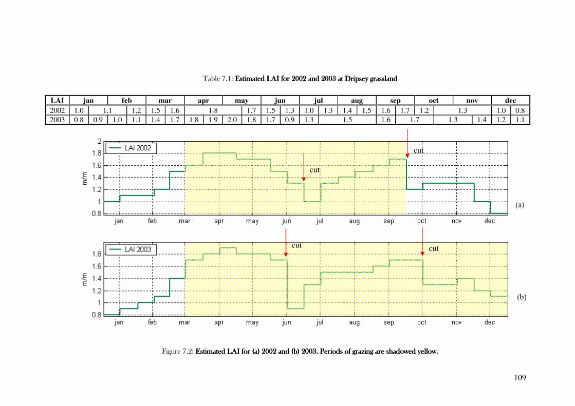
109
Table 7.1: Estimated LAI for 2002 and 2003 at Dripsey grasslan Estimated LAI for 2002 and 2003 at Dripsey grasslan Estimated LAI for 2002 and 2003 at Dripsey grasslan Estimated LAI for 2002 and 2003 at Dripsey grasslandddd
LAI jan feb mar apr may jun jul aug sep oct nov dec
2002 1.0 1.1 1.2 1.5 1.6 1.8 1.7 1.5 1.3 1.0 1.3 1.4 1.5 1.6 1.7 1.2 1.3 1.0 0.8 2003 0.8 0.9 1.0 1.1 1.4 1.7 1.8 1.9 2.0 1.8 1.7 0.9 1.3 1.5 1.6 1.7 1.3 1.4 1.2 1.1
Figure 7.2: Estimated LAI for (a) 2002 and (b) 2003. Periods of grazing are shadowed yellow.Estimated LAI for (a) 2002 and (b) 2003. Periods of grazing are shadowed yellow.Estimated LAI for (a) 2002 and (b) 2003. Periods of grazing are shadowed yellow.Estimated LAI for (a) 2002 and (b) 2003. Periods of grazing are shadowed yellow.
cut
cut
cut cut
(a)
(b)
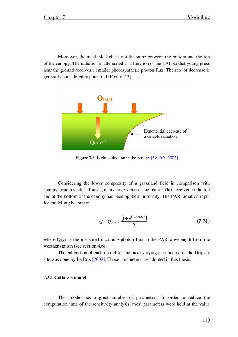
Chapter 7 Modelling
110
Moreover, the available light is not the same between the bottom and the top
of the canopy. The radiation is attenuated as a function of the LAI, so that young grass
near the ground receives a smaller photosynthetic photon flux. The rate of decrease is
generally considered exponential (Figure 7.3).
Considering the lower complexity of a grassland field in comparison with
canopy system such as forests, an average value of the photon flux received at the top
and at the bottom of the canopy has been applied uniformly. The PAR radiation input
for modelling becomes:
( )( )2
1 4.0 LAI
PAR
eQQ
×−+×= (7.31) (7.31) (7.31) (7.31)
where QPAR is the measured incoming photon flux in the PAR wavelength from the
weather station (see section 4.6).
The calibration of each model for the most varying parameters for the Dripsey
site was done by Le Bris [2002]. Those parameters are adopted in this thesis.
7.3.1 Collatz’s model
This model has a great number of parameters. In order to reduce the
computation time of the sensitivity analysis, most parameters were held at the value
QPAR
Exponential decrease of available radiation
QPAR.e-0.6
Figure 7.3: Light extinction in the canopy [Le Bris, 2002]
Chapter 7 Modelling
111
defined by Farquhar [1980] for C3 grass (Appendix 5). Le Bris [2002] considered only
parameters that were usually different from one site to another or from one type of
grass to another (see values given by Collatz for C4 grass and by Farquhar for C3 grass
in Appendix 5). The sensitivity analysis was done for: qKo, qKc, qτ and m from the
stomatal conductance equation (7.14) [Le Bris, 2002].
A more detailed analysis should be done when the values of the seasonal
variability of the leaf area index (LAI) for the site will be known.
The adopted values for tested parameters are:
qKo = 0.05 qKc = 0.07 qτ = -0.02 m = 6.75
Those results are consistent with usual values for such coefficients and are used for
the modelled CO2 flux analysis.
7.3.2 Jacobs’ model
Jacobs’s model has fewer parameters than Collatz’s model. Four parameters
were tested by Le Bris [2002] and the other parameters were held at the value given
by Jacobs [1994] for C3 grass (Appendix 5). In this study we adopted parameter
values determined by Le Bris [2002].
The adopted values for tested parameters are:
ffffoooo = 0.94 = 0.94 = 0.94 = 0.94 QQQQ10101010((((ΓΓΓΓ) = 1.2 = 1.2 = 1.2 = 1.2 QQQQ10101010((((Am,max) = 1.6 = 1.6 = 1.6 = 1.6 QQQQ10101010((((gm) = 1.6 = 1.6 = 1.6 = 1.6
Those results are consistent with usual values for such coefficients and are used for
the modelled CO2 flux analysis.
7.4 Modelling results and comparisons
The following analysis examines the results of the Collatz’s model and
Jacobs’s models for the study period. The daily, monthly fluxes were examined, and
Collatz’s and Jacobs’s cumulative fluxes compared in terms of global uptake and
photosynthesis.
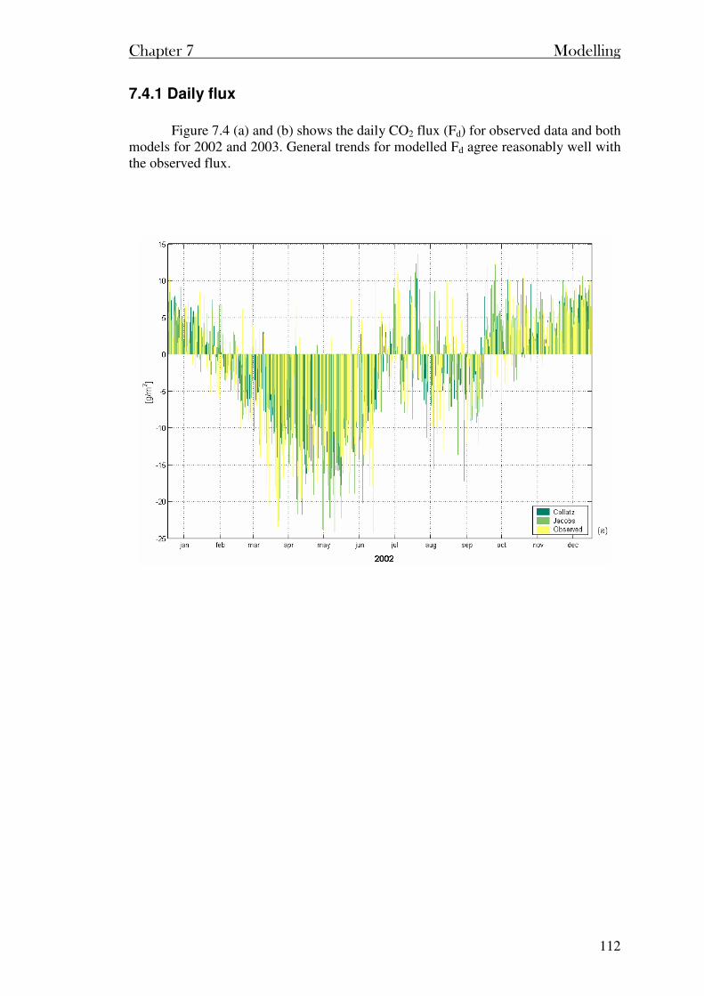
Chapter 7 Modelling
112
7.4.1 Daily flux
Figure 7.4 (a) and (b) shows the daily CO2 flux (Fd) for observed data and both models for 2002 and 2003. General trends for modelled Fd agree reasonably well with the observed flux.
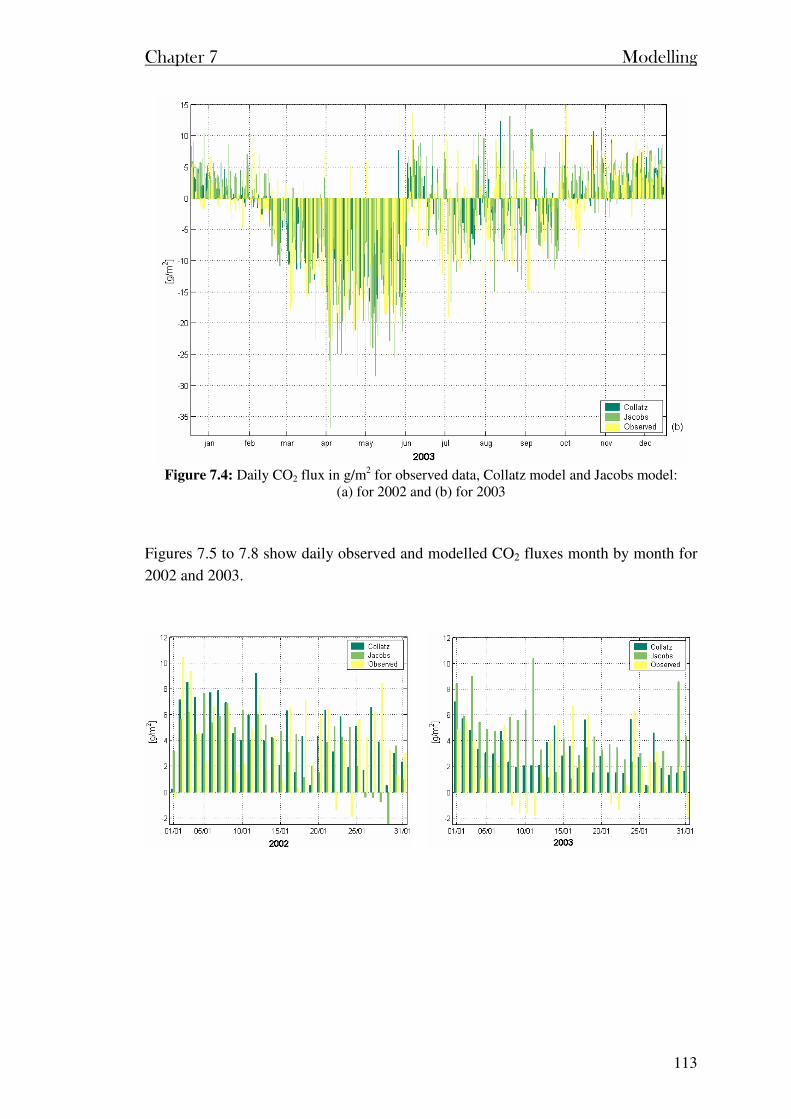
Chapter 7 Modelling
113
Figure 7.4: Daily CO2 flux in g/m2 for observed data, Collatz model and Jacobs model:
(a) for 2002 and (b) for 2003
Figures 7.5 to 7.8 show daily observed and modelled CO2 fluxes month by month for
2002 and 2003.
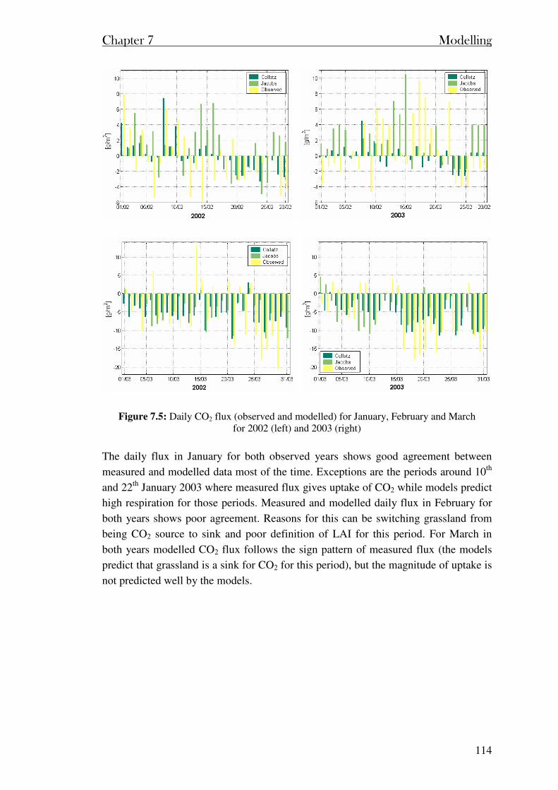
Chapter 7 Modelling
114
Figure 7.5: Daily CO2 flux (observed and modelled) for January, February and March for 2002 (left) and 2003 (right)
The daily flux in January for both observed years shows good agreement between
measured and modelled data most of the time. Exceptions are the periods around 10th
and 22th January 2003 where measured flux gives uptake of CO2 while models predict
high respiration for those periods. Measured and modelled daily flux in February for
both years shows poor agreement. Reasons for this can be switching grassland from
being CO2 source to sink and poor definition of LAI for this period. For March in
both years modelled CO2 flux follows the sign pattern of measured flux (the models
predict that grassland is a sink for CO2 for this period), but the magnitude of uptake is
not predicted well by the models.
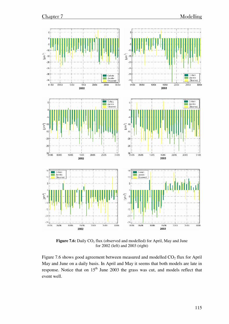
Chapter 7 Modelling
115
Figure 7.6: Daily CO2 flux (observed and modelled) for April, May and June for 2002 (left) and 2003 (right)
Figure 7.6 shows good agreement between measured and modelled CO2 flux for April
May and June on a daily basis. In April and May it seems that both models are late in
response. Notice that on 15th June 2003 the grass was cut, and models reflect that
event well.
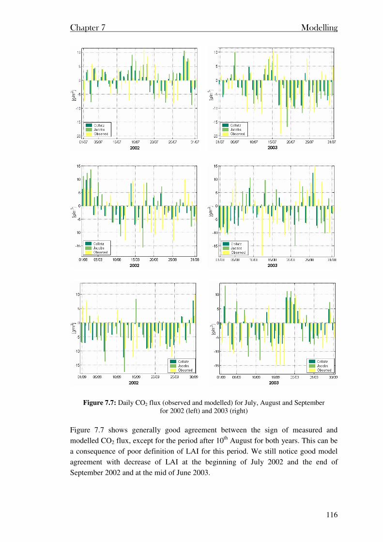
Chapter 7 Modelling
116
Figure 7.7: Daily CO2 flux (observed and modelled) for July, August and September for 2002 (left) and 2003 (right)
Figure 7.7 shows generally good agreement between the sign of measured and
modelled CO2 flux, except for the period after 10th August for both years. This can be
a consequence of poor definition of LAI for this period. We still notice good model
agreement with decrease of LAI at the beginning of July 2002 and the end of
September 2002 and at the mid of June 2003.
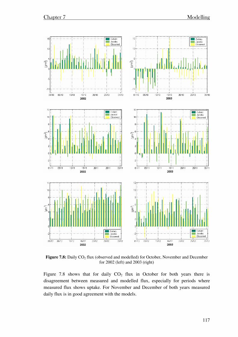
Chapter 7 Modelling
117
Figure 7.8: Daily CO2 flux (observed and modelled) for October, November and December
for 2002 (left) and 2003 (right)
Figure 7.8 shows that for daily CO2 flux in October for both years there is
disagreement between measured and modelled flux, especially for periods where
measured flux shows uptake. For November and December of both years measured
daily flux is in good agreement with the models.
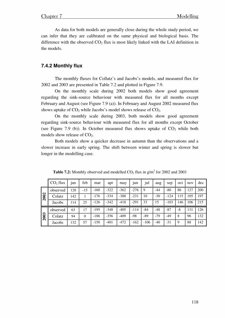
Chapter 7 Modelling
118
As data for both models are generally close during the whole study period, we
can infer that they are calibrated on the same physical and biological basis. The
difference with the observed CO2 flux is most likely linked with the LAI definition in
the models.
7.4.2 Monthly flux
The monthly fluxes for Collatz’s and Jacobs’s models, and measured flux for
2002 and 2003 are presented in Table 7.2 and plotted in Figure 7.9.
On the monthly scale during 2002 both models show good agreement
regarding the sink-source behaviour with measured flux for all months except
February and August (see Figure 7.9 (a)). In February and August 2002 measured flux
shows uptake of CO2 while Jacobs’s model shows release of CO2.
On the monthly scale during 2003, both models show good agreement
regarding sink-source behaviour with measured flux for all months except October
(see Figure 7.9 (b)). In October measured flux shows uptake of CO2 while both
models show release of CO2.
Both models show a quicker decrease in autumn than the observations and a
slower increase in early spring. The shift between winter and spring is slower but
longer in the modelling case.
Table 7.2: Monthly observed and modelled CO2 flux in g/m2 for 2002 and 2003
CO2 flux jan feb mar apr may jun jul aug sep oct nov dec
observed 128 -15 -160 -322 -362 -276 9 -44 -80 86 127 200
Colatz 142 1 -176 -334 -388 -231 10 -30 -124 115 105 197
20
02
Jacobs 114 25 -126 -342 -418 -291 33 15 -103 146 106 215
observed 63 17 -195 -348 -405 -114 -84 -48 -87 -8 131 126
Colatz 94 0 -186 -356 -409 -98 -89 -79 -49 8 96 132
20
03
Jacobs 132 57 -150 -401 -472 -162 -106 -40 -31 9 88 142
Chapter 7 Modelling
119
Figure 7.9: Monthly observed and modelled CO2 flux for
(a) for 2002 and (b) for 2003.
7.4.3 Cumulative photosynthesis and global uptake
The cumulative quantities are important as they represent in a striking way the
main characteristics of a site and its capacity to act as a sink or a source of carbon.
Having reasonably good results for the previous time scales, one can be confident of the
cumulative fluxes be it the photosynthesis flux or the net uptake over the year of study.
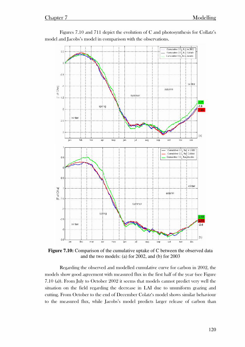
Chapter 7 Modelling
120
Figures 7.10 and 711 depict the evolution of C and photosynthesis for Collatz’s
model and Jacobs’s model in comparison with the observations.
Figure 7.10: Comparison of the cumulative uptake of C between the observed data
and the two models: (a) for 2002, and (b) for 2003
Regarding the observed and modelled cumulative curve for carbon in 2002, the
models show good agreement with measured flux in the first half of the year (see Figure
7.10 (a)). From July to October 2002 it seems that models cannot predict very well the
situation on the field regarding the decrease in LAI due to ununiform grazing and
cutting. From October to the end of December Colatz‘s model shows similar behaviour
to the measured flux, while Jacobs’s model predicts larger release of carbon than
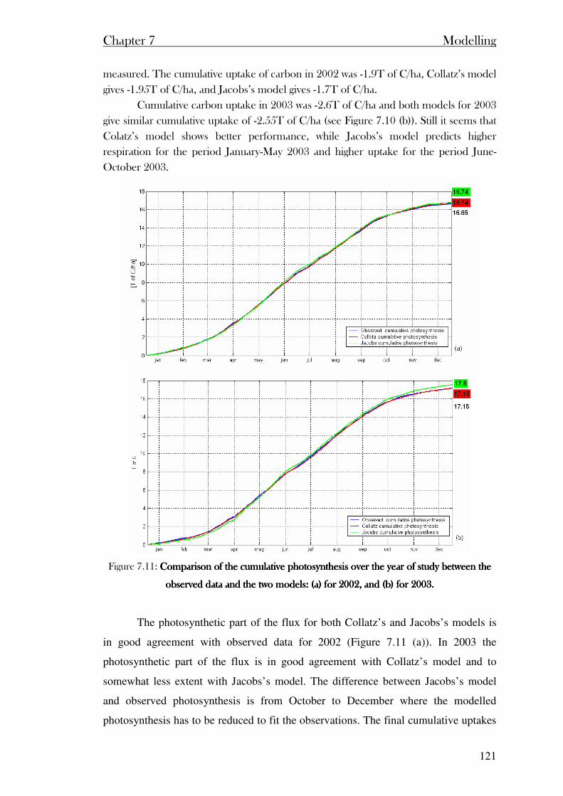
Chapter 7 Modelling
121
measured. The cumulative uptake of carbon in 2002 was -1.9T of C/ha, Collatz’s model
gives -1.95T of C/ha, and Jacobs’s model gives -1.7T of C/ha.
Cumulative carbon uptake in 2003 was -2.6T of C/ha and both models for 2003
give similar cumulative uptake of -2.55T of C/ha (see Figure 7.10 (b)). Still it seems that
Colatz’s model shows better performance, while Jacobs’s model predicts higher
respiration for the period January-May 2003 and higher uptake for the period June-
October 2003.
Figure 7.11: Comparison of the cumulative photosynthesis over the year of study between the Comparison of the cumulative photosynthesis over the year of study between the Comparison of the cumulative photosynthesis over the year of study between the Comparison of the cumulative photosynthesis over the year of study between the
observed data and the two modobserved data and the two modobserved data and the two modobserved data and the two models: (a) for 2002, and (b) for 2003.els: (a) for 2002, and (b) for 2003.els: (a) for 2002, and (b) for 2003.els: (a) for 2002, and (b) for 2003.
The photosynthetic part of the flux for both Collatz’s and Jacobs’s models is
in good agreement with observed data for 2002 (Figure 7.11 (a)). In 2003 the
photosynthetic part of the flux is in good agreement with Collatz’s model and to
somewhat less extent with Jacobs’s model. The difference between Jacobs’s model
and observed photosynthesis is from October to December where the modelled
photosynthesis has to be reduced to fit the observations. The final cumulative uptakes

Chapter 7 Modelling
122
(by the photosynthesis process only, i.e. GPP) agree well for both models and both
studied years.
In conclusion, both Collatz’s model and Jacobs’ model give in general
satisfactory results on the different time scales for both observed years. As for the
senescence and growing transition in autumn and spring, they can be improved by a
better definition of the variation of LAI during the year.

Chapter 8 Conclusion
Chapter 8 Conclusion
123
Chapter 8 Conclusion
8.1 Conclusion
The eddy correlation flux measurements presented here cover two years of a
planned long-term research programme of net ecosystem exchange of CO2 begun in
July 2001 at a humid temperate grassland ecosystem in southern Ireland. The
experimental grassland encompasses eight small dairy farms (of size 10 to 40ha each)
with approximately 2/3rd’s of the area grazed for eight months of the year while in the
other 1/3rd (which is off-limits for grazing from March to September) the grass is cut
(harvested for winter feed) twice per year: June and September. The two cuts of silage
during the study period may have affected the LAI and thus CO2 flux at the beginning
and also at the end of the study The two years are: 2002 which was a wet year
(precipitation at 1785mm, 22% above average); and 2003 which was a dry year
(precipitation at 1185mm, 15% below average). The climate being very temperate in
Ireland, very few days are under 4°C, which is a critical temperature for the
photosynthetic process and no snow occurred during the study period. Therefore, the
leaf area index stays higher with a minimum value around 1. The farmland
management practices in both years were similar, including nitrogen fertilisation rates
(305kg.N/ha and 294kg.N/ha for 2002 and 2003 respectively). We found that the wet
year of 2002 had a NEE of -1.9TC/ha compared to -2.6TC/ha for the dry year of 2003
(a 27% difference). We found that the cumulative NEE from February to September
(Spring plus Summer) was the same in both years. The difference in NEE in the two
years of 0.7 T.C/ha was concentrated in the winter months (October, November,
December and January). The wet year winter had a cumulative NEE of +1.5 T.C/ha
while for the corresponding NEE for the dry year was +0.8 T.C/ha. The precipitation
of the wet winter (2002) was 903 mm while in the dry winter it was 435 mm. As the
land use and land management practices were similar in both years, the main
difference between the two years was in the magnitude of the winter rainfall. We
conclude that the wetter winter of 2002 with its saturating effect on soil moisture had
enhanced ecosystem respiration which was responsible for the lower annual NEE of
2002. Another issue that have been raised here is the use of the site by cattle and the
effects of the silage cuts. They stimulated the growth as well by bringing more light to
the most active and youngest grass situated near the ground. In the meantime the LAI
is reduced and so is the photosynthetic flux. A better understanding of those processes
and long time measurements are required.
Chapter 8 Conclusion
124
8.2 Suggestion for further investigation
Many believe that grasslands may be missing carbon sink [Ham & Knapp,
1998; Robert, 2001; Pacala et al., 2001; Goodale and Davidson, 2002]. In order to
define the amount of carbon sequestered (i.e. fixed to the soil) at Dripsey
experimental site it is very important to define the footprint of tower. Our findings
suggest that during the stable and neutral conditions footprint can be larger (up to 7
km radius) than the area occupied by farms with known management. This estimation
of footprint was done for the instruments positioned at 10 m height. As is described in
section 3.4, size of footprint area depends on surface roughness, change in stability
(i.e. from unstable to stable), and the instrument’s height. It was suggested to decrease
instrumentation height for CO2 fluxes was reduced from 10 to 3m on December 22,
2003. This change will decrease the footprint area and better define the land
management in the smaller footprint.
The carbon budget for the farm can be written:
atm/soilC...)CBA(NEE =+++− (8.1)
where NEE is Net ecosystem exchange [T of C/ha], A, B, C… is carbon leaving the
farm (in milk, in meat, in enteric fermentation) and Csoil/atm is a carbon fixed in the soil
or lost in the atmosphere.
If we assume that new footprint area encompasses eight small dairy farms (of size
10 to 40ha each) with approximately 2/3rd’s of the area grazed for eight months of the
year while in the other 1/3rd, the grass cut (harvested for winter feed) twice per year:
June and September; carbon leaving the farm can be calculated:
A. Carbon in milk [T.C/ha.yr.]
average production 7500L/ha.
density φ = 1.03kg/L
carbon in milk = 4.5%
yr.ha/C.T35.010100
5.403.17500C 3
milk =×××= − (8.2)
B. Carbon in meat [T.C/ha.yr.]
~18% of live weight
1LU = 520kg pasture dry matter per year
Stocking Density for Dripsey = 2.2LU/ha
Assume that 1/3 of animals leave farm for the meat factory
yr.ha/C.T1.0103
1
100
185202.2C 3
meat ≈××××= − (8.3)
C. Carbon in CH4 respired from animal and CH4 from manure for full year
Chapter 8 Conclusion
125
100kg CH4 from animal
15kg CH4 from manure
Stocking Density for Dripsey = 2.2LU/ha
( ) yr.ha/C.T2.01016
122.2115C 3
CH4=×××= − (8.4)
D. Carbon as CO2 from respiring animal indoors for 4 months of year
Diet = 10kgDM/day/LU
DM = 45%Carbon
Assume 40% respire
( ) yr.ha/C.T45.010100
40
12
42.2
100
4536510C 3
CO2=××××××= − (8.5)
It is of great importance to estimate new footprint and to check if there are changes in
NEE. In order to calculate this long-term measurements (at least 6 months) are
needed. That will open new research on carbon sequestration in this grassland
ecosystem.
Thanks to the good collaboration with the farmers the application of nitrogen
fertilizer and slurry for the farms is known. Some investigation should be done on
grass root efficiency to uptake spread fertilizer on the field (i.e during the dry and wet
weather) and contribution of fertilizer to the grass growth in different seasons in the
year.
In the future, some measurements on the site of the leaf area index (LAI)
should improve our knowledge of the growth of plants throughout seasons, highlight
the effects of silage cuts on grass growth and give a good assessment of the amount of
matter removed in summer. Such measurements are widely described in literature and
could be either carried out by remote sensing measurements (from satellite data) or
with manual measurements as it is usually done for sites of field scale size such as our
catchment. This data could then be used to validate a model of growth to simulate a
variable LAI during the year. The LAI found in this way could also be used for
calculating actual evapotranspiration since bulk surface resistance (rs) in Penman-
Monteith equation depend on it.
Very important for future investigation of evapotranspiration and CO2 canopy-
atmosphere exchange is finding not only meteorological, but physiological
explanations for interannual variability (e.g. canopy conductance (gc), ‘omega factor’
(Ω) which is an index of relative importance of meteorological and physiological
limitations to evapotranspiration).

Chapter 8 Conclusion
126
In this study, only two components are considered in the CO2 fluxes: the
ecosystem respiration (nighttime CO2 flux) and the photosynthesis (daytime CO2 flux
minus the daytime CO2 respiration deduced from the nighttime measurements).
However, soil surface carbon dioxide flux, the sum of plant root and microbial
respiration, is an important part of the carbon cycle of terrestrial ecosystem too. In our
case no device measured this component alone, so that it could not be separated from
the plant respiration (they together compose the ecosystem respiration). Many papers
report the method of close-chamber or open-chamber measurements, used to measure
soil respiration, and the accuracy of such method. This could be an interesting part to
add to the instruments present on this Irish grassland site to deepen the understanding
of process of carbon cycle.

Chapter 7 Conclusion
References
References
128
Aber, D. J., and C. A. Federer, A generalized, lumped-parameter model of photosynthesis,
evapotranspiration and net primary production in temperate and boreal forest
ecosystems, Oecologia, 92, 463-474, 1992.
Albertson, J. D., and G. Kiely, On the structure of soil moisture time series in the context of
land surface models, Journal of Hydrology, 243, 101-119, 2001.
Aubinet, M., A. Grelle, A. Ibrom, U. Rannik, J. Moncrieff, T. Foken, A. S. Kowalski, P. H.
Martin, P. Berbigier, C. H. Bernhofer, R. Clement, J. Elbers, A. Granier, T. Grunwald,
K. Morgenstern, K. Pilegaard, C. Rebmann, W. Snijders, R. Valentini, and T. Vesala,
Estimates of annual net carbon and water exchange of forests: the EUROFLUX
methodology, Adv. Ecol. Res., 30, 114-175, 2000.
Baldocchi, D.D., Assessing the eddy covariance technique for evaluating carbon dioxide
exchange rates of ecosystems: past, present and future, Global Change Biol., 9, 479-
492, 2003.
Baldocchi, D., R Valentini, S. Runing, W. Oechel, and R. Dahlman, Strategies for measuring
and modeling carbon dioxide and water vapour fluxes over terrestrial ecosystems,
Global Change Biol., 2, 159-168, 1996.
Ball, J.T., I. E. Woodrow, and J. A. Berry, A model predicting stomatal conductance and its contribution to the control of Photosynthesis under different environmental conditions. Progress in Photosynthesis Research. 4, 221-224, 1987.
Batjes, H. N., Management options for reducing CO2 – concentrations in the atmosphere by
increasing carbon sequestration in the soil, Report no. 410 200 031, 114 pp., Dutch
National Research Programme on Global Air Pollution and Climate Change,
Netherlands, 1999.
Berbigier, P., J.-M. Bonnefond, and P. Mellmann , CO2 and water vapour fluxes for 2 years
above Euroflux forest site, Agric. For. Meteorol., 108, 183-197, 2001.
Berry, J. A., and J. K. Raison, Responses of Macrophytes to temperature. In: Lange, O.L.,
Nobel, P.S., Osmond, C.B., Ziegler, H., Encyclopedia of Plant Physiology, New series,
Vol. 12B, Physiological Plant Ecology II. Springer Verlag, Berlin, 277-338, 1982.
Bruce, P. J., M. Frome, E. Haites, H. Joanne, L. Rattan, and K. Faustian, Carbon sequestration
in soils, J. Soil and Water cons., 382-389,1999.
Bruse, M., ENVI-met implementation of the Jacobs A-gs model to calculate the stomata
conductance. Working paper, 2001.
http://www.geographie.ruhr-uni-bochum.de/agklima/envimet/
References
129
Brutsaert, W., Evaporation into the atmosphere, edited by A. J. Davenport, B. B. Hicks, G. R.
Hilst, R. E. Munn, J. D. Smith, Kluwer Academic Publishers, London, 1991.
Budyko, I. M., Climate and Life, Climatic factors of Photosynthesis, 497, Academic Press
INC, London, 1974.
Calvet, J.C., J. Noilhan, J. L. Roujean, P. Bessemoulin, M. Cabelguenne, A. Olioso, and J. P.
Wigneron, An interactive vegetation SVAT model tested against data from six
contrasting sites. Agric. For. Meteorol. 92, 73-95, 1998.
Calvet, J. C., and J. F.Soussana, Modelling CO2 enrichment effects using an interactive
vegetation SVAT scheme. Agric. For. Meteorol. 108, 129-152, 2001.
Campbell, S. G., and J. M. Norman, An introduction to environmental Biophysics, second
edition, Springer-Verlag New York, 1998.
Campbell, Soil moisture, surface wetness and heat flux sensors, Campbell Scientific, Ltd.
1998. www.campellsci.co.uk
Campbell, Tipping bucket raingauges, ARG100, Campbell Scientific, Ltd. 2000.
www.campellsci.co.uk
Campbell, PTB101B Barometric Pressure Sensor User Guide, Campbell Scientific, Ltd. 2001.
www.campellsci.co.uk
Campbell, CS616 Water Content Reflectometer, Campbell Scientific, Ltd. 2002a.
www.campellsci.co.uk/products/sensors/cs616.htm
Campbell, CR23X Micrologger, Campbell Scientific, Inc. 2002b.
www.campellsci.co.uk/products/sensors/cs616.htm
Campbell, Model HMP45C temperature and relative humidity probe instruction manual,
Campbell Scientific, inc. 2003a. www.campellsci.co.uk
Campbell, Model 107 & 107B temperature probes instruction manual, Campbell Scientific,
inc. 2003b. www.campellsci.co.uk
Cava D., U. Giostra, M. Siqueira, and G. Katul, Organised Motion and Radiative
Perturbations in the Nocturnal Canopy Sublayer above an Even-Aged Pine Forest,
Boundary-Layer Meteorol, 112, No. 1, 129-157, 2004.
Collatz, G.J., J.T Ball, C Grivet, and J.A. Berry, Physiological and environmental regulation
of stomatal conductance, photosynthesis and transpiration: a model that includes a
laminar boundary layer. Agric. For. Meteorol. 54, 107-136, 1991.
References
130
Conant, T.R., K. Paustian, and E. T. Elliott, Grassland management and conversion into
grassland: effects on soil carbon, Ecol. Applications, 11, No. 2, pp. 343-355, 2001.
Cruickshank, M.M., R.W. Tomlinson, P.M. Devine, and R. Milne, Carbon in the vegetation
and soils of Northern Ireland, Biology and Environment: Proceedings of the Royal Irish
Academy, vol. 98B, No. 1, 9-21, 1998.
Dabberdt, W. F., D. H. Lenschow, T. W. Horst, P. R. Zimmerman, S. P. Oncley, and A. C.
Delany, Atmosphere-surface exchange measurements, Science, 260, 1472-1481, 1993.
Daly, K., An Environmentalappraisal of the phosphorous of the Irish grassland soils, PhD.
Thesis, Trinity College Dublin, 1999.
Dingman, S. L., Physical Hydrology, editor Robert McConnin, Macmillan Publishing
Company, New York, 1994.
Dugas, W.A., M.L. Heuer, and H.S. Mayeux, Carbon dioxide fluxes over a Bermuda grass,
native prairie, and sorghum. Agric. For. Meteorol. 93,121-139, 1999.
Earlham College, http://www.earlham.edu/~biol/syllabi/ecobio02/notes.htm, 2002
EMS (Environmental Media Service), Pentagon Report Describes Global Warming
Dangers, 2003.
http://www.ems.org/climate/pentagon_climate_change.html#report
Encyclopedia Britannica, 20th Edition
EPA (Environmental Protection Agency-Ireland), Ireland’s environment, chapter 4:
Emissions to air, A Millennium Report, edited by Michael McGettigan, April 2000.
EPA (Environmental Protection Agency-Ireland), National Inventory Report 2003,
Greenhouse gas emissions 1990-2001 reported to the United Nations framework
convention on climate change, edited by Michael McGettigan and Paul Duffy, 2003.
Falge, E., D. Baldocchi, J. Tenhunen, M. Aubinet, P. Bakwin, P. Berbigier, C. Bernhofer, G.
Burba, R. Clement, K. J. Davis, J. A. Elbers, A. H. Goldstein, A. Grelle, A. Granier, J.
Guðmundsson, D. Hollinger, A. Kowalski, G. Katul, B. E. Law, Y. Malhi,T. Meyers, R.
K. Monson, J. W. Munger, W. Oechel, K. Tha Paw U, K. Pilegaard, Ü. Rannik, C.
Rebmann, A. Suyker, R. Valentini, K. Wilson, and S. Wofsy, Seasonality of ecosystem
respiration and gross primary production as derived from FLUXNET measurements,
Agric. For. Meteorol., 113, 53-74, 2002.
Falge, E., D. Baldocchi, R. Olson, P. Athoni, M. Aubinet, C. Bernhofer, G. Burba, R.
Ceulemans, R. Clement, H. Dolman, A. Granier, P. Gross, T. Grünward, D. Hollinger,
N-O. Jensen, G. Katul, P. Keronen, A. Kowalski, C. T. Lai, B. E. Law, T. Meyers, J.
Moncrieff, E. Moors, J. W. Munger, K. Pilegaard, Ü. Rannik, C. Rebmann, A. Suyker, J.
References
131
Tenhunen, K. Tu, S. Verma, T. Vesala, K. Wilson, and S. Wofsy, Gap filling strategies
for defensible annual sums of net ecosystem exchange, Agric. For. Meteorol., 107, 43-69, 2001.
FAO, Crop evapotranspiration – Guidelines for computing crop water requirements – FAO
Irrigation and drainage paper 56, Food and Agriculture Organisation of the United
Nations, Rome, 1998.
Farquhar, G.D., S von Caemmerer, and J. A. Berry, A biochemical model of photosynthetic
CO2 assimilation in leaves of C3 species. Planta. 149, 78-90, 1980.
Foken, Th., and B. Wichura, Tools for quality assessment of surface-based flux
measurements, Agric. For. Meteorol., 78, 83-105, 1996.
Frank, B. A., and Dugas, A. W., Carbon dioxide fluxes over northern, semiarid, mixed-grass
prairie, Agric. For. Meteorol., 108, 317-326, 2001.
Frank, B.A., P. L. Sims, J. A. Bratford, P. C. Milenick, W. A. Dugas, and H. S. Mayeux,
Carbon dioxide fluxes over three great plains grasslands, The Potential of U.S. Grazing
Lands to Sequester Carbon and Mitigate the Greenhouse Effect, edited by R. F. Follett,
J. M. Kimble, and R. Lal, 167-187, Lewis Puplishers, New York, 2001.
Garatt, R. J., The atmospheric boundary layer, Edited by J. T. Houghton, M. J. Rycroft, A. J.
Dessler, Cambridge University Press, 1992.
Gash, J. H. C., A note on estimating the effect of a limited fetch on on micrometeorological
evaporation measurements. Boundary-Layer Meteor., 35, 409-413, 1986.
Gash, J. H. C., F. Valente, and J. S. David, Estimates and measurements of evaporation from
wet, sparse pine forest in Portugal, Agric. For. Meteorol., 94, 149-158, 1999.
Gardiner, M. J., and T. Radford, Soil associations of Ireland and their land use potential, An
Foras Taluntais, Sandymount Avenue, Dublin, Ireland, 1980.
Goodale, L. C., and E. A. Davidson, Uncertain sinks in the shrubs, Nature, 418, 593-594,
2002.
Goudriaan, J., H.H. van Laar, H. van Keulen, and W. Lovwerse, Photosynthesis, CO2 and
plant production. In: Day, W. Day & R.K. Atkin (Eds.), Wheat growth and modelling.
NATO ASI Series, Series A, Vol. 86. Plenum Press, New York, 107-122, 1985.
Goulden, M.L., J.W., Munger, S.M., Fan, B.C., Daube, and S.C., Wofsy, Measurements of
carbon sequestration by long-term eddy covariance: methods and critical evaluation of
accuracy, Global Change Biol., 2, Pages 196-182, 1996.
References
132
Guenther, B. A., and A. J. Hills, Eddy covariance measurement of isoprene fluxes, J.
Geophysical Res., 103, No. D11, 13,145-13,152, 1998.
Hall, O. D., J. M. O. Scurlock, D. S. Ojima, and W. J. Parton, Grasslands and the Global
Carbon Cycle: Modeling the Effects of Climate Change, in The Carbon Cycle, edited
by T.M.L. Wigley and D.S. Schimel, pp. 102-114,Cambridge Univ. Press, UK, 2000.
Ham, M. J., and A. K. Knapp, Fluxes of CO2, water vapor, and energy from a prairie
ecosystem during the seasonal transition from carbon sink to carbon source, Agric. For.
Meteorol., 89, 1-14, 1998.
Horst, T. W., and J. C. Weil, How far is far enough? The fetch requirements for
micrometeorological measurement of surface fluxes, J.Atmos Oceanic Technol, 12, 447,
1995.
Houghton, J., Global Climate change digest report, 1990.
Hsieh, C-I., G. G. Katul, J. Schieldge, J. T. Sigmon, and K. K. Knoerr, The Lagrangian
stochastic model for fetch and latent heat flux estimation above uniform and
nonuniform terrain, Water Resources Res., 33, No. 3, 427-438, 1997.
Hsieh, C-I., G. G. Katul, and T-W. Chi, An approximate analytical model for footprint
estimation of scalar fluxes in thermally stratified atmospheric flows, Advances in Water
Resources, 23, 765-772, 2000.
Humphreys, E. R., T. A. Black, G. J. Ethier, G. B. Drewitt, D. L. Spittlehouse, E.-M. Jork, Z.
Nesic, N. J. Livingston, Annual and seasonal variability of sensible and latent heat
fluxes above coastal Douglas-fir forest, British Columbia, Canada, Agric. For.
Meteorol., 115, 109-125, 2003.
Hunt, E. J., F. M. Kelliher, T. M. McSeveny, and J. N. Byers, Evaporation and carbon dioxide
exchange between the atmosphere and a tussock grassland during a summer drought,
Agric. For. Meteorol., 111, 65-82, 2002.
IPCC (Intergovernmental Panel on Climate Change), Revised 1996 Guidelines for National
Greenhouse Gas Inventories, OECD, Paris, 1997.
Jackson, B. R., J. L. Banner, E. G. Jobbágy, W. T. Pockman, and D. H. Wall, Ecosystem
carbon loss with woody plant invasion of grasslands, Nature, 418, 623-626, 2002.
Jacobs, C.M.J., Direct impact of atmospheric CO2 enrichment on regional transpiration. Ph.D.
Thesis. Agricultural University, Wageningen, 1994.
Jarvis, P.G., The interpretation of leaf water potential and stomatal conductance found in
canopies in the field. Phil. Trans. R. Soc. London B. 273, 593-610, 1976.
Kiely, G., Global climate change-greenhouse gases, in Environmental Engineering , pp. 358-
362,McGraw-Hill Publishing Company, UK, 1997.
References
133
Kipp & Zonen, CNR1 Net-Radiometer instruction manual, Kipp & Zonen, Delft, Netherlands
2000. http://www.campbellsci.ca/CampbellScientific/Catalogue/CNR1_Br.pdf
Kipp & Zonen, PAR LITE Sensor for photosynthetic photon flux, Kipp & Zonen, Delft,
Netherlands 2001.
http://www.campbellsci.ca/CampbellScientific/Catalogue/PAR_Lite_Br.pdf
Kirschbaum, U. F. M., The temperature dependence of soil organic matter decomposition, and
the effect of global warming on soil organic C storage, Soil Biol. Biochem, 27 (D6),
753-760, 1995.
Kirschbaum, M. U. F., D. Eamus, R. M. Gifford, S. H Roxburgh,. and P. J. Sands, Definitions
of some ecological terms commonly used in carbon accounting. Net Ecosystem
Exchange, edited by Kirschbaum, M.U.F. and Mueller, R, Cooperative Research Centre
for Greenhouse Accounting, Canberra, pp. 2-5, 2001.
http://www.ffp.csiro.au/nfm/staff/kirschbaum/definitions.pdf
Knapp, K. A., P. A. Fay, J. M. Blair, S. L. Collins, M. D. Smith, J. D. Carlisle, C. W. Harper,
B. T. Danner, M. S. Lett, and J. K. McCarron, Rainfall variability, carbon cycling, and
plant species diversity in a mesic grassland, Science, 298, 2202-2205, 2002.
Kozaki, A., and G. Takeba, Photorespiration protects C3 plants from photooxidation, Nature
384, 557 – 560, 1996; doi:10.1038/384557a0
Kramm, G., R. Dlugi, and D. H. Lenschow, A re-evaluation of the Webb correction using
density-weighted averages, Journal of Hydrology, 166, 283-292, 1995.
Kyoto Protocol, the text of the Kyoto Protocol is available at: www.unfccc.de
Lafleur, P. M., N. T. Roulet, and S. W. Admiral, Annual cycle of CO2 exchange at a bog
peatland, J. Geophysical Res., 106, No. D3, 3071-3081, 2001.
Lai, C.-T., G. Katul, J. Butnor, D. Ellsworth, and R. Oren, Modelling night-time ecosystem
respiration by a constrained source optimization method, Global Change Biol., 8, 124-141, 2002.
Law, E. B., E. Falge, L. Gu, D. D. Baldocchi, P. Bakwin, P. Berbigier, K. Davis, A. J. Dolman,
M. Falk, J. D. Fuentes, A. Goldstein, A. Granier, A. Grelle, D. Hollinger, I. A. Janssens,
P. Jarvis, N. O. Jansen, G. Katul, Y. Mahli, G. Matteucci, T. Meyers, R. Monson, W.
Munger, W. Oechel, R. Olson, K. Pilegaard, K. T. Paw U, H. Thorgeirsson, R.
Valentini, S. Verma, T. Vesala, K. Wilson, and S. Wofsy, Environmental controls over
carbon dioxide and water vapor exchange of terrestrial vegetation, Agric. For. Meteorol., 113, 97-120, 2002.
References
134
Le Bris, C., Observations and modelling of carbon dioxide flux from an Irish Grassland for a
one year campaign, A Master thesis submitted to the National University of Ireland,
Department of Civil Engineering, UCC, Oct. 2002.
Leclerc, M. Y., and G. W. Thurtell, Footprint prediction of scalar fluxes using a Markovian
analysis, Boundary-Layer Meteorology, 52, 247-258, 1990.
Lewis, C., Phosphorus, Nitrogen and Suspended Sediment loss from Soil to Water from
Agricultural Grassland, A Master thesis submitted to the National University of Ireland,
Department of Civil Engineering, UCC, Oct. 2003.
LI-COR, LI-7500 Product Information, LI-COR, inc., 2001. www.licor.com.
Lloyd, J., and J.A Taylor, On the temperature dependence of soil respiration. Funct. Ecol. 8, 315–323, 1994.
McGettigan, M., and Duffy P., Emissions to air in Ireland 1990-1998, Environmental
Protection Agency, Wexford, 2000.
McMillen, R. T., An eddy correlation technique with extended applicability to non-simple
terrain, Boundary Layer Meteorology, 43, 231-245, 1988.
Michaelis, L., and M. L. Menten, Die Kinetik der Invertinwirkung, Biochem. Z. 49, 333, 1913.
Meidner, H., and T. A Mansfield, Physiology of Stomata, McGraw-Hill, London, 1968.
Mizutani, K., K. Yamanoi, T. Ikeda, T. Watanabe, Applicability of eddy correlation method to
measure sensible heat transfer to forest under rainfall conditions, Agric. For. Meteorol., 86, 193-203, 1997.
Moncrieff, J.B., J. M. Massheder, H. de Bruin, J. Elbers, T. Friborg, B. Heusinkveld, P.
Kabat, S. Scott, H. Soegaard, and A. Verhoef, A system to measure surface fluxes of
momentum, sensible heat, water vapour and carbon dioxide, J. Hydrol., 188-189, 589-
611, 1997.
Moncrieff, J.B., Y. Mahli, and R. Leuning, The propagation oferrors in long term
measurements of land atmosphere fluxes of carbon and water. Global Change Biol. 2, 231-240, 1996.
Monteith, J., Climate and the efficiency of crop production in Britain, Phil. Tans. Res. Soc.,
281, 277-329, London, 1965.
Nederhoff, E., How to use RH and other humidity measures, Humidity in Greenhouses, Hot
Research Publication, 2004.
http://www.hortnet.co.nz/publications/science/n/neder/humid02.htm
References
135
Novick, K.A., P. C. Stoy, G. G. Katul, D. S. Ellsworth, M. B. S. Siqueira, J. Juang, R. Oren, ,
Carbon dioxide and water vapor exchange in a warm temperate grassland, Oecologia,
138: 259–274, 2004.
Ortega-Farias, O. S., R. H. Cuenca, and M. Ek, Daytime variation of sensible heat flux
estimated by the bulc aerodynamic method over a grass canopy, Agric. For. Meterol.,
81, 131-143, 1996.
Pacala, W. S., G. C. Hurtt, D. Baker, P. Peylin, R. A. Houghton, R. A. Birdsey, L. Heath, E.
T. Sundquist, R. F. Stallard, P. Ciais, P. Moorcroft, J. P. Caspersen, E. Shevliakova, B.
Moore, G. Kohlmaier, E. Holland, M. Gloor, M. E. Harmon, S. -M. Fan, J. L.
Sarmiento, C. L. Goodale, D. Schimel, and C. B. Field, Consistent Land- and
Atmosphere-Based U.S. Carbon Sink Estimates, Science, 292, 2316-2319, 2001.
Pattey E., I. B. Strachan, R. L. Desjardins, and J. Massheder, Measuring nightime
CO2 flux over terrestrial ecosystems using eddy covariance and nocturnal
boundary layer methods, Agric. For. Meteorol., 113, 145-158, 2002.
Pidwirny, M., Fundamentals of physical geography, chapter8: Introduction to the
Hydrosphere, 2004. http://www.physicalgeography.net/fundamentals/8j.html
Post, M. W., T-H. Peng, W. R. Emanuel, A. W. King, V. H. Dale, and D. L. DeAngelis, The
Global Carbon Cycle, Amer. Sci., 78, 310-326. 1990.
Priestley, C. H. B., and R. J. Taylor, On the assessment of surface heat flux and evaporation
using large scale parameters, Mon. Weath. Rev., 100, 81-92, 1972.
Radford University, Temperate Grasslands, Oct. 2000.
http://www.runet.edu/~swoodwar/CLASSES/GEOG235/biomes/tempgrass/tempgras.ht
ml
Reynolds, O., On the dynamical theory of incompressible viscous fluids and the
determination of criterion, Phil. Trans. Of Royal Soc. Of London, A174, 935-982.
Rind, D., C. Rosenzweig, and M. Stieglitz, The role of moisture transport between ground and
atmosphere in global change, Annu. Rev. Energy Environ, 22, 47-74, 1997.
Robert, M., Soil Carbon Sequestration for improved land management, World Soil Resources
Report 96, 58 pp., FAO (Food and Agriculture Organization of UN), Rome, 2001.
Royer, L. D., S. L. Wing, D. J. Beerling, D. W. Jolley, P. L. Koch, L. J. Hickey and R. A.
Berner, Paleobotanical evidence for near present-day levels of atmospheric CO2 during
part of the tertiary, Science, 292, 2310-2313, 2001.
References
136
Ruimy, A., P. G. Jarvis, D. D. Baldocchi, and B. Saugier, CO2 fluxes over plant canopies and
solar radiation: a review, Adv. Ecol. Res. 26, 1-63, 1995.
Saigusa, N., T. Oikawa, and S. Liu, Seasonal variations of the exchange of CO2 and H2O
between a grassland and the atmosphere: An experimental study, Agric. For.
Meteorol., 89, 131-139, 1998.
Sarmiento, L. J., and N. Gruber, Sinks for anthropogenic carbon, Phisics Today, 30-36, 2002.
Scanlon, M. T., G. Kiely, and Q. Xie, A nested catchment approach for defining the
hydrological controls on non-point phosphorus transport, Journal of Hydrology, xx,
xxx-xxx, 2004.
Schimel, D., I. G. Enting M. Heimann, T. M. L. Wigley, D. Raynaud, D. Alves, and U.
Siegenthaler, CO2 and the Carbon cycle (Extracted from the Intergovernmental Panel
on climate change (IPCC) Report “Climate Change, 1994”), in The Carbon Cycle,
edited by T.M.L. Wigley and D.S. Schimel, pp. 7-36,Cambridge Univ. Press, UK,
2000a.
Schimel, D., D. Alves, I. Enting M. Heimann,F. Joos, D. Raynaud, and T. Wigley, CO2 and
the Carbon cycle (Extracted from the 1995 Intergovernmental Panel on climate change
(IPCC) “Second Assessment Report,” Climate Change 1995 The science of Climate
Change), in The Carbon Cycle, edited by T.M.L. Wigley and D.S. Schimel, pp. 37-
49,Cambridge Univ. Press, UK, 2000b.
Schmid, P.H., Footprint modelling for vegetation atmosphere exchange studies: a review and
perspective, Agric. For. Meteorol., 113, 159-183, 2002.
Schmid, H.P., C.S.B. Grimmond, F. Cropley, B. Offerle, and H.B. Su, Measurements of CO2
and energy fluxes over a mixed hardwood forest in the mid-western United States.
Agric. For. Meteorol. 103, 357-374, 2000.
Sims, P.L., and J. A. Bradford, Carbon dioxide fluxes in a southern plains prairie.
Agric.For. Meteorol. 109, 117-134, 2001.
Smith, E., Limiting factors in photosynthesis: light and carbon dioxide, Gen. Physiol.
22, 21–35, 1938.
Soussana, J.-F., P. Loiseau, N. Vuichard, E. Ceschia, J. Balesdent, T. Chevallier, and D.
Arrouays, Carbon cycling and sequestration opportunities in temperate grasslands, Soil
Use and Management, in press, 2003.
Suyker, E. A., S. B. Verma, and G. G. Burba, Interannual variability in net CO2
exchange of a native tallgrass prairie, Global Change Biol., 9, 255-265, 2003.
References
137
Twine, T. E., W. P. Kustas, J. M. Norman, D. R. Cook, P. R. Houser, T. P. Meyers, J. H.
Prueger, P. J. Starks, and M. L. Weseley, Correcting eddy-covariance flux
underestimates over a grassland, Agric. For. Meterol., 103, 279-300, 2000.
UC Berkeley, Grasslands, This page was created by the Biomes Group of the Fall 96 Biology
1B class, section 115, Oct. 2000
http://www.ucmp.berkeley.edu/glossary/gloss5/biome/grasslan.html
UMIST, Atmospheric Physics Research Group, Introduction to the eddy covariance method,
Manchester, UK, 2002. http://cloudbase.phy.umist.ac.uk/people/dorsey/Edco.htm
Valentini, R., G. Matteucci, A. J. Dolman, E.-D. Schulze, C. Rebmann, E. J. Moors, A.
Granier, P. Gross, N. O. Jensen, K. Pilegaard, A. Lindroth, A. Grelle, C. Bernhofer, T.
Grünwald, M. Aubinet, R. Ceulemans, A.S. Kowalski, T. Vesala, Ü. Rannik, P.
Berbigier, D. Loustau, J. Guðmundsson, H. Thorgeirsson, A. Ibrom, K. Morgenstern, R.
Clement, J. Moncrieff, L. Montagnani, S. Minerbi, and P. G. Jarvis, Respiration as the
main determinant of carbon balance in European forests, Nature, 404, 861-865, 2000.
Van der Tol, C., J. H. C. Gash, S. J. Grant, D. D. McNeil, M. Robinson, Average wet conopy
evaporation for Sitka spruce forest derived using the eddy correlation-energy balance
technique, Journal of Hydrology, 276, 12-19, 2003.
Vourlitis, L. G., and W. C. Oechel, Eddy covariance measurements of CO2 and energy fluxes
of an Alaskan tussock tundra ecosystem, Ecology, 80(2), 686-701, 1999.
WCRP/SCOR, Working Group on AirSea Fluxes, Direct flux observations, The Working
Group Report, 55-63, 2000.
http://www.soc.soton.ac.uk/JRD/MET/WGASF/get_chapters.html
Webb, E.K., G. I. Pearman, and R. Leuning, Correction of flux measurementsWebb, E.K., G. I. Pearman, and R. Leuning, Correction of flux measurementsWebb, E.K., G. I. Pearman, and R. Leuning, Correction of flux measurementsWebb, E.K., G. I. Pearman, and R. Leuning, Correction of flux measurements for density for density for density for density
effects due to heat and water vapor transfer, effects due to heat and water vapor transfer, effects due to heat and water vapor transfer, effects due to heat and water vapor transfer, Quart. J. R. Meteorol. Soc. 106Quart. J. R. Meteorol. Soc. 106Quart. J. R. Meteorol. Soc. 106Quart. J. R. Meteorol. Soc. 106, 85, 85, 85, 85----100, 100, 100, 100,
1980.1980.1980.1980.
Wever, A. L., L.B. Flanagan, and P. J. Carlson, Seasonal and interannual variation in
evapotranspiration, energy balance and surface conductance in northern temperate
grassland, Agric. For. Meteorol., 112, 31-49, 2002.
Wilkinson, J., and M. Janssen, BIOME3, National Emissions Inventory Workshop,
Denver, Colorado, May 1-3, 2001.
Wilson, B. K., P. J. Hanson, and D. D. Baldocchi, Factors controlling evaporation and energy
partitioning beneath a deciduous forest over an annual cycle, Agric. For. Meteorol.,
102, 83-103, 2000.

References
138
Young, Model 81000 Ultrasonic anemometer, manual PN 81000-90, RM Young Company,
Michigan, USA, 2001. http://www.youngusa.com/81000.pdf

Appendix 1
Hsieh’s model
matlab codes
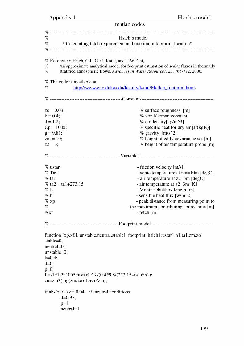
Appendix 1 Hsieh’s model matlab codes
139
% =========================================================== % Hsieh’s model % * Calculating fetch requirement and maximum footprint location* % =========================================================== % Reference: Hsieh, C-I., G. G. Katul, and T-W. Chi, % An approximate analytical model for footprint estimation of scalar fluxes in thermally % stratified atmospheric flows, Advances in Water Resources, 23, 765-772, 2000. % The code is available at % http://www.env.duke.edu/faculty/katul/Matlab_footprint.html. % --------------------------------------------Constants-------------------------------------------- zo = 0.03; % surface roughness [m] k = 0.4; % von Karman constant d = 1.2; % air density[kg/m^3] Cp = 1005; % specific heat for dry air [J/(kgK)] g = 9.81; % gravity [m/s^2] zm = 10; % height of eddy covariance set [m] z2 = 3; % height of air temperature probe [m] % -------------------------------------------Variables---------------------------------------------- % ustar - friction velocity [m/s] % TaC - sonic temperature at zm=10m [degC] % ta1 - air temperature at z2=3m [degC] % ta2 = ta1+273.15 - air temperature at z2=3m [K] % L - Monin-Obukhov length [m] % h - sensible heat flux [w/m^2] % xp - peak distance from measuring point to % the maximum contributing source area [m] %xf - fetch [m] % ------------------------------------------Footprint model--------------------------------------- function [xp,xf,L,unstable,neutral,stable]=footprint_hsieh1(ustar1,h1,ta1,zm,zo) stable=0; neutral=0; unstable=0; k=0.4; d=0; p=0; L=-1*1.2*1005*ustar1.^3./(0.4*9.8/(273.15+ta1)*h1); zu=zm*(log(zm/zo)-1.+zo/zm); if abs(zu/L) <= 0.04 % neutral conditions d=0.97; p=1; neutral=1

Appendix 1 Hsieh’s model matlab codes
140
elseif (zu/L) > 0.04 % stable conditions d=2.44; p=1.33; stable=1; else % unstable conditions d=0.28; p=0.59; unstable=1; end xf=d/(0.105*k*k)*(abs(L).^(1-p))*(zu^p); xp=d/(2.*k*k)*(abs(L).^(1.-p))*(zu^p); %===========================================================

Appendix 2.1:
Penman-Monteith equation
matlab codes
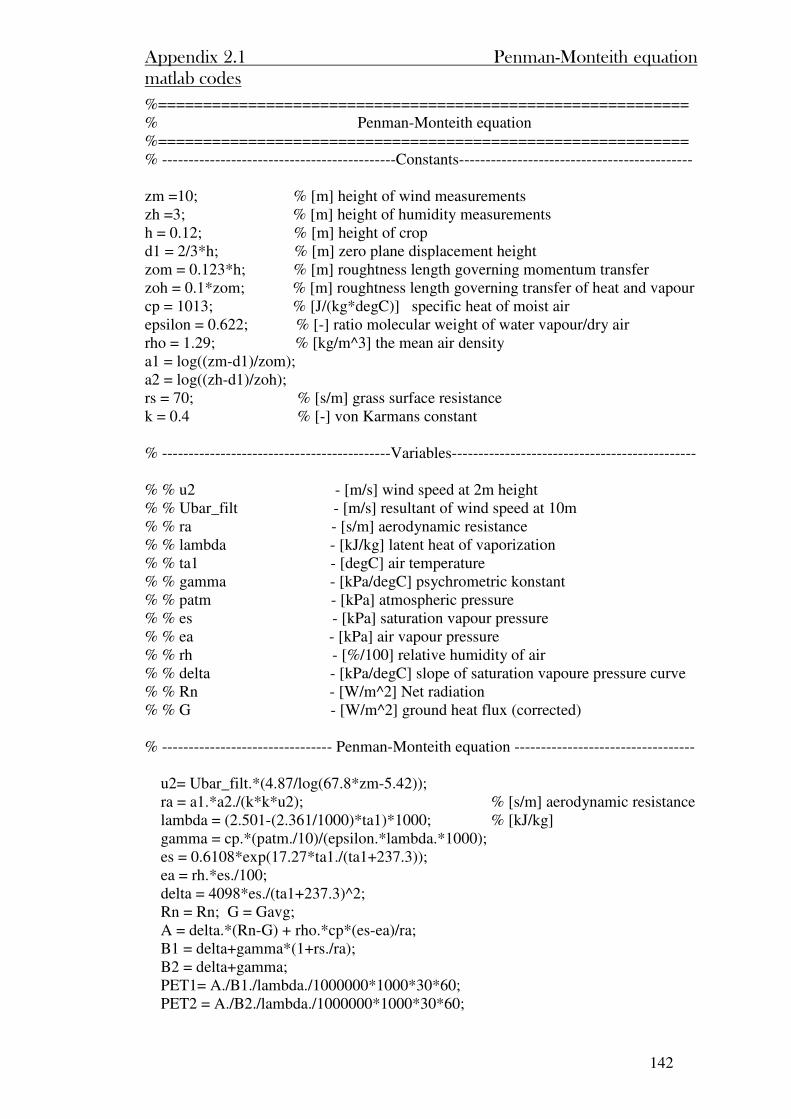
Appendix 2.1 Penman-Monteith equation matlab codes
142
%=========================================================== % Penman-Monteith equation %=========================================================== % --------------------------------------------Constants-------------------------------------------- zm =10; % [m] height of wind measurements zh =3; % [m] height of humidity measurements h = 0.12; % [m] height of crop d1 = 2/3*h; % [m] zero plane displacement height zom = 0.123*h; % [m] roughtness length governing momentum transfer zoh = 0.1*zom; % [m] roughtness length governing transfer of heat and vapour cp = 1013; % [J/(kg*degC)] specific heat of moist air epsilon = 0.622; % [-] ratio molecular weight of water vapour/dry air rho = 1.29; % [kg/m^3] the mean air density a1 = log((zm-d1)/zom); a2 = log((zh-d1)/zoh); rs = 70; % [s/m] grass surface resistance k = 0.4 % [-] von Karmans constant % -------------------------------------------Variables---------------------------------------------- % % u2 - [m/s] wind speed at 2m height % % Ubar_filt - [m/s] resultant of wind speed at 10m % % ra - [s/m] aerodynamic resistance % % lambda - [kJ/kg] latent heat of vaporization % % ta1 - [degC] air temperature % % gamma - [kPa/degC] psychrometric konstant % % patm - [kPa] atmospheric pressure % % es - [kPa] saturation vapour pressure % % ea - [kPa] air vapour pressure % % rh - [%/100] relative humidity of air % % delta - [kPa/degC] slope of saturation vapoure pressure curve % % Rn - [W/m^2] Net radiation % % G - [W/m^2] ground heat flux (corrected) % -------------------------------- Penman-Monteith equation ---------------------------------- u2= Ubar_filt.*(4.87/log(67.8*zm-5.42)); ra = a1.*a2./(k*k*u2); % [s/m] aerodynamic resistance lambda = (2.501-(2.361/1000)*ta1)*1000; % [kJ/kg] gamma = cp.*(patm./10)/(epsilon.*lambda.*1000); es = 0.6108*exp(17.27*ta1./(ta1+237.3)); ea = rh.*es./100; delta = 4098*es./(ta1+237.3)^2; Rn = Rn; G = Gavg; A = delta.*(Rn-G) + rho.*cp*(es-ea)/ra; B1 = delta+gamma*(1+rs./ra); B2 = delta+gamma; PET1= A./B1./lambda./1000000*1000*30*60; PET2 = A./B2./lambda./1000000*1000*30*60;

Appendix 2.2:
Priestley-Taylor equation
matlab codes
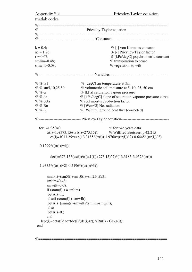
Appendix 2.2 Priestley-Taylor equation matlab codes
144
%=========================================================== % Priestley-Taylor equation %=========================================================== % --------------------------------------------Constants-------------------------------------------- k = 0.4; % [-] von Karmans constant ae = 1.26; % [-] Priestley-Taylor factor r = 0.67; % [kPa/degC] psychrometric constant smlim=0.48; % transpiration to cease smwilt=0.08; % vegetation to wilt % -------------------------------------------Variables---------------------------------------------- % % ta1 % [degC] air temperature at 3m % % sm5,10,25,50 % volumetric soil moisture at 5, 10, 25, 50 cm % % es % [kPa] saturation vapour pressure % % de % [kPa/degC] slope of saturation vapoure pressure curve % % beta % soil moisture reduction factor % % Rn % [W/m^2] Net radiation % % G % [W/m^2] ground heat flux (corrected) % -------------------------------- Priestley-Taylor equation------------------------------------- for i=1:35040 % for two years data tr(i)=1.-(373.15/(ta1(i)+273.15)); % Wilfried Brutsaert p.42;215
es(i)=1013.25*exp(13.3185*(tr(i))-1.9760*((tr(i))^2)-0.6445*((tr(i))^3)-
0.1299*((tr(i))^4));
de(i)=373.15*(es(i))/(((ta1(i))+273.15)^2)*(13.3185-3.952*(tr(i))-
1.9335*((tr(i))^2)-0.5196*((tr(i))^3));
smm(i)=(sm5(i)+sm10(i)+sm25(i))/3.; smlim=0.48; smwilt=0.08; if (smm(i) >= smlim) beta(i)=1.; elseif (smm(i) > smwilt) beta(i)=(smm(i)-smwilt)/(smlim-smwilt); else beta(i)=0.; end lept(i)=beta(i)*ae*(de(i)/(de(i)+r))*(Rn(i) - Gavg(i)); end %===========================================================
Appendix 3
Contribution of Webb correction
to CO2 flux
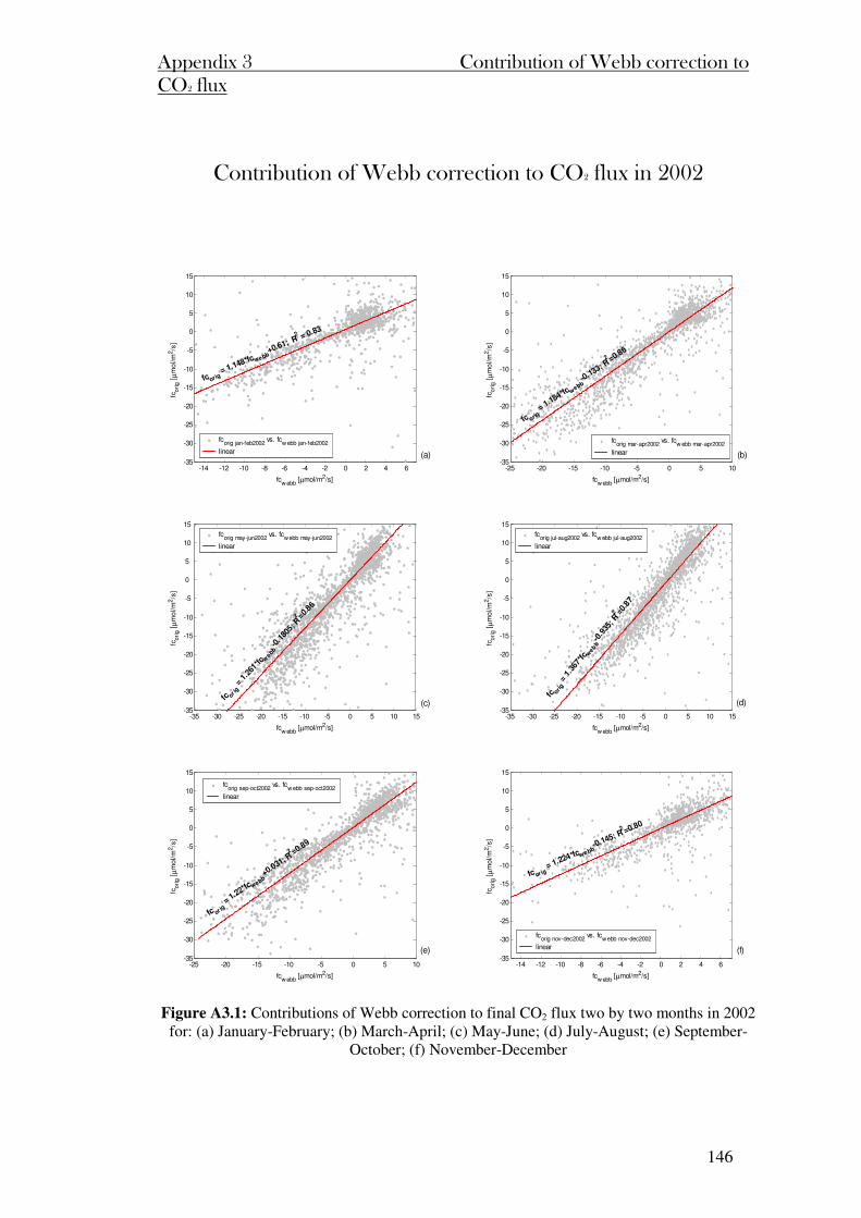
Appendix 3 Contribution of Webb correction to CO2 flux
146
Contribution of Webb correction to CO2 flux in 2002
-14 -12 -10 -8 -6 -4 -2 0 2 4 6-35
-30
-25
-20
-15
-10
-5
0
5
10
15
fcw ebb
[µmol/m2/s]
fcorig [
µm
ol/m
2/s
]
fcorig
jan-feb2002
vs. fcw ebb
jan-feb2002
linear
fcorig = 1.148*fcwebb
+0.61; R2 = 0.83
(a)
-25 -20 -15 -10 -5 0 5 10
-35
-30
-25
-20
-15
-10
-5
0
5
10
15
fcw ebb
[µmol/m2/s]
fcorig [
µm
ol/m
2/s
]
fcorig
mar-apr2002
vs. fcw ebb
mar-apr2002
linear
fc orig = 1.184*fcw
ebb-0.133; R
2 =0.86
(b)
-35 -30 -25 -20 -15 -10 -5 0 5 10 15-35
-30
-25
-20
-15
-10
-5
0
5
10
15
fcw ebb
[µmol/m2/s]
fcorig [
µm
ol/m
2/s
]
fcorig
may-jun2002
vs. fcwebb
may-jun2002
linear
fc orig =
1.2
61*fc
webb
-0.1
805;
R2 =0.
86
(c)
-35 -30 -25 -20 -15 -10 -5 0 5 10 15
-35
-30
-25
-20
-15
-10
-5
0
5
10
15
fcw ebb
[µmol/m2/s]
fcorig [
µm
ol/m
2/s
]
fcorig
jul-aug2002
vs. fcw ebb
jul-aug2002
linearfc ori
g =
1.3
67*fc w
ebb
-0.9
35; R
2 =0.8
7
(d)
-25 -20 -15 -10 -5 0 5 10-35
-30
-25
-20
-15
-10
-5
0
5
10
15
fcw ebb
[µmol/m2/s]
fcorig [
µm
ol/m
2/s
]
fcorig
sep-oct2002
vs. fcwebb
sep-oct2002
linear
fc or ig = 1.22*fcwebb
+0.031; R2 =0.89
(e)
-14 -12 -10 -8 -6 -4 -2 0 2 4 6
-35
-30
-25
-20
-15
-10
-5
0
5
10
15
fcw ebb
[µmol/m2/s]
fcorig [
µm
ol/m
2/s
]
fcorig
nov-dec2002
vs. fcwebb
nov-dec2002
linear
fcorig = 1.224*fcwebb
-0.145; R2 =0.80
(f)
Figure A3.1: Contributions of Webb correction to final CO2 flux two by two months in 2002 for: (a) January-February; (b) March-April; (c) May-June; (d) July-August; (e) September-
October; (f) November-December

Appendix 3 Contribution of Webb correction to CO2 flux
147
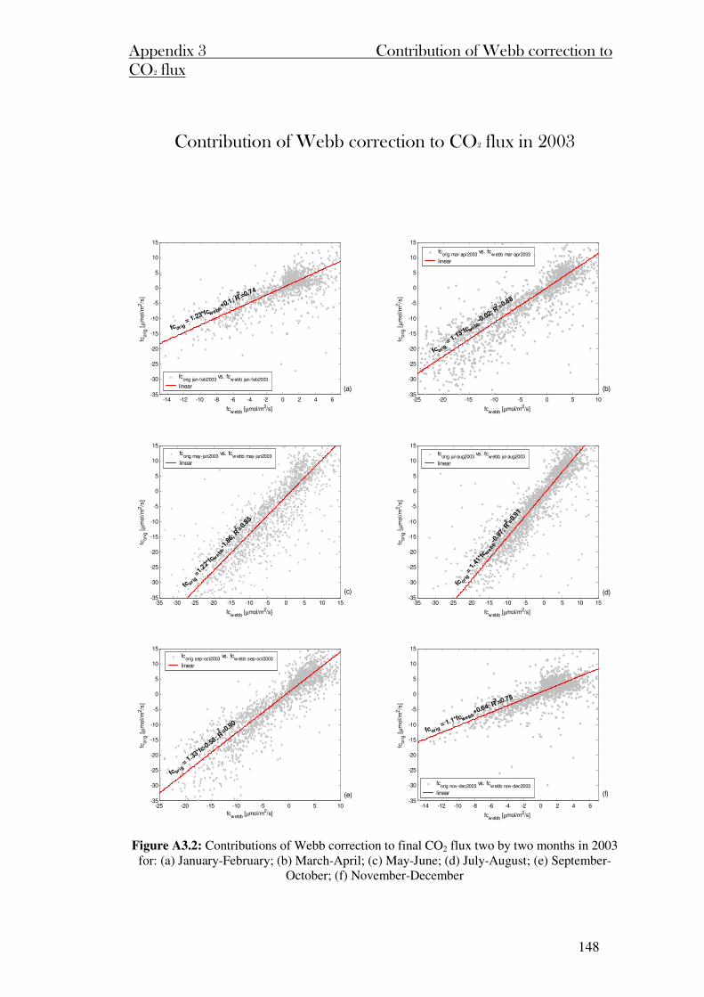
Appendix 3 Contribution of Webb correction to CO2 flux
148
Contribution of Webb correction to CO2 flux in 2003
-14 -12 -10 -8 -6 -4 -2 0 2 4 6-35
-30
-25
-20
-15
-10
-5
0
5
10
15
fcwebb
[µmol/m2/s]
fcorig [
µm
ol/m
2/s
]
fcorig
jan-feb2003
vs. fcwebb
jan-feb2003
linear
fcorig = 1.23*fcwebb
+0.1; R2 =0.74
(a)
-25 -20 -15 -10 -5 0 5 10
-35
-30
-25
-20
-15
-10
-5
0
5
10
15
fcwebb
[µmol/m2/s]
fcorig [
µm
ol/m
2/s
]
fcorig
mar-apr2003
vs. fcwebb
mar-apr2003
linear
fcorig = 1.13*fcwebb
-0.02; R2 =0.88
(b)
-35 -30 -25 -20 -15 -10 -5 0 5 10 15-35
-30
-25
-20
-15
-10
-5
0
5
10
15
fcwebb
[µmol/m2/s]
fcorig [
µm
ol/m
2/s
]
fcorig
may-jun2003
vs. fcwebb
may-jun2003
linear
fc orig =
1.22*
fcweb
b-1
.86;
R2 =0.
85
(c)
-35 -30 -25 -20 -15 -10 -5 0 5 10 15
-35
-30
-25
-20
-15
-10
-5
0
5
10
15
fcwebb
[µmol/m2/s]
fcorig [
µm
ol/m
2/s
]
fcorig
jul-aug2003
vs. fcwebb
jul-aug2003
linear
fc orig
= 1
.41*
fcwebb
-0.9
7; R
2 =0.9
1
(d)
-25 -20 -15 -10 -5 0 5 10-35
-30
-25
-20
-15
-10
-5
0
5
10
15
fcwebb
[µmol/m2/s]
fcorig [
µm
ol/m
2/s
]
fcorig
sep-oct2003
vs. fcw ebb
sep-oct2003
linear
fc orig =
1.33
*fc-0
.58; R2 =0.9
0
(e)
-14 -12 -10 -8 -6 -4 -2 0 2 4 6
-35
-30
-25
-20
-15
-10
-5
0
5
10
15
fcwebb
[µmol/m2/s]
fcorig [
µm
ol/m
2/s
]
fcorig
nov-dec2003
vs. fcwebb
nov-dec2003
linear
fcorig = 1.1*fcwebb
+0.64; R2 =0.75
(f)
Figure A3.2: Contributions of Webb correction to final CO2 flux two by two months in 2003 for: (a) January-February; (b) March-April; (c) May-June; (d) July-August; (e) September-
October; (f) November-December

Appendix 3 Contribution of Webb correction to CO2 flux
149
Appendix 4.1
Daytime fitting for 2002
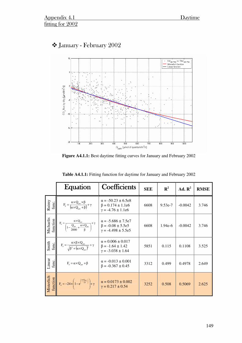
Appendix 4.1 Daytime fitting for 2002
149
January - February 2002
Figure A4.1.1: Best daytime fitting curves for January and February 2002
Table A4.1.1: Fitting function for daytime for January and February 2002
EquationEquationEquationEquation CoefficientsCoefficientsCoefficientsCoefficients SEE R
2 Ad. R
2 RMSE
Rui
my
func
.
( )γ
βQα
βQαF
par
par
d ++×
××=
α = -50.23 ± 6.5e8 β = 0.174 ± 1.1e6 γ = -4.76 ± 1.1e6
6608 9.53e-7 -0.0042 3.746
Mic
hael
is
func
tion
γ
β
Qα
2000
Q1
QαF
parpar
par
d +
×+−
×=
α = -5.686 ± 7.5e7 β = -0.08 ± 5.5e5 γ = -4.498 ± 5.5e5
6608 1.94e-6 -0.0042 3.746
Sm
ith
func
.
( )γ
Qαβ
QβαF
2
par
2
par
d +×+
××=
α = 0.006 ± 0.017 β = -1.64 ± 1.42 γ = -3.038 ± 1.64
5851 0.115 0.1108 3.525
Lin
ear
func
.
βQαF pard +×= α = -0.013 ± 0.001 β = -0.367 ± 0.45
3312 0.499 0.4978 2.649
Mis
terl
ich
func
tion
γe124F24
Qα
d
par
+
−×−=
−
× α = 0.0173 ± 0.002 γ = 0.217 ± 0.54
3252 0.508 0.5069 2.625
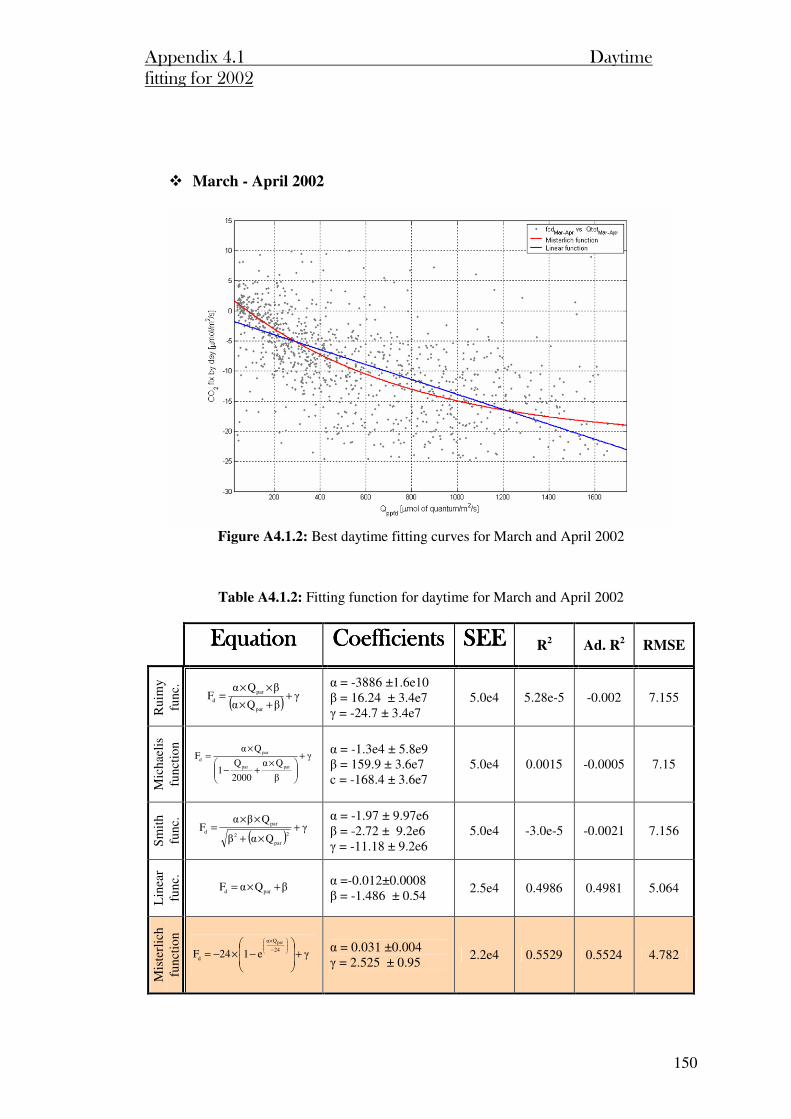
Appendix 4.1 Daytime fitting for 2002
150
March - April 2002
Figure A4.1.2: Best daytime fitting curves for March and April 2002
Table A4.1.2: Fitting function for daytime for March and April 2002
EquationEquationEquationEquation CoefficientsCoefficientsCoefficientsCoefficients SEESEESEESEE R
2 Ad. R
2 RMSE
Rui
my
func
.
( )γ
βQα
βQαF
par
par
d ++×
××=
α = -3886 ±1.6e10 β = 16.24 ± 3.4e7 γ = -24.7 ± 3.4e7
5.0e4 5.28e-5 -0.002 7.155
Mic
hael
is
func
tion
γ
β
Qα
2000
Q1
QαF
parpar
par
d +
×+−
×=
α = -1.3e4 ± 5.8e9 β = 159.9 ± 3.6e7 c = -168.4 ± 3.6e7
5.0e4 0.0015 -0.0005 7.15
Sm
ith
func
.
( )γ
Qαβ
QβαF
2
par
2
par
d +×+
××=
α = -1.97 ± 9.97e6 β = -2.72 ± 9.2e6 γ = -11.18 ± 9.2e6
5.0e4 -3.0e-5 -0.0021 7.156
Lin
ear
func
.
βQαF pard +×= α =-0.012±0.0008 β = -1.486 ± 0.54
2.5e4 0.4986 0.4981 5.064
Mis
terl
ich
func
tion
γe124F24
Qα
d
par
+
−×−=
−
× α = 0.031 ±0.004 γ = 2.525 ± 0.95
2.2e4 0.5529 0.5524 4.782
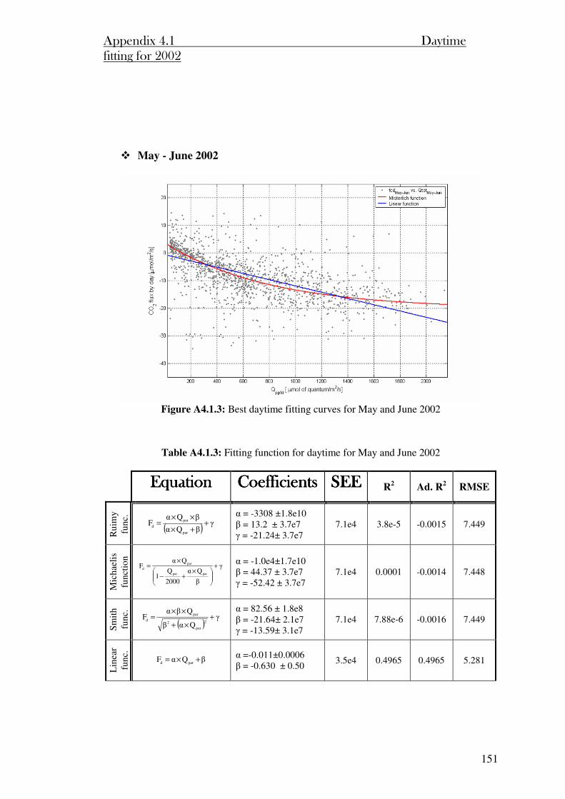
Appendix 4.1 Daytime fitting for 2002
151
May - June 2002
Figure A4.1.3: Best daytime fitting curves for May and June 2002
Table A4.1.3: Fitting function for daytime for May and June 2002
EquationEquationEquationEquation CoefficientsCoefficientsCoefficientsCoefficients SEESEESEESEE R
2 Ad. R
2 RMSE
Rui
my
func
.
( )γ
βQα
βQαF
par
par
d ++×
××=
α = -3308 ±1.8e10 β = 13.2 ± 3.7e7 γ = -21.24± 3.7e7
7.1e4 3.8e-5 -0.0015 7.449
Mic
hael
is
func
tion
γ
β
Qα
2000
Q1
QαF
parpar
par
d +
×+−
×=
α = -1.0e4±1.7e10 β = 44.37 ± 3.7e7 γ = -52.42 ± 3.7e7
7.1e4 0.0001 -0.0014 7.448
Sm
ith
func
.
( )γ
Qαβ
QβαF
2
par
2
par
d +×+
××=
α = 82.56 ± 1.8e8 β = -21.64± 2.1e7 γ = -13.59± 3.1e7
7.1e4 7.88e-6 -0.0016 7.449
Lin
ear
func
.
βQαF pard +×= α =-0.011±0.0006 β = -0.630 ± 0.50
3.5e4 0.4965 0.4965 5.281
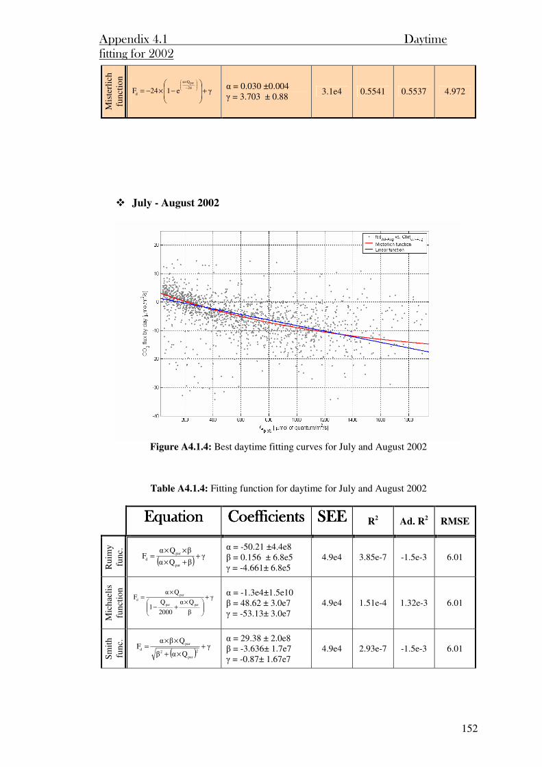
Appendix 4.1 Daytime fitting for 2002
152
Mis
terl
ich
func
tion
γe124F24
Qα
d
par
+
−×−=
−
× α = 0.030 ±0.004 γ = 3.703 ± 0.88
3.1e4 0.5541 0.5537 4.972
July - August 2002
Figure A4.1.4: Best daytime fitting curves for July and August 2002
Table A4.1.4: Fitting function for daytime for July and August 2002
EquationEquationEquationEquation CoefficientsCoefficientsCoefficientsCoefficients SEESEESEESEE R
2 Ad. R
2 RMSE
Rui
my
func
.
( )γ
βQα
βQαF
par
par
d ++×
××=
α = -50.21 ±4.4e8 β = 0.156 ± 6.8e5 γ = -4.661± 6.8e5
4.9e4 3.85e-7 -1.5e-3 6.01
Mic
hael
is
func
tion
γ
β
Qα
2000
Q1
QαF
parpar
par
d +
×+−
×=
α = -1.3e4±1.5e10 β = 48.62 ± 3.0e7 γ = -53.13± 3.0e7
4.9e4 1.51e-4 1.32e-3 6.01
Sm
ith
func
.
( )γ
Qαβ
QβαF
2
par
2
par
d +×+
××=
α = 29.38 ± 2.0e8 β = -3.636± 1.7e7 γ = -0.87± 1.67e7
4.9e4 2.93e-7 -1.5e-3 6.01
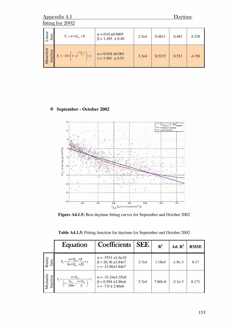
Appendix 4.1 Daytime fitting for 2002
153
Lin
ear
func
.
βQαF pard +×= α =-0.01±0.0005 β = 1.495 ± 0.40
2.5e4 0.4811 0.481 4.328
Mis
terl
ich
func
tion
γe124F
24
Qα
d
par
+
−×−=
−
× α = 0.018 ±0.001 γ = 3.501 ± 0.55
2.3e4 0.5215 0.521 4.156
September - October 2002
Figure A4.1.5: Best daytime fitting curves for September and October 2002
Table A4.1.5: Fitting function for daytime for September and October 2002
EquationEquationEquationEquation CoefficientsCoefficientsCoefficientsCoefficients SEESEESEESEE R
2 Ad. R
2 RMSE
Rui
my
func
.
( )γ
βQα
βQαF
par
par
d ++×
××=
α = -5531 ±1.6e10 β = 26.36 ±3.84e7 γ = -32.86±3.84e7
3.7e4 1.18e4 -1.9e-3 6.17
Mic
hael
is
func
tion
γ
β
Qα
2000
Q1
QαF
parpar
par
d +
×+−
×=
α = -31.24±1.55e8 β = 0.504 ±2.86e6 γ = -7.0 ± 2.86e6
3.7e4 7.60e-6 -2.1e-3 6.171
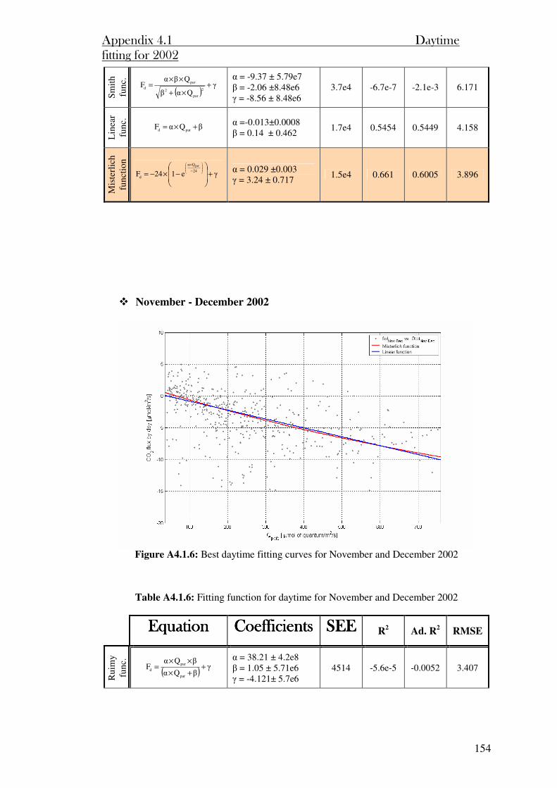
Appendix 4.1 Daytime fitting for 2002
154
Sm
ith
func
.
( )γ
Qαβ
QβαF
2
par
2
par
d +×+
××=
α = -9.37 ± 5.79e7 β = -2.06 ±8.48e6 γ = -8.56 ± 8.48e6
3.7e4 -6.7e-7 -2.1e-3 6.171
Lin
ear
func
. βQαF pard +×= α =-0.013±0.0008
β = 0.14 ± 0.462 1.7e4 0.5454 0.5449 4.158
Mis
terl
ich
func
tion
γe124F24
Qα
d
par
+
−×−=
−
× α = 0.029 ±0.003 γ = 3.24 ± 0.717
1.5e4 0.661 0.6005 3.896
November - December 2002
Figure A4.1.6: Best daytime fitting curves for November and December 2002
Table A4.1.6: Fitting function for daytime for November and December 2002
EquationEquationEquationEquation CoefficientsCoefficientsCoefficientsCoefficients SEESEESEESEE R
2 Ad. R
2 RMSE
Rui
my
func
.
( )γ
βQα
βQαF
par
par
d ++×
××=
α = 38.21 ± 4.2e8 β = 1.05 ± 5.71e6 γ = -4.121± 5.7e6
4514 -5.6e-5 -0.0052 3.407
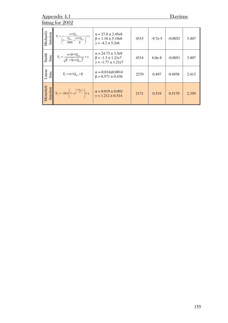
Appendix 4.1 Daytime fitting for 2002
155
Mic
hael
is
func
tion
γ
β
Qα
2000
Q1
QαF
parpar
par
d +
×+−
×=
α = 27.8 ± 2.45e8 β = 1.18 ± 5.19e6 γ = -4.2 ± 5.2e6
4515 -9.7e-5 -0.0052 3.407
Sm
ith
func
.
( )γ
Qαβ
QβαF
2
par
2
par
d +×+
××=
α = 24.73 ± 3.5e8 β = -1.3 ± 1.21e7 γ = -1.77 ± 1.21e7
4514 6.0e-8 -0.0051 3.407
Lin
ear
func
.
βQαF pard +×= α =-0.014±0.0014 β = 0.571 ± 0.436
2270 0.497 0.4958 2.413
Mis
terl
ich
func
tion
γe124F24
Qα
d
par
+
−×−=
−
× α = 0.019 ± 0.002 γ = 1.212 ± 0.514
2171 0.519 0.5179 2.359

Appendix 4.2
Daytime fitting for 2003
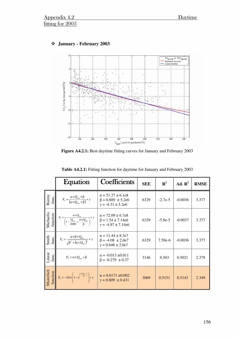
Appendix 4.2 Daytime fitting for 2003
156
January - February 2003
Figure A4.2.1: Best daytime fitting curves for January and February 2003
Table A4.2.1: Fitting function for daytime for January and February 2003
EquationEquationEquationEquation CoefficientsCoefficientsCoefficientsCoefficients SEE R
2 Ad. R
2 RMSE
Rui
my
func
.
( )γ
βQα
βQαF
par
par
d ++×
××=
α = 51.27 ± 6.1e8 β = 0.889 ± 5.2e6 γ = -4.31 ± 5.2e6
6329 -2.7e-5 -0.0036 3.377
Mic
hael
is
func
tion
γ
β
Qα
2000
Q1
QαF
parpar
par
d +
×+−
×=
α = 72.09 ± 6.7e8 β = 1.54 ± 7.14e6 γ = -4.97 ± 7.14e6
6329 -5.8e-5 -0.0037 3.377
Sm
ith
func
.
( )γ
Qαβ
QβαF
2
par
2
par
d +×+
××=
α = 11.44 ± 8.3e7 β = -4.08 ± 2.0e7 γ = 0.646 ± 2.0e7
6329 7.50e-6 -0.0036 3.377
Lin
ear
func
.
βQαF pard +×= α = -0.013 ±0.011 β = -0.279 ± 0.37
3146 0.503 0.5021 2.379
Mis
terl
ich
func
tion
γe124F24
Qα
d
par
+
−×−=
−
× α = 0.0171 ±0.002 γ = 0.809 ± 0.431
3069 0.5151 0.5143 2.349
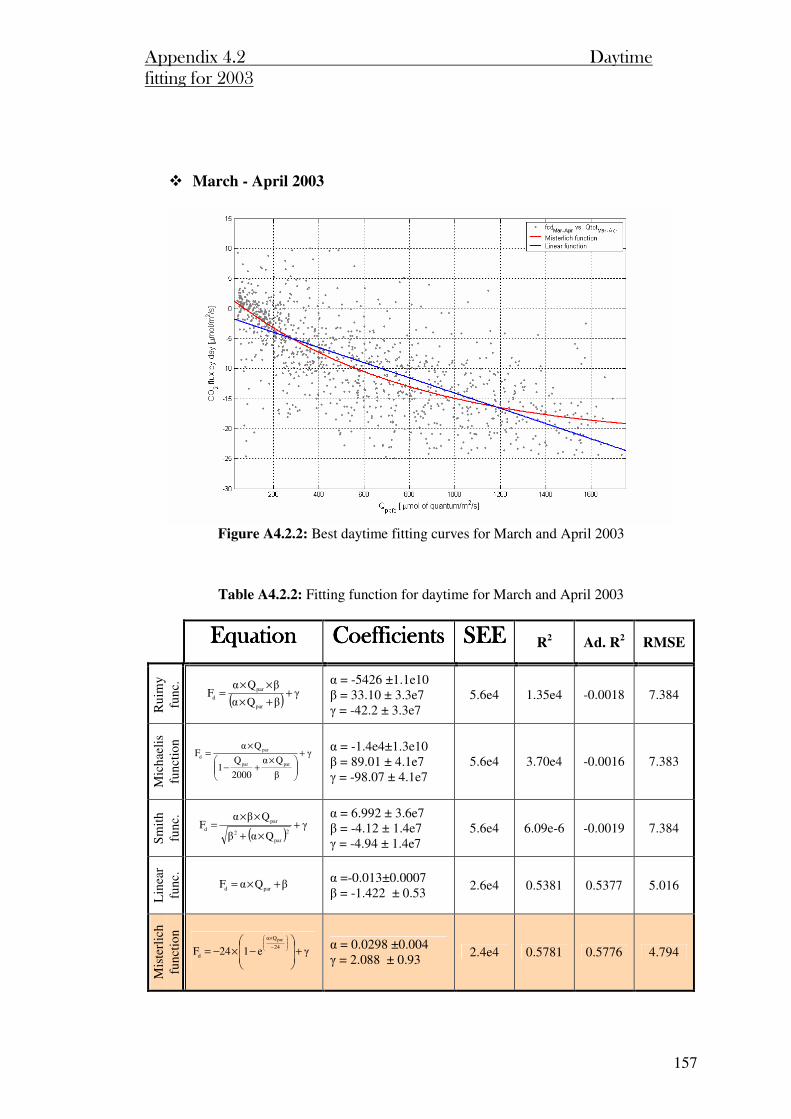
Appendix 4.2 Daytime fitting for 2003
157
March - April 2003
Figure A4.2.2: Best daytime fitting curves for March and April 2003
Table A4.2.2: Fitting function for daytime for March and April 2003
EquationEquationEquationEquation CoefficientsCoefficientsCoefficientsCoefficients SEESEESEESEE R
2 Ad. R
2 RMSE
Rui
my
func
.
( )γ
βQα
βQαF
par
par
d ++×
××=
α = -5426 ±1.1e10 β = 33.10 ± 3.3e7 γ = -42.2 ± 3.3e7
5.6e4 1.35e4 -0.0018 7.384
Mic
hael
is
func
tion
γ
β
Qα
2000
Q1
QαF
parpar
par
d +
×+−
×=
α = -1.4e4±1.3e10 β = 89.01 ± 4.1e7 γ = -98.07 ± 4.1e7
5.6e4 3.70e4 -0.0016 7.383
Sm
ith
func
.
( )γ
Qαβ
QβαF
2
par
2
par
d +×+
××=
α = 6.992 ± 3.6e7 β = -4.12 ± 1.4e7 γ = -4.94 ± 1.4e7
5.6e4 6.09e-6 -0.0019 7.384
Lin
ear
func
.
βQαF pard +×= α =-0.013±0.0007 β = -1.422 ± 0.53
2.6e4 0.5381 0.5377 5.016
Mis
terl
ich
func
tion
γe124F24
Qα
d
par
+
−×−=
−
× α = 0.0298 ±0.004 γ = 2.088 ± 0.93
2.4e4 0.5781 0.5776 4.794
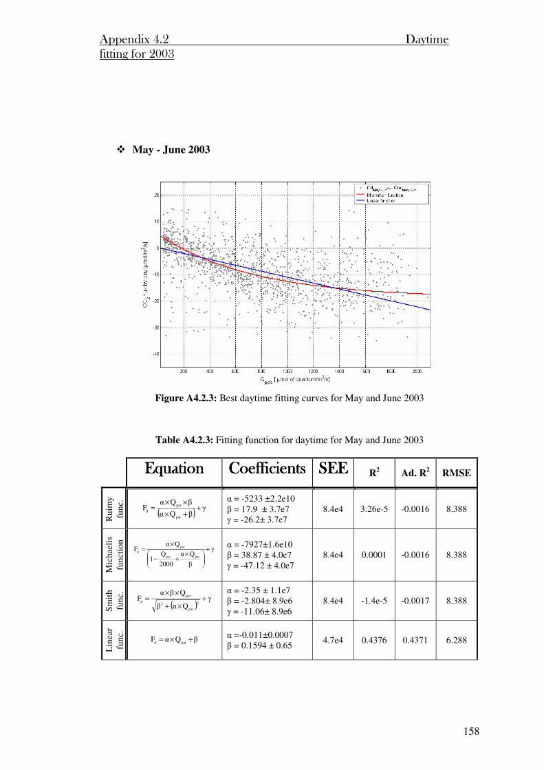
Appendix 4.2 Daytime fitting for 2003
158
May - June 2003
Figure A4.2.3: Best daytime fitting curves for May and June 2003
Table A4.2.3: Fitting function for daytime for May and June 2003
EquationEquationEquationEquation CoefficientsCoefficientsCoefficientsCoefficients SEESEESEESEE R
2 Ad. R
2 RMSE
Rui
my
func
.
( )γ
βQα
βQαF
par
par
d ++×
××=
α = -5233 ±2.2e10 β = 17.9 ± 3.7e7 γ = -26.2± 3.7e7
8.4e4 3.26e-5 -0.0016 8.388
Mic
hael
is
func
tion
γ
β
Qα
2000
Q1
QαF
parpar
par
d +
×+−
×=
α = -7927±1.6e10 β = 38.87 ± 4.0e7 γ = -47.12 ± 4.0e7
8.4e4 0.0001 -0.0016 8.388
Sm
ith
func
.
( )γ
Qαβ
QβαF
2
par
2
par
d +×+
××=
α = -2.35 ± 1.1e7 β = -2.804± 8.9e6 γ = -11.06± 8.9e6
8.4e4 -1.4e-5 -0.0017 8.388
Lin
ear
func
.
βQαF pard +×= α =-0.011±0.0007 β = 0.1594 ± 0.65
4.7e4 0.4376 0.4371 6.288
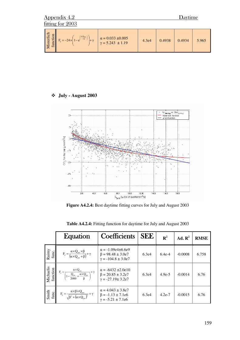
Appendix 4.2 Daytime fitting for 2003
159
Mis
terl
ich
func
tion
γe124F24
Qα
d
par
+
−×−=
−
× α = 0.033 ±0.005 γ = 5.243 ± 1.19
4.3e4 0.4938 0.4934 5.965
July - August 2003
Figure A4.2.4: Best daytime fitting curves for July and August 2003
Table A4.2.4: Fitting function for daytime for July and August 2003
EquationEquationEquationEquation CoefficientsCoefficientsCoefficientsCoefficients SEESEESEESEE R
2 Ad. R
2 RMSE
Rui
my
func
.
( )γ
βQα
βQαF
par
par
d ++×
××=
α = -1.09e4±6.6e9 β = 98.48 ± 3.0e7 γ = -104.8 ± 3.0e7
6.3e4 6.4e-4 -0.0008 6.758
Mic
hael
is
func
tion
γ
β
Qα
2000
Q1
QαF
parpar
par
d +
×+−
×=
α = -6432 ±2.0e10 β = 20.85 ± 3.2e7 γ = -27.19± 3.2e7
6.3e4 4.9e-5 -0.0014 6.76
Sm
ith
func
.
( )γ
Qαβ
QβαF
2
par
2
par
d +×+
××=
α = 4.043 ± 3.8e7 β = -1.13 ± 7.1e6 γ = -5.21 ± 7.1e6
6.3e4 4.2e-7 -0.0015 6.76
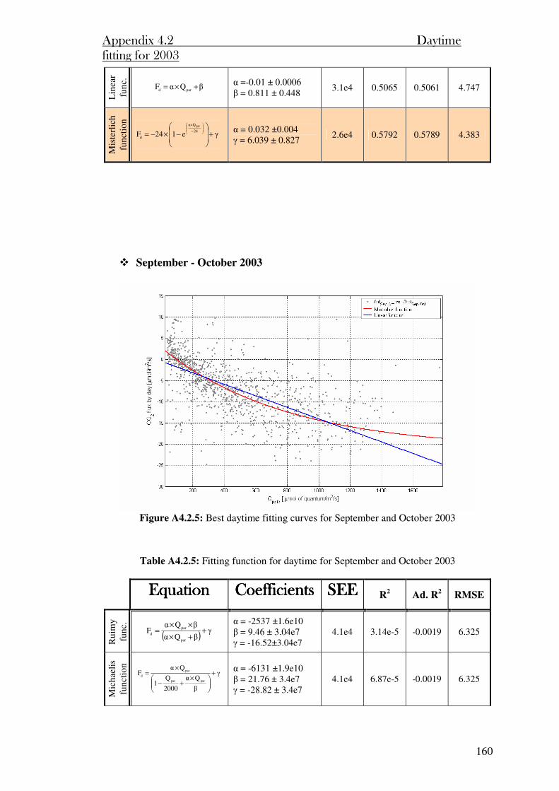
Appendix 4.2 Daytime fitting for 2003
160
Lin
ear
func
.
βQαF pard +×= α =-0.01 ± 0.0006 β = 0.811 ± 0.448
3.1e4 0.5065 0.5061 4.747
Mis
terl
ich
func
tion
γe124F
24
Qα
d
par
+
−×−=
−
× α = 0.032 ±0.004 γ = 6.039 ± 0.827
2.6e4 0.5792 0.5789 4.383
September - October 2003
Figure A4.2.5: Best daytime fitting curves for September and October 2003
Table A4.2.5: Fitting function for daytime for September and October 2003
EquationEquationEquationEquation CoefficientsCoefficientsCoefficientsCoefficients SEESEESEESEE R
2 Ad. R
2 RMSE
Rui
my
func
.
( )γ
βQα
βQαF
par
par
d ++×
××=
α = -2537 ±1.6e10 β = 9.46 ± 3.04e7 γ = -16.52±3.04e7
4.1e4 3.14e-5 -0.0019 6.325
Mic
hael
is
func
tion
γ
β
Qα
2000
Q1
QαF
parpar
par
d +
×+−
×=
α = -6131 ±1.9e10 β = 21.76 ± 3.4e7 γ = -28.82 ± 3.4e7
4.1e4 6.87e-5 -0.0019 6.325

Appendix 4.2 Daytime fitting for 2003
161
Sm
ith
func
.
( )γ
Qαβ
QβαF
2
par
2
par
d +×+
××=
α =-1.6e-3±6.5e-3 β =0.761 ± 1.493 γ = -6.29 ± 1.561
3.9e4 0.0440 0.0422 6.185
Lin
ear
func
. βQαF pard +×= α =-0.014±0.0008
β = -0.458 ± 0.45 1.9e4 0.5397 0.5393 4.289
Mis
terl
ich
func
tion
γe124F24
Qα
d
par
+
−×−=
−
× α = 0.030 ±0.003 γ = 2.788 ± 0.736
1.7e4 0.5938 0.5934 4.029
November - December 2003
Figure A4.2.6: Best daytime fitting curves for November and December 2003
Table A4.2.6: Fitting function for daytime for November and December 2003
EquationEquationEquationEquation CoefficientsCoefficientsCoefficientsCoefficients SEE R
2 Ad. R
2 RMSE
Rui
my
func
.
( )γ
βQα
βQαF
par
par
d ++×
××=
α = 33.27 ± 1.8e8 β = 1.34 ± 3.63e6 γ = -4.04± 3.63e6
4729 -1.3e-4 -0.0038 2.935

Appendix 4.2 Daytime fitting for 2003
162
Mic
hael
is
func
tion
γ
β
Qα
2000
Q1
QαF
parpar
par
d +
×+−
×=
α = 27.86 ± 8.9e7 β = 1.52 ± 2.43e6 γ = -4.22 ± 2.43e6
4730 -2.1e-4 -0.0039 2.935
Sm
ith
func
.
( )γ
Qαβ
QβαF
2
par
2
par
d +×+
××=
α = 9.59 ± 7.72e7 β = -1.46 ± 7.8e6 γ = -1.24 ± 7.8e6
4729 7.43e-7 -0.0036 2.935
Lin
ear
func
.
βQαF pard +×= α =-0.012±0.0012 β = 0.230 ± 0.298
2344 0.5043 0.5034 2.064
Mis
terl
ich
func
tion
γe124F24
Qα
d
par
+
−×−=
−
× α = 0.015 ± 0.002 γ = 0.544 ± 0.334
2298 0.514 0.5131 2.044
Appendix 5
Parameters for CO2 flux modelling
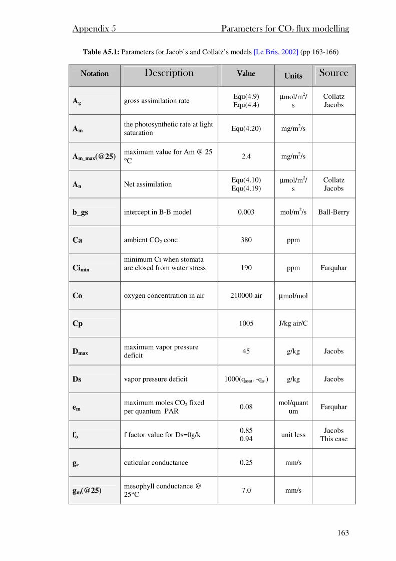
Appendix 5 Parameters for CO2 flux modelling
163
Table A5.1: Parameters for Jacob’s and Collatz’s models [Le Bris, 2002] (pp 163-166)
NotationNotationNotationNotation Description ValueValueValueValue Units Source
Ag gross assimilation rate Equ(4.9) Equ(4.4)
µmol/m2/s
Collatz Jacobs
Am the photosynthetic rate at light saturation
Equ(4.20) mg/m2/s
Am_max(@25) maximum value for Am @ 25 °C
2.4 mg/m2/s
An Net assimilation Equ(4.10) Equ(4.19)
µmol/m2/s
Collatz Jacobs
b_gs intercept in B-B model 0.003 mol/m2/s Ball-Berry
Ca ambient CO2 conc 380 ppm
Cimin minimum Ci when stomata are closed from water stress
190 ppm Farquhar
Co oxygen concentration in air 210000 air µmol/mol
Cp 1005 J/kg air/C
Dmax maximum vapor pressure deficit
45 g/kg Jacobs
Ds vapor pressure deficit 1000(qasat. -qa.) g/kg Jacobs
em maximum moles CO2 fixed per quantum PAR
0.08 mol/quant
um Farquhar
fo f factor value for Ds=0g/k 0.85 0.94
unit less Jacobs
This case
gc cuticular conductance 0.25 mm/s
gm(@25) mesophyll conductance @ 25°C
7.0 mm/s
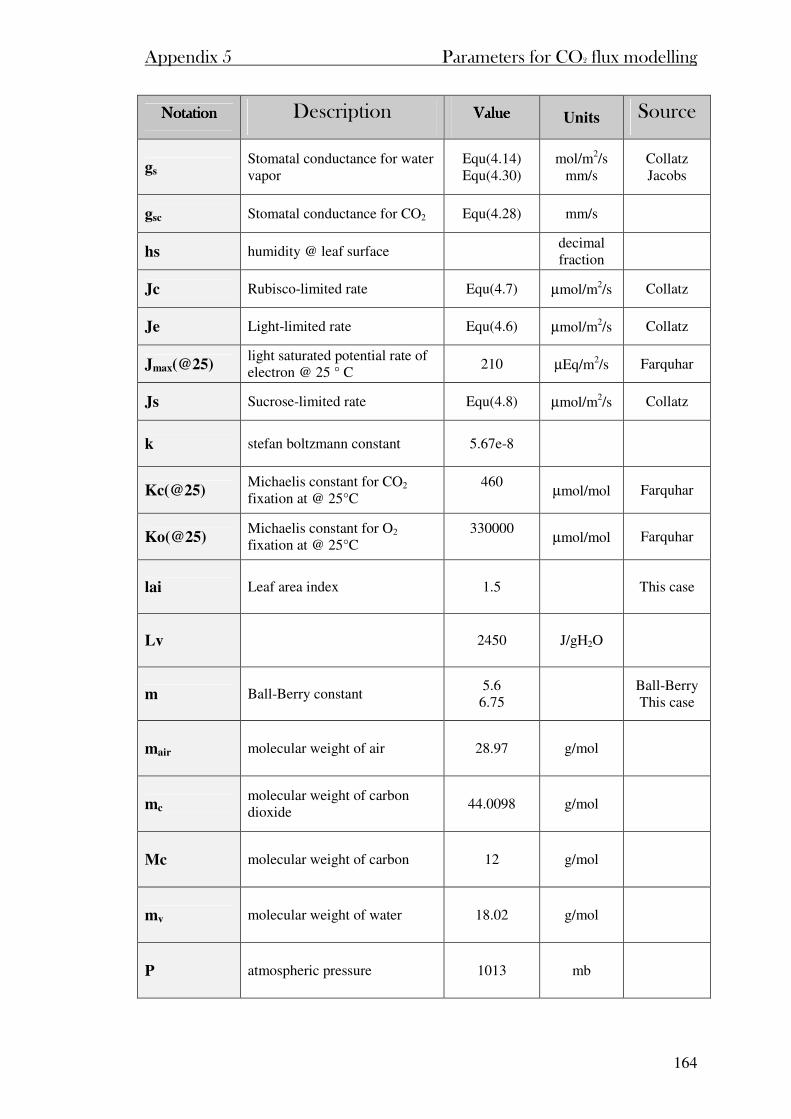
Appendix 5 Parameters for CO2 flux modelling
164
NotationNotationNotationNotation Description ValueValueValueValue Units Source
gs Stomatal conductance for water vapor
Equ(4.14) Equ(4.30)
mol/m2/s mm/s
Collatz Jacobs
gsc Stomatal conductance for CO2 Equ(4.28) mm/s
hs humidity @ leaf surface decimal fraction
Jc Rubisco-limited rate Equ(4.7) µmol/m2/s Collatz
Je Light-limited rate Equ(4.6) µmol/m2/s Collatz
Jmax(@25) light saturated potential rate of electron @ 25 ° C
210 µEq/m2/s Farquhar
Js Sucrose-limited rate Equ(4.8) µmol/m2/s Collatz
k stefan boltzmann constant 5.67e-8
Kc(@25) Michaelis constant for CO2 fixation at @ 25°C
460
µmol/mol Farquhar
Ko(@25) Michaelis constant for O2 fixation at @ 25°C
330000 µmol/mol Farquhar
lai Leaf area index 1.5 This case
Lv 2450 J/gH2O
m Ball-Berry constant 5.6
6.75
Ball-Berry This case
mair molecular weight of air 28.97 g/mol
mc molecular weight of carbon dioxide
44.0098 g/mol
Mc molecular weight of carbon 12 g/mol
mv molecular weight of water 18.02 g/mol
P atmospheric pressure 1013 mb
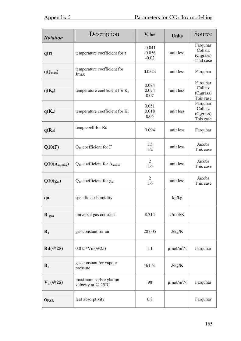
Appendix 5 Parameters for CO2 flux modelling
165
Notation Description ValueValueValueValue Units Source
q(ττττ) temperature coefficient for τ -0.041 -0.056 -0.02
unit less
Farquhar Collatz
(C4grass) Thid case
q(Jmax) temperature coefficient for Jmax
0.0524 unit less Farquhar
q(Kc) temperature coefficient for Kc 0.084 0.074 0.07
unit less
Farquhar Collatz
(C4grass) This case
q(Ko) temperature coefficient for Ko 0.051 0.018 0.05
unit less
Farquhar Collatz
(C4grass) This case
q(Rd) temp coeff for Rd
0.094 unit less Farquhar
Q10(ΓΓΓΓ) Q10 coefficient for Γ 1.5 1.2
unit less Jacobs
This case
Q10(Am,max) Q10 coefficient for Am,max 2
1.6 unit less
Jacobs This case
Q10(gm) Q10 coefficient for gm 2
1.6 unit less
Jacobs This case
qa specific air humidity kg/kg
R_gas universal gas constant 8.314 J/mol/K
Ra gas constant for air 287.05 J/kg/K
Rd(@25) 0.015*Vm(@25) 1.1 µmol/m2/s Farquhar
Rv gas constant for vapour pressure
461.51 J/kg/K
Vm(@25) maximum carboxylation velocity at @ 25°C
98 µmol/m2/s Farquhar
ααααPAR leaf absorptivity 0.8 Farquhar
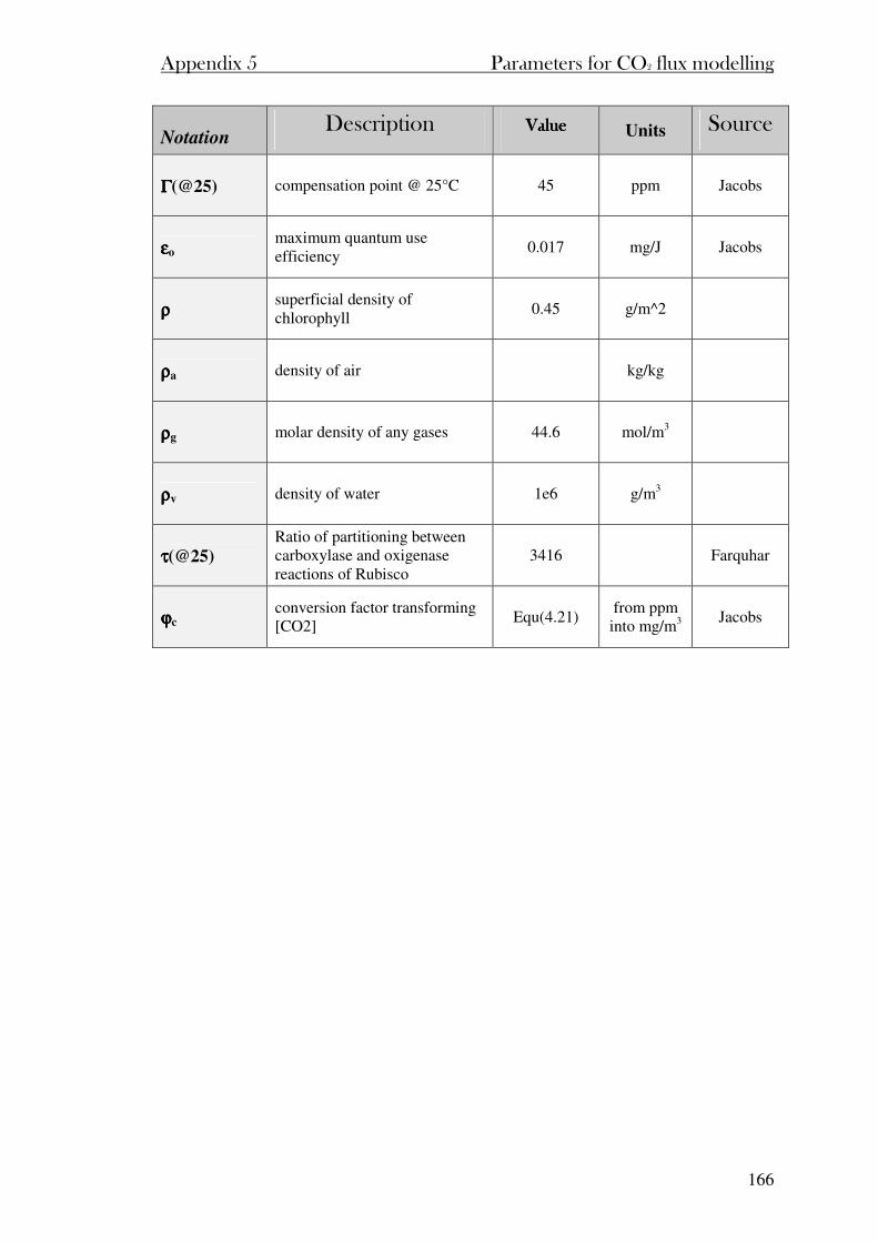
Appendix 5 Parameters for CO2 flux modelling
166
Notation Description ValueValueValueValue Units Source
ΓΓΓΓ(@25) compensation point @ 25°C 45 ppm Jacobs
εεεεo maximum quantum use efficiency
0.017 mg/J Jacobs
ρρρρ superficial density of chlorophyll
0.45 g/m^2
ρρρρa density of air kg/kg
ρρρρg molar density of any gases 44.6 mol/m3
ρρρρv density of water 1e6 g/m3
ττττ(@25) Ratio of partitioning between carboxylase and oxigenase reactions of Rubisco
3416 Farquhar
ϕϕϕϕc conversion factor transforming [CO2]
Equ(4.21) from ppm
into mg/m3 Jacobs

Chapter 7 Conclusion
Appendix 6
Wexford grassland
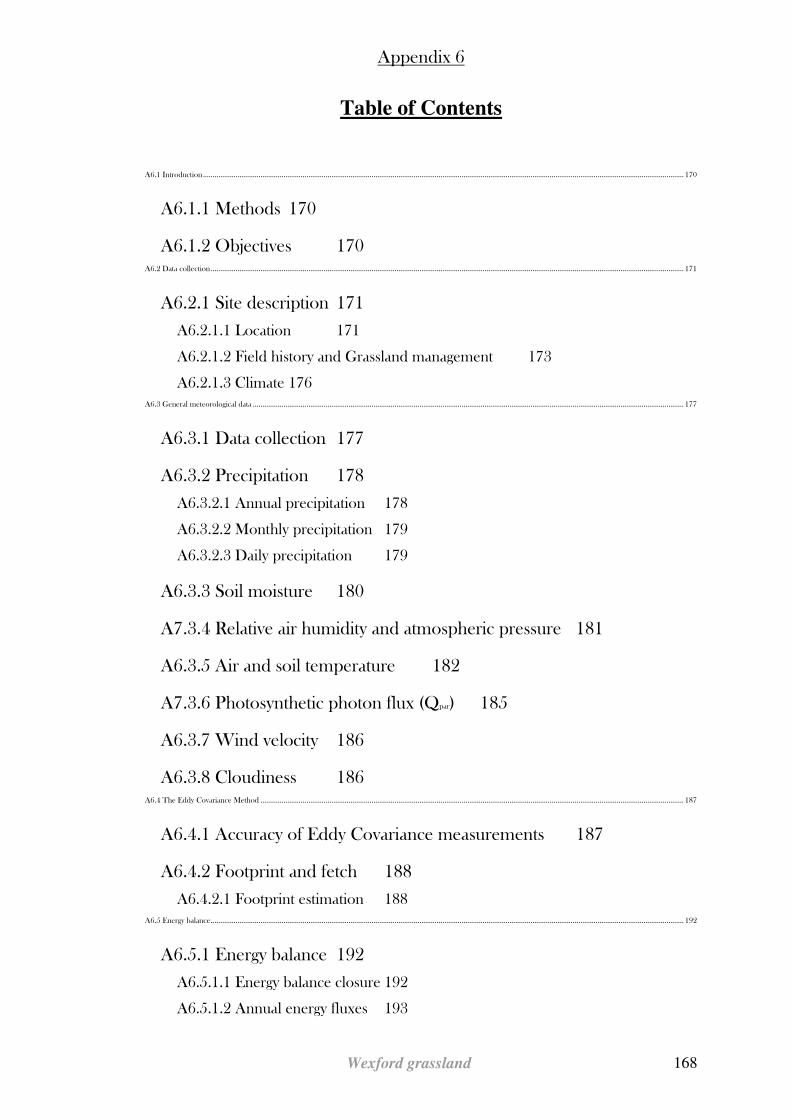
Appendix 6
Wexford grassland 168
Table of Contents
A6.1 Introduction........................................................................................................................................................................................................................................................... 170
A6.1.1 Methods 170
A6.1.2 Objectives 170 A6.2 Data collection....................................................................................................................................................................................................................................................... 171
A6.2.1 Site description 171
A6.2.1.1 Location 171
A6.2.1.2 Field history and Grassland management 173
A6.2.1.3 Climate 176 A6.3 General meteorological data ................................................................................................................................................................................................................................. 177
A6.3.1 Data collection 177
A6.3.2 Precipitation 178
A6.3.2.1 Annual precipitation 178
A6.3.2.2 Monthly precipitation 179
A6.3.2.3 Daily precipitation 179
A6.3.3 Soil moisture 180
A7.3.4 Relative air humidity and atmospheric pressure 181
A6.3.5 Air and soil temperature 182
A7.3.6 Photosynthetic photon flux (Qpar) 185
A6.3.7 Wind velocity 186
A6.3.8 Cloudiness 186 A6.4 The Eddy Covariance Method ............................................................................................................................................................................................................................. 187
A6.4.1 Accuracy of Eddy Covariance measurements 187
A6.4.2 Footprint and fetch 188
A6.4.2.1 Footprint estimation 188 A6.5 Energy balance....................................................................................................................................................................................................................................................... 192
A6.5.1 Energy balance 192
A6.5.1.1 Energy balance closure 192
A6.5.1.2 Annual energy fluxes 193
Appendix 6
Wexford grassland 169
A6.5.1.3 Monthly energy fluxes 194
A6.5.1.4 Daily energy fluxes 195
A6.5.1.5 Bowen ratio 196
A6.5.2 Evapotranspiration 197
A6.5.2.1 Annual evapotranspiration 197
A6.5.2.2 Monthly evapotranspiration 198
A6.5.2.3 Measured and modelled evapotranspiration 199 A6.6 Carbon dioxide flux............................................................................................................................................................................................................................................... 201
A6.6.1 Data analysis 201
A6.6.1.1 Precipitation filter 201
A6.6.1.2 Momentum flux filter 201
A6.6.1.3 CO2 filter for nighttime 202
A6.6.1.4 CO2 filter for daytime 203
A6.6.1.5 Quality of data 203
A6.6.1.6 Contribution of Webb correction 205
A6.6.2 Gap filling 208
A6.6.2.1 Nighttime gap filling 208
A6.6.2.2 Daytime gap filling 209
A6.6.3 Results and discussion 209
A6.6.3.1 Daily flux 209
A6.6.3.2 Monthly flux 210
A6.6.3.3 Annual flux 215
A6.6.3.4 Carbon balance 216 A6. References................................................................................................................................................................................................................................................................ 217
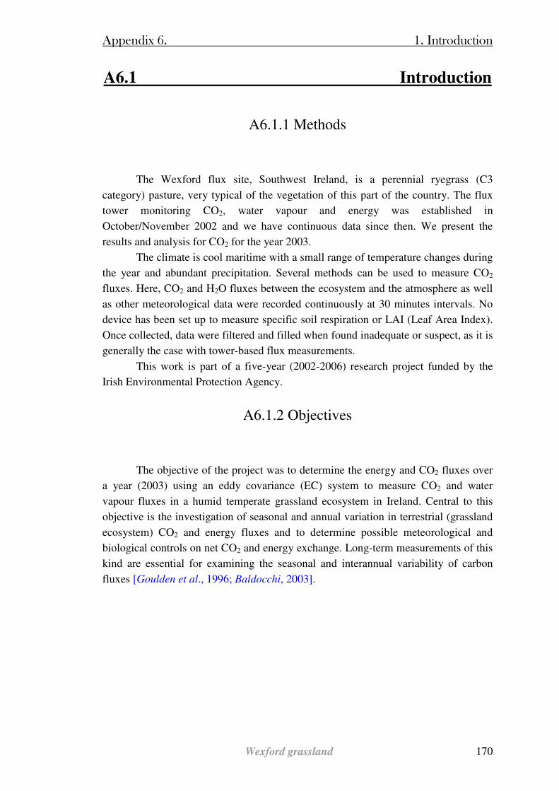
Appendix 6. 1. Introduction
Wexford grassland 170
A6.1 Introduction
A6.1.1 Methods
The Wexford flux site, Southwest Ireland, is a perennial ryegrass (C3
category) pasture, very typical of the vegetation of this part of the country. The flux
tower monitoring CO2, water vapour and energy was established in
October/November 2002 and we have continuous data since then. We present the
results and analysis for CO2 for the year 2003.
The climate is cool maritime with a small range of temperature changes during
the year and abundant precipitation. Several methods can be used to measure CO2
fluxes. Here, CO2 and H2O fluxes between the ecosystem and the atmosphere as well
as other meteorological data were recorded continuously at 30 minutes intervals. No
device has been set up to measure specific soil respiration or LAI (Leaf Area Index).
Once collected, data were filtered and filled when found inadequate or suspect, as it is
generally the case with tower-based flux measurements.
This work is part of a five-year (2002-2006) research project funded by the
Irish Environmental Protection Agency.
A6.1.2 Objectives
The objective of the project was to determine the energy and CO2 fluxes over
a year (2003) using an eddy covariance (EC) system to measure CO2 and water
vapour fluxes in a humid temperate grassland ecosystem in Ireland. Central to this
objective is the investigation of seasonal and annual variation in terrestrial (grassland
ecosystem) CO2 and energy fluxes and to determine possible meteorological and
biological controls on net CO2 and energy exchange. Long-term measurements of this
kind are essential for examining the seasonal and interannual variability of carbon
fluxes [Goulden et al., 1996; Baldocchi, 2003].

Appendix 6. 2. Data collection
Wexford grassland 171
A6.2A6.2A6.2A6.2 Data collection Data collection Data collection Data collection
A6.2.1 Site description
A6.2.1.1 Location
The Wexford experimental grassland is located at Johnstown Castle near the
town of Wexford, in South East Ireland, (52º 30’ North latitude, 6º 40’ West
longitude), see Figure A6.2.1.
Figure A6.2.1: Location of the site area
The site location is within the National Agriculture Research Station lands
(Co-ordinates of CO2 tower: 117289.525 N; 302396.928 E). The Wexford grassland is situated at an elevation about 50 m above sea level
(see Figure A6.2.2 (a)). Soils at Johnstown Castle estate are shown in figure A6.2.2
(b). The types of soils within footprint (see section A6.4.2.1) are A1 (brown earth),
A2 (gley), C1 (brown earth), and C2 (gley).
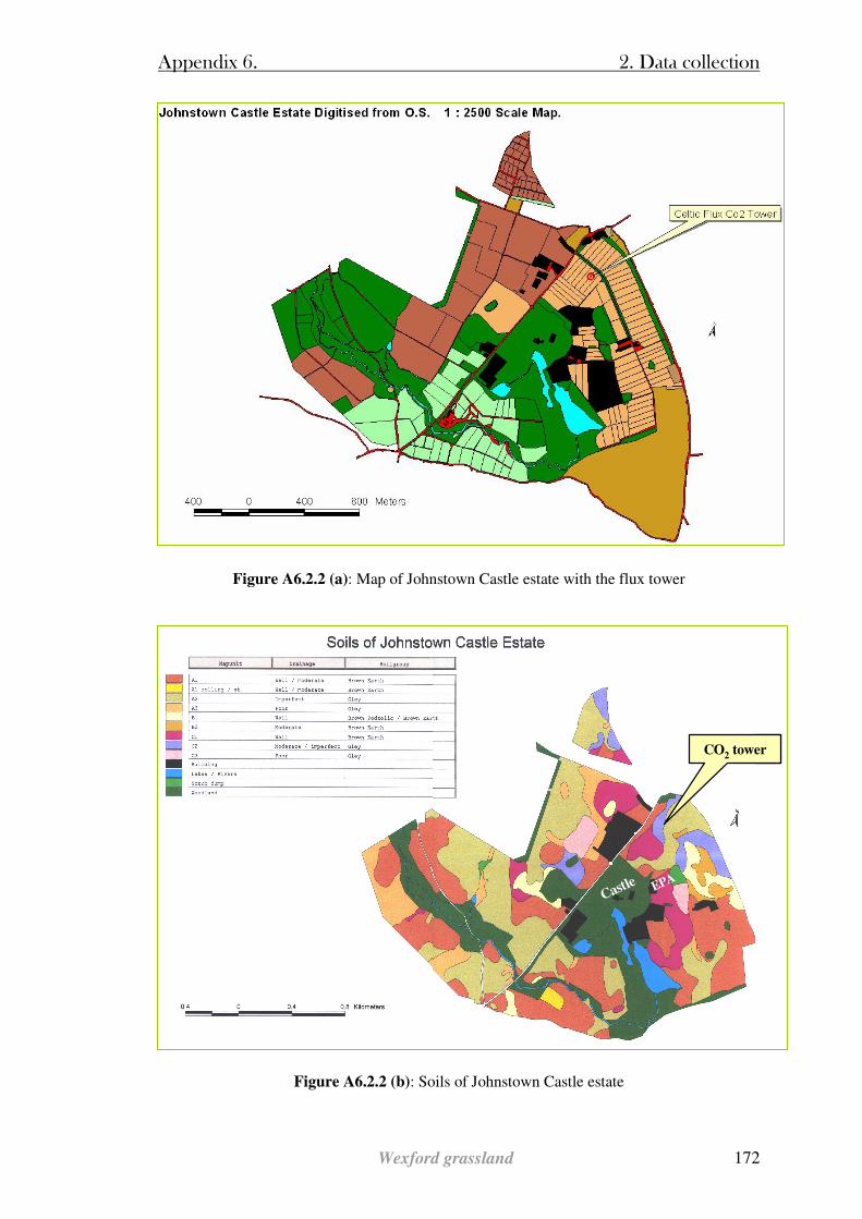
Appendix 6. 2. Data collection
Wexford grassland 172
Figure A6.2.2 (a): Map of Johnstown Castle estate with the flux tower
Figure A6.2.2 (b): Soils of Johnstown Castle estate
Castle EPA
CO2 tower
Castle EPA
CO2 tower
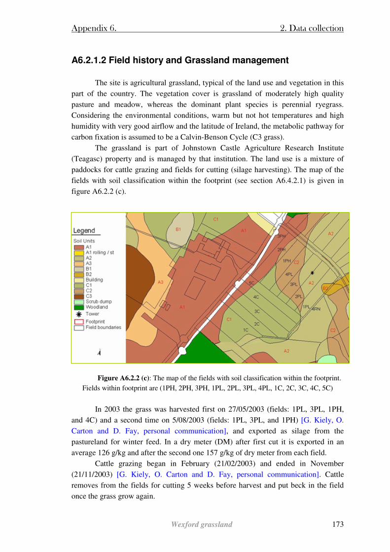
Appendix 6. 2. Data collection
Wexford grassland 173
A6.2.1.2 Field history and Grassland management
The site is agricultural grassland, typical of the land use and vegetation in this
part of the country. The vegetation cover is grassland of moderately high quality
pasture and meadow, whereas the dominant plant species is perennial ryegrass.
Considering the environmental conditions, warm but not hot temperatures and high
humidity with very good airflow and the latitude of Ireland, the metabolic pathway for
carbon fixation is assumed to be a Calvin-Benson Cycle (C3 grass).
The grassland is part of Johnstown Castle Agriculture Research Institute
(Teagasc) property and is managed by that institution. The land use is a mixture of
paddocks for cattle grazing and fields for cutting (silage harvesting). The map of the
fields with soil classification within the footprint (see section A6.4.2.1) is given in
figure A6.2.2 (c).
Figure A6.2.2 (c): The map of the fields with soil classification within the footprint.
Fields within footprint are (1PH, 2PH, 3PH, 1PL, 2PL, 3PL, 4PL, 1C, 2C, 3C, 4C, 5C)
In 2003 the grass was harvested first on 27/05/2003 (fields: 1PL, 3PL, 1PH,
and 4C) and a second time on 5/08/2003 (fields: 1PL, 3PL, and 1PH) [G. Kiely, O.
Carton and D. Fay, personal communication], and exported as silage from the
pastureland for winter feed. In a dry meter (DM) after first cut it is exported in an
average 126 g/kg and after the second one 157 g/kg of dry meter from each field.
Cattle grazing began in February (21/02/2003) and ended in November
(21/11/2003) [G. Kiely, O. Carton and D. Fay, personal communication]. Cattle
removes from the fields for cutting 5 weeks before harvest and put beck in the field
once the grass grow again.
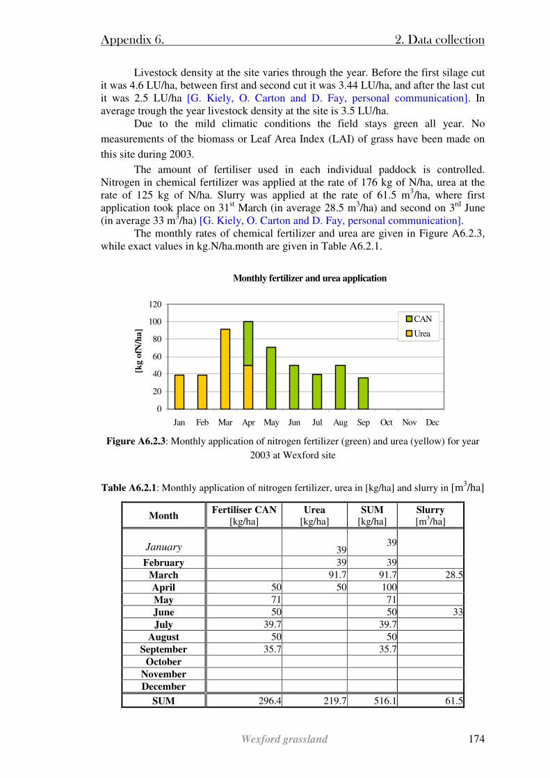
Appendix 6. 2. Data collection
Wexford grassland 174
Livestock density at the site varies through the year. Before the first silage cut it was 4.6 LU/ha, between first and second cut it was 3.44 LU/ha, and after the last cut it was 2.5 LU/ha [G. Kiely, O. Carton and D. Fay, personal communication]. In average trough the year livestock density at the site is 3.5 LU/ha.
Due to the mild climatic conditions the field stays green all year. No
measurements of the biomass or Leaf Area Index (LAI) of grass have been made on
this site during 2003.
The amount of fertiliser used in each individual paddock is controlled. Nitrogen in chemical fertilizer was applied at the rate of 176 kg of N/ha, urea at the rate of 125 kg of N/ha. Slurry was applied at the rate of 61.5 m3/ha, where first application took place on 31st March (in average 28.5 m3/ha) and second on 3rd June (in average 33 m3/ha) [G. Kiely, O. Carton and D. Fay, personal communication].
The monthly rates of chemical fertilizer and urea are given in Figure A6.2.3, while exact values in kg.N/ha.month are given in Table A6.2.1.
Monthly fertilizer and urea application
0
20
40
60
80
100
120
Jan Feb Mar Apr May Jun Jul Aug Sep Oct Nov Dec
[kg
ofN
/ha
]
CAN
Urea
Figure A6.2.3: Monthly application of nitrogen fertilizer (green) and urea (yellow) for year
2003 at Wexford site
Table A6.2.1: Monthly application of nitrogen fertilizer, urea in [kg/ha] and slurry in [m3/ha]
Month Fertiliser CAN
[kg/ha] Urea
[kg/ha] SUM
[kg/ha] Slurry [m3/ha]
January 39 39
February 39 39March 91.7 91.7 28.5April 50 50 100May 71 71June 50 50 33July 39.7 39.7
August 50 50September 35.7 35.7
October November December
SUM 296.4 219.7 516.1 61.5

Appendix 6. 2. Data collection
Wexford grassland 175

Appendix 6. 2. Data collection
Wexford grassland 176
A6.2.1.3 Climate
The climate is temperate and humid (from the influence of warm Gulf Stream in
the North East Atlantic Ocean) with mean annual precipitation in the Wexford region
of about 1002 mm [Ryan, 1998]. The rainfall regime is characterized by long duration
events of low intensity (values up to 5 mm/day). Short duration events of high
intensity are more seldom and occur in summer.
Daily air temperatures have a very small range of variation during the year, going
from a maximum of 24ºC to a minimum of -2ºC, with an average of 15ºC in summer
and 6ºC in winter. The mean wind velocity is 4 m/s at the site with peaks up to 13
m/s. The main wind comes from the southwest.
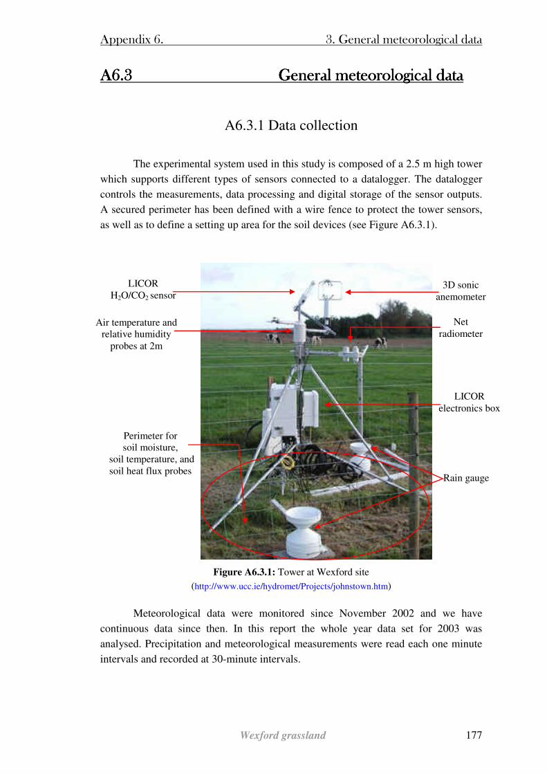
Appendix 6. 3. General meteorological data
Wexford grassland 177
A6.3A6.3A6.3A6.3 General meteorological dat General meteorological dat General meteorological dat General meteorological dataaaa
A6.3.1 Data collection
The experimental system used in this study is composed of a 2.5 m high tower
which supports different types of sensors connected to a datalogger. The datalogger
controls the measurements, data processing and digital storage of the sensor outputs.
A secured perimeter has been defined with a wire fence to protect the tower sensors,
as well as to define a setting up area for the soil devices (see Figure A6.3.1).
Figure A6.3.1: Tower at Wexford site
(http://www.ucc.ie/hydromet/Projects/johnstown.htm)
Meteorological data were monitored since November 2002 and we have
continuous data since then. In this report the whole year data set for 2003 was
analysed. Precipitation and meteorological measurements were read each one minute
intervals and recorded at 30-minute intervals.
3D sonic anemometer
LICOR H2O/CO2 sensor
Air temperature and relative humidity
probes at 2m
Net radiometer
Perimeter for soil moisture,
soil temperature, and soil heat flux probes
Rain gauge
LICOR electronics box
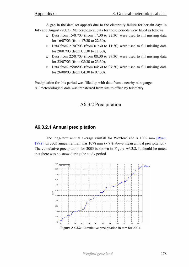
Appendix 6. 3. General meteorological data
Wexford grassland 178
A gap in the data set appears due to the electricity failure for certain days in
July and August (2003). Meteorological data for those periods were filled as follows:
Data from 15/07/03 (from 17:30 to 22:30) were used to fill missing data
for 16/07/03 (from 17:30 to 22:30),
Data from 21/07/03 (from 01:30 to 11:30) were used to fill missing data
for 20/07/03 (from 01:30 to 11:30),
Data from 22/07/03 (from 08:30 to 23:30) were used to fill missing data
for 23/07/03 (from 08:30 to 23:30),
Data from 25/08/03 (from 04:30 to 07:30) were used to fill missing data
for 26/08/03 (from 04:30 to 07:30).
Precipitation for this period was filled up with data from a nearby rain gauge.
All meteorological data was transferred from site to office by telemetry.
A6.3.2 Precipitation
A6.3.2.1 Annual precipitation
The long-term annual average rainfall for Wexford site is 1002 mm [Ryan,
1998]. In 2003 annual rainfall was 1078 mm (~ 7% above mean annual precipitation).
The cumulative precipitation for 2003 is shown in Figure A6.3.2. It should be noted
that there was no snow during the study period.
Figure A6.3.2: Cumulative precipitation in mm for 2003.
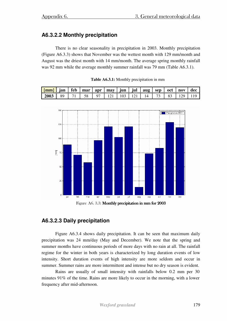
Appendix 6. 3. General meteorological data
Wexford grassland 179
A6.3.2.2 Monthly precipitation
There is no clear seasonality in precipitation in 2003. Monthly precipitation
(Figure A6.3.3) shows that November was the wettest month with 129 mm/month and
August was the driest month with 14 mm/month. The average spring monthly rainfall
was 92 mm while the average monthly summer rainfall was 79 mm (Table A6.3.1).
Table A6.3.1: Monthly precipitation in mm
[mm] jan feb mar apr may jun jul aug sep oct nov dec
2003 89 71 58 97 121 103 121 14 73 83 129 119
Figure A6. 3.3: Monthly precipitation in mm for 2003 Monthly precipitation in mm for 2003 Monthly precipitation in mm for 2003 Monthly precipitation in mm for 2003
A6.3.2.3 Daily precipitation
Figure A6.3.4 shows daily precipitation. It can be seen that maximum daily
precipitation was 24 mm/day (May and December). We note that the spring and
summer months have continuous periods of more days with no rain at all. The rainfall
regime for the winter in both years is characterized by long duration events of low
intensity. Short duration events of high intensity are more seldom and occur in
summer. Summer rains are more intermittent and intense but no dry season is evident.
Rains are usually of small intensity with rainfalls below 0.2 mm per 30
minutes 91% of the time. Rains are more likely to occur in the morning, with a lower
frequency after mid-afternoon.
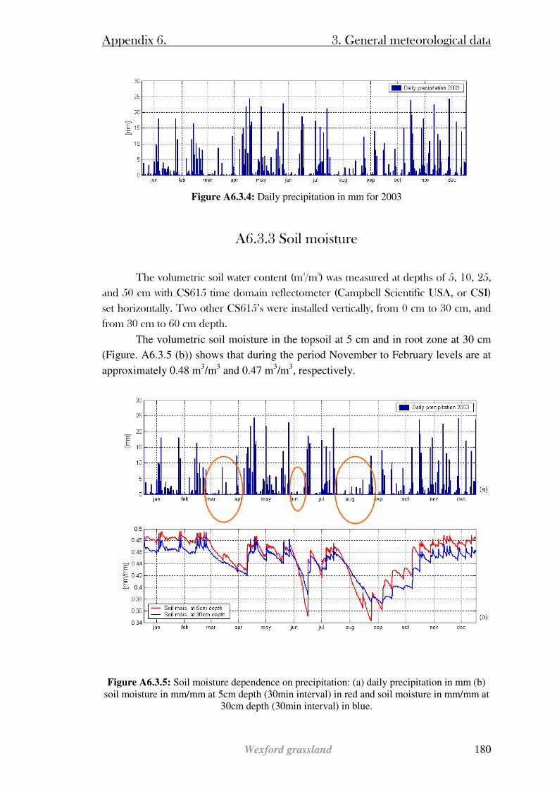
Appendix 6. 3. General meteorological data
Wexford grassland 180
Figure A6.3.4: Daily precipitation in mm for 2003
A6.3.3 Soil moisture
The volumetric soil water content (m3/m3) was measured at depths of 5, 10, 25,
and 50 cm with CS615 time domain reflectometer (Campbell Scientific USA, or CSI)
set horizontally. Two other CS615’s were installed vertically, from 0 cm to 30 cm, and
from 30 cm to 60 cm depth.
The volumetric soil moisture in the topsoil at 5 cm and in root zone at 30 cm
(Figure. A6.3.5 (b)) shows that during the period November to February levels are at
approximately 0.48 m3/m3 and 0.47 m3/m3, respectively.
Figure A6.3.5: Soil moisture dependence on precipitation: (a) daily precipitation in mm (b) soil moisture in mm/mm at 5cm depth (30min interval) in red and soil moisture in mm/mm at
30cm depth (30min interval) in blue.
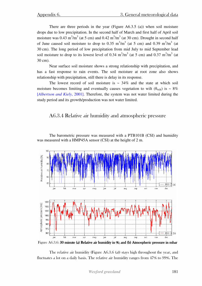
Appendix 6. 3. General meteorological data
Wexford grassland 181
There are three periods in the year (Figure A6.3.5 (a)) when soil moisture
drops due to low precipitation. In the second half of March and first half of April soil
moisture was 0.43 m3/m3 (at 5 cm) and 0.42 m3/m3 (at 30 cm). Drought in second half
of June caused soil moisture to drop to 0.35 m3/m3 (at 5 cm) and 0.39 m3/m3 (at
30 cm). The long period of low precipitation from mid July to mid September lead
soil moisture to drop to its lowest level of 0.34 m3/m3 (at 5 cm) and 0.37 m3/m3 (at
30 cm).
Near surface soil moisture shows a strong relationship with precipitation, and
has a fast response to rain events. The soil moisture at root zone also shows
relationship with precipitation, still there is delay in its response.
The lowest record of soil moisture is ~ 34% and the state at which soil
moisture becomes limiting and eventually causes vegetation to wilt (θwilt) is ~ 8%
[Albertson and Kiely, 2001]. Therefore, the system was not water limited during the
study period and its growth/production was not water limited.
A6.3.4 Relative air humidity and atmospheric pressure
The barometric pressure was measured with a PTB101B (CSI) and humidity was measured with a HMP45A sensor (CSI) at the height of 2 m.
Figure A6.3.6: 30 minute (a) Relative air humidity in %; and (b) Atmospheric pressure in mba30 minute (a) Relative air humidity in %; and (b) Atmospheric pressure in mba30 minute (a) Relative air humidity in %; and (b) Atmospheric pressure in mba30 minute (a) Relative air humidity in %; and (b) Atmospheric pressure in mbarrrr
The relative air humidity (Figure A6.3.6 (a)) stays high throughout the year, and
fluctuates a lot on a daily basis. The relative air humidity ranges from 47% to 99%. The
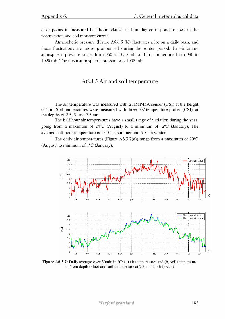
Appendix 6. 3. General meteorological data
Wexford grassland 182
drier points in measured half hour relative air humidity correspond to lows in the
precipitation and soil moisture curves.
Atmospheric pressure (Figure A6.3.6 (b)) fluctuates a lot on a daily basis, and
those fluctuations are more pronounced during the winter period. In wintertime
atmospheric pressure ranges from 960 to 1030 mb, and in summertime from 990 to
1020 mb. The mean atmospheric pressure was 1008 mb.
A6.3.5 Air and soil temperature
The air temperature was measured with a HMP45A sensor (CSI) at the height
of 2 m. Soil temperatures were measured with three 107 temperature probes (CSI), at the depths of 2.5, 5, and 7.5 cm.
The half hour air temperatures have a small range of variation during the year,
going from a maximum of 24ºC (August) to a minimum of -2ºC (January). The
average half hour temperature is 15º C in summer and 6º C in winter.
The daily air temperatures (Figure A6.3.7(a)) range from a maximum of 20ºC
(August) to minimum of 1ºC (January).
Figure A6.3.7: Daily average over 30min in °C: (a) air temperature; and (b) soil temperature
at 5 cm depth (blue) and soil temperature at 7.5 cm depth (green)
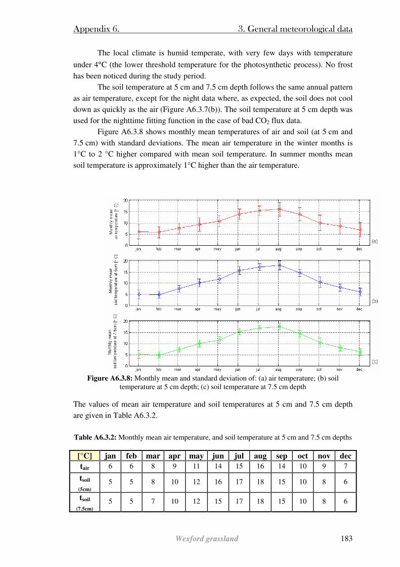
Appendix 6. 3. General meteorological data
Wexford grassland 183
The local climate is humid temperate, with very few days with temperature
under 4°C (the lower threshold temperature for the photosynthetic process). No frost
has been noticed during the study period.
The soil temperature at 5 cm and 7.5 cm depth follows the same annual pattern
as air temperature, except for the night data where, as expected, the soil does not cool
down as quickly as the air (Figure A6.3.7(b)). The soil temperature at 5 cm depth was
used for the nighttime fitting function in the case of bad CO2 flux data.
Figure A6.3.8 shows monthly mean temperatures of air and soil (at 5 cm and
7.5 cm) with standard deviations. The mean air temperature in the winter months is
1°C to 2 °C higher compared with mean soil temperature. In summer months mean
soil temperature is approximately 1°C higher than the air temperature.
Figure A6.3.8: Monthly mean and standard deviation of: (a) air temperature; (b) soil
temperature at 5 cm depth; (c) soil temperature at 7.5 cm depth The values of mean air temperature and soil temperatures at 5 cm and 7.5 cm depth
are given in Table A6.3.2.
Table A6.3.2: Monthly mean air temperature, and soil temperature at 5 cm and 7.5 cm depths
[°C] jan feb mar apr may jun jul aug sep oct nov dec
tair 6 6 8 9 11 14 15 16 14 10 9 7
tsoil
(5cm)
5 5 8 10 12 16 17 18 15 10 8 6
tsoil
(7.5cm)
5 5 7 10 12 15 17 18 15 10 8 6

Appendix 6. 3. General meteorological data
Wexford grassland 184
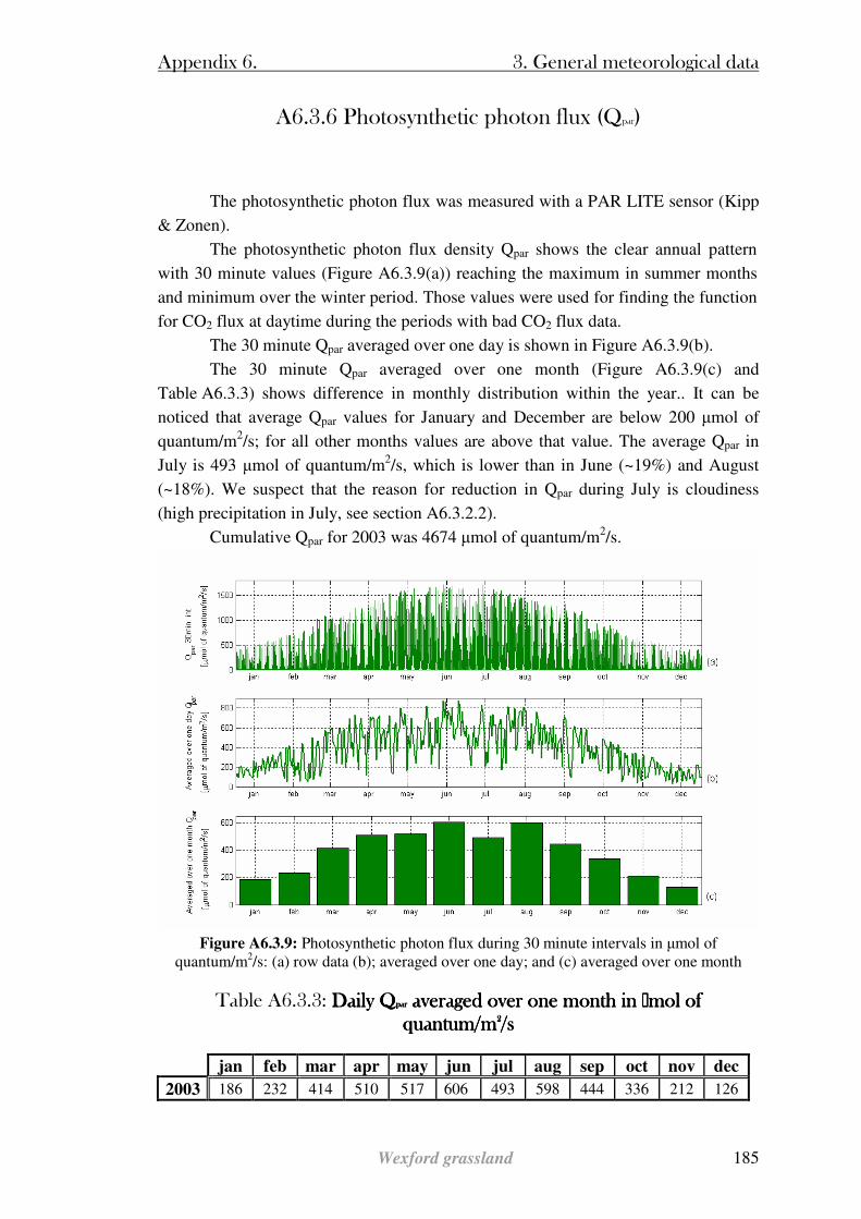
Appendix 6. 3. General meteorological data
Wexford grassland 185
A6.3.6 Photosynthetic photon flux (Qpar)
The photosynthetic photon flux was measured with a PAR LITE sensor (Kipp
& Zonen).
The photosynthetic photon flux density Qpar shows the clear annual pattern
with 30 minute values (Figure A6.3.9(a)) reaching the maximum in summer months
and minimum over the winter period. Those values were used for finding the function
for CO2 flux at daytime during the periods with bad CO2 flux data.
The 30 minute Qpar averaged over one day is shown in Figure A6.3.9(b).
The 30 minute Qpar averaged over one month (Figure A6.3.9(c) and
Table A6.3.3) shows difference in monthly distribution within the year.. It can be
noticed that average Qpar values for January and December are below 200 µmol of
quantum/m2/s; for all other months values are above that value. The average Qpar in
July is 493 µmol of quantum/m2/s, which is lower than in June (~19%) and August
(~18%). We suspect that the reason for reduction in Qpar during July is cloudiness
(high precipitation in July, see section A6.3.2.2).
Cumulative Qpar for 2003 was 4674 µmol of quantum/m2/s.
Figure A6.3.9: Photosynthetic photon flux during 30 minute intervals in µmol of
quantum/m2/s: (a) row data (b); averaged over one day; and (c) averaged over one month
Table A6.3.3: Daily QDaily QDaily QDaily Qparparparpar averaged over one month in averaged over one month in averaged over one month in averaged over one month in Mmol of Mmol of Mmol of Mmol of quantum/mquantum/mquantum/mquantum/m2222/s/s/s/s
jan feb mar apr may jun jul aug sep oct nov dec
2003 186 232 414 510 517 606 493 598 444 336 212 126
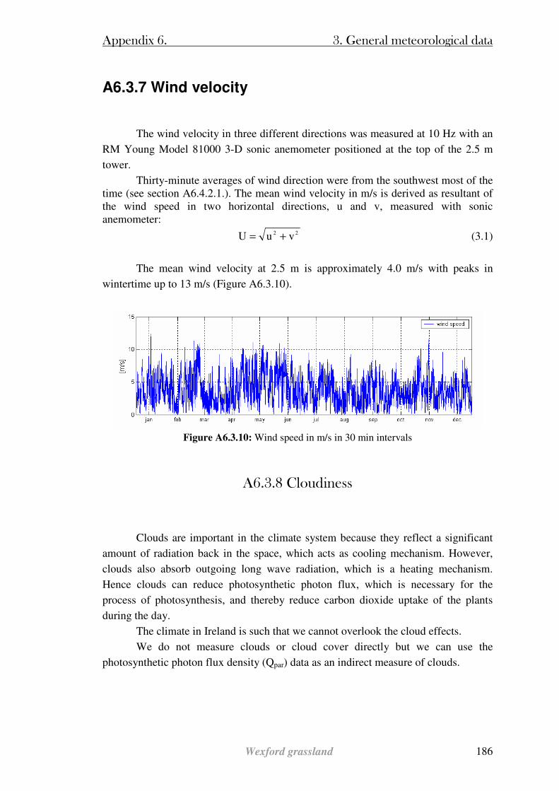
Appendix 6. 3. General meteorological data
Wexford grassland 186
A6.3.7 Wind velocity
The wind velocity in three different directions was measured at 10 Hz with an
RM Young Model 81000 3-D sonic anemometer positioned at the top of the 2.5 m
tower.
Thirty-minute averages of wind direction were from the southwest most of the time (see section A6.4.2.1.). The mean wind velocity in m/s is derived as resultant of the wind speed in two horizontal directions, u and v, measured with sonic anemometer:
22 vuU += (3.1)
The mean wind velocity at 2.5 m is approximately 4.0 m/s with peaks in
wintertime up to 13 m/s (Figure A6.3.10).
Figure A6.3.10: Wind speed in m/s in 30 min intervals
A6.3.8 Cloudiness
Clouds are important in the climate system because they reflect a significant
amount of radiation back in the space, which acts as cooling mechanism. However,
clouds also absorb outgoing long wave radiation, which is a heating mechanism.
Hence clouds can reduce photosynthetic photon flux, which is necessary for the
process of photosynthesis, and thereby reduce carbon dioxide uptake of the plants
during the day.
The climate in Ireland is such that we cannot overlook the cloud effects.
We do not measure clouds or cloud cover directly but we can use the
photosynthetic photon flux density (Qpar) data as an indirect measure of clouds.
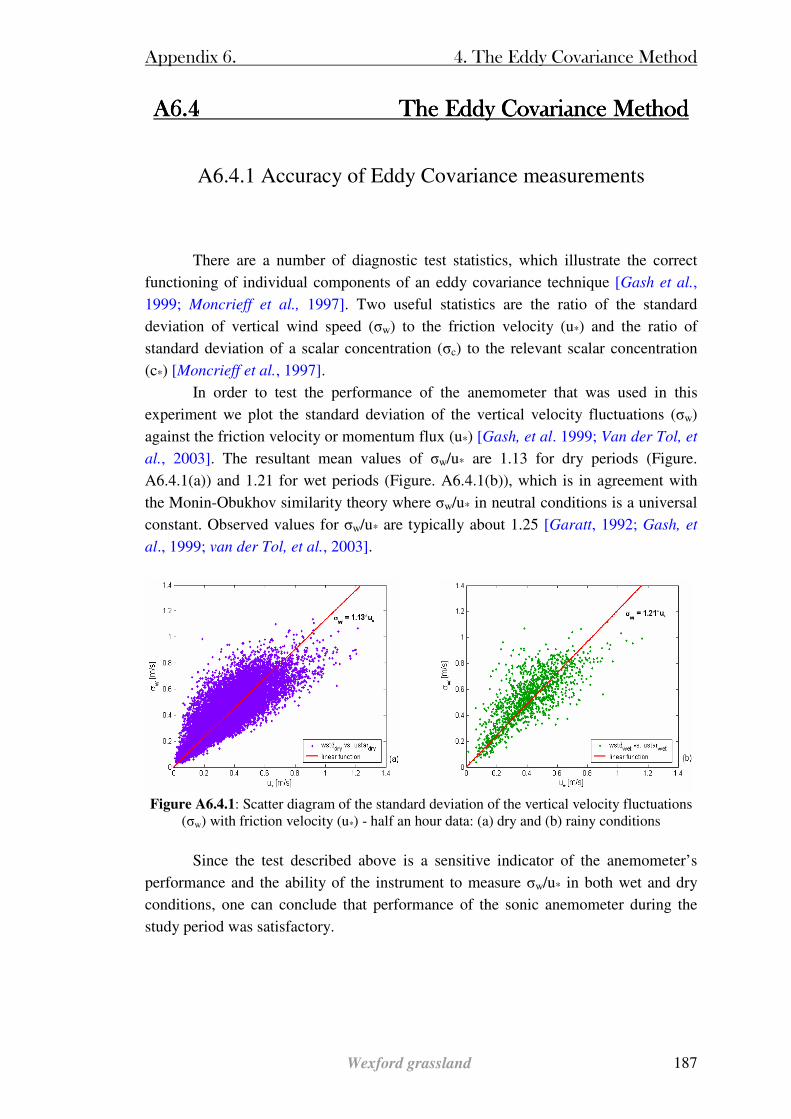
Appendix 6. 4. The Eddy Covariance Method
Wexford grassland 187
A6.4A6.4A6.4A6.4 The Eddy Covariance Method The Eddy Covariance Method The Eddy Covariance Method The Eddy Covariance Method
A6.4.1 Accuracy of Eddy Covariance measurements
There are a number of diagnostic test statistics, which illustrate the correct
functioning of individual components of an eddy covariance technique [Gash et al.,
1999; Moncrieff et al., 1997]. Two useful statistics are the ratio of the standard
deviation of vertical wind speed (σw) to the friction velocity (u*) and the ratio of
standard deviation of a scalar concentration (σc) to the relevant scalar concentration
(c*) [Moncrieff et al., 1997].
In order to test the performance of the anemometer that was used in this
experiment we plot the standard deviation of the vertical velocity fluctuations (σw)
against the friction velocity or momentum flux (u*) [Gash, et al. 1999; Van der Tol, et
al., 2003]. The resultant mean values of σw/u* are 1.13 for dry periods (Figure.
A6.4.1(a)) and 1.21 for wet periods (Figure. A6.4.1(b)), which is in agreement with
the Monin-Obukhov similarity theory where σw/u* in neutral conditions is a universal
constant. Observed values for σw/u* are typically about 1.25 [Garatt, 1992; Gash, et
al., 1999; van der Tol, et al., 2003].
Figure A6.4.1: Scatter diagram of the standard deviation of the vertical velocity fluctuations
(σw) with friction velocity (u*) - half an hour data: (a) dry and (b) rainy conditions
Since the test described above is a sensitive indicator of the anemometer’s
performance and the ability of the instrument to measure σw/u* in both wet and dry
conditions, one can conclude that performance of the sonic anemometer during the
study period was satisfactory.
Appendix 6. 4. The Eddy Covariance Method
Wexford grassland 188
A6.4.2 Footprint and fetch
A6.4.2.1 Footprint estimation
Numerous models have been developed to investigate the relationship between
scalar flux and its source areas, e.g. Eulerian analytical model [Gash, 1986; Horst and
Weil, 1995], Lagrangian stochastic dispersion model [Hsieh et al., 1997].
To interpret the eddy correlation measured scalar flux and understand the fetch
requirement and contributing source areas for these measurements, the flux footprint
model developed by Hsieh et al. [2000] was adopted. The model describes the
relationship between footprint, atmospheric stability, observation height, and surface
roughness.
Figure A6.4.2. shows the scatter plots of xf (the fetch requirement) and xp (the
peak source distance) versus wind directions. Table A6.4.1 shows percentage of the
measurements during the neutral, unstable and stable atmospheric condition.
Table A6.4.1: Atmospheric conditions occurrence in %
Atmospheric condition [%]
Neutral 43
Unstable 24
Stable 32
In Figure A6.4.2 the fetch requrements for unstable (and neutral) conditions
(67% of time), is less than 500 m and the strongest source areas are within 25 m from
the tower. For stable conditions (32% of time), xf and xp are within 1km and 50 m,
respectively, except for some (~18%) very stable cases. Also, it is noted that 90% of
the xf and xp values are less than 1 km and 50 m, respectively, for the whole year
2003.
With this footprint analysis, it can be interpreted that most of the time (~ 90%)
the eddy-correlation scalar flux measurements (i.e., sensible heat, latent heat, and CO2
fluxes) represent the space averaged fluxes resulted from the circle area 1 km in
radius from the tower, and the strongest source area is just 50 m away. Also, from the
information given by the wind direction histogram shown in Figure A6.4.3, it is clear
that the eddy correlation measured fluxes are mainly from the southwest part of the
field. This suggests that the footprint is changeable during the time and it is not within
a circle around the tower, but it shaped according to the wind direction and wind
speed (the plot is more scattered in directions other than S-W in Figure A6.4.2).
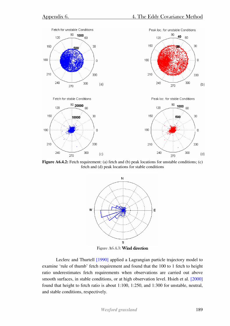
Appendix 6. 4. The Eddy Covariance Method
Wexford grassland 189
Figure A6.4.2: Fetch requirement: (a) fetch and (b) peak locations for unstable conditions; (c)
fetch and (d) peak locations for stable conditions
Figure A6.4.3: Wind directi Wind directi Wind directi Wind directionononon
Leclerc and Thurtell [1990] applied a Lagrangian particle trajectory model to
examine ‘rule of thumb’ fetch requirement and found that the 100 to 1 fetch to height
ratio underestimates fetch requirements when observations are carried out above
smooth surfaces, in stable conditions, or at high observation level. Hsieh et al. [2000]
found that height to fetch ratio is about 1:100, 1:250, and 1:300 for unstable, neutral,
and stable conditions, respectively.
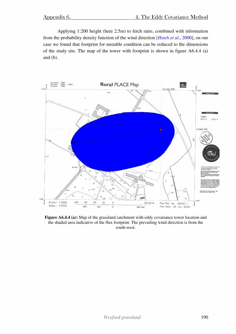
Appendix 6. 4. The Eddy Covariance Method
Wexford grassland 190
Applying 1:200 height (here 2.5m) to fetch ratio, combined with information
from the probability density function of the wind direction [Hsieh et al., 2000], on our
case we found that footprint for unstable condition can be reduced to the dimensions
of the study site. The map of the tower with footprint is shown in figure A6.4.4 (a)
and (b).
Figure A6.4.4 (a): Map of the grassland catchment with eddy covariance tower location and
the shaded area indicative of the flux footprint. The prevailing wind direction is from the south-west.
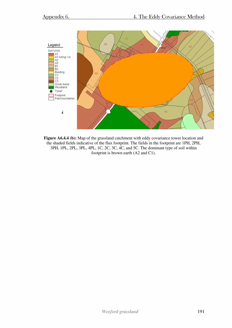
Appendix 6. 4. The Eddy Covariance Method
Wexford grassland 191
Figure A6.4.4 (b): Map of the grassland catchment with eddy covariance tower location and the shaded fields indicative of the flux footprint. The fields in the footprint are 1PH, 2PH,
3PH, 1PL, 2PL, 3PL, 4PL, 1C, 2C, 3C, 4C, and 5C. The dominant type of soil within footprint is brown earth (A2 and C1).
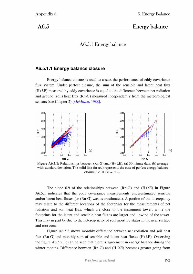
Appendix 6. 5. Energy Balance
Wexford grassland 192
A6.5A6.5A6.5A6.5 Energy balance Energy balance Energy balance Energy balance
A6.5.1 Energy balance
A6.5.1.1 Energy balance closure
Energy balance closure is used to assess the performance of eddy covariance
flux system. Under perfect closure, the sum of the sensible and latent heat flux
(H+λE) measured by eddy covariance is equal to the difference between net radiation
and ground (soil) heat flux (Rn-G) measured independently from the meteorological
sensors (see Chapter 2) [McMillen, 1988].
Figure A6.5.1: Relationships between (Rn-G) and (H+ λE): (a) 30 minute data; (b) average with standard deviation. The solid line (in red) represents the case of perfect energy balance
closure, i.e. H+λE=Rn-G.
The slope 0.9 of the relationships between (Rn-G) and (H+λE) in Figure
A6.5.1 indicates that the eddy covariance measurements underestimated sensible
and/or latent heat fluxes (or (Rn-G) was overestimated). A portion of the discrepancy
may relate to the different locations of the footprints for the measurements of net
radiation and soil heat flux, which are close to the instrument tower, while the
footprints for the latent and sensible heat fluxes are larger and upwind of the tower.
This may in part be due to the heterogeneity of soil moisture status in the near surface
and root zone.
Figure A6.5.2 shows monthly difference between net radiation and soil heat
flux (Rn-G) and monthly sum of sensible and latent heat fluxes (H+λE). Observing
the figure A6.5.2, it can be seen that there is agreement in energy balance during the
winter months. Difference between (Rn-G) and (H+λE) becomes greater going from
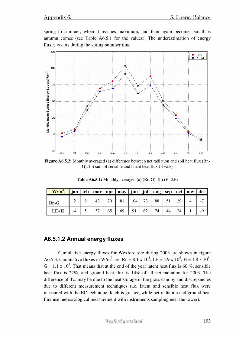
Appendix 6. 5. Energy Balance
Wexford grassland 193
spring to summer, when it reaches maximum, and than again becomes small as
autumn comes (see Table A6.5.1 for the values). The underestimation of energy
fluxes occurs during the spring-summer time.
Figure A6.5.2: Monthly averaged (a) difference between net radiation and soil heat flux (Rn-
G); (b) sum of sensible and latent heat flux (H+λE)
Table A6.5.1: Monthly averaged (a) (Rn-G); (b) (H+λE)
[W/m2] jan feb mar apr may jun jul aug sep oct nov dec
Rn-G 2 8 43 70 81 104 73 88 51 29 4 -7
LE+H -4 5 37 65 69 91 62 74 44 24 1 -9
A6.5.1.2 Annual energy fluxes
Cumulative energy fluxes for Wexford site during 2003 are shown in figure
A6.5.3. Cumulative fluxes in W/m2 are: Rn = 8.1 x 10⁵; LE = 4.9 x 10⁵; H = 1.8 x 10⁵;
G = 1.1 x 10⁵. That means that at the end of the year latent heat flux is 60 %, sensible
heat flux is 22%, and ground heat flux is 14% of all net radiation for 2003. The
difference of 4% may be due to the heat storage in the grass canopy and discrepancies
due to different measurement techniques (i.e. latent and sensible heat flux were
measured with the EC technique, fetch is greater, while net radiation and ground heat
flux use meteorological measurement with instruments sampling near the tower).
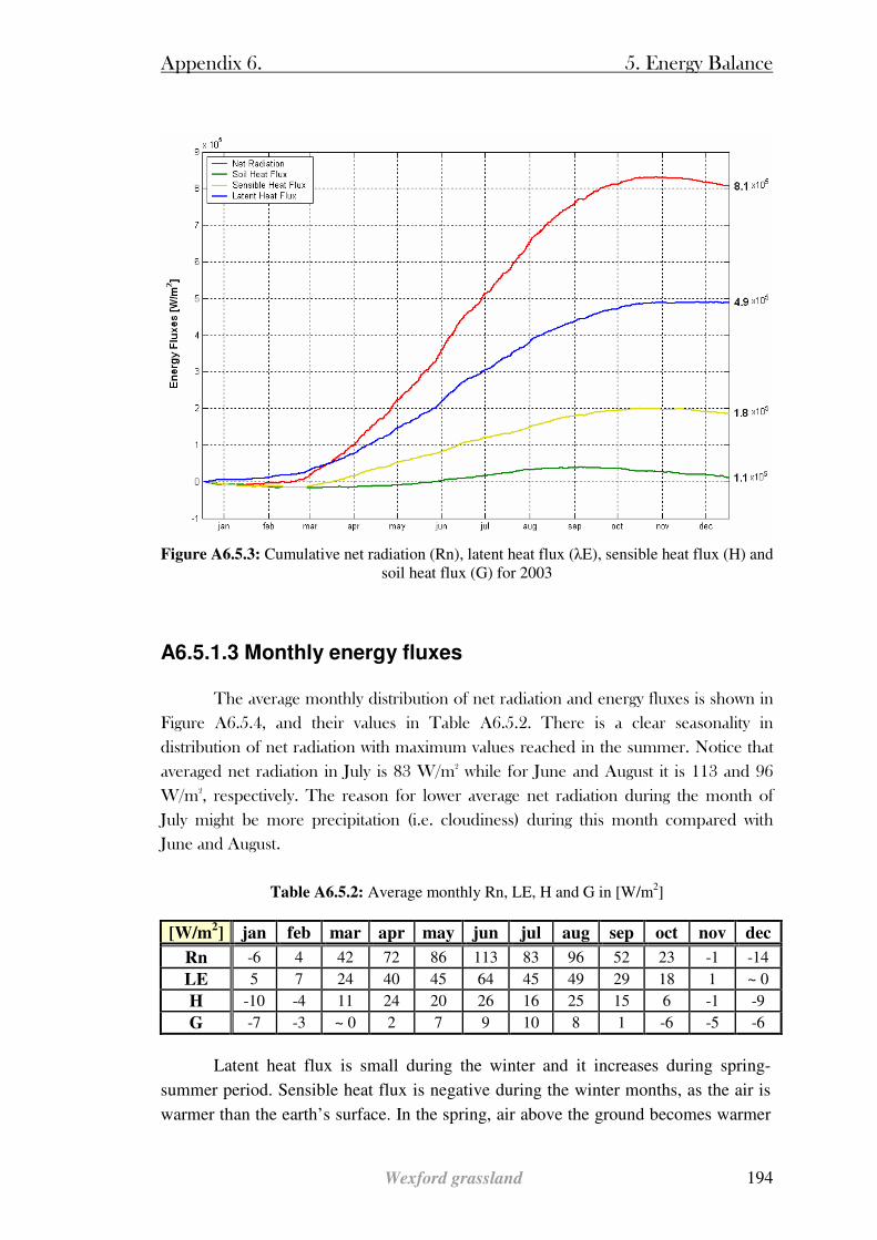
Appendix 6. 5. Energy Balance
Wexford grassland 194
Figure A6.5.3: Cumulative net radiation (Rn), latent heat flux (λE), sensible heat flux (H) and
soil heat flux (G) for 2003
A6.5.1.3 Monthly energy fluxes
The average monthly distribution of net radiation and energy fluxes is shown in
Figure A6.5.4, and their values in Table A6.5.2. There is a clear seasonality in
distribution of net radiation with maximum values reached in the summer. Notice that
averaged net radiation in July is 83 W/m2 while for June and August it is 113 and 96
W/m2, respectively. The reason for lower average net radiation during the month of
July might be more precipitation (i.e. cloudiness) during this month compared with
June and August.
Table A6.5.2: Average monthly Rn, LE, H and G in [W/m2]
[W/m2] jan feb mar apr may jun jul aug sep oct nov dec
Rn -6 4 42 72 86 113 83 96 52 23 -1 -14
LE 5 7 24 40 45 64 45 49 29 18 1 ~ 0
H -10 -4 11 24 20 26 16 25 15 6 -1 -9
G -7 -3 ~ 0 2 7 9 10 8 1 -6 -5 -6
Latent heat flux is small during the winter and it increases during spring-
summer period. Sensible heat flux is negative during the winter months, as the air is
warmer than the earth’s surface. In the spring, air above the ground becomes warmer
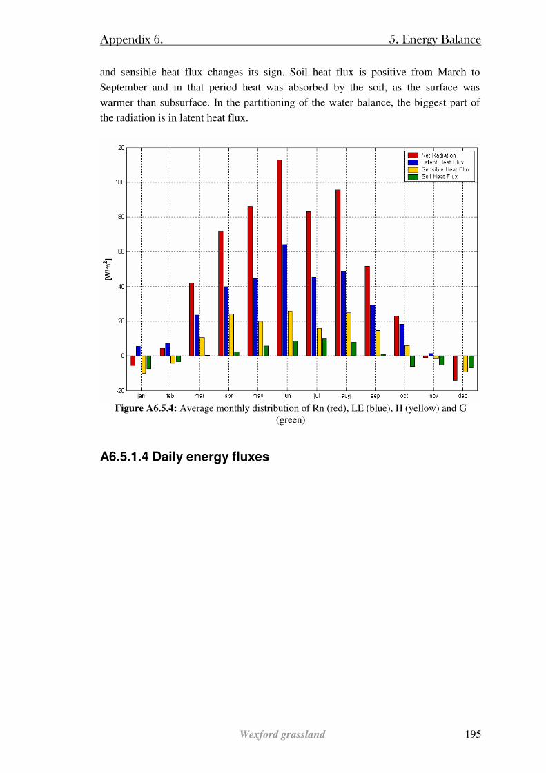
Appendix 6. 5. Energy Balance
Wexford grassland 195
and sensible heat flux changes its sign. Soil heat flux is positive from March to
September and in that period heat was absorbed by the soil, as the surface was
warmer than subsurface. In the partitioning of the water balance, the biggest part of
the radiation is in latent heat flux.
Figure A6.5.4: Average monthly distribution of Rn (red), LE (blue), H (yellow) and G
(green)
A6.5.1.4 Daily energy fluxes
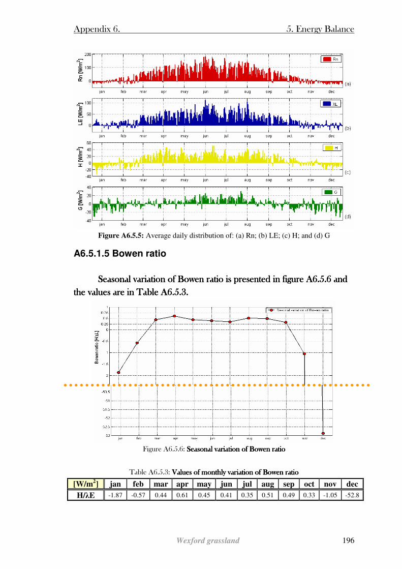
Appendix 6. 5. Energy Balance
Wexford grassland 196
Figure A6.5.5: Average daily distribution of: (a) Rn; (b) LE; (c) H; and (d) G
A6.5.1.5 Bowen ratio
Seasonal variation of Bowen ratio is presented in figure Seasonal variation of Bowen ratio is presented in figure Seasonal variation of Bowen ratio is presented in figure Seasonal variation of Bowen ratio is presented in figure AAAA6.6.6.6.5.6 and 5.6 and 5.6 and 5.6 and
the values are in Table the values are in Table the values are in Table the values are in Table A6.A6.A6.A6.5.3.5.3.5.3.5.3.
Figure A6.5.6: Seasonal variation of Bowen ratio Seasonal variation of Bowen ratio Seasonal variation of Bowen ratio Seasonal variation of Bowen ratio
Table A6.5.3: Values of monthly variation of Bowen ratio Values of monthly variation of Bowen ratio Values of monthly variation of Bowen ratio Values of monthly variation of Bowen ratio
[W/m2] jan feb mar apr may jun jul aug sep oct nov dec
H/λE -1.87 -0.57 0.44 0.61 0.45 0.41 0.35 0.51 0.49 0.33 -1.05 -52.8
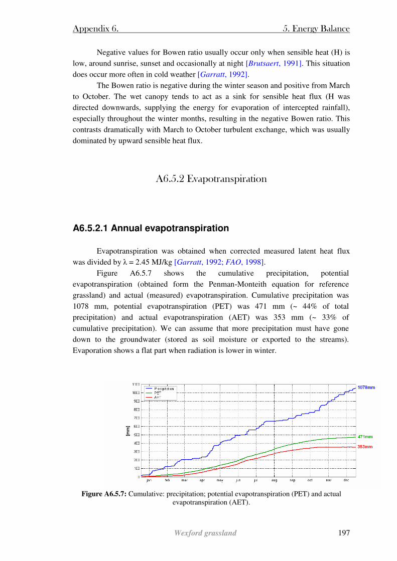
Appendix 6. 5. Energy Balance
Wexford grassland 197
Negative values for Bowen ratio usually occur only when sensible heat (H) is
low, around sunrise, sunset and occasionally at night [Brutsaert, 1991]. This situation
does occur more often in cold weather [Garratt, 1992].
The Bowen ratio is negative during the winter season and positive from March
to October. The wet canopy tends to act as a sink for sensible heat flux (H was
directed downwards, supplying the energy for evaporation of intercepted rainfall),
especially throughout the winter months, resulting in the negative Bowen ratio. This
contrasts dramatically with March to October turbulent exchange, which was usually
dominated by upward sensible heat flux.
A6.5.2 Evapotranspiration
A6.5.2.1 Annual evapotranspiration
Evapotranspiration was obtained when corrected measured latent heat flux
was divided by λ = 2.45 MJ/kg [Garratt, 1992; FAO, 1998].
Figure A6.5.7 shows the cumulative precipitation, potential
evapotranspiration (obtained form the Penman-Monteith equation for reference
grassland) and actual (measured) evapotranspiration. Cumulative precipitation was
1078 mm, potential evapotranspiration (PET) was 471 mm (~ 44% of total
precipitation) and actual evapotranspiration (AET) was 353 mm (~ 33% of
cumulative precipitation). We can assume that more precipitation must have gone
down to the groundwater (stored as soil moisture or exported to the streams).
Evaporation shows a flat part when radiation is lower in winter.
Figure A6.5.7: Cumulative: precipitation; potential evapotranspiration (PET) and actual
evapotranspiration (AET).
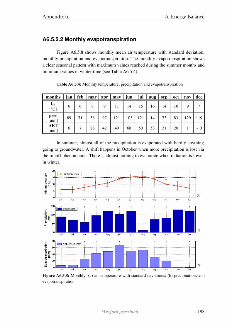
Appendix 6. 5. Energy Balance
Wexford grassland 198
A6.5.2.2 Monthly evapotranspiration
Figure A6.5.8 shows monthly mean air temperature with standard deviation,
monthly precipitation and evapotranspiration. The monthly evapotranspiration shows
a clear seasonal pattern with maximum values reached during the summer months and
minimum values in winter time (see Table A6.5.4).
Table A6.5.4: Monthly temperature, precipitation and evapotranspiration
months jan feb mar apr may jun jul aug sep oct nov dec
tair
[°C] 6 6 8 9 11 14 15 16 14 10 9 7
prec [mm]
89 71 58 97 121 103 121 14 73 83 129 119
AET [mm]
6 7 26 42 49 68 50 53 31 20 1 ~ 0
In summer, almost all of the precipitation is evaporated with hardly anything
going to groundwater. A shift happens in October when more precipitation is lost via
the runoff phenomenon. There is almost nothing to evaporate when radiation is lower
in winter.
Figure A6.5.8: Monthly: (a) air temperature with standard deviations; (b) precipitation; and
evapotranspiration
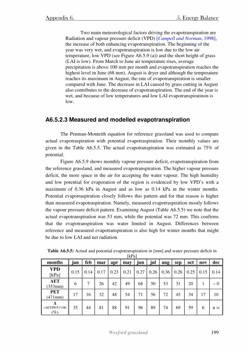
Appendix 6. 5. Energy Balance
Wexford grassland 199
Two main meteorological factors driving the evapotranspiration are Radiation and vapour pressure deficit (VPD) [Campell and Norman, 1998], the increase of both enhancing evapotranspiration. The beginning of the year was very wet, and evapotranspiration is low due to the low air temperature, low VPD (see Figure A6.5.9 (a)) and the short height of grass (LAI is low). From March to June air temperature rises, average precipitation is above 100 mm per month and evapotranspiration reaches the highest level in June (68 mm). August is dryer and although the temperature reaches its maximum in August, the rate of evapotranspiration is smaller compared with June. The decrease in LAI caused by grass cutting in August also contributes to the decrease of evapotranspiration. The end of the year is wet, and because of low temperatures and low LAI evapotranspiratinon is low.
A6.5.2.3 Measured and modelled evapotranspiration
The Penman-Monteith equation for reference grassland was used to compare
actual evapotraspiration with potential evapotraspiration. Their monthly values are
given in the Table A6.5.5. The actual evapotranspiration was estimated as 75% of
potential.
Figure A6.5.9 shows monthly vapour pressure deficit, evapotranspiration from
the reference grassland, and measured evapotranspiration. The higher vapour pressure
deficit, the more space in the air for accepting the water vapour. The high humidity
and low potential for evaporation of the region is evidenced by low VPD’s with a
maximum of 0.36 kPa in August and as low as 0.14 kPa in the winter months.
Potential evapotraspiration closely follows this pattern and for that reason is higher
than measured evapotraspiration. Namely, measured evapotraspiration mostly follows
the vapour pressure deficit pattern. Examining August (Table A6.5.5) we note that the
actual evapotranspiration was 53 mm, while the potential was 72 mm. This confirms
that the evapotranspiration was water limited in August. Differences between
reference and measured evapotranspiration is also high for winter months that might
be due to low LAI and net radiation.
Table A6.5.5: Actual and potential evapotranspiration in [mm] and water pressure deficit in
[kPa]
months jan feb mar apr may jun jul aug sep oct nov dec
VPD [kPa]
0.15 0.14 0.17 0.23 0.21 0.27 0.26 0.36 0.26 0.25 0.15 0.14
AET (353mm)
6 7 26 42 49 68 50 53 31 20 1 ~ 0
PET (471mm)
17 16 32 48 54 71 56 72 45 34 17 10
∆ (AET/PET)*100
(%) 35 44 81 88 91 96 89 74 69 59 6 ± ∞
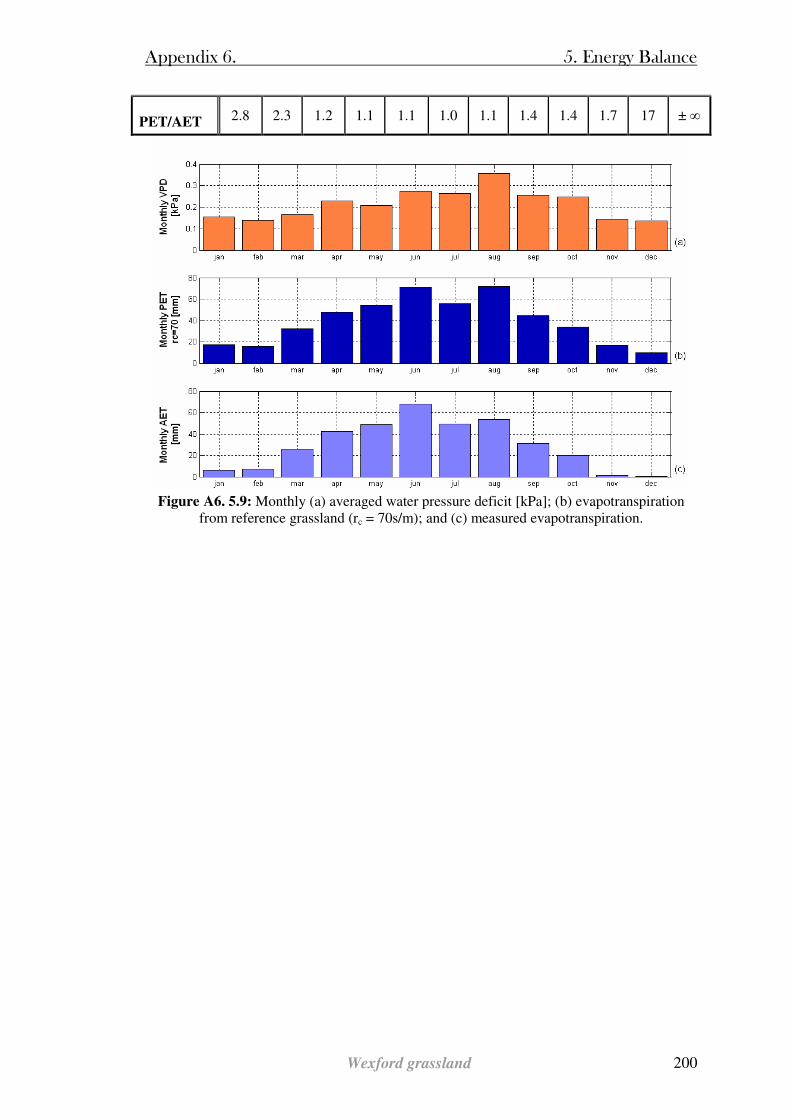
Appendix 6. 5. Energy Balance
Wexford grassland 200
PET/AET 2.8 2.3 1.2 1.1 1.1 1.0 1.1 1.4 1.4 1.7 17 ± ∞
Figure A6. 5.9: Monthly (a) averaged water pressure deficit [kPa]; (b) evapotranspiration
from reference grassland (rc = 70s/m); and (c) measured evapotranspiration.
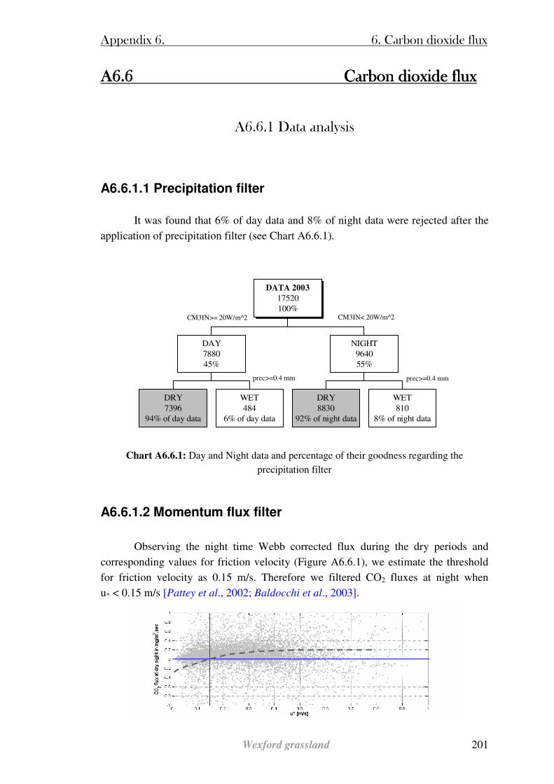
Appendix 6. 6. Carbon dioxide flux
Wexford grassland 201
A6.6A6.6A6.6A6.6 Carbon dioxide flux Carbon dioxide flux Carbon dioxide flux Carbon dioxide flux
A6.6.1 Data analysis
A6.6.1.1 Precipitation filter
It was found that 6% of day data and 8% of night data were rejected after the
application of precipitation filter (see Chart A6.6.1).
CM3IN>= 20W/m^2
prec>=0.4 mm prec>=0.4 mm
CM3IN< 20W/m^2
DRY7396
94% of day data
WET484
6% of day data
DAY788045%
DRY8830
92% of night data
WET810
8% of night data
NIGHT964055%
DATA 2003
17520100%
Chart A6.6.1: Day and Night data and percentage of their goodness regarding the
precipitation filter
A6.6.1.2 Momentum flux filter
Observing the night time Webb corrected flux during the dry periods and
corresponding values for friction velocity (Figure A6.6.1), we estimate the threshold
for friction velocity as 0.15 m/s. Therefore we filtered CO2 fluxes at night when
u* < 0.15 m/s [Pattey et al., 2002; Baldocchi et al., 2003].
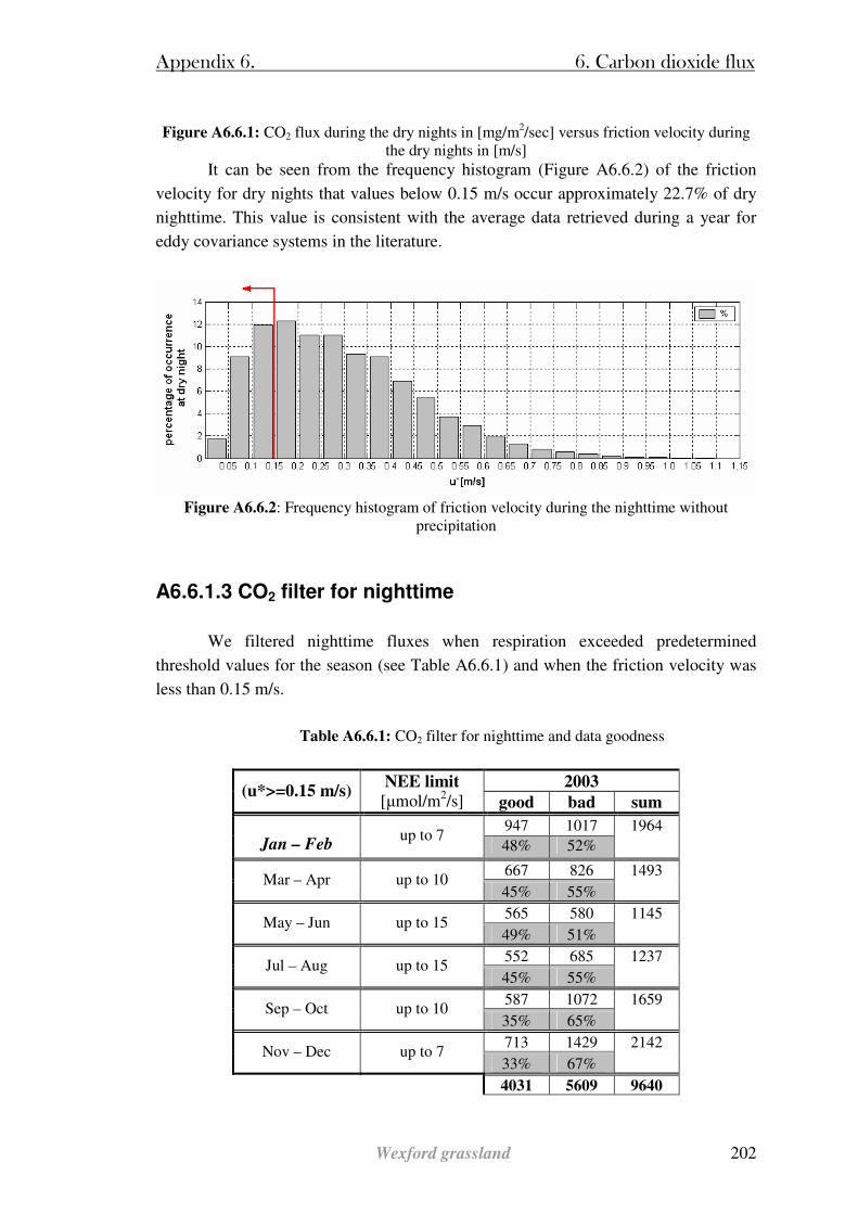
Appendix 6. 6. Carbon dioxide flux
Wexford grassland 202
Figure A6.6.1: CO2 flux during the dry nights in [mg/m2/sec] versus friction velocity during
the dry nights in [m/s] It can be seen from the frequency histogram (Figure A6.6.2) of the friction
velocity for dry nights that values below 0.15 m/s occur approximately 22.7% of dry
nighttime. This value is consistent with the average data retrieved during a year for
eddy covariance systems in the literature.
Figure A6.6.2: Frequency histogram of friction velocity during the nighttime without
precipitation
A6.6.1.3 CO2 filter for nighttime
We filtered nighttime fluxes when respiration exceeded predetermined
threshold values for the season (see Table A6.6.1) and when the friction velocity was
less than 0.15 m/s.
Table A6.6.1: CO2 filter for nighttime and data goodness
2003 (u*>=0.15 m/s)
NEE limit [µmol/m2/s] good bad sum
947 1017 Jan – Feb
up to 7 48% 52%
1964
667 826 Mar – Apr up to 10
45% 55%
1493
565 580 May – Jun up to 15
49% 51%
1145
552 685 Jul – Aug up to 15
45% 55%
1237
587 1072 Sep – Oct up to 10
35% 65%
1659
713 1429 Nov – Dec up to 7
33% 67%
2142
4031 5609 9640
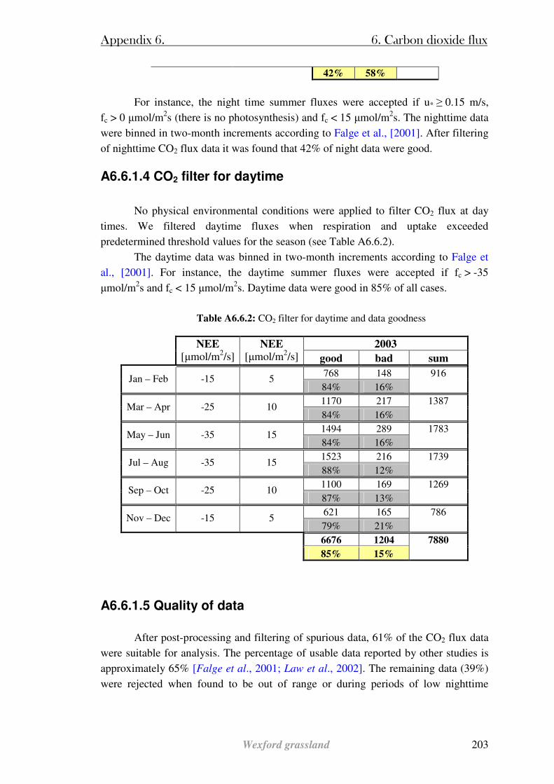
Appendix 6. 6. Carbon dioxide flux
Wexford grassland 203
42% 58%
For instance, the night time summer fluxes were accepted if u* ≥ 0.15 m/s,
fc > 0 µmol/m2s (there is no photosynthesis) and fc < 15 µmol/m2s. The nighttime data
were binned in two-month increments according to Falge et al., [2001]. After filtering
of nighttime CO2 flux data it was found that 42% of night data were good.
A6.6.1.4 CO2 filter for daytime
No physical environmental conditions were applied to filter CO2 flux at day
times. We filtered daytime fluxes when respiration and uptake exceeded
predetermined threshold values for the season (see Table A6.6.2).
The daytime data was binned in two-month increments according to Falge et
al., [2001]. For instance, the daytime summer fluxes were accepted if fc > -35
µmol/m2s and fc < 15 µmol/m2s. Daytime data were good in 85% of all cases.
Table A6.6.2: CO2 filter for daytime and data goodness
2003
NEE [µmol/m2/s]
NEE [µmol/m2/s] good bad sum
768 148 Jan – Feb -15 5
84% 16%
916
1170 217 Mar – Apr -25 10
84% 16%
1387
1494 289 May – Jun -35 15
84% 16%
1783
1523 216 Jul – Aug -35 15
88% 12%
1739
1100 169 Sep – Oct -25 10
87% 13%
1269
621 165 Nov – Dec -15 5
79% 21%
786
6676 1204
85% 15%
7880
A6.6.1.5 Quality of data
After post-processing and filtering of spurious data, 61% of the CO2 flux data
were suitable for analysis. The percentage of usable data reported by other studies is
approximately 65% [Falge et al., 2001; Law et al., 2002]. The remaining data (39%)
were rejected when found to be out of range or during periods of low nighttime

Appendix 6. 6. Carbon dioxide flux
Wexford grassland 204
friction velocity or due to water drops on the LI-7500 during the rain and within hour
after the rain.
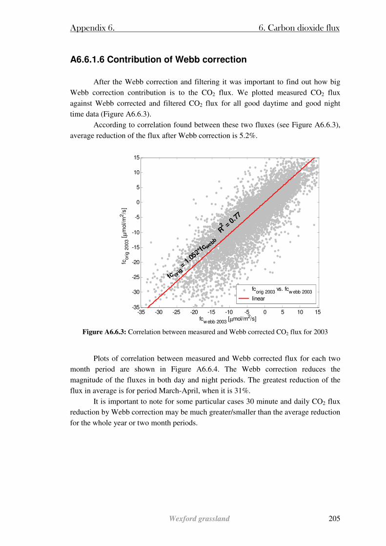
Appendix 6. 6. Carbon dioxide flux
Wexford grassland 205
A6.6.1.6 Contribution of Webb correction
After the Webb correction and filtering it was important to find out how big
Webb correction contribution is to the CO2 flux. We plotted measured CO2 flux
against Webb corrected and filtered CO2 flux for all good daytime and good night
time data (Figure A6.6.3).
According to correlation found between these two fluxes (see Figure A6.6.3),
average reduction of the flux after Webb correction is 5.2%.
-35 -30 -25 -20 -15 -10 -5 0 5 10 15-35
-30
-25
-20
-15
-10
-5
0
5
10
15
fcorig
2003
vs. fcwebb
2003
linear
fc orig =
1.0
52*fcw
ebb
R2 =
0.7
7
fcwebb
2003
[µmol/m2/s]
fcorig 2
003 [
µm
ol/m
2/s
]
Figure A6.6.3: Correlation between measured and Webb corrected CO2 flux for 2003
Plots of correlation between measured and Webb corrected flux for each two
month period are shown in Figure A6.6.4. The Webb correction reduces the
magnitude of the fluxes in both day and night periods. The greatest reduction of the
flux in average is for period March-April, when it is 31%.
It is important to note for some particular cases 30 minute and daily CO2 flux
reduction by Webb correction may be much greater/smaller than the average reduction
for the whole year or two month periods.
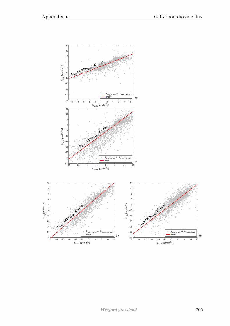
Appendix 6. 6. Carbon dioxide flux
Wexford grassland 206
-14 -12 -10 -8 -6 -4 -2 0 2 4 6-35
-30
-25
-20
-15
-10
-5
0
5
10
15
fcw ebb
[µmol/m2/s]
fco
rig [
µm
ol/m
2/s
]
fcorig
jan-feb
vs. fcw ebb
jan-feb
linear
fcorig = 1.047*fcwebb
R2 = 0.80
(a)
-25 -20 -15 -10 -5 0 5 10-35
-30
-25
-20
-15
-10
-5
0
5
10
15
fcwebb
[µmol/m2/s]
fcorig [
µm
ol/m
2/s
]
fcorig
mar-apr
vs. fcwebb
mar-apr
linear
fc orig = 1.31
*fcwebb
R2 = 0.76
(b)
-35 -30 -25 -20 -15 -10 -5 0 5 10 15-35
-30
-25
-20
-15
-10
-5
0
5
10
15
fcw ebb
[µmol/m2/s]
fcorig [
µm
ol/m
2/s
]
fcorig
may-jun
vs. fcwebb
may-jun
linear
fc orig =
1.0
3*fcw
ebb
R2 =
0.8
5
(c)
-35 -30 -25 -20 -15 -10 -5 0 5 10 15
-35
-30
-25
-20
-15
-10
-5
0
5
10
15
fcwebb
[µmol/m2/s]
fcori
g [
µm
ol/m
2/s
]
fcorig
jul-aug
vs. fcw ebb
jul-aug
linear
fc orig =
0.91*fcw
ebb
R2 =
0.83
(d)
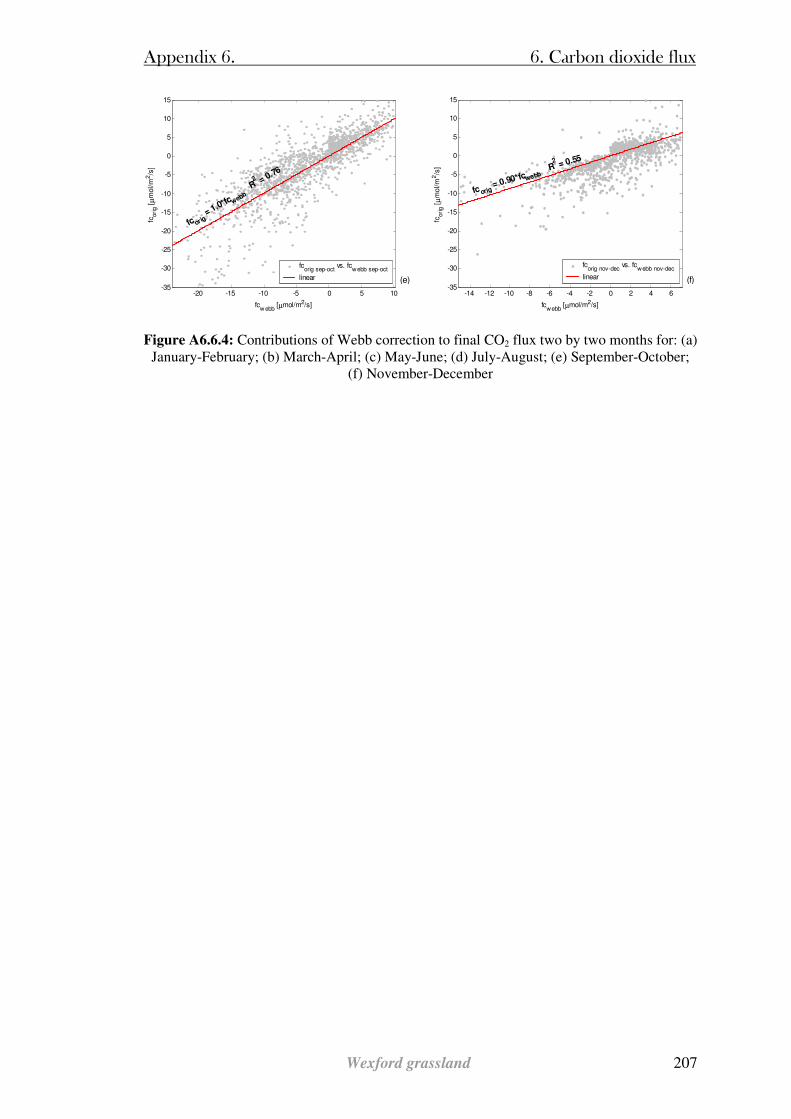
Appendix 6. 6. Carbon dioxide flux
Wexford grassland 207
-20 -15 -10 -5 0 5 10-35
-30
-25
-20
-15
-10
-5
0
5
10
15
fcw ebb
[µmol/m2/s]
fcori
g [
µm
ol/m
2/s
]
fcorig
sep-oct
vs. fcwebb
sep-oct
linear
fc orig = 1.0*fcwebb
R2 = 0.76
(e)
-14 -12 -10 -8 -6 -4 -2 0 2 4 6
-35
-30
-25
-20
-15
-10
-5
0
5
10
15
fcwebb
[µmol/m2/s]
fcori
g [
µm
ol/m
2/s
]
fcorig
nov-dec
vs. fcwebb
nov-dec
linear
fcorig = 0.90*fcwebb
R2 = 0.55
(f)
Figure A6.6.4: Contributions of Webb correction to final CO2 flux two by two months for: (a)
January-February; (b) March-April; (c) May-June; (d) July-August; (e) September-October; (f) November-December
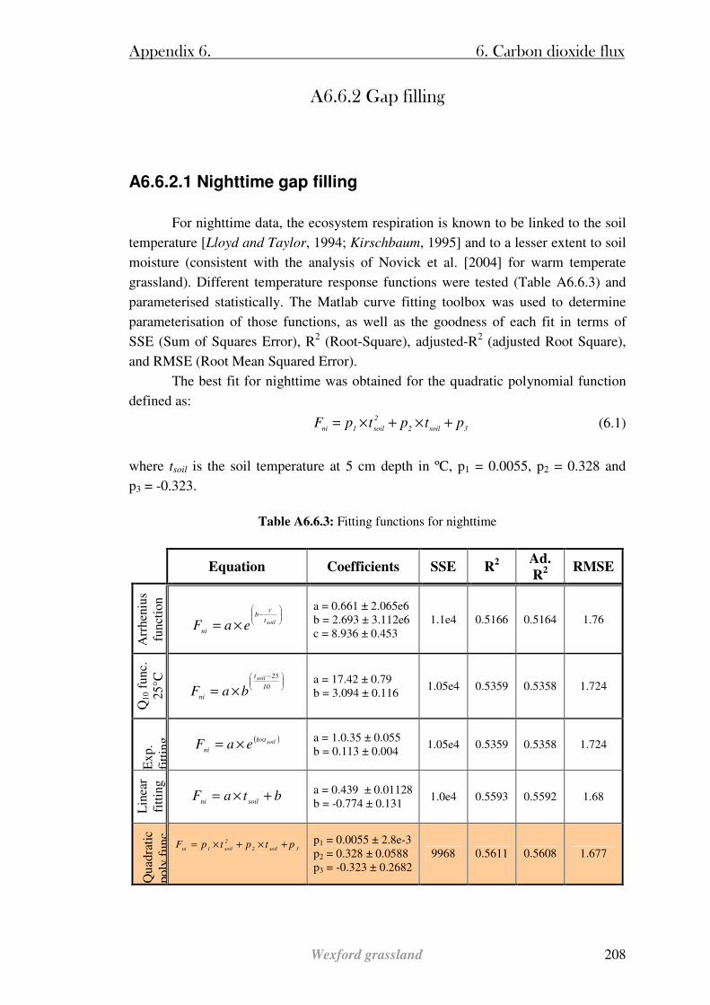
Appendix 6. 6. Carbon dioxide flux
Wexford grassland 208
A6.6.2 Gap filling
A6.6.2.1 Nighttime gap filling
For nighttime data, the ecosystem respiration is known to be linked to the soil
temperature [Lloyd and Taylor, 1994; Kirschbaum, 1995] and to a lesser extent to soil
moisture (consistent with the analysis of Novick et al. [2004] for warm temperate
grassland). Different temperature response functions were tested (Table A6.6.3) and
parameterised statistically. The Matlab curve fitting toolbox was used to determine
parameterisation of those functions, as well as the goodness of each fit in terms of
SSE (Sum of Squares Error), R2 (Root-Square), adjusted-R2 (adjusted Root Square),
and RMSE (Root Mean Squared Error).
The best fit for nighttime was obtained for the quadratic polynomial function
defined as:
3soil2
2
soil1niptptpF +×+×= (6.1)
where tsoil is the soil temperature at 5 cm depth in ºC, p1 = 0.0055, p2 = 0.328 and
p3 = -0.323.
Table A6.6.3: Fitting functions for nighttime
Equation Coefficients SSE R2
Ad.
R2 RMSE
Arr
heni
us
func
tion
−
×= soilt
cb
nieaF
a = 0.661 ± 2.065e6 b = 2.693 ± 3.112e6 c = 8.936 ± 0.453
1.1e4 0.5166 0.5164 1.76
Q10
fun
c.
25°C
−
×= 10
25t
ni
soil
baF a = 17.42 ± 0.79 b = 3.094 ± 0.116
1.05e4 0.5359 0.5358 1.724
Exp
. fi
ttin
g ( )soiltb
nieaF
××= a = 1.0.35 ± 0.055 b = 0.113 ± 0.004
1.05e4 0.5359 0.5358 1.724
Lin
ear
fitt
ing
btaFsoilni
+×= a = 0.439 ± 0.01128 b = -0.774 ± 0.131
1.0e4 0.5593 0.5592 1.68
Qua
drat
ic
poly
fun
c.
3soil2
2
soil1niptptpF +×+×=
p1 = 0.0055 ± 2.8e-3 p2 = 0.328 ± 0.0588 p3 = -0.323 ± 0.2682
9968 0.5611 0.5608 1.677
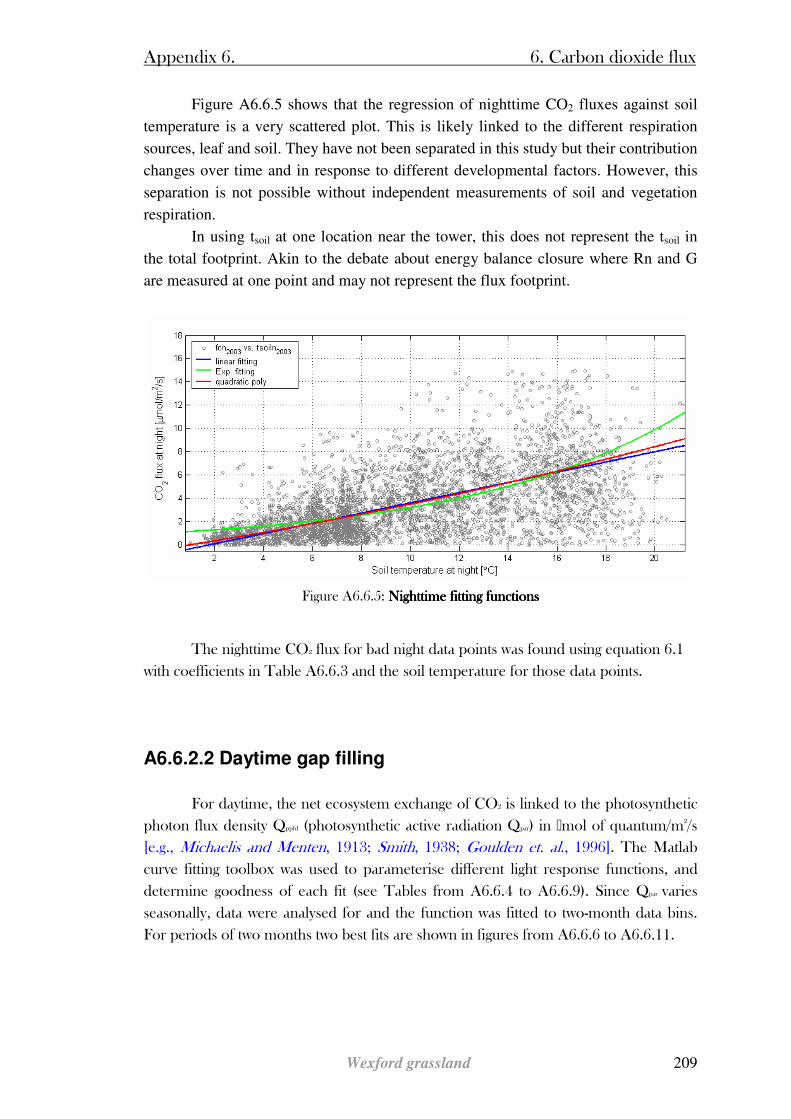
Appendix 6. 6. Carbon dioxide flux
Wexford grassland 209
Figure A6.6.5 shows that the regression of nighttime CO2 fluxes against soil
temperature is a very scattered plot. This is likely linked to the different respiration
sources, leaf and soil. They have not been separated in this study but their contribution
changes over time and in response to different developmental factors. However, this
separation is not possible without independent measurements of soil and vegetation
respiration.
In using tsoil at one location near the tower, this does not represent the tsoil in
the total footprint. Akin to the debate about energy balance closure where Rn and G
are measured at one point and may not represent the flux footprint.
Figure A6.6.5: Nighttime fitting functions Nighttime fitting functions Nighttime fitting functions Nighttime fitting functions
The nighttime CO2 flux for bad night data points was found using equation 6.1
with coefficients in Table A6.6.3 and the soil temperature for those data points.
A6.6.2.2 Daytime gap filling
For daytime, the net ecosystem exchange of CO2 is linked to the photosynthetic
photon flux density Qppfd (photosynthetic active radiation Qpar) in Mmol of quantum/m2/s
[e.g., Michaelis and Menten, 1913; Smith, 1938; Goulden et. al., 1996]. The Matlab curve fitting toolbox was used to parameterise different light response functions, and
determine goodness of each fit (see Tables from A6.6.4 to A6.6.9). Since Qpar varies
seasonally, data were analysed for and the function was fitted to two-month data bins.
For periods of two months two best fits are shown in figures from A6.6.6 to A6.6.11.

Appendix 6. 6. Carbon dioxide flux
Wexford grassland 210
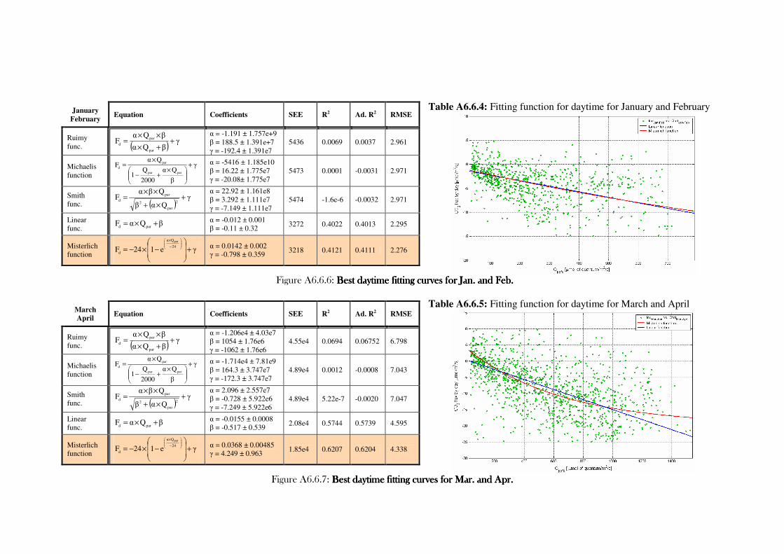
Table A6.6.4: Fitting function for daytime for January and February
Figure A6.6.6: Best daytime fitting curves for Jan. and Feb. Best daytime fitting curves for Jan. and Feb. Best daytime fitting curves for Jan. and Feb. Best daytime fitting curves for Jan. and Feb.
Table A6.6.5: Fitting function for daytime for March and April
Figure A6.6.7: Best daytime fitting curves for Mar. and Apr. Best daytime fitting curves for Mar. and Apr. Best daytime fitting curves for Mar. and Apr. Best daytime fitting curves for Mar. and Apr.
January
February Equation Coefficients SEE R2 Ad. R2 RMSE
Ruimy func. ( )
γβQα
βQαF
par
par
d ++×
××=
α = -1.191 ± 1.757e+9 β = 188.5 ± 1.391e+7 γ = -192.4 ± 1.391e7
5436 0.0069 0.0037 2.961
Michaelis function
γ
β
Qα
2000
Q1
QαF
parpar
par
d +
×+−
×=
α = -5416 ± 1.185e10 β = 16.22 ± 1.775e7 γ = -20.08± 1.775e7
5473 0.0001 -0.0031 2.971
Smith func. ( )
γQαβ
QβαF
2
par
2
par
d +×+
××=
α = 22.92 ± 1.161e8 β = 3.292 ± 1.111e7 γ = -7.149 ± 1.111e7
5474 -1.6e-6 -0.0032 2.971
Linear func.
βQαF pard +×= α = -0.012 ± 0.001 β = -0.11 ± 0.32
3272 0.4022 0.4013 2.295
Misterlich function
γe124F24
Qα
d
par
+
−×−=
−
×
α = 0.0142 ± 0.002 γ = -0.798 ± 0.359
3218 0.4121 0.4111 2.276
March April
Equation Coefficients SEE R2 Ad. R2 RMSE
Ruimy func. ( )
γβQα
βQαF
par
par
d ++×
××=
α = -1.206e4 ± 4.03e7 β = 1054 ± 1.76e6 γ = -1062 ± 1.76e6
4.55e4 0.0694 0.06752 6.798
Michaelis function
γ
β
Qα
2000
Q1
QαF
parpar
par
d +
×+−
×=
α = -1.714e4 ± 7.81e9 β = 164.3 ± 3.747e7 γ = -172.3 ± 3.747e7
4.89e4 0.0012 -0.0008 7.043
Smith func. ( )
γQαβ
QβαF
2
par
2
par
d +×+
××=
α = 2.096 ± 2.557e7 β = -0.728 ± 5.922e6 γ = -7.249 ± 5.922e6
4.89e4 5.22e-7 -0.0020 7.047
Linear func.
βQαF pard +×= α = -0.0155 ± 0.0008 β = -0.517 ± 0.539
2.08e4 0.5744 0.5739 4.595
Misterlich function
γe124F24
Qα
d
par
+
−×−=
−
×
α = 0.0368 ± 0.00485 γ = 4.249 ± 0.963
1.85e4 0.6207 0.6204 4.338
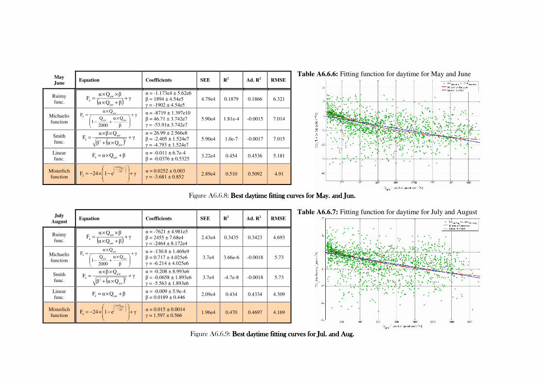
Table A6.6.6: Fitting function for daytime for May and June
Figure A6.6.8: Best daytime fitting curves for May. and Jun. Best daytime fitting curves for May. and Jun. Best daytime fitting curves for May. and Jun. Best daytime fitting curves for May. and Jun.
Table A6.6.7: Fitting function for daytime for July and August
Figure A6.6.9: Best daytime fitting curves for Jul. and Aug. Best daytime fitting curves for Jul. and Aug. Best daytime fitting curves for Jul. and Aug. Best daytime fitting curves for Jul. and Aug.
May June
Equation Coefficients SEE R2 Ad. R2 RMSE
Ruimy func. ( )
γβQα
βQαF
par
par
d ++×
××=
α = -1.173e4 ± 5.62e6 β = 1894 ± 4.54e5 γ = -1902 ± 4.54e5
4.79e4 0.1879 0.1866 6.321
Michaelis function
γ
β
Qα
2000
Q1
QαF
parpar
par
d +
×+−
×=
α = -8719 ± 1.397e10 β = 46.71 ± 3.742e7 γ = -53.91± 3.742e7
5.90e4 1.81e-4 -0.0015 7.014
Smith func. ( )
γQαβ
QβαF
2
par
2
par
d +×+
××=
α = 26.99 ± 2.566e8 β = -2.405 ± 1.524e7 γ = -4.793 ± 1.524e7
5.90e4 1.0e-7 -0.0017 7.015
Linear func.
βQαF pard +×= α = -0.011 ± 6.7e-4 β = -0.0376 ± 0.5325
3.22e4 0.454 0.4536 5.181
Misterlich function
γe124F24
Qα
d
par
+
−×−=
−
×
α = 0.0252 ± 0.003 γ = -3.681 ± 0.852
2.89e4 0.510 0.5092 4.91
July
August Equation Coefficients SEE R2 Ad. R2 RMSE
Ruimy func. ( )
γβQα
βQαF
par
par
d ++×
××=
α = -7621 ± 4.981e5 β = 2455 ± 7.68e4 γ = -2464 ± 8.172e4
2.43e4 0.3435 0.3423 4.693
Michaelis function
γ
β
Qα
2000
Q1
QαF
parpar
par
d +
×+−
×=
α = -130.8 ± 1.469e9 β = 0.717 ± 4.025e6 γ = -6.214 ± 4.025e6
3.7e4 3.66e-6 -0.0018 5.73
Smith func. ( )
γQαβ
QβαF
2
par
2
par
d +×+
××=
α = -0.208 ± 8.993e6 β = -0.0658 ± 1.893e6 γ = -5.563 ± 1.893e6
3.7e4 -4.7e-8 -0.0018 5.73
Linear func.
βQαF pard +×= α = -0.009 ± 5.9e-4 β = 0.0189 ± 0.446
2.09e4 0.434 0.4334 4.309
Misterlich function
γe124F24
Qα
d
par
+
−×−=
−
×
α = 0.015 ± 0.0014 γ = 1.597 ± 0.566
1.96e4 0.470 0.4697 4.169
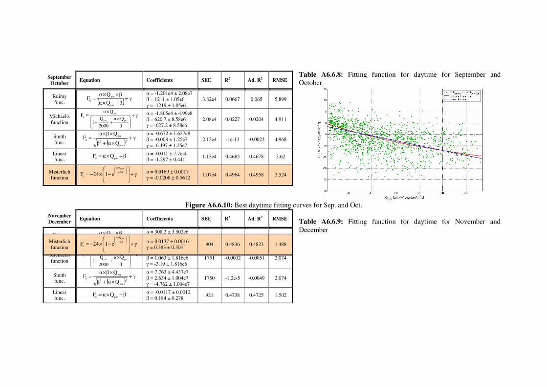
Table A6.6.8: Fitting function for daytime for September and October
Figure A6.6.10: Best daytime fitting curves for Sep. and Oct.
Table A6.6.9: Fitting function for daytime for November and December
September
October Equation Coefficients SEE R2 Ad. R2 RMSE
Ruimy func. ( )
γβQα
βQαF
par
par
d ++×
××=
α = -1.201e4 ± 2.08e7 β = 1211 ± 1.05e6 γ = -1219 ± 1.05e6
3.82e4 0.0667 0.065 5.899
Michaelis function
γ
β
Qα
2000
Q1
QαF
parpar
par
d +
×+−
×=
α = -1.805e4 ± 4.99e8 β = 620.7 ± 8.58e6 γ = -627.2 ± 8.58e6
2.08e4 0.0227 0.0204 4.911
Smith func. ( )
γQαβ
QβαF
2
par
2
par
d +×+
××=
α = -0.672 ± 1.637e8 β = -0.008 ± 1.25e7 γ = -6.497 ± 1.25e7
2.13e4 -1e-13 -0.0023 4.968
Linear func.
βQαF pard +×= α = -0.011 ± 7.7e-4 β = -1.297 ± 0.441
1.13e4 0.4685 0.4678 3.62
Misterlich function
γe124F24
Qα
d
par
+
−×−=
−
×
α = 0.0169 ± 0.0017 γ = -0.0208 ± 0.5612
1.07e4 0.4964 0.4958 3.524
November
December Equation Coefficients SEE R2 Ad. R2 RMSE
Ruimy func. ( )
γβQα
βQαF
par
par
d ++×
××=
α = 308.2 ± 3.502e6 β = 44.66 ± 2.534e5 γ = -46.74 ± 2.534e5
1793 -0.0242 -0.0292 2.099
Michaelis function
γ
β
Qα
2000
Q1
QαF
parpar
par
d +
×+−
×=
α = 20.59 ± 7.036e7 β = 1.063 ± 1.816e6 γ = -3.19 ± 1.816e6
1751 -0.0002 -0.0051 2.074
Smith func. ( )
γQαβ
QβαF
2
par
2
par
d +×+
××=
α = 7.763 ± 4.437e7 β = 2.634 ± 1.004e7 γ = -4.762 ± 1.004e7
1750 -1.2e-5 -0.0049 2.074
Linear func.
βQαF pard +×= α = -0.0117 ± 0.0012 β = 0.184 ± 0.278
921 0.4738 0.4725 1.502
Misterlich function
γe124F24
Qα
d
par
+
−×−=
−
×
α = 0.0137 ± 0.0016 γ = 0.383 ± 0.304
904 0.4836 0.4823 1.488
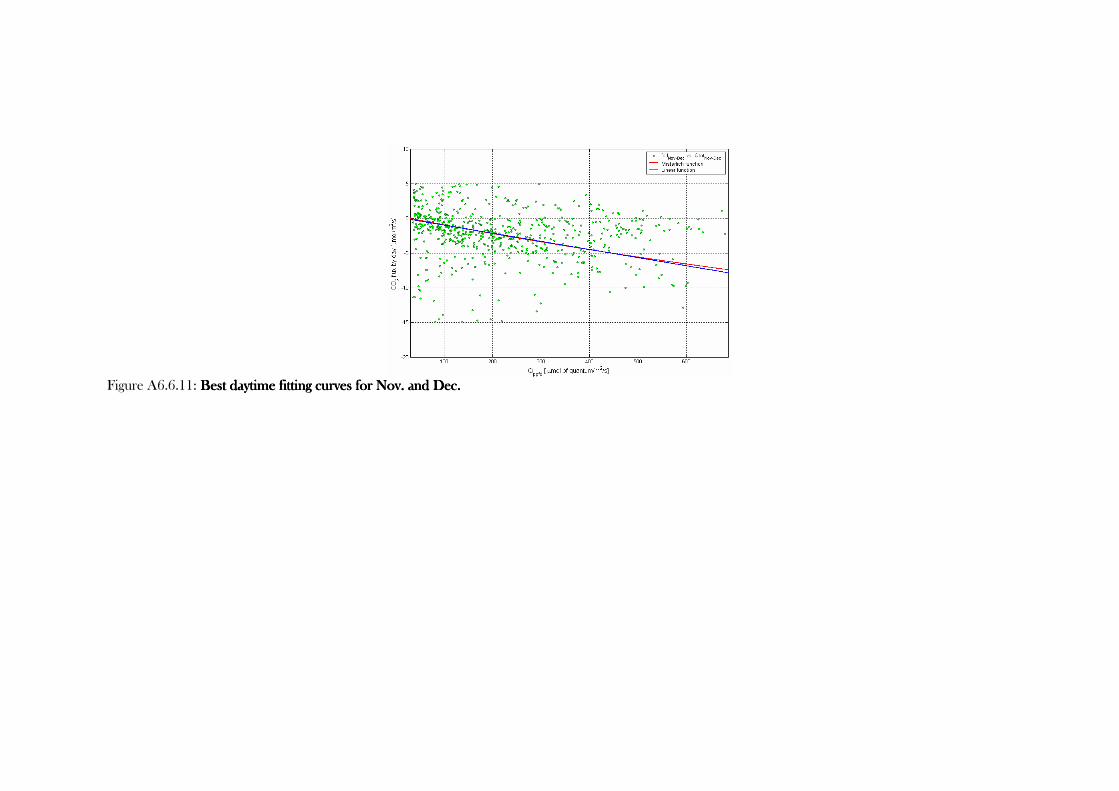
Figure A6.6.11: Best daytime fitting curves for Nov. and Dec. Best daytime fitting curves for Nov. and Dec. Best daytime fitting curves for Nov. and Dec. Best daytime fitting curves for Nov. and Dec.
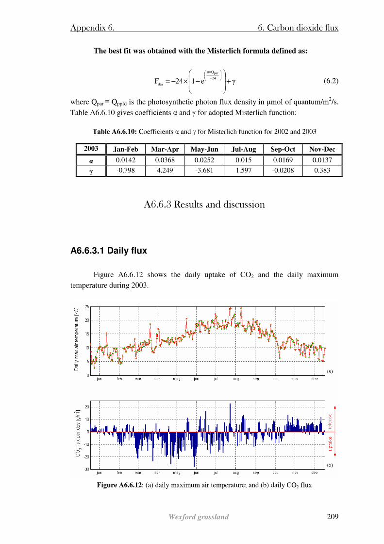
Appendix 6. 6. Carbon dioxide flux
Wexford grassland 209
The best fit was obtained with the Misterlich formula defined as:
γe124F24
Qα
day
par
+
−×−=
−
×
(6.2)
where Qpar ≡ Qppfd is the photosynthetic photon flux density in µmol of quantum/m2/s.
Table A6.6.10 gives coefficients α and γ for adopted Misterlich function:
Table A6.6.10: Coefficients α and γ for Misterlich function for 2002 and 2003
2003 Jan-Feb Mar-Apr May-Jun Jul-Aug Sep-Oct Nov-Dec
α 0.0142 0.0368 0.0252 0.015 0.0169 0.0137
γ -0.798 4.249 -3.681 1.597 -0.0208 0.383
A6.6.3 Results and discussion
A6.6.3.1 Daily flux
Figure A6.6.12 shows the daily uptake of CO2 and the daily maximum
temperature during 2003.
Figure A6.6.12: (a) daily maximum air temperature; and (b) daily CO2 flux
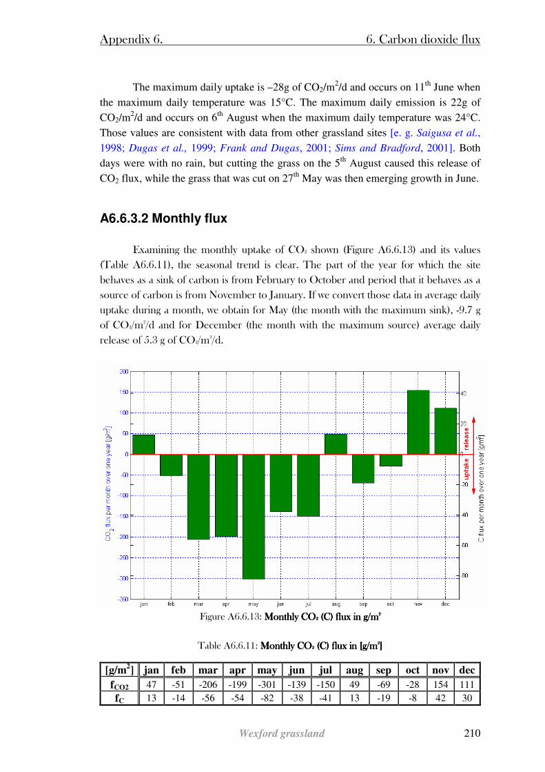
Appendix 6. 6. Carbon dioxide flux
Wexford grassland 210
The maximum daily uptake is –28g of CO2/m2/d and occurs on 11th June when
the maximum daily temperature was 15°C. The maximum daily emission is 22g of
CO2/m2/d and occurs on 6th August when the maximum daily temperature was 24°C.
Those values are consistent with data from other grassland sites [e. g. Saigusa et al.,
1998; Dugas et al., 1999; Frank and Dugas, 2001; Sims and Bradford, 2001]. Both
days were with no rain, but cutting the grass on the 5th August caused this release of
CO2 flux, while the grass that was cut on 27th May was then emerging growth in June.
A6.6.3.2 Monthly flux
Examining the monthly uptake of CO2 shown (Figure A6.6.13) and its values
(Table A6.6.11), the seasonal trend is clear. The part of the year for which the site
behaves as a sink of carbon is from February to October and period that it behaves as a
source of carbon is from November to January. If we convert those data in average daily
uptake during a month, we obtain for May (the month with the maximum sink), -9.7 g
of CO2/m2/d and for December (the month with the maximum source) average daily
release of 5.3 g of CO2/m2/d.
Figure A6.6.13: Monthly CO Monthly CO Monthly CO Monthly CO2222 (C) flux in g/m (C) flux in g/m (C) flux in g/m (C) flux in g/m2222
Table A6.6.11: Monthly CO Monthly CO Monthly CO Monthly CO2222 (C) flux in [g/m (C) flux in [g/m (C) flux in [g/m (C) flux in [g/m2222]]]]
[g/m2] jan feb mar apr may jun jul aug sep oct nov dec
fCO2 47 -51 -206 -199 -301 -139 -150 49 -69 -28 154 111
fC 13 -14 -56 -54 -82 -38 -41 13 -19 -8 42 30
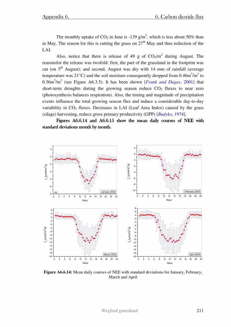
Appendix 6. 6. Carbon dioxide flux
Wexford grassland 211
The monthly uptake of CO2 in June is -139 g/m2, which is less about 50% than
in May. The reason for this is cutting the grass on 27th May and thus reduction of the
LAI.
Also, notice that there is release of 49 g of CO2/m2 during August. The
reasonsfor the release was twofold: first, the part of the grassland in the footprint was
cut (on 5th August); and second, August was dry with 14 mm of rainfall (average
temperature was 21°C) and the soil moisture consequently dropped from 0.46m3/m3 to
0.36m3/m3 (see Figure A6.3.5). It has been shown [Frank and Dugas, 2001] that
short-term droughts during the growing season reduce CO2 fluxes to near zero
(photosynthesis balances respiration). Also, the timing and magnitude of precipitation
events influence the total growing season flux and induce a considerable day-to-day
variability in CO2 fluxes. Decreases in LAI (Leaf Area Index) caused by the grass
(silage) harvesting, reduce gross primary productivity (GPP) [Budyko, 1974].
Figures A6.6.14 and A6.6.15 show the mean daily coursFigures A6.6.14 and A6.6.15 show the mean daily coursFigures A6.6.14 and A6.6.15 show the mean daily coursFigures A6.6.14 and A6.6.15 show the mean daily courses of NEE with es of NEE with es of NEE with es of NEE with
standard deviations month by month.standard deviations month by month.standard deviations month by month.standard deviations month by month.
0 2 4 6 8 10 12 14 16 18 20 22 24
-8
-6
-4
-2
0
2
4
f C [
µm
ol/m
2/s
]
Hour
January 2003(a)
0 2 4 6 8 10 12 14 16 18 20 22 24
-10
-8
-6
-4
-2
0
2
4
f C [
µm
ol/m
2/s
]
Hour
February 2003
0 2 4 6 8 10 12 14 16 18 20 22 24
-20
-18
-16
-14
-12
-10
-8
-6
-4
-2
0
2
4
6
f C [
µm
ol/m
2/s
]
Hour
March 2003
0 2 4 6 8 10 12 14 16 18 20 22 24
-20
-18
-16
-14
-12
-10
-8
-6
-4
-2
0
2
4
6
8
f C [
µm
ol/m
2/s
]
Hour
April 2003
Figure A6.6.14: Mean daily courses of NEE with standard deviations for January, February,
March and April
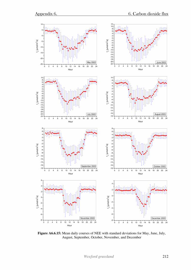
Appendix 6. 6. Carbon dioxide flux
Wexford grassland 212
0 2 4 6 8 10 12 14 16 18 20 22 24
-25
-20
-15
-10
-5
0
5
10
f C [
µm
ol/m
2/s
]
Hour
May 2003
0 2 4 6 8 10 12 14 16 18 20 22 24
-22
-20
-18
-16
-14
-12
-10
-8
-6
-4
-2
0
2
4
6
8
10
12
f C [
µm
ol/m
2/s
]
Hour
June 2003
0 2 4 6 8 10 12 14 16 18 20 22 24
-24
-22
-20
-18
-16
-14
-12
-10
-8
-6
-4
-2
0
2
4
6
8
10
f C [
µm
ol/m
2/s
]
Hour
July 2003
0 2 4 6 8 10 12 14 16 18 20 22 24
-18
-16
-14
-12
-10
-8
-6
-4
-2
0
2
4
6
8
10
f C [
µm
ol/m
2/s
]
Hour
August 2003
0 2 4 6 8 10 12 14 16 18 20 22 24
-18
-16
-14
-12
-10
-8
-6
-4
-2
0
2
4
6
8
f C [
µm
ol/m
2/s
]
Hour
September 2003
0 2 4 6 8 10 12 14 16 18 20 22 24
-18
-16
-14
-12
-10
-8
-6
-4
-2
0
2
4
6
8
f C [
µm
ol/m
2/s
]
Hour
October 2003
0 2 4 6 8 10 12 14 16 18 20 22 24
-8
-6
-4
-2
0
2
4
6
f C [
µm
ol/m
2/s
]
Hour
November 2003
0 2 4 6 8 10 12 14 16 18 20 22 24
-8
-6
-4
-2
0
2
4
f C [
µm
ol/m
2/s
]
Hour
December 2003
Figure A6.6.15: Mean daily courses of NEE with standard deviations for May, June, July, August, September, October, November, and December
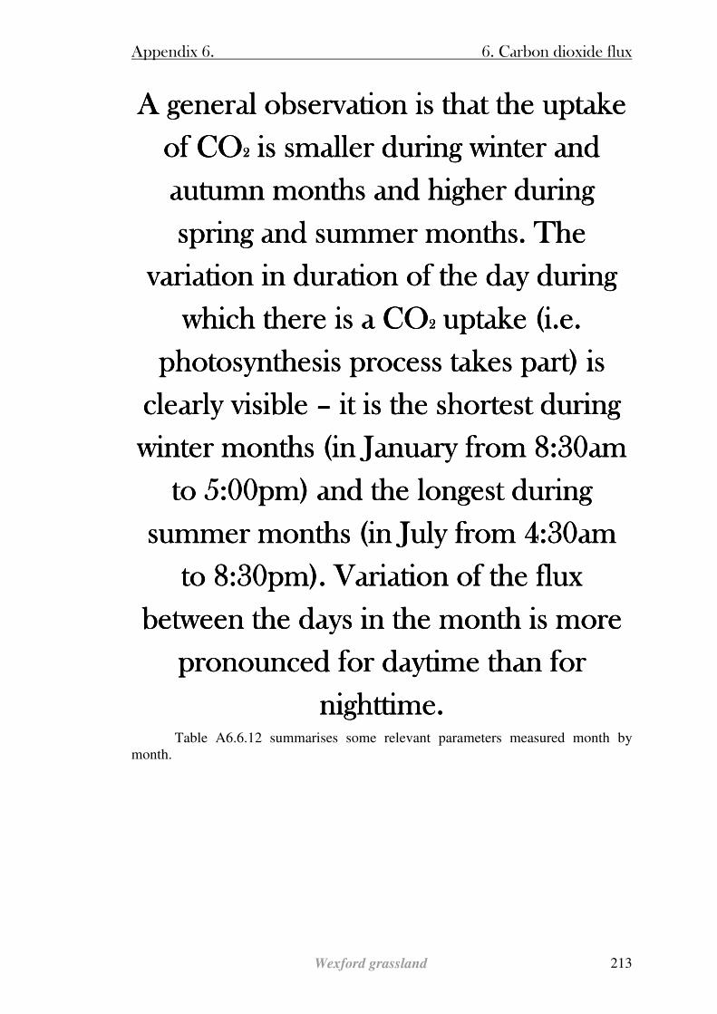
Appendix 6. 6. Carbon dioxide flux
Wexford grassland 213
A general observation is that the uptake A general observation is that the uptake A general observation is that the uptake A general observation is that the uptake
of COof COof COof CO2222 is smaller during winter and is smaller during winter and is smaller during winter and is smaller during winter and
autumn months and higher during autumn months and higher during autumn months and higher during autumn months and higher during
spring and summer monthspring and summer monthspring and summer monthspring and summer months. The s. The s. The s. The
variation in duration of the day during variation in duration of the day during variation in duration of the day during variation in duration of the day during
which there is a COwhich there is a COwhich there is a COwhich there is a CO2222 uptake (i.e. uptake (i.e. uptake (i.e. uptake (i.e.
photosynthesis process takes part) is photosynthesis process takes part) is photosynthesis process takes part) is photosynthesis process takes part) is
clearly visible clearly visible clearly visible clearly visible –––– it is the shortest during it is the shortest during it is the shortest during it is the shortest during
winter months (in January from 8:30am winter months (in January from 8:30am winter months (in January from 8:30am winter months (in January from 8:30am
to 5:00pm) and the longest during to 5:00pm) and the longest during to 5:00pm) and the longest during to 5:00pm) and the longest during
summer months (in Julsummer months (in Julsummer months (in Julsummer months (in July from 4:30am y from 4:30am y from 4:30am y from 4:30am
to 8:30pm). Variation of the flux to 8:30pm). Variation of the flux to 8:30pm). Variation of the flux to 8:30pm). Variation of the flux
between the days in the month is more between the days in the month is more between the days in the month is more between the days in the month is more
pronounced for daytime than for pronounced for daytime than for pronounced for daytime than for pronounced for daytime than for
nighttime. nighttime. nighttime. nighttime. Table A6.6.12 summarises some relevant parameters measured month by
month.
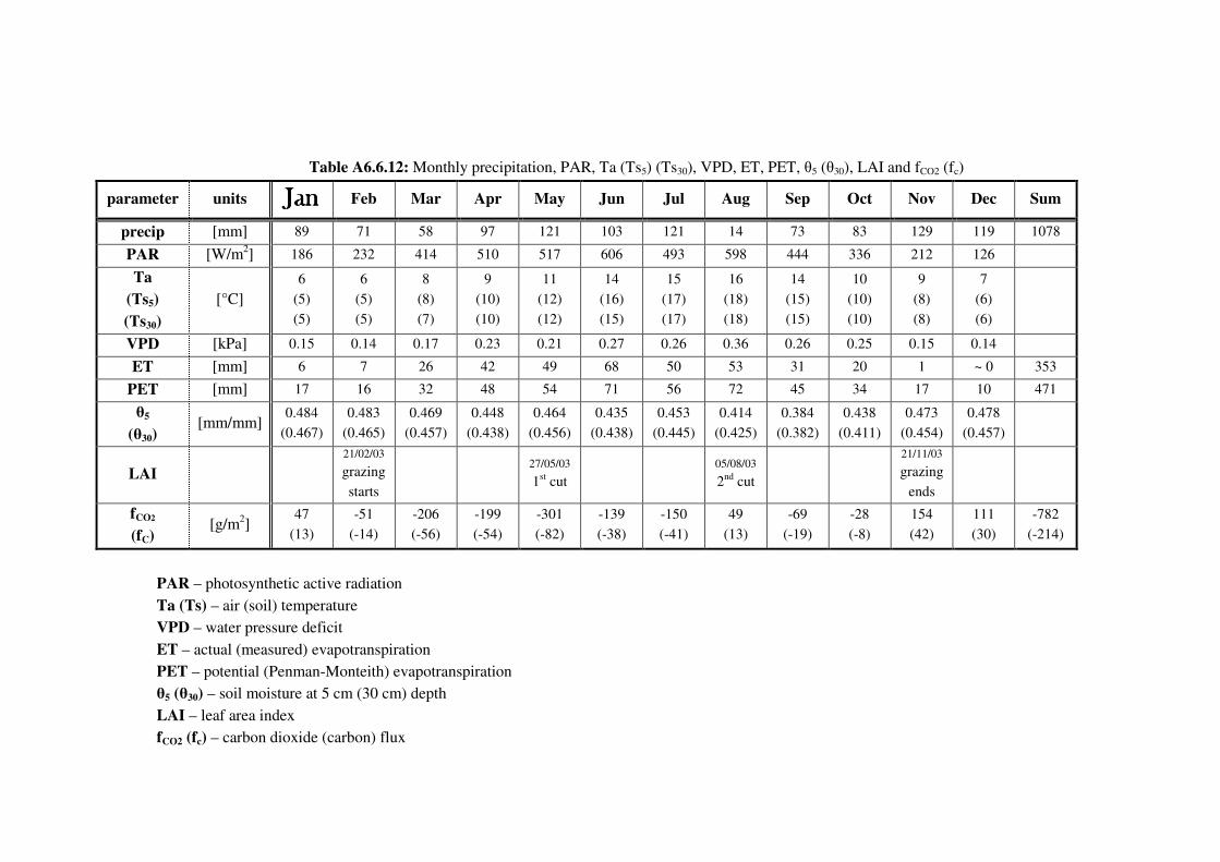
Table A6.6.12: Monthly precipitation, PAR, Ta (Ts5) (Ts30), VPD, ET, PET, θ5 (θ30), LAI and fCO2 (fc)
parameter units JanJanJanJan Feb Mar Apr May Jun Jul Aug Sep Oct Nov Dec Sum
precip [mm] 89 71 58 97 121 103 121 14 73 83 129 119 1078
PAR [W/m2] 186 232 414 510 517 606 493 598 444 336 212 126
Ta
(Ts5)
(Ts30)
[°C] 6
(5)
(5)
6
(5)
(5)
8
(8)
(7)
9
(10)
(10)
11
(12)
(12)
14
(16)
(15)
15
(17)
(17)
16
(18)
(18)
14
(15)
(15)
10
(10)
(10)
9
(8)
(8)
7
(6)
(6)
VPD [kPa] 0.15 0.14 0.17 0.23 0.21 0.27 0.26 0.36 0.26 0.25 0.15 0.14
ET [mm] 6 7 26 42 49 68 50 53 31 20 1 ~ 0 353
PET [mm] 17 16 32 48 54 71 56 72 45 34 17 10 471
θ5
(θ30) [mm/mm]
0.484
(0.467)
0.483
(0.465)
0.469
(0.457)
0.448
(0.438)
0.464
(0.456)
0.435
(0.438)
0.453
(0.445)
0.414
(0.425)
0.384
(0.382)
0.438
(0.411)
0.473
(0.454)
0.478
(0.457)
LAI
21/02/03
grazing
starts
27/05/03
1st cut
05/08/03
2nd cut
21/11/03
grazing
ends
fCO2
(fC) [g/m2]
47
(13)
-51
(-14)
-206
(-56)
-199
(-54)
-301
(-82)
-139
(-38)
-150
(-41)
49
(13)
-69
(-19)
-28
(-8)
154
(42)
111
(30)
-782
(-214)
PAR – photosynthetic active radiation
Ta (Ts) – air (soil) temperature
VPD – water pressure deficit
ET – actual (measured) evapotranspiration
PET – potential (Penman-Monteith) evapotranspiration
θ5 (θ30) – soil moisture at 5 cm (30 cm) depth
LAI – leaf area index
fCO2 (fc) – carbon dioxide (carbon) flux
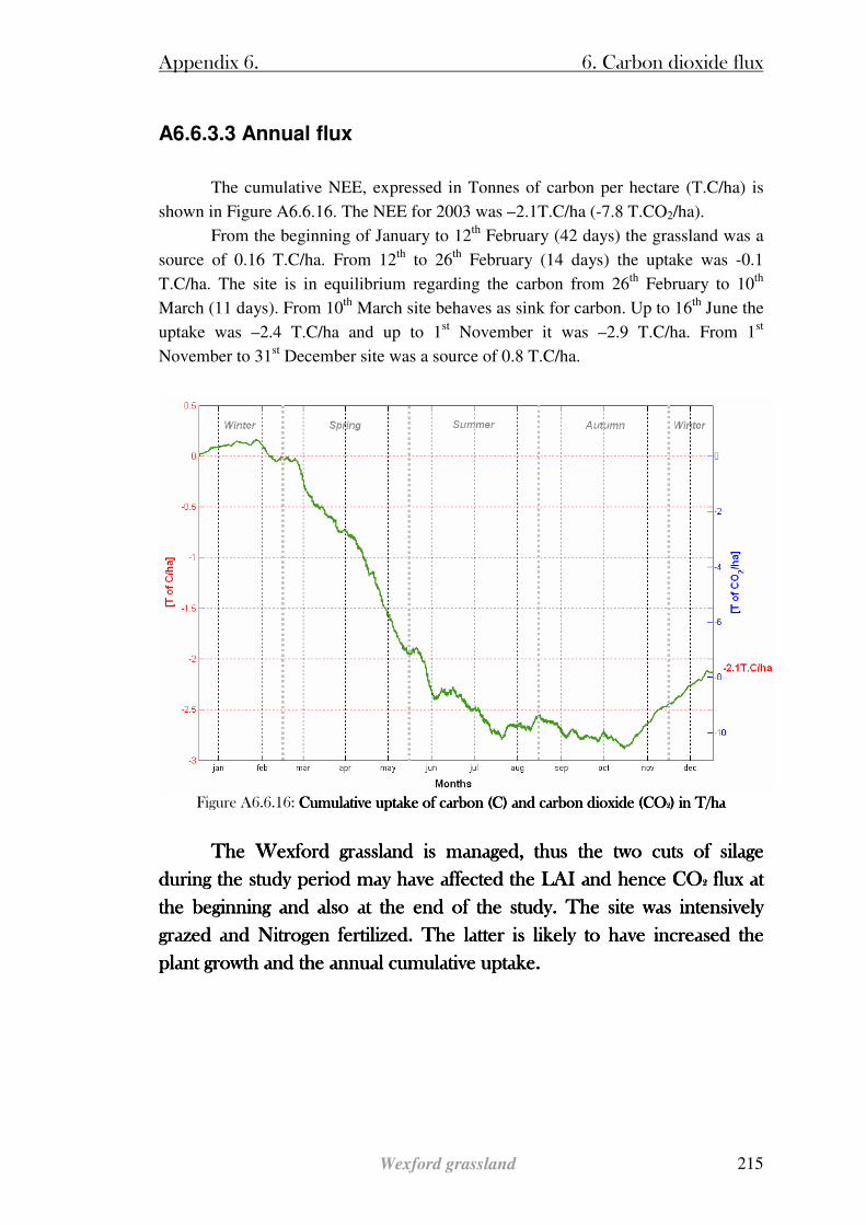
Appendix 6. 6. Carbon dioxide flux
Wexford grassland 215
A6.6.3.3 Annual flux
The cumulative NEE, expressed in Tonnes of carbon per hectare (T.C/ha) is
shown in Figure A6.6.16. The NEE for 2003 was –2.1T.C/ha (-7.8 T.CO2/ha).
From the beginning of January to 12th February (42 days) the grassland was a
source of 0.16 T.C/ha. From 12th to 26th February (14 days) the uptake was -0.1
T.C/ha. The site is in equilibrium regarding the carbon from 26th February to 10th
March (11 days). From 10th March site behaves as sink for carbon. Up to 16th June the
uptake was –2.4 T.C/ha and up to 1st November it was –2.9 T.C/ha. From 1st
November to 31st December site was a source of 0.8 T.C/ha.
Figure A6.6.16: CumulativCumulativCumulativCumulative uptake of carbon (C) and carbon dioxide (COe uptake of carbon (C) and carbon dioxide (COe uptake of carbon (C) and carbon dioxide (COe uptake of carbon (C) and carbon dioxide (CO2222) in T/ha) in T/ha) in T/ha) in T/ha
The Wexford grassland is managed, thus the two cuts of silage The Wexford grassland is managed, thus the two cuts of silage The Wexford grassland is managed, thus the two cuts of silage The Wexford grassland is managed, thus the two cuts of silage
during the study period may have affected the LAI and hence COduring the study period may have affected the LAI and hence COduring the study period may have affected the LAI and hence COduring the study period may have affected the LAI and hence CO2222 flux at flux at flux at flux at
the beginning and also at the end of the study. The site was inthe beginning and also at the end of the study. The site was inthe beginning and also at the end of the study. The site was inthe beginning and also at the end of the study. The site was intensively tensively tensively tensively
grazed and Nitrogen fertilized. The latter is likely to have increased the grazed and Nitrogen fertilized. The latter is likely to have increased the grazed and Nitrogen fertilized. The latter is likely to have increased the grazed and Nitrogen fertilized. The latter is likely to have increased the
plant growth and the annual cumulative uptake.plant growth and the annual cumulative uptake.plant growth and the annual cumulative uptake.plant growth and the annual cumulative uptake.
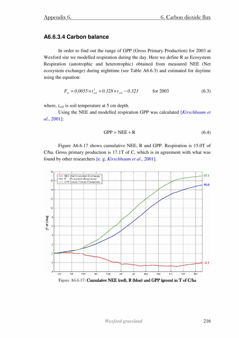
Appendix 6. 6. Carbon dioxide flux
Wexford grassland 216
A6.6.3.4 Carbon balance
In order to find out the range of GPP (Gross Primary Production) for 2003 at
Wexford site we modelled respiration during the day. Here we define R as Ecosystem
Respiration (autotrophic and heterotrophic) obtained from measured NEE (Net
ecosystem exchange) during nighttime (see Table A6.6.3) and estimated for daytime
using the equation:
323.0t328.0t0055.0Fsoil
2
soilni−×+×= for 2003 (6.3)
where, tsoil is soil temperature at 5 cm depth.
Using the NEE and modelled respiration GPP was calculated [Kirschbaum et
al., 2001]:
RNEEGPP += (6.4)
Figure A6.6.17 shows cumulative NEE, R and GPP. Respiration is 15.0T of
C/ha. Gross primary production is 17.1T of C, which is in agreement with what was
found by other researchers [e. g. Kirschbaum et al., 2001].
Figure A6.6.17: Cumulative NEE (red), R (blue) and GPP (green) in T of C/ha Cumulative NEE (red), R (blue) and GPP (green) in T of C/ha Cumulative NEE (red), R (blue) and GPP (green) in T of C/ha Cumulative NEE (red), R (blue) and GPP (green) in T of C/ha
Appendix 6 References
217
A6. References
Albertson, J. D., and G. Kiely, On the structure of soil moisture time series in the context of
land surface models, Journal of Hydrology, 243, 101-119, 2001.
Baldocchi, D.D., Assessing the eddy covariance technique for evaluating carbon dioxide
exchange rates of ecosystems: past, present and future, Global Change Biol., 9, 479-
492, 2003.
Brutsaert, W., Evaporation into the atmosphere, edited by A. J. Davenport, B. B. Hicks, G. R.
Hilst, R. E. Munn, J. D. Smith, Kluwer Academic Publishers, London, 1991.
Budyko, I. M., Climate and Life, Climatic factors of Photosynthesis, 497, Academic Press
INC, London, 1974.
Campbell, S. G., and J. M. Norman, An introduction to environmental Biophysics, second
edition, Springer-Verlag New York, 1998.
Dugas, W.A., M.L. Heuer, and H.S. Mayeux, Carbon dioxide fluxes over a Bermuda grass,
native prairie, and sorghum. Agric. For. Meteorol. 93,121-139, 1999.
FAO, Crop evapotranspiration – Guidelines for computing crop water requirements – FAO
Irrigation and drainage paper 56, Food and Agriculture Organisation of the United
Nations, Rome, 1998.
Falge, E., D. Baldocchi, R. Olson, P. Athoni, M. Aubinet, C. Bernhofer, G. Burba, R. Falge, E., D. Baldocchi, R. Olson, P. Athoni, M. Aubinet, C. Bernhofer, G. Burba, R. Falge, E., D. Baldocchi, R. Olson, P. Athoni, M. Aubinet, C. Bernhofer, G. Burba, R. Falge, E., D. Baldocchi, R. Olson, P. Athoni, M. Aubinet, C. Bernhofer, G. Burba, R.
Ceulemans, R. CleCeulemans, R. CleCeulemans, R. CleCeulemans, R. Clement, H. Dolman, A. Granier, P. Gross, T. Grünward, D. Hollinger, ment, H. Dolman, A. Granier, P. Gross, T. Grünward, D. Hollinger, ment, H. Dolman, A. Granier, P. Gross, T. Grünward, D. Hollinger, ment, H. Dolman, A. Granier, P. Gross, T. Grünward, D. Hollinger,
NNNN----O. Jensen, G. Katul, P. Keronen, A. Kowalski, C. T. Lai, B. E. Law, T. Meyers, J. O. Jensen, G. Katul, P. Keronen, A. Kowalski, C. T. Lai, B. E. Law, T. Meyers, J. O. Jensen, G. Katul, P. Keronen, A. Kowalski, C. T. Lai, B. E. Law, T. Meyers, J. O. Jensen, G. Katul, P. Keronen, A. Kowalski, C. T. Lai, B. E. Law, T. Meyers, J.
Moncrieff, E. Moors, J. W. Munger, K. Pilegaard, Ü. Rannik, C. Rebmann, A. Suyker, J. Moncrieff, E. Moors, J. W. Munger, K. Pilegaard, Ü. Rannik, C. Rebmann, A. Suyker, J. Moncrieff, E. Moors, J. W. Munger, K. Pilegaard, Ü. Rannik, C. Rebmann, A. Suyker, J. Moncrieff, E. Moors, J. W. Munger, K. Pilegaard, Ü. Rannik, C. Rebmann, A. Suyker, J.
Tenhunen, K. Tu, S. Tenhunen, K. Tu, S. Tenhunen, K. Tu, S. Tenhunen, K. Tu, S. Verma, T. Vesala, K. Wilson, and S. Wofsy, Gap filling strategies Verma, T. Vesala, K. Wilson, and S. Wofsy, Gap filling strategies Verma, T. Vesala, K. Wilson, and S. Wofsy, Gap filling strategies Verma, T. Vesala, K. Wilson, and S. Wofsy, Gap filling strategies
for defensible annual sums of net ecosystem exchange, for defensible annual sums of net ecosystem exchange, for defensible annual sums of net ecosystem exchange, for defensible annual sums of net ecosystem exchange, Agric. For. Meteorol., 107Agric. For. Meteorol., 107Agric. For. Meteorol., 107Agric. For. Meteorol., 107, 43, 43, 43, 43----69, 69, 69, 69,
2001.2001.2001.2001.
Frank, B. A., and Dugas, A. W., Carbon dioxide fluxes over northern, semiarid, mixed-grass
prairie, Agric. For. Meteorol., 108, 317-326, 2001.
Garatt, R. J., The atmospheric boundary layer, Edited by J. T. Houghton, M. J. Rycroft, A. J.
Dessler, Cambridge University Press, 1992.
Gash, J. H. C., A note on estimating the effect of a limited fetch on on micrometeorological
evaporation measurements. Boundary-Layer Meteor., 35, 409-413, 1986.
Gash, J. H. C., F. Valente, and J. S. David, Estimates and measurements of evaporation from
wet, sparse pine forest in Portugal, Agric. For. Meteorol., 94, 149-158, 1999.
Appendix 6 References
218
Goulden, M.L., J.W., Munger, S.M., Fan, B.C., Daube, and S.C., Wofsy, Measurements of
carbon sequestration by long-term eddy covariance: methods and critical evaluation of
accuracy, Global Change Biol., 2, Pages 196-182, 1996.
Horst, T. W., and J. C. Weil, How far is far enough? The fetch requirements for
micrometeorological measurement of surface fluxes, J.Atmos Oceanic Technol, 12, 447,
1995.
Hsieh, C-I., G. G. Katul, J. Schieldge, J. T. Sigmon, and K. K. Knoerr, The Lagrangian
stochastic model for fetch and latent heat flux estimation above uniform and
nonuniform terrain, Water Resources Res., 33, No. 3, 427-438, 1997.
Hsieh, C-I., G. G. Katul, and T-W. Chi, An approximate analytical model for footprint
estimation of scalar fluxes in thermally stratified atmospheric flows, Advances in Water
Resources, 23, 765-772, 2000.
Kirschbaum, U. F. M., The temperature dependence of soil organic matter decomposition, and
the effect of global warming on soil organic C storage, Soil Biol. Biochem, 27 (D6),
753-760, 1995.
Kirschbaum, M. U. F., D. Eamus, R. M. Gifford, S. H Roxburgh,. and P. J. Sands, Definitions
of some ecological terms commonly used in carbon accounting. Net Ecosystem
Exchange, edited by Kirschbaum, M.U.F. and Mueller, R, Cooperative Research Centre
for Greenhouse Accounting, Canberra, pp. 2-5, 2001.
http://www.ffp.csiro.au/nfm/staff/kirschbaum/definitions.pdf
Law, E. B., E. Falge, L. Gu, D. D. Baldocchi, P. Bakwin, P. Berbigier, K. Davis, A. J. Dolman, Law, E. B., E. Falge, L. Gu, D. D. Baldocchi, P. Bakwin, P. Berbigier, K. Davis, A. J. Dolman, Law, E. B., E. Falge, L. Gu, D. D. Baldocchi, P. Bakwin, P. Berbigier, K. Davis, A. J. Dolman, Law, E. B., E. Falge, L. Gu, D. D. Baldocchi, P. Bakwin, P. Berbigier, K. Davis, A. J. Dolman,
M. Falk, J. D. Fuentes, A. GoldsteinM. Falk, J. D. Fuentes, A. GoldsteinM. Falk, J. D. Fuentes, A. GoldsteinM. Falk, J. D. Fuentes, A. Goldstein, A. Granier, A. Grelle, D. Hollinger, I. A. Janssens, , A. Granier, A. Grelle, D. Hollinger, I. A. Janssens, , A. Granier, A. Grelle, D. Hollinger, I. A. Janssens, , A. Granier, A. Grelle, D. Hollinger, I. A. Janssens,
P. Jarvis, N. O. Jansen, G. Katul, Y. Mahli, G. Matteucci, T. Meyers, R. Monson, W. P. Jarvis, N. O. Jansen, G. Katul, Y. Mahli, G. Matteucci, T. Meyers, R. Monson, W. P. Jarvis, N. O. Jansen, G. Katul, Y. Mahli, G. Matteucci, T. Meyers, R. Monson, W. P. Jarvis, N. O. Jansen, G. Katul, Y. Mahli, G. Matteucci, T. Meyers, R. Monson, W.
Munger, W. Oechel, R. Olson, K. Pilegaard, K. T. Paw U, H. Thorgeirsson, R. Munger, W. Oechel, R. Olson, K. Pilegaard, K. T. Paw U, H. Thorgeirsson, R. Munger, W. Oechel, R. Olson, K. Pilegaard, K. T. Paw U, H. Thorgeirsson, R. Munger, W. Oechel, R. Olson, K. Pilegaard, K. T. Paw U, H. Thorgeirsson, R.
Valentini, S. Verma, T. Vesala, K. WilsonValentini, S. Verma, T. Vesala, K. WilsonValentini, S. Verma, T. Vesala, K. WilsonValentini, S. Verma, T. Vesala, K. Wilson, and S. Wofsy, Environmental controls over , and S. Wofsy, Environmental controls over , and S. Wofsy, Environmental controls over , and S. Wofsy, Environmental controls over
carbon dioxide and water vapor exchange of terrestrial vegetation,carbon dioxide and water vapor exchange of terrestrial vegetation,carbon dioxide and water vapor exchange of terrestrial vegetation,carbon dioxide and water vapor exchange of terrestrial vegetation, Agric. For. Meteorol., Agric. For. Meteorol., Agric. For. Meteorol., Agric. For. Meteorol., 113113113113, 97, 97, 97, 97----120, 2002.120, 2002.120, 2002.120, 2002.
Leclerc, M. Y., and G. W. Thurtell, Footprint prediction of scalar fluxes using a Markovian
analysis, Boundary-Layer Meteorology, 52, 247-258, 1990.
Lloyd, J., and J.A Taylor, On the temperature dependence of soil respiration. Lloyd, J., and J.A Taylor, On the temperature dependence of soil respiration. Lloyd, J., and J.A Taylor, On the temperature dependence of soil respiration. Lloyd, J., and J.A Taylor, On the temperature dependence of soil respiration. Funct. Ecol. 8Funct. Ecol. 8Funct. Ecol. 8Funct. Ecol. 8, , , , 315315315315––––323, 1994.323, 1994.323, 1994.323, 1994.
McMillen, R. T., An eddy correlation technique with extended applicability to non-simple
terrain, Boundary Layer Meteorology, 43, 231-245, 1988.
Michaelis, L., and M. L. Menten, Die Kinetik der Invertinwirkung, Michaelis, L., and M. L. Menten, Die Kinetik der Invertinwirkung, Michaelis, L., and M. L. Menten, Die Kinetik der Invertinwirkung, Michaelis, L., and M. L. Menten, Die Kinetik der Invertinwirkung, Biochem. Z. 49Biochem. Z. 49Biochem. Z. 49Biochem. Z. 49, 333, 1913., 333, 1913., 333, 1913., 333, 1913.
Appendix 6 References
219
Moncrieff, J.B., J. M. Massheder, H. de Bruin, J. Elbers, T. Friborg, B. Heusinkveld, P.
Kabat, S. Scott, H. Soegaard, and A. Verhoef, A system to measure surface fluxes of
momentum, sensible heat, water vapour and carbon dioxide, J. Hydrol., 188-189, 589-
611, 1997.
Novick, K.A., P. C. Stoy, G. G. Katul, D. S. Ellsworth, M. B. S. Siqueira, J. Juang, R. Oren, ,
Carbon dioxide and water vapor exchange in a warm temperate grassland, Oecologia,
138: 259–274, 2004.
Pattey E., I. B. Strachan, R. L. Desjardins, and J. Massheder, Measuring nightime COPattey E., I. B. Strachan, R. L. Desjardins, and J. Massheder, Measuring nightime COPattey E., I. B. Strachan, R. L. Desjardins, and J. Massheder, Measuring nightime COPattey E., I. B. Strachan, R. L. Desjardins, and J. Massheder, Measuring nightime CO2222 flux flux flux flux
over terrestrial ecosystems using eddy covariance and nocturnal bounover terrestrial ecosystems using eddy covariance and nocturnal bounover terrestrial ecosystems using eddy covariance and nocturnal bounover terrestrial ecosystems using eddy covariance and nocturnal boundary layer methods, dary layer methods, dary layer methods, dary layer methods,
Agric. For. Meteorol., 113Agric. For. Meteorol., 113Agric. For. Meteorol., 113Agric. For. Meteorol., 113, 145, 145, 145, 145----158, 2002.158, 2002.158, 2002.158, 2002.
Ryan, M., Water movement in a structured soil in the southRyan, M., Water movement in a structured soil in the southRyan, M., Water movement in a structured soil in the southRyan, M., Water movement in a structured soil in the south----east of Ireland: preliminary east of Ireland: preliminary east of Ireland: preliminary east of Ireland: preliminary
evidence for preferential flow, evidence for preferential flow, evidence for preferential flow, evidence for preferential flow, Irish Geography, vol.31(2)Irish Geography, vol.31(2)Irish Geography, vol.31(2)Irish Geography, vol.31(2), 124, 124, 124, 124----137, 1998.137, 1998.137, 1998.137, 1998.
Saigusa, N., T. Oikawa, and S. Liu, Seasonal variations of the exchange of CO2 and H2O
between a grassland and the atmosphere: An experimental study, Agric. For. Meteorol.,
89, 131-139, 1998.
Sims, P.L., and J. A. Bradford, Carbon dioxide fluxes in a southern plains prairie. Sims, P.L., and J. A. Bradford, Carbon dioxide fluxes in a southern plains prairie. Sims, P.L., and J. A. Bradford, Carbon dioxide fluxes in a southern plains prairie. Sims, P.L., and J. A. Bradford, Carbon dioxide fluxes in a southern plains prairie. Agric.FAgric.FAgric.FAgric.For. or. or. or. Meteorol. 109Meteorol. 109Meteorol. 109Meteorol. 109, 117, 117, 117, 117----134, 2001.134, 2001.134, 2001.134, 2001.
Sims, P.L., and J. A. Bradford, Carbon dioxide fluxes in a southern plains prairie. Sims, P.L., and J. A. Bradford, Carbon dioxide fluxes in a southern plains prairie. Sims, P.L., and J. A. Bradford, Carbon dioxide fluxes in a southern plains prairie. Sims, P.L., and J. A. Bradford, Carbon dioxide fluxes in a southern plains prairie. Agric.For. Agric.For. Agric.For. Agric.For. Meteorol. 109Meteorol. 109Meteorol. 109Meteorol. 109, 117, 117, 117, 117----134, 2001.134, 2001.134, 2001.134, 2001.
Smith, E., Limiting factors in photosynthesis: light and carbon dioxide, Smith, E., Limiting factors in photosynthesis: light and carbon dioxide, Smith, E., Limiting factors in photosynthesis: light and carbon dioxide, Smith, E., Limiting factors in photosynthesis: light and carbon dioxide, Gen. Physiol. 22Gen. Physiol. 22Gen. Physiol. 22Gen. Physiol. 22, 21, 21, 21, 21––––33335, 1938.5, 1938.5, 1938.5, 1938.
Van der Tol, C., J. H. C. Gash, S. J. Grant, D. D. McNeil, M. Robinson, Average wet conopy
evaporation for Sitka spruce forest derived using the eddy correlation-energy balance
technique, Journal of Hydrology, 276, 12-19, 2003.
Appendix 7
Complementary Production
Appendix 7 Complementary Production
221
EGS – AGU – EUG Joint Assembly
Nice, France, 06 Nice, France, 06 Nice, France, 06 Nice, France, 06 –––– 11 April 2003 11 April 2003 11 April 2003 11 April 2003
At the occasion of the EGS (European Geophysical Society), AGU (American
Geophisical Union) and EUG (European Union of Geosciences) conference 2003 in
Nice, a poster has been elaborated. Carbon dioxide flux for 2002 at Dripsey site has
been analysed. Notice that NEE differ from results presented in this thesis the reasons
for that are:
1) using the uniform filters for whole year day data and night data
Nighttime CO2 fluxes are filtered when:
The momentum flux u* < 0.2 m/s
The CO2 flux fc < 0 µmol/m2/s
The CO2 flux fc > 10 µmol/m2/s
Daytime CO2 fluxes are filtered when:
The CO2 flux fc > 7.5 µmol/m2/s
The CO2 flux fc < -30 µmol/m2/s
2) using the one fitting function for all day and all night data.
−
×= 10
10t
ni
soil
baFc ; a=3.972; b=1.87 (A6.1)
γe124Fc24
Qα
day
par
+
−×−=
−
×
; α=0.01963; γ=1.314 (A6.2)
Hereunder are joined the submitted Hereunder are joined the submitted Hereunder are joined the submitted Hereunder are joined the submitted
abstract aabstract aabstract aabstract as well as the complete poster.s well as the complete poster.s well as the complete poster.s well as the complete poster.
Appendix 7 Complementary Production
222
Abstract:Abstract:Abstract:Abstract:
Carbon Dioxide Flux For One Year Above
a Temperate Grazed Grassland
Vesna Jaksic1, Gerard Kiely
1, John Albertson
2, Gabriel Katul
3 and Todd Scanlon1
1 Dept. of Civil and Environmental Engineering, University College Cork, Ireland
2 Dept. of Civil and Environmental Engineering, Duke University, NC, USA
3 Nicholas School of the Environment and Earth Science, Duke University, NC, USA
The Dripsey flux site in Cork, Ireland is a perennial ryegrass (C3 category)
pasture and is grazed for approximately 8 to 10 months of the year. The lands are
fertilised with approximately 200kg/ha/year of nitrogen. The flux tower monitoring
CO2, water vapour and energy was established in June 2001 and we have continuous
data since then. The site also includes streamflow hydrology and stream water
chemistry. We present the results and analysis for CO2 for the year 2002. The Net
Ecosystem Exchange (NEE) is estimated to be 3.0 T.C/ha/year. This work is part of a
five-year (2002-2006) research project funded by the Irish Environmental Protection
Agency.
Poster: (see end of the thesis)
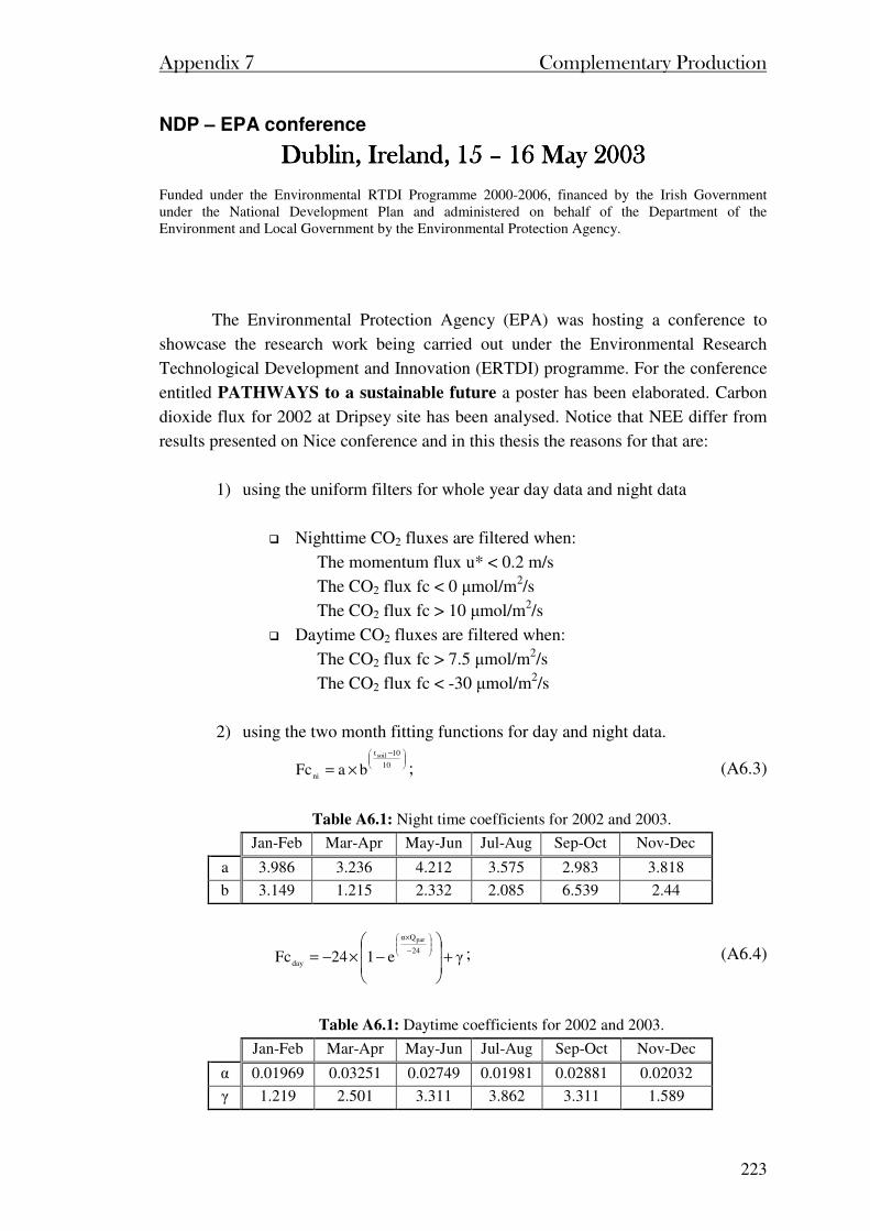
Appendix 7 Complementary Production
223
NDP – EPA conference
Dublin, Ireland, 15 Dublin, Ireland, 15 Dublin, Ireland, 15 Dublin, Ireland, 15 –––– 16 May 2003 16 May 2003 16 May 2003 16 May 2003 Funded under the Environmental RTDI Programme 2000-2006, financed by the Irish Government under the National Development Plan and administered on behalf of the Department of the Environment and Local Government by the Environmental Protection Agency.
The Environmental Protection Agency (EPA) was hosting a conference to
showcase the research work being carried out under the Environmental Research
Technological Development and Innovation (ERTDI) programme. For the conference
entitled PATHWAYS to a sustainable future a poster has been elaborated. Carbon
dioxide flux for 2002 at Dripsey site has been analysed. Notice that NEE differ from
results presented on Nice conference and in this thesis the reasons for that are:
1) using the uniform filters for whole year day data and night data
Nighttime CO2 fluxes are filtered when:
The momentum flux u* < 0.2 m/s
The CO2 flux fc < 0 µmol/m2/s
The CO2 flux fc > 10 µmol/m2/s
Daytime CO2 fluxes are filtered when:
The CO2 flux fc > 7.5 µmol/m2/s
The CO2 flux fc < -30 µmol/m2/s
2) using the two month fitting functions for day and night data.
−
×= 10
10t
ni
soil
baFc ; (A6.3)
Table A6.1: Night time coefficients for 2002 and 2003.
Jan-Feb Mar-Apr May-Jun Jul-Aug Sep-Oct Nov-Dec
a 3.986 3.236 4.212 3.575 2.983 3.818
b 3.149 1.215 2.332 2.085 6.539 2.44
γe124Fc24
Qα
day
par
+
−×−=
−
×
; (A6.4)
Table A6.1: Daytime coefficients for 2002 and 2003.
Jan-Feb Mar-Apr May-Jun Jul-Aug Sep-Oct Nov-Dec
α 0.01969 0.03251 0.02749 0.01981 0.02881 0.02032
γ 1.219 2.501 3.311 3.862 3.311 1.589
Appendix 7 Complementary Production
224
Hereunder are joined the submitted abstract as well as the complete poster.
Abstract:Abstract:Abstract:Abstract:
Carbon Dioxide Flux For One Year Above
a Temperate Grazed Grassland
Vesna Jaksic1, Gerard Kiely
1, John Albertson
2, Gabriel Katul
3 and Todd Scanlon1
1 Dept. of Civil and Environmental Engineering, University College Cork, Ireland
2 Dept. of Civil and Environmental Engineering, Duke University, NC, USA
3 Nicholas School of the Environment and Earth Science, Duke University, NC, USA
The Dripsey flux site in Cork, Ireland is a perennial ryegrass (C3 category)
pasture and is grazed for approximately 8 to 10 months of the year. The lands are
fertilised with approximately 200kg/ha/year of nitrogen. The flux tower monitoring
CO2, water vapour and energy was established in June 2001 and we have continuous
data since then. The site also includes streamflow hydrology and stream water
chemistry. We present the results and analysis for CO2 for the year 2002. The Net
Ecosystem Exchange (NEE) is estimated to be 3.25 T.C./ha/year. This work is part of
a five-year (2002-2006) research project funded by the Irish Environmental Protection
Agency.
Poster: (see end of the thesis)
Appendix 7 Complementary Production
225
Walsh Fellowships Seminar
Dublin, Ireland, 11 November 2003
At the occasion of the annual Teagasc Walsh Fellowships Seminar
presentation was given on work in progress. NEE has been analysed and possibilities
for carbon sequestration has been considered for Dripsey and Wexford site.
Abstract:Abstract:Abstract:Abstract:
Opportunities of Carbon Sequestration in Irish Grasslands
Vesna Jaksic1 Supervisors: Ger Kiely1, Owen Carton2 and Deirdre Fay2
1Dept. of Civil and Environmental Engineering, University College Cork, Ireland 2Environment and Land Use Department, Research Centre Johnstown Castle, Wexford, Ireland
The Dripsey catchment in North Cork has a dominant land cover of perennial
ryegrass (C3 category) and a land use of pasture and silage fields. A 10m high flux
tower for carbon measurements is located at the head of the catchment at an elevation
of 200masl. The fertiliser applications are approximately 190kgN/ha in chemical
fertiliser and approximately 80kgN/ha in the form of slurry/manure. The farms are
grazed for approximately 8 months of the year. The Wexford grassland site (20masl),
also a perennial ryegrass (C3) pasture, is fertilized with about 300kgN/ha.year and
grazed for about 8 months of the year. At both sites we continuously monitor CO2
flux measurements using the eddy covariance technique. The Cork site is operational
since July 2001, and the Wexford site since November 2002. The aim of this research
is to measure and model the CO2 flux at the two grassland ecosystems. Central to this
objective is the investigation of seasonal, annual and interannual fluxes with the aim
of estimating the carbon budget for the two sites. For the first year at the Cork site, the
Net Ecosystem exchange (NEE) was 3.7T of C/ha and for the second year 2.2T of
C/ha. The interannual variability is significant. The carbon uptake or NEE at the
Wexford site was 2.5T of C/ha for the year (November 1, 2002 to October 30, 2003).
In accounting for the various exports of carbon (e.g. off-farm carbon in meat and
meat) we estimate the carbon sequestration (i.e. the carbon fixed to the soil or carbon
sink) for the year 2002 at the Cork site to be 1.2T of C/ha. These preliminary results
suggest that the Cork site is a sink for carbon. However, due to interannual variability
this may change from year to year.
Appendix 7 Complementary Production
226
Net Ecosystem Exchange of a Fertilised Grassland: How Significant
is the Variability between a Wet and a Dry Year?
Vesna Jaksic1, Gerard Kiely1*, John Albertson2,3, Gabriel Katul2,3, Ram Oren3
1 Department of Civil and Environmental Eng., University College Cork, Ireland
2 Department of Civil and Environmental Eng., Duke University, NC. USA
3 Nicholas School of the Environment and Earth Sciences, Duke University, NC. USA
*Corresponding author: [email protected]
ph.353-21-4902965 fax 353-21-4276648
Submitted to: Geophysical Research Letters
April, 2004.
Appendix 7 Complementary Production
227
Abstract
An eddy covariance (EC) system for CO2 fluxes was used for two years (2002
and 2003) to study the variability of the net ecosystem exchange (NEE) at a humid
grassland site in southern Ireland. Over 90% of Irish agricultural land is under
grassland suggesting the importance of quantifying the carbon fluxes in this
ecosystem type. Some of the grassland fields within the EC footprint were grazed by
dairy cattle while other fields were harvested twice per year, (June and September).
The area averaged nitrogen fertilisation rate was ~300 kg.N/ha per year. 2002 was wet
(precipitation at 1785mm, 24% above average) and 2003 was dry (precipitation at
1185mm, 18% below average). We use the meteorological sign convention that,
minus is uptake and plus is respiration. The wet year had a NEE of -193 g.C/m2
compared to -260 g.C/m2 for the dry year. One impact of 2002 being wet was that the
first cut of silage was two weeks late (July 1) by comparison with the more normal
date of June 15 for 2003. The NEE for June (July) 2002 was -75 (+2) g.C/m2 and for
June (July) 2003 was -31 (-23) g.C/m2. The sum of the NEE for the eight months
(February to September) was -340 g.C/m2 for 2002 and -345 g.C/m2 for 2003. The
difference in NEE between the years was in the winter months (October to January)
with 2002 having an NEE of +148 g.C/m2 and 2003 with an NEE of + 85 g.C/m2 .The
rainfall in these four months was 903mm in 2002 and 435mm in 2003. The rainfall of
2002 caused the soil moisture status to be more frequently saturated than in 2003.
This resulted in a wetter soil environment that respired more. We conclude that the
wetter winter of 2002 with its saturating effect on soil moisture caused enhanced
ecosystem respiration which was responsible for the lower NEE of 2002.
Appendix 7 Complementary Production
228
1. Introduction1. Introduction1. Introduction1. Introduction
The earth’s vegetative cover is a key component in the global carbon cycle due
to its dynamic response to photosynthetic and respirative processes. Oceanic and
forestry ecosystems have been studied in much detail because of their significant
carbon sink attributes [e.g., Post et al., 1990; Cruickshank et al., 1998; Valentini et
al., 2000; Berbigier et al., 2001; Falge et al., 2002]. Studies of carbon fluxes in
temperate grassland have been overlooked due to the perception that this ecosystem is
carbon neutral [Hall et al., 2000; Ham and Knapp, 1998; Hunt et al., 2002].
Representing approximately 40 % of earth’s natural vegetation, carbon fluxes of
grasslands are now being revisited [Saigusa et al., 1998; Frank and Dugas, 2001;
Hunt et al., 2002; Jackson et al., 2002; Novick et al., 2004] and may yet play a role in
the missing global carbon sink [Ham & Knapp, 1998; Robert, 2001; Pacala et al.,
2001; Goodale and Davidson, 2002]. Grassland is the dominant ecosystem in Ireland,
representing 90% of agricultural land [Gardiner and Radford, 1980]. Several short-
term studies have shown that grassland ecosystems can sequester atmospheric CO2
[e.g. Bruce et al., 1999; Batjes et al, 1999; Conant et al., 2001; Soussana et al., 2003]
but few multi-annual data sets are available [Frank et al., 2001; Frank and Dugas,
2001; Falge et al., 2002; Knapp et al., 2002; Novick et al., 2004, Verburg et al, 2004].
To quantify the source-sink potential of grasslands in different climatic zones, long-
term surface flux measurements are required [Goulden et al., 1996; Ham and Knapp,
1998; Knapp et al., 2002; Baldocchi, 2003] to build and test models that represent the
biological and physical processes at the land surface interface. Such models (e.g.
BIOME3, Pnet, PaSim, Canveg) [Aber and Federer, 1992; Wilkinson and Janssen,
2001; Soussana et al., 2003, Reido et al, 1998] can be used to examine scenarios of
variation in land use and management as well as climate change. While it is known
that most forest ecosystems are sinks for carbon, it is not at all so well defined for
grasslands. The literature (summarised by Novick et al., 2004) shows that the wide
annual range of NEE for grasslands varies from an uptake of -800g.C/m2 to an
emission of +521 g.C/m2 with most grassland ecosystems in the range ±100 g.C/m2.
In this paper, we present the eddy covariance measured CO2 fluxes for two years
(2002 and 2003) in a humid temperate grassland ecosystem in Ireland. Long-term
measurements are essential for examining the seasonal and interannual variability of
carbon fluxes, particularly in humid temperate climates where grasslands are the
largest ecosystem [Goulden et al., 1996; Baldocchi, 2003]. Our aim is to examine the
processes involved in the variability of the net ecosystem exchange (NEE) between a
wet year and a dry year.
2. Site Description and Methods2. Site Description and Methods2. Site Description and Methods2. Site Description and Methods
Appendix 7 Complementary Production
229
The experimental grassland, at 220 m above sea level is located in South West
Ireland, 25 km northwest of Cork city (52º North latitude, 8º30’ West longitude). The
climate is temperate (summer average 15º C, winter average 5º C) and humid (mean
annual precipitation 1470mm). The soil is classified as brown-grey podzols and the
topsoil is rich in organic matter to a depth of about 15cm (about 12% organic matter,
[Daly, 1999]), overlying a dark brown B-horizon of sand texture. A yellowish brown
B-horizon of sand texture progressively changes to a brown, gravely sand which
constitutes the parent material at a depth of approximately 0.3m and the underlying
bedrock is old red sandstone [Scanlon et al., 2004]. Depth averaged over the top 30cm
the volumetric soil porosity was 0.49 (m3/m3), the saturation moisture level was 0.45,
the field capacity was 0.32, the wilting point was 0.12, and the air dried moisture was
0.02. The grassland type is moderately high quality pasture and meadow, with
perennial ryegrass the dominant plant species (C3 grass). The land use is a mixture,
2/3rds of fields for cattle grazing and 1/3rd of fields for cutting (silage harvesting).
Cattle grazing begins in March and ends in October. The rotational paddock grazing
periods lasts approximately one week in four. Grass productivity is enhanced with
applications of ~ 300kg of nitrogen in fertiliser and slurry, spread at intervals of
approximately six weeks between February and September. In the harvested fields the
grass is cut in the summer, firstly in June and secondly in September. The grass height
in the grazing fields varies from 0.1m to 0.2m. The grass height in the silage fields
reaches a maximum of ~ 0.45m prior to harvesting. The annual yield of silage in the
region has been 8 to 12 Tonnes of dry matter per hectare per year depending on the
weather (precipitation) and nitrogen application. The dry matter of silage is 46%
carbon.The footprint area of the flux tower (Fig. 1) was estimated on a fetch to sensor
height ratio of 100:1, combined with information from the probability density
function of the wind direction [Hsieh et al., 2000]. The prevailing wind direction is
from the south-west (Fig. 1).
Precipitation and meteorological measurements were sampled at one minute
and recorded at 30 minute intervals. The barometric pressure was measured with a
PTB101B and the air temperature and humidity were measured with a HMP45A
sensor (Campbell Scientific USA, (CSI)) at the height of 3m. Soil temperatures were
measured with three 107 temperature probes (CSI), at 2.5 cm, 5cm and 7.5 cm deep.
The volumetric soil water content (m3/m3) was measured at depths of 5, 10, 25, and
50 cm with CS615 time domain reflectometry (CSI) set horizontally. Two other
CS615’s were installed vertically, from 0 cm to 30 cm, and from 30 cm to 60 cm
depth. The datalogger was a CR23X (CSI). Net radiation was measured with a CNRI
net radiometer (Kipp & Zonen) and the photosynthetic photon flux was measured
with a PAR LITE sensor (Kipp & Zonen). All meteorological data was transferred
from site to office by telemetry.
The 3D wind velocity and virtual potential temperature were measured at 10
Hz with an RM Young Model 81000 3-D sonic anemometer positioned at the top of
Appendix 7 Complementary Production
230
the 10 m tower. Water vapour and CO2 densities were measured at 10 Hz with an LI-
7500 open path infrared gas analyser (LICOR Inc. USA) placed within 20 cm of the
centre of the anemometer air volume. The 30 minute eddy covariance CO2 fluxes are
defined as:
'' cc wF ρ−≅ (1)
where w’ is the vertical wind velocity fluctuations [m/s] and ρc’ the CO2 density
fluctuations [mol/m3]. We adopt the micrometeorological convention in which fluxes
from the biosphere to the atmosphere are positive. The CO2 flux data was firstly
adjusted for the Webb correction [Kramm et al., 1995; Webb et al., 1980; Baldocchi,
2003]. This correction is important for CO2 fluxes for which the density fluctuations
range is comparable to the mean density value.
The cF best represents the surface flux for steady-state, planar homogeneous,
and well developed turbulent flow [e.g., Goulden, et al., 1996; Moncrieff et al., 1997;
Falge et al., 2001]. During calm climatic conditions the measured fluxes are
underestimated: 1) as the fluctuations in the vertical wind speed are too small to be
resolved by sonic anemometry [Goulden, et al., 1996], and 2) for nocturnal and very
stable conditions, the flow statistics may be dominated by transient phenomena or
even the lack of turbulence (e.g. canopy waves). Cava et al. (2004) found that when
canopy waves dominate night-time runs, the local CO2 production from ecosystem
respiration and observed mean fluxes above the canopy are, to a first order, de-
coupled presumably through a storage term. What is important here is that when
canopy waves dominate, there is “gross” mass and heat exchange between the canopy
and the atmosphere; however, the net exchange over the lifecycle of the wave is
negligible. Occasionally, these waves are under-sampled because of a short flux-
averaging period leading to an apparent and spurious “photosynthesis” (or canopy C
uptake) values at night in the case of CO2. Correcting night-time fluxes with runs
collected under high u* (or more precisely for near-neutral to slightly stable
conditions) ensures that the turbulent regime is fully-developed. Another reason why
runs with high u* (or near-neutral conditions) are preferred for night-time flux
corrections is a much smaller (and perhaps the more realistic) footprint [Novick et al,
2003].
Uncertainties in night-time fluxes have been examined by many researchers
and remains a challenge because a minor underestimation of night-time CO2 fluxes
(respiration) imply overestimations of the annual carbon uptake [Falge et al., 2001;
Pattey et. al., 2002; Baldocchi et al., 2003]. To compare with other long-term studies
from various ecosystems, we use a friction velocity (u*) to filter transients and weak
turbulence conditions [e.g., Goulden, et al., 1996; Moncrieff et al., 1996; Falge et al.,
Appendix 7 Complementary Production
231
2001; Pattey et al., 2002]. Specifically, we filtered CO2 fluxes at night when u* < 0.2
m/s [Pattey et al., 2002; Baldocchi et al., 2003]. After the Webb correction, double
rotation and u* filtering, we further filtered fluxes that exceeded predetermined
threshold values for the season. For instance, the summer day-time fluxes were
accepted if >-30 µmol/m2s and <0 µmol/m2s. The night-time summer fluxes were
accepted if >0 µmol/m2s and <15 µmol/m2s. The daytime data was binned in two-
month increments according to Falge et al., (2001).
After post-processing and filtering of spurious data, 54 % of the CO2 flux data
for 2002 and 58 % for 2003 were suitable for analysis. The percentage of usable data
reported by other studies is approximately 65 % [Falge et al., 2001; Law et al., 2002].
About 13 % of the 2002 data and 8 % of the 2003 data were rejected due to water
drops on the LI-7500 during rain and within two hours after rain. The rest of the non-
usable data (33% for 2002, and 34% for 2003) were rejected when found to be out of
range or during periods of low night-time friction velocity.
The gap filling functions tested were non-linear regressions [see Goulden et
al., 1996; Falge et al., 2001; Lai et al., 2002]. For night-time data, the ecosystem
respiration is known to be linked to the soil temperature [Lloyd and Taylor, 1994;
Kirschbaum, 1995] and to a lesser extent to soil moisture. The correlation with
different temperatures (air, surface, different soil depths) showed best correlation with
soil temperature at 5 cm depth, whereas the data set was less well correlated to soil
moisture (consistent with the analysis of Novick et al. 2004, for a warm temperate
grassland). Different temperature response functions were tested and parameterised
statistically (Sum of Squares Error (SSE), Root-Square (R2), adjusted Root Square
(adjusted-R2), and Root Mean Squared Error (RMSE)). A linear relationship, an
exponential relationship, the Arrhenius function and a Q10 relation were first
considered. The best fit (for night-time) was obtained for the exponential function
defined as:
)( soiltb
ni eaF××= (2)
where where where where ttttsoilsoilsoilsoil is the soil temperature at 5 cm is the soil temperature at 5 cm is the soil temperature at 5 cm is the soil temperature at 5 cm
depth in depth in depth in depth in ºCºCºCºC. The coefficient . The coefficient . The coefficient . The coefficient aaaa = 1.476 = 1.476 = 1.476 = 1.476
and 1.109 for 2002 and 2003 and 1.109 for 2002 and 2003 and 1.109 for 2002 and 2003 and 1.109 for 2002 and 2003
respectively. The coefficient respectively. The coefficient respectively. The coefficient respectively. The coefficient bbbb = 0.095 = 0.095 = 0.095 = 0.095
Appendix 7 Complementary Production
232
and 0.122 for 2002 and 2003 and 0.122 for 2002 and 2003 and 0.122 for 2002 and 2003 and 0.122 for 2002 and 2003
rrrrespectively. This function was applied espectively. This function was applied espectively. This function was applied espectively. This function was applied
to the data for the full year (separately to the data for the full year (separately to the data for the full year (separately to the data for the full year (separately
for 2002 and 2003) because the range of for 2002 and 2003) because the range of for 2002 and 2003) because the range of for 2002 and 2003) because the range of
nightnightnightnight----time soil temperature throughout time soil temperature throughout time soil temperature throughout time soil temperature throughout
the year was small (2 to 18º C). the year was small (2 to 18º C). the year was small (2 to 18º C). the year was small (2 to 18º C).
For daytime, the net ecosystem exchange of CO2 is linked to the
photosynthetic photon flux density Q in µmol of quantum/m2/s [e.g., Michaelis and
Menten, 1913; Smith, 1938; Goulden et. al., 1996]. Different light response functions
tested included: a linear relationship, Smith formula [Smith, 1938; Falge et al., 2001],
Michaelis-Menten formula (rectangular hyperbola), [Michaelis & Menten, 1913;
Falge et al., 2001], Misterlich formula [Falge et al., 2001], and Ruimy formula
[Ruimy et al., 1995; Lai et al., 2002]. The best fit was achieved with the Misterlich
formula defined as:
ceF
ppfdQa
day +
−×−=
−
×
24124 (3)
where Qppfd is the photosynthetic photon flux density (or PAR) in µmol of
quantum/m2/s. As PAR varies seasonally, the values of the coefficients in two
monthly bins are listed in Table 1.
3. Results and Discussion 3. Results and Discussion 3. Results and Discussion 3. Results and Discussion
As evidenced from Figure 2a, (and Table 2) 2002 was wet year, with an
annual rainfall of 1785mm and 2003 was dry, with an annual rainfall of 1185mm
(compared to the long-term average rainfall of 1470mm). No snow fell in either year.
The monthly average vapour pressure deficit (VPD) is shown in Fig.2b. (and Table2).
The high humidity and low potential for evaporation of the region is evidenced by the
low VPD’s with a maximum of 0.36 kPa in August 2003 and as low as 0.1 kPa in the
winter months. The annual evapotranspiration measured using EC techniques
[Brutsaert, 1982], (Fig.2c) was 372 and 368mm for 2002 and 2003 respectively with
Appendix 7 Complementary Production
233
little differences in the monthly ET between the two years. This evapotranspiration
was 21% and 31% of annual precipitation in 2002 and 2003 respectively. The
corresponding potential evapotranspiration (PET, no water limitation) estimated using
the Penman-Monteith equation (Fig.2d) was 422 and 455mm for 2002 and 2003
respectively. The actual evapotranspiration was 88% and 81% of potential in 2002
and 2003 respectively. We note from Fig.2a (VPD) and Fig.2c (PET) that the PET
mimics the VPD. For instance, examining August (Table 2) we note that the actual
evapotranspiration was 49 mm and 48 mm in 2002 and 2003 respectively, while the
potential was 60 and 75 mm in 2002 and 2003 respectively. This confirms that the
evapotranspiration was water limited in both Augusts but more so in 2003. The
volumetric soil moisture (m3/m3), depth averaged over the top 30cm (Fig. 2e) is
shown in both years to vary from highs of 0.45 (note that saturation is ~ 0.45) to lows
of 0.21 (note that the wilting point is ~0.12 and field capacity is ~0.32). Examining
Fig.2e (and Table 2) we see that the root zone (0 to 30cm depth) soil moisture was
much drier in 2003 particularly during the months of June to October. In addition, the
winter months, October to January were much drier in 2003 (see Table 2).
The photosynthetic photon flux density (Fig.3a, PAR in µmol/m2.s) show that
there is approximately 5% more PAR radiation in 2003 than in 2002. The mean
annual air temperature was 9.63 ºC and 9.64 ºC in 2002 and 2003 respectively. The
daily air temperatures (Fig. 3b) has a small range of variation during the year, going
from a maximum of 21º C (in August) to a minimum of 0º C (January), with an
average value of 15º C in summer and 5º C in winter verifying the temperate nature of
the local climate. The local climate is humid temperate, with mild winters where very
few daytime temperatures drop below 4 °C, (the lower air threshold temperature for
the photosynthetic process). The soil temperature (at 5cm depth, Fig.3c) mimics the
air temperature.
In Fig.4 we show the monthly net ecosystem exchange (NEE) for both years.
There is net uptake (carbon sink) in the seven months, March to September and net
respiration (carbon source) in the months, October to January. In February the
ecosystem is close to equilibrium. The monthly NEE varies between the same months
in the two years.
The net uptake of C in May 2002 of -99 g.C/m2 is similar to -110 g.C/m2 in
2003. The net uptake of C in June, 2002 of -75 g.C/m2 was more than double the -31
g.C/m2 of June, 2003. The reasons for the differences in NEE in June was twofold.
Firstly, on June 15, 2003 part of the grassland in the footprint was cut (harvested to
within 5cm of the bare soil). So, the first half of June 2003 had a strong uptake while
the second half of June was net respiration with the net effect for June being a low
uptake of -31 g.C/m2. Secondly, On July 1, 2002 part of the grassland in the footprint
Appendix 7 Complementary Production
234
was cut. So, all of June 2002 had the benefit of a maximum uptake of -75 g.C/m2. The
reason for the delay in harvesting in 2002 was that farm equipment could not access
the fields due to the elevated soil moisture (see Fig.2e). The second half of June 2003
was much drier that that of the second half of June 2002. It has been shown [Frank
and Dugas, 2001] that short-term droughts during the growing season reduce CO2
fluxes to near zero (photosynthesis balances respiration). Decreases in LAI (Leaf Area
Index) caused by the grass (silage) harvesting, reduces gross primary productivity
(GPP), [Budyko, 1974].
In the spring months (March, April and May), there was a little more uptake in
2003 than there was in 2002. This may be explained by higher radiation and slightly
drier soils. The NEE (uptake) in August and September 2002 was the same as August
and September 2003. This occurred in spite of much drier soil moisture status in
August and September 2003.
The sum of the NEE for the eight months (February to September) was -340
g.C/m2 for 2002 and -345 g.C/m2 for 2003. The difference in NEE between the years
was in the winter months (October to January) with 2002 having an NEE of +148
g.C/m2 and 2003 with an NEE of + 85 g.C/m2 .The rainfall in these four months was
903mm in 2002 and 435mm in 2003. The rainfall of 2002 caused the soil moisture
status to be more frequently saturated than in 2003. This resulted in a wetter soil
environment that respired more. In addition, in the drier year (2003), cattle grazed the
fields (during the daytime) during the parts of the months of October to January. By
contrast, in the wet winter (2002) cattle did not graze the fields because to do so, they
would have damaged the soil surface to an unacceptable level. So in the winter of
2002, there was a greater standing biomass (than in 2003), which enhanced the
respiration. This suggests that the wetter winter of 2002 with its saturating effect on
soil moisture, it’s higher standing biomass and enhanced ecosystem respiration was
responsible for the lower NEE of 2002.
The cumulative NEE, expressed in Tonnes of carbon per hectare (TC/ha) for
both years is shown in Fig. 5. The NEE for 2002 was -1.9 TC/ha while for 2003 it was
-2.6 TC/ha. The cumulative uptake to from January 1 to July 1, 2002 was -2.7 T.C/ha.
The cumulative uptake from January 1 to June 15, 2003 was also -2.7 TC/ha. The
uptake period that continued longer by two weeks in 2002, was due to the delay in
cutting (because of wet weather). In Fig.6 we show the cumulative NEE for both
years, for the months October, November, December and January. The NEE for these
four months was +1.5 T.C./ha (respiration) for 2002 and +0.8 T.C/ha for 2003. The
difference in the NEE between the two years was differences in these four winter
months. Precipitation leading to near saturation soil moisture (as in 2002 but not in
2003), enhances the release of C, because of its effect on soil aeration and CO2
transport within the soil profile [Suyker, et al., 2003].
Appendix 7 Complementary Production
235
4. Summary4. Summary4. Summary4. Summary
The EC flux measurements presented here cover two years of a planned long-
term research programme of net ecosystem exchange (of CO2) begun in July 2001 at a
humid temperate grassland ecosystem in southern Ireland. The grassland footprint
encompasses eight small dairy farms (of size 10 to 40ha each) with approximately
2/3rd’s of the area grazed for eight months of the year (March to October) while in the
other 1/3rd (which is off-limits for grazing from March to September) the grass is cut
(harvested for winter feed) twice per year: June and September. The two years are:
2002 which was a wet year (precipitation at 1785mm, 24% above average); and 2003
which was a dry year (precipitation at 1185mm, 18% below average). The farmland
management practices in both years were similar, including nitrogen fertilisation rates
(305 and 294 kg.N/ha for 2002 and 2003 respectively). We found that the wet year of
2002 had a NEE of -1.9 TC/ha compared to -2.6 TC/ha for the dry year of 2003 (a
27% difference). We found that the cumulative NEE from February to September
(Spring plus Summer) was the same in both years. The difference in NEE in the two
years of 0.7 T.C/ha was concentrated in the winter months (October, November,
December and January). The wet year winter had a cumulative NEE of +1.5 T.C/ha
while for the corresponding NEE for the dry year was +0.8 T.C/ha (see Fig.6). The
precipitation of the wet winter (2002) was 903 mm while in the dry winter it was 435
mm. As the land use and land management practices were similar in both years, the
main difference between the two years was in the magnitude of the winter rainfall. We
conclude that the wetter winter of 2002 with its saturating effect on soil moisture had
enhanced ecosystem respiration which was responsible for the lower annual NEE of
2002.
5. Acknowledgments 5. Acknowledgments 5. Acknowledgments 5. Acknowledgments
This work has been prepared as part of the Environmental Research
Technological Development which is managed by the Environmental Protection
Agency and financed by the Irish Government under the National Development Plan
2000-2006 (CELTICFLUX, Grant No. 2001-CC/CD-(5/7)). The Walsh Scholarship
administered by Teagasc funds the first author. We appreciate the support of Dr.Owen
Carton and Dr.Deidre Fay of Teagasc. We especially appreciate the experimental
support by Mr. Adrian Birkby of the Civil and Environmental Engineering
Department at University College Cork. We appreciate the co-operation of the
landowners.
Appendix 7 Complementary Production
236
List of FiguresList of FiguresList of FiguresList of Figures
Figure 1. Map of the grassland catchment with eddy covariance tower location and
the shaded fields of the flux footprint. There are many small fields in the footprint
varying in size from 1 to 5ha. The prevailing wind direction is from the south-west.
Figure 2. (a) Monthly precipitation for 2002 (grey) and 2003 (black); (b) monthly
vapour pressure deficit (VPD) in kPa. (c) monthly evapotranspiration for 2002 (grey)
and 2003 (black); (d) monthly potential evapotranspiration using Penman-Monteith;
(e) near surface soil moisture at 30 minutes interval over a depth of 0-30 cm for 2002
(grey) and 2003 (black).
Figure 3. (a) Monthly photosynthetic photon flux (Qpar) for 2002 (grey) and 2003
(black); (b) daily averaged air temperature for 2002 (grey) and 2003 (black); (c) daily
averaged soil temperature at a depth of 5.0 cm for 2002 (grey) and 2003 (black).
Figure 4. Monthly carbon flux in g/m2 for 2002 (grey) and 2003 (black).
Figure 5. Cumulative uptake of carbon in T.C/ha for 2002 (grey) and 2003 (black).
The NEE for 2002 was -1.9 T.C/ha and for 2003 was -2.6 T.C/ha.
Figure 6. Cumulative uptake of carbon for the winter months (October, November,
December and January) in T.C/ha for 2002 (grey) and 2003 (black). The winter NEE
for 2002 was +1.5 T.C/ha and for 2003 was +0.8 T.C/ha.
Appendix 7 Complementary Production
237
References References References References
Aber, D. J., and C. A. Federer, A generalized, lumpedAber, D. J., and C. A. Federer, A generalized, lumpedAber, D. J., and C. A. Federer, A generalized, lumpedAber, D. J., and C. A. Federer, A generalized, lumped----parameter model of photosynthesis, parameter model of photosynthesis, parameter model of photosynthesis, parameter model of photosynthesis,
evapotranspiration and net primary production in temperate and boreal forest evapotranspiration and net primary production in temperate and boreal forest evapotranspiration and net primary production in temperate and boreal forest evapotranspiration and net primary production in temperate and boreal forest
ecosystems, ecosystems, ecosystems, ecosystems, Oecologia, 92Oecologia, 92Oecologia, 92Oecologia, 92, 463, 463, 463, 463----474, 1992.474, 1992.474, 1992.474, 1992.
Baldocchi, D.D., AssessinBaldocchi, D.D., AssessinBaldocchi, D.D., AssessinBaldocchi, D.D., Assessing the eddy covariance technique for evaluating carbon dioxide g the eddy covariance technique for evaluating carbon dioxide g the eddy covariance technique for evaluating carbon dioxide g the eddy covariance technique for evaluating carbon dioxide
exchange rates of ecosystems: past, present and future, exchange rates of ecosystems: past, present and future, exchange rates of ecosystems: past, present and future, exchange rates of ecosystems: past, present and future, Global Change Biol., 9Global Change Biol., 9Global Change Biol., 9Global Change Biol., 9, 479, 479, 479, 479----
492, 2003.492, 2003.492, 2003.492, 2003.
Batjes, H. N., Management options for reducing CO2 – concentrations in the atmosphere by
increasing carbon sequestration in the soil, Report no. 410 200 031, 114 pp., Dutch
National Research Programme on Global Air Pollution and Climate Change,
Netherlands, 1999.
Berbigier, P., J.Berbigier, P., J.Berbigier, P., J.Berbigier, P., J.----M. Bonnefond, and P. Mellmann , COM. Bonnefond, and P. Mellmann , COM. Bonnefond, and P. Mellmann , COM. Bonnefond, and P. Mellmann , CO2222 and water vapour fluxes for 2 years and water vapour fluxes for 2 years and water vapour fluxes for 2 years and water vapour fluxes for 2 years
above Euroflux forest site, above Euroflux forest site, above Euroflux forest site, above Euroflux forest site, Agric. For. Meteorol., 108Agric. For. Meteorol., 108Agric. For. Meteorol., 108Agric. For. Meteorol., 108, 183, 183, 183, 183----197, 2001.197, 2001.197, 2001.197, 2001.
Bruce, P. J., M. Frome, E. Haites, H. Joanne, L. Rattan, and K. Faustian, Carbon sequestration
in soils, J. Soil and Water cons., 382-389,1999.
Brutaert WH. (1982). Evaporation into the Atmosphere. “Environmental Fluid Mechanics”,
D.Reidel, Dordrecht, Holland.
Budyko, I. M., Climate and Life, Climatic factors of Photosynthesis, 497, Academic Press
INC, London, 1974.
Conant, T.R., K. Paustian, and E. T. Elliott, Grassland management and conversion into grassland: effects on soil carbon, Ecol.
Applications, 11, No. 2, pp. 343-355, 2001.
Cruickshank, M.M., R.W. Tomlinson, P.M. Devine, and R. Milne, Carbon in the vegetation
and soils of Northern Ireland, Biology and Environment: Proceedings of the Royal
Irish Academy, vol. 98B, No. 1, 9-21, 1998.
Daly K 1999. An environmental appraisal of the phosphorous of the Irish grassland soils.
Ph.D Thesis.Trinity College Dublin,Ireland.
Falge, E., D. Baldocchi, R. Olson, P. Athoni, M. Aubinet, Falge, E., D. Baldocchi, R. Olson, P. Athoni, M. Aubinet, Falge, E., D. Baldocchi, R. Olson, P. Athoni, M. Aubinet, Falge, E., D. Baldocchi, R. Olson, P. Athoni, M. Aubinet, C. Bernhofer, G. Burba, R. C. Bernhofer, G. Burba, R. C. Bernhofer, G. Burba, R. C. Bernhofer, G. Burba, R.
Ceulemans, R. Clement, H. Dolman, A. Granier, P. Gross, T. Grünward, D. Ceulemans, R. Clement, H. Dolman, A. Granier, P. Gross, T. Grünward, D. Ceulemans, R. Clement, H. Dolman, A. Granier, P. Gross, T. Grünward, D. Ceulemans, R. Clement, H. Dolman, A. Granier, P. Gross, T. Grünward, D.
Hollinger, NHollinger, NHollinger, NHollinger, N----O. Jensen, G. Katul, P. Keronen, A. Kowalski, C. T. Lai, B. E. Law, T. O. Jensen, G. Katul, P. Keronen, A. Kowalski, C. T. Lai, B. E. Law, T. O. Jensen, G. Katul, P. Keronen, A. Kowalski, C. T. Lai, B. E. Law, T. O. Jensen, G. Katul, P. Keronen, A. Kowalski, C. T. Lai, B. E. Law, T.
Meyers, J. Moncrieff, E. Moors, J. W. Munger, K. Pilegaard, Ü. Rannik, C.Meyers, J. Moncrieff, E. Moors, J. W. Munger, K. Pilegaard, Ü. Rannik, C.Meyers, J. Moncrieff, E. Moors, J. W. Munger, K. Pilegaard, Ü. Rannik, C.Meyers, J. Moncrieff, E. Moors, J. W. Munger, K. Pilegaard, Ü. Rannik, C. Rebmann, Rebmann, Rebmann, Rebmann,
A. Suyker, J. Tenhunen, K. Tu, S. Verma, T. Vesala, K. Wilson, and S. Wofsy, Gap A. Suyker, J. Tenhunen, K. Tu, S. Verma, T. Vesala, K. Wilson, and S. Wofsy, Gap A. Suyker, J. Tenhunen, K. Tu, S. Verma, T. Vesala, K. Wilson, and S. Wofsy, Gap A. Suyker, J. Tenhunen, K. Tu, S. Verma, T. Vesala, K. Wilson, and S. Wofsy, Gap
filling strategies for defensible annual sums of net ecosystem exchange, filling strategies for defensible annual sums of net ecosystem exchange, filling strategies for defensible annual sums of net ecosystem exchange, filling strategies for defensible annual sums of net ecosystem exchange, Agric. For. Agric. For. Agric. For. Agric. For. Meteorol., 107Meteorol., 107Meteorol., 107Meteorol., 107, 43, 43, 43, 43----69, 2001.69, 2001.69, 2001.69, 2001.
Appendix 7 Complementary Production
238
Falge, E., D. Baldocchi, J. Tenhunen, M. Aubinet, Falge, E., D. Baldocchi, J. Tenhunen, M. Aubinet, Falge, E., D. Baldocchi, J. Tenhunen, M. Aubinet, Falge, E., D. Baldocchi, J. Tenhunen, M. Aubinet, P. Bakwin, P. Berbigier, C. Bernhofer, G. P. Bakwin, P. Berbigier, C. Bernhofer, G. P. Bakwin, P. Berbigier, C. Bernhofer, G. P. Bakwin, P. Berbigier, C. Bernhofer, G.
Burba, R. Clement, K. J. Davis, J. A. Elbers, A. H. Goldstein, A. Grelle, A. Granier, J. Burba, R. Clement, K. J. Davis, J. A. Elbers, A. H. Goldstein, A. Grelle, A. Granier, J. Burba, R. Clement, K. J. Davis, J. A. Elbers, A. H. Goldstein, A. Grelle, A. Granier, J. Burba, R. Clement, K. J. Davis, J. A. Elbers, A. H. Goldstein, A. Grelle, A. Granier, J.
Guðmundsson, D. Hollinger, A. Kowalski, G. Katul, B. E. Law, Y. Malhi,T. Meyers, Guðmundsson, D. Hollinger, A. Kowalski, G. Katul, B. E. Law, Y. Malhi,T. Meyers, Guðmundsson, D. Hollinger, A. Kowalski, G. Katul, B. E. Law, Y. Malhi,T. Meyers, Guðmundsson, D. Hollinger, A. Kowalski, G. Katul, B. E. Law, Y. Malhi,T. Meyers,
R. K. Monson, J. W. Munger, W. Oechel, K. ThR. K. Monson, J. W. Munger, W. Oechel, K. ThR. K. Monson, J. W. Munger, W. Oechel, K. ThR. K. Monson, J. W. Munger, W. Oechel, K. Tha Paw U, K. Pilegaard, Ü. Rannik, C. a Paw U, K. Pilegaard, Ü. Rannik, C. a Paw U, K. Pilegaard, Ü. Rannik, C. a Paw U, K. Pilegaard, Ü. Rannik, C.
Rebmann, A. Suyker, R. Valentini, K. Wilson, and S. Wofsy, Seasonality of ecosystem Rebmann, A. Suyker, R. Valentini, K. Wilson, and S. Wofsy, Seasonality of ecosystem Rebmann, A. Suyker, R. Valentini, K. Wilson, and S. Wofsy, Seasonality of ecosystem Rebmann, A. Suyker, R. Valentini, K. Wilson, and S. Wofsy, Seasonality of ecosystem
respiration and gross primary production as derived from FLUXNET measurements, respiration and gross primary production as derived from FLUXNET measurements, respiration and gross primary production as derived from FLUXNET measurements, respiration and gross primary production as derived from FLUXNET measurements,
Agric. For. Meteorol., 113Agric. For. Meteorol., 113Agric. For. Meteorol., 113Agric. For. Meteorol., 113, 53, 53, 53, 53----74, 2002.74, 2002.74, 2002.74, 2002.
Flanagan LB, WFlanagan LB, WFlanagan LB, WFlanagan LB, Wever LA, Carlson PJ (2002) Seasonal and interannual variation in carbon ever LA, Carlson PJ (2002) Seasonal and interannual variation in carbon ever LA, Carlson PJ (2002) Seasonal and interannual variation in carbon ever LA, Carlson PJ (2002) Seasonal and interannual variation in carbon
dioxide exchange and carbon balance in a northern temperate grassland. dioxide exchange and carbon balance in a northern temperate grassland. dioxide exchange and carbon balance in a northern temperate grassland. dioxide exchange and carbon balance in a northern temperate grassland. Glob Change Glob Change Glob Change Glob Change BiolBiolBiolBiol 8:599 8:599 8:599 8:599––––615615615615
Frank, B. A., and Dugas, A. W., Carbon dioxide fluxes over northern, semiarid, mixedFrank, B. A., and Dugas, A. W., Carbon dioxide fluxes over northern, semiarid, mixedFrank, B. A., and Dugas, A. W., Carbon dioxide fluxes over northern, semiarid, mixedFrank, B. A., and Dugas, A. W., Carbon dioxide fluxes over northern, semiarid, mixed----grass grass grass grass
prairie, prairie, prairie, prairie, Agric. For. Meteorol., 108Agric. For. Meteorol., 108Agric. For. Meteorol., 108Agric. For. Meteorol., 108, 317, 317, 317, 317----326, 2001.326, 2001.326, 2001.326, 2001.
Frank, B.A., P. L. Sims, J. A. Bratford, P. C. Milenick, W. A. Dugas, and H. S. Mayeux, Frank, B.A., P. L. Sims, J. A. Bratford, P. C. Milenick, W. A. Dugas, and H. S. Mayeux, Frank, B.A., P. L. Sims, J. A. Bratford, P. C. Milenick, W. A. Dugas, and H. S. Mayeux, Frank, B.A., P. L. Sims, J. A. Bratford, P. C. Milenick, W. A. Dugas, and H. S. Mayeux,
Carbon dioxide fluxes over three great plains grasslands, Carbon dioxide fluxes over three great plains grasslands, Carbon dioxide fluxes over three great plains grasslands, Carbon dioxide fluxes over three great plains grasslands, The Potential of U.S. Grazing The Potential of U.S. Grazing The Potential of U.S. Grazing The Potential of U.S. Grazing Lands to Sequester CaLands to Sequester CaLands to Sequester CaLands to Sequester Carbon and Mitigate the Greenhouse Effect, rbon and Mitigate the Greenhouse Effect, rbon and Mitigate the Greenhouse Effect, rbon and Mitigate the Greenhouse Effect, edited by R. F. Follett, edited by R. F. Follett, edited by R. F. Follett, edited by R. F. Follett,
J. M. Kimble, and R. Lal, 167J. M. Kimble, and R. Lal, 167J. M. Kimble, and R. Lal, 167J. M. Kimble, and R. Lal, 167----187, Lewis Puplishers, New York, 2001.187, Lewis Puplishers, New York, 2001.187, Lewis Puplishers, New York, 2001.187, Lewis Puplishers, New York, 2001.
Gardiner M.J., T., Radford, (1980). Soil Associations if Ireland and their Land Use Potential. Gardiner M.J., T., Radford, (1980). Soil Associations if Ireland and their Land Use Potential. Gardiner M.J., T., Radford, (1980). Soil Associations if Ireland and their Land Use Potential. Gardiner M.J., T., Radford, (1980). Soil Associations if Ireland and their Land Use Potential.
An Foras Talúntais. DublAn Foras Talúntais. DublAn Foras Talúntais. DublAn Foras Talúntais. Dublin, Ireland.in, Ireland.in, Ireland.in, Ireland.
Goodale, L. C., and E. A. Davidson, Uncertain sinks in the shrubs, Nature, 418, 593-594,
2002.
Goulden, M.L., J.W., Munger, S.M., Fan, B.C., Daube, and S.C., Wofsy, Measurements of
carbon sequestration by long-term eddy covariance: methods and critical evaluation
of accuracy, Global Change Biol., 2, Pages 196-182, 1996.
Hall, O. D., J. M. O. Scurlock, D. S. Ojima, and W. J. Parton, Grasslands and the Global
Carbon Cycle: Modeling the Effects of Climate Change, in The Carbon Cycle, edited
by T.M.L. Wigley and D.S. Schimel, pp. 102-114,Cambridge Univ. Press, UK, 2000.
Ham, M. J., and A. K. Knapp, Fluxes of COHam, M. J., and A. K. Knapp, Fluxes of COHam, M. J., and A. K. Knapp, Fluxes of COHam, M. J., and A. K. Knapp, Fluxes of CO2222, water vapor, and energy from a prairie ecosystem , water vapor, and energy from a prairie ecosystem , water vapor, and energy from a prairie ecosystem , water vapor, and energy from a prairie ecosystem
during the seasonal transition from carbon sink to carbon source, during the seasonal transition from carbon sink to carbon source, during the seasonal transition from carbon sink to carbon source, during the seasonal transition from carbon sink to carbon source, Agric. For. Agric. For. Agric. For. Agric. For. MeteoMeteoMeteoMeteorol., 89rol., 89rol., 89rol., 89, 1, 1, 1, 1----14, 1998.14, 1998.14, 1998.14, 1998.
Hsieh, C-I., G. Katul, and T. Chi, An approximate analytical model for footprint estimation
of scalar fluxes in thermally stratified atmospheric flows, Advances in Water Res. 23,
765-772, 2000.
Hunt, E. J., F. M. Kelliher, T. M. McHunt, E. J., F. M. Kelliher, T. M. McHunt, E. J., F. M. Kelliher, T. M. McHunt, E. J., F. M. Kelliher, T. M. McSeveny, and J. N. Byers, Evaporation and carbon dioxide Seveny, and J. N. Byers, Evaporation and carbon dioxide Seveny, and J. N. Byers, Evaporation and carbon dioxide Seveny, and J. N. Byers, Evaporation and carbon dioxide
exchange between the atmosphere and a tussock grassland during a summer drought, exchange between the atmosphere and a tussock grassland during a summer drought, exchange between the atmosphere and a tussock grassland during a summer drought, exchange between the atmosphere and a tussock grassland during a summer drought,
Agric. For. Meteorol., 111Agric. For. Meteorol., 111Agric. For. Meteorol., 111Agric. For. Meteorol., 111, 65, 65, 65, 65----82, 2002.82, 2002.82, 2002.82, 2002.
Appendix 7 Complementary Production
239
Jackson, B. R., J. L. Banner, E. G. Jobbágy, W. T. Pockman, and D. H. Wall, Ecosystem
carbon loss with woody plant invasion of grasslands, Nature, 418, 623-626, 2002.
Kirschbaum, U. F. M., The temperature dependence of soil organic matter decomposition, and
the effect of global warming on soil organic C storage, Soil Biol. Biochem, 27 (D6),
753-760, 1995.
Knapp, K. A., P. A. Fay, J. M. Blair, S. L. Collins, M. D. Smith, J. D. Carlisle, C. W. Harper,
B. T. Danner, M. S. Lett, and J. K. McCarron, Rainfall variability, carbon cycling,
and plant species diversity in a mesic grassland, Science, 298, 2202-2205, 2002.
Kramm, G., R. Dlugi, and D. H. Lenschow, A re-evaluation of the Webb correction using
density-weighted averages, Journal of Hydrology, 166, 283-292, 1995.
Lai, C.Lai, C.Lai, C.Lai, C.----T., G. Katul, J. Butnor, D. Ellsworth, and R. Oren, ModelliT., G. Katul, J. Butnor, D. Ellsworth, and R. Oren, ModelliT., G. Katul, J. Butnor, D. Ellsworth, and R. Oren, ModelliT., G. Katul, J. Butnor, D. Ellsworth, and R. Oren, Modelling nightng nightng nightng night----time ecosystem time ecosystem time ecosystem time ecosystem
respiration by a constrained source optimization method, respiration by a constrained source optimization method, respiration by a constrained source optimization method, respiration by a constrained source optimization method, Global Change Biol., 8Global Change Biol., 8Global Change Biol., 8Global Change Biol., 8, 124, 124, 124, 124----
141, 2002.141, 2002.141, 2002.141, 2002.
Law, E. B., E. Falge, L. Gu, D. D. Baldocchi, P. Bakwin, P. Berbigier, K. Davis, A. J. Dolman, Law, E. B., E. Falge, L. Gu, D. D. Baldocchi, P. Bakwin, P. Berbigier, K. Davis, A. J. Dolman, Law, E. B., E. Falge, L. Gu, D. D. Baldocchi, P. Bakwin, P. Berbigier, K. Davis, A. J. Dolman, Law, E. B., E. Falge, L. Gu, D. D. Baldocchi, P. Bakwin, P. Berbigier, K. Davis, A. J. Dolman,
M. Falk, J. D. Fuentes, A. Goldstein, A.M. Falk, J. D. Fuentes, A. Goldstein, A.M. Falk, J. D. Fuentes, A. Goldstein, A.M. Falk, J. D. Fuentes, A. Goldstein, A. Granier, A. Grelle, D. Hollinger, I. A. Granier, A. Grelle, D. Hollinger, I. A. Granier, A. Grelle, D. Hollinger, I. A. Granier, A. Grelle, D. Hollinger, I. A.
Janssens, P. Jarvis, N. O. Jansen, G. Katul, Y. Mahli, G. Matteucci, T. Meyers, R. Janssens, P. Jarvis, N. O. Jansen, G. Katul, Y. Mahli, G. Matteucci, T. Meyers, R. Janssens, P. Jarvis, N. O. Jansen, G. Katul, Y. Mahli, G. Matteucci, T. Meyers, R. Janssens, P. Jarvis, N. O. Jansen, G. Katul, Y. Mahli, G. Matteucci, T. Meyers, R.
Monson, W. Munger, W. Oechel, R. Olson, K. Pilegaard, K. T. Paw U, H. Monson, W. Munger, W. Oechel, R. Olson, K. Pilegaard, K. T. Paw U, H. Monson, W. Munger, W. Oechel, R. Olson, K. Pilegaard, K. T. Paw U, H. Monson, W. Munger, W. Oechel, R. Olson, K. Pilegaard, K. T. Paw U, H.
Thorgeirsson, R. Valentini, S. Verma, T. Vesala, K. Wilson, anThorgeirsson, R. Valentini, S. Verma, T. Vesala, K. Wilson, anThorgeirsson, R. Valentini, S. Verma, T. Vesala, K. Wilson, anThorgeirsson, R. Valentini, S. Verma, T. Vesala, K. Wilson, and S. Wofsy, d S. Wofsy, d S. Wofsy, d S. Wofsy,
Environmental controls over carbon dioxide and water vapor exchange of terrestrial Environmental controls over carbon dioxide and water vapor exchange of terrestrial Environmental controls over carbon dioxide and water vapor exchange of terrestrial Environmental controls over carbon dioxide and water vapor exchange of terrestrial
vegetation,vegetation,vegetation,vegetation, Agric. For. Meteorol., 113 Agric. For. Meteorol., 113 Agric. For. Meteorol., 113 Agric. For. Meteorol., 113, 97, 97, 97, 97----120, 2002.120, 2002.120, 2002.120, 2002.
Liukang X, and DD.Baldocchi. Seasonal variation in carbon dioxide exchanges over a Liukang X, and DD.Baldocchi. Seasonal variation in carbon dioxide exchanges over a Liukang X, and DD.Baldocchi. Seasonal variation in carbon dioxide exchanges over a Liukang X, and DD.Baldocchi. Seasonal variation in carbon dioxide exchanges over a
Mediterranean annual grMediterranean annual grMediterranean annual grMediterranean annual grassland in California. In press. Ag & Forest Met 2004.assland in California. In press. Ag & Forest Met 2004.assland in California. In press. Ag & Forest Met 2004.assland in California. In press. Ag & Forest Met 2004.
Lloyd, J., and J.A Taylor, On the temperature dependence of soil respiration. Lloyd, J., and J.A Taylor, On the temperature dependence of soil respiration. Lloyd, J., and J.A Taylor, On the temperature dependence of soil respiration. Lloyd, J., and J.A Taylor, On the temperature dependence of soil respiration. Funct. Ecol. 8Funct. Ecol. 8Funct. Ecol. 8Funct. Ecol. 8, , , , 315315315315––––323, 1994.323, 1994.323, 1994.323, 1994.
Michaelis, L., and M. L. Menten, Die Kinetik der Invertinwirkung, Michaelis, L., and M. L. Menten, Die Kinetik der Invertinwirkung, Michaelis, L., and M. L. Menten, Die Kinetik der Invertinwirkung, Michaelis, L., and M. L. Menten, Die Kinetik der Invertinwirkung, Biochem. Z. 49Biochem. Z. 49Biochem. Z. 49Biochem. Z. 49, 333, 191, 333, 191, 333, 191, 333, 1913.3.3.3.
Moncrieff, J.B., Y. Mahli, and R. Leuning, The propagation of errors in long term Moncrieff, J.B., Y. Mahli, and R. Leuning, The propagation of errors in long term Moncrieff, J.B., Y. Mahli, and R. Leuning, The propagation of errors in long term Moncrieff, J.B., Y. Mahli, and R. Leuning, The propagation of errors in long term
measurements of land atmosphere fluxes of carbon and water. measurements of land atmosphere fluxes of carbon and water. measurements of land atmosphere fluxes of carbon and water. measurements of land atmosphere fluxes of carbon and water. Global Change Biol. 2Global Change Biol. 2Global Change Biol. 2Global Change Biol. 2, , , , 231231231231----240, 1996.240, 1996.240, 1996.240, 1996.
Moncrieff, J.B., J. M. Massheder, H. de Bruin, J. Elbers, T. Friborg, BMoncrieff, J.B., J. M. Massheder, H. de Bruin, J. Elbers, T. Friborg, BMoncrieff, J.B., J. M. Massheder, H. de Bruin, J. Elbers, T. Friborg, BMoncrieff, J.B., J. M. Massheder, H. de Bruin, J. Elbers, T. Friborg, B. Heusinkveld, P. Kabat, . Heusinkveld, P. Kabat, . Heusinkveld, P. Kabat, . Heusinkveld, P. Kabat,
S. Scott, H. Soegaard, and A. Verhoef, A system to measure surface fluxes of S. Scott, H. Soegaard, and A. Verhoef, A system to measure surface fluxes of S. Scott, H. Soegaard, and A. Verhoef, A system to measure surface fluxes of S. Scott, H. Soegaard, and A. Verhoef, A system to measure surface fluxes of
momentum, sensible heat, water vapour and carbon dioxide, momentum, sensible heat, water vapour and carbon dioxide, momentum, sensible heat, water vapour and carbon dioxide, momentum, sensible heat, water vapour and carbon dioxide, J. Hydrol., 188J. Hydrol., 188J. Hydrol., 188J. Hydrol., 188----189189189189, 589, 589, 589, 589----
611, 1997.611, 1997.611, 1997.611, 1997.
Appendix 7 Complementary Production
240
Novick, K.A., P. C. Stoy, G. G. Katul, D. S. Ellsworth, M. B. S. Siqueira, J. Juang, and R.
Oren, Carbon dioxide and water vapor exchange in a warm temperate grassland,
Oecologia, 138: 259–274, 2004.
Pacala, W. S., G. C. Hurtt, D. Baker, P. Peylin, R. A. Houghton, R. A. Birdsey, L. Heath, E.
T. Sundquist, R. F. Stallard, P. Ciais, P. Moorcroft, J. P. Caspersen, E. Shevliakova,
B. Moore, G. Kohlmaier, E. Holland, M. Gloor, M. E. Harmon, S. -M. Fan, J. L.
Sarmiento, C. L. Goodale, D. Schimel, and C. B. Field, Consistent Land- and
Atmosphere-Based U.S. Carbon Sink Estimates, Science, 292, 2316-2319, 2001.
Pattey E., I. B. Strachan, R. L. Desjardins, and J. Massheder, Measuring nightime COPattey E., I. B. Strachan, R. L. Desjardins, and J. Massheder, Measuring nightime COPattey E., I. B. Strachan, R. L. Desjardins, and J. Massheder, Measuring nightime COPattey E., I. B. Strachan, R. L. Desjardins, and J. Massheder, Measuring nightime CO2222 flux flux flux flux
over terrestrial ecosystems using eddy covariance and nocturnal boundary layer over terrestrial ecosystems using eddy covariance and nocturnal boundary layer over terrestrial ecosystems using eddy covariance and nocturnal boundary layer over terrestrial ecosystems using eddy covariance and nocturnal boundary layer
methods, methods, methods, methods, Agric. For. Meteorol., 113Agric. For. Meteorol., 113Agric. For. Meteorol., 113Agric. For. Meteorol., 113, 145, 145, 145, 145----158158158158, 2002., 2002., 2002., 2002.
Post, M. W., T-H. Peng, W. R. Emanuel, A. W. King, V. H. Dale, and D. L. DeAngelis, The
Global Carbon Cycle, Amer. Sci., 78, 310-326. 1990.
Reido M, A.Grub, M.Rosset, J.Fuhrer. A pasture simulation model for dry matter production,
and fluxes of carbon, nitrogen and water. Ecological Modelling 105 (1998), 141-183.
Robert, M., Soil Carbon Sequestration for improved land management, World Soil Resources
Report 96, 58 pp., FAO (Food and Agriculture Organization of UN), Rome, 2001.
Ruimy, A., P. G. Jarvis, D. D. Baldocchi, and B. Saugier, CO2 fluxes over plant canopies and
solar radiation: a review, Adv. Ecol. Res. 26, 1-63, 1995.
Saigusa, N., T. Oikawa, and S. Liu, Seasonal variations of the exchange of COSaigusa, N., T. Oikawa, and S. Liu, Seasonal variations of the exchange of COSaigusa, N., T. Oikawa, and S. Liu, Seasonal variations of the exchange of COSaigusa, N., T. Oikawa, and S. Liu, Seasonal variations of the exchange of CO2 2 2 2 and Hand Hand Hand H2222O O O O
between a grassland and the atmosbetween a grassland and the atmosbetween a grassland and the atmosbetween a grassland and the atmosphere: An experimental study, phere: An experimental study, phere: An experimental study, phere: An experimental study, Agric. For. Agric. For. Agric. For. Agric. For. Meteorol., 89Meteorol., 89Meteorol., 89Meteorol., 89, 131, 131, 131, 131----139, 1998.139, 1998.139, 1998.139, 1998.
Scanlon T.M., G.Kiely, X.Quishi (2004). A nested catchment approach for defining the Scanlon T.M., G.Kiely, X.Quishi (2004). A nested catchment approach for defining the Scanlon T.M., G.Kiely, X.Quishi (2004). A nested catchment approach for defining the Scanlon T.M., G.Kiely, X.Quishi (2004). A nested catchment approach for defining the
hydrological controls of nonhydrological controls of nonhydrological controls of nonhydrological controls of non----point source pollution. In press. point source pollution. In press. point source pollution. In press. point source pollution. In press. J. of Hydrology.J. of Hydrology.J. of Hydrology.J. of Hydrology.
Smith, E., LimSmith, E., LimSmith, E., LimSmith, E., Limiting factors in photosynthesis: light and carbon dioxide, iting factors in photosynthesis: light and carbon dioxide, iting factors in photosynthesis: light and carbon dioxide, iting factors in photosynthesis: light and carbon dioxide, Gen. Physiol. 22Gen. Physiol. 22Gen. Physiol. 22Gen. Physiol. 22, 21, 21, 21, 21––––35, 1938.35, 1938.35, 1938.35, 1938.
Suyker, E. A., S. B. Verma, and G. G. Burba, Interannual variability in net COSuyker, E. A., S. B. Verma, and G. G. Burba, Interannual variability in net COSuyker, E. A., S. B. Verma, and G. G. Burba, Interannual variability in net COSuyker, E. A., S. B. Verma, and G. G. Burba, Interannual variability in net CO2222 exchange of a exchange of a exchange of a exchange of a
native tallgrass prairie, native tallgrass prairie, native tallgrass prairie, native tallgrass prairie, Global Change Biol., 9Global Change Biol., 9Global Change Biol., 9Global Change Biol., 9, 255, 255, 255, 255----265, 2003.265, 2003.265, 2003.265, 2003.
SoussSoussSoussSoussana, J.ana, J.ana, J.ana, J.----F., P. Loiseau, N. Vuichard, E. Ceschia, J. Balesdent, T. Chevallier, and D. F., P. Loiseau, N. Vuichard, E. Ceschia, J. Balesdent, T. Chevallier, and D. F., P. Loiseau, N. Vuichard, E. Ceschia, J. Balesdent, T. Chevallier, and D. F., P. Loiseau, N. Vuichard, E. Ceschia, J. Balesdent, T. Chevallier, and D.
Arrouays, Carbon cycling and sequestration opportunities in temperate grasslands, Arrouays, Carbon cycling and sequestration opportunities in temperate grasslands, Arrouays, Carbon cycling and sequestration opportunities in temperate grasslands, Arrouays, Carbon cycling and sequestration opportunities in temperate grasslands, Soil Soil Soil Soil Use and Management,Use and Management,Use and Management,Use and Management, in press, 2003. in press, 2003. in press, 2003. in press, 2003.
Valentini, R., Valentini, R., Valentini, R., Valentini, R., G. Matteucci, A. J. Dolman, E.G. Matteucci, A. J. Dolman, E.G. Matteucci, A. J. Dolman, E.G. Matteucci, A. J. Dolman, E.----DDDD. Schulze, C. Rebmann, E. J. Moors, A. . Schulze, C. Rebmann, E. J. Moors, A. . Schulze, C. Rebmann, E. J. Moors, A. . Schulze, C. Rebmann, E. J. Moors, A.
Granier, P. Gross, N. O. Jensen, K. Pilegaard, A. Lindroth, A. Grelle, C. Bernhofer, Granier, P. Gross, N. O. Jensen, K. Pilegaard, A. Lindroth, A. Grelle, C. Bernhofer, Granier, P. Gross, N. O. Jensen, K. Pilegaard, A. Lindroth, A. Grelle, C. Bernhofer, Granier, P. Gross, N. O. Jensen, K. Pilegaard, A. Lindroth, A. Grelle, C. Bernhofer,
T. Grünwald, M. Aubinet, R. Ceulemans, A.S. Kowalski, T. Vesala, Ü. Rannik, P. T. Grünwald, M. Aubinet, R. Ceulemans, A.S. Kowalski, T. Vesala, Ü. Rannik, P. T. Grünwald, M. Aubinet, R. Ceulemans, A.S. Kowalski, T. Vesala, Ü. Rannik, P. T. Grünwald, M. Aubinet, R. Ceulemans, A.S. Kowalski, T. Vesala, Ü. Rannik, P.
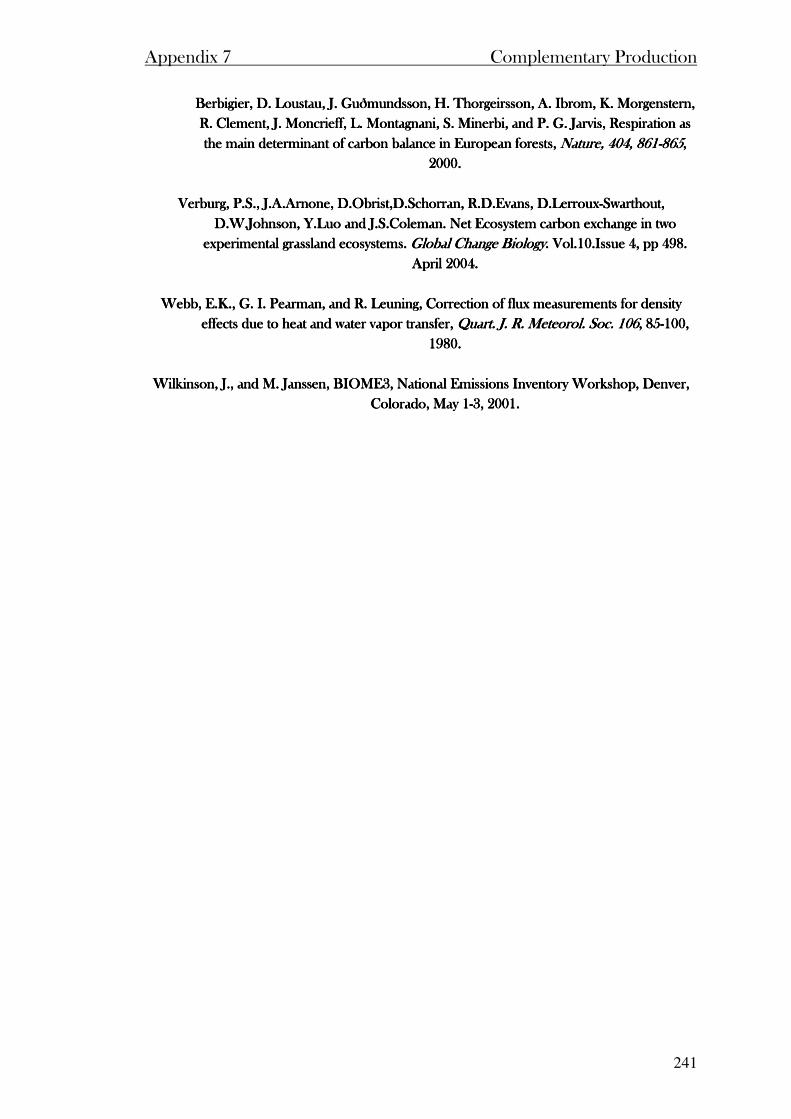
Appendix 7 Complementary Production
241
Berbigier, D. Loustau, J. Guðmundsson, H. ThorgeirssoBerbigier, D. Loustau, J. Guðmundsson, H. ThorgeirssoBerbigier, D. Loustau, J. Guðmundsson, H. ThorgeirssoBerbigier, D. Loustau, J. Guðmundsson, H. Thorgeirsson, A. Ibrom, K. Morgenstern, n, A. Ibrom, K. Morgenstern, n, A. Ibrom, K. Morgenstern, n, A. Ibrom, K. Morgenstern,
R. Clement, J. Moncrieff, L. Montagnani, S. Minerbi, and P. G. Jarvis, Respiration as R. Clement, J. Moncrieff, L. Montagnani, S. Minerbi, and P. G. Jarvis, Respiration as R. Clement, J. Moncrieff, L. Montagnani, S. Minerbi, and P. G. Jarvis, Respiration as R. Clement, J. Moncrieff, L. Montagnani, S. Minerbi, and P. G. Jarvis, Respiration as
the main determinant of carbon balance in European forests, the main determinant of carbon balance in European forests, the main determinant of carbon balance in European forests, the main determinant of carbon balance in European forests, Nature, 404, 861Nature, 404, 861Nature, 404, 861Nature, 404, 861----865865865865, , , , 2000.2000.2000.2000.
Verburg, P.S., J.A.Arnone, D.Obrist,D.Schorran, R.D.Verburg, P.S., J.A.Arnone, D.Obrist,D.Schorran, R.D.Verburg, P.S., J.A.Arnone, D.Obrist,D.Schorran, R.D.Verburg, P.S., J.A.Arnone, D.Obrist,D.Schorran, R.D.Evans, D.LerrouxEvans, D.LerrouxEvans, D.LerrouxEvans, D.Lerroux----Swarthout, Swarthout, Swarthout, Swarthout,
D.W.Johnson, Y.Luo and J.S.Coleman. Net Ecosystem carbon exchange in two D.W.Johnson, Y.Luo and J.S.Coleman. Net Ecosystem carbon exchange in two D.W.Johnson, Y.Luo and J.S.Coleman. Net Ecosystem carbon exchange in two D.W.Johnson, Y.Luo and J.S.Coleman. Net Ecosystem carbon exchange in two
experimental grassland ecosystems. experimental grassland ecosystems. experimental grassland ecosystems. experimental grassland ecosystems. Global Change BiologyGlobal Change BiologyGlobal Change BiologyGlobal Change Biology. Vol.10.Issue 4, pp 498. . Vol.10.Issue 4, pp 498. . Vol.10.Issue 4, pp 498. . Vol.10.Issue 4, pp 498.
April 2004. April 2004. April 2004. April 2004.
Webb, E.K., G. I. Pearman, and R. Leuning, Correction of fWebb, E.K., G. I. Pearman, and R. Leuning, Correction of fWebb, E.K., G. I. Pearman, and R. Leuning, Correction of fWebb, E.K., G. I. Pearman, and R. Leuning, Correction of flux measurements for density lux measurements for density lux measurements for density lux measurements for density
effects due to heat and water vapor transfer, effects due to heat and water vapor transfer, effects due to heat and water vapor transfer, effects due to heat and water vapor transfer, Quart. J. R. Meteorol. Soc. 106Quart. J. R. Meteorol. Soc. 106Quart. J. R. Meteorol. Soc. 106Quart. J. R. Meteorol. Soc. 106, 85, 85, 85, 85----100, 100, 100, 100,
1980.1980.1980.1980.
Wilkinson, J., and M. Janssen, BIOME3, National Emissions Inventory Workshop, Denver, Wilkinson, J., and M. Janssen, BIOME3, National Emissions Inventory Workshop, Denver, Wilkinson, J., and M. Janssen, BIOME3, National Emissions Inventory Workshop, Denver, Wilkinson, J., and M. Janssen, BIOME3, National Emissions Inventory Workshop, Denver,
Colorado, May 1Colorado, May 1Colorado, May 1Colorado, May 1----3, 2001.3, 2001.3, 2001.3, 2001.
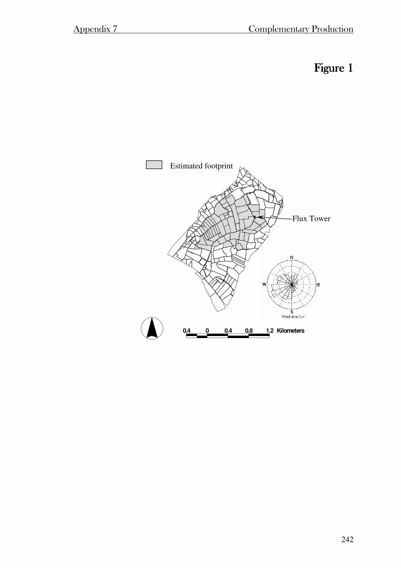
Appendix 7 Complementary Production
242
Figure 1Figure 1Figure 1Figure 1
0. 4 0 0.4 0. 8 1.2 K i lomet er s
Estimated footprint
Flux Tower
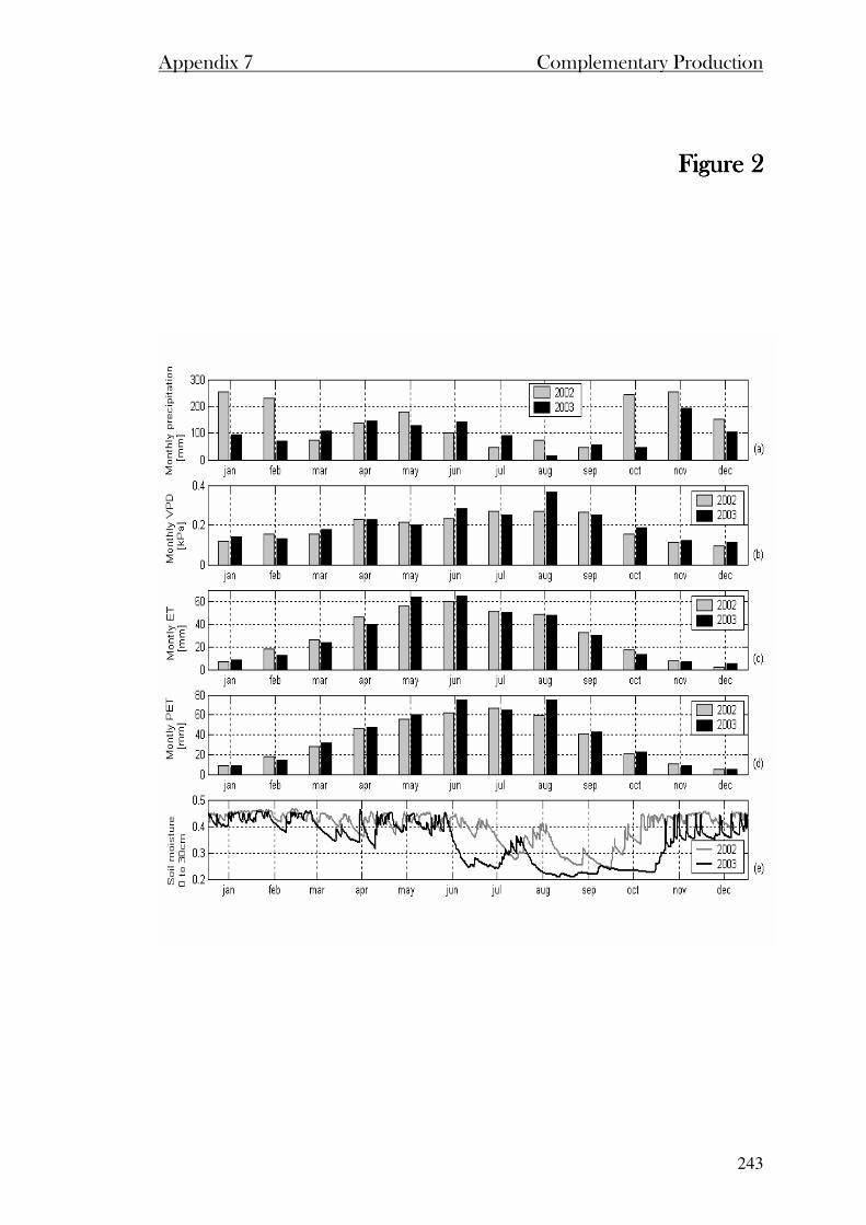
Appendix 7 Complementary Production
243
Figure 2Figure 2Figure 2Figure 2
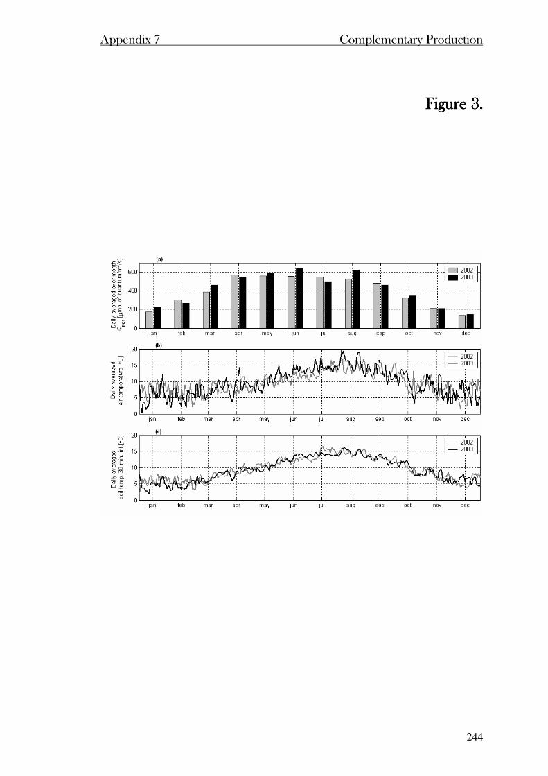
Appendix 7 Complementary Production
244
Figure 3.Figure 3.Figure 3.Figure 3.

Appendix 7 Complementary Production
245
Figure 4.Figure 4.Figure 4.Figure 4.
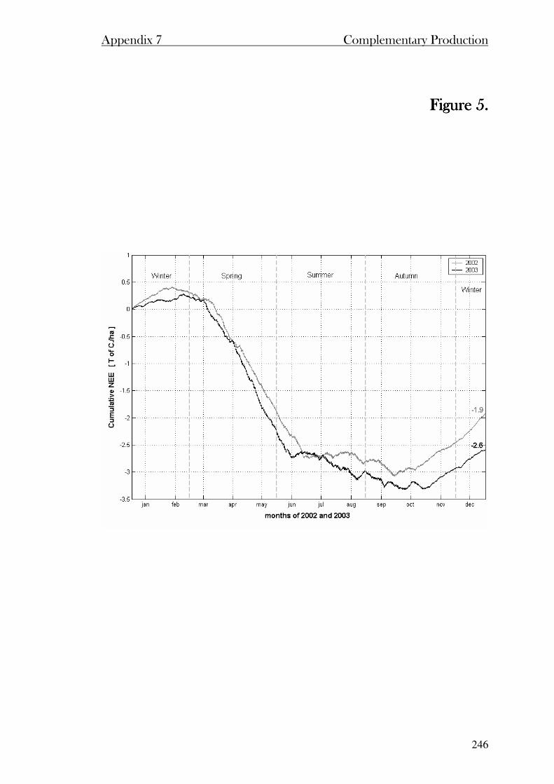
Appendix 7 Complementary Production
246
Figure 5.Figure 5.Figure 5.Figure 5.
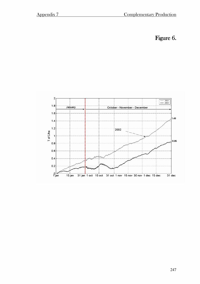
Appendix 7 Complementary Production
247
Figure 6.Figure 6.Figure 6.Figure 6.
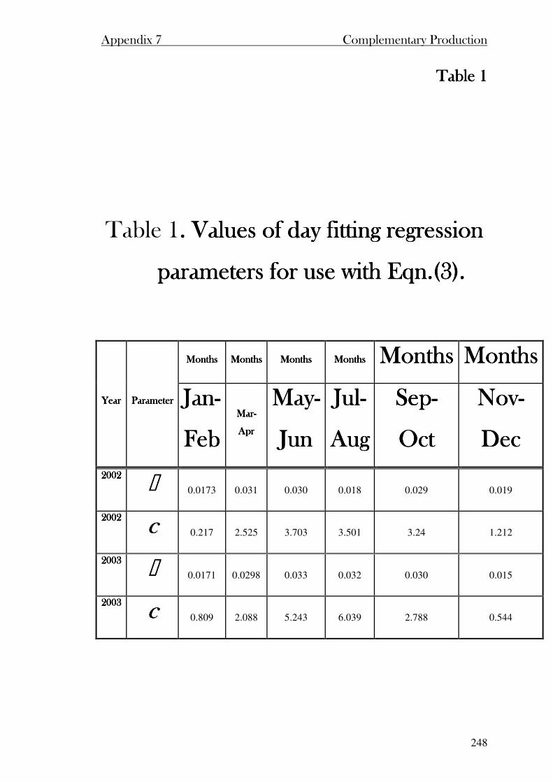
Appendix 7 Complementary Production
248
Table 1Table 1Table 1Table 1
Table 1. Values of day fitting regression . Values of day fitting regression . Values of day fitting regression . Values of day fitting regression
parameters for use with Eqn.(3).parameters for use with Eqn.(3).parameters for use with Eqn.(3).parameters for use with Eqn.(3).
MonthsMonthsMonthsMonths MonthsMonthsMonthsMonths MonthsMonthsMonthsMonths MonthsMonthsMonthsMonths MMMMonthsonthsonthsonths MonthsMonthsMonthsMonths
YearYearYearYear ParameterParameterParameterParameter JanJanJanJan----
FebFebFebFeb MarMarMarMar----
AprAprAprApr
MayMayMayMay----
JunJunJunJun
JulJulJulJul----
AugAugAugAug
SepSepSepSep----
OctOctOctOct
NovNovNovNov----
DecDecDecDec
2002200220022002 MMMM 0.0173 0.031 0.030 0.018 0.029 0.019
2002200220022002 cccc 0.217 2.525 3.703 3.501 3.24 1.212
2003200320032003 MMMM 0.0171 0.0298 0.033 0.032 0.030 0.015
2003200320032003 cccc 0.809 2.088 5.243 6.039 2.788 0.544

Appendix 7 Complementary Production
249
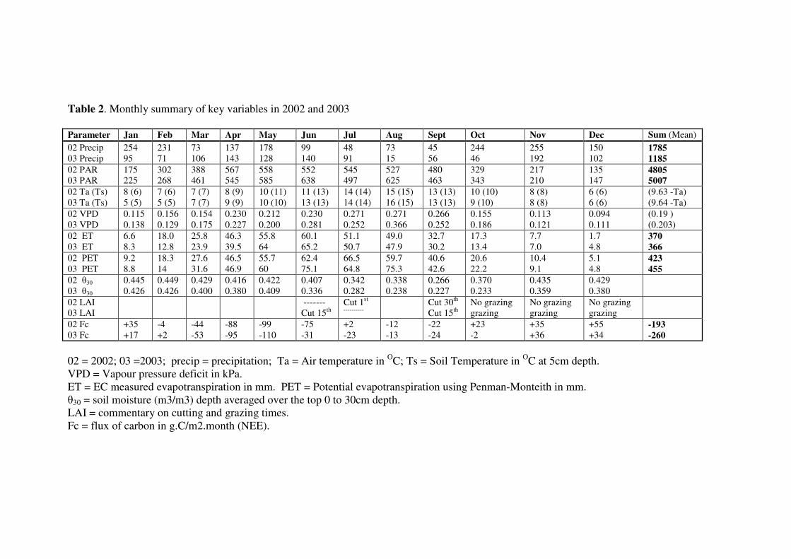
Table 2. Monthly summary of key variables in 2002 and 2003 Parameter Jan Feb Mar Apr May Jun Jul Aug Sept Oct Nov Dec Sum (Mean)
02 Precip 03 Precip
254 95
231 71
73 106
137 143
178 128
99 140
48 91
73 15
45 56
244 46
255 192
150 102
1785
1185
02 PAR 03 PAR
175 225
302 268
388 461
567 545
558 585
552 638
545 497
527 625
480 463
329 343
217 210
135 147
4805
5007
02 Ta (Ts) 03 Ta (Ts)
8 (6) 5 (5)
7 (6) 5 (5)
7 (7) 7 (7)
8 (9) 9 (9)
10 (11) 10 (10)
11 (13) 13 (13)
14 (14) 14 (14)
15 (15) 16 (15)
13 (13) 13 (13)
10 (10) 9 (10)
8 (8) 8 (8)
6 (6) 6 (6)
(9.63 -Ta) (9.64 -Ta)
02 VPD 03 VPD
0.115 0.138
0.156 0.129
0.154 0.175
0.230 0.227
0.212 0.200
0.230 0.281
0.271 0.252
0.271 0.366
0.266 0.252
0.155 0.186
0.113 0.121
0.094 0.111
(0.19 ) (0.203)
02 ET 03 ET
6.6 8.3
18.0 12.8
25.8 23.9
46.3 39.5
55.8 64
60.1 65.2
51.1 50.7
49.0 47.9
32.7 30.2
17.3 13.4
7.7 7.0
1.7 4.8
370
366
02 PET 03 PET
9.2 8.8
18.3 14
27.6 31.6
46.5 46.9
55.7 60
62.4 75.1
66.5 64.8
59.7 75.3
40.6 42.6
20.6 22.2
10.4 9.1
5.1 4.8
423
455
02 θ30 03 θ30
0.445 0.426
0.449 0.426
0.429 0.400
0.416 0.380
0.422 0.409
0.407 0.336
0.342 0.282
0.338 0.238
0.266 0.227
0.370 0.233
0.435 0.359
0.429 0.380
02 LAI 03 LAI
------- Cut 15th
Cut 1st
---------- Cut 30th
Cut 15th No grazing grazing
No grazing grazing
No grazing grazing
02 Fc 03 Fc
+35 +17
-4 +2
-44 -53
-88 -95
-99 -110
-75 -31
+2 -23
-12 -13
-22 -24
+23 -2
+35 +36
+55 +34
-193
-260
02 = 2002; 03 =2003; precip = precipitation; Ta = Air temperature in OC; Ts = Soil Temperature in OC at 5cm depth. VPD = Vapour pressure deficit in kPa. ET = EC measured evapotranspiration in mm. PET = Potential evapotranspiration using Penman-Monteith in mm. θ30 = soil moisture (m3/m3) depth averaged over the top 0 to 30cm depth. LAI = commentary on cutting and grazing times. Fc = flux of carbon in g.C/m2.month (NEE).
Related Documents