Observation system simulation experiments for the PREMIER mission Sub-task of the project ‘Quantification of Atmospheric Pollution and Climate Aspects’ (ESTEC contract No. 4000101294/10/NL/CBi) Y. Rochon, J.W. Kaminski, S. Heilliette, L. Garand, J. de Grandpré, and R. Ménard Environment Canada 5 h WMO Workshop on the Impact of Various Observing Systems on NWP Sedona, AZ, 22-25 May 2012

Observation system simulation experiments for the PREMIER mission Sub-task of the project ‘Quantification of Atmospheric Pollution and Climate Aspects’
Dec 25, 2015
Welcome message from author
This document is posted to help you gain knowledge. Please leave a comment to let me know what you think about it! Share it to your friends and learn new things together.
Transcript

Observation system simulation experiments for the PREMIER mission Sub-task of the project ‘Quantification of Atmospheric Pollution and
Climate Aspects’ (ESTEC contract No. 4000101294/10/NL/CBi)
Y. Rochon, J.W. Kaminski, S. Heilliette, L. Garand, J. de Grandpré, and R. Ménard Environment Canada5h WMO Workshop on the Impact of Various ObservingSystems on NWPSedona, AZ, 22-25 May 2012

WMO workshop – Observing Systems and NWP slide 2 22-25 May 2012
Introduction
• Objective: Acquire insight on the potential impact of PREMIER limb observations of temperature, water vapour and ozone in numerical weather (and ozone) prediction.
• Applied methodology: The level of impact of PREMIER observations is estimated through Observation System Simulation Experiments (OSSEs).
– Synthetic observation sets reflecting the characteristics of the projected PREMIER retrieval-type data and of existing observation systems are derived from a virtual truth, i.e. a nature run.
▪ Target PREMIER-type data consists of retrieved profiles from the– InfraRed Limb Sounder (IRLS; T, water vapour, ozone, …)
and– Millimetre-Wave Limb Sounder (MWLS; water vapour, ozone, …).
▪ MLS-type data serves as additional benchmark for comparison.
– Various assimilation and forecasting experiments with and without the PREMIER and MLS-type data are conducted and assessed.
WMO workshop – Observing Systems and NWP slide 3 22-25 May 2012
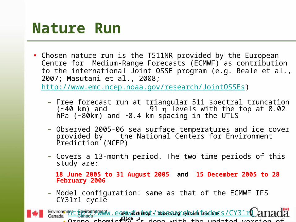
Nature Run
• Chosen nature run is the T511NR provided by the European Centre for Medium-Range Forecasts (ECMWF) as contribution to the international Joint OSSE program (e.g. Reale et al., 2007; Masutani et al., 2008; http://www.emc.ncep.noaa.gov/research/JointOSSEs)
– Free forecast run at triangular 511 spectral truncation (~40 km) and 91 levels with the top at 0.02 hPa (~80km) and ~0.4 km spacing in the UTLS
– Observed 2005-06 sea surface temperatures and ice cover provided by the National Centers for Environment Prediction (NCEP)
– Covers a 13-month period. The two time periods of this study are:
18 June 2005 to 31 August 2005 and 15 December 2005 to 28 February 2006
– Model configuration: same as that of the ECMWF IFS CY31r1 cycle
▪ http://www.ecmwf.int/research/ifsdocs/CY31r1 ▪ Ozone chemistry is done with the updated version of the Cariolle
and Déqué (1986) parameterization

WMO workshop – Observing Systems and NWP slide 4 22-25 May 2012
Assimilation and forecasting system
• NWP model:– Operational Global Environmental Multi-scale model (GEM) of
Environment Canada▪ 800x600 (~33 km at 49) ▪ 80 levels up to 0.1 hPa (0.3 to 0.6 km in the UTLS)▪ added linearized ozone chemistry (LINOZ; McLinden et al.,
2000)
• Initial conditions close to the NR (GEM 5-day forecasts from NR)
• Assimilation approach:– 3D-VAR with FGAT (First Guess at Appropriate Time)
▪ Incremental assimilation at T108▪ Incremental control variables: , ’, T’, ln(q), O3, Ps
– Global data assimilation every successive 6-hours – No background check applied for the OSSE assimilations– Surfaces conditions taken from CMC/EC (and not from the NR)
WMO workshop – Observing Systems and NWP slide 5 22-25 May 2012
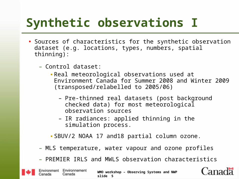
Synthetic observations I
• Sources of characteristics for the synthetic observation dataset (e.g. locations, types, numbers, spatial thinning):
– Control dataset:▪ Real meteorological observations used at Environment
Canada for Summer 2008 and Winter 2009 (transposed/relabelled to 2005/06)
– Pre-thinned real datasets (post background checked data) for most meteorological observation sources
– IR radiances: applied thinning in the simulation process.
▪ SBUV/2 NOAA 17 and18 partial column ozone.
– MLS temperature, water vapour and ozone profiles
– PREMIER IRLS and MWLS observation characteristics
WMO workshop – Observing Systems and NWP slide 6 22-25 May 2012
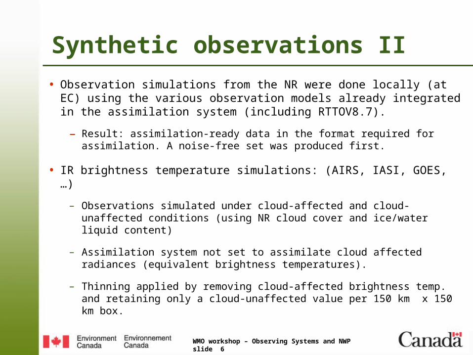
Synthetic observations II
• Observation simulations from the NR were done locally (at EC) using the various observation models already integrated in the assimilation system (including RTTOV8.7).
– Result: assimilation-ready data in the format required for assimilation. A noise-free set was produced first.
• IR brightness temperature simulations: (AIRS, IASI, GOES, …)
– Observations simulated under cloud-affected and cloud-unaffected conditions (using NR cloud cover and ice/water liquid content)
– Assimilation system not set to assimilate cloud affected radiances (equivalent brightness temperatures).
– Thinning applied by removing cloud-affected brightness temp. and retaining only a cloud-unaffected value per 150 km x 150 km box.

WMO workshop – Observing Systems and NWP slide 7 22-25 May 2012
Meteorological control observations to be assimilated, excluding radiances (partly based on Laroche and Sarrazin, 2010)
Observing network AtmosphericVariables
Applied resolution and or coverage (after thinning)
Approximate number ofobservations per 6h
Radiosondes/dropsondesU, V, T, (T-Td), Ps 28 vertical levels ~750 stations (<1000)
usually for 00 and 12UTC
Surface reports (ground stations, ships and buoys)
T, (T-Td), Ps, U and V over water
1 report / 6h ~6 000
Wind profilers (NOAA network of UHF radars)
U, V 0.5 km to 16 km vert. range with a 750 m vert. resol.
35 sites
Aircrafts U, V, T, humidity 1o x1o x 50 hPa covers 100 - 1025 hPa
~14 000 to 22 000
GPS RO micro satellites (COSMIC (6), GRACE, METOP,
CHAMP)
T, humidity ~1 km to 40 km vert. range with a 830 m vert. resol.
~600 profiles
Scatterometer winds from the SeaWinds microwave radar (13.4GHz) on the Quikscat polar-orbiter
Ocean surface U,V _~10 000
AMVs from MODIS on TERRA and AQUA (polar orbiting)
U,V over water (+land in tropics)
~180km for polar winds550-700hPa range
~2 500
AMVs from 5 GEO sats U,V over water (+ land in tropics)
1.5o x1.5o
400-700 hPa range ~14 000 to 26 000

WMO workshop – Observing Systems and NWP slide 8 22-25 May 2012
Control radiance observations Instrument Platform Number (one
typical day)Orbit
Channels used Target variable
AMSU-A (ATOVS)
NOAA-15 338 000
Polar
Ch. 3-14 over oceanCh. 6-14 over land
T
NOAA-18 472 000
AQUA 332 000
AMSU-B (ATOVS)
NOAA-15 41 000 Ch. 2-5 over oceanCh. 3-4 over land
q
NOAA-16 84 000
NOAA-17 93 000
MHS NOAA-18 96 000
SSMI DMSP-13 61 000 Ch. 1-7 for cloud-free regions over the ocean
q and surface windSSMIS DMSP-16 39 000
AIRS AQUA 660 000 87 channels with peak below
150 hPa (650-2100 cm-1)- cloud-free pixels
T, q,surface
and clouds
IASI METOP-2 501 000 62 channels with peak below150hPa (650-770 cm-1)- cloud-free pixels
T, surfaceand
clouds
GOES imagers
GOES-11 35 000
Geo-stationary(GEORAD)
One channel per instrumentin the 6.2 to 6.8 micronsrange
-Cloud-free pixels
qGOES-12 42 000
MVIRI METEOSAT-7 69 000
SEVIRI METEOSAT-9 (MSG-2) 42 000
MTSAT-01 METSAT-1R 21 000
IR
WMO workshop – Observing Systems and NWP slide 9 22-25 May 2012
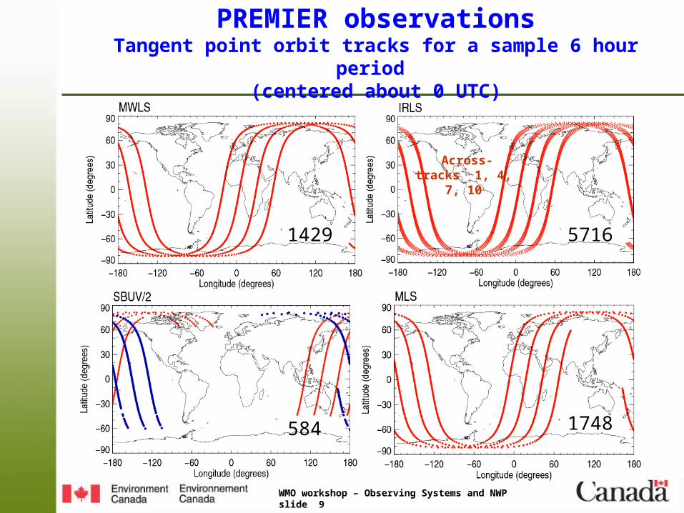
PREMIER observationsTangent point orbit tracks for a sample 6 hour period
(centered about 0 UTC)
57161429
1748584
Across-tracks 1, 4, 7, 10

WMO workshop – Observing Systems and NWP slide 10 22-25 May 2012
PREMIER observations (cont’d)
• Vertical ranges and resolutions
- Minimum altitude:
- IRLS: up to 50 km with 1 km vert. resolution- MWLS: up to ~35 km with unequally spaced levels (>= 1.6 km)
• Water dependent rejection conditions:
- affecting about 50% of IRLS and 30% of MWLS H2O of profiles in the lower tropospheric levels.
• Averaging kernels: Not applied (except for SBUV-2 ozone)
- Current PREMIER averaging kernel matrices for T, H2O and O3 not used since they are nearly identity matrices in most (or all) of the vertical range
• Observation error variances:
- Given random error variances plus added error variance offsets.
•.
(km) )90cos(48min oz
WMO workshop – Observing Systems and NWP slide 11 22-25 May 2012
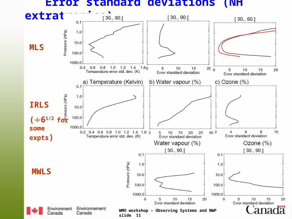
Error standard deviations (NH extratropics)
IRLS
(61/2 for
some expts)
MWLS
MLS

WMO workshop – Observing Systems and NWP slide 12 22-25 May 2012
Calibration: Observation random errors
• Perturbations applied to the synthetic observations using Gaussian-distributed random errors.
• Purpose of error level calibration: Provide greater confidence on the pertinence of the OSSE results.
• Simple approach: – Desire statistical scores of 2 /N (and its contributing terms) similar to
those obtained from the assimilation of real observations, e.g.
– Introduced error std. dev. scaling factors f (following Errico et al.) for different observation grouping (families) – derived here from ratios of the above two terms.
• Limitations:– Adjustments (scaling factors) not dependent on vertical level– Some observation groupings contain sub-types (or channels) which
may ideally require different adjustments– No application of spatial and inter-channel obs. error correlations.
observedsimulated
NxJNxJ aoao /2/2

WMO workshop – Observing Systems and NWP slide 13 22-25 May 2012
sk(xa)=2Jok/Nk
Real obs.
Jan. 2009
Control
(synthetic)Winter/Summer
Jan-Feb ‘06
Jul-Aug ‘05
not well calibrated
Real RealControl Control
f spectrally constant for this study

WMO workshop – Observing Systems and NWP slide 14 22-25 May 2012
Comparison of 6h forecasts to radiosondes:
(January)
Real and synthetic
Solid: mean difference Dashed: std. dev.
Control vs real observation assimilation

WMO workshop – Observing Systems and NWP slide 15 22-25 May 2012
Global
6h forecast error levels
(July)
Solid: Mean errorDashed: Error std. dev.
Black: Control
Blue: Control+MLS
Red: Control+IRLS
U T
q O3
Impact study results
Important caveat: max. iterations of 70 for most assim. expts (affects CRTL+IRLS assim. the most)

WMO workshop – Observing Systems and NWP slide 16 22-25 May 2012
Tropics
6h forecast error levels
(July)
Solid: Mean errorDashed: Error std. dev.
Black: Control
Blue: Control+MLS
Red: Control+IRLS
U T
q O3

WMO workshop – Observing Systems and NWP slide 17 22-25 May 2012
South Pole
6h forecast error levels
(July)
Solid: Mean errorDashed: Error std. dev.
Black: Control
Blue: Control+MLS
Red: Control+IRLS
U T
q O3
WMO workshop – Observing Systems and NWP slide 18 22-25 May 2012
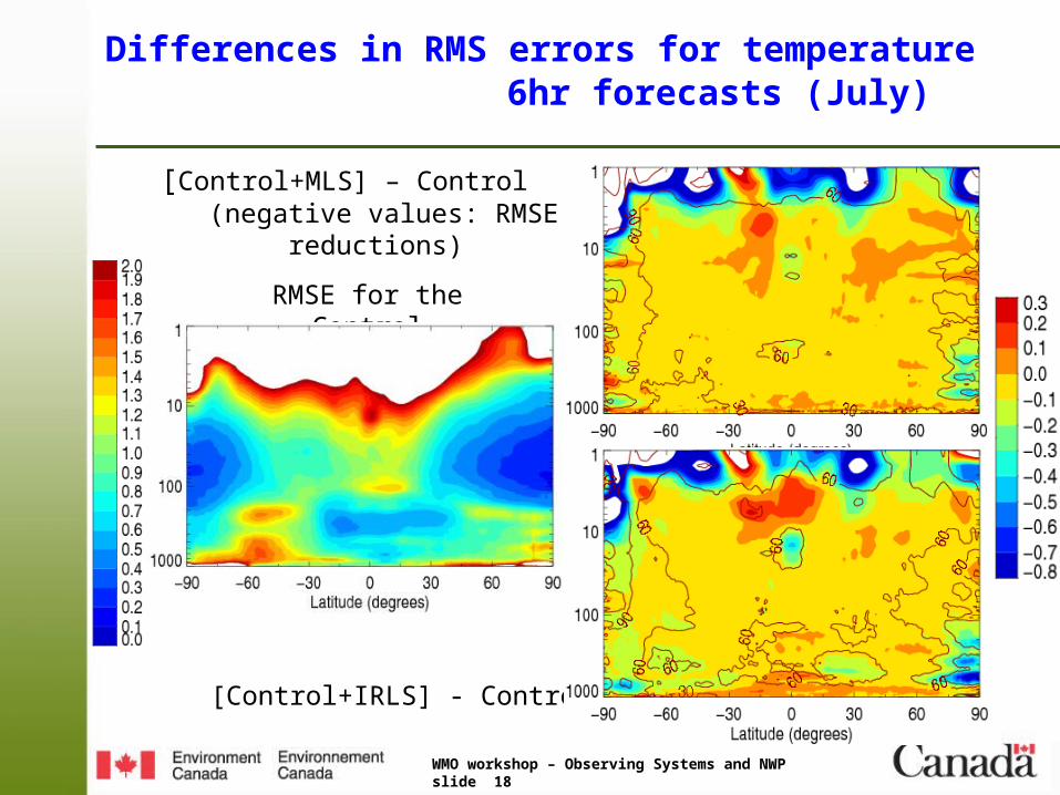
Differences in RMS errors for temperature 6hr forecasts (July)
RMSE for the Control
[Control+IRLS] - Control
[Control+MLS] – Control (negative values: RMSE reductions)

WMO workshop – Observing Systems and NWP slide 19 22-25 May 2012
Comparison of ratio of RMS errors (IRLS,Control) for temperature 6hr forecasts (July)
Temperature Zonal wind component

WMO workshop – Observing Systems and NWP slide 20 22-25 May 2012
Time mean error differences of Control+IRLS minus Control for temperature 6hr forecasts (July)
=0.5 = 0.6

WMO workshop – Observing Systems and NWP slide 21 22-25 May 2012
Sample medium range forecast results for temperature (August)
6-day forecast time mean differences at =0.2:
[CTRL+IRLS] - CRTL
Anomaly correlations (relative to the NR)
CRTL CRTL+MLS
CRTL+IRLS
WMO workshop – Observing Systems and NWP slide 22 22-25 May 2012
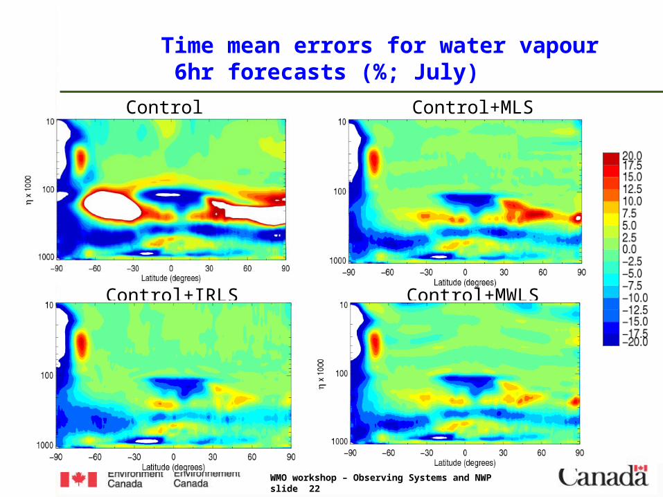
Time mean errors for water vapour 6hr forecasts (%; July)
Control Control+MLS
Control+IRLS Control+MWLS

WMO workshop – Observing Systems and NWP slide 23 22-25 May 2012
Ratio of RMS errors (IRLS, Control) for water vapour (lnq) 6hr forecasts (July)
=0.2
6-day forecasts

WMO workshop – Observing Systems and NWP slide 24 22-25 May 2012
Source analyses: Control, Control+MLS, Control+IRLS
Global mean and RMS errors, and anomaly correlation coefficients for water vapour (August)
Smaller due to cancelling of +/- errors

WMO workshop – Observing Systems and NWP slide 25 22-25 May 2012
Final remarks
• Synthetic bias-free dataset reflecting realistic measurement network can be easily produced following the specification of the NR.
• Zeroth order observation perturbation calibration feasible through a comparison of
• Temperature (and winds): – RMS error reductions (zonal) usually within ~0.1-0.3 K and 0.2 m/s for
IRLS and similar to half for MLS-type.– Increase in T predictability (avg over latitudes) of ~¼ (UTLS) to ½ (mid-
strato) day.– More notable improvements near poles for T at about 1K– Improvement in T and U near 10 hPa at equator
• Water vapour (and ozone): – IRLS (largest) and MWLS potential benefit over MLS-type in
troposphere and UTLS (greater for ozone).– Error reductions extend downward to the mid-troposphere and below.– Present impact differences with MLS decrease with forecast length.– Notably persistent improvements over 10-day forecasts
• Setup applicable to other studies.
NxJ ao /2

WMO workshop – Observing Systems and NWP slide 26 22-25 May 2012
Acknowledgements
• Nature run: ECMWF and the Joint OSSEs program (Michiko Masutani et al.).
• Discussions on error calibration and setting of =1 level of NR: Ronald Errico (GMAO/NASA and GESTC)
• Discussions and information on PREMIER data: Lars Hoffmann, Bärbel Vogel, Joachim Urban, and Richard Siddans.
• PREMIER Impact Study project management: Bärbel Vogel (Julich) and Joerg Langen (ESTEC)
• MLS-Aura and SBUV/2 science and instrument teams for the availability of data.
• Assimilation and forecasting system: Various EC colleagues

WMO workshop – Observing Systems and NWP slide 27 22-25 May 2012
Extras

WMO workshop – Observing Systems and NWP slide 28 22-25 May 2012
NR fields used
91 vertical level data Source of constructed 92nd level
Geopotential height Surface geopotential (converted to geopotential height)
Wind 10 metre wind (U and V components)
Temperature 2 metre temperature
Specific humidity 2 metre dew point temperature (converted to specific humidity)
Ozone Copy of level # 91
Cloud cover Copy of level # 91
Cloud ice water Copy of level # 91
Cloud liquid water Copy of level # 91
Surface fields: Sea-ice cover, albedo, snow depth (to set snow cover field), skin temperature.

WMO workshop – Observing Systems and NWP slide 29 22-25 May 2012
• Monthly based RMS, std. dev. and time mean errors relative to the NR.
• Ratios of RMS errors over individual months: (similarly to Lahoz et al., 2005)
A value of <1 indicates a beneficial impact from X2 relative to X1.
• Monthly mean differences (X2-NR) – (X1-NR)
• Above accompanied by significance tests
• Student t-test (mean diff.) anf F-test (applied to RMS errors)
• Anomaly correlation coefficients relative to the NR.
Some measures of performance
NR)(X
NR)(X)X,(X
1
212
RMS
RMSρ
Impact of PREMIER observations

WMO workshop – Observing Systems and NWP slide 30 22-25 May 2012
Comparison of ratio of RMS errorsfor ozone 6hr forecasts (July)
(IRLS, Control) (IRLS, MLS)
(MWLS, Control) (MWLS, MLS)

WMO workshop – Observing Systems and NWP slide 31 22-25 May 2012
RMS errors ozone 6hr forecasts (%; July)
Control Control+MLS
Control+MWLS Control+IRLS

WMO workshop – Observing Systems and NWP slide 32 22-25 May 2012
July time mean error ozone 6hr forecasts (%)
Control
Control+MLS
Control+IRLS
Control+MWLS

WMO workshop – Observing Systems and NWP slide 33 22-25 May 2012
Source analyses: Control, Control+MLS, Control+IRLS
Global mean errors, RMS errors, and anomaly correlation coefficients for ozone (August)
Related Documents