Object tracking and credal classification with kinematic data in a multi-target context

Information Fusion 20 (2014) 174–188

Contents lists available at ScienceDirect

Information Fusion

journal homepage: www.elsevier .com/locate / inf fus

Object tracking and credal classification with kinematic datain a multi-target context

http://dx.doi.org/10.1016/j.inffus.2014.01.0071566-2535/� 2014 Elsevier B.V. All rights reserved.

⇑ Corresponding author. Tel.: +33 0617525772.E-mail addresses: [email protected] (S. Hachour), francois.

[email protected] (F. Delmotte), [email protected] (D. Mercier),[email protected] (E. Lefèvre).

Samir Hachour ⇑, François Delmotte, David Mercier, Eric LefèvreUniv. Lille Nord de France, F-59000 Lille, FranceUArtois, LGI2A, F-62400 Béthune, France

a r t i c l e i n f o

Article history:Received 15 February 2013Received in revised form 25 January 2014Accepted 25 January 2014Available online 6 February 2014

Keywords:Multi-target trackingCredal classificationData assignmentTarget management

a b s t r a c t

This article proposes a method to classify multiple maneuvering targets at the same time. This task is amuch harder problem than classifying a single target, as sensors do not know how to assign capturedobservations to known targets. This article extends previous results scattered in the literature and unifiesthem in a single global framework with belief functions. Through two examples, it is shown that the fullalgorithm using belief functions improves results obtained with standard Bayesian classifiers and that itcan be applied to a large variety of applications.

� 2014 Elsevier B.V. All rights reserved.

1. Introduction

The problem of joint multi-target tracking and classification,which is as old as the invention of radars, is a much more complextask than the problem of tracking one target. Indeed it includes astep, called the assignment problem, where sensors have to associ-ate known objects to new captured observations. A full multi-target tracking solution includes several interlaced componentssuch as the tracking component, the assignment component, thehypothesis rejection (new or disappeared targets, etc.) and finallythe classification step. Probability-based solutions already existin the literature [1–7].

For about 40 years, other uncertainty models based on non-additive measures have been developed, in particular the Transfer-able Belief Model [8] based on belief functions [9,10] which issometimes referred to as the credal model. Applications of thismodel can be found for example in classification tasks and decisionsupport systems [11]. Direct comparisons with Bayesian solutionsare presented in [12,13] with discrete variables or in [14] withcontinuous variables.

Applications of this theory to multi-target tracking and classifi-cation problems are scattered through several articles presentingdifferent approaches. In [15,13] and in [16] various distances

between belief functions are used to tackle the assignment prob-lem. Ref. [15] has been recently improved in [17], but these tworeferences only tackles the assignment problem with uncertainobservations and do not cope with the tracking problem. In [14]a solution to track and classify a single dynamical target isproposed, but no extension to multi-target tracking is proposed.

The aim of this article is to gather these scattered results, to uni-fy them in a single and consonant framework based on belief func-tions, and to propose a solution for multi-target tracking andclassification using belief functions when no one exists in the re-cent literature. The proposed solution also includes a step ofhypothesis rejection, which means that it manages new and disap-peared targets.

The result is a complete solution to multi-target tracking andclassification in a cluttered environment. It mimics the standardand well accepted Bayesian solutions, but it extends them, whenpossible, with belief functions. A short preliminary version of thisarticle was presented in [18].

The well known Interacting Multiple Model (IMM) algorithm isused to track multiple targets. The assignment of the observationsto known targets is performed by the means of a generalized Glo-bal Nearest Neighbor algorithm. Target management is ensured bya score functions representing the quality of targets tracks. Finally,the classification step is realized with the Transferable Belief Modelinstead of a classical Bayesian solution.

This article is organized as follows. An introduction to belieffunction theory is presented in Section 2. Section 3 deals withtracking problems. Assignment and hypothesis rejection problems

S. Hachour et al. / Information Fusion 20 (2014) 174–188 175

are tackled in Section 4. Bayesian and proposed algorithms aresummarized in Section 5. Finally, two application examples aredetailed in Section 6. The first one involves an academic exampleon aircraft classification with constant classes, it allows a compar-ison with a Bayesian solution. The second example concerns apedestrian activity recognition, it highlights a first extension ofthe proposed algorithm to time varying classes.

2. Belief functions

2.1. Main functions

This section introduces basic notions on belief functions theory,which was firstly introduced by Dempster in [9] and extended byShafer [10] and Smets [8]. Knowledge is expressed on a discreteset C ¼ fc1; c2; . . . ; cncg of nc mutually exclusive and exhaustivehypotheses. Frame C is called the frame of discernment. A massmðAÞ with A # C is the part of belief supporting A that, due to a lackof information, cannot be given to any strict subset of A [8]. A massfunction m (or basic belief assignment) has to satisfy:XA # C

mðAÞ ¼ 1: ð1Þ

Throughout this article, 2C represents all the subsets of C. A set Asuch that mðAÞ > 0 is called a focal element of m.

In addition to the mass function, two other functions aredefined in the following manner. The plausibility function Pl repre-sents the total amount of belief that may be given to a subset A of Cwith further pieces of evidence:

PlðAÞ ¼X

A\B–;mðBÞ: ð2Þ

Unlike the plausibility function, the belief function Bel repre-sents the amount of belief that is certain and cannot be reduced:

BelðAÞ ¼XA�B

mðBÞ: ð3Þ

These functions are in one-to-one correspondence [10], so theyare used indifferently with the same term belief function when thecontext is clear.

A belief function whose focal elements are singletons is called aBayesian belief function, it corresponds to a probability distributionand respects the property of additivity:

PlðA [ BÞ ¼ PlðAÞ þ PlðBÞ; ð4Þ

with ðA; BÞ# 2C and A \ B – ;. In general, this relation is false andbelief functions are non-additive measures.

A belief function such that mðCÞ ¼ 1 respects PlðAÞ ¼ 1 for all Asubsets of C, A – ;. Denoted by m0, it is called the vacuous belieffunction and represents the full ignorance.

2.2. Fusion rule and discounting

When more than one mass function is expressed on the sameframe of discernment, they can be fused to obtain a single repre-sentation. The conjunctive combination used in this work assumesindependent and absolutely reliable sources. Let m1 and m2 be twomass functions provided by two distinct sources and expressed onthe same frame of discernment C, their conjunctive combination isdefined as follows:

m12ðAÞ ¼ ðm1 m2ÞðAÞ ¼X

A1\A2¼A

m1ðA1Þm2ðA2Þ: ð5Þ

Eq. (5) is the unnormalized rule, the normalized rule is referred toas Dempster’s rule of combination, and is defined by:

m12ðAÞ ¼P

A1\A2¼Am1ðA1Þm2ðA2Þ1�

PA1\A2¼;m1ðA1Þm2ðA2Þ

: ð6Þ

This rule is used in order to update a priori beliefs with onlinemeasurements, as in Section 2.4.

The last example in this article involves the discounting of asource of information. Such a discounting assumes that you canestimate the reliability of a source by a factor k 2 ½0;1�. If k ¼ 1,the source is considered as absolutely reliable, while if k ¼ 0, thesource must be discarded and replaced by a vacuous belief. Thusthe discounting mk of a given source mass function m is defined by:

mkðAÞ ¼ kmðAÞ if A – C;

mkðCÞ ¼ kmðCÞ þ 1� k otherwise:

�ð7Þ

If several sources of information mi have to be fused, each onewith its own reliability ki, a classical approach is to first discountall of them, and then to conjunctively fuse them using Eq. (5).Several other fusion rules are defined, and for a review, readerscan refer to [19]. For example, contextual data can be included alsoin the fusion process, see [20], and reliability factors can beadapted online [21], although this is not used in this article.

2.3. Decision rule

Several belief function interpretations exist, among them theUpper/Lower Probabilities (ULP), usually called imprecise probabil-ities, and the Transferable Belief Model (TBM) of Smets. Basicallythese models are equal when considering static knowledge, butdiffer when conditioning steps are involved. Readers interestedin this topic can refer to [22]. In a few words, within an ULP model,conditioning requires to condition every probability measure PðAÞcompatible with the bounds defined by BelðAÞ 6 PðAÞ 6 PlðAÞ. Then,the new bounds Belð:j:Þ and Plð:j:Þmust be recomputed by checkingevery conditioned probability measures, and taking the new max-imum and minimum, while within the TBM it suffices to conditiononly the original BelðAÞ and PlðAÞ. Thus, the ULP model is morecomputationally demanding. In a recent article [23], the ULP modelhas been advocated in a classification problem. But the authors ofthis article do not find the provided examples conclusive and theadvantage of the ULP model over the TBM remains unclear. Sinceit is more complex to use, the TBM has been chosen in this article,as in [14] for instance.

The TBM represents and manages knowledge with a two levelmodel. The first one, referred to as the credal level, concerns therepresentation and the manipulation of the data. It is the placewhere data are encoded, combined and updated with belief func-tions without assuming probability measures [12]. Decisions aremade when necessary at a second level called the pignistic level,where belief functions are transformed into a probability measuresusing the pignistic transformation justified in [24] through ratio-nality requirements and basic axioms. Pignistic probability BetPis defined by:

BetPðfcigÞ ¼Xci2A

mðAÞjAjð1�mð;ÞÞ : ð8Þ

Let us remark that other decision rules have been introduced forbelief functions, among them the maximum of plausibility [25].Comparing the drawbacks and advantages of all the decision rulesis outside the scope of this article, farther information can be foundin [24].

2.4. Generalized Bayes theorem

Bayes theorem enables to compute the a posteriori probabilityfrom an a priori one. With likelihoods lðcijzÞ ¼ PðzjciÞ, where z is a

0 20 40 60 80 100−50

−40

−30

−20

−10

0

10

Time

Posi

tion

True positionParticle filter estimateKalman filter estimate

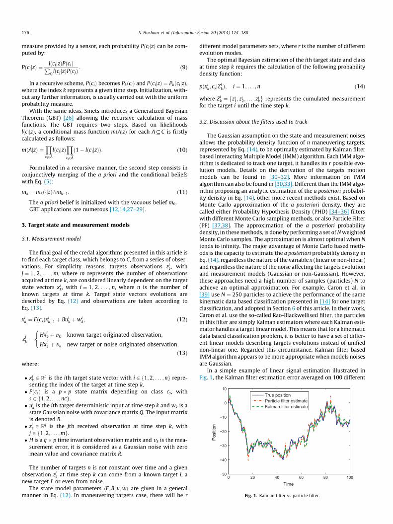
Fig. 1. Kalman filter vs particle filter.

176 S. Hachour et al. / Information Fusion 20 (2014) 174–188

measure provided by a sensor, each probability PðcijzÞ can be com-puted by:

PðcijzÞ ¼lðcijzÞPðciÞPcj

lðcjjzÞPðcjÞ: ð9Þ

In a recursive scheme, PðciÞ becomes PkðciÞ and PðcijzÞ ¼ PkðcijzÞ,where the index k represents a given time step. Initialization, with-out any further information, is usually carried out with the uniformprobability measure.

With the same ideas, Smets introduces a Generalized BayesianTheorem (GBT) [26] allowing the recursive calculation of massfunctions. The GBT requires two steps. Based on likelihoodslðcijzÞ, a conditional mass function mðAjzÞ for each A # C is firstlycalculated as follows:

mðAjzÞ ¼Yci2A

lðcijzÞYci2A

ð1� lðcijzÞÞ: ð10Þ

Formulated in a recursive manner, the second step consists inconjunctively merging of the a priori and the conditional beliefswith Eq. (5):

mk ¼ mkð�jzÞ mk�1: ð11Þ

The a priori belief is initialized with the vacuous belief m0.GBT applications are numerous [12,14,27–29].

3. Target state and measurement models

3.1. Measurement model

The final goal of the credal algorithms presented in this article isto find each target class, which belongs to C, from a series of obser-vations. For simplicity reasons, targets observations zj

k, withj ¼ 1; 2; . . . ; m, where m represents the number of observationsacquired at time k, are considered linearly dependent on the targetstate vectors xi

k, with i ¼ 1; 2; . . . ; n, where n is the number ofknown targets at time k. Target state vectors evolutions aredescribed by Eq. (12) and observations are taken according toEq. (13).

xik ¼ FðcsÞxi

k�1 þ Buik þwi

k; ð12Þ

zjk ¼

Hxik þ vk known target originated observation;

Hxi0

k þ vk new target or noise originated observation;

(

ð13Þ

where:

� xik 2 Rp is the ith target state vector with i 2 f1;2; . . . ;ng repre-

senting the index of the target at time step k.� FðcsÞ is a p� p state matrix depending on class cs, with

s 2 f1;2; . . . ;ncg.� ui

k is the ith target deterministic input at time step k and wk is astate Gaussian noise with covariance matrix Q. The input matrixis denoted B.� zj

k 2 Rq is the jth received observation at time step k, withj 2 f1;2; . . . ;mg.� H is a q� p time invariant observation matrix and vk is the mea-

surement error, it is considered as a Gaussian noise with zeromean value and covariance matrix R.

The number of targets n is not constant over time and a givenobservation zj

k at time step k can come from a known target i, anew target i0 or even from noise.

The state model parameters hF;B;u;wi are given in a generalmanner in Eq. (12). In maneuvering targets case, there will be r

different model parameters sets, where r is the number of differentevolution modes.

The optimal Bayesian estimation of the ith target state and classat time step k requires the calculation of the following probabilitydensity function:

pðxik; csjZi

kÞ; i ¼ 1; . . . ;n ð14Þ

where Zik ¼ zi

1; zi2; . . . ; zi

k

� �represents the cumulated measurement

for the target i until the time step k.

3.2. Discussion about the filters used to track

The Gaussian assumption on the state and measurement noisesallows the probability density function of n maneuvering targets,represented by Eq. (14), to be optimally estimated by Kalman filterbased Interacting Multiple Model (IMM) algorithm. Each IMM algo-rithm is dedicated to track one target, it handles its r possible evo-lution models. Details on the derivation of the targets motionmodels can be found in [30–32]. More information on IMMalgorithm can also be found in [30,33]. Different than the IMM algo-rithm proposing an analytic estimation of the a posteriori probabil-ity density in Eq. (14), other more recent methods exist. Based onMonte Carlo approximation of the a posteriori density, they arecalled either Probability Hypothesis Density (PHD) [34–36] filterswith different Monte Carlo sampling methods, or also Particle Filter(PF) [37,38]. The approximation of the a posteriori probabilitydensity, in these methods, is done by performing a set of N weightedMonte Carlo samples. The approximation is almost optimal when Ntends to infinity. The major advantage of Monte Carlo based meth-ods is the capacity to estimate the a posteriori probability density inEq. (14), regardless the nature of the variable x (linear or non-linear)and regardless the nature of the noise affecting the targets evolutionand measurement models (Gaussian or non-Gaussian). However,these approaches need a high number of samples (particles) N toachieve an optimal approximation. For example, Caron et al. in[39] use N ¼ 250 particles to achieve the performance of the samekinematic data based classification presented in [14] for one targetclassification, and adopted in Section 6 of this article. In their work,Caron et al. use the so-called Rao-Blackwellised filter, the particlesin this filter are simply Kalman estimators where each Kalman esti-mator handles a target linear model. This means that for a kinematicdata based classification problem, it is better to have a set of differ-ent linear models describing targets evolutions instead of unifiednon-linear one. Regarded this circumstance, Kalman filter basedIMM algorithm appears to be more appropriate when models noisesare Gaussian.

In a simple example of linear signal estimation illustrated inFig. 1, the Kalman filter estimation error averaged on 100 different

S. Hachour et al. / Information Fusion 20 (2014) 174–188 177

simulations has a mean value of 5.5721, while the obtained meanerror with a particle filter for N ¼ 150 is about 7.1466. Knowingthat one particle is approximately equivalent to a Kalman filterin terms of computation complexity, this example illustrates thegreat need on computation resource of the particle filter. The esti-mation error in this comparison is calculated by: ðx� xÞ2, wherethe real state x and the estimated one x are scalars.

This article is mainly devoted to the classification task. To sim-plify the problem only linear models are considered. Of course, ifnon linear models are required to describe the targets dynamic,Kalman filters, therefore IMMs, would be out performed by suchparticle or PHD filters. This would not impact the classificationstage where only likelihoods of targets models are needed.

3.3. Difference between single object and multiple object classifications

This article deals with multiple target classification, where thedifference between the number of known targets n and the numberof observations m could be strictly greater than 1.

As illustrated by the following examples, this task is much morecomplex in a multi-target context as the classifier has to infer theassociation of captured observations zk with already knowntargets.

When only one target has to be classified, the Bayesian ap-proach provides directly the solution using Bayes rule (Eq. (9)) asit can be observed in Fig. 2 with Pk�1 representing the a prioriprobabilities and Pk the a posteriori ones.

As illustrated in Fig. 3, with more than one target to track andclassify, Bayes rule can no more be applied directly and an associ-ation step is needed to assign new observations to known targets.

A solution to the assignment problem is presented in Section 4.

Remark. As readers can notice it, state and measurement equa-tions presented in this section are based on real numbers. This is incontrast with the work of Smets and Ristic [14] on singledynamical target classification. Indeed in their approach, theauthors have decided to use belief functions at every step of theclassification chain. So, they have introduced continuous belieffunctions to describe targets states. Generalized Kalman filterswere used to handle continuous belief functions at that stage. Thisis not the case here, since classical Kalman Filter based IMMs are

Fig. 2. Illustration of a single target classification task with a Bayesian approach.

Fig. 3. Illustration of the assignment que

used. But, as readers will be able to check it, results proposed insimulation Section 6 behave similarly as the ones of Smets andRistic. The major improvement over the Bayesian classificationseems to lie in the use of belief functions at the classification stageand in particular the use of the Generalized Bayesian Theorem. Thecrucial importance of this component when trying to classifyobjects from observations was also studied in [12].

4. Assignment problem and target management

Assignment problem and target management is an intermediatestep between the prediction and the update steps of the IMMs. It issupplied by a set of predicted observations and their correspondingcovariance matrices, respectively, zi and Si, with i ¼ f1;2; . . . ;ng, ofthe n already known targets. For each target i, the quantities zi andSi are aggregations of the corresponding IMM models predictedquantities, namely zi

l and Sil, where l ¼ 1; . . . ; r and r is the number

of models in the IMM, see [30, pp. 225–226] for detailedinformation.

Targets predicted observations zi, with i ¼ f1;2; . . . ;ng, arecompared with a set of m real observations zj; j ¼ f1;2; . . . ;mgreceived at time step k, then an assignment problem is resolvedin such a way to answer the following questions:

� How to assign the m received observations zj to the n already pre-dicted ones zi?� How to manage targets appearances, reappearances and

disappearances?

The answers that should be given to the above questions are:

� Targets that have received an observation are updated followingthe IMMs update process.� Targets that have not received any observation are considered

as non-detected.� The non-assigned observations are used to initialize new targets.

The following paragraphs discuss the main existing assignmentsolutions in literature, and the adopted solution to obtain theabove expected answers.

4.1. Overview of assignment solutions for multi-target tracking

The problem of false assignments in multi-target tracking andrecognition is treated by researchers from various application do-mains. Namely, in the domain of artificial vision where the prob-lem becomes less difficult since complementary information(texture, color, etc.) can help to distinguish the kinematic observa-tions of the objects and get less conflicting assignment problem.Readers can refer for example to [40] where appearance

stion in a 2-target classification task.

Table 1General formulation of the assignment matrix.

Real observations n Known targets m Possible new targets

z1 z2 . . . zn NT1 NT2 . . . NTm

z1 D1;1 D1;2 . . . D1;n T 1 . . . 1z2 D2;1 D2;2 . . . D2;n 1 T . . . 1

..

. ... ..

. ... ..

. ... ..

. ... ..

.

zm Dm;1 Dm;2 . . . Dm;n 1 1 . . . T

178 S. Hachour et al. / Information Fusion 20 (2014) 174–188

information (color, texture) are added to distinguish tracked peoplein a video, this increases the robustness to false assignments.The same method benefits of the low calculation complexity ofthe Hungarian algorithm used to resolve the assignment problem,which makes it feasible online. Other works in artificial visionusing complementary information (color and sound characterizingthe targets) to distinguish the targets observations can be found in[41,42].

In this work, the only available data are the kinematic ones. Inthis context, several categories of approaches have been developedprincipally with probability measures, deterministic approachesand Monte Carlo sampling based approaches.

Probabilistic approaches update each target with a weightedsum of the observations falling within its neighborhood. Theweights represent the a posteriori probabilities that the observationsare originated from the considered targets. Examples are Joint Prob-ability Data Association (JPDA), Integrated Probability Data Associa-tion (IPDA) [43–45], etc. These approaches consider as a new targetthe observation having a low probability to be assigned to all theexisting targets, and consider as a non-detected target, the one goingto be updated with a low weighted sum of observations. Multi-Hypotheses Tracking (MHT) algorithm [5] has a different principle,it is a multi-scan approach that holds off the assignment decisionuntil having more clear and non-conflicting data. Considered asthe best approach, it is also the most computationally demanding.MHT, JPDA and IPDA computational complexities increase rapidlywith the number of targets and observations. Their performancesare known to be weak in a dense targets environment.

Deterministic approaches, like Nearest Neighbor (NN) which up-dates each target with its nearest neighbor and Global NearestNeighbor (GNN) [3,46] which takes the optimal solution whichminimizes the global distance between the targets and observa-tions. Credal versions of the GNN algorithm are proposed in[15,17] but have not yet been tested in a tracking context wheresensors noises are permanently changing over time. Deterministicapproaches are known to present some weakness when it comesto track nearby or crossing targets (see Section 6.2). However, theyare well suited for real time applications, given their simplicity, lowcomputational complexity and their efficiency to handle appear-ances and disappearances, even in a dense targets environments.

More recently, Markov Chain Monte Carlo (MCMC) based meth-ods [47–49] have been proposed to resolve the assignment prob-lem. They are sub-optimal methods that do not carry on thestatistical distribution of the variables. Their performances tendto the optimal one, when the number of performed Monte Carlosamples tends to infinity. The problem of false assignments still re-mains even in MCMC based methods. For example, the approachproposed in [47] presents a low rate of false assignments for multi-ple interacting ants tracking, thanks to the use of a targets interact-ing model and extended information such as ants orientationsbefore and after crossing. MCMC methods are preferred for theirgeneral aspect (no assumption on variables statistics) but theyare known to be computationally very complex.

To avoid the assignment problem in multi-target tracking, otherconceptions of the problem have emerged. For example, the workpresented in [50] presents a so-called ‘‘One State Filter’’ method.It gathers all state vectors of the tracked targets in one extendedstate vector, modify accordingly the measurement models andthen a single unified estimator can be designed, be it an ExtendedKalman Filter (EKF) or an Unscented Kalman Filter (UKF). This way,explicit data association methods (GNN, JPDA, MHT, etc.) can bedisregarded. Although very interesting, this method suffers froma major issue, as recognized by the authors: currently this ap-proach can handle two targets only, and it seems difficult to gener-alize it to more. A second issue, as mentioned in [50], is thatidentities of crossing or nearby targets are lost. This means that

in a context of kinematic data based classification approach, likethe one proposed here, this approach cannot be applied, becauseeach target is classified based on its own explicit observations.

4.2. Adopted assignment solution: GNN algorithm

In a few recent references [13,30], the standard GNN algorithmis presented based on a square matrix representing the distancesbetween the n predicted observations and the m real ones, withn ¼ m.

To use the standard Munkres solution with a varying number oftargets (which means that possibly n – m), a more general GNNalgorithm is considered in this article. Its resolution is performedby the generalized Munkres algorithm [51] in such a way to handlerectangular assignment matrices. The Generalized GNN algorithmis composed of two main steps: the generalized affectation matrixcalculation and its resolution.

A general formulation of the assignment matrix is given inTable 1. In this table, ½Dj;i� 2 Rm�n represents the Mahalanobis dis-tances, between the targets and the observations, which followsa v2 distribution with a degree of freedom q (dimension of themeasurement vector) [52]. The distance is calculated as follows:

Dj;i ¼ zj � zi� �TðSiÞ

�1zj � zi� �

; ð15Þ

with j ¼ f1;2; . . . ;mg; i ¼ f1;2; . . . ;ng, where Si represents target iexpected observation error covariance matrix. It is related to thecovariance matrices of the Kalman filters in the correspondingIMM. Threshold T in Table 1 is drawn from the v2 table based onan a priori probability p that an observation j is generated by aknown target i traduced by: PðDj;i < TÞ ¼ p. If Dj;i > T , observationj is considered as a new target, noted NT.

Using modified Munkres algorithm [51], the assignment prob-lem can be efficiently resolved and the result is used in the follow-ing manner:

� Observations assigned to known targets are processed by thetargets corresponding IMM algorithms.� Observations assigned to NT are used to initialize new IMMs. Let

us note that an observation assigned to NT is either originatedby a real new target or by noise, so the observation is not imme-diately confirmed as a new target. The confirmation is done bythe means of a score function described in the followingparagraph.� Target which does not receive any observation is updated by its

predicted one (trajectory prediction). Its score will decrease upto the point it will be considered as a disappeared target. Thisaction is ensured by the score function.

In some previous works [30], targets are confirmed or deleteddepending on how often they are detected or not.

A more efficient manner to validate and delete targets is to use ascore function which represents the quality of the targets tracks.

S. Hachour et al. / Information Fusion 20 (2014) 174–188 179

4.3. Target management

The score function is a sequential probability ratio test. The testwas first introduced by Wald in [53] and its use in target trackingframework is clearly detailed in [30, pp. 327–334]. Since it is wellknown and clearly presented in textbooks, only the outline of thetest is given next. They are two hypothesis for each tracked target:a true one, or a false one.

The log-likelihood ratio LiðkÞ for each target i at time step k isupdated sequentially by:

LiðkÞ ¼ Liðk� 1Þ þ DLiðkÞ: ð16Þ

Once the ratio is calculated, it is compared to two thresholds T1 andT2 which depend on the false target confirmation and true targetdeletion probabilities. Then either a target is confirmed, deleted,or the test continues until a decision is made.

Example of multi-target appearances and disappearances manage-ment This simulated scenario is based on the model described inEq. (23), Section 6.1.1. Figs. 4 and 5 show respectively the y direc-tion evolutions of four targets and the evolutions of their scorefunctions. Difficulties managed in this simulation are summarizedhereafter:

� Targets 3 and 4 appear respectively at time steps 15 and 45.Their respective score functions are initialized at the same time(cf Fig. 5).� Targets 2, 3 and 4 are not detected respectively at time steps 35,

55 and 90. Their score functions adopt a decreasing evolution. Itis possible to see that target 2 is deleted at time step 100, whenits score function reaches the deletion threshold T1. In real lifethe missing detection can be caused by a remoteness targets,a possible occlusion and so on.� Target 3 reappeared at time step 69 after a missing detection

period, its corresponding score function increases again after adecreasing period.

Fig. 6 gives an overall view of the global architecture for multi-target tracking which is used in this article. In this figure, ‘‘IMM nUpdate?’’, for example, means that target n is updated only if anobservation is associated to it, else it is considered as non-detected.

Next section deals with the last step of the global algorithmwhich is the classification step.

5. Targets classification

A kinematic data based classification is considered. The prob-lem is firstly studied for a single target problem [6], where the pro-vided solution is based on Bayesian model. Using the credal

0 20 400

200

400

600

800

1000

1200

1400

T

y−di

stan

ce

Target 1 Target 2 Target 3 Target 4

Fig. 4. y-Direction evolutions

formalism, the Bayesian solution was then enhanced in [14]. Theidea is based on the discretization of the state space in the IMMs(set of linear models), this allows the characterization of the differ-ent behaviors of the different targets types. It is considered that theIMM algorithms contain an exhaustive list of all the possible evo-lution models. The list of models is given by M ¼ m1;m2; . . . ;mr½ �,where r represents the total number of models.

Based on an a priori knowledge, the different models are clus-tered so that each group of models corresponds to a specific behav-ior. Finally, knowing the behavior(s) of a given target, its class canbe determined.

The set of possible behaviors can be defined by B ¼ b1; b2;½. . . ; bnb�, where nb is the number of behaviors. The set of modelsbelonging to behavior bi is defined by Mbi

# M, with i ¼ 1; . . . ; nb.The number of models in Mbi

is noted by rbi.

As an example, in pedestrian recognition, if the set M containsfive constant velocity models in an increasing order, the behaviorof slowly walking mode can gather the two first models, whichcan correspond to the class of old persons for instance.

Bayesian and credal classification methodologies used in thisarticle are now described in the sequel. Note that for simplicityreasons, targets indices have been removed.

5.1. Bayesian classification

5.1.1. Behaviors likelihoods calculationAt each time step k, each IMM provides the a posteriori probabil-

ity lj and the likelihood Kj of r different models mj in M, wherej ¼ 1; . . . ; r. Models likelihoods for each given target evolutionare calculated as follows:

Kj ¼exp½�d2

j =2�ffiffiffiffiffiffiffiffiffiffiffiffiffiffiffiffiffiffið2pÞqjSjj

q ; ð17Þ

where d2j is the Mahalanobis distance between the jth model pre-

dicted observation zj and its assigned real observation, it is calcu-lated as in Eq. (15), q is the measurement dimension and Sj is thejth model expected measurement error covariance matrix.

Once the probabilities and likelihoods of the models areobtained, the clustering described above is adopted to determinethe behaviors likelihoods lbi

:

lbi¼

Xj:mj2Mbi

l0jKj; i ¼ 1; . . . ;nb; ð18Þ

with:

l0j ¼ljP

l:ml2Mbill; l ¼ 1; . . . ; rbi

: ð19Þ

60 80 100 120

ime

predict 1 predict 2 predict 3 predict 4

over time of four targets.

0 20 40 60 80 100 120−20

0

20

40

60

80

100

120

Time

Scor

e fu

nctio

n va

lue

Score 1Score 2Score 3Score 4

T1

T2

Fig. 5. Targets score functions.

Fig. 6. Multi-target tracking algorithm architecture.

180 S. Hachour et al. / Information Fusion 20 (2014) 174–188

Based on the already calculated behaviors likelihoods and an apriori probability distribution PðbijZk�1Þ, the a posteriori probabili-ties PðbijZkÞ of the behaviors can be calculated using Bayes infer-ence rule given by Eq. (9).

In order to calculate probabilities on the set C ¼ fc1; c2; . . . ; cncgof nc possible classes, a projection of the behaviors probabilities onthe classes space is realized. This operation is referred to as prob-abilities conditioning.

5.1.2. Probabilities conditioningThe probabilities conditioning is necessary in the case where

the behaviors set B and classes set C are not in one-to-onecorrespondence. As explained in [14], the conditioning step canbe performed using the following equation:

PðCÞ ¼ M � PðBÞ; ð20Þ

where PðCÞ is an nc dimension vector containing the probabilities ofC elements, PðBÞ is an nb dimension vector containing the probabil-ities of B elements and M is an nc � nb matrix expressing the behav-iors and classes relations (conditional probabilities PðcijbjÞ).

For example, if the slowly walking mode behavior probability isequal to 1, by knowing that a slowly walking person can corre-spond to an old person or a middle-aged person, the conditionalprobabilities can be expressed by: P(old person—slowly walkingmode) = 1/2 and P(middle-aged person—slowly walking mode)= 1/2. As it can be remarked, the conditioning step depends onthe considered application, therefore more details are provided inthe proposed simulation examples in Section 6.

5.2. Classification within the TBM

As in the Bayesian classification, the credal classification usesthe IMM models probabilities lj and likelihoods Kj to calculatebehaviors plausibilities computed as behaviors likelihoods in theBayesian case by:

PlðfbigÞ ¼X

j:mj2Mbi

l0jKj i ¼ 1; . . . ;nb; ð21Þ

where likelihoods Kj are calculated using Eq. (17) and l0j are nor-malized as in Eq. (19). Once the plausibility PlðfbigÞ of each behaviorðbi 2 BÞ is obtained, a mass function on B can be computed using theGeneralized Bayesian Theorem [12,26] with Eqs. (10) and (11).

The Generalized Bayesian Theorem provides a mass function onthe behaviors set B. In order to obtain the targets classes, thebehaviors mass function has to be projected on the classes space C.

5.2.1. Belief function conditioningThe conditioning step is crucial in the new classification chain

when the relation between behaviors and classes are known. Inthe credal classification method, it is more precise than in theBayesian case. It transfers mass functions defined on B to massfunctions defined on C using the following equation:

mC ¼ M �mB; ð22Þ

where M is a matrix expressing the relations between behaviorsand classes, it contains masses mðAjDÞ, with A # C and D # B. Forexample, if mB(slowly walking mode) = 1, the corresponding condi-tioning for this simple example can be expressed as follows:

Fig. 8. Credal classification.

S. Hachour et al. / Information Fusion 20 (2014) 174–188 181

mðfold person;middle� aged persongjslowly walking mode) = 1, be-cause, even old and middle-aged persons can walk slowly. This con-ditioning example illustrates a big difference between belieffunction and Bayesian models. With belief functions, it is not re-quired to estimate the respective a priori frequencies of the twoclasses old and middle� aged when walking (1/2 with the Bayesianapproach).

5.2.2. Decision makingThe resulting cumulated mass function mk is supposed having

all the available information. In order to make a decision aboutthe tracked targets classes, the cumulated mass function is simplytransformed into a pignistic probability using Eq. (8).

Bayesian and credal classification schemes are respectivelyillustrated in Fig. 7 and in Fig. 8.

6. Simulation examples

6.1. Multi-aircraft tracking and classification example

6.1.1. DescriptionIn this simulation, targets dynamic models are chosen in the

same manner as those used in the works of Ristic et al. [6], Risticand Smets [14], and Caron et al. [39] which treat the case of a sin-gle target tracking and classification problem.

The state vector of all the targets is given by: x ¼ x _x y _y½ �. It rep-resents the position and the velocity in ðx; yÞ directions. The statevector of each target evolves according to the following equation:

xk ¼ Fxk�1 þ Buk þwk; ð23Þ

where:

F ¼

1 DT 0 00 1 0 00 0 1 DT

0 0 0 1

26664

37775; B ¼

ðDTÞ2=2 0DT 00 ðDTÞ2=20 DT

266664

377775;

with DT the sampling time. The state noise covariance matrix is ta-ken equal to 0:005ðB� B0Þ, where B0 is matrix B transpose.

Targets observations are taken according to Eq. (13), with ameasurement noise variance taken equal to 0.2 and

H ¼1 0 0 00 0 1 0

� :

Vector u ¼ ax ay �T in Eq. (23) represents a given acceleration

mode. The acceleration limitations for the a priori known targetsclasses are expressed as follows:

Fig. 7. Bayesian classification.

�Li 6 fax; ayg 6 Li; ð24Þ

where Li ¼ 0g;2g and 4g are respectively the acceleration limits ofthe classes c1; c2 and c3, with g ¼ 9:81m=s2 being the gravitationalacceleration.

The different acceleration modes, in this example, are initiallydefined in [6]. Their distribution over possible classes are illus-trated in Fig. 9, taken from the same reference. Let us denote theset of models in Fig. 9 by M ¼ fm1; . . . ;m13g. Based on a prioriknowledge, the behaviors models sets Mbi

# M can be defined. Inthis example, three different behaviors are defined:

� Behavior 1 ðb1Þ corresponds to targets evolving with constantvelocity only (e.g. liners). The models set Mb1 ¼ fm1g containsthe only model corresponding to a zero accelerationðu ¼ 0 0½ �TÞ.� Behavior 2 ðb2Þ concerns targets evolving with constant velocity

and performing medium maneuvers (e.g. bombers). The modelsset of behavior b2 is given by: Mb2 ¼ fm1; . . . ;m5g, it containsthe models whose acceleration is limited to 2g.

Fig. 9. Acceleration modes over targets classes (taken from [6]).

200 300 400 500 600 700 800 900 1000 1100

200

400

600

800

1000

1200

x−distance

y−di

stan

ce

Measure 1Measure 2Measure 3Measure 4Estimation 1Estimation 2Estimation 3Estimation 4

182 S. Hachour et al. / Information Fusion 20 (2014) 174–188

� Behavior 3 ðb3Þ is associated to targets evolving with constantvelocity and performing both medium and sharp maneuvers(e.g. fighters). Models set of behavior b3 is given by:Mb3 ¼ fm1; . . . ;m13g, it contains all the possible evolution models.

6.1.2. Classes conditioningTracked targets are classified according to the set of classes

C ¼ fc1; c2; c3g with:

� Class 1 ðc1Þ: liners class.� Class 2 ðc2Þ: bombers class.� Class 3 ðc3Þ: fighters class.

Beliefs/probabilities on the set of classes C can be obtained byconverting the behaviors beliefs/probabilities using the followingrelations:

� Relation 1: a target with behavior 1 can correspond to a liner, abomber or a fighter. All of them can evolve with a constantvelocity. This relation can be written as: b1 ¼ fc1; c2; c3g.� Relation 2: a target with behavior 2 performs a medium maneu-

ver, may correspond to a bomber or a fighter. Liners are sup-posed unable to perform any maneuver. This relation can bewritten as b2 ¼ fc2; c3g.� Relation 3: a target in behavior 3 performs a sharp maneuver, it

can only be a fighter, because liners and bombers cannot per-form sharp maneuvers. This relation can be written as b3 ¼ fc3g.

For the Bayesian classification task, the conditioning is per-formed using the Eq. (20), according to the relations above. Thecorresponding conditioning matrix M is given by:

M ¼1=3 0 01=3 1=2 01=3 1=2 1

264

375:

which corresponds to the following conditions:

� if Pðb1Þ ¼ 1 ) Pðc1jb1Þ ¼ 13 ; Pðc2jb1Þ ¼ 1

3 ; Pðc3jb1Þ ¼ 13.

� If Pðb2Þ ¼ 1 ) Pðc1jb2Þ ¼ 0; Pðc2jb2Þ ¼ 12 ; Pðc3jb2Þ ¼ 1

2.� If Pðb3Þ ¼ 1 ) Pðc1jb3Þ ¼ 0; Pðc2jb3Þ ¼ 0; Pðc3jb3Þ ¼ 1.

For the credal classification, a different conditioning is madefollowing Eq. (22). It transfers beliefs expressed on the set ofbehaviors B to the set of classes C such that:

� mkðfc1; c2; c3gjb1Þ ¼ 1 (cf Relation 1).� mkðfc2; c3gjb2Þ ¼ 1 (cf Relation 2).� mkðfc1; c2; c3gjfb1; b2gÞ ¼ 1 (cf Relations 1 and 2).� mkðc3jb3Þ ¼ 1 (cf Relation 3).� mkðfc1; c2; c3gjfb1; b3gÞ ¼ 1 (cf Relations 1 and 3).� mkðfc2; c3gjfb2; b3gÞ ¼ 1 (cf Relations 2 and 3).� mkðfc1; c2; c3gjfb1; b2; b3gÞ ¼ 1 (cf Relations 1–3).

The corresponding complete conditioning matrix M has a sizeð23 ¼ 8Þ � ð23 ¼ 8Þ, and is given by:

M ¼

1 0 0 0 0 0 0 00 0 0 0 0 0 0 00 0 0 0 0 0 0 00 0 0 0 0 0 0 00 0 0 0 1 0 0 00 0 0 0 0 0 0 00 0 1 0 0 0 1 00 1 0 1 0 1 0 1

266666666666664

377777777777775:

Belief conditioning, in this example is similar to those per-formed in [14] for single target classification. This matrix enablesto compute the mass functions on the classes space C in order toperform the credal classifications.

6.1.3. Simulation resultsIn the considered scenario, four targets are involved and per-

form some maneuvers in ðx; yÞ space. Observations and estimationsare presented in Figs. 10 and 11.

For example, it can be noticed that targets 3 and 4 respectivelyappear at time steps 30 and 70.

Target 2 evolves firstly with a constant velocity in order to min-imize fuel use and then performs two maneuvers: a first mediumacceleration in x direction during time period 50–54, and a sharpdeceleration during time period 70–75. Finally it disappears attime step 100. The algorithm continues to predict its trajectory un-til the end of the simulation at time step 120 because its scorefunction has not yet reached the deletion threshold.

According to this scenario, a full ignorance is expected on thetrue class of target 2 before its first medium maneuver (as it hasonly flown with a constant velocity), then a complete doubt be-tween the bomber and fighter classes is expected after the firstmedium maneuver and before the sharp maneuver. Finally afterthis second maneuver, only the fighter class remains possible.

The evolution of target 2 behaviors likelihoods and probabilitiesare, respectively, presented in Figs. 12 and 13. These results corre-spond to averages of 20 Monte Carlo simulations.

Behaviors likelihoods/plausibilities are calculated using Eq. (18)(or (21)). It can be remarked that the likelihood/plausibility ofbehavior b1 drops to zero during the two performed maneuversand the likelihood/plausibility of behavior b2 drops to zero duringthe sharp maneuver.

More significantly, it can be observed that during the period oftime preceding the first maneuver the likelihood/plausibility ofbehavior b1 is slightly more important than the likelihoods/plausi-bilities of behaviors b2 and b3. As a consequence, it can be seen inFig. 13 that during this same period of time before the first maneu-ver, the probability corresponding to behavior b1 tends to growwhile all behaviors are supposed to be equally probable.

This deviation is due to the fact that as the behaviors are nestedðb1 � b2 � b3Þ and behavior b1 is composed of the least number ofmodels (only m1Þ, its likelihood during the period of constantvelocity is less influenced by non-concerned models unlike behav-iors b2 and b3. Formally it can be observed from Eq. (18). The sameexplanation can be adopted after the second maneuver, where b2 is

Fig. 10. Targets observations (measures) and estimations on x and y positions.

0 20 40 60 80 100 120−200

0

200

400

600

800

1000

Time

x−di

stan

ce

Measure 1Measure 2Measure 3Measure 4Estimation 1Estimation 2Estimation 3Estimation 4

Fig. 11. Targets observations (measures) and estimations on x positions over time.

20 40 60 80 100 1200

0.2

0.4

0.6

0.8

1

Time

Beha

vior

s lik

elih

oods

/pla

usib

ilitie

s

Behavior 1Behavior 2Behavior 3

Fig. 12. Behaviors likelihoods/plausibilities of target 2.

20 40 60 80 100 1200

0.2

0.4

0.6

0.8

1

Time

Beha

vior

s pr

obab

ilitie

s

Behavior 1Behavior 2Behavior 3

Fig. 13. Behaviors probabilities of target 2.

20 40 60 80 100 1200

0.2

0.4

0.6

0.8

1

Time

Prob

abilit

ies

Class 1Class 2Class 3

Fig. 14. Target 2 Bayesian classification (after conditioning).

20 40 60 80 100 1200

0.2

0.4

0.6

0.8

1

Time

Pign

istic

pro

babi

litie

s

Class 1Class 2Class 3

Fig. 15. Target 2 credal classification.

S. Hachour et al. / Information Fusion 20 (2014) 174–188 183

also unjustifiably advantaged over b3 because the number of mod-els in behavior b2 is less than the number of models in behavior b3.

Fig. 13 is based on Bayes rule and does not concern the credalclassification. The conditioning operations described above areused to correct such an issue.

Using Bayesian conditioning on the behaviors probabilities inFig. 13, classes probabilities are obtained as shown in Fig. 14. It

can be seen that, even if the target is finally classified as a fighter(which is the truth), the Bayesian classifier fails in doubt situations.On the other hand, the pignistic probabilities derived from the con-ditioned classes mass function, given in Fig. 15, shows that the cre-dal classifier succeeds to manage the imprecision on behaviors andclassification results are as expected.

It can also be mentioned that after time step 100, when target 2is not detected, the behaviors likelihoods are still constant becausethe target is updated with its predicted observation. In the non-detection time, the classifiers (Bayesian and credal) still believethat target 2 is a fighter.

Results presented in this section shows therefore that the credalmodel improves the Bayesian classification results obtained in [6].They also illustrate the strength of the credal classification in amulti-target context by assuming that each target is at each timeupdated with its corresponding observation.

Influences on the classification of false assignments are pre-sented in Section 6.2.

6.2. Tracking and classification of nearby targets

The problem of crossing and nearby targets is addressed in thissection which aims at studying the robustness of the tracking algo-rithm, especially the assignment step ensured here by the general-ized GNN algorithm.

6.2.1. Case of two targets evolving very closelyThe extreme situation of two targets evolving very closely is

considered. The goal is to measure the rate of false assignments

0 0.4 0.8 1.2 1.6 2 2.4 2.80%

5%

10%

15%

20%

25%

30%

35%

40%

Measurement noise variance

Fals

e as

sign

men

ts ra

te

Fig. 16. Rate of false assignments of GNN algorithm for two closely moving targets,with different sensor noise values.

184 S. Hachour et al. / Information Fusion 20 (2014) 174–188

by varying sensor noise variance. In this simulation, sensor noisevaries from 0% to 200% of the distance between the two targets.For each value of noise variance, an average value, of the falseassignments rate on 100 Monte Carlo simulations, is calculated.Results are presented in Fig. 16. It can be observed that the rateof false assignments is relatively low even for an extreme scenarioof targets evolving closely and sensor noise exceeding the distancebetween the targets.

The false assignment rate would be more important if theobservations were assigned to the targets estimates of time stepk� 1. The capacity of the IMMs to predict the expected observa-tions of the targets at time step k allows the reduction of the falseassignment rate.

6.2.2. Case of a fighter crossing an unknown target and evolvingclosely

In this section, a simple scenario is considered to illustrate whatcan be the impact of false assignments on the proposed multi-tar-get classification. A fighter and an unknown aircraft evolve in ðx; yÞ

0 20 40 60 80 100 120 10

50

100

150

200

250

300

Time

y−di

stan

ce

Target 1Target 2Measure 1Measure 2

Fig. 17. False assignment of the observation

space according to the previously described models. Fig. 17 illus-trates the time evolution of the targets according to y direction(the scenario is the same in x direction). Targets pass each otherand then evolve closely. The same figure shows the false assign-ment happened at time step 38. The influence of this false assign-ment on the two targets classifications is presented in Fig. 18.

Note that in this example, during all the surveillance period, tar-get 2 evolves only with a constant velocity while target 1 starts itsmovement with a constant velocity and makes two strong maneu-vers, namely, acceleration and deceleration around time steps 23and 35. Given this information, target 1 is expected to be classifiedas a fighter (class c3Þ after its strong maneuvers, and a perfectdoubt concerning the classification of target 2 is expected.

Fig. 18 gives the credal classification results of targets 1 and 2respectively. As expected, it can be seen that target 1 is correctlyclassified as a fighter after its first strong maneuver and its classi-fication is not influenced by the false assignment occurred at timestep 38 (a target classified in the third class cannot be brought intodoubt). On the other hand, it can be seen that the false assignmentat time step 38 has deteriorated the classification of the second tar-get, each class having to be equally probable. The false assignmentmisleads the classifier to a wrong classification by advantaging thethird and second classes over the first one.

This article is focused on the classification stage, so only a sim-ple assignment algorithm is used, i.e. the GNN algorithm. It couldbe replaced by any advanced assignment algorithm like JPDA andMHT to overcome such problem of conflicting situations. Some cre-dal solutions [15,17,41,54–56] can also be integrated to overcomethe problem tackled in this section. This would enhance the resultsof the proposed classification strategy.

6.3. Pedestrians tracking and classification example

6.3.1. DescriptionThis section proposes a classification problem concerning

pedestrian activity recognition. The structure of the dynamical

40

30 32 34 36 38 40 42 44 46105

110

115

120

125

130

135

140

Time

y−di

stan

ce

Target 1Target 2Measure 1Measure 2

False assignment

s of a fighter and an unknown aircraft.

20 40 60 80 100 1200

0.2

0.4

0.6

0.8

1

Time

Pign

istic

pro

babi

litie

sClass 1Class 2Class 3

20 40 60 80 100 1200

0.2

0.4

0.6

0.8

1

Time

Pign

istic

pro

babi

litie

s

Class 1Class 2Class 3

Fig. 18. Credal classification results of two crossing targets: target 1 (on the left) and target 2 (on the right).

S. Hachour et al. / Information Fusion 20 (2014) 174–188 185

models is close to the one used in the previous aircraft trackingexample. Indeed, this example is designed to be interesting, notfor the tracking issue, but for the classification stage.

However, compared to the previous examples based on aircrafttargets, two important differences are introduced. First, two classesof pedestrians are considered. They contain a common pedestrianbehavior and a distinct one (there is no relation of strict inclusionas in the aircraft example). Secondly, pedestrians classes are notconstant over time which conducts to a different classificationproblem.

With slight adaptations, the credal classification algorithm isshown to provide correct results, demonstrating that the method-ology presented in this article can be applied to a wide variety ofapplications.

As in the former example, the state vector consists in the posi-tion and velocity on x and y directions. The dynamical model is gi-ven by xk ¼ Aðsx; syÞxk�1 þwk, with:

Aðsx; syÞ ¼

1 sxDT 0 00 1 0 00 0 1 syDT

0 0 0 1

26664

37775;

where sx and sy represent the targets speeds ðmeter=secondÞ accord-ing to x and y directions, respectively. According to different valuesof sx and sy, a set M ¼ fm1;m2; . . . ;m7g of seven different models aredesigned and used by each target IMM to track its movement.Pedestrians behaviors are defined according to the set of modelsM as follows:

� Behavior 1 ðb1Þ corresponds to the static mode. Behavior 1 mod-els set is given by: Mb1 ¼ fm1g, where m1 corresponds to thematrix Aðsx; syÞ with, ðsx; syÞ ¼ ð0; 0Þ.� Behavior 2 ðb2Þ corresponds to a walking mode. Behavior 2

models set is given by Mb2 ¼ fm2;m3;m4g, corresponding toðsx; syÞ ¼ fð2;0Þ; ð0;2Þ; ð2;2Þg.� Behavior 3 ðb3Þ corresponds to a running mode. Behavior 3

models set is given by Mb3 ¼ fm5;m6;m7g, corresponding toðsx; syÞ ¼ fð6;2Þ; ð2;6Þ; ð6;6Þg.

6.3.2. Classes conditioningAccording to the behaviors described above, the problem con-

sists in distinguishing among the pedestrians, the ramblers andthe sportsmen. This means to decide on the set C ¼ fc1; c2g whichcorresponds to C = {ramblers, sportsmen}. The conditioning step inthis example is done according to the following relations:

� Relation 1: ramblers with static and walking behaviorsðc1 ¼ fb1; b2gÞ.� Relation 2: sportsmen with walking and running behaviorsðc2 ¼ fb2; b3gÞ.

These relations show that the two classes are overlapping. Bothramblers and sportsmen can adopt a walking mode. It is supposedthat sportsmen do not stay static and ramblers do not run.

In order to obtain a mass function on the classes space, the massfunction on behaviors space B is conditioned according to Eq. (20),with a matrix M expressing the following conditions from Rela-tions 1 and 2:

� mkðc1jb1Þ ¼ 1.� mkðfc1; c2gjb2Þ ¼ 1.� mkðfc1; c2gjfb1; b2gÞ ¼ 1.� mkðc2jb3Þ ¼ 1.� mkðfc1; c2gjfb1; b3gÞ ¼ 1.� mkðfc1; c2gjfb2; b3gÞ ¼ 1.� mkðfc1; c2gjfb1; b2; b3gÞ ¼ 1.

The complete conditioning matrix M transforms the belief masson power set 23 of three behaviors on a power set 22 of two classes,it is given as follows:

M ¼

1 0 0 0 0 0 0 00 1 0 0 0 0 0 00 0 0 0 1 0 0 00 0 1 1 0 1 1 1

26664

37775:

This conditioning provides a mass function on classes set Cwhich is used to classify pedestrians as explained in credal classi-fication section.

6.3.3. Simulation resultsAn example including two pedestrians is provided. Pedestrians

evolve in ðx; yÞ space. Pedestrians time evolutions according to ydirection are exposed in Fig. 19. Evolutions in x direction are iden-tical. Pedestrian 1 first walks, then runs and then stops. It is thenexpected that after a doubt, Pedestrian 1 should be classified as asportsman and after that as a rambler.

As this is shown in Fig. 20, the standard classification algorithmdescribed in Section 5.2 fails. In fact, it cannot even compute thepignistic probabilities after time step 120. This is due to the factthat the class of pedestrian 1 has converged to a sportsman, andsuddenly at time step 120 the likelihoods are associated to anotherclass, and there is an absolute conflict between the two beliefmasses in Eq. (11). The credal classification algorithm exposed inSection 5.2 is not adapted for time varying classes.

A simple solution to enable classification of such targets con-sists in adding a discounting operation of the instantaneous beliefmkð:jzÞ in Eq. (11), which is obtained from the likelihoods and theGeneralized Bayesian Theorem, before applying the conjunctive fu-sion rule. This way the conflict is lowered between old and new be-liefs, and there is an adaptation of the inferred classes. Thisdiscounting phase, performed as described in Eq. (7) with a value

0 20 40 60 80 100 120 140 160 1800

100

200

300

400

500

600

700

800

Time

y−di

stan

ce

Pedestrian 1Pedestrian 2

Fig. 19. Pedestrians trajectories.

20 40 60 80 100 120 140 160 1800

0.2

0.4

0.6

0.8

1

Time

Pign

istic

pro

babi

litie

s

RamblerSportive

Fig. 20. Activity of pedestrian 1 with the standard algorithm (without discounting).

20 40 60 80 100 120 140 160 1800

0.2

0.4

0.6

0.8

1

Time

Pign

istic

pro

babi

litie

s

RamblerSportive

Fig. 21. Activity of pedestrian 1 with the twisted algorithm and discountingparameter k ¼ 0:3.

50 100 150 200 250 3000

0.2

0.4

0.6

0.8

1

Time

Pign

istic

pro

babi

litie

s

RamblerSportive

Fig. 22. Cumulative belief ðmk�1Þ discounting, with k ¼ 0:9.

50 100 150 200 250 3000

0.2

0.4

0.6

0.8

1

1.2

Time

Pign

istic

pro

babi

litie

s

RamblerSportive

Fig. 23. Instantaneous belief ðmkÞ discounting, with k ¼ 0:9.

186 S. Hachour et al. / Information Fusion 20 (2014) 174–188

of k ¼ 0:3 (any value lower than 1 will work) allows the classifier tofollow the pedestrian class even if it changes in time, as shown inFig. 21.

Let us also note that discounting the a priori belief mk�1, in Eq.(11), instead of mkð:jzÞ deduced from the GBT also enables to obtaina correct result, but different from the previous one. Indeed, thelikelihoods are favored in that scheme. They are associated to thedoubt if the sportsman starts to walk again, depending on k. Thus,sooner or later, the classification of pedestrian 1 converges to a

doubt again. In Figs. 22 and 23, the previous simulation is contin-ued so that a walking mode appears near time step 240. These fig-ures show the differences in the classifications outputs based onthe two distinct discountings. Depending on the application, oneor the other may be preferable.

More generally, a discounting of both belief functions could beintroduced simultaneously, with optimization of the discountingfactors ki, according to the dynamics of the targets classes andother factors. The fusion rule could also be changed. But theseparameters would be very application dependent, and they cannotbe studied further in this article.

To conclude this section, the pedestrian example shows that thestandard algorithm proposed here can serve as a basis for morecomplex problems, since it can be adapted easily to handle varioussituations while providing satisfactory results.

7. Conclusion

Multi-target classification is a fundamental problem, when itcomes to classify multiple targets simultaneously. It is much morecomplex than the single target classification problem, and evenmore when targets randomly appear and disappear for variousreasons.

S. Hachour et al. / Information Fusion 20 (2014) 174–188 187

This article presents a solution for multi-target classificationwith belief functions exploiting the results provided by InteractingMultiple Model (IMM) algorithms in charge of the tracking of thetargets. Including the generalized Global Nearest Neighbor (GNN)algorithm to solve assignment problems and a score function tohandle targets appearances and disappearances, this full completescheme for multi-target tracking and classification has been testedon two different kind of examples: one with constant class targetsand one with time varying class targets. It is shown that the fullalgorithm using belief functions outperforms standard Bayesianclassifiers.

In future work, tests of the credal classification may be under-taken by replacing any elementary component of the decisionchain by a more advanced one. For example, the tracking taskcan be handled by PHD or particular filters and in the same waythe assignment task can be ensured by other solutions like JPDA,MHT and so on.

More deep investigations on time varying classes may be real-ized (for example, the automatic computation of the discountingrate). Likewise, the assignment problem may be developed withbelief functions.

Acknowledgement

The authors are very grateful to the anonymous reviewers fortheir valuable comments, which have helped to improve the clarityand the quality of this article.

References

[1] Y. Bar-Shalom, K-C. Chang, H.A.P. Blom, Automatic track formation in clutterwith a recursive algorithm, in: Proceedings of the 28th IEEE Conference onDecision and Control, IEEE, 1989, pp. 1402–1408.

[2] Y. Bar-Shalom, X.R. Li, T. Kirubarajan, J. Wiley, Estimation with Applications toTracking and Navigation, Wiley Library, 2001.

[3] S.S. Blackman, Multiple-Target Tracking with Radar Applications, Artech HouseRadar Library, 1986.

[4] Y. Bar-Shalom, Tracking and Data Association, Academic Press Professional,San Diego, USA, 1987.

[5] S.S. Blackman, Multiple hypothesis tracking for multiple target tracking,Aerospace and Electronic Systems Magazine 19 (1) (2004) 5–18.

[6] B. Ristic, N. Gordon, A. Bessell, On target classification using kinematic data,Information Fusion 5 (1) (2004) 15–21.

[7] W. Mei, G. Shan, Y. Wang, A second-order uncertainty model for targetclassification using kinematic data, Information Fusion 12 (2) (2011) 105–110.

[8] P. Smets, R. Kennes, The Transferable Belief Model, Artificial Intelligence 66 (2)(1994) 191–234.

[9] A.P. Dempster, A generalization of Bayesian inference, Journal of the RoyalStatistical Society, Series B (1968) 205–247.

[10] G. Shafer, A Mathematical Theory of Evidence, Princeton University Press,Princeton, NJ, USA, 1976.

[11] K. Sentz, S. Ferson, Combination of Evidence in Dempster-Shafer Theory,Technical report SAND 2002-0835, Sandia National Laboratories, Albuquerque,New Mexico, 2002.

[12] F. Delmotte, P. Smets, Target identification based on the Transferable BeliefModel interpretation of Dempster-Shafer model, IEEE Transactions onSystems, Man and Cybernetics, Part A: Systems and Humans 34 (4) (2004)457–471.

[13] B. Ristic, P. Smets, The TBM global distance measure for the association ofuncertain combat ID declarations, Information Fusion 7 (1) (2006) 276–284.

[14] P. Smets, B. Ristic, Kalman filter and joint tracking and classification based onbelief functions in the TBM framework, Information Fusion 8 (1) (2007) 16–27.

[15] D. Mercier, É. Lefèvre, D. Jolly, Object association with belief functions, anapplication with vehicles, Information Sciences 181 (24) (2011) 5485–5500.

[16] N. Wartelle, F. Delmotte, D. Gaquer, Classification de scènes à nombre d’objetsinconnu, in: MAnifestation des Jeunes Chercheurs STIC, Presse UniversitairesFrançaise (PUF), 2006, pp. 22–24.

[17] N. El Zoghby, V. Cherfaoui, T. Denoeux, Optimal object association frompairwise evidential mass functions, in: Proceedings of the 16th InternationalConference on Information Fusion, IEEE, 2013.

[18] S. Hachour, F. Delmotte, E. Lefèvre, D. Mercier, Tracking and identification ofmultiple targets, In: Proceedings of the 7th Workshop Interdisciplinaire sur laSécurité Globale, Agence Nationale de Recherche (ANR), Troyes, France,2013. <http://www.agence-nationale-recherche.fr/Colloques/WISG2013/articles/Article_Delmotte.pdf>

[19] P. Smets, Analyzing the combination of conflicting belief functions, InformationFusion 8 (4) (2007) 387–412.

[20] D. Mercier, É. Lefèvre, F. Delmotte, Belief functions contextual discounting andcanonical decompositions, International Journal of Approximate Reasoning 53(2) (2012) 146–158.

[21] F. Delmotte, Detection of defective sources in the setting of possibility theory,Fuzzy Sets and Systems 158 (5) (2007) 555–571.

[22] P. Smets, What is Dempster-Shafer’s model, Advances in the Dempster-Shafertheory of evidence (1994) 5–34.

[23] A. Benavoli, B. Ristic, Classification with imprecise likelihoods: a comparison ofTBM, random set and imprecise probability approach, in: Proceedings of the14th International Conference on Information Fusion, IEEE, 2011, pp. 1–8.

[24] P. Smets, Decision making in the TBM: the necessity of the pignistictransformation, International Journal of Approximate Reasoning 38 (2)(2005) 133–147.

[25] B.R. Cobb, P.P. Prakash, On the plausibility transformation method fortranslating belief function models to probability models, InternationalJournal of Approximate Reasoning 41 (3) (2006) 314–330.

[26] P. Smets, Belief functions: the disjunctive rule of combination and theGeneralized Bayesian Theorem, International Journal of ApproximateReasoning 9 (1) (1993) 1–35.

[27] T-D. Le Duy, D. Vasseur, M. Couplet, L. Dieulle, C. Bérenguer, A study onupdating belief functions for parameter uncertainty representation in NuclearProbabilistic Risk Assessment, in: 7th International Symposium on ImpreciseProbability: Theories and Applications, Society for Imprecise Probability:Theories and Applications (SIPTA), Innsbruck, 2011.

[28] A. Aregui, T. Denœux, Constructing consonant belief functions from sampledata using confidence sets of pignistic probabilities, International Journal ofApproximate Reasoning 49 (3) (2008) 575–594.

[29] A.-S. Capelle, O. Colot, C. Fernandez-Maloigne, Evidential segmentationscheme of multi-echo MR images for the detection of brain tumors usingneighborhood information, Information Fusion 5 (3) (2004) 203–216.

[30] S.S. Blackman, R. Popoli, Design and Analysis of Modern Tracking Systems,Artech House, Norwood, MA, USA, 1999.

[31] G.A Watson, W.D Blair, IMM algorithm for tracking targets that maneuverthrough coordinated turns, in: Aerospace Sensing, International Society forOptics and Photonics, 1992, pp. 236–247.

[32] R.A. Singer, Estimating optimal tracking filter performance for mannedmaneuvering targets, IEEE Transactions on Aerospace and Electronic Systems(4) (1970) 473–483.

[33] Y. Bar-Shalom, K. Birmiwal, Variable dimension filter for maneuvering targettracking, IEEE Transactions on Aerospace and Electronic Systems (5) (1982)621–629.

[34] W. Li, Y. Jia, J. Du, J. Zhang, PHD filter for multi-target tracking with glint noise,Signal Processing 94 (2014) 48–56.

[35] Y. Li, H. Xiao, Z. Song, R. Hu, H. Fan, A new multiple extended targettracking algorithm using PHD filter, Signal Processing 93 (12) (2013)3578–3588.

[36] B-N. Vo, S. Singh, A. Doucet, Sequential Monte Carlo implementation of thePHD filter for multi-target tracking, in: Proceeding of the 6th InternationalConference on Information Fusion, IEEE, 2003, pp. 792–799.

[37] M-C. Ho, C-C. Chiang, Y-Y. Su, Object tracking by exploiting adaptive region-wise linear subspace representations and adaptive templates in an iterativeparticle filter, Pattern Recognition Letters 33 (5) (2012) 500–512.

[38] A. Mukherjee, A. Sengupta, Likelihood function modeling of particle filter inpresence of non-stationary non-Gaussian measurement noise, SignalProcessing 90 (6) (2010) 1873–1885.

[39] F. Caron, B. Ristic, E. Duflos, P. Vanheeghe, Least committed basic belief densityinduced by a multivariate Gaussian: formulation with applications,International Journal of Approximate Reasoning 48 (2) (2008) 419–436.

[40] B. Yang, R. Nevatia, An online learned CRF model for multi-target tracking, in:IEEE Conference on Computer Vision and Pattern Recognition, IEEE, 2012, pp.2034–2041.

[41] N. Megherbi, S. Ambellouis, O. Colot, F. Cabestaing, Multimodal dataassociation based on the use of belief functions for multiple target tracking,in: Proceedings of the 8th International Conference on Information Fusion, vol.2, IEEE, 2005, pp. 7–14.

[42] C. Royère, D. Gruyer, V. Cherfaoui, Data association with belief theory, in:Proceedings of the 3rd International Conference on Information Fusion, vol. 1,IEEE, 2000, pp. TUD2–3.

[43] T.E. Fortmann, Y. Bar-Shalom, M. Scheffe, Multi-target tracking using jointprobabilistic data association, in: Proceedings of the 19th IEEE Conference onDecision and Control including the Symposium on Adaptive Processes., vol. 19,IEEE, 1980, pp. 807–812.

[44] D. Musicki, R. Evans, S. Stankovic, Integrated probabilistic data association,IEEE Transactions on Automatic Control 39 (6) (1994) 1237–1241.

[45] H.A.P. Blom, E.A. Bloem, Combining IMM and JPDA for tracking multiplemaneuvering targets in clutter. in: Proceedings of the 5th InternationalConference on Information Fusion, vol. 1, IEEE, 2002, pp. 705–712.

[46] P. Konstantinova, A. Udvarev, T. Semerdjiev, A study of a target trackingalgorithm using global nearest neighbor approach, in: Proceedings of theInternational Conference on Computer Systems and Technologies(CompSysTech-03), Communication of the ACM, 2003.

[47] Z. Khan, T. Balch, F. Dellaert, MCMC-based particle filtering for tracking avariable number of interacting targets, IEEE Transactions on Pattern Analysisand Machine Intelligence 27 (11) (2005) 1805–1819.

188 S. Hachour et al. / Information Fusion 20 (2014) 174–188

[48] F. Septier, S-K. Pang, A. Carmi, S. Godsill, On MCMC-based particle methods forBayesian filtering: application to multitarget tracking, in: Proceedings of the3rd IEEE International Workshop on Computational Advances in Multi-SensorAdaptive Processing, IEEE, 2009, pp. 360–363.

[49] C. Hue, J-P. Le Cadre, P. Pérez, Sequential Monte Carlo methods for multipletarget tracking and data fusion, IEEE Transactions on Signal Processing 50 (2)(2002) 309–325.

[50] M. Baum, U-D. Hanebeck, Association-free tracking of two closely spacedtargets, in: IEEE Conference on Multisensor Fusion and Integration forIntelligent Systems, IEEE, 2010, pp. 62–67.

[51] F. Bourgeois, J-C. Lassalle, An extension of the Munkres algorithm for theassignment problem to rectangular matrices, Communications of the ACM 14(12) (1971) 802–804.

[52] G-J. McLachlan, Mahalanobis distance, Resonance 4 (6) (1999) 20–26.[53] A. Wald, Sequential tests of statistical hypotheses, The Annals of Mathematical

Statistics 16 (2) (1945) 117–186.[54] A. Ayoun, P. Smets, Data association in multi-target detection using the

Transferable Belief Model, International Journal of Intelligent Systems 16 (10)(2001) 1167–1182.

[55] Y. Lemeret, É. Lefèvre, D. Jolly, Improvement of an association algorithm forobstacle tracking, Information Fusion 9 (2) (2008) 234–245.

[56] J. Daniel, J.-P. Lauffenburger, Multi-object association decision algorithms withbelief functions, in: Proceedings of the 15th International Conference onInformation Fusion, IEEE, 2012, pp. 669–676.