Published as a conference paper at ICLR 2021 O NE N ETWORK F ITS A LL ?MODULAR VERSUS MONOLITHIC TASK F ORMULATIONS IN N EURAL N ETWORKS Atish Agarwala & Abhimanyu Das Google Research {thetish,abhidas}@google.com Brendan Juba Washington U. St. Louis * [email protected] Rina Panigrahy Google Research [email protected] Vatsal Sharan MIT † [email protected] Xin Wang & Qiuyi Zhang Google Research {wanxin,qiuyiz}@google.com ABSTRACT Can deep learning solve multiple tasks simultaneously, even when they are unre- lated and very different? We investigate how the representations of the underlying tasks affect the ability of a single neural network to learn them jointly. We present theoretical and empirical findings that a single neural network is capable of si- multaneously learning multiple tasks from a combined data set, for a variety of methods for representing tasks—for example, when the distinct tasks are en- coded by well-separated clusters or decision trees over certain task-code attributes. More concretely, we present a novel analysis that shows that families of simple programming-like constructs for the codes encoding the tasks are learnable by two-layer neural networks with standard training. We study more generally how the complexity of learning such combined tasks grows with the complexity of the task codes; we find that combining many tasks may incur a sample complexity penalty, even though the individual tasks are easy to learn. We provide empirical support for the usefulness of the learning bounds by training networks on clusters, decision trees, and SQL-style aggregation. 1 I NTRODUCTION Standard practice in machine learning has long been to only address carefully circumscribed, often very related tasks. For example, we might train a single classifier to label an image as containing objects from a certain predefined set, or to label the words of a sentence with their semantic roles. Indeed, when working with relatively simple classes of functions like linear classifiers, it would be unreasonable to expect to train a classifier that handles more than such a carefully scoped task (or related tasks in standard multitask learning). As techniques for learning with relatively rich classes such as neural networks have been developed, it is natural to ask whether or not such scoping of tasks is inherently necessary. Indeed, many recent works (see Section 1.2) have proposed eschewing this careful scoping of tasks, and instead training a single, “monolithic” function spanning many tasks. Large, deep neural networks can, in principle, represent multiple classifiers in such a monolithic learned function (Hornik, 1991), giving rise to the field of multitask learning. This combined function might be learned by combining all of the training data for all of the tasks into one large batch–see Section 1.2 for some examples. Taken to an extreme, we could consider seeking to learn a universal circuit—that is, a circuit that interprets arbitrary programs in a programming language which can encode various tasks. But, the ability to represent such a monolithic combined function does not necessarily entail that such a function can be efficiently learned by existing methods. Cryptographic hardness theorems (Kearns & Valiant, 1994) establish that this is not possible in general by any method, let alone the specific training methods used in practice. Nevertheless, we still can ask how * Work performed in part while visiting Google. † Work performed in part while affiliated with Stanford, and in part while interning at Google. 1

Welcome message from author
This document is posted to help you gain knowledge. Please leave a comment to let me know what you think about it! Share it to your friends and learn new things together.
Transcript
Published as a conference paper at ICLR 2021
ONE NETWORK FITS ALL? MODULAR VERSUSMONOLITHIC TASK FORMULATIONS IN NEURAL
NETWORKS
Atish Agarwala & Abhimanyu DasGoogle Research
thetish,[email protected]
Brendan JubaWashington U. St. Louis∗
Rina PanigrahyGoogle Research
Vatsal SharanMIT†
Xin Wang & Qiuyi ZhangGoogle Research
wanxin,[email protected]
ABSTRACT
Can deep learning solve multiple tasks simultaneously, even when they are unre-lated and very different? We investigate how the representations of the underlyingtasks affect the ability of a single neural network to learn them jointly. We presenttheoretical and empirical findings that a single neural network is capable of si-multaneously learning multiple tasks from a combined data set, for a varietyof methods for representing tasks—for example, when the distinct tasks are en-coded by well-separated clusters or decision trees over certain task-code attributes.More concretely, we present a novel analysis that shows that families of simpleprogramming-like constructs for the codes encoding the tasks are learnable bytwo-layer neural networks with standard training. We study more generally howthe complexity of learning such combined tasks grows with the complexity of thetask codes; we find that combining many tasks may incur a sample complexitypenalty, even though the individual tasks are easy to learn. We provide empiricalsupport for the usefulness of the learning bounds by training networks on clusters,decision trees, and SQL-style aggregation.
1 INTRODUCTION
Standard practice in machine learning has long been to only address carefully circumscribed, oftenvery related tasks. For example, we might train a single classifier to label an image as containingobjects from a certain predefined set, or to label the words of a sentence with their semantic roles.Indeed, when working with relatively simple classes of functions like linear classifiers, it would beunreasonable to expect to train a classifier that handles more than such a carefully scoped task (orrelated tasks in standard multitask learning). As techniques for learning with relatively rich classessuch as neural networks have been developed, it is natural to ask whether or not such scoping of tasksis inherently necessary. Indeed, many recent works (see Section 1.2) have proposed eschewing thiscareful scoping of tasks, and instead training a single, “monolithic” function spanning many tasks.
Large, deep neural networks can, in principle, represent multiple classifiers in such a monolithiclearned function (Hornik, 1991), giving rise to the field of multitask learning. This combined functionmight be learned by combining all of the training data for all of the tasks into one large batch–seeSection 1.2 for some examples. Taken to an extreme, we could consider seeking to learn a universalcircuit—that is, a circuit that interprets arbitrary programs in a programming language which canencode various tasks. But, the ability to represent such a monolithic combined function does notnecessarily entail that such a function can be efficiently learned by existing methods. Cryptographichardness theorems (Kearns & Valiant, 1994) establish that this is not possible in general by anymethod, let alone the specific training methods used in practice. Nevertheless, we still can ask how
∗Work performed in part while visiting Google.†Work performed in part while affiliated with Stanford, and in part while interning at Google.
1

Published as a conference paper at ICLR 2021
Figure 1: Our framework shows that it is possible to learn analytic functions such as the gravitationalforce law, decision trees with different functions at the leaf nodes, and programming constructs suchas those on the right, all using a non-modular monolithic architecture.
rich a family of tasks can be learned by these standard methods. In this work, we study the extent towhich backpropagation with stochastic gradient descent (SGD) can learn such monolithic functionson diverse, unrelated tasks. There might still be some inherent benefit to an architecture in which tasksare partitioned into sub-tasks of such small scope, and the training data is correspondingly partitionedprior to learning. For example, in the early work on multitask learning, Caruana (1997) observed thattraining a network to solve unrelated tasks simultaneously seemed to harm the overall performance.Similarly, the seminal work of Jacobs et al. (1991) begins by stating that “If backpropagation is usedto train a single, multilayer network to perform different subtasks on different occasions, there willgenerally be strong interference effects that lead to slow learning and poor generalization”. Wetherefore ask if, for an unfortunate choice of tasks in our model, learning by standard methods mightbe fundamentally impaired.
As a point of reference from neuroscience, the classical view is that distinct tasks are handled in thebrain by distinct patches of the cortex. While it is a subject of debate whether modularity exists forhigher level tasks (Samuels, 2006), it is accepted that there are dedicated modules for low-level taskssuch as vision and audio processing. Thus, it seems that the brain produces a modular architecture,in which different tasks are handled by different regions of the cortex. Conceivably, this divisioninto task-specific regions might be driven by fundamental considerations of learnability: A single,monolithic neural circuit might simply be too difficult to learn because the different tasks mightinterfere with one another. Others have taken neural networks trained by backpropagation as a modelof learning in the cortex (Musslick et al., 2017); to the extent that this is reasonable, our work hassome bearing on these questions as well.
1.1 OUR RESULTS
We find, perhaps surprisingly, that combining multiple tasks into one cannot fundamentally impairlearning with standard training methods. We demonstrate this for a broad family of methods forcombining individual tasks into a single monolithic task. For example, inputs for each individualtasks may come from a disjoint region (for example, a disjoint ball) in a common input space, andeach individual task could then involve applying some arbitrary simple function (e.g., a separatelinear classifier for each region). Alternately there may be an explicit “task code” attribute (e.g., aone-hot code), together with the usual input attributes and output label(s), where examples with thesame task code are examples for the same learning task. Complementing our results that combiningmultiple tasks does not impair learning, we also find that some task coding schemes do incur a samplecomplexity penalty.
A vast variety of task coding schemes may be used. As a concrete example, when the data pointsfor each task are well-separated into distinct clusters, and the tasks are linear classification tasks, weshow that a two-layer architecture trained with SGD successfully learns the combined, monolithicfunction; the required amount of data simply scales as the sum of the amount required to learn each
2

Published as a conference paper at ICLR 2021
task individually (Theorem 2). Meanwhile, if the tasks are determined by a balanced decision tree ofheight h on d code attributes (as in Fig. 1, left), we find that the training time and amount of dataneeded scales as ∼ dh—quasipolynomial in the 2h leaves (distinct tasks) when d is of similar size toh, and thus when the coding is efficient (Theorem 3). We also prove a corresponding lower bound,which shows that this bound is in fact asymptotically tight (Theorem 3). More generally, for taskcodings based on decision trees using linear splits with a margin of at least γ (when the data has unit`2 norm), the training time and required data are asymptotically bounded by ∼ eO(h/γ2), which forconstant γ is polynomial in the 2h functions (Theorem 4).
We generalize from these cluster-based and decision-tree based task codings to more complex codesthat are actually simple programs. For instance, we show that SQL-style aggregation queries over afixed database, written as a functions of the parameters of the query, can also be learned this way.More generally, simple programming constructs (such as in Fig. 1, right), built by operations suchas compositions, aggregation, concatenation, and branching on a small number of such learnablefunctions, are also learnable (Theorem 5). In general, we can learn a low-depth formula (circuit withfan-out 1) in which each gate is not merely a switch (as in a decision tree), but can be any analyticfunction on the inputs, including arithmetic operations. Again, our key technical contribution is thatwe show that all of these functions are efficiently learned by SGD. This is non-trival since, althoughuniversal approximation theorems show that such functions can be expressed by (sufficiently wide)two-layer neural networks, under standard assumptions some expressible functions are not learnableKlivans & Sherstov (2009). We supplement the theoretical bounds with experiments on clusters,decision trees, and SQL-style aggregation showing that such functions are indeed learned in practice.
We note that the learning of such combined functions could have been engineered by hand: forexample, there exist efficient algorithms for learning clusterings or such decision trees, and it is easyto learn the linear classifiers given the partitioned data. Likewise, these classes of functions are allknown to be learnable by other methods, given an appropriate transformation of the input features.The key point is that the two-layer neural network can jointly learn the task coding scheme and thetask-specific functions without special engineering of the architecture. That is, it is unnecessary toengineer a way of partitioning of the data into separate tasks prior to learning. Relatedly, the timeand sample requirements of learning multiple tasks on a single network in general is insufficient toexplain the modularity observed in biological neural networks if their learning dynamics are similarto SGD —i.e., we cannot explain the presence of modularity from such general considerations.
All our theoretical results are based upon a fundamental theorem that shows that analytic functionscan be efficiently learnt by wide (but finite-width) two-layer neural networks with standard activationfunctions (such as ReLU), using SGD from a random initialization. Specifically, we derive novelgeneralization bounds for multivariate analytic functions (Theorems 1 and 8) by relating widenetworks to kernel learning with a specific network-induced kernel (Jacot et al., 2018; Du et al.,2019; Allen-Zhu et al., 2019; Arora et al., 2019a; Lee et al., 2019), known as the neural tangentkernel (NTK) (Jacot et al., 2018). We further develop a calculus of bounds showing that the sum,product, ratio, and composition of analytic functions is also learnable, with bounds constructedusing the familiar product and chain rules of univariate calculus (Corollaries 1, 2). These abovelearnability results may be of independent interest; for example, they can be used to show that naturalphysical laws like the gravitational force equations (shown in Fig. 1) can be efficiently learnt by neuralnetworks (Section B.1). Furthermore, our bounds imply that the NTK kernel for ReLU activation hastheoretical learning guarantees that are superior to the Gaussian kernel (Section A.2), which we alsodemonstrate empirically with experiments on learning the gravitational force law (Section B.2).
1.2 RELATED WORK
Most related to our work are a number of works in application areas that have sought to learn a singlenetwork that can perform many different tasks. In natural language processing, Tsai et al. (2019) showthat a single model can solve machine translation across more than 50 languages. Many other worksin NLP similarly seek to use one model for multiple languages, or even multiple tasks (Johnson et al.,2017; Aharoni et al., 2019; Bapna et al., 2019; Devlin et al., 2018). Monolithic models have also beensuccessfully trained for tasks in very different domains, such as speech and language (Kaiser et al.,2017). Finally, there is also work on training extremely large neural networks which have the capacityto learn multiple tasks (Shazeer et al., 2017; Raffel et al., 2019). These works provide empirical clues
3
Published as a conference paper at ICLR 2021
that suggest that a single network can successfully be trained to perform a wide variety of tasks. But,they do not provide a systematic theoretical investigation of the extent of this ability as we do here.
Caruana (1997) proposed multitask learning in which a single network is trained to solve multipletasks on the same input simultaneously, as a vector of outputs. He observed that average generalizationerror for the multiple tasks may be much better than when the tasks are trained separately, and thisobservation initiated an active area of machine learning research (Zhang & Yang, 2017). Multitasklearning is obviously related to our monolithic architectures. The difference is that whereas inmultitask learning all of the tasks are computed simultaneously and output on separate gates, hereall of the tasks share a common set of outputs, and the task code inputs switch between the varioustasks. Furthermore, contrary to the main focus of multitask learning, we are primarily interested inthe extent to which different tasks may interfere, rather than how much similar ones may benefit.
Our work is also related to studies of neural models of multitasking in cognitive science. In particular,Musslick et al. (2017) consider a similar two-layer architecture in which there is a set of task codeattributes. But, as in multitask learning, they are interested in how many of these tasks can beperformed simultaneously, on distinct outputs. They analyze the tradeoff between improved samplecomplexity and interference of the tasks with a handcrafted “gating” scheme, in which the parts ofactivity are zeroed out depending on the input (as opposed to the usual nonlinearities); in this model,they find out that the speedup from multitask learning comes at the penalty of limiting the number oftasks that can be correctly computed as the similarity of inputs varies. Thus, in contrast to our modelwhere the single model is computing distinct tasks sequentially, they do find that the distinct taskscan interfere with each other when we seek to solve them simultaneously.
2 TECHNICAL OVERVIEW
We now give a more detailed overview of our theoretical techniques and results, with informalstatements of our main theorems. For full formal statements and proofs, please see the Appendix.
2.1 LEARNING ANALYTIC FUNCTIONS
Our technical starting point is to generalize the analysis of Arora et al. (2019b) in order to show thattwo-layer neural networks with standard activation, trained by SGD from random initialization, canlearn analytic functions on the unit sphere. We then obtain our results by demonstrating how ourrepresentations of interest can be captured by analytic functions with power series representations ofappropriately bounded norms. Formal statements and proofs for this section appear in Appendix A.2.Let Sd denote the unit sphere in d dimensions.
Theorem 1. (Informal) Given an analytic function g(y), the function g(β ·x), for fixed β ∈ Rd (with
βdef= ‖β‖2) and inputs x ∈ Sd is learnable to error ε with n = O((βg′(β) + g(0))2/ε2) examples
using a single-hidden-layer, finite width neural network of width poly(n) trained with SGD, with
g(y) =
∞∑k=0
|ak|yk (1)
where the ak are the power series coefficients of g(y).
We will refer to g′(1) as the norm of the function g—this captures the Rademacher complexity oflearning g, and hence the required sample complexity. We also show that the g function in fact tightlycaptures the Rademacher complexity of learning g, i.e. there is a lower bound on the Rademachercomplexity based on the coefficients of g for certain input distributions (see Corollary 5 in Section Cin the appendix).
We also note that we can prove a much more general version for multivariate analytic functions g(x),with a modified norm function g(y) constructed from the multivariate power series representationof g(x) (Theorem 8 in Appendix A.2). The theorems can also be extended to develop a “calculusof bounds” which lets us compute new bounds for functions created via combinations of learnablefunctions. In particular, we have a product rule and a chain rule:
4
Published as a conference paper at ICLR 2021
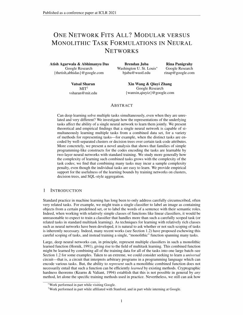
Figure 2: Some of the task codings which fit in our framework. On the left, we show a task codingvia clusters. Here, c(i) is the code for the ith cluster. On the right, we show a task coding based onlow-depth decision trees. Here, ci is the ith coordinate of the code c of the input datapoint.
Corollary 1 (Product rule). Let g(x) and h(x) meet the conditions of Theorem 1. Then the productg(x)h(x) is efficiently learnable as well, with O(Mg·h/ε
2) samples where√Mg·h = g′(1)h(1) + g(1)h′(1) + g(0)h(0). (2)
Corollary 2 (Chain rule). Let g(y) be an analytic function and h(x) be efficiently learnable, withauxiliary functions g(y) and h(y) respectively. Then the composition g(h(x)) is efficiently learnableas well with O(Mgh/ε
2) samples where√Mgh = g′(h(1))h′(1) + g(h(0)), (3)
provided that h(0) and h(1) are in the radius of convergence of g.
The calculus of bounds enables us to prove learning bounds on increasingly expressive functions, andwe can prove results that may be of independent interest. As an example, we show in Appendix B.1that forces on k bodies interacting via Newtonian gravitation, as shown in Figure 1, can be learned toerror ε using only kO(ln(k/ε)) examples (even though the function 1/x has a singularity at 0).
2.2 TASK CODING VIA CLUSTERS
Our analysis of learning analytic functions allows us to prove that a single network with standardtraining can learn multiple tasks. We formalize the problem of learning multiple tasks as follows. Ingeneral, these networks take pairs of inputs (c,x) where c is a task code and x is the input (vector)for the chosen task represented by c. We assume both c and x have fixed dimensionality. Thesepairs are then encoded by the concatenation of the two vectors, which we denote by c;x. Given ktasks, corresponding to evaluation of functions f1, . . . , fk respectively on the input x, the ith taskhas a corresponding code c(i). Now, we wish to learn a function g such that g(c(i);x) = fi(x) forexamples of the form (c(i);x, fi(x)). This g is a “monolithic” function combining the k tasks. Moregenerally, there may be some noise (bounded within a small ball around c(i)) in the task codes whichwould require learning the monolithic function g(c, x) = fj(x) where j = argmini‖c − c(i)‖2 .Alternately the task-codes are not given explicitly but are inferred by checking which ball-center c(i)
(unique per task) is closest to the input x (see Fig. 2 (left) for an example). Note that these are allgeneralizations of a simple one-hot coding.
We assume throughout that the fi are analytic, with bounded-norm multinomial Taylor series rep-resentations. Our technical tool is the following Lemma (proved in Appendix A.2) which showsthat the univariate step function 1(x ≥ 0) can be approximated with error ε and margin γ using alow-degree polynomial which can be learnt using SGD.
Lemma 1. Given a scalar x, let
Φ(x, γ, ε) = (1/2)(
1 + erf(Cx√
log(1/ε)/γ))
5

Published as a conference paper at ICLR 2021
where erf is the Gauss error function and C is a constant. Let Φ′(x, γ, ε) be the function Φ(x, γ, ε)with its Taylor series truncated at degree O(log(1/ε)/γ). Then,
Φ′(x, γ, ε) =
O(ε) x ≤ −γ/2,1−O(ε) x ≥ γ/2.
Also, Φ′(x, γ, ε) can be learnt using SGD with at most eO((log(1/ε)/γ2)) examples.
Using this lemma, we show that indicator functions for detecting membership in a ball near aprototype c(i) can also be sufficiently well approximated by functions with such a Taylor seriesrepresentation. Specifically, we use the truncated representation of the erf function to indicate that‖c− c(i)‖ is small. As long as the centers are sufficiently well-separated, we can find a low-degree,low-norm function this way using Lemma 1. For example, to check if c is within distance r of centerc(i) we can use 1(‖c− c(i)‖2 ≤ r2), which can be approximated using the φ′ function in Lemma 1.Then given such approximate representations for the task indicators I1(c), . . . , Ik(c), the functiong(c;x) = I1(c)f1(x) + · · ·+ Ik(c)fk(x) has norm linear in the complexities of the task functions,so that they are learnable by Theorem 1 (we scale to inputs to lie within the unit ball as required byTheorem 1). We state the result below, for the formal statement and proof see Appendix A.3.Theorem 2. (Informal) Given k analytic functions having Taylor series representations with normat most poly(k/ε) and degree at most O(log(k/ε)), a two-layer neural network trained with SGDcan learn the following functions g(c;x) on the unit sphere to accuracy ε with sample complexitypoly(k/ε) times the sum of the sample complexities for learning each of the individual functions:
• for Ω(1)-separated codes c(1), . . . , c(k), if ‖c− c(i)‖2 ≤ O(1), then g(c;x) = fi(x).
2.3 TASK CODING VIA LOW-DEPTH DECISION TREES
Theorem 2 can be viewed as performing a single k-way branching choice of which task functionto evaluate. Alternatively, we can consider a sequence of such choices, and obtain a decision treein which the leaves indicate which task function is to be applied to the input. We first considerthe simple case of a decision tree when c is a ±1-valued vector. We can check that the valuesc1, . . . , ch match the fixed assignment c(i)1 , . . . , c
(i)h that reaches a given leaf of the tree using the
function Ic(i)(c) =∏hj=1
cj+c(i)j
2 (or similarly for any subset of up to h of the indices). Theng(c;x) = Ic(1)(c)f1(x) + · · ·+ Ic(k)(c)fk(x) represents our decision tree coding of the tasks (seeFig. 2 (right) for an example). For the theorem, we again scale the inputs to lie within the unit ball:Theorem 3. (Informal) Two-layer neural networks trained with SGD can learn such a decision treewith depth h within error ε with sample complexity O(dh/ε2) times the sum of the sample complexityfor learning each of the individual functions at the leaves. Furthermore, conditioned on the hardnessof learning parity with noise, dΩ(h) examples are in fact necessary to learn a decision tree of depth h.
We can generalize the previous decision tree to allow a threshold based decision at every internalnode, instead of just looking at a coordinate. Assume that the input data lies in the unit ball andthat each decision is based on a margin of at least γ. We can then use a product of our truncated erfpolynomials to represent branches of the tree. We thus show:Theorem 4. (Informal) If we have a decision tree of depth h where each decision is based on amargin of at least γ, then we can learn such a such a function within error ε with sample complexityeO(h log(1/ε)/γ2) times the sample complexity of learning each of the leaf functions.
For the formal statements and proofs, see Appendix A.4. Note that by Theorem 3, the exponentialdependence on the depth in these theorems is necessary.
2.4 SIMPLE PROGRAMMING CONSTRUCTS
So far, we have discussed jointly learning k functions with task codings represented by clustersand decision trees. We now move to a more general setup, where we allow simple programmingconstructs such as compositions, aggregation, concatenation, and branching on different functions. Atthis stage, the distinction between “task codes” and “inputs” becomes somewhat arbitrary. Therefore,
6

Published as a conference paper at ICLR 2021
we will generally drop the task codes c from the inputs. The class of programming constructs we canlearn is a generalization of the decision tree and we refer to it as a generalized decision program.Definition 1. We define a generalized decision program to be a circuit with fan-out 1 (i.e., a treetopology). Each gate in the circuit computes a function of the outputs of its children, and the root(top) node computes the final output. All gates, including the leaf gates, have access to the input x.
We can learn generalized decision programs where each node evaluates one among a large family ofoperations, first described informally below, and then followed by a formal definition.
Arithmetic/analytic formulas As discussed in Section 2.1, learnability of analytic functions notonly allows us to learn functions with bounded Taylor series, but also sums, products, and ratios ofsuch functions. Thus, we can learn constant-depth arithmetic formulas with bounded outputs andanalytic functions (with appropriately bounded Taylor series) applied to such learnable functions.
Aggregation We observe that the sum of k functions with bounded Taylor representations yields afunction of the same degree and norm that is at most k times greater; the average of these k functions,meanwhile does not increase the magnitude of the norm. Thus, these standard aggregation operationsare represented very efficiently. These enable us to learn functions that answer a family of SQL-stylequeries against a fixed database as follows: suppose I(x, r) is an indicator function for whether ornot the record r satisfies the predicate with parameters x. Then a sum of the m entries of a databasethat satisfy the predicate given by x is represented by I(x, r(1))r(1) + · · ·+ I(x, r(m))r(m). Thus,as long as the predicate function I and records r(i) have bounded norms, the function mapping theparameters x to the result of the query is learnable. We remark that max aggregation can also berepresented as a sum of appropriately scaled threshold indicators, provided that there is a sufficientgap between the maximum value and other values.
Structured data We note that our networks already receive vectors of inputs and may producevectors of outputs. Thus, one may trivially structured inputs and outputs such as those in Fig. 1 (right)using these vectors. We now formalize this by defining the class of functions we allow.Definition 2. We support the following operations at any gate in the generalized decision program.Let every gate have at most k children. Let g be the output of some gate and f1, . . . , fk be theoutputs of the children of that gate.
1. Any analytic function of the child gates which can be approximated by a polynomial of degree atmost p, including sum g =
∑ki=1 fi and product of p terms g = Πp
i=1fi.2. Margin-based switch (decision) gate with children f1, f2 and some constant margin γ, i.e.,g = f1 if 〈β,x〉 − α ≤ −γ/2, and g = f2 if 〈β,x〉 − α ≥ γ/2, for a vector β and constant α.
3. Cluster-based switch gate with k centers c(1), . . . , c(k), with separation r (for some constantr), i.e. the output is fi if ‖x− c(i)‖ ≤ r/3. A special case of this is a look-up table which returnsvalue vi if x = c(i), and 0 if x does not match any of the centers.
4. Composition of two functions, g(x) = f1(f2(x)).5. Create a tuple out of separate fields by concatenation: given inputs f1, . . . , fk g outputs a
tuple [f1, . . . , fk], which creates a single data structure out of the children. Or, extract a field outof a tuple: for a fixed field i, given the tuple [f1, . . . , fk], g returns fi.
6. For a fixed table T with k entries r1, . . . , rk, a Boolean-valued function b, and an analyticfunction f , SQL queries of the form SELECT SUM f(r_i), WHERE b(r_i, x) for theinput x, i.e., g computes
∑i:b(ri,x)=1 f(ri). (We assume that f takes bounded values and b can
be approximated by an analytic function of degree at most p.) For an example, see the functionavg_income_zip_code() in Fig. 1 (right).
As an example of a simple program we can support, refer to Fig. 1 (right) which involves tablelookups, decision nodes, analytic functions such as Euclidean distance, and SQL queries. Theorem 5is our learning guarantee for generalized decision programs. See Section A.5 in the Appendix forproofs, formal statements, and a detailed description of the program in Fig. 1 (right).Theorem 5. (Informal) Any generalized decision program of constant depth h using the aboveoperations with p ≤ O(log(k/ε)) can be learnt within error ε with sample complexity kpoly(log(k/ε)).For the specific case of the program in Fig. 1 (right), it can be learnt using (k/ε)O(log(1/ε)) examples,where k is the number of individuals in the database.
7
Published as a conference paper at ICLR 2021
101 102 103
Number of examples per cluster
50
60
70
80
90
100
Test
acc
urac
y
k = 1k = 50k = 100k = 250k = 500k = 1000
(a) Random linear classifier for each cluster.
102 103 104
Number of examples per cluster45
50
55
60
65
70
75
80
85
Test
acc
urac
y
k = 1k = 10k = 30k = 50
(b) Random teacher network for each cluster.
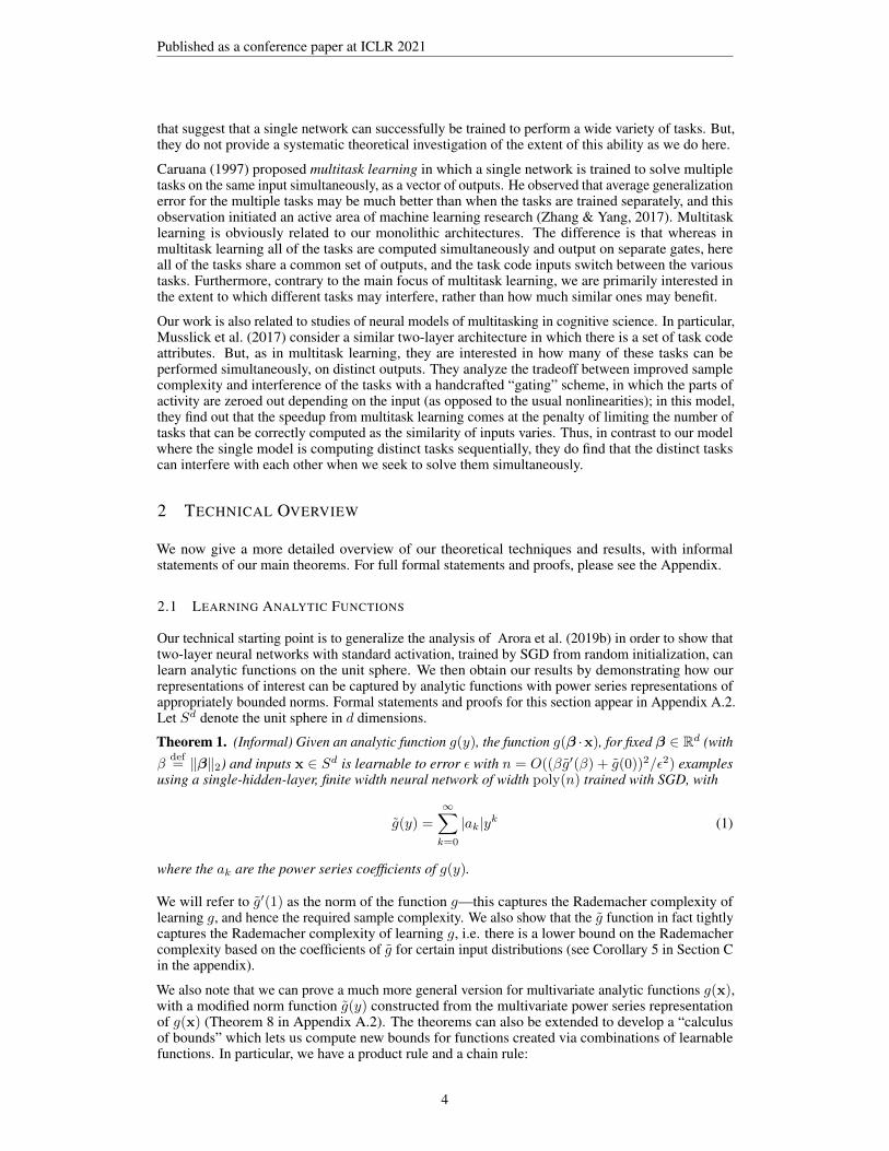
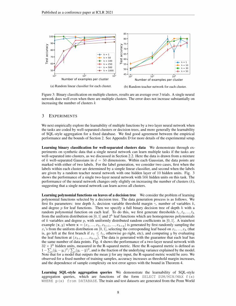
Figure 3: Binary classification on multiple clusters, results are an average over 3 trials. A single neuralnetwork does well even when there are multiple clusters. The error does not increase substantially onincreasing the number of clusters k
3 EXPERIMENTS
We next empirically explore the learnability of multiple functions by a two layer neural network whenthe tasks are coded by well-separated clusters or decision trees, and more generally the learnabilityof SQL-style aggregation for a fixed database. We find good agreement between the empiricalperformance and the bounds of Section 2. See Appendix D for more details of the experimental setup.
Learning binary classification for well-separated clusters data We demonstrate through ex-periments on synthetic data that a single neural network can learn multiple tasks if the tasks arewell-separated into clusters, as we discussed in Section 2.2. Here the data is drawn from a mixtureof k well-separated Gaussians in d = 50 dimensions. Within each Gaussian, the data points aremarked with either of two labels. For the label generation, we consider two cases, first when thelabels within each cluster are determined by a simple linear classifier, and second when the labelsare given by a random teacher neural network with one hidden layer of 10 hidden units. Fig. 3shows the performance of a single two-layer neural network with 50k hidden units on this task. Theperformance of the neural network changes only slightly on increasing the number of clusters (k),suggesting that a single neural network can learn across all clusters.
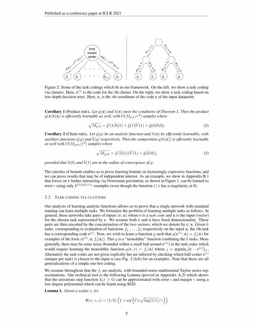
Learning polynomial functions on leaves of a decision tree We consider the problem of learningpolynomial functions selected by a decision tree. The data generation process is as follows. Wefirst fix parameters: tree depth h, decision variable threshold margin γ, number of variables k,and degree p for leaf functions. Then we specify a full binary decision tree of depth h with arandom polynomial function on each leaf. To do this, we first generate thresholds t1, t2, ..., thfrom the uniform distribution on [0, 1] and 2h leaf functions which are homogeneous polynomialsof k variables and degree p, with uniformly distributed random coefficients in [0, 1]. A train/testexample (x, y) where x = (x1, ..., xh, xh+1, ..., xh+p) is generated by first randomly sampling thexi’s from the uniform distribution on [0, 1], selecting the corresponding leaf based on x1, ..., xh (thatis, go left at the first branch if x1 ≤ t1, otherwise go right, etc), and computing y by evaluatingthe leaf function at (xh+1, ..., xh+p). The data is generated with the guarantee that each leaf hasthe same number of data points. Fig. 4 shows the performance of a two-layer neural network with32 × 2h hidden units, measured in the R-squared metric. Here the R-squared metric is defined as1−∑i(yi−yi)2/
∑i(yi−y)2, and is the fraction of the underlying variance explained by the model.
Note that for a model that outputs the mean y for any input, the R-squared metric would be zero. Weobserved for a fixed number of training samples, accuracy increases as threshold margin increases,and the dependence of sample complexity on test error agrees with the bound in Theorem 4.
Learning SQL-style aggregation queries We demonstrate the learnability of SQL-styleaggregation queries, which are functions of the form SELECT SUM/MIN/MAX f(x)WHERE p(x) from DATABASE. The train and test datasets are generated from the Penn World
8

Published as a conference paper at ICLR 2021
0.001 0.002 0.003 0.004 0.005 0.0061 - Test R-squared
100
200
300
400
500
# ex
ampl
es p
er le
af
depth=6depth=7depth=8depth=9depth=10
(a) Fixed threshold margin γ = 0.1.
0.025 0.050 0.075 0.100 0.125 0.150 0.175 0.200Decision variable threshold margin
0.9955
0.9960
0.9965
0.9970
0.9975
0.9980
Test
R-s
quar
ed
# examples per leaf=64# examples per leaf=128# examples per leaf=256# examples per leaf=512
(b) Fixed tree depth h = 10.
Figure 4: Learning random homogeneous polynomials of 4 variables and degree 4 on the leaves of adecision tree, the results are averaged over 7 trials. (a) Sample complexity scales as eO(h log(1/ε)/γ2)
with error ε, where error is measured by (1-Test R-squared). (b) For fixed tree depth, accuracyincreases with increasing margin.
Table dataset (Feenstra et al., 2015), which contains 11830 rows of economic data. The WHEREclause takes the form of (xi1 ≥ ti1) AND . . . AND (xik ≥ tik), where xi1 , . . . , xik are k randomlyselected columns and ti1 , . . . , tik are randomly selected values from the columns. The query targetfunction is randomly selected from SUM, MAX, and MIN and is over a fixed column (pl_x in thetable, which stands for price level for imports). The R-squared metric for a two-layer neural networkwith 40k hidden units is summarized in Table 1. We observe that a neural network learns to doSQL-style aggregation over dozens of data points, and for a fixed database, the test error only variesslightly for different numbers of columns in the WHERE clause.
Table 1: R-Squared for SQL-style aggregation. A single network with one hidden layer gets highR-Squared values, and the error does not increase substantially if the complexity of the aggregation isincreased by increasing the number of columns in the WHERE clause.
# columns in WHERE clause 1 2 3 4 5
Median # data points 21 12 9 4 3
Test R-Squared (93.31± 0.11) % (93.01± 2.7)% (91.86± 2.59) % (94.84± 1.86) % (92.51± 2.2) %
4 CONCLUSION AND FUTURE WORK
Our results indicate that even using a single neural network, we can still learn tasks across multiple,diverse domains. However, modular architectures may still have benefits over monolithic ones: theymight use less energy and computation, as only a portion of the total network needs to evaluateany data point. They may also be more interpretable, as it is clearer what role each part of thenetwork is performing. It is an open question if any of these benefits of modularity can be extendedto monolothic networks. For instance, is it necessary for a monolithic network to have modular partswhich perform identifiable simple computations? And if so, can we efficiently identify these from thelarger network? This could help in interpreting and understanding large neural networks.
Our work also begins to establish how neural networks can learn functions which are represented assimple programs. This perspective raises the question, how rich can these programs be? Can we learnprograms from a full-featured language? In particular, supposing that they combine simpler programsusing other basic operations such as composition, can such libraries of tasks be learned as well, i.e.,can these learned programs be reused? We view this as a compelling direction for future work.
9
Published as a conference paper at ICLR 2021
ACKNOWLEDGEMENTS
Brendan Juba was partially supported by NSF Awards CCF-1718380, IIS-1908287, and IIS-1939677,and was visiting Google during a portion of this work. Vatsal Sharan was supported in part by NSFaward 1704417.
REFERENCES
Roee Aharoni, Melvin Johnson, and Orhan Firat. Massively multilingual neural machine translation.arXiv preprint arXiv:1903.00089, 2019.
Zeyuan Allen-Zhu, Yuanzhi Li, and Yingyu Liang. Learning and Generalization in OverparameterizedNeural Networks, Going Beyond Two Layers. In Advances in Neural Information ProcessingSystems 32, pp. 6155–6166. Curran Associates, Inc., 2019.
Sanjeev Arora, Simon Du, Wei Hu, Zhiyuan Li, and Ruosong Wang. Fine-Grained Analysisof Optimization and Generalization for Overparameterized Two-Layer Neural Networks. InInternational Conference on Machine Learning, pp. 322–332, May 2019a.
Sanjeev Arora, Simon S Du, Wei Hu, Zhiyuan Li, and Ruosong Wang. Fine-grained analysis ofoptimization and generalization for overparameterized two-layer neural networks. arXiv preprintarXiv:1901.08584, 2019b.
Ankur Bapna, Colin Andrew Cherry, Dmitry Dima Lepikhin, George Foster, Maxim Krikun, MelvinJohnson, Mia Chen, Naveen Ari, Orhan Firat, Wolfgang Macherey, et al. Massively multilingualneural machine translation in the wild: Findings and challenges. 2019.
Avrim Blum, Adam Kalai, and Hal Wasserman. Noise-tolerant learning, the parity problem, and thestatistical query model. Journal of the ACM (JACM), 50(4):506–519, 2003.
Rich Caruana. Multitask learning. Machine learning, 28(1):41–75, 1997.
Jacob Devlin, Ming-Wei Chang, Kenton Lee, and Kristina Toutanova. Bert: Pre-training of deepbidirectional transformers for language understanding. arXiv preprint arXiv:1810.04805, 2018.
Simon S. Du, Xiyu Zhai, Barnabás Póczos, and Aarti Singh. Gradient Descent Provably OptimizesOver-parameterized Neural Networks. In 7th International Conference on Learning Representa-tions, ICLR 2019, New Orleans, LA, USA, May 6-9, 2019. OpenReview.net, 2019.
Robert C Feenstra, Robert Inklaar, and Marcel P Timmer. The next generation of the penn worldtable. American economic review, 105(10):3150–82, 2015.
Kurt Hornik. Approximation capabilities of multilayer feedforward networks. Neural networks, 4(2):251–257, 1991.
Robert A Jacobs, Michael I Jordan, Steven J Nowlan, and Geoffrey E Hinton. Adaptive mixtures oflocal experts. Neural computation, 3(1):79–87, 1991.
Arthur Jacot, Franck Gabriel, and Clement Hongler. Neural Tangent Kernel: Convergence andGeneralization in Neural Networks. In Advances in Neural Information Processing Systems 31, pp.8571–8580. Curran Associates, Inc., 2018.
Melvin Johnson, Mike Schuster, Quoc V Le, Maxim Krikun, Yonghui Wu, Zhifeng Chen, NikhilThorat, Fernanda Viégas, Martin Wattenberg, Greg Corrado, et al. Google’s multilingual neuralmachine translation system: Enabling zero-shot translation. Transactions of the Association forComputational Linguistics, 5:339–351, 2017.
Lukasz Kaiser, Aidan N Gomez, Noam Shazeer, Ashish Vaswani, Niki Parmar, Llion Jones, andJakob Uszkoreit. One model to learn them all. arXiv preprint arXiv:1706.05137, 2017.
Michael Kearns. Efficient noise-tolerant learning from statistical queries. Journal of the ACM (JACM),45(6):983–1006, 1998.
10

Published as a conference paper at ICLR 2021
Michael Kearns and Leslie Valiant. Cryptographic limitations on learning boolean formulae andfinite automata. Journal of the ACM (JACM), 41(1):67–95, 1994.
Adam R Klivans and Alexander A Sherstov. Cryptographic hardness for learning intersections ofhalfspaces. Journal of Computer and System Sciences, 75(1):2–12, 2009.
Jaehoon Lee, Lechao Xiao, Samuel Schoenholz, Yasaman Bahri, Roman Novak, Jascha Sohl-Dickstein, and Jeffrey Pennington. Wide Neural Networks of Any Depth Evolve as Linear ModelsUnder Gradient Descent. In Advances in Neural Information Processing Systems 32, pp. 8570–8581.Curran Associates, Inc., 2019.
Sebastian Musslick, Andrew Saxe, Kayhan Özcimder, Biswadip Dey, Greg Henselman, andJonathan D Cohen. Multitasking capability versus learning efficiency in neural network ar-chitectures. In CogSci, pp. 829–834, 2017.
Colin Raffel, Noam Shazeer, Adam Roberts, Katherine Lee, Sharan Narang, Michael Matena,Yanqi Zhou, Wei Li, and Peter J. Liu. Exploring the Limits of Transfer Learning with a UnifiedText-to-Text Transformer. arXiv:1910.10683 [cs, stat], October 2019.
Oded Regev. On lattices, learning with errors, random linear codes, and cryptography. Journal of theACM (JACM), 56(6):1–40, 2009.
Richard Samuels. Is the mind massively modular? 2006.
Noam Shazeer, Azalia Mirhoseini, Krzysztof Maziarz, Andy Davis, Quoc Le, Geoffrey Hinton, andJeff Dean. Outrageously large neural networks: The sparsely-gated mixture-of-experts layer. arXivpreprint arXiv:1701.06538, 2017.
Le Song, Santosh Vempala, John Wilmes, and Bo Xie. On the complexity of learning neural networks.In Advances in neural information processing systems, pp. 5514–5522, 2017.
Michel Talagrand. Sharper bounds for gaussian and empirical processes. The Annals of Probability,pp. 28–76, 1994.
Henry Tsai, Jason Riesa, Melvin Johnson, Naveen Arivazhagan, Xin Li, and Amelia Archer. Smalland practical bert models for sequence labeling. arXiv preprint arXiv:1909.00100, 2019.
Gregory Valiant. Finding correlations in subquadratic time, with applications to learning parities andthe closest pair problem. Journal of the ACM (JACM), 62(2):1–45, 2015.
Yu Zhang and Qiang Yang. A survey on multi-task learning. arXiv preprint arXiv:1707.08114, 2017.
11
Published as a conference paper at ICLR 2021
A THEORETICAL RESULTS
A.1 KERNEL LEARNING BOUNDS
In this section, we develop the theory of learning analytic functions. For a given function g, we definea parameter Mg related to the sample complexity of learning g with small error with respect to agiven loss function:
Definition 3. Fix a learning algorithm, and a 1-Lipschitz loss function L. For a function g over adistribution of inputsD, a given error scale ε, and a confidence parameter δ, let the sample complexityng,D(ε, δ) be the smallest integer such that when the algorithm is given ng,D(ε, δ) i.i.d. examplesof g on D, with probability greater than 1 − δ, it produces a trained model g with generalizationerror Ex∼D[L(g(x), g(x))] less than ε. Fix a constant C > 0. We say g is efficiently learned bythe algorithm (w.r.t. C) if there exists a constant Mg (depending on g) such that for all ε, δ, anddistributions D on the inputs of g, ng,D(ε, δ) ≤ C([Mg + log(δ−1)]/ε2).
For example, it is known (Talagrand (1994)) that there exists a suitable choice ofC such that empiricalrisk minimization for a class of functions efficiently learns those functions with Mg at most theVC-dimension of that class.
Previous work focused on computing Mg, for functions defined on the unit sphere, for wide neuralnetworks trained with SGD. We extend the bounds derived in Arora et al. (2019a) to analytic functions,and show that they apply to kernel learning methods as well as neural networks.
The analysis in Arora et al. (2019a) focused on the case of training the hidden layers of wide networkswith SGD. We first show that these bounds are more general and in particular apply to the case whereonly the final layer weights are trained (corresponding to the NNGP kernel in Lee et al. (2019)), andtherefore our results will apply to general kernel learning as well. The proof strategy consists ofshowing that finite-width networks have a sensible infinite-width limit, and showing that trainingcauses only a small change in parameters of the network.
Let m be the number of hidden units, and n be the number of data points. Let y be the n × 1dimensional vector of training outputs. Let h be a n×m random matrix denoting the activations ofthe hidden layer (as a function of the weights of the lower layer) for all n data points. We will firstshow the following:
Theorem 6. For sufficiently large m, a function g can be learned efficiently in the sense of Definition3 by training the final layer weights only with SGD, where the constant Mg given by
Mg ≤ yT(H∞)−1y (4)
where we define H∞ asH∞ = E[hhT] (5)
which is the NNGP kernel from Lee et al. (2019).
We require some technical lemmas in order to prove the theorem. We first need to show that H∞ is,with high probability, invertible. If K(x,x′), the kernel function which generates H∞ is given by ainfinite Taylor series in x · x′ it can be argued that H∞ has full rank for most real world distributions.For example, the ReLU activation this holds as long as no two data points are co-linear (see Definition5.1 in Arora et al. (2019a)). We can prove this more explicitly in the following lemma:
Lemma 2. If all the n data points x are distinct and the Taylor series of K(x,x′) in x · x′ haspositive coefficients everywhere then H∞ is not singular.
Proof. First consider the case where the input x is a scalar. Since the Taylor series correspondingto K(x, x′) consists of monomials of all degrees of xx′, we can view it as some inner product ina kernel space induced by the function φ(x) = (1, x, x2, . . .), where the inner product is diagonal(but with potentially different weights) in this basis. For any distinct set of inputs x1, .., xn theset of vectors φ(xi) are linearly independent. The first n columns produce the Vandermonde matrixobtained by stacking rows 1, x, x, ..., xn−1 for n different values of x, which is well known to benon-singular (since a zero eigenvector would correspond to a degree n− 1 polynomial with n distinctroots x1, .., xn).
12
Published as a conference paper at ICLR 2021
This extends to the case of multidimensional x if the values, projected along some dimension, aredistinct. In this case, the kernel space corresponds to the direct sum of copies of φ applied elementwiseto each coordinate xi. If all the points are distinct and and far apart from each other, the probabilitythat a given pair coincides under random projection is negligible. From a union bound, the probabilitythat a given pair coincide is also bounded – so there must be directions such that projections alongthat direction are distinct. Therefore, H∞ can be considered to be invertible in general.
As m→∞, hhT concentrates to its expected value. More precisely, (hhT)−1 approaches (H∞)−1
for large m if we assume that the smallest eigenvalue λmin(H∞) ≥ λ0, which from the above lemmawe know to be true for fixed n. (For the ReLU NTK the difference becomes negligible with highprobability for m = poly(n/λ0) Arora et al. (2019a).) This allows us to replace hhT with H∞ inany bounds involving the former.
We can get learning bounds in terms of hhT by studying the upper layer weights w of the networkafter training. After training, we have y = w · h. If hhT is invertible (which the above argumentsshow is true with high probability for large m), the following lemma holds:Lemma 3. If we initialize a random lower layer and train the weights of the upper layer, then thereexists a solution w with norm
√yT(hhT)−1y.
Proof. The minimum norm solution to y = wTh is
w∗ = (hTh)−1hTy. (6)
The norm squared (w∗)Tw∗ of this solution is given by yTh(hTh)−2hTy.
We claim that h(hTh)−2hT = (hhT)−1. To show this, consider the SVD decomposition h =USVT. Expanding we have
h(hTh)−2hT = USVT(VS2VT)−2VSUT. (7)
Evaluating the right hand side gets us US−2UT = (hhT)−1.
Therefore, the norm of the minimum norm solution is yT(hhT)−1y.
We can now complete the proof of Theorem 6.
Proof of Theorem 6. For large m, the squared norm of the weights approaches yT(H∞)−1y. Sincethe lower layer is fixed, the optimization problem is linear and therefore convex in the trained weightsw. Therefore SGD with small learning rate will reach this optimal solution. The Rademachercomplexity of this function class is at most
√yT(H∞)−1y which we at most by
√Mg where Mg is
an upper bound on yT(H∞)−1y. The optimal solution has 0 train error based on the assumption that
H∞ is full rank and the generalization error will be no more than O(√
yT(H∞)−1y2n ) which is at most
ε if we use at least n = Ω(Mg/ε2) training samples - note that this is identical to the previous results
for training the hidden layer only Arora et al. (2019a); Du et al. (2019).
A.2 LEARNING ANALYTIC FUNCTIONS
Now, we derive our generalization bounds for single variate functions. We use Theorem 6 to provethe following corollary, a more general version of Corollary 6.2 proven in Arora et al. (2019a) forwide ReLU networks with trainable hidden layer only:Corollary 3. Consider the function g : Rd → R given by:
g(x) =∑k
ak(βTk x)k (8)
Then, if g is restricted to ||x|| = 1, and the NTK or NNGP kernel can be written as H(x,x′) =∑k bk(x · x′)k, the function can be learned efficiently with a wide one-hidden-layer network in the
sense of Definition 3 with √Mg =
∑k
b−1/2k |ak|||βk||k2 (9)
13

Published as a conference paper at ICLR 2021
up to g-independent constants ofO(1), where βk ≡ ||βk||2. In the particular case of a ReLU network,the bound is √
Mg =∑k
k|ak|||βk||k2 (10)
The original corollary applied only to networks with trained hidden layer, and the bound on the ReLunetwork excluded odd monomials of power greater than 1.
Proof. The extension to NNGP follows from Theorem 6, which allows for the application of thearguments used to prove Corollary 6.2 from Arora et al. (2019a) (particularly those found in AppendixE).
The extension of the ReLu bound to odd powers can be acheived with the following modification.consider appending a constant component to the input x so that the new input to the network is(x/√
2, 1/√
2). The kernel then becomes:
K(x,x′) =x · x′ + 1
4π
(π − arccos
(x · x′ + 1
2
)). (11)
Re-writing the power series as an expansion around x · x′ = 0, we have terms of all powers. Anasymptotic analysis of the coefficients using known results shows that coefficients bk are asymp-totically O(k−3/2) - meaning in Equation 10 applies to these kernels, without restriction to evenk.
Equation 9 suggests that kernels with slowly decaying (but still convergent) bk will give the bestbounds for learning polynomials. Many popular kernels do not meet this criteria. For example, forinputs on the sphere of radius r, the Gaussian kernel K(x,x′) = e−||x−x
′||2/2 can be written asK(x,x′) = e−r
2
ex·x′. This has b−1/2
k = er2/2√k!, which increases rapidly with k. This provides
theoretical justification for the empirically inferior performance of the Gaussian kernel which we willpresent in Section B.2.
Guided by this theory, we focus on kernels where b−1/2k ≤ O(k), for all k (or, bk ≥ O(k−2)). The
modified ReLu meets this criterion, as well as hand-crafted kernels of the form
K(x,x′) =∑k
k−s(x · x′)k (12)
with s ∈ (1, 2] is a valid slowly decaying kernel on the sphere. We call these slowly decaying kernels.We note that by Lemma 3, the results of Corollary 3 apply to networks with output layer trainingonly, as well as kernel learning (which can be implemented by training wide networks).
Using the extension of Corollary 3 to odd powers, we first show that analytic functions with appropri-ately bounded norms can be learnt.Theorem 7. Let g(y) be a function analytic around 0, with radius of convergence Rg. Define theauxiliary function g(y) by the power series
g(y) =
∞∑k=0
|ak|yk (13)
where the ak are the power series coefficients of g(y). Then the function g(β · x), for some fixedvector β ∈ Rd with ||x|| = 1 is efficiently learnable in the sense of Definition 3 using a model with aslowly decaying kernel K with √
Mg = βg′(β) + g(0) (14)if the norm β ≡ ||β||2 is less than Rg .
Proof. We first note that the radius of convergence of the power series of g(y) is also Rg since g(y)is analytic. Applying Equation 10, pulling out the 0th order term, and factoring out β, we get√
Mg = |a0|+ β
∞∑k=1
k|ak|βk = βg′(β) + g(0) (15)
since β < Rg .
14
Published as a conference paper at ICLR 2021
The tilde function is the notion of complexity which measures how many samples we need to learna given function. Informally, the tilde function makes all coefficients in the Taylor series positive.The sample complexity is given by the value of the function at 1 (in other words, the L1 norm of thecoefficients in the Taylor series). For a multivariate function g(x), we define its tilde function g(y)by substituting any inner product term 〈α,x〉 by a univariate y. The above theorem can then also begeneralized to multivariate analytic functions:
Lemma 4. Given a collection of p vectors βi in Rd, the function f(x) =∏pi=1 βi · x is efficiently
learnable with √Mf = p
∏i
βi (16)
where βi ≡ ||βi||2.
Proof. The proof of Corollary 6.2 in Arora et al. (2019a) relied on the following statement: givenpositive semi-definite matrices A and B, with A B, we have:
PBA−1PB B+ (17)
where + is the Moore-Penrose pseudoinverse, and P is the projection operator.
We can use this result, along with the Taylor expansion of the kernel and a particular decompositionof a multivariate monomial in the following way. Let the matrix X to be the training data, such thatthe αth column xi is a unit vector in Rd. Given K ≡ XTX, the matrix of inner products, the Grammatrix H∞ of the kernel can be written as
H∞ =
∞∑k=0
bkKk (18)
where is the Hadamard (elementwise) product. Consider the problem of learning the functionf(x) =
∏pi=1 βi · x. Note that we can write:
f(X) = (Xk)T ⊗ki=1 βi. (19)
Here⊗ is the tensor product, which for vectors takes an n1-dimensional vector and an n2 dimensionalvector as inputs vectors and returns a n1n2 dimensional vector:
w ⊗ v =
w1v1
w1v2
· · ·w1vn2
w2v1
· · ·wn1
vn2
. (20)
The operator is the Khatri-Rao product, which takes an n1 × n3 matrix A = (a1, · · · ,an3) and an2 ⊗ n3 matrix B = (b1, · · · ,bn3
) and returns the n1n2 × n3 dimensional matrix
AB = (a1 ⊗ b1, · · · ,an3 ⊗ bn3). (21)
For p = 2, this form of f(X) can be proved explicitly:
(X2)Tβ1 ⊗ β2 = (x1 ⊗ x1, · · · ,xP ⊗ xP )Tβ1 ⊗ β2. (22)
The αth element of the matrix product is
(xα ⊗ xα) · (β1 ⊗ β2) = (β1 · xα)(β2 · xα) (23)
which is exactly f(xα). The formula can be proved for p > 2 by finite induction.
With this form of f(X), we can follow the steps of the proof in Appendix E of Arora et al. (2019a),which was written for the case where the βi were identical:
yT(H∞)−1y = (⊗pi=1βi)TXp(H∞)−1(Xp)T ⊗pi=1 βi. (24)
15
Published as a conference paper at ICLR 2021
Using Equation 17, applied to Kp, we have:
yT(H∞)−1y ≤b−1p (⊗pi=1βi)
TXpPKp(Kp)+PKp(Xp)T ⊗pi=1 βi. (25)
Since the Xp are eigenvectors of PKp with eigenvalue 1, and Xp(Kp)+(Xp)T = PXp , wehave:
yT(H∞)−1y ≤ b−1p (⊗pi=1βi)
TPXp ⊗pi=1 βi (26)
yT(H∞)−1y ≤ b−1p
p∏i=1
βi · βi. (27)
For the slowly decaying kernels, bp ≥ p−2. Therefore, we have√
yT(H∞)−1y ≤√Mf for√
Mf = p∏i
βi (28)
where βi ≡ ||βi||2, as desired.
This leads to the following generalization of Theorem 7:Theorem 8. Let g(x) be a function with multivariate power series representation:
g(x) =∑k
∑v∈Vk
av
k∏i=1
(βv,i · x) (29)
where the elements of Vk index the kth order terms of the power series. We define g(y) =∑k aky
k
with coefficients
ak =∑v∈Vk
|av|k∏i=1
βv,i. (30)
If the power series of g(y) converges at y = 1 then with high probability g(x) can be learnedefficiently in the sense of Definition 3 with
√Mg = g′(1) + g(0).
Proof. Follow the construction in Theorem 7, using Lemma 4 to get bounds on the individual terms.Then sum and evaluate the power series of g′(1) to arrive at the bound.
Remark 1. Note that the g function defined above for multivariate functions depends on the repre-sentation, i.e. choice of the vectors β. Therefore to be fully formal g(y) should instead be gβ(y). Forclarity, we drop β from the expression gβ(y) and it is implicit in the g notation.
Remark 2. If g(x) can be approximated by some function gapp such that |g(x)− gapp| ≤ ε′ for all xin the unit ball, then Theorem 8 can be used to learn g(x) within error ε′ + ε with sample complexityO(Mgapp/ε
2).
To verify Remark 2, note that we are doing regression on the upper layer of the neural network,where the lower layer is random. So based on gapp there exists a low-norm solution for the regressioncoefficients for the upper layer weights which gets error at most ε′. If we solve the regression underthe appropriate norm ball, then we get training error at most ε′, and the generalization error will be atmost ε with O(Mgapp/ε
2) samples.
We can also derive the equivalent of the product and chain rule for function composition.
Proof of Corollary 1. Consider the power series of g(x)h(x), which exists and is convergent sinceeach individual series exists and is convergent. Let the elements of Vj,g and Vk,h index the jth orderterms of g and the kth order terms of h respectively. The individual terms in the series look like:
avbw
j∏j′=1
(βv,j′ · x)
k∏k′=1
(βw,k′ · x) for v ∈ Vj,g, w ∈ Vk,h (31)
16
Published as a conference paper at ICLR 2021
with bound
(j + k)|av||bw|j∏
j′=1
βv,j′k∏
k′=1
βw,k′ for v ∈ Vj,g, w ∈ Vk,h (32)
for all terms with j + k > 0 and g(0)h(0) for the term with j = k = 0.
Distribute the j + k product, and first focus on the j term only. Summing over all the Vk,h for all k,we get
∑k
∑w∈Vk,h
j|av||bw|j∏
j′=1
βv,j′k∏
k′=1
βw,k′ =
|av|j∏
j′=1
βv,j′ h(1).
(33)
Now summing over the j and Vj,g we get g′(1)h(1). If we do the same for the k term, after summingwe get g(1)h′(1). These bounds add and we get the desired formula for
√Mgh, which, up to the
additional g(0)h(0) term looks is the product rule applied to g and h.
One immediate application for this corollary is the product of many univariate analytic functions. Ifwe define
G(x) =∏i
gi(βi · x) (34)
where each of the corresponding gi(y) have the appropriate convergence properties, then G isefficiently learnable with bound MG given by√
MG =d
dy
∏i
gi(βiy)
∣∣∣∣∣y=1
+∏i
gi(0). (35)
Proof of Corollary 2. Writing out g(h(x)) as a power series in h(x), we have:
g(h(x)) =
∞∑k=0
ak(h(x))k. (36)
We can bound each term individually, and use the k-wise product rule to bound each term of (h(x))k.Doing this, we have: √
Mgh =
∞∑k=1
k|ak|h′(1)h(1)k−1 +
∞∑k=0
|ak|h(0)k. (37)
Factoring out h′(1) from the first term and then evaluating each of the series gets us the desiredresult.
The following corollary considers the case where the function g(x) is low-degree and directly followsfrom Theorem 8.Fact 1. The following facts about the tilde function will be useful in our analysis—
1. Given a multivariate analytic function g(x) of degree p for x in the d-dimensional unit ball,there is a function g(y) as defined in Theorem 8 such that g(x) is learnable to error ε withO(pg(1)/ε2) samples.
2. The tilde of a sum of two functions is at most the sum of the tilde of each of the functions, i.e.if f = g + h then f(y) ≤ g(y) + h(y) for y ≥ 0.
3. The tilde of a product of two functions is at most the product of the tilde of each of thefunctions, i.e. if f = g · h then f(y) ≤ g(y)h(y) for y ≥ 0.
17
Published as a conference paper at ICLR 2021
4. If g(x) = f(αx), then g(y) ≤ f(αy) for y ≥ 0.
5. If g(x) = f(x + c) for some ‖c‖ ≤ 1, then g(y) ≤ f(y + 1) for y ≥ 0. By combining thiswith the previous fact, if g(x) = f(α(x− c)) for some ‖c‖ ≤ 1, then g(1) ≤ f(2α).
To verify the last part, note that in the definition of g we replace 〈β,x〉 with y. Therefore, we willhave an additional 〈β, c〉 term when we compute the tilde function for g(x) = f(x+c). As ‖c‖ ≤ 1,the additional term is at most 1.
The following lemma shows how we can approximate the indicator 1(x > α) with a low-degreepolynomial if x is at least γ/2 far away from α. We will use this primitive several times to constructlow-degree analytic approximations of indicator functions. The result is based on the followingsimple fact.Fact 2. If the Taylor series of g(x) is exponentially decreasing, then we can truncate it at degreeO(log(1/ε)) to get ε error. We will use this fact to construct low-degree approximations of functions.Lemma 5. Given a scalar x, let the function
Φ(x, γ, ε, α) = (1/2)(
1 + erf(
(x− α)c√
log(1/ε)/γ))
for some constant c. Let Φ′(x, γ, ε, α) be the function Φ(x, γ, ε, α) with its Taylor series truncated atdegree O(log(1/ε)/γ). Then for |α| < 1,
Φ′(x, γ, ε, α) =
ε x ≤ α− γ/2,1− ε x ≥ α+ γ/2.
Also, MΦ′ is at most eO((log(1/ε)/γ2)).
Proof. Note that Φ(x, γ, ε, α) is the cumulative distribution function (cdf) of a normal distributionwith mean α and standard deviation O(γ/
√log(1/ε)). Note that at most ε/100 of the probability
mass of a Gaussian distribution lies more than O(√
log(1/ε)) standard deviations away from themean. Therefore,
Φ(x, γ, ε, α) =
ε/100 x ≤ α− γ/2,1− ε/100 x ≥ α+ γ/2.
Note that
erf(x) =2√π
∫ x
0
e−t2
dt
=2√π
( ∞∑i=0
(−1)ix2i+1
i!(2i+ 1)
).
Therefore, the coefficients in the Taylor series expansion of erf((x − α)c√
log(1/ε)/γ)) in termsof (x − α) are smaller than ε for i > O(log(1/ε)/γ2) and are geometrically decreasing hence-forth. Therefore, we can truncate the Taylor series at degree O(log(1/ε)/γ2) and still have an O(ε)approximation. Note that for f(x) = erf(x),
f(y) ≤ 2√π
∫ y
0
et2
dt ≤ 2√πyey
2
≤ eO(y2).
After shifting by α and scaling by O(√
log(1/ε)/γ), we get Φ′(y) = eO((y+α)2 log(1/ε)/γ2). Forx = 1, this is at most eO(log(1/ε)/γ2). Hence the result now follows by Fact 1.
A.3 LEARNABILITY OF CLUSTER BASED DECISION NODE
In the informal version of the result for learning cluster based decisions we assumed that the task-codesc are prefixed to the input datapoints, which we refer to as xinp. For the formal version of the theorem,we use a small variation. The task code and the input c,xinp gets mapped to x = c + xinp · (r/3) for
18
Published as a conference paper at ICLR 2021
some constant r < 1/6. Since xinp resides on the unit sphere, x will be distance at most (r/3) fromthe center it gets mapped to. Note that the overall function f can be written as follows,
f(x) =
k∑j=1
1(‖x− cj‖2 ≤ (r/2)2
)fj ((x− cj)/(r/3))
where fj is the function corresponding to the center cj . The main idea will be to show that theindicator function can be expressed as an analytic function.
Theorem 9. (formal version of Theorem 2) Assume that d ≥ 10 log k (otherwise we can pad by extracoordinates to increase the dimensionality). Then we can find k centers in the unit ball which are atleast r apart, for some constant r. Let
f(x) =
k∑j=1
1(‖x− cj‖2 ≤ (r/2)2
)fj ((x− cj)/(r/3))
where fj is the function corresponding to the center cj . Then if each fj is a degree p polynomial,Mf of the function f is p · poly(k/ε)
∑fj(6/r) ≤ p · poly(k/ε)(6/r)p
∑fj(1).
Proof. Let
fapp(x) =
k∑j=1
Φ′(‖x− cj‖2, (r/2)2, ε/k, (r/4)2
)fj ((x− cj)/(r/3))
where Φ′ is defined in Lemma 5. Let
Ij(x) = Φ′(‖x− cj‖2, (r/2)2, ε/k, (r/4)2).
The indicator Ij(x) checks if ‖x−cj‖ is a constant fraction less than r/2, or a constant fraction morethan r/2. Note that if x is from a different cluster, then ‖x− cj‖ is at least some constant, and henceIj(x) is at most ε/k. The contribution from k such clusters would be at most ε. If ‖x− cj‖ < ε/k,then the indicator is at least 1−O(ε/k). Hence as fapp is an O(ε)-approximation to f , by Remark 2it suffices to show learnability of fapp.
If y = 〈x, cj〉 and assuming x and the centers cj are all on unit sphere,
Ij(y) = Φ′(2 + 2y, r/3, ε/k, r/3) ≤ eO(log(k/ε) = poly(k/ε).
By Fact 1,
f(y) ≤ poly(k/ε)∑j
fj(6/r).
As fj are at most degree p,
f(y) ≤ poly(k/ε)∑j
fj(6/r) ≤ p · poly(k/ε)(6/r)p∑
fj(1).
Corollary 4. The previous theorem implies that we can also learn f where f is a lookup table withMf = poly(k/ε), as long as the keys ci are well separated. Note that as long as the keys ci aredistinct (for example, names) we can hash them to random vectors on a sphere so that they are allwell-separated.
Note that the indicator function for the informal version of Theorem 9 stated in the main body isthe same as that for the lookup table in Corollary 4. Therefore, the informal version of Theorem 9follows as a Corollary of Theorem 9.
19
Published as a conference paper at ICLR 2021
A.4 LEARNABILITY OF FUNCTIONS DEFINED ON LEAVES OF A DECISION TREE
We consider decision trees on inputs drawn from −1, 1d. We show that such a decision tree g canbe learnt with Mg ≤ O(dh). From this section onwards, we view the combined input c,x as x.
The decision tree g can be written as follows,
g(x) =∑j
Ij(x)vj ,
where the summation runs over all the leaves, Ij(x) is the indicator function for leaf j, and vj ∈[−1, 1] is the constant value on the leaf j. We scale the inputs by
√d to make them lie on the unit
sphere, and hence each coordinate of x is either ±1/√d.
Let the total number of leaves in the decision tree be B. The decision tree indicator function of thej-th leaf can be written as the product over the path of all internal decision nodes. Let jl be variableat the l-th decision node on the path used by the j-th leaf. We can write,
Ij(x) =∏l
(ajlxjl + bjl) ,
where each xjl ∈ −1/√d, 1/√d and ajl ∈ −
√d/2,√d/2 and bjl ∈ −1/2, 1/2. Note that
the values of ajl and bj,l are chosen depending on whether the path for the j-th leaf choses the leftchild or the right child at the l-th decision variable. For ease of exposition, the following theorem isstated for the case where the leaf functions are constant functions, and the case where there are someanalytic functions at the leaves also follows in the same way.
Theorem 10. If a function is given by g(x) =∑Bj=1 Ij(x)vj , where Ij(x) is a leaf indicator function
in the above form, with tree depth h, then Mg is at most O(dh).
Proof. Note that
g(y) ≤∑
Ij(y)|vj |
≤∑∏
l
(√dy/2 + 1/2
)=⇒ g(1) ≤ 2h(
√d/2 + 1/2)h ≤ dh.
As the degree of g is at most h, therefore Mg ≤ hg(1) ≤ hdh.
Remark 3. Note that by Theorem 10 we need O((log k)log kε−2
)samples to learn a lookup table
based on a decision tree. On the other hand, by Corollary 4 we need poly(k/ε) samples to learn alookup table using cluster based decision nodes. This shows that using a hash function to obtain arandom O(log k) bit encoding of the indexes for the k lookups is more efficient than using a fixedlog k length encoding for the k lookups.
We also prove a corresponding lower bound in Theorem 14 which shows that dΩ(h) samples arenecessary to learn decision trees of depth h.
We will now consider decision trees where the branching is based on the inner product of x withsome direction βj,l. Assume that there is a constant gap for each decision split, then the decision treeindicator function can be written as,
Ij(x) =∏l
1(〈x,βj,l〉 > αj,l).
Theorem 11. (formal version of Theorem 4) A decision tree of depth h where every node partitionsin a certain direction with margin γ can be written as g(x) =
∑Bj=1 Ij(x)fj(x), then the final
Mg = eO(h log(1/ε)/γ2)(p+ h log 1/ε)∑
fj(1),
where p is the maximum degree of fj .
20
Published as a conference paper at ICLR 2021
Proof. Define gapp,
gapp(x) =
B∑j=1
ΠlΦ′(〈x,βj,l〉, γ, ε/h, αj,l)fj(x)
where Φ′ is as defined in Lemma 5. Note that for all y = 1,
Φ′(1, γ, ε/h, αj,l) ≤ eO(log(1/ε)/γ2).
Therefore,
gapp(1) ≤B∑j=1
ΠlΦ′(1, γ, ε/h, αj,l)fj(1),
≤ eO(log(1/ε)/γ2)∑
fj(1).
Note that the degree of gapp is at most O(p+ h log(1/ε)/γ2). Therefore,
Mgapp ≤ eO(h log(1/ε)/γ2)(p+ h log(1/ε)/γ2)∑
fj(1).
By Remark 2, learnability of g follows from the learnability of its analytic approximation gapp.
A.5 GENERALIZED DECISION PROGRAM
In this section, instead a decision tree, we will consider a circuit with fan-out 1, where each gate(node) evaluates some function of the values returned by its children and the input x. A decision treeis a special case of such circuits in which the gates are all switches.
So far, the function outputs were univariate but we will now generalize and allow multivariate (vector)outputs as well. Hence the functions can now evaluate and return data structures, represented byvectors. We assume that each output is at most d dimensional and lies in the unit ball.
Definition 4. For a multivariate output function f , we define f(y) as the sum of fi(y) for each ofthe output coordinates fi.
Remark 4. Theorem 9 , 10 and 11 extend to the multivariate output case. Note that if each of theindividual functions has degree at most p, then the sample complexity for learning the multivariateoutput f is at most O(pf(1)/ε2)) (where the multivariate tilde function is defined in Definition 4).
We now define a generalized decision program and the class of functions that we support.Definition 5. We define a generalized decision program to be a circuit with fan-out 1 (i.e., a treetopology) where each gate evaluates a function of the values returned by its children and the input x,and the root node evaluates the final output. All gates, including those at the leaves, have access tothe input x. We support the following gate operations. Let h be the output of a gate, let each gatehave at most k children, and let f1, . . . , fk be the outputs of its children.
1. Any analytic function of the child gates of degree at most p, including sum h =∑ki=1 fi
and product of p terms h = Πpi=1fi.
2. Margin based switch (decision) gate with children f1, f2, some constant margin γ, vectorβ and constant α,
h =
f1 if 〈β,x〉 − α ≤ −γ/2,f2 if 〈β,x〉 − α ≥ γ/2.
3. Cluster based switch gate with k centers c(1), . . . , c(k), with separation r for someconstant r, and the output is fi if ‖x− c(i)‖ ≤ r/3. A special case of this is a look-up tablewhich returns value vi if x = c(i), and 0 if x does not match any of the centers.
4. Create a data structure out of separate fields by concatenation such as constructing a tuple[f1, . . . , fk] which creates a single data structure out of its children, or extract a field out ofa data structure.
21

Published as a conference paper at ICLR 2021
5. Given a table T with k entries r1, . . . , rk, a Boolean-valued function p and an analyticfunction f , SQL queries of the form SELECT SUM f(r_i), WHERE p(r_i, x).Here, we assume that f has bounded value and p can be approximated by an analyticfunction of degree at most p.
6. Compositions of functions, h(x) = f(g(x)).
First, we note that all of the above operators can be approximated by low-degree polynomials.Claim 1. If p ≤ O(log(k/ε)), each of the above operators in the generalized decision program canbe expressed as a polynomial of degree at most O(log(k/ε)), where k is maximum out-degree of anyof the nodes.Remark 5. Note that for the SQL query, we can also approximate other aggregation operators apartfrom SUM, such as MAX or MIN. For example, to approximate MAX of x1, . . . , xk up to ε where theinput lies between [0, 1] we can first write it as
MAX(x1, . . . , xk) = ε∑j
1
(∑i
(1(xi > εj) > 1/2)
),
and then approximate the indicators by analytic functions.
Lemma 6 shows how we can compute the tilde function of the generalized decision program.Lemma 6. The tilde function for a generalized decision program can be computed recursively withthe following steps:
1. For a sum gate h = f + g, h(y) = f(y) + g(y).
2. For a product gate, h = f.g, h(y) = f(y) · g(y).
3. For a margin based decision gate (switch) with children f and g, h = Ileftf + (1− Ileft)gand h(y) = Ileft(f(y) + g(y)) + g(y). Here Ileft is the indicator for the case where theleft child is chosen.
4. For cluster based decision gate (switch) with children f1, ..., fk, h(y) ≤∑i Iifi(6y/r).
Here Ii is the indicator for the cluster corresponding to the i-th child.
5. For a look-up table with k key-values, h(y) ≤ kI(y) as long as the `1 norm of each key-valueis at most 1.
6. Creating a data structure out of separate fields can be done by concatenation, and h for theresult is at most sum of the original tilde functions. Extracting a field out of a data structurecan also be done in the same way.
7. Given an analytic function f and a Boolean function p, for a SQLoperator h over a table T with k entries r1, . . . , rk representingSELECT SUM f(r_i), WHERE p(r_i, x), or in other words h =∑i f(ri)p(ri, x), h(y) ≤
∑i Ip,ri(y), where Ip,ri is the indicator for p(ri, x). For
example, x here can denote some threshold value to be applied to a column of the table, orselecting some subset of entries (in Fig. 1, x is the zip-code).
8. For h(x) = f(g(x)), h(y) ≤ f(g(y)).
All except for the last part of the above Lemma directly follow from the results in the previoussub-section. Below, we prove the result for the last part regarding function compositions.Lemma 7. Assume that all functions have input and output dimension at most d. If f and g aretwo functions with degree at most p1 and p2, then h(x) = f(g(x)) has degree at most p1p2 andh(y) ≤ f(g(y)).
Proof. Note that this follows if f and g are both scalar outputs and inputs. Let g(x) =(g1(x), ..., gd(x)). Let us begin with the case where f = 〈β,x〉, where ‖β‖ = 1. Then
22

Published as a conference paper at ICLR 2021
h(y) =∑i |βi|gi(y) ≤
∑i gi(y) ≤ g(y). When f = Πp1
i=1〈βi,x〉, h(y) ≤ g(y)p1 ≤ f(g(y)).The same argument works when we take a linear combination, and also for a multivariate function f(as f for a multivariate f is the summation of individual fi, by definition).
We now present our result for learning generalized decision programs.
Theorem 12. Let the in-degree of any gate be at most k. The sample complexity for learning thefollowing classes of generalized decision programs is as follows:
1. If every gate is either a decision node with margin γ, a sum gate, or a lookup of size at mostk, then Mg ≤ eO(h log(1/ε)/γ2)kO(h).
2. For some constant C, if there are at most C product gates with degree at most C, and everyother gate is a decision gate with margin γ or a sum gate with constant functions at theleaves, then Mg ≤ eO(h log(1/ε)/γ2).
3. Given a function f and a Boolean function p which can be approximated by a polynomial ofdegree at mostO(log(k/ε)), for a SQL operator g over a table T with k entries r1, . . . , rkrepresenting SELECT SUM f(r_i), WHERE p(r_i, x), Mg ≤
∑i Ip,ri(1).
4. Let the function at every gate be an analytic function f of degree at most p and the sum of thecoefficients of f is upper bounded by cp for some constant c. Then note that f(y) ≤ (cy)p
for y ≥ 1. Therefore, the final function g(y) ≤ (cky)ph
and hence Mg ≤ (ck)ph
.
Proof. The first three claims can be obtained using Lemma 6.
For the final claim, consider the final polynomial obtained by expanding the function at each gatein a bottom-up way. We will upper bound g(y) for the overall function g corresponding to thegeneralized decision program. g(y) can be upper bounded by starting with f(y) for the leaf nodes f .For any internal gate i, let gi(x) = fi(fj1(x), . . . , fjp(x)) where fjt are the outputs of the childrenof the gate i. We recursively compute gi(y) = fi(
∑l fjl(y)). Therefore, for a gate with k children
gi(y) ≤ (c∑l gjl(y))p. Therefore, for the root gate g0, g0(y) ≤ (cky)p
h
.
Remark 6. Note that the dependence on h is doubly exponential. We show a corresponding lowerbound in Theorem 15 that this is necessary.
Theorem 12 implies that we can learn programs such as the following formal version of Fig. 1(right)—which involves analytic functions, SQL queries, data structures, and table look-up.
Example 1. Consider the following program:
class Personstring name;Address address;int income;public string get_zip_code()
return address.zip_code;init(input_name, input_address, input_income)
name = input_name;address = input_address;income = input_income;
class Address
int street_number;string street_name;string city;string state;string zip_code;
23

Published as a conference paper at ICLR 2021
public string get_zip_code()return zip_code;
init(...)
... # function to create new object with input values
dictionary name_to_address_table;dictionary zip_code_to_lat_long; #maps zip_code to tuple of (latitute, longitude)
boolean in_same_zip_code(Person A, Person B)return A.get_zip_code() == B.get_zip_code();
float get_straight_line_distance(Person A, Person B)lat_longA = zip_code_to_lat_long[A.get_zip_code()];lat_longB = zip_code_to_lat_long[B.get_zip_code()];return euclidean_distance(lat_longA, lat_longB);
float avg_income_zip_code(string zip_code)construct SQL table T with income, zip_code from name_to_address_table;return output of SQL query "SELECT AVG(INCOME) FROM T WHERE ZIP_CODE=zip_code"
The following claim follows from Theorem 12.
Claim 2. The above classes and functions can be implemented and learnt using (k/ε)O(log(1/ε))
samples, where the tables are of size at most k.
Proof. We begin with the in_same_zip_code() function. Note that this is a special case of thecluster based functions. As in Corollary 4 all attributes such as zip-code are appropriately hashedsuch that they are well-separated. We can now test equality by doing an indicator function for aball around the zip-code of Person A. The indicator function for a ball can be approximated by alow-degree polynomial as in the cluster-based branching results in Theorem 9. As the total numberof individuals is at most k, therefore by Theorem 9 the sample complexity is at most poly(k/ε).
For the avg_income_zip_code() function, we use the SQL query result in Theorem 12. Notethat the indicators are testing equality in the case of our program, and hence as in the previouscase we can use the cluster-based branching result in Theorem 9 to approximate these indicators bypolynomial functions, to obtain a sample complexity of poly(k/ε).
Finally, we argue that we can learn the get_straight_line_distance() function. Here,we are composing two functions f and (g1, g2) where f is the distance function and (g1, g2) arethe lookups for the latitude and longitude for Person A and B. By Corollary 4, the lookups havegi(1) ≤ poly(k/ε). By part 6 of Lemma 6, the tilde for the concatenation is the sum of the tilde forthe individual functions. For computing the Euclidean distance
√∑(xi − yi)2, note that the square
root function does not have a Taylor series defined at 0. However, we can use the same analysis as inthe proof for learning the 1/x function in the gravitational law (see Appendix B.1) to get a polynomialof degree at most O(log(1/ε)), and hence f(y) ≤ (O(y))log(1/ε). Thus using the composition rulein Lemma 6, the sample complexity is (k/ε)O(log(1/ε)).
24

Published as a conference paper at ICLR 2021
B LEARNING DYNAMICAL SYSTEMS
B.1 GRAVITATIONAL FORCE LAW
We can use the product and chain rules to show that many functions important in scientific applicationscan be efficiently learnable. This is true even when the function has a singularity. As an exampledemonstrating both, we prove the following bound on learning Newton’s law of gravitation:
Theorem 13. Consider a system of k bodies with positions xi ∈ R3 and masses mi, interacting viathe force:
Fi =∑j 6=i
mimj
r3ij
(xj − xi) (38)
where rij ≡ ||xi − xj ||. We assume that R = rmax/rmin, the ratio between the largest and smallestpairwise distance between any two bodies, is constant. Suppose the mi have been rescaled to bebetween 0 and 1. Then the force law is efficiently learnable in the sense of Definition 3 using themodified ReLU kernel to generalization error less than ε using kO(ln(k/ε)) samples.
Proof. We will prove learning bounds for each component of F separately, showing efficient learningwith probability greater than 1−δ/3k. Then, using the union bound, the probability of simultaneouslylearning all the components efficiently will be 1− δ.
There are two levels of approximation: first, we will construct a function which is within ε/2 of theoriginal force law, but more learnable. Secondly, we will prove bounds on learning that function towithin error ε/2.
We first rescale the vector of collective xi so that their collective length is at most 1. In these newunits, this gives us r2
max ≤ 2k . The first component of the force on x1 can be written as:
(F1)1 =
k∑j=2
m1mj
r21j
((xj)1 − (x1)1)
r1j. (39)
If we find a bound√Mf for an individual contribution f to the force, we can get a bound on the total√
MF = (k − 1)√Mf . Consider an individual force term in the sum. The force has a singularity at
r1j = 0. In addition, the function r1j itself is non-analytic due to the branch cut at 0.
We instead will approximate the force law with a finite power series in r21j , and get bounds on
learning said power series. The power series representation of (1− x)−3/2 is∑∞n=0
(2n+1)!!(2n)!! x
n. Ifwe approximate the function with d terms, the error can be bounded using Taylor’s theorem. TheLagrange form of the error gives us the bound∣∣∣∣∣ 1
(1− x)3/2−
d∑n=0
(2n+ 1)!!
(2n)!!xn
∣∣∣∣∣ ≤√πd|x|d+1
(1− |x|)5/2+d(40)
where we use (2n+1)!!(2n)!! ≈
√πn for large n. We can use the above expansion by rewriting
r−31j = a−3(1− (1− r2
1j/a2))−3/2 (41)
for some shift a. Approximation with fd(r21j), the first d terms of the power series in (1− r2
1j/a2)
gives us the error:
|fd(r21j)− r−3
1j | ≤√πd|1− r2
1j/a2|d+1
a3(1− |1− r21j/a
2|)5/2+d(42)
which we want to be small over the range rmin ≤ r1j ≤ rmax.
The bound is optimized when it takes the same value at rmin and rmax, so we set a2 = (r2min +
r2max)/2. In the limit that rmax rmin, where learning is most difficult, the bound becomes
|fd(r21j)− r−3
1j | ≤√
8πd
r3max
(R2/2
)5/2+de−2(d+1)/R2
(43)
25
Published as a conference paper at ICLR 2021
where R = rmax/rmin, which is constant by assumption.
In order to estimate an individual contribution to the force force to error ε/2k (so the total error isε/2), we must have:
m1mjrmax|fd(r1j)− r−31j | ≤
ε
2k(44)
This allows us to choose the smallest d which gives us this error. Taking the logarithm of both sides,we have:
1
2ln(d)− (5/2 + d) ln
(2/R2
)− 2(d+ 1)/R2 ≤ ln(ε/k2). (45)
where we use that r2max ≤ 2/k after rescaling. The choice d ≥ R2 ln(k2/ε) ensures error less than
ε/2k per term.
Using this approximation, we can use the product and chain rules to get learning bounds on the forcelaw. We can write the approximation
Fε(x) =∑j 6=1
m1mjfd(hj(x))kj(x) (46)
where hj(x) = ||x1 − xj || and kj(x) = (x1)1 − (xj)j The number of samples needed for efficientlearning is bounded by
√MFε =
√8k
r3max
AFε , for
AFε = f ′d(h(1))h′(1)k(1) + fd(h(1))k′(1) (47)
withk(y) =
√2y, h(y) = 6y2, fd(y) =
√πd(1 + y/a2)d. (48)
Evaluating, we have
AFε =√
2πd
(1 +
12
r2max
)d+√πd3
(1 +
12
r2max
)d−1
(49)
which, after using r2max ≤ 2/k and d = R2 ln(k2/ε) gives us the bound√
MFε ≤ k−1/2(R2 ln(k2/ε)
)3/2(24k)
R2 ln(k2/ε). (50)
The asymptotic behavior is √MFε = kO(ln(k/ε)) (51)
since R is bounded.
We can therefore learn an ε/2-approximation of one component of F1, with probability at least1 − δ/3k and error ε/2 with O(4(MFε + log(3k/δ))/ε2) samples. Therefore, we can learn F1 toerror ε with the same number of samples. Using a union bound, with probability at least 1− δ we cansimultaneously learn all components of all Fi with that number of samples.
We note that since the cutoff of the power series at d(ε) = O(R2 ln(k2/ε)) dominates the bound,we can easily compute learning bounds for other power-series kernels as well. If the dth powerseries coefficient of the kernel is bd, then the bound on
√MFε is increased by (d(ε)2bd(ε))
−1/2. Forexample, for the Gaussian kernel, since b−1/2
d =√d!, the bound becomes√
MFε = (R2 ln(k2/ε)k)O(ln(k/ε)) (52)
which increases the exponent of k by a factor of ln(R2 ln(k2/ε)).
B.2 EMPIRICAL CONFIRMATION OF LEARNING BOUNDS
We empirically validated our analytical learning bounds by training models to learn the gravitationalforce function for k bodies (with k ranging from 5 to 400) in a 3−dimensional space. We createdsynthetic datasets by randomly drawing k points from [0, 1]3 corresponding to the location of kbodies, and compute the gravitational force (according to Figure 1) on a target body also drawnrandomly from [0, 1]3. To avoid singularities, we ensured a minimum distance of 0.1 between thetarget body and the other bodies (corresponding to the choice R = 10). As predicted by the theory,
26

Published as a conference paper at ICLR 2021
none of the models learn well if R is not fixed. We randomly drew the masses corresponding tothe k + 1 bodies from [0, 10]. We generated 5 million such examples - each example with 4(k + 1)features corresponding to the location and mass of each of the bodies, and a single label correspondingto the gravitational force F on the target body along the x-axis. We held out 10% of the dataset astest data to compute the root mean square error (RMSE) in prediction. We trained three differentneural networks on this data, corresponding to various kernels we analyzed in the previous section:
1. A wide one hidden-layer ReLU network (corresponding to the ReLU NTK kernel).2. A wide one hidden-layer ReLU network with a constant bias feature added to the input
(corresponding to the NTK kernel).3. A wide one hidden-layer network with exponential activation function, where only the top
layer of the network is trained (corresponding to the Gaussian kernel).
We used a hidden layer of width 1000 for all the networks, as we observed that increasing the networkwidth further did not improve results significantly. All the hidden layer weights were initializedrandomly.
In Figure 5 we show the normalized RMSE (RMSE/[Fmax − Fmin]) for each of the neural networksfor different values of the number of bodies k.
0 50 100 150 200 250 300 350 400
k (number of bodies)
10-3
10-2
10-1
100
Norm
aliz
ed R
MSE
Generalization error vs. k
ReLU
ReLU with bias
Gaussian kernel
Figure 5: RMSE vs number of bodies k for learning gravitational force law for different kernels.Normalized by the range Fmax − Fmin of the forces. Gaussian kernels learn worse than ReLU atlarge k.
All three networks are able to learn the gravitational force equation with small normalized RMSEfor hundreds of bodies. Both the ReLU network and ReLU with bias outperform the networkcorresponding to the Gaussian kernel (in terms of RMSE) as k increases. In particular, the Gaussiankernel learning seems to quickly degrade at around 400 bodies, with a normalized RMSE exceeding50%. This is consistent with the learning bounds for these kernels in Section A.2, and suggests thatthose bounds may in fact be useful to compare the performances of different networks in practice.
We did not, however, observe much difference in the performance of the ReLU network when addinga bias to the input, which suggests that the inability to get an analytical bound due to only even powersin the ReLU NTK kernel might be a shortcoming of the proof technique, rather than a property whichfundamentally limits the model.
C LOWER BOUNDS
First, we show an exponential dependence on the depth h is necessary for learning decision trees.The result depends on the hardness of solving parity with noise.Conjecture 1. (hardness of parity with noise) Let a,x ∈ 0, 1d be d-dimensional Boolean vectors.In the parity with noise problem, we are given noisy inner products modulo 2 of the unknown vectorx with the examples ai, i.e. bi = 〈ai,x〉+ ηi mod 2 where ηi is a Binomial random variable whichis 1 with probability 0.1. Then any algorithm for finding x needs at least 2Ω(d) time or examples
27

Published as a conference paper at ICLR 2021
(where Ω hides poly-logarithmic factors in d). Similarly, if x is given to be s-sparse for s d, thenany algorithm for finding x needs at least dΩ(s) time or examples.
Note that the hardness of learning parity with noise is a standard assumption in computational learningtheory and forms the basis of many cryptographic protocols (Regev, 2009). The best known algorithmfor solving parity needs 2O(d/ log d) time and examples (Blum et al., 2003). Learning parities isalso known to provably require 2Ω(d) samples for the class of algorithm known as statistical queryalgorithms—these are algorithms are only allowed to obtain estimates of statistical properties of theexamples but cannot see the examples themselves (Kearns, 1998). Note that the usual stochasticalgorithms for training neural networks such as SGD can be implemented in the statistical querymodel (Song et al., 2017). Similar hardness result are conjectured for the problem of learning sparseparity with noise, and the best known algorithm runs in time dΩ(s) (Valiant, 2015).
Based on the hardness of parity with noise, we show that exponential dependence on the depth forlearning decision trees is necessary.
Theorem 14. Conditioned on the hardness of the sparse parity with noise problem, any algorithmfor learning decision trees of depth h needs at least dΩ(h) time or examples.
Proof. Note that we can represent a parity with noise problem where the answer is h-sparse by adecision tree of depth h where the leaves represent the solutions to the parity problem. The resultthen follows by the hardness of the sparse parity with noise problem.
We also show that the doubly exponential dependence on the depth for learning generalized decisionprograms is necessary.
Theorem 15. Learning a generalized decision program which is a binary tree of depth h usingstochastic gradient descent requires at least 22Ω(h)
examples. Conditioned on the hardness oflearning noisy parities, any algorithm for learning a generalized program of depth h needs at least22Ω(h)
time or examples (where Ω hides poly-logarithmic factors in h).
Proof. Note that a generalized decision program of depth h can encode a parity function overD = 2h
bits. Any statistical query algorithm to learn a parity over D bits needs at least 2Ω(D) samples. Asstochastic gradient descent can be implemented in the statistical query model, hence the bound forstochastic gradient descent follows.
To prove the general lower bound, note that a generalized decision program of depth h can alsoencode a noisy parity function over D = 2h bits. Conditioned on the hardness of parity with noise,any algorithm for learning noisy parities needs at least 2Ω(D) samples. Hence the bound for generalalgorithms also follows.
In our framework, we assume that all the underlying functions that we learn are analytic, or havean analytic approximation. It is natural to ask if such an assumption is necessary. Next, we showthat learning even simple compositions of functions such as their sum is not possible without someassumptions on the individual functions.
Lemma 8. There exists function classes F1 and F2 which can be learnt efficiently but for everyf1 ∈ F1 there exists f2 ∈ F2 such that f1 + f2 is hard to learn (conditioned on the hardness oflearning parity with noise)
Proof. Both f1 and f2 are modifications of the parity with noise problem. The input in both cases isx ∈ 0, 1d. Let β be the solution to the noisy parity problem. The output for the function class F1
is [β, y], where y is the value of the noisy parity for the input. The output for the function class F2 is[−β, y], where y is again the value of the noisy parity for the input. Note that F1 and F2 are trivial tolearn, as the solution β to the noisy parity problem is already a part of the output. For any f1 ∈ F1,choose f2 ∈ F2 to be the function with the same vector β. Note that conditioned on the hardness oflearning parity with noise, f1 + f2 is hard to learn.
28

Published as a conference paper at ICLR 2021
C.1 LOWER BOUNDS FOR LEARNING ANY ANALYTIC FUNCTION
In this section, we show that there is a lower bound on the Rademacher complexity yT H−1y basedon the coefficients in the polynomial expansion of the g function. Hence the g function characterizesthe complexity of learning g.
For any J = (J1, . . . , Jn) ∈ Nn, write a monomial XJ = xJ11 . . . xJnn . Define |J | =
∑k Jk. For a
polynomial p(x) =∑J aJxJ , where aJ ∈ C, its degree deg(p) = maxaJ 6=0 |J |. The following fact
shows that monomials form an orthogonal basis over the unit circle in the complex plane.
Fact 3. 〈XJ , XJ′〉Cn = 1 if J = J ′ and 0 otherwise (here, 〈·, ·〉Cn denotes the inner product overthe unit circle in the complex plane).
Note that according to Theorem 7 the sample complexity for learning g(x) depends on g′(1) =∑j j|aj |, and hence is the `1 norm of the derivative. The following Lemma shows that this is tight in
the sense that Ω(∑j ja
2j ) samples or the `2 norm of the derivative are necessary for learning g(x).
For any variable x let x denote the complex conjugate of x. Let x1,x2, . . . ,xn denote the trainingexamples. Let Q denote the kernel polynomial so that K(xi,xj) = Q(xi
Txj). Let Q(t) =∑i qit
i.For simplicity, let us look at the case where the power series and the kernel polynomial are univariatepolynomials of a bounded degree deg(q). We will assume that we have enough samples that Fact 3hold when averaging over all samples. Let qJ be the coefficient of TJ in the polynomial expansion ofQ(t1 + · · ·+ tn).
Lemma 9. For a univariate polynomial y = p(x) , yTH−1y =∑j a
2j/qj asymptotically in the
sample size, where aj are the coefficients of the polynomial p. For a multivariate polynomial,yTH−1y =
∑j a
2J/qJ asymptotically in the sample size. Here, H−1 denotes the pseudoinverse of
H .
Proof. We will begin with the univariate case. Let (x1, y1), (x2, y2, . . . , (xn, yn) denote thetraining examples and their labels. Let y be the vector of all the labels yi. Let d =maxdeg(p),deg(q) (where we assume that deg(q) is bounded for simplicity). Now considerthe matrix G with n rows and d columns where the (i, j)-th entry is xji . Note that GT trans-forms y from the standard basis to the monomial basis, i.e. the expected value of (1/n)GTyis (a1, . . . , ad) (by Fact 3). Therefore, (1/n)GTy = (a1, . . . , ad) asymptotically in the samplesize n. We claim that H = GDGT where D is the diagonal matrix where Dk,k = qk. Toverify this, let G(i) denote that i-th row of G and observe that the (i, j)-th entry G(i)DG
T(j) =∑
k xki qkxj
k = qk(xixj)k = K(xi, xj) = Hi,j . Now given the orthonormality of the monomial
basis, (1/n)GTG = I . Therefore since H = GDGT is the SVD of H , H−1 = (1/n2)GD−1GT .Hence yTH−1y = ((1/n)GT y)
TD−1((1/n)GTy) =
∑j(1/qj)a
2j .
For the multivariate case, instead of having d columns for G, we will have one column for everypossible value of J of degree at most d. In the diagonal entry DJ,J we put qJ , where qJ is thecoefficient of TJ in the polynomial expansion of Q(t1 + · · ·+ tn).
Corollary 5. For the ReLU activation qj = Ω(1/j), and hence yT H−1y ≥ Ω(∑j ja
2j ) asymptoti-
cally in the sample size.
Note that in Theorem 7, the upper bound for the sample complexity was O(∑j j|aj |), hence
Theorem 7 is tight up to the distinction between the `1 and `2 norm (which can differ by at most√deg(p)).
D ADDITIONAL DETAILS FOR EXPERIMENTS
D.1 SETUP DETAILS
All the experiments are done in TensorFlow, trained with a GPU accelerator. We use the defaultTensorFlow values for all hyper parameters involved in the training of the neural networks. All theexperiment results averaged over 3 runs. The number of training epochs for each experiment and
29
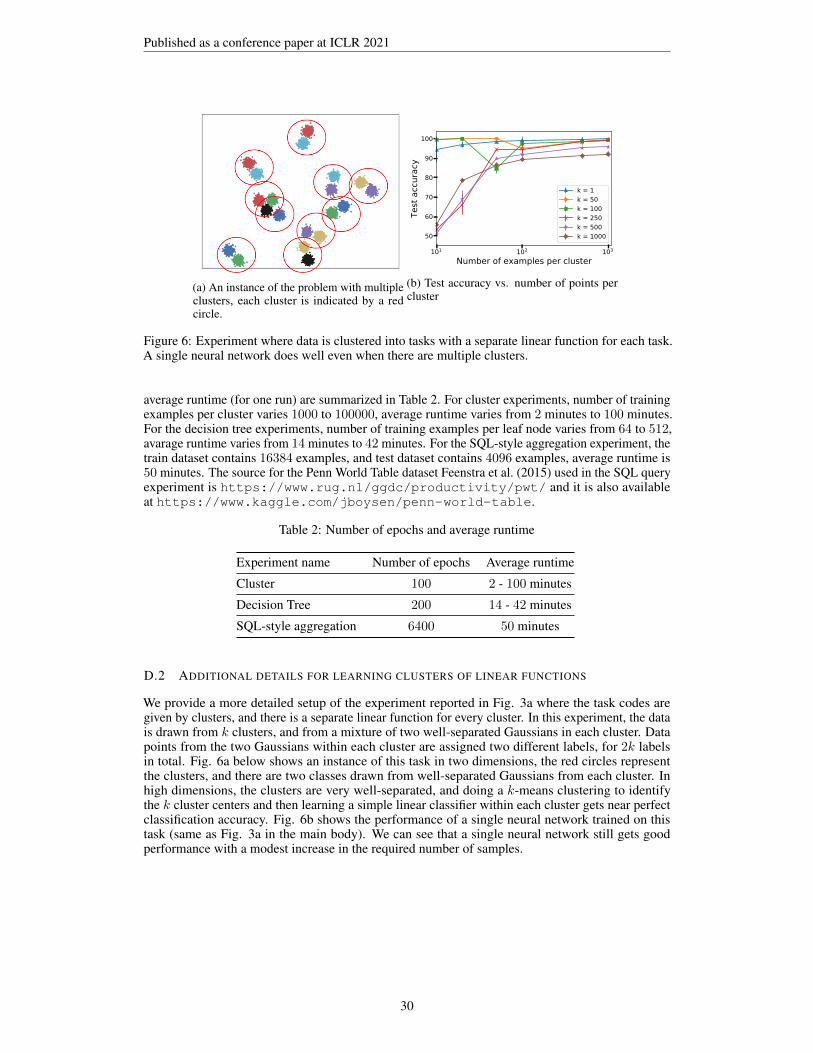
Published as a conference paper at ICLR 2021
(a) An instance of the problem with multipleclusters, each cluster is indicated by a redcircle.
101 102 103
Number of examples per cluster
50
60
70
80
90
100
Test
acc
urac
y
k = 1k = 50k = 100k = 250k = 500k = 1000
(b) Test accuracy vs. number of points percluster
Figure 6: Experiment where data is clustered into tasks with a separate linear function for each task.A single neural network does well even when there are multiple clusters.
average runtime (for one run) are summarized in Table 2. For cluster experiments, number of trainingexamples per cluster varies 1000 to 100000, average runtime varies from 2 minutes to 100 minutes.For the decision tree experiments, number of training examples per leaf node varies from 64 to 512,avarage runtime varies from 14 minutes to 42 minutes. For the SQL-style aggregation experiment, thetrain dataset contains 16384 examples, and test dataset contains 4096 examples, average runtime is50 minutes. The source for the Penn World Table dataset Feenstra et al. (2015) used in the SQL queryexperiment is https://www.rug.nl/ggdc/productivity/pwt/ and it is also availableat https://www.kaggle.com/jboysen/penn-world-table.
Table 2: Number of epochs and average runtime
Experiment name Number of epochs Average runtime
Cluster 100 2 - 100 minutes
Decision Tree 200 14 - 42 minutes
SQL-style aggregation 6400 50 minutes
D.2 ADDITIONAL DETAILS FOR LEARNING CLUSTERS OF LINEAR FUNCTIONS
We provide a more detailed setup of the experiment reported in Fig. 3a where the task codes aregiven by clusters, and there is a separate linear function for every cluster. In this experiment, the datais drawn from k clusters, and from a mixture of two well-separated Gaussians in each cluster. Datapoints from the two Gaussians within each cluster are assigned two different labels, for 2k labelsin total. Fig. 6a below shows an instance of this task in two dimensions, the red circles representthe clusters, and there are two classes drawn from well-separated Gaussians from each cluster. Inhigh dimensions, the clusters are very well-separated, and doing a k-means clustering to identifythe k cluster centers and then learning a simple linear classifier within each cluster gets near perfectclassification accuracy. Fig. 6b shows the performance of a single neural network trained on thistask (same as Fig. 3a in the main body). We can see that a single neural network still gets goodperformance with a modest increase in the required number of samples.
30
Related Documents