O BJ C UT

OBJ CUT

M. Pawan Kumar

Philip Torr

Andrew Zisserman

UNIVERSITYOF

OXFORD

Aim• Given an image, to segment the object

Segmentation should (ideally) be• shaped like the object e.g. cow-like• obtained efficiently in an unsupervised manner• able to handle self-occlusion

Segmentation

ObjectCategory

Model

Cow Image Segmented Cow

Challenges

Self Occlusion

Intra-Class Shape Variability

Intra-Class Appearance Variability

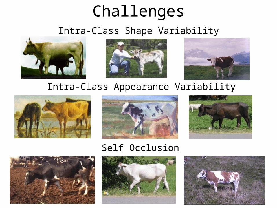
MotivationMagic Wand

Current methods require user intervention• Object and background seed pixels (Boykov and Jolly, ICCV 01)• Bounding Box of object (Rother et al. SIGGRAPH 04)

Cow Image

Object Seed Pixels

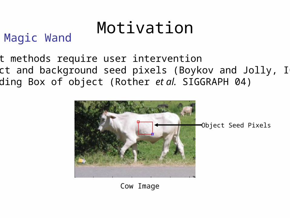
MotivationMagic Wand

Current methods require user intervention• Object and background seed pixels (Boykov and Jolly, ICCV 01)• Bounding Box of object (Rother et al. SIGGRAPH 04)

Cow Image

Object Seed Pixels

Background Seed Pixels

MotivationMagic Wand

Current methods require user intervention• Object and background seed pixels (Boykov and Jolly, ICCV 01)• Bounding Box of object (Rother et al. SIGGRAPH 04)

Segmented Image

MotivationMagic Wand

Current methods require user intervention• Object and background seed pixels (Boykov and Jolly, ICCV 01)• Bounding Box of object (Rother et al. SIGGRAPH 04)

Cow Image

Object Seed Pixels

Background Seed Pixels

MotivationMagic Wand

Current methods require user intervention• Object and background seed pixels (Boykov and Jolly, ICCV 01)• Bounding Box of object (Rother et al. SIGGRAPH 04)

Segmented Image

Problem • Manually intensive

• Segmentation is not guaranteed to be ‘object-like’

Non Object-like Segmentation

Motivation

Our Method• Combine object detection with segmentation

– Borenstein and Ullman, ECCV ’02– Leibe and Schiele, BMVC ’03

• Incorporate global shape priors in MRF

• Detection provides– Object Localization– Global shape priors

• Automatically segments the object– Note our method is completely generic– Applicable to any object category model

Outline

• Problem Formulation

• Form of Shape Prior

• Optimization

• Results

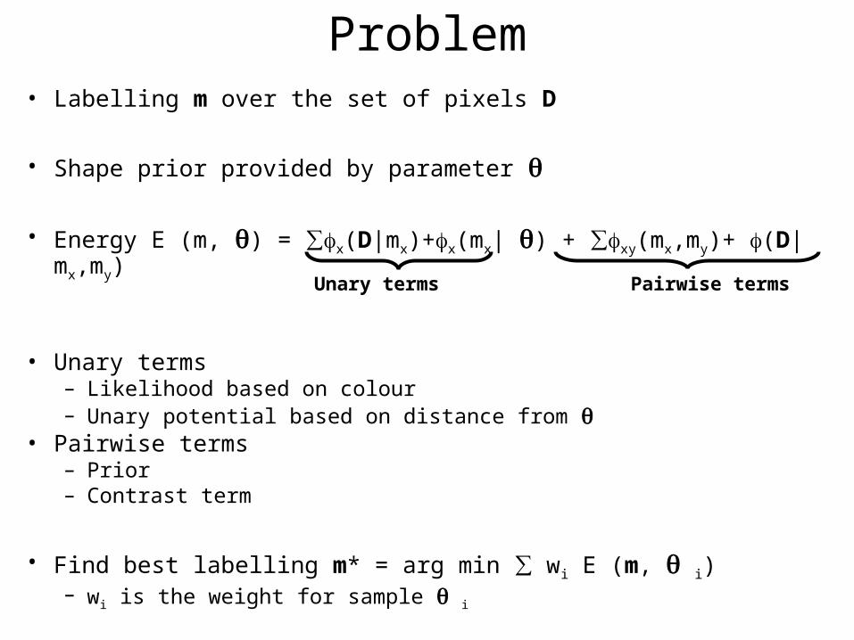
Problem• Labelling m over the set of pixels D

• Shape prior provided by parameter

• Energy E (m, ) = ∑x(D|mx)+x(mx| ) + ∑xy(mx,my)+ (D|mx,my)

• Unary terms– Likelihood based on colour– Unary potential based on distance from

• Pairwise terms– Prior– Contrast term

• Find best labelling m* = arg min ∑ wi E (m, i)– wi is the weight for sample i

Unary terms Pairwise terms

MRF

Probability for a labelling consists of• Likelihood

• Unary potential based on colour of pixel• Prior which favours same labels for neighbours (pairwise potentials)

D (pixels)

m (labels)

Image Plane

x

y

mx

my Unary Potential

x(D|mx)

Pairwise Potential

xy(mx, my)

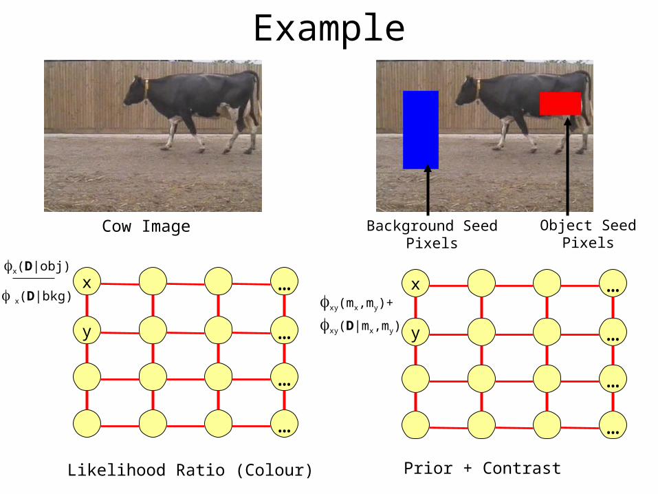
Example

Cow Image Object SeedPixels

Background SeedPixels

Prior

x …

y …

…

…

x …

y …

…

…

x(D|obj)

x(D|bkg) xy(mx,my)

Likelihood Ratio (Colour)

Example

Cow Image Object SeedPixels

Background SeedPixels

PriorLikelihood Ratio (Colour)

Contrast-Dependent MRF

Probability of labelling in addition has• Contrast term which favours boundaries to lie on image edges

D (pixels)

m (labels)

Image Plane

Contrast Term (D|mx,my)

x

y

mx

my

Example

Cow Image Object SeedPixels

Background SeedPixels

Prior + Contrast

x …

y …

…

…

x …

y …

…

…

Likelihood Ratio (Colour)

x(D|obj)

x(D|bkg) xy(mx,my)+

xy(D|mx,my)

Example

Cow Image Object SeedPixels

Background SeedPixels

Prior + ContrastLikelihood Ratio (Colour)

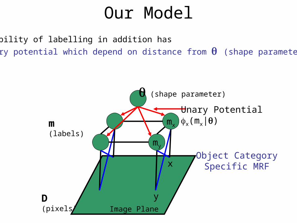
Our Model

Probability of labelling in addition has• Unary potential which depend on distance from (shape parameter)

D (pixels)

m (labels)

(shape parameter)

Image Plane

Object CategorySpecific MRFx

y

mx

my

Unary Potentialx(mx|)

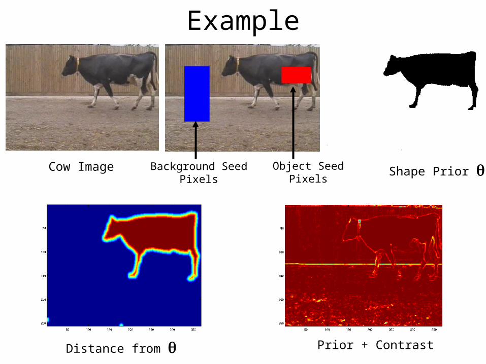
Example

Cow Image Object SeedPixels

Background SeedPixels

Prior + ContrastDistance from

Shape Prior

Example

Cow Image Object SeedPixels

Background SeedPixels

Prior + ContrastLikelihood + Distance from

Shape Prior

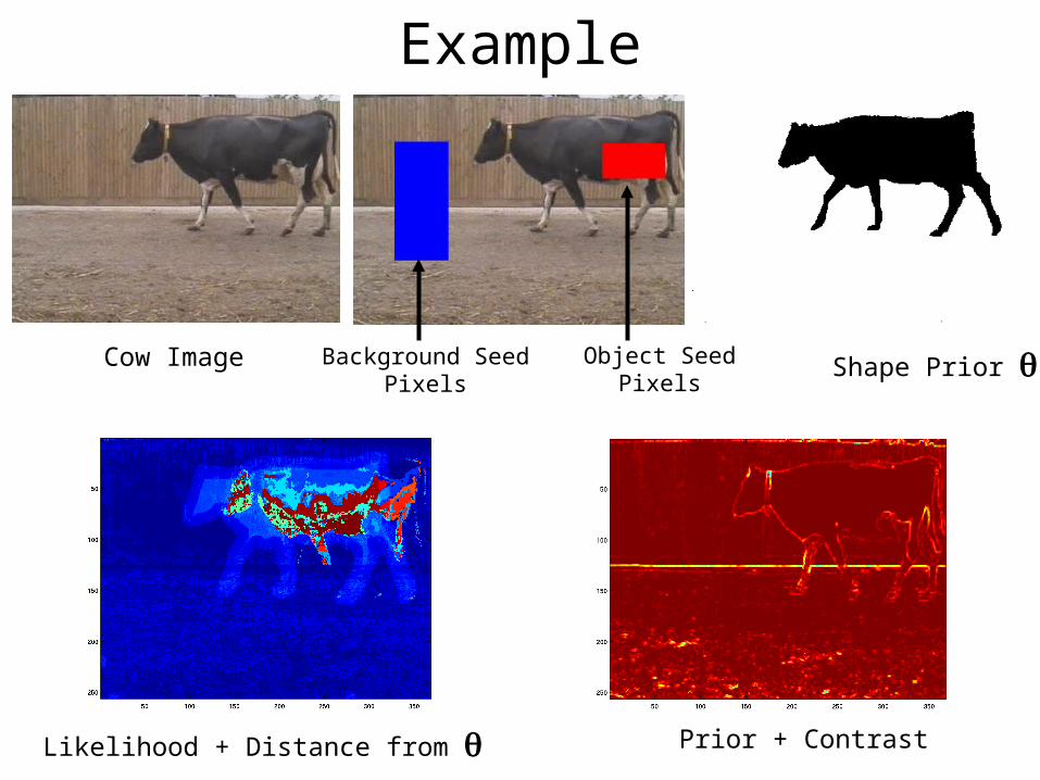
Example

Cow Image Object SeedPixels

Background SeedPixels

Prior + ContrastLikelihood + Distance from

Shape Prior

Outline

• Problem Formulation– Energy E (m, ) = ∑x(D|mx)+x(mx| ) + ∑xy(mx,my)+ (D|mx,my)

• Form of Shape Prior

• Optimization

• Results

Layered Pictorial Structures (LPS)• Generative model

• Composition of parts + spatial layout

Layer 2

Layer 1

Parts in Layer 2 can occlude parts in Layer 1

Spatial Layout(Pairwise Configuration)

Layer 2

Layer 1

Transformations

1

P(1) = 0.9

Cow Instance

Layered Pictorial Structures (LPS)

Layer 2

Layer 1

Transformations

2

P(2) = 0.8

Cow Instance

Layered Pictorial Structures (LPS)

Layer 2

Layer 1

Transformations

3

P(3) = 0.01

Unlikely Instance

Layered Pictorial Structures (LPS)

LPS for Detection• Learning

– Learnt automatically using a set of videos– Part correspondence using Shape Context

Shape Context Matching

Multiple Shape Exemplars

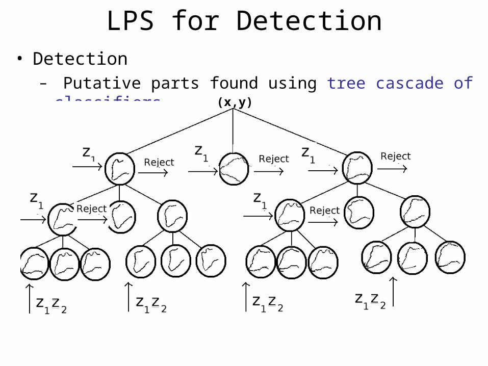
LPS for Detection• Detection

– Putative parts found using tree cascade of classifiers(x,y)

LPS for Detection

• MRF over parts

• Labels represent putative poses

• Prior (pairwise potential) - Robust Truncated Model

• Match LPS by obtaining MAP configuration

Potts Model Linear Model Quadratic Model

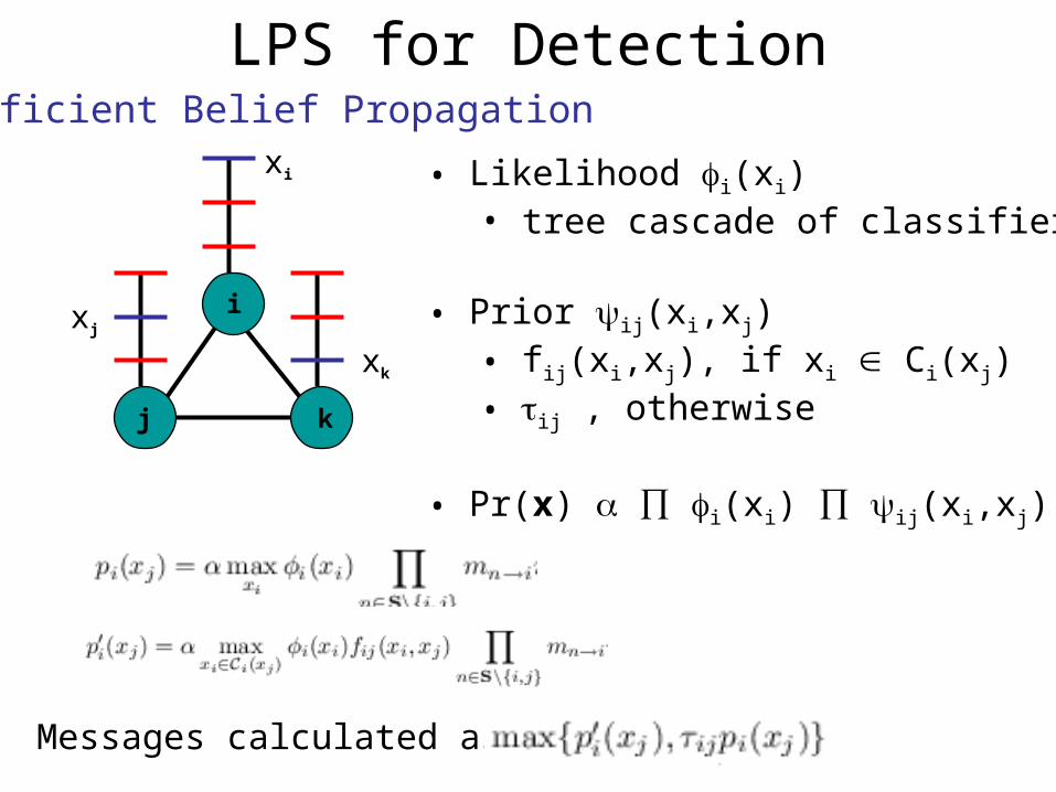
LPS for DetectionEfficient Belief Propagation

j

i

k

• Likelihood i(xi)• tree cascade of classifiers

• Prior ij(xi,xj)• fij(xi,xj), if xi Ci(xj)• ij , otherwise

• Pr(x) i(xi) ij(xi,xj)

xi

xj

xk

ij

jk

ki

i

j

k

Messages

mj->i

LPS for DetectionEfficient Belief Propagation

j

i

k

• Likelihood i(xi)• tree cascade of classifiers

• Prior ij(xi,xj)• fij(xi,xj), if xi Ci(xj)• ij , otherwise

• Pr(x) i(xi) ij(xi,xj)

xi

xj

xk

Messages calculated as

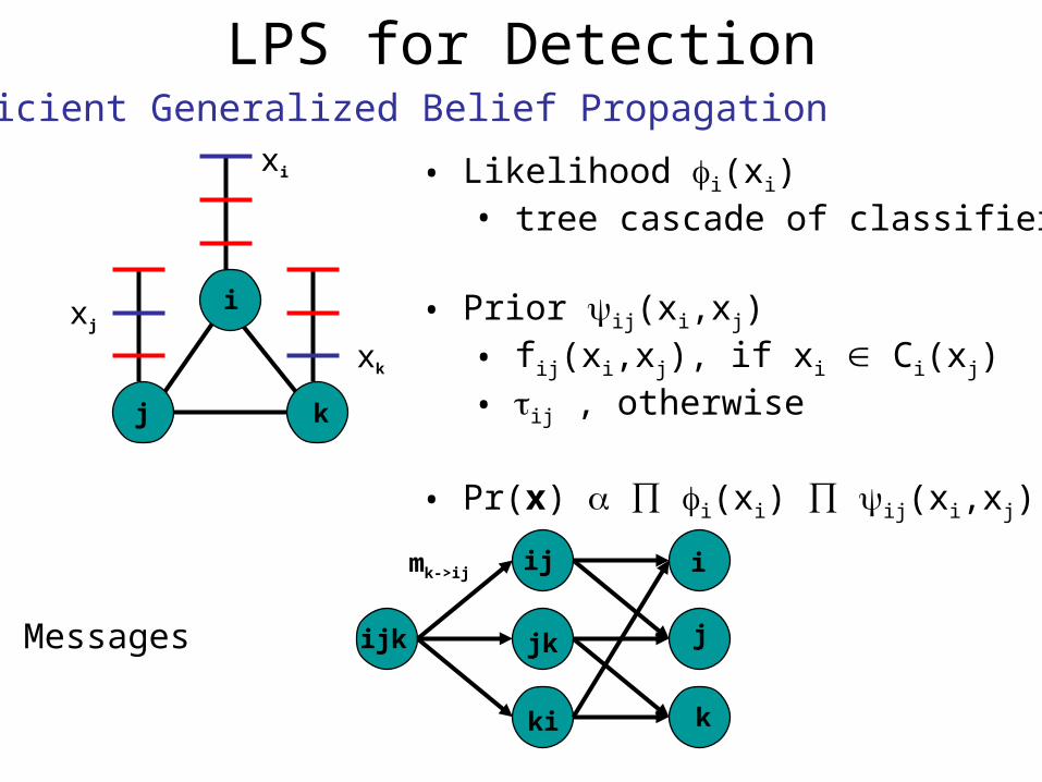
LPS for DetectionEfficient Generalized Belief Propagation

j

i

k

• Likelihood i(xi)• tree cascade of classifiers

• Prior ij(xi,xj)• fij(xi,xj), if xi Ci(xj)• ij , otherwise

• Pr(x) i(xi) ij(xi,xj)

xi

xj

xk

ij

jk

ki

i

j

k

Messages

mk->ij

ijk

LPS for DetectionEfficient Generalized Belief Propagation

j

i

k

• Likelihood i(xi)• tree cascade of classifiers

• Prior ij(xi,xj)• fij(xi,xj), if xi Ci(xj)• ij , otherwise

• Pr(x) i(xi) ij(xi,xj)

xi

xj

xk

Messages calculated as

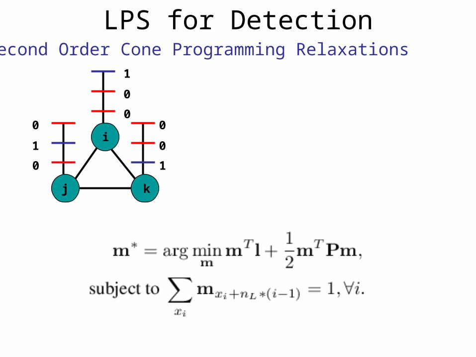
LPS for DetectionSecond Order Cone Programming Relaxations

j

i

k

• Likelihood i(xi)• tree cascade of classifiers

• Prior ij(xi,xj)• fij(xi,xj), if xi Ci(xj)• ij , otherwise

• Pr(x) i(xi) ij(xi,xj)

xi

xj

xk

LPS for DetectionSecond Order Cone Programming Relaxations

j

i

k

• Likelihood i(xi)• tree cascade of classifiers

• Prior ij(xi,xj)• fij(xi,xj), if xi Ci(xj)• ij , otherwise

• Pr(x) i(xi) ij(xi,xj)

0

1

0

0

0

1

1

0

0

m - Concatenation of all binary vectors

l - Likelihood vector

P - Prior matrix

LPS for DetectionSecond Order Cone Programming Relaxations

j

i

k

0

1

0

0

0

1

1

0

0

LPS for DetectionSecond Order Cone Programming Relaxations

j

i

k

0

1

0

0

0

1

1

0

0

LPS for DetectionSecond Order Cone Programming Relaxations

j

i

k

0

1

0

0

0

1

1

0

0

Outline

• Problem Formulation

• Form of Shape Prior

• Optimization

• Results

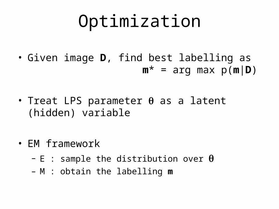
Optimization

• Given image D, find best labelling as m* = arg max p(m|D)

• Treat LPS parameter as a latent (hidden) variable

• EM framework– E : sample the distribution over – M : obtain the labelling m

E-Step

• Given initial labelling m’, determine p( | m’,D)

• Problem Efficiently sampling from p( | m’,D)

• Solution• We develop efficient sum-product Loopy Belief

Propagation (LBP) for matching LPS.

• Similar to efficient max-product LBP for MAP estimate

Results

• Different samples localize different parts well.• We cannot use only the MAP estimate of the LPS.

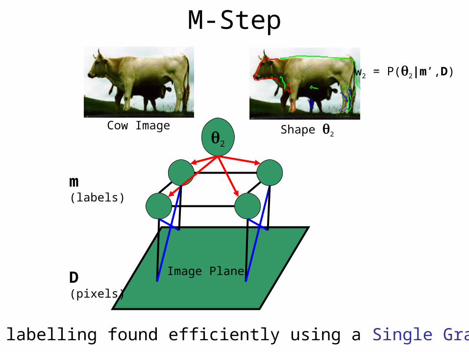
M-Step

• Given samples from p( |m’,D), get new labelling mnew

• Sample i provides– Object localization to learn RGB distributions of object and background– Shape prior for segmentation

• Problem– Maximize expected log likelihood using all samples– To efficiently obtain the new labelling

M-Step

Cow Image Shape 1

w1 = P(1|m’,D)

RGB Histogram for Object RGB Histogram for Background

Cow Image

M-Step

1

Image PlaneD (pixels)

m (labels)

• Best labelling found efficiently using a Single Graph Cut

Shape 1

w1 = P(1|m’,D)

Segmentation using Graph Cuts

x …

y … … …

z … …

Obj

Bkg

Cutx(D|bkg) + x(bkg|)

m

z(D|obj) + z(obj|)

xy(mx,my)+

xy(D|mx,my)

Segmentation using Graph Cuts

x …

y … … …

z … …

Obj

Bkg

m

M-Step

Cow Image

RGB Histogram for BackgroundRGB Histogram for Object

Shape 2

w2 = P(2|m’,D)

M-Step

Cow Image2

Image PlaneD (pixels)

m (labels)

• Best labelling found efficiently using a Single Graph Cut

Shape 2

w2 = P(2|m’,D)

M-Step

2

Image Plane

1

Image Plane

w1 + w2 + ….

• Best labelling found efficiently using a Single Graph Cut

m* = arg min ∑ wi E (m,i)

Outline

• Problem Formulation

• Form of Shape Prior

• Optimization

• Results

SegmentationImage

ResultsUsing LPS Model for Cow

In the absence of a clear boundary between object and background

SegmentationImage

ResultsUsing LPS Model for Cow

SegmentationImage

ResultsUsing LPS Model for Cow

SegmentationImage

ResultsUsing LPS Model for Cow

SegmentationImage

ResultsUsing LPS Model for Horse

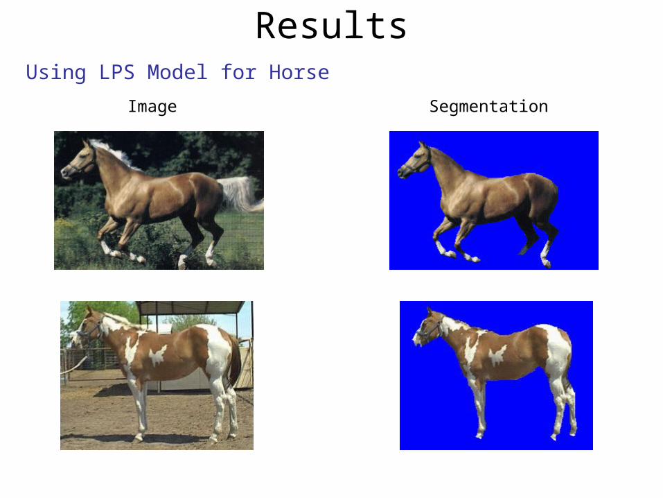
SegmentationImage

ResultsUsing LPS Model for Horse

Our Method Leibe and SchieleImage

Results

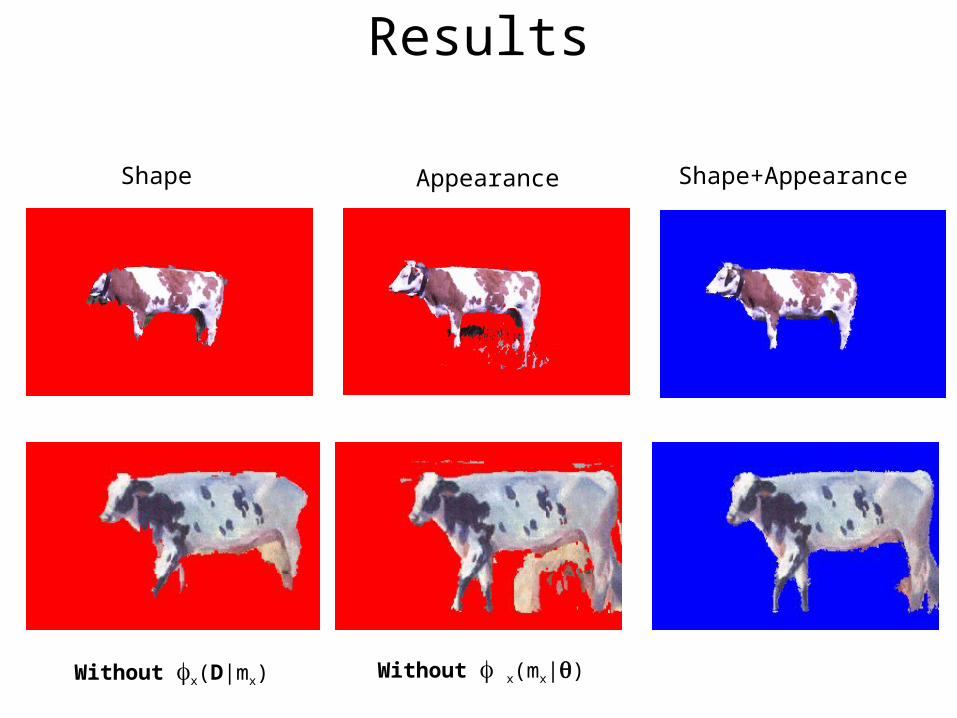
AppearanceShape Shape+Appearance

Results

Without x(D|mx) Without x(mx|)

• Conclusions

– New model for introducing global shape prior in MRF– Method of combining detection and segmentation– Efficient LBP for detecting articulated objects

• Future Work

– Other shape parameters need to be explored– Method needs to be extended to handle multiple

visual aspects