Introduction Discretization Preconditioning of the Fine Grid Systems Numerical Upscaling and Preconditioning of Flows in Highly Heterogeneous Porous Media R. Lazarov , TAMU, Y. Efendiev, J. Galvis, and J. Willems WS#4: Numerical Analysis of Multiscale Problems & Stochastic Modelling RICAM, Linz, Dec. 12-16, 2011 Thanks: NSF, KAUST 1 / 51

Welcome message from author
This document is posted to help you gain knowledge. Please leave a comment to let me know what you think about it! Share it to your friends and learn new things together.
Transcript
IntroductionDiscretization
Preconditioning of the Fine Grid Systems
Numerical Upscaling and Preconditioning of Flows in HighlyHeterogeneous Porous Media
R. Lazarov, TAMU,Y. Efendiev, J. Galvis, and J. Willems
WS#4: Numerical Analysisof Multiscale Problems & Stochastic Modelling
RICAM, Linz, Dec. 12-16, 2011Thanks: NSF, KAUST
1 / 51
IntroductionDiscretization
Preconditioning of the Fine Grid Systems
Outline
1 IntroductionMotivation and Problem Formulation
2 DiscretizationSingle Grid ApproximationSubgrid Approximation and Its Performance
3 Preconditioning of the Fine Grid SystemsOverlapping DD methodSome Numerical ExamplesWhen one can use this method ? Examples
2 / 51

IntroductionDiscretization
Preconditioning of the Fine Grid SystemsMotivation and Problem Formulation
Outline
1 IntroductionMotivation and Problem Formulation
2 DiscretizationSingle Grid ApproximationSubgrid Approximation and Its Performance
3 Preconditioning of the Fine Grid SystemsOverlapping DD methodSome Numerical ExamplesWhen one can use this method ? Examples
3 / 51
IntroductionDiscretization
Preconditioning of the Fine Grid SystemsMotivation and Problem Formulation
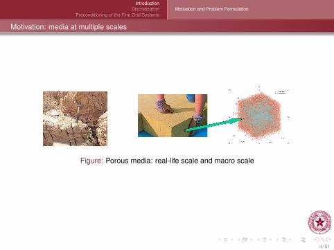
Motivation: media at multiple scales
Figure: Porous media: real-life scale and macro scale
4 / 51
IntroductionDiscretization
Preconditioning of the Fine Grid SystemsMotivation and Problem Formulation
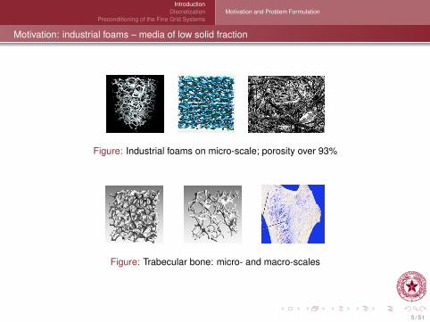
Motivation: industrial foams – media of low solid fraction
Figure: Industrial foams on micro-scale; porosity over 93%
Figure: Trabecular bone: micro- and macro-scales
5 / 51
IntroductionDiscretization
Preconditioning of the Fine Grid SystemsMotivation and Problem Formulation
Modeling of flow in porous media
(1) Flows in porous media are modeled by linear Darcy law that relates themacroscopic pressure p and velocity u:
∇p = −µκ−1u, κ − permeability, µ − viscosity (1)
(2) Another venue for a two-phase flow is a Richards model:
∇p = −µκ−1u, where κ = k(x)λ(x , p) (2)
with k(x) heterogeneous function is the intrinsic permeability, while λ(x , p) isa smooth function that varies moderately in both x and p, related to therelative permeability.(3) For flows in highly porous media Brinkman (1947) enhanced Darcy’s lawby adding dissipative term scaled by viscosity:
∇p = −µκ−1u + µ∆u. (3)
6 / 51
IntroductionDiscretization
Preconditioning of the Fine Grid SystemsMotivation and Problem Formulation
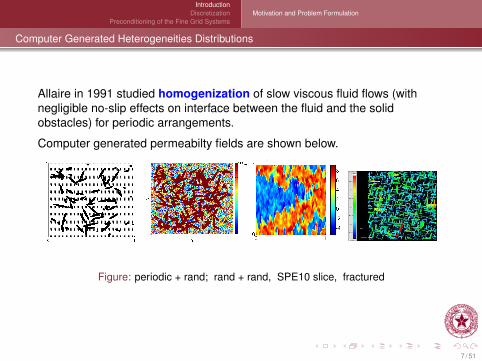
Computer Generated Heterogeneities Distributions
Allaire in 1991 studied homogenization of slow viscous fluid flows (withnegligible no-slip effects on interface between the fluid and the solidobstacles) for periodic arrangements.
Computer generated permeabilty fields are shown below.
Figure: periodic + rand; rand + rand, SPE10 slice, fractured
7 / 51

IntroductionDiscretization
Preconditioning of the Fine Grid SystemsMotivation and Problem Formulation
The Goals of Our Research
Our aim is development and study of numerical method that address thefollowing main issues of the above classes of problem:
Works well in both limits, Darcy and Brinkman;
Applicable to linear and nonlinear highly heterogeneous problems;
Could be used as a stand alone numerical upscaling procedure;
Is robust with respect to high variations of the permeability field.
8 / 51
IntroductionDiscretization
Preconditioning of the Fine Grid SystemsMotivation and Problem Formulation
State of the Art: Available Numerical Methods and Tools
Numerical upscaling as subgrid approximation methods:
(1) standard FEM for Darcy: Hou & Wu, 1997, Wu, Efendiev, & Hou,2002, comprehensive exposition in the book of Efendiev & Hou, 2009,
(2) mixed methods for Darcy: Aarnes, 2004, Arbogast, 2002, Chen &Hou, 2002,
(3) DG FEM for Brinkman equation: Willems, 2009, Iliev, Lazarov &Willems, 2010, Juntunen & Stenberg, 2010, Könö & Stenberg, 2011
(4) Galerkin FEM augmented with multiscale finite element functions:Pechstein & Scheichl, 2008, 2011, Chu, Graham, & Hou, 2010.
9 / 51

IntroductionDiscretization
Preconditioning of the Fine Grid SystemsMotivation and Problem Formulation
State of the Art: Available Numerical Methods and Tools
Preconditioning techniques based on coarse grid space with multiscalefinite element functions:
(1) FETI and other DD methods: Graham, Klie, Lechner, Pechstein, &Scheichl, 2007, 2008, 2009, 2011
(2) Using energy-minimizing coarse spaces: Xu & Zikatanov, 2004
(3) Spectral Element Agglomerate Algebraic Multigrid Methods,Efendiev, Galvis, & Vassielvski, 2011
(4) Use of multiscale basis in DD, Aarnes and Hou (2002)
10 / 51

IntroductionDiscretization
Preconditioning of the Fine Grid SystemsMotivation and Problem Formulation
Objectives:
1 Derive, study, implement, and test a numerical upscaling procedure forhighly porous media that works well in both limits, Brinkman and Darcy,so it could cover both, natural porous media and man-made materials;
2 Design and study of preconditioning techniques for such problems forporous media of high contrast with targeted applications to oil/waterreservoirs, bones, filters, insulators, etc
11 / 51
IntroductionDiscretization
Preconditioning of the Fine Grid SystemsMotivation and Problem Formulation
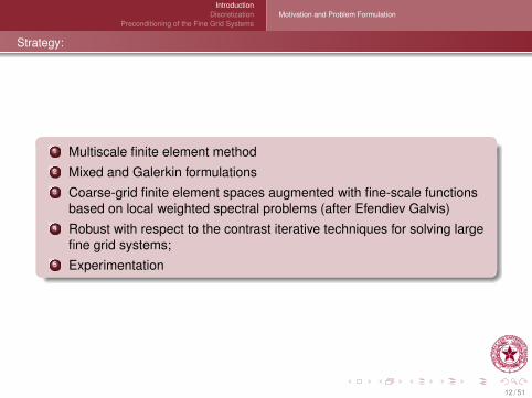
Strategy:
1 Multiscale finite element method2 Mixed and Galerkin formulations3 Coarse-grid finite element spaces augmented with fine-scale functions
based on local weighted spectral problems (after Efendiev Galvis)4 Robust with respect to the contrast iterative techniques for solving large
fine grid systems;5 Experimentation
12 / 51

IntroductionDiscretization
Preconditioning of the Fine Grid Systems
Single Grid ApproximationSubgrid Approximation and Its Performance
Outline
1 IntroductionMotivation and Problem Formulation
2 DiscretizationSingle Grid ApproximationSubgrid Approximation and Its Performance
3 Preconditioning of the Fine Grid SystemsOverlapping DD methodSome Numerical ExamplesWhen one can use this method ? Examples
13 / 51
IntroductionDiscretization
Preconditioning of the Fine Grid Systems
Single Grid ApproximationSubgrid Approximation and Its Performance
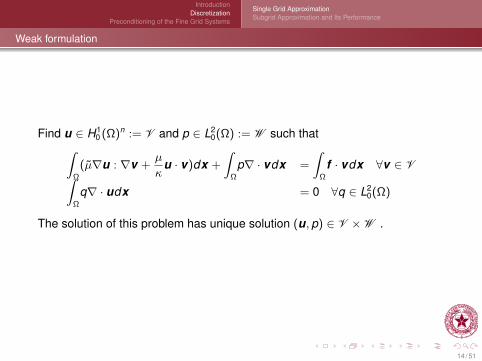
Weak formulation
Find u ∈ H10 (Ω)n := V and p ∈ L2
0(Ω) := W such that∫Ω
(µ∇u : ∇v +µ
κu · v)dx +
∫Ω
p∇ · vdx =
∫Ω
f · vdx ∀v ∈ V∫Ω
q∇ · udx = 0 ∀q ∈ L20(Ω)
The solution of this problem has unique solution (u, p) ∈ V ×W .
14 / 51

IntroductionDiscretization
Preconditioning of the Fine Grid Systems
Single Grid ApproximationSubgrid Approximation and Its Performance
The finite element of Brezzi, Douglas, and Marini of degree 1
For this finite element we have:
On a rectangle T the polynomial space is characterized by
v = P21 + spancurl(x2
1 x2), curl(x1x22;
with dofnormal velocity
pressureH
(VH ,WH) ⊂ (H0(div ; Ω), L20(Ω)) := V ×W ;
Has a natural variant for n = 3.
15 / 51
IntroductionDiscretization
Preconditioning of the Fine Grid Systems
Single Grid ApproximationSubgrid Approximation and Its Performance
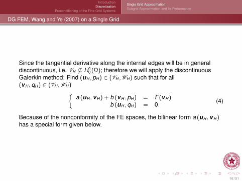
DG FEM, Wang and Ye (2007) on a Single Grid
Since the tangential derivative along the internal edges will be in generaldiscontinuous, i.e. VH * H1
0 (Ω); therefore we will apply the discontinuousGalerkin method: Find (uH , pH) ∈ (VH ,WH) such that for all(vH , qH) ∈ (VH ,WH)
a (uH , vH) + b (vH , pH) = F (vH)b (uH , qH) = 0. (4)
Because of the nonconformity of the FE spaces, the bilinear form a (uH , vH)has a special form given below.
16 / 51

IntroductionDiscretization
Preconditioning of the Fine Grid Systems
Single Grid ApproximationSubgrid Approximation and Its Performance
Discretization of Wang and Yang 2007 on Single Grid
b (vH , pH) :=
∫Ω
pH∇ · vHdx
F (vH) :=
∫Ω
f · vHdx
τ+en+
en−eT+
τ−eT−
a (uH , vH) :=∑
T∈TH
∫T
(µ∇uH : ∇vH +µ
κuH · vH)dx
−∑
e∈EH
∫eµ
(uH JvHK + vH JuHK︸ ︷︷ ︸
symmetrization
− α
|e| JuHK JvHK︸ ︷︷ ︸stabilization
)ds
v|e := 12 (n+
e · ∇(v · τ+e )|e+ + n−e · ∇(v · τ−e )|e−)
JvK |e := v |e+ · τ+e + v |e− · τ−e
17 / 51

IntroductionDiscretization
Preconditioning of the Fine Grid Systems
Single Grid ApproximationSubgrid Approximation and Its Performance
Fine and Coarse Grid Spaces: Arbogast (2004)
Fine and coarse triangulation Th and TH .
FE spaces with (Wh consist of bubbles)WH,h = Wh ⊕WH ⊂ L2
0, VH,h = Vh ⊕ VH ⊂ H0(div)
Crucial properties:
1 ∇ · Vh = Wh and ∇ · VH = WH
2 vh · n = 0 on ∂T , ∀vh ∈ Vh and ∂T ∈ TH
3 WH ⊥ Wh
Ω
TH
Th
18 / 51

IntroductionDiscretization
Preconditioning of the Fine Grid Systems
Single Grid ApproximationSubgrid Approximation and Its Performance
Splitting of the Spaces
Unique decomposition in coarse and fine-grid components yields: finduH + uh ∈ Wh ⊕WH , and pH + ph ∈ Vh ⊕ VH such that
decomposed solution
a (uH + uh, vH + vh) + b (vH + vh, pH + ph) = F (vH + vh),
b (uH + uh, qH + qh) = 0,
for all vH + vh ∈ Wh ⊕WH and qH + qh ∈ Vh ⊕ VH .
19 / 51
IntroductionDiscretization
Preconditioning of the Fine Grid Systems
Single Grid ApproximationSubgrid Approximation and Its Performance
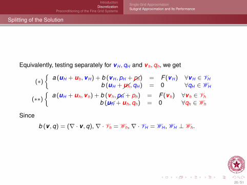
Splitting of the Solution
Equivalently, testing separately for vH , qH and vh, qh, we get
(∗)
a (uH + uh, vH) + b (vH , pH +ph) = F (vH) ∀vH ∈ VH
b (uH +uh, qH) = 0 ∀qH ∈ WH
(∗∗)
a (uH + uh, vh) + b (vh,pH + ph) = F (vh) ∀vh ∈ Vh
b (uH + uh, qh) = 0 ∀qh ∈ Wh
Since
b (v , q) = (∇ · v , q), ∇ · Vh = Wh, ∇ · VH = WH , WH ⊥ Wh.
20 / 51

IntroductionDiscretization
Preconditioning of the Fine Grid Systems
Single Grid ApproximationSubgrid Approximation and Its Performance
Decompose (∗∗) further into
(∗∗)
a (δu(uH), vh) + b (vh, δp(uH)) = −a (uH , vh) ∀vh ∈ Vh
b (δu(uH), qh) = 0 ∀qh ∈ Wha(δu , vh
)+ b
(vh, δp
)= F (vh) ∀vh ∈ Vh
b(δu , qh
)= 0 ∀qh ∈ Wh
Note that
(δu(uH), δp(uH)) is linear in uH
(δu , δp) and (δu(uH), δp(uH)) can be computed locally
21 / 51
IntroductionDiscretization
Preconditioning of the Fine Grid Systems
Single Grid ApproximationSubgrid Approximation and Its Performance
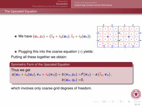
The Upscaled Equation
We have (uh, ph) = (δu + δu(uH), δp + δp(uH)).
Plugging this into the coarse equation (∗) yields:
Putting all these together we obtain:
Symmetric Form of the Upscaled Equation
Thus we geta (uH + δu(uH), vH + δu(vH)) + b (vH , pH) =F (vH)− a
(δu , vH
),
b (uH , qH) =0,
which involves only coarse-grid degrees of freedom.
22 / 51

IntroductionDiscretization
Preconditioning of the Fine Grid Systems
Single Grid ApproximationSubgrid Approximation and Its Performance
Sub-grid Algorithm, Willems, 2009
Sub-grid Algorithm: Willems, 2009
1 Solve for the fine responses (δu , δp) and (δu(ϕH), δp(ϕH)) for coarsebasis functions ϕH and each coarse cell.
2 Solve the upscaled equation for (uH , pH).3 Piece together the solutions to get
(uH,h, pH,h) = (uH , pH) + (δu(uH), δp(uH)) + (δu , δp).
For pure Darcy this reduces to the method of Arbogast, 2002, for BDM FEs.
23 / 51
IntroductionDiscretization
Preconditioning of the Fine Grid Systems
Single Grid ApproximationSubgrid Approximation and Its Performance
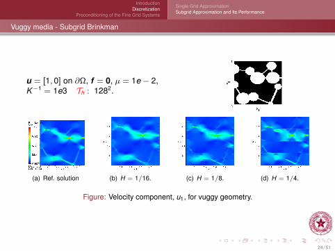
Vuggy media - Subgrid Brinkman
u = [1, 0] on ∂Ω, f = 0, µ = 1e − 2,K−1 = 1e3 Th : 1282.
(a) Ref. solution (b) H = 1/16. (c) H = 1/8. (d) H = 1/4.
Figure: Velocity component, u1, for vuggy geometry.
24 / 51
IntroductionDiscretization
Preconditioning of the Fine Grid Systems
Single Grid ApproximationSubgrid Approximation and Its Performance
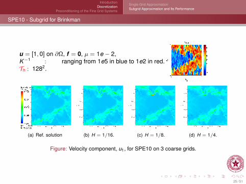
SPE10 - Subgrid for Brinkman
u = [1, 0] on ∂Ω, f = 0, µ = 1e − 2,K−1 : ranging from 1e5 in blue to 1e2 in red.Th : 1282.
(a) Ref. solution (b) H = 1/16. (c) H = 1/8. (d) H = 1/4.
Figure: Velocity component, u1, for SPE10 on 3 coarse grids.
25 / 51
IntroductionDiscretization
Preconditioning of the Fine Grid Systems
Single Grid ApproximationSubgrid Approximation and Its Performance
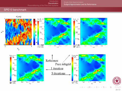
SPE10 benchmark
26 / 51

IntroductionDiscretization
Preconditioning of the Fine Grid Systems
Overlapping DD methodSome Numerical ExamplesWhen one can use this method ? Examples
Outline
1 IntroductionMotivation and Problem Formulation
2 DiscretizationSingle Grid ApproximationSubgrid Approximation and Its Performance
3 Preconditioning of the Fine Grid SystemsOverlapping DD methodSome Numerical ExamplesWhen one can use this method ? Examples
27 / 51

IntroductionDiscretization
Preconditioning of the Fine Grid Systems
Overlapping DD methodSome Numerical ExamplesWhen one can use this method ? Examples
Preconditioning of the fine grid system
The algebraic system is an ill-conditioned system due to two mainfactors:
(1) the permeability K (orders of magnitude) and(2) the mesh size h.
The discussed numerical upscaling of Brinkman equations leads to asaddle-point system;
The matrix corresponding to the form a(·, ·) is very ill-conditioned due tothe large heterogeneous variation of K and very small h;
The known iterative methods, e.g. Uzawa, Bramble-Pasciak, etc eitherconverge slow or practically do not converge for media with very highcontrast.
28 / 51
IntroductionDiscretization
Preconditioning of the Fine Grid Systems
Overlapping DD methodSome Numerical ExamplesWhen one can use this method ? Examples
Abstract form of DD for s.p.d. forms a(u, v) (Efendiev,Galvis,L.,Willems,2011)
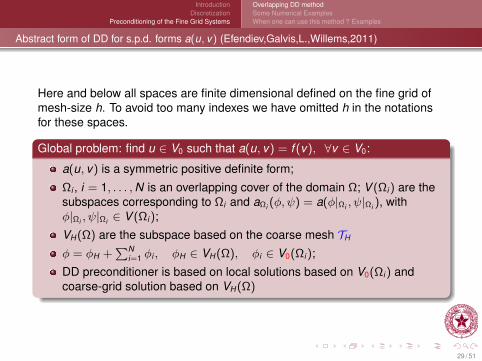
Here and below all spaces are finite dimensional defined on the fine grid ofmesh-size h. To avoid too many indexes we have omitted h in the notationsfor these spaces.
Global problem: find u ∈ V0 such that a(u, v) = f (v), ∀v ∈ V0:
a(u, v) is a symmetric positive definite form;
Ωi , i = 1, . . . ,N is an overlapping cover of the domain Ω; V (Ωi ) are thesubspaces corresponding to Ωi and aΩi (φ, ψ) = a(φ|Ωi , ψ|Ωi ), withφ|Ωi , ψ|Ωi ∈ V (Ωi );
VH(Ω) are the subspace based on the coarse mesh TH
φ = φH +∑N
i=1 φi , φH ∈ VH(Ω), φi ∈ V0(Ωi );
DD preconditioner is based on local solutions based on V0(Ωi ) andcoarse-grid solution based on VH(Ω)
29 / 51
IntroductionDiscretization
Preconditioning of the Fine Grid Systems
Overlapping DD methodSome Numerical ExamplesWhen one can use this method ? Examples
Abstract form of DD for s.p.d. forms a(u, v) (Efendiev,Galvis,L.,Willems,2011)
Ω
xjΩj
Ωj
Ωsj ,i
Ωpj
Ωsj
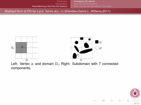
Left: Vertex xi and domain Ωi ; Right: Subdomain with 7 connectedcomponents.
30 / 51
IntroductionDiscretization
Preconditioning of the Fine Grid Systems
Overlapping DD methodSome Numerical ExamplesWhen one can use this method ? Examples
Robust DD Preconditioners for the Global Fine Grid System
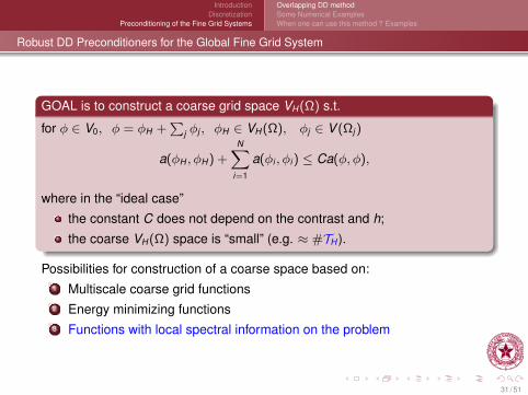
GOAL is to construct a coarse grid space VH(Ω) s.t.
for φ ∈ V0, φ = φH +∑
j φj , φH ∈ VH(Ω), φj ∈ V (Ωj )
a(φH , φH) +N∑
i=1
a(φi , φi ) ≤ Ca(φ, φ),
where in the “ideal case”
the constant C does not depend on the contrast and h;
the coarse VH(Ω) space is “small” (e.g. ≈ #TH ).
Possibilities for construction of a coarse space based on:1 Multiscale coarse grid functions2 Energy minimizing functions3 Functions with local spectral information on the problem
31 / 51

IntroductionDiscretization
Preconditioning of the Fine Grid Systems
Overlapping DD methodSome Numerical ExamplesWhen one can use this method ? Examples
Abstract Spectral Problems
Let ξj : Ω→ [0, 1] be a partition of unity subordinated to the partition Ωj , sothat supp(ξj ) = Ωj .For any φ ∈ V0 the function (ξjφ)|Ωj ∈ V0(Ωj ) and define
mΩj (φ, ψ) :=∑
i
aΩj (ξiξjφ, ξiξjψ),
where the summation is over all i s.t. Ωj ∩ Ωi 6= ∅.Consider the spectral problem: find (λj
i , φji ) ∈ (R,V (Ωi )), s.t.
aΩj (ψ, φji ) = λj
imΩj (ψ, φji ) ∀ψ ∈ V (Ωi )
and order the eigenvalues 0 ≤ λ1i ≤ · · · ≤ λ
Lii ≤ . . . .
32 / 51
IntroductionDiscretization
Preconditioning of the Fine Grid Systems
Overlapping DD methodSome Numerical ExamplesWhen one can use this method ? Examples
Coarse Space Based on Spectral Problems - Efendiev&Galvis, 2009
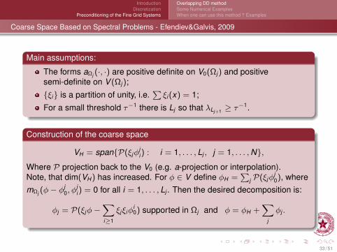
Main assumptions:
The forms aΩj (·, ·) are positive definite on V0(Ωj ) and positivesemi-definite on V (Ωj );
ξi is a partition of unity, i.e.∑ξi (x) = 1;
For a small threshold τ−1 there is Lj so that λLj+1 ≥ τ−1.
Construction of the coarse space
VH = spanP(ξjφji ) : i = 1, . . . , Lj , j = 1, . . . ,N,
Where P projection back to the V0 (e.g. a-projection or interpolation).Note, that dim(VH) has increased. For φ ∈ V define φH =
∑j P(ξjφ
j0), where
mΩj (φ− φj0, φ
ji ) = 0 for all i = 1, . . . , Lj . Then the desired decomposition is:
φj = P(ξjφ−∑i≥1
ξjξiφi0) supported in Ωj and φ = φH +
∑j
φj .
33 / 51
IntroductionDiscretization
Preconditioning of the Fine Grid Systems
Overlapping DD methodSome Numerical ExamplesWhen one can use this method ? Examples
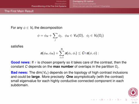
The First Main Result
For any φ ∈ V0 the decomposition
φ = φH +∑
j
φj , φH ∈ VH(Ω), φj ∈ V0(Ωj )
satisfies
a(φH , φH) +N∑
i=1
a(φi , φi ) ≤ Cτa(φ, φ) :
Good news: If τ is chosen properly so it takes care of the contrast, then theconstant C depends on the max number of overlaps in the partition Ωj .
Bad news: The dim(VH) depends on the topology of high contrast inclusionsand could be large. More precisely: One asymptotically (with the contrast)small eigenvalue for each highly conductive connected component in eachsubdomain.
34 / 51
IntroductionDiscretization
Preconditioning of the Fine Grid Systems
Overlapping DD methodSome Numerical ExamplesWhen one can use this method ? Examples
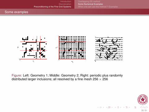
Some examples
Figure: Left: Geometry 1; Middle: Geometry 2; Right: periodic plus randomlydistributed larger inclusions; all resolved by a fine mesh 256× 256
35 / 51
IntroductionDiscretization
Preconditioning of the Fine Grid Systems
Overlapping DD methodSome Numerical ExamplesWhen one can use this method ? Examples
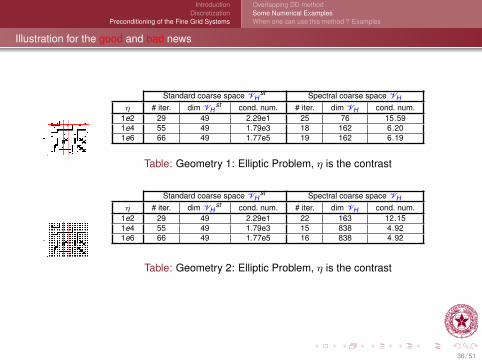
Illustration for the good and bad news
Standard coarse space VHst Spectral coarse space VH
η # iter. dim VHst cond. num. # iter. dim VH cond. num.
1e2 29 49 2.29e1 25 76 15.591e4 55 49 1.79e3 18 162 6.201e6 66 49 1.77e5 19 162 6.19
Table: Geometry 1: Elliptic Problem, η is the contrast
Standard coarse space VHst Spectral coarse space VH
η # iter. dim VHst cond. num. # iter. dim VH cond. num.
1e2 29 49 2.29e1 22 163 12.151e4 55 49 1.79e3 15 838 4.921e6 66 49 1.77e5 16 838 4.92
Table: Geometry 2: Elliptic Problem, η is the contrast
36 / 51
IntroductionDiscretization
Preconditioning of the Fine Grid Systems
Overlapping DD methodSome Numerical ExamplesWhen one can use this method ? Examples
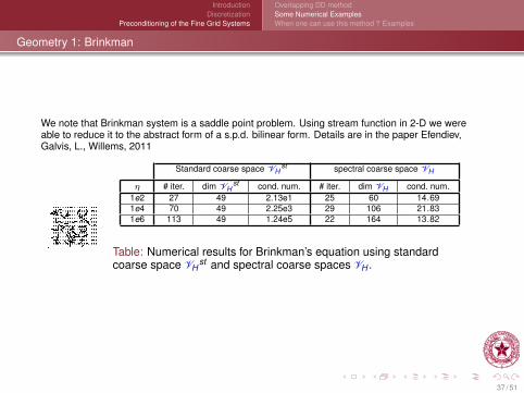
Geometry 1: Brinkman
We note that Brinkman system is a saddle point problem. Using stream function in 2-D we wereable to reduce it to the abstract form of a s.p.d. bilinear form. Details are in the paper Efendiev,Galvis, L., Willems, 2011
Standard coarse space VHst spectral coarse space VH
η # iter. dim VHst cond. num. # iter. dim VH cond. num.
1e2 27 49 2.13e1 25 60 14.691e4 70 49 2.25e3 29 106 21.831e6 113 49 1.24e5 22 164 13.82
Table: Numerical results for Brinkman’s equation using standardcoarse space VH
st and spectral coarse spaces VH .
37 / 51
IntroductionDiscretization
Preconditioning of the Fine Grid Systems
Overlapping DD methodSome Numerical ExamplesWhen one can use this method ? Examples
Reducing the Dimension of the Coarse Space: Efendiev&Galvis, 2010
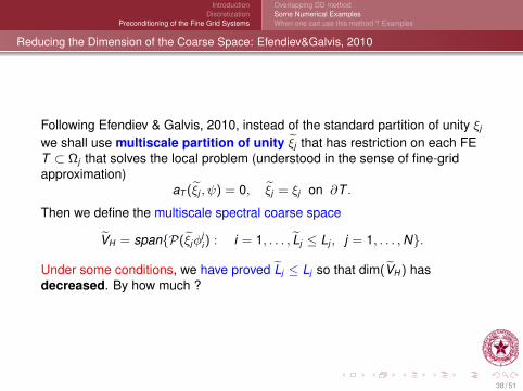
Following Efendiev & Galvis, 2010, instead of the standard partition of unity ξj
we shall use multiscale partition of unity ξj that has restriction on each FET ⊂ Ωj that solves the local problem (understood in the sense of fine-gridapproximation)
aT (ξj , ψ) = 0, ξj = ξj on ∂T .
Then we define the multiscale spectral coarse space
VH = spanP(ξjφji ) : i = 1, . . . , Lj ≤ Lj , j = 1, . . . ,N.
Under some conditions, we have proved Lj ≤ Lj so that dim(VH) hasdecreased. By how much ?
38 / 51
IntroductionDiscretization
Preconditioning of the Fine Grid Systems
Overlapping DD methodSome Numerical ExamplesWhen one can use this method ? Examples
Reduction of the dimention of VH (Efendiev,Galvis,L.,Willems,2011)
Ωpj
Ωsj
Ωj
Ωj
Ωsj ,k , k = 1, . . . , Lj
Ωsj ,k , k = Lj + 1, . . . , Lj
Ωj
Ωsj ,i
Ωpj
Ωsj
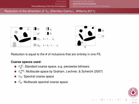
Reduction is equal to the # of inclusions that are entirely in one FE.
Coarse spaces used:V st
H : Standard coarse space, e.g. piecewise bilinears
V msH : Multiscale space by Graham, Lechner, & Scheichl (2007)
VH : Spectral coarse space
VH : Multiscale spectral coarse space
39 / 51
IntroductionDiscretization
Preconditioning of the Fine Grid Systems
Overlapping DD methodSome Numerical ExamplesWhen one can use this method ? Examples
Geometry 2: Second Order Elliptic Problem
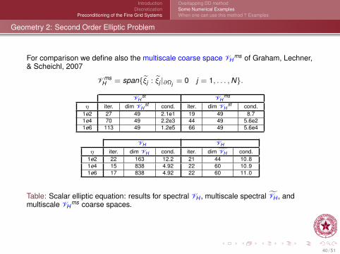
For comparison we define also the multiscale coarse space VHms of Graham, Lechner,
& Scheichl, 2007
V msH = spanξj : ξj |∂Ωj = 0 j = 1, . . . ,N.
VHst VH
ms
η iter. dim VHst cond. iter. dim VH
st cond.1e2 27 49 2.1e1 19 49 8.71e4 70 49 2.2e3 44 49 5.6e21e6 113 49 1.2e5 66 49 5.6e4
VH VHη iter. dim VH cond. iter. dim VH cond.
1e2 22 163 12.2 21 44 10.81e4 15 838 4.92 22 60 10.91e6 17 838 4.92 22 60 11.0
Table: Scalar elliptic equation: results for spectral VH , multiscale spectral VH , andmultiscale VH
ms coarse spaces.
40 / 51

IntroductionDiscretization
Preconditioning of the Fine Grid Systems
Overlapping DD methodSome Numerical ExamplesWhen one can use this method ? Examples
What about the computational complexity of this method ? In one word it isexpensive ! Then the question is
When one can see some advantages in using this method ?
There is a number of situations when this method will be useful, these aremostly cases when the precomputed coarse grid space can be usemultiple times:
1 In nonlinear problems when the heterogeneity is separated from thenonlinearity, e.g. Richards equation;
2 In computations of various scenarios of the boundary and source data;3 In stochastic environment.
Also, due it the inherently parallel nature of the constructions, these could bevery useful in parallel computations.
41 / 51

IntroductionDiscretization
Preconditioning of the Fine Grid Systems
Overlapping DD methodSome Numerical ExamplesWhen one can use this method ? Examples
Richards Equation
we assume that the coefficient could be represented in the formk(x , p) = k(x)λ(x , p), where k(x) is highly heterogeneous. We have testedtwo models:
Haverkamp λ(x , p) =A
A + (|p|/B)γ,
and
Van Genuchten λ(x , p) =1− (α|p|/B)n−1[1 + (α|p|)n]−m2
[1 + (α|p|)n]m2
.
Here the coefficients A, B, γ, α, m, n are fitted to the experimental data.
42 / 51

IntroductionDiscretization
Preconditioning of the Fine Grid Systems
Overlapping DD methodSome Numerical ExamplesWhen one can use this method ? Examples
Richards Equation
Then for the nonlinear Richards equation we run a simple Picard iteration
−div(k(x)λ(x , pn)∇pn+1) = f
with pn being the previous iterate and apply our preconditioning technique forthis linear equation.
Details about the theory, the conditions it is valid and more computations werefer to Efendiev, Galvis, Ki Kang, L. (2011)
43 / 51
IntroductionDiscretization
Preconditioning of the Fine Grid Systems
Overlapping DD methodSome Numerical ExamplesWhen one can use this method ? Examples
Richards Equation
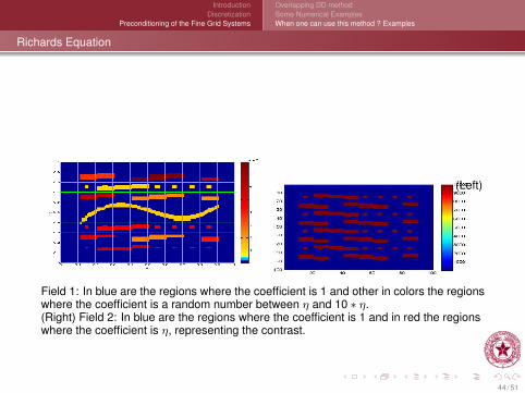
(Left)
Field 1: In blue are the regions where the coefficient is 1 and other in colors the regionswhere the coefficient is a random number between η and 10 ∗ η.(Right) Field 2: In blue are the regions where the coefficient is 1 and in red the regionswhere the coefficient is η, representing the contrast.
44 / 51
IntroductionDiscretization
Preconditioning of the Fine Grid Systems
Overlapping DD methodSome Numerical ExamplesWhen one can use this method ? Examples
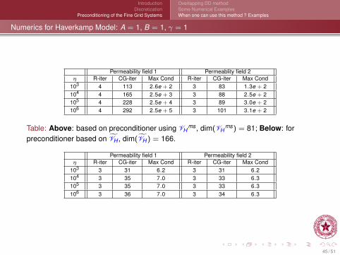
Numerics for Haverkamp Model: A = 1, B = 1, γ = 1
Permeability field 1 Permeablity field 2η R-iter CG-iter Max Cond R-iter CG-iter Max Cond
103 4 113 2.6e + 2 3 83 1.3e + 2104 4 165 2.5e + 3 3 88 2.5e + 2105 4 228 2.5e + 4 3 89 3.0e + 2106 4 292 2.5e + 5 3 101 3.1e + 2
Table: Above: based on preconditioner using VHms , dim(VH
ms) = 81; Below: forpreconditioner based on VH , dim(VH ) = 166.
Permeability field 1 Permeability field 2η R-iter CG-iter Max Cond R-iter CG-iter Max Cond
103 3 31 6.2 3 31 6.2104 3 35 7.0 3 33 6.3105 3 35 7.0 3 33 6.3106 3 36 7.0 3 34 6.3
45 / 51

IntroductionDiscretization
Preconditioning of the Fine Grid Systems
Overlapping DD methodSome Numerical ExamplesWhen one can use this method ? Examples
Numerics for Haverkamp Model: A = 1, B = 0.01, γ = 0.5
Permeability field 1 Permeability field 2η R-iter CG-iter Max Cond R-iter CG-iter Max Cond
103 11 120 3.9e + 2 8 98 1.9e + 2104 11 190 3.6e + 3 8 104 3.9e + 3105 11 250 3.6e + 4 8 107 4.6e + 4106 11 315 3.6e + 5 8 111 4.6e + 5
Table: Above: based on preconditioner using VHms , dim(VH
ms) = 81; Below: forpreconditioner based on VH , dim(VH ) = 166.
Permeability field 1 Permeability field 2η R-iter CG-iter Max Cond R-iter CG-iter Max Cond
103 8 38 9.6 8 38 9.6104 8 41 9.7 8 40 9.7105 8 41 9.7 8 41 9.7106 8 43 9.7 8 42 9.7
46 / 51
IntroductionDiscretization
Preconditioning of the Fine Grid Systems
Overlapping DD methodSome Numerical ExamplesWhen one can use this method ? Examples
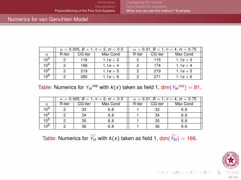
Numerics for van Genuhten Model
α = 0.005, B = 1, n = 2, m = 0.5 α = 0.01, B = 1, n = 4, m = 0.75η R-iter CG-iter Max Cond R-iter CG-iter Max Cond
103 2 116 1.1e + 3 2 115 1.1e + 3104 2 168 1.1e + 4 2 174 1.1e + 4105 2 219 1.1e + 5 2 219 1.1e + 5106 2 280 1.1e + 6 2 271 1.1e + 6
Table: Numerics for VHms with k(x) taken as field 1, dim(VH
ms) = 81.
α = 0.005, B = 1, n = 2, m = 0.5 α = 0.01, B = 1, n = 4, m = 0.75η R-iter CG-iter Max Cond R-iter CG-iter Max Cond
103 2 33 6.8 1 33 6.8104 2 34 6.8 1 34 6.8105 2 35 6.8 1 35 6.8106 2 36 6.8 1 36 6.8
Table: Numerics for VH with k(x) taken as field 1, dim(VH ) = 166.
47 / 51

IntroductionDiscretization
Preconditioning of the Fine Grid Systems
Overlapping DD methodSome Numerical ExamplesWhen one can use this method ? Examples
Conclusions
In summary, multiscale computations involving media with heterogeneity onvarious spacial scales is a very challenging problem. For a class of problemsmodeling flows in porous media, we have developed:
(1) methods for numerical upscaling of flows in porous media that works wellin both limits, Darcy and Brinkman.
(2) robust DD preconditioners that use coarse spaces augmented withfunctions (that take care of the high contrast on fine level) obtained by solvingsome local spectral problems.
48 / 51

IntroductionDiscretization
Preconditioning of the Fine Grid Systems
Overlapping DD methodSome Numerical ExamplesWhen one can use this method ? Examples
Thank you for your attention !!!
49 / 51

IntroductionDiscretization
Preconditioning of the Fine Grid Systems
Overlapping DD methodSome Numerical ExamplesWhen one can use this method ? Examples
References I
J. Aarnes and T.Y. Hou, Multiscale Domain Decomposition Methods for Elliptic Problems with High AspectRatios Acta Mathematicae Applicatae Sinica (English Series), 18 (1), 2002, 63-76
J.Galvis, and Y.Efendiev, Domain decomposition preconditioners for multiscale flows in high contrast media,Multiscale Model. Simul. 8, 2010, pp. 1461-1483.
Y. Efendiev, J. Galvis, and X.-H. Wu, Multiscale finite element methods for high-contrast problems using localspectral basis functions. J. Comp. Phys., 230 (4) 2011, p.937-955.
J.Galvis, and Y.Efendiev, DD preconditioners for multiscale flows in high contrast media. Reduced dimensioncoarse spaces, MMS, 8, 2010, pp. 1621-1644.
Y. Efendiev, J. Galvis, S. Ki Kang, and R. Lazarov, Robust multiscale iterative solvers for nonlinear flows inhighly heterogeneous media, Mathematics: Theory, Methods and Applications (to appear in 2012)
Y. Efendiev and T. Hou, Multiscale FEMs. Theory and applications, Springer, 2009.
Y. Efendiev, J. Galvis, R. Lazarov, J. Willems, Robust DD Preconditioners for Astract Symmetric Positive
Definite Bilinear Forms, M2AN (to appear in 2012)
Y. Efendiev, J. Galvis, R. Lazarov, J. Willems, Robust Solvers for SPD Operators and Weighted PoincareInequalities, Lect. Notes in Computer Science, 2011 p. 41–50
I.G. Graham, P.O. Lechner, and R. Scheichl, Domain decomposition for multiscale PDEs, Numer. Math., 106(4), 2007, 589-626.
A. Hannukainen, M. Juntunen, and R. Stenberg, Computations with finite element methods for the Brinkmanproblem Computational Geosciences, 15 (1), 2011, 155-166, DOI: 10.1007/s10596-010-9204-4
50 / 51

IntroductionDiscretization
Preconditioning of the Fine Grid Systems
Overlapping DD methodSome Numerical ExamplesWhen one can use this method ? Examples
References II
M. Juntunen and R. Stenberg, Analysis of finite element methods for the Brinkman problem, Calcolo 47(3),2010, 129–147.
J. Könnö and R. Stenberg, Numerical computations with H(div)-finite elements for the Brinkman problem,Computational Geosciences, 16 (1), 2012, 139-158, DOI: 10.1007/s10596-011-9259-x
O. Iliev, R.D. Lazarov, and J. Willems, Variational Multiscale Finite Element Method for Flows in Highly PorousMedia, SIAM Multiscale Model. Simul., 9 (4), (2011) 1350-1372
J. Wang and X. Ye, New finite element methods in computational fluid dynamics by H(div) elements, SIAM J.Numer. Anal., 45(3):1269–1286, 2007.
J. Willems, Numerical Upscaling for Multiscale Flow Problems. PhD thesis, University of Kaiserslautern, 2009.
J. Xu and L. Zikatanov, On an energy minimizing basis for algebraic multigrid methods, Comput. Visual. Sci.,7, 2004, pp. 121-127.
51 / 51
Related Documents