Numerical study of the hydrodynamic interaction between ships in viscous and inviscid flow José Miguel Ahumada Fonfach (Licenciado) Dissertação para obtenção do Grau de Mestre em Engenharia e Arquitectura Naval Júri Presidente: Doutor Yordan Ivanov Garbatov Orientador: Doutor Sergey Sutulo Co-orientador: Doutor Carlos Guedes Soares Vogal: Doutor Luis Miguel Chagas Costa Gil Dezembro 2010

Welcome message from author
This document is posted to help you gain knowledge. Please leave a comment to let me know what you think about it! Share it to your friends and learn new things together.
Transcript

Numerical study of the hydrodynamic interaction between ships
in viscous and inviscid flow
José Miguel Ahumada Fonfach
(Licenciado)
Dissertação para obtenção do Grau de Mestre em
Engenharia e Arquitectura Naval
Júri
Presidente: Doutor Yordan Ivanov Garbatov Orientador: Doutor Sergey Sutulo Co-orientador: Doutor Carlos Guedes Soares Vogal: Doutor Luis Miguel Chagas Costa Gil
Dezembro 2010

Abstract
i
Abstract
A study was performed of the hydrodynamic interaction between a tug and a tanker ship
model, using Computational Fluid Dynamics (CFD) code to calculate the hydrodynamic
interaction force coefficients and the associated wave pattern generated by the two vessels.
The study was conducted for two velocities (full scale) of 4.0 and 6.0kn and depth-
draught ratio 1.1 and 1.51, respectively. Two set of variables were considered, which are the
longitudinal offset, and the lateral distance. A simulation of the Tug sailing freely was
conducted to determine the pure interaction loads with or without deformable free surface.
Several CFD models were carried out using viscous and inviscid fluid flow, with and
without taking into account the free surface. For viscous fluid flow the use of a zone with
turbulent properties was simulated. Two turbulence models were used: The Shear Stress
Transport, for computations with rigid free surface and the Standard Spartar Allarmar for the
other case. The appropriate mesh size and time step were estimated based on previous
sensitivity study of the mesh. Subsequently to obtaining these numerical results, the data were
validated with experimental results.
The comparison between the numerical and experimental analysis showed in general
good agreement. Two main aspects were found for the lateral distance variable by the CFD
model evaluation. First, the free surface influence is much more important than viscosity,
when the tug is close to the other ship, and secondly, an extremely fine was required mesh for
the interaction ship zone.
Key words: Computational Fluid Dynamics, Hydrodynamics, Interaction between Ships, Free Surface Flow, Turbulence model

Resumo
ii
Resumo
Realizou-se um estudo da interacção hidrodinâmica entre um rebocador e um modelo de
navio-tanque, utilizando Dinâmica dos Fluidos Computacional (CFD) para calcular os
coeficientes das forças de interacção hidrodinâmica e o padrão das ondas geradas pelos dois
navios. O estudo foi realizado para duas velocidades de 4.0 e 6.0Kn e a relação de
profundidade e imersão de 1,1 e 1,51, respectivamente. Consideraram-se dois conjuntos de
variáveis que são o deslocamento longitudinal e a distância lateral. Realizou-se uma
simulação da navegação livre do rebocador para calcular as forças puras de interacção.
Realizaram-se vários modelos CFD utilizando escoamento viscoso e inviscido, com e
sem superfície livre. Para o escoamento viscoso simulou-se a utilização de uma zona com
propriedades turbulentas. Utilizaram-se dois modelos de turbulência: o “Shear Stress
Transport”, para os modelos sem superfície livre e o Standard Spartar Allarmar para o outro
caso. A dimensão da malha e o passo de tempo foram estimado com base nos resultados de
um estudo de sensibilidade da malha. Posteriormente os dados foram validados com
resultados experimentais. A comparação entre a análise numérica e experimental mostrou
uma boa concordância em geral. Da avaliação do modelo CFD obtiveram-se duas conclusões
principais relacionadas com a variável distância lateral. Em primeiro lugar, a superfície livre é
muito mais importante do que a viscosidade, quando o rebocador fica perto do outro navio,
sendo necessária uma malha muito fina para a zona da interacção.
Palabra chave: Dinâmica dos Fluidos Computacional (CFD), Hidrodinâmica, Interação entre duas Embarcaçoes, Superficie Livre, Modelos de Turbulencia.

Acknowledgemnts
iii
Acknowledgements
This work has been performed within the project “Effective Operation in Ports Project no:
FP6-031486”. The project has been financed by the Foundation for Science and Technology
(“Fundação para a Ciência e a Tecnologia”), from the Portuguese Ministry of Science and
Technology.
The author would also like to thank professor Sergey Sutulo, professor Carlos Guedes
Soares and my friend Richard Villavicencio for all the guidance and unlimited help during the
research and completion of this thesis. The author would also like to thank his family and
friends for all their patience, understanding and support.
..........................................................................A mi eterna enamorada y a mis queridos padres

Table of contests
iv
Table of contents
List of figures……………………………………………………...……………………... vii
List of tables…………………………………...…............................................................. xii
Nomenclature…………………………….....……............................................................ xiii
Chapter 1 Introduction ……….......................................................................................... 1
1.1 General………………………...................................................................................... 1
1.2 Objectives……………………………...….....……………...………………..………. 4
1.3 Organization of the thesis…………………………………………….…..…............. 5
1.4 State of the art: Ships hydrodynamic interaction ...............….......................…….. 5
Chapter 2 Problem Statement……………….……….........…........................................ 13
2.1 Governing equations……………………………….................................................... 13
2.1.1 Reynolds Averaged Navier-Stokes equations………….….….........………………... 15
2.2 Fluid dynamics models................................................................................................ 16
2.2.1 Direct Numerical Simulation……………………………………………………….. 16
2.2.2 Large Eddy Simulation……………………………………………………………... 17
2.2.3 Detached Eddy Simulation…………………………………………………………. 17
2.2.4 RANS…………………………………………………………………………..….… 18
2.2.5 Unsteady RANS………………………………………………………...…………… 19
2.4 Linear Eddy viscosity turbulence models.................................................................. 19
2.4.2 Standard Spalart Allmaras model...……...…….............. …...………....………...… 20
2.4.1 Two-equations turbulence model ( ε−k and ω−k )……………………………..... 21
2.4 Boundary conditions....…………................................................................................ 23
2.2 Computational Fluid Dynamics solver……………................................................... 24
2.3 Numerical method……………….……....................................................................... 26

Table of contents
v
2.3.1 Finite Difference method………………………………………………...…………. 26
2.3.2 Finite Element method…………………………………………………...…………. 27
2.3.3 Finite Volume method……………………………………………………………… 27
Chapter 3 Application of the numerical method………………………........................ 30
3.1 3.1 Study of the sensitivity of results to the mesh resolution……………………… 30
3.1.1 Hull form……………………………………………………………………………. 30
3.1.2 Experimental set up……………………...………………………………………….. 31
3.1.4 Criteria for selecting the mesh.……………………………………………………... 31
3.1.5 Mesh analysis.………………………………………………………………………. 32
3.1 Problem Statement: Hydrodynamic interaction between ships………………..… 36
3.2 Ship model………........................................................................................................ 37
3.3 Simulation setup……………....................................................................................... 39
3.4 Definition of the mesh and computational domain …….......................................... 40
3.5 Computational boundary conditions………………………….................................. 44
Chapter 4 Analysis of the numerical results.................................................................... 45
4.1 Isolated tug….………………….................................................................................. 45
4.2 Interaction between ships….…………………......................................................... 50
4.2.1 Case I (Fn of 0.121)……...……………………………………………………….... 50
4.2.2 Case II (Fn of 0.181)…..........…………..…………………………………………. 60
Conclusion……………..………........................................................................................ 70
Reference……………….................................................................................................... 72
Appendix A: Convergence curve of Series 60 model….................................................. 78
Appendix B: Predicted wave profile of Series 60 model…............................................ 80
Appendix C: Forces monitor at Fn of 0.121…................................................................ 81

Table of contents
vi
Appendix D: Table of coefficients at Fn of 0.121…........................................................ 83
Appendix E: Table of difference between numerical and experimental coefficients
at Fn of 0.121….................................................................................................................. 84
Appendix F: Forces and moment monitor at Fn of 0.181….......................................... 85
Appendix G: Table of coefficient at Fn of 0.181…......................................................... 88
Appendix H: Table of difference between numerical and experimental coefficients
at Fn of 0.181…………………………………………………………………..………… 88

List of figures
vii
List of Figures
Figure 1.1 Interaction between ships and their boundary: a) A vessel is assisted by a tug
near the harbour; b) Two ships sailing in a river in head encounter; c) Manoeuvring of
overtaking between two ships in calm water; c) Ship sailing in a narrow canal………...…. 2
Figure 1.2 Different position of the Tug assisting the merchant ship in a
harbour………………………………………………………………………………........… 3
Figure 3.1 Longitudinal profile of the 3D model……………………………………...….… 30
Figure 3.2 Computational mesh on Series 60 surface, at different size mesh…………….... 33
Figure 3.3 Computational grid on water surface around Series 60 ship model, at different
size mesh………………………………………………………………………..................... 34
Figure 3.4 Total coefficients at mesh N°1 and N°2 for ε−k and ω−k turbulent model,
for differentFn ………......…………………………………………………………....…… 35
Figure 3.5 Total coefficients at mesh N°3 and N°4 for SST turbulent models for different
Fn ……....…………………………………………………………………….................... 35
Figure 3.6 Experimental and predicted wave contour for mesh N°2, at 0.32 = Fn …......… 35
Figure 3.7 Predicted wave contour for mesh N°3 and N°4, at 0.32 = Fn …………....…… 35
Figure 3.8 Hull form of the tug vessel……………………………………….……………... 38
Figure 3.9 Hull form of the tanker vessel……………………………...…………………… 38
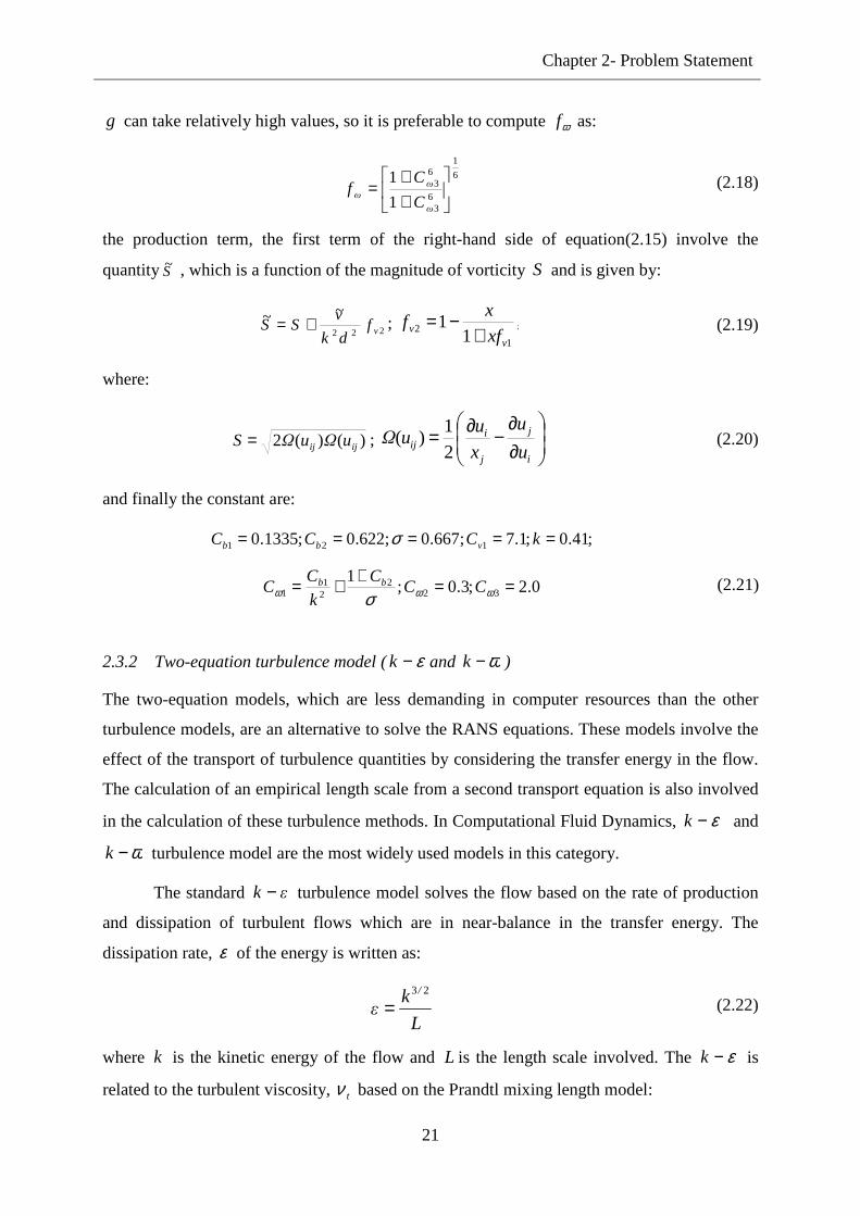
Figure 3.10 Model of simulation in CFX with waveless……..………………..…………… 39
Figure 3.11 Model of simulation in STAR CCM+ with wavemaking……………………… 39
Figure 3.12 Computational mesh on tug hull surface for simulations with waveless........... 41
Figure 3.13 Mesh section of the CFX domain for 0.121 = Fn at 15.0/ =tugLx .…………. 41
Figure 3.14 Mesh section of the CFX domain for 0.181 = Fn at 15.0/ =tugLx .………... 41
Figure 3.15 Mesh section of the CFX domain and zoom in the prism layer mesh for
0.181 = Fn at 15.0/ −=tugLx ………………….....……..……………………….......….… 42
Figure 3.16 Computational mesh on Tug hull surface for simulations with
wavemaking………………………………………………...……………………………….. 43
Figure 3.17 Mesh section of the STAR CCM+ domain for 0.121 = Fn at
15.0/ =tugLx ………………….…………………………………………………........…… 43
Figure 3.18 Mesh section of the STAR CCM+ domain for 0.181 = Fn at
15.0/ =tugLx ………………….…………………………………………………...…...….. 43

List of figures
viii
Figure 3.19 Mesh section of the STAR CCM+ domain and zoom in the prism layer mesh
for 0.181 = Fn at 15.0/ −=tugLx ………………………….………………………………... 43
Figure 4.1 Predicted wave patterns generated by the tug and wave cuts at tugLy / of 0.19
and -0.19: a) Free surface for Fn of 0.121; b) Free surface for Fn of 0.181…………….... 47
Figure 4.2 Distribution of the pressure on the tug hull surface at Fn of 0.121: a) Pressure
distribution without wavemaking; b) Pressure distribution with wavemaking……………... 48
Figure 4.3 Distribution of the pressure on the tug hull surface at Fn of 0.181: a) Pressure
distribution without wavemaking; b) Pressure distribution with wavemaking……………... 48
Figure 4.4 Flow velocities distribution around transversal sections of the tug hull for
Fn of 0.121: a) Velocity with waveless; b) Velocity with wavemaking…………...……… 49
Figure 4.5 Flow velocities distribution around transversal sections of the tug hull for
Fn of 0.181: a) Velocity with waveless; b) Velocity with wavemaking…………...……… 49
Figure 4.6 Interaction force and moment coefficients in shallow water as functions of
dimensionless lateral displacement with dimensionless longitudinal shift +0.0014:
a) Surge force coefficient; b) Sway force coefficient; c) Yaw moment coefficient……...… 51
Figure 4.7 Predicted interaction wave patter generated by the ships for Fn of 0.121 with
dimensionless longitudinal shift +0.0014 and wave cut at tugLy / of 0.19 and -0.19: a)
Free surface for y′of 1.34; b) Free surface for y′of 1.38…………………………….….… 52
Figure 4.8 Predicted interaction wave patter generated by the ships for Fn of 0.121 with
dimensionless longitudinal shift +0.0014 and wave cut at tugLy / of 0.19 and -0.19: a)
Free surface for y′of 1.41; b) Free surface for y′of 1.46……………………………..…… 53
Figure 4.9 Predicted interaction wave patter generated by the ships for Fn of 0.121 with
dimensionless longitudinal shift +0.0014 and wave cut at tugLy / of 0.19 and -0.19: a)
Free surface for y′of 1.95; b) Free surface for y′of 2.26………………………..………… 53
Figure 4.10 Distribution of the pressure on the tug hull surface for Fn of 0.121 with
dimensionless longitudinal shift +0.0014 and dimensionless lateral shift +1.34:
a) Pressure distribution with waveless; b) Pressure distribution with wavemaking…...…… 55
Figure 4.11 Distribution of the pressure on the tug hull surface for Fn of 0.121 with
dimensionless longitudinal shift +0.0014 and dimensionless lateral shift +1.38:
a) Pressure distribution with waveless; b) Pressure distribution with wavemaking…...…… 55

List of figures
ix
Figure 4.12 Distribution of the pressure on the tug hull surface for Fn of 0.121 with
dimensionless longitudinal shift +0.0014 and dimensionless lateral shift +1.41:
a) Pressure distribution with waveless; b) Pressure distribution with wavemaking……...… 56
Figure 4.13 Distribution of the pressure on the tug hull surface for Fn of 0.121 with
dimensionless longitudinal shift +0.0014 and dimensionless lateral shift +1.46:
a) Pressure distribution with waveless; b) Pressure distribution with wavemaking……...… 56
Figure 4.14 Distribution of the pressure on the tug hull surface for Fn of 0.121 with
dimensionless longitudinal shift +0.0014 and dimensionless lateral shift +1.95:
a) Pressure distribution with waveless; b) Pressure distribution with wavemaking……...… 57
Figure 4.15 Distribution of the pressure on the tug hull surface for Fn of 0.121 with
dimensionless longitudinal shift +0.0014 and dimensionless lateral shift +2.26:
a) Pressure distribution with waveless; b) Pressure distribution with wavemaking……...… 57
Figure 4.16 Flow velocities distribution around of transversal sections of the tug hull for
Fn of 0.121 with dimensionless longitudinal shift +0.0014 and dimensionless lateral shift
+1.34: a) Velocity with waveless; b) Velocity with wavemaking…………………….. 58
Figure 4.17 Flow velocities distribution around of transversal sections of the tug hull for
Fn of 0.121 with dimensionless longitudinal shift +0.0014 and dimensionless lateral shift
+1.38: a) Velocity with waveless; b) Velocity with wavemaking…………………….. 59
Figure 4.18 Flow velocities distribution around of transversal sections of the tug hull for
Fn of 0.121 with dimensionless longitudinal shift +0.0014 and dimensionless lateral shift
+1.41: a) Velocity with waveless; b) Velocity with wavemaking…………………….. 59
Figure 4.19 Flow velocities distribution around of transversal sections of the tug hull for
Fn of 0.121 with dimensionless longitudinal shift +0.0014 and dimensionless lateral shift
+1.46: a) Velocity with waveless; b) Velocity with wavemaking…………………….. 59
Figure 4.20 Flow velocities distribution around of transversal sections of the tug hull for
Fn of 0.121 with dimensionless longitudinal shift +0.0014 and dimensionless lateral shift
+1.95: a) Velocity with waveless; b) Velocity with wavemaking…………………….. 60
Figure 4.21 Flow velocities distribution around of transversal sections of the tug hull for
Fn of 0.121 with dimensionless longitudinal shift +0.0014 and dimensionless lateral shift
+2.26: a) Velocity with waveless; b) Velocity with wavemaking…………………….. 61
Figure 4.22 Interaction force and moment coefficients in shallow water as functions of
dimensionless lateral displacement with dimensionless longitudinal shift +0.061:
a) Surge force coefficient; b) Sway force coefficient; c) Yaw moment coefficient………... 62

List of figures
x
Figure 4.23 Predicted interaction wave patter generated by the ships for Fn of 0.181
with dimensionless longitudinal shift +0.061 and wave cut at tugLy / of 0.19 and -0.19: a)
Free surface for y′ of 1.34; b) Free surface for y′ of 1.38…………………………….. 62
Figure 4.24 Predicted interaction wave patter generated by the ships for Fn of 0.181
with dimensionless longitudinal shift +0.061 and wave cut at tugLy / of 0.19 and -0.19: a)
Free surface for y′ of 1.41; b) Free surface for y′ of 1.64…………………………….. 63
Figure 4.25 Predicted interaction wave patter generated by the ships for Fn of 0.181
with dimensionless longitudinal shift +0.061 and wave cut at tugLy / of 0.19 and -0.19: a)
Free surface for y′ of 1.95…………………………………………………………….. 63
Figure 4.26 Distribution of the pressure on the tug hull surface for Fn of 0.181 with
dimensionless longitudinal shift +0.061 and dimensionless lateral shift +1.34:
a) Pressure distribution with waveless; b) Pressure distribution with wavemaking………... 64
Figure 4.27 Distribution of the pressure on the tug hull surface for Fn of 0.181 with
dimensionless longitudinal shift +0.061 and dimensionless lateral shift +1.38:
a) Pressure distribution with waveless; b) Pressure distribution with wavemaking………... 65
Figure 4.28 Distribution of the pressure on the tug hull surface for Fn of 0.181 with
dimensionless longitudinal shift +0.061 and dimensionless lateral shift +1.41:
a) Pressure distribution with waveless; b) Pressure distribution with wavemaking………... 65
Figure 4.29 Distribution of the pressure on the tug hull surface for Fn of 0.181 with
dimensionless longitudinal shift +0.061 and dimensionless lateral shift +1.64:
a) Pressure distribution with waveless; b) Pressure distribution with wavemaking………... 66
Figure 4.30 Distribution of the pressure on the tug hull surface for Fn of 0.181 with
dimensionless longitudinal shift +0.061 and dimensionless lateral shift +1.95:
a) Pressure distribution with waveless; b) Pressure distribution with wavemaking………... 66
Figure 4.31 Flow velocities distribution around of transversal sections of the tug hull for
Fn of 0.181 with dimensionless longitudinal shift +0.061 and dimensionless lateral shift
+1.34: a) Velocity with waveless; b) Velocity with wavemaking………………………….. 67
Figure 4.32 Flow velocities distribution around of transversal sections of the tug hull for
Fn of 0.181 with dimensionless longitudinal shift +0.061 and dimensionless lateral shift
+1.38: a) Velocity with waveless; b) Velocity with wavemaking………………………….. 67

List of figures
xi
Figure 4.33 Flow velocities distribution around of transversal sections of the tug hull for
Fn of 0.181 with dimensionless longitudinal shift +0.061 and dimensionless lateral shift
+1.41: a) Velocity with waveless; b) Velocity with wavemaking………………………….. 68
Figure 4.34 Flow velocities distribution around of transversal sections of the tug hull for
Fn of 0.181 with dimensionless longitudinal shift +0.061 and dimensionless lateral shift
+1.64: a) Velocity with waveless; b) Velocity with wavemaking………………………….. 68
Figure 4.35 Flow velocities distribution around of transversal sections of the tug hull for
Fn of 0.181 with dimensionless longitudinal shift +0.061 and dimensionless lateral shift
+1.95: a) Velocity with waveless; b) Velocity with wavemaking………………………….. 68

List of tables
xii
List of tables
Table 3.1 Environment condition measured in the Towing tank………………………..... 31
Table 3.2 Different size meshes used in the hull and free surface (F.S.). …….………..… 33
Table 3.3 Parameters for prism layer mesh applied in the hull and free surface…..….….. 33
Table 3.4 Set of the velocity……...………………………………………………………. 36
Table 3.5 Set of longitudinal distance...................…………………………………........ 37
Table 3.6 Set of lateral distance…………..…………………………………...........…….. 37
Table 3.7 Mesh size for simulation with rig free surface……….…….……………….…. 41
Table 3.8 Mesh size for simulation with deformable free surface (F.S.)……………….... 42
Table 4.1 Hydrodynamics coefficients for 0.121 = Fn ….………………….……….…... 46
Table 4.2 Hydrodynamics coefficients for 0.181 = Fn ….………………………….….... 46

Nomenclature
xiii
Nomenclature
U Velocity vector or speed of advance
),,( wvuu i = Velocity components in the directions of ),,( zyxxi =
p Pressure
g Gravity
τ Stress tensor
qα Volume Fraction
ρ Density
ν Kinematic viscosity
tν Turbulent kinematic viscosity
k Turbulent kinetic energy
ε Turbulence eddy dissipation rate
ω Dissipation rate per unit kinetic energy
ν~ Eddy-viscosity variable
ppL Ship length
Re Reynolds number
Fn Froude number
X Surge force
Y Sway force
N Yaw moment
X ′ Surge coefficient
Y′ Sway coefficient
N ′ Yaw coefficient
ξ Longitudinal distance
η Lateral distance
x′ Dimensionless longitudinal distance
y′ Dimensionless longitudinal distance

Chapter 1- Introduction
1
CHAPTER 1 Introduction
1.1 General
Many problems that interfere with navigation are due to the manoeuvres of ships, and one of
these problems is the hydrodynamic interaction between ships, which occur frequently due to
increase in the ship traffic density. According to UNCATD (2003) the maritime transportation
represents more than 90% of the world fleet, and the world fleet in 2002 becomes more than
800 million Dwt. In 2008 the merchant vessels higher than 100 GT were 99.741 ships
completing 830.7 million GT between them (Fairplay World Fleet Statistics, 2008).
The interaction problem in navigation is usually produced when the ships are moving
in restricted waterways, such as harbours or canals (King, 1977). The encounter of two
vessels can fall into one of two main categories. In the first case, a ship passing another one at
a close distance, which commonly happens when sailing in narrow channels. In the second
case, a ship manoeuvring very close to another one due some routine operation, like the tug
assistant. In the interaction problem the flow around the ship hulls is modified, generating
additional forces in the horizontal plane on the ships (surge and sway forces, and yaw
moment). Some examples are show in Fig 1.1.
The interaction phenomenon is also influenced and caused by the two navigation
boundaries which are: the bottom, and the lateral boundaries of the navigation area. The
former, is usually given by introducing depth dependent hydrodynamic coefficients. The
latter is limited by bank or quay walls, causing the so-called bank effect to a ship navigating
in parallel course thus, producing the hydrodynamic interaction forces on a ship in a channel
towards or away from the nearby obstacles (Ch´ng, 1991, 1993). Some examples can be seen
in Fig 1.1.
In restricted water, the shallow water condition has a strong influence in the
hydrodynamic interaction forces (Fortson, 1969). In shallow water, the average depth is about
10 to 20 m, which is usually smaller that the ship length (50 to 100 m). Here, the wave
generated by the ship has a larger length than the wave generated in deep waters at the same
velocity. Thus, the magnitude of the wave length in general may be considered similar to the
ship length and also the wave can show an anomalous wave height. The generated ship waves
are hardly dissipated when interacting with the shorelines, affecting the water conditions of
the navigation. In case of interaction, the effect on each vessel increase, either in a moored or
the sailing vessel.

Chapter 1- Introduction
2
Figure 1.1 Interaction between ships and their boundary: a) A vessel is assisted by a tug near the harbour; b) Two ships sailing in a river in head encounter; c) Manoeuvring of overtaking
between two ships in calm water; c) Ship sailing in a narrow canal.
The phenomenon produced in the interaction problem can cause serious accidents,
when it is not considered. Chatterton (1994) comments the famous accident of Queen
Elizabeth II. Chatterton describes that the vessel was sailing at high speed in shallow waters
and then the suction force between the bottom and the ship caused the Queen Elizabeth II to
run aground off the Cutty Hunk Island.
The Marine Accident Investigation Branch (MAIB) reports the maritime accidents
yearly. In their reports the accidents due to the interaction between ships are the most
common ones. A collision reported by MAIB, between MV Asch and MV Dutch Aquamarine
in the South West lane of the Dover Strait TSS, with the loss of one life and which, occurred
in October of 2001. They found that the cause of the collision was because the two vessels
were on coincident tracks and travelling at different speeds. The interaction between the ships
was described as follow: “The two vessels became very close it was apparent from witness
observations that Dutch Aquamarine’s track was, in fact, a few meters to starboard of Ash’s.
As Dutch Aquamarine’s bow approached Ash’s stern on her starboard quarter, hydrodynamic
interaction caused Ash’s heading to alter to starboard. The flare on the port side of Dutch

Chapter 1- Introduction
3
Aquamarine’s bow first made contact with the extreme starboard quarter of Ash’s bridge
deck, causing damage to railings, the lifeboat and its davit arm.”
When the differences in the ship dimensions are large, the effect produced during the
interaction between ships increases and the risk of accident is higher for the smaller ship. A
typical situation which involves differences in ship dimensions is the ship-tug assistance.
When a tug assists a ship, the position of the tug with respect to the assisted ship and the
lateral distance, can be constantly changing. The consecutive positions of a tug when is
approaching to assist a ship, are shown in Fig. 1.2.
Figure 1.2 Different position of the Tug assisting the merchant ship in a harbour
When the tug is near the stern of the ship (position 1), an increase in its velocity may
occur due to the flow velocity from the aft of the ship. In close proximity to the ship hull, a
low pressure starts moving the tug in the ship´s direction. For ships in ballast condition, or
ships having particular overhanging stern, the tug can easily go to the position 2, generating
damages to its hull or superstructure.
Going forward and near the hull (position 3), the tug is in under action of an important
suction force in the direction of the ship hull, and negative yaw moment (according with
right-handed Cartesian frame of reference) is due to the accumulated water in the tug bow.
When the tug is attracted by the ship, it is in general difficult to recover its course. When the
tug is in position 4 (side of the bow) she enters on area of high-pressure the negative yaw
moment is growing, and must be compensated by the appropriate use of the rudder and
propeller to avoid the risk of accident.

Chapter 1- Introduction
4
In position 5 when the tug is near the bow, a strong a negative sway force acting on
the stern brings the tug to the front and under the bow with the risk of capsizing. Then,
proper operational condition must be applied
The study of the interference when a tug is operating near to another ship is important
to define the prediction of the manoeuvring characteristics of the tug and is useful to optimize
the waterway operation. Therefore, developing a model able to predict the interaction forces
with accuracy and considering restricted waters, and course keeping of ships is necessary. The
hydrodynamic interaction prediction of a ship in restricted waters has been investigated for
several decades, as is described in the following section. Trough, it is necessary to perform
more detailed studies.
1.2 Objectives
The main objective of this work is to develop numerical simulations of manoeuvring
operations of a tug interacting with a ship in shallow water. The Computational Fluid
Dynamics (CFD) software is used for the computation, which is able to predict the
hydrodynamic interaction forces, moment, and the behaviour of the free surface, in the
general situation of interacting ships.
This thesis presents general observations on the tested models considering the
hydrodynamic interaction between two ships in movement. The hull forms tested are a typical
tanker ship and a typical tug vessel. Special emphasis is set in the range of the side distance
between ships, and the relative heading angle of the supply vessel.
The ship manoeuvres that were selected to be simulated in the present study are the simulation
of the flow around both ship hulls in a parallel course sailing at the same velocity. Two cases
of tug position along the length of the tanker and two cases of velocity are studied. Several
variations of side distances are considered to obtain the favourable case considering the
interaction forces.
The obtained results are useful to determine the characteristics of the interaction
phenomenon, and to obtain a practical solution on interaction between ships, providing data
for validation of numerical fluid dynamic simulation.
Another aim of this dissertation is to show the potential of CFD to solve manoeuvring
problems in naval architecture and marine engineering with accuracy and short resources and
time. Thus, the CFD code can be presented as an efficient tool in the ship hull design.

Chapter 1- Introduction
5
1.3 Organization of the thesis
The present thesis consists of four main chapters:
Chapter 1 Introduction: Here it is presented the motive, objectives, and general
presentation of the interaction problem, providing the state of the art of the hydrodynamics
interaction forces necessary for carrying out.
Chapter 2 Problem Statement: This chapter describes the theoretical background and a
review of the method used to solve the hydrodynamic interaction problem, explaining the
basic principles of the governing equation and the numerical method to solve.
Chapter 3 Application of the numerical method: The problems under study are
presented. Defined are all parameters used in the Computational Fluid Dynamics simulation,
including general criteria, boundary conditions, the configuration of the mesh and the volume
domain.
Chapter 4 Analysis of the numerical results: Finally, the results are summarized and
discussed giving the most important conclusions of this study and proposing further improved
work.
1.4 State of the art: Ships hydrodynamics interaction
The phenomenon of hydrodynamic interaction between ships is a subject of several research
works. The interest to study the interaction problem started around the 1900´s, considering
primarily experimental efforts dealing with the interaction force and moments developed
between ships in proximity. One of the first experiments performed and reported on the
interaction between ships was conducted by Davis W. Taylor (1909), who explained the
suction that tends to bring ships together when they are passing close to one another. His
investigation was focused on the quantitative measurement, and was carried out for two
models. The first test was with a relativity narrow models, with the following dimensions for
each ship: Ship (A): length = 20.512m, breath = 3.69m, draft = 1.26m; Ship (B): length =
20.512m, breath = 3.50m, draft = 1.20m. The second test was with fuller models, whose
dimensions were: Ship (A): length = 20.512m, breath = 3.59m, draft = 0.96m; Ship (B):
length= 20.512m, breath = 2.78m, draft = 1.24m. Taylor stated that the models were tested at
speeds between 2.0 and 3.0Kn. The total forces on the models were determined by adding the
measured forces at each end of model. He also comments that the results may have

Chapter 1- Introduction
6
inaccuracies due to problems encountered in the models on a parallel course and stated that
the results for the thinner models were less consistent.
After the test of Taylor, several experimental works have been carried out with more
accuracy, describing the hydrodynamic interaction forces. Newton (1960) based on the studies
of Taylor, investigated the interaction effects during overtaking manoeuvres by experiments
between two ship models in deep water, The tests conducted include an experiment with
scaled models of the battleship H.M.S. KING GEORGE and the R.F.A. OLNA. (Ship (A) and
Ship (B) respectively) the characteristic of these ship were: ship (A): length = 4.51m, breath =
0.63m, draft = 0.18m, CB = 0.61; ship (B): length = 3.46m, breath = 0.43m, draft = 0.18m, CB
= 0.71. The experimental tests were carried out using freely propelled and controllable models
to study the behaviour during manoeuvring alongside and breaking away. Newton also
conducted experiment at sea with real ships, giving valuable data in this respect.
Later the experimental tests were performed to study the influence of the restricted
water on hydrodynamic interaction forces Müller (1967) studied the overtaking and encounter
of ships in a narrow canal. New variables were considered by Remrey (1974) investigating the
effect of the size passing vessel and the separation between the passing and moored vessel.
In parallel with the experimental tests, two numerical methods based in the slender-
body and the potential theory were developed, to calculate the interaction sway forces and
yaw moment. These methods have been used extensively for many authors giving important
information, to understand the behaviour of the hydrodynamics interaction between ships.
Newman (1965) used the slender-body theory to develop a code that can solve the
hydrodynamics interaction problem. Newman supported his work assuming that the fluid flow
is ideal, incompressible, and unbounded except by the wall and the body. He also assumed
that the body is axisymmetric and slender if r/L << 1, and the body is in proximity to the wall
if z/L <<1, (here r is the radius of the body, L is the body length, and z is the distance from the
centerline of the body to the obstacle). The aerodynamic theory used the source distribution
to calculate inside the body. For allowing the presence of the wall, the source distribution was
offset from the body axis. The body was considered to be fixed in space, with a free stream
flowing past in the opposite direction to the body. Legally´s theorem (1953) was used to
calculate the force and moment. The results of Newman have been extensively used for
evaluating the result of other methods.

Chapter 1- Introduction
7
Tuck (1966) extended the slender-body method to study the problem of the
hydrodynamic interaction in shallow water flow passing a fixed slender obstacle in a stream.
He provided a model for the behaviour of ships moving in still water with restrictions in
depth, which was subsequently applied to a variety of problems involving shallow water, such
as river flow past obstacles. Tuck (1967) also extended his earlier method and introduced the
concept of effective width in order to deal with ship dynamics in shallow water of restricted
width.
Yeung (1978) used the shallow-water sources, including the effect of circulation, to
calculate sway forces and yaw moments on each ship. Davis and Geer (1982) developed an
alternative method for calculating the slender-body sway forces and yaw moments, based on
an asymptotic analysis.
King (1977) developed a technique for the unsteady hydrodynamics interaction
between two ships moving along parallel paths in shallow water using the slender-body
theory. The problem was analogous to that for two porous airfoils passing each other. A
system of singular integral equations was derived and solved numerically. The sway force and
yaw moment were calculated for each ship. For testing this model and numerical procedure, a
comparisons was made with publishes experimental and theoretical results for the far field
obtaining good agreement.
In the other hand, Fortson (1969) developed a method to calculate the sway forces and
yaw moment, assuming that, when ships are close together, the potential field is the main
source of the interaction force. The flow around the ships was represented using half bodies of
revolution generated with axial singularity distributions. Axial distributions of doublets were
included to correct for cross flow and thus maintain the rigid body boundary condition. The
main result of Fortson was a computerized model to predict forces resulting from steady
parallel motion of bodies of revolution moving in an infinite ideal fluid. The code was capable
of handling ship geometries in rectilinear motions. It was found that the theoretical model
produced similar results when compared with model test conducted by Taylor (1909). Fortson
concluded that is necessary to obtain a set of more valid empirical data.
Ashe (1975) continued the work of Fortson assuming that interaction forces arise only
from disturbance and therefore, a rigid free surface can exist, and the fluid flow is ideal and
infinite therefore, potential theory is applicable. As well as with Fortson (1969), Ashe used an
axial distribution of dipoles to take into account the wall effects. As in the previous methods,

Chapter 1- Introduction
8
Ashe also uses Legally’s theorem to calculate the forces and moments on the body, but he
includes the unsteady terms. Here the steady-state force is due to interaction effects as shown
by D´Alembert paradox. Ashe extended the theory presented by Fortson and included the
unsteady effects associated with the acceleration, vertical velocities, and rotational velocities
in a quasi-steady state.
Beck et al. (1975) extended the analysis of interaction between ships including the
case of a ship operating in a dredged channel surrounded on both sides by shallow water.
Beck (1977) examined the case of a ship travelling parallel to, but displaced from, the
centreline of a shallow channel.
Chatterton (1994) presented an evaluation of the proximity codes. These codes were
developed to predict the interaction force moment experienced by an Unmanned Underwater
Vehicle when is in proximity with an obstacle. The theory used a potential flow model of a
body operating in an ideal fluid based in the Ashe (1975) theory. The codes were extended
including unsteady motion, inclined bottom, and automatic convergence. The validation of
these codes involved performing model testing at the Massachusetts Institute of Technology
(MIT) towing tank as well as collecting previously published data examining the theoretical
trends. A theoretical database was compiled to examine the trends associated with changes in
vehicles shape and orientation.
In order to improve the accuracy of the prediction of interaction forces and moments
between ships, a semi-empirical method was developed by Brix (1993), estimating the time
histories of the forces and moments in the horizontal plane due to interaction with another
ship as a function of geometry speed and environmental parameters based on his previous
work (Brix, 1979). The method to estimate the forces and moments acting on a ship during an
overtaking manoeuvre was presented in the Manoeuvring Technical Manual. Here
approximations were formulated for the maximum values of the longitudinal and transverse
forces and for the yawing moment. The method was subjected to some restrictions: it was
only valid for overtaking manoeuvres. Thus, the influence of water depth was not taken into
account, and also the ratio of ships' lengths is limited. Brix states: "Besides some theoretical
approaches and experimental results no reliable results are available except of a semi-
empirical nature.”
Varyani et al. (1999) presented empirical formulae for predicting the peaks of the
lateral force and the yawing moment during interactions between two ships. Here the validity

Chapter 1- Introduction
9
of the method was also restricted being: the cases VT = 0 or VO = 0 were not covered, the
length ratio was limited, and the method was only valid for encountering manoeuvres.
Vantorre et al. (2002) reported results from a large series of ship-ship interaction
model experiments using an empirical method to calculate the extreme peaks in typical time
traces of interaction forces. The investigation was carried out for four ship models in shallow
water towing tank, covering a large variety of parameters such as overtaking/overtaken,
speeds, distances, and water depths. In the work they suggested that it is an impossible
develop a full empirical method taking into account all the possible parameters that influence
the interaction forces between two ships passing each other.
The mooring forces on a container ship induced by a passing bulk carrier were
reported by Varyani et al. (2003). The mooring system was modelled as linear and the results
were obtained using an empirical method for calculation of ship-ship interaction forces acting
on a ship at zero speed. Similar works have been presented by Krishnankutty and Varyani
(2003, 2004).
Recently, new experimental tests have provided fresh information, about of the
parameters and variables that influence the interaction phenomenon. Kyulevcheliev et al.
(2003) presented a general overview and initial findings of a set of model experiments on
hydrodynamic impact of a moving ship on a stationary one in restricted water. They found
that the wave effects increase drastically the peak values of the interaction loads and change
substantially their time histories.
Taggart et al. (2003) examined experimentally the hydrodynamic interactions between
ships that can influence seakeeping during operations. In the experiments a semi captive
model was used, and the numerical code was modified to include restraining forces for
specific modes. The numerical predictions and the experiments showed that the presence of a
larger ship can significantly influence the motions of the smaller ship in close proximity.
Kriebel (2005) carried out an experimental measurement of the loads on a moored ship
resulting from a passing ship moving in parallel to the moored vessel. Variations in the model
tests were included which consider changes in the passing vessel speed, vessel displacement,
water depth, and separation between the two ships. The experimental data were analyzed in
two manners. First, the empirical equations were developed, describing variation in the peak
mooring loads with changes in the parameters. Second, two existing models were evaluated in
blind test to determine their ability to predict the measured mooring loads.

Chapter 1- Introduction
10
With the new information and mathematical techniques, the numerical solvers have
been improved, expanding their application and allowing performance of other situation, such
as seakeeping during the interaction phenomenon. Most of these codes follow the trend of the
modern hydrodynamic research works, which are based in the potential theory and solved by
the panel method. Chen and Fang (2001) used a 3D panel method based on the source
distribution technique to analyze the hydrodynamic interaction problem between two moving
ship in waves. The numerical solution was evaluated by applying the method to two pairs of
models and compared with experimental data and the strip theory. From the comparisons the
result showed that the hydrodynamics interaction calculated by 3D method is more
reasonable. However, it is not so significant using the 2D method.
Varyani et al. (2002) developed a potential theory method for calculation of ship-ship
interaction forces. The method was validated against results of Dand (1981) and Yasukawa
(1990). The results were presented for two and three, ships meeting in channel.
The three-dimensional (3D) panel method based in the potential theory was developed
by Yasukawa (2003) to calculate the ship-ship interaction forces between two ships in an
overtaking situation. The motions were simulated using coupled equations of motion and the
3D panel method provided hydrodynamics interaction forces and added masses as function of
the ships relative positions.
Sutulo and Guedes Soares (2009) created a module of a manoeuvring simulating
system using potential forces based on the Hess and Smith panel method aiming to calculating
the hydrodynamics interaction forces. The comparative computations of the added masses,
surge and sway interaction forces and yaw interaction moments with varying number of
surface computational panels showed that on a typical modern computer, an acceptable
accuracy in terms of the integrated loads can be reached with a relatively small number of
panels allowing real-time simulations with the developed algorithm in the loop. Comparisons
with available experimental data and with an empirical interaction prediction method
demonstrated that the code works adequately and can be considered as validated, although
disagreements with the experimental data were observed in the cases when the viscous effects
were significant.
Other methods have been applied in the interaction phenomenon, obtaining good
result, e.g. the Wave Equation Model (WEM) developed by Jiankang et al. (2001), which
solve the shallow water equations with moving surface pressure. The model was applied to a

Chapter 1- Introduction
11
numerical investigation of two moving ships Series 60 with a CB = 0.6. The ships have
streamline-stern or blunt-stern moving in parallel. The 3D wave interaction patterns were
investigated, finding that the wave interaction occurs mainly behind the ships.
A higher-order boundary element method (HOBEM) combined with generalized mode
approach was applied by Hong et al. (2005) to analysed of motion and drift forces of side-by-
side moored multiple vessels (LNG FPSO, LNGC and shuttle tankers). The models were
compared with experimental result finding good agreement between the methods.
The oldest method of Newman has been updated for applications in new ships
interaction situation. Gourlay (2009) investigated the sinkage and trim of two moving ships
when they pass each other, either from opposite directions, or when one ship overtaking the
other. The work was simplified to open water of shallow constant depth. The investigation
was carried out using linear superposition of slender-body shallow-water flow solutions. It
was shown that even for head-on encounters, oscillatory heave and pitch effects are small.
Also it was found that the sinkage and trim can be calculated using hydrostatic balancing. The
results were compared with available experimental data, on a container ship and a bulk carrier
in a head-on or overtaking encounter.
The recent advances in hydrodynamic theories and computation capacity have been
developed of high level Computational Fluid Dynamics (CFD) simulators for design
applications, which allow the use of this tool to solve some manoeuvring problems. Wnek et
al. (2009, 2010) presented the results of a CFD analysis of the wind forces acting on a LNG
ship and a barge model. The comparisons between the numerical and experimental result were
in good agreement.
Burg and Marcum (2003) developed a nonlinear scheme based on Farhat’s algorithm
to calculate the free surface elevation for unsteady Reynolds-Averaged Navier-Stokes
(RANS) code. The results for a DTMB Model 5415 in small drift angles, constant turning
radius and a prescribed manoeuvre although fairly good, were not mesh independent and
showed that more work is needed on the turbulence models and grid deformation rate.
Lee, et al (2003) used both experimental and unsteady RANS approach to obtain
quantitatively the hydrodynamics forces under the lateral motion, and a view to generalize the
obtained hydrodynamics forces that in a practical use. The water depth was an important
factor to exercise the influence on the inertial forces and transitional lateral forces acting on

Chapter 1- Introduction
12
ship hull. They concluded that using a concept of circulation is effective to express the lateral
drag coefficient qualitatively.
Some authors have been used the CFD codes to solve the problem of interaction
between ships. Chen et al. (2003) present ship-ship interaction forces calculated from an
unsteady RANS code comparing the ship-ship interaction model test results performed by
Dand (1981). Good agreement was found between the calculations and the measurements.
They concluded that the free surface is important for the interaction between the two ships.
Huang and Chen (2003) presented potential hazards to vessels moored at nearby piers.
A Chimera RANS code was used to explore the fluid activities induced by passing ships and
their impacts to moored vessels at a complex waterfront next to a navigation channel. This
model captured details of ship-ship and ship-pier interactions evolving the time, and taking
into full account the viscous flow physics, exact seafloor bathymetry and basin boundaries, as
well as nonlinear couplings between moored ship and pier. The results of the simulation
clearly show that the significance of site specific factors to the dynamics of moored vessels
induced by passing ships.

Chapter 2- Problem Statement
13
CHAPTER 2 Problem statement
In the previous chapter, the interaction phenomenon was presented, showing typical
conditions in which the encounter of ships can occur. The effect of interaction between ships
is based on reviewing previous research work, presenting a series of methods that can be used
to solve the interaction problem, accurately. It is mentioned that a numerical solution to the
Navier-Stokes equation can be applied to solve many manoeuvring problems. Thus, the
hydrodynamic interaction between ships can be solved by a Computational Fluid Dynamics
(CFD) code, even though a considerable computational cost is involved.
In the present chapter, the theoretical background of CFD for solving three-
dimensional (3D) fluid flow problems is introduced. The CFD code is extended from different
solver techniques, discussing influences and impacts on the fluid flow simulation.
The chapter is divided in three main sections. The first one is an outline of
mathematical equations and the boundary conditions, describing the fluid flow. The second
section discusses various turbulence models, with special emphasis to the mathematical
formulation of the Reynolds-Averaged Navier–Stokes (RANS) method. The third section is a
review of the numerical methods and solvers describing the characteristic of CFD in the fluid
flow study; the section also summarizes the theoretical background for Finite Volume (FV)
method.
2.1 Governing equations
The continuity equation for the mass conservation and the Navier–Stokes equations, for the
momentum transport, govern the 3D motion of the incompressible and viscous fluid. These
equations are expressed in terms the set of partial differential equation as follows:
0=∂∂
j
i
x
u (2.1)
( ) ( )i
ij
ij
j
iji ρgx
p
x
τ
x
uρu
t
ρu+
∂∂−
∂∂
=∂
∂+
∂∂
(2.2)
where ρ is the density, p is the pressure, iu
is the velocity in the stream direction, ijτ
is
stress tensor, and g is the component of the gravitational acceleration g
in the direction of
the Cartesian coordinate ix . In the case of constant density and gravity, the term gρ can be
written as grad( )rg ⋅ρ , where r is the position vector, ii ixr ,= (usually, gravity is assumed

Chapter 2- Problem Statement
14
to act in the negative z-direction, i.e. kgzg = , zg being negative; in this case zgzrg =⋅ ).
Then zgzρ− is the hydrostatic pressure, and it is convenient for numerical solution more
efficient to define zgzpp ρ−=~ as the head and use it in place of the pressure. The term igρ
then disappears from the above equation. If the actual pressure is needed, one has only to add
gzρ to p~ .
The homogenous multiphase Eulerian fluid approach utilizes the Volume of Fluid
method (VOF) to describe the free surface flow problem mathematically. The VOF method
developed by Hirt and Nichols (1981) is a fixed mesh technique designed for two or more
fluids, where in each cell of a mesh it is necessary to use only one value for each dependent
variable defining the fluid state. The variables can be defined by a function qα (where q
represents the fraction of volume; ...2,1=q ).The value of this variable is one at any point
occupied by the fluid and is zero in other cases and is writing as:
11
=∑=
n
qqα (2.3)
the average value of α in a cell represents the position of the interface of the fluid. In
particular, a unity value of α corresponds to a cell full of fluid, while a zero value indicates
that the cell is empty, so the cells with α values between zero and one must contain a free
surface. The tracking of the interface is obtained by solving the continuity equation of the
volume fraction. For the q liquid, troughs of the density as follow:
qqαρρ ∑= (2.4)
For a Newtonian fluid the viscous stress tensor can be expressed as:
∂∂
−=
∂∂
−∂∂
+∂∂
=k
kijij
k
kij
i
j
j
iij u
uδsν
x
uδ
x
u
x
uντ
3
12
3
2 (2.5)
where ijs is the strain-rate tensor and ν is the dynamic viscosity. For an incompressible
fluid, Equation 2.5 reduces to:
ijij νsτ 2= (2.6)
the Navier-Stokes equations are a highly non-linear system. The strong non-linearity of the
equations produces high frequency oscillations when the Reynolds number is increased, and
the flow becomes unstable and turbulent. It is computationally very expensive to solve the

Chapter 2- Problem Statement
15
equations directly, which makes that presently, only in very simple geometry configurations it
is possible to solve the Navier-Stokes equations using direct methods (DNS). The most
common approach at the moment in hydraulic engineering practice is to solve the Reynolds
Averaged Navier-Stokes.
2.1.1 Reynolds Averaged Navier-Stokes equations
The Reynolds Averaged Navier-Stokes (RANS) equations have been developed based on the
concept that a velocity and a length scale are sufficient to describe the effect of turbulence in a
flow. For instance, eddy viscosity model, estimates the velocity and length scales of the flow
from the local mean flow quantities, which is done by relating the turbulent viscosity to the
mean velocity gradient of the flow. However, the RANS model may fail to simulate more
complex flow (Liaw, 2005).
In a statistically steady flow, every variable can be written as the sum of a time-
averaged value )U( and a fluctuation )u( ′ about that value:
uUU ′+= (2.7)
where the time-averaging velocity component is defined as:
∫=T
UdtT
U0
1 (2.8)
where T is the averaging interval. This interval must be large compared to the typical time
scale of the fluctuations. Thus, if T is large enough, )U( does not depend on the time at
which the averaging is started.
If the flow is unsteady, time averaging cannot be used and it must be replaced by
ensemble averaging described by Ferziger (2002) defining as follow:
∑=
=N
n
UN
U1
1 (2.9)
where N is the number of members of the ensemble and must be large enough to eliminate the
effects of the fluctuations. This type of averaging can be applied to any flow. The term
Reynolds averaging is used to refer to any of these averaging processes; applying it to the
Navier-Stokes equations yields the Reynolds-averaged Navier-Stokes (RANS) equations.
Averaged continuity and the momentum equations can, for incompressible flows
without body forces, be written in tensor notation and Cartesian coordinates as:

Chapter 2- Problem Statement
16
∂∂
+∂∂−=
∂+∂
+∂
∂
j
ij
ij
jiiji
x
τ
x
p
ρx
)uuuu(
t
u 1 (2.10)
0=∂∂
j
i
x
u (2.11)
which is the correlation between the fluctuating velocity components and is known as the
Reynolds stress term. The existence of the Reynolds stress means that there is no longer a
closed set of equations, that is to say, they contain more variables than there are equations.
Closure requires use of some approximations, which usually take the form of prescribing the
Reynolds stress tensor and turbulent scalar fluxes in terms of the mean quantities.
2.2 Fluid dynamic models
The turbulent flow is highly unsteady and irregular, being necessary high computational
resources for representing all the turbulence from the smallest scale corresponding to the
dissipative motions to the largest dimension responsible for the majority of the moment
transport in high speed. The turbulence models were developed as alternatives to describing
the turbulence based on simplified assumptions, being these models summarized as follow:
2.2.1 Direct Numerical Simulation
In the Direct Numerical Simulation (DNS) the Navier-Stokes equations are solved without
averaging or approximation to describe the turbulence, only using numerical discretization,
thus the errors can be estimated and controlled. This means that the governing equations are
solved directly. In the DNS simulation, all of the motions in the flow are solved capturing
small scale turbulence. With the use of this method the computed flow field obtained is
equivalent to a single realization of a flow or can be considered as short-duration laboratory
experiment Tremblay (2001).
In order to capture all the flow motion, in the DSN method the domain in which the
computation is performed must be at least as large as the physical domain to be considered or
the largest turbulent eddy. Blazek (2001) found that the number of nodes in 3D is
proportional to 4/9Re and the time step is related with the mesh size, making the cost of the
required computer time proportional to 3Re , Blazek agreed with Frolich et al (1998) who
studied the required resolution for DNS. Thus, it is still not practical to solve accurately the
non-linear nature and three dimensional characteristics of turbulence at high speed flow using
DNS, since the number of grid points to be used is limited by the computational resources.

Chapter 2- Problem Statement
17
The DNS it possible to use only for flows at relatively low Reynolds numbers and in
geometrically simple domains, being not practical in engineering problems.
2.2.2 Large Eddy Simulation
The Large Eddy Simulation (LES) is just an approach and is classified as a space filtering
method in CFD. The LES directly computes large-scale turbulent structures which are
responsible for the transfer of energy and momentum in a flow, modelling the smaller scale of
dissipative and isotropic structures.
For distinguishing between large and small scales, a filter function is used in LES. A
filter function dictates which eddies are large by introducing a length scale, usually denoted as
∆ in LES, in the characteristic filter width of the simulation. All eddies larger than ∆ are
resolved directly, while those smaller are approximated (Feguizer, 2002).
The simulations by LES method are three dimensional, time dependent and expensive,
but cheaper than DNS at the same flow. LES is the preferred method for flows in which the
Reynolds number is high or the geometry is complex to allow application of DNS.
The main problem of LES is the simulation of the near wall region. Close to the walls
the size of the turbulent structures becomes very small. In order to have a well resolved LES it
is necessary to have a very fine mesh in the near wall region in order to be able to capture
those structures. This makes that in practice the near wall grid size should be almost as small
as in DNS. This requirement precludes the use of fully LES for industrial applications at the
present time. Spalart (2000) estimates that until later than 2050 the computer's power will not
be enough to apply fully LES and DNS techniques to hydrodynamics industrial applications.
A common solution is to solve the RANS equations near the wall and the LES equations far
away from the wall. This approach is called Detached Eddy Simulation (DES), and it is
presently more commonly used than LES.
2.2.3 Detached Eddy Simulation
Detached Eddy Simulation (DES) is an hybrid model that combines the RANS model near to
the wall and the LES model in the wake region of a flow, being unsteady and irregular motion
of flow is usually found. Basically, the DES model uses a turbulent length scale, tL to select
the approach to use during a simulation. The DES starts with the RANSE model at the inlet
boundary, the formulation is the same as the standard two equations model without
consideration of the length scale used in the dissipation rate computation, being replaced by

Chapter 2- Problem Statement
18
local grid spacing. If the turbulent length scale is greater than the grid spacing, which is
common in regions with large eddies and chaotic flow nature, the LES is activated in the DES
formulation (Liaw, 2005).
2.2.4 RANS turbulence models
The most commonly used approach in engineering practice nowadays is to solve the Reynolds
Averaged Navier-Stokes equations coupled with a turbulence model. Here, all the turbulent
structures occurring in the flow are modelled. The RANS turbulence models are usually
derived for fully turbulent flow and their constants are obtained from experimental data on
boundary layers or other simple shear flows. While the turbulence models used in LES are
only responsible for modelling the sub mesh scales, in RANS they are responsible for
modelling the whole turbulence spectrum.
Several kinds of RANS turbulence models exist. The most used in practise are the
linear eddy viscosity models, in which the Boussinesq assumption is used to compute the
Reynolds stresses from the mean velocity gradients via a linear relation. There are also non-
linear eddy viscosity models, in which the Reynolds stresses and the mean velocity gradients
are linked by a non-linear relation. None of the eddy viscosity models can be considered
clearly superior to the other ones. The most popular RANS model is the ε−k model of Jones
and Launder (1975) (with all its low-Reynolds versions), which was proposed in the early
seventies, and it is still widely used in all fluid dynamics areas.
Other popular models are the Shear Stress Transport (SST) model, the ω−k and the
Spalart-Allmaras models (Spalart and Allamaras, 1994), which are mainly used in the ship
hydrodynamics area. New versions of the models are still appearing, and much work is still
being done in order to improve the existing models introducing correction terms which
account for specific flow conditions (near wall terms, curvature and rotation corrections,
anisotropy effects). The fact of the original ε−k model being one of the most commonly
used two-equation models shows that there has not yet appeared any clearly superior model.
A possible reason for the similar results given by the different models under some flow
conditions was pointed out by Hunt (1990), who considers that the influence of the turbulence
model may be smeared in regions where the time scale of the mean flow distortions is smaller
than the characteristic turbulent time scale.
In the Reynolds Stress Turbulence Models (RSTM), instead of using the Boussinesq
assumption, a transport equation is solved for each Reynolds stress. The fact of solving one

Chapter 2- Problem Statement
19
equation for each Reynolds stress allows accounting for curvature effects and anisotropy. In
the Algebraic Stress Models (ASM) the Reynolds stresses are approximated with non-linear
algebraic expressions. The ASM can be thought of either as a simplification of the RSTM or
as an extension of Boussinesq eddy viscosity models. Nevertheless, the fact that the equations
for the Reynolds stresses still contain modelled terms, and the higher complexity of RSTM
compared with eddy viscosity models, make the latter be more commonly used in engineering
practise.
2.2.5 Unsteady RANS turbulence model
The purpose of unsteady RANS (URANS) is to simulate the largest eddies present in the flow
and their non-linear interaction. Therefore, URANS solutions are unsteady in time even with
steady boundary conditions. Durbin (1995) found that the Reynolds stresses created behind a
bluff body by time averaging of URANS are larger than those given by the turbulence model,
removing in such a way much responsibility from the model.
In principle, URANS is an intermediate approach between steady RANS and LES.
The main difference between URANS and LES is that in LES the eddy viscosity of the sub
mesh model depends explicitly on the grid size, while URANS is mesh independent by
definition. Nonetheless, there are many facts about URANS simulations that are still not clear,
which makes LES/DES a more common approach at the present time.
A 3D-URANS computation is able to produce 3D solutions over 2D geometries, like
LES, but they appear to be much more dependent on the span wise size of the domain, which
is chosen arbitrarily in the computations (Spalart, 2000). In addition, the accuracy of the
results depends on the kind of flow, and the solutions have been found to be quite sensitive to
the turbulence model (Travin et al, 2004). Although URANS solutions should be mesh
independent by definition, there are some recently formulations (Menter et al, 2003) which
reduce the value of the eddy viscosity in some regions of the flow in order to be able to
resolve smaller turbulent structures, obtaining in such a way an LES-like behaviour. These
facts show that there is not yet a complete understanding of the results given by URANS
simulations (Travein et al, 2004).
2.3 Linear eddy viscosity turbulence models
The Boussinesq assumption is the base of all the eddy viscosity models. It relates the
Reynolds stresses with the mean velocity gradients via the eddy viscosity as:

Chapter 2- Problem Statement
20
ijijkkijtji kδδssνuu3
2
3
12 +
−−=′′ (2.12)
where iu′ is the fluctuating velocity, tν is the eddy viscosity, ijs is the mean strain-rate
tensor, and k is the turbulent kinematic energy defined as 2
kkuuk
′′= . The evaluation of the
eddy viscosity, which is assumed to be isotropic, is left to the turbulence model. For a long
time simple turbulence models based on algebraic formulations have been used due to their
simplicity and robustness. More sophisticated models exist, which solve one or more transport
equations for different turbulent quantities, as the turbulent kinetic energy or the dissipation
rate.
2.3.1 Standard Spalart Allmaras model
The Standard Spalart Allmaras model is one-equation turbulence model available to
calculate the turbulence in unsteady state flow model (Houzeaux, 2002). This model involves
an eddy-viscosity variablev~ , related to the eddy-viscosity tv by:
vfv vt~
1= (2.13)
where:
31
3
3
1
v
vcx
xf
+= ;
tv
vx
~= (2.14)
The transport equation for v~ is:
( )2
2
11
2
21
d
v~~~~1~~~
~ωω
j
b
jt
jbi fC
x
v
σ
C
x
vvv
xσvSCvU
t
v −
∂∂+
∂∂+
∂∂+=∇⋅+
∂∂
(2.15)
where d is the short distance to the wall and k is the Von-Karman constant. The constants of
the model are given in the set of constant below, where the function ωf is given by:
6
1
63
6
631
++=
ω
ωω Cg
Cgf
(2.16)
with:
( )rrCrg ω −+= 6;
22~~
dkS
vr = (2.17)
Chapter 2- Problem Statement
21
g can take relatively high values, so it is preferable to compute ωf as:
6
1
63
63
1
1
++
=ω
ω
ωC
Cf
(2.18)
the production term, the first term of the right-hand side of equation(2.15) involve the
quantityS~ , which is a function of the magnitude of vorticity S and is given by:
222
~~vf
dk
vSS += ;
12 1
1v
v xf
xf
+−= ; (2.19)
where:
)()(2 ijij uΩuΩS = ;
∂∂
−∂=i
j
j
iij u
u
x
uuΩ
2
1)( (2.20)
and finally the constant are:
;41.0;1.7;667.0;622.0;1335.0 121 ===== kCCC vbb σ
0.2;3.0;1
322
21
1 ==++= ωωω σCC
C
k
CC bb
(2.21)
2.3.2 Two-equation turbulence model ( ε−k and ω−k )
The two-equation models, which are less demanding in computer resources than the other
turbulence models, are an alternative to solve the RANS equations. These models involve the
effect of the transport of turbulence quantities by considering the transfer energy in the flow.
The calculation of an empirical length scale from a second transport equation is also involved
in the calculation of these turbulence methods. In Computational Fluid Dynamics, ε−k and
ω−k turbulence model are the most widely used models in this category.
The standard εk − turbulence model solves the flow based on the rate of production
and dissipation of turbulent flows which are in near-balance in the transfer energy. The
dissipation rate, ε of the energy is written as:
L
kε
/ 23
= (2.22)
where k is the kinetic energy of the flow and L is the length scale involved. The ε−k is
related to the turbulent viscosity, tν based on the Prandtl mixing length model:

Chapter 2- Problem Statement
22
ε
kρCν µt
2
= (2.23)
where µC is an empirical constant and ρ is the density the flow. Applying this constant to
the equations governing fluid flow, the k equation of the standard ε−k model is written as:
( )ρε
x
U
x
U
x
U
x
Uν
x
k
σ
ν
xx
kρUU
j
i
j
j
j
i
j
it
jε
t
jj
j
i −∂∂
∂∂
+∂∂
∂∂
+
∂∂
∂∂=
∂∂
(2.24)
and the ε equation:
( )k
ερC
x
U
x
U
x
Uν
k
εC
x
ε
σ
ν
xx
ερUU ε
j
j
j
i
j
itε
jε
t
jj
ji
2
21 −
∂∂
+∂∂
∂∂+
∂∂
∂∂=
∂∂
(2.25)
and based on extensive examination of a wide range of turbulent flows, the constant
parameters used in the equations take the following values:
090.Cµ = ; 4411 .Cε = ; 9212 .Cε = ; 01.σk = ; 31.σε =
(2.26)
The Shear Stress Transport (SST) ω−k model was developed as an alternative to
cover the deficiencies of the standard ε−k model at the walls. The SST ω−k is similar in
structure to the ε−k model, but the variable ε is replaced by the dissipation rate per unit
kinetic energyω . The k equations in the SST model are written as:
( )ρkω
x
U
x
U
x
U
x
Uν
x
k
σ
ν
xx
kρUU
j
i
j
j
j
i
j
it
jε
t
jj
ji −
∂∂
∂∂
+∂∂
∂∂+
∂∂
∂∂=
∂∂
(2.27)
and the ω equation:
( )2βρω
x
U
x
U
x
Uν
k
ωα
x
ω
σ
ν
xx
ερUU
j
j
j
i
j
it
jε
t
jj
ji −
∂∂
+∂∂
∂∂+
∂∂
∂∂=
∂∂
(2.28)
where:
ω
kρνt = (2.29)
Although the two equations models ( ε−k and ω−k ) provide a good compromise
between complexity and accuracy among RANS models, the applications are restricted to a

Chapter 2- Problem Statement
23
steady state flow. Thus, solution is sought to achieve both computational efficiency and
capability of predicting the irregular nature of flow such as vortex shedding.
2.4 Boundary conditions
For the equations described in section 2.1.1, it is necessary to indicate a series of
Boundary Conditions (BC), for defining the physical problem of the fluid flow. The BC in the
present work are described below and are applicable to study the interaction phenomenon.
The physical BC deal with the wall of the domain, indicating the type of fluid, which
can be a viscous fluid or assumed as an inviscid fluid, using the No-Slip or slip condition
respectively (Anderson, 1995).
The No-Slip BC on a surface assumes zero relative velocity between the surface and
the fluid flow immediately at the surface. If the surface is stationary, with the fluid moving
and passing through, the condition is writing as follow:
0=iwallu (2.30)
where iwallu is the tangential velocity at the surfaces.
The Slip BC for ideal flow considers that there is no friction interacting with the
surface boundaries. Hence, the normal velocity of the wall is set to zero and the tangential
velocity is a finite non-zero value. If n is a unit normal vector at the point on the surface, the
wall boundary condition is given as:
0=⋅→
nui (2.31)
and the term of stress tensor is:
0=ijτ (2.32)
The governing equation requires that the boundary flows be expressed in terms of
known quantities and interior values. It is necessary to indicate the inlet and outlet condition
of the flow and the calculation can be simplified with a symmetry condition is possible
(Ferziger, 2002).
In the inlet BC, the magnitude of the velocity can be specified in the normal direction
to the boundary. The direction constraint requires that the flow direction is parallel to the
boundary surface normal, which is calculated at the surface on the inlet boundary. The

Chapter 2- Problem Statement
24
boundary velocity components are specified, with a non-zero resultant into the domain in
Cartesian way and can be written as:
ispcinlet uu = (2.33)
where iespu is the specified velocity
In the outlet BC, in general relative static pressure is specified over the outlet
boundary by:
specoutletstac pp =, (2.34)
being in general the specp equal to the hydrostatics pressure.
The symmetry plane boundary condition imposes constraints which mirror of the flow
on either side. For example, the normal velocity component at the symmetry plane boundary
is set to zero:
0=⋅→
nu i (2.35)
and the scalar variable gradients normal to the boundary are also set to zero:
0=∂∂n
φ (2.36)
where φ is a general scalar variable.
2.5 Computational Fluid Dynamics solver
When the fluid flow problems are numerically solved, the surfaces, BC and spaces around the
boundaries of the computational domain are discretized to be used in Computational Fluid
Dynamics (CFD) code. Typical CFD software contains three main modules: the pre-
processor, the solver and the post-processor.
Pre-processor: In the pre-processor are included all variables that define the problem
setup. In the region of fluid to be analysed it must be defined the properties of the fluid acting
on the domain, including external constraints or boundary conditions, such as pressure and
velocity to implement realistic situations.
Solver: Here the solution to a CFD problem is computed. The governing equations are
solved iteratively to compute the flow parameters of the fluid as the time lapses. Convergence
is important to produce an accurate solution of the partial differential equations.

Chapter 2- Problem Statement
25
Post-processor: This module is used to process and visualize the results obtained from
the solver.
To obtain an approximate solution of the governing equations, a discretized method is
used, reviewed in the next section, which approximates the original differential equations with
a system of algebraic equations, solved by the CFD software. Discretization in space and time
must be defined. The accuracy of numerical solutions depends on the quality of the
discretization used.
Spatial discretization divides the computational domain into small sub-domains where
the mesh is generated. The fluid flow is described mathematically by specifying its velocity at
all points in space and time. Meshes in CFD comprise nodes at which flow parameters are
resolved. The three main types of meshes commonly used in computational modelling are:
structured (Hexahedral mesh), Unstructured (Tetrahedral mesh), and multi-block structured
mesh. The former is used in general for simple geometry such as square or rectangular section
shape. The unstructured mesh is used to complex computational boundaries or geometries,
thus being discretized, even though require a higher computational cost. The later multi-block
mesh is more complicated than the previous one. However combines the advantage of both,
structured and unstructured, obtaining a better approach of the space (Liaw, 2005).
The discretization of the time is represented by discrete time steps in the continuous
flow. In time-dependent formulations (unsteady state), there is an additional time variable t in
the governing equations compared to the steady state analysis. This leads to a system of
partial differential equations in time, which comprise unknown terms in the governing
equation, at a given time as a function of the variables of the previous time step. Thus,
unsteady simulation normally requires longer computational time compared to a steady case
due to the smaller time step used to solve de equations.
Either explicit or implicit method can be used for unsteady time-dependent
calculation. In an explicit calculation, a forward difference in time is taken when calculating
the following time 1+nt by using the previous time step value (n denotes state at time t and
1+n at time tt ∆+ ) (Stoesser, 2001). The explicit method is straight forward, but each time
step has to be kept minimum to maintain computation stability and convergence. On the other
hand, the implicit method computes values of the time step 1+nt at the same time level in a
simulation at different nodes based on a backward difference method. This results in a larger

Chapter 2- Problem Statement
26
system of linear equations where unknown values at time step 1+nt have to be solved
simultaneously.
The principal advantage of implicit schemes compared to explicit ones is that
significantly larger time steps can be used, whilst maintaining the stability of the time
integration process (Blazek, 2001). A smaller time step t∆ in an explicit method implies
longer computational running time but it is more accurate.
One important aspect to consider in the calculation is the residual of the solutions. The
equations describing fluid flow are solved iteratively obtaining residual values give the
accuracy of the result. In engineering application, a residual value is usually situated between
four to six orders of magnitude of the actual values (Stangroom, 2001) to achieve
convergence of the solution to an acceptable level.
2.6 Numerical methods
In CFD, equation discretization is usually performed by using the following three methods
independently: Finite Difference (FD) method, the Finite Element (FE) method and the Finite
Volume (FV) method.
2.6.1 Finite Difference method
The Finite Difference (FD) method is the oldest one. It was first developed by Euler in 1768,
and is used to obtain numerical solutions to differential equations with simple geometries that
cannot be solved analytically. In the method, at each node point of the mesh the Reynolds-
averaged Navier–Stokes (RANS) equation is approximated by replacing the partial
derivatives by finite difference in terms of the nodal values of the functions (The Taylor series
expansions or polynomial fitting is used to obtain the first and second derivative of the
variable, see Stroud 1996). The result is one algebraic equation per mesh node, where the
variable value at that and a certain number of neighbour nodes appear as unknowns (Feguizer,
2002).
The FD method is the simplest method to apply, but requires a high degree of
regularity of the mesh. The method can be used for any mesh type, but in general is used for a
structured mesh, because of its simplicity and effectiveness. The node points should form an
array in three dimensions, allowing the finite difference approximations to be formed from
local and, easily addressed locations.

Chapter 2- Problem Statement
27
2.6.2 Finite Element method
The Finite Element (FE) method was developed initially as a procedure for constructing
matrix solutions for stress and displacement calculations in structural analysis and later has
been adapted in CFD solver. Here the domain is divided into a set of discrete volumes or
finite elements that are generally unstructured; in 2D are used triangles or quadrilaterals,
whereas in 3D are most often used tetrahedral or hexahedral mesh.
The FE method uses simple piecewise polynomial functions on local elements to
describe the variations of the unknown flow variables. When these approximate functions are
substituted into the governing equation, the concept of residual values is introduced to
measure the errors. These residuals values are minimized by multiplying by a set of weighting
functions and then integrating. This results in a set of algebraic equations for the unknown
terms of the approximating functions of each node and hence the flow solution can be found
(Feguizer, 2002).
The methods are not used extensively in CFD, although there are a number of
commercial and research based codes available. For certain classes of flow FE methods bring
a high degree of formalized accuracy to the numerical modelling process. However, it has
generally been found that FE methods require greater computational resources effort than
equivalent Finite Volume methods.
2.6.3 Finite Volume method
The Finite Volume (FV) method is similar to the FE method described above. The FV uses
the integral form of the conservation equations as its starting point and the solution domain is
subdivided into a finite number of contiguous control volumes. The governing equations of
fluid flow are integrated and solved iteratively based on the conservation laws on each control
volume. The discretization process results in a set of algebraic equations that resolve the
variables at a specified finite number of points within the control volumes using an integration
method. Through the integration on the control volumes, the flow around the domain can be
fully modelled. The FV method can be used both for the structured and unstructured meshes.
Since this method involves direct integration, it is more efficient and easier to program in
terms of CFD codes. Hence, FV method has been more recently used in CFD applications
than the FE or FD method.
The conservation equations described in section 2.1 can be discretized using an
element-based finite volume method. The mesh may consist of tetrahedral, prismatic,

Chapter 2- Problem Statement
28
pyramid, and hexahedral elements. Integration point quantities, such as pressure and velocity
gradients, are obtained from node values using finite element shape functions, with the
exception of advected variables, which are obtained using an upwind-based discretization
described by Pertila and Trif (2005).
Hence, the discretization of the conservation Equations (2.1) and (2.2) at each control
volume can consider which is fully conservative and implicit. The conservation equations are
integrated over each control volume, and the volume integrals are converted to surface
integrals using Gauss’ divergence theorem (see Altintas, 1990). The discrete representation of
Equation (2.1) evaluated with the volume fraction is:
( ) ( ) 01 =+∑ nq,ip
ipip,ipiiq αAuρ (2.37)
where, ipiA ,
is the area vector of a sub face corresponding to an integration point, the
superscripts 1+n and n mean that the quantity is evaluated at the new and old time step,
respectively, in a time interval, t∆ .
The advection scheme used to evaluate ipq,α in terms of contiguous vertex values must
give solutions which are both bounded and accurate. These expressions are written:
→⋅
∂+= R
x
αβαα
j
qq,ipq,ip (2.38)
where ipq,α is the upwind vertex value and →R is the vector from the upwind vertex to the
integration point. A bounded high-resolution scheme can be obtained by making β as close
to one as possible, but reducing it where necessary to prevent overshoots and undershoots.
The calculation procedure is similar to that described by Barth and Jespersen (1989).
This high-resolution scheme described by Pertila and Trif (2005), gives good
advection accuracy when modelling most flows. However, for free surface applications it is
still overly diffusive when applied to ipq,α in Equation (2.37). In this situation a compressive
scheme is introduced by allowing 1>β , but boundedness is still maintained by reducing it as
much as necessary to prevent overshoots and undershoot. The bounding algorithm is the same
as that for the high-resolution scheme described above. The compressiveness of this scheme
arises from the fact that it is antidiffusive for 1>β . It should be that this scheme does not rely
on small time steps to obtain its compressiveness, and is therefore equally applicable to steady

Chapter 2- Problem Statement
29
state and transient problems. Examples of its compressive characteristics are described by
Zwart (2005).
The mass flows must be discretized in a careful manner to avoid pressure–velocity
decoupling. This is performed by generalizing the interpolation scheme proposed by Rhie and
Chow (1983) for the unstructured mesh-based method used here. Due to that, the equation
(2.37) is fully implicit, and therefore it involves the product of implicit variables iu and qα at
time level 1+n . This implicit product is linearized as follows:
nqαn)
i(un
qαn)
i(un
qαn)
i(u
n
qα
iu −+++≈
+
11
1
(2.39)
The discrete representation of eq. (2.2) is:
( ) ( )( ) ( ) ( )( )ipip
jn
ijin
iip
nip
ni
n
ipji
ni
ni AτVgρAp)(uAρuuu
∆t
ρV∑∑∑ ++++++ ++−=+− 111111
(2.40)
where V represent the volume of control.
As with the volume fraction equation, a first-order transient scheme is used as a means
of under-relaxing the solution in a physical manner; for time-accurate simulations, a second
order scheme is used instead. For the advected velocity, a standard second-order or higher
solution scheme is used. Note also that the buoyancy term is fully implicit and, therefore, it
introduces coefficients on the volume fraction in the coupled matrix system.
For the volume continuity constraint, the discrete representation of Eq. (2.3) is:
∑=
+ =N
q
nqα
1
1 1 (2.41)
The set of algebraic equations (2.38), (2.39), and (2.41) represent equations for the
volume fraction, velocity, and pressure fields, respectively. With two phases, these equations
form a 6 x 6-coupled system of equations at each control volume. These equations are solved
simultaneously, leading to a fully coupled algorithm. Retaining the variable coupling is a key
component of a scalable solution algorithm. “Scalable” means that the solution cost increases
linearly with grid size. It must be noted that additional transport equations, such as turbulence,
are not implicitly coupled with the mass and momentum system, because they involve weaker
inter-equation couplings.

Chapter 3 – Application of the numerical method
30
CHAPTER 3 Application of the numerical method
In the previous chapters the hydrodynamic interaction between ships and the Computational
Fluid Dynamics (CFD) method were described to define the appropriate conditions and
numerical method to apply in the governing equations used in the present work.
Definition of the problem to be analyzed by CFD is presented in this chapter. Different
parameters that have influence on the calculation of the interaction forces and moments are
specified as well as the characteristics of the ships model establishing the configuration of the
mesh and the computational criteria and boundary conditions that are applied in the all CFD
simulation software.
3.1 Study of the sensitivity of results to the mesh resolution
Due to computational resource limitations comparative computations were carried out using
different mesh size on the ship hull and free surface in order to explore the influence of
different mesh size and local refinement on the observed accuracy of the results.
3.1.1 Hull form
The ship model used for this study is a series 60 with block coefficient, BC of 0.6, which is a
single-propeller merchant type ship and is a standard for ship hydrodynamics research, and
widely used in ITTC research program. The characteristics of based hull in model scale used
for the experimental and computational test are given bellow, and the longitudinal profile of
the 3D model is shown in Figure 3.1.
Length between perpendicular ppL 7.000 (m)
Breadth B 0.933 (m)
Draft T 0.373 (m)
Displacement ∇ 1.462 (m3)
Wetted Surface Area S 8.349 (m2)
Figure 3.1 Longitudinal profile of the 3D model.

Chapter 3 – Application of the numerical method
31
3.1.2 Experimental set up
To compare and validate the numerical results, use has been made of the experimental results
presented by the ITTC Cooperative Experiment on a Series 60 Model, at the Ship Research
Institute in the study “Flow Measurement and Resistance Test” (Takeshi et al. 1987).
In the experiments, the resistance test was carried out under free condition. The range
of Froude number Fn was 0.07 to 0.34 and its step is 0.01. The resistance force was
measured by a resistance dynamometer of the strain gauge type which has the capacity of
20kg and a tolerance of 0.05% of the full scale. The wave profiles along the hull surface were
measured by photographs at values of Fn of 0.18; 0.22; 0.25; 0.28; 0.30; 0.32 and 0.34. The
horizontal and vertical scales were drawn on the model surface for this purpose. The
photographs were taken by the three 35mm cameras.
The viscous flow field was measured using 5-hole Pitot tube, which is the NPL type
(apex angle is 100deg.) and its diameter is 5mm. The ship model was fixed to the towing
carriage in order to assure the accuracy of measuring position. The Froude number was set to
0.18, for calibration. The water conditions in the towing tank are shown in Table 3.1.
Table 3.1 Environment condition measured in the Towing tank.
T° 21.50 °C ρ 997 Kg/m3
ν 0.963 610− m2/s
The obtained experimental results are shown below together with the results of
computations.
3.1.3 Criteria for selecting the mesh
In CFD analyses the flow domain is subdivided into a large number of computational cells.
The number of cells in the mesh should be sufficiently large for an adequate representation of
the geometry and the phenomena in the flow domain.
A mesh of quality is essential for performing a reliable CFD analysis. Thus, previous
analyses of the mesh for large and complex CFD study are necessary. Most of the mesh
generators and CFD solvers check the mesh on some parameters, such as the aspect ratio,
internal angle, face warpage, right handiness, negative volumes, cracks, and tetrahedral
quality (ANSYS, 2004). Some recommendations for grid generation are summarized as
follow:

Chapter 3 – Application of the numerical method
32
a) Avoid high grid stretching ratios: Aspect ratios, should be between 20 to 50 in regions
away of the boundary. Aspect ratios may be larger than 50 in unimportant regions. Aspect
ratios should not be larger than 20 in the boundary layers. For well resolved boundary layers
at high Re numbers, the near-wall aspect ratios can be of the order of 105–106
b) Avoid jumps in grid density: Growth factors should be smaller than 1.3.
c) Use a finer and more regular mesh in critical regions, e.g. regions with high gradients
of pressure or large changes of the velocity flow.
d) Avoid the arbitrary grid interfaces, meshes finer, or changes in the type element in
critical regions. An arbitrary grid interface occurs when there is no one-to-one correspondence
between the cell faces on both sides of a common interface, or between adjacent mesh parts.
e) If possible, determine the size of the cells adjacent to wall boundaries in case of
turbulence models and before the grid generation.
f) Numerical diffusion is high when computational cells are not orthogonal to the fluid
flow. Thus, they must be avoid
g) The quality of the mesh should be checked by the mesh generator (aspect ratio,
internal angle, face warpage, right handiness, negative volumes, cracks, and tetrahedral
quality).
h) In general CFD methods allow the application of grid adaptation procedures, where
the grid is refined in critical regions (high truncation errors, large solution gradients, et
cetera). Thus, the selection of appropriate indicator functions for the adaptation is essential for
the success of the simulations. They should be based on the most important flow features to
be computed.
i) As a general rule, any important shear layer in the model should be resolved with at
least 10 nodes normal to the layer. This is a requirement that requires the use of grids aligned
with the shear layers.
3.1.4 Mesh analysis
The geometry of the hull and the volume of control of the grid were obtained in appropriate
external software, and the modelled offsets of the transverse section of the model were
obtained from the polynomial definition of the cross section for series 60. The modelled
surface of the hull was compared with the original one; the difference was only 0.2%, and
thus it was considered that the surface was modelled appropriately by the generated mesh.

Chapter 3 – Application of the numerical method
33
The volume of control was chosen to be of box shape. The height of the computational
domain is ppL25.0 and its width is taken to be of ppL5.1 due to the symmetry of the problem.
The domain inlet boundary is at a distance of ppL5.1 ahead of the ship, while the outlet
boundary is located at ppL6.2 from the ship stern.
The meshes were generated in ICEM CFD using the option low transition to refine the
mesh gradually in the zone of interest until a remote zone of the domain. Unstructured
tetrahedral grid was chosen in the domain and walls, for free surface and hull surface a
prismatic layer mesh (inflation mesh) was applied with an exponential increment between
layers. The initial height and the number of layers were determined by the follow parameters.
In the free surface total layer height in the interface zone was twice the draft of the hull, and
the total thickness around to hull approximately equal to one quarter of draft. The mesh size
for the hull and free surface are summarized in Tables 3.2 and 3.3 and the mesh generated are
shown in Figs 3.2 and 3.3.
Table 3.2 Different size meshes used in the hull and free surface (F.S.).
Mesh N° Hull Size F.S. Size Domain N° Node
Mesh N°1 ppL%2 ppL%2 425,940
Mesh N°2 ppL%5.0 ppL%2 596,313
Mesh N°3 ppL%5.0 ppL%1 1,874,160
Mesh N°4 ppL%25.0 ppL%1 2,391,549
Table 3.3 Parameters for prism layer mesh applied in the hull and free surface.
Item N° Layers Initial height Hull 20 0.035 F. S. 20 0.001
Figure 3.2 Computational mesh on Series 60 surface, at different size mesh.

Chapter 3 – Application of the numerical method
34
Figure 3.3 Computational grid on water surface around Series 60 ship model, at different size mesh.
The boundary conditions used are summarised as follow: For free surface calculations,
the air and water flow around the series 60 ship model using Volume of Fluid (VOF) model
available in CFX (ANSYS, 2004). The standard ε−k and shear stress transport ω−k
turbulent model were employed in the CFD simulations with the standard coefficients. Both
turbulence models are widely used in the marine hydrodynamics application and these models
have a good performance for high accuracy boundary layer simulations. A velocity inlet
boundary condition was used upstream; the flow velocity was considered equal to the velocity
experimental. A hydrostatic pressure outlet boundary condition was used downstream; the
hydrostatic pressure at the outlet was calculated assuming an undisturbed free surface.
Smooth walls with a free-slip condition were assumed for the top, floor and the side wall,
only half of the model was considered in the simulations by using a symmetry plane condition
at 0=Y . Smooth walls with a non-slip condition ( 0,, =wvu ) were assumed in the entire
hull. The sink and trim of the hull was not taken into account, thus it was considered that the
hull was fixed.
The results obtained for different mesh are shown in Figs. 3.4 to 3.7. It was observed
that the use of prismatic mesh improves the prediction of the turbulent boundary layer, where
the SST model was the best approximation. In higher Froude Number, the predicted
resistance is more exact, defining a velocity range where the CFD code gives accurate results
without requiring a great computational cost. For the lower Froude Number it is necessary to
use a fine mesh capable to consider small differences in the gradient of pressure and free
surface deformation. The fine mesh in the interface of the fluid permits a good approximation
of the wave pattern by the ship. However the fine mesh in the hull improves the prediction of
the resistance better than the fine mesh in the free surface.

Chapter 3 – Application of the numerical method
35
Figure 3.4 Total coefficients at mesh N°1 and N°2 for εk − and ωk − turbulent model, for differentFn .
Figure 3.5 Total coefficients at mesh N°3 and N°4 for SST turbulent models for different Fn .
Figure 3.6 Experimental and predicted wave contour for mesh N°2, at 0.32 = Fn .
Figure 3.7 Predicted wave contour for mesh N°3 and N°4, at 0.32 = Fn .

Chapter 3 – Application of the numerical method
36
3.2 Problem Statement: Hydrodynamic interaction between ships
The numerical study was organized to match experimental data on interaction between two
ships, a tug and a tanker. Ships are interacting at different positions sailing at the same
velocity and in parallel course. Different cases were studied for the ship interaction, the set of
velocity are summarized in Table 3.4, where 0.32 = Fn is defined as:
tuggL
U=Fn (3.1)
and Re is defined as:
ν
ULtug=Re
(3.2)
Additional simulations with the tug model sailing freely were performed, being the
interaction force obtained as the difference between the values in presence and absence of the
tanker model, the interaction forces and moments were obtained by the following expressions:
pei XXX −= (3.3)
pei YYY −= (3.4)
pei NNN −= (3.5)
where peX , , peY , and peN , are the horizontal component of the proper hydrodynamics inertial
forces on the tug whit the presence and the absence of the tanker, respectively, and iX , iY
and iN are the pure interaction forces.
Table 3.4 Set of the velocity
U (Kn) Fn Re 4 0.121 4.82 E+7 6 0.181 7.22 E+7
During the numerical study varied were the side distance η and the longitudinal offset
ξ of the tug with respect to the tanker, and the numerical values for all parameters are given
in Tables 3.5, and 3.6. The following non-dimensional parameters are used to represent the
results:

Chapter 3 – Application of the numerical method
37
kertan
2
L
ξx =′ (3.6)
kertan
2
B
ηy =′ (3.7)
For the force coefficients the expressions are:
2
2ρAU
XiX =′ (3.8)
2
2
ρAU
YiY =′ (3.9)
2
2
UρAL
NiN
tug
=′ (3.10)
where:
3kertan∇∇= tugA (3.11)
The studies are performed for two shallow water depths denoted by Depth 1 and Depth
2. The Depth 1 and Depth 2 correspond to the depth-draught ratio, TH / of 1.19 and 1.51,
respectively.
Table 3.5 Set of longitudinal distance
Fn 0.121 0.181 ξ (m) 1.3 58.7
Table 3.6 Set of lateral distance
Fn η (m)
0.121 21.5 22.1 22.5 23.2 - 31.2 36.2 0.181 21.5 22.1 - 23.2 26.2 31.2 -
3.3 Ships Model
The vessels used for the simulation were modelled in natural scale (1:1) using Rhinoceros
V4.0 (Tutorial Rhinoceros). The main dimensions and shape coefficients are summarized
below and the hulls forms are sketched in Fig. 3.8 and 3.9.

Chapter 3 – Application of the numerical method
38
tug tanker
Length between perpendicular PPL 26.60 (m) 186.0 (m)
Breadth B 11.00 (m) 31.6 (m)
Draft T 4.60 (m) 10.3 (m)
Displacement ∇ 650.0 (m3) 49197 (m3)
Block Coefficent BC 0.43 (-) 0.81 (-)
Figure 3.8 Hull form of the tug vessel.
Figure 3.9 Hull form of the tanker vessel.
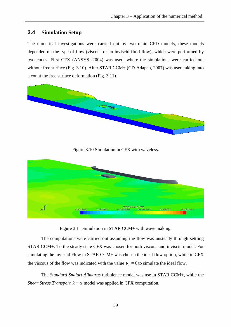
Chapter 3 – Application of the numerical method
39
3.4 Simulation Setup
The numerical investigations were carried out by two main CFD models, these models
depended on the type of flow (viscous or an inviscid fluid flow), which were performed by
two codes. First CFX (ANSYS, 2004) was used, where the simulations were carried out
without free surface (Fig. 3.10). After STAR CCM+ (CD-Adapco, 2007) was used taking into
a count the free surface deformation (Fig. 3.11).
Figure 3.10 Simulation in CFX with waveless.
Figure 3.11 Simulation in STAR CCM+ with wave making.
The computations were carried out assuming the flow was unsteady through settling
STAR CCM+. To the steady state CFX was chosen for both viscous and inviscid model. For
simulating the inviscid Flow in STAR CCM+ was chosen the ideal flow option, while in CFX
the viscous of the flow was indicated with the value 0=tν to simulate the ideal flow.
The Standard Spalart Allmaras turbulence model was use in STAR CCM+, while the
Shear Stress Transport ω−k model was applied in CFX computation.

Chapter 3 – Application of the numerical method
40
The water condition was modelled as fresh water at 21.5°C, (ρ = 999kg/m3, νt=
1.137E-3kg*s/m). The air was assumed compressible (for computational stability reason) and
was modelled with a molecular mass of 28.96kg/kmole and a νt = 1.80E-5kg*s/m. The
buoyancy forces due to fluid density difference were modelled in the STAR CCM+
simulation.
The total time of the simulation was fixed in STAR CCM+ and equal to 30s using a
time step equal to 0.05s with 10 iterations for each step. In CFX the maximum number of
iterations was equal to 500 using a time step equal to 0.1 seconds. However, if the CFX
convergence criteria described below were reached for all residuals, the simulation was
stopped before reaching 500 iterations. For most of simulations, convergence of all residuals
forces and monitoring points was achieved in around 300 iterations.
In both programs, the convergence was assessed by plotting the flow parameters
against the iteration number these were: residuals for mass, momentum and turbulence (target
criteria = 10-4), surge and sway force, and yaw moment.
3.5 Definition of the mesh and Computational Domain
In both simulations, the Volume Control was chosen as a Box Shape, and the dimension was
estimated using the proposed by Fonfach and Guedes Soares (2009). The height of the air
phase was taken equal to kertan25.0 L (the computation with rigid free surface the air phase was
not considered), the domain inlet boundary is at a distance of kertan5.1 L ahead of the ship,
while the outlet boundary is located at kertan6.2 L from the ship stern, and its width is taken to
be of kertan5.1 L . Finally the height of the water phase was the water depth defined in section
3.1 for each case.
In the computation with rigid free surface the mesh generator ICEM CFD was used for
meshing the computational domain with unstructured tetrahedral grid. Here, only the water
phase was meshed. For meshing the volume domain was considered the hulls surface (tug and
tanker) with a value tugL%0.1 and kertan%5.0 L , using low transition for refining the mesh
gradually in the volume around the ships. For meshing the free surface it was considered like
the boundary wall without parameter for fine mesh. For simulating the viscous flow, a
prismatic layer mesh was applied in the surface of the tug hull, and thus the height of the layer

Chapter 3 – Application of the numerical method
41
was determined based in the previous mesh sensitivity study. The values of the mesh sizes are
given in Table 3.7 and the generated meshes are shown in Figs. 3.13 to 3.16.
Table 3.7 Mesh size for simulation with rigid free surface
Part Tug Hull
(m) Tanker Hull
(m) Other wall
(m) Prims
layers (m) CFX Inviscid Model
0.2 1.00 5.00 -
CFX Viscous Model
0.2 1.00 5.00 0.01
Figure 3.12 Computational mesh on tug hull surface for simulations without wave.
Figure 3.13 Mesh section of the CFX domain for 0.121 = Fn at 0.15x/Ltug = .
Figure 3.14 Mesh section of the CFX domain for 0.181 = Fn at 0.15=x/Ltug .

Chapter 3 – Application of the numerical method
42
Figure 3.15 Mesh section of the CFX domain and zoom in the prism layer mesh for 0.181 = Fn at 0.15−=x/Ltug .
The hexahedral mesh used in the other simulation was generated in STAR CCM+. It
should be noticed that in the rigid free surface of the computation for the viscous flow
simulation, the prismatic layer mesh was applied around the hull of the tug. The mesh size
was determined using the previous mesh sensitivity analysis. The meshes of the hulls and free
surface were determined as a percentage of the length of the ship, which gave good result for
a large range of Fn. For meshing the surface of the tug hull a mesh size equal to tugL%25.0
was used, whereas for the tanker a mesh size of kertan%0.1 L was used.
For the interphase of the water and air a block shape was used to refine the free
surface zone, and the box height was equal to 1.0m, where z is 0.5m and -0.5m in each fluid,
respectively. Three different zones were considered on the free surface for the decrease of the
mesh. One of them is the total dimension of the horizontal plane of the volume domain (far
away from the both hull) considering a mesh size equal to kertan%5.0 L . Other is half of the
width and the total longitudinal dimension of the box (near of the tanker ship) considering a
mesh size equal to kertan%25.0 L . Finally using the dimension of the recommendation given by
Fonfach and Guedes Soares (2010), taking the length of the tug based for the determined the
zone near the tug, and using a mesh size equal to kertan%125.0 L . In Star CCM+ a growing
factor value equal to 1 was fixed for a smooth transition between the different cell sizes. The
meshes are shown in Figs. 3.17 to 3.20 and the mesh sizes are summarized in Tables 3.8.
Table 3.8 Mesh size for simulation with deformable free surface (F.S.)
Part Tug Hull
(m) Tanker Hull
(m) F. S. (m)
Other wall (m)
Prism layers (m)
STAR CCM+ Inviscid Model
0.0725 1 1 0.5 0.25 5 -
STAR CCM+ Viscose Model
0.0725 1 1 0.5 0.25 5 0.01

Chapter 3 – Application of the numerical method
43
Figure 3.16 Computational mesh on tug hull surface for simulations with wave making
Figure 3.17 Mesh section of the STAR CCM+ domain for 0.121 = Fn at 0.15=x/Ltug
Figure 3.18 Mesh section of the STAR CCM+ domain for 0.181 = Fn at 0.15=x/Ltug
Figure 3.19 Mesh section of the STAR CCM+ domain and zoom in the prism layer mesh for 0.181 = Fn at 0.15=x/Ltug .

Chapter 3 – Application of the numerical method
44
3.6 Computational Boundary Conditions
The non-zero flow velocity condition was considered for 0=t (the value of velocity
corresponds to each case simulated), with a reference pressure of to 101,325Pa in all
simulations. In STAR CCM+ the free surface was considered initially as plane surface,
defining a hydrostatic pressure for the water volume. For free surface calculations, the air and
water flow around the tug and the tanker models, were simulated using the standard
homogenous Volume of Fluid (VOF) model (or free surface model which is available in
STAR CCM+ for both inviscid and viscous flow simulation). In the VOF model, a single
moment equation is shared by the fluid volume fraction of each of the fluids in each
computational cell and is tracked throughout the domain. The surface tension was not applied
in the models. The coupled volume fraction was used to improve the convergence. The free
surface in CFX was considered as a rigid wall without friction for both ideal and viscous flow
simulation
The boundary condition was employed to simulate the experimental condition on the
towing tank. An initial velocity boundary condition was used at the beginning of the flow
domain in both CFD codes; the flow velocity was considered according to each case studied.
In STAR CCM+ the hydrostatic pressure outlet boundary condition was used at the
end of the flow domain; the hydrostatic pressure at the outlet was calculated assuming an
undisturbed free surface. While in CFX the outlet hydrostatic pressure was considered 0=p .
Smooth walls with a free-slip condition were assumed for the top, floor and the side
wall. Only half of the tank model was considered in the simulations by using a symmetry
plane condition at 0=Y , in the other hand the tug was full model. Smooth walls with a non-
slip condition ( 0,, =wvu ) were assumed in both ship hulls in the viscous flow simulation.

Chapter 4 – Analysis of the numerical results
45
CHAPTER 4 Analysis of the numerical results
Results of the numerical analysis carried out using the formulation and techniques described
above will be present here.
The description of the interaction coefficients of surge and sway force components and
the interaction coefficient of yaw moment acting on the tug are analysed. Comparison
between several numerical result and experimental data were also performed.
The summarized the qualitative analysis of the CFD simulation are analysed. This
analysis considers the interaction of the wave pattern generated by both ships, the pressure on
the tug, and comparison of the velocity around various sections of the tug.
Concerning the tug position with respect to the tanker and the water depth, a
distinction is made between:
Case I : Ship to ship navigation at 1H , Fn of 0.121 and x′ of +0.014
Case II : Ship to ship navigation at 2H , Fn of 0.181 and x′ of +0.61
Additional analyses of the isolated tug were carried out calculating the forces and
moments in each case above, to obtain finally the pure interaction forces.
4.1 Isolated tug
The main objective in the calculation of the hydrodynamic coefficient of the isolated tug is to
calculate the pure hydrodynamic coefficients for the Cases I and II, considering their
respective Fn .
The hydrodynamic coefficients in Table 4.1 are summarized for 1210.=Fn and
compared with the experimental result. The surge coefficient show good agreement between
the computed and the experimental data. Here, the simulations were carried out with
deformable free surface to have a better accuracy. A difference of 3.3% for inviscid fluid and
4.5% for the viscous fluid, respect to the experimental was considered. On the other hand, the
computations with rigid free surface were less accurate, having a difference of 25% for
inviscid fluid and 7% for viscous fluid when compared with the experimental result. In case
of the sway coefficient, the computed coefficients were near to zero value, as must be because
of the symmetry. Similar analysis for the yaw moment can be adopted.

Chapter 4 – Analysis of the numerical results
46
For 1810.=Fn the numerical coefficients are summarized in table 4.2. The surge
coefficient can be observed to converge. The sway and yaw coefficients are close to zero
value were due for the residual value in the computation.
Table 4.1 Hydrodynamics coefficients for 0.121 = Fn
Item Numerical Experimental Coefficient Inviscid Fs Inviscid Sfs Viscous Fs Viscous Sfs Total
X ′ 0.0106 0.0087 0.0110 0.0119 0.01095
Y′ 0.0003 0.0007 0.0002 0.0009 0.00363 N ′ 0.0001 0.0000 0.0000 0.0000 0.00071
Table 4.2 Hydrodynamics coefficients for 0.181 = Fn
Item Numerical Experimental Coefficient Inviscid Fs Inviscid Sfs Viscous Fs Viscous Sfs Total
X ′ 0.0245 0.0256 0.258 0.262 -
Y′ 0.0000 0.0002 0.0030 0.0088 - N ′ 0.0000 0.0000 0.0013 0.0001 -
The properties of the wave pattern around the hull of the tug and the effects of shallow
water on the generated wave at Fn of 0.121 and 0.181 can be seen from the predicted
numerical results in Fig. 4.1. It is observed that the generated wave patterns for both Fn have
similar distribution. A crest at the bow of the tug followed by a valley at the forward side and
a pronounced crest of the wave at the mid of the ship, produce a lager valley in the stern side.
However, differences are observed between bothFn . In the first case of Fn of 0.121, the
length of the valley is smooth at the forward side of the tug whereas in the other case of Fn
of 0.181 the valley is pronounced. For Fn of 0.181 the peak of the crest at the mid-section of
the tug is higher at the lower Fn of 0.181 reaching almost the double high. The valley of the
wave at the stern side is deeper and short for higherFn .
The deformation of the free surface at the stern of the ship for both Fn , shows an
elevation of the water, being for the first one almost the same at the bow of the tug, whereas
the second Fn the height is higher in stern. This situation is unusual and is due to the shallow
water effect. A wake in the flow at the stern of the tug can be noticed due to the robust shape
of the hull.

Chapter 4 – Analysis of the numerical results
47
a) b)
Figure 4.1 Predicted wave patterns by the tug and wave cuts at tugy/L of 0.19 and -0.19: a)
Free surface for Fn of 0.121; b) Free surface for Fn of 0.181.
The distribution of pressure on the Tug hull at both Fn of 0.121 and 0.181 and
calculated by ANSYS CFX and STAR CCM+ are shown in Fig. 4.2 and 4.3. Differences
were found in the distribution of the pressure between the model without waves and with
wave making (Fig. 4.2). It is noted that the distribution of the pressure on the tug hull is only
the hydrodynamic pressure in computation without waves (Fig 4.2a). In computation with
wave making the distribution of the pressure on the hull is dominated by the hydrostatic
pressure, and the hydrodynamic pressure is smaller (Fig 4.2b).
The same analysis can be adopted for Fn of 0.181 (Fig 4.3). The distribution of the
pressure on the hull computed without waves are similar for both Fn . High pressure is
observed at the bow of the tug which decreases between tugLx / between -0.5 to -0.25. Low
pressure is produced in the mid of the tug increasing between tugLx / between -0.5 to -0.85,
and a high pressure is distributed at the stern of the ship.
The distribution of pressure on the hull computed with deformable free surface for
both Fn shows a similar patter with the maximum high pressure in the keel which decrease
going up to the free surface. However, differences are observed, due to the position of the
generated wave at the free surface. For Fn of 0.121 the pressure on the hull is almost constant

Chapter 4 – Analysis of the numerical results
48
due to the small deformation of the free surface whereas for the Fn of 0.181 the high
pressure is produced in the bow and is followed by a decreasing when the flow enters in the
gap between the ships and is increased again at the mid-section of the tug reaching a constant
magnitude close to the stern.
a)
b)
Figure 4.2 Distribution of the pressure on the tug hull surface at Fn of 0.121: a) Pressure distribution without wave making; b) Pressure distribution with wave making.
a)
b)
Figure 4.3 Distribution of the pressure on the tug hull surface at Fn of 0.181: a) Pressure distribution without wave making; b) Pressure distribution with wave making.

Chapter 4 – Analysis of the numerical results
49
The velocity flow around the tug is plotted in Figs. 4.4 to 4.5. It is observed that both
models, with and without wave making show agreement with the predicted velocity for the
flow. In Froude numbers of 0.121 and 0.181, it is observed that the velocity decrease around
the bow section. However, the velocity increased at the mid-section of the tug reaching the
maximum value. The maximum velocity flow was found at the bilges of the tug ship where it
was noticed an increment in the velocity. The velocity remains constant at the bilges in the
stern zone. The velocity is the same that in the mid ship section of the tug. Below the bottom,
the velocity flow decrease to a minimum value (close to zero).
a) b)
Figure 4.4 Flow velocities distribution around transversal sections of the tug´s hull for Fn of 0.121: a) Velocity without waves; b) Velocity with wave making.
a) b)
Figure 4.5 Flow velocities distribution around transversal sections of the tug´s hull for Fn of 0.181: a) Velocity without waves; b) Velocity with wave making.

Chapter 4 – Analysis of the numerical results
50
4.2 Interaction between the ships
4.2.1 Case I (Fn of 0.121)
The pure interaction force and moment coefficients with the dimensionless lateral distance
between the ships are shown in Fig. 4.6. It is observed that the magnitude of the surge
coefficients increases in the negative direction for small gaps. The sway coefficient shows a
variation in the direction of the lateral clearance. The tug experiences a repulsion sway force
at small gaps between the ships, changing to suction force when the tug vessel increases the
lateral distance (between positions y′ 1.34 to 1.38). For the remaining the lateral distances,
the sway coefficients are in negative direction, being the tug attracted by the tanker vessel.
The yaw moment coefficients have important variations, when the ships are widely separated
( 9.1>′y ) the coefficients are near to zero. On the other hand, for small gaps, the yaw
moment coefficients experience large increments.
In computations without waves, when the free surface is modelled with a rigid wall all
coefficients (without free surface) show good agreement with the experimental results for
relative large side clearance. When the tug is very close the tanker this model loses accuracy.
This disagreement is critical in the calculation of the sway coefficient at small lateral distance.
The yaw moment is smaller than the experimental results. This is noticed clearly at 34.1=′y
where the yaw moment is near to zero.
The simulations carried out with accurate boundary condition on free surface followed
the trend of the experimental results. However, even this model presented not very accurate
results for the three hydrodynamic coefficients at y′ of 1.34 and 1.38. The analysis indicates
that for small distances, the accuracy can be improved using an appropriate discretization in
the free surface region. It is observed for the larger gaps, both with rigid and deformable free
surface are able for predicting the interaction coefficient.
Figs. 4.7 to 4.9 illustrate the computed interaction wave pattern for each lateral
distance and along the two planes which is between -0.19 and 0.19m away of the plane of
symmetry. In Fig. 4.7a ( 34.1=′y ) it is possible to observe a pronounced asymmetrical free
surface. The waves generated on the interaction side are distributed above the design water
line of the tug, while on the free side the waves are produced below the water line. Fig. 4.7b
( 38.1=′y ) shows the generated wave with the tanker suction over the tug, that means, at the

Chapter 4 – Analysis of the numerical results
51
mid-section of the tug a valley ( tugLz / ) of -0.018 is produced between the interacting ships
while at the free side, the valley is of -0.006.
a)
b)
c)
Figure 4.6 Interaction force and moment coefficients in shallow water as functions of dimensionless lateral displacement with dimensionless longitudinal shift +0.014: a) Surge force coefficient; b) Sway force coefficient; c) Yaw moment coefficient.

Chapter 4 – Analysis of the numerical results
52
Figs. 4.8a and 4.8b show the free surfaces for y′ 1.41 and 1.46, respectively. It is
observed that both lateral distances are close, producing similar wave patterns, as was
commented for the lateral gap of 1.38. The interaction between the ships generated a valley at
mid-section of the tug in both cases y′ 1.41 and 1.46, However, for y′ of 1.41 the peak
value of the valley are different in both sides of the tug, whereas the y′ of 1.46 the wave is
almost symmetrical in both sides along of the tug hull.
Here, in these cases of lateral distances the effect of the tanker in the wave pattern
produced by the tug can be observed clearly, being the wave patterns generated evidently
differently than in the free navigation. In Fig. 4.11 can be seen the free surface for y′ of 1.95
(Fig 4.9a) and 2.26 (Fig 4.19b). In these two lateral distances the ships produce symmetric
wave patterns because the tug is relatively far away from the tanker, here the valley in the
interaction side is less pronounced than in the previous cases, and the amplitude for both y′
have the same value in the free side. Considering the cases of lateral distances 1.38 to 2.26,
the wave patterns generated by the ships have similar characteristics. It is observed that the
wave generated in the bow is slightly higher when the ships interact, and also in the valley
generated in the mid-ship section of the tug.
a) b)
Figure 4.7 Predicted interaction wave patter by the ships for Fn of 0.121 with dimensionless longitudinal shift +0.014 and wave cut at
tugy/L of 0.19 and -0.19: a) Free surface for y′ of
1.34; b) Free surface for y′ of 1.38.

Chapter 4 – Analysis of the numerical results
53
a) b)
Figure 4.8 Predicted interaction wave patter by the ships for Fn of 0.121 with dimensionless longitudinal shift +0.0014 and wave cut at
tugy/L of 0.19 and -0.19: a) Free surface for y′ of
1.41; b) Free surface for y′ of 1.46.
a) b)
Figure 4.9 Predicted interaction wave patter by the ships for Fn of 0.121 with dimensionless longitudinal shift +0.014 and wave cut at
tugy/L of 0.19 and -0.19: a) Free surface for y′ of
1.95; b) Free surface for y′ of 2.26.

Chapter 4 – Analysis of the numerical results
54
When 34.1=′y , both solutions (with and without deformable free surface) show
differences in the distribution of pressure on the hull, as shown in Fig. 4.10. Fig. 4.10a shows
high pressure at the bow that decrease between tugLx / -0.5 to 0.25. A low pressure is
observed near to the mid-ship of the tug (between tugLx / -0.25 to 0) producing that the tug
ship is suctioned by the tanker ship. In the positions between tugLx / 0.25 to 0.5 the pressure
is increased but is smaller than the pressure in the bow. These distributions of the pressure
suggest that the position of the sway forces is forward of the mid-ship. In the body view is
noted the asymmetric pressure, which is higher at the interaction than at the free side.
The surge force is positioned in the interaction side. It is noticed that the resultant yaw
moment on the tug ships is the difference between the moments produced by the two
component forces, which is observed in the yaw coefficients (Fig 4.6c). In the Fig. 4.10b
(with deformable free surface) is shown the increment of the generated pressure at the bow,
compared with the isolated tug. This effect is due to the stationary water in the zone of the
curvature of the bow of the tug and at the side of the tanker (between tugLx / -0.5 to 0.25).
This is followed of the small gap between the ships (between tugLx / -0.25 to 0.5)
where an increment of the pressure generating a repulsion sway forces can be noted. The
small distance between the ships is different of the computation with the rigid free surface.
However, this phenomenon is in agreement with the experimental as can be seen in the
experimental sway coefficient.
When y′ is 1.38 to 2.26 (Figs. 4.10 to 4.15) the distribution of the hull pressure is
almost the same in both simulations, the high pressure is observed at the bow of the tug. In the
body view is observed that the distribution of the pressure is higher at the interaction than at
the free side. The pressure decreased in the aft direction until the mid-section of the ship. The
low pressure generated on the tug hull produces a suction sway force. Similar to y′ of 1.34,
the interaction yaw moment is produced by the difference of the forces due to the sway force,
which is forward to the mid ship section whereas the surge force is at the interaction side.
The flow velocities around the transverse sections of the tug hull are shown in Figs.
4.16 to 4.21 where it is observed the influence of the lateral gap along of the tug. When y′ of
1.34 (Fig. 4.16), differences between the computations (with and without free deformable free
surface) were found at the mid-section going to the stern of the tug. In the calculation with
rigid free surface, is observed an increment of the velocity flow in the interaction side. In the

Chapter 4 – Analysis of the numerical results
55
calculation with deformable free surface, the velocity flow decreased flow to zero in the gap
between the ships.
a)
b)
Figure 4.10 Distribution of the pressure on the tug hull surface for Fn of 0.121 with dimensionless longitudinal shift +0.014 and dimensionless lateral shift +1.34: a) Pressure
distribution without waves; b) Pressure distribution with wave making.
a)
b)
Figure 4.11 Distribution of the pressure on the tug hull surface for Fn of 0.121 with dimensionless longitudinal shift +0.014 and dimensionless lateral shift +1.38: a) Pressure
distribution without waves; b) Pressure distribution with wave making.

Chapter 4 – Analysis of the numerical results
56
a)
b)
Figure 4.12 Distribution of the pressure on the tug hull surface for Fn of 0.121 with dimensionless longitudinal shift +0.0014 and dimensionless lateral shift +1.41: a) Pressure
distribution without waves; b) Pressure distribution with wave making.
a)
b)
Figure 4.13 Distribution of the pressure on the tug hull surface for Fn of 0.121 with dimensionless longitudinal shift +0.014 and dimensionless lateral shift +1.46: a) Pressure
distribution without waves; b) Pressure distribution with wave making.

Chapter 4 – Analysis of the numerical results
57
a)
b)
Figure 4.14 Distribution of the pressure on the tug hull surface for Fn of 0.121 with dimensionless longitudinal shift +0.014 and dimensionless lateral shift +1.95: a) Pressure
distribution without waves; b) Pressure distribution with wave making.
a)
b)
Figure 4.15 Distribution of the pressure on the tug hull surface for Fn of 0.121 with dimensionless longitudinal shift +0.014 and dimensionless lateral shift +2.26: a) Pressure
distribution without waves; b) Pressure distribution with wave making.

Chapter 4 – Analysis of the numerical results
58
On the stern of the ship, the differences between the models persist. In the simulation
without deformable free surface, the velocity decrease in the gap between the ships. However,
in the free bilge the velocity increases and is observed a low velocity below the bottom. In the
other simulation with deformable free surface, the velocity decrease to zero between the ships.
In the rest of the sections the velocity has a constant distribution. In both computations, the
velocity of the flow at the keel is asymmetrical, differing with the isolated tug. In the
interaction between the ships, the velocity increase more at the side with interaction than in
the free side. In the bow of the tug (between tugLx / -0.15 and -0.44) both computation
(with and without deformable free surface) show a similar predicted velocity.
In the first section a stationary flow can be seen around the section and in de second an
increment of the velocity in the space of between the ships. Between y′ 1.38 and 1.46 (Figs
17 to 19) both computations (with a without free surface) are in agreement with the predicted
velocity flow, being the flow pattern similar for this range of lateral distances. The velocity at
the bow decreases to zero near to the section where the velocity increase highly between the
space of the ships going to mid of the ship. This velocity remains constant increasing until
tugLx / of 0.44. As in the previous lateral distance, the velocity in the keel is modified in the
interaction side only.
The flow at the stern is slightly affected by the tanker and the velocity decreases while
in the free side the velocity increases in the bilge as in the isolated tug case. In the cases
where the ships have more separation (Figs. 20 and 21), the distribution of flow velocity
distribution around the sections is the same observed in the cases of the tug sailing freely (Fig.
4.5).
a) b)
Figure 4.16 Flow velocities distribution around of transversal sections of the tug hull for Fn
of 0.121 with dimensionless longitudinal shift +0.014 and dimensionless lateral shift +1.34: a) Velocity without waves; b) Velocity with wave making.

Chapter 4 – Analysis of the numerical results
59
a) b)
Figure 4.17 Flow velocities distribution around of transversal sections of the tug hull for Fn of 0.121 with dimensionless longitudinal shift +0.014 and dimensionless lateral shift +1.38: a)
Velocity without waves; b) Velocity with wave making.
a) b)
Figure 4.18 Flow velocities distribution around of transversal sections of the tug hull for Fn of 0.121 with dimensionless longitudinal shift +0.014 and dimensionless lateral shift +1.41:
a) Velocity without waves; b) Velocity with wave making.
a) b)
Figure 4.19 Flow velocities distribution around of transversal sections of the tug hull for Fn of 0.121 with dimensionless longitudinal shift +0.014 and dimensionless lateral shift +1.46:
a) Velocity without waves; b) Velocity with wave making.

Chapter 4 – Analysis of the numerical results
60
a) b)
Figure 4.20Flow velocities distribution around of transversal sections of the tug hull for Fn of 0.121 with dimensionless longitudinal shift +0.014 and dimensionless lateral shift +1.95:
a) Velocity without waves; b) Velocity with wave making.
a) b)
Figure 4.21 Flow velocities distribution around of transversal sections of the tug hull for Fn of 0.121 with dimensionless longitudinal shift +0.014 and dimensionless lateral shift +2.26:
a) Velocity without waves; b) Velocity with wave making.
4.2.2 Case II (Fn of 0.181)
The hydrodynamic interaction coefficients with the lateral distances are plotted in Fig. 4.22.
The coefficients have a distribution similar to that in the previous Fn of 0.121. However at
y′ of 1.95 the magnitude of the surge coefficient increases with respect to the lateral distance
at y′ of 1.64. Thus, the interaction surge coefficients increase the ship resistant in all lateral
distances.
The sway coefficient shows a variation in the direction of the lateral clearance where
the tug experiences repulsion at small gaps between the ships, however this force is less than
in the previous case changing to suction force when the tug vessel increases the lateral
distance, As in the other case the yaw moment coefficients have important variations, when

Chapter 4 – Analysis of the numerical results
61
the ships are widely separated the coefficients are near to zero. On the other hand, for small
gaps, the yaw moment coefficients experience large increments. The numerical coefficients
computed with wave making improved accuracy of the interaction forces for small distances
although the yaw coefficient ( 34.1=′y ) was highly underestimated at the same distance
when compared with the experiments. The numerical coefficients without wave making gave
similar results than in the previous case improving the trend of the curve.
a)
b)
c)
Figure 4.22 Interaction force and moment coefficients in shallow water as functions of dimensionless lateral displacement with dimensionless longitudinal shift +0.61:
a) Surge force coefficient; b) Sway force coefficient; c) Yaw moment coefficient.

Chapter 4 – Analysis of the numerical results
62
The free surface interactions and their cross sections are illustrated in Figs. 4.23 to
4.25. At the lateral gap of 1.34, the effect of the tanker on the tug is asymmetric. In the gap
between the ships, the wave has a short length with higher amplitude than in the free side of
the tug. It is noted in the curvature of the bow water cumulated at the interaction side. Near
the stern it is noted that the generated wave behind the tug is affected by the tanker, being
irregular and asymmetrical.
Fig. 4.24a and 4.24b show the free surface in the lateral distances of 1.46 and 1.64,
respectively. Lateral distances of 1.46 and 1.64 have a similar wave pattern than the observed
in the previous Fn . In the gap between the ships, a valley at mid-section of the tug is
generated. The valley generated at the free side (mid-section of the tug) is smaller than in the
interaction side. In Fig. 4.25 can be seen the free surface for y′ of 1.95. In this lateral
distance, the tug is producing a symmetrical wave patterns because the tug is far away from
the tanker, and thus the valley in the interaction side has the same peak value than in the free
side ( tugLz / of -0.0140).
a) b)
Figure 4.23 Predicted interaction wave patter by the ships for Fn of 0.181 with dimensionless longitudinal shift +0.61 and wave cut at
tugy/L of 0.19 and -0.19: a) Free
surface for y′of 1.34; b) Free surface for y′of 1.38.

Chapter 4 – Analysis of the numerical results
63
a) b)
Figure 4.24 Predicted interaction wave patter by the ships for Fn of 0.181 with dimensionless longitudinal shift +0.61 and wave cut at
tugy/L of 0.19 and -0.19: a) Free
surface for y′of 1.41; b) Free surface for y′of 1.64.
a)
Figure 4.25 Predicted interaction wave patter by the ships for Fn of 0.181 with dimensionless longitudinal shift +0.61 and wave cut at
tugy/L of 0.19 and -0.19: a) Free
surface for y′of 1.95.

Chapter 4 – Analysis of the numerical results
64
The distribution of the pressure is shown in Figs. 4.26 to 4.30. The pressure has a similar
patter than in the previous Fn analysed. At the lateral distance of 1.34 (without deformable
free surface) Fig. 4.26a shows a high pressure at the bow, which decrease in de region of
curvature of the bow (between tugLx / -0.5 to 0.125). The low pressure in the mid-ship of the
tug is producing suction in the tug due to the presence of the tanker. In the positions between
tugLx / of 0.125 to 0.5, the pressure increase. However, it is smaller than in the bow pressure.
In Fig. 4.26b (with deformable free surface), an increment of the pressure is noted in the
interaction side between the ships at the mid-section. Repulsion sway forces accrued at Fn of
0.121 where the lateral distance is the same. The high pressure in the bow is generated by the
accumulated water. Near the stern, the pressure is close to the initial hydrostatic pressure
(when the free surface is non-deformed). In the case of y′ between 1.38 and 1.95 (Fig. 27 to
30) the pattern of the distribution of the pressure on the hull is the same in both simulation,
being the high pressure at the bow of the tug. It is show in the body view that this distribution
of the pressure is higher in the interaction side than the in free side.
The pressure decreases in the bow between tugLx / -0.5 to -0.125. For the stern
between tugLx / -0.125 to 0.125 the low pressure is generated on the tug hull, producing
suction on the tug hull. The distribution of the pressure increases between tugLx / 0.125 to
0.5 and is constant going to the stern.
a)
b)
Figure 4.26 Distribution of the pressure on the tug hull surface for Fn of 0.181 with dimensionless longitudinal shift +0.61 and dimensionless lateral shift +1.34: a) Pressure
distribution without waves; b) Pressure distribution with wave making.

Chapter 4 – Analysis of the numerical results
65
a)
b)
Figure 4.27 Distribution of the pressure on the tug hull surface for Fn of 0.181 with dimensionless longitudinal shift +0.61 and dimensionless lateral shift +1.38: a) Pressure
distribution without waves; b) Pressure distribution with wave making.
a)
b)
Figure 4.28 Distribution of the pressure on the tug hull surface for Fn of 0.181 with dimensionless longitudinal shift +0.61 and dimensionless lateral shift +1.41: a) Pressure
distribution without waves; b) Pressure distribution with wave making.

Chapter 4 – Analysis of the numerical results
66
a)
b)
Figure 4.29 Distribution of the pressure on the tug hull surface for Fn of 0.181 with dimensionless longitudinal shift +0.61 and dimensionless lateral shift +1.64: a) Pressure
distribution without waves; b) Pressure distribution with wave making.
a)
b)
Figure 4.30 Distribution of the pressure on the tug hull surface for Fn of 0.181 with dimensionless longitudinal shift +0.61 and dimensionless lateral shift +1.95: a) Pressure
distribution without waves; b) Pressure distribution with wave making.

Chapter 4 – Analysis of the numerical results
67
The flow velocities around the tug are shown in Fig. 4.31 to 4.35, where the velocity
of flow represents similar qualitative characteristics as in the previous Froude number
calculated. At the lateral gap of 1.34 (Fig 31) with rigid free surface the velocity between the
ships in the mid-section increments, while in the other computation is near to zero.
In the remaining lateral distances (Fig 32 to 35), both models predicted similar
velocities. In the bow, the flow round the section is stationary whereas going to the mid-
section is produced an increment of the velocity between the ships. In stern zone, the flow
decreased the velocity at the interaction side while it increased in the free side.
a) b)
Figure 4.31 Flow velocities distribution around of transversal sections of the tug hull for Fn of 0.181 with dimensionless longitudinal shift +0.61 and dimensionless lateral shift +1.34:
a) Velocity without waves; b) Velocity with wave making.
a) b)
Figure 4.32 Flow velocities distribution around of transversal sections of the tug hull for Fn of 0.181 with dimensionless longitudinal shift +0.61 and dimensionless lateral shift +1.38:
a) Velocity without waves; b) Velocity with wave making.

Chapter 4 – Analysis of the numerical results
68
a) b)
Figure 4.33 Flow velocities distribution around of transversal sections of the tug hull for Fn of 0.181 with dimensionless longitudinal shift +0.61 and dimensionless lateral shift +1.41:
a) Velocity without waves; b) Velocity with wave making.
a) b)
Figure 4.34 Flow velocities distribution around of transversal sections of the tug hull for Fn of 0.181 with dimensionless longitudinal shift +0.61 and dimensionless lateral shift +1.64:
a) Velocity without waves; b) Velocity with wave making.
a) b)
Figure 4.35 Flow velocities distribution around of transversal sections of the tug hull for Fn of 0.181 with dimensionless longitudinal shift +0.61 and dimensionless lateral shift +1.95:
a) Velocity without waves; b) Velocity with wave making.

Chapter 4 – Analysis of the numerical results
69
The interaction between ships showed that the Fn of 0.181 is better predicted when wave-
making is used. This is because the deformation on the free surface is higher than in the case
Fn of 0.121, where the mesh selected is fine enough for the VOF method. All movements in
the free surface were computed for higher Fn whereas in the other Fn the predicted wave
patterns were less accurate.
Another problem observed for the lowFn , is the distribution of the predicted pressure, which
were invariable along of the hull. However, the viscous and inviscid fluid computation in
general (with and with wave-making) show good agreement between numerical and
experimental results.
The behaviour of the tug, when is assisting the tanker, has an associated risk due to
their proximity during the manoeuvre. It is observed that the lateral movement of the tug
respect to the tanker has a strong influence in the results when the position of the tug along of
the tanker is changing or the velocity of the tug increases.
The lateral movement of the tug with respect to the tanker could cause accidents if not
proper operations during the navigation are implemented. For example, the suction produced
when both the tug and the tanker are sailing very close the risk of collision between them
increases significantly.
The negative yaw moment at the bow of the tug is due to accumulated water, which
can take over it from its sailing direction. Thus, the risk of hitting the stern and the propeller
of the tug in wall side of the tanker increases.
The increment of the hydrodynamic ship resistance is a negative effect. For example,
it is necessary an engine with high power to keep the sailing velocity of the tug. In the same
line, it was observed that the flow entering on the propeller region is irregular and caused that
the propeller lost efficiency.
The information obtained from the analysis is useful to predict the manoeuvre of a tug
assisting a merchant ship when the additional forces and moment generated by their
interaction is known. The variation of forces and moments can define properly the energy of
the engine or the condition in which the ruder could operate. In the current study, the
interaction between the ships can be used to avoid accidents. Also it can be useful for the
selection of ropes, based on the design loads obtained from the interaction when the tanker is
assisted.
Conclusion
70
Conclusions
Computational Fluid Dynamics (CFD) models were developed for computing the
hydrodynamic interaction forces and moments between two sailing ships models in shallow
water. The computations were carried out using viscous and inviscid flow formulations and
with deformable or rigid free surface. The computed surge and sway force coefficients and the
numerical yaw moment coefficient showed good agreement in general with the experimental
results. Both viscous and inviscid flow models predicted almost the same values for the
hydrodynamic force coefficients. However, substantial disagreements were found between the
numerical coefficients with and without deformable free surface, giving indications of the
hydrodynamics phenomena that have influenced the interaction between ships.
The hydrodynamic interaction forces between ships in shallow water at short lateral
distance range (between y′ 1.34 to 1.41) are dominated by the intensive wave generation and
the complicated wave transformation due to the presence of the tanker.
The numerical calculations with free surface showed two main wave effects in the
component forces. First, the surge force magnitude in the tug vessel was increased drastically
in the smaller lateral distances. Second, a repulsion sway force was generated between the
ships at y′= 1.34 for both values of the Froude number.
The interaction yaw moment coefficients showed different effects for different Fn . At
smaller Fn , the moment increases drastically while at a larger Fn the moment decreases.
This situation is due to the resultant component forces and their location which is defined
mainly by the wave positions on the tug. On the other hand, the numerical analysis without
free surface at small gaps showed large sway suction coefficients and relatively small surge
force and yaw moment on the tug being underestimated with respect to the experimental
coefficients.
The interaction forces for large lateral clearances showed that the main source is the
velocity potential of the flow, generating additional surge and sway suction forces. The
additional yaw moment on the tug was calculated accurately by all proposed models.
Discrepancies were noticed between numerical (with deformable free surface) and
experimental values of the hydrodynamics coefficients at smaller lateral distances. This
suggested that the meshes in the free surface region were not fine enough and this was most
unfavourable for the Fn of 0.121.

Conclusion
71
The longitudinal position did not have strong influence on the results. However, it is
mentioned that the tug position at the mid-ship section of the tanker is less favourable. Here
the coefficients were not smaller than when the tug was at the bow position while that the
velocity was smaller at the first longitudinal position.
The main result of the study concerns the effect of wave making and viscosity on the
interaction forces demonstrating predominance of the former. The present work demonstrated
the ability of CFD simulation models to quantify the interaction between two vessels in
typical harbour manoeuvring.
Also it should be noticed that for a more detailed investigation it would be useful to test a
wider range of hull shapes and ship-length ratios for a variety of waterway configurations.

Reference
72
References
Anderson JD. (1995). Computational Fluid Dynamics: The Basics with Applications,
McGraw Hill, pp. 81–83.
Altintas A. (1990). Archimedes' Principle as an Application of the Divergence Theorem,
IEEE Transactions on Education, Vol. 33, No. 2, pp. 222.
Ansys (2004), CFX-5 Documentation, Ansys Canada Ltd.
Ashe GM. (1975). Trajectory prediction for ships engaged in close proximity operations. BSc
thesis, Ocean Engineering, Massachusetts Institute of Technology (MIT).
Barth TJ, Jesperson DC. (1989). The design and application of upwind schemes on
unstructured meshes. American Institute of Aeronautics and Astronautics, Washington
D.C. AIAA No 89–366.
Beck RF, Tuck EO, Newman JN. (1975). Hydrodynamics Forces on ships in dredged
channels. Journal of Ship Research, Vol.19, pp. 71–166.
Beck RF. (1975). Forces and Moments on a ship moving in a shallow channel. Journal of
Ship Research, Vol. 21, pp.107–119.
Blazek J. (2001). Computational Fluid Dynamics: Principles and Applications. Elsevier
Science Ltd, Oxford England.
Brix J. (1979). MTI-StellungnahmezumThema "Aus-dem-Ruder-laufen" von Schiffen. Sog-
und GierbeeinflussungenbeiPassiervorgängen. Vol. 116, No 18, pp. 1383–1388.
Brix, J. (editor) (1993). Manoeuvring Technical Manual. Seehafen Verlag GmbH, Hamburg.
Burg COE, Marcum DL. (2003). Moving towards high fidelity RANS calculations of
maneuvering surface vessels using unstructured grids. 8th International Conference on
Numerical Ship Hydrodynamics, Busan, Korea.
Chatterton JR. (1994). An evaluation of the prediction of near bottom interaction forces and
moments on unmanned undersea vehicles. Msc. Thesis, Naval Architecture and
Engineering, Massachusetts Institute of Technology (MIT).
CD-Adapco (2007), STAR CCM+ Documentation, CD-Adapco Group.
Chen G-R, Fang M-C. (2001). Hydrodynamics interaction between two ships advancing in
waves. Journal Ocean Engineering, Vol. 28, pp. 1053–1078.

Reference
73
Chen HC, Lin WM, Liut DA, Hwang WY. (2003). An advanced flow computation method
for ship-ship dynamic interactions in shallow and restricted waterway. MARSIM
2003, Kanazawa, Japan.
Ch’ng PW. (1991). An investigation into the influence of bank effect on ship manoeuvring
and its mathematics modeling for a ship-handling simulator. Ms. Thesis, Mechanical
and Manufacturing Engineering, University of New South Wales.
Ch’ng PW, Renilson LJ. (1993). A method of calculating the ship bank interaction forces and
moments in restricted water. International Shipbuilding Progress, Vol. 40, pp. 7–23.
Cummins WE. (1953). The forces and moment acting on a body moving in an arbitrary
potential stream. DTMB report 780, Washington DC.
Dand IW. (1981). Simulation of the behavior of a moored ship when passed by other ships.
National Maritime Institute, R111.
Davis AMJ, GeerJF. (1982). The application of uniform-slender-body theory to the motion of
two ships in shallow water. Journal of Fluid Mechanics, Vol. 114, pp. 419–441.
Durbin P. (1995). Separated flow computations using the k-ε v2 model. AIAA J. 33, 4
Fairplay World Fleet Statistics, 2008.
Ferziger JH, and Peric M. (2002) Computational Methods for Fluid Dynamics, 3rd ed.,
Springer-Verlag, pp. 157–206.
Fonfach JM. (2010). Evaluación numérica de la resistencia al avance de buques. BSc. Tesis,
Ingeniería Naval. Universidad Austral de Chile.
Fonfach JM, Guedes C. (2010). Improving the Resistance of a series 60 vessel with a CFD
Code. Proceedings of the V European Conference on Computational Fluid Dynamics
(CFD 2010). ECCOMAS.
Fortson RM. (1974). Interaction forces between ships. BSc. Thesis, Ocean Engineering,
Massachusetts Institute of Technology (MIT).
Gourlay T. (2009). Sinkage and trim of two ships passing each other on parallel courses.
Journal Ocean Engineering, Vol. 36, pp. 1119–127.
Hirt CW, Nichols BD. (1981). Volume of fluid method for thedynamics of free boundaries.
Journal Comput. Phys. Vol. 39, pp. 201–225.

Reference
74
Hong SY, Kim JH, Cho SK, Choi YR, Kim YS. (2005). Numerical and experimental study on
hydrodynamic interaction of side-by-side moored multiple vessels. Journal Ocean
Engineering, Vol. 32, pp. 783–801.
Houzeaux G. (2002). A Geometrical Domain Decomposition Methods in Computational Fluid
Dynamics. Phd. Thesis, Escuela Superior de Ingenieros de Cataluña, Barcelona.
Huang ET, Chen H-C. (2003). Passing Ship Effects on Moored Vessels at Piers. Naval
Facilities Engineering Service Center.
Hunt JCR. (1990) Developments in computational modelling of turbulent flows. In Proc.
ERCOFTAC Work 1990, Cambridge University Press.
Jones WP and Launder B. (1972). The prediction of laminarization with a two-equation model
of turbulence. Int. J. Heat Mass Transfer, Vol. 15, pp. 301–314.
Jiankang W, Lee TS, Shu C. (2001). Numerical study of wave interaction generated by two
ships moving parallely in shallow water. Journal Ocean Engineering, Vol. 190, pp.
2099–2110.
Kriebel D. (2005). Mooring loads due to parallel passing ships. Naval Facilities Engineering
Service Center, Technical report No 6056.
King GW. (1977). Unsteady hydrodynamic interactions between ships in shallow water. 6th
Australasian hydraulic and Fluid Mechanics Conference, Adelaide, Australia.
King GW. (1977). Unsteady hydrodynamic interactions between ships. Journal of Ship
Research, Vol. 21, pp. 157–164.
Krishnankutty P, Varyani KS. (2003). Ship form effects on the forces and moment on a
stationary ship induced by a passing ship. MCMC, Girona.
Krishnankutty P, Varyani KS. (2004). Force on the mooring lines of a ship due to the
hydrodynamic interaction effects of a passing ship. Journal of International
Shipbuilding Progress, Vol. 51, pp. 194–101.
Kyulevcheliev S, Georgiev S, Ivanov I. (2003). Hydrodynamic interaction between moving
and stationary ship in a shallow canal. Shipbuilding Department, Technical University
of Varna, Bulgaria.

Reference
75
Lee YS, Toda Y, Sadakane H. (2003). The prediction of hydrodynamic forces acting on a ship
hull undergoing lateral berthing maneuver in shallow water. MARSIM 2003,
Kanazawa, Japan.
Liaw K. (2005). Simulation of Flow around Bluff Bodies and Bridge Deck Sections using
CFD. Phd Thesis, Schoolof Civil Engineering, University of Nottingham.
Müller E. (1967). Untersuchungenüber die gegenseitigeKursbeeinflussung von Schiffen auf
Binnenwasserstrassen. Schiff und Hafen, 19. Jahrgang, Heft 6.
Menter FR, Kuntz M, and Bender RA. (2003)). Scale-adaptive simulation model for turbulent
flow predictions. AIAA 2003, paper N° 767.
Newman JN. (1965). The Force and Moment on a slender body of revolution moving near a
wall. David Taylor Basin, Washington D.C, Report No 2127.
Newton RN. (1960). Some notes on interaction effects between ships close aboard in deep
water. First Symposium on Ship Maneuverability, Washington D.C., Paper No 146,
pp. 1–24.
Petrila T. and Trif D. (2005). Basics of fluid mechanics and introduction to computational
fluid dynamics. 1st ed., Springer, Vol3, pp. 397–433.
Remery GFM. (1974). Mooring forces induced by passing ships. Offshore Technology
Conference, Dallas, Paper No. 2066, pp. 1–20.
Rhie CM, Chow WL. (1983). Numerical study of the turbulent flow past an airfoil with
trailing edge separation. Vol. 21, pp. 1525–1532.
Spalart PR. (2000). Strategies for turbulence modelling and simulations. Int. J. Heat
FluidFlow, Vol. 21, pp. 252–263.
Sutulo S, Guedes C. (2009). Effective operation in ports. Report on Development of a
hydrodynamics interaction module, No: FP6–031486.
Stoesser T. (2001). Development and Validation of a CFD-Code for Turbulent Open-Channel
flow. Dissertation Submitted for the degree of Doctor of Philosophy (PhD), University
of Bristol.
Stangroom P. (2001). Computational fluid dynamics for wind farm optimisation. First year
report for the degree of PhD, School of Civil Engineering, University of Nottingham.

Reference
76
Stroud K . (1996). Further engineering mathematics, Macmillan Press Ltd.
Takeshi H, Hino T, Hinatsu M, Tsukada Y, and Fujisawa J. (1987) Flow Measurements and
resistance Tests, ITTC Cooperative Experiments on a Series 60 Model At ship
Research Institute, 17th Towing Tank Conference, (ITTC).
Taggart KM, Cumming D, Hsiung C, Li L. (2003). Seakeeping of two ships in close
proximity. Ocean Engineering, Vol.36, pp. 1051–1063.
Taylor DW. (1909). Some model experiments on suction of vessels. Transaction of the
Society of Naval Architects and Marine Engineers, Vol. 17, pp. 2–22.
The Marine Accident Investigation Branch (MAIB), 2003.
Travin A, Shur M, Spalart PR, and Strelets M. (2004). On URANS solutions with LES-like
behaviour. In Proceedings of the 4th European Congress on Computational Methods in
Applied Sciences and Engineerin 2004. ECCOMAS.
Tuck EO. (1966). Shallow water flow past slender bodies. Journal of Ship Research, Vol. 26,
pp. 8–95.
Tuck EO. (1967). Sinkage and trim in shallow water of finite width. Schiffstechnik, Vol. 14,
pp. 92– 4.
UNCTAD (2003). Review of Maritime Transport. United Nations, New York and Geneva.
Vantorre M, Laforce E, verzhbitskaya E. (2002). Model test based formulations of ship-ship
interaction forces for simulation purposes. Ghent University.
Varyani KS, McGregor RC, Wold P. (1999). Empirical formulae to predict peak of forces and
moments during interactions. Hydronav - Manoeuvring'99, Gdańsk-Ostróda. pp. 338–
349.
Varyani KS, Krishnankutty P, Vantorre M. (2003). Prediction of load on mooring ropes of a
container ship due to the forces induced by a passing bulk carrier. MARSIM,
Kanazawa, Japan.
Varyani KS, McGregor RC, Wold P. (2002). Identification of trends in extremes of sway-yaw
interference for several ships meeting in restricted waters. Ship Technology Research,
Schiffahrts-VerlagHansa, Vol. 49, pp. 174–191.
Reference
77
Wnęk A, Paço A, Zhou X, Guedes C. (2009). Numerical and Experimental Analysis of the
Wind Forces Acting on LNG Platform. Proceedings of the 13th Congress of
International Maritime Association of the Mediterranean IMAM 2009 Vol. 2, pp. 697
–702.
Wnęk A, Paço A, Zhou X, GuedesSoares C. (2010). Numerical and Experimental Analysis of
the Wind Forces Acting on LNG Carrier. Proceedings of the V European Conference
on Computational Fluid Dynamics (CFD 2010). ECCOMAS.
Yasukawa H. (1990). Bank effect on ship manoeuvrability in a channel with varying width.
Transactions of West-Japan Society of Naval Architects, n. 81.
Yasukawa H. (2003). Maneuvering motion of two ships in close proximity. Journal of the
Society of Naval Architects of Japan Vol. 105, pp. 43–54.
Yeung RW. (1978). On the interaction of slender ships in shallow water. Journal of Fluid
Mechanics, Vol. 85, pp. 143–159.
Zwart PJ. (2005). Numerical modeling of free surface and cavitating flows. Industrial two-
phase flow CFD. In: von Karman Institute Lecture Series 2004–2005. Von Karman
Institute, Belgium, pp. 25.
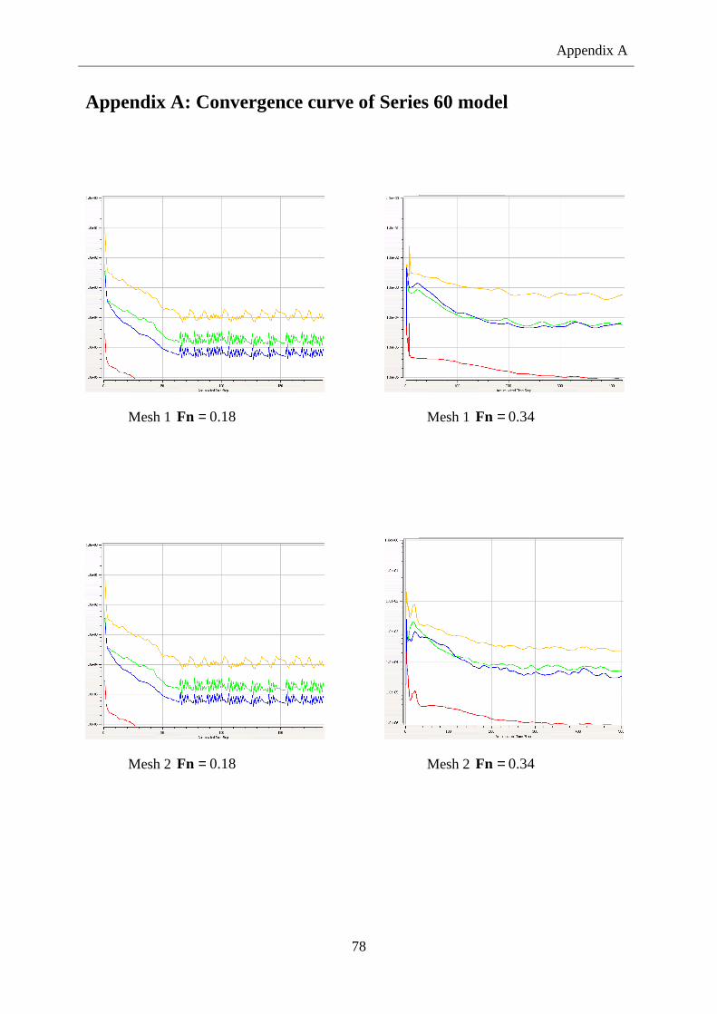
Appendix A
78
Appendix A: Convergence curve of Series 60 model
Mesh 1 0.18 = Fn Mesh 1 0.34 = Fn
Mesh 2 0.18 = Fn Mesh 2 0.34 = Fn

Appendix A
79
Mesh 3 0.18 = Fn Mesh 3 0.34 = Fn
Mesh 4 0.18 = Fn Mesh 4 0.34 = Fn

Appendix B
82
Appendix B: Predicted wave profile of Series 60 model

Appendix C
81
Appendix C: Forces monitor at Fn of 0.121
Surge force at 34.1=′y Sway force at 34.1=′y
Surge force at 38.1=′y Sway force at 38.1=′y
Surge force at 41.1=′y Sway force at 41.1=′y

Appendix C
82
Surge force at 46.1=′y Sway force at 46.1=′y
Surge force at 95.1=′y Sway force at 95.1=′y
Surge force at 26.2=′y Sway force at 26.2=′y

Appendix D
83
Appendix D: Table of coefficients at Fn of 0.121
Experimental y′ X ′ Y ′ N ′
1.34 0.03972 -0.02000 0.00709 1.38 0.02321 0.02026 0.00548 1.41 0.01132 0.04259 0.00180 1.45 0.00704 0.03381 0.00168 1.95 0.00418 0.01238 0.00048 2.26 0.00356 0.01138 0.00054
Viscous (vavemaking) Invicisd (vavemaking) y′
X ′ Y ′ N ′ X ′ Y ′ N ′ 1.34 0.02147 -0.05135 0.00363 0.02593 -0.04249 0.00358 1.38 0.01510 0.05077 0.00104 0.00967 0.05713 0.00118 1.41 0.01383 0.05364 0.00071 0.00880 0.04925 0.00078 1.45 0.01149 0.03945 0.00060 0.00807 0.03662 0.00059 1.95 0.00785 0.01296 0.00043 0.00674 0.01073 0.00028
2.26 0.00602 0.01003 0.00028 0.00580 0.01019 0.00012
Viscous (waveless) Invicisd (waveless) y′ X ′ Y ′ N ′ X ′ Y ′ N ′
1.34 0.01431 0.14013 0.00001 0.01047 0.14943 0.00010 1.38 0.01302 0.08590 0.00099 0.00979 0.09464 0.00143 1.41 0.01297 0.06935 0.00100 0.00902 0.07921 0.00150 1.45 0.01166 0.04702 0.00039 0.00763 0.04857 0.00029 1.95 0.00785 0.00867 0.00008 0.00503 0.00940 -0.00004
2.26 0.00621 0.00649 0.00020 0.00435 0.01024 0.00018

Appendix E
84
Appendix E: Table of difference between numerical and
experimental coefficients at Fn of 0.121
Viscous (wavemaking) Invicisd (wavemaking) y′ X ′ Y ′ N ′ X ′ Y ′ N ′
1.34 -84.971 61.055 95.147 -53.160 52.928 49.490 1.38 -53.699 60.092 81.046 -140.110 64.537 78.434 1.41 18.144 20.598 60.803 -28.625 13.529 56.523 1.45 38.721 14.299 64.286 12.763 7.684 64.592 1.95 46.745 4.489 10.400 37.989 -15.333 40.916 2.26 40.885 -13.443 48.373 38.629 -11.730 78.608
Viscous (waveless) Invicisd (waveless) y′ X ′ Y ′ N ′ X ′ Y ′ N ′
1.34 -177.569 114.273 -99.904 -73.643 -847.142 -98.584 1.38 -78.278 76.416 -81.888 -57.802 367.141 -73.915 1.41 12.734 38.586 -44.627 -20.345 85.992 -16.527 1.45 39.619 28.088 -77.019 8.395 43.648 -82.885 1.95 46.770 -42.757 -83.270 20.337 -24.087 -108.202 2.26 42.672 -75.460 -63.462 22.064 -9.997 -67.461

Appendix F
85
Appendix F: Forces and moment monitor at Fn of 0.181
Surge force at 34.1=′y Sway force at 34.1=′y
Surge force at 38.1=′y Sway force at 38.1=′y
Surge force at 41.1=′y Sway force at 41.1=′y

Appendix F
86
Surge force at 64.1=′y Sway force at 64.1=′y
Surge force at 95.1=′y Sway force at 95.1=′y

Appendix G
87
Appendix G: Table of coefficient at Fn of 0.181
Experimental y´
X ′ Y ′ N ′ 1.34 0.0377 -0.0074 0.0172 1.38 0.0289 0.0214 0.0157 1.41 0.0160 0.0467 0.0118 1.95 0.0134 0.0086 0.0081
2.26 0.0377 -0.0074 0.0172
Viscous (wavemaking) Invicisd (wavemaking) y′ X ′ Y ′ N ′ X ′ Y ′ N ′
1.34 0.0335 -0.0580 0.0113 0.0322 -0.0520 0.0108 1.38 0.0264 0.0146 0.0119 0.0241 0.0142 0.0112 1.41 0.0128 0.0319 0.0089 0.0110 0.0352 0.0096 1.64 0.0113 0.0193 0.0073 0.0101 0.0184 0.0080 1.95 0.0148 0.0060 0.0076 0.0126 0.0085 0.0080
Viscous (waveless) Invicisd (waveless) y′ X ′ Y ′ N ′ X ′ Y ′ N ′
1.34 0.0110 0.1342 0.0089 0.0087 0.1420 0.0090 1.38 0.0118 0.0902 0.0084 0.0091 0.0914 0.0082 1.41 0.0134 0.0580 0.0080 0.0113 0.0580 0.0079 1.64 0.0078 0.0242 0.0071 0.0065 0.0225 0.0070 1.95 0.0110 0.0105 0.0071 0.0101 0.0087 0.0067

Appendix H
88
Appendix H: Table of difference between numerical and
experimental coefficients at Fn of 0.181
Viscous (wavemaking) Invicisd (wavemaking) y′ X ′ Y ′ N ′ X ′ Y ′ N ′
1.34 -12.6578 87.2331 -52.3657 -17.0148 85.7650 -58.9655 1.38 -9.0907 -46.3322 -32.2616 -19.5818 -50.9758 -40.8762 1.41 -25.5305 -46.4713 -32.6731 -45.7464 -32.5636 -22.3669 1.64 -4.2003 -19.5382 -30.8329 -17.0985 -25.3904 -19.7178 1.95 9.6917 -43.5400 -5.7018 -6.2800 -2.0288 -0.1066
Viscous (waveless) Invicisd (waveless) y′
X ′ Y ′ N ′ X ′ Y ′ N ′ 1.34 -70.8484 105.5144 -93.0328 -76.9344 105.2119 -89.9829 1.38 -59.0719 76.2736 -87.3722 -68.4760 76.5902 -92.1882 1.41 -16.4565 19.5442 -46.9285 -29.5920 19.5232 -48.5338 1.64 -33.7646 4.6721 -35.0260 -44.5737 -2.5312 -37.8019 1.95 -17.9363 17.9508 -13.9485 -24.4276 1.2903 -19.9727
Related Documents