Numerical solution of a virtual internal bond model for material fracture

Numerical Solution of a Virtual Internal Bond Model for

Material Fracture

Ping Lin∗ and Chi-Wang Shu†

Abstract

A virtual internal bond (VIB) model is proposed recently in mechanical engineeringliteratures for simulating dynamic fracture. The model is a nonlinear wave equation ofmixed type (hyperbolic or elliptic). There is instability in the elliptic region and usualnumerical methods might not work. We examine the artificial viscosity method for themodel and apply central type schemes directly to the corresponding viscous system toensure appropriate numerical viscous term for such a mixed type problem. We providea theoretical justification of the convergence of the scheme despite the difficulty of thetype change. The exact solution of a Riemann problem is used to justify the numericalmethod for one dimensional cases. We then generalize the method to a two dimensionalmaterial with a triangular or hexagonal lattice structure. Computational results for atwo dimensional example are given.

1 Introduction

Modeling and simulation of material motion play an important rule in understanding andpredicting material behaviors, such as dislocation and dynamic fracture (cf. [3, 4, 8, 18, 9]).Most problems in this area are very challenging to analysts and many are new in the sensethat not much study has been done. Modeling, theoretical analysis and explanation ofvarious phenomena observed are far from complete. We shall consider a virtual internalbond (VIB) model with randomized cohesive interactions between material particles inthe literature of material science (e.g. [3]). It differs from an atomistic model in that aphenomenological “cohesive force law” is assumed to act between “material particles” whichare not necessarily atoms. It also differs from a cohesive surface model in that, rather thanimposing a cohesive law along a prescribed set of discrete surfaces, a randomized networkof cohesive bonds is statistically incorporated into the constitutive law of the materialand the macroscopic collective behavior of this random bond network is obtained through

∗Department of Mathematics, The National University of Singapore, Singapore 119260 (e-mail:[email protected]). The work of this author was supported in part by the Singapore academicresearch grant R-146-000-016-112.

†Division of Applied Mathematics, Brown University, Providence, Rhode Island 02912, USA (e-mail:[email protected]). The research of this author was supported in part by the ARO grant DAAD19-00-1-0405, NSF grant DMS-9804985, NASA Langley grant NCC1-01035 and AFOSR grant F49620-99-1-0077.

1

2

the so called Cauchy-Born rule [11], i.e. by equating the strain energy function on thecontinuum level to the potential energy stored in the cohesive bonds due to an imposeddeformation. The VIB model is intended to integrate the macroscopic view of cohesivesurfaces dispersed in a continuum background with the “atomistic” view of interatomicbonding. One application we are concerned of is the fracture dynamics, where near thecrack tip we generally need to consider the atomistic scale. As pointed in [3, 4] the prospectof this type of models in numerical simulations of fracture is highly promising. As in [6]we shall adopt the 6-12 Lennard-Jones atomic interacting potential which is a reasonableapproximation to atomic interaction of a number of real materials.

The model is derived from hyperelastic principle combined with the so-called Cauchy-Born rule and is a wave-like partial differential equation. One main difficulty of the PDEmodel is that its type may change from hyperbolic to elliptic in the case of large deformation(e.g. the fracture case we are mainly concerned of). In the case of large deformationthe corresponding one dimensional linear constant coefficient equation is equivalent to theCauchy-Riemann equations for which the initial value problem is ill-posed (cf. [13]). Thereis almost no theory considered for the PDE with the Lennard-Jones potential energy density.We pointed out in [6] for the one dimensional case that in some fracture situation the modelcan be simplified to a Riemann problem of the PDE. Therefore techniques in analyzing theRiemann problem of conservation laws of mixed type can be borrowed in analyzing thisPDE. The solution of the Riemann problem is studied in [6] to illustrate various shockphenomena associated with the model. There is no much study of numerical methods forconservation laws of mixed type. In this paper we will use a central difference scheme plusa small viscous term to approximate the shock waves and to ensure that the numericalviscosity coincides with the continuous one. More advanced schemes may be tested later.We will analyze the linear stability and the convergence of a linearized discrete problemfor this mixed-type equation. We will give the rarefaction and shock wave solution for theRiemann problem of the model based on the analysis in [6] and use it to quantitativelyjustify the reliability of the numerical method. We then generalize the method to thetwo dimensional case to simulate a two dimensional dynamic fracture for materials witha triangular or hexagonal lattice structure. Another difficulty is that ill-posedness in theelliptic region implies very severe instability of the discrete system (i.e. a small error in thedata causes an exponentially increasing error in the solution as t increases). Any numericalmethods would fail for such instability. Nevertheless, our numerical tests indicate that thesimulation of early stage of the fracture is trustable.

2 Continuous virtual internal bond model via hyperelasticity

In the hyperelasticity theory of continuum mechanics (cf. [10]) material points in theundeformed configuration are described by the reference (Lagrangian) coordinates X =(X1,X2,X3); points in the deformed body are described by spatial (Eulerian) coordinatesx = (x1, x2, x3). We define φ : D0 −→ R to be a mapping describing the deformationx = φ(X, t) of the body D0 (cf. Figure 2.1). The (Jacobian) matrix of partial derivativesof φ is denoted as F = ∂φ

∂X and is called the deformation gradient. Thus (denoting φ =

3

(φ1, φ2, φ3)T ),

Fij =∂φi(X, t)

∂Xj. (2.1)

The determinant of F is always positive since φ is assumed to preserve deformation orien-tation. The Green-Lagrangian strain tensor is defined as

X

X

X

X

x

D

D

O

reference configuration

current configuration

1

02

3

φ

Figure 2.1: The material and the deformation function

E =12(FTF − I). (2.2)

Let r0 stand for the length of bond when unstretched and ξ = (sin θ0 cosφ0, sin θ0 sinφ0, cos θ0)T

for the bond orientation in the spherical coordinates (r0, θ0, φ0). Then from continuum me-chanics theory the “stretch” of an atomic bond from the undeformed bond r0 in an arbitrarydirection ξ will be

r = r0

√1 + 2ξTEξ. (2.3)

We consider a homogeneous, isotropic, hyperelastic solid which has a microstructureconsisting of randomized internal cohesive bonds between a network of randomly distributedmaterial particles. We assume that each bond can be described by a potential energyfunction Φ(r) where r is the stretched bond length as defined in (2.3). By the Cauchy-Bornrule ([11, 18]) the strain energy per unit undeformed area in such a random network ofbonds can be defined as

Θ(F) =∫ ∞

0

∫ π

0

∫ 2π

0D(r0, θ0, φ0)Φ(r) sin θ0 dr0dθ0dφ0, (2.4)

where D(r0, θ0, φ0) is the bond density per unit undeformed volume of the material.1 Notethat E is a function of F. So Θ is either a function of E or a function of F. We will writeΘ as a function of F. Let the material range over a region X ∈ D0 then the equilibriumconfiguration can be obtained from minimizing the energy

Econt(φ) =∫

D0

Θ(F(X)dX (2.5)

1The precise definition of D(r0, θ0, φ0) is that D(r0, θ0, φ0) sin θdr0dθ0dφ0 is the number of bonds perunit volume in the undeformed solid with bond length between r0 and r0+dr0 and bond orientation between(θ0, φ0) and (θ0 + dθ0, φ0 + dφ0).

4

subject to boundary conditions for φ(X, t). This gives the equilibrium equation

divσ(F) = 0, (2.6)

where σ(F) = ∂Θ∂F is a matrix (called (first) Piola-Kirchhoff stress tensor) with entries given

by σij = ∂Θ∂Fij

and divσ is a column vector and its i-th component is

(divσ)i =∑

j

∂σij

∂Xj.

The equations (2.6) stands for the balance of the forces of the material. In the dynamiccase these forces are not balanced but are equal to the product of the mass and accelerationaccording to Newton’s Law, that is, we have the following equations of motion:

ρ0∂2φ

∂t2= divσ(F), (2.7)

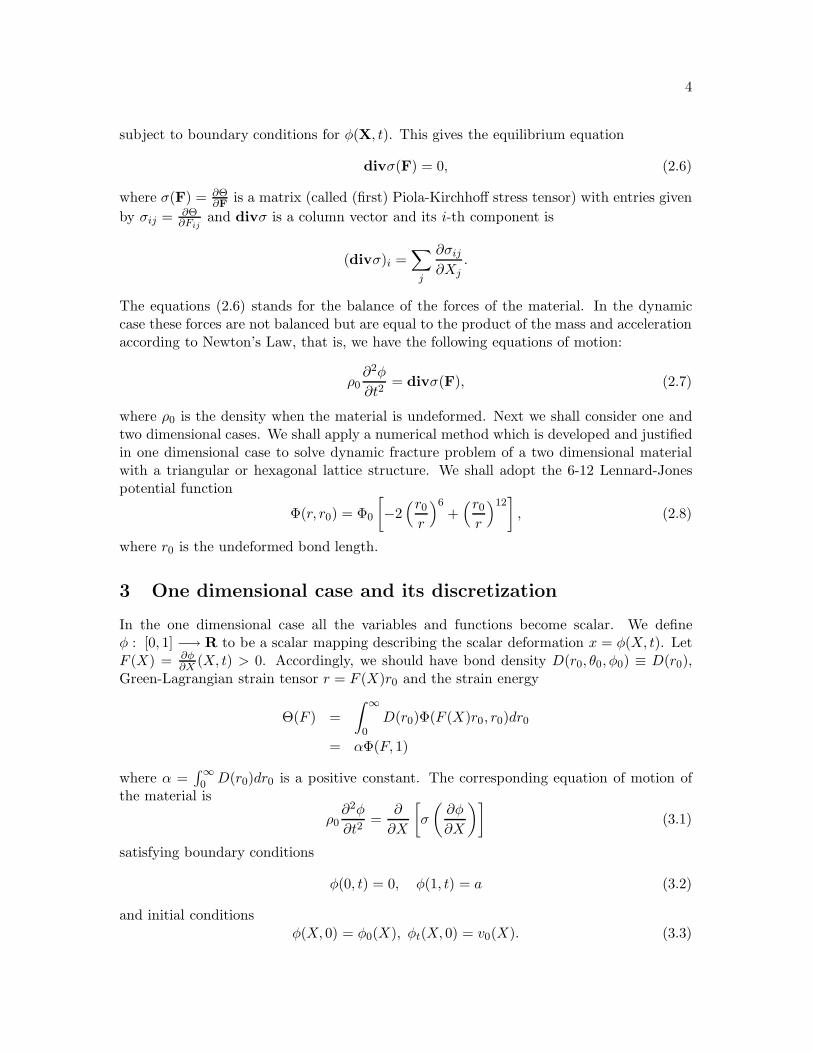
where ρ0 is the density when the material is undeformed. Next we shall consider one andtwo dimensional cases. We shall apply a numerical method which is developed and justifiedin one dimensional case to solve dynamic fracture problem of a two dimensional materialwith a triangular or hexagonal lattice structure. We shall adopt the 6-12 Lennard-Jonespotential function

Φ(r, r0) = Φ0

[−2(r0

r

)6+(r0

r

)12], (2.8)

where r0 is the undeformed bond length.

3 One dimensional case and its discretization

In the one dimensional case all the variables and functions become scalar. We defineφ : [0, 1] −→ R to be a scalar mapping describing the scalar deformation x = φ(X, t). LetF (X) = ∂φ

∂X (X, t) > 0. Accordingly, we should have bond density D(r0, θ0, φ0) ≡ D(r0),Green-Lagrangian strain tensor r = F (X)r0 and the strain energy

Θ(F ) =∫ ∞

0D(r0)Φ(F (X)r0, r0)dr0

= αΦ(F, 1)

where α =∫∞0 D(r0)dr0 is a positive constant. The corresponding equation of motion of

the material is

ρ0∂2φ

∂t2=

∂

∂X

[σ

(∂φ

∂X

)](3.1)

satisfying boundary conditions

φ(0, t) = 0, φ(1, t) = a (3.2)

and initial conditionsφ(X, 0) = φ0(X), φt(X, 0) = v0(X). (3.3)

5

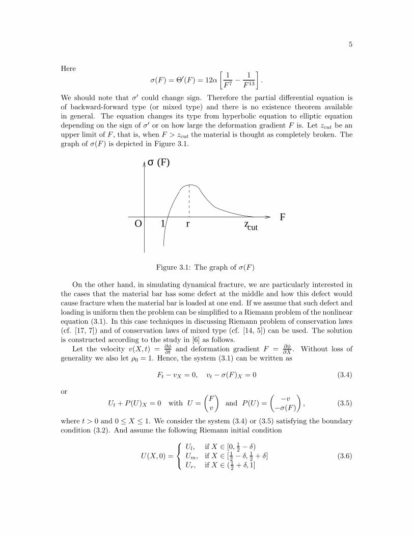
Here

σ(F ) = Θ′(F ) = 12α[1F 7

− 1F 13

].

We should note that σ′ could change sign. Therefore the partial differential equation isof backward-forward type (or mixed type) and there is no existence theorem availablein general. The equation changes its type from hyperbolic equation to elliptic equationdepending on the sign of σ′ or on how large the deformation gradient F is. Let zcut be anupper limit of F , that is, when F > zcut the material is thought as completely broken. Thegraph of σ(F ) is depicted in Figure 3.1.

Fr zcut1

(F)σ

O

Figure 3.1: The graph of σ(F )

On the other hand, in simulating dynamical fracture, we are particularly interested inthe cases that the material bar has some defect at the middle and how this defect wouldcause fracture when the material bar is loaded at one end. If we assume that such defect andloading is uniform then the problem can be simplified to a Riemann problem of the nonlinearequation (3.1). In this case techniques in discussing Riemann problem of conservation laws(cf. [17, 7]) and of conservation laws of mixed type (cf. [14, 5]) can be used. The solutionis constructed according to the study in [6] as follows.

Let the velocity v(X, t) = ∂φ∂t and deformation gradient F = ∂φ

∂X . Without loss ofgenerality we also let ρ0 = 1. Hence, the system (3.1) can be written as

Ft − vX = 0, vt − σ(F )X = 0 (3.4)

or

Ut + P (U)X = 0 with U =(Fv

)and P (U) =

( −v−σ(F )

), (3.5)

where t > 0 and 0 ≤ X ≤ 1. We consider the system (3.4) or (3.5) satisfying the boundarycondition (3.2). And assume the following Riemann initial condition

U(X, 0) =

Ul, if X ∈ [0, 12 − δ)

Um, if X ∈ [12 − δ, 12 + δ]

Ur, if X ∈ (12 + δ, 1]

(3.6)

6

where Ul =(Fl

vl

)=(10

), Um =

(Fm

vm

)=(1 + η0

)and Ur =

(Fr

vr

)=(10

). Here F = 1

corresponds to a stable state (i.e. zero force state) and thus η stands for the initial defectappeared in a relatively small middle region of the material. Note that it is a system ofconservation laws of mixed type since σ′(F ) < 0 when F > r. A solution diagram isillustrated in Figure 3.2 (η > 0) According to the shock analysis of [6] and following the

general technique described, for example, in [17], the intermediate state U1 =(F1

v1

)can be

calculated from the nonlinear equation

∫ F

Fl

√σ′(F )dF −

√(Fm − F )(σ(Fm)− σ(F ) + vl − vm = 0 (3.7)

and

v = vl +∫ F

Fl

√σ′(F )dF. (3.8)

Then the left shock speed can be calculated by

s =√(σ(Fm)− σ(F ))/(Fm − F ) (3.9)

if η > 0 and

s = −√(σ(Fm)− σ(F ))/(Fm − F ) (3.10)

if η < 0. The rarefaction solution can be obtained from the following formulas:

F

(x− 1

2 + δ

t

)= (σ′)−1

(x− 1

2 + δ

t

)2 , (3.11)

v

(x− 1

2 + δ

t

)= v −

∫ F

F

√σ′(F )dF. (3.12)

U2 can be obtained similarly.

x

t

_

O

UU

t

1

1/2- 1/2+

U UU

δ δ

l m r

12

0

_

Figure 3.2: Solution of the Riemann problem for η > 0

7

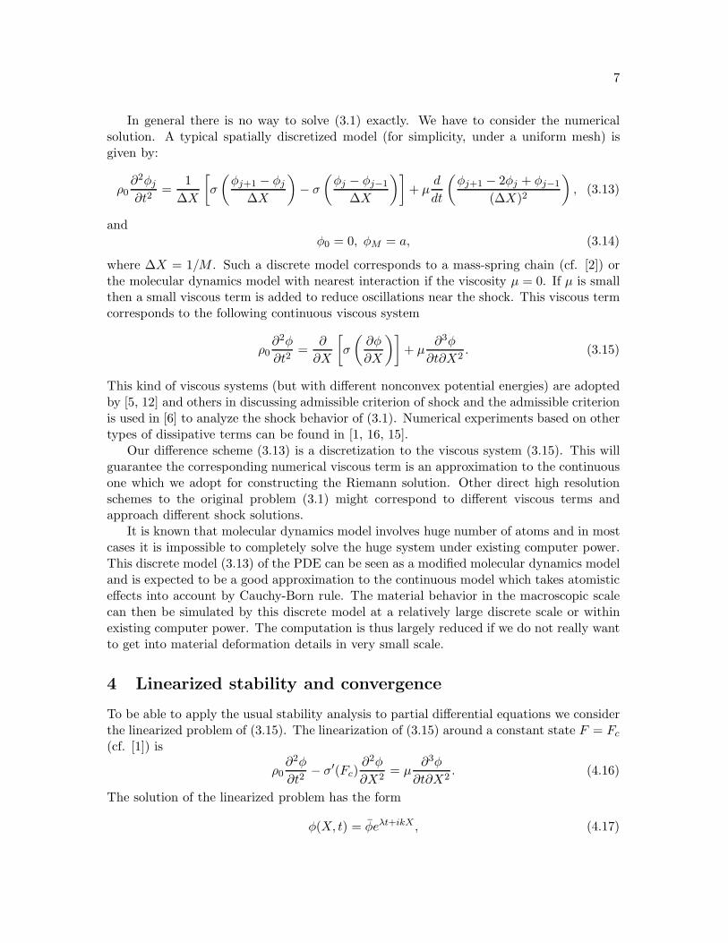
In general there is no way to solve (3.1) exactly. We have to consider the numericalsolution. A typical spatially discretized model (for simplicity, under a uniform mesh) isgiven by:

ρ0∂2φj

∂t2=

1∆X

[σ

(φj+1 − φj

∆X

)− σ

(φj − φj−1

∆X

)]+ µ

d

dt

(φj+1 − 2φj + φj−1

(∆X)2

), (3.13)

andφ0 = 0, φM = a, (3.14)

where ∆X = 1/M . Such a discrete model corresponds to a mass-spring chain (cf. [2]) orthe molecular dynamics model with nearest interaction if the viscosity µ = 0. If µ is smallthen a small viscous term is added to reduce oscillations near the shock. This viscous termcorresponds to the following continuous viscous system

ρ0∂2φ

∂t2=

∂

∂X

[σ

(∂φ

∂X

)]+ µ

∂3φ

∂t∂X2. (3.15)

This kind of viscous systems (but with different nonconvex potential energies) are adoptedby [5, 12] and others in discussing admissible criterion of shock and the admissible criterionis used in [6] to analyze the shock behavior of (3.1). Numerical experiments based on othertypes of dissipative terms can be found in [1, 16, 15].

Our difference scheme (3.13) is a discretization to the viscous system (3.15). This willguarantee the corresponding numerical viscous term is an approximation to the continuousone which we adopt for constructing the Riemann solution. Other direct high resolutionschemes to the original problem (3.1) might correspond to different viscous terms andapproach different shock solutions.

It is known that molecular dynamics model involves huge number of atoms and in mostcases it is impossible to completely solve the huge system under existing computer power.This discrete model (3.13) of the PDE can be seen as a modified molecular dynamics modeland is expected to be a good approximation to the continuous model which takes atomisticeffects into account by Cauchy-Born rule. The material behavior in the macroscopic scalecan then be simulated by this discrete model at a relatively large discrete scale or withinexisting computer power. The computation is thus largely reduced if we do not really wantto get into material deformation details in very small scale.

4 Linearized stability and convergence

To be able to apply the usual stability analysis to partial differential equations we considerthe linearized problem of (3.15). The linearization of (3.15) around a constant state F = Fc

(cf. [1]) is

ρ0∂2φ

∂t2− σ′(Fc)

∂2φ

∂X2= µ

∂3φ

∂t∂X2. (4.16)

The solution of the linearized problem has the form

φ(X, t) = φeλt+ikX , (4.17)

8

where k is the wave number and λ is the frequency which may be a complex number.Substitute this solution into (4.16) we obtain

λ± =−µk2 ±

√µ2k4 − 4σ′(Fc)k2ρ0

2ρ0. (4.18)

From (4.17) we see that Re λ < 0 indicates the stability of the solution of (4.16) and thatRe λ > 0 indicates the instability of the solution of (4.16) and the solution exponentiallyincreases to infinity. It is not difficult to see that if σ′(Fc) > 0 or if Fc locates in thehyperbolic region (where the wave equation is a hyperbolic equation) then we have Re λ < 0or the solution is stable, and that if σ′(Fc) < 0 or if Fc locates in the elliptic region (wherethe wave equation becomes an elliptic equation) then we have Re λ > 0 or the solution isunstable.

Next we consider the spatially discretized (or semi-discrete) problem (3.13). Let theerror Ej(t) = φ(xj , t)− φj(t). The it satisfies

ρ0∂2Ej

∂t2− σ′Ej+1 − 2Ej + Ej−1

∆X2− µ

d

dt

(Ej+1 − 2Ej + Ej−1

(∆X)2

)= O((∆X)2), (4.19)

where O((∆X)2) is the truncation error of the spatial discretization. For studying thestability we only need to consider the homogeneous equation of (4.19). Suppose

Ej(t) = Eeλt+ikj∆X .

Then λ satisfies the following quadratic equation:

ρ0λ2 +

4σ′

∆X2sin2 k∆X

2+

4µ∆X2

sin2 k∆X

2λ = 0 (4.20)

Again Re λ < 0 indicates stability and Re λ > 0 indicates instability. The solution of (4.20)is

λ± =

(− 2µ∆X2

sin2 k∆X

2± 2

õ2

∆X4sin4 k∆X

2− σ′ρ0

∆X2sin2 k∆X

2

)/ρ0. (4.21)

Hence, if σ′ > 0 or in hyperbolic region the solution of (3.13) is stable and if σ′ < 0 or inelliptic region the solution of (3.13) is unstable.

Since the sign of σ′ may change at larger deformation gradient φX or its discrete corre-spondence φj−φj−1

∆X the discrete problem would have positive eigenvalues. This fact impliesthat the problem would have exponentially increasing solution with respect to time t. Verysevere instability would occur and any numerical methods would fail. Fortunately, we foundin [6] that the solution of the original nonlinear problem is always bounded. So such anexponential increase would not happen for the original problem. Also, in practice, the frac-ture time is not very long and the material would usually have defect or fracture only in asmall local region, e.g. in the 1D case, the defect region (which is roughly a fracture region)δ is small compared with the length of the material bar. Under such practical assumptionswe use the energy method to analyze the convergence of the discrete solution φj of (3.13)to the continuous solution φ(Xj) of (3.15). Due to the difficulty of the mixed-type problemour discussion would depend more on physical situations.

9

Unlike above we now linearize (3.13) at a time dependent state Fj = F (Xj , t) =∂φ∂t (Xj , t), that is, we write

σ

(φj+1 − φj

∆X

)≈ σ(Fj)+σ′(Fj)

(φj+1 − φj

∆X− Fj

), σ

(φj − φj−1

∆X

)≈ σ(Fj)+σ′(Fj)

(φj − φj−1

∆X− Fj

).

Then (3.13) becomes

ρ0∂2φj

∂t2= σ′(Fj)

φj+1 − 2φj + φj−1

(∆X)2+ µ

d

dt

(φj+1 − 2φj + φj−1

(∆X)2

), (4.22)

(3.15) can be written as

ρ0∂2φ(Xj , t)

∂t2= σ′(Fj)

φ(Xj+1, t)− 2φ(Xj , t) + φ(Xj−1, t)(∆X)2

+

µd

dt(φ(Xj+1, t)− 2φ(Xj , t) + φ(Xj−1, t)

(∆X)2) +O((∆X)2). (4.23)

Subtracting (4.23) from (3.13) we obtain the error equation (4.19) again where σ′ =σ′(F (Xj , t)) is a function of Xj and t but not a constant σ′(Fc). The error Ej = φ(Xj , t)−φj(t) satisfies homogeneous boundary and initial conditions. To deal with the sign changeof σ′(F ) we divide the function into three parts as shown in Figure 4.3. When F is in the

σ’ (F)

OF

z cut

I IIIII

r_f

Figure 4.3: σ′(F ) and its partition

regions I and II, σ′(F ) may be negative. |σ′(F )| and |∂σ′(F )∂X | are very small in the region

II, say

supF∈II

|σ′| and supF∈II

|∂σ′

∂X| ≤ δII < µ. (4.24)

In the region III, σ′(F ) has a positive lower bound, say

infF∈III

σ′(F ) ≥ c > 0. (4.25)

Region I is a difficult part to deal with theoretically. We use δt to represent the time whenF stays in the region I. In many practical fracture situations, we may expect that δt is

10

quite short. On the other hand, multiplying the equation (3.15) by ∂φ∂t , it is not difficult to

obtain that the total energy

Htotal =ρ0

2(∂φ

∂t)2 +Θ(F )

decreases with respect to the time t. Thus

Θ(F ) ≤ Htotal|t=0

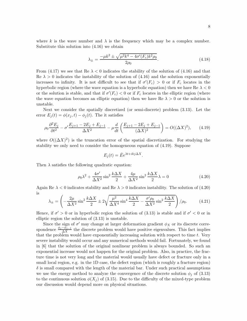
is bounded. From the definition of Θ(F ) at the beginning of §3 we conclude that F should beaway from zero, otherwise Θ(F ) would approach infinity and cannot be bounded. Thereforewe can have F (X, t) ≥ f > 0. From this result, we know that σ(F ) and all its derivativesare bounded, say, by a generic constant K.

Multiplying the error equation (4.19) by 1M (Ej)t, summing the equations from 1 to

M − 1 and noting that

1M

M−1∑j=1

σ′(Fj)Ej+1 − 2Ej + Ej−1

(∆X)2(Ej)t

=1

M∆X

M−1∑

j=1

σ′(Fj)Ej+1 − Ej

∆X(Ej)t −

M−1∑j=1

σ′(Fj)Ej − Ej−1

∆X(Ej)t

=1

M∆X

M∑

j=2

σ′(Fj−1)Ej − Ej−1

∆X(Ej−1)t −

M−1∑j=1

σ′(Fj)Ej − Ej−1

∆X(Ej)t

= − 1M

M∑j=1

σ′(Fj)Ej − Ej−1

∆X

(Ej − Ej−1

∆X

)t

+1M

M∑j=2

∂σ′

∂X(ξj)

Ej − Ej−1

∆X(Ej−1)t,

(where σ′(Fj−1) = σ′(Fj) + ∂σ′∂X (ξj)∆X is used), we can obtain

µ

2M

M∑j=1

(Ej − Ej−1

∆X)2t +

ρ0

2M

M−1∑

j=1

(Ej)2t

t

+1

2M

∑

Fj∈III

σ′(Fj)(Ej − Ej−1

∆X)2

t

=1

2M

∑Fj∈III

∂σ′

∂t(Fj)(

Ej − Ej−1

∆X)2 +

1M

∑Fj∈III

∂σ′

∂X(ξj)

Ej − Ej−1

∆X(Ej−1)t

− 12M

∑F (Xj ,t)∈I

σ′(Fj)((Ej − Ej−1

∆X)2)

t

+1M

∑Fj∈I

∂σ′

∂X(ξj)

Ej − Ej−1

∆X(Ej−1)t

− 1M

∑F (Xj ,t)∈II

σ′(Fj)Ej − Ej−1

∆X(Ej − Ej−1

∆X)t +

1M

∑Fj∈II

∂σ′

∂X(ξj)

Ej − Ej−1

∆X(Ej−1)t

+1M

M−1∑j=1

(Ej)tO((∆X)2).

Physically, if F ≥ zcut orφj−φj−1

∆X ≥ zcut the fracture is considered to be finished and thematerial is broken down. So we are only interested in F < zcut and

φj−φj−1

∆X < zcut and then

11

we can have Ej−Ej−1

∆X ≤ 2zcut. This bound is going to be used below to obtain the errorestimate. Based on (4.24), and denoting

Hd =1

2M

M−1∑j=1

(Ej)2t +1

2M

∑Fj∈III

σ′(Fj)(Ej − Ej−1

∆X)2,

we have

(Hd)t +µ

4M

M∑j=1

(Ej − Ej−1

∆X)2t ≤ k0H

d +KδII1M

∑Fj∈II

(Ej − Ej−1

∆X)2 (4.26)

− 12M

∑F (Xj ,t)∈I

σ′(Fj)((Ej − Ej−1

∆X)2)

t

+1M

∑Fj∈I

∂σ′

∂X(ξj)(

Ej − Ej−1

∆X)2 +O((∆X)4),

Hd|t=0 = 0, (4.27)

where k0 and K are generic positive constants independent of j, t, ∆X and µ. Multiplying(4.26) by e−k0t then integrating from 0 to t we obtain the following error estimate

Hd +µ

M

M∑j=1

∫ t

0(Ej − Ej−1

∆X)2t ds (4.28)

≤ K(z2cutδIIiII∆X + z2

cutδtiI∆X + (∆X)4),

where iII (or iI) represents the number of grid points at which Fj ∈ II (or Fj ∈ I, respec-tively) and we have used

∫ t

0

((Ej − Ej−1

∆X)2)

t

e−k0sds = e−k0t(Ej − Ej−1

∆X)2|t0 + k0

∫ t

0(Ej − Ej−1

∆X)2e−k0sds

(then |Ej−Ej−1

∆X | ≤ 2zcut can be used to bound it). Note that the generic constant K woulddepend on t this time. However, for dynamic fracture problems, fracture always takes placein a finite time. So K would be of reasonable size for all t. From the error estimate (4.28)we conclude that if the defect and the fracture only take place in a small local region and/orthe time δt when the deformation gradient stays in the region I is short, the accuracy of themethod can be pretty good in the average sense. Otherwise, we cannot guarantee a goodaccuracy of the method although the method may still work.

5 Numerical demonstration of the 1D difference scheme

In this section we demonstrate that the numerical solution of the Riemann problem agreeswith the exact solution. We simply choose ρ0 = 1, α = 0.25 and M = 128 grid points andtake the time step size small enough so that the CFL condition is satisfied. Any good ODEsolver can be used to solve (3.13). To show our difference scheme works well with shockswe choose a pretty large δ = 0.2 and the numerical solution of the Riemann problem will becompared with the exact solution computed from (3.7)-(3.8), (3.10)-(3.9) and (3.11)-(3.12).

12

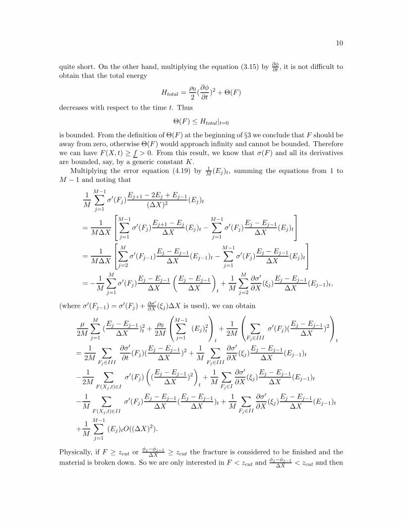
We are thus more confident to apply the numerical scheme to more general problem and toa two dimensional problem in the next section. The initial values of the Riemann problemsare of the form (3.6). Figure 5.4 shows the shock propagation in the variable F = φX wherewe choose Fl = Fr = 1 and Fm = 1.1. U = (F, v) is always located in the hyperbolic region.In Figure 5.5 we choose Fl = Fr = 1 and Fm = 1.2 and the initial U is in elliptic regionwhen X ∈ [12 − δ, 1

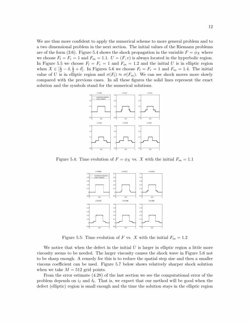
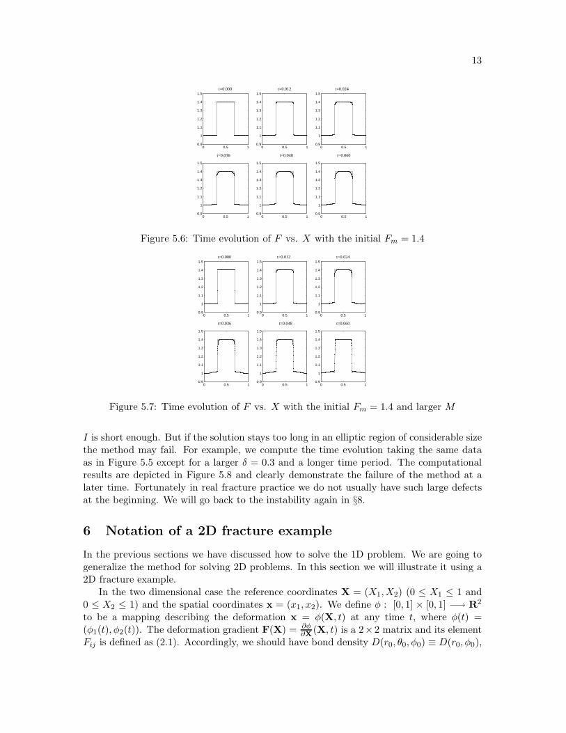
2 + δ]. In Figures 5.6 we choose Fl = Fr = 1 and Fm = 1.4. The initialvalue of U is in elliptic region and σ(Fl) ≈ σ(Fm). We can see shock moves more slowlycompared with the previous cases. In all these figures the solid lines represent the exactsolution and the symbols stand for the numerical solutions.

0 0.5 10.9

1

1.1

1.2

1.3

numerical solutionexact solution

0 0.5 10.9

1

1.1

1.2

1.3

0 0.5 10.9

1

1.1

1.2

1.3

0 0.5 10.9

1

1.1

1.2

1.3

0 0.5 10.9

1

1.1

1.2

1.3

0 0.5 10.9

1

1.1

1.2

1.3

t=0.036 t=0.048 t=0.060

t=0.012 t=0.024t=0.000

Figure 5.4: Time evolution of F = φX vs. X with the initial Fm = 1.1

0 0.5 10.9

1

1.1

1.2

1.3

1.4

1.5

0 0.5 10.9

1

1.1

1.2

1.3

1.4

1.5

0 0.5 10.9

1

1.1

1.2

1.3

1.4

1.5

0 0.5 10.9

1

1.1

1.2

1.3

1.4

1.5

0 0.5 10.9

1

1.1

1.2

1.3

1.4

1.5

0 0.5 10.9

1

1.1

1.2

1.3

1.4

1.5

numerical solutionexact solution

t=0.000 t=0.012 t=0.024

t=0.036 t=0.048 t=0.060

Figure 5.5: Time evolution of F vs. X with the initial Fm = 1.2

We notice that when the defect in the initial U is larger in elliptic region a little moreviscosity seems to be needed. The larger viscosity causes the shock wave in Figure 5.6 notto be sharp enough. A remedy for this is to reduce the spatial step size and then a smallerviscous coefficient can be used. Figure 5.7 below shows relatively sharper shock solutionwhen we take M = 512 grid points.

From the error estimate (4.28) of the last section we see the computational error of theproblem depends on iI and δt. That is, we expect that our method will be good when thedefect (elliptic) region is small enough and the time the solution stays in the elliptic region

13

0 0.5 10.9

1

1.1

1.2

1.3

1.4

1.5

0 0.5 10.9

1

1.1

1.2

1.3

1.4

1.5

0 0.5 10.9

1

1.1

1.2

1.3

1.4

1.5

0 0.5 10.9

1

1.1

1.2

1.3

1.4

1.5

0 0.5 10.9

1

1.1

1.2

1.3

1.4

1.5

0 0.5 10.9

1

1.1

1.2

1.3

1.4

1.5

t=0.000 t=0.012 t=0.024

t=0.036 t=0.048 t=0.060

Figure 5.6: Time evolution of F vs. X with the initial Fm = 1.4

0 0.5 10.9

1

1.1

1.2

1.3

1.4

1.5

0 0.5 10.9

1

1.1

1.2

1.3

1.4

1.5

0 0.5 10.9

1

1.1

1.2

1.3

1.4

1.5

0 0.5 10.9

1

1.1

1.2

1.3

1.4

1.5

0 0.5 10.9

1

1.1

1.2

1.3

1.4

1.5

0 0.5 10.9

1

1.1

1.2

1.3

1.4

1.5

t=0.000 t=0.012 t=0.024

t=0.036 t=0.048 t=0.060

Figure 5.7: Time evolution of F vs. X with the initial Fm = 1.4 and larger M

I is short enough. But if the solution stays too long in an elliptic region of considerable sizethe method may fail. For example, we compute the time evolution taking the same dataas in Figure 5.5 except for a larger δ = 0.3 and a longer time period. The computationalresults are depicted in Figure 5.8 and clearly demonstrate the failure of the method at alater time. Fortunately in real fracture practice we do not usually have such large defectsat the beginning. We will go back to the instability again in §8.

6 Notation of a 2D fracture example

In the previous sections we have discussed how to solve the 1D problem. We are going togeneralize the method for solving 2D problems. In this section we will illustrate it using a2D fracture example.

In the two dimensional case the reference coordinates X = (X1,X2) (0 ≤ X1 ≤ 1 and0 ≤ X2 ≤ 1) and the spatial coordinates x = (x1, x2). We define φ : [0, 1] × [0, 1] −→ R2

to be a mapping describing the deformation x = φ(X, t) at any time t, where φ(t) =(φ1(t), φ2(t)). The deformation gradient F(X) = ∂φ

∂X (X, t) is a 2×2 matrix and its elementFij is defined as (2.1). Accordingly, we should have bond density D(r0, θ0, φ0) ≡ D(r0, φ0),

14

0 0.5 1

1

1.2

1.4

0 0.5 1

1

1.2

1.4

0 0.5 1

1

1.2

1.4

0 0.5 1

1

1.2

1.4

0 0.5 1

1

1.2

1.4

0 0.5 1

1

1.2

1.4

t=0.000 t=0.060 t=0.120

t=0.180 t=0.240 t=0.300

Figure 5.8: Longer time evolution of F vs. X with Fm = 1.2 and δ = 0.3

Green-Lagrangian strain tensor r = r0

√1 + 2ξT Eξ where ξ = (cosφ0, sinφ0). The strain

energy is thus

Θ(F) =∫ ∞

0

∫ 2π

0D(r0, φ0)Φ(r0

√1 + 2ξTEξ, r0)dr0dφ0, (6.1)

where1 + 2ξTEξ = F 2

11 + F 221 + (F11F12 + F21F22) sinφ0 cosφ0 + F 2

12 + F 222. (6.2)

For simplicity we select the bond density function as

D(r0, φ0) = β0δ(r0 − r∗)[δ(φ0) + δ(φ0 − 2π/3) + δ(φ0 − 4π/3)]

which corresponds to materials with a triangular or a hexagonal lattice structure (cf. [3]).β0 is a scaling constant. Hence, we can obtain

Θ(F) = α0β0

{[−2 1

(F 212 + F 2

22)3+

1(F 2

12 + F 222)6

]+[

−2 1

(34 (F

211 + F 2

21)−√

32 (F11F12 + F21F22) + 1

4(F212 + F 2

22))3+

1

(34 (F

211 + F 2

21)−√

32 (F11F12 + F21F22) + 1

4(F212 + F 2

22))6

]+ (6.3)

[−2 1

(34 (F

211 + F 2

21) +√

32 (F11F12 + F21F22) + 1

4(F212 + F 2

22))3+

1

(34 (F

211 + F 2

21) +√

32 (F11F12 + F21F22) + 1

4(F212 + F 2

22))6

]}.

15

O X

X

1

2 pull upwards

fixed bottom

(a )

x or

x or φ

φ2 2

1 1

(b ) initial configuration

1.0

1.0

B

Aθ

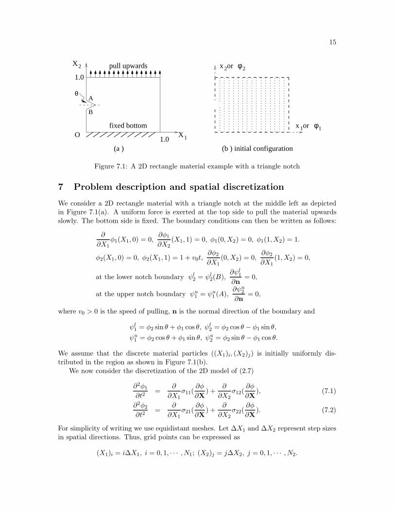
Figure 7.1: A 2D rectangle material example with a triangle notch

7 Problem description and spatial discretization

We consider a 2D rectangle material with a triangle notch at the middle left as depictedin Figure 7.1(a). A uniform force is exerted at the top side to pull the material upwardsslowly. The bottom side is fixed. The boundary conditions can then be written as follows:

∂

∂X1φ1(X1, 0) = 0,

∂φ1

∂X2(X1, 1) = 0, φ1(0,X2) = 0, φ1(1,X2) = 1.

φ2(X1, 0) = 0, φ2(X1, 1) = 1 + v0t,∂φ2

∂X1(0,X2) = 0,

∂φ2

∂X1(1,X2) = 0,

at the lower notch boundary ψl2 = ψl

2(B),∂ψl

1

∂n= 0,

at the upper notch boundary ψu1 = ψu

1 (A),∂ψu

2

∂n= 0,

where v0 > 0 is the speed of pulling, n is the normal direction of the boundary and

ψl1 = φ2 sin θ + φ1 cos θ, ψl

2 = φ2 cos θ − φ1 sin θ,

ψu1 = φ2 cos θ + φ1 sin θ, ψu

2 = φ2 sin θ − φ1 cos θ.

We assume that the discrete material particles ((X1)i, (X2)j) is initially uniformly dis-tributed in the region as shown in Figure 7.1(b).

We now consider the discretization of the 2D model of (2.7)

∂2φ1

∂t2=

∂

∂X1σ11(

∂φ

∂X) +

∂

∂X2σ12(

∂φ

∂X), (7.1)

∂2φ2

∂t2=

∂

∂X1σ21(

∂φ

∂X) +

∂

∂X2σ22(

∂φ

∂X). (7.2)

For simplicity of writing we use equidistant meshes. Let ∆X1 and ∆X2 represent step sizesin spatial directions. Thus, grid points can be expressed as

(X1)i = i∆X1, i = 0, 1, · · · , N1; (X2)j = j∆X2, j = 0, 1, · · · , N2.

16

Denote

(·)X1 =(·)i+1,j − (·)i,j

∆X1, (·)X2 =

(·)i,j+1 − (·)i,j+1

∆X2,

(·)X1=

(·)i,j − (·)i−1,j

∆X1, (·)X2

=(·)i,j − (·)i,j−1

∆X2,

Similarly (·)X stands for backward difference approximation and (·)X stands for forwarddifference approximation of derivatives involved in ∂(·)

∂X . We can then write down a secondorder difference scheme for spatial derivatives.

∂2φ1

∂t2=

12[(σ11(φX)X1 + (σ11(φX)X1

] +12[(σ12(φX)X2 + (σ12(φX)X2

], (7.3)

∂2φ2

∂t2=

12[(σ21(φX)X1 + (σ21(φX)X1

] +12[(σ22(φX)X2 + (σ22(φX)X2

]. (7.4)

To capture shock wave solutions correctly we add a viscous term µ ∂∂t [(φ1)X1X1

+ (φ1)X2X2]

to (7.3) and µ ∂∂t [(φ2)X1X1

+ (φ2)X2X2] to (7.4) as we did for the 1D case. We can then

solve the problem by using any initial value ODE solvers, for example, a second orderRunge-Kutta method.

8 Computational results of the 2D example

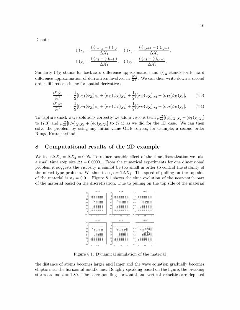
We take ∆X1 = ∆X2 = 0.05. To reduce possible effect of the time discretization we takea small time step size ∆t = 0.00001. From the numerical experiments for one dimensionalproblem it suggests the viscosity µ cannot be too small in order to control the stability ofthe mixed type problem. We thus take µ = 2∆X1. The speed of pulling on the top sideof the material is v0 = 0.01. Figure 8.1 shows the time evolution of the near-notch partof the material based on the discretization. Due to pulling on the top side of the material

0 0.5 1−0.2

0

0.2

0.4

0.6

0.8

1

1.2t=1.35

0 0.5 1−0.2

0

0.2

0.4

0.6

0.8

1

1.2t=1.50

0 0.5 1−0.2

0

0.2

0.4

0.6

0.8

1

1.2t=1.65

0 0.5 1−0.2

0

0.2

0.4

0.6

0.8

1

1.2t=1.80

0 0.5 1−0.2

0

0.2

0.4

0.6

0.8

1

1.2t=1.86

0 0.5 1−0.2

0

0.2

0.4

0.6

0.8

1

1.2t=1.92

Figure 8.1: Dynamical simulation of the material

the distance of atoms becomes larger and larger and the wave equation gradually becomeselliptic near the horizontal middle line. Roughly speaking based on the figure, the breakingstarts around t = 1.80. The corresponding horizontal and vertical velocities are depicted

17

0

0.51

0

0.5

10

0.005

0.01

0.015

t=1.35

00.5

1

0

0.5

10

0.01

0.02

t=1.50

0

0.51

0

0.5

10

0.02

0.04

t=1.65

0

0.51

0

0.5

1

0

t=1.80

00.5

1

0

0.5

1−0.5

0

0.5

t=1.86

0

0.51

0

0.5

10

1

2

t=1.92

Figure 8.2: Time evolution of the horizontal velocity

0

0.51

0

0.5

1−5

0

5

10

x 10−3

t=1.35

00.5

1

0

0.5

1−5

0

5

10

x 10−3

t=1.50

0

0.51

0

0.5

1−0.01

0

0.01

t=1.65

0

0.51

0

0.5

1

0

t=1.80

00.5

1

0

0.5

1

0

t=1.86

0

0.51

0

0.5

1−1

0

1

2

t=1.92

Figure 8.3: Time evolution of the vertical velocity

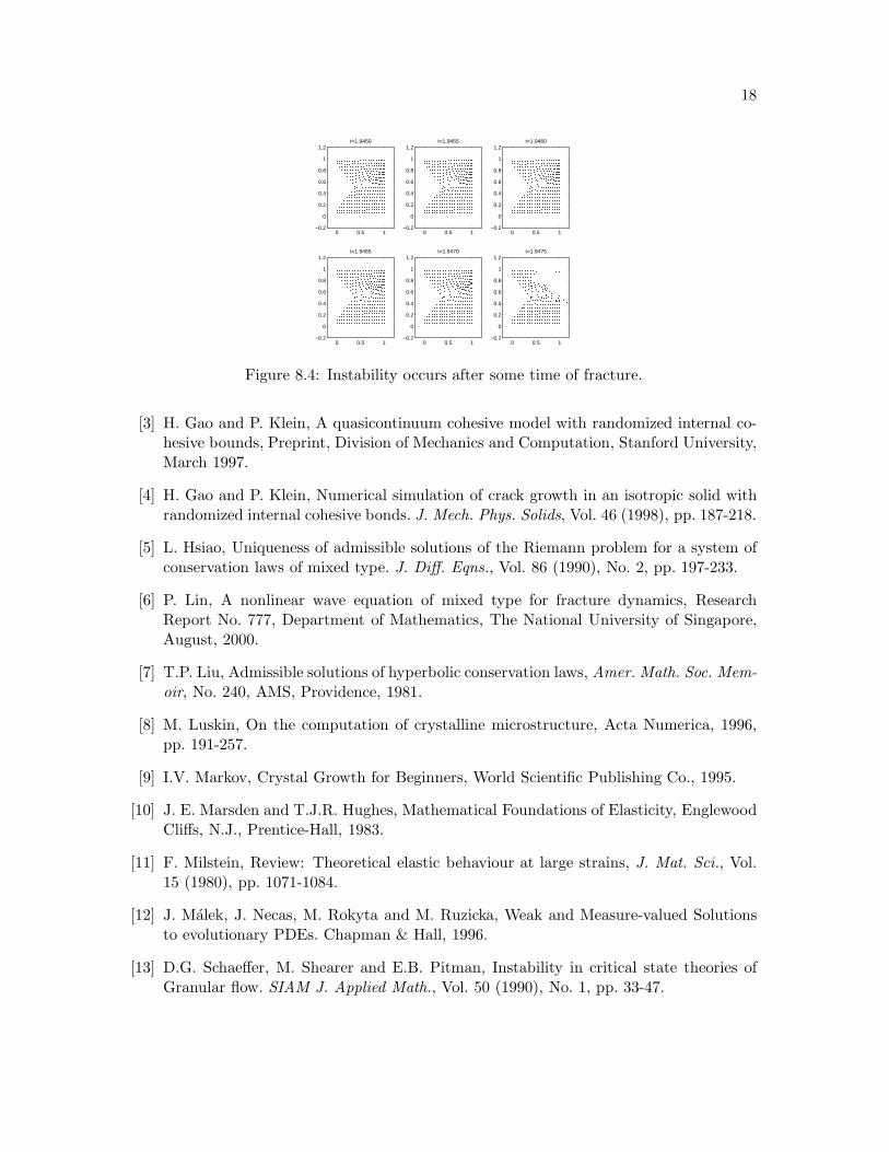
in Figures 8.2-8.3. We observe that when the material is pulled to approach the breakingstate the velocities start to increase faster. The wave equation becomes elliptic near thebreaking region. Once this situation lasts long enough instability may occur. Figure 8.4shows the material motion at a little bit later time and we see instability indeed takes place.The result implies that if δt in the error estimate (4.28) in §4 is long to some extent thenwe cannot ensure the convergence of our approximation. Nevertheless, the simulation ofearly stage of fracture should be trustable.

References

[1] M. Affouf and R.E. Caflisch, A numerical study of Riemann problem solutions andstability for a system of viscous conservation laws of mixed type. SIAM J. Appl. Math.,Vol. 51 (1991), No. 3, pp. 605-634.

[2] A. Balk, A. Cherkaev and L. Slepyan, Dynamics of solids with non-monotone stress-strain relations, I. Gibbs principle. J. Mech. Phys. Solids, to appear.

18

0 0.5 1−0.2

0

0.2

0.4

0.6

0.8

1

1.2t=1.9450

0 0.5 1−0.2

0

0.2

0.4

0.6

0.8

1

1.2t=1.9455

0 0.5 1−0.2

0

0.2

0.4

0.6

0.8

1

1.2t=1.9460

0 0.5 1−0.2

0

0.2

0.4

0.6

0.8

1

1.2t=1.9465

0 0.5 1−0.2

0

0.2

0.4

0.6

0.8

1

1.2t=1.9470

0 0.5 1−0.2

0

0.2

0.4

0.6

0.8

1

1.2t=1.9475

Figure 8.4: Instability occurs after some time of fracture.

[3] H. Gao and P. Klein, A quasicontinuum cohesive model with randomized internal co-hesive bounds, Preprint, Division of Mechanics and Computation, Stanford University,March 1997.

[4] H. Gao and P. Klein, Numerical simulation of crack growth in an isotropic solid withrandomized internal cohesive bonds. J. Mech. Phys. Solids, Vol. 46 (1998), pp. 187-218.

[5] L. Hsiao, Uniqueness of admissible solutions of the Riemann problem for a system ofconservation laws of mixed type. J. Diff. Eqns., Vol. 86 (1990), No. 2, pp. 197-233.

[6] P. Lin, A nonlinear wave equation of mixed type for fracture dynamics, ResearchReport No. 777, Department of Mathematics, The National University of Singapore,August, 2000.

[7] T.P. Liu, Admissible solutions of hyperbolic conservation laws, Amer. Math. Soc. Mem-oir, No. 240, AMS, Providence, 1981.

[8] M. Luskin, On the computation of crystalline microstructure, Acta Numerica, 1996,pp. 191-257.

[9] I.V. Markov, Crystal Growth for Beginners, World Scientific Publishing Co., 1995.

[10] J. E. Marsden and T.J.R. Hughes, Mathematical Foundations of Elasticity, EnglewoodCliffs, N.J., Prentice-Hall, 1983.

[11] F. Milstein, Review: Theoretical elastic behaviour at large strains, J. Mat. Sci., Vol.15 (1980), pp. 1071-1084.

[12] J. Malek, J. Necas, M. Rokyta and M. Ruzicka, Weak and Measure-valued Solutionsto evolutionary PDEs. Chapman & Hall, 1996.

[13] D.G. Schaeffer, M. Shearer and E.B. Pitman, Instability in critical state theories ofGranular flow. SIAM J. Applied Math., Vol. 50 (1990), No. 1, pp. 33-47.

19

[14] M. Shearer, The Riemann problem for a class of conservation laws of mixed type. J.Diff. Eqns., Vol. 46 (1982), pp. 426-443.

[15] C.-W. Shu, A numerical method for systems of conservation laws of mixed type ad-mitting hyperbolic flux splitting, J. Comp. Phys., Vol. 100 (1992), pp. 424-429.

[16] M. Slemrod and J.E. Flaherty, Numerical integration of a Riemann problem for a vander Waals fluid. Preprint.

[17] J.A. Smoller, Shock Waves and Reaction-Diffusion Equations, Springer-Verlag, NewYork, 1983.

[18] E.B. Tadmor, M. Ortiz and R. Phillips, Quasicontinuum analysis of defects in solids,Philosophical Magazine A, Vol. 73, No. 6, 1996, pp. 1529-1563.