Journal of Computational and Applied Mathematics 140 (2002) 537–557 www.elsevier.com/locate/cam Numerical solution of a nonuniquely solvable Volterra integral equation using extrapolation methods Pedro Lima ∗; 1 , Teresa Diogo 1 Departamento de Matem atica, Instituto Superior T ecnico, Av. Rovisco Pais, 1049-001 Lisbon, Portugal Received 20 September 2000; received in revised form 6 February 2001 Abstract In this work the numerical solution of a Volterra integral equation with a certain weakly singular kernel, depending on a real parameter , is considered. Although for certain values of this equation possesses an innite set of solutions, we have been able to prove that Euler’s method converges to a particular solution. It is also shown that the error allows an asymptotic expansion in fractional powers of the stepsize, so that general extrapolation algorithms, like the E-algorithm, can be applied to improve the numerical results. This is illustrated by means of some examples. c 2002 Elsevier Science B.V. All rights reserved. MSC: 65R20 Keywords: Volterra integral equations; Weakly singular kernel; Euler’s method; Asymptotic expansions; E-algorithm 1. Introduction We consider the second kind Volterra integral equation L u(t )= g(t ); t ∈ [0;T ]; (1.1) with L u(t ) := u(t ) − t 0 s −1 t u(s)ds; (1.2) ∗ Corresponding author. E-mail addresses: [email protected] (P. Lima), [email protected] (T. Diogo). 1 Work supported by Funda c˜ ao para a Ciˆ encia e Tecnologia, Centro de Matem atica Aplicada= I.S.T. (Lisbon, Portugal). 0377-0427/02/$ - see front matter c 2002 Elsevier Science B.V. All rights reserved. PII: S0377-0427(01)00408-3

Welcome message from author
This document is posted to help you gain knowledge. Please leave a comment to let me know what you think about it! Share it to your friends and learn new things together.
Transcript
Journal of Computational and Applied Mathematics 140 (2002) 537–557www.elsevier.com/locate/cam
Numerical solution of a nonuniquely solvable Volterra integralequation using extrapolation methods
Pedro Lima ∗; 1, Teresa Diogo1
Departamento de Matem�atica, Instituto Superior T�ecnico, Av. Rovisco Pais, 1049-001 Lisbon, Portugal
Received 20 September 2000; received in revised form 6 February 2001
Abstract
In this work the numerical solution of a Volterra integral equation with a certain weakly singular kernel, depending ona real parameter �, is considered. Although for certain values of � this equation possesses an in6nite set of solutions, wehave been able to prove that Euler’s method converges to a particular solution. It is also shown that the error allows anasymptotic expansion in fractional powers of the stepsize, so that general extrapolation algorithms, like the E-algorithm,can be applied to improve the numerical results. This is illustrated by means of some examples. c© 2002 Elsevier ScienceB.V. All rights reserved.
MSC: 65R20
Keywords: Volterra integral equations; Weakly singular kernel; Euler’s method; Asymptotic expansions; E-algorithm
1. Introduction
We consider the second kind Volterra integral equation
L�u(t) = g(t); t ∈ [0; T ]; (1.1)
with
L�u(t) := u(t) −∫ t
0
s�−1
t�u(s) ds; (1.2)
∗ Corresponding author.E-mail addresses: [email protected] (P. Lima), [email protected] (T. Diogo).1 Work supported by FundaBcao para a Ciencia e Tecnologia, Centro de MatemEatica Aplicada=I.S.T. (Lisbon, Portugal).
0377-0427/02/$ - see front matter c© 2002 Elsevier Science B.V. All rights reserved.PII: S 0377-0427(01)00408-3
538 P. Lima, T. Diogo / Journal of Computational and Applied Mathematics 140 (2002) 537–557
where �¿0 and g is a given function. The above equation can arise in connection with some heatconduction problems with mixed-type boundary conditions [1,8]. A simple example is given by
@2u@x2 =
1a2
@u@t
; 06 x6 l; (1.3)
with the conditions
u(x;−∞) = 0; (1.4)
@u@x
(0; t) − u(0; t) = �1(t); (1.5)
−@u@x
(l; t) − u(l; t) = �2(t): (1.6)
By expressing the solution in terms of single layer potentials (see e.g. [24, pp. 462–465]), a systemof two coupled integral equations is obtained. Under certain conditions on the parameter l, thissystem can be simpli6ed yielding two independent equations with the form
F(t) +∫ t
0
1√�
1√ln(t=s)
1sF(s) ds = H (t); t ∈ [0; T ]: (1.7)
Following the approach used in [9], the above equation can be transformed into one of the type of(1.1). We note that a more complex problem leading to a system of equations of the type of (1.7)was considered by Bartoshevich [1]. The analytical study of this and other related equations hasbeen pursued by several authors ([25,23,17,26,18,13]). In particular, it was proved in [26] that (1.1)has a unique solution in the continuity class Cm[0; T ] if g is in Cm[0; T ] and �¿1. However, if0¡�6 1, then (1.1) has a family of solutions in C[0; T ], of which only one has C1 continuity [13](compare also [6] for the study of a certain homogeneous Volterra integral equation of the secondkind).
For the numerical solution of (1.1), in the case �¿1, certain classes of product integration meth-ods were studied. We note that the kernel of (1.1), that is, the function p(t; s) = s�−1=t�, is in-tegrable with respect to s in [0; T ]. For this reason we say that p is a weakly singular function.The numerical solution of Volterra integral equations with weakly singular kernels of the formq(t; s) = (t − s)−�; 0¡�¡1, has been considered by many authors. In particular, methods based ongeneralized Newton–Cotes formulae combined with product integration techniques were studied in[19,7,15]. For a comprehensive study of numerical methods for Volterra integral equations we referto [5]. Among more recent works we refer to [11] and the references therein. It should be notedthat, unlike the Abel-type kernel q, p does not satisfy
∫ t0 p(t; s) ds → 0 as t → 0+. Moreover, all the
iterated kernels associated with p are unbounded. Owing to these properties, the classical argumentsin the convergence analysis of discretization methods for weakly singular equations are not applica-ble. In [26] approximations to the solution of (1.7) of orders one and two were obtained with theEuler and trapezoidal methods, respectively. In [9] a fourth order Hermite-type collocation methodwas applied to (1.1) and, recently, the analysis and construction of higher order product integrationmethods has been investigated in [8]. In [18] we were concerned with the use of a low order methodin conjunction with extrapolation procedures. Eq. (1.1) was transformed into a new one, so that thetwo equations were equivalent away from the origin. Under appropriate conditions, although for acertain g the solution of the original equation could be unbounded at the origin, the corresponding
P. Lima, T. Diogo / Journal of Computational and Applied Mathematics 140 (2002) 537–557 539
solution of the new equation was smooth. Euler’s method was then used to approximate the solutionof the new equation and 6rst order convergence was proved. Moreover, under certain conditions,the error was shown to allow an asymptotic error expansion in integer powers of the stepsize whichpermitted the use of Richardson’s extrapolation. Extrapolation methods based on the midpoint rulehave been studied in [14] for nonlinear Volterra equations with smooth kernels (see also [12,4] andthe references therein). The idea of solution regularization transformations was used in [21,22,10]with Abel-type equations and, recently, in [11], for both continuous and Abel-type kernels.
In the present paper we further develop the work carried out in [18]. We shall be mainly concernedwith the case when 0¡�6 1. Although for these values of � Eq. (1.1) has a family of solutions inC[0; T ], we have been able to prove that Euler’s method converges to a certain particular solution.This work is organized as follows. In Section 2 we present some de6nitions and preliminary resultson existence and uniqueness of solution. We also prove a smoothness property which will be used inthe convergence analysis. In Section 3 the application of Euler’s method is considered and a generalconvergence result is obtained for all �¿0, under the assumption that g∈C1[0; T ]. The case wheng is not suNciently smooth is dealt with by using an appropriate transformation of the equation.Section 4 is devoted to a detailed error analysis and, in the case 0¡�¡1, convergence of order � isproved. Furthermore, using a sharper analysis than the one in [18], we obtain new asymptotic errorexpansions for the case �¿1. In particular, if 1¡�6 2 and g∈C2[0; T ] with g′(0) �= 0, then theasymptotic error expansion will contain fractional powers of h and powers of h multiplied by ln h.We point out that, although only the case when 1¡�6 2 has been considered, the same argumentcan in principle be employed to deal with higher values of �. Such expansions will permit the use ofmore general extrapolation procedures, like the E-algorithm, and some numerical examples illustratetheir application in Section 5.
2. Smoothness of solutions
We start by presenting some de6nitions and lemmas. For T¿0 and m a nonnegative integer,Vm[0; T ] denotes the normed space of the real valued functions f such that f∈Cm[0; T ] with
‖f‖m := max06 j6m
maxt ∈ [0;T ]
|f(j)(t)|: (2.1)
De�nition 2.1. For T¿0, �¿ 0 and m¿ 0, Vm;�[0; T ] denotes the normed space of real valuedfunctions f such that t�f∈Vm[0; T ] with
‖f‖m;� := ‖t�f‖m = max06 j6m
maxt ∈ [0;T ]
∣∣∣∣ d j
dtj(t�f(t))
∣∣∣∣ : (2.2)
De�nition 2.2. Let m¿ 1. Then f∈V 0m[0; T ] if and only if f∈Vm[0; T ] and f(0) = f′(0) = · · · =
f(m−1)(0) = 0. If m = 0, we have V 00 [0; T ] = V0[0; T ].
De�nition 2.3. Let m¿ 1 and �¿ 0. Then f∈V 0m;�[0; T ] if and only if t�f∈V 0
m[0; T ]. If m = 0,we have V 0
0; �[0; T ] = V0; �[0; T ].
540 P. Lima, T. Diogo / Journal of Computational and Applied Mathematics 140 (2002) 537–557
The following result concerning existence and uniqueness of solution can be found in [18].
Lemma 2.1. Let �¿ 0 and �¿1 + �. (i) If the function g in (1:1) belongs to Vm;�[0; T ] then(1:1) has a unique solution u∈Vm;�[0; T ]. (ii) If g∈V 0
m;�[0; T ]; then (1:1) has a unique solutionu∈V 0
m;�[0; T ].
A further result was proved by [13] which includes the case when 0¡�6 1.
Lemma 2.2. (a) If 0¡�6 1 and g∈V1[0; T ] (with g(0) = 0 if � = 1) then (1:1) has a family ofsolutions u∈V0[0; T ] given by the formula
u(t) = c0t1−� + g(t) + + t1−�∫ t
0s�−2(g(s) − g(0)) ds; (2.3)
where
:=
1� − 1
g(0) if �¡1;
0 if � = 1;(2.4)
and c0 is an arbitrary constant. Out of the family of solutions there is one particular solutionu∈V1[0; T ]. Such a solution is unique and can be obtained from (2:3) by taking c0 = 0.
(b) If �¿1 and g∈Vm[0; T ]; m¿ 0; then the unique solution u∈Vm[0; T ] of (1:1) is
u(t) = g(t) + t1−�∫ t
0s�−2g(s) ds: (2.5)
We note that (2:5) can be obtained from (2:3) with c0 = 0. Indeed; it follows from (2:3) that
c0 = limt→0+
t�−1u(t); (2.6)
and this limit is zero when �¿1.
We now obtain a result which characterizes the particular solution referred to in part (a) of theprevious lemma.
Theorem 2.1. Consider Eq. (1:1) with g∈V1[0; T ].
(a) If �¿0 and � �= 1 then (1:1) has a unique solution of the form
u(t) = u0 + z(t); (2.7)
where z(t) = O(t); as t → 0+; and u0 is a constant.(b) If � = 1 and g(0) = 0; then (1:1) has a unique solution which satis9es
u(t) = z(t); (2.8)
where z(t) = O(t); as t → 0+.
P. Lima, T. Diogo / Journal of Computational and Applied Mathematics 140 (2002) 537–557 541
Proof. The ideas of this proof will be used in the discretization of (1.1) in the next sections.Consider 6rst the case when 0¡�6 1. Writing
g(t) = g(0) + g1(t); (2.9)
this suggests splitting (1.1) into two equations
L�y(t) = g(0) (2.10)
and
L�z(t) = g1(t): (2.11)
Then the solution u of (1.1) can be represented in the form
u(t) = y(t) + z(t); (2.12)
where y and z are the solutions of (2.10) and (2.11), respectively. It follows from (2.3) that thegeneral solution y is given by the formula
y(t) = c0t1−� + u0; (2.13)
where
u0 :=
�� − 1
g(0) if �¡1;
0 if � = 1:(2.14)
An expression for z(t) can also be obtained from (2.3) and, using the fact that g1(0) = 0, we get
z(t) = d0t1−� + g1(t) + t1−�∫ t
0s�−2g1(s) ds; (2.15)
where
d0 = limt→0+
t�−1z(t) = limt→0+
t�z(t)t
: (2.16)
We note that if z(t)=t is continuous at t = 0 then d0 = 0, in which case we obtain the (unique)particular solution of (2.11) which is in V1[0; T ]. Setting c0 = 0 in (2.13), we may conclude that
u(t) = u0 + g1(t) + t1−�∫ t
0s�−2g1(s) ds (2.17)
is a particular solution to (1.1) of the form (2.7) and it remains to show that z(t) =O(t). It followsfrom (2.15), with d0 = 0,
limt→0+
z(t)t
= g′(0) + limt→0+
t−�∫ t
0s�−2g1(s) ds
= g′(0) + limt→0+
∫ 1
0%�−1 g1(t%)
t%d%
= g′(0) + limt→0+
g1(t&)t&
∫ 1
0%�−1 d%
= g′(0)(
1 +1�
): (2.18)
542 P. Lima, T. Diogo / Journal of Computational and Applied Mathematics 140 (2002) 537–557
We have thus proved that z(t) = O(t), as t → 0+. In the case � = 1 we require that g(0) = 0. Thenwe have u0 = 0 and we may rewrite (2.17) as
u(t) = g(t) + t1−�∫ t
0s�−2g(s) ds: (2.19)
Therefore, we have obtained a particular solution of form (2.8) which satis6es u(t)=O(t), as t → 0+.Finally, we note that the same analysis applies to the case when �¿1, by using the fact that
c0 = 0 in (2.3).
Corollary 2.1. Let � be a real number such that g(t) = t� Og(t) in (1:1); with Og∈V1[0; T ].
(a) If � + �¿0 and � + � �= 1 then (1:1) has a unique solution of the form
u(t) = u0t� + Oz(t); (2.20)
where Oz(t) = O(t�+1); as t → 0+; and v0 is a constant.(b) If � + � = 1 and Og(0) = 0; then
u(t) = Oz(t); (2.21)
where Oz(t) = O(t�+1); as t → 0+.
Proof. The above result can be easily obtained by applying Theorem 2.1 to the equation
L�+�v(t) = Og(t); (2.22)
where
Og(t) := t−�g(t) (2.23)
and
v(t) := t−�u(t): (2.24)
Remark 2.1. It may happen that, although �¿1, we might have � + �¡1. In this case, Eq. (1.1)has a unique solution but the auxiliary equation (2.22) has an in6nite set of solutions (accordingto Lemma 2.2). Therefore equality (2.24) is valid only for the particular solution of (2.22) whichbelongs to V1[0; T ].
3. Numerical solutions
In this section we consider the application of Euler’s method to Eq. (1.1). The case when �¿1was studied in [18]. Assuming g∈V0[0; T ], the Euler’s method was shown to converge to the uniquesolution u of (1.1). Here we shall give a general convergence result valid for all values of �¿0under the assumption that g∈V1[0; T ]. In the case 0¡�6 1, we have seen that (1.1) has a familyof solutions of which only one is in the continuity class C1 (cf. Theorem 2.1). Here we show thatthe approximate solution obtained by Euler’s method converges to this particular solution.
P. Lima, T. Diogo / Journal of Computational and Applied Mathematics 140 (2002) 537–557 543
Let Xh := {ti = ih; 06 i6N} be an uniform grid with stepsize h :=T=N . Consider in RN+1 themaximum norm
‖vh‖ := max06 i6N
|vi| (3.1)
and de6ne the linear restriction operator rh :V0[0; T ] → RN+1 by
(rhf(t))i :=f(ti); 06 i6N: (3.2)
Let us associate with the operator L� de6ned by (1.2) the linear discrete operator Lh� : RN+1 → RN+1
such that
(Lh�v
h)k :=
vh0�−1� ; k = 0;
vhk − t−�k
∑k−1
i=0Divhi ; 16 k6N;
(3.3)
where
D0 :=∫ t1
t0
s�−1 ds = h�=�; Di :=∫ ti+1
ti
s�−1 ds = h� (i + 1)� − i�
�; 16 i6N − 1: (3.4)
Then Euler’s method for (1.1) is given by
Lh�u
h = rhg; (3.5)
with initial value uh0 = u(0) = u0, where u0 is given by (2.14). In the convergence analysis it will be
convenient to consider the following equivalent approach based on the ideas of splitting (1.1) intotwo equations (2.10) and (2.11). We seek an approximation uh to the solution of (1.1) in the form
uh = yh + zh; (3.6)
where yh and zh are approximate solutions of Eqs. (2.10) and (2.11), respectively. Then we considerthe following discretization of Eq. (2.10):
Lh�y
h = g0; (3.7)
where each entry yhk of the vector yh is an approximation to y(tk); k = 1; : : : ; N; and g0 = (g(0); : : : ;
g(0))T. An initial value is needed and, if � �= 1, we take
yh0 = g(0)
�� − 1
= u0: (3.8)
Then (3.7) has only one solution given by
yhk = g(0)
�� − 1
; k = 1; 2; : : : ; N: (3.9)
If �= 1, we require that g(0) = 0 and set yhk = 0; k = 0; 1; : : : ; N . In order to obtain an approximation
to the solution z of (2.11), we instead consider the following equation:
L�+1�(t) = G(t); (3.10)
where G and � are the continuous functions
G(t) :=g1(t)t
; �(t) :=z(t)t
: (3.11)
544 P. Lima, T. Diogo / Journal of Computational and Applied Mathematics 140 (2002) 537–557
Now let �h be the solution of
Lh�+1�
h = rhG; (3.12)
where each component �hk of the vector �h is an approximation to �(tk); k = 1; 2; : : : ; N . Here we
take
�h0 =
� + 1�
limt→0+
g1(t)t
= g′(0)� + 1�
: (3.13)
Then, using (3.12), we obtain that tk�hk will be an approximation to z(tk), that is, we set
zhk = tk�hk ; k = 1; 2; : : : ; N: (3.14)
We now prove the following convergence result.
Theorem 3.1. Consider Eq. (1:1) with g∈V1[0; T ]. If �¿0 and � �= 1 then the approximate solutionuh de9ned by (3:6) converges to the particular solution of (1:1) which has the form (2:7). If � = 1and g(0)=0; then the approximate solution uh de9ned by (3:6) converges to the particular solutionof (1:1) which has the form (2:8).
Proof. Let us 6rst consider the case � �= 1 and let u be the particular solution referred to in Theorem2.1. That is, u is given by (2.17) and, using (2.12) and (3.6), we may write
‖rhu− uh‖6 ‖rhy − yh‖ + ‖rhz − zh‖: (3.15)
From (3.9) it follows immediately that
‖rhy − yh‖ = 0: (3.16)
In order to prove that ‖rhz − zh‖ → 0, as h → 0+, we 6rst note that, since z(t) = t�(t), we have
(rhz − zh)k = tk(rh�− �hk): (3.17)
We follow the ideas of Theorem 3:2 of [18] to prove that
‖Lh�+1(rh�) − rh(L�+1�)‖ → 0: (3.18)
We have
(Lh�+1(rh�) − rh(L�+1�))k = t−�
k
k−1∑i=0
(∫ ti+1
ti
s�−1�(s) ds− Di�(ti))
; 16 k6N: (3.19)
Using the mean value theorem for integrals yields∫ ti+1
ti
s�−1�(s) ds = �(&i)∫ ti+1
ti
s�−1 ds: (3.20)
with &i ∈ (ti; ti+1), 06 i6 k − 1. Substituting (3.20) into (3.19), we obtain
(Lh�+1(rh�) − rh(L�+1�))k = t−�
k
k−1∑i=0
Di(�(&i) − �(ti)); 16 k6N; (3.21)
P. Lima, T. Diogo / Journal of Computational and Applied Mathematics 140 (2002) 537–557 545
which yields, after taking modulus,
|(Lh�+1(rh�) − rh(L�+1�))k |6 t−�
k max06 i6 k−1
|�(&i) − �(ti)|k−1∑i=0
Di; 16 k6N: (3.22)
Since �∈V0[0; T ] then max06 i6N |�(&i) − �(ti)| → 0 as h → 0+ and we obtain (3.18). Next, wenote that
Lh�+1(�h − rh�) = Lh
�+1(�h) − Lh�+1(rh�) = rh(L�+1�) − Lh
�+1(rh�): (3.23)
On the other hand, it can be shown that the following stability condition is satis6ed:
‖�h − rh�‖6 1� + 1
‖rh(L�+1�) − Lh�+1(rh�)‖; (3.24)
which, combined with (3.23), gives
‖rh�− �h‖ → 0 as h → 0+: (3.25)
Then from (3.17) we obtain
‖rhz − zh‖ → 0 as h → 0+: (3.26)
Finally, using (3.16) and (3.26) in (3.15), the desired result follows.In the case � = 1, we note that y(t) ≡ 0 and yh
k = 0; k = 1; : : : ; N . Hence u(t) = z(t) and uh = zh.The convergence result concerning zh may be proved in the same way as when � �= 1.
Remark 3.1. It should be noted that the case when g �∈V1[0; T ] can be dealt with using Corollary2.1. If there exists �∈R such that g(t) = t� Og(t), with Og∈V1[0; T ], then Eq. (1.1) has a uniquesolution u of form (2.20) or (2.21), respectively, if �+� �= 1 or �+�= 1. This solution is obtainedby introducing the auxiliary equation (2.22)
L�+�v(t) = Og(t);
and taking u(t) = t�v(t). Then we consider the following discretization of (2.22):
Lh�+�v
h = rh Og; (3.27)
where vh is the vector with components vhi := t−�i uh
i , i = 1; : : : ; N . Since Og∈V1[0; T ], it follows fromTheorem 3.1 that uh converges to u as h → 0 in the sense that
‖t�uh − rht�u‖ → 0; (3.28)
provided that � + �¿ 0.
4. Error analysis
In order to apply extrapolation methods, we need to know not only the main term of the asymp-totic error expansion but also terms of higher orders. In [18], we have proved that if g∈V 0
m[0; T ],
546 P. Lima, T. Diogo / Journal of Computational and Applied Mathematics 140 (2002) 537–557
m¿ 1, and �¿1, the numerical solution uh, obtained by Euler’s method, allows an asymptotic errorexpansion in integer powers of h
(rhu− uh)k =m−1∑q=1
Cq(tk)hq + O(hm); (4.1)
where Cq ∈V 0m−q[0; T ] do not depend on h. The above expansion was the basis for applying the
Richardson’s extrapolation method in order to improve the numerical results.In this section it will be shown that if g′(0) �= 0 the asymptotic error expansions will contain
terms of more general forms. Both cases when 0¡�¡1 and �¿1 will be considered. In particular,if 0¡�¡1 convergence of order � is obtained.
We shall need the following auxiliary lemma.
Lemma 4.1. Let Lh� be de9ned by (3:3) and consider the following di;erence equation:
Lh�e
h = r; (4.2)
where
r = (0; c; : : : ; c); r ∈RN+1; c∈R:Then eh does not depend on h and the following asymptotic equalities hold:
(a) If � = 1; ehk = c ln k + O(1); as k → ∞;(b) If �¡1; ehk = C�k1−� + O(1); as k → ∞; where C� ∈RN+1 is independent of k.
Proof. (a) If � = 1, from (3.4) we have
Di = ti+1 − ti = h; i = 1; : : : ; N: (4.3)
Then the diPerence equation (4.2) reduces to the form
ehk −htk
k−1∑i=0
ehi = rk ; k = 1; : : : ; N: (4.4)
Substituting into (4.4) the explicit form of r, we obtain eh0 = 0,
ehk = c +1h
k−1∑i=0
ehi = rk ; k = 1; : : : ; N: (4.5)
From (4.5) it follows that
ehk − ehk−1 =ck: (4.6)
Since eh0 = 0, (4.6) implies that
ehk = ck∑
i=0
1i; k = 1; : : : ; N: (4.7)
P. Lima, T. Diogo / Journal of Computational and Applied Mathematics 140 (2002) 537–557 547
The sum on the right-hand side of (4.7) does not depend on h and its asymptotic expansion is wellknown (see e.g. [16, p. 220]):
k∑i=0
1i
= ln k + + O(
1k
); (4.8)
where is the so-called Euler’s constant. The desired result follows from (4.7) and (4.8).(b) Let us write (4.2) in the form
ehk − t−�k
k−1∑i=0
Diehi = c; k = 1; : : : ; N; (4.9)
where the weights Di are given by (3.4). From (4.9), it follows that
t�k ehk − (t�k + Dk−1)ehk−1 = c(t�k − t�k−1); k = 1; : : : ; N; (4.10)
Dividing both sides of (4.10) by h�, we obtain
k�ehk −[
(k − 1)� +k� − (k − 1)�
�
]ehk−1 = c(k� − (k − 1)�); k = 1; : : : ; N: (4.11)
The last equation is a 6rst order linear diPerence equation. Its solution does not depend on h andtherefore we shall denote it ek . In order to solve it using the methods described in [16, Chapter 3],let us introduce the variable substitution
Oek = k�−1ek : (4.12)
Then (4.11) reduces to
k Oek −[
(k − 1) +k� − (k − 1)�
�(k − 1)�−1
]Oek−1 = c(k� − (k − 1)�); k = 1; : : : ; N: (4.13)
Let us 6rst consider the homogeneous equation associated with (4.13) and denote the general solutionof this equation Oe0
k . We have
Oe 0k = d
k∏i=0
[i − 1i
+i� − (i − 1)�
�(i − 1)�−1i
]; (4.14)
where d is an arbitrary constant. The general term of the product (4.14) may be rewritten as
k − 1k
+k� − (k − 1)�
�(k − 1)�−1k= 1 − 1
k+
1k
(1 + O
(1k
))= 1 + O
(1k2
): (4.15)
Therefore, the product on the right-hand side of (4.14) is convergent. Moreover, if we consider thelogarithm of this product and analyse the resulting series, using the Euler–Maclaurin theorem (see[27, pp. 32–42]) we obtain the following asymptotic expansion:
Oe 0k = C� + O
(1k
)as k → ∞; (4.16)
where C� does not depend on k. From (4.16) and (4.12) it follows immediately that
e0k = C�k1−� + O(k−�) as k → ∞: (4.17)
548 P. Lima, T. Diogo / Journal of Computational and Applied Mathematics 140 (2002) 537–557
Let us now 6nd a particular solution of the non-homogeneous equation (4.11). Using the method ofvariation of parameters as in [16, p. 67], it can be shown that (4.11) has a solution of the form
e1k = e0
kak ; (4.18)
where ak satis6es
e0k+1Qak = c
k� − (k − 1)�
k� (4.19)
and Qak := ak+1 − ak . Since e0k = C�k1−� + O(k−�) and
k� − (k − 1)�
k� = O(k−1);
it follows from (4.19) that Qak =O(k�−2). Therefore, ak =O(k�−1) and, substituting this into (4.18),we may conclude that e1
k = O(1). Finally, using the theory of linear nonhomogeneous equations, weobtain that the general solution of (4.11) is given by
ek = e0k + e1
k = C�k1−� + O(1) + O(k−�) = C�k1−� + O(1): (4.20)
This concludes the proof of Lemma 4.1.
Theorem 4.1. Consider Eq. (1:1) with g∈V2[0; T ] and g′(0) �= 0. If 0¡�¡1 then the approximatesolution uh de9ned by (3:6) satis9es the error estimate
(rhu− uh)k = C�(tk)h� + O(h); (4.21)
where C� does not depend on h.
Proof. Since g∈V2[0; T ] and g′(0) �= 0, it follows from Theorem 2.1 that there exists a solution u,such that u∈V2[0; T ] and u′(0) �= 0. Then we may write
u(t) = u0 + at + tu(t); (4.22)
where u0 = u(0) is given by (2.14), a := u′(0) �= 0 and u(t)∈V 01 [0; T ]. We shall again make use
of the decomposition (3.6). Since we have ‖rhy − yh‖ = 0 (cf. (3.16)), then the value of u0 doesnot aPect the error of the numerical solution and we may consider, without loss of generality, thatu0 = 0. In this case (4.22) reduces to u(t) = at + tu(t). Similarly, let us write
g(t) = bt + tg(t); b := g′(0): (4.23)
Then we consider the splitting of (1.1) into the two equations
L�(at) = bt; L�tu(t) = tg(t): (4.24)
Associated with the last equation is
L�+1u(t) = g(t); (4.25)
to which corresponds the following discrete equation:
Lh�+1u
h = rhg: (4.26)
Let us set
ehk := (rhu− uh)k
P. Lima, T. Diogo / Journal of Computational and Applied Mathematics 140 (2002) 537–557 549
and
ehk := tk(rhu− u h)k :
Since � + 1¿1 and u(t)∈V 01 [0; T ], then it follows that (4.1) is valid with m = 1, therefore
ehk = O(h): (4.27)
If we denote
ehk := ehk − ehk ; (4.28)
then
Lh�e
h = Lh�r
h(at) − rh(L�at): (4.29)
Using similar arguments to the ones of the proof of [18, Theorem 3.3], where the case �¿1 wasconsidered, we have
(Lh�r
h(at) − rh(L�at))k = C1(tk)h; (4.30)
where
C1(tk) =
{0 if k = 0;
�0a=� if k¿0;(4.31)
with
�0 = −∫ 1
01 d1 = −1
2: (4.32)
Therefore, Eq. (4.29) may be rewritten in the form
Lh�e
h = vh; (4.33)
where the components of v are given by
vk :=
{0 if k = 0;
�0a=� if k¿0:(4.34)
Now we can use Lemma 4.1 to estimate e h. Since �¡1 and k = tk =h, we have
e hk = (C�k1−� + O(1))h = C�t
1−�k h� + O(h): (4.35)
Finally, from (4.27), (4.28) and (4.35), we obtain
ehk = C�t1−�k h� + O(h): (4.36)
This concludes the proof of Theorem 4.1.
To deal with the case when the solution is not suNciently smooth, we use the approach describedin Remark 3.1. If, for some �∈R, we have Og(t)=t−�g(t)∈V2[0; T ], we replace (1.1) by the auxiliaryequation (2.22) and approximate this equation by means of the discretization (3.27). An applicationof Theorem 4.1 gives the following corollary.
550 P. Lima, T. Diogo / Journal of Computational and Applied Mathematics 140 (2002) 537–557
Corollary 4.1. Let g(t) = t� Og(t); with Og∈V2[0; T ] and Og′(0) �= 0; and de9ne uhi := t�i v
hi ; i = 1; : : : ; N;
where vh is the solution of (3.27). Then; if � + �¡1 we have
(rhu− uh)k = C�+�t1−�−�k h�+� + O(h): (4.37)
Therefore; the order of the main term of the error depends only on the sum � + �; and not on thevalue of �.
Theorem 4.2. Consider Eq. (1.1) with g∈V2[0; T ] and g′(0) �= 0. If 1¡�6 2 then the approximatesolution uh de9ned by (3.6) allows an asymptotic error expansion with the form
(rhu− uh)k = C1(tk)h + C�(tk)h� + O(h2) if �¡2; (4.38)
and
(rhu− uh)k = C1(tk)h + C ′2(tk)h� ln h + O(h2) if � = 2: (4.39)
Proof. Here we use a similar technique to the one developed by [20] for deriving asymptotic errorexpansions. Since g∈V2[0; T ] and �¿1 then the exact solution u of (1.1) is also in V2[0; T ].Moreover, the following asymptotic expansion for the consistency error is valid [18]
(Lh�r
hu− rhL�u)k = hD1(tk) + h2D2(tk) + o(h2); (4.40)
where D1; D2 are continuous functious given by
D1(t) = t−��0
∫ t
0s�−1u′(s) ds; (4.41)
and
D2(t) = t−��1
∫ t
0s�−1u′′(s) ds + (1=t)
∫ 1
030(1)B1(1) d1 (4.42)
×(s�−1u′(st)|s=1 − s�−1u′(st)|s=0) if � = 2; (4.43)
D2(t) = t−��1
∫ t
0s�−1u′′(s) ds + (1=t)
∫ 1
030(1) (0; 1 − 1) d1 (4.44)
×(s�−1u′(st)|s=1) if �¡2: (4.45)
Above �r =∫ 1
0 (−1)r+11r+1=(r + 1)! and (a; s) is the generalized zeta function [18]. From (4.40)we obtain
(Lh�r
hu)k = (rhL�u)k + hD1(tk) + h2D2(tk) + o(h2); (4.46)
which can be rewritten in operator form as follows. Let 5j be the linear operators de6ned by
5jv = Dj; j = 1; 2; (4.47)
and let 5h2 be the operator de6ned by
Lh�(rhv) = rhL�v + hrh(51v) + h25h
2(rhv): (4.48)
P. Lima, T. Diogo / Journal of Computational and Applied Mathematics 140 (2002) 537–557 551
Comparing (4.40) and (4.48) we see that
5h2(rhv) = rh(52v) + o(1) when h → 0: (4.49)
Writing the error in the form
(uh − rhu)k = hC1(tk) + %h(tk); (4.50)
where %h(t) = o(h) is the remainder, gives
(uh)k = (rhu)k + hC1(tk) + %h(tk): (4.51)
Then we obtain from (4.48)
Lh�(rhu) = rh(L�u) + hrh(L�C1) + hrh51(u) + h2rh(51C1) (4.52)
+ h25h2(rhu) + h35h
2(rhC1) + rhL�%h + hrh51%h + h25h2r
h%h: (4.53)
Using the fact that Lh�u
h = rhg and collecting terms of equal powers of h gives
51u + L�C1 = 0 ⇔ L�C1 = −51u; (4.54)
h25h2(rhu) + h2rh(51C1) + rhL�%h + o(h2) = 0: (4.55)
Since u∈V2[0; T ] then 51u=D1 is in V1[0; T ], therefore (4.54) has a unique solution in V1[0; T ].We now consider Eq. (4.55) which, taking into account (4.49), can be rewritten as
Lh�r
h%h = h2(−rh51C1 − rh52u− o(1)): (4.56)
We begin by noting that the functions 51C1 and 52u may not be de6ned at the origin. However itcan be shown that
t51C1(t) =: 61(t) =
{0 if t = 0;
61 + O(t) if t �= 0;(4.57)
and
t52u(t) =: 62(t) =
{0 if t = 0;
62 + O(t) if t �= 0;(4.58)
where 61; 62 are diPerent from zero and do not depend on t. Then we are led to consider the equation
Lh�−1r
h(t%h) = −h2(rh(61 + 62) + o(1)): (4.59)
Since 0¡� − 16 1 we are in a position to apply Lemma 4.1 which gives
t%h =
{C�(t)h� + O(h2) if 1¡�¡2;
C ′2(t)h2 ln h + O(h2) if � = 2:
(4.60)
Finally, substituting (4.60) into (4.50) yields (4.38) and (4.39).
We note that the argument of the above proof extends to higher values of � but with greatercomplexity of the analysis.
552 P. Lima, T. Diogo / Journal of Computational and Applied Mathematics 140 (2002) 537–557
Corollary 4.2. Let g(t)=t� Og(t); with Og(t)∈V2[0; T ] and Og′(0) �= 0; and de9ne uhi := t�i v
hi ; i=1; : : : ; N;
where vh is the solution of (3.27). Then; if 1¡� + �6 2; we have
(uh − rhu)k = C1(tk)h + C�+�(tk)h�+� + O(h2) if � + �¡2; (4.61)
and
(uh − rhu)k = C1(tk)h + C ′2(tk)h2 ln h + O(h2) if � + � = 2: (4.62)
This result may be proved in the same way as Corollary 4.1.
5. Numerical examples and convergence acceleration
In this section the theoretical results of the previous sections are illustrated by means of somenumerical examples. We shall consider the numerical solution of (1.1), with
g(t) := t�(1 + t); (5.1)
for several choices of the constants � and � such that � + �¿0 and � + � �= 1. Then Corollary 2.1is applicable with Og(t) = t−�g(t) = 1 + t and it follows that (1.1) has a unique solution of the formu(t) = t�u0 + O
(t1+�
). More precisely this solution is given by
u(t) = t�v(t) = t�� + �
� + �− 1+ t�+1 � + � + 1
� + �; (5.2)
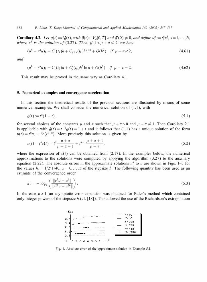
where the expression of v(t) can be obtained from (2.17). In the examples below, the numericalapproximations to the solutions were computed by applying the algorithm (3.27) to the auxiliaryequation (2.22). The absolute errors in the approximate solutions uh to u are shown in Figs. 1–3 forthe values hn = 1=2n1=40; n = 0; : : : ; 5 of the stepsize h. The following quantity has been used as anestimate of the convergence order
k := − log2
( ‖rhu− uh‖‖r2hu− u2h‖
): (5.3)
In the case �¿1, an asymptotic error expansion was obtained for Euler’s method which containedonly integer powers of the stepsize h (cf. [18]). This allowed the use of the Richardson’s extrapolation
Fig. 1. Absolute error of the approximate solution in Example 5.1.
P. Lima, T. Diogo / Journal of Computational and Applied Mathematics 140 (2002) 537–557 553
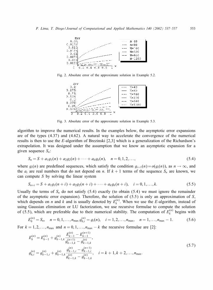
Fig. 2. Absolute error of the approximate solution in Example 5.2.
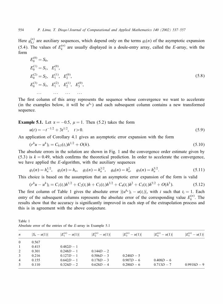
Fig. 3. Absolute error of the approximate solution in Example 5.3.
algorithm to improve the numerical results. In the examples below, the asymptotic error expansionsare of the types (4.37) and (4.62). A natural way to accelerate the convergence of the numericalresults is then to use the E-algorithm of Brezinski [2,3] which is a generalization of the Richardson’sextrapolation. It was designed under the assumption that we know an asymptotic expansion for agiven sequence Sn:
Sn = S + a1g1(n) + a2g2(n) + · · · + akgk(n); n = 0; 1; 2; : : : ; (5.4)
where gi(n) are prede6ned sequences, which satisfy the condition gi+1(n) =o(gi(n)), as n → ∞, andthe ai are real numbers that do not depend on n. If k + 1 terms of the sequence Sn are known, wecan compute S by solving the linear system
Sn+i = S + a1g1(n + i) + a2g2(n + i) + · · · + akgk(n + i); i = 0; 1; : : : ; k: (5.5)
Usually the terms of Sn do not satisfy (5.4) exactly (to obtain (5.4) we must ignore the remainderof the asymptotic error expansion). Therefore, the solution of (5.5) is only an approximation of S,which depends on n and k and is usually denoted by E(n)
k . When we use the E-algorithm, instead ofusing Gaussian elimination or LU factorization, we use recursive formulae to compute the solutionof (5.5), which are preferable due to their numerical stability. The computation of E(n)
k begins with
E(n)0 = Sn; n = 0; 1; : : : ; nmax g
(n)0; i = gi(n); i = 1; 2; : : : ; nmax; n = 1; : : : ; nmax − 1: (5.6)
For k = 1; 2; : : : ; nmax and n = 0; 1; : : : ; nmax − k the recursive formulae are [2]:
E(n)k = E(n)
k−1 + g(n)k−1; k
E(n)k−1 − E(n+1)
k−1
g(n+1)k−1; k − g(n)
k−1; k
;
g(n)k; i = g(n)
k−1; i + g(n)k−1; k
g(n)k−1; i − g(n+1)
k−1; i
g(n)k−1; k − g(n)
k−1; k
; i = k + 1; k + 2; : : : ; nmax:
(5.7)
554 P. Lima, T. Diogo / Journal of Computational and Applied Mathematics 140 (2002) 537–557
Here g(n)k; i are auxiliary sequences, which depend only on the terms gi(n) of the asymptotic expansion
(5.4). The values of E(n)k are usually displayed in a doule-entry array, called the E-array, with the
form
E(0)0 = S0;
E(1)0 = S1; E(0)
1 ;
E(2)0 = S2; E(1)
1 ; E(0)2 ;
E(3)0 = S3; E(2)
1 ; E(1)2 ; E(0)
3 ;
: : : : : : : : : : : :
(5.8)
The 6rst column of this array represents the sequence whose convergence we want to accelerate(in the examples below, it will be uhn) and each subsequent column contains a new transformedsequence.
Example 5.1. Let � = −0:5, � = 1. Then (5.2) takes the form
u(t) = −t−1=2 + 3t1=2; t¿0: (5.9)
An application of Corollary 4.1 gives an asymptotic error expansion with the form
(rhu− uh)i = C0:5(ti)h1=2 + O(h): (5.10)
The absolute errors in the solution are shown in Fig. 1 and the convergence order estimate given by(5.3) is k = 0:49, which con6rms the theoretical prediction. In order to accelerate the convergence,we have applied the E-algorithm, with the auxiliary sequences
g1(n) = h1=2n ; g2(n) = hn; g3(n) = h3=2
n ; g4(n) = h2n; g5(n) = h5=2
n : (5.11)
This choice is based on the assumption that an asymptotic error expansion of the form is valid
(rhu− uh)i = C1(ti)h1=2 + C2(ti)h + C3(ti)h3=2 + C4(ti)h2 + C5(ti)h5=2 + O(h3): (5.12)
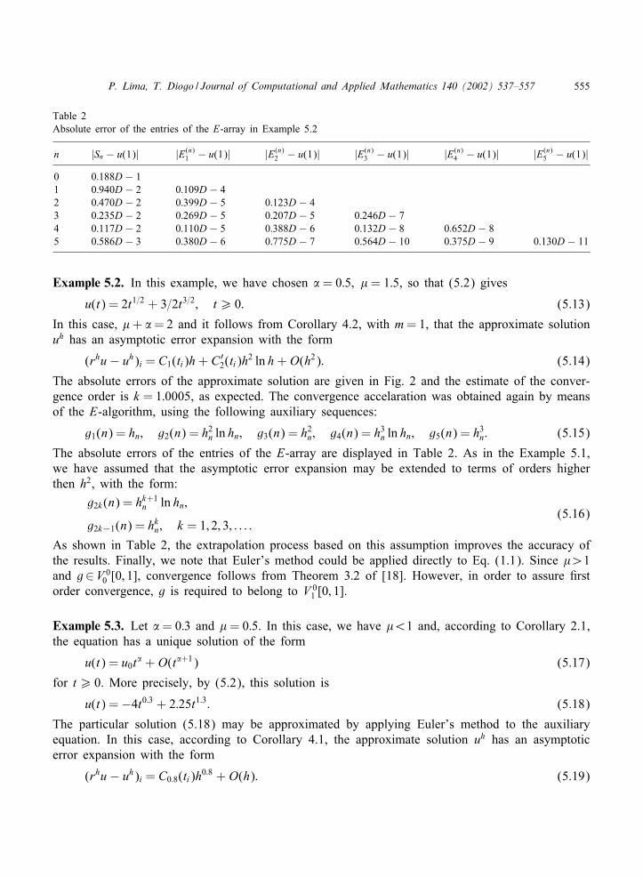
The 6rst column of Table 1 gives the absolute error |(uhn)i − u(ti)|, with i such that ti = 1. Eachentry of the subsequent columns represents the absolute error of the corresponding value E(n)
k . Theresults show that the accuracy is signi6cantly improved in each step of the extrapolation process andthis is in agreement with the above conjecture.
Table 1Absolute error of the entries of the E-array in Example 5.1
n |Sn − u(1)| |E(n)1 − u(1)| |E(n)
2 − u(1)| |E(n)3 − u(1)| |E(n)
4 − u(1)| |E(n)5 − u(1)|
0 0.5671 0.415 0:482D − 12 0.301 0:248D − 1 0:144D − 23 0.216 0:127D − 1 0:506D − 3 0:240D − 54 0.155 0:642D − 1 0:178D − 3 0:907D − 6 0:408D − 65 0.110 0:324D − 2 0:628D − 4 0:280D − 6 0:713D − 7 0:9918D − 9
P. Lima, T. Diogo / Journal of Computational and Applied Mathematics 140 (2002) 537–557 555
Table 2Absolute error of the entries of the E-array in Example 5.2
n |Sn − u(1)| |E(n)1 − u(1)| |E(n)
2 − u(1)| |E(n)3 − u(1)| |E(n)
4 − u(1)| |E(n)5 − u(1)|
0 0:188D − 11 0:940D − 2 0:109D − 42 0:470D − 2 0:399D − 5 0:123D − 43 0:235D − 2 0:269D − 5 0:207D − 5 0:246D − 74 0:117D − 2 0:110D − 5 0:388D − 6 0:132D − 8 0:652D − 85 0:586D − 3 0:380D − 6 0:775D − 7 0:564D − 10 0:375D − 9 0:130D − 11
Example 5.2. In this example, we have chosen � = 0:5; � = 1:5, so that (5.2) gives
u(t) = 2t1=2 + 3=2t3=2; t¿ 0: (5.13)
In this case, � + � = 2 and it follows from Corollary 4.2, with m = 1, that the approximate solutionuh has an asymptotic error expansion with the form
(rhu− uh)i = C1(ti)h + C ′2(ti)h2 ln h + O(h2): (5.14)
The absolute errors of the approximate solution are given in Fig. 2 and the estimate of the conver-gence order is k = 1:0005, as expected. The convergence accelaration was obtained again by meansof the E-algorithm, using the following auxiliary sequences:
g1(n) = hn; g2(n) = h2n ln hn; g3(n) = h2
n; g4(n) = h3n ln hn; g5(n) = h3
n: (5.15)
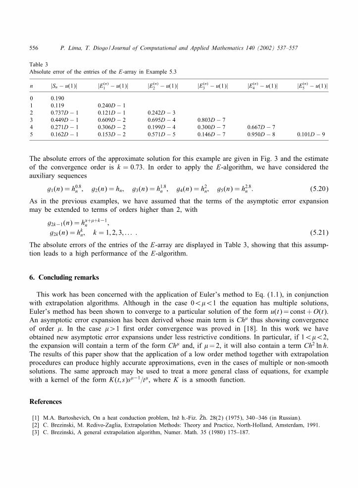
The absolute errors of the entries of the E-array are displayed in Table 2. As in the Example 5.1,we have assumed that the asymptotic error expansion may be extended to terms of orders higherthen h2, with the form:
g2k(n) = hk+1n ln hn;
g2k−1(n) = hkn; k = 1; 2; 3; : : : :
(5.16)
As shown in Table 2, the extrapolation process based on this assumption improves the accuracy ofthe results. Finally, we note that Euler’s method could be applied directly to Eq. (1.1). Since �¿1and g∈V 0
0 [0; 1], convergence follows from Theorem 3:2 of [18]. However, in order to assure 6rstorder convergence, g is required to belong to V 0
1 [0; 1].
Example 5.3. Let � = 0:3 and � = 0:5. In this case, we have �¡1 and, according to Corollary 2.1,the equation has a unique solution of the form
u(t) = u0t� + O(t�+1) (5.17)
for t¿ 0. More precisely, by (5.2), this solution is
u(t) = −4t0:3 + 2:25t1:3: (5.18)
The particular solution (5.18) may be approximated by applying Euler’s method to the auxiliaryequation. In this case, according to Corollary 4.1, the approximate solution uh has an asymptoticerror expansion with the form
(rhu− uh)i = C0:8(ti)h0:8 + O(h): (5.19)
556 P. Lima, T. Diogo / Journal of Computational and Applied Mathematics 140 (2002) 537–557
Table 3Absolute error of the entries of the E-array in Example 5.3
n |Sn − u(1)| |E(n)1 − u(1)| |E(n)
2 − u(1)| |E(n)3 − u(1)| |E(n)
4 − u(1)| |E(n)5 − u(1)|
0 0.1901 0.119 0:240D − 12 0:737D − 1 0:121D − 1 0:242D − 33 0:449D − 1 0:609D − 2 0:695D − 4 0:803D − 74 0:271D − 1 0:306D − 2 0:199D − 4 0:300D − 7 0:667D − 75 0:162D − 1 0:153D − 2 0:571D − 5 0:146D − 7 0:950D − 8 0:101D − 9
The absolute errors of the approximate solution for this example are given in Fig. 3 and the estimateof the convergence order is k = 0:73. In order to apply the E-algorithm, we have considered theauxiliary sequences
g1(n) = h0:8n ; g2(n) = hn; g3(n) = h1:8
n ; g4(n) = h2n; g5(n) = h2:8
n : (5.20)
As in the previous examples, we have assumed that the terms of the asymptotic error expansionmay be extended to terms of orders higher than 2, with
g2k−1(n) = h�+�+k−1n ;
g2k(n) = hkn; k = 1; 2; 3; : : : : (5.21)
The absolute errors of the entries of the E-array are displayed in Table 3, showing that this assump-tion leads to a high performance of the E-algorithm.
6. Concluding remarks
This work has been concerned with the application of Euler’s method to Eq. (1.1), in conjunctionwith extrapolation algorithms. Although in the case 0¡�¡1 the equation has multiple solutions,Euler’s method has been shown to converge to a particular solution of the form u(t) = const +O(t).An asymptotic error expansion has been derived whose main term is Ch� thus showing convergenceof order �. In the case �¿1 6rst order convergence was proved in [18]. In this work we haveobtained new asymptotic error expansions under less restrictive conditions. In particular, if 1¡�¡2,the expansion will contain a term of the form Ch� and, if �= 2, it will also contain a term Ch2 ln h.The results of this paper show that the application of a low order method together with extrapolationprocedures can produce highly accurate approximations, even in the cases of multiple or non-smoothsolutions. The same approach may be used to treat a more general class of equations, for examplewith a kernel of the form K(t; s)s�−1=t�, where K is a smooth function.
References
[1] M.A. Bartoshevich, On a heat conduction problem, InTz h.-Fiz. TZh. 28(2) (1975), 340–346 (in Russian).[2] C. Brezinski, M. Redivo-Zaglia, Extrapolation Methods: Theory and Practice, North-Holland, Amsterdam, 1991.[3] C. Brezinski, A general extrapolation algorithm, Numer. Math. 35 (1980) 175–187.
P. Lima, T. Diogo / Journal of Computational and Applied Mathematics 140 (2002) 537–557 557
[4] H. Brunner, Open problems in the discretization of Volterra integral equations, Numer. Funct. Anal. Optim. 17(1996) 717–736.
[5] H. Brunner, P.J. van der Houwen, The Numerical Solution of Volterra Equations, North-Holland, Amsterdam, 1986.[6] E. Buckwar, Numerical treatment of a non-uniquely solvable Volterra integral equation, in: A. Sydov (Ed.),
Proceedings of the 15th IMACS World Congress on Scienti6c Computation, Modelling and Applied Mathematics,24–29 August, Berlin, Germany, 1997, 439–444.
[7] R.F. Cameron, S. McKee, Product integration methods for second-kind Abel integral equations, J. Comput. Appl.Math. 11 (1984) 1–10.
[8] T. Diogo, N.B. Franco, P.M. Lima, High order product integration methods for a Volterra integral equation withlogarithmic singular kernel, Preprint 24 (2000), Department of Mathematics, Instituto Superior TEecnico Lisbon,submitted.
[9] T. Diogo, S. McKee, T. Tang, A Hermite-type collocation method for the solution of an integral equation with acertain weakly singular kernel, IMA J. Numer. Anal. 11 (1991) 595–605.
[10] T. Diogo, S. McKee, T. Tang, Collocation methods for second-kind Volterra integral equations with weakly singularkernels, Proc. Roy. Soc. Edinburgh 124A (1994) 199–210.
[11] E.A. Galperin, E.J. Kansa, A. Makroglou, S.A. Nelson, Variable transformations in the numerical solution of secondkind Volterra integral equations with continuous and weakly singular kernels; extensions to Fredholm integralequations, J. Comput. Appl. Math. 115 (2000) 193–211.
[12] H. Guoqiang, K. Hayami, K. Sugihara, W. Jiong, Extrapolation method of iterated collocation solution fortwo-dimensional nonlinear Volterra integral equations, Appl. Math. Comput. 112 (2000) 49–61.
[13] W. Han, Existence, uniqueness and smoothness results for second-kind Volterra equations with weakly singularkernels, J. Integral Equations Appl. 6 (1994) 365–384.
[14] W. Hock, An extrapolation method with step size control for nonlinear Volterra integral equations, Numer. Math.38 (1981) 155–178.
[15] F. de Hoog, R. Weiss, Higher order methods for a class of Volterra integral equations with weakly singular kernels,SIAM J. Numer. Anal. 11 (1974) 1166–1180.
[16] W.G. Kelley, A.C. Peterson, DiPerence Equations, an Introduction with Applications, Academic Press Inc., NewYork, 1991.
[17] W. Lamb, A spectral approach to an integral equation, Glasgow Math. J. 26 (1985) 83–89.[18] P.M. Lima, T. Diogo, An extrapolation method for a Volterra integral equation with weakly singular kernel, Appl.
Numer. Math. 24 (1997) 131–148.[19] P. Linz, Numerical methods for Volterra integral equations with singular kernels, SIAM J. Numer. Anal. 6 (1969)
365–374.[20] G.I. Marchuk, V.V. Shaidurov, DiPerence Methods and Their Extrapolations, Springer, Berlin, 1983.[21] J. Norbury, A.M. Stuart, Volterra integral equations and a new Gronwall inequality, Part I: The linear case, Proc.
Roy. Soc. Edinburgh 106A (1987a) 361–373.[22] J. Norbury, A.M. Stuart, Volterra integral equations and a new Gronwall inequality, Part II: The nonlinear case,
Proc. Roy. Soc. Edinburgh 106A (1987b) 375–384.[23] P.G. Rooney, On an integral equation of sub-Sizonenko, Glasgow Math. J. 24 (1983) 207–210.[24] V. Smirnov, Cours de MathEematiques SupEerieurs, Tome IV, 2iXeme partie, EEditions Mir, Moscou, 1984.[25] J.A. Sub-Sizonenko, Inversion of an integral operator by the method of expansion with respect to orthogonal Watson
operators, Siberian Math. J. 20 (1979) 318–321.[26] T. Tang, S. McKee, T. Diogo, Product integration methods for an integral equation with logarithmic singular kernel,
Appl. Numer. Math. 9 (1992) 259–266.[27] R. Wong, Asymptotic Approximations of Integrals, Academic Press Inc., New York, 1989.
Related Documents