UNLV eses/Dissertations/Professional Papers/Capstones 8-1-2014 Numerical Simulations of Traffic Flow Models Puneet Lakhanpal University of Nevada, Las Vegas, [email protected] Follow this and additional works at: hp://digitalscholarship.unlv.edu/thesesdissertations Part of the Applied Mathematics Commons , Mathematics Commons , and the Transportation Commons is esis is brought to you for free and open access by Digital Scholarship@UNLV. It has been accepted for inclusion in UNLV eses/ Dissertations/Professional Papers/Capstones by an authorized administrator of Digital Scholarship@UNLV. For more information, please contact [email protected]. Repository Citation Lakhanpal, Puneet, "Numerical Simulations of Traffic Flow Models" (2014). UNLV eses/Dissertations/Professional Papers/Capstones. Paper 2189.

Numerical Simulations of Traffic Flow Models
Dec 10, 2015
About numerical
Welcome message from author
This document is posted to help you gain knowledge. Please leave a comment to let me know what you think about it! Share it to your friends and learn new things together.
Transcript

UNLV Theses/Dissertations/Professional Papers/Capstones
8-1-2014
Numerical Simulations of Traffic Flow ModelsPuneet LakhanpalUniversity of Nevada, Las Vegas, [email protected]
Follow this and additional works at: http://digitalscholarship.unlv.edu/thesesdissertations
Part of the Applied Mathematics Commons, Mathematics Commons, and the TransportationCommons
This Thesis is brought to you for free and open access by Digital Scholarship@UNLV. It has been accepted for inclusion in UNLV Theses/Dissertations/Professional Papers/Capstones by an authorized administrator of Digital Scholarship@UNLV. For more information, please [email protected].
Repository CitationLakhanpal, Puneet, "Numerical Simulations of Traffic Flow Models" (2014). UNLV Theses/Dissertations/Professional Papers/Capstones.Paper 2189.

NUMERICAL SIMULATIONS OF TRAFFIC FLOW
MODELS
By
Puneet Lakhanpal
Bachelor of Technology – Electronics and Communication
Indian Institute of Technology, Guwahati
2009
Masters of Science – Electrical Engineering
University of Nevada, Las Vegas
2011
A thesis submitted in partial fulfillment
of the requirements for the
Master of Science – Mathematical Sciences
Department of Mathematical Sciences
College of Sciences
The Graduate College
University of Nevada, Las Vegas
August 2014

ii
THE GRADUATE COLLEGE
We recommend the thesis prepared under our supervision by
Puneet Lakhanpal
entitled
Numerical Simulations of Traffic Flow Models
is approved in partial fulfillment of the requirements for the degree of
Master of Science - Mathematical Sciences
Department of Mathematical Sciences
Monika Neda, Ph.D., Committee Co-Chair
Pushkin Kachroo, Ph.D., Co-Chair
Amei Amei, Ph.D., Committee Member
Hongtao Yang, Ph.D., Additional Committee Member
Yingtao Jiang, Ph.D., Graduate College Representative
Kathryn Hausbeck Korgan, Ph.D., Interim Dean of the Graduate College
August 2014
ABSTRACT
NUMERICAL SIMULATIONS OF TRAFFIC FLOW MODELS
by
Puneet Lakhanpal
〈Dr. Monika Neda〉, Examination Committee Co-Chair
Associate Professor of Mathematical Sciences
University of Nevada, Las Vegas
〈Dr. Pushkin Kachroo〉, Examination Committee Co-Chair
Professor of Electrical and Computer Engineering
University of Nevada, Las Vegas
Traffic flow has been considered to be a continuum flow of a compressible liquid
having a certain density profile and an associated velocity, depending upon density,
position and time. Several one-equation and two-equation macroscopic continuum
flow models have been developed which utilize the fluid dynamics continuity equa-
tion and help us find analytical solutions with simplified initial and boundary condi-
tions. In this thesis, the one-equation Lighthill Witham and Richards (LWR) model
combined with the Greenshield’s model, is used for finding analytical and numerical
solutions for four problems: Linear Advection, Red Traffic Light turning into Green,
Stationary Shock and Shock Moving towards Right. In all these problems, the nu-
merical solutions are computed using the Godunov Method and the Finite Element
Method, and later they are compared to each other. Furthermore, the finite element
time relaxation method is introduced for the treatment of the shocks in two numer-
iii

ical problems : (a) Stationary Shock and (b) Shock moving towards the right. The
optimal time relaxation parameters are numerically computed using three accuracy
measures and finally, the effects of multiple time relaxation settings are explored.
iv
ACKNOWLEDGEMENTS
I would like to express my respects to co-advisor Prof. Monika Neda, who has
given me direction and supported me throughout my efforts in Mathematical Sciences.
I am thankful to my co-advisor Prof. Pushkin Kachroo, who has been an elder brother
to me and has always supported me in all my endeavours. Also, I am very grateful
to Prof. Yingtao Jiang, Prof. Hongtao Yang and Prof. Amei Amei for their helpful
remarks.
I am honored to have the love and support of my parents, Mr. Ashok Lakhanpal
and Mrs. Veena Kumari, and my brother, Manuj. Without them, I would be nowhere
in this world.
Last but not the least, I am greatly indebted to a few friends for their love and
support during the entire period of my study.
v

TABLE OF CONTENTS
ABSTRACT iii
ACKNOWLEDGEMENTS v
LIST OF TABLES viii
LIST OF FIGURES xi
1 Introduction 11.1 Outline of the Thesis . . . . . . . . . . . . . . . . . . . . . . . . . . . 2
2 Traffic Flow 32.1 Introduction . . . . . . . . . . . . . . . . . . . . . . . . . . . . . . . . 3
2.1.1 Conservation Laws . . . . . . . . . . . . . . . . . . . . . . . . 32.1.2 Traffic Flow Theory . . . . . . . . . . . . . . . . . . . . . . . . 4
3 Problem Description 63.1 Introduction . . . . . . . . . . . . . . . . . . . . . . . . . . . . . . . . 63.2 LWR and Greenshield’s model . . . . . . . . . . . . . . . . . . . . . . 63.3 Numerical Problems . . . . . . . . . . . . . . . . . . . . . . . . . . . 7
3.3.1 Linear Advection . . . . . . . . . . . . . . . . . . . . . . . . . 93.3.2 Red Traffic Light Turning Into Green . . . . . . . . . . . . . . 123.3.3 Stationary Shock . . . . . . . . . . . . . . . . . . . . . . . . . 163.3.4 Shock moving towards right . . . . . . . . . . . . . . . . . . . 18
4 Numerical Methods 224.1 Introduction . . . . . . . . . . . . . . . . . . . . . . . . . . . . . . . . 224.2 Godunov method . . . . . . . . . . . . . . . . . . . . . . . . . . . . . 22
4.2.1 Basics of Godunov method . . . . . . . . . . . . . . . . . . . . 224.2.2 LWR-Greenshield’s Traffic Flow PDE used in Godunov analysis 25
4.3 Finite Element method . . . . . . . . . . . . . . . . . . . . . . . . . . 264.3.1 Basics of Finite Element method . . . . . . . . . . . . . . . . 264.3.2 LWR-Greenshield’s Traffic Flow PDE used in FEM analysis . 284.3.3 Finite Element method with Time Relaxation . . . . . . . . . 29
5 Numerical Simulations 325.1 Introduction . . . . . . . . . . . . . . . . . . . . . . . . . . . . . . . . 325.2 Equations . . . . . . . . . . . . . . . . . . . . . . . . . . . . . . . . . 325.3 Accuracy measures . . . . . . . . . . . . . . . . . . . . . . . . . . . . 33
5.3.1 Comparing the solutions . . . . . . . . . . . . . . . . . . . . . 355.4 Common Parameters . . . . . . . . . . . . . . . . . . . . . . . . . . . 365.5 Linear Advection . . . . . . . . . . . . . . . . . . . . . . . . . . . . . 37
5.5.1 Godunov solution . . . . . . . . . . . . . . . . . . . . . . . . . 38
vi

5.5.2 FEM solution . . . . . . . . . . . . . . . . . . . . . . . . . . . 395.5.3 Comparison of solutions obtained from Godunov method and
FEM method . . . . . . . . . . . . . . . . . . . . . . . . . . . 405.6 Red Traffic Light turning into Green . . . . . . . . . . . . . . . . . . 42
5.6.1 Godunov solution . . . . . . . . . . . . . . . . . . . . . . . . . 435.6.2 FEM solution . . . . . . . . . . . . . . . . . . . . . . . . . . . 435.6.3 Comparison of solutions obtained from Godunov method and
FEM method . . . . . . . . . . . . . . . . . . . . . . . . . . . 455.7 Stationary Shock . . . . . . . . . . . . . . . . . . . . . . . . . . . . . 45
5.7.1 Godunov solution . . . . . . . . . . . . . . . . . . . . . . . . . 485.7.2 FEM solution without time relaxation . . . . . . . . . . . . . 495.7.3 FEM solution with time relaxation . . . . . . . . . . . . . . . 495.7.4 Comparison of solutions obtained from Godunov method and
FEM time relaxation method . . . . . . . . . . . . . . . . . . 545.8 Shock moving towards right . . . . . . . . . . . . . . . . . . . . . . . 55
5.8.1 Godunov solution . . . . . . . . . . . . . . . . . . . . . . . . . 575.8.2 FEM solution without time relaxation . . . . . . . . . . . . . 585.8.3 FEM solution with time relaxation . . . . . . . . . . . . . . . 595.8.4 Comparison of solutions obtained from Godunov method and
FEM time relaxation method . . . . . . . . . . . . . . . . . . 63
6 Conclusion 666.1 Summary . . . . . . . . . . . . . . . . . . . . . . . . . . . . . . . . . 666.2 Future Work . . . . . . . . . . . . . . . . . . . . . . . . . . . . . . . . 67
BIBLIOGRAPHY 69
VITA 71
vii
LIST OF TABLES
5.1 Common Parameters used in numerical simulations . . . . . . . . . . 365.2 Linear Advection: Parameters used in numerical simulation . . . . . . 375.3 Red Traffic Light turning into Green: Parameters used in numerical
simulation . . . . . . . . . . . . . . . . . . . . . . . . . . . . . . . . . 425.4 Stationary Shock: Parameters used in numerical simulation . . . . . . 475.5 Parameters used in numerical simulation of a shock moving towards
right . . . . . . . . . . . . . . . . . . . . . . . . . . . . . . . . . . . . 55
viii

LIST OF FIGURES
2.1 Distance travelled in ∆t hours . . . . . . . . . . . . . . . . . . . . . . 5
2.2 v =Q
ρrepresents the surface of admissible traffic flow model, where
ρj represents the jam density and Vf represents the free-flow velocity(Source: Huber (4)). . . . . . . . . . . . . . . . . . . . . . . . . . . . 5
3.1 Experimental relationship between density, flow and velocity based onLWR and Greenshield’s model (Source: Kachroo (9)) . . . . . . . . . 8
3.2 Linear Advection: Initial Density Profile u0(x) . . . . . . . . . . . . . 113.3 Linear Advection: Analytical solution of the Density Profile u(x, t),
given that t > 0 c > 0 . . . . . . . . . . . . . . . . . . . . . . . . . . 123.4 Characteristic speed (Source: Kachroo (9)) . . . . . . . . . . . . . . . 133.5 Red Light turning into Green: Characteristics generating blank region
in x− t space (Source: Kachroo (9)) . . . . . . . . . . . . . . . . . . 143.6 Red Light turning into Green: Rarefaction solution (Source: Kachroo
(9)) . . . . . . . . . . . . . . . . . . . . . . . . . . . . . . . . . . . . . 163.7 Shock solution and its characteristics (Source: Kachroo (9)) . . . . . 183.8 Stationary Shock: Initial Condition at time t = 0 . . . . . . . . . . . 193.9 Stationary Shock: Solution ∀t . . . . . . . . . . . . . . . . . . . . . . 193.10 Shock moving towards right: Initial Condition at time t = 0 . . . . . 203.11 Shock moving towards right: Solution at time t > 0 . . . . . . . . . . 21
4.1 Definition Sketch for Riemann Problem . . . . . . . . . . . . . . . . . 234.2 Godunov Dynamics (Source: Kachroo(12)) . . . . . . . . . . . . . . . 244.3 (a) 2−D domain of dependent variable φ(x, y) (b) Three node Finite
Element defined in domain (c) Additional elements showing partialmesh of domain . . . . . . . . . . . . . . . . . . . . . . . . . . . . . . 27
5.1 Linear Advection: Initial density profile . . . . . . . . . . . . . . . . . 375.2 Linear Advection: Godunov solution at time T = 5 seconds . . . . . . 385.3 Linear Advection: l2 norm and the bounded variation (bv) norm of the
error for Godunov solution . . . . . . . . . . . . . . . . . . . . . . . . 395.4 Linear Advection: FEM solution at time T = 5 seconds . . . . . . . . 395.5 Linear Advection: l2 norm and the bounded variation (bv) norm of the
error for FEM solution . . . . . . . . . . . . . . . . . . . . . . . . . . 405.6 Linear Advection: Comparison of numerical simulations obtained from
Godunov method and FEM method . . . . . . . . . . . . . . . . . . . 415.7 Linear Advection: Comparison of l2 norm and bounded variation (bv)
norm of the errors obtained from Godunov method and FEM method 415.8 Red Traffic Light turning into Green: Initial density profile . . . . . . 425.9 Red Traffic Light turning into Green: Godunov solution at time T = 5
seconds . . . . . . . . . . . . . . . . . . . . . . . . . . . . . . . . . . . 435.10 Red Traffic Light turning into Green: l2 norm and the bounded varia-
tion (bv) norm of the error for Godunov solution . . . . . . . . . . . . 44
ix

5.11 Red Traffic Light turning into Green: FEM solution at time T = 5seconds . . . . . . . . . . . . . . . . . . . . . . . . . . . . . . . . . . . 44
5.12 Red Traffic Light turning into Green: l2 norm and the bounded varia-tion (bv) norm of the error for FEM solution . . . . . . . . . . . . . . 45
5.13 Red Traffic Light turning into Green: Comparison of numerical simu-lations obtained from Godunov method and FEM method . . . . . . 46
5.14 Red Traffic Light turning into Green: Comparison of l2 norm andbounded variation (bv) norm of the errors obtained from Godunovmethod and FEM method . . . . . . . . . . . . . . . . . . . . . . . . 46
5.15 Stationary Shock: Initial density profile . . . . . . . . . . . . . . . . . 475.16 Stationary Shock: Godunov solution at time T = 5 seconds . . . . . . 485.17 Stationary Shock: l2 norm and the bounded variation (bv) norm of the
error for Godunov solution . . . . . . . . . . . . . . . . . . . . . . . . 495.18 Stationary Shock: FEM solution without any time relaxation . . . . . 505.19 Stationary Shock: l2 norm and bounded variation (bv) norm of the
error for FEM solution without any time relaxation . . . . . . . . . . 505.20 Stationary Shock: Usage of l2 norm of the error, bounded variation
(bv) norm of the error and Smoothness of Estimated Solution to findthe optimal χ− δ combination. . . . . . . . . . . . . . . . . . . . . . 52
5.21 Stationary Shock: FEM solution for Time Relaxation with N = 1 . . 525.22 Stationary Shock: l2 norm and bounded variation (bv) norm of the
error for FEM solution with Time Relaxation and N = 1 . . . . . . . 535.23 Stationary Shock: FEM solutions for different orders of time relaxation
schemes where χ = 100 and δ = 0.5h . . . . . . . . . . . . . . . . . . 535.24 Stationary Shock: l2 norm and bounded variation (bv) norm of the
error for different orders of time relaxation schemes where χ = 100and δ = 0.5h . . . . . . . . . . . . . . . . . . . . . . . . . . . . . . . . 54
5.25 Stationary Shock: Comparison of numerical simulations obtained fromGodunov method and FEM method for Time Relaxation with N = 1 55
5.26 Stationary Shock: Comparison of l2 norm and bounded variation (bv)norm of the errors obtained from Godunov method and FEM methodfor Time Relaxation with N = 1 . . . . . . . . . . . . . . . . . . . . . 56
5.27 Shock moving towards right: Initial density profile . . . . . . . . . . . 575.28 Shock moving towards right: Godunov solution at time T = 5 seconds 575.29 Shock moving towards right: l2 norm and the bounded variation (bv)
norm of the error for Godunov solution . . . . . . . . . . . . . . . . . 585.30 Shock moving towards right: FEM solution without any time relaxation 585.31 Shock moving towards right: l2 norm and bounded variation (bv) norm
of the error for FEM solution without any time relaxation . . . . . . 595.32 Shock moving towards right: Usage of l2 norm of the error, Bounded
Variation (bv) norm of the error and Smoothness of Estimated Solutionto find the optimal χ− δ combination. . . . . . . . . . . . . . . . . . 60
5.33 Shock moving towards right: FEM solution for Time Relaxation withN = 1 . . . . . . . . . . . . . . . . . . . . . . . . . . . . . . . . . . . 61
x
5.34 Shock moving towards right: l2 norm and bounded variation (bv) normof the error in FEM solution for Time Relaxation with N = 1 . . . . 62
5.35 Shock moving towards right: FEM solutions for different orders of timerelaxation schemes where χ = 9 and δ = 5h . . . . . . . . . . . . . . . 62
5.36 Shock moving towards right: l2 norm and bounded variation (BV)norm of the errors for different orders of time relaxation schemes whereχ = 9 and δ = 5h . . . . . . . . . . . . . . . . . . . . . . . . . . . . . 63
5.37 Shock moving towards right: Comparison of numerical simulations ob-tained from Godunov method and FEM method for Time Relaxationwith N = 1 . . . . . . . . . . . . . . . . . . . . . . . . . . . . . . . . 64
5.38 Shock moving towards right: Comparison of l2 norm and boundedvariation (bv) norm of the errors obtained from Godunov method andFEM method for Time Relaxation with N = 1 . . . . . . . . . . . . . 65
xi

CHAPTER 1
Introduction
Traffic flow can be defined as the study of how the vehicles move between ori-
gin and destination, and how the individual drivers interact with others. Since the
driver behavior cannot be predicted with absolute certainity, mathematical models
have been built which study the consistent behavior between the traffic streams via
relationships such as flow q, density ρ and the mean velocity v. These mathematical
models try to describe how these relationships evolve in space and time, and how
they can be used to solve the real traffic flow conditions to be further used in traffic
flow control and optimization (3). The Lighthill William and Richards (LWR) model
is one such model that tries to capture the traffic behavior.
In this thesis, two tasks are explored.
1. Study of the LWR model with two techniques:
Finite Volume Godunov method
Finite Element Galerkin method with Time relaxation
2. Comparison of the solutions of following numerical problems with the above
methods:
Linear Advection
A red traffic light turning into green
Stationary Shock
1

Shock moving towards right
1.1 Outline of the Thesis
This thesis is divided into the following chapters.
1. Chapter 1 presents the motivation and outline of the thesis.
2. Chapter 2 presents a brief overview of the LWR traffic flow model and describes
the speed-flow relationships.
3. Chapter 3 presents four problems in traffic flow for which numerical simulations
are desired.
4. Chapter 4 presents the theory behind the Finite Volume Godunov method and
the Finite Element method with time relaxation. These two methods will be
cross-evaluated and their performance will be measured against each numerical
problem.
5. Chapter 5 presents the numerical results obtained for each problem using Go-
dunov and Finite Element method.
6. Chapter 6 presents the conclusion and outlines the areas of further research.
2

CHAPTER 2
Traffic Flow
2.1 Introduction
If a vehicle is assumed to be a molecule, then the traffic can be defined to be an
incompressible fluid which cannot be compressed after a certain density. In 1955 and
1956, Lighthill, Whittam and Richards proposed a macroscopic traffic flow model,
which is very popularly known as the LWR model. According to this model, the
traffic flow was represented using a first order partial differential equation and was
based on a hyperbolic system of conversation laws, as defined below.
2.1.1 Conservation Laws
A conservation law is a Partial Differential Equation of the form
∂ρ
∂t+∂f
∂x= 0 (2.1)
where t represents the time coordinate; x represents the space coordinate, ρ :
R × R → Rm is an m dimensional vector of conserved quantities and f : Rm → Rm
reprents the flux or the rate of flow of the conserved quantity ρ. Furthermore, the
flux in a given direction represents the amount of ρ which has crossed a unit surface
in the given direction per unit time.
The system (2.1) is said to be hyperbolic if for each value of ρ, the eigen values
of the Jacobian matrix f ′(ρ) are real and there exists a complete set of m linearly
3
independent eigen vectors, representing the diagonalizability of the matrix.
2.1.2 Traffic Flow Theory
The Traffic flow theory is the study of following three variables.
1. Density ρ(x, t): Number of cars per unit distance, per lane.
2. Velocity v(x, t)
3. Traffic Flow Q(x, t): Average number of cars passing per unit time, per lane.
The relationship between the above three variables is presented in the following sub-
section.
Relationship between Traffic Flow variables
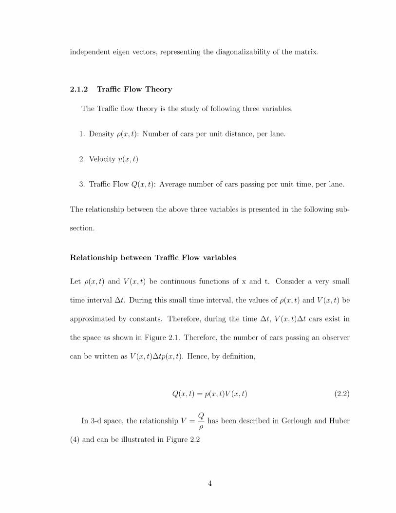
Let ρ(x, t) and V (x, t) be continuous functions of x and t. Consider a very small
time interval ∆t. During this small time interval, the values of ρ(x, t) and V (x, t) be
approximated by constants. Therefore, during the time ∆t, V (x, t)∆t cars exist in
the space as shown in Figure 2.1. Therefore, the number of cars passing an observer
can be written as V (x, t)∆tp(x, t). Hence, by definition,
Q(x, t) = p(x, t)V (x, t) (2.2)
In 3-d space, the relationship V =Q
ρhas been described in Gerlough and Huber
(4) and can be illustrated in Figure 2.2
4

Figure 2.1: Distance travelled in ∆t hours
Figure 2.2: v =Q
ρrepresents the surface of admissible traffic flow model, where ρj
represents the jam density and Vf represents the free-flow velocity (Source: Huber(4)).
5

CHAPTER 3
Problem Description
3.1 Introduction
In this chapter, we consider the one-equation Lighthill William and Richards
(LWR) model of traffic flow, which will be used in conjunction with the Greenshield’s
model. Both these models formulate the basis of the numerical simulations in this
thesis. Later, different variations of the LWR model will be used to define several
well known numerical problems in the research literature.
3.2 LWR and Greenshield’s model
The Lighthill-Whitham-Richards Model, commonly known as the LWR model,
was introduced back in mid-1950s as a one dimensional macroscopic model to study
the traffic flow. In this model, the traffic was considered to be an inviscid but com-
pressible fluid (fluid-dynamic model) and the traffic flow variables: density ρ, velocity
v and flow f , were defined as continuous variables in time and space. According to
this model, the traffic flow f was defined to be a function of density ρ and velocity
as shown in Equation (3.1)
∂
∂tρ(t, x) +
∂
∂xf(t, x) = 0 (3.1)
In Equation (3.1), ρ represents the traffic density of the vehicles which is related to
the flux f and velocity v according to the relation f = ρv, which was also introduced
6
in Equation (2.2).
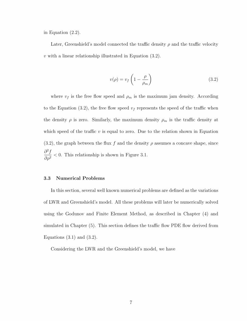
Later, Greenshield’s model connected the traffic density ρ and the traffic velocity
v with a linear relationship illustrated in Equation (3.2).
v(ρ) = vf
(1− ρ
ρm
)(3.2)
where vf is the free flow speed and ρm is the maximum jam density. According
to the Equation (3.2), the free flow speed vf represents the speed of the traffic when
the density ρ is zero. Similarly, the maximum density ρm is the traffic density at
which speed of the traffic v is equal to zero. Due to the relation shown in Equation
(3.2), the graph between the flux f and the density ρ assumes a concave shape, since
∂2f
∂ρ2< 0. This relationship is shown in Figure 3.1.
3.3 Numerical Problems
In this section, several well known numerical problems are defined as the variations
of LWR and Greenshield’s model. All these problems will later be numerically solved
using the Godunov and Finite Element Method, as described in Chapter (4) and
simulated in Chapter (5). This section defines the traffic flow PDE flow derived from
Equations (3.1) and (3.2).
Considering the LWR and the Greenshield’s model, we have
7
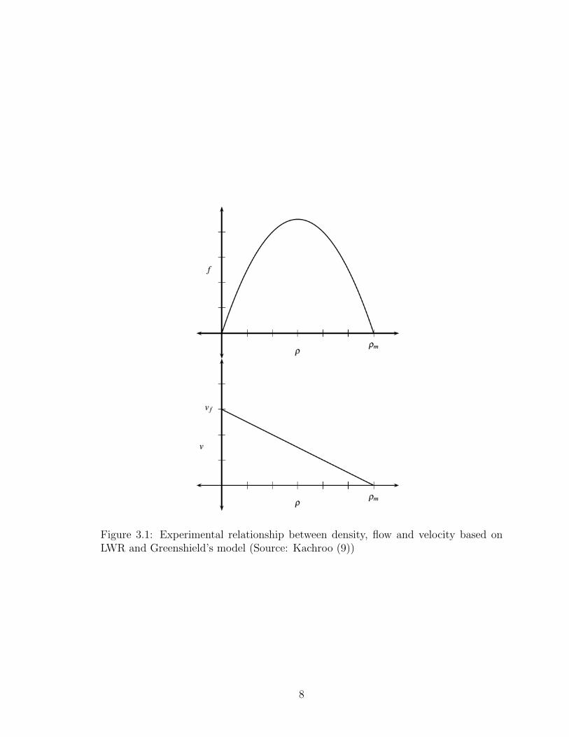
Figure 3.1: Experimental relationship between density, flow and velocity based onLWR and Greenshield’s model (Source: Kachroo (9))
8

∂
∂tρ(t, x) +
∂
∂xf(ρ) = 0
f(ρ) = ρv(ρ)
v(ρ) = vf (1−ρ
ρm)
(3.3)
Replacing v(ρ) in f(ρ) and later f(ρ) in the partial differential Equation (3.3), we
get
∂ρ
∂t+
(vf −
2vfρm
ρ
)∂ρ
∂x= 0 (3.4)
where the variables x, t have been suppressed with the notation definition that
ρ = ρ(x, t). Equation (3.4) is the general form of traffic flow PDE that will be used
in this thesis.
3.3.1 Linear Advection
In Trangenstein (13), Linear Advection has been described as the motion of a
conserved quantity along a constant velocity field. Therefore, contrary to the velocity
being a function of density v(ρ), the velocity assumes as constant speed c. This
converts the equation (3.3) into,
∂ρ
∂t+ c
∂ρ
∂x= 0 ∀x ∈ < ∀t > 0
ρ(x, 0) = ρ0(x) ∀x ∈ <(3.5)
The differential equation (3.5) can be re-written as follows,
9

0 = [1 c]
∂ρ
∂t∂ρ
∂x
(3.6)
In other words, the density gradient seems to be orthogonal to a constant vector.
Therefore, the density ρ must be constant on lines parallel to the constant vector.
These lines are called as characteristic lines, which in this case would be written as
x− ct = constant. Hence,
ρ(x0 + cτ, t0 + τ) = constant ∀(x0, t0) ∀τ
If τ = t− t0 is chosen,
ρ(x0 + c(t− t0), t) = ρ(x0 − ct0, 0) = ρ0(x0 − ct0)
If x is given, x0 can be chosen such that x0 = x − ct + ct0 yields Equation (3.7),
which will be the solution to the differential Equation (3.5).
u(x, t) = u0(x− ct) (3.7)
The statement that Equation (3.7) is the solution to the differential Equation (3.5)
can be verified as below.
Define new variables ξ, τ and the corresponding density ˜ρ(ξ, τ) such that
ξ = x− ct, τ = t
ρ(ξ, t) = ρ(x, t)
(3.8)
10

If the chain rule is now applied to the system of equations (3.8), we get
∂ρ
∂t=
∂ρ
∂τ− ∂ρ
∂ξc
∂ρ
∂x=
∂ρ
∂ξ
Therefore, we get the following equation
0 =∂ρ
∂t+ c
∂ρ
∂x=∂ρ
∂τ
ρ(ξ, 0) = u0(ξ)
(3.9)
which proves that ρ is the solution to the initial value problem defined in Equation
(3.9).
Consider the initial profile of the density ρ in Equation (3.5) to have a discontinuity
in the middle of a road segment, as shown in Figure 3.2. Therefore, provided that
c > 0, the density ρ at time t will have the same profile, but only will be shifted c ∗ t
units in space, as shown in Figure 3.3.
Figure 3.2: Linear Advection: Initial Density Profile u0(x)
11

Figure 3.3: Linear Advection: Analytical solution of the Density Profile u(x, t), giventhat t > 0 c > 0
3.3.2 Red Traffic Light Turning Into Green
Studying the behavior of how traffic density changes over time when a red traffic
light turns into green, is a classic problem in traffic research. In this problem, it is
assumed that a traffic light becomes red at time t = 0 such that the density behind
the traffic light ρ(x < 0; t = 0) = ρl becomes greater than the density ahead of the
traffic light ρ(x > 0; t = 0) = ρr further down the road. As a simpler case, it can
also be assumed that the traffic behind the traffic light is lined up bumper to bumper
such that ρ(x < 0; t = 0) = ρm. As an additional simplication, it can further be
assumed that no traffic exists ahead of the traffic light further down the road such
that ρ(x > 0, t = 0) = 0. However, let’s study this problem in a general case when
ρl > ρr.
The partial differential equation to be solved in this problem is as follows,
12

∂ρ
∂t+
(vf −
2vfρm
ρ
)∂ρ
∂x= 0
This equation was also introduced as Equation (3.4) earlier.
In quasilinear form, Equation (3.3) could be written as,
∂
∂tρ(t, x) + f ′(ρ)
∂
∂xρ(t, x) = 0 (3.10)
From Equations (3.3) and (3.10), we get the characteristic speed as,
f ′(ρ) = vf (1− 2ρ
ρm) (3.11)
The characteristic speed obtained in Equation (3.11) is the slope of the graph
shown in Figure 3.4.
Figure 3.4: Characteristic speed (Source: Kachroo (9))
Following Equation (3.11), we observe that since ρl > ρr, therefore,
13

f ′(ρl) = vf (1− 2ρlρm
) < f ′(ρr) = vf (1− 2ρrρm
) (3.12)
Since the characteristic speed towards the left of the traffic light is lesser than
the characteristic speed towards the right, a blank region is created by these char-
acteristics in the x − t space. This behavior can be seen in Figure 3.5, as shown
below.
Figure 3.5: Red Light turning into Green: Characteristics generating blank region inx− t space (Source: Kachroo (9))
In Kachroo (9), it has been mentioned that only a symmetry solution can fill in
the gap as shown in Figure 3.5. Let’s attempt to find such a solution.
Set ρ(x, t) = w(x/t) and differentiate it with respect to time coordinate t and the
space coordinate x. We get,
∂
∂tρ(x, t) = − x
t2w′(x/t)
∂
∂xρ(x, t) =
1
tw′(x/t)
(3.13)
Substituting Equation (3.13) into Equation (3.10), we get
14

− xt2w′(x/t) +
1
tf ′ (w(x/t))w′(x/t) = 0 (3.14)
If Equation (3.14) is multiplied by t and rearranged, it turns to Equation (3.15)
f ′ (w(β))w′(β) = βw′(β) (3.15)
Solving Equation (3.15), we get 2 cases:
Case I
w′(β) = 0 (3.16)
i.e. w is a constant for β ≤ β1 and β ≥ β2.
Case II For β1 < β < β2, w varies smoothly with w′ 6= 0. Therefore, Equation
3.15 yields Equation (3.17) as shown below.
f ′ (w(β)) = β , β1 < β < β2 (3.17)
Combining Case I and II, the density ρ becomes
ρ(β) =
ρl , β ≤ f ′(ρl)
w(β) , f ′(ρl) < βf ′(ρr)
ρr , β ≥ f ′(ρr)
(3.18)
15

Now, substituting back w(x/t) by ρ(x, t) in Equation (3.18), we get
ρ(x, t) =
ρl ,
x
t≤ f ′(ρl)
ω(x
t) , f ′(ρl) <
x
t≤ f ′(ρr)
ρr ,x
t≥ f ′(ρr)
(3.19)
where
ω(x
t) =
f ′(ρr)− f ′(ρl)ρr − ρl
(x
t)
The density solution, obtained in Equation (3.19), also known as a rarefaction
solution, can be illustrated in Figure 3.6.
Figure 3.6: Red Light turning into Green: Rarefaction solution (Source: Kachroo(9))
3.3.3 Stationary Shock
A shock in density happens when the characteristics intersect in space and time.
When characteristics intersect, that point in space has multiple values of densities
at the same time. In this problem, the density behind a certain point on the road
16

segment (say x = 0) ρ(x < 0; t = 0) = ρl is taken to be lesser than the density ahead
of that point ρ(x > 0; t = 0) = ρr further down the road. In other words, at time
t = 0, ρl < ρr. As a special case, ρl can be taken to be 0 and ρr can be taken to be
ρm. In this case, according to Haberman (5), the situation will be interpreted as an
initial semi-infinite line of bumper to bumper traffic followed by no traffic.
The partial differential equation to be solved in this problem is defined in Equation
(3.4). Additionally, the characteristic speed was also introduced as follows in Equation
(3.11).
f ′(ρ) = vf (1− 2ρ
ρm)
For shocks in general, since ρl < ρr, therefore,
f ′(ρl) = vf (1− 2ρlρm
) > f ′(ρr) = vf (1− 2ρrρm
) (3.20)
Based upon Equation (3.20), since the characteristic speed on the left f ′(ρl) is
higher than that on the right f ′(ρr), therefore, the characteristic curves from the left
catch up with those on the right. This produces a shock wave with speed λ given by
Rankine-Hugoniot condition, as described in Kachroo (9). These characteristics are
shown in Figure 3.7 and the shock speed is defined in Equation (3.21).
λ =f(ρr)− f(ρl)
ρr − ρl(3.21)
A stationary shock is produced when ρl and ρr are chosen such that the shock
17

Figure 3.7: Shock solution and its characteristics (Source: Kachroo (9))
speed given by Equation (3.21) is 0. In other words, given an initial density profile
shown in Figure 3.8 and stated in Equation (3.22) , the shock stays at the same
position ∀ t > 0, as shown in Figure 3.9 and stated in Equation (3.23).
ρ(x, 0) =
ρl x < a
ρr x >= a
(3.22)
ρ(x, t) =
ρl x < a
ρr x >= a
(3.23)
3.3.4 Shock moving towards right
As introduced earlier in the previous subsection, a shock is formed when charac-
teristics intersect at t > 0. This situation arises when ρl < ρr, thereby leading to
f ′(ρl) > f ′(ρr) as per Equation (3.20).
Additionally, the shock moves towards right if the shock speed defined in Equation
(3.21) is positive. In other words, λ > 0 as per Equation (3.24).
18

Figure 3.8: Stationary Shock: Initial Condition at time t = 0
Figure 3.9: Stationary Shock: Solution ∀t
19

λ =f(ρr)− f(ρl)
ρr − ρl> 0 (3.24)
The partial differential equation to be solved in this problem is as follows,
∂ρ
∂t+ vf
∂ρ
∂x− 2vfρm
ρ∂ρ
∂x= 0
This equation was also introduced as Equation (3.4) earlier. The density profile
at time t = 0 and t > 0 are shown in Figures 3.10 and 3.11 respectively.
Figure 3.10: Shock moving towards right: Initial Condition at time t = 0
20

Figure 3.11: Shock moving towards right: Solution at time t > 0
21

CHAPTER 4
Numerical Methods
4.1 Introduction
In this chapter, the basics of two numerical methods are introduced - Godunov
and Finite Element. Later, the Finite Element method is enhanced by introducing
the concept of time relaxation in traffic flow.
4.2 Godunov method
This section provides the basics of the Godunov method and later specifies the
Traffic Flow PDE being used in the Godunov analysis.
4.2.1 Basics of Godunov method
The Godunov method of numerical simulations is a conservative scheme, where
the solution can be represented in the following form:
ρn+1i = ρni +
∆t
∆x[fi− 1
2− fi+ 1
2] (4.1)
where
fi+ 12
= fi+ 12(ρni−lL , · · · , ρ
ni+lR
) (4.2)
with lL and lR being two non-negative integers and fi+ 12
being a numerical approxi-
mation to the flux f(ρ), as described in Equation (3.1).
This method is widely used for solving Riemann problems, as shown in Figure 4.1
22

and defined in Equation (4.3).
Figure 4.1: Definition Sketch for Riemann Problem
ρ(x, t = 0) =
ρl(x) ; x ≤ a
ρr(x) ; x > a
(4.3)
where ρl and ρr are two functions of coordinate x and a is the location of the
initial discontinuity.
As introduced earlier, Equation (3.21) provides the speed of the shock wave, which
exists when ρl < ρr. However, a rarefaction is obtained when ρl > ρr.
λ =f(ρr)− f(ρl)
ρr − ρl
This analysis of shockwave and rarefaction conditions provides us the Godunov
23
based ODE model for traffic. The conservation law of traffic flow allows us to create
this ODE model and is given in Equation (4.4).
dρ(t)
dt= fin − fout + u(t) (4.4)
where a unit length for the section is considered. This equation is derived from Figure
4.2, as shown below.
Figure 4.2: Godunov Dynamics (Source: Kachroo(12))
In the Figure 4.2, fin(t) represents the inflow, fout(t) represents the outflow, ρl(t)
represents the upstream density and ρr(t) represents the downstream density at time
t. Using the function F (., .) obtained using the Godunov method (11) at the left
junction, the inflow fin(t) can be computed using Equation (4.5).
fin(t) = F (ρl, ρ) (4.5)
Similarly, for the right junction, the outflow fout(t) can be computed using Equa-
tion (4.6).
24

fout(t) = F (ρ, ρr) (4.6)
In Leveque (11), it has been mentioned that the function F (ρl, ρr) can be written
in terms of its arguments using the Godunov method as,
F (ρl, ρr) = f(ρ∗(ρl, ρr)) (4.7)
where the term ρ∗ represents the flow dictating density and is computed as follows,
1. f ′(ρ`), f′(ρr) ≥ 0⇒ ρ∗ = ρ`
2. f ′(ρ`), f′(ρr) ≤ 0⇒ ρ∗ = ρr
3. f ′(ρ`) ≥ 0 ≥ f ′(ρr)⇒ ρ∗ = ρ` if λ > 0, otherwise ρ∗ = ρr
4. f ′(ρ`) < 0 < f ′(ρr)⇒ ρ∗ = ρλ
Here, ρλ is obtained as the solution to f ′(ρλ) = 0.
4.2.2 LWR-Greenshield’s Traffic Flow PDE used in Godunov analysis
As introduced earlier in Equation (3.4), the following Traffic Flow PDE is used
for numerical simulations using Godunov analysis.
∂ρ
∂t+
(vf −
2vfρm
ρ
)∂ρ
∂x= 0
The above definition of F (ρl, ρr) = f(ρ∗(ρl, ρr)) is used to compute the traffic
density ρ, as defined earlier in Equation (4.1).
25

ρn+1i = ρni +
∆t
∆x[fi− 1
2− fi+ 1
2]
4.3 Finite Element method
This section provides the basics of the Finite Element method, specifies the Traffic
Flow PDE being used in the FEM analysis and later introduces the concepts of time
relaxation important while treatment of shocks.
4.3.1 Basics of Finite Element method
According to Hutton (7), Finite Element Method (FEM) is a computational tech-
nique to obtain approximate solutions of boundary value problems, which are mathe-
matical problems where one or more dependent variables satisfy a differential equation
everywhere within a known domain and satisfy specific conditions on the boundary of
the domain. In FEM, a small finite element of size dx×dy that encloses a finite-sized
subdomain is first defined as shown in Figure 4.3(b). The vertices of the element
are called as nodes, where the value of the dependent variable is explicity calculated
for the finite element. At these nodes, the value of the dependent variables are first
computed and then are used to approximate the values at non-nodal points by in-
terpolating those nodal values. For instance, consider φ1, φ2 and φ3 to be the nodal
values of the dependent variable in Figure 4.3(b). Then, with the help of N1, N2 and
N3 interpolation (or shape) functions, the dependent variable within the element is
26
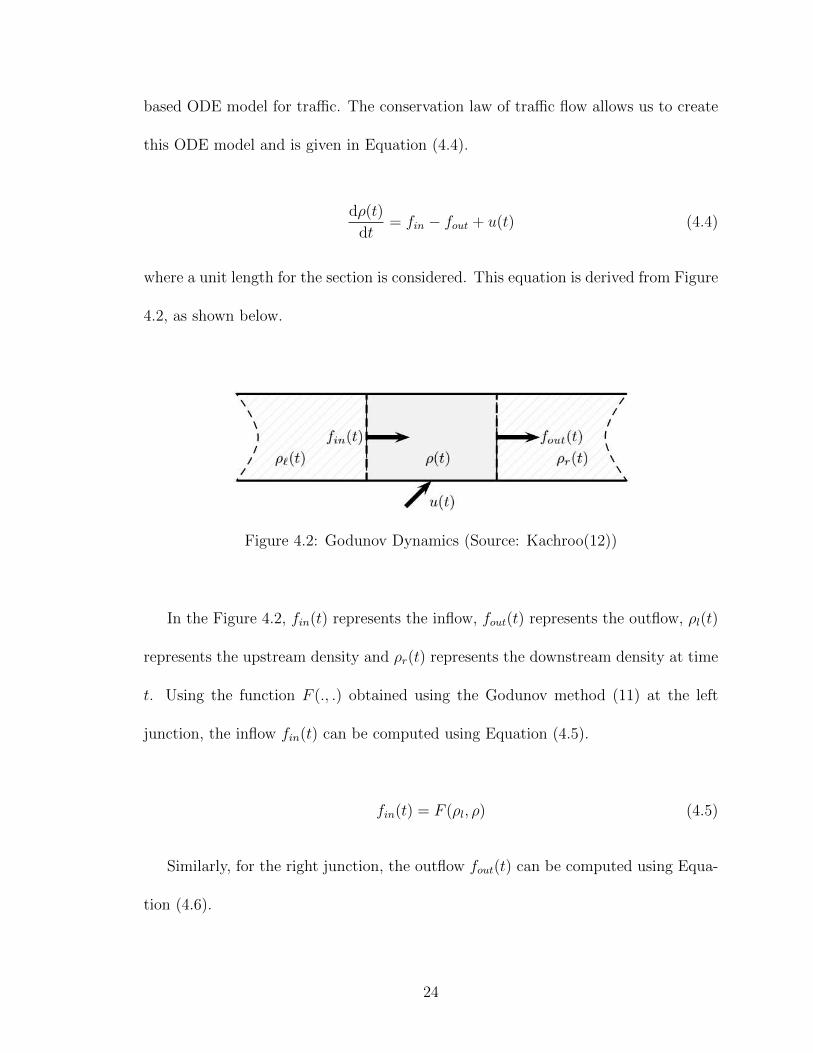
Figure 4.3: (a) 2 − D domain of dependent variable φ(x, y) (b) Three node FiniteElement defined in domain (c) Additional elements showing partial mesh of domain
defined by Equation (4.8).
φ(x, y) = N1(x, y)φ1 +N2(x, y)φ2 +N3(x, y)φ3 (4.8)
The triangulation element shown in Figure 4.3(b) and described in Equation (4.8) is
said to have 3 degrees of freedom, since three nodal values are necessary to describe
the dependent variable within the element. In general, degree of freedom for a finite
element equals the product of number of nodes and the nodal values of the dependent
variable required to be computed at every node. Since each finite element is connected
at an exterior node with its adjacent element as shown in Figure 4.3(c), the finite
element equations are fomulated to maintain the continuity of the dependent variable
at each node. However, it is noted that the interelement continuity of the derivatives
27

of the dependent variable does not necessarily exist. Through this discretization of the
domain, a finite element mesh is generated which nearly includes the entire physical
domain. In general, triangular elements are known to approximate the domain as
well as its boundaries nicely.
4.3.2 LWR-Greenshield’s Traffic Flow PDE used in FEM analysis
As introduced earlier in Equation (3.4), the following Traffic Flow PDE is used
for numerical simulations using FEM analysis.
∂ρ
∂t+ vf
∂ρ
∂x− 2vfρm
ρ∂ρ
∂x= 0
Since we are only considering the one-dimensional traffic flow problem, the above
Equation (3.4) is equivalent to the following Equation (4.11).
ρt +
(vf −
2vfρm
ρ
)ρ′ = 0 (4.9)
This equation is similar to the Navier Stokes Equation as given in Ervin et al.
(14). Before introducing the variational formulation for the above equation, let’s
define a few notations. Considering Ω ∈ <, the L2(Ω) norm and the inner product
are denoted by ‖.‖ and (., .) respectively. For functions v(x, t) defined on entire time
interval (0, T ), define ‖v‖∞,k := sup0<t<T
‖v(t, .)‖k and ‖v‖m,k :=
(∫ T
0
‖v(t, .)‖mk dt) 1
m
.
The function space used in FEM analysis is X := H10 (Ω) and the dual space of X is
denoted as X ′, with norm ‖.‖−1.
A variational formulation of Equation (4.11) can be stated as: Find ρ ∈ L2(0, T ;X)∩
28

L∞(0, T ;L2(Ω)) with ρt ∈ L2(0, T ;X ′) satisfying
(ρt, v) + vf (ρ′, v)− 2vf
ρm(ρ · ρ′, v) = 0 , ∀v ∈ X
ρ(x, 0) = ρ0(x) ,∀x ∈ Ω
(4.10)
4.3.3 Finite Element method with Time Relaxation
In this thesis, the diffusion is not being used to solve the hyperbolic traffic flow
pde given by Equation (3.4). Due to this, several oscillations exist around the shock
solutions. A simple regularization technique was proposed by Adamz , Stoltz and
Kleiser in (1) and (2). In this technique, if ρ represents the variable of interest, h
represents the characteristic mesh width, and δ = O(h) a chosen length scale, ρ∗ is
created to be another variable which represents the part of ρ varying over length scales
< O(δ) i.e. the fluctuating part of ρ. The term χρ∗ is then added to the differential
equation such that our model in Equation (4.11) is transformed to be,
ρt + vfρ′ − 2vf
ρmρ · ρ′ + χρ∗ = 0 (4.11)
According to Ervin et al. (14), the term χρ∗ drives the unresolved density scales
exponentially to zero. The term χ is called as the relaxation coefficient and has
the units1
time. Now, with the introduction of the new term χρ∗, the variational
formulation of Equation (4.11) is stated as: Find ρ ∈ L2(0, T ;X) ∩ L∞(0, T ;L2(Ω))
with ρt ∈ L2(0, T ;X ′) satisfying
29
(ρt, v) + vf (ρ′, v)− 2vf
ρm(ρ · ρ′, v) + χ(ρ−GNρ, v) = 0 ,∀v ∈ X
ρ(x, 0) = ρ0(x) ,∀x ∈ Ω
(4.12)
In Equation (4.12), ρ denotes a spatially averaged function of ρ defined as: ρ :=
G(ρ) satisying
−δ2ρ′′ + ρ = ρ , in Ω
ρ = 0 , on ∂Ω
(4.13)
where δ represents the filter length scale. According to Ervin et al. (14), the oper-
ator GN in Equation (4.12) represents the N th van Cittert approximate deconvolution
operator defined by
GNφ :=N∑n=0
(I −G)nφ, N = 0, 1, 2, . . . (4.14)
For example, the approximate de-convolution operator corresponding to N =
0, 1, 2 are G0ρ = ρ, G1ρ = 2ρ− ρ and G2ρ = 3ρ− 3ρ+ ρ.
Therefore, for N = 0, by substituting G0ρ in Equation (4.12), we get the following
system of equations in which the density goes through filtering once:
(ρt, v) + vf (ρ′, v)− 2vf
ρm(ρ · ρ′, v) + χ(ρ− ρ, v) = 0 ,∀v ∈ X
ρ(x, 0) = ρ0(x) ,∀x ∈ Ω
(4.15)
30
where ρ is computed through Equation (4.13)
Similarly, for N = 1, substituting G1ρ = 2ρ − ρ in Equation (4.12), gives us the
following system of equations:
(ρt, v) + vf (ρ′, v)− 2vf
ρm(ρ · ρ′, v) + χ(ρ− 2ρ+ ρ, v) = 0 , ∀v ∈ X
ρ(x, 0) = ρ0(x) ,∀x ∈ Ω
(4.16)
where ρ is first computed through Equation (4.13), which then is used to get ρ
through solving−δ2 ρ ′′+ρ = ρ. Once ρ is obtained, the density ρ is computed through
Equation (4.17). The same procedure is followed for higher order of deconvolution
N , and for N = 2, where the system of equations obtained by substituting G2ρ =
3ρ− 3ρ+ ρ in Equation (4.12) gives,
(ρt, v) + vf (ρ′, v)− 2vf
ρm(ρ · ρ′, v) + χ(ρ− 3ρ+ 3ρ− ρ, v) = 0 ,∀v ∈ X
ρ(x, 0) = ρ0(x) , ∀x ∈ Ω
(4.17)
31

CHAPTER 5
Numerical Simulations
5.1 Introduction
In this chapter, the one-equation Lighthill William and Richards (LWR) model
of traffic flow has been studied through two techniques: a) Godunov method and
b) Finite element method with time relaxation. For both methods, solutions to
several numerical problems found in the research literature are calculated and the
comparative results are presented. In all the problems, we compare how godunov
solution compares against the finite element solution. For shock problems (Stationary
Shock and Shock moving towards right), we investigated how order of relaxation affect
the solution, given the same relaxation parameter χ and filter length scale δ.
5.2 Equations
As introduced earlier in (3.3), the following equation is of interest.
∂
∂tρ(t, x) +
∂
∂xf(ρ) = 0
f(ρ) = ρv(ρ)
v(ρ) = vf (1−ρ
ρm)
This equation, when unfolded through substitution of variables, could be written
down as follows:
32

∂ρ
∂t+
(vf −
2vfρm
ρ
)∂ρ
∂x= 0
The above equation, given by (3.4) as well, forms the base of the numerical sim-
ulations in this chapter. Its variational formulation is given as below. Considering
Ω ∈ <
(ρt, v) + vf (ρ′, v)− 2vf
ρm(ρ · ρ′, v) + χ(ρ−GNρ, v) = 0 , ∀v ∈ X
ρ(x, 0) = ρ0(x) ,∀x ∈ Ω
For numerical simulations based on finite element method and Backward-Euler
temporal discretization with linear extrapolation ρn = 2ρn−1 − ρn−2 such that the
discretized finite element formualtion for time interval (0, T ] could be written as: For
n = 1, 2, . . . , NT , find ρnh ∈ Xh such that,
(ρnh, v) + ∆tvf (ρnh′, v)− 2vf
ρm∆t((2ρn−1h − ρn−2h ).ρnh
′, v) + χ∆t(ρnh −GNρnh, v)
= (ρn−1h , v)∀v ∈ Xh (5.1)
5.3 Accuracy measures
For computation of numerical accuracy, the following measures were used:
1. l2 norm of the error :
33

The l2 norm of the error vector e is defined as
‖e‖ =
√√√√ n∑k=1
|ek|2
where ek represents one term from the error vector and k = 1, 2, . . . N .
2. Bounded Variation (BV) norm of the error :
The bounded variation (bv) norm of the real valued error function defined on
an interval [a, b] ⊂ < is defined as
V ab (e) = sup
p∈P
np−1∑i=0
|e(xi+1)− e(xi)|
where the supremum is taken over the set
P = x0, . . . , xnP |P is a partition of [a, b]
3. Smoothness of Estimated Solution:
The inverse of Coefficient of Variation (Wikipedia) can be used for calculating
the smoothness of the estimated solution. If e represents the error between
the estimated solution y and it’s lag, we can calculate the smoothness of the
estimated solution s(e) as
s(e) =|µ(e)|σ(e)
=|µ(y(2 : n− 1)− y(1 : n− 2))|σ(y(2 : n− 1)− y(1 : n− 2))
34

where n represents the number of data points in the estimated solution.
5.3.1 Comparing the solutions
The accuracy measures defined above are used in comparing different sets of nu-
merical solutions with the exact solutions.
1. Comparing Godunov and Finite Element Solution:
The l2 norm and the bounded variation (bv) norm of the error defined above are
used for numerically comparing the Godunov solution with the FEM solution.
In each numerical problem, the l2 norm and the bounded variation (bv) norm
of the error is computed over space and plotted at each time t ∈ [0, T ].
2. Getting optimal parameters χ and δ for FEM with Time Relaxation:
As mentioned above, the Finite Element Method with Time Relaxation method
is used for suppressing the oscillations in two problems: a) Stationary Shocks
b) Shock moving towards right. Since different combinations of χ and δ give
different measures of l2 norm of the error, bounded variation (bv) norm of the
error and smoothness of estimated solution, all the three measures are used to
find the best possible χ and δ. The search space consists of the discrete set
χset × δset
where,
χset = 1, 2, 3, . . . , 100 , δset = 0.5h, h, 1.5h, 2h, 2.5h, 3h, 3.5h, 4h, 4.5h, 5h
35

and h represents the mesh width. Therefore, for the Stationary Shock and the
Shock moving towards right problem, a total of 1000 χ and δ combinations are
used to find the best possible χ and δ.
5.4 Common Parameters
This section lists the important parameters that are common to all numerical
simulations below.
Parameter Name Description Value
a Beginning point of the road segment -200b Ending point of the road segment 200l Length of the road segment a− b = 400 unitsT Final time 5 secondsM Number of Nodes 1001h FEM Mesh Width 0.3996004k Time Step 0.008064516N Number of iterations 620ρm Jam density 0.04ρo Initial density 0.02vf Free-Flow speed 25
Table 5.1: Common Parameters used in numerical simulations
Apart from the above parameters, the Finite Element method simulations used
P2 continuous piecewise quadratic basis functions and FreeFEM++ package (6) was
used to perform finite element simulations.
36

5.5 Linear Advection
As introduced in Chapter 3, linear advection refers to the motion of a conserved
quantity along a constant vector field. In this problem, since the velocity is constant,
the flow is only dependent upon the density. Apart from the common parameters
defined above, consider the following parameters:
Parameter Name Description Value
c Advection Velocity 3.0ρl Left density towards x = 0− at t = 0 0.01ρr Right density towards x = 0+ at t = 0 0.03
Table 5.2: Linear Advection: Parameters used in numerical simulation
Based upon the above parameters ρl and ρr, the initial density profile we get for
this problem is shown in Figure 5.1.
Figure 5.1: Linear Advection: Initial density profile
37

In the subsequent sections, the numerical techniques introduced in Chapter 4 are
used to find the numerical solution to the Linear Advection problem.
5.5.1 Godunov solution
Figure 5.2 provides the Godunov solution of this problem at final time T = 5
seconds. Moreover, Figure 5.3 shows the l2 and the bounded variation (bv) norm of
the error for each time t ∈ [0, T ].
Figure 5.2: Linear Advection: Godunov solution at time T = 5 seconds
As observed from the Figures 5.2 and 5.3, the Godunov method simulates this
problem well but has a smooth, continuous solution around the discontinuity at time
T = 5 seconds.
38
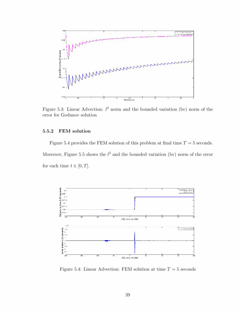
Figure 5.3: Linear Advection: l2 norm and the bounded variation (bv) norm of theerror for Godunov solution
5.5.2 FEM solution
Figure 5.4 provides the FEM solution of this problem at final time T = 5 seconds.
Moreover, Figure 5.5 shows the l2 and the bounded variation (bv) norm of the error
for each time t ∈ [0, T ].
Figure 5.4: Linear Advection: FEM solution at time T = 5 seconds
39

Figure 5.5: Linear Advection: l2 norm and the bounded variation (bv) norm of theerror for FEM solution
As observed from the Figures 5.4 and 5.5, the FEM method simulates this problem
well and is able to capture the discontinuity properly.
5.5.3 Comparison of solutions obtained from Godunov method and FEM
method
In this section, the numerical results obtained from the Godunov method and FEM
method are presented. Figure 5.6 gives an overview of how the Godunov solution
compares with the FEM solution at final time T = 5 seconds. The l2 norm and
the bounded variation norm of the error obtained from Godunov method and FEM
method are also presented in Figure 5.7. The latter figure helps us understand that
the FEM method outperforms the Godunov method in terms of the l2 norm of the
error.
40

Figure 5.6: Linear Advection: Comparison of numerical simulations obtained fromGodunov method and FEM method
Figure 5.7: Linear Advection: Comparison of l2 norm and bounded variation (bv)norm of the errors obtained from Godunov method and FEM method
41
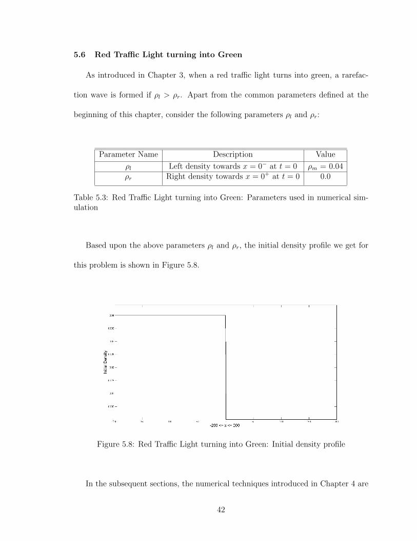
5.6 Red Traffic Light turning into Green
As introduced in Chapter 3, when a red traffic light turns into green, a rarefac-
tion wave is formed if ρl > ρr. Apart from the common parameters defined at the
beginning of this chapter, consider the following parameters ρl and ρr:
Parameter Name Description Value
ρl Left density towards x = 0− at t = 0 ρm = 0.04ρr Right density towards x = 0+ at t = 0 0.0
Table 5.3: Red Traffic Light turning into Green: Parameters used in numerical sim-ulation
Based upon the above parameters ρl and ρr, the initial density profile we get for
this problem is shown in Figure 5.8.
Figure 5.8: Red Traffic Light turning into Green: Initial density profile
In the subsequent sections, the numerical techniques introduced in Chapter 4 are
42

used to find the numerical solution to this problem.
5.6.1 Godunov solution
Figure 5.9 provides the Godunov solution of this problem at final time T = 5
seconds. Moreover, Figure 5.10 shows the l2 and the bounded variation (bv) norm of
the error for each time t ∈ [0, T ].
Figure 5.9: Red Traffic Light turning into Green: Godunov solution at time T = 5seconds
As observed from the Figures 5.9 and 5.10, the Godunov method simulates this
problem well.
5.6.2 FEM solution
Figure 5.11 provides the FEM solution of this problem at final time T = 5 seconds.
Moreover, Figure 5.12 shows the l2 and the bounded variation (bv) norm of the error
43

Figure 5.10: Red Traffic Light turning into Green: l2 norm and the bounded variation(bv) norm of the error for Godunov solution
for each time t ∈ [0, T ].
Figure 5.11: Red Traffic Light turning into Green: FEM solution at time T = 5seconds
As observed from the Figures 5.11 and 5.12, the FEM method also simulates this
problem well.
44

Figure 5.12: Red Traffic Light turning into Green: l2 norm and the bounded variation(bv) norm of the error for FEM solution
5.6.3 Comparison of solutions obtained from Godunov method and FEM
method
In this section, the numerical results obtained from the Godunov method and
FEM method are presented. Figure 5.13 gives an overview of how the Godunov
solution compares with the FEM solution at final time T = 5 seconds. The l2 norm
and the bounded variation norm of the error obtained from Godunov method and
FEM method are also presented in Figure 5.14. The latter figure helps us understand
that the FEM method outperforms the Godunov method in terms of both, the l2
norm and the bounded variation norm of the error.
5.7 Stationary Shock
As introduced in Chapter 3, a shock stays stationary if ρl and ρr are chosen such
that the shock velocity remains zero. Apart from the common parameters defined at
the beginning of this chapter, consider the following parameters ρl and ρr:
45

Figure 5.13: Red Traffic Light turning into Green: Comparison of numerical simula-tions obtained from Godunov method and FEM method
Figure 5.14: Red Traffic Light turning into Green: Comparison of l2 norm andbounded variation (bv) norm of the errors obtained from Godunov method and FEMmethod
46
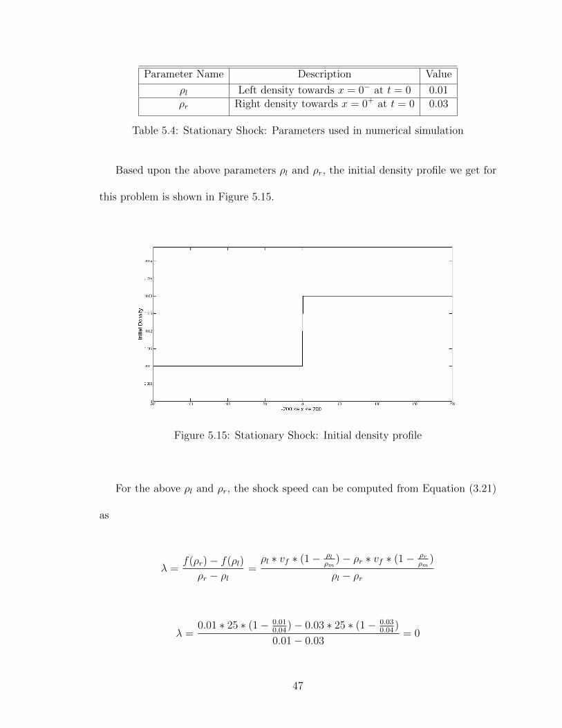
Parameter Name Description Value
ρl Left density towards x = 0− at t = 0 0.01ρr Right density towards x = 0+ at t = 0 0.03
Table 5.4: Stationary Shock: Parameters used in numerical simulation
Based upon the above parameters ρl and ρr, the initial density profile we get for
this problem is shown in Figure 5.15.
Figure 5.15: Stationary Shock: Initial density profile
For the above ρl and ρr, the shock speed can be computed from Equation (3.21)
as
λ =f(ρr)− f(ρl)
ρr − ρl=ρl ∗ vf ∗ (1− ρl
ρm)− ρr ∗ vf ∗ (1− ρr
ρm)
ρl − ρr
λ =0.01 ∗ 25 ∗ (1− 0.01
0.04)− 0.03 ∗ 25 ∗ (1− 0.03
0.04)
0.01− 0.03= 0
47

Therefore, for the chosen ρl and ρr, we get shock speed λ = 0, which causes
the shock to remain stationary ∀ t > 0. In the subsequent sections, the numerical
techniques introduced in Chapter 4 are used to find the numerical solution to this
problem.
5.7.1 Godunov solution
Figure 5.16 provides the Godunov solution of this problem at final time T = 5
seconds. Moreover, Figure 5.17 shows the l2 and the bounded variation (bv) norm of
the error for each time t ∈ [0, T ].
Figure 5.16: Stationary Shock: Godunov solution at time T = 5 seconds
As observed from the Figures 5.16 and 5.17, it seems that the Godunov method
simulates the stationary shock extremely well. This is because the Godunov solution
is based upon the flow at the left and right junctions of a segment, but since the shock
48

Figure 5.17: Stationary Shock: l2 norm and the bounded variation (bv) norm of theerror for Godunov solution
velocity is 0, the flow is 0. Hence, the solution keeps it’s initial profile ∀t > 0.
5.7.2 FEM solution without time relaxation
In Equation (4.12), the relaxation parameter χ can be set to 0 to yield a finite
element variational problem without any relaxation. Figures 5.18 and 5.19 provide the
FEM solution at the final time T = 5 seconds and the l2 and the bounded variation
(bv) norm of the error for each time t ∈ [0, T ] respectively.
As can be observed in the Figures 5.18 and 5.19, the finite element method is not
able to numerically simulate the stationary shock and gets tremendous amounts of
oscillations.
5.7.3 FEM solution with time relaxation
As introduced in Chapter 4, the term χρ∗ can be added to the finite element
variation formulation, which helps to drive the unresolved density scales exponentially
49
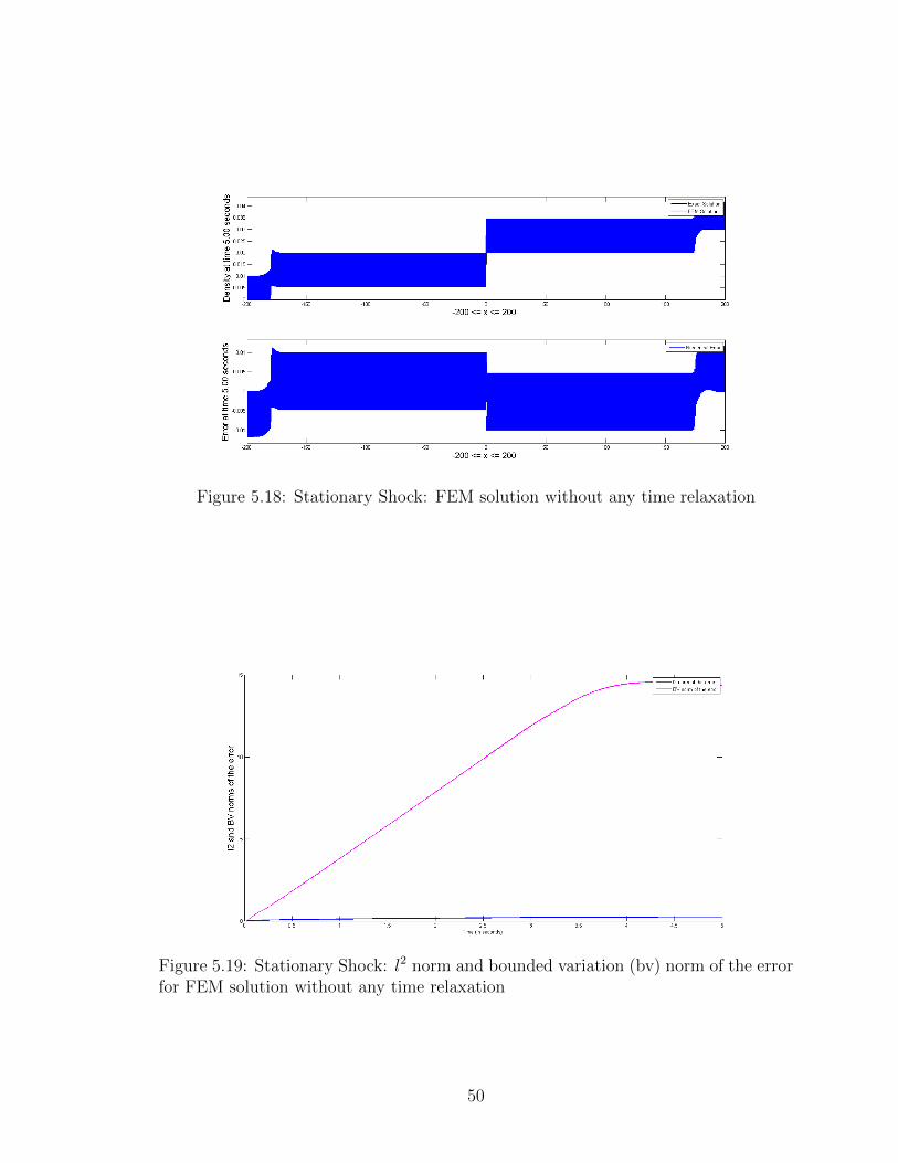
Figure 5.18: Stationary Shock: FEM solution without any time relaxation
Figure 5.19: Stationary Shock: l2 norm and bounded variation (bv) norm of the errorfor FEM solution without any time relaxation
50
to zero. The finite element variational formulation with time relaxation was given in
the beginning of this chapter and also, in Chapter 4.
However, the usage of time relaxation in finite element method requires choosing
the relaxation parameter χ and filter length scale δ. Based upon the process described
earlier in this chapter, numerical computations were done to get the optimal χ and δ
over 1000 such combinations.
For all such combinations, l2 norm of the error, bounded variation (bv) norm of
the error and the smoothness of the estimated solution were calculated by performing
time relaxation twice, whose variational formulation is given in Chapter 4. Following
steps were taken to choose the optimal χ and δ.
1. In order to reduce the search space, only those candidates of χ−δ combinations
were selected for which min(l2) < l2 < 1.3 ∗min(l2).
2. From amongst the above candidates, that χ− δ combination was chosen which
gave the minimal bounded variation (bv) norm of the error and the maximum
smoothness of the estimated solution.
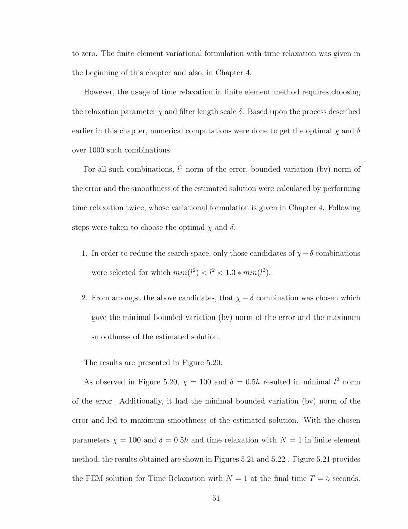
The results are presented in Figure 5.20.
As observed in Figure 5.20, χ = 100 and δ = 0.5h resulted in minimal l2 norm
of the error. Additionally, it had the minimal bounded variation (bv) norm of the
error and led to maximum smoothness of the estimated solution. With the chosen
parameters χ = 100 and δ = 0.5h and time relaxation with N = 1 in finite element
method, the results obtained are shown in Figures 5.21 and 5.22 . Figure 5.21 provides
the FEM solution for Time Relaxation with N = 1 at the final time T = 5 seconds.
51
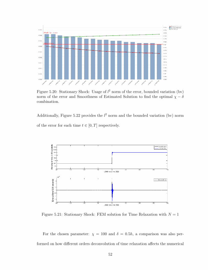
Figure 5.20: Stationary Shock: Usage of l2 norm of the error, bounded variation (bv)norm of the error and Smoothness of Estimated Solution to find the optimal χ − δcombination.
Additionally, Figure 5.22 provides the l2 norm and the bounded variation (bv) norm
of the error for each time t ∈ [0, T ] respectively.
Figure 5.21: Stationary Shock: FEM solution for Time Relaxation with N = 1
For the chosen parameter: χ = 100 and δ = 0.5h, a comparison was also per-
formed on how different orders deconvolution of time relaxation affects the numerical
52
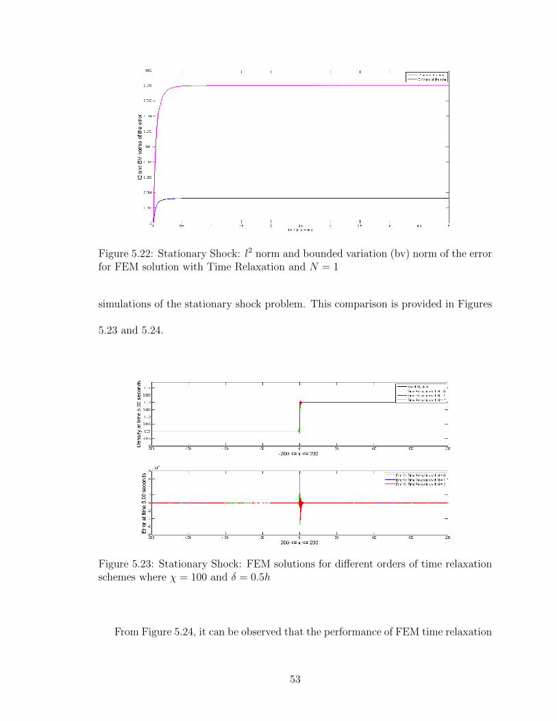
Figure 5.22: Stationary Shock: l2 norm and bounded variation (bv) norm of the errorfor FEM solution with Time Relaxation and N = 1
simulations of the stationary shock problem. This comparison is provided in Figures
5.23 and 5.24.
Figure 5.23: Stationary Shock: FEM solutions for different orders of time relaxationschemes where χ = 100 and δ = 0.5h
From Figure 5.24, it can be observed that the performance of FEM time relaxation
53
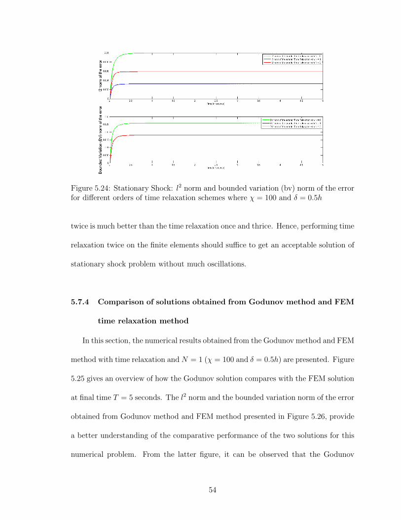
Figure 5.24: Stationary Shock: l2 norm and bounded variation (bv) norm of the errorfor different orders of time relaxation schemes where χ = 100 and δ = 0.5h
twice is much better than the time relaxation once and thrice. Hence, performing time
relaxation twice on the finite elements should suffice to get an acceptable solution of
stationary shock problem without much oscillations.
5.7.4 Comparison of solutions obtained from Godunov method and FEM
time relaxation method
In this section, the numerical results obtained from the Godunov method and FEM
method with time relaxation and N = 1 (χ = 100 and δ = 0.5h) are presented. Figure
5.25 gives an overview of how the Godunov solution compares with the FEM solution
at final time T = 5 seconds. The l2 norm and the bounded variation norm of the error
obtained from Godunov method and FEM method presented in Figure 5.26, provide
a better understanding of the comparative performance of the two solutions for this
numerical problem. From the latter figure, it can be observed that the Godunov
54
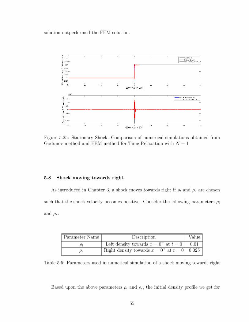
solution outperformed the FEM solution.
Figure 5.25: Stationary Shock: Comparison of numerical simulations obtained fromGodunov method and FEM method for Time Relaxation with N = 1
5.8 Shock moving towards right
As introduced in Chapter 3, a shock moves towards right if ρl and ρr are chosen
such that the shock velocity becomes positive. Consider the following parameters ρl
and ρr:
Parameter Name Description Value
ρl Left density towards x = 0− at t = 0 0.01ρr Right density towards x = 0+ at t = 0 0.025
Table 5.5: Parameters used in numerical simulation of a shock moving towards right
Based upon the above parameters ρl and ρr, the initial density profile we get for
55

Figure 5.26: Stationary Shock: Comparison of l2 norm and bounded variation (bv)norm of the errors obtained from Godunov method and FEM method for Time Re-laxation with N = 1
this problem is shown in Figure 5.27.
For the above ρl and ρr, the shock speed can be computed from Equation (3.21)
as
λ =f(ρr)− f(ρl)
ρr − ρl=ρl ∗ vf ∗ (1− ρl
ρm)− ρr ∗ vf ∗ (1− ρr
ρm)
ρl − ρr
λ =0.01 ∗ 25 ∗ (1− 0.01
0.04)− 0.025 ∗ 25 ∗ (1− 0.025
0.04)
0.01− 0.025= 3.125
Therefore, for the chosen ρl and ρr, we get shock speed λ > 0, which causes the
shock to move towards right. In the subsequent sections, the numerical techniques
introduced in Chapter 4 are used to find the numerical solution to this problem.
56

Figure 5.27: Shock moving towards right: Initial density profile
5.8.1 Godunov solution
Figure 5.28 provides the Godunov solution of this problem at final time T = 5
seconds. Moreover, Figure 5.29 shows the l2 and the bounded variation (bv) norm of
the error for each time t ∈ [0, T ].
Figure 5.28: Shock moving towards right: Godunov solution at time T = 5 seconds
57

Figure 5.29: Shock moving towards right: l2 norm and the bounded variation (bv)norm of the error for Godunov solution
5.8.2 FEM solution without time relaxation
In Equation (4.12), the relaxation parameter χ can be set to 0 to yield a finite
element variational problem without any relaxation. Figures 5.30 and 5.31 provide the
FEM solution at the final time T = 5 seconds and the l2 and the bounded variation
(bv) norm of the error for each time t ∈ [0, T ] respectively.
Figure 5.30: Shock moving towards right: FEM solution without any time relaxation
58

Figure 5.31: Shock moving towards right: l2 norm and bounded variation (bv) normof the error for FEM solution without any time relaxation
As can be observed in the Figures 5.30 and 5.31, the finite element method is
not able to numerically simulate the moving shock and gets tremendous amounts of
oscillations.
5.8.3 FEM solution with time relaxation
As introduced in Chapter 4, the term χρ∗ can be added to the finite element
variation formulation, which helps to drive the unresolved density scales exponentially
to zero. The finite element variational formulation with time relaxation was given in
the beginning of this chapter and also, in Chapter 4.
However, the usage of time relaxation in finite element method requires choosing
the relaxation parameter χ and filter length scale δ. Based upon the process described
earlier in this chapter, numerical computations were done to get the optimal χ and δ
over 1000 such combinations.
59

For all such combinations, l2 error, bounded variation and the smoothness of
the estimated solution were calculated by performing time relaxation twice, whose
variational formulation is given in Chapter 4. Following steps were taken to choose
the optimal χ and δ.
1. In order to reduce the search space, only those candidates of χ−δ combinations
were selected for which min(l2) < l2 < 1.09 ∗min(l2).
2. From amongst the above candidates, that χ− δ combination was chosen which
gave the minimal bounded variation (bv) norm of the error and the maximum
smoothness of the estimated solution.
The results are presented in Figure 5.32.
Figure 5.32: Shock moving towards right: Usage of l2 norm of the error, BoundedVariation (bv) norm of the error and Smoothness of Estimated Solution to find theoptimal χ− δ combination.
As observed in Figure 5.32, χ = 9 and δ = 5h resulted in l2 norm of the error
60
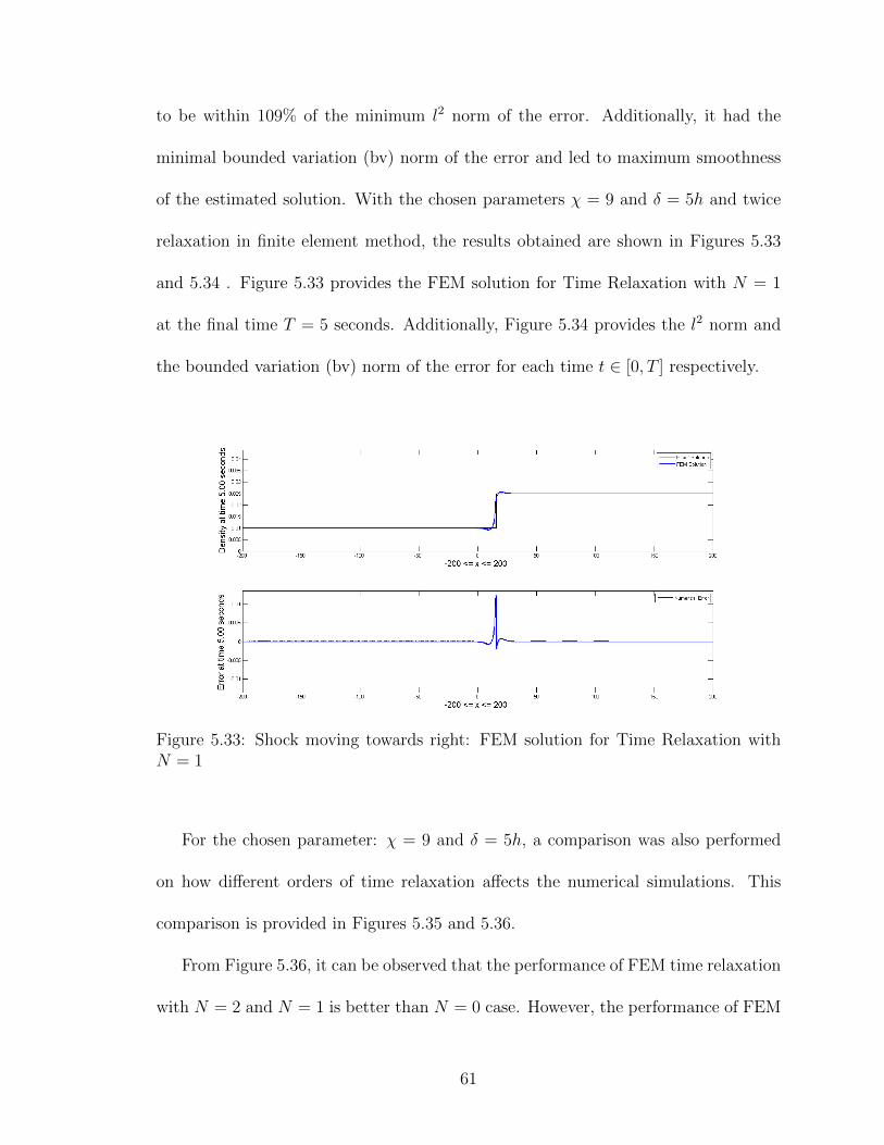
to be within 109% of the minimum l2 norm of the error. Additionally, it had the
minimal bounded variation (bv) norm of the error and led to maximum smoothness
of the estimated solution. With the chosen parameters χ = 9 and δ = 5h and twice
relaxation in finite element method, the results obtained are shown in Figures 5.33
and 5.34 . Figure 5.33 provides the FEM solution for Time Relaxation with N = 1
at the final time T = 5 seconds. Additionally, Figure 5.34 provides the l2 norm and
the bounded variation (bv) norm of the error for each time t ∈ [0, T ] respectively.
Figure 5.33: Shock moving towards right: FEM solution for Time Relaxation withN = 1
For the chosen parameter: χ = 9 and δ = 5h, a comparison was also performed
on how different orders of time relaxation affects the numerical simulations. This
comparison is provided in Figures 5.35 and 5.36.
From Figure 5.36, it can be observed that the performance of FEM time relaxation
with N = 2 and N = 1 is better than N = 0 case. However, the performance of FEM
61

Figure 5.34: Shock moving towards right: l2 norm and bounded variation (bv) normof the error in FEM solution for Time Relaxation with N = 1
Figure 5.35: Shock moving towards right: FEM solutions for different orders of timerelaxation schemes where χ = 9 and δ = 5h
62
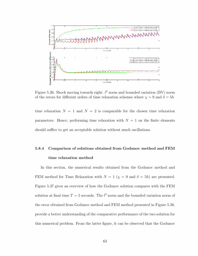
Figure 5.36: Shock moving towards right: l2 norm and bounded variation (BV) normof the errors for different orders of time relaxation schemes where χ = 9 and δ = 5h
time relaxation N = 1 and N = 2 is comparable for the chosen time relaxation
parameters. Hence, performing time relaxation with N = 1 on the finite elements
should suffice to get an acceptable solution without much oscillations.
5.8.4 Comparison of solutions obtained from Godunov method and FEM
time relaxation method
In this section, the numerical results obtained from the Godunov method and
FEM method for Time Relaxation with N = 1 (χ = 9 and δ = 5h) are presented.
Figure 5.37 gives an overview of how the Godunov solution compares with the FEM
solution at final time T = 5 seconds. The l2 norm and the bounded variation norm of
the error obtained from Godunov method and FEM method presented in Figure 5.38,
provide a better understanding of the comparative performance of the two solution for
this numerical problem. From the latter figure, it can be observed that the Godunov
63

solution outperformed the FEM solution because although the FEM solution captured
the movement of the shock and did not give any oscillations, the FEM solution was
smoothed around the discontinuity. However, the Godunov solution not only captured
the movement without much oscillations, but also gave the expected shape of the
discontinous curve.
Figure 5.37: Shock moving towards right: Comparison of numerical simulations ob-tained from Godunov method and FEM method for Time Relaxation with N = 1
64

Figure 5.38: Shock moving towards right: Comparison of l2 norm and bounded vari-ation (bv) norm of the errors obtained from Godunov method and FEM method forTime Relaxation with N = 1
65
CHAPTER 6
Conclusion
6.1 Summary
This thesis applied numerical methods popular in fluid research into traffic flow
problems. Several numerical simulations for the LWR and Greenshield’s model were
presented using both, the Godunov and the Finite Element method. The application
of time relaxation within finite elements allowed finite element simulations to get rid
of the diffusion term and suppress oscillations just by fine tuning the time relaxation
parameters χ and δ.
It was observed that:
1. Finite Element Method outperformed Godunov method in two problems:
Linear Advection
Red Traffic Light turning into Green
2. Godunov method outperformed Finite Element Time Relaxation method in two
problems:
Stationary Shocks
Shock moving towards right
3. In presence of shocks, the Finite Element Method performs bad and has lots of
oscillations, if no time relaxation is added. However, addition of time relaxation
suppresses oscillations to a great extent.
66

4. Increasing the order of time relaxation does not necessarily mean that the so-
lution will become more smooth and will have better properties. As observed,
doing time relaxation with N = 1 outperformed time relaxation with N = 0
and N = 2. This was clearly observed in Stationary Shocks, however, the per-
formance of time relaxation with N = 1 was close to time relaxation with N = 2
for Shock moving towards Right.
5. l2 norm of the error, bounded variation norm of the error and the smoothness
of the estimated solution proved to be extremely helpful measures in selecting
the right candidates for optimal parameters χ and δ.
6.2 Future Work
This section presents the following areas where the thesis can be extended for
further research.
1. Currently, the numerical simulations were computed using the LWR and Green-
shield’s model. However, Kachroo (9) presents other models for the velocity
density relationship where the numerical simulations can be performed using
the Godunov and Finite Element Methods. A few of those models are shown
below:
Greenberg model: v(ρ) = vf ln
(ρmρ
) Underwood model: v(ρ) = vf exp
(− ρ
ρm
) Northwestern University model: v(ρ) = vfexp
(−0.5(
ρ
ρm)2)
67

2. In this thesis, numerical simulations were performed for four benchmark prob-
lems. The simulations can be performed for other problems as well such as: a
shock moving towards left.
3. The thesis can be further extended by performing higher order discretization in
time with Crank-Nicolson schemes, theta schemes etc. Please see Volker (8) for
more details.
4. Last but not the least, a non linear time relaxation can be performed that can
perform better reduction in oscillations more efficiently. Please see Layton (10)
for more details.
68

BIBLIOGRAPHY
[1] Adams, N. and Stolz, S. (2001). Deconvolution methods for subgrid-scale approxi-
mation in large eddy simulation. Modern Simulation Strategies for Turbulent Flow,
pages 21–41.
[2] Adams, N. and Stolz, S. (2002). A subgrid-scale deconvolution approach for shock
capturing. Journal of Computational Physics, 178(2):391–426.
[3] Bellomo, N. and Delitala, M. (2002). On the mathematical theory of vehicular
traffic. Fluid Dynamic and Kinetic Modeling, I.
[4] Gerlough, D. L. and Huber, M. J. (1975). Traffic flow theory: a monograph, vol-
ume 165. Transportation Research Board, National Research Council Washington,
DC.
[5] Haberman, R. (1998). Mathematical Models: mechanical vibrations, population
dynamics and traffic flow. Society for Industrial and Applied Mathematics.
[6] Hecht, F. (2012). New development in freefem++. J. Numer. Math., 20(3-4):251–
265.
[7] Hutton, D. V. (2004). Fundamentals of Finite Element Analysis. McGraw-Hill.
[8] John, V. (2004). Large eddy simulation of turbulent incompressible flows: analyt-
ical and numerical results for a class of LES models, volume 34. Springer.
[9] Kachroo, P. (2009). Pedestrian Dynamics: mathematical theory and evaculation
control. CRC Press.
[10] Layton, W. and Neda, M. (2007). Truncation of scales by time relaxation. Jour-
nal of Mathematical Analysis and Applications, 325(2):788–807.
69

[11] Leveque, R. J. (1999). Numerical Methods for Conservation Laws. Birkhauser
Verlag, Basel Boston Berlin.
[12] P. Kachroo, L. R. and Sastry, S. (2014). Analysis of the godunov based hybrid
model for ramp metering and robust feedback control design. IEEE Transactions
on Intelligent Transportation Systems, 00:00.
[13] Trangenstein, J. (2008). Numerical Solution of Hyperbolic Partial Differential
Equations. Cambridge University Press.
[14] V. J. Ervin, W. J. L. and Neda, M. (2007). Numerical analysis of a higher order
time relaxation model of fluids. International Journal of Numerical Analysis and
Modeling, 4.
[Wikipedia] Wikipedia. Coefficient of variation.
70

VITA
Graduate CollegeUniversity of Nevada, Las Vegas
Puneet Lakhanpal
Home Address:604 Waterbury LnFoster City, CA 94404
Degrees:
Master of Science, Electrical and Computer Engineering, 2011University of Nevada, Las Vegas
Bachelor of Technology, Electronics and Communication Engineering, 2009Indian Institute of Technology, Guwahati
Thesis Title:Numerical Simulations of Traffic Flow Models
Thesis Examination Committee:
Chairperson, Monika Neda, Ph.D.
Chairperson, Pushkin Kachroo, Ph.D., P.E.
Committee Member, Hongtao Yang, Ph.D.
Committeee Member, Amei Amei, Ph.D.
Graduate Faculty Representative, Yingtao Jiang, Ph.D.
71
Related Documents