The Cryosphere, 10, 639–664, 2016 www.the-cryosphere.net/10/639/2016/ doi:10.5194/tc-10-639-2016 © Author(s) 2016. CC Attribution 3.0 License. Numerical simulations of the Cordilleran ice sheet through the last glacial cycle Julien Seguinot 1,2,3 , Irina Rogozhina 3,4 , Arjen P. Stroeven 2 , Martin Margold 2 , and Johan Kleman 2 1 Laboratory of Hydraulics, Hydrology and Glaciology, ETH Zürich, Zürich, Switzerland 2 Department of Physical Geography and the Bolin Centre for Climate Research, Stockholm University, Stockholm, Sweden 3 Helmholtz Centre Potsdam, GFZ German Research Centre for Geosciences, Potsdam, Germany 4 Center for Marine Environmental Sciences, University of Bremen, Bremen, Germany Correspondence to: Julien Seguinot ([email protected]) Received: 21 June 2015 – Published in The Cryosphere Discuss.: 7 August 2015 Revised: 2 February 2016 – Accepted: 19 February 2016 – Published: 16 March 2016 Abstract. After more than a century of geological research, the Cordilleran ice sheet of North America remains among the least understood in terms of its former extent, volume, and dynamics. Because of the mountainous topography on which the ice sheet formed, geological studies have often had only local or regional relevance and shown such a complexity that ice-sheet-wide spatial reconstructions of advance and re- treat patterns are lacking. Here we use a numerical ice sheet model calibrated against field-based evidence to attempt a quantitative reconstruction of the Cordilleran ice sheet his- tory through the last glacial cycle. A series of simulations is driven by time-dependent temperature offsets from six proxy records located around the globe. Although this approach re- veals large variations in model response to evolving climate forcing, all simulations produce two major glaciations during marine oxygen isotope stages 4 (62.2–56.9 ka) and 2 (23.2– 16.9 ka). The timing of glaciation is better reproduced using temperature reconstructions from Greenland and Antarctic ice cores than from regional oceanic sediment cores. During most of the last glacial cycle, the modelled ice cover is dis- continuous and restricted to high mountain areas. However, widespread precipitation over the Skeena Mountains favours the persistence of a central ice dome throughout the glacial cycle. It acts as a nucleation centre before the Last Glacial Maximum and hosts the last remains of Cordilleran ice until the middle Holocene (6.7 ka). 1 Introduction During the last glacial cycle, glaciers and ice caps of the North American Cordillera have been more extensive than today. At the Last Glacial Maximum (LGM), a continuous blanket of ice, the Cordilleran ice sheet (Dawson, 1888), stretched from the Alaska Range in the north to the North Cascades in the south (Fig. 1). In addition, it extended off- shore, where it calved into the Pacific Ocean, and merged with the western margin of its much larger neighbour, the Laurentide ice sheet, east of the Rocky Mountains. More than a century of exploration and geological inves- tigation of the Cordilleran mountains have led to many ob- servations in support of the former ice sheet (Jackson and Clague, 1991). Despite the lack of documented end moraines offshore, in the zone of confluence with the Laurentide ice sheet and in areas swept by the Missoula floods (Carrara et al., 1996), moraines that demarcate the northern and south- western margins provide key constraints that allow reason- able reconstructions of maximum ice sheet extents (Prest et al., 1968; Clague, 1989, Fig. 1.12; Duk-Rodkin, 1999; Booth et al., 2003; Dyke, 2004). As indicated by field evi- dence from radiocarbon dating (Clague et al., 1980; Clague, 1985, 1986; Porter and Swanson, 1998; Menounos et al., 2008), cosmogenic exposure dating (Stroeven et al., 2010, 2014; Margold et al., 2014), bedrock deformation in response to former ice loads (Clague and James, 2002; Clague et al., 2005), and offshore sedimentary records (Cosma et al., 2008; Davies et al., 2011), the LGM Cordilleran ice sheet extent was short-lived. However, former ice thicknesses and, there- Published by Copernicus Publications on behalf of the European Geosciences Union.

Welcome message from author
This document is posted to help you gain knowledge. Please leave a comment to let me know what you think about it! Share it to your friends and learn new things together.
Transcript
The Cryosphere, 10, 639–664, 2016
www.the-cryosphere.net/10/639/2016/
doi:10.5194/tc-10-639-2016
© Author(s) 2016. CC Attribution 3.0 License.
Numerical simulations of the Cordilleran ice sheet through the last
glacial cycle
Julien Seguinot1,2,3, Irina Rogozhina3,4, Arjen P. Stroeven2, Martin Margold2, and Johan Kleman2
1Laboratory of Hydraulics, Hydrology and Glaciology, ETH Zürich, Zürich, Switzerland2Department of Physical Geography and the Bolin Centre for Climate Research, Stockholm University, Stockholm, Sweden3Helmholtz Centre Potsdam, GFZ German Research Centre for Geosciences, Potsdam, Germany4Center for Marine Environmental Sciences, University of Bremen, Bremen, Germany
Correspondence to: Julien Seguinot ([email protected])
Received: 21 June 2015 – Published in The Cryosphere Discuss.: 7 August 2015
Revised: 2 February 2016 – Accepted: 19 February 2016 – Published: 16 March 2016
Abstract. After more than a century of geological research,
the Cordilleran ice sheet of North America remains among
the least understood in terms of its former extent, volume,
and dynamics. Because of the mountainous topography on
which the ice sheet formed, geological studies have often had
only local or regional relevance and shown such a complexity
that ice-sheet-wide spatial reconstructions of advance and re-
treat patterns are lacking. Here we use a numerical ice sheet
model calibrated against field-based evidence to attempt a
quantitative reconstruction of the Cordilleran ice sheet his-
tory through the last glacial cycle. A series of simulations is
driven by time-dependent temperature offsets from six proxy
records located around the globe. Although this approach re-
veals large variations in model response to evolving climate
forcing, all simulations produce two major glaciations during
marine oxygen isotope stages 4 (62.2–56.9 ka) and 2 (23.2–
16.9 ka). The timing of glaciation is better reproduced using
temperature reconstructions from Greenland and Antarctic
ice cores than from regional oceanic sediment cores. During
most of the last glacial cycle, the modelled ice cover is dis-
continuous and restricted to high mountain areas. However,
widespread precipitation over the Skeena Mountains favours
the persistence of a central ice dome throughout the glacial
cycle. It acts as a nucleation centre before the Last Glacial
Maximum and hosts the last remains of Cordilleran ice until
the middle Holocene (6.7 ka).
1 Introduction
During the last glacial cycle, glaciers and ice caps of the
North American Cordillera have been more extensive than
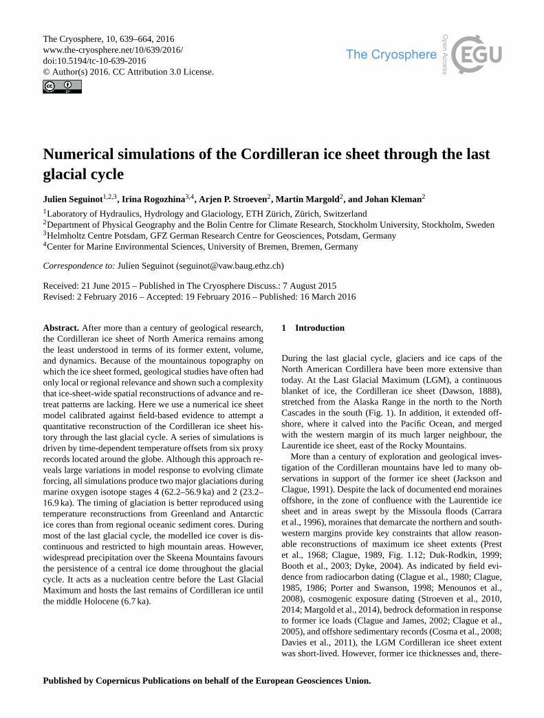
today. At the Last Glacial Maximum (LGM), a continuous
blanket of ice, the Cordilleran ice sheet (Dawson, 1888),
stretched from the Alaska Range in the north to the North
Cascades in the south (Fig. 1). In addition, it extended off-
shore, where it calved into the Pacific Ocean, and merged
with the western margin of its much larger neighbour, the
Laurentide ice sheet, east of the Rocky Mountains.
More than a century of exploration and geological inves-
tigation of the Cordilleran mountains have led to many ob-
servations in support of the former ice sheet (Jackson and
Clague, 1991). Despite the lack of documented end moraines
offshore, in the zone of confluence with the Laurentide ice
sheet and in areas swept by the Missoula floods (Carrara
et al., 1996), moraines that demarcate the northern and south-
western margins provide key constraints that allow reason-
able reconstructions of maximum ice sheet extents (Prest
et al., 1968; Clague, 1989, Fig. 1.12; Duk-Rodkin, 1999;
Booth et al., 2003; Dyke, 2004). As indicated by field evi-
dence from radiocarbon dating (Clague et al., 1980; Clague,
1985, 1986; Porter and Swanson, 1998; Menounos et al.,
2008), cosmogenic exposure dating (Stroeven et al., 2010,
2014; Margold et al., 2014), bedrock deformation in response
to former ice loads (Clague and James, 2002; Clague et al.,
2005), and offshore sedimentary records (Cosma et al., 2008;
Davies et al., 2011), the LGM Cordilleran ice sheet extent
was short-lived. However, former ice thicknesses and, there-
Published by Copernicus Publications on behalf of the European Geosciences Union.
640 J. Seguinot et al.: Numerical simulations of the Cordilleran ice sheet through the last glacial cycle
Brooks Range
Alaska Range
WrangellMts
St Elias Mts
McKenzie MtsSelwyn MtsCassiar M
ountains
Columbia Mts
Rocky Mountains
Coast Mountains
Skeena Mts
N.
Casc
ades
LiardLowland
InteriorPlateau
PugetLowland
Q. Charlotte I.Vancouver Island
ARCTIC OCEAN
PACIFIC
OCEAN
CANADIAN
PRAIRIES
Figure 1. Relief map of the northern American Cordillera showing cumulative last glacial maximum ice cover between 21.4 and
16.8 14Ccalka (Dyke, 2004, red line) and the modelling domain used in this study (black rectangle). The background map consists of
ETOPO1 (Amante and Eakins, 2009) and Natural Earth Data (Patterson and Kelso, 2015).
fore, the ice sheet’s contribution to the LGM sea-level low-
stand (Carlson and Clark, 2012; Clark and Mix, 2002) remain
uncertain.
Our understanding of the Cordilleran glaciation history
prior to the LGM is even more fragmentary (Barendregt and
Irving, 1998; Kleman et al., 2010; Rutter et al., 2012), al-
though it is clear that the Pleistocene maximum extent of
the Cordilleran ice sheet predates the last glacial cycle (Hidy
et al., 2013). In parts of Yukon and Alaska, and in the Puget
Lowland, the distribution of tills (Turner et al., 2013; Troost,
2014) and dated glacial erratics (Ward et al., 2007, 2008;
Briner and Kaufman, 2008; Stroeven et al., 2010, 2014) in-
dicate an extensive marine oxygen isotope (MIS) stage 4
glaciation. Landforms in the interior regions include flow
sets that are likely older than the LGM (Kleman et al., 2010,
Fig. 2), but their absolute age remains uncertain.
In contrast, evidence for the deglaciation history of the
Cordilleran ice sheet since the LGM is considerable, albeit
mostly at a regional scale. Geomorphological evidence from
south-central British Columbia indicates a rapid deglacia-
tion, including an early emergence of elevated areas while
thin, stagnant ice still covered the surrounding lowlands
(Fulton, 1967, 1991; Margold et al., 2011, 2013b). This
model, although credible, may not apply in all areas of the
Cordilleran ice sheet (Margold et al., 2013a). Although solid
evidence for late-glacial glacier readvances has been found in
the Coast, Columbia, and Rocky mountains (Reasoner et al.,
1994; Osborn and Gerloff, 1997; Clague et al., 1997; Friele
and Clague, 2002a, b; Kovanen, 2002; Kovanen and Easter-
brook, 2002; Lakeman et al., 2008; Menounos et al., 2008), it
appears to be sparser than for formerly glaciated regions sur-
rounding the North Atlantic (e.g. Sissons, 1979; Lundqvist,
1987; Ivy-Ochs et al., 1999; Stea et al., 2011). Nevertheless,
recent oxygen isotope measurements from Gulf of Alaska
sediments reveal a climatic evolution highly correlated to that
of Greenland during this period, including a distinct Late
Glacial cold reversal between 14.1 and 11.7 ka (Praetorius
and Mix, 2014).
In general, the topographic complexity of the North Amer-
ican Cordillera and its effect on glacial history have inhibited
the reconstruction of ice-sheet-wide glacial advance and re-
treat patterns such as those available for the Fennoscandian
and Laurentide ice sheets (Dyke and Prest, 1987; Boulton
et al., 2001; Dyke et al., 2003; Kleman et al., 1997, 2010;
Stroeven et al., 2015). Here, we use a numerical ice sheet
model (the PISM authors, 2015), calibrated against field-
based evidence, to perform a quantitative reconstruction of
the Cordilleran ice sheet evolution through the last glacial cy-
cle and analyse some of the long-standing questions related
to its evolution:
The Cryosphere, 10, 639–664, 2016 www.the-cryosphere.net/10/639/2016/
J. Seguinot et al.: Numerical simulations of the Cordilleran ice sheet through the last glacial cycle 641
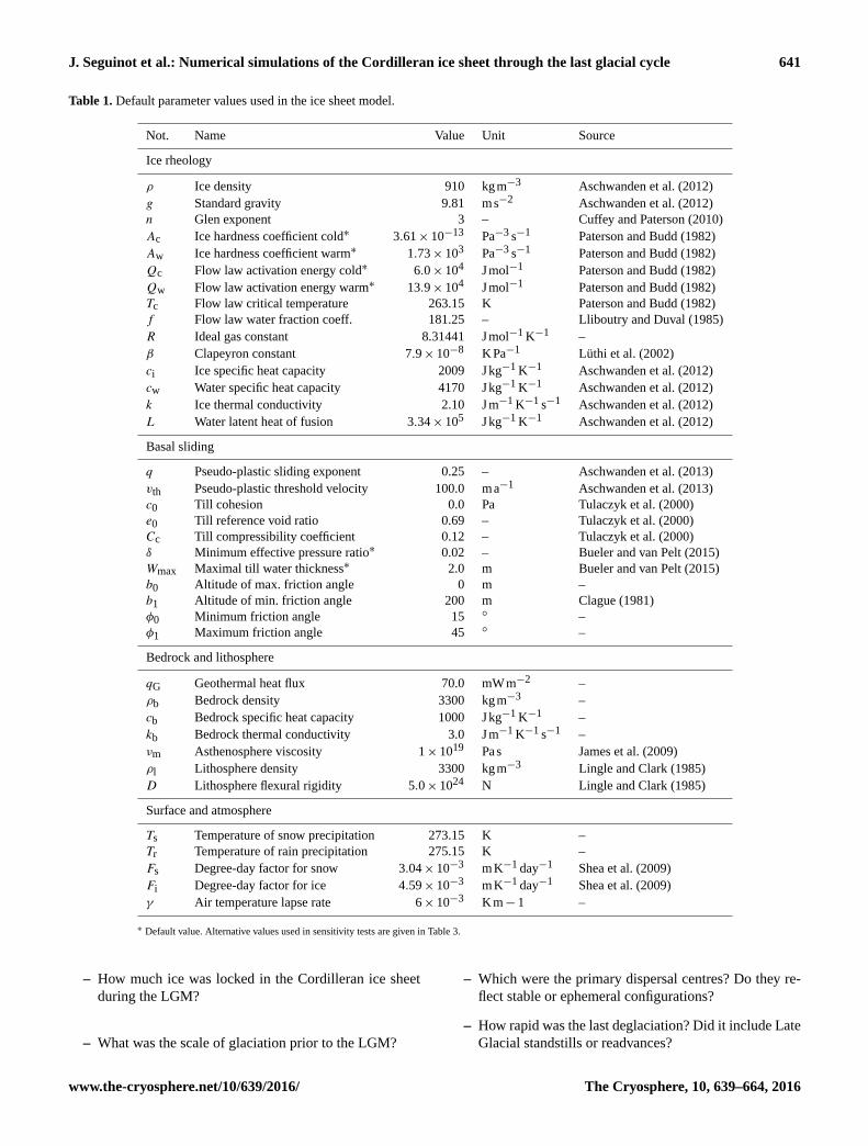
Table 1. Default parameter values used in the ice sheet model.
Not. Name Value Unit Source
Ice rheology
ρ Ice density 910 kgm−3 Aschwanden et al. (2012)
g Standard gravity 9.81 ms−2 Aschwanden et al. (2012)
n Glen exponent 3 – Cuffey and Paterson (2010)
Ac Ice hardness coefficient cold∗ 3.61× 10⁻¹³ Pa−3 s−1 Paterson and Budd (1982)
Aw Ice hardness coefficient warm∗ 1.73× 10³ Pa−3 s−1 Paterson and Budd (1982)
Qc Flow law activation energy cold∗ 6.0× 10⁴ Jmol−1 Paterson and Budd (1982)
Qw Flow law activation energy warm∗ 13.9× 10⁴ Jmol−1 Paterson and Budd (1982)
Tc Flow law critical temperature 263.15 K Paterson and Budd (1982)
f Flow law water fraction coeff. 181.25 – Lliboutry and Duval (1985)
R Ideal gas constant 8.31441 Jmol−1 K−1 –
β Clapeyron constant 7.9× 10⁻⁸ KPa−1 Lüthi et al. (2002)
ci Ice specific heat capacity 2009 Jkg−1 K−1 Aschwanden et al. (2012)
cw Water specific heat capacity 4170 Jkg−1 K−1 Aschwanden et al. (2012)
k Ice thermal conductivity 2.10 Jm−1 K−1 s−1 Aschwanden et al. (2012)
L Water latent heat of fusion 3.34× 10⁵ Jkg−1 K−1 Aschwanden et al. (2012)
Basal sliding
q Pseudo-plastic sliding exponent 0.25 – Aschwanden et al. (2013)
vth Pseudo-plastic threshold velocity 100.0 ma−1 Aschwanden et al. (2013)
c0 Till cohesion 0.0 Pa Tulaczyk et al. (2000)
e0 Till reference void ratio 0.69 – Tulaczyk et al. (2000)
Cc Till compressibility coefficient 0.12 – Tulaczyk et al. (2000)
δ Minimum effective pressure ratio∗ 0.02 – Bueler and van Pelt (2015)
Wmax Maximal till water thickness∗ 2.0 m Bueler and van Pelt (2015)
b0 Altitude of max. friction angle 0 m –
b1 Altitude of min. friction angle 200 m Clague (1981)
φ0 Minimum friction angle 15 ◦ –
φ1 Maximum friction angle 45 ◦ –
Bedrock and lithosphere
qG Geothermal heat flux 70.0 mWm−2 –
ρb Bedrock density 3300 kgm−3 –
cb Bedrock specific heat capacity 1000 Jkg−1 K−1 –
kb Bedrock thermal conductivity 3.0 Jm−1 K−1 s−1 –
νm Asthenosphere viscosity 1× 10¹⁹ Pas James et al. (2009)
ρl Lithosphere density 3300 kgm−3 Lingle and Clark (1985)
D Lithosphere flexural rigidity 5.0× 1024 N Lingle and Clark (1985)
Surface and atmosphere
Ts Temperature of snow precipitation 273.15 K –
Tr Temperature of rain precipitation 275.15 K –
Fs Degree-day factor for snow 3.04× 10⁻³ mK−1 day−1 Shea et al. (2009)
Fi Degree-day factor for ice 4.59× 10⁻³ mK−1 day−1 Shea et al. (2009)
γ Air temperature lapse rate 6× 10⁻³ Km− 1 –
∗ Default value. Alternative values used in sensitivity tests are given in Table 3.
– How much ice was locked in the Cordilleran ice sheet
during the LGM?
– What was the scale of glaciation prior to the LGM?
– Which were the primary dispersal centres? Do they re-
flect stable or ephemeral configurations?
– How rapid was the last deglaciation? Did it include Late
Glacial standstills or readvances?
www.the-cryosphere.net/10/639/2016/ The Cryosphere, 10, 639–664, 2016
642 J. Seguinot et al.: Numerical simulations of the Cordilleran ice sheet through the last glacial cycle
0
2
4
6
8
10
12
Ice s
oft
ness
A (
10
-24
Pa
-3s-1
)
DefaultSoft iceHard ice
20 15 10 5 0
Pressure-adjusted temperature T (°C)pa
10-25
10-24
10-23
Ice s
oft
ness
A (
Pa
s)
-3-1
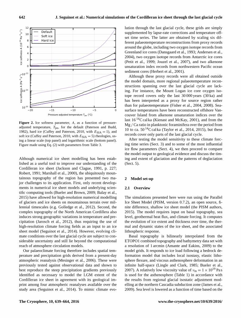
Figure 2. Ice softness parameter, A, as a function of pressure-
adjusted temperature, Tpa, for the default (Paterson and Budd,
1982), hard ice (Cuffey and Paterson, 2010, with ESIA = 1), and
soft ice (Cuffey and Paterson, 2010, with ESIA = 5) rheologies, us-
ing a linear scale (top panel) and logarithmic scale (bottom panel).
Figure made using Eq. (2) with parameters from Table 3.
Although numerical ice sheet modelling has been estab-
lished as a useful tool to improve our understanding of the
Cordilleran ice sheet (Jackson and Clague, 1991, p. 227;
Robert, 1991; Marshall et al., 2000), the ubiquitously moun-
tainous topography of the region has presented two ma-
jor challenges to its application. First, only recent develop-
ments in numerical ice sheet models and underlying scien-
tific computing tools (Bueler and Brown, 2009; Balay et al.,
2015) have allowed for high-resolution numerical modelling
of glaciers and ice sheets on mountainous terrain over mil-
lennial timescales (e.g. Golledge et al., 2012). Second, the
complex topography of the North American Cordillera also
induces strong geographic variations in temperature and pre-
cipitation (Jarosch et al., 2012), thus requiring the use of
high-resolution climate forcing fields as an input to an ice
sheet model (Seguinot et al., 2014). However, evolving cli-
mate conditions over the last glacial cycle are subject to con-
siderable uncertainty and still lie beyond the computational
reach of atmosphere circulation models.
Our palaeoclimate forcing therefore includes spatial tem-
perature and precipitation grids derived from a present-day
atmospheric reanalysis (Mesinger et al., 2006). These were
previously tested against observational data and shown to
best reproduce the steep precipitation gradients previously
identified as necessary to model the LGM extent of the
Cordilleran ice sheet in agreement with its geological im-
print among four atmospheric reanalyses available over the
study area (Seguinot et al., 2014). To mimic climate evo-
lution through the last glacial cycle, these grids are simply
supplemented by lapse-rate corrections and temperature off-
set time series. The latter are obtained by scaling six dif-
ferent palaeotemperature reconstructions from proxy records
around the globe, including two oxygen isotope records from
Greenland ice cores (Dansgaard et al., 1993; Andersen et al.,
2004), two oxygen isotope records from Antarctic ice cores
(Petit et al., 1999; Jouzel et al., 2007), and two alkenone
unsaturation index records from northwestern Pacific ocean
sediment cores (Herbert et al., 2001).
Although these proxy records were all obtained outside
the model domain, more regional palaeotemperature recon-
structions spanning over the last glacial cycle are lack-
ing. For instance, the Mount Logan ice core oxygen iso-
tope record covers only the last 30 000 years (30 ka) and
has been interpreted as a proxy for source region rather
than for palaeotemperature (Fisher et al., 2004, 2008). Sea-
surface temperatures have been reconstructed offshore Van-
couver Island from alkenone unsaturation indices over the
last 16 14Ccalka (Kienast and McKay, 2001), and from the
Mg /Ca ratio in planktonic foraminifera over the period from
10 to ca. 50 14Ccalka (Taylor et al., 2014, 2015), but these
records cover only parts of the last glacial cycle.
After testing the model sensitivity to these climate forc-
ing time series (Sect. 3) and to some of the most influential
ice flow parameters (Sect. 4), we then proceed to compare
the model output to geological evidence and discuss the tim-
ing and extent of glaciation and the patterns of deglaciation
(Sect. 5).
2 Model set-up
2.1 Overview
The simulations presented here were run using the Parallel
Ice Sheet Model (PISM, version 0.7.2), an open source, fi-
nite difference, shallow ice sheet model (the PISM authors,
2015). The model requires input on basal topography, sea
level, geothermal heat flux, and climate forcing. It computes
the evolution of ice extent and thickness over time, the ther-
mal and dynamic states of the ice sheet, and the associated
lithospheric response.
Basal topography is bilinearly interpolated from the
ETOPO1 combined topography and bathymetry data set with
a resolution of 1 arcmin (Amante and Eakins, 2009) to the
model grids. It responds to ice load following a bedrock de-
formation model that includes local isostasy, elastic litho-
sphere flexure, and viscous asthenosphere deformation in an
infinite half-space (Lingle and Clark, 1985; Bueler et al.,
2007). A relatively low viscosity value of νm = 1× 10¹⁹ Pas
is used for the asthenosphere (Table 1) in accordance with
the results from regional glacial isostatic adjustment mod-
elling at the northern Cascadia subduction zone (James et al.,
2009). Sea level is lowered as a function of time based on the
The Cryosphere, 10, 639–664, 2016 www.the-cryosphere.net/10/639/2016/
J. Seguinot et al.: Numerical simulations of the Cordilleran ice sheet through the last glacial cycle 643
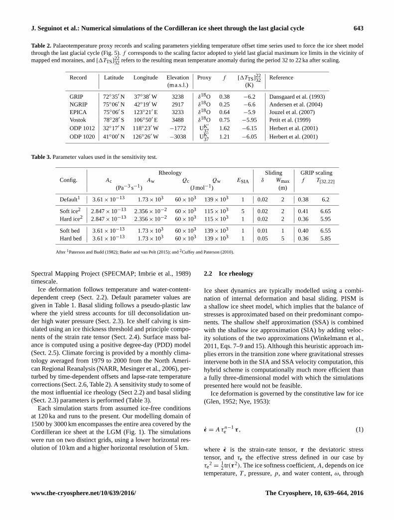
Table 2. Palaeotemperature proxy records and scaling parameters yielding temperature offset time series used to force the ice sheet model
through the last glacial cycle (Fig. 5). f corresponds to the scaling factor adopted to yield last glacial maximum ice limits in the vicinity of
mapped end moraines, and [1TTS]2232
refers to the resulting mean temperature anomaly during the period 32 to 22 ka after scaling.
Record Latitude Longitude Elevation Proxy f [1TTS]2232
Reference
(ma.s.l.) (K)
GRIP 72◦35′ N 37◦38′W 3238 δ18O 0.38 −6.2 Dansgaard et al. (1993)
NGRIP 75◦06′ N 42◦19′W 2917 δ18O 0.25 −6.6 Andersen et al. (2004)
EPICA 75◦06′ S 123◦21′ E 3233 δ18O 0.64 −5.9 Jouzel et al. (2007)
Vostok 78◦28′ S 106◦50′ E 3488 δ18O 0.75 −5.95 Petit et al. (1999)
ODP 1012 32◦17′ N 118◦23′W −1772 UK′
371.62 −6.15 Herbert et al. (2001)
ODP 1020 41◦00′ N 126◦26′W −3038 UK′
371.21 −6.05 Herbert et al. (2001)
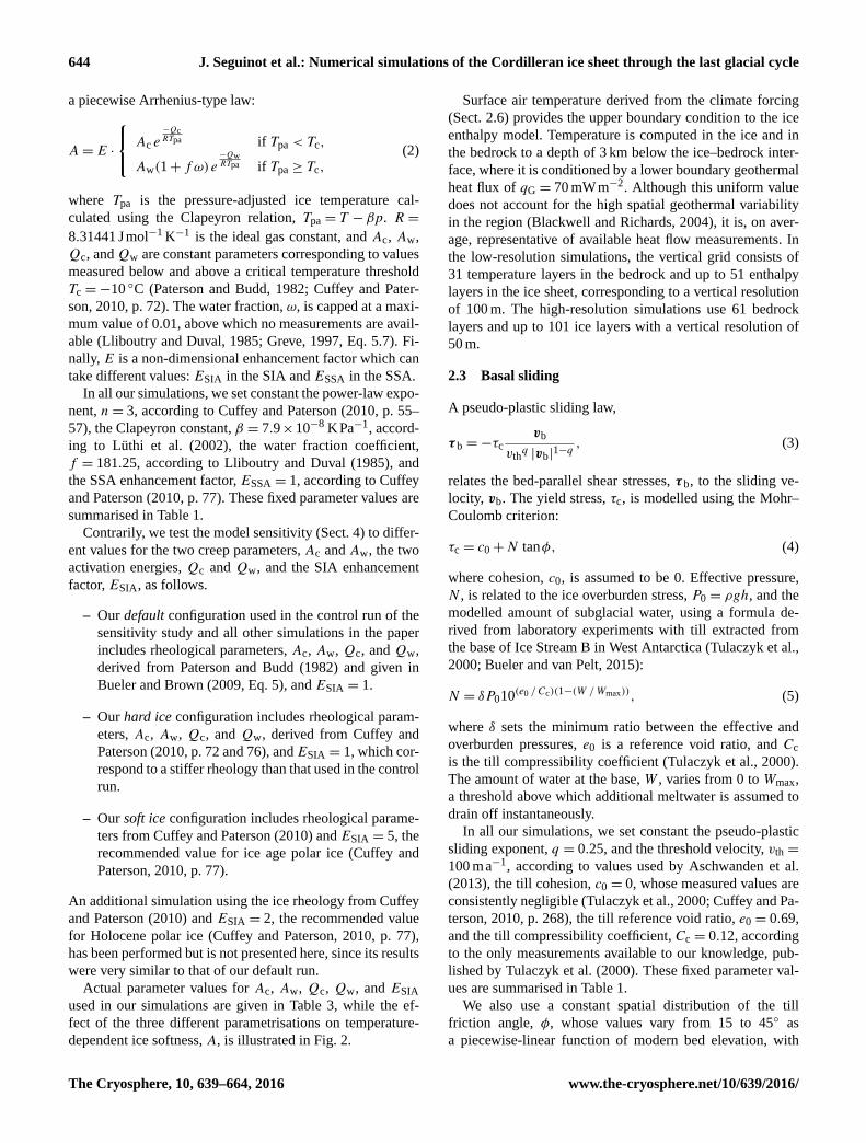
Table 3. Parameter values used in the sensitivity test.
Rheology Sliding GRIP scaling
Config. Ac Aw Qc Qw ESIA δ Wmax f T[32,22]
(Pa−3 s−1) (Jmol−1) (m)
Default1 3.61× 10⁻¹³ 1.73× 10³ 60× 103 139× 103 1 0.02 2 0.38 6.2
Soft ice2 2.847× 10⁻¹³ 2.356× 10⁻² 60× 103 115× 103 5 0.02 2 0.41 6.65
Hard ice2 2.847× 10⁻¹³ 2.356× 10⁻² 60× 103 115× 103 1 0.02 2 0.36 5.95
Soft bed 3.61× 10⁻¹³ 1.73× 10³ 60× 103 139× 103 1 0.01 1 0.40 6.55
Hard bed 3.61× 10⁻¹³ 1.73× 10³ 60× 103 139× 103 1 0.05 5 0.36 5.85
After 1Paterson and Budd (1982); Bueler and van Pelt (2015); and 2Cuffey and Paterson (2010).
Spectral Mapping Project (SPECMAP; Imbrie et al., 1989)
timescale.
Ice deformation follows temperature and water-content-
dependent creep (Sect. 2.2). Default parameter values are
given in Table 1. Basal sliding follows a pseudo-plastic law
where the yield stress accounts for till deconsolidation un-
der high water pressure (Sect. 2.3). Ice shelf calving is sim-
ulated using an ice thickness threshold and principle compo-
nents of the strain rate tensor (Sect. 2.4). Surface mass bal-
ance is computed using a positive degree-day (PDD) model
(Sect. 2.5). Climate forcing is provided by a monthly clima-
tology averaged from 1979 to 2000 from the North Ameri-
can Regional Reanalysis (NARR, Mesinger et al., 2006), per-
turbed by time-dependent offsets and lapse-rate temperature
corrections (Sect. 2.6, Table 2). A sensitivity study to some of
the most influential ice rheology (Sect 2.2) and basal sliding
(Sect. 2.3) parameters is performed (Table 3).
Each simulation starts from assumed ice-free conditions
at 120 ka and runs to the present. Our modelling domain of
1500 by 3000 km encompasses the entire area covered by the
Cordilleran ice sheet at the LGM (Fig. 1). The simulations
were run on two distinct grids, using a lower horizontal res-
olution of 10 km and a higher horizontal resolution of 5 km.
2.2 Ice rheology
Ice sheet dynamics are typically modelled using a combi-
nation of internal deformation and basal sliding. PISM is
a shallow ice sheet model, which implies that the balance of
stresses is approximated based on their predominant compo-
nents. The shallow shelf approximation (SSA) is combined
with the shallow ice approximation (SIA) by adding veloc-
ity solutions of the two approximations (Winkelmann et al.,
2011, Eqs. 7–9 and 15). Although this heuristic approach im-
plies errors in the transition zone where gravitational stresses
intervene both in the SIA and SSA velocity computation, this
hybrid scheme is computationally much more efficient than
a fully three-dimensional model with which the simulations
presented here would not be feasible.
Ice deformation is governed by the constitutive law for ice
(Glen, 1952; Nye, 1953):
ε = Aτn−1e τ , (1)
where ε is the strain-rate tensor, τ the deviatoric stress
tensor, and τe the effective stress defined in our case by
τe2=
12
tr(τ 2). The ice softness coefficient,A, depends on ice
temperature, T , pressure, p, and water content, ω, through
www.the-cryosphere.net/10/639/2016/ The Cryosphere, 10, 639–664, 2016
644 J. Seguinot et al.: Numerical simulations of the Cordilleran ice sheet through the last glacial cycle
a piecewise Arrhenius-type law:
A= E ·
Ac e−QcRTpa if Tpa < Tc,
Aw(1+ fω)e−QwRTpa if Tpa ≥ Tc,
(2)
where Tpa is the pressure-adjusted ice temperature cal-
culated using the Clapeyron relation, Tpa = T −βp. R =
8.31441 Jmol−1 K−1 is the ideal gas constant, and Ac, Aw,
Qc, andQw are constant parameters corresponding to values
measured below and above a critical temperature threshold
Tc =−10 ◦C (Paterson and Budd, 1982; Cuffey and Pater-
son, 2010, p. 72). The water fraction, ω, is capped at a maxi-
mum value of 0.01, above which no measurements are avail-
able (Lliboutry and Duval, 1985; Greve, 1997, Eq. 5.7). Fi-
nally, E is a non-dimensional enhancement factor which can
take different values: ESIA in the SIA and ESSA in the SSA.
In all our simulations, we set constant the power-law expo-
nent, n= 3, according to Cuffey and Paterson (2010, p. 55–
57), the Clapeyron constant, β = 7.9×10⁻⁸ KPa−1, accord-
ing to Lüthi et al. (2002), the water fraction coefficient,
f = 181.25, according to Lliboutry and Duval (1985), and
the SSA enhancement factor, ESSA = 1, according to Cuffey
and Paterson (2010, p. 77). These fixed parameter values are
summarised in Table 1.
Contrarily, we test the model sensitivity (Sect. 4) to differ-
ent values for the two creep parameters, Ac and Aw, the two
activation energies, Qc and Qw, and the SIA enhancement
factor, ESIA, as follows.
– Our default configuration used in the control run of the
sensitivity study and all other simulations in the paper
includes rheological parameters, Ac, Aw, Qc, and Qw,
derived from Paterson and Budd (1982) and given in
Bueler and Brown (2009, Eq. 5), and ESIA = 1.
– Our hard ice configuration includes rheological param-
eters, Ac, Aw, Qc, and Qw, derived from Cuffey and
Paterson (2010, p. 72 and 76), and ESIA = 1, which cor-
respond to a stiffer rheology than that used in the control
run.
– Our soft ice configuration includes rheological parame-
ters from Cuffey and Paterson (2010) and ESIA = 5, the
recommended value for ice age polar ice (Cuffey and
Paterson, 2010, p. 77).
An additional simulation using the ice rheology from Cuffey
and Paterson (2010) and ESIA = 2, the recommended value
for Holocene polar ice (Cuffey and Paterson, 2010, p. 77),
has been performed but is not presented here, since its results
were very similar to that of our default run.
Actual parameter values for Ac, Aw, Qc, Qw, and ESIA
used in our simulations are given in Table 3, while the ef-
fect of the three different parametrisations on temperature-
dependent ice softness, A, is illustrated in Fig. 2.
Surface air temperature derived from the climate forcing
(Sect. 2.6) provides the upper boundary condition to the ice
enthalpy model. Temperature is computed in the ice and in
the bedrock to a depth of 3 km below the ice–bedrock inter-
face, where it is conditioned by a lower boundary geothermal
heat flux of qG = 70 mWm−2. Although this uniform value
does not account for the high spatial geothermal variability
in the region (Blackwell and Richards, 2004), it is, on aver-
age, representative of available heat flow measurements. In
the low-resolution simulations, the vertical grid consists of
31 temperature layers in the bedrock and up to 51 enthalpy
layers in the ice sheet, corresponding to a vertical resolution
of 100 m. The high-resolution simulations use 61 bedrock
layers and up to 101 ice layers with a vertical resolution of
50 m.
2.3 Basal sliding
A pseudo-plastic sliding law,
τ b =−τc
vb
vthq |vb|
1−q, (3)
relates the bed-parallel shear stresses, τ b, to the sliding ve-
locity, vb. The yield stress, τc, is modelled using the Mohr–
Coulomb criterion:
τc = c0+N tanφ, (4)
where cohesion, c0, is assumed to be 0. Effective pressure,
N , is related to the ice overburden stress, P0 = ρgh, and the
modelled amount of subglacial water, using a formula de-
rived from laboratory experiments with till extracted from
the base of Ice Stream B in West Antarctica (Tulaczyk et al.,
2000; Bueler and van Pelt, 2015):
N = δP010(e0 /Cc)(1−(W /Wmax)), (5)
where δ sets the minimum ratio between the effective and
overburden pressures, e0 is a reference void ratio, and Cc
is the till compressibility coefficient (Tulaczyk et al., 2000).
The amount of water at the base, W , varies from 0 to Wmax,
a threshold above which additional meltwater is assumed to
drain off instantaneously.
In all our simulations, we set constant the pseudo-plastic
sliding exponent, q = 0.25, and the threshold velocity, vth =
100 ma−1, according to values used by Aschwanden et al.
(2013), the till cohesion, c0 = 0, whose measured values are
consistently negligible (Tulaczyk et al., 2000; Cuffey and Pa-
terson, 2010, p. 268), the till reference void ratio, e0 = 0.69,
and the till compressibility coefficient, Cc = 0.12, according
to the only measurements available to our knowledge, pub-
lished by Tulaczyk et al. (2000). These fixed parameter val-
ues are summarised in Table 1.
We also use a constant spatial distribution of the till
friction angle, φ, whose values vary from 15 to 45◦ as
a piecewise-linear function of modern bed elevation, with
The Cryosphere, 10, 639–664, 2016 www.the-cryosphere.net/10/639/2016/
J. Seguinot et al.: Numerical simulations of the Cordilleran ice sheet through the last glacial cycle 645
the lowest value occurring below the modern sea level (0 m
above sea level, m a.s.l.) and the highest value occurring
above the generalised elevation of the highest shorelines
(200 ma.s.l.; Clague, 1981, Fig. 5). This range of values span
over the range of measured values for glacial till of 18 to 40◦
(Cuffey and Paterson, 2010, p. 268). It accounts for frictional
basal conditions associated with discontinuous till cover at
high elevations and for a weakening of till associated with
the presence of marine sediments (cf. Martin et al., 2011; As-
chwanden et al., 2013, Supplement; the PISM authors, 2015).
An additional simulation with a constant till friction an-
gle, φ = 30◦, corresponding to the average value in Cuffey
and Paterson (2010, p. 268), has been performed but is not
presented here, since the induced variability was small.
Additionally, we test the model sensitivity (Sect. 4) to dif-
ferent values for the minimum ratio between the effective and
overburden pressures, δ, and the maximum water height in
the till, Wmax, as follows.
– Our default configuration used in the control run of the
sensitivity study and all other simulations in the paper
includes δ = 0.02 andWmax = 2 m as in Bueler and van
Pelt (2015).
– Our soft bed configuration uses δ = 0.01 and Wmax =
1 m.
– Our hard bed configuration uses δ = 0.05 and Wmax =
5 m.
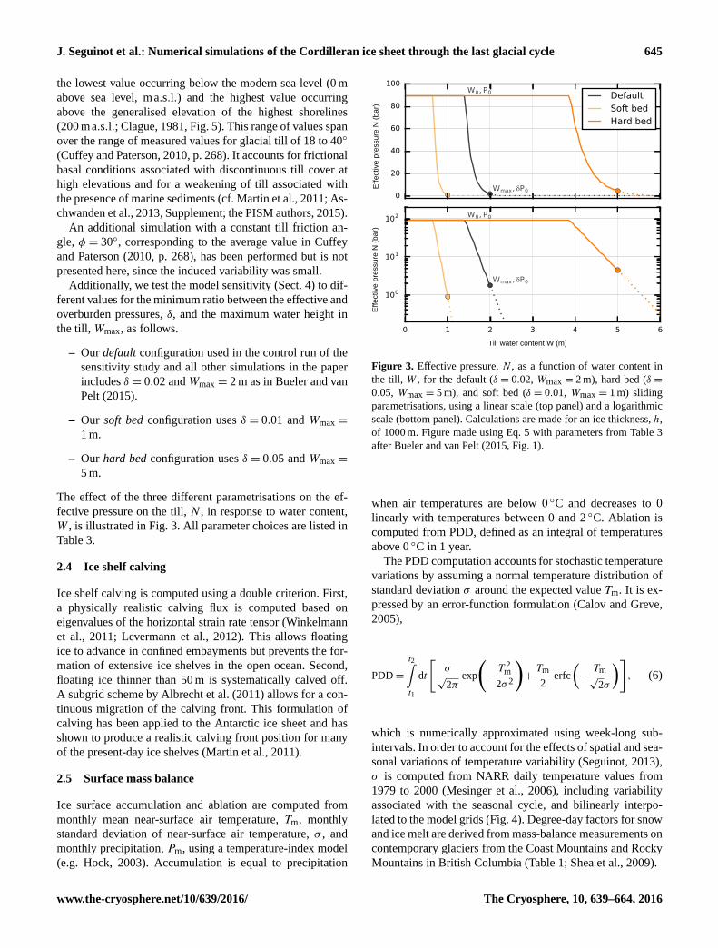
The effect of the three different parametrisations on the ef-
fective pressure on the till, N , in response to water content,
W , is illustrated in Fig. 3. All parameter choices are listed in
Table 3.
2.4 Ice shelf calving
Ice shelf calving is computed using a double criterion. First,
a physically realistic calving flux is computed based on
eigenvalues of the horizontal strain rate tensor (Winkelmann
et al., 2011; Levermann et al., 2012). This allows floating
ice to advance in confined embayments but prevents the for-
mation of extensive ice shelves in the open ocean. Second,
floating ice thinner than 50 m is systematically calved off.
A subgrid scheme by Albrecht et al. (2011) allows for a con-
tinuous migration of the calving front. This formulation of
calving has been applied to the Antarctic ice sheet and has
shown to produce a realistic calving front position for many
of the present-day ice shelves (Martin et al., 2011).
2.5 Surface mass balance
Ice surface accumulation and ablation are computed from
monthly mean near-surface air temperature, Tm, monthly
standard deviation of near-surface air temperature, σ , and
monthly precipitation, Pm, using a temperature-index model
(e.g. Hock, 2003). Accumulation is equal to precipitation
0
20
40
60
80
100
Effe
ctiv
e pr
essu
re N
(bar
)
W0, P0
Wmax, P0
DefaultSoft bedHard bed
0 1 2 3 4 5 6
Till water content W (m)
100
101
102
Effe
ctiv
e pr
essu
re N
(bar
)
W0, P0
Wmax, P0
Figure 3. Effective pressure, N , as a function of water content in
the till, W , for the default (δ = 0.02, Wmax = 2 m), hard bed (δ =
0.05, Wmax = 5 m), and soft bed (δ = 0.01, Wmax = 1 m) sliding
parametrisations, using a linear scale (top panel) and a logarithmic
scale (bottom panel). Calculations are made for an ice thickness, h,
of 1000 m. Figure made using Eq. 5 with parameters from Table 3
after Bueler and van Pelt (2015, Fig. 1).
when air temperatures are below 0 ◦C and decreases to 0
linearly with temperatures between 0 and 2 ◦C. Ablation is
computed from PDD, defined as an integral of temperatures
above 0 ◦C in 1 year.
The PDD computation accounts for stochastic temperature
variations by assuming a normal temperature distribution of
standard deviation σ around the expected value Tm. It is ex-
pressed by an error-function formulation (Calov and Greve,
2005),
PDD=
t2∫t1
dt
[σ√
2πexp
(−T 2
m
2σ 2
)+Tm
2erfc
(−Tm√
2σ
)], (6)
which is numerically approximated using week-long sub-
intervals. In order to account for the effects of spatial and sea-
sonal variations of temperature variability (Seguinot, 2013),
σ is computed from NARR daily temperature values from
1979 to 2000 (Mesinger et al., 2006), including variability
associated with the seasonal cycle, and bilinearly interpo-
lated to the model grids (Fig. 4). Degree-day factors for snow
and ice melt are derived from mass-balance measurements on
contemporary glaciers from the Coast Mountains and Rocky
Mountains in British Columbia (Table 1; Shea et al., 2009).
www.the-cryosphere.net/10/639/2016/ The Cryosphere, 10, 639–664, 2016
646 J. Seguinot et al.: Numerical simulations of the Cordilleran ice sheet through the last glacial cycle
Table 4. Extremes in Cordilleran ice sheet grounded ice extent and sea-level relevant ice volume corresponding to MIS 4, 3, and 2 for each
of the six low-resolution simulations (Fig. 5).
Age (ka) Ice extent (106 km2) Ice volume (m s.l.e.)
Record MIS 4 MIS 3 MIS 2 MIS 4 MIS 3 MIS 2 MIS 4 MIS 3 MIS 2
GRIP 57.59 42.91 19.14 1.93 0.67 2.09 7.43 1.54 8.62
NGRIP 60.27 45.87 22.85 2.13 0.73 2.11 8.71 1.70 8.60
EPICA 61.90 52.40 17.36 1.48 0.98 2.08 4.84 2.55 8.56
Vostok 62.21 55.87 16.86 1.50 1.01 2.09 4.94 2.81 8.57
ODP 1012 56.88 47.46 23.21 1.36 0.90 2.13 4.18 2.30 8.75
ODP 1020 60.37 52.72 20.41 1.25 0.73 2.09 3.66 1.65 8.62
Minimum 56.88 42.91 16.86 1.25 0.67 2.08 3.66 1.54 8.56
Maximum 62.21 55.87 23.21 2.13 1.01 2.13 8.71 2.81 8.75
2.6 Climate forcing
Climate forcing driving ice sheet simulations consists of
a present-day monthly climatology, {Tm0 , Pm0}, where tem-
peratures are modified by offset time series,1TTS, and lapse-
rate corrections, 1TLR:
Tm(t,x,y)= Tm0(x,y)+1TTS(t)+1TLR(t,x,y), (7)
Pm(t,x,y)= Pm0(x,y). (8)
The present-day monthly climatology was bilinearly interpo-
lated from near-surface air temperature and precipitation rate
fields from the NARR, averaged from 1979 to 2000. Modern
climate of the North American Cordillera is characterised by
strong geographic variations in temperature seasonality, tim-
ing of the maximum annual precipitation, and daily tempera-
ture variability (Fig. 4). Although the ability of the NARR to
reproduce the steep climatic gradients is limited by its spatial
resolution of 32 km (Jarosch et al., 2012), it has been tested
against observational data in our previous sensitivity study
and identified as yielding a closer fit between the modelled
LGM extent of the Cordilleran ice sheet and the geological
evidence than other atmospheric reanalyses (Seguinot et al.,
2014).
Temperature offset time series, 1TTS, are derived from
palaeotemperature proxy records from the Greenland Ice
Core Project (GRIP; Dansgaard et al., 1993), the North
Greenland Ice Core Project (NGRIP; Andersen et al., 2004),
the European Project for Ice Coring in Antarctica (EPICA;
Jouzel et al., 2007), the Vostok ice core (Petit et al., 1999),
and Ocean Drilling Program (ODP) sites 1012 and 1020,
both located off the coast of California (Herbert et al., 2001).
Palaeotemperature anomalies from the GRIP and NGRIP
records were calculated from oxygen isotope (δ18O) mea-
surements using a quadratic equation (Johnsen et al., 1995),
1TTS(t)=− 11.88[δ18O(t)− δ18O(0)]
− 0.1925[δ18O(t)2− δ18O(0)2], (9)
while temperature reconstructions from Antarctic and
oceanic cores were provided as such. For each proxy record
January
July
24 12 0 12 24
Temperature (°C)
2 10 46 215 1000
Precipitation (mm)
3 6 9 12
PDD SD (°C)
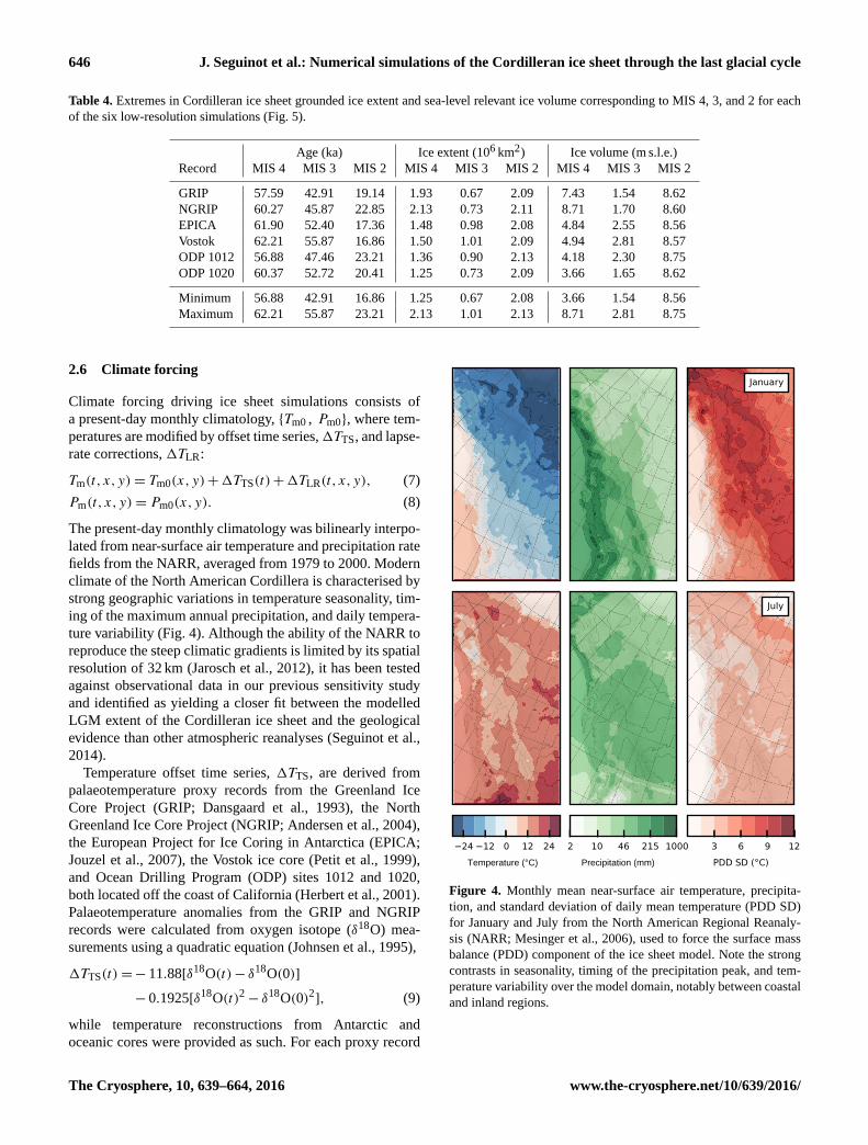
Figure 4. Monthly mean near-surface air temperature, precipita-
tion, and standard deviation of daily mean temperature (PDD SD)
for January and July from the North American Regional Reanaly-
sis (NARR; Mesinger et al., 2006), used to force the surface mass
balance (PDD) component of the ice sheet model. Note the strong
contrasts in seasonality, timing of the precipitation peak, and tem-
perature variability over the model domain, notably between coastal
and inland regions.
The Cryosphere, 10, 639–664, 2016 www.the-cryosphere.net/10/639/2016/
J. Seguinot et al.: Numerical simulations of the Cordilleran ice sheet through the last glacial cycle 647
10
8
6
4
2
0
2
Tem
pera
ture
offs
et (K
)
020406080100120
Model age (ka)
0
2
4
6
8
Ice
volu
me
(m s
.l.e.
)
MIS 5
MIS 4
MIS 3
MIS 2
MIS 1GRIPNGRIPEPICA
VostokODP 1012ODP 1020
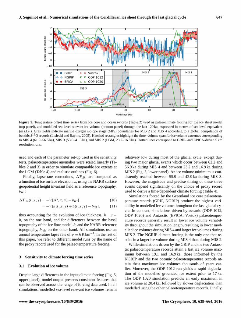
Figure 5. Temperature offset time series from ice core and ocean records (Table 2) used as palaeoclimate forcing for the ice sheet model
(top panel), and modelled sea-level relevant ice volume (bottom panel) through the last 120 ka, expressed in metres of sea-level equivalent
(m s.l.e.). Grey fields indicate marine oxygen isotope stage (MIS) boundaries for MIS 2 and MIS 4 according to a global compilation of
benthic δ18O records (Lisiecki and Raymo, 2005). Hatched rectangles highlight the time–volume span for ice volume extremes corresponding
to MIS 4 (61.9–56.5 ka), MIS 3 (53.0–41.3 ka), and MIS 2 (LGM, 23.2–16.8 ka). Dotted lines correspond to GRIP- and EPICA-driven 5 km
resolution runs.
used and each of the parameter set-up used in the sensitivity
tests, palaeotemperature anomalies were scaled linearly (Ta-
bles 2 and 3) in order to simulate comparable ice extents at
the LGM (Table 4) and realistic outlines (Fig. 6).
Finally, lapse-rate corrections, 1TLR, are computed as
a function of ice surface elevation, s, using the NARR surface
geopotential height invariant field as a reference topography,
bref:
1TLR(t,x,y)=−γ [s(t,x,y)− bref] (10)
=−γ [h(t,x,y)+ b(t,x,y)− bref], (11)
thus accounting for the evolution of ice thickness, h= s−
b, on the one hand, and for differences between the basal
topography of the ice flow model, b, and the NARR reference
topography, bref, on the other hand. All simulations use an
annual temperature lapse rate of γ = 6Kkm−1. In the rest of
this paper, we refer to different model runs by the name of
the proxy record used for the palaeotemperature forcing.
3 Sensitivity to climate forcing time series
3.1 Evolution of ice volume
Despite large differences in the input climate forcing (Fig. 5,
upper panel), model output presents consistent features that
can be observed across the range of forcing data used. In all
simulations, modelled sea-level relevant ice volumes remain
relatively low during most of the glacial cycle, except dur-
ing two major glacial events which occur between 62.2 and
56.9 ka during MIS 4 and between 23.2 and 16.9 ka during
MIS 2 (Fig. 5, lower panel). An ice volume minimum is con-
sistently reached between 55.9 and 42.9 ka during MIS 3.
However, the magnitude and precise timing of these three
events depend significantly on the choice of proxy record
used to derive a time-dependent climate forcing (Table 4).
Simulations forced by the Greenland ice core palaeotem-
perature records (GRIP, NGRIP) produce the highest vari-
ability in modelled ice volume throughout the last glacial cy-
cle. In contrast, simulations driven by oceanic (ODP 1012,
ODP 1020) and Antarctic (EPICA, Vostok) palaeotemper-
ature records generally result in lower ice volume variabil-
ity throughout the simulation length, resulting in lower mod-
elled ice volumes during MIS 4 and larger ice volumes during
MIS 3. The NGRIP climate forcing is the only one that re-
sults in a larger ice volume during MIS 4 than during MIS 2.
While simulations driven by the GRIP and the two Antarc-
tic palaeotemperature records attain a last ice volume max-
imum between 19.1 and 16.9 ka, those informed by the
NGRIP and the two oceanic palaeotemperature records at-
tain their maximum ice volumes thousands of years ear-
lier. Moreover, the ODP 1012 run yields a rapid deglacia-
tion of the modelled grounded ice extent prior to 17 ka.
The ODP 1020 simulation predicts an early maximum in
ice volume at 20.4 ka, followed by slower deglaciation than
modelled using the other palaeotemperature records. Finally,
www.the-cryosphere.net/10/639/2016/ The Cryosphere, 10, 639–664, 2016
648 J. Seguinot et al.: Numerical simulations of the Cordilleran ice sheet through the last glacial cycle
57.6 ka
GRIP
MIS
4
60.3 ka
NGRIP
61.9 ka
EPICA
62.2 ka
Vostok
56.9 ka
ODP 1012
60.4 ka
ODP 1020
42.9 ka
MIS
3
45.9 ka 52.4 ka
SM
55.9 ka 47.5 ka 52.7 ka
19.1 ka
MIS
2
22.9 ka 17.4 ka 16.9 ka 23.2 ka 20.4 ka
0
1
2
3
4
Surfa
ce e
leva
tion
(km
)
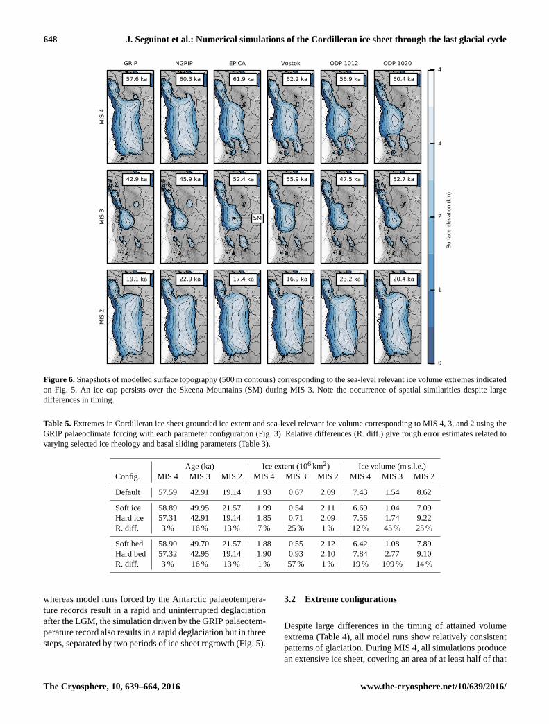
Figure 6. Snapshots of modelled surface topography (500 m contours) corresponding to the sea-level relevant ice volume extremes indicated
on Fig. 5. An ice cap persists over the Skeena Mountains (SM) during MIS 3. Note the occurrence of spatial similarities despite large
differences in timing.
Table 5. Extremes in Cordilleran ice sheet grounded ice extent and sea-level relevant ice volume corresponding to MIS 4, 3, and 2 using the
GRIP palaeoclimate forcing with each parameter configuration (Fig. 3). Relative differences (R. diff.) give rough error estimates related to
varying selected ice rheology and basal sliding parameters (Table 3).
Age (ka) Ice extent (106 km2) Ice volume (m s.l.e.)
Config. MIS 4 MIS 3 MIS 2 MIS 4 MIS 3 MIS 2 MIS 4 MIS 3 MIS 2
Default 57.59 42.91 19.14 1.93 0.67 2.09 7.43 1.54 8.62
Soft ice 58.89 49.95 21.57 1.99 0.54 2.11 6.69 1.04 7.09
Hard ice 57.31 42.91 19.14 1.85 0.71 2.09 7.56 1.74 9.22
R. diff. 3 % 16 % 13 % 7 % 25 % 1 % 12 % 45 % 25 %
Soft bed 58.90 49.70 21.57 1.88 0.55 2.12 6.42 1.08 7.89
Hard bed 57.32 42.95 19.14 1.90 0.93 2.10 7.84 2.77 9.10
R. diff. 3 % 16 % 13 % 1 % 57 % 1 % 19 % 109 % 14 %
whereas model runs forced by the Antarctic palaeotempera-
ture records result in a rapid and uninterrupted deglaciation
after the LGM, the simulation driven by the GRIP palaeotem-
perature record also results in a rapid deglaciation but in three
steps, separated by two periods of ice sheet regrowth (Fig. 5).
3.2 Extreme configurations
Despite large differences in the timing of attained volume
extrema (Table 4), all model runs show relatively consistent
patterns of glaciation. During MIS 4, all simulations produce
an extensive ice sheet, covering an area of at least half of that
The Cryosphere, 10, 639–664, 2016 www.the-cryosphere.net/10/639/2016/
J. Seguinot et al.: Numerical simulations of the Cordilleran ice sheet through the last glacial cycle 649
0
2
4
6
8
Ice
volu
me
(m s
.l.e.
)
DefaultSoft iceHard ice
020406080100120
Model age (ka)
0
2
4
6
8
Ice
volu
me
(m s
.l.e.
)
MIS 5
MIS 4
MIS 3
MIS 2
MIS 1DefaultSoft bedHard bed
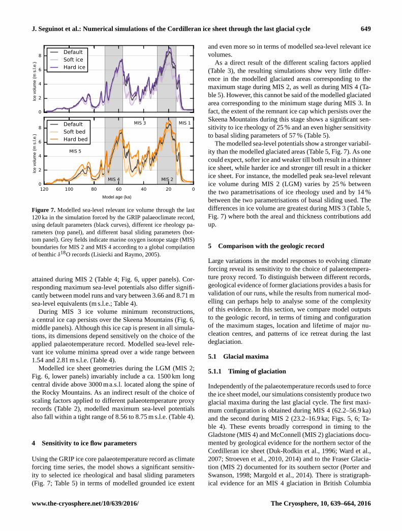
Figure 7. Modelled sea-level relevant ice volume through the last
120 ka in the simulation forced by the GRIP palaeoclimate record,
using default parameters (black curves), different ice rheology pa-
rameters (top panel), and different basal sliding parameters (bot-
tom panel). Grey fields indicate marine oxygen isotope stage (MIS)
boundaries for MIS 2 and MIS 4 according to a global compilation
of benthic δ18O records (Lisiecki and Raymo, 2005).
attained during MIS 2 (Table 4; Fig. 6, upper panels). Cor-
responding maximum sea-level potentials also differ signifi-
cantly between model runs and vary between 3.66 and 8.71 m
sea-level equivalents (m s.l.e.; Table 4).
During MIS 3 ice volume minimum reconstructions,
a central ice cap persists over the Skeena Mountains (Fig. 6,
middle panels). Although this ice cap is present in all simula-
tions, its dimensions depend sensitively on the choice of the
applied palaeotemperature record. Modelled sea-level rele-
vant ice volume minima spread over a wide range between
1.54 and 2.81 m s.l.e. (Table 4).
Modelled ice sheet geometries during the LGM (MIS 2;
Fig. 6, lower panels) invariably include a ca. 1500 km long
central divide above 3000 ma.s.l. located along the spine of
the Rocky Mountains. As an indirect result of the choice of
scaling factors applied to different palaeotemperature proxy
records (Table 2), modelled maximum sea-level potentials
also fall within a tight range of 8.56 to 8.75 m s.l.e. (Table 4).
4 Sensitivity to ice flow parameters
Using the GRIP ice core palaeotemperature record as climate
forcing time series, the model shows a significant sensitiv-
ity to selected ice rheological and basal sliding parameters
(Fig. 7; Table 5) in terms of modelled grounded ice extent
and even more so in terms of modelled sea-level relevant ice
volumes.
As a direct result of the different scaling factors applied
(Table 3), the resulting simulations show very little differ-
ence in the modelled glaciated areas corresponding to the
maximum stage during MIS 2, as well as during MIS 4 (Ta-
ble 5). However, this cannot be said of the modelled glaciated
area corresponding to the minimum stage during MIS 3. In
fact, the extent of the remnant ice cap which persists over the
Skeena Mountains during this stage shows a significant sen-
sitivity to ice rheology of 25 % and an even higher sensitivity
to basal sliding parameters of 57 % (Table 5).
The modelled sea-level potentials show a stronger variabil-
ity than the modelled glaciated areas (Table 5, Fig. 7). As one
could expect, softer ice and weaker till both result in a thinner
ice sheet, while harder ice and stronger till result in a thicker
ice sheet. For instance, the modelled peak sea-level relevant
ice volume during MIS 2 (LGM) varies by 25 % between
the two parametrisations of ice rheology used and by 14 %
between the two parametrisations of basal sliding used. The
differences in ice volume are greatest during MIS 3 (Table 5,
Fig. 7) where both the areal and thickness contributions add
up.
5 Comparison with the geologic record
Large variations in the model responses to evolving climate
forcing reveal its sensitivity to the choice of palaeotempera-
ture proxy record. To distinguish between different records,
geological evidence of former glaciations provides a basis for
validation of our runs, while the results from numerical mod-
elling can perhaps help to analyse some of the complexity
of this evidence. In this section, we compare model outputs
to the geologic record, in terms of timing and configuration
of the maximum stages, location and lifetime of major nu-
cleation centres, and patterns of ice retreat during the last
deglaciation.
5.1 Glacial maxima
5.1.1 Timing of glaciation
Independently of the palaeotemperature records used to force
the ice sheet model, our simulations consistently produce two
glacial maxima during the last glacial cycle. The first maxi-
mum configuration is obtained during MIS 4 (62.2–56.9 ka)
and the second during MIS 2 (23.2–16.9 ka; Figs. 5, 6; Ta-
ble 4). These events broadly correspond in timing to the
Gladstone (MIS 4) and McConnell (MIS 2) glaciations docu-
mented by geological evidence for the northern sector of the
Cordilleran ice sheet (Duk-Rodkin et al., 1996; Ward et al.,
2007; Stroeven et al., 2010, 2014) and to the Fraser Glacia-
tion (MIS 2) documented for its southern sector (Porter and
Swanson, 1998; Margold et al., 2014). There is stratigraph-
ical evidence for an MIS 4 glaciation in British Columbia
www.the-cryosphere.net/10/639/2016/ The Cryosphere, 10, 639–664, 2016
650 J. Seguinot et al.: Numerical simulations of the Cordilleran ice sheet through the last glacial cycle
(Clague and Ward, 2011) and in the Puget Lowland (Troost,
2014), but their extent and timing are still highly conjectural
(perhaps MIS 4 or early MIS 3; e.g. Cosma et al., 2008).
The exact timing of modelled MIS 2 maximum ice vol-
ume depends strongly on the choice of applied palaeotem-
perature record, which allows for a more in-depth compari-
son with geological evidence for the timing of the maximum
Cordilleran ice sheet extent. In the Puget Lowland (Fig. 1),
the LGM advance of the southern Cordilleran ice sheet mar-
gin has been constrained by radiocarbon dating on wood be-
tween 17.4 and 16.4 14Ccalka (Porter and Swanson, 1998).
These dates are consistent with radiocarbon dates from the
offshore sedimentary record, which reveals an increase of
glaciomarine sedimentation between 19.5 and 16.2 14Ccalka
(Cosma et al., 2008; Taylor et al., 2014). Radiocarbon dating
of the northern Cordilleran ice sheet margin is much less con-
strained but straddles presented constraints from the south-
ern margin. However, cosmogenic exposure dating places the
timing of the maximum northern ice sheet margin extent dur-
ing the McConnell glaciation close to 17 10Beka (Stroeven
et al., 2010, 2014). A sharp transition in the sediment record
of the Gulf of Alaska indicates a retreat of regional outlet
glaciers onto land at 14.8 14Ccalka (Davies et al., 2011).
Among the simulations presented here, only those forced
with the GRIP, EPICA, and Vostok palaeotemperature
records yield Cordilleran ice sheet maximum extents that
may be compatible with these field constraints (Fig. 5,
lower panel; Table 4). Simulations driven by the NGRIP,
ODP 1012, and ODP 1020 palaeotemperature records, on the
contrary, yield MIS 2 maximum Cordilleran ice sheet vol-
umes that pre-date field-based constraints by several thou-
sands of years (about 6, 6, and 4 ka respectively). Concern-
ing the simulations driven by oceanic records, this early
deglaciation is caused by an early warming present in the
alkenone palaeotemperature reconstructions (Fig. 5, upper
panel; Herbert et al., 2001, Fig. 3). However, this early warm-
ing is a local effect, corresponding to a weakening of the
California current (Herbert et al., 2001). The California cur-
rent, driving cold waters southwards along the south-western
coast of North America, has been shown to have weakened
during each peak of global glaciation (in SPECMAP) during
the past 550 ka, including the LGM, resulting in paradoxi-
cally warmer sea-surface temperatures at the locations of the
ODP 1012 and ODP 1020 sites (Herbert et al., 2001).
Because most of the marine margin of the Cordilleran ice
sheet terminated in a sector of the Pacific Ocean unaffected
by variations in the California current, it probably remained
insensitive to this local phenomenon. However, the above
paradox illustrates the complexity of ice-sheet feedbacks on
regional climate and demonstrates that, although located in
the neighbourhood of the modelling domain, the ODP 1012
and ODP 1020 palaeotemperature records cannot be used as
a realistic forcing to model the Cordilleran ice sheet through
the last glacial cycle. Similarly, the simulation using the
NGRIP palaeotemperature record depicts an early onset of
GRIP, 19.1 ka EPICA, 17.3 ka
10 31 100 316 1000Surface velocity (m a )-1
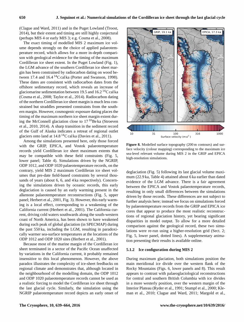
Figure 8. Modelled surface topography (200 m contours) and sur-
face velocity (colour mapping) corresponding to the maximum ice
sea-level relevant volume during MIS 2 in the GRIP and EPICA
high-resolution simulations.
deglaciation (Fig. 5) following its last glacial volume maxi-
mum (22.9 ka, Table 4) attained about 6 ka earlier than dated
evidence of the LGM advance. There is a fair agreement
between the EPICA and Vostok palaeotemperature records,
resulting in only small differences between the simulations
driven by those records. These differences are not subject to
further analysis here; instead we focus on simulations forced
by palaeotemperature records from the GRIP and EPICA ice
cores that appear to produce the most realistic reconstruc-
tions of regional glaciation history, yet bearing significant
disparities in model output. To allow for a more detailed
comparison against the geological record, these two simu-
lations were re-run using a higher-resolution grid (Sect. 2;
Fig. 5, lower panel, dotted lines). A supplementary anima-
tion presenting their results is available online.
5.1.2 Ice configuration during MIS 2
During maximum glaciation, both simulations position the
main meridional ice divide over the western flank of the
Rocky Mountains (Figs. 6, lower panels and 8). This result
appears to contrast with palaeoglaciological reconstructions
for central and southern British Columbia with ice divides
in a more westerly position, over the western margin of the
Interior Plateau (Ryder et al., 1991; Stumpf et al., 2000; Kle-
man et al., 2010; Clague and Ward, 2011; Margold et al.,
The Cryosphere, 10, 639–664, 2016 www.the-cryosphere.net/10/639/2016/
J. Seguinot et al.: Numerical simulations of the Cordilleran ice sheet through the last glacial cycle 651
2013b). These indicate that a latitudinal saddle connected
ice-dispersal centres in the Columbia Mountains with the
main ice divide (Ryder et al., 1991; Kleman et al., 2010;
Clague and Ward, 2011; Margold et al., 2013b). A latitudi-
nal saddle does indeed feature in our modelling results, how-
ever, in an inverse configuration between the main ice divide
over the Columbia Mountains and a secondary divide over
the southern Coast Mountains (Fig. 8).
Such deviation from the geological inferences could re-
flect the fact that the NARR has difficulties with simulat-
ing orographic processes in some areas of steep topogra-
phy (Jarosch et al., 2012). In our previous study (Seguinot
et al., 2014), we have evaluated an applicability of the
climate forcing bilinearly interpolated from the NARR to
constant-climate simulations of the Cordilleran ice sheet dur-
ing the LGM against that of an observation-based data set
(WorldClim, Hijmans et al., 2005). Indeed, the use of NARR
in these simulations produced slightly different patterns of
glaciation relative to WorldClim, including a more extensive
ice cover on the Columbia and Rocky mountains (Seguinot
et al., 2014, Figs. 6–7). Our simulations have shown that
these differences are mainly caused by disparities between
the precipitation fields of the two data sets (Seguinot et al.,
2014, Figs. 13–14). It has been shown that over the south-
ern part of our model domain that temperature and precipi-
tation downscaling can potentially address these limitations
(e.g. Jarosch et al., 2012). However, extending this downscal-
ing method to the entire model domain used in our study is
challenging, because the northern part of the model domain
is characterized by stronger precipitation gradients (Fig. 4)
and fewer weather stations than the southern part where the
previous analysis has been performed (Hijmans et al., 2005).
Since the model does not include feedback mechanisms
between the ice sheet topography and the regional climate,
the modelled easterly positions of the ice divide and eastern
ice sheet margin may also be sensitive to the assumption of
fixed modern-day spatial patterns of air temperature and pre-
cipitation. In fact, it is reasonable to think that the cooling
during the last glacial cycle was greater inland than near the
coast, prohibiting melt at the eastern margin. However, our
simulations already produce an excess of ice inland. Includ-
ing such a temperature continentality gradient in the model
while keeping the precipitation pattern constant would thus
cause an even greater mismatch between the model results
and the geologically reconstructed ice margins during the
LGM.
Consequently, the mismatch between the modelled and re-
constructed LGM ice margins is likely due to the assumption
of the fixed modern-day precipitation patterns rather than the
assumption of the fixed modern-day temperature patterns.
Firstly, during the build-up phase preceding the LGM, rapid
accumulation over the Coast Mountains enhanced the to-
pographic barrier formed by these mountain ranges, which
likely resulted in a decrease of precipitation and, therefore,
a decrease of accumulation in the interior. Secondly, latent
warming of the moisture-depleted air parcels flowing over
this enhanced topography could have resulted in an inflow of
potentially warmer air over the eastern flank of the ice sheet,
thereby counterbalancing the potential continentality gradi-
ent discussed above through increasing melt along the ad-
vancing margin (cf. Langen et al., 2012). Because these two
processes, both with a tendency to limit ice-sheet growth, are
absent from our model, the eastern margin of the ice sheet
and the position of the main meridional ice divide are cer-
tainly biased towards the east in our simulations (Seguinot
et al., 2014).
However, field-based palaeoglaciological reconstructions
have struggled to reconcile the more westerly centred ice di-
vide in south-central British Columbia with evidence in the
Rocky Mountains and beyond that indicates the Cordilleran
ice sheet invaded the western Interior Plains, where it merged
with the south-western margin of the Laurentide ice sheet
and was deflected to the south (Jackson et al., 1997; Bed-
narski and Smith, 2007; Kleman et al., 2010; Margold et al.,
2013a, b). Ice geometries from our model runs do not have
this problem, because the position and elevation of the ice di-
vide ensure significant ice drainage across the Rocky Moun-
tains at the LGM (Fig. 8).
During MIS 2, the modelled sea-level potential peaks
at 8.62 m s.l.e. (19.1 ka) in the GRIP simulation and at
8.56 m s.l.e. (17.4 ka) in the EPICA simulation. However,
these numbers are subject to significant uncertainties in the
ice flow parameters embedded in the reference model set-up.
The range of parameter values tested in our sensitivity study
(Sect. 4) yielded relative errors of 25 % with regard to ice
rheological parameters and 14 % regarding basal sliding pa-
rameters (Fig. 7; Table 5).
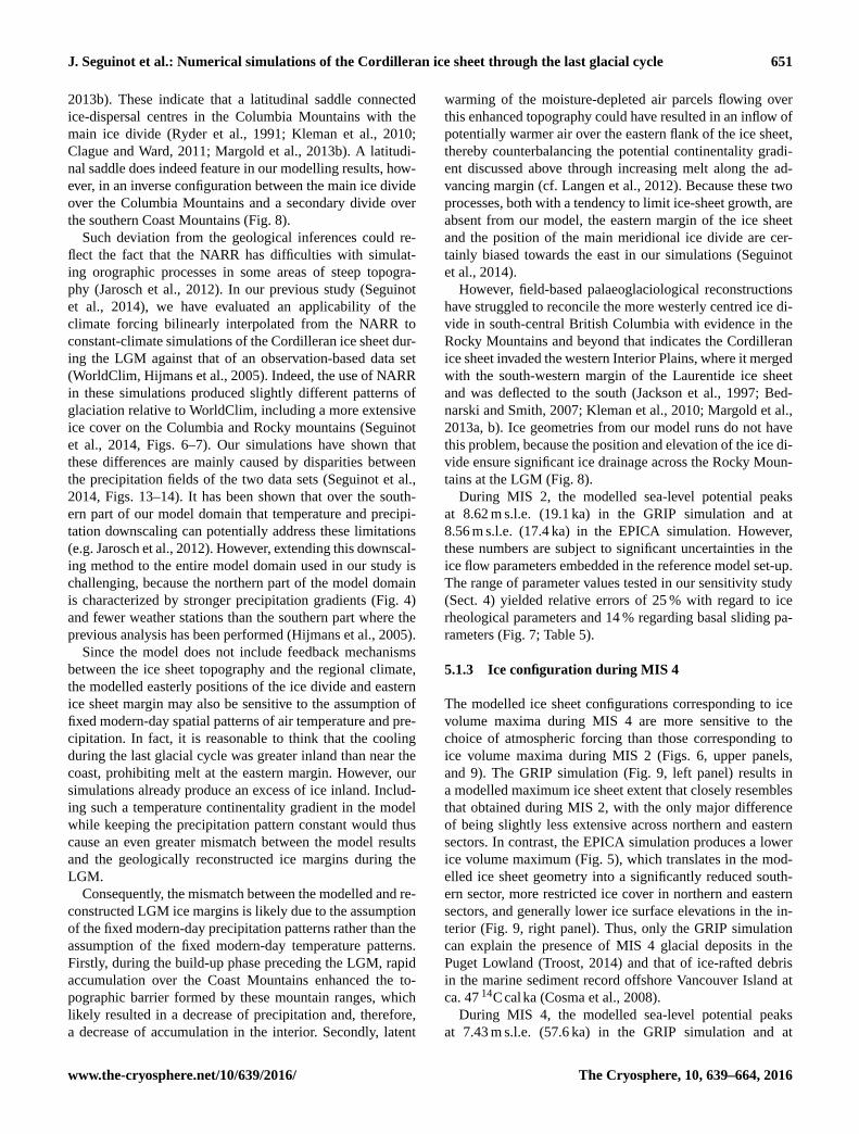
5.1.3 Ice configuration during MIS 4
The modelled ice sheet configurations corresponding to ice
volume maxima during MIS 4 are more sensitive to the
choice of atmospheric forcing than those corresponding to
ice volume maxima during MIS 2 (Figs. 6, upper panels,
and 9). The GRIP simulation (Fig. 9, left panel) results in
a modelled maximum ice sheet extent that closely resembles
that obtained during MIS 2, with the only major difference
of being slightly less extensive across northern and eastern
sectors. In contrast, the EPICA simulation produces a lower
ice volume maximum (Fig. 5), which translates in the mod-
elled ice sheet geometry into a significantly reduced south-
ern sector, more restricted ice cover in northern and eastern
sectors, and generally lower ice surface elevations in the in-
terior (Fig. 9, right panel). Thus, only the GRIP simulation
can explain the presence of MIS 4 glacial deposits in the
Puget Lowland (Troost, 2014) and that of ice-rafted debris
in the marine sediment record offshore Vancouver Island at
ca. 47 14Ccalka (Cosma et al., 2008).
During MIS 4, the modelled sea-level potential peaks
at 7.43 m s.l.e. (57.6 ka) in the GRIP simulation and at
www.the-cryosphere.net/10/639/2016/ The Cryosphere, 10, 639–664, 2016
652 J. Seguinot et al.: Numerical simulations of the Cordilleran ice sheet through the last glacial cycle
GRIP, 57.3 ka EPICA, 61.9 ka
10 31 100 316 1000Surface velocity (m a )-1
Figure 9. Modelled surface topography (200 m contours) and sur-
face velocity (colour mapping) corresponding to the maximum ice
sea-level relevant volume during MIS 4 in the GRIP and EPICA
high-resolution simulations.
4.84 m s.l.e. (61.9 ka) in the EPICA simulation, correspond-
ing to respectively 86 and 57 % of modelled MIS 2 ice vol-
umes. These estimates show little sensitivity to the range
of parameter values tested in our sensitivity study (Sect. 4),
which yielded relative errors of 12 % to ice rheological pa-
rameters and 19 % to basal sliding parameters (Fig. 7; Ta-
ble 5).
5.2 Nucleation centres
5.2.1 Transient ice sheet states
Palaeoglaciological reconstructions are generally more ro-
bust for maximum ice sheet extents and late ice sheet con-
figurations than for intermediate or minimum ice sheet ex-
tents and older ice sheet configurations (Kleman et al., 2010).
However, these maximum stages are, by nature, extreme con-
figurations, which do not necessarily represent the domi-
nant patterns of glaciation throughout the period of ice cover
(Porter, 1989; Kleman and Stroeven, 1997; Kleman et al.,
2008, 2010).
For the Cordilleran ice sheet, geological evidence from ra-
diocarbon dating (Clague et al., 1980; Clague, 1985, 1986;
Porter and Swanson, 1998; Menounos et al., 2008), cosmo-
genic exposure dating (Stroeven et al., 2010, 2014; Margold
et al., 2014), bedrock deformation in response to former ice
GRIP
34 ka
EPICA
AR
SM
CM
NC
WSEM
SMKM
NRM
CRM
28 ka
0 10 20 40 80 120
Durat ion of glaciat ion (ka)
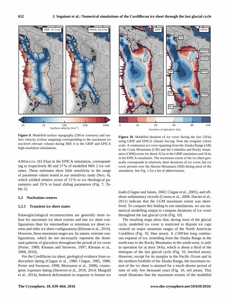
Figure 10. Modelled duration of ice cover during the last 120 ka
using GRIP and EPICA climate forcing. Note the irregular colour
scale. A continuous ice cover spanning from the Alaska Range (AR)
to the Coast Mountains (CM) and the Columbia and Rocky moun-
tains (CRM) exists for about 32 ka in the GRIP simulation and 26 ka
in the EPICA simulation. The maximum extent of the ice sheet gen-
erally corresponds to relatively short durations of ice cover, but ice
cover persists over the Skeena Mountains (SM) during most of the
simulation. See Fig. 1 for a list of abbreviations.
loads (Clague and James, 2002; Clague et al., 2005), and off-
shore sedimentary records (Cosma et al., 2008; Davies et al.,
2011) indicate that the LGM maximum extent was short-
lived. To compare this finding to our simulations, we use nu-
merical modelling output to compute durations of ice cover
throughout the last glacial cycle (Fig. 10).
The resulting maps show that, during most of the glacial
cycle, modelled ice cover is restricted to disjoint ice caps
centred on major mountain ranges of the North American
Cordillera (Fig. 10, blue areas). A 2 500 km long continu-
ous expanse of ice, extending from the Alaska Range in the
north-east to the Rocky Mountains in the south-west, is only
in operation for at most 34 ka, which is about a third of the
timespan of the last glacial cycle (Fig. 10, hatched areas).
However, except for its margins in the Pacific Ocean and in
the northern foothills of the Alaska Range, the maximum ex-
tent of the ice sheet is attained for a much shorter period of
time of only few thousand years (Fig. 10, red areas). This
result illustrates that the maximum extents of the modelled
The Cryosphere, 10, 639–664, 2016 www.the-cryosphere.net/10/639/2016/
J. Seguinot et al.: Numerical simulations of the Cordilleran ice sheet through the last glacial cycle 653
ice sheet during MIS 4 and MIS 2 were both short-lived and
therefore out of balance with contemporary climate.
A notable exception to the transient character of the maxi-
mum extent of the Cordilleran ice sheet is the northern slope
of the Alaska Range, where modelled glaciers are confined to
its foothills during the entire simulation period (Fig. 10, AR).
This apparent insensitivity of modelled glacial extent to tem-
perature fluctuations results from a combination of low pre-
cipitation, high summer temperature, and large temperature
standard deviation in the plains of the Alaska Interior (Fig. 4)
which confines glaciation to the foothills of the mountains.
This result could potentially explain the local distribution
of glacial deposits, which indicates that glaciers flowing on
the northern slope of the Alaska Range have remained small
throughout the Pleistocene (Kaufman and Manley, 2004).
5.2.2 Major ice-dispersal centres
It is generally believed that the Cordilleran ice sheet formed
by the coalescence of several mountain-centred ice caps
(Davis and Mathews, 1944). In our simulations, major ice-
dispersal centres, visible on the modelled ice cover duration
maps (Fig. 10), are located over the Coast Mountains, the
Columbia and Rocky mountains, the Skeena Mountains, and
the Selwyn and Mackenzie mountains.
The location of the modelled ice-dispersal centres is poten-
tially biased by the present-day ice volumes contained in the
ETOPO1 basal topography data. The most problematic part
of the model domain in this respect is that of the Wrangell
and Saint Elias mountains, where ice thicknesses of up to
1200 m have been measured by a low-frequency radar (Rig-
not et al., 2013). In this area, located over the USA–Canada
border just north of 60◦ N, temperate ice, glacier surging dy-
namics, and deep subglacial depressions in the ice-field inte-
rior pose a fundamental challenge to the reconstruction basal
topography for the entire ice cap (Rignot et al., 2013). Recent
ice thickness reconstructions available for all glaciers around
the globe (Huss and Farinotti, 2012), for Canadian glaciers
south of 60◦ N (Clarke et al., 2013), and for Alaska tidewater
glaciers (McNabb et al., 2015) have not been implemented in
our simulations. However, this drawback seem to have little
effect on modelled Cordilleran ice sheet dynamics. In fact,
the Wrangell and Saint Elias mountains, heavily glacierized
at present, host an ice cap for the entire length of both sim-
ulations, but that ice cap does not appear to be a major feed
to the Cordilleran ice sheet (Fig. 10, WSEM). With this ex-
ception of the Wrangell and Saint Elias mountains ice field,
present-day ice volumes are small relative to the ice volumes
concerned in our study.
Although the Coast, Skeena, Columbia, and Rocky moun-
tains are covered by mountain glaciers for most of the last
glacial cycle, providing durable nucleation centres for an ice
sheet, this is not the case for the Selwyn and Mackenzie
mountains, where ice cover on the highest peaks is limited
to a small fraction of the last glacial cycle. In other words,
the Selwyn and Mackenzie mountains only appear as a sec-
ondary ice-dispersal centre during the coldest periods of the
last glacial cycle. The Northern Rocky Mountains (Fig. 10,
NRM) do not act as a nucleation centre, but rather as a pin-
ning point for the Cordilleran ice sheet margin coming from
the west.
Perhaps the most striking feature displayed by the distribu-
tions of modelled ice cover is the persistence of the Skeena
Mountains ice cap throughout the entire last glacial period
(ca. 100–10 ka) and its predominance over the other ice-
dispersal centres (Figs. 6 and 10, SM). Regardless of the ap-
plied forcing, this ice cap appears to survive MIS 3 (Fig. 6,
middle panels) and serves as a nucleation centre at the onset
of the glacial readvance towards the LGM (MIS 2). This situ-
ation appear similar to the neighbouring Laurentide ice sheet,
for which the importance of residual ice for the glacial his-
tory leading up to the LGM has been illustrated by the MIS 3
residual ice bodies in northern and eastern Canada as nucle-
ation centres for a much more extensive MIS 2 configuration
(Kleman et al., 2010).
The presence of a Skeena Mountains ice cap during most
of the last glacial cycle can be explained by meteorological
conditions more favourable for ice growth there than else-
where. In fact, reanalysed atmospheric fields used to force
the surface mass balance model show that high winter pre-
cipitations are mainly confined to the western slope of the
Coast Mountains, except in the centre of the modelling do-
main where they also occur further inland than along other
east–west transects (Fig. 4). In fact, along most of the north-
western coast of North America, coastal mountain ranges
form a pronounced topographic barrier for westerly winds,
capturing atmospheric moisture in the form of orographic
precipitation and resulting in arid interior lowlands. How-
ever, near the centre of our modelling domain, this barrier
is less pronounced than elsewhere, allowing westerly winds
to carry moisture further inland until it is captured by the ex-
tensive Skeena Mountains in north-central British Columbia,
thus resulting in a more widespread distribution of winter
precipitation (Fig. 4).
The modelled sea-level potential corresponding to these
persistent ice-dispersal centres attains a minimum of
1.54 m s.l.e. (42.9 ka) in the GRIP simulation and of
2.55 m s.l.e. (52.4 ka) in the EPICA simulation, correspond-
ing to respectively 18 and 30 % of the MIS 2 ice volumes.
However, these numbers should be considered with caution
as our sensitivity study (Sect. 4) shows that the minimum ice
volume during MIS 3 is highly sensitive to ice flow parame-
ters, with relative errors of 45 % to the range of ice rheologi-
cal parameters tested and 109 % to the range of basal sliding
parameters tested (Fig. 7; Table 5).
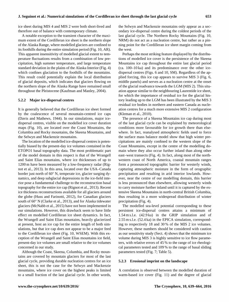
5.2.3 Erosional imprint on the landscape
A correlation is observed between the modelled duration of
warm-based ice cover (Fig. 11) and the degree of glacial
www.the-cryosphere.net/10/639/2016/ The Cryosphere, 10, 639–664, 2016
654 J. Seguinot et al.: Numerical simulations of the Cordilleran ice sheet through the last glacial cycle
GRIP EPICA
SM
MKM
0 20 40 60 80 100 120
Duration of warm-based ice cover (ka)
Figure 11. Modelled duration of warm-based ice cover during the
last 120 ka. Long ice cover durations combined with basal temper-
atures at the pressure melting point may explain the strong glacial
erosional imprint of the Skeena Mountains (SM) landscape. Hatches
indicate areas that were covered by cold ice only.
modification of the landscape (mainly in terms of the de-
velopment of deep glacial valleys and troughs). We find ev-
idence for this on the slopes of the Coast Mountains, the
Columbia and Rocky mountains, the Wrangell and Saint
Elias mountains, and radiating off the Skeena Mountains
(Figs. 10 and 11; Kleman et al., 2010, Fig. 2). The Skeena
Mountains, for example, indeed bear a strong glacial im-
print that indicates ice drainage in a system of distinct glacial
troughs emanating in a radial pattern from the centre of the
mountain range (Kleman et al., 2010, Fig. 2) that appear to
predate the LGM phase of the Cordilleran ice sheet (Stumpf
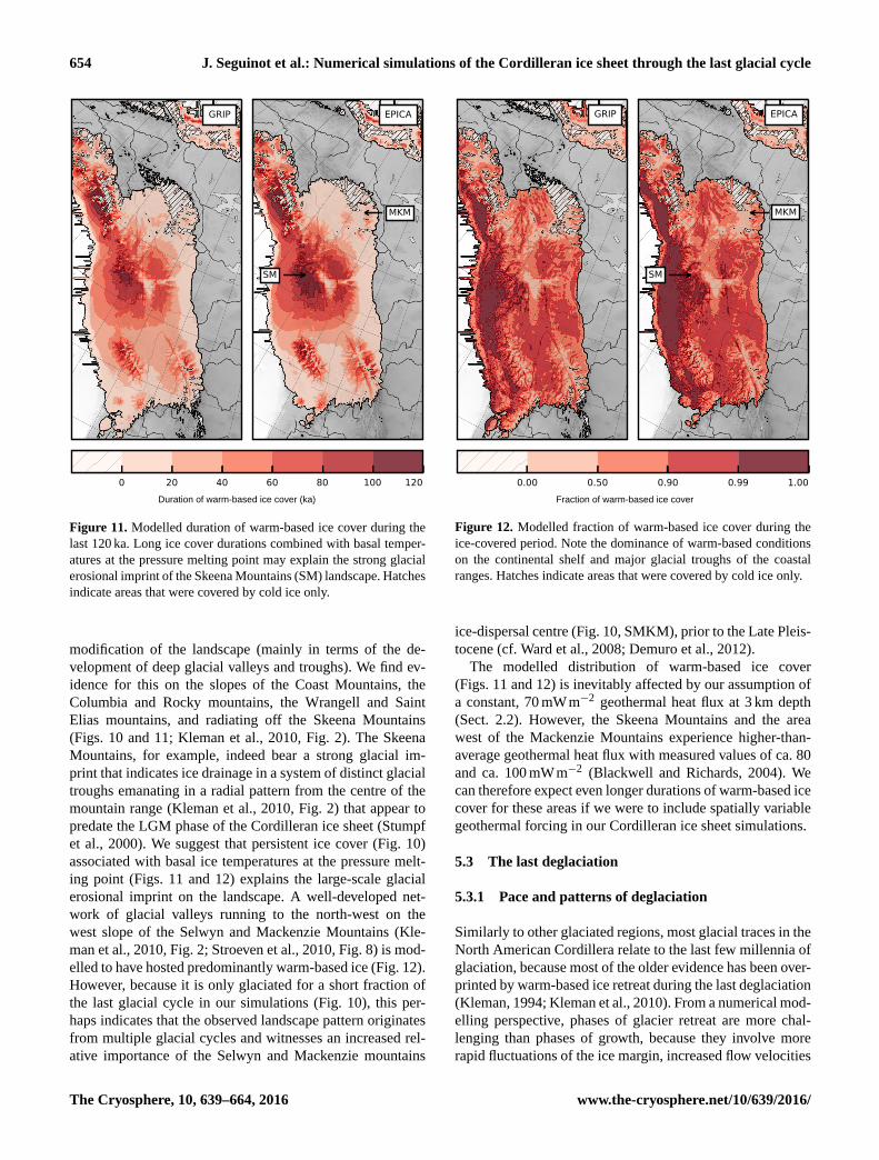
et al., 2000). We suggest that persistent ice cover (Fig. 10)
associated with basal ice temperatures at the pressure melt-
ing point (Figs. 11 and 12) explains the large-scale glacial
erosional imprint on the landscape. A well-developed net-
work of glacial valleys running to the north-west on the
west slope of the Selwyn and Mackenzie Mountains (Kle-
man et al., 2010, Fig. 2; Stroeven et al., 2010, Fig. 8) is mod-
elled to have hosted predominantly warm-based ice (Fig. 12).
However, because it is only glaciated for a short fraction of
the last glacial cycle in our simulations (Fig. 10), this per-
haps indicates that the observed landscape pattern originates
from multiple glacial cycles and witnesses an increased rel-
ative importance of the Selwyn and Mackenzie mountains
GRIP EPICA
SM
MKM
0.00 0.50 0.90 0.99 1.00
Fraction of warm-based ice cover
Figure 12. Modelled fraction of warm-based ice cover during the
ice-covered period. Note the dominance of warm-based conditions
on the continental shelf and major glacial troughs of the coastal
ranges. Hatches indicate areas that were covered by cold ice only.
ice-dispersal centre (Fig. 10, SMKM), prior to the Late Pleis-
tocene (cf. Ward et al., 2008; Demuro et al., 2012).
The modelled distribution of warm-based ice cover
(Figs. 11 and 12) is inevitably affected by our assumption of
a constant, 70 mWm−2 geothermal heat flux at 3 km depth
(Sect. 2.2). However, the Skeena Mountains and the area
west of the Mackenzie Mountains experience higher-than-
average geothermal heat flux with measured values of ca. 80
and ca. 100 mWm−2 (Blackwell and Richards, 2004). We
can therefore expect even longer durations of warm-based ice
cover for these areas if we were to include spatially variable
geothermal forcing in our Cordilleran ice sheet simulations.
5.3 The last deglaciation
5.3.1 Pace and patterns of deglaciation
Similarly to other glaciated regions, most glacial traces in the
North American Cordillera relate to the last few millennia of
glaciation, because most of the older evidence has been over-
printed by warm-based ice retreat during the last deglaciation
(Kleman, 1994; Kleman et al., 2010). From a numerical mod-
elling perspective, phases of glacier retreat are more chal-
lenging than phases of growth, because they involve more
rapid fluctuations of the ice margin, increased flow velocities
The Cryosphere, 10, 639–664, 2016 www.the-cryosphere.net/10/639/2016/
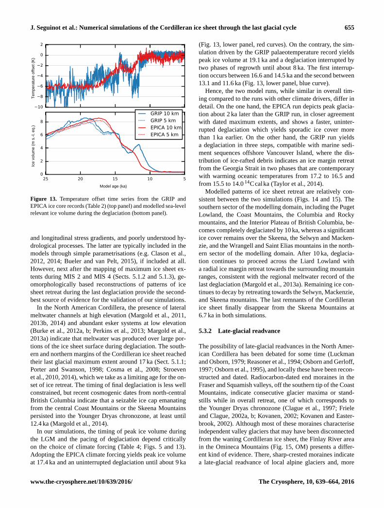
J. Seguinot et al.: Numerical simulations of the Cordilleran ice sheet through the last glacial cycle 655
10
8
6
4
2
0
2
Tem
pera
ture
offs
et (K
)
510152025
Model age (ka)
0
2
4
6
8
Ice
volu
me
(m s
.-l. e
q.)
GRIP 10 kmGRIP 5 kmEPICA 10 kmEPICA 5 km
Figure 13. Temperature offset time series from the GRIP and
EPICA ice core records (Table 2) (top panel) and modelled sea-level
relevant ice volume during the deglaciation (bottom panel).
and longitudinal stress gradients, and poorly understood hy-
drological processes. The latter are typically included in the
models through simple parametrisations (e.g. Clason et al.,
2012, 2014; Bueler and van Pelt, 2015), if included at all.
However, next after the mapping of maximum ice sheet ex-
tents during MIS 2 and MIS 4 (Sects. 5.1.2 and 5.1.3), ge-
omorphologically based reconstructions of patterns of ice
sheet retreat during the last deglaciation provide the second-
best source of evidence for the validation of our simulations.
In the North American Cordillera, the presence of lateral
meltwater channels at high elevation (Margold et al., 2011,
2013b, 2014) and abundant esker systems at low elevation
(Burke et al., 2012a, b; Perkins et al., 2013; Margold et al.,
2013a) indicate that meltwater was produced over large por-
tions of the ice sheet surface during deglaciation. The south-
ern and northern margins of the Cordilleran ice sheet reached
their last glacial maximum extent around 17 ka (Sect. 5.1.1;
Porter and Swanson, 1998; Cosma et al., 2008; Stroeven
et al., 2010, 2014), which we take as a limiting age for the on-
set of ice retreat. The timing of final deglaciation is less well
constrained, but recent cosmogenic dates from north-central
British Columbia indicate that a seizable ice cap emanating
from the central Coast Mountains or the Skeena Mountains
persisted into the Younger Dryas chronozone, at least until
12.4 ka (Margold et al., 2014).
In our simulations, the timing of peak ice volume during
the LGM and the pacing of deglaciation depend critically
on the choice of climate forcing (Table 4; Figs. 5 and 13).
Adopting the EPICA climate forcing yields peak ice volume
at 17.4 ka and an uninterrupted deglaciation until about 9 ka
(Fig. 13, lower panel, red curves). On the contrary, the sim-
ulation driven by the GRIP palaeotemperature record yields
peak ice volume at 19.1 ka and a deglaciation interrupted by
two phases of regrowth until about 8 ka. The first interrup-
tion occurs between 16.6 and 14.5 ka and the second between
13.1 and 11.6 ka (Fig. 13, lower panel, blue curve).
Hence, the two model runs, while similar in overall tim-
ing compared to the runs with other climate drivers, differ in
detail. On the one hand, the EPICA run depicts peak glacia-
tion about 2 ka later than the GRIP run, in closer agreement
with dated maximum extents, and shows a faster, uninter-
rupted deglaciation which yields sporadic ice cover more
than 1 ka earlier. On the other hand, the GRIP run yields
a deglaciation in three steps, compatible with marine sedi-
ment sequences offshore Vancouver Island, where the dis-
tribution of ice-rafted debris indicates an ice margin retreat
from the Georgia Strait in two phases that are contemporary
with warming oceanic temperatures from 17.2 to 16.5 and
from 15.5 to 14.0 14Ccalka (Taylor et al., 2014).
Modelled patterns of ice sheet retreat are relatively con-
sistent between the two simulations (Figs. 14 and 15). The
southern sector of the modelling domain, including the Puget
Lowland, the Coast Mountains, the Columbia and Rocky
mountains, and the Interior Plateau of British Columbia, be-
comes completely deglaciated by 10 ka, whereas a significant
ice cover remains over the Skeena, the Selwyn and Macken-
zie, and the Wrangell and Saint Elias mountains in the north-
ern sector of the modelling domain. After 10 ka, deglacia-
tion continues to proceed across the Liard Lowland with
a radial ice margin retreat towards the surrounding mountain
ranges, consistent with the regional meltwater record of the
last deglaciation (Margold et al., 2013a). Remaining ice con-
tinues to decay by retreating towards the Selwyn, Mackenzie,
and Skeena mountains. The last remnants of the Cordilleran
ice sheet finally disappear from the Skeena Mountains at
6.7 ka in both simulations.
5.3.2 Late-glacial readvance
The possibility of late-glacial readvances in the North Amer-
ican Cordillera has been debated for some time (Luckman
and Osborn, 1979; Reasoner et al., 1994; Osborn and Gerloff,
1997; Osborn et al., 1995), and locally these have been recon-
structed and dated. Radiocarbon-dated end moraines in the
Fraser and Squamish valleys, off the southern tip of the Coast
Mountains, indicate consecutive glacier maxima or stand-
stills while in overall retreat, one of which corresponds to
the Younger Dryas chronozone (Clague et al., 1997; Friele
and Clague, 2002a, b; Kovanen, 2002; Kovanen and Easter-
brook, 2002). Although most of these moraines characterise
independent valley glaciers that may have been disconnected
from the waning Cordilleran ice sheet, the Finlay River area
in the Omineca Mountains (Fig. 15, OM) presents a differ-
ent kind of evidence. There, sharp-crested moraines indicate
a late-glacial readvance of local alpine glaciers and, more
www.the-cryosphere.net/10/639/2016/ The Cryosphere, 10, 639–664, 2016
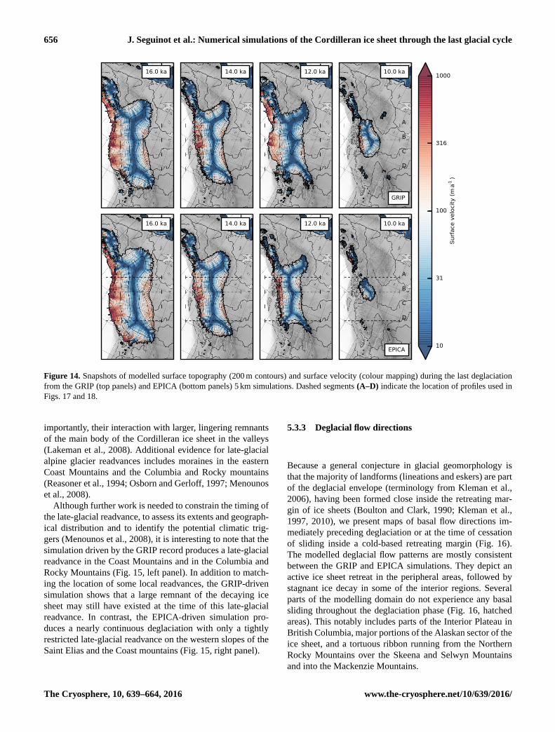
656 J. Seguinot et al.: Numerical simulations of the Cordilleran ice sheet through the last glacial cycle
16.0 ka 14.0 ka 12.0 ka 10.0 ka
A
B
C
D
GRIP
16.0 ka 14.0 ka 12.0 ka 10.0 ka
A
B
C
D
EPICA10
31
100
316
1000
Surf
ace
velo
city
(m
a)
-1
Figure 14. Snapshots of modelled surface topography (200 m contours) and surface velocity (colour mapping) during the last deglaciation
from the GRIP (top panels) and EPICA (bottom panels) 5 km simulations. Dashed segments (A–D) indicate the location of profiles used in
Figs. 17 and 18.
importantly, their interaction with larger, lingering remnants
of the main body of the Cordilleran ice sheet in the valleys
(Lakeman et al., 2008). Additional evidence for late-glacial
alpine glacier readvances includes moraines in the eastern
Coast Mountains and the Columbia and Rocky mountains
(Reasoner et al., 1994; Osborn and Gerloff, 1997; Menounos
et al., 2008).
Although further work is needed to constrain the timing of
the late-glacial readvance, to assess its extents and geograph-
ical distribution and to identify the potential climatic trig-
gers (Menounos et al., 2008), it is interesting to note that the
simulation driven by the GRIP record produces a late-glacial
readvance in the Coast Mountains and in the Columbia and
Rocky Mountains (Fig. 15, left panel). In addition to match-
ing the location of some local readvances, the GRIP-driven
simulation shows that a large remnant of the decaying ice
sheet may still have existed at the time of this late-glacial
readvance. In contrast, the EPICA-driven simulation pro-
duces a nearly continuous deglaciation with only a tightly
restricted late-glacial readvance on the western slopes of the
Saint Elias and the Coast mountains (Fig. 15, right panel).
5.3.3 Deglacial flow directions
Because a general conjecture in glacial geomorphology is
that the majority of landforms (lineations and eskers) are part
of the deglacial envelope (terminology from Kleman et al.,
2006), having been formed close inside the retreating mar-
gin of ice sheets (Boulton and Clark, 1990; Kleman et al.,
1997, 2010), we present maps of basal flow directions im-
mediately preceding deglaciation or at the time of cessation
of sliding inside a cold-based retreating margin (Fig. 16).
The modelled deglacial flow patterns are mostly consistent
between the GRIP and EPICA simulations. They depict an
active ice sheet retreat in the peripheral areas, followed by
stagnant ice decay in some of the interior regions. Several
parts of the modelling domain do not experience any basal
sliding throughout the deglaciation phase (Fig. 16, hatched
areas). This notably includes parts of the Interior Plateau in
British Columbia, major portions of the Alaskan sector of the
ice sheet, and a tortuous ribbon running from the Northern
Rocky Mountains over the Skeena and Selwyn Mountains
and into the Mackenzie Mountains.
The Cryosphere, 10, 639–664, 2016 www.the-cryosphere.net/10/639/2016/
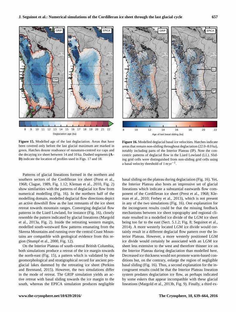
J. Seguinot et al.: Numerical simulations of the Cordilleran ice sheet through the last glacial cycle 657
GRIP
A
B
C
D
OM
EPICA
A
B
C
D
8 9 10 11 12 13 14 15 16 17 18 19 20 21 22
Deglaciation age (ka)
Figure 15. Modelled age of the last deglaciation. Areas that have
been covered only before the last glacial maximum are marked in
green. Hatches denote readvance of mountain-centred ice caps and
the decaying ice sheet between 14 and 10 ka. Dashed segments (A–
D) indicate the location of profiles used in Figs. 17 and 18.
Patterns of glacial lineations formed in the northern and
southern sectors of the Cordilleran ice sheet (Prest et al.,
1968; Clague, 1989, Fig. 1.12; Kleman et al., 2010, Fig. 2)
show similarities with the patterns of deglacial ice flow from
numerical modelling (Fig. 16). In the northern half of the
modelling domain, modelled deglacial flow directions depict
an active downhill flow as the last remnants of the ice sheet
retreat towards mountain ranges. Converging deglacial flow
patterns in the Liard Lowland, for instance (Fig. 16), closely
resemble the pattern indicated by glacial lineations (Margold
et al., 2013a, Fig. 2). Inside the retreating western margin,
modelled south-westward flow patterns emanating from the
Skeena Mountains and running over the central Coast Moun-
tains are compatible with geological evidence from this re-
gion (Stumpf et al., 2000, Fig. 12).
On the Interior Plateau of south-central British Columbia,
both simulations produce a retreat of the ice margin towards
the north-east (Fig. 15), a pattern which is validated by the
geomorphological and stratigraphical record for ancient pro-
glacial lakes dammed by the retreating ice sheet (Perkins
and Brennand, 2015). However, the two simulations differ
in the mode of retreat. The GRIP simulation yields an ac-
tive retreat with basal sliding towards the ice margin to the
south, whereas the EPICA simulation produces negligible
GRIP EPICA
LL
IP
8 10 12 14 16 18 20 22
Age of last basal sliding (ka)
Figure 16. Modelled deglacial basal ice velocities. Hatches indicate
areas that remain non-sliding throughout deglaciation (22.0–8.0 ka),
notably including parts of the Interior Plateau (IP). Note the con-
centric patterns of deglacial flow in the Liard Lowland (LL). Slid-
ing grid cells were distinguished from non-sliding grid cells using
a basal velocity threshold of 1 myr−1.
basal sliding on the plateau during deglaciation (Fig. 16). Yet,
the Interior Plateau also hosts an impressive set of glacial
lineations which indicate a substantial eastwards flow com-
ponent of the Cordilleran ice sheet (Prest et al., 1968; Kle-
man et al., 2010; Ferbey et al., 2013), which is not present
in any of the two simulations (Fig. 16). One explanation for
the incongruent results could be that the missing feedback
mechanisms between ice sheet topography and regional cli-
mate resulted in a modelled ice divide of the LGM ice sheet
being too far to the east (Sect. 5.1.2; Fig. 8; Seguinot et al.,
2014). A more westerly located LGM ice divide would cer-
tainly result in a different deglacial flow pattern over the In-
terior Plateau. However, a more westerly positioned LGM
ice divide would certainly be associated with an LGM ice
sheet less extensive to the west and therefore thinner ice on
the Interior Plateau during deglaciation than modelled here.
Decreased ice thickness would not promote warm-based con-
ditions but, on the contrary, enlarge the region of negligible
basal sliding (Fig. 16). Thus, a second explanation for the in-
congruent results could be that the Interior Plateau lineation
system predates deglaciation ice flow, as perhaps indicated
by some eskers that appear incompatible with these glacial
lineations (Margold et al., 2013b, Fig. 9). Finally, a third ex-
www.the-cryosphere.net/10/639/2016/ The Cryosphere, 10, 639–664, 2016
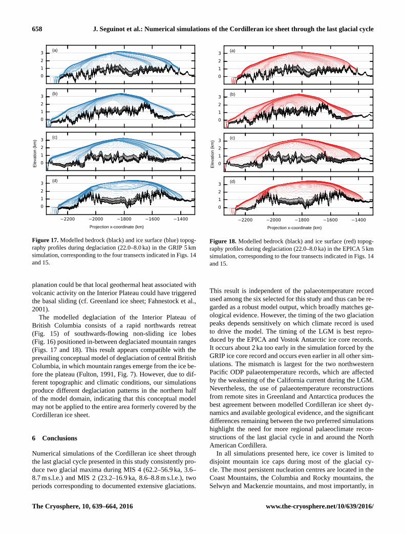
658 J. Seguinot et al.: Numerical simulations of the Cordilleran ice sheet through the last glacial cycle
0
1
2
3(a)
0
1
2
3(b)
0
1
2
3
Elev
atio
n (k
m) (c)
2200 2000 1800 1600 1400
Projection x-coordinate (km)
0
1
2
3(d)
Figure 17. Modelled bedrock (black) and ice surface (blue) topog-
raphy profiles during deglaciation (22.0–8.0 ka) in the GRIP 5 km
simulation, corresponding to the four transects indicated in Figs. 14
and 15.
planation could be that local geothermal heat associated with
volcanic activity on the Interior Plateau could have triggered
the basal sliding (cf. Greenland ice sheet; Fahnestock et al.,
2001).
The modelled deglaciation of the Interior Plateau of
British Columbia consists of a rapid northwards retreat
(Fig. 15) of southwards-flowing non-sliding ice lobes
(Fig. 16) positioned in-between deglaciated mountain ranges
(Figs. 17 and 18). This result appears compatible with the
prevailing conceptual model of deglaciation of central British
Columbia, in which mountain ranges emerge from the ice be-
fore the plateau (Fulton, 1991, Fig. 7). However, due to dif-
ferent topographic and climatic conditions, our simulations
produce different deglaciation patterns in the northern half
of the model domain, indicating that this conceptual model
may not be applied to the entire area formerly covered by the
Cordilleran ice sheet.
6 Conclusions
Numerical simulations of the Cordilleran ice sheet through
the last glacial cycle presented in this study consistently pro-
duce two glacial maxima during MIS 4 (62.2–56.9 ka, 3.6–
8.7 m s.l.e.) and MIS 2 (23.2–16.9 ka, 8.6–8.8 m s.l.e.), two
periods corresponding to documented extensive glaciations.
0
1
2
3(a)
0
1
2
3(b)
0
1
2
3
Elev
atio
n (k
m) (c)
2200 2000 1800 1600 1400
Projection x-coordinate (km)
0
1
2
3(d)
Figure 18. Modelled bedrock (black) and ice surface (red) topog-
raphy profiles during deglaciation (22.0–8.0 ka) in the EPICA 5 km
simulation, corresponding to the four transects indicated in Figs. 14
and 15.
This result is independent of the palaeotemperature record
used among the six selected for this study and thus can be re-
garded as a robust model output, which broadly matches ge-
ological evidence. However, the timing of the two glaciation
peaks depends sensitively on which climate record is used
to drive the model. The timing of the LGM is best repro-
duced by the EPICA and Vostok Antarctic ice core records.
It occurs about 2 ka too early in the simulation forced by the
GRIP ice core record and occurs even earlier in all other sim-
ulations. The mismatch is largest for the two northwestern
Pacific ODP palaeotemperature records, which are affected
by the weakening of the California current during the LGM.
Nevertheless, the use of palaeotemperature reconstructions
from remote sites in Greenland and Antarctica produces the
best agreement between modelled Cordilleran ice sheet dy-
namics and available geological evidence, and the significant
differences remaining between the two preferred simulations
highlight the need for more regional palaeoclimate recon-
structions of the last glacial cycle in and around the North
American Cordillera.
In all simulations presented here, ice cover is limited to
disjoint mountain ice caps during most of the glacial cy-
cle. The most persistent nucleation centres are located in the
Coast Mountains, the Columbia and Rocky mountains, the
Selwyn and Mackenzie mountains, and most importantly, in
The Cryosphere, 10, 639–664, 2016 www.the-cryosphere.net/10/639/2016/
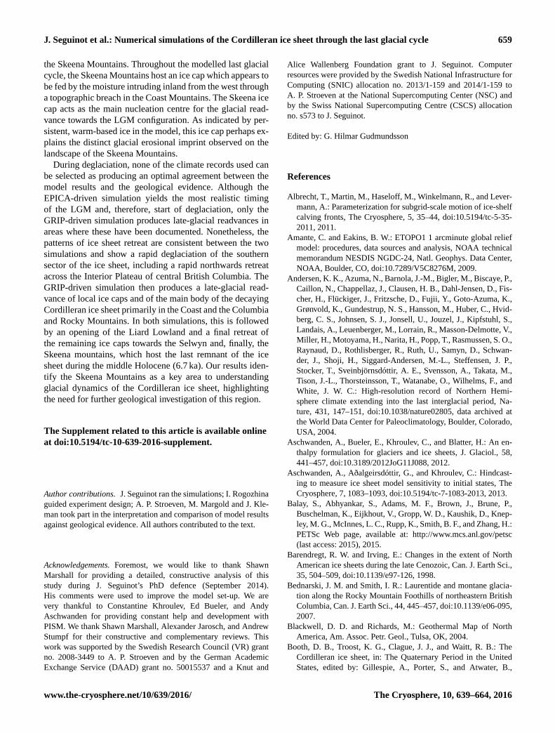
J. Seguinot et al.: Numerical simulations of the Cordilleran ice sheet through the last glacial cycle 659
the Skeena Mountains. Throughout the modelled last glacial
cycle, the Skeena Mountains host an ice cap which appears to
be fed by the moisture intruding inland from the west through
a topographic breach in the Coast Mountains. The Skeena ice
cap acts as the main nucleation centre for the glacial read-
vance towards the LGM configuration. As indicated by per-
sistent, warm-based ice in the model, this ice cap perhaps ex-
plains the distinct glacial erosional imprint observed on the
landscape of the Skeena Mountains.
During deglaciation, none of the climate records used can
be selected as producing an optimal agreement between the
model results and the geological evidence. Although the
EPICA-driven simulation yields the most realistic timing
of the LGM and, therefore, start of deglaciation, only the
GRIP-driven simulation produces late-glacial readvances in
areas where these have been documented. Nonetheless, the
patterns of ice sheet retreat are consistent between the two
simulations and show a rapid deglaciation of the southern
sector of the ice sheet, including a rapid northwards retreat
across the Interior Plateau of central British Columbia. The
GRIP-driven simulation then produces a late-glacial read-
vance of local ice caps and of the main body of the decaying
Cordilleran ice sheet primarily in the Coast and the Columbia
and Rocky Mountains. In both simulations, this is followed
by an opening of the Liard Lowland and a final retreat of
the remaining ice caps towards the Selwyn and, finally, the
Skeena mountains, which host the last remnant of the ice
sheet during the middle Holocene (6.7 ka). Our results iden-
tify the Skeena Mountains as a key area to understanding
glacial dynamics of the Cordilleran ice sheet, highlighting
the need for further geological investigation of this region.
The Supplement related to this article is available online
at doi:10.5194/tc-10-639-2016-supplement.
Author contributions. J. Seguinot ran the simulations; I. Rogozhina
guided experiment design; A. P. Stroeven, M. Margold and J. Kle-
man took part in the interpretation and comparison of model results
against geological evidence. All authors contributed to the text.
Acknowledgements. Foremost, we would like to thank Shawn
Marshall for providing a detailed, constructive analysis of this
study during J. Seguinot’s PhD defence (September 2014).
His comments were used to improve the model set-up. We are
very thankful to Constantine Khroulev, Ed Bueler, and Andy
Aschwanden for providing constant help and development with
PISM. We thank Shawn Marshall, Alexander Jarosch, and Andrew
Stumpf for their constructive and complementary reviews. This
work was supported by the Swedish Research Council (VR) grant
no. 2008-3449 to A. P. Stroeven and by the German Academic
Exchange Service (DAAD) grant no. 50015537 and a Knut and
Alice Wallenberg Foundation grant to J. Seguinot. Computer
resources were provided by the Swedish National Infrastructure for
Computing (SNIC) allocation no. 2013/1-159 and 2014/1-159 to
A. P. Stroeven at the National Supercomputing Center (NSC) and
by the Swiss National Supercomputing Centre (CSCS) allocation
no. s573 to J. Seguinot.
Edited by: G. Hilmar Gudmundsson
References
Albrecht, T., Martin, M., Haseloff, M., Winkelmann, R., and Lever-
mann, A.: Parameterization for subgrid-scale motion of ice-shelf
calving fronts, The Cryosphere, 5, 35–44, doi:10.5194/tc-5-35-
2011, 2011.
Amante, C. and Eakins, B. W.: ETOPO1 1 arcminute global relief
model: procedures, data sources and analysis, NOAA technical
memorandum NESDIS NGDC-24, Natl. Geophys. Data Center,
NOAA, Boulder, CO, doi:10.7289/V5C8276M, 2009.
Andersen, K. K., Azuma, N., Barnola, J.-M., Bigler, M., Biscaye, P.,
Caillon, N., Chappellaz, J., Clausen, H. B., Dahl-Jensen, D., Fis-
cher, H., Flückiger, J., Fritzsche, D., Fujii, Y., Goto-Azuma, K.,
Grønvold, K., Gundestrup, N. S., Hansson, M., Huber, C., Hvid-
berg, C. S., Johnsen, S. J., Jonsell, U., Jouzel, J., Kipfstuhl, S.,
Landais, A., Leuenberger, M., Lorrain, R., Masson-Delmotte, V.,
Miller, H., Motoyama, H., Narita, H., Popp, T., Rasmussen, S. O.,
Raynaud, D., Rothlisberger, R., Ruth, U., Samyn, D., Schwan-
der, J., Shoji, H., Siggard-Andersen, M.-L., Steffensen, J. P.,
Stocker, T., Sveinbjörnsdóttir, A. E., Svensson, A., Takata, M.,
Tison, J.-L., Thorsteinsson, T., Watanabe, O., Wilhelms, F., and
White, J. W. C.: High-resolution record of Northern Hemi-
sphere climate extending into the last interglacial period, Na-
ture, 431, 147–151, doi:10.1038/nature02805, data archived at
the World Data Center for Paleoclimatology, Boulder, Colorado,
USA, 2004.
Aschwanden, A., Bueler, E., Khroulev, C., and Blatter, H.: An en-
thalpy formulation for glaciers and ice sheets, J. Glaciol., 58,
441–457, doi:10.3189/2012JoG11J088, 2012.
Aschwanden, A., Aðalgeirsdóttir, G., and Khroulev, C.: Hindcast-
ing to measure ice sheet model sensitivity to initial states, The
Cryosphere, 7, 1083–1093, doi:10.5194/tc-7-1083-2013, 2013.
Balay, S., Abhyankar, S., Adams, M. F., Brown, J., Brune, P.,
Buschelman, K., Eijkhout, V., Gropp, W. D., Kaushik, D., Knep-
ley, M. G., McInnes, L. C., Rupp, K., Smith, B. F., and Zhang, H.:
PETSc Web page, available at: http://www.mcs.anl.gov/petsc
(last access: 2015), 2015.
Barendregt, R. W. and Irving, E.: Changes in the extent of North
American ice sheets during the late Cenozoic, Can. J. Earth Sci.,
35, 504–509, doi:10.1139/e97-126, 1998.
Bednarski, J. M. and Smith, I. R.: Laurentide and montane glacia-
tion along the Rocky Mountain Foothills of northeastern British
Columbia, Can. J. Earth Sci., 44, 445–457, doi:10.1139/e06-095,
2007.
Blackwell, D. D. and Richards, M.: Geothermal Map of North
America, Am. Assoc. Petr. Geol., Tulsa, OK, 2004.
Booth, D. B., Troost, K. G., Clague, J. J., and Waitt, R. B.: The
Cordilleran ice sheet, in: The Quaternary Period in the United
States, edited by: Gillespie, A., Porter, S., and Atwater, B.,
www.the-cryosphere.net/10/639/2016/ The Cryosphere, 10, 639–664, 2016
660 J. Seguinot et al.: Numerical simulations of the Cordilleran ice sheet through the last glacial cycle
vol. 1 of Dev. Quaternary Sci., Elsevier, Amsterdam, 17–43,
doi:10.1016/s1571-0866(03)01002-9, 2003.
Boulton, G. S. and Clark, C. D.: A highly mobile Laurentide ice
sheet revealed by satellite images of glacial lineations, Nature,
346, 813–817, doi:10.1038/346813a0, 1990.
Boulton, G. S., Dongelmans, P., Punkari, M., and Broadgate, M.:
Palaeoglaciology of an ice sheet through a glacial cycle: the Eu-
ropean ice sheet through the Weichselian, Quaternary Res., 20,
591–625, doi:10.1016/s0277-3791(00)00160-8, 2001.
Briner, J. P. and Kaufman, D. S.: Late Pleistocene mountain glacia-
tion in Alaska: key chronologies, J. Quaternary Sci., 23, 659–
670, doi:10.1002/jqs.1196, 2008.
Bueler, E. and Brown, J.: Shallow shelf approximation as a “sliding
law” in a thermodynamically coupled ice sheet model, J. Geo-
phys. Res., 114, F03008, doi:10.1029/2008JF001179, 2009.
Bueler, E. and van Pelt, W.: Mass-conserving subglacial hydrology
in the Parallel Ice Sheet Model version 0.6, Geosci. Model Dev.,
8, 1613–1635, doi:10.5194/gmd-8-1613-2015, 2015.
Bueler, E., Lingle, C. S., and Brown, J.: Fast computation of a vis-
coelastic deformable Earth model for ice-sheet simulations, Ann.
Glaciol., 46, 97–105, doi:10.3189/172756407782871567, 2007.
Burke, M. J., Brennand, T. A., and Perkins, A. J.: Transient sub-
glacial hydrology of a thin ice sheet: insights from the Chasm
esker, British Columbia, Canada, Quaternary Res., 58, 30–55,
doi:10.1016/j.quascirev.2012.09.004, 2012a.
Burke, M. J., Brennand, T. A., and Perkins, A. J.: Evolution of
the subglacial hydrologic system beneath the rapidly decaying
Cordilleran Ice Sheet caused by ice-dammed lake drainage: im-
plications for meltwater-induced ice acceleration, Quaternary
Res., 50, 125–140, doi:10.1016/j.quascirev.2012.07.005, 2012b.
Calov, R. and Greve, R.: A semi-analytical solution for the positive
degree-day model with stochastic temperature variations, J.
Glaciol., 51, 173–175, doi:10.3189/172756505781829601,
2005.
Carlson, A. E. and Clark, P. U.: Ice sheet sources of sea level rise
and freshwater discharge during the last deglaciation, Rev. Geo-
phys., 50, RG4007, doi:10.1029/2011rg000371, 2012.
Carrara, P. E., Kiver, E. P., and Stradling, D. F.: The southern limit of
Cordilleran ice in the Colville and Pend Oreille valleys of north-
eastern Washington during the Late Wisconsin glaciation, Can. J.
Earth Sci., 33, 769–778, doi:10.1139/e96-059, 1996.
Clague, J., Armstrong, J., and Mathews, W.: Advance of the
late Wisconsin Cordilleran Ice Sheet in southern British
Columbia since 22 000 yr BP, Quaternary Res., 13, 322–326,
doi:10.1016/0033-5894(80)90060-5, 1980.
Clague, J. J.: Late Quaternary Geology and Geochronology
of British Columbia Part 2: Summary and Discussion of
Radiocarbon-Dated Quaternary History, Geol. Surv. of Can., Ot-
tawa, ON, Paper 80-35, doi:10.4095/119439, 1981.
Clague, J. J.: Delaciation of the Prince Rupert – Kitimat area, British
Columbia, Can. J. Earth Sci., 22, 256–265, doi:10.1139/e85-022,
1985.
Clague, J. J.: The Quaternary stratigraphic record of British
Columbia – evidence for episodic sedimentation and erosion
controlled by glaciation, Can. J. Earth Sci., 23, 885–894,
doi:10.1139/e86-090, 1986.
Clague, J. J.: Character and distribution of Quaternary deposits
(Canadian Cordillera), in: Quaternary Geology of Canada and
Greenland, edited by: Fulton, R. J., vol. 1 of Geology of Canada,
Geol. Surv. of Can., Ottawa, ON, 34–48, doi:10.4095/127905,
1989.
Clague, J. J. and James, T. S.: History and isostatic effects of the
last ice sheet in southern British Columbia, Quaternary Res., 21,
71–87, doi:10.1016/s0277-3791(01)00070-1, 2002.
Clague, J. J. and Ward, B.: Pleistocene Glaciation of British
Columbia, in: Dev. Quaternary Sci., vol. 15, edited by: Ehlers, J.,
Gibbard, P. L., and Hughes, P. D., Elsevier, Amsterdam, 563–
573, doi:10.1016/b978-0-444-53447-7.00044-1, 2011.
Clague, J. J., Mathewes, R. W., Guilbault, J.-P., Hutchinson, I.,
and Ricketts, B. D.: Pre-Younger Dryas resurgence of the
southwestern margin of the Cordilleran ice sheet, British
Columbia, Canada, Boreas, 26, 261–278, doi:10.1111/j.1502-
3885.1997.tb00855.x, 1997.
Clague, J. J., Froese, D., Hutchinson, I., James, T. S., and
Simon, K. M.: Early growth of the last Cordilleran ice
sheet deduced from glacio-isostatic depression in south-
west British Columbia, Canada, Quaternary Res., 63, 53–59,
doi:10.1016/j.yqres.2004.09.007, 2005.
Clark, P. U. and Mix, A. C.: Ice sheets and sea level of the Last
Glacial Maximum, Quaternary Res., 21, 1–7, doi:10.1016/s0277-
3791(01)00118-4, 2002.
Clason, C., Mair, D. W., Burgess, D. O., and Nienow, P. W.:
Modelling the delivery of supraglacial meltwater to the ice/bed
interface: application to southwest Devon Ice Cap, Nunavut,
Canada, J. Glaciol., 58, 361–374, doi:10.3189/2012jog11j129,
2012.
Clarke, G. K. C., Anslow, F. S., Jarosch, A. H., Radic, V., Me-
nounos, B., Bolch, T., and Berthier, E.: Ice Volume and Sub-
glacial Topography for Western Canadian Glaciers from Mass
Balance Fields, Thinning Rates, and a Bed Stress Model, J. Cli-
mate, 26, 4282–4303, doi:10.1175/jcli-d-12-00513.1, 2013.
Clason, C., Applegate, P., and Holmlund, P.: Modelling Late We-
ichselian evolution of the Eurasian ice sheets forced by sur-
face meltwater-enhanced basal sliding, J. Glaciol., 60, 29–40,
doi:10.3189/2014jog13j037, 2014.
Cosma, T., Hendy, I., and Chang, A.: Chronological constraints
on Cordilleran Ice Sheet glaciomarine sedimentation from core
MD02-2496 off Vancouver Island (western Canada), Quaternary
Sci. Rev., 27, 941–955, doi:10.1016/j.quascirev.2008.01.013,
2008.
Cuffey, K. M. and Paterson, W. S. B.: The physics of glaciers, Else-
vier, Amsterdam, 2010.
Dansgaard, W., Johnsen, S. J., Clausen, H. B., Dahl-Jensen, D.,
Gundestrup, N. S., Hammer, C. U., Hvidberg, C. S., Stef-
fensen, J. P., Sveinbjörnsdottir, A. E., Jouzel, J., and Bond, G.:
Evidence for general instability of past climate from a 250-kyr
ice-core record, Nature, 364, 218–220, doi:10.1038/364218a0,
data archived at the World Data Center for Paleoclimatology,
Boulder, Colorado, USA., 1993.
Davies, M. H., Mix, A. C., Stoner, J. S., Addison, J. A., Jaeger, J.,
Finney, B., and Wiest, J.: The deglacial transition on the south-
eastern Alaska Margin: Meltwater input, sea level rise, ma-
rine productivity, and sedimentary anoxia, Paleoceanography, 26,
PA2223, doi:10.1029/2010pa002051, 2011.
Davis, N. F. G. and Mathews, W. H.: Four phases of glaciation with
illustrations from Southwestern British Columbia, J. Geol., 52,
403–413, doi:10.1086/625236, 1944.
The Cryosphere, 10, 639–664, 2016 www.the-cryosphere.net/10/639/2016/
J. Seguinot et al.: Numerical simulations of the Cordilleran ice sheet through the last glacial cycle 661
Dawson, G. M.: III. – Recent observations on the glaciation of
British Columbia and adjacent regions, Geol. Mag., 5, 347–350,
doi:10.1017/s0016756800182159, 1888.
Demuro, M., Froese, D. G., Arnold, L. J., and Roberts, R. G.:
Single-grain OSL dating of glaciofluvial quartz constrains Reid
glaciation in NW Canada to MIS 6, Quaternary Res., 77, 305–
316, doi:10.1016/j.yqres.2011.11.009, 2012.
Duk-Rodkin, A.: Glacial limits map of Yukon Territory, Open File
3694, Geol. Surv. of Can., Ottawa, ON, doi:10.4095/210739,
1999.
Duk-Rodkin, A., Barendregt, R. W., Tarnocai, C., and
Phillips, F. M.: Late Tertiary to late Quaternary record in
the Mackenzie Mountains, Northwest Territories, Canada:
stratigraphy, paleosols, paleomagnetism, and chlorine-36,
Can. J. Earth Sci., 33, 875–895, doi:10.1139/e96-066, 1996.
Dyke, A. S.: An outline of North American deglaciation with em-
phasis on central and northern Canada, in: Dev. Quaternary Sci.,
vol. 2, edited by: Ehlers, J. and Gibbard, P. L., Elsevier, Amster-
dam, 373–424, doi:10.1016/S1571-0866(04)80209-4, 2004.
Dyke, A. S. and Prest, V. K.: Late wisconsinan and holocene history
of the laurentide ice sheet, Geogr. Phys. Quatern., 41, 237–263,
doi:10.7202/032681ar, 1987.
Dyke, A. S., Moore, A., and Robertson, L.: Deglaciation of North
America, Open File 1547, Geol. Surv. of Can., Ottawa, ON,
2003.
Fahnestock, M., Abdalati, W., Joughin, I., Brozena, J., and Gogi-
neni, P.: High geothermal heat flow, basal melt, and the origin
of rapid ice flow in central greenland, Sience, 294, 2338–2342,
doi:10.1126/science.1065370, 2001.
Ferbey, T., Arnold, H., and Hickin, A.: Ice-flow indicator com-
pilation, British Columbia., British Columbia Geol. Surv.,
Victoria, BC, Open-File 2013-06, http://www.em.gov.bc.ca/
Mining/Geoscience/PublicationsCatalogue/OpenFiles/2013/
Pages/2013-06.aspx, 2013.
Fisher, D., Osterberg, E., Dyke, A., Dahl-Jensen, D., De-
muth, M., Zdanowicz, C., Bourgeois, J., Koerner, R. M.,
Mayewski, P., Wake, C., Kreutz, K., Steig, E., Zheng, J., Yal-
cin, K., Goto-Azuma, K., Luckman, B., and Rupper, S.: The
Mt Logan Holocene–late Wisconsinan isotope record: tropi-
cal Pacific–Yukon connections, The Holocene, 18, 667–677,
doi:10.1177/0959683608092236, 2008.
Fisher, D. A., Wake, C., Kreutz, K., Yalcin, K., Steig, E., Mayewski,
P., Anderson, L., Zheng, J., Rupper, S., Zdanowicz, C., Demuth,
M., Waszkiewicz, M., Dahl-Jensen, D., Goto-Azuma, K., Bour-
geois, J. B., Koerner, R. M., Sekerka, J., Osterberg, E., Abbott,
M. B., Finney, B. P., and Burns, S. J.: Stable Isotope Records
from Mount Logan, Eclipse Ice Cores and Nearby Jellybean
Lake. Water Cycle of the North Pacific Over 2000 Years and
Over Five Vertical Kilometres: Sudden Shifts and Tropical Con-
nections, Géogr. phys. Quatern., 58, 337, doi:10.7202/013147ar,
2004.
Friele, P. A. and Clague, J. J.: Readvance of glaciers in the British
Columbia Coast Mountains at the end of the last glaciation,
Quatern. Int., 87, 45–58, doi:10.1016/s1040-6182(01)00061-1,
2002a.
Friele, P. A. and Clague, J. J.: Younger Dryas readvance
in Squamish river valley, southern Coast mountains, British
Columbia, Quaternary Res., 21, 1925–1933, doi:10.1016/s0277-
3791(02)00081-1, 2002b.
Fulton, R. J.: Deglaciation studies in Kamloops region, an area of
moderate relief, British Columbia, vol. 154 of Bull., Geol. Surv.
of Can., Ottawa, ON, doi:10.4095/101467, 1967.
Fulton, R. J.: A Conceptual model for growth and decay of the
Cordilleran Ice Sheet, Geogr. Phys. Quatern., 45, 281–286,
doi:10.7202/032875ar, 1991.
Glen, J.: Experiments on the deformation of ice, J. Glaciol., 2, 111–
114, 1952.
Golledge, N. R., Mackintosh, A. N., Anderson, B. M., Buck-
ley, K. M., Doughty, A. M., Barrell, D. J., Denton, G. H.,
Vandergoes, M. J., Andersen, B. G., and Schaefer, J. M.: Last
Glacial Maximum climate in New Zealand inferred from a
modelled Southern Alps icefield, Quaternary Res., 46, 30–45,
doi:10.1016/j.quascirev.2012.05.004, 2012.
Greve, R.: A continuum-mechanical formulation for shallow poly-
thermal ice sheets, Philos. T. R. Soc. A, 355, 921–974,
doi:10.1098/rsta.1997.0050, 1997.
Herbert, T. D., Schuffert, J. D., Andreasen, D., Heusser, L.,
Lyle, M., Mix, A., Ravelo, A. C., Stott, L. D., and Her-
guera, J. C.: Collapse of the California current during glacial
maxima linked to climate change on land, Sience, 293, 71–76,
doi:10.1126/science.1059209, data archived at the World Data
Center for Paleoclimatology, Boulder, Colorado, USA, 2001.
Hijmans, R. J., Cameron, S. E., Parra, J. L., Jones, P. G.,
and Jarvis, A.: Very high resolution interpolated climate sur-
faces for global land areas, Int. J. Climatol., 25, 1965–1978,
doi:10.1002/joc.1276, 2005.
Hidy, A. J., Gosse, J. C., Froese, D. G., Bond, J. D., and
Rood, D. H.: A latest Pliocene age for the earliest and most exten-
sive Cordilleran Ice Sheet in northwestern Canada, Quaternary
Res., 61, 77–84, doi:10.1016/j.quascirev.2012.11.009, 2013.
Hock, R.: Temperature index melt modelling in mountain areas, J.
Hydrol., 282, 104–115, doi:10.1016/S0022-1694(03)00257-9,
2003.
Huss, M. and Farinotti, D.: Distributed ice thickness and volume of
all glaciers around the globe, J. Geophys. Res. Earth Surf., 117,
F04010, doi:10.1029/2012JF002523, 2012.
Imbrie, J., McIntyre, A., and Mix, A.: Oceanic response to orbital
forcing in the late quaternary: observational and experimental
strategies, in: Climate and Geo-Sciences, edited by: Berger, A.,
Schneider, S., and Duplessy, J., vol. 285 of NATO ASI Series C,
Kluwer, Norwell, MA, 121–164, doi:10.1007/978-94-009-2446-
8_7, 1989.
Ivy-Ochs, S., Schluchter, C., Kubik, P. W., and Denton, G. H.:
Moraine exposure dates imply synchronous Younger Dryas
Glacier advances in the European Alps and in the Southern Alps
of New Zealand, Geogr. Ann. A, 81, 313–323, doi:10.1111/1468-
0459.00060, 1999.
Jackson, L. E. and Clague, J. J.: The Cordilleran ice sheet: one hun-
dred and fifty years of exploration and discovery, Geogr. Phys.
Quatern., 45, 269–280, doi:10.7202/032874ar, 1991.
Jackson, L. E., Phillips, F. M., Shimamura, K., and Lit-
tle, E. C.: Cosmogenic 36Cl dating of the Foothills erratics
train, Alberta, Canada, Geology, 25, 195, doi:10.1130/0091-
7613(1997)025<0195:ccdotf>2.3.CO;2, 1997.
James, T. S., Gowan, E. J., Wada, I., and Wang, K.: Viscosity
of the asthenosphere from glacial isostatic adjustment and sub-
duction dynamics at the northern Cascadia subduction zone,
www.the-cryosphere.net/10/639/2016/ The Cryosphere, 10, 639–664, 2016
662 J. Seguinot et al.: Numerical simulations of the Cordilleran ice sheet through the last glacial cycle
British Columbia, Canada, J. Geophys. Res., 114, B04405,
doi:10.1029/2008jb006077, 2009.
Jarosch, A. H., Anslow, F. S., and Clarke, G. K. C.: High-resolution
precipitation and temperature downscaling for glacier models,
Clim. Dynam., 38, 391–409, doi:10.1007/s00382-010-0949-1,
2012.
Johnsen, S. J., Dahl-Jensen, D., Dansgaard, W., and Gundestrup, N.:
Greenland palaeotemperatures derived from GRIP bore hole
temperature and ice core isotope profiles, Tellus B, 47, 624–629,
doi:10.1034/j.1600-0889.47.issue5.9.x, 1995.
Jouzel, J., Masson-Delmotte, V., Cattani, O., Dreyfus, G.,
Falourd, S., Hoffmann, G., Minster, B., Nouet, J., Barnola, J. M.,
Chappellaz, J., Fischer, H., Gallet, J. C., Johnsen, S., Leuen-
berger, M., Loulergue, L., Luethi, D., Oerter, H., Parrenin, F.,
Raisbeck, G., Raynaud, D., Schilt, A., Schwander, J., Selmo, E.,
Souchez, R., Spahni, R., Stauffer, B., Steffensen, J. P.,
Stenni, B., Stocker, T. F., Tison, J. L., Werner, M., and
Wolff, E. W.: Orbital and millennial antarctic climate vari-
ability over the past 800 000 years, Sience, 317, 793–796,
doi:10.1126/science.1141038, data archived at the World Data
Center for Paleoclimatology, Boulder, Colorado, USA., 2007.
Kaufman, D. S. and Manley, W. F.: Pleistocene maximum and late
wisconsinan glacier extents across Alaska, USA, in: Dev. Quater-
nary Sci., vol. 2, edited by: Ehlers, J. and Gibbard, P. L., Elsevier,
Amsterdam, 9–27, doi:10.1016/S1571-0866(04)80182-9, 2004.
Kienast, S. S. and McKay, J. L.: Sea surface temperatures in the
subarctic northeast Pacific reflect millennial-scale climate oscil-
lations during the last 16 kyrs, Geophys. Res. Lett., 28, 1563–
1566, doi:10.1029/2000GL012543, 2001.
Kleman, J.: Preservation of landforms under ice sheets and ice caps,
Geomorphology, 9, 19–32, doi:10.1016/0169-555x(94)90028-0,
1994.
Kleman, J. and Stroeven, A. P.: Preglacial surface remnants and
Quaternary glacial regimes in northwestern Sweden, Geomor-
phology, 19, 35–54, doi:10.1016/s0169-555x(96)00046-3, 1997.
Kleman, J., Hättestrand, C., Borgström, I., and Stroeven, A.:
Fennoscandian paleoglaciology reconstructed using a glacial ge-
ological inversion model, J. Glaciol., 43, 283–299, 1997.
Kleman, J., Hättestrand, C., Stroeven, A. P., Jansson, K. N.,
De Angelis, H., and Borgström, I.: Reconstruction of palaeo-
ice sheets – inversion of their glacial geomorphologi-
cal record, in: Glacier Science and Environmental Change,
edited by: Knight, P. G., Blackwell, Malden, MA, 192–198,
doi:10.1002/9780470750636.ch38, 2006.
Kleman, J., Stroeven, A. P., and Lundqvist, J.: Patterns of quater-
nary ice sheet erosion and deposition in Fennoscandia and a the-
oretical framework for explanation, Geomorphology, 97, 73–90,
doi:10.1016/j.geomorph.2007.02.049, 2008.
Kleman, J., Jansson, K., De Angelis, H., Stroeven, A., Hättes-
trand, C., Alm, G., and Glasser, N.: North American ice sheet
build-up during the last glacial cycle, 115–21 kyr, Quaternary
Sci. Rev., 29, 2036–2051, doi:10.1016/j.quascirev.2010.04.021,
2010.
Kovanen, D. J.: Morphologic and stratigraphic evidence for
Allerød and Younger Dryas age glacier fluctuations of the
Cordilleran Ice Sheet, British Columbia, Canada and Northwest
Washington, USA, Boreas, 31, 163–184, doi:10.1111/j.1502-
3885.2002.tb01064.x, 2002.
Kovanen, D. J. and Easterbrook, D. J.: Timing and extent of
Allerød and Younger Dryas age (ca. 12 500–10 000 14C yr BP)
oscillations of the Cordilleran Ice Sheet in the Fraser Low-
land, Western North America, Quaternary Res., 57, 208–224,
doi:10.1006/qres.2001.2307, 2002.
Lakeman, T. R., Clague, J. J., and Menounos, B.: Advance of alpine
glaciers during final retreat of the Cordilleran ice sheet in the
Finlay River area, northern British Columbia, Canada, Quater-
nary Res., 69, 188–200, doi:10.1016/j.yqres.2008.01.002, 2008.
Langen, P. L., Solgaard, A. M., and Hvidberg, C. S.: Self-inhibiting
growth of the Greenland ice sheet, Geophys. Res. Lett., 39,
L12502, doi:10.1029/2012GL051810, 2012.
Levermann, A., Albrecht, T., Winkelmann, R., Martin, M. A.,
Haseloff, M., and Joughin, I.: Kinematic first-order calving law
implies potential for abrupt ice-shelf retreat, The Cryosphere, 6,
273–286, doi:10.5194/tc-6-273-2012, 2012.
Lingle, C. S. and Clark, J. A.: A numerical model of interactions
between a marine ice sheet and the Solid Earth: application to
a West Antarctic ice stream, J. Geophys. Res., 90, 1100–1114,
doi:10.1029/JC090iC01p01100, 1985.
Lisiecki, L. E. and Raymo, M. E.: A Pliocene-Pleistocene stack of
57 globally distributed benthic δ18O records, Paleoceanography,
20, PA1003, doi:10.1029/2004pa001071, 2005.
Lliboutry, L. A. and Duval, P.: Various isotropic and anisotropic
ices found in glaciers and polar ice caps and their corresponding
rheologies, Ann. Geophys., 3, 207–224, 1985.
Luckman, B. and Osborn, G.: Holocene glacier fluctuations in the
middle Canadian Rocky Mountains, Quaternary Res., 11, 52–77,
doi:10.1016/0033-5894(79)90069-3, 1979.
Lundqvist, J.: Glaciodynamics of the Younger Dryas Marginal zone
in Scandinavia: implications of a revised glaciation model, Ge-
ogr. Ann. A, 69, 305, doi:10.2307/521191, 1987.
Lüthi, M., Funk, M., Iken, A., Gogineni, S., and Truffer, M.:
Mechanisms of fast flow in Jakobshavns Isbræ, Greenland; Part
III: measurements of ice deformation, temperature and cross-
borehole conductivity in boreholes to the bedrock, J. Glaciol.,
48, 369–385, doi:10.3189/172756502781831322, 2002.
Margold, M., Jansson, K. N., Kleman, J., and Stroeven, A. P.:
Glacial meltwater landforms of central British Columbia, J.
Maps, 7, 486–506, doi:10.4113/jom.2011.1205, 2011.
Margold, M., Jansson, K. N., Kleman, J., and Stroeven, A. P.:
Lateglacial ice dynamics of the Cordilleran Ice Sheet in northern
British Columbia and southern Yukon Territory: retreat pattern of
the Liard Lobe reconstructed from the glacial landform record, J.
Quaternary Sci., 28, 180–188, doi:10.1002/jqs.2604, 2013a.
Margold, M., Jansson, K. N., Kleman, J., Stroeven, A. P., and
Clague, J. J.: Retreat pattern of the Cordilleran Ice Sheet in cen-
tral British Columbia at the end of the last glaciation recon-
structed from glacial meltwater landforms, Boreas, 42, 830–847,
doi:10.1111/bor.12007, 2013b.
Margold, M., Stroeven, A. P., Clague, J. J., and Heyman, J.:
Timing of terminal Pleistocene deglaciation at high eleva-
tions in southern and central British Columbia constrained
by 10Be exposure dating, Quaternary Res., 99, 193–202,
doi:10.1016/j.quascirev.2014.06.027, 2014.
Marshall, S. J., Tarasov, L., Clarke, G. K., and Peltier, W. R.: Glacio-
logical reconstruction of the Laurentide Ice Sheet: physical pro-
cesses and modelling challenges, Can. J. Earth Sci., 37, 769–793,
doi:10.1139/e99-113, 2000.
The Cryosphere, 10, 639–664, 2016 www.the-cryosphere.net/10/639/2016/
J. Seguinot et al.: Numerical simulations of the Cordilleran ice sheet through the last glacial cycle 663
Martin, M. A., Winkelmann, R., Haseloff, M., Albrecht, T.,
Bueler, E., Khroulev, C., and Levermann, A.: The Potsdam Paral-
lel Ice Sheet Model (PISM-PIK) – Part 2: Dynamic equilibrium
simulation of the Antarctic ice sheet, The Cryosphere, 5, 727–
740, doi:10.5194/tc-5-727-2011, 2011.
McNabb, R. W., Hock, R., and Huss, M.: Variations in Alaska tide-
water glacier frontal ablation, 1985–2013, J. Geophys. Res. Earth
Surf., 120, 120–136, doi:10.1002/2014JF003276, 2015.
Menounos, B., Osborn, G., Clague, J. J., and Luckman, B. H.:
Latest Pleistocene and Holocene glacier fluctuations in
western Canada, Quaternary Sci. Rev., 28, 2049–2074,
doi:10.1016/j.quascirev.2008.10.018, 2008.
Mesinger, F., DiMego, G., Kalnay, E., Mitchell, K., Shafran, P. C.,
Ebisuzaki, W., Jovic, D., Woollen, J., Rogers, E., Berbery, E. H.,
Ek, M. B., Fan, Y., Grumbine, R., Higgins, W., Li, H.,
Lin, Y., Manikin, G., Parrish, D., and Shi, W.: North Ameri-
can regional reanalysis, B. Am. Meteorol. Soc., 87, 343–360,
doi:10.1175/BAMS-87-3-343, 2006.
Nye, J. F.: The Flow Law of Ice from Measurements in Glacier Tun-
nels, Laboratory Experiments and the Jungfraufirn Borehole Ex-
periment, Proc. R. Soc. London, Ser. A, 219, 477–489, 1953.
Osborn, G. and Gerloff, L.: Latest pleistocene and early Holocene
fluctuations of glaciers in the Canadian and northern Amer-
ican Rockies, Quatern. Int., 38–39, 7–19, doi:10.1016/s1040-
6182(96)00026-2, 1997.
Osborn, G., Clapperton, C., Davis, P., Reasoner, M., Rodbell, D. T.,
Seltzer, G. O., and Zielinski, G.: Potential glacial evidence for
the younger dryas event in the Cordillera of North and South
America, Quaternary Sci. Rev., 14, 823–832, doi:10.1016/0277-
3791(95)00064-x, 1995.
Paterson, W. S. B. and Budd, W. F.: Flow parameters for ice sheet
modeling, Cold Reg. Sci. Technol., 6, 175–177, 1982.
Patterson, T. and Kelso, N. V.: Natural Earth, Free vector and raster
map data, available at: http://naturalearthdata.com (last access:
2015), 2015.
Perkins, A. J. and Brennand, T. A.: Refining the pattern and style of
Cordilleran Ice Sheet retreat: palaeogeography, evolution and im-
plications of lateglacial ice-dammed lake systems on the south-
ern Fraser Plateau, British Columbia, Canada, Boreas, 44, 319–
342, doi:10.1111/bor.12100, 2015.
Perkins, A. J., Brennand, T. A., and Burke, M. J.: Gene-
sis of an esker-like ridge over the southern Fraser Plateau,
British Columbia: implications for paleo-ice sheet reconstruc-
tion based on geomorphic inversion, Geomorphology, 190, 27–
39, doi:10.1016/j.geomorph.2013.02.005, 2013.
Petit, J. R., Jouzel, J., Raynaud, D., Barkov, N. I., Barnola, J.-M.,
Basile, I., Bender, M., Chappellaz, J., Davis, M., Delaygue, G.,
Delmotte, M., Kotlyakov, V. M., Legrand, M., Lipenkov, V. Y.,
Lorius, C., Pépin, L., Ritz, C., Saltzman, E., and Stievenard, M.:
Climate and atmospheric history of the past 420,000 years
from the Vostok ice core, Antarctica, Nature, 399, 429–436,
doi:10.1038/20859, data archived at the World Data Center for
Paleoclimatology, Boulder, Colorado, USA., 1999.
Porter, S. C.: Some geological implications of average Qua-
ternary glacial conditions, Quaternary Res., 32, 245–261,
doi:10.1016/0033-5894(89)90092-6, 1989.
Porter, S. C. and Swanson, T. W.: Radiocarbon age constraints on
rates of advance and retreat of the Puget Lobe of the Cordilleran
Ice Sheet during the last glaciation, Quaternary Res., 50, 205–
213, doi:10.1006/qres.1998.2004, 1998.
Praetorius, S. K. and Mix, A. C.: Synchronization of North Pa-
cific and Greenland climates preceded abrupt deglacial warming,
Sience, 345, 444–448, doi:10.1126/science.1252000, 2014.
Prest, V. K., Grant, D. R., and Rampton, V. N.: Glacial map of
Canada, “A” Series Map 1253A, Geol. Surv. of Can., Ottawa,
ON, doi:10.4095/108979, 1968.
Reasoner, M. A., Osborn, G., and Rutter, N. W.: Age of
the Crowfoot advance in the Canadian Rocky Moun-
tains: A glacial event coeval with the Younger Dryas
oscillation, Geology, 22, 439–442, doi:10.1130/0091-
7613(1994)022<0439:AOTCAI>2.3.CO;2, 1994.
Rignot, E., Mouginot, J., Larsen, C. F., Gim, Y., and Kirchner,
D.: Low-frequency radar sounding of temperate ice masses
in Southern Alaska, Geophys. Res. Lett., 40, 5399–5405,
doi:10.1002/2013gl057452, 2013.
Robert, B. L.: Modeling the Cordilleran ice sheet, Geogr. Phys.
Quatern., 45, 287–299, doi:10.7202/032876ar, 1991.
Rutter, N., Coronato, A., Helmens, K., Rabassa, J., and Zárate, M.:
Glaciations in North and South America from the Miocene to the
Last Glacial Maximum: Comparisons, Linkages and Uncertain-
ties, Springer Briefs in Earth System Sciences, Springer, Dor-
drecht, doi:10.1007/978-94-007-4399-1, 2012.
Ryder, J. M., Fulton, R. J., and Clague, J. J.: The Cordilleran
ice sheet and the glacial geomorphology of southern and cen-
tral British Colombia, Geogr. Phys. Quatern., 45, 365–377,
doi:10.7202/032882ar, 1991.
Seguinot, J.: Spatial and seasonal effects of temperature variability
in a positive degree-day glacier surface mass-balance model, J.
Glaciol., 59, 1202–1204, doi:10.3189/2013JoG13J081, 2013.
Seguinot, J., Khroulev, C., Rogozhina, I., Stroeven, A. P., and
Zhang, Q.: The effect of climate forcing on numerical simu-
lations of the Cordilleran ice sheet at the Last Glacial Max-
imum, The Cryosphere, 8, 1087–1103, doi:10.5194/tc-8-1087-
2014, 2014.
Shea, J. M., Moore, R. D., and Stahl, K.: Derivation of melt factors
from glacier mass-balance records in western Canada, J. Glaciol.,
55, 123–130, doi:10.3189/002214309788608886, 2009.
Sissons, J. B.: The Loch Lomond Stadial in the British Isles, Nature,
280, 199–203, doi:10.1038/280199a0, 1979.
Stea, R. R., Seaman, A. A., Pronk, T., Parkhill, M. A., Allard, S.,
and Utting, D.: The Appalachian Glacier Complex in Maritime
Canada, in: Dev. Quaternary Sci., vol. 15, edited by: Ehlers, J.,
Gibbard, P. L., and Hughes, P. D., Elsevier, Amsterdam, 631–
659, doi:10.1016/b978-0-444-53447-7.00048-9, 2011.
Stroeven, A. P., Fabel, D., Codilean, A. T., Kleman, J., Clague, J. J.,
Miguens-Rodriguez, M., and Xu, S.: Investigating the glacial his-
tory of the northern sector of the Cordilleran ice sheet with cos-
mogenic 10Be concentrations in quartz, Quaternary Sci. Rev., 29,
3630–3643, doi:10.1016/j.quascirev.2010.07.010, 2010.
Stroeven, A. P., Fabel, D., Margold, M., Clague, J. J., and Xu, S.:
Investigating absolute chronologies of glacial advances in the
NW sector of the Cordilleran ice sheet with terrestrial in
situ cosmogenic nuclides, Quaternary Sci. Rev., 92, 429–443,
doi:10.1016/j.quascirev.2013.09.026, 2014.
Stroeven, A. P., Hättestrand, C., Kleman, J., Heyman, J., Fabel, D.,
Fredin, O., Goodfellow, B. W., Harbor, J. M., Jansen, J. D.,
Olsen, L., Caffee, M. W., Fink, D., Lundqvist, J., Rosqvist, G. C.,
www.the-cryosphere.net/10/639/2016/ The Cryosphere, 10, 639–664, 2016
664 J. Seguinot et al.: Numerical simulations of the Cordilleran ice sheet through the last glacial cycle
Strömberg, B., and Jansson, K. N.: Deglaciation of Fennoscan-
dia, Quaternary Sci. Rev., in review, 2015.
Stumpf, A. J., Broster, B. E., and Levson, V. M.: Multiphase flow of
the late Wisconsinan Cordilleran ice sheet in western Canada,
Geol. Soc. Am. Bull., 112, 1850–1863, doi:10.1130/0016-
7606(2000)112<1850:mfotlw>2.0.co;2, 2000.
Taylor, M., Hendy, I., and Pak, D.: Deglacial ocean warming
and marine margin retreat of the Cordilleran Ice Sheet in
the North Pacific Ocean, Earth Planet. Sc. Lett., 403, 89–98,
doi:10.1016/j.epsl.2014.06.026, 2014.
Taylor, M. A., Hendy, I. L., and Pak, D. K.: The California Current
System as a transmitter of millennial scale climate change on the
northeastern Pacific margin from 10 to 50 ka, Paleoceanography,
30, 1168–1182, doi:10.1002/2014pa002738, 2015.
the PISM authors: PISM, a Parallel Ice Sheet Model, available at:
http://www.pism-docs.org (last access: 2015), 2015.
Troost, K. G.: The penultimate glaciation and mid-to late-
pleistocene stratigraphy in the Central Puget Lowland, Washing-
ton, in: 2014 GSA Annual Meeting, Vancouver, 19–22 October
2014, abstract no. 138-9, 2014.
Tulaczyk, S., Kamb, W. B., and Engelhardt, H. F.: Basal mechanics
of Ice Stream B, west Antarctica: 1. Till mechanics, J. Geophys.
Res., 105, 463, doi:10.1029/1999jb900329, 2000.
Turner, D. G., Ward, B. C., Bond, J. D., Jensen, B. J., Froese, D. G.,
Telka, A. M., Zazula, G. D., and Bigelow, N. H.: Middle to
Late Pleistocene ice extents, tephrochronology and paleoenvi-
ronments of the White River area, southwest Yukon, Quaternary
Res., 75, 59–77, doi:10.1016/j.quascirev.2013.05.011, 2013.
Ward, B. C., Bond, J. D., and Gosse, J. C.: Evidence for a
55–50 ka (early Wisconsin) glaciation of the Cordilleran ice
sheet, Yukon Territory, Canada, Quaternary Res., 68, 141–150,
doi:10.1016/j.yqres.2007.04.002, 2007.
Ward, B. C., Bond, J. D., Froese, D., and Jensen, B.: Old Crow
tephra (140 ± 10 ka) constrains penultimate Reid glaciation
in central Yukon Territory, Quaternary Res., 27, 1909–1915,
doi:10.1016/j.quascirev.2008.07.012, 2008.
Winkelmann, R., Martin, M. A., Haseloff, M., Albrecht, T.,
Bueler, E., Khroulev, C., and Levermann, A.: The Potsdam Par-
allel Ice Sheet Model (PISM-PIK) – Part 1: Model description,
The Cryosphere, 5, 715–726, doi:10.5194/tc-5-715-2011, 2011.
The Cryosphere, 10, 639–664, 2016 www.the-cryosphere.net/10/639/2016/
Related Documents