Numerical Simulation of Synthetic, Buoyancy-Induced ...

Copyright

by

Nicholas Penha Malaya

2016

The Dissertation Committee for Nicholas Penha Malayacertifies that this is the approved version of the following dissertation:

Numerical Simulation of Synthetic,

Buoyancy-Induced Columnar Vortices

Committee:

Robert D. Moser, Supervisor

David G. Bogard

Ofodike A. Ezekoye

Charles S. Jackson

Todd A. Oliver

Numerical Simulation of Synthetic,

Buoyancy-Induced Columnar Vortices

by

Nicholas Penha Malaya, B.S.; M.S.E.

DISSERTATION

Presented to the Faculty of the Graduate School of

The University of Texas at Austin

in Partial Fulfillment

of the Requirements

for the Degree of

DOCTOR OF PHILOSOPHY

THE UNIVERSITY OF TEXAS AT AUSTIN

December 2016

To my wife, Emily.

Acknowledgments

While only one author is listed, a document of this magnitude necessarily relies

upon the assistance of others. There have been many obstacles in my path, many

of which were self-imposed, but I’ve been incredibly fortunate to have support from

my family, friends and colleagues. I am deeply indebted to Fatima Bridgewater, Amy

Harding, and Tara Upchurch for always conjuring ways to sneak me into Prof. Moser’s

schedule, often on particularly short notice.

I wish to thank the entire PECOS center over the many years it has existed. I’ve

learned something from everyone in the group, and formed many friendships I hope

will last a lifetime. Chris, Karl, Marco, MK, Rhys, Todd– thank you. I’m particularly

indebted to Damon and David for graciously providing comments on chapters, and

for Paul and Roy for the numerous contributions and help with GRINS to get things

running.

I would like to thank our experimental colleagues, lead by Dr. Ari Glezer and

his entire team at Georgia Institute for Technology, and Dr. Arne Pearlstein from UIUC

and Dr. Duane McCormick at UTRC for their hard work and attention to detail.

The greatest thanks belongs to my advisor, Dr. Robert D. Moser. It has been a

great honor to be your student. Without your many years of patience with my short-

comings, encouragement when I was stuck, and a sharp eye for “mysteries”, this thesis

would not have been possible. I owe you a debt I cannot repay, but I shall pay it forward.

v

Finally, the author acknowledges the Institute for Computational Science and

Engineering in conjunction with the Texas Advanced Computing Center at The Uni-

versity of Texas at Austin for providing high-performance computing resources that

contributed to the reported results. The material produced in this work was supported

by the Department of Energy [ARPA-E] under Award Number [DE-FOA-0000670].

vi

Numerical Simulation of Synthetic,

Buoyancy-Induced Columnar Vortices

Nicholas Penha Malaya, Ph.D.

The University of Texas at Austin, 2016

Supervisor: Robert D. Moser

Much of the solar energy incident on the Earth’s surface is absorbed into the

ground, which in turn heats the air layer above the surface. This buoyant air layer

contains considerable gravitational potential energy. The energy in this layer can drive

the formation of columnar vortices (“Dust Devils”) which arise naturally in the atmo-

sphere. A new energy harvesting approach makes use of this phenomena by creating

and anchoring the vortices artificially and extracting energy from them. In this docu-

ment, we explore the characteristics of these vortices through numerical simulation.

Computational models of the turning vane system which generates the vortex and the

turbine used to extract energy have been developed and are presented here. These

models have been tested against available experimental measurements and high fi-

delity simulations. Results from these studies are investigated, as well as details of the

columnar vortex structure. Finally, we introduce a new approach used to optimize the

system configuration to maximize the power extraction and the resulting proposed

configuration from this effort. This work explored a wide variety of configurations

vii

and ultimately provides an assessment of the technological feasibility of the overall

endeavor.

viii

Table of Contents

Acknowledgments v

Abstract vii

List of Tables xii

List of Figures xiii

Chapter 1. Introduction / Executive Summary 11.1 Motivation . . . . . . . . . . . . . . . . . . . . . . . . . . . . . . . . . . . . . 11.2 Objectives . . . . . . . . . . . . . . . . . . . . . . . . . . . . . . . . . . . . . . 21.3 Outline . . . . . . . . . . . . . . . . . . . . . . . . . . . . . . . . . . . . . . . 4

Chapter 2. Physical Background 52.1 Phenomenological Character of Dust Devils . . . . . . . . . . . . . . . . . 52.2 Estimate of Dust Devil Power . . . . . . . . . . . . . . . . . . . . . . . . . . 92.3 Dust Devil Generation Concept . . . . . . . . . . . . . . . . . . . . . . . . . 152.4 Previous Concepts for Extracting Gravitational Potential Energy . . . . 18

Chapter 3. Mathematical Modeling 203.1 The Governing Equations of Fluid Motion . . . . . . . . . . . . . . . . . . 213.2 Viscosity Model . . . . . . . . . . . . . . . . . . . . . . . . . . . . . . . . . . 22

3.2.1 Shortcomings of Monin-Obukhov Theory . . . . . . . . . . . . . . 293.3 Eddy Viscosity in the Device . . . . . . . . . . . . . . . . . . . . . . . . . . . 303.4 Vane Representation . . . . . . . . . . . . . . . . . . . . . . . . . . . . . . . 313.5 Turbine Representation . . . . . . . . . . . . . . . . . . . . . . . . . . . . . . 35

3.5.1 Specification of the Lift and Drag Coefficients . . . . . . . . . . . . 393.6 Solid Surface Representation . . . . . . . . . . . . . . . . . . . . . . . . . . 423.7 Separation Model . . . . . . . . . . . . . . . . . . . . . . . . . . . . . . . . . 44

ix

3.8 Effect of Surface Roughness . . . . . . . . . . . . . . . . . . . . . . . . . . . 463.9 Simulation Geometry and Boundary Conditions . . . . . . . . . . . . . . 48

Chapter 4. Computational Methods and Software 554.1 Discretization Scheme . . . . . . . . . . . . . . . . . . . . . . . . . . . . . . 554.2 Mesh Discretization . . . . . . . . . . . . . . . . . . . . . . . . . . . . . . . . 584.3 Software . . . . . . . . . . . . . . . . . . . . . . . . . . . . . . . . . . . . . . . 604.4 Tool Chain and Simulation Custodianship . . . . . . . . . . . . . . . . . . 62

Chapter 5. Validation 645.1 Thermal-Only Validation . . . . . . . . . . . . . . . . . . . . . . . . . . . . . 665.2 Wind Cases . . . . . . . . . . . . . . . . . . . . . . . . . . . . . . . . . . . . . 705.3 Comparisons between Steady and Unsteady Virtual Vanes . . . . . . . . 735.4 Field Configurations . . . . . . . . . . . . . . . . . . . . . . . . . . . . . . . 74

Chapter 6. Characteristics of Synthetic Dust-Devils 806.1 Thermal-Only Simulations . . . . . . . . . . . . . . . . . . . . . . . . . . . . 806.2 Wind Simulations . . . . . . . . . . . . . . . . . . . . . . . . . . . . . . . . . 876.3 Optimization . . . . . . . . . . . . . . . . . . . . . . . . . . . . . . . . . . . . 906.4 The Effect of the Wind . . . . . . . . . . . . . . . . . . . . . . . . . . . . . . 95

Chapter 7. 2016 Field Tests 987.1 System Geometry . . . . . . . . . . . . . . . . . . . . . . . . . . . . . . . . . 98

7.1.1 Turning Vane Interpolation Functions . . . . . . . . . . . . . . . . . 1077.2 Turbine Design . . . . . . . . . . . . . . . . . . . . . . . . . . . . . . . . . . . 1137.3 Scenario Parameters . . . . . . . . . . . . . . . . . . . . . . . . . . . . . . . 1177.4 Solution Structure of the Field Configuration . . . . . . . . . . . . . . . . 123

7.4.1 Sources of Error . . . . . . . . . . . . . . . . . . . . . . . . . . . . . . 1267.5 Turning Vane Drag . . . . . . . . . . . . . . . . . . . . . . . . . . . . . . . . . 1287.6 Blade Solidity Modification . . . . . . . . . . . . . . . . . . . . . . . . . . . 1297.7 Estimating the Upper Limit on Power Extraction . . . . . . . . . . . . . . 134

x

Chapter 8. Conclusions and Future Work 1418.1 Summary of the Present Work . . . . . . . . . . . . . . . . . . . . . . . . . 1418.2 System Feasibility Assessment . . . . . . . . . . . . . . . . . . . . . . . . . 1438.3 Conclusions and Future Work . . . . . . . . . . . . . . . . . . . . . . . . . . 145

Appendices 147

Appendix A. Derivation of the Stabilization and Weak Formulation 148A.1 Weak Formulation of the Equations of Interest . . . . . . . . . . . . . . . 149A.2 The Stabilization Operators, L and S . . . . . . . . . . . . . . . . . . . . . 150A.3 Tau Stabilization Terms . . . . . . . . . . . . . . . . . . . . . . . . . . . . . 153

Appendix B. Scaling Analysis for a Characteristic Dust-Devil 155

Appendix C. Impact of the Coriolis Force 157

Appendix D. Archived Simulations 160

Bibliography 164

Vita 178

xi

List of Tables

5.1 Available truth data from the laboratory experiments (cold wind andthermal-only), the field tests, and the gridded vanes. . . . . . . . . . . . 67

5.2 The range of conditions represented in Figure 5.9. The heading is withrespect to the presumed wind direction. The heading may at first appearnot to be significant, as the vanes are axisymmetric. However, the rakeholding the anemometer was placed at a 90 relative to the presumedfreestream velocity, and the SoV solution structure is not symmetric. . 79

7.1 The parameters used in the top tier system geometry. Parameters la-beled with φ are angles relative to streamwise direction (i), while theθ parameters are angles relative to radial direction (r). α is the anglefrom origin to inner terminus of vane, and so in this way some vaneangles are smoothly varying as a function of polar angle. See Figure 7.3for a schematic depicting the vanes. The superscript t denotes top, orthe second tier vanes. Among the top tier vanes, l is left, r right (whenviewed from upstream of the device). . . . . . . . . . . . . . . . . . . . . . 103

7.2 The parameters used in the bottom tier system geometry. See Figure 7.4for a schematic depicting these vanes. The superscript b denotes bottomtier, d is downstream, u for upstream vanes. In this case, both φ and θare angles relative to radial (r). . . . . . . . . . . . . . . . . . . . . . . . . 104

7.3 The values of the parameters shown in Figure 7.5, which is a side viewof the SoV apparatus. . . . . . . . . . . . . . . . . . . . . . . . . . . . . . . . 105

7.4 The parameters for the optimized turbine design. . . . . . . . . . . . . . 117

D.1 The available model classes for each SoV run. Not all model classes arenecessary to perform a run. . . . . . . . . . . . . . . . . . . . . . . . . . . 162

D.2 Instantaneous fields and other details comprising a restart file . . . . . 163

xii

List of Figures

2.1 Cartoon of the structure of a dust devil. The lower region is the principlelocation of radial inflow, with the higher second layer flow becomingentrained by the upwardly circulating vortex. Notice also the downwardflow in the center of the vortex. . . . . . . . . . . . . . . . . . . . . . . . . 8

2.2 An example of the velocity profiles from Sinclair’s 1973 study of the in-ner structure of a dust devil. These profiles can be integrated to providea direct estimate of the power contained inside one of these objects. . 11

2.3 Image of a possible two tier turning vane configuration for generatingsynthetic dust devils. This image depicts a vertical slice through theproposed configuration, and does not show the reflection of the two tierturning vanes, which would be expected to encircle the dust devil core. 16

2.4 An image of the field configuration from the June 2015 tests in Arizona.The second (upper) tier of vanes and the cone are clearly visible. Thisapparatus has an outer diameter of approximately six meters. . . . . . . 17

3.1 Comparison between three common interpolation functions for theMonin-Obukhov universal function of momentum. The plots closelycoincide, as the functions are generally in close agreement under neu-tral and unstable conditions, with the disagreement primarily occurringfor ξ > 0, which is unimportant for this work. . . . . . . . . . . . . . . . 29

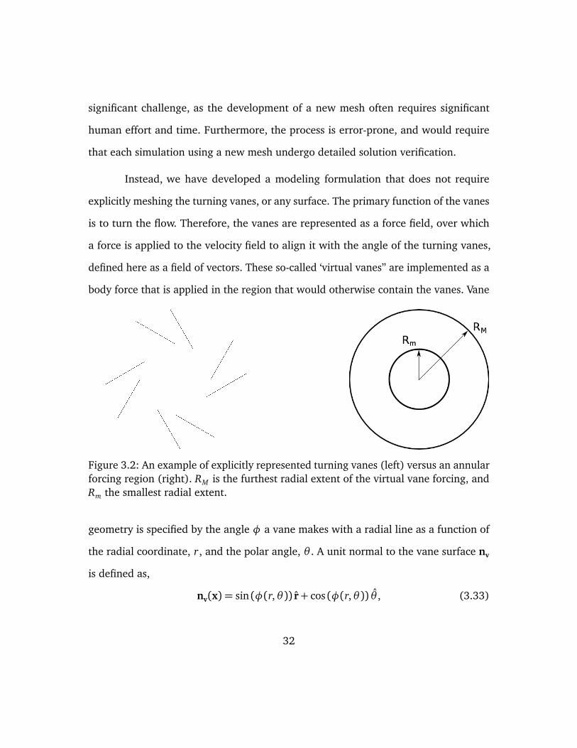
3.2 An example of explicitly represented turning vanes (left) versus an an-nular forcing region (right). RM is the furthest radial extent of the virtualvane forcing, and Rm the smallest radial extent. . . . . . . . . . . . . . . 32

3.3 The average misfit between the gridded vanes and the flow. The aver-aging is accomplished through azimuthal averaging. This was taken athalf the height of the turning vanes, although the results do not differ atgreater or lower height. The subfigure shows the logarithmic derivativein black and the average of the logarithmic derivative in red. RM is thefurthest radial extent of the gridded vanes, and Rm the smallest radialextent. The subfigure shows the logarithmic derivative of this quantityin black, and the average value of the logarithmic derivative in red. . . 34

3.4 The actuator disk model represents a turbine blade geometry (shownon the left) as a spinning “disk” region (shown on the right). . . . . . . 37

3.5 The represented turbine blade geometry. β , the blade angle, is measuredrelative to the horizontal plane. c, the chord length of the turbine, isdefined as the straight line distance from leading to trailing edge. . . . 38

xiii

3.6 The flat plate lift and drag coefficients as a function of the angle ofattack, α. . . . . . . . . . . . . . . . . . . . . . . . . . . . . . . . . . . . . . . 41

3.7 The semicircle (180 degree) lift and drag coefficients as a function ofthe angle of attack, α. . . . . . . . . . . . . . . . . . . . . . . . . . . . . . . 42

3.8 The 90 degree (quarter circle) lift and drag coefficient as a function ofthe angle of attack, α. . . . . . . . . . . . . . . . . . . . . . . . . . . . . . . 43

3.9 Schematic depicting the separation model that extends past the trailingedge of the vanes. The vane surface is not moving, and the line labelledflow is a path of the flow relative to the vane. In the top case, the flowentering the virtual vane region is forced to align with the vane an-gle despite this resulting in a reversal of the flow direction. This is aconsequence of the forcing function acting on the fluid to ensure thevelocity vector aligns with the vane. The second case depicts the sep-aration model, where the flow under certain conditions is not forcedand continues to move tangent to the vanes due to the separation of theboundary layer off the trailing edge. . . . . . . . . . . . . . . . . . . . . . 45

3.10 Domain for the thermal-only scenario. The diagram scale is represen-tative of typical cases. Note the SoV apparatus in the center, whichprovides perspective on the extent of the domain with respect to theturning vane diameter. The ground, sides and top boundaries are labeledwith the discussion the precise boundary conditions on each providedin Section 3.9. Notice also the finite thickness, high viscosity “spongelayer” at the top of the domain. . . . . . . . . . . . . . . . . . . . . . . . . 50

3.11 Domain for the wind and thermal scenario. The diagram scale is rep-resentative of typical cases. Note the SoV apparatus which providesperspective on the extent of the domain with respect to the turningvane diameter. The ground, sides, inflow, back and top boundaries arelabeled with the discussion the precise boundary conditions on eachprovided in Section 3.9. Notice also the finite thickness, high viscosity“sponge layer” at the top and back of the domain. . . . . . . . . . . . . . 51

4.1 Horizontal slice through the domain, to show a representative meshing.The single refinement region around the vanes is visible, along with thefiner boundary layer mesh near the ground. . . . . . . . . . . . . . . . . . 60

5.1 This figure depicts the validation hierarchy. The experimental measure-ments are at the top, where the data is expected to be the most reliable,but simultaneously the most limited. Moving down the table leads tosimulated data sources that are less reliable but increasingly cheaper intime to generate. At the bottom are the steady virtual vane solutions. . 66

5.2 An example of the gridded mesh, where the turning vanes are explicitlyrepresented and a no-slip boundary condition is imposed on the surface.This mesh was generated using gridgen. . . . . . . . . . . . . . . . . . . . 67

xiv

5.3 An example of the single tier straight vane laboratory configuration.The apparatus is shown with a turbine, but that was removed for datagathering. The particles for PIV were seeded outside of the turning vanesand entrained into the central region. . . . . . . . . . . . . . . . . . . . . 68

5.4 Azimuthal (left figure) and vertical (right figure) velocity as a functionof radius for the thermal-only cases. Shown are single tier straight 30

vanes. V Vθ

(gold line) is the virtual vane simulation, V Eθ

(blue line) theexperiment, and V G

θ(red line) the gridded vane. These results were all

generated by unsteady simulations and then temporally averaged. Thelack of smoothness in the data is believed to be attributable to finite-time averaging, particularly in the case of the gridded vanes, which wereexpensive calculations. . . . . . . . . . . . . . . . . . . . . . . . . . . . . . 70

5.5 Horizontal slices through the top of the vanes for the wind validationcases. On the left are the explicitly gridded vanes, and on the right thevirtual vanes. The streamwise velocity (top images), which moves left toright, shows penetration through the region where the vanes are alignedwith the flow in both the gridded and virtual vanes. The second rowshows the spanwise velocity (red for flow moving up the page, blue forflow moving down the page) where it can be seen that the virtual vanecase correctly reproduces the direction and magnitude of velocity insidethe vanes. . . . . . . . . . . . . . . . . . . . . . . . . . . . . . . . . . . . . . . 72

5.6 A comparison between the streamwise velocity in the averaged tran-sient virtual vane solution (right image) and the steady virtual vanesolution (left image). These horizontal slices were taken at the heightof the second tier of vanes. The black lines indicate the annular vaneforcing region. While the steady solution is more diffuse, it possessesa similar qualitative structure as the higher fidelity solution. The un-steady solution has a larger peak velocity inside the apparatus, whilesimultaneously possessing a larger and more intense wake region. . . . 75

5.7 The azimuthal velocity profile as a function of radius for the steady andunsteady cases. The profile is extracted from θ = 90. The unsteadyvanes were temporally averaged. The steady solution has a similar radialpeak location, but a lower velocity magnitude and a more diffuse structure. 76

5.8 A comparison between the change in kinetic energy flux due to a per-turbation in system parameters (vane angle) between the steady and un-steady virtual vanes. For each iteration, a design parameter was changed,and the % change in kinetic energy flux was recorded. . . . . . . . . . . 77

5.9 A comparison between simulated and experimental data for the August2015 field test. Azimuthal velocity data from the actual field test isshown in blue. Two virtual vane simulations with different scenarioparameters are shown in red and gold. The velocity field was temporallyaveraged but not averaged in space, to reproduce the measurementsfrom the field. . . . . . . . . . . . . . . . . . . . . . . . . . . . . . . . . . . . 78

xv

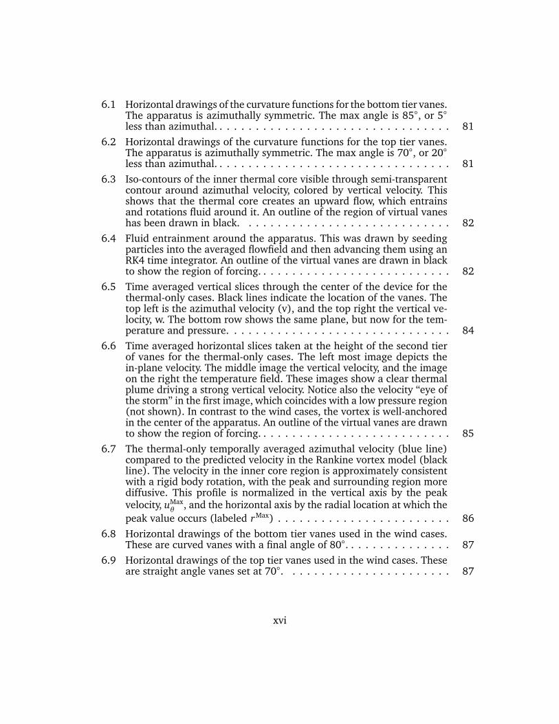
6.1 Horizontal drawings of the curvature functions for the bottom tier vanes.The apparatus is azimuthally symmetric. The max angle is 85, or 5less than azimuthal. . . . . . . . . . . . . . . . . . . . . . . . . . . . . . . . . 81

6.2 Horizontal drawings of the curvature functions for the top tier vanes.The apparatus is azimuthally symmetric. The max angle is 70, or 20less than azimuthal. . . . . . . . . . . . . . . . . . . . . . . . . . . . . . . . . 81

6.3 Iso-contours of the inner thermal core visible through semi-transparentcontour around azimuthal velocity, colored by vertical velocity. Thisshows that the thermal core creates an upward flow, which entrainsand rotations fluid around it. An outline of the region of virtual vaneshas been drawn in black. . . . . . . . . . . . . . . . . . . . . . . . . . . . . 82

6.4 Fluid entrainment around the apparatus. This was drawn by seedingparticles into the averaged flowfield and then advancing them using anRK4 time integrator. An outline of the virtual vanes are drawn in blackto show the region of forcing. . . . . . . . . . . . . . . . . . . . . . . . . . . 82

6.5 Time averaged vertical slices through the center of the device for thethermal-only cases. Black lines indicate the location of the vanes. Thetop left is the azimuthal velocity (v), and the top right the vertical ve-locity, w. The bottom row shows the same plane, but now for the tem-perature and pressure. . . . . . . . . . . . . . . . . . . . . . . . . . . . . . . 84

6.6 Time averaged horizontal slices taken at the height of the second tierof vanes for the thermal-only cases. The left most image depicts thein-plane velocity. The middle image the vertical velocity, and the imageon the right the temperature field. These images show a clear thermalplume driving a strong vertical velocity. Notice also the velocity “eye ofthe storm” in the first image, which coincides with a low pressure region(not shown). In contrast to the wind cases, the vortex is well-anchoredin the center of the apparatus. An outline of the virtual vanes are drawnto show the region of forcing. . . . . . . . . . . . . . . . . . . . . . . . . . . 85

6.7 The thermal-only temporally averaged azimuthal velocity (blue line)compared to the predicted velocity in the Rankine vortex model (blackline). The velocity in the inner core region is approximately consistentwith a rigid body rotation, with the peak and surrounding region morediffusive. This profile is normalized in the vertical axis by the peakvelocity, uMax

θ, and the horizontal axis by the radial location at which the

peak value occurs (labeled rMax) . . . . . . . . . . . . . . . . . . . . . . . . 866.8 Horizontal drawings of the bottom tier vanes used in the wind cases.

These are curved vanes with a final angle of 80. . . . . . . . . . . . . . . 876.9 Horizontal drawings of the top tier vanes used in the wind cases. These

are straight angle vanes set at 70. . . . . . . . . . . . . . . . . . . . . . . 87

xvi

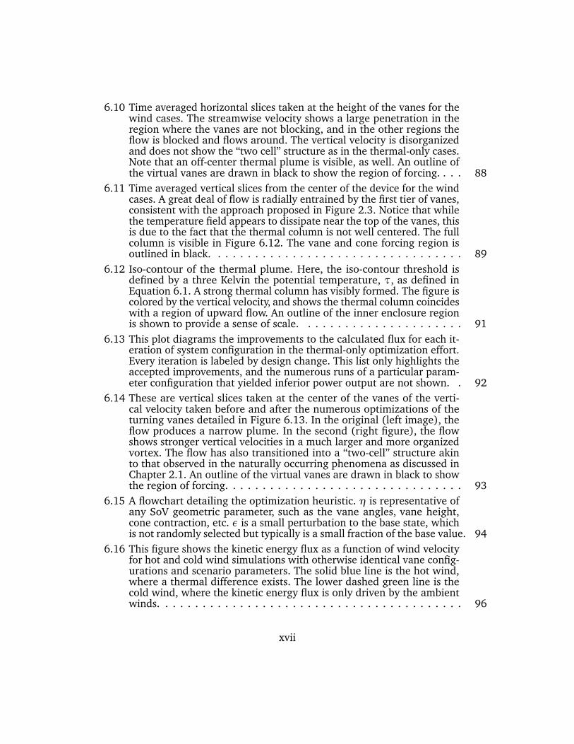
6.10 Time averaged horizontal slices taken at the height of the vanes for thewind cases. The streamwise velocity shows a large penetration in theregion where the vanes are not blocking, and in the other regions theflow is blocked and flows around. The vertical velocity is disorganizedand does not show the “two cell” structure as in the thermal-only cases.Note that an off-center thermal plume is visible, as well. An outline ofthe virtual vanes are drawn in black to show the region of forcing. . . . 88

6.11 Time averaged vertical slices from the center of the device for the windcases. A great deal of flow is radially entrained by the first tier of vanes,consistent with the approach proposed in Figure 2.3. Notice that whilethe temperature field appears to dissipate near the top of the vanes, thisis due to the fact that the thermal column is not well centered. The fullcolumn is visible in Figure 6.12. The vane and cone forcing region isoutlined in black. . . . . . . . . . . . . . . . . . . . . . . . . . . . . . . . . . 89

6.12 Iso-contour of the thermal plume. Here, the iso-contour threshold isdefined by a three Kelvin the potential temperature, τ, as defined inEquation 6.1. A strong thermal column has visibly formed. The figure iscolored by the vertical velocity, and shows the thermal column coincideswith a region of upward flow. An outline of the inner enclosure regionis shown to provide a sense of scale. . . . . . . . . . . . . . . . . . . . . . 91

6.13 This plot diagrams the improvements to the calculated flux for each it-eration of system configuration in the thermal-only optimization effort.Every iteration is labeled by design change. This list only highlights theaccepted improvements, and the numerous runs of a particular param-eter configuration that yielded inferior power output are not shown. . 92

6.14 These are vertical slices taken at the center of the vanes of the verti-cal velocity taken before and after the numerous optimizations of theturning vanes detailed in Figure 6.13. In the original (left image), theflow produces a narrow plume. In the second (right figure), the flowshows stronger vertical velocities in a much larger and more organizedvortex. The flow has also transitioned into a “two-cell” structure akinto that observed in the naturally occurring phenomena as discussed inChapter 2.1. An outline of the virtual vanes are drawn in black to showthe region of forcing. . . . . . . . . . . . . . . . . . . . . . . . . . . . . . . . 93

6.15 A flowchart detailing the optimization heuristic. η is representative ofany SoV geometric parameter, such as the vane angles, vane height,cone contraction, etc. ε is a small perturbation to the base state, whichis not randomly selected but typically is a small fraction of the base value. 94

6.16 This figure shows the kinetic energy flux as a function of wind velocityfor hot and cold wind simulations with otherwise identical vane config-urations and scenario parameters. The solid blue line is the hot wind,where a thermal difference exists. The lower dashed green line is thecold wind, where the kinetic energy flux is only driven by the ambientwinds. . . . . . . . . . . . . . . . . . . . . . . . . . . . . . . . . . . . . . . . . 96

xvii

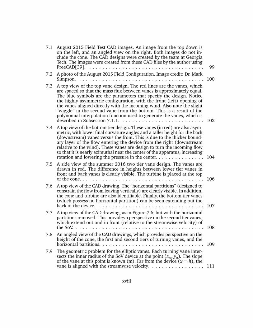
7.1 August 2015 Field Test CAD images. An image from the top down ison the left, and an angled view on the right. Both images do not in-clude the cone. The CAD designs were created by the team at GeorgiaTech. The images were created from these CAD files by the author usingFreeCAD[39]. . . . . . . . . . . . . . . . . . . . . . . . . . . . . . . . . . . . 99

7.2 A photo of the August 2015 Field Configuration. Image credit: Dr. MarkSimpson. . . . . . . . . . . . . . . . . . . . . . . . . . . . . . . . . . . . . . . 100

7.3 A top view of the top vane design. The red lines are the vanes, whichare spaced so that the mass flux between vanes is approximately equal.The blue symbols are the parameters that specify the design. Noticethe highly asymmetric configuration, with the front (left) opening ofthe vanes aligned directly with the incoming wind. Also note the slight“wiggle” in the second vane from the bottom. This is a result of thepolynomial interpolation function used to generate the vanes, which isdescribed in Subsection 7.1.1. . . . . . . . . . . . . . . . . . . . . . . . . . 102

7.4 A top view of the bottom tier design. These vanes (in red) are also asym-metric, with lower final curvature angles and a taller height for the back(downstream) vanes versus the front. This is due to the thicker bound-ary layer of the flow entering the device from the right (downstreamrelative to the wind). These vanes are design to turn the incoming flowso that it is nearly azimuthal near the center of the apparatus, increasingrotation and lowering the pressure in the center. . . . . . . . . . . . . . . 104

7.5 A side view of the summer 2016 two tier vane design. The vanes aredrawn in red. The difference in heights between lower tier vanes infront and back vanes is clearly visible. The turbine is placed at the topof the cone. . . . . . . . . . . . . . . . . . . . . . . . . . . . . . . . . . . . . . 106

7.6 A top view of the CAD drawing. The “horizontal partitions” (designed toconstrain the flow from leaving vertically) are clearly visible. In addition,the cone and turbine are also identifiable. Finally, the bottom tier vanes(which possess no horizontal partition) can be seen extending out theback of the device. . . . . . . . . . . . . . . . . . . . . . . . . . . . . . . . . 107

7.7 A top view of the CAD drawing, as in Figure 7.6, but with the horizontalpartitions removed. This provides a perspective on the second tier vanes,which extend out and in front (relative to the streamwise velocity) ofthe SoV. . . . . . . . . . . . . . . . . . . . . . . . . . . . . . . . . . . . . . . . 108

7.8 An angled view of the CAD drawings, which provides perspective on theheight of the cone, the first and second tiers of turning vanes, and thehorizontal partitions. . . . . . . . . . . . . . . . . . . . . . . . . . . . . . . . 109

7.9 The geometric problem for the elliptic vanes. Each turning vane inter-sects the inner radius of the SoV device at the point (x0, y0). The slopeof the vane at this point is known (m). Far from the device (x = h), thevane is aligned with the streamwise velocity. . . . . . . . . . . . . . . . . 111

xviii

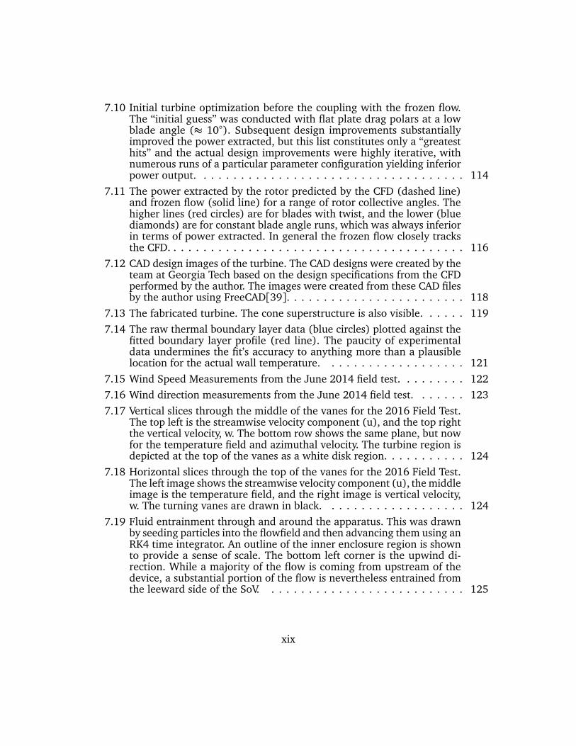
7.10 Initial turbine optimization before the coupling with the frozen flow.The “initial guess” was conducted with flat plate drag polars at a lowblade angle (≈ 10). Subsequent design improvements substantiallyimproved the power extracted, but this list constitutes only a “greatesthits” and the actual design improvements were highly iterative, withnumerous runs of a particular parameter configuration yielding inferiorpower output. . . . . . . . . . . . . . . . . . . . . . . . . . . . . . . . . . . . 114

7.11 The power extracted by the rotor predicted by the CFD (dashed line)and frozen flow (solid line) for a range of rotor collective angles. Thehigher lines (red circles) are for blades with twist, and the lower (bluediamonds) are for constant blade angle runs, which was always inferiorin terms of power extracted. In general the frozen flow closely tracksthe CFD. . . . . . . . . . . . . . . . . . . . . . . . . . . . . . . . . . . . . . . . 116

7.12 CAD design images of the turbine. The CAD designs were created by theteam at Georgia Tech based on the design specifications from the CFDperformed by the author. The images were created from these CAD filesby the author using FreeCAD[39]. . . . . . . . . . . . . . . . . . . . . . . . 118

7.13 The fabricated turbine. The cone superstructure is also visible. . . . . . 1197.14 The raw thermal boundary layer data (blue circles) plotted against the

fitted boundary layer profile (red line). The paucity of experimentaldata undermines the fit’s accuracy to anything more than a plausiblelocation for the actual wall temperature. . . . . . . . . . . . . . . . . . . 121

7.15 Wind Speed Measurements from the June 2014 field test. . . . . . . . . 1227.16 Wind direction measurements from the June 2014 field test. . . . . . . 1237.17 Vertical slices through the middle of the vanes for the 2016 Field Test.

The top left is the streamwise velocity component (u), and the top rightthe vertical velocity, w. The bottom row shows the same plane, but nowfor the temperature field and azimuthal velocity. The turbine region isdepicted at the top of the vanes as a white disk region. . . . . . . . . . . 124

7.18 Horizontal slices through the top of the vanes for the 2016 Field Test.The left image shows the streamwise velocity component (u), the middleimage is the temperature field, and the right image is vertical velocity,w. The turning vanes are drawn in black. . . . . . . . . . . . . . . . . . . 124

7.19 Fluid entrainment through and around the apparatus. This was drawnby seeding particles into the flowfield and then advancing them using anRK4 time integrator. An outline of the inner enclosure region is shownto provide a sense of scale. The bottom left corner is the upwind di-rection. While a majority of the flow is coming from upstream of thedevice, a substantial portion of the flow is nevertheless entrained fromthe leeward side of the SoV. . . . . . . . . . . . . . . . . . . . . . . . . . . 125

xix

7.20 The power extracted by the turbine as a function of blade count. Theblue straight line indicates the turbine model as defined in Section 3.5,and the red dashed line indicates the power output of the turbine afterthe solidity modification. . . . . . . . . . . . . . . . . . . . . . . . . . . . . 132

7.21 The uncalibrated idealized drag polars. These drag polars are constant,discontinuous functions. The lift coefficient (solid blue line) can attain anegative value, but the drag coefficient (dashed red line) is constrainedto never drop below zero. . . . . . . . . . . . . . . . . . . . . . . . . . . . . 139

xx

Chapter 1

Introduction / Executive Summary

1.1 Motivation

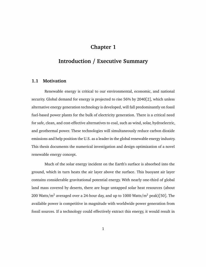
Renewable energy is critical to our environmental, economic, and national

security. Global demand for energy is projected to rise 56% by 2040[2], which unless

alternative energy generation technology is developed, will fall predominantly on fossil

fuel-based power plants for the bulk of electricity generation. There is a critical need

for safe, clean, and cost-effective alternatives to coal, such as wind, solar, hydroelectric,

and geothermal power. These technologies will simultaneously reduce carbon dioxide

emissions and help position the U.S. as a leader in the global renewable energy industry.

This thesis documents the numerical investigation and design optimization of a novel

renewable energy concept.

Much of the solar energy incident on the Earth’s surface is absorbed into the

ground, which in turn heats the air layer above the surface. This buoyant air layer

contains considerable gravitational potential energy. With nearly one-third of global

land mass covered by deserts, there are huge untapped solar heat resources (about

200 Watts/m2 averaged over a 24-hour day, and up to 1000 Watts/m2 peak)[50]. The

available power is competitive in magnitude with worldwide power generation from

fossil sources. If a technology could effectively extract this energy, it would result in

1

a low-cost, scalable approach to electrical power generation that could create a new

class of renewable energy ideally suited for arid regions.

How then, is one to efficiently extract this gravitational potential energy and

convert it into usable work? We turn to Nature to provide a guide, with the observation

that there are natural objects that provide precisely this mechanism. Namely, naturally

occurring “dust devils” characterized by a vertically stratified, ground-heated air layer

that produces a coherent columnar vortex. These “dust devil”s are ubiquitous, naturally

appearing in regions as diverse as Arizona, Siberia, over water, or even Mars[8, 104,

108]. They are observed to occur over a wide range of length scales (1 - 30 meters)

with large variations in velocities (1 to over 40 m/s)[104].

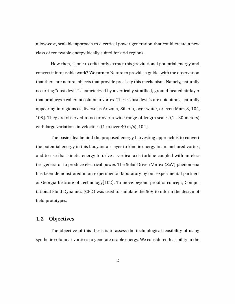
The basic idea behind the proposed energy harvesting approach is to convert

the potential energy in this buoyant air layer to kinetic energy in an anchored vortex,

and to use that kinetic energy to drive a vertical-axis turbine coupled with an elec-

tric generator to produce electrical power. The Solar-Driven Vortex (SoV) phenomena

has been demonstrated in an experimental laboratory by our experimental partners

at Georgia Institute of Technology[102]. To move beyond proof-of-concept, Compu-

tational Fluid Dynamics (CFD) was used to simulate the SoV, to inform the design of

field prototypes.

1.2 Objectives

The objective of this thesis is to assess the technological feasibility of using

synthetic columnar vortices to generate usable energy. We considered feasibility in the

2

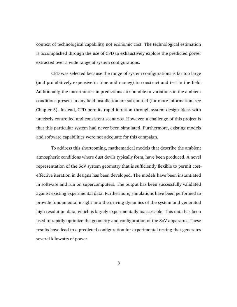
context of technological capability, not economic cost. The technological estimation

is accomplished through the use of CFD to exhaustively explore the predicted power

extracted over a wide range of system configurations.

CFD was selected because the range of system configurations is far too large

(and prohibitively expensive in time and money) to construct and test in the field.

Additionally, the uncertainties in predictions attributable to variations in the ambient

conditions present in any field installation are substantial (for more information, see

Chapter 5). Instead, CFD permits rapid iteration through system design ideas with

precisely controlled and consistent scenarios. However, a challenge of this project is

that this particular system had never been simulated. Furthermore, existing models

and software capabilities were not adequate for this campaign.

To address this shortcoming, mathematical models that describe the ambient

atmospheric conditions where dust devils typically form, have been produced. A novel

representation of the SoV system geometry that is sufficiently flexible to permit cost-

effective iteration in designs has been developed. The models have been instantiated

in software and run on supercomputers. The output has been successfully validated

against existing experimental data. Furthermore, simulations have been performed to

provide fundamental insight into the driving dynamics of the system and generated

high resolution data, which is largely experimentally inaccessible. This data has been

used to rapidly optimize the geometry and configuration of the SoV apparatus. These

results have lead to a predicted configuration for experimental testing that generates

several kilowatts of power.

3

1.3 Outline

This dissertation is organized as follows. Chapter 2 begins with a discussion

of the naturally occurring phenomenon, the presently understood dynamics of dust

devils and similar columnar vortices, and the implications for systems designed to gen-

erate their synthetic counterparts. Chapter 3 outlines a mathematical model of the

entire system, and Chapter 4 discusses the algorithms and software implementation

used to simulate the system. Chapter 5 reviews the validation of these resulting sim-

ulations against existing experimental data and high fidelity simulations. Chapter 6

examines the simulation results in detail, to discern the physical processes driving the

SoV. Chapter 7 details the final system design, and the predicted performance in the

field. Finally, with the preceding sections outlining the present simulation capabilities

and predictions, Chapter 8 concludes with a discussion of the ultimate technological

feasibility of the SoV venture and recommendations for future work.

4

Chapter 2

Physical Background

This chapter addresses what is known about naturally occurring dust devils, to

motivate how best to engineer a synthetic version. It begins with a qualitative discussion

of dust devils, followed by a review of the known physics and pertinent literature. We

then introduce a novel concept to leverage these physical processes as a method of

usable, low-grade energy generation. The chapter concludes with a brief survey of

previous approaches related to harvesting gravitational potential energy.

2.1 Phenomenological Character of Dust Devils

There is no rigorous definition of a dust devil, despite the fact that the phe-

nomenon is ubiquitous. These whirlwinds have been observed across a wide variety

of terrains, climates and even on other planets[15, 94, 104]. While a precise defini-

tion is elusive, several features are characteristic of a dust devil. These self-sustaining

vortices maintain a funnel-like chimney driven by hot air moving both upward and

circularly. They are regions of intense rotation, coupled with upward motions that are

strong enough to lift particles into the flow. It is the entrainment of dust that gives the

eponymous whirlwind its striking visual appearance as a violent coherent structure.

While there are characteristic features of a dust devil, they exist over a wide

5

range of scales and conditions. They typically survive for only a few minutes, but they

have been observed to endure hours[54]. The velocities are generally several meters

per second, but dust devils are occasionally strong enough to cause damage and injury,

with some reaching F1 on the Fujita Tornado intensity scale, with velocities between

33 and 49 m/s[42]. This is sufficiently powerful to result in, “Surface of roofs peeled

off; mobile homes pushed off foundations or overturned; moving autos pushed off the

road” [38]. Diameters range from about one meter to greater than thirty. Their average

height is on the order of tens of meters, but a few have been observed as high as one

kilometer or more. They do not have a preferred rotation direction [103]. Although

the vertical velocity is predominantly upward, the flow along the a central axis of large

dust devils may be downward. Visibly similarly structured atmospheric vortices have

been observed over water (Waterspouts), in intense forest fires (Fire Whirls), and in

cold or freezing environments (Snownado).

While the phenomenon is pervasive, certain environmental conditions impact

the frequency of dust devil formation. Sinclair[104] performed perhaps the most sys-

tematic investigation characterizing conditions favorable for formation. He noted that

dust devils are most likely to form at solar noon, the time of the greatest incident solar

radiation. Furthermore, they are more likely to form in locations with a higher surface

temperature. Moderate to high wind speeds (2-5 m/s) encourage dust devil genesis,

but greater velocities (11 m/s) impede formation[108]. They form more frequently in

relatively flat locations, such as deserts. Despite the name, the lifting of dust does not

actually appear to be of major importance [104, 105, 108]. Rather, it is likely that only

a small number of dust devils are visible, and even then, only a fraction of the actual

6

vortex’s physical extent is populated with dust.

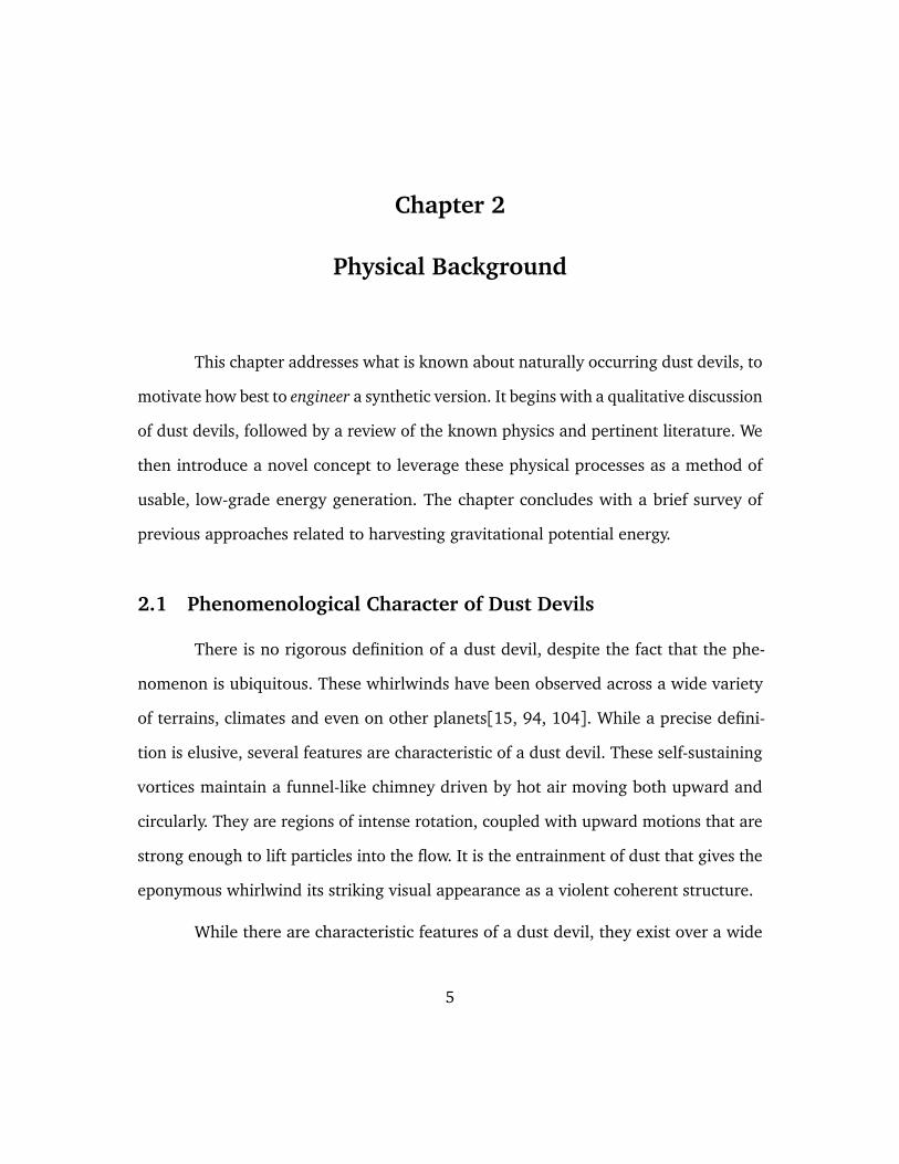
Actual measurements made inside a dust devil are limited. The available data

hints that dust devils contain two regions: a low surface layer and a higher inviscid

region. These regions are indicated in a cartoon in Figure 2.1. The low surface region

is the principle location of radial inflow. At the top of this region the flow reaches

its peak velocity, with that peak dropping with increasing height. The strong radial

and azimuthal flow is drawn into a low pressure core where it gains vertical velocity.

Earlier experimental and computational studies have observed a “two-cell” structure

characterized by a cool downdraft in the center of stronger dust devils[105, 117].

The higher region is characterized by a largely inviscid potential flow with

warm air rising and circling around a cool, low pressure core. This region is typically

many times larger in height than the surface layer. While this region also has radial

inflow, it is significantly weaker than in the lower region. Previous studies have found

this region is relatively well described by a Rankine vortex model[69, 105, 109].

Renewed interest in naturally occurring dust devils has resulted from the obser-

vation of them on Mars, first photographed by the Viking Probe [95], and more recently

by the NASA’s Mars Reconnaissance Orbiter and the Mars rover, Opportunity. Their

presence on Mars, with 1/100 of the atmospheric density of the Earth, speaks to the

universal character of the phenomenon. Due to the greatly decreased atmospheric den-

sity, the Martian dust devils are substantially larger, ranging several kilometers across

at their base and over twenty kilometers tall[89]. The interest in dust devils is due in

part to their influence on atmospheric mixing and transport, and the ExoMars lander

is designed to measure some of the impact on the environment by these objects[90].

7

Figure 2.1: Cartoon of the structure of a dust devil. The lower region is the principlelocation of radial inflow, with the higher second layer flow becoming entrained by theupwardly circulating vortex. Notice also the downward flow in the center of the vortex.

The physics of dust devils have also been investigated via numerical simulations.

While these studies have produced dust devil like convective vortices, they have been

observed in within existing climate and atmospheric models[60, 117], not in simulation

codes designed specifically to probe the dynamics of a dust devil. Many of these results

were conducted on numerical grid spacings that are too coarse (for instance, 35 meters

in the horizontal direction in Kanak’s study[61]) to generate dust devils that possess

a size consistent with the observed phenomenon. Furthermore, most of these studies

are conducted with no mean wind, and so cannot comment on the impact versus an

8

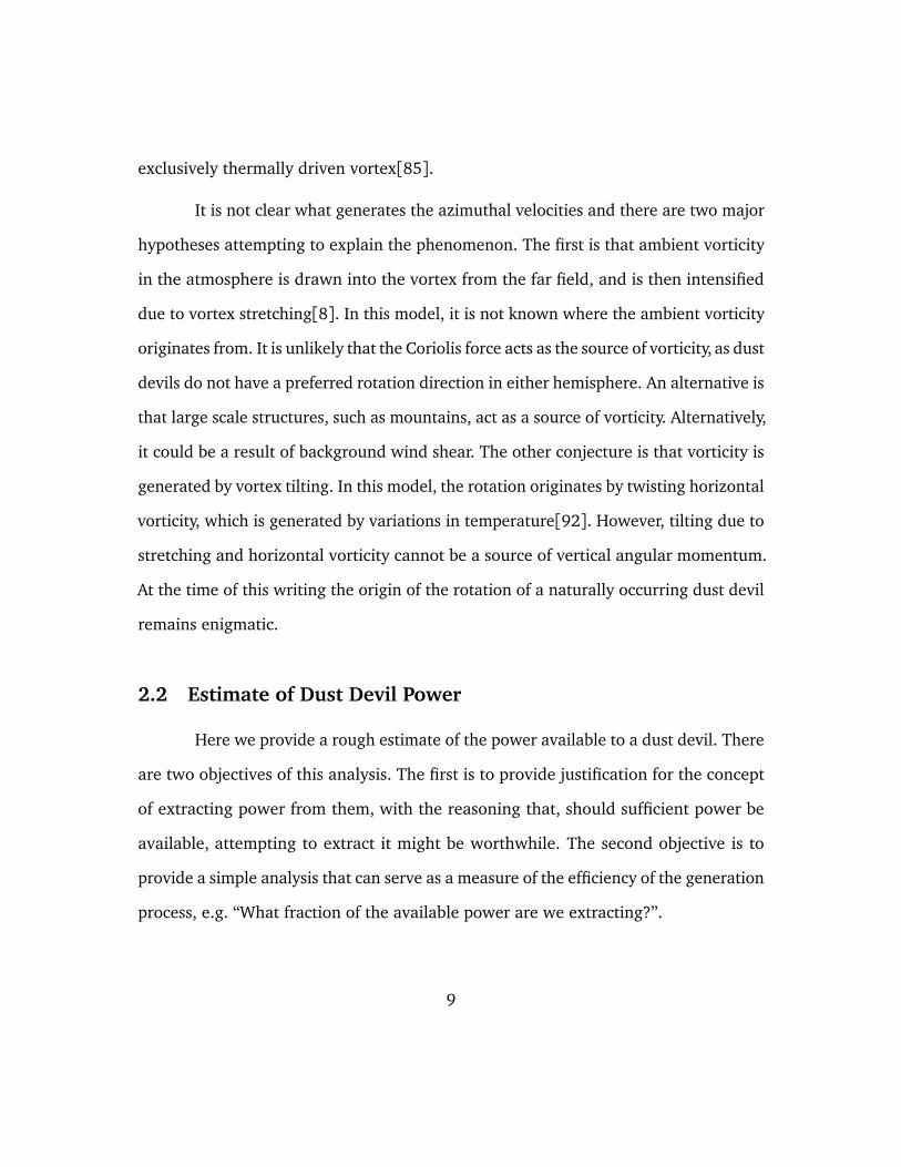
exclusively thermally driven vortex[85].

It is not clear what generates the azimuthal velocities and there are two major

hypotheses attempting to explain the phenomenon. The first is that ambient vorticity

in the atmosphere is drawn into the vortex from the far field, and is then intensified

due to vortex stretching[8]. In this model, it is not known where the ambient vorticity

originates from. It is unlikely that the Coriolis force acts as the source of vorticity, as dust

devils do not have a preferred rotation direction in either hemisphere. An alternative is

that large scale structures, such as mountains, act as a source of vorticity. Alternatively,

it could be a result of background wind shear. The other conjecture is that vorticity is

generated by vortex tilting. In this model, the rotation originates by twisting horizontal

vorticity, which is generated by variations in temperature[92]. However, tilting due to

stretching and horizontal vorticity cannot be a source of vertical angular momentum.

At the time of this writing the origin of the rotation of a naturally occurring dust devil

remains enigmatic.

2.2 Estimate of Dust Devil Power

Here we provide a rough estimate of the power available to a dust devil. There

are two objectives of this analysis. The first is to provide justification for the concept

of extracting power from them, with the reasoning that, should sufficient power be

available, attempting to extract it might be worthwhile. The second objective is to

provide a simple analysis that can serve as a measure of the efficiency of the generation

process, e.g. “What fraction of the available power are we extracting?”.

9

Steady state conditions requires that the dust devil not extract more energy than

is provided by the thermal resource, the Sun. The peak direct solar insolation in Arizona

on a hot summer day is greater than 1000 W/m2. However, this estimate is problematic.

On one hand it is an optimistic upper bound, as dust devils are only converting a

fraction of this solar resource into kinetic energy. On the other hand, it is not clear how

large of a region that dust devils draw their energy from. Furthermore, Renno and

Ingersoll[91] used an idealized heat engine frame-work to study natural convection

and to propose a theory for convective available potential energy (CAPE), and found

that the predictions from this substantially underestimate the observed velocities in

the real objects. Finally, dust devils are highly intermittent, typically existing only for a

short time. It is not certain that they are accurately represented in a steady state context.

Lending some credence to this are the 2002 measurements of Renno[92] which found

that instantaneous surface heat fluxes could rise to several orders of magnitude larger

than the average solar insolation.

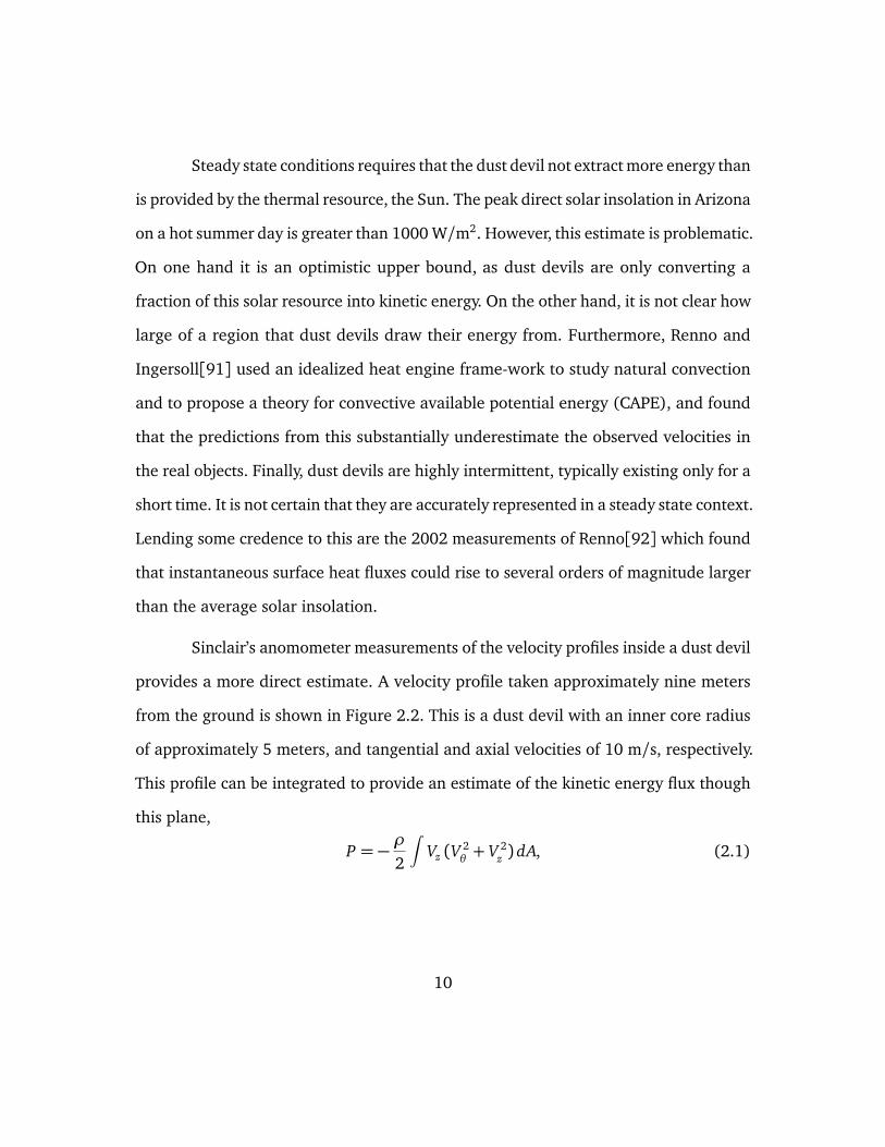
Sinclair’s anomometer measurements of the velocity profiles inside a dust devil

provides a more direct estimate. A velocity profile taken approximately nine meters

from the ground is shown in Figure 2.2. This is a dust devil with an inner core radius

of approximately 5 meters, and tangential and axial velocities of 10 m/s, respectively.

This profile can be integrated to provide an estimate of the kinetic energy flux though

this plane,

P = −ρ

2

∫Vz (V

2θ+ V 2

z ) dA, (2.1)

10

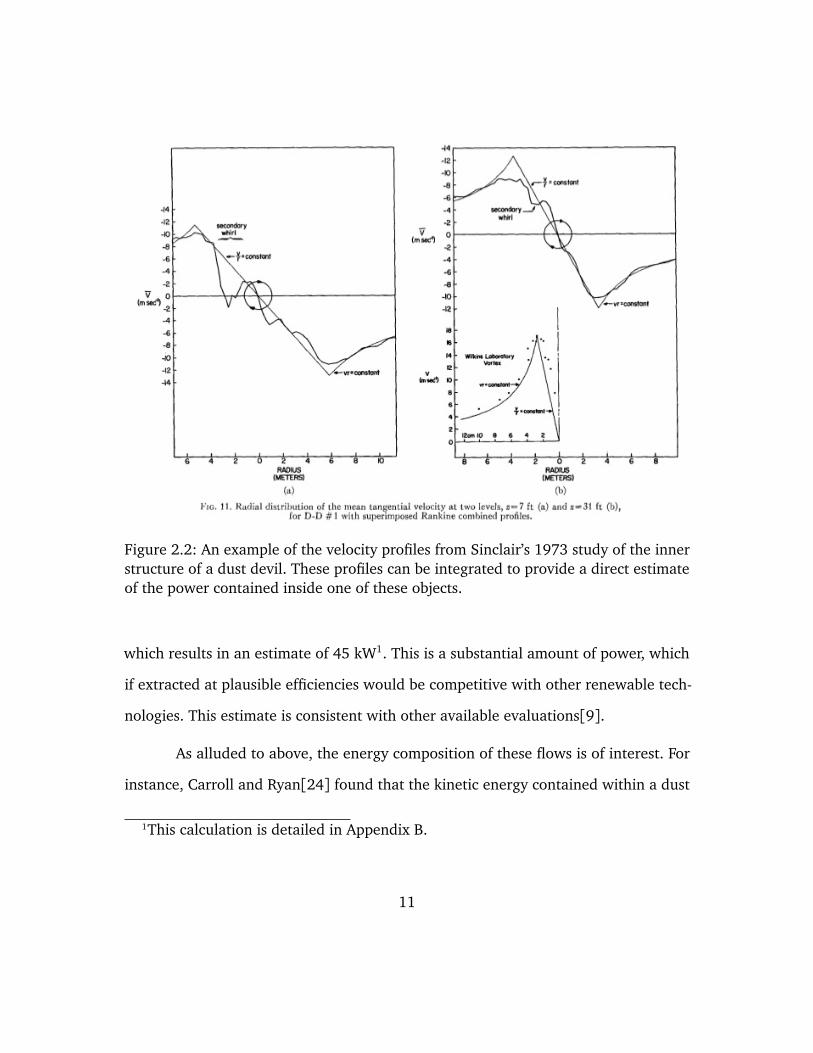
Figure 2.2: An example of the velocity profiles from Sinclair’s 1973 study of the innerstructure of a dust devil. These profiles can be integrated to provide a direct estimateof the power contained inside one of these objects.

which results in an estimate of 45 kW1. This is a substantial amount of power, which

if extracted at plausible efficiencies would be competitive with other renewable tech-

nologies. This estimate is consistent with other available evaluations[9].

As alluded to above, the energy composition of these flows is of interest. For

instance, Carroll and Ryan[24] found that the kinetic energy contained within a dust

1This calculation is detailed in Appendix B.

11

devil exceeds that which is attributable to buoyancy. Furthermore, Kaimal and Busigner

observed that dust devils possessed an order of magnitude greater vertical flux in kinetic

energy than similarly sized convective plumes [58]. The interplay between rotation,

ambient winds and thermal potential energy are critical to the velocity intensities

observed in these phenomena.

As an example of this, consider only the energy flowing into the entrainment

region due to the ambient conditions, in particular, the incoming wind and heat flowing

through a cylindrical control volume around the dust devil. The dust devil is medium-

sized (3m radius) with an incoming freestream velocity of 5 m/s. The surface tem-

perature is 343 Kelvin, with a specified inflow boundary layer between the ground

temperature and the ambient air conditions of 313 Kelvin. 2

In this example, there are two forms of energy to consider: kinetic and gravi-

tational potential. First, we examine the kinetic energy flux through the front of the

control volume. The kinetic energy flux is a surface integral over the upstream face of

the control volume,

KE=∫ ~V 2

2ρ~V · n dA.

Several simplifying assumptions are made. The freestream velocity is assumed to have

no components in the span and height and the variation in height of the streamwise

velocity is only due to the thin boundary layer near the ground. The boundary layer

profile is modeled using the common 7th power function for a turbulent boundary

2These numbers were selected based on information provided by the Georgia Techfield team from measurements performed in Arizona during the summer of 2014. SeeSection 7.3 for more details.

12

layer,

u(z) = U minÇÅ zδ

ã7

, 1å

where U is the constant freestream velocity andδ the assumed boundary layer thickness.

The result for the kinetic energy is then,

KE= RKEρU3ïzmax −

1011δò

. (2.2)

Where RKE is the radius of the vortex. Typical values of these quantities are, U = 5 m/s,

ρ = 1.225 Kg/m3, RKE = 3 m, zmax = 3 m and δ ≈ 10 cm. This provides an estimate of

1144 Watts as the incoming kinetic energy flux.

The gravitational potential energy flux is estimated by integrating the boussi-

nesq potential energy flux over the upstream flow. This is the maximum energy that

could be extracted from the flow by an adiabatic redistribution of the density variation

from the ambient density of the freestream flow, ρ∞ [46]. This potential energy (Ep)

has the form of a surface integral over the front half of the control volume, where the

ambient winds convect energy across this surface,

Ep =∫

u(z)(ρ(z)−ρ∞) g z dA.

As the density only varies with height, the integral is simplified to only vary in this

direction,

Ep = g∫ zmax

0u(z)(ρ(z)−ρ∞) zπRp dz.

Using the bousinesq approximation, (ρ(z)−ρ∞) = ρ0β∆T , the integral becomes,

Ep = gπRp βρ0∆T∫ zmax

0u(z) zdz,

13

which is solved to show,

Ep = gπRpβρ0U∆T

[z2

max

2−

7δ2

18

]. (2.3)

Characteristic values for a dust devil are ρ0 = 1.225 Kg/m3, ∆T = 30 Kelvin,

β = 0.002915 1/Kelvin (e.g. 1/Tground), Rp = 3 m, zmax = 3 m, δ ≈ 10 cm, g = 9.81

m/s2, and a freestream velocity of five meters per second results in an estimate of 217

Watts for the gravitational potential energy flux.

This result implies that a significant fraction of the available energy convecting

into the the dust devil region is attributable to the kinetic energy of the wind, not the

gravitational potential energy of the air. However, the above assumes that the potential

energy input to dust devils is only drawn in through a region identical to the kinetic

energy. It is also interesting to consider the area that must be accessed by the dust devil

for the potential energy to be as large as the kinetic energy. To accomplish this, the

radii in Equations 2.2 and 2.3 are no longer assumed to be equal. Instead, assume that

kinetic energy radius remains the same (RKE = 3) but that the radius of entrainment

for the potential energy (Rp) is unknown. Solving for Rp yields,

Rp =RKE U2

îzmax −

1011δó

gπβ∆T[

z2max2 −

7δ2

18

] . (2.4)

Using the same values as above, Rp = 15.83 meters. This implies that the dust devil

must pull from more than five times the area to draw in as much potential energy as

kinetic energy. Further discussion on the interplay between the impact on dust devil

structure and wind velocities due to the thermal and wind contributions of energy are

examined in detail in Section 6.4.

14

2.3 Dust Devil Generation Concept

The discussion in Section 2.2 suggests that dust devils are carriers of significant

kinetic and gravitational potential energy from the environment. This section provides

a brief discussion on how the physics of naturally occurring dust devils informs the

generation of a synthetic variety that might be used as a means of extracting usable

work.

In contrast to the naturally occuring dust devils, our synthetic solar driven

vortex (SoV) design makes use of control surfaces. These turning vanes also serve as

an anchor for the synthetic vortex, locking it into a small region. An abstract concept

of the turning vane geometry is shown in Figure 2.3.

The characteristics of natural dust devils shown in Figure 2.1 suggest that the

turning vanes be structured with two tiers (see Figure 2.3). The lower tier would be

designed to manipulate the surface layer that lifts up into the core of the vortex, while

the upper tier would control entrainment into the vortex. In both tiers, the design of the

turning vanes must balance between the need to turn the flow from the radial direction

to the azimuthal direction to create vortical motion and the requirement to not block

flow into the vortex. Furthermore, in the presence of a cross wind, the vanes need to

prevent flow that would pass right through the device and disrupt the vortex. Finally,

in field tests of design concepts for a solar vortex device conducted by our colleagues

at the Georgia Tech, it was found that cross winds over the facility will also disrupt the

vortical flow, and that this could be controlled by introducing a conical wind-block on

top of the upper tier of vanes. One such field test configuration is shown in Figure 2.4.

Within this broad conceptual design, there remains a large design space to explore,

15

Figure 2.3: Image of a possible two tier turning vane configuration for generatingsynthetic dust devils. This image depicts a vertical slice through the proposed config-uration, and does not show the reflection of the two tier turning vanes, which wouldbe expected to encircle the dust devil core.

including design parameters for both tiers of vanes and the wind-block cone.

To extract energy from the synthetic dust devil formed by the vane system

described briefly above, a turbine would be placed near the top of the upper vanes.

The turbine would extract energy from both the vertical and azimuthal flow in the

vortex, and so the design considerations are different from those for a classical wind

turbine. Furthermore, there is presumably an analog to the Betz limit on how much of

the energy can be extracted, without disrupting the flow so much that the vortex cannot

16

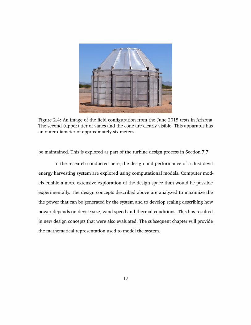
Figure 2.4: An image of the field configuration from the June 2015 tests in Arizona.The second (upper) tier of vanes and the cone are clearly visible. This apparatus hasan outer diameter of approximately six meters.

be maintained. This is explored as part of the turbine design process in Section 7.7.

In the research conducted here, the design and performance of a dust devil

energy harvesting system are explored using computational models. Computer mod-

els enable a more extensive exploration of the design space than would be possible

experimentally. The design concepts described above are analyzed to maximize the

the power that can be generated by the system and to develop scaling describing how

power depends on device size, wind speed and thermal conditions. This has resulted

in new design concepts that were also evaluated. The subsequent chapter will provide

the mathematical representation used to model the system.

17

2.4 Previous Concepts for Extracting Gravitational Potential En-ergy

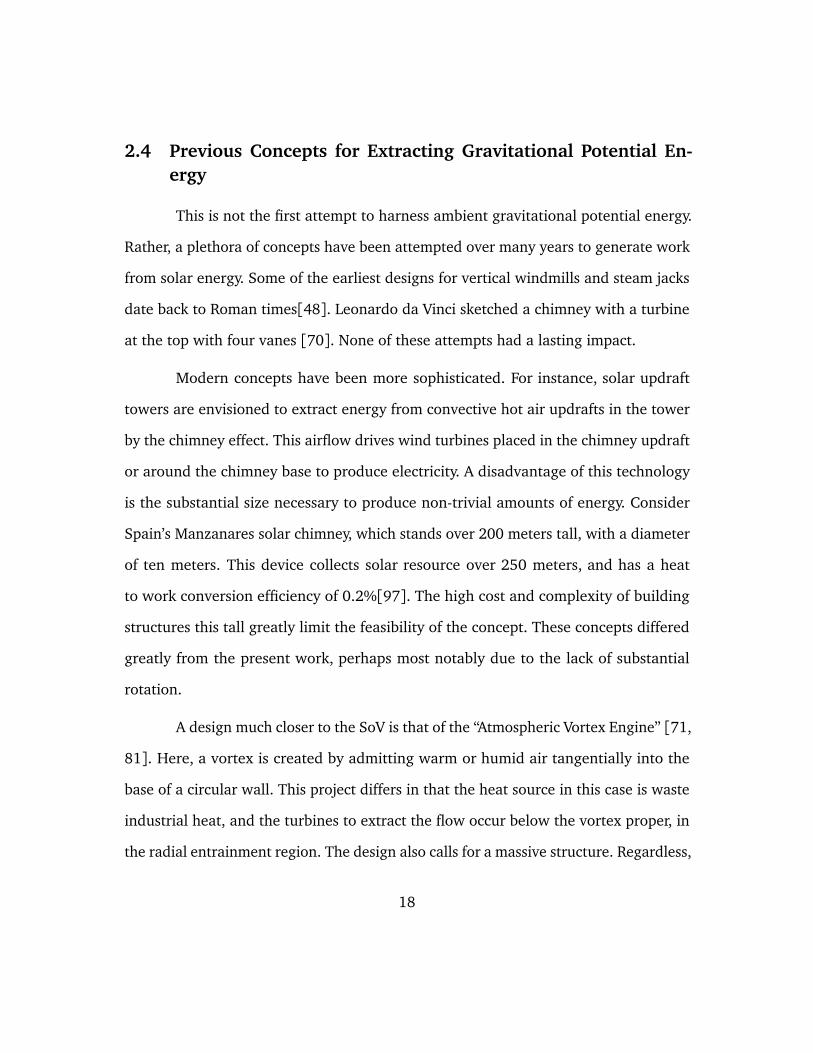
This is not the first attempt to harness ambient gravitational potential energy.

Rather, a plethora of concepts have been attempted over many years to generate work

from solar energy. Some of the earliest designs for vertical windmills and steam jacks

date back to Roman times[48]. Leonardo da Vinci sketched a chimney with a turbine

at the top with four vanes [70]. None of these attempts had a lasting impact.

Modern concepts have been more sophisticated. For instance, solar updraft

towers are envisioned to extract energy from convective hot air updrafts in the tower

by the chimney effect. This airflow drives wind turbines placed in the chimney updraft

or around the chimney base to produce electricity. A disadvantage of this technology

is the substantial size necessary to produce non-trivial amounts of energy. Consider

Spain’s Manzanares solar chimney, which stands over 200 meters tall, with a diameter

of ten meters. This device collects solar resource over 250 meters, and has a heat

to work conversion efficiency of 0.2%[97]. The high cost and complexity of building

structures this tall greatly limit the feasibility of the concept. These concepts differed

greatly from the present work, perhaps most notably due to the lack of substantial

rotation.

A design much closer to the SoV is that of the “Atmospheric Vortex Engine” [71,

81]. Here, a vortex is created by admitting warm or humid air tangentially into the

base of a circular wall. This project differs in that the heat source in this case is waste

industrial heat, and the turbines to extract the flow occur below the vortex proper, in

the radial entrainment region. The design also calls for a massive structure. Regardless,

18

the core thermodynamic principle is similar.

Nevertheless, none of these concepts are identical to that investigated here.

In particular, none attempt to harness external winds, nor have they turned to the

naturally occurring dust devil physics to inform the design of the apparatus.

19

Chapter 3

Mathematical Modeling

The aim of this work is to simulate synthetic dust devils in the field. This

requires a model of the ambient conditions for a representative case, such as Arizona,

where experimental data is available from tests that have been performed. Furthermore,

for this to be generally useful in the prediction of flows in a variety of conditions, we

need a model applicable to any flow near the surface of the earth.

This chapter details an analysis of surface fluid mechanics, and develops a

mathematical model for turbulence in a thermally stratified medium. We seek to emu-

late the operation of the apparatus during the day, when dust devils are observed to

form readily. At these times, the atmospheric surface layer has the following charac-

ter. Incident radiation from the Sun does not significantly interact with the air, which

is nearly transparent[45]. Instead, this radiation is absorbed by the ground, which

causes its temperature to rise. This results in a temperature difference between the hot

ground and the cooler air. The ground heats the air, causing expansion and lowering

the density of the air. This reduced density air near the surface is then driven upwards

by buoyancy.

For sufficiently large temperature differences, the hot surface layer is unstable,

and as the warm air is driven upwards the flow will transition to turbulence. For the

20

typical use case we consider, namely Arizona in summer, the temperature difference can

be in excess of 30 Kelvin. Rayleigh numbers associated with temperature differences

of this magnitude are between 109 − 1011 and therefore meets the criterion[53] for

transition to a turbulent regime. The flow is that of an unstably stratified fluid.

This chapter begins by describing the governing equations of the system of

interest. It then proceeds to the development of a viscosity model used to resolve the

large scale features of the solution. Next, models used to represent the vanes and

turbine, are introduced. Finally, the models for the computational domain extent and

the boundary conditions are discussed.

3.1 The Governing Equations of Fluid Motion

The equations describing fluid flow with natural convection are,

∂ u∂ t+ u · ∇u= −

1ρ∇P + ν∇2u− g

T ′

T0(3.1)

∇ · u=0 (3.2)

ρcp∂ T∂ t+ u · ∇T =∇ · (k∇T ) (3.3)

under the assumption that the temperature variation is small in comparison to the mean

temperature of the region. These are the incompressible Navier-Stokes equations with

the Boussinesq approximation[17], a representation of buoyancy coupled with the

heat equation. Note that in Equations 3.1-3.3, and throughout this document, boldface

denotes a vector quantity, for example, u = u, v, w. Furthermore, these equations

ignore the action of the Coriolis force. Monin and Obukhov [75] demonstrated that

21

the Coriolis force is negligible for the surface layer below fifty meters1, a distance well

below our region of interest.

As discussed above, we anticipate that the flow will be sufficiently high Reynolds

number as to be turbulent [93]. Turbulence significantly alters the character of the

flow, and necessitates either resolving the resulting small scales or providing a model

that represents their impact. In this case, the turbulent viscosity and thermal conductiv-

ities are permitted to vary in space, and the flow is decomposed into constant laminar

(νl , Kl), varying turbulent (νt , Kt), and vane (νV , KV ) components,

ν= νl + νt(z) + νV (r, z), (3.4)

K = Kl + Kt(z) + KV (r, z). (3.5)

This is an effective eddy viscosity model[16], and the subsequent two sections

will elaborate on the spatial dependence and character ofνt , Kt ,νV and KV . The laminar,

base diffusivities are νl and Kl , and do not vary in space.

3.2 Viscosity Model

We use the well-known similarity model of Monin and Obukhov[57, 76] as a

guide to the specification of an eddy viscosity model to describe the vertical mixing

in the atmosphere. This formulation is an extension of the mixing-length model of

Prandtl, where the concepts of gradient diffusion and mixing length were generalized

1This argument is detailed in Appendix C.

22

to thermally stratified flow. This section details the Monin-Obukhov scaling through

the lens of dimensional analysis.

Monin and Obukhov argued that under statistically stationary, horizontally ho-

mogeneous conditions, the dynamics of any mean turbulent quantity ( f ) in a thermally

stratified medium depend only on,

f = f (z,gT0

,νl , Kl , u∗,ρ0,qρ0 cp

). (3.6)

Aside from near the surface, the laminar diffusivities νl and Kl will be small compared

to their turbulent counterparts, νt and Kt , and are therefore negligible. The remaining

parameters are: the distance from the ground, z; the buoyancy coefficient, gT0

; the

density of the fluid, ρ0; a velocity scale, u∗ (in particular, the freestream velocity); and

the turbulent heat flux to the ground, qρ0cp

. These primary quantities have the following

dimensions,

Height: z = [m] (3.7)

Buoyancy: gT0= [kg][m][s]−2[K]−1 (3.8)

Velocity: u∗ = [m][s]−1 (3.9)

Density: ρ0 = [kg][m]−3 (3.10)

Heat Flux: qρ0cp

= [K][m]−1[s]−1 (3.11)

(3.12)

The unknown mean turbulent quantity ( f ) depends on four dimensions: length,

23

time, temperature and mass. Dimensional analysis implies that this should then only

be a function of a single dimensionless group[80]. This is chosen to be,

ξ= −κ g

T0

qcpρ0

z

u∗3. (3.13)

where κ is the (dimensionless) von Karman constant. The physical meaning of this

quantity bears some discussion. The numerator, κ gT0

qcpρ0

, is proportional to the buoyant

production of kinetic energy. The denominator, u∗3

z , is a shear production rate. The

non-dimensional group ξ is typically cast into the following form,

ξ=z

LM−O, (3.14)

where LM−O is the famous, “Monin-Obukhov” length,

LM−O = −u∗3

κ gT0

qcpρ0

. (3.15)

This length can be interpreted as the vertical location where the production of buoy-

antly generated kinetic energy is approximately equal to the energy generated by wind

shear. When the magnitude of LM−O is large, the flow is dominated by shear effects,

and the impact of buoyancy is small. Conversely, a small magnitude of LM−O implies

that buoyant effects largely dominate the kinetic energy production. Notice also that

the sign convention in Equation 3.15 is such that for the systems we consider (q > 0,

heat flux from the surface to the air), LM−O will always be negative. This is as expected,

as the convection from the high temperature surface to cooler air is unstable. The

scenarios considered in this document are for ξ < 0, which corresponds to heat flux

from the ground into the air.

24

The results of the scaling analysis imply that appropriately normalized mean

turbulent quantities should be functions only of a single non-dimensional group,

ffMO= φ(

zLM−O

), (3.16)

where fMO is a normalizing constant with units of f , and φ is a function only of

ξ. Monin-Obuhkov similarity theory has been shown to apply to a wide variety of

quantities[113], but we consider the velocity and temperature fields here. For instance,

the mean velocity field would have scaling, u∗

κ and the temperature fields would be

scaled as T ∗ = 1κu∗

qcpρ0

. In this way, the mean velocity and temperature fields would

have the form,

u(z) =u∗

κφu(

zLM−O

), (3.17)

T (z) = T ∗φT (z

LM−O). (3.18)

Taking the derivative of these equations results in the mean vertical gradients of the

velocity and temperature, which are,

∂ u(z)∂ z

=u∗

κ LM−Oϕu(

zLM−O

), (3.19)

∂ T (z)∂ z

=T ∗

LM−OϕT (

zLM−O

). (3.20)

Where φ and ϕ are different (and unknown) universal functions. Eddy viscosity is

defined as, u′v′ = νt∂ u∂ z [36], in which case, using equation 3.19, it can be expressed as,

νt =u∗2∂ u∂ z

=u∗κ LM−O

ϕu(ξ). (3.21)

While the eddy thermal diffusivity (defined as, q = cpρ0KT∂ T∂ z ) is,

Kt =q/cpρ0∂ T∂ z

=u∗κ LM−O

ϕT (ξ). (3.22)

25

Note that while we have not assumed thatϕu andϕT are identical, for turbulent Prandtl

numbers of unity (e.g. Prt = 1), they will be. We now consider the asymptotic behavior

of ϕT and ϕu at large and small values of ξ to provides guidance as to the more general

character of the functions.

Case One: ξ→ 0

The first case is the limit LM−O >> z, ξ→ 0. This occurs as the heat flux at the

wall approaches zero (e.g. q → 0). This is purely wind driven flow with no thermal

variation. In this limit, the profile is expected to be the “log-law”. Equation 3.19 can

be rearranged to obtain,∂ u(z)∂ z

=u∗

κzξϕu(ξ). (3.23)

In the log-layer,∂ u(z)∂ z

=u∗

κz, (3.24)

if u∗ is the friction velocity, uτ. Therefore, for neutral stratification (ξ= 0),

limξ→0

ξϕ(ξ) = 1. (3.25)

When | zLM−O|<< 1 it is therefore expected that,

ϕu(ξ)≈ ln |z

LM−O|+ C . (3.26)

Identical arguments can be made for the asymptotic behavior of the temperature func-

tion.

26

Case Two: ξ→−∞

The case where ξ→−∞ implies z >> LM−O. This is most readily interpreted

as the instance where u∗→ 0, e.g. the buoyancy-dominated case with no wind (free-

convection). This condition is typically referred to as, “Thermal-only” in this text. For

Equation 3.20 to be non-trivial (and non-singular) in the limit as ξ→ −∞, it must

have no dependence on u∗. A glance at this equation shows that T ∗ s 1u∗ , and L s u∗3.

The non-dimensional scale, ξ, includes a (u∗)−3 factor through the dependence on the

M-O length, LM−O, in the denominator. Therefore, the overall function will not depend

on u∗ only when the function ϕ is proportional to ξ−43 .

This means that the gradient in temperature has the following form,

∂ T (z)∂ z

= −CT

(q

cpρ0

) 23Ç

gT0

å− 13

z−43 for z L. (3.27)

Where CT is some unknown multiplicative scaling constant. Using this infor-

mation in Equation 3.22 provides an expression for the asymptotic behavior of the

thermal diffusivity,

Kt = −q

cpρ0∂ T (z)∂ z

=1

CT

(q

cpρ0

gT0

) 13

z43 for z LM−O. (3.28)

So long as the turbulent Prandtl number remains constant in space, a reason-

able assumption [27], then identical arguments regarding the asymptotic behavior at

large ξ provide the analogous result for the eddy viscosity’s variation with respect to

distance from the ground,

νt =1

Cνt

(q

cpρ0

gT0

) 13

z43 for z LM−O. (3.29)

27

Approximations of the Universal Function

We have now derived two criterion that our desired function of ξmust capture.

Namely, that for small values of negative ξ, the function should be nearly identical to the

logarithmic profiles associated with neutral stratification. Secondly, at large negative

values of ξ, the function should go to ξ−43 . Finally, the function should smoothly vary

between these conditions.

There are several different functions, which are essentially different calibra-

tions of the same underlying function for different regimes with varying relative merits.

Most functions are formulated in terms of Φ(ξ), not ϕ(ξ). As ϕ(ξ)s ξ−43 , and recall-

ing that Φ(ξ) = ξϕ(ξ), we expect Φ(ξ) to scale as ξ−13 . However, the functions are

generally in close agreement under neutral and unstable conditions, with the disagree-

ment primarily occurring for z/L > 0. As we expect to only simulate conditions of

unstable or neutrally stratified flow, our choice of interpolation function does not have

a significant impact on the predicted value.

Figure 3.1 shows three common interpolation functions, the Businger [23],

Högström [49] and Dyer [37] functions. All have similar qualitative form, and yield

nearly identical predictions. As a result, we use functions that are simple to compute.

The original functions proposed by Monin and Obukhov were avoided as they had a

discontinuity in the derivative, and are more inaccurate than modern functions due to

the fact that they were calibrated on less accurate experimental data. The Högström

28

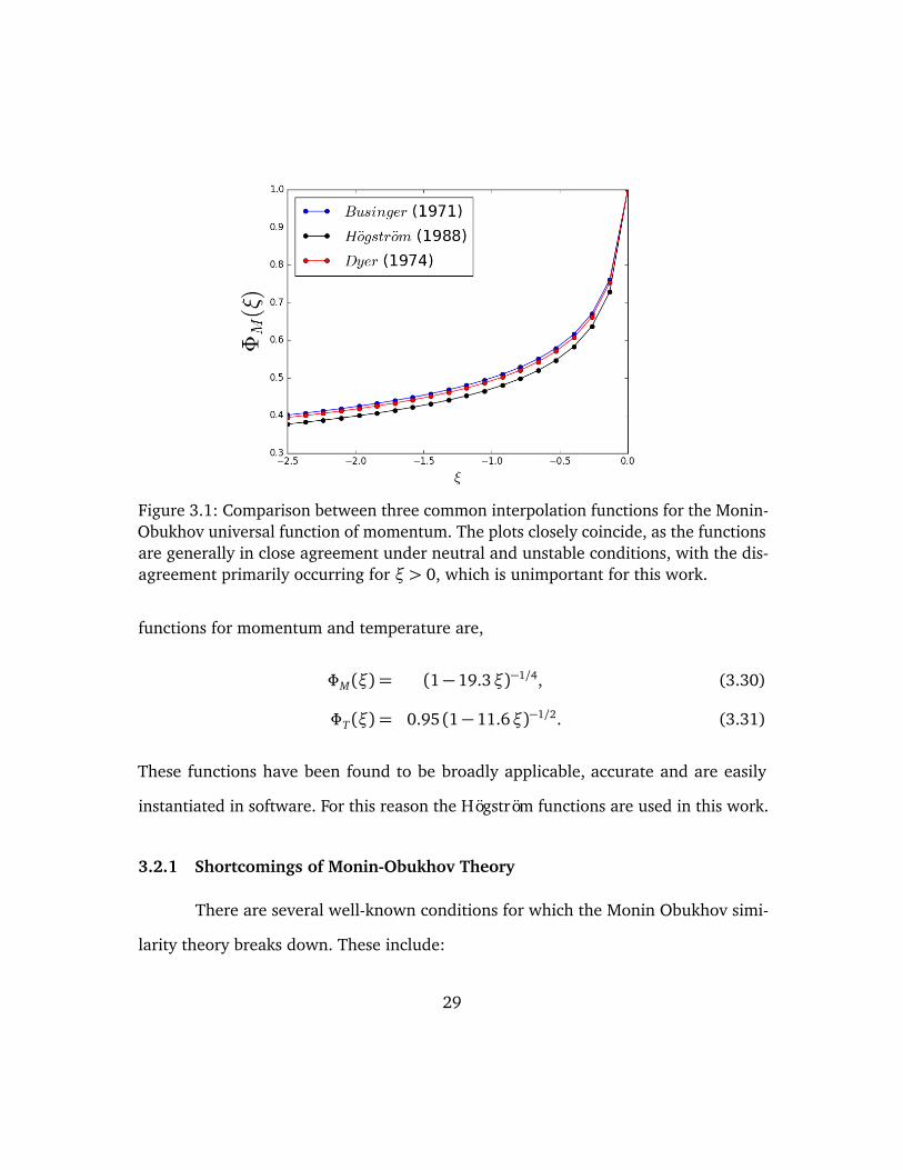
Figure 3.1: Comparison between three common interpolation functions for the Monin-Obukhov universal function of momentum. The plots closely coincide, as the functionsare generally in close agreement under neutral and unstable conditions, with the dis-agreement primarily occurring for ξ > 0, which is unimportant for this work.

functions for momentum and temperature are,

ΦM(ξ) = (1− 19.3ξ)−1/4, (3.30)

ΦT (ξ) = 0.95 (1− 11.6ξ)−1/2. (3.31)

These functions have been found to be broadly applicable, accurate and are easily

instantiated in software. For this reason the Högström functions are used in this work.

3.2.1 Shortcomings of Monin-Obukhov Theory

There are several well-known conditions for which the Monin Obukhov simi-

larity theory breaks down. These include:

29

• Surfaces with large spatial variations in roughness

• Outside of the surface layer (several hundred meters) where the Coriolis effect

is no longer negligible

But neither of these are relevant here. In “ideal” situations, the theory has been

found to be accurate to better than 10%[47, 59]. For our case, with minimal surface

roughness and our interest constrained to the near surface layer, these functions are

applicable and reasonably accurate[41], and are easily implemented in software.

3.3 Eddy Viscosity in the Device

The atmospheric boundary layer model discussed in the previous section does

not account for the presence of the SoV device. To account for this, an augmented

turbulent diffusivity is used in the vortical plume region to account for the turbulence

in the device. The diffusivity is enhanced due to vortex shedding from the trailing edge

of the vanes, and other effects not represented in the virtual vane model (discussed in

Section 3.4).

The eddy-viscosity in the region of the vanes and interior is set based on scaling

relations for a turbulent self-similar circular jet, as described in Pope[87],

νV = U0 y1/2νC . (3.32)

In this equation, U0 is the peak velocity, and is set based on the observed ve-

locities that exist in the SoV. The dimensionless constant νC was calibrated against

30

laboratory generated experimental data (the laboratory experiment is detailed in Sec-

tion 5), and is set to zero outside the device. The thermal diffusivity inside the device,

KV , is then fixed with the assumption that the Prandtl number is unity.

Finally, the length scale y1/2 is set either to the separation distance between

neighboring vanes, or the radius of the SoV apparatus. The former is used for the un-

steady virtual vanes, when greater spatial and temporal fidelity is required to capture

the dynamics of the plume and wake. This viscosity is designed to represent the fluc-

tuations inside the device due to separation of flow off the turning vanes, for instance.

This is in contrast to the case of the steady virtual vanes, where the radius of the SoV

apparatus is used as the length scale and no dynamics of the flow are are resolved.

Here, the resolved scale is that of the vortical plume itself, and not any fluctuating

quantities. This is principally for design purposes, and is intended only to capture the

largest scale features of the flow. These simulation regimes are discussed in further

detail in Chapter 5.

3.4 Vane Representation

To rapidly prototype general system configurations, the computations must

be able to explore a large space of possible geometries and settings. This presents

a significant meshing and computational challenge if the detailed flow around the

vanes is to be computed. In the region near the vanes, where a no-slip boundary

condition is imposed, the flow will necessarily form a thin momentum boundary layer.

Resolving this boundary layer requires high resolutions immediately adjacent to the

walls. Changing the vane location requires that a new mesh be generated. This is a

31

significant challenge, as the development of a new mesh often requires significant

human effort and time. Furthermore, the process is error-prone, and would require

that each simulation using a new mesh undergo detailed solution verification.

Instead, we have developed a modeling formulation that does not require

explicitly meshing the turning vanes, or any surface. The primary function of the vanes

is to turn the flow. Therefore, the vanes are represented as a force field, over which

a force is applied to the velocity field to align it with the angle of the turning vanes,

defined here as a field of vectors. These so-called ‘virtual vanes” are implemented as a

body force that is applied in the region that would otherwise contain the vanes. Vane

Figure 3.2: An example of explicitly represented turning vanes (left) versus an annularforcing region (right). RM is the furthest radial extent of the virtual vane forcing, andRm the smallest radial extent.

geometry is specified by the angle φ a vane makes with a radial line as a function of

the radial coordinate, r, and the polar angle, θ . A unit normal to the vane surface nv

is defined as,

nv(x) = sin (φ(r,θ )) r+ cos (φ(r,θ )) θ , (3.33)

32

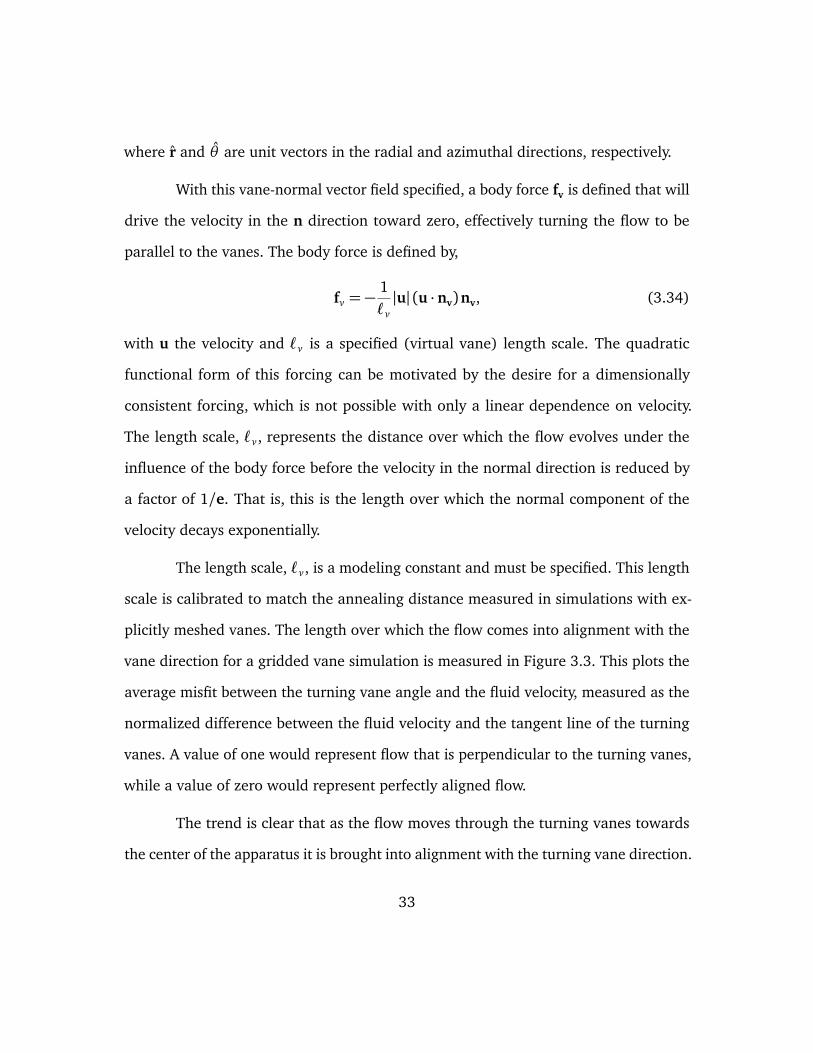
where r and θ are unit vectors in the radial and azimuthal directions, respectively.

With this vane-normal vector field specified, a body force fv is defined that will

drive the velocity in the n direction toward zero, effectively turning the flow to be

parallel to the vanes. The body force is defined by,

fv = −1`v|u| (u · nv)nv, (3.34)

with u the velocity and `v is a specified (virtual vane) length scale. The quadratic

functional form of this forcing can be motivated by the desire for a dimensionally

consistent forcing, which is not possible with only a linear dependence on velocity.

The length scale, `v, represents the distance over which the flow evolves under the

influence of the body force before the velocity in the normal direction is reduced by

a factor of 1/e. That is, this is the length over which the normal component of the

velocity decays exponentially.

The length scale, `v, is a modeling constant and must be specified. This length

scale is calibrated to match the annealing distance measured in simulations with ex-

plicitly meshed vanes. The length over which the flow comes into alignment with the

vane direction for a gridded vane simulation is measured in Figure 3.3. This plots the

average misfit between the turning vane angle and the fluid velocity, measured as the

normalized difference between the fluid velocity and the tangent line of the turning

vanes. A value of one would represent flow that is perpendicular to the turning vanes,

while a value of zero would represent perfectly aligned flow.

The trend is clear that as the flow moves through the turning vanes towards

the center of the apparatus it is brought into alignment with the turning vane direction.

33

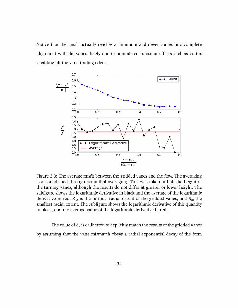
Notice that the misfit actually reaches a minimum and never comes into complete

alignment with the vanes, likely due to unmodeled transient effects such as vortex

shedding off the vane trailing edges.

Figure 3.3: The average misfit between the gridded vanes and the flow. The averagingis accomplished through azimuthal averaging. This was taken at half the height ofthe turning vanes, although the results do not differ at greater or lower height. Thesubfigure shows the logarithmic derivative in black and the average of the logarithmicderivative in red. RM is the furthest radial extent of the gridded vanes, and Rm thesmallest radial extent. The subfigure shows the logarithmic derivative of this quantityin black, and the average value of the logarithmic derivative in red.

The value of `v is calibrated to explicitly match the results of the gridded vanes

by assuming that the vane mismatch obeys a radial exponential decay of the form

34

f (r) = Ae−λr , where λ= 1`v

. Taking the logarithmic derivative of this quantity,

f ′

f=

Ae−λr ∗ −λAe−λr

= −λ. (3.35)

The logarithmic derivative is shown in the subfigure of Figure 3.3. If the misfit

between vanes was perfectly described by an exponential decay, the line would be flat.

While the curve does not perfectly coincide with this, the curve does not have severe

convexity and the average is sufficient for this work. Based on this, the length scale

`v was set to one third of a meter. For larger or smaller configurations, this value was

then scaled based on the total system diameter of the design.

This virtual vane formulation is similar to the “actuator disk” model commonly

used to represent the rotor of a wind turbine and described in the subsequent section.

3.5 Turbine Representation

The turbine is modeled similarly to the virtual vanes. As with the vanes, it is

desirable to avoid explicitly representing the turbine blade control surfaces. Instead,

the turbine is modeled using the actuator disc simplification. This model (also often

referred to as a “Blade Element Momentum” theory) is commonly used in wind turbine

design[66, 100, 111]. The essence of this model is to approximate the individual

spinning turbine blades as a “disk” in which the effects of the turbine are represented by

body forces on the fluid, as shown in Figure 3.4. This method assumes an axisymmetric

representation of the turbine geometry, and in doing so completely neglects unsteady

effects due to the rotation of turbine blades in a plane.

35

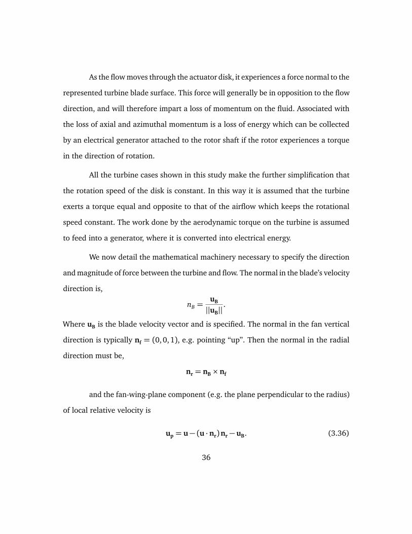
As the flow moves through the actuator disk, it experiences a force normal to the

represented turbine blade surface. This force will generally be in opposition to the flow

direction, and will therefore impart a loss of momentum on the fluid. Associated with

the loss of axial and azimuthal momentum is a loss of energy which can be collected

by an electrical generator attached to the rotor shaft if the rotor experiences a torque

in the direction of rotation.

All the turbine cases shown in this study make the further simplification that

the rotation speed of the disk is constant. In this way it is assumed that the turbine

exerts a torque equal and opposite to that of the airflow which keeps the rotational

speed constant. The work done by the aerodynamic torque on the turbine is assumed

to feed into a generator, where it is converted into electrical energy.

We now detail the mathematical machinery necessary to specify the direction

and magnitude of force between the turbine and flow. The normal in the blade’s velocity

direction is,

nB =uB

||uB||.

Where uB is the blade velocity vector and is specified. The normal in the fan vertical

direction is typically nf = (0,0, 1), e.g. pointing “up”. Then the normal in the radial

direction must be,

nr = nB × nf

and the fan-wing-plane component (e.g. the plane perpendicular to the radius)

of local relative velocity is

up = u− (u · nr)nr − uB. (3.36)

36

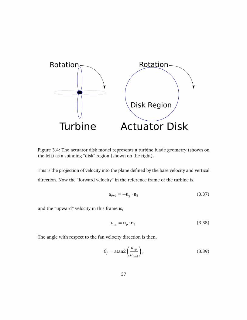
Rotation Rotation

Disk Region

Turbine Actuator Disk

Figure 3.4: The actuator disk model represents a turbine blade geometry (shown onthe left) as a spinning “disk” region (shown on the right).

This is the projection of velocity into the plane defined by the base velocity and vertical

direction. Now the “forward velocity” in the reference frame of the turbine is,

ufwd = −up · nB (3.37)

and the “upward” velocity in this frame is,

uup = up · nf. (3.38)

The angle with respect to the fan velocity direction is then,

θ f = atan2Ç

uup

ufwd

å, (3.39)

37

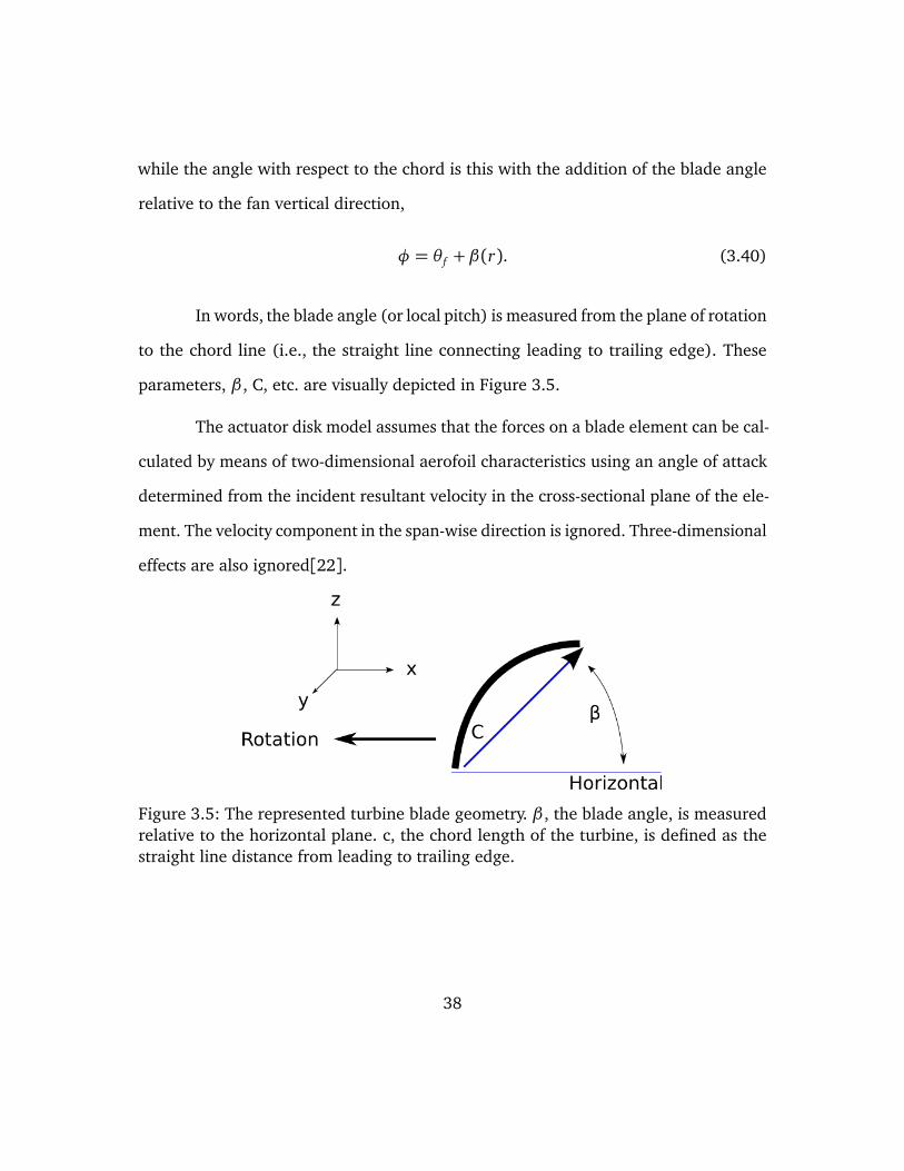
while the angle with respect to the chord is this with the addition of the blade angle

relative to the fan vertical direction,

φ = θ f + β(r). (3.40)

In words, the blade angle (or local pitch) is measured from the plane of rotation

to the chord line (i.e., the straight line connecting leading to trailing edge). These

parameters, β , C, etc. are visually depicted in Figure 3.5.

The actuator disk model assumes that the forces on a blade element can be cal-

culated by means of two-dimensional aerofoil characteristics using an angle of attack

determined from the incident resultant velocity in the cross-sectional plane of the ele-

ment. The velocity component in the span-wise direction is ignored. Three-dimensional

effects are also ignored[22].

Figure 3.5: The represented turbine blade geometry. β , the blade angle, is measuredrelative to the horizontal plane. c, the chord length of the turbine, is defined as thestraight line distance from leading to trailing edge.

38

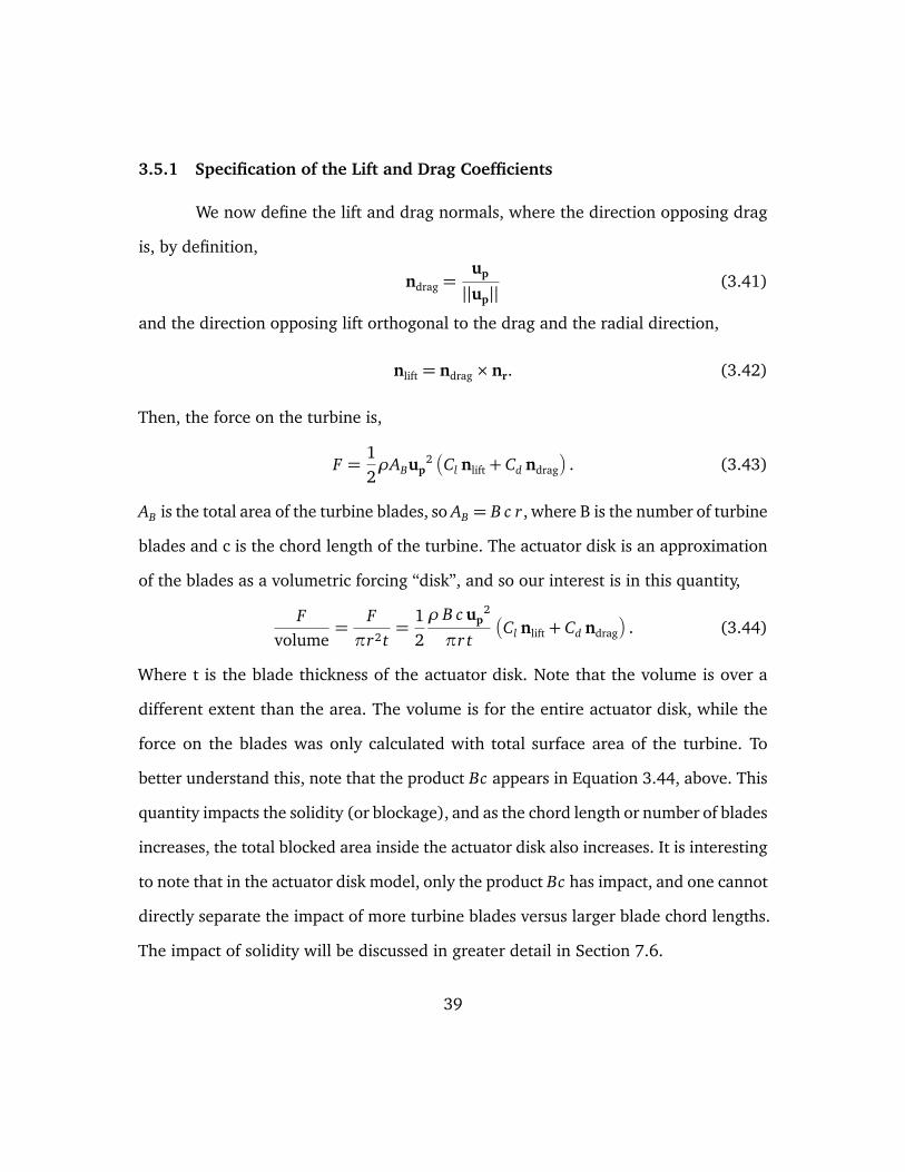
3.5.1 Specification of the Lift and Drag Coefficients

We now define the lift and drag normals, where the direction opposing drag

is, by definition,

ndrag =up

||up||(3.41)

and the direction opposing lift orthogonal to the drag and the radial direction,

nlift = ndrag × nr. (3.42)

Then, the force on the turbine is,

F =12ρABup

2ÄCl nlift + Cd ndrag

ä. (3.43)

AB is the total area of the turbine blades, so AB = B c r, where B is the number of turbine

blades and c is the chord length of the turbine. The actuator disk is an approximation

of the blades as a volumetric forcing “disk”, and so our interest is in this quantity,

Fvolume

=Fπr2 t

=12

ρ B c up2

πr t

ÄCl nlift + Cd ndrag

ä. (3.44)

Where t is the blade thickness of the actuator disk. Note that the volume is over a

different extent than the area. The volume is for the entire actuator disk, while the

force on the blades was only calculated with total surface area of the turbine. To

better understand this, note that the product Bc appears in Equation 3.44, above. This

quantity impacts the solidity (or blockage), and as the chord length or number of blades

increases, the total blocked area inside the actuator disk also increases. It is interesting

to note that in the actuator disk model, only the product Bc has impact, and one cannot

directly separate the impact of more turbine blades versus larger blade chord lengths.

The impact of solidity will be discussed in greater detail in Section 7.6.

39

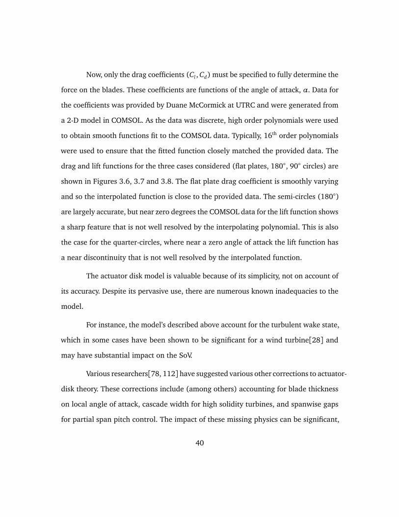
Now, only the drag coefficients (Cl , Cd) must be specified to fully determine the

force on the blades. These coefficients are functions of the angle of attack, α. Data for

the coefficients was provided by Duane McCormick at UTRC and were generated from

a 2-D model in COMSOL. As the data was discrete, high order polynomials were used

to obtain smooth functions fit to the COMSOL data. Typically, 16th order polynomials

were used to ensure that the fitted function closely matched the provided data. The

drag and lift functions for the three cases considered (flat plates, 180, 90 circles) are

shown in Figures 3.6, 3.7 and 3.8. The flat plate drag coefficient is smoothly varying

and so the interpolated function is close to the provided data. The semi-circles (180)

are largely accurate, but near zero degrees the COMSOL data for the lift function shows

a sharp feature that is not well resolved by the interpolating polynomial. This is also

the case for the quarter-circles, where near a zero angle of attack the lift function has

a near discontinuity that is not well resolved by the interpolated function.

The actuator disk model is valuable because of its simplicity, not on account of

its accuracy. Despite its pervasive use, there are numerous known inadequacies to the

model.

For instance, the model’s described above account for the turbulent wake state,

which in some cases have been shown to be significant for a wind turbine[28] and

may have substantial impact on the SoV.

Various researchers[78, 112] have suggested various other corrections to actuator-

disk theory. These corrections include (among others) accounting for blade thickness

on local angle of attack, cascade width for high solidity turbines, and spanwise gaps

for partial span pitch control. The impact of these missing physics can be significant,

40

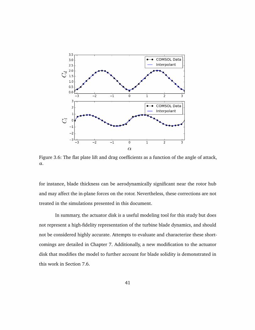
Figure 3.6: The flat plate lift and drag coefficients as a function of the angle of attack,α.

for instance, blade thickness can be aerodynamically significant near the rotor hub

and may affect the in-plane forces on the rotor. Nevertheless, these corrections are not

treated in the simulations presented in this document.

In summary, the actuator disk is a useful modeling tool for this study but does

not represent a high-fidelity representation of the turbine blade dynamics, and should

not be considered highly accurate. Attempts to evaluate and characterize these short-

comings are detailed in Chapter 7. Additionally, a new modification to the actuator

disk that modifies the model to further account for blade solidity is demonstrated in

this work in Section 7.6.

41

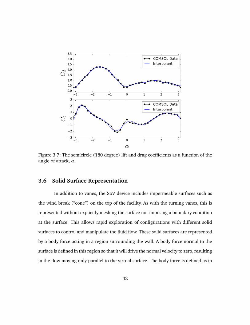
Figure 3.7: The semicircle (180 degree) lift and drag coefficients as a function of theangle of attack, α.

3.6 Solid Surface Representation

In addition to vanes, the SoV device includes impermeable surfaces such as

the wind break (“cone”) on the top of the facility. As with the turning vanes, this is

represented without explicitly meshing the surface nor imposing a boundary condition

at the surface. This allows rapid exploration of configurations with different solid

surfaces to control and manipulate the fluid flow. These solid surfaces are represented

by a body force acting in a region surrounding the wall. A body force normal to the

surface is defined in this region so that it will drive the normal velocity to zero, resulting

in the flow moving only parallel to the virtual surface. The body force is defined as in

42

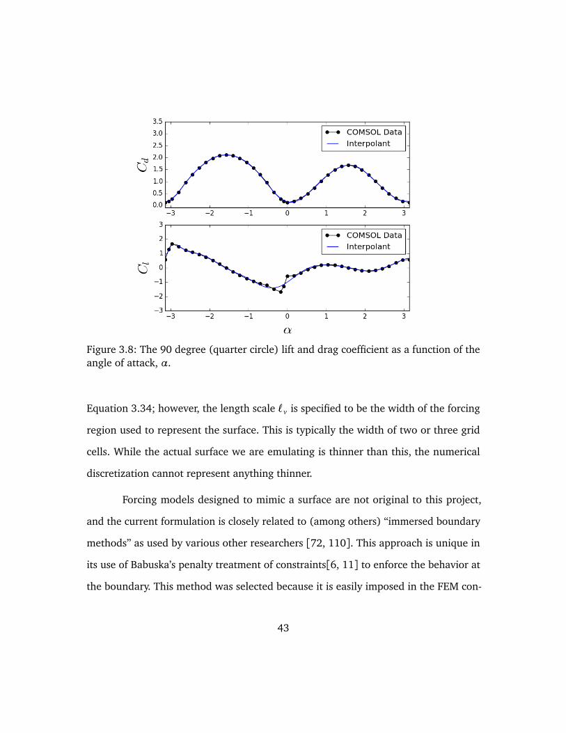
Figure 3.8: The 90 degree (quarter circle) lift and drag coefficient as a function of theangle of attack, α.

Equation 3.34; however, the length scale `v is specified to be the width of the forcing

region used to represent the surface. This is typically the width of two or three grid

cells. While the actual surface we are emulating is thinner than this, the numerical

discretization cannot represent anything thinner.

Forcing models designed to mimic a surface are not original to this project,

and the current formulation is closely related to (among others) “immersed boundary

methods” as used by various other researchers [72, 110]. This approach is unique in

its use of Babuska’s penalty treatment of constraints[6, 11] to enforce the behavior at

the boundary. This method was selected because it is easily imposed in the FEM con-

43

text, and the penalty method properties have been explored in detail in the literature.

Note that despite the similarity in name, this is a distinct technique from the “penalty

immersed boundary method” of Kim and Peskin[62].

3.7 Separation Model

In the presence of wind, it was found that there was a significant flow out

through the vanes in the back of the device. This was obviously inconsistent with the

findings of our colleagues in the field, who observed no such outflows. Moreover, this

resulted in large inconsistencies between our predictions and the field results, almost

certainly because of the kinetic and thermal energy that our vane representation was

permitting to leave out the back of the device.

This exposed a weakness of the turning vane representation outlined previously.

When the flow entered the virtual vane forcing region it was always turned to align

with the vane angle, even when the forcing was in the opposite direction of the present

velocity. This is in contrast to the physical situation, in which we expect the flow to

continue along an averaged streamline separating from the trailing edges of the vanes,

instead of turning around it. The averaged streamline will continue past the trailing

edge of the vane due to the separation of the boundary layer off the edge surface. An

image depicting these two cases in shown in Figure 3.9.

Let nv be the normal vector to the vanes, and nr the normal vector pointing

out of the vane region2. Then, tv is the tangent vector to the vanes pointing out of the

2The subscripts “v” and “r” stand for vane and radial, respectively.

44

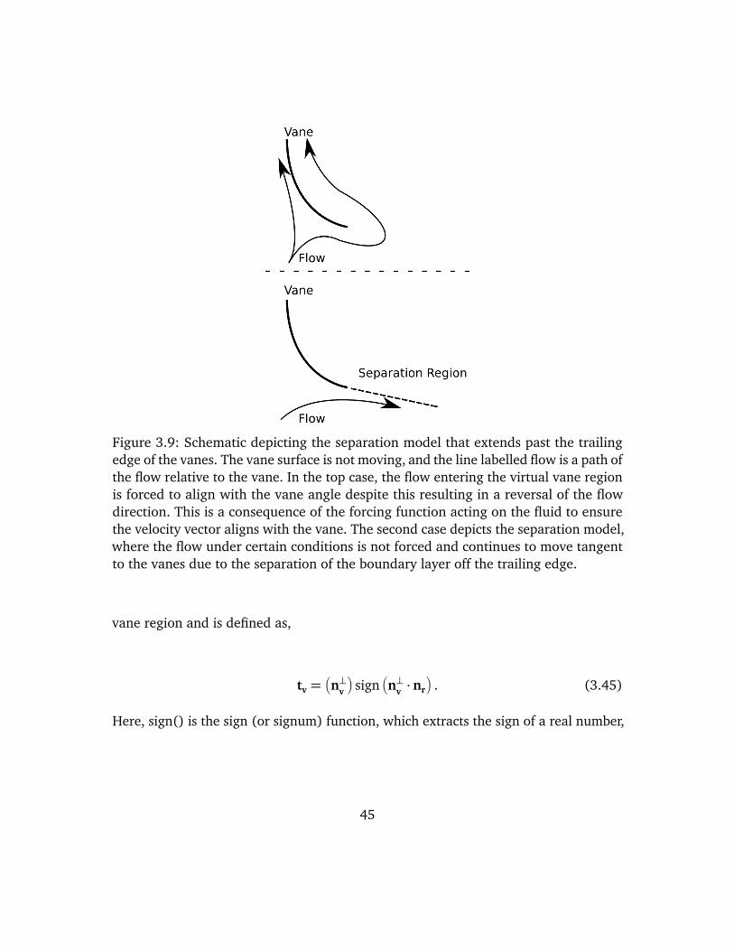
Figure 3.9: Schematic depicting the separation model that extends past the trailingedge of the vanes. The vane surface is not moving, and the line labelled flow is a path ofthe flow relative to the vane. In the top case, the flow entering the virtual vane regionis forced to align with the vane angle despite this resulting in a reversal of the flowdirection. This is a consequence of the forcing function acting on the fluid to ensurethe velocity vector aligns with the vane. The second case depicts the separation model,where the flow under certain conditions is not forced and continues to move tangentto the vanes due to the separation of the boundary layer off the trailing edge.

vane region and is defined as,

tv =Än⊥vä

signÄn⊥v · nr

ä. (3.45)

Here, sign() is the sign (or signum) function, which extracts the sign of a real number,

45

and n⊥v is the vector perpendicular to the normal vector of the vanes, which is simply,

n⊥v =ñ

nx

ny

ô⊥=ñ−ny

nx

ô.

The forcing is modified when the velocity vector of the local flow, u is pointing

into the forcing region: u ·nr < 0, and when the velocity vector is in the same direction

as the tangent line to the vanes: u · tv > 0,

n(x) =

r if u · nr < 0 and u · tv > 0,

sin (φ) r+ cos (φ) θ else.(3.46)

In these instances, the forcing acts as if there was a rigid surface past the vane edge,

and gives the appearance of a special “no-penetration” condition for the velocity for

these cases.

The addition of this simple separation model significantly reduced the flow that

penetrated the back of the vanes, and produces results consistent with the observations

provided by our experimental colleagues.

3.8 Effect of Surface Roughness

Surface roughness effects have been shown to play a role in the formation of

dust devils and related atmospheric phenomena[86]. For the flat and sandy regions we

are simulating, the impact is expected to be a small vertical velocity perturbation which

triggers the convective instability caused by stratification near the surface. Assuming

azimuthal symmetry, this is modeled as a volumetric forcing in a narrow region above

46

the surface in the region of the vanes,

F′′′

z0=

12ρV 2

f /z0, (3.47)

where z0 is the forcing region height and Vf is the magnitude of the induced velocity

fluctuation which is estimated as,

Vf =»

2az0. (3.48)

The forcing region height z0 is set to the boundary layer thickness of 10 centimeters.

The acceleration was estimated at 0.05 m/s2, based on the observed surface roughness

impact on tornado-like vortices of Natarajan and Hangan[82].

We ensure that the energy introduced into the flow is a small fraction of total

flow energy by comparing this with the energy flux through the top of the vanes. The

total energy added is measured as,

Einjected =∫ 2π

0

∫ R

0

∫ z0

0F′′′

z0dzdrdθ . (3.49)

R is the outer diameter of the vanes. The value of Einjected is typically a few percent of

the total kinetic energy flux measured through the top of the vanes.

Leslie [67] and Dessens [33] found that the introduction of surface roughness

effects caused a slight decrease in tangential velocity for simulated vortices, but an

increase in radial and axial velocities. On a related note, hurricane studies have con-

sistently found enhanced heat transport near the surface lead to storm intensification,

indicating an important role due to roughness effects [1, 74, 116]. The interaction

with the surface and therefore, the impact of roughness, is likely complicated and is not

47

considered in detail in this work. It should be noted that in the simulations performed

in the course of this study, the surface roughness model was observed to modestly

intensify the thermal vortex, typically by several percent. While this formulation was

undoubtedly ad hoc, studies performed on representative test cases found that results

were not sensitive to small changes in the forcing region height, radial distance, or

forcing magnitude.

3.9 Simulation Geometry and Boundary Conditions

In this project, two principle modeling regimes are considered. One is the

“thermal-only” scenario, in which there is no wind and there is an imposed elevated

temperature on the ground. In the other, there are also ambient winds that contribute

to the SoV energy (“wind” cases) and elevated ground temperature. The computational

domain and boundary conditions for these two scenarios are described below.

Computational Domain

All simulations are performed in a cuboid domain, with six faces. The domain

is denoted Ω ⊂ R3. The domain extents are scaled by the system diameter, D, created

by the outer vane radius. The extents are defined in terms of Lx , L y , Lz indicating the

streamwise, spanwise and vertical directions, respectively. For both simulation regimes,

sensitivity analyses were performed to ensure that the results were not sensitive to the

domain extents. For the thermal-only case, for which Lx = L y , the system extents Lx/D

and L y/D are chosen to be 3. The height (Lz/D) is three times the system diameter,

which is typically nearly equal to the height of the vanes. This defines the thermal-only

48

domain ΩT , as ΩT = [−Lx , Lx]×î−L y , L y

ó× [0, Lz].

For the wind cases, the streamwise extent is no longer equal to the spanwise

length, L y . In these cases, the domain length extends two diameters in front of the vanes

and three behind. The spanwise direction is symmetric and extends two diameters in

each direction from the center (L y/D = 2). The height is identical to the thermal-

only case, at three system diameters (Lz/D = 3). Thus, the wind domain is defined as

ΩW = [−2D, 3D]×î−L y , L y

ó× [0, Lz].

The boundary for the thermal only case is decomposed as, ∂ΩT = ΓG⋃ΓT⋃ΓP .

ΓG is the boundary along the “Ground”, ΓT the “Top” boundary, and ΓP the four periodic

“Sides”. A 3D diagram labeling these boundaries appears in Figure 3.10. For this case

(no mean wind), periodic boundary conditions are used on the four sides , with a mod-

ified “inflow-outflow” Neumann condition[44] on the top boundary. On the ground, a

“no-slip” velocity boundary condition is imposed, and a Dirichlet condition uniformly

fixes the temperature of the surface. Each of the Γ boundary terms are defined in the

paragraphs below. Note that a finite thickness “Sponge Layer” is indicated on the figure

along the top boundary and is defined below.

The boundary for the wind cases is decomposed as,

∂ΩW = ΓG⋃ΓT⋃ΓO⋃ΓI⋃ΓS.

Where ΓG is the boundary along the “Ground”, ΓT the “Top” boundary, ΓS the two “Sides”,

ΓI the inflow boundary, and ΓO the “Outflow” boundary. The “wind” simulation domain

is diagrammed in Figure 3.11, with the boundaries labeled. In this wind case (a heated

ground with an ambient wind), there is a proscribed inlet boundary layer along the

49

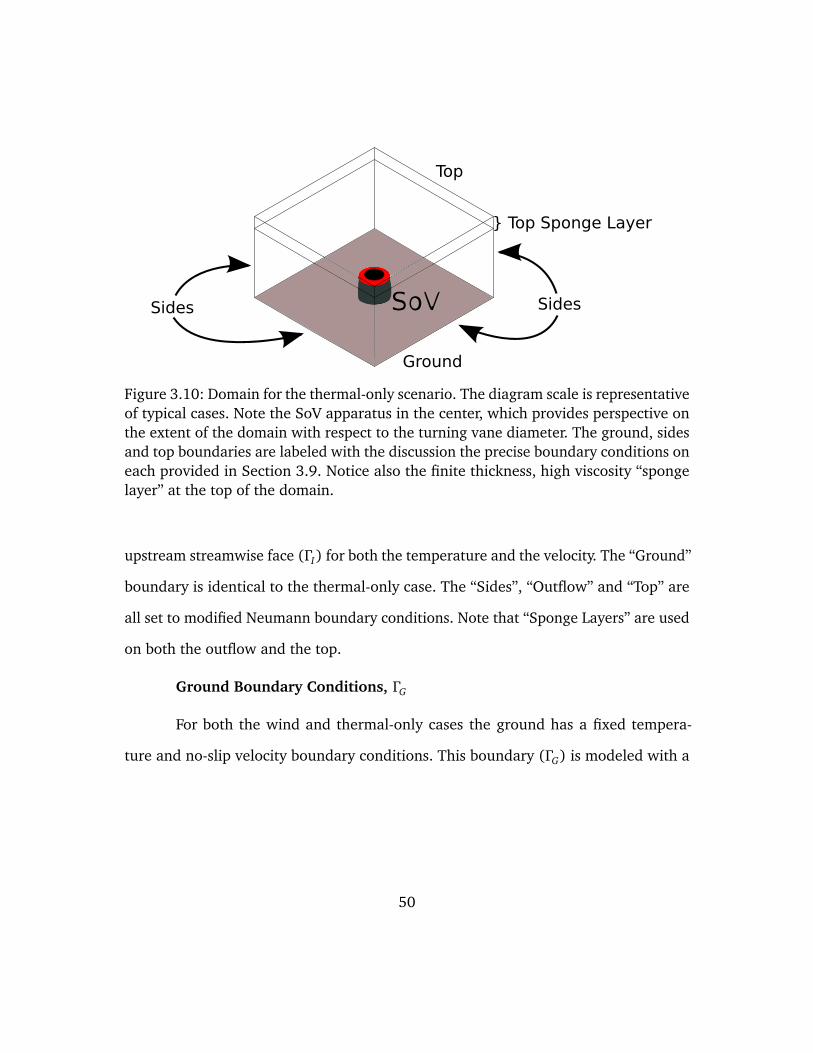
SoV

Top Sponge Layer

Ground

Top

Sides Sides

Figure 3.10: Domain for the thermal-only scenario. The diagram scale is representativeof typical cases. Note the SoV apparatus in the center, which provides perspective onthe extent of the domain with respect to the turning vane diameter. The ground, sidesand top boundaries are labeled with the discussion the precise boundary conditions oneach provided in Section 3.9. Notice also the finite thickness, high viscosity “spongelayer” at the top of the domain.

upstream streamwise face (ΓI) for both the temperature and the velocity. The “Ground”

boundary is identical to the thermal-only case. The “Sides”, “Outflow” and “Top” are

all set to modified Neumann boundary conditions. Note that “Sponge Layers” are used

on both the outflow and the top.

Ground Boundary Conditions, ΓG

For both the wind and thermal-only cases the ground has a fixed tempera-

ture and no-slip velocity boundary conditions. This boundary (ΓG) is modeled with a

50

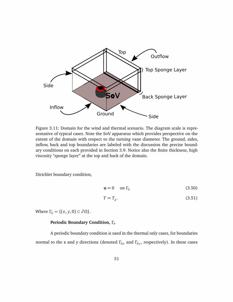
SoV

Top Sponge Layer

Ground

Top

Side

Side

Back Sponge Layer

Outflow

Inflow

Figure 3.11: Domain for the wind and thermal scenario. The diagram scale is repre-sentative of typical cases. Note the SoV apparatus which provides perspective on theextent of the domain with respect to the turning vane diameter. The ground, sides,inflow, back and top boundaries are labeled with the discussion the precise bound-ary conditions on each provided in Section 3.9. Notice also the finite thickness, highviscosity “sponge layer” at the top and back of the domain.

Dirichlet boundary condition,

u= 0 on ΓG (3.50)

T = Tg . (3.51)

Where ΓG = (x , y, 0) ⊂ ∂Ω.

Periodic Boundary Condition, ΓP

A periodic boundary condition is used in the thermal only cases, for boundaries

normal to the x and y directions (denoted ΓP,x and ΓP,y , respectively). In these cases

51

the state variables are constrained to have the same value on the opposite faces of the

domain, for instance in the streamwise direction the boundary conditions are,

u(−Lx , y, z) = u(Lx , y, z) on ΓP,x (3.52)

T (−Lx , y, z) = T (Lx , y, z) (3.53)

and in the spanwise direction,

u(x ,−L y , z) = u(x , L y , z) on ΓP,y (3.54)

T (x ,−L y , z) = T (x , L y , z). (3.55)

Where ΓP,x = (−Lx , y, z)⋃(Lx , y, z) ⊂ ∂Ω and ΓP,y = (x ,−L y , z)

⋃(x , L y , z) ⊂ ∂Ω.

Inflow Boundary Condition, ΓI

On the inflow boundary (ΓI), Dirichlet conditions are used for both velocity

and temperature. The boundary-normal, or streamwise component is a function of the

surface normal coordinate (z), representing a boundary layer below a uniform velocity,

U. The common 7th power model of a turbulent boundary layer is used,

uin(z) = U minÇÅ zδ

ã7

, 1å

,

where δ, the boundary layer thickness, is set based on data measured by our experi-

mental partners in the field. The thermal boundary layer is assumed to have a similar

boundary layer, but, as observed in real atmospheric flows, there remains a vertical

temperature gradient outside the thin boundary layer. The thermal inflow has the form,

Tin(z) =∆TÇ

1− minÇÅ zδ

ã7

, 1åå+ T0 − βz.

52

Based on results in the literature, β = 2/3 Kelvin per meter[14]. This inflow boundary

is at the surface x = −Lx .

Mixed inflow/outflow Boundary Conditions on ΓT , ΓS and ΓB

At outflow boundaries, a homogeneous Neumann condition is appropriate[88],

∂ u∂ n

∣∣∣∣∣ΓT

= 0, (3.56)

∂ T∂ n

∣∣∣∣∣ΓT

= 0. (3.57)

However, for the cases in this study, a modified Neumann condition is necessary due

to the possibility that there will be an inflow on these boundaries. For example, in

the region above the vanes, the concentrated hot plume is lifted by buoyancy upward

and out of the simulation domain. However, the radial inflow towards the apparatus

is drawn in by large scale convection cells larger than the system diameter. Thus, our

boundary conditions must permit inflow along the areas above and external to the

vanes, while simultaneously permitting outflow in the area above the vanes.

To accomplish this, the boundary condition is,

∂ un

∂ n

∣∣∣∣∣ΓT

= 0 (3.58)

if (w< 0) then

ut = 0,

T = Tin(3.59)

else

∂ ut∂ n

∣∣∣∣∣ΓT

= 0,

∂ T∂ n

∣∣∣∣∣ΓT

= 0(3.60)

where un and ut are normal and tangential components of the velocity, respectively.

This boundary condition is applied on the top boundary ΓT (z = Lz) and downstream

53

side boundary ΓB in the wind case. This mixed boundary condition appears to be a

unique implementation of a modified Neumann condition condition, which has been

demonstrated previously in other instances [18, 40]. In particular, the well-posedness

of this general class of boundary condition is treated in [21].

Sponge Layer

Finally, a finite thickness “sponge layer” is used in the region adjacent to the

mixed inflow/outflow boundaries ΓT and ΓB. These regions are referred to by many

names in the literature[30], such as absorbing layers, fringe regions, buffer zones,

sponges, etc. This layer artificially increases the momentum diffusivity by a factor of

ten over the nominal value. This was designed to stabilize the modified Neumann

boundary conditions which can exhibit an instability when there is a compact jet of

fluid leaving the domain. These small outflows would create small high velocity inflows,

and the feedback loop would result in instabilities and numerical blow-up. Use of this

stabilizing sponge layer is justified because we are not interested in the flow in this

region. No results are quoted from this “sacrificial” region, as it is not considered

physically meaningful. The top sponge layer in both the wind and thermal-only cases

are half a system diameter (Lz/D = 1/2) thick. For the wind cases, the downstream

sponge layer is also half a system diameter (Lx/D = 1/2) thick.

54

Chapter 4

Computational Methods and Software

The previous chapter described a set of models for the system of interest. This

chapter details the numerical formulation and solution of these models. It begins with

a discussion of the numerical discretization of the equations of interest. The mesh

discretization is then described. Next, the scientific software in which these numerical

models are used is discussed. Finally, the tool chain and supercomputer systems are

briefly introduced.

4.1 Discretization Scheme

The finite element method (FEM) is used to numerically solve the Navier-

Stokes equations. The starting point for the FEM is to cast the equations in Section 3.1

into a weak form. Use of the weak form reduces the continuity requirements on the

basis functions, thereby allowing the use of functions that are easy to construct and

implement, such as piece-wise polynomials. Manipulating these partial differential

equations into a variational formulation is accomplished by multiplying the equations

by appropriate test functions and integrating over the domain, Ω. The resulting weak

problem is: find (u, p, T ) ∈ H1(Ω)3 × L2(Ω)×H1(Ω) such that

55

(∂ u∂ t

,v) + (u · ∇u,v) + (ν∇u,∇v)− (p,∇ · u) = (g T ′/T0, v), (4.1)

(∇ · u, q) = 0, (4.2)

(∂ T∂ t

, w) + (u · ∇T, w) + (k∇T,∇w) = 0, (4.3)

∀(v, q, w) ∈ H1(Ω)3× L2(Ω)×H1(Ω), where (·, ·) denotes the L2 inner product

(u,v) =∫Ω u·v d x and H1(Ω) is the Sobolov space with one square integrable derivative

on the domain Ω[84]. As noted previously, boldface letters denote vector quantities

(such as u= u, v, w). Some of the simulations presented here were conducted under

steady conditions, for which the ∂∂ t terms vanish. An FEM scheme is obtained by posing

the weak form in terms of finite-dimensional subspaces of the function spaces specified

above defined using piecewise-polynomial basis functions. This discretization has the

form, vh ∈ v, where vh is formed through a linear combination of a finite number (N)

of basis functions φi,

vh =N∑

i=1

αiφi, (4.4)

where αi are coefficients[12]. All of the simulations discussed in this work were ac-

complished using piecewise linear basis functions for both the velocity and pressure.

Typically, the use of equal order elements for velocity and pressure is ruled out in the

standard Galerkin FEM formulation because of the Babuska-Brezzi condition[5]. This

is overcome here by the introduction of a pressure stabilization term[12]. The resulting

system is still susceptible to convective instabilities, and so streamline upwind/Petrov-

Galerkin (SUPG) stabilization terms are used, as first described by Hughes[20, 51] and

extended to natural convection as in Becker and Braack[13]. These stabilization terms

56

add a residual dependent artificial dissipation that approaches zero as the solution con-

verges. This scheme is called consistent because the underlying order of convergence

of the numerical method is not affected[52].

The stabilization described above is accomplished by introducing an additional

term, ⟨Lc, Sφ⟩τ, to the weak form defined in Equations 4.1-4.3. Here L is the operator

for the PDEs in 3.1, and S is a stabilization operator which is chosen to be the negative

adjoint of the differential operator terms of L, and c and φ are state and test function

vectors, i.e. c= (u, p, T ), and φ = (v, w, q). The angle brackets ⟨·, ·⟩ signify integration

of the element interiors for each of the K elements, that is:

⟨u,v⟩τ =∑

KτK(u,v)K . (4.5)

This results in three stabilization parameters,τP ,τv,τT , which are selected as proposed

by Becker and Braack1.

After spatial discretization, the system of ODEs are discretized in time using the

backward Euler method[73]. The time interval (0, T ) is sliced into Nt steps of uniform

temporal length, ∆t, where n= 0, . . . , Nt . This has the form,

yn+1 = yn +∆t f (yn+1, tn+1). (4.6)

Where yn+1 denotes the solution vector at the time step n + 1, for instance. As f is

non-linear, a Newton-Raphson method is used to solve the resulting implicit nonlinear

problem.

1Derivations of the weak form and stabilization terms are provided in Appendix A

57

4.2 Mesh Discretization

The domains described in Section 3.9 are consistently discretized. This means

that the domain extents, Lx , L y , Lz, are scaled by system diameter (D) but the same

number of grid points are used for every simulation. Thus, while the ratio of the domain

length to system diameter remains fixed, the grid spacing ∆x ,∆y,∆z increases

proportionally with domain length.

The eddy diffusivities (νt , Kt) in Equations 3.4 and 3.5 are proportionally scaled

with grid spacing to ensure that the cell Reynolds number,

Recell =max(∆x ,∆y)u

νt, (4.7)

is maintained for every simulation, to ensure stability. In this way, larger domains have

higher eddy viscosities which serve to dissipate effects of scales that are smaller than

the grid spacing.

The mesh has a uniform spacing in the lateral directions, except for a single

refinement in the region of the vanes. Typically, the grid is roughly one hundred points

in the streamwise and spanwise directions before the refinement. The refinement

halves the spacing (doubles the number of points) in all three coordinate directions,

x,y,z, in this region. The refinement is introduced from the ground to 1.5 times the

height of the vanes and cone.

The vertical mesh spacing is non-uniform to resolve the boundary layer. This

is accomplished by redistributing a mesh which is uniformly spaced over the interval

0, Lz in height, z, to a non-uniform mesh, z, over the same interval. A mapping

z = χ(z) is defined by the following conditions. The minimum and maximum extents

58

are preserved so that χ(0) = 0 and χ(Lz) = Lz. The map spacing between points is

initially a specified minimum value,

hmin = χ′(0) h, (4.8)

where h= Lz/nz. The map is strictly increasing until the point zb, where the spacing

reaches a constant, hmax = χ ′(zb) h. From this point onward, the mesh has a constant

uniform spacing, hmax = χ ′(Lz) h. Finally, the mapping is assumed to hold an exponen-

tial functional form, χ(z) = Aeβ z.

Then, by specifying hmin, hmax and zb (chosen thickness of the boundary layer

mesh), these conditions are sufficient to define a mapping,

z = χ(z) =

C1(z − Lz) + Lz if z ≥ zb,

C2 exp(C3 z − 1) if z < zb.(4.9)

Here, C1 − C3 are coefficients, and are defined as,

C1 = C2 C3eC3 zb , (4.10)

C2 =zb

hr − 1, (4.11)

C3 =ln (hr)

zb, (4.12)

where hr is the ratio between the largest and smallest spacing,

hr =hmax

hmin, (4.13)

and,

zb =Lz

1+ Lz−zbC2 hr ln (hr )

. (4.14)

59

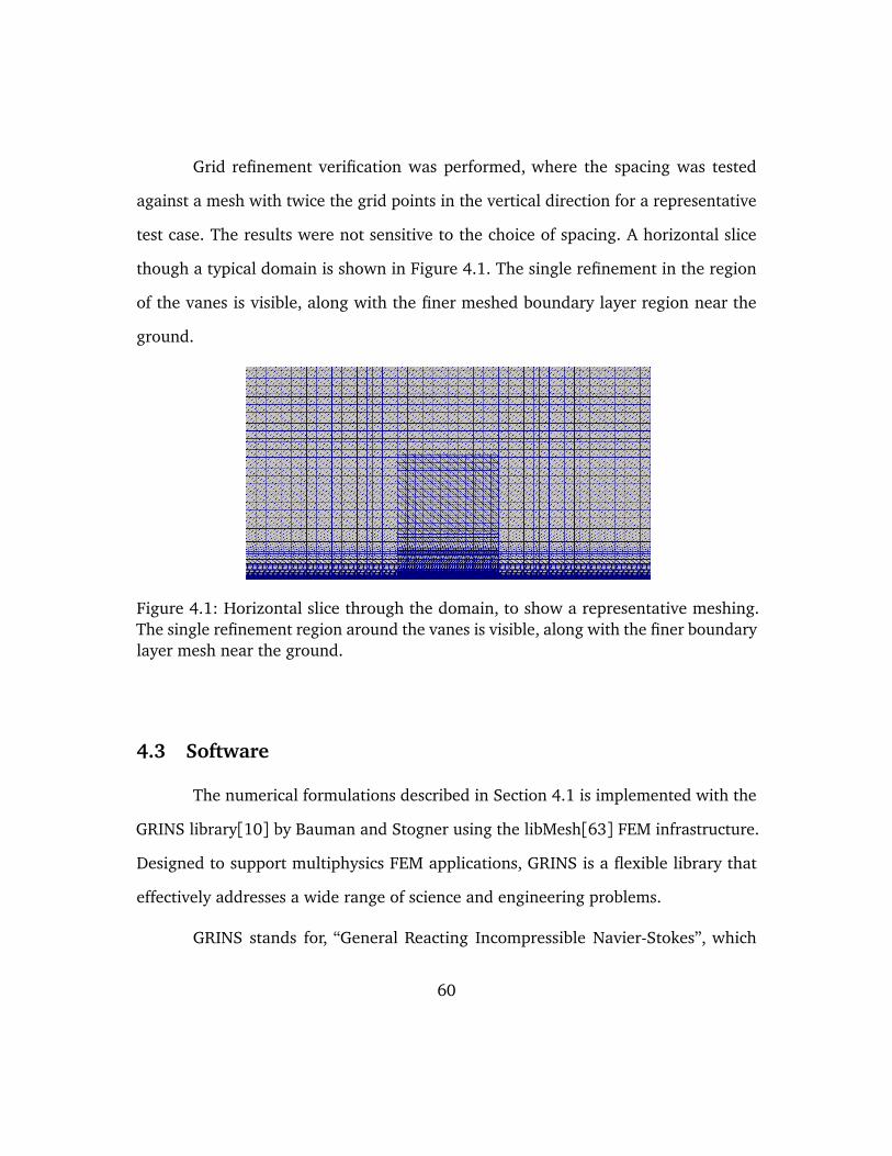
Grid refinement verification was performed, where the spacing was tested

against a mesh with twice the grid points in the vertical direction for a representative

test case. The results were not sensitive to the choice of spacing. A horizontal slice

though a typical domain is shown in Figure 4.1. The single refinement in the region

of the vanes is visible, along with the finer meshed boundary layer region near the

ground.

Figure 4.1: Horizontal slice through the domain, to show a representative meshing.The single refinement region around the vanes is visible, along with the finer boundarylayer mesh near the ground.

4.3 Software

The numerical formulations described in Section 4.1 is implemented with the

GRINS library[10] by Bauman and Stogner using the libMesh[63] FEM infrastructure.

Designed to support multiphysics FEM applications, GRINS is a flexible library that

effectively addresses a wide range of science and engineering problems.

GRINS stands for, “General Reacting Incompressible Navier-Stokes”, which

60

roughly encapsulates the physical regimes it was originally designed to simulate. GRINS

is open-source, and available on GitHub. It is released under LGPL2.1.

GRINS uses the fparser [56] library to support both parsing and compilation

of mathematical functions into high performance kernels. This capability allows for

easy specification of boundary conditions, initial conditions, or constitutive equations

from an input file. Some of these inputs are detailed in Appendix D.

GRINS/libMesh are built on the PETSc[7] solver package, which provides the

numerical linear algebra packages used for constructing and using sparse matrices,

finding the solution of linear systems, and for preconditioning.

While a variety of solver options have been tested in PETSc, all the results

shown in this document use GMRES with block Jacobi for preconditioning[96] the

linear solve. This uses the inverse of the diagonal block for that processor for precondi-

tioning of the entire linear system. In addition, a preconditioner is used for the solution

of the diagonal block. This is approximated with incomplete LU factorization[25]. Here,

the “incomplete” refers to the level of fill, with greater levels of fill approaching the

“complete” LU factorization.

In principle, alternative software libraries/frameworks such as FEniCS[4] or

OpenFOAM[55] would be capable of simulating this problem. While these and other

libraries have various strengths and weaknesses, the pre-eminent concern is the par-

allel performance at the intended processor count, due to the rapid design iterations

necessary for this research campaign. Given these concerns, the GRINS library is a

satisfactory tool.

61

At the time of this writing, GRINS has 94 regression tests, which provides a

reasonable degree of confidence in verification testing of the library. Several of these

tests directly test the capabilities in GRINS used in this study. In particular, several of

the tests were contributed to GRINS by the author over the course of this work during

the addition of several of the models detailed in Chapter 3.

4.4 Tool Chain and Simulation Custodianship

Simulations are performed on the Texas Advanced Computing Center’s (TACC)

supercomputers Lonestar Four, Lonestar Five, and Stampede. Run durations for tran-

sient cases are typically twelve hours to perform several hundred timesteps. The steady

runs are considerably shorter, and require less than ten minute runtimes. Typically the

wall clock times of the steady-state runs are two or three minutes to solution. These

runs use 264-528 processing cores, or 22-44 nodes on Lonestar4 (with 12 cores per

node), and a similar number for Stampede. The runs have several million degrees of

freedom (DoF), and the local number of DoF per core is maintained at O(104). This was

selected due to memory constraints, after a strong scaling analysis of the performance

of the code on these resources, and after consulting with the software developers. At

the time of this writing libMesh has been scaled to tens of thousands of cores and

has been run on over 100,000 cores on the BG/Q machine Mira at Argonne National

Lab[43], and the scaling results here are consistent with the performance expectations

for this library.

Runs are submitted via job scripts to the SLURM[115] scheduling system. After

a run terminates, several additional scripts are automatically invoked. These archive

62

the run (outside of the volatile /scratch production directories) and simultaneously,

label the concluded run with unique metadata that defines the system environment;

the jobs input files and run definitions; and information detailing the hypothesis or

physics the job was intended to investigate. Finally, once a week a script performs

rsync on the entire archived database to maintain redundant storage of the simulation

data. Appendix D details the archived simulations and storage patterns.

In other words, the workflow is designed to permit rapid queuing of a series

of runs (in parallel) to investigate a variety of conditions or scenario parameters. This

capability is necessary for the optimization campaign detailed in Section 6, where

running many concurrent investigations are required to sample the configuration space.

63

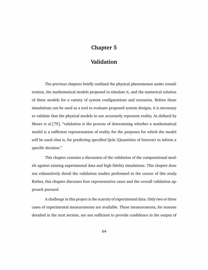
Chapter 5

Validation

The previous chapters briefly outlined the physical phenomenon under consid-

eration, the mathematical models proposed to simulate it, and the numerical solution

of these models for a variety of system configurations and scenarios. Before these

simulations can be used as a tool to evaluate proposed system designs, it is necessary

to validate that the physical models in use accurately represent reality. As defined by

Moser et al.[79], “validation is the process of determining whether a mathematical

model is a sufficient representation of reality for the purposes for which the model

will be used–that is, for predicting specified QoIs (Quantities of Interest) to inform a

specific decision.”

This chapter contains a discussion of the validation of the computational mod-

els against existing experimental data and high fidelity simulations. This chapter does

not exhaustively detail the validation studies performed in the course of this study.

Rather, this chapter discusses four representative cases and the overall validation ap-

proach pursued.

A challenge in this project is the scarcity of experimental data. Only two or three

cases of experimental measurements are available. These measurements, for reasons

detailed in the next section, are not sufficient to provide confidence in the output of

64

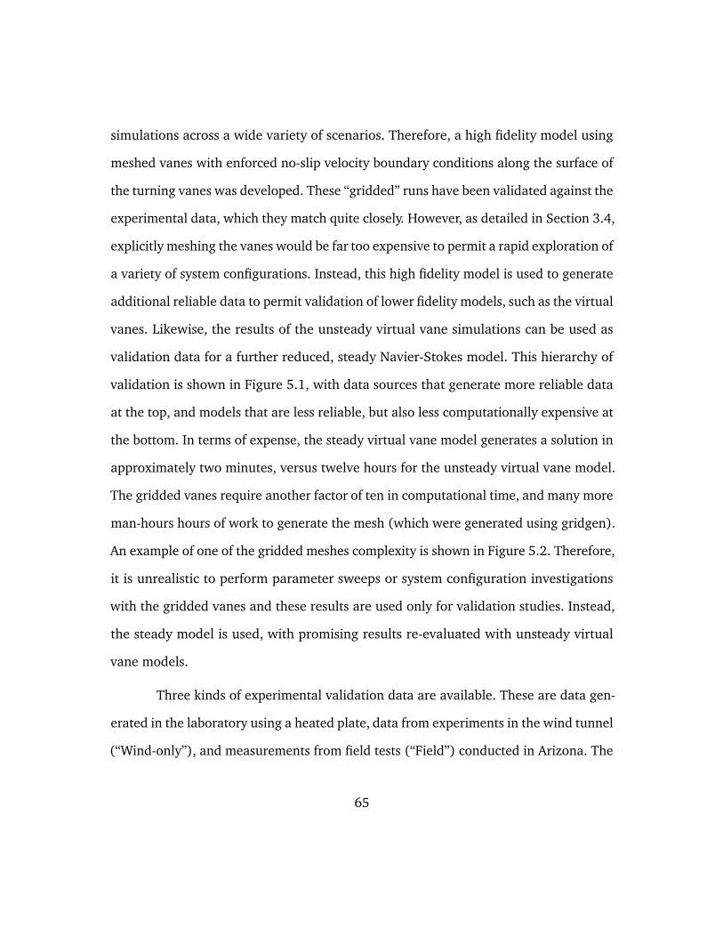
simulations across a wide variety of scenarios. Therefore, a high fidelity model using

meshed vanes with enforced no-slip velocity boundary conditions along the surface of

the turning vanes was developed. These “gridded” runs have been validated against the

experimental data, which they match quite closely. However, as detailed in Section 3.4,

explicitly meshing the vanes would be far too expensive to permit a rapid exploration of

a variety of system configurations. Instead, this high fidelity model is used to generate

additional reliable data to permit validation of lower fidelity models, such as the virtual

vanes. Likewise, the results of the unsteady virtual vane simulations can be used as

validation data for a further reduced, steady Navier-Stokes model. This hierarchy of

validation is shown in Figure 5.1, with data sources that generate more reliable data

at the top, and models that are less reliable, but also less computationally expensive at

the bottom. In terms of expense, the steady virtual vane model generates a solution in

approximately two minutes, versus twelve hours for the unsteady virtual vane model.

The gridded vanes require another factor of ten in computational time, and many more

man-hours hours of work to generate the mesh (which were generated using gridgen).

An example of one of the gridded meshes complexity is shown in Figure 5.2. Therefore,

it is unrealistic to perform parameter sweeps or system configuration investigations

with the gridded vanes and these results are used only for validation studies. Instead,

the steady model is used, with promising results re-evaluated with unsteady virtual

vane models.

Three kinds of experimental validation data are available. These are data gen-

erated in the laboratory using a heated plate, data from experiments in the wind tunnel

(“Wind-only”), and measurements from field tests (“Field”) conducted in Arizona. The

65

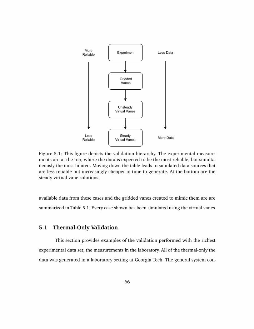
Figure 5.1: This figure depicts the validation hierarchy. The experimental measure-ments are at the top, where the data is expected to be the most reliable, but simulta-neously the most limited. Moving down the table leads to simulated data sources thatare less reliable but increasingly cheaper in time to generate. At the bottom are thesteady virtual vane solutions.

available data from these cases and the gridded vanes created to mimic them are are

summarized in Table 5.1. Every case shown has been simulated using the virtual vanes.

5.1 Thermal-Only Validation

This section provides examples of the validation performed with the richest

experimental data set, the measurements in the laboratory. All of the thermal-only the

data was generated in a laboratory setting at Georgia Tech. The general system con-

66

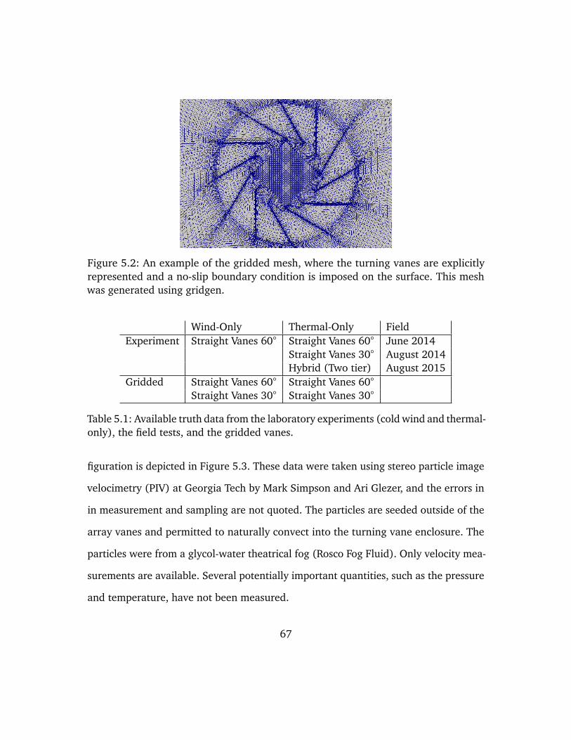
Figure 5.2: An example of the gridded mesh, where the turning vanes are explicitlyrepresented and a no-slip boundary condition is imposed on the surface. This meshwas generated using gridgen.

Wind-Only Thermal-Only FieldExperiment Straight Vanes 60 Straight Vanes 60 June 2014

Straight Vanes 30 August 2014Hybrid (Two tier) August 2015

Gridded Straight Vanes 60 Straight Vanes 60

Straight Vanes 30 Straight Vanes 30

Table 5.1: Available truth data from the laboratory experiments (cold wind and thermal-only), the field tests, and the gridded vanes.

figuration is depicted in Figure 5.3. These data were taken using stereo particle image

velocimetry (PIV) at Georgia Tech by Mark Simpson and Ari Glezer, and the errors in

in measurement and sampling are not quoted. The particles are seeded outside of the

array vanes and permitted to naturally convect into the turning vane enclosure. The

particles were from a glycol-water theatrical fog (Rosco Fog Fluid). Only velocity mea-

surements are available. Several potentially important quantities, such as the pressure

and temperature, have not been measured.

67

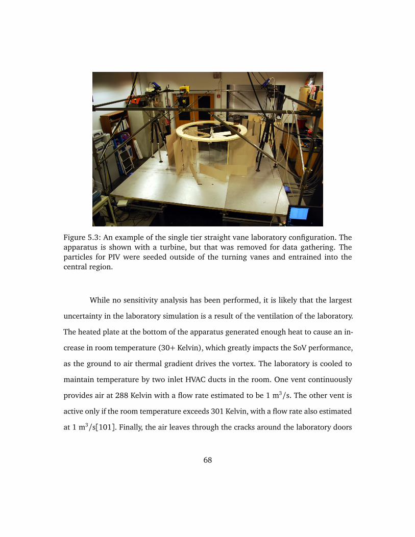
Figure 5.3: An example of the single tier straight vane laboratory configuration. Theapparatus is shown with a turbine, but that was removed for data gathering. Theparticles for PIV were seeded outside of the turning vanes and entrained into thecentral region.

While no sensitivity analysis has been performed, it is likely that the largest

uncertainty in the laboratory simulation is a result of the ventilation of the laboratory.

The heated plate at the bottom of the apparatus generated enough heat to cause an in-

crease in room temperature (30+ Kelvin), which greatly impacts the SoV performance,

as the ground to air thermal gradient drives the vortex. The laboratory is cooled to

maintain temperature by two inlet HVAC ducts in the room. One vent continuously

provides air at 288 Kelvin with a flow rate estimated to be 1 m3/s. The other vent is

active only if the room temperature exceeds 301 Kelvin, with a flow rate also estimated

at 1 m3/s[101]. Finally, the air leaves through the cracks around the laboratory doors

68

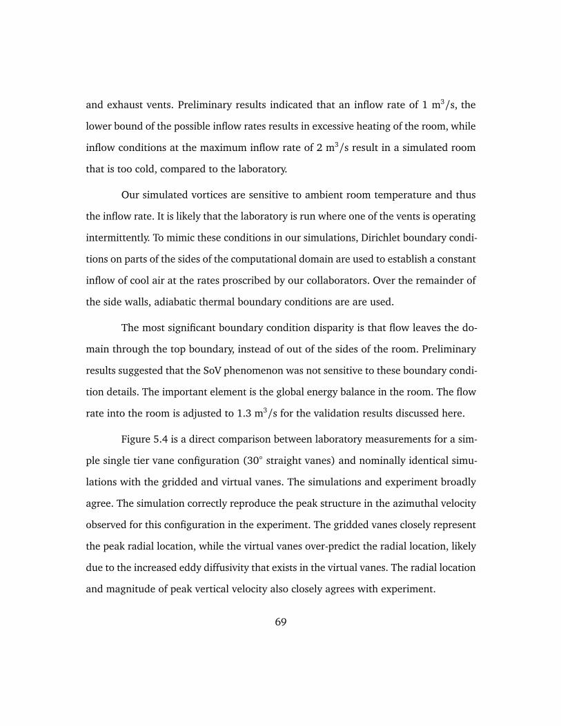
and exhaust vents. Preliminary results indicated that an inflow rate of 1 m3/s, the

lower bound of the possible inflow rates results in excessive heating of the room, while

inflow conditions at the maximum inflow rate of 2 m3/s result in a simulated room

that is too cold, compared to the laboratory.

Our simulated vortices are sensitive to ambient room temperature and thus

the inflow rate. It is likely that the laboratory is run where one of the vents is operating

intermittently. To mimic these conditions in our simulations, Dirichlet boundary condi-

tions on parts of the sides of the computational domain are used to establish a constant

inflow of cool air at the rates proscribed by our collaborators. Over the remainder of

the side walls, adiabatic thermal boundary conditions are are used.

The most significant boundary condition disparity is that flow leaves the do-

main through the top boundary, instead of out of the sides of the room. Preliminary

results suggested that the SoV phenomenon was not sensitive to these boundary condi-

tion details. The important element is the global energy balance in the room. The flow

rate into the room is adjusted to 1.3 m3/s for the validation results discussed here.

Figure 5.4 is a direct comparison between laboratory measurements for a sim-

ple single tier vane configuration (30 straight vanes) and nominally identical simu-

lations with the gridded and virtual vanes. The simulations and experiment broadly

agree. The simulation correctly reproduce the peak structure in the azimuthal velocity

observed for this configuration in the experiment. The gridded vanes closely represent

the peak radial location, while the virtual vanes over-predict the radial location, likely

due to the increased eddy diffusivity that exists in the virtual vanes. The radial location

and magnitude of peak vertical velocity also closely agrees with experiment.

69

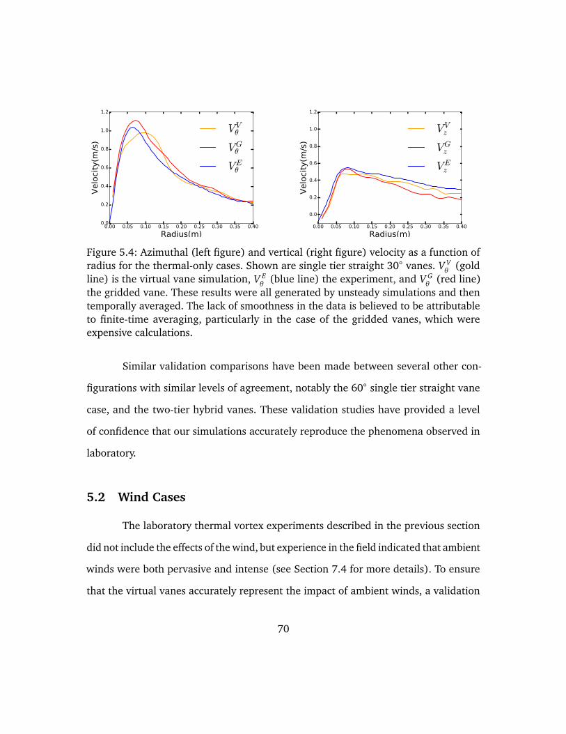
0.00 0.05 0.10 0.15 0.20 0.25 0.30 0.35 0.40

Radius(m)

0.0

0.2

0.4

0.6

0.8

1.0

1.2

Velo

city

(m/s

)

VVθ

VGθ

VEθ

0.00 0.05 0.10 0.15 0.20 0.25 0.30 0.35 0.40

Radius(m)

0.0

0.2

0.4

0.6

0.8

1.0

1.2

Velo

city

(m/s

)

VVz

VGz

VEz

Figure 5.4: Azimuthal (left figure) and vertical (right figure) velocity as a function ofradius for the thermal-only cases. Shown are single tier straight 30 vanes. V V

θ(gold

line) is the virtual vane simulation, V Eθ

(blue line) the experiment, and V Gθ

(red line)the gridded vane. These results were all generated by unsteady simulations and thentemporally averaged. The lack of smoothness in the data is believed to be attributableto finite-time averaging, particularly in the case of the gridded vanes, which wereexpensive calculations.

Similar validation comparisons have been made between several other con-

figurations with similar levels of agreement, notably the 60 single tier straight vane

case, and the two-tier hybrid vanes. These validation studies have provided a level

of confidence that our simulations accurately reproduce the phenomena observed in

laboratory.

5.2 Wind Cases

The laboratory thermal vortex experiments described in the previous section

did not include the effects of the wind, but experience in the field indicated that ambient

winds were both pervasive and intense (see Section 7.4 for more details). To ensure

that the virtual vanes accurately represent the impact of ambient winds, a validation

70

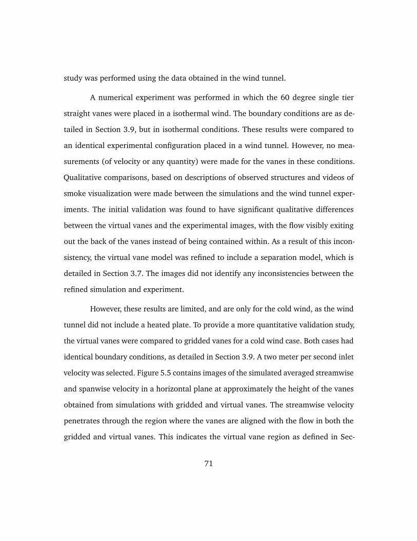
study was performed using the data obtained in the wind tunnel.

A numerical experiment was performed in which the 60 degree single tier

straight vanes were placed in a isothermal wind. The boundary conditions are as de-

tailed in Section 3.9, but in isothermal conditions. These results were compared to

an identical experimental configuration placed in a wind tunnel. However, no mea-

surements (of velocity or any quantity) were made for the vanes in these conditions.

Qualitative comparisons, based on descriptions of observed structures and videos of

smoke visualization were made between the simulations and the wind tunnel exper-

iments. The initial validation was found to have significant qualitative differences

between the virtual vanes and the experimental images, with the flow visibly exiting

out the back of the vanes instead of being contained within. As a result of this incon-

sistency, the virtual vane model was refined to include a separation model, which is

detailed in Section 3.7. The images did not identify any inconsistencies between the

refined simulation and experiment.

However, these results are limited, and are only for the cold wind, as the wind

tunnel did not include a heated plate. To provide a more quantitative validation study,

the virtual vanes were compared to gridded vanes for a cold wind case. Both cases had

identical boundary conditions, as detailed in Section 3.9. A two meter per second inlet

velocity was selected. Figure 5.5 contains images of the simulated averaged streamwise

and spanwise velocity in a horizontal plane at approximately the height of the vanes

obtained from simulations with gridded and virtual vanes. The streamwise velocity

penetrates through the region where the vanes are aligned with the flow in both the

gridded and virtual vanes. This indicates the virtual vane region as defined in Sec-

71

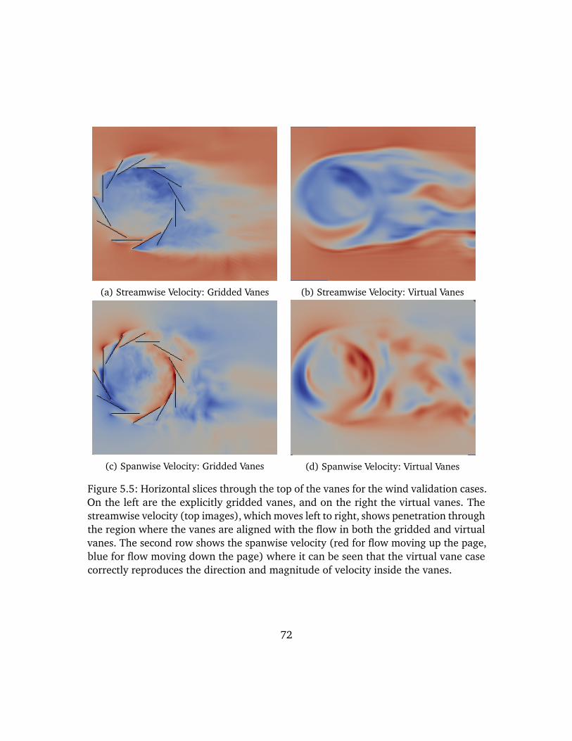
(a) Streamwise Velocity: Gridded Vanes (b) Streamwise Velocity: Virtual Vanes

(c) Spanwise Velocity: Gridded Vanes (d) Spanwise Velocity: Virtual Vanes

Figure 5.5: Horizontal slices through the top of the vanes for the wind validation cases.On the left are the explicitly gridded vanes, and on the right the virtual vanes. Thestreamwise velocity (top images), which moves left to right, shows penetration throughthe region where the vanes are aligned with the flow in both the gridded and virtualvanes. The second row shows the spanwise velocity (red for flow moving up the page,blue for flow moving down the page) where it can be seen that the virtual vane casecorrectly reproduces the direction and magnitude of velocity inside the vanes.

72

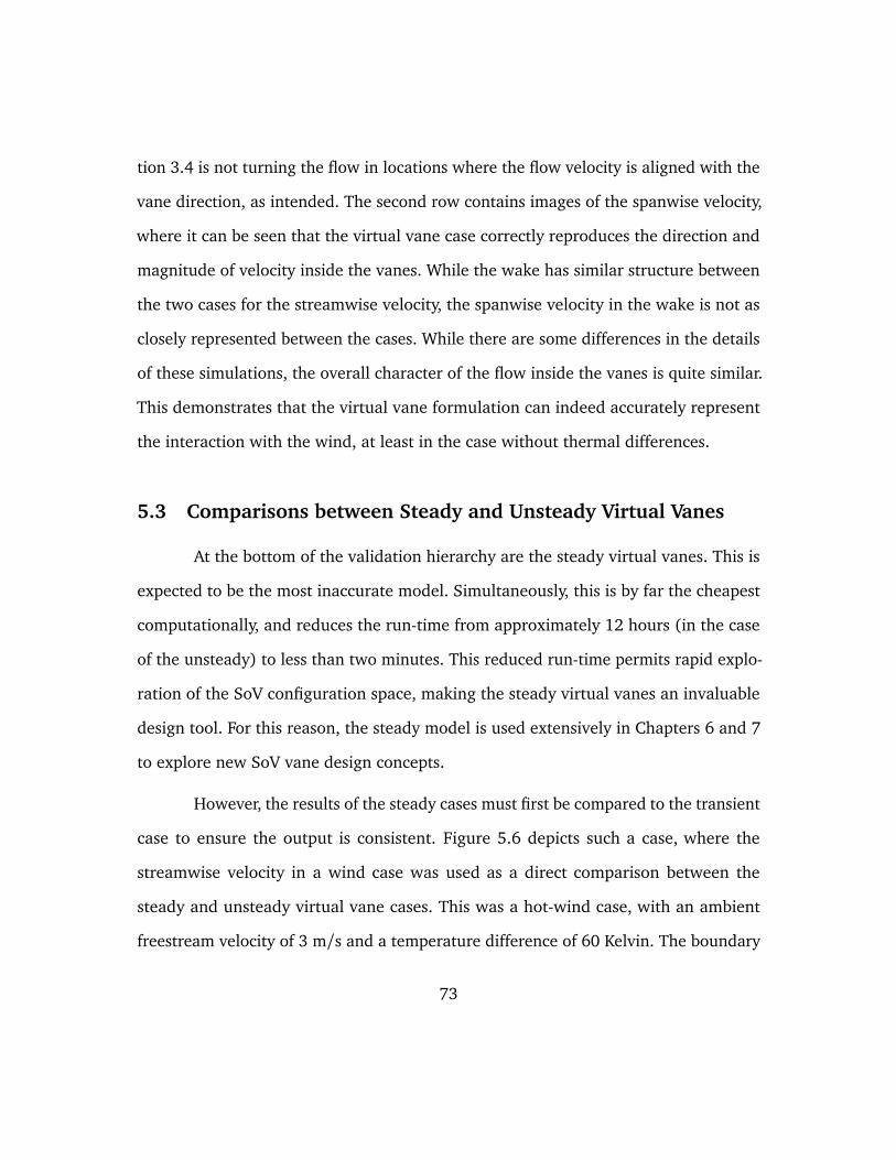
tion 3.4 is not turning the flow in locations where the flow velocity is aligned with the

vane direction, as intended. The second row contains images of the spanwise velocity,

where it can be seen that the virtual vane case correctly reproduces the direction and

magnitude of velocity inside the vanes. While the wake has similar structure between

the two cases for the streamwise velocity, the spanwise velocity in the wake is not as

closely represented between the cases. While there are some differences in the details

of these simulations, the overall character of the flow inside the vanes is quite similar.

This demonstrates that the virtual vane formulation can indeed accurately represent

the interaction with the wind, at least in the case without thermal differences.

5.3 Comparisons between Steady and Unsteady Virtual Vanes

At the bottom of the validation hierarchy are the steady virtual vanes. This is

expected to be the most inaccurate model. Simultaneously, this is by far the cheapest

computationally, and reduces the run-time from approximately 12 hours (in the case

of the unsteady) to less than two minutes. This reduced run-time permits rapid explo-

ration of the SoV configuration space, making the steady virtual vanes an invaluable

design tool. For this reason, the steady model is used extensively in Chapters 6 and 7

to explore new SoV vane design concepts.

However, the results of the steady cases must first be compared to the transient

case to ensure the output is consistent. Figure 5.6 depicts such a case, where the

streamwise velocity in a wind case was used as a direct comparison between the

steady and unsteady virtual vane cases. This was a hot-wind case, with an ambient

freestream velocity of 3 m/s and a temperature difference of 60 Kelvin. The boundary

73

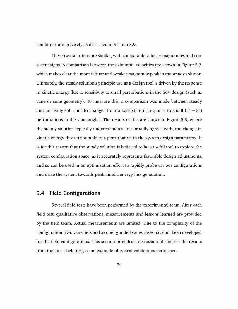
conditions are precisely as described in Section 3.9.

These two solutions are similar, with comparable velocity magnitudes and con-

sistent signs. A comparison between the azimuthal velocities are shown in Figure 5.7,

which makes clear the more diffuse and weaker magnitude peak in the steady solution.

Ultimately, the steady solution’s principle use as a design tool is driven by the response

in kinetic energy flux to sensitivity to small perturbations in the SoV design (such as

vane or cone geometry). To measure this, a comparison was made between steady

and unsteady solutions to changes from a base state in response to small (1 − 5)

perturbations in the vane angles. The results of this are shown in Figure 5.8, where

the steady solution typically underestimates, but broadly agrees with, the change in

kinetic energy flux attributable to a perturbation in the system design parameters. It

is for this reason that the steady solution is believed to be a useful tool to explore the

system configuration space, as it accurately represents favorable design adjustments,

and so can be used in an optimization effort to rapidly probe various configurations

and drive the system towards peak kinetic energy flux generation.

5.4 Field Configurations

Several field tests have been performed by the experimental team. After each

field test, qualitative observations, measurements and lessons learned are provided

by the field team. Actual measurements are limited. Due to the complexity of the

configuration (two vane tiers and a cone) gridded vanes cases have not been developed

for the field configurations. This section provides a discussion of some of the results

from the latest field test, as an example of typical validations performed.

74

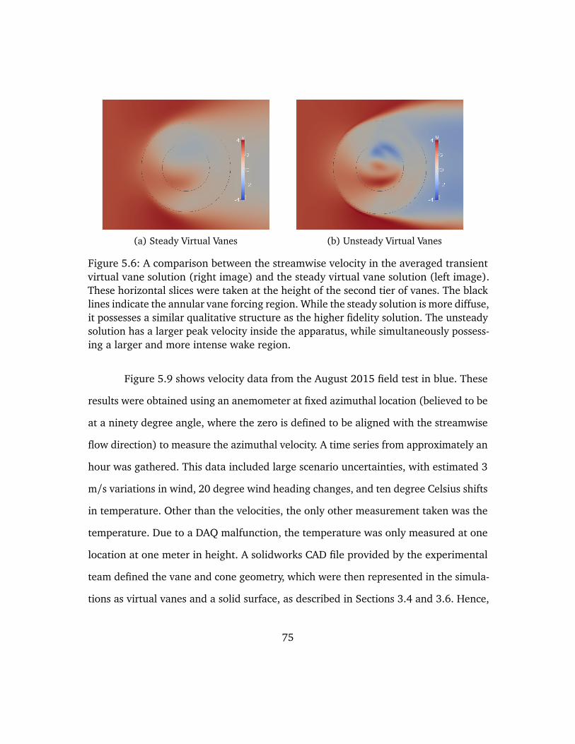
(a) Steady Virtual Vanes (b) Unsteady Virtual Vanes

Figure 5.6: A comparison between the streamwise velocity in the averaged transientvirtual vane solution (right image) and the steady virtual vane solution (left image).These horizontal slices were taken at the height of the second tier of vanes. The blacklines indicate the annular vane forcing region. While the steady solution is more diffuse,it possesses a similar qualitative structure as the higher fidelity solution. The unsteadysolution has a larger peak velocity inside the apparatus, while simultaneously possess-ing a larger and more intense wake region.

Figure 5.9 shows velocity data from the August 2015 field test in blue. These

results were obtained using an anemometer at fixed azimuthal location (believed to be

at a ninety degree angle, where the zero is defined to be aligned with the streamwise

flow direction) to measure the azimuthal velocity. A time series from approximately an

hour was gathered. This data included large scenario uncertainties, with estimated 3

m/s variations in wind, 20 degree wind heading changes, and ten degree Celsius shifts

in temperature. Other than the velocities, the only other measurement taken was the

temperature. Due to a DAQ malfunction, the temperature was only measured at one

location at one meter in height. A solidworks CAD file provided by the experimental

team defined the vane and cone geometry, which were then represented in the simula-

tions as virtual vanes and a solid surface, as described in Sections 3.4 and 3.6. Hence,

75

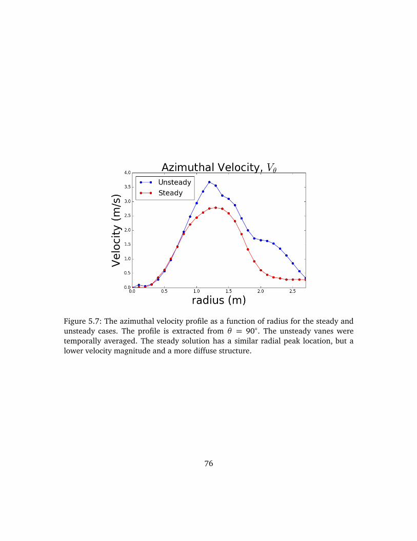
Figure 5.7: The azimuthal velocity profile as a function of radius for the steady andunsteady cases. The profile is extracted from θ = 90. The unsteady vanes weretemporally averaged. The steady solution has a similar radial peak location, but alower velocity magnitude and a more diffuse structure.

76

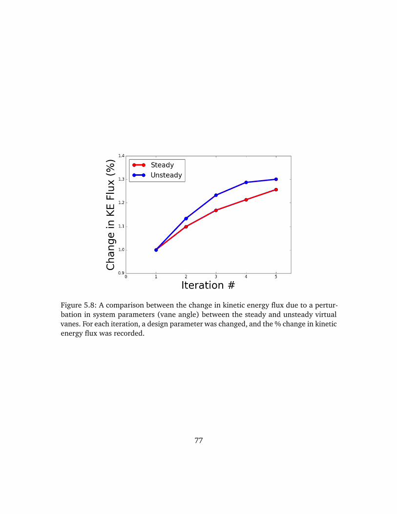
Figure 5.8: A comparison between the change in kinetic energy flux due to a pertur-bation in system parameters (vane angle) between the steady and unsteady virtualvanes. For each iteration, a design parameter was changed, and the % change in kineticenergy flux was recorded.

77

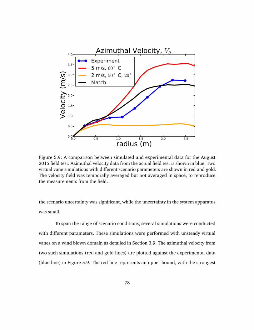
0.0 0.5 1.0 1.5 2.0 2.5

radius (m)0.0

0.5

1.0

1.5

2.0

2.5

3.0

3.5

4.0

Velo

city

(m

/s)

Azimuthal Velocity, VθExperiment

5 m/s, 60 C

2 m/s, 50 C, 20

Match

Figure 5.9: A comparison between simulated and experimental data for the August2015 field test. Azimuthal velocity data from the actual field test is shown in blue. Twovirtual vane simulations with different scenario parameters are shown in red and gold.The velocity field was temporally averaged but not averaged in space, to reproducethe measurements from the field.

the scenario uncertainty was significant, while the uncertainty in the system apparatus

was small.

To span the range of scenario conditions, several simulations were conducted

with different parameters. These simulations were performed with unsteady virtual

vanes on a wind blown domain as detailed in Section 3.9. The azimuthal velocity from

two such simulations (red and gold lines) are plotted against the experimental data

(blue line) in Figure 5.9. The red line represents an upper bound, with the strongest

78

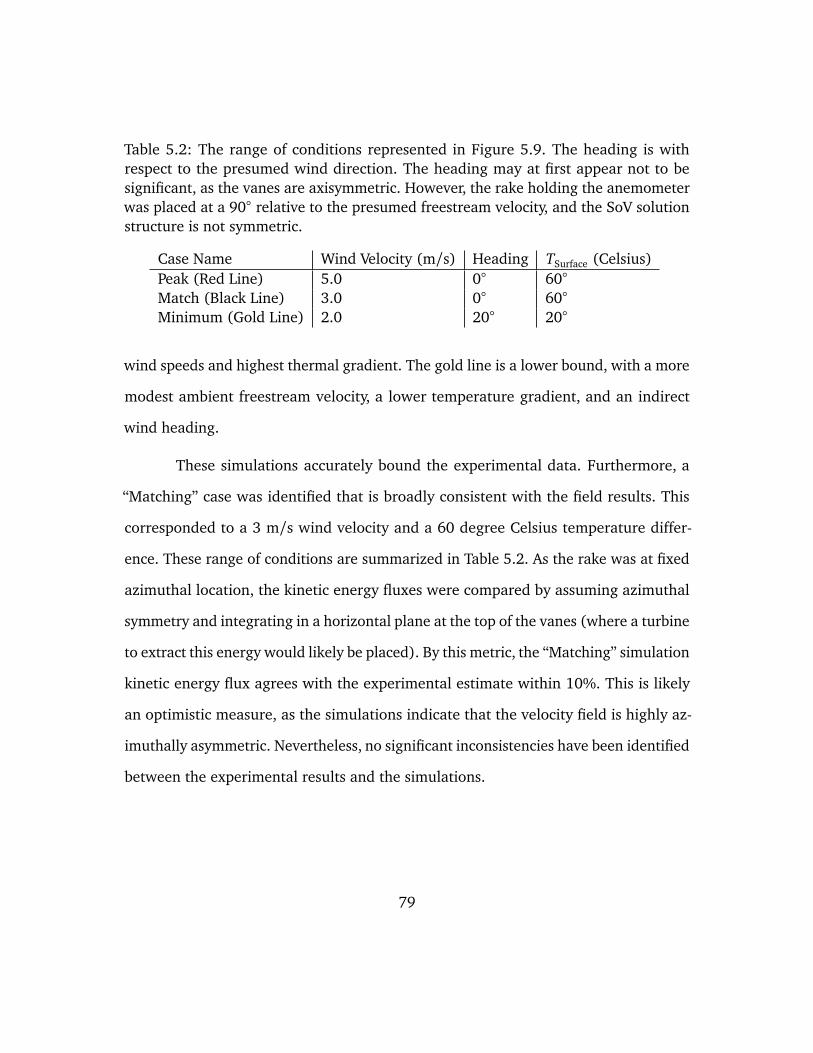
Table 5.2: The range of conditions represented in Figure 5.9. The heading is withrespect to the presumed wind direction. The heading may at first appear not to besignificant, as the vanes are axisymmetric. However, the rake holding the anemometerwas placed at a 90 relative to the presumed freestream velocity, and the SoV solutionstructure is not symmetric.

Case Name Wind Velocity (m/s) Heading TSurface (Celsius)Peak (Red Line) 5.0 0 60

Match (Black Line) 3.0 0 60

Minimum (Gold Line) 2.0 20 20

wind speeds and highest thermal gradient. The gold line is a lower bound, with a more

modest ambient freestream velocity, a lower temperature gradient, and an indirect

wind heading.

These simulations accurately bound the experimental data. Furthermore, a

“Matching” case was identified that is broadly consistent with the field results. This

corresponded to a 3 m/s wind velocity and a 60 degree Celsius temperature differ-

ence. These range of conditions are summarized in Table 5.2. As the rake was at fixed

azimuthal location, the kinetic energy fluxes were compared by assuming azimuthal

symmetry and integrating in a horizontal plane at the top of the vanes (where a turbine

to extract this energy would likely be placed). By this metric, the “Matching” simulation

kinetic energy flux agrees with the experimental estimate within 10%. This is likely

an optimistic measure, as the simulations indicate that the velocity field is highly az-

imuthally asymmetric. Nevertheless, no significant inconsistencies have been identified

between the experimental results and the simulations.

79

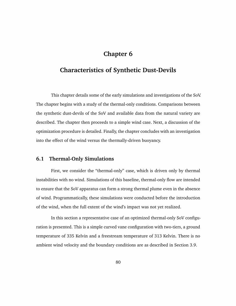
Chapter 6

Characteristics of Synthetic Dust-Devils

This chapter details some of the early simulations and investigations of the SoV.

The chapter begins with a study of the thermal-only conditions. Comparisons between

the synthetic dust-devils of the SoV and available data from the natural variety are

described. The chapter then proceeds to a simple wind case. Next, a discussion of the

optimization procedure is detailed. Finally, the chapter concludes with an investigation

into the effect of the wind versus the thermally-driven buoyancy.

6.1 Thermal-Only Simulations

First, we consider the “thermal-only” case, which is driven only by thermal

instabilities with no wind. Simulations of this baseline, thermal-only flow are intended

to ensure that the SoV apparatus can form a strong thermal plume even in the absence

of wind. Programmatically, these simulations were conducted before the introduction

of the wind, when the full extent of the wind’s impact was not yet realized.

In this section a representative case of an optimized thermal-only SoV configu-

ration is presented. This is a simple curved vane configuration with two-tiers, a ground

temperature of 335 Kelvin and a freestream temperature of 313 Kelvin. There is no

ambient wind velocity and the boundary conditions are as described in Section 3.9.

80

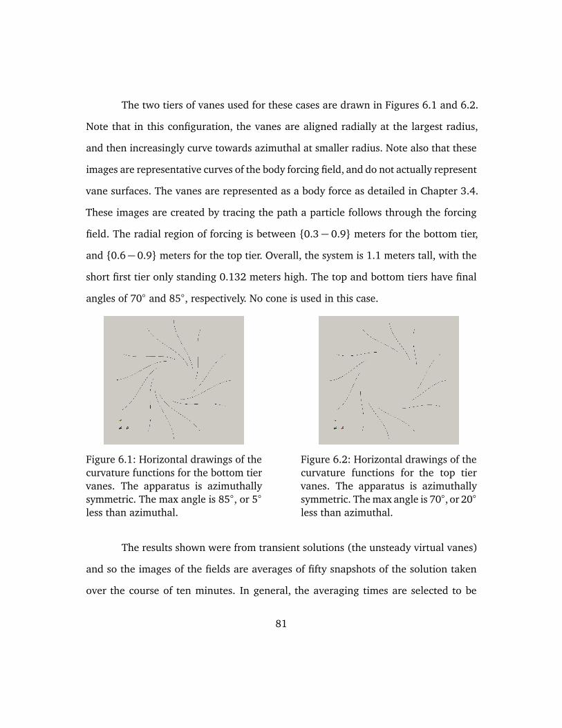
The two tiers of vanes used for these cases are drawn in Figures 6.1 and 6.2.

Note that in this configuration, the vanes are aligned radially at the largest radius,

and then increasingly curve towards azimuthal at smaller radius. Note also that these

images are representative curves of the body forcing field, and do not actually represent

vane surfaces. The vanes are represented as a body force as detailed in Chapter 3.4.

These images are created by tracing the path a particle follows through the forcing

field. The radial region of forcing is between 0.3− 0.9 meters for the bottom tier,

and 0.6− 0.9 meters for the top tier. Overall, the system is 1.1 meters tall, with the

short first tier only standing 0.132 meters high. The top and bottom tiers have final

angles of 70 and 85, respectively. No cone is used in this case.

Figure 6.1: Horizontal drawings of thecurvature functions for the bottom tiervanes. The apparatus is azimuthallysymmetric. The max angle is 85, or 5

less than azimuthal.

Figure 6.2: Horizontal drawings of thecurvature functions for the top tiervanes. The apparatus is azimuthallysymmetric. The max angle is 70, or 20

less than azimuthal.

The results shown were from transient solutions (the unsteady virtual vanes)

and so the images of the fields are averages of fifty snapshots of the solution taken

over the course of ten minutes. In general, the averaging times are selected to be

81

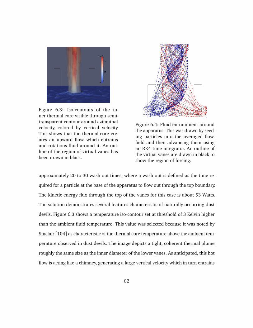
Figure 6.3: Iso-contours of the in-ner thermal core visible through semi-transparent contour around azimuthalvelocity, colored by vertical velocity.This shows that the thermal core cre-ates an upward flow, which entrainsand rotations fluid around it. An out-line of the region of virtual vanes hasbeen drawn in black.

Figure 6.4: Fluid entrainment aroundthe apparatus. This was drawn by seed-ing particles into the averaged flow-field and then advancing them usingan RK4 time integrator. An outline ofthe virtual vanes are drawn in black toshow the region of forcing.

approximately 20 to 30 wash-out times, where a wash-out is defined as the time re-

quired for a particle at the base of the apparatus to flow out through the top boundary.

The kinetic energy flux through the top of the vanes for this case is about 53 Watts.

The solution demonstrates several features characteristic of naturally occurring dust

devils. Figure 6.3 shows a temperature iso-contour set at threshold of 3 Kelvin higher

than the ambient fluid temperature. This value was selected because it was noted by

Sinclair [104] as characteristic of the thermal core temperature above the ambient tem-

perature observed in dust devils. The image depicts a tight, coherent thermal plume

roughly the same size as the inner diameter of the lower vanes. As anticipated, this hot

flow is acting like a chimney, generating a large vertical velocity which in turn entrains

82

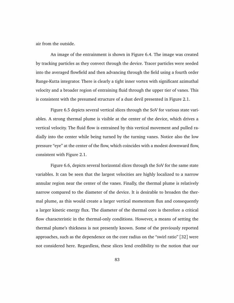
air from the outside.

An image of the entrainment is shown in Figure 6.4. The image was created

by tracking particles as they convect through the device. Tracer particles were seeded

into the averaged flowfield and then advancing through the field using a fourth order

Runge-Kutta integrator. There is clearly a tight inner vortex with significant azimuthal

velocity and a broader region of entraining fluid through the upper tier of vanes. This

is consistent with the presumed structure of a dust devil presented in Figure 2.1.

Figure 6.5 depicts several vertical slices through the SoV for various state vari-

ables. A strong thermal plume is visible at the center of the device, which drives a

vertical velocity. The fluid flow is entrained by this vertical movement and pulled ra-

dially into the center while being turned by the turning vanes. Notice also the low

pressure “eye” at the center of the flow, which coincides with a modest downward flow,

consistent with Figure 2.1.

Figure 6.6, depicts several horizontal slices through the SoV for the same state

variables. It can be seen that the largest velocities are highly localized to a narrow

annular region near the center of the vanes. Finally, the thermal plume is relatively

narrow compared to the diameter of the device. It is desirable to broaden the ther-

mal plume, as this would create a larger vertical momentum flux and consequently

a larger kinetic energy flux. The diameter of the thermal core is therefore a critical

flow characteristic in the thermal-only conditions. However, a means of setting the

thermal plume’s thickness is not presently known. Some of the previously reported

approaches, such as the dependence on the core radius on the “swirl ratio” [32] were

not considered here. Regardless, these slices lend credibility to the notion that our

83

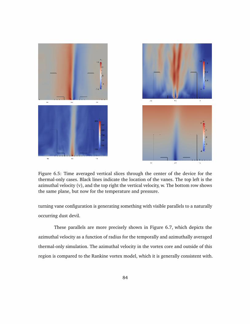
Figure 6.5: Time averaged vertical slices through the center of the device for thethermal-only cases. Black lines indicate the location of the vanes. The top left is theazimuthal velocity (v), and the top right the vertical velocity, w. The bottom row showsthe same plane, but now for the temperature and pressure.

turning vane configuration is generating something with visible parallels to a naturally

occurring dust devil.

These parallels are more precisely shown in Figure 6.7, which depicts the

azimuthal velocity as a function of radius for the temporally and azimuthally averaged

thermal-only simulation. The azimuthal velocity in the vortex core and outside of this

region is compared to the Rankine vortex model, which it is generally consistent with.

84

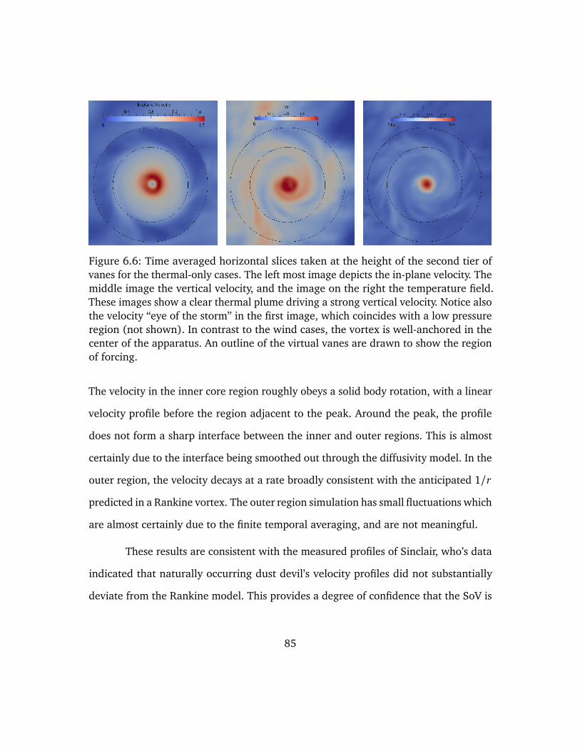
Figure 6.6: Time averaged horizontal slices taken at the height of the second tier ofvanes for the thermal-only cases. The left most image depicts the in-plane velocity. Themiddle image the vertical velocity, and the image on the right the temperature field.These images show a clear thermal plume driving a strong vertical velocity. Notice alsothe velocity “eye of the storm” in the first image, which coincides with a low pressureregion (not shown). In contrast to the wind cases, the vortex is well-anchored in thecenter of the apparatus. An outline of the virtual vanes are drawn to show the regionof forcing.

The velocity in the inner core region roughly obeys a solid body rotation, with a linear

velocity profile before the region adjacent to the peak. Around the peak, the profile

does not form a sharp interface between the inner and outer regions. This is almost

certainly due to the interface being smoothed out through the diffusivity model. In the

outer region, the velocity decays at a rate broadly consistent with the anticipated 1/r

predicted in a Rankine vortex. The outer region simulation has small fluctuations which

are almost certainly due to the finite temporal averaging, and are not meaningful.

These results are consistent with the measured profiles of Sinclair, who’s data

indicated that naturally occurring dust devil’s velocity profiles did not substantially

deviate from the Rankine model. This provides a degree of confidence that the SoV is

85

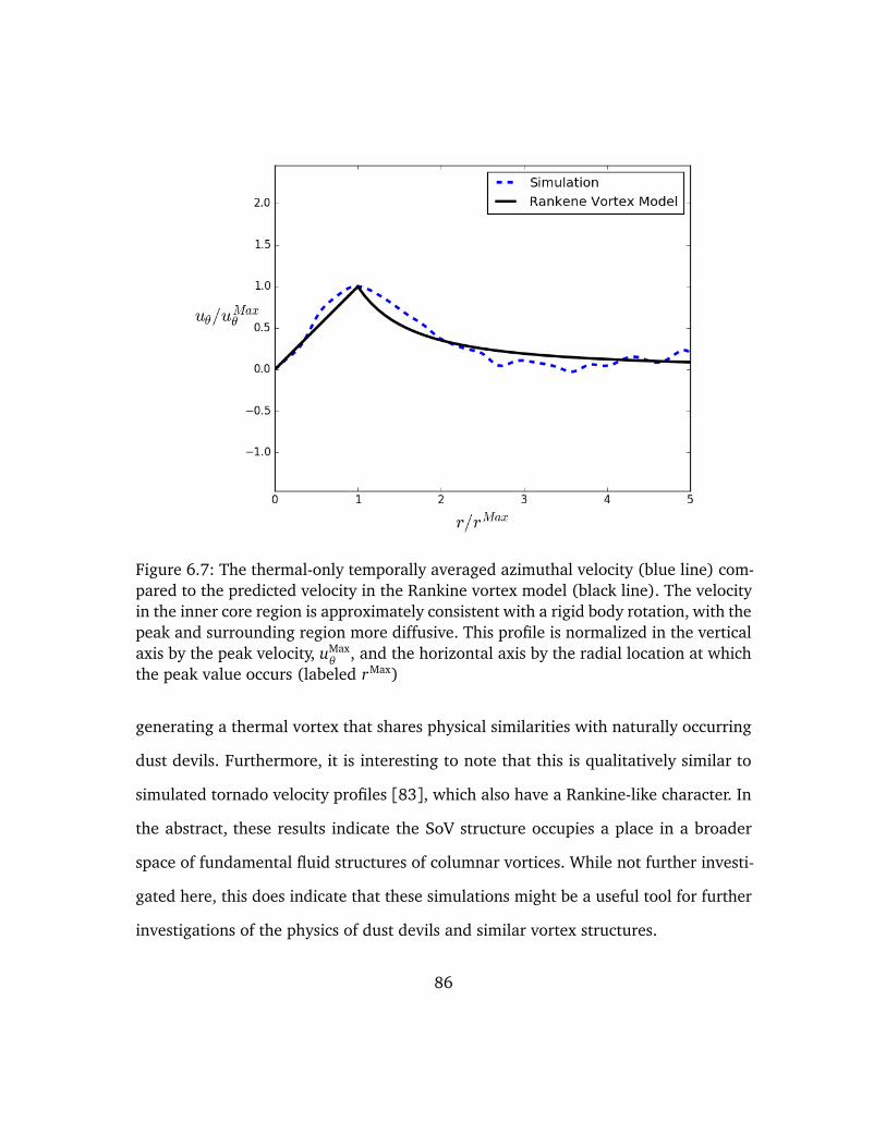
Figure 6.7: The thermal-only temporally averaged azimuthal velocity (blue line) com-pared to the predicted velocity in the Rankine vortex model (black line). The velocityin the inner core region is approximately consistent with a rigid body rotation, with thepeak and surrounding region more diffusive. This profile is normalized in the verticalaxis by the peak velocity, uMax

θ, and the horizontal axis by the radial location at which

the peak value occurs (labeled rMax)

generating a thermal vortex that shares physical similarities with naturally occurring

dust devils. Furthermore, it is interesting to note that this is qualitatively similar to

simulated tornado velocity profiles [83], which also have a Rankine-like character. In

the abstract, these results indicate the SoV structure occupies a place in a broader

space of fundamental fluid structures of columnar vortices. While not further investi-

gated here, this does indicate that these simulations might be a useful tool for further

investigations of the physics of dust devils and similar vortex structures.

86

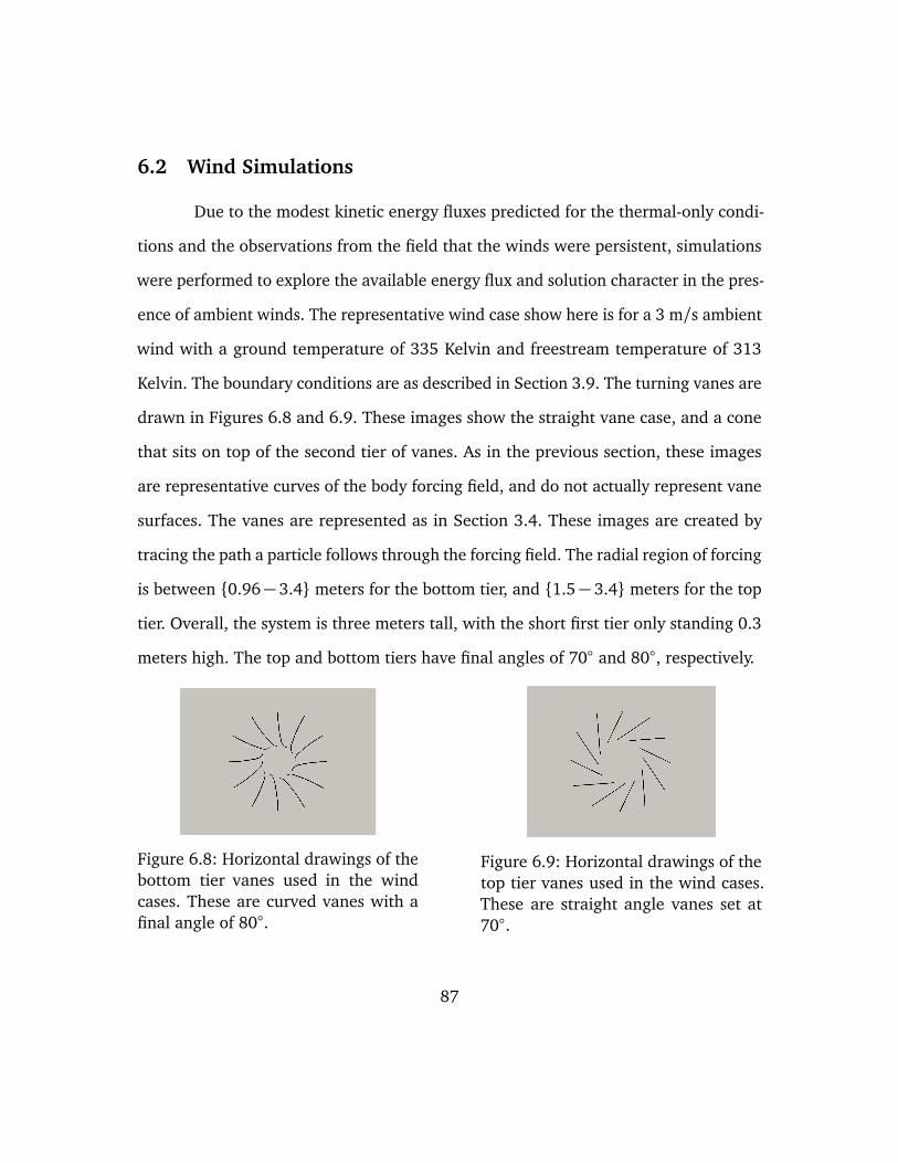
6.2 Wind Simulations

Due to the modest kinetic energy fluxes predicted for the thermal-only condi-

tions and the observations from the field that the winds were persistent, simulations

were performed to explore the available energy flux and solution character in the pres-

ence of ambient winds. The representative wind case show here is for a 3 m/s ambient

wind with a ground temperature of 335 Kelvin and freestream temperature of 313

Kelvin. The boundary conditions are as described in Section 3.9. The turning vanes are

drawn in Figures 6.8 and 6.9. These images show the straight vane case, and a cone

that sits on top of the second tier of vanes. As in the previous section, these images

are representative curves of the body forcing field, and do not actually represent vane

surfaces. The vanes are represented as in Section 3.4. These images are created by

tracing the path a particle follows through the forcing field. The radial region of forcing

is between 0.96− 3.4 meters for the bottom tier, and 1.5− 3.4 meters for the top

tier. Overall, the system is three meters tall, with the short first tier only standing 0.3

meters high. The top and bottom tiers have final angles of 70 and 80, respectively.

Figure 6.8: Horizontal drawings of thebottom tier vanes used in the windcases. These are curved vanes with afinal angle of 80.

Figure 6.9: Horizontal drawings of thetop tier vanes used in the wind cases.These are straight angle vanes set at70.

87

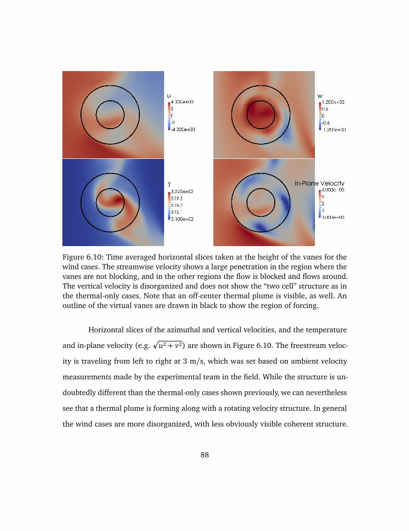
Figure 6.10: Time averaged horizontal slices taken at the height of the vanes for thewind cases. The streamwise velocity shows a large penetration in the region where thevanes are not blocking, and in the other regions the flow is blocked and flows around.The vertical velocity is disorganized and does not show the “two cell” structure as inthe thermal-only cases. Note that an off-center thermal plume is visible, as well. Anoutline of the virtual vanes are drawn in black to show the region of forcing.

Horizontal slices of the azimuthal and vertical velocities, and the temperature

and in-plane velocity (e.g.p

u2 + v2) are shown in Figure 6.10. The freestream veloc-

ity is traveling from left to right at 3 m/s, which was set based on ambient velocity

measurements made by the experimental team in the field. While the structure is un-

doubtedly different than the thermal-only cases shown previously, we can nevertheless

see that a thermal plume is forming along with a rotating velocity structure. In general

the wind cases are more disorganized, with less obviously visible coherent structure.

88

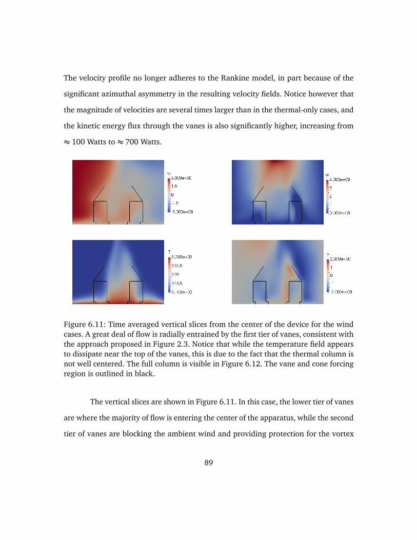
The velocity profile no longer adheres to the Rankine model, in part because of the

significant azimuthal asymmetry in the resulting velocity fields. Notice however that

the magnitude of velocities are several times larger than in the thermal-only cases, and

the kinetic energy flux through the vanes is also significantly higher, increasing from

≈ 100 Watts to ≈ 700 Watts.

Figure 6.11: Time averaged vertical slices from the center of the device for the windcases. A great deal of flow is radially entrained by the first tier of vanes, consistent withthe approach proposed in Figure 2.3. Notice that while the temperature field appearsto dissipate near the top of the vanes, this is due to the fact that the thermal column isnot well centered. The full column is visible in Figure 6.12. The vane and cone forcingregion is outlined in black.

The vertical slices are shown in Figure 6.11. In this case, the lower tier of vanes

are where the majority of flow is entering the center of the apparatus, while the second

tier of vanes are blocking the ambient wind and providing protection for the vortex

89

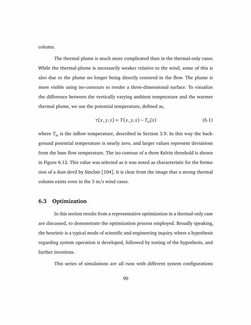
column.

The thermal plume is much more complicated than in the thermal-only cases.

While the thermal-plume is necessarily weaker relative to the wind, some of this is

also due to the plume no longer being directly centered in the flow. The plume is

more visible using iso-contours to render a three-dimensional surface. To visualize

the difference between the vertically varying ambient temperature and the warmer

thermal plume, we use the potential temperature, defined as,

τ(x , y, z) = T (x , y, z)− Tin(z) (6.1)

where Tin is the inflow temperature, described in Section 3.9. In this way the back-

ground potential temperature is nearly zero, and larger values represent deviations

from the base flow temperature. The iso-contour of a three Kelvin threshold is shown

in Figure 6.12. This value was selected as it was noted as characteristic for the forma-

tion of a dust devil by Sinclair [104]. It is clear from the image that a strong thermal

column exists even in the 3 m/s wind cases.

6.3 Optimization

In this section results from a representative optimization in a thermal-only case

are discussed, to demonstrate the optimization process employed. Broadly speaking,

the heuristic is a typical mode of scientific and engineering inquiry, where a hypothesis

regarding system operation is developed, followed by testing of the hypothesis, and

further iterations.

This series of simulations are all runs with different system configurations

90

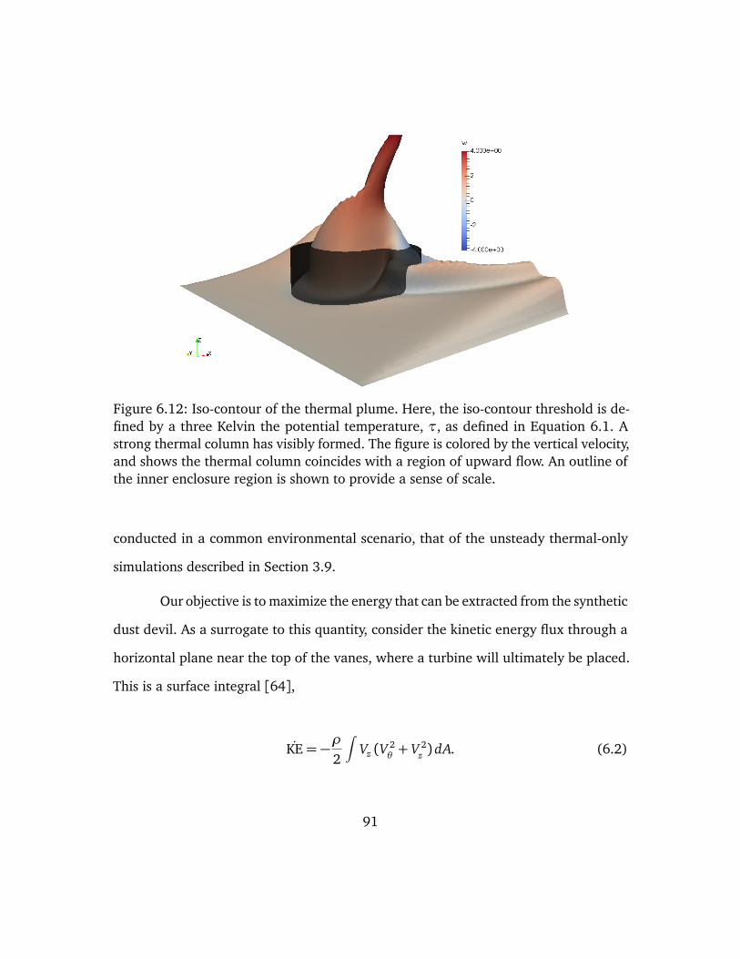
Figure 6.12: Iso-contour of the thermal plume. Here, the iso-contour threshold is de-fined by a three Kelvin the potential temperature, τ, as defined in Equation 6.1. Astrong thermal column has visibly formed. The figure is colored by the vertical velocity,and shows the thermal column coincides with a region of upward flow. An outline ofthe inner enclosure region is shown to provide a sense of scale.

conducted in a common environmental scenario, that of the unsteady thermal-only

simulations described in Section 3.9.

Our objective is to maximize the energy that can be extracted from the synthetic

dust devil. As a surrogate to this quantity, consider the kinetic energy flux through a

horizontal plane near the top of the vanes, where a turbine will ultimately be placed.

This is a surface integral [64],

KE= −ρ

2

∫Vz (V

2θ+ V 2

z ) dA. (6.2)

91

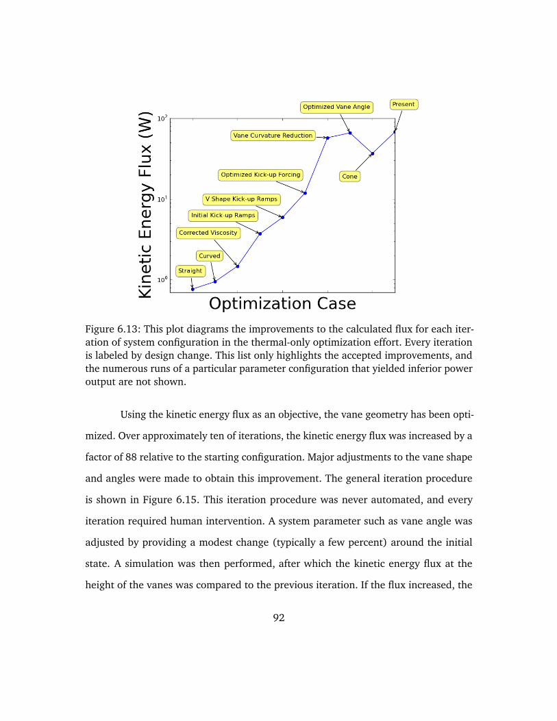
Figure 6.13: This plot diagrams the improvements to the calculated flux for each iter-ation of system configuration in the thermal-only optimization effort. Every iterationis labeled by design change. This list only highlights the accepted improvements, andthe numerous runs of a particular parameter configuration that yielded inferior poweroutput are not shown.

Using the kinetic energy flux as an objective, the vane geometry has been opti-

mized. Over approximately ten of iterations, the kinetic energy flux was increased by a

factor of 88 relative to the starting configuration. Major adjustments to the vane shape

and angles were made to obtain this improvement. The general iteration procedure

is shown in Figure 6.15. This iteration procedure was never automated, and every

iteration required human intervention. A system parameter such as vane angle was

adjusted by providing a modest change (typically a few percent) around the initial

state. A simulation was then performed, after which the kinetic energy flux at the

height of the vanes was compared to the previous iteration. If the flux increased, the

92

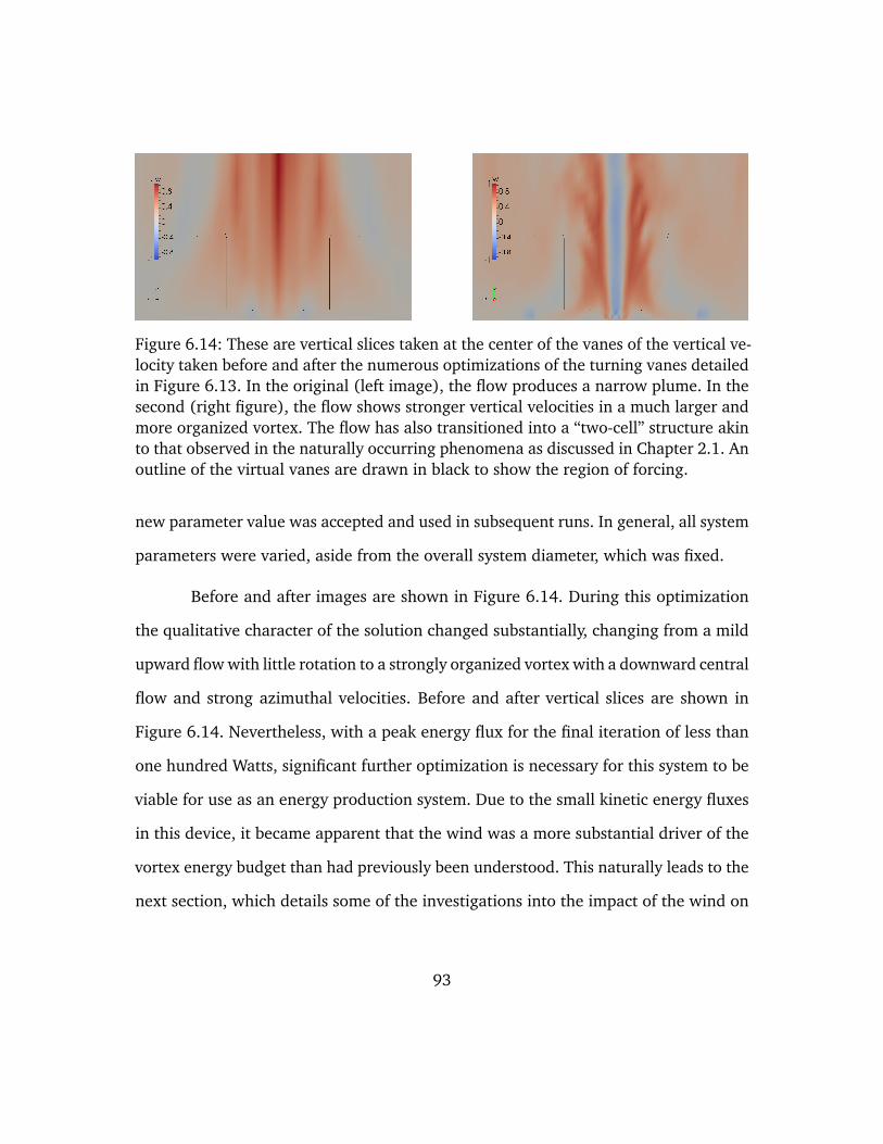
Figure 6.14: These are vertical slices taken at the center of the vanes of the vertical ve-locity taken before and after the numerous optimizations of the turning vanes detailedin Figure 6.13. In the original (left image), the flow produces a narrow plume. In thesecond (right figure), the flow shows stronger vertical velocities in a much larger andmore organized vortex. The flow has also transitioned into a “two-cell” structure akinto that observed in the naturally occurring phenomena as discussed in Chapter 2.1. Anoutline of the virtual vanes are drawn in black to show the region of forcing.

new parameter value was accepted and used in subsequent runs. In general, all system

parameters were varied, aside from the overall system diameter, which was fixed.

Before and after images are shown in Figure 6.14. During this optimization

the qualitative character of the solution changed substantially, changing from a mild

upward flow with little rotation to a strongly organized vortex with a downward central

flow and strong azimuthal velocities. Before and after vertical slices are shown in

Figure 6.14. Nevertheless, with a peak energy flux for the final iteration of less than

one hundred Watts, significant further optimization is necessary for this system to be

viable for use as an energy production system. Due to the small kinetic energy fluxes

in this device, it became apparent that the wind was a more substantial driver of the

vortex energy budget than had previously been understood. This naturally leads to the

next section, which details some of the investigations into the impact of the wind on

93

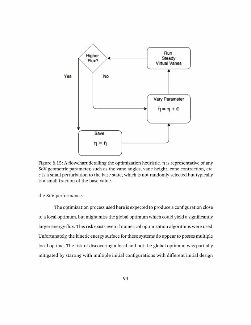
Figure 6.15: A flowchart detailing the optimization heuristic. η is representative of anySoV geometric parameter, such as the vane angles, vane height, cone contraction, etc.ε is a small perturbation to the base state, which is not randomly selected but typicallyis a small fraction of the base value.

the SoV performance.

The optimization process used here is expected to produce a configuration close

to a local optimum, but might miss the global optimum which could yield a significantly

larger energy flux. This risk exists even if numerical optimization algorithms were used.

Unfortunately, the kinetic energy surface for these systems do appear to posses multiple

local optima. The risk of discovering a local and not the global optimum was partially

mitigated by starting with multiple initial configurations with different initial design

94

parameters. However, typically this was performed only a handful of times for each

configuration, and the variation in the initial state of the parameters was arbitrary.

6.4 The Effect of the Wind

An important question throughout this work is: to what extent does the wind

drive the kinetic energy flux through the SoV device? At the same time, it is not in-

tended for the SoV to be a direct competitor to convention wind turbines, where the

device is entirely driven by kinetic energy from ambient winds which drive a verti-

cal axes (instead of the horizontal axis turbines more typically used in conventional

wind turbines). It is expected that the buoyancy contributed by the heated ground also

plays a critical role in the formation and sustainment of the synthetic dust devils, just

as it is necessary in the natural phenomenon. At the same time, as was discussed in

Section 6.3, the kinetic energy flux through an optimized device in the thermal-only

conditions with no ambient winds never attains a magnitude that would make the

device practical. Furthermore, the kinetic energy flux in the thermal-only conditions

is substantially lower than estimated in the naturally occurring phenomenon, perhaps

indicating that these natural vortices are driven by additional energy sources, namely,

ambient winds. This section represents a more systematic investigation into the role

of the wind in the present SoV device.

Figure 6.16 shows two simulated wind cases, both using the geometry and

boundary conditions described in Section 6.2. The first case is where the wind is also

accompanied by a heated surface (solid blue line, labeled “hot wind”), while in the

other case the flow has no temperature variations (dashed green line, the “cold wind”).

95

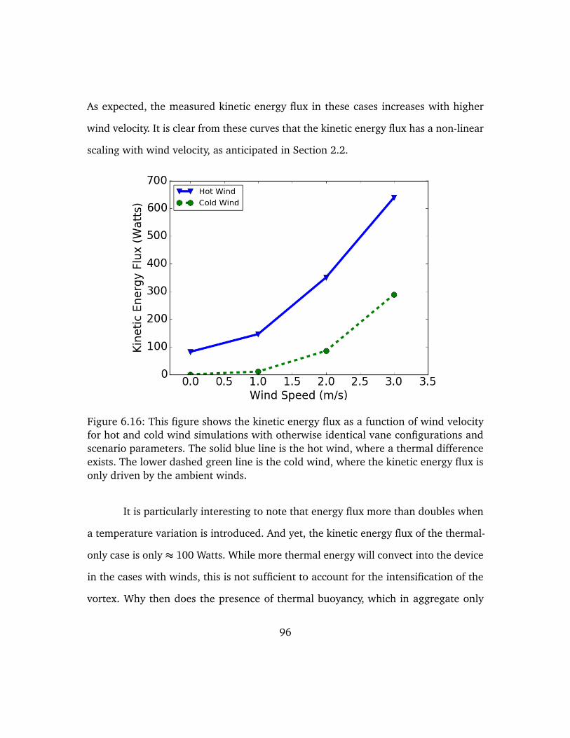
As expected, the measured kinetic energy flux in these cases increases with higher

wind velocity. It is clear from these curves that the kinetic energy flux has a non-linear

scaling with wind velocity, as anticipated in Section 2.2.

Figure 6.16: This figure shows the kinetic energy flux as a function of wind velocityfor hot and cold wind simulations with otherwise identical vane configurations andscenario parameters. The solid blue line is the hot wind, where a thermal differenceexists. The lower dashed green line is the cold wind, where the kinetic energy flux isonly driven by the ambient winds.

It is particularly interesting to note that energy flux more than doubles when

a temperature variation is introduced. And yet, the kinetic energy flux of the thermal-

only case is only ≈ 100 Watts. While more thermal energy will convect into the device

in the cases with winds, this is not sufficient to account for the intensification of the

vortex. Why then does the presence of thermal buoyancy, which in aggregate only

96

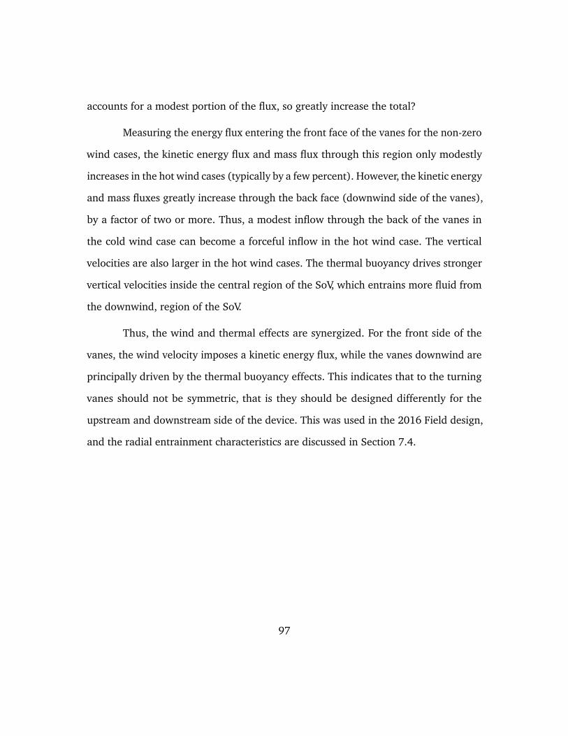
accounts for a modest portion of the flux, so greatly increase the total?

Measuring the energy flux entering the front face of the vanes for the non-zero

wind cases, the kinetic energy flux and mass flux through this region only modestly

increases in the hot wind cases (typically by a few percent). However, the kinetic energy

and mass fluxes greatly increase through the back face (downwind side of the vanes),

by a factor of two or more. Thus, a modest inflow through the back of the vanes in

the cold wind case can become a forceful inflow in the hot wind case. The vertical

velocities are also larger in the hot wind cases. The thermal buoyancy drives stronger

vertical velocities inside the central region of the SoV, which entrains more fluid from

the downwind, region of the SoV.

Thus, the wind and thermal effects are synergized. For the front side of the

vanes, the wind velocity imposes a kinetic energy flux, while the vanes downwind are

principally driven by the thermal buoyancy effects. This indicates that to the turning

vanes should not be symmetric, that is they should be designed differently for the

upstream and downstream side of the device. This was used in the 2016 Field design,

and the radial entrainment characteristics are discussed in Section 7.4.

97

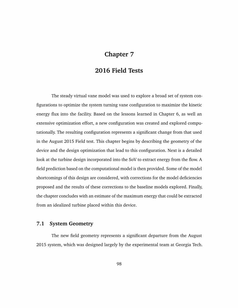
Chapter 7

2016 Field Tests

The steady virtual vane model was used to explore a broad set of system con-

figurations to optimize the system turning vane configuration to maximize the kinetic

energy flux into the facility. Based on the lessons learned in Chapter 6, as well an

extensive optimization effort, a new configuration was created and explored compu-

tationally. The resulting configuration represents a significant change from that used

in the August 2015 Field test. This chapter begins by describing the geometry of the

device and the design optimization that lead to this configuration. Next is a detailed

look at the turbine design incorporated into the SoV to extract energy from the flow. A

field prediction based on the computational model is then provided. Some of the model

shortcomings of this design are considered, with corrections for the model deficiencies

proposed and the results of these corrections to the baseline models explored. Finally,

the chapter concludes with an estimate of the maximum energy that could be extracted

from an idealized turbine placed within this device.

7.1 System Geometry

The new field geometry represents a significant departure from the August

2015 system, which was designed largely by the experimental team at Georgia Tech.

98

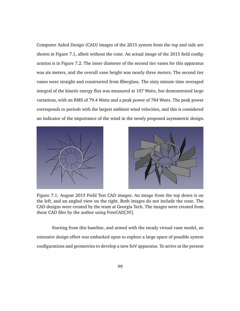
Computer Aided Design (CAD) images of the 2015 system from the top and side are

shown in Figure 7.1, albeit without the cone. An actual image of the 2015 field config-

uration is in Figure 7.2. The inner diameter of the second tier vanes for this apparatus

was six meters, and the overall vane height was nearly three meters. The second tier

vanes were straight and constructed from fiberglass. The sixty minute time averaged

integral of the kinetic energy flux was measured at 107 Watts, but demonstrated large

variations, with an RMS of 79.4 Watts and a peak power of 784 Watts. The peak power

corresponds to periods with the largest ambient wind velocities, and this is considered

an indicator of the importance of the wind in the newly proposed asymmetric design.

Figure 7.1: August 2015 Field Test CAD images. An image from the top down is onthe left, and an angled view on the right. Both images do not include the cone. TheCAD designs were created by the team at Georgia Tech. The images were created fromthese CAD files by the author using FreeCAD[39].

Starting from this baseline, and armed with the steady virtual vane model, an

extensive design effort was embarked upon to explore a large space of possible system

configurations and geometries to develop a new SoV apparatus. To arrive at the present

99

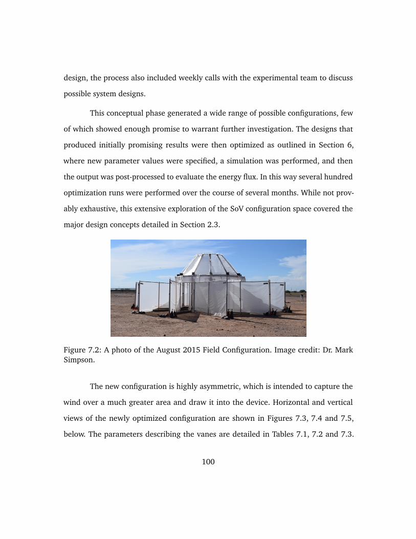
design, the process also included weekly calls with the experimental team to discuss

possible system designs.

This conceptual phase generated a wide range of possible configurations, few

of which showed enough promise to warrant further investigation. The designs that

produced initially promising results were then optimized as outlined in Section 6,

where new parameter values were specified, a simulation was performed, and then

the output was post-processed to evaluate the energy flux. In this way several hundred

optimization runs were performed over the course of several months. While not prov-

ably exhaustive, this extensive exploration of the SoV configuration space covered the

major design concepts detailed in Section 2.3.

Figure 7.2: A photo of the August 2015 Field Configuration. Image credit: Dr. MarkSimpson.

The new configuration is highly asymmetric, which is intended to capture the

wind over a much greater area and draw it into the device. Horizontal and vertical

views of the newly optimized configuration are shown in Figures 7.3, 7.4 and 7.5,

below. The parameters describing the vanes are detailed in Tables 7.1, 7.2 and 7.3.

100

This design does have some notable similarities to the previous iterations. It retains the

two-tier design outlined Section 2.3. The inner diameter of the 2nd tier vanes remains

six meters, and the bottom tier is much shorter than the second tier. A brief summary

of the differences are provided below:

• The bottom tier vanes are taller than in the previous field test, and their height

is asymmetric, with taller vanes on the down-wind side

• An impermeable cylinder was introduced along the arc π < θ < 0, e.g. the bot-

tom two quadrants in the images below, replacing the vanes in those quadrants.

• The upper tier vanes were configured to align with the freestream velocity, to

provide a larger wind-driven flux into the facility.

• Horizontal partitions were added to the top of the upper vanes, to prevent flow

in the vanes from rising up and out of the vanes

• The cone is taller providing a greater contraction

We now discuss each of these changes in detail. Simulations indicated that

the bottom tier vanes were too short, and were constricting the flow through them.

Originally, the height of the lower tier vanes was set based on the thickness of the ther-

mal boundary layer, but the original boundary layer inside the vanes was considerably

thicker than measurements indicated. This is presumed to be a result of the convection

of ground-heated air into the device by ambient winds and the strong radial entrain-

ment by the vortex. If true, then a shorter first tier is a substantial impediment to the

101

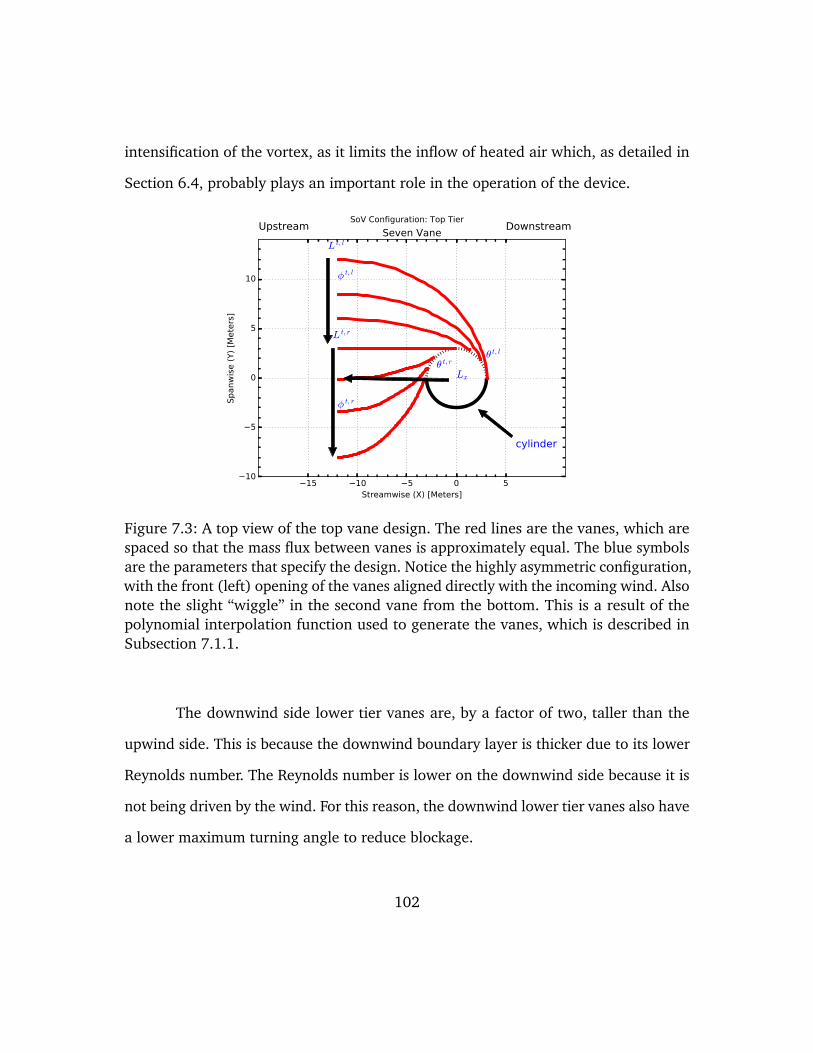
intensification of the vortex, as it limits the inflow of heated air which, as detailed in

Section 6.4, probably plays an important role in the operation of the device.

15 10 5 0 5Streamwise (X) [Meters]

10

5

0

5

10

Spanw

ise (

Y)

[Mete

rs]

Upstream Downstream

θ t, rθ t, l

φ t, r

φ t, l

Lx

cylinder

L t, r

L t, lSeven Vane

SoV Configuration: Top Tier

Figure 7.3: A top view of the top vane design. The red lines are the vanes, which arespaced so that the mass flux between vanes is approximately equal. The blue symbolsare the parameters that specify the design. Notice the highly asymmetric configuration,with the front (left) opening of the vanes aligned directly with the incoming wind. Alsonote the slight “wiggle” in the second vane from the bottom. This is a result of thepolynomial interpolation function used to generate the vanes, which is described inSubsection 7.1.1.

The downwind side lower tier vanes are, by a factor of two, taller than the

upwind side. This is because the downwind boundary layer is thicker due to its lower

Reynolds number. The Reynolds number is lower on the downwind side because it is

not being driven by the wind. For this reason, the downwind lower tier vanes also have

a lower maximum turning angle to reduce blockage.

102

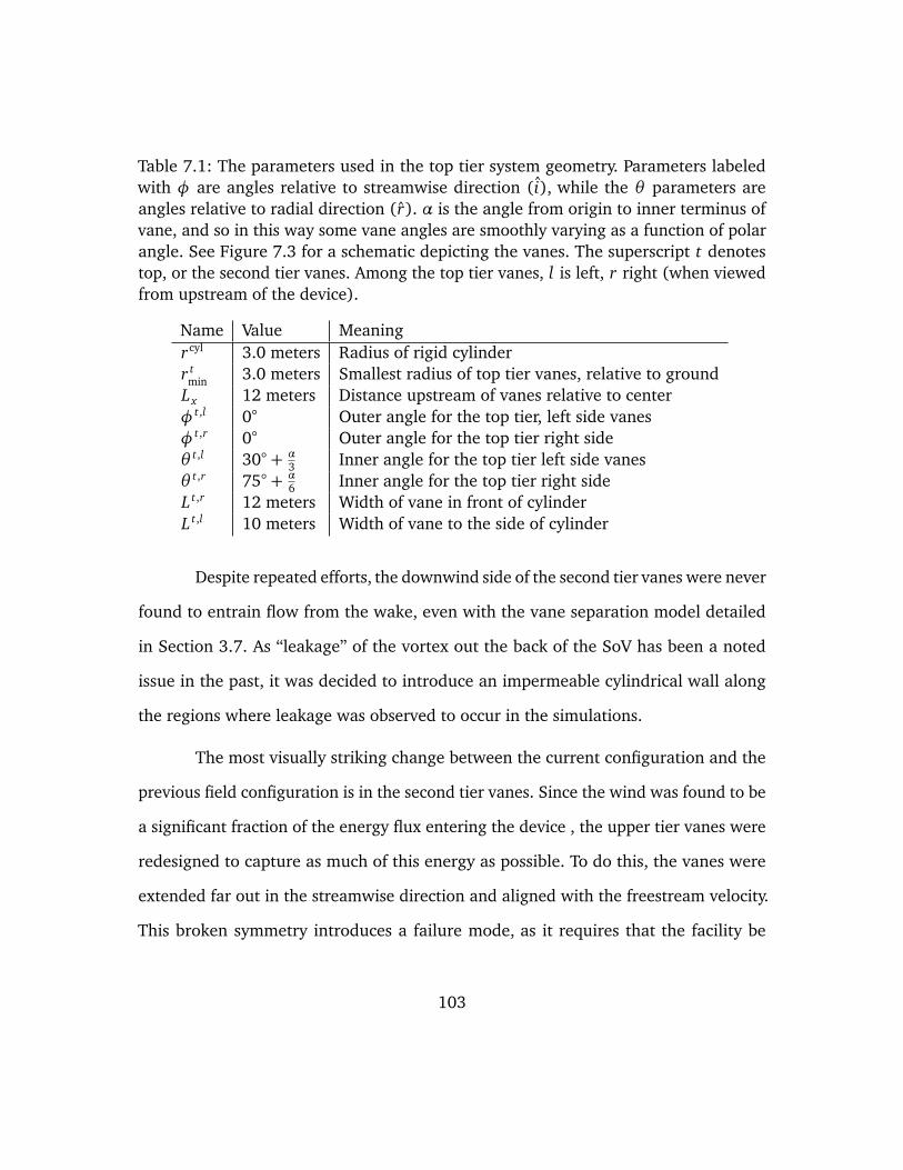
Table 7.1: The parameters used in the top tier system geometry. Parameters labeledwith φ are angles relative to streamwise direction (i), while the θ parameters areangles relative to radial direction (r). α is the angle from origin to inner terminus ofvane, and so in this way some vane angles are smoothly varying as a function of polarangle. See Figure 7.3 for a schematic depicting the vanes. The superscript t denotestop, or the second tier vanes. Among the top tier vanes, l is left, r right (when viewedfrom upstream of the device).

Name Value Meaningrcyl 3.0 meters Radius of rigid cylinderr t

min 3.0 meters Smallest radius of top tier vanes, relative to groundLx 12 meters Distance upstream of vanes relative to centerφ t,l 0 Outer angle for the top tier, left side vanesφ t,r 0 Outer angle for the top tier right sideθ t,l 30 + α

3 Inner angle for the top tier left side vanesθ t,r 75 + α

6 Inner angle for the top tier right sideL t,r 12 meters Width of vane in front of cylinderL t,l 10 meters Width of vane to the side of cylinder

Despite repeated efforts, the downwind side of the second tier vanes were never

found to entrain flow from the wake, even with the vane separation model detailed

in Section 3.7. As “leakage” of the vortex out the back of the SoV has been a noted

issue in the past, it was decided to introduce an impermeable cylindrical wall along

the regions where leakage was observed to occur in the simulations.

The most visually striking change between the current configuration and the

previous field configuration is in the second tier vanes. Since the wind was found to be

a significant fraction of the energy flux entering the device , the upper tier vanes were

redesigned to capture as much of this energy as possible. To do this, the vanes were

extended far out in the streamwise direction and aligned with the freestream velocity.

This broken symmetry introduces a failure mode, as it requires that the facility be

103

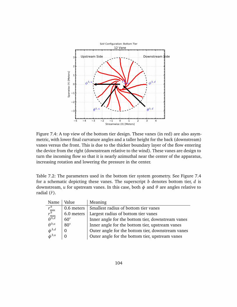
5 4 3 2 1 0 1 2 3 4Streamwise (X) [Meters]

3

2

1

0

1

2

3

Spanw

ise (

Y)

[Mete

rs]

Upstream Side Downstream Side

φ b, u φ b, d

θ b, u θ b, d

rbmax

12 VaneSoV Configuration: Bottom Tier

Figure 7.4: A top view of the bottom tier design. These vanes (in red) are also asym-metric, with lower final curvature angles and a taller height for the back (downstream)vanes versus the front. This is due to the thicker boundary layer of the flow enteringthe device from the right (downstream relative to the wind). These vanes are design toturn the incoming flow so that it is nearly azimuthal near the center of the apparatus,increasing rotation and lowering the pressure in the center.

Table 7.2: The parameters used in the bottom tier system geometry. See Figure 7.4for a schematic depicting these vanes. The superscript b denotes bottom tier, d isdownstream, u for upstream vanes. In this case, both φ and θ are angles relative toradial (r).

Name Value Meaningr b

min 0.6 meters Smallest radius of bottom tier vanesr b

max 6.0 meters Largest radius of bottom tier vanesθ b,d 60 Inner angle for the bottom tier, downstream vanesθ b,u 80 Inner angle for the bottom tier, upstream vanesφb,d 0 Outer angle for the bottom tier, downstream vanesφb,u 0 Outer angle for the bottom tier, upstream vanes

104

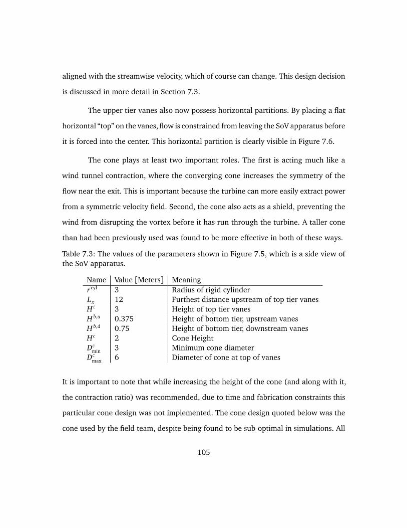
aligned with the streamwise velocity, which of course can change. This design decision

is discussed in more detail in Section 7.3.

The upper tier vanes also now possess horizontal partitions. By placing a flat

horizontal “top” on the vanes, flow is constrained from leaving the SoV apparatus before

it is forced into the center. This horizontal partition is clearly visible in Figure 7.6.

The cone plays at least two important roles. The first is acting much like a

wind tunnel contraction, where the converging cone increases the symmetry of the

flow near the exit. This is important because the turbine can more easily extract power

from a symmetric velocity field. Second, the cone also acts as a shield, preventing the

wind from disrupting the vortex before it has run through the turbine. A taller cone

than had been previously used was found to be more effective in both of these ways.

Table 7.3: The values of the parameters shown in Figure 7.5, which is a side view ofthe SoV apparatus.

Name Value [Meters] Meaningrcyl 3 Radius of rigid cylinderLx 12 Furthest distance upstream of top tier vanesH t 3 Height of top tier vanesH b,u 0.375 Height of bottom tier, upstream vanesH b,d 0.75 Height of bottom tier, downstream vanesH c 2 Cone HeightDc

min 3 Minimum cone diameterDc

max 6 Diameter of cone at top of vanes

It is important to note that while increasing the height of the cone (and along with it,

the contraction ratio) was recommended, due to time and fabrication constraints this

particular cone design was not implemented. The cone design quoted below was the

cone used by the field team, despite being found to be sub-optimal in simulations. All

105

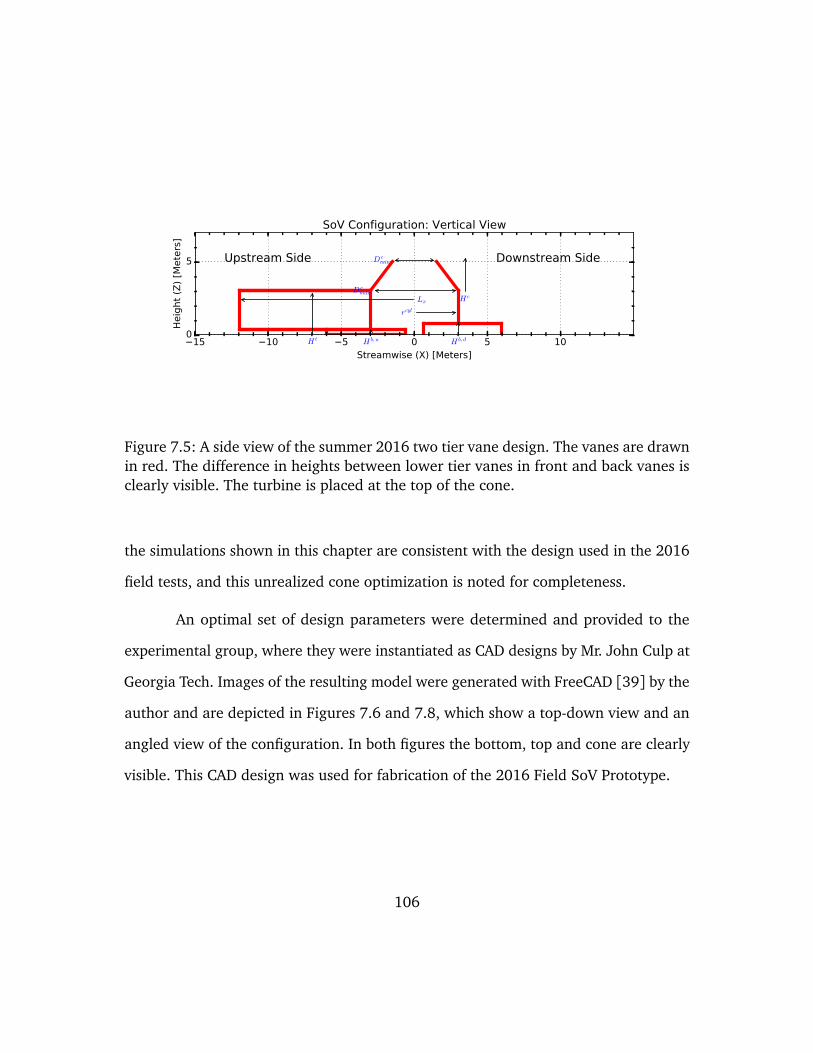
15 10 5 0 5 10Streamwise (X) [Meters]

0

5

Heig

ht

(Z)

[Mete

rs]

Upstream Side Downstream Side

Lx

rcyl

H t H b, u H b, d

H c

D cmin

D cmax

SoV Configuration: Vertical View

Figure 7.5: A side view of the summer 2016 two tier vane design. The vanes are drawnin red. The difference in heights between lower tier vanes in front and back vanes isclearly visible. The turbine is placed at the top of the cone.

the simulations shown in this chapter are consistent with the design used in the 2016

field tests, and this unrealized cone optimization is noted for completeness.

An optimal set of design parameters were determined and provided to the

experimental group, where they were instantiated as CAD designs by Mr. John Culp at

Georgia Tech. Images of the resulting model were generated with FreeCAD [39] by the

author and are depicted in Figures 7.6 and 7.8, which show a top-down view and an

angled view of the configuration. In both figures the bottom, top and cone are clearly

visible. This CAD design was used for fabrication of the 2016 Field SoV Prototype.

106

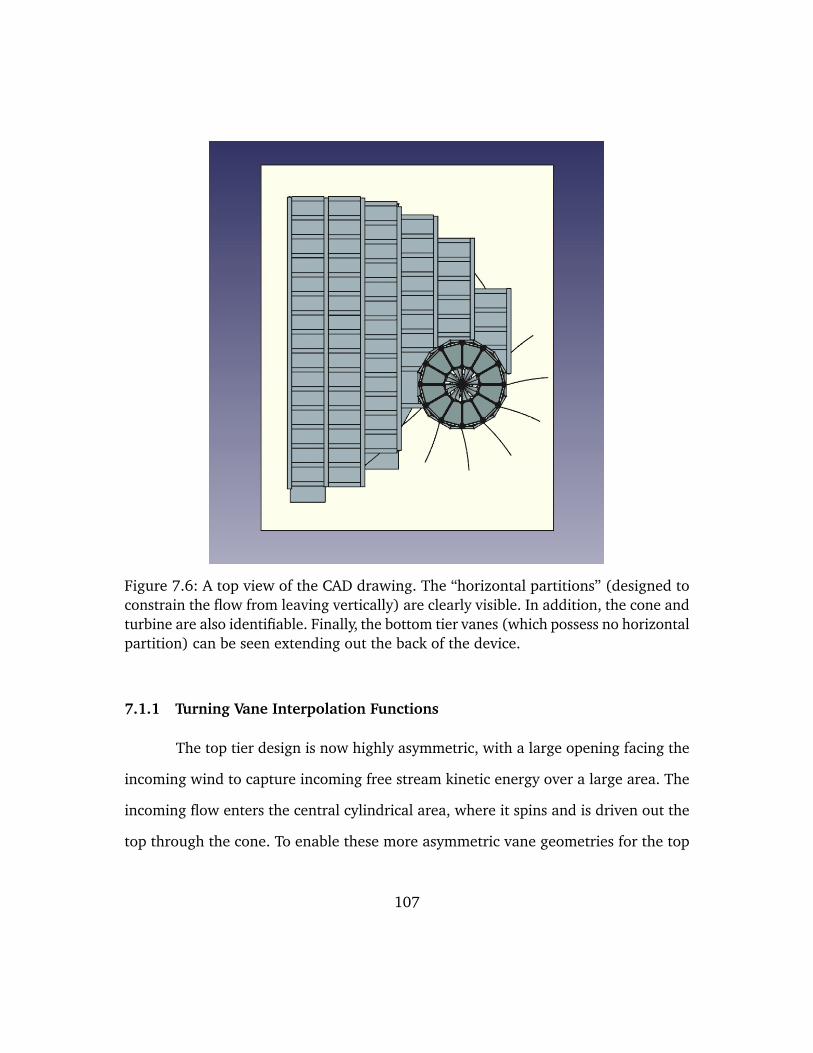
Figure 7.6: A top view of the CAD drawing. The “horizontal partitions” (designed toconstrain the flow from leaving vertically) are clearly visible. In addition, the cone andturbine are also identifiable. Finally, the bottom tier vanes (which possess no horizontalpartition) can be seen extending out the back of the device.

7.1.1 Turning Vane Interpolation Functions

The top tier design is now highly asymmetric, with a large opening facing the

incoming wind to capture incoming free stream kinetic energy over a large area. The

incoming flow enters the central cylindrical area, where it spins and is driven out the

top through the cone. To enable these more asymmetric vane geometries for the top

107

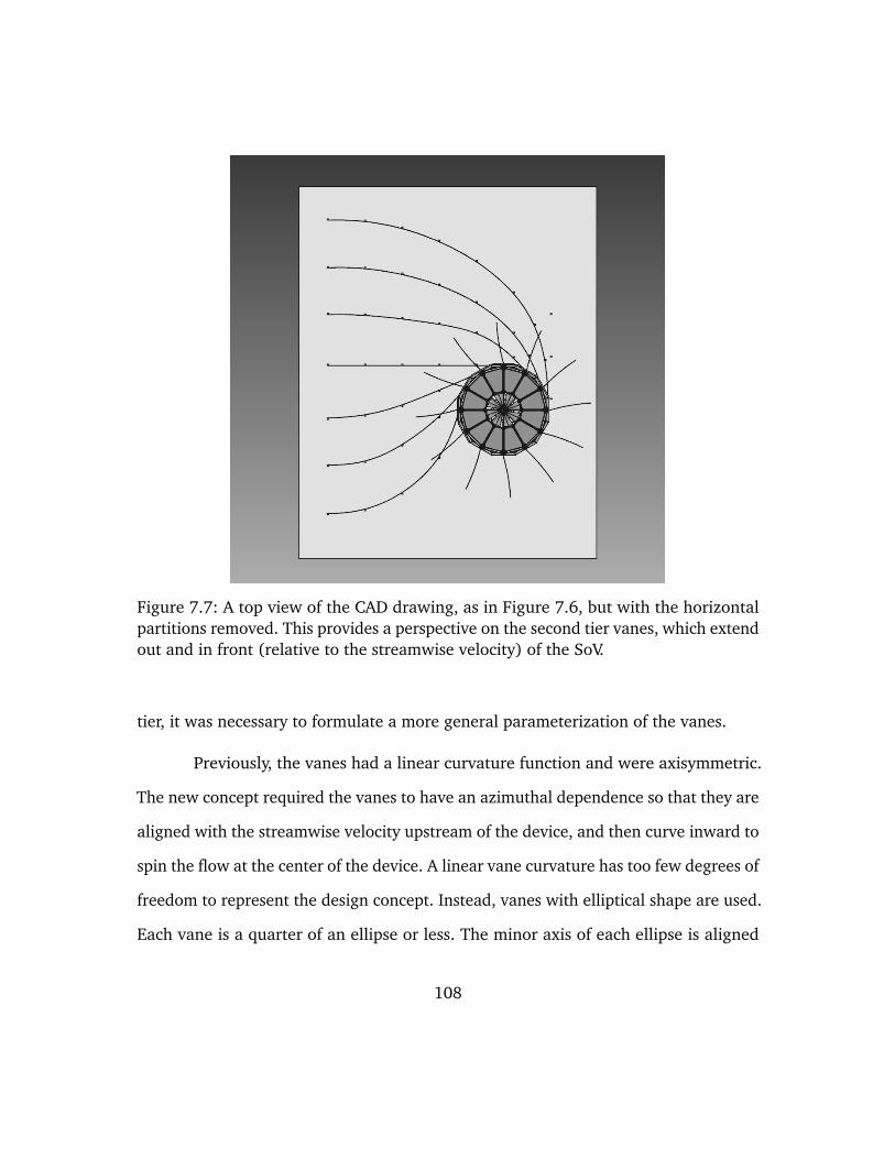
Figure 7.7: A top view of the CAD drawing, as in Figure 7.6, but with the horizontalpartitions removed. This provides a perspective on the second tier vanes, which extendout and in front (relative to the streamwise velocity) of the SoV.

tier, it was necessary to formulate a more general parameterization of the vanes.

Previously, the vanes had a linear curvature function and were axisymmetric.

The new concept required the vanes to have an azimuthal dependence so that they are

aligned with the streamwise velocity upstream of the device, and then curve inward to

spin the flow at the center of the device. A linear vane curvature has too few degrees of

freedom to represent the design concept. Instead, vanes with elliptical shape are used.

Each vane is a quarter of an ellipse or less. The minor axis of each ellipse is aligned

108

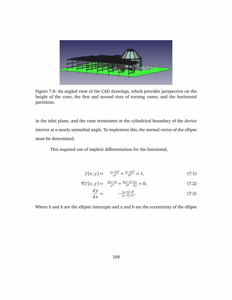
Figure 7.8: An angled view of the CAD drawings, which provides perspective on theheight of the cone, the first and second tiers of turning vanes, and the horizontalpartitions.

in the inlet plane, and the vane terminates at the cylindrical boundary of the device

interior at a nearly azimuthal angle. To implement this, the normal vector of the ellipse

must be determined.

This required use of implicit differentiation for the functional,

f (x , y) = (x−h)2

a2 + (y−k)2

b2 = 1, (7.1)

∇ f (x , y) = 2(x−h)a2 + 2(y−k)

b2d yd x = 0, (7.2)

d yd x= − (x−h)

(y−k)b2

a2 . (7.3)

Where h and k are the elliptic intercepts and a and b are the eccentricity of the ellipse

109

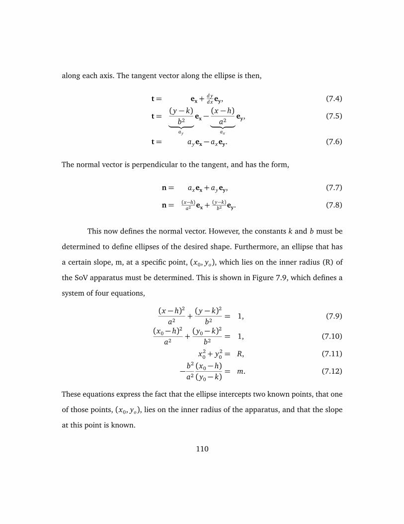
along each axis. The tangent vector along the ellipse is then,

t= ex +d yd x ey, (7.4)

t=(y − k)

b2︸ ︷︷ ︸ay

ex −(x − h)

a2︸ ︷︷ ︸ax

ey, (7.5)

t= ayex − axey. (7.6)

The normal vector is perpendicular to the tangent, and has the form,

n= axex + ayey, (7.7)

n= (x−h)a2 ex +

(y−k)b2 ey. (7.8)

This now defines the normal vector. However, the constants k and b must be

determined to define ellipses of the desired shape. Furthermore, an ellipse that has

a certain slope, m, at a specific point, (x0, yo), which lies on the inner radius (R) of

the SoV apparatus must be determined. This is shown in Figure 7.9, which defines a

system of four equations,

(x − h)2

a2+(y − k)2

b2= 1, (7.9)

(x0 − h)2

a2+(y0 − k)2

b2= 1, (7.10)

x20 + y2

0 = R, (7.11)

−b2

a2

(x0 − h)(y0 − k)

= m. (7.12)

These equations express the fact that the ellipse intercepts two known points, that one

of those points, (x0, yo), lies on the inner radius of the apparatus, and that the slope

at this point is known.

110

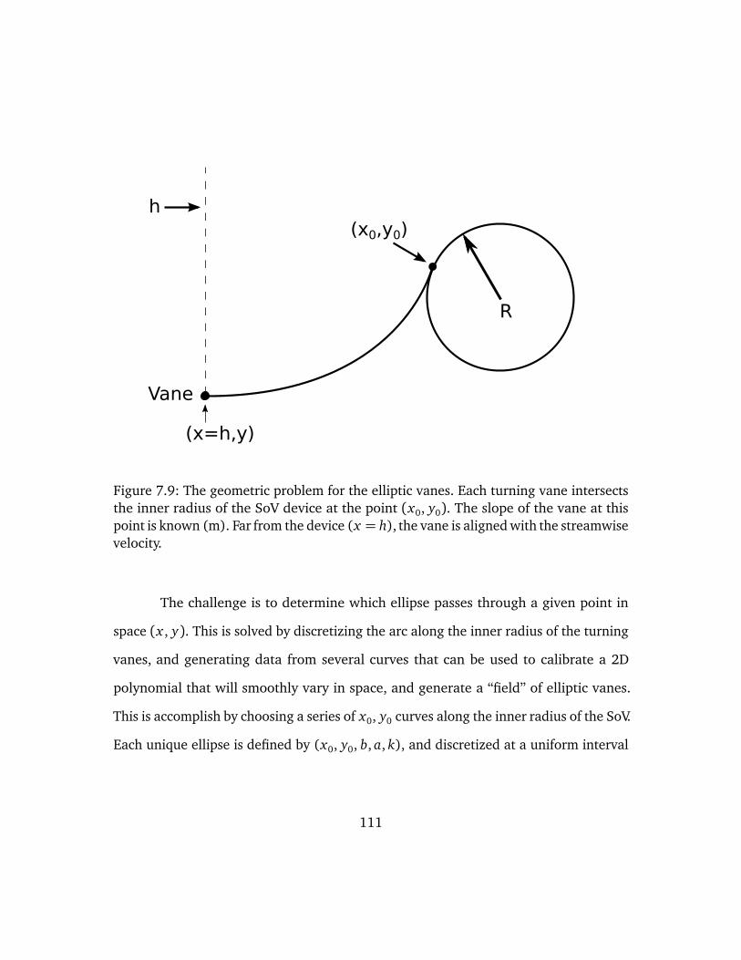
R

Vane

h

(x=h,y)

(x0,y0)

Figure 7.9: The geometric problem for the elliptic vanes. Each turning vane intersectsthe inner radius of the SoV device at the point (x0, y0). The slope of the vane at thispoint is known (m). Far from the device (x = h), the vane is aligned with the streamwisevelocity.

The challenge is to determine which ellipse passes through a given point in

space (x , y). This is solved by discretizing the arc along the inner radius of the turning

vanes, and generating data from several curves that can be used to calibrate a 2D

polynomial that will smoothly vary in space, and generate a “field” of elliptic vanes.

This is accomplish by choosing a series of x0, y0 curves along the inner radius of the SoV.

Each unique ellipse is defined by (x0, y0, b, a, k), and discretized at a uniform interval

111

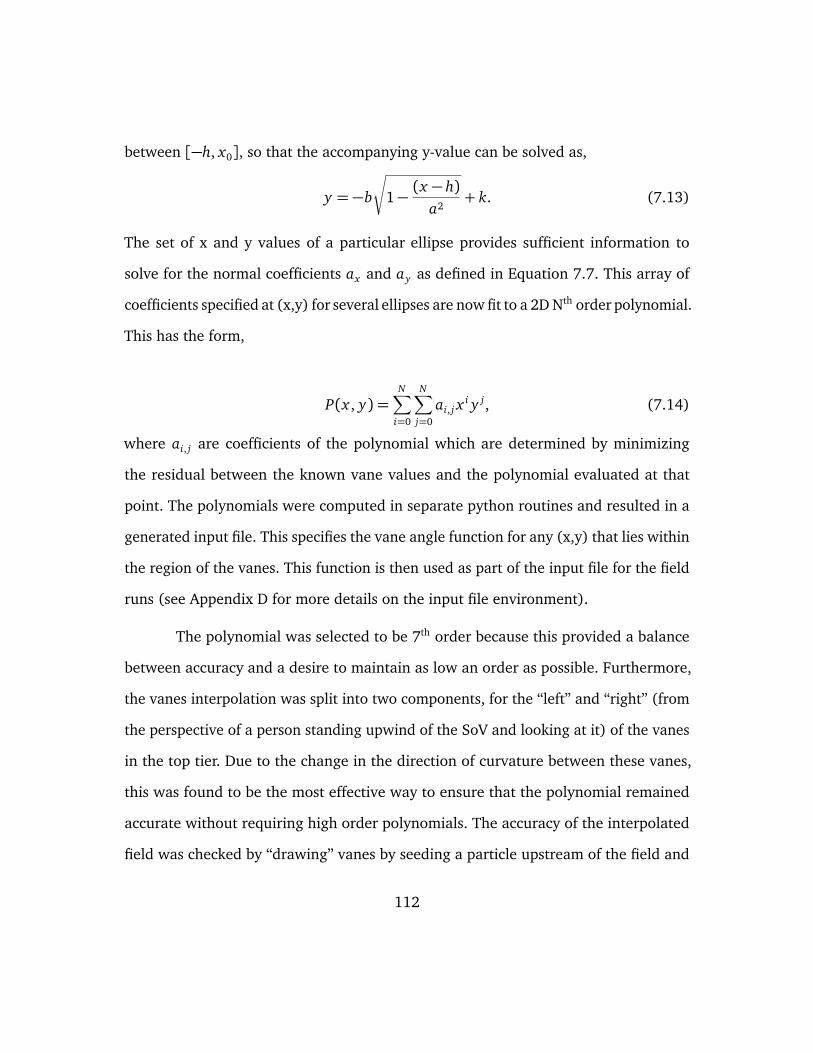
between [−h, x0], so that the accompanying y-value can be solved as,

y = −b

√1−(x − h)

a2+ k. (7.13)

The set of x and y values of a particular ellipse provides sufficient information to

solve for the normal coefficients ax and ay as defined in Equation 7.7. This array of

coefficients specified at (x,y) for several ellipses are now fit to a 2D Nth order polynomial.

This has the form,

P(x , y) =N∑

i=0

N∑j=0

ai, j xi y j, (7.14)

where ai, j are coefficients of the polynomial which are determined by minimizing

the residual between the known vane values and the polynomial evaluated at that

point. The polynomials were computed in separate python routines and resulted in a

generated input file. This specifies the vane angle function for any (x,y) that lies within

the region of the vanes. This function is then used as part of the input file for the field

runs (see Appendix D for more details on the input file environment).

The polynomial was selected to be 7th order because this provided a balance

between accuracy and a desire to maintain as low an order as possible. Furthermore,

the vanes interpolation was split into two components, for the “left” and “right” (from

the perspective of a person standing upwind of the SoV and looking at it) of the vanes

in the top tier. Due to the change in the direction of curvature between these vanes,

this was found to be the most effective way to ensure that the polynomial remained

accurate without requiring high order polynomials. The accuracy of the interpolated

field was checked by “drawing” vanes by seeding a particle upstream of the field and

112

then manually integrating it through the field using the SciPy integrate.ode packages

and verifying visually that the vane had the correct character. Figures 7.3 and 7.4 were

generated using this technique.

7.2 Turbine Design

In addition to the final vane design, a turbine design was developed and tested

over a range of design conditions. The design parameters defining the turbine are listed

in Table 7.4. The exploration of the turbine design space was performed as outlined in

Figure 6.15. The major design improvements are detailed in Figure 7.10. The “initial

guess” was crude, with flat plate drag polars and a poor initial guess for the blade

angle of ≈ 10. Later designs use a higher blade angle often exceeding 40. The design

parameters that lead to the largest improvements in power extracted were changes to

the turbine blade geometry (from flat plate to 180 half cylinders to 90 semicircles),

optimization of the blade angle and optimization of the turbine rotation rate. However,

several other interesting improvements were also found, and are detailed below.

An open area in the center of the turbine was found to improve energy ex-

traction. In some cases, simulations showed a mild downward flow as observed in the

fully-developed thermal-only cases detailed in Section 6.1. The present simulations

do not form a two-celled vortex, but an open center of the turbine is still favorable.

Similarly, while individual blades are not explicitly represented in an actuator-disk

model, the total projected area of blades is a design parameter and can be optimized.

This represents the solidity or blockage, with more blades providing more surface area

to extract power from the fluid while simultaneously impeding the flow. A balance

113

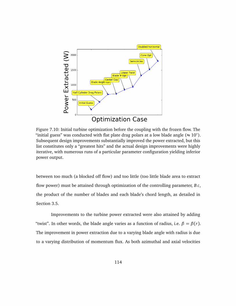
Figure 7.10: Initial turbine optimization before the coupling with the frozen flow. The“initial guess” was conducted with flat plate drag polars at a low blade angle (≈ 10).Subsequent design improvements substantially improved the power extracted, but thislist constitutes only a “greatest hits” and the actual design improvements were highlyiterative, with numerous runs of a particular parameter configuration yielding inferiorpower output.

between too much (a blocked off flow) and too little (too little blade area to extract

flow power) must be attained through optimization of the controlling parameter, B c,

the product of the number of blades and each blade’s chord length, as detailed in

Section 3.5.

Improvements to the turbine power extracted were also attained by adding

“twist”. In other words, the blade angle varies as a function of radius, i.e. β = β(r).

The improvement in power extraction due to a varying blade angle with radius is due

to a varying distribution of momentum flux. As both azimuthal and axial velocities

114

depend on the circulation, Γ , so the optimal β varies radially to capture the optimal

turbine blade angle.

After this initial exploration of the turbine design space, further investigations

were conducted in collaboration with Duane McCormick at UTRC. This design was

arrived at by comparisons between a “frozen flow” optimization routine from UTRC

with the “fully coupled” CFD described previously. This frozen flow Matlab code also

used an actuator disk model as described in Section3.5, and required the velocity

profiles immediately upstream of the actuator disk location from runs conducted with

and without the actuator disk present. Thus, the frozen flow UTRC code was incapable

of estimating the impact of a turbine on the flow, and typically required updated velocity

fields from the fully coupled runs after several iterations. The UTRC code was not

directly connected to the UT CFD code. Rather, human intervention was required to

prepare the velocity field outputs from the UT CFD effort so that they could be used in

the UTRC code. Thus, the UTRC code would iterate through design parameters, and

then the CFD code was used as a higher fidelity confirmation.

The UTRC frozen flow optimization was largely consistent with the fully cou-

pled CFD prediction (see Figure 7.11, below). This has resulted in two final rotor

designs, with and without twist. This was because the experimental team was not cer-

tain that a twisted design would be feasible. Regardless, the twisted rotor was always

predicted to out-perform the zero-twist rotor. The peak power extracted is predicted

to be 2.14 kW for the rotor with twist, and slightly more than 1.51 kW for a rotor with

no twist. This indicates that the twisted rotor design is extracting 45% of the available

power from the flow. This is an efficiency: the power extracted by the turbine (PTurbine)

115

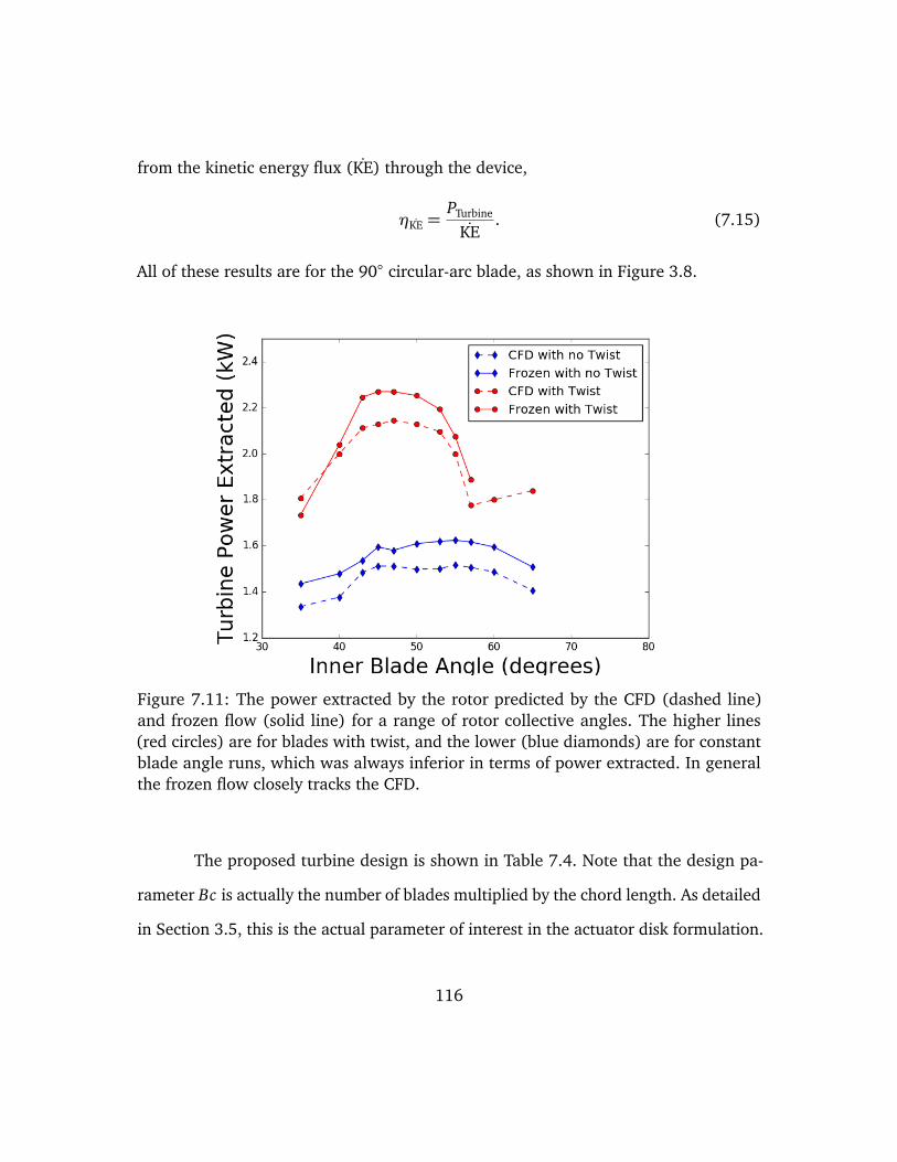
from the kinetic energy flux (KE) through the device,

ηKE =PTurbine

KE. (7.15)

All of these results are for the 90 circular-arc blade, as shown in Figure 3.8.

Figure 7.11: The power extracted by the rotor predicted by the CFD (dashed line)and frozen flow (solid line) for a range of rotor collective angles. The higher lines(red circles) are for blades with twist, and the lower (blue diamonds) are for constantblade angle runs, which was always inferior in terms of power extracted. In generalthe frozen flow closely tracks the CFD.

The proposed turbine design is shown in Table 7.4. Note that the design pa-

rameter Bc is actually the number of blades multiplied by the chord length. As detailed

in Section 3.5, this is the actual parameter of interest in the actuator disk formulation.

116

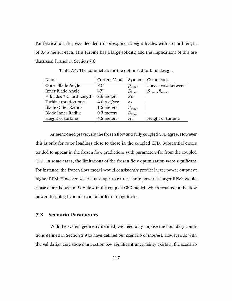
For fabrication, this was decided to correspond to eight blades with a chord length

of 0.45 meters each. This turbine has a large solidity, and the implications of this are

discussed further in Section 7.6.

Table 7.4: The parameters for the optimized turbine design.

Name Current Value Symbol CommentsOuter Blade Angle 70 βouter linear twist betweenInner Blade Angle 47 βinner βinner,βouter

# blades * Chord Length 3.6 meters BcTurbine rotation rate 4.0 rad/sec ωBlade Outer Radius 1.5 meters Bouter

Blade Inner Radius 0.3 meters Binner

Height of turbine 4.5 meters HB Height of turbine

As mentioned previously, the frozen flow and fully coupled CFD agree. However

this is only for rotor loadings close to those in the coupled CFD. Substantial errors

tended to appear in the frozen flow predictions with parameters far from the coupled

CFD. In some cases, the limitations of the frozen flow optimization were significant.

For instance, the frozen flow model would consistently predict larger power output at

higher RPM. However, several attempts to extract more power at larger RPMs would

cause a breakdown of SoV flow in the coupled CFD model, which resulted in the flow

power dropping by more than an order of magnitude.

7.3 Scenario Parameters

With the system geometry defined, we need only impose the boundary condi-

tions defined in Section 3.9 to have defined our scenario of interest. However, as with

the validation case shown in Section 5.4, significant uncertainty exists in the scenario

117

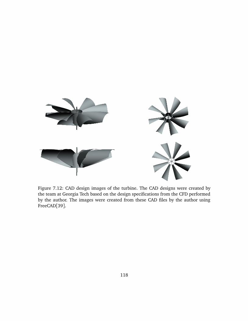
Figure 7.12: CAD design images of the turbine. The CAD designs were created bythe team at Georgia Tech based on the design specifications from the CFD performedby the author. The images were created from these CAD files by the author usingFreeCAD[39].

118

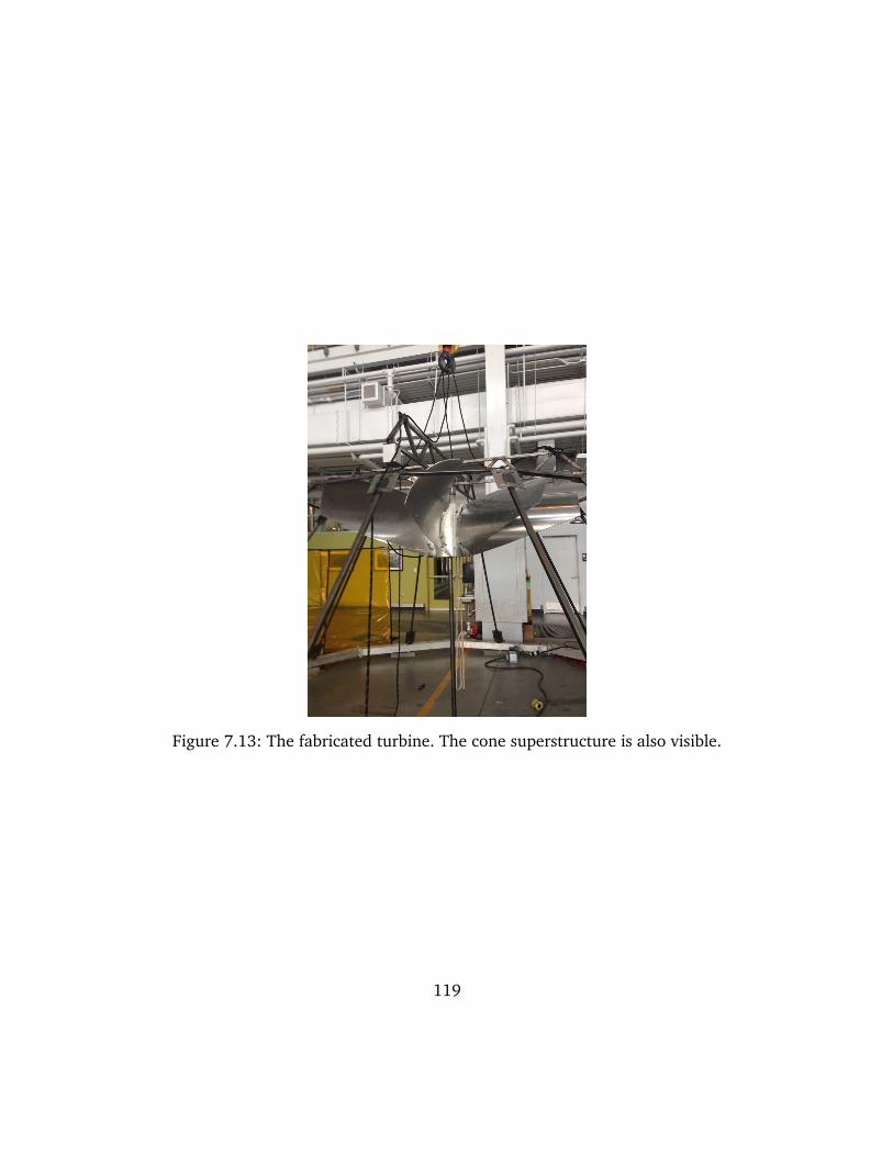
Figure 7.13: The fabricated turbine. The cone superstructure is also visible.

119

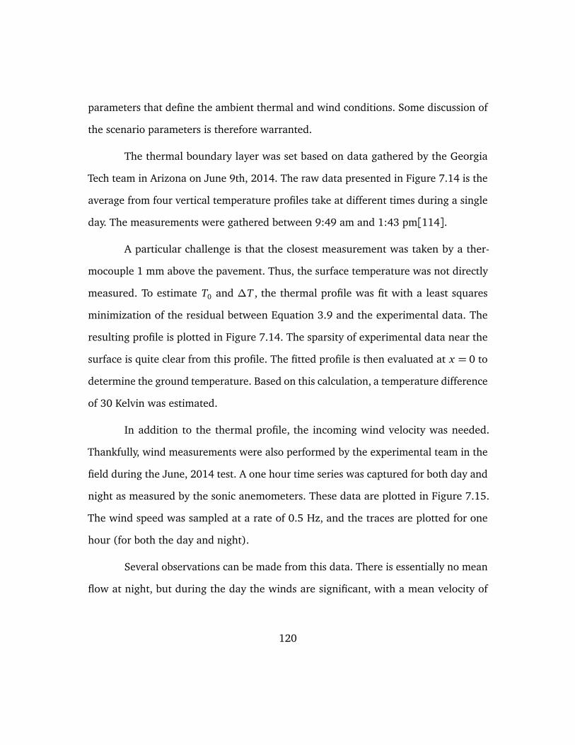
parameters that define the ambient thermal and wind conditions. Some discussion of

the scenario parameters is therefore warranted.

The thermal boundary layer was set based on data gathered by the Georgia

Tech team in Arizona on June 9th, 2014. The raw data presented in Figure 7.14 is the

average from four vertical temperature profiles take at different times during a single

day. The measurements were gathered between 9:49 am and 1:43 pm[114].

A particular challenge is that the closest measurement was taken by a ther-

mocouple 1 mm above the pavement. Thus, the surface temperature was not directly

measured. To estimate T0 and ∆T , the thermal profile was fit with a least squares

minimization of the residual between Equation 3.9 and the experimental data. The

resulting profile is plotted in Figure 7.14. The sparsity of experimental data near the

surface is quite clear from this profile. The fitted profile is then evaluated at x = 0 to

determine the ground temperature. Based on this calculation, a temperature difference

of 30 Kelvin was estimated.

In addition to the thermal profile, the incoming wind velocity was needed.

Thankfully, wind measurements were also performed by the experimental team in the

field during the June, 2014 test. A one hour time series was captured for both day and

night as measured by the sonic anemometers. These data are plotted in Figure 7.15.

The wind speed was sampled at a rate of 0.5 Hz, and the traces are plotted for one

hour (for both the day and night).

Several observations can be made from this data. There is essentially no mean

flow at night, but during the day the winds are significant, with a mean velocity of

120

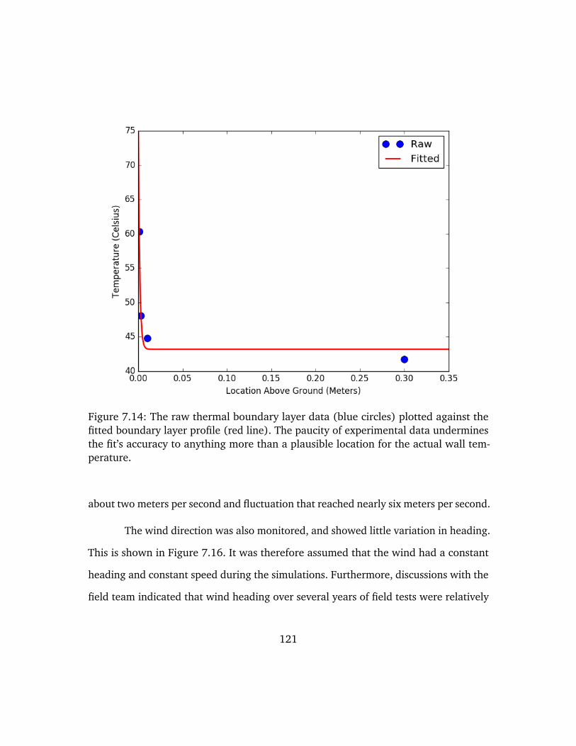
Figure 7.14: The raw thermal boundary layer data (blue circles) plotted against thefitted boundary layer profile (red line). The paucity of experimental data underminesthe fit’s accuracy to anything more than a plausible location for the actual wall tem-perature.

about two meters per second and fluctuation that reached nearly six meters per second.

The wind direction was also monitored, and showed little variation in heading.

This is shown in Figure 7.16. It was therefore assumed that the wind had a constant

heading and constant speed during the simulations. Furthermore, discussions with the

field team indicated that wind heading over several years of field tests were relatively

121

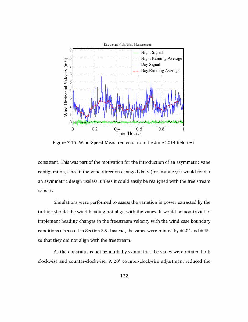
0 0.2 0.4 0.6 0.8 1Time (Hours)

0

1

2

3

4

5

6

7

8

9

Win

d H

ori

zonta

l V

eloci

ty (

m/s

)

Night Signal

Night Running Average

Day Signal

Day Running Average

Day versus Night Wind Measurements

Figure 7.15: Wind Speed Measurements from the June 2014 field test.

consistent. This was part of the motivation for the introduction of an asymmetric vane

configuration, since if the wind direction changed daily (for instance) it would render

an asymmetric design useless, unless it could easily be realigned with the free stream

velocity.

Simulations were performed to assess the variation in power extracted by the

turbine should the wind heading not align with the vanes. It would be non-trivial to

implement heading changes in the freestream velocity with the wind case boundary

conditions discussed in Section 3.9. Instead, the vanes were rotated by ±20 and ±45

so that they did not align with the freestream.

As the apparatus is not azimuthally symmetric, the vanes were rotated both

clockwise and counter-clockwise. A 20 counter-clockwise adjustment reduced the

122

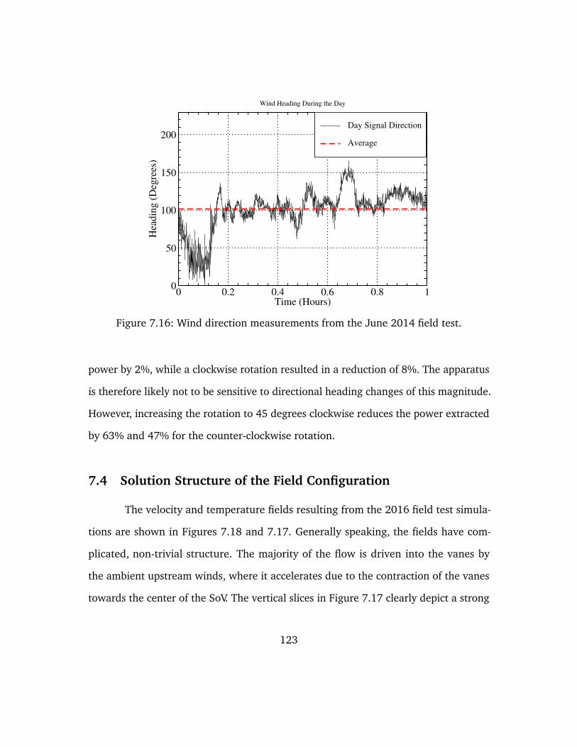
0 0.2 0.4 0.6 0.8 1Time (Hours)

0

50

100

150

200

Hea

din

g (

Deg

rees

)

Day Signal Direction

Average

Wind Heading During the Day

Figure 7.16: Wind direction measurements from the June 2014 field test.

power by 2%, while a clockwise rotation resulted in a reduction of 8%. The apparatus

is therefore likely not to be sensitive to directional heading changes of this magnitude.

However, increasing the rotation to 45 degrees clockwise reduces the power extracted

by 63% and 47% for the counter-clockwise rotation.

7.4 Solution Structure of the Field Configuration

The velocity and temperature fields resulting from the 2016 field test simula-

tions are shown in Figures 7.18 and 7.17. Generally speaking, the fields have com-

plicated, non-trivial structure. The majority of the flow is driven into the vanes by

the ambient upstream winds, where it accelerates due to the contraction of the vanes

towards the center of the SoV. The vertical slices in Figure 7.17 clearly depict a strong

123

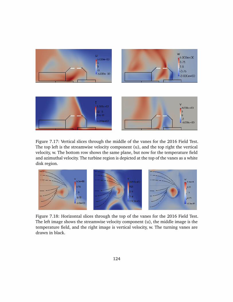
Figure 7.17: Vertical slices through the middle of the vanes for the 2016 Field Test.The top left is the streamwise velocity component (u), and the top right the verticalvelocity, w. The bottom row shows the same plane, but now for the temperature fieldand azimuthal velocity. The turbine region is depicted at the top of the vanes as a whitedisk region.

Figure 7.18: Horizontal slices through the top of the vanes for the 2016 Field Test.The left image shows the streamwise velocity component (u), the middle image is thetemperature field, and the right image is vertical velocity, w. The turning vanes aredrawn in black.

124

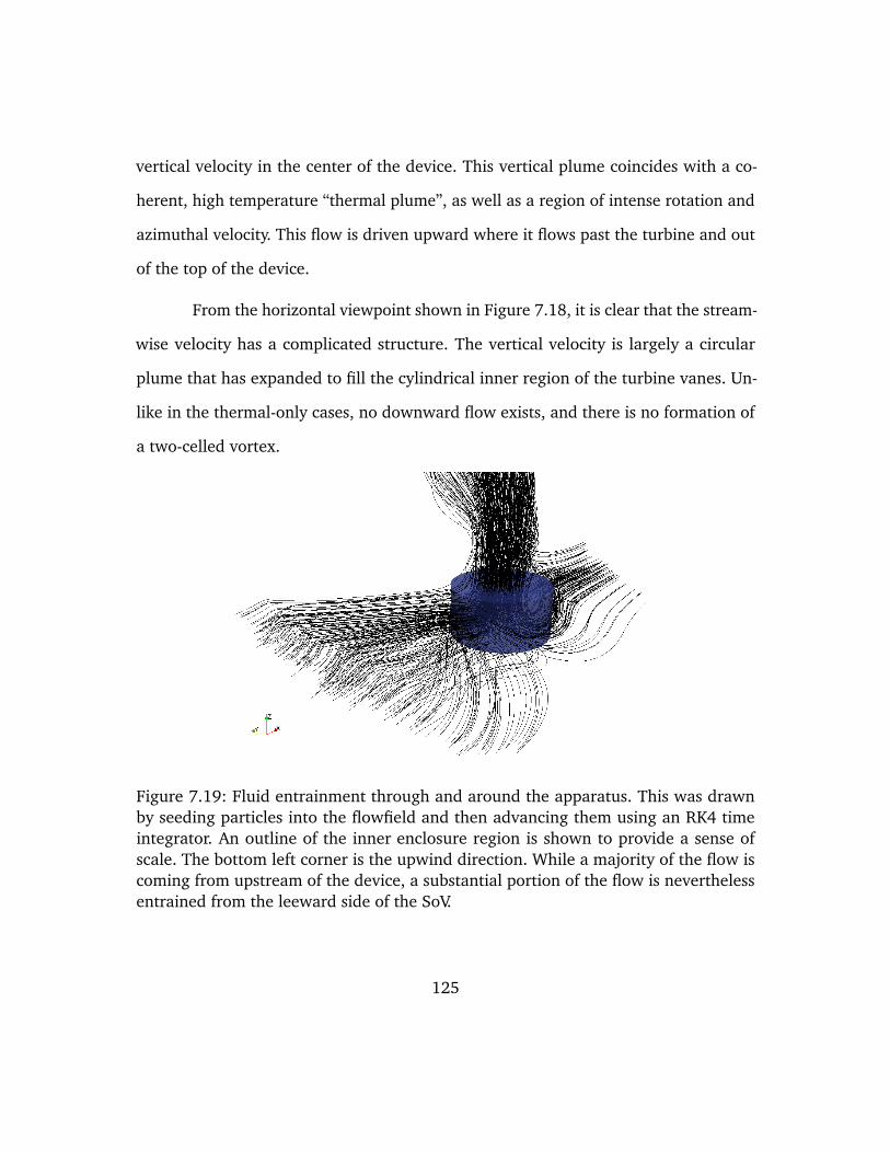
vertical velocity in the center of the device. This vertical plume coincides with a co-

herent, high temperature “thermal plume”, as well as a region of intense rotation and

azimuthal velocity. This flow is driven upward where it flows past the turbine and out

of the top of the device.

From the horizontal viewpoint shown in Figure 7.18, it is clear that the stream-

wise velocity has a complicated structure. The vertical velocity is largely a circular

plume that has expanded to fill the cylindrical inner region of the turbine vanes. Un-

like in the thermal-only cases, no downward flow exists, and there is no formation of

a two-celled vortex.

Figure 7.19: Fluid entrainment through and around the apparatus. This was drawnby seeding particles into the flowfield and then advancing them using an RK4 timeintegrator. An outline of the inner enclosure region is shown to provide a sense ofscale. The bottom left corner is the upwind direction. While a majority of the flow iscoming from upstream of the device, a substantial portion of the flow is neverthelessentrained from the leeward side of the SoV.

125

Figure 7.19 shows tracing particles advanced forward and backward in time

from the center of the device. This clearly shows that the flow is drawn in from both the

front and back of the SoV, and that the device is entraining air from a region far larger

than the SoV vane diameter. While a majority of the flow is coming from upstream of

the device, a substantial portion of the flow is nevertheless entrained from the leeward

side of the SoV. Most of the entrained flow from downstream of the vanes appears to

be constrained come from the wake of the SoV. It is also interesting to note that most

of the backflow from downwind side occurs near the surface. While most of the radial

inflow to the SoV is from the downside side is near the surface, the vortex is strong

enough to entrain flow from outside the vanes above the device.

The 2016 field configuration has 4.77 kW of kinetic energy flux through the

top of the vanes, taken from a plane just below the turbine, which is 608% higher

kinetic energy flux than the peak measurement produced in the August 2015 Field

test.

7.4.1 Sources of Error

While these results are promising, there are several significant shortcomings to

these models and scenario conditions that substantially impact the SoV performance. A

major uncertainty is the opacity of the device. Ideally, the device would be completely

transparent. However, previous field tests found that the SoV device shaded the inner

region, which resulted in a lower temperature inside the device than outside. As the

physical trigger for the SoV is thermal buoyancy, this greatly reduces the velocities

inside the device, and so the kinetic energy flux and power extracted by the turbine. For

126

instance, simulations performed with the ground temperature inside the vane region

set to the ambient air temperature (an admittedly “worst-case scenario”) found that the

energy extracted by the turbine was reduced to only 800 Watts. Thus, consistent with

the results shown in Section 6.4, the absence of a thermal to drive the flow reduces the

available kinetic energy flux (and thus, the power extracted by the turbine) by more

than half.

No dynamics in the wind were considered, only a steady, mean wind velocity.

It may well be that even in the "thermal only" cases there could be significant, zero

mean wind fluctuations contributing energy. However, crude sensitivity analyses were

performed by adjusting the mean velocity of the wind by ±1m/s, which indicated that

the power generated by the turbine only increases with higher wind velocity, and that

most of the vortex structure and character of the solution discussed in Section 7.4

remains valid, with only modestly reduced velocities.

An August field test in 2016 reported only modest velocities through the proto-

type apparatus. While substantial, the uncertainties describe above are not sufficient

to account for the weakness of the observed flow, indicating a potentially significant

model error that had not previously been considered. The subsequent sections detail

two possible modeling errors that were investigated in detail, and may account for the

significantly reduced flow observed in the field.

127

7.5 Turning Vane Drag

The first model correction proposed is to introduce drag along the turning

vanes to account for the skin friction along their surfaces. To introduce a drag force,

the turning vane forcing representation described in Section 3.4 need only be modified

to introduce an additional force that acts in opposition to the fluid velocity. Thus, in

addition to forcing the flow to align with the vane surface, the flow will also be slowed.

The unit drag forcing vector, f, is simply the negative normalized inner product

of the velocity, u, and the turning vane tangent vector tv,

−u · tv

||u · tv||= f. (7.16)

The volumetric force applied is,

F = f C f12ρ||u||2

δ. (7.17)

Where C f is the skin friction coefficient (which must be determined), ρ is the density

and δ is half the distance between adjacent vanes.

Some roughness elements exist across the vanes. In addition to non-smooth

surface materials, the design of the field test apparatus ultimately relied upon posts to

hold the turning vanes. These posts were pieces of wood which were modeled as rough-

ness elements. In order to determine C f for these cases, the Colebrook formula[29],

was used to provide an estimate for the friction factor given a roughness height, ε/D,

1»C f= −2.0 log

Ñε/D3.7+

2.51

Re»

f

é. (7.18)

128

With the assumption that for large roughness the Reynolds number term is not signifi-

cant, the function is no longer implicit in C f and can be determined directly,

C f =Ç

2.0 logÇε/D3.7

åå2

. (7.19)

Note that D is the hydraulic diameter which must account for the two plates (we treat

the vanes as a channel),

DH =4AP=

4(2w)δ2w

= 4δ, (7.20)

where δ is again half the distance between the vanes. To construct a “worst-case”

scenario, we consider the smallest distance between the vanes, which occurs near the

center of the SoV. Furthermore, we consider roughness heights based on a four-by-four

(which were used as supports for the vanes). Even for this worst case scenario, the

velocities in the vanes are not substantially reduced with the addition of the drag model.

The flow field kinetic energy flux was never reduced more than 12%. This crude model

indicates that the reduced flows observed during the August 2016 field tests are not

attributable to skin friction drag on the turning vanes.

7.6 Blade Solidity Modification

The 2016 field test indicated that there was little or no flow through the turbine

region. Furthermore, it was noted that the chord length of the turbine blades was

indeed substantial, and the number of blades (eight) larger than typically used in wind

turbines (which often operate with two or three blades).

The turbine is represented by an actuator disk model in which the lift and

drag forces on the blades are determined from a two-dimensional CFD simulation of

129

the flow over an isolated blade. Use of this drag and lift force model in the turbine

implicitly assumes that the turbine blades do not significantly block the flow through

the turbine, which would be the case if the flow remained attached to the turbine

blades as it passes through the turbine. However, this is not likely to be the case over

the entire turbine area.

To determine whether this blockage effect can explain the August 2016 field

observations a worst-case blockage assumption was made in which the air is said to

pass through the turbine as if each blade blocked the flow according to its projected

area. This increases the vertical velocity experienced by the blades and used in the

calculation of blade lift and drag. This model essentially assumes that the flow is

completely separated on each blade, which is not expected to be the case, so this may

be an overly pessimistic estimate of the blockage effect.

It was noted that wind turbines typically possess three blades, versus the eight

blades used in the 2016 field test. This is therefore a substantially increased turbine

solidity versus common engineering designs. It is expected that we are operating in a

regime not common to typical actuator disk models. There are some other studies that

have found blade solidity can greatly negatively impact the power extraction from a

turbine[31].

The length of each blade blocking vertical flow in the actuator disk is,

c ∗Cos(β(r)) = cx(r). (7.21)

While the total circumferential length in an annular region that is blocked is therefore,

B ∗ cx(r) = lB(r), (7.22)

130

where B is the number of blades. Then, the fraction of the circumference that is impeded

by blades is,

B(r) = 2πr−lB(r)2πr , (7.23)

B(r) = 1− lB(r)2πr . (7.24)

Note that a “floor” function is needed to ensure the solidity ratio does not go below

zero.

For a 1D control volume analysis for the region, the continuity equation is,

ρV ′z A′ = ρVzA, (7.25)

V ′z = VzAA′ , (7.26)

V ′z =Vz

B(r) . (7.27)

This implies that V ′z →∞ as A′ → 0. This is as expected, as the blockage becomes

more severe, the flow would need to move at greater speed to go through it.

The flow angle with respect to turbine velocity is therefore modified from

Equation 3.39 in Section 3.5,

θ f = tan−1(uup

ufwd), (7.28)

to,

θ f = tan−1(uup

B(r)ufwd). (7.29)

As B(r)→ 0, θ f → π, e.g. 90 degrees. In this way the velocity vector will be completely

aligned with drag. Finally Equation 3.43,

F =12

cρu2p

A(CL nlift + Cd ndrag), (7.30)

131

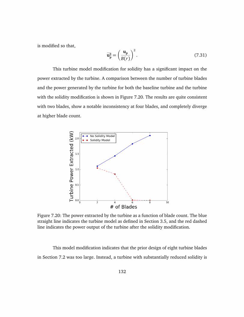
is modified so that,

u2p =Ç

up

B(r)

å2

. (7.31)

This turbine model modification for solidity has a significant impact on the

power extracted by the turbine. A comparison between the number of turbine blades

and the power generated by the turbine for both the baseline turbine and the turbine

with the solidity modification is shown in Figure 7.20. The results are quite consistent

with two blades, show a notable inconsistency at four blades, and completely diverge

at higher blade count.

Figure 7.20: The power extracted by the turbine as a function of blade count. The bluestraight line indicates the turbine model as defined in Section 3.5, and the red dashedline indicates the power output of the turbine after the solidity modification.

This model modification indicates that the prior design of eight turbine blades

in Section 7.2 was too large. Instead, a turbine with substantially reduced solidity is

132

preferred. Based on Figure 7.20, a turbine with similar characteristics in terms of length,

location and twist but reduced from eight blades to four or two blades is expected

to mitigate the substantially reduced performance observed in the field. This is the

only model correction that was explored that is capable of explaining the 2016 field

observations noted in Subsection 7.4.1.

This crude model is admittedly extreme, as it effectively models the blades as

flat plate bluff bodies, with the flow completely separated on the leeward side. Ideally,

the flow should be smoothly turning through the blades, and not separate. Thus, while

the blockage correction developed here is probably overly pessimistic, it could sensibly

be used as a predictive or design tool by introducing a calibration constant which could

be tuned if appropriate data were available. However, such a correction is not generally

used in the wind turbine community, which is in part why such a modification was

not considered in the original model. It is interesting to speculate why, this correction

has not been used in wind turbine analysis, and yet, the design optimization used for

such turbines has not pushed the designs to every more blades. It is likely that the

cost of additional wind turbine blades past two or three is not justified, even assuming

the optimistic increased power capacity that the non-blockage-corrected model would

predict. This would essentially move the design away from the conditions in which the

blockage effect is important.

Interesting enough, there have been actuator disk models used with wind tur-

bines that indicate operating at low tip speed ratios with high solidity ratios would

possess power coefficients close to Betz-like limits of efficiency[99]. It is therefore

possible that the actuator disk model is generally unsuited for high solidity regimes,

133

and that the correction presented here is more generally useful.

7.7 Estimating the Upper Limit on Power Extraction

All of the results in Section 7.4 were generated using 90 semicircle blade ge-

ometries, as shown in Figure 3.8. The only other blade geometries considered were the

flat plate and 180 arcs, which were universally found to be inferior. Time constraints

required fabrication of the turbine in short order, and a limited budget encouraged

inexpensive (and therefore simple) turbine blades. Risk mitigation also played a role,

with an emphasis on traditional, and therefore well-vetted turbine blade design. This

section details an additional computational research effort pursued after the turbine

fabrication with the intent of estimating the upper limit of power extraction with an

idealized turbine.

Practical utility-scale wind turbines achieve a peak of 75% to 80% of the Betz

limit[22]. The Betz-limit places a theoretical maximum of 59% of the wind’s power

that can be captured. Therefore, practical wind turbines extract less than half of the

available kinetic energy flux. Comparing the kinetic energy flux of simulations without

the turbine to the power extracted by the turbine, we note that our simulations typically

predict power extraction ratios slightly less than fifty percent, indicating that our efforts

are not significantly better or worse than could be expected. While this provides an

estimate, the Betz-limit for wind turbines does not apply to the SoV turbine.

The objective then, is to formulate a generalized approach to treating the

blades to permit an optimization that is not constrained to a particular blade geometry.

134

Rather, this approach seeks to estimate the upper limit of the possible power extracted.

The rationale behind this is to provide an upper bound on the power that can be

extracted for a particular configuration, which can then be used as input for feasibility

considerations of the SoV.

It is desirable to perform these estimates within the context of the actuator disk

model (see Section 3.5). While actuator disk models are commonly optimized[3, 34,

65, 98], the lift and drag polars are not parameters that are varied in these schemes.

Rather, a given blade geometry is assumed and then the rotation rate, blade angle and

chord length (for instance) are optimized.

Conversely, airfoil optimization is a rich field with sophisticated and well-vetted

techniques [26, 35, 68], but these methods do not use an actuator disk model, and

focus on the shape optimization of the airfoil geometry (and through this, the lift and

drag polars).

To address the possibility of further turbine blade improvements, while con-

tinuing to use an abstract actuator disk model, this section details a formulation for

a generic set of drag polars. These generalized drag polars permit exploration of a

broader design space. The optimization of this model can be fully coupled to the flow,

and so does not violate any Betz-like considerations that might similarly arise in an

analysis of frozen flow fields. The drag polars are selected to be generic functions and

are optimized to maximize the power extracted by the rotor. While the resulting drag

polars might not be physically realizable, they represent a “best case” upper bound

indicating the peak power that might be extracted with further rotor design iterations.

This “limiting case” is useful for evaluating the system feasibility from a technologi-

135

cal standpoint, by providing the peak power that could be extracted for a given vane

geometry.

The power extracted by the turbine is,

P = ΩQ, (7.32)

where the torque, Q, is[77],

Q = AR

∫ 2π

0

∫ rmax

rmin

F ′′τ

r dr dθ . (7.33)

Here, AR is the relative area coefficient which is,

AR =Bc(rmax − rmin)π(r2

max − r2min)

, (7.34)

where B is the number of blades, rmax and rmin are the turbine radii, and F ′′τ

is the force

per unit area on the turbine, which is,

F ′′τ=

Fτcl=

12ρU2

R Cτ. (7.35)

with UR the magnitude of relative velocity and c is the blade chord length, which is

assumed to be constant (not a function of the radius, for instance). Finally, Cτ is the

tangential force coefficient, which depends on the local lift and drag coefficients, and

the flow angle, φ,

Cτ = CL sin(φ) + CD cos(φ). (7.36)

Combining the equations above results in an expression for the power that explicitly

depends on the lift and drag coefficients,

P =ΩρBc(rmax − rmin)

2π(r2max − r2

min)

∫ 2π

0

∫ rmax

rmin

UR(r,θ ,Ω)2 (CL sin(φ) + CD cos(φ)) r drdθ .

136

Lumping the constant terms together,

Eτ =ΩρBc(rmax − rmin)

2π(r2max − r2

min), (7.37)

and separating this equation,

PL = Eτ∫ 2π

0

∫ rmax

rmin

UR(r,θ ,Ω)2 CL(φ, r) sin(φ) r drdθ , (7.38)

PD = Eτ∫ 2π

0

∫ rmax

rmin

UR(r,θ ,Ω)2 CD(φ, r) cos(φ) r drdθ . (7.39)

Note that we have assumed CD = CD(φ, r) and CL = CL(φ, r), namely, that the coef-

ficients vary with the flow direction and may vary radially, due to twisting the blade

angle. Furthermore, the flow direction,φ, varies with the location and the blade speed,

in that φ = φ(r,θ ,Ω). The relative velocity is the quantity, UR = U − Uτ, e.g. the dif-

ference in velocity between the turbine and the flow. The turbine has no axial velocity

(wτ = 0) and a constant rotation speed, and so the two components of velocity in the

plane of rotation can be expressed as,

uτ = Ω r sin(θ ), (7.40)

vτ = Ω r cos(θ ). (7.41)

Our objective is now to discover what these unknown functions of lift and drag

are. To do this, we specify an optimization problem such that,

Max P(CL, CD) subject to:

|CL|< CMaxL ,

0< CD < CMaxD .

In words, the drag must be specified to be greater than zero, but the lift can

be negative. This is a problem in the calculus of variations, where the objective is to

maximize a functional subject to imposed constraints [19, 106, 107].

137

The integral shown in Equation 7.38 above can be bounded by Schwarz’s

inequality, ñ∫ 2π

0

∫ rmax

rmin

CL(φ, r)UR(r,θ ,Ω)2 sin(φ) r drdθô2

≤∫ 2π

0

∫ rmax

rmin

C2L (φ, r)drdθ

∫ 2π

0

∫ rmax

rmin

UR(r,θ ,Ω)4 sin2(φ) r2 drdθ .

In this way the first integral quantity,∫ 2π

0

∫ rmax

rmin

C2L (φ, r)drdθ , (7.42)

is clearly maximized when CL(φ, r) = CmaxL . The result for Equation 7.39 is identical.

Now, for these conditions, we are interested in the largest attainable values. For the

drag coefficient, CMaxD , we select a peak value of two. This corresponds to a flat plate

perpendicular to the flow. The lift coefficient peak value is 1.75. This design is not

necessarily physically realizable, but represents an absolute maximum.

Therefore, our lift/drag functions may be expressed as,

CD(φ) = CDψ(φ)

ψ(φ) = 1 if sin(φ)> 0,

0 else

CL(φ) = CL Ψ(φ)

Ψ(φ) = 1 if cos(φ)> 0,

−1 else.

Where CL = 1.7 and CD = 2.0. The plot of these drag polars are shown in Figure 7.21.

Under this approach, the turbine extracts so much energy from the flow that

the vortex loses its coherence and the power extracted becomes negative (e.g. the

constant velocity turbine is adding energy to the flow). This implies a limit on how

much of the energy can be extracted before disrupting the flow so greatly that the

vortex cannot be maintained.

138

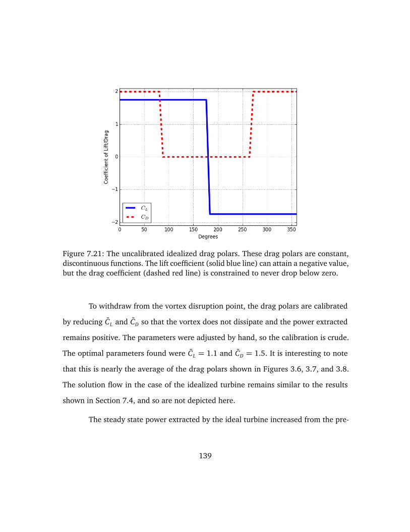
Figure 7.21: The uncalibrated idealized drag polars. These drag polars are constant,discontinuous functions. The lift coefficient (solid blue line) can attain a negative value,but the drag coefficient (dashed red line) is constrained to never drop below zero.

To withdraw from the vortex disruption point, the drag polars are calibrated

by reducing CL and CD so that the vortex does not dissipate and the power extracted

remains positive. The parameters were adjusted by hand, so the calibration is crude.

The optimal parameters found were CL = 1.1 and CD = 1.5. It is interesting to note

that this is nearly the average of the drag polars shown in Figures 3.6, 3.7, and 3.8.

The solution flow in the case of the idealized turbine remains similar to the results

shown in Section 7.4, and so are not depicted here.

The steady state power extracted by the ideal turbine increased from the pre-

139

vious best attained with the 90 degree semicircles, to 2.76 kW. This is 58% of the

available kinetic energy flux measured just upstream of the turbine. This provides a

loose band on the power that can be derived from this flow. Furthermore, this indi-

cates that previous estimates of the power that might be extracted from the flow are

not greatly limited by the present turbine design. This is an important element of the

system feasibility assessment, as it provides evidence against the turbine as modeled

being a source of considerable inefficiency.

140

Chapter 8

Conclusions and Future Work

8.1 Summary of the Present Work

Observed velocities indicates that naturally occurring dust devils contain a

considerable amount of energy, from the gravitational potential energy contained in

air near the hot surface of the Earth and ambient winds. While rudimentary proof-of-

concept devices have shown that artificial dust devils can be created and anchored in

place by turning vanes, no previous studies have attempted to methodically explore

how best to intensify the produced vortex, and yield a stronger and more powerful

dust devil.

This thesis has developed and validated computational models that have subse-

quently explored a broad configuration space of turning vanes to estimate how much

power might be produced by one of these synthetic dust devils. The purpose behind

this is to provide an assessment of the technological feasibility of the entire synthetic

columnar vortex concept as a means of generating renewable energy.

Such a system had never been simulated previously. Developing simulations

capable of modeling the SoV apparatus and for the scenarios of interest therefore re-

quired the development of new models and software capabilities. This required the

development and implementation of mathematical models for the turbulent diffusiv-

141

ities in the ambient conditions, and the representation of the SoV vanes, cone and

turbine. The latter required the development of a novel representation of the SoV sys-

tem geometry that is sufficiently flexible to permit cost-effective iteration in designs.

These virtual vanes were further extended to include both a separation model and a

modification to account for the drag due to skin friction along the surface. In addition,

a modification to the actuator-disk model to account for the observed impact of the

turbine blade solidity was developed.

The ultimate simulation capability was a complicated coupled system that

accounted for buoyancy effects, ambient winds and a wide variety of turning vane

and turbine geometries. These simulations were validated across a range of conditions

and system configurations and were largely consistent with available experimental

data and observations. Furthermore, a steady state simulation was validated against

unsteady simulations, which permitted computationally inexpensive explorations of

the design space.

These capabilities supported the principle objective of this work, which was

to explore a large space of possible system configurations and geometries to discover

mechanisms that intensify the vortex velocities and the power extracted by the turbine.

These simulations indicated that the synthetic flow generated by the SoV do indeed

have a dust devil-like character. The flow is buoyancy driven, with a coherent thermal

plume corresponding to a region of intense vertical and azimuthal velocity. These flows

are consistent with the Rankine vortex model, which has generally been found to be

an accurate representation of the velocities in the naturally occurring phenomenon.

A contribution of this work is in indicating the role of ambient winds are more

142

substantial than previously indicated. The wind provides a significant contribution of

kinetic energy to the flow, but it also changes the structure of the vortex. The expec-

tation that the more powerful naturally occurring dust devils are similarly driven by

substantial winds also implies that the structure of dust devils may be more asymmetric

than previously realized.

8.2 System Feasibility Assessment

The results of the simulations indicate that over tens of square meters, several

kilowatts of energy can be produced. These results are not promising with regards

to the competitiveness of the power generated by the device. For comparison, a pho-

tovoltaic array typically converts the peak solar insolation of ≈ 1000 W/m2 at an

efficiency of approximately 15%. Thus, the power generated by a solar array with an

area comparable to the six meter inner diameter of the turning vanes for the 2016

SoV field test would be substantially larger than the estimated power predicted in the

simulations (4 kW for the PV vs. 2 kW from the SoV).

In addition to this unpromising result, two major additional risks exist that

likely limit the expected utility of the SoV paradigm. The first is that at this time no

experimental validation accompanies the computational results, and it is conceivable

that the apparatus will not perform as well as predicted by simulation.

Furthermore, the simulations indicated that the synthetic dust devils are fragile,

and the kinetic energy flux in the plume is highly sensitive to ambient conditions and

the complex interplay between the ambient winds and the thermal buoyancy effects.

143

In some cases, small perturbations to the system parameters such as the turbine blade

number or the turning vane angles would result in orders of magnitude weaker vortices.

This indicates that any energy generation system that uses dust devils may not be a

reliable and regular means of energy generation. It is interesting to note that this may

indicate that the naturally occurring dust devils, while pervasive, are not robust, and

that individual whirlwinds are easily dissipated when interfered with.

However, it must also be emphasized that feasibility is focused on technical

viability, namely energy produced by the apparatus, and does not include an economic

assessment. The SoV is almost certainly cheaper to fabricate and install than competing

renewable technologies such as photovoltaics or wind turbines. Thus, while simulations

indicate that the SoV lags these technologies in terms of power production, it may be

more competitive on a dollar per watt basis. Economic considerations such as these

are not considered in this work.

One outstanding question is: why do the synthetic dust devils generated by

the SoV possess substantially reduced velocities versus the naturally occurring phe-

nomenon. The scaling of the velocity of these objects with respect to the diameter of

the apparatus is not known, and it is possible that the larger diameters of the natu-

rally occurring dust devils also corresponds to intensified velocities. Alternatively, the

solidity or blockage of the device in the vanes and turbine was found to be a signifi-

cant limit to the power produced. As the natural variety do not have control surfaces

that also serve to block the flow, these vortices may have larger mass flow rates and

consequently, kinetic energy fluxes.

144

8.3 Conclusions and Future Work

Despite the considerable simulation campaign, the SoV extracts considerably

less energy than other renewable technologies. It is therefore unlikely that the SoV

technology is competitive versus presently existing approaches. It is possible that the

technology could be useful in radically different scenarios, such as harvesting waste

industrial heat, where the ambient conditions and scales would so differ from those

considered in this work that further investigation would be necessary.

Another possible venue of research would be a marked departure from the two

tier vane paradigm in this work. For instance, dynamically adjustable vanes might be

capable of harmoniously "building up" the vortex. Or, additional turning tiers might be

necessary to provide a more continuous entrainment region. However, these concepts

would certainly require a much more expensive design configuration and the simula-

tions presented in this work do not clearly indicate a promising path of investigation.

While the technological feasibility of the SoV is questionable, the enabling

models and simulation capabilities developed in the course of this investigation have

independent value. The turning vane formulation is a useful tool where explicitly

meshing surfaces is prohibitively expensive or difficult, and at least for the conditions

present in this work, the resulting simulations with the virtual vanes were a useful

design tool. Broadly speaking, the optimization heuristics and steady models used to

explore the turning vane and turbine configuration were powerful tools, and could be

much more broadly applied for optimization and design in many other systems.

Finally, dust devils remain a relatively poorly understood phenomenon, in part

145

due to the lack of simulation data that permits detailed investigations of the underlying

fluid-dynamical structure of these objects. The simulations here have generated dust

devil-like structures that could be used as a research tool to further investigate the

physics of dust devils and cyclonic phenomenon in general.

146

Appendices

147

Appendix A

Derivation of the Stabilization and Weak Formulation

This appendix details the weak formulation of the Navier Stokes equations

instantiated in the software GRINS, and provides a derivation of the τ stabilization

terms shown in Equation 4.5.

In brief, our process is the following:

• Cast Navier Stokes + Boussinesq equations into weak form

• Prepare as an operator L c= f

• Calculate Fréchet derivative

• Separate into differential (P) and constant (Z) components, L′[c] = P + Z

• Choose stabilization operator such that S = −P∗

• Then stabilization has form, ah(c,φ) = a(c,φ) + ⟨Lc, Sφ⟩τ

This is essentially the least-squares stabilization proposed by Hughes and ex-

tended to natural convection by Becker and Braack.

148

A.1 Weak Formulation of the Equations of Interest

We begin with the incompressible Navier-Stokes equations with Boussinesq

buoyancy,

∇ · u= 0 (A.1)

∂ u∂ t+ u · ∇u= −

1ρ∇p+ ν∇2u+ g

T ′

T0(A.2)

ρcp∂ T∂ t+ u · ∇T =∇ · (k∇T ) (A.3)

e.g. the continuity, momentum and energy equations, respectively. Our state vector is

c = [p,u, T]. To cast these into weak form we multiply by appropriate test functions

φ = [q,v, w] ∈ H10(Ω) and integrate over the domain, Ω ∈ Rn. Our system of equations

now appears as,

∫Ω

q∇ · u d x = 0 (A.4)∫Ω

u · v d x +∫Ω(u · ∇)u · v d x =

∫Ω

pρ∇ · v d x −

∫Ων∇u · ∇v d x +

∫Ω

gT ′

T0· v d x

(A.5)

ρcp

∫Ω

T ·w d x +∫Ω(u · ∇)T ·w d x = −

∫Ω(k∇T ) · ∇w d x (A.6)

where an “over-dot” denotes time differentiation, e.g. u = ∂ u∂ t . Note that both the

pressure term as well as the viscous term were integrated by parts to reduce the

required order of the solution on those state variables.

The inner product is abbreviated by the shorthand notation (u,v) =∫Ω u · v d x ,

149

giving our equations the form,

(∇ · u, q) = 0 (A.7)

(u,v) + (u · ∇u,v)− (p,∇ · v) + (ν∇u,∇v) = (gT ′

T0,v) (A.8)

ρcp(T, w) + (u · ∇T, w) + (k∇T,∇w) = 0. (A.9)

This defines our weak form operator, a(c,φ). Our full equations will also include a

stabilization term such that,

ah(c,φ) = a(c,φ) + ⟨L c, Sφ⟩τ. (A.10)

The subsequent section will define the operators L and S, so that we might then fully

define the stabilization term ⟨L c, Sφ⟩τ.

A.2 The Stabilization Operators, L and S

To form the stabilization terms,

⟨L c, Sφ⟩τ (A.11)

we must define the operators L and S. The operator L is simply the PDEs in

Equations A.1 - A.3 written in operator form. S is defined as the negative adjoint of

the differential terms in L, e.g.

L′[c] = P + Z (A.12)

S = −P∗. (A.13)

150

Where P are the differential terms, and Z the constant terms.

Our objective is now to construct the adjoint operator of L. This is accomplished

using the Fréchet derivative, which defines the functional derivative on L. In general

this is accomplished by taking the first variation of a function Π(u) around a base state,

u,

δΠ(u) = limε→0

Π(u+ ε u)−Π(u)ε

=∂Π(u+ ε u)

∂ ε

∣∣∣∣∣ε=0

(A.14)

∀u,ε > 0 with u+ ε u ∈ H10(Ω). This is recognizable as the Gâteaux derivative of the

functional.

We now consider the first variation of state for the momentum equation term

by term. The convective term is,

∂

∂ ε(u+ ε u) · ∇(u+ εu) (A.15)

= limε→0

u · ∇(u+ ε u) (A.16)

= u · ∇u (A.17)

= −u · ∇u (A.18)

and the viscous term is,

∂

∂ ε∇2(u+ ε u) (A.19)

=∇2u (A.20)

151

while the buoyancy term is,

δ

Ç−g

T ′

T0

å= δ

Ç−g

T − T0

T0

å(A.21)

= −g∂

∂ ε

(T − T0 + εT

T0

)(A.22)

= −g

(TT0

)(A.23)

and thus the full adjoint equation for momentum appears as,

−u · ∇u−∇2u= −1ρ∇p. (A.24)

The continuity equation is straightforward,

∂

∂ ε∇ · (u+ ε u) = 0, (A.25)

∇ · u= 0. (A.26)

Finally, consider the convective term of the energy equation,

∂

∂ εu · ∇(T + ε T ) = u · ∇T (A.27)

and the thermal diffusion term,

∂

∂ ε· (−k∇(T + εT )) =∇ · (−k∇T ). (A.28)

The full adjoint energy equation is therefore,

u · ∇T +∇ · (k∇T ) = 0. (A.29)

We are now in a position to define the matrices L and S. L comes directly from

the PDEs in Equations A.1 - A.3 and is defined as thus,

152

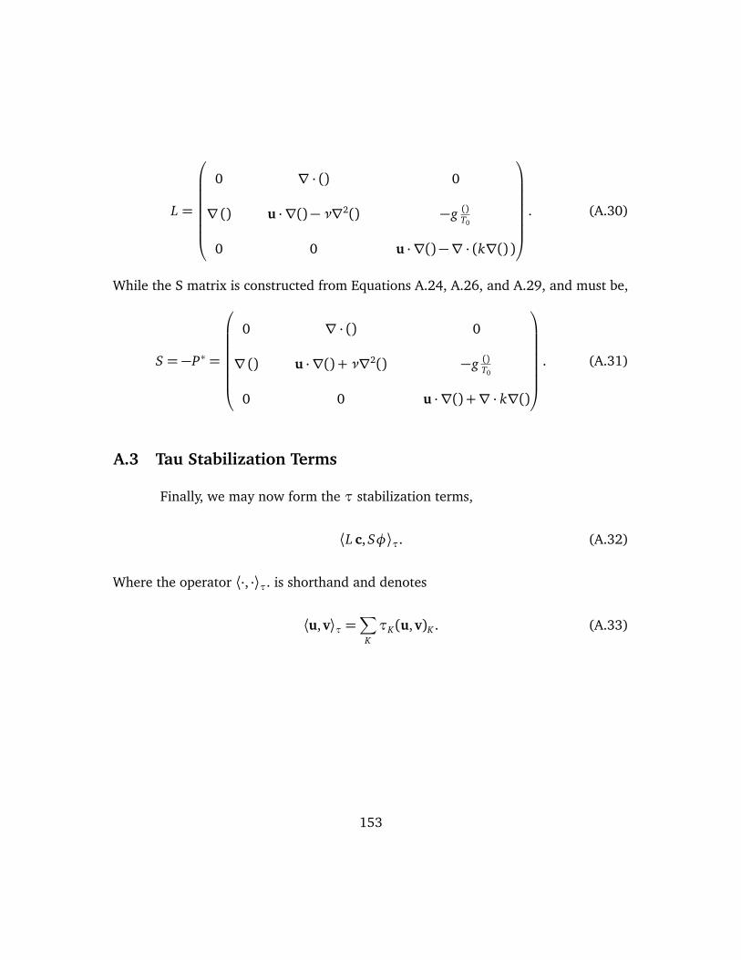
L =

0 ∇ · () 0

∇ () u · ∇()− ν∇2() −g ()T0

0 0 u · ∇()−∇ · (k∇() )

. (A.30)

While the S matrix is constructed from Equations A.24, A.26, and A.29, and must be,

S = −P∗ =

0 ∇ · () 0

∇ () u · ∇() + ν∇2() −g ()T0

0 0 u · ∇() +∇ · k∇()

. (A.31)

A.3 Tau Stabilization Terms

Finally, we may now form the τ stabilization terms,

⟨L c, Sφ⟩τ. (A.32)

Where the operator ⟨·, ·⟩τ. is shorthand and denotes

⟨u,v⟩τ =∑

KτK(u,v)K . (A.33)

153

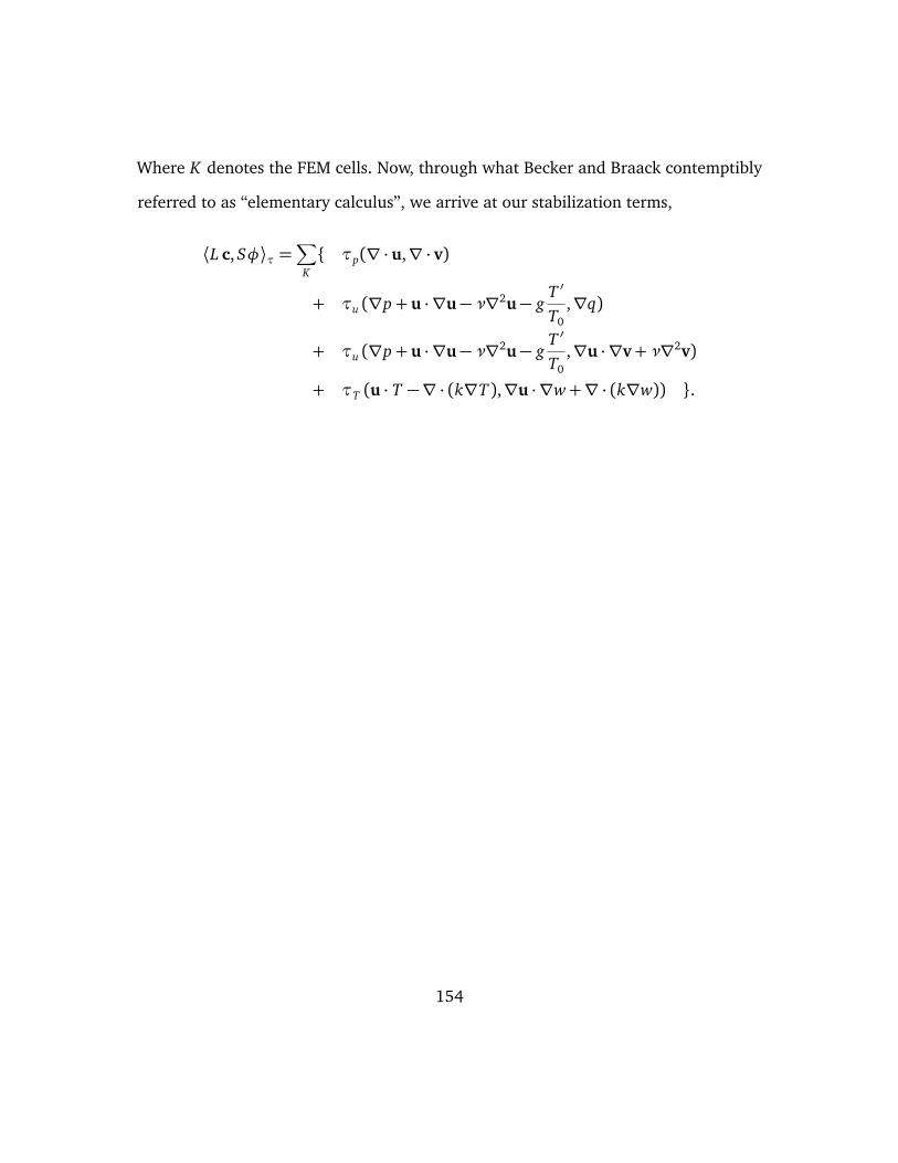
Where K denotes the FEM cells. Now, through what Becker and Braack contemptibly

referred to as “elementary calculus”, we arrive at our stabilization terms,

⟨L c, Sφ⟩τ =∑

K τp(∇ · u,∇ · v)

+ τu (∇p+ u · ∇u− ν∇2u− gT ′

T0,∇q)

+ τu (∇p+ u · ∇u− ν∇2u− gT ′

T0,∇u · ∇v+ ν∇2v)

+ τT (u · T −∇ · (k∇T ),∇u · ∇w+∇ · (k∇w)) .

154

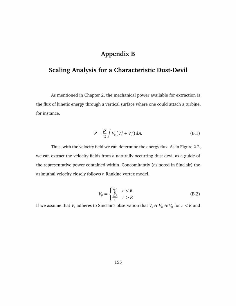
Appendix B

Scaling Analysis for a Characteristic Dust-Devil

As mentioned in Chapter 2, the mechanical power available for extraction is

the flux of kinetic energy through a vertical surface where one could attach a turbine,

for instance,

P =ρ

2

∫Vz (V

2θ+ V 2

z ) dA. (B.1)

Thus, with the velocity field we can determine the energy flux. As in Figure 2.2,

we can extract the velocity fields from a naturally occurring dust devil as a guide of

the representative power contained within. Concomitantly (as noted in Sinclair) the

azimuthal velocity closely follows a Rankine vortex model,

Vθ =

V0rR r < R

V0Rr r > R

(B.2)

If we assume that Vz adheres to Sinclair’s observation that Vz ≈ Vθ ≈ V0 for r < R and

155

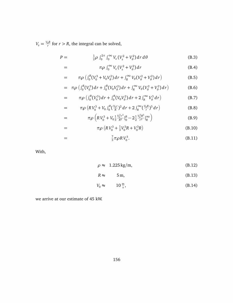
Vz =V0R

r for r > R, the integral can be solved,

P = 12ρ∫ 2π

0

∫∞0 Vz (V 2

z + V 2θ) dr dθ (B.3)

= πρ∫∞

0 Vz (V 2z + V 2

θ) dr (B.4)

= πρÄ∫ R

0 (V3

0 + V0V 2θ) dr +

∫∞R Vθ (V 2

θ+ V 2

θ) drä

(B.5)

= πρÄ∫ R

0 (V3

0 ) dr +∫ R

0 (V0V 2θ) dr +

∫∞R Vθ (V 2

θ+ V 2

θ) drä

(B.6)

= πρÄ∫ R

0 (V3

0 ) dr +∫ R

0 (V0V 2θ) dr + 2

∫∞R V 3

θdrä

(B.7)

= πρÄR V 3

0 + V0

∫ R0 (

V0rR )

2 dr + 2∫∞

R (V0R

r )3 drä

(B.8)

= πρÅ

R V 30 + V0

13

V 20 r3

R2 |R0 − 212

V 30 R3

r2 |∞Rã

(B.9)

= πρÄR V 3

0 +13 V 3

0 R+ V 30 Rä

(B.10)

= 73πρR V 3

0 . (B.11)

With,

ρ ≈ 1.225kg/m, (B.12)

R≈ 5m, (B.13)

V0 ≈ 10 ms , (B.14)

we arrive at our estimate of 45 kW.

156

Appendix C

Impact of the Coriolis Force

This appendix briefly details the arguments of Monin and Obukhov[75] esti-

mating the impact of the Coriolis force on the dynamics of flow near the surface, in

the so-called Eckman layer. This section provides justification for the neglect of this

force in our equations of motion (Equation 3.1, in particular).

To begin, assume statistically stationary, spatially homogeneous, neutrally strat-

ified flow that varied only in height, z. The Reynolds equations for the wind-velocity

direction can be simplified to be,

∂ ρu′w′

∂ z= −

∂ P∂ x+ρ f v, (C.1)

where ρu′w′ is the turbulent momentum flux, ∂ P∂ x the mean pressure gradient, f is

the Coriolis frequency (often called the Coriolis parameter) and v the averaged wind

velocity. Dividing by density and integrating over height, z,

∫ H

0

∂ u′w′

∂ zdz =

∫ H

0

Ç−

1ρ

∂ P∂ x+ f v

ådz. (C.2)

Assuming constant density and replacing with the turbulent shear stress, τ = ρu′w′,

the left integrand can be solved,

τ(0)−τ(H)ρ

=∫ H

0

Ç1ρ

∂ P∂ x− f v

ådz. (C.3)

157

Careful readers should note the sign change in the equation above. The right hand

side is bounded by, ∫ H

0

Ç1ρ

∂ P∂ x− f v

ådz <

∫ H

0

Ç1ρ

∂ P∂ x

ådz, (C.4)

as the Coriolis effect opposes the action of the pressure gradient. Substituting for the

friction velocity, u∗ =√τρ , our inequality has the form,

u2∗(H)− u2

∗(0)<∫ H

0

Ç1ρ

∂ P∂ x

ådz. (C.5)

Consider a pressure wind velocity scale,

vp =1ρ f∂ P∂ x

(C.6)

f vp =1ρ

∂ P∂ x

(C.7)

which, when used in Equation C.5, greatly simplifies our inequality to,

u2∗(H)− u2

∗(0)< f vp H. (C.8)

As we only seek to estimate the region where the change attributable to the Coriolis

effect is less than some tolerance, we bound the difference as,

u2∗(H)− u2

∗(0)u2∗(0)

≤ a, (C.9)

u2∗(H)− u2

∗(0)≤ au2∗(0), (C.10)

where the tolerance a is selected to be 20%. Combining Equations C.10 and C.8, the

height H at which the Coriolis force meets our tolerance is found to be,

a u2∗(0)≤ H f vp (C.11)

au2∗(0)

f vp≤ H . (C.12)

158

Monin and Obukhov further estimated the values of the inputs to this equation as

u∗vp= 0.05, vp ≈ 10 meters/second, f ≈ 10−4 1/seconds and a = 0.20, which results in

an H of 50 meters. Thus, the dynamics of flow below this height are estimated to have

a less than 20% impact on account of the Coriolis effect, which we further neglect fully

in the simulations presented in this document.

Incidentally, this argument may also been seen as evidence for why dust devils

have no preferred direction of rotation. The Coriolis effect is too small to impose a direc-

tion, and only (very mildly) intensifies cyclonic dust devils while modestly weakening

the anti-cyclonic variety.

159

Appendix D

Archived Simulations

The entirety of data used in this document have been captured and are on the

tape archival system Ranch1 at the Texas Advanced Computing Center2 (TACC). These

complete archives will be made available on request.

The files are stored in a format identical to that of the SVN archive located

at, https://svn.ices.utexas.edu/repos/pecos/solar_vortex/. The organi-

zation of the repository bears some discussion. The root level, contains the folders:

documents, grids, input, postproc, and single_shot_input. documents contains quarterly

reports and model documentation in LaTeX and MSFT word format. grids contains the

raw gridgen files used to generate meshes for the gridded vanes. postproc contains

the files used to perform temporal averaging, as well as paraview and python scripts

used to visualize the fields and generate images of the simulations. single_shot_input

is a deprecated set of input files from the earliest investigations into the SoV. These

input files represent an older format where all the definitions and file settings were

contained in a single input file. Due to the volume and complexity of input required

for these simulations, these older files are cumbersome and difficult to read. Finally,

1npm7@ranch:/home2/00000/npm7/sov_huge_backup2http://www.tacc.utexas.edu/

160

input is the directory that contains the input files and the output of the simulations

(on Ranch, not on SVN).

The input directory is broken into four directories. The first, field, contains

all the physical investigations for the SoV Field tests with the virtual vanes, typically

steady, but some unsteady virtual vane investigations are also contained here. gridded

are directories that contain the input files and simulation output from the gridded

runs, and laboratory contains the table-top laboratory runs. Finally, opt contains the

optimization runs where runs where rapidly iterated with perturbed system parameters.

These were entirely “Steady” virtual vane cases.

All these directories then have a common structure. They have a common

directory that contains all the sub-input files, and then a unique problem folder that

details the unique run and the output of this file. For instance, the a problem folder

might be entitled, “field_2016_august_3m” for the 2016 August field test conducted

with a three meter per second wind velocity. Inside each problem directory, there are

two files, an “initial.in” and a “gold.in”. The initial file starts a run, even if steady,

typically with enhanced (and likely un-physical) viscosity, to help the solver converge.

Subsequent runs are restarted from this base state but with the viscosity model detailed

in Chapter 3. No results from this initial solve are quoted in this document. In some

cases for complicated geometries, multiple initial steps were required, in which the

viscosity was stepped down from the high initial state to the model derived values.

In addition to the input files, each of these directories contains two directories,

gold and output. After each run, all of the output files are moved into output where

they are saved in a directory labeled by the unique slurm id for that particular run. In

161

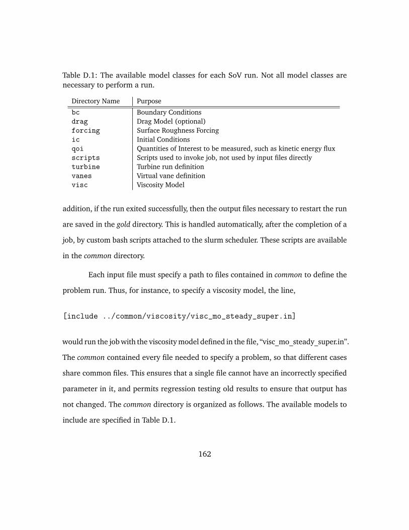
Table D.1: The available model classes for each SoV run. Not all model classes arenecessary to perform a run.

Directory Name Purpose

bc Boundary Conditionsdrag Drag Model (optional)forcing Surface Roughness Forcingic Initial Conditionsqoi Quantities of Interest to be measured, such as kinetic energy fluxscripts Scripts used to invoke job, not used by input files directlyturbine Turbine run definitionvanes Virtual vane definitionvisc Viscosity Model

addition, if the run exited successfully, then the output files necessary to restart the run

are saved in the gold directory. This is handled automatically, after the completion of a

job, by custom bash scripts attached to the slurm scheduler. These scripts are available

in the common directory.

Each input file must specify a path to files contained in common to define the

problem run. Thus, for instance, to specify a viscosity model, the line,

[include ../common/viscosity/visc_mo_steady_super.in]

would run the job with the viscosity model defined in the file, “visc_mo_steady_super.in”.

The common contained every file needed to specify a problem, so that different cases

share common files. This ensures that a single file cannot have an incorrectly specified

parameter in it, and permits regression testing old results to ensure that output has

not changed. The common directory is organized as follows. The available models to

include are specified in Table D.1.

162

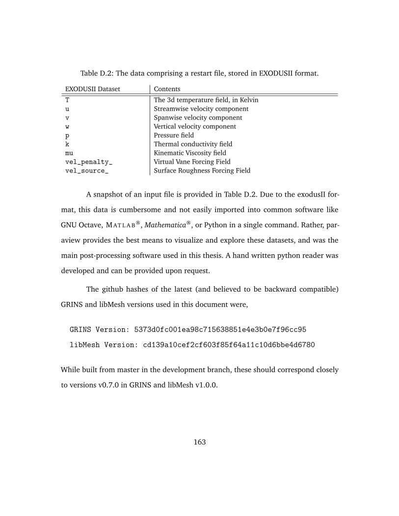
Table D.2: The data comprising a restart file, stored in EXODUSII format.

EXODUSII Dataset Contents

T The 3d temperature field, in Kelvinu Streamwise velocity componentv Spanwise velocity componentw Vertical velocity componentp Pressure fieldk Thermal conductivity fieldmu Kinematic Viscosity fieldvel_penalty_ Virtual Vane Forcing Fieldvel_source_ Surface Roughness Forcing Field

A snapshot of an input file is provided in Table D.2. Due to the exodusII for-

mat, this data is cumbersome and not easily imported into common software like

GNU Octave, MAT L A B®, Mathematica®, or Python in a single command. Rather, par-

aview provides the best means to visualize and explore these datasets, and was the

main post-processing software used in this thesis. A hand written python reader was

developed and can be provided upon request.

The github hashes of the latest (and believed to be backward compatible)

GRINS and libMesh versions used in this document were,

GRINS Version: 5373d0fc001ea98c715638851e4e3b0e7f96cc95

libMesh Version: cd139a10cef2cf603f85f64a11c10d6bbe4d6780

While built from master in the development branch, these should correspond closely

to versions v0.7.0 in GRINS and libMesh v1.0.0.

163

Bibliography

[1] High Wind Drag Coefficient and Sea Surface Roughness in Shallow Water. Tech-nical report, National Oceanic and Atmospheric Administration, 6 2008. (page47).

[2] Annual Energy Outlook 2015. Technical report, U.S. Department of Energy,April 2015. (page 1).

[3] Charles N. Adkins and Robert H. Liebeck. Design of optimum propellers. (page135).

[4] Martin S. Alnæs, Jan Blechta, Johan Hake, August Johansson, Benjamin Kehlet,Anders Logg, Chris Richardson, Johannes Ring, Marie E. Rognes, and Garth N.Wells. The fenics project version 1.5. Archive of Numerical Software, 3(100),2015. doi: 10.11588/ans.2015.100.20553. (page 61).

[5] Ivo Babuška. Error-bounds for finite element method. Numerische Mathematik,16(4):322–333, 1971. (page 56).

[6] Ivo Babuška. The finite element method with penalty. Mathematics of Computa-tion, 27(122):pp. 221–228, 1973. ISSN 00255718. URL http://www.jstor.org/stable/2005611. (page 43).

[7] Satish Balay, Shrirang Abhyankar, Mark F. Adams, Jed Brown, Peter Brune, KrisBuschelman, Lisandro Dalcin, Victor Eijkhout, William D. Gropp, Dinesh Kaushik,Matthew G. Knepley, Lois Curfman McInnes, Karl Rupp, Barry F. Smith, StefanoZampini, Hong Zhang, and Hong Zhang. PETSc users manual. Technical ReportANL-95/11 - Revision 3.7, Argonne National Laboratory, 2016. URL http://www.mcs.anl.gov/petsc. (page 61).

[8] Matt Balme and Ronald Greeley. Dust devils on earth and mars. Reviews of Geo-physics, 44(3):n/a–n/a, 2006. ISSN 1944-9208. doi: 10.1029/2005RG000188.URL http://dx.doi.org/10.1029/2005RG000188. (pages 2, 9).

164

[9] Louis J Battan. Energy of a dust devil. Journal of Meteorology, 15(2):235–237,1958. (page 11).

[10] P. T. Bauman and R. H. Stogner. Grins: A multiphysics framework based onthe libmesh finite element library. submitted, http://arxiv.org/abs/1506.06102. (page 60).

[11] E.B. Becker, G.F. Carey, and J.T. Oden. Finite Elements: Fluid mechanics. Numberv. 6 in Texas Finite Element Series. Prentice-Hall, 1986. ISBN 9780133171327.URL https://books.google.com/books?id=eaYoAQAAMAAJ. (page 43).

[12] Eric B Becker, Graham F Carey, and John Tinsley Oden. Finite elements, an in-troduction: Volume i. ., 258, page 1981, 1981. URL https://books.google.com/books?id=T3kAkAEACAAJ. (page 56).

[13] Roland Becker and Malte Braack. Solution of a stationary benchmark problemfor natural convection with large temperature difference. InternationalJournal of Thermal Sciences, 41(5):428 – 439, 2002. ISSN 1290-0729.doi: http://dx.doi.org/10.1016/S1290-0729(02)01335-2. URL http://www.sciencedirect.com/science/article/pii/S1290072902013352.(page 56).

[14] Bert Blocken, Ted Stathopoulos, and Jan Carmeliet. Cfd simulation of the atmo-spheric boundary layer: wall function problems. Atmospheric environment, 41(2):238–252, 2007. doi: http://dx.doi.org/10.1016/j.atmosenv.2006.08.019.(page 53).

[15] Howard B. Bluestein, Christopher C. Weiss, and Andrew L. Pazmany.Doppler radar observations of dust devils in texas. Monthly Weather Re-view, 132(1):209–224, Jan 2004. ISSN 0027-0644. doi: 10.1175/1520-0493(2004)132<0209:DROODD>2.0.CO;2. URL http://dx.doi.org/10.1175/1520-0493(2004)132<0209:DROODD>2.0.CO;2. (page 5).

[16] Joseph Boussinesq. Essai sur la théorie des eaux courantes. Imprimerie nationale,1877. (page 22).

[17] Joseph Boussinesq. Théorie de l’écoulmnent tourbillonnant et tumultuex des liq-uides dans les lits rectilignes à grande section, volume 1. Gauthier-Villars, 1897.(page 21).

165

[18] Malte Braack and Piotr Boguslaw Mucha. Directional do-nothing condition forthe navier-stokes equations. J. Comput. Math, 32(5):507–521, 2014. (page54).

[19] T.C. Bradbury. Theoretical Mechanics: By T.C. Bradbury. Robert E. KriegerPublishing Company, 1968. URL https://books.google.com/books?id=EpeQnAEACAAJ. (page 137).

[20] A. N. Brooks and T. J. R. Hughes. Streamline upwind/petrov-galerkin formula-tions for convection dominated flows with particular emphasis on the incom-pressible navier-stokes equations. Comput. Methods Appl. Mech. Eng., pages199–259, September 1990. ISSN 0045-7825. URL http://dl.acm.org/citation.cfm?id=99300.99305. (page 56).

[21] C-H Bruneau and P Fabrie. New efficient boundary conditions for incompressiblenavier-stokes equations: a well-posedness result. RAIRO-Modélisation mathé-matique et analyse numérique, 30(7):815–840, 1996. (page 54).

[22] T. Burton, D. Sharpe, N. Jenkins, and E. Bossanyi. Wind Energy Handbook. JohnWiley & Sons, 2001. ISBN 9780471489979. URL https://books.google.com/books?id=4UYm893y-34C. (pages 38, 134).

[23] Joost A Businger, John C Wyngaard, Yl Izumi, and Edward F Bradley. Flux-profile relationships in the atmospheric surface layer. Journal of the atmosphericSciences, 28(2):181–189, 1971. (page 28).

[24] J. J. Carroll and J. A. Ryan. Atmospheric vorticity and dust devil rota-tion. Journal of Geophysical Research, 75(27):5179–5184, 1970. ISSN 2156-2202. doi: 10.1029/JC075i027p05179. URL http://dx.doi.org/10.1029/JC075i027p05179. (page 11).

[25] Tony F Chan and Henk A Van der Vorst. Approximate and incomplete factoriza-tions. In Parallel numerical algorithms, pages 167–202. Springer, 1997. (page61).

[26] Adam Chehouri, Rafic Younes, Adrian Ilinca, and Jean Perron. Re-view of performance optimization techniques applied to wind tur-bines. Applied Energy, 142:361 – 388, 2015. ISSN 0306-2619. doi:

166

http://dx.doi.org/10.1016/j.apenergy.2014.12.043. URL http://www.sciencedirect.com/science/article/pii/S0306261914013002.(page 135).

[27] H Chuang and RB Renda. Turbulent prandtl number in thermally stratified shearflows of air. International Journal of Heat and Mass Transfer, 12(12):1585–1594,1969. (page 27).

[28] Matthew J Churchfield, Sang Lee, John Michalakes, and Patrick J Moriarty. Anumerical study of the effects of atmospheric and wake turbulence on windturbine dynamics. Journal of turbulence, (13):N14, 2012. (page 40).

[29] C. F. Colebrook and C. M. White. Experiments with fluid friction in roughenedpipes. Proceedings of the Royal Society of London A: Mathematical, Physicaland Engineering Sciences, 161(906):367–381, 1937. ISSN 0080-4630. doi:10.1098/rspa.1937.0150. URL http://rspa.royalsocietypublishing.org/content/161/906/367. (page 128).

[30] Tim Colonius. Modeling artificial boundary conditions for compressibleflow. Annual Review of Fluid Mechanics, 36(1):315–345, 2004. doi:10.1146/annurev.fluid.36.050802.121930. URL http://dx.doi.org/10.1146/annurev.fluid.36.050802.121930. (page 54).

[31] Claudio A. Consul. Hydrodynamic analysis of a tidal cross-flow turbine. PhDthesis, University of Oxford, 2011. https://ora.ox.ac.uk:443/objects/uuid:0f9c201f-882d-4f44-b4c6-96f7658b1621. (page 130).

[32] Robert P Davies-Jones. The dependence of core radius on swirl ratio in a tornadosimulator. Journal of the Atmospheric Sciences, 30(7):1427–1430, 1973. (page83).

[33] Jean Dessens Jr. Influence of ground roughness on tornadoes: A laboratorysimulation. Journal of Applied Meteorology, 11(1):72–75, 1972. (page 47).

[34] Mads Døssing, Helge Aa Madsen, and Christian Bak. Aerodynamic optimizationof wind turbine rotors using a blade element momentum method with correc-tions for wake rotation and expansion. Wind Energy, 15(4):563–574, 2012.(page 135).

167

[35] Mark Drela. Pros and cons of airfoil optimization. Frontiers of computationalfluid dynamics, 1998, 1998. (page 135).

[36] P.A. Durbin and B.A.P. Reif. Statistical theory and modeling for turbulent flows.Wiley, 2001. ISBN 9780471497363. URL https://books.google.com/books?id=9_FQAAAAMAAJ. (page 25).

[37] AJ Dyer. A review of flux-profile relationships. Boundary-Layer Meteorology, 7(3):363–372, 1974. (page 28).

[38] Roger Edwards, James G LaDue, John T Ferree, Kevin Scharfenberg, Chris Maier,and William L Coulbourne. Tornado intensity estimation: Past, present, andfuture. Bulletin of the American Meteorological Society, 94(5):641–653, 2013.(page 6).

[39] Daniel Falck and Brad Collette. FreeCAD [How-to]. Packt Publishing, 2012. ISBN1849518866, 9781849518864. (pages xviii, xix, 99, 106, 118).

[40] Miloslav Feistauer and Tomáš Neustupa. On non-stationary viscous incompress-ible flow through a cascade of profiles. Mathematical methods in the appliedsciences, 29(16):1907–1941, 2006. (page 54).

[41] Thomas Foken. 50 years of the monin–obukhov similarity theory. Boundary-Layer Meteorology, 119(3):431–447, 2006. (page 30).

[42] T.T. Fujita. Proposed Characterization of Tornadoes and Hurricanes by Areaand Intensity. Chicago. University. Satellite and Mesometeorology ResearchProject. SMRP research paper. University of Chicago, 1971. URL https://books.google.com/books?id=E2fTSgAACAAJ. (page 6).

[43] DR Gaston, CJ Permann, D Andrs, and JW Peterson. Massive hybrid parallelismfor fully implicit multiphysics. In Proceedings of the 2013 International Confer-ence on Mathematics and Computational Methods Applied to Nuclear Science andEngineering-M and C 2013, 2013. (page 62).

[44] M.D. Gunzburger. Finite element methods for viscous incompressible flows: a guideto theory, practice, and algorithms. Computer science and scientific computing.Academic Press, 1989. ISBN 9780123073501. URL https://books.google.com/books?id=JqpRAAAAMAAJ. (page 49).

168

[45] G.J. Haltiner and F.L. Martin. Dynamical and Physical Meteorology. McGraw-Hill, 1957. URL https://books.google.com/books?id=YrIJAQAAIAAJ.(page 20).

[46] G.N. Hatsopoulos and J.H. Keenan. Principles of general thermodynamics. Wi-ley, 1965. URL https://books.google.com/books?id=sQ5RAAAAMAAJ.(page 13).

[47] D. A. Haugen, J. C. Kaimal, and E. F. Bradley. An experimental study ofreynolds stress and heat flux in the atmospheric surface layer. Quarterly Jour-nal of the Royal Meteorological Society, 97(412):168–180, 1971. ISSN 1477-870X. doi: 10.1002/qj.49709741204. URL http://dx.doi.org/10.1002/qj.49709741204. (page 30).

[48] R.L. Hills. Power from Wind: A History of Windmill Technology. CambridgeUniversity Press, 1996. ISBN 9780521566865. URL https://books.google.com/books?id=FoVkfkBV1_8C. (page 18).

[49] ULF Högström. Non-dimensional wind and temperature profiles in the atmo-spheric surface layer: A re-evaluation. In Topics in Micrometeorology. A Festschriftfor Arch Dyer, pages 55–78. Springer, 1988. (page 28).

[50] Douglas V. Hoyt. A model for the calculation of solar global insola-tion. Solar Energy, 21(1):27 – 35, 1978. ISSN 0038-092X. doi:http://dx.doi.org/10.1016/0038-092X(78)90113-5. URL http://www.sciencedirect.com/science/article/pii/0038092X78901135. (page1).

[51] Thomas J.R. Hughes, Leopoldo P. Franca, and Marc Balestra. A new finiteelement formulation for computational fluid dynamics: V. circumventing thebabuska-brezzi condition: a stable petrov-galerkin formulation of the stokesproblem accommodating equal-order interpolations. Computer Methods inApplied Mechanics and Engineering, 59(1):85 – 99, 1986. ISSN 0045-7825.doi: http://dx.doi.org/10.1016/0045-7825(86)90025-3. URL http://www.sciencedirect.com/science/article/pii/0045782586900253. (page56).

169

[52] T.J.R. Hughes. The Finite Element Method: Linear Static and Dynamic FiniteElement Analysis. Dover Civil and Mechanical Engineering. Dover Publications,2000. ISBN 9780486411811. URL https://books.google.com/books?id=yarmSc7ULRsC. (page 57).

[53] F.P. Incropera and D.P. DeWitt. Fundamentals of heat and mass transfer. Wiley,1996. ISBN 9780471304609. URL https://books.google.com/books?id=UAZRAAAAMAAJ. (page 21).

[54] Ronald L Ives. Behavior of dust devils. Bull. Am. Meteorol. Soc, 28:168–174,1947. (page 6).

[55] Hrvoje Jasak, Aleksandar Jemcov, Zeljko Tukovic, et al. Openfoam: A c++ libraryfor complex physics simulations. In International workshop on coupled methodsin numerical dynamics, volume 1000, pages 1–20. IUC Dubrovnik, Croatia, 2007.(page 61).

[56] Joel Yliluoma Juha Nieminen. Function parser for c++, 2011. URLhttp://warp.povusers.org/FunctionParser/fparser.html. Librarydistributed under Lesser General Public License (LGPL) version 3. (page 61).

[57] B. A. Kader and A. M. Yaglom. Mean fields and fluctuation moments in unstablystratified turbulent boundary layers. Journal of Fluid Mechanics, 212:637–662,1990. doi: 10.1017/S0022112090002129. (page 22).

[58] J. C. Kaimal and J. A. Businger. Case studies of a convective plume and a dustdevil. Journal of Applied Meteorology, 9(4):612–620, 1970. doi: 10.1175/1520-0450(1970)009<0612:CSOACP>2.0.CO;2. URL http://dx.doi.org/10.1175/1520-0450(1970)009<0612:CSOACP>2.0.CO;2. (page 12).

[59] JC Kaimal, JC Wyngaard, DA Haugen, OR Coté, Y Izumi, SJ Caughey, andCJ Readings. Turbulence structure in the convective boundary layer. Journal ofthe Atmospheric Sciences, 33(11):2152–2169, 1976. (page 30).

[60] Katharine M. Kanak. Numerical simulation of dust devil-scale vortices. QuarterlyJournal of the Royal Meteorological Society, 131(607):1271–1292, 2005. ISSN1477-870X. doi: 10.1256/qj.03.172. URL http://dx.doi.org/10.1256/qj.03.172. (page 8).

170

[61] Katharine M Kanak, Douglas K Lilly, and John T Snow. The formation of ver-tical vortices in the convective boundary layer. Quarterly Journal of the RoyalMeteorological Society, 126(569):2789–2810, 2000. (page 8).

[62] Yongsam Kim and Charles S. Peskin. Penalty immersed boundary method foran elastic boundary with mass. Physics of Fluids, 19(5):053103, 2007. doi:http://dx.doi.org/10.1063/1.2734674. URL http://scitation.aip.org/content/aip/journal/pof2/19/5/10.1063/1.2734674. (page 44).

[63] B. S. Kirk, J. W. Peterson, R. H. Stogner, and G. F. Carey. libMesh: A C++ Libraryfor Parallel Adaptive Mesh Refinement/Coarsening Simulations. Engineeringwith Computers, 22(3–4):237–254, 2006. http://dx.doi.org/10.1007/s00366-006-0049-3. (page 60).

[64] L. D. Landau, E. M. Lifshitz, J. B. Sykes, and W. H. Reid. Fluid Mechanics.Pergamon Press Oxford, England, 1959. (page 91).

[65] E. Eugene Larrabee. Practical design of minimum induced loss propellers. InSAE Technical Paper. SAE International, 02 1979. doi: 10.4271/790585. URLhttp://dx.doi.org/10.4271/790585. (page 135).

[66] Christophe Leclerc and Christian Masson. Wind turbine performance pre-dictions using a differential actuator-lifting disk model. Journal of Solar En-ergy Engineering, 127:9, 2005. ISSN 2. doi: doi: 10.1115/1.1889466. URLhttp://dx.doi.org/10.1115/1.1889466. (page 35).

[67] Fred W Leslie. Surface roughness effects on suction vortex formation: A labora-tory simulation. Journal of the Atmospheric Sciences, 34(7):1022–1027, 1977.(page 47).

[68] R Michael Lewis and Luc Huyse. Aerodynamic shape optimization of two-dimensional airfoils under uncertain conditions. Technical report, DTIC Docu-ment, 2001. (page 135).

[69] Samuel E Logan. An approach to the dust devil vortex. AIAA Journal, 9(4):660–665, 1971. (page 7).

171

[70] H.J. Lugt. Vortex flow in nature and technology. Wiley, 1983.ISBN 9780471869252. URL https://books.google.com/books?id=DLURAQAAIAAJ. (page 18).

[71] L.M. Michaud. Atmospheric vortex engine, August 8 2006. URL http://www.google.com/patents/US7086823. US Patent 7,086,823. (page 18).

[72] Rajat Mittal and Gianluca Iaccarino. Immersed boundary methods. An-nual Review of Fluid Mechanics, 37(1):239–261, 2005. doi: 10.1146/an-nurev.fluid.37.061903.175743. URL http://dx.doi.org/10.1146/annurev.fluid.37.061903.175743. (page 43).

[73] P. Moin. Fundamentals of Engineering Numerical Analysis. Cambridge Univer-sity Press, 2010. ISBN 9780521711234. URL https://books.google.com/books?id=uvpwKK7ZVwMC. (page 57).

[74] Andrea Molod, Max Suarez, and Gary Partyka. The impact of limiting oceanroughness on geos-5 agcm tropical cyclone forecasts. Geophysical ResearchLetters, 40(2):411–416, 2013. ISSN 1944-8007. doi: 10.1029/2012GL053979.URL http://dx.doi.org/10.1029/2012GL053979. (page 47).

[75] A. S. Monin and A. M. Obukhov. Basic laws of turbulent mixing in the surfacelayer of the atmosphere. Contributions of the Geophysical Institute of the SlovakAcademy of Sciences, 24(151):163–187, 1954. (pages 21, 157).

[76] A.S. Monin, A.M. Yaglom, and J.L. Lumley. Statistical Fluid Mechanics: Mechanicsof Turbulence. Number v. 1 in Dover books on physics. Dover Publications,2007. ISBN 9780486458830. URL https://books.google.com/books?id=EtTyyI4_DvIC. (page 22).

[77] J Morgado, MAR Silvestre, and JC Páscoa. Validation of new formulations forpropeller analysis. Journal of Propulsion and Power, 31(1):467–477, 2014. (page136).

[78] Patrick J. Moriarty, A. Craig Hansen, Patrick J. Moriarty, and A. Craig Hansen.Aerodyn theory manual, 2005. (page 40).

172

[79] Robert D. Moser, Gabriel Terejanu, Todd A. Oliver, and Christopher S. Simmons.Validating the prediction of unobserved quantities. ICES Report 12-32, August2012. URL http://www.ices.utexas.edu/media/reports/2012/1232.pdf. (page 64).

[80] B.R. Munson, A.P. Rothmayer, and T.H. Okiishi. Fundamentals of Fluid Mechanics,7th Edition. John Wiley & Sons, Incorporated, 2012. ISBN 9781118214596.URL https://books.google.com/books?id=GQMcAAAAQBAJ. (page 24).

[81] Diwakar Natarajan. Numerical Simulation of Tornado-like Vortices. PhD thesis,The University of Western Ontario, 2 2011. http://ir.lib.uwo.ca/etd/89.(page 18).

[82] Diwakar Natarajan and Horia Hangan. Large eddy simulations of translation andsurface roughness effects on tornado-like vortices. Journal of Wind Engineeringand Industrial Aerodynamics, 104:577–584, 2012. (page 47).

[83] David S Nolan and Brian F Farrell. The structure and dynamics of tornado-likevortices. Journal of the Atmospheric Sciences, 56(16):2908–2936, 1999. (page86).

[84] J.T. Oden. An Introduction to Mathematical Modeling: A Course in Mechanics.Wiley Series in Computational Mechanics. Wiley, 2012. ISBN 9781118105740.URL https://books.google.com/books?id=hIP54aX54xAC. (page 56).

[85] Hiroshi Ohno and Tetsuya Takemi. Mechanisms for intensification and mainte-nance of numerically simulated dust devils. Atmospheric Science Letters, 11(1):27–32, 2010. (page 9).

[86] T.R. Oke. Boundary Layer Climates. Vie juridique des peuples [par la] Biblio-thèque de droit contemporain. Routledge, 1987. ISBN 9780415043199. URLhttps://books.google.com/books?id=K_2dW7crfVIC. (page 46).

[87] S.B. Pope. Turbulent Flows. Cambridge University Press, 2000.ISBN 9780521598866. URL https://books.google.com/books?id=HZsTw9SMx-0C. (page 30).

173

[88] Rolf Rannacher. Finite Element Methods for the Incompressible Navier-StokesEquations, pages 191–293. Birkhäuser Basel, Basel, 2000. ISBN 978-3-0348-8424-2. (page 53).

[89] Dennis Reiss and Ralph D. Lorenz. Dust devil track survey at elysium planitia,mars: Implications for the insight landing sites. Icarus, 266:315 – 330, 2016.ISSN 0019-1035. doi: http://dx.doi.org/10.1016/j.icarus.2015.11.012.URL http://www.sciencedirect.com/science/article/pii/S0019103515005229. (page 7).

[90] Nilton Renno. personal communication. (page 7).

[91] Nilton O Rennó and Andrew P Ingersoll. Natural convection as a heat engine:A theory for cape. Journal of the Atmospheric Sciences, 53(4):572–585, 1996.(page 10).

[92] Nilton O Renno, Vincent J Abreu, Jacquelin Koch, Peter H Smith, Oscar K Har-togensis, Henk AR De Bruin, Dirk Burose, Gregory T Delory, William M Farrell,Christopher J Watts, et al. Matador 2002: A pilot field experiment on convectiveplumes and dust devils. Journal of Geophysical Research: Planets, 109(E7), 2004.(pages 9, 10).

[93] Osborne Reynolds. An experimental investigation of the circumstances whichdetermine whether the motion of water shall be direct or sinuous, and of the lawof resistance in parallel channels. Philosophical Transactions of the Royal Societyof London, 174:935–982, 1883. doi: 10.1098/rstl.1883.0029. URL http://rstl.royalsocietypublishing.org/content/174/935.short. (page22).

[94] J. A. Ryan and J. J. Carroll. Dust devil wind velocities: Mature state.Journal of Geophysical Research, 75(3):531–541, 1970. ISSN 2156-2202.doi: 10.1029/JC075i003p00531. URL http://dx.doi.org/10.1029/JC075i003p00531. (page 5).

[95] JA Ryan and RD Lucich. Possible dust devils, vortices on mars. Journal ofGeophysical Research: Oceans, 88(C15):11005–11011, 1983. (page 7).

174

[96] Y. Saad. Iterative Methods for Sparse Linear Systems. Society for Industrial and Ap-plied Mathematics, Philadelphia, PA, USA, 2nd edition, 2003. ISBN 0898715342.(page 61).

[97] Jörg Schlaich, Rudolf Bergermann, Wolfgang Schiel, and Gerhard Weinrebe.Design of commercial solar updraft tower systems-utilization of solar inducedconvective flows for power generation. Journal of Solar Energy Engineering, 127(1):117–124, 2005. (page 18).

[98] Peter J. Schubel and Richard J. Crossley. Wind turbine blade design. Energies,5(9):3425, 2012. ISSN 1996-1073. doi: 10.3390/en5093425. URL http://www.mdpi.com/1996-1073/5/9/3425. (page 135).

[99] D. J. Sharpe. A general momentum theory applied to an energy-extractingactuator disc. Wind Energy, 7(3):177–188, 2004. ISSN 1099-1824. doi:10.1002/we.118. URL http://dx.doi.org/10.1002/we.118. (page 133).

[100] R.S. Shevell. Fundamentals of flight. Prentice-Hall, 1983. ISBN 9780133390933.URL https://books.google.com/books?id=N3hTAAAAMAAJ. (page 35).

[101] Mark Simpson. personal communication. (page 68).

[102] Mark William Simpson. Buoyancy-induced, columnar vortices with application topower generation. PhD thesis, Georgia Institute of Technology, 11 2015. http://hdl.handle.net/1853/54434. (page 2).

[103] PETER C. SINCLAIR. Some preliminary dust devil measurements.Monthly Weather Review, 92(8):363–367, 1964. doi: 10.1175/1520-0493(1964)092<0363:SPDDM>2.3.CO;2. URL http://dx.doi.org/10.1175/1520-0493(1964)092<0363:SPDDM>2.3.CO;2. (page 6).

[104] Peter C. Sinclair. General characteristics of dust devils. Journal of AppliedMeteorology, 8(1):32–45, Feb 1969. ISSN 0021-8952. doi: 10.1175/1520-0450(1969)008<0032:GCODD>2.0.CO;2. URL http://dx.doi.org/10.1175/1520-0450(1969)008<0032:GCODD>2.0.CO;2. (pages 2, 5, 6, 82,90).

175

[105] Peter C. Sinclair. The lower structure of dust devils. Journal of the AtmosphericSciences, 30(8):1599–1619, Nov 1973. ISSN 0022-4928. doi: 10.1175/1520-0469(1973)030<1599:TLSODD>2.0.CO;2. URL http://dx.doi.org/10.1175/1520-0469(1973)030<1599:TLSODD>2.0.CO;2. (pages 6, 7).

[106] D. Sondak, L. M. Smith, and F. Waleffe. Optimal heat transport solutions forRayleigh-Bénard convection. Journal of Fluid Mechanics, 784:565–595, Decem-ber 2015. doi: 10.1017/jfm.2015.615. (page 137).

[107] S.T. Thornton and J.B. Marion. Classical Dynamics of Particles and Systems.Brooks/Cole, 2004. ISBN 9780534408961. URL https://books.google.fr/books?id=HOqLQgAACAAJ. (page 137).

[108] Anthony D. Toigo, Mark I. Richardson, Shawn P. Ewald, and Peter J.Gierasch. Numerical simulation of martian dust devils. Journalof Geophysical Research: Planets, 108(E6):n/a–n/a, 2003. ISSN 2156-2202. doi: 10.1029/2002JE002002. URL http://dx.doi.org/10.1029/2002JE002002. 5047. (pages 2, 6).

[109] David M Tratt, Michael H Hecht, David C Catling, Eric C Samulon, and Peter HSmith. In situ measurement of dust devil dynamics: Toward a strategy for mars.Journal of Geophysical Research: Planets, 108(E11), 2003. (page 7).

[110] R Verzicco, J Mohd-Yusof, P Orlandi, and D Haworth. Les in complex geometriesusing boundary body forces. Center for Turbulence Research Proceedings of theSummer Program, pages 171–186, 1998. (page 43).

[111] R. E. Wilson and P. B. S. Lissaman. Applied aerodynamics of wind power ma-chines. NASA STI/Recon Technical Report N, 75:22669, July 1974. (page 35).

[112] Robert E Wilson and EM Patton. Design analysis of performance and aerody-namic loading of non-flexible horizontal-axis wind turbines. Technical report,Oregon State Univ., Corvallis (USA). Dept. of Mechanical Engineering, 1978.(page 40).

[113] J.C. Wyngaard. Turbulence in the Atmosphere. Cambridge University Press,2010. ISBN 9781139485524. URL https://books.google.com/books?id=YLeBN1qYn-0C. (page 25).

176

[114] Ann Xu. personal communication. (page 120).

[115] Andy B Yoo, Morris A Jette, and Mark Grondona. Slurm: Simple linux utilityfor resource management. In Workshop on Job Scheduling Strategies for ParallelProcessing, pages 44–60. Springer, 2003. (page 62).

[116] Zhihua Zeng, Yuqing Wang, Yihong Duan, Lianshou Chen, and Zhiqiu Gao. Onsea surface roughness parameterization and its effect on tropical cyclone struc-ture and intensity. Advances in Atmospheric Sciences, 27(2):337–355, 2010. ISSN1861-9533. doi: 10.1007/s00376-009-8209-1. URL http://dx.doi.org/10.1007/s00376-009-8209-1. (page 47).

[117] Y. Z. Zhao, Z. L. Gu, Y. Z. Yu, Y. Ge, Y. Li, and X. Feng. Mechanism andlarge eddy simulation of dust devils. Atmosphere-Ocean, 42(1):61–84, 2004.doi: 10.3137/ao.420105. URL http://dx.doi.org/10.3137/ao.420105.(pages 7, 8).

177

Vita

Nicholas Penha Malaya was born in Westport, Connecticut. He got to Texas assoon as he could, where he attended Saint Stephen’s Episcopal School in Austin, Texas.

He was admitted to Georgetown University in Washington D.C., from whichhe would receive a double major in Physics and Mathematics. In 2005 he worked as aSummer Undergraduate Research Fellow (SURF) at the National Institute for Standardsand Technology in Gaithersburg, Maryland. His Georgetown undergraduate honorsthesis, prepared under Drs. David Egolf and Jeffrey Urbach, was entitled, “SpontaneousSymmetry Breaking in a Shaken and Sheared Granular Flow”. He graduated in 2007,receiving the Treado Medal.

He then returned to Texas to attend the University of Texas at Austin, wherehe received a Masters in Engineering in 2009, under Dr. Robert D. Moser. After this hetook a position as a Research Engineering/Scientist Associate at the PECOS Center, inthe Institute for Computational Engineering and Sciences, before he began his doctoralwork.

Permanent address: [email protected]

This dissertation was typeset with LATEX† by the author.

†LATEX is a document preparation system developed by Leslie Lamport as a special version of DonaldKnuth’s TEX Program.

178