Retrospective eses and Dissertations 2003 Numerical simulation of low Reynolds number pipe orifice flow Chunjian Ni Iowa State University Follow this and additional works at: hp://lib.dr.iastate.edu/rtd Part of the Mechanical Engineering Commons is esis is brought to you for free and open access by Digital Repository @ Iowa State University. It has been accepted for inclusion in Retrospective eses and Dissertations by an authorized administrator of Digital Repository @ Iowa State University. For more information, please contact [email protected]. Recommended Citation Ni, Chunjian, "Numerical simulation of low Reynolds number pipe orifice flow" (2003). Retrospective eses and Dissertations. Paper 17015.

Welcome message from author
This document is posted to help you gain knowledge. Please leave a comment to let me know what you think about it! Share it to your friends and learn new things together.
Transcript

Retrospective Theses and Dissertations
2003
Numerical simulation of low Reynolds numberpipe orifice flowChunjian NiIowa State University
Follow this and additional works at: http://lib.dr.iastate.edu/rtd
Part of the Mechanical Engineering Commons
This Thesis is brought to you for free and open access by Digital Repository @ Iowa State University. It has been accepted for inclusion in RetrospectiveTheses and Dissertations by an authorized administrator of Digital Repository @ Iowa State University. For more information, please [email protected].
Recommended CitationNi, Chunjian, "Numerical simulation of low Reynolds number pipe orifice flow" (2003). Retrospective Theses and Dissertations. Paper17015.

Numerical simulation of low Reynolds number pipe orifice flow
by
Ch unjia n Ni
A t hesis s ubmitted to the graduate facu lty
in part ial fulfillm ent of the requ irements for the degree of
MASTER OF SCIENCE
Ma.jor: Mechanical Engineering
Program of Study Committee: Richard H. Pletcher, Major Professor
Francine Battaglia John C. Tannehill
Iowa State University
Ames, Iowa
2003
Copyrigh t © Cbunjian Ni, 2003. All rights reserved.

II
Graduate allege lowa State University
This is to certify LhaL the master 's t hesis of
C hunjian Ni
has met the thesis requirements o [ lowa St.ate Uni versity
Major Professor
For the Major Program

Ill
DEDICATION
I would like to dedicate this thesis to my wife Xiaoping without whose support 1 would not
have been able to complete this work. I would also like lo thank my friend s and family for
their loving guida,nce during the writing of th is work.

lV
TABLE OF CONTENTS
LIST OF TABLES .
LIST OF FIGURES
NOMENCLATURE
1. INTRODUCTION
1.1 Background and Motivation
1.2 Scope of the C urrent Research
1.3 Thesis Organ ization . .... .
CHAPTER 2. LITERATURE REVIEW . . ..... . . .
2.1 ewtonia n F lu id Flow .... . . .
2.1. l Steady State Lam inar F low
2.1.2 Transient Flow . . .... .
2.1.3 Transit ion from Laminar Flow Lo Turbu lent F low .
2.1.4 Turbu lent F low
2.2 Non-Newton ia n F low .
2.3 Sum mary .. .. .. .
C HAPTER 3. NUMERICAL SIMULATION WITH PRIMITIVE VARI-
ABLE APPROACH . .. . ....... .. . ...... .
3.1 General Govern ing Equations .......... .
3.2 Governing Equations fo r Two-Dimensional F lows
3.3 The on-dimensional Form of the Governi ng Eq uations
3.4 Equations in Transformed Coordinates ......... .
ix
x.J I
xix
l
1
2
4
G
6
6
9
10
11
13
16
17
17
1
l
20

v
3.5 Centerline Equations for Two-dimensional Axisy mmet ric Pipe Flow
3.6 Boundary Conditions .
3.6.l Inflow Boundary
3.6.2 Outflow Boundary
3.6.3 Symmetry Boundary
3.6.4 Wall Boundary
3.7 Mesh Generation ... 3.8 Artificial Compressibili ty and Dual-time Iteration .
3.9 Discretization Method
3.10 Linea.rization Method
3.11 Comments on the Energy Equation
3.12 Coupled Strongly Implicit Procedure (CSIP)
3.13 Convergence Criterion .
3.14 Verification of the Code
3. 14.l Axisymmetric Pipe Flows
CHAPTER 4. NUMERICAL SIMULATION WITH STREAM FUNCTION
VORTICITY APPROACH .
4.1 Governing Equations ....
4.2 The Non-dimensional DVE and VTE .
4.3 DVE and VTE in Tra nsformed Coordinate System .
4.4 Boundary Condi t ions .... . . .
4.4.l Inlet Bou11dary Condition
4.4.2 Centerline Boundary Condition
4.4.3 Wall Boundary Condit ion .
4.4.4 Outlet Bou nclary Condition
4.5 Disc retization Method
4.6 Precondi t ioning ..
4.7 Solution Procedure
...... . .
22
24
24
24
24.
24
2,5
2
29
31
32
33
36
37
37
42
42
43
43
44
44
45
46
48
50
51
52

vi
4. The EITecl of the Under-relaxation Factor and the Preco nditioning Treatment 53
4 .9 . olving for the Pressu re Field . . . 54
·l.10 olving for the Temperature Field .55
4. I J e rificalio n o f t he Code . . . . . . 55
CH APTER 5. N U MERICAL SIMULATION BY F LUENT
5. 1 lntroductio n . . . . . . . . ...... . ... . ... . .. . .
5.2 Computation D omain Co nfiguratio n and Mes lt Generation .
5.3 Governing Equations
5 . I Numerical Algorithm
5 .5 Mes h ensilivity
.5.6 imulation W ith sing Constant Properties
CH AP TER 6. PRIM ITIVE VARIABLE AND STR EAM FUNCTION V OR-
57
57
5
.59
61
62
61
T ICIT Y R E SULTS . . . . . . . . . . . . . . . . . . . . . . . . . . . . . . . . . 70
6. 1 La min a r Flow th ro ug h Sq ua re-edged O rifice with a Diameter Ratio of 0.5 70
6 .1. l Mesh Sens it iv ity . . . . . . . . . . . . . . . . . . . . . . . . . . . . 71
6.1.2 Comparison of t he P rimitive Variable Approach and the trearn Function
Vorticity Approach . . . . . . . . . . . 73
6.1.3 Laminar F low Pattern through Orifice 74
6.1.4 Comparisons of the Discharge 'oe fficients
6.2 Orifice Flow with fJ of 0 .2 .. . .... . .... .
6.3 Ori fice F low with a Ve ry Small O rifice/ pipe Diameter Ratio
6.3 . l Computation Domain 'onfigu ration and Mesh Generation.
6.3.2 Detail l nfo rma.t.ion of t he Nu merical Calculation
6.3.3
6.3.4
6.3.5
6 .3.6
Mesh Sensitivity . ..
Theoretical P red iction of t.he Pressure Drop across the Orifices with
Small O rifice/ pipe Diam Ler Ratios for the \'ewtonian Flow
Low Reynolds umber 'imulalion Results .
F low Pattern through the Orifice . . ... .
1
2
,5
7
7
9
90

Vil
6.3.7 Comparison of l he Reu lts . . . . . . . . . . . . . . . . . . . . . . . . . . 90
CHAPT ER 7. MODELIN G N ON-NEW T ON IAN F LOW A N D T H E NU-
M ERICAL SIMULATION S . . . . . . . . . . . . . . . . . . . . . . . . . . . 102
7.1 ium erical Simulatio n of Non-Newtonia n F low wit h t he Modified Stream F unction-
Vo rtici ty Approach . . .... . . 103
7.2 Power-law Lamina r F low in Pi pes . 105
7.3 o n-Newtonian Modeling in FL ENT 109
7.3.l The P ower Law Model L09
7.3.2 The Carreau Model lLO
CHAPTER 8. NUMERICAL SIMULATION BY THE MULTI-GRID METHOD I L5
.1 T he Delta Form Equat ions for the C JP Met.hod
.2 Fu ll Approximation Storage(FAS) Method .. . .
.3 The Forcing Functio n a nd t.he Modified Eq uatio n
8 .4 T he Solu t ion Proced ure . .. . .... .
.5 T he Efficiency of the M ult i-g rid Method
.6 Comments on t he Fo rcing Functio n .
.7 Concl usion
CHAPTER 9 . PARALLEL C OMPUTATION WITH MPI
9.1 Domain Decomposition
9.2 Solu t io n P rocedure
9.3 Data Excha nge . .
9.4 Pa rallel Compu t a t ion Efficiency .
9.5 A Sample Res ult by P ara llel Comput ing
CHAPTER 10. CONCLUDIN G REMARKS
10.l Concl us ions . . ..... . . . . ... .
10.2 Recommendations for F utu re Research
BIBLIOGRAPHY .. ..... .. . .. . ..... . . .. . .
115
117
11
L2l
122
123
12
. . . ..... 129
129
L30
L32
133
133
. . ... . . 141
141
143
... . . . . 144

viii
APPENDIX A. FORMULA FOR CALCULATING [L] and [U] MATRICES
FOR CSIP METHOD .................... .
A.l T wo- Dime ns iona l 9-P oin t Eq uaLio ns ......... . .. .
ACKNOWLEDGMENTS .................... .
149
149
151

Table 3.1
Ta ble 3.2
Table 3.3
Table 4.1
Table 4.2
Table 5 .1
Table 5 .2
Ta ble 5 .3
Table 5 .4
IX
LIST OF TABLES
Comparison between t he numerical simulat ion results a nd the t heoret-
ical prediction ...................... .
Comparison between the numerical simulation resu lts and the theo-
retical prediction for the thermal entry problem with co nstant su rface
temperature ..... . ..... . ....... .
Comparison between t he numerical simu latio n resu lts a nd t he theoreti-
cal prediction for the thermal entry problem with constant surface heat
3
41
flux . . . . . . . . . . . . . . . . . . . . . . . . . . . . . . . . . . . . . . 41
Comparison between the numerical simulation results and the t heoret-
ical prediction . . . . . . . . . . . . . . . . . . . . . ..
Comparison between t he numerical s imulation results a nd t he theo-
ret ical predict.ion fo r t he t hermal ent ry problem wit h constant s urface
temperature ... ..... .. . .. .. . ... .
Computation domain configurations for the 1 mm diamete r orifice with
55
56
1 mm thick orifice plate . . . . . . . . . . . . . . . . . . . . . . . . . . 60
Computation domain configurations for t he 1 mm diameter orifice wit h
2 mm t hick orifice plate . . . . . . . . . . . . . . . . . . . . . . . . . . 60
Computatio n domain configurations for the 1 mm d ia meter orifice wit h
3 mm t hick o rifice plate . . . . . . . . . . . . . . . . . . . . . . . . . . 60
Comparison of t he pressure drop resul ts for the 1 mm diameter o ri fice
with 1 mm thick orifice plate at -25 °C . . . . . . . . . . . . . . . . . . 65

Table 5 .5
Table 5.6
Table 5.7
Table 5.8
Table 5.9
Table 6.1
Table 6.2
Table 6.3
Table 6.4
Table 6.5
Table 6.6
Table 6.7
Table 6.8
Table 6.9
Table 6.10
Table 6.11
x.
Comparison of the pressure drop resul ts for t he 1 mm diameter orifice
with 1 mm th ick o rifice plate at -20 °C 65
Comparison of the pressu re drop results for t he 1 mm diameter o rifice
wit h 1 mm thick o rifice plate-10 °C ................... 65
Compa rison of the pressure d rop resu lts fo r t he 1 mm diameter orifice
with 1 mm t hick o rifice plate 0 °C . . . . . . . . . . . . . . . . . . . . 66
Com pa rison of the press ure drop results for the 1 mm diameter orifice
with 1 mm t hick orifice plate 10 °C . . . . . . . . . . . . . . . . . . . . 66
Compa rison of t he pressu re drop results for t he 1 mm diameter orifice
with 1 mm thick orifice plate 20 °C . . . . . . . . . . . . . . . . . . . . 66
Comparison of flow s tructures of lamina r flow t hrough orifices by dif-
ferent a pproaches, Re0 = 15.9089 ..... ....... .
Compa riso n of flow s tructures fo r lami nar flow th rough orifices with
different aspecl ratios ........... .
Non-dimension al configuration para meters
Simulation resu lts for an o rifice wit h f3 = 0.0445 (the 1 mm diameter
orifice with 1 mm th ick o rifice plate) at -25 °C
Simulation results for an orifice with f3 = 0.044.5 (the 1 mm diameter
orifice with 1 mm thick orifice plate) at -20 °C
77
1
87
94
94
Simulation results for an o rifi ce with fJ = 0.0445 (the 1 mm diameter
orifi ce wit h 1 mm t hick orifi ce plate) at -10 °C . . . . . . . . . . . . . 94
Simulatio n resu lts fo r an o rifice wit h f3 = 0.0445 (the 1 mm diameter
orifice with 1 mm t hick orifice plate) at 20 °C 95
Comparison of res ults at -25 °C 98
Comparison of results at -20 °C 98
Comparison of results at - 10 °C 98
Comparison of resul ts a t 20 °C 99

Table 7.1
Table 7.2
Table 7.3
Table 7.4
Table 7.5
Table .1
Table 9.1
Table 9.2
Table 9.3
XI
Analytical solut ions or power- law flow in pipes . . . . . . . . . . . . . . L07
Comparison of the analytical solution and the simulation results by
modined stream function vorticity approach 109
'on- ewtonian simulation results al -25 °C 113
Non-Newtonian simulation resul ts al -20 °C' 113
on-Newtonian simu lation results a.l - LO 0 C' 113
Comparison or the equivalent fine grid iterations for multigrid methods
with one, two. and three grid layers . . . . . . . . . . . . . . . . . . . . 12:3
Computation time for different numbers or processors . 137
Test case configurat ion parameters . . . . . . . . . . . L31
Comparison or simulation results by parallel code and serial code 137
XII
LIST OF FIGURES
Figure 3.1 Boundary conditions for axisy mmetric pipe flow .... 25
Figure 3.2 Boundary conditions for axisy mmetric pipe orifice fl ow 25
F igure 3.3 Rectang ula r mesh stretching to t he right end a long x 27
Figure 3.4 Rectangular mesh stretching to the left end a long x 27
Figure 3.5 Rectangular mesh stretch ing to both ends along x . 27
F igu re 3.6 Rectangular mesh stretching to the upper end a long y 27
F ig ure 3.7 Confi guration of o rifice mesh generation 2
Figure 3.8 An example of orifice mesh ...... . . 2
Figure 3.9 Two-dimensioal computational molecule fo r A},j , Al,j, ... A~ . t,J 33
Figure 3.10 Comparison between the numerical simulation results and the t heo-
retical prediction for t he therm al ent ry problem with constant surface
temperature . . . . . . . . . . . . . . . . . . . . . . . . . . . . . . . . . 40
F ig ure 3.11 Comparison between the numerical simulation results and the theoreti-
cal pred iction for t he thermal entry problem wit h constant s urface heat
flu x . . . . . . . . . . . . . . . . . . . . . . . . . . . . . . . . . . 40
Figure 5.1 Confi gu ration of the computational domain for the pipe o rifice . 57
Figu re 5.2 Computation mesh (.50 + 20 + 70) x (20 + 50) fo r t he 1 mm diameter
o rifice with 1 mm t hick orifi ce plate . . . . . . . . . . . . . . . . . . . . 59
F ig ure 5.3 An en la rgement of t he com putation mesh in the orifice region fo r t he 1
mm d iameter o rifi ce wit h l mm t,h ick orifice plate . . . . . . . . . . . . 59

XIII
F ig ure 5.4 Com pa rison of t he press ure distribution alo ng t he centerline from t he
simula tio n resu lts based on t he mesh of (50 + 20 + 70) x (20 + 50) and
(100 + 40 + 140) x (4 0 + 100) . . . . . . . . . . . . . . . . . . . . . . . 64
F igure 5.5 Compa rison of the axial velocity dis tribution a long the centerline from
t he simulation resu lts based on th e mesh of (50 + 20 + 70) x (20 + 50)
and (100 + 40 + 140) x (40 + 100) . . . . . . . . . . . . . . . . . . . . . 64
Fig ure 5.6 Simulated streamline distri but ion for Case 1 of Table 5.5 , Re0 = 1.143 67
Fig ure 5.7 An enlargement of t he s imulated streamline dist ri butio n in t he orifice
regio n for Case 1 o f Table 5.5, Re0 = 1.143 . . . . . . . . . . . . . . . 67
Figure 5.8 Simulated streamli ne d istrib utio n fo r Case 2 of Table 5.5, Re0 = 0.911 67
Fig ure 5.9 An enlargement o f t he simu lated streamli ne distribution in the orifice
regio n fo r Case 2 of Ta ble 5.5, Re0 = 0.911 . . . . . . . . . . . . . . . 67
F igure 5.10 Simula ted s treamline distribu tion fo r Case 1 of Table 5.9, R e0 = 57.456 6
Fig ure 5.11 An enla rgement of t he simulated streamli ne distributio n in the orifice
region for Case l of Table 5.9 , Re0 = 57.456 . . . . . . . . . . . . . . . 68
F igure 5 .12 Simulated streamline distribut ion for Case 2 of Table 5 .9, Re0 = 88.574 68
Figure 5 .13 An enla rgement of the si mulated st reamline d ist ri bution in the orifice
region fo r Case 2 of Table 5.9, Re0 = .574 . . . . . . . . . . . . . . . 6
Fig ure 5.14 Simulated static press ure distribution for Case 1 of Table 5.5, R e0 =
1.143 69
Fig ure 5.15 Simula ted static pressu re distribu Lion fo r Case 2 of Table 5.5, R e0 =
0.911 69
F ig ure 5.16 Simulated static pressure distri but ion fo r Case 1 of Table 5.9 , Re0 =
57.456 . . . . . . . . . . . . . . . . . . . . . . . . . . . . . . . . . . . . 69
F ig ure 5.17 Simulated static pressure distri bution for Case 2 of Table 5 .9, Re0 =
88.574 ..... . .. . ... .... .... .
F ig ure 6.1 Configuratio n of t he Compu tational Domain
F ig ure 6.2 A uniform mesh of 50 x 40 ... ... ... .
69
71
72

xiv
Figure 6.3 A stretched mes h of 50 x 40 . . . . . . . . . . . . . . . . . . . . . . . . 72
Figure 6.4 Plot of streamlines of laminar flow through an orifice at R eo = 0.87 9
with t he uniform mesh the by the primitive variable approach . . . . . 73
Figure 6.5 Plot of streamlines of la minar fl ow thro ugh an orifice at, R eo = 0.8789
with t he stretched mesh by t he primitive variable approach . . . . . . 73
Figure 6.6 Plot of st reamlines of laminar flow through an orifice at, R eo = 0.87 9
with the mesh of 25 x 20 by the primitive variable approach . . . 74
Figu re 6.7 Plot of streamlines for laminar flow t hrough an o rifice at Re0 = 0. 7 9
with t he mesh of 120 x 80 by the primitive variable approach . . 74
Figure 6. Plot of st reamlines for laminar flow t hrough an o rifi ce at R e0 = 0.87 9
with the mesh of 2.5 x 20 by the stream function vorticity approach . . 75
Figure 6.9 Plot of streamlines for laminar flow th rough an orifice at R e0 = 0.87 9
with the mesh of 50 x 40 by the stream fun ction vortici ty approach . . 75
Figure 6.10 Plot of streamlines for laminar flow through an orifice at R e0 = 0. 7 9
with the mesh of 120 x 80 by the s trea,m function vorticity approach . 75
Figu re 6.11 Pressure distribution for t he laminar flow t,hrough an orifice with Re0 =
0.8789, t he stream function vorticity approach . . . . . . . . . . . . . . 76
Fig ure 6.12 Pressure distribution for t he lamina r fl ow through an orifice with Re0 =
0.8789 , the primi t ive variable approach . . . . . . . . . . . . . . . . . . 76
Figure 6.13 Comparison of t he centerline press ure from the simulations by the two
a pproaches . . . . . . . . . . . . . . . . . . . . . . . . . . . . . . . . . . 76
Figure 6.14 Streamline plot [or laminar flow through an orifice with aspect ratio of
1 at Re0 = 3.9545 . . . . . . . . . . . . . . . . . . . . . . . . . . . . . . 7
F ig ure 6.15 Streamline plot for laminar flow t hrou gh an orifice with aspect ratio of
1 at Re0 = 25.4 . . . . . . . . . . . . . . . . . . . . . . . . . . . . . . . 7
Figure 6.16 Streamline plot for laminar :flow t hrough an orifice with aspect ratio of
1 at Re0 = 35.9 . . . . . . . . . . . . . . . . . . . . . . . . . . . . . . . 78

xv
Figure 6.17 Streamline plot for lamina r flow through an orifice with aspect ratio of
1 at Re0 = 62.6 . . . . . . . . . . . . . . . . . . . . . . . . . . . . . . . 79
Figure 6.18 Streamline plot for laminar Bow through an orifice with aspect ratio of
1 at Re0 = 99 .8 . . . . . . . . . . . . . . . . . . . . . . . . . . . . . . . 79
F igure 6.19 Streamline plot fo r laminar flow t hrough an orifice with aspect ratio of
1 at Re0 = 121.9 . . . . . . . . . . . . . . . . . . . . . . . . . . . . . . 79
Figure 6.20 Strea.mline plot for laminar flow through an orifice with aspect ratio of
l a t Re0 = 15.9089 . . . . . . . . . . . . . . . . . . . . . . . . . . . . . 80
Figure 6.21 Streamline plot for lam ina r flow through a n orifice with aspect ratio of
0.5 at Re0 = 15.9089 . . . . . . . . . . . . . . . . . . . . . . . . . . . . 80
Figure 6.22 St reamline plot for laminar Aow through an orifice with aspect ratio of
0.25 at Re0 = 15.9089. . . . . . . . . . . . . . . . . . . . . . . . . . . . 0
Figure 6.23 Comparison of the discharge coefficient versus square root of orifice
Reynolds number for a n orifice with aspect ratio of 1 . . . . . . . . . . 2
Figure 6.24 Compa rison of the discharge coefficient versus square root of orifice
Reynolds number for a n orifice with aspect ratio of 0.5 . . . . . . . . . 83
Figure 6.25 Comparison of the discharge coefficient versus square root of orifice
Reynolds number for an orifice wit h aspect ratio of 0.25 83
Figure 6.26 Orifice configuratio n for s imulation of Hayse, et a l. [7] 84
Figure 6.27 Orifice configuration for primitive variable simulation at small inlet
Reynolds numbers . . . . . . . . . . . . . . . . . . . . . . . . . . . . . . 85
Figure 6.28 Comparison of discharge coefficients of Aow through orifice with o ri-
fice/pipe diameter ratio of 0.2 . . . . . . . . . . . . . . . . . . . . . . . 6
Figure 6.29 Comparison of reattatchment lengths of flow t hrough orifice with ori-
fice/p ipe d iameter ratio of 0.2 . . . . . . . . . . . . . . . . . . . . . . . 6
Figu re 6.30 Comparison of the p ressure dist ribution a long t he centerline from the
simulat ion results based on the mesh of (100 + 40 + 140) x (45 + 955)
and (120 + 48 + 168) x (45 + 955) . . . . . . . . . . . . . . . . . . . . . 92

xvi
Figure 6.31 Comparison of the axial velocity dis tribution a long t he centerline from
the simulation results based on the mesh of ( I 00 +40 +140) x ( 45+955)
a nd (120 + 4 + 168) x (45 + 955) . . . . . . . . . . . . . . . . . . . . . 92
Figure 6.32 Static pressure dis tribution for the flow through an orifice with f3 =
0.0445 ( the 1 mm d iameter orifice with 1 mm t hick orifice plate),
Re0 = 1.143 . . . . . . . . . . . . . . . . . . . . . . . . . . . . . . 93
Figure 6.33 An en largement of the static pressure dist.ribution in t he orifi ce region
for the flow t hroug h an orifi ce with f3 = 0.0445 ( t he 1 mm diameter
orifice wit h 1 mm thick orifice plate), Re0 = 1.143 . 93
Figure 6.34 Simulated s tream line d istribution, Re0 = 1.143 . . 96
Figure 6.35 An en la rgemen t of the simu lated streamli ne distribution in t he orifice
region , R e0 = 1.143 . . . . . . . . . . . . . . . 96
Figure 6.36 Simulated streamline dis tribution. Re0 = 6.901 96
F igu re 6.37 An enlargement of t he si mulated s treamline distribut ion in t he orifice
region , Re0 = 6.901 . . . . . . . . . . . . . . . . 96
Figure 6.38 Simulated streamline d istribution , Re0 = 57.456 97
Figure 6.39 An enlargement of the simulated streamline dis tribution in the orifice
region , Re0 = 57.4.56 . . . . . . . . . . . . . . . . 97
Figure 6.40 Simulated s treamline distribution, Re0 = 237.846 97
Figure 6.41 An enlargement of the simulated streamline dist ribu t ion in t he orifi ce
region , Re0 = 237 .846 . . . . . . . . . . . . . . . . . . . . . . . . . . 97
Figure 6.42 Comparison oft.he E uler numbers at low orifice Reynolds numbers 100
Figure 6.43 Comparison of the E uler numbers . . . . . . . . . . . . . . . . . . . 100
Figu re 6.44 Comparison of th e Eule r numbers at high orifice Reynolds numbers 101
Figure 6.45 Compariso n of the Eu le r numbers . . . . . . . . . . . . . . . . . . . 101
F igure 7.1 Comparisons of t he velocity profiles with differen t power-law indexes 108
F igure 7.2 Comparison of t he axia l velocity distribution a t, the outlet for t he prim-
itive variable a pproach and the theoretical prediction . . . . . . . . . . 108

F ig ure 7.a
Figure 7.4
Figure 7.5
Figure 7.6
Figu re . l
Figure .2
Figure .3
Figure A
F igure .5
Figure .6
F igure .7
Figure .
F igure .9
xvii
Compa.rison of the axial velocity distribu t ion at the ou llet
Comparison of the Euler numbers
Comparison of the Euler numbers
Comparison of the Euler numbers
Linear interpolation configuration . . . .. .
Multigrid configuration wit h t~\'O grid layers
Multigrid configuration wilh three grid layers
llO
112
112
114
11
119
119
'onvergence rates of the simulations of the pipe flow with different grid
laye rs with the finest 111csh of 61 x 21, st rcamwisc central di fference . . 12-1
Convergence rales of Lh e simulations of the pipe flow with different. grid
layers with Lhe finest 1nesh of 61 x 21, slr<'aniwise upwind difference . . 124
Convergence rates of the simulalions of the orifice flow with different
grid layers wilh the fin est mesh of 97 x 65, streamwise central difference 12.5
onvergence rates of the simulations of the orifi ce flow with different
grid layers with the finest mesh of 97 x 65. streamwise upwind scheme 125
Convergence rates of the simulations of the orifice flow with different
grid layers with the fi nest mesh of 121 x 1, streamwise central differencel26
'onvergence rates of Ure simulations of Lhe orifice flow with different
grid layers with the finest mesh of 121 x J , stream wise upwind differencel26
Figure .JO Comparison of l it e con,·ergence rates of the simulation with the multi-
Figure 9.1
Figure 9.2
Figure 9.3
Figure 9.4
Figure 9.5
grid method by using different forcing fun ction . streamwise central dif-
f erence . . ... . .. . .... . ......... .
One dimensional domaiu decomposition
Two dimensional domttin decomposilion
127
131
131
Two dimensional domain decomposition wi th least number of sub-domains 131
Another example of two-dimensional domain decomposition
A sub-domain and its neighbors .. . ............ .
134
134
Figure 9 .6
Figure 9.7
F igure 9.
Figure 9.9
Figure 9.10
Figure 9.11
xviii
Da.ta exchange between Sub-domain I and its no rth neighbor.
Data exchange between Sub-domain I and its east neighbor .
Data excha nge between Sub-domain I and its south neighbor
Data exchange between Sub-domain I and its west neighbor
Special Sub-domain 1 and its neighbors ........ . .. .
Data exchange between Special Sub-domain 1 and its neighbors
134
135
135
135
136
136
Figure 9.12 Special Sub-domain 2 and its neighbors . . . . . . . . . . . . . . 136
Figure 9.13 Data exchange between Special Sub-dom ain 2 and its neighbors 13
Figure 9.14 NIPI para llel computation speed up . . . . . . . . . . . . . . . . 13
F igure 9.15 Pressure d is tribu tion for t he orifice fl ow by parallel computing simula-
tion (Re0 = 16.0) . . . . . . . . . . . . . . . . . . . . . . . . . . . . . . 139
Figu re 9.16 Streamline pattern for t he orifice flow by parallel computing simu lation
(R e0 = 16.0) . . . . . . . . . . . . . . . . . . . . . . . . . . . . . . . . . 139
Figure 9.17 An enlargement of the eddy before the orifice by parallel computing
simulation (Re0 = 16.0) . . . . . . . . . . . . . . . . . . . . . . . . . . 139
Figure 9.18 An enlargement of t he eddy after the orifice by parallel com puting si m-
ulat ion (Re0 = 16.0) . . . . . . . . . . . . . . . . . . . . . . . . . . . . 140
Figure 9 .19 An enlargement of t he secondary edd y afte r the orifice by paralle l com-
puting simulat ion (Re0 = 16.0) . . . . . . . . . . . . . . . . . . . . . . 140

[A]
[B]
B
d
D
D
De
h
e
J f J
k
I<
[L]
L
xix
NOMENCLATURE
coefficient matrix
auxi liary matrix
constant
viscosity coefficient
velocity p rofi le coefficient
specific heat at constant pressure
vena contracta coeffi cient
s pecific heat at constant volume
coefficient of discharge
orifice diameter
pipe diameter
Deborah number
convection conductance, or heat-transfer coefficient
in tern al energy per unit mass
body fo rce per unit mass
friction factor
J aco bian
thermal cond uctivity
consistency
Lower block t riangular matri x
pipe length

m
n
Nne,B
P r
q
q
q~'
Q
Q
7'
r
r t"/
R
R e
T
t*
xx
consis tency
power-law index
gene ra lized Rey nolds number
local N usselt nu mber
static pressure
volumetric production of t urbulent kinetic energy
/d issipation rate of turbu lent kinetic energy
Prand t l number (Pr= 0 ;/)
heaL cond uction vector
primitive variable vector
surface heat flux
heat production by external agencies
volumetric fl ow rate
orifice radius (r = ~)
radial coordinate of cylind rical coordinates
metric of coo rdinate t ransformation
metric of coo rdinate transformation
pipe radius (R = 11-)
inlet Rey nolds number (or flow Reynolds nu mber)
based on t he pipe diameter (Re = P~ D)
orifice Rey nolds number
based on the o rifi ce d iameter a nd o rifice mean axial velocity
( R e0 = pu;d)
reference Rey nolds number
genera lized Rey nolds number
temperature
physical t ime
aspect ratio

T r
Um/et
u
u [U] v
v,. ~
v x
X/R
a
f3 {3
"I
r 6
6.t
xxi
Trou Lou ra.lio
orifice mean axial velocity
inleL mean axial velociLy
axial velocity
inlet, mea11 axial velocit.y
upper block tr ia ng ul a r matrix
radial velocity
axial velocity
radial velocity
velociLy vector
height ax is of cylindrical coordinates
metric of coordinate transformation
metric of coordi nate t ra nsform a t ion
distance a long t he axis/ pipe rad ius
G reek Symbols
unde r-relaxation factor
orifice/pipe d iameter rat io (/3=1/;) a paramete r fo r the artificial density
s hear rate
characteristic time of flow
a geometry parameter
physical time s tep
pseudo Lime step
pressu re difference
residual
verti cal Lra11s formed coordin at.e

t]x
7lr
(}
(}
),
),
Tyx
T'
w
XXll
metric of coordinate transformation
metric of coordi nate transformation
azimuthal coordinate of cylindrical coordinates
precondi t ion ing coefficient
characteristic relaxation t ime of a flu id
t ime constant for Carreau model
flu id viscosity
viscosity at very high shear rate
viscosity at zero s hear rate
horizontal transformed coord inate
metric of coordinate transform ation
metric of coordinate transformation
stress tensor
density
shear stress
shear stress
shear stress
s hear stress
s hear stress
pseudo t ime for t he energy equation
dissipation function
general dependent. variable
viscous cl issi pation
stream fu net.ion
vorticity

* l
n
n - 1
n+ l
k
k - 1
k+l
ref
E
N
.VW
' E
E
SW
w i, j
im
jn
x
r
xx iii
Superscripts
non-dime nsional value
grid level
physical t ime index
p revious physical t.im c step
next physical ti me step
pseudo time ind ex
previous pseudo time step
next physical time step
reference value
east
north
north west
north east
south
sout h east
sout h west
west
Subscripts
grid point index
maximum grid index in t he~ directio n
maximum grid index in the T/ di rectio n
de ri vative o r value with respect to x
deri vative o r value with respect to r
derivative o r value with respect to~
derivative o r value with respect to 'l

xx iv
Other Symbols
gradient operator
dou blc-dot produc t

1
CHAPTER 1. INTRODUCTION
1.1 Background and Motivation
Orifice mete rs a re t he most com monly used devices fo r measuring t he vol umetric Oow rate
due to their simplicity a nd relatively low maintenance requ irement . Since t he 1 00s, orifice
plates have been used as t he stand ard fluid metering device by the natu ral gas indus try. On
t he other hand, flows through s mall constrictions are always encoun tered in many aulomotive
and hydraulic a pplications . The square-edged ci rcular orifice is an idealized co ns tricLion which
can simulate cons tric tions in ma ny hydraulic control applications.
For f:low measuremen t , the relationshi p between the pressure dirfercnce and Lhe volumetric
flow rate is always desired. So Jots of research effort ha.5 been dedicated to the measurement
and prediction of the coeffici ents of discha rge of the fl ows t hrough orifices. (The so-called coef-
fi cient of discharge Cd . which is a lso refe rred to as discha rge coefficient, relates the volu metric • . ('ll'd°l /4)21/2 Np fl ow rate Q Lo t he pressure drop b:.P across an onf1ce as CJ= Cd \I -P , where d and
l-(d/D)4
Dare orifi ce and pipe diamete rs, respectively, and p is the fluid dens ity [l ].) Mos t of these in-
vestigations have dealt with orifices wit h la rge orifice/pipe diam eter ratios (/3) (0.2 ~ ,13 ~ 0.75)
and large Rey nolds number flows. However. in many automotive a nd hydrau lic applications,
highly viscous oi l Rows t hrough very small orifice/ pipe diameter raLio orifices. Since the oil is
hig hly viscous, the flow would remain lam ina r even at a quite la rge flow rate.
The characle ris tics of the relationship between the pressure difference and the volumetric
fl ow rate is of great interest in many applications . A project combi ning the experimental ap-
preach and computational approach has been carried oul at Iowa State Uni versity (lSU) to
investigate th ese phenomena. In the experimental part which was carried out by Mincks [2] ,
Bohra [3] and Garime lla (4] the fl ow rates at different temperatures under different pressure

2
differences across Lhe orifices were meas ured and recorded for highly viscous oil Oowing Lhrough
sq uare-edged orifices with orifice/pipe diameter ratios of 0.022, 0.0445, and 0.1:32. The com-
putational part of this project was carric<l out by the author under Dr. Plelcher·s direction.
The most important task for the computational part of this project is to develop the
numerical schemes to s imulate the oi l flows th rough t he small orifi ce/pipe d iameter ratio orifices
and predict the pressure differen ces al different volu metric flow rates and make comparisons
with the experimental results.
1.2 Scop e of t h e C urrent Research
Since the oil is highly viscous, many flows of interes t arc laminar. To simulate lhe low
Reynolds number flows through orifices, a CFD (computational fluid dynamics) code. wh ich can
solve both incom pressible and compressible two-dimensional . avier- tokes equations including
the energy equation, has been developed. This code solves Lhc co upled equations with primitive
variables ( u, v, p, T).
This new code was developed based on a modified version of Chen ·s code [5] for solving
compressible gas flows . Chen's code was written to solve compressible gas flows with primitive
variables by taking the ideal gas state equation as the slaLe eq uation of the gas. ll owcvcr,
Chen's code ca nnot solve liquid fl ows because there isn't a state equation directly relating Lhe
liquid d ensity to Lhc liquid flow cond itions (pressure a nd temperatu re).
In the new primitive variable code developed by the author , the liquid density was con-
structed as an external function of the pressure and temperature which inherited values from
a former iteration. Other variable properties can also be treated similarly. On the other hand,
by reducing the density function Lo a co nstant, the code can solve incompressible flows. An
artificial compressibility term was added into the continuity equation to avoid the s ingulari ty
in the coefficient matrix. Thus, primitive variables can be used to solve the Navier- tokes
equations for liquid flows with finite differences and ewton linearization. The disc retized and
linearized equations were soh-ed by the CSIP (coupled s trongly implicit procedure) method
which was developed by Chen [5]. The boundary condi tions were modified to accommodate

3
the flows through the orifices.
To validate the code, an incompressible pipe flow case and pipe orifice flow cases were simu-
lated. The simulation results were compared with t he analytical solutions and the experimental
da ta.
All the simulations for the flows through pipe orifices with large orifice/ pipe diameter ratios
(.8) converged rapidly. However, fo r the flows through orifices wit h small orifi ce/pipe diameter
rat ios ({3) ({3 = 0.022 a nd 0.0445) t he simulat ions converged very slowly. Generally for this
approach , the simula tions became more d ifficult when t he orifice diameter ratio (/3) became
s maller. To converge the simulations for t he flows through orifices with s mall orifice/ pipe
d iameter ratios, the artificial compressibility coefficient and the pseudo time step were adjusted.
However, there was no obvious improvement of t he convergence rate.
A lso in order to accelerate t he convergence, the multi-g rid method was applied with the
CSIP method to solve the coupled Navier-Stokes equat ions . The mu lti-grid method didn 't
accelerate the convergence rate for t he cases of the small orifice/ pipe d iameter ratio orifices ;
however, it accelerated the convergence rate for simulations of pipe flows a nd the flows through
orifices with large orifice/ pipe diameter ratios.
ln order t o reduce the calculation time, parallel computation wit h M PI (message passing
interface) was used to solve the coupled Na.vier-Stokes eq uations. The performance was quite
similar to the mult i-grid method. Again , t he parallel computation didn 't help to accelerate
the calculation of the fl ows through small orifice/pipe diameter ratio orifices.
At the same time the a ut hor a lso used the commercial CFD software, FLUENT, to carry
out t he simulations for t he flows through small orifice/pipe diameter ratio orifices. It was
found that by using a coupled solver in the software, t he simulation also converged very slowly
for t he small orifice/ pipe diameter ratio orifice cases; however, it converged quite quickly by
using a segregated solver.
The author believes that it is difficult to solve for t he pressure field for t he small orifice/ pipe
diameter ratio cases by the primit ive variable a pproach. In order to simulate the flows through
small orifice/ pipe diameter ratio orifices quickly, t he stream function and vorticity approach
4
was also employed. A code was develo ped by t he aut hor based on t,hese new variables. The
stream function a nd vort,icity approach avoided solving for t he pressure fi eld when resolving
t he velocity field. The stream functio n and vorticity were denned based on the velocity fi eld ,
and t he vortici ty t ra nsport equation (VTE) was derived from Lhe incompressible momentum
equations . T he vorticit,y transport equation (VTE) a nd definit ion of vorUcity equation (DVE)
are a lso cou pled equations that can be d iscretized and solved by the CSIP method. By using
under-relaxation and preconditioning, th e stream function and vorticity approach can solve
the flows t hrough small o rifice/ pipe diameter ratio o rifices quite qu ickly. To validate the code
by t he new approach, la rge orifice/pipe diameter ratio o rifice flow cases were simu lated and
compared with experimental resul ts.
Simulatio n res ul ts from both approaches for incom pressible laminar flows through orifices
with an orifice/ pipe diameter ratio of 0.5 and different aspect ratios (aspec t, ratio = orifice
t hickness/orifice diameter) were com pared with Sahin and Ceyhan's [6] expe riments and sim-
ulations . T he d ischarge coefficients calc ul ated by t he current research matched the referenced
data quite well. Also sim ulation res ults by both a pproaches for the incompressible laminar
flows thro ugh o rifices wit h a diameter ratio of 0.2 matched Hayase and Cheng's [7] s imulation
results . The main interest of this work was focused on t he orifice with an orifice/pipe diameter
ratio of 0.0445 used in the ISU experi ments . Since t he primitive variable simu latio ns converged
very s lowly for t he flows t hrough orifices wit h s uch a s mall orifice/pipe d iameter ratio , only
the s tream function and vorticity s im ulation resul ts a nd t he FLUENT simulation results will
be presented in t his wo rk.
The experiments by 1SU showed t hat t he oil used in Lhe experiments may display some
non-Newtonian behavior [3] . T hese phenomena were a lso stud ied and some s imple m odeling
was used to accommodate these phenomena.
1.3 Thesis Organization
T his t hesis is organized as follows:
-Chapter 2 provides a rev iew of the literatu re on experimental and t heoretical studies of orifice

5
flow characteristics and discusses the need fo r further research in this area.
-Chapter 3 describes t he numerical simulation method and code validation for the primitive
variable a pproach.
-Chapter 4 describes I.he num e rical s imulation met.hod a nd code ,·alidation for the stream func-
tion and vort icity approach .
- ha ptcr 5 desc ri bes the nume rical simulat.ions by FLUENT.
-Chapt.er 6 provides the resu lts of I.he simulations by both methods including results of the
orifice flows with orifice/pipe diameter ratio of 0.5 and 0.2 and the o rifice flows wit.h an
orifice/pipe diameter ratio of 0.0.+-t .5 . All these simulation results were compared with corre-
sponding cxperimentaJ or computat.ional results by other researche rs .
-Chapter 7 discusses some simple non-l\ewtonian models and corresponding numerical simu-
lations. Also non- ewton ian flow simulatio ns with FLUENT were attempted for the oil flows
through the orifice with an o rifi ce/pipe diameter ratio of 0.0445.
- 'h a.pt.er describes the nume rical simulations with the multi-grid met hod .
-Cha pter 9 describes pa ra llel com puta tion with M Pl.
-Fina lly C hapter 10 s umma rizes the impo rtant conclusion of th is study and provides some
recommendations for further work in this area.

6
CHAPTER 2. LITERATURE REVIEW
The literature review will be organized into two general categories: Newton ian fluid !low
and non- Newtonian fluid flow.
2.1 Newtonian Fluid Flow
2.1.1 Steady State Laminar Flow
In 1930, J oha nsen [8] const ructed a n a pparatus to measu re t he d ischarge coefficients of
the flows t hrough a. series of s ha rp-edged orifi ces over a range of Reynolds numbers extending
from over 25 ,000 down to less than unity. He used water , castor oil , a nd mineral lubricating
oil as work ing ·fluids to evaluate the discharge coeffi cient of the flow th rough orifices with
orifice/ pipe d iameter ratios of 0.090 , 0.209 , 0 .401 , 0.595 and 0.794. He found that in the
range of low Reynolds numbers, t he discharge coefficient Cd is a linear function of the square
root of t he orifice Reynolds number (Re0 ). Jo hansen a lso found t hat for a ll the orifices with
different diameter ratios t he discharge coefficent Cd, eventua lly reaches constant values in
t he turbulent flow regime characterized by high flow Rey no lds nu mbers. In t he laminar to
t urbulent t ransition region, the discharge coefficent inc reased to its maximum val.ue and t hen
decreased to a constant value in the turbulent flow regime. J ohanse n pointed out t hat t he
Reynolds number at which t ransit ion occu rs is somewhat higher fo r t he orifices with la rger
diameter ratios.
In 1968, Mills [l] solved the Navier-Stokes equations numerically for axisymrnetric, viscous
incompressible flow through a square-edged o rifice in a ci rcu la r pipe for Reynolds numbers
Reo = 0 - 50 a nd fixed diameter ratio of 0.5. He used central differences to discretize the
govern ing eq uations in the form of the stream func tion and vort icity and used a n iterative
7
rouLine proposed by Thom [9) to solve the system of eq uat ions . l n his s imulations the orifice
wall thick ness was specified as 1/16 of the pipe rad ius . It. was found that there we re two
eddies sy mmet rically located ups tream and dow nstream of' Lhe orifice for t he creeping fl ow
(Re0 = 0) . As the Reynolds num be r increased , the downstrea m eddy lengthened while the
upstream eddy shrank in s ize and becomes a lmosL imperceptible a t Reo = 50. Mills found
that the d ischarge coefficients calculated by his simulation showed good agreement with the
values obtained experimentally by Johansen [ ] even though there was no com plete s im ila rity
in regard Lo orifice geometry at Lile locaLion of pressure Laps.
l n 1973, Greens pan [10) stated thaL a steady flow problem of interest to both engi neers and
mat hematicians was that of a visco us, incompressible fluid through an orifice. He developed a
new nume rical method for the study of such t hree-dimensional problems under t he assu mption
of axia l sym metry. Greenspan used upwind differences to discre tize the eq uations for s t ream
function and vorticity t ransport and solved t he discretized equations iterat.i vely. Wi t h the
application of a sim ple s moothing process and t he upwind difference, t his method could sol ve
the fl ow fo r a ll inlet Rey nolds numbers, e:iccording to him. In his sim ulations, the o rifice/pipe
diameter ratio was 0.5. He re ported that solutions could be obtained for inlet Rey nolds numbers
in the range 0 < Re ~ 500 and solu t ions could also be obtained wit h boundary modificatio ns
for inle t Rey nolds numbers up to 25 ,000 , noi taking in to account t he turbulent t ransport
mechanis ms .
In 197 , l igro et al. [11) developed a nume rica l algori t hm for t he sol ution o f the steady Row
of a visco us fluid through a pipe orifice which allowed fo r cons iderable flexibility in the choice
of orifi ce plate geometry. They used a qua.5i-streamline orthogonal mesh to solve the equations
fo r st.ream function and vorticity transport. They co mpared their results to expe rimental data
fo r a wide range of orifice Rey nolds numbers in Lhe lamina r regime and a range of orifice/pipe
diamete r ra tios for a 45° sharp edged o rifice plate, a square-edged orifice plate, and a th in
o rifice plate . Solutions were presented for orifice Rey nolds numbers up to 1000. The a uthors
deemed ihe nume rical algorithm as a fas t , accurate, and relatively easy way of examining tlie
effects of a wide variety of orifice plate geomeLries and flow s ituations.
In 19 3, Grose [12] used the simplified avier- tokes equations along the centerline to
analyze the discharge coefficients (Cd) for lhe low Reynolds number flow through knife-edged
orifices. The effects of viscosity were expli cit ly brought into the determination of t he orifice flow
coeffi cient under laminar flow conditions. According Lo his analysis, t he discharge coefficient
Cd is the product of three coefficients: the velocity profile coefficient Cp, the vena conLracLa
coeffi cient Cc, and the viscosity coefficient Cv .
(2.1)
Grose found that at very low Reynolds number, the contracLion coefficient Cc is unity, the
velocity proTile coefficient Gp is invari ant and U1 e viscosity coefficient Cv is proportional to the
sq uare root of the Reynolds number. Thus, the coefficient of discharge at very low Reynolds
number is also proportional to the square root of the Reynolds number. This is in com pl<'Le
agreement with the empirically determined relation determined by Mi ller [13] :
(2.:2)
where B is a constant.
In 1996, Sahin and Ceyhan (6) studied the axisymmetric, viscous , steady, incompress-
ible, and laminar flow through square-edged orifices. The effect of orifice plate thickness and
Reynolds number on t he flow characteristics were inves tigated numerically and experimentally.
A numerical solut ion was obtained for the steady-s tate vorticity transport eq uation derived
from the two-dimensional 1avier-Stokes eq uat ions. To calcu late the axial pressure distribu-
tions through the orifice, the Na.vier-Stokes equations were integrated . From these results, the
discharge coefficients were computed. l 11 Lhei r ex peri men ts, a gea.r pump was used Lo control
t he oil fl ow rate in the hydraulic circuit. The pressure difference was measu red across the
orifice plate with the upst ream pressure tap placed at a distance D (pipe diameter) before the
orifice and the downstream pressu re tap placed aL a distance D/ 2 behind t he orifice. They
studied the square-edged orifice with orifi ce/pipe diameter ralio of 0.5; and they studied sev-
eral plate thickness/orifice diameter ratios of 1/ 16, 1/ , 1/·1, and 1/ 1. The range of the orifice
Reynolds number was 0-150. They found t lt at the variation of the orifice plate thickness docs

9
not a lter t. he size of the separated fl ow regions. The discharge coefficien ts calculated from their
numerical s imulations agreed with t he experimental rcsu lt.s .
2.1.2 Transient Flow
Jn 1974, Coder and Buckley [14) presented a technique for t he numerical solution of the
uns teady a.vie r-S tokes equations for la.minar fl ow th rough a n orifice wit hin a pipe. They
accomplished the solu t io ns through the rearrangement of the equations of the motion into a
vorticity t ra nsport equation (VTE) and a defi nit ion-of-vorticity eq uat ion (DYE) which we re
solved by an implicit numerical method. They performed a n initial series of studies to analyze
fl ow development at upst ream and downstream infinity for t.he case of constanLly increasing
fl ow unti l a Reynolds number (here Lhe Rey nolds number was defined based on t.he pipe
radius: R en = eU R, where U was t he in let mean ax ial velocity) of 5 was reached followed by a µ
period of constant flow un t il stea.dy now was approached. They found t he solut io n during this
se ries of s tudies neve r failed to produce conve rgent results, a ltho ug h a damped instability was
observed when very la rge time inc rements were usc<l. They presented resu lts for the uns teady
development of fl ow far upstream of the ori·fi ce for no n-dimensional flow acceleratio ns of 1,
10, a nd JOO. Results were also presented for the asy mptotic solu tion for steady Oow t hrough
a n orifice at Reynolds num ber of 5 with t he o rifice/pipe d iameter ratio of 0.5. These results
com pared very favo ra bly wit h the steady flow solutions obtained by other researchers.
Jn 1991, .J ones and Bajura [15) s tudied lamina r pulsating flow through a 45 degree beveled
pipe orifice. They applied finite-difference approximations to the governing stream function
and vorticity t ransport eq uations. Al the same time, they transfo rmed the distance from (-oo)
to (+oo) into t he region fro m (-1) to (+l) for t he transformed coordinate. They verified their
numerical scheme by showing t ha t numerical solut io ns ag reed closely wit h avai lable experirn en-
Lal data for steady fl ow d ischa rge coefficients. Then t hey obtained solutions for orifice/pipe
diameter ratios of 0.2 and 0.5 for orifi ce Rey nolds numbers in the ra nge from O. to 64 and
t ro uh a l numbers from 10- 5 to 102 . They found that the average d ischarge coefficient. which
was t he t ime average of the instantaneous discharge coefficients computed at each t ime in-

10
terval dec reased at a given Reynolds number wit h increasing the pulsating frequency (h igher
Strouhal number). They believe t hat the flow rate pulsation through an orifice meter causes
more energy to be dissipated across t he orifice plate which leads to the increase in pressu re dis-
s ipation. Also, as the pulsation frequency was increased, t he recirculation region downstream
of the orifice was altered. The point of reattachment moved far t he r downstream at higher
pulsation frequencies.
ln 1995, Hayase and Cheng [7] st udied t ransient flow Lhrough a pipe o rifice via numeri-
cal analysis. They first investigated steady ax isym metric viscous fluid flow to confirm t heir
SIMPLER-based finite volume methodology. They found that the l ime-dependent calculation
for a sudd enly im posed pressure gradient showed two dist inct characteristic time constants
for t he transient s tate. The firs t characteris tic time is common ly considered to correspond
to the flow rate cha nge, while the second one concerns the variation of flow structu re. The
final settling of flow was completed in the second characteristic t ime wh ich is almost ten t imes
larger than the first one under the given cond ition.
2 .1.3 Transition from Laminar Flow to Turbulent Flow
1n 1930, Johansen [8] a lso carried out visualizatio n experiments to observe low Reynolds
number orifice flows. He used one meter of straight glass pipe ins ide of which a knife-edge
orifice with a diameter ratio of 0.5 was mounted. Col.oring matte r, consisting of 0.2% solution
of methy l.e ne blue was added to t lt e dis tilled water to assist the observation. He showed the fl.ow
patterns downstream of t he orifice at Reynolds numbers of 30, 100, 150, 250 , 600 , 1000 and
2000 in his paper. Johansen found t hat in the low Rey nolds number regime the flow t hrough
the orifice was laminar and a dead -water annulus was formed downstream of the orifice plate.
He found that at low Reynolds numbers a rapidly divergent jet was formed whose boundary
curve finally rounded to meet t he pipe wall beyond the orifice and the color accumulated in a
stagnation ring in this reg ion and event ua lly passed slowly downstream near the pipe wall. As
the Reynolds number increased to 150, which Johansen considered to be somewhat critical, a
small increase of velocity was s ufficient to produce a s light degree of instabili ty in the form of

l1
ripples at the boundary of the jet. For fl ows wilh Reynolds numbers between 600 and 2000,
the transition from laminar to tu rbulence occurred. In this region, irregular vortex rings were
formed. When the Reynolds number exceeded 2000, the flow downstream of the orifice was
turbulent. Johansen a lso pointed out that the critical Rey nolds number is diffe rent for different
size of orifi ces and t hat the c ri t ical Rey nolds nu mber was found to increase progressively as
t he ratio orifice/pipe diameter ratio d/ D was increased.
In 1976, Rao et al. [16] designed an experiment to measu re the critical Rey nolds number
at which the flow dow nstream of an orifice or nozzle in a pipe becomes turbu lent. Their ex-
periment was conducted in an oil recirculation system with an approach length of 1760 (pipe
d iameter) before the test section to ensure a fully establ is hed approach flow. The test section
had a length of 30D upstream and 270D downstream of the orifice or nozzle. Twenty- two ori-
fices and nozzles, covering sharp-edged orifices, quad rant-edged orifices . and long radius nozzles
for diameter ratios of 0.2 , 0.4 0.6 , and 0. were used in their experiments and four oils were
used as working fl uids to cover the orifice Rey nolds number ra nge of 1 to 10000. T he value of
the c ritical orifi ce Rey nolds num ber was es l.i mated for sharp-edged o rifi ces, quad rant-edged ori-
fices and lo ng radius nozzles from indirect evidences us ing mean flow measu rements. Different
criteria were considered such as the variatio ns of coefficient of d ischarge. loss coefficient, loss
as percentage of piezometric head differential across the meler , and press ure recovery length
downstream of the or.ifice. These criteria identified a range of t ransitional orifice Rey nolds
numbers for different orifices and nozzles . The critical orifice Reynolds number was seen to
approach a constant value for low values of orifice or nozzle diameter lo pipe ratio. They also
poi nted out that t he crit.ical Rey nolds number increased wit h inc reases in edge radius.
2.1.4 Turbulent Flow
In 19 6, Patel and Sheikholeslami [L7] cond ucted adf'ta ilcd numerical s imulation oflhe Oow
t hroug h an orifice. They used FLUENT which is a general purpose flow modeling program that
uses a finite volume technique with Cartesian or cylindrical coordinates and solves the governing
equations via t.he IMPLE algorithm. This is fully desc ribed by Patankar [l ]. Turbulence

12
e ffects were incorporated by FLU E. -T t hro ugh use of t he standard two equation k-€ model of
Lau nder a nd Spald ing [19) . They sim ula ted an orifice plate wit h a orifice/ pipe d iameter ratio
of 0.4 at a n o rifice Reynolds n umber of 1,000 ,000. T hey cond ucted a grid- independence study
based on t he computed discharge coeffi cient. us ing fi ve increasingly fine grids. The value of the
discha rge coefficient became grid inde pend ent when us ing a.n 0 x 60 (axia l and radial) gri d.
The nume rical resul ts ena bled the computation of th e discha rge coefficient Lo within 1.5% of
st a ndard values . T hey a lso presented axial veloci ty pro fi les a nd p ressure dist ri butions from
Lhe numerical s imulat ions . Computations of the discha rge coeffi cient at d ifferent Reynolds
num bers were in agreement with the previo usly experime ntally known fact that the coefficient
decreases with increasing Reynolds nu mbers.
In 1990, Mo rrison et a l. [20). constructed two experiment facilities . One was fo r the mea-
surement of the pressure d istributio n on t he pipe wall upstream and downstream of the orifice
plate as well as o n t he orifice pla te s urface; and t he other was to use a laser Do ppler anemometer
system to measure the complex flow fi eld in side the orifi ce run. They pe rformed the press ure
measurement at an inlet Rey nolds number o f L ,'100. Their res ults showed t hat t he influence of
t he o rifi ce plate extended less th an 1.0 radi us upstream . On the upstream su rface oft.he orifice
plate, t he press ure remained constant over t he oute r regio ns of the plat.e a nd then decreased
ra pi d ly near t he ho le . The pressure remained constant on t he downstream face of the orifice
plate. The pressure recovery on the pi pe wall dow nstream of the orifice plate was characterized
by a minim u m p ress ure occu rri ng at X/ n = 1.00, and a d islance of app roximately eight pipe
rad ii was req uired fo r full pressu re recovery. T hey performed three-dimensiona l LOA (laser
Do ppler anemomete r) flow field measurements dow nstream of t he orifice plate for an orifice
wit h orifice/pipe dia mete r ratio (/3) of 0.-50 a nd an inlet Rey nolds nu mber of 1 ,400 . Their flow
fi e.Id measurement showed t he vena contracta, Lhe prima ry reci rculation zone extendiug 4 .2-5
pi pe radii downs tream, a seco nd a ry recirc ulation zo ne at the downstream base of t he ori fice
plate, a nd the development of the flow in to full y d eveloped pipe fl ow downstream of the o rifice
plat.e.
Jn 1997 , Erda I a nd Andersson [21) conducted a study wit.h a commercial CFD program

l3
to evaluate various numerical effects in calculating the complex flow through a geometrically
sim ple o rifi ce. Bot h the pressure drop and the fl ow variables downstream of the plate were
simulated and compared with measured data. T hey recommended that the grid spacing must
be approximat..ely O.OOID (pipe diameter) just ups tream of the plate to resolve the flow field
there a nd to calc ulate t he pressure loss correctly. T hey also recommended the use of higher-
o rde r differencing schemes a nd the non-equil ibriu m log- law for calculating both the pressur<'
drop and t urbulent kinetic energy. Their study s howed a negative correlation between the
predicted turbu lent kinetic energy and axial velocity downst.. ream of the orifice. They poin ted
out that the k - E model can provide the trends in the fi ow field in an orifice, but more
advanced models are needed to accommodate the flow behaviour affected by the turbulence
structure. They found that farther downs tream of the orifice, where the turbulence structure
was relatively unimportant the predictions of turbulent.. kinetic energy and axial velocity werE'
satisfactory. They suggested a modification of the Chen-1\im k -€ model by replacing a model
cons ta nt wit h a function of Pk/E (volumetric production of turbulent kinetic energy /d issipation
rate of turbulent kinetic ene rgy) to improve the simu lation of flow through orifices.
2.2 Non-N ewtonian Flow
In 19 7, Boger [22) stud ied ewto nian and inelastic shear-thinning fluids, both with and
without inertia in a tubular ent..ry flow (circular contraction 4.0 :1), and also made great
st.rides in gaining an understand ing of the com plexity of tubular entry flows of viscoelastic
fluids. He pointed out that further challe nges in mathematics, in numerical methods, in the
development of s imple but effective constitutive equations, ttnd in the definition of the precise
experimentatio n requi red wo uld be encountered in order to understand the viscoelastic fluid
flow. T hey a lso began to realize t hat the no-sli p bo und a ry conditions at surfaces in regions of
high s tress may be inadequate. They believed that the ultirnat..e <1im of studying t he viscoelastic
tubular entry Oow was to predict the influence of the e ntry-flow geometry on the kinematics
and press ure drop in orde r to both minimize the latte r and optimize the former by elimina ting
secondary flows and regions of high st ress.

14
In 199 1 Binding et al. (23] modified a capillary rhcometer to analyze the pressure de-
pendence of the shear and elongaLional properlies or polymer melts. They added a second
chamber and valve a rrangement below the main die in order to measure the pressure drops
associated with Lhe capillary and ent ry fl ow of polymer melts as a function of pressure. They
used two dies: a capillary of diameter of 1 mm and length of 25 mm and an orifice of Lhe same
diameter , but of nom ina lly zero length . (The acLual length was a pproximately 0.25 mm.) The
capillary pressure drop data were used to obtain shear viscosity functions using conventional
capillary rheometry expressions, whilst ex tensional viscosities were estimated from the orifice
pressure drop data via the Cogswell-Binding analysis [24, 25] . They found that both the shear
and extensional viscosity curves for a ll of the polymers were seen to exhibit an exponential
pressure dependence that can be characterized by pressure coefficients that were found to be
independent of temperatu re. The Trouton ratios (The Trouton ratio Tr is the ratio of the shear
viscosity 77 and the extensional viscosity 77s: T r = ~ [26]) on the pressure for t he polymers
ca,n be specified by an expression with separable strain rate a nd pressu re dependence terms,
the taller of which is a.gai n exponent ia l. They concl ud ed t hat th e Trou ton ratio for some of
the polymer melts can be a strong fun ction of t he pressure, indicating that the variaLion of
extensio nal properties with press ure can be greater than that of the shear properties.
In 1999 Rot hstein and McKinley [27] expe rimentally observed t he creeping flow of a dilute
(0.025 wt%) monodisperse polystyrene/polysty rene Boger fluid (the so-called Boger Auicl s are
dilute solutions of polymers in highly viscous solvents [2 ] ) through a 4:1:4. axisymmelric
contraction /ex pansion for a wide range of Deborah numbers. The relative importance of the
fluid elasticity is characterized by the Deborah nu mber, De= Afr.where A is a characteristic
relaxatio n time of t he fluid and r is the characteristic Lime scale of t he flow (eg . residence
l ime in the contraction region ) . They found that pressure drop measurements across the
o rifice plate s howed a large extra pressure drop that increases monotonically with Deborah
number above the value observed for a s imila r Newtonia n fluid at t he same flow rate. They
pointed out t ha t t his enhancement in the dimensionless pressure drop is not associated with the
onset of a fl ow instability, yet it is not predicted by existing steady-state or transient numerical

15
computations with simple dumbbell models [29]. They believed that t his extra pressure drop is
t he resul t of a n add it ional dissipative cont ribution to the poly meric stress a rising from a s tress-
confo rm ation hysteresis in the strong non-homogeneous extensional flow near t he contraction
plane. Such a hysteresis has been independently measured and corn puted in recent studies
of homogeneous t ransient uniaxial st retching of PS/PS Boger fluids [30]. They used digital
particle image velocimetry(DPIV) to do t he flow visuali zation and velocity fi eld visualization
and t he vis ualization resul ts showed large upst ream growth of the corner vo rtex with increasing
Deborah number.
In 2000, Vall e et a l. [31] studied t he cha racteristics of t he extensional properties of com plex
fluids using a n o rifice flowmeter. They pointed out that a n orifice rheometer was used to
in vestigate t he extensional propert ies of com plex fluids at very high st ra in rates. The procedure
is based on the measurement of t he pressure drop across a small orifice/pipe diameter ratio
o rifice as a function of t he .flow rate. They used flow simu lations with POLY2D (Rheotek
Inc.) and the experimental pressure and fl ow raLe data to investigate t he apparent extensional
viscosity vers us an appa rent extensional ra te for various fluids. They first tested Newtonian
fluid s a nd excellent agreement was observed between the data and t he simulation results. The
fl ow t hrough the orifice was found to be largely controlled by extensional components. They
t hen used t his method to characte rize the extensional properties of a polymeric solution (Boger
fluid ) and clay s uspensions in a Newtonian fluid. They found t hat the apparent extensional
viscosity of t hese more complex fluids was much larger than three times t he shear viscosity, as
predicted for Newtonian fluids by t he Trouton rela tion. At t he same time, they numerically
simu lated t he flows of the power-law (pu rely viscous) flui ds fo r a wide ra nge of the power-law
index. They found t hat a unique master curve can be obtained by p.lotting the Euler nu mber
vers us the generalized Reynolds number which is given as follows:
(2.3)
where d is t he orifice diameter, u0 is the ori'fice mean ax.ia l velocity, n is t he power-law index,
and m is the consistency.

16
2.3 Summary
F lows through pipe orifices have been investigated extensively, both experimentally and
nu merically, in a ll t he fl ow regimes including steady s t a te la minar fl ow, transient flow. tu rbulent
tlow, and t ransi t ion from laminar flow to t ur bulent. flow.
Pipe o rifi ces have been used as fl ow meters to measure t he volumetric flow rate fo r a long
t ime. T he relat ionships between the discharge coeffi cients and Lhe flow rates have been of
most interest and mos t. frequently investigated. Unde rstandi ng the flow field details and the
dy na mics o f t he flows t hro ugh orifices is very crit ical for t he improvement of the accuracy of the
pi pe orifice fl ow meters. Thus, t here has been much research effort dedicated to the evaluatio n
of t he velocity field a nd press ure distribu t io n a.cross orince plates both experi mentally and
numerically. M ost of th ese in vestigati ons dealt wit h la rge orifice/pipe diameter rat io orifices
(0.2 ~ (3 ~ 0.75) fo r laminar and t urbulent ilows. At t he same t ime, the t ransient flows t hrough
pipe o rifices were of interest because t he t ransient flow dy namics wou ld affect the performance
of t he flow meter s.ignificantly. Also, some investigators carried out ex periments to estimate t he
critical Reynolds numbers at which t he t ransit ion from laminar flow to tur bulent flow occurs.
On t he other hand , non-Newtonian fl uid fl ows t hrough orifices are encountered in many
industri al applicatio ns . O ne of the most import.ant non-Newtonian flu ids is the viscoelastic fluid
which is al ways encounte red in polymer processing. Some researchers conducted experiments
of viscoelastic fl uid flow throu gh orifices to study t he fl ow dynamics of t he non-Newtonian
fl ow. Examples of nu merical s imulations a re rare because of t he complex ity of the constitutive
eq uatio n of t he viscoelastic fl uid. T he shear- thinning power-law flu ids a re relatively easier for
numerical modeling a nd the numerical solut ions can be stra.ightforwardly realized by solving
the Navie r-Stokes eq uatio ns.
17
CHAPTER 3. NUMERICAL SIMULATION WITH PRIMITIVE
VARIABLE APPROACH
In this cha pter , the numerical simulat.ion method and t,he code verification with the prim-
it ive variable approach a re presented . When using the primi tive variables: u, v, p, and T ,
t he coupled Navier-Stokes equations were discretized and linearized by a Newto n linearization
method. The discretized a nd linearized equations were solved by the CSIP (coupled strongly
implicit proced ure) method .
3 .1 General Governing Equations
The general governing equations used to model fluid fl ow a re the Navier-Stokes equations.
These eq uations state t he conservation of mass, moment,um a nd energy. The usual form of
these equations for a Newtonia n fluid wit h Stokes hypothesis [32] can be expressed as follows:
_.
Dp _. -+PV' · V = 0 Dt fJ(p \! ) .......... --' -ot +9 · (p V V)=pf+9· II De _. oQ .....
p- + p V' . V = - - V' · q +<P Dt 8t
(3.1)
(3 .2)
(3 .3)
where p is t he density, V is the velocity vecto r, p is Lhe hydrostatic pressure, e is the internal
energy per uni t mass,! is t he body force per unit mass (here it will not be considered. ), IT is
t he stress tensor,~ represents heat energy production by extern al agencies (here it wiLI also --'
not be considered) , q is the heat conduction and <Pis dissipation. Equations (3.1-3.3) are t he
cont inuity equation, momentum eq uation, and energy equation, respectively.

1
3 .2 Governing Equat ions for Two-D im ensional F lows
Incompressible pipe flow wil l be modeled by t he following equations derived from the above
general govern ing equat ions (Eqs.(3.1)-(3.3)):
8p + 8pu + ~ a(rspv) = 0 Bt ax r0 Br (3.4)
Opu 0(pu2 + p - Txx) ] ar0(p1LV - Txr) O 8t + ax + r0 or = (3.5) · !lo 2 ) r OpV O(puv - Txi·) 1 ur (pv + p - Trr U( ) at + ax + r0 Br = ;: p - 7 88 (3.6)
aCvT + u fJCvT + v 8CvT = _!!_ (1,; BT) + ~ i_ (rc5 k BT) P Bt P ax P Br ax ax rcS a7· or - p - + - + 8- + J.l'I? (
OU OV V) / ax fJr r (3.7)
where pis the density, u is t he velocity in the x direction , v is the velocity in the r direction, p is
the hydrostatic pressure, Cv is t he specific heat,µ is t he viscosity, k is the t hermal conductivity,
8 is a geometric parameter (see below), and
Txx = 2J.l ( 2ou _ Bv _ o~) 3 Bx Br r
Txi· = µ (OV +au) ax 8r
Trr = 2µ (20V - OU - 0~) 3 Br· ax r
TBB = 2J.t (2~ _ OU _ fJv) 3 r ox Br
'*' -2 - + u- + - + -+- -- -+-+o-if../ _ [ (au) 2 ( r v) 2
( 8v) 2] ( 8v au) 2 2 (au av r v) ax r or ax or 3 ox Br r
Equations(3.4-3.7) a re continuity eq uation, x momentu m equat ion , r momentum equation,
and energy equation, respectively. When 8 is 0, t hese equations ca.n be used to model two-
dimensional channel ·flow. When 8 is 1, t hese equations can be used to model two-dimensional
axisy mmetr:ic pipe flow.
3.3 The Non-dimen sional Form of the Governing E quat ions
The advantage of using non-dimensional forms of the equations is t hat the need to do many
dimensional conversions is avoided, and if proper reference values a re used, a ll variables have
numerical values within a specifi c range (i.e. , 0 .0 - 1.0).

19
T he following non-di mensiona l varia bles a re defined (non-d imensiona l va ria bles are indi-
cated by ast erisk):
t * - t - lr<ff Ur ef
v· = _ u_ 'Uref
* x x = r;;j
- - p p - Pref
µ* = _ µ_ G* - Cy ·v - 2 / T µref 1Lre/ r ef
R e _ Pref 1trefLref Pr _ Curcfi.'re f r ef - µre f r ef - kref
P* - p - 2 PrefUref
G" - c ... f vref - (u~ef/Tre f)
u* = ......'.!L Ure /
k* - _L - kre/
(Commonly, t he P randtl nu mber Pr s hould be de fi ned by using Gp as Pr = 0Jt . However , Gp
eq ua ls to Gv for mos t liqu ids . T hus, in t his work , t he PrandLl number was d efined by using
T he no n-dimensio na l fo rm gove rning equations a re prescri bed as follows :
Op* Op* 1L• 1 O(r*0 p*v") ot* + ox"' + r*0 or• = 0 (3.8)
[)p* i t* [) (p*u*2 + p* - r;x) 1 8r* 0 (p*u*v* - r;,.) 0 ~ + ox* + r*0 or* = (3.9)
op*v" 8 (p*u*v" - r * ) 1 /)r*0 (p* v*2 + p* - r * ) 8 _ _ + xr + _ · rr _ - (p* _ r "' ) ot* ox* 1·•.s 8r• - ,... 88 (3.10)
8-$-T• fJ 0~; T" 80~·~ T" p* curef + p*u* vref + p*v* v re/
f}t* ox* o r* 1 [ 8 (k*[)T") 1 o ( •0k,.aT")]
R e,·ef Pr ref ox* . {)x* + r *0 ar• r . ar•
(au* ov* v" ) *
-p* - + - +8- /C" + µ 4>"1 ax· [)r• 1"" vi·ef R e fG* r e ur ef (3.11)
whe re p* is t he non-dimensiona l d ensity, u* is t he non-di mensiona l velocity in t he x d irection ,
v· is the non-d imensional velocity in the r direction , p* is the non-di mensional hydrostatic
pressure, T* is t he non-d imensio na l tempera tu re,
.. 2µ* ( au• av· v*) ru = 3Reref 2 {)x* - or* - 8 r"'
* f-L" ([)v* [)u*) r xr = R eref [)x• + or"
* 2t-L* ( 2 {)v * _ Ou* _ ;v* ) r,.,. = u 3R eref [)r * ox* r *
* 2µ* ( v" au· [)v*) roe = 3Reref 2 r * - ox• - or*
4>"' ' = 2 [(81L"') 2 + ({J v"')2
+ (8v*)2] + ( f)v* + fJu")2
_ ~ (O'a• + ov· +f>v"' ) ax· r * or"' ox* 81·* 3 {)x * or* r*

20
When 8 is 0, t hese equations can be used to model two-di mensional channel flow. When 6 is
l , these equations can be used to model two-dimensional axisy mmet.ric pipe flow.
3.4 Equations in Transform ed Coordinates
Generally it is convenient to solve t.he a bove governi ng equa tions (Eqs. (3. )-(3.11)) based
on a variably s paced mesh. A coordi nate t ransforma Lion is applied Lo Lhe governing equa-
tions. Then th e eq uations in t he t ransformed coordinate can be solved on a uniformly spaced
computational mesh . The fo llowing generalized coordinate t.ransformation is used :
t = t ~ = ~(x, r ) 77 = 17(x, r) (3 .12)
The met rics of the transform ations a re:
~x = J r.,, ~r = -Jx,, 1Jx = -Jr~ (3 .13)
and the J acobia n is: 8(C 77)
J = f.l( ) = ~xfJr - T/x~r· = u x, r Xt;r,1 - x.,,r~
(3.14)
The coordinate transformation can be appli ed by the chain rule:
a a a ax = ~x a~ + T/x 01] (3.15)
D a a Dr = ~ •. 8~ + ry,. 811 (3 .16)
Equations (3. - 3.10) have the conservation law form. The application of coordinate trans-
fo rmation descri bed a bove will cause a loss of the desired conservation law form. A procedure
outlined by Vinokur [33] to recom bine t hese t ra nsformed equations can be applied to recover
the conse rvations law property. For an equation of conservative fo rm as follows:
8Q 8E 1 8r° F -+-+---= H 8t 8x 1·0 (Jr (3.17)
After tra ns format io n and recombination, finally we can obtain the conservative form of the
transformed eq ualion:
2- 8Q + i_ (E~:r + p~r) + _.!_~,.cS (ET/x + pT/1·) = H J 8t 8~ J J r0 OTJ J J J
(3.1 )

21
So the transformed equations fo r Eqs. (3. - 3.10) become as follows: (For co nven ience,
most of t he aste risks i 11dicati ng the non-di mensionaJ va riablcs don't a ppear in these equations.
All t he variables are non-dimens ional.)
op(p,T)u/ J 8p(p.T)u/ J a1 + at
+ :f, ~(p(p , T)u (u f.x + vf,,.) + P~x - (xl:i·x - ( ,. i x,.]
i a ,..s + ro 877 J[p(p , T)u(u11x + vry,.) + p1]r - 71rlxx - IJrlrr] = 0
8p(p T)v/ J + ~8p~(p~. T~)~u/~J 81 at
+ :(J[p(]J, T)v(u(x + v( r) + pf,,. - ( xl:rr - ( r1,.,.]
l a r 0 6 + ,.o ary J[p(p , T) v(U71x + t'T/r) + P1Jr - T/xT.rr - 7],.lrr] = r J (p - T/JO)
ap/ ([JJ) op(p, T )/J ar + at a i 1 a ,.0
+of, j[p(p, T)(u(x + vf.r)] + 1•0 01J J[p(p, T)(u17x + v17,.)] = 0
2 2 8 Ct(p,T)T acpp,T)T ap(p, T)( ~ )T/ J p(p, T) : .. , p(p. T) u(r + p(p, T )t:f,,. ·:,.1
ch' + J at + .1 a( f) C~ (p,T)T
p(p , T) ttTJ:r + p(p, T)v17,. ·:,.1 1 +------'---- - ----J Dry fleref Pr·rcf
(3.19)
(3.20)
(3 .21)
[ ~ :( k- (p, T)(xT{ + ~ :f, k* (p, T)(r1{ + j :77
k* (p, T) 1Jx T17 + r~ 1~ :T/ 1·6 k. (p, T ) 17,.T11 ]
l R eref P1·ref
[~ :f,k*(p,T)11xT11 + ~ :(k"'(p,T) 11,.T11 + j :17
k*(p, T)f.xT€+ ,:0 ~ : 17r 0 k*(p,T)f.rT{]
( 01l au av av v) • /l(}J , T) I
-p f.x {)C + 7J:ra; + f.r ac + 1Jra + 6;: /Cvref + R c· <I> (3.22) '> 7 '> 71 Cref i•ref
where a ll the variables are non-dimensional quant ities, an<l C~(p, T) , C~ref' a nd k*(p , T ) are
specially ma rked by asteris ks even though t hey a re a lso non-dimensio nal variables. The quan-
Lilies T and r' a rc the pseudo t ime. To use r ' for t he energy eq uation means th at. different
pse udo t ime s tep may be used when it is being solved. Also, I is the phys ical time , p(p, T) is

22
the non-dimensional fluid density which is a function of the s tate of the fluid (p, T) , 1-t (p, T ) is
t he non-d imens ional fluid viscosity w hich is also a fun ction of the state of the fluid, u is the
non -dime nsio na l velocity in the x direction, v is t. he no n-dimensional velocity in the r direction ,
p is the non-dim ensional hydrostatic pressure, T is t he non-d imensional temperatu re, (x, f,,. ,
1Jx, a nd 17,. a re t he metrics of the transformatio n, a ncJ J is t l1 e J aco bian of the transformat io n,
2µ(v, T ) [ ( Bit fJu) ( av ov) v] T xx = 3Reref 2 ( x of, + 17x 017 - (,. ae, + 77r 07] - 8;
µ(p, T ) [ ( av av) ( au au)] Txr = R eref Ex of, + 'l'}:r a17 + f,,. of, + 'l'}r a17
2µ(p, T) [ ( au au) ( au au) v] Trr = 3Reref 2 ( r of,+ 17r 817 - ( x of, + 17x a11 - 8;
2µ(p, T) [ u ( au o·u) ( av av)] Too = 3Reref 2; - fr 8( + 11x 017 - f,,. of, + 7lr 871
[( au au) 2 ( v) 2
( av 8v) 2] <I> ' = 2 (x of, + 71x a17 + 8; + ( ,. of, + 7Jr 07]
[( av au) ( a'u 8u) ]2
+ ( x ae, + 7Jx a71 + (,. ae, + 77r 877 2 [ ( au au) ( av av) v] -3 ( x 8( + 7Jx 871 + (,. ae, + 17,. 07] + 8;
When 8 is 0, these equations can be used to mod el two-dimens ional channel flow. When 8 is
1, these eq uations can be used to model axisymmetric pipe flow.
3 .5 Centerline E quations fo r Two-dimensional Axisymmetric Pipe F low
Whe n 8 is 1, l he govern ing equations (Eqs. (3.19)-(3.22)) arc for two-dimensional axisym-
metric pipe fl ows. These eq uations become s ingul a r on the ce nterlin e where the pipe radius r is
zero. Specia l t reatm e nts are prescribed o n t he cente rline to overcome the singulari ty problem.
According Lo L'Hospital's Rul e:
. f ( r) df ( r) elf ( 1·) Jim - = lim --=--Ji· = 0, ·if lim f( 1·) = 0 r --tO 7' r--+0 d1· dr r--tO
The follow ing equatio ns valid on t he centerline ca n be derived by assum ing that the fl ow inside
the pipe is axisy rnmetric abo ut the centerline:

23
8p(p, T) ·u/ J 8p(p, T)u/ J f)r + 8t
a i +-8
-[p(p T )u(u(x + v( r) + P(x - (xr:cx - (rrx,.] (J
f) 2 +- -(p(p, T)u('U1Jx + V1Jr) + P1Jx - 1J.i·T:rx - 1]rTJ'r] = 0 a17 J
v=O
8p/((3J) 8p(p,T)/J 8r + 8t 8 l . f) 2
+DE, 7[p(p, T)(u(x + V(r)] + 01] y[p(p T){U1Jx + V1Jr)] = 0
(3.24)
(3.25)
(3.26)
where Eq. (3 .24) is the momentum equaion in the E, di rection, Eq. (3.25) is the moment.um
equation in the 17 di rection (since iL is assumed Lhat Lhe pipe fl ow is axisymmet.ric, t.he velocity
in the ry direction on the centerline is zero.), Eqs. (3.26-3.27) are the continuity and energy
equations on t.he centerli ne correspondingly, a lso
2µ(p, T ) [ ( &u au) ( 8v 8v) ( 8v av)] Txx = 3Reref 2 ( i; 8E, + 1'/.i: 817 - (r fJE, + 1Jr B1] - b E,,. BE, + 1Jr B17
µ(p, T) [( 8u 8v) ( Bu au)] Txr = R eref f.x f)E, + T/x 01] + ( r fJE, + 1Jr 817
, _. [( au 8u) 2 (c 8v av) ( Bv av) 2]
q> - 2 E.x BE, + 1Jx 017 + 8 s.r BE, + 1Jr 0 '7 + E,,. fJE, + 11r 01J

24
3.6 Boundary C onditions
Following C hen [5], the boundary conclit.ions are prescribed as fo llows:
3.6.1 Inflow Boundary
For s ubson ic flows, u, v and Tare specified at this boundary. However, pressure is ext.rap-
olated from interior points due to the elliptic nature of the pressure signal propagation in lhc
s ubsonic regime. For s uperson ic flows, all variables mus t be specifi ed. The flow of inte resl he re
is subsonic.
3 .6 .2 Outflow Boundary
For s ubsonic flows, the full Navier-Stokes equatio ns a re s till wri tten at the outflow bou11d-
ary. The real boundary conditions are then technica lly specified at the points outs ide the
computationa l domain . The free stream or atmospheric pressure is prescribed at these extra
points and ext ra polation is applied to obtain other variables. For s upersonic flows . all variables
are ex trapolated from the interior points.
3.6.3 Symmetry Bounda ry
lf a line of symmetry exists, it is com mon t.o solve the problem for only one half the domain
by using a sy mmet ric boundary cond ition. The governin g equations are prescribed on t he line
of sy mmetry. All variables at the points outside Lhe dom ain s hou ld be obtained by symn1et.ric
condition fo r 'U , p, and T and an a ntisy mmet ry condiLion for v .
3.6.4 Wall Boundary
o-slip boundary cond itions a re used for veloci ty components . Either a fixed tem perature
or a specified heat flu x cond it ion is used for the temperatu re boundary. For pressure a zero

ln lcl
u.v and T specified, p cxtrnpolatcd
Axisymmclric Axis j= I
25
Wall
j=2
- ______ ___ ________ .,_ -·---j=O
u(i,0)= u(i,2), v(i,0) =-v(i,2) p(i,0)= p(i,2), T(i,0) = T(i,2)
Oullel p specified , u,v, and T extrapolaled
Figure 3 .1 Boundary conditions fo r ax isymnietric pipe flow
lnlc1
u,v andT specified, p extrapolated
Axisymmelric Axis j=l
Wall
j=2
j=O
u(i,0)= u(i,2), v(i,O) =-v(i,2) p(i,0)= p(i,2), T(i,0) = T(i,2)
Oullc1 p specified, u,v, andT cxtrapollllcd
Figure 3.2 Bounda ry cond it ions for axisy mmetric pipe orifice fl ow
pressure g radient cond it ion can be used. Instead of doing Lhis, the favored treatment is to
wri te the normal momentum equation aL this boundary and apply no-slip velocity boundary
conditions to s impli fy it . For sim plicity, a zero pressure g rad ient co ndi t ion was used in t his
work .
Fig ures 3.1 and 3.2 illustrate the bou nd a ry co ndi t ions fo r Lhe pipe flow and o rifice flow.
3. 7 Mesh Generation
To simulate t he fl ows through orifi ces, special meshes s hould be gene rated for Lhe com pu-
tation. T here s hould be more mesh points near the walls accord ing to the characteristics of
o rifice flows. So the mesh shou ld cl uster not on ly to the pipe wall but a lso to t he orifice walls .
This can be realized by generating the mesh block by block. Each block's mesh has its own
cl ustering cha racteristics.

26
A clus tered squ a re mesh can be generated by a pplying the following equations: e-o;r
(20-.r + f3x) (§;!+)I-oz + 20!.c - f3x x · . = :ro
I,] (20!;i; + 1) [ 1 + ( §::~) f=~; l (3 .2 )
(3.29)
When ax is 0.5, the mesh clus ters to bolh ends along Lhe axis of x; when O'x is 0. the mesh
clusters to x0 , t he right end on the axis of x . f3x (l < f3x ~ 2) controls the clustering density.
When f3x is 2, a uniform mesh will be generated; when [32• is between 1 and 2, a clustered mesh
wiU be generated. When f3x approaches l , t he gene rated mesh will have dense r clustering.
The rules are the same for clustering illong t hey axis. The meshes clus te rin g to t he left end
along t he x axis or the lower end along the axis of y (commonly it is zero) can be genera ted
by applying the following equations: ~
(2a,. + f3x) (~) l-o.r + 2a-x - f3x
Xim+ 1-;,; = Xo - XO (2<>x + l) [l + ( ~;:': : ) f::; l (3.30)
'1-"y
(2a-y + (3y) (~) t-oy + 2ay - {3y
Y;,;n+H =Yo - Yo (2<>, + l ) [l + (g::'::) ;=:: l (3 .31)
By applying Eqs . (3 .28-3.31) block mes hes that have diffe rent clustering cha rac teristics
can be generated. Examples are given in Figs. 3.3-3.6. F ig. 3.3 shows a reel.angular mesh
stretching to t.h e right end along x. Fig. 3.-1 shows a rectangula r mesh stretching t.o t.he left
end a long x . Fig. 3.5 s hows a rectangular mesh st retching to both ends a long x . Fig. 3.6
shows a rectang ular mesh s t re tching t.o the upper end along y.
The grid for o rifice fl ow simulation can be divid ed to five blocks a nd the mes h can be
ge nerated block by block by applying Eqs. (3.28-3.3 L) .
In Fig. 3.7, x 1 is the length before the orifice plate; x 2 is the thickness of the orifice plate;
x3 is the le11 gl.h downs t ream of Lhe orifice plate; y1 is the orifice radius; y2 is t.he pipe radius.
m 1 is the g rid number for x i ; m2 is the g rid number !'or x2; m 3 is the grid number for x3; n 1

27
06
o• 1- t
0 2 -+
0 0
F igure 3.3 Rectangular mesh stretching to tbe righ t end a lo ng x
T µ: -, +---= r-It t-- ·- 1---
08 I I-'- -t 0.8 ·-·- - 1-- -
>- IT +- - --··- ' o• t-f- ~
,_ I-- 1- - ~ .----, - -f- --+--r-----µ_ ~ ,__
-~-- -r-02 - - --H- j- I--
-r--- 1- -
0.
F ig ure 3.4 Rectangular mesh stretching to t he left end along x
O& ,--- -+·
•• -,
.. 02 -
••
F ig ure 3.5 Rectangu.la r mesh stretching to both ends a long x
00 - -t t- - I--- 1---I
•• _j_ l -- - - -- - - - -.. I - -Fr- - -
- t-t-••
••
Figure 3.6 Rectangu lar mesh stre tching to t he upper end along y

Length: y2-yl Grid points: n2
Leoglh: yl Grid points: n I
2
~---------,- ----- ---,-------- -,
Length: id Grid points: m I
I I Length: x 2 Length: x3 Grid points: m2 Grid points: 1113
Figure 3.7 Configurat ion of orifice mesh generation
>-+- .. - . •• ~
oi~-l--+---+---+--+--l-+-+-t-h+t!HH-1-1-+1-tt.litttt-'-H--~µ..~~--+-_.__-~,_-~~--~---~-;-----_---1~ f----1- • t
Figure 3. An example of orifice mesh
is the grid number for y 1 ; n2 is the grid number for y2 - y 1• Figure 3. shows one example of
the orifi ce meshes.
3.8 Art ificial Compressibility and Dual-time Iterat ion
In order to numerically solve Eqs. (3.19-3.22) together with the boundary condtions, a finite
difference scheme and coupled IP (strongly implicit procedure) procedure were used. The
coupled equa tions were solved for the primitive vari ables (u, v, p, T ). However, in the cont inui ty
equation, there is no term directly related Lo Lite variable pressure (p), which introduces a
singu larity in the physical t ime marching matrix. A form of t he artificial com pressibility
method (first proposed by Charin [34]) is used to overcome this problem. A pseudo-time Lenn
contain ing an a rtificial density Lerm is added Lo the conLinui Ly equation , Eq. (3.21) . 'horin
suggested thaL the artificial density should be related Lo Lhe static pressure as fo llows :
A p'" p=-
/3 (3.:32)
where /3 is a parameter for the artificial density. The other th ree equations a re a lso precondi-

29
tioned by adding pseudo-time terms. Commonly ;3 was specified as 1.0. Howe,·er, /3 s hould be
pecified according to other parameters, such as the pseudo t ime step and the physical time
step. In Eqs. (3.19-3.22) , the terms related tor art' the pseudo-time terms.
By so lving the governing eq uations with dual-time steps [5] (pseudo-time iteration and
physirnl t.ime marching) , both unsteady state solutions and steady state solutions can be
achicv('d . For the unsteady solutions, the physical time step is fixed and just pseudo-time
iteration is applied . When the pseudo-Lime iteration converges, the preconditioned terms in
Eqs. {:3 .19- 3.22) \'anish, which makes these equations the same as the original equations
without any preconditioning. Leady stale bolutions can be achieved by two iteration patterns.
One is to specify a large value to physical time s tep which makes the physical time derivative
term vanis h. Another way is to march t.he unsteady solulion in physical time until steady slate
sol u lions are achieved . The first method was mos l often used to get the steady state sol u lions.
In orde r Lo solve both incompressible and compressible now with the coupled SIP solver, a
special techn ique was used to t rea t t.he dens it y terms in these eq uations. For the incompressible
now, the density will not depend on prcssu re . If the flow is assumed to be isothermal, the
density will be constant. For the compm:>siblc fl ow, the density is a function of pressure and
temperature. ince the CSIP solver uses primitive variables (u, v, p, and T), the density s hould
be calculated from the pressure and temperature. An equation of state can be used if it exists;
otherwise, the density should be tabulated. Later in this chapter, the technique Lo treat the
density will be discussed further.
3.9 Discretization Method
Letting <I> be a general depend ent variable, a first order forward difference was usf'd for the
t,ime terms (for both pseudo-time and physical t ime terms)
8<1? ¢>n+ I _ <J> t1
fJL ~l (3 .33)
i)<I? <J>n+ l ,k+ I _ <f>n+l,k (3.34) 8r ~r
where n is an index for the physical t,imc, and k is an index for the pseudo time iteration. tit
and fir are Lhe physical time step and t he pse udo time s tep, respectively.

30
Except in the energy equat ion , the first order spa tial convective te rms were differenced by
upwind differences with (or without) cor rection. These up\\'ind differences can be expressed as
follows: 84' 1 O{ = <Pi,j - <Pi- l ,J + 2dc[<I>1+l ,3 - 2<J?i,J + <Pi- t,j] (3 .35)
(for U = (u{x+V~r) > 0)
8<1> l a~ = <l?i+ l ,J - <Pi,J - 2ctc[<I>,+1,j - 2<l?1,j + <I>i-1,j ] (3 .36)
(for U = (uc;x + V~r) < 0 )
84' 1 OTJ = <l?i.i - <l?i,j- 1 - 2dc[<I>i,j+1 - 2<1> 1.1 + <Pi,i-d (3.37)
(for V = (U1Jx + VTJ,.) > 0 )
{)<f? l OT) = <J> i,j+ l - <J> ,,j - 2dc(<I> ,,j+I - 2<J>i,j + <J>i,j-iJ (3 .3 )
(for V = (UTJx + 'V fJr) < 0) where de is a smoothing coeffi cient. (In this work , de was specified
as 0.)
In th e e nergy eq uation , the firs t order s patia l convective terms were differenced on ly by
centra l diffe re nces. For pressure derivatives, in the~ direction first order forward diffe re nces
were used , and in t he rJ direction eit her cent ral differe nces or forward differences were used.
Second ord er spat ial deriva tives in the { diredion were d ifferenced as follows:
whe re
a ;- 1/2,j = 0.5( ai- 1 ,j + a;,j )
8<l? 8(11+ 1/2,j = <I>i+ l,j - <I> ;,j
8<1> 8~ 11- 112.1 = <P;,1 - <I>;- 1,;
econd order spatial deriva ti ves in th e ri direc tion were differenced as follows :
(3 .39)
(3.40)

31
where
econd order cross spatia.l derivatives were differenced as follows:
(3 .41)
(3.42)
3.10 Linearization Method
A ewton linearization method was used to linearized a ll the terms after differencing.
ccording to Tanneh ill et al. [32], the ewton linearization is based on a truncated Taylor
expansion. If f is a fun ction of the primitive variables: u, v, p a nd T it can be li nearized as
follows:
(3.43)
where index n + l indicates the latest function value at a physical t ime, index k + 1 indicates
the latest function value at pseudo time, and the index k implies the function \'alue from the
la.st pseudo time step. After rearra ngement Eq. (3.43) becomes:
r+ L,k+I (u, v, p, T)::::::
(f)f)n+ l ,k (f)f)n+t ,k (f)f)n+L,k (Df)n+t ,k OU un+t,k+I + Ov vn+l,k+I + Op pn+l ,k+ L + {)T rn+l.k+I
- - un+l ,k + - vn+ l,k + - µn+l ,k + - rn+l,k [ (of) n+ t,k (8f) n+l ,k (8f)n+l,k (f)f)n+l,k l ~ ~ ~ ~
+ r+i,k(u , v, p, T) (3.44)

32
Since t here was no state equation directly relat ing t he density to t he fl uid state (p, T) ,
a lagging techn ique was used when t he terms con tai ning t he density were linearized , which
means t ha t t he density was trea ted as a known varia ble de termined by t he state of {luid (p, T )
from t he last pseudo time step. For example, [p(p, T)u(u~x + vc;,.)]n+l,k+l can be linearized as
follows:
(3.45)
W hen t he pseudo-ti me iterations converge, t he differences between t he pri mitive variables at
two d ifferent pseudo- t ime levels vanish; so the va.ria bles a re ident ical at k a nd k+ 1 then. This
ensures t ha t t he converged solutions a re really t he solutions of the governi ng equations .
3 .11 Comments on the Energy Equation
T he t hermal energy eq uat ion, Eq. (3.22), was chosen for use and its convective terms were
discretized and linearized as following:
0 c ,:(p,T)y p(p, T)u~:i; + p(p, T)v~" c:ret
J {)~
[p(pn+l,k 1 yn+l ,k) itn+l ,k~x ; p(pn+l,k 1 y n+l ,k)vn+l ,k( ,· ] . . X
t ,J
(3.46)
(3.47)

33
8 I Ai,j Aij
7 9 Aij AiJ
6 5 A ij Ai.i
i-1
2 A i,j . l j +
3 A ij .
J
4 A
i+l
ij . 1 J-
F igure 3.9 Two-d imensioal computational molecule for A[,j, A~,j•
... , A[,j
The thermal energy was chosen and Lrea.ted in this way Lo prevent excessive coupling be-
tween the four governing equations, including the continuity equation, two momentum equa-
t ions, and the energy equation.
3 .12 Coupled Strongly Implicit Procedure (CSIP )
Foll owing Chen [5], t he coupled partial. different.ial eq ua tions will become a coupled al-
gebraic system of eq uations after the above discretization a nd linearization. The resulting
equa tions a re in the fo llowing form:
->n +l,k+l where q · · t,J
n+1 ,k+1 U· . l ,J
->n+ l ,k+ J ' b i,j
p '.' +1 ,k+ L t,J
T~7 1 ,k+i i,3
The difference molec ule can be seen in Fig .
bn.J:-1.'k+l u,113
bn~ l.,k+ I p,1,1
bn+ l ,k+ I T,i,j
3.9.
, i = l ,im, and j = 1,jn.
These coupled eq uations can be expressed in the block mat rix form as
->n+ I ,k+ l -->
[A) q =b
(3.4 )
(3.49)

34
where
[A]= A'? . i, ] AL A~ l,J
A~ . I ,]
A l? . 1,3 A~.i
Alm.jn A~m.jn
is the coe ffi cient ma t ri x in which every element is a 4 --'n+J ,k+ J [ q = (u v, p,T )f.i ... (u ,v, p,T )'[J
x •I a rray; and
]
n+ J ,k+ LT
(u, v, p, T )fm,in
b= [ (bu, bv, bp, bT) f.i (b u, bv, bp1 br) ?,~ (bu, bu, bp. by)!m,jn ] T
These a lgebra ic equ a tions can be solved by t he coupled s trongly im plicit procedure (CSIP)
which was described by Chen [5] . T his procedure in t rod uces a n a uxiliary matrix [B] to both
sides of Eq. (3.49) . Then t he following equations a re achieved:
_.n + l ,k+ I --' _.n+ J ,k [A + B] q =b +[B] q (3.50)
->n+ l ,k+ I _.n+l ,k+ l _.n+ J,k _.n+ l ,k ->n + l ,k Let o = q - q and R = b - [.4] q . Then Eq. (3.50) becomes :
-"n + J,k+ L ->n+ L,k [A + B] o = R (3 .51)
where [A +B] can be co nveniently decomposed into lower and upper block t ria ng ular matrices,
each of which has o nly fi ve non-zero di agonals (see below).
[A + B] = [L][U] (3.52)
3.5
where
[l] =
[U] =

36
The details of[£] and [U] are presented in APPE 1DlX A.
Replacing [A + B] by the [l ][U] product in Eq . (3 .. 51) leads to:
-"n+ l ,k+ l _.n+ l ,k [L] [U] o = R (3 .53)
_.n+J ,k+ I -"n+t ,k+ l Defining a provisional vector W by W = [U] 8 , the solutions can be obtained in
th rec s teps:
Step l :
(3.54)
Lep 2:
(3 .. 55)
Lep 3: _,.n+ 1,k+ I ...... n+ I ,k -"n+ I ,k+l q = Q + 0 (3.56)
These th ree steps should be repealed unt.il convergence. There could be several diITerenl
convergence criteria . However, it is most important to ensure that t he differences between ->r1+ 1,k+1
th latest primi tive variable values q and the most recent primitive variable values ...... n+ l ,k _.n+ l ,k+ I q are small enough. By ensuring this, 8 could be deemed as zero at convergence.
Thus, when the solutions converge, Eq. (3.19), which originates from the original governing
equations is really satisfied.
3.13 Convergence C rite rion
The resid ual € for each iteration can b calcu laLed as follows:
'"°'· . [ ( un+t ,k+t -un+t ,k ) 2 + ( vn+1,k+l -ur1+ 1,k )
2 + (pn+1 ,k+l _fn+1 .k ) 2
(Tn+l,k+l-Tri+l ,k ) 2]
WI ,] n+ t.k r1+1 ,li n+I ,. + rn+l ,li Uavg Vaug 'Pavg Ol'9
€= ·lim x jn
(3.57)
When f is small enough. the simulation can be assumed to be converged. Generally, the
convergence cri te ria of € ~ 10-6 shou ld be small enough. llowe\·er, in order Lo get more
accurate solutions , c: ~ io- 9 was taken as the convergence criterion for many cases.

37
3 .14 Verification of the Code
To verify the code, severa l test cases have been simula ted . The test cases a re al l axisym-
met ric pipe flow cases. By t hese test cases t he velocity fi eld, t he p ressure distri bution a nd t he
temperature fi eld have been examined a nd verifi ed.
3 .14.1 Axisymmetric Pipe Flows
3.14.1.1 Case 1: Steady State Axisy mmetric Incompressible Pipe F low w ith
Fully D eveloped Flow at Inlet
Th is test case is to model steady state axisym metric incom pressible pipe flow with a fully
developed inlet velocity. Since the flow was axisymmet ric, only half of t he flow regio n was
simulated. The computational domain had a non-dime ns io na l length of 10 an d radius of l.
Three different mes hes (101 x 81, 61 x 41 , a nd 51 x 21) were used to run the s imulations . The
fu lly developed veloci ty profile was as follows:
'Lt= 2U(l - r 2 ) (3.58)
whe re U is t he inlet mean axial velocity.
By taking the re fe rence velocity Uref as U, the non-dimens ional fu lly d eveloped velocity
profile becomes :
(3.59)
T his velocity profile is p resc ri bed on t he inlet boundary. Also the fl ow Reynolds numbe r Re
which is based o n t he pipe d ia meter is:
pU D p1i,. e1R R e = - - = 2 = 2Reref
µ µ (3 .60)
According to Jncropera a nd Dewitt [35], t he pressure g rad ie nt fo r the fully develo ped pipe
laminar flow is : dp 64 pU2 1 dx=- ReTD
So t he non-dime ns ional pressure drop a long a pipe with a non-dime ns ional length L is :
6 P. = _ 6,p = _ * L = _ 32 x !:_ pure] pU2 Re D
(3.61)
(3 .62)

3
Table 3 .1 Comparison between the numerical simulation results and the theoretical prediction
Mesh on-dimensional Pressure Drop Size Simulation Results T heoretical Pred iction
101 x 81 15.997 61 x 41 15.9 7 ] 6.0 51 x 21 15.955
By setting both t he density funct io n p(p, T) and viscosity funct ion µ(p. T) to 1, the code
is really calcu lating incompressible flow with constant viscosity. The simulation results s how
that when the flow Reynolds number is lO , the non-dimensional pressure drop along the pipe
with a non-dimensional length of 10 is almost the same as the theoretically predicted ,·alue
(~p- = ~ x fJ = 16 .0). Table 3.1 lis ts the comparison between the numerical simulation
resu lts and the t heoretical prediction. T his table shows that the computational mesh 51 x 21
should be good eno ugh. Fo r I.he simulations , € S 10- 9 was taken as t he co nvergence cri teria.
It. co rrespo ndingly takes 1735, 1915, a nd l 93 iteratio ns for t he computatio n with a mes h of
lO l x 1, 61 x 4 1, and 51 x 21 Lo converge.
3 .14 .1.2 Case 2: N ume rical Solut ions o f C irc ula r-t ube T he rma l-Entr y Prob-
le m
In order Lo verify the solution of t.he energy eq ualion. the numerical solutions of the circular-
tube thermal-entry- length problem was investigated. This problem is hydrodynamically fully
developed and t hermally developing wit h constant. fl uid propert ies. According to l~ays and
'rawford [36], t he governin g eq uation fo r t his problem can be expressed by :
~a(r+~) 1·+ or+ (3.63) -2 -ox-·+ - (R e Pr )2 ox+ 2
where r+ = ..!:... u+ = _ u_ x+ = ~ Re= pu., , 2r o and Pr= ~ r o 1 Ure/ 1 R ePr' µ 1 k
Cquation {3.63) is indeed consistent with Eq. (3. l l) . After elimi11ating the Lime derivative
terms, the convective term in the 1· direction a nd the dissipation term from Eq. (3.11), Eq .
(3.63) is obtained .

39
T he last term in Eq. (3 .63) takes into account heat conduction in t he ax.ial direct.io n.
When t he magni tu de of RePr is large enough, this Lerm can be neglected. T hen this eq uation
becomes: 1 8 ( 1·+ ~) u+ 8'I'
r+ fJr+ = 2 8:r+ (3.64)
Equa tion (3 .64 ) can be discre tized and linearized following l.he method described before;
a nd it. can be numerically sol ved by t he SIP met.hod, which is s imil a r to the CSJP method.
In t he numerical s imula tio n, t he compu tational domain correspo ndingly has a length of 1 and
rad ius of l. Accord ing to ·ewton 's law of cooli ng, t he s urface heat fl ux is:
(3 .65)
At Lite same Lime, t he surface heat flu x can be oblained from Fou rier's law. in which case,
q~ = k 88T l··=ro ,. (3 .66)
The local Nusselt number is defined a.s follows:
hD tlx = - k
(3.67)
T hermal ent ry problems wit h constant s urface te mperatu re and constant s urface heat flux
have been numerical ly sim ul ated. The usselt. num bers calculated from the nu merical s imu-
latioJ1s agree with t he t heoretical pred ictio n by Kays and Crawford (36) . Table 3.2 and Table
3.3 list t he comparison of t he local Nusselt. nu mbers in t he t hermally developed region for
both problems wit h constant su rface tempe ra ture a nd cons tant. surface heat fl ux. Also F igs.
3.10 a nd 3.11 show the compa riso n of the local Nusselt numbers a lo ng t he pipe wall for both
problems with constant s urface temperature and constant. s urface heat flu x . The s imulation
with very fin e mesh , s uch as 2001 x401 , can lead to high accuracy. However, it ta kes too much
com pu tation t ime. f n fact, even t he s imu lation with t he coarsest mesh used can lead to q uite
good accuracy.

40
Thennal entry with constant surface temperature
1 2 _ \ \ __.,_ Kays and Crawford's theoretical predlciton
10
8
4
\ - - • - - Simulation result by mesh of 51 x21 \ - -- v- -- simulation result by a mesh of 201x101 \ ~ - _._-Simulation result by a mesh of 401x101 \ \ -- -- <> ---- simulation result by a mesh of 101 x301 \, \ • Simulation result by a mesh of 2001 x401 ~ -
\ \ ~ ,, \ -. . \ \,, \
\ " . \ \ . \ ~ ·. \
10-2
~- \ \ \, \
\
- - - - ._.. - -
10--=l 10°
Figure 3.10 Comparison between the numerica l s imu lation resul ts and the t heoretical pred iction for t he thermal ent ry problem with cons tant surface temperature
12 1 1 10
9 8
6
5
Thermal entry with constant surface heat flux
1 11
a-- Kays and Crawford's theoretical prediction - - • - - Simulation result by a mesh of 51 x21
v Simulation result by a mesh of 201x101 - -- - - Simulation result by a mesh of 401x101 - -- - <> - - - Simulation result by a mesh of 101 x301
Simulation result by a mesh of 2001x401
\ \ ~
10-2 10°
Figure 3.11 Comparison between the numerical s imulation results and the theoretical prediction for the thermal entry problem with constant surface heat flu x

41
Table 3.2 Comparison bet.ween the numerical s imulation results and t he t heoretical prediction for t he ther ma l entry prob-lem with constant surface tem pera t ure
Mes h Local usselt number in t he thermally developed region 1ze Simulation Results Theoretical Prediction
51 x 21 3.5551 20l x l01 3.6532 3.65 401 x 101 3.6516 2001 x 401 3.656
Table 3.3 Comparison between the numerical s imulation resul t s and the theo retical prediction fo r t he th ermal entry prob-lem wit h constant surface heat flu x
Mes h Local ~usselt num ber in t he l hcrm ally developed region Size Simulation Res ul ts Theoretical Pred iction
51 x 21 4.3671 201 x 101 4 .3638 4.36 401 x 101 4.3638 2001 x 401 4.3636

42
CHAPTER 4. NUMERICAL SIMULATION WITH STREAM
FUNCTION VORTICITY APPROACH
In this chapter , t he numerical me t hod and simu latio n resu lts obtai ned by t he l:> tream
fu nctio n-vort icity a pproach a re presented. For t wo-dimensiona l incompressible fl ow, the stream-
vortici ty a pproach is a common method. When the o ri fice/pipe d iameter ratio is small
(;3 = d/ D ~ 0.05), t he primitive vari able a p proach. which calculates the velocity and pressu re
fi elds at t he same t ime, converges slowly. ll e re t he s tream function-vorticity a pproach is used
to by pass t he calcu latio n of th e pressure fi eld when sol ving t he velocity fi e ld of the now th rough
a s ma ll o rifice/pipe diameter ratio o rifi ce .
4.1 Governing Equations
The governing equa tio ns fo r axisy mmetric inco mpressible flow in the cylind rical coordina te
syste m a re de rived fro m th e equations given by W hi te (37], which a rc co ns ist. •nt. with th e
equ atio ns give n in t he form er chapte rs w hen t he density is cons tant.
Lrea rn fu net io n a nd vort icity a re defined as follows:
i av u=--
1' 8r L O'll' v=---r ax
OU ov w=---8r ax
(4 .l)
(4 .2)
('1 .3)
(-1.-1 )
( 1..5)
(11.6)
43
Then t he defini t ion of vort icity equation (DVE) and t he vort icity transport equation (VTE)
can be derived from t he governing eq uations together with t he deOnilions of the stream function
and vorticity.
(4.7)
(4. )
4.2 The Non-dimensional DVE and VTE
It is always convenient to solve t he non-dimensional equations. Here Eqs . (4.7-4.8) are
non-dimensiona lized as foll ows: U* - .!!. -u V"' - .!!.. -u X • - .:!<. -R r * - !.:.. -R
·'·* _ 1/1 w~ _ wR t* _ t 'f' - UR'l - U -1
where U is t he inlet mean axial velocity, R is the pipe radius, and p is density. So the non-
dimensiona l DVE a nd VT E are prescribed as follows:
h R eUR w ere e,·e/ = µ .
out adding asteris ks.
di mensional.)
82 1/J l 81/J 82 1/J rw= --- - - + -or2 r 8r 8x2 (4.9)
cP·w + 82w +! ow _ ~ = Rere [ow+ 8vw + 8uw ]
8x2 8r2 r or r2 J 8t or ox {4.10)
(For convenience, a ll t he non-dimensional variables a re written with-
Hereafter, a ll the variables appeari ng in t he original form are non-
4.3 DVE and VTE in Transformed Coordinate System
A coord ina t e t ra nsformation is a pp.lied to t he governing eq ua tions (Eqs . (4 .9-4.10)) . T hen
the equations in t he tra nsformed coordinates can be solved on a uniform ly spaced computa-
t ional mesh.
T he t ransformation can be carried out as indicated in C hapter 3. l f the coordinate t rans-
formation is realized by ensu ri ng t hat both t he horizontal and vertical mesh li nes of the original
mesh a nd t he t ransformed mesh are para llel to each other, the transformation metrics can be
simplified .

44
~,. = 0 17x = 0
Then, tlte t ransform ed equations are as follows:
(4 .11 )
(4.12)
4.4 Boundary Conditions
4.4.1 Inlet Boundary Condition
The strea.mwise velocity was s pecified al the inlet eit he r as uniform or full y developed.
Since the velocity was non-dimensionalized by the inlet mean velocity, th e uniform velocity
profile is :
( 4 .13)
and t he full y developed velocity profile is:
u = 2(1 -r2 ) (4.14 )
However, corresponding distribut ions of the s tream function and vorticity are needed at
t he inlet. According to t he definition of the s tream function , t he inlet values can be calculated
by in tegrat ion at the inlet. For the uniform velocity inlet, t he st ream function is described as
follows : r r ur2
'I/; = lo rudt = u Jo rdr = T (4 .15)
a.nd for t he full y developed velocity in let , the s tream function is:
(4 .1 6)
The in let values of vorticity can be found fro m its definition . For t he uniform velocity inlet,
it can be t reated as zero-vorticity inlet :
w = 0 ( 4 .17)
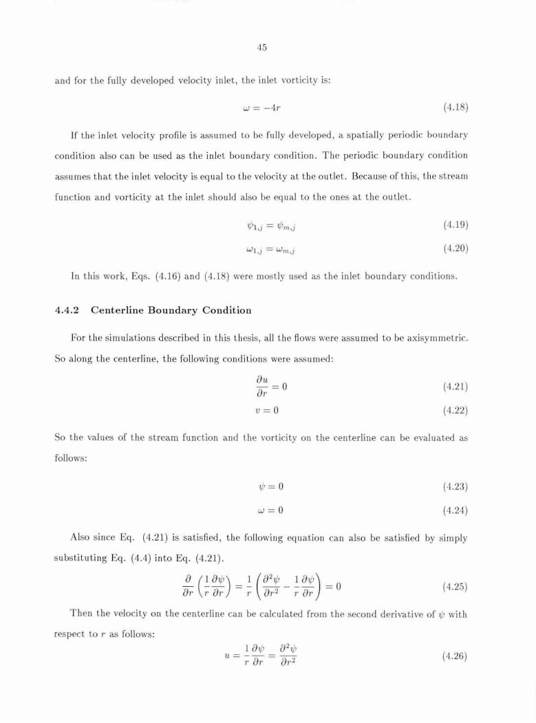
45
and for the fully developed velocity inlet, the inlet vorticity is:
vJ = -4r
If Lhe inlet velocity profile is assumed lo be fully developed, a spatially periodic boundary
co ndit ion a lso can be used as the in let bou ndary cond ition . The period ic boundary condition
assumes t h at t he inlet velocity is eq ua l to the veloci Ly at the outlet. Because of th is, t he st.ream
function and vorticity at the inlet shou ld a lso be equal to the ones at t he outlet.
lt-'1 ,) = l/Jm .J
WJ,) = Wm ,j
(4.19)
(4.20)
In this work, Eqs. (4.16) and (·I. I ) were mostly used as the inlet boundary conditions.
4.4.2 Cente rline Boundary Condition
For th e simu lations described in t his thesis, a ll t he nows were assum ed to be ax isy mmctric.
o a long the centerlin e , t he fo llowing co nditio ns were ass um ed :
Du = 0 a,. v= O
(·1.2l)
( I. 22)
o Lhe values of the stream function and the vorticity on the centerline can be evaluated as
follows:
~I= Q
w= O
(·1.2:3)
(•1.2·1)
Also s ince Eq. (4.21) is satis fi ed, t he follow ing equation can also be satis fied by sim ply
substituting Eq. (4.4) in to Eq. (4.21).
!. ( ~ ~~) = ~ ( ~:.~ - ~ ~~) = 0 (4.2.5)
Then the velocity on the centerline can be calcu lated from the second derivative of u with
respect to r as follows : l {) ~) {)2 i.,,
u=--=--1· or a,.2 (4.26)

46
In t he trans formed coord inate system , the centerline velocity can be calculated as follows:
J + J · 2 X< . + .t< . 2 _ 2J . . t, I r, '-r, I '>r, ('' ' _ . J, ) U - r, J X~i, I 2 2 'f't,2 'f'1,l (4.27)
4.4.3 Wall Boundary Condition
T he boundary value of t he s tream fun ction on the no-slip wall is constant .
·!/J = fo 1 2r(l - r2)dr = 0.5 or '!/J = fo 1
rdr = 0.5 (4 .2 )
According to the non-sli p wall bou ndary condit ion, both u and v on the wall are zero.
However, for t he vorticity boundary value, the horizontal wall and t he vertical wall shou ld be
treated diffe ren t ly.
4.4.3.1 Horizonta l Wall Vorticity Boundary Condition
A ccording Lo the de finition of I.he vo rticity, t he vorticity on the horizontal wall can be
d escri bed as fo llows:
(4 .29)
The vorticity on th e wall can be calcul ated from t he vorticity at the points neighboring the
boundary. Fo llowing t he derivation given by Tao [3 ], the equation for the wall vorticity can
be derived.
For the s tream function 1/; at node (i jn-1), a Taylor ex pa ns ion is car ried out corresponding
t.o the stream function 'r/J at node (i,jn) .
(4.30)
Since u = 0, ~~ = 0 . By s ubs tituting Eq. (4 .29) in to Eq. (4 .30), the wall vo rticity formu la
can be derived:
. . __ 1_2('!/Ji,Jn- 1 - 'l/Ji,jn) + O{' ·) w,,111 - 01 r · · 8r2
1,Jn ( 4 .31)
Jn th is work Eq. (4.31) was mos tly used as the horizontal wall vorticity boundary condition.

47
To get a more accurate formu la for wal.I vort icity, a hig her order Taylor expansion can be
carried out for 7/Ji.jn- 1.
(-1.32)
Along the horizontal wall gr (~) = 0 can be assumed, then
aw a (au) a (av) a ( 8 (1 a.,µ )) or = ar 8r - 8r ax = 8r a.,. -;:a;: 1 a3 w 2 82 w 2 a'!f;
= ;: ar3 - 1·2 fJr2 + r 3 8r (4.33)
By substitu t ing Eq . (4.29) and Eq. (4.4) into Eq. (LJ.:33), the following equation can be
derived: 83·!/; 8w 2 8w - = r- + 2w - - u = r - + 2w 8r3 8r r or (4.34)
By substituting Eq. (4.29) and Eq . (4.34) into Eq. (-l.32), a higher order wall vorticity
formu la can be derived:
(4.35)
4.4.3 .2 Vertical Wall Vort icity Boundary Condition
Similarly the vorticity on t he vertical wall can be described as follows:
(4.36)
For the stream function 1f; at node (i + 1, j) or ( i - 1. j), a Tay lor expansion can be carried
out correspond in g to t he stream function 'I,' at node (i,j).
( 4.37)
Since v = 0, ~ = 0. By s ubstituting Eq. (4.36) into Eq. (4.37) the formula for t he
vertical wall vorticity can be deri ved:
.. = _l 2(¢t±1,j - '1/.\3) + O(r ·) W1 J r 2 uX
' 7'i,J uX (4 .3 )
In t his work, Eq. (4.3 ) was mostly used as the vertical wall vorticity boundary condi tion.

4
To get a more accu rate for mula for wall vorticity. a higher o rder Taylor expansion can be
carried out for l/J1± l ,J ·
(-!.39)
Along t he vertical wall /;; ( ~) = 0 can be assu med, then
( 4.40)
So 83'1J) aw --=r-8x3 ax (4.41)
By s ubs tituting Sq. (4.36) a nd Eq. (4.41) into Sq. (·1.39) , a hig her order vertical wall
vorticity formula can be derived:
1/ 1 ± - 1. 1 1 •) ..... I ,) '+'I.) + O(A 2) w · - " - -w·±1 u:r t,J - . r .2 2 I ,) r 111uX (4.42)
4.4.3.3 The Vorticity Value on the Wall Corne r
The vorticity value on the wall co rner can be calcu lated by averaging the vorticity values
on both x and r direction.
(4.43)
4.4.4 Outlet Boundary Condition
There arc four options for the outlet boundary conditions. Generally the strongest outlet
boundary condition is to prescribe values on the boundary for both the s tream function and
vorticity. To give the firs t or second order derivative values on the boundary wou ld be weaker
bo undary condi t io ns . T he higher I. he o rder of t he derivative value t hat. is prescribed , t he weake r
Lhe boundary condition is.
4.4.4.1 Fixed Va lue Outlet Bounda ry Condition
This boundary condition is only used lo refine the s imu lation after some initial s imulations
have been done . For the fl ow through pipe orifices, when the Rey nolds number becomes larger,

49
Lhe co rresponding pipe length after t he orifice plate s hould a lso be longer. Due Lo the li miLation
of the compuLing power, a relatively coa rse mesh is used fo r the s imu lation. ll owevcr, if detailed
fl ow patte rns are needed, a refined simula tion can be car ried out by using this oulleL boundary
condition. The prescribed value on the outlet boundary can be imported from a coarse grid
simu lation res ults at t he same Reynolds number .
So t he first type o ut le t bounda ry co ndition is:
lp =cl
w = c2 (4.44)
where cl and c2 a re co nstants .
4.4.4.2 Fully D eveloped Outle t Boundary Condition
lf the distance downstream of th e o rifice is long enough , iL can be assumed that the flow
a.L t he outlet is fully developed (39], wh ich means
0
au = 0 ax v= O
ow a (au av) a (au) 8x = fJ:r /Jr - /Jx = Br Ox = O
fh/J = 0 ox
(4.4.5)
( 4.46)
( 4 .47)
( 4.4 )
Then the o utle t. bounda ry values for both t he s tream function a nd t he vort icity can be
prescribed as follows:
Vm,J = tPm-1 ,j
Wm,) = Wm- l,j
(4.49)
( -1..50)
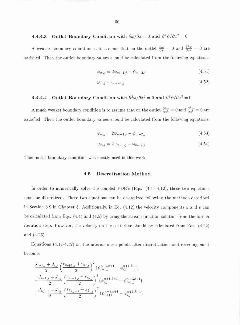
50
4.4.4.3 Outlet Boundary Condition with ow/ox= 0 a nd fJ2'1f;/fJx 2 = 0
A weaker boundary condition is to assume that on the outlet ~~ = 0 a nd fx# = 0 a re
sat isfied. T hen t he o ut let boundary values s hou ld be calculated from the followi ng equatio ns:
'1f;m,j = 21/Jm- l ,j - Wm-2,J
Wm,j = Wm- Lj
4.4.4.4 Outlet Boundary Condit ion w it h 82w/8x2 = 0 and 82'1j;/8x2 = 0
(4 .51)
(4 .52)
A much weaker boundary condit ion is to assume that on the outlet ~ = 0 a nd ~ = 0 are
satisfied. Then t he o ut let boundary values s hou ld be calculated from t he followi ng equ ations:
Wm,j = 2wm- l ,j - Wm-2,j
This o utlet bounda ry condit ion was mostly used in thi.s work.
4.5 Discretization Method
( 4 .53)
( 4.54)
In order to numerically solve t he coupled PDE's (Eqs . (4.11-4.12), these two eq uations
must be discretized. T hese two eq uations can be discret ized following t he methods described
in Section 3.9 in C hapter 3. Additionally, in Eq. (4.12) the velocity components 1t and v can
be calcu lated from Eqs. (4.4) and (4 .. 5) by using the stream function solution fro m the fo rmer
iteration step. However , t he velocity on the centerline s hould be calculated from Eqs . (4 .22)
and (4.26).
Equations (4 .11-4.12) on the in terior mesh points after d iscretization and rearrangement
become:

J i - 1,j + J i,j
2
+ J i ,j+ l +hi 2
51
J . ·+ J· · (x~ . · +x~ . ·) 2 k k 1 i,1 1,3- 1 ~1.1- 1 ~ i.1 (w~Tl , ·+1 _ w'!l"!- 1, -+ )
2 2 1,J 1,3- l
n+ 1,k+ 1 1 w~i-!- 1 ,k+1 _ w!l. wi,i R i,1 i,1
,. 2 J ·. - eref-J. . '' t I i,j l 1J l.J £..). '
(4.5.5 )
lu.•,J I n+l ,k+l Ui,j n+ t ,k+ J Ju., ,J I n+ l,k+J (1-~ - l -~ )
- R eref rTJi,j --2--"'-Ui+1,jWiH ,j + lui, j l U.i,jWi,j + 2 Ui - t ,j Wi- l ,j
R IV1,1 I . . n+l ,k+ l + ~ .. n+ l,k+ l + JVi,11 • . n+t,k+l (1-~ . . - 1 -~ )
- e,·ef x~i,j 2 Vi,3+Lwi,j+ 1 Iv· ·I tJi,1Wi,j 2 V1,3-lwi,j- 1 1,J
=0 (4.56)
4 .6 Preconditioning
Physically, the stream fun ction 'I/; a nd t he vo rt icity w shou ld have a high level of coupling.
From t he coupled eq uations (Eqs . (4.11)-(4.12)) , it is easy to see that the stream function
dis t ribution affects t he distribu t ion of t he vorticity t hrough its gradien t, which is in fact t he
velocity field. However, t he coupling between the discretized DYE, Eq. (4 .5.5) and VTE, Eq.
( 4.56) is ha mpered because of the way the velocity components u and v a re t reated in Eq.
(4 .56) . In this disc retized equa tion , the velocity com ponents u. and v are calcu lated from the
st ream function solu t io n from t he previous iteration step. Then, th ese two components in
Eq. (4.56) a re treated as constants in the new iteration step. Thus, the discretized VTE, Eq.
(4.56), is somehow decoupled from the discretized DYE, Eq. (4 .55) . fn order to enha nce the
coupling between t he discret ized DYE and YTE, a precondi t ioning term -J8 ?/Jij, which is in ,,J '
fact the local stream function mu lt iplied by a factor , was add ed to bot h s ides of the discretized

52
VTE, Eq.(4.56) . The mod ifi ed discretized VTE is described as follows:
where 'f/J~j1 •k+l is t he stream funct ion from the new iteration step, and 'lf.1F,J 1'k is t he stream
fun ction from the former iteration step. When t he solution converges, t he d ifference between
the -L 'f/7~"!° 1 •k+I a nd -J8 'f/77J-T- 1·k would va nish. Thus, at convergence, t he original VTE is J,,J 1,3 •,) '
satisfi ed.
4.7 Solution Procedure
The d iscretized DVE, Eq. (4.55), a nd t he modifi ed discreLized VTE, Eq . (4 .57) were
solved by ihe CSIP (coupled st rongly implicit procedure), which was described in Section 3.12.
After rearrangement , the coupled equa tions can be expressed in ihe block matrix fo rm as
-->.n+ l ,k+.l __. [A] q = b (4 .5 )
where (A] is a lmost the same as t he one in Eq. (3.49) except its elements a re 2 x 2 arrays; and T _.n+l ,k+l [ J n+l ,k+l
q = ('f/7,w)f.i ... ... ('f/7,w)[; ... ('f/7,w)'fn,n
b= [ (b.µ, bw)[1 (bw, bw)[j (b~, bw)'f:i,n ]T

53
Then t he solution procedu re follows t he same steps from Step 1 to Step 3 described in Chapter
3. However , t he solution is updated slight ly different ly by adding an under-relaxation facto r:
-"n+l ,k+ l _...n + l ,k ->.n+ l ,k+l q = q +a 8 (4.59)
where Cl' is t he under-relaxation factor .
After every iteration , t he upd ated solutions of t he stream fu nction and t he vorticity a re
used to calcu late t he velocity field by using Eqs. (4.4) and (4.5) . However, the velocity on
the centerli ne should be calculated from Eqs. (4.26) a nd (4 .22) . Then the computed velocity
field is used in the next itera tion. These procedu res a re repeated until convergence . Also t he
convergence c ri terion is similar to t he one described by Eq. (3.57):
'\' . . [ ( y,.n+1,k+1 _.q,n+l ,k) 2
( wn+ l ,k t I -w"+ 1,k) 2
] wt,] • 1.ntl ,k + n + l ,k
Y-Fovg Woug
€ = 4-im x jn
( 4 .60)
4.8 The Effect of the Under-relaxation Factor and the Preconditioning
Treatment
The und er-relaxation factor and t he precondition ing treatment are com bined to be used
to ensure the convergence. Tannehill et a l. [32) mentioned t hat under- relaxation appears to
be most a ppropri.ate when the convergence at a poin t is taking on an oscillato ry pattern and
tendi ng to 'overshoot" the a pparent final solution. However , the preconditioning term is added
to enha nce t he coupling between t he two equations (the discretized DVE a nd d iscretized VTE).
Wit.h t he coupling enhanced, the convergence can be improved.
The simulations of t he pipe and orifice flows wit h a la rge orifice/ pipe dia meter ratio are
easy to converge witho ut under- relaxation and not much precond itioning is needed . Thus, t he
under-relaxation factor a: can be 1 and t he precondition ing coefficient() can be a small nu mber
(genera lly it is less t ha n 1).
When the orifi ce/pipe di amete r ratio decreases, t he simulations may blow up without under-
relaxation and preconditioning. Generally, the under- relaxation factor takes on a value less
t han 1 in order to converge t he simula tion . From t he numerical experi ments with d ifferent
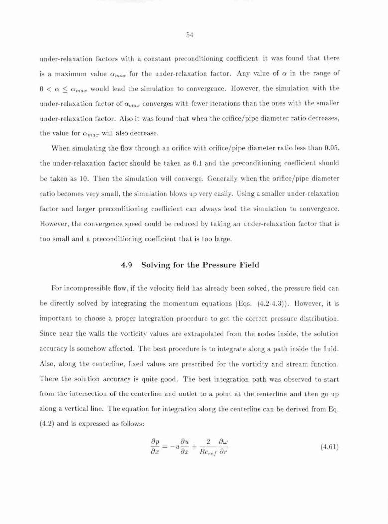
under-relaxation factors with a constant. preconditioning coefficient it was found t hat there
is a maximum value frmax for the under-relaxation factor. Any value of a in the range of
O < o ~ O'ma.c would lead the simulation Lo convergence. However. the simulation wi th the
under-relaxation facto r of ll'rnax converges with fewer iterations than the ones with the smaller
under-relaxation facto r. Also it was fou nd that when t.hc orifi ce/pipe diamete r rat.io decreases,
the value fo r ll'max will also decrease.
When simulating the fl ow through an orifi ce with orifice/ pipe diameter ratio less than 0.0.5.
the under-relaxat ion factor should be taken as 0.1 and Lhe preconditioning coefficient should
be taken as 10. Then the simulation wil l converge. Generally when the orifice/pipe diameter
ratio becomes very small, t he simu lation blows up very easily. Using a smaller under-relaxation
factor and larger preconditioning coefficient can always lead the simulation to convergence.
However, the convergence speed could be reduced by taking an under-relaxation factor that is
too small and a precondit ioning coefficient that is too large.
4.9 Solving fo r t he Pressur e F ield
For incompressible flow, if the velocity fi eld has already been solved. the pressure field can
be directly solved by in tegrating the momentum equations (Eqs. (4 .2-4.3)). However. it is
important to choose a proper integration procedu re lo get the correct pressure distribution.
ince near the walls the vorticity value are extrapolated from lhe nodes inside, the solu tion
accuracy is somehow affected. The best procedure is lo integrate along a path inside Lhe fluid.
Also, along the centerl ine, fi xed values arc prescribed for the vorticity and stream funct.ion.
There the solutiou accuracy is quite good. The bes t integ ration path was ob ervcd Lo s tart
f'rorn the in tersection of the centerline a n<l out.let Lo a poin t a.t the centerline an<l then go up
along a vertica l line. The eq uation for integration a long the centerline can be deri ved from Eq.
(4.2) and is expressed as follows:
8p 8tt 2 8...; -=-tt-+---8x 8x Reref 8r (4.61)
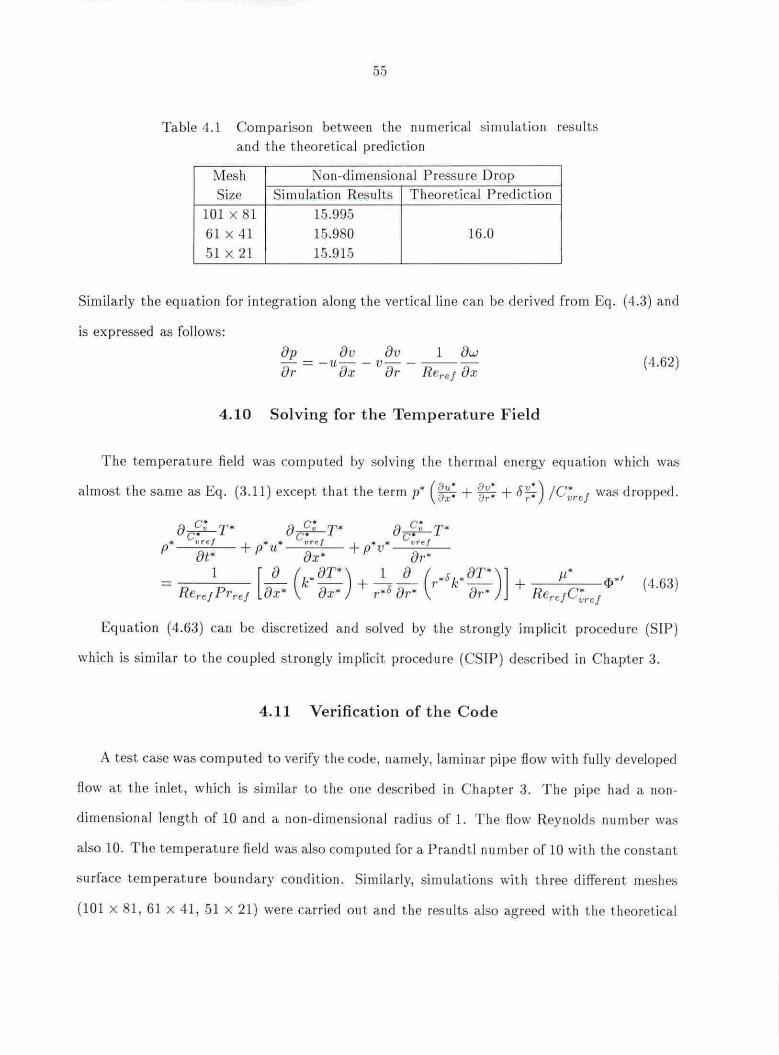
55
Table 4.1 Comparison between t he numerical simulation results and the t heoretical prediction
Mesh Non-dimensional Pressure Drop Size Sim ulation Results Theore t.icaJ Prediction
101 x 81 15.995 61 x 41 15.980 16.0 51 x 21 15.915
Similarly the equation for integration along the vertical line can be derived from Eq. (4 .3) and
is expressed as follows : op fJv fJv 1 ow -= -u-- v- ----8r Bx or R e,·ef 8:c
(4.62)
4.10 Solving for t he Temperature Field
The temperat ure field was computed by solving the thermal energy equation which was
almost t he same as Eq. (3.11) except that the t erm p* ( ~~: + ~~ : + o~: ) /C;,.ef was dro pped.
Equation (4.63) can be discretized and solved by t he s trongly implicit procedure (SIP)
which is s imila r to the co upled s trongly implicit procedure (CSlP) described in Chapter 3.
4.11 Verification of the Code
A test case was computed to verify the code, namely, laminar pipe flow wit h fully develo ped
flow at the inlet which is simila r to the one desc ribed in C hapter 3. The pipe had a non-
dimensional length of 10 and a non-dimensional radius of l. The fl ow Rey nolds number was
a lso 10. The temperature fi eld was a lso computed for a P randtl nu mber of 10 wit h the constan t
surface temperature boundary condition. Similarly, simulations with three diffe rent meshes
(101 x 81, 61 x 41 , 51 x 21) were carried out and the res ults a lso agreed with the theoretical

56
Table .J.2 Comparison between Lhe numerical simulation results and the theoretical prediction for the thermal entry prob-lem with constant surface t.cmpNature
Mesh Size
l 0 L x l 61 x 41 .51 x 21
Local usscl t nu 111 bcr i 11 the l he rrnally developed region Simulation Resu lts Theoretical Prediction
3.6.5
predictions (Table 4.1).
The 1usselt numbers simulated here agree with the theoretical prediction, even though they
are not as accurate as the ones presented in hapler 3. Table 4.2 lists the re ults simulated
basPd on the three meshes. It is believed that the simulation based on the finer mesh lead
to the more accurate res ult. Thus the usselt number calcu lated based on the 101 x l mesh
in Table 4 .2 s hou ld be the most accu rate one. Its value exceeds the theoretical prediction.
H seems t hat the simulated Nusselt numbe r will approach a value larger than t.he t.heoret.ical
predict.ion by refi ning the com putational mes h. JJ owever, in Chapter 3, it can be observed that
the Nusselt. number in Table 3.2 will approach Lhe value of theoretical predict.ion. The reason
why Lhe s imulated usselt numbers in Chapter 3 and 'I are s light ly different may be that
the s imulation in Chapter 4 were solving the energy equation, Eq. (4 .63), without dropping
the conduction term in t he x direction, which is the first term in the right ha11d s ide of the
equation.

57
CHAPTER 5. NUMERICAL SIMULATION BY FLUENT
5.1 Introduction
The commercia l com putatio nal fluid dynamics (CFD) software FLUENT was also used
to simulate Lhe highly viscous oil flows t hrough small o rifice/pipe diameter ratio orifices. To
run a simula tion in FLUENT, a mes h generation package GAMBIT was used to generate
t he cornputat.ion mesh with the boundaries specifi ed . ln t his work, the FLUENT sim ula,t ions
modeled t he fluid flow in physical dimensions.
Since the flows t hrough orifices are axisymmetric, a two-dimensional axisym metric s imula-
t ion can be carried out to pred ict t he flow field a nd t he pressure drop across the orifice. The
pipe orifice configuration is shown in Fig. 5.1. A uniform velocity was s pecified at the in let,
while fixed pressure was used at the outlet. Axisymmetri c bounda ry cond itions we re ap plied
on the centerUn e. No slip boundary conditions were used a t t he walls.
The computation mes h generated by GAMBIT was imported into FLUENT. To ini tialize
t he simulation , the fluid propert ies, s uch as the density and t he viscosity, were specified . The
in let velocity was also specified . Ini t ia l values were given before running the simu latio ns. The
coupled solvers provided by FLUENT were found to converge ve ry slowly for t.he s imu lation
L I t 1 L2
Wall R
Outlet - --x lnlcL ... __.__ __ -------- -----"""--------- - - - - ---------- - -
Centerline
Figure 5 .1 Configura tion of t he computational domain for the pipe orifi ce

,5
of t he flows t hroug h s ma ll orifice/ pipe d iameter ratio orifices . However, the segregaLed solvers
provided by F L E T converged quite quickly.
5.2 C omputation Doma in C onfigura tion a nd Mesh G en era tion
T he FLUENT simulatio ns conce nt.ratcd on t he fl ows t.h rough I mm diameter orifices (their
orifice/ pipe diameter ratios {3 were 0.044.5), especially the flows through the I mm diameter
orifice with 1 mm thick orifice plaLe. The pipe radius, t he orifice radius, and the orifice plate
t hickness were set up exactly the same as in the experiment. The length upstream of the orifice
was s pecified 4 t imes the pipe radius and the length downstream the orifice was specified with
10, 20 , 30, 40, or 50 Limes the pipe radi us, depending 011 t he o rifice Rey nolds n umber. The
length upstream of Lhe orifice a nd the length downstream of the orifice are not exactly the
same as Lhe experiment. These two lengths were cha en for the ease of numerical s imulation.
In fact t hese two lengLhs do noL affect Lite pressu re drop across small o rifice/ pipe diameter
ratio orifices very much. The pressure drop across sma ll o rifice/pipe diameter ratio orifices
mostly occurs in the vicinity of the ori fice. The pressure drop caused by the pipe itself is quite
small. For example, the simulated pressure drop across the I mm diameter orifice with 1 mm
thick orifice plate is 100,6-12 Pa when the inlet velocity is 0.0 L.5 :3-1 m/ with the constant fluid
properties (the flu id density is 76 .57534 kg/m3 and t he fluid viscosity is 0.1234 kg/(m.s)).
However, t he s imulated press ure d rop, a lo ng the pipe with the rad ius of 11.375 mm and the
same pipe length as the orifice pipe, is just 16.4 Pa. which is just 0.016% of the pressure drop
across the small orifice.
Tables 5.1-5.3 present the computation domain configurations for the 1 mm diameter orifice
with 1 mm , 2 mm , 3 mm th ick ori fi ce plaLes .
T he com putat.ion mes hes we re generated by GAMB IT block by block in five blocks. Two
mesh blocks were for the region upstream of the orifice, one mesh block was for t he orifice
region. and two mesh blocks were for the region downstream of the orifice. The mes h clustered
to a ll walls, while the mes h in the orifice region was uniform. Figures 5.2 and 5.3 show one of
the com pu tatio n meshes for Lhe l mm diamet.er ori fice with a l mm t hick o ri fice plate. T he

,59
Figure 5.2 Com putation mesh (50 + 20 + 70) x (20 + 50) for t he 1 mm diameter o rifice with 1 mm th ick o rifice plate
1~ - ~
---~ - - -=
~
-0
0.0455 q.046 0 .0465
Figure 5.3 An enla rgement of t he computa tion mesh in t he orifice region fo r the 1 mm di ameter orifice with 1 mm t hick orifice pla te
mesh s ize is (50 + 20 + 70) x (20 + 50). The expression (50 + 20 + 70) x (20 + 50) indicates
t hat t he axia l grid number for t he region upstream of the orifice was 50, the axial grid number
for th e orifice region was 20, t he axial g rid number for region downstream of t he orifi ce was
70, t he rad ia l g rid number for t he o rifice region was 20, and the radial grid number fo r t he
region up of the o rifice was 50. Also a fine r mesh, mes h size (100 +40 +140) x (40 + 100), was
generated for the l mm dia meter orifi ce with l mm t hick orifi ce plate .
5.3 Governing Equations
The governing equations for two-dimensional axisym metric pipe flow include the continuity
equ a t io n, t he axia l and radial momentu m equations, and t he energy equation. These equaLious

60
Table 5.1 Computation domain configurations for the 1 mm diam-eter orifice with 1 mm thick orifice plate
Pipe length Orifice plate Pipe length Radius of the Radius of the beforP the thickness (t) behind the 01·ifice(r) pipe (R) 01-ifice ( l I ) (mm) (mm) orifice (L2) (mm) (mm) (mm) 45.5 45.5 45.5 45.5 45.5
1.029 113.75 0.5065 11.375 1.029 227.5 0.5065 11.375 1.029 341.25 0 .. 5065 11.375 1.029 455 0.5065 11.375 1.029 56 .7.5 0.506.5 11.375
Table 5.2 Computation domain configurations for the l mm diam-eter orifice with 2 mm thick orifice plate
Pipe length Orifice plate Pipe Length Radius of the Radius of lhe before the thickness (t) behind the orifice(r) pipe (R) orifice ( l l ) (mm) (mm) orifice (1.,2) (mm) (mm) (mm) 45.5 1.9561 113.75 0.5015 11.37.5
Table .5 .3 Computation domain con fi gurations for the 1 mm diam-eter orifice wit h 3 mm t hick o rifice plate
Pipe length Or'ifice plate Pipe length Radius of the Radius of the befor·e the thickness ( t) behind the orifice (r) pipe (R) orifice (Li} (mm) {mm) orifice ( L2) (mm) (mm) (mm) 45.5 2. 859 11 3.75 0.50545 11.37.5
are given by [40]
fJp 8 fJ PVr fJt + fJx (pvx) + {Jr (pvr) + -
1-. = 0
0 1 8 l [) fJp {)t
(pvx) + - -8 ( r pvx vx) + - -8 ( r pv,. Vx) = - -8 r x r r x 1 O [ ( 2 fJvx 2 ( OV:r 8vr Vr ) ) ] I o [ ( ov:r ovr ) ] +-- rµ -- - -+-+- + -- ,. - +-r fJx ox 3 ox a,. 1· 1' 01' µ or ox
a 1 fJ i a ap 8l
(pvr) + --8 (rpvxvr ) + --8 (rpvrv,.) = -'"!) r x r r ur
l fJ [ ( fJv,. OVx ) ] 1 8 [ ( 2 fJ v,. 2 ( Bvx fJvr Vr ))] +-- rµ - +- +-- 1'/L --- -+-+-7' fJx fJx or 1' or 01' 3 f);i; fJr r
2 'Ur 2 µ ( OVx a Ur l'r ) - µ-+ -- -+ - +-r 2 3 r ax fJr r a ~ ~ fJt (pE) + \1 · (v (pE+ p)) = \J. (k\lT +¥· v)
(5. 1)
(5 .2)
(5 .3)
(5.4)

61
where pis t he density, Vx is the axial velocity, Vr is t he rad ial velocity, pis t he static pressure,
T is tem perature, µ is t he viscosity, k is t hermal conductivity,'¥ is the stress tensor, ~ is t he
velocity vecto r, a nd E is t he intern al energy per un it mass.
In t his work, t he highly viscous oil fl ow through orifices was assumed to be a simple single
phase flow. T here were no gravitational body forces or extern al body forces; and also there
was no rotation. T hus, in Eqs. (5.1-5.4) t hese terms don't show up.
5.4 Numerical Algorithm
FLUENT uses a control-volume-based techniq ue to convert t he governing equations to
alge braic equations t hat can be solved numerically. The in tegral for m of the govern ing equa-
tions can be discretized by first-ord er upwind scheme, power-law scheme, second-order upwind
scheme, or cent ral-differencing scheme [40]. In t his work, fi rst-order upwind scheme was chosen
in t he simulations by F LUENT. One of t he segregated solvers, SIMPLE [40], was used to solve
the discretized and linearized algebraic equations. T he segregated solver provided by FLUE T
solves t he gove rning equations seq uentially (i.e. , segregated from one another). Because t he
governing equations are non-linear and coupled, several iterations of the solution loops must
be perfor med before a converged solution is obtained . Each iteration consists of the following
steps:
1. F luid properties are updated, based on the current solution. (If the calculation has just
begun , t he flu id propert ies will be updated on t he ini tialized solution .)
2. The u, v, a nd w mo ment um equations a re each solved in tu rn using current values for
pressure and face mass fl uxes, in order to update the velocity field .
3. Since t he velocities obtained in Step 2 may not satisfy t he contin ui ty equation locally, a
"Poisson-type" equation for t he pressure correction is derived from the continuity equation
and t he linearized moment um eq uations. T his press ure correction equation is t hen solved to
obtain t he necessary corrections to the pressure and velocity fields a nd the face mass fluxes
such that cont inuity is satisfied .
4. Where appropriate, equations for scalars s uch a.5 tu rbulence, energy, species, and radiation
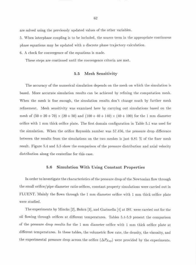
62
are solved using t he previously updated values of t he other variables.
5. When in terph ase coupling is to be included , the source term in t he a ppropria te continuous
phase eq uations may be updated with a discrete phase t rajectory calculation.
6. A check for convergence of the equations is made.
T hese steps are continued until the convergence criteria are met.
5.5 M esh Sensitivity
The accuracy of t he nu merical s imulation depends on t he mesh on wl1ich the simulation is
based. More accurate sim ulatio n resul ts can be achieved by refini ng t he computation mesh.
When the mes h is fi ne eno ugh, t he s imu lation res ults don't change much by further mesh
refinement . Mesh sensit ivity was examined here by carry ing out simulations based on t he
mesh of (50 + 20 + 70) x (20 + 50) and (100 + 40 + 140) x (40 + 100) fo r t he 1 mm diameter
orifice with 1 mm t hick o rifice plate. The first domain configu ration in Table 5.1 was used for
the simulation. When t he orifice Reynolds num ber was 57.4.56, the p ressure d rop difference
between the results from t he simu lations on the two meshes is j ust 0.81 % of the finer mesh
result. F ig ure 5.4 and 5 .5 show the comparison of t he press ure distribution and axial velocity
distribution along the centerline for this case.
5.6 Simulation With Using Constant Properties
In o rd er to investigate t he characteristics of the pressure d rop of t he ewto ni an flow t hrough
the small orifice/ pipe dia meter ra.tio orifices constant property si mulations were carried out in
FLUENT. Main ly the fl ows t hrough the l mm diameter orifice with 1 mm thick orifice plate
were studied .
T he experiments by M incks [2], Bohra [3], and Garimella (4] at ISU were car ried out fo r the
oil flowing t h rough orifices at different temperatures. Tables 5.4-5.9 present t he comparison
of the pressure drop resul ts fo r t he 1 mm d iameter ori fice with 1 mm th ick orifice plate a t
different temperatures . In t hese tables, the volumetric flow rate, t he densit.y, the viscosity, and
the experimental pressu re drop across t he orifice (6.PExp) were provided by t he ex periments.

63
Also in these tables 6.Psim is the pressure drop ac ross the orifi ce from t he simula tions by
FL ENT.
ln fact , the inlet velocity (u inlet) in t his cha pter is t he inlet mean velocity, which ca n be
cal cula ted from t he volumetric flow ra te (Q) by Eq. (5.5) . At the sam e time, the orifice
Rey nolds number was calculated based on t he orifi ce mean axial velocity Uo , which also can
be calc ula ted from the volumetric flow rate, Q, by Eq. (6 .10) .
w he re R is the pipe radius .
where r is t he orifice radius .
Q Uinlet = 7r R2
Q llo = - 2 7r r
(5 .5)
(5.6)
The orifice Rey nolds number was calcula ted based on the mean velocity in th e orifi ce region
a nd the orifice diame te r:
(5.7)
Some of the flow s tru ctures a nd t he s tatic pressure d istributions of the ewt o ni a n flow
throug h the 1 mm diame te r o rifi ce with 1 mm t hick o rifice plate computed by FLUB T us ing
const a nt prope rties will be presented in the following fi gures. Figures 5 .6 a nd 5. s how th a t
there were a recirc ulation edd y downs tream of the o rifice a nd a recirculation eddy ups trea m of
the orifice. (Fig ures 5 .7 and 5 .9 a re the enla rgeme nts of Figs. 5 .6 a nd 5 . . ) When th e orifice
Rey nolds numbe r was small , these two recirculation eddies were almos t the same size. Wh en
th e o rifice Reynolds number becam e la rger, the recirc ula tion eddy downs tream of th e orifice
inc reased its size a nd the one upstream o f t he orifi ce shrank. Fig ures 5.10 and .5 .12 clearly
illus tra te this tre nd. (Fig ures 5 .11 and 5.13 a re the enla rgeme nts of Figs. 5 .10 a nd 5.12.) At
t he same t ime, t he re was a s ma ll second recircula tion eddy between t he la rge recirc ulatio n eddy
downs tream of the orifice a nd t he corner , as s hown in F igs . 5 .11 a nd 5.13. Fig ures .5. 14-5.17
s how t he s imu lated s ta tic pressure dis tribu t ions of th e oil flows across the orifice. The static
pressure d ropped rapid ly in t he o rifi ce reg ion a nd recovered s lowly downstream of the o rifice.
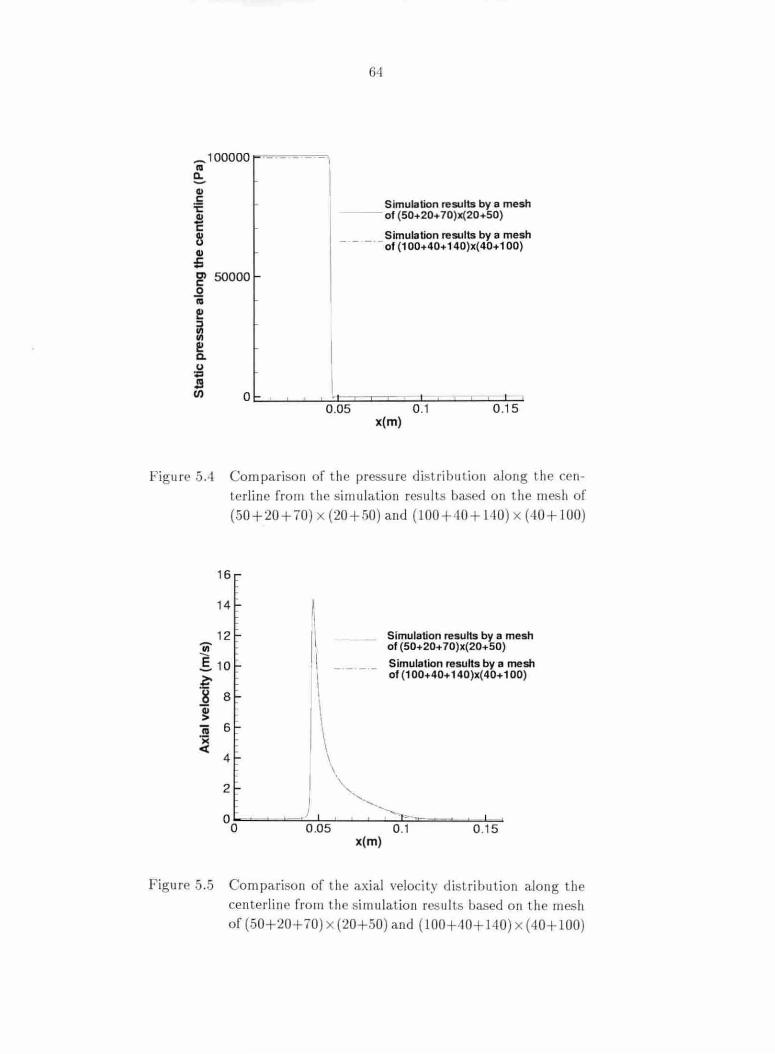
....... 100000 Ill a. Cll c :c ~ 8 Cll ;; g> 50000 .Q Ill
e! ~ e! c.. u ~
J!I
64
Simulation results by a mesh of (50+20+ 70)x(20+50)
Simulation results by a mesh - - -·-of (100+40+140)x(40+100)
~ Ot::.._...__...__J.._J........::.t::=:i:::::i:::::i:::::c:.L-.l--.l--.l--.J..._.L.....l 0 .05 0.1 0 .15
x(m)
Figure 5A Comparison of the pressure distribtt lion along the cen-terline from t he simulation results based on the mesh of (50+20+ 70) x (20+50) and (100+'10+ l40) x (40+ 100)
16
14
12 Iii 110 : ~
'8 8 ] jij 6
~ 4
2
00
11
1\ - - - -
I )
\ \
0 .05 x(m)
Simulation results by a mesh of (50+20+ 70)x(20+50) Simulation results by a mesh of (1 00+40+ 140)x(40+100)
0 .1 0 .15
Figure 5.5 Comparison of the axial velocity distribution along the centerline from the simulat ion results based on the mesh of (50+20+ 70) x (20+50) and (100+'10+140) x (40+ 100)

Case
No. j
2 3 4 5
Case
No. 1 2 3 4 5 6 7
Case
'o. 1 2 3 4 5 6 7
6.5
Table 5.4 Comparison of the pressure drop res ults for the 1 mm diameter orifice with 1 mm thick orifice plate at -25 °C
Volumetric Inle t Density Viscos·ity Orifice 6.Psim flow velocity Reynolds rate (m3 / s) (m/s) {kg/m3) (kg/(m · s)) number (kpa) 2.4 l2 x 10-6 5.932 4 x 10- 3 905.636 7.703 0.356 1140.84 2.625 x 10- 6 6.457 4 x 10⁻³ 906.249 .267 0.362 1332.82 4.995 x 10- 6 i.22882 x io-2 906.635 8.7-15 0.651 26 .5 .1 9.609 x io-6 2.36390 x 10- 2 906. j 29 .:346 1.311 4941.5 9.451 x 10- 6 2.32497 x 10- 2 906.659 9.1 7 1.172 5346.775
Table 5.5 Comparison of t.he pressure drop res ults for the l mm diameter orifice with 1 mm t.hick orifi ce plate at -20 °C
Volumetric Inlet Density Viscosity Orifice 6.Ps;m flow velocity Reynolds mte (m3 /s) (m/s) (kg/m3) (kg/( m · s)) number (kpa) 3.390 x io-6 8.33942 x 10- 3 90 l. 233 3.359 1.143 701.19 3.363 x 10- 6 8.27311 x 10- 3 902.778 4.1 87 0.911 866.21 5.729 x 10⁻⁶ 1.40938 x L0- 2 902.390 3.921 1.657 1386.21 6.251 x io-6 1.53777 x 10- 2 903. 159 4.44 1.595 1715.2 1.242 x 10⁻⁶ 3.05655 x 10⁻² 902.378 4.05 3.473 3140. 64 1.697 x 10- 6 4.17411 x 10- 2 902.75 4.299 4 .479 4575.467 2.3 3 x lo-6 5. 6l16 x l0- 2 902.19·1 3.915 6.901 5976.3.5
Table 5.6 Comparison of t.he pressure drop results for the 1 mm diameter orifice with 1 mm thick orifice plate -10 °C
Volumetric Inlet Density Viscosity Orifice f::::.Ps1m flow velocity Reynolds 1'CLle (m 3 / s) (m /s) (kg/m3) (kg /( m · s)) number (kpa) 3.627 x 10- 6 8.92164 x 10⁻³ 95.844 1.298 3.145 292.764 8.425 x 10- 6 2.01212 x io- 2 895.614 1.318 7.19 713.53 l.095 x io- 5 2.69406 x 10- 2 895.420 1.247 9.884 906.14 1.476 x 10- 5 3.63098 x 10- 2 9.5.701 l.335 12.443 1356.61 1.766 x 10- 5 4.3450 x 10⁻² 95.226 1.23 16.050 1593.99 2.666 x 10- 5 6.55757 x 10⁻² 95.331 1.273 23.560 2794.67 3.6 2 x 10- 5 9.05 7 x 10⁻² 895.430 1.282 32.32 4432.24 4.273 x 10- 5 i.os12.5 x 10- 1 94. 60 1.197 40.142 5331.42
6.Pexp
(kpa) l016. 62 1209.122 2003.878 292 .256 3..J96.235
6.PExp
(kpa) 523.544 701.835 JO ll.255 120 .309 202 .1 2 2 67.494 349.5.238
.C.PExp
(kpa) 203.179 507 .6 7 704.7 If 1007.943 1206.9 ' 2031.993 3064.679 3502.612

Case
No. 1 2 3 4 5 6 7 8 9 10
Case
No. 1 2 3 4 5 6 7
Case
No. 1 2 3 4 5 6 7 8
66
Table 5.7 Comparison of t he pressure drop results for t he 1 mm dia meter orifi ce with 1 mm thick orifice plate 0 °C
Volumetric Inlet Density Viscosit y Orifice 6.Psim 6. PExp flow velocity Reynolds rate (m 3 /s) (m /s) (kg / m3) (kg / (m · s )) number ( kpa) (kpa) 3.413 x 10- 6 8.39650 x 10- 3 89.020 0.486 7.848 107.419 97.86 6.757 x 10- 6 1.66219 x 10- 2 889.992 0.534 14.143 255.033 205. 21 1.275 x 10- 5 3.13726 x 10- 2 889.776 0.516 27.630 576.48 499.130 1.633 x 10- 5 4.01688 x 10- 2 889.375 0.498 36.680 808.033 693.579 2.114 x 10- 5 5.20115 x 10- 2 889.275 0.504 46.886 1201.05 1018.530 2.419 x 10- 5 5.95023 x 10- 2 888.83 0.470 57.462 1435.655 1205.342 3.453 x 10- 5 8.49450 x 10- 2 888.699 0.478 80.710 2560.3 2015.372 4.554 x 10⁻⁵ 1.12024 x 10- 1 889.217 0.514 99.077 4182.78 3001.986 5.10 x 10- 5 1.25653 x 10- 1 889.116 0.506 112.830 5053.9 3498.540 5.403 x 10- 5 1.32913 x 10- 1 88 .798 0.4-87 124.003 549 .87 38 8.553
Ta ble 5.8 Compa rison of the pressure drop results for t he l mm dia meter orifice wit h 1 mm thick orifice plate 10 °C
Volum etric Inlet Density Vis cosily Orifice 6.Psim 6.Psxp flow velocity Reynolds rate (m 3/s) (m / s) (kg / m 3) (kg / (m · s)) number (kpa) (kpa) 5.345 x 10⁻⁶ 1.31493 x 10- 2 883.098 0.224 26.512 103.120 100.216 8.732 x 10⁻⁶ 2.14809 x 10- 2 883.763 0.232 41.854 215.403 203.876 i.622 x 10- 5 3.9 930 x 10- 2 883.183 0.225 80.034 566.202 507.918 1.990 x 10- 5 4.89672 x 10⁻² 883.549 0.230 96.168 801.784 698.876 2.588 x 10- 5 6.36100 x 10- 2 882.827 0.221 129.918 1237.04 1035.267 2.840 x 10- 5 6.98735 x 10- 2 883.266 0.227 139.19 1462.79 1203.346 3.964 x 10- 5 9.75264 x 10- 2 882.982 0.223 197.163 2618.49 2050.133
Table 5.9 Compa rison of the pressure drop results fo r the 1 mm diamete r orifice with 1 mm thick orifi ce pla te 20 °C
Volumetric I nlet Density Viscosity 0 1'ifice 6.Psim 6.Psxp flow velocity Reynolds rate (m 3 /s) (m / s) (kg / m 3 ) (kg/(m · s )) mtmber (kpo) {kpa) 6.436 x 10- 6 0.015834 876.575 0.123 57.456 100.642 101.271 9.929 x 10- 6 0.024426 876.610 0.124 88.574 203.390 210.5 4 1.735 x 10- 5 0.042692 876.276 0.121 158.265 524.091 502.443 2.118 x 10- 5 0.052113 876.516 0.123 1 9.792 74 .357 705.406 2.595 x 10- 5 0.06384 876.231 0.120 237.846 1071.242 1003.657 2.933 x 10- 5 0.072162 876.417 0.122 265.115 1341.57 1217.131 3.941 x 10- 5 0.0969.53 876.161 0.119 364.225 2300.546 1997.635 4.975 x 10- 5 0.1224 76.197 0.119 460.011 3.5.57.718 3035.921

67
Streamllne distribution
x 0.1 0 .15
Figure 5.6 Simulated streamli ne dis tribution for Case 1 of Table 5.5, Re0 = 1.143
Streamllne distribution 0.012
0.01 ~iiiiiiil
0.008
- 0.006 0.004
0 .002
o c========~~iba~
Figure 5 .7 An enl argement of the s imulated s treamline distribut ion in t he orifice region for Case 1 of Table 5 .. 5, Re0 = 1.143
Streamline dlstrlbutlon
Figure 5 .8 Simulated streamline dist ribution for Case 2 of Table 5.5 , Re0 = 0.911
0.012
0.01 0.008 0.006
Streamllne distribution
~~?.ii
0.045 x 0.05
Figure 5.9 An enl a rgement of t he s imulated streamline distr ibut.ion in the orifice region for Case 2 of Table 5.5, Re0 = 0.911
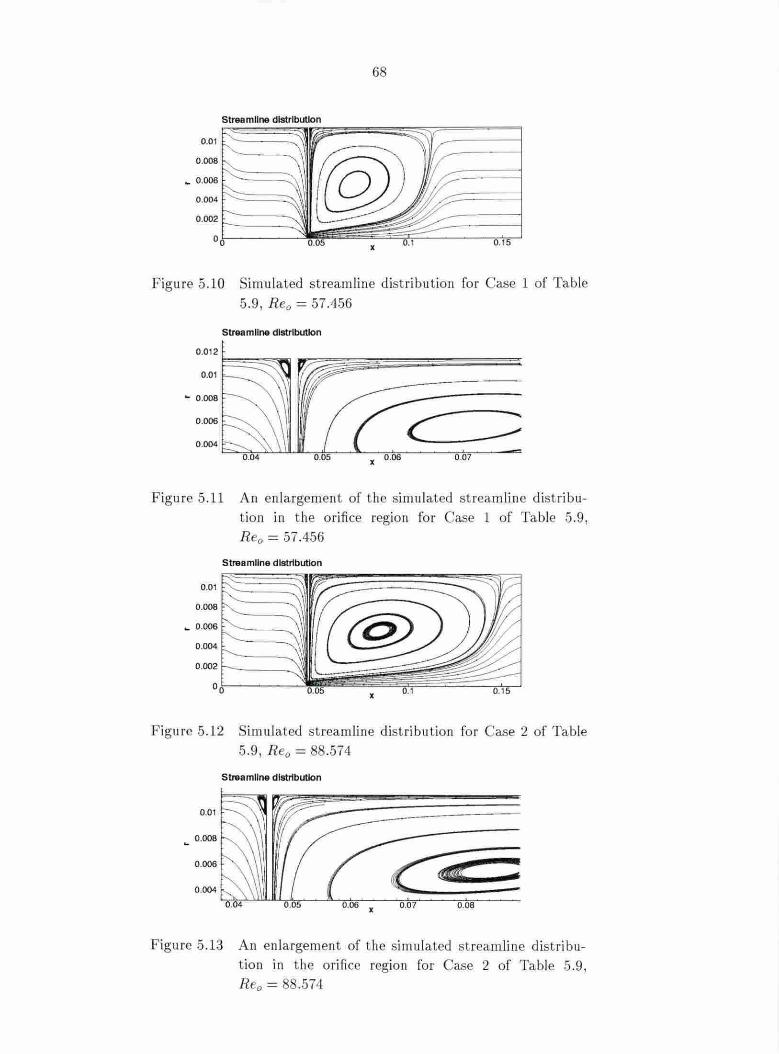
68
Streamline distribution
0.01
0.008
~ 0.006
0.004
0.002
0 .05 x 0.1 0.15
Figure 5.10 Simulated streamline distribution fo r Case 1 of Table 5.9, Rea= 57.456
Streamline distribution
0.012
0.01
~ 0 .008
0.006
0 .004
F igure 5.11 An enlargement of t he sim ulated streamline distrib u-tion in t he orifice region for Case 1 of Table 5.9, Re0 = 57.456
Streamline distribution
Figure 5.12 Simulated st reamline dist ribu t ion fo r Case 2 of Table 5.9, R ea= 8 .574
Streamline distribution
: F igure 5.13 An enla rgement of t he simulated streamli ne dist ribu-
t ion in t he o rifice region for Case 2 of Table 5.9, Re0 = 88.574
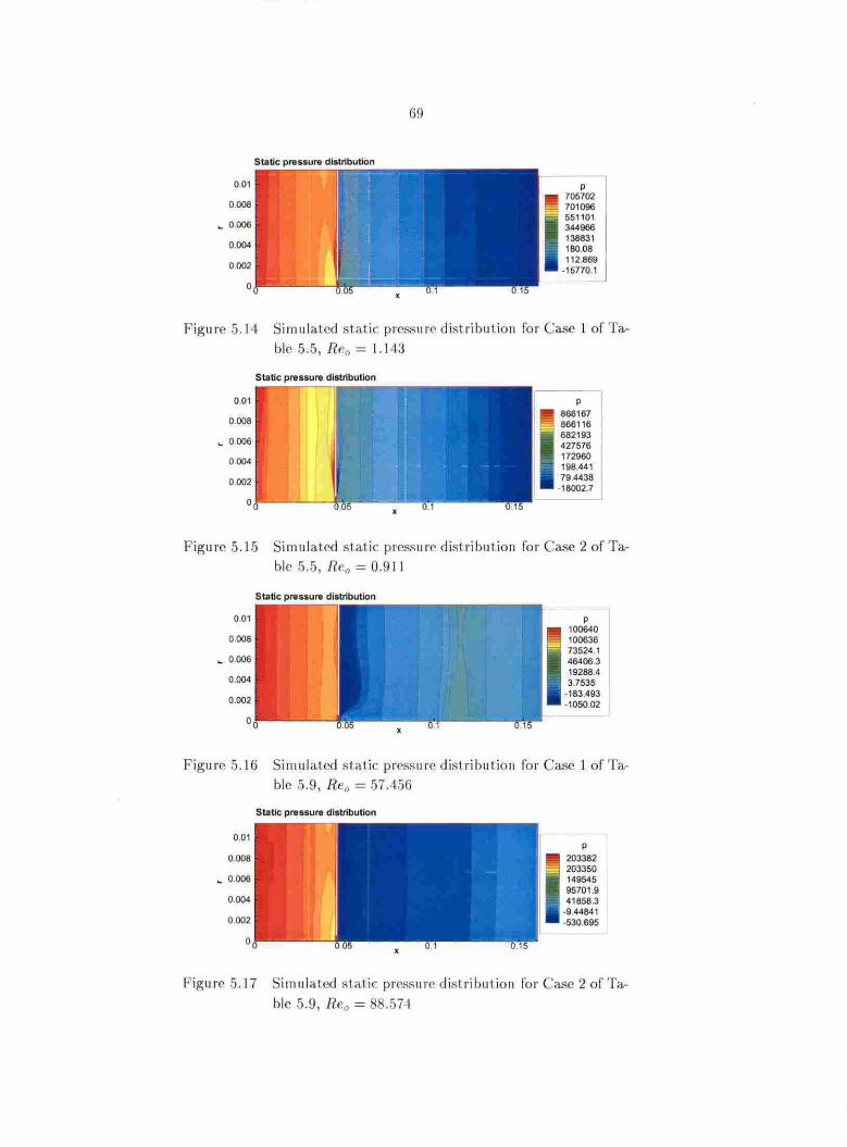
0.01
0.008
~ 0.006
0.004
0.002
0
69
p 705702 701096 551101 344966 138831 180.08 112.869
-1 5770.1
Figure 5. l4 Simulated st atic pr<'ssurc distribution for Case l of Ta-ble 5.5, Ren = 1.1 43
O.Q1 p 866167
0.008 866116
~ 0.006 682193 427576
0.004 172960 198.441
0.002 79.4438 ·18002.7
0
Figure 5. 15 Simulated st at ic pressure' distribul ion for Ca.<1e 2 of Ta-ble .5.5 , Re0 = 0.91 1
F igure 5.16
p 100640 100636 73524.1 46406.3 19288.4 3.7535
·183.493 -1050.02
Simulalcd st aJic pressure distribu t ion for Case 1 of Ta-ble 5.9, Re0 = 57.456
Static pressure distribution
0.01 p
0.008 203382 203350
~ 0.006 149545 95701 .9
0.004 41858.3 ·9.44841
0.002 ·530.695
0
Figure 5.17 Simulated st a1ic pressure> distribution forCase2ofTa-ble 5.9, Re0 = .574

70
CHAPTER 6. PRIMITIVE VARIABLE AND STREAM FUNCTION
VORTICITY RESULTS
In this chapter, t he numerical simulation resul ts for the laminar flow through o ri1ices with
orifice/ pipe diameter rat ios (/3) of 0 .5, 0 .2 and 0.0445 (ISU experiments) are presented and ana-
lyzed. The simulat ion results by both the primitive varia ble approach and t he s tream-fun ction
vort icity a pproach are presented ; a nd a ll t he simulations are st eady state. The simulation
results wit h a /3 of 0.5 a re compared with Sahin and Ceyhan 's [6] experiment results; and
t he resu lts with a /3 of 0.0445 are compared wit h t he experim ents carried ou t by M incks [2],
Bohra [3], a nd Garimell a [4] at Iowa Stat e Uni versity. The simulation results with a f3 of 0.2
are compared with Hayase, et a l. 's [7] numerical simulat ion res ul ts.
6 .1 Laminar F low t hrough Square-edged Orifice with a Diameter R atio of
0.5
In 1996, Sahin a nd Ceyhan [6] meas ured discharge coeffi cients for laminar fl ow t hrough a
squa re edged orifice wit h different th icknesses; a t the same t ime, t hey solved the incompressible
Navier-Stokes eq uations numerically for t he oriflce flows. T heir numerical simu lation results
agreed well wit h t he experiment results . In t his t hesis, in order to verify both nu merical
approaches described in Chapters 3 and 4, similar nu merica.J s imulations were set up a nd
carried out. T he results from both approaches agreed well with Sahin and Ceyhan's resul ts.
Incompressible la min ar flow t hrough a square edged orifice with orifice/ pipe diameter ratio
of 0.5 and variable thick ness was modeled and simulated . The as pect ratio t~ is defi ned as:
• t t = -d (6.1)
where tis t he orifi ce plate thickness a nd d is t he orifi ce diameter.
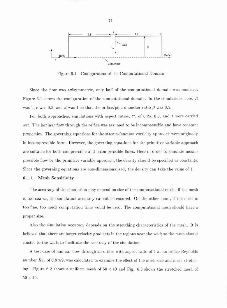
71
LI L'2
!'---Wall R
l~_lruc_L ~- __ _________ __ ""-_________ ______________ _ Oullel
Centerline
Figure 6.1 Configuration of the Computational Domain
Since the flow was axisymmetric , only half of th e computational domain was modeled.
Figure 6.1 shows the configuration of the computational domain. ln the simulations here, R
was 1, r was 0.5, and d was 1 so t hat the orifice/ pipe dia meter ratio /3 was 0.5.
For both approaches, simulations with aspect ratios, t*, of 0.25 , 0.5 , and 1 were carried
out. The laminar flow through the orifice was assum ed to be incompressible and have constant
properties. T he governing equat ions for t he stream-function vorticity approach were o riginall y
in incompressible form. However, t he governing equations for the primitive variable ap proach
are suitable for both compressible and incompressible flows. Here in order to simulate incom-
pressible flow by the primitive variable a pproach, the density should be specified as constants.
Since the governing equations a re non-d imensionalized , the density can take the value of l.
6.1.1 Mesh Sensitivity
The accuracy of the simulation may depend on size of the computational mesh. lf the mes h
is too coarse, the s imulation accuracy cannot be ensured. On the other hand , if the mesh is
too fine, too much computation time wo uld be used . The computational mesh shou ld have a
proper size.
Also the simulation accuracy depends on the stretching characteristics of t he mesh. lt is
believed that there are la rger velocity gradients in the regions near the wall ; so t he mesh should
cluster to t he walls to facilitate the accuracy of the simulation.
A test case of lamina r flow through a n orifice wit h aspect ratio of 1 at an orifice Rey nolds
number Rea of 0.8789, was calculated to exa.mine t he effect of the mesh size and mesh stretch-
ing. Figure 6 .2 shows a. uniform mesh of 50 x 40 a nd Fig . 6.3 shows the stretched mesh of
50 x 4.0.

72
I= -'- r- I- 1-t- rs= r~ I- +; i-;.
I-
~ ~ ~
= ~
00
"" ~, .... ,- r ~
':!-- • i..: :_::__ ~~
:.:); .::: ~ I= :p: t • • 1-.1 I- I-' . -,-,.-,.-- ~ -l ·· ·~
Figure 6.2 A uniform mesh of 50 x 40
-
·--~
.- - - - ~ -~ 1-l- ~ l=t ,-- ,_ --r ~
•• -~
·~ ·- - t -1 - 1-L- i--
~ ~ ·- - ~~
-!- ,_____ ·- ,_ f-•• I I I I
Figure 6.3 A stretched mesh of 50 x 40
For the laminar flow t hrough a n orifice, t he o rifice Rey nolds number R e0 can be related to
the reference Reynolds number R ere/'.
p·nod 2D pU R 2D _ 2 R e0 = -- = ---= -Re1·ef = -Reref
µ d µ d f3 (6.2)
where u0 is t he mean axial velocity in the orifice region, U is the in let mean axial velocity, D
is t he pipe diameter , and d is the orifice di ameter. So fo r t he o rifice wit h /3 of 0.5, the orifi ce
Reynolds number is Re0 = 4Reref.
Figures 6.4 a nd 6.5 s how t he s imulation results with t he two d ifferent meshes at an orifice
Reynolds number of 0.8789 by t he primi tive varia ble a pproach. O bviously the simulation with
t he stretched mesh is more accurate than that wit h the uniform mesh.
For both a pproaches, simulatio ns wit h meshes of 25 x 20 . 50 x 40 , and 120 x 80 were
computed to find out t he proper mesh size. All of t hese meshes were stretched meshes clustered
to t he wall. T he simulation resul ts showed that the 120 x 80 mes h was good enough to

73
Streamline distribution, Re = 0.8789, mesh size: 50 x 40, uniform mesh
x
Figure 6.4 Plot of streamline. of laminar flow tl1rough an o rifi ce at Re0 = 0. 7 9 with the uniform mesh the by the primi-t ive variable approach
Streamline distribution, Re0 = 0.8789, mesh size: 50 x 40, stretched mesh
1~~~~
... o~
x
Figure 6.5 Plot of s treamlines of laminar flow through an orifice at Re0 = 0. 7 9 with the stretched mesh by the primitive variable approach
obtain acc urate res ults. For both approaches, the 120 x 0 mesh was good enoug h lo obtain
accu rate results. The s imulation results obtained with different meshes for both approaches
a re p resented in Figs. 6.4-6.10.
6.1.2 Comparison of the Primit ive Variable Approach and t he Stream F unct ion
Vorticity Approach
In the previous section. the plots of s treamlines of the s imulation results obtained by both
approaches were presented. By just look ing at the plots, it seems that both approaches lead
Lo almost the same results. Table 6.1 lists the pa ra meters of the main fl ow stru ctu res for the
fl ow through a n o rifi ce wit h an aspect ratio of 1 at a n orifi cr> Rey nolds number of 15.90 9.

74
Streamline distribution, Re0
= 0.8789, mesh size: 25 x 20 I F=========~;_;;;_-- --==~~~~~
... os r----~
x
figure 6.6 Plot of streamlines of laminar flow through an orifice at R e0 = 0. 7 9 with the mesh of 25 x 20 by the primiti ve variable ap proach
Streamline distribution, Re0 = 0.8789, mesh size: 120 x 80
... 05 t------
oot========+:========t2=::::::;.:::::::;::::::;:::i::::::::::=:=:~======~ x
F igure 6.7 Plot of streamlines fo r laminar flow through an orifice at Re0 = 0. 7 9 with t he mesh of 120 x 0 by the primit ive variable approach
The flow st ructures predicted by the two approaches agree with each other quite well. The
s mall differences between the s imulation results may be caused by the different, numerical
treatments of the two approaches. Also, the simulat ion resu lts for the pressure distribution
are also com pa red for the two approaches in Figs. 6.11-6.13. The simulation were calculated
with the 120 x 0 nicsh at R e0 = 0. 7 9.
6.1.3 La mina r F low P attern t hro ug h Orifice
Laminar flow through orifices has different flow patterns a t d ifferent orifice Reynolds num-
be rs. ln t he followi ng, the stream Ii ne plots of the laminar flow th rough ori nee wi Lh the three
aspect ratios (r = 1, 0.5 , 0.2.5) at. diffe rent orifice Reynolds numbers are presen ted . ince the

75
08
O• r------
x
Figure 6.8 Plot of streamli nes for laminar flow t hrough an orifice at Re0 = 0.87 9 with the mesh of 25 x 20 by the stream function vorticity approach
Streamline distribution, Re0 = 0.8789, mesh size: 50 x 40
... 0.5 t-------
x
Figure 6.9 P lot of streamlines for la minar flow t hrough an orifice at Re0 = 0.8789 wiih the mesh of 50 X 40 by t he stream function vortici ty approach
Streamline distribution, Re0 = 0 .8789, mesh size: 120 x 80 1r======-=========:::::::::"iiii~
... ost-- - ---
x
F ig ure 6.10 Plot of streamlines for laminar flow t hrou gh an orifice at. Re0 = 0.8789 with the mesh of 120 X 80 by the stream fu nction vorticity approach

76
Static pressure distribution, Re0 = 0.8789, mesh size: 120 x 80 1..----- --.
... 0.5
x
p 1261.08 978.909 964.729 942176 830.779 400.482 77.759 11.5558
-244.964
F igure 6.11 Pressure dist r ibution for the la,minar flow t hrough an oriflce with R e0 = 0.8789, t he stream fu nction vor ticity approach
Static pressure distribution, Re0 = 0.8789, mesh size: 120 x 80
I ~~~~
x
p 1392.8 1020.66 963.912 941.226 648.52 276.378 39.5489 13.0704
-343.858
Figure 6. 12 Pressure distribut ion for t he laminar flow t hrough an orifl ce with Re0 = 0. 7 9, the primit ive variable ap-proach
Cll c: :c .s c: ~ 900 Q) •
=aoo O> c: .2 700 "' l!! soo :I I/)
~ 500 Q.
~400
~ 300 ca g 200 'iii ; 100 . E .
-. ._ ·- -.... ' •
' \ \
' \ \ ' o,
Stream function vorticity simulation
Primitive variable simulation
."' ~ Oo'-'--'-'-'--'-'-'--'-'--'-..J......J-'--'-1~-'--'--L...l.__r:::::cs._;
C:
.,..___ _ 2 3 4 5
0 z x
Figure 6.13 Com parison of t he ccntcrliue pr<'.<>.<>11rc from the simu-lations by the two a.pproaches

77
Table 6.1 Comparison of Oow structures of lamina r flow lhrough orifices by different approaches, Rea= 15.90 9
Aspect ratio Reattachment Center of Center of =l length recirculation eddy recirculation eddy
upstream of orifice plate downstream of orifice plate Primitive variable 0.7691 (-0.05648, 0.94326) (0.2 159, 0.73733) app roach Stream function 0.74443 (-0.06008, 0.93984) (0.27106, 0.74241) vorticity approach
simulation res ults from the two a pproaches a re very s imilar, only t he resul ts obtained by the
primitive variable a pproach a re presented.
Figures 6 .14.-6.19 s how the streamlines at orifice Reynolds numbers, Rea, of 3.9545, 25.4,
35.9, 62.6, 99. , and 121.9. Also , Figs. 6.20-6.22 show t he streamlines for lami nar flow through
orifices with different aspect ratios a t the same orifi ce Reynolds num ber of 15.90 9.
From Figs. 6.14-6.19, it can be observed t hat when t he Reynolds number was small enough,
the How was in fact c reeping flow, and t he recirculation eddy upstream of the orifice plate and
t he recirculation eddy downstream of the orifi ce had a lmost t he same size; a lso when the
Reynolds number increased , the recircu lation eddy upstream of the orifice shrank , while the
recirculation eddy downstream of the o rifice lengthened . A t t he same time, it was found
t hat the orifice plate thickness would not affect t he s ize of t he recircu lation eddies, which is
consistent with Sahin a nd Ceyhan 's [6] simulat ions . Table 6.2 lists the parameters of the main
flow structures for t he flow through an orifice with different aspect ratios at an orifice Reynolds
number of 15.9089. In this ta ble, the center positions of the reci rculation eddy upstream of
the orifice plate was calculated by referencing the t.he front s ide of the orifice plate; and the
center positio ns of the recirculatio n eddy downstream of the orifice plated was caJculated by
refe rencing t he back side of lhc o rifi ce plate.

78
Streamline distribution, Re0 = 3 .9545 1i============:::::::==:'iil
.. 05
x
F igure 6.14 Streamline plot for lam inar flow th rough an orifice with aspect ratio of 1 at Re0 = 3.9545
Streamline distribution, Re0 = 25.4
.. 0.5 1:-------
x
Figure 6 .15 Streamline plot for laminar flow through an orifice with aspect ratio of 1 at Re0 = 25.4
F igure 6.16 Stream line plot for laminar flow through an orifice with aspect ratio of 1 at Re0 = 35.9

79
x
Figure 6.17 Streamli ne plot for laminar flow through an orifice with aspect ratio of 1 at Re0 = 62.6
Streamline distribution, Re0 = 99.8
x
Figure 6 .18 Streamline plot for laminar flow through an orifice with aspect ratio of 1 at Re0 = 99.8
Streamline distribution, Re0
= 121 .9
x
Figure 6.19 Streamline plot for laminar flow through an orifice with aspect ratio of 1 at Re0 = 121.9
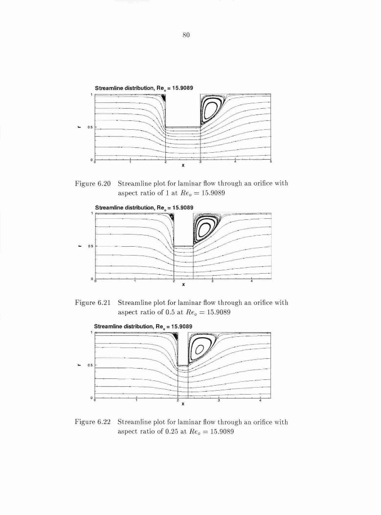
80
Streamline distribution, Re0
= 15.9089
... 0 .5 i-------
x
F igu re 6.20 St.rea.mline plot for lam inar flow t hrough an orifice with aspect ratio of 1 at Re0 = 15.9089
... 0.5 r---- --- --
x
Figure 6.21 Streamline plot for laminar flow t hroug h an orifice with aspect ratio of 0.5 a t Re0 = 15.9089
Streamline distribution, Re0 = 15.9089
x
Figure 6.22 Streamline plot for laminar flow t hrough a n orifice with aspect ratio of 0.25 at Re0 = 15.9089

l
Table 6.2 Compa rison of flow structures for laminar fl ow through orifices with different aspect ratios
Aspect ratio Reattachment Center of Center of length r·ecirculation eddy recfrculrtlion eddy
upstream of th e 01·ifice plate downstream of orifice plate l 0.7691 (-0 .0564 I 0.94326) (0.2 159, 0.73733) 0.5 0.76928 (-0 .05698, 0.94339) (0.28032, 0.73792) 0.25 0.7626 (-0.0.5742, 0 .94333) (0.27956, 0.73649)
6 .1.4 Comparisons of the Discharge Coefficients
As ment ioned in Chapter 1, th e discha rge coefficient., Cd, relates t he volumetric flow rate
Q to the pressure drop 6.P across the orifice as follows [l]:
_ (rrd2 /4)2112 ~ Q - Cd Jl - (d/ D)4 VP (6.3)
where d a nd D a re t he orifice and pipe di amete rs, respectively, p is t he fluid density and
Q = rrD2U/4 , and U is the inlet mean velocity.
So t he discha rge coefficient , Cd, can be calculated from the non-dimensional pressure drop
Cd= _1 (.!.)2 .j1 - f34_l _ V2 {3 / 6.P*
(6..t)
where /3 = d/ D , and the non-dimensional pressure d rop 6.P* can be related t.o the dimensio nal
pressure drop 6.P as D.P* = 6.P/(pU2).
It is commonly known that the wall static pressu re distribution a nd the static pressure
distribu tion along the centerl ine differ from each other start ing at a. pipe cross-section where
t.he fl ow begins to accele rate continuously and st reamline curvature becomes significant some
distance upstream of the orifice plate [6). However, the wall and centerlin e st.atic press ures have
the same values a t the posit ions of the pressure taps at. D upstream and D / 2 (41) downst ream
(D is t.he pipe diameter) . Thus, Lhe non-dimensional pressure drop b.P"' can be calcu lated
from the difference between the prf'ssure at. the dis tance D before the orifice plate and the
pressure at the distance D / 2 behind t.he orifi ce plate.
The simulation results for the discharge coefficient.s are compared wit h Sabin a nd Cey-
han 's [6) experimental and simulation resul ts in Figs. 6.23-6.25. Acco rdi ng to Mi ller [13), the

0 .6
rt;' ~0.5
QJ
~ -2 0.4 ~ ;:; ()0 .3 c QJ
~0.2
8 (..) 0 .1
t* = t:d= 1 :1
82
..
Stream-function vorticity simulation Sahin's numerical simulation Sahin's experiments
10
F igure 6.23 Comparison of the discharge coefficient vers us square root of orifice Reynolds number for an orifice with as-pect ratio of l
discharge coefficient Cd is proportional to the square root of t he orifice Reynolds num berRe0
when t he Reynolds number is low. So t he discharge coefficients were plotted against t he square
root of orifice Reynolds number. Figures 6.23-6.25 show t hat the simula tion results from the
two numerical methods agree with Sahin and Ceyhan's ex perimental a nd simulation res ul ts.
These figures show that in t he low Rey nolds number range, t he d ischa rge coefficient is
proportional to the square root of orifice Reynolds number. Also from t hese plots it is found
t hat the t hicker orifice pla t e leads to a smaller discharge coeffi cient. That is a lso to say t hat a
larger aspect ratio wou ld lead to a smaller discha rge coeffi cient.
6.2 Orifice F low with (J of 0.2
When the orifice/pipe diameter ratio becomes sma JJer , t he simulation becomes harder to
converge. Here simulation res ults for lamina r fl ow t hrough orifice with f3 = 0.2 are compared
with Lhe simulation results by Hayase, et al. [7].
In Hayase e t a l. 's paper, t he orifice was set up as s hown in F ig. 6.26. T he non-dimensional
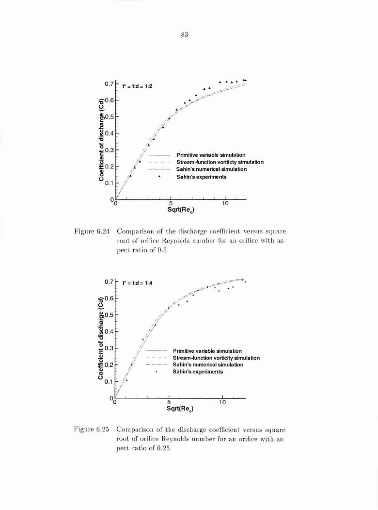
0 .7 - r = t:d = 1 :2
:oo.6 ~ ~
e>o.s .2 ~0.4 :s -2o.3 -c -QI ·c; !E0.2 8 -(..) 0 .1 -
I/ /
83
Primitive variable simulation Stream-function voriticty simulation Sahin's numerical simulation Sahin's experiments
10
Figu re 6.24 Compa rison of t he discharge coefficient vers us sq uare root of o ri fice Reynolds number for an orifice with as-pect ratio of 0.5
0. 7 t* = t:d = 1 :4
:o0.6 (..) - 'J 8,o.5 // ~ 11/ .c ~l ~ 0.4 ~ 1/ ~0.3 .! ---QI I/ --- -u - ii ~0 .2 _/_I. 0 - I
(..) : 0 .1 l .
00
Primitive variable simulation Stream-function vorticity simulation Sahin's numerical simulation Sahin's experiments
F igure 6.25 Compa rison of t he discharge coefficient versus sq uare root of orifi ce Reynolds number for a n orifice with as-pect ratio of 0.25

Inlet
-
10.2 - LL
84
28 Wall
---- --- ------r·-------- ------ --- --- -----------------Centerline
Outlet
Figure 6.26 Orifice configu ration for simulation of Hayse, et a l. [7]
pi pe radius was 1, the non-dimensional orifice radius was 0.2 , a nd the orifi ce plate th ickn ess
was 0.1. For the simulations by the primitive variable approach, I.he pipe length behind I.he
orifi ce was 8 for the s mall inlet Reynolds number (F ig. 6.27 ); it was 2 fo r la rger inlet Reynolds
number (Fig. 6.26 ) . Here the in let Reynolds number Re is defi ned as:
pUD . Re = -- = 2Reref µ
(6.5)
where U is t he inlet mean velocity, and Dis the pipe dia meter. A stretched mesh of 150 X 70
was used for the simulation by the primitive va.riable a pproach. Cases with t he inlet Reynolds
number in the ran ge of 0.02 to 40 were calculated. Around 50,000 itera tions were needed fo r
the simula t ions to converge to E < 10-6 .
For the simula tion by Lhe stream fund ion vorticity approach, t he orifice configu ration fo r
simulation was t he same as Hayase's. A st retched mesh of 160 x 100 was used for I.he simulation.
Around 1000 ite ra t ions were needed for the simulations to converge t o E < 10- 6 .
The simula tion results from the t wo approaches were compared wit h Hayase 's simul a tion
results in F igs . 6.2 -6.29. Genera lly, the simulation results agree wit h Hayase s resul ts qui te
well . In the low inlet Reynolds number region , both t he discha rge coeffi cient and the reat-
taichmen t lengt h exac tly match Hayase's simulation. However, in t he la rge Reynolds num ber
region , t here are some small differences between our simula tion and Ha.yase's simulat.ion . Even
so, t he trends agree fairly well.

85
4
l 0.2
lnlel ---- ---------r------ ----- ----- Outlet
Centerline
Figure 6.27 Orifice configuration for primitive variable simulation at small inlet Reynolds numbers
6.3 Orifice Flow with a Very Small Orifice/pipe Diameter Ratio
The orifice/pipe diameter ratios of the orifices used in the lSU experiments [2-4] were
quite small. In this work, only the orifices with an orifice/pipe diameLer ratio of 0.0445 were
studied . This orifice was also referred to as t,he 1 mm diameter orifice in Chapter 5. The
orifice radius and pipe radius were 1.013 mm and 11.375 mm (its o rifice/pipe diameter ratio
f3 = 1.013/11.375 = 0.0445), respectively. The ex periments considered orifices with three
different plate thicknesses. [n t his work, only the orifice with a nominally 1 mm thick plate
was studied. The exact orifice plate thickness was 1.029 mm.
The oil used in the experiments was high ly viscous. Thus, the Reynolds number of the flow
was generally quite small . According to the experiments [2]- [4), the oil properties depended
on the flow conditions (pressure and temperature). The oil properties were very sensitive to
the change of temperature, while they were less sensitive to t he change of pressure. Since the
flow temperature in the experimen ts was well controlled, the oil properties can still be treated
approximately as constants in t he whole {iow field.
The simulation was very difficult to converge for the low Reynolds number flow through
the orifice with such a smal l orifice/pipe diameter ratio using the primitive variable approach .
However, the si mulat ion converged quite quickly using t he stream function vorticity approach.
So in t he following , only the simulation results from t he stream function vor ticity approach
will be presented.

Pigure 6.2
0.7
:0-0.6 ~
Cll eio.5 al
ii .!!1 0.4 -0 0 c o.s ·fi ~0.2 0
(.) 0.1
6
Primitive variable simulation - .....e.- - Stream-function vorticity simulation - ·- • -··- Hayase's simulation
0.0002 10.0002 20.0002 30.0002 40.0002 Inlet Reynolds number (Re)
.J:
Comparison of discharge coeffi cients of flow through o rifice wit h orifi ce/pipe diamete r ratio of 0.2
20
18
16
• . ; /
• A
'& 14 c: , • A
~
c 12 CD E 10 ii £! 111
8 Cll 6 a:
4
2
/ /
. , .; · , ,
•;/ /
~ ~
IL - Primitive variable simulation / - .....e.- - Stream-fonctlon vorticity simulation
rf - - • - - Hayase's simulation
10.0002 20.0002 30.0002 40.0002 Inlet Reynolds number (Re)
F igure 6.29 Comparison of reattatchment lengths of flow through orifice with orifice/ pipe diameter ratio of 0.2

7
Table 6.3 No n-d ime ns io nal config uration parameters
Pipe length Orifice plate Pipe length Radius of the Radiu of the b fore the thicknes b hind the orifice ptpe orific (LI) (t) orifice {L2) (,.) (R) 5 0.0905 20 0.044.5 1
6 .3.1 C omputation Doma in C onfigura tion a nd M es h Gen e ra tion
For the stream function vorticity simulation, the pipe length upstream of the orifice and the
length downstream of the o ri fice were chosen by the author lo assist the imulatio11. The l U
experime nts [2]- [4) proved t hat t he pressu re drop caused by t he pipe itself was o nly a small
portion of th e large pressure d rop across t he orifi ce. Large r> ressu re d rop occu rs in lhe vicinity
of the o rifice (observed from the simulation res ults) . o the pipe length upst ream of the orifice
was specified as 5 pipe radii and the pipe length downstream of the orifice was l:>pecified as 20
pipe radii . The configuration of the orifice studied here is similar lo the one shown by Fig.
6. L. Table 6.3 lists t he non-d imensiona l configu ration para meters.
A mesh of (100+40+ 140) x (45+955) and a mesh of (120+4 + 16) x (-l.5+955) were
generated for the s imulations. ( 100+,10+ 140) x (45+95.5) means that along the axial d irection,
there were 100 g rid points upstream of the orifice , 40 grid points in the orifice region , and 140
grid points dow 11st.ream of the orifice; along t he radial direct ion, there were 4.5 grid poi nts in
the o rifice regio n, and 955 g rid points above t he orifice region . (120 + 4 + 16 ) x (45 + 955)
s hould be interpreted simil arly. At the same time, the mesh a long the axial direction was
cl ustered to the walls; the mesh a long the radia l direction was almost un ifo rm.
6.3.2 D etail Info rmat ion of t he N u mer ica l Calculat ion
Because t he orifice/pipe diameler ratio was very s mall (/3 = 0.0445) , the under-relaxation
facto r O' and the preconditioni ng coefficie nt() were carefully chosen. Here o was take n as 0.1
and B was taken as 10. A fu lly developed velocity in let and outlet boundary with 82w/8x2 = O
and 82 </J/ 8x2 = 0 were used in the s imu lations. The details of specifying boundary cond itions
were described in hapter 4 . Arou nd 5000 iterations were needed fo r t he simulation to converge
to E < i o- 6 .
6.3.3 Mes h Sensit iv ity
T he mesh sensiti vity was discussed in t he previo us sectio ns . It was found t hat the (100 + 40+ 140) x (45+ 955) mes h was good enoug h for th e simula tions . Sim ulations were carried o ut
based on th ese t wo meshes at a reference Reynolds number of l.279177. The cor res po ndi ng
o rifice Reyno lds number was 57.45565. The diffe rence between t he pressu re drop results from
t he two s imula tio ns was just 0.39 % of t he resul t from t he fin er mesh. Fig ures 6.30 and 6.31
show th e comparison of t he s t atic pressure and Lite axial velocity a long t he centerline fo r t his
case.
6.3.4 T heoretical Prediction of t he Pressure Drop across the Orifices w ith Small
Orifice/pipe Dia m eter R atios for the Newtonian Flow
In 1 91, Sam pson [42] first solved Lhc pressur<>-driven fi ow of a . ewtonian fluid a l low
Rey nolds number t hroug h a n infinitesima lly t hin circula r ho le in an infinite rigid wall using
o blate spheroida l coordinates. The pressure drop across the orifice can be s imply expressed as
tiP = 3Q: r
(6.6)
whe re Q is t he volumetric fl ow rate of t he fl uid AL is the fl uid viscosity, a nd r is the orifice
rad ius. However, because t he orifice plate is not infi nitely th in and has fi nite aspect ratio
(t/r =I= 0), t here is an addit iona l cont ribut ion to t he press ure d rop. Dagan et al.'s [43] numerical
ca.Jculations can be accura tely a pp roximated by linearly combining t he p ressure d rop associated
with th e Sampson flow a nd t he pressure drop of t he assum ed Poiseulle flow thro ug h t he orifice
itself to give
ti P =CJµ (3 + ~) r 3 1rr
(6.7)
In L999, Rothstein and Mckinley [27] carried ou t the experiments o n an o rifice with /3 =
0.25. T hey fo und that Eq. (6 .7) was very acc urate when the orifice Reynolds number was
relatively s mall.

9
6.3.5 Low Reynolds Number Simulation Res ult s
The orifice Reynolds number o f the I C experiments was in Lhe range of 0.2055 to 460.011.
o t he stream function vorticity s imulation was atlempted to cover the range for the orifice
Reynolds number. Even t hough the simulaLion results of the stream function vorticity ap-
proach jus t depe nded on t he oriri ce Rey nolds number, the s imu lation cases were sLill desig ned
co rresponding to the ex perimen tal cases with same orifice Rey nolds numbers al d ifferent tem-
peralures (here just -25 °C, -20 °C, - 10 °C, and 20 °C).
The pressure drop calculated by the stream function vorticity approach was the non-
dimensio na l pressure drop.
D.P* = D. p pU2 (6. )
where p is t he fluid density, and U is the inlet mean velocity. Figures 6.32 and 6.33 show one
exam ple of the non-d imensional static pressu re distribution at Re0 = l. 143. From these two
fi gures, it can also be obse rved that the s tatic pressure dropped rapidly in the orifice region
a nd recovered s lowly downstream of the o rifi ce.
E uler number is d efi ned as fo llows:
D.P Eu=-pu~
(6.9)
where U o i. the orifice mean axial velocity. o the Euler numbers for t he experi me11 tal results
can be calc ulated directly us ing 8q. (6.9).
For i ncom prcssi ble flow, the orifice mean velocity v0 can be calculated from the in let mean
velocity U:
(6.10)
where r and R a rc th e orifice a nd pipe radius, respectively.
Then t he Euler number can also be calcu lated from the non-d imensional pressu re drop:
Eu= !J.P* ( r / R(' (6 .11)
Also,the Eul er numbers for the theo retical prediction (EuPrd) can be de rived from Eq.(6 .7):
""' 611" + 16.f. E11Prd = r
Re0 (6 .12)

90
where t is the orifice plate thickn ess, r is the orifice radius. a nd R e0 is the orifice Rey nolds
number.
Tables 6.4-6.7 show the Euler numbers from l hc experiments, simulations and theoretical
prediction. ln these t a bles, E u is t he Eule r number calcu lated from the st, ream functio11
vort,icity s imulations, Eup1t is t, hc Eu le r number calcula ted from t he F LUE T simulat ions,
EuPrd is t he Euler number calculated from t,he t,heorcLical predict ion. a nd EttE:rp is Lhe Eule r
nu m ber calcu lated from the experimenta l resul ts.
6.3.6 Flow Patte rn through t he Orifice
The lamina r flow through the orifice wit.h {3 = 0.0445 was simulated as ewtonian fl ow.
The Row pa tte rns o btained from the st,ream function vorticity sim ulation were quite simila r t,o
the o nes obtained from the FLUE T s imulation , i.e ., Lha t there were two main rccirculat,ion
eddies ups t ream a nd downstream of t he o rifice, and t here was a secondary edd y between the
downs tream edd y a nd the orifice corne r. Fig ure::; 6.34-6.41 s how t he streamline dis tributions
fo r t he flows t hroug h t he o rifice. F rom Figs. 6.34, 6.36, 6.3 , 6.40, il can be observed th a t the
recirculation eddy ups t ream of t he orifice shrank , while th e recirculat ion eddy downs tream of
the o rifice lcngthe 11ed when the orifice Reynolds number increased . Figures 6.35 6.37. 6.39 ,
6.41 a re the enlargements of Figs . 6.34, 6.36, 6.3 , 6.40. Also, Figs. 6.35, 6.37 , 6.39, 6.41 s how
t hat there was a seconda ry eddy downstream of the orifice.
6.3.7 Comparison of the Reults
Tables 6. -6.11 list t he differe nces between the resu lts from the stream function vo rt icity
simulation , FLUENT simulation , t he t heore tical pred ic t ion a nd t he ex peri ments. T hese ta bles
s how t hat a t low o ri-fice Rey nolds numbers , the E uler nu mbers from t he s tream function vor-
ticity simu lation , FLUENT simulation, and t he t heo retical pred iction were close to each other.
Howeve r, when t he o rifice Rey nolds number becomes la rger, t he theoretical prediction became
much smaller t han the resulls from t he two si mulat.ion met.hods. This means that at low orifice
Rey nolds numbers, t he theoretical prediction was quite acc urate to predict the E uler number

91
(also the pressure d rop) of t he Newtoni an fl ow (see Fig. 6.42). The simulation resu lts from
t he stream function vort icity s imula tions were q uite close to t he F LUENT simulation, except
when the orifice Rey no lds num ber was quite la rge (see Figs.6.43 and 6.44).
T he E uler num bers calculated from t he experimental res ul ts were a lso compared to the
simulation results . From Tables 6.8-6.11 , it can be found that a t low orifice Rey nolds num-
bers, the Euler number from t he experimental results were much lower t han t he resul ts from
F LUENT Newtonia n simula tio n (in t he tables and fig ures, the F LUENT Newtonian simula-
t ion was referred to as FLUE T simulation. ) . Figure 6.45 show t he compa rison of t he Euler
nu mbers from t he experi mental results and t he simulatio n results.

Cl) c :c E4soooo ~ : e11400000 -
= g>350000 0 (ij 300000 ~ -i}l 250000 -Ill -
~200000 : ~ i 150000
~ 100000
·~ 50000 Cl)
E ~ 0 z
92
Simulation resutts by a mesh of (100+40+140)x(45+955) Simulation resutts by a mesh of (120+48+16B)x(45+955)
x
Figure 6.30 Comparison of the press ure distribution along t he centerline from t he simulation resul ts based on t he mes h of (100 + 40 + 140) x (45 + 9.5.5) and (120+ 48+16) x (45+955)
Cll c :c E soo ~ 800 ~ O> 700 c .2 ca 600 ~ 8 500
~ 400 ] )( ca 300
~ ~ 200 c Cl) 100 E ~ g 0 z
--- Simulation resutts by a mesh of
10
(100+40+140)x (45+955) Simulation resutts by a mesh of (120+48+16B)x(45+955)
20 x
Figure 6.31 Comparison of the axial velocity distribution along t he centerline from the simulation resu lts based on the mesh of (100 + 40 + 140) x (45 + 955) and (120 + 48 + 168) x (45 + 95.5)

93
x
p 1.19201E+07 1.14941 E+07 7.9348E+06 3.94954E+06 7948.9 5096.22 2049.07
-1.03204E+06
Figure 6.32 Static pressur<' distribution for I he flow through an ori-fic<' with f3 = 0.0445 ( th<' 1 mm diamct·er orifice with I mm thick orifk<• plat<•), Re0 = 1.143
Static pressure distribution, Re0 = 1.143
x
p 1.19201 E+07 1.14941E+07 8.93112E +06 4.94585E+06 960589 5096.22 2049.07
-1.03204E+06
Pigure 6.33 An enlarg<'ment of th<' static pressure distribution in the orificc> region for I hC' fl ow through an orific.c with f3 = 0.0445 ( the 1 mm diameter orifice with 1 mm thick o rific<' plate). Rr ,, = 1. 143
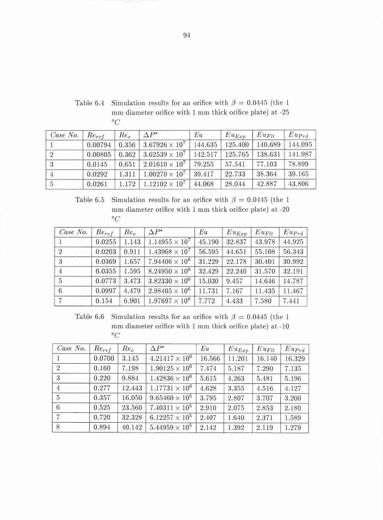
94
Table 6.4 Simulation results for an orifice with f3 = 0.0445 (the 1 mm diameter orifice with 1 mm thick orifice plate) at -2.5 oc
Case No. R eref Re0 6.P* Eu Eu Exp Eupu EuPrd 1 2 3 4 5
0.00794 0.356 3.67926 x 10⁷ 144.635 125.400 140.6 9 144.095 0.00 05 0.362 3.62539 x 10⁷ 142.517 125.765 138.631 141.9 7 0.0145 0.651 2.01610 x 10⁷ 79.255 57.541 77.103 7 . 99 0.0292 1.311 1.00270 x 10⁷ 39.417 22.733 38.364 39.165 0.0261 1.172 1.12102 x 10⁷ 44.068 28.044 42.887 43.806
Table 6.5 Simulation res ul ts for an orifice with {J = 0.0445 (the 1 mm diameter ori fice with 1 mm t.hick orifice plate) at -20 oc
Case No. R e ref R e0 6.P* Eu E usxp Eu Fu EuPrd 1 2 3 4 5 6 7
0.0255 1.143 1.14955 x 10⁷ 45.190 32.837 43.978 44.925 0.0203 0.911 1.43968 x 10⁷ 56.595 44.651 55.108 56.343 0.0369 1.657 7.94406 x 10⁶ 31.229 22.178 30.401 30.992 0.0355 1.595 8.24950 x 10⁶ 32.429 22.240 31 .570 32.191 0.0773 3.473 3.82330 x 10⁶ 15.030 9.457 14.646 14.787 0.0997 4.479 2.98405 x 10⁶ 11.731 7.167 11.435 11.467 0.154 6.901 1.97697 x 10⁶ 7.772 4.433 7.580 7.441
Table 6.6 Simulation results for an orifice with f3 = 0.0445 (the 1 mm diameter orifice with 1 mm thick orifice pla te) at -10 oc
Case No. R e,·ef R e0 6.P* Eu E ·usxp Eu Fil EuPrd l 0.0700 3.145 4.21417 x 10⁶ 16.566 11.201 16.140 16.329 2 0.160 7.198 1.90125 x 10⁶ 7.474 5.1 7 7.290 7.135 3 0.220 9.884 1.42836 x 10⁶ 5.61.5 4.263 5.4 1 5.196 4 0.277 12.443 1.17731 x 10⁶ 4.628 3.355 4.516 4.127 5 0.357 16.050 9.65460 x 10⁵ 3.795 2.807 3.707 3.200 6 0.525 23.560 7.40311 x 10⁵ 2.910 2.07.5 2.853 2.180 7 0.720 32.328 6.12257 x 10⁵ 2.407 l.640 2.371 1.589 8 0.894 40.142 5.44959 x 10⁵ 2.142 l.392 2.119 1.279

95
Table 6.7 Simulation results fo r an orifice with /3 = 0.0445 (the 1 mm diameter orifice with 1 mm thick orifice plate) at 20 oc
Case No. Re ref Re0 b.P· Eu Eus xp Eu Flt EuPrd l 1.279 57.456 4.58989 x 10⁵ 1.804 1.811 1.800 0.894 2 1.972 8 .574 3.844 79 x 105 1.511 1.515 1.529 0.580 3 3.524 158.265 3.16101 x 10⁵ 1.243 1.237 1.290 0.324 4 4.225 1 9.792 2.99743 x 10⁵ 1.178 1.165 1.236 0.271 5 5.295 237.846 2.81890 x 10⁵ 1.108 1.105 1.179 0.216 6 5.902 265.115 2.74182 x 10⁵ 1.078 1.048 1.156 0.194 7 8 .109 364.225 2.53820 x 10⁵ 0.998 0.954 1.098 0.141 8 10.242 460.011 2.40895 x 10⁵ 0.947 0.909 1.065 0.112

96
Streamline dlstrtbutlon, Re0 = 1.143
o• \ If ~I
I( '(
~ t ~ {I'
00
o•
02
00 10 x
Figure 6.34 Simulat.ed stream li ne distribution Rea = 1.143
Streamline distribution, Re0 = 1.143
x
Figure 6 .35 An enlargement of t he simulated st reamline d istribu-t ion in the o rifice region , Re0 = 1.143
Streamline dlstr1butlon, Re0 = 6.901 1
\\ If \ If
08
\ l(r \
¥ 10 20
0.0
o•
02
o. x
Figure 6.36 Simulated streamline distribution , R ea = 6.901
Streamline distribution, Re0 = 6.901
x
Fig ure 6.37 An en largemenL of t he s imulated streamline d ist ribu-tion in t.he orifice region, R ea = 6.901
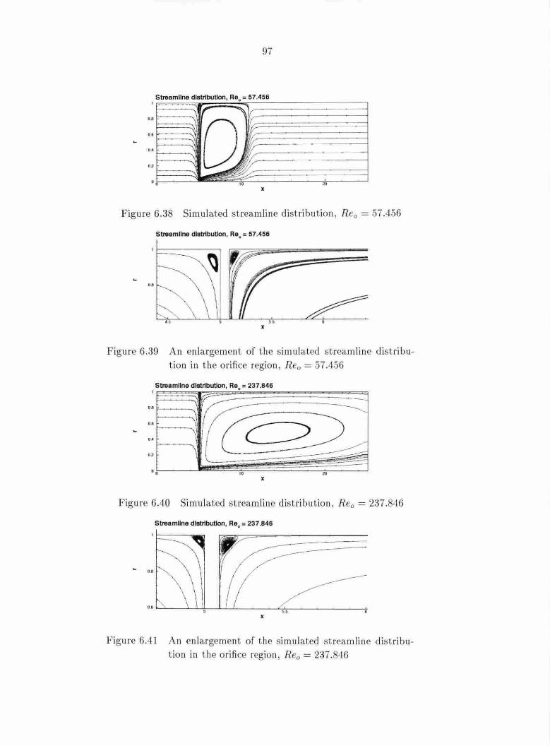
97
Streamline distribution, Re0 = 57.456
r ~
•• ,Q r o•
00
02
/
0 0 10 x
Fig ure 6 .38 Simulated streamline d istribution, Re0 = 57.456
Streamline distribution, Re0 = 57.456
0 8
x
F ig ure 6.39 An enla rgement of t he simu lated stream li ne d ist r ibu-tio n in t he orifice region, Re0 = 57.456
OBF-----
01
...
x
Fig ure 6.40 Simulated s t reamli ne dis tribution, Re0 = 237.846
Streamline distribution, Re0 = 237.846
x
F igure 6 .41 An enla rgement of t he s imulated stream line distribu-t io n in t he orifice region , Re0 = 237. 46

98
Table 6.8 Comparison of result s at -25 °C
Case No. Re0 Eu-E u Eli
E up11 Eu e_~-EuE.ll
E u Fl t E ue.rr1. -E'U
E u cu Exe. -l:.:up11
Eup11
x l00% x l00% x l00% xl00% 1 0.356 2.80% 2.42% -0.37% -10.87 % 2 0.362 2.80% 2.42% -0.37% -9.28 % 3 0.651 2.79% 2.33% -0.45% -25.37% 4 1.311 2.74% 2.09% -0.64% -40.74% 5 1.172 2.75% 2.14% -0 .. 59% -34.61%
Table 6.9 Comparison of results at -20 °C
Case No. R e0 E u -Eu E.1' Eue.rci - E u E.1' Eu e.ru.-Eu bue:r;l!.-73up1 1
E up11 E u. F lt Eu Eu Flt x l00% x l00% x l00% x l00%
1 1.143 2.75% 2.15% -0.59% -25.33% 2 0.911 2.70% 2.24% -0.45% -18.98% 3 1.657 2.72% 1.94% -0.76% -27.05% 4 1.595 2.72% 1.97% -0.73% -29.55% 5 3.473 2.62% 0.97% -1.61% -35.43% 6 4.479 2.58% 0.27% -2.25% -37.33% 7 6.901 2.53% -1. 3% -4.25% -41.52%
Table 6.10 Comparison of res ul ts at -10 °C
Case No. Re0 Eu - EuE.1 1 Eue.r g_ -Eue.11 E u'1J'u- Eu t;v.e,, l!.- JiUF/t
Eu p11 E up11 E v.p11
x 100% x l00% x 100% x l00% 1 3.145 2.64% 1.17% -1.43% -30.60% 2 7.198 2.52% -2.13% -4.54% -2 .8.5% 3 9.884 2.44% -5.21% -7.47% -22.22% 4 12.443 2.48% - .61% -10.82% -2.5.70% 5 16.050 2.37% -13.69% -15.69% -24.28% 6 23.560 1.99% -23.61% -25.10% -27.29% 7 32.328 1.51% -33.00% -34.00% -30.85% 8 40.142 1.08% -39.63% -40.28% -34.30%

99
Table 6. Ll Comparison of results at. 20 °C
Case o. R e0 E u-Euf.ll Eu~-Euf.ll Eu~-Eu t:;us:r,,-t:;u p 11
E u p1r U f'f I t i Eup11
x l00% x 100% x lOO% x l00% 1 -57.456 0.23% -50.35% -50.45% 0.63% 2 .574 -1.13% -62.07% -61.64% -0. 9% 3 15 .265 -3.67% -74. 5% -73.89% -.J.13% 4 1 9.792 -4.66% -7 .11% -77.04% -5 .74% 5 237. 46 -6.03% - 1.69% - 0.52% -6.31 % 6 265.115 -6.73% - 3 .2-1% - 2.03% -9.28% 7 364.225 -9.J 3% -87.16% - 5. 7% -13.17%
460.011 - 1 L.12% - 9.52% - .21% -1'1 .67%

140 120 100 80 60
3' ~40 ... .8 E :J c: 20 ... CIJ '3 w
...
100
Stream function • - vorticity simulation
- · __,._ -- FLU ENT simulation
- ··-+- ··- Theoretical prediction
.....
• ~> '
2 4 6 8 Orifice Reynolds number (Re
0)
F ig ure 6.42 Comparison of t he Euler numbers at low orifice Reynolds numbers
10' '~ - ·---......n-----·-+-··-
Stream function vorticity simulation FLUENT simulation
Theoretical prediction
3' ~10' _ ... .8 E :J c: ... CIJ
~ 10° :
' • •, •• 10~ ~~._.._,..__...__..._._._........._ ......... ~._. ......... _._._ .......... __ _..__.._...J.J
10 10 10 Orifice Reynolds number (Re0 )
Figu re 6.43 Comparison oft.he Euler numbers
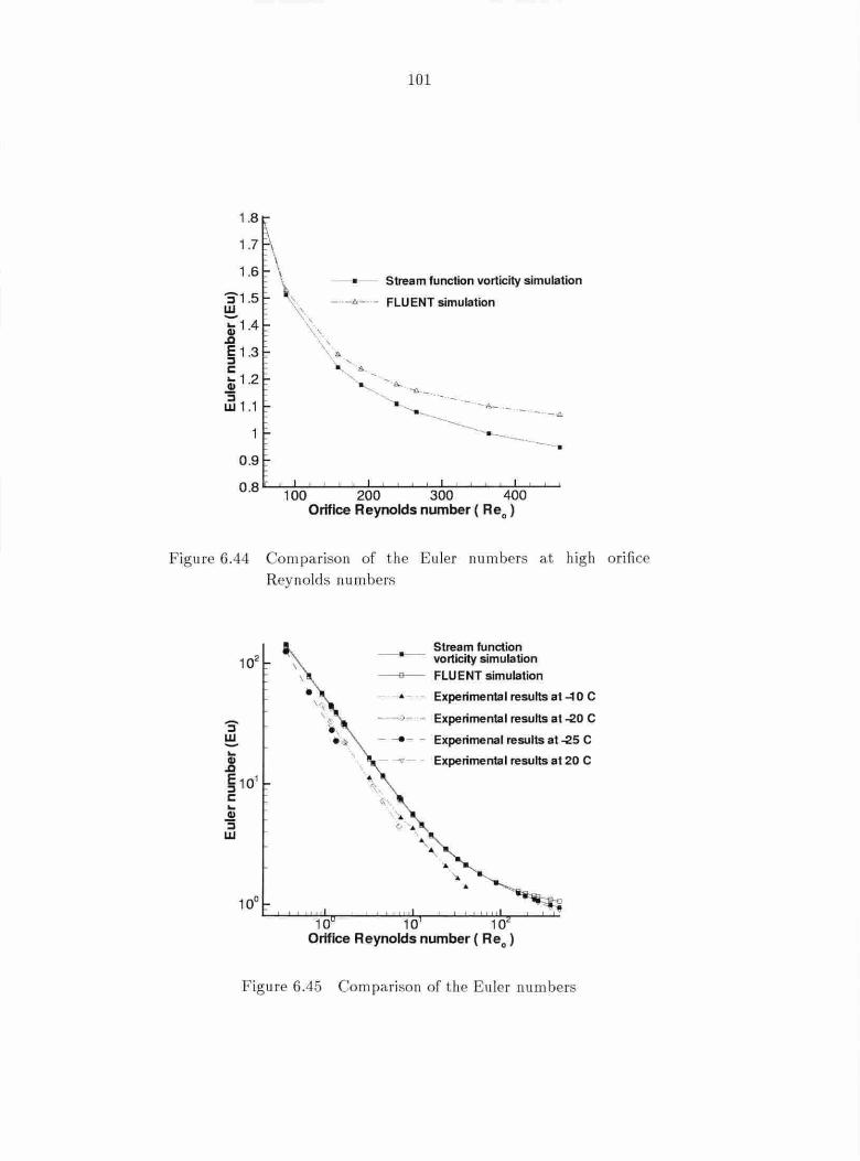
1.8
1.7
1.6 ~
3'1 .5 ~ w t1 .4 .a § 1.3 c lii 1.2 -"3 w 1.1
0 .9 ~
101
- •- Stream function vorticity simulation
-··-A-··- FLU ENT simulation
- e.- ·-
--......
0 ·8 "--'-1-'-oo-'--'--......__,_-20 ...... o-'--..L........l--'-3--'o'-o-'--"L......J..-'-4 ...... 0-0.1.......J.__J Orifice Reynolds number ( Re0 )
F igure 6.44 Compa rison of the Eule r numbers a t hig h orifice Reynolds numbers
Stream function 1 02 _ vorticity simulation
3' w -... .8 §101 -c .. G> "3 w
10°
FLUENT simulation
- - • - - Experimenta I resutts at ....:t 0 C
- -->-- - Experimental resutts at -20 C
- - - - Experimenal results at -25 C
v -... \
Experimental resutts at 20 C
10 10 10 Orifice Reynolds number ( Re0 )
Figure 6.45 Comparison of t he Eu ler num bers

102
CHAP TER 7. MODELING N ON- EWT ON IAN FLOW AN D THE
N UMERICAL SIMULATIONS
Fo r the purely viscous fluid without vi coelaslic behavior, the numerical modeling and nu-
merical s imulations are quite st raightforwa rd. However . fo r the more complicated viscoelastic
fluid, the constitutive equations wh ich relate the shear s tresse to the shear rates together
wit h the momentum and continuity equations s hou ld be sim ultaneous ly solved to predict the
non- ewtonian flow.
The high ly v iscous oil used in t he IS experim e nts is believed to dis play a shear-th.inni ng
nature a nd Lo be a purely viscous fluid. C enerally, t he purely viscous non-Newtonia n flui d can
be modeled in a similar man ner as the th e ewton ia n fluid by treating the viscosity 11 as the
fun ction of the shear rate ~; . Then, th e shear s tress can be ex pressed as follows:
where /L is a funct ion of ~; : µ = µ ( ~~ )
du Ty.r = /L dy (7. I)
The power-law model (44] is the simples t model that can be used lo described t he shear-
th in ning behav ior:
. (du)" Ty.r = /\ -dy (7.2)
where 11 is th e powe r-law index, f( is the consis tency; a11d from w hich
_ 1. ,rlu l"-1 du T x- \ - -
y dy dy (7.:J)
To account for the purely viscous non- cwlon ian behavior t he two numerical methods
described in Chapters 3 a nd 4 were adj us ted appropriately. For the primitive variable approach,
the viscosity µ has been already treated as a fun ction whose value could change according t.o
different conditions at diffe rent positions. No s pecia l cha nge is needed fo r this met.hod except
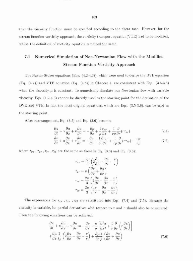
103
that t he viscosity function must be specified accordi ng to I he shear rate. Howewr, for the
stream fun ction-vor ticity approach, the vorticity transport equation( TE) had to be modified,
whilsl the definition of vorticity equation remained the same.
7.1 Numerical Simulation of Non-Newtonian F low with t he Modified
Stream Function-Vorticity Approach
The Navier- tokes equations (Eqs. (-1.2-·l.3)). which were used to derive lhe OVE equation
(Eq. (4.7)) and VTE eq uation (Eq. (<!. )) in Chapter ·I , are consistent with 8qs . (3.5-3.6)
when the viscosily /t is constanl. To numerically simulate non-l\ewlonian flow with variable
viscosity, Eqs. (4.2-4.3) cannot be direct ly used as lhe starting point [o r the deri vation of t he
DYE and VTE. In fact the most original eq uations, which are Eqs. (3.5-3.6). can be used as
the starting point.
After rear rangement, Eq. (3 .5) and Eq. (3.6) become:
ou fJu Du 8p 1 T r:r l D - + u-+ v- = -- + --+ --(1'T:rr) Dt fJx or fh p fJx rp or av av OU op l OTxr I a Too - + 'U- + 'U- = -- + --- + --(rTrr) - -fJt ax Dr or p ox rp 8r rp
where Trr . Txr , Tr,. . TOO are the same as those in Eq. (3.5) and Eq. (3.6):
Txr = 2Jl ( 28u _ 81 _ ~) 3 ax {j,. ,.
( fJv au)
Trr = /l OX + 01'
Trr = 2/t ( 28v _Du_:_) 3 01' ax 7'
TOO = '!:!!._ (2~ - au - ?V) 3 ,. ax [),.
(7.4)
(7.5)
The expressio ns fo r Trx , Tx r , Too arC' s ubstituted into 8qs. (7 .<1 ) an d (7.5) . Because the
viscosity is variable, its partial derivatives with respect to :r and 1· should also be considered.
Then the following equations can be achieved:
Dtt au ait Dp f-t [82u 1 a ( Du)] -+u- +v-=--+- -+-- 1'-8t ax 8r ax p 8x2 r 8r or
+ 8µ -3._ (2au - av - ~) + 8µ ~(av+ au) ox 3p a:c or r or p a:r Dr (7 .6}

104
(7.7)
Here, Eqs . ( 4.4-4.6) are still used as the defi nitions of the stream fu nction and vortic-
ity. So t he defini t ion of vorticity remains t he same. And the mod ified vorticity transport
equation (VTE) fi nally becomes:
[a2w [)2w 1 ow w l [aw O'llW fJvw ]
~t - +-+--- - -p - +-+-ax2 8r2 '/' or r 2 at ax or
81t ow 8µ ( ow w) 82µ (8u 8v) - 2 ox ax - 8r 2 07' + -;: - 2 8x8r ax - or
(02µ a2µ ) (av au)
- 81·2 - 8x2 ax + 8r (7.8)
Again t he modified VTE(7.8) and DVE can be non-d imensionalized as in Chapter 4 except
t hat t he viscosity is non-d imensionalized as follows:
T hen t he non-dimensional VTE can be achieved:
[o2w fJ2w 1 ow w l [ow 8uw Dvw] µ -+-+-- - - - Re,.e - +-- +-- = 8x2 Dr2 r or r 2 . 1 8t ax ar
- 28µow - 8µ (2ow + ~)-2 82µ (au - av)
ax ox or or 1· . 8x8r ox or
(a2µ 82µ) (av ou)
- ar2 - ox2 ox + or (7.9)
whe re R eref = eVR _ (Also, fo r convenience, all the non-dimensional varia bles are written µref
wit hout addi ng asterisks.) The non-dimensional DVE shou ld be the same as Eq. (4.9) .
T he modified VTE and t he DVE can be d iscretized and numerically so lved by t he method
given in Chapter 4. The t reatment of boundary condi tions is the same.
T he equations to be used for integration along the centerline and t he vertical line to ob-
tain t he pressu re field sho uld be adjusted . T he equation fo r integration along t he centerline
becomes:
(7 .10)
105
And the equation fo r in tegration along the vert ical line is:
op av av 1 ow 1 (av fJu) 8µ 2 Dv 81-t or = -u ox - v or - R e,.ef ax + R eref ax + 8t ax + R eref 81· 8r
7.2 Power-law Laminar Flow in Pipes
(7.11)
For fu lly developed power-law laminar flow in pipes, t he analytical solut ion achieved the
following Q - 6.P relations hip [44]:
Q n (Tw) 1/n 7r R3 = 3n + 1 I<
(7 .12)
Since th e la minar fl ow is fully developed , T w can be related to 6.P as in t he following
expression [44] : R6.P
Tw =~ (7 .13)
By substituting Eq. (7.13) into Eq. (7.12) , t he following expression for 6.P fo r power law
la minar flow can be derived :
6.P = 2I< ( 3n + 1) n un L n R n+i
(7 .14)
where U is t he mean velocity.
The friction factor f is defined as:
J = (D6.P/4L ) = __!i:_ pU2 /2 pU2/2
(7 .15)
By s ubstituting equation (7. 15) into equa tion(7.14), the friction factor can be calcul ated as
follows:
[pDnu2-n ( n ) nl 16 != 16/ 8 = --
]\_ 6n + 2 N Re B '
(7 .16)
where NRe,B is the genera lized Reynolds number NRe,B = [pD'X2- n 8 ( 6n~2 ) n] .
Thus, the no n-dim ensional pressure g rad ient in full y developed la mina r fl ow can be calcu-
lated from t he friction factor:
6.P* = 6.P/(pU2
) = 21 R = J = ~ L* L/ R D NRe,B
(7 .17)
From Eq. (7.3) , the dimensional viscosity µ for the power-law model is :
_ ·1 du 1n-1_ ·(U)n-llcfo*ln- 1. µ - f( - - I t - -dr R dr~
(7.18)

106
By using µrr:.J = J<(~)n- 1 , t he viscosity can be non-dimensionalized as follows:
• J.L I du• in- I µ - -- J.Lref - dr *
(7.19)
So t he reference Rey nolds number is Reref = eUR . Thus the generalized Rey no lds number µref
can be related to the reference Reynolds number as follows:
(7.20)
Skelland also gave t he analytical solution for the velocity distribution of the power-law
lam inar flow:
(7.21)
Several test cases were s imulated by bot.h the modified stream function vorticity approach
and the primitive variable approach. Simulation results were compared with t he analytical
solutions . Since t he laminar flow was axisymmetric, j ust hal f of the domain was meshed
and simulated . T he pipe had a non-dimensional length of 10 and a non-dimensional radius
of 1. A uniform velocity was specified at the inlet. T he power-law laminar fully develo ped
velocity profi le a nd the non-dimensional pressure gradient downstream will be compared with
the analytical solu t ions.
In t he numeri cal simulations, the power-law viscosity model was specified as follows:
µ• = [ max(0.01 , (/Ju*)2 + (8v*)2 )] n -1 or* ox· (7 .22)
Also, t he viscosit.y was li mited to values in t be range 0.01 to 3.0. If it was smaller than 0.01,
it was taken as 0.01 ; on the other hand, if it was larger t ha n 3.0, the value of 3.0 was taken.
The reference viscosity µref was chosen so that the reference Reynolds number R eref was
5.0. By the modified stream function vorticity approach, s imulations with the power-law index,
n, of 0.75, 0.8, 0.8.5, 0 .9, 0.95, 1.0, L.1, a nd 1.2 were carried out with th ree d iffe rent meshes:
101 X 101, 101 x 201 , and 101 x 401. The simulation results s howed t hat t he fully developed
velocity profi les and the non-dimensional pressure gradients agreed with t he a nalytical solu-
t ions. The theoretical solutions are listed in Table 7.1. As shown by Fig. 7.1 , the velocity

107
Table 7.1 Analytical solu t ions of power-law flow in pipes
Powe1·-law Generalized R eynolds ¥;- in fully developed Fully developed index{n) number (Nne,B) flow region velocity profile
" _ ~ ( l _ ( ,. ){n+ L)/n) U - n+ I R
0.75 13.3181 1.2014 u"' = 1.8571(1 - ( ~)2.3333) 0.80 12.5704 1.272 u* = 1.8 89(1 - ( f?) 2·25) 0.85 11.8678 1.34 2 u* = 1.9189(1 - (f?)2.1765) 0.90 11.2072 1.4277 u* = 1.9474(1- (-fl)2.1 111 ) 0.95 10.5855 1.5115 u* = 1.9774(1 - ( fl)2.os2a) 1.0 10.0 1.60 u"' = 2.0(1 - (N)2) 1.1 .92 5 1.7920 u"' = 2.0476(1- (-f?)l.9091 ) 1.2 7.9757 2.0061 u* = 2.0909(1- (f?)t.8333)
profiles calculated from t he simulations with t he mesh of 101 x 101 agree with the t heoretical
solutions very well. However, as shown by Table 7.2, only the finest mesh 101 x 40 l here can
predict t he pressu re gradient in the full y developed region accurately.
T he s imulations wit h t he power-law index of less than 0.75 blew up even if a very small
under- relaxation factor and very large preconditioning coefficient was used . T he reason for
th is is perhaps that the viscosity across t he whole field changed too much and this promotes
an instability.
Also a simulation with the power-law index, n, of 1/3 was carried out by the primitive
variable approach. When the reference Reynolds number Reref was 5.0 and n is L/ 3, the gen-
eralized Reynolds number N Re,B was calcu lated by Eq. (7.20), and its value was 22.012 . The
theoretical non-dimensional pressure grad ient in fully developed laminar flow was calculated by
Eq. (7.17), and its value is 0.7268. T he primitive variable simulation resu lt was 0.726 5. These
two resu lLs matched with each other very well. Also the ouLlet axial velocity was compa red
with the theoretical prediction (Eq . (7.21)) in Fig. 7.2.

108
Axial velocity distribution at the pipe outlet
~ ·u 0 Qi > Ill ·x <( 0 .5
0.25 0.5 r
- - n:0.75 simulation - -o- - n:0.75 theoretical
n:0.8 simulation n:0.8 lheoretical n:0.85 simulation n:0.85 theoretical
• n:0.9 simulation - - • - - n:0.9 lheorellcal -~- n:0.95 simulation
n:0.95 theoretical n:1 simulation n:1 theoretical
- -+-- n=1 .1 slmulallon _ --o- _ n:1 .1 theoretical - __, - - n:1 .2 simulation - - • - - n:1.2 theoretical
0 .75
Figure 7.1 Comparisons of the velocity profiles with different power-law indexes
1.4
1.2
Axial velocity distribution at the pipe outlet (n = 1 /3)
~-
- •- Pimitivevariable smulation result
' It
\ .
\ - ---.:.- - Theoretical prediction \
\ \
. r
Figu re 7.2 Comparison of the axial velocity dis tribution a t the out-let for the primitive variable a pproach a nd t he t heoret-ical prediction

109
Table 7.2 Comparison of the analytical solut.ion and t.he simulation results by modified stream funct.ion vorticit.y approach
Power-law Generalized C::.r c::.~r ~ ~ £• £• £• £•
index(n) Reynolds (Theoretical (mesh (mesh (me~h
number (N Re,B) Solution) 101 x 101) 101 x 201) 101 x 401} 0.75 13.3181 1.2014 1.2681 1.2134 1.2066 0.80 12.5704 1.2728 1.3243 1.2846 1.27 2 o. 5 11.8678 1.34 2 1.38.55 1.373 1.3528 0.90 11.2072 1.4277 1.4516 1.4519 1.4313 0.95 10.5 55 1.5115 1.5230 1.5232 1.5141 1.0 10.0 1.60 1.600 1.600 1.600 1.1 8 .92 .5 1.7920 1.7697 1.7700 1.7701 1.2 7.9757 2.0061 1.9636 1.9641 1.9642
7.3 Non-Newtonian Modeling in FLUENT
7.3.1 T he Powe r Law Mode l
FLUENT provides some simple non-Newtoni an modeling for purely viscous flu id . In FLU-
ENT, the power Jaw model, the Carreau model, the cross model, and the Herschel-Bulkley
model (40] can be used to define the non- ewtonian viscosity.
In order to verify the FLUE T non- ewton ian simulation , an axisymmetric pipe case was
set up. The pipe radius was 1 and the pipe length was 10. Its inlet mean velocity U was also
l. The non- ewtonian viscosity was defined by the power law model:
·n- l J-L = f( 'Y (7.23)
where i' =JD: D, a nd D = (~ + ~), n is the power law index. K was specified as 0.2 vX, CJx1
and n was 1/3.
Accord ing to Eq. (7.14), the pressure g radient for fully developed power- law now in pipes
IS:
t::,.p = 2[( (3n + l)n }E_ L n n n+1 (7.24)
The t heoretical pressure gradient for fully developed power-law flow ¥ s hould be 0.726 ,
while the FLUENT sim ulation res ult was 0.7243. These two resu lts were quite close. Also the
outlet axial velocity was compared with the t heoretical prediction ( Eq.(7.21) ) in Fig. 7.3.

1.6
, .4
1.2 u;-]_ , ~ 80.8 ] iii 0 .6 ~
0 .4
0 .2
110
Axial velocity distribution at the pipe outlet ( n = 1 /3)
"'·
- - - Resuh from Fluent simulation
Theoretical Prediction
0.25 0 .5 r
0 .75
'
Fig ure 7.3 Comparison of the axial velocity dis tribution a t th e out-let
7.3.2 The Carrea u M ode l
According lo the analysis in Chapter 6, the IS expe rim ent.a l results we re much smaller
than the ewtonian s imulation results a t. low orifice Rey nolds numbers . This suggesLs that the
oil may be s howing s hea r- t hi nning non-Newtonian behavior. o attempts were made lo model
the fl uid as a shear-thin ning Ouid. T he Carreau mod el is one of t he shear- th inni ng model
provided by FL E T. According to ' orab et a l. [45], the viscosity of multigrade oils might
display this kind of characteris t ic. Even though there was no experiment.al evidence s howing
lhal the fluid was obeying il, the arreau model was cons ide red for modeling the fluid used
in the lS ex peri ments. In FL E T , Lhe non-Newtonian viscosity of the C a rreau model was
defined as follows:
(7.25)
where JLoo is lite viscosity at ve ry high shear rale, µo is the viscosity a t zero shear ra te, >.is a
lime constant, n is a power law index , and 1 is the same as in Eq. (7.23 ) .
In t he fo llowi ng , t he sim ulation result s obtained by using the a r reau model for the nom-

11 1
in a lly 1 mm diameter orifi ce with l mm Ll1ick orifice pl ale al different tempera.t ures will be
presented. The orifice Reynolds numbers for these cases were the same as those lis ted in Tables
6. -6.10. These orifice Reynolds numbers were quite small. Attempts were made lo use the
modified stream function vorticity approach lo simulate the non- 1ewtonian behavior in the
orifice. However, because the o rifi ce Reynolds number was too s ma ll , correct s innilation results
could not be ach ieved .
ince there was no experimental evidence for guidance, the parameters for the Carreau
model was picked up by the author by tria l and error. The index n was taken as O. and >.was
given as l. Also µ00 was assumed lo be related to J.Lo in the following way:
(7.26)
where a was less than 1 for a shear-thinning fluid.
The Euler numbers for the PLUE T non-Newtonian simulations were a lso calculated in the
way descri bed in C hapter 6. Tables 7.3-7.5 show the results of the FLUE T non-Newtonian
simulation. Figures 7.4-7.6 show the co mparison of the Euler numbers from the FL E T
non- ewtonian s imulation and experimental resul ts. It was found that the non-Newtonian
resu lts were closer to the experimenta l results compared to the FLL'E:'\T . ewtonian results.

30
112
•- FLU ENT simulation - -~-··-Experimen1al results at -25 C
• FLUENT non-Newtonian simulation
' '· · .... ~ ,, ,, ''• 4
20'---'-___.~.__..._..._..._.___.,__.._....._.__.._._..._.._._..._._.._._......_._.._
0.4 0 .6 0 .8 1 1.2 Orifice Reynolds number ( Re0 )
F igure 7.4 Comparison of t he E ule r nu mbers
~~ : 40 35 30
'S 25 -w -... 2 0 .8 E 15 ~ c ... cu '3 10 w
5
II.
4..·,,"· .. ,... - • - FLUENT simulation
._ ' , ... ". --~- - Experimental results at -20 C · i ,, "•., _ -.- _ FLUENT non-Newtonian
"'·. simulation
• '
2 3 4 5 6 7 Orifice Reynolds number ( Re0 )
F ig ure 7.5 Comparison of t he Euler numbers
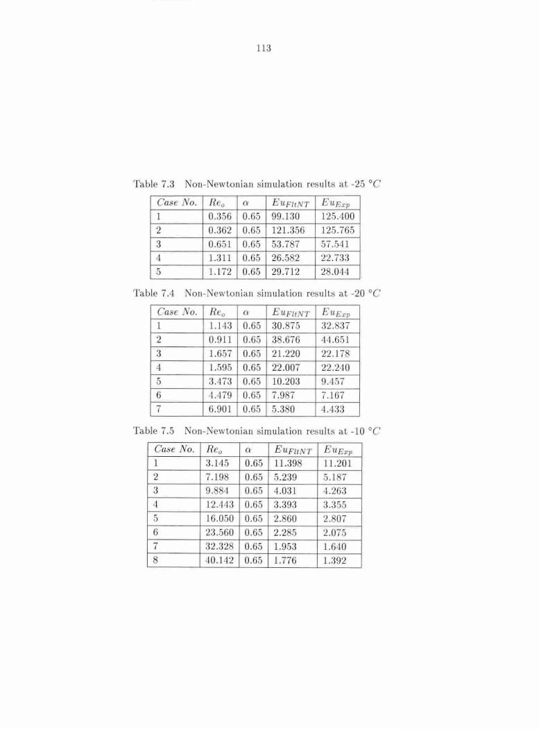
113
Table 7.3 on-Newtonian simulation results at -2.5 °C' Case No. R e0 fr EUF/tNT Eu Exp
1 0.356 0.65 99.130 125.400 2 0.362 0.65 121.3.56 12.5.765 3 0.651 0.65 53.7 7 57..5-11 4 l.311 0.65 26.5 2 22.733 5 l.172 0.65 29.712 2 .044
Table 7.4 Non- ewlonian simulation rcsuhs at -20 °C'
CasE . o. Rt0 a EUF/tNT ElLE:cp
1 1.1-13 0.65 30.875 32. 37 2 0.9ll 0.65 38.676 4tl .651 3 l.6.57 0.65 21.220 22. 17 4 1.595 0.65 22.007 22.240 5 3.413 0.65 10.203 9.457 6 ·l .<179 0.6.5 7.9 7 7.167 7 6 .901 0.65 5 .3 0 -1.433
Table 7.5 Oih ewtonian simulation results at -10 °C
Case No . Reo ll' E1lFitNT EuETp
1 3.145 0.65 11.39 ~ 11.201 2 7.198 0.65 5.239 5.1 7 3 9. 4 0.6.5 -1.031 4 .:263 4 12.44:3 0.65 3 .393 3.355 5 16.0.50 0.65 2.860 2.807 6 :23.560 0.65 2.2 5 2.075 7 32.32 0.65 1.953 1.640 8 40.142 0.65 1.776 L.392

11-t
f~ : • • FLU ENT simulation 14 12 10
- · .....,_ - Experimental results a1 ~ O C - -+- - FLUENT non~ewtonian
simulation 3" 8 w -... 6 .8 E ::::i 4 c • ... ~
"3 • • w ' . •
2 't. • • ..
10 20 30 40 Orifice Reynolds number (Re0 )
Figure 7.6 'omparison of t,he 8u ler numbers

115
CHAPTER 8. NUMERICAL SIMULATION BY THE MU LTI-GRID
METHOD
T he mult i-grid method is believed to be one of the most efficient general itera tive methods.
Acco rding to Tannehill et a l. (32] it is the removal of th e low-frequency component of t he
error that usually slows convergence of iterative schemes on a fixed grid. However , a low-
frequency component o n a fine grid becomes a high freq uency component on a coarse grid.
T herefore it makes good sense to use coarse grids to remove the low-frequency errors a nd
propagate boundary information throughout t he domain in combination with fine grids to
improve accuracy.
Since the convergence rate for simulating t he flow through a pipe orifice with small ori-
fice/ pipe d iameter ratios (/3 = d/ D) is very s low, t he multi-grid method was attempted to
accele rate the convergence. This method wo rked well fo r t he simulation of the pipe fiow and
orifice flow wit h a large d iameter ratio . However, mul t ig rid didn't seem to accele rate t he com-
putation of the very s mall diameter ratio orifice flow. Here t.he mul t i-grid method was applied
along with t he CSIP method to solve t he coupled Navier-Stokes equ a t ions on several stretched
computational meshes.
8.1 The Delta Form Equations for the CSIP M ethod
The mu lti-grid method is always a pplied to the delta fo rm of the equations. The avier-
Stokes equations (Eqs.3.19-3 .22) were solved iteratively by the CSIP method, which was de-
scribed in C hapter 3. In general, t hey become Eq. (8 .1 ) a fLe r discretization and linearization .
_.k+ I _.. [A] q =b ( . L)

whern
A=
116
A1m,1n .l;m,Jrt
is t he coefficient matrix in which every element is a 4 x 4 a rray; a nd _.k+ l [ ] k+l T - T T T q - (u,v, p,T)i ,1 ... (u,v p,T)i,J ...... (u,v, p, T )im,jn
b= [ ((bu ,bv,bp,br )f 1 (bu,bv,bp,br)~1 .11 , 1 J.,)
(bu ,bv ,bp,bT) im,in r ]T J,m ,J n
T his eq uation is s lig ht ly diffe rent compared with Eq. (3 .49) in C ha pter 3. However, they
a re consistent wit h each other. For Eq. (3.49) in Chapter 3, t he J acobians didn't s how up and
were contained in t he matrix elements . T he J acobians a re s hown d elibe rately here in order to
define t he forcing function correctly in th e following sections . ....... ,..
The residual or d elta form of Eq. (8.1) can be derived by subt racting [A] q from its bot h
sides. _...1-.;+1 _... k __... _.k
[A](q - q ) = b - [A] q (8.2)
To make the LU decomposition easie r, equation(8.2) is mod ifi ed as follows:

117
_.. _. [A + BJ 8=R ( .3)
where --" ->k+ 1 --k 8= q - q ( .4)
and ~ ~ ~k
R= b -[A] q (8.5)
and [B J is a n a uxilia ry matrix. By ad ding the matrix [BJ Lo the matrix [AJ, t he matrix [A+ B]
can be easily deco mposed into [LJ[U] (4 6J.
T hus, Eq. (8 .3) becomes: _.. _..
[L] [UJ 8=R (8.6)
where R is Lhe residua l.
8. 2 Full Approximation St orage(FAS) Method
Eq uatio ns (3 .19-3 .22) are non linear equa tions . To solve t he coupled nonli near equations
with t he mu ltigrid method, Lhe solut ion as well as the residual shou ld be transfer red between
t he diffe rent layers of t he g rids. This is know n as the fu ll approximatio n storage (FAS) method
[32J. _. _.k+ l
For t he FAS method, not only t he resid ua l R but also t he solut io n q s hould be t ra ns-
fer red bet ween diffe rent grid layers. Tn t his t hesis, t he m ul tigrid method just used two or t hree
g ri d laye rs . T he g rid layers were generated such that the grid points of t he coarser grid layer
were a lways at t he same place as t he correspond ing finer grid layer (see F igs. 8.2- 8.3 ) . T hus,
t be solution and resid ua l transfer fro m the finer grid layer Lo the coarser grid layer was quite
easy. T hese values can be d irectly injected from t he fine r g rid layer to the coarser grid I.ayer.
However , t he transfer fro m the coarser grid layer to the finer grid layer should be t reated
carefully. T he values on t he ident ical points can be transferred d irectly. For t hose grid poi nts
lying between t he coarser grid points, linear interpolation s hould be used to obtain t he val ues.
As s hown in Fig. 8.1 , t he <I> value o n t he cenLer grid should be linearly inte rpolated as follows:

118
N NE
c W--------- E
SW s SE
Figure .l Linear interpolation configurat ion
lf..L-1 lf.. L '.l.'N W = '¥ NW
,n.L-1 ,T..L '.l.'NE = '¥ NE
lf..L-1 if.. l '.l.'SW = '.l'SW
lf.. l- 1 ,-i;.l., '.l.'SE ='¥SE
lf..l- 1 _ X N - XNw ( <PL _ q>L ) + q>L '.l'N - v v NE N W W
.1\ NE - .1\ N W
if..L-1 _ Xs-Xsw (<l> l _ m L )+<l>L 'lt'S - v X SE '1<' SW SW
.1\ SE - SW
l- i Yw - Ysw c, L ) c, <l>w = y ~ (<l>Nlv - <l>sw + <l>sw
NW- SW
.;r,.L- 1 _ Ys - Yss (<l>L _ <P L ) + q>L '.l.'E - v y NE SE SE
I NE - SE
mL-1 = Xe - Xiv (<1>[, - <l>[,) + <l>L '.l.'G X v E W W s- .1\ W
8 .3 The Forcing F\:inction and the Modified Equation
( .7)
( . )
( .9)
( .10)
( .11)
( .12)
( .13)
( .14)
( .15)
On the fin est g rid 1 the mul t igrid method always solves the origina l equation . However
on the coarse grid, t he origina l eq uation is mod ifi ed by add ing a forcing func tion term to the
residua l in the equa tion.
__,.£ __. [, __.[, [L] [U]o = R + P ( .16)
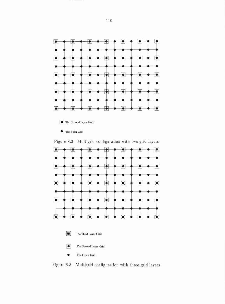
119
~ The Second Layer Grid
• The Finer Grid
Fig ure 8 .2 Mult igrid configu ration with (,wo grid layers
~ The Third Layer Grid
~ The Second Layer Grid
• The Finest Grid
Figure 8.3 M ul tigrid configuration wit,h t,hree grid layers

120
_,.[, where p is the forcing function. According to Tannehi ll et a l. (32], the forcing function is
given by t he following equation :
( .17)
-"IL-1 -"L-1 _,.£-1 In Eq. (8.17), R =R + P , and 1t_ 1 ind icates data transferring from the finer grid
_,., L-1 _,., L-1 level L-1 to the coarse r g rid level L. So I f_ 1 (R ) means transferring residual R from
__. _,.f,-L the finer grid to the coarser grid. And R (lt_ 1(q )) means t he residual calculated from the
solution transferred from the finer grid. The forcing fun ction was d esigned so that when the
solution on the finer grid converges, the correction being solved on the coarser grid vanishes.
However, eq uation {8.17) should be modifi ed according to the special treat,ment, of t,he
current CSIP solver. As s hown in Eq .. ( . L) , every li ne of t he coefficient matrix (A] and the
right hand s ide array b a re div ided by a local J acobian J i,i· Correspondingly the forcing
function pL becomes:
1l-l 2 r-1 2J -1 RIL -1
1L 2i- 1,2j- 1 .. , ( .1 )
J L-l 2 rm -1,2zr1-l R IL- L
Jl 2im-l ,2jn- l •m,Jn
where t he index L re presents t he 2 grid and t he index L-1 represents t he finer grid; and ->-IL- L __.£-1 -"L-1 R = R + P
For t he bo und aries on t he coarser grid layers, the res idua ls on the finer grid boundaries
should not be t ra nsferred. This means on the coarser grid layer boundaries R1L- I should be
zero .

L 21
8.4 The Solution Procedure
In Lhis the!:>is, the mult igrid method just used the simple \" cycle. Jn t he simple V cycle>, Lhe
calcula tion proceeded from the finest grid down to the coa rses t and the n back up Lo the fi nest.
Also. just Lwo or three grid layers were used. llerc the solution procedure fo r the 111ultigrid
method wit h t hree g rid layers is introduced. Th' solution proced ure for the method with two
grid layers wou ld be quite the same as the one with three grid layers by red ucing the s teps for
the coarsest grid layer.
Before the rnultigrid method cycle, it is necessary to generate all the grid layers and calcu-
late the metrics and Jacobian for each grid layer.
T he solu t ion procedure is shown as follows:
1. On grid layer level 1 (the finest grid) Eq. ( .1 9) is iterated fo r one iteration .
_. _. J
[L][U] o= fl ( .19)
and the solu Lion is updated by:
( .W) _.1 _.2
2. Solutions q e on grid layer level l are t ransferred to q s Lo grid layer level 2. Th' fo rci ng _.2 _.,I -"I
function P is calculated by Eq. ( .l ' ) by taking L as 2. and R =R .
3. On grid layer level 2. Eq. ( .21) is iterated for one iteration .
_. _.2 _.2 [L][U] o = R + P ( .21)
and the solution is updated by:
( .22) _.2 _.3
4. Solutions q e on grid layer level 2 arc transferred Lo q s ou grid layer level 3. The forcing _.3 _.,2 _. 2 _.2
fun ction P again is calcu lated by Eq. ( . I ) with taking L as 3; however R = R + p .
. 5. On grid layer level 3, Eq. ( .23) is iterated for 30 iterations.
_. _.3 _.J
[ l ][ U] o = R + P ( .23)
and the solution is updated by: ....a.3 _.3 q e= q e + 0 ( .2-1)

122
6 . On grid layer level 3 , t he change 83 is calculated by:
83 = q~ - q~ (8.25)
Then 63 is transferred to 82 on grid level 2 by using Eqs.(8.7)-(8.15). Then the solution q; on
grid layer level 2 is updated by:
(8.26)
7. On grid layer level 2 , Eq. (8.21) is again iterated for one iteration; a nd the solut,ion is also
updated as indicated in Eq. (8.22).
8. On grid layer level 2, the cha nge 8'2 is calcu lated by:
( .27)
Then again 8'2 is transferred to 61 by using Eqs. (8.7-8.15). Then the solution q; on g rid layer
level 1 is upda ted by:
( .2 )
9. On grid layer level 1, Eq. ( .19) is again iterated for one ite ration ; and t he solution is also
upda ted as Eq. (8.20). If the solution has not converged , t he cycle from step 1 to step 9 s hould
be repeated until convergence.
For every cycle from step l to s tep 9, the equivalent, fine grid ite rations can be calculated
approximately by E I = 1+1/4 + 30/ 16 + 1/4 + l = 4.375 = 5.
8.5 The Efficiency of t he M ul ti-grid Method
Several cases were calcu lated in order to test the efficiency of t he mul tigrid method. The
first case is axisymmetric pipe flow wit h a n in let Rey nolds number of 10. Simulations with a
single grid layer, two grid layers , a nd three g rid layers were carried out. For t his simulation
the fin est grid layer em ployed a 61 x 21 mesh.
The second case was axisymmet ric pipe orifice flow with diameter rat io of 0.5 and inlet
Reynolds number of 10. Simulat ions with one, two , and three grid layers were canied out. For
th is simulation , the finest g rid layer had a mesh of 97 x 65.
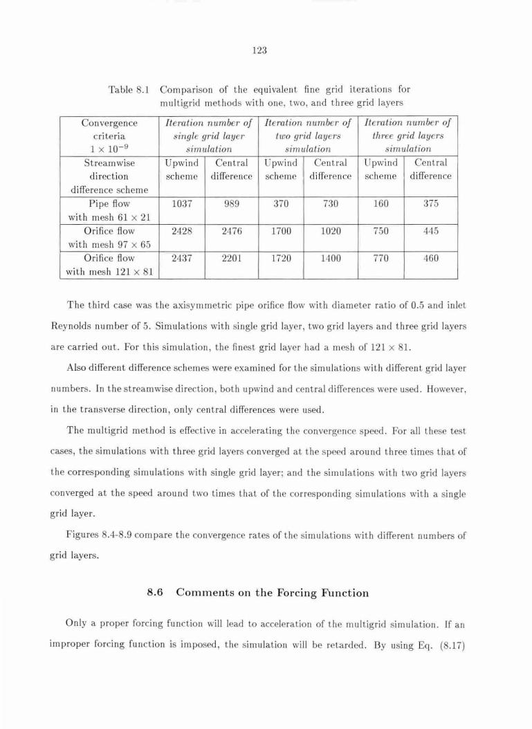
123
Table .l Comparison of the equivalent fine grid iterations for multigrid methods with one, two, and three grid layers
Convergence Iteration number of Iteration n1tmb r of It eration number of c rite ria single grid layer f ll'O g1·icl Lay r th1·cc grid laye1·. 1 x 10⁻⁹ imulation simulation . imulation
Stream wise Upwind Central Upwind Central Upwind Central direction scheme difference scheme differe nce scheme diffe rence
difference scheme Pipe flow 1037 9 9 370 730 160 375
with mesh 61 x 21 Orifice flow 242 2476 1700 1020 750 4<15
with mesh 97 x 65 Orifice flow 2437 2201 1720 1400 770 460
with mesh 121 x l
The third case was the axisymmetric pipe orifice fl ow with diameter ratio of 0.5 and inlet
Rey nolds number of 5. imu lations with single grid layer, two grid layers a nd three grid layers
are carried out. For th is sim ulat,ion , the finest grid layer had a mesh of 12 L x 1.
Also different difference sche mes were examined fo r the simula tions with different grid layer
numbers. In the streamwise direction. both upwind and central differences were used . llowever,
in the transverse direction, only ce ntral differences were used.
The mu lt igrid method is effective in accelerating the convergence speed. For all these te t
cases, the simulations with three grid laye rs converged at the s peed around three times that of
the corresponding simulations with single grid layer· and the simulations with two grid layer
co nverged at the speed around two Limes that of the corresponding simulations with a single
g rid layer.
Figures .4- .9 compare the convergence rates of the simulatious with different numbers of
grid layers.
8.6 Comments on t he Forcing Function
Only a proper forcing function will lead to acceleration of the mul t igrid simulation. ff an
improper forcing fun ction is imposed, the simulation will be retarded. Dy using Eq. ( .17)
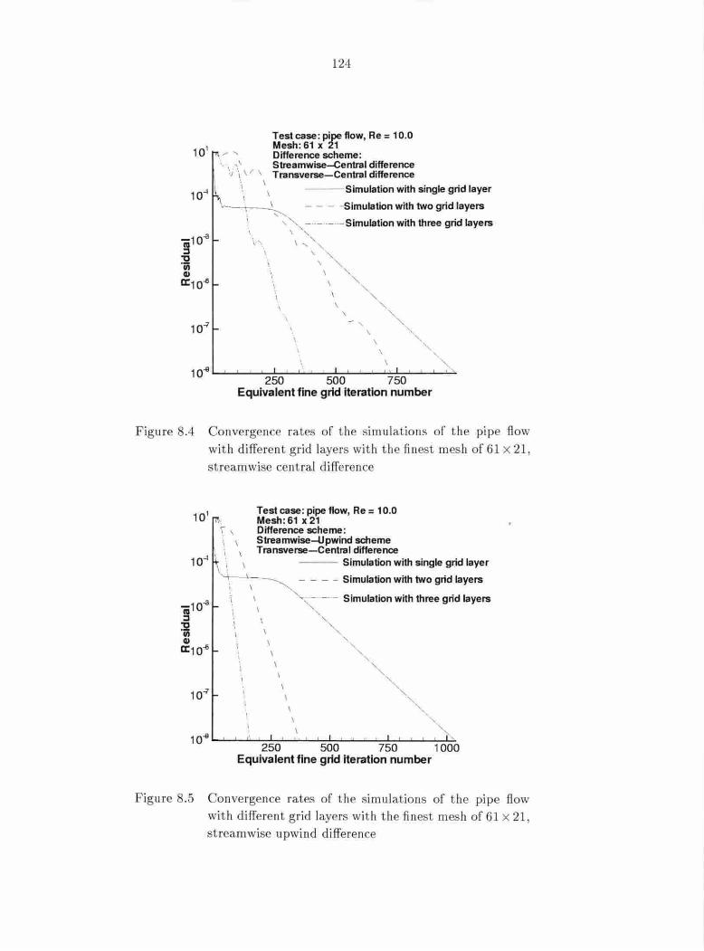
1 o""'
,,., •. '\ \
'., \\I' \ \ I . \
124
Test case : pipe flow, Re= 10.0 Mesh : 61 x 21 Difference scheme: Streamwise-Central difference Transverse-Central difference
---Simulation with single grid layer
~-.---1 - - - -Simulation with two grid layers ""-
\' I
\
''-, -··- ··-··- Simulation with three grid layers \ ',
\ I, I \
\ .._ '" ' "
\ " \ ' \ "
\
' ' ' \
\
' ", ' '· '·-
'· 10~ ....._.___.____.___.__.____,__._.......__._.....__..__.__.......__.____.___.__.__._~
250 500 750 Equivalent fine grid iteration number
Fig ure .4 Convergence rates of the si mulations of the pipe flow wit h different grid layers with t he finest mesh of 61x21, streamwise central difference
101 ' \ \
\ \ I
\ ~ I
Test case: pipe flow, Re= 10.0 Mesh : 61 x21 Difference scheme: Streamwise-Upwind scheme Transverse-Central difference
--- Simulation with single grid layer
-~~ ~ - - - - Simulation with two grid layers
i 1 '... - -· - Simulation with three grid layers I I \ \ \ \
\ \ \
\ " 10~ ......... __..-"'-'--'-_,__.._.__...___.___.____,_.......__,_...._.__ .......... ___.___.__,_ 250 500 750 1 000
Equivalent fine grid iteration number
Figure 8 .5 Convergence rates of t he simulations of the pipe flow with different grid laye rs wit h the TI.nes t mes h of 61 x 21, streamwise upwind difference

10°
10~
10-8
\
125
Test case : orifice flow, Re= 10.0 Mesh: 97 x 65 Differenc Scheme: Streamwise-Central Difference Transverse-Central Difference
1 Simulation with single grid layer
, [\ - - - - Simulation with two grid layers
'. \~----- - - Simulation with three grid layers
' \ \
I \ ·,
I. i ' ' \
' ' \ 1000 2000
Equivalent fine grid Iteration number
Figure 8 .6 Convergence rates of the simulaLions of the o rifi ce flow with different g rid layers with th e finest mesh of 97 x 65, streamwise central d ifference
Test case: orifice flow, Re= 10.0 Mesh: 97 x65 Difference scheme: Streamwise-Upwind scheme Transverse- Central difference
\ 10-t \
Simulation with single grid layer
- - - - Simulation with two grid layers \\ "
'.
10-7
\
\
II I I
' ' ' ' '
Simulation with three grid layers
' ' ' ' 10~.____,_~.._____,_~...____._~...____._~~'..:,._"'----'-~"'--~
1000 2000 Equivalent fine grid Iteration number
F igure 8.7 Convergence rates of t he simulatio ns of th e o rifice flow wit h different grid layers with the finest mesh of 97 x 65, streamwise upw ind scheme

10°
126
Test case: orifice flow, Re= 10.0 Mesh: 121 x 81 Difference scheme: Streamwi~entral difference Transverse-Central difference
~\ , Simulation with single grid layer
1 O.;? ' '~ - - - - Simulation with two grid layers
IQ \ r ~ - Simulat.ion with three grid layers ::J I I :210-4 J1
~ ''., ~ a: ,, •'
1 0~ ·' '',, ~
\ ' "-.. 1 0~
1'1, ~
,~
I•
500 1 000 1500 2000 Equivalent fine grid iteration number
Figure 8.8 Convergence ra.Les of the simulations of the o rifice flow with different g rid layers wit h the finest mesh of 121 x 1, streamwise central d ifference
10-1
10-1
I
'
Test case : orifice flow, Re = 10.0 Mesh: 121 x 81 Difference scheme: Streamwise-U pwind difference Transverse-Central difference
'~ -- --' .. ",~
Simulation with single grid layer Simulation with two grid layers
Simulation with t hree grid layers I ''~
\ ' '. ' \
\
\
'.
' ' ' '
1000
' ' ' ' ' ' ' 2000
Equivalent fine grid iteration number
Figure 8 .9 Convergence rates of the simulations of Lhe orifice Row with different grid layers with the finest mesh of 121x81, st rea.mwise upwind difference
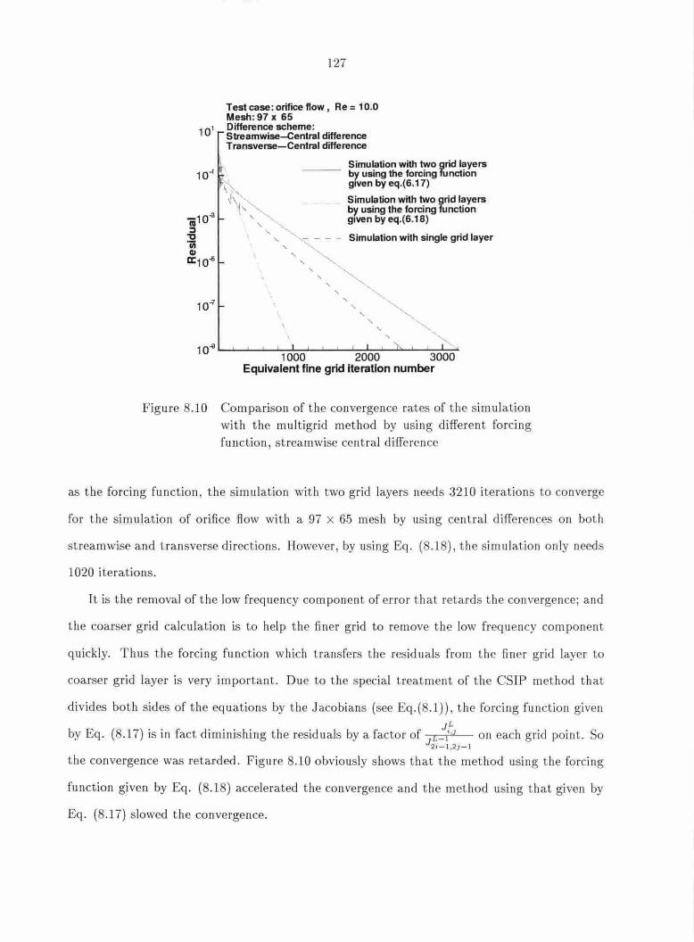
101
10-1
127
Test case : orifice flow, Re= 10.0 Mesh: 97 x 65 Difference scheme: Streamwise-Central difference Transverse-Central difference
' '
Simulation with two grid layers by using the forcing function gtven by eq.(6.17)
Simulation with two grid layers by using the forcing function given by eq.(6.18)
Simulation with single grid layer
' ' ' '"-.
10~ .._..___.___.__._~----~~___.~~~~~~~-
1000 2000 3000
Figure 8 .10
Equivalent fine grid Iteration number
Comparison of t he convergence rates of t he simu lation with the multigricl method by using different fo rcing function, s treamwise central difference
as the forcing function, the simulation with two grid layers needs 3210 iterations to converge
fo r the simulation of orifice ·flow with a 97 x 65 mesh by using central differences on both
streamwise and transverse directions. However, by using Eq. (8 .18), the simulation on ly needs
1020 iteratio ns.
It is the removal of the low freq uency component of error t hat retards t he convergence; and
the coarser grid calculation is to help the finer grid to remove the low frequency component
quickly. Thus t he forci ng function which t ransfers the residuals from t he finer grid layer to
coarse r grid layer is very important. Due to the special treatment of the CSIP method t hat
divides both sides of t he equat ions by t he Jacobians (see Eq.(8. 1)), t he forcing function given
by Eq. ( .17) is in fact diminishing t he resid uals by a factor of JL ~;,2 on each grid point. So 21 - 1,21-1
the convergence was retarded . F ig ure 8.10 obviously shows that t he method using the forcing
function given by Eq. (8 .18) accelerated the convergence and t he method using that given by
Eq. (8.17) slowed t he convergence.

12
8. 7 Conclus ion
The m ul t igrid method using a proper forcing function can accelerate t he conv"' rgence. With
usi ng more grid layers, t he convergence accelera tion would be more effective.

129
CHAPTER 9 . PARALLEL COMPU TATION WITH MPI
In order to accelerate t he compu tation, parallel com pu tation was applied to solve t hese
coupled equa tions wit h the CSIP met hod . The basic idea of pa ra llel comp utation is to divide
a big task into several small ones, which can be carried ou t by several processors working at the
same time. Information should be exchanged among these processors working in parallel from
time to time. On distri buted memory parallel computers, information is commonly exchanged
using t he message passing interface (MPJ).
9 .1 Domain D ecomposition
In t he present stud y, domain decom position was used to d ivide the large computation task
into smaller ones. By domain decomposit ion, t he com putational domai n was divided into
several small s ub-domains. These s ub-domains overl ap with each other using ghost cells. On
the s ub-domains, the coupled NS equat ions were solved simultaneously. The sub-domains can
exchange t he informat ion on the ghost cells by passing data wit h MPI among the p rocessors.
The compu tation on each processo r and communication between t he processors was iteratively
carried ou t until a fi nal converged solu tion was achieved.
Only two-dimensiona l simulations were considered. So one-d imensional or two-d imensional
domain decom posit ion was ap plied to decompose the computational domain . For axisymmetric
pipe fl ow, the com putat ional domain is straight and can be decomposed by a one-d imensional
decomposition method . For axisymmetric pi pe o rifice Row, the computational domain is not
s tra ight a nd can only be decomposed by t he t wo-dimensional decomposition method. Figu res
9.1 and 9.2 show the two types of domain decomposit ion.
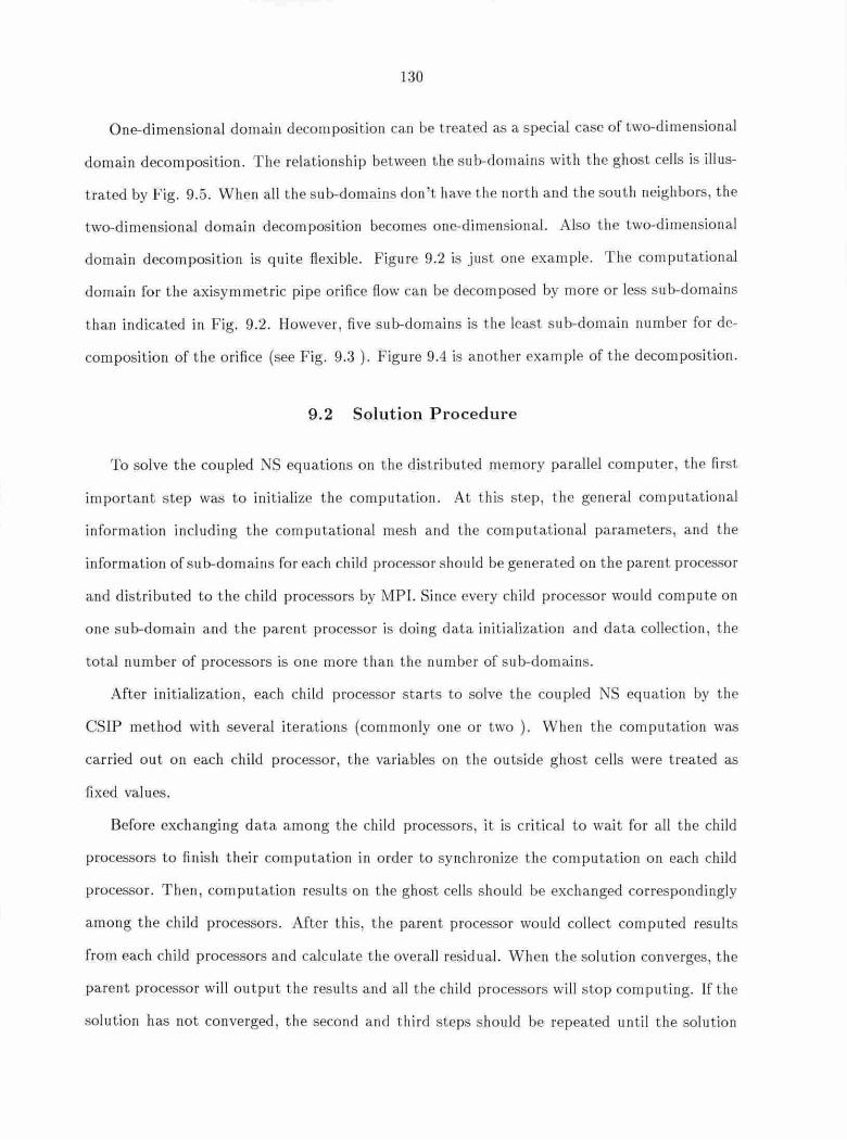
130
One-d imensional domain decomposition can be t reated as a special case of two-dimensional
domain decomposition. The relationship between t he s ub-domains with t he ghost cells is illus-
trated by Fig. 9.5. When all the s ub-domains don't have the north and t he sou t h neighbors, the
two-d imensional domain decomposition becomes one-dimensional. Also t he two-dimensional
domain decomposition is quite flexible. Figure 9.2 is just one example. The computationaJ
domain for the ax.isymmetric pipe orifice flow can be decomposed by more or less sub-domains
than indicated in Fig. 9.2 . However, ·five sub-domains is t he least s ub-domain number fo r de-
composition of the orifi ce (see Fig. 9.3 ). Figure 9.4 is another example of the decomposition.
9.2 Solution Procedure
To solve the coupled NS equations on the distributed memory parallel computer the first
important s tep was to initialize the computation. At t his step, the general computational
information including the computat ional mesh and the computational parameters , and the
information of sub-domains for each child processor should be generated on the parent processor
and distributed to the child processors by MPL Since every child processor would com pute on
one s ub-domain and the paren t processor is doing data initializat ion and data collection , t he
total number of processors is one more than the number of sub-domains .
After initialization, each child processor starts to solve the coupled NS equation by the
CSIP method with several iterations (commonly one or two ) . When the computation was
carried out on each child processor, the varia bles on the outside ghost cells were treated as
fixed values.
Before exchanging data among the child processors, it is critical to wait for all t he child
processors to finish their com pu tat ion in order to synchronize the com pu tal.ion on each child
processo r. Then, computation resu lts on the ghost cells shou ld be excha nged correspondingly
among the child processors . After this, the parent processor wou ld collect computed res ults
from each child processors and calcul ate the overall residual. When t he solution converges, the
parent processor will output the resu lts and a ll the child processors will stop computing. If the
solution has not converged t he second and t hird s teps s hould be repeated until the solution
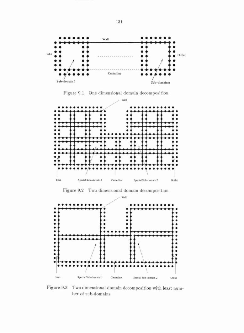
• • • Inlet •
• • •
131
••••••• Wall ••••••• ,1
. l .. 1 ! ---------- _______________ !_i_. J ._ e r- -~ e e e Centerline e e ;1-;-. e
Sub-domain I Sub-domain n
figure 9.1 One dimensional domain dccomposilion
/ Wall
• • • e Oullct
• • •
. .... .................... ~~................. . • • • • . ..... ................ ~~~.................. . . .... .................... ~.................... . • • . .... ................... ~~.................. . . .............................................................................. ......................................... . • • • • • • • • • • • • •
Inlet Specilll Sub-domain 1 Centerline Spcclll Sub-domain 2 Outlet
Figure 9.2 Two dimensional domain decomposition
•••••••••••• . ... ....................................... ~ • • • • • •
Wall
•••••••••••• . ................................................... . • • • • • • • . ....................................................................... . ....................................... . . .. ....................................... ~
• • • • • . .............. ..... . .... ,........ .. ... ·······;·······r······· Inlet Special Sub-domain I CcntcrlJnc Special Sub-<lomaln 2
Figure 9.3 Two d imensional domain decomposiLion wiLh leasl num-ber of s ub-domains

132
co nve rges.
9.3 Data Exchange
The sub-domains overlap wilh each other using lhe ghost cells . The g host cells are des igned
Lo enable the exchange of computa tional information wit.h neighboring s ub-domains. Primitive
variables (u,v,p and T) are stored on the ghost. cells as well on the comput.ational mes h points.
Exchanging information between the sub-domains through t.he ghost cells is essential in order
to make the whole sol ut ion field continuous.
Data exchange between t he sub-dom ains becomes easie r wit h t he assistance of t he neigh-
bor information and bound a ry information a rrays. The neig hbo r information a.rray is a two-
dimensional array that records the indices of every sub-domain's su rround ing sub-domains:
and the boundary informatio n array is a lso a two-di mensiona l a rray that stores every sub-
domain 's bounda ry i11forrnation. If one side oft.he sub-domain is connected with a s ub-domain
by t he g host cells, t he correspond ing element in t he boundary information array would be zero.
I3ased o n t. hese two ar rays, the s ub-domains can send data on the ghost cells to corresponding
neighboring sub-domains or receive data from corresponding neighboring sub-domains. Figure
9.6-9.9 show t he four modes oft.he d aLa exchange between the sub-domain and its neighbors.
Data on the g ho t cells on ub-domain I re presented by the filled circles s hould be sent to
its neighboring s ub-domain. Meanwhile, the ghost cells on Sub-domain I represented by the
empty ci rcles s hould get corresponding data from t. he neighbo ring s ub-dom ain.
Data exchange bet.ween lhe s ub-domai 11s near t he orifice wall corners and their neighbors
needs to be specially treated. As shown in Fig. 9.10, the Special Sub-domain l has one less grid
line than it.s east neig hbor. F igure 9.11 illustrates the Oow of the data exchange. Pa rticu la rly,
the right lowe r co rner of the nor t h neighbor and the left upper corner of Lhe east neighbor
s hou ld excha nge data with each o ther as shown in Fig . 9.11 . D ata exchange between the
pecial Sub-domain 2 and its neighbors is treated in a manner similar Lo t hal of the . pecial
ub-domain 1 (refe r Lo Fig. 9.12-9.L:3).
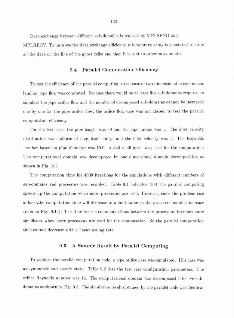
133
Dat a. excha nge between different s ub-domains is realized by MPLSEND a nd
MPLRECV. To improve the data. excha nge effi ciency, a tempora ry array is generated to store
all t he data on the line of the ghost cells; and t hen it is sent to other s ub-domains.
9.4 Parallel Computation Efficiency
To test t he efficiency of t he pa rallel computing, a test case of two-dimensional axisymmetric
laminar pipe flow was computed . Because there would be at least fi ve s ub-domains required to
simulate the pipe orifice ·Aow and the number of decomposed sub-domains cannot be increased
one by one fo r t he pipe orifice flow, the o rifice flow case was not chosen to test t he parallel
computation efficiency.
For the test case, t he pipe length was 60 and the pipe radius was l. T he inlet velocity
distribution was uniform of magni t ude uni ty; a nd the inlet velocity was l. T he Reynolds
num ber ba.5ed on pipe diameter was 10.0. A 320 x 40 mesh was used for t he computation.
T he computational domain was decomposed by one dimensional domain decomposit ion as
shown in Fig. 9.1.
The computation time for 4000 iterations fo r t he simulations with different nu mbers of
s ub-domains and processors was recorded . Ta ble 9.1 indicates t hat t he pa rallel com pu ting
s peeds up t he compu tation when more processors are used . However, since the problem size
is fi xed ,the computation time will decrease to a limit value as the processor number increase
(refer to F ig. 9.14) . The time for t he communications between t he processors becomes more
significant when more processors a re used for the computation. So t he pa rallel computation
t ime cannot decrease wit h a linear scaling rate.
9 .5 A Sample Result by Parallel Computing
To validate the pa rallel comp utation code, a pipe o rifice case was simulated. T his case was
axisymmetric a nd steady state. Table 9.2 lists t he test case configuration para meters. The
orifice Reynolds number was 16. The computational domain was decomposed in to fi ve sub-
domains as shown in Fig. 9.3. T he simulation resuJ t obtai ned by t he pa rallel code was identical

•••••••••••• . .... ~~ ............................... ~. • • • .... ................ .-.i.-.i ............ .... • .... ............ .-.i.-.i ................ ....
• •
j 3..J
\\all
•••••••••••• . ............ ~~~ ....................... • • • ................ .-.i .......................... ....
. .... ................ ~~........................................... . ................................. . . .... ................ ~ ..................... • . .... ................ ~ ............ ~ ...................................... ~ .... ~ ................... ... . .... ................ ~ ........................................................ ~ .... ~~ ............... ... • • . ·•·•••· .. ·•·• .... ,...... ·•·•
• . ·•••·•· ~
\ •••••• • 1 ••••••••••••••••••••••• Inlet Special Sub-domain I U,niullnc Spccl•I Sub-dom:aln 2 Outlet
Figure 9.4 Anothe r example of two-d imensional domain decompo-sition
West Neighbour 0 r
ri O v r; ('
Nonh Ndahbour
- - -.J ") -
South Neighbour
East Nelgbbour
ObostCclls
Figure 9.5 A sub-domain and its neighbors
Ohoi1 Cells \,,,.) r I) \.')
) 0
.)
Co
' -
SulH!omaln I
North lloclabbot:r , '
~•o·O 0 .... 0 . •. '· !! 0 •••••
line DuL1 fachnnll" OhoSl Cells
Figure 9.6 Data exchange between ub-dornain I a nd its north neighbor

135
0() .)Qr
Sub-domain I "'o-· ,, ,-, ' 0 V ' ' (.) Ghost Cell• 0 l. • ..
0 lo.: - (._i
ooc.:.·'.)
Line Da<a fachnngc
0 0 0 G (•
Ghost Cello : o· : ' ~ e , , , ') East Ne ighbour ., _.)')
oc:~o
Figure 9.7 Data exchange between Sub-domain I and its east neigh-bor
Oho.i Cello
•••••
Sub-domsln I
0 CJ G ·~· 0 ·:i·o··) 0 ' ' ~ Ci 0 ' '' :i 0 \ ~ \J
•.) ... ......_ ()
Ci ·: G 0 r. ~o·;~. r'J; Linc Dalli Exchange OhOllt Cells
1)' .. , (' 0 ,_ - ~ :J )
(')000 South Neighbour
Figure 9.8 Data exchange between Sub-domain 1 and its south neighbor
0 0 •J 0 0
West Neighbour ~ o-, r. ,- , :
0 ' • (. ' - :.. ~· -· .
J000
ObostCclls
Unc Dato Exchange
0 .-. ........ .......-~ •)
Obo5t Cells ( 0
Sub-domain I
F igure 9.9 Data exchange between Su b-clomain l and its west neigh-bor

North Neighbour (J0~)(;(;
() ,,,__,,,,,__,++......,
Special Sub-<lomnln I
136
Eosl Neighbour
Figure 9.10 Special Sub-domain 1 and its neighbors E!asl Neighbour 1) 0 c ....
0 C· ) 0
r j Linc Daill Exchange
•••••o ••• 0 Line Dal• Exchange 0 ' O
0 'Ht'-t--=--9 0
Speci:tl Sub-<lon1:tln I
Figure 9.11 Data exchange between Special Sub-domain 1 a nd it,s neighbors
0
North Neighbour 0 Cr C• 0
West Neighbour
Special Sub-domain 2
F igure 9.12 Special Sub-domain 2 and its neigh bors
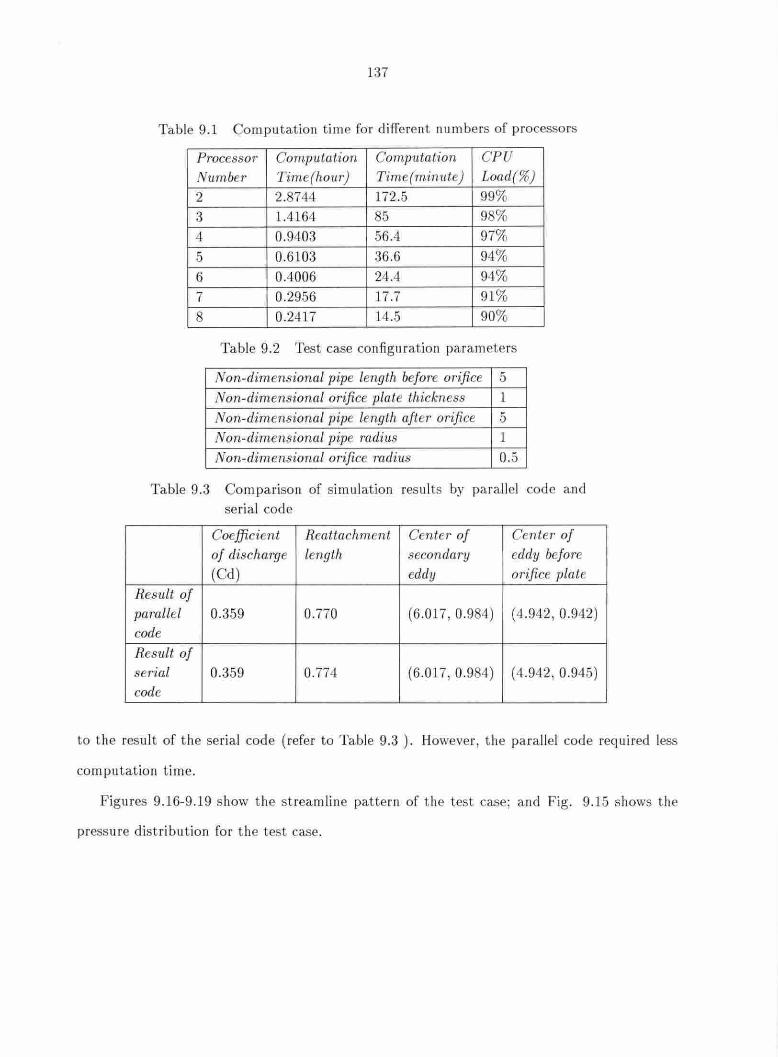
137
Table 9.1 Computat.ion time for di fferent numbers of processors
Processor Computation Cornputatfon CPU Number T ime(hour) Time( minute) load(%) 2 2.8744 172.5 99% 3 1.4164 85 9 % 4 0.9403 56.4 97% 5 0.6103 36.6 94% 6 0.4006 24.4 94% 7 0.2956 17.7 91% 8 0.2417 14.5 903
Table 9.2 Test case configuration para.mete rs
Non-dimensional pipe length before orifice 5 Non-dimensional orifice plate thickness 1 Non-dimensional pipe length after orifice 5 Non-dimensional pipe radius 1 Non-dimensional orifice rarlitLs 0.5
Table 9.3 Comparison of simulation resul ts by parallel code and serial code
Coefficient Reattachment Center of Center of of discharge length secondary eddy before (Cd) eddy orifice plate
Result of parallel 0.359 0.770 (6.017, 0.984) (4 .942, 0.942) code Result of serial 0.359 0.774 (6 .017, 0.984) {4.942, 0.945) code
to the result of t he serial code (refer to Table 9.3 ). However, t he parallel code req uired less
computation t ime.
Figures 9.16-9.19 s how t he streamline pattern of the test case; and Fig . 9.15 shows the
pressure distribution for the test case.
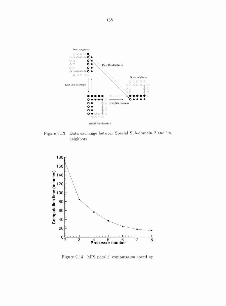
13
West cisJibour
') ~t~D· ~ ~ ~ ~. r.. • •) . 0 • C..· .... * ... - •
Nonh Neighbour
Linc D•ta Exdumge ~o- = - -.~
••••• ~ ~ · 0 I'.: 0 .. :;;
" I. I , ~
·~ ... & :.' 'o ••••
Linc Data Exchange
F igu re 9.13 Data exchange between Special ub-domain 2 and its neighbors
180
160
~140 : 'S c ·- 120 E --~ 100 -+= g 80 += s 60 c.. g 40 (.)
20 ---3 4 5 6
Processor number 7 8
F igure 9.14 MPl parallel computation s peed up

139
Re,=16.0
~·.
Figure 9.15 Pres.<>urc distribution for the ori·fice flow by paral lel computing simu lation (Ren= 16.0)
Re0=16.0
Figure 9. 16 Streamline pattern for the orifice flow by parallel com-puting simulation (Rt>n = 16.0)
Re,=16.0
.. Figure 9.17 An enlargement of the eddy before the orifi ce by par-
allel computin(!; simulation (Re0 = 16.0)

140
Ra0: 16.0
..
.. "'·
Figure 9.1 An enlargement of the eddy after the orifice by parallel computing simulation (Re0 = 16.0)
Re0: 16.0
.. .. .. an,
Figure 9.19 An enlargement of Lhe secondary eddy after t.he orifice by parallel com puting simulation (Re0 = J.6.0)

141
CHAPTER IO. CONCLUDING REMARKS
IO.I Conclusions
In order to investigate low Reynolds number fl ows t hrough pipe orifi ces, numerical sim u-
lations by the primit ive variable approach, the stream function and vorticity approach, and
FLUENT were carried out.
Even though the nume ri cal simulations with the primitive va.riable ap proach can handle
compressible flow wit h variable properties, in t his t hesis , on ly result,s for incompressible flow
with constant propert ies were presented . However, the numerica.J simu lations with the s tream
function vort icity approach can only s im ulate incompressible flow. Both approaches can com-
pute the temperature field. To validate t he simulations, an incompressible axisymmetric pi pe
Bow case with constant properties and a. circular-tube thermal-entry problem were simu lated
by both approaches. The sim ulation resul ts matched corresponding analy tical solu tions qui te
well.
Nu merical simulations were carried o ut for incompressible fl ows through o rifices with an
orifice/pipe diameter ratio of 0.5 with different. aspect ratios by using both approaches. The
coefficients of discharge calculated from simulation results by both app roaches matched Sahin
a nd Ceyhan 's [6] simulations and experimental results quite well. Also t he fl ow structu res
obtained from t he two approaches were similar and consistent, as shown in t he figures in
Chapter 6. Numerical simulations were also carried out for incom pressible flows through orifices
wit h an orifice/pipe d iameter ratio of 0.2. The reattachment lengths and the coefficients of
discharge were compared wit h Hayase and Cheng's [7] numerical sim ulation results . Al though
there were some small differences between the simu lation results, the trends agreed fairly well.
142
T he fl ows t hrough o rifices with very small ori fice/pipe diameter ratios were of great interest.
The investigato rs in ISU [2-4] conducted ex periment s on o rifices with orifice/pipe diameter
ratios of 0 .022, 0 .0445, a nd 0.132 using highly viscous oil at different temperatures. Because
the temperature was controlled quite well in the ISU experiments, the oil properties still can be
treated as constants, even t hough the propert ies were sensit ive to the change of temperatu re.
It was fo und t hat t he coupled solvers including t he primitive variable approach and the
coupled solvers p rovided by F LUENT converged very slowly when solving for flows through
orifices wit h very small orifice/pipe diameter ratios. However, the segregated solvers provided
by FLUENT, and t he stream function vorticity approach wh ich avoided solving for the pres-
s ure fi eld when solving t he velocity field, converged at qu ite fast rates. In this thesis, the main
research interest was focused on t he o ri fice wit h a n orifice/pipe d iamete r ratio of 0.0445 used
in t he ISU experiments. T he orifice Reynolds number was in the range of 0.2055 to 460.011.
Dagan et a l. [43] provided a theoretical pred iction of t he E uler number for the low Reynolds
num ber Newton ian flows t hrough small diameter ratio orifices . The E uler numbers calculated
from t he stream fu nction vorticity approach a nd t he FLUENT simulation matched the theo-
retical prediction very well at low orifice Reynolds nu mbers (R e0 less than 10). This means
t hat both simulation results and t he theo retical prediction we re rel iable for the low Reynolds
number Newtonia n flow. However, when orifice Reynolds nu mber increased, the t heoretical
prediction became much smalle r t han t he two sim ulation resu lts. At t he same t ime, the simu-
lation results by t he stream function vort icity approach and FLUENT were somewhat different
at high orifi ce Reynolds nu mbers.
T he sirnu.lation res ults were compared wit h t he experi mental results. It was found that the
experim ental results fo r the Euler nu mber were lower than t he simulation results throughout
most of t he range of t he Reynolds num bers. Especially at low orifice Reynolds numbers, the
experimental E uler number resul ts were much lower than the simulation results. Thus, the oil
used in t he experiments was believed to have shear-thin ning non-Newtonian behavio r. Some
simple non-Newtonian modeli ng was tested in FLUENT. T he Carrea.u model was used to model
t he oil's non-Newtonian behavior. It was found t hat t he non-Newtonian results were closer to

143
the experimental resu lts compared to the ewtonian results .
As additiona l works, numerical s imulations with I.he multigrid method and parallel com-
putation with MPI were also achieved in th is thesis in an effort to reduce I.he computation
time.
10.2 Recommendations for Future R esearch
There are few studies recorded in the literature discussing the characterist.ics of flows
through orifices with s mall orifice/ pipe diameter ratios. Also very few s tudies reporting nu-
merical simulations for this configu ration can be found. To simulate the flows through the
small diameter ratio orifices, the aut.hor s truggled considerably with the coupled solvers, as
pointed out in the previous section. Maybe solving for the pressure field by the coupled solvers
is very difficu lt. On the other hand , those solvers avoidi ng directly solving for the pressure field
when solv.ing the velocity field seem to converge qu ite qu ickly, such as the segregated solvers
in FL ENT and t he stream function vorticity approach. T he reason why the coupled solvers
converge very s lowly needs to be investigated in the future. And hopefully some ways can be
found to accelerate the convergence.
l n the simulations, the properties of the oil used in the ISU experiments were treated as
constants because the oil temperature was controlled quite well. In fact, the oil properties s till
changed slightly. Even though it is really difficult to match the real experimental conditions,
at least some add itional factors, such as viscous heating, can also be added . Also t he non-
Newtonian modeling used in th is study was very simple. It on ly considered shear-th inning
behavior. However, t he real s ituation cou ld be very complicated . Some more complicated
non-Newtonian modeling can be considered in the numerical s imulations.
144
BIBLIOGRAPHY
(l ] Mills, R.D. "N umerical Solutions of Viscous Flow through a P ipe Orifice at Low Reynolds
Numbers." Journal of Mechanical Engineering Science, Vol. 10, No. 2, 133-140, 1968.
[2] Mi ncks , L. M. "Pressure Drop Characteristics of Viscous Fluid Flow across Orifices."
M.Sc. Thesis, Iowa State University, 2002.
[3) Bohra, L. K. Private communication , 2003.
(4) Garimella, S. Private communication , 2003.
[5] Chen, K.H. "A Primitive Variable, Strongly [mplicit Calculation Procedure for Two and
Three-dimensional Unsteady Viscous Flows: Applicat.ions to Compressible and [ncom-
pressible F lows Including Flows with Free Surfaces." P h.D. Dissertation, Iowa State Uni-
versity, 1989.
(6) Sahin, B. and Ceyhan, H. "Numerical and Experimental Analysis of Laminar Flow through
Square-edged Orifice with Variable Thickness .'' Transactions of the Institute of Measttf'e-
ment and Control, Vol. 1 , No. 4, 166-174, 1996.
[7) Hayase, Toshiyuki a nd Cheng, Ping "Numerical Analysis of Tra.nsient Flow t hrough a
Pipe Orifice (T ime Constant for Settling Flow)." JSME i nternational Journal, Series B
Vol. 33, No. 2, 157-163, 1995.
[ J Johansen, F.C. "F low through P ipe Orifices at Low Reynolds Numbers." P1·oceedings of
the Royal Society of London, Series A, Vol. 126, Issue 801, 231-245, 1930.

115
[9) Thorn, A. and Apelt. C.J . Field Compulalions in Engineering and Physics, D. Van 1 ·o -
t rand Company, LTD, London, pllO, 1961.
[10] Greenspan, Donald "r umerical Studies of Viscous, [ncompressible Flow through an Ori-
fice for Arbit ra ry Reynolds Nu mber." International Journal for Numericol Methods in
Engineering, Vol.6, 4 9-496, 1973.
(11] igro, F.E.8. Strong, A.B., and Alpay, .A. "A ' umerical Study of the Laminar iscous
Incompressible Flow through a Pipe Orifice:· Journal of Fluids Engineering, Vol.100 ,
·157-<17:2 , 197 .
(12] Grose, R.D. '"Orifice Flow al Low Reynolds umber ." Jo11rnal of P ipelines. 3, 207-21.J ,
l9 3.
(13) Miller, R.P. and Nemecek I.V. "The Coeffi cie11ls of Discharge of Short Pipe Ori fi ces for
111compressible Flow at Reynolds Numbers less than One. ' ASME Paper o. 5 f3-A-J06.
(14] oder, David W. and Buckley, .J r. Frank T. "lmplicil Solutions of the · nsleady avier-
' tokes Equations for Laminar Flow through an Orifice with in a Pipe.'' Computer and
Fluids, ol. 2. 295-31-5, 1974.
[15) Jones J r. , E.H. and Baju ra. R.A. '·A ' umerical Analysis of Pulsating Laminar Flow
through a Pi pe Ori fice.'' Journal of Fluids Enginccr·ing, Vol. 113, 199-205 J une , 1991.
[L6] Rao, Lakshmana N.S. , Sridharan, K. , Alvi, .II. '" ri tical Reynolds umber for Orifice
and Nozzle Plows in Pipes. ' Joumal of llydrattlic Research, No.2, 167-177, 1977.
(l7] Patel, B.R. and Sheikholesla.mi , z. "N umerical Mod •li ng of Turbulent, Flow Lhrough Ori-
fice Mete rs.'· I nternational Symposium on Flttid Flow Measurement, Washington , DC.
ov, 19 6.
[l ] Patankar , .V. Heat Tran fer and Fluid Flow, Hemisphere, 19 0.

146
[19) Launder, B.E. and Spalding D .B. "The Numerical Computation of Turbulent Flows . '
Comp'Ulational Methods for Applied Mechanics and Enginee1'ing, Vol. 3, 269-289, 1974.
(20] Morrison, G .L., DeOtte, R.E. , Panak, D.L., a nd Nail, G .H. "The F low Field inside an
Orifice Flow Meter." Chemical Engineering Progress, 75-80, July, 1990.
[21] Erda! , A. and Andersson, H.J. ''Numerical Aspects of Flow Computation through Ori-
fices ." Flow Measurement and Instrumentation, Vol. 8, No. 1, 27-37, Mar , 1997.
[22) Boger , D. V. "Viscoelastic F lows th rough Contractions." A nn'Uctl Review of Fluid M echan-
ics, Vol.19, 157-182, 1987.
[23) Binding, D .M. , Couch, M.A., and Walters, K. "The Pressure Dependence of the Shear and
Elongational Properties of Polymer Melts." Journal of Non-Newtonian Fluid Mechanics,
Vol.79 , 137-155, 199 .
[24] CogswelJ, F .N. "Converging Flow of Polymer Melts in Extrusion Dies ." Polymer Engi-
neering and Science, Vol. 12, To . 1, 64-73, 1972.
(25] Binding, D.M. "An Approximate Analysis for Contraction and Converging Flows." Jour-
nal of Non-Newtonian Ffoid Mechanics, Vol. 27, Issue 2, 173-189, 1988.
[26] Trouton , F.T. "On the Coefficient of Viscous Traction and Its Relation to that of Vis-
cosity." Proceedings of the Royal Society of London, Series A, Vol. 77, No. 519, 426-440,
1906.
[27] Rothstein , Jonathan P. and McKinley Gareth H. "Extensional F low of a Polystyrene
Boger Fluid t hrough a 4:1:4 Axisymmetric Contraction/expansion." Journal of Non-
Newtonian Fl'Uid Mechanics, Vol. 86, 61-88, 1999.
[28] Boger, D .V. and Binnington , R. "Seperation of E lastic a nd Shear Thinning Effects in the
Capillary Rheometer." Transactions of the Society of Rheology, Vol. 21, 515-534, 1977.

147
(29] Huilgol, R.R. a nd N.Pha n-T hien Fluid Mechanics of Viscoela /icily, Elsevier , Amste rd am,
1996.
('.30) Doy le, Pa t rick ., Shaqfeh , 8 ric S.G, and McKi nley, Gareth II. ' Relaxatio n of Dilu te Poly-
mer ol ut ions Following ExLensional Flow." Joumal of on-Newtonian Fluid .\fechanics,
Vol. 76, 79- 110, 199 .
[31) Valle, Della D. , Tanguy, P hili ppe A .. and Carrcau, Pier re J. ··Characterization of the
E xt ens iona l Pro perties of 'o mplex fluids Using an Orifi ce F low meLer.'' Journal of Non-
Newloninn Fluid Mechanic , Vol. 9-1, l-13, 2000.
[32) Tannehill , J. C ., Anderso n D. A ., a nd Pletche r, ll. H. Computalio'llal Fluid J'v/ echanics
and /feat Tran f er, Second Edition. Taylo r &Francis , P hiladelphia, 1997.
[33] Vinokur , M. "Conserva t io n of Eq uatio ns of Gas Dy namics in C urvilinear Coord in ate
Systems." Journal of Computational Physics, 14, 10.5-125, l 97-1.
[34) C hori n, A.J . '·A umerical rvie thod for Solving Incompressible Viscous Flows Problems:·
J ournal of Computational Phy ics, 2, 12-26, 1967.
[3.5] Incropera, Fran k P. and Dewitt. David P. Fundamentals of Heal and Mas Tmn8fer,
Second Edi tion, .J ohn Wiley & ons, l ew York p372, 19 l.
[36] Kays. W.M. and Crawford, ~J. E . Convective /!cal and Mas TransfC1', 'econd Cdition,
McGraw- Hill , ew York , p l 07, 19 0 .
[37) Whi le, Fran k M. Viscous Fluid Flou·, McG raw- ll ill, ! ew York, 199 1.
[3 ] Tao , We nqu a n umerical [feat Transfe1·, Publishing Coopera tio n of Xi'an Jianto ng nt-
versiLy, Xi'an, 'hi na, 322-323, 19 6.
[39) P a ris, J . a nd Whitaker, S . " oufincd Wa kes,a Numerical Solution o f t he Navier-Sto kes
Equations." Al hE. J. , Vol. 11 , 1033-1041, 196.5.
[4 0) FLUE T rnc. FL UE T 6.0 User's Guide, 2001.

[-11] Wa rd- mi th, A.J. I nternal Fluid Flow, Cla rendon Press, Oxford, UK , 19 0.
(-t2] Sampson , R .A. "On tokes' Current Funct ion .'' Philosophical Transactions of the Royal
Society of London, Series A Vol. 1 2, 449-51 , l 9 l.
[43] Daga n , Z., Weinbau m S. , a nd Pfe ffe r, R. An Infini te-seri es Solution for t he C reeping
Motion l hroug h an O rifi ce of Fi ni te Length." Journal of Fluid Mechanics, Vol. 115, 505-
523, 19 2.
[44) Skella nd , A.H. on-Newtonian Flow and Hecil Transfer, J ohn Wiley & Sons, ew Yo rk.
1967.
(45] Sorab, J agadish , Holdeman , Hollia.nne A. , and hui . Granger K. "Viscosity P rediction fo r
Mult ig rade Oils ." SAE Technical pa per series . 932 33.
[46] Schneider G .E . and Zed a n M. ' A Mod ified St ron gly lmplicil P rocedure for l he Numerical
olutio n of Field Problems." Nmneriral Heat Transfer, Vol. 4, 1-19, 19 1.

149
APPENDIX A . FORMULA FOR CALCULATING [L] and [VJ
MATRICES FOR CSIP METHOD
A.1 Two-Dimensional 9-Point Equations
ai.i = A?,i (A. I)
bi,; = (A?,j - ai,ili-1,i-1 - aA1.ift+1,i-d(l - afi.j-1li+1,j-1)- 1 (A.2)
Ci,j = At,j - bi,j fi ,j-1 (A.3)
+a(2<l>},; + <I>l,3 + wr,j + 2<1>(,j) (A.5)

150
(A.9)
where a is called partial cancellation parameter which is used to reduce to the effect of lhe
auxiliary mat rix [BJ. One can also t hink it is convergence acceleration factor . Its value shou ld
range between 0 and l. For t he present coupled system of equations, a is usually chosen as 0.
T he defi ni t ion of <I> f,i, <I>l,3, <I>r.i, and <I>1,j are ex pressed as follows :
(A.10)
<l>f,j = ai,j9 i- I ,j- L (A.11)
<I>r,j = Ci,jSi+ J ,j- 1 (A.12)
(A.13)
151.
ACKNOWLEDGMENTS
First J want to express my sincere gratitude Lo my major professor, D r. Richard H. P letcher.
I would like to thank him for his creative ideas, usefu l suggestions, and continuous financial
su pport. Tt is because of his able guidance t hat I could progress in my graduate studies at Iowa
State University. I am also t hankful to Dr. Francine Battagli a and Dr . . Jo hn C. Tanneh ill for
having consented to be on my committee.
I would li ke to thank Dr. Garimell a, Leo M. Mincks. a nd La.lit K. Bohra for providing
me their experimental data a.nd participating in many helpful discussions. Also , I would like
to t hank Professor Sahin in Cukurova University, Turkey and Professor Hayase in Tohoku
University, Japan for providing me experimental data and numerical s imulation resu lts for
comparison purposes. At t he same time, I would like to thank my friends at lowa State
University : Andrew, Anup , Farshid , Hong Wai, Jin , Joan, John , f<unlun , Nan, Madhusudan ,
Ravikanth, Ross, Steve, Wenny, Xiaofeng, Ying, Yang Yang, Yang, Zhaohui for thei r help and
support. F inally I would like to thank my wife Xiaoping a nd my family for their love, support ,
a nd encouragement .
The au thor gratefully acknowledges t he partial financial s upport provided by Iowa State
University Center for Advanced Technology Developement under project IPRT-CATD-01-0 .
Related Documents