Numerical Simulation of Dense Solid-Liquid Mixing in Stirred ...

Citation: Xiong, X.; Liu, Z.; Tao, C.;

Wang, Y.; Cheng, F. Numerical

Simulation of Dense Solid-Liquid

Mixing in Stirred Vessel with

Improved Dual Axial Impeller.

Separations 2022, 9, 122. https://

doi.org/10.3390/separations9050122

Academic Editor: Sohrab

Zendehboudi

Received: 9 April 2022

Accepted: 10 May 2022

Published: 16 May 2022

Publisher’s Note: MDPI stays neutral

with regard to jurisdictional claims in

published maps and institutional affil-

iations.

Copyright: © 2022 by the authors.

Licensee MDPI, Basel, Switzerland.

This article is an open access article

distributed under the terms and

conditions of the Creative Commons

Attribution (CC BY) license (https://

creativecommons.org/licenses/by/

4.0/).

separations

Article

Numerical Simulation of Dense Solid-Liquid Mixing in StirredVessel with Improved Dual Axial ImpellerXia Xiong 1,2, Zuohua Liu 1,2,*, Changyuan Tao 1,2, Yundong Wang 3 and Fangqin Cheng 4

1 School of Chemistry and Chemical Engineering, Chongqing University, Chongqing 400044, China;[email protected] (X.X.); [email protected] (C.T.)

2 State Key Laboratory of Coal Mine Disaster Dynamics and Control, Chongqing 400044, China3 Department of Chemical Engineering, Tsinghua University, Beijing 100084, China; [email protected] Institute of Resources and Environment Engineering, Shanxi University, Taiyuan 030006, China;

[email protected]* Correspondence: [email protected]

Abstract: Computational fluid dynamics (CFDs) were adopted in order to investigate the solidsuspending process in a dense solid–liquid system (with a solid volume fraction of 30%), agitatedby a traditional dual axial impeller and a modified dual axial impeller, otherwise known as a dualtriple blade impeller (DTBI) and a dual rigid-flexible triple blade impeller (DRFTBI), respectively.The effects of rotational speed, connection strap length/width, and off-bottom clearance on the soliddistribution were investigated. The results show that the proportion of solid concentration largerthan 0.4 in the DTBI system was 26.56 times of that in the DRFTBI system. This indicates that theDRFTBI system can strengthen the solid suspension and decrease the solid accumulation in thebottom of the tank. Furthermore, the velocity and turbulent kinetic energy in the DRFTBI systemwere promoted. In addition, for an optimal selection, the optimum length of connection strap was1.2 H1, the optimum range of connection strap width was D/7–D/8, and the off-bottom clearanceselected as T/4 was better.

Keywords: solid–liquid suspension; numerical simulation; high solid concentration; modified impeller

1. Introduction

Solid suspension in a stirred tank is a common operation in the process industry. It iscommon in the processes of hydrogenation, crystallization, leaching, precipitation, etc. [1].In general, when the equipment requires a major upgrade, the production capacity of aplant is limited. Therefore, solid loading increasing could maximize the throughput or yieldwithin the current production capacity. Moreover, it could improve the volume utilizationrate of current tanks besides promoting the throughput. Thus, it has application value inthe study of solid suspension in a stirred tank with high solid loading.

The accumulation of solid in the bottom of the tank is a common phenomenon in ahigh solid loading stirred tank, making it difficult to achieve good mixing effect. Dreweret al. [2] found that with increasing solid concentrations, a point was reached wheresuspension is unattainable. Tamburini et al. [3] found that with a solid concentration of25% wsolid/wliquid, the sufficient suspension speed reaches up to 1100 rpm. This not onlyconsumes high energy, but also places higher demands on the safety and stability of theequipment. Thus, studying the actions required to improve solid suspension in the highsolid loading stirred tanks by process intensification is necessary.

Generally speaking, large stirring speed is a common way to improve solid suspensionin stirred tanks. However, power consumption will increase sharply following an increasein rotation speed. There are some other methods available to strengthen mixing, suchas eccentric stirring [4,5] and unsteady speed stirring [6]. These two methods are notconducive to the safe and stable operation of the equipment. There are some researchers

Separations 2022, 9, 122. https://doi.org/10.3390/separations9050122 https://www.mdpi.com/journal/separations

Separations 2022, 9, 122 2 of 16

who intensified the mixing process by improving the structure of the impeller. Xu et al. [7]found that the logarithmic helicoidal impeller could promote the solid suspension com-pared with rushton disc turbine impeller at the same power consumption. Zhao et al. [8]applied an improved Intermig impeller in the solid suspension process, and found thatthe improved Intermig impeller could promote the fluid circulation compared with thestandard Intermig impeller. Gu et al. [9,10] designed a kind of rigid-flexible impeller andfound that a longer and wider flexible connection piece is conducive to solid particles insuspension. Nevertheless, all of these methods were simply employed in concentrationsystems with low solidity. So far, only few efforts have been devoted to improving the solidsuspension with a high solid loading. Thus, studies relevant to enhancing the high solidmixing system need to be carried out.

In order to observe the internal flow field, both experimental methods and numericalsimulation methods could be adopted. Particle image velocimetry (PIV), laser dopplervelocimetry (LDV), radioactive particle tracking (RPT), positron emission particle tracking(PEPT), and new invasive image velocimetry (NIIV) are some examples of experimentalmethods. Furthermore, the upper limit values of solid concentration that the fluid field canaccurately measure are 8% [11], 15% [12], 7% [13], 10.4% [14], and 8.8% [15], respectively.Thus, the maximum value of the solid volume fraction which can be accurately measuredby the fluid field is 15%. To sum up, there is still no suitable technique to measure theflow pattern of dense solid–liquid systems. One possible approach to predict suspensioncurves has been proposed by Tamburini et al. [16]. This model has reliable predictionsstarting from low impeller speed to complete suspension agitation speed. In addition,Tamburini et al. [17] predicted the minimum impeller speed for complete suspension ina dense solid–liquid suspension system using CFD simulation. Moreover, the conceptof sufficient suspension was proposed to take the place of complete suspension. Thissuggests that the CFD method could effectively reveal the flow field of the dense solid–liquid suspension system. In summary, CFD simulation is more suitable than experimentalstudies for analyzing the flow field structure of the high solid loading system.

In this work, the CFD simulation was used to investigate the solid suspension in thedense solid concentration mixing system. Both the dual triple blade impeller (DTBI) anddual rigid-flexible triple blade impeller (DRFTBI) were used in this study. The effects of theimpeller type, impeller speed, length and width of a connect piece, and off-bottom clearanceon the solid–liquid mixing process were studied. The solid dispersion, the velocity profile,and the degree of uniformity were also analysed. The purpose was to explore an efficientimpeller to strengthen solid suspension in a high solid loading mixing system.

2. System Studied

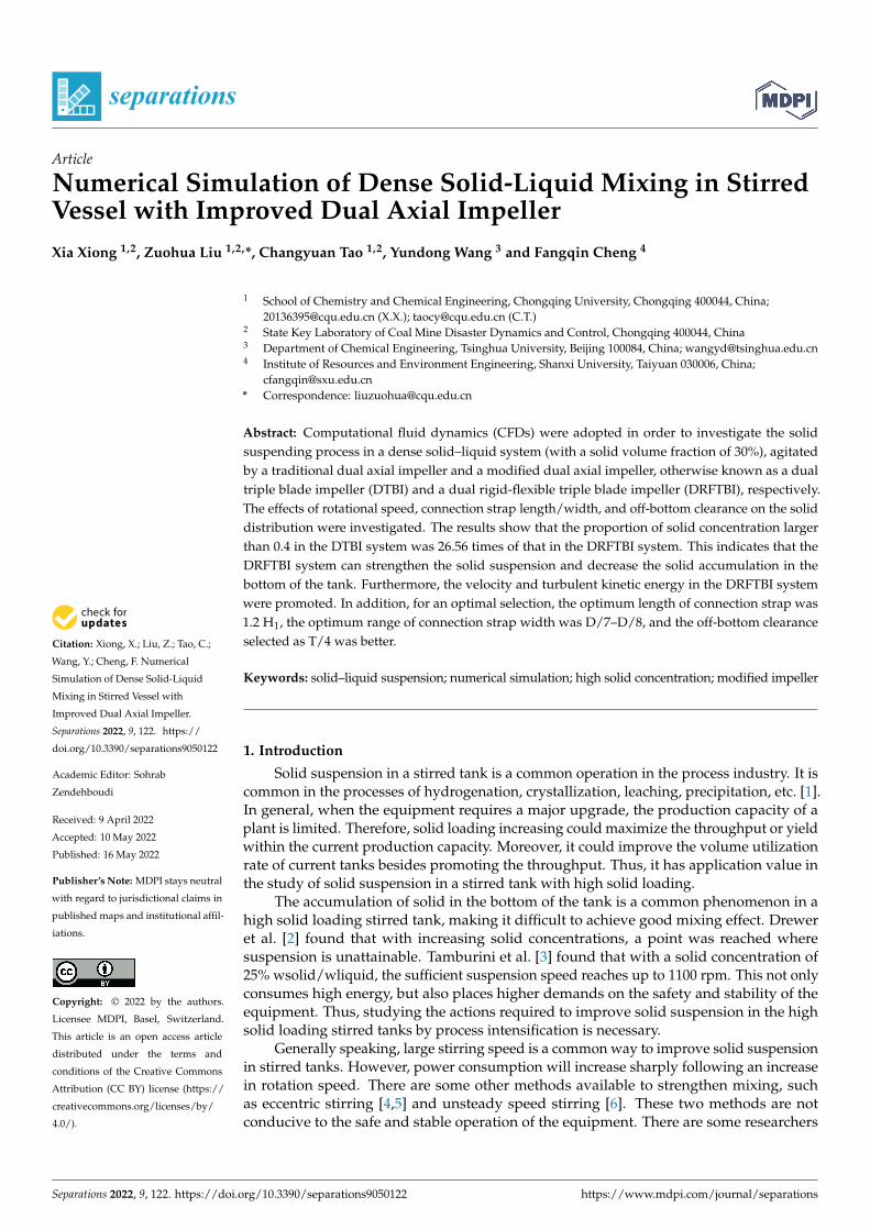
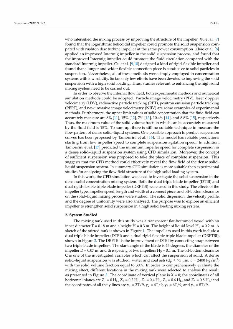
The mixing tank used in this study was a transparent flat-bottomed vessel with aninner diameter T = 0.18 m and a height H = 0.3 m. The height of liquid level HL = 0.2 m. Asketch of the stirred tank is shown in Figure 1. The impellers used in this work include adual triple blade impeller (DTBI) and a dual rigid-flexible triple blade impeller (DRFTBI),shown in Figure 2. The DRFTBI is the improvement of DTBI by connecting strap betweentwo triple blade impellers. The slant angle of the blade is 45 degrees, the diameter of theimpeller D = 0.07 m, and th e spacing of two impellers HS = 0.1 m. The off-bottom clearanceC is one of the investigated variables which can affect the suspension of solid. A densesolid–liquid suspension was studied: water and coal ash (dp ≤ 75 µm; ρ = 2400 kg/m3)with the solid volume fraction equal to 30%. In order to comprehensively evaluate themixing effect, different locations in the mixing tank were selected to analyse the result,as presented in Figure 3. The coordinate of vertical plane is X = 0; the coordinates of allhorizontal planes are Z1 = 0 HL, Z2 = 0.2 HL, Z3 = 0.4 HL, Z4 = 0.6 HL, and Z5 = 0.8 HL; andthe coordinates of all the y lines are y1 = 2T/9, y2 = 4T/9, y3 = 6T/9, and y4 = 8T/9.

Separations 2022, 9, 122 3 of 16

Separations 2022, 9, x FOR PEER REVIEW 3 of 17

the solid volume fraction equal to 30%. In order to comprehensively evaluate the mixing effect, different locations in the mixing tank were selected to analyse the result, as pre-sented in Figure 3. The coordinate of vertical plane is X = 0; the coordinates of all horizon-tal planes are Z1 = 0 HL, Z2 = 0.2 HL, Z3 = 0.4 HL, Z4 = 0.6 HL, and Z5 = 0.8 HL; and the coordinates of all the y lines are y1 = 2T/9, y2 = 4T/9, y3 = 6T/9, and y4 = 8T/9.

Figure 1. Sketch of the stirred tank.

(a) (b)

Figure 2. Structure of the impeller and the tank used in this work. (a) Dual triple blade impeller; (b) dual rigid-flexible triple blade impeller.

Figure 3. Distribution of the monitoring position in the vessel.

3. Computational Model and Details The numerical solution of this 3D mixing system was implemented in the commercial

CFD solver ANSYS Fluent 15.0. The Eulerian–Eulerian multi-fluid model was adopted for the simulation of a two-phase system. The continuity and momentum equations were solved separately and simultaneously. The coupling between the two phases was

Figure 1. Sketch of the stirred tank.

Separations 2022, 9, x FOR PEER REVIEW 3 of 17

the solid volume fraction equal to 30%. In order to comprehensively evaluate the mixing effect, different locations in the mixing tank were selected to analyse the result, as pre-sented in Figure 3. The coordinate of vertical plane is X = 0; the coordinates of all horizon-tal planes are Z1 = 0 HL, Z2 = 0.2 HL, Z3 = 0.4 HL, Z4 = 0.6 HL, and Z5 = 0.8 HL; and the coordinates of all the y lines are y1 = 2T/9, y2 = 4T/9, y3 = 6T/9, and y4 = 8T/9.

Figure 1. Sketch of the stirred tank.

(a) (b)

Figure 2. Structure of the impeller and the tank used in this work. (a) Dual triple blade impeller; (b) dual rigid-flexible triple blade impeller.

Figure 3. Distribution of the monitoring position in the vessel.

3. Computational Model and Details The numerical solution of this 3D mixing system was implemented in the commercial

CFD solver ANSYS Fluent 15.0. The Eulerian–Eulerian multi-fluid model was adopted for the simulation of a two-phase system. The continuity and momentum equations were solved separately and simultaneously. The coupling between the two phases was

Figure 2. Structure of the impeller and the tank used in this work. (a) Dual triple blade impeller;(b) dual rigid-flexible triple blade impeller.

Separations 2022, 9, x FOR PEER REVIEW 3 of 17

the solid volume fraction equal to 30%. In order to comprehensively evaluate the mixing effect, different locations in the mixing tank were selected to analyse the result, as pre-sented in Figure 3. The coordinate of vertical plane is X = 0; the coordinates of all horizon-tal planes are Z1 = 0 HL, Z2 = 0.2 HL, Z3 = 0.4 HL, Z4 = 0.6 HL, and Z5 = 0.8 HL; and the coordinates of all the y lines are y1 = 2T/9, y2 = 4T/9, y3 = 6T/9, and y4 = 8T/9.

Figure 1. Sketch of the stirred tank.

(a) (b)

Figure 2. Structure of the impeller and the tank used in this work. (a) Dual triple blade impeller; (b) dual rigid-flexible triple blade impeller.

Figure 3. Distribution of the monitoring position in the vessel.

3. Computational Model and Details The numerical solution of this 3D mixing system was implemented in the commercial

CFD solver ANSYS Fluent 15.0. The Eulerian–Eulerian multi-fluid model was adopted for the simulation of a two-phase system. The continuity and momentum equations were solved separately and simultaneously. The coupling between the two phases was

Figure 3. Distribution of the monitoring position in the vessel.

3. Computational Model and Details

The numerical solution of this 3D mixing system was implemented in the commercialCFD solver ANSYS Fluent 15.0. The Eulerian–Eulerian multi-fluid model was adoptedfor the simulation of a two-phase system. The continuity and momentum equations weresolved separately and simultaneously. The coupling between the two phases was obtainedvia inter-phase exchange terms. All the details of the model equations have been listedas following:

Separations 2022, 9, 122 4 of 16

3.1. Equations of Motion

The continuity equations [16]:

∂

∂t(αlρl) +

→∇(

αlρl→Ul

)= 0 (1)

∂

∂t(αsρs) +

→∇(

αsρs→Us

)= 0 (2)

where the subscripts l and s refer to the continuous and dispersed phases, respectively; α isthe volumetric fraction; ρ is the density; and U is the mean velocity.

Clearly,αl + αs = 1 (3)

The momentum balance equations:

∂∂(t)

(αlρl

→Ul

)+→∇·{

αl

[ρl→Ul→Ul − (µl + µtl)

(→∇→Ul +

(→∇→Ul

)T)]}

= αl

(ρl→g −

→∇P)+→F l,s

(4)

∂∂(t)

(αsρs

→Us

)+→∇·{

αs

[ρs→Us→Us − (µs + µts)

(→∇→Us +

(→∇→Us

)T)]}

= αs

(ρs→g −

→∇P)+→F s,l

(5)

where g is the gravitational acceleration, µ is the viscosity, µt is the turbulent viscosity, P isthe pressure (the continuous and dispersed phases are assumed to share the same pressurefield), and F is the interphase momentum transfer term.

3.2. Turbulence Model

The standard k-ε turbulence model was used to simulate the dense solid–liquidsuspensions system in light of the research of Tamburini et al. [16,17]. In addition, theresults were verified to be reliable. Thus, the standard k-ε turbulence model was applied inthis work. Then, the continuous and dispersed phases were assumed to share the sameturbulent kinetic energy k and the same turbulent energy dissipation rate ε. The equationsare given as follows [16,17]:

∂∂t (αlρlk) +

→∇[

αlρl→Ulk− αl

(µl +

µtlσk

)→∇k]

= αl

(µtl→∇→Ul

(→∇→Ul +

(→∇→Ul

)T)− ρlε

) (6)

∂∂t (αlρlε) +

→∇[

αlρl→Ulε− αl

(µl +

µtlσε

)→∇ε

]= αl

(C1

εk µtl

→∇→Ul

(→∇→Ul +

(→∇→Ul

)T)− C2ρl

ε2

k

) (7)

where

µtl = ρlCµk2

ε(8)

Separations 2022, 9, 122 5 of 16

3.3. Interphase Drag Force and Drag Coefficient

Interactions between the two phases were simulated by inter-phase drag force termswithin the momentum equations [16]:

→F D,s = −

→F D,l =

[34

CDdp

αlρs

∣∣∣∣→Ul −→Us

∣∣∣∣](→Ul −→Us

)(9)

where CD is the inter-phase drag coefficient and was estimated using the Gidaspow dragmodel for densely distributed solid particles [14,18]:

CD =

{24

αl Res

[1 + 0.15(αl Res)

0.687], Res < 1000

0.44, Res > 1000(10)

3.4. Numerical Details

In this study, the multiple reference frame (MRF) approach was employed to simulateimpeller rotation [19–21]. The stirred tank was divided into two parts: the inner part wasthe rotating zone while the outer part was the non-rotating domain. The optimum grid sizewas obtained when the change in velocity and solid concentration profiles was less than5%. The number of cells used for DTBI and DRFTBI was 754,916 and 895,634, respectively.

In this work, the SIMPLEC algorithm was used for pressure velocity coupling alongwith the standard pressure interpolation scheme. The hybrid-upwind discretization schemewas employed for the convective terms. In the initial simulation condition, a solid uniformaverage concentration of 30% was taken in the computational domain. The time step usedin the simulation was 0.01 s, and the relative residual was set as 10−5, which is consideredas the index of convergence.

4. Results and Discussions4.1. Verification of Modelling

Simulated results of the specific power consumption Pv were compared with ex-perimental data in Figure 4a to validate the CFD model. The specific power consump-tion is defined as the impeller power draw divided by the total volume of solid andliquid. The power consumption in the agitated system could be calculated according to theformula [22–26]:

Psum= 2πNMa (11)

Thus, the specific power consumption is:

Pv =Psum

V=

2πNMa

V(12)

where Psum is the impeller power draw (W); V is the total volume of solid and liquid (m3);N is the impeller rotational speed in revolutions per second (rps); and Ma is the absolutetorque that could be obtained by using the torque transducer, determined according to thefollowing equation [27]:

Ma = Mm −Mr (13)

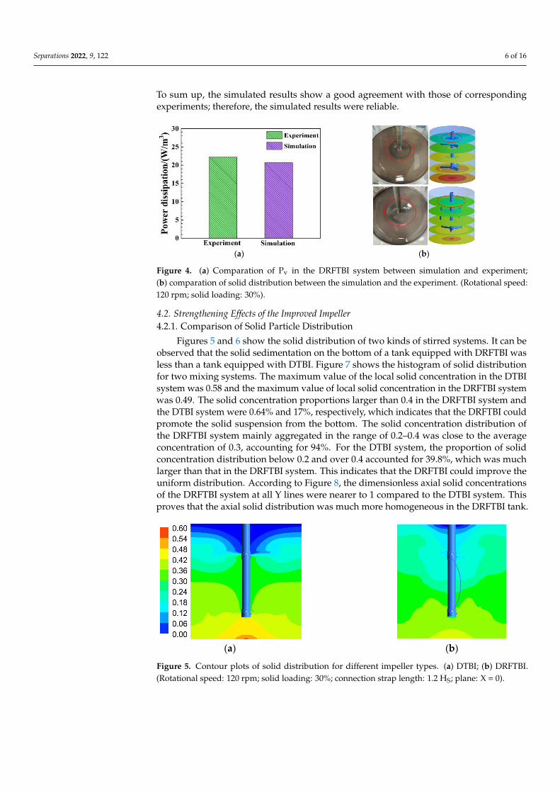
where Mm is the torque measured by the experiments, and Mr represents the residualtorque cause of the mechanical friction in the bearing, determined by operating the impellerwithout any liquid or solid in the tank. Figure 4a shows that when the rotational speed wasequal to 2 rps and the solid volume fraction was equal to 30%, the power consumptionper unit volume of the experiment and simulation was 22.21 W/m3 and 20.68 W/m3,respectively. The variation of experimental data and the simulation result was 6.9%.Figure 4b shows the solid distribution between the simulation and the experiment. Thestratification of solid distribution on the DTBI system can be seen as obvious, both in thesimulation and experimental results, while the DRFTBI system significantly improved.

Separations 2022, 9, 122 6 of 16

To sum up, the simulated results show a good agreement with those of correspondingexperiments; therefore, the simulated results were reliable.

Separations 2022, 9, x FOR PEER REVIEW 6 of 17

a m rM =M -M (13)

where Mm is the torque measured by the experiments, and Mr represents the residual torque cause of the mechanical friction in the bearing, determined by operating the impel-ler without any liquid or solid in the tank. Figure 4a shows that when the rotational speed was equal to 2 rps and the solid volume fraction was equal to 30%, the power consumption per unit volume of the experiment and simulation was 22.21 W/m3 and 20.68 W/m3, re-spectively. The variation of experimental data and the simulation result was 6.9%. Figure 4b shows the solid distribution between the simulation and the experiment. The stratifi-cation of solid distribution on the DTBI system can be seen as obvious, both in the simu-lation and experimental results, while the DRFTBI system significantly improved. To sum up, the simulated results show a good agreement with those of corresponding experi-ments; therefore, the simulated results were reliable.

(a) (b)

Figure 4. (a) Comparation of Pv in the DRFTBI system between simulation and experiment; (b) com-paration of solid distribution between the simulation and the experiment. (Rotational speed: 120 rpm; solid loading: 30%.)

4.2. Strengthening Effects of the Improved Impeller 4.2.1. Comparison of Solid Particle Distribution

Figures 5 and 6 show the solid distribution of two kinds of stirred systems. It can be observed that the solid sedimentation on the bottom of a tank equipped with DRFTBI was less than a tank equipped with DTBI. Figure 7 shows the histogram of solid distribution for two mixing systems. The maximum value of the local solid concentration in the DTBI system was 0.58 and the maximum value of local solid concentration in the DRFTBI sys-tem was 0.49. The solid concentration proportions larger than 0.4 in the DRFTBI system and the DTBI system were 0.64% and 17%, respectively, which indicates that the DRFTBI could promote the solid suspension from the bottom. The solid concentration distribution of the DRFTBI system mainly aggregated in the range of 0.2–0.4 was close to the average concentration of 0.3, accounting for 94%. For the DTBI system, the proportion of solid concentration distribution below 0.2 and over 0.4 accounted for 39.8%, which was much larger than that in the DRFTBI system. This indicates that the DRFTBI could improve the uniform distribution. According to Figure 8, the dimensionless axial solid concentrations of the DRFTBI system at all Y lines were nearer to 1 compared to the DTBI system. This proves that the axial solid distribution was much more homogeneous in the DRFTBI tank.

Figure 4. (a) Comparation of Pv in the DRFTBI system between simulation and experiment;(b) comparation of solid distribution between the simulation and the experiment. (Rotational speed:120 rpm; solid loading: 30%).

4.2. Strengthening Effects of the Improved Impeller4.2.1. Comparison of Solid Particle Distribution

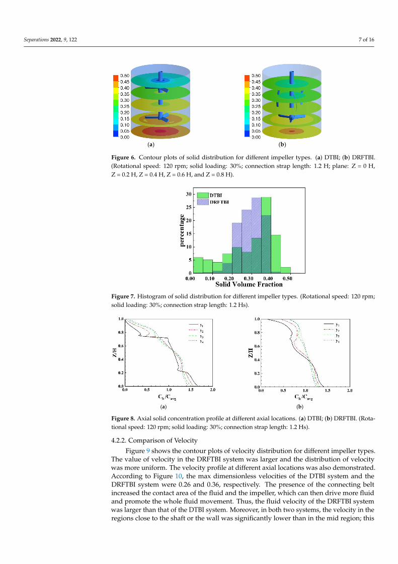
Figures 5 and 6 show the solid distribution of two kinds of stirred systems. It can beobserved that the solid sedimentation on the bottom of a tank equipped with DRFTBI wasless than a tank equipped with DTBI. Figure 7 shows the histogram of solid distributionfor two mixing systems. The maximum value of the local solid concentration in the DTBIsystem was 0.58 and the maximum value of local solid concentration in the DRFTBI systemwas 0.49. The solid concentration proportions larger than 0.4 in the DRFTBI system andthe DTBI system were 0.64% and 17%, respectively, which indicates that the DRFTBI couldpromote the solid suspension from the bottom. The solid concentration distribution ofthe DRFTBI system mainly aggregated in the range of 0.2–0.4 was close to the averageconcentration of 0.3, accounting for 94%. For the DTBI system, the proportion of solidconcentration distribution below 0.2 and over 0.4 accounted for 39.8%, which was muchlarger than that in the DRFTBI system. This indicates that the DRFTBI could improve theuniform distribution. According to Figure 8, the dimensionless axial solid concentrationsof the DRFTBI system at all Y lines were nearer to 1 compared to the DTBI system. Thisproves that the axial solid distribution was much more homogeneous in the DRFTBI tank.

Separations 2022, 9, x FOR PEER REVIEW 7 of 17

(a) (b)

Figure 5. Contour plots of solid distribution for different impeller types. (a) DTBI; (b) DRFTBI. (Rotational speed: 120 rpm; solid loading: 30%; connection strap length: 1.2 HS; plane: X = 0.)

(a) (b)

Figure 6. Contour plots of solid distribution for different impeller types. (a) DTBI; (b) DRFTBI. (Ro-tational speed: 120 rpm; solid loading: 30%; connection strap length: 1.2 H; plane: Z = 0 H, Z = 0.2 H, Z = 0.4 H, Z = 0.6 H, and Z = 0.8 H.)

Figure 7. Histogram of solid distribution for different impeller types. (Rotational speed: 120 rpm; solid loading: 30%; connection strap length: 1.2 HS.)

Figure 5. Contour plots of solid distribution for different impeller types. (a) DTBI; (b) DRFTBI.(Rotational speed: 120 rpm; solid loading: 30%; connection strap length: 1.2 HS; plane: X = 0).

Separations 2022, 9, 122 7 of 16

Separations 2022, 9, x FOR PEER REVIEW 7 of 17

(a) (b)

Figure 5. Contour plots of solid distribution for different impeller types. (a) DTBI; (b) DRFTBI. (Rotational speed: 120 rpm; solid loading: 30%; connection strap length: 1.2 HS; plane: X = 0.)

(a) (b)

Figure 6. Contour plots of solid distribution for different impeller types. (a) DTBI; (b) DRFTBI. (Ro-tational speed: 120 rpm; solid loading: 30%; connection strap length: 1.2 H; plane: Z = 0 H, Z = 0.2 H, Z = 0.4 H, Z = 0.6 H, and Z = 0.8 H.)

Figure 7. Histogram of solid distribution for different impeller types. (Rotational speed: 120 rpm; solid loading: 30%; connection strap length: 1.2 HS.)

Figure 6. Contour plots of solid distribution for different impeller types. (a) DTBI; (b) DRFTBI.(Rotational speed: 120 rpm; solid loading: 30%; connection strap length: 1.2 H; plane: Z = 0 H,Z = 0.2 H, Z = 0.4 H, Z = 0.6 H, and Z = 0.8 H).

Separations 2022, 9, x FOR PEER REVIEW 7 of 17

(a) (b)

Figure 5. Contour plots of solid distribution for different impeller types. (a) DTBI; (b) DRFTBI. (Rotational speed: 120 rpm; solid loading: 30%; connection strap length: 1.2 HS; plane: X = 0.)

(a) (b)

Figure 6. Contour plots of solid distribution for different impeller types. (a) DTBI; (b) DRFTBI. (Ro-tational speed: 120 rpm; solid loading: 30%; connection strap length: 1.2 H; plane: Z = 0 H, Z = 0.2 H, Z = 0.4 H, Z = 0.6 H, and Z = 0.8 H.)

Figure 7. Histogram of solid distribution for different impeller types. (Rotational speed: 120 rpm; solid loading: 30%; connection strap length: 1.2 HS.)

Figure 7. Histogram of solid distribution for different impeller types. (Rotational speed: 120 rpm;solid loading: 30%; connection strap length: 1.2 Hs).

Separations 2022, 9, x FOR PEER REVIEW 8 of 17

(a) (b)

Figure 8. Axial solid concentration profile at different axial locations. (a) DTBI; (b) DRFTBI. (Rota-tional speed: 120 rpm; solid loading: 30%; connection strap length: 1.2 HS.)

4.2.2. Comparison of Velocity Figure 9 shows the contour plots of velocity distribution for different impeller types.

The value of velocity in the DRFTBI system was larger and the distribution of velocity was more uniform. The velocity profile at different axial locations was also demonstrated. Ac-cording to Figure 10, the max dimensionless velocities of the DTBI system and the DRFTBI system were 0.26 and 0.36, respectively. The presence of the connecting belt increased the contact area of the fluid and the impeller, which can then drive more fluid and promote the whole fluid movement. Thus, the fluid velocity of the DRFTBI system was larger than that of the DTBI system. Moreover, in both two systems, the velocity in the regions close to the shaft or the wall was significantly lower than in the mid region; this is because the fluid flow was mainly influenced by the rotational motion of the impellers. Naturally, the fluid in the area close to the impeller could be more significantly influenced. Thus, in the near-shaft area, the flow velocity was smaller than the other areas.

(a) (b)

Figure 9. Contour plots of velocity distribution for different impeller types. (a) DTBI; (b) DRFTBI. (Rotational speed: 120 rpm, Solid loading: 30%, Connection strap length: 1.2 HS, Plane: X = 0).

Figure 8. Axial solid concentration profile at different axial locations. (a) DTBI; (b) DRFTBI. (Rota-tional speed: 120 rpm; solid loading: 30%; connection strap length: 1.2 Hs).

4.2.2. Comparison of Velocity

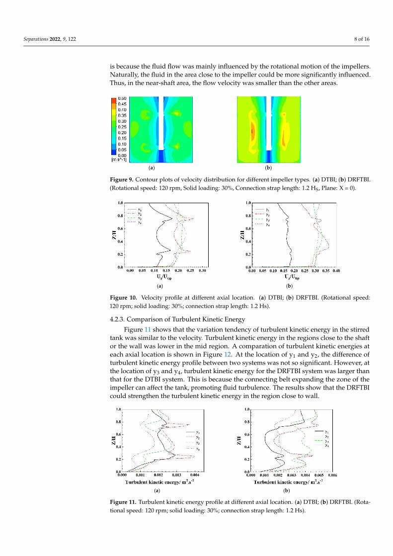
Figure 9 shows the contour plots of velocity distribution for different impeller types.The value of velocity in the DRFTBI system was larger and the distribution of velocitywas more uniform. The velocity profile at different axial locations was also demonstrated.According to Figure 10, the max dimensionless velocities of the DTBI system and theDRFTBI system were 0.26 and 0.36, respectively. The presence of the connecting beltincreased the contact area of the fluid and the impeller, which can then drive more fluidand promote the whole fluid movement. Thus, the fluid velocity of the DRFTBI systemwas larger than that of the DTBI system. Moreover, in both two systems, the velocity in theregions close to the shaft or the wall was significantly lower than in the mid region; this

Separations 2022, 9, 122 8 of 16

is because the fluid flow was mainly influenced by the rotational motion of the impellers.Naturally, the fluid in the area close to the impeller could be more significantly influenced.Thus, in the near-shaft area, the flow velocity was smaller than the other areas.

Separations 2022, 9, x FOR PEER REVIEW 8 of 17

(a) (b)

Figure 8. Axial solid concentration profile at different axial locations. (a) DTBI; (b) DRFTBI. (Rota-tional speed: 120 rpm; solid loading: 30%; connection strap length: 1.2 HS.)

4.2.2. Comparison of Velocity Figure 9 shows the contour plots of velocity distribution for different impeller types.

The value of velocity in the DRFTBI system was larger and the distribution of velocity was more uniform. The velocity profile at different axial locations was also demonstrated. Ac-cording to Figure 10, the max dimensionless velocities of the DTBI system and the DRFTBI system were 0.26 and 0.36, respectively. The presence of the connecting belt increased the contact area of the fluid and the impeller, which can then drive more fluid and promote the whole fluid movement. Thus, the fluid velocity of the DRFTBI system was larger than that of the DTBI system. Moreover, in both two systems, the velocity in the regions close to the shaft or the wall was significantly lower than in the mid region; this is because the fluid flow was mainly influenced by the rotational motion of the impellers. Naturally, the fluid in the area close to the impeller could be more significantly influenced. Thus, in the near-shaft area, the flow velocity was smaller than the other areas.

(a) (b)

Figure 9. Contour plots of velocity distribution for different impeller types. (a) DTBI; (b) DRFTBI. (Rotational speed: 120 rpm, Solid loading: 30%, Connection strap length: 1.2 HS, Plane: X = 0).

Figure 9. Contour plots of velocity distribution for different impeller types. (a) DTBI; (b) DRFTBI.(Rotational speed: 120 rpm, Solid loading: 30%, Connection strap length: 1.2 HS, Plane: X = 0).

Separations 2022, 9, x FOR PEER REVIEW 9 of 17

(a) (b)

Figure 10. Velocity profile at different axial location. (a) DTBI; (b) DRFTBI. (Rotational speed: 120 rpm; solid loading: 30%; connection strap length: 1.2 Hs.)

4.2.3. Comparison of Turbulent Kinetic Energy Figure 11 shows that the variation tendency of turbulent kinetic energy in the stirred

tank was similar to the velocity. Turbulent kinetic energy in the regions close to the shaft or the wall was lower in the mid region. A comparation of turbulent kinetic energies at each axial location is shown in Figure 12. At the location of y1 and y2, the difference of turbulent kinetic energy profile between two systems was not so significant. However, at the location of y3 and y4, turbulent kinetic energy for the DRFTBI system was larger than that for the DTBI system. This is because the connecting belt expanding the zone of the impeller can affect the tank, promoting fluid turbulence. The results show that the DRFTBI could strengthen the turbulent kinetic energy in the region close to wall.

(a) (b)

Figure 11. Turbulent kinetic energy profile at different axial location. (a) DTBI; (b) DRFTBI. (Rota-tional speed: 120 rpm; solid loading: 30%; connection strap length: 1.2 Hs.)

Figure 10. Velocity profile at different axial location. (a) DTBI; (b) DRFTBI. (Rotational speed:120 rpm; solid loading: 30%; connection strap length: 1.2 Hs).

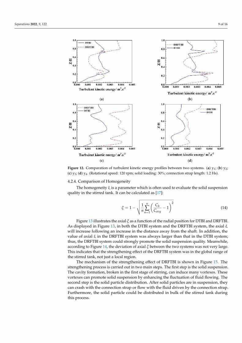
4.2.3. Comparison of Turbulent Kinetic Energy

Figure 11 shows that the variation tendency of turbulent kinetic energy in the stirredtank was similar to the velocity. Turbulent kinetic energy in the regions close to the shaftor the wall was lower in the mid region. A comparation of turbulent kinetic energies ateach axial location is shown in Figure 12. At the location of y1 and y2, the difference ofturbulent kinetic energy profile between two systems was not so significant. However, atthe location of y3 and y4, turbulent kinetic energy for the DRFTBI system was larger thanthat for the DTBI system. This is because the connecting belt expanding the zone of theimpeller can affect the tank, promoting fluid turbulence. The results show that the DRFTBIcould strengthen the turbulent kinetic energy in the region close to wall.

Separations 2022, 9, x FOR PEER REVIEW 9 of 17

(a) (b)

Figure 10. Velocity profile at different axial location. (a) DTBI; (b) DRFTBI. (Rotational speed: 120 rpm; solid loading: 30%; connection strap length: 1.2 Hs.)

4.2.3. Comparison of Turbulent Kinetic Energy Figure 11 shows that the variation tendency of turbulent kinetic energy in the stirred

tank was similar to the velocity. Turbulent kinetic energy in the regions close to the shaft or the wall was lower in the mid region. A comparation of turbulent kinetic energies at each axial location is shown in Figure 12. At the location of y1 and y2, the difference of turbulent kinetic energy profile between two systems was not so significant. However, at the location of y3 and y4, turbulent kinetic energy for the DRFTBI system was larger than that for the DTBI system. This is because the connecting belt expanding the zone of the impeller can affect the tank, promoting fluid turbulence. The results show that the DRFTBI could strengthen the turbulent kinetic energy in the region close to wall.

(a) (b)

Figure 11. Turbulent kinetic energy profile at different axial location. (a) DTBI; (b) DRFTBI. (Rota-tional speed: 120 rpm; solid loading: 30%; connection strap length: 1.2 Hs.)

Figure 11. Turbulent kinetic energy profile at different axial location. (a) DTBI; (b) DRFTBI. (Rota-tional speed: 120 rpm; solid loading: 30%; connection strap length: 1.2 Hs).

Separations 2022, 9, 122 9 of 16Separations 2022, 9, x FOR PEER REVIEW 10 of 17

(a) (b)

(c) (d)

Figure 12. Comparation of turbulent kinetic energy profiles between two systems. (a) y1; (b) y2; (c) y3; (d) y4. (Rotational speed: 120 rpm; solid loading: 30%; connection strap length: 1.2 Hs.)

4.2.4. Comparison of Homogeneity The homogeneity ξ is a parameter which is often used to evaluate the solid suspen-

sion quality in the stirred tank. It can be calculated as [17]:

2

1

1=1- 1n

h

n avg

Cn C

(14)

Figure 13 illustrates the axial ξ as a function of the radial position for DTBI and DRFTBI. As displayed in Figure 13, in both the DTBI system and the DRFTBI system, the axial ξ will increase following an increase in the distance away from the shaft. In addition, the value of axial ξ in the DRFTBI system was always larger than that in the DTBI system; thus, the DRFTBI system could strongly promote the solid suspension quality. Mean-while, according to Figure 14, the deviation of axial ξ between the two systems was not very large. This indicates that the strengthening effect of the DRFTBI system was in the global range of the stirred tank, not just a local region.

The mechanism of the strengthening effect of DRFTBI is shown in Figure 15. The strengthening process is carried out in two main steps. The first step is the solid suspen-sion. The cavity formation, broken in the first stage of stirring, can induce many vortexes. These vortexes can promote solid suspension by enhancing the fluctuation of fluid flow-ing. The second step is the solid particle distribution. After solid particles are in suspen-sion, they can crash with the connection strap or flow with the fluid driven by the

Figure 12. Comparation of turbulent kinetic energy profiles between two systems. (a) y1; (b) y2;(c) y3; (d) y4. (Rotational speed: 120 rpm; solid loading: 30%; connection strap length: 1.2 Hs).

4.2.4. Comparison of Homogeneity

The homogeneity ξ is a parameter which is often used to evaluate the solid suspensionquality in the stirred tank. It can be calculated as [17]:

ξ = 1−

√√√√ 1n

n

∑n=1

(Ch

Cavg− 1)2

(14)

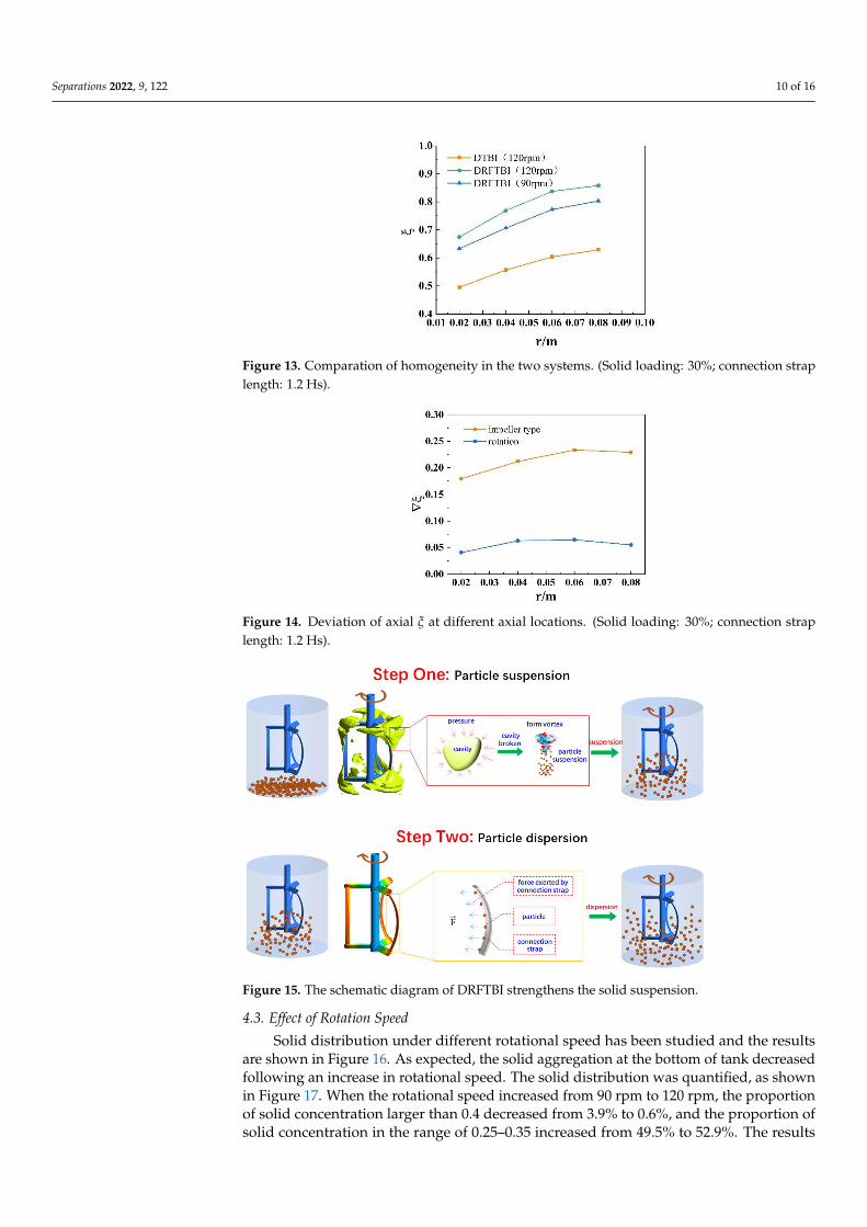
Figure 13 illustrates the axial ξ as a function of the radial position for DTBI and DRFTBI.As displayed in Figure 13, in both the DTBI system and the DRFTBI system, the axial ξwill increase following an increase in the distance away from the shaft. In addition, thevalue of axial ξ in the DRFTBI system was always larger than that in the DTBI system;thus, the DRFTBI system could strongly promote the solid suspension quality. Meanwhile,according to Figure 14, the deviation of axial ξ between the two systems was not very large.This indicates that the strengthening effect of the DRFTBI system was in the global range ofthe stirred tank, not just a local region.

The mechanism of the strengthening effect of DRFTBI is shown in Figure 15. Thestrengthening process is carried out in two main steps. The first step is the solid suspension.The cavity formation, broken in the first stage of stirring, can induce many vortexes. Thesevortexes can promote solid suspension by enhancing the fluctuation of fluid flowing. Thesecond step is the solid particle distribution. After solid particles are in suspension, theycan crash with the connection strap or flow with the fluid driven by the connection strap.Furthermore, the solid particle could be distributed in bulk of the stirred tank duringthis process.

Separations 2022, 9, 122 10 of 16

Separations 2022, 9, x FOR PEER REVIEW 11 of 17

connection strap. Furthermore, the solid particle could be distributed in bulk of the stirred tank during this process.

Figure 13. Comparation of homogeneity in the two systems. (Solid loading: 30%; connection strap length: 1.2 Hs.)

Figure 14. Deviation of axial ξ at different axial locations. (Solid loading: 30%; connection strap length: 1.2 Hs.)

Figure 13. Comparation of homogeneity in the two systems. (Solid loading: 30%; connection straplength: 1.2 Hs).

Separations 2022, 9, x FOR PEER REVIEW 11 of 17

connection strap. Furthermore, the solid particle could be distributed in bulk of the stirred tank during this process.

Figure 13. Comparation of homogeneity in the two systems. (Solid loading: 30%; connection strap length: 1.2 Hs.)

Figure 14. Deviation of axial ξ at different axial locations. (Solid loading: 30%; connection strap length: 1.2 Hs.)

Figure 14. Deviation of axial ξ at different axial locations. (Solid loading: 30%; connection straplength: 1.2 Hs).

Separations 2022, 9, x FOR PEER REVIEW 11 of 17

connection strap. Furthermore, the solid particle could be distributed in bulk of the stirred tank during this process.

Figure 13. Comparation of homogeneity in the two systems. (Solid loading: 30%; connection strap length: 1.2 Hs.)

Figure 14. Deviation of axial ξ at different axial locations. (Solid loading: 30%; connection strap length: 1.2 Hs.)

Figure 15. The schematic diagram of DRFTBI strengthens the solid suspension.

4.3. Effect of Rotation Speed

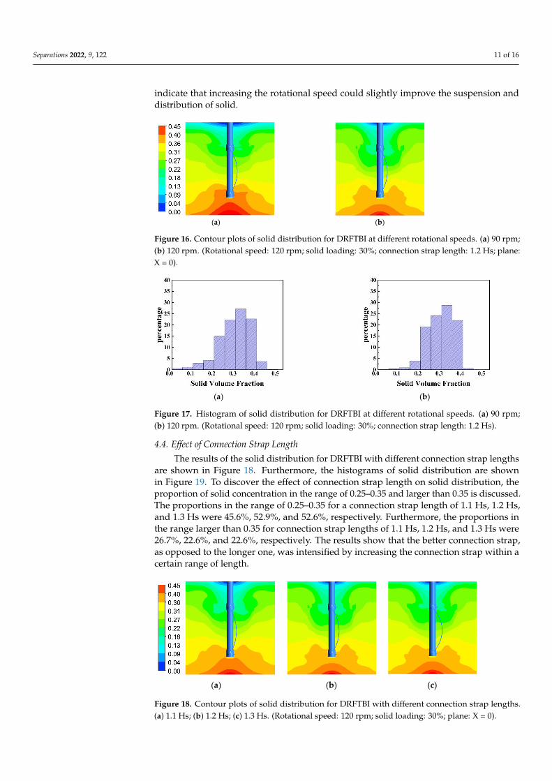
Solid distribution under different rotational speed has been studied and the resultsare shown in Figure 16. As expected, the solid aggregation at the bottom of tank decreasedfollowing an increase in rotational speed. The solid distribution was quantified, as shownin Figure 17. When the rotational speed increased from 90 rpm to 120 rpm, the proportionof solid concentration larger than 0.4 decreased from 3.9% to 0.6%, and the proportion ofsolid concentration in the range of 0.25–0.35 increased from 49.5% to 52.9%. The results

Separations 2022, 9, 122 11 of 16

indicate that increasing the rotational speed could slightly improve the suspension anddistribution of solid.

Separations 2022, 9, x FOR PEER REVIEW 12 of 17

Figure 15. The schematic diagram of DRFTBI strengthens the solid suspension.

4.3. Effect of Rotation Speed Solid distribution under different rotational speed has been studied and the results

are shown in Figure 16. As expected, the solid aggregation at the bottom of tank decreased following an increase in rotational speed. The solid distribution was quantified, as shown in Figure 17. When the rotational speed increased from 90 rpm to 120 rpm, the proportion of solid concentration larger than 0.4 decreased from 3.9% to 0.6%, and the proportion of solid concentration in the range of 0.25–0.35 increased from 49.5% to 52.9%. The results indicate that increasing the rotational speed could slightly improve the suspension and distribution of solid.

(a) (b)

Figure 16. Contour plots of solid distribution for DRFTBI at different rotational speeds. (a) 90 rpm; (b) 120 rpm. (Rotational speed: 120 rpm; solid loading: 30%; connection strap length: 1.2 Hs; plane: X = 0.)

(a) (b)

Figure 17. Histogram of solid distribution for DRFTBI at different rotational speeds. (a) 90 rpm; (b) 120 rpm. (Rotational speed: 120 rpm; solid loading: 30%; connection strap length: 1.2 Hs.)

4.4. Effect of Connection Strap Length The results of the solid distribution for DRFTBI with different connection strap

lengths are shown in Figure 18. Furthermore, the histograms of solid distribution are shown in Figure 19. To discover the effect of connection strap length on solid distribution, the proportion of solid concentration in the range of 0.25–0.35 and larger than 0.35 is dis-cussed. The proportions in the range of 0.25–0.35 for a connection strap length of 1.1 Hs, 1.2 Hs, and 1.3 Hs were 45.6%, 52.9%, and 52.6%, respectively. Furthermore, the propor-tions in the range larger than 0.35 for connection strap lengths of 1.1 Hs, 1.2 Hs, and 1.3 Hs were 26.7%, 22.6%, and 22.6%, respectively. The results show that the better connection strap, as opposed to the longer one, was intensified by increasing the connection strap within a certain range of length.

Figure 16. Contour plots of solid distribution for DRFTBI at different rotational speeds. (a) 90 rpm;(b) 120 rpm. (Rotational speed: 120 rpm; solid loading: 30%; connection strap length: 1.2 Hs; plane:X = 0).

Separations 2022, 9, x FOR PEER REVIEW 12 of 17

Figure 15. The schematic diagram of DRFTBI strengthens the solid suspension.

4.3. Effect of Rotation Speed Solid distribution under different rotational speed has been studied and the results

are shown in Figure 16. As expected, the solid aggregation at the bottom of tank decreased following an increase in rotational speed. The solid distribution was quantified, as shown in Figure 17. When the rotational speed increased from 90 rpm to 120 rpm, the proportion of solid concentration larger than 0.4 decreased from 3.9% to 0.6%, and the proportion of solid concentration in the range of 0.25–0.35 increased from 49.5% to 52.9%. The results indicate that increasing the rotational speed could slightly improve the suspension and distribution of solid.

(a) (b)

Figure 16. Contour plots of solid distribution for DRFTBI at different rotational speeds. (a) 90 rpm; (b) 120 rpm. (Rotational speed: 120 rpm; solid loading: 30%; connection strap length: 1.2 Hs; plane: X = 0.)

(a) (b)

Figure 17. Histogram of solid distribution for DRFTBI at different rotational speeds. (a) 90 rpm; (b) 120 rpm. (Rotational speed: 120 rpm; solid loading: 30%; connection strap length: 1.2 Hs.)

4.4. Effect of Connection Strap Length The results of the solid distribution for DRFTBI with different connection strap

lengths are shown in Figure 18. Furthermore, the histograms of solid distribution are shown in Figure 19. To discover the effect of connection strap length on solid distribution, the proportion of solid concentration in the range of 0.25–0.35 and larger than 0.35 is dis-cussed. The proportions in the range of 0.25–0.35 for a connection strap length of 1.1 Hs, 1.2 Hs, and 1.3 Hs were 45.6%, 52.9%, and 52.6%, respectively. Furthermore, the propor-tions in the range larger than 0.35 for connection strap lengths of 1.1 Hs, 1.2 Hs, and 1.3 Hs were 26.7%, 22.6%, and 22.6%, respectively. The results show that the better connection strap, as opposed to the longer one, was intensified by increasing the connection strap within a certain range of length.

Figure 17. Histogram of solid distribution for DRFTBI at different rotational speeds. (a) 90 rpm;(b) 120 rpm. (Rotational speed: 120 rpm; solid loading: 30%; connection strap length: 1.2 Hs).

4.4. Effect of Connection Strap Length

The results of the solid distribution for DRFTBI with different connection strap lengthsare shown in Figure 18. Furthermore, the histograms of solid distribution are shownin Figure 19. To discover the effect of connection strap length on solid distribution, theproportion of solid concentration in the range of 0.25–0.35 and larger than 0.35 is discussed.The proportions in the range of 0.25–0.35 for a connection strap length of 1.1 Hs, 1.2 Hs,and 1.3 Hs were 45.6%, 52.9%, and 52.6%, respectively. Furthermore, the proportions inthe range larger than 0.35 for connection strap lengths of 1.1 Hs, 1.2 Hs, and 1.3 Hs were26.7%, 22.6%, and 22.6%, respectively. The results show that the better connection strap,as opposed to the longer one, was intensified by increasing the connection strap within acertain range of length.

Separations 2022, 9, x FOR PEER REVIEW 12 of 18

(a) (b)

Figure 17. Histogram of solid distribution for DRFTBI at different rotational speeds. (a) 90 rpm; (b) 120 rpm. (Rotational speed: 120 rpm; solid loading: 30%; connection strap length: 1.2 Hs.)

4.4. Effect of Connection Strap Length The results of the solid distribution for DRFTBI with different connection strap

lengths are shown in Figure 18. Furthermore, the histograms of solid distribution are shown in Figure 19. To discover the effect of connection strap length on solid distribution, the proportion of solid concentration in the range of 0.25–0.35 and larger than 0.35 is dis-cussed. The proportions in the range of 0.25–0.35 for a connection strap length of 1.1 Hs, 1.2 Hs, and 1.3 Hs were 45.6%, 52.9%, and 52.6%, respectively. Furthermore, the propor-tions in the range larger than 0.35 for connection strap lengths of 1.1 Hs, 1.2 Hs, and 1.3 Hs were 26.7%, 22.6%, and 22.6%, respectively. The results show that the better connection strap, as opposed to the longer one, was intensified by increasing the connection strap within a certain range of length.

(a) (b) (c)

Figure 18. Contour plots of solid distribution for DRFTBI with different connection strap lengths. (a) 1.1 Hs; (b) 1.2 Hs; (c) 1.3 Hs. (Rotational speed: 120 rpm; solid loading: 30%; plane: X = 0).

Figure 18. Contour plots of solid distribution for DRFTBI with different connection strap lengths.(a) 1.1 Hs; (b) 1.2 Hs; (c) 1.3 Hs. (Rotational speed: 120 rpm; solid loading: 30%; plane: X = 0).

Separations 2022, 9, 122 12 of 16

Separations 2022, 9, x FOR PEER REVIEW 13 of 18

(a) (b) (c)

Figure 19. Histogram of solid distribution for DRFTBI with different connection strap length. (a) 1.1 Hs; (b) 1.2 Hs; (c) 1.3 Hs. (Rotational speed: 120 rpm; solid loading: 30%.)

4.5. Effect of Connection Strap Width The results of solid distribution for DRFTBI with different connection strap widths

are shown in Figure 20. Furthermore, the histograms of solid distribution are shown in Figure 21. According to Figure 20, the proportions in the range larger than 0.35 for con-nection strap widths of D/5, D/6, D/7, D/8, and D/9 were 16.5%, 25.3%, 22.6%, 24.1%, and 25.5%, respectively. Except for D/5 and D/9, the accumulation of solid in the bottom of the tank had no significant difference between the other strap width investigated in this study, as the maximum difference among them is lower than 3%. The wider the connec-tion strap, the greater the resistance. For D/5, the strap was wider than the others; thus, the power consumption must be higher than others. Thus, from the perspective of power consumption, D/5 was not the best choice of strap width. However, for a narrow connec-tion strap, although the resistance was lower, the solid accumulation rate was relatively high. So, D/9 was also not the best choice of strap width. To maintain the balance of power consumption and the mixing effect, a better option for a connection strap width should be the range of D/8–D/7.

(a) (b) (c)

(d) (e)

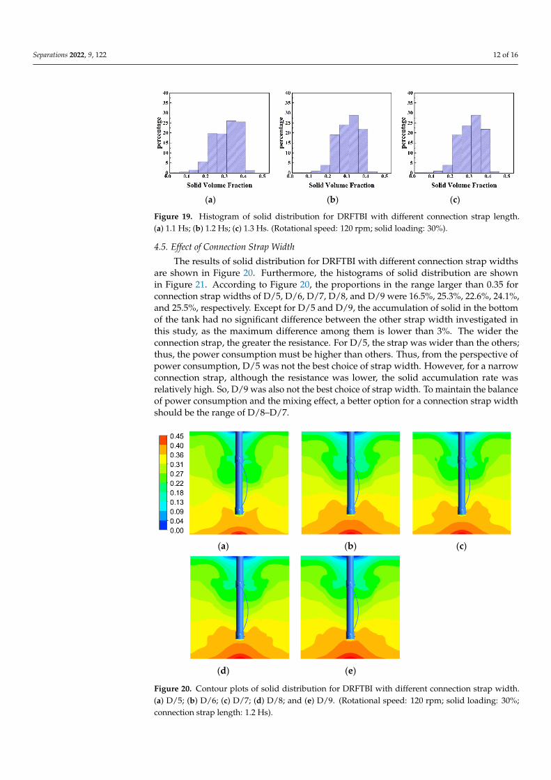
Figure 19. Histogram of solid distribution for DRFTBI with different connection strap length.(a) 1.1 Hs; (b) 1.2 Hs; (c) 1.3 Hs. (Rotational speed: 120 rpm; solid loading: 30%).

4.5. Effect of Connection Strap Width

The results of solid distribution for DRFTBI with different connection strap widthsare shown in Figure 20. Furthermore, the histograms of solid distribution are shownin Figure 21. According to Figure 20, the proportions in the range larger than 0.35 forconnection strap widths of D/5, D/6, D/7, D/8, and D/9 were 16.5%, 25.3%, 22.6%, 24.1%,and 25.5%, respectively. Except for D/5 and D/9, the accumulation of solid in the bottomof the tank had no significant difference between the other strap width investigated inthis study, as the maximum difference among them is lower than 3%. The wider theconnection strap, the greater the resistance. For D/5, the strap was wider than the others;thus, the power consumption must be higher than others. Thus, from the perspective ofpower consumption, D/5 was not the best choice of strap width. However, for a narrowconnection strap, although the resistance was lower, the solid accumulation rate wasrelatively high. So, D/9 was also not the best choice of strap width. To maintain the balanceof power consumption and the mixing effect, a better option for a connection strap widthshould be the range of D/8–D/7.

Separations 2022, 9, x FOR PEER REVIEW 13 of 17

Figure 19. Histogram of solid distribution for DRFTBI with different connection strap length. (a) 1.1 Hs; (b) 1.2 Hs; (c) 1.3 Hs. (Rotational speed: 120 rpm; solid loading: 30%.)

4.5. Effect of Connection Strap Width The results of solid distribution for DRFTBI with different connection strap widths

are shown in Figure 20. Furthermore, the histograms of solid distribution are shown in Figure 21. According to Figure 20, the proportions in the range larger than 0.35 for con-nection strap widths of D/5, D/6, D/7, D/8, and D/9 were 16.5%, 25.3%, 22.6%, 24.1%, and 25.5%, respectively. Except for D/5 and D/9, the accumulation of solid in the bottom of the tank had no significant difference between the other strap width investigated in this study, as the maximum difference among them is lower than 3%. The wider the connec-tion strap, the greater the resistance. For D/5, the strap was wider than the others; thus, the power consumption must be higher than others. Thus, from the perspective of power consumption, D/5 was not the best choice of strap width. However, for a narrow connec-tion strap, although the resistance was lower, the solid accumulation rate was relatively high. So, D/9 was also not the best choice of strap width. To maintain the balance of power consumption and the mixing effect, a better option for a connection strap width should be the range of D/8–D/7.

(a) (b) (c)

(d) (e)

Figure 20. Contour plots of solid distribution for DRFTBI with different connection strap width. (a) D/5; (b) D/6; (c) D/7; (d) D/8; and (e) D/9. (Rotational speed: 120 rpm; solid loading: 30%; connection strap length: 1.2 Hs.)

Commented [M99]: We moved the subfigure explanations into figure caption. Please confirm.

Commented [a100R99]: ok

Commented [JE101]: Please check that the original meaning has been retained.

Commented [a102R101]: ok

Commented [JE103]: Please check that the original meaning has been retained.

Commented [M104]: We moved the subfigure explanations into figure caption. Please confirm.

Commented [a105R104]: ok

Figure 20. Contour plots of solid distribution for DRFTBI with different connection strap width.(a) D/5; (b) D/6; (c) D/7; (d) D/8; and (e) D/9. (Rotational speed: 120 rpm; solid loading: 30%;connection strap length: 1.2 Hs).

Separations 2022, 9, 122 13 of 16Separations 2022, 9, x FOR PEER REVIEW 14 of 17

(a) (b) (c)

(d) (e)

Figure 21. Histogram of solid distribution for DRFTBI with different connection strap widths. (a) D/5; (b) D/6; (c) D/7; (d) D/8; and (e) D/9. (Rotational speed: 120 rpm; solid loading: 30%; connection strap length: 1.2 Hs.)

4.6. Effect of Off-Bottom Clearance The results of solid distribution for DRFTBI with different off-bottom clearances are

shown in Figure 22. Furthermore, the histograms of solid distribution are shown in Figure 23. With the increase in off-bottom clearance, the accumulation of solid in the bottom of tank decreased, and the distribution of solid in the upper part of the tank improved. When the off-bottom clearance increased from T/5 to T/3, the proportions of solid concentration larger than 0.4 were 23.1%, 0.65%, and 0.96%, respectively, while the proportions of solid concentration lower than 0.2 were 22.9%, 16.38%, and 14.03%, respectively. For the low solid loading system, when the impeller was close to the bottom, the mixing effect and driving force for solid suspension in the lower part of the tank was relatively better than in the upper part. Unlike the low solid loading system, a mass of solid weight on the blades of the impeller in the high loading system weakened the solid suspension effect and resulted in an accumulation of solid in the bottom of the tank.

(a) (b) (c)

Figure 22. Contour plots of solid distribution for DRFTBI with different off-bottom clearance. (a) T/3; (b) T/4; and (c) T/5. (Rotational speed: 120 rpm; solid loading: 30%; connection strap length: 1.2 Hs).

Figure 21. Histogram of solid distribution for DRFTBI with different connection strap widths. (a) D/5;(b) D/6; (c) D/7; (d) D/8; and (e) D/9. (Rotational speed: 120 rpm; solid loading: 30%; connectionstrap length: 1.2 Hs).

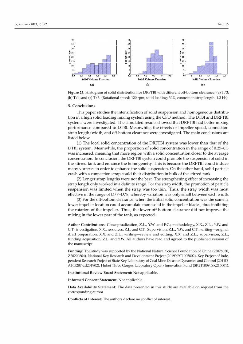
4.6. Effect of Off-Bottom Clearance

The results of solid distribution for DRFTBI with different off-bottom clearancesare shown in Figure 22. Furthermore, the histograms of solid distribution are shown inFigure 23. With the increase in off-bottom clearance, the accumulation of solid in thebottom of tank decreased, and the distribution of solid in the upper part of the tankimproved. When the off-bottom clearance increased from T/5 to T/3, the proportionsof solid concentration larger than 0.4 were 23.1%, 0.65%, and 0.96%, respectively, whilethe proportions of solid concentration lower than 0.2 were 22.9%, 16.38%, and 14.03%,respectively. For the low solid loading system, when the impeller was close to the bottom,the mixing effect and driving force for solid suspension in the lower part of the tank wasrelatively better than in the upper part. Unlike the low solid loading system, a mass ofsolid weight on the blades of the impeller in the high loading system weakened the solidsuspension effect and resulted in an accumulation of solid in the bottom of the tank.

Separations 2022, 9, x FOR PEER REVIEW 14 of 17

(a) (b) (c)

(d) (e)

Figure 21. Histogram of solid distribution for DRFTBI with different connection strap widths. (a) D/5; (b) D/6; (c) D/7; (d) D/8; and (e) D/9. (Rotational speed: 120 rpm; solid loading: 30%; connection strap length: 1.2 Hs.)

4.6. Effect of Off-Bottom Clearance The results of solid distribution for DRFTBI with different off-bottom clearances are

shown in Figure 22. Furthermore, the histograms of solid distribution are shown in Figure 23. With the increase in off-bottom clearance, the accumulation of solid in the bottom of tank decreased, and the distribution of solid in the upper part of the tank improved. When the off-bottom clearance increased from T/5 to T/3, the proportions of solid concentration larger than 0.4 were 23.1%, 0.65%, and 0.96%, respectively, while the proportions of solid concentration lower than 0.2 were 22.9%, 16.38%, and 14.03%, respectively. For the low solid loading system, when the impeller was close to the bottom, the mixing effect and driving force for solid suspension in the lower part of the tank was relatively better than in the upper part. Unlike the low solid loading system, a mass of solid weight on the blades of the impeller in the high loading system weakened the solid suspension effect and resulted in an accumulation of solid in the bottom of the tank.

(a) (b) (c)

Figure 22. Contour plots of solid distribution for DRFTBI with different off-bottom clearance. (a) T/3; (b) T/4; and (c) T/5. (Rotational speed: 120 rpm; solid loading: 30%; connection strap length: 1.2 Hs).

Commented [M106]: We moved the subfigure explanations into figure caption. Please confirm.

Commented [a107R106]: ok

Commented [JE108]: Please check that the original meaning has been retained.

Commented [a109R108]: ok

Commented [JE110]: Please check that the original meaning has been retained.

Commented [a111R110]: ok

Commented [JE112]: Please check that the original meaning has been retained.

Commented [a113R112]: ok

Commented [M114]: We moved the subfigure explanations into figure caption. Please confirm.

Commented [a115R114]: ok

Figure 22. Contour plots of solid distribution for DRFTBI with different off-bottom clearance. (a) T/3;(b) T/4; and (c) T/5. (Rotational speed: 120 rpm; solid loading: 30%; connection strap length: 1.2 Hs).

Separations 2022, 9, 122 14 of 16

1

Figure 23. Histogram of solid distribution for DRFTBI with different off-bottom clearance. (a) T/3;(b) T/4; and (c) T/5. (Rotational speed: 120 rpm; solid loading: 30%; connection strap length: 1.2 Hs).

5. Conclusions

This paper studies the intensification of solid suspension and homogeneous distribu-tion in a high solid loading mixing system using the CFD method. The DTBI and DRFTBIsystems were investigated. The simulated results showed that DRFTBI had better mixingperformance compared to DTBI. Meanwhile, the effects of impeller speed, connectionstrap length/width, and off-bottom clearance were investigated. The main conclusions arelisted below.

(1) The local solid concentration of the DRFTBI system was lower than that of theDTBI system. Meanwhile, the proportion of solid concentration in the range of 0.25–0.3was increased, meaning that more region with a solid concentration closer to the averageconcentration. In conclusion, the DRFTBI system could promote the suspension of solid inthe stirred tank and enhance the homogeneity. This is because the DRFTBI could inducemany vortexes in order to enhance the solid suspension. On the other hand, solid particlecrash with a connection strap could their distribution in bulk of the stirred tank.

(2) Longer strap lengths were not the best. The strengthening effect of increasing thestrap length only worked in a definite range. For the strap width, the promotion of particlesuspension was limited when the strap was too thin. Thus, the strap width was mosteffective in the range of D/7–D/8, whereby variation was only small between each width.

(3) For the off-bottom clearance, when the initial solid concentration was the same, alower impeller location could accumulate more solid in the impeller blades, thus inhibitingthe rotation of the impeller. Thus, the lower off-bottom clearance did not improve themixing in the lower part of the tank, as expected.

Author Contributions: Conceptualization, Z.L., Y.W. and F.C.; methodology, X.X., Z.L., Y.W. andC.T.; investigation, X.X.; resources, Z.L. and C.T.; Supervision, Z.L., Y.W. and C.T.; writing—originaldraft preparation, X.X. and Z.L.; writing—review and editing, X.X. and Z.L.; supervision, Z.L.;funding acquisition, Z.L. and Y.W. All authors have read and agreed to the published version ofthe manuscript.

Funding: The study was supported by the National Natural Science Foundation of China (22078030,Z20200804), National Key Research and Development Project (2019YFC1905802), Key Project of Inde-pendent Research Project of State Key Laboratory of Coal Mine Disaster Dynamics and Control (2011D-A105287-zd201902), Hubei Three Gorges Laboratory Open/Innovation Fund (SK211009, SK215001).

Institutional Review Board Statement: Not applicable.

Informed Consent Statement: Not applicable.

Data Availability Statement: The data presented in this study are available on request from thecorresponding author.

Conflicts of Interest: The authors declare no conflict of interest.

Separations 2022, 9, 122 15 of 16

Nomenclature

C off-bottom clearance (m)Ch local solid volume fraction at height of hCavg average solid volume fractionCε1, Cε2, Cε3, Cµ

Separations 2022, 9, x FOR PEER REVIEW 16 of 17

Acknowledgments: The study was supported by the National Natural Science Foundation of China (22078030 and Z20200804), the National Key Research and Development Project (2019YFC1905802), the Key Project of Independent Research Project of State Key Laboratory of Coal Mine Disaster Dy-namics and Control (2011DA105287-zd201902), and the Hubei Three Gorges Laboratory Open/In-novation Fund (SK211009 and SK215001).

Conflicts of Interest: The authors declare no conflict of interest

Nomenclature C off-bottom clearance (m) Ch local solid volume fraction at height of h Cavg average solid volume fraction Cε1, Cε2, Cε3, Cμ ὺparameters in the standard k-ε model CD drag coefficient D impeller diameter (m) dp particle diameter (m) F interphase momentum transfer term (N) Fdrag drag force (N) g gravitational acceleration (m/s2) H stirred vessel height (m) HL liquid height (m) HS interlayer spacing of two impeller (m) k turbulent kinetic energy (m2/s2) Ma absolute torque (N.m) Mm torque measured experimentally (N.m) Mr residual torque (N.m) N impeller speed (rpm) n number of sampling points P pressure (Pa) Psum power consumption (W) Pv specific power consumption (W/m3) r radial coordinate (m) T inner diameter of stirred vessel (m) t time (s) Ui velocity (m/s) V total volume of solid and liquid (m3) Greek Letters ρl liquid density (kg/m3) ρs solid density (kg/m3) ρ density (kg/m3) α volume fraction αl liquid phase volume fraction αs solid phase volume fraction ε turbulent energy dissipation rate μ viscosity (Pa⸱s) μl liquid phase viscosity (Pa⸱s) μt turbulent viscosity (Pa⸱s) μtl liquid phase turbulent viscosity (Pa⸱s) σk, σε k and ε turbulent Prandtl number ξ homogeneity

References 1. Carletti, C.; Montante, G.; Westerlund, T.; Paglianti, A. Analysis of solid concentration distribution in dense solid–liquid stirred

tanks by electrical resistance tomography. Chem. Eng. Sci. 2014, 119, 53–64. 2. Drewer, G.R.; Ahmed, N.; Jameson, G.J. Suspension of High Concentration Solids in Mechanically Stirred Vessels. In Institution

of Chemical Engineers Symposium Series; Hemisphere Publishing Corporation: London, UK, 1994; Volume 136, p. 41.

parameters in the standard k-εmodelCD drag coefficientD impeller diameter (m)dp particle diameter (m)F interphase momentum transfer term (N)Fdrag drag force (N)g gravitational acceleration (m/s2)H stirred vessel height (m)HL liquid height (m)HS interlayer spacing of two impeller (m)k turbulent kinetic energy (m2/s2)Ma absolute torque (N.m)Mm torque measured experimentally (N.m)Mr residual torque (N.m)N impeller speed (rpm)n number of sampling pointsP pressure (Pa)Psum power consumption (W)Pv specific power consumption (W/m3)r radial coordinate (m)T inner diameter of stirred vessel (m)t time (s)Ui velocity (m/s)V total volume of solid and liquid (m3)Greek Lettersρl liquid density (kg/m3)ρs solid density (kg/m3)ρ density (kg/m3)α volume fractionαl liquid phase volume fractionαs solid phase volume fractionε turbulent energy dissipation rateµ viscosity (Pa · s)µl liquid phase viscosity (Pa · s)µt turbulent viscosity (Pa · s)µtl liquid phase turbulent viscosity (Pa · s)σk , σε k and ε turbulent Prandtl numberξ homogeneity

References1. Carletti, C.; Montante, G.; Westerlund, T.; Paglianti, A. Analysis of solid concentration distribution in dense solid–liquid stirred

tanks by electrical resistance tomography. Chem. Eng. Sci. 2014, 119, 53–64. [CrossRef]2. Drewer, G.R.; Ahmed, N.; Jameson, G.J. Suspension of High Concentration Solids in Mechanically Stirred Vessels. In Institution of

Chemical Engineers Symposium Series; Hemisphere Publishing Corporation: London, UK, 1994; Volume 136, p. 41.3. Tamburini, A.; Cipollina, A.; Micale, G.; Brucato, A.; Ciofalo, M. CFD simulations of dense solid–liquid suspensions in baffled

stirred tanks: Prediction of solid particle distribution. Chem. Eng. J. 2013, 223, 875–890. [CrossRef]4. Woziwodzki, S.; Jedrzejczak, A. Effect of eccentricity on laminar mixing in vessel stirred by double turbine impellers. Chem. Eng.

Res. Des. 2011, 89, 2268–2278. [CrossRef]5. Zhang, M.; Hu, Y.; Wang, W.; Shao, T.; Cheng, Y. Intensification of viscous fluid mixing in eccentric stirred tank systems. Chem.

Eng. Processing Process Intensif. 2013, 66, 36–43. [CrossRef]6. Nomura, T.; Uchida, T.; Takahashi, K. Enhancement of Mixing by Unsteady Agitation of an Impeller in an Agitated Vessel. J.

Chem. Eng. Jpn. 1997, 30, 875–879. [CrossRef]

Separations 2022, 9, 122 16 of 16

7. Lin, R.; Stuckman, M.; Howard, B.H.; Bank, T.L.; Roth, E.A.; Macala, M.K.; Lopano, C.; Soong, Y.; Granite, E.J. Application ofsequential extraction and hydrothermal treatment for characterization and enrichment of rare earth elements from coal fly ash.Fuel 2018, 232, 124–133. [CrossRef]

8. Zhao, H.L.; Zhang, Z.M.; Zhang, T.A.; Yan, L.I.U.; Gu, S.Q.; Zhang, C. Experimental and CFD studies of solid-liquid slurry tankstirred with an improved Intermig impeller. Oral Oncol. 2014, 50, 2650–2659. [CrossRef]

9. Gu, D.; Liu, Z.; Xie, Z.; Li, J.; Tao, C.; Wang, Y. Numerical simulation of solid-liquid suspension in a stirred tank with a dualpunched rigid-flexible impeller. Adv. Powder Technol. 2017, 28, 2723–2734. [CrossRef]

10. Gu, D.; Liu, Z.; Qiu, F.; Li, J.; Tao, C.; Wang, Y. Design of impeller blades for efficient homogeneity of solid-liquid suspension in astirred tank reactor. Adv. Powder Technol. 2017, 28, 2514–2523. [CrossRef]

11. Li, G.; Gao, Z.; Li, Z.; Wang, J.; Derksen, J.J. Particle-resolved PIV experiments of solid-liquid mixing in a turbulent stirred tank.AIChE J. 2018, 64, 389–402. [CrossRef]

12. Kohnen, C.; Bohnet, M. Measurement and Simulation of Fluid Flow in Agitated Solid/Liquid Suspensions. Chem. Eng. Technol.2001, 24, 639–643. [CrossRef]

13. Guha, D.; Ramachandran, P.A.; Dudukovic, M.P. Flow field of suspended solids in a stirred tank reactor by Lagrangian tracking.Chem. Eng. Sci. 2007, 62, 6143–6154. [CrossRef]

14. Liu, L.; Barigou, M. Numerical modelling of velocity field and phase distribution in dense monodisperse solid–liquid suspensionsunder different regimes of agitation: CFD and PEPT experiments. Chem. Eng. Sci. 2013, 101, 837–850. [CrossRef]

15. Wang, H.; Li, X.; Mao, Z.S.; Yang, C. New invasive image velocimetry applicable to dense multiphase flows and its application insolid–liquid suspensions. AIChE J. 2019, 65, e16668. [CrossRef]

16. Tamburini, A.; Cipollina, A.; Micale, G.; Brucato, A.; Ciofalo, M. CFD simulations of dense solid–liquid suspensions in baffledstirred tanks: Prediction of suspension curves. Chem. Eng. J. 2011, 178, 324–341. [CrossRef]

17. Tamburini, A.; Cipollina, A.; Micale, G.; Brucato, A.; Ciofalo, M. CFD simulations of dense solid–liquid suspensions in baffledstirred tanks: Prediction of the minimum impeller speed for complete suspension. Chem. Eng. J. 2012, 193, 234–255. [CrossRef]

18. Li, X.K. Multiphase Flow and Fluidization, Continuum and Kinetic Theory Descriptions; Gidaspow, D., Ed.; Academic Press: New York,NY, USA, 1993; p. 467, Price $60.00; ISBN 0-12-282770-9. J. Non-Newton. Fluid Mech. 1994, 55, 207–208.

19. Klenov, O.P.; Noskov, A.S. Solid dispersion in the slurry reactor with multiple impellers. Chem. Eng. J. 2011, 176, 75–82. [CrossRef]20. Hosseini, S.; Patel, D.; Ein-Mozaffari, F.; Mehrvar, M. Study of Solid−Liquid Mixing in Agitated Tanks through Computational

Fluid Dynamics Modeling. Ind. Eng. Chem. Res. 2010, 49, 4426–4435. [CrossRef]21. Qi, N.; Zhang, H.; Zhang, K.; Xu, G.; Yang, Y. CFD simulation of particle suspension in a stirred tank. Particuology 2013, 11,

317–326. [CrossRef]22. Hashemi, N.; Ein-Mozaffari, F.; Upreti, S.R.; Hwang, D.K. Analysis of mixing in an aerated reactor equipped with the coaxial

mixer through electrical resistance tomography and response surface method. Chem. Eng. Res. Des. 2016, 109, 734–752. [CrossRef]23. Hashemi, N.; Ein-Mozaffari, F.; Upreti, S.R.; Hwang, D.K. Analysis of power consumption and gas holdup distribution for an

aerated reactor equipped with a coaxial mixer: Novel correlations for the gas flow number and gassed power. Chem. Eng. Sci.2016, 151, 25–35. [CrossRef]

24. Jegatheeswaran, S.; Kazemzadeh, A.; Ein-Mozaffari, F. Enhanced aeration efficiency in non-Newtonian fluids using coaxialmixers: High-solidity ratio central impeller with an anchor. Chem. Eng. J. 2019, 378, 122081. [CrossRef]

25. Hashemi, N.; Ein-Mozaffari, F.; Upreti, S.R.; Hwang, D.K. Experimental investigation of the bubble behavior in an aerated coaxialmixing vessel through electrical resistance tomography (ERT). Chem. Eng. J. 2016, 289, 402–412. [CrossRef]

26. Jegatheeswaran, S.; Ein-Mozaffari, F. Investigation of the detrimental effect of the rotational speed on gas holdup in non-Newtonian fluids with Scaba-anchor coaxial mixer: A paradigm shift in gas-liquid mixing. Chem. Eng. J. 2020, 383, 123118.[CrossRef]

27. Wang, S.; Parthasarathy, R.; Wu, J.; Slatter, P. Optimum Solids Concentration in an Agitated Vessel. Ind. Eng. Chem. Res. 2014, 53,3959–3973. [CrossRef]