Numerical Simulation of Benchmark Problem 2 Xiaoming Wang Philip L.-F. Liu and Alejandro Orfila Philip L.-F. Liu and Alejandro Orfila Dept. of Civil Engineering,

Numerical Simulation of Numerical Simulation of Benchmark Problem 2Benchmark Problem 2

Xiaoming WangXiaoming Wang Philip L.-F. Liu and Alejandro Orfila Philip L.-F. Liu and Alejandro Orfila

Dept. of Civil Engineering, Cornell UniversityDept. of Civil Engineering, Cornell University

The 3The 3rdrd Intl. Workshop on long wave propagations Intl. Workshop on long wave propagations

Catalina Island, June 17-19, 2004Catalina Island, June 17-19, 2004

Numerical Method - SWENumerical Method - SWE

Program: COMCOTProgram: COMCOT

COMCOT is a tsunami simulation program.COMCOT is a tsunami simulation program.It adopts finite difference scheme to solve It adopts finite difference scheme to solve the depth-averaged Shallow Water the depth-averaged Shallow Water Equations.Equations.

Multiple nested grids can be employed Multiple nested grids can be employed simultaneously to save CPU time as well simultaneously to save CPU time as well as obtain enough resolution at target as obtain enough resolution at target region.region.

Governing EquationsGoverning Equations

• COMCOT solves the depth-averaged Shallow COMCOT solves the depth-averaged Shallow Water Equations. Water Equations.

Linear equations:

Governing EquationsGoverning EquationsNonlinear equations:

For both linear and nonlinear equations, P=Hux and Q=Huy.

H=+h. is the free surface displacement; h is the still water depth; and H is the total water depth.

Governing EquationsGoverning Equations

The bottom friction is expressed as

which come from Manning’s formula.n is roughness coefficient.In this simulation, n takes 0.01.

Finite difference schemeFinite difference scheme

COMCOT uses an explicit leCOMCOT uses an explicit leap-frog scheme :ap-frog scheme :

The free surface elevation is evaluated at the center of a grid cell on the (n+1/2)-th time step;

The volume flux components, P and Q, are evaluated at the center of four sides of the grid cell on the n-th time step.

The differencing schemes are shown in the right figure.

Moving boundary schemeMoving boundary scheme

Where,h - takes positive values for water regions (wet cells) and negative values for land region (dry cells).Initially =-h at dry cell at t=0.

Moving boundary applies When Hi>0 and Hi+1<=0:

1. If hi+1 + i<0, shoreline at i+1/2 and Pi+1/2=0. Total water depth is 0 at cell i+1.

2. If hi+1 + i>0, shoreline moves between i+1 and i+2. Pi+1/2 may have a none-zero value. Total water depth is H=hi+1 + i at cell i+1.

The following figure shows a 1-D example of the moving boundary scheme used in COMCOT.

Computational domainComputational domain

Left boundary : input wave boundary, Shut down at t = 30sRight boundary : solid wallTop boundary : solid wallBottom boundary: solid wallBilinear interpolation is used to get a higher resolution (for dx<0.01435m)

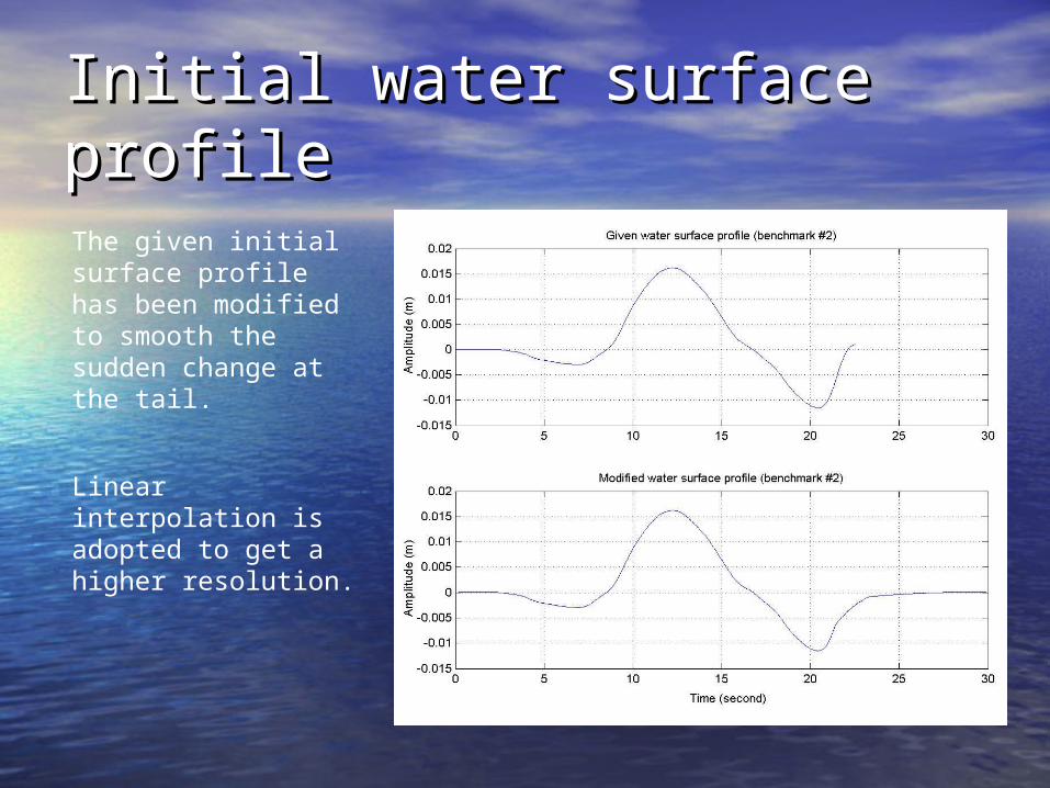
Initial water surface profileInitial water surface profile

The given initial surface profile has been modified to smooth the sudden change at the tail.

Linear interpolation is adopted to get a higher resolution.

Numerical SimulationsNumerical Simulations

• Coarse grid simulations:Coarse grid simulations: 1. Using linear Shallow Water Equations (without bottom friction)1. Using linear Shallow Water Equations (without bottom friction) 2. Using nonlinear Shallow Water Equations (w/o bottom friction)2. Using nonlinear Shallow Water Equations (w/o bottom friction) configurations for both cases:configurations for both cases: dx=0.01435m, dimension: 393*244dx=0.01435m, dimension: 393*244 dt=0.001s, Courant No. = 0.08dt=0.001s, Courant No. = 0.08 Roughness coeff. = 0.01 (Manning’s formula, if using bottom frictRoughness coeff. = 0.01 (Manning’s formula, if using bottom frict

ion) ion) • Finer grid simulationFiner grid simulation Using nonlinear Shallow Water Equations.Using nonlinear Shallow Water Equations. Configuration:Configuration: dx=0.005m, dimension: 1098*681dx=0.005m, dimension: 1098*681 dt=0.0002s, Courant No. = 0.05dt=0.0002s, Courant No. = 0.05 without bottom frictionwithout bottom friction

NumericalNumerical characteristics characteristics• Platform - IBM compatible PCPlatform - IBM compatible PC OS : Windows 2000 ProfessionalOS : Windows 2000 Professional CPU: AMD Athlon XP 2600+ (2.13 GHz)CPU: AMD Athlon XP 2600+ (2.13 GHz) RAM: 1.0 GB DDR400 Dual ChannelRAM: 1.0 GB DDR400 Dual Channel

• CPU TimeCPU Time 1. For coarse grid simulation (nonlinear):1. For coarse grid simulation (nonlinear): 0.074s per step (total steps: 150000)0.074s per step (total steps: 150000) Total CPU time: 3.08hrs (for 150s physical simulation)Total CPU time: 3.08hrs (for 150s physical simulation)

2. 1.193s per step For finer grid simulation (nonlinear eq.):2. 1.193s per step For finer grid simulation (nonlinear eq.): 1.193s per step (total steps: 200000)1.193s per step (total steps: 200000) Total CPU time: 2days+18hrs (for 40s physical simulation)Total CPU time: 2days+18hrs (for 40s physical simulation)

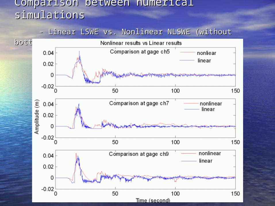
Comparison between numerical simulationsComparison between numerical simulations

- Linear LSWE vs. Nonlinear NLSWE (without bottom - Linear LSWE vs. Nonlinear NLSWE (without bottom friction)friction)

Comparison between numerical simulationsComparison between numerical simulations – bottom friction vs. no bottom friction (nonlinear eq.)– bottom friction vs. no bottom friction (nonlinear eq.)

Comparison between numerical simulationsComparison between numerical simulations - - Coarse grid vs. Finer gridCoarse grid vs. Finer grid

Comparison with gage data – Coarse grid Comparison with gage data – Coarse grid simulationsimulation

Comparison with gage data – Finer grid Comparison with gage data – Finer grid simulationsimulation

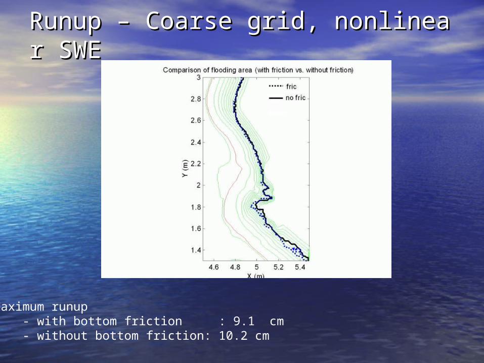
Runup – Coarse grid, nonlinear SWERunup – Coarse grid, nonlinear SWE

Maximum runup - with bottom friction : 9.1 cm - without bottom friction: 10.2 cm

Animation – RunupAnimation – Runup

Entire region movieLab movie

ConclusionsConclusions• The numerical results show that the problem can be The numerical results show that the problem can be

well simulated as a first attempt with the linear well simulated as a first attempt with the linear system without including bottom friction.system without including bottom friction.

• An agreement between grid size and time An agreement between grid size and time consumptions has to be considered since the consumptions has to be considered since the reduction of the grid does not lead to a much reduction of the grid does not lead to a much accurate results.accurate results.

• COMCOT results match the records very good for both COMCOT results match the records very good for both the arrival time and amplitude of leading waves.the arrival time and amplitude of leading waves.

• In the near shore region, the waves becomes very In the near shore region, the waves becomes very nonlinear and will break. COMCOT is no longer nonlinear and will break. COMCOT is no longer capable to deal with it. The wave amplitude may be capable to deal with it. The wave amplitude may be exaggerated.exaggerated.