Numerical prediction of the frictional losses in sliding ...

Friction 9(3): 583–597 (2021) ISSN 2223-7690 https://doi.org/10.1007/s40544-020-0417-9 CN 10-1237/TH

RESEARCH ARTICLE

Numerical prediction of the frictional losses in sliding bearings during start–stop operation

Florian KÖNIG*, Christopher SOUS, Georg JACOBS Institute for Machine Elements and Systems Engineering, Rheinisch-Westfälische Technische Hochschule Aachen University,

Schinkelstraße 10, Aachen 52062, Germany

Received: 25 January 2020 / Revised: 15 April 2020 / Accepted: 09 June 2020

© The author(s) 2020.

Abstract: With the increased use of automotive engine start–stop systems, the numerical prediction and

reduction of frictional losses in sliding bearings during starting and stopping procedures has become an

important issue. In engineering practice, numerical simulations of sliding bearings in automotive engines

are performed with statistical asperity contact models with empirical values for the necessary surface

parameters. The aim of this study is to elucidate the applicability of these approaches for the prediction of

friction in sliding bearings subjected to start–stop operation. For this purpose, the friction performance of

sliding bearings was investigated in experiments on a test rig and in transient mixed elasto-hydrodynamic

simulations in a multi-body simulation environment (mixed-EHL/MBS). In mixed-EHL/MBS, the extended

Reynold’s equation with flow factors according to Patir and Cheng has been combined on the one hand

with the statistical asperity contact model according to Greenwood and Tripp and on the other hand with

the deterministic asperity contact model according to Herbst. The detailed comparison of simulation and

experimental results clarifies that the application of statistical asperity contact models with empirical

values of the necessary inputs leads to large deviations between experiment and simulation. The actual

distribution and position of surface roughness, as used in deterministic contact modelling, is necessary

for a reliable prediction of the frictional losses in sliding bearings during start–stop operation.

Keywords: sliding bearing; friction; wearing-in; contact model, mixed elasto-hydrodynamic simulation

1 Introduction

In the last decade, automotive engine start–stop systems

have led to a significant increase of start–stop cycles

during the expected engine lifetime [1–4]. Low friction

for the desired lifetime is a key requirement for engine

bearings [5–7]. In sliding bearings, methods to improve

the frictional performance range from improved

mechanical design [8] over different lubricant for-

mulation [8, 9] and novel bearing material solutions

[1, 2, 10] to modern surface engineering [11–13].

Furthermore, the frictional losses of sliding bearings

can be reduced by wear-induced change of the contact

geometry—hereafter referred to as wearing-in—under

boundary or mixed-friction conditions [14–17].

In recent years, the frictional losses in sliding bearings

in start–stop operation has gained a significant amount

of attention. In a fundamental study, Bouyer and

Fillon [18] studied the breakaway torque of sliding

bearings made from bronze and white metal. For

bronze bearings, the breakaway torque was pro-

portional to the applied load and slightly influenced

by shaft roughness. In contrast, the frictional losses

in white metal bearings were significantly influenced

by the load and the shaft’s roughness. Thus, a nearly

stationary breakaway coefficient of friction (CoF)

* Corresponding author: Florian KÖNIG, E-mail: [email protected]

584 Friction 9(3): 583–597 (2021)

| https://mc03.manuscriptcentral.com/friction

Nomenclature

Latin letters A Nominal contact area, m² Aa Real contact area, m² Af Contact area of single asperity contact, m²

D Bearing diameter, m Ff Friction force, N FR Radial force, N H Bearing hardness, Pa Hs Nominal gap height h Average film thickness, m h Nominal film thickness / surface separation, m

oilh Minimum nodal oil film thickness, m K Elastic factor in Greenwood/Tripp model

FM Friction torque, N p Projected pressure, Pa

ap Asperity contact pressure, Pa p Oil film pressure, Pa

fP Single asperity contact force, N

Asperityp Maximum nodal asperity contact pressure, Pa

oilp Maximum nodal oil film pressure, Pa u Linear velocity, m/s r Bearing radius, m Ra Mean roughness, m Rq Root mean square (RMS) roughness, m Rz Surface roughness, m

t Time, s u Sliding velocity, m W Bearing width, m

Y Yield stress, Pa

sz Summit height, m

Greek letters Mean summit radius, m Dynamic viscosity, Pa·s Flow/shear/contact factor Bearing angle, deg s Summit height rms, m s Mean summit height, m

Fill ratio μ Boundary friction coefficient

s Density distribution of all summit heights, m

a Asperity shear stress, Pa

h

Viscous shear stress, Pa

s Asperity density, m–2

Abbreviations CoF Coefficient of friction EHL Elasto-hydrodynamic lubrication LSM Laser scanning microscopy MBS Multi-body simulation

Subscripts 1 Journal 2 Bearing x Sliding direction y Cross direction

was observed only for bronze bearings. Furthermore,

it was shown that boundary and mixed lubrication

occurred only in the first shaft revolutions of a start–up

procedure. Based upon multiple variations of material

and surface roughness, the authors concluded that

the frictional behavior throughout a starting procedure

is directly connected to the roughness of the shaft and

the bearing surfaces.

In numerical simulations, the effects of acceleration

time [19], wearing-in of the bearing contour [20–22],

and the surface roughness [14, 21, 23, 24] on the

frictional losses of sliding bearings during starting

and stopping were studied. In transient multi-body

simulation (MBS) with an mixed-elasto-hydrodynamic

coupling (mixed-EHL/MBS), it was shown that the

breakaway friction during starting was nearly inde-

pendent of the surface roughness of bearing and shaft,

which is in agreement to the experimental observations

by Bouyer and Fillon [18]. With increasing sliding

speed, the effects of surface roughness on the transient

characteristics of hydrodynamic cylindrical bearings

become more prominent. In further simulation studies

[21, 25], it was shown that the time duration of

asperity contact during startup can be reduced by

lowering surface roughness, which is in agreement

to experimental observations [26].

Reviewing the aforementioned articles revealed

that most of the experimental and simulation studies

investigated the startup procedure of sliding bearings.

In contrast, little attention has been given to the

stopping procedures that were denoted to be evenly

critical in terms of mixed-friction conditions [27].

In stopping procedures, it was shown that the

transition from hydrodynamic lubrication to mixed

lubrication shifts to lower rotational speeds after

multiple thousand start–stop cycles due to wearing-in.

Friction 9(3): 583–597 (2021) 585

∣www.Springer.com/journal/40544 | Friction

http://friction.tsinghuajournals.com

Furthermore, it was shown that the maximum friction

torque was significantly reduced with increasing

number of start–stop cycles [21, 28–30]. Mokhtar et

al. even observed that asperity interaction was only

present after the shaft rotation fully ceased. Until then,

the surfaces were separated by the lubricant [26].

Consequently, a reliable prediction of friction during

start–stop operation in mixed-EHL/MBS simulation

requires the consideration of wearing-in effects, i.e.,

asperity contact pressure reduction due to change of

bearing contour and roughness. However, in engineer-

ing practice, the asperity contact pressure in sliding

bearings is commonly modelled with the statistical

contact model according to Greenwood and Tripp

(GT) [31]. The necessary input parameters, i.e., surface

parameters are often chosen on the basis of empirical

knowledge and without verifying a Gaussian distri-

bution of surface heights and summit radii. A Gaussian

distribution may not be present after wearing-in [32, 33].

Therefore, the aim of this study is to elucidate the

applicability of state-of-the-art empirical approaches

as well as the deterministic asperity contact modelling

for the prediction of friction in sliding bearings

subjected to start–stop operation. For this purpose,

the frictional losses in sliding bearings during start-

stop operation were experimentally investigated

and numerically simulated in transient mixed elasto-

hydrodynamic simulations in an MBS environment

(mixed-EHL/MBS). In the experimental study, sliding

bearings were subjected to 10,000 start–stop cycles

with continuous friction measurements. The surface

roughness of the bearings and the shaft sleeves

was measured before and after the experiments.

Furthermore, the new and the worn contour of the

bearings was measured. In mixed EHL-simulation,

the averaged Reynold’s equation with flow factors

according to Patir and Cheng [34, 35] was combined

on the one hand with statistical and on the other

hand deterministic asperity contacts models. The

frictional losses during start–stop operation from

transient mixed-EHL/MBS simulation were compared

to the experimental results.

2 Materials and methods

2.1 Materials

In the experimental part, tests were performed with

sliding bearings made of bronze CuSn12Ni2C-GCB

with an average hardness of 122.5 ± 7.5 HBW 5/250,

a 30 mm diameter D, 15 mm width W, and 25 µm

radial clearance. The roughness target was aimed

to be at Ra 1 μm (Rz 4 µm). The counterbody shaft

sleeve was ground-finished hardened (62 HRC) steel

AISI 52100 (100Cr6) with a roughness of Ra 0.25 µm

(Rq 0.45 µm, Rz 1 μm), in accordance to automotive

crankshaft journals ISO/CD 27507. All specimens

were cleaned with acetone prior to testing. The

bearings were lubricated with an additive-free mineral

oil with a viscosity grade of ISO VG 32 (kinematic

viscosities of 32 mm²s–1 at 40 ℃ and 5.35 mm²s–1 at

100 ℃ ) [36]. An additive-free mineral oil was

chosen to reduce chemical reactions between oil and

rubbing surfaces and their potential influence on

the wear behavior.

2.2 Methods

2.2.1 Sliding bearing experiments

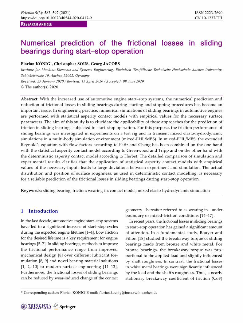
The friction and the wear behavior during start–stop

cycles was investigated using a special test rig for

sliding bearings, as shown in Fig. 1.

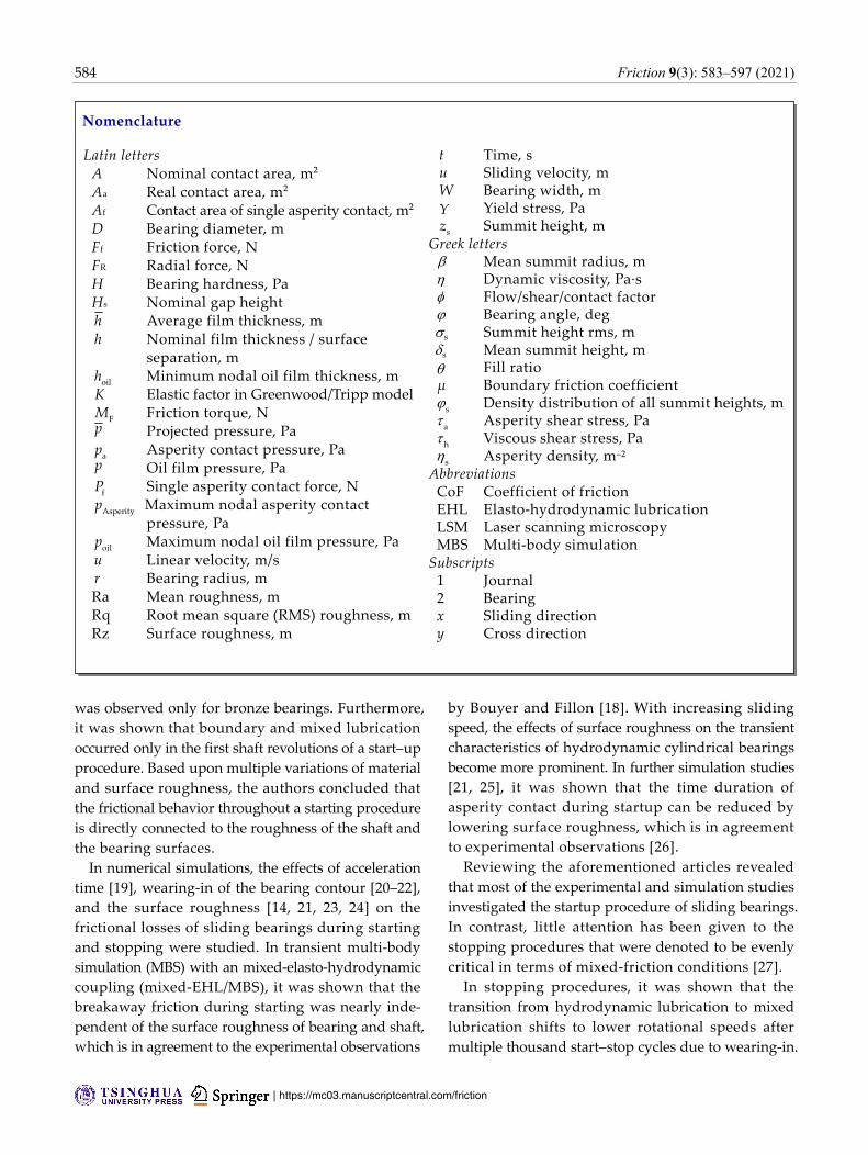
In this study, multiple experiments with distinct

number of start–stop cycles (250/2,500/10,000—all ex-

periments were performed in duplicate) were conducted

under stationary projected pressure 1

R( )p F D W

and predefined speed profile according to Fig. 2. A

projected pressure of 2 N/mm² was chosen to remain

below the permissible maximum projected pressure

valid for a few start–stop cycles according to DIN

31652 [37]. In each cycle, the shaft was driven from

standstill to its rated operational speed at 600 min–1

and vice versa with a period of constant operation

Fig. 1 Schematic and photographic representation of the bearing test rig.

586 Friction 9(3): 583–597 (2021)


in between. The radial load was applied to the bearing

housing using a flexible load unit with five low-

friction ball bearings. A friction gauge directly

connected to the load unit was used to determine

the friction torque without the friction torque generated

in the supporting bearings. The speed, radial load,

friction force as well as inlet- and bearing temperatures

were continually measured during the experiments

with a frequency of 100 Hz. For each time step, the

bearing’s coefficient of friction (CoF) was calculated

according to CoF 1

F R( )M F r under consideration

of the measured friction torque F

M , the radial force

RF , and the radius of the bearing r . The experiments

were performed under isothermal conditions regulated

by circumferentially positioned heating cartridges

in the bearing housing. Additionally, the oil inlet

was preheated with an electrically heated hose and

filtered with a micron rating of 5 μm. The testing

parameters are summarized in Table 1.

Fig. 2 Speed and load profile. Table 1 Properties of the used oil and summarized testing parameters.

Lubricant

Kinematic viscosity (40 ℃)/mm²s–1 32

Kinematic viscosity (100 ℃)/mm²s–1 5.35

Testing parameters

Bearing temperature/℃ 80

Oil inlet temperature/℃ 70

Oil inlet pressure/bar 3

Operating conditions

Stationary pressure/Nmm–2 2

Rotational speed/min–1 0–600

Linear speed/ms–1 0–0.94

Radial clearance/µm 25

Cycle count 250

2,500

10,000

2.2.2 Specimen analysis

In this study, the bearings and the shaft sleeve’s

topographies were measured using a confocal laser

scanning microscopy (LSM) Keyence VK-X210 (Key-

ence GmbH, Neu-Isenburg, Germany). In accordance

to Bergmann et al. [38], a 50-fold magnification was

chosen for the determination of surface parameters

from three-dimensional surface analysis for asperity

contact modelling. Each measured surface patch

thereby contains the height profile in an area of

141 μm × 141 μm with a resolution of 1,000 × 1,000

pixels in circumferential and axial direction, respectively.

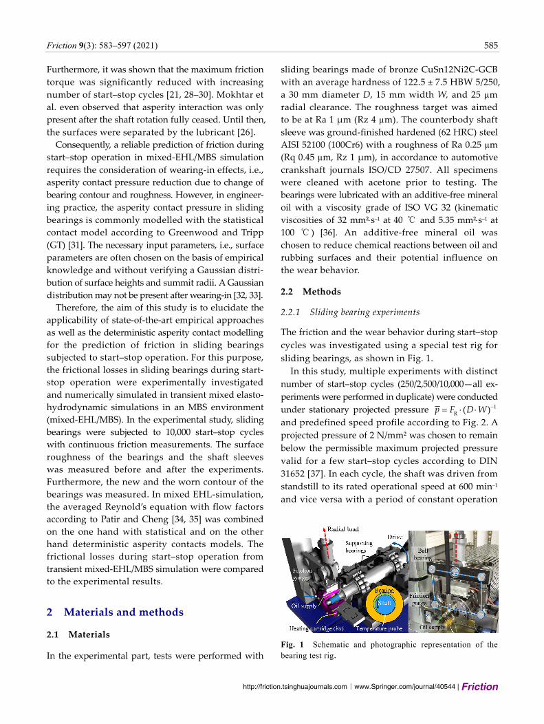
After tribological testing, six measurements at

randomly selected positions in the load area for

each shaft sleeve and bearing were conducted. These

measurements were used to evaluate the distribution

of surface and summit parameters. Additionally,

six measurements were performed on shaft sleeve

and bearing specimen in an unloaded region. The

measurement spots for this procedure are exemplarily

shown in Fig. 3.

In the three dimensional (3D) surface data, asperity

peaks on 3D engineering surfaces have been defined

as a point higher than its eight neighbors, referred

to 8P+1 [39] or 9PP-3D [40]. The radii were determined

via curve fitting over the eight nearest neighbors

[40]. The bearing contour in new state and after

10,000 cycles was measured with a form tester (Mar-

Form MMQ 100 with probe T2W Mahr, Göttingen,

Germany).

2.2.3 Simulation workflow

The frictional losses in sliding bearings subjected

to start–stop cycles under steady load and temperature

were investigated in numerical simulations. In these

transient mixed-EHL/MBS simulations, the topography,

Fig. 3 Positions and distribution of surface parameter measurements on bearing and shaft sleeve.

Friction 9(3): 583–597 (2021) 587



i.e., roughness and bearing contour, has been considered

as boundary conditions. The measured bearing contour

was deterministically implemented in the simulations.

In contrast, the influence of roughness on the oil

film pressure (micro-hydrodynamics) was considered

through flow factors obtained from flow-simulations

on the microscopic scale. Both, the statistical contact

model according to Greenwood and Tripp (GT) [31]

and the deterministic model according to Herbst

[40] were employed for the asperity contact pressure

calculation between two rough surfaces.

2.2.4 Statistical contact model according to Greenwood

and Tripp (GT) [31]

The asperity contact a

p between two rough surfaces

with the asperity density s, mean summit radius

and root-mean-square summit height s and

mean Young’s modulus is calculated in terms of

the nominal gap height s.H

2 *

a s s 5/2 s

16 2

15p E F H

(1)

In the original work, 5/2 sF H is the probability

density function of the load carrying asperities

with the height s.

2

s

2.52

5/2 s s

1 e d

2

s

H

F H s H s

(2)

For numerical implementation, a simplified formulation

was introduced by Hu et al. [41], as shown in Eq. (3).

6.8045

s s5/2 s

s

4.4086 10 4 , 4;

0, 4

H HF H

H

(3)

The input quantities are obtained from elastic material

properties and the surface parameters of both surfaces

(Eqs. (4–9)). It is worth to point out that Eqs. (6–9)

are limited to statistically independent rough surfaces.

After wearing-in, a Gaussian distribution may not

be present [32, 33]. Consequently, the modelling of

worn-in asperity contacts with the GT-model may

lead to inaccuracies. In Eq. (4), the mean summit

height s, which defines the distance between

centerlines of the roughness height and summit

roughness height, is introduced, to ensure a proper

application of the contact model in the mixed lubrication

model.

ss

s

hH

(4)

2 2

1 2

*1 2

1 11

E EE

(5)

1 2

2 2

s s s (6)

1 2s s s (7)

1 2

2 2

s s s (8)

1 2

1 1 1

s s (9)

In engineering practice, the product of asperity

density s

, mean summit radius , and summit

height distribution s

has been set to values

between s s

= 0.02 and 0.1, based on the

experimental observations [42, 43]. It is worth to

point out that positive and negative deviations

from this range were reported [33, 44]. Following

the same idea, Beheshti and Khonsari [42] reviewed

several manuscripts and suggested a variation range

for / between 0.0001 and 0.1. For further

simplification, it is common to simplify the model

by combining surface properties of asperity density,

summit height, and mean summit radius within

the so called elastic factor K [45].

2

ss s

16 2π

15K

(10)

The elastic factor K represents the slope of the

asperity pressure over gap height.

*

a 5/2 sp K E F H

(11)

It is straightforward to conclude that the elastic factor

strongly influences the calculated asperity contact

pressure. Under consideration of the variation range

of surface parameters ( s s

and / ), Hu et al.

[41] and Xiang et al. [46] chose an elastic factor of

K = 0.000119 ( s s

= 0.05, / = 0.01). However,

it should be noted that K may vary between 0.000019

and 0.015 with the aforementioned variation range.

Consequently, the computed asperity contact pressure

at a specific gap height would change by almost

three orders of magnitude. In other works, an elastic

factor 0.0003 K 0.003 was suggested for piston

rings and sliding bearings [47]. This refinement reduces

588 Friction 9(3): 583–597 (2021)


the potential deviation to one order of magnitude.

Based upon this uncertainty, the aim of this study

is to elucidate the applicability of these empirical

approaches for the prediction of friction in sliding

bearings subjected to start–stop operation. Therefore,

in this study, a variation of the elastic factor K in

the range of 0.0003 K 0.003 was considered.

2.2.5 Deterministic contact modelling

In order to evaluate the statistical asperity contact

model according to Greenwood and Tripp (GT) [31],

the asperity contact pressure ap h and the real area

of contact aA h (Eqs. (12) and (13)) were compared

to calculations by the deterministic contact model

according to Herbst [40]. The equations are solved

numerically for a number of given surface separations

to determine a relationship between gap height and

mean asperity contact pressure. The two measured

surfaces are treated as one composite rough and

one ideal flat surface.

s

a s f s s s s d

z h

p h P z h z z

(12)

s

a s f s s s s d

z h

A h A A z h z z

(13)

Within the deterministic model, the actual distribution

s s

z , the location of summit heights and the

asperity radii are taken into account. The asperity

contact force f,P area

f,A and pressure

mHertzp of a

single asperity are determined by Hertzian equations

as a function of compliance w of the contacting

surfaces (Eqs. (14–17)). If the local pressure exceeds

the critical yield stress Y of the bearing material

( m

1.16 ,p Y with / 2.75Y H ), the asperity defor-

mation is expected to show elasto-plastic up to

plastic behavior, which is treated in a semi-analytical

relationship [40].

1 3* 2 2

f

4

3P E w

(14)

with * * *

1 2

1 1 1

E E E,

1,2*

1,2 2

1,21

EE

(15)

f πA w

(16)

1* 2

mHertz

4

3π

E wp

(17)

The contact model was applied to calculate the asperity

contact pressure between the measured bearing

and shaft sleeve surface spots. Here, six randomly

distributed measurement spots from each bearing

and each shaft sleeve as described in Section 2.2.2 were

used as input. Combinations for all measurement

spots were evaluated, which resulted in 36 results

individual results of asperity contact pressure as a

function of gap height. Due to the fact that each LSM-

measurement only represents a small patch of the

bearing and shaft surface, the results of this approach

strongly depend upon the chosen contact pair. Thus,

an averaged asperity contact pressure ap h and

the real area of contact aA h were determined from

the individual results of the measured contact pairs.

Additionally, the contact pressure was calculated

for the contact between the measured shaft sleeve

and synthetically worn bearing surfaces. The syn-

thetically worn bearing surfaces were created with

method described in Ref. [28]. For the reader’s

convenience, a short summary is given here. First,

for each point in width direction, the maximum peak

asperity in circumferential direction was taken from

the LSM-measurements of the shaft sleeve. The

resulting line of maxima was inverted. As reported

by Mokthar et al., bearing surface roughness after

repeated starting and stopping was approximately

the same as that of the hardened shaft [48]. Therefore,

the inverted peak asperities from the shaft sleeve were

elongated to the LSM-dimensions and then used as

synthetically worn bearing surface for deterministic

contact modelling. In this case, the measured shaft

sleeve topography is used as the counterbody. A

2D-line scan of bearing roughness and inverted peak

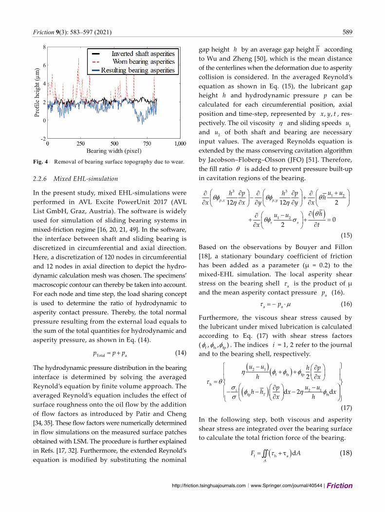
asperities is exemplarily shown in Fig. 4.

In this procedure, the actual location and dimensions

of grooves and ridges created by summits and

valleys (familiarity factor) were taken into account

when calculating the asperity contact pressure. In

contrast, the familiarity factor was not considered

in the asperity contact pressure curves derived from

the measured bearing and shaft sleeve topographies

as the measurements were performed in random

positions on the worn surface.

Friction 9(3): 583–597 (2021) 589



Fig. 4 Removal of bearing surface topography due to wear.

2.2.6 Mixed EHL-simulation

In the present study, mixed EHL-simulations were

performed in AVL Excite PowerUnit 2017 (AVL

List GmbH, Graz, Austria). The software is widely

used for simulation of sliding bearing systems in

mixed-friction regime [16, 20, 21, 49]. In the software,

the interface between shaft and sliding bearing is

discretized in circumferential and axial direction.

Here, a discretization of 120 nodes in circumferential

and 12 nodes in axial direction to depict the hydro-

dynamic calculation mesh was chosen. The specimens’

macroscopic contour can thereby be taken into account.

For each node and time step, the load sharing concept

is used to determine the ratio of hydrodynamic to

asperity contact pressure. Thereby, the total normal

pressure resulting from the external load equals to

the sum of the total quantities for hydrodynamic and

asperity pressure, as shown in Eq. (14).

Total ap p p

(14)

The hydrodynamic pressure distribution in the bearing

interface is determined by solving the averaged

Reynold’s equation by finite volume approach. The

averaged Reynold’s equation includes the effect of

surface roughness onto the oil flow by the addition

of flow factors as introduced by Patir and Cheng

[34, 35]. These flow factors were numerically determined

in flow simulations on the measured surface patches

obtained with LSM. The procedure is further explained

in Refs. [17, 32]. Furthermore, the extended Reynold’s

equation is modified by substituting the nominal

gap height h by an average gap height h according

to Wu and Zheng [50], which is the mean distance

of the centerlines when the deformation due to asperity

collision is considered. In the averaged Reynold’s

equation as shown in Eq. (15), the lubricant gap

height h and hydrodynamic pressure p can be

calculated for each circumferential position, axial

position and time-step, represented by , ,x y t , res-

pectively. The oil viscosity and sliding speeds 1

u

and 2

u of both shaft and bearing are necessary

input values. The averaged Reynolds equation is

extended by the mass conserving cavitation algorithm

by Jacobson–Floberg–Olsson (JFO) [51]. Therefore,

the fill ratio is added to prevent pressure built-up

in cavitation regions of the bearing.

3 31 2

, ,

1 2

12 12 2

02

p x p y

s s

u up ph hh

x x y y x

hu u

x t

(15)

Based on the observations by Bouyer and Fillon

[18], a stationary boundary coefficient of friction

has been added as a parameter (μ = 0.2) to the

mixed-EHL simulation. The local asperity shear

stress on the bearing shell a is the product of μ

and the mean asperity contact pressure a

p (16).

a a p

(16)

Furthermore, the viscous shear stress caused by

the lubricant under mixed lubrication is calculated

according to Eq. (17) with shear stress factors

( f fs fp, , ) . The indices i = 1, 2 refer to the journal

and to the bearing shell, respectively.

2 1

f fs fp

h

i 2 1fp fs

2

d 2 dT

u u ph

h x

u uph h x x

x h

(17)

In the following step, both viscous and asperity

shear stress are integrated over the bearing surface

to calculate the total friction force of the bearing.

f h a

τ dA

F A∬ (18)

590 Friction 9(3): 583–597 (2021)


The latter can be used to calculate the bearing CoF

using the bearing radial load (R

F ).

f

R

CoFF

F (19)

3 Results and discussion

In order to further explore and elucidate the app-

licability of state-of-the-art empirical approaches for

the prediction of friction in sliding bearings subjected

to start–stop operation, the sliding bearing test rig

was transferred into a mixed-EHL/MBS simulation

model. For an accurate modeling of the sliding bearing

system, the bearing contour and surface roughness

were measured and used as input for asperity contact

modelling. Multiple simulation runs were performed.

Variations include the use of the statistic asperity


(see Section 2.2.4.) and the deterministic asperity

contact model according to Herbst (see Section

2.2.5.). The models were used with varying input

parameters, i.e., empirical input parameters and input

parameters from surface roughness measurements

(new state and after 10,000 start–stop cycles). Further-

more, a synthetically worn-in bearing surface was

used in the deterministic contact model (see Section

2.2.5.). The calculated friction losses are compared

to the experimental results.

3.1 Surface analysis for asperity contact modelling

As a consequence of frequent start–stop operation,

the wear-induced changes of the surface topography

have to be considered for the asperity contact modeling.

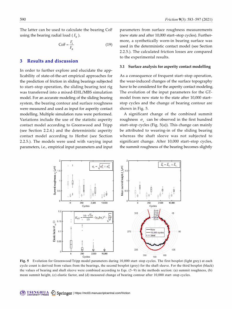
The evolution of the input parameters for the GT-

model from new state to the state after 10,000 start–

stop cycles and the change of bearing contour are

shown in Fig. 5.

A significant change of the combined summit

roughness s can be observed in the first hundred

start–stop cycles (Fig. 5(a)). This change can mainly

be attributed to wearing-in of the sliding bearing

whereas the shaft sleeve was not subjected to

significant change. After 10,000 start–stop cycles,

the summit roughness of the bearing becomes slightly

Fig. 5 Evolution for Greenwood/Tripp model parameters during 10,000 start–stop cycles. The first boxplot (light grey) at each cycle count is derived from values from the bearings, the second boxplot (grey) for the shaft sleeve. For the third boxplot (black) the values of bearing and shaft sleeve were combined according to Eqs. (5–9) in the methods section: (a) summit roughness, (b) mean summit height, (c) elastic factor, and (d) measured change of bearing contour after 10,000 start–stop cycles.

Friction 9(3): 583–597 (2021) 591



smoother than the roughness of the counterbody

(shaft sleeve). Furthermore, the mean summit height

of the bearing’s surface becomes lower than the mean

summit height of the shaft sleeve, which is not

subjected to change (Fig. 5(b)). With a value of K =

0.038, the analytically determined elastic factor K

for the new state was more than twelve times higher

than the suggested value range (0.0003 < K < 0.003).

Even after 10,000 start–stop cycles, the mean elastic

factor K = 0.0075 was two times higher than the

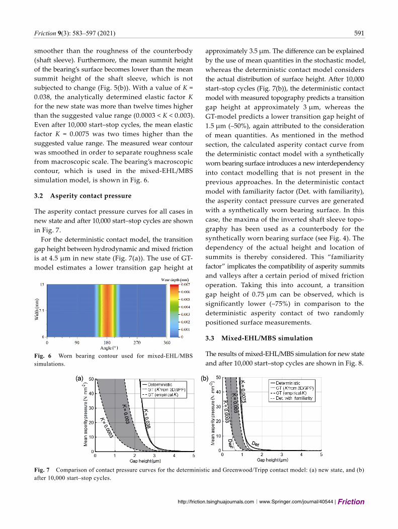
suggested value range. The measured wear contour

was smoothed in order to separate roughness scale

from macroscopic scale. The bearing’s macroscopic

contour, which is used in the mixed-EHL/MBS

simulation model, is shown in Fig. 6.

3.2 Asperity contact pressure

The asperity contact pressure curves for all cases in

new state and after 10,000 start–stop cycles are shown

in Fig. 7.

For the deterministic contact model, the transition

gap height between hydrodynamic and mixed friction

is at 4.5 μm in new state (Fig. 7(a)). The use of GT-

model estimates a lower transition gap height at

Fig. 6 Worn bearing contour used for mixed-EHL/MBS simulations.

approximately 3.5 μm. The difference can be explained

by the use of mean quantities in the stochastic model,

whereas the deterministic contact model considers

the actual distribution of surface height. After 10,000

start–stop cycles (Fig. 7(b)), the deterministic contact

model with measured topography predicts a transition

gap height at approximately 3 μm, whereas the

GT-model predicts a lower transition gap height of

1.5 μm (–50%), again attributed to the consideration

of mean quantities. As mentioned in the method

section, the calculated asperity contact curve from

the deterministic contact model with a synthetically

worn bearing surface introduces a new interdependency

into contact modelling that is not present in the

previous approaches. In the deterministic contact

model with familiarity factor (Det. with familiarity),

the asperity contact pressure curves are generated

with a synthetically worn bearing surface. In this

case, the maxima of the inverted shaft sleeve topo-

graphy has been used as a counterbody for the

synthetically worn bearing surface (see Fig. 4). The

dependency of the actual height and location of

summits is thereby considered. This “familiarity

factor” implicates the compatibility of asperity summits

and valleys after a certain period of mixed friction

operation. Taking this into account, a transition

gap height of 0.75 μm can be observed, which is

significantly lower (–75%) in comparison to the

deterministic asperity contact of two randomly

positioned surface measurements.

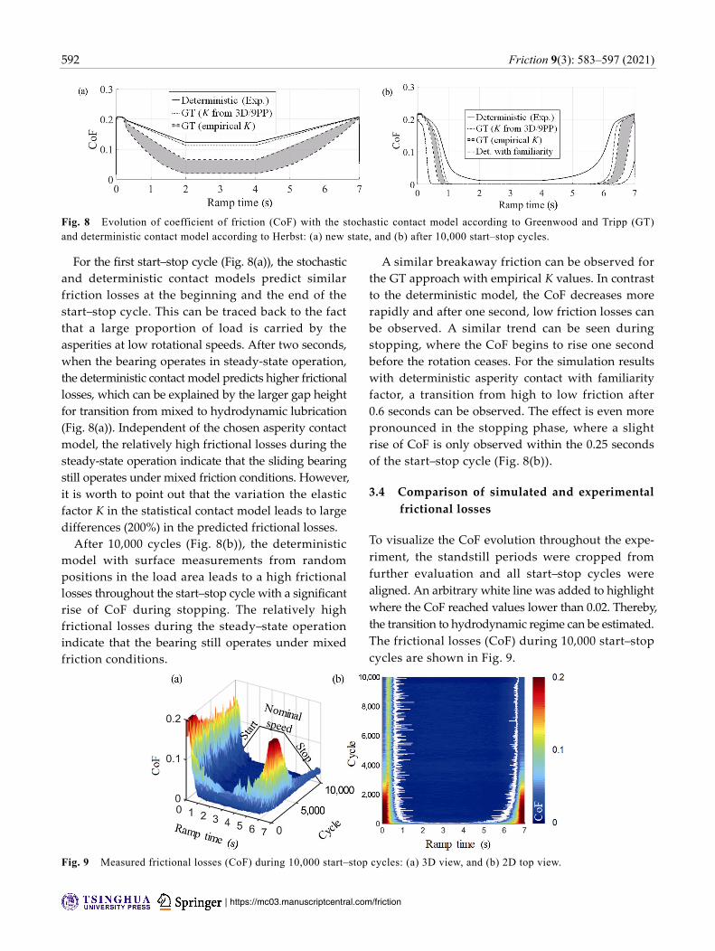
3.3 Mixed-EHL/MBS simulation

The results of mixed-EHL/MBS simulation for new state

and after 10,000 start–stop cycles are shown in Fig. 8.

Fig. 7 Comparison of contact pressure curves for the deterministic and Greenwood/Tripp contact model: (a) new state, and (b) after 10,000 start–stop cycles.

592 Friction 9(3): 583–597 (2021)


Fig. 8 Evolution of coefficient of friction (CoF) with the stochastic contact model according to Greenwood and Tripp (GT) and deterministic contact model according to Herbst: (a) new state, and (b) after 10,000 start–stop cycles.

For the first start–stop cycle (Fig. 8(a)), the stochastic

and deterministic contact models predict similar

friction losses at the beginning and the end of the

start–stop cycle. This can be traced back to the fact

that a large proportion of load is carried by the

asperities at low rotational speeds. After two seconds,

when the bearing operates in steady-state operation,

the deterministic contact model predicts higher frictional

losses, which can be explained by the larger gap height

for transition from mixed to hydrodynamic lubrication

(Fig. 8(a)). Independent of the chosen asperity contact

model, the relatively high frictional losses during the

steady-state operation indicate that the sliding bearing

still operates under mixed friction conditions. However,

it is worth to point out that the variation the elastic

factor K in the statistical contact model leads to large

differences (200%) in the predicted frictional losses.

After 10,000 cycles (Fig. 8(b)), the deterministic

model with surface measurements from random

positions in the load area leads to a high frictional

losses throughout the start–stop cycle with a significant

rise of CoF during stopping. The relatively high

frictional losses during the steady–state operation

indicate that the bearing still operates under mixed

friction conditions.

A similar breakaway friction can be observed for

the GT approach with empirical K values. In contrast

to the deterministic model, the CoF decreases more

rapidly and after one second, low friction losses can

be observed. A similar trend can be seen during

stopping, where the CoF begins to rise one second

before the rotation ceases. For the simulation results

with deterministic asperity contact with familiarity

factor, a transition from high to low friction after

0.6 seconds can be observed. The effect is even more

pronounced in the stopping phase, where a slight

rise of CoF is only observed within the 0.25 seconds

of the start–stop cycle (Fig. 8(b)).

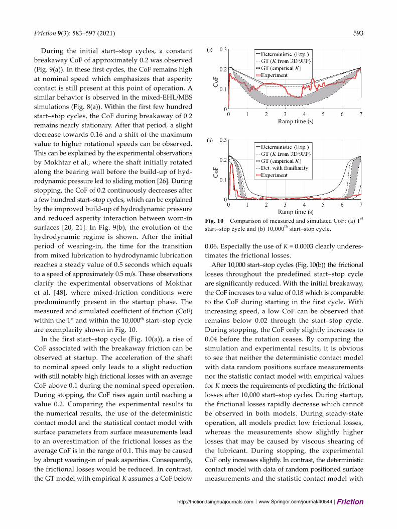
3.4 Comparison of simulated and experimental

frictional losses

To visualize the CoF evolution throughout the expe-

riment, the standstill periods were cropped from

further evaluation and all start–stop cycles were

aligned. An arbitrary white line was added to highlight

where the CoF reached values lower than 0.02. Thereby,

the transition to hydrodynamic regime can be estimated.

The frictional losses (CoF) during 10,000 start–stop

cycles are shown in Fig. 9.

Fig. 9 Measured frictional losses (CoF) during 10,000 start–stop cycles: (a) 3D view, and (b) 2D top view.

Friction 9(3): 583–597 (2021) 593



During the initial start–stop cycles, a constant

breakaway CoF of approximately 0.2 was observed

(Fig. 9(a)). In these first cycles, the CoF remains high

at nominal speed which emphasizes that asperity

contact is still present at this point of operation. A

similar behavior is observed in the mixed-EHL/MBS

simulations (Fig. 8(a)). Within the first few hundred

start–stop cycles, the CoF during breakaway of 0.2

remains nearly stationary. After that period, a slight

decrease towards 0.16 and a shift of the maximum

value to higher rotational speeds can be observed.

This can be explained by the experimental observations

by Mokhtar et al., where the shaft initially rotated

along the bearing wall before the build-up of hyd-

rodynamic pressure led to sliding motion [26]. During

stopping, the CoF of 0.2 continuously decreases after

a few hundred start–stop cycles, which can be explained

by the improved build-up of hydrodynamic pressure

and reduced asperity interaction between worn-in

surfaces [20, 21]. In Fig. 9(b), the evolution of the

hydrodynamic regime is shown. After the initial

period of wearing-in, the time for the transition

from mixed lubrication to hydrodynamic lubrication

reaches a steady value of 0.5 seconds which equals

to a speed of approximately 0.5 m/s. These observations

clarify the experimental observations of Mokthar

et al. [48], where mixed-friction conditions were

predominantly present in the startup phase. The

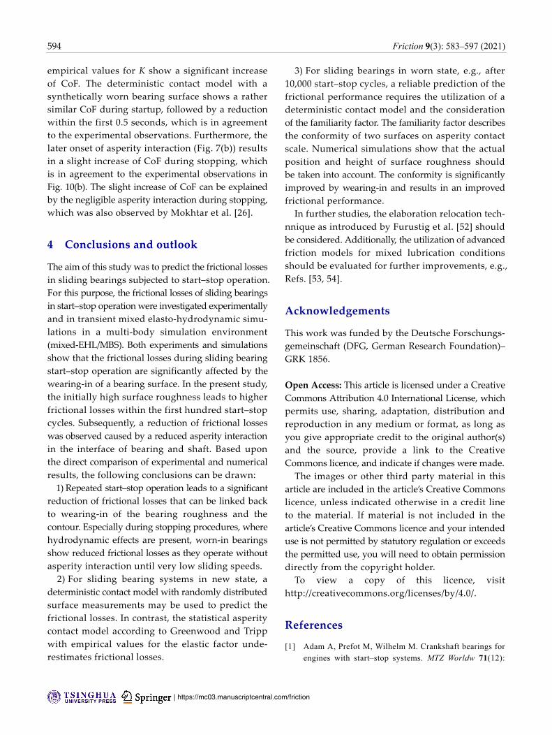
measured and simulated coefficient of friction (CoF)

within the 1st and within the 10,000th start–stop cycle

are exemplarily shown in Fig. 10.

In the first start–stop cycle (Fig. 10(a)), a rise of

CoF associated with the breakaway friction can be

observed at startup. The acceleration of the shaft

to nominal speed only leads to a slight reduction

with still notably high frictional losses with an average

CoF above 0.1 during the nominal speed operation.

During stopping, the CoF rises again until reaching a

value 0.2. Comparing the experimental results to

the numerical results, the use of the deterministic

contact model and the statistical contact model with

surface parameters from surface measurements lead

to an overestimation of the frictional losses as the

average CoF is in the range of 0.1. This may be caused

by abrupt wearing-in of peak asperities. Consequently,

the frictional losses would be reduced. In contrast,

the GT model with empirical K assumes a CoF below

Fig. 10 Comparison of measured and simulated CoF: (a) 1st start–stop cycle and (b) 10,000

th start–stop cycle.

0.06. Especially the use of K = 0.0003 clearly underes-

timates the frictional losses.

After 10,000 start–stop cycles (Fig. 10(b)) the frictional

losses throughout the predefined start–stop cycle

are significantly reduced. With the initial breakaway,

the CoF increases to a value of 0.18 which is comparable

to the CoF during starting in the first cycle. With

increasing speed, a low CoF can be observed that

remains below 0.02 through the start–stop cycle.

During stopping, the CoF only slightly increases to

0.04 before the rotation ceases. By comparing the

simulation and experimental results, it is obvious

to see that neither the deterministic contact model

with data random positions surface measurements

nor the statistic contact model with empirical values

for K meets the requirements of predicting the frictional

losses after 10,000 start–stop cycles. During startup,

the frictional losses rapidly decrease which cannot

be observed in both models. During steady-state

operation, all models predict low frictional losses,

whereas the measurements show slightly higher

losses that may be caused by viscous shearing of

the lubricant. During stopping, the experimental

CoF only increases slightly. In contrast, the deterministic

contact model with data of random positioned surface

measurements and the statistic contact model with

594 Friction 9(3): 583–597 (2021)


empirical values for K show a significant increase

of CoF. The deterministic contact model with a

synthetically worn bearing surface shows a rather

similar CoF during startup, followed by a reduction

within the first 0.5 seconds, which is in agreement

to the experimental observations. Furthermore, the

later onset of asperity interaction (Fig. 7(b)) results

in a slight increase of CoF during stopping, which

is in agreement to the experimental observations in

Fig. 10(b). The slight increase of CoF can be explained

by the negligible asperity interaction during stopping,

which was also observed by Mokhtar et al. [26].

4 Conclusions and outlook

The aim of this study was to predict the frictional losses

in sliding bearings subjected to start–stop operation.

For this purpose, the frictional losses of sliding bearings

in start–stop operation were investigated experimentally

and in transient mixed elasto-hydrodynamic simu-

lations in a multi-body simulation environment

(mixed-EHL/MBS). Both experiments and simulations

show that the frictional losses during sliding bearing

start–stop operation are significantly affected by the

wearing-in of a bearing surface. In the present study,

the initially high surface roughness leads to higher

frictional losses within the first hundred start–stop

cycles. Subsequently, a reduction of frictional losses

was observed caused by a reduced asperity interaction

in the interface of bearing and shaft. Based upon

the direct comparison of experimental and numerical

results, the following conclusions can be drawn:

1) Repeated start–stop operation leads to a significant

reduction of frictional losses that can be linked back

to wearing-in of the bearing roughness and the

contour. Especially during stopping procedures, where

hydrodynamic effects are present, worn-in bearings

show reduced frictional losses as they operate without

asperity interaction until very low sliding speeds.

2) For sliding bearing systems in new state, a

deterministic contact model with randomly distributed

surface measurements may be used to predict the

frictional losses. In contrast, the statistical asperity


with empirical values for the elastic factor unde-

restimates frictional losses.

3) For sliding bearings in worn state, e.g., after

10,000 start–stop cycles, a reliable prediction of the

frictional performance requires the utilization of a

deterministic contact model and the consideration

of the familiarity factor. The familiarity factor describes

the conformity of two surfaces on asperity contact

scale. Numerical simulations show that the actual

position and height of surface roughness should

be taken into account. The conformity is significantly

improved by wearing-in and results in an improved

frictional performance.

In further studies, the elaboration relocation tech-

nnique as introduced by Furustig et al. [52] should

be considered. Additionally, the utilization of advanced

friction models for mixed lubrication conditions

should be evaluated for further improvements, e.g.,

Refs. [53, 54].

Acknowledgements

This work was funded by the Deutsche Forschungs-

gemeinschaft (DFG, German Research Foundation)–

GRK 1856.

Open Access: This article is licensed under a Creative

Commons Attribution 4.0 International License, which

permits use, sharing, adaptation, distribution and

reproduction in any medium or format, as long as

you give appropriate credit to the original author(s)

and the source, provide a link to the Creative

Commons licence, and indicate if changes were made.

The images or other third party material in this

article are included in the article’s Creative Commons

licence, unless indicated otherwise in a credit line

to the material. If material is not included in the

article’s Creative Commons licence and your intended

use is not permitted by statutory regulation or exceeds

the permitted use, you will need to obtain permission

directly from the copyright holder.

To view a copy of this licence, visit

http://creativecommons.org/licenses/by/4.0/.

References

[1] Adam A, Prefot M, Wilhelm M. Crankshaft bearings for engines with start–stop systems. MTZ Worldw 71(12):

Friction 9(3): 583–597 (2021) 595



22–25 (2010) [2] Gudin D, Mian O, Sanders S. Experimental measurement

and modelling of plain bearing wear in start–stop applications. Proc Inst Mech Eng, Part J: J Eng Tribol 227(5): 433–446 (2013)

[3] Garnier T. EHD+T analysis and calibration investigate the effect of the waviness of a rod crankpin. Ulm, 2018.

[4] Knorr R. Start/stopp-systeme auf der zielgeraden. ATZ-Automobiltech Z 113(9): 664–669 (2011)

[5] Wong V W, Tung S C. Overview of automotive engine friction and reduction trends—Effects of surface, material, and lubricant–additive technologies. Friction 4(1): 1–28 (2016)

[6] Ligier J L, Noel B. Friction reduction and reliability for engines bearings. Lubricants 3(3): 569–596 (2015)

[7] Holmberg K, Erdemir A. Influence of tribology on global energy consumption, costs and emissions. Friction 5(3): 263–284 (2017)

[8] Aufischer R, Walker R, Offenbecher M, Feng O, Hager G. Friction reduction opportunities in combustion engine crank train bearings. In ASME 2015 Internal Combustion Engine Division Fall Technical Conference, Houston, Texas, USA, 2015: V002T07A008.

[9] Durak E, Adatepe H, Biyiklioğlu A. Experimental study of the effect of additive on the tribological properties journal bearing under running-in and start-up or shut-down stages. Ind Lubr Tribol 60(3): 138–146 (2008)

[10] Summer F, Grün F, Offenbecher M, Taylor S. Challenges of friction reduction of engine plain bearings—Tackling the problem with novel bearing materials. Tribol Int 131: 238–250 (2019)

[11] Grützmacher P G, Rosenkranz A, Szurdak A, König F, Jacobs G, Hirt G, Mücklich F. From lab to application—Improved frictional performance of journal bearings induced by single-and multi-scale surface patterns. Tribol Int 127: 500–508 (2018)

[12] Grützmacher P G, Profito F J, Rosenkranz A. Multi- scale surface texturing in tribology—Current knowledge and future perspectives. Lubricants 7(11): 95 (2019)

[13] König F, Rosenkranz A, Grützmacher P G, Mücklich F, Jacobs G. Effect of single-and multi-scale surface patterns on the frictional performance of journal bearings—A numerical study. Tribol Int 143: 106041 (2020)

[14] Nilsson D, Prakash B. Influence of different surface modification technologies on friction of conformal tribopair in mixed and boundary lubrication regimes. Wear 273(1): 75–81 (2011)

[15] Bartel D, Bobach L, Illner T, Deters L. Simulating transient wear characteristics of journal bearings subjected to mixed friction. Proc Inst Mech Eng, Part J: J Eng Tribol 226(12): 1095–1108 (2012)

[16] Sander D E, Allmaier H, Priebsch H H, Witt M, Skiadas A.

Simulation of journal bearing friction in severe mixed lubrication—Validation and effect of surface smoothing due to running-in. Tribol Int 96: 173–183 (2016)

[17] Grützmacher P G, Rammacher S, Rathmann D, Motz C, Mücklich F, Suarez S. Interplay between microstructural evolution and tribo-chemistry during dry sliding of metals. Friction 7(6): 637–650 (2019)

[18] Bouyer J, Fillon M. Experimental measurement of the friction torque on hydrodynamic plain journal bearings during start–up. Tribol Int 44(7–8): 772–781 (2011)

[19] Prölß M, Schwarze H, Hagemann T, Zemella P, Winking P. Theoretical and experimental investigations on transient run-up procedures of journal bearings including mixed friction conditions. Lubricants 6(4): 105 (2018)

[20] Sander D E, Allmaier H. Starting and stopping behavior of worn journal bearings. Tribol Int 127: 478–488 (2018)

[21] Sander D E, Allmaier H, Priebsch H H. Friction and wear in automotive journal bearings operating in today’s severe conditions. In Advances in Tribology. Darji P H, Ed. Rijeka: IntechOpen, 2016.

[22] Fricke S, Hager C, Solovyev S, Wangenheim M, Wallaschek J. Influence of surface form deviations on friction in mixed lubrication. Tribol Int 118: 491–499 (2018)

[23] Knoll G, Boucke A, Winijsart A, Stapelmann A, Auerbach P. Reduction of friction losses in journal bearings of valve train shaft by application of running–in profile. Tribol Schmierungstechnik 63(4): 14–21 (2016)

[24] Isaksson P, Nilsson D, Larsson R, Almqvist A. The influence of surface roughness on friction in a flexible hybrid bearing. Proc Inst of Mech Eng, Part J: J Eng Tribol 225(10): 975–985 (2011)

[25] Cui S H, Gu L, Fillon M, Wang L Q, Zhang C W. The effects of surface roughness on the transient characteristics of hydrodynamic cylindrical bearings during startup. Tribol Int 128: 421–428 (2018)

[26] Mokhtar M O A, Howarth R B, Davies P B. The behavior of plain hydrodynamic journal bearings during starting and stopping. A S L E Trans 20(3): 183–190 (1977)

[27] Affenzeller J, Gläser H. Lagerung und Schmierung von Verbrennungsmotoren. Vienna (Austria): Springer-Verlag, 1996.

[28] König F, Ouald Chaib A, Jacobs G, Sous C. A multiscale-approach for wear prediction in journal bearing systems—From wearing-in towards steady-state wear. Wear 426–427: 1203–1211 (2019)

[29] König F, Jacobs G, Sous C. Wear prediction of journal bearings in start–stop operation. In 9th VDI Conference on Cylinder Barrel, Piston, Connecting Rod 2018: The Crank Drive in the Stress Field of Different Requirements, 2018: 197–208.

596 Friction 9(3): 583–597 (2021)


[30] König F, Jacobs G, Burghardt G. Running-in of plain bearings in start–stop operation. In 12th VDI Conference on Sliding and Rolling Bearings 2017: Design, Calculation, Use, 2017: 53–62.

[31] Greenwood J A, Tripp J H. The contact of two nominally flat rough surfaces. Proc Inst Mech Eng 185(1): 625–633 (2016)

[32] Zhang Y, Kovalev A, Hayashi N, Nishiura K, Meng Y. Numerical prediction of surface wear and roughness parameters during running-in for line contacts under mixed lubrication. J Tribol 140(6): 061501 (2018)

[33] Tomanik E. Modelling of the asperity contact area on actual 3D surfaces. SAE paper 2005–01–1864, 2005.

[34] Patir N, Cheng H S. An average flow model for determining effects of three-dimensional roughness on partial hydrodynamic lubrication. J Lubr Technol 100(1): 12–17 (1978)

[35] Patir N, Cheng H S. Application of average flow model to lubrication between rough sliding surfaces. J Lubr Technol 101(2): 220–229 (1979)

[36] Schilling M. Referenzöle für wälz– und Gleitlager–, Zahnrad– und Kupplungsversuche: Datensammlung für Mineralöle; Berichtszeitraum: 1976/84. Frankfurt (Germany): FVA, 1985.

[37] DIN Deutsches Institut für Normung. Gleitlager– hydrodynamische radial–gleitlager im stationären betrieb– Teil 3: Betriebsrichtwerte für die berechnung von kreiszylinderlagern (DIN 31652–3: 2017). Berlin: Beuth Verlag, 2017.

[38] Bergmann P, Grün F, Gódor I, Stadler G, Maier–Kiener V. On the modelling of mixed lubrication of conformal contacts. Tribol Int 125: 220–236 (2018)

[39] Kalin M, Pogačnik A. Criteria and properties of the asperity peaks on 3D engineering surfaces. Wear 308(1–2): 95–104 (2013)

[40] Herbst HM. Theoretical modeling of the cylinder lubrication in internal combustion engines and its influence on piston slap induced noise, friction and wear. Graz (Austria): Graz University of Technology, 2008.

[41] Hu Y Z, Cheng H S, Arai T, Kobayashi Y, Aoyama S. Numerical simulation of piston ring in mixed lubrication—A nonaxisymmetrical analysis. J Tribol 116(3): 470–478 (1994)

[42] Beheshti A, Khonsari M M. An engineering approach for the prediction of wear in mixed lubricated contacts. Wear 308(1–2): 121–131 (2013)

[43] Greenwood J A, Williamson J B P. Contact of nominally flat surfaces. Proc Roy Soc A Math Phys Eng Sci 295(1442): 300–319 (1966)

[44] Tomanik E, Chacon H, Teixeira G. A simple numerical procedure to calculate the input data of Greenwood– Williamson model of asperity contact for actual engineering surfaces. Tribol Ser 41: 205–215 (2003)

[45] Jocsak J, Tomanik E, Wong V W, Tian T. The characterization and simulation of cylinder liner surface finishes. In ASME 2005 Internal Combustion Engine Division Spring Technical Conference, Chicago, 2005: 457–467.

[46] Xiang G, Han Y F, Wang J X, Wang J F, Ni X K. Coupling transient mixed lubrication and wear for journal bearing modeling. Tribol Int 138: 1–15 (2019)

[47] AVL. AVL Power Unit Theory 2017. [48] Mokhtar M O A, Howarth R B, Davies P B. Wear

characteristics of plain hydrodynamic journal bearings during repeated starting and stopping. A S L E Trans 20(3): 191–194 (1977)

[49] Allmaier H, Sander D E, Reich F M. Simulating friction power losses in automotive journal bearings. Proc Eng 68: 49–55 (2013)

[50] Wu C W, Zheng L Q. An average Reynolds equation for partial film lubrication with a contact factor. J Tribol 111(1): 188–191 (1989)

[51] Jakobsson B F L. The Finite Journal Bearing Considering Vaporization. Göteborg: Gumpert, 1957.

[52] Furustig J, Dobryden I, Almqvist A, Almqvist N, Larsson R. The measurement of wear using AFM and wear interpretation using a contact mechanics coupled wear model. Wear 350–351: 74–81 (2016)

[53] Offner G, Knaus O. A generic friction model for radial slider bearing simulation considering elastic and plastic deformation. Lubricants 3(3): 522–538 (2015)

[54] Bewsher S R, Leighton M, Mohammadpour M, Rahnejat H, Offner G, Knaus O. Atomic force microscopic measurement of a used cylinder liner for prediction of boundary friction. Proc Inst Mech Eng, Part D: J Autom Eng 233(7): 1879–1889 (2019)

Friction 9(3): 583–597 (2021) 597



Florian KÖNIG. He received his

B.S., M.S., and Ph.D. degrees in

mechanical engineering from the

RWTH Aachen University, Germany,

focusing on mechanical engineering

and tribology. Currently, he is head

of department in the field of tribology at the Institute

for Machine Elements and Systems Engineering,

Germany. His research interests include the friction

and wear behavior of plain bearings, tribolayers,

surface texturing, condition monitoring, and machine

learning methods.

Christopher SOUS. He received

his B.S., M.S., and Ph.D. degrees in

mechanical engineering from the

RWTH Aachen University, Germany,

focusing on mechanical engineering

and tribology. He currently is head

of department in the field of bearing technology at

the Institute for Machine Elements and Systems

Engineering, Germany. His research areas cover

the tribological behavior and failure mechanisms

of rolling and plain bearings, condition monitoring

as well as material characterization.

Georg JACOBS. He received his

diploma and Ph.D. degree in me-

chanical engineering from RWTH

Aachen University, Germany. Sub-

sequently, he worked as a chief

engineer at the Institute for Fluid

Power Drives and Controls at

RWTH Aachen University, Germany.

After several years in industry, he joined the Institute

for Machine Elements and Systems Engineering at

RWTH Aachen University in 2008. His current position

is a professor and the director of the institute.

Since 2013 he has been director of the Chair for

Wind Power Drives and speaker of the board of

the Center for Wind Power Drives at RWTH Aachen

University. Since 2016 he has been the director of

the Chair and Institute for Engineering Design at

RWTH Aachen University.

Numerical prediction of the frictional losses in sliding ...

Documents